
Physics of the Lorentz Group - ysfine.com of the Lorentz Group Sibel Ba˘skal Department of Physics,...
141
Physics of the Lorentz Group Sibel Ba¸ skal Department of Physics, Middle East Technical University, 06800 Ankara, Turkey e-mail: [email protected] Young S. Kim Center for Fundamental Physics, University of Maryland, College Park, Maryland 20742, U.S.A. e-mail: [email protected] Marilyn E. Noz Department of Radiology, New York University, New York, NY 10016 U.S.A. e-mail: [email protected] To be published in the IOP Concise Book Series.
Transcript of Physics of the Lorentz Group - ysfine.com of the Lorentz Group Sibel Ba˘skal Department of Physics,...

Physics of the Lorentz Group
Sibel Baskal
Department of Physics, Middle East Technical University, 06800 Ankara, Turkey
e-mail: [email protected]
Young S. Kim
Center for Fundamental Physics, University of Maryland, College Park, Maryland 20742,
U.S.A.
e-mail: [email protected]
Marilyn E. Noz
Department of Radiology, New York University, New York, NY 10016 U.S.A.
e-mail: [email protected]
To be published in the IOP Concise Book Series.

Preface
When Newton formulated his law of gravity, he wrote down his formula applicable to two
point particles. It took him 20 years to prove that his formula works also for extended objects
such as the sun and earth.
When Einstein formulated his special relativity in 1905, he worked out the transformation
law for point particles. The question is what happens when those particles have space-time
extensions. The hydrogen atom is a case in point. The hydrogen atom is small enough to
be regarded as a particle obeying Einstein’s law of Lorentz transformations including the
energy-momentum relation E =√p2 +m2.
Yet, it is known to have a rich internal space-time structure, rich enough to provide the
foundation of quantum mechanics. Indeed, Niels Bohr was interested in why the energy levels
of the hydrogen atom are discrete. His interest led to the replacement of the orbit by a
standing wave.
Before and after 1927, Einstein and Bohr met occasionally to discuss physics. It is possible
that they discussed how the hydrogen atom with an electron orbit or as a standing-wave looks
to moving observers. However, there are no written records. If they were not able to see this
problem, it is because there were and still are no hydrogen atoms with relativistic speed.
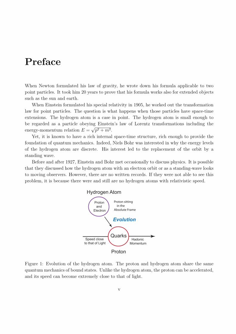
Proton sitting
in the
Absolute Frame
Hadonic
Momentum
Speed close
to that of Light
Evolution
Proton
and
Electron
Hydrogen Atom
Proton
Quarks
Figure 1: Evolution of the hydrogen atom. The proton and hydrogen atom share the same
quantum mechanics of bound states. Unlike the hydrogen atom, the proton can be accelerated,
and its speed can become extremely close to that of light.
v

vi
However, an evolution has taken place in the way we look at the hydrogen atom. These
days, there are moving protons. Fortunately, the proton is also a bound state of more fun-
damental particles called quarks. Since the proton and the hydrogen atom share the same
quantum mechanics, it is possible to study the original Bohr-Einstein problem of moving
hydrogen atoms while looking at accelerated protons. This transition is shown in Fig. 1.
In 1971 in an attempt to construct a Lorentz-covariant picture of the quark model, Feyn-
man and his students wrote down a Lorentz-invariant differential equation for the harmonic
oscillator potential. This partial differential equation has many different solutions depending
on the choice of coordinate systems and boundary conditions.
Earlier, in 1927, 1945, and 1949, Paul A. M. Dirac noted the problem of constructing
wave functions which can be Lorentz-boosted. He had to approach this problem mathatically
because there were no moving bound states. In 1949, he concluded that the solution to this
problem is to construct a suitable reprsentation of the Poincare group.
Indeed, the purpose of this book is to develop mathematical tools to approach this problem.
In 1939, Eugene Wigner published a paper dealing with subgroups of the Lorentz group whose
transformations leave the four-momentum of a given particle invariant. If the momentum is
invariant, these subgroups deal with the internal space-time symmetries. For instance, for a
massive particle at rest, the subgroup is O(3) or the three-dimensional rotation group. Spher-
ical harmonics constitute a representation of the three-dimensional rotation group. Likewise,
it is possible to construct a representation of Wigner’s little group for massive particles using
harmonic oscillator wave functions.
Wigner however did not deal with the problem of what happens when the O(3) symmetry
is Lorentz-boosted. Of particular interest is what happens when the system is boosted to the
infinite-momentum frame. On the other hand, Wigner’s 1939 paper provides a framework to
carry out this Lorentz completion of his little group, and we shall do so in this book. In so
doing it is possible to provide the solutions of the problems left unsolved in the papers of
Dirac and Feynman.
This Lorentz completion allows us to deal with the Bohr-Einstein question of how the
hydrogen atom appears to a moving observer. We can study the same problem using harmonic
oscillator wave functions, and study what we observe in high-energy particle physics. If the
proton is at rest, it is a bound state just like the hydrogen atom. If the proton moves
with a velocity close to that of light, it appears like a collection of Feynman’s partons. The
Lorentz completion therefore shows that the quark and parton models are two limiting cases
of one covariant entity just as the case of E = p2/2m and E = cp are two limiting cases of
E =√p2 +m2.
While the group of transformations applicable to the four-dimensional Minkowskian space
is represented by four-by-four matrices, it is possible to represent the same group with two-
by-two matrices. This allows the study of the property of the group with more transparent
matrices. In addition, this group allows the study of mathematical languages for the branch
of physics based on two-by-two matrices.

vii
Modern optics is a case in point. Two-by-two matrices serve as the basic mathematical
languages for the squeezed state of light, polarization optics, lens optics, and beam trans-
fer matrices commonly called the ABCD matrices. It is known that those matrices are not
rotation matrices because they are the matrices of the Lorentz group. Since Lorentz trans-
formations and modern optics share the same mathematics, it is possible to learn lessons for
one subject from the other, as illustrated in Fig. 2.
Figure 2: One mathematical language serving two branches of physics. A second-order dif-
ferential equation can serve as the underlying mathematical language for both the damped
harmonic oscillator and the resonance circuit. Likewise, the Lorentz group serves as the
underlying language for both special relativity and modern optics.
As for mathematical techniques, what lessons can we learn? We are quite familiar with
the two-by-two matrix
R(θ) =
(cos(θ/2) − sin(θ/2)
sin(θ/2) cos(θ/2)
),
which performs rotations in the two-dimensional space of x and y. Its transpose becomes its
inverse. This matrix is Hermitian.
We can consider another matrix which takes the form
B(η) =
(eη/2 0
0 e−η/2
).
This matrix squeezes the coordinate axes. It expands one axis while contracting the other,
in such a way that the area is preserved. This matrix transforms a circle into an ellipse, and
its geometry is very familiar to us, but its role in modern physics is not well known largely
because it is not a Hermitian matrix. Judicious combinations of the rotation and squeeze

viii
matrices lead to a very effective mathematics capable of addressing many different aspects of
modern physics.

Contents
Preface . . . . . . . . . . . . . . . . . . . . . . . . . . . . . . . . . . . . . . . . . . . v
1 Lorentz group and its representations 1
1.1 Generators of the Lorentz Group . . . . . . . . . . . . . . . . . . . . . . . . . 1
1.2 Two-by-two representation of the Lorentz group . . . . . . . . . . . . . . . . . 3
1.3 Representations based on harmonic oscillators . . . . . . . . . . . . . . . . . . 4
References . . . . . . . . . . . . . . . . . . . . . . . . . . . . . . . . . . . . . . . . . 5
2 Wigner’s little groups for internal space-time symmetries 7
2.1 Euler decomposition of Wigner’s little group . . . . . . . . . . . . . . . . . . . 7
2.2 O(3)-like little group for massive particles . . . . . . . . . . . . . . . . . . . . 8
2.3 E(2)-like little group for massless particles . . . . . . . . . . . . . . . . . . . . 9
2.4 O(2,1)-like little group for imaginary-mass particles . . . . . . . . . . . . . . . 11
2.5 Summary . . . . . . . . . . . . . . . . . . . . . . . . . . . . . . . . . . . . . . 12
References . . . . . . . . . . . . . . . . . . . . . . . . . . . . . . . . . . . . . . . . . 14
3 Two-by-two representations of Wigner’s little groups 15
3.1 Representations of Wigner’s little groups . . . . . . . . . . . . . . . . . . . . . 16
3.2 Lorentz completion of the little groups . . . . . . . . . . . . . . . . . . . . . . 18
3.3 Bargmann and Wigner decompositions . . . . . . . . . . . . . . . . . . . . . . 19
3.4 Conjugate transformations . . . . . . . . . . . . . . . . . . . . . . . . . . . . . 21
3.5 Polarization of massless neutrinos . . . . . . . . . . . . . . . . . . . . . . . . . 23
3.6 Scalars, four-vectors, and four-tensors . . . . . . . . . . . . . . . . . . . . . . . 25
3.6.1 Four-vectors . . . . . . . . . . . . . . . . . . . . . . . . . . . . . . . . . 26
3.6.2 Second-rank Tensor . . . . . . . . . . . . . . . . . . . . . . . . . . . . . 29
References . . . . . . . . . . . . . . . . . . . . . . . . . . . . . . . . . . . . . . . . . 31
4 One little group with three branches 33
4.1 One expression with three branches . . . . . . . . . . . . . . . . . . . . . . . . 33
4.2 Classical damped oscillators . . . . . . . . . . . . . . . . . . . . . . . . . . . . 35
4.3 Little groups in the light-cone coordinate system . . . . . . . . . . . . . . . . . 37
4.4 Lorentz completion in the light-cone coordinate system . . . . . . . . . . . . . 41
ix

x CONTENTS
References . . . . . . . . . . . . . . . . . . . . . . . . . . . . . . . . . . . . . . . . . 41
5 Lorentz-covariant harmonic oscillators 43
5.1 Dirac’s plan to construct Lorentz-covariant quantum mechanics . . . . . . . . 44
5.2 Dirac’s forms of relativistic dynamics . . . . . . . . . . . . . . . . . . . . . . . 45
5.3 Running waves and standing waves . . . . . . . . . . . . . . . . . . . . . . . . 47
5.4 Little groups for relativistic extended particles . . . . . . . . . . . . . . . . . . 51
5.5 Further properties of covariant oscillator wave functions . . . . . . . . . . . . . 52
5.6 Lorentz contraction of harmonic oscillators . . . . . . . . . . . . . . . . . . . . 54
5.7 Feynman’s rest of the universe . . . . . . . . . . . . . . . . . . . . . . . . . . . 56
References . . . . . . . . . . . . . . . . . . . . . . . . . . . . . . . . . . . . . . . . . 60
6 Quarks and partons in the Lorentz-covariant world 63
6.1 Lorentz-covariant quark model . . . . . . . . . . . . . . . . . . . . . . . . . . . 65
6.2 Feynman’s parton picture . . . . . . . . . . . . . . . . . . . . . . . . . . . . . 66
6.3 Proton structure function . . . . . . . . . . . . . . . . . . . . . . . . . . . . . 70
6.4 Proton form factor and Lorentz coherence . . . . . . . . . . . . . . . . . . . . 73
6.5 Coherence in momentum-energy space . . . . . . . . . . . . . . . . . . . . . . 77
6.6 Hadronic temperature and boiling quarks . . . . . . . . . . . . . . . . . . . . . 79
References . . . . . . . . . . . . . . . . . . . . . . . . . . . . . . . . . . . . . . . . . 80
7 Coupled oscillators and squeezed states of light 83
7.1 Two coupled oscillators . . . . . . . . . . . . . . . . . . . . . . . . . . . . . . . 84
7.2 Squeezed states of light . . . . . . . . . . . . . . . . . . . . . . . . . . . . . . . 86
7.3 O(3,2) symmetry from Dirac’s coupled oscillators . . . . . . . . . . . . . . . . 89
7.4 O(3,3) symmetry from Dirac matrices . . . . . . . . . . . . . . . . . . . . . . . 91
7.5 Non-canonical transformations in quantum mechanics . . . . . . . . . . . . . . 93
7.6 Entropy and the expanding Wigner phase space . . . . . . . . . . . . . . . . . 95
References . . . . . . . . . . . . . . . . . . . . . . . . . . . . . . . . . . . . . . . . . 96
8 Lorentz group in ray optics 99
8.1 Group of ABCD matrices . . . . . . . . . . . . . . . . . . . . . . . . . . . . . 99
8.2 Equi-diagonalization of the ABCD matrix . . . . . . . . . . . . . . . . . . . . 100
8.3 Decomposition of the ABCD matrix . . . . . . . . . . . . . . . . . . . . . . . . 102
8.4 Laser cavities . . . . . . . . . . . . . . . . . . . . . . . . . . . . . . . . . . . . 103
8.5 Multilayer optics . . . . . . . . . . . . . . . . . . . . . . . . . . . . . . . . . . 106
8.6 Camera optics . . . . . . . . . . . . . . . . . . . . . . . . . . . . . . . . . . . . 109
References . . . . . . . . . . . . . . . . . . . . . . . . . . . . . . . . . . . . . . . . . 112

CONTENTS xi
9 Polarization optics 113
9.1 Jones vectors . . . . . . . . . . . . . . . . . . . . . . . . . . . . . . . . . . . . 113
9.2 Squeeze and phase shift . . . . . . . . . . . . . . . . . . . . . . . . . . . . . . 115
9.3 Rotation of the polarization axes . . . . . . . . . . . . . . . . . . . . . . . . . 116
9.4 Optical activities . . . . . . . . . . . . . . . . . . . . . . . . . . . . . . . . . . 119
References . . . . . . . . . . . . . . . . . . . . . . . . . . . . . . . . . . . . . . . . . 122
10 Poincare sphere 123
10.1 Coherency matrix . . . . . . . . . . . . . . . . . . . . . . . . . . . . . . . . . . 123
10.2 Entropy problem . . . . . . . . . . . . . . . . . . . . . . . . . . . . . . . . . . 127
10.3 Symmetries derivable from the Poincare sphere . . . . . . . . . . . . . . . . . . 128
10.4 O(3,2) symmetry . . . . . . . . . . . . . . . . . . . . . . . . . . . . . . . . . . 129
References . . . . . . . . . . . . . . . . . . . . . . . . . . . . . . . . . . . . . . . . . 130

Chapter 1
Lorentz group and its representations
The Lorentz group starts with a group of four-by-four matrices performing Lorentz transfor-
mations on the four-dimensional Minkowski space of (t, z, x, y). The transformation leaves
invariant the quantity (t2 − z2 − x2 − y2). There are three generators of rotations and three
boost generators. Thus, the Lorentz group is a six-parameter group.
It was Einstein who observed that this Lorentz group is applicable also to the four-
dimensional energy and momentum space of (E, pz, px, py) . In this way, he was able to derive
his Lorentz-covariant energy-momentum relation commonly known as E = mc2. This trans-
formation leaves(E2 − p2z − p2x − p2y
)invariant. In other words, the particle mass is a Lorentz
invariant quantity.
1.1 Generators of the Lorentz Group
Let us start with rotations applicable to the (z, x, y) coordinates. The four-by-four matrix for
this operation is
Z(ϕ) =
1 0 0 0
0 1 0 0
0 0 cosϕ − sinϕ
0 0 sinϕ cosϕ
, (1.1)
which can be written as
Z(ϕ) = exp (−iϕJ3), (1.2)
with
J3 =
0 0 0 0
0 0 0 0
0 0 0 −i0 0 i 0
. (1.3)
The matrix J3 is known as the generator of the rotation around the z axis. It is not difficult
to write the generators of rotations around the x and y axes, and they can be written as J1
1
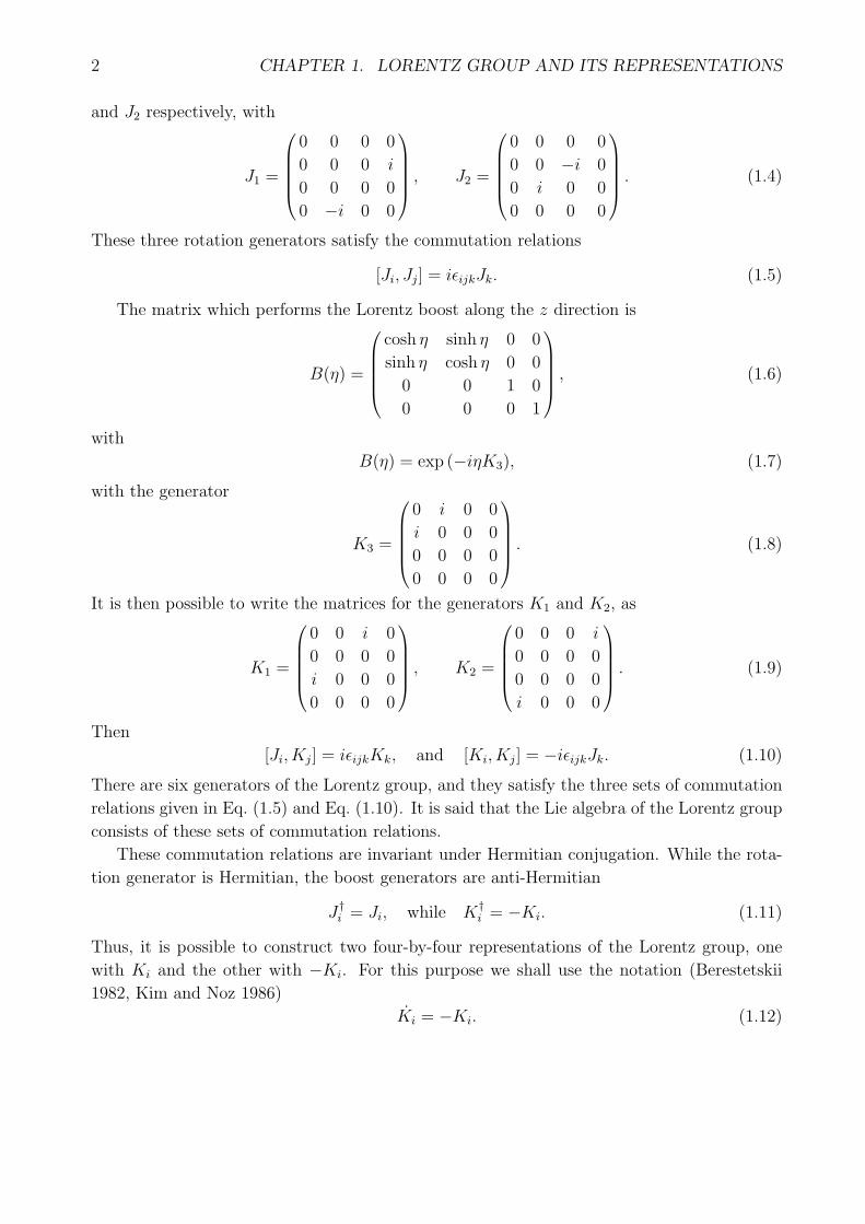
2 CHAPTER 1. LORENTZ GROUP AND ITS REPRESENTATIONS
and J2 respectively, with
J1 =
0 0 0 0
0 0 0 i
0 0 0 0
0 −i 0 0
, J2 =
0 0 0 0
0 0 −i 0
0 i 0 0
0 0 0 0
. (1.4)
These three rotation generators satisfy the commutation relations
[Ji, Jj] = iϵijkJk. (1.5)
The matrix which performs the Lorentz boost along the z direction is
B(η) =
cosh η sinh η 0 0
sinh η cosh η 0 0
0 0 1 0
0 0 0 1
, (1.6)
with
B(η) = exp (−iηK3), (1.7)
with the generator
K3 =
0 i 0 0
i 0 0 0
0 0 0 0
0 0 0 0
. (1.8)
It is then possible to write the matrices for the generators K1 and K2, as
K1 =
0 0 i 0
0 0 0 0
i 0 0 0
0 0 0 0
, K2 =
0 0 0 i
0 0 0 0
0 0 0 0
i 0 0 0
. (1.9)
Then
[Ji, Kj] = iϵijkKk, and [Ki, Kj] = −iϵijkJk. (1.10)
There are six generators of the Lorentz group, and they satisfy the three sets of commutation
relations given in Eq. (1.5) and Eq. (1.10). It is said that the Lie algebra of the Lorentz group
consists of these sets of commutation relations.
These commutation relations are invariant under Hermitian conjugation. While the rota-
tion generator is Hermitian, the boost generators are anti-Hermitian
J†i = Ji, while K†
i = −Ki. (1.11)
Thus, it is possible to construct two four-by-four representations of the Lorentz group, one
with Ki and the other with −Ki. For this purpose we shall use the notation (Berestetskii
1982, Kim and Noz 1986)
Ki = −Ki. (1.12)

1.2. TWO-BY-TWO REPRESENTATION OF THE LORENTZ GROUP 3
Since there are two representations, transformations with Ki are called the covariant trans-
formations, while those with Ki are called contravariant transformations.
1.2 Two-by-two representation of the Lorentz group
It is possible to construct the Lie algebra of the Lorentz group from the three Pauli matri-
ces (Dirac 1945b, Naimark 1954, Kim and Noz 1986, Baskal et al. 2014). Let us define
Ji =1
2σi, and Ki =
i
2σi, (1.13)
These two-by-two matrices satisfy the Lie algebra of the Lorentz group given in Eq. (1.5) and
Eq. (1.10).
These generators will lead to a two-by-two matrix of the form
G =
(α β
γ δ
), (1.14)
with four complex matrix elements, thus eight real parameters. Since its determinant is
fixed and is equal to one, there are six independent parameters. This six-parameter group is
commonly called SL(2, c). Since the Lorentz group has six generators, this two-by-two matrix
can serve as a representation of the Lorentz group. It is said in the literature that SL(2, c)
serves as the covering group for the Lorentz group.
For each G matrix of SL(2, c), there exists one four-by-four Lorentz transformation matrix.
We can start with the Minkowskian four-vector (t, z, x, y) written as
X =
(t+ z x− iy
x+ iy t− z
), (1.15)
whose determinant is
t2 − z2 − x2 − y2. (1.16)
The correspondence between the two-by-two and four-by-four representations of the Lorentz
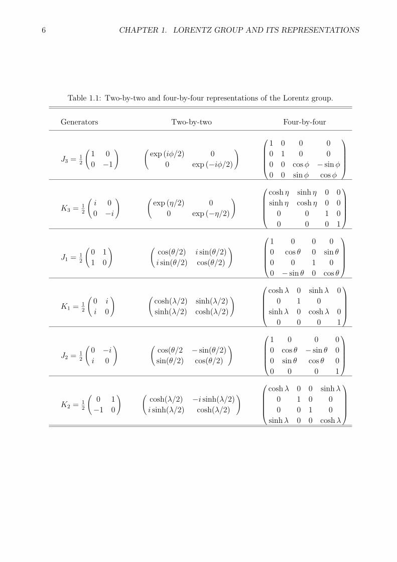
group along with the generators are given in Table 1.1. These representations can be used
for coordinate or momentum transformations, as well as other four-vector quantities such as
electromagnetic four-potentials. We can now consider the transformation
X ′ = G X G†, (1.17)
The transformation of Eq. (1.17) can be explicitly written as(t′ + z′ x′ − iy′
x′ + iy′ t′ − z′
)=
(α β
γ δ
)(t+ z x− iy
x+ iy t− z
)(α∗ γ∗
β∗ δ∗
). (1.18)

4 CHAPTER 1. LORENTZ GROUP AND ITS REPRESENTATIONS
We can now translate this formula intot′ + z′
t′ − z′
x′ − iy′
x′ + iy′
=
α∗α γ∗β γ∗α α∗β
β∗γ δ∗δ δ∗γ β∗δ
β∗α δ∗α β∗β δ∗β
α∗γ γ∗γ α∗δ γ∗δ
t+ z
t− z
x− iy
x+ iy
. (1.19)
This then leads to t′
z′
x′
y′
=1
2
1 1 0 0
1 −1 0 0
0 0 1 1
0 0 i −i
t′ + z′
t′ − z′
x′ − iy′
x′ + iy′
. (1.20)
It is important to note that the transformation of Eq. (1.17) is not a similarity transformation.
In the SL(2, c) regime, not all the matrices are Hermitian (Baskal et al. 2014)
Likewise, the two-by-two matrix for the four-momentum of the particle takes the form
P =
(p0 + pz px − ipypx + ipy p0 − pz
)(1.21)
with p0 =√m2 + p2z + p2x + p22. The transformation of this matrix takes the same form as that
for space-time given in Eqs. (1.17) and (1.18). The determinant of this matrix is m2 and
remains invariant under Lorentz transformations. The explicit form of the transformation is
P ′ = G P G† =
(p′0 + p′z p′x − ip′yp′x + ip′y p′0 − p′z
)
=
(α β
γ δ
)(p0 + pz px − ipypx + ipy p0 − pz
)(α∗ γ∗
β∗ δ∗
). (1.22)
1.3 Representations based on harmonic oscillators
The matrix representations in the previous section are primarily for coordinate transforma-
tions. The question then is how can we transform functions. This problem has a stormy
history. For plane waves, the form
exp (ip · x) (1.23)
is widely used in the literature. Since
p · x = Et− pxx− pyy − pzz
is a Lorentz-invariant quantity, there are no problems from the mathematical point of view.
However, for standing waves, we have to consider boundary conditions. The issue is then
how to transform these conditions. One way to circumvent this difficulty is to study harmonic
oscillators with built-in boundary conditions.
1.3. REPRESENTATIONS BASED ON HARMONIC OSCILLATORS 5
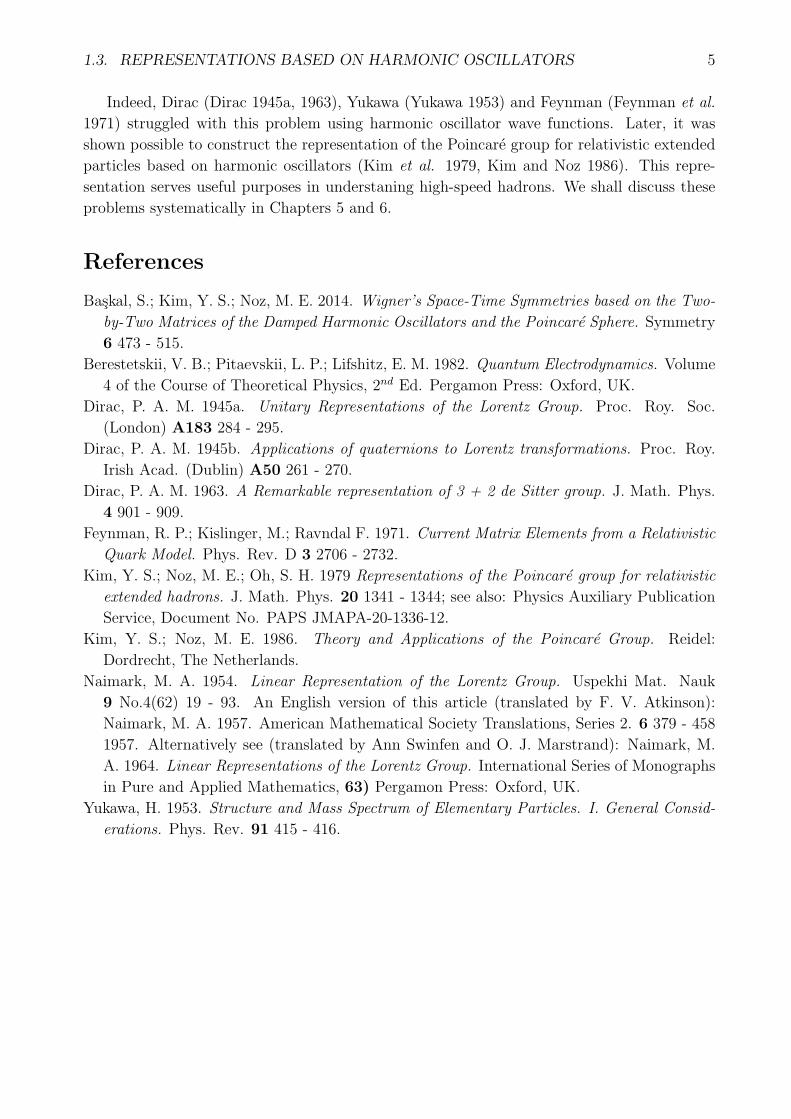
Indeed, Dirac (Dirac 1945a, 1963), Yukawa (Yukawa 1953) and Feynman (Feynman et al.
1971) struggled with this problem using harmonic oscillator wave functions. Later, it was
shown possible to construct the representation of the Poincare group for relativistic extended
particles based on harmonic oscillators (Kim et al. 1979, Kim and Noz 1986). This repre-
sentation serves useful purposes in understaning high-speed hadrons. We shall discuss these
problems systematically in Chapters 5 and 6.
References
Baskal, S.; Kim, Y. S.; Noz, M. E. 2014. Wigner’s Space-Time Symmetries based on the Two-
by-Two Matrices of the Damped Harmonic Oscillators and the Poincare Sphere. Symmetry
6 473 - 515.
Berestetskii, V. B.; Pitaevskii, L. P.; Lifshitz, E. M. 1982. Quantum Electrodynamics. Volume
4 of the Course of Theoretical Physics, 2nd Ed. Pergamon Press: Oxford, UK.
Dirac, P. A. M. 1945a. Unitary Representations of the Lorentz Group. Proc. Roy. Soc.
(London) A183 284 - 295.
Dirac, P. A. M. 1945b. Applications of quaternions to Lorentz transformations. Proc. Roy.
Irish Acad. (Dublin) A50 261 - 270.
Dirac, P. A. M. 1963. A Remarkable representation of 3 + 2 de Sitter group. J. Math. Phys.
4 901 - 909.
Feynman, R. P.; Kislinger, M.; Ravndal F. 1971. Current Matrix Elements from a Relativistic
Quark Model. Phys. Rev. D 3 2706 - 2732.
Kim, Y. S.; Noz, M. E.; Oh, S. H. 1979 Representations of the Poincare group for relativistic
extended hadrons. J. Math. Phys. 20 1341 - 1344; see also: Physics Auxiliary Publication
Service, Document No. PAPS JMAPA-20-1336-12.
Kim, Y. S.; Noz, M. E. 1986. Theory and Applications of the Poincare Group. Reidel:
Dordrecht, The Netherlands.
Naimark, M. A. 1954. Linear Representation of the Lorentz Group. Uspekhi Mat. Nauk
9 No.4(62) 19 - 93. An English version of this article (translated by F. V. Atkinson):
Naimark, M. A. 1957. American Mathematical Society Translations, Series 2. 6 379 - 458
1957. Alternatively see (translated by Ann Swinfen and O. J. Marstrand): Naimark, M.
A. 1964. Linear Representations of the Lorentz Group. International Series of Monographs
in Pure and Applied Mathematics, 63) Pergamon Press: Oxford, UK.
Yukawa, H. 1953. Structure and Mass Spectrum of Elementary Particles. I. General Consid-
erations. Phys. Rev. 91 415 - 416.
6 CHAPTER 1. LORENTZ GROUP AND ITS REPRESENTATIONS
Table 1.1: Two-by-two and four-by-four representations of the Lorentz group.
Generators Two-by-two Four-by-four
J3 =12
(1 0
0 −1
) (exp (iϕ/2) 0
0 exp (−iϕ/2)
) 1 0 0 0
0 1 0 0
0 0 cosϕ − sinϕ
0 0 sinϕ cosϕ
K3 =12
(i 0
0 −i
) (exp (η/2) 0
0 exp (−η/2)
) cosh η sinh η 0 0
sinh η cosh η 0 0
0 0 1 0
0 0 0 1
J1 =12
(0 1
1 0
) (cos(θ/2) i sin(θ/2)
i sin(θ/2) cos(θ/2)
) 1 0 0 0
0 cos θ 0 sin θ
0 0 1 0
0 − sin θ 0 cos θ
K1 =12
(0 i
i 0
) (cosh(λ/2) sinh(λ/2)
sinh(λ/2) cosh(λ/2)
) coshλ 0 sinhλ 0
0 1 0
sinhλ 0 coshλ 0
0 0 0 1
J2 =12
(0 −ii 0
) (cos(θ/2 − sin(θ/2)
sin(θ/2) cos(θ/2)
) 1 0 0 0
0 cos θ − sin θ 0
0 sin θ cos θ 0
0 0 0 1
K2 =12
(0 1
−1 0
) (cosh(λ/2) −i sinh(λ/2)i sinh(λ/2) cosh(λ/2)
) coshλ 0 0 sinhλ
0 1 0 0
0 0 1 0
sinhλ 0 0 coshλ

Chapter 2
Wigner’s little groups for internal
space-time symmetries
When Einstein formulated his special relativity, he was interested in point particles, without
internal space-time structures. For instance, particles can have intrinsic spins. Massless
photons have helicities. The hydrogen atom is a bound state of the electron and proton with
a nonzero size. The question is how these particles look to moving observers.
In order to address this question, let us studyWigner’s little groups. In 1939, Wigner (Wigner
1939) considered the subgroup of the Lorentz group whose transformations leave the particle
momentum invariant. On the other hand, they can transform the internal space-time struc-
ture of the particles. Since the particle momentum is fixed and remains invariant, we can
assume that the particle momentum is along the z direction.
This momentum is invariant under rotations around this axis. In addition, these rotations
commute with the Lorentz boost along the z axis. According to the Lie algebra of Eq. (1.10),
[J3, K3] = 0. (2.1)
With these preparations, we can simplify the problem using the Euler coordinate sys-
tem (Goldstein 1980). Euler formulated his coordinate system in order to understand spinning
tops in classical mechanics. In quantum mechanics, we study this problem by constructing
representations of the rotation group, such as the spherical harmonics and Pauli matrices.
Now the pressing issue is what happens if the system is Lorentz-boosted.
2.1 Euler decomposition of Wigner’s little group
The Euler angles constitute a convenient parameterization of the three-dimensional rota-
tions (Goldstein 1980). The Euler kinematics consists of two rotations around the z axis with
one rotation around the y axis between them. These three operations cover also the rotation
7
8CHAPTER 2. WIGNER’S LITTLE GROUPS FOR INTERNAL SPACE-TIME SYMMETRIES
around the x axis, thanks to the commutation relation
[J2, J3] = iJ1. (2.2)
In this way, it is possible to study the essential features of three-dimensional rotations
using the two dimensional space of z and x. This aspect is well known.
The first question is what happens if we add a Lorentz boost along the z direction to this
traditional procedure (Han et al. 1986). Since the rotation around the z axis is not affected
by the boost along the same axis, we are asking what happens to the rotation around the y
axis if it is boosted along the z direction.
2.2 O(3)-like little group for massive particles
If the particle has a positive mass, there is a Lorentz frame in which the particle is at rest,
with its four-momentum proportional to
P = (1, 0, 0, 0). (2.3)
This momentum remains invariant under rotations. Thus, the little group of the massive
particle at rest is the three-dimensional rotation group.
The three generators of this little group are J1, J2, and J3, satisfying the Lie algebra of
Eq. (1.5). The dynamical variables associated with these Hermitian operators are known to
be particle spins.
The system can be boosted along the z axis, with the boost matrix B(η) given in Eq. (1.6).
If this matrix is applied to the four-momentum of Eq. (2.3), it becomes
P ′ = (cosh η, sinh η, 0, 0). (2.4)
The generators become
J ′i = B(η)JiB
−1(η). (2.5)
Under this boost operation, J3 remains invariant, but J ′2 becomes
J ′2 = (cosh η)J2 − (sinh η)K1. (2.6)
As for J1, the boost results in
J ′1 = (cosh η)J1 + (sinh η)K2. (2.7)
However, we can obtain the same result by rotating J ′2 by −90o around the z axis, thanks to
the Euler effect discussed in Sec. 2.1.
Although the generators J ′i satisfy the same Lie algebra as that for Ji, they are not the
same. Thus, we shall call the operators J ′i generators of the O(3)-like little group for the
massive particle with a non-zero momentum.
An interesting issue is what happens when η becomes infinite, and sinh η = cosh η. We
shall discuss this problem in Chapter 4.
2.3. E(2)-LIKE LITTLE GROUP FOR MASSLESS PARTICLES 9
2.3 E(2)-like little group for massless particles
If the particle is massless, its four-momentum is proportional to
P = (1, 1, 0, 0). (2.8)
This expression is of course invariant under rotations around the z axis.
In addition, Wigner (Wigner 1939) observed that it is also invariant under the transfor-
mation
D(γ, ϕ) = exp [−iγ (N1 sinϕ+N2 cosϕ)] (2.9)
with
N1 = J1 +K2 =
0 0 0 i
0 0 0 i
0 0 0 0
i −i 0 0
, N2 = K1 − J2 =
0 0 i 0
0 0 i 0
i −i 0 0
0 0 0 0
. (2.10)
As a consequence,
D(γ, ϕ) =
1 + γ2/2 −γ2/2 γ cosϕ γ sinϕ
γ2/2 1− γ2/2 γ cosϕ γ sinϕ
γ cosϕ −γ cosϕ 1 0
γ sinϕ −γ sinϕ 0 1
. (2.11)
Thus the generators of the little group are N1, N2, and J3. They satisfy the following set
of commutation relations.
[N1, N2] = 0, [N1, J3] = iN2, [N2, J3] = −iN1. (2.12)
As Wigner notes, this Lie algebra is the same as that for the two-dimensional Euclidean group,
with
[P1, P2] = 0, [P1, J3] = iP2, [P2, J3] = −iP1, (2.13)
where P1 and P2 generate translations along the x and y directions respectively. They can be
written as
P1 = −i ∂∂x, P2 = −i ∂
∂y, (2.14)
while the rotation generator J3 takes the form
J3 = −i(x∂
∂y− y
∂
∂x
). (2.15)
In addition, Kim and Wigner (Kim and Wigner 1987) considered the following operators,
Q1 = −ix ∂∂z, Q2 = iy
∂
∂z, (2.16)

10CHAPTER 2. WIGNER’S LITTLE GROUPS FOR INTERNAL SPACE-TIME SYMMETRIES
Side ViewTop View
x
y
Gauge
Transform
zHelicity
Figure 2.1: Cylindrical picture of the internal space-time structure of photons. The top view
of this cylinder is a circle whose rotational degree of freedom corresponds to the helicity of
the photon, while the top-down translation corresponds to a gauge transformation (Kim and
Wigner 1990).
with x2 + y2 = constant. They generate translations along the z direction on the surface
of a circular cylinder as described in Fig. 2.1. Then they satisfy the following commutation
relations:
[Q1, Q2] = 0, [Q1, J3] = iQ2, [Q2, J3] = −iQ1. (2.17)
We can say that this is the Lie algebra for the “cylindrical group.”
Let us consider a photon whose momentum is along the z direction. It has the four-
potential
(A0, Az, Ax, Ay) . (2.18)
According to the Lorentz condition, A0 = Az. Thus the four-potential is
(A0, A0, Ax, Ay) . (2.19)
If we apply the D(γ, ϕ) of Eq. (2.11):
1 + γ2/2 −γ2/2 γ cosϕ γ sinϕ
γ2/2 1− γ2/2 γ cosϕ γ sinϕ
γ cosϕ −γ cosϕ 1 0
γ sinϕ −γ sinϕ 0 1
A0
A0
Ax
Ay
, (2.20)
2.4. O(2,1)-LIKE LITTLE GROUP FOR IMAGINARY-MASS PARTICLES 11
the result is A0 + γ (Ax cosϕ+ Ay sinϕ)
A0 + γ (Ax cosϕ+ Ay sinϕ)
Ax
Ay
. (2.21)
If we boost the four-momentum of Eq. (2.8) along the z direction, the four-momentum
becomes
P ′ = eη(1, 1, 0, 0), (2.22)
and N1 and N2 become eηN1 and eηN2 respectively. J3 remains invariant.
The little group transformation D(γ, ϕ) leaves the transverse components Ax and Ay in-
variant, but provides an addition to A0. This is a cylindrical transformation. In the language
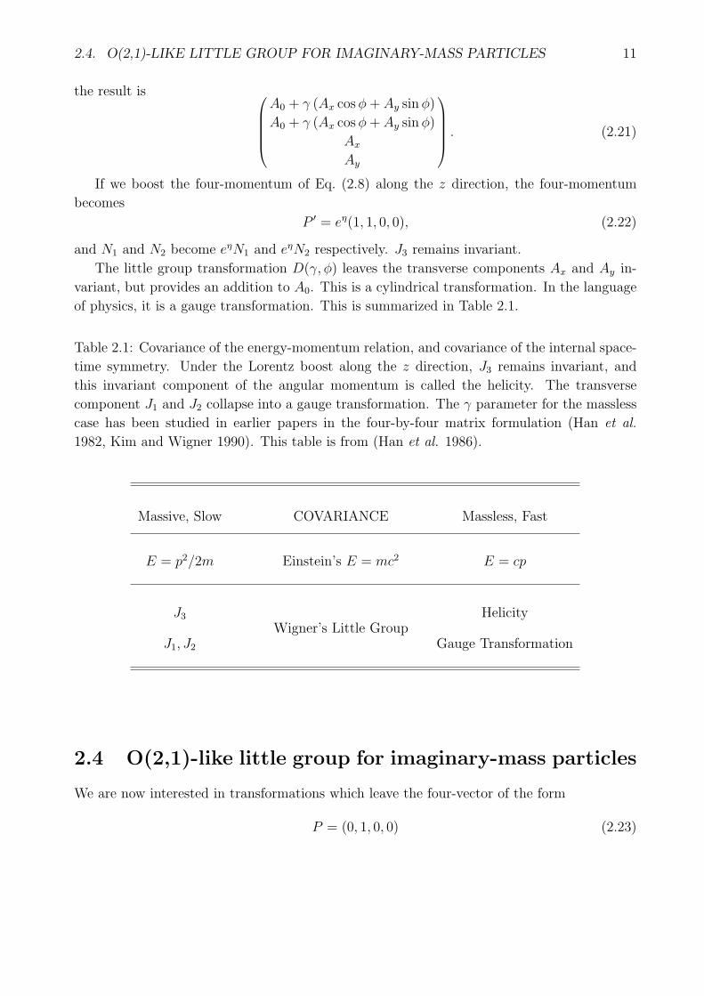
of physics, it is a gauge transformation. This is summarized in Table 2.1.
Table 2.1: Covariance of the energy-momentum relation, and covariance of the internal space-
time symmetry. Under the Lorentz boost along the z direction, J3 remains invariant, and
this invariant component of the angular momentum is called the helicity. The transverse
component J1 and J2 collapse into a gauge transformation. The γ parameter for the massless
case has been studied in earlier papers in the four-by-four matrix formulation (Han et al.
1982, Kim and Wigner 1990). This table is from (Han et al. 1986).
Massive, Slow COVARIANCE Massless, Fast
E = p2/2m Einstein’s E = mc2 E = cp
J3 HelicityWigner’s Little Group
J1, J2 Gauge Transformation
2.4 O(2,1)-like little group for imaginary-mass particles
We are now interested in transformations which leave the four-vector of the form
P = (0, 1, 0, 0) (2.23)
12CHAPTER 2. WIGNER’S LITTLE GROUPS FOR INTERNAL SPACE-TIME SYMMETRIES
invariant. Then P 2 = −1, and it is a negative number. We are accustomed to positive values
of P 2 = (mass)2. This means that the particle mass is imaginary, and it moves faster than
light. We are thus talking about a particle we cannot observe in the real world. On the other
hand, these particles play a major theoretical role in Feynman diagrams.
We are now interested in transformations which leave the four-vector of Eq. (2.23) invari-
ant. Let us consider the Lorentz boost along the y direction, with
S(λ) =
coshλ 0 0 sinhλ
0 1 0 0
0 0 1 0
sinhλ 0 0 coshλ
, (2.24)
which is generated by K2. Likewise, it is invariant under the boost along the x direction.
Thus, we can consider the set of commutation relations
[J3, K1] = iK2, [J3, K2] = −iK1, [K1, K2] = −iJ3. (2.25)
This is a Lie algebra of the Lorentz group applicable to two space and one time dimensions.
This group is known in the literature as O(2, 1).
If we boost the four-momentum of Eq. (2.23) along the z direction, it becomes
(sinh η, cosh η, 0, 0), (2.26)
while J3 remains invariant. K1 and K2 become
K ′1 = (cosh η)K1 − (sinh η)J2, K ′
2 = (cosh η)K2 + (sinh η)J1, (2.27)
respectively. The generators K ′1, K
′2, and J3 satisfy the same Lie algebra as that of Eq. (2.25).
If we interchange sinh η and cosh η, these generators become those of Eq. (2.6). If η
becomes very large, the four-momentum takes the same form for the massive, massless, and
imaginary mass cases. The generators of the little groups also become the same. We shall
discuss this issue in Chapter 4.
Even though we are talking about imaginary-mass particles in this section, the mathemat-
ics of this little group is applicable to many branches of physics.
2.5 Summary
In this Chapter, we discussed the Lorentz group applicable to one time and two space di-
mensions, namely to the (z, x, t) coordinates. The rotation around the z axis will leave the
four-momenta listed in this Chapter invariant. It will also extend the representation to the
the full (z, x, y, t) space. With this point in mind, we can list the four-vectors and matrices
2.5. SUMMARY 13
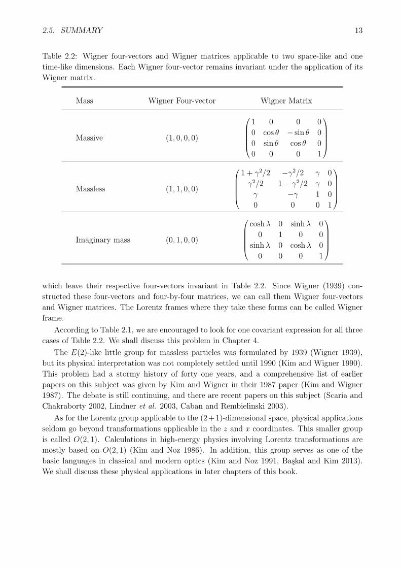
Table 2.2: Wigner four-vectors and Wigner matrices applicable to two space-like and one
time-like dimensions. Each Wigner four-vector remains invariant under the application of its
Wigner matrix.
Mass Wigner Four-vector Wigner Matrix
Massive (1, 0, 0, 0)
1 0 0 0
0 cos θ − sin θ 0
0 sin θ cos θ 0
0 0 0 1
Massless (1, 1, 0, 0)
1 + γ2/2 −γ2/2 γ 0
γ2/2 1− γ2/2 γ 0
γ −γ 1 0
0 0 0 1
Imaginary mass (0, 1, 0, 0)
coshλ 0 sinhλ 0
0 1 0 0
sinhλ 0 coshλ 0
0 0 0 1
which leave their respective four-vectors invariant in Table 2.2. Since Wigner (1939) con-
structed these four-vectors and four-by-four matrices, we can call them Wigner four-vectors
and Wigner matrices. The Lorentz frames where they take these forms can be called Wigner
frame.
According to Table 2.1, we are encouraged to look for one covariant expression for all three
cases of Table 2.2. We shall discuss this problem in Chapter 4.
The E(2)-like little group for massless particles was formulated by 1939 (Wigner 1939),
but its physical interpretation was not completely settled until 1990 (Kim and Wigner 1990).
This problem had a stormy history of forty one years, and a comprehensive list of earlier
papers on this subject was given by Kim and Wigner in their 1987 paper (Kim and Wigner
1987). The debate is still continuing, and there are recent papers on this subject (Scaria and
Chakraborty 2002, Lindner et al. 2003, Caban and Rembielinski 2003).
As for the Lorentz group applicable to the (2+1)-dimensional space, physical applications
seldom go beyond transformations applicable in the z and x coordinates. This smaller group
is called O(2, 1). Calculations in high-energy physics involving Lorentz transformations are
mostly based on O(2, 1) (Kim and Noz 1986). In addition, this group serves as one of the
basic languages in classical and modern optics (Kim and Noz 1991, Baskal and Kim 2013).
We shall discuss these physical applications in later chapters of this book.

14CHAPTER 2. WIGNER’S LITTLE GROUPS FOR INTERNAL SPACE-TIME SYMMETRIES
References
Baskal, S.; Kim. Y. S. 2013. Lorentz Group in Ray and Polarization Optics. Chapter 9 in
”Mathematical Optics: Classical, Quantum and Computational Methods” edited by Va-
sudevan Lakshminarayanan, Maria L. Calvo, and Tatiana Alieva, CRC Taylor and Francis:
Boca Raton, FL, pp 303 - 349.
Caban, P.; Rembielinski, J. 2003. Photon polarization and Wigner’s little group. Phys. Rev.
A 68 042107 - 042111.
Goldstein, H. 1980. Classical Mechanics. 2nd Ed. Addison Wesley: Boston, MA
Han, D.; Kim, Y. S.; Son, D. 1982. E(2)-like little group for massless particles and polarization
of neutrinos. Phys. Rev. D 26 3717 - 3725.
Han, D.; Kim, Y. S.; D. Son, D. 1986. Eulerian parametrization of Wigner little groups and
gauge transformations in terms of rotations in 2-component spinors. J. Math. Phys. 27
2228 - 2235.
Kim, Y. S.; Noz, M. E. 1986 Theory and Applications of the Poincare Group. Reidel: Dor-
drecht, The Netherlands.
Kim, Y. S.; Wigner, E. P. 1987. Cylindrical group and massless particles. J. Math. Phys. 28
1175 - 1179.
Kim, Y. S.; Wigner, E. P. 1990. Space-time geometry of relativistic-particles. J. Math. Phys.
31 55 - 60.
Kim, Y. S.; Noz, M. E. 1991. Phase Space Picture of Quantum Mechanics. World Scientific:
Singapore.
Lindner, N. H.; Peres, A. ; Terno, D. R. 2003. Wigner’s little group and Berry’s phase for
massless particles. J. Phys. A 26 L449 - L454.
Scaria, T; Chakraborty, B. 2002. Wigner’s little group as a gauge generator in linearized
gravity theories. Classical and Quantum Gravity 19 4445 - 4462.
Wigner, E. 1939. On unitary representations of the inhomogeneous Lorentz group. Ann.
Math. 40 149 - 204.

Chapter 3
Two-by-two representations of
Wigner’s little groups
It was noted in Sec. 1.2 that the Lorentz transformation of the four-momentum can be repre-
sented by two-by-two matrices. An explicit form for the Lorentz transformation was given in
Eq. (1.22) as (Kim and Noz 1986, Baskal et al. 2014)
P ′ = G P G†, (3.1)
where the two-by-two form of the G matrix is given in Eq. (1.14). If the particle moves along
the z direction, the four-momentum matrix becomes
P =
(E + p 0
0 E − p
), (3.2)
where E and p are the energy and the magnitude of momentum respectively.
Let us use W as a subset of matrices which leaves the four-momentum invariant, then we
can write
P =W P W †. (3.3)
These matrices of course constitute Wigner’s little group dictating the internal the space-time
symmetry of the particle.
If the particle is massive, it can be brought to the system where it is at rest with p = 0.
The four-momentum matrix is proportional to
P =
(1 0
0 1
). (3.4)
For the massless particle, E = p. Thus the four-momentum matrix is proportional to
P =
(1 0
0 0
). (3.5)
15
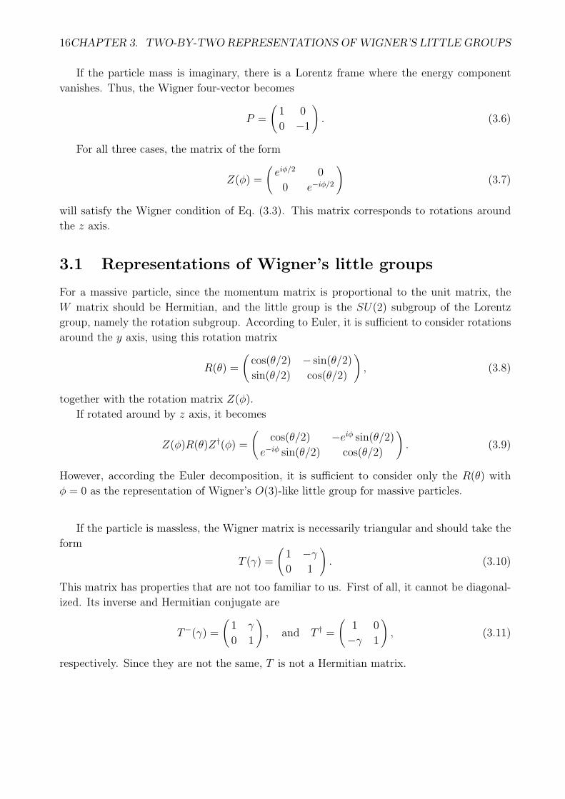
16CHAPTER 3. TWO-BY-TWO REPRESENTATIONS OFWIGNER’S LITTLE GROUPS
If the particle mass is imaginary, there is a Lorentz frame where the energy component
vanishes. Thus, the Wigner four-vector becomes
P =
(1 0
0 −1
). (3.6)
For all three cases, the matrix of the form
Z(ϕ) =
(eiϕ/2 0
0 e−iϕ/2
)(3.7)
will satisfy the Wigner condition of Eq. (3.3). This matrix corresponds to rotations around
the z axis.
3.1 Representations of Wigner’s little groups
For a massive particle, since the momentum matrix is proportional to the unit matrix, the
W matrix should be Hermitian, and the little group is the SU(2) subgroup of the Lorentz
group, namely the rotation subgroup. According to Euler, it is sufficient to consider rotations
around the y axis, using this rotation matrix
R(θ) =
(cos(θ/2) − sin(θ/2)
sin(θ/2) cos(θ/2)
), (3.8)
together with the rotation matrix Z(ϕ).
If rotated around by z axis, it becomes
Z(ϕ)R(θ)Z†(ϕ) =
(cos(θ/2) −eiϕ sin(θ/2)
e−iϕ sin(θ/2) cos(θ/2)
). (3.9)
However, according the Euler decomposition, it is sufficient to consider only the R(θ) with
ϕ = 0 as the representation of Wigner’s O(3)-like little group for massive particles.
If the particle is massless, the Wigner matrix is necessarily triangular and should take the
form
T (γ) =
(1 −γ0 1
). (3.10)
This matrix has properties that are not too familiar to us. First of all, it cannot be diagonal-
ized. Its inverse and Hermitian conjugate are
T−(γ) =
(1 γ
0 1
), and T † =
(1 0
−γ 1
), (3.11)
respectively. Since they are not the same, T is not a Hermitian matrix.
3.1. REPRESENTATIONS OF WIGNER’S LITTLE GROUPS 17
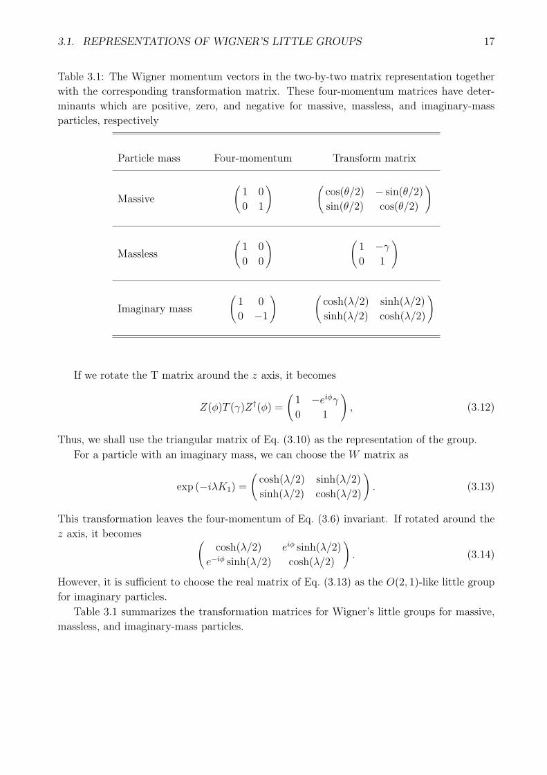
Table 3.1: The Wigner momentum vectors in the two-by-two matrix representation together
with the corresponding transformation matrix. These four-momentum matrices have deter-
minants which are positive, zero, and negative for massive, massless, and imaginary-mass
particles, respectively
Particle mass Four-momentum Transform matrix
Massive
(1 0
0 1
) (cos(θ/2) − sin(θ/2)
sin(θ/2) cos(θ/2)
)
Massless
(1 0
0 0
) (1 −γ0 1
)
Imaginary mass
(1 0
0 −1
) (cosh(λ/2) sinh(λ/2)
sinh(λ/2) cosh(λ/2)
)
If we rotate the T matrix around the z axis, it becomes
Z(ϕ)T (γ)Z†(ϕ) =
(1 −eiϕγ0 1
), (3.12)
Thus, we shall use the triangular matrix of Eq. (3.10) as the representation of the group.
For a particle with an imaginary mass, we can choose the W matrix as
exp (−iλK1) =
(cosh(λ/2) sinh(λ/2)
sinh(λ/2) cosh(λ/2)
). (3.13)
This transformation leaves the four-momentum of Eq. (3.6) invariant. If rotated around the
z axis, it becomes (cosh(λ/2) eiϕ sinh(λ/2)
e−iϕ sinh(λ/2) cosh(λ/2)
). (3.14)
However, it is sufficient to choose the real matrix of Eq. (3.13) as the O(2, 1)-like little group
for imaginary particles.
Table 3.1 summarizes the transformation matrices for Wigner’s little groups for massive,
massless, and imaginary-mass particles.

18CHAPTER 3. TWO-BY-TWO REPRESENTATIONS OFWIGNER’S LITTLE GROUPS
Table 3.2: Lorentz-boosted Wigner vectors and the Wigner matrices in the two-by-two repre-
sentation. They take the same form for infinite values of η, if the parameters θ, λ, and γ are
made to decrease by e−η.
Particle mass Four-momentum W ′ matrix
Massive
(eη 0
0 e−η
) (cos(θ/2) −eη sin(θ/2)
e−η sin(θ/2) cos(θ/2)
)
Massless
(eη 0
0 0
) (1 −eηγ0 1
)
Imaginary mass
(eη 0
0 −e−η
) (cosh(λ/2) eη sinh(λ/2)
e−η sinh(λ/2) cosh(λ/2)
)
3.2 Lorentz completion of the little groups
We are now interested in boosting the Wigner four-vectors and the representation matrices
along the z direction. The boosted four-momentum is
P ′ = B(η) P B†(η), (3.15)
with
B(η) =
(eη/2 0
0 e−η/2
), (3.16)
The boosted four-momentum should then take the form(eη 0
0 e−η
), (3.17)
for the massive particle, and (eη 0
0 0
),
(eη 0
0 −e−η
). (3.18)
respectively for massless and imaginary-mass particles.
However, the boosted Wigner matrix becomes
W ′ = B(η) W B−1(η). (3.19)

3.3. BARGMANN AND WIGNER DECOMPOSITIONS 19
It should be noted that B†(η) is not the same as B−1(η). This is a similarity transformation,
unlike the transformation of the four-momentum given in Eq. (3.15).
The boosted W matrix becomes
W ′ =
(cos(θ/2) −eη sin(θ/2)
e−η sin(θ/2) cos(θ/2)
), (3.20)
for the massive particle. For massless and imaginary particles, they become(1 eηγ
0 1
), and
(cosh(λ/2) eη sinh(λ/2)
e−η sinh(λ/2) cosh(λ/2)
), (3.21)
respectively.
These results are tabulated in Table 3.2. In the limit of large η, all three momentum ma-
trices take the same form. If they are multiplied by e−η, they all become the four-momentum
of the massless particle. The boosted Wigner matrices become sin(θ/2), γ, and sinh(λ/2).
This leads us to look for three little groups as three different branches of one little group. We
shall discuss this problem more systematically in Chapter 4.
3.3 Bargmann and Wigner decompositions
Let us restate the contents of Sec. 3.2. In the case of a massive particle moving with the
four-momentum P ′ of Eq. (3.17), the representation of the little group is W ′ of Eq. (3.20).
This is also a Lorentz-boosted form of the W matrix. Indeed, it can be written as
B(η)WB(−η) = B(η) {B(−η) [B(η)WB(−η)] B(η)} B(−η), (3.22)
meaning that the system is brought back to the frame in which the particle is at rest, a
rotation is made without changing the momentum, and then the system is boosted back to a
frame where it gains regains its original momentum. This three-step operation is illustrated
on the left side in Fig. 3.1. Since this operation consists of three matrices, we shall call it the
Wigner decomposition.
However, this is not the only momentum-preserving transformation. We can start with a
momentum along the z direction, as illustrated in right hand side of Fig. 3.1. We can rotate
this momentum around the y axis, boost along the negative x direction, and then rotate back
to the original momentum along the z direction. Then this operation can be written as
R(α)S(−2χ)R(α) (3.23)
This is a product of one boost matrix sandwiched between two rotation matrices. This form
is called the Bargmann decomposition (Bargmann 1947).
The multiplication of these three matrices leads to
D(α, χ) =
((cosα) coshχ − sinhχ− (sinα) coshχ
− sinhχ+ (sinα) coshχ (cosα) coshχ
)(3.24)

20CHAPTER 3. TWO-BY-TWO REPRESENTATIONS OFWIGNER’S LITTLE GROUPS
x
x
x
z
z
z
Momentum
Momentum
B
B
-1
Boost
Boost
Rotate without
changing momentum
x
z
αχ
χ
momentum
-
-
Figure 3.1: Wigner decomposition (left) and Bargmann decomposition (right). These figures
illustrate momentum preserving transformations. In the Wigner transformation, a massive
particle is brought to its rest frame. It can be rotated while the momentum remains the same.
This particle is then boosted back to the frame with its original momentum. In the Bargmann
decomposition, the momentum is rotated, boosted, and rotated to its original position (Baskal
et al. 2014).
We can now compare this formula with the momentum preserving W ′ matrices given in
Table 3.2.
1. If the particle is massive, the off-diagonal elements should have opposite signs,
cos(θ/2) = (cosα) coshχ, e2η =(sinα) coshχ− sinhχ
sinhχ+ (sinα) coshχ, (3.25)
with (sinα) coshχ > sinhχ.
2. If the particle is massless, one of the off-diagonal elements should vanish, and
sinhχ− (sinα) coshχ = 0. (3.26)
Thus, the diagonal elements become (cosα) coshχ = 1, and the non-vanishing off-
diagonal element becomes 2 sinhχ = γ.
3. If the particle mass is imaginary, the off-diagonal elements have the same sign,
cosh(λ/2) = (coshχ) cosα, and e−2η =sinhχ− (coshχ) sinα
(coshχ) sinα + sinhχ. (3.27)
It is now clear that the transformation matrices become the same triangular form in the limit
of large η.
3.4. CONJUGATE TRANSFORMATIONS 21
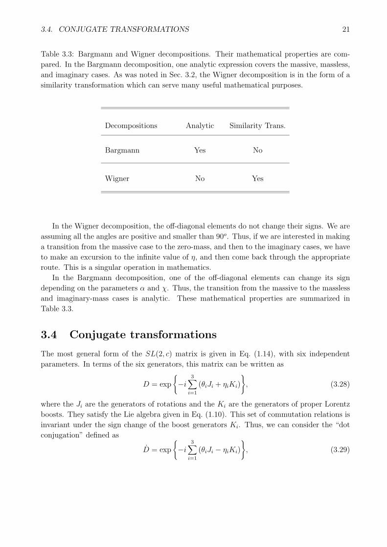
Table 3.3: Bargmann and Wigner decompositions. Their mathematical properties are com-
pared. In the Bargmann decomposition, one analytic expression covers the massive, massless,
and imaginary cases. As was noted in Sec. 3.2, the Wigner decomposition is in the form of a
similarity transformation which can serve many useful mathematical purposes.
Decompositions Analytic Similarity Trans.
Bargmann Yes No
Wigner No Yes
In the Wigner decomposition, the off-diagonal elements do not change their signs. We are
assuming all the angles are positive and smaller than 90o. Thus, if we are interested in making
a transition from the massive case to the zero-mass, and then to the imaginary cases, we have
to make an excursion to the infinite value of η, and then come back through the appropriate
route. This is a singular operation in mathematics.
In the Bargmann decomposition, one of the off-diagonal elements can change its sign
depending on the parameters α and χ. Thus, the transition from the massive to the massless
and imaginary-mass cases is analytic. These mathematical properties are summarized in
Table 3.3.
3.4 Conjugate transformations
The most general form of the SL(2, c) matrix is given in Eq. (1.14), with six independent
parameters. In terms of the six generators, this matrix can be written as
D = exp
{−i
3∑i=1
(θiJi + ηiKi)
}, (3.28)
where the Ji are the generators of rotations and the Ki are the generators of proper Lorentz
boosts. They satisfy the Lie algebra given in Eq. (1.10). This set of commutation relations is
invariant under the sign change of the boost generators Ki. Thus, we can consider the “dot
conjugation” defined as
D = exp
{−i
3∑i=1
(θiJi − ηiKi)
}, (3.29)
22CHAPTER 3. TWO-BY-TWO REPRESENTATIONS OFWIGNER’S LITTLE GROUPS
fig. (b) fig. (a)
fig. (d) fig. (c)
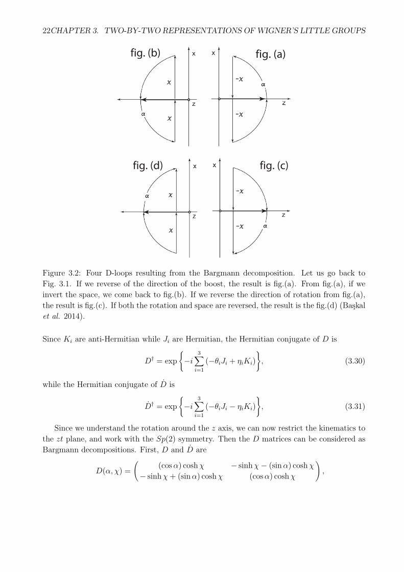
Figure 3.2: Four D-loops resulting from the Bargmann decomposition. Let us go back to
Fig. 3.1. If we reverse of the direction of the boost, the result is fig.(a). From fig.(a), if we
invert the space, we come back to fig.(b). If we reverse the direction of rotation from fig.(a),
the result is fig.(c). If both the rotation and space are reversed, the result is the fig.(d) (Baskal
et al. 2014).
Since Ki are anti-Hermitian while Ji are Hermitian, the Hermitian conjugate of D is
D† = exp
{−i
3∑i=1
(−θiJi + ηiKi)
}, (3.30)
while the Hermitian conjugate of D is
D† = exp
{−i
3∑i=1
(−θiJi − ηiKi)
}, (3.31)
Since we understand the rotation around the z axis, we can now restrict the kinematics to
the zt plane, and work with the Sp(2) symmetry. Then the D matrices can be considered as
Bargmann decompositions. First, D and D are
D(α, χ) =
((cosα) coshχ − sinhχ− (sinα) coshχ
− sinhχ+ (sinα) coshχ (cosα) coshχ
),

3.5. POLARIZATION OF MASSLESS NEUTRINOS 23
D(α, χ) =
((cosα) coshχ sinhχ− (sinα) coshχ
sinhχ+ (sinα) coshχ (cosα) coshχ
). (3.32)
These matrices correspond to the “D loops” given in fig.(a) and fig.(b) of Fig. 3.2 respectively.
The “dot” conjugation changes the direction of boosts. The dot conjugation leads to the
inversion of the space which is called the parity operation.
We can also consider changing the direction of rotations. This results in using the Hermi-
tian conjugates. We can write the Hermitian conjugate matrices as
D†(α, χ) =
((cosα) coshχ − sinhχ+ (sinα) coshχ
− sinhχ− (sinα) coshχ (cosα) coshχ
),
D†(α, χ) =
((cosα) coshχ sinhχ+ (sinα) coshχ
sinhχ− (sinα) coshχ (cosα) coshχ
). (3.33)
The exponential expressions from Eq. (3.28) to Eq. (3.31), lead to
D† = D−1, and D† = D−1, (3.34)
and the Bargmann forms of Eq. (3.32) and Eq. (3.33) are consistent with these relations.
The dot conjugation changes the direction of momentum, and the Hermitian conjugation
changes the direction of rotation and the angular momentum. The dot conjugation therefore
corresponds to the parity operation, and the Hermitian conjugation to charge conjugation.
3.5 Polarization of massless neutrinos
To apply this analysis to spin-12particles, we use the group generated by Eq. (1.13)
Ji =1
2σi, and Ki =
i
2σi. (3.35)
These are identical to those for the proper Lorentz group and have the same algebraic prop-
erties as the SL(2, c) group. Additionally, the Lie algebra for these generators is invariant if
the sign of the boost operators is changed. In the case of SL(2, c), or spin-12particles, it is
necessary to consider both signs. Also in Chapter 1, we considered that SL(2, c) consists of
non-singular two-by-two matrices which have the form defined in Eq. (1.14)
G =
(α β
γ δ
). (3.36)
This matrix is applicable to spinors that have the form:
U =
(1
0
), and V =
(0
1
), (3.37)

24CHAPTER 3. TWO-BY-TWO REPRESENTATIONS OFWIGNER’S LITTLE GROUPS
for spin-up and spin-down states respectively.
Among the subgroups of SL(2, c), there are E(2)-like little groups which correspond to
massless particles. If we consider a massless particle moving along the z direction, then the
little group is generated by J3, N1 and N2, defined in Eq. (2.10). These N operators are the
generators of gauge transformations in the case of the photon, thus we will refer to them as
the gauge transformation in the SL(2, c) regime (Wigner 1939, Han et al. 1982). We shall
examine their role with respect to massless particles of spin-12.
Since the sign of the generators of this subgroup remains invariant under a sign change in
Ki, these generators remain unambiguous when applied to the space-time coordinate variable
and the photon four-vectors. Here we choose the Ji to be the generators of rotations, but,
because of the sign change allowed for Ki we must consider both N(+)i and N
(−)i , where
N(+)1 =
(0 i
0 0
), N
(+)2 =
(0 1
0 0
). (3.38)
The Hermitian conjugates of the above provide N(−)1 and N
(−)2 . The transformation ma-
trices then can be written as:
D(+)(α, β) = exp(−i[αN [+]1 + βN
[+]2 ]) =
(1 α− iβ
0 1
),
D(−)(α, β) = exp(−i[αN [−]1 + βN
[−]2 ]) =
(1 0
−α− iβ 1
). (3.39)
Since there are two sets of spinors in SL(2, c), the spinors whose boosts are generated by
Ki = (i/2)σ will be written as u and v, following the usual Pauli notation. For the boosts
generated by Ki = (−i/2)σ we will use u and v. These spinors are gauge-invariant in the
sense that
D(+)(α, β)u = u, D(−)(α, β)v = v. (3.40)
However, these spinors are gauge-dependent in the sense that
D(+)(α, β)v = v + (α− iβ)u, D(−)(α, β)u = u− (α + iβ)v (3.41)
The gauge-invariant spinors of Eq. (3.40) appear as polarized neutrinos (Han et al. 1982,
1986). In the massless limit,
D(+)(α, β) =
(1 γ
0 1
),
D(−)(α, β) =
(1 0
−γ 1
). (3.42)
This is summarized in Table 3.4.
3.6. SCALARS, FOUR-VECTORS, AND FOUR-TENSORS 25
Table 3.4: Hermitian and dot conjugations of the triangular T (γ) matrix.
Original Dot conjugate
Original
(1 −γ0 1
) (1 0
γ 1
)
Hermitian conjugate
(1 0
−γ 1
) (1 γ
0 1
)
3.6 Scalars, four-vectors, and four-tensors
We are quite familiar with the process of constructing three spin-1 states and one spin-0 state
from two spinors. Since each spinor has two states, there are four states if combined.
In the Lorentz-covariant world, there are two-more states coming from the dotted repre-
sentation (Berestetskii 1982, Kim and Noz 1986), as we noted in Sec. 1.1. If four of those
two-state spinors are combined, there are 16 states. In this section, we shall construct all
sixteen states.
For particles at rest, it is known that the addition of two one-half spins result in spin-
zero and spin-one states. Hence, we have two different spinors behaving differently under the
Lorentz boost. Around the z direction, both spinors are transformed by
Z(ϕ) = exp (−iϕJ3) =(e−iϕ/2 0
0 eiϕ/2
). (3.43)
However, they are boosted by
B(η) = exp (−iηK3) =
(eη/2 0
0 e−η/2
),
B(η) = exp (iηK3),=
(e−η/2 0
0 eη/2
)(3.44)
applicable to the undotted and dotted spinors respectively. These two matrices commute with
each other, and also with the rotation matrix Z(ϕ) of Eq. (3.43). Since K3 and J3 commute
with each other, we can work with the matrix Q(η, ϕ) defined as
Q(η, ϕ) = B(η)Z(ϕ) =
(e(η−iϕ)/2 0
0 e−(η−iϕ)/2
),
Q(η, ϕ) = B(η)Z(ϕ) =
(e−(η+iϕ)/2 0
0 e(η+iϕ)/2
). (3.45)
26CHAPTER 3. TWO-BY-TWO REPRESENTATIONS OFWIGNER’S LITTLE GROUPS
When this combined matrix is applied to the spinors,
Q(η, ϕ)u = e(η−iϕ)/2u, Q(η, ϕ)v = e−(η−iϕ)/2v,
Q(η, ϕ)u = e−(η+iϕ)/2u, Q(η, ϕ)v = e(η+iϕ)/2v. (3.46)
If the particle is at rest, we can construct the combinations
uu,1√2(uv + vu), vv, (3.47)
to obtain the spin-1 state, and1√2(uv − vu), (3.48)
for the spin-zero state. There are four bilinear states. In the SL(2, c) regime, there are two
dotted spinors. If we include both dotted and undotted spinors, there are sixteen independent
bilinear combinations. They are given in Table 3.5. This table also gives the effect of the
operation of Q(η, ϕ).
Among the bilinear combinations given in Table 3.5, the following two equations are in-
variant under rotations and also under boosts.
S =1√2(uv − vu), and S = − 1√
2(uv − vu). (3.49)
They are thus scalars in the Lorentz-covariant world. Are they the same or different? Let us
consider the following combinations
S+ =1√2
(S + S
), and S− =
1√2
(S − S
). (3.50)
Under the dot conjugation, S+ remains invariant, but S− changes sign. The boost is performed
in the opposite direction and therefore is the operation of space inversion. Thus S+ is a scalar
while S− is called a pseudo-scalar.
3.6.1 Four-vectors
Let us consider the bilinear products of one dotted and one undotted spinor as uu, uv, uv, vv,
and construct the matrix
U =
(uv vv
uu vu
). (3.51)
Under the rotation Z(ϕ) and the boost B(η) they become(eηuv e−iϕvv
eiϕuu e−ηvu
). (3.52)
3.6. SCALARS, FOUR-VECTORS, AND FOUR-TENSORS 27
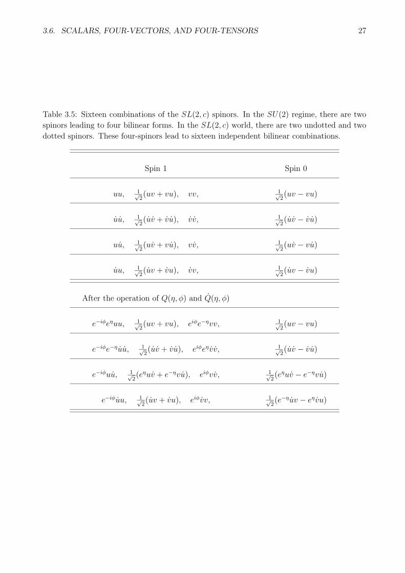
Table 3.5: Sixteen combinations of the SL(2, c) spinors. In the SU(2) regime, there are two
spinors leading to four bilinear forms. In the SL(2, c) world, there are two undotted and two
dotted spinors. These four-spinors lead to sixteen independent bilinear combinations.
Spin 1 Spin 0
uu, 1√2(uv + vu), vv, 1√
2(uv − vu)
uu, 1√2(uv + vu), vv, 1√
2(uv − vu)
uu, 1√2(uv + vu), vv, 1√
2(uv − vu)
uu, 1√2(uv + vu), vv, 1√
2(uv − vu)
After the operation of Q(η, ϕ) and Q(η, ϕ)
e−iϕeηuu, 1√2(uv + vu), eiϕe−ηvv, 1√
2(uv − vu)
e−iϕe−ηuu, 1√2(uv + vu), eiϕeηvv, 1√
2(uv − vu)
e−iϕuu, 1√2(eηuv + e−ηvu), eiϕvv, 1√
2(eηuv − e−ηvu)
e−iϕuu, 1√2(uv + vu), eiϕvv, 1√
2(e−ηuv − eηvu)
28CHAPTER 3. TWO-BY-TWO REPRESENTATIONS OFWIGNER’S LITTLE GROUPS
Indeed, this matrix is consistent with the transformation properties given in Table 3.5, and
transforms like the four-vector (t+ z x− iy
x+ iy t− z
). (3.53)
This form was given in Eq. (1.15). Under space inversion, this matrix becomes(t− z −(x− iy)
−(x+ iy) t+ z
). (3.54)
This space inversion is known as the parity operation.
The form of Eq. (3.51) for a particle or field with four-components, is given by (V0, Vz, Vx, Vy).
The two-by-two form of this four-vector is
U =
(V0 + Vz Vx − iVyVx + iVy V0 − Vz
). (3.55)
If boosted along the z direction, this matrix becomes(eη (V0 + Vz) Vx − iVyVx + iVy e−η (V0 − Vz)
). (3.56)
In the mass-zero limit, the four-vector matrix of Eq. (3.56) becomes(2A0 Ax − iAy
Ax + iAy 0
), (3.57)
with the Lorentz condition A0 = Az. The gauge transformation applicable to the photon
four-vector was discussed in detail in Sec. 2.3.
Let us go back to the matrix of Eq. (3.51); we can construct another matrix U . Since the
dot conjugation leads to the space inversion,
U =
(uv vv
uu vu
). (3.58)
Then
uv ≃ (t− z), vu ≃ (t+ z),
vv ≃ −(x− iy), uu ≃ −(x+ iy), (3.59)
where the symbol ≃ means “transforms like.”
Thus, U of Eq. (3.51) and U of Eq. (3.58) used up eight of the sixteen bilinear forms. Since
there are two bilinear forms in the scalar and pseudo-scalar as given in Eq. (3.50), we have to
give interpretations to the six remaining bilinear forms.
3.6. SCALARS, FOUR-VECTORS, AND FOUR-TENSORS 29
3.6.2 Second-rank Tensor
In this subsection, we are studying bilinear forms with both spinors dotted and undotted. In
Subsec. 3.6.1, each bilinear spinor consisted of one dotted and one undotted spinor. There are
also bilinear spinors which are both dotted or both undotted. We are interested in two sets
of three quantities satisfying the O(3) symmetry. They should therefore transform like
(x+ iy)/√2, (x− iy)/
√2, z, (3.60)
which are like
uu, vv, (uv + vu)/√2, (3.61)
respectively in the O(3) regime. Since the dot conjugation is the parity operation, they are
like
−uu, −vv, −(uv + vu)/√2. (3.62)
In other words,
(uu) = −uu, and (vv) = −vv. (3.63)
We noticed a similar sign change in Eq. (3.59).
In order to construct the z component in this O(3) space, let us first consider
fz =1
2[(uv + vu)− (uv + vu)] , gz =
1
2i[(uv + vu) + (uv + vu)] , (3.64)
where fz and gz are respectively symmetric and anti-symmetric under the dot conjugation or
the parity operation. These quantities are invariant under the boost along the z direction.
They are also invariant under rotations around this axis, but they are not invariant under
boost along or rotations around the x or y axis. They are different from the scalars given in
Eq. (3.49).
Next, in order to construct the x and y components, we start with f± and g± as
f+ =1√2(uu− uu) g+ =
1√2i
(uu+ uu)
f− =1√2(vv − vv) g− =
1√2i
(vv + vv) . (3.65)
Then
fx =1√2(f+ + f−) =
1
2[(uu− uu) + (vv − vv)]
fy =1√2i
(f+ − f−) =1
2i[(uu− uu)− (vv − vv)] . (3.66)
and
gx =1√2(g+ + g−) =
1
2i[(uu+ uu) + (vv + vv)]
gy =1√2i
(g+ − g−) = −1
2[(uu+ uu)− (vv + vv)] . (3.67)

30CHAPTER 3. TWO-BY-TWO REPRESENTATIONS OFWIGNER’S LITTLE GROUPS
Here fx and fy are symmetric under dot conjugation, while gx and gy are anti-symmetric.
Furthermore, fz, fx, and fy of Eqs. (3.64) and (3.66) transform like a three-dimensional
vector. The same can be said for gi of Eqs. (3.64) and (3.67). Thus, they can grouped into
the second-rank tensor
T =
0 −gz −gx −gygz 0 −fy fxgx fy 0 −fzgy −fx fz 0
, (3.68)
whose Lorentz-transformation properties are well known. The gi components change their
signs under space inversion, while the fi components remain invariant. They are like the
electric and magnetic fields respectively.
If the system is Lorentz-booted, fi and gi can be computed from Table 3.5. We are
now interested in the symmetry of photons by taking the massless limit. According to the
procedure developed in Sec. 3.2, we can keep only the terms which become larger for larger
values of η. Thus,
fx → 1
2(uu− vv) , fy →
1
2i(uu+ vv) ,
gx → 1
2i(uu+ vv) , gy → −1
2(uu− vv) , (3.69)
in the massless limit.
Then the tensor of Eq. (3.68) becomes
F =
0 0 −Ex −Ey
0 0 −By Bx
Ex By 0 0
Ey −Bx 0 0
, (3.70)
with
Bx ≃ 1
2(uu− vv) , By ≃
1
2i(uu+ vv) ,
Ex =1
2i(uu+ vv) , Ey = −1
2(uu− vv) . (3.71)
The electric and magnetic field components are perpendicular to each other. Furthermore,
Ex = By, Ey = −Bx. (3.72)
In order to address symmetry of photons, let us go back to Eq. (3.65). In the massless
limit,
B+ ≃ E+ ≃ uu, B− ≃ E− ≃ vv (3.73)
3.6. SCALARS, FOUR-VECTORS, AND FOUR-TENSORS 31
The gauge transformations applicable to u and v are the two-by-two matrices(1 −γ0 1
), and
(1 0
γ 1
). (3.74)
respectively as noted in Sec. 2.3 and Sec. 3.5. Both u and v are invariant under gauge
transformations, while u and v are not.
The B+ and E+ are for the photon spin along the z direction, while B− and E− are for
the opposite direction. Weinberg (Weinberg 1964) constructed gauge-invariant state vectors
for massless particles starting from Wigner’s 1939 paper (Wigner 1939). The bilinear spinors
uu and and vv correspond to Weinberg’s state vectors.
References
Baskal, S.; Kim, Y. S.; Noz, M. E. 2014. Wigner’s Space-Time Symmetries based on the Two-
by-Two Matrices of the Damped Harmonic Oscillators and the Poincare Sphere. Symmetry
6 473 - 515.
Bargmann, V. 1947. Irreducible unitary representations of the Lorentz group. Ann. Math. 48
568 - 640.
Berestetskii, V. B; Pitaevskii, L. P.; Lifshitz, E. M. 1982. Quantum Electrodynamics. Volume
4 of the Course of Theoretical Physics, 2nd Ed. Pergamon Press: Oxford, UK.
Han, D.; Kim, Y. S.; Son, D. 1982. E(2)-like little group for massless particles and polarization
of neutrinos. Phys. Rev. D 26 3717 - 3725.
Han, D.; Kim, Y. S.; Son, D. 1986. Photons, neutrinos, and gauge transformations. Am. J.
Phys. 54 818 - 821.
Kim, Y. S.; Noz, M. E. 1986. Theory and Applications of the Poincare Group. Reidel:
Dordrecht, The Netherlands.
Weinberg, S. 1964. Photons and gravitons in S-Matrix theory: Derivation of charge conser-
vation and equality of gravitational and inertial mass. Phys. Rev. 135 B1049 - B1056.
Wigner, E. 1939. On unitary representations of the inhomogeneous Lorentz group. Ann.
Math. 40 149 - 204.

32CHAPTER 3. TWO-BY-TWO REPRESENTATIONS OFWIGNER’S LITTLE GROUPS
Chapter 4
One little group with three branches
We have noted that J2 and K1 can serve as the starters of the representation of Wigner’s
little groups in their respective Wigner frames. They are for the massive and imaginary-mass
particles respectively. It was noted also that, when Lorentz boosted, they become
J ′2 = (cosh η)J2 − (sinh η)K1, K ′
1 = −(sinh η)J2 + (cosh η)K1. (4.1)
These two equations can be combined into one formula, and we are led to consider the trans-
formation matrix
D(x, y) = exp [−i (yJ2 − xK1)] (4.2)
as a function of the parameters x and y. We shall study this form of the Wigner matrix in
detail.
During this study, there will be a problem of handling singularities that are not too familiar
to us. We shall use the classical damped harmonic oscillator to study this singularity problem
in detail, and conclude that this is not an analytic but can be called a “tangential” continuity.
It was noted in Sec. 2.3 that a cylinder can be used for describing internal space-time
symmetry for photons. Later in this section, we shall study how this cylindrical symmetry
arises when the system of a massive particle is boosted along the z direction.
4.1 One expression with three branches
Let us write the D matrix of Eq. (4.2) as (Baskal and Kim 2010, 2013, Baskal et al. 2014)
D(x, y) = exp
{(0 −(x+ y)
−x+ y 0
)}. (4.3)
1. If y > x, we write
x+ y = eη√y2 − x2, x− y = e−η
√y2 − x2, (4.4)
33

34 CHAPTER 4. ONE LITTLE GROUP WITH THREE BRANCHES
with
eη =
√x+ y
|y − x|, (4.5)
and D(x, y) becomes
exp
{√y2 − x2
(0 −eηe−η 0
)}=
(cos(θ/2) −eη sin(θ/2)
e−η sin(θ/2) cos(θ/2)
), (4.6)
with cos(θ/2) = cos(√
y2 − x2).
2. If x = y, this expression becomes
D(x, y) = exp
{(0 −2x
0 0
)}=
(1 −2x
0 1
). (4.7)
This form is for the little group for massless particles, as shown in T (γ) of Eq. (3.10).
3. If y < x, we can write
x− y = e−η√x2 − y2, x+ y = eη
√x2 − y2. (4.8)
Then the D matrix becomes
exp
{√x2 − y2
(0 −eη
−e−η 0
)}=
(cosh(λ/2) −eη sinh(λ/2)
−e−η sinh(λ/2) cosh(λ/2)
), (4.9)
with
cosh(λ/2) = cosh(√
x2 − y2). (4.10)
This expression is the same as that for the Lorentz-boostedW matrix given in Eq. (3.21)
for imaginary-mass particles, and eη is given in Eq. (4.5).
Indeed, it is possible to derive three different forms of the W ′ matrix. The matrix(0 −(x+ y)
−(x− y) 0
)(4.11)
is analytic in the x and y variables. However, this D matrix has three distinct branches. In
order to understand the nature of this let us look at what happens when x − y is a small
number
ϵ = x− y. (4.12)
We can then write the D matrix as
D(x, ϵ) = exp
{(0 2x
ϵ 0
)}. (4.13)
4.2. CLASSICAL DAMPED OSCILLATORS 35
If ϵ is positive, the Taylor expansion leads to
D =
(cosh
(√2xϵ
)−[√
2x/ϵ]sinh
√2xϵ
−[√ϵ/2x
]sinh
(√2xϵ
)cosh
(√2xϵ
) ). (4.14)
If ϵ becomes zero, this expression becomes(1 −2x
0 1
)(4.15)
If ϵ becomes negative,
√2xϵ = i
√−2xϵ,
√ϵ/2x = i
√−2x/ϵ,
√2x/ϵ = −i
√−2x/ϵ, (4.16)
if we take√−1 = i. Thus, D becomes
D =
(cos
(√−2xϵ
)−[√
−2x/ϵ]sin
(√−2xϵ
)[√
−ϵ/2x]sin
(√−2xϵ
)cos
(√−2xϵ
) ). (4.17)
The result remains the same if we take√−1 = −i.
This type of singularity is not common in literature. Let us study this point further from
a physical example familiar to us.
4.2 Classical damped oscillators
Let us start with the second-order differential equation
d2y
dt2+ 2µ
dy
dt+ ω2y = 0, (4.18)
for a classical damped harmonic oscillator. If we introduce the function ψ(t) as
ψ(t) = e−µty(t) (4.19)
then ψ(t) satisfies the simplified differential equation
d2ψ(t)
dt2+ (ω2 − µ2)ψ(t) = 0. (4.20)
This second-order differential equation has two independent solutions. Let us call them
ψ1 and ψ2. They satisfy the first-order differential equations
d
dt
(ψ1
ψ2
)=
(0 −(ω + µ)
(ω − µ) 0
)(ψ1
ψ2
). (4.21)
This coupled equation leads to the second order equation Eq(4.20) for ψ1(t) and ψ2(t). The
physical solution is an appropriate linear combination of these two wave functions.
36 CHAPTER 4. ONE LITTLE GROUP WITH THREE BRANCHES
sine to sinh cosine to cosh
Figure 4.1: Transitions from sine to sinh, and from cosine to cosh . They are continuous
transitions. Their first derivatives are also continuous, but the second derivatives are not.
Thus, they are not analytically but only tangentially continuous (Baskal and Kim 2014).
The solution of this first order differential equation is
(ψ1
ψ2
)= exp
{(0 −(ω + µ)t
(ω − µ)t
)}(C1
C2
), (4.22)
where C1 = ψ1(0) and C2 = ψ2(0). We can then obtain the solutions by following the
procedure developed in Sec. 4.1.
1. If ω > µ, the solution becomes(ψ1
ψ2
)=
(cos(ω′t) −eη sin(ω′t)
e−η sin(ω′t) cos(ω′t)
)(C1
C2
), (4.23)
with
ω′ =√ω2 − µ2, and eη =
√ω + µ
|ω − µ|. (4.24)
2. If ω = µ, the solution becomes(ψ1
ψ2
)=
(1 −2ωt
0 1
)(C1
C2
). (4.25)
3. If µ > ω, the solution matrix becomes(cosh(µ′t) eη sinh(µ′t)
e−η sinh(µ′t) cosh(µ′t)
), (4.26)
with eη given in Eq. (4.24), and
µ′ =√µ2 − ω2. (4.27)

4.3. LITTLE GROUPS IN THE LIGHT-CONE COORDINATE SYSTEM 37
Let us now turn to the main issue of what happened when µ is close to ω. If ω is sufficiently
close to µ, we can let
µ− ω = 2µϵ, and µ+ ω = 2ω. (4.28)
If ω is greater than µ, then ϵ defined in Eq. (4.28) becomes negative. The solution matrix
becomes (1− (−ϵ/2)(2ωt)2 −2ωt
−(−ϵ)(2ωt) 1− (−ϵ/2)(2ωt)2
), (4.29)
which can be written as 1− (1/2)[(2ω
√−ϵ)t]2
−2ωt
−√−ϵ
[(2ω
√−ϵ)t]
1− (1/2)[(2ω
√−ϵ)t]2 . (4.30)
If ϵ is positive, Eq. (4.26) can be written as(1 + (1/2) [(2ω
√ϵ) t]
2 −2ωt
−√ϵ [(2ω
√ϵ) t] 1 + (1/2) [(2ω
√ϵ) t]
2
). (4.31)
The transition from Eq. (4.30) to Eq. (4.31) is continuous as they become identical when
ϵ = 0. As ϵ changes its sign, the diagonal elements of above matrices tell us how cos(ω′t)
becomes cosh(µ′t). The upper-right element remains as sin(ω′t) during this transitional pro-
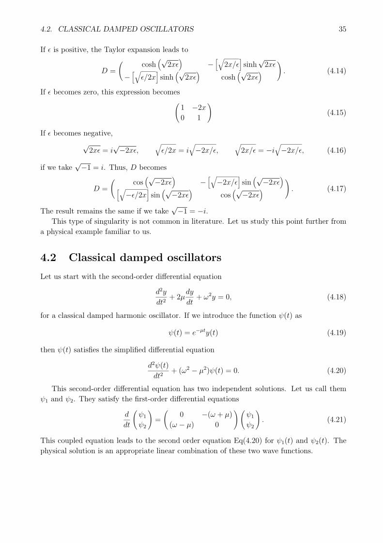
cess. The lower left element becomes sinh(µ′t). This non-analytic continuity is illustrated in
Fig. 4.1.
During this continuation process, the function remains the same. So does its first deriva-
tive, but the second derivative does not. Thus, the two functions share the same tangential
line. It is indeed a tangential coninuity. The continuity from one little group to another was
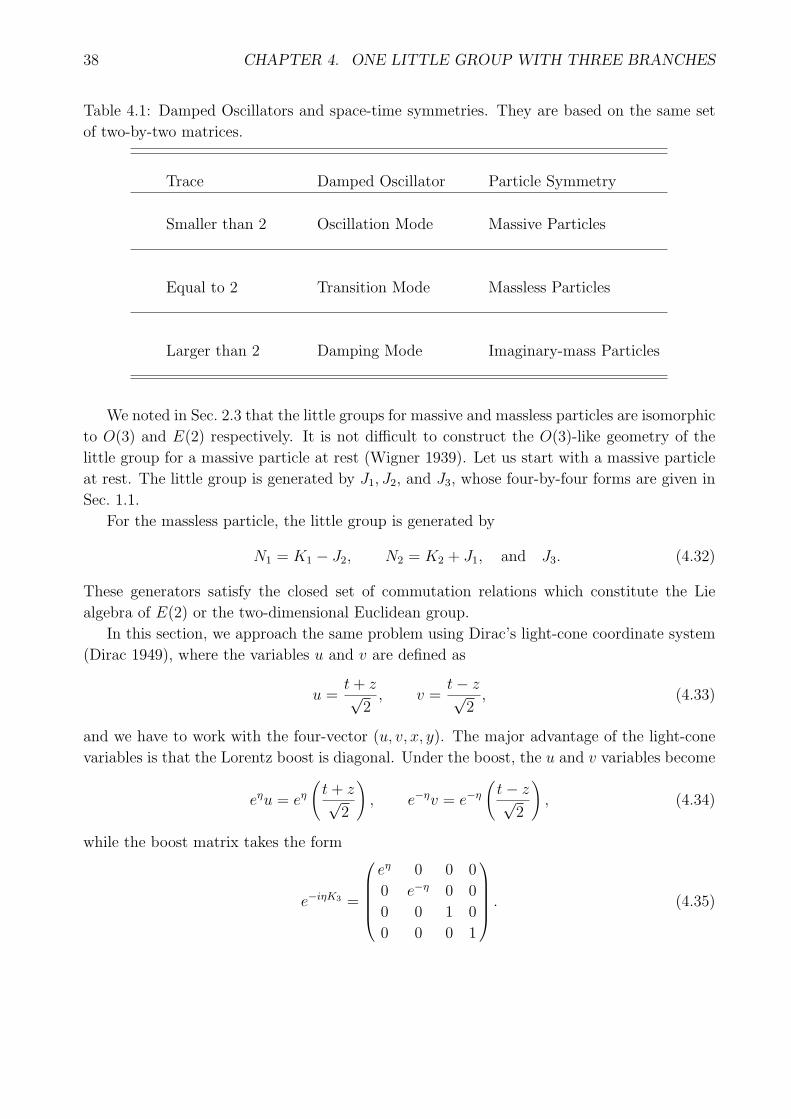
discussed in Sec. 4.1. This mathematical similarity is summarized in Table 4.1.
4.3 Little groups in the light-cone coordinate system
Speaking of tangential continuity, it was Inonu and Wigner (Inonu and Wigner 1953) who
first considered that the E(2) (two-dimensional Euclidean) group can be constructed as a
contraction of the O(3) group, by considering a flat plane tangential to a sphere. This is
very easy to visualize. A football field is clearly a flat two-dimensional surface, but it is also
part of the surface of the spherical earth. Thus, the E(2) group can be constructed as a
contraction of the O(3) group, by considering a flat plane tangential to a sphere. Hence, E(2)
can be constructed from O(3) in the large-radius limit. For convenience, we can choose a
plane tangent to the north pole.
For the same sphere, we can consider also a cylinder tangent to the equatorial belt. We
shall consider that the four-by-four representation of the Lorentz group can produce both the
E(2) and the cylindrical symmetries. This aspect is illustrated in fig.(a) of Fig. 4.2.
38 CHAPTER 4. ONE LITTLE GROUP WITH THREE BRANCHES
Table 4.1: Damped Oscillators and space-time symmetries. They are based on the same set
of two-by-two matrices.
Trace Damped Oscillator Particle Symmetry
Smaller than 2 Oscillation Mode Massive Particles
Equal to 2 Transition Mode Massless Particles
Larger than 2 Damping Mode Imaginary-mass Particles
We noted in Sec. 2.3 that the little groups for massive and massless particles are isomorphic
to O(3) and E(2) respectively. It is not difficult to construct the O(3)-like geometry of the
little group for a massive particle at rest (Wigner 1939). Let us start with a massive particle
at rest. The little group is generated by J1, J2, and J3, whose four-by-four forms are given in
Sec. 1.1.
For the massless particle, the little group is generated by
N1 = K1 − J2, N2 = K2 + J1, and J3. (4.32)
These generators satisfy the closed set of commutation relations which constitute the Lie
algebra of E(2) or the two-dimensional Euclidean group.
In this section, we approach the same problem using Dirac’s light-cone coordinate system
(Dirac 1949), where the variables u and v are defined as
u =t+ z√
2, v =
t− z√2, (4.33)
and we have to work with the four-vector (u, v, x, y). The major advantage of the light-cone
variables is that the Lorentz boost is diagonal. Under the boost, the u and v variables become
eηu = eη(t+ z√
2
), e−ηv = e−η
(t− z√
2
), (4.34)
while the boost matrix takes the form
e−iηK3 =
eη 0 0 0
0 e−η 0 0
0 0 1 0
0 0 0 1
. (4.35)

4.3. LITTLE GROUPS IN THE LIGHT-CONE COORDINATE SYSTEM 39
fig. (a)
fig. (b)
Figure 4.2: Contractions of the three-dimensional rotation group. This group can be illus-
trated by a sphere. This group can become the two-dimensional Euclidean group on a plane
tangent at the north pole as illustrated in fig.(a). It was later noted that there is a cylinder
tangential to this sphere, and the up and down translations on this cylinder correspond to
the gauge transformation for photons (Kim and Wigner 1987). As illustrated in fig.(b), the
four-dimensional representation of the Lorentz group contains both elongation and contraction
of the z axis, as the system is boosted along this direction. The elongation and contraction
become the cylindrical and Euclidean groups, respectively (Kim and Wigner 1987, 1990).
In the light-cone coordinate system, the generators take the form
J3 =
0 0 0 0
0 0 0 0
0 0 0 −i0 0 i 0
, K3 =
i 0 0 0
0 −i 0 0
0 0 0 0
0 0 0 0
,
J1 =1√2
0 0 0 i
0 0 0 i
0 0 0 0
−i −i 0 0
, K1 =1√2
0 0 i 0
0 0 −i 0
i −i 0 0
0 0 0 0
,
J2 =1√2
0 0 −i 0
0 0 −i 0
i i 0 0
0 0 0 0
, K2 =1√2
0 0 0 i
0 0 0 −i0 0 0 0
i −i 0 0
. (4.36)
(4.37)

40 CHAPTER 4. ONE LITTLE GROUP WITH THREE BRANCHES
If a massive particle is at rest, its little group is generated by J1, J2, in addition to J3. For
a massless particle moving along the z direction, the little group is generated by N1, N2 and
J3, where
N1 = K1 − J2, N2 = K2 + J1, (4.38)
which can be written as
N1 =
0 0 i 0
0 0 0 0
0 −i 0 0
0 0 0 0
, N2 =
0 0 0 i
0 0 0 0
0 0 0 0
0 −i 0 0
. (4.39)
For convenience, we have dropped the normalization factor of√2.
These matrices satisfy the commutation relations:
[J3, N1] = iN2, [J3, N2] = −iN1, [N1, N2] = 0. (4.40)
The transformation generated by the N1 and N2 matrices is
D(γ, ϕ) = exp {−iγ [(cosϕ)N1 + (sinϕ)N2]}. (4.41)
Since N31 = N3
2 = 0, the Taylor expansion of this exponential form truncates, and it becomes1 γ2/2 γ cosϕ γ sinϕ
0 1 0 0
0 −γ cosϕ 1 0
0 −γ sinϕ 0 1
. (4.42)
In the light-cone coordinate system, the four components of the vector particle takes the
form
(A+, A−, Ax, Ay) exp {i (p+v + p+u)}, (4.43)
with
A+ =A0 + Az√
2, A− =
A0 − Az√2
. (4.44)
Thus, for massless photons, the Lorentz condition leads to A0 = Az or A− = 0 . When the D
matrix is applied to this photon four-vector,1 γ2/2 γ cosϕ γ sinϕ
0 1 0 0
0 −γ cosϕ 1 0
0 −γ sinϕ 0 1
A+
0
Ax
Ay
=
A+ + γ(Ax cosϕ+ Ay sinϕ)
0
Ax
Ay
, (4.45)
the transverse components Ax and Ay are not affected. The transformation changes only the
A0 and Az components. This is a gauge transformation.
This cylindrical transformation has been discussed in Sec. 2.3. The light-cone coordinate
system gives a more transparent mathematics. Indeed, this coordinate system is the natural
language for the photon internal symmetry.

4.4. LORENTZ COMPLETION IN THE LIGHT-CONE COORDINATE SYSTEM 41
4.4 Lorentz completion in the light-cone coordinate sys-
tem
As was noted in Sec. 4.3, the matrix for the Lorentz boost is diagonal in the light-cone
coordinate system. Let us start with the four-vector for a massive particle
V = (V+, V−, Vx, Vy) . (4.46)
If the particle is at rest, this should represent the three-dimensional symmetry, with three
independent coordinate variables. This means V+ = V− in the light-cone coordinate system.
If we boost the system, this four-vector becomes(eηV+, e
−ηV−, Vx, Vy). (4.47)
For large values of η, the e−ηV− component vanishes. In the language of photons, it is called
the Lorentz condition or A0 = Az. The interesting problem is what happens between those
two limits.
To study this problem we can start with two spheres, both with the unit horizontal radius.
One of them has the vertical radius eη and the other with e−η. Since
eη =
[√p2 +m2 + p√p2 +m2 − p
]1/2, (4.48)
this expression is one when the particle is at rest with p = 0. In the limit of large values of p,
this number is infinite, while e−η becomes zero.
As p increases, both go through elliptic deformations as illustrated in fig.(b) of Fig. 4.2. In
the large-η limit, one of them becomes a cylinder, and the other a flat surface. This picture
is equivalent to the tangential plane and cylinder described in fig.(a) of Fig. 4.2.
References
Baskal, S.; Kim, Y. S. 2010. One analytic form for four branches of the ABCD matrix. J.
Mod. Opt. 57 1251 - 1259.
Baskal, S.; Kim, Y. S. 2013. Lorentz Group in Ray and Polarization Optics. Chapter 9 in
”Mathematical Optics: Classical, Quantum and Computational Methods” edited by Va-
sudevan Lakshminarayanan, Maria L. Calvo, and Tatiana Alieva, CRC Taylor and Francis:
Boca Raton, FL. pp 303 - 349.
Baskal, S.; Kim Y.S. 2014. Lens Optics and the continuity problems of the ABCD matrix J.
Mod. Optics, 61, 161 - 166.
Baskal, S.; Kim, Y. S.; Noz, M. E. 2014. Wigner’s Space-Time Symmetries based on the Two-
by-Two Matrices of the Damped Harmonic Oscillators and the Poincare Sphere. Symmetry
6 473 - 515.
42 CHAPTER 4. ONE LITTLE GROUP WITH THREE BRANCHES
Dirac, P. A. M. 1949. Forms of relativistic dynamics. Rev. Mod. Phys. 21 392 - 399.
Inonu, E.; Wigner, E. P. 1953. On the contraction of groups and their representations. Proc.
Natl. Acad. Sci. USA 39 510 - 524.
Kim, Y. S.; Wigner, E. P. 1987. Cylindrical group and massless particles. J. Math. Phys. 28
1175 - 1179.
Kim, Y. S.; Wigner, E. P. 1990. Space-time geometry of relativistic-particles. J. Math. Phys.
31 55 - 60.
Wigner, E. 1939. On unitary representations of the inhomogeneous Lorentz group. Ann.
Math. 40 149 - 204.

Chapter 5
Lorentz-covariant harmonic oscillators
Einstein and Bohr met occasionally, before and after 1927, to discuss physics. Einstein was
interested in how things look to moving observers, while Bohr was interested in why the energy
levels of the hydrogen atom are discrete. Then they must have talked about how the electron
orbit of the hydrogen atom looks to a moving observer. There does not seem to be written
records to indicate how they sketched the orbits.
However, it is not uncommon to see in the literature the description of the Lorentz defor-
mation as described in Fig. 5.1. This figure became outdated in 1927. The electron orbit is
now a standing wave. Thus, the question is how the standing wave appears when the it is
boosted along a given direction.
As is indicated in Fig. 5.1, the longitudinal component is affected while the transverse
components remain unchanged. With this point in mind, we shall study harmonic oscillators.
Since the wave equation for the three-dimensional oscillator is separable in the Cartesian coor-
dinate system, it is sufficient to study the effect of the Lorentz boost only for the longitudinal
component of the wave function.
Paul A. M. Dirac spent many years trying to construct a quantum mechanics consistent
with special relativity. In his three papers published in 1927, 1945, and 1949 (Dirac 1927, 1945,
1949), Dirac essentially presented all essential ideas on how to construct harmonic oscillator
wave functions that can be Lorentz transformed. However, Dirac’s most serious problem was
the lack of physical phenomena to which his ideas were applicable. The physical example
did not exist until Gell-Mann published his paper on the quark model in 1964 (Gell-Mann
1964), where the proton was described as a bound state of three quarks. The proton can be
accelerated to speeds very close to that of light.
Dirac (Dirac 1949) said that the problem of Lorentz covariant quantum mechanics is the
same as that of constructing a representation of the Poincare group. Thus, he was telling
us to construct the representation based on harmonic oscillators. Since the standing wave is
for a bound state, its symmetry is that of Wigner’s little group which dictates the internal
space-time symmetry (Wigner 1939).
Indeed, the most serious problem in Dirac’s paper is that he did not specify the standing
43

44 CHAPTER 5. LORENTZ-COVARIANT HARMONIC OSCILLATORS
Longitudinal Axis
contracted to
Figure 5.1: Classical picture of Lorentz contraction of the electron orbit in the hydrogen
atom. It is expected that the longitudinal component becomes contracted while the transverse
components are not affected. In his the first edition of his book published in 1987, 60 years
after 1927, John S. Bell included this picture of the orbit viewed by a moving observer (Bell
2004). While talking about quantum mechanics in his book, Bell overlooked the fact that
the electron orbit in the hydrogen atom had been replaced by a standing wave in 1927. The
question then is how standing waves look to moving observers.
wave as a bound state. This problem was clarified later in the paper of Feynman, Kislinger,
and Ravndal (Feynman et al. 1971). They start with a system of two quarks bound together
by a harmonic oscillator force, and write down a Lorentz-invariant differential equation. This
differental equation has many different forms of solutions. It is possible to construct a set of
solutions which constitute a representation of Wigner’s little group. We shall thus start with
the Lorentz-invariant differential equation of Feynman et al.
5.1 Dirac’s plan to construct Lorentz-covariant quan-
tum mechanics
The year 1927 is known for Heisenberg’s uncertainty relation. In the same year, based on the
line width and lifetime of excited energy levels, Paul A. M. Dirac formulated his c-number
time energy uncertainty relation (Dirac 1927).
During World War II, Dirac was looking into the possibility of constructing representations
of the Lorentz group using harmonic oscillator wave functions (Dirac 1945). The Lorentz group
is the language of special relativity, and the present form of quantum mechanics starts with
harmonic oscillators. Therefore, he was interested in making quantum mechanics Lorentz
covariant by constructing representations of the Lorentz group using harmonic oscillators.
In his 1945 paper (Dirac 1945), Dirac considers the Gaussian form
exp{−1
2
(x2 + y2 + z2 + t2
)}. (5.1)
We note that this Gaussian form is in the (x, y, z, t) coordinate variables. Thus, if we
consider a Lorentz boost along the z direction, we can drop the x and y variables, and write

5.2. DIRAC’S FORMS OF RELATIVISTIC DYNAMICS 45
t
z
T-E Uncertainty
without Excitations
Heisenberg’s
Uncetainty with
Excitations
Dirac (1927)
t
z
Gaussian
Cut-o!Dirac (1945)
Figure 5.2: Space-time picture of quantum mechanics. In 1927, Dirac noted that there is an
uncertainty in the time and energy variables, but there are no excitations along the time axis.
He called it the “c-number” time-energy relation. In 1945, Dirac attempted to construct a
reprsentation of the Lorentz group using harmonic oscillator wave functions. According to his
1927 paper, the Gaussian cut-off along the time axis represents the time-energy uncertainty
relation. His c-number relation means that only the ground state is allowed along the time
axis (Kim and Noz 1986).
the above equation as
exp{−1
2
(z2 + t2
)}. (5.2)
This is a strange expression for those who believe in Lorentz invariance where (z2 − t2) is an
invariant quantity.
On the other hand, this expression is consistent with his earlier papers on the time-energy
uncertainty relation (Dirac 1927). In those papers, Dirac observed that there is a time-energy
uncertainty relation, while there are no excitations along the time axis.
Let us look at Fig. 5.2 carefully. This figure is a pictorial representation of Dirac’s Eq. (5.2),
with localization in both space and time coordinates. Then Dirac’s fundamental question
would be how this figure appears to a moving observer.
5.2 Dirac’s forms of relativistic dynamics
In 1949, the Reviews of Modern Physics published a special issue to celebrate Einstein’s 70th
birthday. This issue contains Dirac’s paper entitled “Forms of Relativistic Dynamics” (Dirac
1949). In this paper, Dirac points out problems that have to be overcome in extending
quantum mechanics to be relativistic. He considers possible constraints that can be imposed
on the Lorentz transformations.
1. In this paper also, Dirac’s main problem was to deal with the time variable, and he
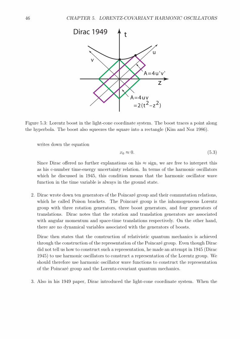
46 CHAPTER 5. LORENTZ-COVARIANT HARMONIC OSCILLATORS
A=4u'v '
u
v
A=4uv
=2(t2–z
2)
z
tDirac 1949
Figure 5.3: Lorentz boost in the light-cone coordinate system. The boost traces a point along
the hyperbola. The boost also squeezes the square into a rectangle (Kim and Noz 1986).
writes down the equation
x0 ≈ 0. (5.3)
Since Dirac offered no further explanations on his ≈ sign, we are free to interpret this
as his c-number time-energy uncertainty relation. In terms of the harmonic oscillators
which he discussed in 1945, this condition means that the harmonic oscillator wave
function in the time variable is always in the ground state.
2. Dirac wrote down ten generators of the Poincare group and their commutation relations,
which he called Poison brackets. The Poincare group is the inhomogeneous Lorentz
group with three rotation generators, three boost generators, and four generators of
translations. Dirac notes that the rotation and translation generators are associated
with angular momentum and space-time translations respectively. On the other hand,
there are no dynamical variables associated with the generators of boosts.
Dirac then states that the construction of relativistic quantum mechanics is achieved
through the construction of the representation of the Poincare group. Even though Dirac
did not tell us how to construct such a representation, he made an attempt in 1945 (Dirac
1945) to use harmonic oscillators to construct a representation of the Lorentz group. We
should therefore use harmonic oscillator wave functions to construct the representation
of the Poincare group and the Lorentz-covariant quantum mechanics.
3. Also in his 1949 paper, Dirac introduced the light-cone coordinate system. When the
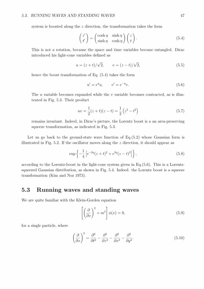
5.3. RUNNING WAVES AND STANDING WAVES 47
system is boosted along the z direction, the transformation takes the form(z′
t′
)=
(cosh η sinh η
sinh η cosh η
)(z
t
). (5.4)
This is not a rotation, because the space and time variables become entangled. Dirac
introduced his light-cone variables defined as
u = (z + t)/√2, v = (z − t)/
√2, (5.5)
hence the boost transformation of Eq. (5.4) takes the form
u′ = eηu, v′ = e−ηv. (5.6)
The u variable becomes expanded while the v variable becomes contracted, as is illus-
trated in Fig. 5.3. Their product
uv =1
2(z + t)(z − t) =
1
2
(z2 − t2
)(5.7)
remains invariant. Indeed, in Dirac’s picture, the Lorentz boost is a an area-preserving
squeeze transformation, as indicated in Fig. 5.3.
Let us go back to the ground-state wave function of Eq.(5.2) whose Gaussian form is
illustrated in Fig. 5.2. If the oscillator moves along the z direction, it should appear as
exp{−1
4
[e−2η(z + t)2 + e2η(z − t)2
]}, (5.8)
according to the Lorentz-boost in the light-cone system given in Eq.(5.6). This is a Lorentz-
squeezed Gaussian distribution, as shown in Fig. 5.4. Indeed. the Lorentz boost is a squeeze
transformation (Kim and Noz 1973).
5.3 Running waves and standing waves
We are quite familiar with the Klein-Gorden equation( ∂
∂x
)2
+m2
ϕ(x) = 0, (5.9)
for a single particle, where (∂
∂x
)2
=∂2
∂t2− ∂2
∂z2− ∂2
∂x2− ∂2
∂y2. (5.10)
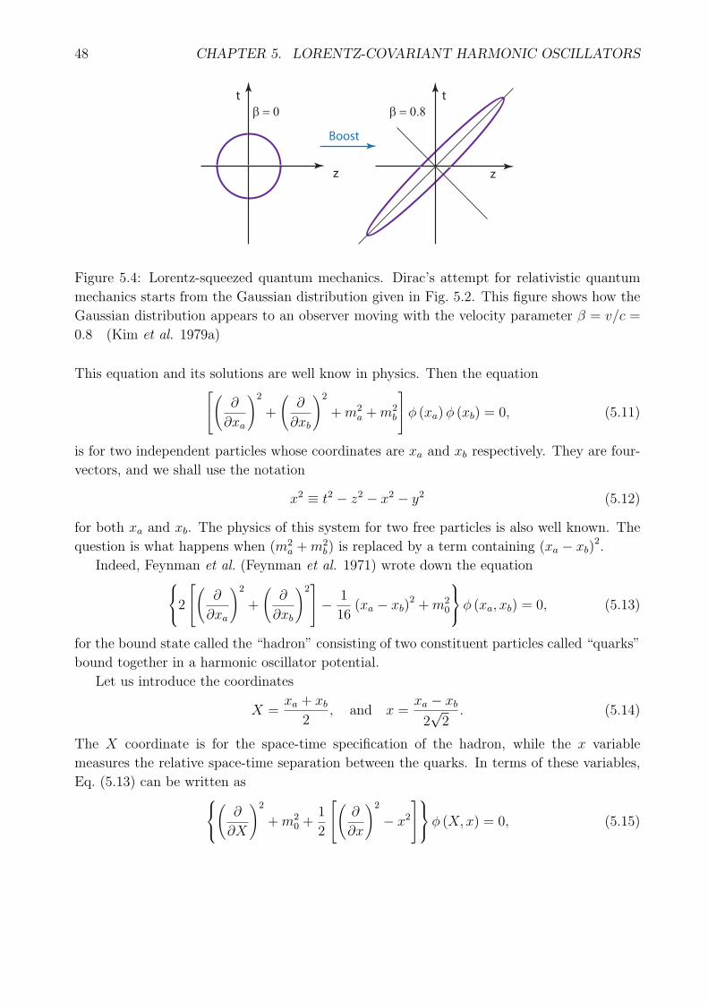
48 CHAPTER 5. LORENTZ-COVARIANT HARMONIC OSCILLATORS
t
z
t
z
β = 0.8
Boost
β = 0
Figure 5.4: Lorentz-squeezed quantum mechanics. Dirac’s attempt for relativistic quantum
mechanics starts from the Gaussian distribution given in Fig. 5.2. This figure shows how the
Gaussian distribution appears to an observer moving with the velocity parameter β = v/c =
0.8 (Kim et al. 1979a)
This equation and its solutions are well know in physics. Then the equation( ∂
∂xa
)2
+
(∂
∂xb
)2
+m2a +m2
b
ϕ (xa)ϕ (xb) = 0, (5.11)
is for two independent particles whose coordinates are xa and xb respectively. They are four-
vectors, and we shall use the notation
x2 ≡ t2 − z2 − x2 − y2 (5.12)
for both xa and xb. The physics of this system for two free particles is also well known. The
question is what happens when (m2a +m2
b) is replaced by a term containing (xa − xb)2.
Indeed, Feynman et al. (Feynman et al. 1971) wrote down the equation2( ∂
∂xa
)2
+
(∂
∂xb
)2− 1
16(xa − xb)
2 +m20
ϕ (xa, xb) = 0, (5.13)
for the bound state called the “hadron” consisting of two constituent particles called “quarks”
bound together in a harmonic oscillator potential.
Let us introduce the coordinates
X =xa + xb
2, and x =
xa − xb
2√2. (5.14)
The X coordinate is for the space-time specification of the hadron, while the x variable
measures the relative space-time separation between the quarks. In terms of these variables,
Eq. (5.13) can be written as(∂
∂X
)2
+m20 +
1
2
( ∂
∂x
)2
− x2
ϕ (X, x) = 0, (5.15)
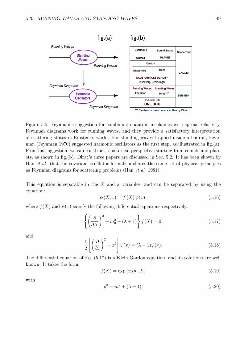
5.3. RUNNING WAVES AND STANDING WAVES 49
Figure 5.5: Feynman’s suggestion for combining quantum mechanics with special relativity.
Feynman diagrams work for running waves, and they provide a satisfactory interpretation
of scattering states in Einstein’s world. For standing waves trapped inside a hadron, Feyn-
man (Feynman 1970) suggested harmonic oscillators as the first step, as illustrated in fig.(a).
From his suggestion, we can construct a historical perspective starting from comets and plan-
ets, as shown in fig.(b). Dirac’s three papers are discussed in Sec. 5.2. It has been shown by
Han et al. that the covariant oscillator formalism shares the same set of physical principles
as Feynman diagrams for scattering problems (Han et al. 1981).
This equation is separable in the X and x variables, and can be separated by using the
equation:
ϕ (X, x) = f (X)ψ(x), (5.16)
where f(X) and ψ(x) satisfy the following differential equations respectively:(∂
∂X
)2
+m20 + (λ+ 1)
f(X) = 0, (5.17)
and1
2
( ∂
∂x
)2
− x2
ψ(x) = (λ+ 1)ψ(x). (5.18)
The differential equation of Eq. (5.17) is a Klein-Gordon equation, and its solutions are well
known. It takes the form
f(X) = exp (±ip ·X) (5.19)
with
p2 = m20 + (λ+ 1), (5.20)
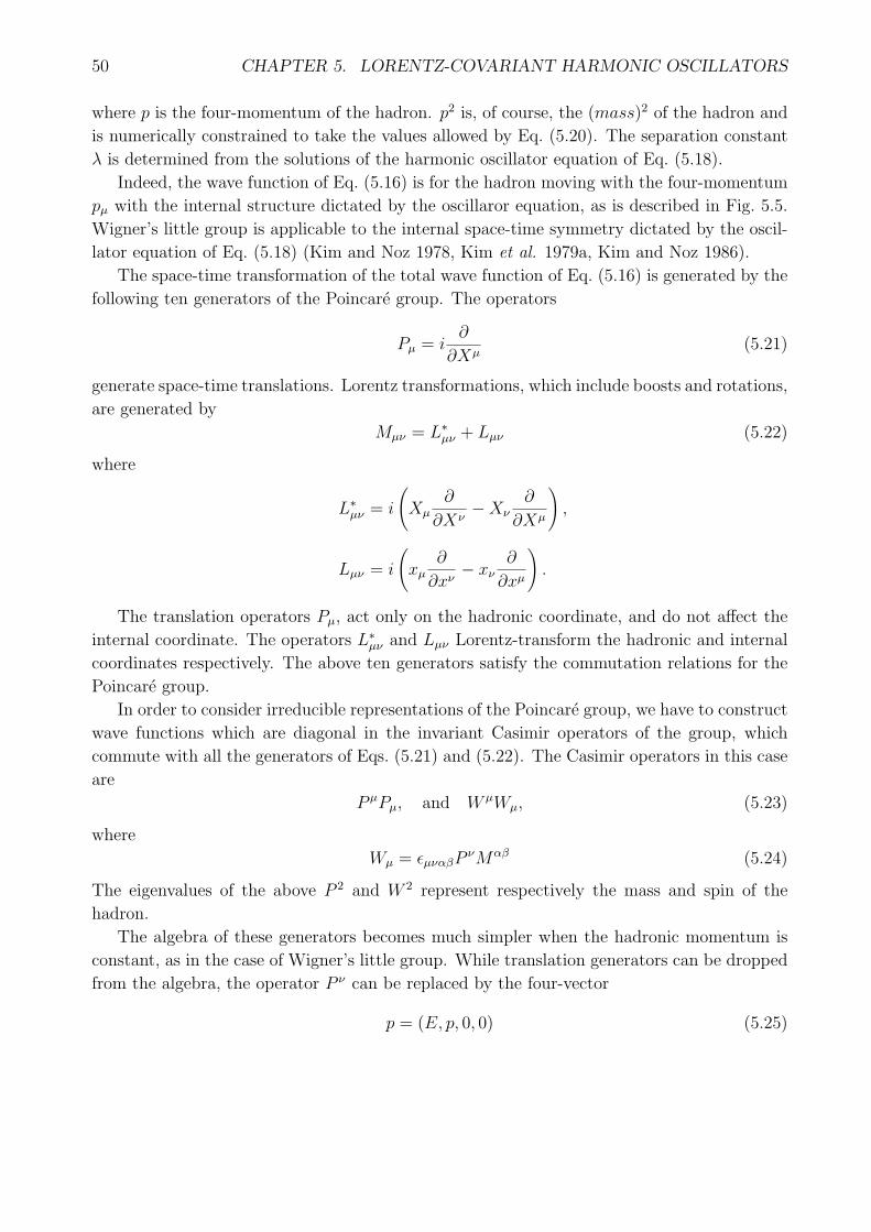
50 CHAPTER 5. LORENTZ-COVARIANT HARMONIC OSCILLATORS
where p is the four-momentum of the hadron. p2 is, of course, the (mass)2 of the hadron and
is numerically constrained to take the values allowed by Eq. (5.20). The separation constant
λ is determined from the solutions of the harmonic oscillator equation of Eq. (5.18).
Indeed, the wave function of Eq. (5.16) is for the hadron moving with the four-momentum
pµ with the internal structure dictated by the oscillaror equation, as is described in Fig. 5.5.
Wigner’s little group is applicable to the internal space-time symmetry dictated by the oscil-
lator equation of Eq. (5.18) (Kim and Noz 1978, Kim et al. 1979a, Kim and Noz 1986).
The space-time transformation of the total wave function of Eq. (5.16) is generated by the
following ten generators of the Poincare group. The operators
Pµ = i∂
∂Xµ(5.21)
generate space-time translations. Lorentz transformations, which include boosts and rotations,
are generated by
Mµν = L∗µν + Lµν (5.22)
where
L∗µν = i
(Xµ
∂
∂Xν−Xν
∂
∂Xµ
),
Lµν = i
(xµ
∂
∂xν− xν
∂
∂xµ
).
The translation operators Pµ, act only on the hadronic coordinate, and do not affect the
internal coordinate. The operators L∗µν and Lµν Lorentz-transform the hadronic and internal
coordinates respectively. The above ten generators satisfy the commutation relations for the
Poincare group.
In order to consider irreducible representations of the Poincare group, we have to construct
wave functions which are diagonal in the invariant Casimir operators of the group, which
commute with all the generators of Eqs. (5.21) and (5.22). The Casimir operators in this case
are
P µPµ, and W µWµ, (5.23)
where
Wµ = ϵµναβPνMαβ (5.24)
The eigenvalues of the above P 2 and W 2 represent respectively the mass and spin of the
hadron.
The algebra of these generators becomes much simpler when the hadronic momentum is
constant, as in the case of Wigner’s little group. While translation generators can be dropped
from the algebra, the operator P ν can be replaced by the four-vector
p = (E, p, 0, 0) (5.25)
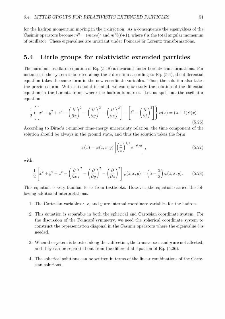
5.4. LITTLE GROUPS FOR RELATIVISTIC EXTENDED PARTICLES 51
for the hadron momentum moving in the z direction. As a consequence the eigenvalues of the
Casimir operators becomem2 = (mass)2 andm2ℓ(ℓ+1), where ℓ is the total angular momenum
of oscillator. These eigenvalues are invariant under Poincare or Lorentz transformations.
5.4 Little groups for relativistic extended particles
The harmonic oscillator equation of Eq. (5.18) is invariant under Lorentz transformations. For
instance, if the system is boosted along the z direction according to Eq. (5.4), the differential
equation takes the same form in the new coordinate variables. Thus, the solution also takes
the previous form. With this point in mind, we can now study the solution of the diffential
equation in the Lorentz frame where the hadron is at rest. Let us spell out the oscillator
equation.
1
2
x2 + y2 + z2 −
(∂
∂x
)2
−(∂
∂y
)2
−(∂
∂z
)2−
t2 − (∂
∂t
)2ψ(x) = (λ+ 1)ψ(x).
(5.26)
According to Dirac’s c-number time-energy uncertainty relation, the time component of the
solution should be always in the ground state, and thus the solution takes the form
ψ(x) = φ(z, x, y)
[(1
π
)1/4
e−t2/2
], (5.27)
with
1
2
x2 + y2 + z2 −(∂
∂x
)2
−(∂
∂y
)2
−(∂
∂z
)2φ(z, x, y) = (
λ+3
2
)φ(z, x, y). (5.28)
This equation is very familiar to us from textbooks. However, the equation carried the fol-
lowing additional interpretations.
1. The Cartesian variables z, x, and y are internal coordinate variables for the hadron.
2. This equation is separable in both the spherical and Cartesian coordinate system. For
the discussion of the Poincare symmetry, we need the spherical coordinate system to
construct the representation diagonal in the Casimir operators where the eigenvalue ℓ is
needed.
3. When the system is boosted along the z direction, the transverse x and y are not affected,
and they can be separated out from the differential equation of Eq. (5.26).
4. The spherical solutions can be written in terms of the linear combinations of the Carte-
sian solutions.

52 CHAPTER 5. LORENTZ-COVARIANT HARMONIC OSCILLATORS
The solution in the spherical coordinate system should take the form
φ(r, θ, ϕ) = Rnℓm(r)Yℓm(θ, ϕ), (5.29)
where Yℓm(θ, ϕ) are the spherical harmonics. The radial function Rnℓm(r) is well defined, but
its explicit form is not readily available in the literature. It should take the form
Rnℓm(r) = rmgnℓ(r)e−r2/2, (5.30)
with
gnℓ =∑k
a2kr2k, (5.31)
wherea2k+2
a2k=
2(λ− ℓ− 2k)
ℓ(ℓ+ 1)− (ℓ+ 2k + 3)(ℓ+ 2k + 2). (5.32)
For large values of k, this ratio becomes 1/k, which is like the expansion of the exponential
exp (r2) leading the radial function of Eq. (5.30) to increase as exp (r2/2). Thus the series has
to be truncated with
λ = 2k + ℓ. (5.33)
The first term a0 in the series is determined by the normalization condition∫ ∞
0[rRnℓm(r)]
2 dr = 1. (5.34)
The increases in ℓ and n are called the orbital and radial excitations in the literature.
If the system is Lorentz-boosted along the z direction according to Eq. (5.4), the Lorentz-
invariant differential equation of Eq. (5.18) remains invariant. The z and t variables in
Eq. (5.26) become z′ and t′ respectively, and the wave function becomes modified accord-
ingly. The important point is that the eigenvalue λ remains invariant.
5.5 Further properties of covariant oscillator wave func-
tions
Since the x and y coordinates are not affected, we drop their terms from the differential
equation from Eq. (5.18), and consider the equation
1
2
z2 − (
∂
∂z
)2−
t2 − (∂
∂t
)2ψ(z, t) = λψ(z, t). (5.35)
The solution of this equation should take the form
ψn0 (z, t) =
[1
π2nn!
]1/2Hn(z) exp
[−1
2
(z2 + t2
)], (5.36)

5.5. FURTHER PROPERTIES OF COVARIANT OSCILLATOR WAVE FUNCTIONS 53
where Hn(z) is the Hermite polynomial of order n.
The differential equation of Eq. (5.35) is invariant under the Lorentz boost along the z
direction, and is invariant under the replacements of z and t by z′ and t′ respectively, where(z′
t′
)=
(cosh η − sinh η
− sinh η cosh η
)(z
t
). (5.37)
This is the inverse of the transformation given in Eq. (5.4). We thus achieve the Lorentz boost
of the wave function by writing
ψnη (z, t) = ψn
0 (z′, t′)
=[
1
π2nn!
]1/2Hn(z
′) exp[−1
2
(z′2 + t′2
)]. (5.38)
It is possible to expand this in terms of the functions of z and t variables (Ruiz 1974, Kim et
al. 1979b, Kim and Noz 1986, Rotbart 1981), and the result is
ψnη (z, t) =
(1
cosh η
)(n+1)∑k
[(n+ k)!
n!k!
]1/2(tanh η)kχn+k(z)χk(t), (5.39)
where χn(z) is the nth excited state oscillator wave function which takes the familiar form
χn(z) =
[1√π2nn!
]1/2Hn(z) exp
(−z2
2
). (5.40)
If n = 0, this formula becomes simplified to (Ruiz 1974)
ψ0η(z, t) =
(1
cosh η
)1/2∑k
(tanh η)kχk(z)χk(t). (5.41)
This formula plays an important role also in squeezed states of light (Yuen 1976) and also in
continuous-variable entanglement (Giedke et al. 2003, Dodd and Halliwell 2004, Braunstein
and van Loock 2005, Adesso and Illuminati 2007, Paz and Roncaglia 2008, Chou et al. 2008,
Xiang et al. 2011).
According to the Gaussian form of Eq.(5.8), the ground-state wave function of Eq. (5.41)
takes the form (Kim and Noz 1973)
ψ0η(z, t) =
(1
π
)1/2
exp{−1
4
[e−2η(z + t)2 + e2η(z − t)2
]}. (5.42)
This is precisely the formula for Dirac’s picture of the Lorentz squeeze, as illustrated in Fig. 5.2.
Relativity and quantum mechanics are the two most important physical theories developed
in the 20th century. Thus, the most pressing issue in modern physics is to make quantum me-
chanics consistent with special relativity and then with general relativity. Since the harmonic
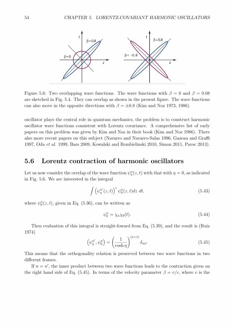
54 CHAPTER 5. LORENTZ-COVARIANT HARMONIC OSCILLATORS
Figure 5.6: Two overlapping wave functions. The wave functions with β = 0 and β = 0.08
are sketched in Fig. 5.4. They can overlap as shown in the present figure. The wave functions
can also move in the opposite directions with β = ±0.8 (Kim and Noz 1973, 1986).
oscillator plays the central role in quantum mechanics, the problem is to construct harmonic
oscillator wave functions consistent with Lorentz covariance. A comprehensive list of early
papers on this problem was given by Kim and Noz in their book (Kim and Noz 1986). There
also more recent papers on this subject (Navarro and Navarro-Salas 1996, Gazeau and Graffi
1997, Oda et al. 1999, Bars 2009, Kowalski and Rembielinski 2010, Simon 2011, Pavsc 2013).
5.6 Lorentz contraction of harmonic oscillators
Let us now consider the overlap of the wave function ψnη (z, t) with that with η = 0, as indicated
in Fig. 5.6. We are interested in the integral∫ (ψn′
η (z, t))∗ψn0 (z, t)dz dt, (5.43)
where ψn0 (z, t), given in Eq. (5.36), can be written as
ψn0 = χnχ0(t). (5.44)
Then evaluation of this integral is straight-foward from Eq. (5.39), and the result is (Ruiz
1974) (ψn′
η , ψn0
)=
(1
cosh η
)(n+1)
δnn′ (5.45)
This means that the orthogonality relation is preserved between two wave functions in two
different frames.
If n = n′, the inner product between two wave functions leads to the contraction given on
the right hand side of Eq. (5.45). In terms of the velocity parameter β = v/c, where v is the

5.6. LORENTZ CONTRACTION OF HARMONIC OSCILLATORS 55
Figure 5.7: Orthogonality relations for covariant oscillator wave functions. The harmonic
oscillator can be excited and can also be Lorentz boosted as illustrated in fig.(a). The orthog-
onality relations remain invariant under Lorentz boosts, and their inner products have the
Lorentz-contraction property given in fig.(b) (Ruiz 1974, Kim and Noz 1986).
hadronic velocity,1
cosh η=√1− β2. (5.46)
This expression is more familar to us, and the right-hand side of Eq. (5.45) is
(√1− β2
)(n+1)
. (5.47)
For the ground-state wave function with n = 0, it is like the Lorentz contraction of a rigid
body. For the first excited state, it is like an additional rod. This is not surprising in view
of the fact that the excited states are obtained through application of the step-up operator.
The nth excited state |n > can be written as
1√n!
(a†)n
|0 >, (5.48)
The additional contraction factor√1− β2 comes from the step-up operator.
If the value of η in one of the wave functions is replaced by nonzero value η′, cosh η in
Eq. (5.39) should become cosh(η − η′). Of particular interest is the case with η′ = −η, asshown in Fig.(5.6). In this case, this is an overlap of two wave functions moving in the opposite
directions, and the contaction factor is
(1
cosh(2η)
)(n+1)
, (5.49)
56 CHAPTER 5. LORENTZ-COVARIANT HARMONIC OSCILLATORS
which, in the language of β, becomes
(1− β2
1 + β2
)(n+1)
. (5.50)
Based on these orthogonality and contraction properties, it appears possible to give a quan-
tum probability interpretation to the covariant harmonic oscillator in the Lorentz-covariant
world as shown in Fig.(5.7). On the other hand, these wave functions contain the time sepa-
ration variable between the constituent particles. What is the meaning of the distribution in
terms of this variable, which is thoroughly hidden (Kim and Noz 2003) in the present form of
quatum mechanics? In order clarify this issue, let us examine the concept of Feynman’s rest
of the universe.
5.7 Feynman’s rest of the universe
As was noted in the previous section, the time-separation variable has an important role in
the covariant formulation of the harmonic oscillator wave functions. It should exist wherever
the space separation exists. The Bohr radius is the measure of the separation between the
proton and electron in the hydrogen atom. If this atom moves, the radius picks up the time
separation, according to Einstein.
On the other hand, the present form of quantum mechanics does not include this time-
separation variable. The best way we can interpret it at the present time is to treat this time
separation as a variable in Feynman’s rest of the universe (Han at al. 1999). In his book on
statistical mechanics (Feynman 1972), Feynman states
When we solve a quantum-mechanical problem, what we really do is divide the
universe into two parts - the system in which we are interested and the rest of
the universe. We then usually act as if the system in which we are interested
comprised the entire universe. To motivate the use of density matrices, let us see
what happens when we include the part of the universe outside the system.
The failure to include what happens outside the system results in an increase of entropy.
The entropy is a measure of our ignorance and is computed from the density matrix (von
Neumann 1932). The density matrix is needed when the experimental procedure does not an-
alyze all relevant variables to the maximum extent consistent with quantum mechanics (Fano
1957). If we do not take into account the time-separation variable, the result is an increase in
entropy (Kim and Wigner 1990, Kim and Noz 2014).
For the covariant oscillator wave functions defined in Eq. (5.38), the pure-state density
matrix is
ρnη (z, t; z′, t′) = ψn
η (z, t)ψnη (z
′, t′), (5.51)

5.7. FEYNMAN’S REST OF THE UNIVERSE 57
which satisfies the condition ρ2 = ρ :
ρnη (z, t; x′, t′) =
∫ρnη (z, t; x”, t”)ρ
nη (z”, t”; z
′, t′)dz”dt”. (5.52)
However, in the present form of quantum mechanics, it is not possible to take into account
the time separation variables. Thus, we have to take the trace of the matrix with respect to
the t variable. Then the resulting density matrix is
ρnη (z, z′) =
∫ψnη (z, t)ψ
nη (z
′, t)dt
=
(1
cosh η
)2(n+1)∑k
(n+ k)!
n!k!(tanh η)2kψn+k(z)ψ
∗n+k(z
′). (5.53)
The trace of this density matrix is one, but the trace of ρ2 is less than one, as
Tr(ρ2)=∫ρnη (z, z
′)ρnη (z′, z)dzdz′
=
(1
cosh η
)4(n+1)∑k
[(n+ k)!
n!k!
]2(tanh η)4k, (5.54)
which is less than one. This is due to the fact that we do not know how to deal with the
time-like separation in the present formulation of quantum mechanics. Our knowledge is less
than complete.
The standard way to measure this ignorance is to calculate the entropy defined as
S = −Tr (ρ ln(ρ)) . (5.55)
If we pretend to know the distribution along the time-like direction and use the pure-state
density matrix given in Eq. (5.51), then the entropy is zero. However, if we do not know how
to deal with the distribution along t, then we should use the density matrix of Eq. (5.53) to
calculate the entropy, and the result is
S = (n+ 1){(cosh η)2 ln(cosh η)2 − (sinh η)2 ln(sinh η)2
}
−(
1
cosh η
)2(n+1)∑k
(n+ k)!
n!k!ln
[(n+ k)!
n!k!
](tanh η)2k. (5.56)
In terms of the velocity paramter β of the hadron,
tanh η = β =v
c, (5.57)
and
S = −(n+ 1)
{ln(1− β2
)+β2 ln β2
1− β2
}
−(1− β2
)(n+1)∑k
(n+ k)!
n!k!ln
[(n+ k)!
n!k!
]β2k. (5.58)
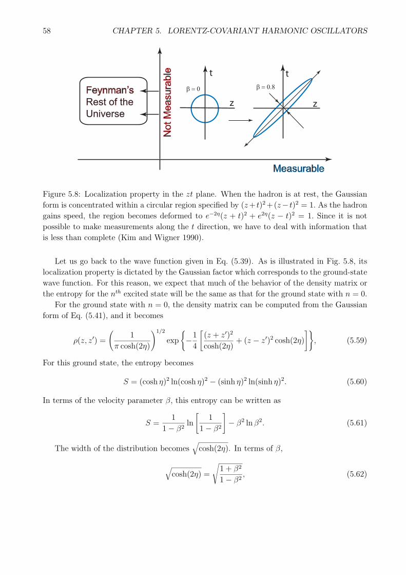
58 CHAPTER 5. LORENTZ-COVARIANT HARMONIC OSCILLATORS
z
t t
z
β = 0.8β = 0
MeasurableN
ot M
ea
su
rab
le
Feynman’s
Rest of the
Universe
Figure 5.8: Localization property in the zt plane. When the hadron is at rest, the Gaussian
form is concentrated within a circular region specified by (z+ t)2+(z− t)2 = 1. As the hadron
gains speed, the region becomes deformed to e−2η(z + t)2 + e2η(z − t)2 = 1. Since it is not
possible to make measurements along the t direction, we have to deal with information that
is less than complete (Kim and Wigner 1990).
Let us go back to the wave function given in Eq. (5.39). As is illustrated in Fig. 5.8, its
localization property is dictated by the Gaussian factor which corresponds to the ground-state
wave function. For this reason, we expect that much of the behavior of the density matrix or
the entropy for the nth excited state will be the same as that for the ground state with n = 0.
For the ground state with n = 0, the density matrix can be computed from the Gaussian
form of Eq. (5.41), and it becomes
ρ(z, z′) =
(1
π cosh(2η)
)1/2
exp
{−1
4
[(z + z′)2
cosh(2η)+ (z − z′)2 cosh(2η)
]}, (5.59)
For this ground state, the entropy becomes
S = (cosh η)2 ln(cosh η)2 − (sinh η)2 ln(sinh η)2. (5.60)
In terms of the velocity parameter β, this entropy can be written as
S =1
1− β2ln
[1
1− β2
]− β2 ln β2. (5.61)
The width of the distribution becomes√cosh(2η). In terms of β,
√cosh(2η) =
√1 + β2
1− β2, (5.62)

5.7. FEYNMAN’S REST OF THE UNIVERSE 59
Entropy Uncertainty
Figure 5.9: Entropy and uncertainty in the Lorentz-covariant system. The horizontal axis
measures β in both graphs. The formulas for the entropy and uncertainty are given in
Eq. (5.60) and Eq. (5.65) respectively. These quantites arise from our ignorance about the
time-separation variable, which is hidden in the present form of quantum mechanics (Kim and
Noz 2014).
Figure 5.10: The uncertainty from the hidden time-separation coordinate. The small circle
indicates the minimal uncertainty when the hadron is at rest. More uncertainty is added when
the hadron moves. This is illustrated by a larger circle. The radius of this circle increases by√cosh(2η) (Kim and Noz 2014) .

60 CHAPTER 5. LORENTZ-COVARIANT HARMONIC OSCILLATORS
which becomes very large as β → 1, as is illustrated in Fig. 5.9
The time-separation variable exists in the Lorentz-covariant world, but we pretend not to
know about it. It thus is in Feynman’s rest of the universe. If we do not measure this time
separation, it becomes translated into the entropy.
We can see the uncertainty in our measurement process from the Wigner function defined
as (Wigner 1932, Kim and Noz 1991)
W (z, q) =1
π
∫ρ(z + y, z − y)e2iqydy. (5.63)
After integration, this Wigner function becomes
W (z, q) =1
π cosh(2η)exp
{−(z2 + q2
cosh(2η)
)}. (5.64)
We use here q instead of p for the momentum conjugate to z. The notation p has been used
for the hadronic momentum.
This Wigner phase-space distribution is illustrated in Fig. 5.10. The smaller inner circle
corresponds to the minimal uncertainty of the single oscillator. The larger circle is for the
total uncertainty including the statistical uncertainty from our failure to observe the time-
separation variable. The larger radius is
√cosh(2η) =
√1 + β2
1− β2. (5.65)
The behavior of this radius is illustrated in Fig. 5.9. This radius takes the minimum value of
one when β = 0, and increases rapidly when β becomes close to one.
References
Adesso, G.; Illuminati, F. 2007. Entanglement in continuous-variable systems: recent advances
and current perspectives. J. Phys. A 40 7821 - 7880.
Bars, I. 2009. Relativistic harmonic oscillator revisited. Phys. Rev. D 79 045009-1 - 045009-
22.
Bell, J. S. 2004. Speakable and Unspeakable in Quantum Mechanics: Collected Papers on
Quantum Philosophy. 2nd Ed. Cambridge University Press: Cambridge, UK.
Braunstein, S. L.; van Loock, P. 2005. Quantum information with continuous variables. Rev.
Mod. Phys. 28 513 - 676.
Chou, Chung-Hsien; Yu, Ting; Hu, B. L. 2008. Exact master equation and quantum deco-
herence of two coupled harmonic oscillators in a general environment. Phys. Rev. E 77
011112-1 - 011112-18.
Dirac, P. A. M. 1927. The Quantum Theory of the Emission and Absorption of Radiation.
Proc. Roy. Soc. (London) A114 243 - 265.

5.7. FEYNMAN’S REST OF THE UNIVERSE 61
Dirac, P. A. M. 1945. Unitary Representations of the Lorentz Group. Proc. Roy. Soc.
(London) A183 284 - 295.
Dirac, P. A. M. 1949. Forms of relativistic dynamics. Rev. Mod. Phys. 21 392 - 399.
Dodd, P. J.; Halliwell, J. J. 2004. Disentanglement and decoherence by open system dynamics.
Phys. Rev. A 69 052105 -1 - 052105 - 6.
Fano, U. 1957. Description of States in Quantum Mechanics by Density Matrix and Operator
Techniques. Rev. Mod. Phys. 29 74-93.
Feynman, R. P. 1970. Relativistic quark model. talk given at the April Meeting of the
American Physical Society, Washington, DC, U.S.A.
Feynman, R. P.; Kislinger, M.; Ravndal F. 1971. Current Matrix Elements from a Relativistic
Quark Model. Phys. Rev. D 3 2706 - 2732.
Feynman, R. P. 1972. Statistical Mechanics. Benjamin Cummings: Boston, MA.
Gazeau, J. P.; Graffi, S. 1997 Quantum harmonic oscillator: a relativistic and statistical point
of view. Bollett. Unione Mat. Italiana 11A 815 - 839.
Gell-Mann M. 1964. A Schematic Model of Baryons and Mesons. Phys. Lett. 8 214 - 215.
Giedke, G.; Wolf, M. M.; Krueger, O; Werner, R. F.; Cirac, J. J. 2003. Entanglement of
formation for symmetric Gaussian states. Phys. Rev. Lett. 91 107901 - 107904.
Han, D.; Kim, Y. S.; Noz, M. E. 1981. Physical Principles in Quantum Field Theory and in
Covariant Harmonic Oscillator Formalism. Foundations of Physics 11 895 - 903.
Han, D.; Kim, Y. S.; Noz, M. E. 1999. Illustrative example of Feynman’s rest of the universe.
Am. J. Phys. 67 61 - 66.
Kim, Y. S.; Noz, M. E. 1973. Covariant Harmonic Oscillators and the Quark Model. Phys.
Rev. D. 8 3521 - 3526.
Kim, Y. S.; Noz, M. E. 1978. Group-Theory of Covariant Harmonic Oscillators. Am. J.
Phys. 46 480 - 483.
Kim, Y. S.; Noz, M. E.; Oh, S. H. 1979a. Representations of the Poincare group for relativistic
extended hadrons. J. Math. Phys. 20 1341 - 1344; see also: Physics Auxiliary Publication
Service, Document No. PAPS JMAPA-20-1336-12.
Kim, Y. S.; Noz, M. E.; Oh, S. H. 1979b, A Simple Method for Illustrating the Difference
between the Homogeneous and Inhomogeneous Lorentz Groups. Am. J. Phys. 47 892 -
897.
Kim, Y. S.; Noz, M. E. 1986. Theory and Applications of the Poincare Group. Reidel:
Dordrecht, The Netherlands.
Kim, Y. S.; Wigner, E. P. 1990. Entropy and Lorentz Transformations. Phys. Lett. A 147
343 - 347.
Kim, Y. S.; Noz, M. E. 2003. Feynman’s Decoherence. Optics and Spectroscopy 47 733 - 740.
Kim, Y. S.; Noz, M. E. 2005. Coupled oscillators, entangled oscillators, and Lorentz-covariant
Oscillators. J. Optics B: Quantum and Semiclassical 7 S459 - S467.
Kim, Y. S.; Noz, M. E. 2014. Entropy and Temperature from Entangled Space and Time.
Phys. Sci. Int. J. 4 1015 - 1039.

62 CHAPTER 5. LORENTZ-COVARIANT HARMONIC OSCILLATORS
Kowalski, K.; Rembielinski, J. 2010. Relativistic massless harmonic oscillator. Phys. Rev. A
81 012118 -1 012118 - 6.
Navarro, D. J; Navarro-Salas, J. 1996. Special-relativistic harmonic oscillator modeled by
Klein-Gordon theory in anti-de Sitter space. J. Math. Phys. 37 6060 - 6073.
Oda, M.; Ishida, M.; Ishida, S. 1999. Exclusive semi-leptonic decays of heavy mesons in the
covariant oscillator quark model. Prog. of Theor. Phys. 101 1285 - 1311.
Pavsc, M. 2013. Pais-Uhlenbeck oscillator with a benign friction force. Phys. Rev. D 87
107502 -1 - 107502 - 3.
Paz, P. J.; Roncaglia, A. J. 2008. Dynamics of the Entanglement between Two Oscillators in
the Same Environment. Phys. Rev. Lett. 100 220401-1 - 220401-4.
Rotbart, F.C. 1981. Complete orthogonality relations for the covariant harmonic oscillator.
Phys.Rev.D 12 3078 - 3090.
Ruiz, M. J. 1974. Orthogonality relations for covariant harmonic oscillator wave functions.
Phys. Rev. D 10 4306 - 4307.
Simon, D. S. 2011. Supersymmetry and duality in relativistic oscillator systems. Phys. Lett.
A 375 3751 - 3754.
von Neumann, J. 1932. Die mathematische Grundlagen der Quanten-mechanik. Springer-
Verlag: Berlin, Germany. See also von Neumann, J. 1955. Mathematical Foundation of
Quantum Mechanics. Princeton University Press: Princeton, NJ.
Wigner, E. 1932. On the Quantum Corrections for Thermodynamic Equilibrium. Phys. Rev.
40 749-759.
Xiang, S. H.; Song, K. H.; Wen, W.; Shi, Z. G. 2011. Entanglement behaviors of two-mode
squeezed thermal states in two different environments. Euro. Phys. J. D 62 289 - 296.
Yuen, H. P. 1976. Two-photon coherent states of the radiation field. Phys. Rev. A 13 2226 -
2243.
Chapter 6
Quarks and partons in the
Lorentz-covariant world
Since the time of Einstein and Bohr, there has been an evolution of the way in which we look
at quantum bound states, as illustrated in Fig. 6.1. The evolution took place in the following
three steps.
1. The energy levels of the hydrogen atom played the pivotal role by replacing the electron
orbit of the hydrogen atom with a standing wave, leading to bound states in quantum
mechanics. However, the hydrogen atom cannot play a role in the Lorentz covariant
world since it cannot be accelerated to a relativistic speed.
2. 1964, the proton became a bound state of the more fundamental constituents called
“quarks” (Gell-mann 1964). Of course, the proton is different from the hydrogen atom,
but inherits the same quantum mechanics from the hydrogen atom. Unlike the hydrogen
atom, the proton can be accelerated, and its speed can become very close to that of light.
Thus, it is possible to study the quantum mechanics of the hydrogen atom or bound
states in the Lorentz-covariant world by studying the proton in the quark model. Fig. 6.1
illustrates this transition.
3. In 1969, Feynman observed that the proton, when it moves with a velocity close to
that of light, appears like a collection of partons with a wide-spread momentum dis-
tribution (Feynman 1969). Partons are like free particles. Quarks and partons are
the same particles but they appear differently to observers in two different reference
frames. Therefore, there must be a Lorentz-covariant model for quantum bound states,
as illustrated in Fig. 6.2.
At the time of Einstein and Bohr, both the proton and electron were regarded as point
particles. However, the discovery of Hofstadter and McAllister changed our picture of the
proton (Hofstadter and McAllister 1955). The proton charge has an internal distribution.
63

64 CHAPTER 6. QUARKS AND PARTONS IN THE LORENTZ-COVARIANT WORLD
Bohr
Gell-Mann
Feynm
an
Quarks
Proton
Electron
Partons
Evolution of the
Hydrogen Atom
Figure 6.1: Evolution of the hydrogen atom. The electron orbit was replaced by a standing
wave, but the hydrogen atom cannot not be accelerated. In 1964, the proton as a bound state
inherited the quantum mechanics of the hydrogen atom (Gell-mann 1964). The proton these
days can move with a speed very close to that of light and exhibits the properties of quantum
bound states in the Lorentz-covariant world.
Figure 6.2: Two distinct ways in which the proton appears in the real world. If the proton is
at rest, it appears as a bound state of three quarks (Gell-mann 1964). If it moves with a speed
close to that of light, it appears like a collection of an infinite number of partons (Feynman
1969). Then the question is whether quarks and partons are two different manifestations of
the same Lorentz-covariant entity.

6.1. LORENTZ-COVARIANT QUARK MODEL 65
Within the framework of quantum electrodynamics, it is possible to calculate the Rutherford
formula for electron-proton scattering when both electron and proton are point particles.
Because the proton is not a point particle, there is a deviation from the Rutherford formula.
We describe this deviation as the “proton form factor” which depends on the momentum
transfer during electron-proton scattering.
Indeed, the study of the proton form factor has been and still is one of the central issues in
high-energy physics. The proton form factor decreases as the momentum transfer increases.
Its behavior is called the “dipole cut-off” meaning an inverse-square decrease, and it has been
a challenging problem in quantum field theory and other theoretical models (Frazer and Fulco
1960). Since the emergence of the quark model in 1964 (Gell-Mann 1964), the hadrons are
regarded as quantum bound states of quarks with space-time extensions.
Furthermore, the hadronic mass spectra indicate that the binding force between the quarks
is like that of the harmonic oscillator (Feynman et al. 1971). This leads us to suspect that
the quark model with harmonic oscillator wave functions could explain the behavior of the
proton form factor. There are indeed many papers written on this subject. We shall return
to this problem in Sec. 6.4.
Another problem in high-energy physics is Feynman’s parton picture (Feynman 1969). If
the hadron is at rest, we can approach this problem within the framework of bound-state
quantum mechanics. If it moves with a speed close to that of light, it appears as a collection
of an infinite number of partons, which interact with external signals incoherently. This phe-
nomenon raises the question of whether the Lorentz boost destroysquantum coherence (Kim
1998).
6.1 Lorentz-covariant quark model
In the quark model, mesons are two-body bound states of one quark and one anti-quark, and
baryons are bound states of three quarks. The early successes of the quark model include
the ratio of the proton-neutron electromagnetic potential and magnetic moments (Beg et
al. 1964). Also the hadronic mass spectra are like those of three-dimensional harmonic
oscillators (Feynman et al. 1971).
The question then is how the mass spectrum calculated within the framework of non-
relativistic quantum mechanics is valid for this relativistic case, while ignoring the time-
separation variable. For this question, the answer given in the 1971 paper of Feynman et
al. is not satisfactory. The correct answer to this question is that Wigner’s little group for
massive particles is like the three-dimensional rotation group as was spelled out in Chapter 2
and in Chapter 5. The role of the time-separation variable is discussed there.
Our original question is how the hydrogen atom looks to a moving observer. The question
now is how much we can learn about this Bohr-Einstein issue by studying the proton in the
quark model based on the three-dimensional harmonic oscillator. For the hydrogen atom, we

66 CHAPTER 6. QUARKS AND PARTONS IN THE LORENTZ-COVARIANT WORLD
use the Coulomb potential, while the binding force between quarks is that of the oscillator.
The point is that those two different potentials share the same quantum mechanics.
For this purpose, we will need a bound-state wave function which can be Lorentz-boosted.
Here the natural choice is the harmonic oscillator wave function discussed in Chapter 5. We
can start with the ground-state wave function which can be Lorentz boosted. Since the
harmonic oscillator wave function is separable in the Cartesian coordinate system, we can
leave out the transverse components of the wave function, and consider only the longitudinal
and time-like coordinates. For this purpose, let us rewrite the wave function of Eq. (5.42) as
ψη(z, t) =1√πexp
{−1
4
[(e2η(z + t)2 + e−2η(z − t)2
)]}, (6.1)
which becomes
ψη(z, t) =1√πexp
{−1
2
[(z2 + t2
)]}, (6.2)
for η = 0.
6.2 Feynman’s parton picture
Let us go back to the two-body problem and discuss what happens to the wave function
when the proton is Lorentz-boosted. For this system, we have discussed the Lorentz-squeeze
problem in Sec. 5.2.
It is a widely accepted view that hadrons are quantum bound states of quarks having a
localized probability distribution. As in all bound-state cases, this localization condition is
responsible for the existence of discrete mass spectra. The most convincing evidence for this
bound-state picture is the hadronic mass spectra (Feynman et al. 1971, Kim and Noz 1986).
However, this picture of bound states is applicable only to observers in the Lorentz frame
in which the hadron is at rest. How would the hadrons appear to observers in other Lorentz
frames?
In 1969, Feynman observed that a fast-moving hadron can be regarded as a collection of
many “partons” whose properties appear to be quite different from those of the quarks (Feyn-
man 1969, Kim and Noz 1986). For example, the number of quarks inside a static proton is
three, while the number of partons in a rapidly moving proton appears to be infinite. The
question then is how the proton looking like a bound state of quarks to one observer can ap-
pear so differently to an observer in a different Lorentz frame? Feynman made the following
systematic observations.
a. The picture is valid only for hadrons moving with velocity close to that of light.
b. The interaction time between the quarks becomes dilated, and partons behave as free
independent particles.
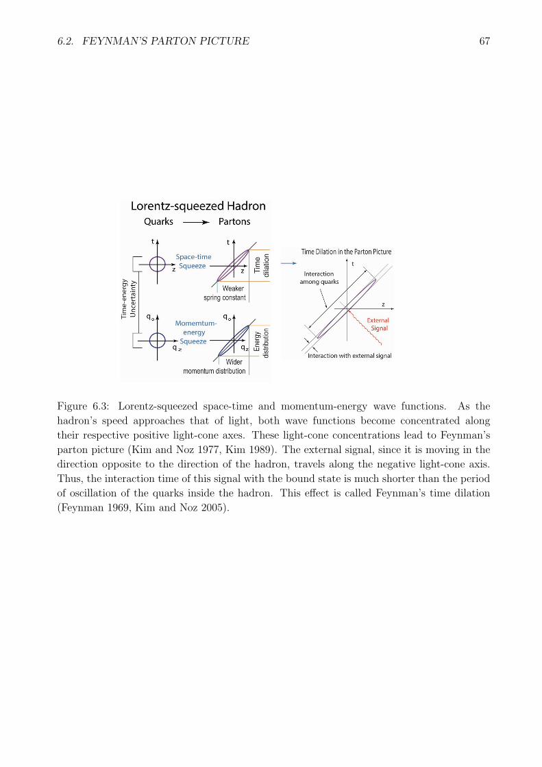
6.2. FEYNMAN’S PARTON PICTURE 67
Figure 6.3: Lorentz-squeezed space-time and momentum-energy wave functions. As the
hadron’s speed approaches that of light, both wave functions become concentrated along
their respective positive light-cone axes. These light-cone concentrations lead to Feynman’s
parton picture (Kim and Noz 1977, Kim 1989). The external signal, since it is moving in the
direction opposite to the direction of the hadron, travels along the negative light-cone axis.
Thus, the interaction time of this signal with the bound state is much shorter than the period
of oscillation of the quarks inside the hadron. This effect is called Feynman’s time dilation
(Feynman 1969, Kim and Noz 2005).

68 CHAPTER 6. QUARKS AND PARTONS IN THE LORENTZ-COVARIANT WORLD
c. The momentum distribution of partons becomes widespread as the hadron moves fast.
d. The number of partons seems to be infinite or much larger than that of quarks.
Because the hadron is believed to be a bound state of two or three quarks, each of the above
phenomena appears as a paradox, particularly b) and c) together. How can a free particle
have a wide-spread momentum distribution?
In order to resolve this paradox, let us construct the momentum-energy wave function
corresponding to Eq. (5.42). If the quarks have the four-momenta pa and pb, we can construct
two independent four-momentum variables (Feynman et al. 1971)
P = pa + pb, q =√2 (pa − pb) . (6.3)
The four-momentum P is the total four-momentum and is thus the hadronic four-momentum
while q measures the four-momentum separation between the quarks.
The resulting momentum-energy wave function is
ϕη(qz, q0) =(1
π
)1/2
exp{−1
4
[e−2η (qz + q0)
2 + e2η (qz − q0)2]}. (6.4)
For large values of η, we can let q0 = qz, and the wave function becomes
ϕη(qz) =(1
π
)1/4
exp{−[e−2η (qz)
2]}. (6.5)
Because we are using here the harmonic oscillator, the mathematical form of the above
momentum-energy wave function is identical to that of the space-time wave function of
Eq. (5.42). The Lorentz Squeeze properties of these wave functions are also the same. This
aspect of the squeeze has been exhaustively discussed in the literature (Kim and Noz 1977,
Kim 1989), and it is illustrated again in Fig. 6.3. The hadronic structure function calculated
from this formalism is in reasonable agreement with the experimental data (Hussar 1981).
When the hadron is at rest with η = 0, both wave functions behave like those for the static
bound state of quarks. As η increases, the wave functions become continuously squeezed until
they become concentrated along their respective positive light-cone axes. Let us look at the
z-axis projection of the space-time wave function. Indeed, the width of the quark distribution
increases as the hadronic speed approaches that of the speed of light. The position of each
quark appears widespread to the observer in the laboratory frame, and the quarks appear like
free particles.
The momentum-energy wave function is just like the space-time wave function. The lon-
gitudinal momentum distribution becomes wide-spread as the hadronic speed approaches the
velocity of light. This is in contradiction with our expectation from non-relativistic quantum
mechanics that the width of the momentum distribution is inversely proportional to that of
the position wave function. Our expectation is that if quarks are free, they must have a
sharply defined momenta, not a wide-spread distribution.
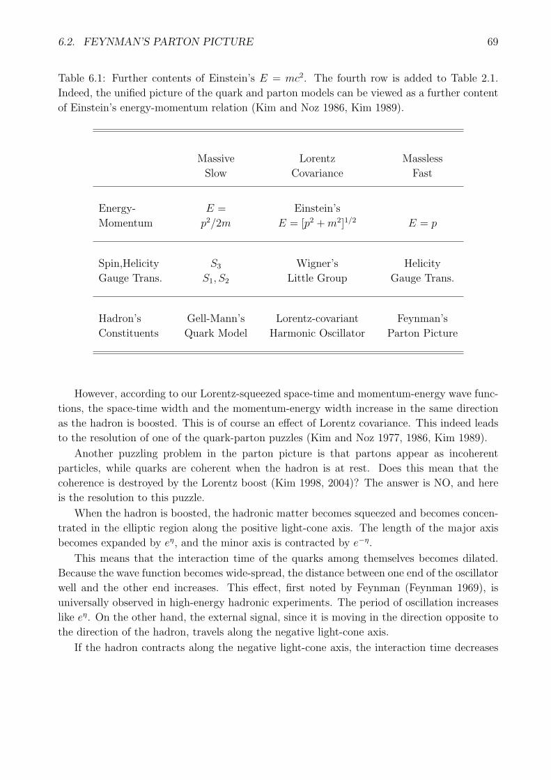
6.2. FEYNMAN’S PARTON PICTURE 69
Table 6.1: Further contents of Einstein’s E = mc2. The fourth row is added to Table 2.1.
Indeed, the unified picture of the quark and parton models can be viewed as a further content
of Einstein’s energy-momentum relation (Kim and Noz 1986, Kim 1989).
Massive Lorentz Massless
Slow Covariance Fast
Energy- E = Einstein’s
Momentum p2/2m E = [p2 +m2]1/2 E = p
Spin,Helicity S3 Wigner’s Helicity
Gauge Trans. S1, S2 Little Group Gauge Trans.
Hadron’s Gell-Mann’s Lorentz-covariant Feynman’s
Constituents Quark Model Harmonic Oscillator Parton Picture
However, according to our Lorentz-squeezed space-time and momentum-energy wave func-
tions, the space-time width and the momentum-energy width increase in the same direction
as the hadron is boosted. This is of course an effect of Lorentz covariance. This indeed leads
to the resolution of one of the quark-parton puzzles (Kim and Noz 1977, 1986, Kim 1989).
Another puzzling problem in the parton picture is that partons appear as incoherent
particles, while quarks are coherent when the hadron is at rest. Does this mean that the
coherence is destroyed by the Lorentz boost (Kim 1998, 2004)? The answer is NO, and here
is the resolution to this puzzle.
When the hadron is boosted, the hadronic matter becomes squeezed and becomes concen-
trated in the elliptic region along the positive light-cone axis. The length of the major axis
becomes expanded by eη, and the minor axis is contracted by e−η.
This means that the interaction time of the quarks among themselves becomes dilated.
Because the wave function becomes wide-spread, the distance between one end of the oscillator
well and the other end increases. This effect, first noted by Feynman (Feynman 1969), is
universally observed in high-energy hadronic experiments. The period of oscillation increases
like eη. On the other hand, the external signal, since it is moving in the direction opposite to
the direction of the hadron, travels along the negative light-cone axis.
If the hadron contracts along the negative light-cone axis, the interaction time decreases
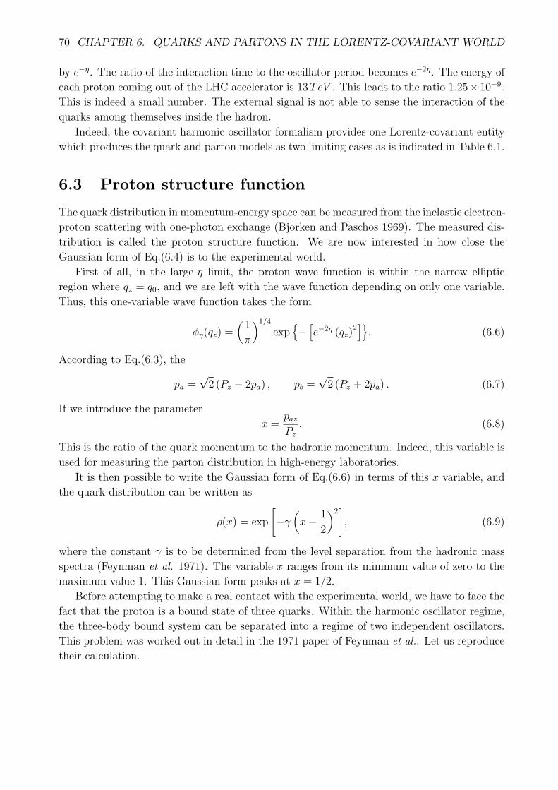
70 CHAPTER 6. QUARKS AND PARTONS IN THE LORENTZ-COVARIANT WORLD
by e−η. The ratio of the interaction time to the oscillator period becomes e−2η. The energy of
each proton coming out of the LHC accelerator is 13TeV . This leads to the ratio 1.25×10⁻⁹.
This is indeed a small number. The external signal is not able to sense the interaction of the
quarks among themselves inside the hadron.
Indeed, the covariant harmonic oscillator formalism provides one Lorentz-covariant entity
which produces the quark and parton models as two limiting cases as is indicated in Table 6.1.
6.3 Proton structure function
The quark distribution in momentum-energy space can be measured from the inelastic electron-
proton scattering with one-photon exchange (Bjorken and Paschos 1969). The measured dis-
tribution is called the proton structure function. We are now interested in how close the
Gaussian form of Eq.(6.4) is to the experimental world.
First of all, in the large-η limit, the proton wave function is within the narrow elliptic
region where qz = q0, and we are left with the wave function depending on only one variable.
Thus, this one-variable wave function takes the form
ϕη(qz) =(1
π
)1/4
exp{−[e−2η (qz)
2]}. (6.6)
According to Eq.(6.3), the
pa =√2 (Pz − 2pa) , pb =
√2 (Pz + 2pa) . (6.7)
If we introduce the parameter
x =pazPz
, (6.8)
This is the ratio of the quark momentum to the hadronic momentum. Indeed, this variable is
used for measuring the parton distribution in high-energy laboratories.
It is then possible to write the Gaussian form of Eq.(6.6) in terms of this x variable, and
the quark distribution can be written as
ρ(x) = exp
[−γ
(x− 1
2
)2], (6.9)
where the constant γ is to be determined from the level separation from the hadronic mass
spectra (Feynman et al. 1971). The variable x ranges from its minimum value of zero to the
maximum value 1. This Gaussian form peaks at x = 1/2.
Before attempting to make a real contact with the experimental world, we have to face the
fact that the proton is a bound state of three quarks. Within the harmonic oscillator regime,
the three-body bound system can be separated into a regime of two independent oscillators.
This problem was worked out in detail in the 1971 paper of Feynman et al.. Let us reproduce
their calculation.

6.3. PROTON STRUCTURE FUNCTION 71
Let xa, xb, xc represent the space-time coordinates for those quarks. If there is an oscillator
force between two quarks, we are led the quadratic form[(xa − xb)
2 + (xb − xc)2 + (xc − xa)
2]. (6.10)
In order to deal with this expression, Feynman et al. introduced the following three variables:
X =xa + xb + xc
3,
r =xa + xb − 2xc
6,
s =xb − xa
2, (6.11)
and
xa = X − 2r,
xb = X + r −√3s,
xc = X + r +√3s. (6.12)
In terms of the r and s variables, the quadratic form becomes
18(r2 + s2
), (6.13)
and does not depend on the X variable, which specifies the space-time coordinate of the
proton.
As for the momentum-energy four-vectors, let us call them pa, pb, and pc for the quarks a, b,
c respectively, and introduce the following variables. For the momentum-energy four-vectors,
we can introduce the following three variables.
P = pa + pb + pc,
q = pa + pb − 2pc,
k =√3 (pb − pa) . (6.14)
Then
pa =1
3P +
1
6q − 1
2√3k,
pb =1
3P +
1
6q +
1
2√3k,
pc =1
3P − 1
3q. (6.15)

72 CHAPTER 6. QUARKS AND PARTONS IN THE LORENTZ-COVARIANT WORLD
Figure 6.4: Parton distribution function compared with experimental data. The boosted
oscillator has its peak at x = 1/3 . This Gaussian form gives a reasonable agreement with
experimental data for large values of x, but the disagreement is substantial for small values
of x. This figure is from Paul Hussar’s paper (Hussar 1981).
In terms of these variables we are led to consider the quadratic form of
18(q2 + k2
). (6.16)
This form does not depend on the variable P , which measures the momentum and energy of
the proton.
If the external signal interacts with quark c, its momentum depends only on the q variable,
which can be written as
q = P − 3pc. (6.17)
We can then define the x variable as
x =pczPz
. (6.18)
Then the quark distribution should take the form
ρ(x) =
(1
πγ
)1/2
exp
[−γ
(1− 1
3
)2]. (6.19)
The constant γ is to be determined from the hadronc mass spectra based on the oscillator
model (Feynman et al. 1971). Figure 6.4 shows this Gaussian form, and its comparison with
what we observe in the real world.
On the same figure, there is a curve derived from the distribution derived from the experi-
mental data. This distribution is measured from inelastic electron-proton scattering (Bjorken
and Paschos 1969). These two curves are somewhat different because the quarks do not
interact with the incoming photon as a point particle.

6.4. PROTON FORM FACTOR AND LORENTZ COHERENCE 73
The simplest model is to put all those effects into one additional quark in the oscillator
system. This leads to the proton as a bound state of four quarks. The fourth quark is
responsible for all those un-explained effects (Kim and Noz 1978). Another model is to use
the valon model (Hwa 1980, Hwa and Zahir 1981) which allows us to screen out all those
non-point effects. Using this valon model, Hussar (1981) derived the experimental curve to
be compared with the Gaussian form as shown in Fig. 6.4.
This graph may not be as accurate as we desire. However, the remarkable feature is that
the Gaussian form was calculated from the proton at rest. So is the constant γ. It came
from the level spacing in the hadronic mass spectra. It is remarkable that these two features
manifest themselves for the proton whose speed is very close to that of the light.
There are many other models to deal with the problem of providing corrections to the
parton distribution. QCD (quantum chromodyanics) is a case in point (Buras 1980). QCD
can provide corrections to the distribution, but it does not produce the distribution from
which to start. The covariant harmonic oscillator function provides this starting point.
It is like the case of quantum electrodynamics. QED was quite successful in producing
the Lamb shift in the the hydrogen energy spectrum, but QED cannot produce the Rydberg
energy levels to which the correction is made. The hydrogen energy levels are still obtained
from the Schrodinger or Dirac equation with the localization condition on wave functions.
6.4 Proton form factor and Lorentz coherence
Let us now consider the elastic scattering of proton and electron with one photon exchange.
If the proton is a point particle, the scattering cross section can be calculated from the one-
photon exchange Feynman diagram. The calculation is straight-forward if the proton is a
point particle. This process is called the Rutherford scattering, and the cross section becomes
the same as the classical Coulomb scattering if the proton’s recoil is negligible.
As the momentum transfer becomes substantial as indicated in Fig. 6.5 the cross section
deviates from the that of the Rutherford scattering, as was observed first by Hofstadter and
McCallister in 1955 (Hofstadter and McCallister 1955). Subsequently, it was observed that
the cross section decreases as1
(momentum transfer)8. (6.20)
This deviation comes from the fact that the proton is not a point particle and that the electric
charge inside the proton is distributed with a finite radius. The portion of the scattering
amplitude describing this distribution is called the proton form factor. The proton form
factor should therefore decrease as
1
(momentum transfer)4. (6.21)
This behavior of decrease is known as the dipole cut-off in the literature. This dipole cut-off
and possible deviations from it constitute one of the major branches of high-energy physics.
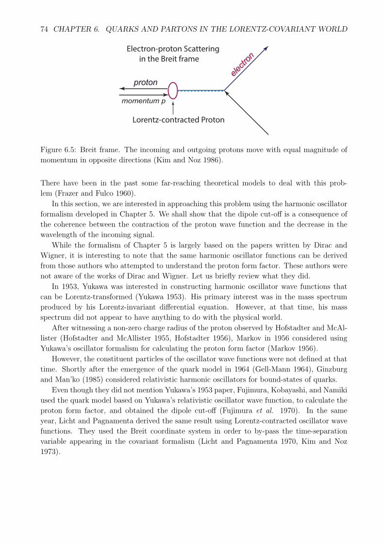
74 CHAPTER 6. QUARKS AND PARTONS IN THE LORENTZ-COVARIANT WORLD
Lorentz-contracted Proton
Electron-proton Scattering
in the Breit frame
elec
tron
proton
momentum p
Figure 6.5: Breit frame. The incoming and outgoing protons move with equal magnitude of
momentum in opposite directions (Kim and Noz 1986).
There have been in the past some far-reaching theoretical models to deal with this prob-
lem (Frazer and Fulco 1960).
In this section, we are interested in approaching this problem using the harmonic oscillator
formalism developed in Chapter 5. We shall show that the dipole cut-off is a consequence of
the coherence between the contraction of the proton wave function and the decrease in the
wavelength of the incoming signal.
While the formalism of Chapter 5 is largely based on the papers written by Dirac and
Wigner, it is interesting to note that the same harmonic oscillator functions can be derived
from those authors who attempted to understand the proton form factor. These authors were
not aware of the works of Dirac and Wigner. Let us briefly review what they did.
In 1953, Yukawa was interested in constructing harmonic oscillator wave functions that
can be Lorentz-transformed (Yukawa 1953). His primary interest was in the mass spectrum
produced by his Lorentz-invariant differential equation. However, at that time, his mass
spectrum did not appear to have anything to do with the physical world.
After witnessing a non-zero charge radius of the proton observed by Hofstadter and McAl-
lister (Hofstadter and McAllister 1955, Hofstadter 1956), Markov in 1956 considered using
Yukawa’s oscillator formalism for calculating the proton form factor (Markov 1956).
However, the constituent particles of the oscillator wave functions were not defined at that
time. Shortly after the emergence of the quark model in 1964 (Gell-Mann 1964), Ginzburg
and Man’ko (1985) considered relativistic harmonic oscillators for bound-states of quarks.
Even though they did not mention Yukawa’s 1953 paper, Fujimura, Kobayashi, and Namiki
used the quark model based on Yukawa’s relativistic oscillator wave function, to calculate the
proton form factor, and obtained the dipole cut-off (Fujimura et al. 1970). In the same
year, Licht and Pagnamenta derived the same result using Lorentz-contracted oscillator wave
functions. They used the Breit coordinate system in order to by-pass the time-separation
variable appearing in the covariant formalism (Licht and Pagnamenta 1970, Kim and Noz
1973).
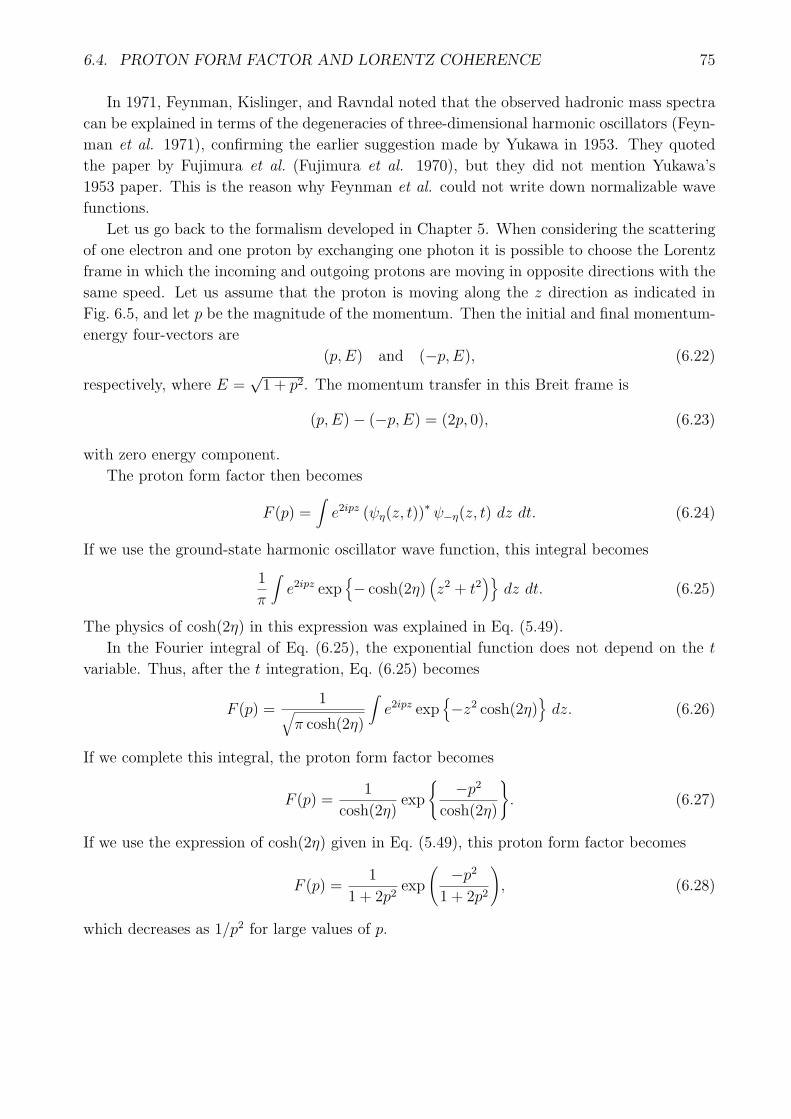
6.4. PROTON FORM FACTOR AND LORENTZ COHERENCE 75
In 1971, Feynman, Kislinger, and Ravndal noted that the observed hadronic mass spectra
can be explained in terms of the degeneracies of three-dimensional harmonic oscillators (Feyn-
man et al. 1971), confirming the earlier suggestion made by Yukawa in 1953. They quoted
the paper by Fujimura et al. (Fujimura et al. 1970), but they did not mention Yukawa’s
1953 paper. This is the reason why Feynman et al. could not write down normalizable wave
functions.
Let us go back to the formalism developed in Chapter 5. When considering the scattering
of one electron and one proton by exchanging one photon it is possible to choose the Lorentz
frame in which the incoming and outgoing protons are moving in opposite directions with the
same speed. Let us assume that the proton is moving along the z direction as indicated in
Fig. 6.5, and let p be the magnitude of the momentum. Then the initial and final momentum-
energy four-vectors are
(p, E) and (−p, E), (6.22)
respectively, where E =√1 + p2. The momentum transfer in this Breit frame is
(p, E)− (−p, E) = (2p, 0), (6.23)
with zero energy component.
The proton form factor then becomes
F (p) =∫e2ipz (ψη(z, t))
∗ ψ−η(z, t) dz dt. (6.24)
If we use the ground-state harmonic oscillator wave function, this integral becomes
1
π
∫e2ipz exp
{− cosh(2η)
(z2 + t2
)}dz dt. (6.25)
The physics of cosh(2η) in this expression was explained in Eq. (5.49).
In the Fourier integral of Eq. (6.25), the exponential function does not depend on the t
variable. Thus, after the t integration, Eq. (6.25) becomes
F (p) =1√
π cosh(2η)
∫e2ipz exp
{−z2 cosh(2η)
}dz. (6.26)
If we complete this integral, the proton form factor becomes
F (p) =1
cosh(2η)exp
{−p2
cosh(2η)
}. (6.27)
If we use the expression of cosh(2η) given in Eq. (5.49), this proton form factor becomes
F (p) =1
1 + 2p2exp
(−p2
1 + 2p2
), (6.28)
which decreases as 1/p2 for large values of p.

76 CHAPTER 6. QUARKS AND PARTONS IN THE LORENTZ-COVARIANT WORLD
Incr
ea
sin
g F
req
ue
ncy
Incr
ea
sin
g M
om
en
tum
Tra
nsf
er
without
Contraction
with
Contraction
Lorentz
Coherence without
Coherence
Figure 6.6: Coherence between the wavelength and the proton size. Referring back to Fig. 6.5,
the proton sees the incoming photon. The wavelength of this photon becomes smaller for in-
creasing momentum transfer. If the proton size remains unchanged, there is a rapid oscillation
cutoff in the Fourier integral for the form factor leading to a Gaussian cutoff. However, if the
proton size decreases coherently with the wavelength, there are no oscillation effects, leading
to a polynomial decrease of the form factor (Kim and Noz 1986, 2011).
In order to illustrate the effect of the role of this Lorentz contraction in more detail, let
us perform the integral of Eq. (6.26) without the contraction factor cosh(2η). This means
that the wave function ψη(z, t) in the Eq. (6.24) is replaced by the Gaussian form ψ0(z, t) of
Eq. (6.2). With this non-squeezed wave function, the Fourier integral becomes
G(p) =∫e2ipz (ψ0(z, t))
∗ ψ0(z, t) dz dt. (6.29)
The result of this integral is
G(p) =1√πexp (−p2). (6.30)
This leads to a Gaussian cutoff of the proton form factor. This does not happen in the real
world, and the calculation of G(p) is for an illustrative purpose only.
Let us go back to the Fourier integrals of Eq. (6.24) and Eq. (6.29). The only difference
is the cosh(2η) factor in Eq. (6.24). This factor is in the normalization constant and comes
from the integration over the t variable which does not affect the Fourier integral.
However, it causes the Gaussian width to shrink by 1/√2p for large values of p. The
wavelength of the sinusoidal factor is inversely proportional to the momentum 2p. Thus, both
the Gaussian width and the wavelength of the incoming signal shrink at the same rate of 1/p
as p becomes large. Without this coherence, the cutoff is Gaussian as noted in Eq. (6.30).
The effect of this Lorentz coherence is illustrated in Fig. 6.6.

6.5. COHERENCE IN MOMENTUM-ENERGY SPACE 77
There still is a gap between F (p) of Eq. (6.28) and the real world. Before comparing this
expression with the experimental data, we have to realize that there are three quarks inside
the proton with two oscillator modes.
One of the modes goes through the Lorentz coherence process discussed in this section.
The other mode goes through the contraction process given in Eq. (5.49). The net effect is
F3(p) =
(1
1 + 2p2
)2
exp
(−p2
1 + 2p2
). (6.31)
This will lead to the desired dipole cut-off of (1/p2)2.
In addition, the effect of the quark spin should be addressed. There are also reports
of deviations from the exact dipole cut-off. There have been attempts to study the proton
form factors based on the four-dimensional rotation group with an imaginary time coordinate.
There are also many papers based on the lattice QCD. A brief list of the references to these
efforts is given in (Kim and Noz 2011).
The purpose of this section was limited to studying in detail the role of Lorentz coherence
in keeping the proton form factor from the steep Gaussian cutoff in the momentum transfer
variable. The coherence problem is one of the primary issues of the current trend in physics.
6.5 Coherence in momentum-energy space
We are now interested in how Lorentz coherence manifests itself in momentum-energy space.
We start with the Lorentz-squeezed wave function in momentum-energy space, which can be
written as
ϕη (qz, q0) =1
2π
∫e−i(qzz−q0t)ψη(z, t)dt dz. (6.32)
This is a Fourier transformation of the Lorentz-squeezed wave function of Eq. (6.1), where qzand q0 are Fourier conjugate variables to z and t respectively. The result of this integral is
ϕη (qz, q0) =1√πexp
{−1
4
[e−2η (qz + q0)
2 + e2η (qz − q0)2]}. (6.33)
In terms of this momentum-energy wave function, the proton form factor of Eq. (6.24) can
be written as
F (p) =∫ϕ∗−η (q0, qz − p)ϕη (q0, qz + p) dq0 dqz. (6.34)
The evaluation of this integral leads to the proton form factor F (p) given in Eq. (6.28).
In order to see the effect of the Lorentz coherence, let us look at two wave functions in
Fig. 6.7. The integral is carried out over the qz qo plane. As the momentum p increases, the
two wave functions become separated. Without the Lorentz squeeze, the wave functions do
not overlap, and this leads to a sharp Gaussian cutoff as in the case of G(p) of Eq. (6.30).
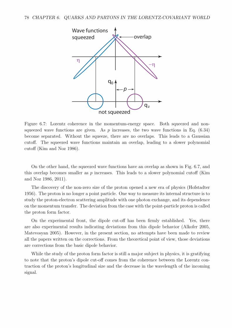
78 CHAPTER 6. QUARKS AND PARTONS IN THE LORENTZ-COVARIANT WORLD
p
q
q
0
z
Wave functions
squeezed
not squeezed
overlap
−ηη
Figure 6.7: Lorentz coherence in the momentum-energy space. Both squeezed and non-
squeezed wave functions are given. As p increases, the two wave functions in Eq. (6.34)
become separated. Without the squeeze, there are no overlaps. This leads to a Gaussian
cutoff. The squeezed wave functions maintain an overlap, leading to a slower polynomial
cutoff (Kim and Noz 1986).
On the other hand, the squeezed wave functions have an overlap as shown in Fig. 6.7, and
this overlap becomes smaller as p increases. This leads to a slower polynomial cutoff (Kim
and Noz 1986, 2011).
The discovery of the non-zero size of the proton opened a new era of physics (Hofstadter
1956). The proton is no longer a point particle. One way to measure its internal structure is to
study the proton-electron scattering amplitude with one photon exchange, and its dependence
on the momentum transfer. The deviation from the case with the point-particle proton is called
the proton form factor.
On the experimental front, the dipole cut-off has been firmly established. Yes, there
are also experimental results indicating deviations from this dipole behavior (Alkofer 2005,
Matevosyan 2005). However, in the present section, no attempts have been made to review
all the papers written on the corrections. From the theoretical point of view, those deviations
are corrections from the basic dipole behavior.
While the study of the proton form factor is still a major subject in physics, it is gratifying
to note that the proton’s dipole cut-off comes from the coherence between the Lorentz con-
traction of the proton’s longitudinal size and the decrease in the wavelength of the incoming
signal.
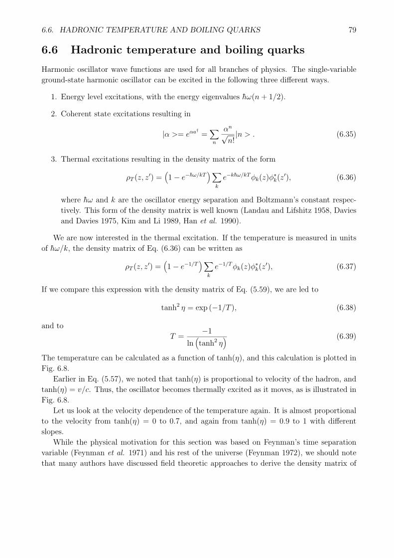
6.6. HADRONIC TEMPERATURE AND BOILING QUARKS 79
6.6 Hadronic temperature and boiling quarks
Harmonic oscillator wave functions are used for all branches of physics. The single-variable
ground-state harmonic oscillator can be excited in the following three different ways.
1. Energy level excitations, with the energy eigenvalues hω(n+ 1/2).
2. Coherent state excitations resulting in
|α >= eαa†=∑n
αn
√n!|n > . (6.35)
3. Thermal excitations resulting in the density matrix of the form
ρT (z, z′) =
(1− e−hω/kT
)∑k
e−khω/kTϕk(z)ϕ∗k(z
′), (6.36)
where hω and k are the oscillator energy separation and Boltzmann’s constant respec-
tively. This form of the density matrix is well known (Landau and Lifshitz 1958, Davies
and Davies 1975, Kim and Li 1989, Han et al. 1990).
We are now interested in the thermal excitation. If the temperature is measured in units
of hω/k, the density matrix of Eq. (6.36) can be written as
ρT (z, z′) =
(1− e−1/T
)∑k
e−1/Tϕk(z)ϕ∗k(z
′), (6.37)
If we compare this expression with the density matrix of Eq. (5.59), we are led to
tanh2 η = exp (−1/T ), (6.38)
and to
T =−1
ln(tanh2 η
) (6.39)
The temperature can be calculated as a function of tanh(η), and this calculation is plotted in
Fig. 6.8.
Earlier in Eq. (5.57), we noted that tanh(η) is proportional to velocity of the hadron, and
tanh(η) = v/c. Thus, the oscillator becomes thermally excited as it moves, as is illustrated in
Fig. 6.8.
Let us look at the velocity dependence of the temperature again. It is almost proportional
to the velocity from tanh(η) = 0 to 0.7, and again from tanh(η) = 0.9 to 1 with different
slopes.
While the physical motivation for this section was based on Feynman’s time separation
variable (Feynman et al. 1971) and his rest of the universe (Feynman 1972), we should note
that many authors have discussed field theoretic approaches to derive the density matrix of

80 CHAPTER 6. QUARKS AND PARTONS IN THE LORENTZ-COVARIANT WORLD
Figure 6.8: Hadronic temperature plotted against β. As the hadron gains in speed, the
quarks inside become excited and this results in a rise in temperature. If the temperature is
sufficiently high, those quarks start boiling and become partons (Kim and Noz 2014).
Eq. (6.36). Among them are two-mode squeezed states of light (Yuen 1976, Yurke et al. 1986,
Han et al. 1993, Kim and Noz 1991) and thermo-field-dynamics (Fetter and Walecka 1971,
Ojima 1981, Umezawa et al. 1982, Mann and Revzen 1989).
The mathematics of two-mode squeezed states is the same as that for the covariant har-
monic oscillator formalism discussed in Chapter 5 (Dirac 1963, Yurke 1986, Kim and Noz
1991, Han et al. 1993). Instead of the z and t coordinates, there are two measurable photons.
If we choose not to observe one of them (Yurke and Potasek 1987, Ekert and Knight 1989), it
belongs to Feynman’s rest of the universe (Han et al. 1999)
Another remarkable feature of two-mode squeezed states of light is that its formalism
is identical to that of thermo-field-dynamics. The temperature is related to the squeeze
parameter in the two-mode case. It is therefore possible to define the temperature of a
Lorentz-squeezed hadron within the framework of the covariant harmonic oscillator model.
References
Alkofer, R.; Holl, A.; Kloker, M.; Karssnigg, A.; Roberts, C. D. 2005. On Nucleon Electro-
magnetic Form Factors. Few-Body Sys. 37 1 - 31.
Beg, M. A. B.; Lee, B. W.; Pais, A. 1964. SU(6) and Electromagnetic Interactions. Phys.
Rev. Lett. 13 514 - 517.
Bjorken, J. D.; Paschos, E. A. 1969. Inelastic Electron-Proton and γ-Proton Scattering and
the Structure of the Nucleon. Phys Rev. 185 1975 - 1982.
Buras, A. J., 1980. Asymptotic freedom in deep inelastic processes in the leading order and
beyond. Rev. Mod. Phys. 52 199 - 276.
Davies, R. W.; Davies, K. T. R. 1975. On the Wigner distribution function for an oscillator.
Ann. Phys. 89 261 - 273.
Dirac, P. A. M. 1963. A Remarkable representation of 3 + 2 de Sitter group. J. Math. Phys.
4 901 - 909.

6.6. HADRONIC TEMPERATURE AND BOILING QUARKS 81
Ekert, A. K.; Knight, P. L. 1989. Correlations and squeezing of two-mode oscillations. Am.
J. Phys. 57 692 - 697.
Fetter, A. L.; Walecka, J. D. 1971. Quantum Theory of Many-Particle Systems. McGraw-Hill:
New York, NY.
Feynman, R. P. 1969. Very High-Energy Collisions of Hadrons. Phys. Rev. Lett. 23 1415
- 1417; See also Feynman, R. P. The Behavior of Hadron Collisions at Extreme Energies
in High-Energy Collisions. in the Proceedings of the 3rd International Conference (Stony
Brook, New York, U.S.A., C. N. Yang et al. eds.), Gordon and Breach: New York, NY,
See pages 237-249.
Feynman, R. P.; Kislinger, M.; Ravndal F. 1971. Current Matrix Elements from a Relativistic
Quark Model. Phys. Rev. D 3 2706 - 2732.
Feynman, R. P. 1972. Statistical Mechanics. Benjamin Cummings: Boston, MA.
Frazer, W.; Fulco, J. 1960, Effect of a Pion-Pion Scattering Resonance on Nucleon Structure.
Phys. Rev. Lett. 2 365 - 368.
Fujimura, K.; Kobayashi, T.; Namiki, M. 1970. Nucleon Electromagnetic Form Factors at
High Momentum Transfers in an Extended Particle Model Based on the Quark Model.
Prog. Theor. Phys. 43 73 - 79.
Gell-Mann M. 1964. A Schematic Model of Baryons and Mesons. Phys. Lett. 8 214 - 156 .
Ginzburg, V. L.; Man’ko, V. I. 1965. Relativistic oscillator models of elementary particles.
Nucl. Phys. 74 577 - 588.
Han, D.; Kim, Y. S.; Noz, M. E. 1990. Lorentz-Squeezed Hadrons and Hadronic Temperature.
Phys. Lett. A 144 111 - 115.
Han, D.; Kim, Y. S.; Noz, M. E. 1999. Illustrative example of Feynman’s rest of the universe.
Am. J. Phys. 67 61 - 66.
Han, D.; Kim, Y. S.; Noz, M. E.; Yeh, L.; 1993. Symmetries of Two-mode Squeezed States.
J. Math. Phys. 34 5493 - 5508.
Hofstadter, R.; McAllister, R. W. 1955. Electron Scattering from the Proton. Phys. Rev. 98
217 - 218.
Hofstadter, R. 1956. Electron Scattering and Nucler Structure. Rev. Mod. Phys. 18 214-254.
Hussar, P. E. 1981. Valons and harmonic oscillators. Phys. Rev. D 23 2781 - 2783.
Hwa, R. C. 1980. Evidence for valence-quark clusters in nucleon structure functions. Phys.
Rev. D 22 759 - 764.
Hwa, R. C.; Zahir, M. S. 1981. Parton and valon distributions in the nucleon. Phys. Rev. D
23 2539 - 2553.
Kim, Y. S.; Noz, M. E. 1973. Covariant Harmonic Oscillators and the Quark Model. Phys.
Rev. D. 8. 3521 - 3526.
Kim, Y. S.; Noz, M. E. 1977. Covariant Harmonic Oscillators and the Parton Picture. Phys.
Rev. D 15 335 - 338.
Kim, Y. S.; Noz, M. E. 1978. Quarks, Partons, and Lorentz-deformed Hadrons. Prog. Theor.
Phys. 60 801 - 816.

82 CHAPTER 6. QUARKS AND PARTONS IN THE LORENTZ-COVARIANT WORLD
Kim, Y. S.; Noz, M. E. 1986. Theory and Applications of the Poincare Group. Reidel:
Dordrecht, The Netherlands.
Kim, Y. S. 1989. Observable gauge transformations in the parton picture. Phys. Rev. Lett.
63 348 - 351.
Kim, Y. S.; Li, M. 1989. Squeezed States and Thermally Excited States in the Wigner Phase-
Space Picture of Quantum Mechanics. Phys. Lett. A 139 445 - 448.
Kim, Y. S.; Noz, M. E. 1991. Phase Space Picture of Quantum Mechanics. World Scientific:
Singapore.
Kim, Y. S. 1998. Does Lorentz Boost Destroy Coherence? Fortschr. der Physik 46 713 - 724.
Kim, Y. S. 2004. Einstein, Wigner and Feynman: From E = mc2 to Feynman’s decoherence
via Wigner’s little groups. Acta Physica Hungarica New Series-Heavy Ion Physics 19 317
- 328.
Kim, Y. S.; Moz, M. E. 2005. Coupled oscillators, entangled oscillators, and Lorentz-covariant
oscillators J. Opt. B: Quantum and Semiclass. Opt 7, S458 - S467.
Kim, Y. S.; Noz, M. E. 2011. Lorentz Harmonics, Squeeze Harmonics and Their Physical
Applications. Symmetry 3 16 - 36.
Kim, Y. S.; Noz, M. E. 2014. Entropy and Temperature from Entangled Space and Time
Phys. Sci. Int. J. 4 1015 - 1039.
Landau, L. D.; Lifshitz, E. M. 1958. Statistical Physics. Pergamon Press: London, UK.
Licht, A. L.; Pagnamenta, A. 1970. Wave Functions and Form Factors for Relativistic Com-
posite Particles I. Phys. Rev. D 2 1150 - 1156.
Mann; A.; Revzen, M. 1989. Thermal coherent states. Phys. Lett. A 134 273 - 275.
Markov, M. 1956. On Dynamically Deformable Form Factors in the Theory of Particles.
Suppl. Nuovo Cimento 3 760 - 772.
Matevosyan, H. H.; Thomas, A. W.; Miller, G. A. 2005. Study of lattice QCD form factors
using the extended Gari-Krumpelmann model. Phys. Rev. C 72 065204 -1 - 065204 - 5.
Ojima, I. 1981. Gauge Fields at Finite Temperatures-“Thermo Field Dynamics” and the KMS
Condition and Their Extension to Gauge Theories. Ann. Phys. (NY), 137 1 - 32.
Umezawa, H.; Matsumoto, H.; Tachiki, M. 1982. Thermo Field Dynamics and Condenced
States. North-Holland: Amsterdam, The Netherlands.
Yuen, H. P. 1976. Two-photon coherent states of the radiation field. Phys. Rev. A 13 2226 -
2243.
Yurke, B. S. 1986. Quantizing the Damped Harmonic-Oscillator. Am. J. Phys. 54 1133 -
1139.
Yurke, B; Potasek, M. 1987. Obtainment of Thermal Noise from a Pure State. Phys. Rev. A
36 3464 - 3466.
Yukawa, H. 1953. Structure and Mass Spectrum of Elementary Particles. I. General Consid-
erations. Phys. Rev. 91 415 - 416.
Chapter 7
Coupled oscillators and squeezed
states of light
Let us start with the one-dimensional harmonic oscillator equation
1
2
−( ∂
∂x
)2
+ x2
χn(x) =(n+
1
2
)χn(x), (7.1)
whose solution takes the form
χn(x) =
[1√π2nn!
]1/2Hn(x) exp
(−x2
2
), (7.2)
where Hn(x) is the Hermite polynomial of the nth degree. The properties of this wave function
are well known.
We can now consider two oscillators with coordinates x1 and x2 respectively. There are thus
two differential equations with the x1 and x2 variables respectively. If we take the difference
of these two equations, we obtain
1
2
−( ∂
∂x1
)2
+
(∂
∂x2
)2
+ x21 − x22
ψ(x1, x2) = (n− n′)ψ(x1, x2). (7.3)
In terms of the light-cone variables defined in Sec. 4.3
u =x1 + x2√
2, and v =
x1 − x2√2
, (7.4)
the differential equation of Eq. (7.3) takes the form
1
2
[− ∂
∂u
∂
∂v+ uv
]ψ(u, v) = (n− n′)ψ(u, v). (7.5)
This equation is invariant under the transformation
u→ eηu and v → e−ηv. (7.6)
83

84 CHAPTER 7. COUPLED OSCILLATORS AND SQUEEZED STATES OF LIGHT
Indeed, this was the property of the Lorentz-invariant differential equation which was the
starting point of Chapter 5.
For the ground state, the solution takes the form
ψη(u, v) =1√πexp
{−1
2
(e−2ηu2 + e2ηv2
)}. (7.7)
In terms of the x1 x2 variables, it can be written as
ψη(x1, x2) =1√πexp
{−1
4
[e−2η(x1 + x2)
2 + e2η(x1 − x2)2]}. (7.8)
We noted further that this Gaussian form can be expanded as
ψη(x1, x2) =
(1
cosh η
)∑k
(tanh η)kχk(x1)χk(x2). (7.9)
In this chapter, we are interested in what happens if the two oscillators given in Eq. (7.3)
are coupled with the equation
1
2
−( ∂
∂x1
)2
−(∂
∂x2
)2
+ x21 + x22 +K(x1 − x2)2
f (x1, x2) = λf(x1, x2), (7.10)
where K measures the strength of the coupling.
7.1 Two coupled oscillators
The variables u and v of Eq. (7.4) are called the normal coordinates for two coupled oscillators.
In terms of these variables, the differential equation of Eq. (7.10) becomes separable and can
be written as1
2
−( ∂
∂u
)2
−(∂
∂v
)2
+ u2 + e4ηv2
f(u, v) = λf(u, v), (7.11)
where
e4η = 1 +K.
If we make the coordinate transformation
u→ eηu, v → e−ηv, (7.12)
the differential equation of Eq. (7.11) becomes
1
2
[(e2ηp2u − e−2ηp2v
)+ e−2ηu2 + e2ηv2
]f(u, v) = λf(u, v), (7.13)
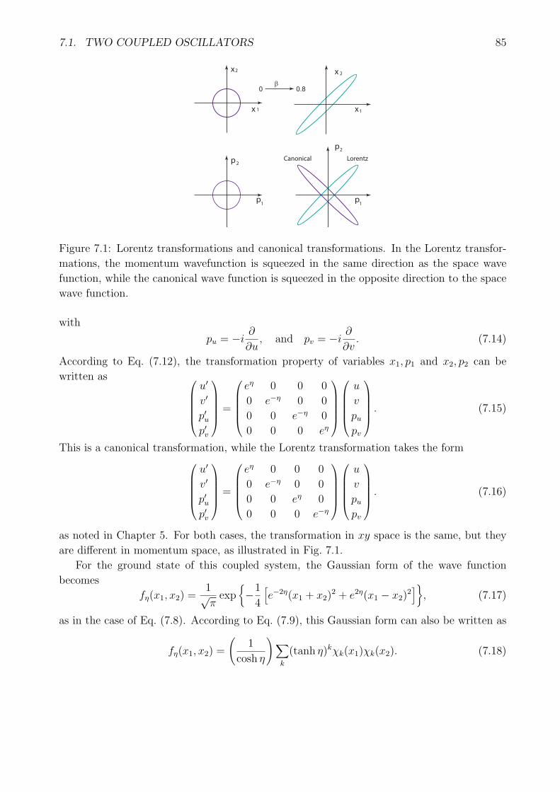
7.1. TWO COUPLED OSCILLATORS 85
Canonical Lorentz
β0 0.8
x x
xx
p
p
pp
22
2
2
1 1
1 1
Figure 7.1: Lorentz transformations and canonical transformations. In the Lorentz transfor-
mations, the momentum wavefunction is squeezed in the same direction as the space wave
function, while the canonical wave function is squeezed in the opposite direction to the space
wave function.
with
pu = −i ∂∂u, and pv = −i ∂
∂v. (7.14)
According to Eq. (7.12), the transformation property of variables x1, p1 and x2, p2 can be
written as u′
v′
p′up′v
=
eη 0 0 0
0 e−η 0 0
0 0 e−η 0
0 0 0 eη
u
v
pupv
. (7.15)
This is a canonical transformation, while the Lorentz transformation takes the formu′
v′
p′up′v
=
eη 0 0 0
0 e−η 0 0
0 0 eη 0
0 0 0 e−η
u
v
pupv
. (7.16)
as noted in Chapter 5. For both cases, the transformation in xy space is the same, but they
are different in momentum space, as illustrated in Fig. 7.1.
For the ground state of this coupled system, the Gaussian form of the wave function
becomes
fη(x1, x2) =1√πexp
{−1
4
[e−2η(x1 + x2)
2 + e2η(x1 − x2)2]}, (7.17)
as in the case of Eq. (7.8). According to Eq. (7.9), this Gaussian form can also be written as
fη(x1, x2) =
(1
cosh η
)∑k
(tanh η)kχk(x1)χk(x2). (7.18)

86 CHAPTER 7. COUPLED OSCILLATORS AND SQUEEZED STATES OF LIGHT
It is interesting to note that both the coupled oscillators and the covariant oscillator lead to
the same Gaussian form of Eq. (7.17) with its series expansion. This series serves also as the
starting formula for the two-photon coherent (Yuen 1976) as well as the Gaussian entangled
state (Giedke et al. 2003, Dodd and Halliwell 2004, Braunstein and van Loock 2005, Adesso
and Illuminati 2007, Paz and Roncaglia 2008, Chou et al. 2008, Xiang et al. 2011).
If η = 0, which means k = 0 in Eq. (7.10), the Gaussian form of Eq. (7.17) becomes
f0(x1, x2) =1√πexp
{−1
2
(x21 + x22
)}, (7.19)
and the series of Eq. (7.18) becomes disentangled to
f0(x1, x2) = χ0(x1)χ0(x2). (7.20)
7.2 Squeezed states of light
Let us go back to the complete set of oscillator functions given in Eq. (7.2) and introduce the
operators a and a†, defined as
a =1√2
(x+
∂
∂x
), and a† =
1√2
(x− ∂
∂x
). (7.21)
When these operators are applied to the wave functions, we obtain
a χn(x) =√n χn−1(x), and a† χn =
√n+ 1 χn+1(x). (7.22)
Thus, χn(x) can be used for the state of n photons, while a and a† can serve as the
annihilation and creation operators respectively. If there are two kinds of photons, we can use
a1 =1√2
(x1 +
∂
∂x1
), a†1 =
1√2
(x1 −
∂
∂x1
),
a2 =1√2
(x2 +
∂
∂x2
), a†2 =
1√2
(x2 −
∂
∂x2
). (7.23)
The single-photon coherent state takes the form
|α >= e−αα∗/2∑n
αn
√n!|n >, (7.24)
which can be expanded as
|α >= e−αα∗/2∑n
αn
n!
(a†)n
|0 >={e−αα∗/2
}exp
{αa†
}|0 > . (7.25)
This aspect of the single-photon coherent state is well known. Here we are dealing with one
kind of photon, namely with a given momentum and polarization. The state |n > means there

7.2. SQUEEZED STATES OF LIGHT 87
are n photons of the same kind, and |0 > is for the zero-photon vacuum state corresponding
to the ground state oscillator wave function.
Let us next consider a state of two kinds of photons, and write |n1, n2 > as the state of n1
photons of the first kind, and n2 photons of the second kind (Yuen 1976). We are then led to
the exponential form
|β >=(1− β2
)1/2exp
{βa†1a
†2
}|0, 0 > . (7.26)
The Taylor expansion of this formula leads to
|β >=(1− β2
)1/2∑k
βk|k, k >, (7.27)
which is the two-photon coherent state (Yuen 1976). In the language of harmonic oscillators,
this formula is fη (x1, x2) of Eq. (7.18) with
β = tanh η. (7.28)
In view of Fig. 7.1, it is quite appropriate to call this two-photon state the “squeezed state”.
The total energy of the state with n1 and n2 photons is clearly
ω1n1 + ω2n2, (7.29)
where ω1 and ω2 are the frequencies of the first and second kinds respectively. Then the energy
of the squeezed state of Eq. (7.8) is
(ω1 + ω2)(1− β2
)∑k
kβ2k = (ω1 + ω2)(1− β2
) β2
(∂
∂β
∑k
β2k
). (7.30)
which becomes(ω1 + ω2) β
2
(1− β2)= (ω1 + ω2) (sinh η)
2. (7.31)
The energy is zero for the vacuum state with η = 0, but it increases as the system gets
squeezed with increasing values of η.
Since the two-mode squeezed state and the covariant harmonic oscillators share the same
set of mathematical formulas, it is possible to transmit physical interpretations from one to
the other. For the two-mode squeezed state, both photons carry physical interpretations,
while the interpretation is yet to be given to the time-separation variable in the covariant
oscillator formalism. It is clear from Eq. (5.39) and Eq. (5.53) that the time-like excitations
are like the second-photon states. What would happen if the second photon is not observed
as is illustrated in Fig. 7.2?
This interesting problem was addressed by Yurke and Potasek (Yurke and Potasek 1987)
and by Ekert and Knight (Ekert and Knight 1989). They used the density matrix formalism
and integrated out the second-photon states, by using the same mathematics as in Sec. 5.7.

88 CHAPTER 7. COUPLED OSCILLATORS AND SQUEEZED STATES OF LIGHT
Feynman’s
Rest of the
Universe
First photon - observed
Se
con
d p
ho
ton
no
t o
bse
rve
d
y y
x x
Squeeze
Figure 7.2: Feynman’s rest of the universe in the entangled system of two photons. If one
of the photons is not observed, it is in the rest of the universe. This figure is identical with
Fig. 5.8 except for the labeling of the coordinate axes.
According to Yurke et al. (Yurke et al. 1986), it is possible to consider interferometers
applicable to two-mode states. First of all, they picked the following three Hermitian operators
J1 =1
2
(a†1a2 + a†2a1
),
J2 =1
2i
(a†1a2 − a†2a1
),
J3 =1
2
(a†1a1 − a†2a2
), (7.32)
in addition to the number operator
N = a†1a1 + a†2a2. (7.33)
Since these operators satisfy the commutation relations
[Ji, Jj] = iϵijkJj, (7.34)
it is possible to study the symmetry property of the three-dimensional rotation group.
In addition, they wrote down another set of operators which could lead to effects on the
two-mode states. They are
S3 =1
2
(a†1a1 + a2a
†2
),
Q3 =i
2
(a†1a
†2 − a1a2
),
K3 =1
2
(a†1a
†2 + a1a2
), (7.35)
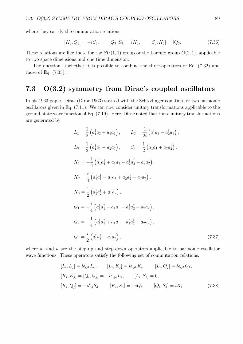
7.3. O(3,2) SYMMETRY FROM DIRAC’S COUPLED OSCILLATORS 89
where they satisfy the commutation relations
[K3, Q3] = −iS3, [Q3, S3] = iK3, [S3, K3] = iQ3. (7.36)
These relations are like those for the SU(1, 1) group or the Lorentz group O(2, 1), applicable
to two space dimensions and one time dimension.
The question is whether it is possible to combine the three-operators of Eq. (7.32) and
those of Eq. (7.35).
7.3 O(3,2) symmetry from Dirac’s coupled oscillators
In his 1963 paper, Dirac (Dirac 1963) started with the Schrodinger equation for two harmonic
oscillators given in Eq. (7.11). We can now consider unitary transformations applicable to the
ground-state wave function of Eq. (7.19). Here, Dirac noted that those unitary transformations
are generated by
L1 =1
2
(a†1a2 + a†2a1
), L2 =
1
2i
(a†1a2 − a†2a1
),
L3 =1
2
(a†1a1 − a†2a2
), S3 =
1
2
(a†1a1 + a2a
†2
),
K1 = −1
4
(a†1a
†1 + a1a1 − a†2a
†2 − a2a2
),
K2 =i
4
(a†1a
†1 − a1a1 + a†2a
†2 − a2a2
),
K3 =1
2
(a†1a
†2 + a1a2
),
Q1 = − i
4
(a†1a
†1 − a1a1 − a†2a
†2 + a2a2
),
Q2 = −1
4
(a†1a
†1 + a1a1 + a†2a
†2 + a2a2
),
Q3 =i
2
(a†1a
†2 − a1a2
), (7.37)
where a† and a are the step-up and step-down operators applicable to harmonic oscillator
wave functions. These operators satisfy the following set of commutation relations.
[Li, Lj] = iϵijkLk, [Li, Kj] = iϵijkKk, [Li, Qj] = iϵijkQk,
[Ki, Kj] = [Qi, Qj] = −iϵijkLk, [Li, S3] = 0,
[Ki, Qj] = −iδijS3, [Ki, S3] = −iQi, [Qi, S3] = iKi. (7.38)
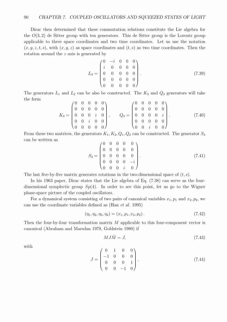
90 CHAPTER 7. COUPLED OSCILLATORS AND SQUEEZED STATES OF LIGHT
Dirac then determined that these commutation relations constitute the Lie algebra for
the O(3, 2) de Sitter group with ten generators. This de Sitter group is the Lorentz group
applicable to three space coordinates and two time coordinates. Let us use the notation
(x, y, z, t, s), with (x, y, z) as space coordinates and (t, s) as two time coordinates. Then the
rotation around the z axis is generated by
L3 =
0 −i 0 0 0
i 0 0 0 0
0 0 0 0 0
0 0 0 0 0
0 0 0 0 0
. (7.39)
The generators L1 and L2 can be also be constructed. The K3 and Q3 generators will take
the form
K3 =
0 0 0 0 0
0 0 0 0 0
0 0 0 i 0
0 0 i 0 0
0 0 0 0 0
, Q3 =
0 0 0 0 0
0 0 0 0 0
0 0 0 0 i
0 0 0 0 0
0 0 i 0 0
. (7.40)
From these two matrices, the generators K1, K2, Q1, Q2 can be constructed. The generator S3
can be written as
S3 =
0 0 0 0 0
0 0 0 0 0
0 0 0 0 0
0 0 0 0 −i0 0 0 i 0
. (7.41)
The last five-by-five matrix generates rotations in the two-dimensional space of (t, s).
In his 1963 paper, Dirac states that the Lie algebra of Eq. (7.38) can serve as the four-
dimensional symplectic group Sp(4). In order to see this point, let us go to the Wigner
phase-space picture of the coupled oscillators.
For a dynamical system consisting of two pairs of canonical variables x1, p1 and x2, p2, we
can use the coordinate variables defined as (Han et al. 1995)
(η1, η2, η3, η4) = (x1, p1, x2, p2) . (7.42)
Then the four-by-four transformation matrix M applicable to this four-component vector is
canonical (Abraham and Marsdan 1978, Goldstein 1980) if
MJM = J, (7.43)
with
J =
0 1 0 0
−1 0 0 0
0 0 0 1
0 0 −1 0
. (7.44)
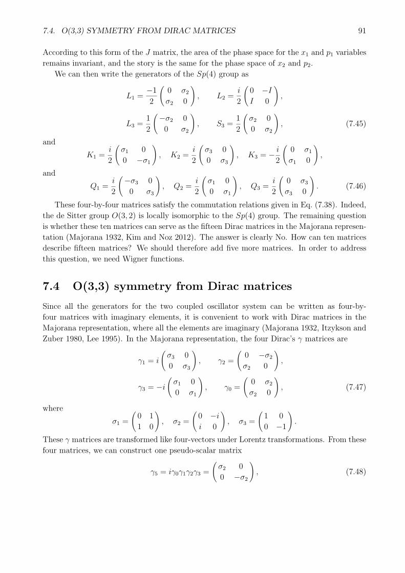
7.4. O(3,3) SYMMETRY FROM DIRAC MATRICES 91
According to this form of the J matrix, the area of the phase space for the x1 and p1 variables
remains invariant, and the story is the same for the phase space of x2 and p2.
We can then write the generators of the Sp(4) group as
L1 =−1
2
(0 σ2σ2 0
), L2 =
i
2
(0 −II 0
),
L3 =1
2
(−σ2 0
0 σ2
), S3 =
1
2
(σ2 0
0 σ2
), (7.45)
and
K1 =i
2
(σ1 0
0 −σ1
), K2 =
i
2
(σ3 0
0 σ3
), K3 = − i
2
(0 σ1σ1 0
),
and
Q1 =i
2
(−σ3 0
0 σ3
), Q2 =
i
2
(σ1 0
0 σ1
), Q3 =
i
2
(0 σ3σ3 0
). (7.46)
These four-by-four matrices satisfy the commutation relations given in Eq. (7.38). Indeed,
the de Sitter group O(3, 2) is locally isomorphic to the Sp(4) group. The remaining question
is whether these ten matrices can serve as the fifteen Dirac matrices in the Majorana represen-
tation (Majorana 1932, Kim and Noz 2012). The answer is clearly No. How can ten matrices
describe fifteen matrices? We should therefore add five more matrices. In order to address
this question, we need Wigner functions.
7.4 O(3,3) symmetry from Dirac matrices
Since all the generators for the two coupled oscillator system can be written as four-by-
four matrices with imaginary elements, it is convenient to work with Dirac matrices in the
Majorana representation, where all the elements are imaginary (Majorana 1932, Itzykson and
Zuber 1980, Lee 1995). In the Majorana representation, the four Dirac’s γ matrices are
γ1 = i
(σ3 0
0 σ3
), γ2 =
(0 −σ2σ2 0
),
γ3 = −i(σ1 0
0 σ1
), γ0 =
(0 σ2σ2 0
), (7.47)
where
σ1 =
(0 1
1 0
), σ2 =
(0 −ii 0
), σ3 =
(1 0
0 −1
).
These γ matrices are transformed like four-vectors under Lorentz transformations. From these
four matrices, we can construct one pseudo-scalar matrix
γ5 = iγ0γ1γ2γ3 =
(σ2 0
0 −σ2
), (7.48)
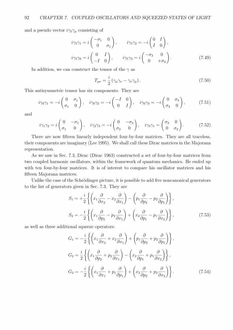
92 CHAPTER 7. COUPLED OSCILLATORS AND SQUEEZED STATES OF LIGHT
and a pseudo vector iγ5γµ consisting of
iγ5γ1 = i
(−σ1 0
0 σ1
), iγ5γ2 = −i
(0 I
I 0
),
iγ5γ0 = i
(0 I
−I 0
), iγ5γ3 = i
(−σ3 0
0 +σ3
). (7.49)
In addition, we can construct the tensor of the γ as
Tµν =i
2(γµγν − γνγµ) . (7.50)
This antisymmetric tensor has six components. They are
iγ0γ1 = −i(
0 σ1σ1 0
), iγ0γ2 = −i
(−I 0
0 I
), iγ0γ3 = −i
(0 σ3σ3 0
), (7.51)
and
iγ1γ2 = i
(0 −σ1σ1 0
), iγ2γ3 = −i
(0 −σ3σ3 0
), iγ3γ1 =
(σ2 0
0 σ2
). (7.52)
There are now fifteen linearly independent four-by-four matrices. They are all traceless,
their components are imaginary (Lee 1995). We shall call these Dirac matrices in the Majorana
representation.
As we saw in Sec. 7.3, Dirac (Dirac 1963) constructed a set of four-by-four matrices from
two coupled harmonic oscillators, within the framework of quantum mechanics. He ended up
with ten four-by-four matrices. It is of interest to compare his oscillator matrices and his
fifteen Majorana matrices.
Unlike the case of the Schrodinger picture, it is possible to add five noncanonical generators
to the list of generators given in Sec. 7.3. They are
S1 = +i
2
{(x1
∂
∂x2− x2
∂
∂x1
)−(p1
∂
∂p2− p2
∂
∂p1
)},
S2 = − i
2
{(x1
∂
∂p2− p2
∂
∂x1
)+
(x2
∂
∂p1− p1
∂
∂x2
)}, (7.53)
as well as three additional squeeze operators:
G1 = − i
2
{(x1
∂
∂x2+ x2
∂
∂x1
)+
(p1
∂
∂p2+ p2
∂
∂p1
)},
G2 =i
2
{(x1
∂
∂p2+ p2
∂
∂x1
)−(x2
∂
∂p1+ p1
∂
∂x2
)},
G3 = − i
2
{(x1
∂
∂x1+ p1
∂
∂p1
)+
(x2
∂
∂p2+ p2
∂
∂x2
)}. (7.54)

7.5. NON-CANONICAL TRANSFORMATIONS IN QUANTUM MECHANICS 93
These five generators perform well-defined operations on the Wigner function. However, the
question is whether these additional generators are acceptable in the present form of quantum
mechanics.
In order to answer this question, let us note that the uncertainty principle in the phase-
space picture of quantum mechanics is stated in terms of the minimum area in phase space for
a given pair of conjugate variables. The minimum area is determined by Planck’s constant.
Thus we are allowed to expand phase space, but are not allowed to contract it. With this
point in mind, let us go back to G3 of Eq. (7.54), which generates transformations which
simultaneously expand one phase space and contract the other. Thus, the G3 generator is
not acceptable in quantum mechanics even though it generates well-defined mathematical
transformations of the Wigner function.
If the five generators of Eq. (7.53) and Eq. (7.54) are added to the ten generators given
in Eq. (7.37) and Eq. (7.38), there are fifteen generators. They satisfy the following set of
commutation relations.
[Li, Lj] = iϵijkLk, [Si, Sj] = iϵijkSk, [Li, Sj] = 0,
[Li, Kj] = iϵijkKk, [Li, Qj] = iϵijkQk, [Li, Gj] = iϵijkGk,
[Ki, Kj] = [Qi, Qj] = [Qi, Qj] = −iϵijkLk,
[Ki, Qj] = −iδijS3, [Qi, Gj] = −iδijS1, [Gi, Kj] = −iδijS2,
[Ki, S3] = −iQi, [Qi, S3] = iKi, [Gi, S3] = 0,
[Ki, S1] = 0, [Qi, S1] = −iGi, [Gi, S1] = iQi,
[Ki, S2] = iGi, [Qi, S2] = 0, [Gi, S2] = −iKi. (7.55)
As was shown previously (Kim and Noz 2012), this set of commutation relations serves as the
Lie algebra for the group SL(4, r) and also for the O(3, 3) Lorentz group.
These fifteen four-by-four matrices are tabulated in Table 7.1. There are six anti-symmetric
and nine symmetric matrices. These anti-symmetric matrices were divided into two sets of
three rotation generators in the four-dimensional phase space. The nine symmetric matrices
can be divided into three sets of three squeeze generators. However, this classification scheme
is easier to understand in terms the group O(3, 3).
7.5 Non-canonical transformations in quantummechan-
ics
As we noted before, among the fifteen Dirac matrices, ten of them can be used for canonical
transformations in classical mechanics, and thus in quantum mechanics. They play a special
role in quantum optics (Yuen 1976, Yurke et al. 1986, Kim and Noz 1991, Han et al. 1993).
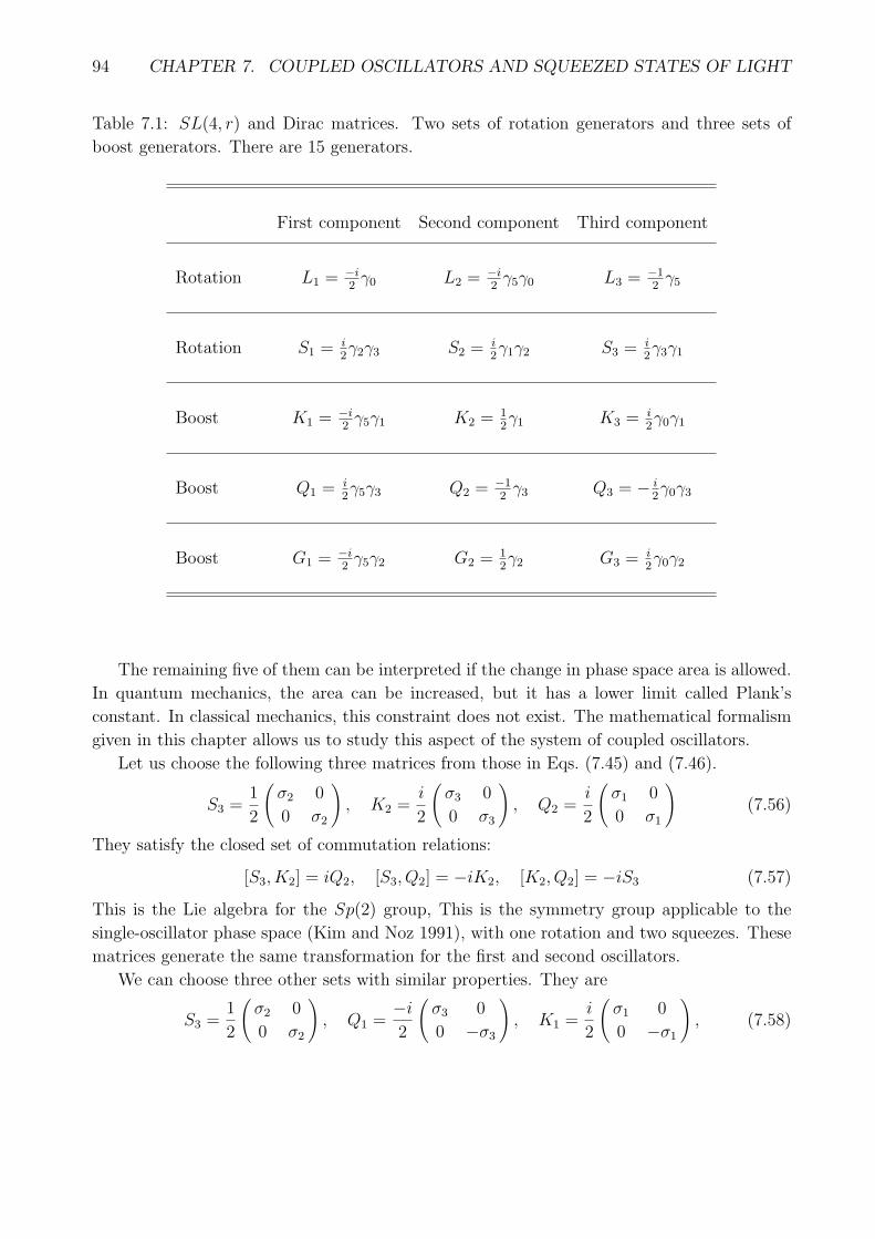
94 CHAPTER 7. COUPLED OSCILLATORS AND SQUEEZED STATES OF LIGHT
Table 7.1: SL(4, r) and Dirac matrices. Two sets of rotation generators and three sets of
boost generators. There are 15 generators.
First component Second component Third component
Rotation L1 =−i2γ0 L2 =
−i2γ5γ0 L3 =
−12γ5
Rotation S1 =i2γ2γ3 S2 =
i2γ1γ2 S3 =
i2γ3γ1
Boost K1 =−i2γ5γ1 K2 =
12γ1 K3 =
i2γ0γ1
Boost Q1 =i2γ5γ3 Q2 =
−12γ3 Q3 = − i
2γ0γ3
Boost G1 =−i2γ5γ2 G2 =
12γ2 G3 =
i2γ0γ2
The remaining five of them can be interpreted if the change in phase space area is allowed.
In quantum mechanics, the area can be increased, but it has a lower limit called Plank’s
constant. In classical mechanics, this constraint does not exist. The mathematical formalism
given in this chapter allows us to study this aspect of the system of coupled oscillators.
Let us choose the following three matrices from those in Eqs. (7.45) and (7.46).
S3 =1
2
(σ2 0
0 σ2
), K2 =
i
2
(σ3 0
0 σ3
), Q2 =
i
2
(σ1 0
0 σ1
)(7.56)
They satisfy the closed set of commutation relations:
[S3, K2] = iQ2, [S3, Q2] = −iK2, [K2, Q2] = −iS3 (7.57)
This is the Lie algebra for the Sp(2) group, This is the symmetry group applicable to the
single-oscillator phase space (Kim and Noz 1991), with one rotation and two squeezes. These
matrices generate the same transformation for the first and second oscillators.
We can choose three other sets with similar properties. They are
S3 =1
2
(σ2 0
0 σ2
), Q1 =
−i2
(σ3 0
0 −σ3
), K1 =
i
2
(σ1 0
0 −σ1
), (7.58)

7.6. ENTROPY AND THE EXPANDING WIGNER PHASE SPACE 95
L3 =1
2
(−σ2 0
0 σ2
), K2 =
i
2
(σ3 0
0 σ3
), K1 =
−i2
(−σ1 0
0 σ1
), (7.59)
and
L3 =1
2
(−σ2 0
0 σ2
), Q1 =
i
2
(−σ3 0
0 σ3
), Q2 =
i
2
(σ1 0
0 σ1
). (7.60)
These matrices also satisfy the commutation relations given in Eq. (7.57). In this case, the
squeeze transformations take opposite directions in the second phase space.
Since all these transformations are canonical, they leave the area of each phase space
invariant. However, let us look at the non-canonical generator G3 of Eq. (7.54). It generates
the transformation matrix of the form (eη 0
0 e−η
)(7.61)
If η is positive, this matrix expands the first phase space while contracting the second. This
contraction of the second phase space is allowed in classical mechanics, but it has a lower limit
in quantum mechanics. This is illustrated in Fig. 7.3.
The expansion of the first phase space is exactly like the thermal expansion resulting from
our failure to observe the second oscillator that belongs to the rest of the universe. If we
expand the system of Dirac’s ten oscillator matrices to the world of his fifteen Majorana
matrices, we can expand and contract the first and second phase spaces without mixing them
up. We can thus construct a model where the observed world and the rest of the universe
remain separated. In the observable world, quantum mechanics remains valid with thermal
excitations. In the rest of the universe, since the area of the phase space can decrease without
lower limit, only classical mechanics is valid.
During the expansion/contraction process, the product of the areas of the two phase spaces
remains constant. This may or may not be an extended interpretation of the uncertainty
principle, but we choose not to speculate further on this issue.
Let us turn our attention to the fact that the groups SL(4, r) and Sp(4) are locally iso-
morphic to O(3, 3) and O(3, 2) respectively. This means that we can do quantum mechanics
in one of the O(3, 2) subgroups of O(3, 3), as Dirac noted in his 1963 paper. The remaining
generators belong to Feynman’s rest of the universe.
7.6 Entropy and the expanding Wigner phase space
We have seen how Feynman’s rest of the universe increases the radius of the Wigner function.
It is important to note that the entropy of the system also increases.
Let us go back to the density matrix. The standard way to measure this ignorance is to
calculate the entropy defined as (von Neumann 1932, Landau and Lifshitz 1958, Fano 1957,
Blum 1981, Kim and Wigner 1990, Kim and Noz 2014).
S = −Tr (ρ ln(ρ)) (7.62)
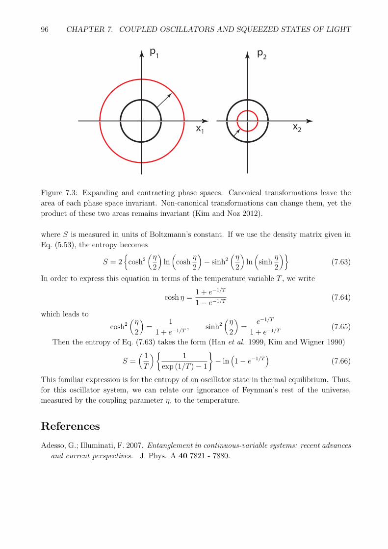
96 CHAPTER 7. COUPLED OSCILLATORS AND SQUEEZED STATES OF LIGHT
p p
x x
1
1
2
2
Figure 7.3: Expanding and contracting phase spaces. Canonical transformations leave the
area of each phase space invariant. Non-canonical transformations can change them, yet the
product of these two areas remains invariant (Kim and Noz 2012).
where S is measured in units of Boltzmann’s constant. If we use the density matrix given in
Eq. (5.53), the entropy becomes
S = 2{cosh2
(η
2
)ln(cosh
η
2
)− sinh2
(η
2
)ln(sinh
η
2
)}(7.63)
In order to express this equation in terms of the temperature variable T , we write
cosh η =1 + e−1/T
1− e−1/T(7.64)
which leads to
cosh2(η
2
)=
1
1 + e−1/T, sinh2
(η
2
)=
e−1/T
1 + e−1/T(7.65)
Then the entropy of Eq. (7.63) takes the form (Han et al. 1999, Kim and Wigner 1990)
S =(1
T
){1
exp (1/T )− 1
}− ln
(1− e−1/T
)(7.66)
This familiar expression is for the entropy of an oscillator state in thermal equilibrium. Thus,
for this oscillator system, we can relate our ignorance of Feynman’s rest of the universe,
measured by the coupling parameter η, to the temperature.
References
Adesso, G.; Illuminati, F. 2007. Entanglement in continuous-variable systems: recent advances
and current perspectives. J. Phys. A 40 7821 - 7880.
7.6. ENTROPY AND THE EXPANDING WIGNER PHASE SPACE 97
Abraham, R.; Marsden, J. E. 1978. Foundations of Mechanics. 2nd Ed Benjamin Cummings:
Boston, MA.
Blum, K. 1981. Density Matrix Theory and Applications. Plenum: New York, NY.
Braunstein, S. L.; van Loock, P. 2005. Quantum information with continuous variables. Rev.
Mod. Phys. 28 513 - 676 (2005).
Chou, Chung-Hsien; Yu, Ting; Hu, B. L. 2008. Exact master equation and quantum deco-
herence of two coupled harmonic oscillators in a general environment. Phys. Rev. E 77
011112 -1 - 011112 - 18.
Dirac, P. A. M. 1963. A Remarkable representation of 3 + 2 de Sitter group. J. Math. Phys.
4 901 - 909.
Dodd, P. J.; Halliwell, J. J. 2004. Disentanglement and decoherence by open system dynamics.
Phys. Rev. A 69 052105 -1 - 052105 - 6.
Ekert, A. K.; Knight, P. L. 1989. Correlations and squeezing of two-mode oscillations. Am.
J. Phys. 57 692 - 697.
Fano, U. 1957. Description of States in Quantum Mechanics by Density Matrix and Operator
Techniques. Rev. Mod. Phys. 29 74 - 93.
Giedke, G.; Wolf, M. M.; Krueger, O; Werner, R. F.; Cirac, J. J. 2003. Entanglement of
formation for symmetric Gaussian states. Phys. Rev. Lett. 91 107901 - 107904.
Goldstein, H. 1980. Classical Mechanics. 2nd Ed Addison Wesley: Boston, MA
Han, D.; Kim, Y. S.; Noz, M. E.; Yeh, L. 1993. Symmetries of Two-mode Squeezed States. J.
Math. Phys. 34 5493 - 5508.
Han, D.; Kim, Y. S.; Noz, M. E. 1995. O(3,3)-like Symmetries of Coupled Harmonic Oscilla-
tors. J. Math. Phys. 36 3940 - 3954.
Han, D.; Kim, Y. S.; Noz, M. E. 1999. Illustrative example of Feynman’s rest of the universe.
Am. J. Phys. 67 61 - 66.
Itzykson, C.; Zuber, J. B. 1980. Quantum Field Theory. McGraw-Hill: New York, NY.
Kim, Y. S.; Wigner, E. P. 1990. Entropy and Lorentz Transformations. Phys. Lett. A 147
343 - 347.
Kim, Y. S.; Noz, M. E. 1991. Phase Space Picture of Quantum Mechanics. World Scientific:
Singapore.
Kim, Y. S.; Noz, M. E. 2012. Dirac Matrices and Feynman’s Rest of the Universe. Symmetry
4 626 - 643.
Kim, Y. S.; Noz, M. E. 2014. Entropy and Temperature from Entangled Space and Time.
Phys. Sci. Int. J. 4 1015 - 1039.
Landau, L. D.; Lifshitz, E. M. 1958. Statistical Physics. Pergamon Press: London, UK.
Lee, D. 1995. The Dirac gamma matrices as “relics” of a hidden symmetry? As fundamental
representation of the algebra Sp(4,r). J. Math. Phys. 36 524 - 530.
Majorana, E. 1932. Relativistic Particles with Arbitrary Instrisic Angular Momenum. Nuovo
Cimento 9 335 - 341.

98 CHAPTER 7. COUPLED OSCILLATORS AND SQUEEZED STATES OF LIGHT
Paz, P. J.; Roncaglia, A. J. 2008. Dynamics of the Entanglement between Two Oscillators in
the Same Environment. Phys. Rev. Lett. 100 220401 -1 - 220401 - 4.
von Neumann, J. 1932. Die mathematische Grundlagen der Quanten-mechanik. Springer-
Verlag: Berlin, Germany. See also von Neumann, J. 1955. Mathematical Foundation of
Quantum Mechanics. Princeton University Press: Princeton, NJ.
Xiang, S. H.; Song, K. H.; Wen, W.; Shi, Z. G. 2011. Entanglement behaviors of two-mode
squeezed thermal states in two different environments. Euro. Phys. J. D 62 289 - 296.
Yuen, H. P. 1976. Two-photon coherent states of the radiation field. Phys. Rev. A 13 2226 -
2243.
Yurke, B. S.; L. McCall, B. L.; Klauder, J. R. 1986. SU(2) and SU(1,1) interferometers.
Phys. Rev. A 33 4033 - 4054.
Yurke, B; Potasek, M. 1987. Obtainment of Thermal Noise from a Pure State. Phys. Rev. A
36 3464 - 3466.

Chapter 8
Lorentz group in ray optics
While the Lorentz group serves as the basic language for Einstein’s special theory of relativity,
it can also be considered to be the basic mathematical instrument in optical sciences, partic-
ularly in ray and polarization optics. In this chapter, the two-by-two beam transfer matrix,
commonly called the ABCD matrix, is shown to be a two-by-two representation of the Lorentz
group discussed in Sec. 1.2. It is thus possible to study this matrix in terms of the math-
ematical device developed for studying Wigner’s little groups dictating internal space-time
symmetries of particles in the Lorentz-covariant world discussed extensively in Chapter 3.
8.1 Group of ABCD matrices
The Lorentz group for particle physics is generated by six matrices, however, the elements of
the ABCD matrices are always real and unimodular (determinant = 1). Thus, this matrix
can be generated by J2, K3, and K1 given in Chapter 1, which lead to two-by-two matrices
with real elements. These generators satisfy the closed set of commutation relations
[J2, K1] = −iK3, [J2, K3] = iK1, [K1, K3] = −iJ2, (8.1)
where
J2 =i
2
(0 −1
1 0
), K3 =
i
2
(1 0
0 −1
), K1 =
i
2
(0 1
1 0
). (8.2)
They form the Lie algebra for the Sp(2) group (Georgieva and Kim 2001, Sanchez-Soto et al.
2012, Baskal and Kim 2013).
The representation of the Sp(2) group generated by the these commutation relations consist
of a rotation about the origin, a squeeze along the x direction and another squeeze at along
axes rotated by 45o respectively. These generators are equivalent to another set of generators
which form a representation of the Sp(2) group consisting of two shear transformations and
a squeeze transformation (Baskal and Kim 2001, 2003). Therefore we shall use a rotation, a
99

100 CHAPTER 8. LORENTZ GROUP IN RAY OPTICS
squeeze, and a shear matrix of the form (Baskal and Kim 2009):
R(θ) =
(cos(θ/2) − sin(θ/2)
sin(θ/2) cos(θ/2)
), B(η) =
(eη/2 0
0 e−η/2
), (8.3)
and
T (γ) =
(1 −γ0 1
). (8.4)
The last matrix can also be viewed as an optical filter (Han, el al. 1999), or as a translation
matrix (Baskal and Kim 2003).
The traces of these matrices are smaller than 2, equal to 2, and greater than 2, respectively.
In Chapter 4, we discussed how to make transitions from one to another.
Since the ABCD matrix has real elements and a determinant of one, it has three indepen-
dent parameters. The elements of the ABCD matrix are determined by optical materials and
how they are arranged. The purpose of this chapter is to explore the mathematical properties
of the ABCD matrix which can address more fundamental issues in physics.
8.2 Equi-diagonalization of the ABCD matrix
In dealing with matrices, it is a routine process to diagonalize them. However, it is not always
possible. The triangular matrix in Eq. (8.4) cannot be diagonalized. On the other hand, the
two diagonal elements are equal.
The ABCD matrix with inputs from optical instruments is not always equi-diagonal.
Thus, we have to equi-diagonalize the matrix. Let us start from the matrix
[ABCD] =
(A B
C D
), (8.5)
where A and D are not necessarily equal to each other. Then the transformation
B(η) [ABCD] B(η) =
(eη/2 0
0 e−η/2
)(A B
C D
)(eη/2 0
0 e−η/2
)(8.6)
will lead to the equi-diagonal form (√AD B
C√AD
)(8.7)
with
eη =√D/A.
The diagonal matrix B(η) is given in Eq. (8.3). This form of equi-diagonalization will be
useful in camera optics discussed in Sec. 8.6.
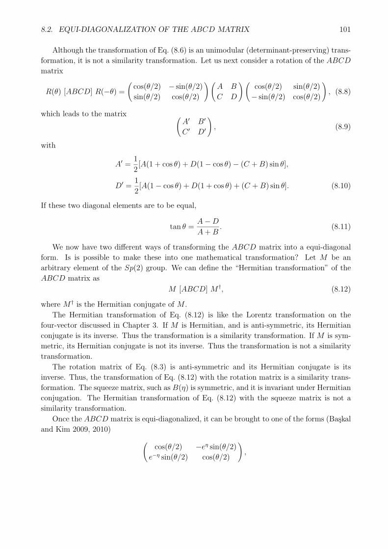
8.2. EQUI-DIAGONALIZATION OF THE ABCD MATRIX 101
Although the transformation of Eq. (8.6) is an unimodular (determinant-preserving) trans-
formation, it is not a similarity transformation. Let us next consider a rotation of the ABCD
matrix
R(θ) [ABCD] R(−θ) =(cos(θ/2) − sin(θ/2)
sin(θ/2) cos(θ/2)
)(A B
C D
)(cos(θ/2) sin(θ/2)
− sin(θ/2) cos(θ/2)
), (8.8)
which leads to the matrix (A′ B′
C ′ D′
), (8.9)
with
A′ =1
2[A(1 + cos θ) +D(1− cos θ)− (C +B) sin θ],
D′ =1
2[A(1− cos θ) +D(1 + cos θ) + (C +B) sin θ]. (8.10)
If these two diagonal elements are to be equal,
tan θ =A−D
A+B. (8.11)
We now have two different ways of transforming the ABCD matrix into a equi-diagonal
form. Is is possible to make these into one mathematical transformation? Let M be an
arbitrary element of the Sp(2) group. We can define the “Hermitian transformation” of the
ABCD matrix as
M [ABCD] M †, (8.12)
where M † is the Hermitian conjugate of M .
The Hermitian transformation of Eq. (8.12) is like the Lorentz transformation on the
four-vector discussed in Chapter 3. If M is Hermitian, and is anti-symmetric, its Hermitian
conjugate is its inverse. Thus the transformation is a similarity transformation. If M is sym-
metric, its Hermitian conjugate is not its inverse. Thus the transformation is not a similarity
transformation.
The rotation matrix of Eq. (8.3) is anti-symmetric and its Hermitian conjugate is its
inverse. Thus, the transformation of Eq. (8.12) with the rotation matrix is a similarity trans-
formation. The squeeze matrix, such as B(η) is symmetric, and it is invariant under Hermitian
conjugation. The Hermitian transformation of Eq. (8.12) with the squeeze matrix is not a
similarity transformation.
Once the ABCD matrix is equi-diagonalized, it can be brought to one of the forms (Baskal
and Kim 2009, 2010) (cos(θ/2) −eη sin(θ/2)
e−η sin(θ/2) cos(θ/2)
),
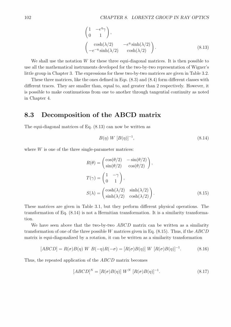
102 CHAPTER 8. LORENTZ GROUP IN RAY OPTICS
(1 −eηγ0 1
),
(cosh(λ/2) −eη sinh(λ/2)
−e−η sinh(λ/2) cosh(λ/2)
). (8.13)
We shall use the notation W for these three equi-diagonal matrices. It is then possible to
use all the mathematical instruments developed for the two-by-two representation of Wigner’s
little group in Chapter 3. The expressions for these two-by-two matrices are given in Table 3.2.
These three matrices, like the ones defined in Eqs. (8.3) and (8.4) form different classes with
different traces. They are smaller than, equal to, and greater than 2 respectively. However, it
is possible to make continuations from one to another through tangential continuity as noted
in Chapter 4.
8.3 Decomposition of the ABCD matrix
The equi-diagonal matrices of Eq. (8.13) can now be written as
B(η) W [B(η)]−1, (8.14)
where W is one of the three single-parameter matrices:
R(θ) =
(cos(θ/2) − sin(θ/2)
sin(θ/2) cos(θ/2)
),
T (γ) =
(1 −γ0 1
),
S(λ) =
(cosh(λ/2) sinh(λ/2)
sinh(λ/2) cosh(λ/2)
). (8.15)
These matrices are given in Table 3.1, but they perform different physical operations. The
transformation of Eq. (8.14) is not a Hermitian transformation. It is a similarity transforma-
tion.
We have seen above that the two-by-two ABCD matrix can be written as a similarity
transformation of one of the three possibleW matrices given in Eq. (8.15). Thus, if the ABCD
matrix is equi-diagonalized by a rotation, it can be written as a similarity transformation
[ABCD] = R(σ)B(η) W B(−η)R(−σ) = [R(σ)B(η)] W [R(σ)B(η)]−1. (8.16)
Thus, the repeated application of the ABCD matrix becomes
[ABCD]N = [R(σ)B(η)] WN [R(σ)B(η)]−1. (8.17)
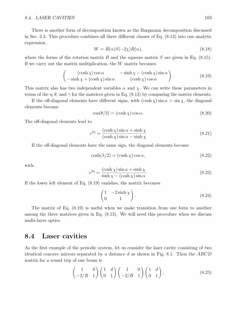
8.4. LASER CAVITIES 103
There is another form of decomposition known as the Bargmann decomposition discussed
in Sec. 3.3. This procedure combines all three different classes of Eq. (8.13) into one analytic
expression.
W = R(α)S(−2χ)R(α), (8.18)
where the forms of the rotation matrix R and the squeeze matrix S are given in Eq. (8.15).
If we carry out the matrix multiplication, the W matrix becomes((coshχ) cosα − sinhχ− (coshχ) sinα
− sinhχ+ (coshχ) sinα (coshχ) cosα
). (8.19)
This matrix also has two independent variables α and χ. We can write these parameters in
terms of the η, θ, and γ for the matrices given in Eq. (8.13) by comparing the matrix elements.
If the off-diagonal elements have different signs, with (coshχ) sinα > sinχ, the diagonal
elements become
cos(θ/2) = (coshχ) cosα. (8.20)
The off-diagonal elements lead to
e2η =(coshχ) sinα+ sinhχ
(coshχ) sinα− sinhχ(8.21)
If the off-diagonal elements have the same sign, the diagonal elements become
cosh(λ/2) = (coshχ) cosα, (8.22)
with
e2η =(coshχ) sinα + sinhχ
sinhχ− (coshχ) sinα. (8.23)
If the lower left element of Eq. (8.19) vanishes, the matrix becomes(1 −2 sinhχ
0 1
). (8.24)
The matrix of Eq. (8.19) is useful when we make transition from one form to another
among the three matrices given in Eq. (8.13). We will need this procedure when we discuss
multi-layer optics.
8.4 Laser cavities
As the first example of the periodic system, let us consider the laser cavity consisting of two
identical concave mirrors separated by a distance d as shown in Fig. 8.1. Then the ABCD
matrix for a round trip of one beam is(1 0
−2/R 1
)(1 d
0 1
)(1 0
−2/R 1
)(1 d
0 1
), (8.25)

104 CHAPTER 8. LORENTZ GROUP IN RAY OPTICS
The cycle starts at the midway between
the lenses when [ABCD] is equi-diagonal.
The cycle can start anywhere
between the lenses.
(d - x)
(d/2)
d
z
z
Co
nca
ve
mirro
r su
rfa
ce
Convex lens
Figure (a)
Figure (b)
(x)
midway
Figure 8.1: Optical rays in the laser cavity. fig.(a) illustrates that reflected beams are like
those going though a series of convex lenses. fig.(b) describes how the beams are reflected
from concave mirror surfaces (Baskal and Kim 2013).
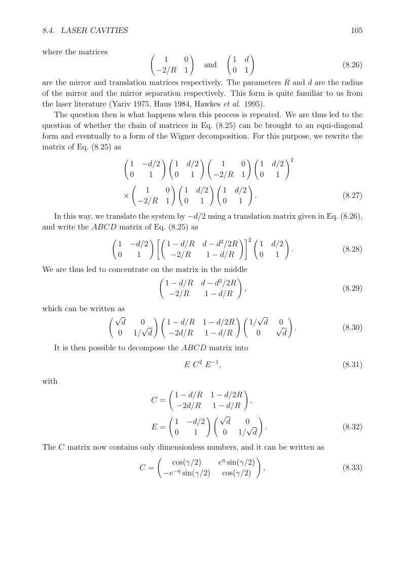
8.4. LASER CAVITIES 105
where the matrices (1 0
−2/R 1
)and
(1 d
0 1
)(8.26)
are the mirror and translation matrices respectively. The parameters R and d are the radius
of the mirror and the mirror separation respectively. This form is quite familiar to us from
the laser literature (Yariv 1975, Haus 1984, Hawkes et al. 1995).
The question then is what happens when this process is repeated. We are thus led to the
question of whether the chain of matrices in Eq. (8.25) can be brought to an equi-diagonal
form and eventually to a form of the Wigner decomposition. For this purpose, we rewrite the
matrix of Eq. (8.25) as (1 −d/20 1
)(1 d/2
0 1
)(1 0
−2/R 1
)(1 d/2
0 1
)2
×(
1 0
−2/R 1
)(1 d/2
0 1
)(1 d/2
0 1
). (8.27)
In this way, we translate the system by −d/2 using a translation matrix given in Eq. (8.26),
and write the ABCD matrix of Eq. (8.25) as(1 −d/20 1
)[(1− d/R d− d2/2R
−2/R 1− d/R
)]2 (1 d/2
0 1
). (8.28)
We are thus led to concentrate on the matrix in the middle(1− d/R d− d2/2R
−2/R 1− d/R
), (8.29)
which can be written as(√d 0
0 1/√d
)(1− d/R 1− d/2R
−2d/R 1− d/R
)(1/√d 0
0√d
). (8.30)
It is then possible to decompose the ABCD matrix into
E C2 E−1, (8.31)
with
C =
(1− d/R 1− d/2R
−2d/R 1− d/R
),
E =
(1 −d/20 1
)(√d 0
0 1/√d
). (8.32)
The C matrix now contains only dimensionless numbers, and it can be written as
C =
(cos(γ/2) eη sin(γ/2)
−e−η sin(γ/2) cos(γ/2)
), (8.33)

106 CHAPTER 8. LORENTZ GROUP IN RAY OPTICS
with
cos(γ/2) = 1− d
R,
eη =
√2R− d
4d. (8.34)
Here both d and R are positive, and the restriction on them is that d be smaller than 2R.
This is the stability condition frequently mentioned in the literature (Haus 1984, Hawkes et
al. 1995).
Thus, the equi-diagonal matrix is C2, and takes the form(cos(γ) eη sin(γ)
−e−η sin(γ) cos(γ)
), (8.35)
which is
B(η)R(2γ)B(−η) (8.36)
The ABCD matrix takes the form
[ABCD] = [E B(η)] R(2χ) [E B(η)]−1. (8.37)
Thus, the repeated application becomes
[ABCD]N = [E B(η)] R(2Nχ) [E B(η)]−1. (8.38)
8.5 Multilayer optics
We consider an optical beam going through a periodic medium with two different refractive
indexes. If the beam traveling in the first medium hits the second medium, it is partially
transmitted and partially reflected. In order to maintain the continuity of the Poynting
vector, we define the electric fields as
E(±)1 =
1√n1
exp (±ik1z − ωt),
E(±)2 =
1√n2
exp (±ik2z − ωt) (8.39)
for the optical beams in the first and second media respectively. The superscript (+) and (−)
are for the incoming and reflected rays respectively.
These two optical rays are related by the two-by-two ABCD matrix, according to(E
(+)2
E(−)2
)=
(A B
C D
)(E
(+)1
E(−)1
). (8.40)

8.5. MULTILAYER OPTICS 107
1 122
one cycle
S(σ) S(-σ)
Figure 8.2: Multi-layers. The cycle can start in such a way that the ABCD matrix becomes
equi-diagonal (Georgieva and Kim 2001, 2003).
Of course the elements of this matrix are determined by transmission coefficients as well as
the phase shifts the beams experience while going through the media (Azzam and Bashara
1977, Georgieva and Kim 2001).
When the beam goes through the first medium to the second, we may use the boundary
matrix given by Azzam and Bashara (Azzam and Bashara 1977) and by Monzon and Sanchez-
Soto (Monzon and Sanchez-Soto 1999, 2000, Dragoman 2010). In terms of the refractive
indexes n1 and n2,
S(σ) =
(cosh(σ/2) sinh(σ/2)
sinh(σ/2) cosh(σ/2)
), (8.41)
where we can write the σ parameter as
cosh(σ
2
)=n1 + n2
2√n1n2
, sinh(σ
2
)=n1 − n2
2√n1n2
. (8.42)
The boundary matrix for the beam going from the second medium should be S(−σ) as seenin Fig. 8.2.
In addition, we have to consider the phase shifts through which the beams have to travel.
When the beam goes through the first media, we can use the phase-shift matrix
P (δ1) =
(e−iδ1/2 0
0 eiδ1/2
), (8.43)
and a similar expression for P (δ2) for the second medium. The phase shift δ is determined
by the wave number and thickness of the medium.
We are thus led to consider one complete cycle starting from the midpoint of the second
medium, and write
P (δ2/2)S(σ)P (δ1)S(−σ)P (δ2/2) . (8.44)

108 CHAPTER 8. LORENTZ GROUP IN RAY OPTICS
If multiplied into one matrix, is this matrix equi-diagonal to accept the Wigner and
Bargmann decompositions? Another question is whether the matrices in the above expression
can be converted into matrices with real elements.
In order to answer the second question, let us consider the similarity transformation
C1 Z(δ)D(σ) C−11 , (8.45)
with
C1 =1√2
(1 i
i 1
). (8.46)
This transformation leads to
R(δ)S(σ), (8.47)
where
R(δ) =
(cos(δ/2) − sin(δ/2)
sin(δ/2) cos(δ/2)
). (8.48)
This notation is consistent with the rotation matrices used in Sec. 8.3.
Let us make another similarity transformation with
C2 =1√2
(1 1
−1 1
). (8.49)
This changes S(σ) into B(σ) without changing R(δ), where
B(σ) =
(eσ/2 0
0 e−σ/2
), (8.50)
again consistent with the B(η) matrix used in Sec. 8.3.
Thus the net similarity transformation matrix is (Georgieva and Kim 2001)
C = C2C1 =1√2
(eiπ/4 eiπ/4
−e−iπ/4 e−iπ/4
), (8.51)
with
C−1 =1√2
(e−iπ/4 −eiπ/4e−iπ/4 eiπ/4
). (8.52)
If we apply this similarity transformation to the long matrix chain of Eq. (8.44), it becomes
another chain
M = R (δ2/2)B(σ)R (δ1)B(−σ)R (δ2/2) , (8.53)
where all the matrices are real.
Let us now address the main question of whether this matrix chain can be brought to one
equi-diagonal matrix. We note first that the three middle matrices can be written in a familiar

8.6. CAMERA OPTICS 109
form
M = B(σ)R (δ1)B(−σ)
=
(cos(δ1/2) −eσ sin(δ1/2)
e−σ sin(δ1/2) cos(δ1/2)
). (8.54)
However, due to the rotation matrix R (δ2/2) at the beginning and at the end of Eq. (8.53),
it is not clear whether the entire chain can be written as a similarity transformation.
In order to resolve this issue, let us write Eq. (8.54) as a Bargmann decomposition
R(α)S(−2χ)R(α), (8.55)
with its explicit expression given in Eq. (8.19). The parameters α and χ are related to σ and
δ1 by
cos(δ1/2) = (coshχ) cosα,
e2η =(coshχ) sinα + sinhχ
(coshχ) sinα− sinhχ. (8.56)
It is now clear that the entire chain of Eq. (8.44) can be written as another Bargmann
decomposition
M = R(α + δ2/2)S(−2χ)R(α + δ2/2). (8.57)
Finally, this expression can be converted to a Wigner deomposition (Georgieva and Kim 2003)
M = B(η)R(θ)B(−η), (8.58)
with
cos(θ/2) = (coshχ) cos(α+ δ2/2),
e2η =(coshχ) sin(α + δ2/2) + sinhχ
(coshχ) sin(α + δ2/2)− sinhχ. (8.59)
The decomposition of Eq. (8.58) allows us to deal with the periodic system of multilayers. For
repeated application of M , we can now write
MN = B(η)R(Nθ)B(−η). (8.60)
8.6 Camera optics
The basic optical arrangement for the camera consists of a lens with focal length f and the
propagation of the ray by an amount d (Saleh and Teich 2007). The lens matrix is given by(1 0
−1/f 1
), (8.61)
110 CHAPTER 8. LORENTZ GROUP IN RAY OPTICS
and a translation of the ray is expressed by the matrix(1 d
0 1
). (8.62)
If the object and the image are d1 and d2 distances away from the lens respectively, the
system is described by (1 d20 1
)(1 0
−1/f 1
)(1 d10 1
). (8.63)
The multiplication of these matrices leads to the camera matrix of the form(1− d2/f d1 + d2 − d1d2/f
−1/f 1− d1/f
). (8.64)
The image becomes focused when the upper right element of this matrix vanishes (Baskal and
Kim 2003), i.e.,1
d1+
1
d2=
1
f. (8.65)
For the camera optics, both d1 and d2 are longer than f . It is then more convenient to
deal with the negative of the matrix given in Eq. (8.64) with positive diagonal elements. In
addition, let us use the dimensionless variables
x1 = d1/f, x2 = d2/f. (8.66)
Then the camera matrix becomes(x2 − 1 (x1 − 1) (x2 − 1)− 1
1 x1 − 1
), (8.67)
with the focal condition1
x1+
1
x2= 1. (8.68)
If we wish to study the formula of the camera matrix Eq. (8.67) as a representation of
the Lorentz group, the first step is to obtain its equi-diagonal form. However, if the focal
condition of Eq. 8.68 is to be preserved, the off-diagonal elements should remain invariant.
We thus have to resort to the Hermitian transformation given in Eq. (8.6). For this purpose,
we can use the transformation matrix (eη/2 0
0 e−η/2
)(8.69)
with
eη =
√1− x21− x1
. (8.70)
The diagonal elements become √(1− x1) (1− x2). (8.71)

8.6. CAMERA OPTICS 111
�3 �2 �1 1 2 3
�5
5
2χ = ξ
2χ = - ξ
Figure 8.3: Tangential continuity in the camera focusing. The vertical axis χ of this graph is
the upper-right element of the camera matrix and is -sin2(θ/2) for ξ < 0, and sinh2(λ/2) for
ξ > 0 (Baskal and Kim 2014).
If the diagonal elements are smaller than one, the camera matrix should take the form(cos(θ/2) −eη sin(θ/2)
e−η sin(θ/2) cos(θ/2)
)(8.72)
with
e−η sin(θ/2) = 1. (8.73)
Thus the matrix becomes (cos(θ/2) − sin2(θ/2)
1 cos(θ/2)
). (8.74)
If the diagonal elements are greater than one, the camera matrix becomes(cosh(λ/2) eη sinh(λ/2)
e−η sinh(λ/2) cosh(λ/2)
)(8.75)
with
e−η sinh(λ/2) = 1, (8.76)
leading to (cosh(λ/2) sinh2(λ/2)
1 cosh(λ/2)
). (8.77)
Thus, the focusing process is the transition from(1− ξ2/2 −ξ2
1 1− ξ2/2
)to
(1 + ξ2/2 ξ2
1 1 + ξ2/2
), (8.78)
via ξ = 0. This transition is illustrated in Fig. 8.3. Indeed, this is the tangential continuity
discussed extensively in Chapter 4.

112 CHAPTER 8. LORENTZ GROUP IN RAY OPTICS
References
Azzam, R. A. M.; Bashara, I. 1977. Ellipsometry and Polarized Light. North-Holland: Ams-
terdam, The Netherlands.
Baskal, S.; Kim, Y. S. 2001. Shear representations of beam transfer matrices. Phys. Rev. E
63 056606 -1 - 056606 - 6.
Baskal, S.; Kim, Y. S. 2003. Lens optics as an optical computer for group contractions. Phys.
Rev. E 67 056601 -1 - 056601 - 8.
Baskal, S.; Kim, Y. S. 2009. ABCD matrices as similarity transformations of Wigner matrices
and periodic systems in optics. J. Opt. Soc. Am. A 26 3049 - 3054.
Baskal, S.; Kim, Y. S. 2010. One analytic form for four branches of the ABCD matrix. J.
Mod. Opt. 57 1251 - 1259.
Baskal, S; Kim, Y. S. 2013. Lorentz Group in Ray and Polarization Optics. Chapter 9 in
”Mathematical Optics: Classical, Quantum and Computational Methods” edited by Va-
sudevan Lakshminarayanan, Maria L. Calvo, and Tatiana Alieva, CRC Taylor and Francis:
Boca Raton, FL, pp 303 - 349.
D. Dragoman, D. 2010. Polarization optics analogy of quantum wavefunctions in graphene.
J. Opt. Soc. Am. B 27 1325 - 1331.
Georgieva, E.; Kim, Y. S. 2001. Iwasawa effects in multilayer optics. Phys. Rev. E 64 26602
-1 - 26602 - 6.
Georgieva, E.; Kim, Y. S. 2003. Slide-rule-like property of Wigner’s little groups and cyclic S
matrices for multilayer optics. Phys. Rev. E 68 026606 -1 - 026606 - 12.
Han, D.; Kim, Y. S.; Noz, M. E. 1999. Wigner rotations and Iwasawa decompositions in
polarization optics. Phys. Rev. E 60 1036 - 1041.
Haus, H. A. 1984. Waves and Fields in Optoelectronics. Prentice Hall: Upper Saddle River,
NJ.
Hawkes, J.; Latimer, I. 1995. Lasers: Theory and Practice. Prentice Hall, Upper Saddle
River, NJ.
Monzon, J. J.; Sanchez-Soto, L. L. 1999. Fully relativistic like formulation of multilayer optics.
J. Opt. Soc. Am. A 16 2013 - 2018.
Monzon, J. J.; Sanchez-Soto, L. L. 2000. Fresnel formulas as Lorentz transformations. J.
Opt. Soc. Am. A 17 1475 - 1481.
Saleh, B. E. A.; Teich, M. C. 2007. Fundamentals of Photonics., 2nd Ed John Wiley and Sons:
Hoboken, NJ.
Sanchez-Soto, L. L.; Monzon, J. J.; Barriuso, A. G.; Carinena, J. F. 2012. The transfer matrix:
A geometrical perspective. Phys. Reports 513 191 - 227.
Yariv, A. 1975. Quantum Electronics. John Wiley and Sons: Hoboken, NJ.

Chapter 9
Polarization optics
In studying polarized light propagating along the z direction, the traditional approach is to
consider the x and y components of the electric fields. Their amplitude ratio and phase
difference determine the state of polarization. Thus, we can change the polarization either by
adjusting the amplitudes, by changing the relative phases, or both. For convenience, we call
the optical device which changes amplitudes an “attenuator” and the device which changes
the relative phase a “phase shifter.”
It is thus possible to describe polarization of light as two-component column vectors, and
two-by-two matrices applicable to those vectors. The two-by-two representation of the Lorentz
group was discussed in Sec. 1.2. We will examine the polarization of light using the methods
developed in the early chapters of this book.
The mathematics of the Lorentz group was originally developed for understanding Ein-
stein’s special relativity. However, it is interesting to note that the same set of mathematical
tools can be used for studying polarization optics. The Jones vectors, Mueller matrices, and
Stokes parameters all constitute appropriate representations of the Lorentz group (Opatrny
and Perina 1993, Tudor 2015, Han et al. 1997, Ben-Aryeh 2005, Red’kov 2011, Baskal and
Kim 2013, Franssens 2015).
9.1 Jones vectors
The traditional language for studying the two-component light vector is the Jones-matrix
formalism which is covered in standard optics textbooks (Hecht 2002, Saleh and Teich 2007).
In this formalism, the two transverse components of the electric fields are combined into one
column matrix with the exponential form for the sinusoidal function(Ex
Ey
)=
(A exp {i(kz − ωt+ ϕ1)}B exp {i(kz − ωt+ ϕ2)}
). (9.1)
This column matrix is called the Jones vector (Jones 1941, 1947) .
113

114 CHAPTER 9. POLARIZATION OPTICS
In the existing textbooks (Hecht 2002), the Jones-matrix formalism (Hecht 1970) starts
with the projection operator (1 0
0 0
), (9.2)
applicable to the Jones vector of Eq. (9.1). This operator keeps the x component and com-
pletely eliminates the y-component of the electric field.
This is an oversimplification of the real world when the attenuation factor in the y direction
is greater than that along the x direction. We shall replace this projection operator by an
attenuation matrix which is closer to the real world.
In this section, we replace the projection operator of Eq. (9.2) by a squeeze matrix. There
are two transverse directions which are perpendicular to each other. The absorption coefficient
in one transverse direction could be different from the coefficient along the other direction.
This can be described by the two-by-two matrix (Opatrny and Perina 1993, Han et al. 1997,
Ben-Aryeh 2005, Tudor 2010, 2015, Baskal and Kim 2013, Franssens 2015)(e−µ1 0
0 e−µ2
)= e−(µ1+µ2)/2
(eµ/2 0
0 e−µ/2
)(9.3)
with µ = µ2 − µ1. Let us look at the projection operator of Eq. (9.2). Physically, it means
that the absorption coefficient along the y direction is much larger than along the x direction.
The absorption matrix in Eq. (9.3) becomes the projection matrix if µ1 is very close to zero
and µ2 becomes infinitely large. The projection operator of Eq. (9.2) is therefore a special
case of the above attenuation matrix.
The attenuation matrix of Eq. (9.3) tells us that the electric fields are attenuated at two
different rates. The exponential factor e−(µ1+µ2)/2 reduces both components at the same rate
and does not affect the state of polarization. The effect of polarization is solely determined
by the squeeze matrix
B(µ) =
(eµ/2 0
0 e−µ/2
). (9.4)
The diagonal matrix of this type served many different purposes in earlier chapters of this
book. It is a key element of the two-by-two representation of the Lorentz group.
Another basic element is the optical filter with different values of the index of refraction
along the two orthogonal directions. The effect on this filter can be written as(e−iδ1 0
0 e−iδ2
)= e−i(δ1+δ2)/2
(e−iδ/2 0
0 eiδ/2
), (9.5)
with δ = δ1 − δ2 . In measurement processes, the overall phase factor e−i(δ2+δ2)/2 cannot be
detected, and can therefore be deleted. The polarization effect of the filter is solely determined
by the matrix
Z(δ) =
(eiδ/2 0
0 e−iδ/2
), (9.6)
9.2. SQUEEZE AND PHASE SHIFT 115
which leads to a phase difference of δ between the x and y components. The mathematical
expression for this matrix is given in Eq. (9.4). It has a different physical meaning in the
symmetry of the Lorentz group.
The polarization axes are not always the x and y axes. For this reason, we need the
rotation matrix
R(θ) =
(cos(θ/2) − sin(θ/2)
sin(θ/2) cos(θ/2)
), (9.7)
to describe the rotation around the z axis.
The traditional Jones-matrix formalism consists of systematic combinations of the three
components given in Eq. (9.2), Eq. (9.6), and Eq. (9.7). However, in this chapter, we shall
use the squeeze matrix of Eq. (9.4) instead of the projection operator of Eq. (9.2). Then they
become the starters of the two-by-two representation of the Lorentz group.
9.2 Squeeze and phase shift
The effect of the phase shift matrix Z(δ) of Eq. (9.6) on the Jones vector is well known, but
the effect of the squeeze matrix of Eq. (9.4) is not addressed adequately in the literature. Let
us discuss the combined effect of these two matrices. First of all both are diagonal and they
commute with each other.
The effect of the squeeze matrix on the Jones vector is straight-forward. If we apply the
squeeze matrix of Eq. (9.4) to the Jones vector, the net result is(eµ/2 0
0 e−µ/2
)(Ex
Ey
)=
(eµ/2Ex
e−µ/2Ey
). (9.8)
This squeeze transformation expands one amplitude, while contracting the other so that the
product of the amplitude remains invariant. This squeeze transformation is illustrated in
Fig. 9.1.
In order to illustrate phase shifts, we start with the Jones vector of the form(exp (ikz)
exp [i(kz − π/2)]
), (9.9)
whose real part is (x
y
)=
(cos(kz)
sin(kz)
), (9.10)
which corresponds to a circular polarization with
x2 + y2 = 1. (9.11)
If we apply the phase shift matrix, the resulting vector is(x
y
)=
(cos(kz + δ/2)
sin(kz − δ/2)
), (9.12)
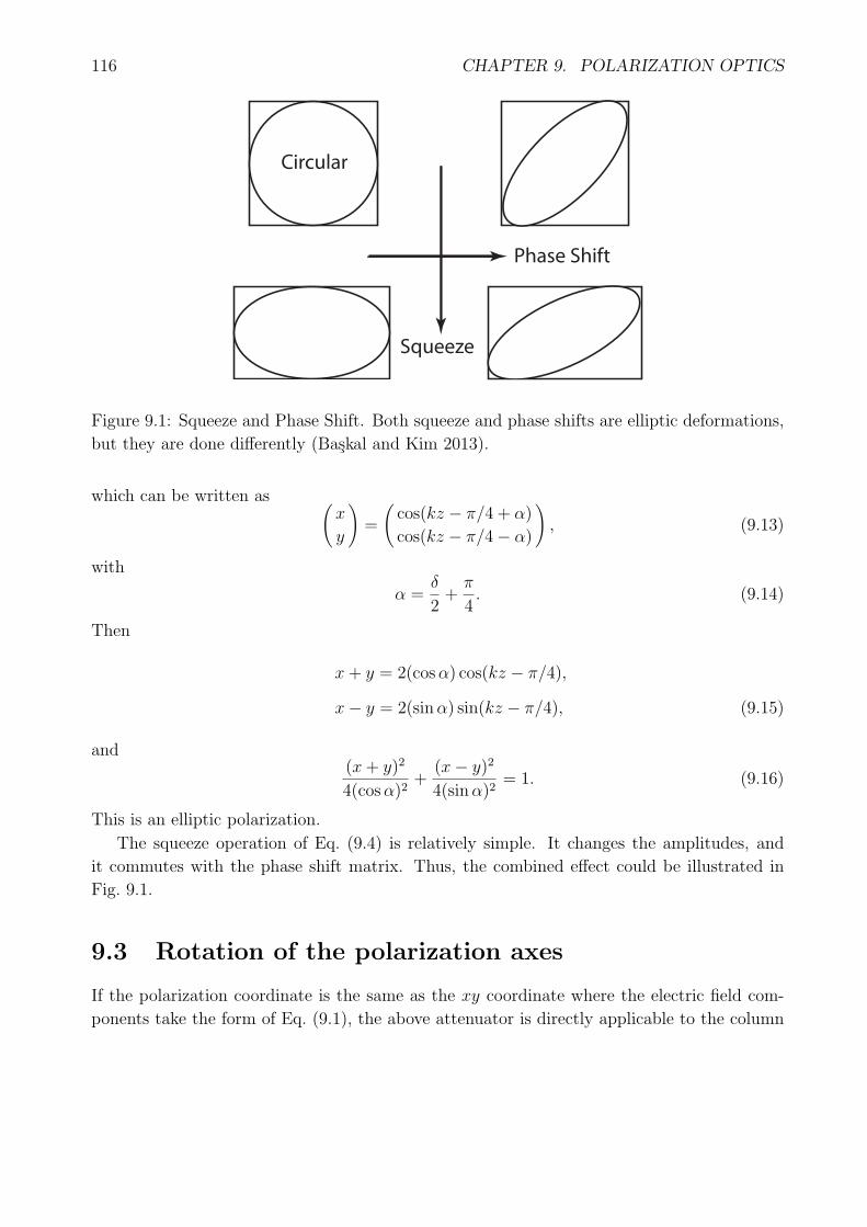
116 CHAPTER 9. POLARIZATION OPTICS
Circular
Phase Shift
Squeeze
Figure 9.1: Squeeze and Phase Shift. Both squeeze and phase shifts are elliptic deformations,
but they are done differently (Baskal and Kim 2013).
which can be written as (x
y
)=
(cos(kz − π/4 + α)
cos(kz − π/4− α)
), (9.13)
with
α =δ
2+π
4. (9.14)
Then
x+ y = 2(cosα) cos(kz − π/4),
x− y = 2(sinα) sin(kz − π/4), (9.15)
and(x+ y)2
4(cosα)2+
(x− y)2
4(sinα)2= 1. (9.16)
This is an elliptic polarization.
The squeeze operation of Eq. (9.4) is relatively simple. It changes the amplitudes, and
it commutes with the phase shift matrix. Thus, the combined effect could be illustrated in
Fig. 9.1.
9.3 Rotation of the polarization axes
If the polarization coordinate is the same as the xy coordinate where the electric field com-
ponents take the form of Eq. (9.1), the above attenuator is directly applicable to the column
9.3. ROTATION OF THE POLARIZATION AXES 117
matrix of Eq. (9.1). If the polarization coordinate is rotated by an angle θ/2, or by the matrix
R(θ) =
(cos(θ/2) − sin(θ/2)
sin(θ/2) cos(θ/2)
), (9.17)
the phase shifter takes the form
Z(θ, δ) = R(θ)Z(δ)R(−θ) (9.18)
=
(cos(δ/2) + i sin(δ/2) cos θ i sin(δ/2) sin θ
i sin(δ/2) sin θ cos(δ/2)− i sin(δ/2) cos θ
). (9.19)
If the polarization coordinate system is rotated by 45o, the phase shifter matrix becomes
Q(δ) =
(cos(δ/2) i sin(δ/2)
i sin(δ/2) cos(δ/2)
). (9.20)
In order to illustrate what this matrix does to the polarized beams, let us start with the
circularly polarized wave (X
Y
)=
(1
−i
)e(ikz−iωt), (9.21)
whose real part is (X
Y
)=
(cos(kz − ωt)
sin(kz − ωt)
). (9.22)
This leads to the familiar equation for the circle
X2 + Y 2 = 1. (9.23)
If the phase shifter of Eq. (9.20) is applied to the above Jones vector, the result is([cos(δ/2) + sin(δ/2)] cos(kz − ωt)
i[sin(δ/2)− cos(δ/2)] sin(kz − ωt)
)(9.24)
with
cos(δ/2) = cos ([δ/2 + π/4]− π/4) ,
sin(δ/2) = cos ([δ/2 + π/4] + π/4) . (9.25)
Thus,
cos(δ/2) + sin(δ/2) =√2 cos (δ/2 + π/4) ,
cos(δ/2)− sin(δ/2) =√2 sin (δ/2 + π/4) . (9.26)

118 CHAPTER 9. POLARIZATION OPTICS
Circular
Phase Shift
Rotation
Circular
Figure 9.2: Phase shift and rotation. They are rotated by 45o. (Baskal and Kim 2013).
After the phase shift, the Jones vector becomes([√2 cosα] cos(kz − ωt)
[√2 sinα] sin(kz − ωt)
), (9.27)
with
α =δ
2+π
4. (9.28)
The the x and y components will satisfy the equation
X2
(√2 cosα)2
+Y 2
(√2 sinα)2
= 1. (9.29)
This is an elliptic polarization. These steps are illustrated in Fig. 9.2.
Let us next consider rotations of the squeeze matrix.
B(θ, µ) = R(θ)B(µ)R(−θ), (9.30)
which leads to
B(θ, µ) =
(cosh(µ/2) + sinh(µ/2) cos θ sinh(µ/2) sin θ
sinh(µ/2) sin θ cosh(µ/2)− sinh(µ/2) cos θ
). (9.31)
We are familiar with this squeeze operation from Sec. 8.3. This changes the amplitudes. If
the squeeze angle become 45o, we use the notation S(µ) for this special angle, and
S(µ) =
(cosh(µ/2) sinh(µ/2)
sinh(µ/2) cosh(µ/2)
). (9.32)
9.4. OPTICAL ACTIVITIES 119
The question is what happens if two squeeze transformations are made in two different
directions. Would the result be another squeeze? The answer is No. The result is another
squeeze matrix followed by a rotation, which can be written as (Baskal and Kim 2005)
B(θ, λ)B(0, η) = B(ϕ, ξ)R(ω), (9.33)
where
cosh ξ = cosh η coshλ+ sinh η sinhλ cos θ,
tanϕ =sin θ[sinhλ+ tanh η(coshλ− 1) cos θ]
sinhλ cos θ + tanh η[1 + (coshλ− 1) cos2 θ],
tanω =2(sin θ)[sinhλ sinh η + C− cos θ]
C+ + C− cos(2θ) + 2 sinhλ sinh η cos θ, (9.34)
with
C± = (coshλ± 1)(cosh η ± 1). (9.35)
Indeed, we write Eq. (9.33) as
R(ω) = B(ϕ,−ξ) B(θ, λ) B(0, η), (9.36)
three squeeze transformations lead to one rotation.
We have done this calculation using the kinematics of Lorentz transformations. On the
other hand, it does not appear possible to do experiments using high-energy particles. How-
ever, it is gratifying to note that this experiment is possible in polarization optics.
If the angle θ is 90o, the calculation becomes simpler, and
B(λ)B(η) = B(ϕ, ξ)R(ω), (9.37)
where
cosh ξ = cosh η coshλ,
tanϕ =sinhλ
tanh η,
tanω =sinhλ sinh η
cosh η + coshλ. (9.38)
9.4 Optical activities
For convenience, let us change the parameters θ and µ as
θ = 2αz, µ = 2βz. (9.39)

120 CHAPTER 9. POLARIZATION OPTICS
Then the R(θ) matrix can be written as
R(αz) =
(cos(αz) − sin(αz)
sin(αz) cos(αz)
), (9.40)
and the rotation angle increases as the beam propagates along the z direction. This version
of optical activity is well known.
In addition, we can consider the squeeze operation
S(−βz) =(
cosh(βz) − sinh(βz)
− sinh(βz) cosh(βz)
). (9.41)
Here the squeeze parameter increases as the beam moves. The negative sign for β is for
convenience.
If this squeeze is followed by the rotation of Eq. (9.40), the net effect is(cosh(βz) − sinh(βz)
− sinh(βz) cosh(βz)
),
(cos(αz) − sin(αz)
sin(αz) cos(αz)
)(9.42)
where z is in a macroscopic scale, perhaps measured in centimeters. However, this is not an
accurate description of the optical process.
When this happens in a microscopic scale of z/N , it can become accumulated into the
macroscopic scale of z after the N repetitions, where N is a very large number. We are thus
led to the transformation matrix of the form (Kim 2010)
M(α, β, z) = [S(−βz/N)R(αz/N)]N . (9.43)
In the limit of large N , this quantity becomes
[(1 −βz/N
−βz/N 1
)(1 −αz/N
αz/N 1
)]N. (9.44)
Since αz/N and βz/N are very small,
M(α, β, z) =
[(1 0
0 1
)+
(0 −(α + β)
(α− β) 0
)z
N
]N. (9.45)
For large N , we can write this matrix as
M(α, β, z) = exp (Gz), (9.46)
with
G =
(0 −(α + β)
(α− β) 0
). (9.47)
9.4. OPTICAL ACTIVITIES 121
We can compute this matrix using the procedure developed in Sec. 8.3. If α is greater
than β, G becomes
G = α′(
0 exp (η)
exp (−η) 0
), (9.48)
with
α′ =√α2 − β2,
exp (η) =
√α + β
α− β, (9.49)
and the M matrix of Eq. (9.46) take the form(cos(α′z) −eη sin(α′z)
e−η sin(α′z) cos(α′z)
). (9.50)
If β is greater than α, the off-diagonal elements have the same sign. We can then write G
as
G = −β′(
0 exp (η)
exp (−η) 0
), (9.51)
with
β′ =√β2 − α2,
exp (η) =
√β + α
β − α, (9.52)
and the M matrix of Eq. (9.46) becomes(cosh(β′z) −eη sinh(β′z)
−e−η sinh(β′z) cosh(β′z)
). (9.53)
If α = β, the lower-left element of the G matrix has to vanish, and it becomes
G =
(0 −2α
0 0
), (9.54)
and the M matrix takes the triangular form(1 −2αz
0 1
). (9.55)
The optical material can be made to provide rotations of the polarization axis. It is much
more interesting to see this additional effect of squeeze.

122 CHAPTER 9. POLARIZATION OPTICS
References
Baskal, S.; Kim, Y. S. 2005. Rotations associated with Lorentz boosts. J. Phys. A 38 6545 -
6556.
Baskal, S; Kim. Y. S. 2013. Lorentz Group in Ray and Polarization Optics. Chapter 9 in
”Mathematical Optics: Classical, Quantum and Computational Methods” edited by Va-
sudevan Lakshminarayanan, Maria L. Calvo, and Tatiana Alieva, CRC Taylor and Francis:
Boca Raton, FL, pp 303 - 349.
Ben-Aryeh, Y. 2005. Nonunitary squeezing and biorthogonal scalar products in polarization
optics. J. Opt. B Quantum Semiclass 7 S452 - S457.
Franssens, G. R. 2015. Relativistic kinematics formulation of the polarization effects of Jones-
Mueller matrices. J. Opt. Soc. Am. A 32 164-172.
Han, D.; Kim, Y. S.; Noz, M. E. 1997. Jones-matrix formalism as a representation of the
Lorentz group. J. Opt. Soc. Am. A 14 2290 - 2298.
Hecht, E. 1970. Note on an operational definition of Stokes parameters. Am. J. Phys. 38
1156 - 1158.
Hecht, E. 2002. Optics. Pearson Education, Ltd.: Essex, UK.
Jones, R. C. 1941. New calculus for the treatment of optical systems. J. Opt. Soc. Am. 31
488 - 493.
Jones, R. C. 1947. A new calculus for the treatment of optical systems. 5. A more general
formulation, and description of another calculus. J. Opt. Soc. Am. 37 107 - 110.
Kim, Y. S. 2010. Optical activities as computing resources for spacetime symmetries. J. Mod.
Op. 7 17 - 22.
Opatrny, T.; Perina, J. 1993. Non-image-forming polarization optical devices and Lorentz
transformations - an analogy. Phys. Lett. A 181 199 - 202.
Red’kov, V. M. 2011. Lorentz Group Theory and Polarization of the Light. Avdances in
Applied Clifford Algebras 21 203-220.
Saleh, B. E. A.; Teich, M. C. 2007. Fundamentals of Photonics. 2nd Ed John Wiley and Sons:
Hoboken, NJ.
Tudor, T. 2010. Vectorial Pauli algebraic approach in polarization optics. I. Device and state
operators. Optik 121 1226-1235.
Tudor, T. 2015 On a quasi-relativistic formula in polarization theory. Opt. Lett. 40 693-696.
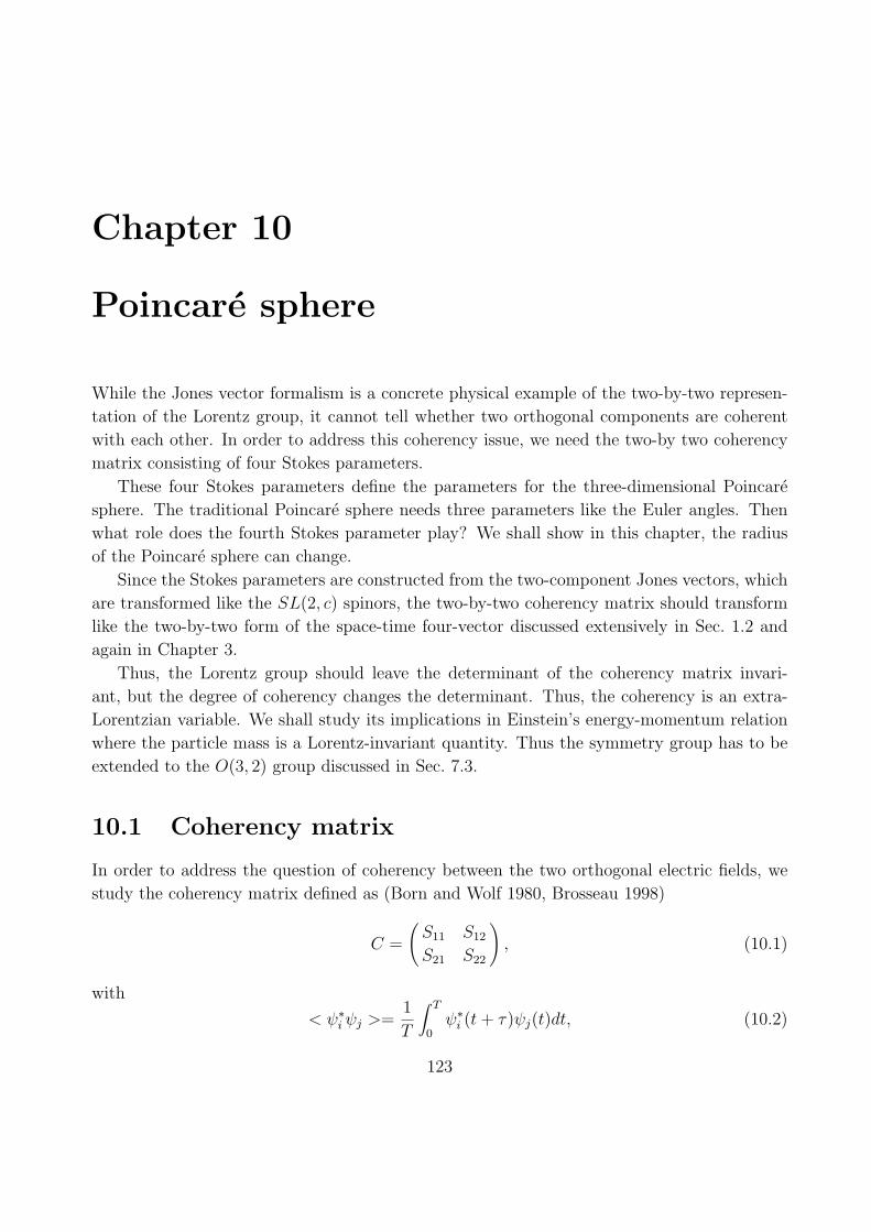
Chapter 10
Poincare sphere
While the Jones vector formalism is a concrete physical example of the two-by-two represen-
tation of the Lorentz group, it cannot tell whether two orthogonal components are coherent
with each other. In order to address this coherency issue, we need the two-by two coherency
matrix consisting of four Stokes parameters.
These four Stokes parameters define the parameters for the three-dimensional Poincare
sphere. The traditional Poincare sphere needs three parameters like the Euler angles. Then
what role does the fourth Stokes parameter play? We shall show in this chapter, the radius
of the Poincare sphere can change.
Since the Stokes parameters are constructed from the two-component Jones vectors, which
are transformed like the SL(2, c) spinors, the two-by-two coherency matrix should transform
like the two-by-two form of the space-time four-vector discussed extensively in Sec. 1.2 and
again in Chapter 3.
Thus, the Lorentz group should leave the determinant of the coherency matrix invari-
ant, but the degree of coherency changes the determinant. Thus, the coherency is an extra-
Lorentzian variable. We shall study its implications in Einstein’s energy-momentum relation
where the particle mass is a Lorentz-invariant quantity. Thus the symmetry group has to be
extended to the O(3, 2) group discussed in Sec. 7.3.
10.1 Coherency matrix
In order to address the question of coherency between the two orthogonal electric fields, we
study the coherency matrix defined as (Born and Wolf 1980, Brosseau 1998)
C =
(S11 S12
S21 S22
), (10.1)
with
< ψ∗iψj >=
1
T
∫ T
0ψ∗i (t+ τ)ψj(t)dt, (10.2)
123

124 CHAPTER 10. POINCARE SPHERE
where T for a sufficiently long time interval, is much larger than τ . Then, those four elements
become (Han et al. 1997)
S11 =< ψ∗1ψ1 >= a2, S12 =< ψ∗
1ψ2 >= ab e−(σ+iϕ),
S21 =< ψ∗2ψ1 >= ab e−(σ−iϕ), S22 =< ψ∗
2ψ2 >= b2. (10.3)
The diagonal elements are the absolute values of ψ1 and ψ2 respectively. The off-diagonal
elements could be smaller than the product of ψ1 and ψ2, if the two transverse components
are not completely coherent. The σ parameter specifies the degree of decoherence. The system
is completely coherent if σ = 0. It is totally incoherent if σ = ∞.
If we start with the Jones vector of the form of Eq. (9.1), the coherency matrix becomes
C =
(a2 ab e−(σ+iϕ)
ab e−(σ−iϕ) b2
). (10.4)
We are interested in the symmetry properties of this matrix. Since the transformation matrix
applicable to the Jones vector is the two-by-two representation of the Lorentz group, we are
particularly interested in the transformation matrices applicable to this coherency matrix.
The trace and determinant of the above coherency matrix are
det(C) = (ab)2(1− e−2σ
),
tr(C) = a2 + b2. (10.5)
Since e−σ is always smaller than one, we can introduce an angle χ defined as
cosχ = e−σ, (10.6)
and call it the “decoherence angle.” If χ = 0, the decoherence is minimum, and it is maximum
when χ = 90o. We can then write the coherency matrix of Eq. (10.4) as
C =
(a2 ab(cosχ)e−iϕ
ab(cosχ)eiϕ b2
). (10.7)
The degree of polarization is defined as (Saleh and Teich 2007)
f =
√√√√1− 4 det(C)
(tr(C))2=
√√√√1− 4(ab)2 sin2 χ
(a2 + b2)2. (10.8)
This degree is one if χ = 0. When χ = 90o, it becomes
a2 − b2
a2 + b2. (10.9)
Without loss of generality, we can assume that a is greater than b. If they are equal, this
minimum degree of polarization is zero.
10.1. COHERENCY MATRIX 125
Under the influence of the Lorentz transformation defined for the Jones vectors of Chap-
ter 9.1 and Sec. 1.2, this coherency matrix is transformed as
C ′ = G C G† =
(S ′11 S ′
12
S ′21 S ′
22
)
=
(α β
γ δ
)(S11 S12
S21 S22
)(α∗ γ∗
β∗ δ∗
). (10.10)
Indeed, this is the Lorentz transformation defined in Sec. 1.2.
Then it is possible to write
S0 =S11 + S22
2, S3 =
S11 − S22
2,
S1 =S12 + S21
2, S2 =
S12 − S21
2, (10.11)
as a four-vector.
These four parameters are called Stokes parameters, and four-by-four transformations
applicable to these parameters are widely known as Mueller matrices (Mueller 1943, Azzam
1977, Brosseau 1998).
The Mueller matrices perform Lorentz transformations on the four Stokes parameters.
The correspondence between the four-by-four and two-by-two representations was discussed
in detail in Chapter 4.
Since we can construct the Jones vector of Eq. (9.1) by making Lorentz transformations
on the simpler form (ψ1
ψ2
)=
(a exp {i(kz − ωt)}a exp {i(kz − ωt)}
), (10.12)
we can now drop the amplitude a and work with the coherency marrix of the form
C =
(1 e−iϕ cosχ
eiϕ cosχ 1
). (10.13)
The Stokes parameters are
S0 = 1, S3 = 0,
S1 = (cosχ) cosϕ, S2 = (cosχ)(sinϕ). (10.14)
The Poincare sphere is defined by S1, S2, and S3.
R =√S21 + S2
2 + S23 . (10.15)
Since S3 = 0 in Eq. (10.14), the sphere collapses into a circle of radius
126 CHAPTER 10. POINCARE SPHERE
Table 10.1: Polarization optics and special relativity sharing the same mathematics. Each ma-
trix has its clear role in both optics and relativity. The determinant of the two-by-two matrix
obtained from the Stokes vector or from the four-mometum remains invariant under Lorentz
transformations. It is interesting to note that the decoherency parameter (least fundamental)
in optics corresponds to the mass (most fundamental) in particle physics.
Polarization Optics Transformation Matrix Particle Symmetry
Phase shift ϕ
(e−iϕ/2 0
0 eiϕ/2
)Rotation around z
Rotation around z
(cos(θ/2) − sin(θ/2)
sin(θ/2) cos(θ/2)
)Rotation around y
Squeeze along x and y
(eµ/2 0
0 e−µ/2
)Boost along z
sin2 χ Determinant (mass)2
R =√S21 + S2
2 = cosχ. (10.16)
Let us go back to the four-momentum matrix of Eq. (1.21) of Sec. 1.2. Its determinant
is m2 and remains invariant under Lorentz transformations defined by Eq. (1.22). Likewise,
the determinant of the coherency matrix of Eq. (10.4) should also remain invariant. The
determinant in this case is
S20 −R2 = sin2 χ. (10.17)
However, this quantity depends on the angle χ variable which measures decoherency of the
two transverse components. This aspect is illustrated in Table 10.1.
While the decoherency parameter is not fundamental and is influenced by environment, it
plays the same mathematical role as in the particle mass which remains as the most funda-
mental quantity since Isaac Newton, and even after Einstein.
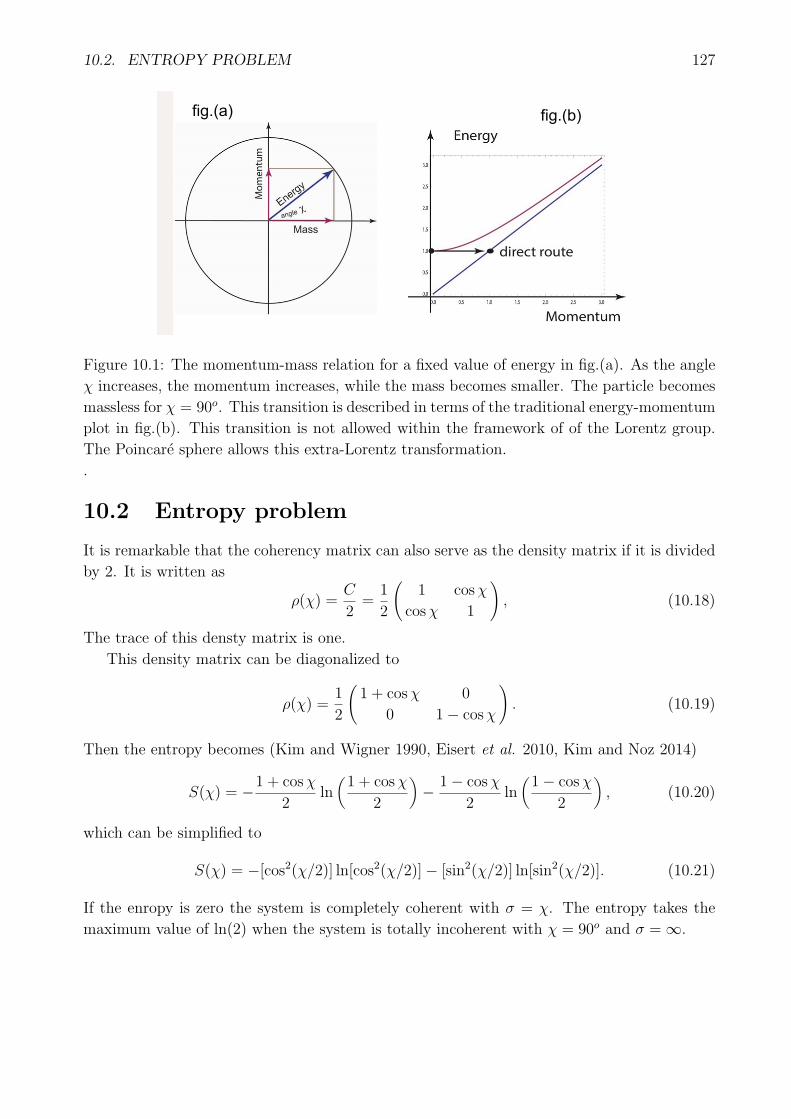
10.2. ENTROPY PROBLEM 127
fig.(a) fig.(b)
Figure 10.1: The momentum-mass relation for a fixed value of energy in fig.(a). As the angle
χ increases, the momentum increases, while the mass becomes smaller. The particle becomes
massless for χ = 90o. This transition is described in terms of the traditional energy-momentum
plot in fig.(b). This transition is not allowed within the framework of of the Lorentz group.
The Poincare sphere allows this extra-Lorentz transformation.
.
10.2 Entropy problem
It is remarkable that the coherency matrix can also serve as the density matrix if it is divided
by 2. It is written as
ρ(χ) =C
2=
1
2
(1 cosχ
cosχ 1
), (10.18)
The trace of this densty matrix is one.
This density matrix can be diagonalized to
ρ(χ) =1
2
(1 + cosχ 0
0 1− cosχ
). (10.19)
Then the entropy becomes (Kim and Wigner 1990, Eisert et al. 2010, Kim and Noz 2014)
S(χ) = −1 + cosχ
2ln(1 + cosχ
2
)− 1− cosχ
2ln(1− cosχ
2
), (10.20)
which can be simplified to
S(χ) = −[cos2(χ/2)] ln[cos2(χ/2)]− [sin2(χ/2)] ln[sin2(χ/2)]. (10.21)
If the enropy is zero the system is completely coherent with σ = χ. The entropy takes the
maximum value of ln(2) when the system is totally incoherent with χ = 90o and σ = ∞.
128 CHAPTER 10. POINCARE SPHERE
10.3 Symmetries derivable from the Poincare sphere
It has been demonstrated in Sec. 10.1 that the Poincare sphere contains the symmetry of
the Lorentz group applicable to the momentum-energy four-vector. While the Lorentz group
cannot tolerate the variable mass, the sphere has an extra-Lorentz variable which can change
the mass. In order to understand this extra variable, we exploit the symmetry between cosχ
and sinχ, write another coherency matrix
C ′ =
(1 e−iϕ sinχ
eiϕ sinχ 1
), (10.22)
with determinant cos2 χ.
It is possible to diagonalize both C and C ′ to
C =
(1 + cosχ 0
0 1− cosχ
), C ′ =
(1 + sinχ 0
0 1− sinχ
). (10.23)
whose determinants are sin2 χ and cos2 χ respectively. The matrices C and C ′ share the same
physics and the same mathematics. The choice is thus only for convenience.
We are now led to write the four-momentum matrix as
P =
(E + p 0
0 E − p
), (10.24)
where E and p are the energy and the magnitude of the momentum respectively. The particle
moves along the z direction.
Let us write p = E cosχ, and then the matrix P becomes
P = E
(1 + cosχ 0
0 1− cosχ
). (10.25)
This matrix is like C of Eq. (10.23). If we let p = E sinχ,
P = E
(1 + sinχ 0
0 1− sinχ
)(10.26)
is like C ′.
Let us pick P of Eq. (10.26). If χ = 0, the matrix becomes the four-momentum of the
particle at rest with a mass E. If χ = 90o, the particle becomes massless with a momentum
of E. The continuous transition from χ = 0 to 90o is illustrated in Fig. 10.2.
Starting from a massive particle at rest, we are interested in reaching a massless particle
with the same energy. This problem is not new in that it was discussed in detail in Chapter 4
within the framework of the Lorentz group. However, the transition from the massive case to
the massless case is a singular transformation, since the mass remains invariant under Lorentz
transformations.
On the other hand, in the case of the Poincare sphere, this transition is continuous as
indicated in Fig. 10.1. The question is whether this extra-Lorentzian transformation can be
accommodated by a larger symmetry group.

10.4. O(3,2) SYMMETRY 129
10.4 O(3,2) symmetry
The group O(3, 2) is the Lorentz group applicable to a five-dimensional space applicable to
three space dimensions and two time dimensions. Likewise, there are two energy variables,
which lead to a five-component vector
(E1, E2, pz, px, py) . (10.27)
In order to study this group, we have to use five-by-five matrices, but we are interested in its
subgroups. First of all, there is a three-dimensional Euclidean space consisting of pz, px, and
py, to which the O(3) rotation group is applicable, as in the case of the O(3, 1) Lorentz group.
If the momentum is in the z direction, this five-vector becomes
(E1, E2, p, 0, 0) . (10.28)
As for these two energy variables, they take the form
E1 =√p2 +m2
1, and E2 =√p2 +m2
2 cos2 χ, (10.29)
with (Zee 2003, Baskal and Kim 2006)
m1 = m cosχ, m2 = m sinχ, (10.30)
and they maintain
E21 + E2
2 = m2 + 2p2, (10.31)
which remains constant for a fixed value of p2. There is thus a rotational symmetry in the two-
dimensional space of E1 and E2. Indeed, this defines the O(3, 2) de Sitter symmetry (Baskal
and Kim 2006, 2013).
For the present purpose, the most important subgroups are two Lorentz subgroups appli-
cable to the Minkowskian spaces of
(E1, p, 0, 0) , and (E2, p, 0, 0) . (10.32)
Then, in the two-by-two matrix representation, these four-momenta take the form(E1 + p 0
0 E1 − p
), and
(E2 + p 0
0 E2 − p
), (10.33)
with determinants equal to m2 cos2 χ and m2 sin2 χ respectively.
With this understanding, we can now concentrate only on the matrix with E1. For χ = 0,
E1 = p, and it takes a maximum value of√p2 +m2. This fixed-momentum variation is
illustrated in Fig. 10.2. Indeed, the de Sitter symmetry allows us to jump from one mass
hyperbola to another.
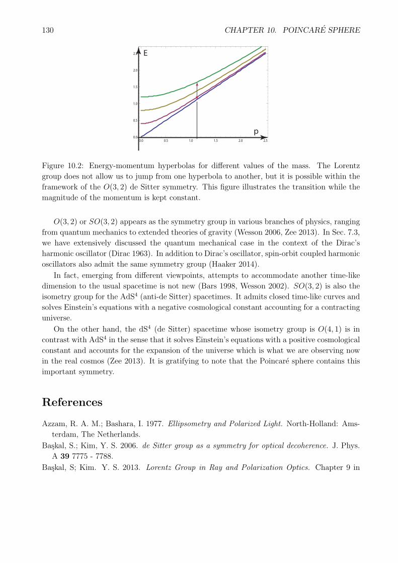
130 CHAPTER 10. POINCARE SPHERE
0.0 0.5 1.0 1.5 2.0 2.5
0.0
0.5
1.0
1.5
2.0
2.5 E
p
Figure 10.2: Energy-momentum hyperbolas for different values of the mass. The Lorentz
group does not allow us to jump from one hyperbola to another, but it is possible within the
framework of the O(3, 2) de Sitter symmetry. This figure illustrates the transition while the
magnitude of the momentum is kept constant.
O(3, 2) or SO(3, 2) appears as the symmetry group in various branches of physics, ranging
from quantum mechanics to extended theories of gravity (Wesson 2006, Zee 2013). In Sec. 7.3,
we have extensively discussed the quantum mechanical case in the context of the Dirac’s
harmonic oscillator (Dirac 1963). In addition to Dirac’s oscillator, spin-orbit coupled harmonic
oscillators also admit the same symmetry group (Haaker 2014).
In fact, emerging from different viewpoints, attempts to accommodate another time-like
dimension to the usual spacetime is not new (Bars 1998, Wesson 2002). SO(3, 2) is also the
isometry group for the AdS4 (anti-de Sitter) spacetimes. It admits closed time-like curves and
solves Einstein’s equations with a negative cosmological constant accounting for a contracting
universe.
On the other hand, the dS4 (de Sitter) spacetime whose isometry group is O(4, 1) is in
contrast with AdS4 in the sense that it solves Einstein’s equations with a positive cosmological
constant and accounts for the expansion of the universe which is what we are observing now
in the real cosmos (Zee 2013). It is gratifying to note that the Poincare sphere contains this
important symmetry.
References
Azzam, R. A. M.; Bashara, I. 1977. Ellipsometry and Polarized Light. North-Holland: Ams-
terdam, The Netherlands.
Baskal, S.; Kim, Y. S. 2006. de Sitter group as a symmetry for optical decoherence. J. Phys.
A 39 7775 - 7788.
Baskal, S; Kim. Y. S. 2013. Lorentz Group in Ray and Polarization Optics. Chapter 9 in

10.4. O(3,2) SYMMETRY 131
”Mathematical Optics: Classical, Quantum and Computational Methods” edited by Va-
sudevan Lakshminarayanan, Maria L. Calvo, and Tatiana Alieva, CRC Taylor and Francis:
Boca Raton, FL, pp 303 - 349.
Bars, I.; Deliduman, C.; Andreev, O. 1988. Gauged duality, conformal symmetry, and space-
time with two times. Phys. Rev. D 58 066004 - 1 - 066004 - 10.
Born, M. and Wolf, E. 1980. Principles of Optics. 6Ed Pergamon Press: Oxford, UK.
Brosseau, C. 1998. Fundamentals of Polarized Light: A Statistical Optics Approach. John
Wiley and Sons: Hoboken, NJ.
Dirac, P. A. M. 1963. A Remarkable representation of 3 + 2 de Sitter group. J. Math. Phys.
4 901 - 909.
Eisert, J.; Cramer, M.; Plenio, M. B. 2010. Colloquium: Area laws for the entanglement
entropy. Rev. Mod. Phys. 82 277-306.
Haaker, S. M.; Bais, F. A.; Schoutens, K. 2014. Noncompact dynamical symmetry of a spin-
orbit-coupled oscillator. Phys. Rev. A 89 032105 -1 - 032105 - 7.
Han, D; Kim, Y. S.; Noz, M. E. 1997. Stokes Parameters as a Minkowskian Four-vector.
Phys. Rev. E 56 6065 - 6076.
Kim, Y. S.; Wigner, E. P. 1990. Entropy and Lorentz Transformations. Phys. Lett. A 147
343 - 347.
Kim, Y. S.; Noz, M. E. 2014. Entropy and Temperature from Entangled Space and Time.
Phys. Sci. Int. J. 4 1015 - 1039.
Mueller, H. 1943. Memorandum on the polarization optics of the photo elastic shutter. Report
no. 2 of the OSRD project OEMsr-576, November 15.
Saleh, B. E. A.; Teich, M. C. 2007. Fundamentals of Photonics. 2nd Ed John Wiley and Sons:
Hoboken, NJ.
Wesson, P. S. 2002. Five-dimensional relativity and two times Physics Letters B 538 159 -
163.
Wesson, P. S. 2006. Five-dimensional Physics: Classical And Quantum Consequences of
Kaluza-Klein Cosmology. 2nd Ed World Scientific: Singapore
Zee, A. 2013. Einstein Gravity in a Nutshell. World Scientific: Singapore.

132 CHAPTER 10. POINCARE SPHERE


![fromHeisenberg’sUncertaintyRelationsarXiv:1911.03818v1 [quant-ph] 10 Nov 2019 Einstein’sE =mc2 derivable fromHeisenberg’sUncertaintyRelations Sibel Ba¸skal Department of Physics,](https://static.fdocuments.net/doc/165x107/5f3ef5e44ae14f065138cfd7/fromheisenbergasuncertaintyrelations-arxiv191103818v1-quant-ph-10-nov-2019.jpg)


