PHYSICS IV: EXPERIMENTS - boun.edu.tr

1

PHYSICS IV: EXPERIMENTS

Erhan Gülmez & Zuhal Kaplan

3

Foreword This book is written with a dual purpose in mind. Firstly, it aims to guide the students in the experiments of the elementary physics courses. Secondly, it incorporates the worksheets that the students use during their 2-hour laboratory session. There are six books to accompany the six elementary physics courses taught at Bogazici University. After renovating our laboratories, replacing most of the equipment, and finally removing the 110-V electrical distribution in the laboratories, it has become necessary to prepare these books. Each book starts with the basic methods for data taking and analysis. These methods include brief descriptions for some of the instruments used in the experiments and the graphical method for fitting the data to a straight line. In the second part of the book, the specific experiments performed in a specific course are explained in detail. The objective of the experiment, a brief theoretical background, apparatus and the procedure for the experiment are given in this part. The worksheets designed to guide the students during the data taking and analysis follows this material for each experiment. Students are expected to perform their experiment and data analysis during the allotted time and then hand in the completed worksheet to the instructor by tearing it out of the book. We would like to thank the members of the department that made helpful suggestions and supported this project, especially Arsin Arşık and Işın Akyüz who taught these laboratory classes for years. Our teaching assistants and student assistants were very helpful in applying the procedures and developing the worksheets. Of course, the smooth operation of the laboratories and the continuous well being of the equipment would not be possible without the help of our technicians, Erdal Özdemir and Hüseyin Yamak, who took over the job from Okan Ertuna. Erhan Gülmez & Zuhal Kaplan İstanbul, September 2007.

5

TABLE OF CONTENTS: PART I. BASIC METHODS ................................................................................................................ 7

Introduction .................................................................................................................................. 9 DATA TAKING AND ANALYSIS ................................................................................................. 11

Dimensions and Units .................................................................................................................. 11 Measurement and Instruments ..................................................................................................... 11

Reading analog scales: ............................................................................................................................. 12 Data Logger ............................................................................................................................................ 16

Basics of Statistics and Data Analysis .......................................................................................... 19 Sample and parent population .................................................................................................................. 19 Mean and Standard deviation ................................................................................................................... 19 Distributions ........................................................................................................................................... 20 Errors ...................................................................................................................................................... 21 Errors in measurements: Statistical and Systematical errors....................................................................... 21 Statistical Errors ...................................................................................................................................... 22 Systematical Errors.................................................................................................................................. 22 Reporting Errors: Significant figures and error values ............................................................................... 24 Rounding off ........................................................................................................................................... 26 Weighted Averages ................................................................................................................................. 27 Error Propagation .................................................................................................................................... 28 Multivariable measurements: Fitting procedures ....................................................................................... 29

Reports........................................................................................................................................ 34 PART II: EXPERIMENTS ................................................................................................................ 35

1. ELEC TRO MA G N E TIC OSC IL LA T IO N S IN A N RLC CI R CU IT .......................................... 37 2. ALT ERN A TI N G C U RR EN TS -SERI E S CI RCU IT S ............................................................... 49 3. REF LE CTI O N A N D RE FRA CT IO N ....................................................................................... 65 4. TH IN LEN SE S ....................................................................................................................... 73 5. TH E PRI SM SPE CT RO ME TE R .............................................................................................. 85 6. DIF FR A CT IO N GR A TI N G ..................................................................................................... 97 7. STE FA N-BO L TZ MA N RA D IA TIO N LA W .......................................................................... 107 8. TH E BA LM ER LIN E S O F HY D RO G EN A N D TH E RY D B ERG CO N ST A N T ..................... 121 APPENDICES .............................................................................................................................. 133

A. Spectra for various Gases: .................................................................................................... 135 B. Physical Constants: .............................................................................................................. 138 C. CONVERSION TABLES: ............................................................................................................. 139

REFERENCES ............................................................................................................................. 141

7

Part I. BASIC METHODS

9

Introduction

Physics is an experimental science. Physicists try to understand how nature works by

making observations, proposing theoretical models and then testing these models through

experiments. For example, when you drop an object from the top of a building, you

observe that it starts with zero speed and hits the ground with some speed. From this

simple observation you may deduce that the speed or the velocity of the object starts from

zero and then increases, suggesting a nonzero acceleration.

Usually when we propose a new model we start with the simplest explanation. Assuming

that the acceleration of the falling object is constant, we can derive a relationship between

the time it takes to reach the ground and the height of the building. Then measuring these

quantities many times we try to see whether the proposed relationship is valid. The next

question would be to find an explanation for the cause of this motion, namely the

Newton’s Law. When Newton proposed his law, he derived it from his observations.

Similarly, Kepler’s laws are also derived from observations. By combining his laws of

motion with Kepler’s laws, Newton was able to propose the gravitational law of

attraction. As you see, it all starts with measuring lengths, speeds, etc. You should

understand your instruments very well and carry out the measurements properly.

Measuring things correctly is absolutely essential for the success of your experiment.

Every time a new model or law is proposed, you can make some predictions about the

outcome of new and untried experiments. You can test the proposed models by

comparing the results of these actual experiments with the predictions. If the results

disagree with the predictions, then the proposed model is discarded or modified.

However, an agreement between the experimental results and the predictions is not

sufficient for the acceptance of the specific model. Models are tested continuously to

make sure that they are valid. Galilean relativity is modified and turned into the special

relativity when we started measuring speeds in the order of the speed of light. Sometimes

the modifications may occur before the tests are done. Of course, all physical laws are

based on experimental studies. Experimental results always take precedence over theory.

Obviously, experiments have to be done carefully and objectively without any bias.

Uncertainties and any contributing systematic effects should be studied carefully.

10

This book is written for the laboratory part of the Introductory Physics courses taken by

freshman and sophomore classes at Bogazici University. The first part of the book gives

you basic information about statistics and data analysis. A brief theoretical background

and a procedure for each experiment are given in the second part.

Experiments are designed to give students an understanding of experimental physics

regardless of their major study areas, and also to complement the theoretical part of the

course. They will introduce you to the experimental methods in physics. By doing these

experiments, you will also be seeing the application of some of the physics laws you will

be learning in the accompanying course.

You will learn how to use some basic instruments and interpret the results, to take and

analyze data objectively, and to report their results. You will gain experience in data

taking and improve your insight into the physics problems. You will be performing the

experiments by following the procedures outlined for each experiment, which will help

you gain confidence in experimental work. Even though the experiments are designed to

be simple, you may have some errors due to systematical effects and so your results may

be different from what you would expect theoretically. You will see that there is a

difference between real-life physics and the models you are learning in class.

You are required to use the worksheets to report your results. You should include all your

calculations and measurements to show that you have completed the experiment fully

and carried out the required analysis yourself.

11

DATA TAKING AND ANALYSIS

Dimensions and Units

A physical quantity has one type of dimension but it may have many units. The

dimension of a quantity defines its characteristic. For example, when we say that a

quantity has the dimension of length (L), we immediately know that it is a distance

between two points and measured in terms of units like meter, foot, etc. This may sound

too obvious to talk about, but dimensional analysis will help you find out if there is a

mistake in your derivations. Both sides of an equation must have the same dimension. If

this is not the case, you may have made an error and you must go back and recheck your

calculations. Another use of a dimensional analysis is to determine the form of the

empirical equations. For example, if you are trying to determine the relationship between

the distance traveled under constant acceleration and the time involved empirically, then

you should write the equation as

where k is a dimensionless quantity and a is the acceleration. Then, rewriting this

expression in terms of the corresponding dimensions:

will give us the exponent n as 2 right away. You will be asked to perform dimensional

analysis in most of the experiments to help you familiarize with this important part of the

experimental work.

Measurement and Instruments

To be a successful experimenter, one has to work in a highly disciplined way. The

equipment used in the experiment should be treated properly, since the quality of the data

you will obtain will depend on the condition of the equipment used. Also, the equipment

has a certain cost and it may be used in the next experiment. Mistreating the equipment

may have negative effects on the result of the experiment, too.

nkatd =

( ) nTLTL 2-=

12

In addition to following the procedure for the experiment correctly and patiently, an

experimenter should be aware of the dangers in the experiment and pay attention to the

warnings. In some cases, eating and drinking in the laboratory may have harmful effects

on you because food might be contaminated by the hazardous materials involved in the

experiment, such as radioactive materials. Spilled food and drink may also cause

malfunctions in the equipment or systematic effects in the measurements.

Measurement is a process in which one tries to determine the amount of a specific

quantity in terms of a pre-calibrated unit amount. This comparison is made with the help

of an instrument. In a measurement process only the interval where the real value exists

can be determined. Smaller interval means better precision of the instrument. The

smallest fraction of the pre-calibrated unit amount determines the precision of the

instrument.

You should have a very good knowledge of the instruments you will be using in your

measurements to achieve the best possible results from your work. Here we will explain

how to use some of the basic instruments you will come across in this course.

Reading analog scales:

You will be using several different types of scales. Examples of these different types of

scales are rulers, vernier calipers, micrometers, and instruments with pointers.

The simplest scale is the meter stick where you can measure lengths to a millimeter. The

precision of a ruler is usually the smallest of its divisions.

Figure 1. Length measurement by a ruler

In Figure 1, the lengths of object A and B are observed to be around 26 cm. Since we use

a ruler with millimeter division the measurement result for the object A should be given

as 26.0 cm and B as 26.2 cm. If you report a value more precise than a millimeter when

0 1 2 24 25 26 27 28

A

B

13

you use a ruler with millimeter division, obviously you are guessing the additional

decimal points.

Vernier Calipers (Figure 2) are instruments designed to extend the precision of a simple

ruler by one decimal point. When you place an object between the jaws, you may obtain

an accurate value by combining readings from the main ruler and the scale on the frame

attached to the movable jaw. First, you record the value from the main ruler where the

zero line on the frame points to. Then, you look for the lines on the frame and the main

ruler that looks like the same line continuing in both scales. The number corresponding

to this line on the frame gives you the next digit in the measurement. In Figure 2, the

measurement is read as 1.23 cm. The precision of a vernier calipers is the smallest of its

divisions, 0.1 mm in this case.

Figure 2. Vernier Calipers.

Micrometer (Figure 3) is similar to the vernier calipers, but it provides an even higher

precision. Instead of a movable frame with the next decimal division, the micrometer has

a cylindrical scale usually divided into a hundred divisions and moves along the main

ruler like a screw by turning the handle. Again the coarse value is obtained from the main

ruler and the more precise part of the measurement comes from the scale around the rim

of the cylindrical part. Because of its higher precision, it is used mostly to measure the

thickness of wires and similar things. In Figure 3, the measurement is read as 1.187 cm.

The precision of a micrometer is the smallest of its divisions, 0.01 mm in this case.

Here is an example for the measurement of the radius of a disk where a ruler, a vernier

calipers, and a micrometer are used, respectively:

0

R=1.2? cm

4 3 2

?=3 R=1.23cm

1 0 5 10

14

Measurement Precision Instrument

1 mm Ruler

0.1 mm Vernier calipers

0.01 mm Micrometer

Figure 3. Micrometer.

Spherometer (Figure 4) is an instrument to determine very small thicknesses and the

radius of curvature of a surface. First you should place the spherometer on a level surface

to get a calibration reading (CR). You turn the knob at the top until all four legs touch

the surface. When the middle leg also touches the surface, the knob will first seem to be

free and then tight. The reading at this position will be the calibration reading (CR). Then

you should place the spherometer on the curved surface and turn the knob until all four

legs again touch the surface. The reading at this position will be the measurement reading

(MR). You will read the value from the vertical scale first and then the value on the dial

will give you the fraction of a millimeter. Then you can calculate the radius of curvature

of the surface as:

where D = |CR-MR| and A is the distance between the outside legs.

( )mmR 123 ±=

( )mmR 1.01.23 ±=

( )mmR 01.014.23 ±=

DADR62

2

+=

R=1.187 cm

1 0 80

90

0

15

Figure 4. Spherometer.

Instruments with pointers usually have a scale along the path that the pointer moves.

Mostly the scales are curved since the pointers move in a circular arc. To avoid the

systematic errors introduced by the viewing angle, one should always read the value from

the scale where the pointer is projected perpendicularly. You should not read the value

by looking at the pointer and the scale sideways or at different angles. You should always

look at the scale and the pointer perpendicularly. Usually in most instruments there is a

mirror attached to the scale to make sure the readings are done similarly every time when

you take a measurement (Figure 5). When you bring the scale and its image on the mirror

on top of each other, you will be looking at the pointer and the scale perpendicularly.

Then you can record the value that the pointer shows on the scale. Whenever you measure

something by such an instrument, you should follow the same procedure.

Figure 5. A voltmeter with a mirror scale.

16

Data Logger

In some experiments we will be using sensors to measure some quantities like position,

angle, angular velocity, temperature, etc. The output of these sensors will be converted

into numbers with the help of a data acquisition instrument called DATA LOGGER

(Figure 6).

Data Logger is a versatile instrument that takes data using changeable sensors. When you

plug a sensor to its receptacle at the top, it recognizes the type of the sensor. When you

turn the data logger on with a sensor attached, it will start displaying the default mode

for that sensor. Data taking with the data logger is very simple. You can start data taking

by pressing the Start/Stop button (7). You may change the display mode by pressing the

button on the right with three rectangles (6). To change the default measurement mode,

you should press the plus or minus buttons (3 or 4). If there is more than one type of

quantity because of the specific sensor you are using, you may select the type by pressing

the button with a check mark (5) to turn on the editing mode and then selecting the desired

type by using the plus and minus buttons (3 or 4). You will exit from the editing mode

by pressing the button with the check mark (5) again. You may edit any of the default

settings by using the editing and plus-minus buttons. For a more detailed operation of the

instrument you should consult your instructor.

17

Figure 6. Data Logger.

1: Turning on/off

3: Cycling within the selected menu (back)

4: Cycling within the selected menu (forward)

6: Cycling between the menus

2: Checking the reading

5: Selecting displayed menu or to confirm the

operation

7: Start & stop the data recording

19

Basics of Statistics and Data Analysis

Here, you will have an introduction to statistical methods, such as distributions and

averages.

All the measurements are done for the purpose of obtaining the value for a specific

quantity. However, the value by itself is not enough. Determining the value is half the

experiment. The other half is determining the uncertainty. Sometimes, the whole purpose

of an experiment may be to determine the uncertainty in the results.

Error and uncertainty are synonymous in experimental physics even though they are two

different concepts. Error is the deviation from the true value. Uncertainty, on the other

hand, defines an interval where the true value is. Since we do not know the true value,

when we say error we actually mean uncertainty. Sometimes the accepted value for a

quantity after many experiments is assumed to be the true value.

Sample and parent population

When you carry out an experiment, usually you take data in a finite number of trials. This

is our sample population. Imagine that you have infinite amount of time, money, and

effort available for the experiment. You repeat the measurement infinite times and obtain

a data set that has all possible outcomes of the experiment. This special sample

population is called parent population since all possible sample populations can be

derived from this infinite set. In principle, experiments are carried out to obtain a very

good representation of the parent population, since the parameters that we are trying to

measure are those that belong to the parent population. However, since we can only get

an approximation for the parent population, values determined from the sample

populations are the best estimates.

Mean and Standard deviation

Measuring a quantity usually involves statistical fluctuations around some value.

Multiple measurements included in a sample population may have different values.

Usually, taking an average cancels the statistical fluctuations to first degree. Hence, the

average value or the mean value of a quantity in a sample population is a good estimate

for that quantity.

20

Even though the average value obtained from the sample population is the best estimate,

it is still an estimate for the true value. We should have another parameter that tells us

how close we are to the true value. The variance of the sample:

gives an idea about how scattered the data are around the mean value. Variance is in fact

a measure of the average deviation from the mean value. Since there might be negative

and positive deviations, squares of the deviations are averaged to avoid a null result.

Because the variance is the average of the squares, square root of variance is a better

quantity that shows the scatter around the mean value. The square root of the variance is

called standard deviation:

However, the standard deviation calculated this way is just the standard deviation of the

sample population. What we need is the standard deviation of the parent population. The

best estimate for the standard deviation of the parent population can be shown to be:

As the number of measurements, N, becomes large or as the sample population

approaches parent population, standard deviation of the sample is almost equal to the

standard deviation of the parent population.

Distributions

The probability of obtaining a specific value can be determined by dividing the number

of measurements with that value to the total number of measurements in a sample

population. Obviously, the probabilities obtained from the parent population are the best

å=

=N

iixN

x1

1

( )å=

-=N

ii xx

N 1

22 1s

( )å=

-=N

iis xx

N 1

21s

( )å=

--

=N

iip xx

N 1

2

11s

21

estimates. Total probability should be equal to 1 and probabilities should be larger as one

gets closer to the mean value. The set of probability values associated with a population

is called the probability distribution for that measurement. Probability distributions can

be experimental distributions obtained from a measurement or mathematical functions.

In physics, the most frequently used mathematical distributions are Binomial, Poisson,

Gaussian, and Lorentzian. Gaussian and Poisson distributions are in fact special cases of

Binomial distribution. However, in most cases, Gaussian distribution is a good

approximation. In fact, all distributions approach Gaussian distribution at the limit

(Central Limit Theorem).

Errors

The result of an experiment done for the first time almost always turns out to be wrong

because you are not familiar with the setup and may have systematic effects. However,

as you continue to take data, you will gain experience in the experiment and learn how

to reduce the systematical effects. In addition to that, increasing number of measurements

will result in a better estimate for the mean value of the parent population.

Errors in measurements: Statistical and Systematical errors

As mentioned above, error is the deviation between the measured value and the true

value. Since we do not know the true value, we cannot determine the error in this sense.

On the other hand, uncertainty in our measurement can tell us how close we are to the

true value. Assuming that the probability distribution for our measurement is a Gaussian

distribution, 68% of all possible measurements can be found within one standard

deviation of the mean value. Since most physical distributions can be approximated by a

Gaussian, defining the standard deviation as our uncertainty for that measurement will

be a reasonable estimate. In some cases, two-standard deviation or two-sigma interval is

taken as the uncertainty. However, for our purposes using the standard deviation as the

uncertainty would be more than enough. Also, from now on, whenever we use error, we

will actually mean uncertainty.

Errors or uncertainties can be classified into two major groups; statistical and

systematical.

22

Statistical Errors

Statistical errors or random errors are caused by statistical fluctuations in the

measurements. Even though some unknown phenomenon might be causing these

fluctuations, they are mostly random in nature. If the size of the sample population is

large enough, then there is equal number of measurements on each side of the mean at

about similar distances. Therefore, averaging over such a large number of measurements

will smooth the data and cancel the effect of these fluctuations. In fact, as the number of

measurements increases, the effect of the random fluctuations on the average will

diminish. Taking as much data as possible improves statistical uncertainty.

Systematical Errors

On the other hand, systematical errors are not caused by random fluctuations. One could

not reduce systematical errors by taking more data. Systematical errors are caused by

various reasons, such as, the miscalibration of the instruments, the incorrect application

of the procedure, additional unknown physical effects, or anything that affects the

quantity we are measuring. Systematic errors caused by the problems in the measuring

instruments are also called instrumental errors. Systematical errors are reduced or

avoided by finding and removing the cause.

Example 1: You are trying to measure the length of a pipe. The meter stick you are going

to use for this purpose is constructed in such a way that it is missing a millimeter from

the beginning. Since both ends of the meter stick are covered by a piece of metal, you do

not see that your meter stick is 1 mm short at the beginning. Every time you use this

meter stick, your measurement is actually 1 mm longer than it should be. This will be the

case if you repeat the measurement a few times or a few million times. This is a

systematical error and, since it is caused by a problem in the instrument used, it is

considered an instrumental error. Once you know the cause, that is, the shortness of your

meter stick, you can either repeat your measurement with a proper meter stick or add 1

mm to every single measurement you have done with that particular meter stick.

Example 2: You might be measuring electrical current with an ammeter that shows a

nonzero value even when it is not connected to the circuit. In a moving coil instrument

this is possible if the zero adjustment of the pointer is not done well and the pointer

23

always shows a specific value when there is no current. The error caused by this is also

an instrumental error.

Example 3: At CERN, the European Research Center for Nuclear and Particle Physics,

there is a 28 km long circular tunnel underground. This tunnel was dug about 100 m

below the surface. It was very important to point the direction of the digging underground

with very high precision. If there were an error, instead of getting a complete circle, one

would get a tunnel that is not coming back to the starting point exactly. One of the inputs

for the topographical measurements was the direction towards the center of the earth.

This could be determined in principle with a plumb bob (or a piece of metal hung on a

string) pointing downwards under the influence of gravity. However, when there is a

mountain range on one side and a flat terrain on the other side (like the location of the

CERN accelerator ring), the direction given by the plumb bob will be slightly off towards

the mountainous side. This is a systematic effect in the measurement and since its

existence is known, the result can be corrected for this effect.

Once the existence and the cause of a systematic effect are known, it is possible to either

change the procedure to avoid it or correct it. However, we may not always be fortunate

enough to know if there is a systematic effect in our measurements. Sometimes, there

might be unknown factors that affect our experiment. The repetition of the measurement

under different conditions, at different locations, and with totally different procedures is

the only way to remove the unknown systematic effects. In fact, this is one of the

fundamentals of the scientific method.

We should also mention the accuracy and precision of a measurement. The meaning of

the word “accuracy” is closeness to the true value. As for “precision,” it means a

measurement with higher resolution (more significant figures or digits). An instrument

may be accurate but not precise or vice versa. For example, a meter stick with millimeter

divisions may show the correct value. On the other hand, a meter stick with 0.1 mm

division may not show the correct value if it is missing a one-millimeter piece from the

beginning of the scale. However, if an instrument is precise, it is usually an expensive

and well designed instrument and we expect it to be accurate.

24

Reporting Errors: Significant figures and error values

As mentioned above, determining the error in an experiment requires almost the same

amount of work as determining the value. Sometimes, almost all the effort goes into

determining the uncertainty in a measurement.

Using significant figures is a crude but an effective way of reporting the errors. A simple

definition for significant figures is the number of digits that one can get from a measuring

instrument (but not a calculator!). For example, a digital voltmeter with a four-digit

display can only provide voltage values with four digits. All these four digits are

significant unless otherwise noted. On the other hand, reporting a six digit value when

using an analog voltmeter whose smallest division corresponds to a four-digit reading

would be wrong. One could try to estimate the reading to the fraction of the smallest

division, but then this estimate would have a large uncertainty.

Significant figures are defined as following:

• Leftmost nonzero digit is the most significant figure.

Examples: 0.00006520 m

1234 m

41.02 m

126.1 m

4120 m

12000 m

• Rightmost nonzero digit is the least significant figure if there is no decimal point.

Examples: 1234 m

4120 m

12000 m

• If there is a decimal point, rightmost digit is the least significant figure even if it is

zero.

Examples: 0.00006520 m

41.02 m

126.1 m

Then, the number of significant figures is the number of digits between the most and the

least significant figures including them.

25

Examples: 0.00006520 m 4 significant figures

1234 m 4 sf

41.02 m 4 sf

126.1 m 4 sf

4120 m 3 sf

12000 m 2 sf

1.2000 x 104 m 5 sf

Significant figures of the results of simple operations usually depend on the significant

figures of the numbers entering into the arithmetic operations. Multiplication or division

of two numbers with different numbers of significant figures should result in a value with

a number of significant figures similar to the one with the smallest number of significant

figure. For example, if you multiply a three-significant-figure number with a two-

significant-figure number, the result should be a two-significant-figure number. On the

other hand, when adding or subtracting two numbers, the outcome should have the same

number of significant figures as the smallest of the numbers entering into the calculation.

If the numbers have decimal points, then the result should have the number of significant

figures equal to the smallest number of digits after the decimal point. For example, if

three values, two with two significant figures and one with four significant figures after

the decimal point, are added or subtracted, the result should have two significant figures

after the decimal point.

Example: Two different rulers are used to measure the length of a table. First, a ruler

with 1-m length is used. The smallest division in this ruler is one millimeter. Hence, the

result from this ruler would be 1.000 m. However, the table is slightly longer than one

meter. A second ruler is placed after the first one. The second ruler can measure with a

precision of one tenth of a millimeter. Let’s assume that it gives a reading of 0.2498 m.

To find the total length of the table we should add these two values. The result of the

addition will be 1.2498, but it will not have the correct number of significant figures since

one has three and the other has four significant figures after the decimal point. The result

should have three significant figures after the decimal point. We can get the correct value

by rounding off the number to three significant figures after the decimal point and report

it as 1.250 m.

26

More Examples for Addition and Subtraction:

4 .122

3 .74

+ 0 .011

7 .873 = 7.87 (2 digits after the decimal point)

Examples for Multiplication and Division:

4.782 x 3.05 = 14.5851 = 14.6 (3 significant figures)

3.728 / 1.6781 = 2.22156 = 2.222 (4 significant figures)

Rounding off

Sometimes you may have more numbers than the correct number of significant figures.

This might happen when you divide two numbers and your calculator may give you as

many digits as it has in its display. Then you should reduce the number of digits to the

correct number of significant figures by rounding it off. One common mistake is by

starting from the rightmost digit and repeatedly rounding off until you reach the correct

number of significant figures. However, all the extra digits above and beyond the number

of correct significant figures have no significance. Usually you should keep one extra

digit in your calculations and then round this extra digit at the end. You should just

discard the extra digits other than the one next to the least significant figure. The

reasoning behind the rounding off process is to bring the value to the correct number of

significant figures without adding or subtracting an amount in a statistical sense. To

achieve this you should follow the procedure outlined below:

• If the number on the right is less than 5, discard it.

• If it is more than 5, increase the number on its left by one.

• If the number is exactly five, then you should look at the number on its left.

- If the number on its left is even then again discard it.

- If the number on the left of 5 is odd, then you should increase it by one.

This special treatment in the case of 5 is because there are four possibilities below and

above five and adding five to any of them will introduce a bias towards that side. Hence,

grouping the number on the left into even and odd numbers makes sure that this ninth

case is divided into exactly two subsets; five even and five odd numbers. We count zero

27

in this case since it is in the significant part. We do not count zero on the right because it

is not significant.

Example: Rounding off 2.4456789 to three significant figures by starting from all

the way to the right, namely starting from the number 9, and repeatedly rounding off until

three significant figures are left would result in 2.45 but this would be wrong. The correct

way of doing this is first dropping all the non-significant figures except one and then

rounding it off, that is, after truncation 2.445 is rounded off to 2.44.

More Examples: Round off the given numbers to 3 significant figures:

43.37468 = 43.37 = 43.4

43.34468 = 43.34 = 43.3

43.35468 = 43.35 = 43.4

43.45568 = 43.45 = 43.4

If we determine the standard deviation for a specific value, then we can use that as the

uncertainty since it gives us a better estimate. In this case, we should still pay attention

to the number of significant figures since reporting extra digits is meaningless. For

example if you have the average and the standard deviation as 2.567 and 0.1,

respectively, then it would be appropriate to report your result as 2.6±0.1.

Weighted Averages

Sometimes we may measure the same quantity in different sessions. As a result we will

have different sets of values and uncertainties. By combining all these sets we may

achieve a better result with a smaller uncertainty. To calculate the overall average and

standard deviation, we can assign weight to each value with the corresponding variance

and then calculate the weighted average.

Similarly we can also calculate the overall standard deviation.

å

å

=

== m

i i

m

i i

ix

12

12

1s

sµ

28

Error Propagation

If you are measuring a single quantity in an experiment, you can determine the final value

by calculating the average and the standard deviation. However, this may not be the case

in some experiments. You may be measuring more than one quantity and combining all

these quantities to get another quantity. For example, you may be measuring x and y and

by combining these to obtain a third quantity z:

or

You could calculate z for every single measurement and find its average and standard

deviation. However, a better and more efficient way of doing it is to use the average

values of x and y to calculate the average value of z. In order to determine the variance

of z, we have to use the square of the differential of z:

Variance would be simply the sum of the squares of both sides over the whole sample

set divided by the number of data points N (or N-1 for the parent population). Then, the

general expression for determining the variance of the calculated quantity as a function

of the measured quantities would be:

for k number of measured quantities.

Applying this expression to specific cases would give us the corresponding error

propagation rule. Some special cases are listed below:

for

å=

= m

i i12

11

s

s µ

byaxz += ( )yxfz ,=

22 )()()( ÷÷

ø

öççè

æ¶¶

+¶¶

= å dyyfdx

xfdz

2

2

1

2j

k

i jz x

f ss å=

÷÷ø

öççè

æ

¶¶

=

22222yxz ba sss += byaxz ±=

29

for or or

for

for

for

for

Multivariable measurements: Fitting procedures

When you are measuring a single quantity or several quantities and then calculating the

final quantity using the measured values, all the measurements involve unrelated

quantities. There are no relationships between them other than the calculated and

measured quantities. However, in some cases you may have to set one or more quantities

and measure another quantity determined by the independent variables. This is the case

when you have a function relating some quantities to each other. For example, the

simplest function would be the linear relationship:

where a is called the slope and b the y-intercept. Since we are setting the value of the

independent variable x, we assume its uncertainty to be negligible compared to the

dependent variable y. Of course, we should be able to determine the uncertainty in y.

From such an experiment, usually we have to determine the parameters that define the

function; a and b. This can be done by fitting the data to a straight line.

The least squares (or maximum likelihood, or chi-square minimization) method would

provide us with the best possible estimates. However, this method involves lengthy

calculations and we will not be using it in this course.

2

2

2

2

2

2

yxzyxz sss

+= axyz =yax

xay

2

22

2

2

xb

zxz ss

= baxz =

( ) 222

2

ln xz abz

ss

= bxaz =

222

2

xz bz

ss

= bxaez =

2

222

xa x

zs

s = ( )bxaz ln=

baxy +=

30

We will be using a graphical method that will give us the parameters that we are looking

for. It is not as precise as the least squares method and does not give us the uncertainties

in the parameters, but it provides answers in a short time that is available to you.

Graphical method is only good for linear cases. However, there are some exceptions to

this either by transforming the functions to make them linear or plotting the data on a

semi-log or log-log or polar graph paper (Figure 7). , , , , are

some examples for nonlinear functions that can be transformed to linear expressions.

type expressions can be linearized by substituting with a simple x:

where . Power functions can be linearized by

taking the logarithm of the function: becomes and then

through , , and transformation it becomes .

Exponential functions can be transformed similar to the power functions by taking the

natural logarithm: becomes and through and

transformation it becomes .

Before attempting to obtain the parameters that we are looking for, we have to plot the

data on a graph paper. As long as we have linearly dependent quantities or transformed

quantities as explained above, we can use regular graph paper.

Figure 7: Different types of graph papers: linear, semi-log, log-log, and polar.

You should use as much area of the graph paper as possible when you plot your data.

Your graph should not be squeezed to a corner with lots of empty space. To do this, first

you should determine the minimum and maximum values for each variable, x and y, then

choose a proper scale value. For example, if you have values ranging from 3 to 110 and

your graph paper is 23 centimeters long, then you should choose a scale factor of 1 cm

to 5 units of your variable and label your axis from 0 to 115 and marking each big square

(usually linear graph papers prepared in cm and millimeter divisions) at increasing

r/1 2/1 r 5axy = bxaey -=

nr/1 nr/1

BxAyrBAy n +=®+= / nrx /1=naxy = xnay logloglog +=

yy log=¢ aa log=¢ xx log=¢ xnay ¢+¢=¢

bxaey -= bxay -= lnln yy ln=¢

aa ln=¢ bxay -¢=¢

31

multiples of 5. You should choose the other axis in a similar way. When you select a

scale factor you should select a factor that is easy to divide by, like 1, 2, 4, 5, 10, etc.

Usually scale factors like 3, 4.5, 7.9 etc., are bad choices. Both axis may have different

scale factors and may start from a nonzero value. You should clearly label each axis and

write down the scale factors. Then you should mark the position corresponding to each

data pair with a cross or similar symbols. Usually you should also include the

uncertainties as vertical bars above and below the data point whose lengths are

determined according to the scale factor. Once you finish marking all your data pairs,

then you should try to pass a straight line through all the data points. Usually, this may

not be possible since the data points may not fall into a straight line. However, since you

know that the relationship is linear there should be a straight line that passes through the

data points even though not all of them fall on a line. You should make sure that the

straight line passes through the data points in a balanced way. An equal number of data

points should be below and above the straight line. Then, by picking two points on the

line as far apart from each other as possible, you should draw parallel lines to the axes,

forming a triangle (Figure 8). The slope is the slope of the straight line. You can calculate

the slope as:

and read the y-intercept from the graph by finding the point where the straight line crosses

the y-axis. You can estimate the uncertainties of the slope and intercept by finding

different straight lines that still pass through all the data points in an acceptable manner.

The minimum and maximum values obtained from these different trials would give us

an idea about the uncertainties. However, obtaining the parameters will be sufficient in

this course.

xySlope

DD

=

32

Figure 8: Determining the slope and y-intercept.

Special graph papers, like semi-log and log-log graph papers, are used when you have

relationships that can be transformed into linear relationships by taking the base-10

logarithm of both sides. Semi-log graph papers are used if one side of the expression

contains powers of ten or single exponential function resulting in a linear variable when

you take the base-10 logarithm of both sides.

Logarithmic graph papers are used when you prefer to use the measured values directly

without taking the logarithms and still obtaining a linear graph. Each logarithmic axis is

divided in such a way that when you use the divisions marked on the paper it will have

the same effect as if you first took the logarithm and then plotted on a regular graph

paper. Logarithmic graph papers are divided linearly into decades and in each decade is

divided logarithmically. There is no zero value in a logarithmic axis. You should plot

your data by choosing appropriate scale factors for each axis and then mark the data

points directly without taking the logarithms. You should again draw a straight line that

will pass through all the data points in a balanced way. The slope of the line would give

us the exponent in the relationship. For example, a relationship like would be

linearized as . If you plot this on a regular graph paper, the slope

will be given by where you will read the logarithms

directly from the graph. On the other hand, when you plot your data on a log-log paper,

you will be using the measured values directly. When you picked the two points from the

straight line that fits the data points best, the slope should be calculated by

naxy =

xnay logloglog +=

( ) ( )1212 loglog/loglog xxyyn --=

data points

slope points

-2 0

90

80

70

60

50

40

-6 -4 2 4 6

y

x

33

where you will calculate the logarithms using the

values read from the graph. y-intercept would be directly the value where the straight line

crosses the vertical axis at .

Figure 9: Determining the slope and y-intercept.

slope point 1: ( 2.0 ; 2.6 ) and slope point 2 : (18.0 ; 7.0 )

and y-intercept = 2.0.

( ) ( )1212 loglog/loglog xxyyn --=

1=x

4507.09542.04301.0

)0.2log()0.18log()6.2log()0.7log(slope ==

--

=

6

x(m)

100 80 60 40 30 20 10 8 5 4 3 2 1

2

3

4

6

10 y(m)

1

8

34

Reports

Obviously, doing an experiment and getting some results are not enough. The results of

the experiment should be published so that others working on the same problem will

know your results and use them in their calculations or compare with their results. The

reports should have all the details so that another experimenter could repeat your

measurements and get the same results. However, in an introductory teaching lab there

is no need for such extensive reports since the experiments you will be doing are well

established and time is limited. You have to include enough details to convince your lab

instructor that you have performed the experiment appropriately and analyzed it

correctly. The results of your analysis, including the uncertainties in the measurements,

should be clearly expressed. The comparisons with the accepted values may also be

included if possible.

35

Part II: EXPERIMENTS

37

1. ELECTROMAGNETIC OSCILLATIONS IN AN RLC CIRCUIT

OBJECTIVE : To study the oscillations of potential difference across a charged capacitor in series with a resistor and an inductor.

THEORY : In a series RLC circuit, the Kirchoff’s loop rule results in the following:

or

since I = dq/dt. This is an equation for a damped oscillator driven by a time dependent voltage source or a signal generator. There are three different combinations of R, L, and C values where we can get specific solutions to this equation for a square wave signal as the applied voltage. Underdamped: If the values satisfy the following conditions, the circuit will be underdamped:

.

Then the solution will be:

and the voltage across the capacitor will be:

,

where V0 is the voltage when the square wave is at the maximum value and d is the phase. w0 is given by:

.

Oscillations decay exponentially with a time constant 2L/R. Signals reach their half values in:

which we can call half-life of the signals.

)(tVCqRi

dtdiL app=++

)(2

2

tVCq

dtdqR

dtqdL app=++

14

2

<LCR

( ) ( )dw += - tAeqtq oLRt

o sin)( 2/

( ) ( )dw += - tBeVtV oLRt

oC sin)( 2/

2

2

41

LR

LCo -=w

2ln22/1 R

Lt =

38

Critically Damped:

If , the circuit is critically damped. As you see from the equation for w0 above,

the frequency of the oscillations is zero which means there is only an exponential decay. Overdamped:

If , the circuit is overdamped. The frequency of the oscillations, w0, is an

imaginary number which means there is only an exponential decay similar to the Critically Damped Case.

APPARATUS : Capacitance and resistance boxes, inductor with an iron block, oscillator, oscilloscope.

PROCEDURE :

• Connect the circuit by using the A-E terminals of the 1000 turn coil for the inductor and 0.001µF capacitor, turn on the oscilloscope and make the initial adjustments. Internal resistance of the square wave generator and the coil resistance will be the total resistance in the circuit.

• Adjust the square wave frequency and the sweep frequency of the oscilloscope so that one complete cycle of decaying oscillations cover the whole screen of the oscilloscope. Record the value of the sweep frequency in your report.

• Choose two peaks at least 5-6 cm far from each other and count the number of

14

2

=LCR

14

2

>LCR

39

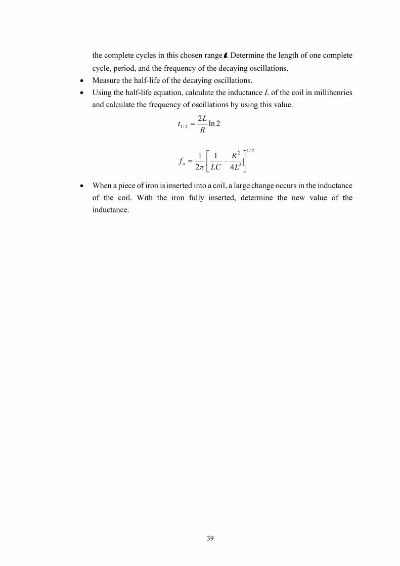
the complete cycles in this chosen range l. Determine the length of one complete cycle, period, and the frequency of the decaying oscillations.

• Measure the half-life of the decaying oscillations. • Using the half-life equation, calculate the inductance L of the coil in millihenries

and calculate the frequency of oscillations by using this value.

• When a piece of iron is inserted into a coil, a large change occurs in the inductance of the coil. With the iron fully inserted, determine the new value of the inductance.

2/1

2

2

2/1

41

21

2ln2

úû

ùêë

é-=

=

LR

LCf

RLt

o p

41

ELECTROMAGNETIC OSCILLATIONS IN AN RLC CIRCUIT

Name & Surname : Experiment # : Section : Date :

DATA and CALCULATIONS: Draw the circuit diagram

Description / Notation Value & Unit Capacitance C = . . . . . . . . . . . . . . . . . . . . . . . . . . . . . . . . . . . . . . . . . . . . . . . . . . . . . . . . . .

Resistance R = . . . . . . . . . . . . . . . . . . . . . . . . . . . . . . . . . . . . . . . . . . . . . . . . . . . . . . . . . .

Frequency of the Square Wave fSWG = . . . . . . . . . . . . . . . . . . . . . . . . . . . . . . . . . . . . . . . . . . . . . . . . . . . . . . . . . . Generator

43

Description / Notation Value & Unit [TIME / DIV] Dial of the Oscilloscope without Iron Block = . . . . . . . . . . . . . . . . . . . . . . . . . . . . . . . . . . . . . . . . . . . . . . . . . . . . . . . . . . . . [TIME / DIV] Dial of the Oscilloscope with Iron Block = . . . . . . . . . . . . . . . . . . . . . . . . . . . . . . . . . . . . . . . . . . . . . . . . . . . . . . . . . . . . Length between the chosen peaks l = . . . . . . . . . . . . . . . . . . . . . . . . . . . . . . . . . . . . . . . . . . . . . . . . . . . . . . . . . . . .

Number of complete Cycles in l n = . . . . . . . . . . . . . . . . . . . . . . . . . . . . . . . . . . . . . . . . . . . . . . . . . . . . . . . . . . . .

W I T H O U T I R O N B L O C K I N S I D E T H E I N D U C T O R

Description / Symbol Value / Calculations Result (show each step)

Half-Life t1/2 (cm) = . . . . . . . . . . . . . . . . . . . . . . . . . . . . . . . . . . . . . . . . . . . . . . . .

Half-Life t1/2(sec) = . . . . . . . . . . . . . . . . . . . . . . . . . . . . . . . . . . . . . . . . . . . . . . . .

Inductance of the coil L1 = . . . . . . . . . . . . . . . . . . . . . . . . . . . . . . . . . . . . . . . . . . . . . . . .

. . . . . . . . . . . . . . . . . . . . . . . . . . . . . . . . . . .

Wavelength l = . . . . . . . . . . . . . . . . . . . . . . . . . . . . . . . . . . . . . . . . . . . . . . . . Period of the Oscillations T = . . . . . . . . . . . . . . . . . . . . . . . . . . . . . . . . . . . . . . . . . . . . . . . .

. . . . . . . . . . . . . . . . . . . . . . . . . . . . . . . . . . .

45

Frequency of the Oscillations f measured = . . . . . . . . . . . . . . . . . . . . . . . . . . . . . . . . . . . . . . . . . . . . . . . .

Frequency of the Oscillations f calculated = . . . . . . . . . . . . . . . . . . . . . . . . . . . . . . . . . . . . . . . . . . . . . . . .

. . . . . . . . . . . . . . . . . . . . . . . . . . . . . . . . . . .

% Error for f:

W I T H I R O N B L O C K I N S I D E T H E I N D U C T O R

Description / Symbol Value / Calculations Result (show each step)

Half-Life t1/2 (cm) = . . . . . . . . . . . . . . . . . . . . . . . . . . . . . . . . . . . . . . . . . . . . . . . .

Half-Life t1/2(sec) = . . . . . . . . . . . . . . . . . . . . . . . . . . . . . . . . . . . . . . . . . . . . . . . .

Inductance of the coil L2 = . . . . . . . . . . . . . . . . . . . . . . . . . . . . . . . . . . . . . . . . . . . . . . . .

. . . . . . . . . . . . . . . . . . . . . . . . . . . . . . . . . . .

Show the Dimensional Analysis of L clearly:

47

QUESTION :

1) What is the reason for the difference you observe when you insert the iron block inside the inductor?

49

2. ALTERNATING CURRENTS -SERIES CIRCUITS

OBJECTIVE : To study the alternating current circuits. THEORY : The alternating current source that we use most commonly is in the form of

(1)

where Vp is the peak voltage and f is the frequency of the power supply. When we connect various circuit elements to an alternating current source, we can determine the current through the circuit by Ohm’s Law. The current through a resistor, a capacitor, and an inductor will be given by:

(2a)

(2b)

(2c)

Hence the current through a resistor is in phase with the voltage across it; the current through a capacitor leads the voltage by 90°; and the current through an inductor lags the voltage by 90°. Because of these differences in the phases, analyzing alternating current circuits involving different types of circuit elements is somewhat tricky and not as simple as the DC circuits. We can solve this problem by using either complex algebra or the phasor method which are similar to each other. In the complex algebra method we define reactances for each element:

(3)

and treat the voltage and the current as real numbers. Then the circuit analysis for the alternating currents turns into a form similar to the DC circuits. Of course, the reactances contain all the information relevant to the alternating current circuit, that is, the frequency and the phases in the form of the imaginary numbers. Solutions will include both real and imaginary parts. As you know, we can also represent the complex numbers as pairs of numbers on a Cartesian coordinate system where the horizontal axis corresponds to the real and the vertical axis corresponds to the imaginary part. Phasor method simply uses the graphical representation of the complex numbers. In this experiment we will be using the phasor method.

)2sin()( ftVtV p p=

)2sin( ftRV

I pR p=

( ))902sin(2

)2sin( op

pC ftfCV

dtftVd

CI +== ppp

ò -== )902sin(2

)2sin(1 oppL ft

fLV

dtftVL

I pp

p

RX R = fCiX C p2

1= fLiX L p2=

50

RC CIRCUIT When you connect a capacitor and a resistor in series to an alternating voltage source, the phase of the current through the capacitor will be 90° ahead of the voltage. If we were to take the current as our reference for the phase, then the voltage across the capacitor will be 90° behind the current hence the voltage across the resistor. The total voltage across the RC series combination will be equal to the applied voltage:

(4)

RL CIRCUIT When you connect an inductor and a resistor in series to an alternating voltage source, the current through the inductor will be 90° behind the voltage. If we were to take the current as our reference for the phase, then the voltage across the inductor will be 90° ahead of the current hence the voltage across the resistor. The total voltage across the RL series combination will be equal to the applied voltage:

(5)

However, the inductor also has some internal resistance, RL. Because of its internal resistance, the voltage across the inductor will not be exactly 90° ahead but at an angle calculated from:

(6)

We should also modify Equation (5) accordingly:

(7)

RLC CIRCUIT When you connect an inductor, a capacitor, and a resistor in series to an alternating voltage source, the current through the inductor and the capacitor will be 90° behind and ahead of the voltage, respectively. If we were to take the current as our reference for the phase, then the voltage across the inductor and the capacitor will be 90° ahead of and behind the current (hence the voltage across the resistor), respectively. The total voltage across the RLC series combination will be equal to the applied voltage:

(8)

Because of its internal resistance, RL, the voltage across the inductor will not be exactly 90° ahead but at an angle calculated from:

(9)

We should also modify Equation (8) accordingly:

( )22CRapp VVV +=

22LRapp VVV +=

LRfLpq 2tan =

( ) 22LLapp XRRIV ++=

( ) 22RCLapp VVVV +-=

LRfLpq 2tan =

51

(10)

where the total impedance of the RLC circuit is given by

(11)

Now the phase difference between the current and the voltage is more complex and given by:

(12)

This F angle is the angle between the applied voltage and the resulting current phasors. It determines the total average power used in an RLC circuit:

(13)

We should remind that the values measured by instruments like voltmeters, ammeters, etc. are root-mean-squared values and not the peak values. You can determine the peak values using an oscilloscope.

APPARATUS : Inductor with an iron block inside, resistance box, capacitor, AC voltmeter and ammeter, 24-V AC power supply.

PROCEDURE :

• Use the two fixed ends of the rheostat as a resistor. Use 24 V, 50 Hz output of the power supply as your AC source.

• Construct an RC circuit and measure the voltage across each element. Then draw the phasor diagram by taking the current (i.e. the voltage across the resistor) as the reference. Then draw two circles with radii equal to VC and Vapp from each end of the phasor corresponding to the voltage across the resistor. Phasors for VC and Vapp will meet each other at the point where the circles intersect. Determine the angle between VC and VR.

• Repeat the previous step by constructing an RL circuit this time. Determine the internal resistance of the inductor by measuring the current through the circuit and the horizontal component of VL from your phasor diagram.

• Repeat the previous step by constructing an RLC circuit this time. Again measure the current value through the circuit. You should draw the phasor diagram in this case by assuming that VC is 90° behind VR (or perpendicular in the negative direction). Then draw two circles centered at the beginning of the phasor for VR and the tip of the phasor for VC with radii equal to Vapp and VL, respectively. Draw Vapp and VL phasors from the centers of the circles to the intersection point. Using the current value and the internal resistance of the inductor determined in the previous step, determine the capacitive and inductive reactances first and then

( ) ( ) IZXXRRIV CLLapp =-++= 22

( ) ( )22CLL XXRRZ -++=

( )total

CL

RXX -

=Ftan

F= cosrmsrms IVP

52

calculate the value of the capacitor and the inductor. Finally determine the phase angle F and the average power dissipated in the RLC circuit.

53

ALTERNATING CURRENTS – SERIES CIRCUITS


DATA:

P A R T – 1 : R C C I R C U I T R C c i r c u i t d i a g r a m :

55

Description / Notation Value & Unit

Potential difference across the resistance VR = . . . . . . . . . . . . . . . . . . . . . . . . . . . . . . . . . . . . . . . . . . . . . . . . . . . . .

.

Potential difference across the capacitor VC = . . . . . . . . . . . . . . . . . . . . . . . . . . . . . . . . . . . . . . . . . . . . . . . . . . . . .

Applied potential Vapp = . . . . . . . . . . . . . . . . . . . . . . . . . . . . . . . . . . . . . . . . . . . . . . . . . . . . .

Phasor Diagram of the RC Circuit: Scaling factor:

Angle between VC and VR = . . . . . . . . . . . . . . . . . . . . . . . . . . . . . . .

P A R T – 2 : R L C I R C U I T R L c i r c u i t d i a g r a m :

57


Current in the circuit I = . . . . . . . . . . . . . . . . . . . . . . . . . . . . . . . . . . . . . . . . . . . . . . . . . . . . . .

Potential difference across the resistance VR = . . . . . . . . . . . . . . . . . . . . . . . . . . . . . . . . . . . . . . . . . . . . . . . . . . . . . .

Potential difference across the inductor VL = . . . . . . . . . . . . . . . . . . . . . . . . . . . . . . . . . . . . . . . . . . . . . . . . . . . . . .

Applied potential Vapp = . . . . . . . . . . . . . . . . . . . . . . . . . . . . . . . . . . . . . . . . . . . . . . . . . . . . . .

Phasor Diagram of the RL Circuit: Scaling factor:

Description / Symbol Value / Calculation Result

Potential difference due to the internal resistance of the inductor VrL = . . . . . . . . . . . . . . . . . . . . . . . . . . . . . . . . . . . . . . . . . . . . . . . . . .

Internal resistance of the inductor rL = . . . . . . . . . . . . . . . . . . . . . . . . . . . . . . . . . . . . . . . . . . . . . . . . . .

. . . . . . . . . . . . . . . . . . . . . . . . . . . . . . . . . . . .

59

PART – 3: RLC CIRCUIT

R L C c i r c u i t d i a g r a m :


Current in the circuit I = . . . . . . . . . . . . . . . . . . . . . . . . . . . . . . . . . . . . . . . . . . . . . . . . . . . . . .

Potential difference across the resistance VR = . . . . . . . . . . . . . . . . . . . . . . . . . . . . . . . . . . . . . . . . . . . . . . . . . . . . . .

Potential difference across the inductor VL = . . . . . . . . . . . . . . . . . . . . . . . . . . . . . . . . . . . . . . . . . . . . . . . . . . . . . .

Potential difference across the capacitor VC = . . . . . . . . . . . . . . . . . . . . . . . . . . . . . . . . . . . . . . . . . . . . . . . . . . . . . .

Applied potential Vapp = . . . . . . . . . . . . . . . . . . . . . . . . . . . . . . . . . . . . . . . . . . . . . . . . . . . . . .

Phasor Diagram of the RLC Circuit: Scaling factor:

61

Description / Symbol Value / Calculation Result (show step by step)

Capacitive reactance XC = . . . . . . . . . . . . . . . . . . . . . . . . . . . . . . . . . . . . . . . . . . . . . . . . . . .

. . . . . . . . . . . . . . . . . . . . . . . . . . . . . . . . . . . . . . .

Value of the capacitor C = . . . . . . . . . . . . . . . . . . . . . . . . . . . . . . . . . . . . . . . . . . . . . . . . . . .

. . . . . . . . . . . . . . . . . . . . . . . . . . . . . . . . . . . . . . .

Inductive reactance XL = . . . . . . . . . . . . . . . . . . . . . . . . . . . . . . . . . . . . . . . . . . . . . . . . . . .

. . . . . . . . . . . . . . . . . . . . . . . . . . . . . . . . . . . . . . .

Value of the inductor L = . . . . . . . . . . . . . . . . . . . . . . . . . . . . . . . . . . . . . . . . . . . . . . . . . . .

. . . . . . . . . . . . . . . . . . . . . . . . . . . . . . . . . . . . . . .

Internal resistance of the inductor rL = . . . . . . . . . . . . . . . . . . . . . . . . . . . . . . . . . . . . . . . . . . . . . . . . . . .

. . . . . . . . . . . . . . . . . . . . . . . . . . . . . . . . . . . . . . .

Total resistance Rtot = . . . . . . . . . . . . . . . . . . . . . . . . . . . . . . . . . . . . . . . . . . . . . . . . . . .

. . . . . . . . . . . . . . . . . . . . . . . . . . . . . . . . . . . . . . .

Impedance Z = . . . . . . . . . . . . . . . . . . . . . . . . . . . . . . . . . . . . . . . . . . . . . . . . . . .

. . . . . . . . . . . . . . . . . . . . . . . . . . . . . . . . . . . . . . .

63

Description / Symbol Value / Calculation Result (show step by step)

Phase angle j = . . . . . . . . . . . . . . . . . . . . . . . . . . . . . . . . . . . . . . . . . . . . . . . . . . .

. . . . . . . . . . . . . . . . . . . . . . . . . . . . . . . . . . . . . . .

Average dissipated power P = . . . . . . . . . . . . . . . . . . . . . . . . . . . . . . . . . . . . . . . . . . . . . . . . . . .

. . . . . . . . . . . . . . . . . . . . . . . . . . . . . . . . . . . .

QUESTION :

• If the angle between VC and VR is different from 90°, what could the reason be?

65

3. REFLECTION AND REFRACTION

OBJECTIVE : To study the law of reflection, principles of mirrors, lenses, and prism by ray tracing.

THEORY : In this experiment you will be tracing the light rays reflected or refracted from various optical elements and determine some relevant quantities of these elements. Here are some crucial points you may need.

• In a plane mirror the incident and reflected angles with respect to the normal are equal

• Focal lengths of concave and convex mirrors are simply half the radius of curvature for the respective surface.

• Focal length and the radius of curvature of a lens is related through the following expression:

where n is the index of refraction. • We can calculate the index of refraction of the transparent material a prism made

of as following:

where A is the prism angle at the corner that the light rays are refracted and Dmin is the minimum angle of deviation between the incident and the refracted rays.

APPARATUS : Ray box, lens, mirror and prism set, ruler, protractor.

PROCEDURE :

• For each of the following experiments, place the optical element and light source on a different sheet of paper. Draw the outline of the optical element, paths of incident, reflected, and refracted rays as needed.

• You will determine the radii of curvatures using the Chord Method. First draw at least two chords on the curved (circular) outline of the elements. Then draw

2Rf =

( )R

nf

211-=

÷øö

çèæ

÷ø

öçè

æ +

=

2sin

2sin min

A

AD

n

66

perpendicular bisectors to each of the chords. The center of the circle is where the bisectors intersect. You can determine the radius by measuring the perpendicular distance between the intersection point and any point on the curved outline.

• Show your Chord Method Analysis on the back of each corresponding sheet.

• In case of the prism, determine the minimum angle of deviation Dmin and then the index of refraction for the material of the prism.

67

REFLECTION AND REFRACTION


DATA, CALCULATIONS and RESULT:

P A R T I : R E F L E C T I O N A) Plane Mirror :

Incident ray angle qi = . . . . . . . . . . . . . . . . . . . . . . . . . . . . . . . . . . . . . .

Reflected ray angle qr = . . . . . . . . . . . . . . . . . . . . . . . . . . . . . . . . . . . . . .

B) Concave – Converging Mirror:

Focal Length of the mirror fEV = . . . . . . . . . . . . . . . . . . . . . . . . . . . . . . . . . . . . . .

Radius of the mirror (From Chord Method) R = . . . . . . . . . . . . . . . . . . . . . . . . . . . . . . . . . . . . . .

Focal length of the mirror (From Chord Method) fCV = . . . . . . . . . . . . . . . . . . . . . . . . . . . . . . . . . . . . . .

% difference in focal lengths = . . . . . . . . . . . . . . . . . . . . . . . . . . . . . . . . . . . . . .

69

C) Convex – Diverging Mirror:

Focal Length of the mirror fEV = . . . . . . . . . . . . . . . . . . . . . . . . . . . . . . . . . . . . . .

Radius of the mirror (From Chord Method) R = . . . . . . . . . . . . . . . . . . . . . . . . . . . . . . . . . . . . . .

Focal length of the mirror (From Chord Method) fCV = . . . . . . . . . . . . . . . . . . . . . . . . . . . . . . . . . . . . . .

Thickness of the mirror x = . . . . . . . . . . . . . . . . . . . . . . . . . . . . . . . . . . . . . .


P A R T I I : R E F R A C T I O N

D) Convex – Converging Lens :

Refraction Index n = . . . . . . . . . . . . . . . . . . . . . . . . . . . . . . . . . . . . . .

Focal Length of the lens fEV = . . . . . . . . . . . . . . . . . . . . . . . . . . . . . . . . . . . . . .

Radius of the convex lens (From Chord Method) R = . . . . . . . . . . . . . . . . . . . . . . . . . . . . . . . . . . . . . .

Focal length of the convex lens (From Chord Method) fCV = . . . . . . . . . . . . . . . . . . . . . . . . . . . . . . . . . . . . . .


71

E) Concave – Diverging Lens:

Refraction Index n = . . . . . . . . . . . . . . . . . . . . . . . . . . . . . . . . . . . . . .

Focal Length of the lens fEV = . . . . . . . . . . . . . . . . . . . . . . . . . . . . . . . . . . . . . .

Radius of the concave lens (From Chord Method) R = . . . . . . . . . . . . . . . . . . . . . . . . . . . . . . . . . . . . . .

Focal length of the concave lens (From Chord Method) fCV = . . . . . . . . . . . . . . . . . . . . . . . . . . . . . . . . . . . . . .


F) Prism:

Minimum deviation between incident Dmin = . . . . . . . . . . . . . . . . . . . . . . . . . . . . . . . . . . and refracted rays

Prism angle A = . . . . . . . . . . . . . . . . . . . . . . . . . . . . . . . . . . . . . .

Index of Refraction nEV = . . . . . . . . . . . . . . . . . . . . . . . . . . . . . . . . . . . . . .

True Value for the Index of Refraction nTV = . . . . . . . . . . . . . . . . . . . . . . . . . . . . . . . . . . . . . .

% difference for n = . . . . . . . . . . . . . . . . . . . . . . . . . . . . . . . . . . . . . .

73

4. THIN LENSES

OBJECTIVE : To determine the focal lengths, radii of curvature and index of refraction of various lenses, and to investigate image formation by lens combinations.

THEORY : A thin lens is defined as a lens whose thickness is much smaller than its focal length. Thin lenses that are thin at the edge and thick at the center bend the light rays toward the optical axis (converging lenses) and those that are thick at the edge and thin at the center bend the light rays away from the optical axis (diverging lenses).

Thin lenses have two basic equations, the lens equation,

and the lens maker's equation:

iof111

+=

( ) ÷÷ø

öççè

æ--=

21

1111rr

nf

o i

i

F

F¢ Object

Image

o

F F¢

Object

Image

Converging Lens (convex):

Diverging Lens (concave):

74

where r1 and r2 are the radii of curvatures of each surface. If both surfaces have the same curvature, the lens maker's equation becomes

where plus and minus signs are for converging and diverging lenses, respectively. The sign conventions for the quantities used in the equations above are as following:

• The image distance is positive if the image is formed on the right side of the lens and negative if it forms on the left side. We assume that the light source is on the left.

• Similarly, the object distance is positive if the object is on the left side of the lens and negative if it is on the right side. (If the object is actually an image from another lens, it may be on the right side.)

• The radii of curvatures are positive if the corresponding center for a surface is on the right side. This is the reason for positive and negative focal lengths for converging and diverging lenses.

• The magnification m, which is the ratio of the image size to the object size, is m= -i/o. To denote the inverted images a minus sign is added.

Spherometer:

Spherometer is an instrument to determine very small thicknesses and the radius of curvature of a surface. First you should place the spherometer on a level surface to get a calibration reading (CR). You turn the knob at the top until all four legs touch the surface. When the middle leg also touches the surface, the knob will first seem to be free and then tight. The reading at this position will be the calibration reading (CR). Then you should place the spherometer on the curved surface and turn the knob until all four legs again touch the surface. The reading at this position will be the measurement reading (MR). You will read the value from the vertical scale first and then the value on the dial will give you the fraction of a millimeter. Then you can calculate the radius of curvature of the surface as:

where D = |CR-MR| and A is the distance between the outside legs.

( )R

nf

211-±=

DADR62

2

+=

75

Figure 4. Spherometer.

APPARATUS : Various thin lenses, light source and cross object, ruler, screen, spherometer.

PROCEDURE :

• Mount large and small converging lenses one by one. Adjust the position of lenses and the screen to obtain a very sharp and clear image of the illuminated cross. By measuring object and image distances for two different positions of lenses, calculate focal length and magnifications of lenses separately.

• Use the two converging lenses to form an image of the object. Measure the image distance from the nearest lens and calculate this distance from the lens equation applied to each lens. Repeat this using converging lens of known focal length and a diverging lens. Calculate the focal length of the diverging lens.

• Measure the radius of curvature of any large lens by a spherometer. (R1=R2=R). Determine the refractive index of the lens.

77

THIN LENSES


DATA, CALCULATIONS and RESULTS:

P A R T I : C O N V E R G I N G L E N S E S

A) Small Converging Lens:

Object distance o1 = . . . . . . . . . . . . . Object distance o2 = . . . . . . . . . . . . . . .

Image distance i1 = . . . . . . . . . . . . . Image distance i2 = . . . . . . . . . . . . . . .

Focal length f1 = . . . . . . . . . . . . . Focal length f2 = . . . . . . . . . . . . . . .

Magnification m = . . . . . . . . . . . . . Magnification m = . . . . . . . . . . . . . . .

Average focal length faverage = . . . . . . . . . . . . . . . . . . . . . . . . . B) Large Converging Lens:

Object distance o1 = . . . . . . . . . . . . . Object distance o2 = . . . . . . . . . . . . . . .

Image distance i1 = . . . . . . . . . . . . . Image distance i2 = . . . . . . . . . . . . . . .

Focal length f1 = . . . . . . . . . . . . . Focal length f2 = . . . . . . . . . . . . . . .

Magnification m = . . . . . . . . . . . . . Magnification m = . . . . . . . . . . . . . . .

Average focal length faverage = . . . . . . . . . . . . . . . . . . . . . . . . .

79

P A R T I I : L E N S C O M B I N A T I O N C) Two Converging Lenses:

Draw the diagram of the system:

Measure:

Object distance for the first lens o1 = . . . . . . . . . . . . . . . . . . . . . . . . . . . . . . . . . . . . . . .

Image distance for the second lens i2 = . . . . . . . . . . . . . . . . . . . . . . . . . . . . . . . . . . . . . . .

Distance between the lenses d = . . . . . . . . . . . . . . . . . . . . . . . . . . . . . . . . . . . . . . .

Calculate:

Image distance for the first lens i1 = . . . . . . . . . . . . . . . . . . . . . . . . . . . . . . . . . . . . . . .

. . . . . . . . . . . . . . . . . . . . . . . . . . . . . . . . . . . . . . .


. . . . . . . . . . . . . . . . . . . . . . . . . . . . . . . . . . . . . . .

% Error for i2 = . . . . . . . . . . . . . . . . . . . . . . . . . . . . . . . . . . . . .

81

D) Large Converging & Large Diverging Lenses:

Draw the diagram of the system:

Measure:

Object distance for the first lens o1 = . . . . . . . . . . . . . . . . . . . . . . . . . . . . . . . . . . . . . . .


Distance between the lenses d = . . . . . . . . . . . . . . . . . . . . . . . . . . . . . . . . . . . . . . .

Calculate:

Image distance for the first lens i1 = . . . . . . . . . . . . . . . . . . . . . . . . . . . . . . . . . . . . . . .

. . . . . . . . . . . . . . . . . . . . . . . . . . . . . . . . . . . . . . .

Object Distanece of 2nd lens O2 = . . . . . . . . . . . . . . . . . . . . . . . . . . . . . . . . . . . . . . .

Focal length of the diverging lens fdiverging = . . . . . . . . . . . . . . . . . . . . . . . . . . . . . . . . . . . . . . .

. . . . . . . . . . . . . . . . . . . . . . . . . . . . . . . . . . . . . . .

. . . . . . . . . . . . . . . . . . . . . . . . . . . . . . . . . . . . . . .

83

P A R T I I I : S P H E R O M E T E R

True Value of the Index of Refraction nTV = . . . . . . . . . . . . . . . . . . . . . . . . . . . . . . . . . . . . . .

Distance between the legs A = . . . . . . . . . . . . . . . . . . . . . . . . . . . . . . . . . . . . . .

Calibration reading CR = . . . . . . . . . . . . . . . . . . . . . . . . . . . . . . . . . . . . . .

Measurement reading MR = . . . . . . . . . . . . . . . . . . . . . . . . . . . . . . . . . . . . . .

Difference in readings D = ½CR - MR½= . . . . . . . . . . . . . . . . . . . . . . . . . . . . . . . .

. . . . . . . . . . . . . . . . . . . . . . . . . . . . . . . . . . . . . .

Radius of curvature

of the lens surface R = = . . . . . . . . . . . . . . . . . . . . . . . . . . . . . . . . . . . . . .

. . . . . . . . . . . . . . . . . . . . . . . . . . . . . . . . . . . . . .

Index of Refraction ncal = . . . . . . . . . . . . . . . . . . . . . . . . . . . . . . . . . . . . . .

. . . . . . . . . . . . . . . . . . . . . . . . . . . . . . . . . . . . . .

% Error for Index of Refraction, n =. . . . . . . . . . . . . . . . . . . . . . . . . . . . . . . . . . . . . .

DAD62

2

+

85

5. THE PRISM SPECTROMETER

OBJECTIVE : To study the refraction of light by a glass prism, and to construct the dispersion curve for the prism. THEORY : Snell’s law states that light at a specific wavelength refracts at an angle determined by

However, index of refraction varies as a function of wavelength. This is called dispersion and when you plot the index of refraction as a function of wavelength, the curve you obtain is called the dispersion curve for that material. The functional dependence of the index of refraction to the wavelength is given by the empirical relationship:

.

We can study the dispersion curve using a prism, since the light shining on a prism will separate into individual lines because of the dispersion phenomenon. If we use a spectral lamp, then the individual lines will belong to the spectrum of the element that the spectral lamp is made of. Orienting the prism until you get the minimum deviation angle between the incident and the refracted light rays for each spectral line will give you the data necessary to plot the dispersion curve for the material of the prism. Then you can calculate the index of refraction for each wavelength using the following expression:

where a is the corner angle of the prism where the light is refracted.

APPARATUS : Spectrometer, mercury lamp and its power supply, prism.

2211 sinsin θ n θn =

2lBAn +=

÷øö

çèæ

÷øö

çèæ +

=

2sin

2sin min

a

aD

n

source

00

1800

900

prism

telescope

a

86

PROCEDURE :

• Adjust the zero position of the spectrometer so that it is equal to the absolute zero. Align the collimator and the telescope such that you can see the slit clearly and sharply through the telescope. Next, adjust the cross-hair so that it is on the slit. Then, fix the telescope and rotate the body until the zero positions of the body and the telescope are aligned. Finally, fix the body and release the telescope to move freely.

• Set the prism in the center of the prism table.

• Using the white light source, place the prism in such a way that the light falls on both faces of the prism. Then measure the reflected ray from both side and calculate the angle A.

• Using the mercury lamp as the light source, determine the angle of minimum deviation for all the lines in the mercury spectrum. Then calculate the refractive index of the prism corresponding to different wavelengths (colors).

• On an ordinary graph paper, plot n versus 1/l2 to obtain the dispersion curve.

87

THE PRISM SPECTROMETER


DATA:

White light reflection:

Angle (left) qleft = . . . . . . . . . . . . . . . . . . . . . . . . . . . . . . . . . . . . . . . . . . . . . . . . . . . . . . . . . .

Angle (right) qright = . . . . . . . . . . . . . . . . . . . . . . . . . . . . . . . . . . . . . . . . . . . . . . . . . . . . . . . . . .

Prism Angle a = . . . . . . . . . . . . . . . . . . . . . . . . . . . . . . . . . . . . . . . . . . . . . . . . . . . . . . . . . .

Measurements for the Mercury spectrum: Show your calculations in detail for the first row, repeat the same for the rest.

COLOR l (Ao) q Dmin

(show your calculations)

Yellow-1 Yellow-2

5790 5769

Green 5460

Blue (weak) 4916

Blue 4358

Violet-1 4077

Violet-2 4046

89

CALCULATIONS:

Show your calculations in detail for the first row, repeat the same for the rest.

COLOR

1/l2

( ) n = n

(result)

Yellow-1 Yellow-2

Green

Blue (weak)

Blue

Violet-1

Violet-2

[ ])2/(2/)( min

aaSin

DSin +

91

From the graph, choose two SLOPE POINTS other than data points, SP1 : ( ; ) SP2 : ( ; )

93

R E S U L T S :

Notation Calculations (show each step) Result

A = . . . . . . . . . . . . . . . . . . . . . . . . . . . . . . . . . . . . . . . . . . . . . . . . . . . . . .

. . . . . . . . . . . . . . . . . . . . . . . . . . . . . . . . . . . . . . . . . . . . . . . . . . . . . . . . . . . . . . . . . . . .

B = . . . . . . . . . . . . . . . . . . . . . . . . . . . . . . . . . . . . . . . . . . . . . . . . . . . . . .

. . . . . . . . . . . . . . . . . . . . . . . . . . . . . . . . . . . . . . . . . . . . . . . . . . . . . . . . . . . . . . . . . . . .

Dimensional Analysis of A:

Dimensional Analysis of B:

97

6. DIFFRACTION GRATING

OBJECTIVE : To use a diffraction grating to determine the wavelengths corresponding to various spectral lines.

THEORY : Light shining perpendicularly on a diffraction grating produces an interference pattern on a screen or on your retina if you are viewing from behind the grating. Positions of the maxima in the resulting interference pattern are given by the grating equation:

where m is the order of the spectrum, l is the wavelength of the incident light, d is the distance between the lines on the grating, and q is the angle at which the maximum intensity occurs. Angles are measured with respect to the incident light direction.

If the incident light has components with many wavelengths then you will see these different wavelengths separated from each other. The resolving power of a grating is given in terms of its ability to separate two wavelengths which differ by Dl:

where l is the average of these two wavelength values. Resolving power is also related to the number of lines (N) on the grating through

The angular dispersion D of a grating is defined as a measure of the angular separation produced between two monochromatic light waves whose wavelengths are close to each other.

where Q is the average of the angles corresponding to the two lines that are close to each other in wavelength and l is the average of these wavelength.

ql sindm =

llD

=R

NmR =

ll /tan/ Q=Q= ddD

00

1800

900 source

m=0

m=1

m=2

grating

telescope

98

APPARATUS : Spectrometer, sodium lamp with its power supply, discharge tube with its power supply

PROCEDURE :


• Mount the diffraction grating carefully on the spectrometer.

• Using the sodium lamp as the light source, determine the angular position of the first order maximum for the yellow line on either side of the center. Calculate the diffraction separation d.

• Using the discharge tube containing unknown gas as the light source, determine the angles for all visible lines. Then calculate the wavelengths of those spectrum lines. Identify the gas in the discharge tube by making use of the table in Appendix A.

• Selecting two barely separated lines in your discharge tube spectrum, determine the angular dispersion of your grating.

• Use the white light source to determine the wavelength limits for visible light.

99

DIFFRACTION GRATING


DATA and CALCULATIONS:

P A R T I : D E T E R M I N A T I O N O F D I F F R A C T I O N G R A T I N G C O N S T A N T , d

Wavelength of sodium doublet l = 5890 Å and 5895 Å average 5893 Å

Order of the spectrum m = . . . . . . . . . . . . . . . . . . . . . . . . . . . . . . . . . . . . . . . . . . . . . . . . . . . . . . . . . . . .

Angle of spectrum line qleft = . . . . . . . . . . . . . . . . . . . . . . . . . . . . . . . . . . . . . . . . . . . . . . . . . . . . . . . . . . . . (Uncalibrated)

Angle of spectrum line qright = . . . . . . . . . . . . . . . . . . . . . . . . . . . . . . . . . . . . . . . . . . . . . . . . . . . . . . . . . . . . (Uncalibrated)

Average angle qave = . . . . . . . . . . . . . . . . . . . . . . . . . . . . . . . . . . . . . . . . . . . . . . . . . . . . . . . . . . . .

Diffraction Separation d = . . . . . . . . . . . . . . . . . . . . . . . . . . . . . . . . . . . . . . . . . . . . . . . . . . . . . . . . . . . .

. . . . . . . . . . . . . . . . . . . . . . . . . . . . . . . . . . . . . . . . . . . . . . . . . . . . . . . . . . . .

101

P A R T I I : U N K N O W N D I S C H A R G E T U B E

Discharge Tube Number : . . . . . . . . . . . . . . . . . . . . . . . . . . . . . . . . . . . . . . . . . . . . . . . . . . . . . .

Show your calculations in detail for the first row, repeat the same for the rest.

Color qleft

(uncalibrated) qright

(uncalibrated) qaverage

l ( )

P A R T I I I : D I S P E R S I O N M E A S U R E M E N T

COLOUR qleft


(uncalibrated) q

l ( )

Average :

-

103

P A R T I V : W H I T E L I G H T S P E C T R U M

COLOUR qleft


(uncalibrated) qaverage

l ( )

Red End

Violet End

RESULTS:

Gas in the Discharge Tube is (check the appropriate box) :

Argon Krypton Hydrogen

Helium Mercury Neon

Dispersion of the spectrometer:

D = tan qave / lave = . . . . . . . . . . . . . . . . . . . . . . . . . . . . . . . . . . . . . . . . . . . . . . . . . . . . . . .

. . . . . . . . . . . . . . . . . . . . . . . . . . . . . . . . . . . . . . . . . . . . . . . . . . . . . . . .

Limits of the visible range :

. . . . . . . . . . . . . < l ( ) < . . . . . . . . . . . . .

-

105

QUESTIONS :

1. What is the maximum number of orders that can be observed with the grating used in the experiment?

2. Why is it preferable to use a grating with a small d for accurate spectral analysis?

3. Should the angular separation between two lines be the same for each order? Answer the question through a mathematical derivation.

4. Prove that the angular dispersion of a grating can be written as:

l/tanQ=D

107

7. STEFAN-BOLTZMANN RADIATION LAW

OBJECTIVE : The aim of this experiment is to determine the rate of temperature dependency in the Stefan-Boltzmann Radiation Law.

THEORY : Radiation from an object is observed to be dependent on its temperature. The distribution of photon frequencies can be understood in terms of quantum physics where the radiation occurs in the form of energy packets or photons. It has been observed that the wavelength at which the maximum intensity occurs (Wien’s displacement law) or the total radiated power integrated over all wavelengths per unit area depends only on the temperature of the object. The latter is the subject of our experiment and is called the Stefan-Boltzmann Radiation Law. It states that the total integrated radiated power per unit area from an object depends on the fourth power of its temperature:

where s is the Stefan-Boltzmann constant ( W/m2K4).

The object that produces the radiation in this experiment is an incandescent tungsten bulb. The actual part that radiates is the tungsten filament. Since the resistance of metals increases as a function of temperature ( where temperature coefficient of resistivity for tungsten is K-1), we can determine its

temperature by measuring its electrical resistance through Ohm’s law: .

We will use an infrared detector that is sensitive over a wavelength region between 0.5 to 40 µm. We will be measuring the total power radiated over this range only, but this should give us a value proportional to the total power radiated. Its output is in millivolts.

APPARATUS : Stefan-Boltzmann Lamp (a 12 V bulb), fuse and switch set, radiation sensor, reflecting heat shield, multimeter set to 200-millivolt range, multimeter set to 10-A range, Data Logger and the charge sensor, Pasco 24-V power supply, various leads and stand for the radiation sensor.

PROCEDURE:

1. Multimeters and the power supply are placed on the workbench at their proper settings. If you notice something is not set right, please inform your instructor, otherwise DO NOT MAKE ANY CHANGES IN THE SETTINGS. Make sure that the heat shield is placed between the bulb and the sensor, reflective side facing the sensor.

,4TR s=

8106703.5 -´=s

))(1( 00 TTRR -+= a3105.4 -´=a

IVR =

108

2. You will determine the resistance of the tungsten filament at room temperature first. For this purpose adjust the power supply current to its minimum value, 0.2 A. You will be reading the current value from the multimeter set to 10-A range and the potential across the filament from the data logger set as a voltmeter.

3. Calculate the resistance using the Ohm’s law. This will be your R0. Your instructor will give you the value of the room temperature. Make sure that all your temperature values are in Kelvin.

4. Make sure that the metal ring on the detector has been pushed all the way to the front, otherwise the detector readings might be faulty.

5. While increasing the current very slowly, record the current, the potential drop across the lamp, and the sensor output at each current setting. DO NOT EXCEED 3 AMPERES.

6. Calculate the resistance of the tungsten filament at each current setting using the Ohm’s law and divide these values by the value at room temperature that you have determined in step 2.

7. Using the temperature coefficient of resistivity for tungsten, K-1, and , determine the temperature of the tungsten filament at each current setting.

8. Plot your radiation sensor output versus temperature data on a log-log paper. Draw a straight line that passes through all the data points symmetrically, that is, either all the points fall on the straight line or equal number of points fall each side of the line.

3105.4 -´=a))(1(/ 00 TTRR -+= a

109

9. A power law expression produces a linear plot when plotted on a log-log graph paper. Determine the slope of this straight line by picking two points far apart from each other. Slope is the ratio of the actual vertical distance to the actual horizontal distance on the graph. Since plotting on a log-log graph paper is equivalent to taking the base-10 logarithm of the values and then plotting them

on a regular paper, slope is calculated through:

where x and y values are direct readings from the graph.

10. Compare your result with the actual value of n = 4. What is your percentage error?

÷÷ø

öççè

æ

÷÷ø

öççè

æ

=--

=

1

2

1

2

12

12

log

log

loglogloglog

xxyy

xxyym

111

STEFAN-BOLTZMANN RADIATION LAW


DATA:

Draw the circuit diagram:

Write down the formula to calculate the temperature from the resistance Solve for T:

. . . . . . . . . . . . . . . . . . . . . . . . . . . . . . . . . . . . . . . . . . . . . . . . . . . . . . . . . . . . . . . . . . . . . . . . . . . . . . . . . . . . . . . . . . . . . . . . . . . . . . . . . .

. . . . . . . . . . . . . . . . . . . . . . . . . . . . . . . . . . . . . . . . . . . . . . . . . . . T = . . . . . . . . . . . . . . . . . . . . . . . . . . . . . . . . .

To = . . . . . . . . . . . . . . . . . . . . . . . . . . . . . .

Io = 0.20 Amp. Vo = . . . . . . . . . . . . . . . . . . . . . . . . . . . .

Ro = . . . . . . . . . . . . . . . . . . . . . . . . . . . . . . a = 4.403 x 10-3 K-1

))(1(/ 00 TTRR -+= a

113

Current I ( )

Potential Across

the lamp V ( )

Radiation Sensor output,

VRad ( )

Resistance of the

filament, R=V/I ( )

R / Ro

Temperature of the

filament, T ( )

115

A) From the graph, choose two SLOPE POINTS other than data points, SP1 : ( ; ) SP2 : ( ; )

117

B) Calculate, Description / Formula Calculations (show each step) Result

n = SLOPE = . . . . . . . . . . . . . . . . . . . . . . . . . . . . . . . . . . .. . . . . . . . . . . . . . . . . . . . . . . . . . . . . . . . . . . .

. . . . . . . . . . . . . . . . . . . . . . . . . . . . . . . . . . .. . . . . . . . . . . . . . . . . . . . . . . . . . . . . . . . . . . . . . . . . . . . . .

% error = . . . . . . . . . . . . . . . . . . . . . . . . . . . . . . . . . . .. . . . . . . . . . . . . . . . . . . . . . . . . . . . . . . . . . . .

QUESTIONS :

1. If the energy spectrum is shifting upward in the frequency and the amount of region that you are sampling with the infrared sensor is decreasing as the temperature increases, how would this affect your final result? Comment qualitatively on the error caused by this effect and other sources of errors in this experiment.

121

8. THE BALMER LINES OF HYDROGEN AND THE RYDBERG CONSTANT

OBJECTIVE : To observe the Balmer line spectra series of Hydrogen and to determine the Rydberg constant for hydrogen using a grating spectrometer.

THEORY : Elements emit light at characteristic wavelengths when they are excited through heating, electrical discharge, etc. In 1885, Balmer observed some of the lines in the Hydrogen spectrum and noticed that a group of them could be described by

.

When Bohr put forward his model for the Hydrogen atom, it was easy to show that the Balmer lines are produced by the photon emissions when excited hydrogen atoms decay to the second energy level from upper levels. Since Bohr model gives the relationship between the wavelength of the emitted light when an electron moves from an energy level ni to nf and the principal quantum numbers ni and nf:

where R is the Rydberg constant that can be expressed as

where m is the mass of the electron. You may show that the Balmer lines are obtained when nf=2 and ni=n.

PROCEDURE :


• Mount the diffraction grating carefully on the spectrometer.

• Using the sodium lamp as the light source, determine the angular position of the first order maximum of the yellow line on either side of the center. Calculate the diffraction separation d.

• Using the discharge tube containing hydrogen gas as the light source, determine the wavelengths of the Balmer lines in the hydrogen spectrum. Calculate the Rydberg constant for each of the determined wavelengths. Calculate the actual

42

2

-=

nnBl

÷÷ø

öççè

æ-= 22

111

if nnR

l

chmeRo

32

4

8e=

122

value of the Rydberg constant using the equation above and compare with your average experimental result.

123

THE BALMER LINES OF HYDROGEN AND THE RYDBERG CONSTANT


DATA :

Order of the spectrum m = . . . . . . . . . . . . . . . . . . . . . . . . . . . . . . . . . . . . . . . . . . . . . . . . . . . . . . . . . . . .

P A R T I : D E T E R M I N A T I O N O F

D I F F R A C T I O N G R A T I N G C O N S T A N T , d

Wavelength of sodium doublet l = 5890 Å and 5895 Å average 5893 Å

Angle of spectrum line qleft = . . . . . . . . . . . . . . . . . . . . . . . . . . . . . . . . . . . . . . . . . . . . . . . . . . . . . . . . . . . . (Uncalibrated)

Angle of spectrum line qright = . . . . . . . . . . . . . . . . . . . . . . . . . . . . . . . . . . . . . . . . . . . . . . . . . . . . . . . . . . . . (Uncalibrated)

Average angle qave = . . . . . . . . . . . . . . . . . . . . . . . . . . . . . . . . . . . . . . . . . . . . . . . . . . . . . . . . . . . .

125

P A R T I I : H Y D R O G E N S P E C T R U M L I N E S

A) For Red Spectrum Line

Angle of spectrum line qleft = . . . . . . . . . . . . . . . . . . . . . . . . . . . . . . . . . . . . . .

Angle of spectrum line qright = . . . . . . . . . . . . . . . . . . . . . . . . . . . . . . . . . . . . . .

Average angle qave = . . . . . . . . . . . . . . . . . . . . . . . . . . . . . . . . . . . . . .

B) For Green Spectrum Line




C) For Violet Spectrum Line




127

CALCULATIONS: Description / Symbol Calculation (show each step) Result

Diffraction Grating Constant d = . . . . . . . . . . . . . . . . . . . . . . . . . . . . . . . . . . . . . . . . . . . . . . .

Wavelength for the Red Line lred = . . . . . . . . . . . . . . . . . . . . . . . . . . . . . . . . . . . . . . . . . . . . . . .

Wavelength for the Green Line lgreen = . . . . . . . . . . . . . . . . . . . . . . . . . . . . . . . . . . . . . . . . . . . . . . .

Wavelength for the Violet Line lviolet = . . . . . . . . . . . . . . . . . . . . . . . . . . . . . . . . . . . . . . . . . . . . . . .

129

A) For Red Spectrum Line

Initial state ni = . . . . . . . . . . . . . . . . . . . . . . . . . . . . . . . . . . . . . . . . . . .

Final state nf = . . . . . . . . . . . . . . . . . . . . . . . . . . . . . . . . . . . . . . . . . . .

Rydberg constant Rred = . . . . . . . . . . . . . . . . . . . . . . . . . . . . . . . . . . . . . . . . . . .

. . . . . . . . . . . . . . . . . . . . . . . . . . . . . . . . . . . . . . . . . . .

B) For Green Spectrum Line

Initial state ni = . . . . . . . . . . . . . . . . . . . . . . . . . . . . . . . . . . . . . . . . . . .

Final state nf = . . . . . . . . . . . . . . . . . . . . . . . . . . . . . . . . . . . . . . . . . . .

Rydberg constant Rgreen = . . . . . . . . . . . . . . . . . . . . . . . . . . . . . . . . . . . . . . . . . . .

. . . . . . . . . . . . . . . . . . . . . . . . . . . . . . . . . . . . . . . . . . .

C) For Violet Spectrum Line

Initial state ni = . . . . . . . . . . . . . . . . . . . . . . . . . . . . . . . . . . . . . . . . . . .

Final state nf = . . . . . . . . . . . . . . . . . . . . . . . . . . . . . . . . . . . . . . . . . . .

Rydberg constant Rviolet = . . . . . . . . . . . . . . . . . . . . . . . . . . . . . . . . . . . . . . . . . . .

. . . . . . . . . . . . . . . . . . . . . . . . . . . . . . . . . . . . . . . . . . .

131

RESULTS: Description / Symbol Calculation (show step by step) Result

Average value of Rydberg constant REV = . . . . . . . . . . . . . . . . . . . . . . . . . . . . . . . . . . . . . . . . . . . . . . . . . . .

. . . . . . . . . . . . . . . . . . . . . . . . . . . . . . . . . . . . . . . . . . . . . . . . . . . . . . .

Calculated value of Rydberg constant RCV = . . . . . . . . . . . . . . . . . . . . . . . . . . . . . . . . . . . . . . . . . . . . . . . . . . .

. . . . . . . . . . . . . . . . . . . . . . . . . . . . . . . . . . . . . . . . . . . . . . . . . . . . . . .

. . . . . . . . . . . . . . . . . . . . . . . . . . . . . . . . . . . . . . . . . . . . . . . . . . . . . . .

% Error for R = . . . . . . . . . . . . . . . . . . . . . . . . . . . . . . . . . . . . . . . . . . . . . . . . . . .

Show the Dimensional Analysis of Rydberg Constant clearly:

chmeRo

32

4

8e=

133

APPENDICES

135

A. Spectra for various Gases:

HYDROGEN (H2): Strong violet, blue and red lines are obvious, although others may be seen.

Color Wavelength, Å Violet 4200 Violet 4400 Blue 4900 Red 6700

HELIUM (He): Strong spectrum with 1 violet, 2 green, 1 yellow, and 2 red lines being prominent.

Color Wavelength, Å Violet 4000 Blue 4500 Blue 4550 Green 5000 Green 5100 Yellow 5850 Red 6500 Red 6800 Red 7200

KRYPTON (Kr): Strong spectral lines in violet, green, orange, and red portions.

Color Wavelength, Å Violet 4300 (hazy) Violet 4400 (hazy) Violet 4500 Violet 4550 Blue 4900 Green 5600 Green 5650 Green 5700 Yellow 5900 Red 6100 Red 6300 Red 6500 Red 6650

136

NEON (Ne): Strong spectrum of multiple lines in green, yellow, orange, and red. Note the absence of violet lines.

Color Wavelength, Å Blue 4750 Blue 4900 Green 5100 Green 5250 Green 5600 Green 5700 Yellow 5800 Yellow 5900 Yellow 6000 Red 6050 Red 6100 Red 6150 Red 6200 Red 6600 Red 6650 Red 6700 Red 6850 Red 7050 Red 7150

MERCURY (Hg): Strong spectrum composed of 2 violet, 1 green, 1 yellow, and 1 orange lines.

Color Wavelength, Å Violet 4500 Violet 4600 Green 5000 Green 5050 Green 5600 Yellow 5900 Red 6100 Red 6250 Red 6600 Red 6800 Red 7200 Red 7300

137

ARGON (Ar) : Weak multiple lines, most intense in violet, least in red.

Color Wavelength, Å Violet 4200 (hazy) Violet 4400 (hazy) Violet 4600 Green 4950 Green 5250 Green 5500 Green 5600 Green 5700 Yellow 5950 Red 6100 Red 6250 Red 6300 Red 6400 Red 6500 Red 6600 Red 6700 Red 6800 Red 7100 Red 7200

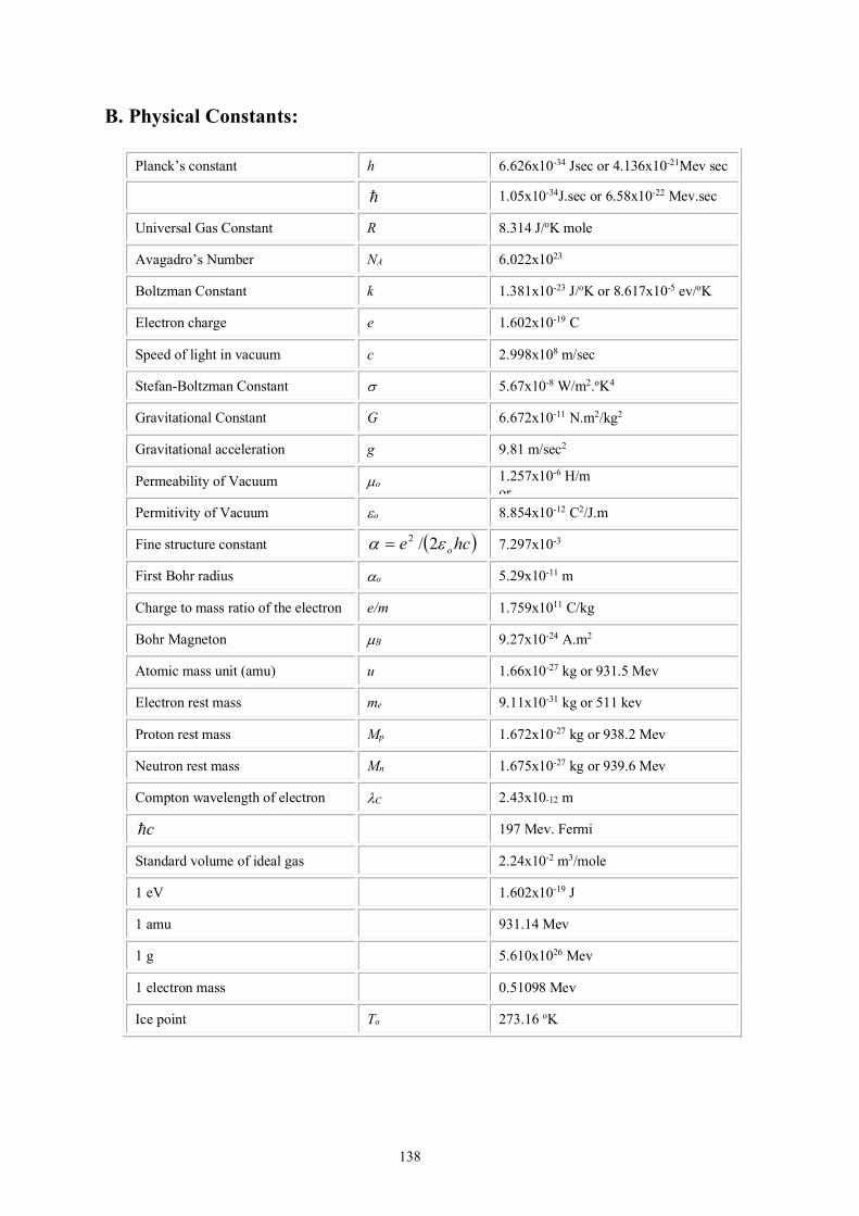
138

B. Physical Constants:

Planck’s constant h 6.626x10-34 Jsec or 4.136x10-21Mev sec

1.05x10-34J.sec or 6.58x10-22 Mev.sec

Universal Gas Constant R 8.314 J/oK mole

Avagadro’s Number NA 6.022x1023

Boltzman Constant k 1.381x10-23 J/oK or 8.617x10-5 ev/oK

Electron charge e 1.602x10-19 C

Speed of light in vacuum c 2.998x108 m/sec

Stefan-Boltzman Constant s 5.67x10-8 W/m2.oK4

Gravitational Constant G 6.672x10-11 N.m2/kg2

Gravitational acceleration g 9.81 m/sec2

Permeability of Vacuum µo 1.257x10-6 H/m or 4p x 10-7 H/m Permitivity of Vacuum eo 8.854x10-12 C2/J.m

Fine structure constant 7.297x10-3

First Bohr radius ao 5.29x10-11 m

Charge to mass ratio of the electron e/m 1.759x1011 C/kg

Bohr Magneton µB 9.27x10-24 A.m2

Atomic mass unit (amu) u 1.66x10-27 kg or 931.5 Mev

Electron rest mass me 9.11x10-31 kg or 511 kev

Proton rest mass Mp 1.672x10-27 kg or 938.2 Mev

Neutron rest mass Mn 1.675x10-27 kg or 939.6 Mev

Compton wavelength of electron lC 2.43x10-12 m

197 Mev. Fermi

Standard volume of ideal gas 2.24x10-2 m3/mole

1 eV 1.602x10-19 J

1 amu 931.14 Mev

1 g 5.610x1026 Mev

1 electron mass 0.51098 Mev

Ice point To 273.16 oK

!

( )hce oea 2/2=

c!

139

C. Conversion Tables: LENGTH cm meter km inch foot mile

cm 1 10-2 10-5 108 0.3937 3.281x10-2 6.214x10-6

meter 100 1 10-3 1010 39.37 3.281 6.214x10-4

km 105 1000 1 1013 3.937x104 3281 0.6214

108 1010 1013 1 3.937x10-9 3.281x10-10 4.214x10-14

inch 28.540 0.0254 2.540x10-5 2.540x108 1 0.0833 1.578x10-5

foot 30.48 0.3048 3.048x10-4 3.048x109 12 1 1.894x10-4

mile 1.609x105 1609 1.609 1.609x1013 6.336x104 5280 1 AREA

m2 cm2 ft2 in.2 circ mile m2 1 104 10.76 1550 1.974x109

cm2 10-4 1 1.076x10-3 0.1550 1.974x105

ft2 9.290x10-2 929.0 1 144 1.833x108

in.2 6.452x10-4 6.452 6.944x10-3 1 1.273x106

circular mill 5.067x10-10 5.065x10-6 5.454x10-9 7.854x10-7 1 VOLUME

m3 cm3 liter ft3 in.3

m3 1 106 1000 35.31 6.102x104

cm3 10-6 1 1.000x10-3 3.531x10-5 6.102x10-2

liter 1.000x10-3 1000 1 3.531x10-2 61.02 ft3 2.832x10-2 2.832x104 28.32 1 1728 in.3 1.639x10-5 16.39 1.639x10-2 5.787x10-4 1

MASS kg gram ounce pound amu m slug ton kg 1 103 35.27 2.205 6.024x1026 1.021x10-1 10-3

gram 10-3 1 3.527x10-2 2.205x10-3 6.024x1023 1.021x10-4 10-6

ounce 2.835x10-2 28.35 1 6.250x10-2 1.708x1025 2.895x10-3 2.835x10-5

pound 4.536x10-1 4.536x102 16 1 2.372x1025 4.630x10-2 4.536x10-4

amu 1.66x10-27 1.66x10-24 5.854x10-26 3.66x10-27 1 1.695x10-28 1.660x10-30

m slug 9.806 9.806x103 3.454x102 21.62 5.9x1027 1 9.806x10-3

ton 103 106 3.527x104 2.205x10-3 6.024x1029 1.021x102 1 TIME

second minute hour year second 1 1.667 x 10-2 2.778 x 10-4 3.165 x 10-8

minute 60 1 1.667 x 10-2 1.901 x 10-6

hour 3600 60 1 1.140 x 10-4

year 3.156 x 107 5.259 x 105 8.765 x 103 1

A0

A0

140

FORCE Nt Dyne Kg F Nt 1 105 0.1020

Dyne 10-5 1 1.020x10-6

Kg F 9.807 9.807x105 1 PRESSURE pa mm Hg mbar kgf/m2 dyne/cm2 atmosphere Pascal 1 7.501x10-3 10-2 0.1020 10 9.869x10-6 torr 1.333x102 1 1.333 13.6 1.333x103 1.316x10-3 mbar 102 0.7501 1 10.20 103 9.869x10-4

dyne/cm2 0.1 7.501x10-4 10-3 10.20x10-3 1 9.869x10-7

kgf/m2 9.807 9.807x10-2 9.807x10-2 1 98.07 9.679x10-5

atm 1.013x105 7.601x102 1.013x10-3 1.033x104 1.013x106 1 ENERGY

Joule kilowatt-hour Btu erg Calorie electron volt Joule 1 2.778x10-7 9.480x10-4 107 0.2389 6.242x1018

kilowatt-hour 3.6x106 1 3.412x103 3.6x1013 8.6x105 2.247x1025

Btu 1.055x103 2.930x10-4 1 1.055x1010 2.468x102 6.585x1021

erg 10-7 2.778x10-14 9.480x10-11 1 2.389x10-8 6.242x1011

calorie 4.187 1.163x10-6 4.053x10-3 4.187x107 1 2.613x1019

electron volt 1.602x10-19 4.450x10-26 1.519x10-22 1.602x10-12 3.827x10-20 1 POWER

watt erg/sec calorie/sec kgfm/sec Btu/sec HP watt 1 107 0.2388 0.1020 3.413 1.360x10-3

erg/sec 10-7 1 2.388x10-8 1.020x10-8 3.413 x10-7 1.360x10-10

calorie/sec 4.187 4.187x107 1 0.4268 14.29 5.694x10-3

kgfm/sec 9.807 9.807x107 2.343 1 33.47 133.3

Btu/sec 0.2931 2.931x106 6.999x10-2 2.987x10-2 1 3.982x10-4

HP 735.5 7.355x109 175.7 75 2.511x103 1 MAGNETIC FIELD

gauss TESLA milligauss gauss 1 10-4 1000 TESLA 104 1 107

milligauss 0.001 10-7 1

141

REFERENCES

1. Yersel, M., “Experiments in Physics,” Boğaziçi University Publications, İstanbul 1997.

2. Resnick, R., Halliday, D. and Krane, K. S., “Physics, 4th Edition,” John Wiley, 1992. 3. Serway, R.A. and Jewett, J. W., “Physics for Scientists and Engineers, 6th edition,”

Brooks Cole, 2003. 4. Product manuals, PASCO. 5. Product manuals, CENCO. 6. Product manuals, LD Didactic GmbH (Leybold). 7. Product manuals, Philip Harris.

PHYSICS IV: EXPERIMENTS - boun.edu.tr

Documents

Transcript of PHYSICS IV: EXPERIMENTS - boun.edu.tr