Portland State University Portland State University

PDXScholar PDXScholar

Dissertations and Theses Dissertations and Theses

Fall 12-4-2017

Physics Based Approach for Seafloor Classification Physics Based Approach for Seafloor Classification

Phu Duy Nguyen Portland State University

Follow this and additional works at: https://pdxscholar.library.pdx.edu/open_access_etds

Part of the Electrical and Computer Engineering Commons

Let us know how access to this document benefits you.

Recommended Citation Recommended Citation Nguyen, Phu Duy, "Physics Based Approach for Seafloor Classification" (2017). Dissertations and Theses. Paper 4060. https://doi.org/10.15760/etd.5944

This Thesis is brought to you for free and open access. It has been accepted for inclusion in Dissertations and Theses by an authorized administrator of PDXScholar. Please contact us if we can make this document more accessible: pdxscholar@pdx.edu.

Physics Based Approach for Seafloor Classification

by

Phu Duy Nguyen

A thesis submitted in partial fulfillment of therequirements for the degree of

Master of Sciencein

Electrical and Computer Engineering

Thesis Committee:Martin Siderius, ChairBranimir Pejcinovic

Jonathan Bird

Portland State University2017

Abstract

The seafloor properties are of high importance for many applications such as marine

biology, oil and gas exploration, laying cables, dredging operations and off-shore construc-

tion. Several approaches exist to classify the properties of the seabed. These include taking

direct samples of the seabed (e.g., coring), however, these methods are are costly and slow.

Underwater acoustic remote sensing techniques are of interest because they are lower cost

and faster. The information about the seabed properties can be extracted by studying the

energy of single beam echo sounders (SBES). This can be done by either phenomenologi-

cal or numerical methods [1], [2]. This research investigates a numerical, model-data fitting

method using a high frequency backscattering model developed by Jackson et al [3]. In

this “inversion modeling” method, the matching process between the model and average

echo envelope provides information about the sediment parameters, namely the sediment

mean grain size (Mz) as the indicator of the seabed type, spectral parameter (W2) as the in-

dicator of seabed roughness and normalized sediment volume parameter σ2 as the indicator

of the scattering due to sediment inhomogeneities.

i

Acknowledgements

I would like to thank the people who provided support and encouragement throughout

my studies in last two years and my final project. Without their support I would not be able

to complete my thesis.

I would like first to thank my advisor Dr. Martin Siderius for his continuous support,

patience to guide me throughout the whole project. He was always the first resource I came

to whenever I need help on my studies and research.

I would also like to acknowledge Dr. Branimir Pejcinovic and Dr. Jonathan Bird for

their serving on my thesis committee.

I am also grateful to all people at Northwest Electromagnetics and Acoustics Research

Laboratory (NEAR Lab) at Portland State University and Metron Scientific Solution for

their help and support. Especially, I would like to thank Dr. Elizabeth Kusel from NEAR

Lab, who was always ready to accompany with me on any field experiments that I need for

my project.

I also would like to thank Dr. D.J Tang and Dr. Todd Hefner from Applied Physics

Laboratory at University of Washington who has supported me by providing his experi-

mental data for my project.

Appreciation goes out to my family, my friends for their patience, understanding dur-

ing my study. Without their moral support, I would not be able to achieve my goal.

ii

Contents

Abstract i

Acknowledgements ii

List of Tables vi

List of Figures 1

1 Introduction 1

2 Background 3

2.1 Fundamental concept and definition . . . . . . . . . . . . . . . . . . . . . 3

2.1.1 Sound waves in medium . . . . . . . . . . . . . . . . . . . . . . . 3

2.1.2 Wavefronts . . . . . . . . . . . . . . . . . . . . . . . . . . . . . . 4

2.1.3 Sound pressure . . . . . . . . . . . . . . . . . . . . . . . . . . . . 5

2.1.4 Speed of sound . . . . . . . . . . . . . . . . . . . . . . . . . . . . 6

2.1.5 Intensity . . . . . . . . . . . . . . . . . . . . . . . . . . . . . . . 6

2.1.6 Characteristic Impedance . . . . . . . . . . . . . . . . . . . . . . . 6

2.1.7 Wave equation . . . . . . . . . . . . . . . . . . . . . . . . . . . . 7

2.1.8 Transmission loss . . . . . . . . . . . . . . . . . . . . . . . . . . . 8

2.1.9 Spreading loss . . . . . . . . . . . . . . . . . . . . . . . . . . . . 9

2.1.10 Absorption loss . . . . . . . . . . . . . . . . . . . . . . . . . . . . 10

2.2 Reflection and scattering . . . . . . . . . . . . . . . . . . . . . . . . . . . 11

2.2.1 Reflection . . . . . . . . . . . . . . . . . . . . . . . . . . . . . . . 11

2.2.2 Scattering . . . . . . . . . . . . . . . . . . . . . . . . . . . . . . . 14

3 Underwater acoustic systems and empirical approach for seabed classification 19

3.1 Acoustic instrument . . . . . . . . . . . . . . . . . . . . . . . . . . . . . . 19

iii

3.1.1 Single-beam echosounder (SBES) . . . . . . . . . . . . . . . . . . 19

3.1.2 Sidescan sonar (SSS) . . . . . . . . . . . . . . . . . . . . . . . . . 20

3.1.3 Multi-row SSS . . . . . . . . . . . . . . . . . . . . . . . . . . . . 21

3.1.4 Multibeam sonar (MBES) . . . . . . . . . . . . . . . . . . . . . . 21

3.2 Phenomenological approach using SBES for seabed classification . . . . . 22

3.2.1 The multi-echo energy approach of RoxAnn system . . . . . . . . 22

3.2.2 Quester Tangent Corporation (QTC) approach . . . . . . . . . . . . 24

4 Theoretical model and methodology for model-based seabed classification 25

4.1 Theoretical model . . . . . . . . . . . . . . . . . . . . . . . . . . . . . . . 25

4.1.1 Model Inputs: Sea floor parameters . . . . . . . . . . . . . . . . . 25

4.1.2 Model for near vertical backscattering due to roughness . . . . . . 26

4.1.3 Volume scattering model . . . . . . . . . . . . . . . . . . . . . . . 32

4.2 Optimization methodology . . . . . . . . . . . . . . . . . . . . . . . . . . 35

4.2.1 Model function . . . . . . . . . . . . . . . . . . . . . . . . . . . . 35

4.2.2 Cost function . . . . . . . . . . . . . . . . . . . . . . . . . . . . . 38

4.2.3 Search Algorithm . . . . . . . . . . . . . . . . . . . . . . . . . . . 41

4.2.4 Testing the optimization with synthetic data . . . . . . . . . . . . . 43

5 Applying the model to measured data 49

5.1 Data processing . . . . . . . . . . . . . . . . . . . . . . . . . . . . . . . . 49

5.1.1 Correcting the signal amplitude . . . . . . . . . . . . . . . . . . . 49

5.1.2 Normalizing the data . . . . . . . . . . . . . . . . . . . . . . . . . 50

5.1.3 Aligning the signal . . . . . . . . . . . . . . . . . . . . . . . . . . 52

5.1.4 Averaging the signal . . . . . . . . . . . . . . . . . . . . . . . . . 52

5.2 Target and Reverberation Experiment 2013 (TREX13) data . . . . . . . . . 53

5.2.1 Description of data set . . . . . . . . . . . . . . . . . . . . . . . . 53

5.2.2 Optimization results . . . . . . . . . . . . . . . . . . . . . . . . . 54

5.3 Mapping with Waldo Lake data . . . . . . . . . . . . . . . . . . . . . . . . 59

iv

5.3.1 Description of data set . . . . . . . . . . . . . . . . . . . . . . . . 59

5.3.2 Optimization result: . . . . . . . . . . . . . . . . . . . . . . . . . 59

6 Discussion 65

Bibliography 68

Appendix A APL model parameterizations 69

Appendix B The roughness scattering approximation 71

Appendix C The volume scattering approximation 79

v

List of Tables

4.1 Parameterization of inputs in term of bulk mean grain size Mz (defined in

[4]). . . . . . . . . . . . . . . . . . . . . . . . . . . . . . . . . . . . . . . 25

4.2 Summary of test with synthetic data . . . . . . . . . . . . . . . . . . . . . 48

5.1 Summary of optimization results with measured data. . . . . . . . . . . . . 63

5.2 Empirical data listed in [4]. . . . . . . . . . . . . . . . . . . . . . . . . . . 63

vi

List of Figures

2.1 Graphical representation of sound wave in water. The figure is adapted

from [5]. . . . . . . . . . . . . . . . . . . . . . . . . . . . . . . . . . . . . 3

2.2 In far field , at a long distance from source, the spherical wavefront (a)

looks like plane wave (b). . . . . . . . . . . . . . . . . . . . . . . . . . . . 5

2.3 Geometry for illustrating angular coordinates used in treating reflections

and scattering (adapted from [3]). . . . . . . . . . . . . . . . . . . . . . . 13

2.4 High level schematic to describe acoustic scattering due to the roughness of

water-sediment interface and heterogeneity of the sediment (adapted from

[3]). . . . . . . . . . . . . . . . . . . . . . . . . . . . . . . . . . . . . . . 15

3.1 An illustration of SBES . The figure is adapted from [6]. . . . . . . . . . . 20

3.2 Simple sidescan consists of single beam echosounder per side . The figure

is adapted from [6]. . . . . . . . . . . . . . . . . . . . . . . . . . . . . . . 20

3.3 Multiple row sidescan consists of multiple single beam echosounder per

side. The figure is adapted from [6]. . . . . . . . . . . . . . . . . . . . . . 21

3.4 The multibeam sonar head is arranged in a Mills Cross with an array of

transmitters and array of beam steered hydrophones. This figure is adapted

from [6]. . . . . . . . . . . . . . . . . . . . . . . . . . . . . . . . . . . . 22

3.5 Illustration of working principle of RoxAnn system. This figure is adapted

from [6]. . . . . . . . . . . . . . . . . . . . . . . . . . . . . . . . . . . . . 23

4.1 Illustration of interface scattering geometry. . . . . . . . . . . . . . . . . . 27

4.2 An example of signal footprint for t0 < t < t0 + τ . . . . . . . . . . . . . . 30

4.3 Illustration of volume scattering geometry . . . . . . . . . . . . . . . . . . 33

4.4 Modeled signal with rectangular pulse. . . . . . . . . . . . . . . . . . . . . 36

4.5 Modeled signal different interface and volume scattering parameters. . . . . 37

vii

4.6 Modeled signal with Gaussian window. . . . . . . . . . . . . . . . . . . . 38

4.7 Best fit model vs. synthetic data. . . . . . . . . . . . . . . . . . . . . . . . 44

4.8 Estimated mean grain size Mz. . . . . . . . . . . . . . . . . . . . . . . . . 45

4.9 Estimated spectral strength W2. . . . . . . . . . . . . . . . . . . . . . . . . 45

4.10 Density ratio ρ. True value is 1.5176. . . . . . . . . . . . . . . . . . . . . . 46

4.11 Speed ratio υ. True value is 1.1660. . . . . . . . . . . . . . . . . . . . . . 46

4.12 Loss parameter δ. True value is 0.0183. . . . . . . . . . . . . . . . . . . . 47

4.13 Interface scattering cross section σs. True value is 0.2097 . . . . . . . . . . 47

4.14 Volume scattering parameter σ2. True value is 0.0021. . . . . . . . . . . . . 48

5.1 Acoustic data collected by NEAR lab at Waldo lake, Sept 2017 . . . . . . . 50

5.2 Diagram of multipaths data . . . . . . . . . . . . . . . . . . . . . . . . . . 51

5.3 Acoustic data collected by Applied Phisycs Laboratory, University of Wash-

ington. . . . . . . . . . . . . . . . . . . . . . . . . . . . . . . . . . . . . . 54

5.4 Model vs. measured data . . . . . . . . . . . . . . . . . . . . . . . . . . . 54

5.5 Estimated mean grain size Mz. . . . . . . . . . . . . . . . . . . . . . . . . 55

5.6 Estimated spectral strength W2. . . . . . . . . . . . . . . . . . . . . . . . 56

5.7 Density ratio ρ. . . . . . . . . . . . . . . . . . . . . . . . . . . . . . . . . 56

5.8 Speed ratio υ. . . . . . . . . . . . . . . . . . . . . . . . . . . . . . . . . . 57

5.9 Loss parameter δ. . . . . . . . . . . . . . . . . . . . . . . . . . . . . . . . 57

5.10 Interface scattering cross section σs. . . . . . . . . . . . . . . . . . . . . . 58

5.11 Volume scattering parameter σ2. . . . . . . . . . . . . . . . . . . . . . . . 58

5.12 Estimated mean grain size Mz. . . . . . . . . . . . . . . . . . . . . . . . . 60

5.13 Estimated spectral strength W2. . . . . . . . . . . . . . . . . . . . . . . . . 60

5.14 Density ratio ρ. . . . . . . . . . . . . . . . . . . . . . . . . . . . . . . . . 61

5.15 Speed ratio υ. . . . . . . . . . . . . . . . . . . . . . . . . . . . . . . . . . 61

5.16 Loss parameter δ. . . . . . . . . . . . . . . . . . . . . . . . . . . . . . . . 62

5.17 Interface scattering cross section σs. . . . . . . . . . . . . . . . . . . . . . 62

5.18 Volume scattering parameter σ2. . . . . . . . . . . . . . . . . . . . . . . . 63

viii

Chapter 1

Introduction

Recently, a variety of alternative technologies for mapping seabed habitats, such as

side-scan sonar, underwater cameras, sediment profiling imagery (SPI), satellite images, as

well as acoustic seabed classification systems [6] have become more common [7]. Some

of them require ground truth for calibration, while others do not. In this report a physics

based method is described to estimate seabed properties from normal incident acoustic

echoes with a single beam echosounder system (SBES). This is a remote sensing approach

and does not require direct sampling of the seabed. The method uses data fitting of a

theoretical model parameterized by seabed properties. The theoretical model simulates the

shape of the echo return based on the environmental inputs which are adjusted to optimize

the fit to the acoustic measurements. The best match of this process is expected to give

the approximate sediment parameters such as scattering cross section, volume and loss

parameters, sediment-water density ratio, sediment water sound speed ratio, mean grain

size and spectral strength. These quantities will be described in more detail in section 2.

The optimization process involves two steps. First, the normal incidence bottom re-

flection coefficient of each ping is estimated from acoustic echo data and an empirical

relationship between reflection coefficient and sediment mean grain size is employed [8].

The mean grain size is then used to infer the range of possible values for each input of the

1

model (based on empirical relationships [4]). This approach reduces computational cost

and constrains the searching results to be physically meaningful. The second step com-

pares the theoretical echo envelope with the measurement and searches over all possible

parameter values to determine the set that minimizes the difference between the modeled

and measured signals. The theoretical model and optimization methodology are described

in section 4. Section 5 presents the results of model fitting to measured data. Section 6

gives a discussion about the results.

2

Chapter 2

Background

2.1 Fundamental concept and definition

2.1.1 Sound waves in medium

A wave motion, in which the particles of the medium oscillate about their mean positions

in the direction of propagation of the wave, is called a longitudinal wave. Sound waves

are classified as longitudinal waves. A sound wave propagating underwater consists of

alternating compression and rarefaction [9] of the medium as shown in Fig.2.1.

Figure 2.1: Graphical representation of sound wave in water. The figure is adapted from[5].

3

2.1.2 Wavefronts

The form of any wave is determined by its source and is described by the shape of the

wavefronts. There are three basic types of waves, plane, spherical and cylindrical. A

plane wave is emitted by a planar source, a cylindrical by line source and spherical by

point source. Plane waves are not really possible to create in reality but it is a useful

approximation [10] as at a long distance spherical waves look like a plane wave. Figure 2.1

illustrates spherical and plane wavefronts. In a 2D plot, the cross section of a spherical wave

is shown in Fig.2.2a, and the same wave at long distance is shown in Fig. 2.2b showing an

example of the spherical wave appearing as a plane wave structure at long distances from

the point source.

4

(a)

(b)

Figure 2.2: In far field , at a long distance from source, the spherical wavefront (a) lookslike plane wave (b).

2.1.3 Sound pressure

The sound pressure is the force of sound on a surface area perpendicular to the direction of

the sound. The sound pressure can also sometimes be called acoustic pressure. The stan-

dardized unit for acoustic pressure is Pascals (Pa). The sound pressure in air can be mea-

sured with microphone and underwater acoustic pressure can be measured by hydrophone.

5

2.1.4 Speed of sound

Three acoustic quantities such as speed of sound cw (i.e., the longitudinal motion of wave),

sound frequency f and wavelength known as λ are related by

f =cwλ. (2.1)

2.1.5 Intensity

A propagating sound wave carries mechanical energy with it in the form of kinetic energy

of the particles in motion plus the potential energy of the stresses set up in the elastic

medium. Because the wave is propagating, a certain amount of energy per second, or

power, is crossing a unit area and this power per unit area, or power density is called the

intensity, I , of the wave. In water, the intensity I is proportional to the square of the

acoustic pressure p by

I =p2

ρmcm(2.2)

where ρm and cm are medium density and speed of sound in the medium.

2.1.6 Characteristic Impedance

The product of two term cm and ρm is called the characteristic impedance of the media. It is

property of a sound medium that is analogous to the impedance in electrical circuit theory.

6

2.1.7 Wave equation

The sound propagates in the medium at the speed cm (or cw for water). The propagation of

the sound can be described mathematically by solution of wave equation,

d2p

dt2= c2(

d2p

dx2+

dp

dy2+d2p

dz2). (2.3)

which can also be written,

∇2p =1

c2d2p

dt2(2.4)

The wave equation is written in a partial differential form in term of acoustic pressure p

with respect to the coordinates x, y, z and time t. For one-dimension, all functions p(x, t)

that fulfill equation 2.4 have the form:

p(x, t) = f(ct± x) (2.5)

If the sound wave was a sinusoidal oscillation (i.e., time-harmnic solution), for dif-

ferent wave types the complex representation of the sound pressure (in units of Pascal) is

written as follows, for plane waves,

p(x, t) = p0ei(±kx+φ)eiωt (2.6)

where the ± is + for waves propagating in the negative x direction and is − for waves

7

propagating in the positive x direction. And, for outgoing spherical waves:

p(r, t) =p0rei(−kr+φ)eiωt (2.7)

where φ is a phase constant, p0 is the amplitude of sinusoidal oscillation, x and r are

distances in Cartesian and spherical coordinate systems respectively. The wavenumber k

and angular frequency ω are defined as,

k =2π

λ(2.8)

where

ω = 2πf (2.9)

and λ is the wavelength.

2.1.8 Transmission loss

Consider a sound source in the sea, the intensity of sound can be measured at any distance

d. The transmission loss TL in decibels (dB) is then,

TL = 10 log10 I0 − 10 log10 I (2.10)

where I0 is the reference intensity and it is measured at the distance 1 meter from the source

and I is the intensity at the distance d meters from the source.

8

2.1.9 Spreading loss

In most cases with a point source and an assumption that the medium is infinite and homo-

geneous, the sound would have a spherical wave front. Under these conditions, the power

P generated by the source is radiated equally in all directions and distributed equally over

the surface of a sphere surrounding the point source. If there is no loss in the medium, the

power P crossing all these spheres is the same. Thus

P = 4πr21I1 = 4πr22I2 = ...4πr2nIn (2.11)

where rn is the radius of nth sphere and In is the intensity of sound wave at surface of that

sphere. If r1 = 1 the changes in power density with the distance r from point source is

TLs = 20 log10 r (2.12)

If the medium is bounded such as in the ocean, the spreading sometimes no longer ap-

pears spherical but is better represented as cylindrical spreading. IfH is the height between

bounds, the power the crossing cylindrical surface range (where here r is in cylindrical co-

ordinates) r1, r2 is,

P = 2πr1HI1 = 2πr2HI2 = ...2πrnHIn (2.13)

9

Thus, the cylindrical spreading loss in dB is

TLc = 10 log10 r (2.14)

where TLs denotes spherical spreading loss and TLc denotes cylindrical spreading loss.

Typically, in the ocean, the wave spreading loss is somewhere between spherical and cylin-

drical due to losses at the boundary interactions. This is one of the reasons the loss at the

seabed boundary is important for understanding downrange TL.

2.1.10 Absorption loss

The primary causes of absorption (in the water column) have been attributed to several pro-

cesses, including viscosity and thermal conductivity. It involves a process of converting the

acoustic energy into heat. The absorption loss is represented by a “logarithmic absorption

coefficient” α as follows [9],

α =10 log10 I1 − 10 log10 I2

r2 − r1(2.15)

The quantity α is often expressed in decibels per kiloyard (dB/kyd) or can also be in dB/km

or dB/m.

10

2.2 Reflection and scattering

In a monostatic configuration with the sound source and receiver co-located in the water

column, an acoustic transmitted pulse will propagate to the seabed and there it can be both

reflected and scattered back to the receiver. A perfect reflection occurs, without scatter-

ing, only if the seafloor is perfectly flat which is not generally realistic. Typically, part of

the incident pulse will be reflected as a coherent signal and another part will be scattered

due to both the roughness at the water-sediment interface and inhomogeneities in the wa-

ter column and sediment. The bottom backscattering strength is equivalent to the bottom

backscattering cross section per unit area per unit solid angle θ, where θ is the grazing an-

gle. The cross section is assumed to be the sum of contributions from interface roughness

and the sediment volume inhomogeneities. The APL-UW model developed by Jackson

et al in Ref [4] separates the received envelope into a component due to roughness and a

component due to volume scattering. For near vertical incidence, the Kirchhoff approxi-

mation is applied to estimate the backscattering due to interface roughness. The model and

necessary inputs are described in more detail in the next sections.

2.2.1 Reflection

Although the seafloor is never perfectly flat and homogeneous, it is useful to consider the

ideal case in that the scattering is neglected. In this ideal case when the acoustic pulse hits

the seafloor, part of the energy will be reflected back to the water column and another part

is transmitted into the second medium. Assumption is that the incident pressure field is a

11

unit amplitude plane wave at angular frequency ω. In the ideal case, if the incident grazing

angle is θ, the pressure field can be approximated at interface as,

Pi = Pi0eiki·r, (2.16)

where Pi0 is the complex pressure amplitude at the origin, r is the position vector, and

ki is the wave vector giving the direction of propagation of plane wave. As indicated in

Fig. 2.3, the z coordinate will be taken perpendicular to the seafloor. For convenience, the

coordinate system will be chosen so that the direction of propagation of the plane wave lies

in the x− z plane. Then the incident wave vector has (x, y, z) components,

ki =ω

cw(cos θ, 0,− sin θ), (2.17)

the reflected wave denoted as Pr will be a plane wave of the form,

Pr = Vww(θ)Pi0eikr.r, (2.18)

where the reflected wave vector kr is defined as:

kr =ω

cw(cos θ, 0, sin θ) (2.19)

for θi = θs = θ, where θi and θs are incident and scattering grazing angles respectively.

12

Figure 2.3: Geometry for illustrating angular coordinates used in treating reflections andscattering (adapted from [3]).

The complex parameter Vww(θ) is the reflection coefficient, with the subscripts ww to

indicate that the incident and reflected fields are both measured in the water. The bottom

loss BL is defined as:

BL = −20 log10(|Vww(θ)|). (2.20)

In the case of normal incidence, Vww(θ = 90) becomes:

Vww(90) =ρscs − ρwcwρscs + ρwcw

, (2.21)

where the subscripts s on ρ and c indicate seabed density and sound speed and w indicates

13

water parameters.

2.2.2 Scattering

Acoustic waves are scattered randomly by irregularities in the seafloor, including the rough-

ness of the water-sediment interface, spatial variation in sediment physical properties and

other objects such as bubbles, solid and organic particles, shell pieces, marine life and in-

homogeneities in ocean sediment. When the sound wave is scattered, part of the reflected

energy is returned to the source as an echo (i.e, is backscattered) some parts are reflected

off in another direction and is lost energy. The scattering processes are described in the

high level schematic shown in Fig. 2.4. The amount of energy scattered is a function of

the size, density, and concentration of foreign bodies present in the sound path, as well

as the frequency of the sound wave. The larger the area of the reflector compared to the

sound wavelength, the more effective it is as a scatterer. At high frequencies (e.g., above

10 kHz), all seafloors have substantial irregularities on the scale of acoustic wavelength.

The treatment of seafloor scattering at high frequencies typically employ statistical meth-

ods to predict the variance of the scattering field. The most commonly used statistical

quantity is the scattering cross section, that is proportional to the variance of the scattered

field.

14

Figure 2.4: High level schematic to describe acoustic scattering due to the roughness ofwater-sediment interface and heterogeneity of the sediment (adapted from [3]).

Typically, the total pressure field P in the random scattering media is decomposed as

follows:

P =< P > +Ps (2.22)

where < P > is treated as the mean of the complex pressure field and Ps is a fluctuation

about this mean.

The mean-square fluctuations are equal to the variance of the field and can be ex-

pressed as :

< |Ps|2 >=< |P 2| > −| < P > |2 (2.23)

The subscript s is attached to fluctuating part of the field as it is the “scattering” part.

15

The mean field can be considered as the coherent part. The scattering by the seafloor

is usually quantified in term of “scattering strength” whose definition follows from the

situation depicted in Fig. 2.4, in which the a small patch with area A is situated in far field

of the source. Then, the mean square pressure fluctuation will be proportional to both the

area of the patch and the squared incident pressure magnitude |Pi|2 and will be inversely

proportional to the square of the distance r from the patch. Thus,

< |Ps|2 >= |Pi|2Aσ1

r2s. (2.24)

Note that i and s subscripts denote “incident” and “scattering”. The attenuation and

refraction in the seawater are neglected here. The proportional factor σ is dimensionless

and is sometimes referred to as the “scattering cross section per unit area per unit solid

angle” because the integral of σ over the upper solid angle hemisphere yields the total

mean scattered power Us as follows

Us =A|Pi|2

2ρwcw

∫2π

σ(θi, θs, φs)dΩs (2.25)

where,

• ρw is the density of seawater

• ρwcw is the acoustic impedance of seawater

• θi is the incident grazing angle

16

• θs is the scattered grazing angle

• φs is the bistatic angle

The factor 2 in the denominator of eq. (2.25) appears because time averages of squared

sinusoidally oscillating functions are one-half the square of the peak magnitude. The quan-

tity σ(θi, θs, φs) is simply referred as the backscattering cross section [3].

It is important to remember that the scattering cross section is defined here as a statis-

tical average. Referring to Fig. 2.3, the scattering cross section depends on three angular

variables: a grazing angle, for the incident field θi, and grazing and azimuthal angles of

scattering fields θs and φs. These dependencies can be shown explicitly by writing the

scattering cross section as σ(θi, θs, φs). The angle φs is often referred to as the “bistatic

angle”. If the seafloor has a preferred direction an azimuthal angle φi is also required for

the incident field. In either case, σ is referred to as the “bistatic” scattering cross section.

A simpler and more common case is backscattering, or the “monostatic” case, in which the

transmitter and receiver are situated at the same point in space. For that case, θs = θi =

and φi = φs + π = φ and Sb is referred as a “backscattering strength”, and is expressed in

dB,

Sb = 10 log10 σ (2.26)

where only two angular variables, θ and φ are needed. If the seafloor has no preferred

direction then the variable φ can be eliminated.

The cross section is assumed to be the sum of the interface and sediment inhomogene-

17

ity scattering. In the literature ([4], [9] [11], [12]), several expressions of scattering cross

section σ are described. In this study, the following expression from [4] and [12] will be

used:

σ = (σsur + σvol) (2.27)

where σsur refers to the scattering strength due to water-seabed interface and, and σvol is

volume scattering strength due to sediment inhomogeneities,

Sb = 10 log10(σsur + σvol). (2.28)

18

Chapter 3

Underwater acoustic systems and empirical approach for seabed classification

This chapters provides a short review of acoustic systems and a phenomenological

approach using single beam echosounders for seabed classification.

3.1 Acoustic instrument

Acoustic instruments that are commonly used for seabed classification are grouped into

four categories as described by Anderson et al in [13] and Hammilton et al in [6]. They are

briefly described in the following subsections.

3.1.1 Single-beam echosounder (SBES)

Single beam echosounders operate one or more transducers which are designed with a

narrow beam at specific frequencies. SBES are reported as the least expensive and least

complex underwater acoustic instrument. They are the most common instrumentation em-

ployed due to low cost, simple operation, and less complexity in data processing [14].

19

Figure 3.1: An illustration of SBES . The figure is adapted from [6].

3.1.2 Sidescan sonar (SSS)

A simple sidescan sonar is equipped with single-beam echosounder on each side of a vehi-

cle (or towfish), and the transducers are tilted towards the seabed. Compared to the SBES,

the swath footprint provides more seabed coverage and it is relatively easy to operate.

Figure 3.2: Simple sidescan consists of single beam echosounder per side . The figure isadapted from [6].

20

3.1.3 Multi-row SSS

More advanced SSS systems consist of multiple elements arranged in a row to improve

the accuracy in estimating the incidence angle, horizontal range and bathymetric measure-

ments.

Figure 3.3: Multiple row sidescan consists of multiple single beam echosounder per side.The figure is adapted from [6].

3.1.4 Multibeam sonar (MBES)

Multibeam sonars are designed for collecting the bathymetric and backscatter for hydro-

graphic seabed mapping and classification. MBES systems are more complex and expen-

sive compared to SBES however they have more advantages such as higher resolution,

ability to detect the angle of incidence and detection of multiple scattering from two differ-

ent targets.

21

Figure 3.4: The multibeam sonar head is arranged in a Mills Cross with an array oftransmitters and array of beam steered hydrophones. This figure is adapted from [6].

3.2 Phenomenological approach using SBES for seabed classification

As mentioned earlier, acoustic remote sensing classification methods are numerous butcan fall under two general categories: phenomenological approaches and physics basedapproaches [1], [2]. While the model-based method uses an inversion procedures to char-acterize the seafloor, the empirical method relies on the the study of signal features thatare correlated with sediment type. The empirical method requires establishing a data base“ground truth”. The typical features of returned signal used for this approach are timespread, echo energy, and skewness [11], [15]. This approach has been used by several com-mercial acoustic bottom classification system, RoxAnn and QTC-View are two of them.The review of these two system was made by Hamiton et al in [6].

3.2.1 The multi-echo energy approach of RoxAnn system

The RoxAnn system uses a multi-echo energy classification method. RoxAnn functions by

integrating components of the first and second seabed echoes to derive two parameters of

the seabed substrate E1 and E2. E1 is an integration of the tail of the first seabed echo, and

is taken to represent seabed “roughness”. E2 is an integration of the whole of the second

bottom echo and provides an index of seabed “hardness” [7].

22

Figure 3.5: Illustration of working principle of RoxAnn system. This figure is adaptedfrom [6].

The first echo is reflected from bottom while the second echo bounced twice, first it

interacted with sea surface then the sea bottom. The data then is presented as a scatter plot

E1 vs. E2. Based on the the cluster pattern of scatter plots, the operator applies the “box

set” to these data in such the way that each box has a maximum and minimum E1 and E2.

Each box represents the particular sediment type which is defined based on the ground-truth

samples. This approach is purely empirical and works well for flatter bottoms, however for

the rougher bottoms, E2 appears an unreliable classifier due to energy lost resulted from

the scattering processes [16].

23

3.2.2 Quester Tangent Corporation (QTC) approach

In contrast to RoxAnn, the QTC system examines the shape characteristics of only the

first returning signal from an echosounder transducer. QTC normalizes the first echo to

unity peak amplitude before calculating shape parameters [6]. A set of 166 parameters are

extracted from acoustic data. Post-processing analysis of the acoustic data is carried out

using the software packages CAPS and QTC IMPACT. Most of the 166 parameters carry

limited information or redundant information. Principal component analysis (PCA) is used

to determine the best combination of the 166 features for discrimination of the echoes. The

166 feature combinations are therefore automatically reduced to three composite values,

known as Q1, Q2, and Q3 . The Q-values are chosen automatically by principal component

analysis by the QTC software from five algorithms as Histogram, Quantiles, Integrated

Energy Slope, and Walet packages [17]. For more details about the principal component

analysis for seabed classification using QTC system see [15]. The QTC system provides

new insights but the usefulness of the acoustic classification depends upon the amount and

quality of ground-truth data [18]. The user relates acoustic class to the physical properties

of the seabed through a calibration process. The ground truth data can be obtained using

bottom grabs or video recordings. The system works well with flatter bottoms.

In a recent study, Hamilton et al in [16] compared the RoxAnn and QTC acoustic

bottom classification systems in terms of performance. They found that the QTC classes

generally had consistent sediment grain size properties and gave a better classification than

the RoxAnn system.

24

Chapter 4

Theoretical model and methodology for model-based seabed classification

This chapter describes the theoretical model and model-based approach for sediment clas-

sification.

4.1 Theoretical model

4.1.1 Model Inputs: Sea floor parameters

The geoacoustic parameters serving as the model inputs are listed in Table. 4.1. They are

needed to represent the seafloor type and are largely taken from the APL-UW Environmen-

tal Handbook [4].

Symbol Description Short name

ρ Ratio of sediment mass density to water density Density ratioυ Ratio of sediment sound speed to water sound

speedSound speed ratio

δ Ratio of imaginary wavenumber to realwavenumber for sediment

Loss parameter

σ2 Ratio of sediment volume scattering cross sec-tion to sediment attenuation coefficient

Volume parameter

γ Exponent of bottom relief spectrum Spectral parameterW2 Strength of bottom relief spectrum cm4 at

wavenumber k = 2πλ

(cm−1)Spectral strength

Mz Mean grain size (in units of φ)

Table 4.1: Parameterization of inputs in term of bulk mean grain size Mz (defined in [4]).

25

The mean grain size is often expressed in units of φ as

Mz = − log2

d

d0, (4.1)

where d0 is reference length equal to 1 mm, d is mean grain size (diameter) in mm. The

mean grain size takes the values from −1φ to 9φ.

According Jackson et al in [3], for near- vertical backscattering the mean square re-

ceived envelope is taken as a sum of components due to roughness and volume scattering,

< |Vr(t)|2 >=< |Vrr(t)|2 > + < |Vrv(t)|2 >, (4.2)

where, < |Vr(t)|2 > is the total received envelope, < |Vrr(t)|2 > is the received envelope

contribution due to interface roughness,< |Vrv(t)|2 > is the received envelope contribution

due to volume scattering.

4.1.2 Model for near vertical backscattering due to roughness

For near vertical backscattering due to a rough interface, the Kirchhoff approximation is

applied. Appendix. B describes in details of this approximation method. This section

presents the very final steps where the model is derived by Jackson et al in [3].

26

Figure 4.1: Illustration of interface scattering geometry.

Figure 4.1 illustrates the geometry of the interface scattering components of the model.

For simplicity, it is assumed that the transmitted signal has a rectangular envelope of length

τ and the source-receiver is at the origin for convenience. With these assumptions, the

backscattered signal received at time t (measured from the beginning of the transmitted

pulse) is due to scatters lying within the slant range interval,

rt −cwτ

2< r < rt, (4.3)

where,

rt =cwt

2(4.4)

is range associated with the time of interest t. The interface scattering eq. (B.18) can be

27

rewritten as,

< |Vrr(t)|2 >=2(s0sr)

2e−4k′′wH

H4

∫σ|br(θ, φ)bx(θ, φ)|2d2R, (4.5)

where H is the height of the source-receiver above the seafloor, and it is assumed that the

scattering is confined to narrow region immediately below the source-receiver.

s0 : RMS source pressure

sr : Receiving sensitivity as voltage/pressure ratio

br : Receiving complex directivity function

bx : Source complex directivity function

k′′w : Imaginary part of wave-number in seawater

θ : Grazing angle

φ : Azimuthal angle

Vww(900) : Reflection coefficient of flat interface at near nadir

The source level (20 log10 s0 ) is measured in the vertical direction which results

in,

|br(π

2, 0)bx(

π

2, 0)| = 1. (4.6)

It will be assumed that the scattering is isotropic so that scattering strength σ does not

depend on the azimuthal angle φ. The integral over φ only involves the directivity so the

28

azimuthal averaged directivity for small angle of incidence near vertical is:

b(θ) =1

2π

∫ −π−π|br(θ, φ)bx(θ, φ)|2dφ. (4.7)

This will be approximated by a Gaussian function,

b(θ) = e− (π/2−θ)2

2σ2b , (4.8)

where σb is beamwidth parameter.

A similar approximation will be used for the scattering cross section. The high fre-

quency Kirchhoff approximation eq. (B.17) near the nadir can be written as

σsur =|Vww(900)|2

8πσ2s

e− (π/2−θ)2

2σ2s . (4.9)

This should be regarded as a parameterization of the scattering cross section near ver-

tical incidence. In this approximation, the parameter σs should be considered as a measure

of the angular width of the backscattering cross section peak at vertical incidence rather

than as an RMS slope of the interface. With these approximations, the two dimensional

integral in eq. (4.5) can be simplified to one dimensional integral as,

< |Vrr(t)|2 >=(s0sr)

2e−4k′′wH |Vww(900)|2

2H4σ2s

∫ R2

R1

e− (π/2−θ)2

2σ2sb RdR, (4.10)

where

1

σ2sb

=1

σ2s

+1

σ2b

. (4.11)

The parameter σ2b is understood to be the variance of the receiver/ source directivity,

σs is variance of scattering cross section, and σ2sb is interpreted as a combined variance of

29

two Gaussian distributions that described by equations 4.9 and 4.8. R is the cylindrical

radial coordinate defined in Fig. 4.1 with the limits defined by eq. (4.3). Defining the angle

of incidence measured from vertical as χ = π/2− θ, one can find the relationship between

the angular limits and elapsed time and pulse length.

The elapsed time between the beginning of the transmission and the leading edge of

the seafloor return is

t0 =2H

cw, (4.12)

where cw is seawater sound speed.

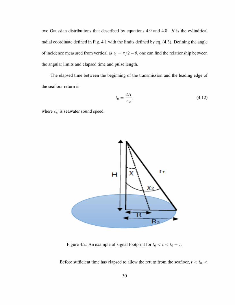
Figure 4.2: An example of signal footprint for t0 < t < t0 + τ .

Before sufficient time has elapsed to allow the return from the seafloor, t < t0, <

30

|Vrr| >= 0. For the time period within one pulse length τ , i.e. t0 < t < t0 + τ , for a small

angle at near normal incidence (where χ1 = 0), the ensonified area is a circle [3] as shown

in Fig. 4.2, and an approximation for the small angle χ2 << 1,

χ22 ≈

R22

H2=rt

2 −H2

H2(4.13)

or,

χ22 =

(cwt)2/4− (cwt0)

2/4

(cwt0)2/4

(4.14)

χ22 =

t2 − t20t20

=(t− t0)(t+ t0)

t20. (4.15)

For the near vertical backscattering t+ t0 ∼= 2t0, the approximation for χ22 becomes,

χ22 =

2(t− t0)t0t20

= 2(t/t0 − 1). (4.16)

For longer time t > t0 + τ , the ensonified area is an annulus defined by the angular

limits as follows (the similar approach for approximation of χ1 is applied),

χ21 = 2[(t− τ)/t0 − 1], (4.17)

and

χ22 = 2(t/t0 − 1). (4.18)

If the integration variable in eq. (4.10) is changed to χ2, and the limits of integration

are changed from R1, R2 to χ21, χ

22 respectively, the integrand becomes a simple exponen-

31

tial, from which one can obtain,

< |Vrr(t)|2 >= V 21 |Vww(900)|2 g(t− t0, Tsb, τ)

1 + σ2s

σ2b

(4.19)

where,

g(t− t0, T, τ) = 0 for t < t0

g(t− t0, T, τ) = 1− e−(t−t0)/T for t0 < t ≤ τ + t0

g(t− t0, T, τ) = e−(t−t0−τ)/T − e−(t−t0)/T for t > τ + t0

Tsb = σ2sbt0, (4.20)

and

V 21 =

(s0sr)2e−4k

′′wH

2H2, (4.21)

is a normalization factor equal to the mean square voltage that would be measured if the

interface was perfectly flat with reflection coefficient having unity magnitude. The normal-

ized intensity (< |Vrr(t)|2 >) at first approaches an asymptote exponentially and then after

a time of one pulse length decays towards zero. The rise time of the < |Vrr(t)|2 > provides

a measure of angular width σs of the backscattering cross section. Narrow width gives the

rapid rise and vice versa.

4.1.3 Volume scattering model

Appendix. C describes in details the approximation for scattering due to sediment inho-

mogeneities, this section describes only last steps leading to the final expression needed to

implement the model.

32

Figure 4.3: Illustration of volume scattering geometry

The volume scattering cross section is parameterized as following,

σvol =|Vwp(θi)|2|Vwp(θs)|2σv

2kw|ρ|2Im[P (θi) + P (θs)](4.22)

where

Vwp(900) = 1 + Vww(900), (4.23)

and σv is the volume scattering cross section and is treated as an empirical quantity that

must be obtained by fitting data [19]. The following dimensionless parameter σ2 is used to

quantify the sediment volume scattering,

σ2 =σvαp

(4.24)

where αp is the attenuation in dB m−1.

The squared averaged received signal due to volume scattering can be found from

33

following,

< |Vrv| >2=8πσvV

21 |Vwp(900)|4

ρ2

∫ r2

r1

∫ χ2

0

b(θ)e−4k′′p (r−H/ cosχ) sinχdχdr. (4.25)

The factor |Vwp|4/ρ2 accounts for round trip transmission through the interface. The

exponential factor accounts for attenuation in the sediment with k′′ being the coefficient of

the imaginary part of the sediment wavenumber. The angular limits are,

χ2 = cos−1(H/r). (4.26)

For t0 < t ≤ t0 + τ , the ensonified volume is a spherical section

r1 = H, (4.27)

and

r2 = rt. (4.28)

For t > t0 + τ , the ensonified volume is a spherical shell

r1 = rt − cwτ/2, (4.29)

and

r2 = rt. (4.30)

Making the small angle approximation (χ << 1), the integrand can be written in

term of a simple exponential in χ2 and r which results in,

< |Vrv| >2=8πσvV

21 |Vwp(900)|4

ρ(σ−2p + σ−2b )[σ2bg(t− t0, Tb, τ)− σ2

pg(t− t0, Tp, τ)] (4.31)

34

with

Tb = σ2b t0, (4.32)

and

Tp = σ2pt0 (4.33)

σ2p =

1

4k′′pH, (4.34)

where k′′p is the imaginary part of seabed compressional wave-number.

4.2 Optimization methodology

All parameters are searched for in the optimization process accept spectral parameter γ

which takes the value of 3.25 if a measurement is not available [3] as is the case here.

4.2.1 Model function

The theoretical model of the bottom return is mathematically represented by < |Vr(t)| >2

in equation (4.2), and its components are described by (4.19) and (4.31). The theoretical

model has five unknown parameters that represent the seabed characteristics. The opti-

mization process then seeds the best combination of the unknown model parameters so

that the model will have the best fit to the bottom echo captured from measured data. For

verification of the correctness of the model described in this research, a plot of modeled

signal with the same set of parameters as specified in Fig.G.7 page 506 of [3] was made

as shown in Fig. 4.4a. Then, the parameters were varied to see the change in shape of the

modeled signal. The panels 4.4b, 4.4c, 4.4d in Fig. 4.4 are to illustrate how the scattering

35

cross section and volume parameters effect to the signal amplitude and shape. The main

pulse (first part of the signal) represents the coherent part of signal. The normal incident

reflection coefficient value is shown as black dashed line in the plots and indicates the level

of an ideally reflected signal for a perfectly flat interface. It can seen that, if the interface

is perfectly flat and there is no scattering due to roughness or inhomogeneities, the level of

total modeled return signal is the coherent reflection as shown in Fig. 4.4b. If the interface

is rough, some energy is scattered away and the return signal level is lower than the ideal

reflected signal. The shape of signal also changes.

(a) (b)

(c) (d)

Figure 4.4: Modeled signal with rectangular pulse.

36

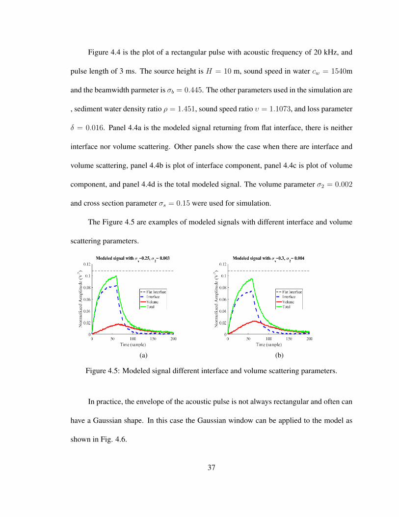
Figure 4.4 is the plot of a rectangular pulse with acoustic frequency of 20 kHz, and

pulse length of 3 ms. The source height is H = 10 m, sound speed in water cw = 1540m

and the beamwidth parmeter is σb = 0.445. The other parameters used in the simulation are

, sediment water density ratio ρ = 1.451, sound speed ratio υ = 1.1073, and loss parameter

δ = 0.016. Panel 4.4a is the modeled signal returning from flat interface, there is neither

interface nor volume scattering. Other panels show the case when there are interface and

volume scattering, panel 4.4b is plot of interface component, panel 4.4c is plot of volume

component, and panel 4.4d is the total modeled signal. The volume parameter σ2 = 0.002

and cross section parameter σs = 0.15 were used for simulation.

The Figure 4.5 are examples of modeled signals with different interface and volume

scattering parameters.

(a) (b)

Figure 4.5: Modeled signal different interface and volume scattering parameters.

In practice, the envelope of the acoustic pulse is not always rectangular and often can

have a Gaussian shape. In this case the Gaussian window can be applied to the model as

shown in Fig. 4.6.

37

(a) (b)

Figure 4.6: Modeled signal with Gaussian window.

4.2.2 Cost function

A cost function is needed to determine the degree that the model fits the data. There are

two cost functions used here for two different steps in the optimization process as follows:

Step 1 cost function

This cost functionE1 is for searching for the optimal mean grain sizeMz (which can also be

related to the sediment type) and is based on a comparison of the normal incident reflection

coefficient. The E1 cost function is defined,

E1 = [Vmod(900)− Vmea(900)]2 (4.35)

where Vmea(900) is reflection coefficient obtained from echo energy of measured data and

Vmod(900) is the model of Rayleigh reflection coefficient.

Based on the relation between mean grain size, acoustic sediment impedance, and

38

bottom reflection coefficient as decribed in [8], [20], Vmod(900) can be derived as follows,

Vmod(900) =ρ(Mz)υ(Mz)− 1

ρ(Mz)υ(Mz) + 1(4.36)

where sediment -water density ratio ρ and sound speed ratio υ are known as

ρ =ρsρw, (4.37)

and

υ =cscw, (4.38)

where cw is sound speed in water, ρw is water density. The value of seawater sound speed

and density can be found from literature (or easily measured). Note that for the simulation

in Fig. 4.4, cw takes the value of 1540 m/s and sediment sound speed ratio υ and density

ratio ρ can be parameterized through different grain sizes according to [4],

ρ = 0.007797M2z − 0.17057Mz + 2.3139 for − 1 <= Mz <= 1.0,

ρ = −0.165406M3z + 0.2290201M2

z − 1.1069031Mz

+ 3.0455 for 1 <= Mz <= 5.3,

ρ = −0.0012973Mz + 1.1565 for 5.3 <= Mz <= 9.0,

39

and

υ = 0.002709M2z − 0.05645Mz + 1.2778 for − 1 <= Mz <= 1.0,

υ = −0.0014881M3z − 0.0213937M2

z − 0.1382798Mz

+ 1.3425 for 1 <= Mz <= 5.3,

υ = −0.0012973Mz + 1.1565 for 5.3 <= Mz <= 9.0.

Step 2 cost function

This cost function is for searching the additional geoacoustic and scattering parameters

such as σs, σ2, and δ through a model-data fitting process. Two options are provided for

comparison. Option 1 has been developed in this thesis, while option 2 has been taken from

existing literature.

Option 1

The cost function O1 is based on the difference between measured time series data

ymeas(tk) and modeled time series data ymod(tk) (envelopes of time series) at each time

sample tk. First, the difference between modeled and measured envelopes are computed at

each time step,

∆(tk, M) = [ymea(tk)− ymod(tk)]2. (4.39)

where, ~M is the vector of search space parameters.

40

The optimal parameter set resulting from the model-data fit for each time step tk is,

O(tk, ~Mk) = argmin(∆(tk, ~M)), (4.40)

where ~Mk is the best set of parameters at time step tk. The optimal set for option 1 for the

entire envelope matching is then,

O1 =1

K

∑k

O(tk, ~Mk) (4.41)

where K is total number of time samples considered.

Option 2

The second option uses the cost function based on a normalized difference over the

entire measured and modeled time series envelopes. It is described in the literature [20] as

follows,

E2( ~M) =1∑

k [(y2meas(tk) + y2mod(tk)]

∑k

[ymeas(tk)− ymod(tk)]2. (4.42)

The optimal set resulting from the model-data fit for each average envelope is,

O2 = argmin(E2( ~M)) (4.43)

4.2.3 Search Algorithm

The estimation of bottom parameters from the model-data matching process is compli-

cated due to the possibility of a large number of good fits in the multidimensional search

space. However, in some cases, the values found from optimization may not have a physical

meaning. Therefore, it is necessary to establish constraints for each search space. Several

41

approaches are described in the literature such as in [1]. In this paper, a two step search

approach is proposed. Before the fitting procedures are applied, an estimate of the bot-

tom reflection coefficient is done and used in step one to obtain grain size as one of the

inputs to the model. The detailed algorithm for this is not described here but the coeffi-

cient is approximated from the measured data. Once the reflection coefficient is estimated,

the mean grain size can be calculated. The relationship between the mean grain size, the

reflection coefficient and the sediment impedance is described in [20]. The mean grain

size is obtained by minimizing the cost function by equation (4.35). Instead of searching

all five parameters at the same time by fitting the model to the measured data, two of the

geoacoustic parameters, sound speed ratio and density ratio are approximated first through

the mean grain size. The spectral strength parameter W2 is also computed from the mean

grain size. The second step is to obtain the three other unknown parameters by optimizing

the model to the measured data. An exhaustive search algorithm is applied for this opti-

mization process. The search range for each parameter is determined by using the mean

grain size and Table 2 in [4] as a constraint. The tests with synthetic data have shown that

by breaking down the optimization process into two steps the computation is more efficient

and the estimation yields better results.

In the second step, the cost function (4.40) is minimized to optimize the agreement

between model and measured data. With the consideration that the unknown parameters

would be treated as the “random variable”, instead of mapping the entire model to each

ensemble of measured data to get one best estimated result for each measurement (as when

42

using option 2 as the cost function), a point-to-point mapping procedure is performed (op-

tion 1 cost function). The final result using option 1 for each run produces the mean of the

estimates found from the point-to-point procedure. For example, the model and one single

measurement has the same length (500 samples) as the measured time series. The point-

to-point mapping procedure will minimize the cost function at every single point (time

sample) and will result in 500 best combination of estimates. The mean of these 500 esti-

mates will be taken as the final result for this run. In this way, some of the smaller values

in the time series that are primarily due to scattering are not dominated by the larger parts

of the curve dominated by the geoacoustic parameters.

4.2.4 Testing the optimization with synthetic data

Synthetic data was generated with known seafloor parameters which were selected from

Table.2 in [4] with additive white noise of about -10dB. One hundred data sets (packets)

were generated. Figures from 4.7 to 4.14 illustrate the results of the model-synthetic data

fit using option 1, cost function O1.

43

Figure 4.7: Best fit model vs. synthetic data.

The Fig.4.7 shows the agreement between the best fit, modeled signal and simulated

signal. The estimated values found from the mapping process was fed back to the model

to generate the plots of the total field and its components (interface and volume scattering).

The synthetic data is shown as the solid blue line, the interface scattering contribution is

shown as the green dashed line, the volume scattering component as the red dashed line, and

the total modeled signal is the blue dashed line. Figures 4.8 to 4.14 present the distribution

of parameters found from the optimization process.

44

Figure 4.8: Estimated mean grain size Mz.

Figure 4.9: Estimated spectral strength W2.

45

Figure 4.10: Density ratio ρ. True value is 1.5176.

Figure 4.11: Speed ratio υ. True value is 1.1660.

46

Figure 4.12: Loss parameter δ. True value is 0.0183.

Figure 4.13: Interface scattering cross section σs. True value is 0.2097

47

Figure 4.14: Volume scattering parameter σ2. True value is 0.0021.

Parameter: Mz(φ) W2 (cm4) ρ (-) υ (-) δ (-) σs σ2 (-)

Estimates: 2.25 0.0031 1.5276 1.229 0.0176 0.1992 0.0021True: - - 1.5162 1.1660 0.0183 0.2097 0.0021

Error (%): - - .75 3.7 3.82 5.01 0

Table 4.2: Summary of test with synthetic data

Note that mean grain size Mz and spectral strength W2 were not the inputs of the

model, so there is no available true value for comparison. The error is due to the noise

added to the signal.

48

Chapter 5

Applying the model to measured data

One set of experimental data was collected by the Applied Physics Laboratory at the Uni-

versity of Washington (APL-UW) along the Main Reverberation Track of the TREX13

experiment. Another set of data was collected by the Northwest Electromagnetics and

Acoustics Research Laboratory (NEAR Lab) and has been used for testing with the model.

Where it is required, the pre-processing steps that are described in Section 5.1 were applied

to these data sets before they were matched to the modeled signal. Each envelope was

computed from an average of 10 successive pings.

5.1 Data processing

Before comparing the measured and modeled signals, there were several pre-processing

steps needed to take care of variations in the return signal due, for example, to differ-

ences in the signal arrival time caused by changes in bathymetry or slight movement of

the source/receiver assembly. These steps are not necessary for synthetic data and they are

described in the following paragraphs.

5.1.1 Correcting the signal amplitude

The signal amplitude needs to be corrected due to the spreading loss and attenuation in

water column, the variation in bottom depth also need to be taken care if one uses the

49

reference depth as an constant input to the model.

5.1.2 Normalizing the data

The measured data need to be normalized such that the source level is unity. This step is

necessary as the model is predicting the shape of the normalized envelope. In practice a

calibrated source level can not always be obtained, however it can be estimated by using

multipath echoes in the acoustic data. For an example, if the acoustic data has multiple

echos as shown in Fig. 5.1, the surface and bottom reflection losses can be obtained using

the wave equation and principles of spreading and transmission loss as described in Section

2. Once the reflection losses are known, the source level can be approximated.

Figure 5.1: Acoustic data collected by NEAR lab at Waldo lake, Sept 2017

In Fig. 5.1, from the top, the second echo at about 11m is the surface bounce, the

third one is the bottom return followed by the surface -bottom and bottom-surface returns.

50

The echo at 40 meter and 48 meter are surface-bottom-surface and bottom-surface-bottom

bounces respectively. The diagram of multipaths is shown in Fig. 5.2.

Figure 5.2: Diagram of multipaths data

Example of using sonar equation for estimation of bottom loss and surface loss is,

BL = S + TLS −BS − TLBS, (5.1)

and,

SL = BS + TLBS − SBS − TLSBS, (5.2)

where,

BL : Bottom loss

SL : Surface loss

S : Surface bounce energy level

51

BS : Bottom-surface bounce energy level

SBS : Surface-Bottom-Surface bounce energy level

TLBS : Transmission loss due to bottom-surface path

TLS : Transmission loss due to surface path

TLSBS : Transmission loss due to surface-bottom-surface path

Note that the energy levels are on dB scale.

5.1.3 Aligning the signal

Generally, the arrival time of signals will not be the same in different transmissions due to

depth variations (bathymetry changes) or ship (source/receiver) movement. Aligning the

return envelope is necessary before going to next step of data fitting. There are several

methods for alignment, the way it was done here is to determine the approximate region of

the return signals then find the peaks and shift all the signals to the same reference time.

5.1.4 Averaging the signal

Typically, the measured signal envelope will show variability in shape and amplitude due

to a variety of factors not related to the parameters of interest such as noise. To reduce

these variations the average envelope is computed from a certain N number of pings. Note

that this step will reduce the size of the data set. The modeled signal will be mapped with

this average envelope.

52

5.2 Target and Reverberation Experiment 2013 (TREX13) data

5.2.1 Description of data set

To perform the model data fitting process the SBES data as shown in Fig. 5.3 that was

collected by the Applied Physics Laboratory at the University of Washington during the

Target and Reverberation Experiment 2013 is considered. Although it is a bit lower fre-

quency (3 kHz) than the frequency the model is designed for (typically for frequencies

>10 kHz), it can still be used to illustrate the model matching procedures. The instrument

used for experiment is a Bottom Backscatter SONAR (BSS), the sensors are an omni-

directional source (ITC-1007) and an omni-directional receiver (ITC-1032) mounted on

a short bracket [21]. The transmitted pulse is a narrowband 3 kHz signal. A Gaussian

bandpass filter is applied to each ping. The data set consists of 500 pings is used for this

optimization process. All the data processing steps have been applied to this data set. The

echo returns are shown in Fig. 5.3. From the top of the figure, the second echo at about 5 m

is the bottom bounce, the third one at 22 m is the surface return followed by the surface -

bottom and bottom-surface returns at 27 m. The echo at 47 m is the bottom-surface-bottom

bounce.

53

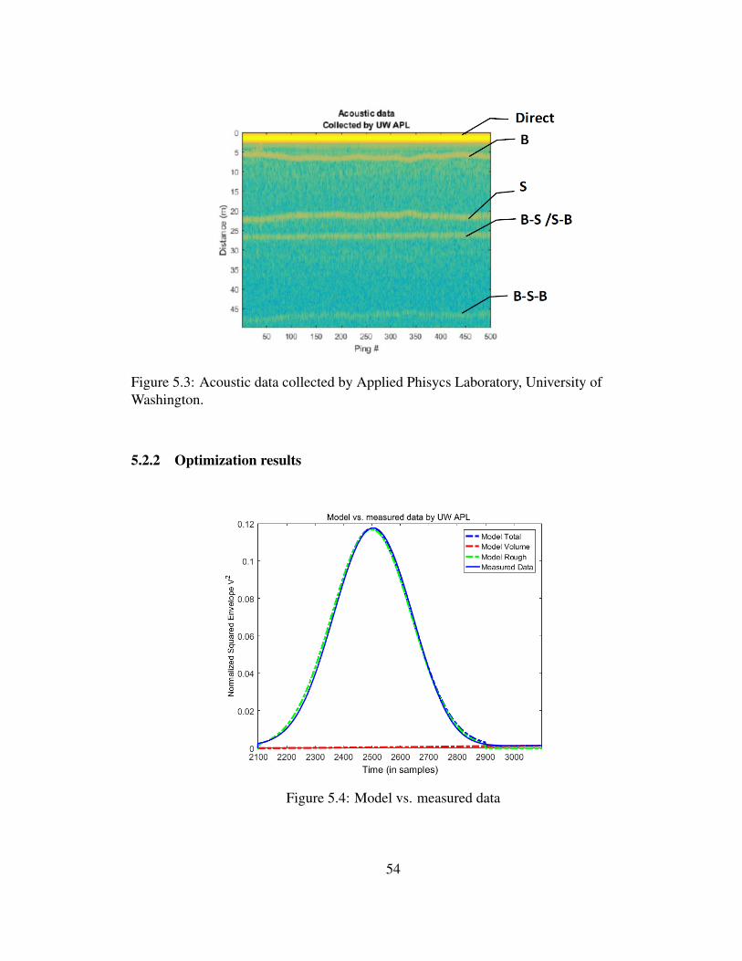
Figure 5.3: Acoustic data collected by Applied Phisycs Laboratory, University ofWashington.

5.2.2 Optimization results

Figure 5.4: Model vs. measured data

54

The blue solid line is the bottom return signal captured from measured data, the dashed red

line and dashed green line are the volume scattering and interface scattering components

of the modeled signal respectively. The dashed blue line is the total modeled signal. It can

be seen that the model matches well with the measured signal.

Figure 5.5: Estimated mean grain size Mz.

55

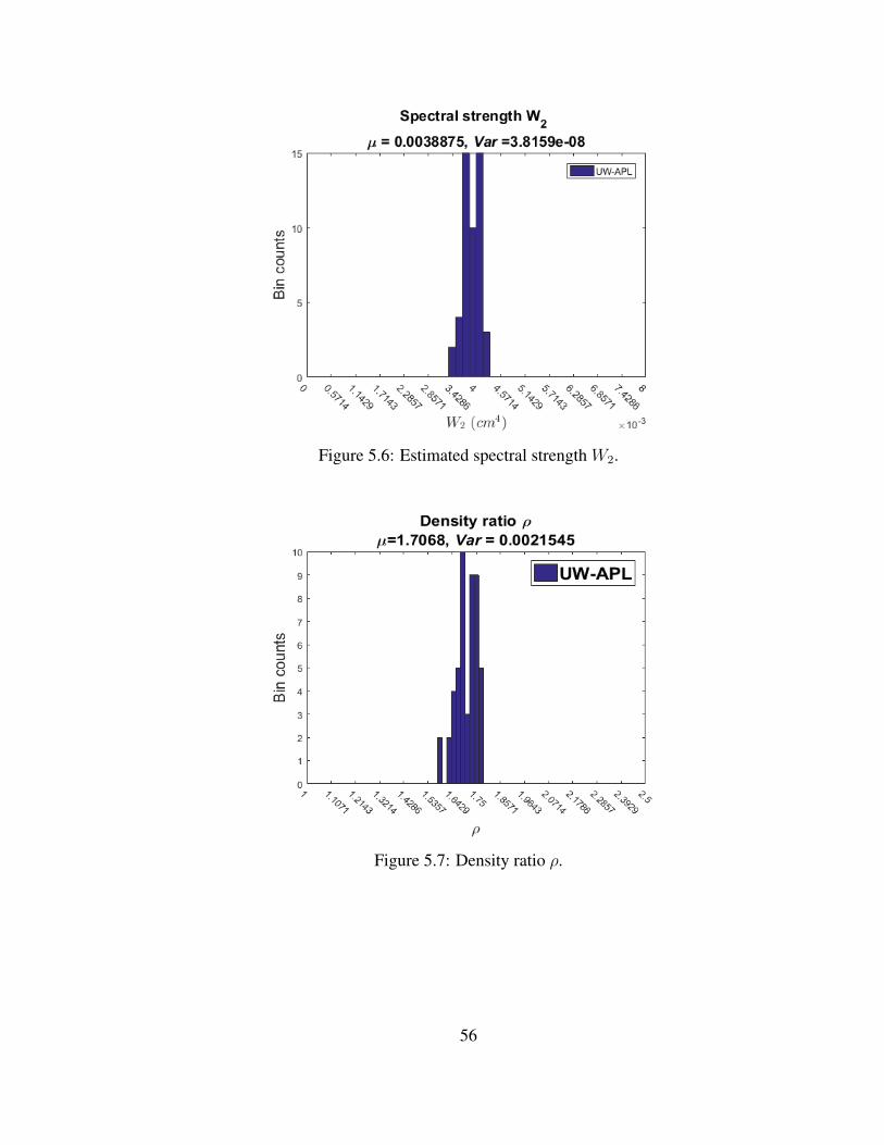
Figure 5.6: Estimated spectral strength W2.

Figure 5.7: Density ratio ρ.

56

Figure 5.8: Speed ratio υ.

Figure 5.9: Loss parameter δ.

57

Figure 5.10: Interface scattering cross section σs.

Figure 5.11: Volume scattering parameter σ2.

58

5.3 Mapping with Waldo Lake data

5.3.1 Description of data set

The data was collected by the author at Waldo lake, Oregon on September 2017. The

instrument used for this experiments includes a conical transducer BII-7562/33IM that has

a center frequency of 33 kHz, the hydrophone BII-7018, , the power amplifier BII-5020

and the data acquisition device NI USB-6281. All equipment is powered by batteries. The

hydrophone was mounted a distance of 1 meter under the transducer on a rigid PCV pipe.

The whole system was hung along side an inflatable boat and was deployed at a depth of 5

meters from the surface. The water column was approximately 14.5 meters. The boat was

drifting slowly to avoid a big deviation of signal arrival times (due to bathymetry changes).

A linear frequency modulated signal of 3 ms swept from 28 to 38kHz was transmitted

downwards every 1 second. A separation of 0.997 second between pings was used to make

sure no overlap occurred between return signals and to have sufficient time for the system

to acquire the multipath data. Two sets of 200 pings were collected.

5.3.2 Optimization result:

Presented here are the results from the fitting process.

59

Figure 5.12: Estimated mean grain size Mz.

Figure 5.13: Estimated spectral strength W2.

60

Figure 5.14: Density ratio ρ.

Figure 5.15: Speed ratio υ.

61

Figure 5.16: Loss parameter δ.

Figure 5.17: Interface scattering cross section σs.

62

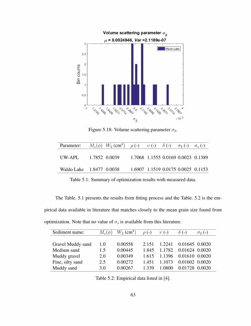
Figure 5.18: Volume scattering parameter σ2.

Parameter: Mz(φ) W2 (cm4) ρ (-) υ (-) δ (-) σ2 (-) σs (-)

UW-APL 1.7852 0.0039 1.7068 1.1555 0.0169 0.0023 0.1389

Waldo Lake 1.8477 0.0038 1.6907 1.1519 0.0175 0.0025 0.1153

Table 5.1: Summary of optimization results with measured data.

The Table. 5.1 presents the results from fitting process and the Table. 5.2 is the em-

pirical data available in literature that matches closely to the mean grain size found from

optimization. Note that no value of σs is available from this literature.

Sediment name: Mz(φ) W2 (cm4) ρ (-) υ (-) δ (-) σ2 (-)

Gravel Muddy sand 1.0 0.00558 2.151 1.2241 0.01645 0.0020Medium sand 1.5 0.00445 1.845 1.1782 0.01624 0.0020Muddy gravel 2.0 0.00349 1.615 1.1396 0.01610 0.0020Fine, silty sand 2.5 0.00272 1.451 1.1073 0.01602 0.0020Muddy sand 3.0 0.00267 1.339 1.0800 0.01728 0.0020

Table 5.2: Empirical data listed in [4].

63

The estimated results showed that the sediment in the areas where the data was taken

is close to medium sand or muddy gravel. This is close to what was expected.

64

Chapter 6

Discussion

A model fitting procedure has been developed to estimate geoacoustic and scattering pa-

rameters of the seabed from normal incident echo sounders. A new cost function was

developed that appears to be better for estimating some of the less sensitive scattering pa-

rameters. Initial tests of the method use modeled data with additive noise as a synthetic data

set. The results showed the optimization process was successful at estimating the relevant

parameters. The method was also applied to measured data however since the true seabed

is not known exactly it is difficult to assess the methods accuracy with these measured data

sets.

Table. 5.1 and 5.2 present the mapping results and the empirical data. These are

close to the estimated sediment characteristics in the regions where the measured data were

collected. Having the value of Mz found from step 1 of the optimization process, the

empirical data can be adapted from Table.2 in [4]. It can be seen that the values of density

ratio ρ, sound speed ratio υ and spectral strength W2 resulting from the mapping process

are slightly higher than the values that they are assumed to be if just the empirical data are

used. It is consistent with some model-data fitting results in published literature (see [12]

for example).

The use of this high frequency model with slightly lower frequency data from APL

UW (the recommended frequency range is from 10kHz to 100kHz as per [4] and the mea-

65

surements were 3 kHz) gives some promise of using the model-data fit with lower frequency

acoustic data. The matching results with 28 kHz data collected from Waldo Lake shows

some supportive features such as the correlation between the estimated values and expected

sediment parameters.

For future work, more comprehensive measurements are needed to further understand

the physics of acoustic backscatter from seabed. Such measurements should be made over

different areas and types of sediment. It would be perfect if the measurements could be

done in the regions that have other empirical data available for comparison (e.g., core sam-

ples taken and analyzed).

The goal of this research is to study the possibility of using a model-based approach

for seabed classification. The methodology presented in this report is still under develop-

ment and needs improvement. However it can be said that it is feasible to employ a physics

based method for seafloor classification without relying on ground truth for calibration.

66

Bibliography

[1] Daniel D Sternlicht and Christian P de Moustier. Remote sensing of sediment charac-teristics by optimized echo-envelope matching. The Journal of the Acoustical Societyof America, 114(5):2727–2743, 2003.

[2] Dimitri Alexandrou and D Pantzartzis. A methodology for acoustic seafloor classifi-cation. IEEE Journal of Oceanic Engineering, 18(2):81–86, 1993.

[3] Darrell Jackson and Michael Richardson. High-frequency seafloor acoustics.Springer Science & Business Media, 2007.

[4] APL-UW High-Frequency Ocean Environmental. Acoustic models handbook. Ap-plied Physics Laboratory, University of Washington, APL-UW TR, 9407, 1994.

[5] Waves-boundless physics. https://courses.lumenlearning.com/boundless-physics/chapter/waves/.

[6] LJ Hamilton. Acoustic seabed classification systems. Technical report, DEFENCESCIENCE AND TECHNOLOGY ORGANISATION VICTORIA (AUSTRALIA)AERONAUTICAL AND MARITIME RESEARCH LAB, 2001.

[7] Simon PR Greenstreet, Ian D Tuck, Gavin N Grewar, Eric Armstrong, David G Reid,and Peter J Wright. An assessment of the acoustic survey technique, roxann, as ameans of mapping seabed habitat. ICES Journal of Marine Science, 54(5):939–959,1997.

[8] Paul A Van Walree, Michael A Ainslie, and Dick G Simons. Mean grain size mappingwith single-beam echo sounders. The Journal of the Acoustical Society of America,120(5):2555–2566, 2006.

[9] R.J Urick. Principle of Underwater Sound. Peninsula Publishing, 1983.

[10] Martin Siderius. Array sensor processing. Lecture note, Sept 2016,Portland StateUniversity, Oregon.

[11] Daniel D Sternlicht and Christian P de Moustier. Time-dependent seafloor acous-tic backscatter (10–100 khz). The journal of the acoustical society of America,114(5):2709–2725, 2003.

[12] Darrell R Jackson and Kevin B Briggs. High-frequency bottom backscattering:Roughness versus sediment volume scattering. The Journal of the Acoustical Societyof America, 92(2):962–977, 1992.

67

[13] John T Anderson, V Holliday, RUDY Kloser, DAVID Reid, and YVAN Simard.Acoustic seabed classification of marine physical and biological landscapes. Interna-tional Council for the Exploration of the Sea, 2007.

[14] Paul G von Szalay and Robert A McConnaughey. The effect of slope and vessel speedon the performance of a single beam acoustic seabed classification system. FisheriesResearch, 56(1):99–112, 2002.

[15] Ali R Amiri-Simkooei, Mirjam Snellen, and Dick G Simons. Principal componentanalysis of single-beam echo-sounder signal features for seafloor classification. IEEEJournal of Oceanic Engineering, 36(2):259–272, 2011.

[16] LJ Hamilton, PJ Mulhearn, and R Poeckert. Comparison of roxann and qtc-viewacoustic bottom classification system performance for the cairns area, great barrierreef, australia. Continental Shelf Research, 19(12):1577–1597, 1999.

[17] BT Prager, DA Caughey, and RH Poeckert. Bottom classification: operational resultsfrom qtc view. In OCEANS’95. MTS/IEEE. Challenges of Our Changing GlobalEnvironment. Conference Proceedings., volume 3, pages 1827–1835. IEEE, 1995.

[18] Kari E Ellingsen, John S Gray, and Erik Bjrnbom. Acoustic classification of seabedhabitats using the qtc view system. ICES Journal of Marine Science, 59(4):825–835,2002.

[19] Darrell R Jackson, Dale P Winebrenner, and Akira Ishimaru. Application of the com-posite roughness model to high-frequency bottom backscattering. The Journal of theAcoustical Society of America, 79(5):1410–1422, 1986.

[20] Mirjam Snellen, Kerstin Siemes, and Dick G Simons. Model-based sediment classifi-cation using single-beam echosounder signals. The Journal of the Acoustical Societyof America, 129(5):2878–2888, 2011.

[21] DJ Tang and Todd Hefner. Bottom reflectivity along the main reverberation track oftrex13. unpublished report.

[22] Darrell R Jackson, Kevin B Briggs, Kevin L Williams, and Michael D Richardson.Tests of models for high-frequency seafloor backscatter. IEEE journal of oceanicengineering, 21(4):458–470, 1996.

[23] Eric I Thorsos. The validity of the kirchhoff approximation for rough surface scat-tering using a gaussian roughness spectrum. The Journal of the Acoustical Society ofAmerica, 83(1):78–92, 1988.

[24] JH Stockhausen. Scattering from the volume of an inhomogeneous half-space. TheJournal of the Acoustical Society of America, 35(11):1893–1893, 1963.

68

Appendix A

APL model parameterizations

The geoacoustic inputs to the APL-UW model listed in Table. 4.1 are parameterized interms of the bulk mean grain size Mz as follows,Density ratio

Range : 1 <= ρ <= 3

ρ = 0.007797M2z − 0.17057Mz + 2.3139 for − 1 <= Mz <= 1.0,

ρ = −0.165406M3z + 0.2290201M2

z − 1.1069031Mz

+ 3.0455 for 1 <= Mz <= 5.3,

ρ = −0.0012973Mz + 1.1565 for 5.3 <= Mz <= 9.0,

Sound speed ratio

υ =c2c1

υ = 0.002709M2z − 0.05645Mz + 1.2778 for − 1 <= Mz <= 1.0

υ = −0.0014881M3z − 0.0213937M2

z − 0.1382798Mz

+ 1.3425 for 1 <= Mz <= 5.3

υ = −0.0012973Mz + 1.1565 for 5.3 <= Mz <= 9.0

Loss parameter

δ =k2ik2r

=α2υc1ln(10)

40πfα2

f= 0.4556 for − 1 <= Mz <= 0

= 0.4556 + 0.0245Mz for 0 <= Mz <= 2.6

= 0.1978 + 0.1245Mz for 2.6 <= Mz <= 4.5

= 8.0399− 2.5228Mz + 0.20098M2z for 4.5 <= Mz <= 6.0

= 0.9431− 0.2041Mz + 0.0117M2z for 6.0 <= Mz <= 9.0

69

Volume parameterσ2 tends to be independent of frequencies over 10-100kHz and 0.001 <= σ2 <= 0.005

[22], [19]

σ2 = 0.002 for − 1 <= Mz <= 5.5

σ2 = 0.001 for 5.5 <= Mz <= 9.0

Spectral exponent γ is obtained from experimental power spectrum by changing the signof spectral slope 2.4 <= γ <= 4. If absence of measurement γ = 3.25.Spectral strength Range: 0 <= W2 <= 1.

h

h0=

2.03846− 0.26923Mz

1 + 0.076923Mz

for − 1 <= Mz <= 5.0

h

h0= 0..5 for 5.0 <= Mz <= 9.0

h0 = 1cm is reference lengthW2 = 0.00207h2h20 For γ = 3.25

70

Appendix B

The roughness scattering approximation

Roughness scattering cross section can be modeled in three ways as listed below and

the method chosen depends on the situaion [3], [23]:

1. The Kirchhoff approximation , valid for smooth and moderately rough seabed inter-

faces with grazing angle near vertical (900).

2. The composite roughness approximation, valid for smooth and moderately rough

seabed interfaces with grazing angles away from 900.

3. The large scale roughness approximation, to account for scattering strengths for

gravel and rock bottom that are relatively large and imply roughness parameters fall

outside Kirchhoff approximation.

The two most widely used approximations for scattering by seafloor roughness are small-

roughness perturbation and Kirchhoff approximation. Each has its own separate domain of

validity, for the scattering near the specular direction, the Kirchhoff works better [23].The

object of primary interest is scattering cross section . It is a function of the angles defining

the direction from source to the scattering region and from scattering region to the receiver.

In term of wave-number, the direction from the source to the scattering region and from

71

scattering region to the receiver can be specified as

ki = kw(ex cos θi cosφi + ey cos θi sinφi − ez sin θi) (B.1)

ks = kw(ex cos θs cosφs + ey cos θs sinφs + ez sin θs) (B.2)

Figure B.1: Definition of angular coordinates used in treating reflection and scattering

Here, kw is the wavenumber in water, the incident direction is denoted as ki and

the direction towards receiver is ks. ex, ey ez are the unit vector in x,y and z direction

respectively. The angles used here are defined in Fig. 2.4 where it is noted that one may set

φi = 0 without loss of generality if seafloor is isotropic. All the components of the wave

vectors can not be specified independently, as the magnitude must be k + w. Thus, the

following horizontal horizontal components of the wave vectors are sufficient to define the

72

incident and scattering directions:

Ki = kw(ex cos θi cosφi + ey cos θi sinφi) (B.3)

Ks = kw(ex cos θs cosφs + ey cos θs sinφs) (B.4)

It is convenient to define the wave vector difference between the incident and scatter-

ing directions

∆k = ks − ki (B.5)

∆K = Ks −Ki (B.6)

and for one dimensional

∆kz = ksz − kiz (B.7)

Note that:

∆k2 = ∆K2 + ∆k2z (B.8)

In this study, the Kirchhoff approximation is applied. The simplified form of backscat-

tering ccross section in high frequency limit reduced to,

σsur =1

4|Vww(θis)|2

∆k4

∆k4zps(s). (B.9)

73

where Vww is the seabed reflection coefficient for a flat interface as a function of grazing

angle θis where

θis = sin−1(∆k

2kw). (B.10)

ps(s) is the bivariate Gaussian probability density function for interface slope,

ps(s) =1

2π||Bs||12

e(−12sTB−1

s s) (B.11)

where s is defined as,

s = [∆Kx

∆kz;∆Ky

∆kz] (B.12)

This column matrix contains the x−and y− components of slope corresponding to

specular reflection and Bs is co-variance matrix for slope with determinant ||Bs||.

Bs =

< ( dfdx

)2> < df

dx>< df

dy>

< dfdx>< df

dy> < ( df

dy)2>

(B.13)

where f(R) is ”interface relief function” with zero mean and quantity h =< f 2(R) > is

referred as RMS roughness for R = (x, y)

In the isotropic case which is considered in this research, the slope covariance matrix

Bs is equal to unit matrix multiplied by constant and the eq. (B.9) becomes,

σsur =|Vww(θis)|2

8πσ2s

∆k4

∆k4ze(− ∆K2

2σ2s∆k2

z)

(B.14)

74

where

σs =< (df

dx)2

>=< (df

dy)2

> (B.15)

is the RMS slope for a 1D track. In terms of an isotropic spectrum,

σ2s = π

∫K3W (K)dK (B.16)

where, W (k) is the surface spatial spectrum. The high frequency Kirchhoff approximation

is most appropriately applied to backscatter from seafloor with isotropic roughness statistic,

for that the equation (B.14) takes the simplified form,

σsur =|Vww(900)|2

8πσ2s sin4 θi

e− cot2 θi

2σ2s (B.17)

The notation that has been used in above subsection is summarized below:

subscripts i and s denote for incident and scattering quaatities

kw wave-number in seawater

k′′w imaginary part of wave-number in seawater

θis local grazing angle for specular reflection

θs incident grazing angle

Vww reflection coefficient for flat interface

∆k magnitude of three dimensional wave vector difference

75

∆kz difference in vertical wave vector component

∆K two-dimensional horizontal wave vector difference

∆k two-dimensional horizontal wave vector difference

∆K magnitude of ∆K

∆Kx x component of ∆K

∆Ky y component of ∆K

K two dimensional horizontal wave number

K magnitude of two dimensional wave-number K

Vww(900) reflection coefficient of flat interface at near nadir

Figure B.2: Geometry for computing the mean square received voltage in bistaticscattering scenario. Note that r=(R,0)

76

The generalization of eq. (2.24) is simply an integration that sums the contribution of

infinitesimal patches of area to obtain the mean-square received voltage,

< |Vr(t)|2 >= s2r

∫|Pi|2σ

e−2k”w|rs−r|

|rs − r|2|br(θr, φr)|2d2R (B.18)

where

RS = 20 log10 sr (B.19)

is the receiver sensitivity giving the voltage per unit pressure and br(θr, φr) is receiver

directivity pattern see appendix F of reference [3]. θ and φ are grazing and azimuthal

angles respectively, and subscript r denotes receiver quantities.

The incoherent sum implied by eq. (B.18) is justified in most cases of interest.

All the factors inside integrand of eq. (B.18) depend on the integration coordinates R =

(x, y) with d2R = dxdy. The integration limits of eq. (B.18) depend on the length of

transmitted pulse and on the time t at which the receiver voltage is evaluated. The time-

range relation is

|r− ri|+ |r− rs| = cwt0(R) (B.20)

where r = (R, 0) is the distance vector from origin to scattering region (point) R

and t0(R) is the time required for acoustic energy to travel the total distance from source

to the scattering patch an then to the receiver. This time varies with the position R of the

scattering patch. In the simplest case , if the transmitted pulse has a rectangular envelope

77

of length τ , the limits of integration can be set by constraining (x, y) such that

t− τ

2< t0(R) < t+

tau

2(B.21)

with t is the time at which one wishes to estimate the scattering mean-square pressure.

Evaluation of eq. (B.18) is simple for the case in which ri = rs. The range limits becomes

rt −cwτ

4< |r− ri| < rt +

cwτ

4(B.22)

where

rt =cwt

2(B.23)

is the range associated with time of interest. Inequality B.22 defines the range limits on the

ensonified region.

78

Appendix C

The volume scattering approximation

The basic fluid sediment volume scattering model was developed by Stockhausen [24]

with the key assumptions that

1. Volume scattering is sufficiently weak that the volume scattered acoustic field in the

sediment is much smaller than incident field.

2. Sediment volume scattering can be characterized by a cross section that increases

linearly with the ensonified volume.

3. Attenuation in the sediment limits the penetration to the depth that are much smaller

than the distance from the source and receiver to scattering area.

4. The scattering effect of sediment -water is negligible.

With these assumption, the sediment volume scattering at high-frequency can be

treated as an interface process and can be characterized experimentally and theoretically

that same way as scattering by seafloor roughness was described. Further with an assump-

tion that the source is unit, the equivalent model for volume scattering cross section is

σvol =|Vwp(θi)|2|Vwp(θs)|2

|ρ|2

∫ 0

−∞σv(z)e2kwIm[P (θi)+P (θs)]zdz (C.1)

79

where,

P (θ) =√

(υ−2 − cos2 θ) (C.2)

and

|Vwp| = |Vww|+ 1 (C.3)

with υ being the complex compressional wave speed/ water sound speed ratio, i and s

subscripts denote for incidence and scattering . If the volume scattering was assumed being

independent on the depth, the integral can be performed resulting in,

σvol =|Vwp(θi)|2|Vwp(θs)|2σv

2kw|ρ|2Im[P (θi) + P (θs)](C.4)

where, kw is the water wavenumber. Equation (C.4) forms the basic for several sediment

volume scattering models, which differ only in the assumption used to obtain the volume

scattering cross section. The following dimensionless parameter, so-called normalized vol-

ume scattering parameter is use to quantify sediment volume scattering,

σ2 =σvαp

(C.5)

where αp is the attenuation in dB m−1.

80

Figure C.1: Illustration of volume scattering geometry

For volume scattering, one must integrate over the ensonified volume as shown in

Fig.C.1. To simplify the problem the interface is assumed flat and ray bending is ignored.

This is reasonable assumption for the signal near vertical incidence.

81