PHYSICS 425 NOTES: PLASMA ASTROPHYSICSkestrel.nmt.edu/~lyoung/425/root.pdf · Physics 425 Notes...
64
PHYSICS 425 NOTES: PLASMA ASTROPHYSICS Original version (2007): Jean Eilek Physics Department, New Mexico Tech Socorro, NM 87801, U.S.A. JEILEK@AOC. NRAO. EDU Minor revisions (2008, 2009+): Lisa Young The goal of this course is to explore the “physics of as- trophysics”. What physics governs the behavior of the astrophysical objects we observe? How can we inter- pret our observations, in light of the relevant physics, to understand what’s going on inside a particular star, nebula or galaxy? To reach this goal we need to bring together a diverse range of physics – some of which you will have seen in other courses, some of which will be new. These ideas cover a broad range of material, not all of which is in a single textbook. Thus, we’ve got the course notes for our text. You should note units and dimensions. These notes are in cgs, as is most of the astrophysical literature. That makes very little difference for “rocks” (analyses that involve mass, length, time); but it makes a big dif- ference for electrodynamics. The E and B fields, as well as the fundamental charge, have different dimen- sions in cgs than in SI; and the coupling constants in Maxwell’s equations are different. Contents 1 Astrophysical plasmas we’ll meet 1 2 Some basic plasma tools 4 2.1 Distribution functions ......... 4 2.2 Collective effects ........... 4 2.2.1 Plasma waves ......... 4 2.2.2 Debye shielding ....... 5 2.3 Single particle motions ........ 5 2.3.1 Gyromotion .......... 5 2.3.2 Particle drifts, external forces 6 2.3.3 Particle drifts, non-uniform B field .............. 6 2.4 Adiabatic invariants .......... 7 2.5 Applications .............. 7 2.5.1 magnetic mirrors ....... 7 2.5.2 Particle acceleration ..... 7 2.5.3 Earth’s radiation belts .... 8 3 Collisions in Plasmas 9 3.1 The Spitzer collision cross section .. 9 3.1.1 the basics ........... 9 3.1.2 mnemonics and extensions . 10 3.2 Anomalous effects .......... 10 3.3 Apply this: conductivity . ....... 11 3.3.1 isotropic conductivity ..... 11 3.3.2 anisotropic conductivity ... 11 3.4 Apply this: diffusion ......... 12 3.4.1 isotropic diffusivity ...... 12 3.4.2 anisotropic diffusivity .... 12 4 Basic fluid dynamics 14 4.1 Fluids: basics ............. 14 4.1.1 mass conservation ...... 14 4.1.2 momentum conservation ... 15 4.1.3 Lagrangian derivative ..... 15 4.2 Apply: hydrostatic equilibrium .... 15 4.2.1 planar atmosphere ...... 16 4.2.2 stellar equilibrium ...... 16 4.2.3 star formation: gravitational instability ........... 16 4.3 Apply: Sound waves ......... 17 4.4 Apply: the Bernoulli effect ...... 17 4.4.1 example: free expansion ... 18 i
Transcript of PHYSICS 425 NOTES: PLASMA ASTROPHYSICSkestrel.nmt.edu/~lyoung/425/root.pdf · Physics 425 Notes...

PHYSICS 425 NOTES: PLASMA ASTROPHYSICS
Original version (2007): Jean Eilek
Physics Department, New Mexico Tech
Socorro, NM 87801, U.S.A.
Minor revisions (2008, 2009+): Lisa Young
The goal of this course is to explore the “physics of as-
trophysics”. What physics governs the behavior of the
astrophysical objects we observe? How can we inter-
pret our observations, in light of the relevant physics,
to understand what’s going on inside a particular star,
nebula or galaxy? To reach this goal we need to bring
together a diverse range of physics – some of which
you will have seen in other courses, some of which will
be new. These ideas cover a broad range of material,
not all of which is in a single textbook. Thus, we’ve
got the course notes for our text.
You should note units and dimensions. These notes
are in cgs, as is most of the astrophysical literature.
That makes very little difference for “rocks” (analyses
that involve mass, length, time); but it makes a big dif-
ference for electrodynamics. The E and B fields, as
well as the fundamental charge, have different dimen-
sions in cgs than in SI; and the coupling constants in
Maxwell’s equations are different.
Contents
1 Astrophysical plasmas we’ll meet 1
2 Some basic plasma tools 4
2.1 Distribution functions . . . . . . . . . 4
2.2 Collective effects . . . . . . . . . . . 4
2.2.1 Plasma waves . . . . . . . . . 4
2.2.2 Debye shielding . . . . . . . 5
2.3 Single particle motions . . . . . . . . 5
2.3.1 Gyromotion . . . . . . . . . . 5
2.3.2 Particle drifts, external forces 6
2.3.3 Particle drifts, non-uniform B
field . . . . . . . . . . . . . . 6
2.4 Adiabatic invariants . . . . . . . . . . 7
2.5 Applications . . . . . . . . . . . . . . 7
2.5.1 magnetic mirrors . . . . . . . 7
2.5.2 Particle acceleration . . . . . 7
2.5.3 Earth’s radiation belts . . . . 8
3 Collisions in Plasmas 9
3.1 The Spitzer collision cross section . . 9
3.1.1 the basics . . . . . . . . . . . 9
3.1.2 mnemonics and extensions . 10
3.2 Anomalous effects . . . . . . . . . . 10
3.3 Apply this: conductivity. . . . . . . . 11
3.3.1 isotropic conductivity . . . . . 11
3.3.2 anisotropic conductivity . . . 11
3.4 Apply this: diffusion . . . . . . . . . 12
3.4.1 isotropic diffusivity . . . . . . 12
3.4.2 anisotropic diffusivity . . . . 12
4 Basic fluid dynamics 14
4.1 Fluids: basics . . . . . . . . . . . . . 14
4.1.1 mass conservation . . . . . . 14
4.1.2 momentum conservation . . . 15
4.1.3 Lagrangian derivative . . . . . 15
4.2 Apply: hydrostatic equilibrium . . . . 15
4.2.1 planar atmosphere . . . . . . 16
4.2.2 stellar equilibrium . . . . . . 16
4.2.3 star formation: gravitational
instability . . . . . . . . . . . 16
4.3 Apply: Sound waves . . . . . . . . . 17
4.4 Apply: the Bernoulli effect . . . . . . 17
4.4.1 example: free expansion . . . 18
i

ii Physics 425 Notes Fall 2014
5 Basic MHD 19
5.1 The Lorentz force . . . . . . . . . . . 19
5.2 Apply: plasma confinement . . . . . . 19
5.3 Apply: Alfven waves . . . . . . . . . 20
5.4 The induction equation . . . . . . . . 21
5.4.1 Ideal limit: flux freezing . . . 21
5.4.2 resistive limit: flux annihilation 22
5.5 Protostellar collapse, revisited . . . . 22
6 One-dimensional flows 25
6.1 The sound speed is important . . . . . 25
6.2 Outflow: 1D channel flow . . . . . . . 25
6.3 Outflow: stellar winds . . . . . . . . 26
6.3.1 Why must there be a solar wind? 26
6.3.2 The basic wind solution . . . 26
6.3.3 What about MHD effects? . . 27
6.3.4 What about shocks? . . . . . 28
6.4 Inflow: Spherical Accretion . . . . . . 28
6.4.1 Basic ideas . . . . . . . . . . 28
6.4.2 Spherical (Bondi) accretion . 28
7 Wave propagation in plasmas 30
7.1 Plasma Oscillations . . . . . . . . . . 30
7.1.1 Cold plasma . . . . . . . . . 30
7.1.2 Warm plasma waves . . . . . 30
7.1.3 Damping: collisional . . . . . 31
7.1.4 Damping: collisionless . . . . 31
7.2 EM wave propagation: B = 0 . . . . . 31
7.2.1 Basic: the dispersion relation . 31
7.2.2 Applications and extensions . 32
7.3 EM wave propagation: finite B . . . . 33
7.3.1 Basic: the dispersion relation . 33
7.3.2 Applications and extensions . 33
8 MHD: more applications 35
8.1 MHD waves, again . . . . . . . . . . 35
8.1.1 Alfven waves: gory details . . 35
8.1.2 Magnetosonic waves . . . . . 36
8.2 The cosmic ray-Alfven wave connection 36
8.2.1 Cosmic rays: a quick overview
of the observations. . . . . . . 36
8.2.2 Cosmic rays in the galactic
setting . . . . . . . . . . . . . 36
8.2.3 Alfven waves and wave-
particle resonance . . . . . . . 37
8.3 Magnetic Buoyancy . . . . . . . . . . 38
8.3.1 Convective stability (unmag-
netized) . . . . . . . . . . . . 38
8.3.2 Bouyant instability, magnetized 39
8.3.3 Parker instability . . . . . . . 40
9 Magnetic Topology: Dynamos and Recon-
nection 41
9.1 Magnetic Reconnection . . . . . . . 41
9.2 Reconnection: other approaches . . . 42
9.2.1 Non-steady reconnection . . . 43
9.2.2 Driven reconnection . . . . . 43
9.2.3 Three-dimensional reconnection 43
9.3 MHD Dynamos . . . . . . . . . . . . 43
9.3.1 Cowling’s theorem . . . . . . 44
9.3.2 Parker’s solar dynamo . . . . 44
9.3.3 Scale separation and turbulent
dynamos . . . . . . . . . . . 45
9.3.4 Astrophysical dynamos in the
lab . . . . . . . . . . . . . . . 46
10 Accretion in astrophysics I: star formation 47
10.1 Star formation, recall the basics . . . . 47
10.2 Molecular Clouds as Precursors . . . 47
10.2.1 Observational constraints . . . 47
10.2.2 How do they fragment? . . . . 48
10.3 Young Stellar Objects: how do they
evolve? . . . . . . . . . . . . . . . . 49
11 Accretion II: compact objects 51
11.1 Basic ideas . . . . . . . . . . . . . . 51
11.1.1 Energetics (“Accretion Power”) 51
11.1.2 Eddington luminosity . . . . . 51
11.1.3 Thermal state . . . . . . . . . 51
11.1.4 The transtion to disk accretion 52
11.1.5 Size Matters . . . . . . . . . 52
11.1.6 Jets and outflows . . . . . . . 52
11.2 The Setting: Compact Stellar Remnants 52

Physics 425 Notes Fall 2014 iii
11.2.1 From main sequence stars to
remnants . . . . . . . . . . . 52
11.2.2 The result: (star-sized) com-
pact objects . . . . . . . . . . 53
11.3 The Setting: Active Galactic Nuclei . 54
11.4 Black Holes (a quick visit) . . . . . . 54
11.4.1 Stable orbits . . . . . . . . . 54
11.4.2 Schwarzchild black holes . . . 55
11.4.3 Kerr black holes . . . . . . . 55
12 Accretion III: Disk models 57
12.1 Models of thin (alpha) disks . . . . . 57
12.1.1 Mass conservation . . . . . . 57
12.1.2 Viscosity and torque . . . . . 58
12.1.3 Angular momentum equation 59
12.1.4 Accretion rate and radial velocity 59
12.1.5 What is ν? . . . . . . . . . . 60
12.1.6 Energy dissipation and lumi-
nosity . . . . . . . . . . . . . 60
12.2 Extensions of the model . . . . . . . . 61
12.2.1 Hot and/or thick disks . . . . 61
12.2.2 Accretion flows . . . . . . . . 61
12.2.3 MHD effects . . . . . . . . . 61

Physics 425 Notes Fall 2014 1
1 Astrophysical plasmas we’ll meet
We will be using several different astrophysical sys-
tems as examples of plasma astrophysics. While
you’ve probably run into all of these before, it may
be worth collecting a brief description of them in one
place. For some objects I’ll put in “typical” parameters
(size, density, temperature, etc); for others, such num-
bers are hard to pin down, & we’ll introduce them as
needed later on.
The terrestrial ionosphere and magnetosphere
Start at the surface of the earth: the atmosphere you’re
breathing, as you read this, is very close to charge neu-
tral. The density of electrons is only ∼ 10− 100 cm−3
(how does this compare to the total number density of
the low-altitude atmosphere?). But this changes when
you get to altitudes & 100 km. The ionized fraction,
and total ionized number density, grows suddenly (due
to what? what ionizes the upper atmosphere?), until at
a few hundred km you reach the highly ionized iono-
sphere. The number density here ∼ 106 cm−3 (but
remember this changes rapidly with height, due to the
exponential density of the atmosphere); the tempera-
ture ∼ 103 K. This is our nearest-by example of an as-
trophysical plasma; we see its signature in the propaga-
tion, bending (refraction) or non-transmission or radio
waves.
Continuing upwards, the ionospheric density drops
off more rapidly than does the earth’s magnetic field
(which is a dipole field, ∼ 1 G at the earth’s surface).
Thus you reach the magnetosphere, a region where the
plasma density is small and the plasma is dominated
dynamically by MHD and plasma effects. On the sun-
ward side of the planet, the magnetopause extends to
several earth radii, and is bounded by the bow shock
where the solar wind runs into the earth’s B field. On
the “downstream” (antisunward) side of the planet, the
magnetotail extends to several tens of RE .
The solar corona and solar wind Now, start at the
sun’s surface and move outward ... the photosphere is
the visible “surface” of the sun, with T ≃ 5800 K. It’s
about 500 km thick, mostly neutral. We know a good
bit about magnetic fields here, because we can observe
sunspots & related phenomena. The mean field B ∼ 1G; sunspot fields are ∼ 1 kG. The chromosphere is
a region 2000-3000 km thick, just above the photo-
sphere. Going upwards, the temperature first drops to
∼ 4000K, then rises to ∼ 104 K; the density drops
rapidly, from & 1015 cm−3 at the base to ∼ 109 cm−3
at the top. Above this is the corona, in which the tem-
perature rises abruptly to & 106 K, and the density
continues to drop (but more gently). Magnetic fields
are “outlined” by the beautiful filaments and promi-
nences which extend from the chromosphere up into
the corona. These structures have typical thicknesses
∼ 6000 km, lengths ∼ 100, 000 km, and extend to
∼ 50, 000 km above the surface. The plasma in a
quiescent prominence is about 300 times colder and
denser than the surrounding coronal gas; B ∼ 10 G is
usually quoted as typical.
The corona is also the source of the solar wind. The
outflow starts in coronal holes, large open regions (vis-
ible in X-ray images) that are associated with “open”
B field lines and high-speed solar wind streams. Solar
wind numbers are of course a function of radius. At
the earth, the wind density ∼ 10 cm−3, T ∼ 105 K,
B ∼ 10−4 G, and the wind is very supersonic, with
v ∼ 500 km/s. Elsewhere in the wind, the velocity
changes only slowly, v2 ∝ ln r, and we think the tem-
perature doesn’t change by much; the behavior of the
other parameters (density, field, pressure) is set by con-
servation laws.
Stars You know stars are held together by gravity,
and supported against collapse by their internal pres-
sure. They are the classic example of hydrostatic equi-
librium, which we’ll work with later in the course. In
addition, stars are almost totally ionized (how do you
know? What’s the temperature, interior and surface, of
your favorite mass of star?), and thus are plasmas. We
also know that stars are magnetized; we measure the
sun’s surface B field directly, and that of other stars in-
directly (through X-ray and radio observations of stel-
lar flares, for instance). That means that magnetohy-
drodynamic (MHD) effects – the forces exerted by the
B fields and the currents which support them – must be
considered. We won’t talk a lot about “normal” stars
in this course, but you should remember that MHD ef-
fects are important to many aspects of their formation
and evolution.
HII regions Put a hot young star down in a region of
neutral ISM. If the star is hot enough – if it produces
a substantial amount of UV photons (with hν > 13.6

2 Physics 425 Notes Fall 2014
eV) – it will photoionize the nearby ISM, making an
HII region. These vary a lot across the galaxy in their
density and size. The spectrum ranges from young,
ultra-compact ones, with diameter < 0.03 pc and den-
sity > 104 cm−3 (which are hidden behind thick dust
clouds, so that you can only see them with radio or
IR); to the older, big, bright, famous ones, which have
blown off their dust shrouds and are beautiful optical
sources (such as the Orion nebula; diameter ∼ 1 pc,
very inhomogeneous, but maybe it has a typical den-
sity ∼ 103 cm−3). The temperature of a photoionized
region is regulated by the microphysics: T <∼ 104K al-
ways (see Physics 426 for the proof).
Supernova remnants The physical picture is easy to
describe: a star goes bang, and ejects a rapidly moving
shell of matter. This shell moves out into the local in-
terstellar medium (or the wind ejected by the pre-SN
star), pushing the ambient matter ahead of it and de-
celerating as it goes. We’ll talk about SNR in more
detail next term; for now, typical sizes are a few pc
(with older ones being bigger, of course). Typical den-
sities and temperatures are harder ... the outer shell is
defined by a shock, and the conditions therein are com-
plex. Inside of the shell, the shocked gas is hot, ∼ 107
K – we see it in X-rays.
Another type of SNR, about 10% of the population, is
a filled remnant, also called a plerion or pulsar wind
nebula. These are the remnants with active pulsars in-
side; the relativistic-plasma wind from the pulsar fills
the SNR. The Crab nebula is a well-known example of
this.
Our galaxy & the interstellar medium Our galaxy
is a typical big spiral. It is rotation supported in the
plane (stars + gas in circular orbits) and supported by
“heat” (i.e., random motions) transverse to the plane.
The stellar disk extends ∼ 15 kpc from the center, with
the sun at 8.5 kpc out; the gas disk in a typical spiral
extends much further, out to ∼ 30 − 50 kpc. The disk
thickness depends a bit on which species you measure
(stars, hot gas, cool gas ..); typically it’s ∼ 1/2 kpc
thick.
The diffuse interstellar medium (ISM) is multiphase:
there is a cold, neutral component; a “warm”, mostly
ionized component; and a hot (“coronal gas”) compo-
nent. As everywhere in diffuse astrophysical plasmas,
the chemical composition is almost all hydrogen; all
heavier elements contribute no more than a few per
cent. Each of these phases has a range of tempera-
tures and densities. For “typical” numbers, let’s say
the cold, neutral HI is at n ∼ 1 cm−3 and T ∼ 100 K;
the warm, partly ionized HII is at n ∼ 0.2 cm−3 and
T ∼ 6000 K; and the coronal gas is at n ∼ 10−2cm−3
and T ∼ 106 K. Note that each of these phases are
in approximate pressure balance: p = nkBT is about
the same for each. Measured as an energy density each
phase is at ∼ 1 eV/cm3. The ISM is of course mag-
netized, and also contains an energetically important
relativistic plasma (the cosmic rays); each of these is
also at ∼ 1 eV/cm3.
The galaxy also has a hot, extended halo. We de-
tect it mostly through its synchrotron emission (from
relativistic particles undergoing gyromotion in the lo-
cal magnetic field). Based on other galaxies, our halo
probably extends a few kpc above and below the plane;
information on its composition (thermal gas, B field,
energy density, etc) is harder to come by.
Cosmic rays These are worth their own paragraph.
Most of the ISM is “thermal” – that is it has a well-
defined temperature (subrelativistic: kT ≪ mc2) and
a Maxwellian distribution of the particle velocities.
However it also contains a component of highly ener-
getic (E = γmc2; the Lorentz factor γ ≫ 1) charged
particles. These particles are accelerated “somewhere”
in or out of the galaxy and remain tied to B field lines
as they move through the ISM. They are “nonthermal”:
their energy/velocity distribution is not a Maxwellian,
rather a power law (which means they haven’t had time
to thermalize via collisions with the ISM. Their lowest
energy ∼ 1011 eV (at least the lowest that we detect);
their highest energy ∼ 1020 − 1021eV.
Elliptical galaxies These are the big round ones.
Sizes: they typically have an inner core, radius ∼ 1−2kpc, and an extended, power-law outer halo (in which
the stellar density ∝ 1/rx, where x ∼ 2 − 3. They
are supported by the random motions of their stars;
they show little or no organized rotation. It used to
be thought that they had no ISM, because you couldn’t
see it in optical pictures, and because they show little
ongoing star formation; we now know that’s wrong.
Their ISM is mostly hot, T ∼ 107 K (we see it with
X-ray telescopes) – so it’s less inclined to star forma-
tion than the cooler, denser ISM in a spiral galaxy. Its

Physics 425 Notes Fall 2014 3
density distribution is roughly similar to that of the
stars; the density ∼ 0.1 cm−3 in the core, and falls
off roughly as a power law outside the core.
Ellipticals do, however, contain a smaller amount of
cooler ISM, which can be detected with radio and
millimeter-wave telescopes. It stands to reason – by
analogy with spiral galaxies and clusters of galaxies –
that the ISM in an elliptical should also be magnetized
and contain a relativistic plasma component. There has
been very little observational work on this question, so
I can’t offer any numbers for the field or the cosmic
rays here.
Radio jets and radio galaxies Let matter accrete
onto a compact object (which could be the core of a
protostar, or a neutron star, or a black hole). Some
part of the accreted matter and energy is driven away,
into an outflow – which in some (many) cases can be
highly collimated. The outflowing plasma is very often
(probably always) magnetized, and it often contains a
relativistic particle component which we see in radio
frequencies through its synchrotron radiation. These
are thus called radio jets. Their size varies from AU
(protostellar jets) to a few pc (jets from galactic ac-
cretion sources) to 100’s of kpc (jets from supermas-
sive black holes in active galaxies). Their internal state
(density, temperature, composition) also varies a lot
between these different objects. What they have in
common is that they all involve energetic, relativistic
plasma which is controlled dynamically by MHD ef-
fects.
Clusters of galaxies These are the largest self-
gravitating structures in the universe. Their structure
is sort of like a big elliptical galaxy, with an inner core,
radius ∼ 300− 500 kpc, and an outer halo where den-
sity (of gas or galaxies) decays roughly as a power law.
The outer halo can be traced to a radius of more than
a Mpc in big clusters. The cluster has a plasma at-
mosphere – the intracluster medium, ICM. It is com-
posed partly of primordial material which accumulated
as the cluster formed, and partly of processed material
that has been through star formation in the galaxies and
then ejected back into the ICM. Typical temperatures,
∼ 108 K; typical densities ∼ 10−3 cm−3 in the core
(and again decaying outwards).
We are beginning to learn that the ICM is magnetized,
and that it also contains a relativistic (“cosmic ray”)
component. Numbers here are not yet well determined.
A “typical” field seems to be B <∼µG, but B can reach
tens of µG in high field regions. The mean cosmic ray
energy density might be ∼ 1 − 10% of the thermal
plasma pressure.
What’s left? Here’s a question for the student: what
astrophysical objects have I not mentioned? How
many objects can you think of that are neither plasmas
nor affected somehow by MHD affects?
Key points
After each chapter I’ll try to highlight the most impor-
tant issues in that chapter. Here, it’s just the objects
themselves: you should be familiar with the range of
astrophysical plasmas we’ll encounter, including typi-
cal sizes, densities, etc for each one.

4 Physics 425 Notes Fall 2014
2 Some basic plasma tools
In these notes I’m storing the ideas and important ex-
pressions for some basic plasma tools.
2.1 Distribution functions
This is an important tool for understanding the micro-
physics of a plasma: what is the distribution function
(DF) of plasma particles (free charges) with momen-
tum, or energy? In terms of momentum, this is defined
so that f(p)dp is “the number of particles at p; the
total number of particles (usually per volume) is
n =
∫
f(p)dp (2.1)
If the particle distribution in momentum space is
isotropic, the dp can be expanded out to give
isotropic : n =
∫
f(p)4πp2dp (2.2)
You’ve probably seen the Maxwell-Boltzmann distri-
bution, for a thermal, subrelativistic plasma:
f(p) = Ae−p2/2mkT (2.3)
where the constant A is written in terms of the total
number density n by plugging (2.3) into (2.2). We can
also take suitable moments of the DF to get other use-
ful things. For instance, the mean kinetic energy per
particle, averaged over the MB distribution, is
〈KE〉 = 1
n
∫
Ap2
2me−p2/2mkT 4πp2dp
=1
2mv2th =
3
2kT
(2.4)
Note, the 1/n term is part of the definition of the mean
energy (do you understand why?). This expression
(2.4) also defines the thermal speed, vth =√
3kT/m(this holds for monatomic particles; more complex
molecules have more degrees of freedom & a differ-
ent numerical factor).
We can also work with relativsitic plasmas.
• You recall that the total energy of a relativistic parti-
cle is given by
E2 = p2c2 +m2c4 (2.5)
we also have the definition
E = γmc2 (2.6)
where
β = v/c and γ2 = 1/(1 − β2) (2.7)
In the limit E ≫ mc2, we also have E ≃ pc; thus
the integrals in (2.1) or (2.2) can be written in terms
of particle energy E (or just the Lorentz factor γ). An
alternative DF, motivated by observations (for instance
of cosmic rays) is often used with relativistic plasmas:
the power law distribution,
f(E) = foE−s , E1 ≤ E ≤ E2 (2.8)
or
n(γ) = noγ−s , γ1 ≤ γ ≤ γ2 (2.9)
The exponent s depends on the system; the scaling
constant fo or no connects to the total number (or num-
ber density) of particles.
• NOTE the way these DF’s are normalized: we want
the total number of particles to be, say,
N =
∫
f(E)dE =
∫
n(γ)dγ (2.10)
This means that f(E)dE = n(γ)dγ .. so that f(E)and n(γ) have different units.1
2.2 Collective effects
Two important pieces of physics appear when we think
about a “clump” of plasma.
2.2.1 Plasma waves
These will be treated more formally later on, but we
can see the basics with a simple cartoon. Start with
a layer of charge-neutral plasma, with number density
n+ = n− = n. Now displace the electrons, relative
to the (heavier) positive charges, by some distance ξin the x-direction, as in the figure. The excess charge
surface density is neξ; this generates an E field, E =4πneξx.2 Each charge layer feels a net force equal to
its charge times the E field. Thus, we can write an
equation of motion for the electrons,
menξd2ξ
dt2= (neξ)(4πneξ) (2.11)
1To the student: what are those units?? Work out the dimen-
sions – they will look funny, but that’s the way it is.2To the student: why?? think about Gauss’s law and capacitors.

Physics 425 Notes Fall 2014 5
But this is clearly an equation for simple harmonic mo-
tion: ξ(t) = ξoe−iωpt, where ξo is the amplitude of the
displacement, and
ω2p = 4πne2/me (2.12)
is the (square of the) electron plasma frequency. This
is a fundamental mode of oscillation of the plasma; it’s
very easy to excite such waves, and in fact we expect
any plasma to have some level, albeit low, of plasma
wave turbulence.
We’ll see later that ωp is a cutoff frequency for EM
wave propagation: only waves with ω > ωp can prop-
agate in an unmagnetized plasma. We’ll also see later
that νp = ωp/2π is the frequency at which some
plasmas emit coherent radiation (for instance in solar
flares, or pulsar radio emission).
(t)
+
++
+
+
+
+++
++
+++
+− −
−−
−
−−
− − −
−−−− −
−−−
−
ξFigure 2.1 A simple cartoon illustrating plasma waves.
The positive charges are displaced by ξ(t) from the neg-
atives; the attractive force turns this system into a simple
harmonic oscillator with frequency ωp.
2.2.2 Debye shielding
An important feature of plasmas is that their charges
are very mobile; they can easily shield out any external
E field we try to apply. Say we put a postive charge
Q down somewhere in the plasma. Plasma particles
of the opposite sign will scoot over to Q and form a
charge cloud of the opposite sign around Q, thus neu-
tralizing its effect on the rest of the system. If the
plasma were cold (if thermal motions didn’t matter),
the charge cloud would be very thin around Q, and the
shielding outside would be perfect. On the other hand,
if the temperature is finite, particles on the edge of the
cloud, where the E field is weak, have enough energy
to escape from the potential well. Thus the nearby
shielding is only partial – there is a region of finite size
within which Q causes a finite E field. The size of this
region is the Debye length; it is given by
λ2D = kT/4πne2 (2.13)
This is one of the important length scales in plasma
physics.
One immediate use for λD is to turn it into ND =(4π/3)nλ3
D – which measures the number of particles
in a “Debye sphere”. If ND ≫ 1, then Debye shielding
is indeed a valid statistical concept, and we can treat
the plasma as macroscopically charge neutral (that’s
what we’ll do in this course). On the other hand, at
high temperatures and/or low densities, it may be that
ND<∼ 1, and we need to worry about single-particle
motion as well as macroscopic effects.
2.3 Single particle motions
We also need to understand how individual particles
move within the plasma.
2.3.1 Gyromotion
You have seen this before (right?). Just recall the ba-
sic analysis: the equation of motion for a particle with
charge q, in a B field, is (in cgs!)
dp
dt= q
v
c×B (2.14)
For a subrelativistic particle, with p = mv, and
putting the z axis along B, the solution to (2.14) de-
scribes gyromotion:
vx,y = v⊥eiΩteiφ
vz = vzo(2.15)
where v⊥ is the (constant) amplitude of the motion
across B; vzo is the (constant) velocity along B; φ is
the phase of the x or y motions; and the gyrofrequency
is
Ω =qB
mc(2.16)
From this we can also get the gyroradius (also called
Larmor radius),
rL =mv⊥c
qB(2.17)
Or, in words: the general motion of a charged parti-
cle in a B field can be described as gyromotion about

6 Physics 425 Notes Fall 2014
a guiding center, plus motion of the guiding center
through space. In this simple case, the guiding cen-
ter just moves along B; but that will change in the next
section.
• How does this change for a relativistic particle? In
the homework, you will show that the gyrofrequency
and gyroradius depend on the particle’s energy, as
Ω =qB
γmc; rL =
γmv⊥c
qB(2.18)
2.3.2 Particle drifts, external forces
Now let’s expand the example above, by adding an E
field. The equation of motion is now
dp
dt= q
v
c×B+ qE. (2.19)
If E has components (0, Ey, Ez) (Fig. 2.2) the solution
for a subrelativistic particle is
vx = v⊥eiΩt − Ey
B
vy = iv⊥eiΩt
vz = vzo +qEz
mt
(2.20)
Thus, we see (i) simple acceleration along B, if E has
a component in that direction; and (ii) sideways drift,
across B, at a rate
vE = cE×B
B2(2.21)
This is called “E×B drift”. Comments:
• What causes the drift? Think about energetics: the
particle alternately gains and loses energy, every half of
its orbit. Thus, its Larmor radius gets alternately larger,
then smaller. This leads to a net drift, as illustrated in
the figure.
• We can also look at this particular drift in terms of
Lorentz transforms. You may remember that E and B
fields are not “relativistically pristine”; changing refer-
ence frames can turn E into B, and vice versa. This
connects directly to E × B drift. What direction do
the particles go? Note, here, both positive and negative
charges drift in the same direction. You can understand
this from the cartoon; also note, vE is independent of
charge.
• We can generalize this. The key ingredient in what
we just did, was the presence of a non-magnetic force
Figure 2.2 Illustrating E×B drift.
(call it F) in the equation of motion. Repeating the
above analysis for this F , we find a generalized drift
velocity,
vF = cF×B
eB2(2.22)
F can be anything relevant: gravity is the most com-
mon application.
2.3.3 Particle drifts, non-uniform B field
We also find drifts when a charge moves in a non-
uniform B field. I’m not going to derive these for-
mally (the algebra gets really tedious); rather we can
do it by cartoon. One case is illustrated in Figure 2.3
– let B vary in space, and let ∇B have a component
perpendicular to B. Once again, the Larmor radius of
the particle will change during its gyro-orbit; and once
again, this will cause a net drift across B. One simple
way to find the drift speed is to remember that a mag-
netic moment, µµµ, feels a force F = −µµµ∇B when it sits
in a nonuniform B field. You remember (of course....)
that the gyromotion creates a magnetic moment (de-
fined for a nonrelativistic particle),3
µ =mv2⊥2B
(2.23)
With this definition, the µµµ∇B force gives us the rate of
“∇B drift”:
v∇B =v2⊥2Ω
B×∇B
B2(2.24)
3why does this definition make sense? To derive this, you’ll
need to know that the definition of magnetic moment, in cgs, is
µ = Ia/c, for a current I going in a circle of area a.

Physics 425 Notes Fall 2014 7
Figure 2.3 Illustrating ∇B drift. In this cartoon, B is out
of the paper again; and it is stronger at the top of the drawing
(∇B ‖ y).
Another effect comes from a particle moving along a
curved B line. Let R be radius of curvature of the
field line, and define κκκ = R/R.4 The curved path
creates a centrifugal force, and again causes a sideways
curvature drift, at a rate
vcurv = −v2‖
RΩ
κκκ×B
B= −
v2‖
Ω
R×B
R2B(2.25)
2.4 Adiabatic invariants
Let’s continue with our particle in a nonuniform B
field. It turns out that several useful constants of the
motion can be found. We’ll just look at one, the mag-
netic moment. Here’s the result:
• If B is constant, or varies only slowly
(compared to the gyroperiod), then µ is a
constant of the motion.
Here’s the outline of the proof. We’re interested in non-
uniform B fields. First, remember that if B changes
with time (this is as seen by the particle in its gyro-
orbit), it generates an EMF:∮
E · dl = −1
c
∫
∂B
∂t· dS
so the rate of work done (current times EMF, right?) is
d
dt
(
1
2mv2⊥
)
=qΩ
2π
πr2Lc
dB
dt→ µ
dB
dt(2.26)
But also, from (2.23), the definition of µ:
d
dt(µB) =
d
dt
(
1
2mv2⊥
)
(2.27)
4Both R and κκκ are defined pointing inward relative to the arc
of the circle (i.e. the curved field line).
Now, compare (2.26) and (2.27): clearly these two are
consistent only if dµ/dt = 0; thus we’ve proved that µis constant.
• I did this for a nonrelativistic particle. It can be gen-
eralized to the relativistic case: if we define
µrel =γmv2⊥2B
=p⊥v⊥2B
(2.28)
it can be shown that µrel is also a constant of the mo-
tion. So we can apply this analysis to cosmic rays –
that’s good.
2.5 Applications
Two applications are particularly interesing.
2.5.1 magnetic mirrors
This is a straightforward consequence of the invariance
of µ. Think about a particle moving into a region of
higher B (i.e., converging field lines, in the usual car-
toon). Because µ is constant, v2⊥ ∝ B must increase.
But, the particle’s energy is constant – so the gain in
v⊥ must come at the expense of v‖. This clearly has a
limit: when all of the particle’s initial energy has been
turned into v2⊥, there is no more v‖, and the particle
can’t go any further along that field line. This point is
called a magnetic mirror.
Mirrors are important for particle trapping .... if you
want to keep a plasma confined magnetically, you
might create it in a region of low B, which is bounded
(at least along the field lines) by a region of high B.
That’s a “magnetic bottle”. If each end of the confin-
ing field has a high-B region, particles are in princi-
ple trapped forever ... they can move back and forth
along a field line (while undergoing gyromotion), but
they can never escape the region (unless you add more
physics ... as we’ll talk about).
2.5.2 Particle acceleration
Magnetic mirror geometries can be used to accelerate
the charged particles trapped therein.
For one method, think about a closed magnetic bot-
tle, and now contrive to have the high-B regions ap-
proach each other. The trapped particles will gain a
little bit of energy each time they collide with the mir-
ror point (e.g., think about a particle bouncing off a
moving brick wall – go back to basic physics). This is
called Fermi acceleration; it was the first mechanism
proposed to accelerate cosmic rays.

8 Physics 425 Notes Fall 2014
For another method, let the magnetic bottle’s geometry
stay fixed (no moving end mirrors), but now let the Bfield go up and down with time, in some cyclic fashion.
In the dB/dt > 0 phase, particles will gain perpendic-
ular energy. If nothing else happens to the particles,
their perpendicular energy will go up and down with
the field (not very interesting). But what if the parti-
cles collide with each other before the field starts its
downwards cycle? A collision between two particles
will, statistically, redistribute energy between v⊥ and
v‖. The parallel part of the velocity will not decrease
when B goes back down – so the particle will have a
net gain of energy on each cycle. This is betatron ac-
celeration or magnetic pumping.
2.5.3 Earth’s radiation belts
The region above the (mostly neutral) atmosphere,
out to about 10 Earth radii, is more properly called
the “inner magnetosphere” – but I’m using the older
name, here, to differentiate from the full magneto-
sphere, which we’ll visit later. The motion of parti-
cles in this region is mainly governed by single parti-
cle effects – gyromotion, E×B drifts, ∇B drifts, and
adiabatic invariants, such as we’ve seen in this chapter.
Some authors talk about three particle populations in
this region. (1) The cool, thermal plasma, at particle
energies below 100 eV, is mostly the magnetospheric
extension of the ionosphere (i.e. terrestrial in origin).
(2) The ring current plasma, particle energies from
100 eV up to several hundred keV, is “injected” into
the radiation belts from magnetic storms in the Earth’s
magnetotail. Their drift motions result in a net cur-
rent around the Earth, hence the name. (3) Trapped
radiation belt or van Allen belt particles are even more
energetic, at and above 1 MeV per particle. These are
the ones whose radiation was detected in the 1950’s
(and thought to be a sign of nefarious, warlike activ-
ities on the part of other terrestrial nations); we now
know these particles come from the solar wind, via the
magnetotail.
Key points
• Relativistic particles: if you don’t remember p =γβmc, E = γmc2, etc., you should go back and re-
view this material.
• Distribution functions: how they’re defined; thermal
vs. non-thermal.
• Plasma waves: what they are, what is ωp?
• Debye shielding: what it is, what is λD?
• gyromotion: Ω, rL, in cgs; for subrelativistic and
relativstic.
• particle drifts: E×B, ∇B, curvature drift.
• adiabatic invariants: µ is constant; magnetic mirrors.

Physics 425 Notes Fall 2014 9
3 Collisions in Plasmas
We want to understand the behavior of a collection of
charges: that is, a plasma. We start with what a “col-
lision” means for a set of charges. To begin, we recall
the basics of hard-sphere collisions. If a “gas” of bil-
liard balls, say, has a number density n and each parti-
cle has a random velocity v and a radius a, we define
the collision cross section,
σc = πa2 (3.1)
From this we find the mean free path (the average dis-
tance between collisions),
λ ≃ 1
nσc(3.2)
and the mean time between collisions,
τcoll ≃1
nσcv. (3.3)
This last can be inverted to describe the collision rate
per particle, τ−1coll ≃ nσcv.
For hard spheres this analysis is straightforward, of
course; they will not interact unless there is a direct
“hit”, and the geometrical cross section is the rele-
vant one to describe energy exchange. Neutral atoms
and molecules behave similarly, in that they need a
very close hit; their cross sections can be calcalated
from basic physics. Typical atomic cross sections
∼ 10−14 cm2. Another “hard-sphere” type of calcu-
lation would describe direct hits between stars. Two
stars must pass within a couple of stellar radii of each
other for either of them to be strongly disturbed by the
encounter; the cross section could be estimated from
eq. (1), with a ∼ 2− 3×R∗.
3.1 The Spitzer collision cross section
There is, however, another type of encounter which is
important in astrophysics: a long-range encounter be-
tween two objects which feel a 1/r2 force. This will
describe collisions between charges in a plasma (an
ionized gas), and will also describe distant collisions
between stars (or any gravitating bodies). In addition it
is the physical mechanism underlying bremsstrahlung
radiation. I’m following the discussion in Longair,
High Energy Astrophysics, Vol. I, chapter 2.
3.1.1 the basics
Start with a single encounter, in which particle A (an
electron, say) scatters on particle B (a proton, say; with
mp ≫ me, we can assume the proton stays at rest. Let
the incoming particle have velocity v and mass me, and
let in come in at impact parameter b.
b
v
Figure 3.1 A ‘soft collision’ at impact parameter b.
We can solve this problem exactly, from classical me-
chanics, and find the deflection angle, θ, and the resul-
tant velocity and momentum changes, ∆p = m∆v.
Here, we will approximate this analysis, following
Longair.
The net impulse on the electron will be ∆p =∫
F(t)dt, integrated over the collision. Now, the force
is strong only when the two particles are close. Since
they are close for a period of time ∆t ≃ 2b/v, we can
approximate F ≃ e2/b2 and ∆p ≃ 2Fb/v. (Since we
know the net deflection is perpendicular to the initial
direction of motion, we can also drop the vector nota-
tion). This gives us the net energy gain per collision,
∆E =(∆p)2
2me≃ 2e4
meb2v2
We want to extend this analysis, to find the net rate
of energy exchange with the plasma. But the collision
rate of our electron, with particles at impact parameter
b is, (collisions/second) = 2πnbv db, we find the net
energy exchange rate by integrating over all allowed b:
dE
dt=
∫ bmax
bmin
2e4
meb2v22πbnvdb =
4πe4n
mevln
(
bmax
bmin
)
(3.4)
Now, we want to express this in terms of a cross sec-
tion:dE
dt=
E
τcoll= nvσcE (3.5)
This defines the Coulomb cross section, σc:
σc = 8π
(
e2
mev2
)2
ln Λ (3.6)
if ln Λ = ln (bmax/bmin) is defined as the Coulomb
logarithm.

10 Physics 425 Notes Fall 2014
The Coulomb logarithm depends on the largest and
smallest impact parameters that are important (clearly,
we cannnot integrate from bmin = 0 to bmax = ∞,
since the integral in (3.4) would diverge). bmin is usu-
ally taken to be the distance corresponding to maxi-
mum energy transfer,
bmin ∼ e2/mev2
bmax is less straightforward. Longair describes
Coulomb scattering for an energetic particle hitting an
electron bound in an atom, and for this case he likes
bmax ≃ v/νo, if νo = h3/(2π)2mee4 is the electron’s
orbital frequency. (He argues that collisions slower
than 1/νo will violate the free-electron model assumed
in the derivation). For unbound electrons, a more com-
mon choice is the Debye shielding length (the scale
over which an extra charge causes charge separation in
a plasma):
bmax ≃ λD =(
kBT/4πne2)1/2
(kB is the Boltzmann constant, and T is the tempera-
ture). Thus, the best choice of ln Λ clearly depends on
the exact situation one is considering. Luckily, for our
purposes, this is only a logarithmic uncertainty, and
will not be critical for most of our calculations. The
choices above, with typical astrophysical parameters,
give ln Λ ≃ 10− 20, in almost any diffuse-matter set-
ting.
Numerically, for a thermal plasma with 12mev
2 =kBT , the Coulomb cross section becomes,
σc ≃ 7× 10⁻¹³ ln Λ
T 24
cm2 (3.7)
where T4 = T/104K; so that
τcoll ≃ 4× 10⁴T3/24
n ln Λsec (3.8)
and
λ ≃ 1× 10¹²T 24
n ln Λcm . (3.9)
3.1.2 mnemonics and extensions
A useful short way to remember the Coulomb cross
section is as follows. Similarly to the bmin estimate
above, we can define an effective “radius”, aeff , by
equating potential and kinetic energies:
e2
aeff=
1
2mev
2 (3.10)
and then, estimating σc = 2πa2eff ln Λ. This re-
covers the form of equaiton (3.6), and resembles the
hard-sphere cross section, (3.1), “with a factor of ln Λtacked on”. The factor of 2 is retained in this estimate
of σc, to match (3.6). In extending this to other ex-
amples, as we will do just below, the exact numerical
factor that scales πa2eff ln Λ cannot be recovered by
this method of guessing; one would have to do a more
formal analysis to get the correct order-unity numerical
factor for each cross section.
Two other inverse-square-law cross sections can be
immediately written down from this guesstimation.
First, extend the Coulomb cross section to a relativis-
tic plasma. If the particle energy is γmec2, where
γ = (1− β2)−1/2 and β = v/c, we get
σc ≃ 2π
(
e2
γmec2
)2
lnΛ (3.11)
so that σc ∝ 1/E2 for this limit as well.
The other extension is to the cross section for energy
exchange in a gravitating system (such as a star clus-
ter). Here, we estimate aeff from
Gm2∗
aeff≃ 1
2m∗v
2
(we have assumed all of the stars have the same mass,
m∗), and the gravitational cross section is
σgrav ≃ 2π
(
2Gm∗
v2
)2
lnΛ (3.12)
3.2 Anomalous effects
In the preceding section, we worked through a spe-
cific, well-formulated, very concrete example of par-
ticle collisions. That is, a free charge feels the elec-
tric field of an adjacent charge, or of all the nearby
charges in the plasma, and changes its momentum and
energy accordingly. This is attractive because we can
write it down explictly. Unfortunately, it isn’t always
the whole answer. We know of several astrophysical
situations where the predictions (for timescale, for in-
stance) of Spitzer collisions disagree strongly with the
observations.
• Plasmas in which the Spitzer collision time (or mean
free path) is much longer than the characteristic age
(or size) of the system are called collisionless. This is
maybe an unfortunate terminology, because...

Physics 425 Notes Fall 2014 11
• ... “collisionless” doesn’t really mean “no particle
ever changes its energy or momentum due to collec-
tive effects”. Rather, collisionless plasmas often “act
collisional” (for instance they support shocks, which
require dissipation). For a while this was not under-
stood; now we believe that plasma turbulence is in-
volved. That means that a random background of
plasma waves (such as those discussed in §2.2.1) ex-
ists. A charged paraticle will scatter on the randomly
fluctuating E fields associated with the turbulence; this
will have the same effect as physical collisions, but
(often) much faster than actual Spitzer/Coulomb col-
lisions. Any such effect associated with plasma turbu-
lence is called anomalous (resistivity, conductivity, etc.
The collective effect of the turbulence is very hard to
calculate from first principles; in these notes, we’ll just
assume that τcoll refers either to Coulomb collisions, or
anomalous effects, as needed.
3.3 Apply this: conductivity.
As an example of this, consider the conductivity in an
ionized plasma. You recall that, in the simple case, the
conductivity σ relates the current density to the local
E field: j = σE.
Notation alert. Yes, I know, the Greek let-
ter σ is doing double duty here. We attempt
to keep them straight by reserving σc for a
Coulomb cross section and σ for the conduc-
tivity.
3.3.1 isotropic conductivity
Let’s start simply, ignoring the effects of any B field.
We can then find σ simply, in terms of the mean time
between collisions, τcoll (or the collision frequency,
νcoll = 1/τcoll), as follows. Consider a free electron,
in a plasma, subjected to an external electric field E.
The net force on the particle can be estimated,
Fnet ≃ eE − ∆p
∆t(3.13)
where ∆p/∆t is the mean rate of momentum change
per collision. But if the charges have a net drift velocity
vD, we can estimate ∆p/∆t ∼ mevD/τcoll; then, in a
steady state we have Fnet ≃ 0, and the drift velocity
must be vD = eEτcoll/me. Next, we can use this in
the (static) Ohm’s law, to relate the conductivity to the
drift velocity:
j = neevD = σE (3.14)
where the second equality defines σ. Collecting every-
thing, we end up with
σ =nee
2
me
1
νcoll=
ω2p
4πτcoll (3.15)
(In the last expression, ωp is the electron plasma fre-
quency, which we’ve already seen). For our purposes
here, the important fact is that σ ∝ τcoll. Thus, in an
ionized, low density plasma, collisions are infrequent,
and the conductivity is very high.
3.3.2 anisotropic conductivity
Now, include a B field; in a general situation in which
E and B exist. We expect single particle motion to
have components along B (regulated by collisions, just
as in the nonmagnetized case); across B (driven totally
by collisions); and also E×B drift, in the third direc-
tion.
To start here, let’s work out the single particle motion.
We have
e(
E+v
c×B
)
−mvνcoll = 0 (3.16)
Put B along z, and write this in components:
eEx +e
cvyB −mνcollvx = 0
eEy −+e
cvxB −mνcollvy = 0
eEz −mνcollvz = 0
(3.17)
Now do some algebra, and solve for each component
of v:
vx
(
1 +Ω2
ν2coll
)
=e
mνcollEx +
Ω2
ν2coll
cEy
B
vy
(
1 +Ω2
ν2coll
)
=e
mνcollEy − Ω2
ν2coll
cEx
B
vz =e
mνcollEz
(3.18)
Or, this can be written in terms of the vectors v‖,v⊥,
and E‖,E⊥ (relative to B:
v⊥
(
1 + Ω2τ2coll)
=eτcollm
E⊥ − Ω2τ2collcE ×B
B2
v‖ =eτcollm
E‖
(3.19)
Thus, single particle motion is a mix of direct flow
along E‖, E × B drift, and a new effect, cross-field
flow due to the collisions.

12 Physics 425 Notes Fall 2014
These three effects each contribute to a current. Re-
membering that in general, j = nev (for each charge
species), the net current can be written,
j = σoE‖ + σ⊥E⊥ + σH b×E (3.20)
where b is a unit vector along B. We have three sepa-
rate conductivities:
σo =ne2
mνcoll; σ⊥ = σo
ν2collν2coll +Ω2
σH = σoνcollΩ
ν2coll +Ω2
(3.21)
where Ω = eB/mc is the gyrofrequency, as usual.
These three terms are called the collisional, Pederson
and Hall conductivities. Comparing the two cross-field
terms, we see that the Hall current dominates if Ω is
large (so that gyromotion is much faster than colli-
sions); or that the Pederson current wins if collisions
dominate.
3.4 Apply this: diffusion
Another example is diffusion of one species into an-
other (for instance, think about diffusion of cosmic
rays into a thermal, subrelativistic part of the ISM).
3.4.1 isotropic diffusivity
We can pull the same trick as above, to estimate the
diffusion rate for the isotropic case. Here, forget about
any applied E field, but put a number of particles in a
density gradient, ∇n. Keep the temperature constant,
so that the density gradient connects to a pressure gra-
dient, ∇p = kT∇n. If the particles have number den-
sity n, and undergo collisions just as they did in the
previous section, the net force per unit volume is
Fnet ≃ −∇p− mnvdiffτcoll
(3.22)
Note I’ve relabeled the drift velocity here, trying to
clarify the notation.
Why does equation (3.22) hold?? This can
be proved in two ways. One way is to use
macroscopic conservation laws – you know
that pressure is a force per area, so a pressure
gradient exerts a net force on a unit volume
of stuff. We’ll do this formally in the next
chapter. Alternatively, one can connect the
micro to the macro by starting with a conser-
vation law in phase space (called the Boltz-
mann equation) for all of the particles, mul-
tiply by v twice, and integrate over dv ... to
get to the same point. We won’t go through
this second approach, but it does make clear
the microscopic, statistical effect of a density
gradient.
So, in this case the net force goes away for a diffusion-
drift velocity, which we express in terms of the flux
(particles/cm2-s), as
nvdiff ≃ −kT
mτcoll∇n (3.23)
We have, thus, a diffusion velocity that depends on the
local density gradient – also note the sign (particles
move towards lower density regions). This result is
usually incorporated into the continuity equation:1
∂n
∂t= −∇ · (nv) = ∇ · (D∇n) (3.24)
where
D =kT
mτcoll (3.25)
is the diffusion coefficient. Note, D has dimensions of
cm2/s, and is often written D ≃ v2charτcoll ∼ vcharλ,
where vchar is the “characteristic” speed (for instance
thermal speed) of the particle distribution, and λ =vcharτcoll is the mean free path of a particle. Thus,
simple diffusion can be thought of as a random walk
with step length λ.
3.4.2 anisotropic diffusivity
How does the presence of a B field change these re-
sults? About as you’d expect – particles have a much
harder time diffusing across a field than along it. Refer
back to the discussion around equations (3.16) through
(3.18). We proceed similarly here, ignoring E but
including a pressure gradient. Motion along B isn’t
changed; the equations of motion across B become
mnvxνcoll = −kT∂n
∂x+ en
vycB
mnvyνcoll = −kT∂n
∂y− en
vxcB
(3.26)
1You’ve probably seen this before, most likely in E&M (re-
member conservation of charge). If not, trust me for a little bit,
we’ll derive in in the next chapter.

Physics 425 Notes Fall 2014 13
and after more algebra, we get to2
vy
(
1 +Ω2
ν2coll
)
≃ −D
n
∂n
∂y
vx
(
1 +Ω2
ν2coll
)
≃ −D
n
∂n
∂x
(3.27)
(with the parallel motion unchanged). Similarly to the
conductivity study, we thus have parallel and perpen-
dicular diffusion coefficients:
D‖ = D =kT
mτcoll ; D⊥ =
Dν2collν2coll +Ω2
(3.28)
Thus – as with electrical conductivity – collisions slow
down diffusion across B. In the limit Ω ≫ νcoll,the perpendicular diffusion coefficient becomes D⊥ ≃kTνcoll/mΩ2 = r2Lνcoll. Thus, cross-field diffusion
can be thought of as a random walk with step length rl(instead of λ).
Key points
• Collisions: mean free path, collision time, etc. – if
you haven’t used these before, make sure you under-
stand them.
• “Spitzer” or “Coulomb” collisions: what they are,
how to estimate the cross section.
• Anomalous effects: what they are, what we think
they are due to.
• Electrical conductivity: how to build isotropic σ from
basics; qualitative effects of B.
• Diffusion coefficients: how to build isotropic D from
basics; qualitative effects of B.
2Doing the full analysis finds a third term, analogous to the
E ×B term in the anisotropic conductivity. It leads to a “density
gradient drift”, a.k.a. “diamagnetic drift”, vD ∝ ∇p × B. It’s
usually slow compared to our diffusion, so I’m omitting it from
these notes.

14 Physics 425 Notes Fall 2014
4 Basic fluid dynamics
Thus far in the course we’ve used a microscopic ap-
proach, emphasizing the effects of individual charges
and single particle trajectories in the behavior of a
plasma. Now, we move to a macroscopic approach.
We want to describe the collective dynamical behavior
of the system in terms of a few macroscopic variables
– density, pressure, temperature, velocity, and (later
on) currents and fields. This approach will be valid
on scales large enough that we can ignore the discrete
nature of the fluid (the fact that the gas, or plasma, or
fluid, is composed of point-like particles). Thus, we
must be working on scales large compared to the in-
terparticle distance. In addition, some of our results
will depend on collisions between the particles being
important – this allows a shock to form, for instance.
In these applications, we have the additional condition
that the effective collision length must be small com-
pared to the system size. This effective length can be
(i) the Coulomb or hard-sphere mean free path; or (ii)
the mean free path of a particle to “collisions” with
microturbulence in the plasma (small-scale, small am-
plitude waves involving electric and/or magnetic field
fluctuations); or (iii) the gyroradius of a charged par-
ticle, if the plasma contains a tangled magnetic field
(in which case the particle motion across the field is
severely restricted, and the effective “collision length”
is somewhere between the gyroradius and the charac-
teristic “tangling length” of the field).
Comments to the Reader.
In this chapter and the next I present the fundamen-
tal laws of astrophysical fluid mechanics: conservation
of mass, momentum and (nearly) magnetic flux.1 The
fundamental relations are expressed as partial differen-
tial equations, and I have chosen (for the sake of having
a thorough reference) to present them semi-formally.
The down side of this is that they may look slightly in-
timidating to a student who does not often solve PDE’s
for fun and relaxation. I therefore offer a summary
table – giving the most useful forms of the basic con-
servation laws, and some other critical results. These
1We’ll defer energy conservation to next term,after we’ve de-
veloped more tools.
are the forms with which said student should be par-
ticularly familiar. There are also some simple, and im-
portant, applications coming. These important formal
results can be found at:
Key (math) points
Mass conservation eq. (4.2)
Momentum conservation eq. (4.4)
Induction eq. (5.11)
Key applications
Hydrostatic equilibrium eq. (4.7)
Sound waves and sound speed eq. (4.13)
Bernoulli’s fact eq. (4.18,19)
Flux freezing eq. (5.14)
Alfven waves eq. (5.9)
You might also note that the formal equations, while
(of course!) necessary, are not the heart of the mate-
rial at this level. Rather, the focus in class and in the
homework will be on physical insight and simple ap-
plications of these basic laws.
4.1 Fluids: basics
Hydrodynamics starts with three basic equations, de-
scribing mass, energy and momentum conservation in
the fluid.2 We will consider the first two in this chap-
ter. To extend to magnetohydrodynamics (MHD), we
need a fourth basic equation, connecting the field to the
fluid, and vice versa. That will come in chapter 5.
4.1.1 mass conservation
Consider an arbtrary volume of fluid, V , bounded by
a closed surface, A; let the surface have an outward
normal, n. The mass within this volume is∫
V ρdV , if
ρ is the mass density. The net rate of change of this
mass isd
dt
∫
VρdV ;
if there are no sources or sinks of matter, this quantity
must equal zero. Now, there are two ways this integral
can change with time. (i) there can be intrinsic varia-
tion of ρ, ∂ρ/∂t 6= 0; or (ii) there can be flow into or
2Terminology warning: hydrodynamics normally talks about
“fluids”; but “gases” obey the same macroscopic laws, as do “plas-
mas”.

Physics 425 Notes Fall 2014 15
out of the volume, at a rate ρv · n per surface area. The
sum of (i) and (ii) must balance out to zero:
d
dt
∫
VρdV =
∫
V
∂ρ
∂tdV +
∫
Aρv · ndA = 0 (4.1)
But the surface integral can be written as∫
A ρv·ndA =∫
V ∇ · (ρv)dV . Since V is arbitrary, we can set the
integrand to zero, and we get the differential form of
this basic equation:
∂ρ
∂t+∇ · (ρv) = 0 (4.2)
This is, of course, the continuity equation, applied to
mass conservation.
4.1.2 momentum conservation
Consider again our surface A, enclosing volume V .
The momentum within this surface is∫
V ρvdV . The
net rate of change of this quantity again must reflect in-
trinsic (∂/∂t 6= 0) variation and advection (flow across
the surface). Thus, we write the net rate of change of
momentum as∫
V
∂
∂t(ρv)dV +
∫
A(ρv)v · ndA
=
∫
V
∂
∂t(ρv)dV +
∫
V∇ · (ρvv)dV
(4.3)
In the second expression, we have used Gauss’s law for
tensors (noting that ρvv is a second-rank tensor).3
Now, the net rate of change of momentum in the vol-
ume must be equal to the net force exerted on the vol-
ume. We consider external forces which act throughout
the volume (“body” forces, such as gravity, electomag-
netism, buoyancy, radiation pressure if the fluid is opti-
cally thin; we let f be the net force per mass), and also
the force exerted on the surface by the fluid outside V .
The net force on the volume V is, then,
∫
VρfdV −
∫
ApndA =
∫
VρfdV −
∫
V∇pdV
3Shriek! you’re probably saying... what the heck does the no-
tation ab mean? In Cartesian coordinates, it’s a 3x3 matrix, where
the ijth component is constructed from the ith component of a and
the jth component of b:
[ab]ij = aibj
I’ve added a page on “vector identities” to the class web page
which has a bit more detail (in fact more than you’ll need in this
course).
where we have again used vector identities in the last
step. If we take its differential form, expand the deriva-
tives in the LHS and use (4.2) to simplify, we get
ρ∂v
∂t+ ρ(v · ∇)v = −∇p+ ρf (4.4)
This is our basic force equation (also known some-
times as Euler’s equation, or the Navier-Stokes equa-
tion).4
4.1.3 Lagrangian derivative
Look at the LHS of (4.2) or (4.4): both terms describe
the “intrinsic” ways in which the mass, or momentum,
in the elemental volume can change. It can be useful
to collect them as
D
Dt=
∂
∂t+ v · ∇ (4.5)
which is called the “Lagrangian derivative”. It de-
scribes the rate of change of whatever (mass, in 4.2;
v, in 4.4; etc) along the trajectory of the particle/fluid
element. With this, the continuity equation becomes
Dρ
Dt+ ρ∇ · v = 0 (4.6)
and the momentum/Euler equation can be written sim-
ilarly (simplifying to Cartesian geometry);
ρDv
Dt= −∇p+ ρf (4.7)
4.2 Apply: hydrostatic equilibrium
After all that math, a couple of simple examples are
in order. The first is a familiar one: consider Euler’s
equation, for force balance, in a fluid at rest (so that
v = 0). The most common application of this is in a
gravitational field, f = g. This gives us just the condi-
tion for hydrostatic equilibrium:
∇p = ρg (4.8)
4You should note that one important additional force term has
not been included: the force between two adjacent fluid elements,
due to the friction of their relative motion. This is the viscous term,
and involves second derivatives of v in the space coordinates. We
won’t use this term in our examples, but it is often included in
terrestrial applications.

16 Physics 425 Notes Fall 2014
4.2.1 planar atmosphere
For instance, if g is uniform, we can use the ideal gas
law,
p = ρkBm
T (4.9)
to write (4.8) as a DE in ρ. If g = −gz, so that gravity
is in the z direction, and if the gas is isothermal,5 we
can show this leads to the usual solution for the expo-
nential atmosphere:
ρ(z) = ρoe−z/H (4.10)
where H = kBT/gm. This is familiar as a description
of the earth’s atmosphere; it also applies to the ISM
in the disk of the galaxy. Around our location in the
plane, g is nearly vertical, so this describes the thick-
ness of the ISM disk.
4.2.2 stellar equilibrium
Change the geometry to spherical: think about a star.
The HSEq equation (4.8) becomes
dp
dr= −ρ
GM(r)
r2(4.11)
where M(r), the mass inside radius r, is of course
M(r) = 4π
∫ r
0r2ρ(r)dr (4.12)
So far so good. However, solving (4.11) is far from
simple, because we can’t assume the interior of the
star is isothermal – so we have to introduce some fur-
ther physics. That physics gets complicated: we must
account for the energy sources within the star (from
nuclear fusion), and how that energy is transported out
from where it’s generated (mostly by radiation, but also
by convection). The details of the transport, combined
with overall energy balance, determine the temperature
structure inside the star ... folding that back into (4.11)
eventually gives us the star’s density structure.
Doing all that is very complicated, requires numerical
solutions, and is far too much to go into in this course.
However one simple scaling argument is useful. Look
back at (4.11). We can approximate the LHS by
dp
dr∼ ∆p
∆r∼ po
R(4.13)
5BIG simplification here!!
if R is the star’s radius and po is the gas pressure near
the star’s core. The RHS, evaluated at the star’s sur-
face, is M/R. Thus, remembering ρ = nm (if m is the
mean mass per particle), (4.11) can be approximated as
nkT
R∼ ρGM
R2;
kT
m∼ GM
R(4.14)
By this point, we’re interpreting n, ρ, T as “typical”
values in the core of the star. Cute result: the sec-
ond expression is just energy balance. When the star
is in hydrostatic equilibrium, its internal energy (per
mass) is approximately equal to its potential energy
(per mass).
That’s a nice result; now let’s consider what happens
when HSEq is not satisfied.
4.2.3 star formation: gravitational instability
A star is a gravitationally bound system. Thus, the
most fundamental idea is that a piece of the ISM can
form a star when it is gravitationally unstable – as (Sir
James) Jeans first pointed out. You have probably al-
ready seen an informal approach to this problem: if
the (magnitude of the) gravitational potential energy
exceeds the internal energy, the gas cloud (protostar)
will collapse. For a cloud of radius R and fixed mass
M , one way to express this is for a single particle of
mass m:
GMm
R& kBT : or
GM2
R& M
kBm
T (4.15)
(if m is the mean mass per particle). This is clearly
an upper limit on the size of a gravitationally unstable
cloud. Alternatively, if we consider a piece of the ISM,
we might want to hold the density fixed: the same cri-
teria now becomes
4π
3GR2ρ &
kBT
m; R & RJ =
(
3
4π
kBT
Gmρ
)1/2
(4.16)
and
M & MJ =
(
kBT
mG
)3/2 ( 3
4πρ
)1/2
(4.17)
which is now a lower limit for the radius of an unstable
region. This latter is usually identified with the original
Jeans analysis: the length and mass scales in (4.16 and
4.17) are called the Jeans’ length and Jeans’ mass.6
6Comment from the author...please note where the apostrophe
goes!

Physics 425 Notes Fall 2014 17
Free-fall time. What happens if the proto-
star is gravitationally unstable? How long
does it take to collapse? If life is simple, this
time is close to the free-fall time. Consider
a piece of star at radius r, which suddenly
loses gravitational support. Through “poten-
tial = kinetic” energy, its collapse speed will
be v2ff ∼ 4πGρR2; so the time it takes to
fall a distance R is
tff ∼ 1/√
Gρ (4.18)
You should also note that two important effects are not
included in this simple approach: rotation and mag-
netic fields. Both will fight against gravitational col-
lapse. We’ll return to this in chapter 5.
4.3 Apply: Sound waves
This is an important concept: if you “hit” a fluid, how
fast does the information (that the fluid has been hit)
travel? Here’s a physical approach, similar to the way
we derived plasma waves.
Let some perturbation (δρ, δp, δT ) be moving at some
cs. Ahead of the wave the fluid has v = 0; behind
the wave the fluid has δv, in the same direction as the
wave motion. Mass conservation at the wave front, in
a frame moving with the wave front, gives
ρcs = (ρ+ δρ)(cs − δv)
and to lowest order small, this gives
δv ≃ csδρ
ρ(4.19)
Thus, δv > 0 if δρ > 0; the passage of a compres-
sion wave leaves behind a fluid moving in the direction
of the wave. Now, apply momentum balance: the net
force on some control volume, from the pressure dif-
ference, equals the rate of change of momentum in that
volume. That is,
p− (p+ δp) = ρcs [(cs − δv)− cs] (4.20)
so that, again to first order small, we have
δp ≃ ρcsδv (4.21)
Combining (4.19) and (4.21), we get a condition on the
wave speed (to allow mass and momentum balancs):
c2s =δp
δρ(4.22)
This is a big result: the fundamental signal speed in
an unmagnetized fluid. Referring back to the ideal gas
law, we also see that c2s ≃ kT/m (the “≃′′ describes
the uncertainty in how T varies when ρ does).
4.4 Apply: the Bernoulli effect
You may have seen this before. It is basically an ex-
pression of energy conservation, for a moving fluid el-
ement. But you remember that one can derive energy
conservation from momentum conservation.7 Here, I
go through the rather formal derivation for the hydro-
dynamic equivalent.
Start with Euler’s equation, in the form (4.4). But now,
note two useful facts. The first is that if the fluid is
barotropic – that is if p = p(ρ) only (as in an adiabatic
gas), we have1
ρ∇p = ∇
∫
dp
ρ(4.23)
(this can be verified using the chain rule; take p =F (ρ), F being some function, and go from there).
Thus, this term is a perfect differential. The second
useful fact is that
v · ∇v = −v×ωωω +∇(
1
2v2)
(4.24)
(this is easiest to verify by expanding out in Cartesian
coordinates). Thus, this term is also a perfect differ-
ential. The first term on the right hand side is written
in terms of ωωω = ∇ × v, the local vorticity (which is
useful in advanced applications). Specify the force to
gravity, which can be expressed in terms of a potential:
g = ∇Φg. If we then consider steady flow, we can
rewrite (4.4) as
∇[
1
2v2 +
∫
dp
ρ+Φg
]
= v ×ωωω (4.25)
But now: the right hand side of (4.25) is normal to both
the local flow field (that is normal to streamlines) and
to the local vorticity ωωω. Thus, we have one form of
Bernoulli’s relation: in inviscid, steady flow, the term
in brackets has zero gradient in the direction of the lo-
cal velocity field. We therefore have one version of
Bernoulli’s law:
1
2v2 +
∫
dp
ρ+Φg = constant along streamline
(4.26)
7Don’t believe me? Start with “F = ma”, let F come from the
gradient of some potential, and integrate once; you’ll get (kinetic
energy) + (potential energy) = constant. Try it!

18 Physics 425 Notes Fall 2014
Further, in an adiabatic gas, p ∝ ργ if γ is the adiatabic
index (the ratio of specific heats). The second term
simplifies, so that Bernoulli’s relation for an inviscid
adiabatic gas is
1
2v2 +
γ
γ − 1
p
ρ+Φg = constant along streamline
(4.27)
Alternatively, in an incompressible fluid, ρ is constant,
and the second term in (4.27) becomes simply p/ρ.
Thus, for an incompressible fluid, Bernoulli’s relation
is
1
2v2 +
p
ρ+Φg = constant along streamline (4.28)
4.4.1 example: free expansion
Now, we can apply this to the case of a piece of fluid
expanding into a low-pressure environment. (For in-
stance, this might describe a newly created HII region,
which has suddenly been heated to T ≃ 104K, and has
an internal pressure ≫ that of its surroundings). If we
are describing a cloud in the ISM, we can probably ig-
nore gravity. First, we note that (4.27) can be written,
c2sγ − 1
+1
2v2 = constant (4.29)
Now, consider a spherical gas cloud, with finite den-
sity and pressure at its center, which is expanding into
vacuum. This is clearly a time-dependent problem; but
for times between its initial “violent” expansion, and
its eventual final dispersion, we might get away with
a nearly steady-state description. (That is, for these
intermediate times, the rate at which the spatial depen-
dence of the flow field changes is small compared to
the rate at which an individual piece of fluid moves
from the center to the outer edge). We can then re-
late conditions at the center of the cloud to conditions
at the edge, by applying (4.29) at these two regions.
Now, at the center, v ≃ 0 (since this is a spherical
expansion, with a center at rest); and the cloud must
have some finite central temperature, so that the cen-
tral sound speed is cso. Thus, the constant in (4.29) is
c2so/(γ − 1). Now, as r → ∞, p → 0, by assumption,
so that cs → 0. (There can be conditions in which this
last does not follow, if the external environment is very
low-density but has a high internal energy per parti-
cle. However, such conditions probably do not hold in
the ISM.) Thus, the constant from (4.29), evaluated at
r → ∞, must be 12v
2∞. Finally, we can equate the con-
stant evaluted at the center of the cloud, to the constant
evaluated far away from the cloud, and infer
v2∞ =2
γ − 1c2so (4.30)
Thus, a cloud having finite pressure, in a near-zero-
pressure environment, will expand at its internal sound
speed. (This makes sense; in the absence of driving
forces, the best the cloud can do is to use its internal
energy to drive the expansion; and cso is a measure of
this internal energy).
Key (physical) points
• mass conservation: how does the basic idea relate to
the ways we use it mathematically?
• momentum conservation: ditto?
• hydrostatic equilibrium and gravitational (in)stability
• sound waves and the sound speed
• the Bernoulli effect, and how it applies to free expan-
sion

Physics 425 Notes Fall 2014 19
5 Basic MHD
In this chapter we carry on with our approach of the
previous chapter, but now include what’s special to
plasmas: their ability to carry currents, and to support
and react to magnetic fields.
5.1 The Lorentz force
The effect of the B field on the force equation, (2.4),
is straightforward. We simply add the Lorentz force to
the momentum equation:
ρDv
Dt= −∇p+
j
c×B+ F (5.1)
(where F is any other external force such as gravity,
and I have ignored viscosity here). Now: expand out
the Lorentz force as
j
c×B =
1
4π(∇×B)×B
= − 1
8π∇B2 +
1
4π(B · ∇)B
(5.2)
This is an important breakdown of the Lorentz force;
it demonstrates that the field exerts a magnetic ten-
sion and a magnetic pressure on the fluid. The first
term in (5.2) represents the gradient of a scalar pres-
sure, pB = B2/8π. It appears in the momentum
equation parallel to the fluid pressure....you can think
of trying to compress a magnetic field, by pushing at
right angles to the field lines, with the field resisting
the compression (“fighting back”). The second term
is non-zero only if the field varies parallel to itself. A
simple illustration is a curved field line. The curva-
ture means there is a current flowing along the field
line; the j×B force points inwards (relative to the cur-
vature). Thus, curved field lines “want to straighten
out”...Some authors combine both effects by describ-
ing magnetic field lines as “elastic bands within the
fluid”, which resist being stretched: either pushed to-
gether, or pulled transverse to their length.
5.2 Apply: plasma confinement
I don’t know of any stars that are held together by mag-
netic fields1 (think: can you come up with a spherically
symmetric magnetic field that can confine a plasma?
I bet not..) However, magnetic confinement is quite
1although there does exist strong evidence that some molecular
clouds, which are the sites of stellar birth in our galaxy, are held
up by magnetic pressure ... that’s for a later discussion.
possible in other geometries. In fact, plasma confine-
ment is the fundamental problem for laboratory plas-
mas, and may well be relevant to some astrophysical
applications as well.
The issue is, can the plasma pressure can just balance
the Lorentz forces from the fields? Most commonly,
flows are ignored, as are resistivity and gravity. The
general condition for equilibrium is, then,
j
c×B = ∇p (5.3)
This is subject, of course, to the constraints
∇ ·B = 0 ; ∇ · j = 0 ; j =c
4π∇×B (5.4)
(The second relation holds in steady state, right?). A
system which satisfies (5.3) also obeys
j · ∇p = 0 ; B · ∇p = 0 (5.5)
That is, constant-pressure surfaces are also “magnetic
surfaces” and “current surfaces”: B and j lines lie in
constant-p surfaces.
Now... (5.3), with its auxilliaries (5.4) and (5.5), is
“all” that is needed for laboratory confinement. We
just have to solve it (and then test for stability). In
these notes I confine myself to infinitely long plas-
mas in cylindrical geometry, which involve the sim-
plest math, and may well be relevant to astrophysical
jets. The basic equation, (5.3), becomes
dp
dr+
d
dr
(
B2φ +B2
z
8π
)
+B2
φ
4πr= 0 (5.6)
Perhaps the most interesting application of this, for
us, is the possibility that a current-carrying plasma can
confine itself.
Example: linear pinch or z pinch Consider a
purely azimuthal field: B = (0, Bφ, 0), so that mag-
netic tension confines the plasma. The plasma can con-
tribute to its own confinement by carrying just the right
net current. The basic relation is
d
dr
(
p+B2
φ
8π
)
= −B2
φ
4πr(5.7)
One possible equilibrium (illustrated in the figure)
is Bφ(r) = Bor/(1 + r2/a2) (exercise for the stu-
dent: what are the corresponding pressure and cur-
rent density profiles?) This type of pinch can be self-
confining. Note that the current within radius r is

20 Physics 425 Notes Fall 2014
I(r) =∫ r0 2πjzrdr, and from Maxwell the B field is
Bφ(r) = 2I(r)/rc. Using these and the pressure bal-
ance condition (5.7),
∫ a
0prdr =
1
4πc2I2a (5.8)
where Ia is the current in the entire pinch (out to radius
a), and we’ve assumed p(a) = 0. (To the student: can
you derive this?). Thus, the plasma can self-confine if
it carries the right current. This type of pinch is attrac-
tive, in that particles don’t escape out the ends, and the
current is carried by the plasma itself. However, this
configuration turns out to be seriously unstable, thus is
also of little practical interest in the lab.2
z
B
j
Figure 5.1a The geometry of a linear pinch: the field is
azimuthal and the current is axial.
0 1 2 30
0.5
1
1.5
2
2.5
r
Figure 5.1b Qualitative solutions for magnetic field, pres-
sure and current within a linear pinch.
Example: theta pinch We can switch the geometry
above, and consider a “plasma solenoid”. That is, run a
2It might, however, be a useful model for radio jets – giving the
plasma an axial velocity doesn’t change the confinement physics.
One must, however, think about how and where the circuit closes:
how does the current return to the “origin” (the compact object that
creates the radio jet)?
current azimuthally around a cylinder of plasma – you
will of course generate a B field parallel to the axis of
the cylinder (as in Figure 5.2). This is not particularly
interesting for astrophysics,3 but it’s common in labo-
ratory plasmas (which live in tin cans). I’m including
it here because I want to point to the figure later, when
I discuss flux freezing.
z
B
j
Figure 5.2 The geometry of a theta pinch: an azimuthal
current supports an axial magnetic field.
5.3 Apply: Alfven waves
We saw above that any small disturbance in a non-
magnetized gas will create sound waves. In a mag-
netized gas, one of the analogous waves (and probably
the most important in astrophysical applications) is an
Alfven wave. These waves also carry information, and
(if the plasma is cold) are the signal-carrying waves.
What is an Alfven wave? These are waves in which the
magnetic field dominates. It exerts the restoring force;
fluctuations in the plasma density and pressure are ei-
ther exactly zero, or unimportant. More specifically, an
Alfven wave is a transverse wave, which is not com-
pressive, and which propagates (in the simplest case)
along the magnetic field. Thus, they can be thought
of as propagating wiggles in the field lines, as in the
figure.
B
mag tension
mag tension mag tension
B
Bv1
1
0
Figure 5.3 Schematic of simple Alfven waves; the per-
turbed B1 and v1 terms are perpendicular to the background
field Bo. Following Cravens Figure 4.16.
Deriving the full details of the wave is long, but we can
guesstimate the likely wave speed. Recall that waves in
3Why? Can this geometry be self-confining, or does it need
some external pressure to hold it together?

Physics 425 Notes Fall 2014 21
an elastic wire propagate due to the tension; as the field
lines in a plasma exert a tension B2o/4π, one might
expect a wave speed
vA =Bo
(4πρo)1/2
(5.9)
This is the Alfven speed, and it is, indeed, a useful scal-
ing speed for waves in a magnetized plasma. We can
also note directly that ∇ · B = 0 ⇒ k · B1 = 0; so
that the magnetic field perturbation must be normal to
the wavevector.
5.4 The induction equation
Now we turn to the magnetic field in the fluid (which
must be ionized, and thus a plasma, in order to interact
with the field, right??)
Consider an arbitrary surface, S, within a fluid,
bounded by some curve C . The magnetic flux within
this surface is ΦB =∫
S B · ndA. We want to find
an expression for dΦB/dt. To get this, we start with
Maxwell’s equations; in particular the ∇×B and ∇×E
ones. Also, we need Ohm’s law for a moving fluid:
j = σ
[
E+1
cv×B
]
(5.10)
where σ is the conductivity of the fluid or plasma.
Now, if we take the curl of (5.10), and also note that
∇× (∇×B) = −∇2B =4π
c∇× j
(since ∇ ·B = 0), we find
∂B
∂t= ∇× (v ×B) + η∇2B (5.11)
where we’ve defined the magnetic diffusivity, η =c2/4πσ. This describes the behavior of the magnetic
field in a moving fluid with a specified conductivity.
The first term describes induction due to the motion of
the fluid, while the second (noting the second deriva-
tive) acts as a “diffusion” term, allowing field lines to
“leak out”of high-field areas, for instance.
What happened to displacement current?
Those of you who are fans of E&M will have
noticed that there is no ∂E/∂t term in the
derivation of (5.11). This is a standard ap-
proximation in MHD; the reasoning goes as
follows.
(1) Our fluids are very good conductors
(why’s that? Remember how ineffective
Coulomb collisions are at dissipating cur-
rents), so we don’t expect any free-charge E
to stay around.
(2) Therefore the only E fields we ex-
pect are induced ones, which are O(vB/c);thus ∂E/∂t ∼ O[(v/l)(vB/c)] →O[(cB/l)(v2/c2)]. But v ≪ c for sub-
relativistic flows (almost always our limit
here), so the displacement current is of order
(small)2, and we can ignore it.
5.4.1 Ideal limit: flux freezing
This is an important application; we’ll use it a lot.
(a) Derivation. From the definition of ΦB, we have
dΦB
dt=
∫
S
∂B
∂t· ndA+
∮
CB · (v × dl) (5.12)
where the second term, a line integral around the
boundary of the surface, accounts for changes in the
enclosed flux due to the motion of the surface. This
line integral can be made a surface integral, and we
find
dΦB
dt=
∫
S
[
∂B
∂t−∇× (v ×B)
]
· ndA (5.13)
From this, and using (5.11), we find our desired result:
dΦB
dt=
∫
Sη∇2B · ndA (5.14)
Thus, the rate of change of the magnetic flux depends
on the inverse of the conductivity. In particular, as-
trophysical fluids are often highly conductive, so that
σ → ∞ and η → 0. In that limit, we have ΦB ≃constant: the magnetic flux through some loop which
is “tied to the plasma” is a constant.
(b) Do magnetic field fines exist? The concept of a
magnetic line of force is an abstraction. In general no
identity can be attached to these lines (they cannot be
labelled in a varying field), nor can we speak of “mo-
tion” of field lines. In a perfect conductor, however,
the concept of field lines becomes meaningful, due to
flux freezing – and turns out to be a very useful way to
envision what’s going on.

22 Physics 425 Notes Fall 2014
Consider a material line in the fluid (say a chain of la-
belled droplets, or particles painted pink), defined by
intersecting material surfaaces. Choose these surfaces
everywhere tangential to B at t = 0. The flux through
both surfaces is therefore zero to start, and their inter-
section defines a field line at that point. Flux freez-
ing guarantees that these surfaces continue to satisfy
ΦB = 0 at any later time. Thus, their intersection
continues to define a field line, in fact the same field
line – it has become identifiable; labelling the mate-
rial (painting it pink) has labelled the field line, and the
local fluid velocity v(x, t) is also the velocity of that
section of the field line. The field line is attached to –
“frozen into” – the fluid.
(c) Flux freezing in practice. If we think of field lines
as real entities, that move with the plasma, we can eas-
ily predict the effects of Lens’ law on B fields in a mov-
ing plasma. Note, the easiest way to understand the
physics, is to evaluate ΦB over some imaginary sur-
face that is parallel to the field lines.
For one example, think about a plasma cylinder with
the B field along the axis, as in Figure 5.2. This might,
for instance, be an astrophysical jet (never mind, right
now, how the B field is maintained). The useful sur-
face is just a cross-section through the cylinder. Now
let the cylinder radius, R, increase – maybe the jet ex-
pands as it its source. Flux freezing means the product
BπR2 is constant; thus B ∝ 1/R2.
For another example, think about a plasma cylinder (or
astrophysical jet) with azimuthal B – as in Figure 5.1a.
The useful surface here might be a square, oriented
with one edge along the jet axis, and the other edge
along the outer surface of the jet. Now let the cylinder
expand, R increase, but without any compression or
stretching parallel to the axis. Exercise for the student:
how does B vary with R now?
We’ll see quite a few other examples as we go along
– star formation, solar wind, the earth’s magnetotail,
neutron star formation in a supernova, accretion flows
onto a black hole – all lean heavily on flux freezing.
5.4.2 resistive limit: flux annihilation
In a fluid with finite conductivity, flux freezing no
longer holds. We can explore this by going to the other
limiting case, when σ is small so that η becomes large.
This is diffusive limit. If we simply ignore the advec-
tion term, equation (5.11) becomes
∂B
∂t= η∇2B (5.15)
This describes the effect of Ohmic dissipation on the
magnetic field; note that it is a standard diffusion equa-
tion.
Do magnetic field lines diffuse? We know
how solutions to (5.15) behave: an initial
field will decay on a timescale ∼ L2/η.
Some authors discuss this in terms of field
line “diffusion” or “slippage” out of the
fluid. Remember that the density of field
lines is related to the strength of the field;
so a lower density of field lines, with time,
should correspond to field lines “diffusing”
out of the field. In particular, when η is fi-
nite, field lines are no longer tied to parcels
of the plasma; some authors talk of field lines
“moving through” the plasma in dissipative
regions.
5.5 Protostellar collapse, revisited
OK, now let’s return to our collapsing molecular cloud
(MC). Assume that the MC somehow fragments into
star-sized pieces. Next, consider the collapse of one
such piece. The simplest physics will be when the ini-
tial cloud/protostar is nonrotating and unmagnetized.
Let’s pretend for now that this is the case.
A self-gravitating isothermal sphere is a useful
model for this idealized collapse of the protostar. Be-
cause this is a simple HSEq solution, we might expect
the collapsing cloud to want to find such a structure, as
long as it can cool (and stay isothermal). The density
structure of an isothermal sphere must obey
kBT
m
dρ
dr= −ρ∇Φg (5.16)
where M(r) =∫ r0 4πr2ρ(r)dr and Φg is the gravi-
tational potential (related to the gravitational field by
g = −∇Φg). We must solve this in conjunction with
Poisson’s equation for gravity:
∇2Φg = 4πGρ (5.17)

Physics 425 Notes Fall 2014 23
(Look familiar? Think about the analogous equation
for the electric potential). When this is done, it turns
out that one simple solution for the density is
ρ(r) ∝ 1
r2
everywhere. Now, this clearly has two problems:
ρ(r) → ∞ as r → 0, and M(r) → ∞ as r → ∞.
Thus, real and finite clouds cannot satisfy this every-
where. This is not the only possible solution, how-
ever. A more satisfying physical solution has a core:
the density is nearly constant (at ρo, say) for r < ro,
where r2o ∝ T/ρo. In addition, a satisfying physical
solution must be truncated at large radii:∫
ρ(r)r2drmust converge.
Now, clouds collapsing under their own self-gravity
can be modelled numerically. Such solutions of
the collapse do find that the collapsing cloud moves
through a series of nearly isothermal solutions – mod-
ified by a central density plateau, and by an outer edge
(naturally; any simulation must be finite). Such a cloud
will collapse “from the inside out” – since the higher
central density will result in a shorter free-fall time (cf.
4.13). We would expect, then, that the core of the cloud
would at some point become opaque to its own radia-
tion, so that it can no longer cool; further collapse will
heat the core. When the temperature reaches ∼ 107K,
nuclear burning will start and a star is born.
In the real world, however, we cannot neglect either the
angular momentum or the magnetic field of the proto-
star.
Angular momentum If the collapsing cloud con-
serves its angular momentum, its angular velocity must
increase as
Ω(r) ∝ 1
r2
Thus, a cloud which starts with only a slow rotation
(for instance the differential galactic rotation,
∆Ωcloud ≃dΩ
dR∆R ∼ Ω(R)
Rrcloud
if R is the galactic radial coordinate and rcloud is the
cloud radius), will quickly speed up as it collapses.
Without any loss of angular momentum, this spin-up
will quickly provide centrifugal force which can bal-
ance the self-gravity: we would expect a large, rotat-
ing disk rather than a star. Clearly the initial angular
momentum must be lost somehow in the collapse pro-
cess. (Also, we note that the current angular momen-
tum of the sun, for instance, ≪ ∆Ωcloud(rcloud/R⊙)2;
in agreement with this.)
Magnetic fields and flux freezing A simple picture
also predicts that the contracting cloud will conserve
magnetic flux. Referring back to (5.14), we recall that
the magnetic flux, ΦB, is nearly constant. This meanss
the mean magnetic field in the cloud will increase, as
B ∝ 1
r2
as the cloud colapses. As with angular momentum,
the enhanced field will stop the collapse long before a
star is reached; we can verify, again, that for the sun
B⊙ ≪ BISM(rcloud/R⊙)2.
How are these problems resolved? We do not
know the answer here, in detail. It is likely that a cou-
ple of processes are important. The first is the possibil-
ity of the conductivity being smaller than the discus-
sion above suggests – which will happen if the cloud
is mostly neutral. This will shorten tcoll and reduce
σ – which will allow the flux inside the cloud to de-
crease, and the collapse to continue. One can picture
the charged particles in the gas, to which the field is
tied, “slipping past” the neutral gas as it collapses. This
is called ambipolar diffusion. In order to estimate the
time for the flux to change, tflux, one must know the
ion-neutral cross section; specific calculations suggest
tflux ∼ 10 − 100× tff for MC conditions.
This will reduce the magnetic flux within the cloud,
and allow slow collapse. However, it does nothing for
the angular momentum problem. The resolution of this
is probably brought about by the torque exerted on the
collapsing cloud by the magnetic field which threads
the cloud. The magnetic field lines are very likely to
connect to the ISM outside of the cloud (rather than
to be contained wholly within the cloud); flux freez-
ing in the ISM will tend to tie the “ends” of the field
lines down, and they will thus exert a torque on the
rotating, collapsing cloud. This will tend to slow the
cloud down, and to transfer its angular momentum to
the surroundings.

24 Physics 425 Notes Fall 2014
Key points
• Magnetic pressure and tension (when the field coex-
ists with a plasma!)
• Self-confinement of a current-carrying plasma
• Flux freezing (when resistivity isn’t important) and
how it’s applied.
• Magnetic “diffusion” or dissipation; when resistivity
is important
• How do B fields affect protostellar collapse?

Physics 425 Notes Fall 2014 25
6 One-dimensional flows
In this chapter we’ll continue exploring simple (well,
fairly simple) examples of steady fluid/plasma flows.
6.1 The sound speed is important
In chapter 4 we introduced the sound speed: c2s =∂p/∂ρ. There are important differences between sub-
sonic and supersonic flows. Subsonic flows can be
thought of as quasi-hydrostatic. That is, the flow field
is strongly influenced by pressure gradients which are
determined by conditions a long distance away (such
as at boundaries). Supersonic flows, however, are
quasi-ballistic. Pressure gradients have only a limited
range of influence, and conditions far away have little
or no effect on a solution locally.
The reason the sound speed is critical to the dynamics
of a fluid or plasma flow, is that it is the speed at which
information can propagate. We can illustrate this with
1D and 3D cartoons.
c c ss
reverse waves forward waves
perturbation
Undisturbed flow
Figure 6.1 Physical illustration of simple waves. The in-
formation that the flow has been “whacked” at some point,
propagates by simple sound waves, moving at speed cs rela-
tive to the fluid in the pipe. Following Thompson figure 8.6.
vt
c
vt
c ts
st
M = 0 M < 1 M > 1
Figure 6.2 Mach’s construction for the propagation of a
disturbance. Consider a point source of sound (Thompson
suggests a bumblebee) in a moving medium. If the source
and flow are stationary, the sound propagates spherically
from the source. If the source/flow are moving subsonically.
the motion only distorts the spherical wavefronts. If, how-
ever, the motion is supersonic, all disturbances are confined
to a Mach cone; an observer located outside of this cone
does not receive any information about the bee.
We can also explore this by checking the magnitude of
the terms in the (steady state) force equation:
ρ (v · ∇)v = − ∇p + ρf
(ρv2/L) (p/L) (ρf)
(v2/c2s) (1) (Uf/c2s)
(6.1)
In the first line I’ve written the basic equation, in terms
of some body force f ; in the second line I’ve estimated
the magnitude of each term, for some scale length L;
in the third line I’ve compared the three terms, using
p ∼ c2sρ and defining a “potential energy” or “work”
associated with f , Uf ∼ fL. Thus: we see that the
pressure gradient dominates the inertial (v ·∇v) terms
for subsonic flow, and vice versa for supersonic flow.
While subsonic flows can easily be smooth and contin-
uous (with internal structure driven by a pressure gradi-
ent), it turns out that supersonic flows can (and usually
do) contain discontinuous jumps in the flow properties
(shocks).
6.2 Outflow: 1D channel flow
In general, a flow can’t adjust smoothly from subsonic
to supersonic; one or more shocks are generated by the
transition. However, there are some special cases in
which a smooth transition is possible.
Let’s start with flow in a channel; and let the channel
have cross section A. If A varies only slowly along the
flow, then we can treat this is a 1D problem. If the flow
is steady, mass conservation requires ρvA = constant.
(Why?) Differentiating this, we find
1
ρ
dρ
dx+
1
v
dv
dx+
1
A
dA
dx= 0 (6.2)
For the same flow, momentum conservation gives
ρvdv
dx+
dp
dx= 0. (6.3)
(Why? What terms have we retained or ignored from
4.4?) We need a third equation relating p and ρ: we use
c2s = ∂p/∂ρ. Combining these results gives the basic
equation for channel flow:
(
v2
c2s− 1
)
1
v
dv
dx=
1
A
dA
dx(6.4)
This is an interesting result. Consider the differences
between subsonic (v2 < c2s) and supersonic (v2 > c2s)
flow.

26 Physics 425 Notes Fall 2014
• Subsonic: a converging channel (dA/dx < 0)
accelerates the flow (leads to dv/dx > 0), and
a diverging channel (dA/dx > 0 decelerates it
(⇒ dv/dx < 0).
• Supersonic: a converging channel (dA/dx < 0)
decelerates the flow (leads to dv/dx < 0), and
a diverging channel (dA/dx > 0 accelerates it
(⇒ dv/dx > 0).
Consider, then, a flow which starts subsonic in a con-
verging channel. It will accelerate as the channel nar-
rows. If things are set up just right, the flow will reach
v = cs just at the narrowest point of the channel. If
the channel broadens again, the flow can accelerate
smoothly to supersonic speeds. Referring to (6.4), we
see that “just right” means the flow must reach v = csexactly at the narrowest point of the channel. If this
is not the case, the flow can do one of several things.
It can (i) change from acceleration to deceleration (or
vice versa); (ii) it may not be able to remain steady; or
(iii) it may set up internal shocks to enable it to adjust
to the local conditions in the channel.
Figure 6.3 Transonic flow in a convergent-divergent noz-
zle. If the throat occurs at just the right place, relative to the
flow, then a smooth transition from subsonic to supersonic
is possible. If, however, the flow is not exactly at v = cswhen it reaches the throat, it cannot remain steady: shocks
and/or time-unsteady flow happen. From Thompson figure
6.3.
6.3 Outflow: stellar winds
Spherical stellar winds – taking the solar wind as a
well-studied example – are an interesting extension
of channel flow. We will break the problem into two
parts: first, demonstrate that the extended atmosphere
of the sun can’t be static; and second, the nature of
the solar wind outflow. We’ll return to the interaction
of the flow with a cooler, finite-density ISM at a later
point.
6.3.1 Why must there be a solar wind?
We know, from simple observations, that the sun has
a hot atmosphere (the chromosphere, and the more ex-
tended corona). Are static solutions possible for the
solar atmosphere? These would be solutions of
dp
dr= −ρ
GM⊙
r2(6.5)
If the temperature structure of the atmosphere T (r),is known, then (6.4) can be integrated easily. We can
consider two simple cases:
• First, think about an isothermal atmosphere. In this
case, solutions of (6.5) predict a finite pressure at infin-
ity:
p∞ = p⊙ exp
(
−GM⊙mp
kBT⊙R⊙
)
(6.6)
where T⊙ ≃ 1.5 × 10⁶K and p⊙ ≃ 0.3N/m2 are the
temperature and pressure at the base of the corona.
Evaluating this limit, one finds that p∞ ≫ pISM ≃10−8N/m2. Thus: a static atmosphere would have a
pressure at infinity that greatly exceeds the surround-
ing pressure of the ISM – and so it can’t be static. The
solution we’ve just derived would have a tendency to
expand outward.
• Can we devise another T (r) profile to alleviate this?
Not easily ... we might expect if the temperature falls
rapidly enough outwards, one might come up with
an acceptible p∞. However, the temperature gradient
can’t be steeper than that allowed by thermal conduc-
tion (heat flow from the hot solar surface). This turns
out to be T (r) ∝ 1/r2/7; which still has an overly
large p∞.
Thus, we need to look at a dynamic solution of the
momentum equation – one which gives an outflow or
“wind”.
6.3.2 The basic wind solution
Next, how does the wind behave (ignoring magnetic
fields for the time being)? The basic solution is due
to Parker. Consider a steady, spherical outflow. Mass
conservation in this case is ρvr2 =constant; or,
1
ρ
dρ
dr+
1
v
dv
dr+
2
r= 0 (6.7)
while the momentum equation becomes in this case
(noting that gravity from the central star is important),
ρvdv
dr+
dp
dr= −ρ
GM
r2(6.8)

Physics 425 Notes Fall 2014 27
Writing dp/dr = c2sdρ/dr, these two equations com-
bine to give the basic wind equation,
(
v − c2sv
)
dv
dr=
2c2sr
− GM
r2(6.9)
This does not have analytic solutions over the whole
range of r. However, we can learn quite a bit about the
nature of the solutions simply by inspection of (6.9), as
follows.
• The left hand side contains a zero, at v2 = c2s . If
we want to consider well-behaved flows, that is to say
those in which the derivative dv/dr does not blow up,
then the right hand side of (6.9) must go to zero at the
same point. This defines the condition that must be met
at the sonic point:
v2 = c2s at r = rs =GM
2c2s(6.10)
Whether or not a particular flow satisfies this condition
depends on the starting conditions, such as with what
velocity and temperature it left the stellar surface, and
also what the boundary conditions at large distances
are. If it does not start in such a way to satisfy this
condition, it either stays subsonic (corresponding to fi-
nite pressure at infinity), or cannot establish a steady
flow.
• The solution beyond the sonic point depends on the
temperature structure of the wind. The only solutions
with dv/dr > 0 for r > rs are those for which c2s(r)drops off more slowly than 1/r; it is only these for
which the right-hand side stays positive. In the case of
an isothermal wind, with c2s = constant, (6.9) can be
solved in the limit r ≫ rs:
v2(r) ≃ 4c2s ln r + constant (6.11)
Thus, the wind will be supersonic, by a factor of a few,
as r → ∞. The question of how the solar wind man-
ages to stay nearly isothermal is not solved; it is prob-
ably due to energy transport by some sort of waves
(MHD or plasma waves, for instance) which are gen-
erated in the photosphere and damped somewhere far
out in the wind.
• Inside the sonic point, the gravity term will domi-
nate the right hand side of (6.9). Thus, solutions with
dv/dr > 0 , and v2 < c2s , will obey
c2sv
dv
dr≃ −GM
r2
This equation looks as if gravity is driving the wind
out! This unlikely-looking result comes from the fact
that the flow is nearly subsonic in this region; there-
fore, the dp/dr term in (6.8) – which actually drives
the wind out – is nearly equal to the gravity term.
6.3.3 What about MHD effects?
How can we justify ignoring the magnetic field in this
analysis? To explore this, go back to the basic mo-
mentum equation (5.1), write it for steady flow, and
estimate the magnitude of each term:
ρv · ∇v = − ∇p +j
c×B − ρ
GM⊙
r2
(ρv2/L) (p/L) (pB/L) (ρGM/r2)
(v2/v2A) (c2s/v2A) (1) (Ugrav/v
2A)
(6.12)
In the first line of (6.12) I’ve written the real equation.
In the second line I’ve estimated the magnitude of each
term (for some scale length L, and gravitational poten-
tial energy Ugrav), and in the third line I’ve compared
the relative magnitudes of each term to the Lorentz
force term. Thus: we can ignore MHD effects when
the Alfven speed is low – when the B field is low, or
when the density is high.
Looking at numbers we know for the solar wind, this
limit holds (i) very close to the sun, where the den-
sity is high; and (ii) past about 10 solar radii, where
v ∼ vA and Ugrav ≪ v2A. Between these limits, in the
range ∼ 2 − 10R⊙, we find that the j ×B term dom-
inates. It is in this region that the B field controls the
geometry of the flow. This is the region in which the
field is changing between “emerging flux ropes”, fully
connected to the sun’s surface, and open field lines,
connected to the solar wind; the plasma is constrained
to flow along open field lines, and thus the configu-
ration of these open field lines determines the “area
function” that channels the plasma flow. Finally, past
∼ 10R⊙, the flow is strongly superalfvenic as well as
supersonic; the plasma is capable of “pushing the field
around”. We can use flux freezing here, and think of
the field lines as being stretched out by the outflowing,
supersonic plasma.
The outer, intertia-dominated regions of the solar wind
include close to earth, where space probes provide
us with good, detailed information about the nearby
structure of the wind. We know that the equatorial
plane of the solar wind contains four sectors, two

28 Physics 425 Notes Fall 2014
with outwards-pointing magnetic field, and two with
inwards-pointing field. We also know that the global
field direction reverses direction above and below the
equatorial plane (as you would expect when the basi-
cally dipolar magnetic field of the sun is stretched out
by the solar wind). Thus, the equatorial plane must
contain a current sheet (think: which way must the cur-
rent flow?). It turns out that this current sheet is also
the explanation of the sectors.
6.3.4 What about shocks?
Just a quick note here. The solar wind flow is highly
supersonic, and superalfvenic, by the time it reaches
earth. But here and there it must slow down: when it
is forced to go around a planet, and when it runs into
the local ISM. We expect a shock transition at each
of these sites. We find a bow shock where the solar
wind encounters the earth’s magnetosphere – and sim-
ilar structures around the other planets. We also find
an outer shock – called the heliopause – where the so-
lar wind’s pressure has dropped to approximately that
of the surrounding ISM. We’ll talk more about these,
later on in the course.
6.4 Inflow: Spherical Accretion
Accretion flows are common in many areas of astro-
physics. Galactic binary systems involving accretion
are common. Cataclysmic variables, novae, and Type
I supernovae involve accretion (usually non-steady)
onto white dwarfs. X-ray binaries (which come in
several different flavors) involve accretion (usually
thought to be steady) onto neutron stars or black holes.
In addition, star formation must proceed through ac-
cretion (as the outer regions of the protostar accrete
onto the inner regions). Millisecond pulsars (“recycled
pulsars”) are often found in binary systems, and are be-
lieved to have been spun-up by accretion of mass and
angular momentum from a compansion. Finally, ac-
cretion onto a massive nuclear black hole is the most
likely explanation for active galactic nuclei (quasars,
radio galaxies, Seyfert galaxies, and all related phe-
nomena).
Most astrophysical accretion flows involve angular
momentum, and thus we need to worry about accre-
tion disks. We’ll do that later; for now, let’s consider
simple spherical accretion.
6.4.1 Basic ideas
To start, we first address simple considerations of en-
ergetics and temperature. Following this, we will look
at models of spherical and then disk accrestion.
Energetics. The basic consideration is that gravita-
tional potential energy is released, at a rate Eg; and can
be turned into radiation with some (as yet unspecified)
efficiency ε:
Eg ∼GMM
r⇒ L = ε
GMM
r(6.13)
This simple formulation is the foundation for a wide
range of models (and pure wild speculation) wherever
accretion is happening in astrophysics (neutron stars,
star-sized black holes, supermassive black holes ..);
we’ll come back to it again and again.
Temperatures. What can we say, simply, about the
temperature of the inflowing material? One simple
limit is when the material is optically thick. In this
case, the luminosity from (6.13) is re-radiated as a
black body, for which we know (from thermodynam-
ics) that the luminosity per surface area is σSBT4,
wher eσSB is the Stefan-Boltzmann constant. Equat-
ing the luminosity in (6.13) to that lost by black
body radiation determines the temperature the gas will
reach. This calculation finds T ∼ 107K for accretion
onto a solar-sized black hole (and thus we have galac-
tic X-ray binaries); and T ∼ 104 − 105K for accretion
onto a massive M ∼ 109M⊙ black hole (as in a galac-
tic nucleus).
6.4.2 Spherical (Bondi) accretion
To continue, consider spherical accretion specifically.
This would describe, for instance, the rate at which a
compact object would accumulate matter from the gen-
eral ISM; or it could describe the growth of a proto-
star inside a dense cloud (until angular momentum and
magnetic fields become important).
We look only at a simple case of spherical accretion,
that of smooth, adiabatic inflow. This simple case will
be describable by the basic wind equation, (6.9), with
dv/dr < 0 solutions. The rate of inflow, then, must be
determined by conditions “at infinity”, that is, in the lo-
cal ISM. Equation (6.9) has smooth, transonic, steady
solutions which start at low velocity at large distances,
pass smoothly through the sonic point (6.10) and be-
come supersonic at small radii. These solutions must
of course shock down somewhere close to the stellar

Physics 425 Notes Fall 2014 29
surface (unless we have a black hole at the origin) –
but if the sonic point is well outside the surface, we can
assume nearly-steady flow as described by the wind
equation, over most of space.
Here, we will consider adiabatic accretion; assuming
the inflowing gas is tenuous and hot, and does not have
time to cool as it is compresses. Rather than consider
full solutions of the force equation (6.9 in this appli-
cation), we will use a simpler approach to study the
nature of these solutions. In particular, we want to es-
timate the mass inflow rate, M = 4πr2ρ(r)v(r), eval-
uated at some r where we know ρ and v.
For adiabatic flow, write p = Kργ and c2s = γp/ρ.
From this,1
ρ
dp
dr=
γ
γ − 1
d
dr
(
p
ρ
)
Thus, the basic momentum equation,
vdv
dr+
1
ρ
dp
dr= −GM
r2
tells us that
1
2v2 +
1
γ − 1c2s −
GM
r= constant (6.14)
We can now evaluate this constant
• at r → ∞: v = 0 by assumption, so the constant
has the value c2s,∞/(γ − 1).
• at r = rs, the sonic point: v = cs, and GM/r =2c2s; so the constant is 1
2c2s(rs) +
1γ−1c
2s(rs) +
2c2s(rs).
Equating these two, we can relate the sound speed (that
is, the internal energy) at rs to that of the ISM:
c2s(rs) =
(
2
5− 3γ
)
c2s,∞ (6.15)
We can also evaluate the density at rs, from c2s =γp/ρ = Kγργ−1:
ρ(rs) = ρ∞
(
cs(rs)
cs,∞
)2/(γ−1)
(6.16)
Thus, we can evalute M at rs, and get our desired re-
sult, in terms of ISM quantities:
M = 4πr2sρ∞cs,∞
(
cs(rs)
cs,∞
)(γ+1)/(γ−1)
(6.17)
where we have used (6.10 and 6.15) to express rs in
terms of the stellar mass, M , and conditions at ∞.
With more algebra we can show
M = π(GM)2ρ∞c3s,∞
(
cs(rs)
cs,∞
)(5−3γ)
(6.18)
Thus, the important dependence is, M ∝M2ρ∞/c3s,∞; the cs(rs)/cs,∞ term is just an
order-unity numerical constant (from 6.15).1
Key points
• Why the sound speed is important; why subsonic and
supersonic flows can behave differently.
• Stellar winds: the sonic point; behavior inside and
outside rs.
• What happens with B fields in the solar wind.
• Spherical accretion: basic energetics
• Spherical accretion: Bondi model, how M relates to
conditions at ∞.
1You might be worried that this constant blows up when γ =5/3, which is our favorite value for γ. Not so; with l’Hopital’s rule
you can show that
limγ→5/3
(
2
5− 3γ
)(5−3γ)/2(γ−1)
→ 1
Try it for yourself .. it’s a nice little exercise.

30 Physics 425 Notes Fall 2014
7 Wave propagation in plasmas
In this chapter we revisit waves in plasmas, more for-
mally. This can be quite a mathematical topic. I’ll
store some of the math details in these notes, but try
to highlight the physics (especially in class). If you
want more detail, or background, good references are
Clarke & Carswell, Principles of Astrophysical Fluid
Dynamics; Chen, An Introduction to Plasma Physics
and Controlled Fusion; and Choudhuri, The Physics of
Fluids and Plasmas.
7.1 Plasma Oscillations
First, let’s revisit the plasma waves, which we’ve seen
once already. We want a more formal derivation: how
do the particle motions and charge separation connect
to each other?
7.1.1 Cold plasma
Start with a cold plasma – that is, ignore thermal ef-
fects; the only particle motions are those in response
to the electric field. The basic equation of motion for
particles of charge q is1
mndv
dt= mn
[
∂v
∂t+ v · ∇v
]
= qnE (7.1)
But the charge distribution determines E; thus we need
to add two more equations,
∂n
∂t+∇ · (nv) = 0 ; ∇ ·E = 4πρ (7.2)
(where ρ is the net charge density). For simple plasma
waves, we will assume the ions don’t move (because
they are so heavy), and just look at the electrons.
Now, we want to look for small-amplitude, wavelike
disturbances. Thus, we first linearize - assume all
dependent variables can be broken down into (unper-
turbed) + (perturbed) parts, with the perturbations be-
ing small. That is:
n → no+n1 ; E → Eo+E1 ; v → vo+v1 (7.3)
We put these into (7.1) and (7.2), and sort terms by
their “order in small”: the zero-th order terms (no, etc)
1We can think of the LHS as the “total” time rate of change, as
seen by the particle moving with velocity v; you can also compare
the LHS of the force equation for a fluid, eqn (4.4).
represent any unperturbed equilibrium state, & should
cancel out; the second-order-small terms (n21, etc) are
small & can be dropped; so we keep just the first-order
small terms. That gives us,
∂n1
∂t+ no∇ · v1 = 0 ; ∇ · E1 = −4πen1 ;
m∂v1
∂t= −eE1
(7.4)
These are the equations we want to solve. We make
two simplifying choices here. One, we assume2 each
perturbation f1(r, t) → f1ei(k·r−ωt), and two, we
choose the geometry: pick E1 ‖ v1 ‖ k. Our three
equations (7.4) become
ikE1 = −4πen1 ; −iωn1 = −noikv1 ;
− iωmv1 = −eE1
(7.5)
(remember that n1, etc, are the amplitudes of the per-
turbations). But now: (7.5) is a linear, homogeneous
system in (n1, E1, v1); it has non-trivial solutions only
if the determinant of the coefficients is zero. This trans-
lates to an important condition on the frequency:
ω2 = ω2p =
4πnoe2
m(7.6)
Thus, we’ve recovered the plasma frequency – the fre-
quency at which charge-separated perturbations oscil-
late. NOTE that these are not propagating waves, be-
cause ω is independent of the wavenumber k (thus the
group velocity vg = dω/dk = 0).
7.1.2 Warm plasma waves
Now, extend this to include the effects of internal en-
ergy in the plasma. That is, add a ∇p term to (7.1):
mndv
dt= mn
[
∂v
∂t+ v · ∇v
]
= qnE−∇p (7.7)
Here, p = nkT as usual. We’ll assume an adiabatic
perturbation, so that ∇p = (γp/n)∇n; and for one-
dimensional motion, with one degree of freedom, we
have γ = 3. Carry through the same analysis as above,
with the extra pressure term; and you find
ω2 = ω2p + k2
3kT
m= ω2
p +3
2k2v2th (7.8)
2Why can we do this? Think about Fourier analysis – any per-
turbation can be expressed as the sum of its Fourier components.
We can get away with this because equations (7.4) are linear in the
dependent variables.

Physics 425 Notes Fall 2014 31
where the (1D) thermal speed is v2th = 2kT/m. These
are now propagating waves; they have a nonzero group
velocity, vg = dω/dk.
7.1.3 Damping: collisional
Plasma waves are subject to two types of damping.
One – which you’d expect – is collisional. If the elec-
trons collide with other charges as they respond to the
wave motion, the wave energy will of course go to
heating. The equation of motion for the electrons gains
a collisional term:
mndv
dt= mn
[
∂v
∂t+ v · ∇v
]
= qnE− νcollnmv
(7.9)
where νcoll is the collision rate of an individual charge.
(This can be due to Coulomb collisions in a fully ion-
ized plasma, or electron-neutral collisions in a partly
ionized one.) It’s easy to show that the effect of this is
to add an imaginary component to the wave frequency,
ω = ωR + iωI ; and thus our waves are exponentially
damped: E1 ∝ eiωt ∝ e−ωI t (the sign of ωI deter-
mines whether the wave grows or is damped; physi-
cally for simple collisions it must be damped, right?)
7.1.4 Damping: collisionless
Another, less intuitive, process is collisionless damp-
ing, also called Landau damping. The derivations of
this are usually quite mathematical — but we really
need a physical understanding more, so that’s all I’ll
do in these notes. Think about a warm-plasma wave,
which travels at a phase speed vph = ω/k; if a charged
particle has vx exactly equal to vph, it will be in “res-
onance” with the wave – it will see exactly the same
phase of the wave as it moves along. Now, consider
another particle moving at a velocity vx which is very
close to vph. This particle will see almost a constant
phase of the wave; in fact, it will be “captured” by the
wave, and will “ride along” with a crest or trough of the
wave. If the particle is slightly slower – if vx <∼vphω/k– it will be accelerated up to vph – draining a wee
bit of the wave energy in the process. Conversely, if
vx & vph, the particle will be decelerated as it is “cap-
tured”, thus giving a bit of energy up to the wave.
Think, then, about the net effect of this particle-wave
interaction in a plasma. Two cases are possible (refer
to class notes for a cartoon).
• If the distribution function f(vx) of the plasma is
“normal”, say a Maxwellian as you’d expect from ther-
mal equilibrium, then it has negative slope: df/dvx <0 at vx ≃ vph. Thus, there will be slightly more par-
ticles at vx < vph then at vx > vph. That means that
more particles will gain energy from the wave than will
lose energy to the wave: the wave is damped, without
needing any particle-particle collisions. This is Lan-
dau damping.
• What if the distribution function has a positive slope
– df/dvx > 0 at vx = vph? Well, the opposite
will occur: the wave will gain energy at the expense
of the plasma. But how do you get such a distribu-
tion function? Think about two plasmas impinging on
one another – or trying to send a “beam” or “stream”
of charges through a thermalized background plasma.
This situation is unstable: the energy of the relative
motion between the plasma streams is fed into waves
of the appropriate phase velocity. This is called the
two-stream instability. Because of this instability, one
plasma trying to penetrate another cannot do so – in-
stead a background of turbulent plasma waves is gen-
erated.
Isn’t this last result curious? You might naively think
that two low-density plasmas could interpenetrate each
other without any problem, as long as Coulomb colli-
sions are unimportant. But that’s not the case: the two-
stream instability, which also arises from long-range
Coulomb interactions, tries to keep the plasmas sepa-
rate.
7.2 EM wave propagation: B = 0
In the last section we considered intrinsic oscillations
in the plasma. Now we change the setup: send in an
EM wave (and let’s stick to cold plasma). This means
we’ll have two important changes in our analysis – (i)
we need to include B effects (at least the B field of the
wave), and (ii) now we take E1,B1 ⊥ k (EM waves
are transverse, after all). We want to know how the
wave propagates and how it affects the plasma; and
– for astrophysics – how to interpret observations in
terms of what’s going on in the plasma.
7.2.1 Basic: the dispersion relation
Start here with the full Maxwell set:
∇ · E = 4πρ ; ∇×E = −1
c
∂B
∂t
∇ ·B = 0 ; ∇×B =1
c
∂E
∂t+
4π
cj
(7.10)

32 Physics 425 Notes Fall 2014
We are still imposing plane waves, ei(k·r−ωt); putting
these into Maxwell, we get
ik · E = 4πρ ; ik×E = iω
cB
ik ·B = 0 ; ik×B = −iω
cE+
4π
cj
(7.11)
Now work on the source terms; we know j = −nev(again, only the electons move). We still have the sim-
ple equation of motion, (7.1), and its linearized/wave
mode form, imωv = eE. Thus, we can write3
j = σE ; σ =ine2
mω(7.12)
We need to close the system with conservation of
charge:
∂ρ
∂t+∇ · j = 0 ⇒ iωρ = ik · j (7.13)
Now, put these back in (7.11) and collect terms:
ik · (ǫE) = 0 ; ik×E = iω
cB
ik ·B = 0 ; ik×B = −iω
c(ǫE)
(7.14)
Here, we’ve identified the dielectric factor
ǫ = 1− 4πσ
iω= 1−
ω2p
ω2(7.15)
(Comment: many books call this the dielectric con-
stant, in analogy with EM propagation in dielectric
materials – but here ǫ is a function of frequency, so
it’s hardly constant). By analogy with what you’ve
seen of EM waves elsewhere, once we have the equa-
tions in the form (7.14), we know the wave solution is
ω2ǫ = c2k2. Thus, our dispersion relation for the wave
propagating in the plasma is
ω2 = k2c2 + ω2p (7.16)
and we want to look at simple applications of this.
7.2.2 Applications and extensions
Several important phenomena deserve mention here.
• Plasma cutoff. It’s clear from (7.16) that real k’s
are allowed only if ω > ωp: waves below the plasma
3What does an imaginary conductivity, σ, mean? Remember
that e−x = cosx+ i sin x; what does an imaginary σ tell us about
the phase relation between j and E?
frequency do not propagate. Why is this? Mathemat-
ically, think about k being imaginary: the wave form
eikx → e−|k|x, that is the wave damps exponentially.
Physically, think about how the plasma responds to an
incoming EM wave of frequency ω. For ω ≪ ωp, the
plasma charges can easily “move up and down” with
the wave – that is they can easily absorb the wave en-
ergy. But for ω ≫ ωp, the charges can’t move fast
enough (think about driving an oscillator well above
its natural frequency) – so the wave happily propagates
through the plasma.
• Plasma dispersion. Because ω(k) in (7.16) is dis-
persive, waves at different frequencies move at differ-
ent phase speeds. This is important when you’re look-
ing at an astrophysical object – such as a pulsar - which
emits very short pulses. The arrival time of such a
pulse at earth, from a distance D away, depends on the
frequency. Remembering that vg = dω/dk, the arrival
time of a pulse is (switching to ν = ω/2π, to connect
to observations)
tp(ν) =
∫ D
0
ds
vg≃∫ D
0
(
1 +ν2pν2
)1/2ds
c(7.17)
(You should note that I’ve assumed ν ≫ νp = ωp/2πhere.) The frequency-dependent term in (7.17) is usu-
ally scaled as
∫ D
0
ne2
πmc
1
ν2ds ≃ 4.15 × 10¹⁵
(DM)
ν2sec (7.18)
where the dispersion measure, DM =∫ D0 nds, is mea-
sured in cm−3pc, and the frequency ν is in Hz.
• collisional damping. As with plasma waves, EM
waves also can damp out in a plasma. Equation (7.9)
is still the starting point. Working this through for our
EM wave, we find the dispersion relation is
ω2 =ω2pω
ω + iνcoll+ c2k2 (7.19)
This looks rough; it’s a cubic equation in ω. However
things simplify if the damping rate is small compared
to the wave frequency (or its real part). The solutions to
(7.19) must be complex. To approach them, we can ei-
ther hold ω real and find complex k, or vice versa. The
first approach corresponds to driving a plasma with an
incoming wave of fixed ω; the imaginary part of k cor-
responds to the spatial damping (wave absorption by
the plasma). Alternatively, we can hold k fixed and

Physics 425 Notes Fall 2014 33
look for the imaginary part of ω – some authors pre-
fer this approach. In either case: (7.19) is a cubic, and
potentially intimidating; but solutions simplify if the
damping is weak, νcoll ≪ ω (or νcoll ≪ ℜ(ω) if you
prefer).
7.3 EM wave propagation: finite B
Well, this has been so much fun, let’s do it again.
Now add a magnetic field B = Bz to the back-
ground plasma, and consider waves propagating along
the field: k ‖ B (this is the only simple geometry!).
7.3.1 Basic: the dispersion relation
We’ll only do the outline here, you have the details
above. The equation of motion for the electrons now is
mdv
dt= −eE− e
cv ×B (7.20)
(caution: here E is the wave field, but B is the back-
ground field. I’m assuming the wave B field is small
& ignoring it). Now: for the incoming EM wave we
choose circular polarization:
E = Eei(k·r−ωt) (x± iy) (7.21)
where the ± signs pick out RH or LH circular polar-
ization. (Why? think about the response of the plasma
charges – the electrons have a preferred sense of gy-
romotion – so we might expect RH and LH circularly
polarized waves to have different phase speeds – as the
electrons might help or hinder them.) Carry out the
same type of analysis – the electron response is
v =−ie
m(ω ±Ω)E (7.22)
where Ω = eB/mc is the gyrofrequency. The dielec-
tric factor becomes
ǫR,L = 1−ω2p
ω(ω ± Ω)(7.23)
Thus, RH and LH waves do propagate at different
phase speeds in the medium. The important applica-
tion of this is to the angle of linear polarization of an
incoming wave. We also get the dispersion relation,
directly, from this, from the definition of ǫ:
ω2 = c2k2 +ω2p
(1± Ω/ω)(7.24)
7.3.2 Applications and extensions
Once again we have some important applications.
• “Plasma” cutoffs also occur here, they’re just a
bit more complicated. We again want the frequency,
from (7.23), at which k = 0 – that’s the transition
between real (propagating) and imaginary (damped)
waves. The answer depends on the sign choice in
(7.23) (that is, on whether the waves are RH or LH
polarized). We get the critical frequencies for trans-
mission:
ωR,L =1
2
[
±Ω+(
Ω2 + 4ω2p
)1/2]
(7.25)
Thus, LH waves only propagate for ω > ωL. However,
RH waves propagate above ωR and also below Ω (you
check the algebra: there are two domains of k2 > 0 for
this polarization).
• Faraday rotation is one of the most important astro-
physical methods for measuring magnetic fields. Re-
member that the phase of a wave, which has travelled a
distance D, is φ =∫ D0 kds. Thus the phase difference
between R,L waves is
∆φ =
∫ D
0(kR − kL)ds ; kR,L =
ω
c
√ǫR,L (7.26)
Now, because a linearly polarized wave can be written
as the sum of RH and LH circularly polarized waves,
the angle χ by which the polarization is rotated is 1/2
of the phase difference: χ = (∆φ)/2.
+
+ =
=
Figure 7.1 Decomposition of linear polarization into com-
ponents of right and left circular polarization. Top, RC and
LC in phase; bottom, phase shift ∆φ between RC and LC
(as due to Faraday rotation), rotates the plane of polarzation
by χ = ∆φ/2. Following Rybicki & Lightman figure 8.1.
But now, going back to (7.21) and assuming that our
observed wave frequency is well above the plasma and

34 Physics 425 Notes Fall 2014
cyclotron frequencies of the plasma, we can expand kas
kR,L ≃ ω
c
[
1−ω2p
2ω2
(
1∓ Ω
ω
)
]
(7.27)
Putting this back in (7.22) and doing more algebra, we
get
χ =λ2
2π
e3
m2c4
∫ D
0nB · ds (7.28)
(Note that I’ve gone to the more general B · ds in the
integrand; for a general direction of wave propagation
relative to B, it turns out to be the component of B
along the line of sight that matters.) This result, (7.27),
is generally scaled as χ = λ2(RM), where the rotation
measure is
RM =1
2π
e3
m2c4
∫ D
0nB · ds (7.29)
A convenient numerical scaling for rotation measure is
(RM) ≃ 810
∫ D
0nB · ds
for n in cm−3, B in µG, s,D in kpc, and RM in rad/m2.
Key (physical) points
• Wave analyses (e.g. plasma waves): the mathemati-
cal attack (start with basic equations; linearize; assume
ei(kx−ωt) single-frequency solutions; do the math and
see what you get.
• Plasma waves: when do they propagate, how fast,
how do they damp?
• Collisional dissipation (of various types of waves)
• EM waves in plasma: plasma dispersion effects
• EM waves in plasma: B 6= 0 effects, Faraday rota-
tion

Physics 425 Notes Fall 2014 35
8 MHD: more applications
In this chapter and the next, we’ll work through some
important fluid-type applications in which MHD ef-
fects are important. Our focus here will be MHD in the
galactic setting. We’ll revisit Alfven waves, and look
at how they interact with galactic cosmic rays. We’ll
also look at magnetic effects on buoyant instabilities,
and again apply it to the galactic setting.
8.1 MHD waves, again
First, let’s revisit Alfven waves, which we’ve seen once
already. We again want a more formal derivation:
how do the particle motions and magnetic tension (the
restoring force here) connect to each other?
8.1.1 Alfven waves: gory details
You remember these waves, from chapter 5. They
are transverse waves, which are not compressive, and
which propagate (in the simplest case) along the mag-
netic field. Thus, they can be thought of as propagating
wiggles in the field lines, as in Figure 8.1.
B
mag tension
mag tension mag tension
B
Bv1
1
0
Figure 8.1 Schematic of (shear) Alfven waves, propagat-
ing along a background field Bo. The perturbed B1 and v1
terms are perpendicular to Bo. Following Cravens Figure
4.16.
In chapter 5 we used simple, restoring-force arguments
to guess their dispersion relation as ω = kvA, with
vA = B/√4πρ. Now let’s derive that, more formally,
to understand how the waves work. To do that, we’ll
use the same mathematical techniques as in the last
chapter. Consider a uniform fluid at rest: zero velocity,
uniform B and mass density ρ. Consider the behav-
ior of a small perturbation – B = Bo + B1. Pick Bo
along z, and the wave field B1 = B1y along y. Be-
cause variable B leads to E (from Maxwell, right?),
we also have the wave electric field E1 ‖ x.
• Starting points & linearization. We need to follow
both E1 and B1, so we need both Maxwell equations:
∇×E = −1
c
∂B
∂t; ∇×B =
4π
cj+
1
c
∂E
∂t(8.1)
We linearize as usual, picking a perturbation ∝
ei(k·x−ωt). Maxwell then becomes
ik×E1 =i
cωB1 ; ik×B1 =
4π
cj1−
i
cωE1 (8.2)
The current density j = ne(vi − ve), so we need the
equation of motion, for charge q, as usual:
mdv
dt= qE+
q
cv ×B ; ⇒
− imωv = qE1 +q
cv ×Bo
(8.3)
In the last, we’ve linearized and implicitly assumed v
is “small” (so we’ve dropped v ×B1).
• Particle motion. We need to follow both electrons
and ions. For ions, we keep all the terms in (8.3), and
write out both components:
−iωmivx = eE1 + evycBo ;
−iωmivy = −evxcBo
(8.4)
These solve to give the ion motion:
vix =ieE1
miω
(
1− Ω2i
ω2
)−1
;
viy =eE1
miω
Ωi
ω
(
1− Ω2i
ω2
)−1(8.5)
For the electrons, we can simplify by assuming Ωe ≫ω; this gives us
vex = 0 ; vey = −E1
Boc (8.6)
• Cut to the chase. These results are all the necessary
bits. We put (8.6) and (8.5) into the definition for j,
then put this into (8.2) and combine the two equations
there into one (by eliminating B1, say). After a page or
so of algebra, we get the dispersion relation for these
Alfven waves:
ω2
(
1 +4πnmic
2
B2
)
= c2k2 (8.7)
With some manipulation, this can be written as
ω2 =v2Ak
2
(
1 + v2A/c2) (8.8)
where v2A = B2/4πρ, as we saw before (the mass den-
sity is ρ = nmi, because the electron mass is so small).
Thus, when vA ≪ c (as is usually the case), we have
ω ≃ kvA; or when vA ≫ c (the low-density, high-field
limit), we get ω → ck.

36 Physics 425 Notes Fall 2014
8.1.2 Magnetosonic waves
Another type of wave is also of interest. Think of a
compressive wave, something like a sound wave, but
propagating across the magnetic field. The magnetic
pressure will modify the restoring force; we might ex-
pect the wave speed to be a mixture of compressive
effects (through cs) and magnetic effects (through vA).
These are called magnetosonic waves.
B o
B1
kv 1
Figure 8.2 Schematic of magnetosonic waves, illustrating
a compressive wave propagating at right angles to the back-
ground Bo. Following Cravens figure 4.17.
The full analysis of the wave is messy, and not worth
doing here; but for the simple case of propagation
across B one finds a wave speed which is what we
might well guessed anyway:
v2MS = c2s + v2A (8.9)
Because these waves are compressive, they tend to
damp out more easily than Alfven waves (think of fric-
tional effects in the dense regions). Thus they may be
of less interest in general astrophysical situations, than
Alfven waves (which turn out to be only very weakly
damped).
8.2 The cosmic ray-Alfven wave connection
Alfven waves are particularly interesting because they
have resonant interactions with relativistic particles,
such as galactic cosmic rays (CR).
8.2.1 Cosmic rays: a quick overview of the obser-
vations.
We have already noted that many astrophysical plas-
mas – including the ISM – contain a significant pop-
ulation of highly relativistic particles which are not in
a thermal distribution. We have direct and indirect ev-
idence of these particles, which I review very briefly
here.
Baryons. Here we have direct evidence – these are
the cosmic rays. We can directly measure their flux
(including details of composition, energy, charge, and
isotropy) at earth; and from there work backwards to
model their distribution above the earth’s atmosphere.
(Connecting further back, to their composition outside
the heliopause, is harder). Significant facts about their
distribution include
• Their energy distribution is a power law, N(E) ∝E−s, with a break at E ∼ 1015eV (the “knee”), and
another at E ∼ 1019eV (the “ankle”). The exponent
s ∼ 2.7 below the ankle, and higher above. Compar-
ison of the gyroradius to the scale of the galaxy sug-
gests that the highest energy CR, above the ankle, are
extragalactic, while the lower energy ones are galactic
in origin.
• Their composition is mostly protons, but there is a
heavy element component, with approximately solar
abundances (so they come from processed material).
• Cosmic rays are very isotropic in arrival direction,
probably at all energies.1 In terms of their origin, this
requires one of three things. (i) The CR are very lo-
cal, from something like the Oort cloud; this seems un-
likely. (ii) If the CR are galactic in origin, they must be
isotropized in propagating from their sources (which
would lie in the plane of the galaxy) to us. (iii) The CR
could be cosmological in origin; this idea has its own
difficulties which arise in interactions between the CR
and photons of the microwave background.
Leptons. Here we have some direct evidence – the
lepton component in the cosmic ray spectrum can be
distinguished from the baryon component. The cosmic
ray lepton distribution falls much more steeply with
energy than that of the baryons, which is probably due
to the stronger radiative losses the leptons suffer. We’ll
return to this topic next term.
8.2.2 Cosmic rays in the galactic setting
We have two big questions: how are cosmic rays accel-
erated to such high energies, and how do they interact
with the ISM? We’ll defer the acceleration question to
next term, but can think here about how they interact
with the ISM.
1NOTE here: this has been an ongoing discussion. Early
work suggested that this was the case only at low energies; above
the ankle, it had been believed that the highest enery CR were
anisotropic, with a tendency to come from the Virgo cluster (re-
member that’s the cluster that hosts one of the nearest AGN,
namely M87). Since then this has come under debate. Some newer
work however shows that even the highest energy CR show no
strong evidence of anisotropy, but other authors still support an
anisotropy.
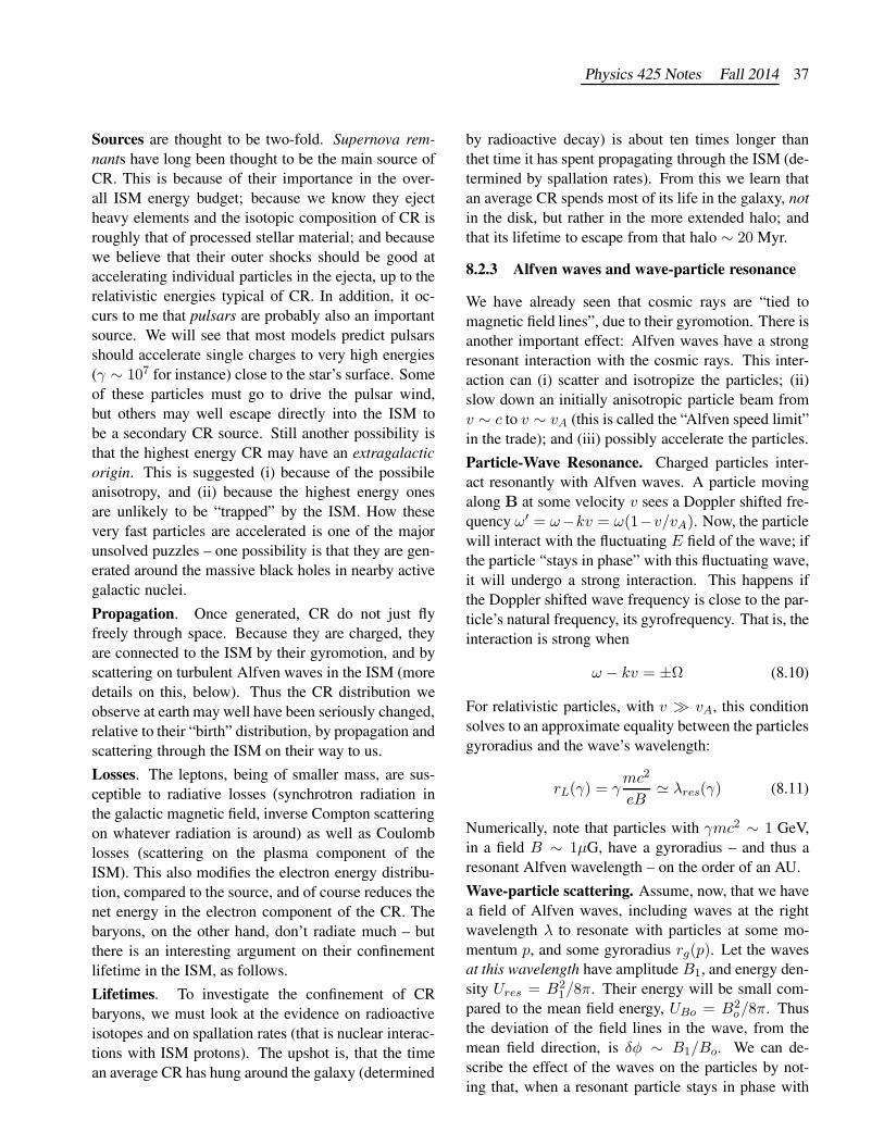
Physics 425 Notes Fall 2014 37
Sources are thought to be two-fold. Supernova rem-
nants have long been thought to be the main source of
CR. This is because of their importance in the over-
all ISM energy budget; because we know they eject
heavy elements and the isotopic composition of CR is
roughly that of processed stellar material; and because
we believe that their outer shocks should be good at
accelerating individual particles in the ejecta, up to the
relativistic energies typical of CR. In addition, it oc-
curs to me that pulsars are probably also an important
source. We will see that most models predict pulsars
should accelerate single charges to very high energies
(γ ∼ 107 for instance) close to the star’s surface. Some
of these particles must go to drive the pulsar wind,
but others may well escape directly into the ISM to
be a secondary CR source. Still another possibility is
that the highest energy CR may have an extragalactic
origin. This is suggested (i) because of the possibile
anisotropy, and (ii) because the highest energy ones
are unlikely to be “trapped” by the ISM. How these
very fast particles are accelerated is one of the major
unsolved puzzles – one possibility is that they are gen-
erated around the massive black holes in nearby active
galactic nuclei.
Propagation. Once generated, CR do not just fly
freely through space. Because they are charged, they
are connected to the ISM by their gyromotion, and by
scattering on turbulent Alfven waves in the ISM (more
details on this, below). Thus the CR distribution we
observe at earth may well have been seriously changed,
relative to their “birth” distribution, by propagation and
scattering through the ISM on their way to us.
Losses. The leptons, being of smaller mass, are sus-
ceptible to radiative losses (synchrotron radiation in
the galactic magnetic field, inverse Compton scattering
on whatever radiation is around) as well as Coulomb
losses (scattering on the plasma component of the
ISM). This also modifies the electron energy distribu-
tion, compared to the source, and of course reduces the
net energy in the electron component of the CR. The
baryons, on the other hand, don’t radiate much – but
there is an interesting argument on their confinement
lifetime in the ISM, as follows.
Lifetimes. To investigate the confinement of CR
baryons, we must look at the evidence on radioactive
isotopes and on spallation rates (that is nuclear interac-
tions with ISM protons). The upshot is, that the time
an average CR has hung around the galaxy (determined
by radioactive decay) is about ten times longer than
thet time it has spent propagating through the ISM (de-
termined by spallation rates). From this we learn that
an average CR spends most of its life in the galaxy, not
in the disk, but rather in the more extended halo; and
that its lifetime to escape from that halo ∼ 20 Myr.
8.2.3 Alfven waves and wave-particle resonance
We have already seen that cosmic rays are “tied to
magnetic field lines”, due to their gyromotion. There is
another important effect: Alfven waves have a strong
resonant interaction with the cosmic rays. This inter-
action can (i) scatter and isotropize the particles; (ii)
slow down an initially anisotropic particle beam from
v ∼ c to v ∼ vA (this is called the “Alfven speed limit”
in the trade); and (iii) possibly accelerate the particles.
Particle-Wave Resonance. Charged particles inter-
act resonantly with Alfven waves. A particle moving
along B at some velocity v sees a Doppler shifted fre-
quency ω′ = ω−kv = ω(1−v/vA). Now, the particle
will interact with the fluctuating E field of the wave; if
the particle “stays in phase” with this fluctuating wave,
it will undergo a strong interaction. This happens if
the Doppler shifted wave frequency is close to the par-
ticle’s natural frequency, its gyrofrequency. That is, the
interaction is strong when
ω − kv = ±Ω (8.10)
For relativistic particles, with v ≫ vA, this condition
solves to an approximate equality between the particles
gyroradius and the wave’s wavelength:
rL(γ) = γmc2
eB≃ λres(γ) (8.11)
Numerically, note that particles with γmc2 ∼ 1 GeV,
in a field B ∼ 1µG, have a gyroradius – and thus a
resonant Alfven wavelength – on the order of an AU.
Wave-particle scattering. Assume, now, that we have
a field of Alfven waves, including waves at the right
wavelength λ to resonate with particles at some mo-
mentum p, and some gyroradius rg(p). Let the waves
at this wavelength have amplitude B1, and energy den-
sity Ures = B21/8π. Their energy will be small com-
pared to the mean field energy, UBo = B2o/8π. Thus
the deviation of the field lines in the wave, from the
mean field direction, is δφ ∼ B1/Bo. We can de-
scribe the effect of the waves on the particles by not-
ing that, when a resonant particle stays in phase with

38 Physics 425 Notes Fall 2014
a wave over one wave period, its pitch angle will have
changed by ∼ δφ compared to its initial pitch angle.
However, this is a random process; after N encounters
with Alfven waves, the particle’s net change in pitch
angle is φ =√Nδφ. Thus, the waves act as scattering
centers. We can define a scattering mean free path as
the distance over which a particle’s pitch angle changes
by φ ∼ 1 rad:
λmfp = Nλ ≃(
Bo
B1
)2
rg =UBo
Uresrg (8.12)
Thus: if we know the energy density of resonant
waves, we can find the mean free path, and thus the
collision time, for the particles to scatter on the waves.
This is the mechanism by which relativistic particles
are tied to the galactic system; and it is probably im-
portant in the acceleration of the particles to these high
energies.
Wave growth. When Alfven waves exist at the right
λres(γ), then, particles with energies satisfying (8.11)
will be strongly tied to the background plasma. We
should note that there are a couple of ways in which
Alfven waves can be generated. First, as mentioned
above, any disturbance to the background plasma will
generate Alfven and sound waves. Wave sources could
include stellar winds, cloud motions, novae and su-
pernovae, stellar random velocities, etc. In addition,
it turns out that the resonant particles themselves can
generate the waves. It turns out that particles with (i) an
anisotropic velocity distribution, such as in a directed
beam, and (ii) streaming speed v ≫ vA will generate
Alfven waves,2 at wavelengths given by (8.11). These
self-generated waves will then scatter and isotropize
the particles, reducing their streaming speed to ∼ vA.
Energy limits for wave-particle interaction. What
are the limits on particle energies that can be scat-
tered and accelerated by Alfven waves? The upper
limit is given by the maximum wavelength that can
exist in the system; this can’t be larger, clearly, than
the scale size of the system. For the lower limit, it
turns out that Alfven waves can only exist for frequen-
cies ω < Ωp = eB/mpc, the subrelativistic proton
gyrofrequency. (At higher frequencies, the proton re-
sponse complicates the wave behavior, and the wave
2Think back to chapter 7 and the two-stream (beam) instabil-
ity, in which a plasma “beam” trying to penetrate another plasma
generates turbulent plasma waves. The detailed physics is different
here and there, but the general picture is the same – a beam/plasma
system and a resonant interaction.
changes nature). Thus, there is a maximum wavenum-
ber kmax = Ωp/vA, and a minimum resonant wave-
length, λmin = 2π/kmax, which can exist for Alfven
waves. From (8.10), we see that there is a minimum
particle energy which can “see” Alfven waves. When
one works out the details of the algebra, it turns out for
protons,
γmin,p = 1 +2v2Ac2µ2
(8.13)
where µ is the cosine of the particle’s pitch angle. For
electrons, the equation is best solved in limiting cases.
In a high-density plasma, with v2A ≪(
m2e/m
2p
)
c2µ2,
the minimum electron energy that satisfies (8.7) is
γmin,e = 1 +v2Ac2µ2
mp
me(8.14)
In the opposite limit, for a low-density plasma, the
minimum energy for resonance becomes
γmin,e =mp
me
vAcµ
(8.15)
Thus, the acceleration of low energy (say, thermal)
particles by any mechanism that depends on resonant
Alfven waves is quite different for electrons and pro-
tons. A significant number of thermal protons can res-
onate with Alfven waves, and can (in principle) be
accelerated by them. But thermal electrons have less
chance of acceleration; in a low density plasma, espe-
cially, they must already have γ ≫ 1 to resonate with
the waves.
8.3 Magnetic Buoyancy
Magnetic fields can affect buoyant behavior in vari-
ous ways. Several situations are possible, involving
simple buoyant bubbles, or buoyant flux tubes. Appli-
cations range from solar prominances, to the gaseous
halo of our galaxy, to the structure of some radio galax-
ies. You’ve already worked with the buoyant rise speed
(in previous homework). Here we need to think about
whether or not an equilibrium (such as a hydrostatic at-
mosphere, or the galactic disk) is buoyantly unstable.
8.3.1 Convective stability (unmagnetized)
To set the stage, we first need to look at the problem
without magnetic effects. Following Shore3, let’s think
about a duck.
3An Introduction to Astrophysical Hydrodynamics (Academic
Press) 1992, ch. 9.

Physics 425 Notes Fall 2014 39
Picture a duck sitting calmly on a pond. . . If we say
that the bird is buoyant, we mean that if we depress
him a bit by pushing from above, he will bob back to
the surface and, ignoring his agitation, bounce up and
down for awhile. This is called neutral buoyancy. If,
on the other hand, our duck is not well preened and
therefore is not waterproof, and we push down on him,
he may sink. Now, think of a blob which is hotter than
its surroundings. It will begin to rise, since we already
know that its density will be lower than that of the sur-
rounding medium, and it will thus be buoyant. If it re-
mains underdense, it will continue to rise – we call this
an instability. It will continue to rise until it reaches
a level at which it is neutrally buoyant again. On the
other hand, if the blob is pushed down, and if it remains
overdense, it will sink until it reaches a point at which
the density again allows for stable balance.
Now, move on to a more relevant example, namely an
unmagnetized, hydrostatic atmosphere. Think about a
blob (“parcel”) in this atmosphere: assume it starts at
some vertical position z, with density and pressure in
balance with its surroundings (as in Figure 3). Thus:
it starts at ρin = ρout = ρ1 and Tin = Tout = T1.
Now, raise it some distance dz, and assume it evolves
adiabatically. Thus, it reaches a new density and tem-
perature,
ρ∗in = ρ1 +
(
dρ
dz
)
ad
; T ∗in = T1 +
(
dT
dz
)
ad
(8.16)
The surroundings, however, are not necessarily adia-
batic: they have some other dT/dz and dρ/dz val-
ues (specified by the situation – for instance the heat-
ing/cooling balance for the outer layers of a star).
But now: the blob will be unstable if, when it has
risen this δz, it is at a lower density than the sur-
rounding atmosphere – in that case it will keep ris-
ing. Thus, our condition for instability is just a con-
dition on the external density and temperature gradi-
ents. Therefore, the atmosphere is buoyantly unstable
if (dρ/dz)ad < (dρ/dz)atm . Because we usually con-
sider situations with dρ/dz < 0, for instance a hydro-
static atmosphere, the condition for instabilty is often
written in terms of absolute values:
∣
∣
∣
∣
dρ
dz
∣
∣
∣
∣
ad
>
∣
∣
∣
∣
dρ
dz
∣
∣
∣
∣
atm
:
∣
∣
∣
∣
dT
dz
∣
∣
∣
∣
ad
<
∣
∣
∣
∣
dT
dz
∣
∣
∣
∣
atm
(8.17)
Thus: if the outside (atmospheric) temperature
changes too rapidly with altitude, the atmosphere is
g
n
n
in
in
*
dz
n
on (z+dz), T (z+dz)o
o(z), T (z)
o
Figure 8.3 Setting the stage for the buoyant (in)stability.
A blob starts at height z, in a local gravitational field g.
The blob is initially at the same pressure and density as its
surroundings: nin = no, Tin = To. It rises slowly, staying
in pressure balance with outside; it expands adiabatically as
it rises, going to some n∗
in. The question is, how does its
new density compare to the density outside?
convectively unstable. An underdense blob will con-
tinue to rise, and an overdense blob will sink.
8.3.2 Bouyant instability, magnetized
How will a B field change things? To think about it,
let’s replace our blob with a more realistic geometry,
such as a flux tube rising from the surface of the sun
(as in Figure 4). We will find another condition is nec-
essary for instability (in addition to the structure of the
surrounding atmosphere). In this geometry, instabil-
ity requires overcoming magnetic tension (holding the
ends of the flux rope down) as well as simple convec-
tive instability. To see this, consider an isolated flux
tube, such as might give rise to a sunspot. Let the ex-
ternal gas have a density scale height H = kBT/mg(refer back to earlier work for hydrostatic equilibrium
with no magnetic field). If the magnetic field is con-
fined in the flux tube, (no B field outside), and the
intial state is in pressure balance, we can again write
internal-external pressure balance as pi+B2/8π = pe.
Assuming the gas inside is at the same temperature, it
must be at lower density than the outside. Thus leads
to a buoyancy force, as you found before:
Fbuoy = g (ρe − ρi) = g∆ρ =B2
8πH(8.18)
Say, now, that the flux tube is bent upwards, locally,
with a radius of curvature R. If R is short, magnetic
tension will pull the tube back towards its initial posi-
tion, giving a stable system. If, however, R is long, the

40 Physics 425 Notes Fall 2014
Figure 8.4 The geometry of a sub-surface flux tube before
it erupts from the sun due to buoyancy, and its possible post-
eruption state; from Tajima &Shibata figure 3.17.
buoyancy force will overcome the tension, leading to
instability. Comparing these two forces, we find insta-
bility occurs if
g∆ρ >B2
4πR(8.19)
and thus the flux rope is unstable if R > 2H .
8.3.3 Parker instability
Now, let’s apply this to a different geometry, a 1D pla-
nar system (such as the ISM in the galaxy). In this
context magnetic buoyancy is referred to as the Parker
instability. Let the magnetic field be horizontal, and
fully mixed with the gas. Picking z as the vertical
direction, that means we take B = By(z)y; and de-
scribe the gas by density ρ(z), pressure and sound
speed p(z) = c2sρ(z), and gravitational field g.
We need a model for the unperturbed state. The sim-
plest assumption we can make is that the ratio of
gas to magnetic pressure is constant at all altitudes:
B2/8πp = αo = constant. Magnetostatic balance,
then, can be written
(1 + αo)dp
dz= − p
c2sg (8.20)
This again gives us a simple exponential atmosphere.
The difference here is that the scale height involves the
magnetic as well as thermal pressures:
p
po=
ρ
ρo=
B2
B2o
= e−z/Λ (8.21)
where Λ =(
c2s + v2A/2)
/g is the new scale height.
(Check: yes this is larger than the unmagnetized H –
which makes sense, due to the extra pressure suport of
the magnetic field).
Now, consider a small perturbation: let a horizontal
layer (or flux tube) be raised some small ∆z. The
plasma in this layer can flow freely along the field
lines – thus it will “slide down to the bottom”, leav-
ing the top part of the perturbation at a lower density
than its surroundings. If the perturbation has horizontal
scale λ, simple geometry gives us its radius of curva-
ture: r ≃ λ2/8∆z. To check the stability of this per-
turbation, we again compare the buoyant forces to the
restoring force, magnetic tension. Let “o” refer to the
altitude of the undisturbed sheet. The density in the gas
at the top of the perturbation does not know about the
B field, because the gas can slide down along the field
lines. So if the perturbation is taken slowly, to reach
a new quasi-hydrostsatic balance “inside”, the density
inside is
ρi(∆z) ≃ ρoe−∆Z/H ≃ ρo
(
1− ∆z
H
)
(8.22)
The external density does know about magnetic pres-
sure, however:
ρe(∆z) ≃ ρoe−∆Z/Λ ≃ ρo
(
1− ∆z
Λ
)
(8.23)
Thus, the difference between the two scale heights
drives the instability in this case. If we again compare
buoyancy to the restoring force of magnetic tension,
we find the instability condition for this case:
λ2 >16Λ2αo
(1 + αo)2 (8.24)
where αo is still the ratio of gas to magnetic pressure.
Key points
• Alfven waves, magnetosonic waves; what they are,
how they work (reprise);
• Cosmic rays – basic picture, in the galactic setting;
• Resonant interaction between CR and Alfven waves;
• Buoyant instability, non-magnetized;
• Magnetic buoyancy, Parker instability.

Physics 425 Notes Fall 2014 41
9 Magnetic Topology: Dynamos and Recon-
nection
Magnetic flux freezing is a very good approximation in
most astrophysical environments (and is a very handy
tool). When flux freezing holds, the topology of the
magnetic field lines remains constant.1 We know, how-
ever, that flux freezing can be violated on small scales,
where resitivity becomes important (such as a thin cur-
rent sheet). It follows that the topology of the field is
no longer invariant – the field lines can “break and re-
connect” (well, sort of) in resistive regions.
There are two particularly important applications of re-
sistive MHD: magnetic reconnection and dynamo the-
ory.
9.1 Magnetic Reconnection
In these notes I’m emphasizing the details of simple,
2D reconnection. For context, note that reconnection
provides one method of heating a magnetized plasma.
I just argued that magnetic topology must be preserved
in the absence of resistivity. But is the converse obvi-
ous? To illustrate how resistivity can “break” and “re-
connect” field lines, think about the geometry in Figure
9.1. We know resistivity is important in regions of high
current density - such as the central region (around
OP). If we set up this geometry and waited awhile, the
central magnetic field would decay as the current layer
supporting them is dissipated. This would deplete the
magnetic pressure in this region. The plasma above
and below this region would be pushed inwards by its
own pressure, bringing a in a fresh supply of field (and
plasma).
Now, look at this in more detail (I’m following Choud-
huri’s discussion here). The field lines ABCD and
A’B’C’D’ move inwards, with velocity vin. Eventu-
ally the BC and B’C’ parts of the field lines decay
away. The AB part of the field line is moved to EO,
and the A’B’ part of that field line is moved to E’O.
Thus, these “fragments” of two original field lines now
make up one new field line, EOE’. And similarly, the
parts CD and C’D’ eventually make up a new field line,
FPF’. Thus, “cutting and pasting” of field lines (other-
wise known as reconnection) takes place in the cen-
1Why is this? You can think about the field lines as being tied to
the fluid; they move and stretch as the fluid moves, but cannot cross
each other (how could they do that without “untying” themselved
from the flow?)
tral region. And, of course, there must be plasma flow
away from the region – sideways in this cartoon – to
conserve mass.
i
A
B C
D
E
E’
F
F’
A’
B’ C’
D’
O P VVoo
Vi
V
Figure 9.1 Illustrating a sinple reconneciton geometry;
see text for discussion. Following Choudhuri figure 15.2.
We can be more quantitative about this geometry, and
find simple scaling laws to describe this situation. The
model I’m describing here is Sweet-Parker reconnec-
tion — it’s illustrated in Figure 9.2.
E
E
v
v
v
B
B
v
Figure 9.2 Geometry of Sweet-Parker reconnection. The
current sheet (grey shaded area) has thickness l and lateral
extent L The input velocity is vin and the output velocity is
vout. Quantities far away from the current sheet are labelled
with subscript o. Following Cowley figure 5.5.
First, assume the flow is incompressible – that it stays
at constant density (which turns out to be a good ap-
proximation if vin and vout are both subsonic. Mass
conservation then requires
vinL = voutl (9.1)
Next, consider force balances. In the vertical direction,
we note that B → 0 at the center of the current sheet,
and that p → pmax there (its maximum value). Pres-
sure balance in this direction therefore requires
B2o
8π≃ pmax − po (9.2)

42 Physics 425 Notes Fall 2014
Along and within the current sheet (call that the y di-
rection), there is no v × B force, so only the pressure
gradient accelerates the flow. We have then,
ρvy∂vy∂y
≃ −∂p
∂y; ρ
v2out2
≃ pmax − po (9.3)
Thus, the outflow speed must be
v2out ≃ v2A =B2
o
4πρ(9.4)
Now, what about the inflow speed vin? Clearly, by
mass conservation, it must be vout ≃ vinL/l; but what
sets l? We can try two different arguments here.
1. First, go back to the induction equation (5.11). In a
steady state, it is ∇ × (v × B) + η∇2B = 0, which
gives (by dimensional/scaling analysis)n
vinB
l≃ ηB
l2; vin ≃ η
l(9.5)
This tells us that we can keep the diffusion region
steady if the rate at which flux is brought in is equal
to the rate at which it is annihilated.
2. Alternatively, note that there must be an E field “out
of the page”, as shown in figure 9.2, to maintain the
current sheet. From Maxwell, we get
j = σE ; ∇×B =4π
cj ⇔ B
l≃ 4π
cσE (9.6)
where σ is the electrical conductivity. But now, the
incoming plasma charges must E × B drift2 into the
region: thus
vin = cE
B≃ c2
4πσ
1
l=
η
l(9.7)
(in that last step I’ve used the definition of the magnetic
resistivitiy, η = c2/4πσ, from chapter 5). And look:
this agrees with (9.5)!
OK: now, combine our answer (9.5 or 9.7) with (9.1),
and we get our result, the inflow velocity and thickness
of the dissipation layer:
v2in ≃ vAη
L; l2 ≃ ηL
vA(9.8)
This gives us, finally, the spontaneous reconnection
rate; the rate of slow inflow that allows things to go
steadily. This is indeed slow – in many situations
2Check back in Chapter 2: vE = c(E×B)/B2, from (2.17).
(for instance solar flares), the plasma conductivity is
high (given by the Coulomb collision value), so that
η is low; and the reconnection timescale (≃ L/vin) is
much to long to explain the observations. People have,
therfore, spent a lot of time trying to invent faster ver-
sions of this model. Some are as follows ..
• Petschek reconnection has gotten a lot of attention
in the literature. The idea was that internal structures in
the flow (shocks toward the edges of the current sheet)
would affect the velocity field and narrow the width of
the sheet, to L ∼ l. This would of course make the
inflow rate nearly independent of η. The last I heard
is that lab experiements (cf.review by Kulsrud, 1998)
were not confirming this model.
• Compressible flow. Another suggestion is that the
plasma in the dissipation region (DR) is compressed.
If this is the case, then (9.1) is replaced by vinρoL ≃voutρDRvout. This will increase vin relative to vout –
its a plausible idea, but I’m not aware of any lab tests
yet.
• Anomalous diffusion. This is my personal favorite,
and is a good example of how plasma microphysics can
be important in macroscopic situations. That is: is the
usual value of η, based on Coulomb collisions in the
plasma, the right value? The answer is almost surely
that it is not. If the current density is high enough, we
have a “two-stream”-like situation in the current sheet,
and can expect plasma turbulence to be generated.
But can this be quantified? One commonly used es-
timate is as follows. Recall the microscopic origin of
plasma conductivity, from chapter 3:
σ =j
E=≃ ne2
mτcoll
But now, what is τcoll when we’re working with plasma
turbulence? A common guesstimate, which is thought
to be an upper limit to the resistivity (lower limit to
τcoll) is to set τcoll = 2π/ωp, if ωp =(
4πne2/m)1/2
is the usual plasma frequency. This gives an estimate
of the anomalous resistivity.
9.2 Reconnection: other approaches
Reconnection is a very active field these days; the sim-
ple 2D models we’ve just seen are probably way too
simple. I’ll just store a few comments here, thinking
about what interests me most.

Physics 425 Notes Fall 2014 43
9.2.1 Non-steady reconnection
Here is my personal impression: who says steady-state
reconnection is relevant to any natural situation? That
is: the arguments above show that steady reconnection
models must be forced, sometimes rather severely, to
connect with what we think is occuring in nature. But
examples of non-steady reconnection events are easy
to find:
• Reconnection in solar flares. Flares are seriously
transient events; the large amount of energy released is
believed to be due to very fast annihilation of magnetic
field, in a reconnection event. Flares have motivated
much of the work on steady-state models; however as
an outsider I suspect time-dependent, patchy, localized
reconnection must be taking place.
• Reconnection at the magnetopause, where the solar
wind hits the earth’s magnetic field. Spacecraft obser-
vations suggest this is very patchy, localized and time-
dependent. Picture, for instance, magnetic flux tubes
being carried along in the solar wind; and let one of
them impact the magnetopause, which also has its field
bunched into ropes. This process can allow solar wind
plasma, and field, to penetrate into the magnetosphere.
9.2.2 Driven reconnection
It’s worth remembering that the 2D models above are
all “spontaneous”: put two misaligned B fields to-
gether and wait to see how quickly they reconnect. But
nature does not always work this way. One can envi-
sion a situation in which the two anti-parallel magnetic
structures are driven together, by large-scale flows in
the system (one example of this is MHD turbulence,
in which different parts of the plasma move in random
directions, at a speed set by the energetics of the turbu-
lence). In this case one (this one at least) expects that
the inflow speed (vin) in our notation above) will be set
by the large-scale flow (say the turbulent speed). How
can the reconnection site adjust to this? Some authors
(e.g. Parker) suggest that the internal structure of the
reconnection layer – its thickness, density or resistivity
(set by microscale turbulence therein) – will adjust as
necessary.
9.2.3 Three-dimensional reconnection
Another observation: only rarely can a reconnection
event be well described by a two-dimensional analy-
sis. My last example in fact assumed this – because
the intersection of two magnetic flux ropes is clearly
a three-dimensional process. Going to 3D is challeng-
ing, and work is only starting here (helped significantly
by numerical simulations).
9.3 MHD Dynamos
Where do magnetic fields come from? In the lab, the
answer is easy: “currents”. In magnetic solids, the cur-
rents are those of well-ordered electrons spins in ferro-
magnetism. More typically, currents in the lab — and
their consequent B fields — come from obvious things
like batteries and wires. The issue is then, what drives
the currents? My dictionary defines a dynamo as
“a device for converting mechanical energy
into electrical energy, usually by expending
the mechanical energy in producing a peri-
odic motion of a conductor and a surround-
ing magnetic field”.
A simple lab version of this is called the unipolar dy-
namo, in Figure 9.3. This involves a conducting disk,
threaded by a B field, which rotates about its axis. This
induces a radial E field, v ×B/c, and thus a potential
drop between the axis and the edge of the disk. If you
hook up wires in the right way you’ll have a current –
and this current will create its own magnetic field.
Figure 9.3 A simple unipolar dynamo (in a less than sim-
ple figure from www.stardrivedevice.com, the best figure I
could find). The conducting disk moves through an (exter-
nally supported) B field as it rotates about its axis. The re-
sultant EMF supports a potential drop between the axis and
edge of the disk — which can drive a current.
What about astrophysical magnetic fields? To be spe-
cific, what is the origin of the earth’s field, or the sun’s
field? It’s easy to think of what doesn’t work. One,
even solid planets like the earth can’t be ferromag-
netic (because the core temperature is well above the
Curie temperature at which permanent magnetism dis-
appears); and clearly stars and galaxies can’t be fer-
romagnetic at all. Two, we can’t assume the fields
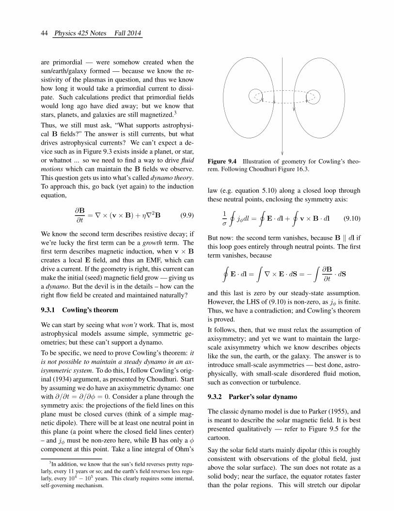
44 Physics 425 Notes Fall 2014
are primordial — were somehow created when the
sun/earth/galaxy formed — because we know the re-
sistivity of the plasmas in question, and thus we know
how long it would take a primordial current to dissi-
pate. Such calculations predict that primordial fields
would long ago have died away; but we know that
stars, planets, and galaxies are still magnetized.3
Thus, we still must ask, “What supports astrophysi-
cal B fields?” The answer is still currents, but what
drives astrophysical currents? We can’t expect a de-
vice such as in Figure 9.3 exists inside a planet, or star,
or whatnot ... so we need to find a way to drive fluid
motions which can maintain the B fields we observe.
This question gets us into what’s called dynamo theory.
To approach this, go back (yet again) to the induction
equation,
∂B
∂t= ∇× (v ×B) + η∇2B (9.9)
We know the second term describes resistive decay; if
we’re lucky the first term can be a growth term. The
first term describes magnetic induction, when v × B
creates a local E field, and thus an EMF, which can
drive a current. If the geometry is right, this current can
make the initial (seed) magnetic field grow — giving us
a dynamo. But the devil is in the details – how can the
right flow field be created and maintained naturally?
9.3.1 Cowling’s theorem
We can start by seeing what won’t work. That is, most
astrophysical models assume simple, symmetric ge-
ometries; but these can’t support a dynamo.
To be specific, we need to prove Cowling’s theorem: it
is not possible to maintain a steady dynamo in an ax-
isymmetric system. To do this, I follow Cowling’s orig-
inal (1934) argument, as presented by Choudhuri. Start
by assuming we do have an axisymmetric dynamo: one
with ∂/∂t = ∂/∂φ = 0. Consider a plane through the
symmetry axis: the projections of the field lines on this
plane must be closed curves (think of a simple mag-
netic dipole). There will be at least one neutral point in
this plane (a point where the closed field lines center)
– and jφ must be non-zero here, while B has only a φcomponent at this point. Take a line integral of Ohm’s
3In addition, we know that the sun’s field reverses pretty regu-
larly, every 11 years or so; and the earth’s field reverses less regu-
larly, every 104 − 105 years. This clearly requires some internal,
self-governing mechanism.
Figure 9.4 Illustration of geometry for Cowling’s theo-
rem. Following Choudhuri Figure 16.3.
law (e.g. equation 5.10) along a closed loop through
these neutral points, enclosing the symmetry axis:
1
σ
∮
jφdl =
∮
E · dl+∮
v×B · dl (9.10)
But now: the second term vanishes, because B ‖ dl if
this loop goes entirely through neutral points. The first
term vanishes, because
∮
E · dl =∫
∇×E · dS = −∫
∂B
∂t· dS
and this last is zero by our steady-state assumption.
However, the LHS of (9.10) is non-zero, as jφ is finite.
Thus, we have a contradiction; and Cowling’s theorem
is proved.
It follows, then, that we must relax the assumption of
axisymmetry; and yet we want to maintain the large-
scale axisymmetry which we know describes objects
like the sun, the earth, or the galaxy. The answer is to
introduce small-scale asymmetries — best done, astro-
physically, with small-scale disordered fluid motion,
such as convection or turbulence.
9.3.2 Parker’s solar dynamo
The classic dynamo model is due to Parker (1955), and
is meant to describe the solar magnetic field. It is best
presented qualitatively — refer to Figure 9.5 for the
cartoon.
Say the solar field starts mainly dipolar (this is roughly
consistent with observations of the global field, just
above the solar surface). The sun does not rotate as a
solid body; near the surface, the equator rotates faster
than the polar regions. This will stretch our dipolar

Physics 425 Notes Fall 2014 45
(b) (c)(a)
Figure 9.5 Parker’s model of the solar dynamo, at the
cartoon level. (a) Differential rotation (the sun’s equator ro-
tates faster than the poles) stretches initially dipolar field
in the toroidal direction. (b) Coriolis forces acting on sur-
face convective cells generates local poloidal fields. (c) The
opposite sense of the Coriolis force in the north and south
hemispheres, combined with the opposite sense of the ini-
tially toroidal field, results in a strong net poloidal field,
rather than a randomly directed set of field loops. (These
loops are shown projected in the meridional plane.) Follow-
ing Choudhuri, Figures 16.4.
field, generating toroidal components. Thus, it is no
problem to generate toroidal field if the body has dif-
ferential rotation. But this cannot be all of the story.
Such a stretched toroidal field will have many local
field-line reversals, and if nothing else happens it will
simply decay away due to resistive dissipation.
However, the upper layers of the sun are convectively
unstable. In this region, plasma blobs rise and fall.4
Now, these vertically moving blobs are subject to a
Coriolis force, due to the sun’s overall rotation. The
blobs therefore rotate as they rise; they act like little
cyclones, and formally we say that their their motion
has a net helicity (that means the small-scale motions
do not have mirror symmetry: for instance a flow with
v · (∇ × v) 6= 0 is helical). Look at (b) of Fig-
ure 9.5: this cyclonic motion twists the magnetic field
back into poloidal loops. Remember that both the di-
rection of Bφ and of the Coriolis rotation are opposite
in the north and south hemispheres: this means the di-
rection of the poloidal field component generated is the
same in the two hemispheres. We therefore have a fully
working dynamo: poloidal fields are generated by the
helical convective (turbulent) motions, while toroidal
fields are generated by differential rotation. The whole
system must be stabilized by dissipation – that is resis-
tivity will keep each field component from getting too
large.
4In chapter 8 we talked about (in)stability to buoyancy – an
unstable atmosphere will develop strong convection.
9.3.3 Scale separation and turbulent dynamos
We argued “by cartoon” that helical, convective mo-
tions on the sun (or the earth) can maintain the large-
scale B field. That is, we’re arguing that small-scale
turbulent motions can add up to a net large-scale dy-
namo.
To get a sense of how this works, and what’s needed
to make it work, we need to be a bit formal. Split the
velocity and magnetic fields into mean and fluctuating
parts:
B = B+ b ; v = V + v (9.11)
where we’re assuming that b and v have zero mean,,
and also that they are small-scale – that they vary over
much smaller spatial scales than V and B do. What ef-
fect do they have on the induction equation (5.11, also
9.9)? Let’s split it into large-scale (mean) and small-
scale (fluctuating) parts. For the mean field, we get
∂B
∂t= ∇× (V ×B)−∇× εεε+ η∇2B (9.12)
where the important new term is
εεε = −〈v × b〉 (9.13)
This describes the net EMF due to the fluctuating v
and b.
But now, we must ask whether εεε has any interesting
large-scale effect. If v and b are rapidly varying, have
zero mean, and uncorrelated, we’d expect the mean of
their product to be zero. It turns out (“can be shown”)
that things are interesting (non-zero) if the turbulence
satisfies two conditions: (i) it must be helical, satisfy-
ing v ·∇×b 6= 0; and (ii) it must be resistive; η 6= 0. If
both of these conditions are met, the turbulent EMF, εεε,
will be non-zero on large scales. In particular, it may
be the case that 〈v × b〉 = αB (i.e., that εεε has a com-
ponent along B). If this is so, then we have an effective
dynamo term:
∂B
∂t= ∇× (αB) + (other stuff) (9.14)
If this works – if εεε = αB — then we can see two
useful astrophysical consequences. One is balancing
ohmic losses, as in the sun or the earth — and (in prin-
ciple) accounting for the occasional field reversals in
each body. The second is “growing” the B field in
the first place. To see this, note that (9.14) allows

46 Physics 425 Notes Fall 2014
solutions B ∝ eαt, if α is constant in time. That’s
a growing B field, with growth time ∼ L/α (some
large-scale length scale L). We might expect that a
small seed field would grow exponentially until some
other physics (dissipation? back reaction on the driv-
ing fluid?) comes into play.
9.3.4 Astrophysical dynamos in the lab
Finally, a few words about trying to do this in the lab.
Everything above is still pure theory — it would be
good to verify directly that an αω dynamo (rotation
plus turbulence, as in the sun), or an α2 dynamo (pure
turbulence) can really make a large-scale ordered B
field. Several groups are working on this, including
NMT’s very own Stirling Colgate. The experiments
use liquid metal — usually liquid sodium — in some
sort of rotating system (the ω in an αω dynamo), and
try various ways to induce turbulence (the α) in the
flow. The last I heard, no one had sucessfully made
their dynamo work — but I think the field’s progress-
ing. Check the Feb 2006 issue of Physics Today if
you’d like more details.
Key points
• Reconnection – simple 2D model; “what is a recon-
nection rate?”
• Reconnection – extensions of the 2D model (anoma-
lous effects, non-steady, driven, etc).
• Dynamos – what they are; what they need (helicity).
Parker’s model for the sun.
• Dynamos — why turbulence matters; αω and α2.

Physics 425 Notes Fall 2014 47
10 Accretion in astrophysics I: star formation
We argued in chapter 6 that accretion flows are com-
mon. They are found in many places – from Young
Stellar Objects (YSO’s), to compact objects (black
holes, neutron stars) in galactic binary systems, to
massive black holes in Active Galactic Nuclei (AGN).
They are potentially important to astrophysics in all
settings. In this chapter we’ll look at star formation
and YSO’s, with an eye to the role of accretion in the
process. In the next two chapters we’ll return to “clas-
sical” accretion, as it applies to compact objects and
standard accretion disks.
10.1 Star formation, recall the basics
The ISM is the source of new stars. We think these
new stars form in some gravitational collapse process
. . . and that star formation should be an ongoing pro-
cess, with each subsequent generation of stars having a
somewhat richer heavy element content, due to nuclear
processing by previous generations of stars.
Think back to our general discussion of gravitational
collapse and star formation (chapters 4, 5). We noted
that a piece of the ISM will be gravitationally unstable
if “gravity wins”; that is, if its gravitational potential
energy exceeds its internal energy. Written in terms of
initial density and temperature, this becomes a condi-
tion on the size, or mass, of the perturbation. If the
initial perturbation has R > RJ (the Jeans length), or
M > MJ , (the Jeans mass), where
4π
3GR2
Jρ ≃ kBT
m; MJ ≃
(
kBT
mG
)3/2( 3
4πρ
)1/2
(10.1)
then it is gravitationally unstable.
We also noted, in chapter 5, that two classic prob-
lems – conservation of magnetic flux and of angular
momentum – make the collapse process more compli-
cated than simple “gravity wins”. We suggested that
these two problems are probably interrelated – for in-
stance torques exerted by the B field may contribute
to slowing down the rotation and transferring angular
momentum to the surroundings. Another possibility is
that the collapsing cloud is mostly neutral; because Bfield lines are only tied to the ionized fraction of the
cloud, it may be that the neutral gas can “slip through”
the ionized fraction. This process goes by the fancy
name, “ambipolar diffusion”. Both ideas are probably
part of the truth. The picture still needs to be expanded,
however, and put in the context of star formation re-
search, which is one of the most active areas in current
astrophysics. That’s where we’re going in this chapter.
10.2 Molecular Clouds as Precursors
We know that young stars are gregarious. They do
not form singly; rather, they form in clusters, inside
dense, molecular clouds (MC’s) in the ISM. We there-
fore need to consider the physical state of the MC’s,
and how stars — as well as planets and possibly life —
form within them.
10.2.1 Observational constraints
Most of what we know about MCs comes directly from
observations.
• Physical conditions. MC’s are found in a range of
sizes, from ∼ 102 M⊙ to ∼ 106 M⊙, with an approx-
imate ∝ M−3/2mc number distribution. Interestingly,
there seems to be a correlation between cloud mass,
cloud distribution in the galaxy, and cloud tempera-
ture. There seem to be two populations of MC’s: the
small clouds (SMC’s), which have internal tempera-
tures ∼ 10K, and the “giant” clouds (GMC’s), which
have internal temperatures & 20 K. The SMC temper-
ature is consistent with heating by the background cos-
mic ray population in the galaxy; they do not seem to
have any internal energy sources (such as hot stars).
This correlates with the absence of young, hot (O and
B) stars in these clouds. The SMC population is dis-
tributed throughout the galaxy, with no particular pref-
erence for spiral arms. The GMC’s, on the other hand,
require internal energy sources, and we do observe
young O and B stars forming in these clouds. Their
higher temperature is thought to be due to heating by
these massive protostars. GMC’s are not distributed
uniformly in the galaxy, but are found in spiral arms
(they provide the young, bright stars by which we see
pretty spiral arms in external galaxies).
• Lifetimes. We know that MC’s are self-gravitating:
their pressure generally exceeds the typical ISM pres-
sure, so they cannot be in pressure balance with the
ISM. We also know their mass exceeds the Jeans’ mass
for their temperatures and densitites. We would ex-
pect them to be in a state of gravitational collapse. If
this were the case, we can use the free-fall time (check
back to equation 4.18) to guesstimate how how quickly
they should collapse. We find tff ∼ 107 years for
typical mean MC densities, n ∼ 100cm−3. Com-

48 Physics 425 Notes Fall 2014
bining this with the total mass in MC’s in our galaxy,
∼ 5× 10⁹M⊙, we can estimate the current star forma-
tion rate that this simple picture (free-fall collapse of
all MC’s) would predict: we get a rate ∼ 500 M⊙/yr.
This prediction is much larger than the observed rate,
∼ a few M⊙/yr. Thus, only about one percent of the
clouds we know about can be collapsing; the rest must
be supported by gravity somehow, and have a lifetime
∼ 100 times longer than this prediction.
• Turbulence. This support against gravity almost cer-
tainly is provided by internal random motions in the
clouds, which are generically called “turbulence”. We
can measure internal ∆v’s, from linewidths; we find
∆v ≫ vth ≃ (kBT/m)1/2. Thus, the internal mo-
tions are highly supersonic. Further, the linewidth does
not come from rotation (which could be detected), nor
does is come from free-fall collapse (from the argu-
ment above). Thus, it must be from random inter-
nal motions – the clouds must contain subclumps, or
waves, which move through the “cloud” at supersonic
velocities, vran ∼ ∆v. These random velocities do
appear able to provide the virial support: the correla-
tion ∆v2 ∝ nR2 ∝ Mmc/R is observed, consistent
with virial balance; the numbers also work out, to have
v2ran ≃ GMmc/R.
MC’s are also magnetized. We know this from Zee-
man splitting of spectral lines, also from polarization
of starlight, which comes from dust grain alignment
with the magnetic field (the grains are dielectrics). The
fields can, in principle, also help support the cloud
against collapse. In practice, the fields and turbulence
are probably intimately mixed (gas flows stretch and
twist field lines; the field fights back and limits turbu-
lent velocities). We also know that turbulent (and thus
magnetic) decay times are very likely short compared
to the MC lifetimes. Thus “turbulence” or “B fields”
aren’t the full answer; something inside the cloud must
drive the turbulence. Current thinking has the driver
being newly formed YSOs within the cloud – their
winds and jets may dump enough energy back into the
MC to stabilize it.
10.2.2 How do they fragment?
We know that the Jeams mass in a MC is much larger
than the mass of a single star (even a big one). We also
know that stars form in large numbers within MCs. It
follows that the gravitational collapse process within
the MC must involve fragmentation into a large num-
ber of star-sized structures. We don’t know how this
happens, but can find a couple of hints in the data.
•The Jeans mass depends on temperature and den-
sity, as MJ ∝ T 3/2/ρ1/2. Thus, as a large cloud
collapses, and its density increases, MJ will drop
if the cloud stays cool. This should allow smaller
and smaller subclumps to become unstable, and frag-
ment out of the larger-scale collapse (recalling tff ∝1/ρ1/2, so that denser subclumps fragment faster).
This process should continue as long as the collapsing
cloud can stay cool. People tend to argue that the cloud
will stay cool as long as it stays transparent, and can
radiate effectively. Once it goes opaque (noting that
opacity ∝ ρR ∝ M/R2 for a cloud of fixed mass1),
it may have trouble radiating away the energy gener-
ated by the gravitational collapse. If this happens, Twill increase, and MJ will increase; this will provide a
smallest fragment size. This process is called “opacity-
limited fragmentation”.
• The Initial Mass Function (IMF), which describes
the mass distribution of newly formed stars, can be de-
termined from the mass distribution of stars that are
currently around. If a star has a visible lifetime τ(m)(which is a function of the mass m of the star), and
if stars are created in the galaxy at a rate S(m, t), the
current distribution of stars N(m, t) is given by
dN(m, t)
dt= S(m, t)− N(m, t)
τ(m)(10.2)
If S(m, t) is not varying in time, this has the simple
solution
N(m, t) = S(m)[
1− e−t/τ(m)]
(10.3)
which allows us to relate N(m, t) (which can, in prin-
ciple, be observed) to S(m), the initial mass function
(which we want to know).
In general S(m) is expected to be a decreasing func-
tion of m, giving many low-mass stars and few high-
mass stars. It is determined by the complex inter-
play between fragmentation, coalescence, accretion,
and outflow, so at present it is quite poorly under-
stood but is held to be one of the holy grails of as-
trophysics. From the observational side it seems that
at high masses (m & M⊙), S(m) can be approxi-
mated by a power law. The form S(m) ∝ m−2.35
is called the Salpeter initial mass function, and has
1We’ll see what this means next term

Physics 425 Notes Fall 2014 49
been around for a long time. Below m ∼ M⊙, it gets
harder to determine N(m, t) accurately. It is clear that
S(m) flattens out; whether or not if turns down below
m ∼ 0.1 − 0.3 M⊙ is less clear. In addition, several
people have suggested that the locally measured IMF
being the superposition of two IMF’s, resulting from
two types or modes of star formation. The suggestion
is that low-mass stars (compared to ∼ 1M⊙) form in
one region – probably the SMC’s – and that high-mass
stars (above ∼ 1M⊙) form elsewhere – probably the
GMC’s – and that different physics governs the two
modes. This is called bimodal star formation.
The range of allowed stellar masses is, on the other
hand, fairly well determined by the physics of the
stars themselves. At the high-mass end, stars with
M & 60M⊙ are unstable; their own luminosity gener-
ates too much radiation pressure for the star to be able
to attain hydrostatic equilibrium from its own grav-
ity. At the low-mass end, 0.1 M⊙ is about the lowest
mass object which can sustain hydrogen fusion. Ob-
jects with masses lower than that certainly do exist but
are not called stars. If they can fuse deuterium they’re
called brown dwarfs, and if they are too low mass for
that they’re planets.
10.3 Young Stellar Objects: how do they evolve?
Somehow or other, a star-sized fragment of a MC sep-
arates out and collapses to form the star. Current think-
ing — based on an impressive amount of new data, as
well as theory — identifies four stages of this process2
(as illustrated in Figure 10.1). A caveat: what follows
is thought to describe the formation process for low-
mass stars only.
(1) Initial Contraction and core collapse. When
the protostar first detaches from its MC environment
and starts to collapse, it’s probably still nearly spher-
ical, and collapsing only slowly. Refer back to chap-
ter 4, where we discussed self-gravitating isothermal
spheres. These are characterized by a core of size
ro ∝ (T/ρo)1/2; they are probably a good approxi-
mation to the initial state of the protostar. As the cloud
slowly gets denser (and/or cools), the core gets smaller;
so we expect an inside-out collapse (the core collapses
most rapidly, the outer layers follow later). Much of
2Jargon warning: many authors break YSOs up into Class 0,
Class I, Class II, Class III objects. These Classes correlate decently
with the four phases I list here, but are more observationally based
— so I won’t describe them in detail here.
Figure 10.1 Illustrating the four likely stages of low-mass
star formation; from Shu etal, Ann.Rev.Ast.Ap, 1987. See
text for details. Note, this cartoon needs to be updated, to
include outflows, which we now know are an important part
of the process.
the MC magnetic field must be lost in this stage, possi-
bly by ambipolar diffusion. Note the protostellar core
is well hidden at this stage, being shrouded by its dusty
outer envelope.
(2) Disk formation and outflows. As the inside-out
collapse proceeds, the inner parts settle into what will
become the core of the protostar. Material continues
to accrete from the surroundings, but now — due to
angular momentum — it settles into a disk around the
core. That was expected; but here’s where the surprise
came. People did not expect gravitational collapse also
to involve outflow (it is the wrong direction), but it
does. Observations show that just about every proto-
star has bipolar outflows, which can be quite broad,
not well collimated. They are usually seen in molec-
ular lines. Some YSOs also produce well-collimated
jets, usually seen in the optical. The optically bright
“nebulae” called Herbig-Haro objects, which used to
seem only a curiosity, are now known to be associated
with shocks in these YSO jets.
In addition, some YSO’s are found to have a disk struc-
ture, oriented perpendicular to the jet or bipolar out-
flow. These are presumably the accretion disks —
or at least the rotation-supported outer regions of the
“reservoir” from which material accretes to form the
star. Some authors estimate that ∼ 1/3 of the in-
falling matter goes out again in the outflow/jet, and
∼ 2/3 makes it onto the protostar. Because there is
still a lot of (dusty) reservoir material, YSOs in this
stage are mostly shrouded objects, detectable only in
radio/molecular lines; one author talks about “deeply

50 Physics 425 Notes Fall 2014
buried protostars with their infalling envelopes and as-
sociated bipolar outflows”.
(4) Post-outflow, pre-Main Sequence star. Eventu-
ally, the outflow slows, as does the general infall of
matter. At some point the YSO becomes visible in
optical and IR, as the surrounding dust/gas is cleared
away. When nuclear burning starts, these young stars3
appear on the HR diagram. They still have disks and
outflows; T Tauri stars are examples here (several of
them have detectable disks). Finally, the outflows re-
duce to normal stellar-wind level, and the disk either
is all accreted or (mostly) dissipates. Remnants of
these circumstellar disks, presumably, become plane-
tary systems.
Caveat 1: magnetic activity. It seems that YSOs,
at least in the PMS/T Tauri stage, have unusually
high levels of magnetic activity (think of solar flares,
eruptive prominences, but at a much stronger level).
They can show strong X-ray emission (which requires
plasma much hotter than the conventional picture,
above, would predict), and also nonthermal radio emis-
sion (which requires relativistic electrons and a mag-
netic field). This interesting area is just starting to be
explored ... stay tuned.
Caveat 2: what about high mass stars? High-mass
star formation seems still to be less well understood;
the problem is that the strong radiation pressure af-
ter nuclear burning starts disrupts the inflow/accretion
process ... and people do not seem sure of what hap-
pens at that point. Once again, stay tuned.
Key points
• Basic gravitational (in)stability criteria;
• Isothermal spheres: what they are, what character-
izes the solution;
• Molecular clouds: their general nature, how they re-
late to the YSO’s which they contain;
• YSO’s: what we observe, and what we think their
evolutionary stages are.
3alternatively, pre-main-sequence, “PMS”, star

Physics 425 Notes Fall 2014 51
11 Accretion II: compact objects
Now, let’s get back to accretion onto compact objects
– dense stellar remnants and black holes.
11.1 Basic ideas
Before we talk about specific objects, let’s start with an
overview of important physical ideas.
11.1.1 Energetics (“Accretion Power”)
Recall what we discussed briefly in chapter 6. The
basic idea is that accreting matter liberates its gravi-
tational energy, at a rate Eg ∼ GMM/r, for some
mass accretion rate M and some “conversion radius”
r. Physically, this energy must be converted to internal
energy of the accreting stuff (via friction, for instance)
and the hot matter then radiates with some (as yet un-
specified) efficiency ε:
L = εGMM
r(11.1)
This applies to general accretion flows, be they onto
YSO’s or neutron stars.
Another approach is sometimes used for accretion onto
black holes. Let’s think about the conversion radius
r. The smallest it’s likely to be is some factor times
the “gravitational radius” around a black hole, rg =GM/c2.1 If we scale r in (11.1) to rg, we have
L = εGMM
rg
rgr
= εrgrMc2 (11.2)
Thus, for conversion close to rg, ε measures the output
luminosity as a fraction of the infalling rest mass en-
ergy; this scaling is often used in black hole accretion
models.
What are typical numbers? A typical galactic X-ray
binary might have L ∼ 1037 erg/s; this requires εM ∼3.5 × 10⁻⁷M⊙/yr, for conversion close to rg. Or, a
bright quasar might have L ∼ 1046erg/s; this requires
εM ∼ 0.35M⊙/yr.
11.1.2 Eddington luminosity
This is an important reference point: at what luminos-
ity can the radiation pressure from a central source of
1Think about the event horizon of a black hole, or the smallest
stable circular orbit – both of these are ∝ rg . We’ll return to this
later in this chapter.
luminosity L can offset gravity from a central mass M ,
and stop the flow? For most accretion problems, the
infalling matter is fully ionized hydrogen. That means
we must consider the gravitational force on a proton,
and note that the radiation pressure is communicated
via Thomson (electron-photon) scattering (which has a
cross section σT = 6.65 × 10⁻²⁵cm2).2 With this we
can derive the Eddington luminosity:
Ledd
4πr2σTc
=GMmp
r2⇒ Ledd =
4πGMmpc
σT(11.3)
and numerically, this is Ledd ≃ 1.3 × 1038(M/M⊙)erg/s.
A related quantity is the Eddington mass flux. This is
the mass flow that produces Ledd in a given system.
Defining
Ledd = εGMMedd
r
gives us
Medd =4π
ε
r
rg
GMmp
cσT(11.4)
11.1.3 Thermal state
This is critical to interpreting observations of accretion
systems. While the full story here can be quite com-
plex,3 one useful simple estimate is possible. If the
infalling matter and radiation it generates are in some-
thing close to thermal equilibrium, we know from ba-
sic thermodynamics that it radiates as a black body.
That means the luminosity coming from its surface
has an intensity (energy per time per surface area)
σSBT4, where σSB = 5.67× 10⁻⁵ (cgs) is the Stefan-
Boltzmann constant. We also know that the typical
photon energy hν ∼ kT . Equating the luminosity in
(11.1) to that lost by black body radiation determines
the lowest temperature the gas will reach. You will find
that T ∼ 107 K for accretion onto a solar-sized black
hole (and thus we have galactic X-ray binaries); and
T ∼ 104 − 105 K (and thus we have UV and optical
sources) for accretion onto a massive M ∼ 109 M⊙
black hole (as in a galactic nucleus).
We must remember, however, that the situation in an
accretion flow is rarely that simple. One complication
2Other physical states for the accreting matter call for other
values of σ and m.3We would need to know how rapidly the plasma is heated by
friction, turbulence, magnetic dissipation, etc; and how effectively
it can lose energy by radiation – which depends on all sorts of
details about the plasma density, temperature, etc..

52 Physics 425 Notes Fall 2014
is that the radiation emitted by the infalling matter may
well not be in thermal equilibrium with the matter; that
will be the case if the flow is transparent to the radia-
tion, meaning that the mean free path for a photon to
be absorbed or scattered is large compared to the size
of the system. Just how the radiation comes out will
be a major topic for next term. For now, I’ll just note
that the inflowing plasma will be hotter, and transpar-
ent (parts of) accretion flows can reach temperatures
∼ 108 − 1010 K. Another complication is that some of
the accretion energy does not simply to go heating, but
(somehow) goes to accelerating a few particles to rela-
tivistic energies. We know this because we know that
many accretion sources are “nonthermal”, with signifi-
cant emission by these relativistic particles due to their
gyromotion in the local magnetic field.
11.1.4 The transtion to disk accretion
We’ve worked so far with spherical accretion – because
it’s simple, and because it’s probably a useful limit-
ing case (for accretion from large distances in a quasi-
symmetric system). But think about conservation of
angular momentum. If the quasi-spherical inflow has
any net angular momentum at all, its angular veloc-
ity will increase as the matter flows inward; eventually
we can no longer assume spherical inflow, and rota-
tion will dominate perpendicular to the rotation axis.
However, parallel to the rotation axis the collapse can
continue – and in most systems will be helped along
by radiative cooling (as the collapsing matter loses its
internal energy and pressure support against gravity).
Thus we expect an inflow that is initially spherical –
say at large distances from its core – to change to disk-
like accretion closer to the core.
From there, the matter must lose angular momentum
in order to keep accreting. This is thought to come
from viscosity in quasi-steady flows (as we’ll see in
chapter 12), or possibly from instabilities in unsteady
flows (i.e., the flow might fragment into blobs, some of
which move inward).
11.1.5 Size Matters
The size of the accretion region is critical to both the
energetics and the thermal state of the accreting matter.
That means it’s critical to both the luminosity and the
spectrum of the accretion flow. For quick reference,
the interesting sizes are:
• The YSO radius is probably comparable to the radius
the YSO will have when it reaches the main sequence.
If the YSO is strongly magnetized, however, magnetic
pressure may stop the accretion flow at a significantly
larger radius.
• The neutron star radius is about 10 km. Most of the
action for accretion onto a neutron star probably occurs
close to this radius.
• Gravitational radius of a star-sized black hole is
rg ≃ 1.5(M/M⊙) km. Most of the action for accre-
tion onto a black hole probably occurs from a few to a
few tens of rg.
• Gravitational radius of a galaxy-sized black hole
is rg ≃ 1.5 × 10¹⁴(M/109M⊙) cm ≃ 10 AU for a
109M⊙ black hole — the radius of Saturn’s orbit. So
most of the action for a massive black hole in a galactic
nucleus occurs well below 1 pc.
11.1.6 Jets and outflows
Finally, we should note that just about every accretion
inflow involves an outflow. This comes from the data:
jets (and sometimes less collimated outflows as well)
are found in connection with just about every accre-
tion disk, everywhere. This has long been known to be
true for massive black holes in AGN. We now know
that many star-sized binary accretion systems within
the galaxy drive out well-collimated jets. We also
now know (as in chapter 10) that jets are commonly
found associated with YSO’s, presumably in their disk-
accretion phase.
With these general ideas in mind, let’s look at some
of the objects and astrophysical settings for “classical
accretion”.
11.2 The Setting: Compact Stellar Remnants
Our focus in this chapter is accretion onto compact ob-
jects – neutron stars and black holes. While this is not
a course in stellar structure, one of our applications has
been the ISM. We remember that the state of being a
“star” ties up that piece of the ISM for quite while.
Let’s bypass that and jump from YSO’s to the very end
of the star’s life.
11.2.1 From main sequence stars to remnants
We can recall the likely events at the end of a star’s
main sequence life, after it has exhausated its nuclear
fuel and nuclear burning has stopped. Its evolution
depends on its mass. One scaling mass is the Chan-

Physics 425 Notes Fall 2014 53
drasekhar mass, Mch ≃ 1.4M⊙; this is the maximum
mass of a star which can be supported by electron de-
generacy pressure. Current thinking as to the end of
a star’s life is as follows – though note this picture is
vastly oversimplified:
•M <∼Mch: the star quietly settles to a state supported
by electron degeneracy pressure, that is a white dwarf.
• Mch<∼M <∼ 8M⊙: the star develops an electron de-
generate core, at M ∼ Mch, which becomes a white
dwarf. The rest of the star’s mass is ejected, in some
form such as a strong stellar wind or a planetary neb-
ula.
• M & 8M⊙: the star meets a violent end. When
its fuel is exhausted, the core collapses suddenly. This
collapse drives the core through the electron degener-
acy density, into a more dense and more compact rem-
nant. The outer layers of the star “bounce”, and are
driven outwards at high speed. This is a Type II super-
nova.4 Detailed models of SN currently predict that the
remnant is a neutron star if the original star’s mass is<∼30M⊙, and is a black hole for larger original masses.
We should note that these arguments are based in the
best current stellar evolution models – but that they are
still somewhat uncertain (the number “8” really means
“several to 10”). In addition, there is still a discrep-
ancy between the supernova rate in the galaxy and the
required pulsar birth rate – so we don’t understand ev-
erything yet. What we can say with certainty, is that
the normal process of stellar evolution ties up some of
the total (baryonic) mass of the galaxy into remnants
– white dwarfs, neutron stars and black holes – which
just sit there, providing gravity but not interacting with
the ISM or galactic evolution any further.
11.2.2 The result: (star-sized) compact objects
Our interest here is the connection between these stel-
lar remnants and accretion processes in astrophysics.
To that end, I’ll group them by how we observe them,
and/or their role in high-energy astrophysics.
• White dwarf stars are the low-mass end of the
compact-object set. We are not going to say much
about them...they are not as important in high-energy
4You recall the two types of supernovae. Type I are believed
to come from accretion of matter onto a white dwarf, which drives
a thermonuclear explosion. They are very uniform in their spectra
and their light curves, with potential use as standard candles. Type
II are much more varied in their properties, and are thought to come
from stellar collapse as described above.
astrophysics.
• Isolated neutron stars can appear as pulsars. These
small (radius ∼ 10 km), rapidly rotating stars have
strong, narrowly beamed “hot spot” sources of co-
herent radio emission; when the beams rotate into
our line of sight we see a “pulse”. A few are also
pulsed X-ray and γ-ray sources, as the radio emission
region seems also to emit beamed X-ray and γ-ray
photons. These stars have very high magnetic fields
(∼ 1012 G), and a dense, corotating charged magne-
tosphere (probably composed of an electron-positron
“pair” plasma). They emit coherent radio radiation
– generated by some (as yet uncertain) plasma pro-
cess in which bunches of charges oscillate together.
Finally, it’s thought that they drive relativistic winds,
which carry mass and energy away from the star; these
winds may be what feeds the filled supernova remnants
(called plerions).
• Neutron stars in binary systems have many op-
tions. Some of these are pulsars, particularly the
rapidly rotating millisecond pulsars which are thought
to have been spun-up by accretion of matter from their
companion. In addition, binary-system neutron stars
are often strong X-ray sources – not beamed but more
isotropic. The energy source here is very likely quasi-
steady accretion, through an accretion disk, from the
companion star. In the accretion process, gravitational
energy is turned into heat (possibly also relativistic,
nonthermal particles), and from there goes to radia-
tion. Jets are also common – but not universal – in such
systems (such objects as SS433, or the “microquasars”
being found recently). As with protostellar jets, the
existence of jets here reinforces the jet-accretion disk
connection.
• Black holes in binary systems can also be accretion-
powered X-ray and γ-ray sources. Just as with neu-
tron star binaries, the radiation in BH binaries comes
from the the accretion process; the fact that the “ac-
tion” is occuring at somewhat smaller radii should lead
to some differences in the details. The most important
point about these systems is probably that they exist.
That is, the parameters of the binary orbit allow us to
determine the mass of the compact, accreting compan-
ion. There are a handful of systems for which the com-
pact object’s mass is comfortably above 3M⊙ (the the-
oretical “Chandrasekhar”-type upper limit on the mass
of a neutron star) — and for these systems, we can ar-
gue strongly that they contain a star-sized black hole.

54 Physics 425 Notes Fall 2014
• Finally, an historical comment. Gamma-ray
bursters used to be included in this list. Until a
few years ago, people argued as to whether they are
galactic or extragalactic (there was no clear measure
of their distance). Mose people favored a galac-
tic location; at such a distance, the energy of their
bursts suggested some explosive accretion event in-
volving a neutron star. Recently, however, it has been
shown conclusively that they are extragalactic (from
the high redshift of spectral lines in the associated op-
tical sources; finding such sources was a major step
forward). This pushes their energies up by a lot – if
they were isotropic emitters, the energy released would
approach the regime where models might involve an
explosive release of the entire binding energy of a neu-
tron star (as in a NS-NS collision?); larger than the
canonical 1051 erg known to be released in a super-
nova. But again, another important observation clari-
fied this: a brand new supernova was found at the exact
spot where a GRB had just gone off. How can we rec-
oncile the energetics? It can all work if the GRB is
beamed – if part of the supernova process is the cre-
ation of a short-lived relativistic jet of material. Rela-
tivistic effects make the γ-radiation emitted by this jet
appear much brighter when viewed close to the jet’s di-
rection of motion – that’s called forward beaming. And
yet the game isn’t over: there are two types of GRBs
(short pulse and long pulse); only one type seems to be
consistent with SN explosions; the origin of the other
type is still being discussed.
11.3 The Setting: Active Galactic Nuclei
Black holes in galactic nuclei aren’t really “stellar”,
but they are related to star-sized compact objects in
the ways they shine (and the ways in which they are
modelled). Active galactic nuclei – Seyfert galaxies,
radio galaxies, quasars – are believed to be powered
by accretion onto supermassive black holes (“SMBH”;
∼ 108 − 109M⊙). In a very few objects spectral lines
or masers can be localized close to the central mass,
with clear signs of ordered (disk-like) rotation. The in-
ferred velocities are used to determine the central mass.
It’s worth pointing out that this isn’t directly a detec-
tion of a black hole; it’s a detection of a small, “mas-
sive dark object” (MDO, the term in some of the litera-
ture). Whether MDO or BH, models of AGN generally
assume an accretion disk flow, with all the associated
physics that can occur in star-sized accretion systems.
Some AGN – those in radio galaxies – are also, of
course, associated with strong, collimated, relativistic
jets. In addition, we now have strong (if indirect) evi-
dence that every galaxy contains a MDO in its heart –
with mass related to the mass of the “bulge” part of the
galaxy. But in most galaxies the MDO is not “active”;
we detect it only by its gravitational effects.5 More on
this next term.
11.4 Black Holes (a quick visit)
This isn’t a course in general relativity, so these notes
are not the place for a full exposition of general rel-
ativity. I will assume that you have seen the basics,
such as in Carroll & Ostlie, and will focus on those as-
pects of black holes which are relevant to their role in
high-energy astrophysics. We will only have a once-
over-lightly visit, emphasizing the aspects of black
holes that are important for their accretion-related as-
trophysics.
In terms of accretion physics – or the black hole’s im-
pact on its surroundings – we only need to understand
a few critical radii. We need to know the size of the
event horizon – that’s the surface inside of which noth-
ing (not a rock, a photon, you or me) can escape. We
also need to know a little bit about stable orbits, as fol-
lows.
11.4.1 Stable orbits
To set the stage, think about circular orbits around a
mass M in Newtonian gravity. They’re easy: grav-
ity provides the centripetal force. Thus, GM/r2 =v2/r = L2/r3 connects r to v (or to the angular mo-
mentum per mass, L = rv), uniquely. At any radius
r, the orbit is described by L2 = GMr. In addition,
you know this orbit is stable: think about perturbing
a planet in orbit around the sun. It will just oscillate
radially around its initial radius – that’s an epicycle. In
other words, any circular orbit in Newtonian gravity is
stable. (This also holds for closed elliptical orbits, the
math just gets longer). You also know about open (hy-
perbolic) orbits: if I start at infinity and throw a rock at
the sun, and it has any angular momentum at all, it will
pass by the sun and escape back to infinity. It won’t be
captured unless I drop it directly at the sun (that means
it has zero angular momentum).
However this changes in General Relativity. At large
radii we can indeed find a stable circular orbit; and as
r → ∞, the solution approaches the Newtonian one.
5Does this mean it’s not accreting matter? If so, why not?

Physics 425 Notes Fall 2014 55
But for small radii, we can no longer find a stable cir-
cular orbit. If you try to put a rock in orbit close to the
black hole, it will either fall in or fly away. You won’t
be able to find an equilibrium. The innermost stable
radius is critical for disk accretion – it’s the smallest
radius for which quasi-stable accretion disks can ex-
ist. This innermost radius is also relevant to capture
orbits: if a rock comes too close to the black hole,
it will be captured (it’s trajectory will pass within the
event horizon), even if it has finite angular momentum.
The capture radius is usually comparable to the inner-
most stable radius although it has to be derived by more
complicated methods.
Now, we carry on to describe (not derive!) black hole
solutions of Einstein’s field equations.
11.4.2 Schwarzchild black holes
Formally, a “black hole” is the name we give to a par-
ticular vacuum solution of Einstein’s field equations.
The fundamental quantity in classical GR is the metric:
the distance between two space-time points. The GR
field equations are a set of second-order PDE’s which
describe the metric and its connection to the sources.6
Solutions to these equations must assume some type of
symmetry, and will involve one or more constants of
integration.
Two important vacuum solutions have been worked
out.7 The simplest is an isotropic, static solution,
which has one constant of integration (we call it M ).
This is the Schwarzchild metric. It is the most famil-
iar: it describes the space around a non-rotating object
of mass M .
A Schwarzchild black hole has one critical surface, the
event horizon, at rs = 2rg = 2GM/c2. This is the
6Want a familiar example? Think of Maxwell’s equations: they
are PDE’s with the field terms (E,B) “on the left”, and the source
terms (ρ, j) “on the right”. The GR field equations are analogous
– the terms on the left involve the metric; the terms on the right
involve the sources, namely, the distribution of mass-energy. A
vacuum solution is analogous to a point charge in empty space –
no external sources.7A third solution is the Reissner-Nordstrom metric; it is not
a vacuum solution, but rather allows a radial electric field to exist
throughout space. This solution adds a third constant, Q, corre-
sponding to the object’s charge. There is little evidence that any
astrophysical body carries significant charge, and good arguments
against that being the case (think: if you charged up a star, how
long would it stay charged, given all those free charges around in
the ISM?) Thus, the R-N solution is rarely invoked; the first two
are the common ones.
surface of no escape; no trajectory (particle or photon)
that starts within rs can reach the outside world. It’s the
surface of infinite time dilation: periodic signals start-
ing at rs are dilated to infinite period. It’s the surface of
stationarity: outside of rs, you can sit still (think of fir-
ing your rocket motors “downward”, to hold yourself
in a fixed position relative to the star), but inside rs, this
is not possible. (Mathematically, it’s easy to show that
dt > 0 – advancing time – requires ds < 0 – motion
in space – inside of rs). However, you should note that
rs is not in any way a physical barrier for something
moving inwards; except for tidal forces, you don’t no-
tice anything dramatic as you cross the event horizon.
The unusual effects are related to how you or your sig-
nals connect with the outside world.
What about astrophysical applications that do not in-
volve a mass crossing the event horizon? This is where
we need to analyze orbits in this geometry. When this
is carried out, we find there is a minimum radius for
which stable circular orbits are possible. It is:
rms = 6rg = 3rs (11.5)
No stable orbits are possible at smaller radii. This is,
thus, another important scale for a Schwarzchild black
hole; it is often taken as the inner edge of an accretion
disk around such a BH.
11.4.3 Kerr black holes
The next simplest is an axisymmetric, static solution,
which has two constants of integration (M and J).
This is the Kerr metric. It describes the space around
an object of mass M and angular momentum J . No-
tation: it’s common to work with the parameter a =J/Mc, the normalized angular momentum per mass.
Well-behaved solutions exist only for a < M . Because
of this mathematical limit,8 the astrophysical specula-
tion is that more rapidly rotating systems can never be-
come black holes.
A Kerr BH has two important scaling radii. It has an
event horizon,
ro =rs2
+
[
(rs2
)2− a2
]1/2
(11.6)
which is the surface of no escape, just as in the
Schwarzchild case. Note this is a spherical surface,
8which is in units with G = c = 1, which relativists love; in
more normal units, the limit is J/Mc < GM/c2.

56 Physics 425 Notes Fall 2014
also as in the Schwarzchild case. The surface of sta-
tionarity is distinct in the Kerr metric:
r+ =rs2
+
[
(rs2
)2− a2 cos2 θ
]1/2
(11.7)
You can escape from within r+, but you can’t sit still.
The direction of increasing time, inside r+, is also
the direction of increasing φ (the angular coordinate).
Note that this surface is not spherical; it bulges out at
the equator.
An interesting related effect is frame dragging. A par-
ticle with no angular momentum at infinity will still
want to move in the direction of increasing φ. The ro-
tation speed of such a particle, seen at r as measured
by a distant observer, is in general
dφ
dt=
rrsa
(r2 + a2)− a2∆(11.8)
where ∆ = r2 − 2Mr + a2. A more useful form
of this can be found by going to the equatorial plane
(θ = π/2), and taking r ≫ a,M . Putting all back in
physical units, and converting to an angular speed, we
have
ωLT ≃ 2GJ
r3c2(11.9)
Orbital mechanics in the Kerr metric are complex. For
circular orbits, one again finds that there is a mini-
mum stable radius. Its limits tell most of the story.
When a → 0, rms → 6rg (which is the Schwarzchild
limit); when a → M (the maximum possible value),
rms → rg. These limits are for prograde orbits; retro-
grade orbits can’t get so close in.
Key points
• Accretion energetics;
• Eddington luminosity;
• Thermal state, black body radiation;
• Compact objects, star sized: what they are, how they
relate to accretion flows;
• SMBH: where we find them, how they relate to ac-
cretion flows;
• MDOs: why can’t we assume they’re all SMBH?

Physics 425 Notes Fall 2014 57
12 Accretion III: Disk models
We’ve already seen spherical (Bondi) accretion and
talked about the general energetics of accretion flow.
We now need a more concrete picture of disk accre-
tion, which we expect to occur when the accreting gas
has significant angular momentum.
The disk geometry may occur in at least two ways. The
common picture is that of matter being dumped onto
one member of a binary star system from its compan-
ion; the mass in this case clearly has significant or-
bital angular momentum and is confined more or less
to a plane. Another possible case would be that of gas
which is initially accreting spherically, with some an-
gular momentum, and which can also lose energy ra-
diatively. Radiative dissipation will reduce the inter-
nal energy and thus lead to a thin disk; but whatever
dissipates the angular momentum of the gas may well
be less efficient, so that the accreting gas remains sup-
ported by rotation in one plane, while cooling and flat-
tening in the other direction.
Consider a binary star accretion disk, to be concrete.
Mass will move from one star to the other when one of
the stars (the companion) expands to fill its Roche lobe.
The mass coming through the Lagrange point will
have significant angular momentum, and will proba-
bly be initially in a non-circular orbit. However, it
can lose energy quickly, by radiation, and will settle
itself into a circular orbit (the lowest energy orbit for
a given angular momentum). This will be a Keplerian
orbit, with vφ = (GM/r)1/2 (orbital velocity), and
l = (GMr)1/2 (specific angular momentum). This
matter can only spread in radius if some of it loses
angular momentum; this will happen, slowly, due to
viscosity (as described below). Thus, if the mass flux
stays fairly steady, the system will develop a steady ac-
cretion disk.
12.1 Models of thin (alpha) disks
One type of accretion disk model – the oldest, the first
one developed – can be treated analytically. To start,
we assume the gas in the disk moves in a circular orbit,
at the local Kepler velocity, vφ = rΩ(r) where the
angular speed is Ω(r) = (GM/r3)1/2. The gas slowly
drifts inward, at a radial/inflow velocity, vr ≪ vφ, and
a mass accretion rate,
M = 2πrvr
∫
ρdz (12.1)
We will limit ourselves to physically thin disks; this
means we can reduce the problem to one dimension.
The vertical thickness of the disk is determined by hy-
drostatic equilibrium. This condition is, again, ∇p =ρg, or ∂p/∂z = ρgz . In the thin-disk limit, we write
∂p/∂z ≃ p/H if H is the disk scale height. For a
disk which is dominated by the gravity of its central
mass (M ), rather than by its own self gravity, we have
gz ≃ GMH/r3. Thus, the vertical support condition
is
H
r≃(
p
ρ
r
GM
)1/2
≃ csvφ
(12.2)
so that a cool disk is a thin disk. The surface density
is, then,
Σ =
∫
ρdz ≃ ρH (12.3)
Past this point, the analysis gets furry. There are many
different models of accretion disks and accretion flows.
The literature is a bit daunting, with a plethora of
differing assumptions (and consequently differing re-
sults). However,
don’t panic
The basic physics of steady accretion disks can be un-
derstood by looking at the simplest of the models that
are out there, namely steady-state, spatially thin disks.
These models are governed by a few simple principles:
mass and momentum conservation and the effects of
viscosity. However, even in the simplest model which
these notes address, understanding how these basics af-
fect the structure of the disk requires some algebra. I’m
trying to lay out the argument in detail in these notes,
following Accretion Power in Astrophysics, by Frank,
King & Raine. Some of the important results in these
notes are:
Mass conservation equation (12.5), (12.6)
Viscous torques equation (12.8), (12.9)
Angular momentum equation (12.11), (12.12)
Inflow velocity equation (12.21)
Alpha (α) equation (12.22)
Accretion luminosity equation (12.25)
So fasten your seatbelt ..
12.1.1 Mass conservation
Let’s start simply. Consider a ring of disk material,
lying between r and r+dr. It has total mass, M(r, r+

58 Physics 425 Notes Fall 2014
dr) = 2πrΣdr. Now, this mass changes due to flows
into and out of the ring; that is,
∂
∂t(2πrΣdr)
= vr(r)2πrΣ(R)− vr(r + dr)2π(r + dr)Σ(r + dr)
And thus, we have
∂
∂t(2πrΣdr) ≃ −2π(dr)
∂
∂r(rvrΣ) (12.4)
Note we have assumed there are no local sources or
sinks of mass, just the flows into and out of the ring.
From this, as dr → 0, we get the mass conservation
equation:
r∂Σ
∂t+
∂
∂r(rvrΣ) = 0 (12.5)
(Compare (4.2), our original form for mass conserva-
tion; can you see the connection to 12.5?). And: in a
steady-state system, we have the expected expression
for mass conservation:
M = 2πrΣvr = constant (12.6)
Thus, as expected, M is constant with radius in a
steady-state flow.
12.1.2 Viscosity and torque
What happens about the angular momentum? How
does gas with finite angular momentum ever manage
to move inwards? To answer this, consider a parcel of
gas at r. It has specific angular momentum l ∝ r1/2,
and this must be lost if the parcel is to move inwards.
This is accomplished by the friction between rings of
the differentially rotating disk. The friction is transmit-
ted by viscosity.
Big fudge coming: Formally viscosity is a
microscopic process, transporting momen-
tum “sideways” by particle collisions. We
know how to treat this for a plasma, using
Coulomb collisions as always. However, as-
trophysically particle-based viscosity is of-
ten very small (due to ionized plasmas being
such good conductors), and turbulent viscos-
ity will dominate. If the turbulence has mean
velocity vturb and mean scale λ, the coef-
ficient of viscosity ν ∼ 13λvturb. This is
conceptually just fine, but very hard to write
down analytically – so just about all accre-
tion disk work makes a standard assumption
(read “fudge”), as discussed below.
A
B
rr+ dr
r-dr
Figure 12.1 Viscous angular momentum transport in a
shearing medium. Parcels A,B can be thought of either
as single particles (for microscopic viscous transport) or as
turbulent “eddies” (for turbulent viscosity). Following Fig-
ure 15 from Frank, King & Raine; connect notation to the
text as λ ↔ dr
We now illustrate the effect of viscosity on angular
momentum transport by considering a ring of matter
at r, and two adjacent rings, at r − λ and r + λ.
The rings have Ω(r), Ω(r + λ) ≃ Ω(r) + dΩdr λ, and
Ω(r − λ) ≃ Ω(r) − dΩdr λ. The scale λ can be any lo-
cal differential, but it is most useful to connect it to the
mean free path of whatever accounts for the viscosity.
To first order, viscous transport between the rings
(which may be carried by single-particle collisions, or
by more efficient turbulent motions) exchanges equal
amounts of mass between the layers. We can write this
mass flux as 2πρvturbrH if vturb is some characteristic
turbulent or microscopic turbulent transport velocity.
Note the rate of mass flux inwards must be the same
as outwards, in a steady state disk. Now, consider an
observer in corotation with the fluid on the surface r =constant. The fluid at r−λ/2 will appear to move with
velocity vφ(r−λ/2) = (r−λ/2)Ω(r−λ/2)−Ω(r)r.
Thus the average angular momentum flux per unit
lengh carried through r =constant in the outward di-
rection is
ρvturbH
(
r − λ
2
)[(
r − λ
2
)
Ω
(
r − λ
2
)
− rΩ
]
A similar expression, changing the sign of λ, gives the
mean inward momentum flux per length. The differ-
ence between in and out gives the net outward momen-
tum flux (which is also the torque per length). If we
multiply this by 2πr we get the net torque exterted by
the outer ring on the inner (and = - the torque of the
inner on the outer, right?):
G(r) ≃ 2πrλvturbΣr2dΩ
dr(12.7)
But now, we can collect λvturb in the viscosity coeffi-
cient, ν, to write this as
G = 2πr3νΣdΩ
dr(12.8)

Physics 425 Notes Fall 2014 59
where we’ve defined ν = λvturb.
G(r+dr)
G(r)
r Ω
Figure 12.2 The net shear force on an annulus at r is the
difference between the shear G(r) on the outer and inner
edges. This net shear force acts on the φ-component of an-
gular momentum.
Finally, then, the net torque on a ring at r is the differ-
ence between the torque exerted by the inner and outer
rings:
G(r + dr)−G(r) ≃ dG
drdr (12.9)
Thus, a Keplerian system in which dΩ/dr < 0 has
a net outwards flux of angular momentum. It is this
which allows the inwards flow of matter, as a packet of
gas slowly loses its l.
12.1.3 Angular momentum equation
Next: we need a conservation law for specific angular
momentum. We’ll use the same approach as we used
for mass conservation – consider a ring of matter at
r. It has total angular momentum 2πr(dr)Σr2Ω. This
changes due to matter flowing in and out of the ring,
and also due to the net torque on the ring (exerted be-
cause we’ve assumed each adjacent ring is in Keplerian
motion, and because the matter is viscous). So we can
repeat the same bookkeeping as above ... giving
∂
∂t
(
2πr(dr)Σr2Ω)
≃
− 2π(dr)∂
∂r
(
rΣvrr2Ω)
+∂G
∂r(dr)
Taking the limit dr → 0, this becomes exact, and we
find the conservation law for angular momentum:
r∂
∂t
(
Σr2Ω)
+∂
∂r
(
rΣvrr2Ω)
=1
2π
∂G
∂r(12.10)
Now – unlike the mass equation, the steady solution
here leads to a “flow of angular momentum” which is
a function of radius. In a steady state, (12.10) becomes
2πd
dr
(
r3ΣvrΩ)
=dJ
dr=
dG
dr(12.11)
where I’ve defined J = 2πr2ΣvrΩ as the rate of angu-
lar momentum flow (outwards); note it is a function of
r.
Now, integrate (12.11) over r:
νΣdΩ
dr= ΣvrΩ+
C
2πr3(12.12)
which can also be written,
r2ΣvrΩ =G
2π+ C (12.13)
Here, C is a constant of integration.
The conventional approach evaluates this at the in-
ner boundary of the disk, at r1 say. If we’re talking
about accretion onto a hard-surface star, r1 is the stel-
lar surface; the flow must approach solid-body rota-
tion at the surface, so that dΩ/dr → 0 there. Alter-
natively, if we’re talking about accretion onto a black
hole, r1 is taken as the minimum stable orbit. Inside
of that the matter just “falls right across the event hori-
zon”, so that (it might be reasonable to assume) there
is no torque on the last ring, G → 0 there. In either
case, this argument shows that the integration constant
C = −M (GMr1)1/2.
We get two important results from this. The first is a
direct solution of (12.12):
νΣ =M
3π
[
1−(r1r
)1/2]
(12.14)
This expression for the product (νΣ) will be useful be-
low. The second is an expression for the rate of angu-
lar momentum flow, J . Going back to the definition,
in (12.11), using (12.12) and the value of C , we get
J(r) = −r1/2(GM)1/2M (12.15)
This thus shows explicitly that J flows outward when
M flows inward, and also that J is a function of radius.
12.1.4 Accretion rate and radial velocity
Now that we have an expression for the viscous force,
we can look at its effect on flow within the disk. We
start with the basic equations of mass conservation,
r∂Σ
∂t+
∂
∂r(rΣvr) = 0 (12.16)
and angular momentum conservation,
r∂
∂t
(
Σr2Ω)
+∂
∂r
(
rΣvrr2Ω)
=1
2π
∂G
∂r(12.17)

60 Physics 425 Notes Fall 2014
Combining these, and noting ∂Ω/∂t = 0, we get
rΣvr∂
∂r
(
r2Ω)
=1
2π
∂G
∂r(12.18)
(compare 12.11). We can also combine this with mass
conservation to get
r∂Σ
∂t= − ∂
∂r
[
1
2π
[
∂(r2Ω)
∂r
]−1∂G
∂r
]
(12.19)
This result will give us the behavior of Σ, once Ω and
G (which involves the viscosity ν) are specified. If we
now assume Kepler orbits, (12.19) becomes
dΣ
∂t=
3
r
∂
∂r
[
r1/2∂
∂r
(
νΣr1/2)
]
(12.20)
This last is the basic equation governing the time/space
evolution of the density in a Keplerian disk. Solutions
to this are not simple – they depend on the local viscos-
ity (discussed below), and also on the local energetics
(which we haven’t even discussed – temperature and
whatnot). When we do get a solution – and the litera-
ture is full of them – we can go back to (12.18) to find
the radial/accretion velocity:
vr = − 3
Σr1/2∂
∂r
(
νΣr1/2)
(12.21)
Thus: the radial velocity (and thus M , from equation
12.6) is determined by the local viscosity and the lo-
cal surface density. We don’t have enough information
here to solve the system – that needs further arguments
about internal energetics which I’m not going to go
into. But we can see, directly from (12.21), that the
inflow velocity vr ∼ ν/r (to order of magnitude).
12.1.5 What is ν?
The catch, of course, is that we do not know how to
find the viscosity ν. This is the quantity which deter-
mines the rate at which matter can move inwards (the
accretion rate); in addition, all of the details of the disk
models (r-dependence of Σ, vr, temperature, etc.) de-
pend sensitively on ν. The common fudge in disk mod-
els is to parameterize the viscous stress in terms of the
pressure, through a factor α = (viscous stress) / ( pres-
sure). Now, viscous forces come from adjacent rings
of matter which are not moving at the same speed – so
one slips against the other if dΩ/dr 6= 0. Collecting
all this, with the definition of α and the proper way to
write the viscous stress, we get
αp ≃ νρrdΩ
dr(12.22)
Remebering that ν has dimensions (turbulent
velocity)×(turbulent length scale), or (mean par-
ticle speed)×(collision mean free path), you should
see that (12.22) makes dimensional sense. This entire,
grand hand-wave is collected in the term “α-disk”. It’s
common to take α = 0.1 in the literature.1
12.1.6 Energy dissipation and luminosity
One nice result is that we can find the radiated energy,
and thus the efficiency ε, without knowing the details
of α. To get this, we use the fact that shear stress dis-
sipates energy. The local heating rate for this disk, in-
tegrated over the disk thickness – call it D(r) (for dis-
sipation) – is
D(r) =G
4πr
dΩ
dr= νΣr2
(
dΩ
dr
)2
(12.23)
(The first equality is the definition of heating by vis-
cous shear stress; the second used the result 12.8 for
G). From this, in a Kepler disk, we can find the local
heating rate in terms of the basic quantities:
D(r) =3GMM
8πr3
[
1−(r1r
)1/2]
(12.24)
Now: where does this energy go? Viscous dissipation
heats the local gas. If the inflow speed is slow – an
important assumption in this type of disk model – then
the gas must be able to radiate this away locally. That
means we can equate D(r) to the local luminosity per
area from the disk. Integrating this over r, we find an
expression for the luminosity:
L =
∫ ∞
r1
D(r)2πrdr =GMM
2r1(12.25)
Thus: if r1 is small – as for a black hole (r1 ≃ rms, the
minimum stable orbit); or even for a neutron star – then
the efficiency (refer back to 11.1) in this type of model
can be high: ε = rs/2r1 where rs is the Schwarzchild
radius.
1Some order-of-magnitude estimates are perfectly valid in as-
trophysics. But perhaps one should not put overmuch confidence in
the details of complicated, ornate accretion disk solutions – houses
of cards – based on assumptions such as this α.

Physics 425 Notes Fall 2014 61
12.2 Extensions of the model
The basic, thin-disk, α-disk model in the previous sec-
tion has been expanded and reworked extensively in
the literature, in order to try to match the models to the
data. Some of the extensions are as follows.
12.2.1 Hot and/or thick disks
In the previous model we assumed the disk is cold (that
is, cs ≪ vφ), and therefore thin. This allowed a one-
dimensional treatment. This isn’t the only possibility,
of course – the disk may be warm or hot, and there-
fore thick. Two versions of this exist in the literature.
One is a “thick disk”, a disk which is hot throughout.
Such disks are still being worked on – their dynamics
can be complicated, and they are probably globally un-
stable (they break up into non-axisymmetric structures
– big “lumps” in the disk). Another variant is a cool,
thin disk with a hot atmosphere (“corona”), or possi-
bly a hot outflowing wind. This hot component does
not radiate as a black body; it can be a source of high-
frequency radiation (for instance γ rays, hν <∼mec2).
12.2.2 Accretion flows
The α-disk model, above, was really developed for ac-
cretion onto a hard-surface star. Quite different inner
boundary conditions, and inner flows, can occur if the
disk sits around a black hole. The innermost gas can
just slide across the event horizon. In such flows, the
radial velocity, vr , can go through a sonic point (much
like Bondi accretion) before it reaches the last stable
orbit. If this happens, a parcel of gas doesn’t have time
to radiate “locally” – so that the assumptions going into
(12.23, 12.24) don’t hold. These solutions – called
ADAFs (for Advection Dominated Accretion Flows)
– are therefore underluminous, with L ≪ GMM/r.
Thus, an accreting black hole can be faint (relative to
its Eddington luminosity) for at least two reasons. It
may have a low accretion rate (M ≪ Medd); or its
accretion flow may have a high M but be ADAF-like.
12.2.3 MHD effects
Everything we’ve done in this chapter has been field-
free, i.e. purely hydrodynamic. That’s probably unreal-
istic, because the accreting plasma is almost certainly
magnetized. Think about the B field in the accreting
material being “tied to infinity”, to start. Flux freezing
means that the field lines will be dragged along with
the plasma; the field will be amplified, and will develop
a toroidal component (forming sort of a helix). Two
things follow from this. The helical field can chan-
nel, and even accelerate, a wind-type outflow (“MHD
winds”). In addition, the field lines tied to the rotat-
ing plasma create a ∂B/∂t, which creates a E field:
E = vrot × B/c. This E field may be able to accel-
erate particles (are accretion disks a source of cosmic
rays?). In addition, this system creates a E×B Poynt-
ing flux, also directed out along the rotation axis; this
may be how jets are made.
Key points
• Thin accretion disk: the basic picture;
• Viscosity: what it is, why its important, how it con-
trols M ;
• Energetics: what is the disk’s luminosity?