PHYSICAL REVIEW D 125029 (2011) WIMP astronomy and particle … · 2012-12-26 · WIMP astronomy...

WIMP astronomy and particle physics with liquid-noble and cryogenicdirect-detection experiments

Annika H.G. Peter*

Department of Physics and Astronomy, University of California, Irvine, California 92697-4575, USAand California Institute of Technology, Mail Code 249-17, Pasadena, California 91125, USA

(Received 11 April 2011; published 27 June 2011)

Once weakly-interacting massive particles (WIMPs) are unambiguously detected in direct-detection

experiments, the challenge will be to determine what one may infer from the data. Here, I examine the

prospects for reconstructing the local speed distribution of WIMPs in addition to WIMP particle-physics

properties (mass, cross sections) from next-generation cryogenic and liquid-noble direct-detection experi-

ments. I find that the common method of fixing the form of the velocity distribution when estimating

constraints on WIMP mass and cross sections means losing out on the information on the speed

distribution contained in the data and may lead to biases in the inferred values of the particle-physics

parameters. I show that using a more general, empirical form of the speed distribution can lead to good

constraints on the speed distribution. Moreover, one can use Bayesian model-selection criteria to

determine if a theoretically-inspired functional form for the speed distribution (such as a Maxwell-

Boltzmann distribution) fits better than an empirical model. The shape of the degeneracy between WIMP

mass and cross sections and their offset from the true values of those parameters depends on the

hypothesis for the speed distribution, which has significant implications for consistency checks between

direct-detection and collider data. In addition, I find that the uncertainties on theoretical parameters

depends sensitively on the upper end of the energy range used for WIMP searches. Better constraints on

the WIMP particle-physics parameters and speed distribution are obtained if the WIMP search is extended

to higher energy (� 1 MeV).

DOI: 10.1103/PhysRevD.83.125029 PACS numbers: 07.05.Kf, 14.80.�j, 95.35.+d, 98.35.Df

I. INTRODUCTION

Dark matter makes up �23% of the energy density ofthe observable Universe, yet its identity is unknown(e.g., [1]). While there are a number of well-motivatedparticle-physics candidates for dark matter (e.g., [2–8]),the most popular particle class is the weakly-interactingmassive particle (WIMP) [9]. This class of dark-mattercandidate is popular because a number of particles in thisclass arise ‘‘for free’’ and at the right relic abundance inextensions to the standard model [10]. Moreover, due totheir weak but non-negligible coupling to standard-modelparticles, it is possible to detect them. Candidates in thisclass include the supersymmetric neutralino and theKaluza-Klein photon [10–13].

There is a wide variety of efforts focused on finding andcharacterizing WIMP dark matter, which can be broadlyclassified as creating (in colliders), destroying (by annihi-lation in dark-matter-dense astrophysical objects), or col-liding with WIMPs (using nuclei in terrestrial detectors)[10,14–20]. This last method, called ‘‘direct detection,’’ isthe subject of this work. There is a broad ongoing effort tofind and identify WIMPs using direct-detection experi-ments. Currently, only the DAMA/LIBRA collaborationclaims a direct detection of dark matter [21], a controver-sial claim given the nondetections from other experiments

[22–24]. Experimental efforts can be roughly divided be-tween those focused on detecting WIMPs through theirspin-dependent (axial-vector) couplings to nuclei andthose focusing on spin-independent scattering on nuclei.The most mature technologies are those associated with

searches for spin-independent WIMP-nucleon scatters.Cryogenic experiments such as CDMS, Edelweiss II,CRESST, and CoGeNT can distinguish nuclear from elec-tronic recoils using different (ionization, scintillation, andheat) signals [25–30]. Liquid-noble gas experiments suchas XENON100, LUX, XMASS, WArP, ArDM, DEAP/CLEAN, DarkSide, and Zeplin-III can distinguish betweenthe two types of recoils using a combination of the amountof scintillation light, ionization yield, pulse shape, andtiming [31–36]. These experiments can resolve the ener-gies but not directions of the recoils. The current best limitson the spin-independent (SI) WIMP-proton cross section(�SI

p ) arise from using & 1000 kg � day of data, and at are

the level of �SIP & 4� 10�44 cm2 for a WIMP mass m� �

50 GeV. The targets for these experiments are increasingrapidly, with �ton-scale liquid-noble and �100 kg cryo-genic experiments expected to be operational within thenext five years (in or around year 2015) [32,35,37].Experiments an order of magnitude bigger than those arebeing discussed, to be constructed approximately ten yearsfrom now [30,35,38,39]. Those 2020- to 2025-era experi-ments should have WIMP sensitivities 4 to 5 orders ofmagnitude better than those today.*[email protected]

PHYSICAL REVIEW D 83, 125029 (2011)

1550-7998=2011=83(12)=125029(24) 125029-1 � 2011 American Physical Society

http://dx.doi.org/10.1103/PhysRevD.83.125029

The question is, if these next-generation direct-detectionexperiments see unambiguous WIMP signals, what will welearn aboutWIMPs from them?Most of the effort thus far hasbeen focused on determining how well one may infer theWIMP mass and cross sections. These are fundamentalparticle-physics WIMP parameters that will allow us, incombination with indirect detection and production at col-liders, to determine towhich extension to the standardmodelthe WIMP belongs. However, the energy spectrum of eventsin direct-detection experiments depends not only on theWIMP mass and cross sections, but also on the dark-matterdistribution function (DF). Thus, any inference of theWIMPmass and cross sections from the data also depends on theDF(see Eq. (1) in Sec. II). The WIMP DF is typically modeledwith a fixed theoretically-inspired form (e.g., an isotropicMaxwell-Boltzmann distribution or direct fits to N-bodysimulations) in which the parameters of the model (e.g., theone-dimensional velocity dispersion vrms) are either fixed oronly allowed to vary in a narrow range [40–47]. Implicit inthis treatment of theWIMPDF is that it iswell described by aglobally smooth dark-matter halo model.

However, the actual local dark-matter DF is unknown.Even if the local dark-matter DF is dominated by a halocomponent, we do not know exactly what to expect. High-resolution dark-matter-only N-body simulations indicatesignificant halo-to-halo variation in the DF of the smoothcomponent of the halo as well as�kpc scale fluctuations inthe DF that are dynamically cold imprints of the haloaccretion history [48,49]. The velocity distribution is typi-cally anisotropic. In addition to a smooth halo componentto the local DF, there could also be significant contributionsfrom a dark disk [50–54] or small-scale velocity streams(below the resolution limit of simulations) that have not yetphase mixed.

Direct-detection experiments and neutrino searches forWIMP annihilation in the Sun and Earth are the onlyprobes of the local DF of WIMPs, unless there is a signifi-cant velocity-dependence in the annihilation cross section.While there have recently been some attempts to constrainthe WIMP mass and cross sections by ‘‘integrating out’’the uncertainty in the WIMP velocity distribution [55,56],it is highly desirable to use the direct-detection data tounderstand the WIMP DF as well as the particle-physicsproperties of dark matter.

In this work, I explore the prospects for determining theWIMP speed distribution (the integral of the DF overconfiguration-space volume and velocity orientation) forseveral benchmark points in m� � �SI

p space and velocity

distribution models from 2015-era cryogenic and liquid-noble direct-detection experiments. Using a Bayesianframework to analyze mock data sets, I show that onemay infer the WIMP speed distribution as well as theWIMP mass and cross section from even a modest numberof events, assuming that WIMP events are identified in atleast one 2015-era direct-detection experiment.

I consider several scenarios. First, I show how well onemay characterize the speed distribution as well as theWIMP particle-physics parameters if the hypothesis forthe speed distribution matches the data, but for which theparameter values of the hypothesis are previously unknown.Since parameter constraints are most accurate and unbiasedif the hypothesis is correct, this is a demonstration of thebest constraints we can get from the data. Second, I considerthe case in which the hypothesis for the speed distribution iswrong, as would be the case if the local WIMP populationhad dark-disk and stream components in addition to asmooth halo component, but one were to analyze datawith the hypothesis that only a single velocity componentexists. Finally, I show the constraints one obtains on theWIMPmass, cross sections, and speed distribution with thehypothesis of a simple empirical form for the speed distri-bution. This is a proof of principle of the usefulness ofempirical speed-distribution models for parameter estima-tion and Bayesianmodel selection.While this is not the firstexploration of empirical treatments of the WIMP speeddistribution [57–60], the unbinned likelihood and theBayesian framework I employ below have the advantageof being easily modified to incorporate backgrounds, sys-tematic errors, and additional data sets of various types (notlimited to direct detection). In addition, this work highlightsthe importance of the hypothesis for the form of the WIMPspeed distribution in inferring WIMP particle-physics pa-rameters from direct-detection data.The outline of this paper is as follows. In Sec. II, I

describe the ansatze and methods used to infer WIMPproperties and the speed distribution from mock datasets. In Sec. III, I apply the methods in Sec. II to mockdata sets for a set of WIMP particle-physics and speed-distribution benchmarks. In Sec. IV, I discuss the implica-tions of the results of Sec. III for estimating the localWIMP speed distribution in the future, and discuss theresults in the context of WIMP characterization using acombination of data sets, including those from the LargeHadron Collider. The key points of this work are summa-rized in Sec. V.

II. ANSATZ & METHOD

The plan is to estimate how well one may reconstruct theWIMP speed distribution as well as the particle-physicsproperties of WIMPs (mass, cross sections) in 2015-eraliquid-noble and cryogenic direct-detection experiments.These experiments can resolve the energy of WIMP-induced nuclear recoils but not the direction of the recoil-ing nucleus.In the absence of energy errors, the differential event

rate per kilogram of a target N with nuclear mass mN in andirect-detection experiment is

dR

dQ¼

�mN

kg

��1 Zvmin

d3vd�N

dQvfðx; vÞ; (1)

ANNIKA H.G. PETER PHYSICAL REVIEW D 83, 125029 (2011)

125029-2

where d�N=dQ is the differential scattering cross section,fðx; vÞ is the local dark-matter DF, and

vmin ¼ ðmNQ=2�2NÞ1=2 (2)

is the minimum speed required for a particle of massm� to

deposit energy Q to the nucleus if the interaction is elastic,and �N is the WIMP-nucleus reduced mass. In this work, Iassume that the interactions are elastic, deferring the dis-cussion of inelastic interactions to future work[61].

If one neglects the annual modulation of the direct-detection signal (due to the Earth’s motion relative to theWIMP velocity distribution), the integral over the WIMPdirections is time independent, and one can thus considerthe speed distribution of WIMPs rather than the full veloc-ity distribution. The speed distribution gðvÞ is defined suchthat

gðvÞ ¼Z

d�vfðx; vÞ=n� (3)

ZgðvÞv2dv ¼ 1; (4)

where n� ¼ ��=m� is the number density of dark-matter

particles. Implicit in Eq. (3) is the assumption that thenumber density is constant throughout the duration of theexperiment, i.e., that the number density does not varysignificantly along the Earth’s path through the SolarSystem. Annual modulation provides an interesting con-straint on the full velocity distribution, not just the speeddistribution, but I will defer a discussion of this to futurework.

I create mock direct-detection data sets using a variety ofparticle-physics (Sec. II A) and speed-distribution bench-marks (Sec. II B) for a set of toy-model 2015-era experi-ments (Sec. II C). I estimate particle-physics and speed-distribution parameters from the mock data sets using thelikelihood and sampling techniques described in Sec. II D.

A. Particle physics

For the time being, I assume that the spin-dependent(SD) WIMP-proton cross section �SD

p ¼ 0, and that all

events result from spin-independent elastic scattering.The scattering cross section for Eq. (1) for a target nucleuswith atomic number A is thus (e.g., Ref. [11])

d�A

dQ¼ mA

2v2�2p

A2�SIp F

2SIðQÞ; (5)

where mA is the nuclear mass, �p is the reduced mass of

the WIMP-proton system, and FSIðQÞ is the nuclear formfactor. I assume that the coupling of WIMPs to protons isidentical to the WIMP-neutron coupling, and use a Helmform factor for FSI [62].

B. Astrophysics

As benchmark models for the mock experiments, I takeone or more isotropic Maxwell-Boltzmann distributions,which in a frame corotating with the Earth have the form

fðvÞ ¼ ��=m�

ð2�v2rmsÞ3=2

e�ðv�vlagÞ2=2v2rms : (6)

Here, �� is the local WIMP density, vrms is the one-

dimensional velocity dispersion of particles, and vlag is

the relative speed of the center of the Maxwell-Boltzmanndistribution with respect to the experiments. The astro-physical reason for choosing this model for the WIMPvelocities is described in Sec. III A. I choose to use dis-tributions that are isotropic in the rest frame of the WIMPsfor simplicity, although, in general, anisotropic velocitydistributions are expected [48]. In principle, one can inputan arbitrary speed distribution to an analysis of the typedone in Sec. III, but that is beyond the scope of this work.For this work, I do not cut off the DF above an escape

velocity vesc from the Galaxy, although this is an easy thingto add. The key points of this work hold regardless ofthe inclusion or exclusion of vesc in the DF. Moreover,there may be WIMPs passing through the experiments thatlie above the escape speed, as the Milky Way is certainlynot in dynamical equilibrium [63–65]. I also neglect theeffect of gravitational focusing due to the gravitationalpotential wells of the Earth and Sun. However, gravita-tional focusing is most relevant for WIMPs with speedsv & 100 km s�1, which, as I show in Sec. III C, are notgenerally accessible to the types of experiments describedin Sec. II C.I define the ‘‘standard halo model’’ (SHM) as a single

Maxwell-Boltzmann distribution with vlag ¼ 220 km s�1,

which is the international astronomical union (IAU) valuefor the speed of the local standard of rest (LSR) [66]. Thisvalue is �10% lower than that inferred from recent astro-metric measurements of masers in star-forming regions inthe Milky Way [67–69]. The rms speed for the SHM is

taken to be vrmsvlag=ffiffiffi2

p. The factor of

ffiffiffi2

parises from the

Jeans equation if one approximates the density profile ofthe galactic halo as �ðrÞ / r�2 and the rotation curve as flat(see Ref. [70], Appendix A of Ref. [71], and Sec. III A).Simulations of disk galaxies in dark-matter halos show

that massive satellites are preferentially dragged into thedisk plane, where they subsequently disrupt due to tidalforces [50,52–54,72]. The disrupted dark matter settles intoflared-disk-like structure coincident on the baryonic disk,thus forming a ‘‘dark disk.’’ Disk galaxies are genericallyexpected to have dark disks, although the properties of thedisk depend strongly on the accretion history of the hosthalo. Thus, we expect that the local WIMP DF should havea dark-disk component. Using Ref. [52] as a guide, I definea ‘‘standard dark disk’’ (SDD) velocity distribution ashaving the form of Eq. (6) with vlag ¼ 100 km s�1 and

WIMP ASTRONOMYAND PARTICLE PHYSICS WITH . . . PHYSICAL REVIEW D 83, 125029 (2011)

125029-3

vrms ¼ 50 km s�1. The weight of the SDD with respect tothe halo models will be described in Sec. III B in which Iconsider multimodal speed distributions.

C. Toy experiments

I simulate data sets for four idealized 2015-era experi-ments. The first two experiments use liquid xenon as theirtarget material, inspired by the planned XENON1T andunder-construction LUX experiments [29,73]. The thirdtoy experiment is based on the several ton-scale liquid-argon experiments planned and under construction (e.g.,the various experiments in the DEAP/CLEAN program[32], ArDM [31]). The last toy experiment is based onthe under-construction SuperCDMS cryogenic germaniumexperiment [37]. I assume a total xenon mass of 1 ton andan exposure of 1 yr for the ‘‘XENON1T-like’’ experiment,350 kg of xenon and an exposure of 1 yr for the ‘‘LUX-like’’ experiment, 1 ton of argon and an exposure time of1 yr for the ‘‘argon’’ experiment, and 100 kg of germaniumand a one-year exposure for the ‘‘SuperCDMS-like’’experiment.

Note that I do not consider constraints on the speeddistribution and WIMP particle-physics parameters foreach experiment individually. As I [43] and others[45,58] have shown, unless one fixes either the WIMPmass or the speed distribution of WIMPs a priori, onedoes not obtain meaningful parameter estimates from asingle experiment. This is because one needs to have ahandle on what sets the energy scale for the recoils: theWIMPmass or the WIMP speeds, since the recoil energy isgiven by

Q ¼ �2A

mA

v2ð1� cos�Þ; (7)

where � is the center-of-mass scattering angle. The truepower comes in having a variety of experiments withdifferent target nuclei, which allows one to break thedegeneracy between WIMP mass and WIMP speeds inthe recoil energy spectrum. Moreover, many experimentsdo and will continue to run simultaneously, and there is noreason not to consider the combined constraints from allexperiments.

These toy experiments are idealized in that I assume thatbackgrounds are negligible, and that they have perfectenergy resolution and no systematic errors. The reasonsfor choosing such idealized scenarios are the following.First, the actual background rates and energy resolution forthe 2015-era experiments are unknown, although the goalof most experiments is to get to the zero-backgroundregime. Energy errors for the current germanium-basedexperiments are negligible for parameter-estimation pur-poses [43], but are potentially a major issue for liquid-noble experiments. For example, there is currently a largesystematic error on the inferred nuclear recoil energiesbased on the scintillation light observed in xenon-based

experiments [24,74–77]. Experiments are underway tobetter characterize the relation between the energy seenin experiments and the nuclear recoil spectrum, so it islikely that the energy resolution, systematics, and back-ground sources will be far better characterized in the futurethan they are now. Second, by using idealized experiments,I show the minimum expected uncertainty in the WIMPparameters. Any backgrounds and energy errors are likelyto increase the expected uncertainty in those parameters. Ifthe methods I used in Sec. III had failed for even ideal setof experiments, they would have certainly failed on the realdeal.There are two key features of current experiments that I

keep. First, I approximate the experimental efficiency EðQÞfor each type of experiment to resemble those of current orrecent experiments. This efficiency is the probability that ifthere is a nuclear recoil of energy Q somewhere in theexperimental volume, it survives the selection cuts into theanalysis. The efficiency EðQÞ includes both a fiducialvolume cut as well as the acceptance probability withinthe fiducial volume. I use the same efficiencies as used inRef. [43]. Second, I retain the analysis windows (i.e., thenuclear recoil search window from the threshold energyQmin to the maximum considered energy Qmax) of currentexperiments, because as I show below in Sec. III, theanalysis window strongly affects parameter estimation.(Qmin, Qmax) is (2 keV, 30 keV) for the XENON1T-likeexperiment, (5 keV, 30 keV) for the LUX-like, (30 keV,130 keV) for the argon experiment, and (10 keV, 100 keV)for the SuperCDMS-like experiment.

D. Parameter estimation

Once I simulate mock data sets, I assess the parameterconstraints using an unbinned likelihood function. Theprobability that a single recoil is observed with energy Qand with theoretical parameters f�g and with experimentalparameters (target nucleus, Qmin, Qmax, etc.) f�g is [43]

P1ðQjf�g; f�gÞ ¼ EðQ; f�gÞdR=dQðf�g; f�gÞRQmax

QmindQ0EðQ0; f�gÞdR=dQ0ðf�g; f�gÞ ;

(8)

such that the likelihood of getting Nie events of energy

fQi1; Q

i2; . . . ; Q

ijg in each experiment i is

L ðfQgjf�gÞ ¼ YNi¼1

ðNieÞNi

oe�Nie

Nio!

YNio

j

P1ðQijjf�g; f�igÞ; (9)

where N is the number of experiments and Nio is the

number of events observed in experiment i. This form ofthe likelihood is currently used by both the CDMS andXENON100 experimental groups [78,79].I use a Bayesian framework in which to determine the

parameter uncertainties. In this framework, the probability


125029-4

of the theoretical parameters of a given model hypothesisand the data is

Pðf�gjfQgÞ / LðfQgjf�gÞPðf�gÞ; (10)

which is also known as the posterior. The coefficient relat-ing the two sides of Eq. (10) is irrelevant for parameterestimation, so I replace ‘‘/’’ with ‘‘¼’’ in that equation.Pðf�gÞ is the prior on the parameters. I use the publicly-available MULTINEST nested sampling code to sample theposterior and determine parameter uncertainties [80,81].For the results in Secs. III A and III B, I used 11 000 livepoints for MULTINEST, and 16 000 live points for the resultsin Sec. III C. For all the results discussed in Sec. III, I useda sampling efficiency of efr ¼ 0:3 and a tolerance on theaccuracy of Bayesian evidence of tol ¼ 10�4. The valuesof efr and tol were chosen to get a good estimate of themaximum likelihood Lmax and the Bayesian evidence Z.The latter is the integral of the posterior over the volume oftheoretical parameters

Z ðHjfQgÞ ¼Z

df�gPðf�g; fQgÞ: (11)

Here, H is the hypothesis for the model [82]. For example,a model hypothesis would be that all recoils in the direct-detection experiments are due to elastic scatters betweenWIMPs and nuclei and that theWIMP distribution functionis described by a Maxwell-Boltzmann distribution. BothLmax and Z need to be calculated for Bayesian model-selection criteria, which I discuss in greater detail inSec. III C.

In addition, the low values of efr and tol allow one toestimate of the profile likelihood [83], which is defined as

LpðfQgj�iÞ ¼ maxðLðfQgj�i; f�gÞÞ; (12)

i.e., the maximum likelihood for a subset of the theoreticalparameters fixed, over the space of the remaining theoreti-cal parameters [83]. The profile likelihood is useful tocalculate in addition to the marginalized posteriors to geta sense of whether the confidence limits based on theposterior are due to the size of the parameter space ordue to high values of the likelihood. See Refs. [83–85]for more discussion. In the following sections, I showconfidence limits based on the marginalized posteriorsand not the profile likelihood, using the latter as a sanitycheck.

The WIMP mass was sampled logarithmically inthe interval 1 MeV<m� < 100 TeV, and the WIMP

cross-section parameter D ¼ ��SIp =m

2� was sampled

logarithmically from 10�60 GeV�1 cm�1 <D<10�40 GeV�1 cm�1. The speed-distribution parameterswere sampled linearly, as described in Sec. III.

It took MULTINEST approximately 4 CPU-hr to convergefor each ensemble of mock data sets in Secs. III A and III Bon a single processor on University of California, Irvine’sGreenplanet cluster, and from 18 to 150 CPU-hr for each

ensemble in Sec. III C depending on the dimensionality ofthe parameter space and the size of the data sets. I foundthat the code slowed down dramatically if the number ofparameters in the hypothesis exceeded �10.

III. RESULTS

In this section, I apply the analysis techniques inSec. II D to mock data sets for several points in WIMPparticle-physics and speed-distribution parameter space.In Sec. III A, I estimate how well one may estimate vlag

and vrms for single-Maxwell-Boltzmann distributionbenchmark speed distributions of the form (6) with asingle-Maxwell-Boltzmann hypothesis. Most forecastingstudies have focused on a single benchmark speed distri-bution, but I show how the uncertainty on the WIMP mass,elastic scattering cross section, vlag and vrms depends

sensitively on the underlying values of vlag and vrms.

In Sec. III B, I consider the case that the speed distribu-tion is multimodal, but analyze the mock data sets with thehypothesis that the velocity distribution is Maxwell-Boltzmann. The goal is to determine how biased the in-ferred WIMP mass and cross sections might be.In Sec. III C, I analyze mock data with the SHM and

Sec. III B multimodal benchmark speed distributions withthe hypothesis that the speed distribution is a set of fivestep functions in geocentric speed. This model of the speeddistribution is supposed to be representative of a class ofempirical models that may be used to fit the data. While itis almost certainly not the optimal empirical hypothesis, itallows me to explore how well one may recover the WIMPmass, cross section, and speed distribution without a fixed,theoretically-inspired form for the DF. In addition, I showthat even for fairly small data sets, one may use Bayesianmodel-selection techniques to determine the relative qual-ity of the fits for different hypotheses for the speeddistribution.In each section, I only consider one value of the parame-

ter D ¼ ��SIp =m

2p, setting D ¼ 3� 10�45 GeV�1 cm�1.

I consider this parameter instead of treating �SIp and ��

independently because of the total degeneracy of theseparameters in direct-detection signals. Only with outsideinformation on �SI

p (e.g., from future collider data sets) or

�� may one place limits directly on the other parameter. If

one assumes �� ¼ 0:3 GeV cm�3 [86,87], then the fidu-

cial value ofD implies �SIp � 10�44 cm2, which is a factor

of several below the minimum of the current m� � �SIp

exclusion curve. This value of D should be accessible tonext-generation direct-detection experiments. Note,though, that the exclusion curve is constructed by fixingthe WIMP speed distribution to a particular model.In both Secs. III A and III B, there are four free parame-

ters to fit:m�,D, vlag, and vrms. In Sec. III C, the number of

free parameters is two plus the number of step functionsused to describe the speed distribution.


125029-5

A. Single Maxwell-Boltzmann distribution, in and out

The first test is to see how well one may infer WIMPparticle-physics and speed-distribution parameters in thecase that the hypothesis for the form of the speed distribu-tion matches the form of the true distribution. In particular,I focus on parameter constraints for the benchmark SHMand variations to it, making the most minimal of priorassumptions about any of the parameters of the WIMPand Maxwell-Boltzmann model hypothesis: f�g ¼fm�;D; vlag; vrmsg. While previous forecasting studies

have considered a variety of benchmark m�, nearly all

(with the exception of Refs. [43,44]) have consideredonly one fiducial speed distribution with fixed vlag and

vrms. However, even with the ansatz that the local WIMPdensity is dominated by a smooth, equilibrium halo com-ponent (neglecting the accretion-history-dependent fea-tures seen in high-resolution N-body simulations and anyanisotropy in the velocity ellipsoid [48,49]) with one of thetheoretically-inspired forms of the speed distribution, thereis still a great deal of uncertainty on the appropriate valuesof vlag and vrms for the Milky Way.

With the ansatz that the local WIMP DF results from asmooth, equilibrium, nonrotating dark-matter halo DF, theappropriate choice for vlag is the sum of the velocity of the

LSR [70], solar motion (the peculiar speed of the Sunrelative to the LSR) [88], and the velocity of the Earthabout the Sun. The largest uncertainty on any of thosecomponents is on the LSR. While the IAU standard isvLSR ¼ 220 km s�1 with approximately 10% uncertainty[66], more recent measurements of the rotation curve andof the mass of the Milky Way halo indicate that slightlylarger values are preferred [67,89]. However, the uncer-tainty in the speed of the LSR from anymeasurement in thepast several decades has not changed (see, e.g., Ref. [90]),so the range of plausibility for the speed of the LSR is200–270 km s�1. With the addition of solar motion and thevelocity of the Earth about the Sun, in this work I considerthe range of plausibility for vlag to be 220–280 km s�1.

It is not clear what the best choice for vrms is. For apower-law dark-matter density profile �ðrÞ / r�� and aflat rotation curve, it can be shown that the distributionfunction is Maxwell-Boltzmann velocity dispersion

vrms ¼ vlag=ffiffiffiffi�

p(13)

if one assumes that the velocity ellipsoid is isotropic [71].If dark-matter profiles are described by a Navarro-Frenk-White density profile with a scale radius rs, then �ðrÞ /r�1 for r � rs, �ðrÞ / r�2 for r� rs, and �ðrÞ / r�3

[91,92]. Neglecting the effects of baryons on dark-matterhalos, for a dark-matter halo of mass ð1–3Þ � 1012M� (theplausible range of values for the Milky Way’s virial mass[67,89,93]), the typical scale radius should be of order 10–30 kpc [94]. Given that the Sun sits �8 kpc from theGalactic center [95], it is plausible that �� 1–2.

The first step in this analysis is to see how the constraintson m� and D are affected by the underlying WIMP speed

distribution. I consider three benchmark WIMP masses:m� ¼ 50, 100, and 500 GeV. I bracket the range of plau-

sible vlag and vrms with the following benchmark Maxwell-

Boltzmann DFs: the SHM; vlag ¼ 220 km s�1 and vrms ¼220 km s�1; vlag ¼ 280 km s�1 and vrms ¼ 200 km s�1;

and vlag ¼ 280 km s�1 and vrms ¼ 280 km s�1. The

mock data sets had of order 100 events for the LUX-likeexperiment, of order tens to a hundred events for theargon experiment, of order ten or tens for theSuperCDMS-like experiment, and several tens to hundredsof events for the XENON1T-like experiment. The latter hasa relatively high number of events due to the low energythreshold Qmin ¼ 2 keV. The total number of events in alltoy experiments decreased with increasing WIMP massdue to the fact that the number density of WIMPs n� /m�1

� and that the typical WIMP speeds were high enough

that there were many events above threshold for allexperiments.As described in Sec. II D, I sampled D and m� logarith-

mically for the MULTINEST nested sampler. I sampled vlag

and vrms linearly in the range 0–2000 km s�1. Even thoughthis range is far broader than the ‘‘plausible’’ ranges forthese parameters, I want to explore parameter constraintswith weak priors. If the data are sufficiently good, theparameter constraints should depend little on the prior.Since my choice of D is somewhat optimistic, if theparameter constraints are prior dependent for even thisvalue of D, then parameter inference for 2015-era direct-detection experiments will be heavily prior dependent. Theupper end of the range for vlag and vrms is far above

the current best estimates for the local escape speed fromthe Galaxy, vesc � 550 km s�1 [96].The reconstructed m� and D are shown with the light-

color-filled contours in Fig. 1, panels of which were madeusing a modified version of the publicly-availableCOSMOMC GETDIST code [84]. Each column in the figure

shows the results for a single WIMP mass, and each rowshows a different speed-distribution benchmark. The 68%and 95% confidence limits (C.L.) are actually central cred-ible intervals, for which equal volumes of the posterior lieoutside the upper and lower edges of the intervals [97].This is how the C.L.’s will be defined for the rest of thiswork. Generically, it is possible to get good constraints onlow-mass WIMPs even without strong priors on the speed-distribution parameters vlag and vrms, although the con-

straints for m� ¼ 50 GeV are much tighter for the SHM

that the other equilibrium halo models. However, the con-straints if m� ¼ 50 GeV are poor if vlag ¼ vrms ¼280 km s�1.The constraints for m� * 100 GeV are much poorer

than for m� & 50 GeV. In general, it is only possible to

find a lower limit for the WIMP mass and cross section.


125029-6

mχ [GeV]

x

10 100 1000

10

100

1000

10 100 1000

10

100

1000

mχ [GeV]

x

10 10010

100

mχ [GeV]

ρ χσ pS

I /mp2 [1

0−46

GeV

−1 c

m−

1 ]

x

vlag

= 220 km/sv

rms = 155 km/s

mχ [GeV]

x

10 100 1000

10

100

1000

10 100 1000

10

100

1000

mχ [GeV]

x

10 10010

100

mχ [GeV]

ρ χσ pS

I /mp2 [1

0−46

GeV

−1 c

m−

1 ]

x

vlag

= 220 km/sv

rms = 220 km/s

mχ [GeV]

x

10 100 1000

10

100

1000

10 100 1000

10

100

1000

mχ [GeV]

x

10 10010

100

mχ [GeV]

ρ χσ pS

I /mp2 [1

0−46

GeV

−1 c

m−

1 ]

x

vlag

= 280 km/sv

rms = 200 km/s

mχ [GeV]

x

10 100 1000

10

100

1000

10 100 1000

10

100

1000

mχ [GeV]

x

10 10010

100

mχ [GeV]

ρ χσ pS

I /mp2 [1

0−46

GeV

−1 c

m−

1 ]

x

vlag

= 280 km/sv

rms = 280 km/s

FIG. 1 (color online). Marginalized probability distributions for m� and D ¼ ��SIP =m

2p. The 68% C.L. region is darker than the

95% C.L. region. The lighter pair of contours is associated with WIMP searches in the analysis windows described in Sec. II C, and thedarker pair is associated with extending the analysis window to 1 MeV. Each row of figures corresponds to a different WIMP speed-distribution benchmark model. For each, a single Maxwell-Boltzmann velocity distribution is assumed [of the form in Eq. (6)], butwith different vlag and vrms. The x’s mark the input m� and �SI

p assuming �� ¼ 0:3 GeV cm�3.


125029-7

This is because the typical recoil energy is Q��Av

2lag=mA, where �A is the reduced mass for the

WIMP-nucleon system. For m�=mA � 1, �A ! mA.

Thus, the recoil spectrum is independent of WIMP massfor sufficiently high-mass WIMPs. This point is illustratedin Fig. 2, in which I plot recoil spectra of xenon as afunction of m�, vlag, and vrms. Each column represents a

different WIMP mass, each row a different vlag, and the

line thickness signifies the value of vrms. The shaded regionis the analysis window for the XENON10 experiment, theanalysis window I use as the default for the LUX-like toyexperiment [98].

The shapes of the recoil spectra in and outside of theanalysis window in Fig. 2 indicate a possible way to moretightly constrain theWIMP parameters: extend the analysiswindows to higher energy. A larger analysis window givesone a longer lever arm on the recoil spectrum. In Fig. 2,there are a number of recoil spectra that look nearlyidentical inside the analysis window but diverge outside.Even a few recorded events at high recoil energy couldprove useful in parameter constraints. The darker set ofcontours in Fig. 1 indicate parameter constraints when theupper end of the analysis window is extended to Qmax ¼1 MeV for all experiments. There is only a modest increasein the number of events relative to the number of events inthe fiducial analysis windows (� 5%–25% depending onthe WIMP mass, target nucleus, and speed distribution),but the constraints in the m�–D plane are obviously

significantly better, especially for the m� ¼ 50 GeV and

100 GeV cases. The question is if backgrounds at higherenergies will limit the constraining power of thehigh-energy nuclear recoils. I defer that subject to futurework.Next, I examine the constraints on the WIMP speed-

distribution parameters vlag and vrms, which are shown in

Fig. 3. As in Fig. 1, the lighter set of marginalized proba-bility contours corresponds to the fiducial analysis win-dows, and the darker set of contours corresponds to theanalysis in which Qmax is increased to 1 MeV. As in them�–D plane, the constraints are tighter for higher Qmax.

The speed-distribution constraints are generally better forlow-mass WIMPs than for m� ¼ 500 GeV. For the lower-

mass WIMPs, there is a long tail in the posterior towardssmall vlag. This has to do with the fact that although the

typical WIMP speed vlag is important in setting the typical

energy scale of the events, the distribution of speeds vrms

governs the shape of the recoil spectrum. For example, ifthe WIMP distribution function were a delta functioncentered on vlag (the limit of infinitely small vrms), the

recoil spectrum divided through by F2SIðQÞ would be a step

function that cuts off when vmin exceeds vlag. If, however,

the distribution function were flat up to some cutoff suchthat the typical speed were vlag (the limit of large vrms),

there would be a longer tail in the recoil spectrum to higherQ since this distribution would have a number of high-speed WIMPs.There are already two conclusions we can draw from

this study. First, one may simultaneously constrain theparameters of the model (m�, D, vlag, and vrms) from

direct-detection data without strong priors on any of thoseparameters, assuming that the true WIMP DF looks some-thing like a Maxwell-Boltzmann distribution and there areat least of order 100 events in all experiments combined.The constraints do vary as a function of all those parame-ters, and appear best for the SHM versus halo models withhigher vlag and vrms. Second, the constraints improve sig-

nificantly if the analysis window is extended to higherenergies, at least if backgrounds are negligible.It is useful to see how the constraints on m� and D

compare to the case in which strong priors are placed onthe speed distribution, as is typically done in WIMP pa-rameter forecasts [40,45]. I consider a prior that consists ofa Gaussian for vlag centered at 220 km s�1 and with a

width of 22 km s�1 multiplied by a Gaussian prior on �

centered onffiffiffi2

pwith a width of 0.4. The width of the prior

on vlag is the IAU value of the uncertainty on the speed of

the LSR, and the prior on � spans the values expected for aNavarro-Frenk-White profile. In Fig. 4, I show the con-straints in the m�–D plane using Qmax ¼ 1 MeV with this

prior (light-colored filled contours) and the constraintswithout the prior with the same Qmax. The constraints onm� and D are not significantly better with the inclusion of

FIG. 2 (color online). Recoil energy spectra for a xenon-basedexperiment for different m�, vlag, and vrms. Each column repre-

sents a differentm�, and each row represents a different vlag. The

lines on the plots represent different vrms, with (thinnest tothickest) vrms ¼ 50, 100, 150, 200, 250 km s�1. The shadedregion shows the XENON10 analysis window [98].


125029-8

vlag

[km/s]

x

mχ=100 GeV

0 100 200 300 400 5000

50

100

150

200

250

300

350

400

450

500

0 100 200 300 400 5000

50

100

150

200

250

300

350

400

450

500

vlag

[km/s]

mχ=500 GeV

x

0 100 200 300 400 500100

150

200

250

300

350

400

450

500

vlag

[km/s]

v rms [k

m/s

]x

mχ=50 GeV

vlag

[km/s]

x

mχ=100 GeV

0 100 200 300 400 5000

50

100

150

200

250

300

350

400

450

500

0 100 200 300 400 5000

50

100

150

200

250

300

350

400

450

500

vlag

[km/s]

mχ=500 GeV

x

0 100 200 300 400 500100

150

200

250

300

350

400

450

500

vlag

[km/s]

v rms [k

m/s

]

x

mχ=50 GeV

vlag

[km/s]

x

mχ=100 GeV

0 100 200 300 400 5000

50

100

150

200

250

300

350

400

450

500

0 100 200 300 400 5000

50

100

150

200

250

300

350

400

450

500

vlag

[km/s]

mχ=500 GeV

x

0 100 200 300 400 500100

150

200

250

300

350

400

450

500

vlag

[km/s]

v rms [k

m/s

]

x

mχ=50 GeV

vlag

[km/s]

x

mχ=100 GeV

0 100 200 300 400 5000

50

100

150

200

250

300

350

400

450

500

0 100 200 300 400 5000

50

100

150

200

250

300

350

400

450

500

vlag

[km/s]

mχ=500 GeV

x

0 100 200 300 400 500100

150

200

250

300

350

400

450

500

vlag

[km/s]

v rms [k

m/s

]

x

mχ=50 GeV

FIG. 3 (color online). Marginalized probability distributions for vlag and vrms assuming a single Maxwellian speed distribution.Contours show 68% and 95% C.L regions. The lighter pair of contours is associated with WIMP searches in the analysis windowsdescribed in Sec. II C, and the darker pair are associated with extending the analysis window to 1 MeV. Each row of figurescorresponds to a different benchmark WIMP velocity model with (top to bottom): vlag ¼ 220 km s�1 and vrms ¼ 155 km s�1; vlag ¼220 km s�1 and vrms ¼ 220 km s�1; vlag ¼ 280 km s�1 and vrms ¼ 200 km s�1; and vlag ¼ 280 km s�1 and vrms ¼ 280 km s�1.

Each column represents a different benchmark WIMP mass.


125029-9

mχ [GeV]

x

10 100 1000

10

100

1000

10 100 1000

10

100

1000

log( mχ [GeV] )

x

10 100

20

50

100

mχ [GeV]

ρ χσ pS

I /mp2 [1

0−46

GeV

−1 c

m−

1 ]

x

vlag

= 220 km/s

vrms

= 155 km/s

log( mχ [GeV] )

x

10 100 1000

10

100

1000

10 100 1000

10

100

1000

mχ [GeV]

x

10 100

20

50

100

mχ [GeV]

ρ χσ pS

I /mp2 [1

0−46

GeV

−1 c

m−

1 ]

x

vlag

= 220 km/s

vrms

= 220 km/s

mχ [GeV]

x

10 100 1000

10

100

1000

10 100 1000

10

100

1000

mχ [GeV]

x

10 100

20

50

100

mχ [GeV]

ρ χσ pS

I /mp2 [1

0−46

GeV

−1 c

m−

1 ]

x

vlag

= 280 km/s

vrms

= 200 km/s

mχ [GeV]

x

10 100 1000

10

100

1000

10 100 1000

10

100

1000

mχ [GeV]

x

10 100

20

50

100

mχ [GeV]

ρ χσ pS

I /mp2 [1

0−46

GeV

−1 c

m−

1 ]

x

vlag

= 280 km/s

vrms

= 280 km/s

FIG. 4 (color online). Marginalized probability distributions form� andD ¼ ��SIP =m

2p with Maxwellian speed distributions for the

WIMPs as the benchmark models and as the hypothesis. The lines outline 68% and 95% C.L. regions. The darker pair of contours isassociated with WIMP searches with flat priors on the velocity parameters withQmax ¼ 1 MeV for all experiments, and the lighter pairare associated with a 10% Gaussian prior on vlag ¼ 220 km s�1 and a prior on � [Eq. (13); see text for details]. Each row of figures

corresponds to a different benchmark WIMP velocity distribution, and each column represents a different benchmark WIMP mass.


125029-10

vlag

[km/s]

x

mχ=100 GeV

0 100 200 300 400 5000

50

100

150

200

250

300

350

400

450

500

0 100 200 300 400 5000

50

100

150

200

250

300

350

400

450

500

vlag

[km/s]

mχ=500 GeV

x

0 100 200 300 400 5000

50

100

150

200

250

300

350

400

450

500

vlag

[km/s]

v rms [k

m/s

]

x

mχ=50 GeV

vlag

[km/s]

x

mχ=100 GeV

0 100 200 300 400 5000

50

100

150

200

250

300

350

400

450

500

0 100 200 300 400 5000

50

100

150

200

250

300

350

400

450

500

vlag

[km/s]

mχ=500 GeV

x

0 100 200 300 400 5000

50

100

150

200

250

300

350

400

450

500

vlag

[km/s]

v rms [k

m/s

]

x

mχ=50 GeV

vlag

[km/s]

x

mχ=100 GeV

0 100 200 300 400 5000

50

100

150

200

250

300

350

400

450

500

0 100 200 300 400 5000

50

100

150

200

250

300

350

400

450

500

vlag

[km/s]

mχ=500 GeV

x

0 100 200 300 400 5000

50

100

150

200

250

300

350

400

450

500

vlag

[km/s]

v rms [k

m/s

]

x

mχ=50 GeV

vlag

[km/s]

x

mχ=100 GeV

0 100 200 300 400 5000

50

100

150

200

250

300

350

400

450

500

0 100 200 300 400 5000

50

100

150

200

250

300

350

400

450

500

vlag

[km/s]

mχ=500 GeV

x

0 100 200 300 400 5000

50

100

150

200

250

300

350

400

450

500

vlag

[km/s]

v rms [k

m/s

]

x

mχ=50 GeV

FIG. 5 (color online). Marginalized probability distributions for vlag and vrms assuming single Maxwellian speed distributions asboth the benchmark models and the hypothesis, and assuming a Gaussian prior on the WIMP mass centered on the benchmark valueswith the width of the Gaussian equal to 0:1m�. The lighter pair of contours is associated with WIMP searches in the analysis windows

described in Sec. II C, and the darker pair are associated with extending the analysis window to 1 MeV. The regions denote 68% and95% C.L. regions. Each row of figures corresponds to a different WIMP velocity model with (top to bottom): vlag ¼ 220 km s�1 and

vrms ¼ 155 km s�1; vlag ¼ 220 km s�1 and vrms ¼ 220 km s�1; vlag ¼ 280 km s�1 and vrms ¼ 200 km s�1; and vlag ¼ 280 km s�1

and vrms ¼ 280 km s�1. Each column represents a different benchmark WIMP mass.


125029-11

the strong prior—the data are sufficient for the likelihoodto influence the posterior away from the prior, although notentirely. This also means that the strong prior does notsignificantly bias the constraints on m� and D. The only

case in which the prior does somewhat improve the fit is forthe SHM, which is unsurprising because the priors arecentered on SHM parameters. The takeaway messagefrom Fig. 4 is that imposing a strong prior on the speed-distribution parameters is unnecessary, at least if there areat least of order 100 events in all experiments combined. Ifthere are fewer events, the parameter constraints may beprior dominated if a strong prior is imposed.

Alternatively, one may view the particle-physics pa-rameters m� and D as being nuisance parameters if the

goal is to determine theWIMP speed distribution as well aspossible from the direct-detection data. In Fig. 5, I considerthe marginalized probabilities of vlag and vrms when im-

posing a Gaussian prior on m� centered on the true value,

with the width on the prior set to 0:1m�. This is the range of

uncertainty on the WIMP mass one might achieve if su-persymmetry is discovered at the Large Hadron Collider(LHC) [99]. As in Fig. 3, the lighter-filled pair of contourscorresponds to the fiducial analysis windows, and thedarker-filled contours correspond to setting Qmax ¼1 MeV. In general, the mass prior sharpens the vrms proba-bility distribution but only alters the constraints in thevlag-direction a little. This is somewhat disappointing be-

cause it means that wewill likely only obtain an upper limiton vlag with 2015-era direct-detection experiments. The

mass prior most strongly affects the probability distributionof the speed parameters for high-mass WIMPs because itdown weights the speed parameters preferred by thelow-m� tail in the posteriors in Fig. 3.

I have also checked the parameter constraints in the casethat the speed distribution deviates significantly from theSHM. For either a SDD or a high-vlag, small-vrms velocity

stream, sampling vrms and vlag linearly in the region

0–2000 km s�1 in MULTINEST leads to good constraintson both the WIMP particle-physics parameters and onvlag and vrms. The only case for which constraints are

poor (at least for the fiducial D) occurs when the typicalrecoil energy Q ¼ �2

Av2lag=mA lies near or below the en-

ergy threshold Qmax for the lower-threshold experiments.This constraint improves with larger D, though. Moreover,I have examined the profile likelihoods in addition to themarginalized posteriors, and find the shape of the profilelikelihoods and the marginalized posteriors to be broadlyconsistent regardless of the actual values of m�, vlag,

and vrms.

B. Multimodal distribution in, Maxwell-Boltzmanndistribution out

So far, I have only considered the case in which thehypothesis for the form of speed distribution matches its

actual form. However, there are strong reasons to believethat the DF could be multimodal. High-resolution dark-matter-only simulations show that there are spatially-varying (on �kpc scales) bumps and wiggles in theWIMP velocity distribution, imprints of the halo’s accre-tion history and the tidal stripping of subhalos [48,49].Simulations of Milky Way-mass dark-matter halos thatinclude baryons show that there exists an additional macro-structure, a dark disk formed through the dragging anddisruption of satellites in the disk plane of the galaxy[50,72]. Moreover, the Milky Way is still accreting moresmall halos, which can disrupt and form tidal streams onsmall scales that have not yet phase mixed. The key pointof this section is to determine how badly m� and D are

biased if one makes the ansatz of a single Maxwell-Boltzmann distribution function even if the distributionfunction is multimodal.I examine two multimodal velocity distributions. First, I

consider a model in which half of local WIMPs are de-scribed by the SHM and half by the SDD. I keepD fixed to3� 10�45 GeV�1 cm�1, so that the combination of �� and

�SIp remain the same as in Sec. III A. This model will be

called the ‘‘SHMþ SDD’’ model. Second, I consider amodel in which half the local WIMPs have a SHM distri-bution function, 30% have a SDD distribution function,10% have a Maxwell-Boltzmann distribution with vlag ¼400 km s�1 and vrms ¼ 50 km s�1, and 10% have aMaxwell-Boltzmann distribution with vlag ¼ 500 km s�1

and vrms ¼ 50 km s�1. These latter two distributions aresupposed to represent tidal streams. This model will becalled ‘‘SHMþ SDDþ 2 streams.’’I create mock data sets for each of these models for

m� ¼ 50, 100, and 500 GeV, and analyze the data sets with

the hypothesis of a single Maxwell-Boltzmann DF. As inSec. III A, I samplem� andD logarithmically, and vlag and

vrms linearly. The two-dimensional marginalized probabil-ity distributions for m� and D are shown in Fig. 6. For the

SHMþ SDD model, the center of the m�–D probability

distribution is offset from the true values by �50% form� ¼ 50 and 100 GeV, for either the fiducial Qmax or for

Qmax ¼ 1 MeV. The direct-detection experiments are gen-erally not overly constraining in the m�–D plane for

m�=mA � 1, regardless of the true speed distribution.

The lower panels in Fig. 6 show the constraints for theSHMþ SDDþ 2 streams input distribution function. Thecenters of the probability contours are offset for m� ¼ 50

and 100 GeV, although not as much as for the SHMþ SDDmodel. This is because events from the high-velocitystreams populate the high-Q end of the recoil spectrum,which balances out the low-Q dominance of the SDD.For the two examples explored in this section, using the

ansatz of a single, smooth distribution function even if theactual distribution function is multimodal leads to �50%biases in m� and D. Although these biases are not as


125029-12

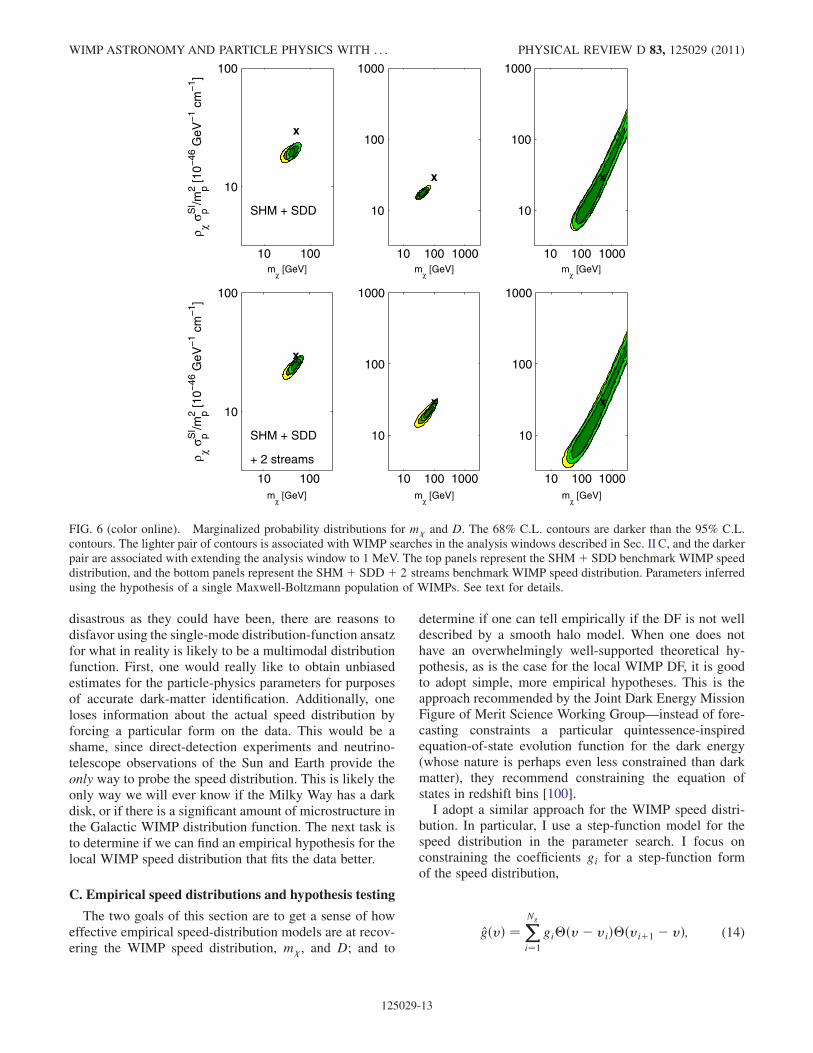
disastrous as they could have been, there are reasons todisfavor using the single-mode distribution-function ansatzfor what in reality is likely to be a multimodal distributionfunction. First, one would really like to obtain unbiasedestimates for the particle-physics parameters for purposesof accurate dark-matter identification. Additionally, oneloses information about the actual speed distribution byforcing a particular form on the data. This would be ashame, since direct-detection experiments and neutrino-telescope observations of the Sun and Earth provide theonly way to probe the speed distribution. This is likely theonly way we will ever know if the Milky Way has a darkdisk, or if there is a significant amount of microstructure inthe Galactic WIMP distribution function. The next task isto determine if we can find an empirical hypothesis for thelocal WIMP speed distribution that fits the data better.

C. Empirical speed distributions and hypothesis testing

The two goals of this section are to get a sense of howeffective empirical speed-distribution models are at recov-ering the WIMP speed distribution, m�, and D; and to

determine if one can tell empirically if the DF is not welldescribed by a smooth halo model. When one does nothave an overwhelmingly well-supported theoretical hy-pothesis, as is the case for the local WIMP DF, it is goodto adopt simple, more empirical hypotheses. This is theapproach recommended by the Joint Dark Energy MissionFigure of Merit Science Working Group—instead of fore-casting constraints a particular quintessence-inspiredequation-of-state evolution function for the dark energy(whose nature is perhaps even less constrained than darkmatter), they recommend constraining the equation ofstates in redshift bins [100].I adopt a similar approach for the WIMP speed distri-

bution. In particular, I use a step-function model for thespeed distribution in the parameter search. I focus onconstraining the coefficients gi for a step-function formof the speed distribution,

gðvÞ ¼ XNg

i¼1

gi�ðv� viÞ�ðviþ1 � vÞ; (14)

mχ [GeV]

x

10 100 1000

10

100

1000

10 100 1000

10

100

1000

mχ [GeV]

x

10 100

10

100

mχ [GeV]

ρ χσ pS

I /mp2 [1

0−46

GeV

−1 c

m−

1 ]

x

SHM + SDD

mχ [GeV]

x

10 100 1000

10

100

1000

10 100 1000

10

100

1000

mχ [GeV]

x

10 100

10

100

mχ [GeV]

ρ χσ pS

I /mp2 [1

0−46

GeV

−1 c

m−

1 ]

x

SHM + SDD

+ 2 streams

FIG. 6 (color online). Marginalized probability distributions for m� and D. The 68% C.L. contours are darker than the 95% C.L.contours. The lighter pair of contours is associated with WIMP searches in the analysis windows described in Sec. II C, and the darkerpair are associated with extending the analysis window to 1 MeV. The top panels represent the SHMþ SDD benchmark WIMP speeddistribution, and the bottom panels represent the SHMþ SDDþ 2 streams benchmark WIMP speed distribution. Parameters inferredusing the hypothesis of a single Maxwell-Boltzmann population of WIMPs. See text for details.


125029-13

where vi is the lower limit of the speed for the ith gðvÞ bin,viþ1 is the upper limit. � is the Heaviside step function.The hat symbol denotes the fact that this speed distributionis estimated from the data regardless of the true gðvÞ. In thelimit of an infinite number of bins Ng ! 1, gðvÞ ! gðvÞ.In this work, I choose bins of equal size in v. Either thestep-function model or the choice of binning may be farfrom the optimal empirical parametrization of the speeddistribution, but these choices for the speed-distributionanalysis serve the purpose of providing a good proof ofprinciple for WIMP speed-distribution recovery and modelcomparison.

For this work, I first consider five bins in speed up to v ¼1000 km s�1. This upper limit is somewhat larger than theestimated escape speed from theMilkyWay in a geocentricframe [96]. By setting the maximum speed for the speed-distribution bins, I am placing a strong prior that the maxi-mum WIMP speed must lie below that value. As in theprevious sections, I choose the usual benchmarks forWIMP mass, m� ¼ 50, 100, and 500 GeV, and fix D ¼3� 10�45 GeV�1 cm�1. As before, I sampled those pa-rameters logarithmically using MULTINEST. I chose threedifferent benchmarks for the speed distributions for themock data sets: the SHM, the SHMþ SDD, and theSHMþ SDDþ two high-speed velocity streams (withthe same weighting of components as used in Sec. III B). Isampled the five velocity-bin coefficients fgig linearly in therange from 0 to fgmax

i g, where gmaxi is the maximum value of

gi if all other gj�i ¼ 0 and satisfying the normalization

condition in Eq. (4). While the marginalized 68% and 95%confidence-level regions in the speed coefficients are notdramatically different if one samples the fgig logarithmi-cally, the marginalized contours generally follow the shapeof the profile likelihood better for linear scans in fgig.

The first benchmark speed distribution I consider is theSHM. The constraints in the m�–D plane are shown in

Fig. 7, and the constraints on fgig are shown in Fig. 8. InFig. 7, I show the marginalized probabilities for the fiducialQmax with the set of light-colored filled regions, and themarginalized probabilities for Qmax ¼ 1 MeV withthe darker pair of regions. The first thing to note is that

mχ [GeV]

x

10 100 1000

10

100

1000

10 100 1000

10

100

1000

mχ [GeV]

x

10 100

10

100

mχ [GeV]

ρ χσ pS

I /mp2 [1

0−46

GeV

−1 c

m−

1 ]

x

vrms

= 155 km/s

vlag

= 220 km/s

FIG. 7 (color online). Marginalized probability distributions for m� and D with the SHM as the velocity benchmark and analyzedwith the five-bin step-function speed-distribution hypothesis. Each panel represents a different benchmark m�. The lighter pair of

contours represents 68% and 95% C.L. regions based on the analysis windows described in Sec. II C, and the darker pair of contoursare the results if the analysis windows are extended to 1 MeV.

FIG. 8 (color online). Inferred WIMP speed distributions forthe SHM benchmark model. The solid error bars denote the68% C.L. region for each gi using the fiducial analysis windows,and the dashed error bars show the same but for Qmax ¼ 1 MeV.The upper panels show the speed constraints when the WIMPmass and cross section are sampled logarithmically, and thebottom panels show the speed constraints when there is anadditional 10% Gaussian prior on the WIMP mass. The solidline denotes the benchmark speed distribution.


125029-14

the parameter uncertainties are no larger than those foundin Sec. III A, although they are biased in the cases ofm� ¼50 and 100 GeV. The bias decreases with increasing Qmax,though. The second thing to note is that the shape of thedegeneracy contours is quite different than with theMaxwell-Boltzmann ansatz used in Sec. III A. This isbecause the shape of the mapping between m� and D

and a fixed recoil spectrum depends on the form of thespeed distribution. Third, for m� ¼ 50 GeV there are dis-

connected regions. This is an artifact of the ‘‘realizationnoise’’ in the data.

The reconstructed speed distributions are shown inFig. 8. Each column in the figure represents a differentWIMP mass. The error bars represent the marginalized68% probability limits for each gi. Note that the probabil-ity contours are in fact correlated. The solid error barsdenote the limits obtained with the fiducial Qmax, and thedotted error bars denote those obtained if Qmax ¼ 1 MeV.In the upper panels, the WIMP mass is only constrained tobe somewhere between 1 MeV and 100 TeV, but in thebottom panels, I impose a Gaussian prior on the WIMPmass centered on the true value and with a width of 0:1m�.

The solid line shows the SHM speed distribution. In gen-eral, using the higher Qmax leads to better fits to the SHMspeed distribution, with the exception of the case in whichm� ¼ 50 GeV. I note that a similar trend towards a larger

low-speed population is also seen in the Maxwell-Boltzmann analysis in Sec. III A for this particular bench-mark. Figures 3 and 5 show that the true speed-parameterpoint barely lies within the 95% C.L. contour. This highinferred density of low-speed particles is an artifact of thisparticular realization of the data for this set of benchmarkparameters.

Although the inferred speed distributions look reason-able, one might want to ask if the inferred speed distribu-tion were consistent withMaxwell-Boltzmann distribution.The issue of model selection is tricky for both the frequent-ist and Bayesian perspectives if one cannot use �2 todetermine the goodness of fit (e.g., [82,101]). In general,the goal is to determine the relative fit between hypothesesinstead of determining the absolute quality of fit for asingle hypothesis. I use three different criteria to assessthe relative quality of fit between the single Maxwell-Boltzmann and step-function speed-distribution hypothe-ses: the Bayes factor, the Akaike information criterion(AIC) [102], and the Bayes information criterion (BIC)[103]. However, for reasons stated below, I will emphasizethe Bayes factor, in particular.

In the Bayesian context, the ratio of Bayesian evidences[Eq. (11)] for two hypotheses (‘‘Bayes factor’’) is oftenused to determine if one hypothesis fits the data better thanthe other. Since the Bayesian evidence is just the averagelikelihood over the parameter space (weighted by theprior), the better-fit hypothesis is assumed to be the onewith the higher average likelihood, regardless of maximum

likelihood Lmax. This means that models with fewer pa-rameters are generally preferred (the ‘‘Occam’s razor’’hypothesis—simpler models are better). Technically, theBayes factor is not strictly the ratio of evidences, but is theratio of evidences multiplied by the ratio of the priors onthe hypotheses. Quantifying the belief in the hypotheses issomething I will not get into in this work, but Ref. [101]provides an interesting introduction to the subject. Fornow, I will assume that the hypotheses are equallyprobable.In general, the evidence is prior and parameter depen-

dent. In the present case, determining whether the step-function hypothesis fits better than a Maxwell-Boltzmanndistribution, the fact that WIMPs cannot travel with infinitespeed allows one to at least define a reasonable parametervolume. For the step-function speed model, the fgig cannotexceed fgmax

i g. This provides a natural volume to use, andwas the volume I used to for the parameter search. As withthe parameter search, I use flat priors on fgig to calculatethe evidence. To calculate the evidence for the Maxwell-Boltzmann model, I use the same priors and parameter-space volume as used in the parameter search in Sec. III A.The upper bound for vlag and vrms are well above the

escape speed from the Galaxy.Although I use the Bayes factor

B ¼ Zð1MBÞZðfgigÞ (15)

to get a sense the relative fit of the single Maxwell-Boltzmann (1MB) and step-function (fgig) models, morein-depth studies are necessary to determine if this is reallythe best fit criterion for direct-detection data. Moreover,even though the way in which I have defined the priorvolume is reasonable, it may not be the best; vlag and vrms

are a completely different way of parametrizing a speeddistribution than fgig. However, as I show below, the Bayesfactor seems to be a not unreasonable criterion by which toclassify fits.Second, I consider the AIC, which is approximated as

AIC ¼ �2 lnLmax þ 2Np; (16)

where Lmax is the maximum likelihood for the data giventhe hypothesis, and Np is the number of parameters of the

hypothesis. The AIC is meant to minimize the Kullback-Leibler information entropy [104], and so the hypothesiswith the smallest AIC is preferred. As with most Bayesianmodel-selection criteria, the AIC penalizes the introduc-tion of additional parameters, but not as much as the BIC,the third model-selection criterion I consider, which isdefined as

BIC ¼ �2 lnLmax þ Np lnðNoÞ: (17)

Here, No is the observed number of events. For the datasets I consider, there are between �200 and �700total events, which gives lnðNoÞ � 6. In the limit that the


125029-15

posterior is a multivariate Gaussian and that the data areindependent and identically distributed, the Bayesian evi-dence and BIC are equivalent in terms of describing thequality of the fit [82].

Even though I consider all three Bayesian model-selection criteria below, I emphasize the Bayes factorbecause it is easiest to interpret and most likely to selectthe better model. The AIC does not necessarily select thecorrect model even if one had an infinite, unbiased data set[105]. The issue with the BIC is that the posteriors for the

direct-detection data sets are clearly not well described bymultivariate Gaussians, and so it is not clear how then tointerpret the BIC. In cosmology, the Bayes factor is thepreferred Bayesian model-selection criterion [106–108]. Ishow the Bayes factor for each benchmark model inTable I.For all the SHM data sets, the SHM is preferred over the

five-bin step-function speed-distribution hypothesis by theAIC and the BIC. However, the preference is not especiallystrong according to the Bayes factor. The mock data setswith the highest B are those with m� ¼ 50 GeV with the

fiducial Qmax and m� ¼ 100 GeV with Qmax ¼ 1 MeV,

for which lnðBÞ � 3, which is almost considered ‘‘moder-ate’’ evidence on the Jeffreys’ scale in favor of the SHM[82]. In the cases in which m� ¼ 500 GeV, there is weak

evidence for the step-function model; it is, however, notespecially significant since any j lnBj< 3 is consideredweak evidence.Next, I consider the multimodal distribution functions I

explored in Sec. III B. The constraints for the SHMþ SDDbenchmark model in the m�–D plane are shown in Fig. 9,

and the speed-distribution fits are shown in Fig. 10. As inFig. 7, the lighter pair of contours indicate the marginalizedprobabilities of the parameters for the fiducial values ofQmax, and the darker pair corresponds to setting Qmax ¼1 MeV. The probability contours in the m�–D plane are

offset from the true point, with the exception of the m� ¼500 GeV cases. The offsets are somewhat less than if onewere to apply the ansatz that the velocity distribution isMaxwell-Boltzmann (Fig. 6), but not much. The offsets arelower if one uses a higher Qmax. The probability contourshave a different shape than those resulting from the hy-pothesis that the velocities have a Maxwell-Boltzmanndistribution.

mχ [GeV]

x

10 100 1000

10

100

1000

10 100 1000

10

100

1000

mχ [GeV]

x

10 100

10

100

mχ [GeV]

ρ χσ pS

I /mp2 [1

0−46

GeV

−1 c

m−

1 ]

x

SHM + SDD

FIG. 9 (color online). Marginalized probability distributions form� andD for the SHMþ SDD benchmark speed-distribution modeland the five-bin step-function speed-distribution hypothesis. Each panel represents a different benchmark m�. The lighter pair of

contours represents 68% and 95% C.L. regions based on the analysis windows described in Sec. II C, and the darker pair of contoursare the results if the analysis windows are extended to 1 MeV.

TABLE I. Bayes’ factor for benchmark speed distributions andWIMP masses

Benchmark speed distributions m� [GeV] Qmax lnB

SHM 50 fiducial 2.7

50 1 MeV 2.1

100 fiducial 0.8

100 1 MeV 2.8

500 fiducial �2:5

500 1 MeV �2:1

SHMþ SDD 50 fiducial �3:1

50 1 MeV �6:6

100 fiducial �4:3

100 1 MeV �6:3

500 fiducial �1:8

500 1 MeV �3:1

SHMþ SDDþ 2 streams 50 fiducial �2:9

50 1 MeV �7:4

100 fiducial �1:9

100 1 MeV �8:5

500 fiducial �3:9

500 1 MeV �3:4


125029-16

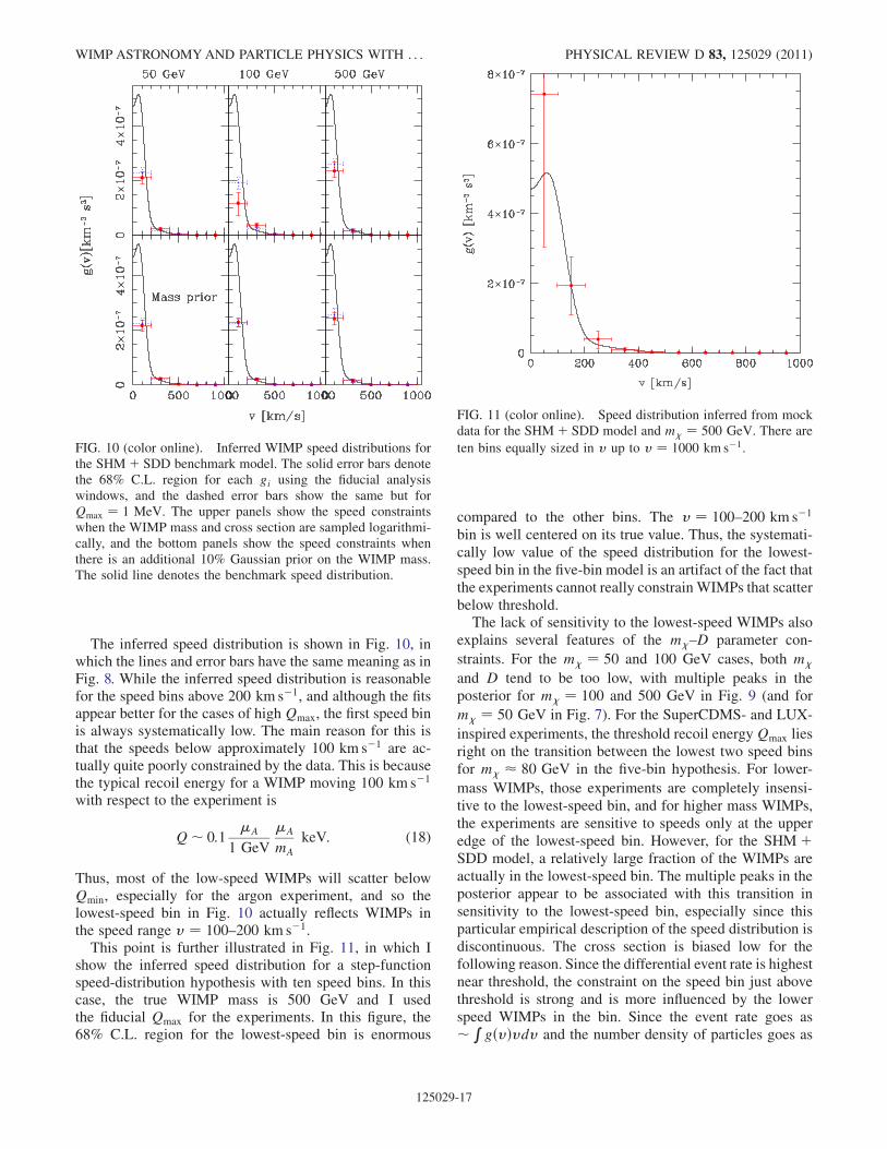
The inferred speed distribution is shown in Fig. 10, inwhich the lines and error bars have the same meaning as inFig. 8. While the inferred speed distribution is reasonablefor the speed bins above 200 km s�1, and although the fitsappear better for the cases of high Qmax, the first speed binis always systematically low. The main reason for this isthat the speeds below approximately 100 km s�1 are ac-tually quite poorly constrained by the data. This is becausethe typical recoil energy for a WIMP moving 100 km s�1

with respect to the experiment is

Q� 0:1�A

1 GeV

�A

mA

keV: (18)

Thus, most of the low-speed WIMPs will scatter belowQmin, especially for the argon experiment, and so thelowest-speed bin in Fig. 10 actually reflects WIMPs inthe speed range v ¼ 100–200 km s�1.

This point is further illustrated in Fig. 11, in which Ishow the inferred speed distribution for a step-functionspeed-distribution hypothesis with ten speed bins. In thiscase, the true WIMP mass is 500 GeV and I usedthe fiducial Qmax for the experiments. In this figure, the68% C.L. region for the lowest-speed bin is enormous

compared to the other bins. The v ¼ 100–200 km s�1

bin is well centered on its true value. Thus, the systemati-cally low value of the speed distribution for the lowest-speed bin in the five-bin model is an artifact of the fact thatthe experiments cannot really constrain WIMPs that scatterbelow threshold.The lack of sensitivity to the lowest-speed WIMPs also

explains several features of the m�–D parameter con-

straints. For the m� ¼ 50 and 100 GeV cases, both m�

and D tend to be too low, with multiple peaks in theposterior for m� ¼ 100 and 500 GeV in Fig. 9 (and for

m� ¼ 50 GeV in Fig. 7). For the SuperCDMS- and LUX-

inspired experiments, the threshold recoil energy Qmax liesright on the transition between the lowest two speed binsfor m� � 80 GeV in the five-bin hypothesis. For lower-

mass WIMPs, those experiments are completely insensi-tive to the lowest-speed bin, and for higher mass WIMPs,the experiments are sensitive to speeds only at the upperedge of the lowest-speed bin. However, for the SHMþSDD model, a relatively large fraction of the WIMPs areactually in the lowest-speed bin. The multiple peaks in theposterior appear to be associated with this transition insensitivity to the lowest-speed bin, especially since thisparticular empirical description of the speed distribution isdiscontinuous. The cross section is biased low for thefollowing reason. Since the differential event rate is highestnear threshold, the constraint on the speed bin just abovethreshold is strong and is more influenced by the lowerspeed WIMPs in the bin. Since the event rate goes as�R

gðvÞvdv and the number density of particles goes as

FIG. 10 (color online). Inferred WIMP speed distributions forthe SHMþ SDD benchmark model. The solid error bars denotethe 68% C.L. region for each gi using the fiducial analysiswindows, and the dashed error bars show the same but forQmax ¼ 1 MeV. The upper panels show the speed constraintswhen the WIMP mass and cross section are sampled logarithmi-cally, and the bottom panels show the speed constraints whenthere is an additional 10% Gaussian prior on the WIMP mass.The solid line denotes the benchmark speed distribution.

FIG. 11 (color online). Speed distribution inferred from mockdata for the SHMþ SDD model and m� ¼ 500 GeV. There are

ten bins equally sized in v up to v ¼ 1000 km s�1.


125029-17

�gðvÞv2dv, the number of WIMPs in the second-lowestspeed bin is biased high while the number of WIMPs in thelowest-speed bin is biased low (also due to the fact that theexperiments are sensitive only to speeds at the upper edgeof the speed bin). The cross section must drop to compen-sate for the relatively high number of WIMPs inferred inthe second-lowest-speed bin.

Next, I consider the question of model selection. Icalculate the Bayes factor, AIC, and BIC for the SHMþSDD data sets. I find that the Bayes factor indicates that thestep-function model is a better fit for each of the sixensembles of mock data sets. The Bayes factor is mostsignificant for m� ¼ 50 and 100 GeV for Qmax ¼ 1 MeV.

In those cases, lnðBÞ ¼ �7 to �6 (Table I), which isconsidered ‘‘strong evidence’’ on the Jeffreys’ scale [82].All ensembles of data sets with the exception of the singleensemble with m� ¼ 500 GeV and the fiducial Qmax in-

dicate a lower AIC for the step-function model than theMaxwell-Boltzmann distribution. However, only thosemock data sets corresponding to m� ¼ 50 or 100 GeV

with Qmax ¼ 1 MeV additionally have a lower BIC forthe step-function model than for the Maxwell-Boltzmanndistribution. Thus, while the Bayes factor and AIC gener-ally show that the Maxwell-Boltzmann distribution is dis-favored for this particular two-component velocitydistribution, it is generally only moderately disfavoredrelative to the step-function model unless Qmax is large.

Last, I consider the SHMþ SDDþ 2 streams model.The probability contours in the m�–D plane for several

values of m� are shown in Fig. 12, and the speed distribu-

tion is shown in Fig. 13. As for the SHMþ SDD case, thecontours in the m�–D plane are typically slightly offset

from the true point in parameter space, but are less offsetfor higher Qmax. Also as for the SHMþ DD case, thelowest-speed bin in is systematically low due to the poorconstraints on the lowest-speed WIMPs, although the

higher-speed bins are well centered on the true speeddistribution.The model-selection patterns also follow those of the

SHMþ SDD benchmark speed distribution. There is onlyone exception to the patterns of the SHMþ SDD findings.

mχ [GeV]

x

10 100 1000

10

100

1000

10 100 1000

10

100

1000

mχ [GeV]

x

10 100

10

100

mχ [GeV]

ρ χσ pS

I /mp2 [1

0−46

GeV

−1 c

m−

1 ]

x

SHM + SDD

+ 2 streams

FIG. 12 (color online). Marginalized probability distributions form� andD for the SHMþ SDDþ 2 streams benchmark model andthe five-bin step-function speed-distribution hypothesis. Each panel represents a different input mass. The lighter pair of contoursrepresents 68% and 95% C.L. regions based on the analysis windows described in Sec. II C, and the darker pair of contours are theresults if the analysis windows are extended to 1 MeV.

FIG. 13 (color online). Inferred WIMP speed distributions forthe SHMþ SDDþ 2 streams benchmark model. The solid errorbars denote the 68% C.L. region for each gi using the fiducialanalysis windows, and the dashed error bars show the same butforQmax ¼ 1 MeV. The upper panels show the speed constraintswhen the WIMP mass and cross section are sampled logarithmi-cally, and the bottom panels show the speed constraints whenthere is an additional 10% Gaussian prior on the WIMP mass.The solid line denotes the benchmark speed distribution.


125029-18

The case of m� ¼ 100 GeV with fiducial Qmax has AIC

and BIC that prefer the Maxwell-Boltzmann velocity dis-tribution model (although in the case of the AIC, thedifference between the two models is quite small, <2),and the Bayes factor is lnðBÞ ¼ �1:9, which indicates aweak-to-moderate preference for the step-function model.Otherwise, the trends in lnðBÞ, AIC, and BIC for theSHMþ SDD input velocity model hold for this morecomplicated input velocity model, too. The Bayes’ factorsfor all benchmarks are given in Table I.

There are a few final points I would like to address in thissection. First, although I have shown for the mock data setswith multimodal velocity distributions that one may rea-sonably reconstruct a speed distribution (taking care withthe low-speed end for which the experiments have littleconstraining power) using the step-function hypothesis,there is still the issue that the m�–D probability distribu-

tion is offset from the true value. In fact, the true point liesoutside of the 95% C.L. contour in most cases I considered.This is because, even though the five-bin step-functionspeed-distribution hypothesis is a better fit to the data, itis by no means the best fit speed-distribution hypothesis forthe data. In fact, the discontinuous nature of the speed-distribution hypothesis is clearly not physical and is re-sponsible for some of the odder features of the probabilitycontours, as discussed in this section.

One may ask if one does better with a larger number ofspeed bins. Even though the speed-distribution hypothesisis still discontinuous, it is a better representation of acontinuous function. I ran a set of tests in which I doubledthe number of speed bins, from five to ten. The maximumlikelihood Lmax barely improved between the two sets ofanalyses (j� lnLmaxj & 3), meaning that the AIC and BICmodel-selection criteria would prefer the five-bin modelover the ten-bin model. The only case in which Lmax

increased enough that the AIC preferred the 10-bin modelwas for the SHMþ SDD benchmark with m� ¼ 100 GeV

and Qmax ¼ 1 MeV. The Bayes factor

Bbin ¼ Zð5 binsÞZð10 binsÞ (19)

was ranged from nearly 1 (no preference in favor of eithermodel) to lnðBbinÞ ¼ 3, which indicates moderate prefer-ence for the five-bin model. Even for the one case in whichthe AIC indicated the ten-bin model was a better fit, theBayes factor indicated a preference for the five-bin model.Usually, the Bayes factor was less significant in distin-guishing between the hypotheses of the number of binsin the step-function speed-distribution model than distin-guishing between the five-bin model and the Maxwell-Boltzmann distribution. It appears that for the mock datasets I considered (and what is likely to hold true for the firstyears of real data), ten speed bins is likely overkill. The oneinteresting feature of the ten-bin model was that the m�–D

probability distributions were better centered on the truevalue than for the five-bin model, although the posterior isstill multimodal. This is illustrated in Fig. 14, in which Ishow the probability distributions for the SHMþ SDDbenchmark for m� ¼ 100 GeV. However, this needs to

be explored for more ensembles of mock data sets to seeif that is generally true.Although I have shown that one may achieve demon-

strably better fits to multimodal velocity distributions usingthe step-function speed-distribution hypothesis, I have notshown that this is truly the best empirical speed-distribution model one could use. In fact, the discontinuousnature of this empirical function has clear downsides, inaddition to only being able to approximate theoretically-inspired functional forms for the speed distribution in thelimit of many bins. In practice, it is likely that direct-detection data sets will need to be analyzed with a varietyof empirical hypotheses for the speed distribution in orderto achieve the best, unbiased constraints on both theparticle-physics parameters ðm�;DÞ and the speed distri-

bution. I leave the development of a strategy for optimalmodel selection to future work.The key points of this section are that one may obtain a

reasonable estimate of the WIMP speed distribution usingthese simple step-function speed-distribution models, andthat one may distinguish between speed-distribution mod-els using Bayesian model-selection criteria. In particular,

mχ [GeV]

ρ χσ pS

I /mp2 [1

0−46

GeV

−1 c

m−

1 ]

x

SHM + SDD

10 100

10

100

FIG. 14 (color online). Marginalized probability distributionsfor m� and D for m� ¼ 100 GeV and SHMþ SDD benchmark

model and the ten-bin step-function speed-distribution hypothe-sis. The lighter pair of contours represents 68% and 95% C.L.regions based on the analysis windows described in Sec. II C,and the darker pair of contours are the results if the analysiswindows are extended to 1 MeV.


125029-19

the simple step-function model is moderately to stronglypreferred over the single-velocity-component model forthe benchmark multimodal velocity distributions.

IV. DISCUSSION

In this work, I studied the prospects of inferring theWIMP speed distribution in addition to the WIMPparticle-physics parameters for several benchmark modelsfrom direct-detection data sets. I created mock data sets foridealized versions of cryogenic and liquid-noble experi-ments expected to be on line by or near 2015. I appliedBayesian inference to estimate WIMP parameter valuesand uncertainties from the mock data sets.

There were three cases I considered. In the first case, Iconsidered constraints on WIMP particle-physics andspeed-distribution parameters in the case that hypothesisfor the speed distribution matched the actual form of thespeed distribution, but for which the parameters of thespeed distribution were otherwise unconstrained. The mo-tivation for this study was twofold. First, most parameterforecasts for direct-detection experiments have focused onthe hypothesis of a smooth halo WIMP DF, with the speedparameters vlag and vrms fixed to something like the SHM

[44,45]. If the speed-distribution parameters were allowedto vary at all, it was typically not over a wide range. Thus, Iwanted to explore a number of benchmark halo DF scenar-ios with weak priors on the parameters to see how well onecould infer both the speed-distribution and WIMP particle-physics parameters. Although Sec. III A focused onbenchmark speed-distribution models that spanned a rea-sonable range for a smooth halo hypothesis, I have alsoconsidered other single-mode models (e.g., if the dark diskor a single large velocity stream dominates the local DF)and found similar results. Second, the best parameter con-straints are obtained when the hypothesis for the speed-distribution model is correct, and I wanted to know howgood those best constraints are likely to be for a variety ofbenchmark speed-distribution and particle-physics pa-rameter sets.

I found that for any benchmark speed-distributionmodel, that one could get reasonable constraints on m�

and D with only the weakest of priors on the theoreticalparameters, and that constraints improved significantly ifQmax was set quite high. Constraints were tightest form� & 100 GeV and for vlag < 280 km s�1. In general,

the degree of uncertainty in m� and D depends on the

underlying speed distribution.The constraints on vlag and vrms depend on the under-

lying speed distribution as well as m� and D. Constraints

were generally tighter for smaller m� and vrms. In general,

vrms is far better constrained than vlag; it is only possible to

place an upper limit on vlag. This was true even when I

introduced a strong prior on the WIMP mass, a prior of thesort one would expect if supersymmetry were discovered at

the LHC. This prior sharpened constraints on vrms but notvlag unless m� * 100 GeV. The somewhat sobering con-

clusion is that while it is possible to get good constraints onthe velocity dispersion of WIMPs, it will be significantlyharder to determine the typical speed of WIMPs withrespect to the Earth with 2015-era experiments.Second, in Sec. III B I considered what constraints one

would obtain under the hypothesis of a Maxwell-Boltzmann distribution in the case that the true DF weremultimodal. The motivation for studying this case is thestrong theoretical prior on the form of the WIMP DF thatusually goes into direct-detection parameter forecasts. Forboth the SHMþ SDD and SHMþ SDDþ 2 streams mul-timodal DF models, I found thatm� andDwere biased low

by �50%, mostly due to the dark-disk component, some-thing that was also found by Ref. [44]. Although theseoffsets are not enormous for these particular WIMP DFmodels, they could be more severe for other models.Moreover, we lose information about the nature of theWIMP speed distribution, such as its multimodal character,if we restrict ourselves to a single-velocity-componenthypothesis.Finally, in Sec. III C I considered a simple empirical

model for the speed distribution, both to get a sense of howwell one may recover WIMP particle-physics and speed-distribution properties as well as its use for Bayesian modelselection. I showed that the five-bin step-function speed-distribution model successfully reproduced the WIMPspeed distribution for speeds above v ¼ 200 km s�1, andthat the bias in the v ¼ 0–200 km s�1 bin was due to theexperiments’ lack of sensitivity to WIMPs with v &100 km s�1. For all benchmark speed-distribution modelsI considered, the inferred values of m� and D were biased

relative to their true values, but no more so than with thesingle Maxwell-Boltzmann hypothesis used in Sec. III B.However, the biases were less severe if the analysis win-dow was extended to higher energies. Moreover, there werehints from the ten-bin step-function model that the bias wasless than for the five-bin model, even though the Occam’srazor philosophy of the Bayesian model-selection criteria Iconsidered favored the five-bin model. The bias shoulddecrease as better empirical speed-distribution hypothesesare found.I found that Bayesian model-selection criteria were

largely successful in ranking hypotheses for the speeddistribution. For the SHM benchmarks, the Bayesianmodel-selection criteria indicated that the Maxwell-Boltzmann hypothesis was a better fit to the data than thestep-function hypothesis, although the significance of thepreference was not strong. For the multimodal bench-marks, these model-selection criteria showed moderate tostrong preference for the step-function model over theMaxwell-Boltzmann model. Moreover, they showed thatdoubling the number of bins in the step-function modeldid not improve the fit over the five-bin model enough


125029-20

to justify the additional bins, except for the one casementioned at the end of Sec. III C. These findings areinteresting for several reasons. First, they show that it ispossible to get reasonable constraints on the speed distri-bution with few-parameter empirical speed-distributionhypotheses. This is good because we do not really knowwhat to expect for the WIMP speed distribution. Second,they show that it is possible to rule in or out populartheoretical models for the WIMP DF.

A. Outstanding issues

Although I have shown that it is possible to distinguishbetween Maxwell-Boltzmann and step-function WIMPspeed-distribution hypotheses with a modest amount ofdirect-detection data, there are still a number of questionsregarding model selection for the speed distribution.

First, although I have shown that the five-bin step-function speed-distribution hypothesis yields reasonableconstraints on the speed distribution and only moderatelybiased constraints on m� and D, I have not shown that it is

the best hypothesis for the speed distribution. In fact, itcannot be the best hypothesis, since the best hypothesiswould be that which matched the form of the benchmarkspeed distributions. Moreover, its discontinuous nature isboth nonphysical and creates strange features in theposterior, such as the multimodality in the m�–D con-

straints in Figs. 7 to 12. However, since we do not reallyknow what to expect for the WIMP speed distribution, itis best to explore a variety of empirical models. In thiswork, I considered equal-sized (in speed) step functions tomodel the speed distribution, but it is possible that allowingthe widths of the step function to vary or choosingsmoother, continuous basis functions is better. For ex-ample, in Sec. III C I showed that gðvÞ below v�100 km s�1 is not well constrained due to the thresholdsof the experiments, but that bins of width 100 km s�1 weretoo small. Perhaps a better strategy would be to have asingle bin for speeds for which the typical recoil energylies below threshold, and other-sized bins for higherspeeds, or to expand the speed distribution into a setof orthogonal functions. Reference [57] uses overlappingstep-function bins of various sizes. The question is, what isthe best strategy to search through these possibilities?This will depend on the true values of the WIMPparticle-physics parameters and the speed distribution,but it is worth putting some thought into how to findempirical hypotheses that will maximize our return onthe data.

Finding a good hypothesis for the speed distribution isimportant not just for the sake of constraining the speeddistribution, but a better hypothesis for the speed distribu-tion should also lead to less biased inferences for theparticle-physics properties of WIMPs. As demonstratedin Sec. III C, even though the step-function hypothesisleads to good constraints on the speed distribution, the

inferred values of the particle-physics parameters are offsetfrom their true values. I will delve into this topic more inSec. IVB.However, there are also several theoretical models for

the speed distribution that would be interesting to test usingdirect-detection data. So far, I have only consideredMaxwell-Boltzmann theoretical models, which are basedon arguments along the lines of those found in Sec. IIB andAppendix A of Ref. [71]. There are other theoretical mod-els for the local speed distribution that are based on N-bodysimulations [47], in particular, for the ansatz that the speeddistribution is dominated by a smooth halo component. Itwould be interesting to use the best empirical models forhypothesis testing against a wider class of specific theo-retical models. For example, if none of the smooth halopredictions fit better than the best empirical fit, then thismight suggest that the WIMP speed distribution is multi-modal or that the velocity distribution is anisotropic.Multimodal speed distributions are a signature of theMilky Way’s accretion history, and it would be interestingto determine how much one could learn about the accretionhistory based on the direct-detection data.An interesting question is if one may infer the escape

speed of WIMPs from the Milky Way. Currently, the bestconstraints on the local escape speed come from measure-ments of the radial velocities of local high-velocity starswith the RAVE survey [96]. The 90% confidence limits forthe escape speed are 498 km s�1 < vesc < 608 km s�1 andare somewhat model dependent. While there is likely apopulation of WIMPs passing through the Solar Systemthat are unbound to the Galaxy due to the fact that theGalaxy is still accreting matter, it is probably small sincethe Sun sits deep inside the halo. If there is a sharp dropoffin the distribution function at the escape speed, this shouldleave an imprint in the nuclear recoil spectra. The questionis if this imprint is large enough to discern even foroptimistic WIMP particle-physics and speed-distributionscenarios. A further complication is that the types of ex-periments I considered in this work are not sensitive todirection, so there will be some uncertainty in the mappingof the geocentric speeds to a galactocentric referenceframe. However, this is an interesting question but I defera study thereof to future work.There are a number of more ‘‘practical’’ issues I have

not addressed yet. First, I have ignored backgrounds, en-ergy uncertainties, and systematics. Obviously, these ex-perimental realities will affect parameter estimation.Furthermore, I have also ignored several theoretical issuesbeyond the ansatz of a WIMP model for dark matter. Forexample, I made the ansatz that �SD

p ¼ �SDn ¼ 0, which is

almost certainly not the case in reality. There are alsouncertainties on the form factor FSI. The uncertaintiesare even greater for spin-dependent scattering [11,109].One way forward is to parametrize all the uncertainties,backgrounds, and systematics; throw them all into a


125029-21

likelihood function; and search a greatly expanded parame-ter space with the use of the types of Bayesian tools I usedin this work.

B. Complementarity with other data sets

Beyond finding a good model for the speed distributionfor its own sake, it is useful to characterize the speeddistribution well for the purpose of WIMP identification.Once WIMPs are discovered through multiple channels(e.g., produced at the Large Hadron Collider, inferredfrom the observed shower of particles from WIMP annihi-lation), one will want to see if the particles discoveredthrough these channels are actually of the same type. Inaddition, if the same WIMP particle is responsible for allthese signals, one will want to characterize the WIMP andthe theory to which it belongs using the data. There havebeen several studies to investigate how data from the LHCand direct-detection experiments can be used to constrainspecific theories for physics beyond the standard model,especially supersymmetry [99,110–112]. Given the highcomplexity of the parameter spaces of these theories, awide network of points in the parameter space can yield thesame set of LHC observables. This can lead to estimates ofthe relic density and spin-independent cross sections thatspan orders of magnitude. It is especially important to beable to estimate the relic density for a theory given the databecause the one thing we know about dark matter to a highdegree of accuracy is the its abundance in the Universe(e.g., [1,113]). If a theory that fits the data reasonably wellresults in a too-large relic abundance of darkmatter, then it is ruled out. If the theory predicts a relicabundance that is significantly below the true relic abun-dance, it indicates that the dark matter created in thecollider is only a subdominant component of dark matteras a whole.

References [99,111] have shown that the addition ofdirect-detection data can significantly improve constraintson the estimated relic abundance given the collider dataand a specific theory. However, these authors fixed theWIMP distribution function in their analyses. As I haveshown in Sec. III, a poor hypothesis for the speed distri-bution will result in biases in m� and D. Even in Sec. III C

in which the step-function speed-distribution hypothesiswas a significantly better fit to the multimodal distribution-function data than the Maxwell-Boltzmann hypothesis, itstill lead to biases in the WIMP particle-physics parame-ters. If these speed-distribution-dependent biases are notfully understood, they could lead to incorrect inferencesabout the WIMP particle model.

In order to facilitate accurate joint analyses amongcollider, direct-detection, and indirect-detection data sets,I recommend performing parameter inference for avariety of speed-distribution hypotheses, including several

empirical models. This will give us a sense of how theuncertainty in the speed-distribution model affects, forexample, the inferred relic density for a specific particlemodel.

V. CONCLUSION

In this work, I have created and analyzed mock data setsfor idealized 2015-era liquid-noble and cryogenic direct-detection experiments. The main point of this work was toexplore how well one might reconstruct the WIMP speeddistribution in addition to the particle-physics properties ofWIMPs (mass, cross sections) from future data sets usingBayesian inference. The main findings are the following:(i) Regardless of the true WIMP distribution function or

of the hypothesis for the form of the WIMP distri-bution function, it is unnecessary at best and mis-leading at worst to place strong priors on theparameters of the distribution-function model.Even using extremely weak priors on the WIMPmass, cross sections, and distribution-function pa-rameters, one is able to get good constraints on allparameters for data sets as small as 200 events for allexperiments combined. If, however, there are signifi-cantly fewer events, parameter constraints will beprior dominated if the prior is strong.

(ii) The constraints improve significantly if the analysiswindows for the direct-detection experiments areextended as high in energy as possible.

(iii) Empirical speed-distribution hypotheses lead togood reconstruction of the WIMP speed distribu-tion. I recommend further investigation into theiruse for direct-detection parameter inference.

(iv) Even for the modest mock data sets in this work, itis possible to use Bayesian model-selection criteriadetermine if a specific functional form for the dis-tribution function fits better than a simple empiricalspeed-distribution model. This is especially usefulfor determining if the local WIMP population isdominated by an equilibrium dark-matter halopopulation or bears significant imprints of theMilky Way’s accretion history.

ACKNOWLEDGMENTS

I thank Vera Gluscevic, Kim Griest, Greg Martinez,Bernard Sadoulet, Pat Scott, and Roberto Trotta for usefuldiscussions, and the Aspen Center for Physics for itshospitality while part of this work was completed. Thiswork made use of the University of California, Irvine,Greenplanet computing cluster. This research was sup-ported by the Gordon and Betty Moore Foundation, theCenter for Cosmology at UC Irvine, NASA GrantNo. NNX09AD09G, and NSF Grant No. 0855462.


125029-22

[1] E. Komatsu et al., Astrophys. J. Suppl. Ser. 192, 18(2011).

[2] M. S. Turner, Phys. Rep. 197, 67 (1990).[3] S. Dodelson and L.M. Widrow, Phys. Rev. Lett. 72, 17

(1994).[4] K. Abazajian, G.M. Fuller, and M. Patel, Phys. Rev. D 64,

023501 (2001).[5] J. L. Feng, S. Su, and F. Takayama, Phys. Rev. D 70,

063514 (2004).[6] J. L. Feng and J. Kumar, Phys. Rev. Lett. 101, 231301

(2008).[7] N. Arkani-Hamed, D. P. Finkbeiner, T. R. Slatyer, and N.

Weiner, Phys. Rev. D 79, 015014 (2009).[8] D. E. Kaplan, M.A. Luty, and K.M. Zurek, Phys. Rev. D

79, 115016 (2009).[9] G. Steigman and M. S. Turner, Nucl. Phys. B253, 375

(1985).[10] K. Griest, Phys. Rev. D 38, 2357 (1988).[11] G. Jungman, M. Kamionkowski, and K. Griest, Phys. Rep.

267, 195 (1996).[12] G. Servant and T.M. P. Tait, New J. Phys. 4, 99 (2002).[13] H.-C. Cheng, J. L. Feng, and K. T. Matchev, Phys. Rev.

Lett. 89, 211301 (2002).[14] M.W. Goodman and E. Witten, Phys. Rev. D 31, 3059

(1985).[15] L.M. Krauss, K. Freese, D. N. Spergel, and W.H. Press,

Astrophys. J. 299, 1001 (1985).[16] J. Silk, K. Olive, and M. Srednicki, Phys. Rev. Lett. 55,

257 (1985).[17] I. Wasserman, Phys. Rev. D 33, 2071 (1986).[18] H. Baer, V. Barger, D. Karatas, and X. Tata, Phys. Rev. D

36, 96 (1987).[19] H. Bengtsson, P. Salati, and J. Silk, Nucl. Phys. B346, 129

(1990).[20] S. Mrenna, G. L. Kane, G.D. Kribs, and J. D. Wells, Phys.

Rev. D 53, 1168 (1996).[21] R. Bernabei et al., Eur. Phys. J. C 67, 39 (2010).[22] Z. Ahmed et al. (CDMS II Collaboration), Science 327,

1619 (2010).[23] Z. Ahmed et al. (CDMS Collaboration), Phys. Rev. Lett.

106, 131302 (2011).[24] E. Aprile et al., Phys. Rev. Lett. 105, 131302 (2010).[25] H. S. Lee et al., Phys. Rev. Lett. 99, 091301 (2007).[26] C. E. Aalseth et al., Phys. Rev. Lett. 101, 251301 (2008).[27] C. E. Aalseth et al., Phys. Rev. Lett. 102, 109903 (2009).[28] E. Armengaud et al. (EDELWEISS Collaboration),

arXiv:1103.4070.[29] D. N. McKinsey et al., J. Phys. Conf. Ser. 203, 012026

(2010).[30] S. Roth et al., Prog. Part. Nucl. Phys. 64, 457 (2010).[31] A. Marchionni et al. (ArDM Collaboration),

arXiv:1012.5967.[32] F. Giuliani, in American Institute of Physics Conference

Series, edited by G. Alverson, P. Nath, and B. Nelson,American Institute of Physics Conference Series Vol. 1200(American Institute of Physics Press, Melville, NY, 2010),pp. 985–988.

[33] A. Minamino (Xmass Collaboration), Nucl. Instrum.Methods Phys. Res., Sect. A 623, 448 (2010).

[34] R. Acciarri et al., J. Phys. Conf. Ser. 203, 012006 (2010).[35] L. Baudis, arXiv:1012.4764 [Proc. Sci. (to be published)].

[36] D. Y. Akimov (Zeplin-III Collaboration), Nucl. Instrum.Methods Phys. Res., Sect. A 623, 451 (2010).

[37] T. Bruch (the CDMS Collaboration), arXiv:1001.3037.[38] S. Golwala, http://www.astro.caltech.edu/~golwala/talks/

20100204GolwalaCaltechWeb.pdf , 2009.[39] R. Gaitskell, http://odessa.phy.sdsmt.edu/~bai/dusel/talks-

pdf/006.pdf, 2010.[40] A.M. Green, J. Cosmol. Astropart. Phys. 7 (2008) 5.[41] L. E. Strigari and R. Trotta, J. Cosmol. Astropart. Phys. 11

(2009) 19.[42] D. S.M. Alves, M. Lisanti, and J. G. Wacker, Phys. Rev. D

82, 031901 (2010).[43] A. H.G. Peter, Phys. Rev. D 81, 087301 (2010).[44] A.M. Green, J. Cosmol. Astropart. Phys. 10 (2010) 34.[45] M. Pato, L. Baudis, G. Bertone, R. Ruiz de Austri, L. E.

Strigari, and R. Trotta, Phys. Rev. D 83, 083505 (2011).[46] Y. Akrami, C. Savage, P. Scott, J. Conrad, and J. Edsjo, J.

Cosmol. Astropart. Phys. 04 (2011) 012.[47] M. Lisanti, L. E. Strigari, J. G. Wacker, and R.H.

Wechsler, Phys. Rev. D 83, 023519 (2011).[48] M. Vogelsberger, A. Helmi, V. Springel, S. D.M. White, J.

Wang, C. S. Frenk, A. Jenkins, A. Ludlow, and J. F.Navarro, Mon. Not. R. Astron. Soc. 395, 797 (2009).

[49] M. Kuhlen, N. Weiner, J. Diemand, P. Madau, B. Moore,D. Potter, J. Stadel, and M. Zemp, J. Cosmol. Astropart.Phys. 2 (2010) 30.

[50] J. I. Read, G. Lake, O. Agertz, and V. P. Debattista, Mon.Not. R. Astron. Soc. 389, 1041 (2008).

[51] T. Bruch, J. Read, L. Baudis, and G. Lake, Astrophys. J.696, 920 (2009).

[52] J. I. Read, L. Mayer, A.M. Brooks, F. Governato, and G.Lake, Mon. Not. R. Astron. Soc. 397, 44 (2009).

[53] C.W. Purcell, J. S. Bullock, and M. Kaplinghat,Astrophys. J. 703, 2275 (2009).

[54] F. Ling, E. Nezri, E. Athanassoula, and R. Teyssier, J.Cosmol. Astropart. Phys. 2 (2010) 12.

[55] P. J. Fox, J. Liu, and N. Weiner, Phys. Rev. D 83, 103514(2011).

[56] P. J. Fox, G. D. Kribs, and T.M. P. Tait, Phys. Rev. D 83,034007 (2011).

[57] M. Drees and C.-L. Shan, J. Cosmol. Astropart. Phys. 6(2007) 11.

[58] M. Drees and C.-L. Shan, J. Cosmol. Astropart. Phys. 6(2008) 12.

[59] C. Shan, arXiv:1103.0481.[60] C. Shan, arXiv:1103.0482.[61] A. H.G. Peter (unpublished).[62] R. H. Helm, Phys. Rev. 104, 1466 (1956).[63] K. Freese, P. Gondolo, and L. Stodolsky, Phys. Rev. D 64,

123502 (2001).[64] V. Belokurov et al., Astrophys. J. 654, 897 (2007).[65] E. F. Bell et al., Astrophys. J. 680, 295 (2008).[66] F. J. Kerr and D. Lynden-Bell, Mon. Not. R. Astron. Soc.

221, 1023 (1986).[67] M. J. Reid et al., Astrophys. J. 700, 137 (2009).[68] J. Bovy, D.W. Hogg, and H.-W. Rix, Astrophys. J. 704,

1704 (2009).[69] P. McMillan and J. J. Binney, Mon. Not. R. Astron. Soc.

402, 934 (2010).[70] J. Binney and S. Tremaine, Galactic Dynamics (Princeton

University Press, Princeton, NJ, 2008).


125029-23

http://dx.doi.org/10.1088/0067-0049/192/2/18

http://dx.doi.org/10.1088/0067-0049/192/2/18

http://dx.doi.org/10.1016/0370-1573(90)90172-X

http://dx.doi.org/10.1103/PhysRevLett.72.17











http://dx.doi.org/10.1016/0550-3213(85)90537-1

http://dx.doi.org/10.1016/0550-3213(85)90537-1


http://dx.doi.org/10.1016/0370-1573(95)00058-5

http://dx.doi.org/10.1016/0370-1573(95)00058-5

http://dx.doi.org/10.1088/1367-2630/4/1/399





http://dx.doi.org/10.1086/163767






http://dx.doi.org/10.1016/0550-3213(90)90241-5

http://dx.doi.org/10.1016/0550-3213(90)90241-5



http://dx.doi.org/10.1126/science.1186112

http://dx.doi.org/10.1126/science.1186112







http://arXiv.org/abs/1103.4070

http://dx.doi.org/10.1088/1742-6596/203/1/012026

http://dx.doi.org/10.1088/1742-6596/203/1/012026

http://dx.doi.org/10.1016/j.ppnp.2009.12.075


http://dx.doi.org/10.1016/j.nima.2010.03.032


http://dx.doi.org/10.1088/1742-6596/203/1/012006





http://www.astro.caltech.edu/~golwala/talks/20100204GolwalaCaltechWeb.pdf

http://www.astro.caltech.edu/~golwala/talks/20100204GolwalaCaltechWeb.pdf

http://odessa.phy.sdsmt.edu/~bai/dusel/talks-pdf/006.pdf

http://odessa.phy.sdsmt.edu/~bai/dusel/talks-pdf/006.pdf

http://dx.doi.org/10.1088/1475-7516/2008/07/005

http://dx.doi.org/10.1088/1475-7516/2009/11/019

http://dx.doi.org/10.1088/1475-7516/2009/11/019




http://dx.doi.org/10.1088/1475-7516/2010/10/034


http://dx.doi.org/10.1088/1475-7516/2011/04/012

http://dx.doi.org/10.1088/1475-7516/2011/04/012


http://dx.doi.org/10.1111/j.1365-2966.2009.14630.x

http://dx.doi.org/10.1088/1475-7516/2010/02/030

http://dx.doi.org/10.1088/1475-7516/2010/02/030

http://dx.doi.org/10.1111/j.1365-2966.2008.13643.x

http://dx.doi.org/10.1111/j.1365-2966.2008.13643.x

http://dx.doi.org/10.1088/0004-637X/696/1/920

http://dx.doi.org/10.1088/0004-637X/696/1/920

http://dx.doi.org/10.1111/j.1365-2966.2009.14757.x

http://dx.doi.org/10.1088/0004-637X/703/2/2275

http://dx.doi.org/10.1088/1475-7516/2010/02/012

http://dx.doi.org/10.1088/1475-7516/2010/02/012





http://dx.doi.org/10.1088/1475-7516/2007/06/011

http://dx.doi.org/10.1088/1475-7516/2007/06/011

http://dx.doi.org/10.1088/1475-7516/2008/06/012

http://dx.doi.org/10.1088/1475-7516/2008/06/012



http://dx.doi.org/10.1103/PhysRev.104.1466



http://dx.doi.org/10.1086/509718

http://dx.doi.org/10.1086/588032

http://dx.doi.org/10.1088/0004-637X/700/1/137

http://dx.doi.org/10.1088/0004-637X/704/2/1704

http://dx.doi.org/10.1088/0004-637X/704/2/1704

http://dx.doi.org/10.1111/j.1365-2966.2009.15932.x

http://dx.doi.org/10.1111/j.1365-2966.2009.15932.x

[71] A. H.G. Peter, Ph.D. thesis, Princeton University, 2008.[72] G. Lake, Astron. J. 98, 1554 (1989).[73] E. Aprile, http://xenon.astro.columbia.edu/presentations/

Aprile_SJTU09.pdf.[74] E. Aprile, L. Baudis, B. Choi, K. L. Giboni, K. Lim, A.

Manalaysay, M. E. Monzani, G. Plante, R. Santorelli, andM. Yamashita, Phys. Rev. C 79, 045807 (2009).

[75] A. Manalaysay, arXiv:1007.3746.[76] A. Manzur, A. Curioni, L. Kastens, D.N. McKinsey, K.

Ni, and T. Wongjirad, Phys. Rev. C 81, 025808 (2010).[77] P. Sorensen and C. E. Dahl, Phys. Rev. D 83, 063501

(2011).[78] Z. Ahmed et al., Phys. Rev. Lett. 102, 011301 (2009).[79] E. Aprile et al. (XENON100 Collaboration),

arXiv:1103.0303.[80] F. Feroz and M. P. Hobson, Mon. Not. R. Astron. Soc. 384,

449 (2008).[81] F. Feroz, M. P. Hobson, and M. Bridges, Mon. Not. R.

Astron. Soc. 398, 1601 (2009).[82] R. Trotta, Contemp. Phys. 49, 71 (2008).[83] F. Feroz, K. Cranmer, M. Hobson, R. Ruiz de Austri, and

R. Trotta, arXiv:1101.3296 [J. High Energy Phys. (to bepublished)].

[84] A. Lewis and S. Bridle, Phys. Rev. D 66, 103511 (2002).[85] Y. Akrami, C. Savage, P. Scott, J. Conrad, and J. Edsjo,

arXiv:1011.4297.[86] K. Kuijken and G. Gilmore, Mon. Not. R. Astron. Soc.

239, 651 (1989).[87] L. Bergstrom, P. Ullio, and J. H. Buckley, Astropart. Phys.

9, 137 (1998).[88] R. Schonrich, J. Binney, and W. Dehnen, Mon. Not. R.

Astron. Soc. 403, 1829 (2010).[89] L. L. Watkins, N.W. Evans, and J. H. An, Mon. Not. R.

Astron. Soc. 406, 264 (2010).[90] S. Tremaine, http://pnm.itp.ucsb.edu/online/milkyway_

c08/tremaine/.[91] J. F. Navarro, C. S. Frenk, and S.D.M. White, Astrophys.

J. 462, 563 (1996).

[92] J. F. Navarro, C. S. Frenk, and S. D.M. White, Astrophys.J. 490, 493 (1997).

[93] X. X. Xue et al., Astrophys. J. 684, 1143 (2008).[94] J. S. Bullock, T. S. Kolatt, Y. Sigad, R. S. Somerville, A. V.

Kravtsov, A.A. Klypin, J. R. Primack, and A. Dekel, Mon.Not. R. Astron. Soc. 321, 559 (2001).

[95] A.M. Ghez et al., Astrophys. J. 689, 1044 (2008).[96] M. C. Smith et al., Mon. Not. R. Astron. Soc. 379, 755

(2007).[97] J. Hamann, S. Hannestad, G.G. Raffelt, and Y.Y. Wong, J.

Cosmol. Astropart. Phys. 8 (2007) 21.[98] J. Angle et al., Phys. Rev. Lett. 100, 021303 (2008).[99] E. A. Baltz, M. Battaglia, M. E. Peskin, and T. Wizansky,

Phys. Rev. D 74, 103521 (2006).[100] A. Albrecht et al., arXiv:0901.0721.[101] B. J. Brewer and M. J. Francis, in American Institute of

Physics Conference Series, edited by P.M. Goggans andC.-Y. Chan, American Institute of Physics ConferenceSeries Vol. 1193 (2009), pp. 179–186.

[102] H. Akaike, IEEE Trans. Autom. Control 19, 716 (1974).[103] G. Schwartz, Ann. Stat. 6, 461 (1978).[104] S. Kullback and R.A. Leibler, Ann. Math. Stat. 19, 716

(1974).[105] R. Kashyap, IEEE Trans. Autom. Control 25, 996 (1980).[106] A. Liddle, P. Mukherjee, and D. Parkinson, Astron.

Geophys. 47, 4.30 (2006).[107] A. Liddle, Mon. Not. R. Astron. Soc. 377, L74 (2007).[108] R. Trotta, Mon. Not. R. Astron. Soc. 378, 72 (2007).[109] J. Ellis, K.A. Olive, and C. Savage, Phys. Rev. D 77,

065026 (2008).[110] B. Altunkaynak, M. Holmes, and B.D. Nelson, J. High

Energy Phys. 10 (2008) 13.[111] G. Bertone, D.G. Cerdeno, M. Fornasa, R. Ruiz de Austri,

and R. Trotta, Phys. Rev. D 82, 055008 (2010).[112] J. Goodman, M. Ibe, A. Rajaraman, W. Shepherd, T.M. P.

Tait, and H. Yu, Phys. Rev. D 82, 116010 (2010).[113] B. A. Reid et al., Mon. Not. R. Astron. Soc. 404, 60

(2010).


125029-24

http://dx.doi.org/10.1086/115238

http://xenon.astro.columbia.edu/presentations/Aprile_SJTU09.pdf

http://xenon.astro.columbia.edu/presentations/Aprile_SJTU09.pdf

http://dx.doi.org/10.1103/PhysRevC.79.045807


http://dx.doi.org/10.1103/PhysRevC.81.025808





http://dx.doi.org/10.1111/j.1365-2966.2007.12353.x

http://dx.doi.org/10.1111/j.1365-2966.2007.12353.x

http://dx.doi.org/10.1111/j.1365-2966.2009.14548.x

http://dx.doi.org/10.1111/j.1365-2966.2009.14548.x

http://dx.doi.org/10.1080/00107510802066753




http://dx.doi.org/10.1016/S0927-6505(98)00015-2

http://dx.doi.org/10.1016/S0927-6505(98)00015-2

http://dx.doi.org/10.1111/j.1365-2966.2010.16253.x

http://dx.doi.org/10.1111/j.1365-2966.2010.16253.x

http://dx.doi.org/10.1111/j.1365-2966.2010.16708.x

http://dx.doi.org/10.1111/j.1365-2966.2010.16708.x

http://pnm.itp.ucsb.edu/online/milkyway_c08/tremaine/

http://pnm.itp.ucsb.edu/online/milkyway_c08/tremaine/

http://dx.doi.org/10.1086/177173

http://dx.doi.org/10.1086/177173

http://dx.doi.org/10.1086/304888

http://dx.doi.org/10.1086/304888

http://dx.doi.org/10.1086/589500

http://dx.doi.org/10.1046/j.1365-8711.2001.04068.x

http://dx.doi.org/10.1046/j.1365-8711.2001.04068.x

http://dx.doi.org/10.1086/592738

http://dx.doi.org/10.1111/j.1365-2966.2007.11964.x

http://dx.doi.org/10.1111/j.1365-2966.2007.11964.x

http://dx.doi.org/10.1088/1475-7516/2007/08/021

http://dx.doi.org/10.1088/1475-7516/2007/08/021




http://dx.doi.org/10.1109/TAC.1974.1100705

http://dx.doi.org/10.1214/aos/1176344136

http://dx.doi.org/10.1109/TAC.1980.1102471

http://dx.doi.org/10.1111/j.1468-4004.2006.47430.x

http://dx.doi.org/10.1111/j.1468-4004.2006.47430.x

http://dx.doi.org/10.1111/j.1745-3933.2007.00306.x

http://dx.doi.org/10.1111/j.1365-2966.2007.11738.x



http://dx.doi.org/10.1088/1126-6708/2008/10/013

http://dx.doi.org/10.1088/1126-6708/2008/10/013



http://dx.doi.org/10.1111/j.1365-2966.2010.16276.x

http://dx.doi.org/10.1111/j.1365-2966.2010.16276.x

PHYSICAL REVIEW D 125029 (2011) WIMP astronomy and particle … · 2012-12-26 · WIMP astronomy...

Documents

Transcript of PHYSICAL REVIEW D 125029 (2011) WIMP astronomy and particle … · 2012-12-26 · WIMP astronomy...