Physical modeling of untrenched submarine pipeline...
22
Ocean Engineering 30 (2003) 1283–1304 www.elsevier.com/locate/oceaneng Physical modeling of untrenched submarine pipeline instability F.P. Gao a,b , X.Y. Gu b , D.S. Jeng c,∗ a Special Research Centre for Offshore Foundation System, The University of Western Australia, Nedlands, WA 6907, Australia b Institute of Mechanics, Chinese Academy of Sciences, Beijing 100080, China c School of Engineering, Gold Coast Campus, Griffith University, Gold Coast, QLD 9726, Australia Received 8 April 2002; accepted 17 July 2002 Abstract Wave-induced instability of untrenched pipeline on sandy seabed is a ‘wave–soil–pipeline’ coupling dynamic problem. To explore the mechanism of the pipeline instability, the hydrodyn- amic loading with U-shaped oscillatory flow tunnel is adopted, which is quite different from the previous experiment system. Based on dimensional analysis, the critical conditions for pipeline instability are investigated by altering pipeline submerged weight, diameter, soil para- meters, etc. Based on the experimental results, different linear relationships between Froude number (Fr) and non-dimensional pipeline weight (G) are obtained for two constraint con- ditions. Moreover, the effects of loading history on the pipeline stability are also studied. Unlike previous experiments, sand scouring during the process of pipe’s losing stability is detected in the present experiments. In addition, the experiment results are compared with the previous experiments, based on Wake II model for the calculation of wave-induced forces upon pipeline. It shows that the results of two kinds of experiments are comparable, but the present experiments provide better physical insight of the wave–soil–pipeline coupling effects. 2002 Elsevier Science Ltd. All rights reserved. Keywords: Pipeline instability; Oscillatory flow; Wave loading; Wake II model; Wave–soil–pipeline coup- ling ∗ Corresponding author. Tel.: +61-7-5552-8683; fax: +61-7-5552-8065. E-mail address: [email protected] (D.S. Jeng). 0029-8018/03/$ - see front matter 2002 Elsevier Science Ltd. All rights reserved. doi:10.1016/S0029-8018(02)00108-7
Transcript of Physical modeling of untrenched submarine pipeline...
Ocean Engineering 30 (2003) 1283–1304www.elsevier.com/locate/oceaneng
Physical modeling of untrenched submarinepipeline instability
F.P. Gaoa,b, X.Y. Gu b, D.S. Jengc,∗
a Special Research Centre for Offshore Foundation System, The University of Western Australia,Nedlands, WA 6907, Australia
b Institute of Mechanics, Chinese Academy of Sciences, Beijing 100080, Chinac School of Engineering, Gold Coast Campus, Griffith University, Gold Coast, QLD 9726, Australia
Received 8 April 2002; accepted 17 July 2002
Abstract
Wave-induced instability of untrenched pipeline on sandy seabed is a ‘wave–soil–pipeline’coupling dynamic problem. To explore the mechanism of the pipeline instability, the hydrodyn-amic loading with U-shaped oscillatory flow tunnel is adopted, which is quite different fromthe previous experiment system. Based on dimensional analysis, the critical conditions forpipeline instability are investigated by altering pipeline submerged weight, diameter, soil para-meters, etc. Based on the experimental results, different linear relationships between Froudenumber (Fr) and non-dimensional pipeline weight (G) are obtained for two constraint con-ditions. Moreover, the effects of loading history on the pipeline stability are also studied.Unlike previous experiments, sand scouring during the process of pipe’s losing stability isdetected in the present experiments. In addition, the experiment results are compared with theprevious experiments, based on Wake II model for the calculation of wave-induced forcesupon pipeline. It shows that the results of two kinds of experiments are comparable, but thepresent experiments provide better physical insight of the wave–soil–pipeline coupling effects. 2002 Elsevier Science Ltd. All rights reserved.
Keywords: Pipeline instability; Oscillatory flow; Wave loading; Wake II model; Wave–soil–pipeline coup-ling
∗ Corresponding author. Tel.:+61-7-5552-8683; fax:+61-7-5552-8065.E-mail address: [email protected] (D.S. Jeng).
0029-8018/03/$ - see front matter 2002 Elsevier Science Ltd. All rights reserved.doi:10.1016/S0029-8018(02)00108-7

1284 F.P. Gao et al. / Ocean Engineering 30 (2003) 1283–1304
1. Introduction
Submarine pipelines are a convenient means to transport natural oil or gas fromoffshore oil wells to an onshore location. One of the main problems encounteredwith the use of the pipeline is the wave-induced instability (Herbich, 1985). Underthe wave loading, there exists a balance between wave forces, submerged weight ofpipelines and soil resistance. To avoid swept sideways, the pipeline ought to be givena heavy enough concrete coating, or it has to be anchored or trenched. However,both designs are expensive and complicated. Thus, a better understanding of thewave-induced untrenched pipeline stability is important for pipeline design.
The interaction between ocean waves, submarine pipeline and seabed has attractedmore and more attention over the past few decades. Coulomb friction theory wasemployed to estimate the friction force between pipeline and soil, under the actionof ocean waves before 1970s. Actually, Coulomb friction theory is far from therealistic wave-induced pipe–soil interaction. Lyons (1973) experimentally exploredthe wave-induced stability of untrenched pipeline, and concluded that the Coulombfriction theory was not suitable to describe the wave-induced interaction betweenpipeline and soil, especially when adhesive clay is involved. This is because thatthe lateral friction between pipeline and soil should be the function of properties ofsoil, pipe and wave.
Two large model test programs have been conducted by SINTEF in 1980s, inwhich the pipeline–seabed interaction was examined with full diameter pipe seg-ments (see Fig. 1). These are the multi-client project ‘PIPESTAB’ (1985–1987) andthe ‘AGA-project’ (1987–1988) (Allen et al., 1989; Brennodden et al., 1986; Wagneret al., 1987; Brennodden et al., 1989). A considerable experience was gained, includ-ing an empirical pipe–soil interaction model and an energy based pipe–soil interac-tion model proposed by Wagner et al. (1987) and Brennodden et al. (1989), respect-
Fig. 1. Typical test facility for pipe–soil interaction study by SINTEF (adapted from Wagner et al.,1987).
1285F.P. Gao et al. / Ocean Engineering 30 (2003) 1283–1304
ively. In both models, the total lateral resistance FH, was assumed as the sum ofsliding resistance component FF and soil passive resistance component FR, i.e.
FH � FF � FR, (1)
where
FF � m(Ws�FL), (2)
where, m is the sliding resistance coefficient, Ws is the pipeline submerged weightper meter, and FL is the wave-induced lift force upon pipeline. The differencebetween two models is the methods for calculating the soil resistance component.In the former model (the empirical pipe–soil interaction model, Wagner et al., 1987)
FR � bg�AT, (3)
where b is an empirical coefficient, g� the soil buoyant weight, and AT is half of thecontact area between pipeline and soil. However, in the latter model (energy basedpipe–soil interaction, Brennodden et al., 1989), FR is relative to the work done bypipe during its movement. These experimental results and the models deduced fromthe results form an important basis for today’s regulations regarding pipeline stabilitydesign (Det norske Veritas, 1988).
In the above experiments, the cyclic loadings are exerted with mechanical actu-ators to simulate the real wave-induced forces upon pipeline (see Fig. 1). Moreover,the pressure upon seabed could not be simulated in their experiments. These pressurefluctuations further induce the variations in effective stresses and pore water pressurewithin non-cohesive marine sediments. They are different from the actual hydrodyn-amic wave situations. In reality, the hydrodynamic forces act not only on pipelinebut also seabed, and the response of seabed to the hydrodynamic forces can directlyaffect the pipeline stability. Therefore, precisely speaking, the wave-induced on-bot-tom stability of the submarine pipeline involves the interaction of wave, soil andpipe, not only pipe–soil interaction. Additionally, in the above pipe–soil interactionmodels (Wagner et al., 1987; Brennodden et al., 1989), numerous empirical coef-ficients have no implicit physical meanings and are difficult to be determined indesign procedure. To date, it seems that the underlying physical mechanism is notyet well understood, as stated by Hale et al. (1991).
Regarding the interaction between waves, pipes and sandy seabeds, many investi-gations have been conducted in the study on sand scouring near pipelines (Sumerand Fredsoe, 1991; Chiew, 1990; Mao, 1988). In the aforementioned experimentalapproaches, the pipeline was installed at the fixed condition, thus, the pipeline insta-bility was not involved.
This paper aims to explore the wave-induced instability of untrenched pipelinewith hydrodynamic experiments through physical modeling. Based on Wake IImodel, the wave-induced forces on pipeline are calculated. With this, the presentexperiment results are compared with that of previous pipe–soil interaction experi-ments.

1286 F.P. Gao et al. / Ocean Engineering 30 (2003) 1283–1304
2. Experimental set-up
2.1. Experimental facilities and instruments
Under the wave action, the water particles oscillate elliptically at upper water levelwith certain frequency. But due to the boundary effect, the particles near the seabottom mainly oscillate horizontally, which directly affect the pipeline stability. Tosimulate the oscillating movement of water particles near the seabed, experimentsare conducted in the U-shaped oscillatory flow water tunnel, as shown in Fig. 2.
The water tunnel is made of apparent plexiglass with section area of0.2 × 0.2m2. By a butterfly valve, periodically opening and closing at the top of alimb of the water tunnel, the water accomplishes a simple harmonic oscillation
A � A0(t)sinwt, (4)
where A0(t) is the amplitude of oscillatory flow; w the angle velocity of oscillatoryflow, i.e. w � 2π/T; T the period of oscillatory flow, T � 2.60s; and t is the loadingtime. By regulating the valve, the effective air flux from air blower can be changed.Thus, the amplitude can be varied continuously within 5–200 mm.
The lower part of the water tunnel constitutes the test section, under which a soilbox with length of 0.60 m, width of 0.20 m, depth of 0.035 m is constructed. Thesoil box is filled with sand, which is regarded as sand bed at the sea bottom.
The test pipe is directly laid upon the surface of sand, as shown in Fig. 3. As toa long distance laid pipeline, the stability of pipeline at separate sections is different.For example, the demand for the stability of pipeline sections near risers is higherthan normal sections. In the actual pipeline design, different safety factors are chosen.Due to the constraints from risers and pipeline’s anti-torsion rigidity, the movementof the pipeline is not purely horizontal or rotational. Thus, the following two con-straint conditions are considered:
Fig. 2. The sketch of U-shaped oscillatory water flow tunnel.

1287F.P. Gao et al. / Ocean Engineering 30 (2003) 1283–1304
Fig. 3. Schematic diagram of testing method.
Case I: Pipeline is free at its ends;Case II: Pipeline’s rolling is restricted, but pipeline can move freely in horizontaland vertical directions.
For this purpose, a device for anti-rolling of pipeline was designed (see Fig. 3).The anti-rolling device is made of thin plexiglass plate and mini bearings. It includestwo parts, which are installed at the two ends of pipeline separately.
To detect the onset of sand scouring, sand scour visualization was carried outunder the sliced light by a video camera. Meanwhile, the instability process of thepipe was also observed and recorded by the video camera, as shown in Fig. 3.
2.2. Froude modeling
Development and testing of offshore pipeline model are of great importancebecause of the difficulty of obtaining data from prototypes. However, care must betaken to make sure that the model simulates the behavior of the prototype as accu-rately as possible.
In the study of wave–pipeline interaction problem, three non-dimensional numbersrelative to flow characteristics can be deduced. They are:
(a) Froude number Fr
Fr �Um
(gD)1/2, (5)
which is the ratio of inertia force to gravitational force, which reflects thedynamic similarity of flow with gravity forces acting;
(b) Keulegan–Carpenter number, KC
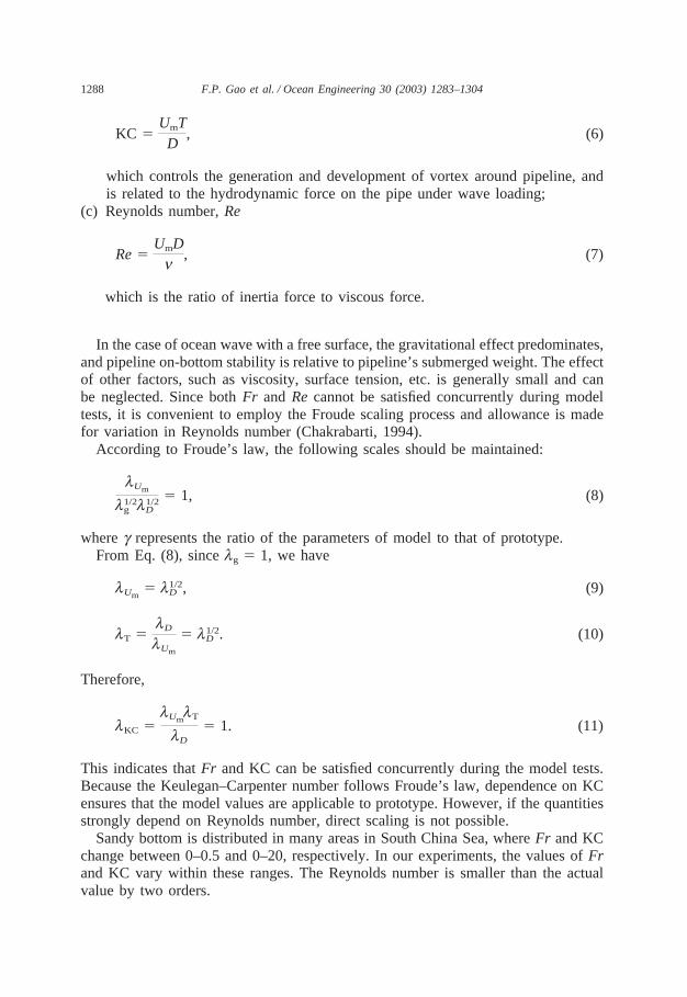
1288 F.P. Gao et al. / Ocean Engineering 30 (2003) 1283–1304
KC �UmT
D, (6)
which controls the generation and development of vortex around pipeline, andis related to the hydrodynamic force on the pipe under wave loading;
(c) Reynolds number, Re
Re �UmDn
, (7)
which is the ratio of inertia force to viscous force.
In the case of ocean wave with a free surface, the gravitational effect predominates,and pipeline on-bottom stability is relative to pipeline’s submerged weight. The effectof other factors, such as viscosity, surface tension, etc. is generally small and canbe neglected. Since both Fr and Re cannot be satisfied concurrently during modeltests, it is convenient to employ the Froude scaling process and allowance is madefor variation in Reynolds number (Chakrabarti, 1994).
According to Froude’s law, the following scales should be maintained:
lUm
l1/2g l1/2
D
� 1, (8)
where g represents the ratio of the parameters of model to that of prototype.From Eq. (8), since lg � 1, we have
lUm� l1/2
D , (9)
lT �lD
lUm
� l1/2D . (10)
Therefore,
lKC �lUmlT
lD
� 1. (11)
This indicates that Fr and KC can be satisfied concurrently during the model tests.Because the Keulegan–Carpenter number follows Froude’s law, dependence on KCensures that the model values are applicable to prototype. However, if the quantitiesstrongly depend on Reynolds number, direct scaling is not possible.
Sandy bottom is distributed in many areas in South China Sea, where Fr and KCchange between 0–0.5 and 0–20, respectively. In our experiments, the values of Frand KC vary within these ranges. The Reynolds number is smaller than the actualvalue by two orders.

1289F.P. Gao et al. / Ocean Engineering 30 (2003) 1283–1304
2.3. Testing materials
2.3.1. SoilsBecause of the proximity of the pipeline to the seafloor, the modeling of soil
characteristic of the foundation may be important. The sand beds consist of mediumsand and fine sand. The index properties of the sands are shown in Table 1. Themoist sand is first saturated, then packed in the soil box under water, and finallytrimmed with a scraper. The difference of the unit weights for different tests iscontrolled within the error of 5‰.
2.3.2. PipelinesThe pipe model spans the soil surface vertically to the direction of oscillatory flow,
as shown in Fig. 3. The length of the pipe model should be sufficient to minimize theending effects. To simulate the two dimensional problem, the pipe ends are close tothe vertical walls of U-shaped tunnel. In the experiments, the gaps between pipeends and the U-shaped tunnel walls are about 5 mm. Thus, scouring at the end ofthe pipe model is not considered a problem, which has been proved in the tests.
The submarine pipeline generally has a large span so that the pipeline model maybe treated as a two-dimensional structure. The submerged weight of pipeline directlydetermines the contact force between pipeline and seabed, and further affects on-bottom stability around the pipeline.
The weight of the pipe is adjusted to model the typical submerged weight of actualpipeline, according to the similarity parameter G, i.e.
G �Ws
g�D2, (12)
where, g� is buoyant unit weight of soil, g� � (rsat�rw)g. That is, the model andprototype can be expressed by
G �(Ws)p
g�pD2p
�(Ws)m
g�mD2m
, (13)
where the subscripts p and m stand for prototype and model, respectively. The testing
Table 1Index properties of the test sands
Mean grain Grain size at Uniformity Unit weight, Dry unit Initial void Relativesize, d50 which 10% coefficient, Cu g(kN/m3) weight, ratio, e0 density, Dr
(mm) of the soil gd(kN/m3)weight isfiner, d10
(mm)
0.38 0.30 1.4 19.00 14.80 0.73 0.370.21 0.11 2.0 21.05 17.47 0.56 0.60

1290 F.P. Gao et al. / Ocean Engineering 30 (2003) 1283–1304
pipes are composed of aluminum, with length of 0.19 m. The pipes are divided intothree groups with different diameters: 0.014, 0.020 and 0.030 m. In each group,pipes have different weights. The diameter D and submerged weight Ws of test pipesare listed in Table 2.
According to dimensional analysis, Eq. (13) can also be expressed as
lWs
lg�l2D
� 1. (14)
When lg� � 1, then the ratio of the pipeline submerged weight of model to that ofprototype is
lWs� l2
D. (15)
Due to the pipe weight and the operation reason, some initial embedment alwaysdoes exist, although the amount of embedment is very small. Conventionally,e /D � 0.03-0.05, where e is pipe initial embedment.
2.4. Testing procedures
To explore the mechanism of pipeline instability induced by rapidly increasingstorm wave, a constant velocity of oscillatory flow amplitude A0, A0 �9 × 10�3cm/s, was adopted first in the experiments.
From Eq. (4), the velocity of oscillatory flow can be deduced
U(t) � A0(t)sinwt � wA0coswt. (16)
Table 2The parameters of test pipes
Case I Case II
Pipe Submerged Pipe Submerged Pipe Submerged Pipe Submergeddiameter, weight, Ws diameter, weight, Ws diameter, weight, Ws diameter, weight, Ws
D (m) (N/m) D (m) (N/m) D (m) (N/m) D (m) (N/m)
0.030 1.52 0.020 1.09 0.030∗ 1.61 0.030 1.510.030 2.00 0.020 1.35 0.030∗ 2.00 0.030 2.040.030 2.40 0.020 1.54 0.030∗ 2.40 0.030 2.590.030 3.12 0.020 1.72 0.030∗ 3.12 0.030 2.940.030 3.53 0.020 1.97 0.030∗ 3.53 0.020 0.780.030 3.93 0.014 0.78 0.030∗ 3.93 0.020 0.980.030 4.22 0.014 0.89 0.030∗ 4.22 0.020 1.120.030 4.40 0.014 1.05 0.030∗ 4.50 0.020 1.290.030 5.00 0.014 1.21 0.030∗ 5.000.030 5.24 0.030∗ 5.29
∗Fine sand; others—medium sand.

1291F.P. Gao et al. / Ocean Engineering 30 (2003) 1283–1304
Fig. 4. Pipe displacement-time curves.
In the experiments, A0(t) is in the order of 10�1 (m), thus A0 /wA0 � 0(10�3). There-fore, the maximum water particle velocity of the oscillating flow Um is as follows:
Um � wA0(t). (17)
In other words, the maximum water particle velocity is mainly relative to the anglevelocity and the current flow amplitude.
Furthermore, since the storm growing is not always continuous, it is necessary toexamine the effects of loading history on pipeline instability, which will be describedin Section 3.3.
During the experiments, the water level change was recorded with a water differen-tial pressure transducer and data acquisition system.
3. Experiment results
3.1. Pipeline instability process
When the amplitude of oscillatory flow A0 increases continuously with a constantvelocity, the pipeline displacements are recorded (see Fig. 4). The following threecharacteristic times can be identified in the pipeline instability process:
1. t � ts: At a certain distance apart from the pipe, the sand grains at the bed surfacestart to move visibly. Onset of scour occurs (see Fig. 5). When the water particle
Fig. 5. Onset of sand scouring.
1292 F.P. Gao et al. / Ocean Engineering 30 (2003) 1283–1304
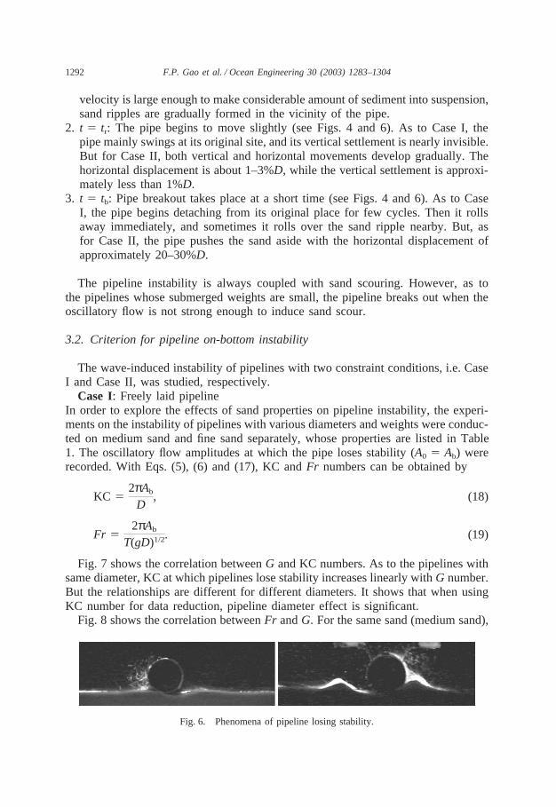
velocity is large enough to make considerable amount of sediment into suspension,sand ripples are gradually formed in the vicinity of the pipe.
2. t � tr: The pipe begins to move slightly (see Figs. 4 and 6). As to Case I, thepipe mainly swings at its original site, and its vertical settlement is nearly invisible.But for Case II, both vertical and horizontal movements develop gradually. Thehorizontal displacement is about 1–3%D, while the vertical settlement is approxi-mately less than 1%D.
3. t � tb: Pipe breakout takes place at a short time (see Figs. 4 and 6). As to CaseI, the pipe begins detaching from its original place for few cycles. Then it rollsaway immediately, and sometimes it rolls over the sand ripple nearby. But, asfor Case II, the pipe pushes the sand aside with the horizontal displacement ofapproximately 20–30%D.
The pipeline instability is always coupled with sand scouring. However, as tothe pipelines whose submerged weights are small, the pipeline breaks out when theoscillatory flow is not strong enough to induce sand scour.
3.2. Criterion for pipeline on-bottom instability
The wave-induced instability of pipelines with two constraint conditions, i.e. CaseI and Case II, was studied, respectively.
Case I: Freely laid pipelineIn order to explore the effects of sand properties on pipeline instability, the experi-ments on the instability of pipelines with various diameters and weights were conduc-ted on medium sand and fine sand separately, whose properties are listed in Table1. The oscillatory flow amplitudes at which the pipe loses stability (A0 � Ab) wererecorded. With Eqs. (5), (6) and (17), KC and Fr numbers can be obtained by
KC �2πAb
D, (18)
Fr �2πAb
T(gD)1/2. (19)
Fig. 7 shows the correlation between G and KC numbers. As to the pipelines withsame diameter, KC at which pipelines lose stability increases linearly with G number.But the relationships are different for different diameters. It shows that when usingKC number for data reduction, pipeline diameter effect is significant.
Fig. 8 shows the correlation between Fr and G. For the same sand (medium sand),
Fig. 6. Phenomena of pipeline losing stability.

1293F.P. Gao et al. / Ocean Engineering 30 (2003) 1283–1304
Fig. 7. KC and G correlation (Case I).
Fig. 8. Fr and G correlation for medium sand (Case I).
all the data with different pipe diameters fall within the range with the same linearrelationship. There is a good correlation between the Fr number and the G numberregardless of the pipeline diameter. It matches with the point of Chakrabarti (1994)and Poorooshasb (1990), which indicates the importance of Fr in case of water–structure–soil interaction. However, there exists some difference between the resultsfor medium sand and fine sand, as shown in Figs. 7 and 8. That is, the sand character-istics influence pipeline stability.
Case II: Anti-rolling pipelineWith the designed anti-rolling device (Fig. 3), experiments were conducted on

1294 F.P. Gao et al. / Ocean Engineering 30 (2003) 1283–1304
Fig. 9. KC and G correlation (Case II).
medium sand for pipelines with different diameters, i.e. D � 0.030,0.020m, as wellas different submerged weight. As the experiments on pipelines were freely laid, theoscillatory flow amplitude also rises at the same speed A0.
Fig. 9 shows the correlation between G and KC numbers for Case II. Similar toCase I, for the pipelines with same diameter, KC at which pipelines lose stabilityincreases linearly with G number, but pipeline diameter effect is also very obvious.
Fig. 10 shows the correlation between Fr and G for Case II. All the data withdifferent pipe diameters fall within the range with the same linear relationship, asCase I shown in Fig. 10.
Herein, it should be mentioned that the experiment results are obtained under the
Fig. 10. Fr and G correlation (Case II).
1295F.P. Gao et al. / Ocean Engineering 30 (2003) 1283–1304
condition of the oscillatory flow amplitude rising at the same speed A0. As to thepipelines with different submerged weights, the Fr number at which pipelines losestability are different. Thus, the oscillating time (t /T) is different in different experi-ments. Their ranges for Case I and Case II are about 80–300, 170–230, respectively.Under the oscillating actions, the effective stress field and pore-pressure field willchange with time. When the oscillatory flow velocity exceeds a certain value, thesand beside pipeline is scoured under the influence of vortexes. The sand ripples areformed step by step. They will affect the flow field near pipeline and even influencepipeline instability.
In addition, the Fr–G relationships for the two constrains are obtained within thecertain range of non-dimensional parameter G. As mentioned, KC can be satisfiedconcurrently with Fr during model tests. The KC range in the experiments is about5–20.
3.3. Effects of loading history
In the aforementioned experiments, the same wave loading method was adoptedto examine the instability induced by rapidly increasing storm. However, real stormwave events are unpredictable and the field conditions are often characterized withsignificant uncertainty. Thus, it is also very necessary to study the effects of loadinghistory upon the pipeline instability.
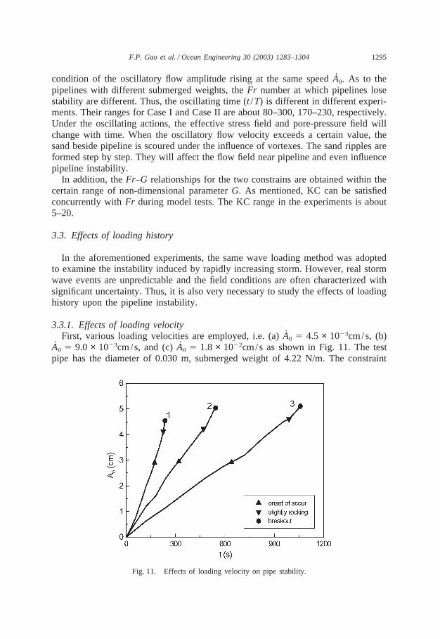
3.3.1. Effects of loading velocityFirst, various loading velocities are employed, i.e. (a) A0 � 4.5 × 10�3cm/s, (b)
A0 � 9.0 × 10�3cm/s, and (c) A0 � 1.8 × 10�2cm/s as shown in Fig. 11. The testpipe has the diameter of 0.030 m, submerged weight of 4.22 N/m. The constraint
Fig. 11. Effects of loading velocity on pipe stability.
1296 F.P. Gao et al. / Ocean Engineering 30 (2003) 1283–1304
condition is chosen as Case I. The test sand is a kind of medium sand, whose proper-ties are listed in Table 1.
Fig. 11 shows that with the increase of A0, the oscillatory flow amplitude at whichthe pipe rocks slightly and the amplitude at which pipe loses stability increase,respectively, but the amplitude of oscillatory flow-induced sand scouring is affec-ted slightly.
Experimental observation indicates that the smaller the A0, the higher the sanddune is formed beside the pipe, at the time when the pipe is losing stability. Asanalyzed in Section 2.3, A0�Um, thus the change of A0 is quasi-static at specificvalue of Um (or A0). Various A0 represents somehow the different oscillating times(t /T) at the vicinity of certain value of Um. Therefore, the loading velocity (or theoscillating times) affects the sand scouring around pipe and eventually has influenceon the stability of pipe.
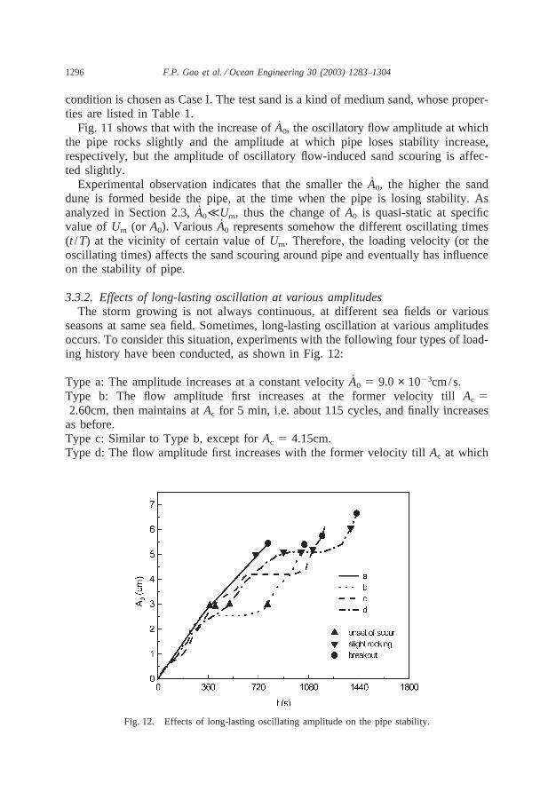
3.3.2. Effects of long-lasting oscillation at various amplitudesThe storm growing is not always continuous, at different sea fields or various
seasons at same sea field. Sometimes, long-lasting oscillation at various amplitudesoccurs. To consider this situation, experiments with the following four types of load-ing history have been conducted, as shown in Fig. 12:
Type a: The amplitude increases at a constant velocity A0 � 9.0 × 10�3cm/s.Type b: The flow amplitude first increases at the former velocity till Ac �2.60cm, then maintains at Ac for 5 min, i.e. about 115 cycles, and finally increases
as before.Type c: Similar to Type b, except for Ac � 4.15cm.Type d: The flow amplitude first increases with the former velocity till Ac at which
Fig. 12. Effects of long-lasting oscillating amplitude on the pipe stability.
1297F.P. Gao et al. / Ocean Engineering 30 (2003) 1283–1304
the pipe rocks slightly, then maintains at Ac 115 cycles, and finally increases asbefore.
Fig. 12 indicates that when long-lasting oscillatory amplitude Ac is less than thatof onset of scour As (Type b), it nearly does not have influence on the pipe stability.When Ac � As (Types c, d), due to the effect of vortex, the sand grains pile up onboth sides of the pipe, thereby the long-lasting oscillation increases the stability ofpipeline. Furthermore, the pipe’s slight rocking is not always followed by losingstability. If the flow amplitude does not rise after pipe begins to slightly rock, thepipe will return to the static condition again and more sediment is observed pilingbeside the pipe (Type d). After the flow amplitude increases to some higher level,the pipe slightly rocks again, and loses stability at higher flow amplitude.
All the types mentioned above imply that the wave-induced pipe instability iscoupled with the sand scouring around pipe, and some intermittently growing stormcould be beneficial for the pipe stability.
4. Comparison with previous experiments
The above experimental results show that, under the action of rapidly rising wave-induced loading, there exist different linear relationships between Fr and G numbersfor freely laid pipelines and anti-rolling pipelines, respectively. As to the mediumsands, the least square fitting equations of the data in Figs. 8 and 10, can be given as
Um
(gD)1/2 (20)
� � 0.043 � 0.37Ws
g’D2�0.18 �Ws
g’D2 � 0.65� freely laid pipes
0.069 � 0.62Ws
g’D2�0.18 �Ws
g’D2 � 0.36� anti-rolling pipes
The equations give the relationships between water particle velocity, soil properties,pipe diameter and submerged weight of the pipe. All the parameters involved haveobvious physical meaning. This line can be regarded as the critical line for pipe on-bottom instability.
However, in the previous experiments (Allen et al., 1989; Brennodden et al., 1986;Wagner et al., 1987; Brennodden et al., 1989), mechanical actuator was used tosimulate the real hydrodynamic forces upon pipelines. So the pipe–soil interactionmodels obtained by the experiments do not include wave parameters (see Eqs. (1),(2) and (3)). In order to compare with the previous experiment results, the calculationof hydrodynamic forces induced by waves on pipeline is essential.
1298 F.P. Gao et al. / Ocean Engineering 30 (2003) 1283–1304
4.1. Calculation of the wave-induced forces upon pipeline with Wake II model
Historically, the wave-induced forces upon submarine pipeline used to be calcu-lated with an adaptation of Morison’s equation for both horizontal and vertical or alift force taken to be proportional to the ambient velocity squared. However, it hasbeen recognized that in the force model, the ambient velocity should be modifiedunder the consideration of wake flow. Measurements showed that Morison’s equationis lacking in its ability to predict the details in shape and magnitude of force time his-tory.
Soedigdo et al. (1999) proposed a Wake II model, in which wake velocity correc-tion was derived based on a closed-form solution to the linearized Navier–Stokesmodel for oscillatory flow and hydrodynamic forces’ coefficients were determinedbased on start-up effects. Wake II model can be used for stability design calculationsfor pipelines on the seabed for regular waves without currents for various diameters.Sabag et al. (2000) pointed out that the Wake II model fits well with experimentresults, and it is a great improvement on Morison’s equation. The Wake II modelis summarized in Appendix A.
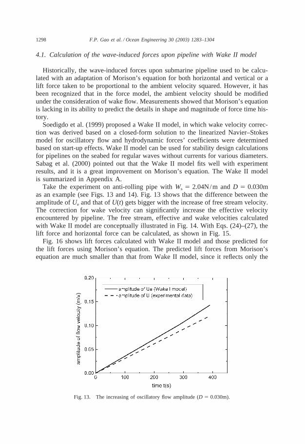
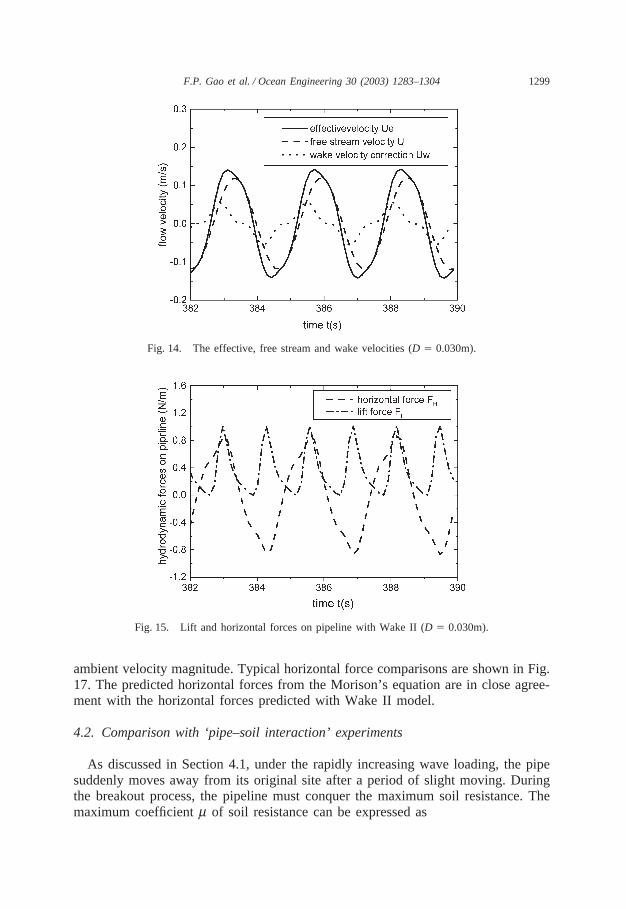
Take the experiment on anti-rolling pipe with Ws � 2.04N/m and D � 0.030mas an example (see Figs. 13 and 14). Fig. 13 shows that the difference between theamplitude of Ue and that of U(t) gets bigger with the increase of free stream velocity.The correction for wake velocity can significantly increase the effective velocityencountered by pipeline. The free stream, effective and wake velocities calculatedwith Wake II model are conceptually illustrated in Fig. 14. With Eqs. (24)–(27), thelift force and horizontal force can be calculated, as shown in Fig. 15.
Fig. 16 shows lift forces calculated with Wake II model and those predicted forthe lift forces using Morison’s equation. The predicted lift forces from Morison’sequation are much smaller than that from Wake II model, since it reflects only the
Fig. 13. The increasing of oscillatory flow amplitude (D � 0.030m).
1299F.P. Gao et al. / Ocean Engineering 30 (2003) 1283–1304
Fig. 14. The effective, free stream and wake velocities (D � 0.030m).
Fig. 15. Lift and horizontal forces on pipeline with Wake II (D � 0.030m).
ambient velocity magnitude. Typical horizontal force comparisons are shown in Fig.17. The predicted horizontal forces from the Morison’s equation are in close agree-ment with the horizontal forces predicted with Wake II model.
4.2. Comparison with ‘pipe–soil interaction’ experiments
As discussed in Section 4.1, under the rapidly increasing wave loading, the pipesuddenly moves away from its original site after a period of slight moving. Duringthe breakout process, the pipeline must conquer the maximum soil resistance. Themaximum coefficient m of soil resistance can be expressed as

1300 F.P. Gao et al. / Ocean Engineering 30 (2003) 1283–1304
Fig. 16. Lift forces with Morison’s equation and Wake II model (D � 0.030m).
Fig. 17. Horizontal forces with Morison’s equation and Wake II model (D � 0.030m).
m � � FH(t)Ws�FL(t)�max
, (21)
where FH(t) and FL(t) are calculated with Eqs. (25) and (27), respectively. Thus,given the ambient velocities during the full period of pipe’s losing stability, themaximum value of soil resistance can be obtained.
The maximum values of soil resistance for anti-rolling pipelines on medium sand

1301F.P. Gao et al. / Ocean Engineering 30 (2003) 1283–1304
Fig. 18. Comparison with pipe–soil interaction experiment results of Wagner et al. (1987).
are shown in Fig. 18, together with that in previous pipe–soil interaction experimentresults of Wagner et al. (1987). Typical test results of Brennodden et al. (1986) aregiven in Fig. 19. The average value of soil resistance in our experiments is about0.83, which is larger than the value obtained in previous pipe–soil interaction experi-ments. In the present experiments, the medium sand is moderate dense, whose rela-tive density is 0.37. Therefore, though our experiments are conducted with differentloading style from previous pipe–soil interaction experiments, their results are com-parable with the latter and more reasonable in the mechanism aspects for reflectingthe coupling of wave–pipe–soil. Because of the insufficiency of the test data, thefinal model has not been obtained yet, but the relationships imply that they can serveas a supplementary analysis tool for pipeline stability.
Fig. 19. Typical test results of Brennodden et al. (1986).
1302 F.P. Gao et al. / Ocean Engineering 30 (2003) 1283–1304
5. Conclusions
Different from the previous experiments, U-shaped oscillatory flow tunnel isemployed to investigate the wave-induced submarine pipeline instability in thispaper. From the results presented above, the following conclusions can be made:
1. Froude number (Fr) and the non-dimensional pipe weight (G) are two mostimportant parameters in modeling wave-induced instability of untrenched pipeline.Based on the experimental results, different linear relationships between Fr andG have been obtained for pipes with different restraint conditions, i.e. (a) freelylaid pipelines and (b) anti-rolling pipelines. Moreover, three characteristic timesin the process of the pipe’s losing stability are revealed.
2. Based on Wake II model, the current wave–soil–pipe interaction test results andthe results of previous pipe–soil interaction tests are compared. It is indicated thatthe results of the two types of tests are comparable. The obtained Fr–G relation-ships can be used for supplementary analysis of criterion for pipeline instabilityin design procedure.
3. In consideration of the actual field conditions, different loading histories are usedto explore the effects of them on the pipeline instability. It is found that thescouring of sand beside the pipeline is the main result of the different loadinghistories, and affects the pipeline stability eventually.
4. Sand scour, as an indicator of the wave–soil–pipe coupling, is detected in ourexperiments. But, in the previous experiments with actuator, it could not be mod-eled. Therefore, the current hydrodynamic experiments are more reasonable in themechanism aspects, which reflect the wave–soil–pipeline coupling effects.
Acknowledgements
This study was jointly supported by the Chinese National Scientific FoundationProjects (19772057) and the key project of the Ninth 5-year Plan of Chinese Acad-emy of Sciences (KZ951-A1-405-01). This work was also supported by ARC SmallGrant (2001) at Griffith University.
Appendix A. Wake II model
Wake II model proposed by Soedigdo et al. (1999) is a hydrodynamic force modelfor prediction of forces on pipelines. The wake and start-up effects are consideredin the model.
The wake velocity correction is corrected by using a closed-form solution to thelinearized Navier–Stokes equations for oscillatory flow. By assuming that the eddy

1303F.P. Gao et al. / Ocean Engineering 30 (2003) 1283–1304
viscosity in the wake is only time dependent and of harmonic sinusoidal form, thewake velocity correction affecting pipe in periodic flow can be derived as
Uw(t) �
(p)1/2erf�12C2sinn(w t � f)�UmC1
C2
, (22)
where C1, C2, f and n are empirical parameters relative to current KC number, asshown in Fig. 20. The effective velocity Ue can be determined as the sum of thefree stream velocity U(t) and the wake velocity correction Uw(t) as
Ue(t) � U(t) � Uw(t). (23)
When the effective velocity is known, the force model expressions for the drag,lift and inertial forces are:
Drag force: FD � 0.5rwDCD(t)�Ue�Ue, (24)
Lift force: FL � 0.5rwDCL(t)U2e, (25)
Inertia force: FI �πD2
4rw�CM
dUdt
�CAW
dUw
dt �. (26)
Fig. 20. Effect of KC on parameters C1, C2, f and n (Soedigdo et al., 1999).
1304 F.P. Gao et al. / Ocean Engineering 30 (2003) 1283–1304
The horizontal hydraulic force is the sum of drag force and inertia force
FH � FD � FI, (27)
where CM is the inertia coefficient for ambient velocity, CM � 2.5; CAM the addedmass coefficient associated with the wake flow passing the pipe, CAM � 0.25; andCD(t), CL(t) are time dependent drag and lift coefficients, respectively and can bedetermined by the so-called ‘start-up’ function, which is relative to the distance thewater particle travels after a zero crossing in the total effective velocity.
References
Allen, D.W., Lammert, W.F., Hale, J.R., Jacobsen, V., 1989. Submarine pipeline on-bottom stability:recent AGA research. Proc. Offshore Technol. Conf., OTC 6055, 121–132.
Brennodden, H., Lieng, J.T., Sotberg, T., Verley, R.L.P., 1989. An energy-based pipe–soil interactionmodel. Proc. Offshore Technol. Conf., OTC 6057, 147–158.
Brennodden, H., Sveggen, O., Wagner, D.A., Murff, J.D., 1986. Full-scale pipe–soil interaction tests.Proc. Offshore Technol. Conf., OTC 5338, 433–440.
Chakrabarti, K., 1994. Offshore Structure Modeling. JBW Printers & Binder Pte Ltd, Southampton, Bos-ton.
Chiew, Y.M., 1990. Mechanics of local scour around submarine pipelines. J. Hydraulic Eng. 116, 515–529.
Det norske Veritas, 1988. On-bottom stability design of submarine pipelines, Recommended PracticeE305.
Hale, J.R., Lammert, W.F., Allen, D.W., 1991. Pipeline on-bottom stability calculations: comparison oftwo state-of-the-art methods and pipe–soil model verification. Proc. Offshore Technol. Conf., OTC6761, 567–581.
Herbich, J.B., 1985. Hydromechanics of submarine pipelines: design problems. Can. J. Civil Eng. 12,863–874.
Lyons, C.G., 1973. Soil resistance to lateral sliding of marine pipelines. Proc. Offshore Technol. Conf.,OTC 1876, 479–484.
Mao, Y., 1988. Seabed scours under pipelines. In: Proceedings of the Seventh International Symposiumon Offshore Mechanics and Arctic Engineering (OMAE), pp. 33–38.
Poorooshasb, F., 1990. On centrifuge use for ocean research. Mar. Geotechnol. 9, 141–158.Sabag, S.R., Edge, B.L., Soedigdo, I.R., 2000. Wake II model for hydrodynamic forces on marine pipe-
lines including waves and currents. Ocean Eng. 27, 1295–1319.Soedigdo, I.R., Lambrakos, K.F., Edge, B.L., 1999. Predicton of hydrodynamic forces on submarine
pipelines using an improved wake II model. Ocean Eng. 26, 431–462.Sumer, B.M., Fredsoe, J., 1991. Onset of scour below a pipeline exposed to waves. Int. J. Offshore Polar
Eng. 1, 189–194.Wagner, D.A., Murff, J.D., Brennodden, H., Sveggen, O., 1987. Pipe–soil interaction model. Proc. Off-
shore Technol. Conf., OTC 5504, 181–190.