Physical interpretation of coarse-grained bead …...Physical interpretation of coarse-grained...

Physical interpretation of coarse-grained bead-spring models

of complex fluids

by

Kirill Titievsky

Submitted to the Department of Chemical Engineeringin partial fulfillment of the requirements for the degree of

Doctor of Philosophy

at the

MASSACHUSETTS INSTITUTE OF TECHNOLOGY

February 2009

c© Massachusetts Institute of Technology 2009. All rights reserved.

Author . . . . . . . . . . . . . . . . . . . . . . . . . . . . . . . . . . . . . . . . . . . . . . . . . . . . . . . . . . . . . . . . . . . . . . . . . . . .Department of Chemical Engineering

Jan 14, 2009

Certified by. . . . . . . . . . . . . . . . . . . . . . . . . . . . . . . . . . . . . . . . . . . . . . . . . . . . . . . . . . . . . . . . . . . . . . . .Gregory C. Rutledge

Lammot du Pont Professor of Chemical EngineeringThesis Supervisor

Certified by. . . . . . . . . . . . . . . . . . . . . . . . . . . . . . . . . . . . . . . . . . . . . . . . . . . . . . . . . . . . . . . . . . . . . . . .Paul I. Barton

Lammot du Pont Professor of Chemical EngineeringThesis Supervisor

Accepted by . . . . . . . . . . . . . . . . . . . . . . . . . . . . . . . . . . . . . . . . . . . . . . . . . . . . . . . . . . . . . . . . . . . . . . .William M. Deen

Chairman, Department Committee on Graduate Theses

Physical interpretation of coarse-grained bead-spring models of complex

fluids

by

Kirill Titievsky

Submitted to the Department of Chemical Engineeringon Jan 14, 2009, in partial fulfillment of the

requirements for the degree ofDoctor of Philosophy

Abstract

Bulk properties and morphology of block copolymers and polymer blends are highly sen-sitive to processing history due to small free energy differences among various stable andmetastable states. Consequently, modeling these materials requires accounting for boththermal fluctuations and non-equilibrium processes. This has proven to be challengingwith traditional approaches of energy minimization and perturbation in field theories. Atthe same time, simulations of highly coarse-grained particle-based models, such as latticechain Monte Carlo and bead-spring simulations, have emerged as a promising alternative.The application of these methods, however, has been hampered by a lack of clear physicalinterpretation of model parameters.

This dissertation gives a rigorous interpretation to such coarse-grained models. First,a general thermodynamic approach to analyzing and comparing coarse-grained particlemodels is developed. Second, based on the analysis, a specific particle-based model is con-structed so that it is unambiguously related to the standard Gaussian chain model andrelated field theories at realistic molecular weights. This model is complementary to fieldtheoretic polymer simulations, which are computationally prohibitive for realistic molec-ular weights. Several applications of the model are demonstrated, including: fluctuationcorrections to mean-field theories of block copolymers as well as a detailed investigation ofthe key effects governing the self-assembly of diblock copolymers confined in cylinders suchas fibers or pores. The latter application introduces a novel impenetrable wall boundarymodel designed to attenuate effects of the walls on the total monomer density. The generalapproach and the specific models proposed here will find immediate application in modelingeffects of flow, metastability, and thermal fluctuations on the morphology of complex fluidswith molecular weights of 104 − 106 g/mol using lattice and continuous space molecularsimulations.

Thesis Supervisor: Gregory C. RutledgeTitle: Lammot du Pont Professor of Chemical Engineering

Thesis Supervisor: Paul I. BartonTitle: Lammot du Pont Professor of Chemical Engineering

3

Acknowledgments

This thesis is a culmination of efforts by many people. I am grateful more than I can say

to:

Greg Rutledge for patiently trying and succeeding, despite my best efforts, in teaching

me what I know about how science is done.

Ken Beers for teaching me to solve problems numerically.

Paul Barton for giving me a chance to be a part of his fantastic reseach group, as brief

as my stay was.

Ed Feng for sympathyzing actively.

Erik Allen, Thierry Savin, Sam Ngai, Frederyk Ngantung for inspiration and company.

My grandmother, Dozya Titievsky, for letting me take my chances.

My grandfather, Aleksandr Tsitrin, for teaching me patience.

My gradmother, Dina Semenchyuk, for teaching me discipline.

My dad, Aleksey Titievsky, for making me curious.

My mom, Anna Titievskaya, for reminding me to stay human.

Rosemary, Leo, and Lola for being constant sources of happiness.

5

Contents

1 Introduction 19

1.1 Motivation . . . . . . . . . . . . . . . . . . . . . . . . . . . . . . . . . . . . 19

1.2 Objectives . . . . . . . . . . . . . . . . . . . . . . . . . . . . . . . . . . . . . 21

1.3 Approach . . . . . . . . . . . . . . . . . . . . . . . . . . . . . . . . . . . . . 21

1.4 Overview . . . . . . . . . . . . . . . . . . . . . . . . . . . . . . . . . . . . . 22

2 Background 25

2.1 Notation and conventions . . . . . . . . . . . . . . . . . . . . . . . . . . . . 25

2.2 The Gaussian chain model . . . . . . . . . . . . . . . . . . . . . . . . . . . . 25

2.2.1 Formal definition . . . . . . . . . . . . . . . . . . . . . . . . . . . . . 26

2.2.2 Physical reasoning behind GCM . . . . . . . . . . . . . . . . . . . . 27

2.2.3 Evaluating the GCM model . . . . . . . . . . . . . . . . . . . . . . . 28

2.3 Explicit chain simulations . . . . . . . . . . . . . . . . . . . . . . . . . . . . 32

2.3.1 Definition and specific examples . . . . . . . . . . . . . . . . . . . . 32

2.3.2 Single chain in mean field (SCMC) simulations . . . . . . . . . . . . 33

2.3.3 Parametrization approaches . . . . . . . . . . . . . . . . . . . . . . . 34

2.4 Key results . . . . . . . . . . . . . . . . . . . . . . . . . . . . . . . . . . . . 36

2.4.1 Qualitative phase behavior . . . . . . . . . . . . . . . . . . . . . . . 36

2.4.2 Quantitative features . . . . . . . . . . . . . . . . . . . . . . . . . . . 37

2.5 Remaining problems and opportunities . . . . . . . . . . . . . . . . . . . . . 37

2.5.1 Non-equilibrium simulations . . . . . . . . . . . . . . . . . . . . . . . 37

2.5.2 Inconsistencies in Flory-Huggins χ values . . . . . . . . . . . . . . . 38

2.5.3 Difficulty in sampling fluctuations . . . . . . . . . . . . . . . . . . . 39

7

2.5.4 Regularization . . . . . . . . . . . . . . . . . . . . . . . . . . . . . . 39

3 Mixtures of interacting particles with well-defined Flory-Huggins χ mis-

cibility parameters 41

3.1 Introduction . . . . . . . . . . . . . . . . . . . . . . . . . . . . . . . . . . . . 41

3.2 Background and definitions . . . . . . . . . . . . . . . . . . . . . . . . . . . 44

3.3 Theory . . . . . . . . . . . . . . . . . . . . . . . . . . . . . . . . . . . . . . . 45

3.3.1 Connecting field and particle models . . . . . . . . . . . . . . . . . . 45

3.3.2 Composition independent χ . . . . . . . . . . . . . . . . . . . . . . . 49

3.3.3 Dependence of χ on composition . . . . . . . . . . . . . . . . . . . . 50

3.3.4 Questions for simulations . . . . . . . . . . . . . . . . . . . . . . . . 52

3.4 Methods . . . . . . . . . . . . . . . . . . . . . . . . . . . . . . . . . . . . . . 54

3.4.1 Potentials . . . . . . . . . . . . . . . . . . . . . . . . . . . . . . . . . 54

3.4.2 Determination of coexistence curves . . . . . . . . . . . . . . . . . . 54

3.4.3 Mixture with externally imposed field . . . . . . . . . . . . . . . . . 55

3.4.4 Results . . . . . . . . . . . . . . . . . . . . . . . . . . . . . . . . . . 56

3.4.5 Non-local effects . . . . . . . . . . . . . . . . . . . . . . . . . . . . . 58

3.5 Discussion . . . . . . . . . . . . . . . . . . . . . . . . . . . . . . . . . . . . . 59

3.6 Conclusions . . . . . . . . . . . . . . . . . . . . . . . . . . . . . . . . . . . . 62

3.7 Appendix . . . . . . . . . . . . . . . . . . . . . . . . . . . . . . . . . . . . . 63

3.7.1 Non-local corrections to χ . . . . . . . . . . . . . . . . . . . . . . . . 63

3.7.2 Special case of sinusoidal composition fields . . . . . . . . . . . . . . 63

4 A bead-spring polymer model with well-defined Flory-Huggins miscibility

and chain density 67

4.1 Introduction . . . . . . . . . . . . . . . . . . . . . . . . . . . . . . . . . . . . 68

4.2 Theory . . . . . . . . . . . . . . . . . . . . . . . . . . . . . . . . . . . . . . . 70

4.2.1 Particle and field models . . . . . . . . . . . . . . . . . . . . . . . . . 70

4.2.2 Miscibility . . . . . . . . . . . . . . . . . . . . . . . . . . . . . . . . . 72

4.2.3 Compressibility . . . . . . . . . . . . . . . . . . . . . . . . . . . . . . 78

4.2.4 Bond model . . . . . . . . . . . . . . . . . . . . . . . . . . . . . . . . 78

4.3 Methods . . . . . . . . . . . . . . . . . . . . . . . . . . . . . . . . . . . . . . 79

4.4 Results . . . . . . . . . . . . . . . . . . . . . . . . . . . . . . . . . . . . . . . 82

8

4.4.1 Bond model . . . . . . . . . . . . . . . . . . . . . . . . . . . . . . . . 82

4.4.2 Miscibility model . . . . . . . . . . . . . . . . . . . . . . . . . . . . . 85

4.4.3 Comparison to experimental results . . . . . . . . . . . . . . . . . . 90

4.5 Discussion . . . . . . . . . . . . . . . . . . . . . . . . . . . . . . . . . . . . . 93

4.6 Conclusions . . . . . . . . . . . . . . . . . . . . . . . . . . . . . . . . . . . . 98

5 Concentric lamellar phase of block copolymers confined in cylinders 99

5.1 Background and introduction . . . . . . . . . . . . . . . . . . . . . . . . . . 100

5.2 Definitions . . . . . . . . . . . . . . . . . . . . . . . . . . . . . . . . . . . . . 102

5.3 Simulation method . . . . . . . . . . . . . . . . . . . . . . . . . . . . . . . . 104

5.3.1 Energy model . . . . . . . . . . . . . . . . . . . . . . . . . . . . . . . 104

5.3.2 Boundary model . . . . . . . . . . . . . . . . . . . . . . . . . . . . . 106

5.3.3 Equilibration and sampling . . . . . . . . . . . . . . . . . . . . . . . 107

5.4 Results . . . . . . . . . . . . . . . . . . . . . . . . . . . . . . . . . . . . . . . 108

5.4.1 Domain size and shape . . . . . . . . . . . . . . . . . . . . . . . . . . 108

5.4.2 Chain conformation . . . . . . . . . . . . . . . . . . . . . . . . . . . 115

5.4.3 Interfaces . . . . . . . . . . . . . . . . . . . . . . . . . . . . . . . . . 117

5.5 Narrow interphase theory . . . . . . . . . . . . . . . . . . . . . . . . . . . . 119

5.5.1 Interfacial energy . . . . . . . . . . . . . . . . . . . . . . . . . . . . . 120

5.5.2 Tangential compression due to curvature . . . . . . . . . . . . . . . . 122

5.5.3 Normal chain stretching . . . . . . . . . . . . . . . . . . . . . . . . . 125

5.5.4 Symmetry breaking . . . . . . . . . . . . . . . . . . . . . . . . . . . 127

5.6 Discussion . . . . . . . . . . . . . . . . . . . . . . . . . . . . . . . . . . . . . 128

5.7 Conclusions . . . . . . . . . . . . . . . . . . . . . . . . . . . . . . . . . . . . 130

5.8 Appendix . . . . . . . . . . . . . . . . . . . . . . . . . . . . . . . . . . . . . 130

5.8.1 Estimate of χN . . . . . . . . . . . . . . . . . . . . . . . . . . . . . . 130

5.8.2 Tracing interfaces . . . . . . . . . . . . . . . . . . . . . . . . . . . . . 131

6 Conclusions 133

7 Future work 135

7.1 Improvements in methodology . . . . . . . . . . . . . . . . . . . . . . . . . . 135

7.2 Applications to complex fluids . . . . . . . . . . . . . . . . . . . . . . . . . . 136

9

7.3 Application in other fields . . . . . . . . . . . . . . . . . . . . . . . . . . . . 136

7.3.1 Path-integral quantum mechanics . . . . . . . . . . . . . . . . . . . . 136

7.3.2 Hydrodynamics . . . . . . . . . . . . . . . . . . . . . . . . . . . . . 137

A Improved integrator for Langevin dynamics 139

10

List of Figures

3-1 Equilibrium composition of symmetric binary fluids: BCC (∗) and cubic

(+) lattice fluids; off-lattice fluids with Gaussian uh and uAB (); Yukawa

uAB and Lennard-Jones uh (H); Yukawa uh and uAB (N). Flory-Huggins

mean field result is plotted for comparison as the solid line [1]: χMF (fA) =

ln[(1− fA)/fA]/(1− 2fA) . . . . . . . . . . . . . . . . . . . . . . . . . . . . 56

3-2 Relative error in χ values predicted by Equation 3.21 compared to Equation

3.6 as a function of the potential width (related to the number of interacting

neighbors per particle). Here χ ≈ 2, εh = 100 corresponding to a single

homogeneous phase; sAB = sh = s . . . . . . . . . . . . . . . . . . . . . . . 57

3-3 Comparison of AB radial distribution functions with χ ≈ 2 (points) and

χ = 0 (lines) for Gaussian and Yukawa-LJ systems. . . . . . . . . . . . . . . 58

3-4 Error in χ predicted by Equation 3.21 as a function of the homogeneous

potential strength, εh. Here χ ≈ 1.9 corresponding to εAB ≈ 2− 3. Gaussian

potentials. . . . . . . . . . . . . . . . . . . . . . . . . . . . . . . . . . . . . . 58

3-5 Comparison of the exact χ Equation 3.7 to the approximate equations Eq.

3.23 (“Taylor”) and Eq. 3.31 (“Gauss”). Results are for a symmetric mixture

with binary interactions and an externally imposed plane wave composition

field with wavelength l. . . . . . . . . . . . . . . . . . . . . . . . . . . . . . 59

3-6 Comparison of u∗(r) = g(r)uAB(r) to the Gaussian distribution, both inte-

grated over spherical angular coordinates and normalized to unity in r. The

system is described in Section 3.4.3 . . . . . . . . . . . . . . . . . . . . . . 64

11

4-1 Average bond length as a function of the strength of homogeneous repulsion,

εh (in the legend) and the unperturbed bond length in a system of single

component dimers with σρ1/3 = 1.3. . . . . . . . . . . . . . . . . . . . . . . 82

4-2 Effect of the non-bond potential range, σρ1/3, (indicated in the legend) on

the bond length in A2 dimers with εh = 100. Compare this to Fig. 4-1. . . . 83

4-3 Radius of gyration versus with the chain length for homopolymers with a

fixed unperturbed bond length, a0ρ1/3, marked on the curves, showing devi-

ations from the ideal random walk scaling. Note that the radii of gyration

are normalized using the bond lengths, a, measured in the dimer systems,

rather than the ideal bond lengths, a. Here, εh = 100, σρ1/3 = 1.0ρ−1/3. . . 83

4-4 Effect of bonds on homogeneous interparticle correlations. The data is for

an A2 dimer system with σρ1/3 = 1.3. . . . . . . . . . . . . . . . . . . . . . 84

4-5 Effect of the potential width, σ, on the bond-related artifacts in homogeneous

particle position correlation. Data for a A2 dimer system with εh = 100. . . 84

4-6 Effect of bonds on the correlation integral in a mixture of A2 and B2 dimers

with values of εAB, indicated in the legend. Here, εh = 100 for all measure-

ments. Lines connecting the dots are guides to the eye. . . . . . . . . . . . 85

4-7 Dependence of the variance of the time-averaged density of A particles over

the system volume (a) and of the average excess non-bond repulsion energy,

UAB per chain (b) on the the excess repulsion, εAB, in A10B10 diblocks with

C = 2 and the values of σρ1/3 indicated in the legends. The order parameter

used here is the variance in the time-averaged density field of A monomers,

ρA(x), over the system volume, normalized by the average squared density of

A monomers. Error bars are 90% confidence intervals from three independent

trials. . . . . . . . . . . . . . . . . . . . . . . . . . . . . . . . . . . . . . . . 86

4-8 The order parameter and average excess non-bond energy data for the sym-

metric diblocks in Fig. 4-7 plotted against the mean field χN values (Eq.

4.2-29). Note that the order-disorder transition appears at Leibler’s mean-

field estimate of χcN = 10.5 [2]. . . . . . . . . . . . . . . . . . . . . . . . . 87

12

4-9 Mean-field estimates of the local, ξl and long-range, ξnl, correlation integrals

for the symmetric diblock system with C = 2, N = 20, σρ1/3 = 1.3. The

order-parameter and excess energy data for this system are found in Fig.

4-7. For comparison, the homogeneous correlation integral, ξ0 ≈ 0.82 here. 88

4-10 Effect of potential width, σρ1/3 (indicated in the legends), on the phase

behavior of symmetric diblocks with C = 2, N = 20. Here, the data from

Fig. 4-7 plotted against χN values calculated using Eq. 4.2-30. . . . . . . 88

4-11 Comparison of time-averaged composition profiles (ρA(x) along the wavevec-

tor of the field) in two diblock simulations with different σ but comparable

χN . The legend indicates the pair of values (σρ1/3, χN) for the two examples. 89

4-12 Effect of resolution, N , marked in the legend of each plot, on the order

parameter (a) and average excess non-bond energy per chain, UAB/n (b) in

a symmetric diblock melt with C = 2 and σρ1/3 = 1.3. Note that the data

for N = 20 is the same as that for σρ1/3 = 1.3 in Fig. 4-10. . . . . . . . . . 90

4-13 Comparison of the critical χN values for symmetric diblocks as a function

of dimensionless chain length, N ≡ 63a30ρN . Dashed line: BLHF theory;

solid line: Barrat-Fredrickson theory [3]; points: simulation data, with 90%

confidence intervals based on three independent sets of simulations. . . . . . 91

4-14 Wavelength of the structure function peak position as a function of the di-

mensionless chain density for PEP-PEE [4] compared with predictions of the

field theoretic perturbation treatment of GCM [3], the strong segregation the-

ory of Helfand et al.[2], and simulation data. Data below the critical point

were obtained from smeared scattering function peaks, while above they were

taken as the lamellar periods in pressure-equalized unit-cell simulations. . 92

4-15 Include comparison of the peak scattering intensity between simulated (A10B10)

and PEP-PEE-5 system described by Bates et al.[4]. Note that in the simu-

lated model, χ/χc = Tc/T . . . . . . . . . . . . . . . . . . . . . . . . . . . . 93

5-1 Typical axial and longitudinal electron transmittance (TEM) views of polystyrene–

polydimethylsiloxane fibers [5, 6]. Polydimethylsiloxane is dark; scale bars

are 56 nm, corresponding to the lamellar period, L0, of this material in the

unconfined case. . . . . . . . . . . . . . . . . . . . . . . . . . . . . . . . . . 100

13

5-2 A schematic view of a slice of a CL system viewed along the axial direction,

illustrating the definitions used in this paper. . . . . . . . . . . . . . . . . . 103

5-3 Typical radial density profiles, averaged over the azimuthal and axial dimen-

sions. Here, the system contains four monolayers, n = 4, and has a radius

R = 2L0. Total density dips by no more than 3% at interfaces and by 7%

near the cylinder boundary. . . . . . . . . . . . . . . . . . . . . . . . . . . . 108

5-4 Periodic variation of the widths of inner three domains with system diameter.

Note the differences in width scales among the figures. . . . . . . . . . . . . 109

5-5 Averages () and ranges (vertical bars) of domain widths observed for all

cylinder diameters, including samples with n = 2 to 7. Widths of domains

in direct contact with the matrix were excluded. The solid line connecting

the points is a guide to the eye. . . . . . . . . . . . . . . . . . . . . . . . . . 110

5-6 Simulated axial transmittance images of the transition from n = 3 to n = 4

monolayers as a function of cylinder diameter. Length of each system in axial

dimension is 2L0. B block is assumed to have zero absorption. Interfaces

positions are indicated by white lines, and the cylinder wall position by the

black line. Time averages are from 1000 time unit simulations. . . . . . . . 111

5-7 Acylindricity of the three innermost interfaces as a function of surplus di-

ameter. Note the difference in scales among the plots. Symbols are shaded

according to the number of monolayers in the sample, n, varying between

black for n = 2 and white for n = 8. Symmetry breaking is apparent near

∆Dn ≈ 0.65 . . . . . . . . . . . . . . . . . . . . . . . . . . . . . . . . . . . . 113

5-8 Width of the two central domains as functions surplus diameter, ∆Dn. Points

are shaded according to total number of monolayers in the system, n = 2 to

8, with darker points corresponding to lower n. “Mean” is the average widths

(area based); “Minor” and “Major” are domain widths measured along the

two principal axes of the innermost AB interface, r1(θ), for both plots. Note

the difference trends of the widths along the minor and major axes between

∆r1 and ∆r2. . . . . . . . . . . . . . . . . . . . . . . . . . . . . . . . . . . 114

14

5-9 The normal component of the chain radius of gyration, Rg⊥, averaged over

all the chain in each of the two inner two monolayers, as indicated by the

subscripts of the y-axis labels. Data is normalized by the corresponding mea-

surements in the unconfined lamellar case. The points are shaded according

to the total number, n, of concentric monolayers in the sample, with lighter

shade corresponding to larger n . . . . . . . . . . . . . . . . . . . . . . . . . 116

5-10 The tangential component of the chain radii of gyration, calculated analo-

gously to the data in Fig. 5-9. . . . . . . . . . . . . . . . . . . . . . . . . . 116

5-11 Radius of gyration components, Rgγ , along interface normals, tangents, and

in the axial dimension for each monolayer averaged over all system diameters.

Values are normalized by the corresponding quantities in unconfined case. 117

5-12 The slopes of the radius of gyration components, Rgγ , along interface nor-

mals, tangents, and in the axial dimension with surplus diameter for each

monolayer. Only samples for ∆Dn ∈ (0, 0.65) were included. . . . . . . . . 117

5-13 Excess energy of non-bond AB interactions per chain relative to the uncon-

fined lamellar phase value, as a function of cylinder diameter. . . . . . . . . 118

5-14 Radial dependence of surface density for a three monolayer system, n = 3,

just above a critical value of the diameter, ∆Dn/L0 = 0.1 and near the

symmetry breaking transition ∆Dn/L0 = 0.65. Points indicate indicate do-

main interfaces; s0 is the interfacial surface density for this system in the

unconfined lamellar phase. Chain density drops off near the cylinder wall, as

expected. . . . . . . . . . . . . . . . . . . . . . . . . . . . . . . . . . . . . . 119

5-15 Curvature of the interface restricts the range of angles accessible to the block

on the concave side and expands it for the block on the convex side. Overall,

entropy is lost. The range of accessible angles is estimated using points

of intersection between the interface and a shell of radius comparable to

characteristic chain dimension l. . . . . . . . . . . . . . . . . . . . . . . . . 123

5-16 Results of interface tracing for a sample with ∆Dn = 0.98, showing estimated

interface normals. . . . . . . . . . . . . . . . . . . . . . . . . . . . . . . . . . 132

15

List of Tables

5.1 Slope 〈Rg,⊥〉i with domain size, wi (Eq.5.5-14) with standard errors obtain

from linear regression. Only axisymmetric samples (∆Dn < 0.65) were con-

sidered. . . . . . . . . . . . . . . . . . . . . . . . . . . . . . . . . . . . . . . 127

17

1Introduction

1.1 Motivation

Common polymers blends and block copolymers self-assemble into heterogeneous and, in

the case of block copolymers, periodic structures with dimensions between 10 nm and 1

µm. Consequently, these materials have many applications including plastics and rubbers

with improved mechanical properties, barrier and conductive materials with non-isotropic

properties, and electronic and photonic devices [7, 8].

Over the last twenty years, explicit simulation of systems of coarse-grained particle

polymers (CGPP) have emerged as a promising approach to studying phase behavior and

non-equilibrium properties of such complex polymer fluids. In these simulations, a polymer

molecule is represented as 10 - 100 point masses connected by spring bonds and interact-

ing through short-range potentials that describe the compressibility of the material and

the miscibility of the component chemical species. CGPP simulation models include the

classical lattice chain models as well as a number of continuous-space bead-spring models.

By sacrificing all chemically-specific information, these models make it feasible to simulate

cooperative phenomena that occur at the scale of hundreds to thousands of molecules and

take anywhere from microseconds to weeks in real materials.

These phenomena in CGPP models are possible to simulate with relatively modest

19

computational resources. A number of researchers have investigated the phase behavior of

various CGPP model block copolymers and homopolymer/polymer blends demonstrating

many of the experimentally-observed complex ordered and metastable morphologies. In the

case of diblock copolymers, the relative stability of the equilibrium phases in CGPP models

have also been found to agree with experimental results under a wide range of compositions

and relative miscibility of the components [9, 10]. CGPP model copolymers have also been

shown to exhibit more subtle physically realistic features related to thermal fluctuations,

such as stretching of diblock copolymers in super-critical (homogeneous) phases and an

increase in critical Flory-Huggins miscibility parameter [11, 12]. CGPP simulations are

also successful in non-equilibrium situations, as illustrated by the shear alignment of phase-

segregated diblock copolymers observed in simulations of Guo and Kremer [13].

Despite these encouraging results, the practical applications of CGPP models are limited

by the lack of a precise relationship between the model parameters and physical properties

of specific materials. In particular, existing literature does not provide a systematic way to

assign a molecular weight to the model polymers, nor are there rigorous quantitative ways to

justify and select among the various non-bond interaction potentials used in these models.

Yet, the ability to chose these model variables systematically is crucial since the material

properties of polymer blends and block copolymers are known to be highly sensitive to

the molecular weight. The rich variety of stable block copolymer morphologies means that

small changes in composition, molecular weight, or temperature of a given block copolymer

may cause an unwanted phase transition [14]. Furthermore, these materials are commonly

trapped in metastable states due to the small differences between the free energies of the

stable morphologies and slow relaxation kinetics [7, 8]. The nature of these metastable

states is determined by shear, surface interactions, or other external influences necessary

during manufacturing processes.

The alternative to explicit chain simulations in studying collective behavior in complex

fluids are field theories based on the standard Gaussian chain model (GCM). The GCM

formalizes the notion that molecular-scale features are independent of monomer structure by

treating each molecule as the continous path of a random flight in a chemical potential field

due to other polymers. While GCM is highly successful in many respects, quantifying effects

of thermal fluctuations as well as modeling non-equilibrium situations with this approach

has proven to be very challenging [15]. The approximations necessary to deal with these

20

problems complicate the interpretation of the disagreements between experimental data

and the model, notably in composition and temperature dependence of the Flory-Huggins

miscibility parameters [10, 16].

Thus, there is a need for a practical computational approach to sampling thermal fluc-

tuations in polymers of realistic molecular weights in both equilibrium and potentially non-

equilibrium simulations. While explicit chain simulations have been cited as the promising

alternative [10, 15], there is a need for a systematic way of comparing the variety of these

models in the current literature to each other and real polymers.

1.2 Objectives

This dissertation addresses this by pursuing three specific aims:

1. A clear systematic basis for comparing various CGPP models.

2. A CGPP model that is physically meaningful, reliable, and still practical.

3. An application showcasing and testing the theory and models developed above.

Achieving these aims will serve as the necessary initial step towards reliable particle-based

models of complex fluids.

1.3 Approach

The central hypothesis of this work is that it is possible to express the parameters of a CGPP

model precisely in terms of the standard Gaussian chain model. Block copolymers, rather

than blends, become the focus of this dissertation because they are particularly convenient to

simulate and pose some well-documented questions that have not been adequately answered

by existing theories. The finite length scale and periodicity of the structure arising in these

materials, due to the fact that the immiscible blocks are covalently connected, allows the

simulations of phase transitions in these systems to be carried out with a relatively small

number of molecules. At the same time, the nature of these correlations is known to broaden

the critical region in these systems considerably, making not only energy minima but also

thermal fluctuations important in determining the phase behavior.

21

1.4 Overview

The core of this dissertation consists of three studies, Chapters 3 – 5, that explore the phase

behavior of blends of interacting particles, CGPP block copolymers, and block copolymers

in cylindrical confinement. A more detailed overview of the background for this study,

expanding on the topics mentioned in this introduction is also included in Chapter 2. The

first half of this work, including 3 and 4 is focused on establishing the parametrization

approach and developing and testing the simulation methodology. The second half of the

thesis, including the end of 4 and Chapter 5 showcases the applications of the resulting

simulation method.

Chapter 2 establishes the context for the following studies, including the specific chal-

lenges posed by block copolymers, by reviewing the advantages and shortcomings of the

existing coarse-grained polymer models in some detail. The chapter discusses the standard

Gaussian chain model (GCM), specific CGPP models, and ways in which they have been

parametrized.

Chapter 3 is a study of blends of particles interacting through various potentials used in

CGPP models, without considering bonds. The aim of this chapter is to express the phase

behavior of these blends in the common terms of Flory-Huggins miscibility parameters and

isothermal compressibility. This chapter identifies the major factors determining how the

phase behavior of such blends depends on the choice of the interaction potentials and means

for minimizing these differences. The key finding of this chapter is that the deviation of

the phase diagram of these models from the Flory-Huggins mean field theory is mainly

determined by the range of the interaction potentials relative to the particle spacing.

Chapter 4 generalizes and refines the above approach for block copolymers. In this

chapter, the way in which bonds contribute to model-specific features of block copolymer

phase behavior is examined in terms of the local and long-range correlations due to bonds.

Based on these considerations, a computationally convenient bead-spring model that min-

imizes these model-specific features is constructed and compared in detail to experimental

data and polymer field theories. The significance of these results is in demonstrating that

a CGPP model may be constructed in a way that enables such direct comparisons to data

on specific polymer systems.

Chapter 5 applies this block copolymer model to a detailed study of symmetric diblock

22

copolymer behavior in cylindrical confinement. The study is motivated by active experi-

mental and theoretical work on the subject that revealed both intriguing and complex phase

behavior and failure of standard approaches to describe some of the observations. The re-

sults showcase the importance of physically realistic parameter choices in detecting the finer

features of phase behavior and explain some of the puzzling experimental observations.

All in all, these results comprise a cohesive CGPP simulation methodology that is firmly

grounded in experimental data and the broader context of existing polymer theories. This

claim and its implications for extending the modeling efforts described here to more sophisti-

cated systems, including blends and non-equilibrium studies, are discussed in the concluding

Chapter 7.

23

2Background

Abstract

This chapter explores in detail current models of complex polymer fluids, mentioned inthe Introduction. The focus is on clarifying the nature of the limitations of existing meth-ods in order to highlight the opportunities and possible approaches to be pursued in thisdissertation and subsequent work. While excellent qualitative results have been obtained,adequate treatment of thermal fluctuations remains the central challenge in the Gaussianchain models and uncertain physical interpretation remains the chief problem with explicitchain simulations.

2.1 Notation and conventions

In this work, kB refers to the Boltzmann constant, and T to the thermodynamic temper-

ature. Wherever kBT is not explicitly specified, it is assumed that the energy units are

chosen so that kBT = 1. “Density” is assumed to refer to number of objects per volume,

unless otherwise noted. All coordinates are specified in three-dimensional real space. As

usual, bold lower case letters indicate vectors x = (x1, x2, x3).

2.2 The Gaussian chain model

The central idea of the most successful polymer models is that sufficiently long molecules

may be studied without regard for their specific molecular structure. A concrete instance of

25

this idea that has been highly successful in modeling complex polymer fluids is the Gaussian

chain model (GCM). In this section, the GCM is introduced briefly, largely on references

[17, 18, 19], where the formal presentation of this material may be found. It solutions and

the applicability to real polymer chains is then discussed informally.

2.2.1 Formal definition

Consider a system of n chains, each composed of N 1 monomers, in a volume V and a

temperature kBT . Each monomer is point mass at a position, xα(t), where α is a chain index

and t is the index of a monomer in a given chain. Let the set of all monomer coordinates be

denoted Γ. Furthermore, different chemical species are identified by assigning a type label,

Kα(t) which may be either A or B, to each monomer.

The free energy of the system of chains is composed of bond-related and non-bond, or

excluded volume, interactions

U(Γ)kBT

= Ub(Γ) + Unb [%A(x; Γ), %B(x; Γ)] (2.1)

The bonds between the particles are assumed to be harmonic springs so that the bond

contribution is

Ub(Γ) =n∑

α=1

N∑i=2

32a2

0

(xα(i)− xα(i− 1))2 (2.2)

The non-bond interactions are written in terms of density fields of each type of the monomer

Unb[%A(x; Γ), %B(x; Γ)] =ζ

2ρ

∫(%A + %B)2 dx +

χ

2

∫%A%B dx (2.3)

where the integrals are carried out over the volume of the system, ρ = nN/V , and explicit

arguments of the density fields were dropped for brevity. The first term assigns energetic

penalties to fluctuations in total density and the second term penalizes contacts between

particles of different types. The scales of these energy penalties, ζ and χ, are referred to as

the Helfand incompressibility parameter and the Flory-Huggins miscibility parameter [20],

correspondingly.

26

2.2.2 Physical reasoning behind GCM

GCM makes sense as a description of a real polymer chain if each monomer corresponds to

a very long section of a real chain. Consider such a long polymer segment, made up of N ′

chemical repeat units. Let the microstate of this chain segment be defined by a Γi be the set

of coordinates describing the (microstate) of this chain section. Also, let the macroscopic

state of the chain section be given in terms of the following thermodynamic variables: the

position of its first monomer in space, xj ; its end-to-end vector, pointing from the first to

the last monomer, r, and the energy associated with non-bond interactions of this chain,

µi.

If N ′ 1, we may treat the chain as a macroscopic system in the sense that the

thermodynamic variables associated with it have small normally distributed fluctuations

with a standard deviation proportional to√N and much smaller than the mean values

[21]. In a fluid where the chain is highly mobile, we expect the average end-to-end vector,

〈ri〉 → 0, corresponding to the probability distribution

P (rα(i)) ≈(

32a2

0N′

)3/2

exp(−3

2rα(i)2

a20N′

)for N ′ 1 (2.4)

Note that this is as standard result for random walk models of polymers, where a0 is known

as the Kuhn, or statistical, segment length [19]. This immediately explains the Harmonic

spring bond model used in Eq. 2.2.

Similar logic may be applied to the free energy associated with non-bond interactions.

When a chain consists of only a few monomers, each monomer will interact with others

in an entirely different way, depending on the precise relative positions of the atoms in

the system. However, when N 1, the monomers of the chain sample greater and greater

fraction of all possible relative conformations, and corresponding energies. Thus, the energy

of the chain approaches an average value which in an isotropic fluid should depend only on

the position of the chain, xi, and the macroscopic state of the system which is specified by

the monomer density ρ and the temperature kBT in the canonical ensemble.

Thus, we may write µi as a function of local monomer density and temperature µ(ρ, kBT ).

In a system where two types of monomer are allowed, µi depends on the density of each com-

ponent: µi = µ(ρA, ρB, kBT ). In GCM a particularly simple, linear form of µ(ρA, ρB, kBT )

27

is assumed. The energy of each monomer of type A is taken to be

µ(ρA, ρB, kBT )ρ

kBT= ζ(ρA + ρB) + χρB (2.5)

Eq. 2.3 may be recovered from this expression by allowing the densities to vary with position

and noting that the number of A monomers in a differential volume dx at x is ρA(x) dx.

(Note that the factor of 1/2 before the first term in Eq. 2.3 is necessary to avoid double

counting interactions. )

The fluctuations in µi should scales as the square root of the total number of other

chains with which a given chain interacts. A variable commonly used to characterized this

number is the dimensionless chain density, C, which is the average number of chains in the

volume equal to the cube of the radius of gyration, Rg of a chain:

C = R3g

ρ

N(2.6)

where ρ is the volume and ensemble average monomer density. The standard deviation of

fluctuations in µi, therefore, should scale as√C.

Overall, the GCM energy model corresponds to a situation where each molecule is so

large that any section of it may be associated with a local environment which itself is a

macroscopic thermodynamic system with well-defined state variables and small, Gaussian

fluctuations. Under these conditions, the behavior of any polymer may be formulated in

terms of variables that do not explicitly depend on the specific molecular structure of a

molecule. In case of real molecules, this implies the limit of infinitely long molecules, but

may be expected to hold approximately for finite molecular weights.

2.2.3 Evaluating the GCM model

The GCM partition function

Thermodynamic averages characterizing a macroscopic system are given by its partition

function. In case of a GCM complex fluid, the partition function is defined as

Z(χ, ζ) =∫

exp (−Ub(Γ)− Unb[%A(x; Γ), %B(x; Γ)]) dΓ (2.7)

28

Notice that the ensemble average composition in the system may be inferred from the

derivatives of Z:

−∂Z∂χ

=1ρ〈%A(x; Γ)%B(x; Γ)〉 (2.8)

−∂Z∂ζ

=12ρ⟨(%A(x; Γ) + %B(x; Γ))2

⟩(2.9)

In general, these equations do not specify a unique set of fields. To solve this problem, it

is useful to consider a restricted partition function, where the system is sampled only over

the states where some function, f(Γ) of the microstate takes on the value φ:

Z(χ, ζ, φ) =∫

exp (−Ub(Γ)− Unb[%A(x; Γ), %B(x; Γ)]) δ(f(Γ)− φ) dΓ (2.10)

where δ is the Dirac function.

Mean field solution to GCM

The most common and successful approach to evaluating the partition function in many

statistical mechanics problems, including the GCM, is to neglect thermal fluctuations and

considering the mean-field limit. This assumption is the basis for the well-known self-

consistent field theory (SCFT) of Helfand et al.[2, 20]. The solution may alternatively be

seen as an analogue of ground-state approximations in quantum physics and minimum free

energy solutions [17]. Strictly speaking, the approach applies in the limit N → ∞ and

corresponds to the limit of very large molecular weights in real polymers.

Specifically, it is assumed that the ensemble average density fields maybe used in place

of instantaneous fields in the non-bond energy term in . Eq. 2.3:

Unb[%A(x; Γ), %B(x; Γ)] = Unb[ρA(x), ρB(x)] (2.11)

where

ρK(x) = 〈%K(x; Γ)〉 (2.12)

To avoid trivial constant composition solutions due to averaging of degenerate states dif-

fering by phase shift and orientation, the density fields may be assumed to have a specific

form, such as a Fourier series with a fixed phase shift and symmetry [2].

29

The mean field assumption eliminates the dependence of the non-bond Unb term on chain

coordinates, Γ. Thus, the partition function of each chain may be evaluated independently.

This reduces the problem to that of a random walk in an externally imposed field. For a

system of identical block copolymer chains, for example, it may be shown that

Z(χ, ζ)Z(0, 0)

=(

1V

∫q(x, 1) dx

)n(2.13)

where the restricted single chain partition function, q(x, t), is approximately given by the

Fokker-Planck equation for N 1

∂q(x, t)∂t

=a2

0N

6∇2q(x, t)−

N2ρ

∑K∈A,B

(ζ + JK(tN)χ)ρK(x)

q(x, t) (2.14)

with q(x, 0) = 0 and JK(tN) = 1 when the type of the (tN)-th monomer along the chain

is not equal to K and zero otherwise. The derivation of this equation is analogous to

the derivation of the Schr odinger’s equation of a quantum particle from the path-integral

formulation as described by Feynman [22]. With this approximation, equations 2.7 through

2.9 may be solved either iteratively, as in classical SCFT [2], or as a minimization problem

[18].

The mean-field solution is found to be fully specified by the composition of the system,

χN and ζN .

Thermal fluctuations

While mean field solutions are generally accurate, accumulating experimental and theoret-

ical evidence indicates that in complex polymer fluids thermal fluctuations have significant

effects [3, 17]. Two approaches have been used to account for the fluctuations in the par-

tition function integral: low-order perturbation approximations [17] and numerical field

theoretic simulation [18]. All these methods are based on the following formal means of

decoupling individual chain partition functions from each other.

First, Eq. 2.7 is rewritten as a functional integral

Z(χ, ζ) =∫

exp (Ub(Γ)− Unb [ρA(x), ρB(x)])∏K

δ [ρK(x)− %K(x; Γ)] dΓDρADρB (2.15)

30

where δ[f(x)] is a functional version of the Dirac function, that enforces the identify f(x) = 0

pointwise for any argument function f . This decouples the integrals over the components

of the individual chain, and the integration over Γ for a given trial set of fields ρK(x) may

be carried out the same way as in the mean field case.

Second, in order to actually perform the calculations δ functionals are then rewritten

using their inverse Fourier transforms, which introduces a set of so called auxiliary fields,

wK :

δ[f(x)] =∫

exp(−i∫f(x)wK(x) dx

)DwK (2.16)

This allows the Z(χ, ζ) to be rewritten in the form of a functional integral over density and

auxiliary fields, rather than chain coordinates

Z(χ, ζ) =∫· · ·∫

exp (−He[wA, wB, ρA, ρB]) DρADρBDwADwB (2.17)

where He[· · · ] is an effective Hamiltonian the precise form of which is not essential for the

present purposes. In practice, the integration over the density fields may be carried out

analytically for GCM, simplifying the problem [18]. The effective Hamiltonian may then

be sampled over the auxiliary fields numerically. Several algorithms to do this have been

advanced by Fredrickson et al.[18, 23] and are known as field theoretic simulation (FTPS).

A number of studies evaluate this partition function by the saddle point method, which

relies on expanding the effective Hamiltonian about its saddle point (or the mean-field ,

in this case) value up the first order term in some small parameter. As noted by Wang

[17], the BLHF (Brazovskii-Leibler-Helfand-Fredrickson) theory and the latter correction

by Barrat and Fredrickson [3], assume a convenient, although physically reasonable, form

of the perturbation term. Wang offers a more general solution [17].

The small parameter in this case may be taken as some power of the inverse dimen-

sionless chain density , 1/Cν , ν > 0 and C is the number of average number of chains per

unperturbed (χ = 0) radius of gyration of a chain

C = (a0

√N/6)3 ρ

N=

163/2

a30ρ√N (2.18)

Thus, for example, Fredrickson and Helfand show that fluctuation correction to the mean

field critical value of the χ in symmetric diblock copolymers scales as 1/C2/3 ∝ 1/N1/3 [24]

31

2.3 Explicit chain simulations

2.3.1 Definition and specific examples

Explicit chain simulation, including continuous space and lattice methods, rely on a polymer

model very similar to GCM, with the biggest difference being that N is always finite and

usually of order 10. Consider the same system as in Section 2.2.1: n chains, each composed

of N monomers, in a volume V and a temperature kBT . Each monomer is point mass

at a position, xα(t), where α is a chain index and t is the index of a monomer in a given

chain. Let the set of all monomer coordinates be denoted Γ. Furthermore, different chemical

species are identified by assigning a type label, Kα(t) which may be either A or B, to each

monomer.

The Hamiltonian of this system using three terms: bond interactions reflecting the

molecular topology; homogeneous, or type-independent, non-bond interactions that reflect

the compressibility of the system; and excess non-bond interactions that reflect the immis-

cibility of the two types of blocks:

H(Γ) = Hb(Γ) +Hh(Γ) +HAB(Γ) (2.19)

Hb =∑

(i,j)∈B

fb(rij/a0) (2.20)

Hh =∑

i,j∈I,i>jεhK(rij/σ) (2.21)

HAB =∑

i∈IA,j∈IB

εABK(rij/σ) (2.22)

rij ≡ |xj − xi|

where B is the set of all unique pairs of indices of particles connected to each other by

bonds; I is the set of all particle indices; and IK is the set of indices of all the particles

of type K; and a0 is the characteristic bond length and σ is the range of the potentials.

Further, the shape of the potentials is defined by the kernel function K(r), assumed to be

spherically symmetric and if the norm exists normalized so that∫K(r)4πr2 dr = 1.

Various methods are distinguished by the shape of the kernel, K(r), and the specific

bond model, fb(r). The model of Grest et al.[12] use the so called FENE bond model and

32

shifted Lennard-Jones kernel:

fb,FENE(r) =

− k

ln(1− r2) if r ≤ 1,

∞ if r > 1.(2.23)

KGrest(r) =

−4(r−12 − r−6 + 1/4) if r ≤ rc

0 r > rc

(2.24)

Dissipative particle dynamics (DPD) simulations of Groot and Madden [9] rely on harmonic

spring bonds and quadratic potentials:

fb(r) =3

2a0r2 (2.25)

KDPD(r) =15

2πr3c

(1− x/rc)2 where x ∈ [0, rc) (2.26)

Schultz et al.use a more complicated model that combines hard core repulsion with a DPD-

like square potential. Continuous space models are typically evaluated in canonical molecu-

lar dynamics simulations, although Monte Carlo sampling methods are equally applicable.

Lattice chain simulations may be seen, such as those in [10, 25, 26], as the bead-spring

model in a discrete space of monomer positions. Generally, the kernel K(r) in these sim-

ulations is a uniform distribution on a sphere, so that the potential values are the same

for all interacting neighbors and bonds energies are chosen so that only extension beyond

a coordination shell are too unlikely to count. The discontinuous nature of the space re-

quires that a Monte Carlo algorithm be used to sample these systems. The advantage of

such a formulation is both is that the phase space of positions is much smaller that the

potentials take on only pre-determined values, considerably reducing the expense of the

energy calculations. The central disadvantage of these methods are not possible to extend

to non-equilibrium simulations in a straightforward way.

2.3.2 Single chain in mean field (SCMC) simulations

Recently, M uller et al.have posited that CGPP simulations described above may be seen

as discretizations of the GCM model [27]. The theory, referred to as SCMC, rests on the

the approximation of explicit definition of the instantaneous density fields in the GCM on

33

a grid of points yi:

ρK(yi)− =∑j∈IK

W (yi − xj) (2.27)

where W is some function that distributes the mass of the particle among the grid points.

The excess non-bond interaction energy of the system may then be estimated as

HAB(Γ) ≈ χρ∫ρA(y)ρB(y)dy (2.28)

where the integral is carried out approximately on the discrete grid. Whith this definition,

the microstates Γ of the chains may be sampled by Monte Carlo methods and retain a direct

connection to GCM.

M uller’s work anticipates most of the ideas introduced in this dissertation. Method-

ologically, it is precisely the field-mediated method for estimating long-range contributions

to electrostatic interactions in molecular simulations (with Ewald summations being the

most famous of these methods). This approach has been described in detail by Hockney

and Eastwood three decades ago [28].

While the instantanous value of HAB(Γ) maybe adequately estimated by M uller’s

method, the average properties may be dramatically affected by correlations in particle

positions or, equivalently, density fields. This fact is neglected in M uller’s approach, and

more generally the methods described by Hockney and Eastwood, due to the adoption of

the mean-field view. As the success of mean field theories indicates, this is often adequate

in the case of block copolymers. However, as will be shown in the following chapters, one of

the the key difference distinguishing various discrete representations of GCM is the treat-

ment of local correlations among particles or, equivalently, in density fields. Therefore, as

M uller et al.explicitly state, their approach is a means of approximationg the mean field

version of GCM. The concern of this thesis is rigorous understanding CGPP without the

mean-field assumptions.

2.3.3 Parametrization approaches

Aside from M uller’s conceptual interpretation of CGPP as a discretization of mean-field

GCM, two approaches have been taken to parametrize bead-spring models: bottom-up and

top-down. The bottom-up approach is to associate the particle positions in the bead-spring

34

model to specific points on a specific molecular model. The interaction potentials may

then be chosen to minimize the difference in some property, generally the pair correlation

function between the exact and bead-spring model. The most general formulation of the

bottom-up approach is the PRISM theory of Curro and Schweizer, [29, 30]. These authors

derive an expression for the non-bond interaction potentials in terms of the generalized

Ornstein-Zernike direct correlation functions under a closure assumption about the shape

of either the potentials or the correlation functions. While this is a valid approach, it is

not useful for our purposes since it does not identify general, model-independent features

of models.

A simpler bottom-up approach, noted by Grest et al.[12] and Fried and Binder [11] is

that

χ ≈ εABρ

∫K(r)gAB(r)4πr2 dr (2.29)

where gAB(r) is the radial distribution function for A-B pairs of monomers. This, in fact,

is the approach taken in this thesis. What makes this work necessary is that the authors

do not systematically study the properties of the radial distribution function itself in any

detail. Thus, Grest et al.[12] use the overall radial distribution function, measured without

distinguishing particle types. Fried and Binder and all lattice chain simulation studies

of blends and block copolymers to my knowledge follow Flory [1] in making a mean-field

assumption in estimating the value of χ, which boils down to the same thing: gAB(r) =

gAA(r) = gBB(r) regardless of the value of εAB.

The alternative, top-down approach is to adjust model parameters to match predictions

macroscopic parameters from the GCM model. For example, Grest et al.[12] estimate the

value of the Flory-Huggins χ parameter from the structure function in their bead-spring

simulations by fitting it it to the mean-field (χ → 0) GCM scattering function related to

χ by de Gennes. The approach taken by Groot et al.is to identify the critical value of εAB

in a blend of disconnected monomers with the Flory mean-field prediction of χc = 2 and

assume that this value remains the same for polymers using the same εh and εAB.

35

2.4 Key results

2.4.1 Qualitative phase behavior

Mean-field GCM solutions have served as the foundation for our the current understanding

of the thermodynamics of complex polymer fluids. Flory’s original mean-field treatment

of the lattice chain blends has since been confirmed to constitute the mean field solutions

for GCM blends [17]. Edwards has applied the approach to the equilibrium properties of

polymer solutions [31]. A number of SCFT studies of block copolymers culminated in a

complete phase diagram of diblock copolymers by Matsen and Bates [2], which since held

up to experimental test [32, 33]. The work work has since been significantly extended to

homopolymer/polymer blends and other block copolymers [18, 23].

The phase diagram of diblocks and blends of lattice and continuous space explicit chain

models has been explored in several studies, demonstrating overall agreement with SCFT

along with significant discrepancies. Groot and Madden demonstrated the existence of all

stable diblock phases predicted by SCFT, except the BCC symmetry, in 10 particle DPD

diblocks with C 1. Vassiliev and Matsen have reported a detailed phase diagram of lattice

diblocks that is qualitatively similar to the SCFT phase diagram [10]. These authors,

however, do not observe the gyroid , citing finite-size and metastability problems. Also,

spherical phases are not observed due to large thermal fluctuations.

Duchs et al.have studied the fluctuation-corrected phase diagram of diblock/homopolymer

emulsions [34]. Dotera reports lattice chain simulations of triblock/homopolymer mixtures

where transitions among three tricontinuous phase: gyroid, diamond, and primitive [25].

Simulations of diblock copolymers with small particle inclusions have been carried in hard-

sphere diblocks by Schultz et al.[35] as well as mean-field GCM theory by Thompson et

al.[36].

During the last several years, there has been a steadily increased interest in morphology

of complex polymer fluids in confinement. Mean-field GCM calculations and experimental

evidence indicated that confinement dramatically increases the number and variety of stable

block copolymer morphologies [37]. The most extensive investigation of these morphologies

has been performed using lattice chain MC simulations [38].

36

2.4.2 Quantitative features

In addition to the overall phase diagrams, several predictions of the details of the structure,

either in as explicit fields or as structure factor are worth mentioning. Helfand et al.applied

SCFT to study the interface widths in blends with some success [20]. Another innovation

by Helfand and Wasserman was to introduce the narrow interphase approximation (NIA),

which they used to study the variation in domain sizes with the Flory-Huggins miscibility

parameter and chain length in block copolymers at strong segregation [39, 40, 41].

In the opposite limit, the application of the mean-field assumption to homogeneous

(supercritical) blends and block copolymers resulted in explicit expressions for the scattering

functions of these materials in terms of the Flory-Huggins χ parameter. The RPA structure

functions are explicitly related to the Flory-Huggins χ miscibility parameter, and therefore,

has served as the common approach to estimating this parameter in recent years [16].

Note that the main consequence of the mean-field assumption in this case is all the chains

find themselves in a perfectly homogeneous environment and are not perturbed by the

immiscibility of different components. These theories are referred to as the random phase

approximation and were initially developed by de Gennes for blends [17].

The effects of fluctuations have been treated approximately in blends by, for example,

Wang [17] and in block copolymers by the BLHF theory and Barrat and Fredrickson [3, 24].

Both theories have shown that the critical regime, where significant transient composition

fluctuations are present, is significant in both blends and block copolymers. Both theories

provide corrections to the RPA structure function. The Barrat-Fredrickson work in par-

ticular has accounted for the increase in the peak wavelength of the scattering function

associated with chain stretching due transient composition fluctuation in diblocks [42] and

observed in lattice chain simulations [11]. Unfortunately, Wang’s results have not been

systematically applied to interpretation of blend data.

2.5 Remaining problems and opportunities

2.5.1 Non-equilibrium simulations

The general consensus in the literature appears to be that the DPD method of Groot et

al.is the most promising approach to non-equilibrium simulations of complex polymeric

fluids [9, 18, 43]. This conclusion is mainly based on the fact that the DPD algorithm

37

conserves momentum precisely. Beyond this technically correct assertion, no systematic

studies comparing rheology of DPD polymers to experimental data is available. Grest et

al.also argue for the promise of their own approach, described above and demonstrate shear

induced alignment of lamellar structure with the direction of shear in simulations of dumb-

bell molecules ordered into a [12, 44]. Similar effects have been demonstrated by Fraaije

et al.[45], who have proposed a scheme to couple a dynamic model to a mean-field GCM

model. Aside from these proof-of-concept studies, the field of systematic non-equilibrium

simulation of complex fluids is largely unexplored.

2.5.2 Inconsistencies in Flory-Huggins χ values

The central difficulty of applying the GCM is that measured χ values have been found to

depend on the method of measurement, composition, and temperature. Typically, the range

of variation in χ with these parameters is between 20-50%. For example, Flory summarizes

measurements obtained through vapor pressure measurements for polymer blends where χ

rises or falls with concentration [1]. Maurer et al.have systematically compred measurements

of χ for blends and diblock copolymers of the same two components based on matching of

RPA structure factors in blends and diblocks and from matching of BLHF and mean field

critical points in diblocks [16]. Again, inconsistencies of order 10-20% were found. Because

all of these methods rely on approximate treatment of fluctuation effects, it is not apparent if

these result reflect a fundamental limitation of the GCM or artifacts of neglecting fluctuation

corrections [10, 17].

Similar or more dramatic inconsistencies are observed when these theories are applied

to explicit chain simulations. Grest et al.the between the estimate obtained a difference of

roughly 25% in values of χ for a single simulation between the results obtained by fitting the

RPA structure function to the simulation results and Eq. 2.29. Unfortunately, the authors

do not elaborate on how this difference may be controlled.

Results are considerably worse in lattice and DPD simulations. DPD calculations reveal

that the ratio between the critical values of the χ parameters between monomer blends and

diblock copolymers is about four times the anticipated mean field values [9]. Similarly, the

Matsen and Vassiliev [10] observe critical points in diblock copolymers several times the

mean-field predictions. In both cases, the results may be explained by the extremely low

chain density, C ≈ 1, which should make the mean-field results uncertain for both blends

38

or diblock copolymers.

Thus, the uncertainty in the Flory-Huggins χ parameters in explicit simulation sys-

tems obtained with current methods cannot be reliably characterized beyond an order-of-

magnitude estimate. The problem is compounded by smaller, but still significant inconsis-

tencies in experimentally measured χ parameters. This calls for more rigorous treatment

of fluctuations in both explicit chain simulations and GCM.

2.5.3 Difficulty in sampling fluctuations

A significant drawback of both the perturbation schemes (BLHF) and FTPS is that they are

generally limited to chain densities much larger than common diblock copolymer systems.

Typical experimental block copolymers have dimensionless chain densities C ∈ (2, 10) [32,

33, 42, 46]. In the case of BLHF and the Barrat-Fredrickson perturbations treatments of

diblocks, the approximations are rigorously justified only for C of order 104 or greater.

Due to computational restrictions, FTPS have only been demonstrated for C > 10 and

in only by restricting fluctuations to two-dimensions [15, 18, 23]. In fact, the majority of

reported FTPS simulations are limited to two-dimensional studies. The computational ex-

pense of these simulations also precludes rigorous treatment of the convergence in resolution

(regularization).

In contrast, explicit chain simulation include fluctuations naturally. Therefore, with

clearly defined parameters, they may provide a better means of sampling fluctuations.

2.5.4 Regularization

Functional integrals arising in field theories such as Eq. 2.17 are meaningful only over some

well-defined space of functions. In practice, the set of possible functions is restricted to have

wavelengths greater than a cutoff wavelength, σ. The process of introducing such a cutoff

is referred to as regularization (or, often, renormalization). Fredrickson et al.have shown

that the chemical potential in GCM in general diverges with as σ → 0, while taking σ to

be insufficiently small results in artifacts in composition profiles [18, 47].

In FTPS this is achieved implicitly by evaluating the field integrals on a finite grid [18].

In analytical perturbation schemes, the approach is to either keep the cutoff wavelength

as an explicit parameter, as done by Wang [17] and [48], or sample fluctuations only over

a minimal basis set, e.g.a single plane wave, as done in the BLHF theory [3]. The latter

39

approach, clearly, is particularly susceptible to artifacts of the specific assumptions of the

regularization, as illustrated, for example, by the differences between the critical point

predictions in BLHF and the Barrat-Fredrickson corrections [3].

While these difficulties may, in general, be avoided by systematic treatment of conver-

gence in observable quantities with σ, the work of Fredrickson et al.[47] on a homopolymer

solution in a θ-solvent is, to my knowledge, the only GCM study where this is actually done.

Thus, regularization adds an additional source of uncertainty in GCM treatment of fluc-

tuations, providing an additional incentive to develop rigorous parametrization of explicit

chain simulations.

40

3Mixtures of interacting particles with

well-defined Flory-Huggins χ miscibility

parameters

Abstract

This article proposes a systematic, quantitative treatment of the problem of associating ascalar Flory-Huggins-like χ parameter directly with the interaction potentials in a binarymixture of point particles. This work fulfills the need for a general, quantitative way tocompare χ values in explicitly simulated ensembles of lattice and off-lattice polymer modelswith field theoretic calculations. Emphasis is placed on constructing particle models whereχ is relatively well-defined. In general, χ is defined through pair correlation functions, whosethermal fluctuations are coupled to local average composition and composition gradients.This implies that χ is composition-dependent even in the simplest particle models. At thesame time, by quantifying this effect, it is found that composition independent χ may bedefined to within a few percent for cases where the range of the potential is large relativeto the interparticle distance. An explicit formula for χ in terms of interaction potentials isgiven. (This chapter has been published as an article in the Journal of Chemical Physics[49].)

3.1 Introduction

Structure and miscibility of block copolymers and polymer blends are modeled using either

field theories or explicit simulations of highly simplified polymers of interacting particles.

41

Both approaches have resulted in some excellent qualitative predictions of polymer behavior

[3, 11, 18, 23, 50]. However, making reliable quantitative predictions remains difficult and

is currently an area of significant interest [18]. Historically, polymer miscibility has been

described in term of the Flory-Huggins χ parameter. This parameter is defined in the

context of field theories of polymer fluids and is a measure of excess chemical potential

due to unfavorable interactions between monomers of different types. Determination of χ

in both real and simplified particle-based model polymer systems is a key challenge in the

quantitative interpretation of model results.

The literature on the fundamental relationship between χ and microscopic properties

of fluids is substantial, but fragmented and limited to providing estimates with significant

uncertainties. First of all, there is some ambiguity in the meaning of χ within the field

theoretic context. Originally, χ arose in a mean-field treatment of lattice fluids by Flory

and Huggins and was later adopted in mean-field theories of the standard Gaussian chain

model, namely, self-consistent field theory. Since the mean-field assumption in these theo-

ries corresponds to the limit of infinite molecular weight [18], the assumptions about local

structure of the polymer become irrelevant. As a consequence, macroscopic definitions of

thermodynamic quantities, such as particle density and chemical potentials, apply at all

relevant length scales.

The same cannot be said of finite chains in explicit polymer simulations and, more re-

cently, in generalized field theoretic polymer simulations (FTPS). For example, Vassiliev

and Matsen point out that local lattice artifacts preclude a direct identification of χ in lat-

tice chain and Gaussian chain models, which are the basis for FTPS [51]. Binder and Muller

reach the same conclusion by pointing out that local composition fluctuations are expected

to affect the validity of the Flory mean-field expression for lattice fluids in real simulations

[52]. Finally, Wang shows that a careful treatment of the standard Gaussian chain model

introduces significant renormalization corrections into the traditional field theoretic χ com-

pared to the usual Flory-Huggins definition and de Gennes’ random phase approximation

(RPA) expression for structure factor, which is used to measure χ experimentally.

The situation is even less clear in off-lattice particle-based models. For example, Curro

and Schweizer argue that a natural extension of the Flory mean field approach makes χ

simply proportional to the norm of the excess interaction potential between monomers of

different types [30]. This leads to an error in χ of an order of magnitude or more. The errors

42

are attributed to renormalization implicit in classic mean field theories and are discussed in

a more general setting by Wang [17]. Grest et al. adopted a formula similar to Curro and

Schweizer’s, but with the excess potential reweighted by the monomer radial distribution

function [12]. This accounts for the effect of correlations among particles and brings the

expression in closer correspondence to the classic Flory-Huggins result, as recast by Muller

et al.[52, 53]. As a result of this renormalization, the difference between predicted and

measured χ is only about 25% in the model system studied by Grest et al.While this is a

significant improvement, the authors point out that their expression for χ is only a lower

bound and perform no further error analysis.

The most sophisticated method of obtaining χ values from microscopic considerations

is based on the PRISM theory of Curro and Schweizer [29, 30]. These authors derive an

expression for χ in terms of the generalized Ornstein-Zernike direct correlation functions un-

der a number of approximations, including the random phase approximation (RPA). This

expression, however, is of limited use for quantitative prediction of scalar χ parameters.

Firstly, PRISM predicts a wavelength-dependent, rather than scalar, χ. Secondly, it is diffi-

cult to asses the quantitative implications of the model assumptions, particularly RPA and

the closure approximation. Moreover, these assumptions complicate extrapolation, partic-

ularly for block copolymers where the RPA breaks down under experimentally important

conditions [42]. Finally, the theory does not predict the correlation functions themselves.

This article focuses on clarifying the relationship between potentials in simple particle-

based models and the χ parameter used in standard polymer field theories. The primary

motivation for this study is an attempt to construct a coarse-grained particle based model of

block copolymers that could be unambiguously compared to field theoretic results on finite

chains. Also, isolating the factors determining whether χ is a constant should improve

our understanding of the non-trivial dependence of experimentally measured χ parameters

on thermodynamic state variables. Specifically, the goal is to obtain a class of particle

models where χ parameters are well-defined scalar constants, insensitive to composition

and temperature. Moreover, χ should be given quantitatively by a simple expression in

terms of the particle interaction potentials. Understanding the conditions required for such

a simple definition to hold is the key result of this paper.

In order to avoid the cascade of approximations that complicates matters in the studies

above, a very direct approach is adopted here. A binary mixture of particles distinguished

43

only by labels, A and B, and penalty potentials for AB interaction is considered. First,

the χ is explicitly defined using a standard field theoretic formula for the excess energy

of interactions between two unlike particles. Next, the same excess energy is written as

an ensemble average of the Hamiltonian of a particle system over all particle coordinates

consistent with a given set of density fields. The conditions required for this ensemble

average to reduce to the field theoretic form are characterized. Under these conditions, χ

is readily identified. The accuracy of the resulting expression for χ is tested by comparing

binary coexistence curves for a number of lattice and off-lattice model mixtures. Finally,

the implications for experimental measurement of χ and for construction of particle-based

models, as well as connections to the literature mentioned above, are discussed.

3.2 Background and definitions

All energies are expressed in the units of kBT , the Boltzmann constant multiplied by the

thermodynamic temperature. Averages of functions over the system volume are denoted

by a bar over the function symbol. For example, ρ is the bulk average density. Bold letters

are used for position vectors in three-dimensional space and corresponding italic symbols

for the magnitudes of these vectors, e.g. r = |r|.

The particle system considered here consists of n point particles of identical mass, m,

in a fixed volume V at a constant temperature T . A particle may be of either type A or

B. The position of particle i is denoted as xi and symbol Γ is used as a short hand for

coordinates of all the particles in the system. The Hamiltonian of the system consists of

homogeneous and heterogeneous parts. The homogeneous part, Hh(Γ) is independent of

particle types, while the heterogeneous part, HAB(Γ), is the extra energy penalty due to

interactions among particles of different types. Both parts are given in terms of spherically

symmetric pair potentials

H(Γ) = Hh(Γ) +HAB(Γ) (3.1)

Hh(Γ) =12

∑i,j∈I

uh(rij) (3.2)

HAB(Γ) =∑i∈IA

∑j∈IB

uAB(rij) (3.3)

rij ≡ |xi − xj | (3.4)

44

Here, I is the set of indices of all the particles, while IK is the set of indices of all particles

of type K.

In the field representation of the system, the state variables are number density fields

of the particles of different types, ρA(x) and ρB(x), specified for all points x in the system

volume. The homogeneous interactions are assumed to be sufficiently strong that the system

is incompressible [18, 20]

ρA(x) + ρB(x) = ρ ≡ n/V (3.5)

The field theoretic analogue of the heterogeneous part of the Hamiltonian is given as a

functional of the density fields,

UAB[ρA, ρB] =χ

ρ

∫ρA(x)ρB(x) dx (3.6)

where χ is the field theoretic analogue of the Flory-Huggins parameter. UAB[ρA, ρB] is an

average of HAB(Γ) over all arrangements of particles consistent with the given density fields,

ρA and ρB. Now Equation 3.6 may be used as the definition of χ for the present purposes,

assuming that UAB[ρA, ρB] is calculated independently, e.g.directly in the particle model.

It turns out to be convenient to use the perfectly homogeneous system as the reference

state, since it is the deviation of the system from this state that is of interest. Therefore,

the following definition is adopted

χ ≡ ρUAB[ρA, ρB]− UAB[ρA, ρB]∫(ρA(x)ρB(x)− ρAρB) dx

(3.7)

The rest of this paper is devoted to obtaining a simple expression for UAB[ρA, ρB] directly

from the particle model and to understanding the properties of the result.

3.3 Theory

3.3.1 Connecting field and particle models

Obtaining an explicit expression for UAB[ρA, ρB] directly from the particle system Hamil-

tonian, H(Γ), requires two definitions. First, a density field ρK(x) must be obtained in

terms of the particle coordinates and, second, a mechanism for averaging HAB(Γ) only over

Γ consistent with a given set of fields must be formalized.

45

Let the function %K(x; Γ) associate density fields with instantaneous particle coordi-

nates, Γ. In FTPS literature it is customary to use the “exact” density field

%∗K(x; Γ) =∑i∈IK

δ(xi − x) (3.8)

The asterisk identifies this particular definition of %K(x; Γ). Unfortunately, this definition

makes it impossible to attain exact equality between %K(x; Γ) and any smoothρK(x). Thus,

sampling smooth density fields requires additional renormalization. Theoretical foundations

and algorithms for doing this are matter of current research [18, 47].

This difficulty may be avoided by defining %K(x; Γ) to be smooth. One way to accomplish

this is to convolve the exact density field with a smoothing function W (x; s):

%K(x; Γ) ≡ %∗K(x; Γ) ∗W (x; s) =∑i∈IK

W (xi − x; s) (3.9)

The smoothing function may be any proper probability density distribution whose width

is characterized by the parameter s. In effect, the above convolution is a generalization of

a simple frequency cutoff, with s corresponding to the cutoff wavelength. The smoothing

function is generally an arbitrary object, whose choice should not influence the macroscopic

predictions of the model. Before discussing a definition of the smoothing further, however,

it is important to clarify its role in the model.

The above definition of the density fields allow UAB[ρA, ρB] to be written explicitly as

an ensemble average of HAB(Γ):

UAB[ρA, ρB] =

⟨HAB(Γ)

∏K=A,B

δ[ρK(x)− %K(x; Γ)]

⟩Γ

(3.10)

〈f(Γ)〉Γ ≡∫f(Γ) exp[−U(Γ)] dΓ∫

exp[−U(Γ)] dΓ(3.11)

δ[f(x)] ≡ δ(∫

f(x)2 dx)

(3.12)

Here, f(x) and f(Γ) indicate any scalar real functions of the corresponding arguments and

δ[f(x)] is the functional version of the Dirac δ function used to enforce equality between

two fields. (See [18] for a slightly different definition of the δ functional.) Thus, the δ

functionals restrict the ensemble to only those Γ that are consistent with the given density

46

fields ρA(x) and ρB(x). Now, χ may be calculated, at least in principle, by substituting the

above expression for UAB[ρA, ρB] into Equation 3.7.

Before attempting any calculations of χ, however, it is useful to recast the energy expres-

sion in a way that separates contributions of long and short range fluctuations in component

density fields. Consider rewriting HAB(Γ) as

HAB(Γ) ≡∫%∗A(x; Γ)%∗B(x + r; Γ)uAB(r) dx dr (3.13)

=∫%A(x; Γ)%B(x + r; Γ)GAB(x, r; Γ)uAB(r) dx dr (3.14)

Here an instantaneous pair density function, GAB(x, r; Γ), is introduced

GAB(x, r; Γ) =%∗A(x; Γ)%∗B(x + r; Γ)%A(x; Γ)%B(x + r; Γ)

(3.15)

Thus, GAB(x, r; Γ) captures the small wavelength information about particle positions,

extracted from the density fields %K(x) by the frequency cutoff in Equation 3.9.

Now Equation 3.10 allows the explicit dependence of the integrand on particle coordi-

nates, Γ, to be isolated in the pair density function:

UAB[ρA, ρB] =∫ρA(x)ρB(x + r)GAB(x, r)uAB(r) dx dr (3.16)

GAB(x, r) =

⟨GAB(x, r; Γ)

∏K=A,B

δ[ρK(x)− %K(x; Γ)

⟩Γ

(3.17)

Here, GAB(x, r) is the ensemble average pair density (referred to as simply “pair density”

from here on). Thus, the pair density will become a central object of study in this article.

Physically, GAB(x, r)ρB(x) corresponds to the density of B particles at x + r given that

the density of B and A particles at x is ρB(x) and ρ−ρB(x), respectively. Thus, GAB(x, r)

reflects local correlations among particles, while the smooth density fields describe the long

range ones. It is crucial to note that GAB(x, r) contains only the high frequency Fourier

components regardless of the long range structure in the system.

The last issue to resolve before the above Equation 3.16 is complete is to define the

smoothing function, W (x; s). A particularly convenient definition is implicit: W (x; s) is

such a function that makes GAB(x, r) be equal to the pair density function in a pure system

(or one with uAB(r) = 0) measured without any frequency cutoff. Mathematically this is

47

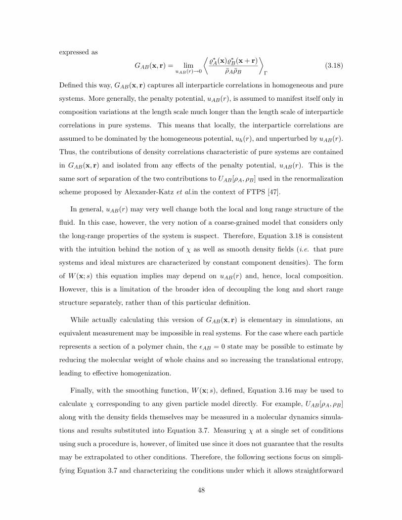
expressed as

GAB(x, r) = limuAB(r)→0

⟨%∗A(x)%∗B(x + r)

ρAρB

⟩Γ

(3.18)

Defined this way, GAB(x, r) captures all interparticle correlations in homogeneous and pure

systems. More generally, the penalty potential, uAB(r), is assumed to manifest itself only in

composition variations at the length scale much longer than the length scale of interparticle

correlations in pure systems. This means that locally, the interparticle correlations are

assumed to be dominated by the homogeneous potential, uh(r), and unperturbed by uAB(r).

Thus, the contributions of density correlations characteristic of pure systems are contained

in GAB(x, r) and isolated from any effects of the penalty potential, uAB(r). This is the

same sort of separation of the two contributions to UAB[ρA, ρB] used in the renormalization

scheme proposed by Alexander-Katz et al.in the context of FTPS [47].

In general, uAB(r) may very well change both the local and long range structure of the

fluid. In this case, however, the very notion of a coarse-grained model that considers only

the long-range properties of the system is suspect. Therefore, Equation 3.18 is consistent

with the intuition behind the notion of χ as well as smooth density fields (i.e. that pure

systems and ideal mixtures are characterized by constant component densities). The form

of W (x; s) this equation implies may depend on uAB(r) and, hence, local composition.

However, this is a limitation of the broader idea of decoupling the long and short range

structure separately, rather than of this particular definition.

While actually calculating this version of GAB(x, r) is elementary in simulations, an

equivalent measurement may be impossible in real systems. For the case where each particle

represents a section of a polymer chain, the εAB = 0 state may be possible to estimate by

reducing the molecular weight of whole chains and so increasing the translational entropy,

leading to effective homogenization.

Finally, with the smoothing function, W (x; s), defined, Equation 3.16 may be used to

calculate χ corresponding to any given particle model directly. For example, UAB[ρA, ρB]

along with the density fields themselves may be measured in a molecular dynamics simula-

tions and results substituted into Equation 3.7. Measuring χ at a single set of conditions

using such a procedure is, however, of limited use since it does not guarantee that the results

may be extrapolated to other conditions. Therefore, the following sections focus on simpli-

fying Equation 3.7 and characterizing the conditions under which it allows straightforward

48

extrapolation of χ from simple calibration experiments to more complex systems.

3.3.2 Composition independent χ

The field energy in Equation 3.10 is particularly simple under two assumptions: (1) macro-

scopic composition variations occur on a sufficiently large scale that ρB(x + r) ≈ ρB(x)

wherever uAB(r) is appreciable; (2) differences between particle types do not affect local

correlations, making GAB(x, r) entirely independent of the local composition. In this sec-

tion, the implications of these assumptions are considered, while the next is dedicated to

the consequences of relaxing them.

The second assumption allows GAB(x,x + r) to be replaced by its volume average,

GAB(r) carried out at any composition, including a pure system. Together with the first,

this neatly transforms Equation 3.10 into the form of Equation 3.6:

UAB[ρA, ρB] =∫GAB(r)uAB(r)r dx dr

∫ρA(x)ρB(x) dx (3.19)

GAB(r) ≡ 1V

∫GAB(x, r) dx (3.20)

This allows χ to be immediately identified as

χ = ρ

∫GAB(r)uAB(r) dr (3.21)

or, for systems with spherically symmetric interactions,

χ = ρ

∫g(r)uAB(r)4πr2 dr (3.22)

where g(r) is just the radial distribution function for a pure system.

The importance of this expression is that it is purely microscopic. More precisely, it

yields χ that is independent of composition. Moreover, this is precisely the formula used

by Grest et al.as a lower bound for χ in off-lattice simulations [12]. Moreover, Muller et

al.show that this reduces precisely to the Flory-Huggins mean field expression for lattice

fluids [52, 53]. Therefore, the case case considered in this section is a generalization of the

Flory-Huggins mean-field approximation. The following section relaxes this approximation.

49

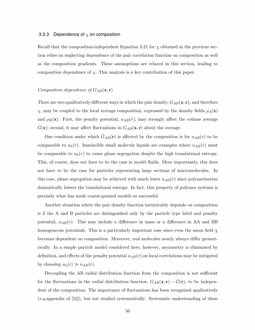
3.3.3 Dependence of χ on composition

Recall that the composition-independent Equation 3.21 for χ obtained in the previous sec-

tion relies on neglecting dependence of the pair correlation function on composition as well

as the composition gradients. These assumptions are relaxed in this section, leading to

composition dependence of χ. This analysis is a key contribution of this paper.

Composition dependence of GAB(x, r)

There are two qualitatively different ways in which the pair density, GAB(x, r), and therefore

χ, may be coupled to the local average composition, expressed by the density fields ρA(x)

and ρB(x). First, the penalty potential, uAB(r), may strongly affect the volume average

G(x); second, it may affect fluctuations in GAB(x, r) about the average.

One condition under which GAB(r) is affected by the composition is for uAB(r) to be

comparable to uh(r). Immiscible small molecule liquids are examples where uAB(r) must

be comparable to uh(r) to cause phase segregation despite the high translational entropy.

This, of course, does not have to be the case in model fluids. More importantly, this does

not have to be the case for particles representing large sections of macromolecules. In

this case, phase segregation may be achieved with much lower uAB(r) since polymerization

dramatically lowers the translational entropy. In fact, this property of polymer systems is

precisely what has made coarse-grained models so successful.

Another situation where the pair density function inextricably depends on composition

is if the A and B particles are distinguished only by the particle type label and penalty

potential, uAB(r). This may include a difference in mass or a difference in AA and BB

homogeneous potentials. This is a particularly important case since even the mean field χ

becomes dependent on composition. Moreover, real molecules nearly always differ geomet-

rically. In a simple particle model considered here, however, asymmetry is eliminated by

definition, and effects of the penalty potential uAB(r) on local correlations may be mitigated

by choosing uh(r) uAB(r).

Decoupling the AB radial distribution function from the composition is not sufficient

for the fluctuations in the radial distribution function, GAB(x, r) − G(r), to be indepen-

dent of the composition. The importance of fluctuations has been recognized qualitatively

(e.g.appendix of [52]), but not studied systematically. Systematic understanding of these

50

fluctuation effects is essential for mitigating the corresponding uncertainty in χ.

For simplicity, consider a symmetric AB Flory-Huggins lattice fluid mixture, essentially

corresponding to a crystal where the magnitude of uh(r) is sufficiently high to overcome

thermal fluctuations. UAB(Γ) in this case is strictly a function of the number of AB in-

teractions. If εAB → 0 and the particle labels are assigned at random, the mean field

approximation must evidently apply. Introducing an energy penalty for interactions must

necessarily shift the average number of AB interactions below the mean field limit, reducing

the exact χ in Equation 3.7 below the mean field estimate of Equation 3.21.

Note that as the concentration of A particles decreases, AA contacts become increasingly

rare as each A particle is surrounded by B particles. Therefore, the lower the concentration

of the minority component, the less the fluctuations affect the number of AB contacts per

minority component particle. Consequently, the decrease in UAB[ρA, ρB] per A particle

is greater for more symmetric mixtures. As a consequence, thermal fluctuations in the

pair density function stabilize concentrated phases with respect to dilute ones. This is

consistent with the finding that fluctuations increase the effective χ parameter required

to achieve phase segregation in model polymer systems, including the standard Gaussian

chains [17, 24].

Thus, thermal fluctuations in pair density lead to composition dependence of χ even for

the simplest lattice fluids of entirely symmetric particles. Attenuating these fluctuations

requires a large number of interactions per particle. In real systems, this corresponds to a

particle that represents a long polymer and in model systems potentials with ranges large

relative to the average interparticle spacing. Determining just how large the range of these

potentials must be and, ultimately, whether the fluctuations may be attenuated is a task

for numerical simulations, described later in the text.

Non-local effects

The other assumption necessary for Equation 3.21 to hold is that the variations in smooth

density fields may be neglected at the scale comparable to the range of the interaction

potential. This is unjustified in at least two important cases: moderately and weakly seg-

regated block copolymers and polymer interfaces. While Helfand and Tagami [20] conclude

that the non-local effects are often negligible if the local scale is taken to be comparable to

the size of the chemical repeat unit, this argument may not stand for coarse-grained models

51

where each chain is represented by a relatively small number of particles.

To simplify the analysis of the effect, assume that GAB(x, r) is statistically independent

from composition and spherically symmetric. Therefore, it may be replaced by a radial dis-

tribution function g(r) in Equation 3.10. In Appendix 3.7.1, it is shown that by introducing

a Taylor expansion of the density fields in r about a common point, χ is approximately

χ ≈ ρ∫g(r)uAB(r)4πr2 dr

(1− 1

2σ2

λ2

)(3.23)

λ2 ≡∫

(ρA(x)− ρA)(ρB(x)− ρB) dx∫∇ρA(x) · ∇ρB(x) dx

(3.24)

σ2 ≡∫g(r)uAB(r)r24πr2 dr∫gAB(r)uAB(r)4πr2 dr

(3.25)

Here, σ and λ are the characteristic length scales of the interparticle correlations, described

by the ideal radial distribution function g(r), and of the variations in the component density

fields, respectively.

To clarify the meaning of the composition field length scale λ, consider a two phase fluid

with domains of constant composition of characteristic size L connected by an interface of

width l with a linear composition gradient. In this case, λ is given by λ ≈√Ll. Another

example is a fluid with a sinusoidal plane wave composition field, λ = l/√

2π, where l is the

wavelength of the component density fields (see Section 3.4.3).

There are two qualitative aspects of the above results that are worth emphasizing.

Firstly, Equation 3.21 always overestimates χ for systems with appreciable gradients in

composition. Secondly, the non-local correction term to χ depends on a macroscopic prop-

erty λ, which itself is determined by the magnitude of AB interactions. Therefore, the

non-local corrections to χ in a particle system may be determined only after its macro-

scopic state has been determined. This is in contrast to the strictly microscopic nature of

Equation 3.21.

3.3.4 Questions for simulations

To review the results so far, it has been shown that χ is composition-independent and given

by the strictly microscopic mean-field Equation 3.21 if uh(r) uAB(r) and there is a large

number of interacting neighbors per particle, σ3ρ 1. Reducing the magnitude of non-

specific interactions or the range of the potentials leads to a decrease in χ or, alternatively,

52

an increase in the mean field, or “effective”, χ required to produce a given degree of phase

segregation.

Moreover, when the the length scale of composition variation and local particle corre-

lations come to within an order of magnitude of each other, χ is reduced by an amount

inversely proportional to the square of their ratio. This non-local correction is by definition

macroscopic and may be calculated for a particle system only once its equilibrium state is

known.

The challenge now is to quantify the former two effects and verify that Equation 3.23

describes the latter accurately. This is done here by numerical simulations. Specifically, the

aims of the following numerical studies are

1. Determine just how great a difference between uh(r) and uAB(r) is required to suppress

the effect of uAB(r) on the average pair density

2. Quantify the effect of fluctuations in the pair density on χ and determine the extent

to which they may be suppressed

3. Test the accuracy of the non-local corrections in Equation 3.23

The first two issues are addressed by examining phase behavior of binary mixtures,

where no long range composition gradients exist away from the critical point. In order to

study the second, a system with artificially imposed long range composition variations is

constructed in order to control them precisely.

53

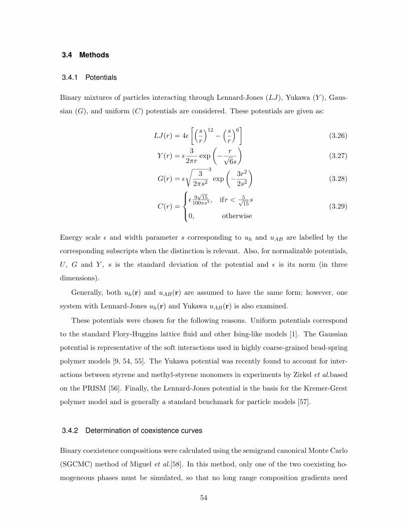
3.4 Methods

3.4.1 Potentials

Binary mixtures of particles interacting through Lennard-Jones (LJ), Yukawa (Y ), Gaus-

sian (G), and uniform (C) potentials are considered. These potentials are given as:

LJ(r) = 4ε[(sr

)12−(sr

)6]

(3.26)

Y (r) = ε3

2πrexp

(− r√

6s

)(3.27)

G(r) = ε

√3

2πs2

3

exp(−3r2

2s2

)(3.28)

C(r) =

ε 9√

15100πs3

, ifr < 5√15s

0, otherwise(3.29)

Energy scale ε and width parameter s corresponding to uh and uAB are labelled by the

corresponding subscripts when the distinction is relevant. Also, for normalizable potentials,

U , G and Y , s is the standard deviation of the potential and ε is its norm (in three

dimensions).

Generally, both uh(r) and uAB(r) are assumed to have the same form; however, one

system with Lennard-Jones uh(r) and Yukawa uAB(r) is also examined.

These potentials were chosen for the following reasons. Uniform potentials correspond

to the standard Flory-Huggins lattice fluid and other Ising-like models [1]. The Gaussian

potential is representative of the soft interactions used in highly coarse-grained bead-spring

polymer models [9, 54, 55]. The Yukawa potential was recently found to account for inter-

actions between styrene and methyl-styrene monomers in experiments by Zirkel et al.based

on the PRISM [56]. Finally, the Lennard-Jones potential is the basis for the Kremer-Grest

polymer model and is generally a standard benchmark for particle models [57].

3.4.2 Determination of coexistence curves

Binary coexistence compositions were calculated using the semigrand canonical Monte Carlo

(SGCMC) method of Miguel et al.[58]. In this method, only one of the two coexisting ho-

mogeneous phases must be simulated, so that no long range composition gradients need

54

be considered. For this study, the translation and particle type exchange moves were cho-

sen at random, with approximately equal probability (except for lattice models where no

displacement moves were allowed). All systems were simulated for about 107 moves, with

acceptance rates around 50%. Thus, each particle underwent about 104 type changes and

translations. Simulations were performed with 1000 particles with ρ = 1 and s = 1 for

all potentials. To maintain incompressibility, εh was chosen to be at least 20 times εAB;

however, εh = 1 was used for the LJ potential. The output of each set of simulations is a

symmetric histogram of compositions, fA = nA/(nA + nB). To speed up convergence, the

histograms were symmetrized by counting 1− fA as a separate sample whenever a compo-

sition fA was observed. The equilibrium coexistence composition for a macroscopic system

was estimated as the most frequently observed composition [43, 58].

3.4.3 Mixture with externally imposed field

In order to examine non-local corrections, a plane wave composition profile was imposed on

a mixture in a standard canonical molecular dynamics simulation(MD, [43]). Specifically,

at each time step a random number η, uniform on [0, 1) was generated for each particle. If

η < 0.5(1 + sin(2πx/l)), where x is the particle position along the x-axis, the particle was

assigned type A; otherwise it was assigned type B. This resulted in a plane wave composition

field

ρA(x) = 0.5 + 0.5ρ sin(2πx/l)) (3.30)

Such composition variation is encountered, for example, in weakly and moderately segre-

gated block copolymer blends [2]. In this case, the composition field wavelength is given by

λ2 = l2/2π.

Gaussian uh(r) and uAB(r) were used (Equation 3.28), with εh = 20 and εAB = 2. The

order of magnitude difference between these scales was assumed to approximate incompress-

ibility (this is checked separately in the Results section). Particle density, ρ, and potential

width, s, were set to one. Simulations were performed with 1000 particles for l ≤ 10s and

(l/s)3 particles for larger wavelengths.

55

0.5 0.6 0.7 0.8 0.92

2.5

3

3.5

ρA/ρ in the A-rich phaseχ

Figure 3-1: Equilibrium composition of symmetric binary fluids: BCC (∗) and cubic (+)lattice fluids; off-lattice fluids with Gaussian uh and uAB (); Yukawa uAB and Lennard-Jones uh (H); Yukawa uh and uAB (N). Flory-Huggins mean field result is plotted forcomparison as the solid line [1]: χMF (fA) = ln[(1− fA)/fA]/(1− 2fA) .

3.4.4 Results

Binary mixture with homogeneous phases

The SGCMC simulations described above produced equilibrium coexistence compositions

of the two phases in a symmetric binary mixture with interactions potentials of a fixed form,

over a range of εAB (the magnitude of the penalty potential). While two systems with the

same εAB but different shapes of the potentials cannot be compared directly, calculating χ

values corresponding to the two systems using Equation 3.21 makes a quantitative compar-

ison possible. Figure 3-1 shows that the coexistence compositions of the fluids examined

here are in close agreement when plotted against χ. All the curves lie within about 15% of

each other. This consistency is remarkable considering that it was achieved for a range of

lattice, soft, and hard-core fluids without any adjustable parameters.

While consistency of these results is very important from the practical standpoint, even

more significant is that the discrepancies among the curves are precisely as anticipated in

Section 3.3.3. First note that all systems appear to converge in the dilute limit, where all

interacting neighbors of the minority component are of the same kind, regardless of the ex-

act composition. Second, the degree of deviation from the mean field result increases with

decreasing coordination number, and hence, magnitude of fluctuations in the composition

of the system of interacting neighbors of any given particle. Thus, each particle in the cubic

system interacts with only six neighbors and falls farthest from the mean-field result. At

56

the other end of the spectrum are the Lennard-Jones and Yukawa systems, which have rel-

atively large radii of interaction (σ ≈ 2s in both systems) and consequently large number of

interactions per particle. The Gaussian system, with σ ≈ 1.1s, falls in the middle along with

the BCC lattice system, which also has an intermediate coordination number. Finally, the

importance of fluctuations in pair density is further corroborated by the dramatic increase

in accuracy of the χ predicted by Equation 3.21 with increasing width of the interaction

potentials (e.g.number of neighbors per particle) for the Gaussian system. This result is

shown in Figure 3-2.

1 1.2 1.4 1.6−0.12

−0.1

−0.08

−0.06

−0.04

Potential widths, sρ1/3

Rel

ative

Err

or

inχ

Figure 3-2: Relative error in χ values predicted by Equation 3.21 compared to Equation3.6 as a function of the potential width (related to the number of interacting neighbors perparticle). Here χ ≈ 2, εh = 100 corresponding to a single homogeneous phase; sAB = sh = s

The distortion of the AB radial distribution function relative to the AA one appears

to have a noticeable, but small effect in this set of simulations. The effect should be most

apparent in the dilute regime, where the number of solute-solvent (AB) interactions per

solute particle is maximized. Yet, this is not the case, suggesting that εh values were indeed

sufficiently high in these simulations. Furthermore, examining the AB radial distribution

functions in Figure 3-3 for the Gaussian and LJ-Yukawa systems (near the critical point)

shows very little difference between the two. (These plots would not account for two and

three-dimensional changes in the pair density.) Nevertheless, as Figure 3-4 shows, the

error in χ for the Gaussian system appears to decrease linearly with the logarithm of εh.

The dependence has important implications for simulations, where smaller values of εh

should reduce the stiffness of the equations of motion, making sampling and equilibration

easier. Thus, on one hand, εh values may be reduced to some extent without significant

loss of accuracy, but on the other, enormous increase in stiffness is required to achieve any

57

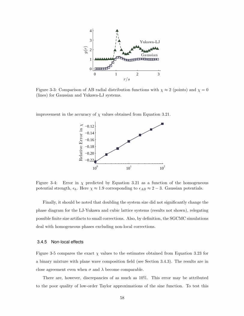
0 1 2 30

1

2

3

4

r/s

g(r

)

Gaussian

Yukawa-LJ

Figure 3-3: Comparison of AB radial distribution functions with χ ≈ 2 (points) and χ = 0(lines) for Gaussian and Yukawa-LJ systems.

improvement in the accuracy of χ values obtained from Equation 3.21.

100

101

102

−0.22

−0.20

−0.18

−0.16

−0.14

−0.12

Rela

tiv

eE

rror

inχ

Figure 3-4: Error in χ predicted by Equation 3.21 as a function of the homogeneouspotential strength, εh. Here χ ≈ 1.9 corresponding to εAB ≈ 2− 3. Gaussian potentials.

Finally, it should be noted that doubling the system size did not significantly change the

phase diagram for the LJ-Yukawa and cubic lattice systems (results not shown), relegating

possible finite size artifacts to small corrections. Also, by definition, the SGCMC simulations

deal with homogeneous phases excluding non-local corrections.

3.4.5 Non-local effects

Figure 3-5 compares the exact χ values to the estimates obtained from Equation 3.23 for

a binary mixture with plane wave composition field (see Section 3.4.3). The results are in

close agreement even when σ and λ become comparable.

There are, however, discrepancies of as much as 10%. This error may be attributed

to the poor quality of low-order Taylor approximations of the sine function. To test this

58

5 10 15 200

0.5

1

1.5

Wavelength, l/s

χ

Taylor

Gauss

Exact

Figure 3-5: Comparison of the exact χ Equation 3.7 to the approximate equations Eq.3.23 (“Taylor”) and Eq. 3.31 (“Gauss”). Results are for a symmetric mixture with binaryinteractions and an externally imposed plane wave composition field with wavelength l.

hypothesis an alternative expression for χ was obtained without invoking Taylor expansions

by taking advantage of the particularly simple features of this system (refer to Appendix

3.7.2 for derivation):

χ ≈ ρ∫g(r)uAB(r)4πr2 dr exp

(−2π2σ2

3l2

)(3.31)

Figure 3-5 shows this to be a much more precise estimate for the particular case of sinusoidal

composition fields. It is also straightforward to check that the expression is nearly identical

to Equation 3.23 up to terms of order (σ/λ)4.

Overall, these results confirm that Equation 3.23 is a good estimate of χ. Moreover,

Equation 3.31 is an even better estimate in the special case of plane wave composition fields

and soft interactions.

3.5 Discussion

The results presented above are put in perspective by considering each particle as a coarse-

grained representation of a large section of a polymer chain. The range, s, of effective

interaction potentials should be comparable to the radius of gyration of the chains, Rg,

and the interactions themselves may be taken to be roughly Gaussian. Now, the number of

interactions per particle may be described by s3ρ = n/V R3g. Incidentally, this is precisely the

Ginsburg parameter, C, defined by Ganesan et al.as a measure of the importance of thermal

fluctuations in determining phase behavior of blends and block copolymers [18]. Figure 3-2

59

indicates that s3ρ must be of order one, with s3ρ = 1 corresponding to approximately 10%

error in the mean-field χ. Thus, for a typical synthetic polymer, each particle must represent

at least 100–1000 repeat units. This number is estimated by calculating the Ginsburg

parameter, the chain density, defined above using Kuhn segment length and density data

for typical polymers. This is comparable to the molecular weights of whole molecules used

in many experimental studies, particularly those of block copolymers. In other words,

achieving even a relatively modest level of uncertainty in experimental values of χ requires

a model with extremely low resolution. Note that considering long chains also allows the

εAB εh condition to be satisfied.

The general idea emerging from these considerations is that the notion of a scalar, com-

position independent χ parameter strictly applies to particle systems only when the mean

field approximation holds and only when particles of different types are distinguished ex-

clusively by their type labels and the penalty potential. What is lost in using a single scalar

parameter to describe excess interactions between particles is the coupling between the pair

density and composition. Accounting for these effects makes χ composition dependent, in

agreement with experimental evidence. While this idea is not new, a crucial point made

by the above analysis is that composition dependence of χ does not have to arise from

complex, chemically-specific interactions among polymers, as suggested by [16, 30]. The

composition dependence of experimentally measured χ values in real and model systems

can be attributed to the fact that the particles corresponding to realistic monomers or even

polymers generally interact with too few other particles at a time for the mean-field assump-

tion to apply. Unlike a model where mean-field behavior is directly assumed to apply locally

(e.g.as in standard field theories), a particle system may compensate for an increase in the

penalty potential uAB(r) through local correlations, damping the change in the macroscopic

state of the system and apparent χ values. Thus, experimental measurements of χ based

on matching mean-field theory predictions, such as critical points or the de Gennes RPA

structure functions, are expected to overestimate χ. Direct evidence for this has been pro-

vided by Kremer and Grest, who determined both the mean field χ and the de Gennes’

RPA value for a particular model polymer and found the latter to be about 25% higher

than the former [52]. This is also consistent with analyses of fluctuations in field theories

of the standard Gaussian chain model, which predict an increase in the apparent critical χ

values with decreasing molecular weight for both block copolymers and blends [3, 17].

60

The results presented here also enrich the explanation of composition and tempera-

ture dependence of χ parameters proposed by Curro and Schweizer based on PRISM. Very

broadly, Curro and Schweizer implicitly relate the effective χ to particle radial distribution

functions through Ornstein-Zernike direct correlation functions. While Curro and Schweizer

suggest that this relationship should simplify studying the dependence of χ on thermody-

namic parameters of a system, they do not address the issue of composition dependence

specifically in any detail. In this study, the arguments are somewhat more direct, leading

to more explicit conclusions. First, as shown above, the behavior of particles representing

finite sections of real chains are strongly affected by fluctuations. This lowers the actual

χ by an extent quantified in a number of test cases and predicted qualitatively in gen-

eral. Second, most real monomers that would correspond to a model particle have different

mass, different statistical segment lengths, and are unlikely to have strictly spherically sym-

metric interactions. Therefore, their radial distribution functions are likely to depend on

composition even if thermal fluctuations are neglected.

In the PRISM, the temperature dependence of experimental χ values is obtained from

the specific form of the PRISM structure function, neglecting the temperature dependence of

direct correlation functions themselves. In the present analysis, if the potentials and radial

distribution functions are assumed to be temperature-independent, Equation 3.21 implies

directly that χ ∝ 1/T . This is somewhat complicated by the temperature dependence of

the radial distribution functions and the free-energy-like nature of the potentials, if they

are to be obtained from more detailed polymer models. Nevertheless, it is important to

emphasize that χ depends on temperature even if the potentials and correlations do not.

Fortunately, the above conclusions still leave room for particle models constructed specif-

ically to have a relatively well-defined χ value and therefore quantitatively comparable to

traditional field theories. This opens the possibility of rigorously supplanting field theoretic

polymer simulation studies beyond the mean field limit with simple bead-spring dynamic

models, such as the Kremer-Grest or dissipative particle dynamics soft particle models

[9, 55]. The results presented here indicate that the error in the mean field Equation 3.23

may be reduced to only a few percent by using a model with a relatively broad potential,

s ≈ 1.5ρ−1/3, and a one to two orders of magnitude difference between the strengths of the

homogeneous and heterogeneous potentials, εh/εAB ≈ 10 − 100. While such models may

not be entirely realistic physically, they may be effective computational analogues to the

61

field theoretic simulations.

Note that in this case, a significant trade-off between resolution and reliability emerges.

If too few particles are used to represent a molecule or too large an interaction radius,

non-local corrections to χ become important. While Equations 3.23 or 3.31 may be used

to compensate for this to some extent, they too should fail for small enough difference in

scales.

Nevertheless, constructing a coarse-grained particle-based model of a heterogeneous

polymer blend with χ parameters specified to within a few percent now appears feasible.

3.6 Conclusions

The aim of this article has been to characterize the conditions required for a particle system

to have a well-defined χ. In summary, these conditions are: the particles of different types

are distinguished only by their labels and the penalty potential; the number of interactions

per particle is large; the energetic difference between particles of different types is too small

to distort local correlations; and the scale of interparticle correlations is much smaller than

the scale of long-range composition gradients. Together, these conditions affect a mean-field

environment for each particle and make it possible to associate a constant, composition

independent χ value as it is used in common field theories. These conditions are not

realistic in physical systems, which explains composition and temperature dependence of

experimentally measured χ values.

Overall, many of the ideas gathered here have been long recognized. The contribution

of this article, however, is in systematizing and quantifying their consequences in a single,

generalized framework treating lattice, hard and soft-core particle models on the same

terms. An important result of this systematic analysis is the clear delineation between

models where χ is well-defined and physically realistic particle models. This should be of

interest in any attempt to compare an explicit simulation of an ensemble of polymers with

traditional field theories.

62

3.7 Appendix

3.7.1 Non-local corrections to χ

This section explains calculations leading to Equation 3.23. The starting point for these

calculations is Equation 3.16 with g(r) used instead of the full pair density for simplicity.

UAB[ρA, ρB] =∫ρA(x− r/2)ρB(x + r/2)g(|r|)uAB(r) dr dx (3.7-1)

Here, the x coordinate has been redefined to symmetrize the equation. Now if both density

fields are replaced by their Taylor expansions around x, only the terms even in the com-

ponents of the vector r, contribute to the ensemble average energy in Equation 3.10. This

leads to

UAB[ρA, ρB] =∫ρA(x)ρB(x) dx

∫g(|r|)uAB(r) dr

− 12∇ρA(x) · ∇ρB(x)

∫g(|r|)uAB(r)|r|2 dr (3.7-2)

Therefore, the excess field energy with respect to the ideal mixture reference state is given

by

∆UAB[ρA, ρB] = UAB[ρA, ρB]− UAB[ρA, ρB] (3.7-3)

=∫

(ρA(x)− ρA)(ρB(x)− ρB) dx∫g(|r|)uAB(r) dr dr

− 12∇ρA(x) · ∇ρB(x)

∫g(|r|)uAB(r)|r|2 dr (3.7-4)

where the excess density fields are defined as ρK(x) ≡ ρK(x) − ρK for K = A,B. Substi-

tuting this expression into Equation 3.7 yields Equation 3.23.

3.7.2 Special case of sinusoidal composition fields

Taylor expansions in the above analysis turn out to be an unnecessary approximation for

the mixture with plane wave composition fields and a soft interaction potential, such as in

63

the case described in Section 3.4.3. Consider estimating uAB(r)g(r) as a Gaussian function

u∗AB(r) ≡ gAB(r)uAB(r) (3.7-5)

u∗AB(r) = χ

(3

2πσ2

) 32

exp(− 3r2

2σ2

)(3.7-6)

χ ≡∫uAB(r)g(r) dr (3.7-7)

Here σ is given by Equation 3.25. Figure 3-6 shows this estimate of uAB(r)g(r) to be at

least a reasonable approximation.

0 0.5 1 1.50

Distance, r/σ

u∗ A

B(r

)4πr2

/‖u∗ A

B‖

u*

Gauss

Figure 3-6: Comparison of u∗(r) = g(r)uAB(r) to the Gaussian distribution, both integratedover spherical angular coordinates and normalized to unity in r. The system is describedin Section 3.4.3

Equation 3.16 may now be evaluated analytically for plane wave fields, resulting in

∆UAB[ρA, ρB]χ

=∫

∆ρA(x)u∗AB(x− y)∆ρB(y) dx dy (3.7-8)

=∫

(0.5 sin(2πx/l))2 exp(−2π2σ2

3l2

)dx (3.7-9)

Substituting this into Equation 3.7 results in

χ = exp(−2π2σ2

3l2

)∫g(|r|)uAB(|r|) dr (3.7-10)

Also, expressing l in terms of λ and Taylor-expanding the exponential yields

χ ≈(

1− 0.524σ2

λ2

)∫uAB(|r|)g(|x|) dx (3.7-11)

64

very nearly recovering the original estimate, Equation 3.23.

65

4A bead-spring polymer model with

well-defined Flory-Huggins miscibility and

chain density

Abstract

We propose a direct interpretation of a family of coarse-grained bead-spring block copoly-mer models with soft non-bond interactions in terms of the standard Gaussian chain model(GCM). Specifically, we show that under conditions of sufficiently low resolution and highchain density, interaction parameters in the particle model may be expressed in terms ofthe Flory-Huggins miscibility parameter, the Helfand compressibility parameter, and thedimensionless chain density to within a controllable and generally acceptable tolerance. Aclose agreement of the prediction of the model with field theoretic results and experimentaldata on critical behavior of symmetric diblocks, including the critical miscibility, scatter-ing function amplitude, and periodicity of the structure are demonstrated. Our approach isdistinguished from similar efforts in that it does not rely on matching of macroscopic proper-ties, but a direct microscopic interpretation of the GCM parameters. Such parametrizationmakes straightforward molecular dynamics simulations of bead-spring chains a comple-mentary but independent alternative to field theoretic simulations. These explicit chainsimulations offer significant practical advantages in sampling thermal fluctuations in sys-tems of moderate molecular weight and, potentially, in non-equilibrium situations withoutsacrificing thermodynamic rigour.

67

4.1 Introduction

Our understanding of polymer blends and block copolymers rests largely on the observation

that many molecular scale features of these systems may be described by macroscopic

parameters, abstracting from the details of molecular structure. This property allows us to

infer the behavior of one polymer system based on observations of another physical, or more

commonly, highly simplified coarse-grained theoretical model polymer system. Making such

inferences, however, requires a way to relate the microscopic parameters defining the nature

of the model system to those of the system whose properties are desired.

In practice, coarse-grained models are parametrized by matching a thermodynamic prop-

erty under a set of conditions where measurements are readily accessible. For example, a

common way to measure the Flory-Huggins miscibility parameter, χ, used in the standard

Gaussian chain model (GCM [18] ) involves matching the low frequency tail of the scatter-

ing function of a material to the analytical estimate available under the nearly ideal mixing

conditions, or random phase approximation (RPA). Another technique involves matching

critical temperature at a single point or as a function of molecular weight [3, 9, 12, 16, 17].

Another, classic example of such extrapolation is the Flory mean-field estimate of site cou-

pling parameters in lattice chain models, which estimates the energy of an immiscible lattice

chain system based on the ideal mixture limit [1, 17].

While usually effective, these means of measuring model parameters assume that the

measured parameter values remain valid away from the conditions used for parametrization.

The uncertainty involved in such extrapolation is difficult to predict and often leads to

significant inconsistencies among various models and measurements on real polymers. For

example, the RPA is found to be too restrictive for many common polymer systems, resulting

in differences in Flory-Huggins parameters measured in blends and block copolymers of the

same components [16, 17]. Similar problems are observed in polymer simulations, such as

the polymer dissipative particle dynamics (PDPD) model of Groot et al.[9] or lattice chain

simulations of, for example, Matsen et al.[10, 51]. In case of the PDPD, χ parameters

estimated by matching critical points in blends of monomers were found to predict the

critical point in block copolymers at a value of χ as much as four times greater than the

commonly accepted mean-field estimate of Liebler. The same discrepancy is found in lattice

chain simulations by Matsen , who follow Flory [1] in extrapolating the χ values from the

68

ideal mixture limit to block copolymers.

Avoiding such discrepancies requires a more direct relationship between the microscopic

parameters of the model and those of a real systems than matching of a single thermo-

dynamic property affords. In this article, we focus on defining such relationships among

members of a class of coarse-grained bead-spring block copolymers with soft repulsive non-

bond interactions of varying range and number of particles representing each chain. The

choice of this type of model is motivated by the work of Grest et al.and Fredrickson et al.who

have argued that continuous space coarse-grained particle-based models have a number of

practical advantages over the more traditional lattice and field-theoretic models [12, 18].

For example, isobaric ensemble studies are easier to formulate in continuous space particle

system than in lattice chain models, which is crucial in studying intrinsically non-isotropic

ordered phases of block copolymers. Compared to field theoretic approaches, particle sim-

ulations are simpler to extend to non-equilibrium situations as well as to measurement of

dynamic properties [18]. We chose to focus on block copolymers rather than blends for

two reasons. Firstly, the length scale of order parameter fluctuations in block copolymer

is bounded by the molecular dimensions, making precise simulation of critical behavior

possible with small periodic systems. Secondly, the widely acknowledged importance of

thermal fluctuations in block copolymers has lead to considerably more significant errors in

the traditional approaches to modeling block copolymers than in blends [3, 17].

The central hypothesis of our study is that it is possible to parametrize the bead-spring

models in a way that would establish both clear relationships among them and the extent

to which their behavior is universal. At the same time, we seek a parametrization scheme

that is sufficiently simple not to compromise the practical advantages of the particle simu-

lations. Specifically, we attempt to express the particle model parameters in terms of the

composition, radius of gyration, the Flory-Huggins miscibility parameter, compressibility,

and dimensionless chain density that fully define block copolymer behavior in the GCM [18].

Emphasis is placed on the relationship between the Flory-Huggins χ parameter associated

with the non-bond interaction potentials in the particle model. One reason we chose the

GCM as the standard is that GCM is the foundation for the most widely used field theories

of block copolymers, including the classical self-consistent field theory of Helfand et al.[20]

and the more recent field theoretic simulation methods of Fredrickson et al.[18]. Equally

compelling is the fact that GCM is the ultimate macroscopic model, abstracting from the

69

specific molecular structure entirely. Rather than dealing with individual molecules, the

GCM is formulated in terms of monomer density and chemical potential fields. Thus, GCM

may be said to contain only universal features of polymer behavior. Consequently, to the ex-

tent that a beads-spring block copolymer may be considered universal, it should be possible

to map directly onto GCM.

Our approach to this challenge of relating particle and field theoretic parameters is an

extension of a similar analysis we have performed for binary blends of particles [49] (also

the preceeding chapter of this thesis). In that study, we reduced the problem to examining

the effect of incompatibility between species on the particle radial distribution function.

Generalizing the approach to polymers poses two major challenges, which we address first

analytically and then in simulations. Firstly, we must address the effect of bonds on particle

position correlations. Secondly, we must develop an explicit definition of the macroscopic

density fields. In our previous study, we followed the GCM literature in defining macroscopic

density fields as instantaneous local averages. This led to the introduction of an implicit

density smoothing function, which effectively enforces a frequency cutoff. Since the previous

study dealt mainly with homogeneous phases, there was no need for detailed examination

of the density averaging function. In block copolymers, however, molecular scale variation

in composition is the central feature of the phase behavior. Therefore, precise measurement

of macroscopic density fields is essential.

4.2 Theory

4.2.1 Particle and field models

The system of interest here is a monodisperse set of n block copolymer chains, each made up

of N monomers, confined to volume V and characterized by temperature T . All monomers

are point particles of identical mass, m. Each particle is described by an index i, position

xi, and a type label Ki ∈ A,B. The first fAN monomers along each chain are of type A

and the rest are of type B. Let Γ be the set of all particle coordinates and Ω be the phase

space of Γ. To simplify notation, we express all energies in units of kBT , all masses in units

of m, and all lengths in units of characteristic interparticle spacing 1/ρ1/3 = (V/n)1/3.

Following Grest et al.[12], we compose the Hamiltonian of this system using three terms:

bond interactions reflecting the molecular topology; homogeneous, or type-independent,

70

non-bond interactions that reflect the compressibility of the system; and excess non-bond

interactions that reflect the immiscibility of the two types of blocks:

H(Γ) = Hb(Γ) +Hh(Γ) +HAB(Γ) (4.2-1)

Hb =∑

(i,j)∈B

k r2ij (4.2-2)

Hh =∑

i,j∈I,i>jεhK(rij) (4.2-3)

HAB =∑

i∈IA,j∈IB

εABK(rij) (4.2-4)

rij ≡ |xj − xi|

where B is the set of all unique pairs of indices of particles connected to each other by bonds;

I is the set of all particle indices; and IK is the set of indices of all the particles of type

K. Further, the shape of the potentials is defined by the kernel function K(r), assumed to

be spherically symmetric and normalized so that∫K(r)4πr2 dr = 1. Here we use a purely

repulsive Gaussian kernel similar to those in references [55, 59],

K(r) ≡(

32πσ2

) 32

exp(− 3r2

2σ2

)(4.2-5)

rather than the hard-core one used by Grest et al.[12]. Finally, let P (Γ) be the probability

density function for Γ ∈ Ω, given as P (Γ) ≡ Z−1 exp(−H(Γ)) where Z is the partition

function such that∫

Ω P (Γ) dΓ = 1.

The macroscopic counterpart of this particle model, the GCM, is generally formulated

as a field theory, describing the state of the same system in terms of monomer density fields

ρA(x) and ρB(x) and their probability density functional P [ρA, ρB] = Z−1f exp(−U [ρA, ρB]).

Zf is the partition function of P [ρA, ρB] with respect to the density fields, such that the

functional integral∫∫

P [ρA, ρB] dρA dρB = 1. The monomer density fields are assumed to

be “smooth” in a sense to be defined shortly. The effective free energy associated with the

71

pair of fields is composed of terms analogous to those of H(Γ):

U = Ub + Uh + UAB (4.2-6)

Uh =ζ

2ρ

∫(ρA(x) + ρB(x))2 dx (4.2-7)

UAB =χ

ρ

∫ρA(x)ρB(x) dx (4.2-8)

where ρ is the volume average particle density, nN/V ; χ is the Flory-Huggins composition

field coupling parameter; and ζ is the Helfand incompressibility parameter [20]. The free

energy associated with conformational entropy of the chains, Ub[ρA, ρB], cannot generally

be evaluated analytically. It is, however, fully determined by the by the unperturbed radius

of gyration of the chains, Rg ≡ a√N/6, where a is the root-mean-squared bond length

measured in the homopolymer limit, where fA = 0 or 1 [18].

Field theoretic calculations generally rely on evaluating various properties of P [ρA, ρB]

by means other than direct sampling of P [ρA, ρB]. We refer the reader to comprehensive

review articles [18, 23] for details of field theoretic calculations and mention some key

observations here. Commonly, only the mean field solution, which in this case is also

minimizes the free energy, of the macroscopic model is obtained. The mean field solution

is fully determined by χN , Rg, fA, and monomer density, ρ. The Ginsburg parameter

characterizing the extent of thermal fluctuations around the mean field solution is the

dimensionless chain density

C =n

VR3g (4.2-9)

4.2.2 Miscibility

Expressing the miscibility of A and B particles in the bead-spring model in terms of the

GCM requires a way to associate smooth density fields with instantaneous particle coordi-

nates. Here we assume that these fields are given by some function ρK(x; Γ) for K ∈ (A,B).

Specific examples of how such a function can be defined are discusseed at the end of this sec-

tion. In the meantime, we proceed to define χ by setting the excess energy terms associated

with the miscibility in the two models equal as follows

〈HAB(Γ)〉Ω[ρA,ρB ] = UAB[ρA(x), ρB(x)] ≡ χ

ρ

∫ρA(x)ρB(x) dx (4.2-10)

72

Here the shorthand 〈·〉Ω[ρA,ρB ] is used for an ensemble average carried out over only the part

of the phase space Ω of the particle positions where ρK(x; Γ) = ρK(x) for K ∈ (A,B). To

make use of the above identity of non-bond excess energies, we rewrite the ensemble average

of the Hamiltonian in terms of the radial distribution function, gAB(r) for A-B particle pairs

and the macroscopic density fields

〈HAB(Γ)〉Ω[ρA,ρB ] ≡ εAB∫∫

ρA(x)ρB(x)gAB(r)K(r)4πr2 dr dx (4.2-11)

where r = |r|. The radial distribution function gAB(r) may be formally defined in terms of

exact density fields, ρ∗K(x), which represent each particle as a three-dimensional version of

the Dirac δ function, as follows

gAB(r) =W [ρ∗A(x)ρ∗B(x + r))] (4.2-12)

ρ∗K(x) ≡∑i∈ΓK

δ(x− xi) ∀ K ∈ (A,B) (4.2-13)

where W [f ] is a linear operator mapping any well-behaved function f(x, r) onto a spheri-

cally symmetric function of r as

W [f(x, r)] ≡∫∫〈f(x, r)〉Ω[ρA,ρB ] δ(|r| − r) dr dx∫

ρA(x)ρB(x) dx(4.2-14)

The expected ensemble average of the Hamiltonian given in Eq. 4.2-4 is recovered by sub-

stituting the definitions in equations 4.2-12 through 4.2-14 into Eq. 4.2-11. The benefit of

these manipulations is that the microscopic details of the bead-spring model are encapsu-

lated in gAB(r).

It is convenient to take this encapsulation process one step further by factoring out the

integral over r from Eq. 4.2-11

〈HAB(Γ)〉Ω[ρA,ρB ] ≡ εABξ∫ρA(x)ρB(x) dx (4.2-15)

where the correlation integral ξ is defined as

ξ ≡∫gAB(r)K(r)4πr2 dr (4.2-16)

73

Finally, this allows us to define the χ miscibility parameter for a given bead-spring model

in terms of the correlation integral

χ ≡ εABξρ (4.2-17)

.

A particularly convenient and common way to estimate ξ is to assume that the correla-

tion integral, ξ0 measured when εAB = 0 does not change as εAB is increased. We will refer

to ξ0 as the “homogeneous” approximation. This is the approximation made by, for exam-

ple, Flory [1] and Binder et al.[52] in lattice models and by Grest et al.[12] in bead-spring

simulations. If the correlations due to bonds may be neglected, this is equivalent to taking

gAB(r) = gAA(r) in a single component fluid. Otherwise, this assumption may be seen

as an ideal mixture approximation, where the interparticle correlations are dominated by

the non-specific interactions and are independent of miscibility. Consequently, χ is strictly

proportional to εAB across the whole range of miscibility (see, for example, [49]).

As we have argued previously [49], excess AB repulsion does affect the interparticle cor-

relations even when the non-specific interactions are dominant (εAB εh). The corrections

to the homogeneous approximation, ξ0, of the correlation integral may be separated into

contributions ξnl and ξl from long-range and local correlations, correspondingly:

ξ = ξ0 + ξl + ξnl (4.2-18)

ξ0 = limεAB→0

W [ρ∗A(x)ρ∗B(x + r)] (4.2-19)

ξnl[ρA, ρB] =W [ρA(x)ρB(x + r)] (4.2-20)

ξl[ρA, ρB] =W [ρ∗A(x)ρ∗B(x + r)− ρA(x)ρB(x + r)]− ξ0 (4.2-21)

In the following discussion we drop the explicit functional arguments for ξnl and ξl unless

they are essential to the meaning. Both terms are negative as they reflect the reduction in

UAB through additional correlations. Consequently, the terms depend on the macroscopic

state of the system, specified by ρA(x), ρB(x) and εAB. Thus, the correction terms ξl and

ξnl make the relationship between χ and εAB non-linear.

The long-range contribution may be estimated using a Taylor expansion, as explained

74

in the Appendix of [49], yielding

ξnl = − σ2

2λ2−O

(σ4

λ4

)(4.2-22)

σ2 =∫K(r)r24πr2 dr (4.2-23)

1/λ[ρA, ρB]2 = −∫∇ρA(x) · ∇ρB(x)∫ρA(x)ρB(x) dx

(4.2-24)

Here λ is the length scale of variations in the macroscopic component density fields mod-

ulated by the amplitude of these variations. For example, for plane wave composition

fields with the wavelength Lz and the direction given by a normal vector ez: ρA(x) =

1/2 + α sin(2πx · ez/Lz), ρB(x) = 1− ρA(x). For α 1, as is the case near and above the

critical temperature in block copolymers [2],

1λ2≈ 8π2α2

l2for α 1 (4.2-25)

When α = 1/2, characteristic of moderately segregated block copolymer systems,

1λ2≈ 4π2

l2for α = 1/2 (4.2-26)

The amplitude dependence of 1/λ2 ensures that ξnl becomes important only in systems with

significant macroscopic phase segregation. Overall, ξnl quantifies how close the scale of the

microscopic scale of the intrinsically model-dependent interparticle potentials, σ, compares

to the macroscopic scale of composition variation.

The value of the local excess correlation integral, ξl, generally requires numerical evalua-

tion. The key feature of this quantity, measured for a number of common potentials in [49],

is that it generally decays in amplitude with increasing σ3ρ. For Gaussian potentials, we

find that ρσ3 ≈ 2− 3, ξ0 may be systematically reduced to a few percent of ξ0. Further, ξl

generally decreases as the concentration of either component in the binary fluids is reduced

below 50%. Consequently, ξl tends to stabilize more homogeneous phases. Fortunately, we

find that the critical miscibility values for different potentials with the same value of ρσ3

are consistent to within several percent. Moreover, the critical values of the Flory-Huggins

χ parameter for ρσ3 > 1 are within 15% the ρσ3 → ∞, or the mean-field limit for the

potentials examined. This suggests that the corrections to phase behavior due to ξl should

75

be small and systematic if the potentials are sufficiently wide compared to the interparticle

spacing.

Calculation of the precise values of the three components of the correlation integral using

Eq. 4.2-18 requires an explicit definition of the smooth density fields in the bead-spring

model. Moreover, it requires a mechanism for sampling only particle coordinates consistent

with a prescribed set of fields (see Eq. 4.2-14). While the latter is a technical problem, the

former poses a fundamental challenge since there is generally no unique way to separate

macroscopic and microscopic components of the density fields. One analytically convenient

way to do so, proposed by us in [49], involves local averaging of the exact instantaneous

density fields. The smoothing filter that accomplishes this, however, is itself not uniquely

determined by any physical considerations. This reflects the more general and long-standing

problem of picking the cutoff wavelength that defines the boundary between “microscopic”

and “macroscopic” in field theories. Wang [17] and Bates and Fredrickson [48] find that the

miscibility parameter χ strongly depends on the specific choice1e of the cutoff wavelength

in the context of fluctuation corrections to GCM. In practical field-theoretic simulations the

cutoff frequency is introduced implicitly by discretizing density and chemical potential fields.

The methods for regularizing the ultraviolet divergence of some thermodynamic averages

with increasing resolution of the discretization grids in GCM models at finite chain density

are just starting to be addressed [15, 47].

An alternative approach to regularizing the density fields explicitly is to consider the

identity of full ensemble averages of the excess non-bond energies in Eq. 4.2-10 rather

than their instantaneous values. Unfortunately, computational properties of the current

field theoretic simulation methods are limited to extremely high chain densities C 10

[15, 23] where explicit simulations become difficult, limiting the usefulness of this approach

to regularization.

The above approach is practical if we make the mean field approximation for the en-

semble average non-bond excess energy

〈UAB[ρA(x), ρB(x)]〉 ≈ UAB(〈ρA(x)〉, 〈ρB(x)〉) (4.2-27)

76

where the ensemble average fields are given by

〈ρK(x)〉 =∫ρ∗K(x)P (Γ) dΓ (4.2-28)

This approximation generally holds for miscibility that is either substantially higher or lower

than the critical value. The critical range of miscibility is known to be relatively narrow

in blends and block copolymers when C → ∞. In block copolymers of realistic molecular

weights, however, the critical region is spanning the ranges of experimental interest [3, 42].

In block copolymer literature, it is common to assume that the mean-field approximation

holds under all conditions. Adopting this assumption we may define the mean-field misci-

bility parameter, χMF . Substituting Eq. 4.2-27 into Eq. 4.2-10, we obtain the following

definition of the mean-field χ

χMF ≡ ρ 〈HAB〉∫〈ρA(x)〉〈ρB(x)〉 dx

(4.2-29)

where all the quantities on the right hand side may be evaluated by simple averaging

in molecular dynamics simulations. This estimate provides a point of contact with the

extensive field theoretic literature on mean-field GCM at the expense of accurate modeling

of composition fluctuations in the critical region [18].

In order to study these fluctuation effects, we need a more general definition. Here, we

adopt a simple estimate based on very high and very low miscibility where the mean field

assumption does apply:

χ ≈ εAB(ξ0 + ξnl[〈ρA(x)〉 , 〈ρB(x)〉]

)ρ (4.2-30)

Notice that in for χN 10.5 [2], the average composition fields are constant, therefore

ξnl = 0 and we may estimate ξ0 as χMF /(εAB ρ). The ξnl term serves as the best estimate

in absence of explicit definition of instantaneous density fields of the change in χ due to

emergence of macroscopic order for χN above the critical value. Thus, the consistency

of thermodynamic observables at χN 10.5 provides an important independent test on

the validity of the above estimate. This estimate does neglect long-range correlations in

instantaneous macroscopic density fields that are known to be important far below and

near the critical χN value [3]. We neglect the local correlation integral ξl in this estimate

77

because it cannot be measured without an independent means of estimating the fluctuation

contributions to 〈UAB〉. Instead, we expect to be able to reduce it to an acceptably small

value by choosing σ3ρ significantly greater than one.

4.2.3 Compressibility

As we have explained in the context of particle blends [49], the Helfand incompressibility

parameter may be estimated as

ζ = εhρξ0 (4.2-31)

The precise value of εh is unimportant to phase behavior of block copolymers as long as

εh εAB [20, 49]. Therefore, in this work we chose εhN = 600, unless noted otherwise.

This value is at least an order of magnitude greater than the εABN values in any of the

block copolymer simulation here. An order of magnitude difference in these scales has been

found to be sufficient for the interfacial composition profiles in GCM blends to be consistent

with the zero compressibility limit to within order of one percent [20] and for doubling of εh

to not produce a statistically significant changes in the the phase diagrams of binary blends

of monomers [49].

4.2.4 Bond model

The radius of gyration of an N monomer chain with harmonic spring bonds of average

length a0 in a dense, homogeneous melt is [19]

Rg = a0

√N

6(4.2-32)

This allow us to deduce the harmonic spring constant for such a chain as

k =3

2a20

(4.2-33)

for unit mass monomers. This, in turn, may be related to the dimensionless chain density,

C, through the bond length,

a0 =√

6(C/(ρ√N))1/3. (4.2-34)

Repulsive interactions between the monomers are likely to expand the bonds somewhat

78

compared to this estimate. If this swelling is significant, the spring constant may have to

be calibrated to attain a desired radius of gyration. Such calibration complicates both the

practical application of the model as well as the connection to the GCM, where the Eq.

4.2-34 applies exactly by definition.

Therefore, in this work we use only the value of the spring constant, given by Eq. 4.2-33,

and calculate the value of C based on the ideal bond length. This approximation is explored

in some detail in the following simulations. To distinguish the actual mean bond length

measured in simulations from the unperturbed bond length, a0, we refer to the former using

the symbol a.

4.3 Methods

We perform a number of simulations on monomers, dimers, homopolymers, and finally block

copolymers to test the limits of the theory presented above. All but the block copolymer

simulations are simple canonical MD, with periodic boundary conditions and random walk

initial conditions described below. The temperature is controlled using the Kremer-Grest

Langevin thermostat with a friction constant set to one in simulation units [60]. Unless

noted otherwise, simulations are conducted at unit particle density, ρ = 1, at unit tempera-

ture, kBT = 1, and with unit particle mass, m = 1. A Verlet-like integrator was used, with

a time step sufficiently small to reduce the error in the temperature to less than 0.5% in all

cases. Typical values of the time step were between 0.04 and 0.1, with larger values used

for wider potentials.

The phase behavior of physical block copolymers is typically studied by performing

temperature scans across critical or phase transition points. Increasing the temperature

has the effect of decreasing the importance of energetic non-bond interactions relative to

the conformational and translational entropy of the chains. Following Fried and Binder

[11] and Grest et al.[12], we study this trade-off in series of independent simulations with

different values of the excess repulsion, εAB, but with fixed homogeneous repulsion strength

εh and bond constant, k. Note that since energies are expressed in units of kBT , increasing

the εAB is equivalent to increasing the inverse temperature. Neglecting the temperature

dependence of the homogeneous repulsion, εh, and the dimensionless chain density, C, is a

rough approximation for many experimental systems, but is consistent with the assumptions

of the GCM. In practice, if the temperature dependence of εh and C may be measured and

79

incorporated in to the model as described, for example, by Bates et al.[16],.

In order to save computational time in diblock simulations, we use a relatively small sys-

tems of 4.53C chains. This corresponds to simulation cells of linear dimensions comparable

to a typical lamellar spacing in well-segregated block copolymers. We address the possible

effects of using such small cells in the following sections. We also use an external fields to

generate lamellar initial conditions. Each simulation is performed in triplicate in order to

estimate the confidence intervals on the measured averages.

The specific steps for each simulation in such εAB scans are as follows. First, the

lamellar structure is established by imposing an external excess potential Uext(xi) = 2.5(1+

Ji sin(2πx · ez/Lz)/2, where Ji is 1 when the i-th particle is of type A and −1 when the

particle is of type B; Lz is the dimension of the simulation cell in the z direction; and

ez is the Cartesian unit vector in the z-direction. This step is performed for 50 time

units, starting from random initial conditions. Second, the dimensions of the simulation

cells are relaxed for 104 time units to minimize the virial stress tensor components in all

three Cartesian directions using a slight modification of the box-search algorithm of Schultz

et al.[61]. At each time step, each dimension of the the simulation cell was updated as,

Li ← Li(1+0.1Pi/P ), where P is the average pressure in the system, and Pi is the magnitude

of the diagonal pressure tensor component in the i-th dimension. Although standard isobaric

molecular dynamics may be a better approach to such pressure equalization, the Schultz

algorithm has the advantage of maintaining constant system volume generally assumed in

GCM. The pressures used to calculate the update are exponential moving averages with a

decay time of 10 time units. The duration of this relaxation step is an order of magnitude

greater than the typical relaxation time of the cell dimensions. Nevertheless, we must note

that some much longer lived metastable states were also observed, possibly resulting in

incomplete pressure equalization. In these stable and metastable states, the cell dimensions

fluctuated by no more than 0.1%, with the magnitude of the fluctuations decreasing with

increasing χN . Finally, the system was sampled for 105/C time units in a straightforward

canonical MD. The initial conditions for the sampling runs were created by rescaling the final

particle positions after the pressure-equalization steps so that the dimensions simulation cell

length, Lz, along the wave-vector of the structure imposed by the external field was equal to

its average value over the last 5000 time units of the pressure equalization simulation. Such

averaging generally resulted in lower excess energies and more consistent critical points that

80

those obtained from simply using end point of the pressure-equalization step.

This choice of the sampling time is based on in several test runs (data not reported), for

simulations of lamellar block copolymer systems starting with different box sizes to converge

to the same lamellar spacing. The sampling time is scaled by the dimensionless chain

density to compensate for the growth in the absolute number of chains per simulation box,

and consequently the computational time per time step, with increasing dimensionless chain

density. Note that the number of chains per simulation cell the dimensions of which are fixed

with with respect to the unperturbed radius of gyration, Rg, is proportional to C. While this

increases the amount of computation per time step, the relative magnitude of the thermal

fluctuations in thermodynamic averages also decreases because the number of molecules

in the cell increases. The uncertainty in thermodynamic averages scales approximately

as the 1/√τn, where τ is the sampling time and n is the number of chains in the system.

Therefore, neglecting the changes in autocorrelation times of thermodynamic variables with

C, this implies that the uncertainty in thermodynamic averages maybe kept constant with

increasing C if the simulation time is reduced in proportion to the increase in n, which

itself is proportional to C. Note that while it is unlikely that the correlation times are

independent of the chain density, the effect should be at least partly compensated by the

overall reduction in thermal fluctuations with increasing chain density. Still, it is important

to note that at least in the εAB scans we do not rely on fluctuations in individual simulations

to estimate error bounds on averages.

The unit cell simulations described above are not adequate in cases where the struc-

ture functions must be measured. In these cases, much larger simulation cells of 163C, or

approximately 3− 4 lamellar periods in each direction, were used. These simulations were

particularly time intensive, especially for disordered systems where the fluctuations in the

scattering functions are large. Therefore, we limited these simulations to disordered and

near-critical systems, forgoing the cell relaxation step. All simulations were started from

unperturbed random walk initial conditions and equilibrated for 1500 time steps, and subse-

quently sampled for 500 time units. The equilibration time is comparable, but greater, than

the relaxation time of the systems above the critical point. All simulations were repeated

in triplicate.

81

4.4 Results

4.4.1 Bond model

The first challenge to be addressed by simulations is to quantify the degree of coupling

between bond and non-bond interactions. We start by examining the effect of non-bond

repulsion on the bond length and radii of gyration of whole chains. This is a crucial step

in understanding how to select the bond spring constant in order to achieve a given chain

density and ensuring that the Gaussian bond statistics assumed in GCM apply to the

particle model.

First, we simulate several A2 dimer systems with different values of the homogeneous

repulsion scale, εh, as well as bond spring constant. Figure 4-1 indicates that significant

deviations from the Gaussian chain bond statistics exist when the repulsion is strong and

bonds lengths are close to the interparticle distance. Note that the ideal bond length, a0,

1 1.2 1.4 1.6 1.8 2

1

1.02

1.04

1.06

1.08

1.1

Ideal bond length, a0ρ1/3

Rea

lbond

length

,a/a0

1

10

100

Figure 4-1: Average bond length as a function of the strength of homogeneous repulsion, εh(in the legend) and the unperturbed bond length in a system of single component dimerswith σρ1/3 = 1.3.

is related to chain density as (a3ρ) = 63/2C/√N . Consequently, the implication of this

results is that the ideal bond spring constants may be assumed only when the chain density

is sufficiently high and resolution is sufficiently low to guarantee that (a3ρ) 1. The

effect of non-bond interaction on bond length may be reduced by increasing the range of

the potentials, σ, as indicated in Figure 4-2. The reduction is significant only for bond

lengths close to a0ρ1/3 = 1. This highlights a trade-off between computational speed and

the expense of additional calibration of the bond model which may be necessary for small

σ.

82

1 1.2 1.4 1.6 1.8 21

1.05

1.1

1.15


Rea

lbond

length

,a/a0

1.0

1.1

1.4

Figure 4-2: Effect of the non-bond potential range, σρ1/3, (indicated in the legend) on thebond length in A2 dimers with εh = 100. Compare this to Fig. 4-1.

5 10 15 20

1

1.05

1.1

Chain length, N

Rg(N

)/√

a2N

/6 1.0

1.5

2.0

Figure 4-3: Radius of gyration versus with the chain length for homopolymers with a fixedunperturbed bond length, a0ρ

1/3, marked on the curves, showing deviations from the idealrandom walk scaling. Note that the radii of gyration are normalized using the bond lengths,a, measured in the dimer systems, rather than the ideal bond lengths, a. Here, εh = 100,σρ1/3 = 1.0ρ−1/3.

While the stretching of the bonds is a practical challenge, what matters in comparing

the bead-spring model to GCM is the scaling of the overall chain dimensions. In GCM, the

average radius of gyration of an single component N -mer in a homogeneous melt scales as√N . Fig. 4-3 suggests that for resolutions N of order 10, chains are swollen compared to

the ideal random walk scaling under the same conditions when individual bonds deviate

from ideal statistics. Such non-Gaussian scaling of Rg may be a more appropriate model for

behavior of real macromolecules [19], but should be avoided for the purposes of comparison

with GCM.

With the effects of the non-bond interaction on the properties of bonds briefly char-

acterized, we proceed to examine the effect of bonds on the correlation integral, ξ in Eq.

4.2-18. We start with a single component system, where ξ = ξ0 by definition. Fig. 4-4

83

1 1.2 1.4 1.6 1.8 21

1.01

1.02

1.03


ξ 0(a

0)/

ξ 0(a

0→

∞)

1

10

100

Figure 4-4: Effect of bonds on homogeneous interparticle correlations. The data is for anA2 dimer system with σρ1/3 = 1.3.

indicates in this case the effect of bonds on ξ0 is significant only when the scales of the bond

and non-bond interactions are comparable. For completeness, we also calculate the effect

of the potential range σ on this increase in ξ0. Fig. 4-5 indicates that the value of σ does

not play a significant role, at least for relatively high εh.

1 1.2 1.4 1.6 1.8 2

0

1

2

3

4

x 10−4


ξ 0(a

0)/

ξ 0(a

0→

∞)−

1

1.0

1.1

1.4

Figure 4-5: Effect of the potential width, σ, on the bond-related artifacts in homogeneousparticle position correlation. Data for a A2 dimer system with εh = 100.

These conclusions, however, do not apply directly to multi-component systems, as indi-

cated by Fig. 4-6. In this simulation, we measured ξ in an equimolar, single phase mixture

of two types of dimers, A2 and B2, significantly below and comparable to the critical values

of the critical repulsion strength. (The critical repulsion strength in such blends is expected

to be somewhat above εABN = 2/ξ0 [49].) The significant difference between the correla-

tion integral in the single component mixture and this blend is explained by the effective

increase in the local concentration around each particle of its bonded neighbors. Since in

this case each particle is bound to one of the same species, the overall effect is to reduce

84

1 1.2 1.4 1.6 1.8 2

−0.08

−0.06

−0.04

−0.02


ξ(a

0)/

ξ(a

0→

∞)−

1

0.001

0.1

1

Figure 4-6: Effect of bonds on the correlation integral in a mixture of A2 and B2 dimerswith values of εAB, indicated in the legend. Here, εh = 100 for all measurements. Linesconnecting the dots are guides to the eye.

the degree to which A and B particles interact. The additional decrease in energy observed

for εAB = 1 may be attributed to the excess correlations, ξl, close to the critical point,

as discussed in detail in [49]. The practical implication of this result is that ξ measured

in monomer simulations is a good approximation for polymers only when a3ρ 1. More

generally, these result suggest that ξ may be different in blends and in block copolymers.

This effect should be negligible when N 1 when most bonds are of the same type – either

AA or BB – in either kind of system.

4.4.2 Miscibility model

The above results provide sufficient information to formulate a well-parametrized block

copolymer model. Our aim here is to quantify the differences among models with different

resolutions and potential widths but the same macroscopic (GCM) parameters. We focus

on the phase behavior of symmetric diblocks, AN/2BN/2 composed of equal number, N/2,

of A and B beads. Specifically, we consider the time averages of the excess energy, UAB,

and the order parameter that is the normalized variance of the time-averaged density of A

monomers,⟨ρ2A

⟩/ 〈ρA〉2−1. Here, the angle brackets indicate averages of ensemble average

fields over the system volume rather than ensamble averages of instantaneous fields. For

this study we use a system with a chain density of C = 2, corresponding to at least two

systematically studied physical materials [32, 33].

The general features of the phase behavior in these systems are illustrated by the data

in Fig. 4-7 and are qualitatively similar to the observations in previous studies [11, 12].

85

10 20 30 40

0

0.2

0.4

0.6

0.8

ǫABN

〈ρ2 A〉/〈ρ

A〉2

−1

1.0

1.3

1.5

(a) Order parameter

10 20 30 402

2.2

2.4

2.6

ǫABN

UA

B/n

1.0

1.3

1.5

(b) Excess non-bond energy

Figure 4-7: Dependence of the variance of the time-averaged density of A particles overthe system volume (a) and of the average excess non-bond repulsion energy, UAB per chain(b) on the the excess repulsion, εAB, in A10B10 diblocks with C = 2 and the values ofσρ1/3 indicated in the legends. The order parameter used here is the variance in the time-averaged density field of A monomers, ρA(x), over the system volume, normalized by theaverage squared density of A monomers. Error bars are 90% confidence intervals from threeindependent trials.

As the excess repulsion increases (Fig. 4-7a), the order parameter stays near zero until it

begins to rise sharply at the critical point. Notice that the critical values closely correspond

to maxima in the excess non-bond energy UAB/n in Fig. 4-7b. These maxima indicate

a qualitative departure from random particle mixing, where increasing repulsion strength

raises the excess non-bond energy. Increasing the system size to roughly 27 times the size

used in these simulations shows no significant change in the width of the energy peak or

the position of its maximum (data not shown). This indicates that the correlation length

of the fluctuations is significantly smaller than the single lamellar period of the ordered

structure (the cell dimension). As the εAB increases further, UAB/n drops sharply while

the order parameter continues its sharp rise, signalling the emergence of stable structure

where A and B monomers are no longer in contact throughout the entire volume but only at

relatively well-defined interfaces. The subsequent minimum in the UAB/n is consistent with

the emergence of stable interfaces. The monotonic increase of UAB/n beyond the minimum

is consistent with lack of any qualitative changes in the system. The significantly weaker

rate of increase in UAB with εAB beyond the minimum reflects the reduced access of the

monomers of different types to each other in the phase-segregated state compared to the

homogeneous case.

While the overall features of the transitions are qualitatively similar for different σ, they

86

10 15 20 25

0

0.2

0.4

0.6

0.8

χMFN

〈ρ2 A〉/〈ρ

A〉2

−1

1.0

1.3

1.5

(a) Order parameter

10 15 20 252

2.2

2.4

2.6

χMFN

UA

B/n

1.0

1.3

1.5


Figure 4-8: The order parameter and average excess non-bond energy data for the symmetricdiblocks in Fig. 4-7 plotted against the mean field χN values (Eq. 4.2-29). Note that theorder-disorder transition appears at Leibler’s mean-field estimate of χcN = 10.5 [2].

do show significant quantitative dependence on σ and in this respect are model-specific.

These differences, however, nearly disappear when the energy and wavelength data are

plotted against the mean-field χMFN instead of εABN in Fig. 4-8. While the excess non-

bond energies UAB/n do show some σ dependence in the ordered regime (Fig. 4-8b), the

order parameters agree to within the statistical tolerance of the data in Fig. 4-8a. Note that

the critical value of the mean-field χMFN is found to be precisely at Leibler’s mean-field

GCM estimate of χcN = 10.5 [2].

The lower values of UAB for lower σ in the ordered regimes reflect the higher degree of

local correlations and, consequently, accessibility of more low energy conformations. The

differences in energies of the ordered states may indicate that the nature of the ensemble

averaged composition profiles across the interfaces depend on σ. An alternative explana-

tion is that for the same average macroscopic composition profiles, the correlations in the

positions of A and B particles are different for σ. Specifically, we expect that increasing σ

also increases the exposure of each A monomer to B monomers, raising UAB.

As we previously mentioned, the mean-field approximation also allows us to provide a

estimate of the local and long-range contributions to the correlation integrals. They are

shown in Fig. 4-9 for the diblock with N = 20 and σρ1/3 = 1.3. As expected, the mean-

field model does not account for the significant degree of spatial correlations in composition

fields, reflected by the drop in ξl well below the critical point. This is consistent with the

experimental data [42] and field theoretic calculations [3] and generally reflects long-range

correlations which are excluded from the mean-field estimate of ξnl. Notice that above the

87

15 20 25 30 35

−0.3

−0.2

−0.1

0

ǫABNC

orr

elation

inte

gra

l

ξl

ξnl

Figure 4-9: Mean-field estimates of the local, ξl and long-range, ξnl, correlation integrals forthe symmetric diblock system with C = 2, N = 20, σρ1/3 = 1.3. The order-parameter andexcess energy data for this system are found in Fig. 4-7. For comparison, the homogeneouscorrelation integral, ξ0 ≈ 0.82 here.

10 15 20 25

0

0.2

0.4

0.6

0.8

χN

〈ρ2 A〉/〈ρ

A〉2

−1

1.0

1.3

1.5

(a) Order parameter

10 15 20 252

2.2

2.4

2.6

χN

UA

B/n

1.0

1.3

1.5


Figure 4-10: Effect of potential width, σρ1/3 (indicated in the legends), on the phase be-havior of symmetric diblocks with C = 2, N = 20. Here, the data from Fig. 4-7 plottedagainst χN values calculated using Eq. 4.2-30.

critical point, where most of the system consists of relatively pure domains separated by

interfaces, ξl quickly reaches a positive value in agreement with our previous observations

that local correlations stabilize more homogeneous phase [49]. Note that the mean-field esti-

mate is likely to overestimate the correlation corrections, since they are explicitly neglected

in the mean-field limit, particularly below the critical χ.

Fig. 4-9 reflects an observation common to all the systems studied here that ξl represents

only approximately 5% or less of the correlation integral even well above the critical point.

This should make any artifacts of our rough mean-field estimate of ξnl negligible compared

to typical uncertainty in experimental data and ξl, which is neglected here.

Finally, we discard the mean-field assumption and examine the simulation data in terms

88

0 1 2 3 40

0.2

0.4

0.6

0.8

1

Position,z/Rg

ρA(z

)/ρ

A

(1.5,24.1)

(1.0,24.6)

Figure 4-11: Comparison of time-averaged composition profiles (ρA(x) along the wavevectorof the field) in two diblock simulations with different σ but comparable χN . The legendindicates the pair of values (σρ1/3, χN) for the two examples.

of the χN as given by Eq. 4.2-30. Fig. 4-10 indicates that the models with different

potential widths retain a similar degree of consistency in terms of χN as in terms of χMF .

As expected, the thermal fluctuations excluded by the mean-field approximations increase

the critical values of χN [3]. The significant dependence of UAB/n on σ may suggest

that the macroscopic states of the systems also significantly depend on σ, despite the close

correspondence of the order parameters. Fig. 4-11 indicates that the average density fields

in models with different σ but the same χN are nearly identical, in agreement with the

order parameter data. Therefore, the differences in UAB/n above the critical point in Fig.

4-10b should be attributed to instantaneous correlations in composition fields, rather than

properties of average composition fields. This is consistent with the observation that the

energies tend to be higher for wider potentials, which should increase the length-scale of

instantaneous correlations between ρA(x) and ρB(x).

We conclude this section by examining the effect of resolution on the phase behavior

of diblocks with the same macroscopic parameters. Fig. 4-12 indicates that decreasing the

resolution from N = 20 used in the previous scans to N = 8 has a negligible effect on the

order parameter or the critical point, but does appear to lower UAB/n appreciably above

the critical point. This is surprising, since lowering the resolution at fixed σρ1/3 effectively

increases the width of the interaction potentials relative to the molecular scale. This may

be attributed to the failure of the simple Taylor expansion used to obtain Eq. 4.2-22 for

high σ/Rg. Fortunately, UAB/n increases, as expected, from N = 20 to N = 14, indicating

that N = 20 is indeed sufficiently high for Eq. 4.2-22 to be a reasonable estimate of ξnl.

89

10 15 20 25

0

0.2

0.4

0.6

0.8

χN

〈ρ2 A〉/〈ρ

A〉2

−1

8

14

20

(a) Order parameter

10 15 20 25

2

2.2

2.4

2.6

χN

UA

B/n

8

14

20


Figure 4-12: Effect of resolution, N , marked in the legend of each plot, on the orderparameter (a) and average excess non-bond energy per chain, UAB/n (b) in a symmetricdiblock melt with C = 2 and σρ1/3 = 1.3. Note that the data for N = 20 is the same asthat for σρ1/3 = 1.3 in Fig. 4-10.

4.4.3 Comparison to experimental results

The consistency of the simulations with different potential widths and resolutions demon-

strated above provides a reasonable assurance that the properties of the our bead-spring

diblocks indeed reflect universal features of diblock copolymers. This finally allows us to

carry out a meaningful comparison of the model with GCM and experiments for which the

GCM parameters have been measured.

First we compare our predictions of the critical value of χcN as a function of chain

density, C, to those of the perturbation treatments of GCM for finite density. The so called

BLHF estimate of this value is commonly used to measure χ values experimentally [16, 24].

The central assumption of the BLHF theory that only the amplitude of thermal composition

fluctuations of a constant wavelength need be considered has been subsequently relaxed by

Barrat and Fredrickson (BF), resulting in a more general prediction of the critical value [3].

We define the critical point in the simulations as the smallest χN where the order

parameter⟨ρ(x)2

⟩/ 〈ρB(x)〉2 − 1 surpasses 0.01 indicating the emergence of stable order

[21]. Increasing this threshold value to 0.1 resulted in an increase of roughly 0.5 (data not

shown) in χcN , however, the lower threshold is more in line with traditional definition of the

critical points. Confidence intervals on critical values are estimated using three independent

estimates for each density.

Fig. 4-13 shows the results. Overall, the simulations fall on the BLHF curve to within

90

7 8 9 10

12

13

14

15

lnN = ln(63C2)χ

cN

Figure 4-13: Comparison of the critical χN values for symmetric diblocks as a function ofdimensionless chain length, N ≡ 63a3

0ρN . Dashed line: BLHF theory; solid line: Barrat-Fredrickson theory [3]; points: simulation data, with 90% confidence intervals based onthree independent sets of simulations.

measurement precision. To our knowledge, this is the first test of either theory where the χ

parameters were measured independently. The Barrat-Fredrickson theory is a generalization

of the BLHF theory and should be more precise, although, its assumptions of neither theory

are strictly justified at chain densities considered here [3]. One reason the simulations

results may be higher than the Barrat-Fredrickson theory is that we have chosen the order

parameter threshold to be too high. Another possibility is that the simulations allow for

three-dimensional long-range composition correlations which stabilize the disordered phase

relative. The Barrat-Fredrickson theory considers only plane-wave composition fluctuations,

which would tend to underestimate the critical point.

Next we consider the wavelength of the position in the scattering peak of poly(ethylene-

propylene)–poly(ethyl-ethylene), or PEP-PEE, diblock copolymers as a function of molec-

ular weight at a fixed temperature, shown in Fig. 4-14. This experiment has been also

studied by Barrat and Fredrickson, providing not only a GCM perturbation prediction

for the wavelength but also experimental values for monomer density and statistical bond

lengths. This allows a comprehensive test of our model.

We conduct comparable measurements on a series ofA10B10 diblocks with εh = 30, σρ1/3 =

1.3. The excess repulsion strength is set to εABN = χN ′/ξ0(C/Cc)2, where χ = 0.0168 is

the experimentally measured value and N ′ is the polymerization index in terms of the

chemical repeat as described by Barrat and Fredrickson [3]; ξ0 = 0.87 is the estimate of

the correlation integral measured in simulations of a homogeneous system of disconnected

91

2 4 6 8

3.5

4

4.5

5

lnN =ln(63C2)2π/(q

∗R

g)

PEP-PEEBF theorySSTA10B10

Figure 4-14: Wavelength of the structure function peak position as a function of the di-mensionless chain density for PEP-PEE [4] compared with predictions of the field theoreticperturbation treatment of GCM [3], the strong segregation theory of Helfand et al.[2],and simulation data. Data below the critical point were obtained from smeared scatteringfunction peaks, while above they were taken as the lamellar periods in pressure-equalizedunit-cell simulations.

model monomers; Cc = 4.6 is the experimental value of the critical density measured in the

PEP-PEE experiment. (Subsequently, we determined that the bonds reduce the value of

ξ0 to approximately 0.82. This discrepancy shifts the critical chain density slightly in our

simulations.) Here the disordered state peak positions were obtained from structure factors.

To emulate the smearing due to the bandwidth of the X-ray source in the experiment, we

convolve the measured structure factors with a Gaussian filter with a standard deviation

equal to 0.25 of the value of the wavelength at the peak of the filter function [42]. Above the

critical point, we used the lamellar period in pressure equalized samples as the estimate of

the structure function peak position. This allowed us to use significantly smaller simulation

cell sizes and avoid the artifacts associated with fast Fourier transform calculations in finite

cells.

Considering the uncertainty of the experimental values and the fact that no adjustable

parameters were used, the agreement of our results with the data and BF predictions is

remarkable. Notice that the BF theory starts to deviate significantly from the experimental

data for ordered samples, reflecting the limitations of the perturbation treatment. Sim-

ulation data, however, remain consistent with the experiment. Remarkably, our results

indicate that the peak position achieves the narrow interphase approximation, NIA, scaling

behavior even at weak segregation even though NIA is based on the assumption of suffi-

ciently strong segregation that the interface width is negligible compared to the domain

widths [2, 20]. This is significant not only in confirming the universality of the behavior of

92

the particle model, but also indicates that the simple, explicit NIA prediction may turn out

to be accurate well outside of its rigorous range of validity.

0.8 1 1.2 1.40

1

2

3

I/I(T

c)

Tc/T

A10B10

PEP-PEE

Figure 4-15: Include comparison of the peak scattering intensity between simulated(A10B10) and PEP-PEE-5 system described by Bates et al.[4]. Note that in the simulatedmodel, χ/χc = Tc/T .

Finally, Fig. 4-15 compares the simulation precision of the the peak scattering inten-

sity, I, as a function of inverse temperature to those measured for a PEP-PEE sample by

Bates et al.[4]. Recall that under the assumptions of our model, varying χN at constant

temperature is equivalent to varying the inverse temperature. To minimize the uncertainty

in the experimental data due to the smearing of the scattering function, we normalize both

the intensity and inverse temperature by their critical values. The critical value of χc used

to normalize the simulation data was used as an adjustable parameter to superimpose the

curves. Minimizing the sum of squared residuals between linear interpolations of the two

curves resulted in χcN = 13.6. This value is only approximately 5% higher than the pre-

diction χcN ≈ 13 predicted independently in Fig. 4-13, further establishing the reliability

of our simulation approach.

4.5 Discussion

The main implication with regard to particle-based models is that attaining straightforward

and explicit mapping among models with different resolutions and interaction potentials is

possible only within certain bounds on the resolution of the model. On one hand, the

resolution must be sufficiently high to allow for a meaningful separation of the macroscopic

and microscopic features. On the other hand, the resolution must be sufficiently low to allow

decoupling of bond, homogeneous non-bond, and excess non-bond interactions. The upper

93

bound on resolution is set by the requirements that the width, σ, of the potentials is such

that σρ1/3 > 1 and the number of particles per chain, N , is such that a3ρ =√

63C/√N 1.

Here, we have successfully used values of a3ρ as low as 3, which was possible due to relatively

soft and wide-ranged repulsion potentials. As we have previously discussed [49], not meeting

the first condition results in the dominance of local correlations over the homogeneous ones.

Consequently, the value of χ associated with a given excess repulsion depends on the local

composition. Moreover, this composition dependence depends on the nature of the monomer

interactions, rather than universal, macroscopic model properties.

It is interesting to note that if each monomer is interpreted literally as a representation of

long section of a flexible macromolecule [49], the lower bound on bond length and σ become

identical. In this case, it is reasonable to assume that σ is comparable to the unperturbed

radius gyration, Rg/√N , which is equal to

√6a0.

Despite this similarity between the restriction on bond lengths and potential ranges,

the artifacts of violating the two conditions compound as increasing resolution eventually

shortens bonds to the point where bond interactions strongly affect local particle position

correlations. This also leads to the breakdown of ideal Gaussian chains statistics of the

whole chain radius of gyration. Consequently, both the miscibility parameter and the

bond strength become resolution dependent and must be calibrated numerically at each

resolution to attain a particular dimensionless chain density. This observation is particularly

significant for lattice chain simulations, where bond lengths are often exactly equal to the

lattice spacing.

The fact that the bead-spring models are meaningful only at a coarse resolution, corre-

sponding to a upper bound on N , is hardly a new idea in itself [20]. However, our analysis

highlights some notable details particularly important for coarse-grained bead-spring mod-

els, where the microscopic length scale is typically much larger than the dimensions of a

chemical repeat unit. First, we introduce the concrete definition of the microscopic and

macroscopic length scales, σ and λ, and define precisely how the macroscopic contribution

to the miscibility parameter scales with the ratio of the two. In contrast, a quantity anal-

ogous to σ, the cutoff frequency, arising in field theoretic approaches of GCM is generally

left as a free parameter [17, 48]. Second, while similar to our previous analysis, the defi-

nition of λ here relies on purely macroscopic density fields, rather than the instantaneous

local fields. This has a third, practical, consequence in that the macroscopic contribution,

94

ξnl, to the correlation integral ξ is negligible. In contrast, our previous definition not only

had the drawback of relying on the implicitly defined smoothing kernel but potentially

non-negligible values of ξnl even in disordered states.

While these problems may be addressed, in principle, by the recently developed field

theoretic polymer simulations methods (FTPS) of Fredrickson et al.[18], the explicit chain

simulation methodology developed here emerges as a viable and necessary complement to

such methods. As noted by Fredrickson et al., sampling thermal fluctuations becomes more

difficult in FTPS at lower chain densities. As a result, to our knowledge, there are no

systematic studies of block copolymers in the GCM-FTPS framework for C < 10, which

accounts for a significant part of experimentally work on block copolymers [4, 16, 32, 33]. In

contrast, the explicit chain simulations require fewer calculations for lower chain densities as

the number of chains per unit cell of an ordered structure is proportional to the dimensionless

chain density. Moreover such simulations in the experimentally relevant range of chain

densities are feasible on readily available computers, as demonstrated by the results reported

here.

Our results are distinguished from from similar studies of Fried and Binder [11] and Grest

et al.[12] by the thorough characterization of the chain densities and miscibility parameters

in our model with respect to GCM. While qualitative trends in domain sizes and critical

behavior observed in our simulations are the same as in the previous works, the reliable

definitions of the model parameters allows us to compare our results to the predictions of

the GCM and observations on real polymers directly and quantitatively across a range of

conditions.

At this point it is appropriate to discuss several issues raised, but unresolved by our

results. First, we must note the systematic difference between the critical χ values observed

in particle simulation and BLHF predictions. The discrepancy may be explained by the

fact that local correlations in the disordered state are not allowed in the BLHF theory, but

are explicitly considered here. As discussed in [49], these correlations stabilize disordered

phases, raising the apparent critical χN somewhat. In the meantime, the discrepancy

should not prevent application of the explicit chain simulation methodology we propose to

the study of GCM since it is systematic and appears to follow the same qualitative trend

as the GCM estimates. Moreover, at less than 10% of the value of χc, the discrepancy is

small compared to the typical uncertainty in measured polymer parameters as well as the

95

rigorous error bounds on the BLHF predictions [3].

Second, it is important to whether the bead-spring models are as consistent transitions

between different field symmetries observed in asymmetric block copolymers as they are near

the critical point of the symmetric diblocks [2, 32]. It is commonly assumed that the effect

of thermal fluctuations in asymmetric block copolymers may be adequately described by

shifting the mean-field diblock phase diagram of Matsen and Bates [2] to attain the correct

critical point. This assumption has not been tested in any framework that adequately

sampled the effects of thermal fluctuations and is of practical importance.

Third, our composition field averaging method, in principle, may be confounded by

translational or rotational drift of an ordered structure with respect to the simulation cell.

This observation also applies to other explicit chain simulation methods as well as FTPS.

Fortunately, the high degree of consistency between independent simulations of identical

systems, and those differing in resolution, potential width, and density reported here in-

dicate that proper momentum conservation is sufficient to eliminate the artifacts of drift.

Nevertheless, it is important to consider other order parameters in addition to 1/λ2, such as

average of instantaneous composition correlation functions. Alternatively, we may introduce

a sampling methodology based on boundary conditions that force a particular structural

orientation. Yet another means of avoiding drift and rotation are available in field theoretic

calculations, where the basis set used to represent density fields to be explicitly restricted

to attain particular orientation and phase shift of periodic structures.

Fourth, this study focuses on a practically important but rather small range of resolu-

tions and potential widths. Although extending our study to a broader range of resolutions

and potential widths, particularly high resolutions, is important, we may anticipate some

challenges of such extensions. Increasing the resolution at constant density must either be

accompanied by an increase in the interaction range or a break-down in the universality of

the model behavior and increasingly composition-dependent miscibility. The former should

lead to increased computational demands while the latter would required additional cali-

bration calculations for rigorous estimates of the macroscopic parameters. Nevertheless, it

is interesting to note that the excess energy observed by Grest et al.in a diblock copolymer

systems with a resolution of N = 100 and hard-core potentials is very close to our estimates,

obtained at a much lower resolution [12].

Finally, we must mention the issue of finite size effects since we effectively simulated

96

systems only a single lamellar period across. While this may be important in absolute mea-

surements, here our main concern was with consistency of observations for different explicit

chain models with GCM. Notably, both results on fluctuation-corrected GCM to which

we could compare our work also rely on single harmonic representation of ordered phases.

Therefore, the unit cell simulations performed here are in fact appropriate. Moreover, as we

have mentioned some limited test comparison between large cell simulations and unit-cell

simulation revealed no differences in the excess energy dependence on χN up to the critical

point, including the position of the maximum. At the same time, we must emphasize that

pressure equalization is absolutely crucial for consistency of simulation of ordered phases,

even those near the critical point.

While these issues warrant further investigation, there are a number of theoretical and

practical considerations emphasized by this study that are relevant in the broader context

of polymer science and physics. For instance, it is interesting to note that explicit chain

simulations of the kind studied here are literally a discrete version of the GCM. The rela-

tionship between the two is analogous to that between the discrete representation of path

integrals and Shr odinger’s wave function equations in quantum mechanics [22, 31, 62]. In

fact, for infinite chain density, C →∞, we may follow Feynman in taking the limit of infi-

nite resolution, Nσ →∞, and recover the exact traditional formulation of GCM [18]. This

is possible because when C →∞ interparticle spacing may be treated as infinitesimally at

any resolution, removing the upper bounds on resolution described here.

More generally, our study formalizes the assumption involved in taking the limit of

infinite resolution, N , at finite dimensionless chain density. This is a significant fundamental

problem considering the recent emergence of FTPS methods for sampling GCM, where the

resolution is infinite by definition, at finite dimensionless chain density. In providing a

consistent way to compute miscibility and bond strength as function of resolution we have

provided an explicit scheme for determining the parameters of the bead-spring model as

functions of resolution. This is, in effect, a concrete renormalization procedure. The limits

on resolution discussed in the first paragraphs of this section allow us to specify explicitly the

values of the repulsion and bond strengths as functions of resolution. Our analysis suggests

that the limit of infinite resolution may be carried out for finite chain density explicitly as

long as the potential widths are kept sufficiently high. The same effect has been achieved

in FTPS by sampling the density fields on finite grids or explicitly subtracting contribution

97

of high-frequency field correlations to thermodynamic averages [47]. However, a systematic

understanding of the issue in the FTPS framework is only starting to emerge.

In the meantime, the explicit chain simulation methodology developed here offers the

first practical way to eliminate the uncertainty due to the unrealistic approximations, such

as the RPA, often necessary in evaluating the GCM. It is well known that traditional approx-

imate treatments of GCM result in considerable inconsistencies of measured χ parameters,

limiting the quantitative application of the theory [16]. As our results indicate, using ex-

plicit chain simulation for prediction and parameter estimation allows us to eliminate these

approximations at realistic chain densities.

Finally, a well-parametrized particle model may offer unprecedented opportunities in

studying rheology of heterogeneous melts. For example, straightforward non-equilibrium

molecular dynamics sampling algorithms may be applied directly to our model to assess

the low frequency contribution of composition correlations to viscoelasticity [18, 63]. More

detailed reptation effects may also be addressed either by increasing the resolution [12] or

explicitly disallowing chain crossing in a low resolution model [64]. While such simulations

have previously in themselves have been possible, now they may be firmly placed in the

thermodynamic context.

4.6 Conclusions

Overall, we may conclude that it is indeed possible to construct a coarse-grained bead-spring

block copolymer model that is precisely parametrized in terms of the standard Gaussian

model. The existence of such a relationship, and universality of the phase behavior of

the particle model, however, requires that, on one hand, the resolution of the model be

sufficiently low that the bonds and range of the non-bond interaction potentials are greater

than the characteristic interparticle distance and on the other, sufficiently high for the

length scale of macroscopic composition fluctuations to be significantly lower than the range

of the potentials. As we have demonstrated, this balance may be effectively struck for even

relatively low molecular weight block copolymers. Thus, continuous-space coarse-grained

particle-based simulations emerge as a straightforward, viable, and rigorous alternative to

field theoretic simulations, particularly in addressing thermal fluctuation and, potentially,

non-equilibrium properties of block copolymers of realistic molecular weights.

98

5Concentric lamellar phase of block

copolymers confined in cylinders

Abstract

This article reports a detailed modeling investigation of the concentric lamellar (CL) phaseof block copolymers confined in cylinders. It is motivated by recent experimental observa-tions of the CL phase in electrospun fibers and the reported failure of the classic strongstretching theory (SST) in the CL case. The equilibrium morphology and dimensions of CLphases are explored in detail as functions of the cylinder diameter. Quantitative results areobtained in a series of molecular simulations of bead-spring chains and explained in termsof a free energy model based on the narrow interphase approximation (NIA). The analysisbrings into focus the importance of interpenetration between monolayers of diblocks andvariation in interfacial chain density and, hence, interfacial energy density, with domainwidths in determining the properties of the CL phases. Simulations reveal three keys fea-tures of CL systems. First is that the dimensions of the domains closer to the axis vary withthe overall cylinder diameter significantly more than those farther out, in agreement withsimilar observations in other computational works. Second is that the domains tend to bethinner and chain dimensions smaller in CL phases than in the unconfined flat film cases.Third is that increasing the cylinder diameter produces periodic second order symmetry-breaking transitions where the central monolayers flatten from cylindrical into ribbon-likeconcentric monolayers. These phenomena are explained in terms of the interplay of chainconformational entropy and interfacial energy, including effects specific to curved interfaces.(At the time of writing, this material in this chapter is review for publication as an articlein the Journal of Chemical Physics.)

99

Figure 5-1: Typical axial and longitudinal electron transmittance (TEM) views ofpolystyrene–polydimethylsiloxane fibers [5, 6]. Polydimethylsiloxane is dark; scale barsare 56 nm, corresponding to the lamellar period, L0, of this material in the unconfined case.

5.1 Background and introduction

Confining block copolymers to cylinders, such as pores or fibers, has been shown to expand

the range of self-assembled morphologies of these materials [37]. While active theoretical

[37, 65, 66] and experimental [6, 67] research efforts are under way to explore the full

range of these morphologies, one of the simplest and commonly observed cases reveals some

remarkable properties. This morphology is described as the concentric lamellar (CL or

L||) phase and is illustrated in Fig. 5-1. The CL phase forms in nearly symmetric block

copolymers when one of the blocks preferentially adsorbs to the confining wall [37, 66]. It

is made up of concentric monolayers of diblocks.

One notable property of CL systems is that only the central one or two domains change

their thicknesses in response to changing cylinder diameter, while the widths of the rest

of the domains remain fixed. Similarly, the number of concentric monolayers in the equi-

librium structure remains constant over a range of cylinder diameters comparable to chain

dimensions. Such behavior has been reported in lattice chain models [66] and confirmed

experimentally in fibers [6]. These properties are important from the technological point of

view, as they could allow production of materials with very consistent properties without

requiring precise control of the confining medium. The way CL phases adapt to incom-

100

mensurable confinement is also interesting from the point of view of fundamental polymer

science, since it is a qualitative deviation from the case of thin films. In contrast to CL sys-

tems, all of the layers in flat films are more or less equivalent and adapt equally to changes

in film thickness [68, 69].

At first glance, the CL phase appears to be a trivial modification of the exhaustively

studied lamellar phase. However, the effects of confinement mentioned above have defied

attempts at precise explanation. The currently accepted theory of block copolymer films

confined between flat substrates is based on the strong stretching theory (SST), which has

successfully accounted for the experimental observations [68, 69]. Extending this approach

to the CL phase fails, as has been recently demonstrated by Wang [70]. Specifically, the

SST model incorrectly predicts the order and location of transitions between CL phases

with different number of concentric monolayers. Moreover, the SST does not account for

the one property of CL phases on which there is a reasonable agreement in the literature: the

disproportionate sensitivity of the central domain widths on the diameter of the confining

cylinder.

It is difficult to diagnose these shortcomings of SST based on the available simulation

and experimental data largely because the data is sparse and inconsistent. For example,

there is no agreement on whether the confinement causes an increase in domain width or

whether the chains themselves are compressed or expanded. The experimental study of

Shin et al.[67], as well as lattice chain simulations of Yu et al.[66] show that the domain

widths are increased by confinement. More recently, Ma et al.[6] found that in CL-forming

polystyrene–polydimethylsiloxane electrospun fibers the central domains are relatively large,

but the rest are slightly smaller than in the unconfined case [6]. In contrast, Li et al.[65]

concluded on the basis of mean field calculations that under confinement all domains are

thinner than in the unconfined case, although the central domains are wider than the outer

ones. Similar calculations by Sevink et al.[71] indicate that the chains near the axis are

considerably compressed with respect to the unconfined copolymer. Such compression is

also suggested by the lattice chain study of Wang [70]. These simulations indicate that the

increase in domain widths relative to the unconfined copolymer values does not necessarily

correspond to stretching of the chains themselves. For example, Yu et al.[66] have found

end-to-end distances both above and below the unconfined copolymer values in systems

with significantly expanded central monolayers.

101

These disagreements may simply reflect the focus of the studies to date on exploring the

variety of morphologies stabilized by confinement rather than detailed investigations of any

single morphology. The lattice chain simulations of Wang are a notable exception in this

regard [70]. Another limitation of existing studies, including Wang’s, is that they consider no

more than two to three concentric monolayers. Finally, inconsistencies in the literature may

stem from the differences in model assumptions, particularly with regard to the extent of

thermal fluctuations [18]. While mean field calculations ignore these fluctuations entirely,

lattice chain studies typically allow them to be unphysically large, since computational

demands restrict these studies to chain densities characteristic of systems with very low

molecular weights.

To address these concerns, we conduct a molecular dynamics study of the CL phase

in a model system of bead-spring block copolymers inspired by the Kremer-Grest models

[12, 55, 60]. Specifically, we conduct a series of independent simulations for a range of

cylinder diameters. The data on variation of equilibrium morphology with cylinder diam-

eter obtained from these simulations is then used to construct and validate a high-level

free energy model. The ultimate aim of this high-level description is to understand how

interfacial curvature affects the free energy balance determining the domain dimensions and

morphology as well as chain conformations in the CL phase.

5.2 Definitions

We consider a system of AB diblock copolymers enclosed in an infinitely long cylindrical

cavity inside a rigid matrix, illustrated in Figure 5-2. The wall of the cavity is a perfect

cylinder of radius R and diameter D. The A and B blocks are assumed to have the same

partial volume, compressibility, mass, and unperturbed radii of gyration. The matrix is

made up of B homopolymers of the same molecular weight as the diblock, ensuring that

B blocks adsorb to the cylinder wall in all cases considered here. In order to simulate a

solid matrix, the homopolymer is kept from diffusing into the system as described in the

Methods section.

The system is made up of Z diblock chains, and each chain consists of N monomers.

When the CL phase is stable, the chains self-assemble into n concentric monolayers. This

CL system is characterized by total and component monomer density fields, ρ(x), ρA(x), and

ρB(x), as well as the average monomer and chain densities, ρ and ρ/N . While all simulations

102

e⊥

e‖

Rr2r1r0 rn

∆r1 ∆rn∆r2

Homopolymer bath

Inerface radii:

Domain widths:

System axis

AB interface

System boundary

Figure 5-2: A schematic view of a slice of a CL system viewed along the axial direction,illustrating the definitions used in this paper.

are carried out in three dimensions, we focus on the radial and azimuthal variation in domain

shapes. Thus, reported density fields are averages over the axial dimension.

Of particular interest here are the radii, ri, of the AB interfaces and the domain widths

∆ri = ri − ri−1 as functions of the cylinder diameter. We define an interface as the radial

position ri where the average concentrations of A and B monomers are equal: ρA(ri) =

ρB(ri). Also, for consistency of notation, we let r0 ≡ 0. An unfortunate property of this

definition is that r0 does not correspond to an interface. Thus, the width of the central

domain, r1 − r0, is more closely analogous to a half-width of a domain enclosed between

two parallel interfaces in the unconfined lamellar phase.

Note that for systems that are not perfectly cylindrical, ri is a function of the azimuthal

angle, θ. To avoid the resulting ambiguity of definitions, we define ri as the radius of a circle

with the same area as that enclosed by the projection of the i-th interface onto the cross

sectional plane of the cylinder. Thus, πr2i h is the volume enclosed by the i-th interface. We

will also use the notation ri(θ) when the interface radius is specified as a function of the

azimuthal angle, θ.

We also examine the surface density, s(r), of chains at a given radial position, r, from

the fiber axis. This is defined as the number of chains crossing a cylindrical shell of radius

r around the axis divided by the area of the shell. A shorthand notation is used for surface

densities at the interfaces: si ≡ s(ri).

Properties of single chains are described using a local Cartesian coordinate system,

whose tangential and normal unit vectors, e‖ and e⊥, are indicated in Fig. 5-2. The origin

of this coordinate system is chosen to be at the center of mass of the chain and the axial

103

unit vector is parallel to the cylinder axis. The e⊥ lies along the normal to the AB interface

at the point nearest to the chain center of mass.

Unless noted otherwise, energies are reported in units of kBT , lengths in units of ρ−1/3,

and masses in units of m, the mass of a single particle, or a monomer, in the simulated

molecules. This implies a time unit of√m/kBT ρ

−1/3. For reference, the Rouse relaxation

time of the chains in homogeneous systems, where A and B blocks are equivalent, is of order

10–100 time units.

5.3 Simulation method

We conduct canonical molecular dynamics simulations of bead-spring polymers with soft

non-bond interactions, following Kremer et al.[57, 60], along with a novel implementation

of the impenetrable wall boundary condition. Each chain is made up of N = 10 particles.

The dimensionless chain density, C = (ρ/N)R3g = 2 was used in all simulations reported

here, where Rg is the unperturbed radius of gyration of the chains. This chain density

corresponds, for example, to polystyrene chains of roughly 21 kg/mol. Rg may be calculated

from the statistical monomer, or bond, length a, as a√N/6.

Using a realistic value of C is a significant distinguishing feature of this study. As

discussed by Fredrickson et al.[18], the C is a Ginsburg parameter characterizing the im-

portance of thermal fluctuations in the thermodynamics of the system. The classic self-

consistent field theory of Gaussian chains corresponds to C →∞, while typical experimen-

tal systems have C = 2−10, allowing significant fluctuations. At the same time, in common

lattice chain studies C is less than 1, often corresponding to systems with molecular weights

of order 1 kg/mol.

5.3.1 Energy model

The particles, or monomers, of each molecule are connected by harmonic springs. The

particles also interact through non-bond potentials that describe the incompressibility of

the system as well as the immiscibility of the blocks. Specifically, the effective Hamiltonian

104

used here was

U(xi) =∑i,j>i

u(rij) +∑

(i,j)∈B

Kr2ij (5.3-1)

rij = |xi − xj | (5.3-2)

Here, xi is the position of the i-th particle, xi is the set of all particle coordinates, and

the indices i, j in the first sum run over all the particles. The second sum is carried over

the unique pairs of indices of bonded particles, denoted by a set B.

The spring constant, K, is calculated assuming that the particles represent equally

spaced points along an ideal Gaussian chain [19]:

K =N

4R2g

(5.3-3)

Here Rg is the ideal radius of gyration, measured in homopolymer simulations where no

distinction between A and B monomers was made. In the system used here, this choice of

K is self-consistent in that the radii of gyration observed in the homopolymer simulations

are very close to the value of Rg used to set K.

The non-bond interactions are purely repulsive and Gaussian in shape:

u(rij) = ε(i, j)(

32πσ

) 32

exp

(−

3r2ij

2σ2

)(5.3-4)

ε(i, j) = εh if τ(i) = τ(j) (5.3-5)

ε(i, j) = εh + εAB if τ(i) 6= τ(j) (5.3-6)

where τ(i) is the type, A or B, of the i-th monomer. Such a Gaussian potential has been

used in coarse-grained polymer simulations by Jendrejack et al.[59] and is similar to the

cosine potential used by Kremer and Grest [60]. The standard deviation of the potential,

σ = 1.3ρ−1/3. This value is a compromise between maintaining the spatial resolution of the

model and suppressing high-frequency density fluctuations and correlations (Chapter 3).

The repulsion energy scale, ε, consists of a homogeneous term, εh, which is the same

for all particle pairs, and an additional energy penalty, εAB, for pairs consisting of different

types of particles. Strong homogeneous interactions maintain the low compressibility of the

105

system, while the heterogeneous penalty introduces the immiscibility of the two monomer

types. For this system, we chose εh = 30 and εAB = 3.

We estimate that χN ≈ 24 for this choice of εAB, where χ is the Flory-Huggins param-

eter, as discussed in Chapter 3 and Appendix 5.8.1. This corresponds to an intermediate

segregation regime, where the system is sufficiently immiscible to self-assemble while main-

taining interfaces that are relatively wide compared to the model resolution set by σ. The

homogeneous repulsion is then chosen to be an order of magnitude larger to suppress the

variation in total density near AB interfaces while maintaining relatively low absolute values

of interparticle forces [20].

The unconfined lamellar period was found to be L0 ≈ 4.7Rg, using the box length search

algorithm of Schultz et al.[61]. Finally, note that the total interfacial energy in this system

may be estimated as

UAB =∑i,j>i

u(rij)εABε(i, j)

(5.3-7)

5.3.2 Boundary model

The cylindrical system was placed inside a square prism simulation cell. The width of the

prism was 2ρ−1/3 greater than the cylinder diameter, and the height was equal to 2L0.

To simulate the matrix material, the space between the cylinder boundaries (in the radial

direction) and the cell boundaries was filled with B10 homopolymer.

In order to keep the matrix chains outside the system, the position and momentum of any

matrix particle that crossed into the system was exchanged with those of a nearby system

particle that was farther from the axis than the trespassing matrix particle. Only particles

within a radius rc = 1.2ρ−1/3 of each other were used in such exchanges. This cutoff radius

was found to be effective, but not systematically optimized. If no suitable system particle

was detected within rc, the coordinates of the matrix particle was left unchanged. Keeping

the matrix particles out of the system was sufficient to keep the system particles out of

the matrix and vice versa due to the low compressibility of the system. Periodic boundary

conditions were used for all particles and interactions. To simplify implementation and to

minimize the volume of the matrix necessary to contain the cylindrical system, the system

particles crossing the cell boundaries were elastically reflected back into the cell. These

events were rare and did not affect observed properties of the system. This fact was verified

106

both by directly counting such reflections and observing the effect of changing the matrix

volume in several test systems.

The exchanges of coordinates described are not generally consistent with canonical en-

semble sampling, leading to a rise in the temperature of the system and bath. This temper-

ature increase was mitigated by rescaling the momenta of the particles within rc/2 of the

cylinder boundary after every time step. While this method of controlling the temperature

could be much improved [43], it was deemed acceptable in this case because it was applied

to a relatively small volume of the system. Moreover, in experimental systems, the structure

of and interactions in the boundary monolayer are not usually characterized precisely.

This boundary condition implementation is designed to minimize the effect of the cylin-

der boundary on the total density of the system. Fixed wall boundary conditions, such as

those obtained by elastic reflections or by freezing the matrix particles, result in a dramatic

change in total density near the wall (data not shown). This is explained by the fact that

the two-particle correlation functions are different near the wall and away from it. Swap-

ping matrix and system particles rather than placing them at independently determined

positions guarantees that each is found where a particle is to be expected in bulk. This

minimizes the distortion in the pair density functions of the nearby particles due to the

cylinder boundary. In homogeneous systems of monomers, this method conserves the ra-

dial distribution functions exactly, eliminating all boundary artifacts. Addition of bonds

and, to a lesser extent, distinguishing particle types makes the system and matrix particles

non-equivalent. Thus, swapping the particles leads to artifacts, requiring the additional

thermostat.

5.3.3 Equilibration and sampling

Stochastic dynamics was used with a friction constant of one in simulation units for sampling

and equilibration [60]. A time step of 0.1 was used in all simulations, with a Verlet integrator

for the conservative forces. The initial conditions were generated by randomly placing all

the chains into their respective domains (system or matrix). Simulations were allowed to

continue until there were no visually detectable differences in the radial component density

profiles, measured at least 1000 time units apart. Systems comprised of two concentric

monolayers typically equilibrated in less than 1000 time units, while the larger ones required

as long as 6000 time units. After equilibration, average composition fields and other system

107

0 0.5 1 1.5 20

0.5

1

Radial position, r/L0

Den

sity

/ρ

A B A+B

Figure 5-3: Typical radial density profiles, averaged over the azimuthal and axial dimen-sions. Here, the system contains four monolayers, n = 4, and has a radius R = 2L0. Totaldensity dips by no more than 3% at interfaces and by 7% near the cylinder boundary.

parameters were sampled over 1000 time units for all systems.

5.4 Results

5.4.1 Domain size and shape

As an initial validation of the simulation method, Fig. 5-3 shows a typical radial volume

fraction profile of A and B components, as well as the total volume fraction relative to the

bulk average density. The profiles are averaged in azimuthal and axial dimensions. The

results confirm that the total density is reduced by no more than a few percent at A-B

interfaces and by as much as 7% at the cylinder boundary. These errors are negligible

for the current purposes since they are smaller than differences between block densities in

many real polymers and the site occupancy variations commonly admitted in lattice chain

simulations [70].

Further, domain widths vary periodically with cylinder diameter, as shown in Fig. 5-

4. As the diameter of the system increases all domain sizes grow almost linearly up to

a discontinuous transition, where a new concentric monolayer forms, incrementing n. The

amplitude of the change in the domain size during this process is smaller for domains located

farther from the axis. This is in agreement with the lattice chain systems [66, 70].

The mean domain widths were obtained by averaging the width of the i-th domain for

cylinders of different diameter, for each i. They are generally less than the unconfined

domain width, L0/2, as indicated in Figure 5-5. Recall that the central domain width, ∆r1,

corresponds to a half-width of a domain in the unconfined lamellar phase. Since the half of

108

0.44

0.46

0.48

0.5

∆r3/L

0

0.4

0.45

0.5∆

r2/L

0

2 4 6 80.2

0.3

0.4

0.5

Cylinder diameter, D/L0

∆r1/L

0

Figure 5-4: Periodic variation of the widths of inner three domains with system diameter.Note the differences in width scales among the figures.

a domain width in the unconfined case is L0/4, the values of ∆r1 observed in simulations

are comparatively high.

Next, we examined the critical cylinder diameters, Dn, at which the CL phases with

n− 1 concentric monolayers become unstable with respect to one with n concentric mono-

layers. The value of Dn for each n was found by locating the two consecutive values of

cylinder diameter D for which the equilibrium CL phases consisted of n− 1 and n concen-

tric monolayers. The value of Dn was then taken to be the average of these two diameters.

Fitting the results to a linear function of n yielded

D∗n/L0 = 1.00n− 0.36 (5.4-1)

The standard error in the slope – or the period of the transitions – was found to be only

109

1 2 3 4 5 60.2

0.3

0.4

0.5

Domain, i∆

ri/L

0

Unconfined

Confined

Figure 5-5: Averages () and ranges (vertical bars) of domain widths observed for allcylinder diameters, including samples with n = 2 to 7. Widths of domains in direct contactwith the matrix were excluded. The solid line connecting the points is a guide to the eye.

0.01. Thus, despite the curvature, transitions between states with different n happen with

a period in cylinder diameter very close to the unconfined lamellar spacing. The intercept

suffers from a much larger standard error of 0.05. Note that the value of the intercept

depends on the properties of the outermost domain, which is qualitatively different from

the rest in that it directly interfaces with the matrix. As a consequence, the value of the

intercept may be sensitive to the specific choices of the boundary conditions in models

and the materials in real systems. Overall, Eq. 5.4-1 accurately describes the number of

concentric monolayers in all simulations reported here.

The periodicity in critical diameter provides a convenient basis for a more detailed

discussion of the changes in the morphology of the concentric monolayers with diameter.

We define the surplus diameter, ∆Dn, as the increase in the system diameter over the

minimum value required for the n concentric monolayers to be the equilibrium state,

∆Dn ≡ D −D∗n ≈ D − (n− 0.36)L0 (5.4-2)

The simulations with the surplus diameter between 0 and approximately 0.65L0 showed the

expected axially symmetric shape. For larger ∆Dn, however, the axial symmetry was broken

as the cross sectional profile of the inner domains increasingly flattened into a ribbon-like

structure with increasing ∆Dn. This is illustrated in Fig. 5-6. This behavior was observed

for all n, indicating that the symmetry breaking is a function of the the surplus diameter,

not the total diameter. This symmetry breaking has not been previously reported. The

flattened states are very stable, persisting several times longer than the time required to

110

∆D3/L0 Instantaneous Time average

0.67

0.83

0.98

1.06

Figure 5-6: Simulated axial transmittance images of the transition from n = 3 to n = 4monolayers as a function of cylinder diameter. Length of each system in axial dimensionis 2L0. B block is assumed to have zero absorption. Interfaces positions are indicated bywhite lines, and the cylinder wall position by the black line. Time averages are from 1000time unit simulations.

111

equilibrate a random initial state into the final structure. This is reflected in the high degree

of consistency between instantaneous and time-averaged transmittance profiles shown in Fig.

5-6. This flattening appears to have the same dependence on surplus diameter in systems

with n = 2 through n = 7.

To quantify the symmetry breaking more precisely, we introduce the acylindricity, A,

of the AB interfaces as the order parameter. Uniformly spaced sets of points along each

interface for each sample were obtained from time and axially averaged composition fields.

The acylindricity of such a set of points xi in the plane is defined in terms of its gyration

matrix,

Gδγ =1m

m∑i,j=1

xiδxjγ (5.4-3)

where xiδ is the δ-th component of xi. The eigenvalues, λδ, of this matrix are the squares

of the principal components and the eigenvectors are the principal axes of the point set.

Thus, in two dimensions, the difference of the eigenvalues is a measure of how much longer

the set of points is than it is wide. The acylindricity is defined as

A ≡ λ1 − λ2

λ1 + λ2(5.4-4)

where λ1 ≥ λ2. Thus, A = 0 only for a set of points uniformly distributed on a circle, and

A > 0 otherwise.

Fig. 5-7 shows A for each of the three inner monolayers as a function of surplus diameter.

Breaking of the axial symmetry is evident near ∆Dn/L0 ≈ 0.65, as the A begins to rise. The

constant value of A for ∆Dn < 0.65 characterizes the fluctuations in the monolayer profiles.

We expect these values to be attenuated with further time averaging of the composition

profiles.

An important aspect of the acylindricity data revealed by Fig. 5-7 is that the values

for different n coincide closely when plotted against the surplus diameter. This fact agrees

with the results of visual inspection, indicating that the symmetry breaking and monolayer

insertion transitions do not depend on the total number of concentric monolayers in the

system.

Next, we examine the dimensions of the domains in more detail. Figure, 5-8a shows

the dimensions of the first interface, which corresponds to the average radius of the cen-

tral domain as well as the radii along the principal component axes. As is the case for

112

0

0.1

A3

0

0.2

A2

0 0.2 0.4 0.6 0.8 10

0.2

0.4

0.6

Surplus diameter, ∆Dn/L0

Inte

rface

acy

lindri

city

,A

1

Figure 5-7: Acylindricity of the three innermost interfaces as a function of surplus diameter.Note the difference in scales among the plots. Symbols are shaded according to the numberof monolayers in the sample, n, varying between black for n = 2 and white for n = 8.Symmetry breaking is apparent near ∆Dn ≈ 0.65

113

0 0.2 0.4 0.6 0.8 1

0.2

0.4

0.6

0.8


Dom

ain

wid

th,∆

r 1/L

0

MinorMajorMean

(a) Central domain dimensions

0 0.2 0.4 0.6 0.8 10.35

0.4

0.45

0.5

0.55

0.6


Dom

ain

wid

th,∆

r 2/L

0

(b) Second domain dimensions

Figure 5-8: Width of the two central domains as functions surplus diameter, ∆Dn. Pointsare shaded according to total number of monolayers in the system, n = 2 to 8, with darkerpoints corresponding to lower n. “Mean” is the average widths (area based); “Minor” and“Major” are domain widths measured along the two principal axes of the innermost ABinterface, r1(θ), for both plots. Note the difference trends of the widths along the minorand major axes between ∆r1 and ∆r2.

the acylindricity, the data for different n coincide very closely when plotted against ∆Dn,

reflecting the periodicity of domain shape with cylinder diameter. The figure shows clearly

that the central domain flattens after the symmetry breaking transition, with the narrow

dimension of the domain reaching the unconfined domain width just before the critical di-

ameter. At this point, the radius of the domain along the minor principal component axis,

which corresponds to half the extent of the domain along the narrowest dimension, reaches

a quarter of the unconfined period, L0/4. The variation in width of the second domain,

∆r2, with D is shown in Fig. 5-8b. Here the width of the monolayer along the narrower

dimensions increases with ∆Dn towards the unconfined value L0/2. Unlike in the central

domain, however, it is the thickness along the major principal component that is smaller.

This is a result of a much greater degree of flattening of the central domain, compared to

the second one. As in the case of ∆r1 and acylindricity, the ∆r2 for different n appear to

fall on the same curve when plotted against ∆Dn.

The azimuthal average width of the third and other monolayers is also generally slightly

below the unconfined value of L0/2 (see Fig. 5-5). The variation in the domain widths

along the principal axes for these outer domains is too small to distinguish from the noise

in the data.

114

5.4.2 Chain conformation

We proceed to examine how changes in domain morphology affect the chain conformations.

Specifically, we measure the radii of gyration, Rg⊥ and Rg‖, of the chains in the local

coordinates introduced in Section 5.2 and illustrated in Fig. 5-2. Thus, Rg⊥, indicates the

degree to which the chains are stretched normal to the AB interfaces, while Rg‖ indicates

the degree of stretching in the direction tangent to the interface and normal to the cylinder

axis.

Figures 5-9 and 5-10 show average Rg⊥ and Rg‖ for the chains in the inner two mono-

layers as functions of surplus diameter, ∆Dn. The data is normalized by the corresponding

values in unconfined copolymer simulations, R∗g⊥ = 0.81√a2N/6 and R∗g‖ = 0.53

√a2N/6.

As the surplus diameter increases, the chains stretch in the normal direction, along with

increasing domain width, until the symmetry-breaking transition is reached. After the

symmetry breaking occurs, the stretching slows and even reverses. This relaxation of the

chains is consistent with the observation that the domain cross section narrows along one

of its the principal axes while elongating along the other. The chains are also slightly

compressed in the tangential direction. As the domains become increasingly flat past the

symmetry-breaking transition, the chain dimensions in the tangential direction relax to the

corresponding unconfined copolymer value. Thus, as the domain narrows and flattens, the

local environment of a large fraction of the chains approaches that found in the unconfined

case.

Fig. 5-11 and 5-12 present a broader view of the chain dimensions. First, Fig. 5-11

shows the relative dimensions of the chains in the three local directions for each monolayer,

averaged over all cylinder diameters. This data indicates that the chains are compressed in

the normal and tangential dimensions, but slightly expanded in the axial direction. Second,

Fig. 5-12 shows the slopes of the best fit lines to the component radii of gyration as functions

of ∆Dn in the axially symmetric regime (∆Dn < 0.65). Note that since ∆Dn ∈ (0, 1) these

slopes also reflect the amplitude of variation in the corresponding radii of gyration. The

slope data indicates that the amplitude of chain stretching with cylinder diameter in the

normal direction is largest for the monolayers closest to the axis, but this sensitivity quickly

decays with increasing monolayer index. In the axial and tangential dimensions, statistically

significant correlation between chain dimensions and the surplus diameter is detectable

115

0.940.960.98

11.021.04

〈Rg⊥

/R

∗ g⊥〉 2

0 0.2 0.4 0.6 0.8 10.8

0.9

1〈R

g⊥

/R

∗ g⊥〉 1


Figure 5-9: The normal component of the chain radius of gyration, Rg⊥, averaged over allthe chain in each of the two inner two monolayers, as indicated by the subscripts of the y-axislabels. Data is normalized by the corresponding measurements in the unconfined lamellarcase. The points are shaded according to the total number, n, of concentric monolayers inthe sample, with lighter shade corresponding to larger n .

0.940.960.98

11.021.04

〈Rg‖/R

∗ g‖〉 2

0 0.2 0.4 0.6 0.8 1

0.9

0.95

1

〈Rg‖/R

∗ g‖〉 1


Figure 5-10: The tangential component of the chain radii of gyration, calculated analogouslyto the data in Fig. 5-9.

116

1 2 3 4 5 60.94

0.96

0.98

1

Monolayer, iR

gγ/R∗ gγ

Normal

Tangent

Axial

Figure 5-11: Radius of gyration components, Rgγ , along interface normals, tangents, andin the axial dimension for each monolayer averaged over all system diameters. Values arenormalized by the corresponding quantities in unconfined case.

1 2 3 4 5 6

−0.1

0

0.1

0.2

0.3

Monolayer, i

(∂R

gγ/∂∆

Dn)/

(R∗ gγ/L

0)

Normal

Tangent

Axial

Figure 5-12: The slopes of the radius of gyration components, Rgγ , along interface normals,tangents, and in the axial dimension with surplus diameter for each monolayer. Onlysamples for ∆Dn ∈ (0, 0.65) were included.

only in the central monolayer. This data indicates that the chains expand slightly in the

tangential direction, while contracting axially towards the unconfined case value as the

surplus diameter grows.

5.4.3 Interfaces

Finally, Fig. 5-13 shows the excess interfacial energy, UAB, per chain, normalized by its

value in the unconfined lamellar phase, as a function of system diameter. Like the domain

sizes and radii of gyration, the interfacial energy shows sharp discontinuities as the new

monolayers are inserted. Unlike those quantities, however, the interfacial energy per chain

decreases with the overall system diameter, commensurate with the decrease in the average

curvature of the interfaces in the system. Between the transitions the interfacial energy

117

2 4 6 8

1

1.1

1.2

Diameter, D/L0

UA

B/U

AB

,bu

lk

Figure 5-13: Excess energy of non-bond AB interactions per chain relative to the unconfinedlamellar phase value, as a function of cylinder diameter.

decreases with diameter; as the chains stretch, the interfacial area per chain and the amount

of contact between the two blocks decreases as well. Interestingly, the interfacial energy per

chain is always greater than the value in the unconfined case, but approaches the unconfined

value as the diameter approaches a critical value from below.

A deeper insight into the structure of the cylindrical domains is possible by examining the

surface density of chains. Fig. 5-14 shows the number of chains that cross a cylindrical shell

of radius r, concentric with the system axis, per unit area for two axially symmetric systems.

Notice that the surface density of chains is lower for ∆Dn/L0 = 0.1 than for ∆Dn/L0 = 0.65.

At the interfaces (marked by bullets in Fig. 5-14), the surface density decreases below

the unconfined value with decreasing radius. This agrees with the observation that the

interfacial energy in the CL phase is consistently higher than that of the unconfined lamellar

phase. Also interesting is the observation that surface densities at all interfaces converge to

the unconfined value near the onset of symmetry-breaking at ∆Dn ≈ 0.65.

In summary, the simulation results presented here reveal several properties of the CL

systems that have not been described before. First is the fact that dependence of chain and

domain dimensions is not only periodic with diameter, but to a large extent independent of

the overall number of monolayers in the system. Second, we discover a symmetry breaking

transition before the discontinuous transition corresponding to insertion of a new concentric

monolayer. This symmetry breaking transforms the central domains of the CL phase into a

locally flat lamellar morphology, resembling the lamellar phase observed in the unconfined

case, for surplus diameters, ∆Dn/L0 above approximately 0.6-0.7. Third, we also find that

the chains are generally compressed in the normal and tangential directions, with the degree

118

0 0.5 1 1.50

0.5

1

Radial position, r/L0

Surf

ace

densi

ty,s(r

)/s0

0.1

0.7

Interface

Figure 5-14: Radial dependence of surface density for a three monolayer system, n = 3,just above a critical value of the diameter, ∆Dn/L0 = 0.1 and near the symmetry breakingtransition ∆Dn/L0 = 0.65. Points indicate indicate domain interfaces; s0 is the interfacialsurface density for this system in the unconfined lamellar phase. Chain density drops offnear the cylinder wall, as expected.

of compression increasing with curvature of the interfaces. Finally, we find that the average

interfacial energy is greater than the value in the unconfined case, while the interfacial chain

densities are less than the unconfined value.

5.5 Narrow interphase theory

As mentioned earlier, in the CL case the SST approach fails to predict the discontinuous

nature of the transitions between states with different numbers of concentric domains. SST

also fails to predict the decrease in the amplitude of variation of domain widths for domains

farther away from the axis. The key assumption of the strong stretching theory is that

the chains are stretched to the point where chain contour fluctuations are negligible and

monolayers comprised of diblock chains are nearly impenetrable to each other.

Evidence indicates that this is not the case in neat block copolymers. It has been shown

both theoretically and experimentally that the scaling exponent of the lamellar period in

block copolymers with molecular weight is roughly between 0.6 and 0.8 [42]. This is qualita-

tively different from the linear scaling required by SST, indicating considerable fluctuations

in chain contours and interpenetration between monolayers of diblocks. SST is also incon-

sistent with the very large amplitude of change in domain sizes and chain radii of gyration

observed in the simulations reported here.

Therefore, we develop a theory of the CL phase based on a less restrictive narrow inter-

phase approximation, NIA. This approximation merely requires that the interfaces between

119

the blocks are narrow relative to the width of the domains and the domains themselves are

pure. Unlike SST, NIA allows large fluctuations in chain contours. NIA is the basis for the

most widely-used and accurate high-level free energy model of unconfined diblock systems,

particularly for understanding the scaling behavior of domain sizes [40, 42]. Note that the

assumption of sharp interfaces between blocks generally implies that the blocks are confined

to their respective domains. Therefore, to avoid confusion in definitions, we emphasize that

the terms “monolayer interpenetration” used in the context of SST will generally refer to

overlap between monolayers of diblocks, rather than such crossing of the domain interface

by blocks within the same monolayer.

As usual [18], we describe the behavior of the block copolymers in terms of the interplay

of the interfacial energy, UAB, which drives segregation and reduces contact between the

blocks at the expense of stretching them, and loss of conformational entropy, Ss, associated

with this stretching. In addition, an extra term, Fc, is introduced to account for the

curvature of interfaces. Thus, the free energy of a CL system per unit length of the cylinder

is

F = UAB − Ss + Fc (5.5-1)

As usual, we assume that the melt is incompressible and the total monomer density is

everywhere equal to its bulk value [18, 72]. Further, we assume that all the monolayers are

concentric and axially symmetric. The assumption of axial symmetry limits the validity of

the theory to ∆Dn < 0.65.

Thus, we focus mainly on accounting qualitatively for the following observations from

the simulations: the domains and chains are generally compressed compared to the uncon-

fined case; the interfacial energy is increased compared to unconfined case; and the inner

monolayers are much more sensitive to the system diameter than the outer ones.

5.5.1 Interfacial energy

The interfacial energy, UAB, corresponds to the extent to which A and B blocks interact

with each other. Correspondingly, the interfacial energy per chain should increase with

decreasing interfacial surface density of chains, si. Therefore, we assume the following

120

linear model for the interfacial energy per chain:

fi = −αsi − s0

s0(5.5-2)

Here si and s0 are interfacial chain surface densities in the i-th interface and in the un-

confined lamellar phase, respectively, α is a positive constant with units of energy, and the

unconfined lamellar phase is taken as the reference state. We expect α to be comparable to

the interfacial energy per chain in the unconfined case, which was determined to be 2.02kBT

for the system used here. Note that fi is positive whenever the surface density is lower, or

the surface area per chain is larger, than that in the unconfined case. This is consistent

with the observed decrease in UAB with increasing cylinder size (Fig. 5-13), since interfacial

density increases with increasing domain width.

The surface density is directly related to domain widths through the incompressibility

assumption. Specifically, we can equate the number of chains contained in a domain written

in terms of the domain volume and chain density to that in terms of the surface chain density

and the area of interfaces of the domain

(2ρ/N)π(r2i − r2

i−1) = 2π(siri + si−1ri−1) (5.5-3)

where we use the fact that the block density is twice the chain density, ρ/N . In the limit

i → ∞, the surface densities tend to their value for flat lamellae, si → s0, and Eq. 5.5-3

may be solved for the surface density in the unconfined lamellar phase, s0 = ρ/N(L0/2).

For finite i the equation may be solved approximately

si ≈ s02∆riL0

(5.5-4)

The estimate is exact for CL systems with i = 1 and i → ∞; more precise relationships

may be derived but are not essential at this point.

We may now calculate the excess interfacial energy of a CL system in terms of domain

121

widths by summing the contributions from all monolayers

UAB2πhkBT

≈n∑i=1

sirifi (5.5-5)

≈ −n∑i=1

s02∆riL0

riα

(2∆riL0− 1)

(5.5-6)

≈ −4αs0

L20

n∑i=1

ri∆ri(∆ri − L0/2) (5.5-7)

where h is the length of the system along the axis. This implies that decreasing the domain

widths below L0/2 leads to an increase in interfacial energy compared to the unconfined case.

This is consistent with the observations that the interfacial energies in the CL simulations

are larger than in the unconfined case and that they decrease with increasing domain width.

More importantly, the amplitude of the energy penalty increases with radius (roughly as r2i

for i ≈ 1 and linearly for i 1). This accounts for the drop in the sensitivity of domain

widths to the cylinder radius as a function of domain index.

This result is also in contrast with the implications of the constant interfacial energy

per interfacial area, σAB, used by Wang [70]. In that case, the interfacial energy of the i-th

monolayer is 2πrihσAB. The energy penalty for perturbing ri by a fixed amount is inde-

pendent of i. Consequently, under Wang’s assumptions, there is no benefit in distributing

a small surplus diameter among different monolayers non-uniformly.

5.5.2 Tangential compression due to curvature

The reason why the cylindrical confinement tends to decrease domain widths, at the expense

of increased interfacial energy, remains to be discussed. Here, we offer an explanation based

on the loss of chain conformational entropy due to curvature, reflected in the compression

of the average chain dimensions in the azimuthal direction.

Under NIA, each block behaves as an ideal chain attached to a solid wall by one end.

Curving this wall expands the volume available to a block on the convex side, but also

reduces the volume accessible to the block on the concave side. To quantify this effect,

consider the number of conformations accessible to a block whose center of mass lies within

a restricted range of azimuthal angles on the concave side of the interface. If the number is

approximately independent of the azimuth, the total number of conformations accessible to

122

Angles accesible to a block ri

l l

ABint

erfac

e

θ

2π − θ

Figure 5-15: Curvature of the interface restricts the range of angles accessible to the blockon the concave side and expands it for the block on the convex side. Overall, entropy islost. The range of accessible angles is estimated using points of intersection between theinterface and a shell of radius comparable to characteristic chain dimension l.

the block is proportional to the range of angles its center of mass may explore, illustrated in

Fig. 5-15. In reality, chains with centers of mass closer to the wall have fewer conformations

than those farther away. Also, the conformational entropy depends on how far the chain is

stretched and other factors. We neglect these effects as a first approximation.

Now, the range of azimuthal angles accessible to a block may be used as a measure

of the number of conformations accessible to that block and therefore, its conformational

entropy. If θ is the range of azimuthal angles accessible to the block on the concave side,

the corresponding range of angles accessible to the block on the convex side is 2π − θ.

Since under NIA, the two blocks are effectively independent chains anchored at the same

point, the number of conformations of the chain as a whole should scale as the product of

the two angles, θ(2π − θ). The logarithm of this product, therefore, is the corresponding

conformational entropy:

Sc,i(θ) = ln[θ(2π − θ)]− ln(π2) (5.5-8)

where the flat interface case, θ = (2π − θ) = π is used as the reference state.

To estimate θ, we introduce a characteristic distance, l, from the block junction to the

block center of mass. A reasonable value of θ may now be obtained from the intersection

points between a circle of radius l, and the AB interface of radius ri, as illustrated in Fig.

5-15, yielding θ = 2 arccos[l/(2ri)]. Linearising this expression in terms of curvature, 1/ri,

123

yields

Sc,i ≈ −(

l

πri

)2

+O(1/r4

i

)(5.5-9)

Finally, we estimate l in terms of the domain width as l = k∆ri, where k is a dimension-

less constant O(1). This assumption is justified by the observation that in the simulations

reported here both the domain sizes and normal radii of gyration of the blocks are approx-

imately linear with ∆Dn for axisymmetric systems. This leads to

Sc,i ≈ −(k

∆riπri

)2

(5.5-10)

Thus, the net effect of curvature is a loss of conformational entropy. This explains the

relatively small tangential Rg‖ in high curvature monolayers, observed in simulations. As

in SST, here the free energy associated with curvature is quadratic in curvature [70, 73];

however, in contrast to SST, the numerator of Sc,i scales with the second, rather than

fourth, power of the domain widths [70]. This weaker dependence reflects the higher degree

of chain contour fluctuations and of monolayer interpenetration – both of which are related

mechanisms for relaxing curvature-induced stresses – under NIA than under SST.

The total free energy increase in an axisymmetric CL system due to the conformational

entropy loss resulting from interfacial curvature is

Fc2πhkBT

= −n∑i=1

risiSc,i (5.5-11)

≈n∑i=1

ris02∆riL0

k2∆r2i

π2r2i

(5.5-12)

=2k2s0

π2L0

n∑i=1

∆r3i

ri(5.5-13)

As expected, the bending free energy penalty decreases with decreasing average curva-

ture in the system. More importantly, the bending free energy is reduced by decreasing

domain widths, ∆ri. Thus, minimizing conformational entropy loss due to bending pro-

vides the driving force behind the observed reduction in domain widths compared to the

unconfined lamellar phase surface density value, ∆ri = L0/2. Evidently, the reduction

in this entropy loss compensates for the increase in the interfacial energy associated with

decreasing domain widths.

124

Note also that the dependence of curvature free energy on domain width is strongest for

small ri, contributing to the higher sensitivity of inner monolayers to the cylinder diameter.

This effect should be even stronger in the SST. The fact that no such difference is observed

in SST may be attributed to the much higher cost for monolayer interpenetration.

5.5.3 Normal chain stretching

Chain stretching normal to the interfaces and the corresponding loss of conformational en-

tropy is due to the need to maintain constant total monomer density across the domains

[18]. Evaluation of this conformational entropy loss is the central problem of coarse-grained

polymer models. In unconfined phases, the extent of chain stretching may be parametrized

in terms of a single characteristic length scale of the structure, such as the unit cell dimen-

sion in periodic phases of block copolymers or interface width in binary mixtures. Such a

relationship has been obtained by Helfand and Wasserman for the unconfined lamellar case

under the NIA, suggesting that the stretching contribution to free energy scales roughly

as a power of 2.5 with lamellar spacing [40] (also see [39, 41] for spherical and cylindrical

phases in bulk). Note that SST requires quadratic scaling of free energy with domain sizes,

based on flat film calculations [70]. This highlights the the difference in assumptions about

the chain stretching under SST and NIA. The difficulty of applying Henlfand’s result to the

CL phase is that no unique definition of the lamellar period exists in this case.

Fortunately, there is a reason to believe that the extent of normal chain stretching is

mainly determined by the widths of the domains in which the chain is found and is not

significantly affected by the curvature of the domains. Consider the effect of curvature in

the i-th interface on a block on the convex side of the (i−1)-th interface. For the curvature

of the i-th interface to alter the conformational statistics of the block originating at the

(i − 1)-th interface, a significant portion the block must be found near the i-th interface.

Direct observations in this series of simulations (data not reported) suggest that the domains

are sufficiently wide that this is rare and cannot change the overall conformational statistics

much. Notice that here this is achieved at a moderate value of χN ≈ 24 and is likely to

hold, at least as a first approximation, for more miscible blocks, since the domain sizes in

the lamellar phase are generally greater than twice the ideal radius of gyration of a single

block [3].

If the chain stretching normal to the interface is indeed independent of the interfacial

125

curvature, the component of the radius of gyration normal to the interface for the chains

forming the i-th monolayer, 〈Rg,⊥〉i, may be accurately described by some local measure

of interface width, without regard to the interface curvature. Since the two blocks of each

chain in the i-th interface are found in both i-th and (i+1)-th domain, we define the relevant

width metric as

wi =

r1 + ∆r2/2 if i = 1

(∆ri + ∆ri+1)/2 if i > 1(5.5-14)

Notice that for axisymmetric systems (∆Dn < 0.65) both the domain widths and the

average normal component of the gyration tensor for the chains in a given monolayer, 〈Rg⊥〉,

are approximately linear with cylinder diameter. This is evident by comparing Figures 5-8

and 5-9. Therefore, we expect that for axisymmetric systems, 〈Rg⊥〉i for the i-th monolayer

is linear with wi. A comparison of these slopes for high curvature monolayers close to the

axis with those further away and, therefore, with lower curvature, should indicate the degree

to which interfacial curvature influences normal chain stretching.

Such a linear relationship would also allow the the free energy due to normal stretching

per chain in the i-th monolayer, fs,i to be estimated in terms of the domain widths. In

general, increasing wi should stretch the chains and increase fs,i. Characterizing the form

of fs,i is beyond the scope of this article, but one reasonable expression is

fs,i = ζ〈Rg⊥〉iR∗g⊥

= ζ∂〈Rg⊥〉i∂wi

wi (5.5-15)

where ζ is a positive constant with units of energy. This yields the following expression for

the conformational entropy associated with normal chain stretching for a whole CL system

Ss2πhkBT

= −n∑i=1

risifs,i (5.5-16)

≈ −2ζs0

L0

n∑i=1

∂〈Rg⊥〉i∂wi

∆ri (5.5-17)

We obtained the slopes ∂〈Rg⊥〉i/∂wi by linear regression of the simulation data. The

results are presented in Table 5.1. The observation that ∂〈Rg⊥〉i/∂wi shows no statistically

significant variation with i is consistent with our hypothesis that chains stretching normal to

the interface is independent of the interfacial curvature. Note that the confidence intervals

126

for the estimates are rather wide due to the fact that the range of variation of both 〈Rg,⊥〉

and domain widths themselves rapidly decrease for increasing i.

Monolayer, i ∂〈Rg,⊥〉i/∂wi1 0.68 ± 0.062 0.7 ± 0.13 0.8 ± 0.34 0.8 ± 0.4

Table 5.1: Slope 〈Rg,⊥〉i with domain size, wi (Eq.5.5-14) with standard errors obtain fromlinear regression. Only axisymmetric samples (∆Dn < 0.65) were considered.

The situation is more complex in the non-axisymmetric region characterized by ∆Dn/L0 >

0.65. Figures 5-8 and 5-9 show that while the average domain sizes continue growing with

system diameter, Rg⊥ does not. Thus, a single scalar metric is no longer enough to describe

the local environment of the chains. Note that the average Rg⊥ for acylindric monolayers

is not only determined by the local domain width but also possibly by how the chains are

distributed among the high- and low-curvature parts of the interface. The precise nature

of this dependence is difficult to infer from the available data. Therefore, we do not at-

tempt to construct a quantitative high-level description of normal chain stretching for the

non-axisymmetric cases.

5.5.4 Symmetry breaking

This non-linear dependence of normal chain dimensions with cylinder diameter suggests a

qualitative explanation for the stability of the non-axisymmetric CL morphologies. Evi-

dently, the flattening of inner monolayers is a way for domain dimensions to increase with

fiber diameter without stretching the chains. Notice that the effect of symmetry breaking

on the dependence of the interfacial energy and tangential chain dimensions on the cylin-

der diameter are not readily apparent in the simulation data in Fig. 5-13 and 5-10. This

observation indicates that reduction in normal chain stretching is the primary reason for

the symmetry breaking.

Unfortunately, a rigorous analysis of stability of the axisymmetric morphology in the

CL phase is not possible based on the NIA energy model proposed here since we assumed

axial symmetry at the outset. The key difficulty in extending the NIA to angle-dependent

interfacial radii is in describing how the interfacial chain density varies with local interface

127

curvature. The interfacial chain density is determined by a combination of interfacial energy

and entropic effects that must be evaluated self-consistently. Establishing the reliability of

parametrization of any particular expression for the free energy per chain described above

may also turn out to be non-trivial, particularly for non-axisymmetric interfaces. These are

challenges for further work.

5.6 Discussion

In this work, we have relaxed the strong stretching approximation to analyze effects of

interface curvature. Although SST is the main analytical approach to treating curvature

effects in block copolymers (see, for example, references [70, 74, 75]), the NIA appears to

be more accurate. As mentioned above, the most compelling evidence for the claim that

significant chain contour fluctuations are typical of neat block copolymer systems is the

well-known observation that the scaling exponent of domain sizes with molecular weight

is significantly smaller than one. The failure of SST and success of the NIA treatment

presented here in explaining the properties of the CL phase provide further evidence of the

fact.

The NIA free energy model developed here for axisymmetric CL systems highlights the

degree to which cylindrical confinement complicates analytical approaches to describing

phase equilibria. In the unconfined lamellar and flat film systems, translational symmetry

makes it possible to describe the domain dimensions in terms of a single scalar domain width.

In contrast, cylindrical confinement makes each domain unique, introducing many more

degrees of freedom. These include not only domain widths, but also additional variables

required to specify the deviation of domain interfaces from cylindrical morphology. These

complications introduce significant uncertainty in the NIA free energy model presented in

this report, making it better suited for broad qualitative description of the key physical

phenomena in the CL system rather than detailed, quantitative studies. Such quantative

studies of the universal features of block copolymers in confinement may be conveniently

performed using direct simulation of simplied bead-spring block copolymers, as we have

done in the first half of this paper.

Perhaps the most significant departure of the results presented here from other compu-

tational studies is the breaking of the axial symmetry in CL phases. Previous reports of

symmetric diblocks under cylindrical confinement, including lattice chain simulations and

128

self-consistent mean field theory calculations, have shown only axially symmetric phases.

Several factors lend credibility to our result. First is the fact that the transition appears to

be insensitive to the total number of concentric monolayers, happening much the same way

in systems with two concentric monolayers as those with six. This excludes any unphys-

ical artifacts of the boundary method employed here. Secondly, flattening of the central

monolayers is observed in experiments, as exemplified by Fig. 5-1. We suggest that this

symmetry breaking and flattening is favored thermodynamically since it reduces the degree

of chain stretching with increasing cylinder diameter.

There are a number of features of this study that may explain why symmetry breaking

was observed here, but not in previous studies. First is that our study uses a higher

resolution in system diameters than others. Second is the more realistic treatment of thermal

fluctuations due to a relatively high chain density. Lattice studies use much lower chain

densities, allowing for unrealistically high fluctuations. Large fluctuations may alter the

free energy balance or simply make the symmetry breaking less obvious. Since there is no

preferred direction to the elongation, the major axis of elongation may also rotate rapidly

with respect to the simulation cell in a highly fluid system. Mean-field calculations exhibit

the opposite problem, neglecting fluctuations entirely. Unfortunately, we are not aware

of any mean field calculations with sufficient resolution in cylinder diameter to draw any

definitive conclusions about the symmetry breaking under such assumptions.

Procedurally, another novel aspect of this study is the relatively soft boundary model.

While perfectly impenetrable walls are possible to implement in lattice and field-theoretic

systems, they are impractical in continuous space particle models. In real systems, the

walls of the confining matrix are generally imperfect and, depending on the material, may

even allow some mixing of the matrix material with the system. This introduces some

uncertainty in the cylinder diameter. Thus, the softer boundary used here may, in fact, be

more physically realistic than smooth impenetrable walls. The softer boundary may also

give systems with few monolayers slightly more freedom to deform than they would if the

walls had been perfectly cylindrical.

An intriguing possibility is raised by the apparently universal behavior of domain sizes,

chain dimensions, and acylindricity for systems of different diameters. Simulations suggest

that the properties of inner monolayers is indeed largely independent of the total number of

concentric monolayers n. This would imply that CL structures with at least eight concentric

129

monolayers may be manufactured reliably. The stability of CL structure of large diameter

is important for practical reasons since the large number of monolayers have the advantage

of both insulating the relatively unstable central monolayers from wall imperfections as well

as simplifying preparation of the confining cylinder itself. Thus, an extension of this work

to larger cylinder diameters as well as a characterization of the stability of the CL phase

with respect to wall imperfections are in order.

5.7 Conclusions

The above results may be organized around the three key features of the CL phase discussed

here. First, the fact that domains closer to the axis are much more sensitive to the overall

cylinder size than those closer to the cylinder boundary is associated with interfacial energy

effects. This analysis highlights the importance of the dependence of interfacial chain density

and energy density on domain width and radius, often neglected in similar analyses. Second,

we find that the domains and chain dimensions are on average thinner in the CL phase

than in the lamellar phase under no confinement or under flat film confinement. This

reduction is driven by the additional chain conformational entropy loss due to the interfacial

curvature. Finally, the periodic second order symmetry-breaking transitions where the

central monolayers flatten into a ribbon-like morphology at large surplus diameter is a way

to reduce conformational entropy loss due to chain stretching normal to the interfaces. These

features appear to be largely universal for CL phases between two and eight monolayers, to

within the precision of the simulations reported here. We hope that these findings, along

with the simulation methodology used here, will solidify the foundation for further analysis

of the rich variety of block copolymer morphologies in confinement.

5.8 Appendix

5.8.1 Estimate of χN

We estimate χN as follows. First, UAB is measured in simulations at εABN = 0.001 and

0.01. We have previously estimated Chapter 3 that in the absence of long range composition

130

fluctuations

UAB = εABNnfAfBξ (5.8-1)

ξ =∫

(uAB(r)/εAB)gAB(r) dr (5.8-2)

where fk = ρk/ρ. Also, from the usual statement of the Gaussian chain model we have

UAB = χNfAfBn (5.8-3)

From the simulations, we calculate ξ = 0.8529 ± 0.0002 and 0.8527 ± 0.0002 for εABN =

0.001 and 0.01 respectively. The error estimates are 90% confidence intervals assuming

Gaussian noise (t-test). Histograms of the measured energies are visually consistent with

this distribution. Therefore, we estimate ξ = 0.853.

Note that for higher values of χN this is likely to be an upper bound, exceeding the

actual χ by about 5%. This finally leads to an estimate of χ:

χN = 0.95ξεABN = 0.81εAB (5.8-4)

Finally, the value of the unconfined lamellar period, L0 = 4.7Rg, measured in simulations

may be used to check our estimate of χN . Mean field calculations of Matsen and Bates

predict a comparable bilayer width at χN ≈ 30 [2]. Extrapolation of the calculations of

Barrat and Fredrickson, who corrected the mean field treatment for thermal fluctuations,

indicates that L0 = 4.7Rg when χN ≈ 19. Thus, our estimate of χN ≈ 24 falls between

these literature results.

5.8.2 Tracing interfaces

The curves describing the AB interfaces in the simulation systems were determined as

follows. We start with a set of monomer positions of an equilibrated system, which is

used to obtain the axial average volume fraction fields of A and B components in the

polar coordinates, (r, θ). Using a grid of 20 points in θ, we calculated the radial positions,

r, corresponding to the interfaces, where densities ρA(r, θ) and ρB(r, θ) were equal. To

reduce the artifacts of noise, the fields were smoothed with a Gaussian filter with the width

comparable to that of the interaction potentials. This produces a set of points, equally

131

spaced in azimuth, along the countour of the A-B interface of each monolayer. In the

overwhelming majority of cases, this procedure yielded a unique interfacial radius for each

monolayer. Fig. 5-16 shows a sample result of this procedure.

Figure 5-16: Results of interface tracing for a sample with ∆Dn = 0.98, showing estimatedinterface normals.

132

6Conclusions

In summary, the dissertation provides significant contributions towards all three objectives

of this work. First, a general framework for interpreting CGPP models as approximations

for GCM (rather than mean-field GCM). Specific characteristics of good approximations

have been identified as well-defined dimensionless chain density, long-ranged potentials,

and harmonic spring bonds significantly longer than characteristic interparticle distance.

Second, a specific models meeting these criteria was constructed and validated against ex-

isting perturbation theories and experimental data on molecular weight dependence of crit-

ical Flory-Huggins parameter values and peak scattering wavelengths in symmetric diblock

copolymer. And finally, the model was fruitfully applied to reveal the details of physical

phenomena responsible for the peculiar features of concentic lamellar phases arising in block

copolymes confined in cylinders. These results establish the model reported here as well

as the general approach to constructing particle based models as a convenient and reliable

computational technique that useful for calculating fluctuation-related properties of fluid

block copolymers and polymer blends of experimentally relevant molecular weights. Thus,

explicit simulations of coarse-grained bead-spring polymers become an attractive compli-

mentary method to field theorietic simulations in equilibrium cases. Moreover, this work

sets the stage for the development of rigorous non-equilibrium simulations of these systems.

The main idea that emerges from the results above is that if the interaction poten-

133

tials between particles are sufficiently broad, it becomes possible to define some effective

instantaneous thermodynamic state associated with each particle. The existence of such

a well-defined instantaneous thermodynamic state is the central assumption of GCM and

is what makes it possible to define a composition independent χ parameter with a given

model. This conclusion parallels the physical justification of the GCM (Section 2.2.2): the

GCM chains are considered to be so long that any finite section of it is also sufficiently long

to interact with a very large number of other chains.

For finite molecules, however, there is a trade-off between resolution of molecule scale

detail and abstraction from monomer scale detail. Increasing the range of potentials de-

creases the uncertainty in instantaneous values of thermodynamic state variables associated

with a particle but at the price of smoothing out long-range correlations. Evidently, as the

dimensionless chain density increases, so does the monomer density at a fixed number of

monomers per chain.

These considerations highlight two problems with existing approaches to constructing

explicit chain simulation models. First, these models are constructed with intentionally

short-ranged potentials, presumably to speed up computation. And second, they are per-

formed at very low chain densities. Consequently, not only are the local fluctuations inflated

but they cannot be suppressed significantly without also introducing artifacts into the long-

range features.

Fortunately, the results of Chapter 4 indicate that an effective balance may be struck

between the uncertainty in local and long-range effects when 10–20 particles are used per

molecule even at the lower end of the experimentally relevant chain densities. Thus, we con-

struct an effective bead-spring model that is equivalent to GCM to within some systematic

composition-dependent error of several percent in the Flory-Huggins miscibility parameter

and chain density. This model provides an effective method for studying phase behavior of

block copolymers without excluding fluctuation effects.

Thus, the main goal of this dissertation – construction of a rigorously parametrized

explicit chain simulation methodology for complex fluids – has been achieved.

134

7Future work

7.1 Improvements in methodology

Without a way to compare the accuracy of different simulation methods on the same basis,

the question of the computational advantages of different simulation methods was moot.

Our results enable a more balanced comparison of various simulation methodologies and

interaction models in terms of their efficiency. Subsequent studies should focus on optimizing

the interaction range and resolution of continuous space models along with comparisons

between Monte Carlo and continuous space approaches.

It is also critical to validate our results using independent means. While agreement with

experimental data reported here is a first step, the most direct way of doing this is through

comparison between field theoretic simulations and bead-spring calculations of the same

system. It appears that such comparison may be practical in the range of dimensionless

chain densities C between 10 – 100, where both particle and FTPS calculations are feasible,

although difficult. Of particular interest is the degree to which cutoff wavelength, or grid

resolution, in FTPS corresponds to the range of the potentials in particle simulations.

135

7.2 Applications to complex fluids

While significant improvements may be possible to the simulation methodology presented

here, it appears to be sufficient to be fruitfully applied to systems more interesting than

symmetric diblock copolymers. An examination of the fluctuation effects on the less stable,

spherical phases of block copolymers would be particularly interesting. Also, a detailed

comparison of scattering functions observed in simulations and experiments is in order since

these are our main source of quantitative information about the morphology of complex

fluids.

Perhaps the most exciting application of the model lies in non-equilibrium studies. Both

periodic and steady shear may be applied to the bead-spring model through the Lees-

Edwards algorithm [44, 63]. It is reasonable to expect that the long time-scale viscoelastic

behavior due to ordering in block copolymers may be captured by the model presented

here. Preliminary studies (data not shown) have demonstrated that the model follows

Rouse relaxation dynamics. Therefore, incorporation of explicit uncrossability constraints

or other means of modeling entanglements should better represent shorter time viscoelastic

behavior.

7.3 Application in other fields

An interplay between field and particle formulations very similar to that between the bead-

spring and GCM has a rich history in other fields, notably in quantum mechanics and, more

recently, hydrodynamics. Therefore, an exploration of the ways in which all three fields may

be enriched through exchange of ideas may potentially be very rewarding.

7.3.1 Path-integral quantum mechanics

Just as polymer field theory, quantum mechanics allows two views of the world to coexist.

While the more traditional quantum field theory generally dispenses with the idea of indi-

vidual particles – much like FTPS – the path integral formulation shows that equivalent

results may be obtained by considering individual paths of individual particles.

In the Feynman path integral formulation of quantum mechanics (QM), the probability

density field of a particle position may be estimated by considering all the possible classical

paths of a point particle. The action (“energy model”) for such a particle is defined so that

136

its displacement over a small time step, τ , is normally distributed with a variance ∼ τ . In

other words, the paths in space-time have the same statistics as a polymer of beads with

ideal spring bonds.

Feynman has shown that as τ → 0, for a fixed time interval, these trajectories will sample

space time according to the probability density given by the solutions to the Schrodinger’s

equation [22]. The equation is mathematically identical to the Fokker-Planck equation for

the partition function of a Gaussian chain in a field Eq. 2.14.

The derivations of the field equations from the “particle” case are identical except for

one important difference. In QM the time step τ is taken to zero in absolute terms, for a

fixed total length of a trajectory in time. In contrast, this limit is only relative in the SGC

model, with the bond length going to zero only relative to the size of the chain, Rg. Thus,

the QM limit applies exactly to finite paths, while the SGC limit applies exactly only to

infinitely long chains.

Much like FTPS, solving the Schrodinger equation in the field form is a very difficult

computational problem that lead to methods based on essentially the mean field assumption

or perturbation (Hartree-Fock) approaches similar to those of Helfand and Fredrickson

[3]. These problems have lead to the development of computational methods based on

sampling path configuration directly. Just as in polymer theory, these methods boil down to

simulating bead and spring polymers using, among others, simple thermostatted molecular

dynamics and Monte Carlo methods [76, 77].

7.3.2 Hydrodynamics

The differences between random walk models may, to a large extent, be in the way they

represent the monomer density field in terms of the chain conformations. The idea that the

a field may be approximated in many different ways – some much more convenient than

others – has been explored in at least two other fields: Lagrangian (or “mesh-free”) nu-

merical methods for solving the Navier-Stokes equation [78, 79] and particle mesh-methods

for solving electrostatic interactions in molecular dynamics [28]. The basic ideas of these

methods are the same and generalize readily to any field theory.

Consider a model formulated in terms of a function – or a field – ρ(x). Numerical

calculations with this model require a discretized version of the field which may be written

137

as

%(x) =∑i

ρiK(xi, x;σ) (7.3-1)

where xi are positions of a set of grid points, ρi is the weight assigned to grid point i (not

necessarily the same as ρ(xi)) and K is an interpolation kernel. An interpolation kernel

here is just a probability density function in x, normalized to unity and with a standard

deviation σ.

With this approximation, the field equations turn into scalar ones for grid point weights

and positions. While traditional field methods fix xi and solve only for the weights, La-

grangian methods relax this restriction and solve for grid point positions as well. Now, if fi

were fixed and only xi allowed to vary, the grid points turn into particles. Hence, classical

particles may be seen as simply a particular choice of grid points.

This statement has one important caveat that is often not recognized in the relevant

literature: allowing the grid points to move as particles lead to interparticle correlations and

fluctuations in local environment of each. This requires a regularization of the particle for-

mulations to match the essentially mean-field parameters commonly used in the traditional

static-grid formulations of hydrodynamic and electrostatic problems. Thus, the literature

in these field may benefit from this work. At the same time, the polymer simulation com-

munity could potentially benefit from the simulation methodology that has developed in

these fields.

138

AImproved integrator for Langevin dynamics

In this work, an improved treatment of stochastic and friction forces in Langein dynamics

was introduced. This section summarizes the algorithm.

Langevin dynamics is given the Ito SDE

dp = −∇U(x) dt− γp dt+√

2kBTmγ dW (A.0-1)

where p is the momentum vector of a particle, x is the position of the particle, U(x) is

a potential; γ is the dimensionless constant effectively determining the strength of the

thermostat forces compared to the conservative forces; m is the mass of a particle, that

we assume is unity in what follows; and dW is a three-element vector of Wiener process

increments. We found that γ = 0.1− 1 is adequate for the diblock copolymer simulations.

See references [80, 81] for reviews of SDEs.

The particular choice of the strength of the random forces ensures that the system

samples the canonical distribution (see [82] for a full account).

To integrate this equation numerically, at each integration step of length ∆t, the αth

139

component of p is updated as follows

pα

(∆t2

)← Fα

∆t2

+ TS(0,∆t/2)∆t (A.0-2)

xα(∆t)← xα(0) + pα(∆t/2)∆t (A.0-3)

Fα ← F (xα(t)) (A.0-4)

pα(∆t)← pα(∆t/2) + TS(∆t/2,∆t/2) (A.0-5)

pα(∆t)← pα(∆t) + F∆t/2 (A.0-6)

TS(t,∆t) = e−γ∆t

(pα(t) + η

√mkBT (e2γ∆t − 1)

)− pα(t) (A.0-7)

F ≡ − ∂U∂xα

(A.0-8)

where η is a random number drawn out a normal distribution with mean zero and stan-

dard deviation of 1; these numbers are generated separately for each direction of particle

momentum.

TS is the contribution of the friction and random thermostatting forces. This expression

is the exact solution to the SDE if the potential is assumed to be constant over the time

increment. The time step, ∆t, must be sufficiently small for the simulation results to become

relatively insensitive to its precise value.

To obtain this expression for TS, consider we consider a simplified form of the SDE

dp = −apdt+ bdW

where a and b are constants. According to Kloeden and Platen [81] the exact solution to

this equation is

p(∆t) = e−a∆t

p(0) + b

∆t∫0

easdW (s)

where

∆t∫0

easdW (s) = lim∆s→0

∆t/∆s∑j=1

ea∆tj∆W (∆s) = z

This is a sum of Gaussian random variables with variance ∆se2a∆tj . Therefore, z has a

normal probability density with a variance obtained by evaluating the sum over j as an

140

integral. The result is

σ2 =12a(e2a∆t − 1

)and

p(∆t) = e−a∆t

(p(0) + η

√b2

2a(e2a∆t − 1)

)where η is a normally distributed random number with variance of one and zero mean. This

expression an the exact change in the momentum of a particle due to the stochastic and

dissipative forces, neglecting the changes due to the conservative forces. The contribution

due to these forces must be evaluated separately.

141

Bibliography

[1] Paul J. Flory. Principles of Polymer Chemistry. Cornell University Press, Ithaca, 1953.

[2] M. W. Matsen and F. S. Bates. Unifying weak- and strong-segregation block copolymertheories. Macromolecules, 29(4):1091–1098, 1996.

[3] Jean-Louis Barrat and Glenn H. Fredrickson. Collective and single-chain correlationsnear the block copolymer order-diosorder transition. Journal of Chemical Physics,95(2):1281–1289, 1991.

[4] F.S. Bates, J. H. Rosedale, and G. H. Fredrickson. Fluctuation effects in a symmetricdiblock copolymer near the order-disorder transition. Journal of Chemical Physics,92(10):6255–6270, 1990.

[5] M. Ma, V. Krikorian, J.H. Yu, E.L. Thomas, and G.C. Rutledge. Electrospun poly-mer nanofibers with internal periodic structure obtained by microphase separation ofcylindrically confined block copolymers. Nano Letters, 6(12):2969–2972, 2006.

[6] M. Ma, K. Titievsky, E.L. Thomas, and G.C. Rutledge. Continuous lamellar blockcopolymer nanofibers with long range order via electrospinning and confined self-assembly. Science, (submitted).

[7] Tao Deng, Cinti Chen, Christian Honeker, and Edwin L. Thomas. Two-dimensionalblock copolymer photonic crystals. Polymer, 44(21):6549 – 6553, 2003.

[8] A.-V. Ruzette and L. Leibler. Block copolymers in tomorrow’s plastics. Nature Mate-rials, 4:19–31, 2005.

[9] Robert. D. Groot and Timothy J. Madden. Dynamic simulation of diblock copolymermicrophase separation. Journal of Chemical Physics, 108(20):8713–8724, 1998.

[10] M.W. Matsen, G.H. Griffiths, and R.A. Wickham. Monte carlo phase diagram fordiblock copolymer melts. Journal of Chemical Physics, 124:024904, 2006.

[11] H. Fried and K. Binder. The microphase separation transition in symmetric diblockcopolymer melts: A Monte Carlo study. The Journal of Chemical Physics, 94(12):8349–8366, 1991.

[12] G. S. Grest, M.-D. Lacasse, K. Kremer, and A.M. Gupta. Efficient continuum modelfor simulating polymer blends and copolymers. J. Chem. Phys., 105:10583, 1996.

143

[13] H. Guo and K Kremer. Molecular dynamics simulation of the phase behavior of lamellaramphiphilic model systems. J. Chem. Phys., 119(17):9308–9319, 2003.

[14] Ian Hamley, editor. Developments in Block Copolymer Science and Technology. JohnWiley & Sons, 2004.

[15] Glenn H. Fredrickson. Computational field theory of polymers: opportunities andchallenges. Soft Matter, 3(11):1329–1334, 2007.

[16] W.W. Maurer, F.S. Bates, T.P. Lodge, K. Almdal, K. Mortensen, and G.H. Fredrick-son. Can a single function for chi account for block copolymer and homopolymer blendphase behavior? Journal of Chemical Physics, 108(7):2989 – 3000, 1998.

[17] Zhen-Gang Wang. Concentration fluctuations in binary polymer blends: Chi parame-ter, spinodal and Ginzburg criterion. Journal of Chemical Physics, 117(1):481, 2002.

[18] G.H. Fredrickson, V. Ganesan, and F. Drolet. Field-theoretic computer simulationmethods for polymers and complex fluids. Macromolecules, 35(1):16–39, 2002.

[19] A. Yu. Grosberg and A. R. Khokhlov. Statistical Physics of Macromolecules. AIPPress, Melville, 1994.

[20] Eugene Helfand and Yukiko Tagami. Theory of interface between immiscible polymers.II. Journal of Chemical Physics, 56(7):3592–3601, 1972.

[21] L.D. Landau, E.M. Lifshitz, and L.P. Pitaevskii. Statistical Physics, Part 1, volume5th of Course of Theoretical Physics. Butterworth-Heinman, 3rd edition, 2000.

[22] R. P. Feynman. Space-time approach to non-relativistic quantum mechanics. Reviewsof Modern Physics, 20(2):367, 1948.

[23] M. Muller and F. Schmid. Incorporating fluctuations and dynamics in self-consistentfield theories for polymer blends. Adv. Polym. Sci., 185:1–58, 2005.

[24] G. H. Fredrickson and E. Helfand. Fluctuation effects in the theory of microphaseseparation in block copolymers. Journal of Chemical Physics, 87(1):697–705, 1987.

[25] T. Dotera. Tricontinuous cubic structures in abc=a=c copolymer and homopolymerblends. Physical Review Letters, 89(20):205502–1–4, 2002.

[26] T. Geisinger, M. Muller, and K. Binder. Symmetric diblock copolymers in thin films.II. Comparison of profiles between self-consistent field calculations and monte carlosimulations. Journal of Chemical Physics, 111(11):5251, 1999.

[27] K.Ch. Daoulas and M Muller. Single chain in mean field simulations: Quasi-instantaneous field approximation and quantitative comparison with Monte Carlo sim-ulations. Journal of Chemical Physics, 15:184904, 2006.

[28] Roger W. Hockney and James W. Eastwood. Computer Simulation Using Particles.McGraw-Hill, 1981.

[29] D.R. Heine, G.S. Grest, and J.G. Curro. Structure of polymer melts and comparisonof integral equation and computer simulations. Advances in Polymer Science, 173:209–249, 2005.

144

[30] K.S. Schweizer and G.C. Curro. J. Chem. Phys., 91(8):5059–5081, 1989.

[31] S. F. Edwards. The statistical mechanics of polymers with excluded volume. Proceed-ings of the Physical Society, 85:613–624, 1965.

[32] A.K. Khandpur, S. Forster, F. S. Bates, I. W. Hamley, A.J. Ryan, W. Bras, K. Almdal,and Mortensen. Polyisoprene-polystyrene diblock copolymer phase diagram near theorder-disorder transition. Macromolecules, 28:8796–8806, 1995.

[33] Mark F. Schulz, Ashish K. Khandpur, Frank S. Bates, Kristoffer Almdal, KellMortensen, Damian A. Hajduk, and Sol M. Gruner. Phase behavior of polystyrene-poly(2-vinylpyridine) diblock copolymers. Macromolecules, 29:2857–2867, 1996.

[34] D. Duchs, G.H. Fredrickson, V. Ganesan, F. Drolet, and F. Schmid. Fluctuation effectsin ternary AB + A + B polymeric emulsions. Macromolecules, 36:9237–9248, 2003.

[35] A. J. Schultz, C. K. Hall, and J. Genzer. Computer simulation of block copoly-mer/nanoparticle composites. Macromolecules, 2005.

[36] R. B. Thompson, V.V. Ginzburg, M.W. Matsen, and A.C. Balazs. Block copolymer-directed assembly of nanoparticles: formin mesoscopically ordered hybrid materials.Macromolecules, 2002.

[37] G.J.A. Sevink and A.V. Zvelindovsky. Block copolymers conned in a nanopore:Pathfinding in a curving and frustrating flatland. Journal of Chemical Physics,128:084901, 2008.

[38] B. Yu, B. Li, Q. Jin, D. Ding, and A.-C. Shi. Self-assembly of symmetric diblockcopolymers confined in spherical nanopores. Macromolecules, 40:9133–9142, 2007.

[39] Eugene Helfand and Z Wasserman. Block copolymer theory. 6. cylindrical domains.Macromolecules, 13(4):994–998, 1980.

[40] Eugene Helfand and Z. R. Wasserman. Block copolymer theory. 4. Narrow interphaseapproximation. Macromolecules, 9(6):879–888, 1976.

[41] Eugene Helfand and Z. R. Wasserman. Block copolymer theory. 5. Spherical domains.Macromolecules, 11(5):960–966, 1978.

[42] K. Almdal, J. H. Rosedale, F.S. Bates, G. D. Wignal, and G.H. Fredrickson. Gaussian-to stretched-coil transition in block copolymer melts. Physical Review Letters, 65:1112–1115, 1990.

[43] Daan Frenkel and Berend Smit. Understanding Molecular Simulation. Academic Press,Inc, London, 1st edition, 2002.

[44] Hongxia Guo, Kurt Kremer, and Thomas Soddemann. Nonequilibrium molecular dy-namics simulation of shear-induced alignment of amphiphilic model systems. PHYSI-CAL REVIEW E, 66:061503, 2002. Dumbell fene representation with LJ forces – veryprimitive. Good picture of alignment. Intuitive. Wierd shear algorithm.

145

[45] N. M. Maurits, A. V. Zvelindovsky, G. J. A. Sevink, B. A. C. van Vlimmeren, andJ. G. E. M. Fraaije. Hydrodynamic effects in three-dimensional microphase separationof block copolymers: Dynamic mean-field density functional approach. The Journal ofChemical Physics, 108(21):9150–9154, 1998.

[46] Frank S. Bates, Jeffrey H. Rosedale, and Glenn H. Fredrickson. Fluctuation effectsin a symmetric diblock copolymer near the order–disorder transition. The Journal ofChemical Physics, 92(10):6255–6270, 1990.

[47] A. Alexander-Katz, A. G. Moreira, S. W. Sides, and G. H. Fredrickson. Field-theoreticsimulations of polymer solutions: Finite-size and discretization effects. Journal ofChemical Physics, 122:4904, January 2005.

[48] Frank S. Bates and Glenn H. Fredrickson. Conformational asymmetry and polymer-polymer thermodynamics. Macromolecules, 27(4):1065–1067, 1994.

[49] K. Titievsky and G.C. Rutledge. Mixtures of interacting particles with well-definedcomposition field coupling χ parameters. Journal of Chemical Physics, 128:124902,2008.

[50] Y. Wu, G. Cheng, K. Katsov, S. Sides, J. Wang, J. Tang, G.H. Fredrickson,M. Moskovits, and G. D. Stucky. Composite structures by nano-confinement. Na-ture Materials, 3:816–822, 2004.

[51] O.N. Vassiliev and M. W. Matsen. Fluctuation effects in block copolymer melts. Jour-nal of Chemical Physics, 118(16):7700–7713, 2003.

[52] M Muller and K Binder. Macromol., 28:1825, 1995.

[53] M. Muller and M. Schick. Bulk and interfacial thermodynamics of a symmetric,ternary homopolymer–copolymer mixture: a Monte Carlo study. J. Chem. Phys.,105(19):8885–8901, 1996.

[54] Richard M. Jendrejack, Juan J. de Pablo, and Michael D. Graham. Stochastic simula-tions of DNA in flow: Dynamics and the effects of hydrodynamic interactions. Journalof Chemical Physics, 116(17):7752–7759, 2002.

[55] K Kremer and G. S. Grest. Dynamics of entangled linear pollymer melts: A molecular-dynamics simulation. J. Chem. Phys., 92:5057, 1990.

[56] A. Zirkel, S. M. Gruner, V. Urban, and P. Thiyagarajan. Small-angle neutron scatter-ing investigation of the q-dependence of the Flory-Huggins interaction parameter in abinary polymer blend. Macromolecules, 35:7375–7386, 2002.

[57] M. Murat, G.S. Grest, and K. Kremer. Statics and dynamics of symmetric diblockcopolymers: a molecular dynamics study. Macromol., 32:595–609, 1999.

[58] E. de Miguel, E.M del Rio, and M. Telo de Gamma. Liquid—liquid phase equilibria ofsymmetrical mixtures by simulation in the semigrand canonical ensemble. Journal ofChemical Physics, 103(14):6188, 1995.

[59] Richard M. Jendrejack, Juan J. de Pablo, and Michael D. Graham. Stochastic simula-tions of dna in flow: Dynamics and the effects of hydrodynamic interactions. Journalof Chemical Physics, 116(17):7752–7759, 2002.

146

[60] G.S. Grest and K. Kremer. Molecular dynamics simulation for polymers in the presenceof a heat bath. Physical Review A, 33(5):3628–3631, 1986.

[61] AJ Schultz, CK Hall, and J Genzer. Box length search algorithm for molecular simu-lation of systems containing periodic structures. J. Chem. Phys., 120(4):2049, 2003.

[62] S.D. Bond, B.B. Laird, and B.J. Leimkuhler. On the approximation of Feynman-Kacpath integrals. J. Comp. Phys., 185, 2003.

[63] A.W. Lees and S.F. Edwards. The computer study of transport processes under extremeconditions. Journal of Physics C: Solid State Physics, 5:1921–1229, 1972.

[64] J. T. Padding and W.J. Briels. Uncrossability constraints in mesoscopic polymermelt simulations: Non-Rouse behavior of C120H242. Journal of Chemical Physics,115(6):2846, 2001.

[65] W. Li, R.A. Wickham, and R.A. Garbary. Phase diagram for a diblock copolymer meltunder cylindrical confinement. Macromolecules, 39:806–811, 2006.

[66] B. Yu, P. Sun, T. Chen, Q. Jin, D. Ding, B. Li, and A.-C. Shi. Self-assembly of diblockcopolymers confined in cylindrical nanopores. J. Chem. Phys., 127:114906, 2007.

[67] K. Shin, H. Xiang, S.I. Moon, T. Kim, T.J. McCarthy, and T.P. Russel. Curving andfrustrating flatland. Science, 306:76, 2004.

[68] N. Koneripalli, N. Singh, R. Levicky, F.S. Bates, P.D. Gallagher, and S. K. Satija.Confined block copolymer thin films. Macromol., 28:2897, 1995.

[69] D.G. Walton, G.J. Kellogg, A.M. Mayes, P. Lambooy, and T.P. Russel. A free energymodel f o r confined diblock copolymers. Macromolecules, 27:6225–6228, 1994.

[70] Q. Wang. Symmetric diblock copolymers in noanopores: Monte Carlo simulations andstrong-stretching theory. JCP, 126:024903, 2007.

[71] G.J.A. Sevink, A.V. Zvelindovsky, J.G.E.M. Fraaije, and H.P. Huinink. Morphologyof symmetric block copolymer in a cylindrical pore. JCP, 115(17):8226–8230, 2001.

[72] Eugene Helfand. Block copolymer theory. III. Statistical mechanics of the microdomainstructure. Macromolecules, 8(4):552–556, 1975.

[73] S. T. Milner, T. A. Witten, and M. E. Cates. Theory of the grafted polymer brush.Macromolecules, 21(8):2610–2619, 1988.

[74] Samuel P. Gido and Edwin L. Thomas. Lamellar diblock copolymer grain boundarymorphology. 2. Scherk twist boundary energy calculations. Macromolecules, 27(3):849–861, 1994.

[75] Matthew S. Turner. Equilibrium properties of a diblock copolymer lamellar phaseconfined between flat plates. Phys. Rev. Lett., 69(12):1788–1791, Sep 1992.

[76] DM Ceperley. Path integrals in the theory of condensed helium. Reviews of ModernPhysics, 1995.

147

[77] S.D. Ivanov, A. P. Lyubartsev, and A. Laaksonen. Bead-fourier path integral moleculardynamics. Physical Review E., 2003.

[78] Petros Koumoutsakos. Multiscale flow simulations using particles. Annual Review ofFluid Mechanics, 37:345–387, 2005.

[79] M. Muller, D. Charypar, and M. Gross. Particle-based fluid interaction. Eurograph-ics/SIGGRAPH symposium on Computer animation, 2005.

[80] Hans C. Ottinger. Stochastic Processes in Polymeric Fluids: Tools and Examples forDeveloping Simulation Algorithms. Springer, 1995.

[81] P.E. Kloeden and E. Platen. Numerical Solution of Stochastic Differential Equations.Springer-Verlag, Berlin, 1992.

[82] R.L. Stratonovich. Nonlinear Nonequilibrium Thermodynamics I: Linear and nonlinearFluctuation-Dissipation Theorems. Springer-Verlag, 1992.

148

Physical interpretation of coarse-grained bead …...Physical interpretation of coarse-grained...

Documents

Transcript of Physical interpretation of coarse-grained bead …...Physical interpretation of coarse-grained...