
PHY 193 Basic Physics For Engineers II - OoCities · Lecture Notes PHY193 UiTM Pulau Pinang Jul...
73
Lecture Notes PHY193 UiTM Pulau Pinang Jul 2007 1 PHY 193 Basic Physics For Engineers II E-Notes Prepared by Mohd Noor Mohd Ali Physics Lecturer Applied Science Department University Teknologi MARA Pulau Pinang Offered Since July 2007
Transcript of PHY 193 Basic Physics For Engineers II - OoCities · Lecture Notes PHY193 UiTM Pulau Pinang Jul...
Lecture Notes PHY193
UiTM Pulau Pinang
Jul 2007
1
PHY 193
Basic Physics For Engineers II
E-Notes
Prepared by
Mohd Noor Mohd Ali
Physics Lecturer
Applied Science Department
University Teknologi MARA Pulau Pinang
Offered Since July 2007

Lecture Notes PHY193
UiTM Pulau Pinang
Jul 2007
2
Electricity. .............................................................................................4 i) Electric Field.(5hr)......................................................................................................... 4
Coulomb’s Law............................................................................................................. 4
Electrostatic Force of three point charges located at the vertices of a triangle ................ 6
Electric Field Line......................................................................................................... 7
Electric Field due to a point charge................................................................................ 7
Electric Field due to two point charges at arbitrary position........................................... 8
Electric Flux.................................................................................................................. 9
Gauss’s Law.................................................................................................................. 9
ii) Electric Potential (6hr) ................................................................................................ 13
Electric Potential Energy. ............................................................................................ 13
Relation between Electric Potential and Electric Field. ................................................ 13
Electric Potential due to a point charge and several charges......................................... 13
Equipotential Surfaces................................................................................................. 14
Capacitance of a parallel plate capacitor ...................................................................... 14
Energy stored in an a charged capacitor, dW = Vdq..................................................... 15
Capacitors in series and in parallel............................................................................... 15
iii) Current and Resistance (3hr)...................................................................................... 17
Electric Current ........................................................................................................... 17
Resistance and Resistivity ........................................................................................... 17
Resistors in Series and Parallel .................................................................................... 17
Ohm’s Law ................................................................................................................. 17
Power in electric circuit ............................................................................................... 18
iv) Circuits (4hr).............................................................................................................. 19
Calculating Current ..................................................................................................... 19
Single Loop Circuit ..................................................................................................... 19
Kirchhoff’s First and Second Rule............................................................................... 19
Ammeter and Voltmeter .............................................................................................. 24
RC Circuit ................................................................................................................... 25
Magnetism ...........................................................................................27 v) Magnetism (4hr) ......................................................................................................... 27
Magnetic Field ............................................................................................................ 27
The definition of Magnetic field, B.............................................................................. 27
Magnetic Force on an Electric Charge ......................................................................... 28
Magnetic force on a current-Carrying Wire ................................................................. 30
Torque on a current Loop ............................................................................................ 31
Magnetic Fields due to Currents .................................................................................. 32
Ampere’s Law............................................................................................................. 32
Force between two parallel wires: parallel & antiparallel currents................................ 33
vi) Inductance(4hr).......................................................................................................... 34
Faraday’s Law............................................................................................................. 36
Lenz’s Law ................................................................................................................. 36
Mutual Inductance....................................................................................................... 39
Self-Inductance ........................................................................................................... 39
Energy stored in a Magnetic Field ............................................................................... 39
RL circuit .................................................................................................................... 40
vii) Alternating Current(3hr) ........................................................................................... 41

Lecture Notes PHY193
UiTM Pulau Pinang
Jul 2007
3
AC Circuit containing only Resistance R..................................................................... 44
AC Circuit containing only Inductance L..................................................................... 45
AC Circuit containing only Capacitance C .................................................................. 46
LR, LC and LRC Series Circuit ................................................................................... 47
Alternating Current Circuit .......................................................................................... 56
Resonance in AC Circuits............................................................................................ 56
Power .......................................................................................................................... 58
Applications ................................................................................................................ 59
viii) Electromagnetic Waves(1hr) .................................................................................... 60
Electromagnetic Spectrum........................................................................................... 60
Production of Electromagnetic waves .......................................................................... 61
Speed of EM Waves .................................................................................................... 61
Light and Optics ..................................................................................62 ix) Geometrical Optics (6 hr)........................................................................................... 62
Plane Mirror: Image formation by Plane Mirror........................................................... 62
Spherical Mirrors: Image formation by Concave and Convex Mirrors. ........................ 62
Refraction: Snell’s Law............................................................................................... 65
Total Internal Reflection.............................................................................................. 66
Thin Lenses: Convex and Concave Lens Equation....................................................... 66
Combination of Lenses: Two-Lens system .................................................................. 69
Magnifying power of Optical Instruments: Magnifying Glass, Telescopes and
Compound Microscope................................................................................................ 70
x) Physical Optics (3hr)................................................................................................... 70
Diffraction................................................................................................................... 70
Constructive and Destructive Interference ................................................................... 70
Young’s Double Slit Experiment. ................................................................................ 70
Lecture Notes PHY193
UiTM Pulau Pinang
Jul 2007
4
Electricity.
i) Electric Field.(5hr)
Coulomb’s Law
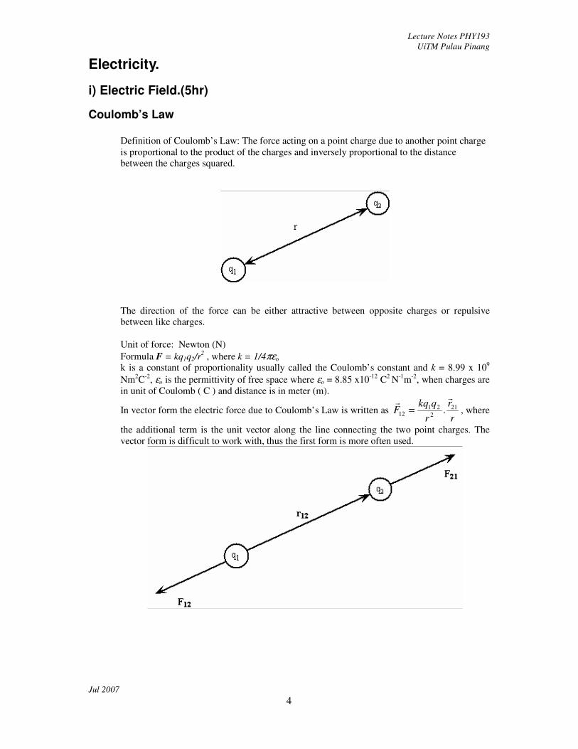
Definition of Coulomb’s Law: The force acting on a point charge due to another point charge
is proportional to the product of the charges and inversely proportional to the distance
between the charges squared.
The direction of the force can be either attractive between opposite charges or repulsive
between like charges.
Unit of force: Newton (N)
Formula F = kq1q2/r2 , where k = 1/4πεo
k is a constant of proportionality usually called the Coulomb’s constant and k = 8.99 x 10⁹
Nm2C
-2, εo is the permittivity of free space where εo = 8.85 x10
-12 C
2 N
-1m
-2, when charges are
in unit of Coulomb ( C ) and distance is in meter (m).
In vector form the electric force due to Coulomb’s Law is written as r
r
r
qkqF 21
2
2112 .
rr
= , where
the additional term is the unit vector along the line connecting the two point charges. The
vector form is difficult to work with, thus the first form is more often used.
Lecture Notes PHY193
UiTM Pulau Pinang
Jul 2007
5
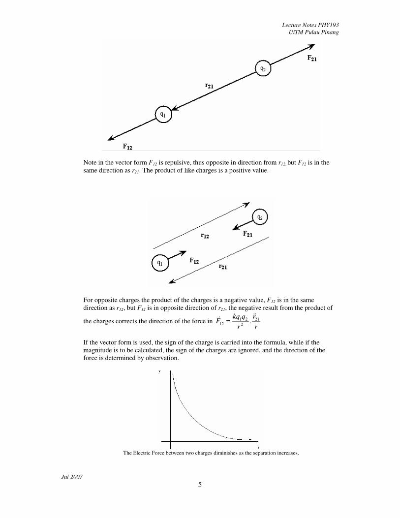
Note in the vector form F12 is repulsive, thus opposite in direction from r12, but F12 is in the
same direction as r21. The product of like charges is a positive value.
For opposite charges the product of the charges is a negative value, F12 is in the same
direction as r12, but F12 is in opposite direction of r21, the negative result from the product of
the charges corrects the direction of the force in r
r
r
qkqF 21
2
2112 .
rr
=
If the vector form is used, the sign of the charge is carried into the formula, while if the
magnitude is to be calculated, the sign of the charges are ignored, and the direction of the
force is determined by observation.
The Electric Force between two charges diminishes as the separation increases.

Lecture Notes PHY193
UiTM Pulau Pinang
Jul 2007
6
Electrostatic Force of three point charges located at the vertices of a triangle
When three point charges are present, the force on a point charge is the vector sum of the
forces acting on that charge due to the other two charges.
F1=F12+F13 in vector form, the force (F1) on charge q1 is the sum of the force (F12) due to
charge q2 and the force (F13) due to charge q3.
In component form, resolving into x-y direction
F1x=F12x+F13x
F1y=F12y+F13y
F1 =( F1x 2+ F1y
2)
½, the direction is determined from the geometry
Similarly charges q1 and q2 exert a net force on q2, and charges q1 and q2 exert a net force on
q3. Thus we also have for q2
F2=F21+F23 And for q3 F3=F31+F32
F2x=F21x+F23x F3x=F31x+F32x
F2y=F21y+F23y F3y=F31y+F32y
F1 =( F2x 2+ F2y
2)
½ F3 =( F3x
2 + F3y
2)
½
The net force on a point charge is the vector sum of the forces acting on that charge. In the diagram above, the
resolved component (x-y components) of the forces are not shown.
Lecture Notes PHY193
UiTM Pulau Pinang
Jul 2007
7
Vector addition of electrostatic force – resolution of force vector in x-y coordinates, add the
forces by its components, find the sum of forces (Pythagoras theorem) and direction (tan φ).
Geometry of triangle is such that the length of sides and / or given angles permits the
resolution of vector in 2 dim (x-y coordinates)
Electric Field Line
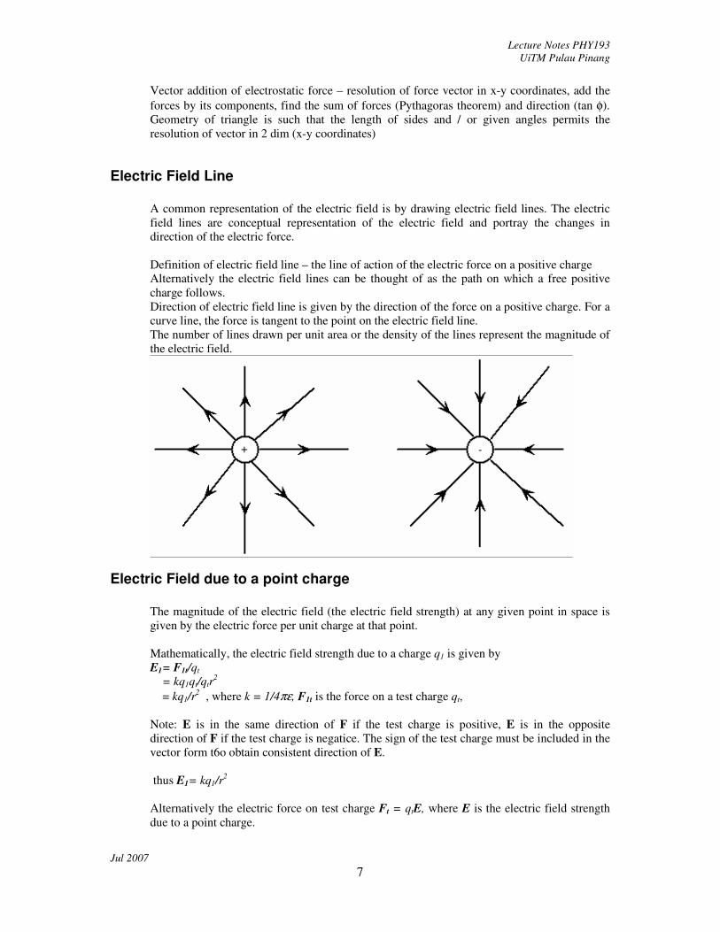
A common representation of the electric field is by drawing electric field lines. The electric
field lines are conceptual representation of the electric field and portray the changes in
direction of the electric force.
Definition of electric field line – the line of action of the electric force on a positive charge
Alternatively the electric field lines can be thought of as the path on which a free positive
charge follows.
Direction of electric field line is given by the direction of the force on a positive charge. For a
curve line, the force is tangent to the point on the electric field line.
The number of lines drawn per unit area or the density of the lines represent the magnitude of
the electric field.
Electric Field due to a point charge
The magnitude of the electric field (the electric field strength) at any given point in space is
given by the electric force per unit charge at that point.
Mathematically, the electric field strength due to a charge q1 is given by
E1= F1t/qt
= kq1qt/qtr2
= kq1/r2 , where k = 1/4πε, F1t is the force on a test charge qt,
Note: E is in the same direction of F if the test charge is positive, E is in the opposite
direction of F if the test charge is negatice. The sign of the test charge must be included in the
vector form t6o obtain consistent direction of E.
thus E1= kq1/r2
Alternatively the electric force on test charge Ft = qtE, where E is the electric field strength
due to a point charge.

Lecture Notes PHY193
UiTM Pulau Pinang
Jul 2007
8
The electric field strength is a vector quantity whose direction is given by the direction of the
electric force on a positive test charge.
The unit for the electric field is NC-1
Like the electric force, the electric field strength for a positive source charge diminishes as the charge is further
away from the source.
Electric Field due to two point charges at arbitrary position
As the electric filed strength is a vector quantity, the electric field due to two point charges is
the vector sum of the electric field due to each of the point charge. Representations of the
electric field around two point charges are given below. The first diagram shows the electric
field around two charges of opposite sign. The following diagram shows the electric field
around two charges of the same sign.

Lecture Notes PHY193
UiTM Pulau Pinang
Jul 2007
9
E = E1 + E2
Ex = E1x + E2x
Ey = E1y + E2y
E = (Ex2+ Ey
2)
½
Resolve the electric field into x-y components, add the components and solve for the
magnitude and direction of the sum of the electric field.
Electric Flux
Electric flus is proportional to the number of electric field lines penetrating some surface.
The electric flux (flux of the electric field) , ΦE = E ⊥ A = EA ⊥ = EA cos θ, where θ is the angle
between E and the normal to the surface.
ΦE = E ⊥ A , is read as the perpendicular component of E multiply by A.
ΦE = EA ⊥ , is read as E multiply by the perpendicular component of A .
Gauss’s Law.
Gauss Law relates the net electric flux of an electric field through a closed surface ( a Gaussian
surface) to the net charge that is enclosed by that surface. The net flux through a closed surface is
proportional to the amount of charge enclosed by the surface.
Lecture Notes PHY193
UiTM Pulau Pinang
Jul 2007
10
ΦE ∝ qenclosed
ΦE = qenclosed / εo or,
εo ΦE = qenclosed
Gauss Law can also be written in the integral form,
enclosedo qAdE =∫rr
.ε
εo is the permittivity of free space, and the above equations hold true for charges in vacuum only.
Gauss Law can be used in two ways, to obtaine the amount of charge enclosed when the flux / electric
field is known or to obtain the electric field if the amount of enclosed charge is known.
Applying gauss Law to;
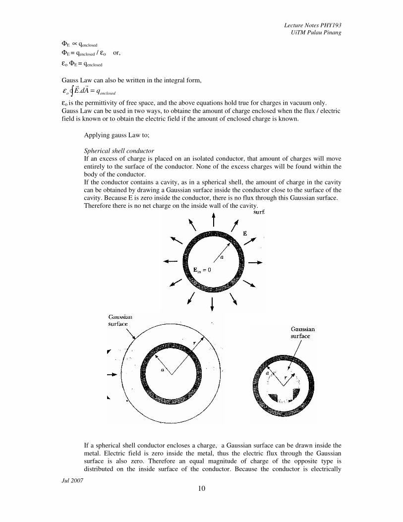
Spherical shell conductor
If an excess of charge is placed on an isolated conductor, that amount of charges will move
entirely to the surface of the conductor. None of the excess charges will be found within the
body of the conductor.
If the conductor contains a cavity, as in a spherical shell, the amount of charge in the cavity
can be obtained by drawing a Gaussian surface inside the conductor close to the surface of the
cavity. Because E is zero inside the conductor, there is no flux through this Gaussian surface.
Therefore there is no net charge on the inside wall of the cavity.
If a spherical shell conductor encloses a charge, a Gaussian surface can be drawn inside the
metal. Electric field is zero inside the metal, thus the electric flux through the Gaussian
surface is also zero. Therefore an equal magnitude of charge of the opposite type is
distributed on the inside surface of the conductor. Because the conductor is electrically

Lecture Notes PHY193
UiTM Pulau Pinang
Jul 2007
11
neutral, an equal magnitude of charge ( same type as the enclosed charge) is distributed on the
outside wall of the spherical conductor.
Long uniform line of charge
A long line of charge can be obtained by charging a long cylindrical plastic rod. The linear
charge density is thus λ. A Gaussian surfave taken would be a cylinder of radius, r and lingth
l, coaxial with the rod. The electric field lines are perpendicular and radially outwards to the
rod. Thus at every point on the cylindrical part of the Gaussian surface E would have the
same magnitude. The electric field coming through the ends of the cylinder is zero. The area
of the cylindrical part is 2πrh, the electric flux is ΦE = E ⊥ A = E2πrh, the charge enclosed is
λh,
thus from εo ΦE = qenclosed,
εo E2πrh =λh
E =λ/ 2πεo r is the elecric field due to an infinitely long line of charge.
Infinite plane of charge
A nonconducting sheet with a uniform (positive) surface charge density σ can be use as a
model. A useful Gaussian surface is a closed cylinder with end caps of area A, arranged to
pierce the sheet perpendicularly. The electric field must be perpendicular to the sheet and also
the end caps, and since the charge is positive the electric field is directed away from the sheet,
and pierce the Gaussian end caps. Because the electric field lines do not pass through the
curve surface, there is no flux through the curve surfave.
Lecture Notes PHY193
UiTM Pulau Pinang
Jul 2007
12
Thus enclosedo qAdE =∫rr
.ε
is εo (EA + EA) = σ A
2εo E = σ
E = σ / 2εo is the electric field due to a sheet of charge.
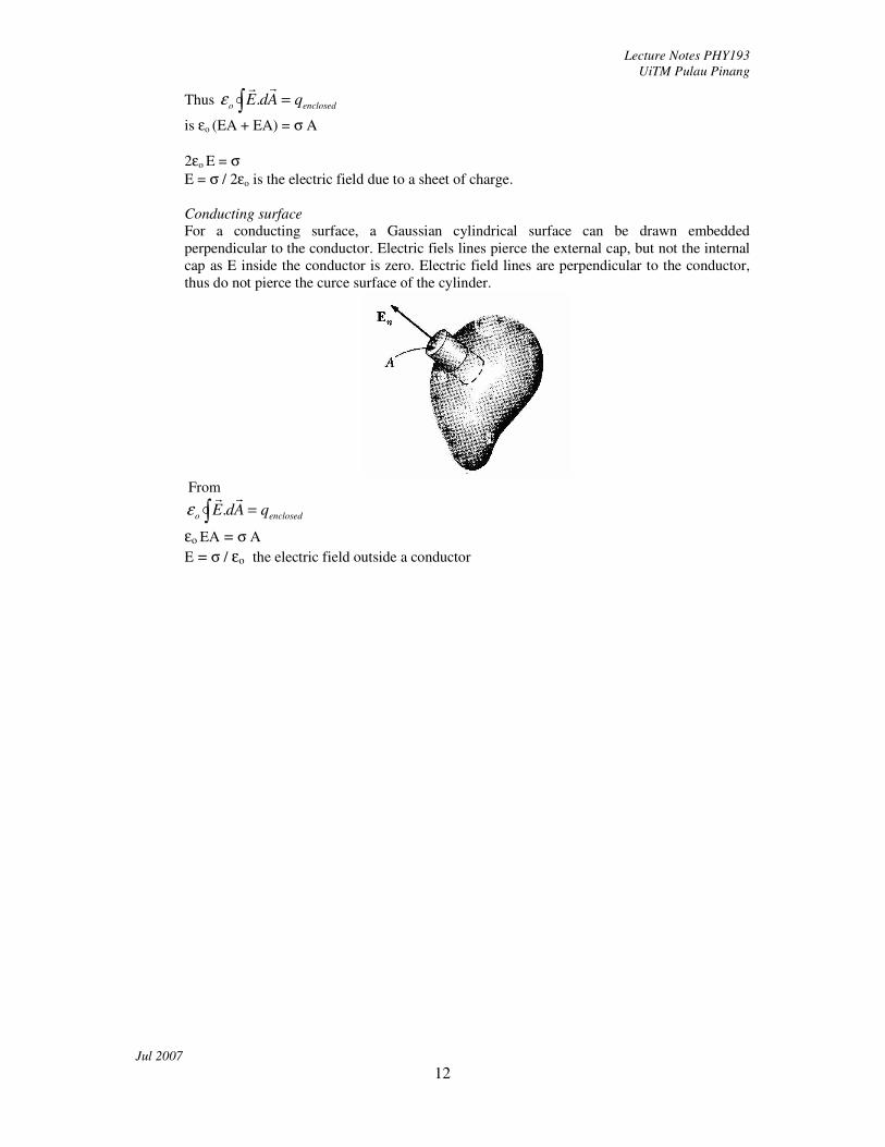
Conducting surface
For a conducting surface, a Gaussian cylindrical surface can be drawn embedded
perpendicular to the conductor. Electric fiels lines pierce the external cap, but not the internal
cap as E inside the conductor is zero. Electric field lines are perpendicular to the conductor,
thus do not pierce the curce surface of the cylinder.
From
enclosedo qAdE =∫rr
.ε
εo EA = σ A
E = σ / εo the electric field outside a conductor

Lecture Notes PHY193
UiTM Pulau Pinang
Jul 2007
13
ii) Electric Potential (6hr)
Electric Potential Energy.
The electric potential energy is the energy available to a charge at a particular point in an
electric field. A charge is then able to do work, it then losses electric potential energy and
ends up in a point of lower electric potential. If work is done by an external agent, then the
charge may gain potential energy and move to a point of higher potential in the electric field.
Consider the electric field due to a single positive point charge. The electric field and the
electric force diminish as a positive test charge is further away from the source of the electric
field. Therefore at r = ∞ (infinity), the force on a charge is zero. Work has to be done by an
external agent against the electric force to move the charge closer into the electric field. By
conservation of energy, the work done by external agent increases the electric potential
energy of the charge.
r
qkqdr
r
qkqdrFW ts
r
ts
r
external =−== ∫∫∞∞
2. = electric potential energy, U when a test qt is
brought from infinity to a distance r from a source charge qs
The electric potential at a point in the electric field is the amount of energy per unit charge
available for the charge at that point in the electric field.
The electric potential V = U/qt
=r
kqq
r
qkq st
ts =÷
Relation between Electric Potential and Electric Field.
The electric field line is the line of action of the electric force acting on a positive charge. If
the charge is not fixed to the point, the force acting on the charge will move the charge in the
direction of the force. As the charge moves it will loose electric potential energy as the charge
has move from a point of higher potential to a point of lower potential along the electric field
lines. In short electric potentials are points on the electric field lines.
Using work energy principle, a charge at a higher potential point has a higher energy, it will
move to a lower potential point and losses energy which is the same amount of work done by
the electric field on the charge.
Change in potential energy, q ∆V = q (Vf – Vi), where Vf is lower than Vi , thus a loss in
potential energy of the system.
Work done by system W = F.s = q E.s, where s is the displacement vector between the two
potential points.
By the principle of conservation of energy, total energy of system is conserved, the change in
potential energy plus the work done by system is equal to zero.
q (Vf – Vi) + q E.s = 0
E.s = - (Vf –Vi)
E = - (Vf –Vi) / s
E = - ∆ V / s, thus the electric field is given as the negative of the gradient of the electric
potential. Common form is E = - ∆ V /∆ x
Electric Potential due to a point charge and several charges

Lecture Notes PHY193
UiTM Pulau Pinang
Jul 2007
14
The electric potential at a point in the electric field is the amount of energy per unit charge
available for the charge at that point in the electric field.
The electric potential V = U/qt
r
kqs=
The electric potential around a positive source charge is positive, while the electric potential
around a negative source charge is negative. The electric potential is not a vector. Therefore
the electric potential due to several source charges is the arithmetic sum of the electric
potential of each source charge.
3
3
2
2
1
1
321
r
kq
r
kq
r
kqV
VVVV
++=
++=
,
where r1, r2 and r3 are the distances from the source charges q1, q2 and q3 respectively.
Equipotential Surfaces
Equipotential surfaces are surfaces which have the same electric potential.
Consider the potential around a point charge. An equipotential surface for the point charge is
a spherical surface with the charge at the center of the sphere, i.e. a constant distance r. There
would be an infinite number of concentric spherical surfaces, each an equipotential surface
around the point charge. In 2-dimensional drawing, an equipotential surface may be represented by a line connecting
points of the same electric potential. The equipotential lines are drawn perpendicular to the
electric field lines.
Examples of equipotental surface / lines VA and VB for different electric fields
Capacitance of a parallel plate capacitor
A capacitor is constructed from two parallel conducting plates. When the plates are placed at
different potential by connecting each plate to the terminal of a voltage source (cell), an
electric field is created between the plates. Charges in the plates are displaced, one plate will
be positively charged, while the other negatively charged. The amount of charged displaced,
transferred from one plate to the other is proportional to the potential difference between the
plates.
VQ ∝ , where V is the potential difference across the capacitor.
CVQ = , C a constant of proportionality called the capacitance.

Lecture Notes PHY193
UiTM Pulau Pinang
Jul 2007
15
Therefore, V
QC =
, the capacitance, can be defined as the amount of charge stored in the
capacitor per unit voltage applied across the capacitor. The capacitance of a capacitor is a
constant physical quantity, the amount of charge stored changes with the applied voltage, the
capacitance remains unchanged.
The capacitance of a parallel plate capacitor can also be expressed in terms of the physical
construction of the capacitor. For a parallel plate capacitor of effective area A, separation d
the capacitance is d
AC o
o
ε=
, where oε= 8.85 x10⁻¹² C2 N-1m-2 is the permittivity of free
space.
If the spaces between the plates are filled with dielectric materials, the capacitance becomes
d
A
d
AC orεεε
==, where ε is the permittivity of the dielectric material and can be expressed
in form of the dielectric constant (relative permittivity) rε .
Energy stored in an a charged capacitor, dW = Vdq
The energy stored in the capacitor comes from the work done by the voltage in moving the
charge from one plate to the other.
The work done dW = Vdq, where V is the voltage across the capacitor at that particular time
(not the applied voltage). Rewriting C
qV = , then dq
C
qdW = . If the cell transfer a
maximum amount of charge Q, then total work done is
dqC
qdW
QW
∫∫ =00
C
QW
2
2
1= , which can also be written in the form QVCVW
2
1
2
1 2 ==
Capacitors in series and in parallel
When capacitors are connected in series or parallel, the total capacitance due to the
arrangements can be computed.
In a series arrangement, the uncharged capacitors are connected end to end. A dc supply is
connected across the whole arrangement. There is only one path for the charges to flow, thus
the end plates will received equal but opposite charges. The charges on one plate will attract
the same magnitude of charge of the opposite type. Thus along the chain of capacitors in
series, each capacitor will accumulate the same amount of charges regardless of their
capacitance.
The total voltage across the capacitors in series is just the sum of the voltage across each
capacitor, given by V=Q/C

Lecture Notes PHY193
UiTM Pulau Pinang
Jul 2007
16
eq
tot
tot
tot
C
QV
CCCQV
C
Q
C
Q
C
QV
=
++=
++=
321
321
111
where
++=
321
1111
CCCCeq
and eqC is called the equivalent capacitance.
In a parallel connection, the uncharged capacitors are connected in parallel to each other and
to a dc supply. Thus the potential difference across each capacitor is the same. As there are
multiple paths for the current/charges from the supply, the total current/charges from the
supply equal the sum of all currents/charges to the capacitors.
321
321
321
33
22
11
321
)(
CCCC
VCQ
VCCCQ
VCVCVCQ
VCQ
VCQ
VCQ
QQQQ
eq
eqt
t
t
t
++=
=
++=
++=
=
=
=
++=
where eqC is the equivalent capacitance of the parallel circuit.

Lecture Notes PHY193
UiTM Pulau Pinang
Jul 2007
17
iii) Current and Resistance (3hr)
Electric Current
Electric current is the time rate of change of charges passing through a point in a conductor
Unit: 1 Coulomb / 1 sec = 1 Ampere
Resistance and Resistivity
Resistance is the measure of the degree to which an object opposes a current passing through
it.
Unit: Ohm
Resistivity is the measure of how strong a material opposes the current which pass through it.
Unit: Ohm.meter
The resistance, R, of an object depends on the resistivity, ρ , of the material it is made up of
and its physical dimensions. For a conductor of length l and constant cross-sectional area, A,
the resistance is given as,
A
lR ρ=
Thus the electrical resistivity ρ of a material is given by
l
AR=ρ
where
ρ is the static resistivity (measured in ohm metres, Ωm);
R is the electrical resistance of a the conductor (measured in ohms, Ω);
l is the length of the conductorn (measured in metres, m);
A is the cross-sectional area of the conductor (measured in square metres, m²).
Note: Resistance of an object is dependent on its resistivity, length and cross sectional area.
The resistivity of an object depends on the material and is independent of its length and cross
sectional area. Copper wires of different length and thickness have different resistance but all
have the same resistivity.
Resistors in Series and Parallel
Resistors in series: The total resistance is the sum of the resistance of each resistors in the
series arrangement, RT = R1 + R2 + R3
Resistors in Parallel: The inverse sum of the total resistance is the sum of the inverse
resistance of the resistors in the parallel arrangements 1321
1111
RRRRT
++=
Ohm’s Law
The ratio of the voltage change across a circuit element to the current passing through the
same element is a constant. This constant is defined as the resistance of the element.

Lecture Notes PHY193
UiTM Pulau Pinang
Jul 2007
18
RI
V= commonly written as IRV =
Power in electric circuit
Power is defined as the rate of change of energy. In a circuit power could be the rate of
change of energy into heat (a resistor) or the rate of change of chemical energy into electrical
energy ( a cell or battery).
When current passes through a circuit element, it goes through a potential change (potential
drop, in case of a resistor). The charge loses potential energy. The rate of change of this
energy is the power across the circuit element.
From t
QI
∆
∆= , the amount of charge passing through a point in the circuit, ∆Q = I ∆t
Therefore the change in potential energy across a potential difference is
∆U = ∆Q ∆V = I ∆V ∆t
∆E= ∆Q ∆V = I ∆V ∆t, rewriting the potential energy as rate of change of electrical energy
PVIt
E=∆=
∆
∆, where P is the power (or rate of change of energy)
Therefore P = V I, where V is the potential difference across the circuit element and I the
current through the circuit element.
Lecture Notes PHY193
UiTM Pulau Pinang
Jul 2007
19
iv) Circuits (4hr)
Calculating Current
Current flows in a complete circuit due to a voltage applied ( voltage difference) across the
conductor. If a circuit is not complete / closed, there is no current flow in the conductor even
though the ends of the conductor are at different electrical potential. Current flow is viewed as
the movement of positive charges in the conductor. As positive charge moves from a higher
potential point to a lower potential point in the circuit, so does current. Thus current flows
from a higher potential point to a lower potential point in the circuit. By definition current is
t
QI
∆
∆= , the amount of charge, ∆Q, passing through a point in the circuit in a given time ∆t.
Current can olso be calculated from Ohm’s Law, RI
V= , thus commonly written as
R
VI = ,
where V is the applied voltage across the conductor and R , the resistance of the conductor.
Single Loop Circuit
A single loop circuit is an electric circuit which is reduced to a voltage source, V and a single
load resistance R. Therefore the voltage across the load resistance is the same as that of the
source. Conducting wires to complete the circuit is assumed to have negligible (zero)
resistance. An electric circuit can be converted into a single loop circuit if it has only one
voltage source and the resistors can be reduced using parallel and series arrangement formula
into a single load resistor.
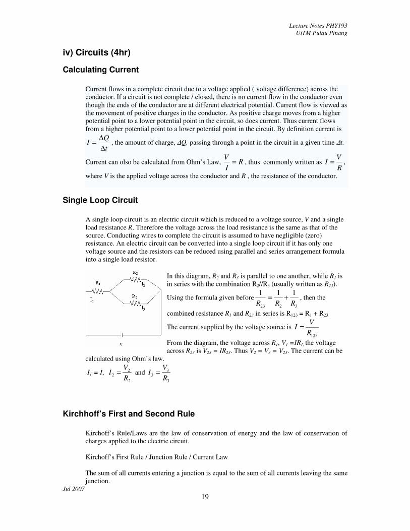
In this diagram, R2 and R3 is parallel to one another, while R1 is
in series with the combination R2//R3 (usually written as R23).
Using the formula given before3223
111
RRR+= , then the
combined resistance R1 and R23 in series is R123 = R1 + R23
The current supplied by the voltage source is 123R
VI =
From the diagram, the voltage across R1, V1 =IR1, the voltage
across R23 is V23 = IR23. Thus V2 = V3 = V23. The current can be
calculated using Ohm’s law.
I1 = I, 2
22
R
VI = and
3
33
R
VI =
Kirchhoff’s First and Second Rule
Kirchoff’s Rule/Laws are the law of conservation of energy and the law of conservation of
charges applied to the electric circuit.
Kirchoff’s First Rule / Junction Rule / Current Law
The sum of all currents entering a junction is equal to the sum of all currents leaving the same
junction.
Lecture Notes PHY193
UiTM Pulau Pinang
Jul 2007
20
∑∑ = outin II
Kirchoff’s Current Law is a restatement of the principle of conservation of charges and mass.
Kirchoff’s Second Rule / Loop Rule / Voltage Law
The algebraic sum of of the potential changes across all elements in a closed circuit loop
must be equal to zero.
∑ =∆ 0V
Kirchoff’s Voltage Law is a restatement of the principle of conservation energy.
(Note: In this case the change in potential has to be carefully considered. Going from the
negative to the positive terminal through a cell gives a positive change in potential. In the
reverse direction a negative potential change is obtained)
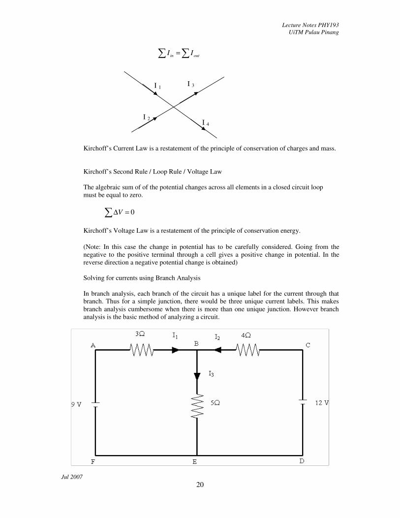
Solving for currents using Branch Analysis
In branch analysis, each branch of the circuit has a unique label for the current through that
branch. Thus for a simple junction, there would be three unique current labels. This makes
branch analysis cumbersome when there is more than one unique junction. However branch
analysis is the basic method of analyzing a circuit.
I 2
I 1
I 4
I 3

Lecture Notes PHY193
UiTM Pulau Pinang
Jul 2007
21
Writing The Equations
Each branch is labeled with a unique current label
Equation satisfying KCL for the junctions are written.
At junction B; I1+I2 = I3 …………..(1)
At junction E; I3 = I1+I2 , which is exactly as that at junction B.
Equations satisfying KVL for the loops are written.
Going around loop ABEFA and taking the potential change, ∆V;
- I1(3Ω) - I3(5Ω) + 9V = 0…………..(2)
Going around loop BCDEB and taking the potential change, ∆V;
I2(4Ω) – 12V + I3(5Ω) = 0………….(3)
Going around loop ABCDEFA and taking potential change, ∆V;
- I1(3Ω) + I2(4Ω) – 12V + 9V = 0
This final equation is actually the combination of the earlier two KVL equations. Therefore,
there are only two unique KVL equations.
A rule of thumb is that each component of the circuit has to be passed at least once when
taking the potential change.
By applying Kirchoff’s Rules to the circuit we obtain simultaneous equations which need to
be solved.
Solving Simultaneous Equations Using Direct Substitution
Substituting (1) into (2) and (3) produce,
- I1(3Ω) – (I1 + I2)(5Ω) + 9V = 0…………..(2)
I2(4Ω) – 12V + (I1 + I2)( (5Ω) = 0………. ..(3)
After collecting similar terms give;
- I1(8Ω) – (I2)(5Ω) + 9V = 0…………..(2)
(I1)(5Ω) + I2(9Ω) – 12V = 0…………...(3)
- 8I1 – 5I2 + 9 = 0…………..(2) (dropping the Ω and V make for easier witing)
5I1 + 9I2 – 12 = 0…………...(3)
Equation (2) can be rewritten for I1 in terms of I2 and substituted in equation (3) or can be
eliminated as follows.
Method Of Elimination
- 8I1 – 5I2 + 9 = 0…………....(2)
5I1 + 9I2 – 12 = 0…………...(3)

Lecture Notes PHY193
UiTM Pulau Pinang
Jul 2007
22
(2) x 5 : - 40I1 – 25I2 + 45 = 0
(3) x 8 : 40I1 + 72I2 – 96 = 0
Adding both up gives
(-40 + 40)I1 + (-25 + 72)I2 + (45 – 96) = 0
Thus I1 is eliminated from the equation and I2 can be calculated.
The value for I2 is then substituted into (2) or (3) to obtain I1.
Another method of solving circuit problems is by using Mesh Analysis.
Each mesh has its own current. The current through a shared branch is the algebraic sum of
the current contributed by each mech.
Writing the equations
Going around loop ABEFA and taking the potential change, ∆V;
- I1(3Ω) –( I1 + I2 )(5Ω) + 9V = 0…………..(1)
Going around loop BCDEB and taking the potential change, ∆V;
I2(4Ω) – 12V + ( I1 + I2 )( (5Ω) = 0………….(2)
Note : KCL is applied at the junction while writing down KVL for the loop.
The total current through a branch is the algebraic sum of the loop currents through the
branch : The superposition of currents.
The simultaneous equations obtained are,
- I1(3Ω) –( I1 + I2 )(5Ω) + 9V = 0…………..(1)
I2(4Ω) – 12V + ( I1 + I2 )( (5Ω) = 0………….(2)
Expanding the equations give
- I1(3Ω) –( I1 )(5Ω) –( I2 )(5Ω) + 9V = 0…………..(1)

Lecture Notes PHY193
UiTM Pulau Pinang
Jul 2007
23
I2(4Ω) – 12V + ( I1)( (5Ω) + (I2 )( (5Ω) = 0………….(2)
Collecting the current terms gives
- I1(3Ω + 5Ω) – ( I2 )(5Ω) + 9V = 0…………..(1)
( I1)( (5Ω) + (I2 )(4Ω + 5Ω) - 12V = 0………….(2)
- I1(8Ω) – ( I2 )(5Ω) + 9V = 0…………..(1)
( I1)( (5Ω) + (I2 )( 9Ω) - 12V = 0………….(2)
- 8I1 – 5I2 + 9 = 0…………..(1)
5I1 + 9I2 - 12 = 0………….(2)
(1) x 5 : - 40I1 – 25I2 + 45 = 0…………..(1)
(2) x 8 : 40I1 + 82I2 - 96 = 0………….(2)
Using the method of elimination I1 and I2 can be obtained as in the previous section.
Another method of solving simultaneous equations is the Matrix Method
The matrix method is used to obtain the values of I1 and I2 without using the method of
elimination. Using either the Branch or Loop currents analysis the equations are obtained as
before.
- 8I1 – 5I2 + 9 = 0…………..(1)
5I1 + 9I2 - 12 = 0………….(2)
Rearranging the equations give
- 8I1 – 5I2 = - 9
5I1 + 9I2 = 12
Rearranging into matrix form will produce
This can be easily solved using the built in matrix solution in a calculator (ex. Casio FX
570MS), which can solve for 2 and 3 loop currents.
CRAMER’S RULE / METHOD OF DETERMINANTS
The method of determinants is especially used to solve for 3 loop currents in a 3 loop problem
where the methods of substitution and elimination become unyielding.
Writing the equations in the matrix form give,
R11 R12 R13 I1 V1
R21 R22 R23 I2 = V2
R31 R32 R33 I3 V3
-8 -5
5 9
I1
I2 =
-9
12

Lecture Notes PHY193
UiTM Pulau Pinang
Jul 2007
24
Ammeter and Voltmeter
Ammeters and voltmeters are devices which are used to measure the current at a point and the
potential difference between two points respectively. To use an ammeter the circuit has to be
broken at the point where current is to be measures, the ammeter is inserted to complete the
circuit. An ammeter has very low resistance so as not to resists current in the circuit. A
voltmeter is connected across the points where potential difference needs to be measured. A
voltmeter has very high resistance so as not to draw current from the circuit. Traditional
bench ammeters and voltmeters (usually called moving coil meter) are constructed using fine
coils and magnets and have fixed range, the pointer swings in one direction usually giving
positive reading only. A multimeter is usually has solid state components which allow larger
range and may even display positive and negative readings.
To entend the range of moving coil ammeters and voltmeters, shunts and multiplier are used.
Converting a microammeter to an ammeter
A bypass path (shunt) is provided to prevent excess current through the
galvanometer. The maximum current allowed through the galvanometer is IFSD,
R11 R12 R13
Det R = R21 R22 R23
R31 R32 R33
Then V1 R12 R13
I1 = 1 / Det R V2 R22 R23
V3 R32 R33
and R11 V1 R13
I2 = 1 / Det R R21 V2 R23
R31 V3 R33
and R11 R12 V1
I3 = 1 / Det R R21 R22 V2
R31 R32 V3

Lecture Notes PHY193
UiTM Pulau Pinang
Jul 2007
25
the current at full scale deflection of the pointer. The value of the shunt resistor in
the bypass is chosen according to the value of the current that need to be
measured.
KCR is applied to the junction as shown and KVR is applied to the loop.
- IFSD rg + (I- IFSD ) Rs = 0
Rs = IFSD rg / (I- IFSD )
Converting an ammeter into a voltmeter
By adding a resistor in series with the galvanometer, a higher potential difference
(voltage) can be measured by the galvanometer. The voltmeter is now able to measure
V = I (rg + Rm)
RC Circuit
An RC circuit is a circuit consisting a resistor a
capacitor and a voltage source connected in series.
When the circuit is closed, current flows from the
voltage source into the capacitor. The resistor
restricts the current flow. The capacitor is in the state
of being charged. The voltage across the capacitor
increases and opposes the flow of current. The
amount of current becomes smaller, and stops
flowing (current becomes zero) when the voltage
across the capacitor is equal to the source voltage.
The graph on the left shows how charge increases in
the capacitor. The voltage across the capacitor
q(t)
t V(t)
t
I(t)
t
q(t) = Qo (1-e-t/RC)
V(t) = Vo (1-e-t/RC)
I(t) = Io e-t/RC
Lecture Notes PHY193
UiTM Pulau Pinang
Jul 2007
26
increases due to the increase in charge. Current flow decreases as the voltage across the capacitor
increase. The charge, voltage across the capacitor and current changes as q(t) = Qo (1-e-t/RC
) ,
V(t) = Vo (1-e-t/RC
) and I(t) = Io e-t/RC
, respectively.
The term RC is called the time constant as it determines the slope of the function.
If a resistor is connected in series with a charged capacitor, current will flow out of the capacitor
(discharges). The charge, voltage across the capacitor and current changes as q(t) = Qo e-t/RC
,
V(t) = Vo e-t/RC
and I(t) = Io e-t/RC
, respectively.

Lecture Notes PHY193
UiTM Pulau Pinang
Jul 2007
27
Magnetism
v) Magnetism (4hr)
Magnetic Field
A magnetic field is a region where magnetic force can be experienced. A magnetic force is the
attractive or repulsive force acting between the poles of a magnetic dipole. A magnetic dipole has two
ends or poles, the north seeking pole and the south seeking pole. It is called as such due to its
interaction with the earth magnetic field.
The earth’s magnetic field
The earth can be viewed as a giant magnet which produces a magnetic field that influence magnetic
dipole within its vicinity. When a magnetic dipole (a bar magnet) is hung freely in the earth magnetic
field, one of its end will point to the geographic north and the other end will point to the geographic
south. The north pointing end is the north seeking pole (or just plain north pole ) of the bar magnet.
The south pointing end is the south seeking pole (or just south pole) of the bar magnet.
When the north poles of two bar magnets (or the south poles) are brought towards each other a
mutually repulsive force is observed acting on the poles. When opposite poles are brought towards
each other, an attractive force is observed. The attraction and repulsion can be viewed as the
interaction of the magnetic lines of forces. The magnetic alignment N-S is due to the magnet orienting
itself with the lines of force (magnetic field lines).
The definition of Magnetic field, B
The magnetic flux, φ is the amount of magnetic field lines passing perpendicularly through a given
area, unit Wb (Weber). This is a scalar quantity.
The magnetic flux density , B– the magnetic field strength at a given point, unit Wb/m2 or T (Tesla).
The magnetic flux density is also called the magnetic field and is a vector quantity.
The magnetic flux is related to the magnetic field density by , magnetic flux = magnetic flux density
perpendicular to the area x the area
S
N
N
S
N N S S
θ
B
N
A
Flux,φ = B . A
= BA cos θ

Lecture Notes PHY193
UiTM Pulau Pinang
Jul 2007
28
Magnetic Force on an Electric Charge
The magnetic force on a charge in a magnetic field is the charge multiplies by
the vector cross product of the velocity of the charge with the magnetic field
density / strength.
Thus for a charge at rest the magnetic force acting on it is zero.
F = qv x B in vector form whose magnitude is given by
F = qvB sin θ, where θ is the angle between v and B, where the direction of F
is given by Fleming’s Left Hand Rule.
F = qv x B
i j k F = q vx vy vz
Bx By Bz
F = q ( (vyBz – Byvz) i + (vzBx –vxBz) j + (vxBy –vyBx) k)
If v = vx i and B = Bx i + By j, then
F = q vxBy k
F = q vBsin θ k
Lecture Notes PHY193
UiTM Pulau Pinang
Jul 2007
29
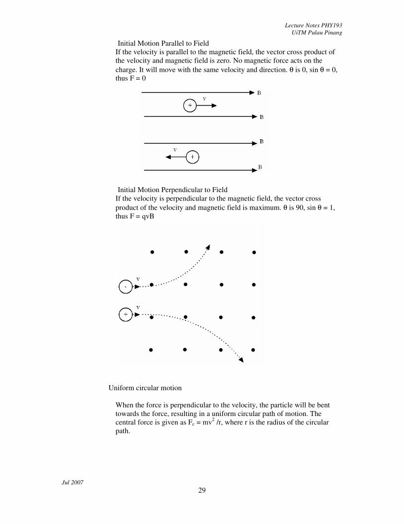
Initial Motion Parallel to Field
If the velocity is parallel to the magnetic field, the vector cross product of
the velocity and magnetic field is zero. No magnetic force acts on the
charge. It will move with the same velocity and direction. θ is 0, sin θ = 0,
thus F = 0
Initial Motion Perpendicular to Field
If the velocity is perpendicular to the magnetic field, the vector cross
product of the velocity and magnetic field is maximum. θ is 90, sin θ = 1,
thus F = qvB
Uniform circular motion
When the force is perpendicular to the velocity, the particle will be bent
towards the force, resulting in a uniform circular path of motion. The
central force is given as Fc = mv2 /r, where r is the radius of the circular
path.
Lecture Notes PHY193
UiTM Pulau Pinang
Jul 2007
30
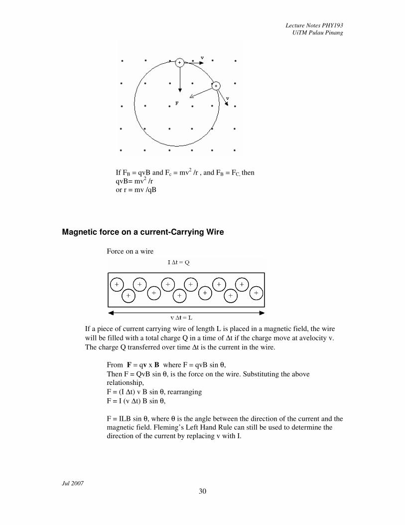
If FB = qvB and Fc = mv2 /r , and FB = FC, then
qvB= mv2 /r
or r = mv /qB
Magnetic force on a current-Carrying Wire
Force on a wire
If a piece of current carrying wire of length L is placed in a magnetic field, the wire
will be filled with a total charge Q in a time of ∆t if the charge move at avelocity v.
The charge Q transferred over time ∆t is the current in the wire.
From F = qv x B where F = qvB sin θ,
Then F = QvB sin θ, is the force on the wire. Substituting the above
relationship,
F = (I ∆t) v B sin θ, rearranging
F = I (v ∆t) B sin θ,
F = ILB sin θ, where θ is the angle between the direction of the current and the
magnetic field. Fleming’s Left Hand Rule can still be used to determine the
direction of the current by replacing v with I.
Lecture Notes PHY193
UiTM Pulau Pinang
Jul 2007
31
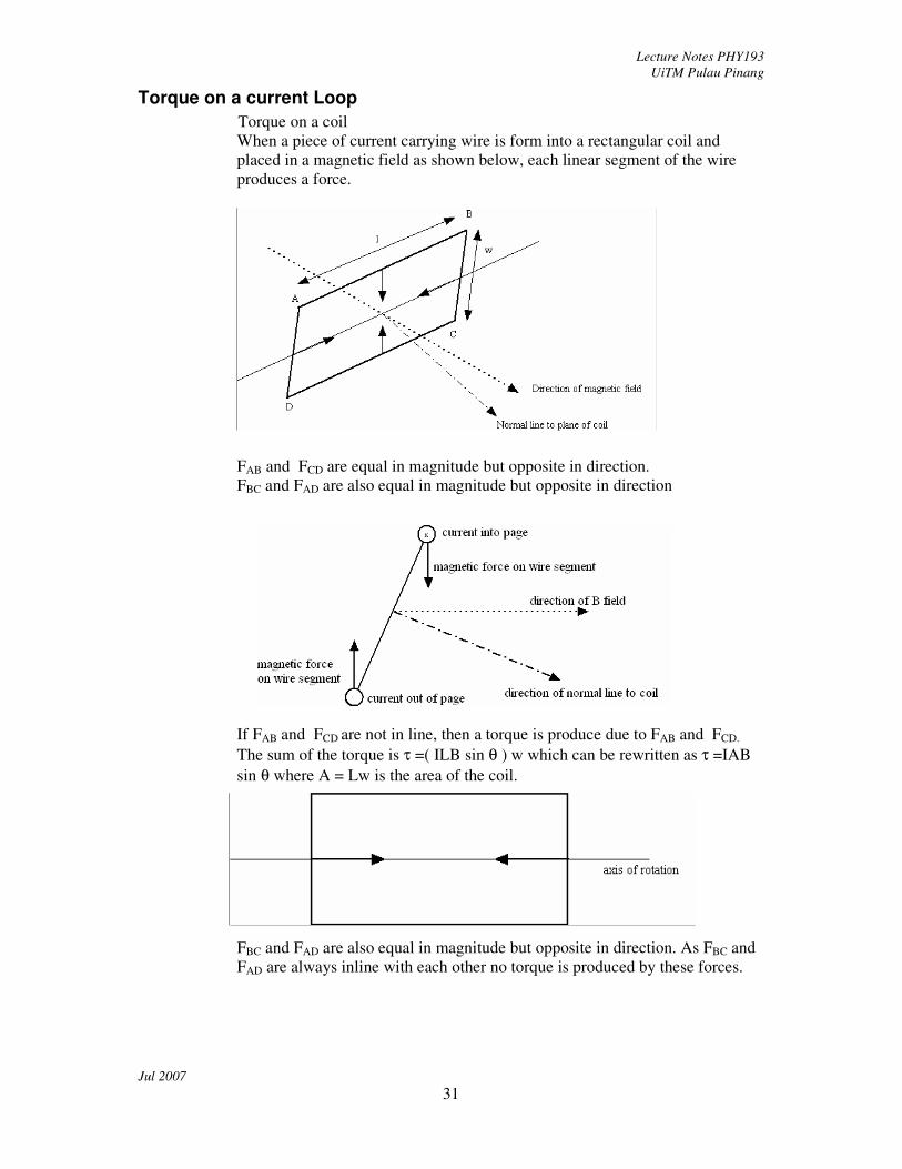
Torque on a current Loop
Torque on a coil
When a piece of current carrying wire is form into a rectangular coil and
placed in a magnetic field as shown below, each linear segment of the wire
produces a force.
FAB and FCD are equal in magnitude but opposite in direction.
FBC and FAD are also equal in magnitude but opposite in direction
If FAB and FCD are not in line, then a torque is produce due to FAB and FCD.
The sum of the torque is τ =( ILB sin θ ) w which can be rewritten as τ =IAB
sin θ where A = Lw is the area of the coil.
FBC and FAD are also equal in magnitude but opposite in direction. As FBC and
FAD are always inline with each other no torque is produced by these forces.

Lecture Notes PHY193
UiTM Pulau Pinang
Jul 2007
32
Magnetic Fields due to Currents
Ampere’s Law
Ampere’s Law – states that the sum of the magnetic field density tangent to the path
multiplied by the path element of a path enclosing a current is propotional to the current
enclosed,
Magnetic field due to straight conductor
Assume a circular path enclosing a straight long conductor, passing through the center of the
circular path, applying Ampere’s Law Σ B ∆∆∆∆l = µo I
B (2πr) = µo I
Therefore, B = r2
Io
π
µ , r = distance between conductor and circular path.
µo is the permeability in free space (4 π x 10 –7
Hm-1
) (ketelapan vakum)
Magnetic field of a circular loop
The magnetic field in the center of a circular coil is given by
B = r2
Ioµ
If the coil has N turns the magnetic field is then B = r2
NIoµ
Magnetic field of a solenoid
A solenoid is a 3 dimensional coil.
Applying Ampere’s Law to a solenoid, the B l = µo N I
l = length of
solenoid
N = no of turns
I = current in each turns
Magnetic field inside a toroid
A toroid is a coil form into a doughnut shape. It can also be viewed as a solenoid whose ends
are joined together.
Applying Amperes’s Law to a toroid, B (2πr) = µo N I
B
r
I
Right Hand Grip Rule

Lecture Notes PHY193
UiTM Pulau Pinang
Jul 2007
33
Force between two parallel wires: parallel & antiparallel currents.
If two current carrying straight conductors (long wires) are placed parrallel to each other,
each wire will create a magnetic field, thus each wire will experienced a force due to the field
of the other wire.
The force on wire B due to the magnetic field produced by wire A is given by FBA = IBLB x
BA
The magnetic field due to wire A is given by BA = r2
IAo
π
µ
Therefore the force is given by FBA = IBLB x r2
IAo
π
µ
Or FBA = r2
II BAo
π
µLB, with the direction given by the FLHR
If the currents in the wires are parallel to each other the force produced causes the wires to be
attracted to each other. If the currents in the wires are anti parallel, the force produced causes
the wires to repel each other.
r
B due to wire
A
Wire
A Wire B
IA I B
FBA

Lecture Notes PHY193
UiTM Pulau Pinang
Jul 2007
34
vi) Inductance (4hr)
Magnetic flux, is a measure of quantity of magnetism, taking account of the strength and
the extent of a magnetic field. The flux through an element of area perpendicular to the
direction of magnetic field is given by the product of the magnetic field density and the area
element.
Conversely, the magnetic flux can also be taken as the product of the perpendicular
component of the magnetic filed density and the area element.
More generally, magnetic flux is defined by a scalar product of the magnetic field density
and the area element vector.
The SI unit of magnetic flux is the weber, and the unit of magnetic flux density is the
weber per square meter, or tesla.
Flux Linkage

Lecture Notes PHY193
UiTM Pulau Pinang
Jul 2007
35
For a coil of N turns, the flux linking the coil is Φ=Nφ=NBA cos θ
Although the actual area of the coil is A, flux linkage in effect looks at the coil
as having an area NA. Thus a larger amount of flux can be obtained using the
effects of flux linkage when the region of magnetic field is small.
Lecture Notes PHY193
UiTM Pulau Pinang
Jul 2007
36
Faraday’s Law
The Faraday’s Law of Electromagnetic Induction states that
The magnitude of the electromotive force induced is directly proportional to the time
rate of change of flux.
In mathematical form this can be written as,
ε ∝ dφ/dt
extending to a coil it can be written as
ε ∝ dΦ/dt
or
ε ∝ Ndφ/dt
Lenz’s Law
The Lenz’s Law of Electromagnetic Induction states that
The direction of the induced electromagnetic force is such that is opposes the action
which produces it.
The Lenz’s Law of Electromagnetic Induction arises from the need to conserve
energy. The electrical energy produced from electromagnetic induction is normally
due to the conversion of mechanical energy to electrical energy.
Combining both laws give us,
ε = - Ndφ/dt or ε = - N∆φ/∆t
where the negative sign determines the direction of the induce e.m.f. with
respect to the changing flux.
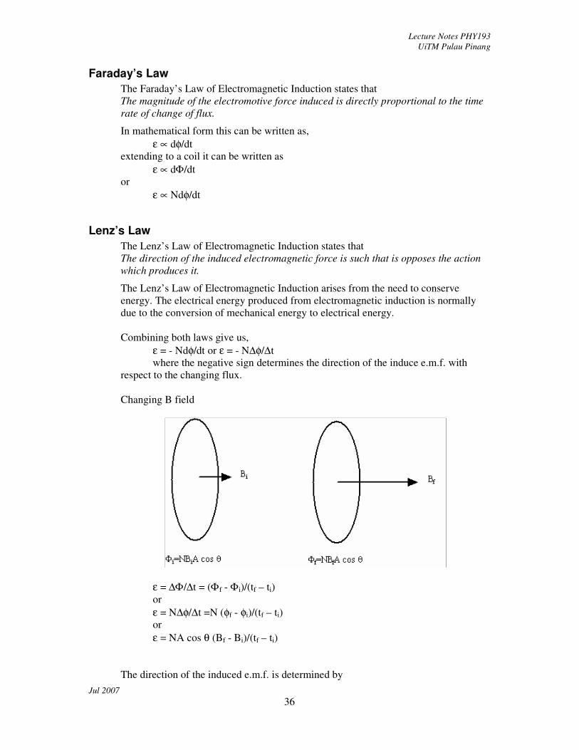
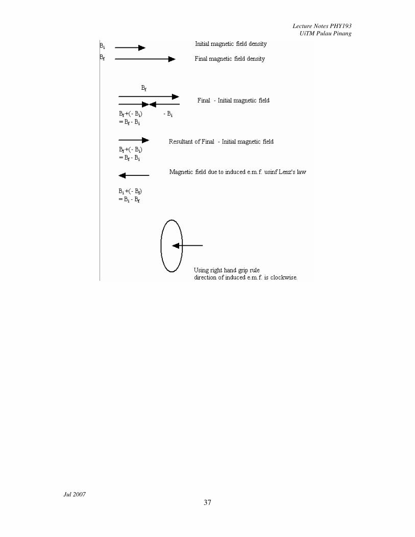
Changing B field
ε = ∆Φ/∆t = (Φf - Φi)/(tf – ti)
or
ε = N∆φ/∆t =N (φf - φi)/(tf – ti)
or
ε = NA cos θ (Bf - Bi)/(tf – ti)
The direction of the induced e.m.f. is determined by
Lecture Notes PHY193
UiTM Pulau Pinang
Jul 2007
37

Lecture Notes PHY193
UiTM Pulau Pinang
Jul 2007
38
ε = N∆φ/∆t =N (φf - φi)/(tf – ti)
ε = NB cos θ (Af - Ai)/(tf – ti)
But (Af - Ai) = Lv∆t = Lv(tf – ti)
therefore,
ε = NB cos θ Lv(tf – ti)/tf – ti)
ε = NB cos θ Lv
ε = NBLv cos θ
Variations of the changing area is i) a single moving wire in the magnetic field, ii) the
sliding wire makes an angle with the rails.
The direction of e.m.f. in the sliding/moving wire can be determined in several ways.
For a coil rotating with a constant angular speed, ω, in a magnetic field, the instantaneous
e.m.f. can be obtain as follows.
ε(t) = - Ndφ/dt
ε(t) = - N d(BA cos θ)/dt
ε(t) = - NBA d(cos θ)/dt
But cos θ = cos ωt where θ = ωt
Then dθ = ω dt
Using chain rule
Lecture Notes PHY193
UiTM Pulau Pinang
Jul 2007
39
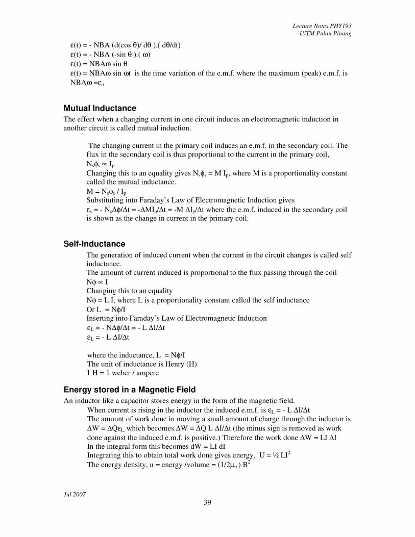
ε(t) = - NBA (d(cos θ)/ dθ ).( dθ/dt)
ε(t) = - NBA (-sin θ ).( ω)
ε(t) = NBAω sin θ
ε(t) = NBAω sin ωt is the time variation of the e.m.f. where the maximum (peak) e.m.f. is
NBAω =εo
Mutual Inductance
The effect when a changing current in one circuit induces an electromagnetic induction in
another circuit is called mutual induction.
The changing current in the primary coil induces an e.m.f. in the secondary coil. The
flux in the secondary coil is thus proportional to the current in the primary coil,
Nsφs ∝ Ip
Changing this to an equality gives Nsφs = M Ip, where M is a proportionality constant
called the mutual inductance.
M = Nsφs / Ip
Substituting into Faraday’s Law of Electromagnetic Induction gives
εs = - Ns∆φ/∆t = -∆MIp/∆t = -M ∆Ip/∆t where the e.m.f. induced in the secondary coil
is shown as the change in current in the primary coil.
Self-Inductance
The generation of induced current when the current in the circuit changes is called self
inductance.
The amount of current induced is proportional to the flux passing through the coil
Nφ ∝ I
Changing this to an equality
Nφ = L I, where L is a proportionality constant called the self inductance
Or L = Nφ/I
Inserting into Faraday’s Law of Electromagnetic Induction
εL = - N∆φ/∆t = - L ∆I/∆t
εL = - L ∆I/∆t
where the inductance, L = Nφ/I
The unit of inductance is Henry (H).
1 H = 1 weber / ampere
Energy stored in a Magnetic Field
An inductor like a capacitor stores energy in the form of the magnetic field.
When current is rising in the inductor the induced e.m.f. is εL = - L ∆I/∆t
The amount of work done in moving a small amount of charge through the inductor is
∆W = ∆QεL, which becomes ∆W = ∆Q L ∆I/∆t (the minus sign is removed as work
done against the induced e.m.f. is positive.) Therefore the work done ∆W = LI ∆I
In the integral form this becomes dW = LI dI
Integrating this to obtain total work done gives energy, U = ½ LI2
The energy density, u = energy /volume = (1/2µo ) B2

Lecture Notes PHY193
UiTM Pulau Pinang
Jul 2007
40
RL circuit
Consider a resistor, an inductor, a voltage source and a switch connected in series. When the
switch is closed completing the circuit, a current begins to flow in the circuit . Voltage drop
across the resistor increases, while voltage drop across the inductor decreases, reducing
impedance to the current. The current increases as I (t) = V/R (1-e-t/τ
), where τ = L/R is the
time constant for the circuit.
If the voltage source is suddenly removed, the current decreases as an exponential decay
curve I = Imax e-t/τ

Lecture Notes PHY193
UiTM Pulau Pinang
Jul 2007
41
vii) Alternating Current (3hr) Alternating Current Source
A coil rotating in a magnetic field, producing induced e.m.f. is an example of an alternating
current source. An alternating current provides current which alternately forward and
backward in the circuit. The e.m.f. of the souce is changing between positive and negative
values.
A coil rotating in a magnetic field has an alternating e.m.f. of the form
ε(t) = εo sin ωt
where εo is the maximum value or the peak value of the e.m.f. and
ω is the rate of change of the e.m.f.
ω = 2πf, (unit for ω is rads-1
)
f = frequency of the source , which is the number of cycle per second (unit for f is Hertz
(Hz))
f= 1/T , T is the period, the time for one complete cycle (unit for T is second)
This is also called the “wave form” of the alternating voltage source.
The household main is supplied by an alternating voltage source of the form V(t) = 339
sin 100πt volts.
As the voltage is changing with time, voltmeters designed for alternating current do not
give the instantaneous value of the voltage, but an “average value” called the
root.mean.square value (r.m.s.). The r.m.s. value of the voltage relates with the peak
value as 2
orms
VV = .
Thus the household main has Vrms = 240 Volt, and a frequency f = 50 Hz.
Similarly the current also changes with time due to the voltage. Therefore ammeters for
alternating current are designed to read the “average value” which is the
root.mean.square (r.m.s.). The r.m.s value of the voltage is 2
orms
II =
Note 1: A plot of the e.m.f. against time produces a graph which changes sinusoidally
with time, thus the “wave form”. This is not a wave equation, there is no wavelength
associated with this equation.

Lecture Notes PHY193
UiTM Pulau Pinang
Jul 2007
42
Note 2: Other alternating voltage source do exist, eg. Triangular, sawtooth, square form.
These forms are more difficult to describe mathematically.
Phasor
A sinusoidal function is easily recognized when a plot against time is obtained. Its
value at any given time can be obtained by looking at the time axis and its
corresponding value from the vertical axis.
A phasor diagram is a representation of the sinusoidal value at a particular time. To
obtain a sinusoidal graph a series of phasor diagrams have to be drawn. However a
phasor diagram is important as it can show the phase different between sinusoidal
function readily.
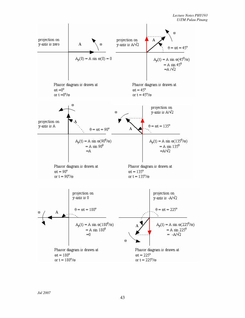
A phasor in the phasor diagram is represented by an arrow with its end fixed on the
origin. The arrow is rotating counterclockwise with a constant angular speed ω. The
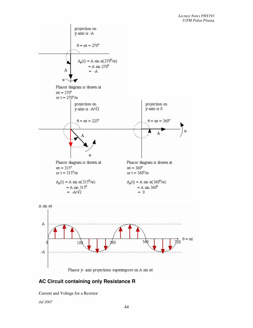
instantaneous value is the projection on the y-axis.
Lecture Notes PHY193
UiTM Pulau Pinang
Jul 2007
43
Lecture Notes PHY193
UiTM Pulau Pinang
Jul 2007
44
AC Circuit containing only Resistance R
Current and Voltage for a Resistor

Lecture Notes PHY193
UiTM Pulau Pinang
Jul 2007
45
The current through a resistor is in phase with the voltage across the resistor. If the current is
given as I(t) = Io sin (ωt + φ), the the voltage is Vr(t) = Vro sin (ωt + φ).
Using Ohm’s Law, we have V = IR, then Vr(t) = IoR sin (ωt + φ), where Vro = IoR.
The instantaneous power P(t) = (V(t) I(t)
= IoR sin (ωt + φ) Io sin (ωt + φ)
= Io2R sin (ωt + φ) sin (ωt + φ)
The graph sin (ωt + φ) sin (ωt + φ) is shown below. φ is called the initial phase and set to zero
in the graph below.
The average power is <P> = Io
2R/2
= Irms2 R = VrmsIrms
where Vrms
2
0V= and Irms =
2
0I=
AC Circuit containing only Inductance L
Current and Voltage for an Inductor
Lecture Notes PHY193
UiTM Pulau Pinang
Jul 2007
46
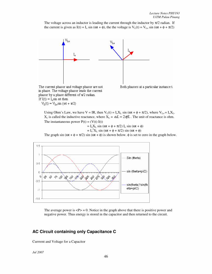
The voltage across an inductor is leading the current through the inductor by π/2 radian. If
the current is given as I(t) = Io sin (ωt + φ), the the voltage is VL(t) = VLo sin (ωt + φ + π/2)
Using Ohm’s Law, we have V = IR, then VL(t) = IoXL sin (ωt + φ + π/2), where VLo = IoXL.
Xc is called the inductive reactance, where XL = fLL πω 2= . The unit of reactance is ohm.
The instantaneous power P(t) = (V(t) I(t)
= IoXL sin (ωt + φ + π/2) Io sin (ωt + φ)
= Io2XL sin (ωt + φ + π/2) sin (ωt + φ)
The graph sin (ωt + φ + π/2) sin (ωt + φ) is shown below. φ is set to zero in the graph below.
The average power is <P> = 0. Notice in the graph above that there is positive power and
negative power. Thus energy is stored in the capacitor and then returned to the circuit.
AC Circuit containing only Capacitance C
Currrent and Voltage for a Capacitor

Lecture Notes PHY193
UiTM Pulau Pinang
Jul 2007
47
The current through a capacitor is leading the voltage across the capacitor by π/2 radian. If
the current is given as I(t) = Io sin (ωt + φ), the the voltage is Vc(t) = Vco sin (ωt + φ - π/2)
Using Ohm’s Law, we have V = IR, then Vc(t) = IoXc sin (ωt + φ- π/2), where Vco = IoXc.
Xc is called the capacitive reactance, where Xc = fCC πω 2
11= . The unit of reactance is ohm.
The instantaneous power P(t) = (V(t) I(t)
= IoXc sin (ωt + φ - π/2) Io sin (ωt + φ)
= Io2Xc sin (ωt + φ - π/2) sin (ωt + φ)
The graph sin (ωt + φ - π/2) sin (ωt + φ) is shown below. φ is set to zero in the graph below.
The average power is <P> = 0. Notice in the graph above that there is positive power and
negative power. Thus energy is stored in the capacitor and then returned to the circuit.
LR, LC and LRC Series Circuit
RC series Circuit

Lecture Notes PHY193
UiTM Pulau Pinang
Jul 2007
48
In a series circuit the current through the circuit is the same at any point. Therefore the current
through the resistor is the same as the current through the capacitor.
The voltage across both components is the sum of the voltage across the resistor and the
voltage across the capacitor.
If the current I(t) = Io sin (ωt ), then the voltage across the resistor is
Vr(t) = Vro sin (ωt ) while the the voltage across the capacitor is
Vc(t) = Vco sin (ωt - π/2)
The sum of the voltages is then VT(t) = Vro sin (ωt ) + Vco sin (ωt - π/2)
As the sum is quite tedious to solve mathematically, we will use phasors to add the voltages.
Note: The initial phase angle φ is not important in the calculations. φ determines the value of
the function when t = 0. The initial phase can be dropped to simplify the equations.
Lecture Notes PHY193
UiTM Pulau Pinang
Jul 2007
49
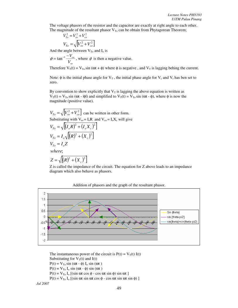
The voltage phasors of the resistor and the capacitor are exactly at right angle to each other.
The magnitude of the resultant phasor VTo can be obtain from Phytagorean Theorem; 222
coroTo VVV +=
[ ]22
coroTo VVV +=
And the angle between VTo and Io is
ro
co
V
V−= −1tanφ , where φ is then a negative value.
Therefore VT(t) = VTo sin (ωt + φ) where φ is negative , and VT is lagging behing the current.
Note: φ is the initial phase angle for VT , the initial phase angle for Vc and Vr has ben set to
zero.
By convention to show explicitly that VT is lagging the above equation is written as
VT(t) = VTo sin (ωt - |φ|) and simplified to VT(t) = VTo sin (ωt - φ), where φ is now the
magnitude (positive value).
[ ]22
coroTo VVV += can be written in other form.
Substituting with Vro = IoR and Vco = IoXc will give
( ) ( )[ ]( ) ( )[ ]
( ) ( )[ ]22
22
22
;
c
oTo
coTo
cooTo
XRZ
where
ZIV
XRIV
XIRIV
+=
=
+=
+=
Z is called the impedance of the circuit. The equation for Z above leads to an impedance
diagram which also behave as phasors.
Addition of phasors and the graph of the resultant phasor.
The instantaneous power of the circuit is P(t) = VT(t) I(t)
Substituting for VT(t) and I(t)
P(t) = VTo sin (ωt - φ) Io sin (ωt )
P(t) = VTo Io sin (ωt - φ) sin (ωt )
P(t) = VTo Io [(sin ωt cos φ - cos ωt sin φ) sin ωt ]
P(t) = VTo Io [(sin ωt sin ωt cos φ - cos ωt sin ωt sin φ) ]
Lecture Notes PHY193
UiTM Pulau Pinang
Jul 2007
50
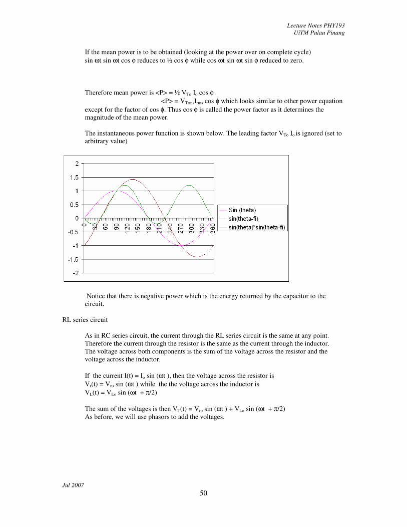
If the mean power is to be obtained (looking at the power over on complete cycle)
sin ωt sin ωt cos φ reduces to ½ cos φ while cos ωt sin ωt sin φ reduced to zero.
Therefore mean power is <P> = ½ VTo Io cos φ
<P> = VTrmsIrms cos φ which looks similar to other power equation
except for the factor of cos φ. Thus cos φ is called the power factor as it determines the
magnitude of the mean power.
The instantaneous power function is shown below. The leading factor VTo Io is ignored (set to
arbitrary value)
Notice that there is negative power which is the energy returned by the capacitor to the
circuit.
RL series circuit
As in RC series circuit, the current through the RL series circuit is the same at any point.
Therefore the current through the resistor is the same as the current through the inductor.
The voltage across both components is the sum of the voltage across the resistor and the
voltage across the inductor.
If the current I(t) = Io sin (ωt ), then the voltage across the resistor is
Vr(t) = Vro sin (ωt ) while the the voltage across the inductor is
VL(t) = VLo sin (ωt + π/2)
The sum of the voltages is then VT(t) = Vro sin (ωt ) + VLo sin (ωt + π/2)
As before, we will use phasors to add the voltages.
Lecture Notes PHY193
UiTM Pulau Pinang
Jul 2007
51
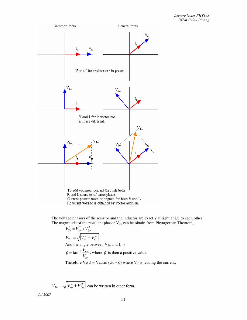
The voltage phasors of the resistor and the inductor are exactly at right angle to each other.
The magnitude of the resultant phasor VTo can be obtain from Phytagorean Theorem; 222
LoroTo VVV +=
[ ]22
LoroTo VVV +=
And the angle between VTo and Io is
ro
Lo
V
V1tan −=φ , where φ is then a positive value.
Therefore VT(t) = VTo sin (ωt + φ) where VT is leading the current.
[ ]22
LoroTo VVV += can be written in other form.

Lecture Notes PHY193
UiTM Pulau Pinang
Jul 2007
52
Substituting with Vro = IoR and VLo = IoXL will give
( ) ( )[ ]( ) ( )[ ]
( ) ( )[ ]22
22
22
;
L
oTo
LoTo
LooTo
XRZ
where
ZIV
XRIV
XIRIV
+=
=
+=
+=
Z is called the impedance of the circuit. The equation for Z above leads to an impedance
diagram which also behave as phasors.
The instantaneous power of the circuit is P(t) = VT(t) I(t)
Substituting for VT(t) and I(t)
P(t) = VTo sin (ωt + φ) Io sin (ωt )
P(t) = VTo Io sin (ωt + φ) sin (ωt )
P(t) = VTo Io [(sin ωt cos φ + cos ωt sin φ) sin ωt ]
P(t) = VTo Io [(sin ωt sin ωt cos φ + cos ωt sin ωt sin φ) ]
If the mean power is to be obtained (looking at the power over on complete cycle)
sin ωt sin ωt cos φ reduces to ½ cos φ while cos ωt sin ωt sin φ reduced to zero.
Therefore mean power is <P> = ½ VTo Io cos φ
<P> = VTrmsIrms cos φ which looks similar to other power equation
except for the factor of cos φ. Thus cos φ is called the power factor as it determines the
magnitude of the mean power.
The instantaneous power function is shown below. The leading factor VTo Io is ignored (set to
an arbitrary value)
Lecture Notes PHY193
UiTM Pulau Pinang
Jul 2007
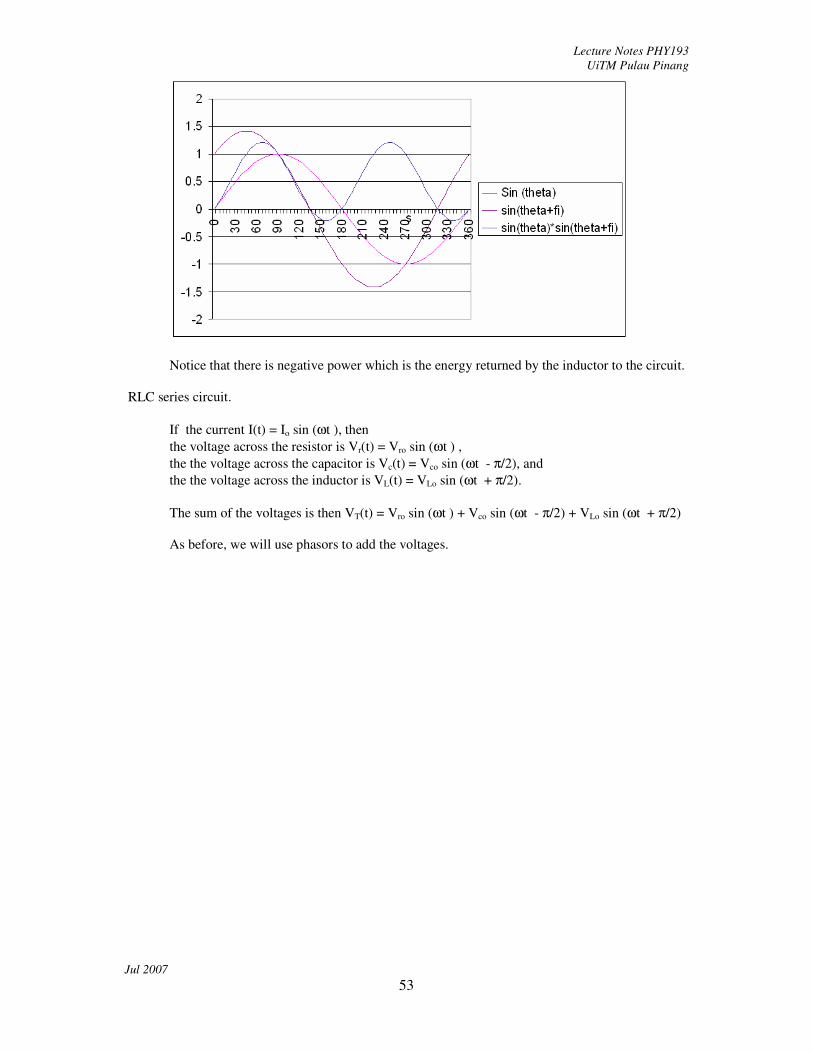
53
Notice that there is negative power which is the energy returned by the inductor to the circuit.
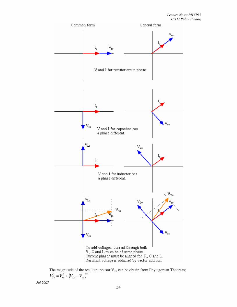
RLC series circuit.
If the current I(t) = Io sin (ωt ), then
the voltage across the resistor is Vr(t) = Vro sin (ωt ) ,
the the voltage across the capacitor is Vc(t) = Vco sin (ωt - π/2), and
the the voltage across the inductor is VL(t) = VLo sin (ωt + π/2).
The sum of the voltages is then VT(t) = Vro sin (ωt ) + Vco sin (ωt - π/2) + VLo sin (ωt + π/2)
As before, we will use phasors to add the voltages.
Lecture Notes PHY193
UiTM Pulau Pinang
Jul 2007
54
The magnitude of the resultant phasor VTo can be obtain from Phytagorean Theorem;
( )222
coLoroTo VVVV −+=

Lecture Notes PHY193
UiTM Pulau Pinang
Jul 2007
55
( )[ ]22
coLoroTo VVVV −+=
And the angle between VTo and Io is
ro
coLo
V
VV −= −1tanφ , where φ can be a positive or negative value.
Therefore VT could be leading or lagging behind the current.
( )[ ]22
coLoroTo VVVV −+= can be written in other form.
Substituting with Vro = IoR , VLo = IoXL and Vco = IoXc will give
( ) ( )[ ]( ) ( )[ ]
( ) ( )[ ]22
22
22
;
cL
oTo
cLoTo
coLooTo
XXRZ
where
ZIV
XXRIV
XIXIRIV
−+=
=
−+=
−+=
Z is called the impedance of the PLC series circuit.
Below are the functions in graphical form.
As in the previous cases the instantaneous power of the circuit is P(t) = VT(t) I(t)
Substituting for VT(t) and I(t)
P(t) = VTo sin (ωt + φ) Io sin (ωt )
P(t) = VTo Io sin (ωt + φ) sin (ωt )
P(t) = VTo Io [(sin ωt cos φ + cos ωt sin φ) sin ωt ]
P(t) = VTo Io [(sin ωt sin ωt cos φ + cos ωt sin ωt sin φ) ]
The mean power is <P> = ½ VTo Io cos φ
<P> = VTrmsIrms cos φ
Lecture Notes PHY193
UiTM Pulau Pinang
Jul 2007
56
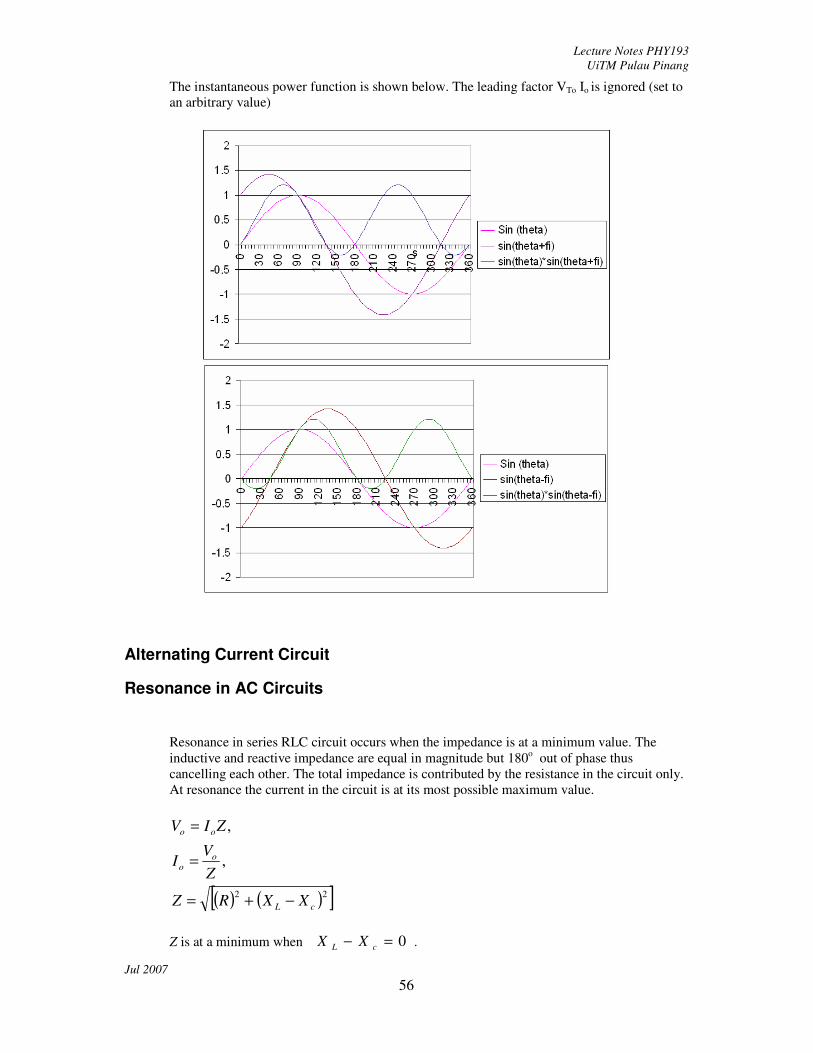
The instantaneous power function is shown below. The leading factor VTo Io is ignored (set to
an arbitrary value)
Alternating Current Circuit
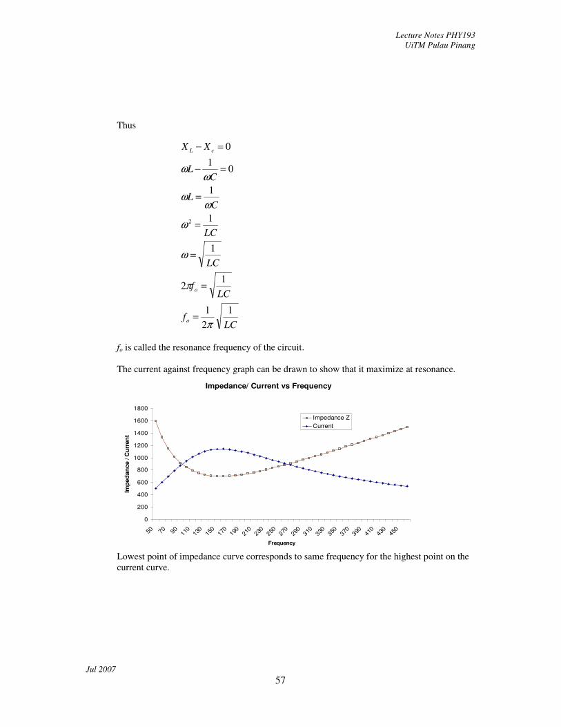
Resonance in AC Circuits
Resonance in series RLC circuit occurs when the impedance is at a minimum value. The
inductive and reactive impedance are equal in magnitude but 180o out of phase thus
cancelling each other. The total impedance is contributed by the resistance in the circuit only.
At resonance the current in the circuit is at its most possible maximum value.
( ) ( )[ ]22
,
,
cL
oo
oo
XXRZ
Z
VI
ZIV
−+=
=
=
Z is at a minimum when 0=− cL XX .
Lecture Notes PHY193
UiTM Pulau Pinang
Jul 2007
57
Thus
fo is called the resonance frequency of the circuit.
The current against frequency graph can be drawn to show that it maximize at resonance.
Impedance/ Current vs Frequency
0
200
400
600
800
1000
1200
1400
1600
1800
50 70 90 110
130
150
170
190
210
230
250
270
290
310
330
350
370
390
410
430
450
Frequency
Imp
ed
an
ce / C
urr
en
t
Impedance Z
Current
Lowest point of impedance curve corresponds to same frequency for the highest point on the
current curve.
LCf
LCf
LC
LC
CL
CL
XX
o
o
cL
1
2
1
12
1
1
1
01
0
2
π
π
ω
ω
ωω
ωω
=
=
=
=
=
=−
=−

Lecture Notes PHY193
UiTM Pulau Pinang
Jul 2007
58
Impedance/ Current vs Frequency
0
200
400
600
800
1000
1200
1400
1600
1800
2000
2200
2400
2600
2800
50 70 90 110
130
150
170
190
210
230
250
270
290
310
330
350
370
390
410
430
450
Frequency
Impedance / C
urr
ent
Impedance Z
Current
The shape of the current curve becomes sharper if resistance is lower. The “spread” of the
hump can be designed to obtain a balance between maximum current and the ability to tune in
to the resonance frequency.
A measure of this ability is the Q factor, where Q = ωo / ∆ω.
∆ω is the bandwidth (the range of frequencies where current is more than Io/2.
Therefore a sharper peak has a higher Q value than a shallower peak.
Power
Instantaneous power
Instantaneous power is the product of the instantaneous voltage and instantaneous
current.
P(t) =(V(t) I(t)
It has little practical value as the power of the circuit is not a constant and is changing
with time.
Average (Mean ) Power / True Power
Average or Mean Power, <P> = VTrmsIrms cos φ, is essentially the power dissipated
across the resistance.
<P> = VTrmsIrms cos φ, substituting cos φ = R/Z and VTrms =Irms Z
reduces to <P> = Irms2R
Reactive Power
Reactive power is the power stored and returned by the reactive components (inductor /
capacitor) P = Irms2 X
X = XL or Xc for RC or RL series circuit, or X = XL- Xc for RLC circuit.
Reactive power is not dissipated but returned to the circuit in each cycle.
Apparent Power
Apparent power is the power that appears to the source, it is the power that has to be
provided by the cource to the circuit.
Apparent power P = Irms2 Z
In another form P = Irms2 ( ) ( )[ ]22
cL XXR −+
Comparing the power, Papparent > Pmean while Preactive is trapped in the circuit.
Lecture Notes PHY193
UiTM Pulau Pinang
Jul 2007
59
Applications
Lecture Notes PHY193
UiTM Pulau Pinang
Jul 2007
60
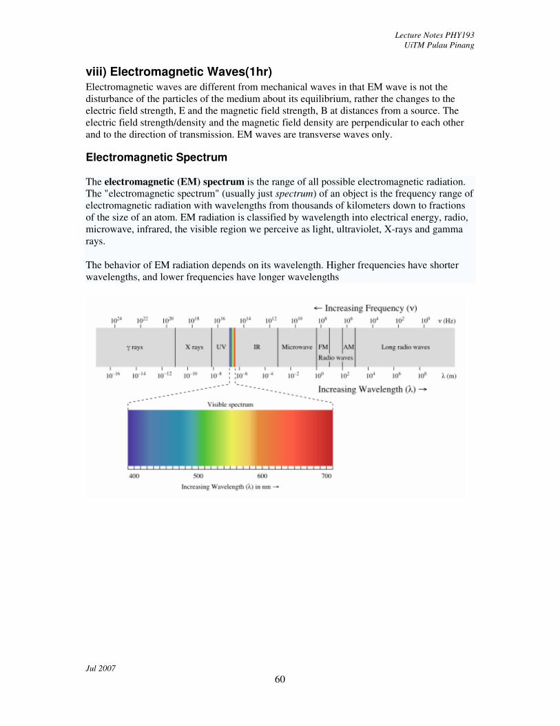
viii) Electromagnetic Waves(1hr) Electromagnetic waves are different from mechanical waves in that EM wave is not the
disturbance of the particles of the medium about its equilibrium, rather the changes to the
electric field strength, E and the magnetic field strength, B at distances from a source. The
electric field strength/density and the magnetic field density are perpendicular to each other
and to the direction of transmission. EM waves are transverse waves only.
Electromagnetic Spectrum
The electromagnetic (EM) spectrum is the range of all possible electromagnetic radiation.
The "electromagnetic spectrum" (usually just spectrum) of an object is the frequency range of
electromagnetic radiation with wavelengths from thousands of kilometers down to fractions
of the size of an atom. EM radiation is classified by wavelength into electrical energy, radio,
microwave, infrared, the visible region we perceive as light, ultraviolet, X-rays and gamma
rays.
The behavior of EM radiation depends on its wavelength. Higher frequencies have shorter
wavelengths, and lower frequencies have longer wavelengths

Lecture Notes PHY193
UiTM Pulau Pinang
Jul 2007
61
Production of Electromagnetic waves
A time-varying electric field generates a magnetic field and vice versa. Therefore, as an
oscillating electric field generates an oscillating magnetic field, the magnetic field in turn
generates an oscillating electric field, and so on. These oscillating fields together form an
electromagnetic wave.
Any electric charge which accelerates, or any changing magnetic field, produces
electromagnetic radiation
Speed of EM Waves
Electromagnetic radiation in a vacuum always travels at the speed of light. In a medium
(other than vacuum), velocity of propagation or refractive index are considered, depending on
frequency and application. Both of these are ratios of the speed in a medium to speed in a
vacuum.

Lecture Notes PHY193
UiTM Pulau Pinang
Jul 2007
62
Light and Optics
ix) Geometrical Optics (6 hr)
Plane Mirror: Image formation by Plane Mirror In optics it its common to measure angle with respect to the normal vector, which is perpendicular to the
surface. The angle between the incoming ray and the normal is called the angle of incidence, θi while the angle
between the outgoing ray and the normal is the angle of reflection, θr. Both angle are measured positive from the
normal.
4.1.1 Reflection from a plane surface
law of reflection – the angle of incidence and the angle of reflection are equal to each other.
θr = θi
The incident ray, the reflective ray and the normal lie in a plane ( the plane of incidence) which is perpendicular
to the reflecting surface.
Spherical Mirrors: Image formation by Concave and Convex Mirrors. Ray diagrams
The reflection of light rays from a spherical surface obeys the law of reflection at each point. A ray diagram can
be constructed to examine the effects of the spherical mirror.
When parallel light rays strikes near the center of a concave mirror they are reflected and pass through a
common point called the focus. The distance between the focus point and the mirror is called the focal length.
Parallel rays that are a distance away from the central axis are not reflected to the common focus of the rays
close to the central axis.
θi θr
Incidence
Plane
Reflecting
plane
Normal
vector

Lecture Notes PHY193
UiTM Pulau Pinang
Jul 2007
63
The law of reflection applies at the point M on the mirror surface. Thus MC is the radius of the mirror. ∠FMC is
θ , so is ∠MCF, thus FM and FC are equal sides of the isosceles triangle. For small angles θ, MC = 2MF.
Thus f = 2
R
Ray Tracing Step 1. Select a scale and mark the position of the object and the mirror on the optical axis.
Draw a line MM’ through the center of the mirror perpendicular to the optical axis.
Mark the focal point of the mirror F at f = 2
R on the optical axis and place the object on the axis all to
scale.
Step 2. Draw ray 1, from the object through the center of the spherical mirror. This ray will reflect along itself
after striking the mirror.
Step 3. Draw ray 2, from the object parallel to the optical axis, this ray will be reflected through the focal point
of a concave mirror ( or from the focal point of a convex mirror).
Step 4. Draw ray 3 from the object through or towards the focal point, this ray will be reflected parallel to the
optical axis
The spherical mirror formula
The image positions for mirrors can be computed using the equation (the spherical mirror formula)
f
1
o
1
i
1=+
where o is the distance from the object to the mirror, i is the distance from the image to the mirror and f is the
focal length of the mirror.
The sign convention when using this equation are;

Lecture Notes PHY193
UiTM Pulau Pinang
Jul 2007
64
The sign of f is positive if the focal point is on the same side of the mirror as the incident light and negative if
otherwise. (f positive for concave mirror, negative for convex mirror)
The distance o and i are positive if the are on the same side of the mirror as the incident light and negative if
they lie on opposite side.
Real images are produced if the image lie on the same side of the mirror as the incident light, while virtual
images lie on the opposite side of the mirror. Thus for a virtual image, i is of a negative value
The magnification of the image is given by o
im −=
A positive value of m indicates the image is upright, while a negative value indicates an inverted image. A
magnitude larger than 1 indicates that the image is larger than the object, while if the magnitude is smaller than
1, the image is smaller than the object.
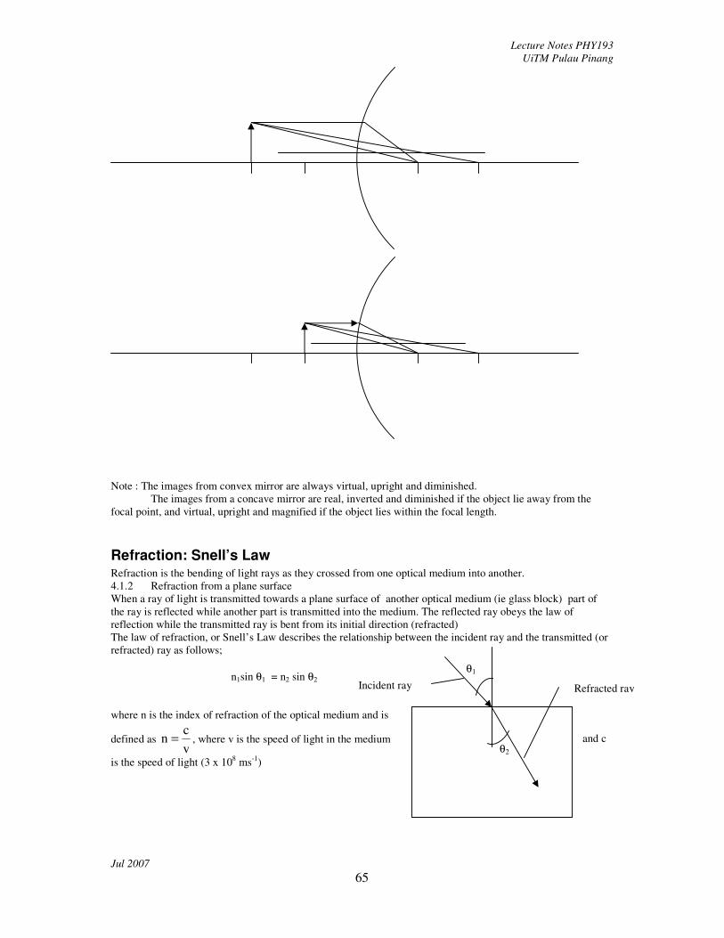
Lecture Notes PHY193
UiTM Pulau Pinang
Jul 2007
65
Note : The images from convex mirror are always virtual, upright and diminished.
The images from a concave mirror are real, inverted and diminished if the object lie away from the
focal point, and virtual, upright and magnified if the object lies within the focal length.
Refraction: Snell’s Law Refraction is the bending of light rays as they crossed from one optical medium into another.
4.1.2 Refraction from a plane surface
When a ray of light is transmitted towards a plane surface of another optical medium (ie glass block) part of
the ray is reflected while another part is transmitted into the medium. The reflected ray obeys the law of
reflection while the transmitted ray is bent from its initial direction (refracted)
The law of refraction, or Snell’s Law describes the relationship between the incident ray and the transmitted (or
refracted) ray as follows;
n1sin θ1 = n2 sin θ2
where n is the index of refraction of the optical medium and is
defined as v
cn = , where v is the speed of light in the medium and c
is the speed of light (3 x 10⁸ ms
-1)
θ1
θ2
Incident ray Refracted ray

Lecture Notes PHY193
UiTM Pulau Pinang
Jul 2007
66
Total Internal Reflection The refracted angle is smaller than the incidence angle when light is transmitted from a medium of low index of
refraction into a medium of higher index of refraction. The refracted angle is larger than the incidence angle
when light is transmitted from a medium of high index of refraction into a medium of lower index of refraction.
This is shown by rewriting Snell’s Law as sin θ2 = 2
1
n
n sin θ1 , where
2
1
n
n is larger than 1 when n1 > n2 and less
than 1 when n1 < n2 .
When light is transmitted from high index to lower index medium, at a certain angle of incidence called the
critical angle, the refracted angle becomes 90o. The refracted ray is transmitted along the interface between the
two medium. If the incident angle is increased, the refracted light will be reflected from
the interface. This phenomenon is called total internal reflection.
Thin Lenses: Convex and Concave Lens Equation Thin concave lenses converges the light rays through a common point (the focus) after passing through the
lenses. Thin convex lenses have a common focus where light rays appear to originate from it.
The distance from the focus point to the center of the lens along the optical axis is called the focal length.
The image location and dimension of an object placed in front of the lens can be obtained by ray tracing on a
ray diagram.
Real image are image on the opposite site of the lens from the object, while virtual image are images on the
same side of the lens as the object. Real image can be formed on a screen, while virtual image can not be formed
on a screen.
Ray tracing is done using the following guide lines;
A ray that passes through the optical center passes unchanged in direction.
A ray parallel to the optical axis canverges throufh the focus for a converging (convex) lens, or appears to
originate from the focus for a diverging (concave lens).
A ray which passes through the focus before entering the convex lens will emerged parallel to the optical axis
while a ray which appears to pass through the focus on the other side of a concave lens will emerged parallel to
the optical axis.
θ1
θ2
θ2
θ1 θ1 θ1
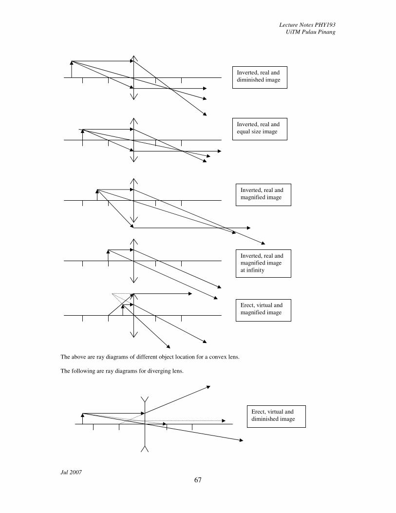
Lecture Notes PHY193
UiTM Pulau Pinang
Jul 2007
67
The above are ray diagrams of different object location for a convex lens.
The following are ray diagrams for diverging lens.
Inverted, real and
diminished image
Inverted, real and
equal size image
Inverted, real and
magnified image
Inverted, real and
magnified image
at infinity
Erect, virtual and
magnified image
Erect, virtual and
diminished image

Lecture Notes PHY193
UiTM Pulau Pinang
Jul 2007
68
The location of the image can also be located using the thin lens formula;
f
1
o
1
i
1=+
where : o is the distance of the object from the lens
i is the distance from the image to the lens, positive if on the opposite side of the lens from the object,
negative if on the same side of the object as the object.
f is the focal length, positive for convex (converging ) lenses, negative for concave (diverging) lenses
and the magnification;
o
im −=
where m is positive indicates an upright image, negative indicate an inverted image. A magnitude larger than 1
indicates that the image is larger than the object, while if the magnitude is smaller than 1, the image is smaller
than the object.
Object and image location, magnification and image type for convex lens.
o i Magnification Real/virtual
Erect, virtual and
diminished image
Erect, virtual and
diminished image
Erect, virtual and
diminished image
Erect, virtual and
diminished image

Lecture Notes PHY193
UiTM Pulau Pinang
Jul 2007
69
infinity f Diminished Real
2f 2f Diminished Real
f Infinity Magnified Real
< f >f (negative) magnified Virtual
The images from concave lenses are always erect, virtual and diminished.
Combination of Lenses: Two-Lens system Two lens system are created to further magnified an object at a distance or a minute object.
A simple telescope and a simple microscope are examples of two lens system. The location of the image is
constructed using a ray diagram.
4.1.3 A compound microscope
- to observe minute object. The lens closest to the object is called the objective (lens), the lens through
which one looks through is the eyepiece or ocular.
The objective (lens) has a short focal length. The object is placed just outside the focal length. A real, inverted
and magnified image is produce by the objective. The eyepiece is used to magnified this image,
4.1.4 The astronomical telescope.
Parallel rays from a point from a distance object are focused on the focal plane. A real, inverted image is
produce. The eyepiece works as a magnified producing a final image (inverted, virtual) at infinity.
A ray diagram for
two lens system,
distance object as in
an astronomical
telescope.
A ray diagram for
two lens system,
close object
0
0.2
0.4
0.6
0.8
1
1.2
0 2 4 6 8 10 12
Virtual, inverted,
magnified image
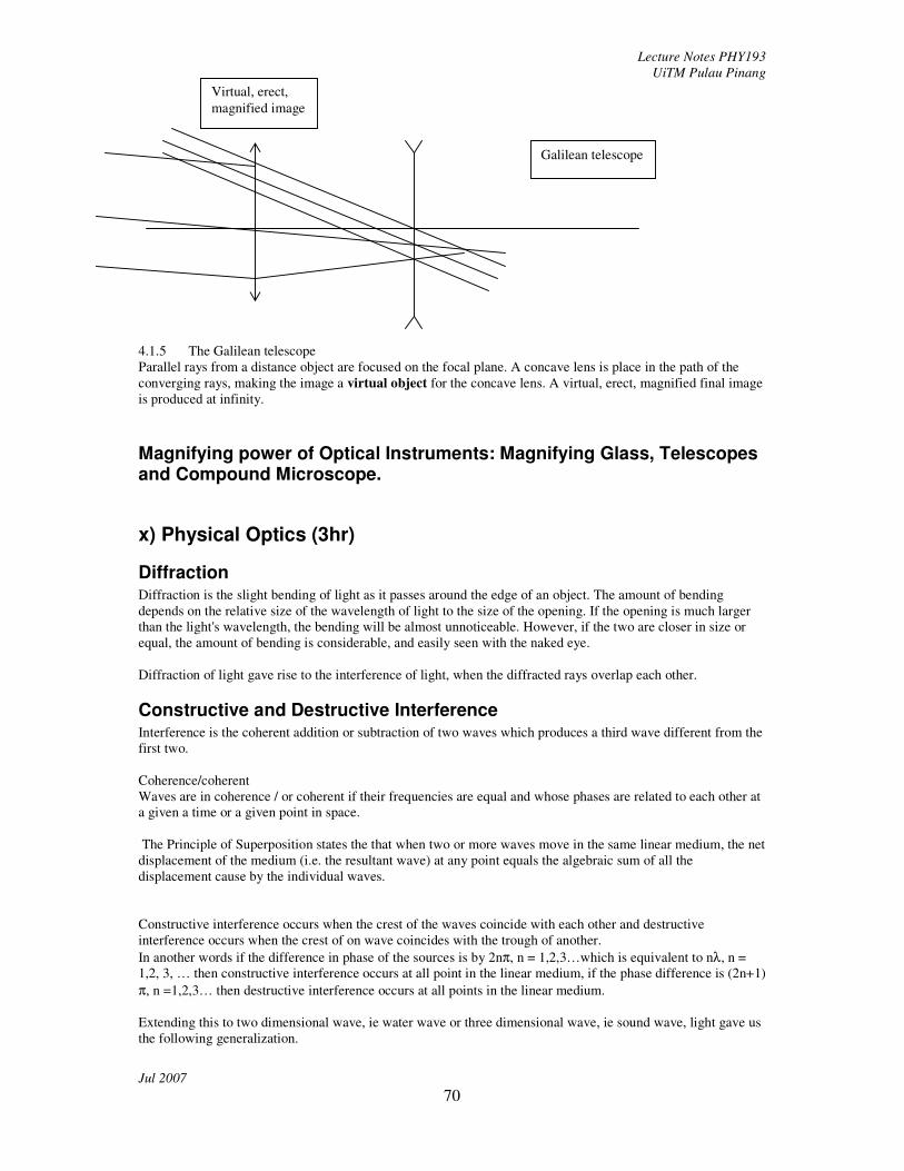
Lecture Notes PHY193
UiTM Pulau Pinang
Jul 2007
70
4.1.5 The Galilean telescope
Parallel rays from a distance object are focused on the focal plane. A concave lens is place in the path of the
converging rays, making the image a virtual object for the concave lens. A virtual, erect, magnified final image
is produced at infinity.
Magnifying power of Optical Instruments: Magnifying Glass, Telescopes and Compound Microscope.
x) Physical Optics (3hr)
Diffraction Diffraction is the slight bending of light as it passes around the edge of an object. The amount of bending
depends on the relative size of the wavelength of light to the size of the opening. If the opening is much larger
than the light's wavelength, the bending will be almost unnoticeable. However, if the two are closer in size or
equal, the amount of bending is considerable, and easily seen with the naked eye.
Diffraction of light gave rise to the interference of light, when the diffracted rays overlap each other.
Constructive and Destructive Interference Interference is the coherent addition or subtraction of two waves which produces a third wave different from the
first two.
Coherence/coherent
Waves are in coherence / or coherent if their frequencies are equal and whose phases are related to each other at
a given a time or a given point in space.
The Principle of Superposition states the that when two or more waves move in the same linear medium, the net
displacement of the medium (i.e. the resultant wave) at any point equals the algebraic sum of all the
displacement cause by the individual waves.
Constructive interference occurs when the crest of the waves coincide with each other and destructive
interference occurs when the crest of on wave coincides with the trough of another.
In another words if the difference in phase of the sources is by 2nπ, n = 1,2,3…which is equivalent to nλ, n =
1,2, 3, … then constructive interference occurs at all point in the linear medium, if the phase difference is (2n+1)
π, n =1,2,3… then destructive interference occurs at all points in the linear medium.
Extending this to two dimensional wave, ie water wave or three dimensional wave, ie sound wave, light gave us
the following generalization.
Virtual, erect,
magnified image
Galilean telescope
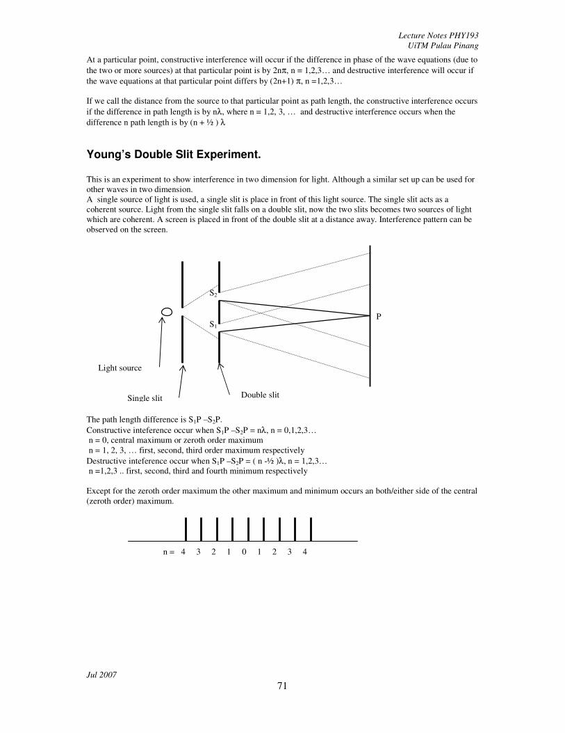
Lecture Notes PHY193
UiTM Pulau Pinang
Jul 2007
71
At a particular point, constructive interference will occur if the difference in phase of the wave equations (due to
the two or more sources) at that particular point is by 2nπ, n = 1,2,3… and destructive interference will occur if
the wave equations at that particular point differs by (2n+1) π, n =1,2,3…
If we call the distance from the source to that particular point as path length, the constructive interference occurs
if the difference in path length is by nλ, where n = 1,2, 3, … and destructive interference occurs when the
difference n path length is by (n + ½ ) λ
Young’s Double Slit Experiment.
This is an experiment to show interference in two dimension for light. Although a similar set up can be used for
other waves in two dimension.
A single source of light is used, a single slit is place in front of this light source. The single slit acts as a
coherent source. Light from the single slit falls on a double slit, now the two slits becomes two sources of light
which are coherent. A screen is placed in front of the double slit at a distance away. Interference pattern can be
observed on the screen.
The path length difference is S1P –S2P.
Constructive inteference occur when S1P –S2P = nλ, n = 0,1,2,3…
n = 0, central maximum or zeroth order maximum
n = 1, 2, 3, … first, second, third order maximum respectively
Destructive inteference occur when S1P –S2P = ( n -½ )λ, n = 1,2,3…
n =1,2,3 .. first, second, third and fourth minimum respectively
Except for the zeroth order maximum the other maximum and minimum occurs an both/either side of the central
(zeroth order) maximum.
Light source
Single slit Double slit
S1
S2
P
n = 4 3 2 1 0 1 2 3 4

Lecture Notes PHY193
UiTM Pulau Pinang
Jul 2007
72
Geometrical Analysis of Young’s double slit experiment
If P is the first order maxima, the path length difference
S2P – S1P = λ = d sin θ
But tan θ = D
x
For small angle, tan θ = sin θ, thus sin θ = d
λ = tan θ =
D
x
thend
λ =
D
x, or x =
d
λ D
for other order maximum S2P – S1P = nλ = d sin θ, then x = d
nλ D, where x is the distance between the
central maxima to the n th order maxima.
d
D
x
S1
S2
P
O

Lecture Notes PHY193
UiTM Pulau Pinang
Jul 2007
73