energies

Article

Photovoltaic and Wind Turbine Integration ApplyingCuckoo Search for Probabilistic ReliableOptimal Placement

R. A. Swief 1, T. S. Abdel-Salam 1 and Noha H. El-Amary 2,*1 Faculty of Engineering, Ain Shams University, 11566 Cairo, Egypt; rania.swief@gmail.com (R.A.S.);

tarekabdelsalam@gmail.com (T.S.A.-S.)2 Arab Academy for Science, Technology and Maritime Transport (AASTMT), 2033 Cairo, Egypt* Correspondence: noha_helamary@ieee.org or noha_helamary@hotmail.com; Tel.: +20-100-471-8562

Received: 12 December 2017; Accepted: 1 January 2018; Published: 6 January 2018

Abstract: This paper presents an efficient Cuckoo Search Optimization technique to improve thereliability of electrical power systems. Various reliability objective indices such as Energy NotSupplied, System Average Interruption Frequency Index, System Average Interruption, and DurationIndex are the main indices indicating reliability. The Cuckoo Search Optimization (CSO) technique isapplied to optimally place the protection devices, install the distributed generators, and to determinethe size of distributed generators in radial feeders for reliability improvement. Distributed generatoraffects reliability and system power losses and voltage profile. The volatility behaviour for bothphotovoltaic cells and the wind turbine farms affect the values and the selection of protection devicesand distributed generators allocation. To improve reliability, the reconfiguration will take placebefore installing both protection devices and distributed generators. Assessment of consumer powersystem reliability is a vital part of distribution system behaviour and development. Distributionsystem reliability calculation will be relayed on probabilistic reliability indices, which can expect thedisruption profile of a distribution system based on the volatility behaviour of added generatorsand load behaviour. The validity of the anticipated algorithm has been tested using a standard IEEE69 bus system.

Keywords: Cuckoo Search Optimization (CSO); Distributed Generator (DG); optimal location;probabilistic power system reliability; reconfiguration; reliability indices

1. Introduction

Owing to the rapid growth in the demand for electricity, ecological constraints, and thecompetitive energy market scenario, the electrical practicalities sectors such as transmission anddistribution systems have often been run under severely loaded circumstances. In the past, assessmentof the capability of the generation system and reliability of the transmission services were amongmajor studies in the system planning. The modern classifications derived from blackouts show that,in many cases, the eliciting events for such extensive failures took place at the distribution level.

Based on statistical studies, most of the service disruptions to the customs come from thedistribution systems. Planning and operation of any power system is based mainly on the reliabilityevaluation of the distribution system. This is conceded with the quantitative reliability calculationof power systems in [1]. This research describes different schemes, assesses techniques, and focuseson the various indices that can be employed in practical applications. Many devices are installedto increase reliability. Static Series Voltage Regulator (SSVR) is employed to assess the reliability ofthe distribution network. A procedure for the reliability valuation is constructed using the model ofan SSVR. The impact of the Distributed Generators (DGs), substitute source, system reconfiguration,

Energies 2018, 11, 139; doi:10.3390/en11010139 www.mdpi.com/journal/energies

Energies 2018, 11, 139 2 of 17

load shedding, and load adding are executed [2]. The reliability concept of operation using aneducational test system is introduced. An existing test system is enhanced by developing the necessarydistribution and sub-transmission networks. The improved system has all facilities, such as generation,switching stations, sub transmission, transmission, and radial distribution networks, found in apractical system [3].

DGs have a great impact on power loss reduction by supplying power to customers in the vicinity.The improvement of reliability is hugely affected by the location and the size of the installed DG.The maximum benefit of using DGs can be achieved if the DGs allocated optimally to increase thereliability as an objective. If DG units operated simultaneously with proper disconnects that willbe installed at sections forming a junction in the system, the behaviour will be better [4]. A newnature-inspired algorithm is implemented to optimally solve the reliability problems. Generally,reliability optimization problems are very complex in nature and non-deterministic polynomial-timehard (NP-hard) from a computational point of view [5]. A differential search (DS) algorithm has beeneffectively applied to determine the optimal allocations of remote control switch (RCS) in a radialdistribution feeder. The performance of DS algorithm has been compared with various techniquesand proved its efficiency over the other optimization techniques. Two algorithms were introduced:one with single objective, and the other with multi-objective formulation. The second algorithm,which was based on the multi-objective formulation, succeeded in delivering a more accurate solutionset by conceding reliability enhancement with the cost acquired [6]. A multi-objective optimizationtechnique for installing switches and protective devices in electric power distribution systems hasbeen applied. The objective function can be hybrid with reliability indices and the total cost to find themost optimal value that compromises between the two parts of the objective function. The solutionidentifies the number and position of switches, reclosers, and fuses to be installed in the distributionsystem [7].

The protection strategy of the distribution feeder is applied without consideration for distributedgeneration DG, and afterward by applying DGs across the feeder [8]. Distributed generation (DG) ispresented into the electrical distribution network to improve power system reliability. The optimalplacement of protection devices and DGs is crucial for achieving such an objective. An ant colony–basedoptimization process algorithm is established to find out the optimal recloser and DG locations.This target can be obtained by minimizing a merged reliability indices equation. The output resultsfrom the two test distribution systems confirm the efficiency of the anticipated method [9]. A timevariant load–based solution, with two optimal placement criterion of a distributed generation (DG),are introduced. The first target is to maximize the reliability development, and the other is to reducethe power loss in the system. The reliability is basically related to three parameters: failure rate, outageduration, and annual outage time. Those parameters are constructing the main reliability indices suchas System Average Interruption Frequency Index (SAIFI), System Average Interruption Duration Index(SAIDI), Customer Average Interruption Duration Index (CAIDI), Expected Energy-Not-Supplied(EENS), etc. DG plays a significant part in improving the reliability of the distribution system.All indices except SAIFI have enhanced the integration of DG. SAIFI may increase if reclosers areassociated to the sections or laterals. The reliability can be improved even without connecting DG ifthe reclosers are optimally connected at sections the distribution system [10].

An optimal and sensitive placement of distributed generation and reclosers has revealed thecapability of improving both system security and reliability. The better system behaviour can beobtained from enhancing feeder performance and operating conditions such as reducing voltage dropand losses and improving efficiency. The availability of continuing the supply of power is basedthe development of a distribution system that relies on the type, number, and size of the distributedgenerators, number of reclosers, and positions of both generators and reclosers on the feeder [11].Another case study pointed out that both reliability and losses vary as a function of loading or timebased on the qualitative analysis of three different systems [12]. The switch placement problem toincrease system reliability for radial distribution systems with the integration of DGs after a fault was

Energies 2018, 11, 139 3 of 17

expressed. A multi-objective optimization problem to improve reliability was formulated. The problemincluded maximizing the amount of load to be unremittingly sustained by the DG in isolation fromthe substation [13]. The Cuckoo Search Optimization (CSO) algorithm is utilized as an optimizerfor designing a Power System Stabilizer (PSS) for the New England system to reduce low frequencyoscillations [14,15].

In this paper, the Cuckoo Search Optimization (CSO) technique is used to maximize the reliabilityat the load points in the system. The Cuckoo search will be operating in two successive steps. In Step1, a reconfiguration will take place to minimize the reliability indices. Step 2 involves installing theprotective devices and allocating the DGs taking into consideration the stochastic behaviour of bothphotovoltaic (PV) and wind turbines (WT) farms. For the sake of improving reliability, DG integrationinto the power system will be vital. The DG natural behaviour and penetration levels will affectthe amount of the reached improvement. However, due to the limitation on increasing the DGspenetrations, from reliability point of view, the recloser will be optimally installed to take the reliabilityto another level, and then the location of switches is set. However, locating DGs further out on thesystem can lead to enhancements in losses, reliability, or both. Applying DGs to a distribution systemcontributes to improving the system reliability.

The paper is divided into seven sections. Section 2 gives an overview of reliability assessmenttechnique used in this paper. Section 3 provides an overview for the proposed test system applied.A description of DG operation and its impact is presented in Section 4. DG penetration with the Cuckoosearch optimization case study and its results is presented in Section 6, while Section 7 illustrates theconclusions of this paper.

2. Reliability

There are fundamental elements to guarantee and describe the continuity of service to customersthat reflect system reliability. The main problem in reliability studies is the need to reduce the numberof disconnected loads during the fault and afterword. After one branch failure, two importantsteps are considered: first, the safety system performance in short circuits (faults), and second,substituting actions for service recovery (upstream and downstream) to optimally save the unsuppliedenergy. These steps are characterised by protective schemes and by switches being opened or closed,with respect to customers being energized or interrupted.

2.1. Reliability Indices

The three basic customer-related indices for reliability analysis of distribution system are rate (orfrequency) of failure λs, average outage time (or average duration of failure) rs, and average annualoutage time Us [7].

λs = Σ λi·Us = Σ λi·ri, (1)

rs = Us/λs, (2)

where λi is the failure rate of load point i and ri is the average outage time of load point i.Although the three prime indices are basically important, they do not always give a complete

image of the system performance and response. To imitate the harshness or importance of a systemoutage, additional reliability indices can be and frequently are evaluated. The additional indices thatare most commonly used are defined in the following sections.

2.2. Reliability Evaluation

There are numerous indices used to evaluate the reliability Radial Distribution System (RDS).The most common indices used by electric services are System Average Interruption Frequency Index(SAIFI) and System Average Interruption Duration Index (SAIDI) [8,9,11–13]. However, in orderto reflect the severity of a system outage, additional reliability indices can be evaluated, like the

Energies 2018, 11, 139 4 of 17

Energy-Not-Supplied (ENS) index and Average Energy-Not-Supplied (AENS) index [2,6]. In thispaper, optimization will be operated by targeting the indices SAIDI and ENS.

3. 69 Bus Test System

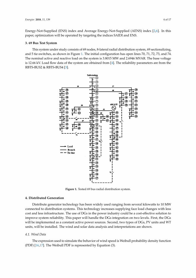
This system under study consists of 69 nodes, 8-lateral radial distribution system, 69 sectionalizing,and 5 tie-switches, as shown in Figure 1. The initial configuration has open lines 70, 71, 72, 73, and 74.The nominal active and reactive load on the system is 3.8015 MW and 2.6946 MVAR. The base voltageis 12.66 kV. Load flow data of the system are obtained from [4]. The reliability parameters are from theRBTS-BUS2 & RBTS-BUS4 [3].

Energies 2018, 11, 139 4 of 17

3. 69 Bus Test System

This system under study consists of 69 nodes, 8-lateral radial distribution system, 69 sectionalizing, and 5 tie-switches, as shown in Figure 1. The initial configuration has open lines 70, 71, 72, 73, and 74. The nominal active and reactive load on the system is 3.8015 MW and 2.6946 MVAR. The base voltage is 12.66 kV. Load flow data of the system are obtained from [4]. The reliability parameters are from the RBTS-BUS2 & RBTS-BUS4 [3].

Figure 1. Tested 69 bus radial distribution system.

4. Distributed Generation

Distribute generator technology has been widely used ranging from several kilowatts to 10 MW connected to distribution systems. This technology increases supplying face load changes with less cost and less infrastructure. The use of DGs in the power industry could be a cost-effective solution to improve system reliability. This paper will handle the DGs integration on two levels. First, the DGs will be implemented as a constant active power sources. Second, two types of DGs, PV units and WT units, will be installed. The wind and solar data analysis and interpretations are shown.

4.1. Wind Data

The expression used to simulate the behavior of wind speed is Weibull probability density function (PDF) [16,17]. The Weibull PDF is represented by Equation (3).

Figure 1. Tested 69 bus radial distribution system.

4. Distributed Generation

Distribute generator technology has been widely used ranging from several kilowatts to 10 MWconnected to distribution systems. This technology increases supplying face load changes with lesscost and less infrastructure. The use of DGs in the power industry could be a cost-effective solution toimprove system reliability. This paper will handle the DGs integration on two levels. First, the DGswill be implemented as a constant active power sources. Second, two types of DGs, PV units and WTunits, will be installed. The wind and solar data analysis and interpretations are shown.

4.1. Wind Data

The expression used to simulate the behavior of wind speed is Weibull probability density function(PDF) [16,17]. The Weibull PDF is represented by Equation (3).

Energies 2018, 11, 139 5 of 17

ϕ(v) =KC(

vC)

K−1exp (−

( vC

)K), (3)

where v represents wind speed and ϕ(v) is the Weibull PDF with the shape parameter K and the scaleparameter C [16]. In this study, the Weibull parameters of the wind speed are assumed to be C = 8.78,K = 1.75 [17], and the Weibull PDF of wind speed is shown in Figure 2. To get the output power of theWTs as an uncertain parameter in the (O-PLF) analysis, the Weibull PDF has been divided into levels.For each level, the wind speed is within specific limits. The probability of each level [18] of wind speedis calculated using Equation (4).

ProbWT(L) =∫ vL2

vL1

ϕ(v) dv, (4)

where vL1 and vL2 are the wind speed limits of level L. The number of wind speed level is carefullyselected because a considerable number of levels causes complexity of the problem, and a smallnumber of levels affects the accuracy.

Energies 2018, 11, 139 5 of 17

( ) = ( ) exp(− ), (3)

where represents wind speed and ( ) is the Weibull PDF with the shape parameter and the scale parameter [16]. In this study, the Weibull parameters of the wind speed are assumed to be = 8.78, = 1.75 [17], and the Weibull PDF of wind speed is shown in Figure 2. To get the output power of the WTs as an uncertain parameter in the (O-PLF) analysis, the Weibull PDF has been divided into levels. For each level, the wind speed is within specific limits. The probability of each level [18] of wind speed is calculated using Equation (4). ( ) = ( ) , (4)

where and are the wind speed limits of level L. The number of wind speed level is carefully selected because a considerable number of levels causes complexity of the problem, and a small number of levels affects the accuracy.

Figure 2. Weibull probability density function (PDF) of wind speed.

Wind farms practically operate between certain speeds. If speed is less than the minimum speed level, the wind farm is able to generate electricity. If the speed is greater than the maximum speed, the wind turbine must not operate or it will be destroyed. In this study, the step of wind speed is adjusted to be 1 m/s. Some levels are collected together to reduce the number of levels, as shown in Figure 3. (e.g., levels up to 4 m/s gives the same output power that is equal to zero, so it is considered as one level, the same for levels above 25 m/s and with levels from 14 m/s to 25 m/s where the output power is constant and equal to ) [18].

Figure 3. Wind probability distribution.

Figure 2. Weibull probability density function (PDF) of wind speed.

Wind farms practically operate between certain speeds. If speed is less than the minimum speedlevel, the wind farm is able to generate electricity. If the speed is greater than the maximum speed,the wind turbine must not operate or it will be destroyed. In this study, the step of wind speed isadjusted to be 1 m/s. Some levels are collected together to reduce the number of levels, as shown inFigure 3. (e.g., levels up to 4 m/s gives the same output power that is equal to zero, so it is consideredas one level, the same for levels above 25 m/s and with levels from 14 m/s to 25 m/s where the outputpower is constant and equal to Prated) [18].

Energies 2018, 11, 139 5 of 17

( ) = ( ) exp(− ), (3)

where represents wind speed and ( ) is the Weibull PDF with the shape parameter and the scale parameter [16]. In this study, the Weibull parameters of the wind speed are assumed to be = 8.78, = 1.75 [17], and the Weibull PDF of wind speed is shown in Figure 2. To get the output power of the WTs as an uncertain parameter in the (O-PLF) analysis, the Weibull PDF has been divided into levels. For each level, the wind speed is within specific limits. The probability of each level [18] of wind speed is calculated using Equation (4). ( ) = ( ) , (4)

where and are the wind speed limits of level L. The number of wind speed level is carefully selected because a considerable number of levels causes complexity of the problem, and a small number of levels affects the accuracy.

Figure 2. Weibull probability density function (PDF) of wind speed.

Wind farms practically operate between certain speeds. If speed is less than the minimum speed level, the wind farm is able to generate electricity. If the speed is greater than the maximum speed, the wind turbine must not operate or it will be destroyed. In this study, the step of wind speed is adjusted to be 1 m/s. Some levels are collected together to reduce the number of levels, as shown in Figure 3. (e.g., levels up to 4 m/s gives the same output power that is equal to zero, so it is considered as one level, the same for levels above 25 m/s and with levels from 14 m/s to 25 m/s where the output power is constant and equal to ) [18].

Figure 3. Wind probability distribution.

Figure 3. Wind probability distribution.

Energies 2018, 11, 139 6 of 17

The generated wind speed samples can be transformed to wind turbine output power [17] usingwind speed-power curve through Equation (5).

PWT =

0, 0 ≤ v ≤ vci

Prated_WT × (v−vci)(vr−vci)

, vci ≤ v ≤ vr

Prated_WT , vr ≤ v ≤ vco

0, vco ≤ v

, (5)

where PWT is power generated from WT (kW), Prated_WT is the rated power of the WT (kW) and vci,vr, and vco are the cut-in speed, rated speed, and cut-off speed of the WT, respectively. The WTused in this study has the following data [18] rated power (Prated_WT), which is determined using theoptimization technique.

4.2. Photovoltaic Data

PVs output power is vastly affected by the solar irradiance [17], which is why solar irradiancemodeling is needed to model the PVs output power. The solar irradiance real data is assembledeveryday hour per hour over the year [16]. The PV’s output power is multi-level variable factor inthe problem formulation. The irradiance data has been separated into levels. In each level, the solarirradiance is within certain limits. The probability (ProbPV) of each level is calculated by countingthe number of h/year for every level of irradiance and dividing it by total number of hours per year,as shown in Figure 4.

Energies 2018, 11, 139 6 of 17

The generated wind speed samples can be transformed to wind turbine output power [17] using wind speed-power curve through Equation (5). 0, 0_ × ( )( ),_ , 0, , (5)

where PWT is power generated from WT (kW), _ is the rated power of the WT (kW) and , , and are the cut-in speed, rated speed, and cut-off speed of the WT, respectively. The WT

used in this study has the following data [18] rated power ( _ ), which is determined using the optimization technique.

4.2. Photovoltaic Data

PVs output power is vastly affected by the solar irradiance [17], which is why solar irradiance modeling is needed to model the PVs output power. The solar irradiance real data is assembled everyday hour per hour over the year [16]. The PV’s output power is multi-level variable factor in the problem formulation. The irradiance data has been separated into levels. In each level, the solar irradiance is within certain limits. The probability ( ) of each level is calculated by counting the number of h/year for every level of irradiance and dividing it by total number of hours per year, as shown in Figure 4.

Figure 4. Solar irradiance yearly distribution probability W/m2.

Figure 4 illustrates the probability density function of the solar radiation versus the expected output power in W/m2 and the hours through the year. For example, the output power probability of the output power from the module that is equal to 0–100 W/m2 over 444 h in the entire year is 0.05. The PV output power as a function of solar irradiance [19] is stated as (6)

= _ × ( × ),_ × ,_ , , (6)

where is the PV output power (MW), signifies the solar irradiance in the standard conditions usually set to 1000 W/m2, is a certain radiation point, usually set to 150 W/m2, and _ is the PV rated power (MW) will be set applying the optimization technique.

5. Cuckoo Search Algorithm

Figure 4. Solar irradiance yearly distribution probability W/m2.

Figure 4 illustrates the probability density function of the solar radiation versus the expectedoutput power in W/m2 and the hours through the year. For example, the output power probability ofthe output power from the module that is equal to 0–100 W/m2 over 444 h in the entire year is 0.05.The PV output power as a function of solar irradiance [19] is stated as (6)

PPV =

Prated_PV × ( R2

RSTD×RC), R < RC

Prated_PV × RRSTD

, RC ≤ R < RSTD

Prated_PV , R ≥ RSTD

, (6)

where PPV is the PV output power (MW), RSTD signifies the solar irradiance in the standard conditionsusually set to 1000 W/m2, RC is a certain radiation point, usually set to 150 W/m2, and Prated_PV is thePV rated power (MW) will be set applying the optimization technique.

Energies 2018, 11, 139 7 of 17

5. Cuckoo Search Algorithm

The Cuckoo Search Algorithm is an evolutionary algorithm for continuous nonlinear optimizationproblems [20–22]. Cuckoo optimization was established by Yang and Deb in 2009 [21], and the CuckooOptimization Algorithm (COA) was urbanized by Rajabioun in 2011 [22]. This method is stimulatedby the life of a bird called the cuckoo [20].

Similar to the other evolutionary algorithms, this one also begins with a random population set ofanswers (cuckoos). These cuckoos lay their eggs in the nests of other birds and wait while the hostbird maintains these eggs beside their eggs. Some of the eggs that have less similarity to the host bird’seggs will be recognized and destroyed, while the eggs that are more similar to the host bird’s eggs willget the chance to grow up. The number of survived eggs in each zone shows the suitability of thiszone, and the greater the number of surviving eggs, the more attention is paid to this zone.

There are two ways for the cuckoo to explore its landscape. It either uses a series of straight flightpaths punctuated by a sudden 90◦ turn that leads to a L’evy flight style intermittent search pattern,or they lay eggs within a maximum distance from their habitat. This maximum range is called the EggLaying Radius (ELR). The two sorts of search mechanism are illustrated in detail, as follows.

5.1. Cuckoo Search via Levy Flights

L’evy flights, rather than a simple random isotropic step, have been the basic motive fordeveloping this innovative evolutionary optimization algorithm. The cuckoo search algorithm usesthe L’evy flight method to increase the diversity of the solution so that the algorithm is prevented frombeing caught in a local optimum to achieve the global optima. The whole behavior of the cuckoo isillustrated by Yang and Deb in [21].

To produce a new solution (xit+1) for each cuckoo (i) at generation (t), a L’evy flight is formed by

Equation (7) with step size (α) greater than zero. It can be used in most cases as 1. The first term inEquation (7) is the current location (xi

t), and the second term represents the transition probability thatconsists of a product of two terms with entry wise multiplications (

Energies 2018, 11, 139 7 of 17

The Cuckoo Search Algorithm is an evolutionary algorithm for continuous nonlinear optimization problems [20–22]. Cuckoo optimization was established by Yang and Deb in 2009 [21], and the Cuckoo Optimization Algorithm (COA) was urbanized by Rajabioun in 2011 [22]. This method is stimulated by the life of a bird called the cuckoo [20].

Similar to the other evolutionary algorithms, this one also begins with a random population set of answers (cuckoos). These cuckoos lay their eggs in the nests of other birds and wait while the host bird maintains these eggs beside their eggs. Some of the eggs that have less similarity to the host bird’s eggs will be recognized and destroyed, while the eggs that are more similar to the host bird’s eggs will get the chance to grow up. The number of survived eggs in each zone shows the suitability of this zone, and the greater the number of surviving eggs, the more attention is paid to this zone.

There are two ways for the cuckoo to explore its landscape. It either uses a series of straight flight paths punctuated by a sudden 90o turn that leads to a L’evy flight style intermittent search pattern, or they lay eggs within a maximum distance from their habitat. This maximum range is called the Egg Laying Radius (ELR). The two sorts of search mechanism are illustrated in detail, as follows.

5.1. Cuckoo Search via Levy Flights

L’evy flights, rather than a simple random isotropic step, have been the basic motive for developing this innovative evolutionary optimization algorithm. The cuckoo search algorithm uses the L’evy flight method to increase the diversity of the solution so that the algorithm is prevented from being caught in a local optimum to achieve the global optima. The whole behavior of the cuckoo is illustrated by Yang and Deb in [21].

To produce a new solution (xit+1) for each cuckoo (i) at generation (t), a L’evy flight is formed by Equation (7) with step size (α) greater than zero. It can be used in most cases as 1. The first term in Equation (7) is the current location (xit), and the second term represents the transition probability that consists of a product of two terms with entry wise multiplications (※).

xit+1 = xit + α ※ Levy(λ) i = 1, 2,......, NP. (7)

5.2. Cuckoo Style for Egg Laying

Each cuckoo starts laying eggs randomly in other host birds’ nests within her egg laying radius (ELR). The concept is clarified in Figure 5, where the red star in the center indicates the cuckoo’s initial habitat, and the pink stars represent the new nest eggs.

Figure 5. Representation of the cuckoo egg laying radius (ELR).

).

xit+1 = xi

t + α

Energies 2018, 11, 139 7 of 17

The Cuckoo Search Algorithm is an evolutionary algorithm for continuous nonlinear optimization problems [20–22]. Cuckoo optimization was established by Yang and Deb in 2009 [21], and the Cuckoo Optimization Algorithm (COA) was urbanized by Rajabioun in 2011 [22]. This method is stimulated by the life of a bird called the cuckoo [20].

Similar to the other evolutionary algorithms, this one also begins with a random population set of answers (cuckoos). These cuckoos lay their eggs in the nests of other birds and wait while the host bird maintains these eggs beside their eggs. Some of the eggs that have less similarity to the host bird’s eggs will be recognized and destroyed, while the eggs that are more similar to the host bird’s eggs will get the chance to grow up. The number of survived eggs in each zone shows the suitability of this zone, and the greater the number of surviving eggs, the more attention is paid to this zone.

There are two ways for the cuckoo to explore its landscape. It either uses a series of straight flight paths punctuated by a sudden 90o turn that leads to a L’evy flight style intermittent search pattern, or they lay eggs within a maximum distance from their habitat. This maximum range is called the Egg Laying Radius (ELR). The two sorts of search mechanism are illustrated in detail, as follows.

5.1. Cuckoo Search via Levy Flights

L’evy flights, rather than a simple random isotropic step, have been the basic motive for developing this innovative evolutionary optimization algorithm. The cuckoo search algorithm uses the L’evy flight method to increase the diversity of the solution so that the algorithm is prevented from being caught in a local optimum to achieve the global optima. The whole behavior of the cuckoo is illustrated by Yang and Deb in [21].

To produce a new solution (xit+1) for each cuckoo (i) at generation (t), a L’evy flight is formed by Equation (7) with step size (α) greater than zero. It can be used in most cases as 1. The first term in Equation (7) is the current location (xit), and the second term represents the transition probability that consists of a product of two terms with entry wise multiplications (※).

xit+1 = xit + α ※ Levy(λ) i = 1, 2,......, NP. (7)

5.2. Cuckoo Style for Egg Laying

Each cuckoo starts laying eggs randomly in other host birds’ nests within her egg laying radius (ELR). The concept is clarified in Figure 5, where the red star in the center indicates the cuckoo’s initial habitat, and the pink stars represent the new nest eggs.

Figure 5. Representation of the cuckoo egg laying radius (ELR).

Levy(λ) i = 1, 2, . . . . . . , NP. (7)

5.2. Cuckoo Style for Egg Laying

Each cuckoo starts laying eggs randomly in other host birds’ nests within her egg laying radius(ELR). The concept is clarified in Figure 5, where the red star in the center indicates the cuckoo’s initialhabitat, and the pink stars represent the new nest eggs.

Energies 2018, 11, 139 7 of 17

The Cuckoo Search Algorithm is an evolutionary algorithm for continuous nonlinear optimization problems [20–22]. Cuckoo optimization was established by Yang and Deb in 2009 [21], and the Cuckoo Optimization Algorithm (COA) was urbanized by Rajabioun in 2011 [22]. This method is stimulated by the life of a bird called the cuckoo [20].

Similar to the other evolutionary algorithms, this one also begins with a random population set of answers (cuckoos). These cuckoos lay their eggs in the nests of other birds and wait while the host bird maintains these eggs beside their eggs. Some of the eggs that have less similarity to the host bird’s eggs will be recognized and destroyed, while the eggs that are more similar to the host bird’s eggs will get the chance to grow up. The number of survived eggs in each zone shows the suitability of this zone, and the greater the number of surviving eggs, the more attention is paid to this zone.

There are two ways for the cuckoo to explore its landscape. It either uses a series of straight flight paths punctuated by a sudden 90o turn that leads to a L’evy flight style intermittent search pattern, or they lay eggs within a maximum distance from their habitat. This maximum range is called the Egg Laying Radius (ELR). The two sorts of search mechanism are illustrated in detail, as follows.

5.1. Cuckoo Search via Levy Flights

L’evy flights, rather than a simple random isotropic step, have been the basic motive for developing this innovative evolutionary optimization algorithm. The cuckoo search algorithm uses the L’evy flight method to increase the diversity of the solution so that the algorithm is prevented from being caught in a local optimum to achieve the global optima. The whole behavior of the cuckoo is illustrated by Yang and Deb in [21].

To produce a new solution (xit+1) for each cuckoo (i) at generation (t), a L’evy flight is formed by Equation (7) with step size (α) greater than zero. It can be used in most cases as 1. The first term in Equation (7) is the current location (xit), and the second term represents the transition probability that consists of a product of two terms with entry wise multiplications (※).

xit+1 = xit + α ※ Levy(λ) i = 1, 2,......, NP. (7)

5.2. Cuckoo Style for Egg Laying

Each cuckoo starts laying eggs randomly in other host birds’ nests within her egg laying radius (ELR). The concept is clarified in Figure 5, where the red star in the center indicates the cuckoo’s initial habitat, and the pink stars represent the new nest eggs.

Figure 5. Representation of the cuckoo egg laying radius (ELR). Figure 5. Representation of the cuckoo egg laying radius (ELR).

Energies 2018, 11, 139 8 of 17

The complete process adopted by the Cuckoo approach for solving any optimization problems isimplemented according to the following steps:

Step (1): Generate a population of habitats (solutions). For Nvar dimensional problem, each habitatis an array of 1xNvar, is formed as follows:

Habitat = [x1, x2, . . . ., xNvar] (8)

Step (2): Evaluate the profit or fitness of each habitat.Step (3): Each cuckoo randomly lays eggs in host birds’ nests within her ELR, where the egg laying

radius (ELR) is the maximum distance at which the cuckoo can lay eggs from its habitat. The egg layingradius (ELR) dedicated to each cuckoo depends on the lower and upper limits of the optimizationproblem variables (VARL, VARH), the whole number of eggs, and current cuckoo’s number of eggs, soELR is determined as:

ELR = β × number o f current cuckoos eggstotal number o f eggs

(VARH − VARL) (9)

where (β) is a number considered to identify the greatest value of ELR.Step (4): The immigration of cuckoos, where mature cuckoos immigrate to a new habitat when the

time of egg laying approaches. Cuckoos fly toward goal points by λ% from the path with a deviationof φ in radians. This part of movement is clearly shown in Figure 6. Both parameters φ and λ allowthe cuckoos to search more areas in the environment.

Energies 2018, 11, 139 8 of 17

The complete process adopted by the Cuckoo approach for solving any optimization problems is implemented according to the following steps:

Step (1): Generate a population of habitats (solutions). For Nvar dimensional problem, each habitat is an array of 1xNvar, is formed as follows:

Habitat = [x1, x2, …., xNvar] (8)

Step (2): Evaluate the profit or fitness of each habitat. Step (3): Each cuckoo randomly lays eggs in host birds’ nests within her ELR, where the egg

laying radius (ELR) is the maximum distance at which the cuckoo can lay eggs from its habitat. The egg laying radius (ELR) dedicated to each cuckoo depends on the lower and upper limits of the optimization problem variables (VARL, VARH), the whole number of eggs, and current cuckoo’s number of eggs, so ELR is determined as: ELR = × ( − ) (9)

where (β) is a number considered to identify the greatest value of ELR. Step (4): The immigration of cuckoos, where mature cuckoos immigrate to a new habitat when

the time of egg laying approaches. Cuckoos fly toward goal points by λ% from the path with a deviation of φ in radians. This part of movement is clearly shown in Figure 6. Both parameters φ and λ allow the cuckoos to search more areas in the environment.

Figure 6. Cuckoo immigration toward the goal point process.

Step (5): Cuckoos in the worst habitats are killed. A number (Nmax) limits the maximum limit of living cuckoos in the environment. It represents the number of cuckoos that survive that have higher profit values. The remainder die.

Step (6): After a number of iterations is reached, all the cuckoo population gathers to the best habitat with the most similarity of eggs. This habitat will have the maximum profit value and least egg losses.

A flowchart of the proposed algorithm is summarized as follows in Figure 7. Meta-Heuristic algorithms are very profound for their parameters, and the setting of the parameters can influence their efficiency. The parameters settings cause more reliability and flexibility of the algorithm. So, settings of the parameters are one of the crucial factors in gaining the optimized solution in all optimization problems [21–23]. Underneath, are the main parameters which affect primarily the algorithm performance:

Figure 6. Cuckoo immigration toward the goal point process.

Step (5): Cuckoos in the worst habitats are killed. A number (Nmax) limits the maximum limit ofliving cuckoos in the environment. It represents the number of cuckoos that survive that have higherprofit values. The remainder die.

Step (6): After a number of iterations is reached, all the cuckoo population gathers to the besthabitat with the most similarity of eggs. This habitat will have the maximum profit value and leastegg losses.

A flowchart of the proposed algorithm is summarized as follows in Figure 7. Meta-Heuristicalgorithms are very profound for their parameters, and the setting of the parameters can influence

Energies 2018, 11, 139 9 of 17

their efficiency. The parameters settings cause more reliability and flexibility of the algorithm. So,settings of the parameters are one of the crucial factors in gaining the optimized solution in alloptimization problems [21–23]. Underneath, are the main parameters which affect primarily thealgorithm performance:

1. The population size (NP) is the parameter representing the number of host nests.2. The maximum number of iterations or the time consumed by the algorithm (Itermax).3. The discovery rate of alien eggs per solution (Pa) is the parameter representing the probability of

recognizing the cuckoo’s egg by the host bird.4. The levy distribution factor (beta).

Energies 2018, 11, 139 9 of 17

1. The population size (NP) is the parameter representing the number of host nests. 2. The maximum number of iterations or the time consumed by the algorithm (Itermax). 3. The discovery rate of alien eggs per solution (Pa) is the parameter representing the probability

of recognizing the cuckoo’s egg by the host bird. 4. The levy distribution factor (beta).

Figure 7. Flowchart for the Cuckoo Optimization Algorithm.

NP = 50, 100, 150, 250, 300, 500 and Pa = 0.05, 0.1, 0.15, 0.2, 0.25, 0.4, 0.5 are tested in the proposed optimization problem of DG allocation and sizing. The simulation results referenced to the previous empirical analysis and previous studies’ results show that NP = 50, Itermax = 200, Pa = 0.25 and beta = 3/2 give the most robust and accurate solution in this thesis case study. Table 1 shows the selected parameters for COA algorithm.

Table 1. Setting parameters for the Cuckoo Optimization Technique.

Parameter ValueTime (iteration number) ≡ Itermax 200

n (number of nests) ≡ NP 50 Pa (Discovery rate of alien eggs/solutions) 0.25

Beta (Levy distribution factor) 3/2

Figure 7. Flowchart for the Cuckoo Optimization Algorithm.

NP = 50, 100, 150, 250, 300, 500 and Pa = 0.05, 0.1, 0.15, 0.2, 0.25, 0.4, 0.5 are tested in the proposedoptimization problem of DG allocation and sizing. The simulation results referenced to the previousempirical analysis and previous studies’ results show that NP = 50, Itermax = 200, Pa = 0.25 and beta =3/2 give the most robust and accurate solution in this thesis case study. Table 1 shows the selectedparameters for COA algorithm.

Energies 2018, 11, 139 10 of 17

Table 1. Setting parameters for the Cuckoo Optimization Technique.

Parameter Value

Time (iteration number) ≡ Itermax 200n (number of nests) ≡ NP 50

Pa (Discovery rate of alien eggs/solutions) 0.25Beta (Levy distribution factor) 3/2

The optimization technique will be operated in two steps:In Step 1, the algorithm will determine the ties that will be open to reconfigure the system to

improve the reliability indices.In Step 2, after reconfiguration, the algorithm will be responsible for setting the optimal locations

for both the recloses and the DGs considering different sizes and types, whether PV or WT farms,taking into consideration the probabilistic behaviour of both types.

An overview for statistical performance evaluation of different evolutionary algorithms has beendetailed in [23]. Extensive simulations and statistical analysis are implemented on each algorithm (CS,PSO, and GA) for different standard test functions, showing that

• CS is more proficient in finding the global optimum solution with higher rates of success;• CS has outperformed both PSO and GA in terms of less number of parameters to be controlled,

as there are mainly two parameters: Pa and the population size NP basically control the elitism;• CS is robust and more generic for numerous optimization problems compared with other

optimization algorithms.

An Artificial Intelligent (AI) comparative study is applied to the base case of the IEEE 69 bussystem to minimize the ENS. Genetic Algorithm (GA), Particle Swarm Optimization (PSO), and COAtechniques are examined. Table 2 shows the results of the three AI techniques, which are tested on thebase case of the system through applying two reclosers on the feeders of the IEEE 69 bus to minimizethe ENS. The result shows the privilege of COA over both GA and PSO.

Table 2. A comparative study applied to the base case of IEEE 69 bus system to minimize theenergy-not-supplied index (ENS).

AI Techniques COA PSO GA

Recloser locations Feeders49 & 61

Feeders26 & 9

Feeders50 & 12

ENS 67,881 68,056 68,003

6. Case Studies

Four case studies are carried out on the system. In Case 1, the optimization takes place todetermine the ties that will be open to reconfigure the system and keeping system radial. Case 2investigates the effect of installing the protective devices only. Case 3 studies the effect of applying DGsand the protective devices with different protective levels. Case 4 compares the effect of photovoltaicand wind turbines farms with their stochastic probable behavior, which will lead to probabilisticreliability indices.

6.1. Case 1

Case 1 assumes the system with no reclosers and no DG; it only considers the effect of thereconfiguration. Since the number of customers and average demand at each load point are specifiedfrom [3,4], the primary indices can be extended to give the customer- and load-oriented indices. Table 3shows the prime reliability indices before applying the optimization algorithm.

Energies 2018, 11, 139 11 of 17

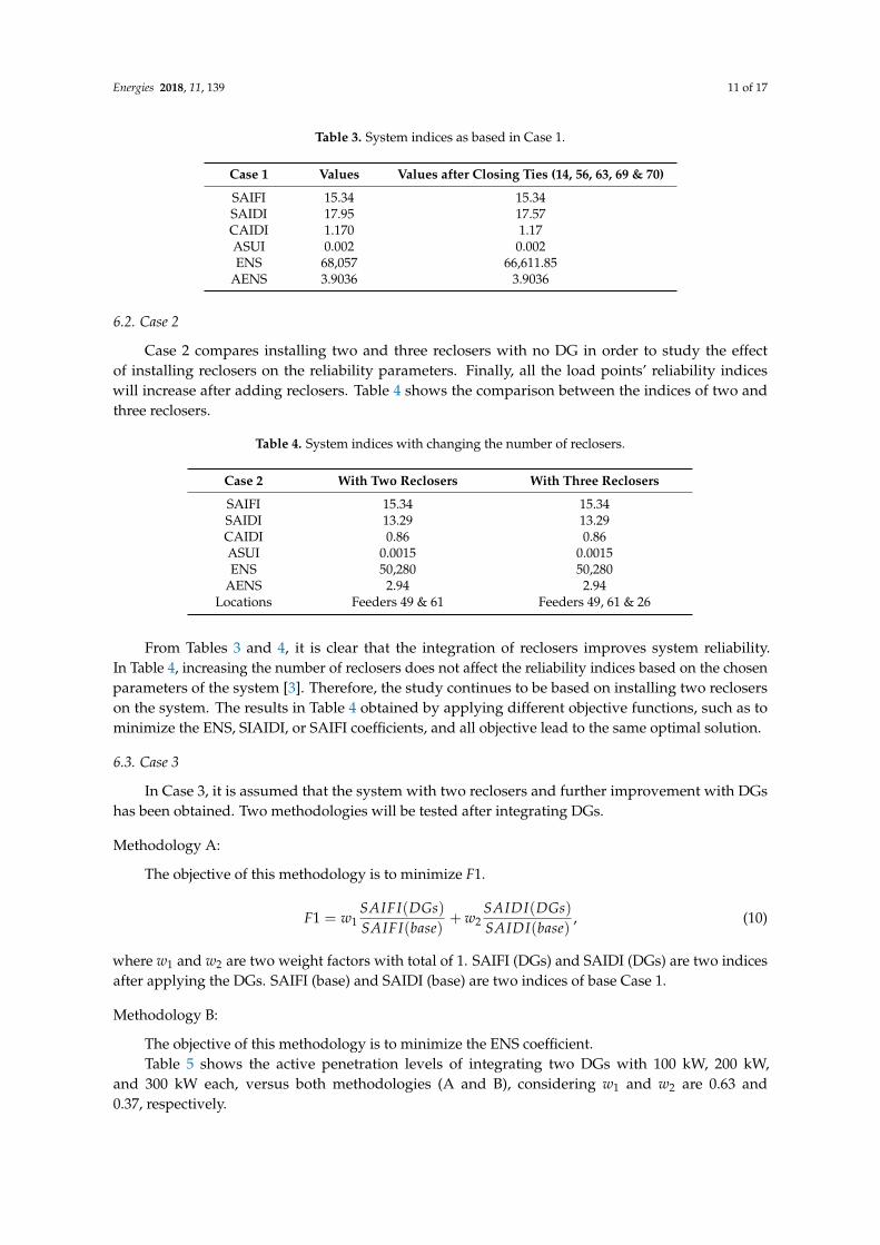
Table 3. System indices as based in Case 1.

Case 1 Values Values after Closing Ties (14, 56, 63, 69 & 70)

SAIFI 15.34 15.34SAIDI 17.95 17.57CAIDI 1.170 1.17ASUI 0.002 0.002ENS 68,057 66,611.85

AENS 3.9036 3.9036

6.2. Case 2

Case 2 compares installing two and three reclosers with no DG in order to study the effectof installing reclosers on the reliability parameters. Finally, all the load points’ reliability indiceswill increase after adding reclosers. Table 4 shows the comparison between the indices of two andthree reclosers.

Table 4. System indices with changing the number of reclosers.

Case 2 With Two Reclosers With Three Reclosers

SAIFI 15.34 15.34SAIDI 13.29 13.29CAIDI 0.86 0.86ASUI 0.0015 0.0015ENS 50,280 50,280

AENS 2.94 2.94Locations Feeders 49 & 61 Feeders 49, 61 & 26

From Tables 3 and 4, it is clear that the integration of reclosers improves system reliability.In Table 4, increasing the number of reclosers does not affect the reliability indices based on the chosenparameters of the system [3]. Therefore, the study continues to be based on installing two recloserson the system. The results in Table 4 obtained by applying different objective functions, such as tominimize the ENS, SIAIDI, or SAIFI coefficients, and all objective lead to the same optimal solution.

6.3. Case 3

In Case 3, it is assumed that the system with two reclosers and further improvement with DGshas been obtained. Two methodologies will be tested after integrating DGs.

Methodology A:

The objective of this methodology is to minimize F1.

F1 = w1SAIFI(DGs)SAIFI(base)

+ w2SAIDI(DGs)SAIDI(base)

, (10)

where w1 and w2 are two weight factors with total of 1. SAIFI (DGs) and SAIDI (DGs) are two indicesafter applying the DGs. SAIFI (base) and SAIDI (base) are two indices of base Case 1.

Methodology B:

The objective of this methodology is to minimize the ENS coefficient.Table 5 shows the active penetration levels of integrating two DGs with 100 kW, 200 kW,

and 300 kW each, versus both methodologies (A and B), considering w1 and w2 are 0.63 and0.37, respectively.

Energies 2018, 11, 139 12 of 17

Table 5. System indices versus different methodologies (A and B).

Case 3 AF1

BENS

200 kW(2 × 100 kW)

OBJ 9.07 46,352

Recloser locations Feeders61, 50

Feeders61, 49

DG size 23.7 kW100 kW

100 kW97 kW

DG Locations 38, 48 2, 64

400 kW(2 × 200 kW)

OBJ 9.0703 42,465

Recloser locations Feeders61, 50

Feeders61, 50

DG size 0.15 kW186 kW

200 kW198 kW

DG Locations 30, 69 2, 50

600 kW(2 × 300 kW)

OBJ 9.0703 40,341

Recloser locations Feeders61, 50

Feeders61, 64

DG size 0.15 kW186 kW

300 kW300 kW

DG Locations 30, 69 50, 49

Table 5 shows that the hybrid equation in Methodology 1 is not sensitive for the optimization,which is logical because in all cases, the load is not changed.

Therefore, the rest of the work is executed based on Methodology B with two reclosers. The bestcase was by integrating a 300 kW in two locations, which gives the best reliability index. The resultindicates that the greatest effect occurs for the load point furthest from supply point and nearest to theDG. Table 6 investigates the effect of distributing the DGs on more than two locations. So, the tablepresents installing the DGs in three and for locations with different ratings. There are limitations onthe distribution that each location can never take more than two DG units.

Table 6. System indices indicating the effect of spreading the number of DG units.

Case 3:Methodology B

ENS

DG Number of Units

2 3 4

(1 × 100 kW)

OBJ 46,352 44,578 43,669

Recloser Locations Feeders61 & 49

Feeders61 & 49

Feeders61 & 49

DG Size 100 kW97 kW

100 kW100 kW90.4 kW

100 kW100 kW99.9 kW59.6 kW

DG Locations 264

645050

50646418

Energies 2018, 11, 139 13 of 17

Table 6. Cont.

Case 3:Methodology B

ENS

DG Number of Units

2 3 4

(1 × 200 kW)

OBJ 42,465 40,766 37,606

Recloser Locations Feeders61 & 50

Feeders61 & 50

Feeders61 & 50

DG Size 200 kW198 kW

86.7 kW200 kW200 kW

198 kW142 kW200 kW

164.8 kW

DG Locations 250

494948

49116450

(1 × 300 kW)

OBJ 40,341 38,035 36,082

Recloser Locations Feeders61 & 64

Feeders61 & 50

Feeders61 & 54

DG Size 300 kW300 kW

23.58 kW300 kW300 kW

300 kW226 kW300 kW228 kW

DG Locations 5049

372968

50644961

Table 6 reveals that, from reliability point of view, the bulky DGs units in a small number oflocations are better than distributing the same power amount throughout the system. In the firstcolumn of Table 6, allocating 400 kW (4 × 100 kW) will make the ENS reach 43,669, while allocatingsame 400 kW (2 × 200 kW) will make the ENS reach 42,465, which gives a better result. The sameconclusion can be obtained by comparing installing 600 kW (3 × 200 kW) versus (2 × 300 kW), as inTable 6. This result agrees with the conclusions reached in [24], which stated that if number of DGs arelimited in certain locations, spreading more generators on the system will give better performance.Table 7 shows an example of the losses achieved in installing 600 kW (3 × 200 kW) versus (2 × 300 kW).

Table 7. System power loss allocating same power with different distribution.

DG Size (3×200 kW) (2×300 kW)

Power Loss 135.1 kW 130.21 kW

6.4. Case 4

In Case 4, it is assumed that the system with two reclosers and further improvement with DGshas been obtained. From Tables 5 and 6, Methodology B is selected to further study implementingstochastic generations such as wind turbine or photovoltaic units. The objective equation this time willrefer to the probabilistic ENS, as shown in Figure 8. Figure 8 illustrates the flowchart for calculatingProbable Energy Not Supplied (PENS). It is progressed through the following steps:

1. Introducing the system line data (Zfeeder) and bus data;

2. Introducing the probable levels of wind or photovoltaic output power and the load level;3. Allocating wind farm at node X and photovoltaic array at node Y;

Energies 2018, 11, 139 14 of 17

4. Updating the bus data (Pload) at nodes of wind and photovoltaic penetration according to theiroutput power level;

(Ploadupdated)nodeX = (Pload)nodeX − PDG (11)

5. Calculating the PENS;PENS = ∑ La(i) Ui (12)

6. Checking the coverage of all probable levels of photovoltaic power;7. Calculating the probable power losses of the system.

Total ENS = ∑ PENS (13)

The results of implementing PV units or WT units are illustrated in Table 8.

Table 8. System indices indicating the effect of DG units type.

Case 3:Methodology B

ENS

WT Units PV Units

2 3 4 2 3 4

(1 × 100 kW)

OBJ 50,634 51,962.5 55,565.3 49,487.2 54,998.7 56,998

RecloserLocations

Feeders61, 50

Feeders61, 69

Feeders68, 62

Feeders12, 61

Feeders2, 61

Feeders34, 2

DG Size 96.4 kW93.5 kW

100 kW4.52 kW

40.12 kW

99.4 kW100 kW88.6 kW14.7 kW

80.7 kW94 kW

23.6 kW83.3 kW100 kW

93.31 kW100 kW48.6 kW76.9 kW

DGLocations

1149

613942

49616252

4950

84953

61601926

(1 × 200 kW)

OBJ 46,604.6 49,614.1 48,508.9 49,368.9 42,062.3 51,083.5

RecloserLocations

Feeders61, 65

Feeders59, 50

Feeders63, 2

Feeders61, 49

Feeders49, 46

Feeders4, 12

DG Size 161.9 kW131.8 kW

41.21 kW184.5 kW101.7 kW

104.3 kW179 kW

194.9 kW33.38 kW

144 kW20.2 kW

200 kW166.7 kW74.3 kW

119.8 kW159 kW

190.5 kW35.91 kW

DGLocations

4950

466162

49116450

6159

615048

50616962

(1 × 300 kW)

OBJ 43,689.46 42,463.5 55,551 41,820.5 41,817.3 42,455.3

RecloserLocations

Feeders2, 52

Feeders3, 61

Feeders50, 31

Feeders64, 54

Feeders50, 49

Feeders68, 21

DG Size 270.3 kW300 kW

279.8 kW148.5 kW281.2 kW

71.5 kW100 kW100 kW94 kW

249.9 kW274.5 kW

241.1 kW96.6 kW213 kW

167.6 kW300 kW93.4 kW300 kW

DGLocations

6149

49 (2 units)32

49616229

5061

616242

50612

49

Energies 2018, 11, 139 15 of 17Energies 2018, 11, 139 15 of 17

Figure 8. Flowchart for calculating Probable Energy Not Supplied (PENS).

7. Conclusions

This paper seeks to improve the reliability of distribution systems under the stochastic behaviour of the renewable DG, PV, and WT units. The study emphasizes the severity of setting the reliability solutions such as the locations of both reclosers and DGs under the natural behavior of sources. The effectiveness of the proposed objective functions has been investigated on a standard test distribution system, showing promising results. The level of improvement depends on the type, number, and size of the distributed generators, number of reclosers, and positions of both generators and reclosers on the feeder. DG is introduced into traditional distribution network to enhance power system reliability. The optimal placement of protection devices and DGs is crucial for achieving such an objective. The reliability of the distribution system can be improved only with the protected devices and even without a connecting DG. However, significant improvement is observed if the DG is connected. The reliability improvement can be maximized if the DG is connected at a location from where it can meet the highest load demand as a colossal DG unit. In this paper, an optimization procedure based on the Cuckoo Search Algorithm is developed to seek out the optimal recloser and DG locations, whether minimizing SAIDI and SAIFI or ENS. The simulation results from the test

Figure 8. Flowchart for calculating Probable Energy Not Supplied (PENS).

From Table 8, the uncertainty in DG types leads to huge differences in the results. The location ofthe reclosers are not consistent in most of cases and relative to Tables 6–8. In Table 7, most of the resultsgive the optimal location to be dominantly on Feeders 61 or 49. However, in Table 8, the location ofprotective devices is not dominantly selected. The same results are not significantly affected by theDGs locations, but the sizes are massively affected. There is a real need to calculate the reliabilityindices based on the nature of DGs that reflects the significance of the proposed study.

Methodology C:

The objective of this methodology is to minimize the probabilistic PENS coefficient.

7. Conclusions

This paper seeks to improve the reliability of distribution systems under the stochastic behaviourof the renewable DG, PV, and WT units. The study emphasizes the severity of setting the reliability

Energies 2018, 11, 139 16 of 17

solutions such as the locations of both reclosers and DGs under the natural behavior of sources.The effectiveness of the proposed objective functions has been investigated on a standard testdistribution system, showing promising results. The level of improvement depends on the type,number, and size of the distributed generators, number of reclosers, and positions of both generatorsand reclosers on the feeder. DG is introduced into traditional distribution network to enhance powersystem reliability. The optimal placement of protection devices and DGs is crucial for achievingsuch an objective. The reliability of the distribution system can be improved only with the protecteddevices and even without a connecting DG. However, significant improvement is observed if theDG is connected. The reliability improvement can be maximized if the DG is connected at a locationfrom where it can meet the highest load demand as a colossal DG unit. In this paper, an optimizationprocedure based on the Cuckoo Search Algorithm is developed to seek out the optimal recloser andDG locations, whether minimizing SAIDI and SAIFI or ENS. The simulation results from the testdistribution systems (Standard IEEE 69 bus system) validate the effectiveness of the proposed method.

Author Contributions: The three authors contribute in the whole work. T. S. Abdel-Salam supervised thesystem modeling; R. A. Swief supervised the AI technique analysis and implementation; and Noha H. El-Amarysupervised the paper writing and reviewing.

Conflicts of Interest: The authors declare no conflicts of interest.

References

1. Billinton, R.; Allan, R. Reliability Evaluation of Power Systems, 2nd ed.; Springer: New York, NY, USA, 1996.2. Hosseini, M.; Shayanfar, H.A.; Fotuhi-Firuzabad, M. Reliability improvement of distribution systems using

SSVR. ISA Trans. 2009, 48, 98–106. [CrossRef] [PubMed]3. Billinton, R. A test system for teaching overall power system reliability assessment. IEEE Trans. Power Syst.

1996, 11, 1670–1676. [CrossRef]4. Das, B.; Deka, B. Impact of location of distributed generation on reliability of distribution system. IOSR J.

Electr. Electron. Eng. 2013, 8, 42–50. [CrossRef]5. Kumar, A.; Pant, S.; Ram, M. System reliability optimization using gray wolf optimizer algorithm. Qual. Reliab.

Eng. Int. J. 2017, 33, 1327–1335. [CrossRef]6. Ray, S.; Bhattacharya, A.; Bhattacharjee, S. Optimal placement of switches in a radial distribution network

for reliability improvement. Int. J. Electr. Power Energy Syst. 2016, 76, 53–68. [CrossRef]7. Tippachon, W.; Rerkpreedapong, D. Multiobjective optimal placement of switches and protective devices

in electric power distribution systems using ant colony optimization. Electr. Power Syst. Res. 2009, 79,1171–1178. [CrossRef]

8. Pregelj, A.; Begovic, M.; Rohatgi, A. Recloser allocation for improved reliability of DG-enhanced distributionnetworks. IEEE Trans. Power Syst. 2006, 21, 1442–1449. [CrossRef]

9. Wang, L.W.L.; Singh, C. Reliability-constrained optimum placement of reclosers and distributed generatorsin distribution networks using an ant colony system algorithm. IEEE Trans. Syst. Man Cybern. Part C(Appl. Rev.) 2008, 38, 757–764. [CrossRef]

10. Qin, Q.; Wu, N.E. Recloser and sectionalizer placement for reliability improvement using discrete eventsimulation. In Proceedings of the 2014 IEEE PES General Meeting, National Harbor, MD, USA, 27–31July 2014.

11. Popovic, D.H.; Greatbanks, J.A.; Begovic, M.; Pregelj, A. Placement of distributed generators and reclosersfor distribution network security and reliability. Int. J. Electr. Power Energy Syst. 2005, 27, 398–408. [CrossRef]

12. Zhu, D.; Broadwater, R.P.; Tam, K.S.; Seguin, R.; Asgeirsson, H. Impact of DG placement on reliability andefficiency with time-varying loads. IEEE Trans. Power Syst. 2006, 21, 419–427. [CrossRef]

13. Mao, Y.M.; Miu, K.N. Switch placement to improve system reliability for radial distribution systems withdistributed generation. IEEE Trans. Power Syst. 2003, 18, 1346–1352.

14. Chitara, D.; Niazi, K.R.; Swarnkar, A.; Gupta, N. Cuckoo search optimization algorithm for designing ofmultimachine power system stabilizer. In Proceedings of the 2016 IEEE 1st International Conference onPower Electronics Intelligent Control and Energy Systems (ICPEICES), Delhi, India, 4–6 July 2016.

Energies 2018, 11, 139 17 of 17

15. Chitara, D.; Niazi, K.R.; Swarnkar, A.; Gupta, N. Robust tuning of multimachine power system Stabilizer viaCuckooSearch Optimization Algorithm. In Proceedings of the 2016 IEEE 1st International Conference onPower Electronics, Intelligent Control and Energy Systems (ICPEICES), New Delhi, India, 4–6 July 2016.

16. Mukund, R.P. Wind and Solar Power Systems; CRC Press: Boca Raton, FL, USA, 1999.17. Soroudi, A.; Aien, M.; Ehsan, M. A probabilistic modeling of photo voltaic modules and wind power

generation impact on distribution networks. IEEE Trans. Power Syst. 2013, 28, 1493–1502. [CrossRef]18. Atwa, Y.M.; El-Saadany, E.F. Probabilistic approach for optimal allocation of wind based distributed

generation in distribution systems. IET Renew. Power Gener. 2011, 5, 79–88. [CrossRef]19. National Solar Radiation Database. Available online: http://rredc.nrel.gov/solar/old_data/nsrdb/

(accessed on 25 December 2015).20. Pentapalli1, V.V.G.; Varma, R.K. Cuckoo Search Optimization and its Applications: A Review. Int. J. Adv. Res.

Comput. Commun. Eng. 2016, 5. [CrossRef]21. Yang, X.S.; Deb, S. Cuckoo search via Lévy Flights. In Proceedings of the 2009 World Congress on Nature &

Biologically Inspired Computing (NaBIC2009), Coimbatore, India, 9–11 December 2009.22. Rajabioun, R. Cuckoo optimization algorithm. Appl. Soft Comput. J. 2011, 11, 5508–5518. [CrossRef]23. Shilane, D.; Martikainen, J.; Dudoit, S.; Ovaska, S.J. A general framework for statistical performance

comparison of evolutionary computation algorithms. Inf. Sci. Int. J. 2008, 178, 2870–2879. [CrossRef]24. Nazih, N.; Sweif, R.A.; Abdel-Salam, T.S.; Mostafa, M.A. Probabilistic Analysis for Wind System using

Differential Evolution Algorithm. In Proceedings of the 17th International Middle East Power SystemsConference (MEPCON 15), El Mansoura, Egypt, 15–17 December 2015.

© 2018 by the authors. Licensee MDPI, Basel, Switzerland. This article is an open accessarticle distributed under the terms and conditions of the Creative Commons Attribution(CC BY) license (http://creativecommons.org/licenses/by/4.0/).