NOMINATE and American Political History: A Primer

by

Phil Everson (Swarthmore College)

Jim Wiseman (Agnes Scott College)

Rick Valelly (Swarthmore College)

The NOMINATE algorithm holds great potential for enriching the analysis of

American political history. This simple and brief primer provides a rigorous but

accessible introduction to NOMINATE (for Nominal Three-Step Estimation) and to its

uses -- without requiring advanced mathematical training. 1

Why have a short primer? Because NOMINATE ought to be widely used. Devised

by Keith Poole (UC-San Diego) and Howard Rosenthal (Princeton and NYU), the results

of NOMINATE illuminate a great deal of American political history – in particular, the

relationships over time among roll-calls, congressional parties, public policies, and

issues in national American politics.2

NOMINATE’s great strength is that it allows one to compare legislative behavior

across time and also within a given chamber of any particular Congress. NOMINATE

reliably scales legislators by their ideological location in so-called issue space within

each and every Congress. Indeed it offers a standard scaling for all members of

Congress over two periods – before and after the Civil War, facilitating cross-time

comparison of congressional party activity and policy-making during these two long

periods.

One advantage of such cross-time comparison has already become quite clear.

NOMINATE scores show that congressional parties are today more polarized than they

have been for a century. The New York Times often publishes op-eds and news stories

that use NOMINATE scores. Taking NOMINATE’s stark portrayal of congressional

party division seriously, two prominent political scientists filed a friend-of-the-court

brief in the Supreme Court’s redistricting case, Vieth v. Jubilerer, urging the Court to take

notice of such polarization as it deliberated whether House districting is justiciable.3

The party polarization story is certainly the “big” story to come out of NOMINATE.4

But there is also a “NOMINATE project” – work undertaken by a “second generation”

of scholars inspired and challenged by NOMINATE. 5 The “NOMINATE project”

thrives on repeated forays into a vast dataset that remains relatively unexplored.

Imagine that groups like the AFL-CIO, the American Conservative Union, and

Americans for Democratic Action had all been issuing “report cards” on all members of

Congress since 1789. The resulting dataset would approximate what is on offer from

NOMINATE’s results. But the NOMINATE results are actually better. Group-

compiled scores classify only divisive votes of interest to the group, and exclude less

divisive votes. Using small and unrepresentative samples of roll-calls they therefore

artificially polarize congressional behavior. In contrast, NOMINATE uses almost all of

the roll calls ever recorded. It excludes only those roll calls where the minority is

smaller than 2.5%.

Not only are NOMINATE scores more accurate than what would be available if there

had been group-compiled scores from the first Congress. NOMINATE scores also

continue to survive technical challenge. There has been something of a debate about

whether to use NOMINATE at all. The resistance has been related in part to the very

striking finding of “low-dimensionality.” NOMINATE shows that congressional

politics has contained at most two cross-cutting “issue spaces” and usually only one.

Some have found that result simply implausible, and respond that there are actually

many issue spaces in congressional decision-making, given the variety of issues and

policy domains which engage the attention of members of Congress, from defense

appropriations to climate policy to whether to intervene to keep Terri Schiavo on life

support to the “defense of marriage.” Also, and more technically, the growing interest

in using Bayesian statistics (parameters are randomly distributed, data distributions are

fixed), instead of a frequentist approach (parameters are fixed, but the unknown data

are assumed to be randomly distributed) has generated scores that rival NOMINATE –

and that can be argued to have a firmer conceptual basis. Nonetheless, the debate

seems to have dissolved. NOMINATE scores correlate closely with the rival scores.

This suggests that low-dimensionality cannot be dismisssed, nor the utility of the

scores.6

The mathematics of the scores, are, however, forbidding. Consider a statement by

Poole and Rosenthal of how they specify their spatial model:

“Let s denote the number of policy dimensions, which are indexed by k = 1,…, s;

let p denote the number of legislators (i = 1,…, p); and q denote the number of

roll call votes (j = 1,…, q). Let legislator i’s ideal point be xi , a vector of length s.”

Although this notation is not difficult, the ensuing discussion gets rapidly more

difficult, proceeding for 16 pages or so. Within short order, we have this equation

!

L = PijlCijl

l=1

2

"j=1

q t

"i=1

p t

"t=1

#

" ,

where

!

Pijl is the probability that the ith legislator votes yea (l=1) or nay (l=2) on the jth

roll call in Congress t. Indeed, there are many passages in the description of the

algorithm that are as (or more) challenging than this expression.

In this article we provide an intuitive and extended tutorial on NOMINATE –

something that is, rather surprisingly, nowhere currently available (although there are

brief intuitive treatments to be found in various places.) Below, using recent

newspaper stories, we first very informally treat the spatial model of politics. The

mathematical foundations of NOMINATE, broadly speaking, are then treated with a

minimum of mathematical difficulty.

Following the mathematical exposition, we illustrate the uses of two particularly

helpful NOMINATE tools, (1) DW-NOMINATE, one of the more widely used scores

produced by the algorithm, and (2) Voteview, which displays two-dimensional plots of

roll-calls. (There are other tools – but a complete treatment of the entire NOMINATE

toolkit is beyond our scope.) As with our treatment of the spatial model and the

mathematics, our primary purpose is instruction – and to thereby broaden the number

of participants in the “NOMINATE project.”

We end with a substantive sketch of how using NOMINATE invites appreciation of a

spatial approach to American political history. Poole and Rosenthal are political

historians in their own right. Had they not thought historically about the spatial model

of politics, and had they not understood that the spatial model could powerfully

illuminate U.S. political history, they might never have developed the tools which they

have made available to us.

We dub their political-historical analysis “low-dimensional political development”

(or LDPD). In doing so, we mean to draw attention to their focus on the oscillation over

time between a politics organized around one axis versus two broad axes of political

conflict. As one works with NOMINATE, it is hard to avoid such inherently

developmental questions as: why have there never been more than two dimensions of

conflict? why two axes at one time but not another? What difference does it make to

policy-making one way or another – that is, why care at all about the relative

dimensionality of American national politics?

A primer about NOMINATE inevitably pulls one into the spatial-theoretical

preoccupations within which the NOMINATE scores are embedded. Our outline of the

central spatial themes behind NOMINATE further contributes to our aim of lowering

the entry costs to the “NOMINATE project.”

The Spatial Model and Its Substantive Developmental Importance

To begin, let us treat the spatial model as it applies to legislative roll-calls. Consider

the use of NOMINATE scores that can be found in a Summer, 2004 op-ed in the New

York Times – reproduced as Figure 1. In it, two Brookings Institution political

scientists, Sarah Binder and Thomas Mann, discussed the graphic accompanying their

piece that showed where today’s major politicians can be located on a left-right

continuum.

As one can see, it features a straight line diagram with labelled arrows for Ted

Kennedy, John Kerry, John Edwards, Joe Lieberman, John McCain, George W. Bush,

and Dick Cheney. Each arrow tilts downward to indicate points on a horizontal line

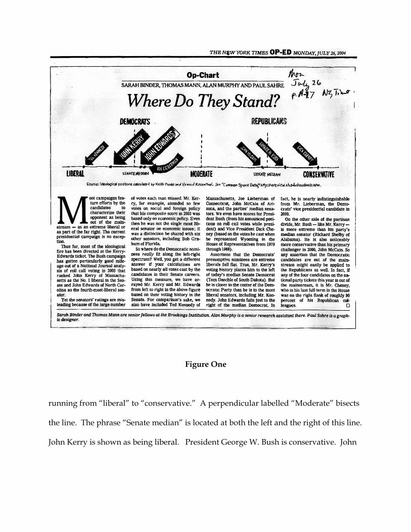
Figure One

running from “liberal” to “conservative.” A perpendicular labelled “Moderate” bisects

the line. The phrase “Senate median” is located at both the left and the right of this line.

John Kerry is shown as being liberal. President George W. Bush is conservative. John

Edwards is shown as more moderate than the ideologically extreme Vice President Dick

Cheney.7

The basic concept that self-evidently informs the plot – namely, that politics

organizes itself on a one-dimensional, left-right ideological space -- is, by convention,

dubbed issue space. Notice that Binder and Mann also regard legislators as arrayed

within issue space. Thus, the horizontal axis depicting issue space implicitly is broken

into identical intervals correlating to degrees of conservatism or liberalism that carry

actual numerical values. Finally, people in issue space evidently occupy fixed locations

within it.

Having pointed out these four (now obvious) elements of the figure – again, the

assumption of left-right issue space, that the issue space has a single dimension, its

underlying disaggregation into intervals, and the locational fixity of the scored politicians

-- we can now introduce a vital complication that takes us an essential step forward.

With a little thought one can quickly grasp that the idea of one-dimensionality is far

from obvious. One-dimensionality is very likely an artifact of something political or of

some political process. (As for the fixity of a legislator’s location we return to that later

in the article.)

Consider the case of the Southern New Deal Democrat, a legislator who voted for

liberal economic positions but voted against anti-lynching legislation. This was a

legislator who operated on two dimensions regularly. On one dimension he was a

liberal; on the other he was the opposite of a liberal: he was a conservative. In other

words, legislators can and do operate within two issue spaces.

But just when is American politics largely one-dimensional (as the plot in the Times

op-ed implied), and when is it two-dimensional (as the example of the Dixiecrat

implies)? Why is American politics one or the other at these times and not others?

How many different dimensions have there been at different times in American

history? Finally, so what if politics is either one-dimensional, two-dimensional, or more

than two dimensional? That is, if dimensions really can be detected, what does the

number of dimensions matter?

Dimensionality matters because it influences political choice and strategy. Take the

example of the Southern Democrat. This case underscores that there were two separate

issue-spaces in American politics during the New Deal, one dominant and one latent --

but potentially very salient. Franklin D. Roosevelt worked with a congressional

Democratic party that had a hidden fault line which gradually became an open crack in

the party’s unity. Roosevelt was thus required, or so he thought, to choose the issue

space in which he would more productively innovate. Either issue space had its own

agenda. On the dominant New Deal agenda, the question was, shall we have more of

an activist approach to economic or social policy or more of another? Mutatis mutandis,

the same was true for the other issue space, the racial dimension. FDR’s need for

legislative majorities, coupled with the disenfranchisement of most black American

voters, forced him (he thought) to accept patterns of policy design and implementation -

- in federal work relief and crop production control – that, while innovative on the “first

dimension,” would not cause overt conflict and debate, let alone cause any deliberate

legislative innovation, on the “second dimension,” that is, on the dimension of racial

politics.

To repeat: whether there are one or two dimensions, and what the content of those

dimensions is, influences both what kinds of policies politicians can choose and who

gets what from government. If so, then there is a corollary issue: whether there can be

more than two issue dimensions in politics. With two dimensions, there is obviously

room for strategy -- although, as the New Deal example suggests, policy choices are

probabilistic and thus will impose gains and losses for dominant coalitions and weaker

political actors. But what happens when there are more than two dimensions?

Surprisingly, the answer is that there is too much room for strategy.

Consider another example -- again drawn from the New York Times. A few years

ago, the Brennan Center at New York University issued a report criticizing the New

York state legislature as deeply dysfunctional and highly oligarchical, stating that its

governance “systematically limits the roles played by rank-and-file legislators and

members of the public in the legislative process.” The report cited a pronounced dearth

of public hearings, near unanimous passage of most laws, and a lopsided ratio of 16,892

bills introduced to 693, or 4%, enacted in 2002 -- suggesting a combination of an active

but small agenda and an ignored but large agenda. Not surprisingly, this portrait of a

do-nothing, oligarchic legislature enraged the New York Senate majority leader, Joseph

L. Bruno. Bruno called the report “pure nonsense,” and added: “Talk to the C.E.O. of

any company. If you want to act on something, and the company has 212 employees,

what are you going to do, have a discussion and let 212 employees do whatever the

agenda is? Is that what you do? So you have 212 different agendas. And that is just

chaotic, doesn’t work. That is Third-World-country stuff.”8

Bruno’s statement is of course ambiguous, and could be read to mean that 212

different priorities line up on one dimension, and he simply is too busy to handle them

sequentially. Nonetheless, to a spatial analyst Bruno’s seeming self-importance reveals

less about his temperament and more about legislatures. That is, it can be read

differently to mean that he, Bruno, could imagine that there really could be all of 212

“different agendas” in his legislature, one for each legislator who, presumably, would

try to organize all of the legislature’s issues around his or her unique set of concerns.

(Although we cannot provide instruction here, the reason why spatial analysts would

find Bruno’s speculation about 212 agendas to be so satisfying has to do with the so-

called “impossibility results,” such as the McKelvey Chaos Theorem or the Condorcet

Paradox, that fundamentally motivate spatial analysis.)9 Bruno clearly did not use the

word “agenda” in the technical sense that spatial analysts have for the word, i.e. a

question-for-action that organizes such legislative decision-making as amendment and

roll-call voting. But he was intriguingly close to the vocabulary of spatial analysis.

Perhaps for him 212 different “issue spaces” were a distinct possibility that he, Bruno, in

his capacity as a legislative leader (or CEO of the New York Senate), had to forestall.

Otherwise, Bruno said, there would be "chaos." Again, the resonance with spatial

terminology is striking. In the spatial analytical vocabulary, “chaos” has a meaning that

is close to what Bruno evidently had in mind: it refers to the politics that ensues when a

group of politicians operate simultaneously, in real time, on more than two dimensions.

When that happens politicians can have a very hard time working with each other at all,

creating strong incentives for them either to defect from the rules of the game or to

combine into a faction that will impose new rules unilaterally. A country can indeed

become ungovernable, spatial theorists hold, when the actual condition of “chaos” -- in

the spatial sense -- emerges. And if by a "Third World country" we mean an

ungovernable country, then Bruno was clearly associating “chaos” (more than 2, indeed

212, issue-spaces) with ungovernability.

Interestingly, an expansion in legislative dimensionality in fact happened once in

congressional development, in the pre- Civil War era. This underscores the tremendous

political and developmental importance that “chaos” – and its aftermath -- can actually

have. Poole and Rosenthal found so much dimensionality in Congress just before the

Civil War that they called the American Congress “chaotic” – unmanageable in just the

way that Joseph Bruno fears the New York legislature might be were it not for his

autocratic leadership.

To return, then, to the question of dimensionality: is politics ever more than two-

dimensional? It could be. Seasoned legislative leaders can certainly imagine that

prospect. How many dimensions could there be? Any number. What is politics like

with n>2 dimensions? Fairly unworkable, probably impossible. The run-up to the

American Civil War is a clear instance.

This brings us to a central finding of the “NOMINATE project:” that American

politics has, except for a very brief period, been a politics of n ≤ 2 dimensions. It is a

great accomplishment of Poole and Rosenthal that their longitudinal NOMINATE

scores frame American political development in such terms. Before we return to that

finding, however, there is quite a bit of further instruction. We turn, therefore, to the

micro-foundations of NOMINATE.

So Where Do the Scores Come From?

What are the micro-foundations of NOMINATE? Poole and Rosenthal have armed

themselves with a theory of individual legislative behavior that they consider good (or at

least good enough) for all legislators at all times. That theory allows them, second, to

extract rather precise information about ideological position from the entire, continuous

record of national legislative behavior, namely, all congressional roll-call votes.

At first blush, such a theory would seem not only unlikely, but also wildly a-

historical. But the question is not the theory’s realism so much as its capacity to order

an enormous amount of information without doing undue damage to the way

politicians actually behave. So let us turn to the theory.

Utility-Maximizing Legislators

One basic idea in the spatial theory of legislative behavior is that legislators, being

professional politicians, know rather precisely what they want -- and by the same token

what they do not want out of the legislative process.10

The great function of democratic legislatures is raising and spending money. These

tasks are measured and reported to everyone according to the national currency’s

metric, which means that democratic legislators routinely operate in easily

comprehensible and metricized ways with respect to policy choices.

For instance, if a legislator prefers one level of appropriation for defense -- say a

moderate hawk really likes appropriating $300 billion for the current fiscal year – s/he

probably would not be happy with a $250 billion appropriation, and s/he would be

even less happy with a $200 billion appropriation, and so forth. Likewise, this legislator

might think that a $400 billion appropriation is foolish, and that $500 billion is even

more foolish than $400 billion. This legislator has a most preferred level, in other words,

and then “around” that most preferred level are increasingly less desirable alternatives

in either direction, up or down, more or less.

It is not hard to see that this prosaic account is inherently spatial. A legislator

derives greater utility for a legislative outcome the closer it is to his or her most

preferred outcome or “ideal point.” Correlatively, the greater the distance of an

outcome away from the ideal point, then the smaller the utility. Furthermore, it is not

hard to see that for defense spending, at least, the legislator’s preferences -- if graphed

in two dimensional space, with “utils” (utility received) on the y axis and spending

levels on the x axis -- would execute something like a bell curve from left to right along

the abcissa.

Of course, fairly close to a legislator’s “ideal point” there is some indifference

between alternatives. Given a choice between a $301 billion and $299 billion

appropriation, with no chance of moving the outcome to $300 billion, the legislator

might feel indifferent between the two choices. Depending on his mood, s/he might

vote for $299 or s/he might vote for $301. The probability of either gaining his or her

vote is identical, about 50%, which is not the case for a choice between a $300 billion

appropriation and $200 billion appropriation.

Absent such a choice between very close outcomes in issue space, the odds that the

legislator would vote for the lower appropriation instead of the ideal point are much

smaller. But, critically, they are not zero. Perhaps his or her niece -- who is a dove --

promised to take him or her out to dinner to his or her favorite restaurant and then to

the opera if s/he voted for the lower appropriation, and s/he happened to know that

his or her preferred appropriation would win no matter what s/he did -- so s/he voted

for the lower appropriation even though that was, for him or her, ordinarily an

improbable choice. Such votes do occur in a legislator’s career. Legislators answer

several hundred roll calls in every congressional session, and over many sessions the

probability of some level of seemingly inexplicable voting probably grows -- if only up

to a certain level and no more. Every legislator has an “error function,” so to speak.

There is, of course, an explanation for each of the incidents of roll-call behavior that give

rises to the head-scratching. That is, the legislator did not really make “errors.” But

his/her “error function” roll call choices are not captured by the utility-maximizing

spatial logic we have just laid out -- hence the label “error function,” which refers to

some residual of observations that cannot be modelled precisely. Roughly speaking,

the error function allows for the possibility that a legislator will sometimes vote for an

outcome that is further from his or her ideal point (“ideal” with respect to those issues

that are included in the model) than its alternative. The spatial model is thus meant to

explain only a certain amount of the variation in roll-call behavior. Correlatively, the

spatial model needs some error in order to capture and explain important variations in

behavior.

Now what comes next may be somewhat challenging for the uninitiated. How

would one know what any legislator’s “ideal point” in some issue space is? Obviously,

the legislator’s roll call choices, the yeas and the nays, provide some guide to a

legislator’s ideal point. They communicate legislators’ revealed preferences. But how

would one take all of a legislator’s yeas and nays and derive some precise measure of

her ideal point? And do the same for all the other legislators? And what metric would

one use?

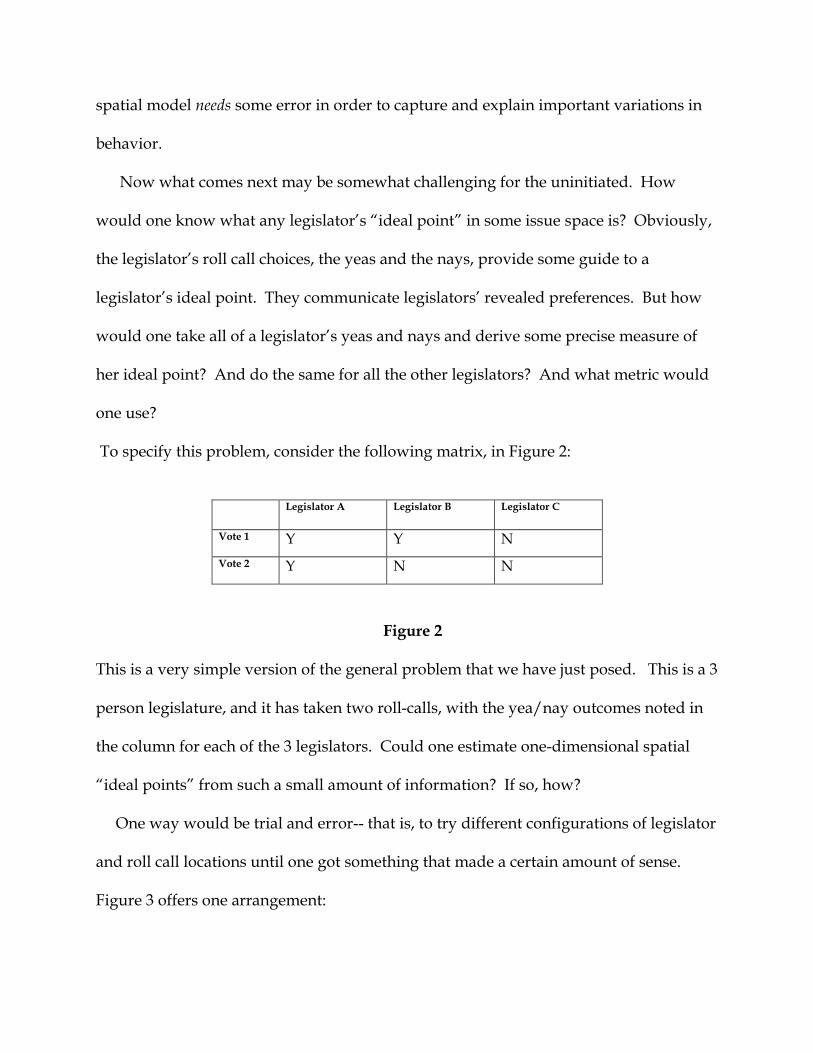
To specify this problem, consider the following matrix, in Figure 2:

Legislator A Legislator B Legislator C

Vote 1 Y Y N

Vote 2 Y N N

Figure 2

This is a very simple version of the general problem that we have just posed. This is a 3

person legislature, and it has taken two roll-calls, with the yea/nay outcomes noted in

the column for each of the 3 legislators. Could one estimate one-dimensional spatial

“ideal points” from such a small amount of information? If so, how?

One way would be trial and error-- that is, to try different configurations of legislator

and roll call locations until one got something that made a certain amount of sense.

Figure 3 offers one arrangement:

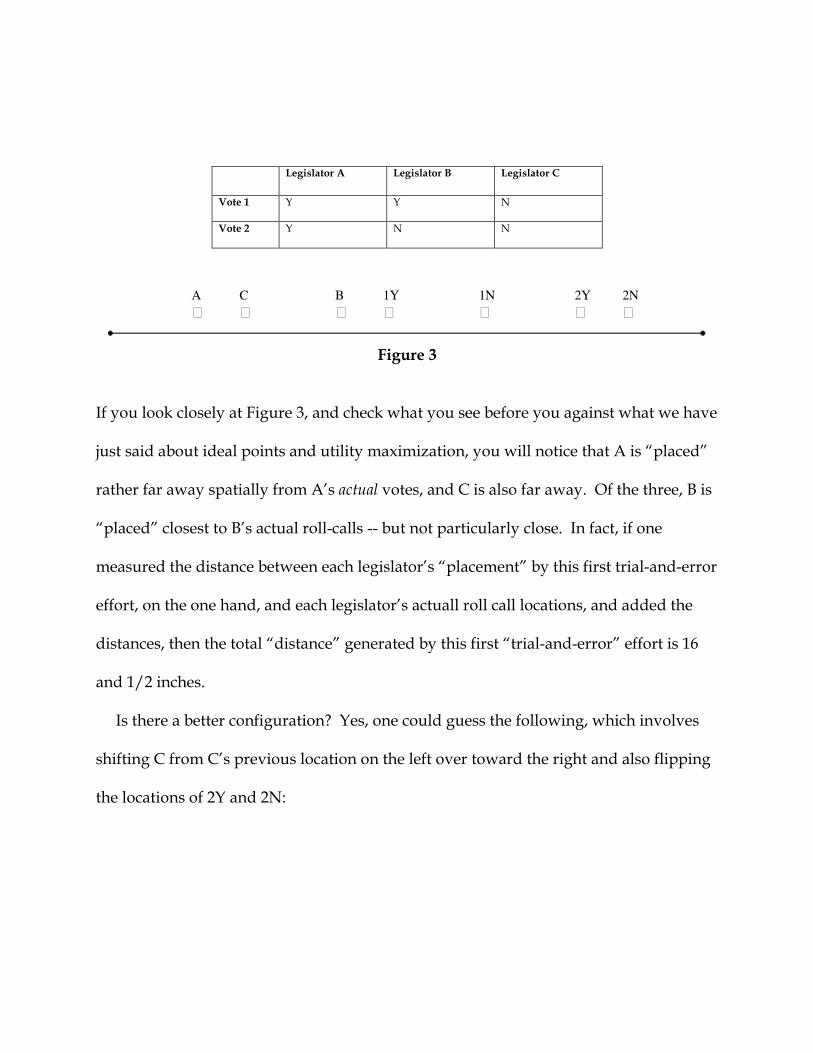
Legislator A Legislator B Legislator C

Vote 1 Y Y N

Vote 2 Y N N

A C B 1Y 1N 2Y 2N

� � � � � � �

Figure 3

If you look closely at Figure 3, and check what you see before you against what we have

just said about ideal points and utility maximization, you will notice that A is “placed”

rather far away spatially from A’s actual votes, and C is also far away. Of the three, B is

“placed” closest to B’s actual roll-calls -- but not particularly close. In fact, if one

measured the distance between each legislator’s “placement” by this first trial-and-error

effort, on the one hand, and each legislator’s actuall roll call locations, and added the

distances, then the total “distance” generated by this first “trial-and-error” effort is 16

and 1/2 inches.

Is there a better configuration? Yes, one could guess the following, which involves

shifting C from C’s previous location on the left over toward the right and also flipping

the locations of 2Y and 2N:

Legislator A Legislator B Legislator C

Vote 1 Y Y N

Vote 2 Y N N

A B 1Y 1N C 2N 2Y � � � � � � �

Figure 4

Notice that this arrangement, Figure 4, represents an improvement over the previous

figure: both Legislators B and C are fairly close in space to their actual votes. But notice

also that A is still pretty far away from A’s second vote. The total “distance” is less than

it was before – but it is nonetheless about 11 ½ inches.

Legislator A Legislator B Legislator C

Vote 1 Y Y N

Vote 2 Y N N

A 2Y 2N B 1Y 1N C � � � � � � �

Figure 5

One further possibility is shown in Figure 5. C is moved all the way to the right, 2Y

and 2N are re-flipped and moved left, B is located in the middle, and finally 1Y and 1N

are put on the right. This does the most to “minimize” the distance between legislators

and their actual roll call choices, namely, down to 8 inches.

By this point one gets the idea. Using the information which you have before you, in

Figure 2, concerning legislators and their roll-call votes, you could “map,” after a

certain amount of moving votes and legislators around on one line, where legislators’

ideal points probably are within this imaginary legislature.

In short, one can take roll call vote information and estimate whether legislators are

“to the right” on the whole or “to the left” on the whole. Thus A is “to the left” in issue

space above, B is “in the middle,” and C is “to the right.” Or, to put it in the language of

Figure 1 (recall that thas is the clipping from the New York Times) C is a

“conservative,” B is a “moderate,” and A is a “liberal.”

Furthermore, if you wanted to develop ideological scores for these legislators, you

could split the line in the figure into 201 intervals and come up with some sort of score

for how “liberal” or how “conservative” each of the three legislators, A, B, and C, is. If

the scale ran from -1 (most liberal) to +1 (most conservative), B would be about “0,” A

would be close to -1, and C would be close to +1.

Now we get to a harder part. If you have lots of legislators, and lots of roll calls,

trying first this and then that obviously cannot be the way to estimate legislator’s ideal

points and to generate scores. It would in fact be impossible, even if you assumed that

there is only one issue space. The House of Representatives has 435 members; each one

runs up about 600 roll calls in a congressional session. If there were two dimensions --

as during the New Deal -- your head would instantly spin even thinking about the

prospect of a trial-and-error effort. (Interestingly, Poole and Rosenthal actually

considered making a supercomputer conduct a kind of trial-and-error iteration, but

concluded that any set of instructions to the computer would cause it to produce

gibberish in a short period of time, what is called “blowing up.”) In short, there has to

be an efficient way to do what we did above with the actual, real world data concerning

each chamber of the U.S. Congress over more than 200 years.

There is such a way, and it is called maximum likelihood estimation, or MLE. This

is the mathematical core of the software program that Poole and Rosenthal devised for

manipulating the data which they collected. MLE differs completely from the kind of

trail-and-error which we just sketched -- it does not involve minimizing distances per

the previous exercise. So it is vital to acquire some sense of MLE in a simple version of

the procedure before extrapolating to what Poole and Rosenthal did with actual roll-call

data in a complicated version of MLE. Our hope here – by tapping the reader’s

memory (or grasp) of calculus, probability, and the nature of frequency distribution -- is

to give an intuitive sense of what Poole and Rosenthal did to “map” legislators in issue

space for several thousand legislators and many thousands of roll calls. Though the

exposition is informal, it pays to read it slowly, with stops for thinking it over.

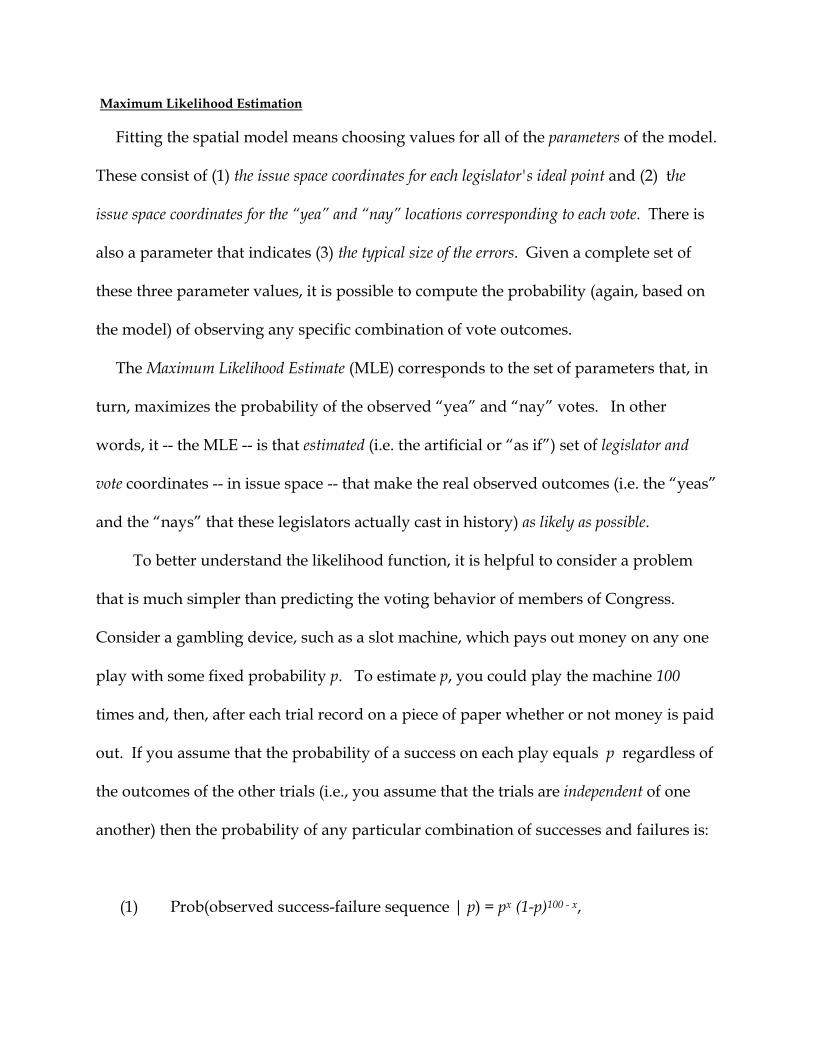
Maximum Likelihood Estimation

Fitting the spatial model means choosing values for all of the parameters of the model.

These consist of (1) the issue space coordinates for each legislator's ideal point and (2) the

issue space coordinates for the “yea” and “nay” locations corresponding to each vote. There is

also a parameter that indicates (3) the typical size of the errors. Given a complete set of

these three parameter values, it is possible to compute the probability (again, based on

the model) of observing any specific combination of vote outcomes.

The Maximum Likelihood Estimate (MLE) corresponds to the set of parameters that, in

turn, maximizes the probability of the observed “yea” and “nay” votes. In other

words, it -- the MLE -- is that estimated (i.e. the artificial or “as if”) set of legislator and

vote coordinates -- in issue space -- that make the real observed outcomes (i.e. the “yeas”

and the “nays” that these legislators actually cast in history) as likely as possible.

To better understand the likelihood function, it is helpful to consider a problem

that is much simpler than predicting the voting behavior of members of Congress.

Consider a gambling device, such as a slot machine, which pays out money on any one

play with some fixed probability p. To estimate p, you could play the machine 100

times and, then, after each trial record on a piece of paper whether or not money is paid

out. If you assume that the probability of a success on each play equals p regardless of

the outcomes of the other trials (i.e., you assume that the trials are independent of one

another) then the probability of any particular combination of successes and failures is:

(1) Prob(observed success-failure sequence | p) = px (1-p)100 - x,

where x is the number of times out of 100 that you win money (possible values of x are

0,1,2,...,100). The two terms being multiplied in (1) correspond to the probability of

getting x successes (each happening with probability p) and of getting 100-x failures

(each with probability 1-p). Changing the order in which the successes and failures

occur does not change the overall probability, as long as there are still x successes and

100 - x failures.

The probability statement in equation (1) treats p as a fixed number and is a

function of x, the count of successes in 100 independent plays. After your experiment of

playing the machine and recording your successes and failures, you will have valuable

information. You will know the value of x. But you will not actually know p. To

estimate it, you will need to compute a likelihood function for it.

The Likelihood Function L(p) is identical to (1), except it treats x as fixed at the

observed value and is a function of the unknown parameter p. The maximum likelihood

estimate (MLE) for p is the value that maximizes L(p). In other words, is the value of

p that makes what happened (observing exactly x successes) as probable as possible.

This does not mean that it is the correct value of p; other values close to it are nearly as

plausible, and there is no ruling out the possibility that something incredibly

improbable (e.g. a run of good or bad luck) happened on your sequence of trials.

However, MLE's are optimal estimators in many ways, and much is known about their

behavior, particularly when the number of trials is large.

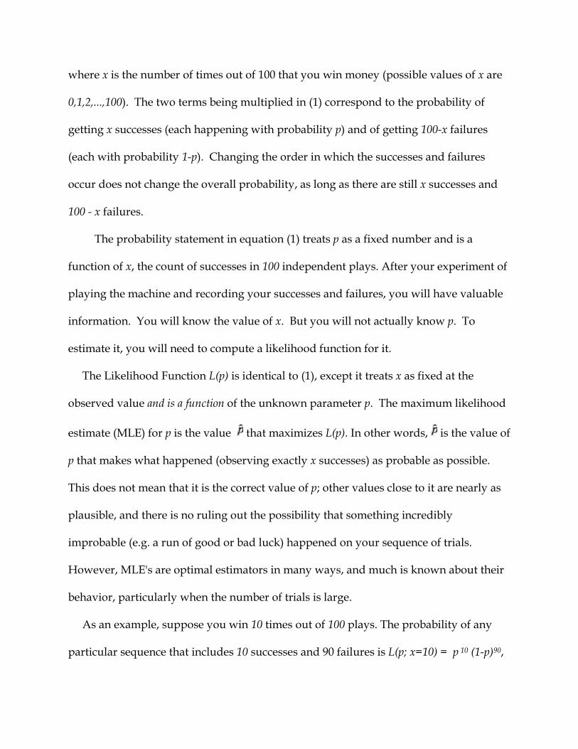
As an example, suppose you win 10 times out of 100 plays. The probability of any

particular sequence that includes 10 successes and 90 failures is L(p; x=10) = p 10 (1-p)90,

which is plotted in the top half of Figure 6, “Visualizing MLE.” This likelihood function

is maximized for p = 0.1, with the result that = 0.1 is the MLE. The maximization can

be seen visually in the simple example plotted in the top half of Figure 6 for 100 trials.

In the second graph, at the bottom of Figure 6, the MLE is also = 0.1 but the number

of trials depicted is 1000, 10 times the number for the graph in the top half. In general,

with x successes in n independent trials, the MLE is = x / n, the observed proportion of

successes. But with the larger number of trials the range of plausible values that might

be the true probability is narrower. (The differences between the rectangles underneath

the curves emphasize that.) The relative accuracy of the estimates thus increases as the

number of trials increases. The analogue for NOMINATE would be to have the results

of a larger number of votes.

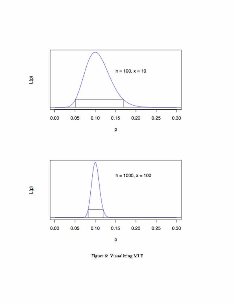
Figure 6: Visualizing MLE

In other words, with more information we narrow the range of plausible estimates –

which is what we want. The rectangles in Figure 6 show 90% confidence intervals for p

corresponding to n=100 and to n=1000 with = 0.1 in each case. The first interval is

larger by a factor of roughly , or about 3, meaning that around three times as

many values of p must be considered "plausible" when using 100 trials compared to

1000 trials. But using a larger sample size will reduce the number of values of p that

can be considered plausible – which means, in turn, greater accuracy and precision.

All of this brings us to a strength of NOMINATE. The above examples have only one

parameter and 100 or 1000 outcomes. But NOMINATE routinely fits models with many

1000's of parameters and outcomes.

Each person who has voted in the time period considered has one or several

associated parameter values (coordinates in issue space) -- as does each question that was

voted on. How might we analogize these legislative facts? Imagine that there are six

hundred different gambling machines (our analogue for roll calls) and, further, imagine

that the machines may have different characteristics (e.g., different p's). Now suppose

there are 435 different people playing each machine, and that the players differ from

each other at the business of winning money. In other words, the probability of a

player winning on a particular play depends on both the player and the machine being

played.

The different players in this example obviously represent different members of the

U.S. House, and the different machines could – pursuing the analogy -- represent

different questions being voted on in a Congress. Voting “yea” on a question, in turn,

could correspond to “winning money” on a play, and its opposite, voting “nay,” would

correspond to “losses.”

Given values for all of the voter and question parameters, Poole and Rosenthal can

write down a function for the probability of votes being cast in a particular way. This

defines the likelihood function L for the set of parameters, and the MLE is the

combination of voter and question coordinates that result in the largest possible value

of L.

Now, there are important complications that require notice. Complications arise due

to the large number of parameters involved in the Poole-Rosenthal likelihood function

(i.e. NOMINATE, with – to recall -- the T and E standing for Three-step Estimation).

While there is an explicit formula for the MLE in the simple example with the slot

machine, much, much more computationally intensive methods were used by Poole

and Rosenthal. What then did they do?

They used a computer algorithm (for those who are interested, it is the BHHH

gradient algorithm) to handle the massive amount of information with which they

worked. What did that involve? Here is another analogy: think of a very, very large

and “bumpy” field with lots of little hillocks of varying height. There are, very

roughly, three dimensions in this large terrain, length, width, and height. Your job is to

find the highest location in this hilly field. This is like finding the MLE for a two-

parameter model. The third dimension, this height, represents the value of the

likelihood function for any particular two-dimensional location in the field.

Now, for the one-dimensional NOMINATE model, the highest “hill” would be

located over a space of dimension equal to the number of legislators plus two times the

number of votes – which is the total number of parameters in the model. A two-

dimensional NOMINATE model would, of course, have twice as many parameters as

the one-dimensional model.

(An aside is in order. You might be wondering why the terms “one-dimensional”

and “two-dimensional” suddenly appeared. Recall, however, our earlier contrast

between the one-dimensionality of the plot in Figure 1 and our discussion of the two-

dimensionality of politics during the New Deal era.)

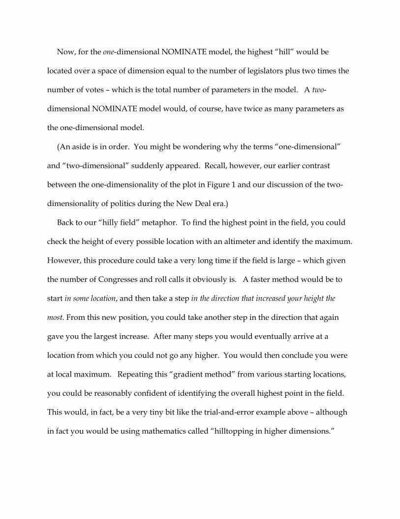
Back to our “hilly field” metaphor. To find the highest point in the field, you could

check the height of every possible location with an altimeter and identify the maximum.

However, this procedure could take a very long time if the field is large – which given

the number of Congresses and roll calls it obviously is. A faster method would be to

start in some location, and then take a step in the direction that increased your height the

most. From this new position, you could take another step in the direction that again

gave you the largest increase. After many steps you would eventually arrive at a

location from which you could not go any higher. You would then conclude you were

at local maximum. Repeating this “gradient method” from various starting locations,

you could be reasonably confident of identifying the overall highest point in the field.

This would, in fact, be a very tiny bit like the trial-and-error example above – although

in fact you would be using mathematics called “hilltopping in higher dimensions.”

To use this procedure with the NOMINATE model, one would first choose a starting set

of parameter values (the coordinates in issue space for the legislator ideal points and

all of the yea and nay locations) and (get ready here for a mathematical term of art)

evaluate the likelihood function L( ). Then one would move to a slightly different set of

values, , and evaluate L(). If L() > L( ), you accept as the new . In this way you keep

moving in the direction of the gradient vector. Repeating this procedure many times

allows you to “climb the hill” until you arrive at the value that maximizes the function

L, at least locally.

It might be helpful here to summarize by reconsidering the simple case displayed

earlier:

Legislator A Legislator B Legislator C Vote 1 Y Y N Vote 2 Y N N

Recall that we tried fiddling around with getting the appropriate relative distances

between possible ideal points and the yea and nay points, even with only three

legislators. We thus did very, very roughly (and without the mathematics of

probability) what NOMINATE does systematically with much, much more information,

and, quite crucially, using probability (not distance minimization.)

To recapitulate, in NOMINATE any given set of estimated coordinates for legislators

in 1 or 2 issue spaces yields a certain probability of the observed votes. The MLE is the

set of coordinates for all legislators in a Congress or in an historical period that makes

this probability the largest. We tried to get the likely issue space locations of 3

legislators by fiddling with their observed yea and nay votes in a trial and error fashion,

but NOMINATE does this for thousands and thousands of legislators and their roll-call

votes through “hill-climbing.” Once a solution is obtained, that is, once NOMINATE

thinks it has found the highest point in the hilly field, the legislator and roll-call

parameters which are associated with that decision – which are the estimated

coordinates – are dropped into a metric of some sort that can be easily interpreted, e.g. a

scale between minus 100 and 100. The resulting scores are the NOMINATE scores available

on the voteview.com website for each member of Congress since the first Congress.

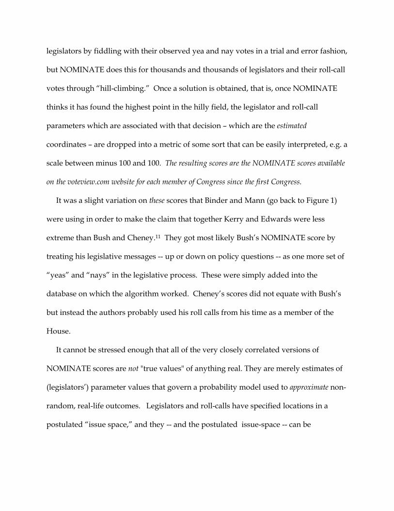
It was a slight variation on these scores that Binder and Mann (go back to Figure 1)

were using in order to make the claim that together Kerry and Edwards were less

extreme than Bush and Cheney.11 They got most likely Bush’s NOMINATE score by

treating his legislative messages -- up or down on policy questions -- as one more set of

“yeas” and “nays” in the legislative process. These were simply added into the

database on which the algorithm worked. Cheney’s scores did not equate with Bush’s

but instead the authors probably used his roll calls from his time as a member of the

House.

It cannot be stressed enough that all of the very closely correlated versions of

NOMINATE scores are not "true values" of anything real. They are merely estimates of

(legislators’) parameter values that govern a probability model used to approximate non-

random, real-life outcomes. Legislators and roll-calls have specified locations in a

postulated “issue space,” and they -- and the postulated issue-space -- can be

mathematically recovered given roll-call votes for each legislators and through a data-

reduction algorithm. The fitted parameters of the model form the basis of the scores.

But, as Figure 1 suggested, these scores tell us something politically substantive

about real people – in that case, how far apart they were ideologically. They also allow

one to “zoom in” on a particular politician, or on cohorts, and get a clear sense of their

conservatism or liberalism on the two dimensions.12

Such properties of the scores, as we see next, permit one to investigate debates about

American political history in useful ways.

The Scores, Voteview, and the “Redlined New Deal” Debate

To illustrate how NOMINATE can be incorporated into existing work, let us consider

an issue in American political history, whether and just how Southern Democrats

weakened, or aided, the New Deal’s social policies. Since the late 1970s and early

1980s, many scholars have asked whether and how the division in Congress between

Northern and Southern Democrats affected New Deal policy design in ways that hurt

the interests of African-American citizens.13

Two major issues have been at stake in addressing those questions: did New Deal

social policy deepen black disadvantage, and if so, by how much and for how long? If

New Deal social policy was meant for whites, first, and blacks only secondarily, then

did that racialized allocation of social rights prime the racial tensions over “welfare”

that erupted once African-American welfare protest made black disadvantage an issue?

Through comparison of key roll-call votes on the Social Security Act and the Fair

Labor Standards Act, we can suggest how NOMINATE tools can be used to explore the

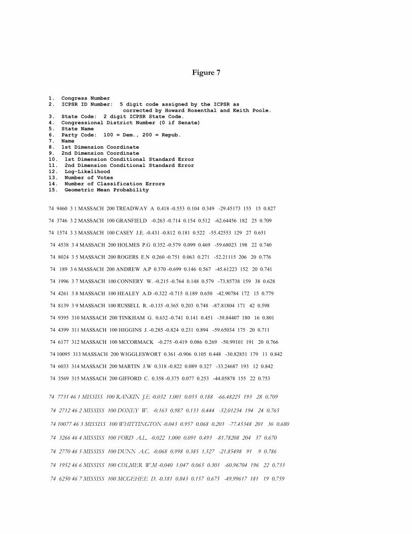
Figure 7 1. Congress Number 2. ICPSR ID Number: 5 digit code assigned by the ICPSR as corrected by Howard Rosenthal and Keith Poole. 3. State Code: 2 digit ICPSR State Code. 4. Congressional District Number (0 if Senate) 5. State Name 6. Party Code: 100 = Dem., 200 = Repub. 7. Name 8. 1st Dimension Coordinate 9. 2nd Dimension Coordinate 10. 1st Dimension Conditional Standard Error 11. 2nd Dimension Conditional Standard Error 12. Log-Likelihood 13. Number of Votes 14. Number of Classification Errors 15. Geometric Mean Probability 74 9460 3 1 MASSACH 200 TREADWAY A 0.418 -0.553 0.104 0.349 -29.45173 155 15 0.827 74 3746 3 2 MASSACH 100 GRANFIELD -0.263 -0.714 0.154 0.512 -62.64456 182 25 0.709 74 1574 3 3 MASSACH 100 CASEY J.E. -0.431 -0.812 0.181 0.522 -55.42553 129 27 0.651 74 4538 3 4 MASSACH 200 HOLMES P.G 0.352 -0.579 0.099 0.469 -59.68023 198 22 0.740 74 8024 3 5 MASSACH 200 ROGERS E.N 0.260 -0.751 0.063 0.271 -52.21115 206 20 0.776 74 189 3 6 MASSACH 200 ANDREW A.P 0.370 -0.699 0.146 0.567 -45.61223 152 20 0.741 74 1996 3 7 MASSACH 100 CONNERY W. -0.215 -0.764 0.148 0.579 -73.85738 159 38 0.628 74 4261 3 8 MASSACH 100 HEALEY A.D -0.322 -0.715 0.189 0.650 -42.90784 172 15 0.779 74 8139 3 9 MASSACH 100 RUSSELL R. -0.135 -0.365 0.203 0.748 -87.81804 171 42 0.598 74 9395 310 MASSACH 200 TINKHAM G. 0.632 -0.741 0.141 0.451 -39.84407 180 16 0.801 74 4399 311 MASSACH 100 HIGGINS J. -0.285 -0.824 0.231 0.894 -59.65034 175 20 0.711 74 6177 312 MASSACH 100 MCCORMACK -0.275 -0.419 0.086 0.269 -50.99101 191 20 0.766 74 10095 313 MASSACH 200 WIGGLESWORT 0.361 -0.906 0.105 0.448 -30.82851 179 11 0.842 74 6033 314 MASSACH 200 MARTIN J.W 0.318 -0.822 0.089 0.327 -33.24687 193 12 0.842 74 3569 315 MASSACH 200 GIFFORD C. 0.358 -0.375 0.077 0.253 -44.05878 155 22 0.753 74 7731 46 1 MISSISS 100 RANKIN J.E -0.032 1.001 0.055 0.188 -66.48225 193 28 0.709 74 2712 46 2 MISSISS 100 DOXEY W. -0.163 0.987 0.133 0.444 -52.01234 194 24 0.765 74 10077 46 3 MISSISS 100 WHITTINGTON -0.043 0.957 0.068 0.203 -77.45348 201 36 0.680 74 3266 46 4 MISSISS 100 FORD A.L. -0.022 1.000 0.091 0.493 -81.78208 204 37 0.670 74 2770 46 5 MISSISS 100 DUNN A.C. -0.068 0.998 0.385 1.527 -21.85498 91 9 0.786 74 1952 46 6 MISSISS 100 COLMER W.M -0.040 1.047 0.065 0.301 -60.96704 196 22 0.733 74 6250 46 7 MISSISS 100 MCGEHEE D. -0.181 0.843 0.157 0.675 -49.99617 181 19 0.759

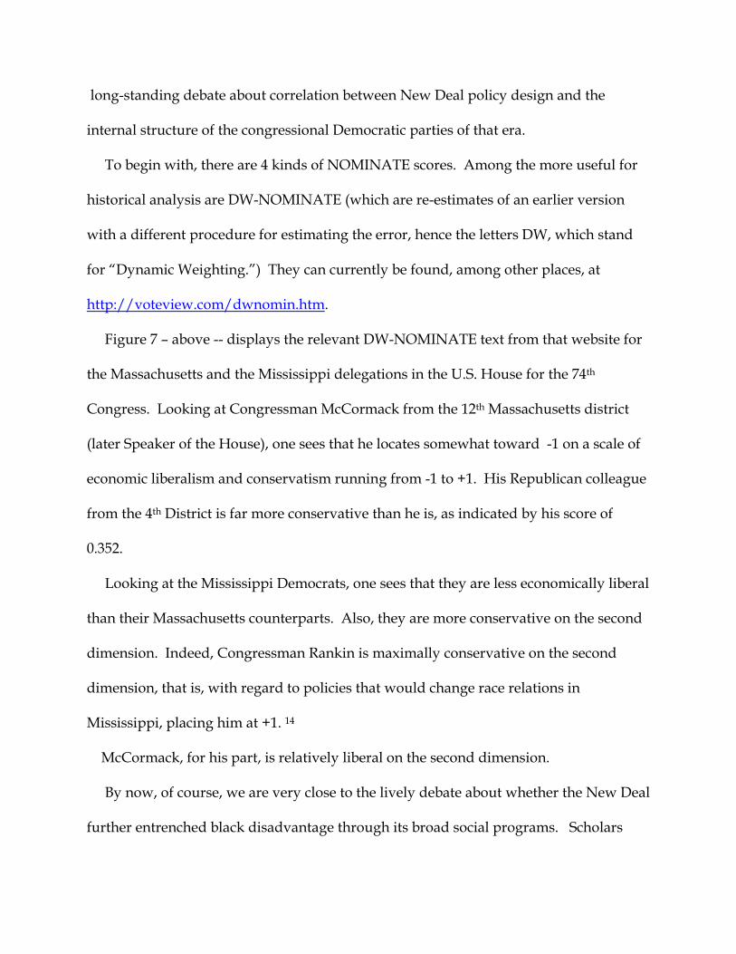
long-standing debate about correlation between New Deal policy design and the

internal structure of the congressional Democratic parties of that era.

To begin with, there are 4 kinds of NOMINATE scores. Among the more useful for

historical analysis are DW-NOMINATE (which are re-estimates of an earlier version

with a different procedure for estimating the error, hence the letters DW, which stand

for “Dynamic Weighting.”) They can currently be found, among other places, at

http://voteview.com/dwnomin.htm.

Figure 7 – above -- displays the relevant DW-NOMINATE text from that website for

the Massachusetts and the Mississippi delegations in the U.S. House for the 74th

Congress. Looking at Congressman McCormack from the 12th Massachusetts district

(later Speaker of the House), one sees that he locates somewhat toward -1 on a scale of

economic liberalism and conservatism running from -1 to +1. His Republican colleague

from the 4th District is far more conservative than he is, as indicated by his score of

0.352.

Looking at the Mississippi Democrats, one sees that they are less economically liberal

than their Massachusetts counterparts. Also, they are more conservative on the second

dimension. Indeed, Congressman Rankin is maximally conservative on the second

dimension, that is, with regard to policies that would change race relations in

Mississippi, placing him at +1. 14

McCormack, for his part, is relatively liberal on the second dimension.

By now, of course, we are very close to the lively debate about whether the New Deal

further entrenched black disadvantage through its broad social programs. Scholars

have increasingly depicted them as internally “redlined” due to Southern Democratic

influence on their design.15

Consider the design of the 1935 Social Security Act: were agricultural workers

deliberately left out of the original coverage of the Act in order to accommodate the

preference of Southern Democrats that black landless workers not receive federal

protection in the form of old age income security? At the time of the bill’s passage, the

NAACP pointed out the gap in coverage. On the other hand, no Southern Democrat

clearly and unmistakably voiced a desire that the Act’s coverage features not disturb

Jim Crow. Also, the Secretary of the Treasury, Henry Morgenthau, underscored the

enormous administrative difficulty of implementing the Act if it were written to cover

agricultural and domestic workers – and tightly focused revisionist research has shown

that this argument was by no means pretextual.16

NOMINATE has a desktop spin-off that throws interesting light on the issue –

Voteview, which can be downloaded from the same sites that provide NOMINATE

scores (such as the one listed earlier.)17

Voteview displays spatial plots of roll-call votes. Visual inspection of these

Voteview plots yields useful information on whether Social Security was “redlined by

design.” Why? Because NOMINATE is expressly set up to detect not one but two

dimensions – and the second dimension is racial. In other words, one would expect a

vote on Social Security to display the patterning that one would see in a vote which taps

the “second dimension.” But it does not – which raises interesting questions of

interpretation that, in turn, bear on the “redlined New Deal” debate. First, though, a

quick Voteview tutorial, (another version of which is available at

http://www.princeton.edu/~voteview/ -- it duplicates some of what we say below.)

A Brief Tutorial on Voteview

Each spatial display provided by Voteview has several useful features. It shows

“clouds” of tokens, each of which represents a particular legislator. For all major party

legislators, the tokens are labelled either R, D, or S for Southern Democrat, and they are

color coded. Those legislators elected by a third party, e.g. the Farmer-Labor Party,

have an obvious label, in this instance F. Additionally, the clouds are bunched or

dispersed in a wide variety of ways. Such bunching or dispersion roughly indicates

partisan or factional cohesion along one of the two NOMINATE dimensions – and the

patterns of bunching or dispersion also reveal how dominant the first dimension is in

any particular vote.

Figure 8

In this connection, consider Figure 8, which displays a House roll call on April 15,

1937, to amend a bill criminalizing lynching. Rep. Howard Smith of Virginia proposed

an amendment to this bill: it proposed striking out the sections of the bill that imposed

fines on counties in which lynchings occurred. As one can see looking at the figure,

almost all of the S tokens (for Southern Democrats) are above the line (we say more

about the “cut line” shortly), and many of the other party-label tokens (R, D, and F) lie

underneath the line in two clouds.

The “cut line” thus shows that the vote on Smith’s amendment was a “second

dimension” vote – but the small cloud to the right, underneath the “cut line,” of course

also indicates that the Republican and Democratic parties had a polarized relationship

to each other on the ordinarily dominant first dimension.

Now to the “cut line.” NOMINATE assumes that the question voted upon has yea

and nay positions in two-dimensional issue space. The yea and nay locations of the

question are unknown parameters. The yea and nay coordinates of the legislators are

also unknown parameters. All of the locations are found by maximizing the overall

likelihood function for all of the unknown coordinates. The “cut line” is a line

perpendicular to the line joining the NOMINATE-estimated yea and nay points of the

question voted on. This (perpendicular) “cut line” furthermore bisects the other (joining)

line at its halfway point. There are misclassifications – NOMINATE is after all

likelihood estimation. But those legislators whose issue space positions make them

likely to vote yea are typically on the yea side of the “cut line,” and vice-versa. Here

the yeas are blue, the nays are red, and the misclassifications are either blue or red tokens

that stand out visually because they are in the “wrong” place.

As an aside, when a legislator is “misclassified” by NOMINATE (and thus by its

visual front-end, Voteview) the initial hypothesis is always that the legislator’s relative

indifference to the outcome of the vote was higher than it was for his co-partisans or

factional colleagues. But Voteview allows you to “inquire” about a misclassified

legislator by toggling on the token to find out who it is – and the result can of course

prompt further useful speculation beyond the standard initial hypothesis.

There is even more information to be had from the “cut line.” Looking at it in Figure

8, the anti-lynching roll-call, one notices that it tends toward the horizontal. This

particular angularity is in fact quite significant. The flatter a “cut line” the more the

vote is a second dimension (“north-south”)18 vote. By the same logic, the more vertical

the “cut line” is (as we will shortly see in considering the display of a vote on Social

Security), the more the vote is a first dimension (“east-west”) vote – that is, much like

the one-dimensional plot of the very first figure we presented, i.e. Figure 1.

Was Social Security Internally and Intentionally Redlined?

In keeping with the exercise of gleaning information from Voteview’s plots, now

consider Figure 9. Recall that the NAACP criticized the proposed design of the Social

Security Act of 1935 for its initial lack of coverage for farmers, farm laborers, and

household workers and servants, on the ground that this feature of the Act’s design

would leave about half of all African-American wage-earners unenrolled in the

program. Several policy scholars have inferred racial intent in the Act’s design.

Ira Katznelson and Sean Farhang, in a recent article, point out that the number of

cases of clear Southern Democratic racial animus in designing policy that would affect

the income, education, and work conditions of black Southerners is large. Given the

regularity of the pattern, they suggest that it makes sense to also code Social Security as

belonging to this larger set of “redlined” policies. But, strictly speaking, this may or

may not be the right inference, since there is no strong, direct evidence – actual

“smoking gun” statements -- of racial animus on the part of Southern Democrats—

whereas with the other policies there is. Social Security could be sui generis – in a set of

1, all by itself.

Indeed, Larry DeWitt, Gareth Davies and Martha Derthick have strongly argued that

administrative necessity better explains the initial restriction of the Act’s coverage

formula to urban and industrial wage-earners. This point cannot, in our view, be

dismissed. It reminds us, after all, that in 1935 the U.S. was an incomparably more

agrarian nation than it is now. Huge regions of rural America were extremely remote.

Furthermore, these areas were mired in a deep economic crisis with no certain outcome.

To ask effectively bankrupt farmers to administer the Social Security system of

contributory finance on behalf of their tenants – an organizational matter which today

we rarely notice as we clock in at highly bureaucratized, modern workplaces – would

have been, once one reflects on the matter, very hard and possibly politically suicidal

for the Roosevelt Administration.

Can Voteview illuminate the difference between these rival scholarly views of Social

Security? Considerations of space preclude a full application of Voteview to all of the

relevant roll calls and to inspecting the angles of the cut lines and displaying

information about them in, for instance, a plot or in histograms. But two more

applications of Voteview do suggest that such a fuller exploration might well be

informative.19

Figure 9, below, displays a House vote from April 11, 1935, on an open rule to permit

20 hours of debate on H.R. 7260, “a bill establishing a system of social security benefits.”

The verticality of the “cut-line” suggests an almost perfect “first-dimension” roll call

with little evidence of the hidden “racial dimension” criticized then by the NAACP and

since then by many policy scholars.

Also consider Figure 10. Figure 10 displays the structure of a December 17, 1937

House vote on a motion by a conservative Republican, Fred Hartley of New Jersey, to

“recommit S. 2475, an act providing for the establishment of fair labor standards in

employments connected with interstate commerce.” The Fair Labor Standards Act was

generally understood to exempt agricultural labor, an exemption that Northern and

Southern Democrats in both chambers collaborated on. Several Southern Democrats

openly expressed concern about the impact on race relations in the South if Congress

followed FDR’s original proposal to have FLSA cover both agricultural and industrial

labor. Nonetheless, the Senate failed to specifically expand the agricultural exemption

for tobacco, cotton, and seasonal activity, though it did so for dairy and the packing of

perishable goods, and for packing and preparation in the “area of production.” In other

words, the bill, while internally “redlined,” was not maximally “redlined” when it came

to the House. It is interesting (see Figure 10, below) that the vote on Hartley’s

successful motion to recommit has a noticeable “second-dimension”/”north-south”

structure to it of the kind that one sees in Figure 8. (That the cut line tips to the left,

rather than to the right, is irrelevant, incidentally.)

Figure 9

Figure 10

In short, using one of NOMINATE’s tools – Voteview – raises the intriguing

possibility that those scholars who want to “code” Social Security as deliberately

“redlined,” in the same way that they code the FLSA as intentionally “redlined,” may

have to review their conclusions. If the differences in the cut-lines persist in a fuller

treatment of the entire set of relevant cases, then the apparent exception for Social

Security may well be there because it fundamentally differed. Social Security may never

have threatened the Southern political economy in the same way that the FLSA did.

Social Security would take many years in the future to pay out – or so it was widely

thought at the time. Only later was the payout schedule accelerated. Second, everyone

in the debate recognized that the program was geared for the industrial economy of the

1930s, not the entire American economy.

It is only today, after decades of experience with non-means tested, contributory

finance programs which have a universal application, that as a country we are much

more likely to aspire to start programs as close to their “universal” level as possible (i.e.

100% of the population). Indeed, that assumption was a major sticking point in the

1993-94 debate over health insurance, and it was interestingly never open to serious

debate. But Social Security’s initial universalism was far from robust. It has become

effectively universal only over the long run. Indeed, the program was instead designed

to be a targeted program at its inception, and the target population was the adult male

wage earner likely to have a stable, lifetime job with a career ladder. Very few Southern

workforce participants, white or black, were in that initial conceptualization of the

target population precisely because the South was rural. On this view, Social Security

was, as Davies and Derthick suggest, never meant to apply to rural America – and the

verticality of the cut line is consistent with that conceptualization of the program.

To summarize, we do not claim to have settled this APD debate. Our point, instead,

is that using Voteview, and NOMINATE more generally, can be useful to those doing

historical work – so helpful that they ought to become more integrated into

developmental analysis.

Low-Dimensional APD

There is more to say about linking NOMINATE and APD – in particular, about the

deep developmentalism which inspires the NOMINATE project.

Consider, first, some of the basic conceptions which we currently have of how

American politics has evolved, very broadly speaking. They include:

Madisonian continuity, in other words, a public sphere that -- notwithstanding the development of national bureaucracy and a permanent military establishment – is constantly churned by the public actions and public rhetoric of the officials occupying the institutions designed by the Founders in ways that make American politics readily comparable across time20 institutional layering, for instance, the construction of a “modern” presidency that coexists with the “traditional” presidency, or the development and survival within the House and Senate of loosely coupled forms of internal structure21

regular cycles of conflict and consensus, mobilization and stability, inclusion and exclusion, such as Morone’s neo-Puritan cycles, Huntington’s creedal passive and creedal active periods and McFarland’s adaptation of this idea22

democratization and de-democratization, for example, the two reconstructions of black voting rights, and the development of governmental and associational capacities to define and to protect political, civil, and social rights23 institution-building (and institution-weakening) sequences over time that close off a range of institutional options, once political actors choose some options instead of others, for example, bureaucratic development,24 de-localization within a federal system,25 the recasting of party politics due to presidential entrepreneurship26or to the joint influence of presidential primaries and television broadcasting,27 the weakening of once-common federated civic organizations during the 1960s and 1970s28 the rise, development, and erosion of policy regimes or other resilient bundles of institutions, social and electoral coalitions, public philosophy, and policies as seen in immigration policy, for instance, or the kinds of regime dynamics sketched by Skowronek for understanding presidential politics, or the “racial orders” conceptualization of King and Smith29

policy feedback processes that recast the terms of participation and civic status, for instance, social policy interventions that allocate civic status differentially, or policy interventions that build civic capacities over the long-haul30 the judicialization of politics, such as the rise of adversarial legalism and the construction by elected officials and judges of judicial review31 intercurrence, that is, the co-existence of relatively autonomous institutional and policy domains operating with different political dynamics and according to different “clocks” of “political time”32

These are some of the ideas developed by scholars in the political science subfield of

American political development for characterizing and capturing historical processes,

dynamics, and political mechanisms. But this catalogue is incomplete, we believe. At

least one more distinctive way of thinking about American political development must

be added to this inventory – namely, the issue-spatial perspective which informs and is

substantiated by NOMINATE.

The concept of “low dimensionality” sits at the core of this additional developmental

perspective. Perhaps the most basic finding of Poole and Rosenthal is that American

politics has almost always exhibited “low dimensionality” -- by which they mean no

more than two, mathematically-recoverable issue dimensions.

To recall, these dimensions are purely formal. This is exceptionally important

because it means that every possible substantive issue “loads” (in the language of factor

analysis) onto one or the other of the two dimensions. But that is of course very odd!

There is a very wide range of seemingly disparate issues in contemporary American

politics – from gay marriage to environmentalism to “intelligent design” in secondary

science education to land use to gasoline prices to foreign policy to immigration, and so

on. Undoubtedly, the same was true in the past. Furthermore, such results as the

Condorcet Paradox and the McKelvey Chaos Theorem dramatize both agenda

instability and the potentially large dimensionality of majority rule.

How can it be that there are only two, truly basic issue dimensions in U.S. politics?

The Poole and Rosenthal answer is, in effect, “surprising, but altogether true.” They fit

a model with one dimension, to see how successfully that captured legislative behavior.

Then they fit two dimensions, to see how much that improved the model's

performance, then three dimensions, and so on.33

They found that the one-dimensional model was about 83% accurate overall,

meaning that in 83% of all the individual votes, the legislator voted for the outcome

whose position in issue space (as estimated by NOMINATE) was closer to the

legislator's ideal point (again as estimated by NOMINATE), while the two-dimensional

model was about 85% accurate. Three or more dimensions offered virtually no

improvement over two, which implied that Congress's issue space has nearly always

been no more than two-dimensional, at least to the extent that a spatial model can

approximate ideal points in congressional roll-call voting over time. As for the other

15%, it is non-dimensional voting lacking any underlying structure – pork-barrel voting

and “error” (as in the discussion early in this article).

Poole and Rosenthal did not, it should be noted, directly estimate the number of

dimensions. Instead, what they did was assume that issue space has been one-

dimensional and then see fit the model to the data. Then they assumed a second

dimension. Ex ante, the improvement in fit (what they call average proportional

reduction of error, or APRE) had to grow. What they did was a bit like throwing another

independent variable into an OLS regression -- R-squared will always go up, even if

only a bit, no matter what plausible variable you add. Assuming a second dimension

doubles the amount of information you are working with. Rather than running a

“climb the hill” algorithm in an “east-west” space, or “north-south” space, one runs it in

a space that has both an “east-west” plane and a “north-south” plane, so there are now

twice as many local maxima to climb, which, in turn, can do only one thing to your

estimated parameter values for your legislators, for you now have two more

coordinates for each – namely, kick these estimated values closer to the real values.

Their cleverness, though, lay in trying to gauge how much change one got from this

trick. That it was only 2% was remarkable. Then they did the trick again and nothing

changed, really. The main exception is the period immediately before the Civil War,

when the U.S. became increasingly ungovernable.

What is – and was -- the content of these dimensions? This part of their analysis was

interpretive. Poole and Rosenthal concluded that, over time, the first dimension was

always socio-economic – state banks vs. a national bank, at one time, currency

expansion vs. currency restriction, at another, high tariffs vs. low tariffs at a third, social

spending vs. spending restraint in a fourth, and so on. From reading their political

history and looking at the specific content of the roll calls associated with the second

dimension, they concluded that it was a “racial” dimension, or more precisely, a race-

relations (often sectional) dimension.

In short, the American regime is an “n ≤ 2 dimensions polity” (so to speak.) It

always has been, in all likelihood. To be sure, Poole and Rosenthal emphasize the

rupture preceding the Civil War. But it is remarkable that the “chaotic” dimensionality

which they find in the early-to-mid 1850s rapidly subsided. The previous basic

dimensionality re-asserted itself – the difference being that a previously subordinated

second dimension became, and for quite some time stayed, highly salient. Hence our

larger point: the “n ≤ 2 dimensions” nature of the regime does not shift.

To put it another way, it appears that over the course of American political history

low-dimensionality co-exists with, and is little disturbed by, other kinds of

developmental patterns, including those catalogued above – i.e. Madisonian continuity,

institutional layering, cycles, sequences that generate “trajectories,” democratization

and de-democratization, and the constitutionalization of politics. This fact of co-

existence is consistent, in truth, with a basic property of American political evolution

that has been identified by Skowronek and Orren. As they note, American political

development is strikingly intercurrent: “the normal condition of the polity will be that

of multiple, incongruous authorities operating simultaneously,” that is, there are

“multiple-orders-in-action” over the course of American history. 34 A very similar

concept is Schickler’s notion of “disjointed pluralism” with which he characterizes

congressional evolution. “Intercurrence” might be thought of as “disjointed pluralism”

writ large. What we point out here is simply that low-dimensionality also forms part of

intercurrence.

Undoubtedly, we think, much of the explanation for the persistence of low-

dimensionality is the party system.35 The United States was the first early modern

polity to develop a mass (though by no means fully inclusive) party system. Party

competition might therefore be counted a centripetal, self-stabilizing “order-in-action”

(to use the language of Orren and Skowronek.) To be sure, elections generate the mass

discussion and speech that would seem to give politicians opportunities for disrupting

the coalitions of their opponents -- what William Riker memorably called

“heresthetics.” 36 A mass, competitive party system is so encompassing, however, and it

operates on such a large scale, that no one has -- nor could have -- a structurally decisive

capacity to abruptly “flip” everyone, during campaigns, to a new dimension of conflict

beyond those that already exist, and also to keep them there on that new dimension.

A party system’s inclusiveness and mass character muffle, in other words. That is,

they muffle the impact of any agenda-setting agitation and politicking. To put the

matter a bit more micro-economically, in any modern electorate, agenda-setters would

have to find some way of achieving the requisite marginal impact on the cognitive

attention that every attentive or potentially attentive voter gives to the existing

dimension(s) of party conflict. Purposive, directed attention-focusing activity would

have to be calibrated to match all the marginal variations in attention that exist among

the public in order to shunt party conflict onto another latent, underlying dimension or

agenda. That seems nearly impossible.

Even if that were possible, furthermore, it is hard to see how the new focus of

attention could be sustained. As agitation, framing, and other attention-focusing

activities generate new symbols and arguments, citizens are faced with a cognitive

choice: are these symbols and arguments really genuinely new and previously unheard

of? The question, for many, answers itself -- no. More plausibly, many individuals will

decide that the supposedly new symbols and arguments can be related to existing

symbols and arguments. They thus “fold them into” existing symbols and arguments.

The pre-existing dimension(s) of conflict thus stay(s) unaltered. The existing

dimensions are, cognitively, Procrustean beds.

Consequently, across American political history one would expect to find politicians

“mapping” new and initially unfamiliar issues onto the existing dimensions. There is

strong, indirect confirmation of this possibility, it turns out, in the fact that legislators’

NOMINATE “scores” are fairly fixed. Once a liberal, always a liberal. Once a

conservative, always a conservative. Once a moderate, always a moderate.

Some legislators do, of course change what they stand for. Think, for instance, of

Strom Thurmond. NOMINATE thus mathematically allows for the possibility that a

legislator's ideal point on a dimension may move over time. What Poole and Rosenthal

found, though, is that most legislators hardly move at all, and any movement is

basically slow and steady, without sudden erratic jumps.

More precisely, they ran estimates of error reduction with the assumption that

legislators never move, and compared the results to what they got when they allowed

linear changes, then more complicated quadratic changes, and so on. They found that

allowing linear changes over time increased NOMINATE’s accuracy somewhat, but

quadratic and higher-order movement models offered essentially no improvement.

Furthermore, what movement there was tended to be small. In other words, the

movement of a legislator's ideal point is essentially a very slow drift in a straight line

(on one dimension, from more liberal to more conservative or vice versa).37

This makes sense. As long as House districts – and states -- stay the same over the

legislator career, the accountability relationship demands considerable fixity. Thus

there is congruence between the district median and legislator preferences, generating

the ideal point that we have discussed. Thurmond is, in fact, the exception who proves

the rule: the South Carolina electorate changed composition sharply during his career.

It would seem, then, that if politicians have careers, and if their careers matter to

them, then they are likely to be “issue mappers” not “issue innovators.” But what

about Riker’s demonstration that politicians engage in “heresthetics?” Riker was

impressed by the potency of heresthetics, and saw it as a possible source of political

instability and disruption. On reflection, though, it seems evident that “heresthetics” is

not dimensional innovation. When politicians engage in Riker’s “heresthetics” they are

not actually pushing American politics toward a system of n>2 dimensions. Instead,

they are exploiting an unstable relationship between dimensions.

To summarize, politicians manage the dimensionality of American politics, and, in

those periods when there are two dimensions, they contest the relative salience of the

basic dimensions. This can, of course, be a high stakes game that is highly

entrepreneurial, as illustrated by the long run-up to the Civil War. Inspired by Riker,

Barry Weingast has recently suggested that the stage for the Civil War was set by an

ultimately failed effort to manage the existing two-dimensionality. The rise of Martin

Van Buren’s “national” party system was the initial, basic device for dimensional

management in the ante-bellum period and until the break-up of the Whig Party it did

work to blunt the party-systemic impact of the second, racialized dimension. But

clearly the second dimension was ever present – as shown by the politics of the gag rule

for blocking congressional reception of abolitionist petitions for outlawing slavery in

the District of Columbia.38

By the time of the Lincoln-Douglas Debates, mainstream, ambitious politicians, not

just politically marginal abolitionist orators, were openly arguing about which

dimension should be salient in party competition – socio-economic or racial – not least

because there was new, successful party dedicated to changing the agenda of American

politics, the Republican party. Lincoln argued that saving the soul of America required

sustained party conflict on the second dimension. Obviously he did not use the term

“second dimension.” But re-reading the Debates one will see that he clearly refers to

something like a “second dimension,” over and over. For his part, Douglas pleaded

with his audiences for the importance of staying on the “first dimension,” the agenda of

socio-economic conflict, and repeatedly warned his audiences that Lincoln’s plan to re-

arrange the relationships between the existing issue dimensions was both dangerous

and unnecessary.

Besides managing dimensions, and contesting their relationship with each other, if

there is more than one, the other exceptionally significant thing that American

politicians have historically done is generate – or mute --polarization on one (or both) of

the basic dimensions. For instance, Andrew Johnson used his presidency to rapidly

and very sharply polarize American party politics on the newly salient racial-sectional

dimension – in all likelihood in order to win the 1868 presidential election. But that was

a choice which he had, which is why congressional Republicans were initially startled

by his behavior. Johnson’s entrepreneurship was exceptional, however. Polarization

happens more gradually, it seems, when it happens -- as illustrated by the past several

decades of American national party politics. Just as there are strong incentives for

politicians to “map,” so there are strong incentives, usually, to maintain, not widen, the

distance between party medians, left and right.

What does the foregoing sketch suggest in terms of research questions, broadly

speaking? First, there are the hypotheses we have put forth – that some institutions

(such as the ante-bellum “national parties” and the gag rule) have historically

functioned as devices for managing dimensional salience, that politicians are issue

mappers, that heresthetics is rarer than mapping, that heresthetics always involves the

exploitation of an unstable relationship between two dimensions, and that

entrepreneurial polarization, perhaps more than heresthetics, has periodically and

decisively influenced political development. These all require substantiation.

Related tasks include documenting and explaining the relative salience of the two

dimensions across time, and of explaining the near disappearance, in the last quarter of

the 20th century, of a second dimension. That certainly is related to the great re-

incorporation of African-American citizens through voting rights and civil rights

policies. But why has the Christian political mobilization of the past generation not re-

activated the second dimension? Are openly conflictual race relations and extreme

sectional tension the only source of a second dimension?

Additionally, there is the problem of explaining the great polarization of the past 45

years – which has not been matched by a similar polarization, in national opinion

survey results, among voters. Is that due to recruitment patterns for national office

from state legislatures? To the development and impact of primary elections? What

role, if any, do mid-term congressional elections play? Presidential agenda-setting?

The development of internal governance mechanisms in the Senate and the House?

What impact has polarization had on the polity? McCarty, Poole and Rosenthal

suggest that polarization has been associated with an increase in income inequality.39

Does that relationship hold for previous polarizations? What other phenomena are

associated with polarization? With partisan convergence?

This sketch of research issues is not meant to be exhaustive, only illustrative. But the

sketch is full enough, we think, to substantiate the claim we made at the outset of the

article – that the marriage of spatial theory and a thorough scaling of all congressional

roll-calls has opened up new and vital developmental questions.

Conclusion

NOMINATE scores, and the desktop tools that have been produced as a by-product

of NOMINATE’s construction and application – a process that took Poole and

Rosenthal decades – represent major breakthroughs in the development of political

science. By now this is widely recognized within contemporary political science, most

notably among congressional scholars and among the somewhat (but not entirely)

overlapping community of scholars who have been influenced by the formal-analytical

applications pioneered by William Riker and others.

There are rich opportunities for the APD subfield to join and participate in this

accomplishment. As Katznelson and Lapinski recently noted, APD’s next “big step”

could very well be in the area of congressional evolution and its role in driving

American political development.40 NOMINATE can help to do this because of the

relative inter-temporal comparability of the scores it generates. It has yielded a full data

series for the entire history of the Republic. Also, NOMINATE will very likely be used

synergistically with another data series which are being generated by Katznelson,

Lapinski, and Razaghian. The time for APD scholarship to adopt both NOMINATE

and these other scaling results would seem to have arrived. We are hardly

recommending that APD jettison all of its previous conceptual categories in favor of

exclusively spatial-analytical categories. We only recommend that APD make room for

them. Poole and Rosenthal – and those scholars who have found their work exciting --

are, after all, very much developmentalists in their own right.

ENDNOTES 1 A good and oft-cited introduction so far has been Jordan Ellenberg, “Growing Apart: The Mathematical Evidence

for Congress’ Growing Polarization,” Slate 26 December 2001.

2 Technically, most uses of NOMINATE are actually uses of a particular version, DW-NOMINATE, i.e. Dynamic

Weight Nominal Three-Step Estimation.

3 Robin Toner, “Good-Will Reserves Run Low for Social Security Talks,” New York Times, 19 December 2004, p. 41,

charting scores from 1901 to 2001 for House; Norman Ornstein and Barry McMillion, “One Nation, Divisible,” New

York Times, 24 June 2005, p. A-23; Brief of Political Scientists Bernard Grofman and Gary Jacobson as Amici Curiae In

Support of Neither Party, No. 02-1580, In the Supreme Court of the United States, Richard Vieth, et al, v. Robert C.

Jubilerer, et al, On Appeal From the United States District Court for the Middle District of Pennsylvania, August

2003, in authors’ possession, courtesy of Bernard Grofman.

4 See, especially, Nolan McCarty, Keith T. Poole, and Howard Rosenthal, Polarized America: The Dance of

Ideology and Unequal Riches (Cambridge, MA: MIT Press, 2006).

5 For instance, Ira Katznelson and John S. Lapinski, “At the Crossroads: Congress and American Political

Development,” Perspectives on Politics 4 (June 2006): 243-260.

6 The example of Bayesian approaches to recovering where legislators are in issue space suggests why the socres

correlate so strong. Scores derived from Bayesian approaches depend on “vague priors:” that is, they assume very

little about the actual location of legislators, thus approximating the frequentist premise that data are random. So

they tend to converge on frequentist results, leading to the high correlations. An accessible introduction to these

matters can be found in Joshua Clinton, Simon Jackman, and Douglas Rivers, “The Statistical Analysis of Roll Call

Data,” American Political Science Review 98 (May 2004): 355-370.

7 Sarah Binder, Thomas Mann, Alan Murphy and Paul Sahre, Op-Chart, “Where Do They Stand? New York Times,

26 July 2004, p. A-17.

8 Michael Cooper, “So How Bad Is Albany? Well, Notorious,” New York Times 22 July 2004, B1 and B5.

9 For an introductory discussion, see Charles Stewart III, Analyzing Congress (New York: W.W. Norton, 2001), ch.

1.

10 Note that what follows sounds more like a quadratic utility function, with the two sides of a bell-shaped function

crossing the abscissa, when in fact the utility model used by Poole and Rosenthal is meant to take account of

legislator awareness of precise ideological differences. Thus the function has two tails that never cross the abscissa.

But to sketch the spatial model we have ignored this critical difference. 11 Binder and Mann used a variant called “common space” scores; these are not available for the entire period of

congressional history.

12 See, for instance, Paul Krugman’s discussion of John McCain’s extreme NOMINATE rating in “The Right’s Man,”

New York Times 13 March 2006, p. A 21.

13 Among others, Ira Katznelson, When Affirmative Action Was White: An Untold History of Racial Inequality in

Twentieth-Century America (New York: W.W. Norton, 2005); Robert C. Lieberman, Shifting the Color Line: Race

and the American Welfare State (Cambridge, MA: Harvard University Press, 1998), and Steve Valocchi, “The Racial

Basis of Capitalism and the State, and the Impact of the New Deal on African-Americans,” Social Problems 41

(August 1994): 347-362.

14 The alert reader will notice that Rankin’s second dimension score is actually just over the upper bound. This

might seem the result of truly fierce white supremacism. That is in fact the explanation. The technical reason for his

score being above the upper limit is related to the estimates of whether his ideal points move in issue space across

time. Poole and Rosenthal found that most legislators do move their location in issue space, and they do this

somewhat over time. Their movement is best estimated as a “linear” movement. On the whole, though, movement

is slight. See Keith T. Poole and Howard Rosenthal, Congress: A Political-Economic History of Roll-Call Voting

(New York: Oxford University Press, 1997), pp. 25, 28, 70-77. If, therefore, someone has moved “over” the bounds

on any dimension, the statistics indicates that there were political pressures that moved them a great deal, relative to

other legislators. Thus, Rankin’s white supremacism caused him to move in issue space, over the course of his career,

a great deal, relative to all other legislators – which reflects his reaction to the destruction of Jim Crow between the

New Deal and the Great Society.

15 “Redlining” refers to racial coding of maps used for allocation of housing credit. We use it here to refer, more

broadly, to the racialization of public policy. It is worth noting that “redlining” as a word came from the discovery

by historians, principally Kenneth Jackson, that the Home Owners’ Loan Corporation of the New Deal era rated

neighborhoods to assess credit risk through the color coding of city maps. Green meant low risk; blue and yellow

moderate risk; red high risk. Predominantly black neighborhoods were typically colored red, hence the term

“redlining.” As a further aside, we note that federal maps, by themselves, did not generate redlining, as is sometimes

thought. Federal maps reflected an ongoing – in other words, they did not create a new – practice in housing

finance. See Amy Hillier, “Redlining in Philadelphia,” in Ann Kelly Knowles, ed., Past Time, Past Place: GIS for

History (Redlands, CA: ESRI Press, 2002).

16 Larry DeWitt, “It Was Not About Race: The Decision to Exclude Agricultural and Domestic Workers from the

U.S. Social Security Program,” unpublished mss., cited with permission of the author, “in-house” historian at the

Social Security Administration.

17 Voteview works, however, only with PC desktops, not Apple machines.

18 Note that “north-south” is nothing more than a pun – in other words, any second dimension vote – on abortion,

for instance, if the House ever voted a national policy proposal – would be “north-south.”

19 We plan to do this in a separate article, we should note.

20 David R. Mayhew, America’s Congress: Actions in the Public Sphere, James Madison through Newt Gingrich

(New Haven: Yale University Press, 2000); Samuel P. Huntington, Political Order in Changing Societies (New

Haven: Yale University Press, 1968), ch. 2.

21 Jeffrey K. Tulis, The Rhetorical Presidency (Princeton: Princeton University Press, 1987); Eric Schickler,

Disjointed Pluralism: Institutional Innovation and the Development of the U.S. Congress (Princeton: Princeton

University Press, 2001).

22 James A. Morone, Hellfire Nation: The Politics of Sin in American History (New Haven: Yale University Press,

2003); Samuel P. Huntington, American Politics: The Promise of Disharmony (Cambridge, MA: Belknap Press,

1981); Andrew S. McFarland, Neopluralism: The Evolution of Political Process Theory (Lawrence: University Press

of Kansas, 2004), esp.ch. 6. More generally see David Resnick and Norman C. Thomas, “Cycling Through American

Politics,” Polity 23 (Fall 1990): 1-21.

23 Richard M. Valelly, The Two Reconstructions: The Struggle for Black Enfranchisement (Chicago: University of

Chicago Press, 2004); Kevin J. McMahon, Reconsidering Roosevelt on Race: How the Presidency Paved the Road to

Brown (Chicago: University of Chicago Press, 2004); Francisco E. Gonzalez and Desmond King, “The State and

Democratization: The United States in Comparative Perspective,” British Journal of Political Science 34 (April 2004):

193-210.

24 Daniel P. Carpenter, The Forging of Bureaucratic Autonomy: Reputations, Networks, and Policy Innovation in

Executive Agencies, 1862-1928 (Princeton: Princeton University Press, 2001); Scott C. James, Presidents, Parties, and

the State: A Party System Perspective on Democratic Regulatory Choice, 1884-1936 (New York: Cambridge

University Press, 2000).

25 Martha Derthick, Keeping the Compound Republic: Essays on American Federalism (Washington, DC:

Brookings Institution Press, 2001), esp. ch. 1.

26 Sidney M. Milkis, The President and the Parties: The Transformation of the American Party System Since the New

Deal (New York: Oxford University Press, 1993)

27 John H. Aldrich, Why Parties? The Origin and Transformation of Political Parties in America (Chicago: University

of Chicago Press, 1995).

28 Theda Skocpol, Diminished Democracy: From Membership to Management in American Civic Life (Norman:

University of Oklahoma Press, 2003).

29 Fred Block, “The Roles of the State in the Economy,” in Neil Smelser and Richard Swedberg, eds., Handbook of

Economic Sociology (Princeton: Princeton University Press, 1994); John L. Campbell and Michael Patrick Allen,

“Identifying Shifts in Policy Regimes: Cluster and Interrupted Time-Series Analyses of U.S. Income Taxes,” Social

Science History 25 (Summer 2001): 187-216; Andrew J. Polsky, “Why Regimes? Ideas, Incentives, and Policies in

American Political Orders,” Polity 29 (1997): 625-40; “Dialogue on `Institutional Complementarity and Political

Economy,’” Socio-Economic Review 3 (May 2005): 359-82; Wolfgang Streeck and Kathleen Thelen, “Institutional

Change in Advanced Political Economies,” in Wolfgang Streeck and Kathleen Thelen, eds., Beyond Continuity:

Institutional Change in Advanced Capitalist Societies (New York: Oxford University Press, 2005); Daniel J. Tichenor,

Dividing Lines: The Politics of Immigration Control in America (Princeton: Princeton University Press, 2002);

Aristide R. Zolberg, A Nation By Design: Immigration Policy in the Fashioning of America (New York: Russell Sage

Foundation,; Cambridge, MA: Harvard University Press, 2006); Stephen Skowronek, The Politics Presidents Make:

Leadership from John Adams to Bill Clinton (Cambridge, MA: The Belknap Press of Harvard University Press, 1997);

Desmond King and Rogers M. Smith, “Racial Orders in American Political Development,” American Political Science

Review 99 (February 2005): 75-92

30 For example: Suzanne Mettler, Dividing Citizens: Gender and Federalism in New Deal Public Policy (Ithaca:

Cornell University Press, 1998); idem, Soldiers to Citizens: The G.I. Bill and the Making of the Greatest Generation

(New York: Oxford University Press, 2005); Lester Salomon, “The Time Dimension in Policy Evaluation: The Case

of the New Deal Land-Reform Experiments,” Public Policy 27 (1979): 129-183.

31 Richard H. Pildes, “The Constitutionalization of Democratic Politics,” Foreword, The Supreme Court, 2003 Term,

Harvard Law Review 118 (November 2004): 28-154; Robert A. Kagan, “Adversarial Legalism and American

Government,” in Marc K. Landy and Martin A. Levin, The New Politics of Public Policy (Baltimore: Johns Hopkins

University Press, 1995); and, among many others, Mark A. Graber, “The Non-Majoritarian Difficulty: Legislative

Deference to the Judiciary,” Studies in American Political Development 7 (1993): 35-73; Keith Whittington,

Constitutional Construction: Divided Powers and Constitutional Meaning (Cambridge, MA: Harvard University

Press, 1999), Ken I. Kersch, Constructing Civil Liberties: Discontinuities in the Development of American

Constitutional Law (New York: Cambridge University Press, 2004).

32 Karen Orren and Stephen Skowronek, The Search for American Political Development (Cambridge: Cambridge

University Press, 2004).

33 Poole and Rosenthal, Congress: A Political-Economic History of Roll-Call Voting, Table 3.1 p. 28.

34 Orren and Skowronek, In Search of American Political Development, at pp. 108 and 113, respectively; Schickler,

Disjointed Pluralism.

35 As do Poole and Rosenthal – see Congress, p. 35: “Parties…help to map complex issues…into a low-dimensional

space.”

36 William H. Riker, The Art of Political Manipulation (New Haven: Yale University Press, 1986).

37 Poole and Rosenthal, Congress, pp. 25, 28, 70-77.

38 Charles Stewart III and Jeffery Jenkins, “The Gag Rule, Congressional Politics, and the Growth of Anti-Slavery

Popular Politics,” unpublished mss., http://web.mit.edu/cstewart/www/papers.html

39 McCarty, Poole, and Rosenthal, Polarized America.

40 Katznelson and Lapinski, “At the Crossroads.”