R E S E A R CH PA P E R

Phenology and time series trends of the dominant seasonalphytoplankton bloom across global scales

Kevin D. Friedland1 | Colleen B. Mouw2 | Rebecca G. Asch3 |

A. Sofia A. Ferreira4 | Stephanie Henson5 | Kimberly J. W. Hyde1 |

Ryan E. Morse1 | Andrew C. Thomas6 | Damian C. Brady6

1National Marine Fisheries Service,

Narragansett, Rhode Island

2Graduate School of Oceanography,

University of Rhode Island, Narragansett,

Rhode Island

3Department of Biology, East Carolina

University, Greenville, North Carolina

4School of Oceanography, University of

Washington, Seattle, Washington

5Ocean and Earth Science, National

Oceanography Centre, Southampton, United

Kingdom

6School of Marine Sciences, University of

Maine, Orono, Maine

Correspondence

Kevin D. Friedland, National Marine

Fisheries Service, 28 Tarzwell Drive,

Narragansett, RI 02882, U.S.A.

Email: kevin.friedland@noaa.gov

Editor: Fabien Leprieur

Abstract

Aim: This study examined phytoplankton blooms on a global scale, with the intention of describing

patterns of bloom timing and size, the effect of bloom timing on the size of blooms, and time series

trends in bloom characteristics.

Location: Global.

Methods: We used a change-point statistics algorithm to detect phytoplankton blooms in time

series (1998–2015) of chlorophyll concentration data over a global grid. At each study location,

the bloom statistics for the dominant bloom, based on the search time period that resulted in the

most blooms detected, were used to describe the spatial distribution of bloom characteristics over

the globe. Time series of bloom characteristics were also subjected to trend analysis to describe

regional and global changes in bloom timing and size.

Results: The characteristics of the dominant bloom were found to vary with latitude and in local-

ized patterns associated with specific oceanographic features. Bloom timing had the most

profound effect on bloom duration, with early blooms tending to last longer than later-starting

blooms. Time series of bloom timing and duration were trended, suggesting that blooms have been

starting earlier and lasting longer, respectively, on a global scale. Blooms have also increased in size

at high latitudes and decreased in equatorial areas based on multiple size metrics.

Main conclusions: Phytoplankton blooms have changed on both regional and global scales, which

has ramifications for the function of food webs providing ecosystem services. A tendency for

blooms to start earlier and last longer will have an impact on energy flow pathways in ecosystems,

differentially favouring the productivity of different species groups. These changes may also affect

the sequestration of carbon in ocean ecosystems. A shift to earlier bloom timing is consistent with

the expected effect of warming ocean climate conditions observed in recent decades.

K E YWORD S

bloom, carbon cycle, phenology, phytoplankton, productivity, trend analysis

1 | INTRODUCTION

Primary production in the oceans accounts for approximately half of

the carbon fixed by photosynthesis on a global scale (Field, Behrenfeld,

Randerson, & Falkowski, 1998). This production fuels the growth and

reproduction of living marine resources and is a crucial factor that

exerts control over which species produce harvestable surpluses, con-

tributing to fishery yields (Chassot et al., 2010; Ryther, 1969; Stock

et al., 2017) and ensuring global food security (Christensen et al., 2015;

Perry, 2011). In addition to the production of continental shelf species

that are exploited in fisheries, there is also significant trophic transfer

between open ocean primary production and mesopelagic fishes on a

Global Ecol Biogeogr. 2018;1–19. wileyonlinelibrary.com/journal/geb VC 2018 JohnWiley & Sons Ltd | 1

Received: 5 May 2017 | Revised: 20 October 2017 | Accepted: 9 December 2017

DOI: 10.1111/geb.12717

global basis (Davison, Checkley, Koslow, & Barlow, 2013; Irigoien et al.,

2014). At a more fundamental level, phytoplankton production is the

central driver of most marine ecosystems (Sigman & Hain, 2012) and

the biogeochemical processes governing carbon flow and export flux

(Doney, Bopp, & Long, 2014; Laufk€otter et al., 2016). However, oce-

anic photosynthetic production is not constant in time and space; geo-

graphical and phenological (bloom timing and duration) variability

occurs because of complex biophysical factors controlling phytoplank-

ton blooms owing to the dynamics between the rates of cell reproduc-

tion and mortality associated with death and grazing (Behrenfeld &

Boss, 2014; Cherkasheva et al., 2014). The variability in blooms affects

energy flow from phytoplankton production to pelagic and demersal

communities, and thus, both horizontal and vertical transport of energy

in the water column (Corbiere, Metzl, Reverdin, Brunet, & Takahashi,

2007).

Phytoplankton bloom dynamics have been characterized on basin

and global scales, identifying differing patterns of bloom phenology by

latitude and oceanic province. Analyses of time series change in bloom

dynamics complement descriptions of the spatial organization of

blooms using a number of different sources of data. For example, a

study with a geographical focus in the North Atlantic found that spring

bloom timing has advanced for some temperate latitude regions and

was delayed in other areas, whereas the autumn and winter blooms

have mostly been delayed (Taboada & Anadon, 2014). Other longer-

term studies identified the effects of changing mixed layer dynamics on

the relative strength of spring and autumn blooms in the North Atlantic

(Martinez, Antoine, D’Ortenzio, & Montegut, 2011) and widespread

shifts in bloom phenology associated with broad-scale changes in the

coupled atmosphere–ocean system (D’Ortenzio, Antoine, Martinez, &

D’Alcala, 2012). Some of the most dramatic changes in bloom charac-

teristics and phenology have occurred in the Arctic, where bloom max-

ima have advanced c. 50 days from 1997 to 2009 as a consequence of

changes in seasonal ice cover (Kahru, Brotas, Manzano-Sarabia, &

Mitchell, 2011). Changes in bloom magnitude and timing alter energy

flow in the ecosystem, which in turn impacts the growth and reproduc-

tion of higher trophic levels in the food web (Cushing, 1990; Hunt

et al., 2002; Malick, Cox, Mueter, Peterman, & Bradford, 2015; Platt,

Fuentes-Yaco, & Frank, 2003; Schweigert et al., 2013).

Climate variation can indirectly modify bloom timing and size

through mechanisms that influence water column conditions, such as

the supply and ratio of nutrients and light availability. As climate sys-

tems shift in response to anthropogenic forcing, there is a need to

understand their impact on bloom dynamics both retrospectively and

in a forecasting context. As an example, in the Baltic Sea, investigators

found that bloom duration has increased in recent years and associated

this change in bloom dynamics with increasing water temperature and

declining wind stress, which they attributed to global climate change

(Groetsch, Simis, Eleveld, & Peters, 2016). Change in climate conditions

may act to modify blooms through the direct effects of nutrient supply

and grazing; additionally, changing distributions of parasites and viruses

associated with climate change will be likely to play a larger role in the

dynamics of blooms and the nature of fixed carbon available to primary

grazers (Frenken et al., 2016). Projections of bloom dynamics by global

earth system models (e.g., CanESM2, GFDL-ESM2M, HadGEM2-CC,

IPSL-CM5A-MR, MPI-ESM-LR and NEMO-MEDUSA) suggest that

regions dominated by seasonal blooms may see diminished bloom

events that are replaced by smaller seasonal blooms more typical of

contemporary subtropical regions (Henson, Cole, Beaulieu, & Yool,

2013). Other simulations suggest that future climate will greatly change

the nature of seasonal and permanent stratification features, which is

one of the more important physical factors controlling the onset and

duration of blooms (Holt et al., 2016). Furthermore, direct effects of

temperature on cell division rates and physiological processes could

also influence bloom timing in a warming climate (Hunter-Cevera et al.,

2016).

In this manuscript, we describe the spatial and temporal dynamics

of the dominant phytoplankton blooms of the global ocean. Although

phytoplankton phenology has been actively investigated, here we

define events detected using change-point statistics (Friedland et al.,

2015, 2016) as opposed to other frequently used algorithms, which

generally rely on threshold methods and curve fitting (Blondeau-Patiss-

ier, Gower, Dekker, Phinn, & Brando, 2014; Brody, Lozier, & Dunne,

2013; Ji, Edwards, Mackas, Runge, & Thomas, 2010; Marchese et al.,

2017; Ueyama & Monger, 2005). Furthermore, many of these methods

rely on the availability of a full yearly cycle of data, which limits their

application at high latitudes owing to the missing winter values from

satellite data (Cole, Henson, Martin, & Yool, 2012; Ferreira, Hatun,

Counillon, Payne, & Visser, 2015; Ferreira, Visser, MacKenzie, & Payne,

2014); noting, however, that productive approaches to deal with this

issue are emerging (Marchese et al., 2017). The change-point approach

provides distinct determinations of bloom start and end, which allows

exploration of the internal relationships among bloom characteristics,

and represents an area of novelty compared with previous analyses of

global, satellite-derived trends in phytoplankton phenology (Kahru

et al., 2011; Racault, Le Quere, Buitenhuis, Sathyendranath, & Platt,

2012). As will be the case with subsequent analyses, our time series is

longer than those used by these previous studies, thus statistics of

association and trend are informed by more data. Using this more

mature remote sensing ocean colour time series, our analysis examines

times series trends in bloom parameters on both regional and global

scales, with summary data for specific latitudinal ranges.

2 | METHODS

2.1 | Chlorophyll data

We analysed phytoplankton blooms using chlorophyll a concentration

([Chl]) data extracted from remote-sensing databases using a global 18

latitudinal/longitudinal grid centred on half degrees. The [Chl] was

based on measurements made with the Sea-viewing Wide Field of

View Sensor (SeaWiFS), Moderate Resolution Imaging Spectroradiome-

ter on the Aqua satellite (MODIS), Medium Resolution Imaging Spec-

trometer (MERIS) and Visible and Infrared Imaging/Radiometer Suite

(VIIRS) sensors. We used the Garver, Siegel, Maritorena Model (GSM)

merged data product at 100 km (equivalent to a 18 grid) and 8-day spa-

tial and temporal resolutions, respectively, obtained from the Hermes

2 | FRIEDLAND ET AL.

GlobColour website (hermes.acri.fr/index.php). These four sensors pro-

vided an overlapping time series of [Chl] during the period 1998–2015

and were combined based on a bio-optical model inversion algorithm

(Maritorena, D’Andon, Mangin, & Siegel, 2010). The compiled time

series from 1 January 1998 to 27 December 2015 consisted of 828 8-

day [Chl] observations for each grid location. There were 38,433 grid

locations with sufficient [Chl] to perform at least one bloom determina-

tion (at least one run of 23 time steps with 12 [Chl] observations),

including some locations that were in inland waters, which were not

factored into the analysis. Some aspects of the analysis do not include

data from high latitudes (> 628 N/S) owing to the increased frequency

of gaps at these latitudes, reflecting the limited period of available data

during the year and the presence of sea ice and cloud cover, both of

which obscure ocean colour satellite imagery.

2.2 | Analyses of dominant plankton bloom

Seasonal phytoplankton blooms, as evidenced by changes in [Chl],

were detected using change-point statistics. In this study, we define a

seasonal bloom as a discernable elevation in [Chl], one that is bracketed

by distinct start and end points as identified using the change-point

algorithm, occurring within a 6-month time frame. For each grid loca-

tion, the search for bloom events started with the first half-year block

of the time series (the first 23 8-day [Chl] measurements), progressed

to search for blooms during the next half-year block beginning with the

second [Chl] measurement of the year, and then continued to step

through the entire time series. Only half-year series with a minimum of

12 observations were considered for analysis; linear interpolation was

used to fill missing values within the range of the data, and missing val-

ues outside the range were filled with the first and last observations at

the beginning or end of the time series, respectively. Hence, for each

grid location, 806 bloom determinations were attempted, and each

detected bloom was associated with one of the 46 search start days of

the year (46 bloom detections over the first 17 years of the times

series and 24 attempts in the final year). From these data, we identified

the search start day of the year that yielded the dominant bloom,

which was defined as the search window that yielded the highest num-

ber of bloom detections. If more than one start day yielded the highest

number of bloom detections, the dates were sorted sequentially and

the median day was used as the dominant bloom. With the 38,433 grid

locations and factoring 806 bloom determinations per location, �31

million bloom determinations were attempted.

Blooms were detected using a sequential averaging algorithm

called STARS or ‘sequential t-test analysis of regime shifts’ (Rodionov,

2004, 2006), which finds the change-points in a time series. STARS

algorithm parameters were specified a priori: the a level used to test

for a change in the mean was set to a5 .1; the length criterion, the

number of time steps to use when calculating the mean level of a new

regime, was set to five; and the Huber weight parameter, which deter-

mines the relative weighting of outliers in the calculation of the regime

mean, was set to three. A bloom was considered to have occurred if

there was a period bracketed by a positive and negative change-point.

We ignored change-points (positive or negative) that occurred in the

first or last two periods of the time series (8-day periods 1, 2, 22 and

23). The minimal duration of a bloom was three sample periods, which

represents the minimal span the algorithm needed to find a positive fol-

lowed by a negative change-point. This method has been used in previ-

ous analyses of U.S. Northeast Shelf (Friedland et al., 2008, 2015),

Arctic (Friedland & Todd, 2012) and North Atlantic bloom patterns

(Friedland et al., 2016).

We extracted a suite of statistics to characterize the timing and

size of each bloom event. For each location, we calculated bloom fre-

quency as the percentage of years with a detected bloom in study

years with sufficient data to carry out a bloom determination (i.e., some

locations might have had persistent cloud cover in a year, so a bloom

detection could not be attempted). The bloom start was defined as the

first day of the year of the bloom period. The bloom duration was

defined as the number of days of the bloom period. The bloom inten-

sity was the mean of the [Chl] during the bloom period, which has the

units milligrams per cubic metre and reflects the biomass of the bloom.

The bloom magnitude is the integral of the [Chl] during the bloom

period and describes the overall size of the event, considering that

short- and long-duration blooms can have the same intensity. Magni-

tude can be calculated as the sum of the [Chl] during the blooms, which

has the units milligrams per cubic metre, or as the product of the mean

[Chl] during the bloom and the duration in 8-day periods, which has

the units milligrams per cubic metre 8-day. We used the latter unit des-

ignation to distinguish it from bloom intensity.

2.3 | Effect of bloom timing on bloom characteristics

For each grid location, we examined the correlation between bloom

start and the duration, magnitude and intensity of the dominant bloom.

Pearson product–moment correlations were calculated and limited to

grid locations with a minimum of eight detected blooms. Significant

correlations with a probability level a < .05 were highlighted in global

maps. Given that regressions were performed on a grid cell-by-cell

basis, it is possible that multiple testing could have led to excess accu-

mulation of type I error. However, spatial patterns shown herein gener-

ally remain consistent if a different threshold of statistical significance

is used.

2.4 | Trends in bloom parameters

We evaluated the time series changes in bloom parameters using

Mann–Kendall non-parametric trend analysis. We calculated Kendall’s s

test for the significance (two-tailed test) of a monotonic time series

trend (Mann, 1945) for bloom start day, magnitude, intensity and dura-

tion of the dominant bloom. We also calculated Theil–Sen slopes of

trend, which is the median slope joining all pairs of observations. In

addition to absolute Theil–Sen slopes, we also calculated relative

Theil–Sen slopes, where the slope is joining each pair of observations

divided by the first of the pair before the overall median is taken. Trend

tests and slope estimates were limited to grid locations with � 10

detected blooms. Mean relative Theil–Sen slopes were calculated over

58 latitude and longitude bands, excluding data from latitudes north

FRIEDLAND ET AL. | 3

and south of 628 N and 628 S, respectively. Absolute trends, calculated

as the product of the absolute Theil–Sen slope and the length of study

period, were summarized on a global and regional basis. In addition to

the data requirements on the number of blooms, outliers, as identified

as estimates outside the range of 6 2 SEM, were removed. Global

mean trends were expressed by trend test probability intervals and

cumulative intervals. Although individual grid cells with proba-

bilities>0.05 inevitably have a Theil–Sen slope whose 95% confidence

interval overlaps zero, we nevertheless opted to examine all probability

intervals in order to see if any global or regional patterns emerged in

the direction and magnitude of the mean Theil–Sen slopes when exam-

ined across all grid cells. Probabilities were rounded to intervals of .1

such that interval .0 includes p< .05, and interval .1 includes

.05� p< .15, etc. The cumulative trends are based on the same data as

the interval trends summing data over each progressive probability

interval. Regional trends were based on eight subdivisions of the world

ocean (see Figure 1) and the contrast between oligotrophic and non-

oligotrophic ocean areas, eutrophic and mesotrophic areas (see: ocean.

acri.fr/multicolore for source of oligotrophic ocean mask). These

regional trends were presented for probability interval .0 and cumula-

tive interval 1.0 only.

2.5 | Effects of abiotic factors on bloom parameters

We considered a suite of five abiotic factors that might be related to

the timing and the size of blooms through regionally varying mecha-

nisms. Sea surface temperature (SST) extracted from the NOAA Opti-

mum Interpolation Sea Surface Temperature Analysis datasets (OISST),

provides SST with a spatial grid resolution of 1.08 and temporal resolu-

tion of 1 month (Reynolds, Rayner, Smith, Stokes, & Wang, 2002). The

dataset uses in situ data from ships and buoys as a means of adjusting

for biases in satellite data. Salinity, mixed layer depth (MLD), and zonal

and meridional wind stress data were extracted from the Ocean Data

Assimilation Experiment, which incorporates near-real-time data into

an ocean model to estimate ocean state parameters (Zhang, Harrison,

Rosati, & Wittenberg, 2007). The data are distributed on a non-

standard global grid (360 longitudinal data points by 200 latitudinal

data points) that was resampled to a 1.08 grid resolution and temporal

resolution of 1 month. Bloom parameters were correlated with the abi-

otic factors at monthly (month and year of the bloom) and annual

(mean of the year of the bloom) time resolutions for each global grid

location. We also calculated relative Theil–Sen slopes of abiotic factors

and calculated mean slopes over 58 latitude and longitude bands

excluding data from latitudes north and south of 628 N and 628 S,

respectively. These latitude and longitude means of the abiotic factors

were correlated with the matching latitude and longitude mean relative

Theil–Sen slopes of bloom parameters.

3 | RESULTS

3.1 | Dominant bloom characteristics

The timing and size of the dominant bloom varied globally, revealing

distinct patterns often associated with latitudinal bands. Bloom fre-

quency had an interquartile range of 67 and 89% over the global ocean

(Figure 2a), which may seem low considering we selected the detection

time frame that produced the most bloom detections. An algorithm

optimized to find the maximal number of blooms may be expected to

detect a bloom in most years. It should be noted that setting a con-

straint on bloom duration was necessary to categorize a spatially and

temporally variable phenomenon, but this constraint can result in ‘miss-

ing’ blooms. For instance, the bloom duration constraint might

FIGURE 1 Global map showing the extent of 18 latitudinal/longitudinal grid locations with � 10 years of data, with detected bloomscolour coded by eight subdivisions of the world ocean. Latitude limits of tropical subdivisions approximate the Tropics of Cancer andCapricorn. Red stippling marks grid locations representing oligotrophic ocean areas

4 | FRIEDLAND ET AL.

underestimate bloom frequency in areas where the dominant bloom

tends to be a multi-season event. This can be seen in the North Atlan-

tic frequency data, where a segment of the Northeast Atlantic has rela-

tively low bloom frequency; detailed analysis of this region showed

that the blooms tended to be of long duration, often exceeding the

duration constraint and resulting in non-detection in some years (Fried-

land et al., 2016). Most of the eastern North Pacific has a bloom fre-

quency closer to the lower end of the interquartile range, in contrast to

the distinct latitudinal patterns found in the South Pacific. The South

Atlantic and Indian oceans were dominated by high bloom frequencies;

however, the highest bloom frequencies at the basin scale appear to be

associated with the North Atlantic.

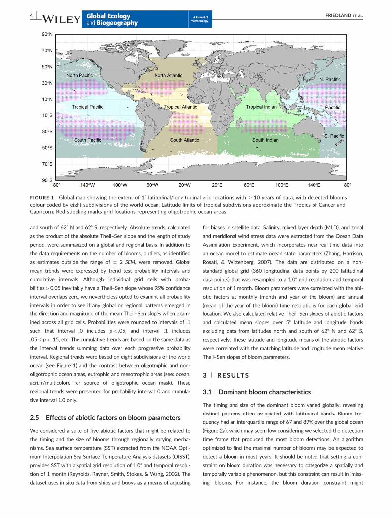
The mean start day of the dominant bloom was arrayed primarily

by latitude. At high latitudes in the Southern Hemisphere, the dominant

bloom started near the end of the calendar year, typically having start

days in the 300s, November–December (Figure 2b). This coincides

with austral spring. Progressing equatorward, the start day of blooms

at lower latitudes in the Southern Hemisphere shifted to earlier in the

year over an approximate range of day 150–250 (June–August), which

corresponds to austral winter. North of the equator, there was a band

of bloom start days at the end of the calendar year with similar timing

to the dominant bloom in the Antarctic. In the temperate Northern

Hemisphere, there was a band of spring blooms with start days ranging

from approximately day 50–150 (March–May), shifting to summer

blooms in the high northern latitudes, with start days in the 200s

(June–July). Thus, in both hemispheres, there are similar latitudinal pat-

terns, where autumun/winter blooms are dominant at low- to mid-

latitudes and spring/summer blooms occur in subpolar and polar

ecosystems.

Bloom magnitude was lowest in the oligotrophic ocean areas and

highest in shelf seas and the Northern Hemisphere. Over much of the

north Atlantic and Pacific, bloom magnitude was between 10.0 and

15.0 mg/m3 8-day [1.0–1.2 log (mg/m3 8-day 1 1); Figure 2c]. For the

areas of the globe between c. 408 N and 608 S, bloom magnitude was

typically < 5.0 mg/m3 8-day [< 0.8 log (mg/m3 8-day11)], with values

in the oligotrophic ocean ranging from 0.5 to 1.5 mg/m3 8-day [0.2–0.3

log (mg/m3 8-day11)]. Bloom intensity followed a similar pattern to

bloom magnitude, with its lowest values in the oligotrophic ocean and

highest in shelf seas and the Northern Hemisphere (see Supporting

Information Appendix S1). In the Northern Hemisphere above 508 N,

bloom intensity was c. 2.0–4.0 mg/m3 [0.5–0.7 log (mg/m3 1 1)] and

tended to be between 1.0 and 1.5 mg/m3 [0.3–0.4 log (mg/m3 1 1)]

over the latitude range of 408 N to 608 S. Bloom intensity in the oligo-

trophic ocean was < 0.2 mg/m3 [< 0.1 log (mg/m3 1 1)] in many areas.

The mean bloom duration of the dominant bloom was longest in

much of the oligotrophic ocean and shortest in shelf seas and the

higher latitude areas of the Northern and Southern Hemispheres.

Bloom duration tended to exceed 60 days, or 2 months, in these oligo-

trophic ocean areas and was often as short as 1 month in continental

shelf ecosystems (Figure 2d).

FIGURE 2 Bloom frequency (a), start day (b), magnitude (c) and duration (d) for the dominant annual bloom based on a global 18latitudinal/longitudinal grid over the study period 1998–2015. Units: bloom frequency5 percentage; bloom start day5 day of the year;day/date550/Feb 19, 100/Apr 9, 150/May 29, 200/Jul 18, 250/Sep 6, 300/Oct 26, 350/Dec 15; bloom magnitude5 log (mg/m3 8-day11); bloom duration5 days

FRIEDLAND ET AL. | 5

3.2 | Effect of bloom timing on bloom durationand size

The timing of the dominant bloom was related to multiple measures of

bloom size, including bloom duration, magnitude and intensity. Over

global scales, bloom timing was negatively correlated with bloom dura-

tion, indicating that early blooms lasted longer than blooms that began

later in the year (Figure 3a). Very few grid locations had significant pos-

itive correlations (�0.1%) indicative of early blooms of short duration.

Instead, fully half (50%) of the global grid was found to have significant

negative relationships between bloom start and duration.

The correlation between bloom start and magnitude was less

robust (Figure 3b), but reflected the strong correlation found with

duration. Over the global grid, most locations had a non-significant

FIGURE 3 Correlation between bloom start day and duration (a), magnitude (b) and intensity (c) for the dominant annual bloom based on aglobal 18 latitudinal/longitudinal grid over the study period 1998–2015. Only grid locations with � 8 years with detected blooms wereincluded; red markers indicate significant negative correlations (q< .05), blue markers indicate significant positive correlations, and beigemarkers indicate non-significant correlations

6 | FRIEDLAND ET AL.

correlation between bloom start and magnitude (70%). For those loca-

tions with significant correlations, 98% had a significant negative corre-

lation, indicating that early blooms produced high-magnitude blooms.

This result was most probably related to the underlying correlation

between bloom start and duration, because duration is a key compo-

nent in the calculation of magnitude; longer-lasting blooms will be likely

to have higher magnitudes. Locations with significant negative correla-

tions between bloom start and magnitude tended to occur at mid-

latitudes in both hemispheres.

The final relationship considered was between bloom timing and

intensity. These data produced the weakest correlation field, with 82%

of the global grid found to be non-significant. Of the significant correla-

tions, 92% were significant positive correlations, indicating that later-

starting blooms were of higher intensity or associated with higher

mean [Chl] (Figure 3c).

3.3 | Relative trends in bloom parameters

The relative Theil–Sen slopes of the bloom parameters start day, mag-

nitude, intensity and duration reveal distinct regional and global pat-

terns. Distinct clusters of negative trends in bloom start day (i.e., earlier

blooms) can be seen in the southern Pacific, Atlantic and Indian oceans

(Figure 4a). Distinct clusters of positive trends in bloom magnitude (i.e.,

increasing magnitude) and bloom intensity (i.e., increases in intensity)

can be seen across higher latitudes in both Northern and Southern

Hemispheres (Figure 4b,c). Also, negative trends in bloom magnitude

and intensity were more common at low latitudes. Although present,

trends in bloom duration were less spatially coherent, making spatial

patterns difficult to identify (Figure 4d).

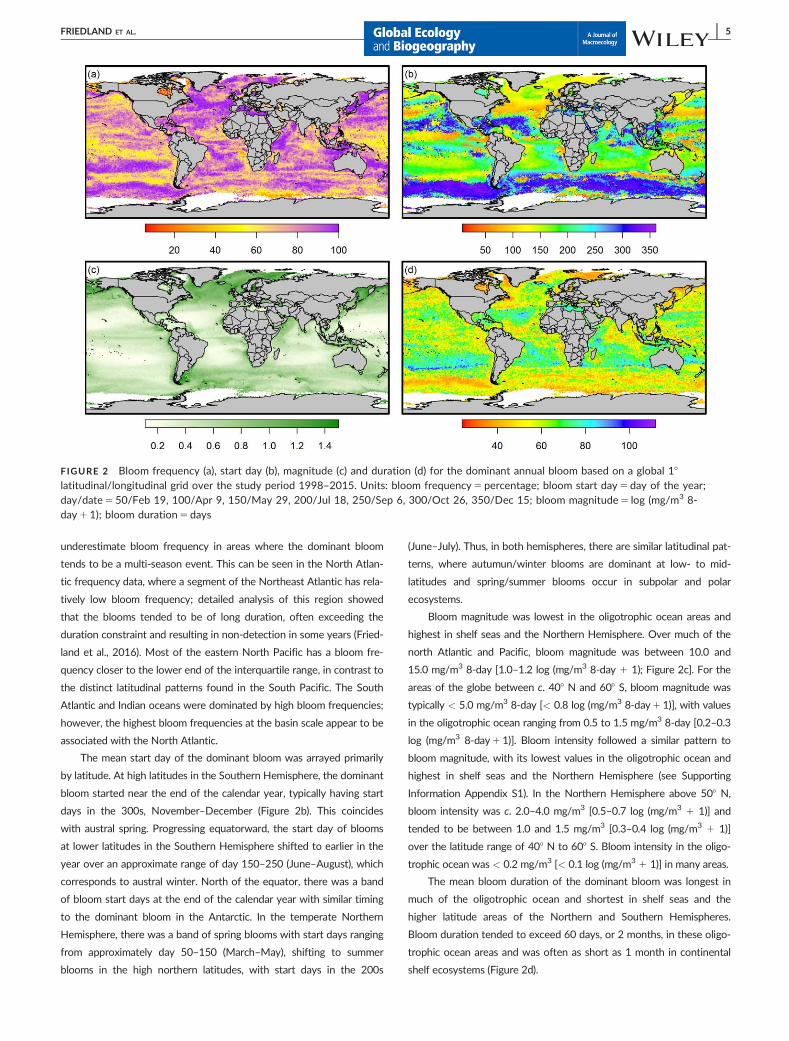
Averaging relative Theil–Sen slopes over latitude and longitude

bins revealed distinct distributional patterns. Mean relative Theil–

Sen slopes for bloom start day binned over latitude show that slopes

tended to be negative over most latitudes, with the largest relative

change found in the Southern Hemisphere (Figure 5a). Mean slopes

for magnitude were positive at high latitudes and negative for bands

around the equator (Figure 5c), with positive slopes increasing with

latitude. Mean slopes for intensity were arrayed by latitude in a simi-

lar fashion to magnitude (Figure 5e). Mean relative Theil–Sen slopes

for bloom duration tended to be positive over most latitudes, with

the exception of a group of five high-latitude northern bands that

were negative, indicating a shortening of blooms at these latitudes

(Figure 5g). Mean relative Theil–Sen slopes for bloom start day

binned over longitude show that slopes tended to be negative over

most longitudes (Figure 5b). Mean slopes for magnitude were posi-

tive for most longitudes, with the exception of a cluster associated

with the Indian Ocean (Figure 5d). Mean slopes for intensity were

arrayed by longitude in a similar fashion to magnitude (Figure 5f).

Mean relative Theil–Sen slopes for bloom duration tended to be

positive over most longitudes, with the exception of ranges of longi-

tudes associated with Indian and Atlantic oceans (Figure 5h). Com-

pared with other variables, fewer slopes for bloom duration were

significantly different from zero.

FIGURE 4 Relative Theil–Sen slope showing time series trends in start day (a), magnitude (b), intensity (c) and duration (d) for thedominant annual bloom based on a global 18 latitudinal/longitudinal grid over the study period 1998–2015. Only grid locations with� 10 years with detected blooms were included. Blue shades denote positive change and red shades negative change

FRIEDLAND ET AL. | 7

3.4 | Effects of abiotic factors on bloom parameters

Our efforts to detect global-scale relationships between abiotic fac-

tors and bloom characteristic yielded mixed results. The correlation

analysis examining the effect of abiotic factors, including SST, salin-

ity, mixed layer depth and wind stress, did not reveal any compre-

hensive global relationships between these factors and dominant

bloom dynamics. The monthly and mean annual correlations are pre-

sented in Supporting Information Appendix S2 (Figures S2-1–S2–

10). These correlation fields are dominated by grid locations with

non-significant correlations. However, some inference on the effect

of the abiotic factors may be made by comparing their time series

trend patterns with the patterns in time series trends in bloom

parameters.

Relative Theil–Sen slopes of trends in SST suggest that the most

dramatic changes in thermal conditions have occurred at high latitudes

associated with changes in patterns of sea ice extent and polar amplifi-

cation of climate change, noting, however, that most of these data fall

outside the latitude constraints (> 628 N/S) used here in most analyses

(Figure 6a). At lower latitudes, SST trends were generally positive, with

the exception of the parts of the North Atlantic, the western North

Pacific and the eastern South Pacific. Salinity has changed dramatically

in isolated high-latitude locations in the North Atlantic, probably

related to an increase in Arctic melting, whereas elsewhere over the

global ocean there has been a high degree of variability in salinity

(Figure 6b). Mixed layer depth trends have been mostly positive, and to

a higher degree in the Southern Hemisphere, although a lot of spatial

FIGURE 5 Mean annual relative Theil–Sen slope binned by 58 latitude and longitude groupings showing time series trends in start day (a and b,respectively), magnitude (c and d, respectively), intensity (e and f, respectively) and duration (g and h, respectively) for the dominant annual bloombased on a global 18 latitudinal/longitudinal grid over the study period 1998–2015. Only grid locations with � 10 years of detected blooms wereincluded. Error bars are 95% confidence intervals, and grey lines are LOESS (Local Polynomial Regression) smoothers using a span setting of 0.5

8 | FRIEDLAND ET AL.

variability in trends is evident in the Northern Hemisphere (Figure 6c).

Both zonal and meridional wind stress have generally declined globally,

with a pattern of zonal wind decline most intense along certain lines of

latitude (60 and 308 S, 08, and 30 and 608 N) and meridional decline

apparently circumscribing basin-scale oceanic gyres (Figure 6d,e,

respectively). Areas with the most intense declines in zonal wind stress

correspond to the transition zones between trade winds and westerly

winds.

Trends in abiotic factors were summarized by latitude and longi-

tude in the same manner as bloom parameter trends were summar-

ized in Figure 5. Mean relative Theil–Sen slopes for SST binned over

latitude show that slopes tended to be positive over most latitudes,

with the largest relative changes found at high latitudes, and a sec-

ondary peak slightly north of the equator (Figure 7a). SST slopes

were also positive over most longitudes, with the exception of bands

associated with parts of the North Atlantic, the western North Pacific

and the eastern South Pacific (Figure 7b). SST was positively corre-

lated with bloom intensity and negatively correlated with bloom

duration over latitudinal bins, whereas it was uncorrelated with

bloom start and magnitude (Table 1). There were no significant corre-

lations between SST and bloom parameters arrayed by longitude.

There did not appear to be a pattern in the latitudinal distribution of

salinity slopes; however, the longitudinal pattern suggests an anoma-

lous freshening of the Indian Ocean compared with other ocean

areas (Figure 7c,d, respectively). Despite weak latitudinal patterns,

salinity over latitude was correlated with the latitudinal pattern of

bloom intensity. The longitudinal patterns of salinity trend were posi-

tively correlated with bloom magnitude and duration. Slopes of

mixed layer depth are mostly positive over latitudinal intervals, with

the higher values at higher latitudes; the only areas with negative

FIGURE 6 Relative Theil–Sen slope showing time series trends in sea surface temperature (a), salinity (b), mixed layer depth (c), zonal windstress (d) and meridional wind stress (e) based on a global 18 latitudinal/longitudinal grid over the study period 1998–2015

FRIEDLAND ET AL. | 9

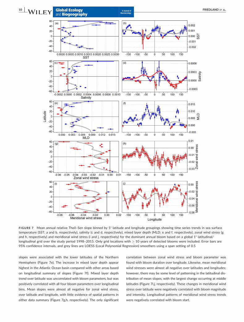
slopes were associated with the lower latitudes of the Northern

Hemisphere (Figure 7e). The increase in mixed layer depth appear

highest in the Atlantic Ocean basin compared with other areas based

on longitudinal summary of slopes (Figure 7f). Mixed layer depth

trend over latitude was uncorrelated with bloom parameters, but was

positively correlated with all four bloom parameters over longitudinal

bins. Mean slopes were almost all negative for zonal wind stress,

over latitude and longitude, with little evidence of spatial patterns in

either data summary (Figure 7g,h, respectively). The only significant

correlation between zonal wind stress and bloom parameter was

found with bloom duration over longitude. Likewise, mean meridional

wind stresses were almost all negative over latitudes and longitudes;

however, there may be some level of patterning in the latitudinal dis-

tribution of mean slopes, with the largest change occurring at middle

latitudes (Figure 7i,j, respectively). These changes in meridional wind

stress over latitude were negatively correlated with bloom magnitude

and intensity. Longitudinal patterns of meridional wind stress trends

were negatively correlated with bloom start.

FIGURE 7 Mean annual relative Theil–Sen slope binned by 58 latitude and longitude groupings showing time series trends in sea surfacetemperature (SST; a and b, respectively), salinity (c and d, respectively), mixed layer depth (MLD; e and f, respectively), zonal wind stress (gand h, respectively) and meridional wind stress (i and j, respectively) for the dominant annual bloom based on a global 18 latitudinal/longitudinal grid over the study period 1998–2015. Only grid locations with � 10 years of detected blooms were included. Error bars are95% confidence intervals, and grey lines are LOESS (Local Polynomial Regression) smoothers using a span setting of 0.5

10 | FRIEDLAND ET AL.

3.5 | Mean absolute trends in bloom parameters

Absolute trends expressed as the change in bloom parameters over the

study period suggest that there have been substantial shifts in bloom

timing and size. Bloom start day has shifted on the order of 3 days ear-

lier on a global basis, and for regions associated with statistically signifi-

cant shifts, blooms have advanced on the order of 2 weeks (Figure 8a).

Bloom magnitude and intensity have both increased on a global basis

on the order of 0.3 mg/m3 8-day and 0.05 mg/m3, respectively, which

represents a c. 10% increase in both parameters (Figure 8b,c). The

increases in these parameters in regions associated with statistically

significant shifts have been much greater and on the order of 0.9 mg/

m3 8-day and 0.4 mg/m3, respectively, which represents a c. 35%

increase again for both. Bloom duration has shifted on the order of 2

days longer on a global basis, and for regions associated with statisti-

cally significant shifts, blooms have lengthened c. 1 week (Figure 8d).

The bloom absolute trends partitioned by the eight subdivisions of

the world ocean and the between oligotrophic and non-oligotrophic

ocean areas differed from the global means in a number of ways.

Bloom start had negative trends, indicating earlier blooms, in all ocean

areas, but the trend was greater in the southern oceans and in

TABLE 1 Pearson product–moment correlation between mean relative Theil–Sen slope binned by 58 latitude and longitude groupings ofbloom parameters start day, magnitude, intensity and duration and abiotic factors sea surface temperature (SST), salinity, mixed layer depth(MLD), zonal wind stress (u-wind) and meridional wind stress (v-wind).

SST Salinity MLD u-wind v-windBloomparameter r p-value r p-value r p-value r p-value r p-value

Latitude Start .173 .429 .159 .447 2.103 .626 .034 .872 .014 .946

Magnitude .345 .107 .336 .100 .201 .334 2.230 .269 2.576 .003Intensity .576 .004 .428 .033 .386 .056 2.265 .200 2.571 .003Duration 2.656 .001 2.128 .543 2.241 .246 .075 .722 .091 .665

Longitude Start 2.074 .534 .185 .117 .303 .009 2.116 .327 2.364 .002

Magnitude .066 .579 .334 .004 .338 .003 .124 .298 .053 .654Intensity .026 .826 .210 .074 .286 .014 .006 .960 .224 .057Duration .072 .547 .382 .001 .239 .042 .343 .003 2.193 .101

Note. Significant correlations are shown in bold. MLD5mixed layer depth; SST5 sea surface temperature.

FIGURE 8 Mean global interval and cumulative absolute trends in bloom start day (a), magnitude (b), intensity (c) and duration (d) versusMann–Kendall trend test probability intervals. Trends are the product of Theil–Sen slopes for the dominant annual bloom and the numberof years in the time series. Probability interval .0 includes p< .05, and interval .1 includes .05� p< .15, etc. Each interval estimate includestrends associated with that interval probability level only and is estimated from all data excluding outliers. Cumulative trends are based ondata from the interval trends and all lower probability intervals. Only grid locations with � 10 years with detected blooms were includedbased on a global 18 latitudinal/longitudinal grid over the study period 1998–2015, excluding data from latitudes north and south of 628 Nand 628 S, respectively. Error bar are 95% confidence intervals

FRIEDLAND ET AL. | 11

oligotrophic areas (Figure 9a). For regions associated with statistically

significant shifts, the North Atlantic had a positive bloom start trend,

suggesting that the bloom started c. 5 days later, whereas the other

ocean areas had negative trends, suggesting shifts of 1–3 weeks (Fig-

ure 10a). Bloom magnitude and intensity had positive trends in the

northern and southern oceans and between oligotrophic and non-

oligotrophic regions (Figure 9b,c). The tropical ocean areas had either

zero or negative trends in these parameters. The pattern of change in

magnitude and intensity in the regions associated with statistically sig-

nificant shifts were nearly identical to the global averages, but the size

of the shifts was larger when considering only statistically significant

results (Figure 10b,c). Bloom duration increased in all areas except the

North Atlantic and tropical Indian oceans, where the trend confidence

interval included zero (Figure 10d). The pattern of change in duration in

the regions associated with statistically significant shifts was similar to

the global patterns; however, four regions had confidence intervals

that included zeros (Figure 10d).

4 | DISCUSSION

Our analysis of phytoplankton blooms on a global scale suggests direc-

tional time series change in the timing, duration and size of blooms,

which portends changes in the functioning of marine ecosystems and

carbon cycling from local to basin scales (Ji et al., 2010). Notably, we

provide evidence that blooms are initiating earlier in the year, having

shifted in timing on the order of weeks in some regions, and are of lon-

ger duration, suggesting that the timing of bloom cessation has also

changed. There have also been changes in the pattern of bloom size,

suggesting an increase in bloom size at high latitudes and a decrease at

low latitudes in a gradated fashion. It is crucial to understand these

changes in bloom dynamics because they provide labile biomass that

forms the basis of food webs and is fundamentally important to the

biogeochemical functioning of marine ecosystems (Sigman & Hain,

2012).

The low spatial coherence between correlations of the abiotic fac-

tors and bloom intensity and magnitude is in stark contrast to the high

spatial coherence of global trends in these bloom parameters and time

series trends in the abiotic factors, suggesting the importance of vari-

ability and local factors in the control of blooms on a global scale. Local

changes in salinity and temperature affect stratification, which can trap

phytoplankton above the pycnocline and decrease nutrient inputs from

deeper layers, and decreased wind-driven mixing will exacerbate this

scenario. In a global comparison of the effects of stratification on chlo-

rophyll biomass, Dave and Lozier (2013) showed mixed trends in strati-

fication over much of the globe, with much of the eastern subtropical

FIGURE 9 Mean absolute trends over ocean areas for bloom start day (a), magnitude (b), intensity (c) and duration (d) for areas regardless ofsignificance level (all p-levels). Trends are the product of Theil–Sen slopes for the dominant annual bloom and the number of years in the timesseries based on a global 18 latitudinal/longitudinal grid over the study period 1998–2015, excluding data from latitudes north of 628 N and southof 628 S. Grid locations are combined as per ocean areas and oligotrophic versus non-oligotrophic area according to Figure 1 [N_Atl,N_Pac5North Atlantic and Pacific (red circles); S_Atl, S_Ind, S_Pac5 South Atlantic, Indian and Pacific (green squares); T_Atl, T_Ind, T_Pac5 -Tropical Atlantic, Indian, and Pacific (blue triangles); Olig, Non-Olig5oligotrophic and non-oligotrophic areas (magenta diamonds)]. Only grid loca-tions with � 10 years with detected blooms were included, and outliers were excluded. Error bar are 95% confidence intervals

12 | FRIEDLAND ET AL.

Pacific experiencing increased stratification, whereas much of the

Atlantic experienced decreased stratification. However these changes

were not well correlated with trends in chlorophyll concentrations, fur-

ther suggesting the importance of local processes controlling blooms.

Similar to the results presented in the present study, Dave and Lozier

(2013) found trends in decreasing stratification over much of the mid-

and lower latitudes, which were driven primarily by increased rates of

warming of subsurface water relative to surface waters, resulting in an

increased mixed layer depth.

Although clearly not a test of hypotheses, the comparison of latitu-

dinal and longitudinal patterns of trends in potential abiotic forcing fac-

tors might offer some insights on both global and regional changes in

bloom dynamics. The latitudinal patterns in SST and meridional wind

stress trends are similar to the latitudinal pattern in bloom duration in

that all show bimodal distributions at low latitudes. This particular pat-

tern is consistent with an increase in bloom duration in the Baltic Sea

that also coincided with warming temperatures and decreased winds

(Groetsch et al., 2016). Likewise, there are features in the latitudinal

pattern of mixed layer depth that match the latitudinal patterns in

bloom magnitude and intensity trends. Furthermore, the advance in

bloom timing over all latitudes might be related to the global changes

in wind stress. The most striking longitudinal pattern in global bloom

dynamics is associated with the Indian Ocean, characterized by

reductions in bloom magnitude, intensity and duration corresponding

roughly with meridians 508–1008 E. Phytoplankton dynamics in the

Indian Ocean have been considered in the context of abiotic forcing.

Goes, Thoppil, Gomes, and Fasullo (2005) and Gregg, Casey, and

McClain (2005) documented increases in net primary production in the

western Indian Ocean; however, a more recent study is consistent with

our findings, suggesting a reduction in [Chl] over the past 16 years

(Roxy et al., 2016). These researchers attributed the change in [Chl] to

a reduction in available nutrients in the euphotic zone as a result of

increasing SST that increased stratification-induced trapping of

nutrients in the deeper Indian Ocean. The confounding influences of

increasing SST trends on mixing and phytoplankton growth rates make

prediction of phytoplankton dynamics difficult, especially in the Indian

Ocean, an area experiencing the largest warming trend in the tropical

ocean (Roxy, Ritika, Terray, & Masson, 2014). However, it is worth not-

ing that the most striking longitudinal pattern in the abiotic data we

found was in the salinity data suggesting a freshening of Indian Ocean

waters, which might have amplified thermal effects on stratification as

described owing to changes in monsoon patterns.

A general decrease in zonal and meridional wind stress has the

potential to impact production by reducing the wind-driven mixing in

areas of light-limited production (Kim, Yoo, & Oh, 2007). Contrary to

this, although our analysis suggests an overall decrease in winds on a

FIGURE 10 Mean absolute trends over ocean areas for bloom start day (a), magnitude (b), intensity (c) and duration (d) for areas withsignificant trends (p< .05). Trends are the product of Theil–Sen slopes for the dominant annual bloom and the number of years in the timesseries based on a global 18 latitudinal/longitudinal grid over the study period 1998–2015, excluding data from latitudes north of 628 N and southof 628 S. Grid locations are combined as per ocean areas and oligotrophic versus non-oligotrophic area according to Figure 1 [N_Atl, N_Pac5North Atlantic and Pacific (red circles); S_Atl, S_Ind, S_Pac5 South Atlantic, Indian and Pacific (green squares); T_Atl, T_Ind, T_Pac5TropicalAtlantic, Indian and Pacific (blue triangles); Olig, Non-Olig5oligotrophic and non-oligotrophic areas (magenta diamonds)]. Only grid locations with� 10 years with detected blooms were included, and outliers were excluded. Error bar are 95% confidence intervals

FRIEDLAND ET AL. | 13

broad scale, there is an associated broad increase in the mixed layer

depth. This might be attributable, in part, to local changes in tempera-

ture and salinity affecting stratification. Although most regions of the

globe are experiencing decreasing wind stress, the few regions where

wind stress is increasing are also experiencing the largest increases in

mixed layer depth, such as in the southern Atlantic Ocean at 608 S.

This is likely to be a result of higher mean wind speeds in these loca-

tions, because the power of wind exerted on the water scales with the

cube of mean wind speed. Therefore, even a small increase in wind

stress in an area can result in profound changes in wind-driven mixing

and increased MLD. The global trends in MLD bear a striking resem-

blance to the global trends in bloom intensity and, to a lesser degree,

bloom magnitude. However, the spatial correlations between MLD and

these bloom parameters is low and bears few spatially significant

regions, save for the oligotrophic southern subtropical Pacific, where

enhanced mixing may enhance nutrient concentrations (de Boyer Mon-

tegut, Madec, Fischer, Lazar, & Iudicone, 2004). In the subpolar and

northern subtropical regions of the North Atlantic, Ueyama and Mon-

ger (2005) found an inverse relationship between bloom intensity and

wind-induced mixing, where decreased mixing during blooms resulted

in enhanced bloom intensity, whereas the opposite was true for the

southern subtropical region, where nutrients may be limiting produc-

tion and light penetration is greater. Atmospheric-related variability in

wind-driven mixing was also found to affect the timing of bloom initia-

tion, where the start day of blooms in the North Atlantic was strongly

associated with the winter North Atlantic Oscillation index (Ueyama &

Monger, 2005). A similar relationship between wind speed and bloom

timing has also been detected in the Japan Sea (Yamada & Ishizaka,

2006). Furthermore, Moore et al. (2013), in a review of nutrient limita-

tion dynamics in the global ocean, concluded that nitrogen was limiting

in much of the surface waters in tropical latitudes, consistent with our

observations. In areas where nitrogen is not limiting, iron limitation

tends to dominate (e.g., the Southern Ocean and the eastern equatorial

Pacific; Behrenfeld, Bale, Kolber, Aiken, & Falkowski, 1996). Iron limita-

tion might play a particularly large role in the differences we observed

between the bloom dynamics in the eastern North and South Pacific

(Behrenfeld & Kolber, 1999).

Despite methodological differences in bloom detections and analy-

ses, our results do align with those from other global and basin-scale

estimates of bloom parameters. Different bloom detection algorithms

lead to varying accuracy and precision of bloom phenology metrics

(Ferreira et al., 2014), and consequently, varying depictions of bloom

dynamics (Brody et al., 2013). Our focus is on the dominant annual

bloom occurring within a grid cell and on the main period of elevated

bloom conditions constrained by the length of our detection time win-

dow. As a number of investigators have characterized (Sapiano, Brown,

Uz, & Vargas, 2012; Taboada & Anadon, 2014), most areas of the globe

are dominated by a single bloom, with the exception of some regions

that are characterized by a secondary bloom in regions predominately

oriented in specific latitudinal bands. Despite this methodological dif-

ference, our characterization of bloom start shows similar patterning to

previous global (Racault et al., 2012; Sapiano et al., 2012) and basin-

scale studies (Henson, Dunne, & Sarmiento, 2009; Taboada & Anadon,

2014; Zhang, Zhang, Qiao, Deng, & Wang, 2017). However, our esti-

mates of bloom duration are at variance with most studies owing to

the contrast in methods applied between studies. In studies estimating

bloom duration using a threshold approach (Siegel, Doney, & Yoder,

2002), bloom duration tended to be twofold longer than ours (Racault

et al., 2012; Sapiano et al., 2012). However, the spatial patterns of long

versus short bloom duration were consistent with our results. The

measures of bloom size, here referred to as magnitude and intensity

and variously named and applied by different investigators, were also

similar between studies and generally followed climatological patterns

of the distribution of [Chl] (Doney, Glover, McCue, & Fuentes, 2003).

On a global scale, the spatial organization of areas with homogene-

ous bloom dynamics appears to have a high degree of zonal band pat-

terning and more complex organization associated with meridional

bands (Sapiano et al., 2012). For example, mean relative Theil–Sen

slopes for bloom duration tended to be positive over most latitudes,

with exception of a group of five high-latitude northern bands, which

were negative, indicating a shortening of blooms at these latitudes.

Mean slopes for magnitude and intensity were positive for most longi-

tudes, with the exception of a cluster associated with the Indian

Ocean.

Changes in bloom timing and size were not uniform over the globe.

Owing to contrasts in oceanographically defined functional regions and

latitudinal patterns, changes in bloom dynamics will be likely to have

different regional impacts. An analysis of spring and autumn blooms in

the north Atlantic and Pacific basins that used a spectral decomposition

approach for bloom detection characterized regional-scale time series

changes in bloom timing and magnitude (equivalent to bloom intensity

as used here) that hold many similarities to the patterns described in

our analysis (Zhang et al., 2017). Bloom timing was alternatively

advanced and delayed on the order of weeks, with coherent trends in

matching areas of both basins. It is difficult to compare our trends in

bloom intensity with their results for trends in magnitude because our

spatial characterization is based on relative Theil–Sen slopes. Likewise,

in a study focused on the North Atlantic, Taboada and Anadon (2014)

provided estimates of bloom intensity trends that match our study

results; however, their method of estimating bloom timing trends dif-

fered from those presented here. Racault et al. (2012) estimated trends

in bloom duration on a global scale also using linear regression, but

with a time series restricted to the length of the SeaWiFS time series

only (1998–2007). Their estimates of global trends in bloom duration

were mostly negative, indicating a tendency for blooms to be short-

ened over global scales. We note, however, that their time series is

shorter than that analysed here, and bloom duration was estimated

using a threshold approach (Siegel et al., 2002), which, as noted above,

provides estimates of bloom duration twofold longer than ours. Hence,

they are estimating a different aspect of phytoplankton dynamics,

whereas we are focusing on the discrete portion of the bloom associ-

ated with highly elevated [Chl].

We view our results in the context of changes that have occurred

and will be likely to occur to the global climate system. Global thermal

conditions are changing, and it is important to consider change in the

level of system variability and its impact on ecosystems (Vazquez,

14 | FRIEDLAND ET AL.

Gianoli, Morris, & Bozinovic, 2017). Change in thermal regime is having

profound effects on atmospheric circulation and the forcing factors

related to bloom development, which might be more important to phy-

toplankton than the direct effect of change in thermal regime itself

(Francis & Vavrus, 2015). The latitudinal changes in bloom magnitude

and intensity are also consistent with the effects of global thermal

change on phytoplankton community composition (Marinov, Doney, &

Lima, 2010), shifting communities to include members that are capable

of different growth rates or resistance to grazing that allow for a

change in [Chl]. Furthermore, changing thermal regimes have been

associated with shifting species composition of blooms, where for a

fixed study site blooms have become increasingly dominated by the

genus Synechococcus (Hunter-Cevera et al., 2016). The changing role of

cyanobacteria is expected to have a profound effect on plankton

dynamics in a range of aquatic systems (Visser et al., 2016). We can

also expect changes to the seasonal nature of blooms (Henson et al.,

2013) and probably impacts on secondary production as well (Litch-

man, Klausmeier, Miller, Schofield, & Falkowski, 2006). The change in

dominant bloom timing we observed is consistent with the effect of an

increase in global temperature and its role in mixed layer dynamics,

although the rate of stratification and turbulent mixing remains unclear

(Franks, 2015). These changes to the base of the food web warrant fur-

ther investigation.

Change in phytoplankton bloom dynamics would be expected to

impact the rate of flux of particulate organic carbon (POC) from the

water column to the benthos. Parts of the world ocean are dominated

by production cycles that are characterized by blooms associated with

high concentrations of biomass, whereas other regions have bloom fea-

tures that are not as prominent, although in many cases primary pro-

duction can still be at a high level (Reygondeau et al., 2013). However,

phytoplankton blooms, in particular, support conditions that result in

the intense flux of POC (Belley, Snelgrove, Archambault, & Juniper,

2016; Reigstad, Carroll, Slagstad, Ellingsen, & Wassmann, 2011). It fol-

lows that changes in the timing and size of a bloom will affect the

amount of POC exported to the benthos. Over most regions of the

globe, blooms appear to have lasted longer, which could result in an

increase in POC flux. Bloom magnitude and intensity have changed

over latitudinal ranges, most notably with decreased bloom magnitude

at low latitude and increases at high latitudes. Similar changes in bloom

magnitude across a range of latitudes were obtained in a study that

used an earth system model that included data assimilation to examine

changes in North Pacific bloom characteristics since the 1960s (Asch,

2013). Together, these results indicate that POC fluxes to the benthos

may increase at high latitudes, while decreasing at lower latitudes.

These changes in bloom dynamics should be taken into account in

global carbon flux estimation models.

The species composition of phytoplankton communities varies

over global scales and is principally influenced by dispersion and com-

petitive exclusion (Barton, Dutkiewicz, Flierl, Bragg, & Follows, 2010).

However, species composition is also influenced by environmental con-

ditions, such as mixing regimes and light conditions (Barton, Lozier, &

Williams, 2015), leading to concerns that shifting thermal conditions

will actuate shifts to smaller size taxa (Moran, Lopez-Urrutia, Calvo-

Diaz, & Li, 2010). These smaller producers have different dynamics and

vertical transport properties, which have the potential to affect both

export flux and the way an ecosystem functions (Mouw, Barnett,

McKinley, Gloege, & Pilcher, 2016). Using phytoplankton size estimated

from remote sensing data (Kostadinov, Milutinovic, Marinov, & Cabre,

2016; Mouw et al., 2017), Mouw et al. (2016) contrasted the difference

in export flux and transfer efficiency during times dominated by small

and large cells within biogeochemical provinces. They found periods

dominated by small cells to have both greater export flux efficiency

and lower transfer efficiency than periods dominated by large cells. Ris-

ing temperatures will be likely to shift phytoplankton niches poleward

and are predicted to have the greatest potential impact on tropical phy-

toplankton diversity (Thomas, Kremer, Klausmeier, & Litchman, 2012).

Considering the importance of species groups to the role of phyto-

plankton production, the phenology of various methods to determine

phytoplankton size has been compared (Kostadinov et al., 2017), and

the phenology of some methods has been connected to environmental

conditions (Cabr�e, Shields, Marinov, & Kostadinov, 2016; Soppa,

Volker, & Bracher, 2016). However, the changes in phenology of vari-

ous phytoplankton groups have yet to be explored, which could pro-

vide refinements to both retrospective and forecasted modelling

efforts.

This study provides substantial evidence to support the observa-

tion that early blooms are longer-lasting blooms, and conversely,

delayed bloom start is associated with shorter blooms. This phenom-

enon has been described previously on a global scale (Racault et al.,

2012) and for the North Atlantic (Friedland et al., 2016), with the latter

study exploring the hypothesis that bloom duration is in large measure

shaped by grazing by zooplankton that have a diapause life cycle. It is

important to note that despite using a different bloom measurement

methodology, results from Racault et al. (2012) and for the North

Atlantic (Friedland et al., 2016) are in agreement with the present study

in the overall nature of the relationship (i.e., the direction of trends and

coherence at large spatial scales), but differ in the fine-scale regional

patterning of this correlation. It may be through this regional patterning

that we are able to evaluate the relative role of nutrient limitation and

grazing in shaping bloom development (Evans & Parslow, 1985;

Fasham, Ducklow, & McKelvie, 1990). The latitudinal banding of this

relationship would have to be reflected in the nature of pre-bloom mix-

ing and initial nutrient supply over a range of physical environments for

nutrient supply to be the unifying factor controlling bloom duration as

a function of bloom initiation. This work has yet to be done, but in a

practical sense has a better chance of being accomplished considering

the paucity of grazing information in most parts of the world ocean.

The observational results of the present study provide some level

of validation for earth systems models that simulate global climate and

ocean systems dynamics. Multiple earth system models suggest that

climate change will have the greatest impact on bloom phenology at

high latitudes (Henson et al., 2013). Under a business-as-usual emis-

sions scenario, the month of maximal primary productivity is projected

to advance by 0.5–1 months by the end of the 21st century across

many ocean ecosystems. The exception to this pattern is the oligotro-

phic subtropical gyres, where delays in the timing of peak primary

FRIEDLAND ET AL. | 15

production have been projected. These changes have been attributed

to earlier easing of light limitation owing to increases in stratification

(Henson et al., 2013). These future projections use earth system model

outputs with a monthly resolution, so additional research that can

detect finer-scale changes in phenology is needed. One study that used

data with a finer temporal resolution, from the NCAR Community Earth

System Model (CESM) model, assimilated historical data on atmos-

pheric observations and SST (Asch, 2013). In contrast to models of

future projections, that study of historical patterns identified the largest

trends in bloom phenology in oligotrophic areas (Asch, 2013), which

might reflect an influence of inter-annual climate variability rather than

climate change. Our observational results are consistent with this pat-

tern, and thus provide an indication of the skill of the NCAR model,

which did not assimilate any ocean colour data.

As ocean colour time series have grown in length, there have been

efforts to describe time series trends in bloom characteristics. Impor-

tantly, these efforts have included disciplined analyses of the require-

ments to detect trends in the face of noisy and incomplete data and

whether trends can be attributed to climate change or not (Beaulieu

et al., 2013; Henson, Beaulieu, & Lampitt, 2016). Furthermore, Henson

et al. (2013) estimates that it would require c. 30 years of data to dis-

tinguish trends in bloom phenology from natural decadal variability.

Given the results of these investigations, we approach our findings

with caution. As encouraging as it is now to have a nearly 20-year time

series of data, it is difficult to be conclusive about the description of

trends and to attribute any of these trends to climate change. How-

ever, it is reasonable to compare these trends with observed climate

variation over the past two decades and discuss whether these trends

are consistent with future projections under different climate change

scenarios.

5 | CONCLUSIONS

The timing and size of phytoplankton blooms have changed on both

regional and global scales. This finding is important because blooms

play a pivotal role in the flow of energy in marine ecosystems, impact-

ing the way food webs work and the way these ecosystems provide a

range of services. The dominant bloom was found to vary with latitude

and in localized patterns associated with specific oceanographic fea-

tures. Blooms have increased in magnitude and intensity at high lati-

tudes and decreased in equatorial areas. Overall, blooms started earlier

and lasted longer, with bloom timing having the most profound effect

on bloom duration; early blooms tended to last longer than later-

starting blooms. This finding has the potential to impact phenological

relationships between producer and consumer species, such as meso-

zooplankton and higher trophic position fish and invertebrates. Timing

mechanisms for reproduction in many species have evolved that ensure

adequate forage for early life stages, which may be impacted by

changes in bloom timing. In regions where blooms last longer and are

associated with higher [Chl], the dynamics of the biological pump are

likely to alter the rates of carbon cycling and export. A shift to earlier

bloom timing is consistent with the expected effect of warming ocean

conditions seen in recent decades. It is incumbent upon assessment

and modelling practitioners to account for the dynamic variability of

phytoplankton production.

ACKNOWLEDGMENTS

We thank C. Stock and M. Scharfe for comments on an early draft

of the paper and GlobColour (http://globcolour.info) for the data

used in this study that have been developed, validated and distrib-

uted by ACRI-ST, France. Funding for A. Thomas on this work

was provided by the NSF Coastal SEES Program (OCE-1325484)

and NASA (NNX16AG59G) and for D. Brady by NSF projects

CBET1360415 and 11A-1355457.

DATA ACCESSIBILITY

All chlorophyll concentration data are available as NCDF files from the

GlobColour products database located at: http://hermes.acri.fr/?class-

5archive. Ocean Data Assimilation Experiment data are located at:

https://www.gfdl.noaa.gov/ocean-data-assimilation.

ORCID

Kevin D. Friedland http://orcid.org/0000-0003-3887-0186

Colleen B. Mouw http://orcid.org/0000-0003-2516-1882

Rebecca G. Asch http://orcid.org/0000-0002-6138-5819

Kimberly J. W. Hyde http://orcid.org/0000-0002-1564-5499

REFERENCES

Asch, R. G. (2013). Interannual-to-decadal changes in phytoplankton phe-

nology, fish spawning habitat, and larval fish phenology (Unpublished

PhD dissertation). University of California, San Diego, CA, 268 pp.

Barton, A. D., Dutkiewicz, S., Flierl, G., Bragg, J., & Follows, M. J.

(2010). Patterns of diversity in marine phytoplankton. Science, 327,

1509–1511.

Barton, A. D., Lozier, M. S., & Williams, R. G. (2015). Physical controls of

variability in North Atlantic phytoplankton communities. Limnology

and Oceanography, 60, 181–197.

Beaulieu, C., Henson, S. A., Sarmiento, J. L., Dunne, J. P., Doney, S. C.,

Rykaczewski, R. R., & Bopp, L. (2013). Factors challenging our ability

to detect long-term trends in ocean chlorophyll. Biogeosciences, 10,

2711–2724.

Behrenfeld, M. J., & Boss, E. S. (2014). Resurrecting the ecological under-

pinnings of ocean plankton blooms. Annual Review of Marine Science,

6, 167–194.

Behrenfeld, M. J., & Kolber, Z. S. (1999). Widespread iron limitation of

phytoplankton in the South Pacific Ocean. Science, 283, 840–843.

Behrenfeld, M. J., Bale, A. J., Kolber, Z. S., Aiken, J., & Falkowski, P. G.

(1996). Confirmation of iron limitation of phytoplankton photosyn-

thesis in the equatorial Pacific Ocean. Nature, 383, 508–511.

Belley, R., Snelgrove, P. V. R., Archambault, P., & Juniper, S. K. (2016).

Environmental drivers of benthic flux variation and ecosystem func-

tioning in Salish Sea and Northeast Pacific sediments. PLoS One, 11,

e0151110.

Blondeau-Patissier, D., Gower, J. F. R., Dekker, A. G., Phinn, S. R., &

Brando, V. E. (2014). A review of ocean color remote sensing meth-

ods and statistical techniques for the detection, mapping and analysis

16 | FRIEDLAND ET AL.

of phytoplankton blooms in coastal and open oceans. Progress in

Oceanography, 123, 123–144.

Brody, S. R., Lozier, M. S., & Dunne, J. P. (2013). A comparison of meth-

ods to determine phytoplankton bloom initiation. Journal of Geophysi-

cal Research-Oceans, 118, 2345–2357.

Cabr�e, A., Shields, D., Marinov, I., & Kostadinov, T. S. (2016). Phenology of

size-partitioned phytoplankton carbon-biomass from ocean color remote

sensing and CMIP5 models. Frontiers in Marine Science, 3, 591–520.

Chassot, E., Bonhommeau, S., Dulvy, N. K., Melin, F., Watson, R., Gas-

cuel, D., & Le Pape, O. (2010). Global marine primary production con-

strains fisheries catches. Ecology Letters, 13, 495–505.

Cherkasheva, A., Bracher, A., Melsheimer, C., Koberle, C., Gerdes, R.,

Nothig, E. M., . . . Boetius, A. (2014). Influence of the physical envi-

ronment on polar phytoplankton blooms: A case study in the Fram

Strait. Journal of Marine Systems, 132, 196–207.

Christensen, V., Coll, M., Buszowski, J., Cheung, W. W. L., Frolicher, T.,

Steenbeek, J., . . . Walters, C. J. (2015). The global ocean is an ecosys-

tem: Simulating marine life and fisheries. Global Ecology and Biogeog-

raphy, 24, 507–517.

Cole, H., Henson, S., Martin, A., & Yool, A. (2012). Mind the gap: The

impact of missing data on the calculation of phytoplankton phenol-

ogy metrics. Journal of Geophysical Research-Oceans, 117, C08030,

https://doi.org/10.1029/2012JC008249.

Corbiere, A., Metzl, N., Reverdin, G., Brunet, C., & Takahashi, A. (2007).

Interannual and decadal variability of the oceanic carbon sink in the

North Atlantic subpolar gyre. Tellus Series B-Chemical and Physical

Meteorology, 59, 168–178.

Cushing, D. H. (1990). Plankton production and year-class strength in

fish populations: An update of the match mismatch hypothesis.

Advances in Marine Biology, 26, 249–293.

Dave, A. C., & Lozier, M. S. (2013). Examining the global record of inter-

annual variability in stratification and marine productivity in the low-

latitude and mid-latitude ocean. Journal of Geophysical Research-

Oceans, 118, 3114–3127.

Davison, P. C., Checkley, D. M., Koslow, J. A., & Barlow, J. (2013). Car-

bon export mediated by mesopelagic fishes in the northeast Pacific

Ocean. Progress in Oceanography, 116, 14–30.

de Boyer Montegut, C., Madec, G., Fischer, A. S., Lazar, A., & Iudicone, D.

(2004). Mixed layer depth over the global ocean: An examination of

profile data and a profile-based climatology. Journal of Geophysical

Research-Oceans, 109, C12003, https://doi.org/10.1029/2004JC002378.

Doney, S. C., Bopp, L., & Long, M. C. (2014). Historical and future trends

in ocean climate and biogeochemistry. Oceanography, 27, 108–119.

Doney, S. C., Glover, D. M., McCue, S. J., & Fuentes, M. (2003). Meso-

scale variability of Sea-viewing Wide Field-of-view Sensor (SeaWiFS)

satellite ocean color: Global patterns and spatial scales. Journal of

Geophysical Research-Oceans, 108, 3024, https://doi.org/10.1029/

2001JC000843, C2.

D’Ortenzio, F., Antoine, D., Martinez, E., & D’Alcala, M. R. (2012). Pheno-

logical changes of oceanic phytoplankton in the 1980s and 2000s as

revealed by remotely sensed ocean-color observations. Global Biogeo-

chemical Cycles, 26, GB4003, https://doi.org/10.1029/2011GB004269.

Evans, G. T., & Parslow, J. S. (1985). A model of annual plankton cycles.

Biological Oceanography, 3, 327–347.

Fasham, M. J. R., Ducklow, H. W., & McKelvie, S. M. (1990). A nitrogen-

based model of plankton dynamics in the oceanic mixed layer. Journal

of Marine Research, 48, 591–639.

Ferreira, A. S., Visser, A. W., MacKenzie, B. R., & Payne, M. R. (2014).

Accuracy and precision in the calculation of phenology metrics. Jour-

nal of Geophysical Research-Oceans, 119, 8438–8453.

Ferreira, A. S. A., Hatun, H., Counillon, F., Payne, M. R., & Visser, A. W.

(2015). Synoptic-scale analysis of mechanisms driving surface chloro-

phyll dynamics in the North Atlantic. Biogeosciences, 12, 3641–3653.

Field, C. B., Behrenfeld, M. J., Randerson, J. T., & Falkowski, P. (1998).

Primary production of the biosphere: Integrating terrestrial and oce-

anic components. Science, 281, 237–240.

Francis, J. A., & Vavrus, S. J. (2015). Evidence for a wavier jet stream in response

to rapid Arctic warming. Environmental Research Letters, 10, 014005.

Franks, P. J. S. (2015). Has Sverdrup’s critical depth hypothesis been

tested? Mixed layers vs. turbulent layers. ICES Journal of Marine Sci-

ence, 72, 1897–1907.

Frenken, T., Velthuis, M., Domis, L. N. D., Stephan, S., Aben, R., Kosten,

S., . . . Van de Waal, D. B. (2016). Warming accelerates termination of

a phytoplankton spring bloom by fungal parasites. Global Change Biol-

ogy, 22, 299–309.

Friedland, K. D., & Todd, C. D. (2012). Changes in Northwest Atlantic

Arctic and Subarctic conditions and the growth response of Atlantic

salmon. Polar Biology, 35, 593–609.

Friedland, K. D., Hare, J. A., Wood, G. B., Col, L. A., Buckley, L. J., Moun-

tain, D. G., . . . Pilskaln, C. H. (2008). Does the fall phytoplankton

bloom control recruitment of Georges Bank haddock, Melanogrammus

aeglefinus, through parental condition? Canadian Journal of Fisheries

and Aquatic Sciences, 65, 1076–1086.

Friedland, K. D., Leaf, R. T., Kane, J., Tommasi, D., Asch, R. G., Rebuck,

N., . . . Saba, V. S. (2015). Spring bloom dynamics and zooplankton

biomass response on the US Northeast Continental Shelf. Continental

Shelf Research, 102, 47–61.

Friedland, K. D., Record, N. R., Asch, R. G., Kristiansen, T., Saba, V. S.,

Drinkwater, K. F., . . . Ji, R. (2016). Seasonal phytoplankton blooms in

the North Atlantic linked to the overwintering strategies of cope-

pods. Elementa, 4, 99.

Goes, J. I., Thoppil, P. G., Gomes, H. D., & Fasullo, J. T. (2005). Warming

of the Eurasian landmass is making the Arabian Sea more productive.

Science, 308, 545–547.

Gregg, W. W., Casey, N. W., & McClain, C. R. (2005). Recent trends in

global ocean chlorophyll. Geophysical Research Letters, 32, L03606,

https://doi.org/10.1029/2004GL021808.

Groetsch, P. M. M., Simis, S. G. H., Eleveld, M. A., & Peters, S. W. M.

(2016). Spring blooms in the Baltic Sea have weakened but length-

ened from 2000 to 2014. Biogeosciences, 13, 4959–4973.

Henson, S., Cole, H., Beaulieu, C., & Yool, A. (2013). The impact of global

warming on seasonality of ocean primary production. Biogeosciences,

10, 4357–4369.

Henson, S. A., Beaulieu, C., & Lampitt, R. (2016). Observing climate

change trends in ocean biogeochemistry: When and where. Global

Change Biology, 22, 1561–1571.

Henson, S. A., Dunne, J. P., & Sarmiento, J. L. (2009). Decadal

variability in North Atlantic phytoplankton blooms. Journal of Geo-

physical Research-Oceans, 114, C04013, https://doi.org/10.1029/

2008JC005139.

Holt, J., Schrum, C., Cannaby, H., Daewel, U., Allen, I., Artioli, Y., . . .

Wakelin, S. (2016). Potential impacts of climate change on the pri-

mary production of regional seas: A comparative analysis of five

European seas. Progress in Oceanography, 140, 91–115.

Hunt, G. L., Stabeno, P., Walters, G., Sinclair, E., Brodeur, R. D., Napp, J.

M., & Bond, N. A. (2002). Climate change and control of the south-

eastern Bering Sea pelagic ecosystem. Deep-Sea Research Part II-

Topical Studies in Oceanography, 49, 5821–5853.

Hunter-Cevera, K. R., Neubert, M. G., Olson, R. J., Solow, A. R.,

Shalapyonok, A., & Sosik, H. M. (2016). Physiological and ecological

FRIEDLAND ET AL. | 17

drivers of early spring blooms of a coastal phytoplankter. Science,

354, 326–329.

Irigoien, X., Klevjer, T. A., Rostad, A., Martinez, U., Boyra, G., Acuna, J. L.,

. . . Kaartvedt, S. (2014). Large mesopelagic fishes biomass and

trophic efficiency in the open ocean. Nature Communications, 5,

3271.

Ji, R. B., Edwards, M., Mackas, D. L., Runge, J. A., & Thomas, A. C.

(2010). Marine plankton phenology and life history in a changing cli-

mate: Current research and future directions. Journal of Plankton

Research, 32, 1355–1368.

Kahru, M., Brotas, V., Manzano-Sarabia, M., & Mitchell, B. G. (2011). Are

phytoplankton blooms occurring earlier in the Arctic? Global Change

Biology, 17, 1733–1739.

Kim, H. C., Yoo, S. J., & Oh, I. S. (2007). Relationship between phyto-

plankton bloom and wind stress in the sub-polar frontal area of the

Japan/East Sea. Journal of Marine Systems, 67, 205–216.

Kostadinov, T. S., Cabr�e, A., Vedantham, H., Marinov, I., Bracher, A.,

Brewin, R. J. W., . . . Uitz, J. (2017). Inter-comparison of phytoplank-

ton functional type phenology metrics derived from ocean color algo-

rithms and Earth System Models. Remote Sensing of Environment,

190, 162–177.

Kostadinov, T. S., Milutinovic, S., Marinov, I., & Cabre, A. (2016). Carbon-

based phytoplankton size classes retrieved via ocean color estimates

of the particle size distribution. Ocean Science, 12, 561–575.

Laufk€otter, C., Vogt, M., Gruber, N., Aumont, O., Bopp, L., Doney, S. C.,

. . . V€olker, C. (2016). Projected decreases in future marine export

production: The role of the carbon flux through the upper ocean eco-

system. Biogeosciences, 13, 4023–4047.

Litchman, E., Klausmeier, C. A., Miller, J. R., Schofield, O. M., &

Falkowski, P. G. (2006). Multi-nutrient, multi-group model of present

and future oceanic phytoplankton communities. Biogeosciences, 3,

585–606.

Malick, M. J., Cox, S. P., Mueter, F. J., Peterman, R. M., & Bradford, M.

(2015). Linking phytoplankton phenology to salmon productivity

along a north-south gradient in the Northeast Pacific Ocean. Cana-

dian Journal of Fisheries and Aquatic Sciences, 72, 697–708.

Mann, H. B. (1945). Nonparametric tests against trend. Econometrica, 13,

245–259.

Marchese, C., Albouy, C., Tremblay, J.-�E., Dumont, D., D’Ortenzio, F.,

Vissault, S., & B�elanger, S. (2017). Changes in phytoplankton

bloom phenology over the North Water (NOW) polynya: A

response to changing environmental conditions. Polar Biology, 40,

1721–1737.

Marinov, I., Doney, S. C., & Lima, I. D. (2010). Response of ocean phyto-

plankton community structure to climate change over the 21st cen-

tury: Partitioning the effects of nutrients, temperature and light.

Biogeosciences, 7, 3941–3959.

Maritorena, S., D’Andon, O. H. F., Mangin, A., & Siegel, D. A. (2010).

Merged satellite ocean color data products using a bio-optical model:

Characteristics, benefits and issues. Remote Sensing of Environment,

114, 1791–1804.

Martinez, E., Antoine, D., D’Ortenzio, F., & Montegut, C. D. (2011). Phy-

toplankton spring and fall blooms in the North Atlantic in the 1980s

and 2000s. Journal of Geophysical Research-Oceans, 116(C11).

Moore, C. M., Mills, M. M., Arrigo, K. R., Berman-Frank, I., Bopp, L.,

Boyd, P. W., . . . Ulloa, O. (2013). Processes and patterns of oceanic

nutrient limitation. Nature Geoscience, 6, 701–710.

Moran, X. A. G., Lopez-Urrutia, A., Calvo-Diaz, A., & Li, W. K. W. (2010).

Increasing importance of small phytoplankton in a warmer ocean.

Global Change Biology, 16, 1137–1144.

Mouw, C. B., Barnett, A., McKinley, G. A., Gloege, L., & Pilcher, D.

(2016). Phytoplankton size impact on export flux in the global ocean.

Global Biogeochemical Cycles, 30, 1542–1562.

Mouw, C. B., Hardman-Mountford, N. J., Alvain, S., Bracher, A., Brewin,

R. J. W., Bricaud, A., . . . Uitz, J. (2017). A consumer’s guide to satel-

lite remote sensing of multiple phytoplankton groups in the global

ocean. Frontiers in Marine Science, 4, 41.

Perry, R. I. (2011). Potential impacts of climate change on marine wild

capture fisheries: An update. Journal of Agricultural Science, 149(S1),

63–75.

Platt, T., Fuentes-Yaco, C., & Frank, K. T. (2003). Spring algal bloom and

larval fish survival. Nature, 423, 398–399.

Racault, M. F., Le Quere, C., Buitenhuis, E., Sathyendranath, S., & Platt,

T. (2012). Phytoplankton phenology in the global ocean. Ecological

Indicators, 14, 152–163.

Reigstad, M., Carroll, J., Slagstad, D., Ellingsen, I., & Wassmann, P. (2011).

Intra-regional comparison of productivity, carbon flux and ecosystem

composition within the northern Barents Sea. Progress in Oceanogra-

phy, 90, 33–46.

Reygondeau, G., Longhurst, A., Martinez, E., Beaugrand, G., Antoine, D.,

& Maury, O. (2013). Dynamic biogeochemical provinces in the global

ocean. Global Biogeochemical Cycles, 27, 1046–1058.

Reynolds, R. W., Rayner, N. A., Smith, T. M., Stokes, D. C., & Wang, W.

Q. (2002). An improved in situ and satellite SST analysis for climate.

Journal of Climate, 15, 1609–1625.

Rodionov, S. N. (2004). A sequential algorithm for testing climate regime

shifts. Geophysical Research Letters, 31, L09204. https://doi.org/

10.1029/2004gl019448.

Rodionov, S. N. (2006). Use of prewhitening in climate regime shift

detection. Geophysical Research Letters, 33, L12707. https://doi.org/

10.1029/2006gl025904.

Roxy, M. K., Modi, A., Murtugudde, R., Valsala, V., Panickal, S., Kumar, S.

P., . . . L�evy, M. (2016). A reduction in marine primary productivity

driven by rapid warming over the tropical Indian Ocean. Geophysical

Research Letters, 43, 826–833.

Roxy, M. K., Ritika, K., Terray, P., & Masson, S. (2014). The curious case

of Indian Ocean warming. Journal of Climate, 27, 8501–8509.

Ryther, J. H. (1969). Photosynthesis and fish production in the sea. Sci-

ence, 166, 72–76.

Sapiano, M. R. P., Brown, C. W., Uz, S. S., & Vargas, M. (2012). Establish-

ing a global climatology of marine phytoplankton phenological char-

acteristics. Journal of Geophysical Research-Oceans, 117, C08026,

https://doi.org/10.1029/2012JC007958.

Schweigert, J. F., Thompson, M., Fort, C., Hay, D. E., Therriault, T. W.,

& Brown, L. N. (2013). Factors linking Pacific herring (Clupea pal-

lasi) productivity and the spring plankton bloom in the Strait of

Georgia, British Columbia, Canada. Progress in Oceanography, 115,

103–110.

Siegel, D. A., Doney, S. C., & Yoder, J. A. (2002). The North Atlantic

spring phytoplankton bloom and Sverdrup’s critical depth hypothesis.

Science, 296, 730–733.

Sigman, D. M., & Hain, M. P. (2012). The biological productivity of the

ocean. Nature Education, 3, 1–16.

Soppa, M. A., Volker, C., & Bracher, A. (2016). Diatom phenology in the

Southern Ocean: Mean patterns, trends and the role of climate oscil-

lations. Remote Sensing, 8, 420.

Stock, C. A., John, J. G., Rykaczewski, R. R., Asch, R. G., Cheung, W. W.

L., Dunne, J. P., . . . Watson, R. A. (2017). Reconciling fisheries catch

and ocean productivity. Proceedings of the National Academy of Scien-

ces USA, 114, E1441–E1449.

18 | FRIEDLAND ET AL.

Taboada, F. G., & Anadon, R. (2014). Seasonality of North Atlantic phyto-

plankton from space: Impact of environmental forcing on a changing

phenology (1998–2012). Global Change Biology, 20, 698–712.

Thomas, M. K., Kremer, C. T., Klausmeier, C. A., & Litchman, E. (2012). A

global pattern of thermal adaptation in marine phytoplankton. Sci-

ence, 338, 1085–1088.

Ueyama, R., & Monger, B. C. (2005). Wind-induced modulation of sea-

sonal phytoplankton blooms in the North Atlantic derived from satel-

lite observations. Limnology and Oceanography, 50, 1820–1829.

Vazquez, D. P., Gianoli, E., Morris, W. F., & Bozinovic, F. (2017). Ecologi-

cal and evolutionary impacts of changing climatic variability. Biological

Reviews, 92, 22–42.

Visser, P. M., Verspagen, J. M. H., Sandrini, G., Stal, L. J., Matthijs, H. C.

P., Davis, T. W., . . . Huisman, J. (2016). How rising CO2 and global

warming may stimulate harmful cyanobacterial blooms. Harmful Algae,

54, 145–159.

Yamada, K., & Ishizaka, J. (2006). Estimation of interdecadal change of

spring bloom timing, in the case of the Japan Sea. Geophysical

Research Letters, 33, L02608.

Zhang, M., Zhang, Y. L., Qiao, F. L., Deng, J., & Wang, G. (2017). Shifting

trends in bimodal phytoplankton blooms in the North Pacific and

North Atlantic oceans from space with the Holo-Hilbert spectral

analysis. IEEE Journal of Selected Topics in Applied Earth Observations

and Remote Sensing, 10, 57–64.

Zhang, S., Harrison, M. J., Rosati, A., & Wittenberg, A. (2007). System

design and evaluation of coupled ensemble data assimilation for global

oceanic climate studies. Monthly Weather Review, 135, 3541–3564.

BIOSKETCH

The lead author, KEVIN FRIEDLAND, is a fisheries oceanographer inter-

ested in the effect of plankton blooms on energy flow and fishery pro-

duction of the global ocean. The research team included members that

specialize in remote sensing oceanography including COLLEEN MOUW,

ANDREW THOMAS, and KIMBERLY HYDE. Members REBECCA ASCH, SOFIA

FERREIRA, and RYAN MORSE carry a main research focus on the effects of

climate change and variability on marine ecosystems. STEPHANIE HENSON

and DAMIAN BRADY share research portfolios that include expertise in

marine biogeochemical systems..

SUPPORTING INFORMATION

Additional Supporting Information may be found online in the sup-

porting information tab for this article.

How to cite this article: Friedland KD, Mouw CB, Asch RG,

et al. Phenology and time series trends of the dominant sea-

sonal phytoplankton bloom across global scales. Global Ecol Bio-

geogr. 2018;00:1–19. https://doi.org/10.1111/geb.12717

FRIEDLAND ET AL. | 19