
PhDthesis Corr Schiesa 6
163
Development of a fundus camera with adaptive optics using a pyramid wavefront sensor Sabine Chiesa Supervised by Professor Chris Dainty An Grúpa Optaic Feidimí Ollscoil na hÉireann, Gaillimh A thesis submitted in partial fulfillment of the requirements for the degree of Doctor of Philosophy and the Diploma of the National University of Ireland, Galway School of Physics, Department of Experimental Physics, College of Science, National University of Ireland, Galway, Ireland Éire January 2012
-
Upload
luis-gomes -
Category
Documents
-
view
223 -
download
0
Transcript of PhDthesis Corr Schiesa 6
Development of a fundus camera with adaptiveoptics using a pyramid wavefront sensor
Sabine Chiesa
Supervised by Professor Chris Dainty
An Grúpa Optaic FeidimíOllscoil na hÉireann, Gaillimh
A thesis submitted in partial fulfillment of the requirements for the degree of Doctorof Philosophy and the Diploma of the National University of Ireland, Galway
School of Physics, Department of Experimental Physics,College of Science, National University of Ireland, Galway,Ireland Éire
January 2012

Contents
List of Figures 5
Abstract 8
Acknowledgements 9
1 Thesis synopsis 11
1.1 Thesis synopsis . . . . . . . . . . . . . . . . . . . . . . . . . . . . . . . . . . 11
1.1.1 Aims of the thesis . . . . . . . . . . . . . . . . . . . . . . . . . . . . . . 11
1.1.2 Summary of Chapters . . . . . . . . . . . . . . . . . . . . . . . . . . . . 12
1.2 Presentations of the work in this thesis . . . . . . . . . . . . . . . . . . . . . 13
1.2.1 Poster presentations . . . . . . . . . . . . . . . . . . . . . . . . . . . . . 13
1.2.2 Oral presentations . . . . . . . . . . . . . . . . . . . . . . . . . . . . . . 14
2 Introduction 15
2.1 Retinal imaging systems and adaptive optics . . . . . . . . . . . . . . . . . 15
2.1.1 Principle of the fundus camera . . . . . . . . . . . . . . . . . . . . . . 15
2.1.2 Influence of the ocular aberration on retinal imaging . . . . . . . . . . 18
2.1.3 High-resolution retinal imaging systems . . . . . . . . . . . . . . . . . 21
2.2 Design requirements for an adaptive optics retinal imaging system . . . . 24
2.2.1 Initial system description . . . . . . . . . . . . . . . . . . . . . . . . . . 24
2.2.2 Discussion of the results, limits of the system . . . . . . . . . . . . . . 26
2.2.3 New system parameter requirements . . . . . . . . . . . . . . . . . . . 29
1
CONTENTS CONTENTS
3 Pyramid wavefront sensing 32
3.1 Pyramid wavefront sensing in astronomy . . . . . . . . . . . . . . . . . . . 32
3.2 Wavefront sensing with a pyramid prism . . . . . . . . . . . . . . . . . . . 35
3.2.1 Wavefront pupil reimaging into 4 sub-pupils . . . . . . . . . . . . . . 35
3.2.2 Modulation . . . . . . . . . . . . . . . . . . . . . . . . . . . . . . . . . . 39
3.2.2.1 Circular modulation at the pyramid . . . . . . . . . . . . . . . . 39
3.2.2.2 Laboratory implementation of the circular modulation . . . . . . 42
3.3 Sensor calibration . . . . . . . . . . . . . . . . . . . . . . . . . . . . . . . . . 48
3.3.1 Sensor signal for circular modulation . . . . . . . . . . . . . . . . . . . 48
3.3.2 Sensitivity range of the sensor . . . . . . . . . . . . . . . . . . . . . . . 52
3.3.2.1 Tip-tilt in the sensor signal . . . . . . . . . . . . . . . . . . . . . . 53
3.3.2.2 Defocus in the sensor signal . . . . . . . . . . . . . . . . . . . . . 54
3.3.3 Wavefront reconstruction for high-order aberrations . . . . . . . . . . 56
3.3.3.1 Aberration map reconstruction . . . . . . . . . . . . . . . . . . . 56
3.3.3.2 Maximal measurable aberration for a Zernike radial order . . . 58
3.3.3.3 Tip/tilt and Defocus in Zernike decomposition . . . . . . . . . . 61
3.3.3.4 Higher-order aberrations in Zernike decomposition . . . . . . . 62
3.3.4 Wavefront and image camera point spread function . . . . . . . . . . 67
3.4 Summary . . . . . . . . . . . . . . . . . . . . . . . . . . . . . . . . . . . . . . 70
4 Adaptive optics 72
4.1 Adaptive optics elements . . . . . . . . . . . . . . . . . . . . . . . . . . . . 72
4.1.1 Deformable mirror . . . . . . . . . . . . . . . . . . . . . . . . . . . . . 73
4.1.2 Direct slope control algorithm . . . . . . . . . . . . . . . . . . . . . . . 77
4.1.3 Adaptive optics control parameters . . . . . . . . . . . . . . . . . . . . 81
4.1.3.1 Reference signal . . . . . . . . . . . . . . . . . . . . . . . . . . . . 81
4.1.3.2 Gain . . . . . . . . . . . . . . . . . . . . . . . . . . . . . . . . . . . 84
4.1.3.3 Condition Number . . . . . . . . . . . . . . . . . . . . . . . . . . 85
4.2 AO system description . . . . . . . . . . . . . . . . . . . . . . . . . . . . . . 86
4.2.1 Zemax design . . . . . . . . . . . . . . . . . . . . . . . . . . . . . . . . 87
4.2.2 Experimental setup . . . . . . . . . . . . . . . . . . . . . . . . . . . . . 89
2
CONTENTS CONTENTS
4.2.3 Wavefront sensor probe beam . . . . . . . . . . . . . . . . . . . . . . . 91
4.2.4 Defocus pre-correction by the Badal mirrors . . . . . . . . . . . . . . . 92
4.3 Static correction of phase plates . . . . . . . . . . . . . . . . . . . . . . . . . 94
4.3.1 Closed loop measurements of phase plates . . . . . . . . . . . . . . . 95
4.3.2 Closed loop point spread function analysis . . . . . . . . . . . . . . . 98
4.3.3 Conclusion: static phase aberration correction . . . . . . . . . . . . . . 100
4.4 AO in the eye . . . . . . . . . . . . . . . . . . . . . . . . . . . . . . . . . . . 100
4.4.1 Wavefront aberration measurement . . . . . . . . . . . . . . . . . . . . 101
4.4.2 Point spread function . . . . . . . . . . . . . . . . . . . . . . . . . . . . 103
4.4.2.1 Single frame exposure dependence . . . . . . . . . . . . . . . . . 106
4.4.2.2 Single frame modulation dependence . . . . . . . . . . . . . . . 107
4.5 Conclusions . . . . . . . . . . . . . . . . . . . . . . . . . . . . . . . . . . . . 108
5 Imaging with the adaptive optics fundus camera 110
5.1 Imaging system . . . . . . . . . . . . . . . . . . . . . . . . . . . . . . . . . . 110
5.1.1 Design of the retinal imaging . . . . . . . . . . . . . . . . . . . . . . . 110
5.1.2 Illumination . . . . . . . . . . . . . . . . . . . . . . . . . . . . . . . . . 112
5.1.3 Experimental set up . . . . . . . . . . . . . . . . . . . . . . . . . . . . . 116
5.2 Resolution targets imaged by the system . . . . . . . . . . . . . . . . . . . . 116
5.2.1 USAF target . . . . . . . . . . . . . . . . . . . . . . . . . . . . . . . . . 118
5.2.2 Microscope reticle . . . . . . . . . . . . . . . . . . . . . . . . . . . . . . 119
5.2.3 Rubber eye . . . . . . . . . . . . . . . . . . . . . . . . . . . . . . . . . . 120
5.3 Retinal imaging with adaptive optics in a real eye . . . . . . . . . . . . . . 125
5.3.1 Retinal imaging of eyes with refractive error <0.25D . . . . . . . . . . 126
5.3.2 Retinal imaging of eyes with refractive error >0.25D . . . . . . . . . . 128
5.4 Conclusions . . . . . . . . . . . . . . . . . . . . . . . . . . . . . . . . . . . . 129
6 Conclusion 131
6.1 General conclusions . . . . . . . . . . . . . . . . . . . . . . . . . . . . . . . . 131
6.2 Recommendations for further work . . . . . . . . . . . . . . . . . . . . . . 133
A Acquisition software 135
3
CONTENTS CONTENTS
A.1 Acquisition and processing interfaces . . . . . . . . . . . . . . . . . . . . . 135
A.1.1 Science camera software . . . . . . . . . . . . . . . . . . . . . . . . . . 136
A.1.2 Adaptive optics software . . . . . . . . . . . . . . . . . . . . . . . . . . 137
A.1.3 Reconstruction interface for results analysis . . . . . . . . . . . . . . . 140
A.2 Open loop acquisition speed from code parameters . . . . . . . . . . . . . 141
B Maximal permissible exposures 143
B.1 Wavefront sensor probe beam . . . . . . . . . . . . . . . . . . . . . . . . . . 143
B.1.1 EU standard for AO beam . . . . . . . . . . . . . . . . . . . . . . . . . 144
B.2 Retinal imaging illumination . . . . . . . . . . . . . . . . . . . . . . . . . . 145
B.2.1 EU standard for retinal illumination . . . . . . . . . . . . . . . . . . . 146
B.2.1.1 EU Photochemical limit . . . . . . . . . . . . . . . . . . . . . . . . 146
B.2.1.2 EU Thermal limit . . . . . . . . . . . . . . . . . . . . . . . . . . . 147
B.2.1.3 Conclusion on EU limit . . . . . . . . . . . . . . . . . . . . . . . . 148
B.3 Conclusion . . . . . . . . . . . . . . . . . . . . . . . . . . . . . . . . . . . . . 148
C Aberration of subject S3 149
C.1 Wavefront reconstruction data for S3 . . . . . . . . . . . . . . . . . . . . . 149
Bibliography 153
4
List of Figures
2.1 Fundus image . . . . . . . . . . . . . . . . . . . . . . . . . . . . . . . . . 16
2.2 Histological section of the retinal layers . . . . . . . . . . . . . . . . . . 17
2.3 Strehl ratio definition . . . . . . . . . . . . . . . . . . . . . . . . . . . . . 192.4 Schematic of ocular scatter . . . . . . . . . . . . . . . . . . . . . . . . . . 202.5 Optical layout of initial pyramid wavefront sensor with adaptive optics
for in-vivo retinal imaging of the human eye . . . . . . . . . . . . . . . 25
2.6 Retinal image with fundus camera . . . . . . . . . . . . . . . . . . . . . 28
3.1 Vertex calibration . . . . . . . . . . . . . . . . . . . . . . . . . . . . . . . 373.2 Modulation using a conjugate pupil plane . . . . . . . . . . . . . . . . . 39
3.3 Modulation in telescopic arrangement . . . . . . . . . . . . . . . . . . . 40
3.4 Modulation path at the pyramid . . . . . . . . . . . . . . . . . . . . . . 41
3.5 Probe beam through Badal stage . . . . . . . . . . . . . . . . . . . . . . 42
3.6 Zemax optical design . . . . . . . . . . . . . . . . . . . . . . . . . . . . . 44
3.7 Sensing mask definition procedure . . . . . . . . . . . . . . . . . . . . . 46
3.8 Sensor signals distribution for flat wavefront . . . . . . . . . . . . . . . 48
3.9 Spherical wavefront tilt . . . . . . . . . . . . . . . . . . . . . . . . . . . . 49
3.10 Calibration of sensor using tip/tilt . . . . . . . . . . . . . . . . . . . . . 53
3.11 Calibration of sensor signal for defocus . . . . . . . . . . . . . . . . . . 55
3.12 Zernike Tilt and Defocus . . . . . . . . . . . . . . . . . . . . . . . . . . . 623.13 Zernike phase plates coefficients after wavefront reconstruction . . . . 63
3.14 Effect of tilt on wavefront sensor measurement . . . . . . . . . . . . . . 653.15 Wavefront reconstruction with increasing tilt (higher orders only) . . . 66
3.16 Wavefronts, experimental and computed psfs . . . . . . . . . . . . . . . 69
5
LIST OF FIGURES LIST OF FIGURES
4.1 Wavefront correctors . . . . . . . . . . . . . . . . . . . . . . . . . . . . . 744.2 Mirao52-D™ mirror and optimal pupil . . . . . . . . . . . . . . . . . . . 75
4.3 Mirao52-D influence functions . . . . . . . . . . . . . . . . . . . . . . . 764.4 Flat mirror commands definition . . . . . . . . . . . . . . . . . . . . . . 824.5 Adaptive optics gain . . . . . . . . . . . . . . . . . . . . . . . . . . . . . 85
4.6 Closed loop sensor signal for condition number . . . . . . . . . . . . . 86
4.7 Science and sensor example designs with model eye. . . . . . . . . . . 88
4.8 Probe beam through Badal stage . . . . . . . . . . . . . . . . . . . . . . 90
4.9 Defocus introduced by Badal stage . . . . . . . . . . . . . . . . . . . . . 93
4.10 Calibration of adaptive optics on phase plates : rms timeline (1) . . . . 96
4.11 Calibration of adaptive optics on phase plates : rms timeline (2) . . . . 97
4.12 Point spread function of corrected Zernike phase plates . . . . . . . . . 99
4.13 RMS and Zernike orders before/after adaptive optics in four subjects . 102
4.14 Experimental psf without and with adaptive optics in human sujects . 104
4.15 100ms open loop and 10ms closed loop psf in the eye . . . . . . . . . . 105
4.16 Single frame open and closed loop psfs for variable exposure . . . . . . 106
4.17 Single frame open and closed loop psfs for variable modulation . . . . 107
5.1 Distribution of the retinal cones density . . . . . . . . . . . . . . . . . . 113
5.2 Illumination system . . . . . . . . . . . . . . . . . . . . . . . . . . . . . . 113
5.3 Fixation target design . . . . . . . . . . . . . . . . . . . . . . . . . . . . . 114
5.4 LED Illumination . . . . . . . . . . . . . . . . . . . . . . . . . . . . . . . 1155.5 Retinal imaging system . . . . . . . . . . . . . . . . . . . . . . . . . . . . 117
5.6 USAF resolution target . . . . . . . . . . . . . . . . . . . . . . . . . . . . 118
5.7 Microscope reticle . . . . . . . . . . . . . . . . . . . . . . . . . . . . . . . 119
5.8 Rubber eye with adaptive optics . . . . . . . . . . . . . . . . . . . . . . 121
5.9 RMS timetrace for rubber eye . . . . . . . . . . . . . . . . . . . . . . . . 122
5.10 Adaptive optics in the rubber eye, initial position . . . . . . . . . . . . 122
5.11 In-depth transition through the rubber eye retina . . . . . . . . . . . . . 124
5.12 Reticle imaged through rubber eye . . . . . . . . . . . . . . . . . . . . . 124
5.13 PSF in a real eye with and without adaptive optics . . . . . . . . . . . . 127
5.14 Low resolution retinal image without adaptive optics . . . . . . . . . . 127
5.15 Low light level retinal image without adaptive optics . . . . . . . . . . 128
5.16 Aberrated eye with and without adaptive optics . . . . . . . . . . . . . 129
6
LIST OF FIGURES LIST OF FIGURES
5.17 Aberrated eye with and without adaptive optics . . . . . . . . . . . . . 130
A.1 Acquisition softwares . . . . . . . . . . . . . . . . . . . . . . . . . . . . . 138
A.2 Offline reconstruction movie interface, closed loop operation in the eye 141
B.1 Illustration of the Maxwellian illumination, from Delori [130]. . . . . . 143
B.2 Illumination schematics for the ocular safety calculations . . . . . . . . 144
B.3 Flash timeline for the retinal imaging illumination . . . . . . . . . . . . 145
C.1 Figures for the S3 wavefront rms sensor data . . . . . . . . . . . . . . . . . 150
C.2 Zernike decomposition of open-loop aberration . . . . . . . . . . . . . . . . 151
C.3 S3 tip, tilt, defocus terms from sensor data . . . . . . . . . . . . . . . . . . . 152
7
Abstract
This PhD thesis presents the building of an adaptive-optics system based on a pyra-mid wavefront sensor applied to the imaging of the human retina (fundus) in vivo.The instrument aims to simultaneaously measure the ocular aberration, and correct itto allow the imaging of the fundus.
The adaptive optics system uses a high-stroke magnetically-actuated deformable mir-ror with 52 elements that presents a correction range best adapted to the refraction inmost non-emmetropic eyes and the appropriate surface deformation required for thecorrection of high-order ocular aberrations. This wavefront correction system is cou-pled with a sensor originally used in astronomy here selected for ophthalmic use dueto its adjustable dynamic range that insures characterization of the ocular measure-ment and due to its robustness in adaptive optics applications. The retinal imaging isbased on a green illumination (530nm) commonly used in commercial fundus cam-eras in clinical environments but to our knowledge not yet applied in the existinghigh-resolution systems imaging the retina at the cellular level.
The calibration of the instrument response to the ocular aberration is performed usingophthalmic lenses and custom phase plates representing typical patterns. Adaptiveoptics correction is applied to these complex refractive elements and to typical test ob-jects to estimate the improvement in retinal image quality. Using safe light levels andan experimental protocol agreed by the Research Ethics Committee of the NationalUniversity of Ireland, Galway, a high-resolution image of the retina was obtained af-ter correction of the refractive error. Use of this system for imaging at the cellularlevel would require additional changes.
8

Acknowledgements
First of all I would like to thank Prof. Chris Dainty for giving me the opportunity towork in his group in Galway on this project and for the guidance and support thor-ough its development stages. It was a great chance to attend the high-quality lectures,colloquia and training sessions in Galway and elsewhere over these four years.
I would like to thank also Prof. Adrian Podoleanu and his group of Applied Optics,from University of Kent, Canterbury, United Kingdom (UK), for hosting this researchover summer 2009.
I would like to thank Dr. Eamonn O’Donoghue from the NUIG Eye Clinic for his re-newed enthusiasm and interest in the ophthalmic research carried out in the AppliedOptics NUIG.
I would like to thank Dr. Stéphane Chamot for reviewing of the 2006 Engineering theeye workshop paper and for his inputs on the project. I would like to thank Dr. DavidLara-Saucedo for double checking of the location of the retinal capillary in Figure 2.6awith the large-field fundus image of Figure 2.6c, and Prof. Ann Elsner for her analysisof the retinal images and identification of the macular pigment signal in Figure 2.6b.
From Galway I would like to thank Dr. Elizabeth Daly for the training on the sys-tem built by Chamot et al., for the Fisba interferometer data of Figure 3.13, and forreviewing of my work. I would like to thank Dr. Andrew O’Brien for the LED-basedillumination system and for the design of the electronics board. I would like to thankDr. Gerard O’Connor for the review of the ocular safety levels.
I would like to thank Dr. Eugénie Dalimier for the numerical analysis of the de-formable mirror, for her review and scientific discussions. I would like to thankProf. Larry Thibos for the access to the model of 100 typical ocular refractions. I wouldlike to thank Dr. Eric Logean for advises in the lab and for discussions about the eye.I would like to thank Dr. Charles Leroux for the Matlab codes of modal wavefrontreconstruction. I thank the Galway University Workshop for the machining of the fix-
9
Acknowledgements
ation target mechanical mount, of the electronics trigger board and help in electronicstesting. I would like to thank Dr. Fabien Bernard from the NCLA for the machiningof the illumination masks.
Many thanks to all the volunteers who have taken of their time for being subject forthe ocular experiments.
Many thanks to all the scientists who took of their time to discuss with me about tech-nical issues and about the potential of this work.
The fundus images in Figure 2.6a were acquired by the author and Dr. Daly using theadaptive optics system built by Dr. Chamot and Dr. Esposito with the retinal imagingsystem developed by Dr. Daly and Dr. O’Brien (2006 -2007).
The fundus image in Figure 2.6c is taken on a modified Zeiss FF450 fundus imager(2007), courtesy of Dr. David Lara, Prof. Dainty and Zeiss Inc.
The phase plates used for the calibration of the ocular measurement were customdesigned and engineered by the University de Santiago de Compostela, Spain, by thegroup of Prof. Salvador Bará for use at the Applied Optics group, Nui Galway.
The experimental protocol followed in this research and the light levels used in theeye were granted agreement by the Galway National University of Ireland ResearchEthics Committee and the ocular safety limits were consistent with results obtainedwith the OcLc.8.8 software developed by Prof. F. Delori and the Schepens Eye Insti-tute.
This research has been funded by the European Union under the FP6 funding MarieCurie Early Stage Training MEST CT-2005-020353 in the project “Training in Methodsand Devices for Non-invasive HIgh REsolution Optical Measurements and Imaging(HIRESOMI)” and by the Science Fundation Ireland SFI under Grant No. 07/IN.1/I906.
10

Chapter 1
Thesis synopsis
1.1 Thesis synopsis
1.1.1 Aims of the thesis
The aim of this work was first to understand the functioning and the limitations of a
prototype adaptive optics system built by Chamot et al. [1] and to use it in the eye,
then to design a new adaptive optics system based on the pyramid wavefront sensor
and a high-stroke deformable mirror, and to implement a retinal imaging system us-
ing adaptive optics.
Over the first year of this project first results were acquired with the existing system,
then the optical design for the new system with the Mirao was made in Zemax, the
software for the adaptive optics control of the new mirror was written in LabVIEW 8.2
and applied to the correction of a static aberration. The second year of this project the
new retinal imaging system was used in one eye with adaptive optics. The third and
fourth year were spent on improving the adaptive optics efficiency and the retinal
imaging through the calibration of the wavefront aberration measured by the sensor
and through the successive implementation of a single-LED flash, a Xenon flashlamp
coupled with Halogen source and of a multiple-LED flash as illumination systems.
11
Chapter 1. Thesis synopsis
1.1.2 Summary of Chapters
Chapter 1 presents the PhD goals, the thesis report contents and the instances of
poster and oral presentations throughout the PhD timeline.
Chapter 2 briefly describes the principles of fundus cameras through the review of
today’s instruments and of their limits. The initial adaptive optics system built by
Dr. S. Chamot and Dr. S. Esposito in which an imaging arm designed by Dr. E. Daly,
a flash-illumination system built by Dr. A. O’Brien and a fixation target designed and
built by the author in the illumination arm retrieved a 1-degree off-axis image of the
fundus in an healthy and young eye. From these results, improved performance was
expected by building a new system with the Mirao52-d (Imagine Eyes, France).
Chapter 3 describes the principles on which the new pyramid wavefront sensor sys-
tem design was developed, and presents the experimental calibration and alignment
procedure. The importance of the beam modulation at the pyramid and the relation
to the sensor dynamic range is demonstrated. Typical open loop wavefront mea-
surements were performed to calibrate the sensor response and the ocular wavefront
reconstruction.
Chapter 4 describes the components of the adaptive optics system and the control al-
gorithm used in conjunction with the deformable mirror. Experimental correction of
static wavefronts used for the open loop calibration is presented. The application of
the closed loop adaptive optics to a static object is illustrated.
Chapter 5 describes the retinal imaging system used in the eye. Light coupling effi-
ciency from the eye to the camera device is presented for a set of static objects. The
resolution limit of the system is estimated and preliminary results of in-vivo retinal
imaging with adaptive optics are described.
Chapter 6 contains the summary of the results and the conclusions of this work. From
the author’s point of view, more characterization and improvements remain to be
done before this technique can be used in a clinical environment. Problems encoun-
tered and possible future works are discussed.
Appendix A describes the software developed for the acquisition of retinal images
12

Chapter 1. Thesis synopsis
and of the wavefront sensor data. The identification of a wavefront sensor frame to a
retinal image frame over time was possible only in the post-processing.
Appendix B contains the ocular safety limits calculations for the instrument for the
data collection protocol, which was granted approval by the NUI Galway Research
Ethics Committee. All volunteers involved in this study gave informed consent.
1.2 Presentations of the work in this thesis
1.2.1 Poster presentations
Adaptive optics system for retinal imaging based on a pyramid wavefront sensor and 52-element magnetically actuated deformable mirror, S. Chiesa, E. Daly, S. Chamot, C. Dainty,
6th International Workshop on Adaptive Optics for Industry and Medicine, Galway,
Ireland, 2007.
Adaptive optics with pyramid wavefront sensing for fundus imaging of the human retina,
S. Chiesa, E. Daly, S. R. Chamot, C. Dainty, Photonics Ireland, Galway, Ireland, 2007.
An adaptive optics assisted retinal imaging system using a pyramid wavefront sensor, S. Chiesa,
C. Dainty, 1rst Workshop on OCT and Adaptive Optics, Canterbury, Kent, UK, 2008.
An adaptive optics assisted retinal imaging system using a pyramid wavefront sensor, S. Chiesa,
C. Dainty, Photonics Ireland, Kinsale, Co. Cork, Ireland, 2009.
An adaptive optics assisted retinal imaging system using a pyramid wavefront sensor: prin-ciple, calibration, in-vivo operation, S. Chiesa, C. Dainty, JTuC6, Frontiers in Optics Joint
AO/COSI/LM Poster Session, San José, CA, USA, 2009.
Investigation of the sensitivity of the pyramid wavefront sensor for ophthalmic applications,
S. Chiesa, C. Dainty, ARVO 2010, Ft Lauterdale, FL, USA, Invest. Ophthalmol. Vis.
Sci. 2010 51: E-Abstract 2308.
An adaptive optics assisted retinal imaging system using a pyramid wavefront sensor, S. Chiesa,
C. Dainty, NUI Maynooth Optoinformatics Summer School, Ireland, 2010.
13
Chapter 1. Thesis synopsis
1.2.2 Oral presentations
Fundus camera with adaptive optics using a pyramid wavefront sensor, S. Chiesa, C. Dainty,
HIRESOMI Workshop, Porto, Portugal, 25-27/10/2007.
Retinal imaging system with adaptive optics using a pyramid wavefront sensor, S. Chiesa,
C. Dainty, HIRESOMI Workshop, NUI Galway, Ireland, 13/07/2009.
Pyramid wavefront sensor, S. Chiesa, C. Dainty, Applied Optics Kent Group Meeting,
University of Kent, Canterbury, UK, 21/08/2009.
An adaptive optics assisted retinal imaging system using a pyramid wavefront sensor, S. Chiesa,
C. Dainty, 7th International OSA Network of Students IONS Meeting, NUI Galway,
Galway, Ireland, 04/03/2010.
Adaptive optics and imaging of the eye, CORIA Rouen Invited Seminars, Rouen Univer-
sity, Saint-Etienne du Rouvray, France, 09/03/2010.
Fundus camera with Adaptive Optics Using a Pyramid Wavefront Sensor, S. Chiesa, C. Dainty,
4th HIRESOMI Workshop, Orsay, France, 15/07/2010.
14
Chapter 2
Introduction
We extended existing work and results obtained in the eye with a pyramid wave-
front sensor-based adaptive-optics system [1] to high-resolution retinal imaging. An
electromagnetically-actuated high-stroke deformable mirror was selected to improve
the range of correction of the ocular aberration. Part of this work was devoted to the
question whether the pyramid sensor is an appropriate sensor for the characterization
of the ocular aberrations. Another part was devoted to in-vivo imaging of the human
fundus using the pyramid sensor in an adaptive optics configuration.
2.1 Retinal imaging systems and adaptive optics
This section is intended to introduce the principles of retinal imaging by commercial
instruments and their importance in the diagnosis of retinal diseases in clinical envi-
ronments. The role of ocular aberrations in high-resolution imaging is related to their
correction by adaptive optics. The recent instruments developed for high-resolution
imaging of the retinal structures have increased the knowledge of the photoreceptor
functionality.
2.1.1 Principle of the fundus camera
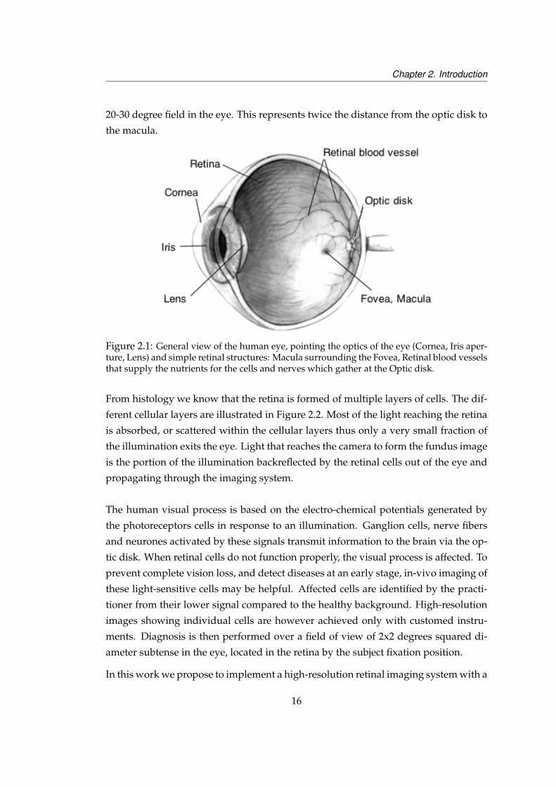
An image of the fundus is obtained by illuminating the eye from the pupil (defined
at the iris) in Figure 2.1. Medical assessment of the retinal health is performed with
images from commercial fundus cameras (Zeiss FF450 for example), which subtend a
15
Chapter 2. Introduction
20-30 degree field in the eye. This represents twice the distance from the optic disk to
the macula.
Figure 2.1: General view of the human eye, pointing the optics of the eye (Cornea, Iris aper-ture, Lens) and simple retinal structures: Macula surrounding the Fovea, Retinal blood vesselsthat supply the nutrients for the cells and nerves which gather at the Optic disk.
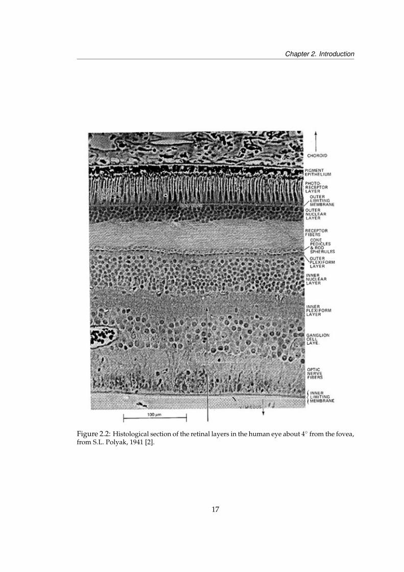
From histology we know that the retina is formed of multiple layers of cells. The dif-
ferent cellular layers are illustrated in Figure 2.2. Most of the light reaching the retina
is absorbed, or scattered within the cellular layers thus only a very small fraction of
the illumination exits the eye. Light that reaches the camera to form the fundus image
is the portion of the illumination backreflected by the retinal cells out of the eye and
propagating through the imaging system.
The human visual process is based on the electro-chemical potentials generated by
the photoreceptors cells in response to an illumination. Ganglion cells, nerve fibers
and neurones activated by these signals transmit information to the brain via the op-
tic disk. When retinal cells do not function properly, the visual process is affected. To
prevent complete vision loss, and detect diseases at an early stage, in-vivo imaging of
these light-sensitive cells may be helpful. Affected cells are identified by the practi-
tioner from their lower signal compared to the healthy background. High-resolution
images showing individual cells are however achieved only with customed instru-
ments. Diagnosis is then performed over a field of view of 2x2 degrees squared di-
ameter subtense in the eye, located in the retina by the subject fixation position.
In this work we propose to implement a high-resolution retinal imaging system with a
16
Chapter 2. Introduction
Figure 2.2: Histological section of the retinal layers in the human eye about 4 from the fovea,from S.L. Polyak, 1941 [2].
17
Chapter 2. Introduction
4x4 degree image to allow rapid identification of the image field location in the retina.
Diffraction-limited cellular sampling in the central part of the image was provided by
adaptive optics. Several illumination sources and types of camera triggering were set
up to obtain an image of short exposure and high resolution of the retina.
2.1.2 Influence of the ocular aberration on retinal imaging
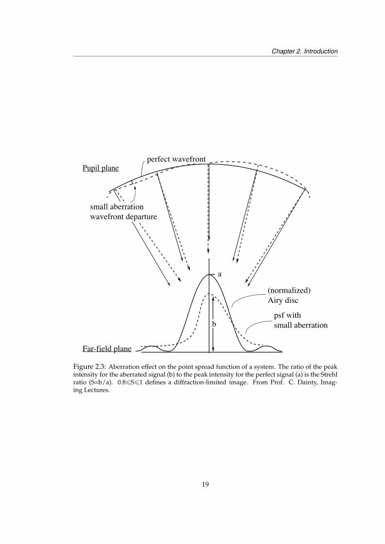
From diffraction theory it is well known that in the absence of aberrations the image
of a point source object located at infinity from a circular aperture becomes an Airy
function after transmission through this pupil which forms a diffraction-limited op-
tical system. The presence of optical aberrations in this system deteriorates the Airy
disk peak intensity, and in turn the signal transmission from the object to the acqui-
sition system. An illustration of the point spread function modification due to an
aberration is presented in Figure 2.3.
The aberration pattern measured at the sensor corresponds to the on-axis wavefront
departure from the ‘perfect’ wavefront applied to the light coming from the retina [3].
Aberrations are separated into low-order and high-order types as a function of their
shape complexity. Large pupil diameters – such as after pupil dilation by ophthalmic
drugs – present larger amplitudes of high-order aberrations than small pupil diam-
eters. The digital image is degraded by the ocular aberrations that affect all the sec-
ondary point-sources of the retina, formed in response to the illumination (wave-
front sensor probe beam or flashed Maxwellian illumination). The image becomes
diffraction-limited after implementation of an aberration compensation system (e.g.
adaptive optics).
Isoplanaticity
The isoplanatic angle is the angle over which the wavefront (and hence point spread
function) are reasonably constant. If the corrected on axis point spread function has a
Strehl ratio of 1.0, then it is generally accepted that the isoplanatic angle is the angle
for which the Strehl ratio of the point spread function is 0.37, which is equivalent to
an rms wavefront aberration of 1 rad. The isoplanatic angle can vary quite widely, but
in a typical eye is on the order of 2-4 degrees [4]. For adaptive optics, the isoplanatic
angle defines the angular subtense of the image for which the diffraction-limited im-
age quality is achieved by referencing the correction on the central (reference) point
spread function. Out of this zone usually centered on the optical axis, the correction is
only partial. To achieve diffraction-limited image quality, additional adaptive optics
18
Chapter 2. Introduction
b
a
(normalized) Airy disc
psf with small aberration
perfect wavefront
small aberrationwavefront departure
Pupil plane
Far-field plane
Figure 2.3: Aberration effect on the point spread function of a system. The ratio of the peakintensity for the aberrated signal (b) to the peak intensity for the perfect signal (a) is the Strehlratio (S=b/a). 0.86S61 defines a diffraction-limited image. From Prof. C. Dainty, Imag-ing Lectures.
19

Chapter 2. Introduction
correction referenced on an outer part of the image define a new isoplanatic angle.
Such an optical configuration represents multi-conjugate adaptive optics.
Chromatic aberrations
Chromatic effects are due to the fact that the refractive index of the optical media is a
function of the wavelength. The longitudinal and transverse chromatic aberrations of
the imaging system are minimized for the static aberration of an artificial eye by the
use of achromat lenses. Compensation of the image focal plane position shift is ob-
served with achromat lenses and use of multiple wavelengths of the visible. Retinal
imaging is however subject to the longitudinal chromatic aberration of the eye com-
pensated by a quantified amount of defocus. The correction requirement as a function
of the imaging wavelength for the observation of a given retinal layer at the science
camera in an healthy eye was developed and used by other teams [5, 6, 7].
Light scatter in the eye
Scatter is not an aberration described by classical optics but is mentioned here as
a factor that reduces the signal to noise ratio. The back-scattered signal from the
retina is the source for the wavefront sensing and for imaging the eye, as illustrated
in Figure 2.4. Scatter occurs in the eye first in the anterior segment and second in the
retina. In the ocular media (that is the cornea, the crystalline lens, and the vitreous
humor), the shorter the wavelength the more the scattering [8, 9, 10]. Meanwhile, in
the retina the longer the wavelength the deeper the light penetration in the tissue and
the more the scattering.
IlluminationCorneal Back ScatterAnterior Segment ScatterRetinal ScatterRetinal Back ScatterDouble pass signal
Retinal ScattererOcular Media Scatterer
Figure 2.4: Schematic of ocular scatter mechanism. Wavefront sensing and image acquisitionis performed with the double pass signal, backscattered from the retina through the ocularmedia. Backscatter by the crystalline lens is not represented for clarity purposes.
For a 3µW laser power (635nm) and fixed camera exposure, the image of the probe
20
Chapter 2. Introduction
beam was first recorded in the human eye and afterwards recorded through an achro-
mat lens with an artificial retina formed by a paper card or formed by a metallic sup-
port. A narrower and more intense probe beam signal than in the human eye was
observed in the artificial eye. The spread of the incoming probe beam was attributed
to in-depth scatter related to the retinal layers (tissues, blood cells and other organic
components).
The most reflective layer for this wavelength was assumed to be at the photorecep-
tors outer segment despite other layers of the volume also backscatter light in the
direction of the acquisition camera. Optical conjugation of the image plane with the
outer segment of the photoreceptors under Maxwellian illumination corresponded to
a background signal intensity peak. Polarization filtering of the retinal signal was
shown to filter the unwanted scattering in the retinal image for confocal scanning
ophthalmoscopes [11]. Improvement of image quality in fundus imaging using po-
larized optics was implemented in a commercial fundus camera used in the work
described further in Figure 2.6c. A pinhole placed in a conjugate plane of the imaged
layer used in confocal microscopy protected the detector from light backscattered by
out-of-focus layers. Fundus images of the systems further described were acquired
without confocal optics, thus contained light from all layers.
2.1.3 High-resolution retinal imaging systems
The following section describes a few existing instruments used for retinal imaging
purposes and how they benefited from the implementation of adaptive optics cor-
rection systems. High-resolution retinal imaging refers to the identification of the
photoreceptor cells outer segment in an image of the human retina. This identifica-
tion had been realized based on statistical methods of speckle interferometry [12], or
deconvolution of the retinal image by the wavefront sensor signal [13]. Adaptive op-
tics refers to the image quality improve obtained in a science camera by mechanical
action (correction) on the phase aberration measured by a wavefront sensor. In 1997,
Liang et al. [14] presented the first images of photoreceptors obtained after correction
of high-order ocular aberrations with adaptive optics. Liang’s correction system was
based on a deformable mirror in a feedback loop controlled by a Shack Hartmann
wavefront measurement. The benefit of adaptive optics on the signal was such that
the technique was extended to other fundus-imaging instruments.
21
Chapter 2. Introduction
Flash-based fundus cameras
Commercial fundus cameras (Zeiss, Topcon) are the most commonly used instru-
ments for imaging of the human retina without adaptive optics. The focus on the
retinal layer of interest is set up using a continuous illumination of low power then
the image is acquired using the aperture of a mechanical shutter triggered with a
high power illumination flash. A high quality image of the retina (or fundus image)
over 20 degree to 40 degree field is obtained but the resolution is too low to image
single photoreceptors. Adaptive optics flash-based fundus cameras have a smaller
image field (typically 1×1 or 2×2 degrees) but retrieve photoreceptor cells images
after correction of the ocular aberrations. Light comes from all the retinal layers and
image post-processing is required to improve the signal. After the demonstration of
signal improvement was realized, research was carried out to obtain fast acquisition
rates that led to a time-resolved identification of the photoreceptor activation [15,16].
Functional imaging of the photoreceptor mosaic [17, 18], identification of the locus of
fixation [19], or imaging of the retinal rods [20] is possible with such instruments.
Confocal systems
In a confocal scanning system, a single pixel detector (photomultiplier) is placed be-
hind a pinhole whose position along the optical axis (z axis in the cartesian coordi-
nates system) defines the retinal layer from which the light is scattered. Lateral and
vertical scanning of the sample is provided by the scanning mirrors on the order of
MHz for the horizontal scan and on the order of kHz for the vertical scan. The final
image is obtained in around 50ms. In these very short integration times and with
the confocal pinhole, the light that reaches the photo-multiplier is free of scattering
from retinal layers other than the one in focus. The main advantage of these sys-
tems is that the high resolution of the instrument is maintained through the in-depth
imaging of the sample layers, which leads to a volumetric reconstruction of the reti-
nal structures. The image is nevertheless only monochromatic, and requires a lot of
post processing for compensating the image jitter related to the scanning speed varia-
tion [21] and for the eye saccades. These systems led to the identification of functional
imaging of retinal cells in AO-SLOs such as the color sensitivity function of the cones
photoreceptors [22]. Additional characterization of this signal was obtained by the
identification of the cones long-course infrared signal changes emitted in response
to a visible light stimulus [23], (or intrinsic optical signal). Many results of in-vivo
observations of a single layers along the retina depth were achieved by AO-SLOs
instruments [24, 25, 26].
22
Chapter 2. Introduction
Two-photon microscropy
Two-photon microscopy images are formed by the emission of a photon induced by
laser excitation of the fluorescent agent inserted in the biological sample. The name
comes from the fact that the absorption of two laser photons by the fluorophore is
necessary to induce the emission. Given the automatic filtering of the volumetric
scattering towards regular fluorescence imaging with adaptive optics in animals [27,
28] the signal is very clear. However, the light levels required to induce the emission
process lead to cell death after bleaching. Two-photon microscopy is a fast process
that was applied to the measurement of the retinal pigment epithelium [29] with a
femtosecond laser and is of growing interest in human applications.
Optical Coherence Tomography (OCT) systems
OCT systems are based on the post processing of the interference signal created be-
tween a reference wave and the signal from the retina. Initial systems (Time Domain
OCT) were based on axial scanning of the reference mirror, providing 3D-imaging
of the sample. Spectral Domain OCT (SD-OCT) has progressively replaced Time-
Domain OCT, avoiding the z-scanning requirement [30]. Speckle deterioration of the
OCT images due to the use of very coherent sources was greatly reduced with use of
swept-source fibre lasers. Retinal imaging OCT systems, unless used in an adaptive
optics configuration, are mainly limited by a low transverse resolution [31, 32, 33].
Volumetric imaging of the retina is obtained at a scanning rate of about 2 second
per stack, whose post processing can take several days but retrieves identification of
the cones slow retinal intrinsic optical signal [34] as a highly punctuated and bright
reflection spot vanishing in adjacent frames or of the Stiles Crawford response [35].
The advantage of adaptive optics was demonstrated in observations of the cones mo-
saic [36] and in the observation of the retinal cellular structure [37, 38].
Between 2006 and 2011, the implementation of high-stroke deformable mirrors in
adaptive optics retinal imaging instruments extended their use to the measurement of
higher amplitudes of ocular aberration [39]. Additional results were obtained using
these new technologies in OCT retinal imaging systems [40].
The adaptive optics system based on the pyramid sensor measurement built during
the thesis is described further in Chapter 4. This system aims at high-resolution retinal
imaging using a high-stroke mirror in the adaptive optics. Ocular aberrations in the
range ±3 diopters (D) as characterized by the sensor measurement can be corrected.
23
Chapter 2. Introduction
2.2 Design requirements for an adaptive optics reti-
nal imaging system
In this section we will present the design requirements in Section 2.2.3. In order to
understand how these requirements were determined, the results obtained with the
OKO19Piezo deformable mirror system are described in Section 2.2.1. The system
limitations that defined the requirements and mechanical constraints are discussed in
Section 2.2.2.
2.2.1 Initial system description
The data acquisition was realized with the optical system represented in Figure 2.5.
The sensing of the aberrations of the eye was obtained by a Helium Neon laser (633nm)
backscattered from the retina to the pyramid prism. The focus error of the subject was
corrected before sensing by modifying the optical path length of the imaging system
with a Badal stage until the probe beam point spread function size was minimal at
the science imaging camera. Circular modulation of the focused beam around the tip
of the pyramid was induced by a Newport fast steering mirror running at 100Hz re-
sulting in 4 pupils reimaged on the wavefront sensing camera. Custom LabVIEW 7.0
(National Instruments, Austin, TX, USA) software detected the wavefront aberrations
after correction of the focus error and determined the mirror command controls re-
quired to correct for the higher-order aberrations by singular value decomposition
of the wavefront gradients. Adjusting the camera binning to get 16 pixels across the
385µm pupil and the modulation radius to small values (7λ/D, where D is the diam-
eter of the pupil image on the steering mirror), the typical residual wavefront error of
the closed–loop mode reached 0.1µm root mean square (λ/8) at 55Hz frame rate and
10ms exposure frame.
From the definition of the point spread function of a diffraction–limited system, a
2.2µm Airy radius was obtained at the retina of a model eye of 16.7mm focal length
with a 6mm pupil diameter at 633nm. The same pupil aperture magnified to 30mm
and focussed by a 400mm focal length lens in the imaging system formed a point
spread function of 10.5µm (633nm) at the imaging camera. From these values, a 5×magnification factor was estimated between the retinal plane and its conjugate plane
at the imaging camera. An adjustable diaphragm was placed in a conjugate retinal
plane to allow adjustment of the imaging field of view, with a 0.6×magnification be-
24

Chapter 2. Introduction
Badal
R
R
R
R
R
P
P
P
P
PP
P
Probe beam632nm
LED 530nm
Fibrecalibrationopen loop 635nm
R
Pupil observation880nm
Wavefrontsensing Retiga EX
Pyramid Newport faststeering mirror
OKO19 piezoDeformable mirror
50:50 BS
Fundus illumination
Fundus imagingRetiga 1300 C
ccd
Pupilmask
Fibre 635nmCalibration closed-loop
MirrorPellicle BS
LensDichroic BS 632/880nmDichroic BS 530/632nm
RP
Retinal plane & conjugatesPupil plane & conjugates
Pupil illumination
Eye
HeNe
Electronic translation stage Thorlabs
Fixationtarget R
Figure 2.5: Layout of the optical system for retinal imaging using the OKO19 Piezo mirror.The average illumination power at the eye was 20µW (530nm), the average wavefront sensorbeacon power at the eye was 3µW (633nm). Exposure time of the wavefront sensor camerawas 10ms and exposure time of the science camera was 200ms. Sensor frame rate was 55Hzfor 16x16 pixels across the pupil.
25
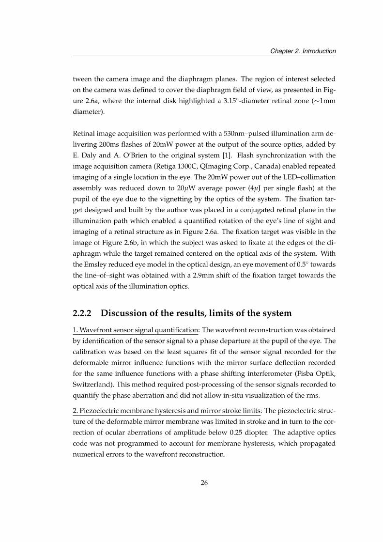
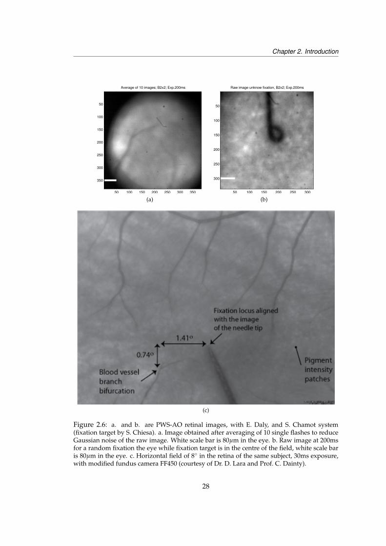
Chapter 2. Introduction
tween the camera image and the diaphragm planes. The region of interest selected
on the camera was defined to cover the diaphragm field of view, as presented in Fig-
ure 2.6a, where the internal disk highlighted a 3.15-diameter retinal zone (∼1mm
diameter).
Retinal image acquisition was performed with a 530nm–pulsed illumination arm de-
livering 200ms flashes of 20mW power at the output of the source optics, added by
E. Daly and A. O’Brien to the original system [1]. Flash synchronization with the
image acquisition camera (Retiga 1300C, QImaging Corp., Canada) enabled repeated
imaging of a single location in the eye. The 20mW power out of the LED–collimation
assembly was reduced down to 20µW average power (4µJ per single flash) at the
pupil of the eye due to the vignetting by the optics of the system. The fixation tar-
get designed and built by the author was placed in a conjugated retinal plane in the
illumination path which enabled a quantified rotation of the eye’s line of sight and
imaging of a retinal structure as in Figure 2.6a. The fixation target was visible in the
image of Figure 2.6b, in which the subject was asked to fixate at the edges of the di-
aphragm while the target remained centered on the optical axis of the system. With
the Emsley reduced eye model in the optical design, an eye movement of 0.5 towards
the line–of–sight was obtained with a 2.9mm shift of the fixation target towards the
optical axis of the illumination optics.
2.2.2 Discussion of the results, limits of the system
1. Wavefront sensor signal quantification: The wavefront reconstruction was obtained
by identification of the sensor signal to a phase departure at the pupil of the eye. The
calibration was based on the least squares fit of the sensor signal recorded for the
deformable mirror influence functions with the mirror surface deflection recorded
for the same influence functions with a phase shifting interferometer (Fisba Optik,
Switzerland). This method required post-processing of the sensor signals recorded to
quantify the phase aberration and did not allow in-situ visualization of the rms.
2. Piezoelectric membrane hysteresis and mirror stroke limits: The piezoelectric struc-
ture of the deformable mirror membrane was limited in stroke and in turn to the cor-
rection of ocular aberrations of amplitude below 0.25 diopter. The adaptive optics
code was not programmed to account for membrane hysteresis, which propagated
numerical errors to the wavefront reconstruction.
26
Chapter 2. Introduction
3. Imaging wavelength: Infrared wavelengths are widely used for the comfort of the
patient and retrieve sharp imaging of the photoreceptors mosaic with adaptive optics
but clinical instruments diagnostics are based on visible light images. Previous results
of the fundus autofluorescence to multi-wavelength illumination were obtained with
flash-based fundus camera 470nm, 550nm and 650nm sources [22] then with a scan-
ning ophthalmoscope at 532nm, 658nm and 840nm [7]. Fluorescence images of the
fundus in medical devices with the use of a fluorescent agent (angiography) rely on
the acquisition of the 500-520nm emission activated with 488nm light. In this work,
no fluorescent agent is used, and the structures contrast in the image obtained with
light backscattered from the retina is chosen for criterion of identification. Extreme at-
tention was required as the human eye sensitivity peaks at 530nm, meaning a healthy
human retina is more likely to detect green light than any other wavelength of same
absolute intensity on a dark background, thus that high light-levels were uncomfort-
able and harmful.
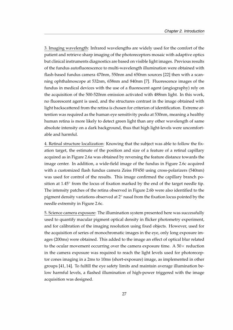
4. Retinal structure localization: Knowing that the subject was able to follow the fix-
ation target, the estimate of the position and size of a feature of a retinal capillary
acquired as in Figure 2.6a was obtained by reversing the feature distance towards the
image center. In addition, a wide-field image of the fundus in Figure 2.6c acquired
with a customized flash fundus camera Zeiss FF450 using cross-polarizers (540nm)
was used for control of the results. This image confirmed the capillary branch po-
sition at 1.45 from the locus of fixation marked by the end of the target needle tip.
The intensity patches of the retina observed in Figure 2.6b were also identified to the
pigment density variations observed at 2 nasal from the fixation locus pointed by the
needle extremity in Figure 2.6c.
5. Science camera exposure: The illumination system presented here was successfully
used to quantify macular pigment optical density in flicker photometry experiment,
and for calibration of the imaging resolution using fixed objects. However, used for
the acquisition of series of monochromatic images in the eye, only long exposure im-
ages (200ms) were obtained. This added to the image an effect of optical blur related
to the ocular movement occurring over the camera exposure time. A 50× reduction
in the camera exposure was required to reach the light levels used for photorecep-
tor cones imaging in a 2ms to 10ms (short-exposure) image, as implemented in other
groups [41, 14]. To fulfill the eye safety limits and maintain average illumination be-
low harmful levels, a flashed illumination of high-power triggered with the image
acquisition was designed.
27
Chapter 2. Introduction
Average of 10 images; B2x2; Exp.200ms
50 100 150 200 250 300 350
50
100
150
200
250
300
350
(a)
Raw image unknow fixation, B2x2; Exp.200ms
50 100 150 200 250 300
50
100
150
200
250
300
(b)
(c)
Figure 2.6: a. and b. are PWS-AO retinal images, with E. Daly, and S. Chamot system(fixation target by S. Chiesa). a. Image obtained after averaging of 10 single flashes to reduceGaussian noise of the raw image. White scale bar is 80µm in the eye. b. Raw image at 200msfor a random fixation the eye while fixation target is in the centre of the field, white scale baris 80µm in the eye. c. Horizontal field of 8 in the retina of the same subject, 30ms exposure,with modified fundus camera FF450 (courtesy of Dr. D. Lara and Prof. C. Dainty).
28

Chapter 2. Introduction
6. Imaging resolution: For a diffraction-limited point source located at the retinal
plane of a model eye, the point spread function of the system observed through the
6mm diameter aperture defined by the iris of the model eye was of 10.5µm at the con-
jugate retinal plane at the imaging camera. The point source image was distributed
over 1.5 pixels of the camera, thus by the Nyquist criterion, any item of the retina of
size below 2.7µm was not resolved in the digital image. The cones photoreceptors of
2µm diameter were thus impossible to identify with this imaging system.
7. Light losses: The 50/50 beamsplitter cube which separated the retinal imaging path
from the wavefront sensing path was a source of light losses out of the eye, in par-
ticular for the retinal imaging path. To maximize the light efficiency of the imag-
ing arm (530nm) while transmitting the maximum of light to the wavefront sensor, a
dual wavelength-specific coated dichroic mirror (CVI Melles Griot Long Wave Pass
Dichroic Filter, unpolarized) was leading to an improve of 35% to 40% in light effi-
ciency in each channel, all other optics remaining identical.
2.2.3 New system parameter requirements
• Zernike coefficients expression of the wavefront aberration
With the circular modulation, the sensor signal was directly related to the wave-
front aberration gradient in physical units. The non-linearity at the edges of
the pupil [42] was not considered as a zero-amplitude of gradient was defined
outside the pupil. The signal saturation (non-linearity) occured when the signal
always marked one for an increasing aberration. The reconstruction will always
show the same value of shape and in turn the same phase at the pupil.
The wavefront reconstruction from the gradients and its decomposition into
Zernike coefficients allowed the calculation of the rms during the experimental
session. For comparison of the wavefront aberration amplitude measured at the
sensor with the results of commercial instruments (e.g. Zywave aberrometer,
Bausch & Lomb, USA), the Zernike polynomials expression is recommended.
Since 2002 an international convention has been defined by the Optical Soci-
ety of America [43] and in 2004 an international standard was defined (ANSI
Z80.28-2004) for the reporting of optical aberration of eyes. This normalized
convention was also convenient for the communication of results.
• Retinal image resolution and field
In the system of Liang et al [41, 14] the image resolution was of 0.13arcmin
29
Chapter 2. Introduction
(0.6µm) per camera pixel at the retina, meaning about 10 times the resolution
ability of the imaging system described in Section 2.2.1. The photoreceptor mo-
saic was imaged in a field of 1 located between 1 and 2 from the fovea (or
fixation center [19]). The cones cells of 2-5µm diameter in the foveal region were
not resolved until the adaptive optics was switched on, and the exact location
of the imaged field in the retina was restricted to the cases in which the fixation
target was visualized.
The new design of the pyramid wavefront sensor-based AO system attempted
to compromise between the necessary increase in the magnification factor γT to
the value resolving a mosaic of pattern size below 2µm diameter, an image field
of subtense including the 2 diameter avascular zone located around the fovea,
and a compact optical system size (below the 1.8m×1.5m limits of the optical
table). A system in which 1pixel of the camera measured 0.18arcmin (0.9µm) at
635nm wavelength, respected the Nyquist sampling criterion for the cones, as
in other systems [17, 44], and provided an image field of 3.5 × 3.5.
• Deformable mirror implementation
The Mirao52® deformable mirror from Imagine Eyes France presented a±25µm
membrane stroke amplitude and a surface flatness of 20nm rms. Based on an
electromagnetic actuation, the mirror was numerically assessed as a suitable re-
placement [45, 46, 47]. It had been incorporated successfully in an AO-fundus
camera based at the Quinze-Vingts hospital in Paris, France for clinical trials
and commercialized in AO-flash fundus systems and AO-corrected visual sim-
ulator, for the correction of ocular aberration during scene visualization. The
membrane stroke amplitude has been applied to the correction of very large
aberrations such as keratoconic eyes [39]. It was sold for use with a Shack-
Hartmann lenslet array and a control software for adaptive optics by the sup-
plying company (Imagine Eyes, France) but required new LabVIEW code to be
developed for adaptive optics operation with the pyramid sensor.
• Synchronous acquisition of adaptive optics data and of retinal image
The use of two independent operating systems, one for the adaptive optics con-
trol and one for the retinal image acquisition retrieved a direct acquisition of
the double pass point spread function not synchronized with the wavefront
sensor data acquisition. Comparison of the direct psf image with a numeri-
cal computation based on the wavefront sensor gradients expected to retrieve
information lost in the noise of the retinal image instead of using deconvolu-
30

Chapter 2. Introduction
tion from the wavefront sensor data was thus impossible. This post-processing
initially discussed in the context of astronomy later increased retinal images
quality [13, 48, 49, 50, 51]. Implementation of the retinal imaging acquisition in
the same operating system as the adaptive optics control was thus required.
Several systems were implemented in the aim to fill these requirements. The follow-
ing report scope was limited to the results useful for the thesis subject. The final
system was consequently the most relevant to this purpose.
31
Chapter 3
Pyramid wavefront sensing
This chapter describes the implementation of the measurement of an aberration with
the pyramid wavefront sensor with a circular modulation. The sensor used in this
thesis was built for the measurement of large aberrations at the pupil of the human
eye. The laboratory implementation, calibration of the sensor measurement and of
the wavefront reconstruction are presented in the following.
3.1 Pyramid wavefront sensing in astronomy
In 1996 Ragazzoni [52] introduced a new type of wavefront sensor for astronomy
which was based on a pyramid prism. Despite its mechanical complexity, this sensor
has an adjustability of its dynamic range, a better photon efficiency, and better results
in closed loop compared to the classical Shack Hartmann in a quad-cell configuration.
Recent advances in algorithms can address now the saturation limit and centroiding
issues [53, 54] in many of today’s Shack Hartmann systems. The first drawback of
the pyramid is mechanical, as the pyramid prism is very difficult to manufacture
compared to lenslet arrays, and is not commercially available despite the recent tech-
nological advances in this domain [55, 56, 57, 58]. The second drawback is related to
the modulation requirement for getting a quantitative slope measurement with the
sensor [59, 30].
The pyramid sensor principle is related to the Foucault knife edge test (1859, [60]) in
that both techniques split the beam at or near the focal plane of the wavefront or ele-
32
Chapter 3. Pyramid wavefront sensing
ment to be tested. In consequence the pyramid sensor could be seen as a ‘focal plane’
or ‘Fourier-plane’ sensor. However, the aberration determination is not obtained by
translation of the knife perpendicular to the propagation axis but by comparing the
intensity of the beam parts detected after splitting by the prism edges. Each part of
the beam is diverted by the prism so in the reconstructed pupil plane a single frame is
sufficient to characterise the wavefront aberration instead of having to process the re-
constructed pupil for multiple positions of the knife-edge near the focus. As the anal-
ysis is performed using a detector placed in a conjugate pupil plane for the wavefront
to be tested, the pyramid sensor is thus effectively a ‘pupil plane’ wavefront sensor.
The pyramid retrieves a wavefront slope measurement equivalent to that of a Shack-
Hartmann physically placed in a conjugate pupil plane.
As the division of the beam focus is made by the 4 facets of the prism, the pyramid
is said to be equivalent to a Shack Hartmann sensor in a quad-cell configuration. The
quad-cell advantage is a lower read-out noise in the sensor due to the lower num-
ber of pixels to read in the detector [61] and does not require access to the wavefront
spot size behind the lenslet. One possible solution proposed to increase the number
of pixels for the detection was to use an array of pyramids instead of a single prism
and to relay each pyramid to the pupil plane of the camera using lenslets [59]. How-
ever further work showed the optimal number of lenslets in the focal plane was a
2x2 arrangement, similar to using the pyramid prism [62]. Using a 2x2 lenslet array
retrieved comparable atmospheric turbulence values as with a quad-cell Shack Hart-
mann [63], and the influence of the lenslet array edges quality for successful operation
was highlighted. This system also showed a lower error propagation than its equiv-
alent lenslet array in closed loop [64]. Comparative turbulence measurements were
also performed with this 4-lenslet pyramid using the static modulation approach [65].
Mechanical modulation of the prism or of the beam is required in theory to measure
quantitative wavefront slopes from the sensor signals [52,66,67] and to provide in-situ
adjustment of the sensor ‘gain’ or sensitivity. In astronomy the mechanical modula-
tion may not be necessary as the residual atmospheric turbulence contains a ‘natural’
modulation term [68, 69] and thus after appropriate calibration the sensor signal still
retrieves a wavefront gradient measurement [70], and provides a good adaptive op-
tics efficiency even in poor seeing conditions [71]. Circular modulation provides a
comprehensive framework for the implementation of the wavefront reconstruction
but is perhaps not essential for pyramid sensing in the eye [72], due to natural eye
33

Chapter 3. Pyramid wavefront sensing
movements. The effects of natural aberration dynamics such as accommodation and
pupil diameter are however limited in ophthalmic applications by cyclopegic drugs.
Other effects to be considered are due to periodical change in the orientation of the
retina of the order of the tens of milliseconds. These natural eye saccades responsible
for ocular blur might provide a pupil drift around the central point of the eye and
modify the ocular aberrations similarly as the inherent turbulence in the atmosphere.
Algorithmic solutions have also been developed for the unmodulated pyramid in as-
tronomy introducing a wavefront reconstruction scheme based on a Jacobian decom-
position of the mirror modes instead of the classical singular-value-decomposition
scheme. This was used successfully in closed loop [73, 74] to increase the dynamic
range of an adaptive optics system. Another replacement for the mechanical mod-
ulation is based on the use of fixed-divergence diffusers (holographic or rotating
type) which are placed in a conjugate pupil plane before the pyramid [75], then the
point spread function (psf) size at the pyramid provides the sensor sensitivity adjust-
ment [72]. This static modulation has been implemented in layer-oriented multicon-
jugate adaptive optics [76, 75, 77] using double pyramids to better control the output
direction after the pyramid [78] for the ELT and in ophthalmic applications [72].
The pyramid measurement has been studied [79] to explain how the slope or the
phase of the wavefront measurement depends on the modulation amplitude consid-
ered, in the circular modulation scheme. When compared to a Shack-Hartmann in
quad cell configuration with weighted center of gravity algorithm [80] and beam fil-
tering [81], the pyramid was estimated to perform similarly [82] in high photon flux.
This confirmed the previous numerical results [83, 67] predicting a better closed loop
efficiency of the pyramid for low-magnitude natural guide stars and was recently
confirmed experimentally, this time without mechanical modulation [71].
To confirm the simulation results between the pyramid and the Shack Hartmann a
special program has been developed and is currently in progress on the high-order
testbench (HOT)-ELT (First Light AO system for the Large Binocular Telescope) [84,
57, 85, 86]. One advantage of the pyramid sensor compared to the Shack Hartmann
is however that it allows the measurement of positioning errors (differential piston)
in the individual segments of this telecope mirror [87, 88]. For this category of ex-
tremely large telescopes the question of the maximal Karhunen-Loeve mode that can
be corrected and by which way is often raised. Those systems also seem to present an
optimal modulation ratio [89] for a specified guide star size which would thus open
34
Chapter 3. Pyramid wavefront sensing
new perspectives such as a possible use with laser guide stars [83].
In ophthalmology, open loop measurement is of major importance in applications
such as laser refractive surgery. The pyramid sensor is usually considered as a poor
system for the determination of the refraction (i.e. focus error). The closed loop effec-
tiveness of wavefront sensors in adaptive optics systems is mainly related to high res-
olution retinal imaging. This research was initiated by Liang, Miller and Williams in
1997 [41,14] after they produced with adaptive optics the first in-vivo high-resolution
imaging of the photoreceptor cells in the human eye. Further developments of this
work showed efficient identification of the functional role of photoreceptors in color
vision [22], leading the way to the development of adaptive optics use in imaging of
the neuronal activity of the retina.
Although Shack-Hartmann wavefront sensors are widely used today in ophthalmic
research instruments, pyramid sensors have been implemented for the eye, firstly by
Iglesias and Ragazzoni [72] using the probe beam size at the retina to set the dynamic
range and rotating diffusers to replace the mechanical modulation, or in closed-loop
configuration using the conventional circular modulation scheme [1, 90, 91, 92, 93]. In
this work we tried to implement a sensor of large enough dynamic range for descrip-
tion of various ocular aberrations and still able to retrive very accurate measurements
for closed loop operation.
3.2 Wavefront sensing with a pyramid prism
The following section discusses the implementation of the pyramid wavefront sens-
ing in an ophthalmic system. The use of several approximations and compromises
is required. In contrast to the Shack-Hartmann, the pyramid does not rely on cen-
troiding algorithm for obtaining a wavefront measurement. The aberration is directly
calculated from the 4 wavefront pupil images at the camera. The price for this com-
putational simplicity however stands in the difficulty of mechanical implementation,
and of identification of the sensor saturation limit during experimental sessions.
3.2.1 Wavefront pupil reimaging into 4 sub-pupils
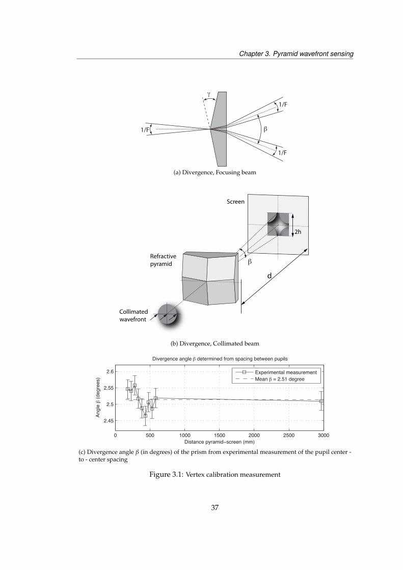
A focusing beam onto the pyramid is divided in 4 parts by the prism facets as illus-
trated in Figure 3.1a. In that case however the divergence β is defined towards the
35

Chapter 3. Pyramid wavefront sensing
on-axis ray, and the rays defining β become principal rays for the rest of the system.
For calibration of the pyramid divergence β, an on-axis collimated beam of 10.5 mm
diameter was sent onto the pyramid as represented in Figure 3.1b. For such a config-
uration the divergence β is given by:
β = 2× arctan
(hd
)(3.1)
Equation 3.1 means that at a distance (d) from the prism the spacing (2h) measured
between the centers of the 4 beam quadrants is resulting of the incident collimated
beam split by the pyramid facets.
From the measurements of (2h) with a collimated beam at multiple distances (d) from
the prism we obtain the graph in Figure 3.1c using Equation 3.1. Measurements at a
close distance are visibly subject to a high variability but their mean value over the
distances considered are consistent with a long distance measurement; thus we esti-
mate that for our case βmean = 2.51 ± 0.01 is a good approximation for the value of
the divergence.
Riccardi [94] showed that the prism vertex angle (γ) relates to the divergence (β) fol-
lowing the geometrical optics for the refraction of a of a ray parallel to the optical axis.
Within the [-6, 6] limits of the geometrical optics approximation:
γ =β
(nglass − 1)=
2.51(1.5157− 1)
= 4.86 ± 0.02 (3.2)
The value of γ is determined from the measured value of β and from Equation 3.2.
This show our measurement is consistent with the value of 5 presented in the litera-
ture for this pyramid which comes from astronomy [94, 66].
In Figure 3.1a, the angle β defines the angular separation between the pupils cen-
ters. To obtain separation of the pupils for a focusing beam in the general case the F-
number of the beam must be higher than a critical value Fc. If overlap of the pupils is
detected the pupil gradient calculation cannot be performed. At the critical F-number,
2 pupils sides are just in contact but do not overlap. Diagonally the pupils centers an-
gular separation is β′ =√
2/Fc [94]. From the prism divergence, we thus define the
critical F-number for the maximal density packing configuration as Fc and derive the
36
Chapter 3. Pyramid wavefront sensing
γ
β1/F
1/F
1/F
(a) Divergence, Focusing beam
d
Screen
2h
βRefractive pyramid
Collimated wavefront
(b) Divergence, Collimated beam
0 500 1000 1500 2000 2500 3000
2.45
2.5
2.55
2.6
Distance pyramid−screen (mm)
Angle
β (
degre
es)
Divergence angle β determined from spacing between pupils
Experimental measurement
Mean β = 2.51 degree
(c) Divergence angle β (in degrees) of the prism from experimental measurement of the pupil center -to - center spacing
Figure 3.1: Vertex calibration measurement
37
Chapter 3. Pyramid wavefront sensing
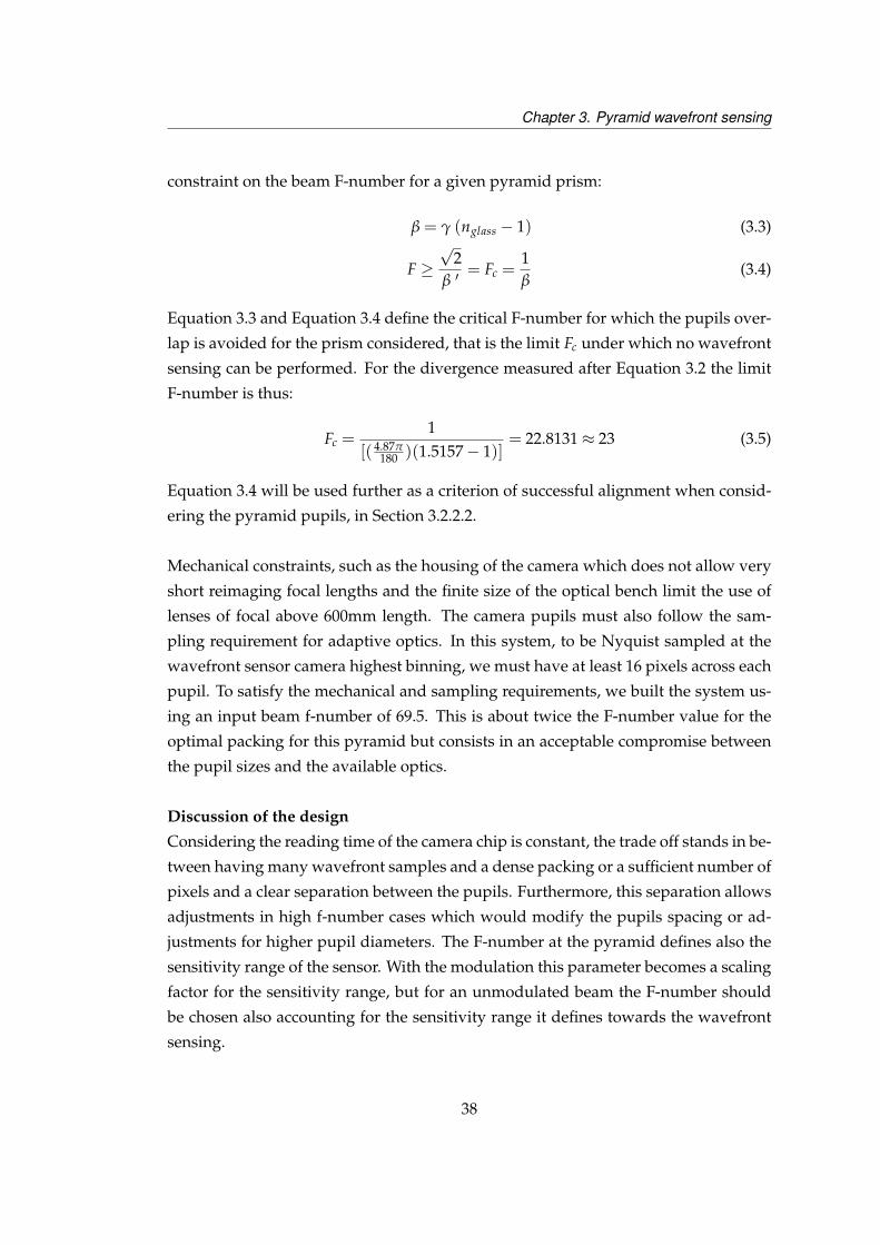
constraint on the beam F-number for a given pyramid prism:
β = γ (nglass − 1) (3.3)
F ≥√
2β ′
= Fc =1β
(3.4)
Equation 3.3 and Equation 3.4 define the critical F-number for which the pupils over-
lap is avoided for the prism considered, that is the limit Fc under which no wavefront
sensing can be performed. For the divergence measured after Equation 3.2 the limit
F-number is thus:
Fc =1
[( 4.87π180 )(1.5157− 1)]
= 22.8131≈ 23 (3.5)
Equation 3.4 will be used further as a criterion of successful alignment when consid-
ering the pyramid pupils, in Section 3.2.2.2.
Mechanical constraints, such as the housing of the camera which does not allow very
short reimaging focal lengths and the finite size of the optical bench limit the use of
lenses of focal above 600mm length. The camera pupils must also follow the sam-
pling requirement for adaptive optics. In this system, to be Nyquist sampled at the
wavefront sensor camera highest binning, we must have at least 16 pixels across each
pupil. To satisfy the mechanical and sampling requirements, we built the system us-
ing an input beam f-number of 69.5. This is about twice the F-number value for the
optimal packing for this pyramid but consists in an acceptable compromise between
the pupil sizes and the available optics.
Discussion of the design
Considering the reading time of the camera chip is constant, the trade off stands in be-
tween having many wavefront samples and a dense packing or a sufficient number of
pixels and a clear separation between the pupils. Furthermore, this separation allows
adjustments in high f-number cases which would modify the pupils spacing or ad-
justments for higher pupil diameters. The F-number at the pyramid defines also the
sensitivity range of the sensor. With the modulation this parameter becomes a scaling
factor for the sensitivity range, but for an unmodulated beam the F-number should
be chosen also accounting for the sensitivity range it defines towards the wavefront
sensing.
38
Chapter 3. Pyramid wavefront sensing
3.2.2 Modulation
Even if the modulation is perhaps not essential for pyramid sensing in the eye [72]
as the inherent aberrations act as the inherent turbulence in the atmosphere [68], it
is convenient to work with a circular modulation [66]. As we will see in the follow-
ing section, the modulation determines the maximal wavefront aberration amplitude
sensed in the system. Providing the mirror stroke is sufficient to correct it, the ad-
justability of the sensing range allows an accurate measurement of the eye aberration
while maintaining the benefit of adaptive optics for the retinal imaging.
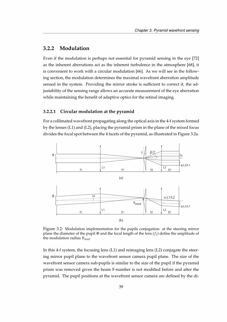
3.2.2.1 Circular modulation at the pyramid
For a collimated wavefront propagating along the optical axis in the 4-f system formed
by the lenses (L1) and (L2), placing the pyramid prism in the plane of the mixed focus
divides the focal spot between the 4 facets of the pyramid, as illustrated in Figure 3.2a.
φ
φ.L2/L1L1
f1 f1’ f2 f2’L2
γ β/2h
(a)
Rmod
α
L1f1 f1’ f2 f2’
L2
α.L1/L2φ
φ.L2/L1
(b)
Figure 3.2: Modulation implementation for the pupils conjugation: at the steering mirrorplane the diameter of the pupil Φ and the focal length of the lens ( f1) define the amplitude ofthe modulation radius Rmod.
In this 4-f system, the focusing lens (L1) and reimaging lens (L2) conjugate the steer-
ing mirror pupil plane to the wavefront sensor camera pupil plane. The size of the
wavefront sensor camera sub-pupils is similar to the size of the pupil if the pyramid
prism was removed given the beam F-number is not modified before and after the
pyramid. The pupil positions at the wavefront sensor camera are defined by the di-
39

Chapter 3. Pyramid wavefront sensing
vergence after the prism as detailed in Section 3.2.1 and Figure 3.2a. If the modulation
is represented as a tilt angle α applied along the vertical axis (Y) at the steering mirror,
as in Figure 3.2b, the focused beam is shifted by a value (Rmod = f ′1 tanα) at the pyra-
mid. The more the incident beam position increases at the pyramid the stronger the
deviation applied to the beam by the prism, thus the wavefront sensor camera pupils
positions remain constant - until the modulation reaches the critical deviation angle
for the prism.
If the modulated beam at the steering mirror is tilted of an angle (+θ) towards the
optical axis, the corresponding transverse aberration in the pyramid plane is a focus
shift of (+∆y). When the modulation projects the focus on the upper part of the
pyramid, in Figure 3.3a for the angle (+α), the wavefront tilt and the modulation
angle subtract thus the focus is shifted of (-∆y) in the pyramid plane.
Rmod
α
L1f1 f1’ f2 f2’
L2
α-θ θ Δy
(a)
α+θ
Rmodα
L1f1 f1’ f2 f2’
L2
θ
Δy
(b)
Figure 3.3: Modulation in telescopic arrangement
When the modulation projects the focus in the lower part of the pyramid in Fig-
ure 3.3b for the angle (−α), the wavefront tilt and the modulation add thus the focus
is shifted of (-∆y) in the pyramid plane. In consequence the optical path becomes
non-uniformly distributed amongst the 4 pyramid facets as in Figure 3.4 (left).
The signal at the wavefront sensing camera for the circular modulation Sy is given by
the difference in the optical path traced by the shifted circle onto the pyramid top and
down facets:
Sy =b2 − b1
2πRmod(3.6)
40
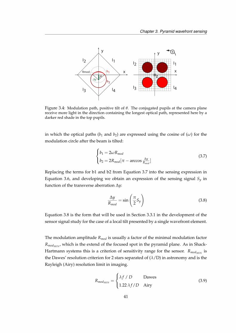
Chapter 3. Pyramid wavefront sensing
Rmod
Δy
I1I2
I3 I4
x
y
ω
b2
b1 x
y
I1I2
I3 I4
+
z
Figure 3.4: Modulation path, positive tilt of θ. The conjugated pupils at the camera planereceive more light in the direction containing the longest optical path, represented here by adarker red shade in the top pupils.
in which the optical paths (b1 and b2) are expressed using the cosine of (ω) for the
modulation circle after the beam is tilted:b1 = 2ωRmod
b2 = 2Rmod[π − arccos ∆yRmod
](3.7)
Replacing the terms for b1 and b2 from Equation 3.7 into the sensing expression in
Equation 3.6, and developing we obtain an expression of the sensing signal Sy in
function of the transverse aberration ∆y:
∆yRmod
= sin
(π
2Sy
)(3.8)
Equation 3.8 is the form that will be used in Section 3.3.1 in the development of the
sensor signal study for the case of a local tilt presented by a single wavefront element.
The modulation amplitude Rmod is usually a factor of the minimal modulation factor
RmodMIN , which is the extend of the focused spot in the pyramid plane. As in Shack-
Hartmann systems this is a criterion of sensitivity range for the sensor. RmodMIN is
the Dawes’ resolution criterion for 2 stars separated of (λ/D) in astronomy and is the
Rayleigh (Airy) resolution limit in imaging.
RmodMIN =
λ f / D Dawes
1.22 λ f /D Airy(3.9)
41

Chapter 3. Pyramid wavefront sensing
In the following the modulation factor was mainly expressed in terms of the Dawes
criterion, which was convenient for comparison with the majority of the literature on
pyramid wavefront sensing.
3.2.2.2 Laboratory implementation of the circular modulation
This section presents the optical system used for calibration of the sensor signal in
Figure 3.5 and its modifications for the optical design software, calibration of the
modulation amplitudes in Figure 3.6a.
RP
Control PC
Wavefront sensing
Retinal Imaging
RP
PPFlat mirror or Mirao 52 Deformable mirror
Steering mirror (PP)Newport
PPPyramid (RP)
Sensor probe beam (1)635nm
Sensor CCD Retiga EX
Imaging cameraRetiga 1300
RPCalibration Lens +
Fibre OL 635nm
PP
Badal
Mirror
Pellicle BS LensRP
PP
Retinal Plane & conjugates
Pupil Plane & conjugates
Translation Stage
Fiber coupled laser diode 635nm
CCD cameraDichroic BS 633/532nm
RP
PPEyePhase plate + Iris +
Lens + Fibre OL 635nmPPPhase plate + Iris +
Lens + Fibre OL 635nmPP
CCD
LED Pupil illumination 880nm (1)
PP
Pupil monitoringCCD (1) 880nm
Figure 3.5: Schematic of optical bench used for calibration of sensor signal. Modificationof the pupil illumination optics was performed for closed loop calibration and use in the 5-subjects aberration measurement and psf imaging of Chapter 4.
System description
The wavefront sensor calibration beam was defined at the pupil plane of the eye by a
fibre laser source output collimated by a 100mm achromat lens and an iris aperture of
6mm diameter. A telescopic assembly conjugated the pupil plane to the deformable
mirror through the Badal optometer mirrors stage set at mid-position of translation
range. A pellicle beamsplitter defined the input of the wavefront sensor probe beam
42

Chapter 3. Pyramid wavefront sensing
focusing into the Badal stage further described in Chapter 4, Section 4.2.4. The magni-
fied collimated calibration beam at the deformable mirror was reflected towards the
wavefront sensor path. A second telescope assembly conjugated the pupil plane at
the deformable mirror to the modulation control steering mirror. A dichroic beam-
splitter defined the starting position of the psf and retinal imaging optical path. A
last telescope assembly formed by a focusing lens and a reimaging lens placed after
the pyramid sensor relayed the steering mirror pupil plane to the wavefront sensor
camera.
The implementation of circular modulation was provided in the pupil plane of the
focusing lens by a steering mirror (Newport FSM-300 Fast Steering mirror). This
plane mirror surface was tilted horizontally and vertically with an amplitude defined
by coupled galvano-actuators located underneath its surface. The surface deviation
amplitude was determined by the voltages sent to the mirror amplifier by two syn-
chronized function generators (Agilent waveform generators 33250A and 33120A),
and was limited by a cut-off frequency above which the mirror response was attenu-
ated. 90 out-of-phase sinusoidal signals of the same frequency provided an elliptic
modulation of the focus at the pyramid. The signal frequency was the inverse of the
integration time of the wavefront sensing camera to obtain a signal at the sensor [66].
Adaptation to the calibration of the modulation
The wavefront sensor optical system was reproduced in Zemax using the manufac-
turer’s specifications for the lenses parameters, physical mirrors apertures and light
sources wavelengths. The adaptation to the modulation calibration for a Zemax de-
sign sketch is presented in Figure 3.6a. Replacing the pyramid by an empty plane
cancelled the beam deviation by a single facet. Replacing the reimaging lens by an
empty element cancelled the steering mirror pupil plane conjugation with the wave-
front sensing camera. Appropriate positioning of a pinhole in the telescope path be-
tween the deformable mirror and the steering mirror formed a finite size modulated
image of the pinhole at the wavefront sensor camera. For a common voltage ampli-
tude and a 90 phase shift between the function generators, the pinhole image initially
formed an ellipsoidal shape onto the camera. Experimental adjustment of the steer-
ing mirror voltages and function generators phase offset was performed to define the
modulation circle at the pyramid as in Figure 3.6b.
The centre of the circle defines the beam propagation direction similar to that of the 4-
f system. The cross section intensity profile in Figure 3.6c identifies the pinhole image
43
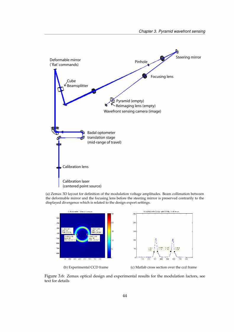
Chapter 3. Pyramid wavefront sensing
Pinhole
Pyramid (empty)
Wavefront sensing camera (image)
Steering mirrorDeformable mirror(`flat’ commands)
Badal optometertranslation stage(mid-range of travel)
Cube Beamsplitter
Calibration lens
Calibration laser(centered point source)
Focusing lens
Reimaging lens (empty)
(a) Zemax 3D layout for definition of the modulation voltage amplitudes. Beam collimation betweenthe deformable mirror and the focusing lens before the steering mirror is preserved contrarily to thedisplayed divergence which is related to the design export settings.
(b) Experimental CCD frame (c) Matlab cross section over the ccd frame
Figure 3.6: Zemax optical design and experimental results for the modulation factors, seetext for details
44
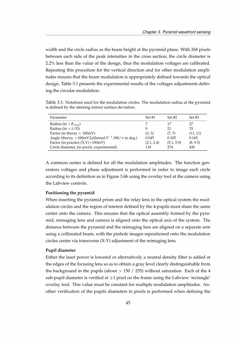
Chapter 3. Pyramid wavefront sensing
width and the circle radius as the beam height at the pyramid plane. With 268 pixels
between each side of the peak intensities in the cross section, the circle diameter is
2.2% less than the value of the design, thus the modulation voltages are calibrated.
Repeating this procedure for the vertical direction and for other modulation ampli-
tudes insures that the beam modulation is appropriately defined towards the optical
design. Table 3.1 presents the experimental results of the voltages adjustments defin-
ing the circular modulation.
Table 3.1: Notations used for the modulation circles. The modulation radius at the pyramidis defined by the steering mirror surface deviation.
Parameter Set #1 Set #2 Set #3
Radius (in ×RAiry) 7 17 27Radius (in ×λ/D) 9 21 33Factor (in theory × 100mV) (3, 3) (7, 7) (11, 11)Angle (theory, ×100mV.2,62mrad.V−1.180/π in deg.) 0.045 0.105 0.165Factor (in practice (X,Y)×100mV) (2.1, 2.4) (5.1, 5.9) (8, 9.5)Circle diameter, (in pixels, experimental) 118 274 430
A common center is defined for all the modulation amplitudes. The function gen-
erators voltages and phase adjustment is performed in order to image each circle
according to its definition as in Figure 3.6b using the overlay tool at the camera using
the Labview controls.
Positioning the pyramid
When inserting the pyramid prism and the relay lens in the optical system the mod-
ulation circles and the region of interest defined by the 4-pupils must share the same
center onto the camera. This ensures that the optical assembly formed by the pyra-
mid, reimaging lens and camera is aligned onto the optical axis of the system. The
distance between the pyramid and the reimaging lens are aligned on a separate arm
using a collimated beam, with the pinhole images repositioned onto the modulation
circles center via transverse (X-Y) adjustment of the reimaging lens.
Pupil diameter
Either the laser power is lowered or alternatively a neutral density filter is added at
the edges of the focusing lens so as to obtain a gray level clearly distinguishable from
the background in the pupils (about > 150 / 255) without saturation. Each of the 4
sub-pupil diameter is verified at ±1 pixel on the frame using the Labview ‘rectangle’
overlay tool. This value must be constant for multiple modulation amplitudes. An-
other verification of the pupils diameters in pixels is performed when defining the
45
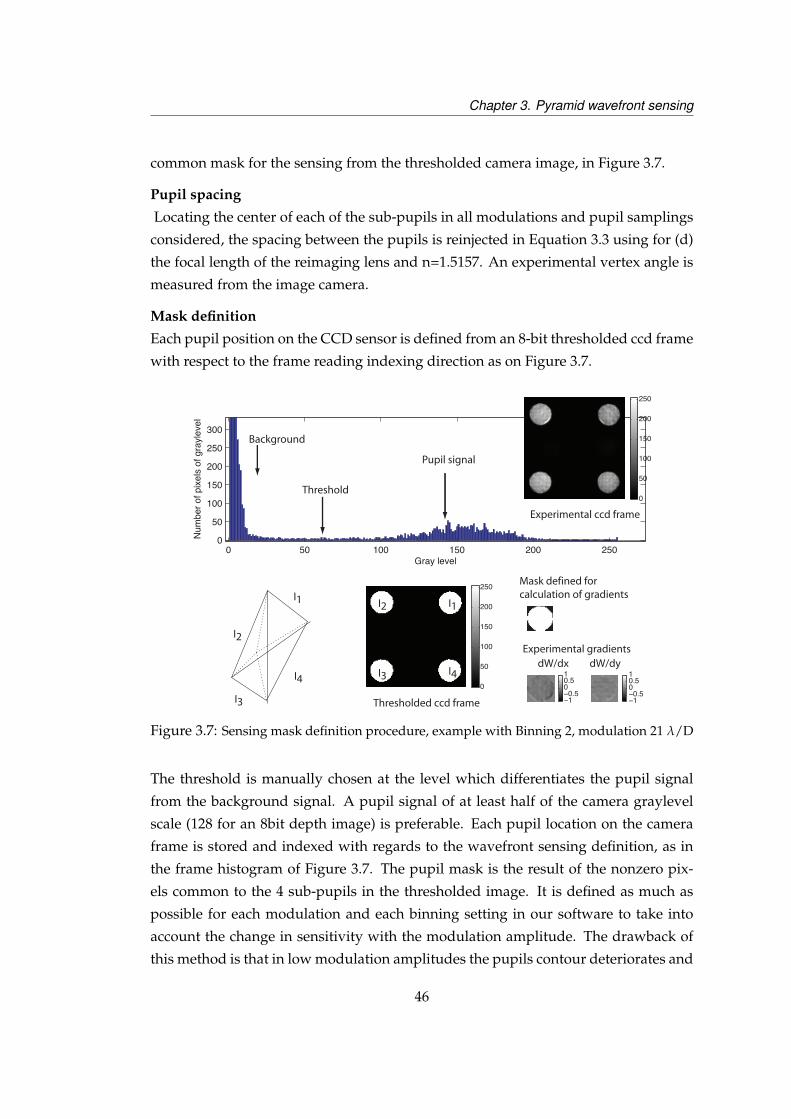
Chapter 3. Pyramid wavefront sensing
common mask for the sensing from the thresholded camera image, in Figure 3.7.
Pupil spacing
Locating the center of each of the sub-pupils in all modulations and pupil samplings
considered, the spacing between the pupils is reinjected in Equation 3.3 using for (d)
the focal length of the reimaging lens and n=1.5157. An experimental vertex angle is
measured from the image camera.
Mask definition
Each pupil position on the CCD sensor is defined from an 8-bit thresholded ccd frame
with respect to the frame reading indexing direction as on Figure 3.7.
Mask defined for calculation of gradients
0 50 100 150 200 2500
50
100
150
200
250
300
Gray level
Num
ber o
f pix
els
of g
rayl
evel
Pupil signal
Background
Threshold
0
50
100
150
200
250
Thresholded ccd frame
I1I2
I3 I4dW/dx dW/dy
Experimental gradients
−1−0.500.51
−1−0.500.51
I1
I2
I3
I4
0
50
100
150
200
250
Experimental ccd frame
Figure 3.7: Sensing mask definition procedure, example with Binning 2, modulation 21 λ/D
The threshold is manually chosen at the level which differentiates the pupil signal
from the background signal. A pupil signal of at least half of the camera graylevel
scale (128 for an 8bit depth image) is preferable. Each pupil location on the camera
frame is stored and indexed with regards to the wavefront sensing definition, as in
the frame histogram of Figure 3.7. The pupil mask is the result of the nonzero pix-
els common to the 4 sub-pupils in the thresholded image. It is defined as much as
possible for each modulation and each binning setting in our software to take into
account the change in sensitivity with the modulation amplitude. The drawback of
this method is that in low modulation amplitudes the pupils contour deteriorates and
46

Chapter 3. Pyramid wavefront sensing
it is better to use a mask defined in median modulation.
Pupil intensity balance
From the theory in Section 3.2.2.1, Equation 3.6, the sensor signals for a flat wavefront
should be only composed of zeros given the equal distribution of the signal over the
4 facets of the prism. Due to the noise in the system instead the gradient signals
spread around the zero-value into a Gaussian shaped curve as seen from Figure 3.8.
As the ‘flat’ wavefront described here is taken as reference for further calibration of
the influence functions for the closed loop the sensor must see it as free of aberration
as possible. If the pyramid is not well centered on the modulation circle the gradients
signal distribution is decentered from the zero, which is for the sensor equivalent to a
wavefront tilt. The centering of the sensor signals thus define a ‘flat’ reference used as
closed loop convergence criterion stability. For an open loop measurement this wave-
front can be used as reference in subtraction only if the aberrated surface is placed in
the pupil plane of the calibration arm. For ocular measurement however there would
be no possible comparison, given the source of the sensor signal at the retina presents
a different initial definition and is subject to different noise characteristics than the
calibration wavefront.
An approximation of the magnitude of the signal deterioration due to the noise can
be obtained by fitting the sensor signal to a Gaussian function. The characteristics
of the fit contain information on the quality of the calibration in relation to the sen-
sor pupil sampling and signal accuracy. The distributions of sensor signal for each
orientation (horizontal and vertical) per pupil sampling (1-4) and modulation ampli-
tude (9-33λ/D) is displayed in Figure 3.8. A single camera frame is considered, the
sensor signal calculated from this frame for a pixel is counted as part of one of the
41 intervals of 0.05 width over the [-1:1] full interval of possible sensor signal values.
Each histogram is normalised by the maximal number of counts and averaged over
all the binnings. The resulting plot in Figure 3.8 represents the distribution profile
for the three tests modulations, averaged over the pixel size in both directions. It can
be approximated by a gaussian which standard deviation at the 1/e2 of the maximal
intensity would be σ ≈ 0.1.
The widening of the distribution around the maximal value for the small modulation
amplitude is expected as the higher signal sensitivity of that dynamic range to small
wavefront aberrations. For higher modulations the loss in signal sensitivity returned
a signal similarly approximated to a Gaussian profile which standard deviation at
47
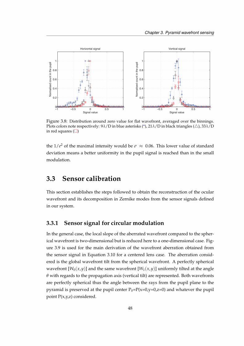
Chapter 3. Pyramid wavefront sensing
−1 −0.5 0 0.5 10
0.2
0.4
0.6
0.8
1
Horizontal signal
Signal value
No
rma
lise
d c
ou
nt in
th
e p
up
il
−1 −0.5 0 0.5 10
0.2
0.4
0.6
0.8
1
Vertical signal
Signal value
No
rma
lise
d c
ou
nt in
th
e p
up
il
Figure 3.8: Distribution around zero value for flat wavefront, averaged over the binnings.Plots colors note respectively: 9λ/D in blue asterisks (*), 21λ/D in black triangles (4), 33λ/Din red squares ()
the 1/e2 of the maximal intensity would be σ ≈ 0.06. This lower value of standard
deviation means a better uniformity in the pupil signal is reached than in the small
modulation.
3.3 Sensor calibration
This section establishes the steps followed to obtain the reconstruction of the ocular
wavefront and its decomposition in Zernike modes from the sensor signals defined
in our system.
3.3.1 Sensor signal for circular modulation
In the general case, the local slope of the aberrated wavefront compared to the spher-
ical wavefront is two-dimensional but is reduced here to a one-dimensional case. Fig-
ure 3.9 is used for the main derivation of the wavefront aberration obtained from
the sensor signal in Equation 3.10 for a centered lens case. The aberration consid-
ered is the global wavefront tilt from the spherical wavefront. A perfectly spherical
wavefront [W0(x,y)] and the same wavefront [W1(x,y)] uniformly tilted at the angle
θ with regards to the propagation axis (vertical tilt) are represented. Both wavefronts
are perfectly spherical thus the angle between the rays from the pupil plane to the
pyramid is preserved at the pupil center P0=P(x=0,y=0,z=0) and whatever the pupil
point P(x,y,z) considered.
48
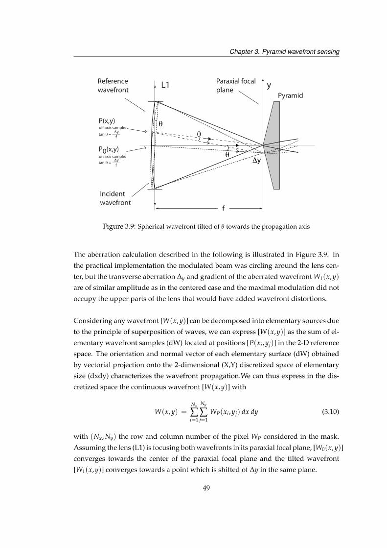
Chapter 3. Pyramid wavefront sensing
yL1Referencewavefront
P(x,y)
Incidentwavefront
Paraxial focalplane
Pyramid
f
Δyθ
θθ
on axis sample:
tan θ =Δyf
off axis sample:
tan θ =Δyf
P0(x,y)
Figure 3.9: Spherical wavefront tilted of θ towards the propagation axis
The aberration calculation described in the following is illustrated in Figure 3.9. In
the practical implementation the modulated beam was circling around the lens cen-
ter, but the transverse aberration ∆y and gradient of the aberrated wavefront W1(x,y)are of similar amplitude as in the centered case and the maximal modulation did not
occupy the upper parts of the lens that would have added wavefront distortions.
Considering any wavefront [W(x,y)] can be decomposed into elementary sources due
to the principle of superposition of waves, we can express [W(x,y)] as the sum of el-
ementary wavefront samples (dW) located at positions [P(xi,yj)] in the 2-D reference
space. The orientation and normal vector of each elementary surface (dW) obtained
by vectorial projection onto the 2-dimensional (X,Y) discretized space of elementary
size (dxdy) characterizes the wavefront propagation.We can thus express in the dis-
cretized space the continuous wavefront [W(x,y)] with
W(x,y) =Nx
∑i=1
Ny
∑j=1
WP(xi,yj) dx dy (3.10)
with (Nx, Ny) the row and column number of the pixel WP considered in the mask.
Assuming the lens (L1) is focusing both wavefronts in its paraxial focal plane, [W0(x,y)]
converges towards the center of the paraxial focal plane and the tilted wavefront
[W1(x,y)] converges towards a point which is shifted of ∆y in the same plane.
49
Chapter 3. Pyramid wavefront sensing
At the center of the pupil in P(x=0,y=0,z=0) the relationship
∆y = f tan(θ) (3.11)
describes the transverse ray aberration in the pyramid plane for the tilted wavefront.
For any wavefront element [P(x,y)] of the pupil, the angle between the normal to the
tilted wavefront [W1(x,y)] and the normal to the spherical wavefront [W0(x,y)] is (θ).
The transverse ray aberration ∆y defined in Equation 3.11 for the central point P0 of
the pupil is thus constant over the whole surface of the tilted spherical wavefront. At
any [P(x,y)] of the plane, the wavefront gradient is :
∂W1(x,y)∂y
= tanθ (3.12)
By using 3.12 into 3.11, we can relate the wavefront gradient to the transverse ray
aberration :
∆y = f∂W1(x,y)
∂y= f tan(θ) (3.13)
We know from the use of circular modulation that the integrated signals sx, sy at the
detector are linked to the transverse aberration ∆y (originated from the tilt θ) by Equa-
tion 3.8 which we write here:
∆y = Rmod sin
(π
2sy
)(3.14)
As Equation 3.13 and Equation 3.14 are equal, we obtain a relationship between the
sensor signal in the vertical direction sy(x′i ,y′j), (i = 1 : Nx, j = 1 : Ny) and the tilt pre-
sented by W1(x,y).
As the tilt is continuous and constant over W1, this gives using Eq. 3.10 into Eq. 3.12
and for tan(θ):
∂W1
∂y=
Nx
∑i=1
Ny
∑j=1
∂WP1(xi,yj)∂y
=Nx
∑i=1
Ny
∑j=1
tan(θij) = tan(θ) (3.15)
As the sensor signal is composed of all the signals of the pupils, from Eq. 3.10, the
conjugated pupil plane can be discretized into ( N = i x j ) wavefront samples, we can
50

Chapter 3. Pyramid wavefront sensing
write for the ensemble of the conjugated pupil elements
Nx
∑i=1
Ny
∑j=1
∂WP(xi ,yj)
∂y=
Nx
∑i=1
Ny
∑j=1
tan(θij) =Nx
∑i=1
Ny
∑j=1
Rmod
fsin
(π
2sy(x′i ,y
′j)
)(3.16)
This relationship also expresses that the wavefront secondary sources are well de-
scribed by the ensemble of local tilts θPij given by the sensor signals obtained from
the intensity in the detector region corresponding to P.
In the following, Eq. 3.16 in its single-element version will be the one mainly used to
describe the relationship between a local wavefront departure and the sensor signal
considering that any local wavefront departure from the ‘ideal’ spherical wavefront
at [P(x,y)] can be decomposed into 2 independently tilted elements.
This will lead to consider that any wavefront gradient at the conjugated pupil plane
can be written by its decomposition:
∂WP(x,y)∂i(i=x,y)
=Rmod
fsin
(π
2si,(i=x,y)(x′,y′)
)(3.17)
In general, the wavefront aberrations are not uniform over the pupil aperture, which
creates the discrepancies of intensity distribution in the conjugated pupils at the ccd.
Equation 3.17 however applies to each pupil element (i)(i=1,Nsamples) which leads to a
distribution of wavefront aberrations θi and transverse aberrations ∆yi.
The sensor signal sy is obtained by vertical differentiation of the detector pupil in-
tensities (Ii)(i=1,4) for the pixel conjugated with P(x,y) from development of Equation
3.6:
sy(x′,y′) =[I1(x′,y′) + I2(x′,y′)]− [I3(x′,y′) + I4(x′,y′)]
I1(x′,y′) + I2(x′,y′) + I3(x′,y′) + I4(x′,y′)
The expression is similar for a tilt in the horizontal direction with the horizontal wave-
front gradient [∂W(x,y)/∂x] with this time sx :
sx(x′,y′) =[I1(x′,y′) + I4(x′,y′)]− [I2(x′,y′) + I3(x′,y′)]
I1(x′,y′) + I2(x′,y′) + I3(x′,y′) + I4(x′,y′)
We see that the sensor saturation occurs when the signal si(x′,y′) reaches ±1, that is
51
Chapter 3. Pyramid wavefront sensing
when the wavefront tilt displaces the signal onto only 2 facets of the prism.
In that case the aberration ∆y of Figure 3.4 is larger than the radius of modulation
Rmod, and in turn the sensor detects a zero-signal in the top (I1=0),(I2=0) pupils and a
maximal signal in the down ones: (I3=Imax), (I4=Imax).
Hence : sx(x,y) = [0+Imax ]−[0+Imax ]0+0+Imax+Imax
= 0
sy(x,y) = [0+0]−[Imax+Imax ]0+0+Imax+Imax
= −1
This limits to sxy=[-1,1] the range of values retrieved by the sensor, and means the
saturation is occurring when the range boundaries are reached.
Reversing Equation 3.17, using the angular equality of Equation 3.16 we can access
the sensor signal sxy for a given tilt θt which defines arcsine(θt)≤ |π/2|. Outside these
boundaries for higher angles Matlab defines complex numbers which, approximated
by the equality arcsine(θt) = |π/2| describe the sensor saturation. Equation 3.18
shows the theoretical sensor signal for an uniform tilt of the spherical wavefront is
constant over the pupil.
sxy =2π
arcsin
[f
Rmodtan(θij)
](3.18)
Higher angles correspond to the saturation of the signal. The arcsine function is at
π/2, that is that the angle θij projects the modulated beam on a single side of the
pyramid:
sxy = ±1 ⇔ tanθij w ±Rmod
f(3.19)
The sign of the gradients is linked to the tilt direction. Equation 3.19 is consistent with
the configuration of saturation described using geometrical optics in Section 3.2.2.1,
Figure 3.4. The theoretical signal defined by the tilt amplitude experimentally ap-
plied at the pupil of the eye is compared to the mean signal calculated over all pupil
samples in Section 3.3.2, Figure 3.10.
3.3.2 Sensitivity range of the sensor
A flat wavefront at the pupil plane of the eye was defined by the Thorlabs fibre-
coupled laser diode output with collimation lens assembly. Introducing a known
52
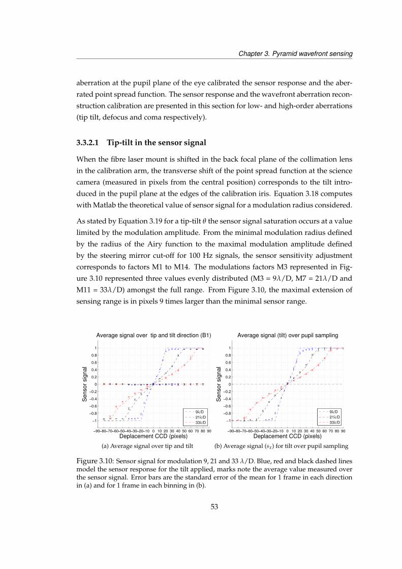
Chapter 3. Pyramid wavefront sensing
aberration at the pupil plane of the eye calibrated the sensor response and the aber-
rated point spread function. The sensor response and the wavefront aberration recon-
struction calibration are presented in this section for low- and high-order aberrations
(tip tilt, defocus and coma respectively).
3.3.2.1 Tip-tilt in the sensor signal
When the fibre laser mount is shifted in the back focal plane of the collimation lens
in the calibration arm, the transverse shift of the point spread function at the science
camera (measured in pixels from the central position) corresponds to the tilt intro-
duced in the pupil plane at the edges of the calibration iris. Equation 3.18 computes
with Matlab the theoretical value of sensor signal for a modulation radius considered.
As stated by Equation 3.19 for a tip-tilt θ the sensor signal saturation occurs at a value
limited by the modulation amplitude. From the minimal modulation radius defined
by the radius of the Airy function to the maximal modulation amplitude defined
by the steering mirror cut-off for 100 Hz signals, the sensor sensitivity adjustment
corresponds to factors M1 to M14. The modulations factors M3 represented in Fig-
ure 3.10 represented three values evenly distributed (M3 = 9λ/D, M7 = 21λ/D and
M11 = 33λ/D) amongst the full range. From Figure 3.10, the maximal extension of
sensing range is in pixels 9 times larger than the minimal sensor range.
−90−80−70−60−50−40−30−20−10 0 10 20 30 40 50 60 70 80 90
−1
−0.8
−0.6
−0.4
−0.2
0
0.2
0.4
0.6
0.8
1
Deplacement CCD (pixels)
Se
nso
r sig
na
l
Average signal over tip and tilt direction (B1)
9λ/D
21λ/D
33λ/D
(a) Average signal over tip and tilt
−90−80−70−60−50−40−30−20−10 0 10 20 30 40 50 60 70 80 90
−1
−0.8
−0.6
−0.4
−0.2
0
0.2
0.4
0.6
0.8
1
Deplacement CCD (pixels)
Se
nso
r sig
na
l
Average signal (tilt) over pupil sampling
9λ/D
21λ/D
33λ/D
(b) Average signal (sx) for tilt over pupil sampling
Figure 3.10: Sensor signal for modulation 9, 21 and 33 λ/D. Blue, red and black dashed linesmodel the sensor response for the tilt applied, marks note the average value measured overthe sensor signal. Error bars are the standard error of the mean for 1 frame in each directionin (a) and for 1 frame in each binning in (b).
53

Chapter 3. Pyramid wavefront sensing
The comparison of the computed sensor signal with the experimental signal recorded
over tip and tilt directions is presented in Figure 3.10a. The amplitude of the standard
deviation of the mean shows that the sensor response is consistent with the theory in
both directions of tilt. The same measurement performed over a single direction (tilt)
but with a variable number of samples in the pupil is presented in Figure 3.10b. The
amplitude of the standard deviation of the mean shows the measured signal is consis-
tent with the theory for all the pupil sampling configurations. In turn, the comparison
of the model with the experimental signal shows few errors for the direction parame-
ter and the same is observed for the wavefront sampling parameter. In both cases the
experimental data and the model are thus in excellent agreement.
3.3.2.2 Defocus in the sensor signal
As the derivative of the defocus aberration is a linear function of the pupil position
[42], the limit sensor signal before saturation can be numerically computed as a linear
distribution across the pupil. At the limit of the sensing range, the signal across the
pupil sxD is linearly distributed from (c = -1) to (c = 1). For higher defocus the (±1)
boundary value overfills the pupil gradient with only (-1) and (1) values. For a given
modulation amplitude, a computed sensor map as expressed in Equation 3.20 with |c|= 1, simulates the defocus derivative along the horizontal direction with 56 wavefront
samples (Binning 1) across the sensor pupil for the two modulation radii Rmod = 9 λ/D
and Rmod = 33 λ/D :
sx∆(xpup) =xpup
rpupwith : xpup = [−rpup : +rpup] (3.20)
∂ϕ∆
∂x=
2π
λtan(Rmod
f
)sin(π
2sx∆
)(3.21)
ϕ∆ describes the phase aberration of the defocus value for which the limit of the sens-
ing range is reached in the geometrical approximation. The notation ∆ replaces in the
following the conventional notation for the wavefront defocus in Dioptres units (D)
here used to describe the pupil diameter for the modulation.
The sensor signal was acquired after implementation in the pupil plane of the cali-
bration assembly of a convex ophthalmic lens of +0.5 ∆ and +1.5 ∆ power. The cross
section of the horizontal and vertical gradient recorded at the three test modulations
is represented in Figure 3.11 as a function of the sample position in the pupil. The ex-
54

Chapter 3. Pyramid wavefront sensing
perimental signal of Figure 3.11 is compared to the typical sensor signal for a defocus
gradient at the saturation limit for the modulation amplitude considered (given by
Equation 3.21).
−7−6.5−6−5.5−5−4.5−4−3.5−3−2.5−2−1.5−1−0.5 0 0.5 1 1.5 2 2.5 3 3.5 4 4.5 5 5.5 6 6.5 7
x 104
−1
−0.8
−0.6
−0.4
−0.2
0
0.2
0.4
0.6
0.8
1Phase defocus gradient Binning 1
Gradient dϕD / dx [m−1]
Sens
or s
igna
l Sx
Figure 3.11: Sensor signal for defocus: sensor signal modelled for a given modulation,(dashed line from -1 to +1). The signals cross-sections for 0.5Dioptre(∆) sphere lens (squared)show the same±2.7m−1 gradient amplitude as the sensor saturation is not reached and showsaturation is reached for 1.5 Dioptre(∆) (crossed marks).
For a small aberration (±0.5 Dioptre(∆) square marks) the sensor signal is distributed
between±0.8 in modulation 9λ/D and±0.4 in modulation 33λ/D. The range bound-
aries are reached at ±1.5 Dioptre(∆) when the sensor signal are at ±1. This highlights
that 0.5 Dioptre(∆) defocus remains in the linear range for the 33λ/D modulation
while it saturates the 9λ/D range. This also shows that the sine function would be cor-
rectly approximated by its argument in the former modulation. However, for a higher
sphere refraction power such as 1.5 Dioptre(∆), given the gradient is distributed over
more than the linear range the linear approximation would not be valid.
The second observation is that the sensor modulation ranges are appropriately cho-
sen with regards to the generally accepted amplitude of refractive errors in the human
population [95,96,97] as the range could again be extended for higher defocus ampli-
tudes.
55
Chapter 3. Pyramid wavefront sensing
3.3.3 Wavefront reconstruction for high-order aberrations
In this section we explain the procedure followed for obtaining the values of the
wavefront aberration measurement in ophthalmic terms. The wavefront decompo-
sition in coefficients of orthonormal Zernike circle polynomials is first presented in
relationship with a given wavefront sampling and sensitivity regime. This establishes
the equivalence of signal processing in the Shack-Hartmann and the pyramid sensors
for a known quantity of low-and high-order aberrations in single pass. The optical
system for aberration measurements in the human eye in-vivo is described and the
results are commented upon.
3.3.3.1 Aberration map reconstruction
Wavefront measurements are expressed in units of phase aberration (waves) or in
metric units (µm), quantifying the wavefront departure from the reference sphere as
the root-mean-square (rms) wavefront error. The guidelines [43] recommend the use
of the Zernike circular polynomials towards other notations [98]. Matlab functions for
the reconstruction are available on-line [99]. The conversion of the sensor signals into
phase gradient maps is performed before the least-squares fit of the sensor gradients
map onto the (1-N) vectors of the basis of Zernike maps derivative. The wavefront is
reconstructed using the coefficients of the fit for each order N.
In this ophthalmic convention a Zernike term Zmn describes a typical aberration pat-
tern in polar coordinates (ρ,θ) with ρ = [0,1] the normalized radius of the pupil and
θ = [0,2π] the angle made to the vertical axis, as a function of a normalization fac-
tor Nmn , a radial-dependent component Rm
n , and an azimuthal-dependent component.
The double indexing scheme (n,m) expresses the polynomial spatial content through
the radial order index n and the pattern shape through the angular frequency m.
Zj(ρ,θ) = Zmn (ρ,θ) =
√
(n + 1)R0n for m = 0√
2(n + 1)R|m|n cos(mθ) for m > 0
−√
2(n + 1)R|m|n sin(mθ) for m < 0
(3.22)
The radial component R|m|n in Equation 3.22 is given by
R|m|n (ρ) =(n−|m|)/2
∑s=0
(−1)s (n− s)s[(n + |m| − s)][(n− |m| − s)]
ρn−2s (3.23)
56
Chapter 3. Pyramid wavefront sensing
In this thesis the single indexing notation j was mainly used, as equivalently defining
the decomposition order :
n = roundup[−3+
√9+8j
2
]m = 2j− n(n + 2)j = 0,1,2, ...N
(3.24)
In the single-indexing notation the first terms of the decomposition (j=0, piston, j=1,
tip and j=2, tilt) are usually excluded from the expression of the wavefront aberration.
The wavefront aberration W is expressed using N polynomial terms of the decompo-
sition:
W(ρ,θ) =N
∑j=3
ajZj(ρ,θ) (3.25)
In which the coefficients amplitude aj in (µm) is given by the integrals of the inner
product over the normalized pupil A.
aj =∫ ∫
AWj(ρ,θ)Zj(ρ,θ)dρdθ (3.26)
Given the Zernike polynomials are defined on an orthonormal basis, the terms of
the decomposition are independent thus for an infinite number of terms only the
wavefront root mean squared error (RMS) is the squared root sum of the squared
coefficients a2j [100]. As the wavefront is reconstructed over a finite number (N) of
modes, the rms obtained by the Matlab sum of coefficients is only approximate.
RMS = σ =
√√√√ N
∑j=3
a2j (3.27)
Tip and tilt coefficients (j = 1 , j = 2) were removed from the rms calculation so as
to consider only the higher orders. The error on a Zernike term for the mean value
presented was defined by the standard deviation of the mean of the term for a series
of static measurements. This variation was very low for the calibration compared to
the measurement of the dynamic ocular aberration.
The maximal number (N) of modes used for the reconstruction is usually determined
by the number of actuators of the deformable mirror. The 52-elements electro-magnetically
actuated membrane of the Mirao deformable mirror has numerically shown a diffraction-
limited fitting of ocular wavefronts was obtained using 30 mirror modes [47] thus (N)
57

Chapter 3. Pyramid wavefront sensing
was set to 35 in the adaptive optics system. For faster computation the reconstruction
of the wavefront aberration from the sensor signal was performed with 15 modes (or-
der n=4) or with 35 modes (order n=7) for a best accuracy of the reconstruction as
recommended by Hampson [101]. For reading clarity most decompositions were dis-
played in the following up to the 21rst term (order n=5). Experimental adjustments
towards this value for the adaptive optics are presented in Chapter 4.
3.3.3.2 Maximal measurable aberration for a Zernike radial order
In a Shack-Hartmann the pupil sampling is determined by the number of lenslets
across the pupil while the sensitivity range depends on the focal length of the lenslets.
The maximal wavefront aberration Wmax measured by the sensor for a given Zernike
radial order can be expressed in function of the lenslet array characteristics [102]:
Wmax
λ=
Nl NFr
4nwith:
Nl Samples (lenslets or pixels) across the pupilNFr = d2
f ′λ Fresnel number of the lenslet
d Lenslet (pupil sample) diameterf ′ Lenslet focal lengthλ Wavelengthn Zernike radial order
(3.28)
Equation 3.28 is useful for the design of an aberrometer as it can determine the choice
of the lenslet array focal length and pitch. Provided indeed that an estimate of the
measurement amplitude is known, the Shack-Hartmann parameters can be defined
so as to sample properly the amplitude of the radial order (n). For an aberrometer of
variable sampling and dynamic range such as the pyramid sensor used in this work
we propose to apply these relationships to compare our sensor to other aberrometers.
In the pyramid, Nl the number of samples of individual size (d) across the pupil can
be varied using the sensor camera binning. A given modulation Rmod determines
the sensor dynamic range. Saturation means a sensor signal at ±1 thus the sensor
58
Chapter 3. Pyramid wavefront sensing
equation for the transverse aberration Equation 3.17 becomes:
∂WP(x,y)∂i(i=x,y)
∣∣∣∣∣max(tiptilt)
=Rmod
fsin[π/2(±1)] (3.29)
=Rmod
f(3.30)
= θmax following Equation 3.15 (3.31)
With f the focal length of the focusing lens before the pyramid and θmax the tip/tilt
amplitude at the saturation limit.
The wavefront aberration tilt for θ = θmax in the pupil plane is Wmax(tiptilt) :
Wmax(tiptilt) = d sinθmax ≈ d θmax if sinθ ≈ θ (small angles approximation) (3.32)
A single pupil sample is of size (d), and the whole pupil of size (D). The angles mea-
sured in this experiment are well within the range that validate the approximation
(±6) and Equation 3.32 thus applies for the pyramid.
For Nl samples in the pupil, D = d× Nl . The binning factor and Nl are related by the
minimal pupil subaperture size (N0) in the camera minimal binning (highest pupil
spatial sampling). Thus :
Nl = binning× N0 (3.33)
Equation 3.33 expresses the change in the number of samples in the pupil with the
binning factor for the pyramid, that is the equivalence with the change in the number
of lenslets.
Replacing in Equation 3.32 the maximal angle by the modulation factor from Equa-
tion 3.31, the maximal wavefront aberration due to tip/tilt for the pyramid subpupil
is :
Wmax(tiptilt) =df
Rmod in the small angles approximation (3.34)
As ( f ) the focusing length is fixed, and (d) is fixed for a given camera binning, Equa-
tion 3.34 shows that in the pyramid the modulation factor determines the limit for the
59

Chapter 3. Pyramid wavefront sensing
maximal wavefront aberration due to tilt.
The equivalence between Equation 3.28 for (n = 1 for tip and tilt) at a given pupil
sampling (Nl) and Equation 3.34 considering a similar sampling and pupil size leads
to a modulation radius value that describes the dynamic range of an equivalent Shack
- Hartmann. For the tip tilt order n=1 thus Rmod = Rmod(n=1) :
From (3.28≡ 3.34) :
(Wmax(tiptilt) =
df ′
dNl
4
)≡(
Wmax(tiptilt) =df
Rmod(n=1)
)(3.35)
We can identify:
[f
dNl
4 f ′= Rmod(n=1)
](3.36)
If f ′SHS = fPWS :
[dNl
4= Rmod(n=1)
f ′= f
](3.37)
If the focal lengths of the Shack-Hartmann and of the pyramid are equal and the pupil
samplings are equal, as in Equation 3.37 then the modulation radius that leads to an
equivalent Shack-Hartmann dynamic range for tilt is Rmod(n=1). The use of a higher
or lower modulation range is equivalent to a change in the Shack-Hartmann lenslet
focal length (f’) in Equation 3.36.
For any order and any sampling, we can use Equation 3.36 into Equation 3.28. The
‘base’ modulation radius of the sensor for any radial order appears for f = f ′, and the
change in sampling across the pupil Nl is also taken into account. For each case :
If f’ 6= f : Wmax(n) =dn
ff ′
dNl
4with thus Rmod(n) =
ff ′
dNl
4n(3.38)
If f’=f : Wmax(n) =dn
dNl
4with thus Rmod(n) =
dNl
4n(3.39)
This means that for a given pupil sampling and modulation at the sensor the maximal
measurable wavefront aberration of a Zernike order in the decomposition is known.
In our case the sensor was built before this study was performed, thus the huge focal
length of the first lens of the relay from the steering mirror to the wavefront sensing
camera turns this analysis into an irrealistic case for the Shack-Hartmann. However,
simulations using pyramid sensor signals in the wavefront reconstruction code show
60
Chapter 3. Pyramid wavefront sensing
a good agreement with the experiment for the tip tilt case and for the defocus.
For the particular case of tip and tilt (n=1) and a pupil sampling of Nl=52 pixels across
the pupil, with each pixel in the pupil plane of size d = 0.067 mm, and a focal length
f ′ = f = 250 mm, we can find the pyramid modulation factor that retrieves a similar
behavior as an equivalent SH. Replacing the values in Equation 3.37 gives Rmod(n=1)f ′= f
= 15×RAiry (M6.7 factor), that is almost the (M7) modulation. Using Equation 3.36
the modulation factor range of the pyramid system relates to the variation in the focal
length (f’) of the equivalent SH.
For further building of another pyramid system this set of relationships could be use-
ful for the designer. The characterization of the sensor dynamic range built in this
system is actually showing a large range for the base values, and small ranges that
are not very sensitive to small aberrations.
3.3.3.3 Tip/tilt and Defocus in Zernike decomposition
In both Figure 3.12a and Figure 3.12b the wavefront aberration presented was exper-
imentally determined after the average reconstruction over 5 single sensor acquisi-
tions. Zernike tilt term was obtained from the sensor signal recorded after transverse
displacement (tilt) of the fibre output at the back focal plane of the calibration lens as
in Section 3.3.2 in steps of 30 pixels at the retinal imaging camera. Zernike defocus
was tested using ophthalmic lenses of ±1.5 D sphere power in steps of ±0.5 D. Part
of this dataset was used for Figure 3.11.
Theoretical Zernike tilt signal was modelled using geometrical optics to relate the
lateral displacement of the point spread function at the science camera to the angu-
lar tilt at the pupil plane of the calibration arm and scaling for the pupil diameter to
obtain the aberration in micrometers. Theoretical defocus amplitude was modelled
using the conversion equations [103] from the refractive power of an ophthalmic lens
into Zernike decomposition.
The standard deviations of the mean for each point was of the order of 10−3µm thus
the measurement stability was verified for such static aberration. Sensor saturation
at a given dynamic range corresponded to a constant value of the aberration. Sensor
non-linearity was represented by the departure of the measurement from the theoret-
61

Chapter 3. Pyramid wavefront sensing
−8−7−6−5−4−3−2−1 0 1 2 3 4 5 6 7 8−8−7−6−5−4−3−2−1
012345678
Theoretical Zernike amplitude(µm)
Mea
sure
d Ze
rnik
e am
plitu
de (µ
m)
Tilt
Theory9!/D21!/D33!/D
(a)
−4 −3 −2 −1 0 1 2 3 4−4
−3
−2
−1
0
1
2
3
4
Zernike defocus expected (µm)
Ze
rnik
e d
efo
cu
s m
ea
su
red
(µ
m)
Zernike defocus reconstructedusing ophthalmic lenses
9λ/D
14λ/D
21λ/D
28λ/D
33λ/D
Theory
(b)
Figure 3.12: Tilt and Defocus measured at the highest pupil sampling (B1, 109µm per sam-ple). Horizontal dashed lines show the saturation limits of the Zernike term for each dynamicrange defined by the modulation factors 9, 21 and 33λ/D. Linearity of the sensor response issatisfied when the theoretical and measured term amplitudes correspond. Sensor saturationfor defocus is reached only at 9λ/D.
ical value. The tip-tilt non linearity range coincided with the saturation range while
the defocus non-linearity spread over a wider range of aberrations before the satura-
tion value.
3.3.3.4 Higher-order aberrations in Zernike decomposition
The static response of the system to typical ocular aberrations was measured in plac-
ing in the pupil plane of the calibration arm plastic plates engineered with a resin sub-
strate deposited in the shape of a known phase aberration [104]. Plate 1 and plate 2
were shaped as typical ocular aberrations of human eyes. Plate 3 and plate 4 were
shaped in a known amplitude of known aberration, defocus (Z20) and trefoil (Z16).
The plates wavefront aberration was first measured using a Twyman-Green interfer-
ometer (Fisba Optik, Switzerland) which provided high-resolution surface character-
isation of the patterns with 10 µm per wavefront sample over the 6 mm measurement
pupil. The plates were then positioned individually in the pupil plane of the calibra-
tion beam and the phase was measured at each of the 4 sensor sampling settings for
the 3 tests modulations. For each pupil sampling setting, 50 sensor measurements of
the aberration were acquired and the respective wavefronts reconstructed. A 10−3 µm
rms variability of the rms error over the 50 frames stated the stability of the sensor
62
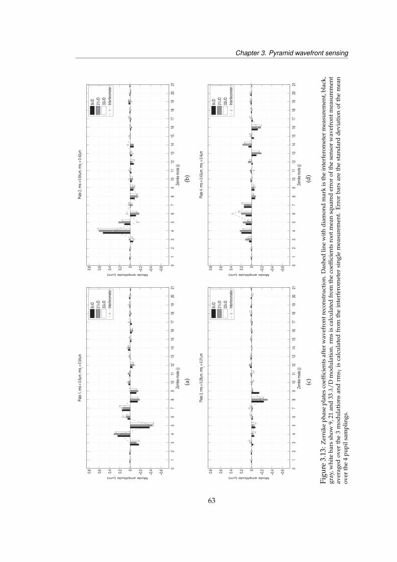
Chapter 3. Pyramid wavefront sensing
01
23
45
67
89
1011
1213
1415
1617
1819
2021
!0.6
!0.4
!0.200.20.40.60.8
Zernik
e mode
(j)
Mode amplitude (!m)Pla
te 1, rm
s = 0.6
!m, rm
s i = 0.54
!m
9"/
D21"
/D33"
/DInte
rferom
eter
(a)
01
23
45
67
89
1011
1213
1415
1617
1819
2021
!0.6
!0.4
!0.200.20.40.60.8
Zernik
e mode
(j)
Mode amplitude (!m)
Plate 2
, rms =
0.64!m
, rms i = 0
.42!m
9"/
D21"
/D33"
/DInte
rferom
eter
(b)
01
23
45
67
89
1011
1213
1415
1617
1819
2021
!0.6
!0.4
!0.200.20.40.60.8
Zernik
e mode
(j)
Mode amplitude (!m)
Plate 3
, rms =
0.28!m
, rms i = 0
.21!m
9"/
D21"
/D33"
/DInte
rferom
eter
(c)
01
23
45
67
89
1011
1213
1415
1617
1819
2021
!0.6
!0.4
!0.200.20.40.60.8
Zernik
e mode
(j)
Mode amplitude (!m)
Plate 4
, rms =
0.43!m
, rms i = 0
.4!m
9"/
D21"
/D33"
/DInte
rferom
eter
(d)
Figu
re3.
13:Z
erni
keph
ase
plat
esco
effic
ient
saf
ter
wav
efro
ntre
cons
truc
tion
.Das
hed
line
wit
hdi
amon
dm
ark
isth
ein
terf
erom
eter
mea
sure
men
t,bl
ack,
gray
,whi
teba
rssh
ow9,
21an
d33
λ/D
mod
ulat
ion.
rms
isca
lcul
ated
from
the
coef
ficie
nts
root
mea
nsq
uare
der
ror
ofth
ese
nsor
wav
efro
ntm
easu
rem
ent
aver
aged
over
the
3m
odul
atio
nsan
drm
s Iis
calc
ulat
edfr
omth
ein
terf
erom
eter
sing
lem
easu
rem
ent.
Erro
rba
rsar
eth
est
anda
rdde
viat
ion
ofth
em
ean
over
the
4pu
pils
ampl
ings
.
63

Chapter 3. Pyramid wavefront sensing
measurement for each pupil sampling. The aberration coefficients averaged over the
sampling setting for each dynamic range for each phase plate are displayed in Fig-
ure 3.13 with the wavefront decompositions fitted from the interferometer measure-
ment. The average wavefront rms for all dynamic ranges compared to the rms of the
plate measured by the interferometer is presented in the title of the displays in Fig-
ure 3.13. Detailed values of rms for each dynamic range averaged over the binning
are presented in Table 3.2.
For low order modes (defocus Z4, astigmatism Z3 and Z5) a higher coefficient vari-
ability with the pupil sampling was observed than for the higher orders. As the pyra-
mid is considered as an appropriate sensor for these modes, this effect could be re-
lated to the change in the pupil sampling. Additional astigmatism in the pyramid
measurement in plate 1 and 3 and defocus, and secondary astigmatism in plate 4
decreased the fit between the 2 measurement systems. These were attributed to the
slight changes in the plate lateral positioning, pupil size and reference wavefronts in
the respective setups [105].
Table 3.2: RMS of phase plates measured at modulation factors 9,21,33λ/D and with Fisbainterferometer. Standard deviation of each rms corresponds to the variation over the pupilsampling setting.
rms (µm) Plate 1 Plate 2 Plate 3 Plate 4
Interferometer 0.54 0.42 0.21 0.40M3 = 9λ/D 0.55±0.01 0.57±0.02 0.30±0.01 0.35±0.01M7 = 21λ/D 0.63±0.01 0.69±0.07 0.32±0.03 0.50±0.02M11 = 33λ/D 0.63±0.06 0.68±0.05 0.28±0.01 0.47±0.03Mean (all M) 0.60±0.04 0.65±0.05 0.30±0.02 0.44±0.06
An average rms variability of±0.03 µm with the pupil sampling was obtained for the
aberration measurement by the sensor. The sensor pupil sampling change was thus
not neglectible in the measurement of an aberration. The number of pupil samplings
sets tested here (4) was not sufficient to determine a trend. An average variability of
±0.04 µm with the dynamic range was obtained for the aberration measurement by
the sensor. This stated the influence of the sensor dynamic range on the aberration
measurement. The average rms measured by the sensor for each plate was of 0.1 µm
higher than the interferometer rms, which represented the differences in positioning
of the plate in the pupil plane and the differences between the sensor settings and the
interferometer settings. The suitability of the pyramid system built for these ranges
of aberrations was confirmed by comparison of the aberration amplitudes measured
64

Chapter 3. Pyramid wavefront sensing
with the calibration curves for defocus in Figure 3.12b. The phase plates aberrations
were well below the sensor limits for the modulation considered.
Influence of tip and tilt of the wavefront on the aberration measurement
The influence of the tip and tilt on the reconstruction of the wavefront is presented
in Figure 3.14 and Figure 3.15. The emphasis was put on the shape of the wavefront
reconstructed with or without account of the tip and tilt terms. A single sensor frame
was recorded for 8 tilts tested between the centering of the fibre position and satu-
ration of the sensor signal for the smallest modulation amplitude (M3=9λ/D) and
the highest pupil wavefront sampling (56 samples across the pupil). Figure 3.14 rep-
resents the average Zernike decomposition determined over the 8 wavefront recon-
structions. The 0.1 µm variability of the term amplitude for defocus (j=4), astigmatism
(j=5), spherical aberration (j=6) and coma (j=7) is due to the tip tilt increase.
0 1 2 3 4 5 6 7 8 9 10 11 12 13 14 15 16 17 18 19 20 21−1.6
−1.4
−1.2
−1
−0.8
−0.6
−0.4
−0.2
0
0.2
0.4
0.6
Zernike mode (j)
Mode a
mplit
ude (
µm
)
Average over 8 tilts amplitudes, with Tip Tilt
Figure 3.14: Plate 2 with increasing tilt measured by the sensor with 56 samples across thepupil and a modulation factor of 9λ/D, (M3). Error bars are the standard deviation of themean coefficient for the 8 tilt amplitudes measured. Interferometer coefficients in green. Blacksquares denote the tilt coefficients tested.
When applying progressively tip to the pupil plane by transverse movement of the
laser fibre head, the sensor phase measurement evolution is shown in Figure 3.15.
Figure 3.15a presented the on-axis measurement of plate no.2 in which the Zernike
tip and tilt coefficients had a zero-amplitude. Figure 3.15b presented the wavefront
reconstruction of the same phase plate for the highest tilt amplitude. Figure 3.15c rep-
resented the wavefront reconstruction of the phase plate measured with the highest
65
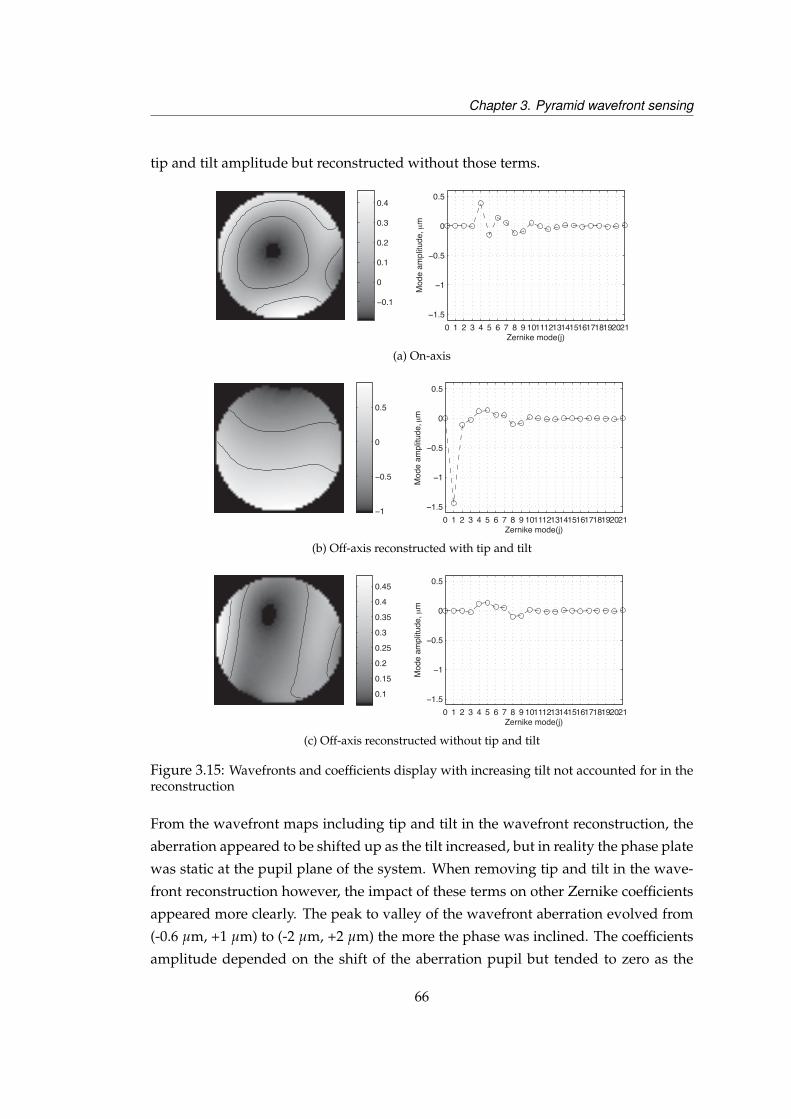
Chapter 3. Pyramid wavefront sensing
tip and tilt amplitude but reconstructed without those terms.
−0.1
0
0.1
0.2
0.3
0.4
0 1 2 3 4 5 6 7 8 9 101112131415161718192021−1.5
−1
−0.5
0
0.5
Zernike mode(j)
Mod
e am
plitu
de, μ
m
(a) On-axis
−1
−0.5
0
0.5
0 1 2 3 4 5 6 7 8 9 101112131415161718192021−1.5
−1
−0.5
0
0.5
Zernike mode(j)
Mod
e am
plitu
de, μ
m
(b) Off-axis reconstructed with tip and tilt
0.1
0.15
0.2
0.25
0.3
0.35
0.4
0.45
0 1 2 3 4 5 6 7 8 9 101112131415161718192021−1.5
−1
−0.5
0
0.5
Zernike mode(j)
Mod
e am
plitu
de, μ
m
(c) Off-axis reconstructed without tip and tilt
Figure 3.15: Wavefronts and coefficients display with increasing tilt not accounted for in thereconstruction
From the wavefront maps including tip and tilt in the wavefront reconstruction, the
aberration appeared to be shifted up as the tilt increased, but in reality the phase plate
was static at the pupil plane of the system. When removing tip and tilt in the wave-
front reconstruction however, the impact of these terms on other Zernike coefficients
appeared more clearly. The peak to valley of the wavefront aberration evolved from
(-0.6 µm, +1 µm) to (-2 µm, +2 µm) the more the phase was inclined. The coefficients
amplitude depended on the shift of the aberration pupil but tended to zero as the
66
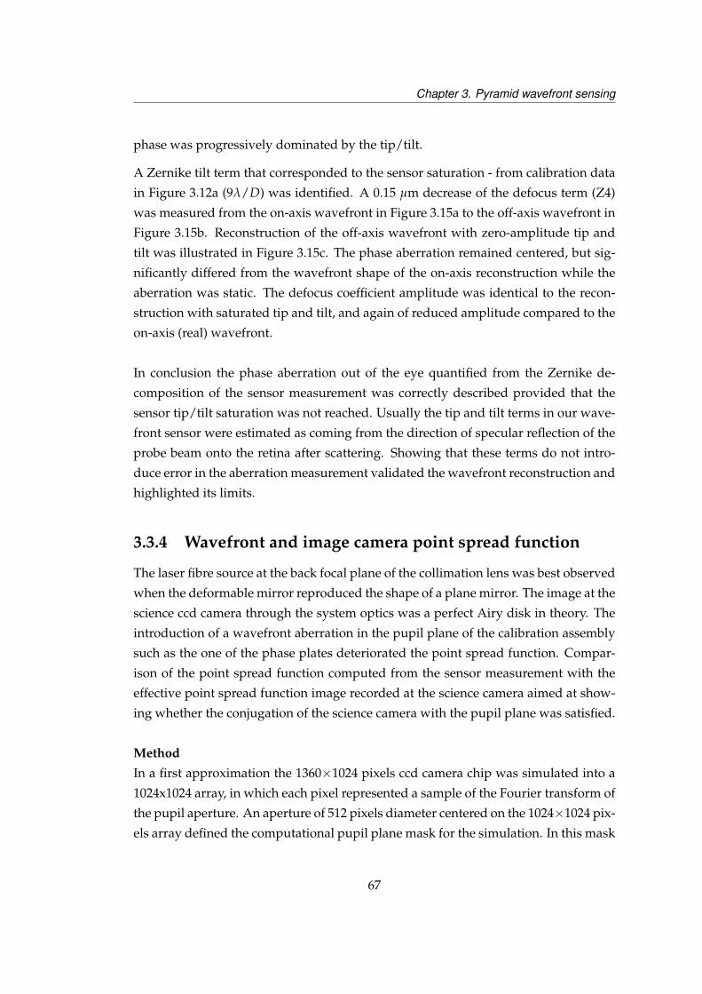
Chapter 3. Pyramid wavefront sensing
phase was progressively dominated by the tip/tilt.
A Zernike tilt term that corresponded to the sensor saturation - from calibration data
in Figure 3.12a (9λ/D) was identified. A 0.15 µm decrease of the defocus term (Z4)
was measured from the on-axis wavefront in Figure 3.15a to the off-axis wavefront in
Figure 3.15b. Reconstruction of the off-axis wavefront with zero-amplitude tip and
tilt was illustrated in Figure 3.15c. The phase aberration remained centered, but sig-
nificantly differed from the wavefront shape of the on-axis reconstruction while the
aberration was static. The defocus coefficient amplitude was identical to the recon-
struction with saturated tip and tilt, and again of reduced amplitude compared to the
on-axis (real) wavefront.
In conclusion the phase aberration out of the eye quantified from the Zernike de-
composition of the sensor measurement was correctly described provided that the
sensor tip/tilt saturation was not reached. Usually the tip and tilt terms in our wave-
front sensor were estimated as coming from the direction of specular reflection of the
probe beam onto the retina after scattering. Showing that these terms do not intro-
duce error in the aberration measurement validated the wavefront reconstruction and
highlighted its limits.
3.3.4 Wavefront and image camera point spread function
The laser fibre source at the back focal plane of the collimation lens was best observed
when the deformable mirror reproduced the shape of a plane mirror. The image at the
science ccd camera through the system optics was a perfect Airy disk in theory. The
introduction of a wavefront aberration in the pupil plane of the calibration assembly
such as the one of the phase plates deteriorated the point spread function. Compar-
ison of the point spread function computed from the sensor measurement with the
effective point spread function image recorded at the science camera aimed at show-
ing whether the conjugation of the science camera with the pupil plane was satisfied.
Method
In a first approximation the 1360×1024 pixels ccd camera chip was simulated into a
1024x1024 array, in which each pixel represented a sample of the Fourier transform of
the pupil aperture. An aperture of 512 pixels diameter centered on the 1024×1024 pix-
els array defined the computational pupil plane mask for the simulation. In this mask
67
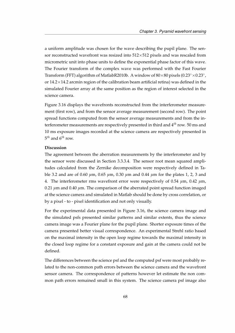
Chapter 3. Pyramid wavefront sensing
a uniform amplitude was chosen for the wave describing the pupil plane. The sen-
sor reconstructed wavefront was resized into 512×512 pixels and was rescaled from
micrometric unit into phase units to define the exponential phase factor of this wave.
The Fourier transform of the complex wave was performed with the Fast Fourier
Transform (FFT) algorithm of MatlabR2010b. A window of 80×80 pixels (0.23×0.23,
or 14.2×14.2 arcmin region of the calibration beam artificial retina) was defined in the
simulated Fourier array at the same position as the region of interest selected in the
science camera.
Figure 3.16 displays the wavefronts reconstructed from the interferometer measure-
ment (first row), and from the sensor average measurement (second row). The point
spread functions computed from the sensor average measurements and from the in-
terferometer measurements are respectively presented in third and 4th row. 50 ms and
10 ms exposure images recorded at the science camera are respectively presented in
5th and 6th row.
Discussion
The agreement between the aberration measurements by the interferometer and by
the sensor were discussed in Section 3.3.3.4. The sensor root mean squared ampli-
tudes calculated from the Zernike decomposition were respectively defined in Ta-
ble 3.2 and are of 0.60 µm, 0.65 µm, 0.30 µm and 0.44 µm for the plates 1, 2, 3 and
4. The interferometer rms wavefront error were respectively of 0.54 µm, 0.42 µm,
0.21 µm and 0.40 µm. The comparison of the aberrated point spread function imaged
at the science camera and simulated in Matlab should be done by cross correlation, or
by a pixel - to - pixel identification and not only visually.
For the experimental data presented in Figure 3.16, the science camera image and
the simulated psfs presented similar patterns and similar extents, thus the science
camera image was a Fourier plane for the pupil plane. Shorter exposure times of the
camera presented better visual correspondence. An experimental Strehl ratio based
on the maximal intensity in the open loop regime towards the maximal intensity in
the closed loop regime for a constant exposure and gain at the camera could not be
defined.
The differences between the science psf and the computed psf were most probably re-
lated to the non-common path errors between the science camera and the wavefront
sensor camera. The correspondence of patterns however let estimate the non com-
mon path errors remained small in this system. The science camera psf image also
68
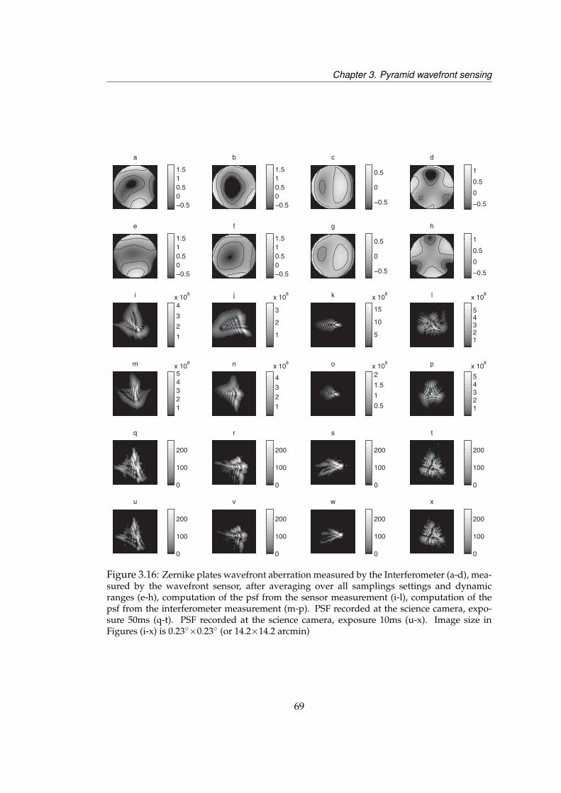
Chapter 3. Pyramid wavefront sensing
a
−0.500.511.5
b
−0.500.511.5
c
−0.5
0
0.5
d
−0.500.51
e
−0.500.511.5
f
−0.500.511.5
g
−0.5
0
0.5
h
−0.500.51
i
1234
x 108 j
1
2
3
x 108 k
5
10
15x 108 l
12345
x 108
m
12345
x 108 n
1234
x 108 o
0.511.52
x 109 p
12345
x 108
q
0
100
200
r
0
100
200
s
0
100
200
t
0
100
200
u
0
100
200
v
0
100
200
w
0
100
200
x
0
100
200
Figure 3.16: Zernike plates wavefront aberration measured by the Interferometer (a-d), mea-sured by the wavefront sensor, after averaging over all samplings settings and dynamicranges (e-h), computation of the psf from the sensor measurement (i-l), computation of thepsf from the interferometer measurement (m-p). PSF recorded at the science camera, expo-sure 50ms (q-t). PSF recorded at the science camera, exposure 10ms (u-x). Image size inFigures (i-x) is 0.23×0.23 (or 14.2×14.2 arcmin)
69

Chapter 3. Pyramid wavefront sensing
depended on factors such as the camera image exposure, gain, binning and the laser
power used.
3.4 Summary
This Chapter described the implementation of the ocular aberration measurement
with the pyramid wavefront sensor. Section 3.1 introduced the applications of the
pyramid wavefront sensor. Section 3.2 described the mathematical basis of the wave-
front sensor measurement and the optical system. All equations for the sensor sen-
sitivity were derived assuming the focusing into an Airy disk pattern. The base sen-
sitivity of the pyramid system was defined by the f-number of the wavefront sens-
ing beam onto the pyramid, and the beam modulation extended the sensor dynamic
range.
Section 3.3 demonstrated a calibration method for verification of our results in terms
of Zernike coefficients. Using a set of phase plates calibrated with a high-resolution
interferometer to introduce an aberration in the pupil plane of the calibration beam,
the aberration reconstruction from the sensor measurement presented an rms in-
creased of 0.1 µm compared to the aberration reconstructed from the interferometer
measurement. The wavefront reconstruction from the sensor signal for 50 successive
frames highlighted an rms standard deviation of±10−3 µm. This value characterized
a high repeatability of the measurement and a low sensor noise. An average rms vari-
ability of ±0.03 µm with the sensor sampling setting highlighted the pupil sampling
influence on the aberration measurement. An average rms variability of ±0.04 µm
with the dynamic range highlighted the test modulations influence on the aberration
measurement. In the particular case of defocus (Plate no.3), for which the comparison
of the measurement with the sensor calibration curves is possible, the test modula-
tions defined a large dynamic range of low sensitivity to the amplitude of the defocus
to measure.
In Section 3.3.4, the point spread function computed using the Fourier transform of
the wavefront reconstructed after the sensor measurement was compared to the op-
tical Fourier transform of this aberration recorded at the science camera behind the
imaging lens. The initial position of the science camera was at the plane which re-
trieved the best focus for the single pass point spread function, and then the phase
70
Chapter 3. Pyramid wavefront sensing
plate was added in the pupil plane of the calibration arm. The point spread function
for the system at the pyramid was a scaled version of the direct recording of the single
pass point spread function imaged at the science camera. The recorded point spread
function was deteriorated only by the aberrations of the phase plate. The qualita-
tive differences observed were not quantified. Contrarily to a numerical simulation
the experimental point spread function image depends on the camera exposure and
gain, and laser power. In-situ adjustments of those parameters were required to have
a sufficient signal-to-noise ratio for both aberrated and aberration-free point spread
function images. As described in Chapter 4 the same adjustments were necessary to
image the ocular point spread function with adaptive optics correcting the aberration.
The corrected point spread function image effectively quantified the static response
of the system before use in the eye. Differences between the experiment and the
simulation may also be related to the dichroic beamsplitter finite thickness and reflec-
tion/transmission coefficients separating the signal between the science path and the
wavefront sensor path.
71
Chapter 4
Adaptive optics
Adaptive optics was initially developed in astronomy (Babcock, 1977) for improving
the image resolution in ground-based telescopes by correcting the deviation of the
starlight caused by the atmospheric turbulence. In a typical adaptive optics system
the wavefront aberration is detected by a wavefront sensor which signal is sent to the
control system. The phase correcting device shape (deformable mirror) is adapted
following the correction calculated by the control system, resulting in a shaper image
of the sky at the science camera.
The pyramid wavefront sensor used in this thesis was described in Chapter 3, and
the science imaging system will be discussed in Chapter 5. The current Chapter
presents the elements of the adaptive optics system, that is the correcting device,
the magnetically-actuated mirror Mirao52-d (Imagine Eyes, France), the control al-
gorithm, and the calibration of the adaptive optics reference wavefront. The adaptive
optics aberration correction was then experimentally tested on static aberrations in
the form of resin plates and in the eyes of 5 healthy volunteers. Images of the cor-
rected point spread function and acquired simultaneously with the sensor frames are
then presented.
4.1 Adaptive optics elements
In this section we will describe the adaptive optics system used in our instrument. The
mirror for the new system was the Mirao 52-D magnetically actuated membrane mir-
72

Chapter 4. Adaptive optics
ror. This mirror was assessed as suitable for the correction of ocular aberrations [47]
following numerical simulations of ability to fit typical ocular wavefronts generated
from measurements of ocular aberrations [96, 45, 106]. The specifications of the mir-
ror are first presented in comparison to the former mirror. The direct slope algorithm
control system for the adaptive optics operation used previously was preserved in the
upgrade of the adaptive optics software, initially written by Chamot.
4.1.1 Deformable mirror
Wavefront correctors coupled with adaptive optics systems are either deformable mir-
rors, segmented phase elements, spatial light modulators (SLM) or liquid crystal de-
vices (LCDs, [107]). The correction by an SLM is provided by phase shifting of the
wavefront obtained by control of the polarisation state in the liquid crystal elements
of the SLM. Those systems do not "mechanically" control the wavefront phase contrar-
ily to a reflective surface as a mirror. Still the action on the wavefront is physical, in
contrast to post processing algorithms of deconvolution, image recentering and filter-
ing. The usual representation for mechanical correctors is schematically reproduced
in Figure 4.1 from Hardy [108]. Discrete action on the wavefront is similarly provided
by segmented mirrors which consist of an array of reflective elements fixed on an ac-
tuator structure with three degrees of freedom; two axes of tilt plus piston motion.
Those however suffer from diffraction effects related to the inter-actuactor spacing.
Single facesheet surfaces are thus preferred, such as bimorph mirrors made into a
multilayered structure in which the reflective surface is bonded to flatdisk piezoelec-
trical actuators.
Deformable mirrors similarly present a single continuous membrane of reflective ma-
terials which deflection (or stroke) is controlled by the action of underneath micro-
electromechanical systems (MEMS). MEMS systems are based on piezoelectric (PZT),
electrostrictive (PMN) and magnetic actuators, depending on their type of physical
interaction with the membrane. Piezoelectric control of the actuator to which is at-
tached the mirror facesheet defines a surface deformation in which hysteresis is non
negligible. This effect is partially compensated for by recalculation of the mirror com-
mands in the adaptive optics control loop. Micromachined devices (MMDM) are not
physically linked to the actuators but the aluminium-coated membrane is attracted
(pull-only) by the control electrode. The fixation of the mirror membrane to the mir-
ror edges limits these mirrors typical stroke to ±5 µm. Using the magnetic force
73
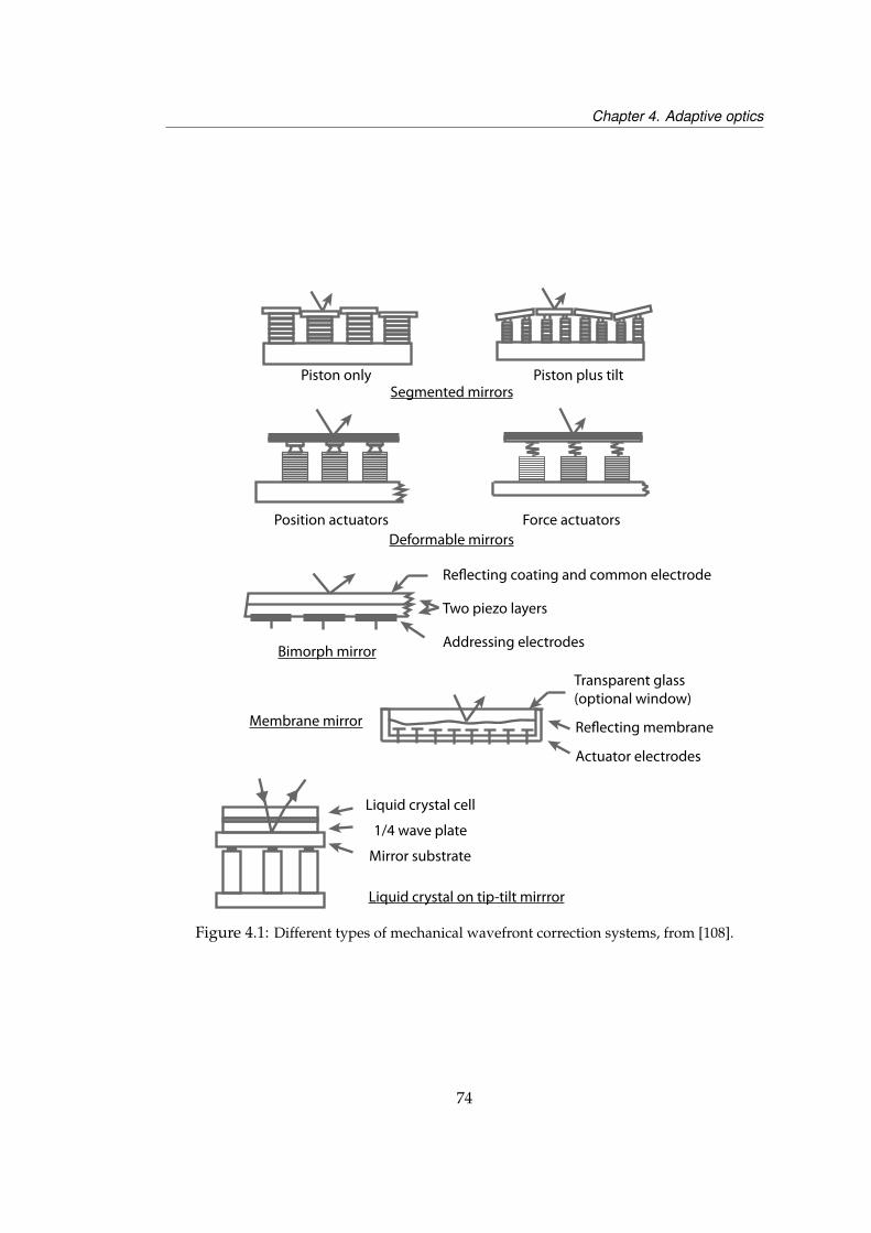
Chapter 4. Adaptive optics
Piston only Piston plus tiltSegmented mirrors
Force actuatorsPosition actuatorsDeformable mirrors
Bimorph mirror
Reecting coating and common electrode
Two piezo layers
Addressing electrodes
Reecting membrane
Transparent glass(optional window)
Membrane mirror
Actuator electrodes
Liquid crystal on tip-tilt mirrror
Liquid crystal cell
1/4 wave plate
Mirror substrate
Figure 4.1: Different types of mechanical wavefront correction systems, from [108].
74

Chapter 4. Adaptive optics
generated by the drive of an electric current in an actuator coil to attract and repulse a
magnet fixed under the mirror facesheet, a push-pull operation of the mirror surface
is obtained and thus increases the mirror available stroke.
The Mirao52-d (Imagine Eyes, France) used in this thesis is shown in Figure 4.2. This
is a magnetically-actuated mirror of very large stroke compared to the typical oper-
ational range of typical deformable mirrors with a ±25 µm deformation ability from
the manufacturer specifications. The 15 mm diameter mirror active pupil contains
52 actuators distributed in a squared array with a 2.5 mm pitch between neighboring
actuators and 8 actuators across the pupil diameter. Its suitability for ophthalmic ap-
plications over the optimal 15 mm clear aperture was demonstrated [47, 109] and is
very similar to the performance estimated over the 12.5 mm aperture [91] of the initial
design.
1112131415161718
1234
5 6 7 8 910
1920212223242526
2728293031323334
3536373839404142
434445464748
49505152
PNI
TU
O S
121314151617
6789
202122232425
282930313233
363738394041
44454647
Figure 4.2: Mirao52-d™ mirror and optimal pupil (photography courtesy of Imagine Eyes,France). The mirror active pupil (15mm diameter) is shadowed in gray.
In one configuration of the optical system the 6 mm diameter of the eye was conju-
gated at the deformable mirror into a 14.4 mm diameter pupil. The mirror influence
functions displayed in Figure 4.3 were recorded using a Twyman-Green interferom-
eter (FISBA OPTIK µphase). The mirror surface deflection was reconstructed by this
instrument from a stack of successive interferograms measured from a reference po-
sition over a 15 mm pupil diameter. The set of influence functions presented was
measured using actuator voltages of ±0.1 V added or subtracted from the initial set
of commands defining a "flat" wavefront. This represented 1/10th of the voltage range
indicated by the manufacturer. Each influence function corresponded to the actuator
as numbered in Figure 4.2 from the rear view of the mirror.
The interferometer measurement highlights that the outer ring of mirror actuators is
out of the clear aperture of the mirror but nevertheless impacts on the surface shape
75
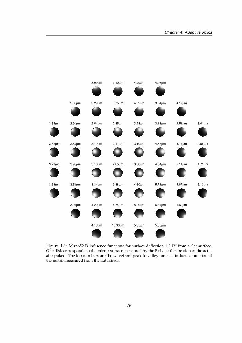
Chapter 4. Adaptive optics
4.13µm 10.30µm 5.35µm 5.55µm
3.91µm 4.20µm 4.74µm 5.20µm 6.34µm 6.69µm
3.38µm 3.51µm 3.34µm 3.88µm 4.60µm 5.71µm 5.87µm 5.13µm
3.29µm 3.95µm 3.16µm 2.85µm 3.38µm 4.34µm 5.14µm 4.71µm
3.82µm 2.87µm 3.49µm 2.11µm 3.10µm 4.67µm 5.17µm 4.08µm
3.35µm 2.94µm 2.54µm 2.35µm 3.23µm 3.11µm 4.51µm 3.41µm
2.86µm 3.29µm 3.75µm 4.59µm 3.54µm 4.19µm
3.09µm 3.10µm 4.29µm 4.06µm
Figure 4.3: Mirao52-D influence functions for surface deflection ±0.1V from a flat surface.One disk corresponds to the mirror surface measured by the Fisba at the location of the actu-ator poked. The top numbers are the wavefront peak-to valley for each influence function ofthe matrix measured from the flat mirror.
76
Chapter 4. Adaptive optics
when active. The values on top of each influence function are the wavefront peak
to valley for 1/10th of the maximal mirror stroke, thus the full range (40 µm) stroke
is under the manufacturer specification for this configuration. A linearity test was
performed for one central actuator over a defocused wavefront until saturation of
the interferometer detection range, but not extended to other actuators or to the full
range, which might have confirmed the membrane hysteresis measurements (manu-
facturer, and [110]).
With only 8 actuators across its pupil the spatial resolution of the mirror is limited to
the correction of higher orders aberration patterns up to the 7th order (52 modes) and
this work was mainly using its large stroke is to correct for high amplitudes of low-
order aberrations (3rd order). Previous observations [1] had suggested the new de-
sign could benefit from a lower number of pupil samples than used (16×16 samples at
the highest binning). The new system at the highest binning presented 14×14 samples
across the pupil, thus following the Nyquist criterion per actuator. For a turbulence
of the Kolmogorov type in a standard noise configuration those settings are suitable
for the Mirao deformable mirror [111]. For ocular aberrations, the experimental de-
termination of the optimal condition number must be performed.
4.1.2 Direct slope control algorithm
Adaptive optics algorithms reconstruct the wavefront from the sensor measurements
to determine the mirror deformation required for its correction. In the direct slope
algorithm, the sensor signals are used as input for the closed-loop control. The closed
loop sensor signal is defined by the calibration beam propagated in the system in
which the deformable mirror commands forms a ‘flat’ surface.
The sensor signal (sre f ) is dependent on the ‘flat’ mirror commands set (c f lat) in that :
M c f lat = sre f (4.1)
M is the influence function matrix of the system. Each element of M is defined from
the difference between the reference signal and the mirror surface deviation obtained
after adding to each mirror actuator a unitary voltage (or command) from the initial
‘flat’ command (mirror bias).
For P the total number of actuators, and N wavefront samples in the sensor pupil
77
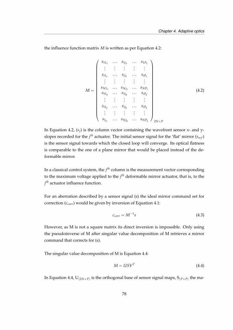
Chapter 4. Adaptive optics
the influence function matrix M is written as per Equation 4.2:
M =
s11x . . . s1jx . . . s1Px...
......
......
si1x . . . sijx . . . siPx...
......
......
sN1x . . . sNjx . . . sNPx
s11y . . . s1jy . . . siPy...
......
......
si1y . . . sijy . . . siPy...
......
......
s1y . . . sNjy . . . sNPy
2N×P
(4.2)
In Equation 4.2, (sj) is the column vector containing the wavefront sensor x- and y-
slopes recorded for the jth actuator. The initial sensor signal for the ‘flat’ mirror (sre f )
is the sensor signal towards which the closed loop will converge. Its optical flatness
is comparable to the one of a plane mirror that would be placed instead of the de-
formable mirror.
In a classical control system, the jth column is the measurement vector corresponding
to the maximum voltage applied to the jth deformable mirror actuator, that is, to the
jth actuator influence function.
For an aberration described by a sensor signal (s) the ideal mirror command set for
correction (ccorr) would be given by inversion of Equation 4.1:
ccorr = M−1s (4.3)
However, as M is not a square matrix its direct inversion is impossible. Only using
the pseudoinverse of M after singular value decomposition of M retrieves a mirror
command that corrects for (s).
The singular value decomposition of M is Equation 4.4:
M = USVT (4.4)
In Equation 4.4, U(2N×P) is the orthogonal base of sensor signal maps, S(P×P) the ma-
78
Chapter 4. Adaptive optics
trix of singular values (λi) for the decomposition of (s) onto all the modes of V(P×P)
the orthogonal base of mirror commands.
The sensor signal (s) is the phase aberration horizontal and vertical gradient mea-
sured with respect to the reference signal (sre f ). Tip and tilt aberrations can optionally
be removed from (s) by subtracting the mean of each gradient signal. Thus :
s = saberration − sre f − (stiptilt) (4.5)
Assuming tip and tilt do not affect the closed loop image quality, this term (stiptilt)
was usually not subtracted in Equation 4.5.
The closed loop algorithm seeks to minimise the signal (s), that is to drive the mirror
towards a set of commands for which the sensor sees no difference between the mea-
surement and the reference wavefront. The ideal mirror command for correction of
(s) is thus given by Equation 4.6:
ccorr = VS−1UTs (4.6)
However in practice this correction is implemented using only a finite number of mir-
ror modes and in several iteration steps.
The limit on the number of modes used for the correction is set by the condition num-
ber (CN), which is the ratio of the highest singular value to the lowest singular value
used in the correction. All singular values of (S) are set to zero beyond this chosen
limit singular value. Low condition numbers are recommended for loop stability and
speed [112], typical values used were between 20 and 30 modes in our case. With this
limit the new singular value matrix (S) is noted (Λ), and the correction ccorr becomes :
ccorr = VΛ−1UTs
A code-based clipping of the correction amplitude to half of the maximal voltage is
recommended as the large mirror stroke could lead to the membrane break up if two
neighboring actuators have an opposite signal or if the actuators voltages remain of
high amplitude for more than a few seconds. For security, the manufacturer had
79
Chapter 4. Adaptive optics
equipped the mirror with an automatic shutdown system avoiding this problem.
At each iteration of the loop a new sensor vector is calculated as in Equation 4.5 and
the adaptive optics closed loop updates the mirror as follows in Equation 4.7 :
ci+1 = ci − gccorr (4.7)
As the sensor signal measured tends towards the reference signal, the correction re-
quired tends towards zero, the mirror commands are stabilized, and the wavefront
aberration is corrected.
As seen in Figure 3.8, Section 3.2.2.2, the experimental realization of the pyramid ref-
erence signal presents a Gaussian distribution while the theoretical reference sensor
signal set expected consists in a uniform zero-amplitude. The mirror shape is con-
trolled by 52 actuators with 16 actuators outside the active pupil, which means the
number of actuators (or mirror modes) used in the closed loop control performance
requires to be experimentally defined. The membrane deflection formed by a single
actuator activation at full amplitude-voltage leads to the sensor saturation. In conse-
quence, the calibration of the influence functions matrix must be performed taking a
maximum value what is only a percentage of the actuator full-poke (arbitrarily cho-
sen at 10%). The adaptive optics control law defined by Equation 4.7 however does
not account for this mirror command rescaling and in the Mirao 52-d the adaptive
optics loop effectiveness revealed dependent on the stabilization time of the voltage
applied to an actuator. In turn when the correction voltages were applied too fast to
the mirror the adaptive optics diverged, requiring an user-defined adjustment of the
gain parameter (g) to a value allowing a stable closed-loop. The usual g=[0,1] gain
range of an adaptive optics system is in this work rescaled to g=[0, 0.1]. The notation
is adjusted in the following for the reader understanding but the actual values are
sometimes mentioned.
The following section is intended to illustrate the dependence of the adaptive op-
tics efficiency towards the reference wavefront, the condition number and gain value
used in the control.
80

Chapter 4. Adaptive optics
4.1.3 Adaptive optics control parameters
This section illustrates the influence of the parameters mentioned previously on the
adaptive optics efficiency. The latter is based on the wavefront reconstruction code,
a dynamic display of the Zernike coefficients slowed down the acquisition. On the
other hand, the off-line reconstruction of long acquisition sequences limited the in−situ experimental adjustment of the parameters value that would have been required.
Based on the system point spread function image at the science camera during the
calibration and during the ocular experiments, the aberration correction is character-
ized by the narrowing of the point spread function.
The reference wavefront defines the ultimate closed loop correction quality that can
be achieved. Simulations of closed loop efficiency as a function of the condition num-
ber value for this mirror have shown a diffraction-limited rms error could be obtained
without the need of using all the mirror modes [47]. This point was verified experi-
mentally with a practical test of correction of a typical aberration. The loop destabi-
lization for the correction of a typical aberration with increasing values of adaptive
optics gain is presented through the observation of the sensor signal with the closed
loop.
4.1.3.1 Reference signal
The reference signals were defined as ‘open loop’ reference and ‘closed loop’ refer-
ence, which corresponded respectively to the mirror command set used for calibration
of the sensor signal and to the mirror command set achieved after implementation of
the adaptive optics.
Open loop reference.
The open loop reference wavefront corresponds to the sensor signal recorded with
the alignment optics placed at the pupil plane of the eye. The collimated beam at the
pupil plane of the eye is propagated to the sensor and thus contains the optical system
aberrations. The ocular aberration measured by the system can be expressed includ-
ing the system aberrations (without subtraction of the reference) or with account of
this reference (subtraction of the reference wavefront). In an adaptive optics system
these aberrations can be cancelled by an initial bias of the deformable mirror surface
experimentally defined. The initial mirror commands ‘flat-IE’ provided by the man-
81

Chapter 4. Adaptive optics
ufacturer defined an aberration-free reference wavefront for the commercial system.
For an adaptive optics system based on another sensor type a new definition of the
‘flat’ command was required to correct for the optical system aberrations.
Reference dW/dX
−0.5
0
0.5Initial DM dW/dX
−0.5
0
0.5Closed loop DM dW/dX
−0.5
0
0.5
Reference dW/dY
−0.5
0
0.5Initial DM dW/dY
−0.5
0
0.5Closed loop DM dW/dY
−0.5
0
0.5
(a) Sensor signals created from 10ms exposure wavefront sensor camera
Reference psf
0
2
4
6
x 104 Initial psf DM "flat"
0
2
4
6
x 104 Closed loop DM "reference"
0
2
4
6
x 104
(b) 0.5ms exposure science image
Figure 4.4: Sensor reference signals for the definition of the deformable mirror ‘flat’ shapein the adaptive optics system with 55samples across the pupil and a 6λ/D modulation factor.This flat mirror was then removed and the deformable mirror was implemented instead inthe conjugated pupil plane. The manufacturer mirror commands defining the ‘flat’ mirrorshape were set up as initial mirror surface bias. A slight shift of the closed loop psf canbe observed compared to the reference psf. The uniformity of the reference signal cannotcompletely be reproduced by the deformable mirror. Edge effects at the pupil are more visiblefor the deformable mirror than in the pupil signal.
This reference was based on the signal of a plane mirror of λ/10 optical quality posi-
tioned at the deformable mirror plane and using the light of the alignment beam. The
sensor signals and psfs for the plane mirror, and deformable mirror ‘flat-IE’, and ‘flat’
are presented in Figure 4.4a. Closing the loop on the plane mirror set of reference sig-
nals corrected for both the system and the calibration optics. This new ‘flat’ defined
an open loop reference wavefront from which the ocular aberration is measured. The
initial calibration of the influence functions was performed using the ‘flat-IE’ com-
mand set and the surface deflection defined using a ±0.1V command from this bias.
82
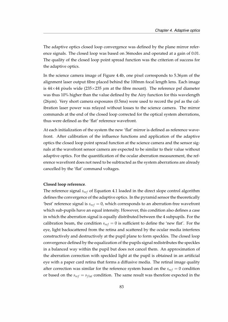
Chapter 4. Adaptive optics
The adaptive optics closed loop convergence was defined by the plane mirror refer-
ence signals. The closed loop was based on 36modes and operated at a gain of 0.01.
The quality of the closed loop point spread function was the criterion of success for
the adaptive optics.
In the science camera image of Figure 4.4b, one pixel corresponds to 5.36µm of the
alignment laser output fibre placed behind the 100mm focal length lens. Each image
is 44×44 pixels wide (235×235 µm at the fibre mount). The reference psf diameter
was thus 10% higher than the value defined by the Airy function for this wavelength
(26µm). Very short camera exposures (0.5ms) were used to record the psf as the cal-
ibration laser power was relayed without losses to the science camera. The mirror
commands at the end of the closed loop corrected for the optical system aberrations,
thus were defined as the ‘flat’ reference wavefront.
At each initialization of the system the new ‘flat’ mirror is defined as reference wave-
front. After calibration of the influence functions and application of the adaptive
optics the closed loop point spread function at the science camera and the sensor sig-
nals at the wavefront sensor camera are expected to be similar to their value without
adaptive optics. For the quantification of the ocular aberration measurement, the ref-
erence wavefront does not need to be subtracted as the system aberrations are already
cancelled by the ‘flat’ command voltages.
Closed loop reference.
The reference signal sre f of Equation 4.1 loaded in the direct slope control algorithm
defines the convergence of the adaptive optics. In the pyramid sensor the theoretically
‘best’ reference signal is sre f = 0, which corresponds to an aberration-free wavefront
which sub-pupils have an equal intensity. However, this condition also defines a case
in which the aberration signal is equally distributed between the 4 subpupils. For the
calibration beam, the condition sre f = 0 is sufficient to define the ‘new flat’. For the
eye, light backscattered from the retina and scattered by the ocular media interferes
constructively and destructively at the pupil plane to form speckles. The closed loop
convergence defined by the equalization of the pupils signal redistributes the speckles
in a balanced way within the pupil but does not cancel them. An approximation of
the aberration correction with speckled light at the pupil is obtained in an artificial
eye with a paper card retina that forms a diffusive media. The retinal image quality
after correction was similar for the reference system based on the sre f = 0 condition
or based on the sre f = s f lat condition. The same result was therefore expected in the
83
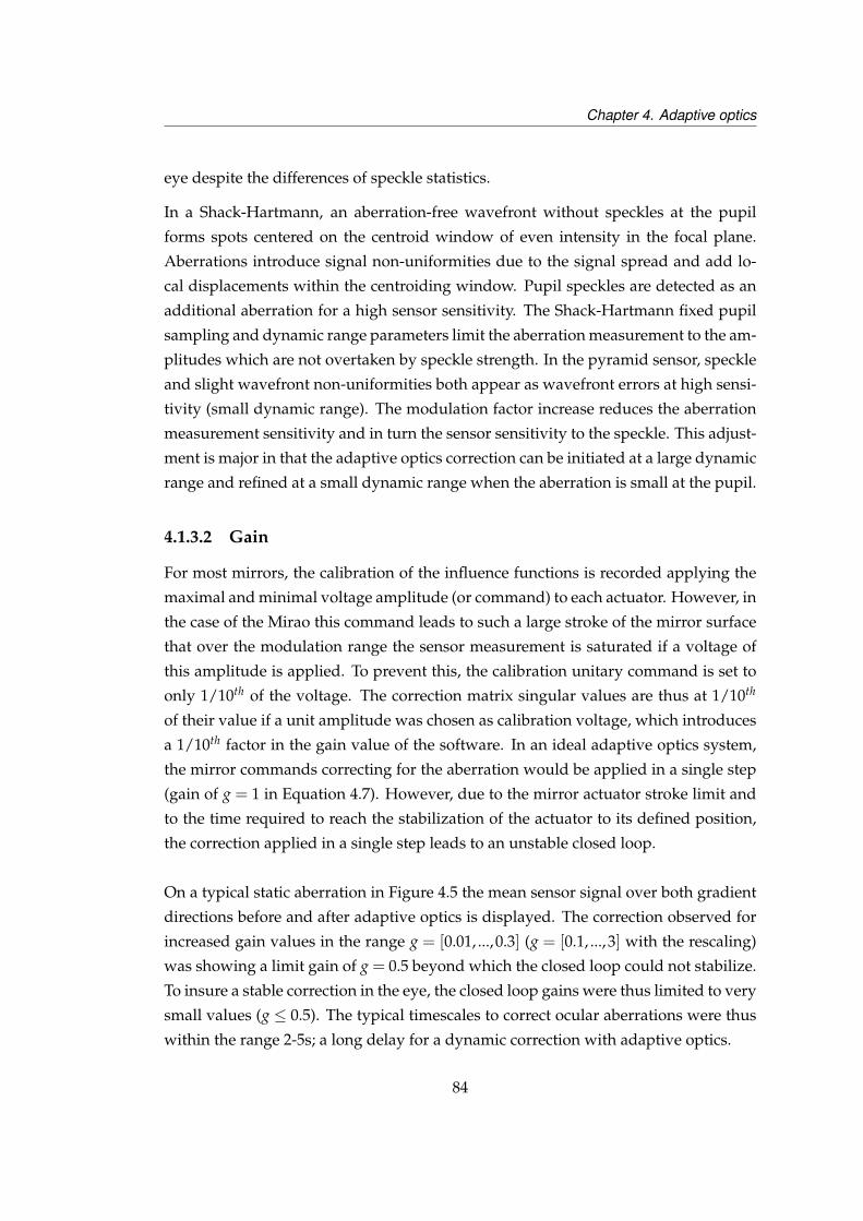
Chapter 4. Adaptive optics
eye despite the differences of speckle statistics.
In a Shack-Hartmann, an aberration-free wavefront without speckles at the pupil
forms spots centered on the centroid window of even intensity in the focal plane.
Aberrations introduce signal non-uniformities due to the signal spread and add lo-
cal displacements within the centroiding window. Pupil speckles are detected as an
additional aberration for a high sensor sensitivity. The Shack-Hartmann fixed pupil
sampling and dynamic range parameters limit the aberration measurement to the am-
plitudes which are not overtaken by speckle strength. In the pyramid sensor, speckle
and slight wavefront non-uniformities both appear as wavefront errors at high sensi-
tivity (small dynamic range). The modulation factor increase reduces the aberration
measurement sensitivity and in turn the sensor sensitivity to the speckle. This adjust-
ment is major in that the adaptive optics correction can be initiated at a large dynamic
range and refined at a small dynamic range when the aberration is small at the pupil.
4.1.3.2 Gain
For most mirrors, the calibration of the influence functions is recorded applying the
maximal and minimal voltage amplitude (or command) to each actuator. However, in
the case of the Mirao this command leads to such a large stroke of the mirror surface
that over the modulation range the sensor measurement is saturated if a voltage of
this amplitude is applied. To prevent this, the calibration unitary command is set to
only 1/10th of the voltage. The correction matrix singular values are thus at 1/10th
of their value if a unit amplitude was chosen as calibration voltage, which introduces
a 1/10th factor in the gain value of the software. In an ideal adaptive optics system,
the mirror commands correcting for the aberration would be applied in a single step
(gain of g = 1 in Equation 4.7). However, due to the mirror actuator stroke limit and
to the time required to reach the stabilization of the actuator to its defined position,
the correction applied in a single step leads to an unstable closed loop.
On a typical static aberration in Figure 4.5 the mean sensor signal over both gradient
directions before and after adaptive optics is displayed. The correction observed for
increased gain values in the range g = [0.01, ...,0.3] (g = [0.1, ...,3] with the rescaling)
was showing a limit gain of g = 0.5 beyond which the closed loop could not stabilize.
To insure a stable correction in the eye, the closed loop gains were thus limited to very
small values (g ≤ 0.5). The typical timescales to correct ocular aberrations were thus
within the range 2-5s; a long delay for a dynamic correction with adaptive optics.
84
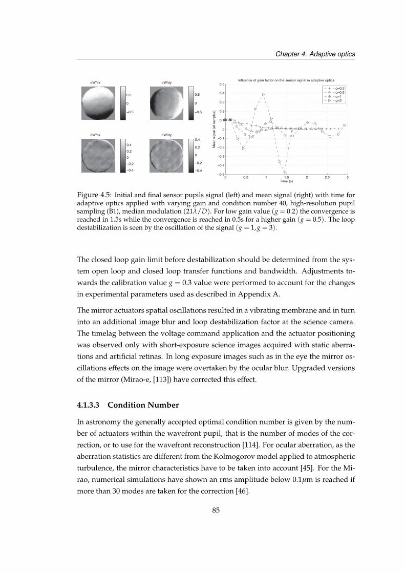
Chapter 4. Adaptive optics
0 0.5 1 1.5 2 2.5 3−0.5
−0.4
−0.3
−0.2
−0.1
0
0.1
0.2
0.3
0.4
0.5
Time (s)
Mean signal (all samples)
g=0.2
g=0.5
g=1
g=3
Influence of gain factor on the sensor signal in adaptive optics
dW/dx
−0.4
−0.2
0
0.2
0.4
dW/dy
−0.4
−0.2
0
0.2
0.4
dW/dx
dW/dy
−0.5
0
0.5
−0.5
0
0.5
Figure 4.5: Initial and final sensor pupils signal (left) and mean signal (right) with time foradaptive optics applied with varying gain and condition number 40, high-resolution pupilsampling (B1), median modulation (21λ/D). For low gain value (g = 0.2) the convergence isreached in 1.5s while the convergence is reached in 0.5s for a higher gain (g = 0.5). The loopdestabilization is seen by the oscillation of the signal (g = 1, g = 3).
The closed loop gain limit before destabilization should be determined from the sys-
tem open loop and closed loop transfer functions and bandwidth. Adjustments to-
wards the calibration value g = 0.3 value were performed to account for the changes
in experimental parameters used as described in Appendix A.
The mirror actuators spatial oscillations resulted in a vibrating membrane and in turn
into an additional image blur and loop destabilization factor at the science camera.
The timelag between the voltage command application and the actuator positioning
was observed only with short-exposure science images acquired with static aberra-
tions and artificial retinas. In long exposure images such as in the eye the mirror os-
cillations effects on the image were overtaken by the ocular blur. Upgraded versions
of the mirror (Mirao-e, [113]) have corrected this effect.
4.1.3.3 Condition Number
In astronomy the generally accepted optimal condition number is given by the num-
ber of actuators within the wavefront pupil, that is the number of modes of the cor-
rection, or to use for the wavefront reconstruction [114]. For ocular aberration, as the
aberration statistics are different from the Kolmogorov model applied to atmospheric
turbulence, the mirror characteristics have to be taken into account [45]. For the Mi-
rao, numerical simulations have shown an rms amplitude below 0.1µm is reached if
more than 30 modes are taken for the correction [46].
85
Chapter 4. Adaptive optics
In practice, the computation of a new control matrix or calculations with a large con-
trol matrix slows down the adaptive optics. In consequence the control matrix is
computed once with a condition number of 30, afterwards only loaded in the exper-
imental sessions. On a single standard aberrated wavefront presenting defocus and
astigmatism, the influence of the condition number on the correction of the adaptive
optics system is presented in Figure 4.6 for the most commonly used sensor settings
(highest wavefront sampling (B1) and median modulation range 21λ/D). As the sen-
sor signal amplitude after correction is constant, it seems that the use of a higher
condition number does not improve the correction obtained with 30 modes.
dW/dx
−1
−0.5
0
0.5
1dW/dy
−1
−0.5
0
0.5
1
dW/dx
−1
−0.5
0
0.5
1dW/dy
−1
−0.5
0
0.5
1
30 35 40 45 50 55 60−0.05
0
0.05
0.1
0.15
Condition number
Me
an
sig
na
l (a
ll sa
mp
les)
Open loop and Closed loop signal (B1 M7)
Open loop
Closed loop
Figure 4.6: The mean of both sensor signals for a single frame describes the amplitude ofthe wavefront aberration. The amplitude of the standard deviation of the mean show theclosed loop wavefront uniformity around zero compared to the open loop signal. A simi-lar efficiency for all condition numbers is reached in the closed loop signal, thus the closedloop convergence for this static aberration is not dependent on the number of modes in theadaptive optics.
4.2 AO system description
The wavefront sensing system and the corrective element of the adaptive optics sys-
tem have been described previously. In the following, the different subsystems around
the adaptive optics are presented. These consist of the pupil monitoring system, the
probe beam system, and the Badal optometer. The imaging camera and illumination
system are presented further in this work.
86
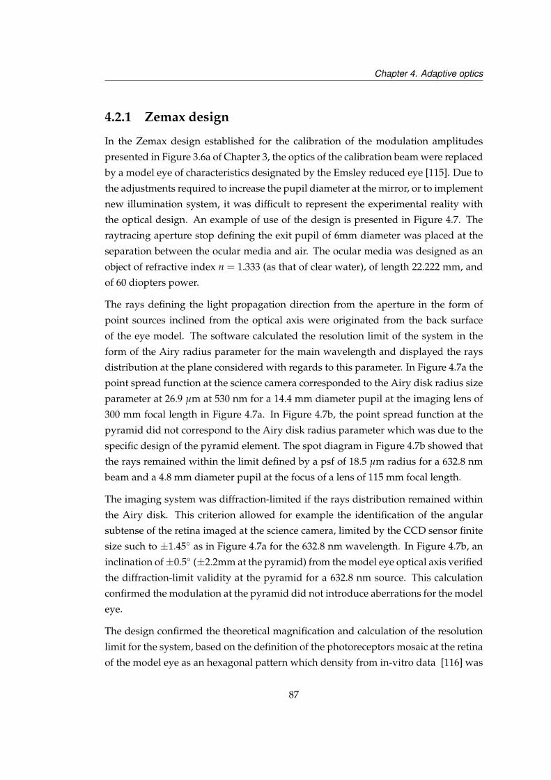
Chapter 4. Adaptive optics
4.2.1 Zemax design
In the Zemax design established for the calibration of the modulation amplitudes
presented in Figure 3.6a of Chapter 3, the optics of the calibration beam were replaced
by a model eye of characteristics designated by the Emsley reduced eye [115]. Due to
the adjustments required to increase the pupil diameter at the mirror, or to implement
new illumination system, it was difficult to represent the experimental reality with
the optical design. An example of use of the design is presented in Figure 4.7. The
raytracing aperture stop defining the exit pupil of 6mm diameter was placed at the
separation between the ocular media and air. The ocular media was designed as an
object of refractive index n = 1.333 (as that of clear water), of length 22.222 mm, and
of 60 diopters power.
The rays defining the light propagation direction from the aperture in the form of
point sources inclined from the optical axis were originated from the back surface
of the eye model. The software calculated the resolution limit of the system in the
form of the Airy radius parameter for the main wavelength and displayed the rays
distribution at the plane considered with regards to this parameter. In Figure 4.7a the
point spread function at the science camera corresponded to the Airy disk radius size
parameter at 26.9 µm at 530 nm for a 14.4 mm diameter pupil at the imaging lens of
300 mm focal length in Figure 4.7a. In Figure 4.7b, the point spread function at the
pyramid did not correspond to the Airy disk radius parameter which was due to the
specific design of the pyramid element. The spot diagram in Figure 4.7b showed that
the rays remained within the limit defined by a psf of 18.5 µm radius for a 632.8 nm
beam and a 4.8 mm diameter pupil at the focus of a lens of 115 mm focal length.
The imaging system was diffraction-limited if the rays distribution remained within
the Airy disk. This criterion allowed for example the identification of the angular
subtense of the retina imaged at the science camera, limited by the CCD sensor finite
size such to ±1.45 as in Figure 4.7a for the 632.8 nm wavelength. In Figure 4.7b, an
inclination of±0.5 (±2.2mm at the pyramid) from the model eye optical axis verified
the diffraction-limit validity at the pyramid for a 632.8 nm source. This calculation
confirmed the modulation at the pyramid did not introduce aberrations for the model
eye.
The design confirmed the theoretical magnification and calculation of the resolution
limit for the system, based on the definition of the photoreceptors mosaic at the retina
of the model eye as an hexagonal pattern which density from in-vitro data [116] was
87
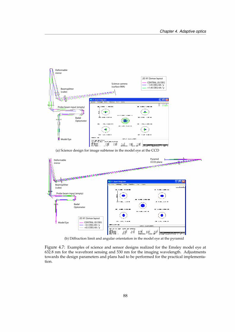
Chapter 4. Adaptive optics
Model Eye
Badal Optometer
Deformable mirror
Science camera (surface IMA)
Probe beam input (empty)
Beamsplitter (cube)
CENTRAL (0) DEG- 1.45 DEG tilt / y+1.45 DEG tilt / y
2D XY Zemax layout
(a) Science design for image subtense in the model eye at the CCD
Model Eye
Badal Optometer
Deformable mirror
Probe beam input (empty)
Beamsplitter (cube)
CENTRAL (0) DEG
+0.5 DEG tilt / y
2D XY Zemax layout
- 0.5 DEG tilt / y
Pyramid(CCD) plane
(b) Diffraction limit and angular orientation in the model eye at the pyramid
Figure 4.7: Examples of science and sensor designs realized for the Emsley model eye at632.8 nm for the wavefront sensing and 530 nm for the imaging wavelength. Adjustmentstowards the design parameters and plans had to be performed for the practical implementa-tion.
88
Chapter 4. Adaptive optics
corresponding to a regular pattern of size between 3 µm (density 96 cones/mm2 at 1
from the fovea) and 4.2 µm (density 44 cones/mm2 at 2 from the fovea). This dis-
tance corresponded to a resolved pattern for an optical system with a 6 mm circular
pupil diameter and a 17 mm focal length in air, which resolution limit was defined
respectively by Airy disk radiuses of 2.2 µm and 1.83 µm for 635 nm and 530 nm
wavelengths. From the system magnification factors defined between the conjugate
retinal planes defined by the eye pupil aperture, the minimal distance between two
adjacent point sources in the retina of the model eye was defined by the camera pix-
els size. For our camera, the distance between two adjacent pixels corresponded to
6.7 µm. The ccd pixels seen from the eye through a circular aperture of infinite size
corresponded to a spacing of 0.9 µm in the eye. The two pixels of the imaging system
were thus estimated as sampling at the Nyquist limit (2.4 pixels for the 635 nm wave-
length and 2.0 pixels for the 530 nm wavelength) the smallest distance between two
sources in the eye defined by the 6 mm numerical aperture.
The inversion of the wavefront sensor arm and of the science arm revealed necessary
on the bench as the dichoic beamsplitter reflected preferentially the green wavelength.
The science camera image plane in Figure 4.7a represented the plane of best focus for
both wavelength considered. The longitudinal chromatic aberration for this system
was stated from the focusing change between both wavelength. Implementation of
a green filter in the science path and defocusing the science camera [5, 6] from the
imaging lens was implemented to compensate for this chromatic aberration.
4.2.2 Experimental setup
The wavefront data presented in the following sections were acquired using the sys-
tem presented in Figure 4.8. The wavefront sensor system has been described in
Chapter 3. The retinal imaging system has been described in Section 4.2.1 and will
be developed further in Chapter 5 along with the retinal illumination system. The
cameras were similar to that described in Chapter 2, Section 2.2.1.
A single computer unit was dedicated to the control of the deformable mirror, retinal
illumination and retinal image acquisition, via custom-written software detailed in
Appendix A. The probe beam direction and power were defined manually. The pupil
illumination and pupil monitoring system remained manually implemented and de-
pending on an additional unit.
89
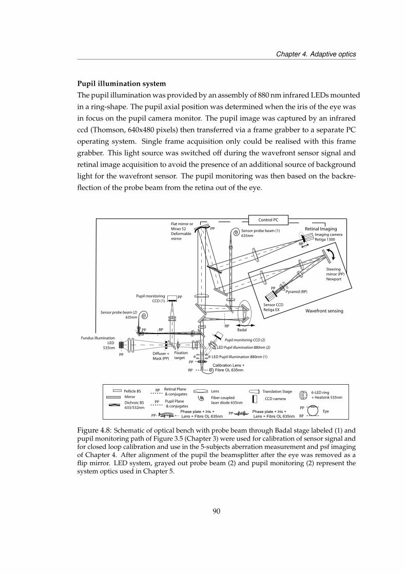
Chapter 4. Adaptive optics
Pupil illumination system
The pupil illumination was provided by an assembly of 880 nm infrared LEDs mounted
in a ring-shape. The pupil axial position was determined when the iris of the eye was
in focus on the pupil camera monitor. The pupil image was captured by an infrared
ccd (Thomson, 640x480 pixels) then transferred via a frame grabber to a separate PC
operating system. Single frame acquisition only could be realised with this frame
grabber. This light source was switched off during the wavefront sensor signal and
retinal image acquisition to avoid the presence of an additional source of background
light for the wavefront sensor. The pupil monitoring was then based on the backre-
flection of the probe beam from the retina out of the eye.
LED Pupil illumination 880nm (2)
Pupil monitoring CCD (2)
RP
Control PC
Wavefront sensing
Retinal Imaging
Fundus illuminationLED
535nm
PP
LED Pupil Illumination 880nm (1)
Pupil monitoringCCD (1)
RP
PPFlat mirror or Mirao 52 Deformable mirror
Steering mirror (PP)Newport
PPPyramid (RP)
Sensor probe beam (1)635nm
Sensor CCD Retiga EX
Imaging cameraRetiga 1300
RPCalibration Lens +
Fibre OL 635nm
PP
Badal
Fixationtarget
Diffuser + Mask (PP)
PP
PP RP
Sensor probe beam (2)635nm
Mirror
Pellicle BS LensRP
PP
Retinal Plane & conjugates
Pupil Plane & conjugates
Translation Stage
Fiber coupled laser diode 635nm
CCD cameraDichroic BS 633/532nm
RP
PPEyePhase plate + Iris +
Lens + Fibre OL 635nmPPPhase plate + Iris +
Lens + Fibre OL 635nmPP
6-LED ring + Heatsink 535nm
Figure 4.8: Schematic of optical bench with probe beam through Badal stage labeled (1) andpupil monitoring path of Figure 3.5 (Chapter 3) were used for calibration of sensor signal andfor closed loop calibration and use in the 5-subjects aberration measurement and psf imagingof Chapter 4. After alignment of the pupil the beamsplitter after the eye was removed as aflip mirror. LED system, grayed out probe beam (2) and pupil monitoring (2) represent thesystem optics used in Chapter 5.
90
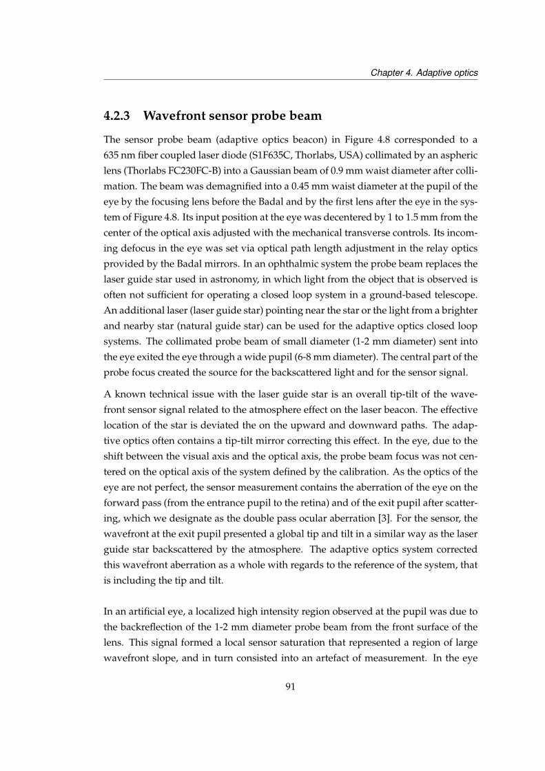
Chapter 4. Adaptive optics
4.2.3 Wavefront sensor probe beam
The sensor probe beam (adaptive optics beacon) in Figure 4.8 corresponded to a
635 nm fiber coupled laser diode (S1F635C, Thorlabs, USA) collimated by an aspheric
lens (Thorlabs FC230FC-B) into a Gaussian beam of 0.9 mm waist diameter after colli-
mation. The beam was demagnified into a 0.45 mm waist diameter at the pupil of the
eye by the focusing lens before the Badal and by the first lens after the eye in the sys-
tem of Figure 4.8. Its input position at the eye was decentered by 1 to 1.5 mm from the
center of the optical axis adjusted with the mechanical transverse controls. Its incom-
ing defocus in the eye was set via optical path length adjustment in the relay optics
provided by the Badal mirrors. In an ophthalmic system the probe beam replaces the
laser guide star used in astronomy, in which light from the object that is observed is
often not sufficient for operating a closed loop system in a ground-based telescope.
An additional laser (laser guide star) pointing near the star or the light from a brighter
and nearby star (natural guide star) can be used for the adaptive optics closed loop
systems. The collimated probe beam of small diameter (1-2 mm diameter) sent into
the eye exited the eye through a wide pupil (6-8 mm diameter). The central part of the
probe focus created the source for the backscattered light and for the sensor signal.
A known technical issue with the laser guide star is an overall tip-tilt of the wave-
front sensor signal related to the atmosphere effect on the laser beacon. The effective
location of the star is deviated the on the upward and downward paths. The adap-
tive optics often contains a tip-tilt mirror correcting this effect. In the eye, due to the
shift between the visual axis and the optical axis, the probe beam focus was not cen-
tered on the optical axis of the system defined by the calibration. As the optics of the
eye are not perfect, the sensor measurement contains the aberration of the eye on the
forward pass (from the entrance pupil to the retina) and of the exit pupil after scatter-
ing, which we designate as the double pass ocular aberration [3]. For the sensor, the
wavefront at the exit pupil presented a global tip and tilt in a similar way as the laser
guide star backscattered by the atmosphere. The adaptive optics system corrected
this wavefront aberration as a whole with regards to the reference of the system, that
is including the tip and tilt.
In an artificial eye, a localized high intensity region observed at the pupil was due to
the backreflection of the 1-2 mm diameter probe beam from the front surface of the
lens. This signal formed a local sensor saturation that represented a region of large
wavefront slope, and in turn consisted into an artefact of measurement. In the eye
91
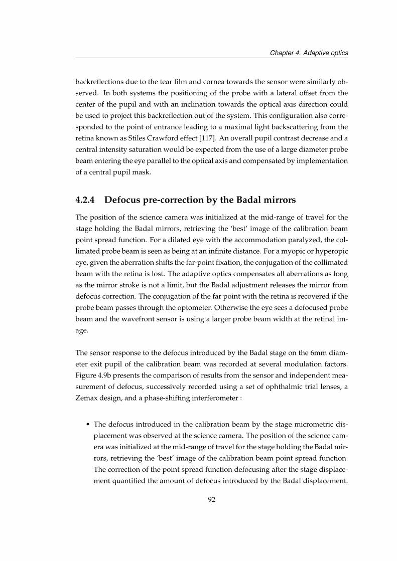
Chapter 4. Adaptive optics
backreflections due to the tear film and cornea towards the sensor were similarly ob-
served. In both systems the positioning of the probe with a lateral offset from the
center of the pupil and with an inclination towards the optical axis direction could
be used to project this backreflection out of the system. This configuration also corre-
sponded to the point of entrance leading to a maximal light backscattering from the
retina known as Stiles Crawford effect [117]. An overall pupil contrast decrease and a
central intensity saturation would be expected from the use of a large diameter probe
beam entering the eye parallel to the optical axis and compensated by implementation
of a central pupil mask.
4.2.4 Defocus pre-correction by the Badal mirrors
The position of the science camera was initialized at the mid-range of travel for the
stage holding the Badal mirrors, retrieving the ‘best’ image of the calibration beam
point spread function. For a dilated eye with the accommodation paralyzed, the col-
limated probe beam is seen as being at an infinite distance. For a myopic or hyperopic
eye, given the aberration shifts the far-point fixation, the conjugation of the collimated
beam with the retina is lost. The adaptive optics compensates all aberrations as long
as the mirror stroke is not a limit, but the Badal adjustment releases the mirror from
defocus correction. The conjugation of the far point with the retina is recovered if the
probe beam passes through the optometer. Otherwise the eye sees a defocused probe
beam and the wavefront sensor is using a larger probe beam width at the retinal im-
age.
The sensor response to the defocus introduced by the Badal stage on the 6mm diam-
eter exit pupil of the calibration beam was recorded at several modulation factors.
Figure 4.9b presents the comparison of results from the sensor and independent mea-
surement of defocus, successively recorded using a set of ophthalmic trial lenses, a
Zemax design, and a phase-shifting interferometer :
• The defocus introduced in the calibration beam by the stage micrometric dis-
placement was observed at the science camera. The position of the science cam-
era was initialized at the mid-range of travel for the stage holding the Badal mir-
rors, retrieving the ‘best’ image of the calibration beam point spread function.
The correction of the point spread function defocusing after the stage displace-
ment quantified the amount of defocus introduced by the Badal displacement.
92
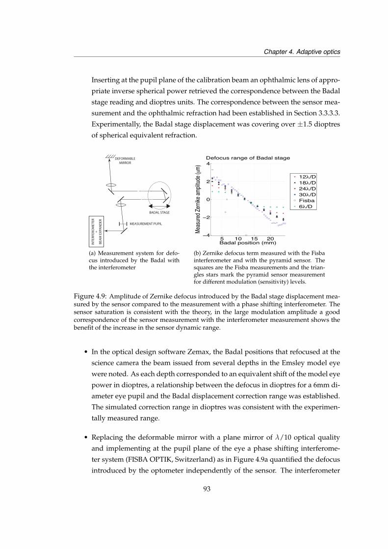
Chapter 4. Adaptive optics
Inserting at the pupil plane of the calibration beam an ophthalmic lens of appro-
priate inverse spherical power retrieved the correspondence between the Badal
stage reading and dioptres units. The correspondence between the sensor mea-
surement and the ophthalmic refraction had been established in Section 3.3.3.3.
Experimentally, the Badal stage displacement was covering over ±1.5 dioptres
of spherical equivalent refraction.
INTE
RFER
OM
ETER
BADAL STAGE
DEFORMABLE MIRROR
MEASUREMENT PUPIL
+BE
AM
EXP
AN
DER
(a) Measurement system for defo-cus introduced by the Badal withthe interferometer
5 10 15 20−4
−2
0
2
4Defocus range of Badal stage
Badal position (mm)
Meas
ured Z
ernike
amplit
ude (
μm)
12λ/D18λ/D24λ/D30λ/DFisba6λ/D
(b) Zernike defocus term measured with the Fisbainterferometer and with the pyramid sensor. Thesquares are the Fisba measurements and the trian-gles stars mark the pyramid sensor measurementfor different modulation (sensitivity) levels.
Figure 4.9: Amplitude of Zernike defocus introduced by the Badal stage displacement mea-sured by the sensor compared to the measurement with a phase shifting interferometer. Thesensor saturation is consistent with the theory, in the large modulation amplitude a goodcorrespondence of the sensor measurement with the interferometer measurement shows thebenefit of the increase in the sensor dynamic range.
• In the optical design software Zemax, the Badal positions that refocused at the
science camera the beam issued from several depths in the Emsley model eye
were noted. As each depth corresponded to an equivalent shift of the model eye
power in dioptres, a relationship between the defocus in dioptres for a 6mm di-
ameter eye pupil and the Badal displacement correction range was established.
The simulated correction range in dioptres was consistent with the experimen-
tally measured range.
• Replacing the deformable mirror with a plane mirror of λ/10 optical quality
and implementing at the pupil plane of the eye a phase shifting interferome-
ter system (FISBA OPTIK, Switzerland) as in Figure 4.9a quantified the defocus
introduced by the optometer independently of the sensor. The interferometer
93
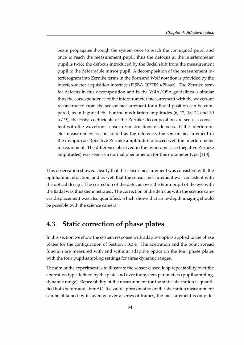
Chapter 4. Adaptive optics
beam propagates through the system once to reach the conjugated pupil and
once to reach the measurement pupil, thus the defocus at the interferometer
pupil is twice the defocus introduced by the Badal shift from the measurement
pupil to the deformable mirror pupil. A decomposition of the measurement in-
terferogram into Zernike terms in the Born and Wolf notation is provided by the
interferometer acquisition interface (FISBA OPTIK µPhase). The Zernike term
for defocus in this decomposition and in the VSIA/OSA guidelines is similar
thus the correspondence of the interferometer measurement with the wavefront
reconstructed from the sensor measurement for a Badal position can be com-
pared, as in Figure 4.9b. For the modulation amplitudes (6, 12, 18, 24 and 30
λ/D), the Fisba coefficients of the Zernike decomposition are seen as consis-
tent with the wavefront sensor reconstructions of defocus. If the interferom-
eter measurement is considered as the reference, the sensor measurement in
the myopic case (positive Zernike amplitude) followed well the interferometer
measurement. The difference observed in the hyperopic case (negative Zernike
amplitudes) was seen as a normal phenomenon for this optometer type [118].
This observation showed clearly that the sensor measurement was consistent with the
ophthalmic refraction, and as well that the sensor measurement was consistent with
the optical design. The correction of the defocus over the 6mm pupil of the eye with
the Badal was thus demonstrated. The correction of the defocus with the science cam-
era displacement was also quantified, which shows that an in-depth imaging should
be possible with the science camera.
4.3 Static correction of phase plates
In this section we show the system response with adaptive optics applied to the phase
plates for the configuration of Section 3.3.3.4. The aberration and the point spread
function are measured with and without adaptive optics on the four phase plates
with the four pupil sampling settings for three dynamic ranges.
The aim of the experiment is to illustrate the sensor closed loop repeatability over the
aberration type defined by the plate and over the system parameters (pupil sampling,
dynamic range). Repeatability of the measurement for the static aberration is quanti-
fied both before and after AO. If a valid approximation of the aberration measurement
can be obtained by its average over a series of frames, the measurement is only de-
94
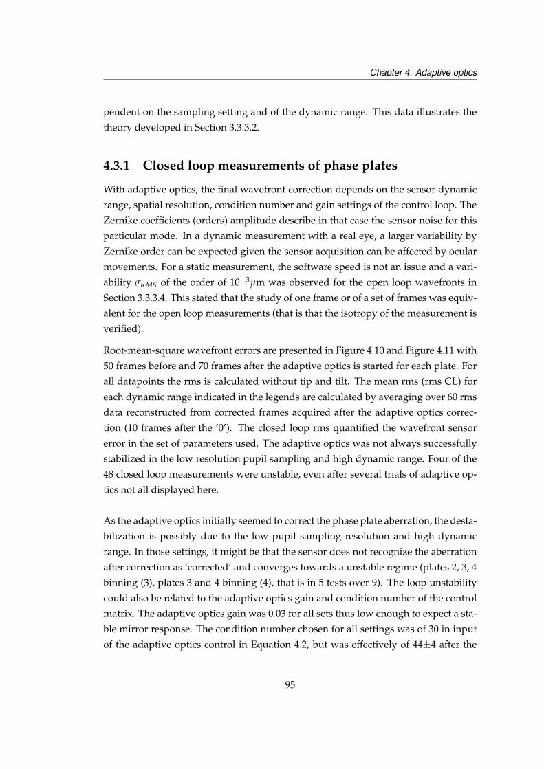
Chapter 4. Adaptive optics
pendent on the sampling setting and of the dynamic range. This data illustrates the
theory developed in Section 3.3.3.2.
4.3.1 Closed loop measurements of phase plates
With adaptive optics, the final wavefront correction depends on the sensor dynamic
range, spatial resolution, condition number and gain settings of the control loop. The
Zernike coefficients (orders) amplitude describe in that case the sensor noise for this
particular mode. In a dynamic measurement with a real eye, a larger variability by
Zernike order can be expected given the sensor acquisition can be affected by ocular
movements. For a static measurement, the software speed is not an issue and a vari-
ability σRMS of the order of 10−3µm was observed for the open loop wavefronts in
Section 3.3.3.4. This stated that the study of one frame or of a set of frames was equiv-
alent for the open loop measurements (that is that the isotropy of the measurement is
verified).
Root-mean-square wavefront errors are presented in Figure 4.10 and Figure 4.11 with
50 frames before and 70 frames after the adaptive optics is started for each plate. For
all datapoints the rms is calculated without tip and tilt. The mean rms (rms CL) for
each dynamic range indicated in the legends are calculated by averaging over 60 rms
data reconstructed from corrected frames acquired after the adaptive optics correc-
tion (10 frames after the ‘0’). The closed loop rms quantified the wavefront sensor
error in the set of parameters used. The adaptive optics was not always successfully
stabilized in the low resolution pupil sampling and high dynamic range. Four of the
48 closed loop measurements were unstable, even after several trials of adaptive op-
tics not all displayed here.
As the adaptive optics initially seemed to correct the phase plate aberration, the desta-
bilization is possibly due to the low pupil sampling resolution and high dynamic
range. In those settings, it might be that the sensor does not recognize the aberration
after correction as ‘corrected’ and converges towards a unstable regime (plates 2, 3, 4
binning (3), plates 3 and 4 binning (4), that is in 5 tests over 9). The loop unstability
could also be related to the adaptive optics gain and condition number of the control
matrix. The adaptive optics gain was 0.03 for all sets thus low enough to expect a sta-
ble mirror response. The condition number chosen for all settings was of 30 in input
of the adaptive optics control in Equation 4.2, but was effectively of 44±4 after the
95
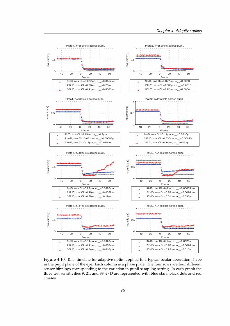
Chapter 4. Adaptive optics
−40 −20 0 20 40 600
0.5
1
Frame
rms (
micro
ns)
Plate1, n=55pixels across pupil,
9λ/D, rms CL=0.077μm, σrms
=0.0054μm21λ/D, rms CL=0.36μm, σ
rms=0.28μm
33λ/D, rms CL=0.11μm, σrms
=0.0035μm
m
−40 −20 0 20 40 600
0.5
1
Frame
rms (
micro
ns)
Plate1, n=28pixels across pupil,
9λ/D, rms CL=0.43μm, σrms
=0.2μm21λ/D, rms CL=0.031μm, σ
rms=0.00098μ
33λ/D, rms CL=0.11μm, σrms
=0.015μm
−40 −20 0 20 40 600
0.5
1
Frame
rms (
micro
ns)
Plate1, n=18pixels across pupil,
9λ/D, rms CL=0.29μm, σrms
=0.0026μm21λ/D, rms CL=0.16μm, σ
rms=0.0029μm
33λ/D, rms CL=0.39μm, σrms
=0.19μm
−40 −20 0 20 40 600
0.5
1
Frame
rms (
micro
ns)
Plate1, n=14pixels across pupil,
9λ/D, rms CL=0.11μm, σrms
=0.0026μm21λ/D, rms CL=0.11μm, σ
rms=0.0034μm
33λ/D, rms CL=0.24μm, σrms
=0.018μm
60
μmμm
μm
−40 −20 0 20 400
0.5
1
Frame
rms (
micro
ns)
Plate2, n=55pixels across pupil,
9λ/D, rms CL=0.077μm, σrms
=0.008621λ/D, rms CL=0.033μm, σ
rms=0.0018
33λ/D, rms CL=0.12μm, σrms
=0.0064
mμm
m
−40 −20 0 20 40 600
0.5
1
Framerm
s (mi
crons
)
Plate2, n=28pixels across pupil,
9λ/D, rms CL=0.14μm, σrms
=0.0016μ21λ/D, rms CL=0.035μm, σ
rms=0.00095
33λ/D, rms CL=0.14μm, σrms
=0.021μ
−40 −20 0 20 40 600
0.5
1
Frame
rms (
micro
ns)
Plate2, n=18pixels across pupil,
9λ/D, rms CL=0.61μm, σrms
=0.00085μm21λ/D, rms CL=0.78μm, σ
rms=0.0026μm
33λ/D, rms CL=0.31μm, σrms
=0.095μm
−40 −20 0 20 40 600
0.5
1
Frame
rms (
micro
ns)
Plate2, n=14pixels across pupil,
9λ/D, rms CL=0.14μm, σrms
=0.0026μm21λ/D, rms CL=0.76μm, σ
rms=0.0026μm
33λ/D, rms CL=0.23μm, σrms
=0.013μm
Figure 4.10: Rms timeline for adaptive optics applied to a typical ocular aberration shapein the pupil plane of the eye. Each column is a phase plate. The four rows are four differentsensor binnings corresponding to the variation in pupil sampling setting. In each graph thethree test sensitivities 9, 21, and 33 λ/D are represented with blue stars, black dots and redcrosses.
96
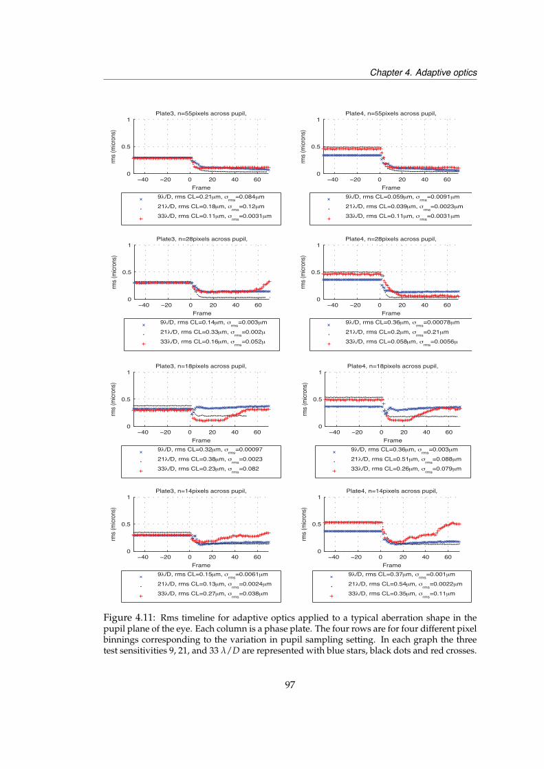
Chapter 4. Adaptive optics
−40 −20 0 20 40 600
0.5
1
Frame
rms (
micro
ns)
Plate3, n=55pixels across pupil,
9λ/D, rms CL=0.21μm, σrms
=0.084μm21λ/D, rms CL=0.18μm, σ
rms=0.12μm
33λ/D, rms CL=0.11μm, σrms
=0.0031μm
mm
−40 −20 0 20 40 600
0.5
1
Frame
rms (
micro
ns)
Plate3, n=28pixels across pupil,
9λ/D, rms CL=0.14μm, σrms
=0.003μm21λ/D, rms CL=0.33μm, σ
rms=0.002μ
33λ/D, rms CL=0.16μm, σrms
=0.052μ
60
μmμm
μm
−40 −20 0 20 400
0.5
1
Frame
rms (
micro
ns)
Plate3, n=18pixels across pupil,
9λ/D, rms CL=0.32μm, σrms
=0.0009721λ/D, rms CL=0.38μm, σ
rms=0.0023
33λ/D, rms CL=0.23μm, σrms
=0.082
−40 −20 0 20 40 600
0.5
1
Frame
rms (
micro
ns)
Plate3, n=14pixels across pupil,
9λ/D, rms CL=0.15μm, σrms
=0.0061μm21λ/D, rms CL=0.13μm, σ
rms=0.0024μm
33λ/D, rms CL=0.27μm, σrms
=0.038μm
−40 −20 0 20 40 600
0.5
1
Frame
rms (
micro
ns)
Plate4, n=55pixels across pupil,
9λ/D, rms CL=0.059μm, σrms
=0.0091μm21λ/D, rms CL=0.039μm, σ
rms=0.0023μm
33λ/D, rms CL=0.11μm, σrms
=0.0031μm
m
−40 −20 0 20 40 600
0.5
1
Frame
rms (
micro
ns)
Plate4, n=28pixels across pupil,
9λ/D, rms CL=0.36μm, σrms
=0.00078μm21λ/D, rms CL=0.2μm, σ
rms=0.21μm
33λ/D, rms CL=0.058μm, σrms
=0.0056μ
−40 −20 0 20 40 600
0.5
1
Frame
rms (
micro
ns)
Plate4, n=18pixels across pupil,
9λ/D, rms CL=0.36μm, σrms
=0.003μm21λ/D, rms CL=0.51μm, σ
rms=0.088μm
33λ/D, rms CL=0.26μm, σrms
=0.079μm
−40 −20 0 20 40 600
0.5
1
Frame
rms (
micro
ns)
Plate4, n=14pixels across pupil,
9λ/D, rms CL=0.37μm, σrms
=0.001μm21λ/D, rms CL=0.54μm, σ
rms=0.0022μm
33λ/D, rms CL=0.35μm, σrms
=0.11μm
Figure 4.11: Rms timeline for adaptive optics applied to a typical aberration shape in thepupil plane of the eye. Each column is a phase plate. The four rows are for four different pixelbinnings corresponding to the variation in pupil sampling setting. In each graph the threetest sensitivities 9, 21, and 33 λ/D are represented with blue stars, black dots and red crosses.
97
Chapter 4. Adaptive optics
control matrix was computed. This effective number of mirror zonal modes should
have been appropriate, even with the variation due to the small change in sensitivity
for each set of binning (B) and modulation amplitude (M).
4.3.2 Closed loop point spread function analysis
For each sequence and each plate, the point spread function before and after the adap-
tive optics was recorded synchronously with the sensor data so as to possibly relate
the closed loop psf quality with the pupil sampling and modulation parameters. The
ratio of the psf intensity maximum before and after adaptive optics at constant cam-
era exposure gives an experimental Strehl ratio value quantifying the efficiency of the
adaptive optics on the phase aberration. To determine if the closed loop efficiency can
really be characterized by the science camera point spread function, a representative
closed loop psf was selected for an adaptive optics wavefront at each dynamic range
and spatial resolution setting. The average acquisition frequency of the science cam-
era was 10.14Hz±0.27Hz.
The results are presented in Figure 4.12 for 1.6ms camera exposure (8 bits image
depth) images acquired at the highest sampling setting (Binning 1, 1360× 1280 pix-
els, 6.45 µm/pixel) and largest dynamic range setting (33λ/D). A common region
of interest was defined around a pixel manually chosen in each closed loop frame as
the central reference point. A common area of 50x50 pixels (0.26x0.26 mm area at the
back focal plane of the collimation lens in the calibration arm) is defined around the
psf centre. As the closed loop point spread functions areas superimpose, it seems that
independently of the dynamic ranges and pupil sampling settings the closed loops all
converge towards the same type of correction quality. The very small psf width in the
high-binning regimes is related to the decrease in the laser power that was meant to
keep a constant signal-to noise ratio at the sensor camera. This lack of power could be
the cause for the closed loop destabilization in Figure 4.10 and Figure 4.11, in partic-
ular at the highest modulation regime in which the light is spread over a larger area
at the pyramid than a small modulation regime for a constant laser power.
The two-fold variation in the point spread function size presented in Figure 4.12
shows that a better solution than decreasing the laser power would have been to
filter the beam at the sensor - even at the risk to introduce additional aberrations. In
addition, the constant area observed for all dynamic ranges after correction at a given
98
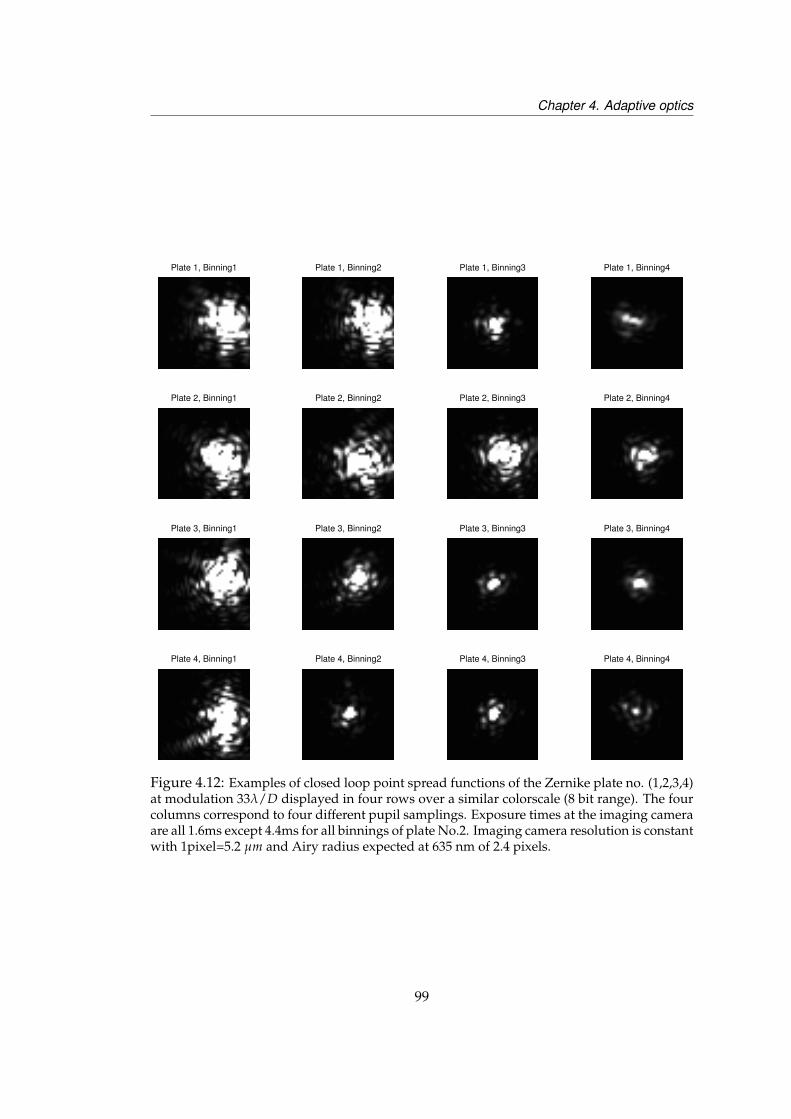
Chapter 4. Adaptive optics
Plate 1, Binning1 Plate 1, Binning2 Plate 1, Binning3 Plate 1, Binning4
Plate 2, Binning1 Plate 2, Binning2 Plate 2, Binning3 Plate 2, Binning4
Plate 3, Binning1 Plate 3, Binning2 Plate 3, Binning3 Plate 3, Binning4
Plate 4, Binning1 Plate 4, Binning2 Plate 4, Binning3 Plate 4, Binning4
Figure 4.12: Examples of closed loop point spread functions of the Zernike plate no. (1,2,3,4)at modulation 33λ/D displayed in four rows over a similar colorscale (8 bit range). The fourcolumns correspond to four different pupil samplings. Exposure times at the imaging cameraare all 1.6ms except 4.4ms for all binnings of plate No.2. Imaging camera resolution is constantwith 1pixel=5.2 µm and Airy radius expected at 635 nm of 2.4 pixels.
99
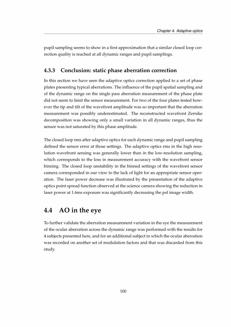
Chapter 4. Adaptive optics
pupil sampling seems to show in a first approximation that a similar closed loop cor-
rection quality is reached at all dynamic ranges and pupil samplings.
4.3.3 Conclusion: static phase aberration correction
In this section we have seen the adaptive optics correction applied to a set of phase
plates presenting typical aberrations. The influence of the pupil spatial sampling and
of the dynamic range on the single pass aberration measurement of the phase plate
did not seem to limit the sensor measurement. For two of the four plates tested how-
ever the tip and tilt of the wavefront amplitude was so important that the aberration
measurement was possibly underestimated. The reconstructed wavefront Zernike
decomposition was showing only a small variation in all dynamic ranges, thus the
sensor was not saturated by this phase amplitude.
The closed loop rms after adaptive optics for each dynamic range and pupil sampling
defined the sensor error at those settings. The adaptive optics rms in the high reso-
lution wavefront sensing was generally lower than in the low-resolution sampling,
which corresponds to the loss in measurement accuracy with the wavefront sensor
binning. The closed loop unstability in the binned settings of the wavefront sensor
camera corresponded in our view to the lack of light for an appropriate sensor oper-
ation. The laser power decrease was illustrated by the presentation of the adaptive
optics point spread function observed at the science camera showing the reduction in
laser power at 1.6ms exposure was significantly decreasing the psf image width.
4.4 AO in the eye
To further validate the aberration measurement variation in the eye the measurement
of the ocular aberration across the dynamic range was performed with the results for
4 subjects presented here, and for an additional subject in which the ocular aberration
was recorded on another set of modulation factors and that was discarded from this
study.
100
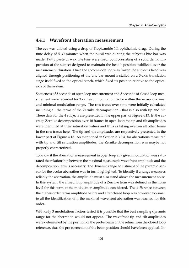
Chapter 4. Adaptive optics
4.4.1 Wavefront aberration measurement
The eye was dilated using a drop of Tropicamide 1% ophthalmic drug. During the
time delay of 5-30 minutes when the pupil was dilating the subject’s bite bar was
made. Putty paste or wax bite bars were used, both consisting of a solid dental im-
pression of the subject designed to maintain the head’s position stabilized over the
measurement duration. Once the accommodation was frozen the subject’s head was
aligned through positioning of the bite bar mount installed on a 3-axis translation
stage itself fixed to the optical bench, which fixed its position relative to the optical
axis of the system.
Sequences of 5 seconds of open loop measurement and 5 seconds of closed loop mea-
surement were recorded for 3 values of modulation factor within the sensor maximal
and minimal modulation range. The rms traces over time were initially calculated
including all the terms of the Zernike decomposition - that is also with tip and tilt.
These data for the 4 subjects are presented in the upper part of Figure 4.13. In the av-
erage Zernike decomposition over 10 frames in open-loop the tip and tilt amplitudes
were identified at their saturation values and thus as taking over on all other terms
in the rms traces here. The tip and tilt amplitudes are respectively presented in the
lower part of Figure 4.13. As mentioned in Section 3.3.3.4, for aberrations measured
with tip and tilt saturation amplitudes, the Zernike decomposition was maybe not
properly characterized.
To know if the aberration measurement in open loop at a given modulation was satu-
rated the relationship between the maximal measurable wavefront amplitude and the
decomposition term is necessary. The dynamic range adjustment of the pyramid sen-
sor for the ocular aberration was in turn highlighted. To identify if a range measures
reliably the aberration, the amplitude must also stand above the measurement noise.
In this system, the closed loop amplitude of a Zernike term was defined as the noise
level for this term at the modulation amplitude considered. The difference between
the higher-order terms amplitude before and after closed loop was however too small
to all the identification of if the maximal wavefront aberration was reached for this
order.
With only 3 modulations factors tested it is possible that the best sampling dynamic
range for the aberration would not appear. The wavefront tip and tilt amplitudes
were determined by the position of the probe beam on the retina from the closed loop
reference, thus the pre-correction of the beam position should have been applied. In-
101
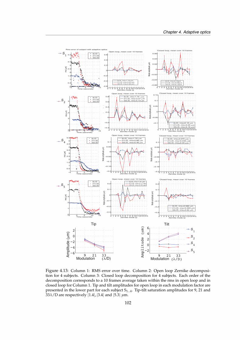
Chapter 4. Adaptive optics
0 1 2 3 4 5 6 7 8 9 101112131415−0.6
−0.4
−0.2
0
0.2
0.4
0.6
Zernike mode (j)
Mode
amplit
ude (μ
m)
Open loop, mean over 10 frames
9λ/D, rms=1.10 μm21λ/D, rms=3.04 μm33λ/D, rms=4.36 μm
−5 0 5 10 150
0.5
1
1.5
2
2.5
3
3.5
4
4.5
Time (seconds)
rms (μ
m)
9λ/D21λ/D33λ/D
0 1 2 3 4 5 6 7 8 9 101112131415−0.06
−0.04
−0.02
0
0.02
0.04
0.06
Zernike mode (j)
Mode
amplit
ude (μ
m)
Closed loop, mean over 10 frames
9λ/D, rms=0.14μm21λ/D, rms=0.09μm33λ/D, rms=0.15μm
0 1 2 3 4 5 6 7 8 9 101112131415−0.4
−0.2
0
0.2
0.4
0.6
0.8
Zernike mode (j)
Mode
amplit
ude (μ
m)
Open loop, mean over 10 frames
9λ/D, rms=1.75 μm21λ/D, rms=3.37 μm33λ/D, rms=5.13 μm
−5 0 5 10 150
1
2
3
4
5
Time (seconds)
rms (μ
m)
9λ/D21λ/D33λ/D
0 1 2 3 4 5 6 7 8 9 101112131415
−0.1
−0.05
0
0.05
0.1
0.15
Zernike mode (j)
Mode
amplit
ude (μ
m)
Closed loop, mean over 10 frames
9λ/D, rms=0.16 μm21λ/D, rms=0.29 μm33λ/D, rms=0.16 μm
0 1 2 3 4 5 6 7 8 9 101112131415−0.2
−0.15
−0.1
−0.05
0
0.05
0.1
Zernike mode (j)
Mode
amplit
ude (μ
m)
Open loop, mean over 10 frames
9λ/D, rms=1.70 μm21λ/D, rms=3.88 μm33λ/D, rms=5.46 μm
−5 0 5 10 15
0.5
1
1.5
2
2.5
3
3.5
4
4.5
5
5.5
Time (seconds)
rms (μ
m)
9λ/D21λ/D33λ/D
0 1 2 3 4 5 6 7 8 9 101112131415−0.2
−0.15
−0.1
−0.05
0
0.05
0.1
Zernike mode (j)
Mode
amplit
ude (μ
m)
Closed loop, mean over 10 frames
9λ/D, rms=0.075 μm21λ/D, rms=0.048 μm33λ/D, rms=0.20 μm
0 1 2 3 4 5 6 7 8 9 101112131415
−0.3
−0.2
−0.1
0
0.1
0.2
Zernike mode (j)
Mode
amplit
ude (μ
m)
Open loop, mean over 10 frames
9λ/D, rms=1.91 μm21λ/D, rms=4.17 μm33λ/D, rms=5.55 mμ
−5 0 5 10 150
1
2
3
4
5
Time (seconds)
rms (μ
m)
9λ/D21λ/D33λ/D
0 1 2 3 4 5 6 7 8 9 101112131415
−0.3
−0.2
−0.1
0
0.1
0.2
Zernike mode (j)
Mode
amplit
ude (
m)
Closed loop, mean over 10 frames
9λ/D, rms=0.085 μm21λ/D, rms=0.093 μm33λ/D, rms=0.64 μm
μ
9 21 33 −6
−4
−2
0
2
Modulation (λ/D)Ampl
itude
(μm
)
Tip
3
9 21 33−2
0
2
4
6
Modulation λ
Amplitude (μm)
TiltS1
S2
S4
S5
/D)(
S1
S2
S4
S5
Rms error of subject with adaptive optics
Figure 4.13: Column 1: RMS error over time. Column 2: Open loop Zernike decomposi-tion for 4 subjects. Column 3: Closed loop decomposition for 4 subjects. Each order of thedecomposition corresponds to a 10 frames average taken within the rms in open loop and inclosed loop for Column 1. Tip and tilt amplitudes for open loop in each modulation factor arepresented in the lower part for each subject S1...4. Tip-tilt saturation amplitudes for 9, 21 and33λ/D are respectively |1.4|, |3.4| and |5.3| µm.
102
Chapter 4. Adaptive optics
stead of maintaining the same probe beam orientation for all subjects, a customed
adjustment of the probe beam direction in the pupil and position at the pupil should
have been performed by adjustment of the probe beam assembly transverse controls.
Nevertheless, due to the deformable mirror stroke amplitude, the sensor saturation
did not stop the adaptive optics to operate. The lack of saturation detection did not
represent a problem for the adaptive optics given the high stroke of the mirror cor-
rected most of aberrations. However, this had the disadvantage that the experimental
parameters adjustment required to obtain a proper ocular aberration quantification
was not performed before the closed loop was started, and second, that the closed
loop sometimes revealed unstable .
In conclusion the mirror wavefront correction capability corresponded to the expec-
tations. Given the amplitude of the error bars in this dataset, the assumption that
the sensitivity range evolution is of benefit for the measurement of a given azimuthal
order of aberrations cannot be verified. For the low speed of the acquisition system
with typically 5 Hz to 10 Hz for the 56 samples across the pupil (each sample mea-
suring 107 µm at the eye), it is likely that the temporal variations of an order would
introduce errors in the characterization.
The second probe beam system was designed so that the probe beam tip and tilt
could be readjusted on the retina in order to limit the aberration correction to the
higher-order terms. The incoming defocus could not be controlled as finely. A wider
closed-loop probe beam image in the eye was observed.
4.4.2 Point spread function
Due to the diffusive properties of the retina, the probe beam image was widened
when observed in the eye compared to its observation after reflection onto a glass sub-
strate, a metallic surface, or a paper card. During the system alignment, closing the
loop on the probe beam shined on the metallic mount and acquiring the flashed-image
of the closed-loop image consisted the proof that the science camera was aligned with
the adaptive optics. The best image plane for the adaptive optics on the calibration
beam in the red thus corresponded to the best focus plane for the red in the retina.
In the eye the adaptive optics was recorded without changing this camera position.
The assumption was that the adaptive optics system was taking the highest level of
103

Chapter 4. Adaptive optics
intensity to calculate the correction, and bring the focus to the corresponding layer
of the retina. The point spread function images for the 4 subjects presented in Sec-
tion 4.4.1 are presented in Figure 4.14. The first two subjects S1 and S2 were imaged
using a 16 bit depth science camera image at the highest camera image resolution at
50 ms and 20 ms exposure and default camera gain (1016/4095 arbitrary units) while
subjects S4 and S5 were imaged using an 8 bit image depth, the highest camera bin-
ning and 5 ms exposures. The lower signal to noise ratio observed in S5 is attributed
to its darker eye color compared to the three other subjects as the laser power was set
constant at 2.5 mW power. All images show a 48×48 arcmin field in the eye using a
higher zoom factor for the subjects S4 and S5. The shift between the open loop posi-
tion and the closed loop position pointed by the centroids is of similar amplitude for
all the subjects and of 12.6 arcmin (63×63 µm for an eye length of 17 mm).
S1 OL M7
S1 CL M7
S2 OL M7
S2 CL M7
S4 OL M7
S4 CL M7
S5 OL M7
S5 CL M7
0
5000
0
5000
0
5000
0
5000
0
50
100
150
0
50
100
150
0
50
0
50
Figure 4.14: PSFs displacement for the 4 subjects without adaptive optics (OL) and withadaptive optics (CL). The lateral shift of the double pass closed loop measured with a centroidalgorithm corresponds to tip and tilt amplitudes leading to the wavefront sensor saturation.Closed loop signal diameter measured with a centroiding algorithm of 40µm ('8arcmin).
This constant shift was consistent with the constant laser position and angular shift
that was measured for all the subjects in this configuration and that had been fixed
after measurement of the first subject (S3, treated separately in the following of this
Section).
The adaptive optics was run in the eye of subject S3 for the highest pupil sampling
(56 pixels), a condition number of 30 modes, a gain of 0.01 and an initial science
camera exposure of 100 ms. The modulation amplitudes used in his measurement
were different from the amplitudes used in the eyes of other subjects, and are thus
104
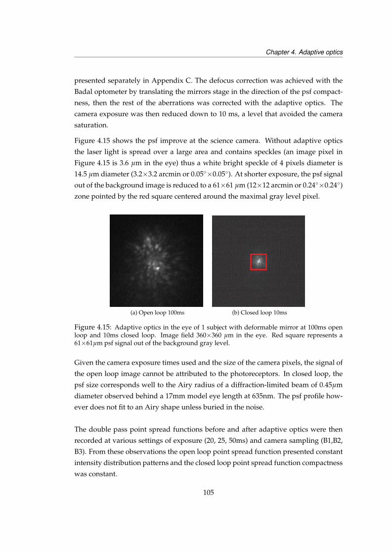
Chapter 4. Adaptive optics
presented separately in Appendix C. The defocus correction was achieved with the
Badal optometer by translating the mirrors stage in the direction of the psf compact-
ness, then the rest of the aberrations was corrected with the adaptive optics. The
camera exposure was then reduced down to 10 ms, a level that avoided the camera
saturation.
Figure 4.15 shows the psf improve at the science camera. Without adaptive optics
the laser light is spread over a large area and contains speckles (an image pixel in
Figure 4.15 is 3.6 µm in the eye) thus a white bright speckle of 4 pixels diameter is
14.5 µm diameter (3.2×3.2 arcmin or 0.05×0.05). At shorter exposure, the psf signal
out of the background image is reduced to a 61×61 µm (12×12 arcmin or 0.24×0.24)
zone pointed by the red square centered around the maximal gray level pixel.
(a) Open loop 100ms (b) Closed loop 10ms
Figure 4.15: Adaptive optics in the eye of 1 subject with deformable mirror at 100ms openloop and 10ms closed loop. Image field 360×360 µm in the eye. Red square represents a61×61µm psf signal out of the background gray level.
Given the camera exposure times used and the size of the camera pixels, the signal of
the open loop image cannot be attributed to the photoreceptors. In closed loop, the
psf size corresponds well to the Airy radius of a diffraction-limited beam of 0.45µm
diameter observed behind a 17mm model eye length at 635nm. The psf profile how-
ever does not fit to an Airy shape unless buried in the noise.
The double pass point spread functions before and after adaptive optics were then
recorded at various settings of exposure (20, 25, 50ms) and camera sampling (B1,B2,
B3). From these observations the open loop point spread function presented constant
intensity distribution patterns and the closed loop point spread function compactness
was constant.
105
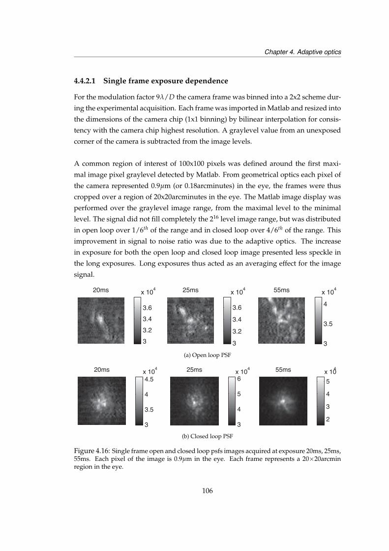
Chapter 4. Adaptive optics
4.4.2.1 Single frame exposure dependence
For the modulation factor 9λ/D the camera frame was binned into a 2x2 scheme dur-
ing the experimental acquisition. Each frame was imported in Matlab and resized into
the dimensions of the camera chip (1x1 binning) by bilinear interpolation for consis-
tency with the camera chip highest resolution. A graylevel value from an unexposed
corner of the camera is subtracted from the image levels.
A common region of interest of 100x100 pixels was defined around the first maxi-
mal image pixel graylevel detected by Matlab. From geometrical optics each pixel of
the camera represented 0.9µm (or 0.18arcminutes) in the eye, the frames were thus
cropped over a region of 20x20arcminutes in the eye. The Matlab image display was
performed over the graylevel image range, from the maximal level to the minimal
level. The signal did not fill completely the 216 level image range, but was distributed
in open loop over 1/6th of the range and in closed loop over 4/6th of the range. This
improvement in signal to noise ratio was due to the adaptive optics. The increase
in exposure for both the open loop and closed loop image presented less speckle in
the long exposures. Long exposures thus acted as an averaging effect for the image
signal.
20ms
25ms
55ms
33.23.43.6
x 104
3
3.2
3.4
3.6
x 104
3
3.5
4
x 104
(a) Open loop PSF
20ms
3
3.5
4
4.5x 10⁴ 25ms
3
4
5
6x 10⁴ 55ms
2
3
4
5x 10⁴
(b) Closed loop PSF
Figure 4.16: Single frame open and closed loop psfs images acquired at exposure 20ms, 25ms,55ms. Each pixel of the image is 0.9µm in the eye. Each frame represents a 20×20arcminregion in the eye.
106
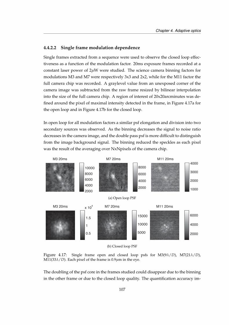
Chapter 4. Adaptive optics
4.4.2.2 Single frame modulation dependence
Single frames extracted from a sequence were used to observe the closed loop effec-
tiveness as a function of the modulation factor. 20ms exposure frames recorded at a
constant laser power of 2µW were studied. The science camera binning factors for
modulations M3 and M7 were respectively 3x3 and 2x2, while for the M11 factor the
full camera chip was recorded. A graylevel value from an unexposed corner of the
camera image was subtracted from the raw frame resized by bilinear interpolation
into the size of the full camera chip. A region of interest of 20x20arcminutes was de-
fined around the pixel of maximal intensity detected in the frame, in Figure 4.17a for
the open loop and in Figure 4.17b for the closed loop.
In open loop for all modulation factors a similar psf elongation and division into two
secondary sources was observed. As the binning decreases the signal to noise ratio
decreases in the camera image, and the double pass psf is more difficult to distinguish
from the image background signal. The binning reduced the speckles as each pixel
was the result of the averaging over NxNpixels of the camera chip.
M3 20ms
200040006000800010000
M7 20ms
2000
4000
6000
8000
M11 20ms
1000
2000
3000
4000
(a) Open loop PSF
M3 20ms
0.5
1
1.5
x 104 M7 20ms
5000
10000
15000
M11 20ms
2000
4000
6000
(b) Closed loop PSF
Figure 4.17: Single frame open and closed loop psfs for M3(9λ/D), M7(21λ/D),M11(33λ/D). Each pixel of the frame is 0.9µm in the eye.
The doubling of the psf core in the frames studied could disappear due to the binning
in the other frame or due to the closed loop quality. The quantification accuracy im-
107
Chapter 4. Adaptive optics
provement theoretically obtained after average over several frames revealed limited
by the recentering method chosen in the averaging process, not presented here.
4.5 Conclusions
This Chapter presented the corrective element of the new adaptive optics system,
and its implementation in an adaptive optics loop. The adaptive optics efficiency
was tested on a set of static aberrations. The optical system for the measurement
and correction of the ocular aberration was described. The influence of the defocus
pre-correction with the Badal mirrors was discussed. Preliminary images of in-vivo
correction of the double-pass ocular psf were presented.
Wavefront sensing measurement
For a dynamic operation the aberration pattern measurement for a young and not
very much aberrated eye was performed in three typical dynamic ranges of the sen-
sor. The aberration patterns showed to be relatively similar in all dynamic ranges but
the Zernike decomposition study could not lead to determining for sure if a dynamic
range was better suited for describing the particular amplitude of one Zernike mode
for the pattern observed. Assuming that more frames would better characterize a
variation of the Zernike term with time, a faster acquisition would be of interest.
If the adaptive optics system correction efficiency must be expressed only in terms of
point spread function extent at the science camera image, for the system presented
here the correction obtained here is much more efficient than in the initial system [1].
Given both systems used a similar number of lenses, the aberrations introduced by
the system were of similar amplitude. For a similar exposure used at the science cam-
era the improve in the psf size confirmed the deformable mirror was able to correct
the full ocular aberration.
The closed loop average rms was of 0.1 µm after correction. This relatively high value
was related to the choice of adaptive optics control parameters of gain, condition
number, influence function calibration, and reference wavefront, which were experi-
mentally defined. Those amplitudes however seemed close to the values of rms error
expected according to the simulation studies [47] for the number of modes used. At
38 Hz maximal speed during coupled acquisition of the imaging camera and wave-
108
Chapter 4. Adaptive optics
front sensor signal, instead of 55Hz acquisition of the wavefront sensor signal only,
the code speed for the adaptive optics was slowed down by the science camera acqui-
sition. Use of high-speed CMOS sensors or other CCD sensors to replace the cameras
was not feasible in this work.
Adaptive optics efficiency
The adaptive optics efficiency has been observed for a single frame and for several
subjects at multiple camera exposures in the eye. The science camera binning (imag-
ing resolution) reduced the signal speckles detected in the high-resolution image of
the static point spread function by introducing a blurr effect. In open and closed loop
it was impossible to state from the single frames if the use of a more sensitive modu-
lation factor led to a better or more compact point spread function. The AO efficiency
was therefore said independent on the dynamic range of the sensor for the aberration
studied and for the frames considered.
The improvement in the signal to noise ratio for a single modulation factor (dynamic
range setting) at long exposure resulting from an averaging over several single frames
was shown to be beneficial only if the average frame was obtained by selection of
typical AO-frames. In that case the psf signal could be compared to the focus of a
gaussian beam backreflected by the retina, and the speckle structures appearing in
the average image were observed to be of similar size as other observations of outer
segment cells.
109
Chapter 5
Imaging with the adaptive opticsfundus camera
5.1 Imaging system
We present in this section the retinal imaging system that has been built for imaging in
the eye. The aims of this system are to retrieve a retinal image of sufficient light level
to allow the focusing of the science image at the appropriate layer in the retina, and
to acquire a sequence of flashed images. The short exposure flashed images sequence
is a requirement for image post-processing operations to be performed and a good
signal-to-noise ratio image of interest for the clinician.
5.1.1 Design of the retinal imaging
The cone mosaic at the retina is considered as an array of hexagonal sources of side
2µm at the highest density (fovea) and 10µm in the periphery of the fovea, from 2 to
10 degrees. From the object plane to the image plane, the system’s ability to transmit
information is defined by the optical transfer function (OTF). Assuming the system
is linear in intensity as the illumination of the LED is spatially incoherent, and that
the image field remains within the isoplanatic angle of the system, the transmission
of the spatial frequency content is expressed by the convolution of the object function
(H) with the system point spread function (P).
110
Chapter 5. Imaging with the adaptive optics fundus camera
For (I) the image signal :
I = H ⊗ P F−→ I = H × T (5.1)
where⊗ defines the convolution,(
F−→)
the Fourier domain transformation and× the
scalar multiplication. The Fourier transform of the point spread function (P) is the
optical transfer function (T). Its modulus is the modulation transfer function MTF
which defines the optical system’s ability to transfer optical information. The highest
spatial frequency of the system, defined by the cutoff frequency of the optical transfer
function, is the size of the smallest feature of the object that appears in the image
observed through the generalized pupil. Following the Nyquist criterion, the highest
spatial frequency of the object must appear onto at least two image samples in the
image plane [119]. For an object like the cone mosaic a pixel of the camera must in
turn represent a maximum of 1µm in the eye.
The light comes from the specular reflection of the illumination of the hexagonal array
of photoreceptors, which become secondary sources forming the image. A first optical
relay formed by the first lens of focal length (f=125mm) after the eye and the lens of
the eye creates a conjugate retinal plane in the system before the Badal optometer.
For the Emsley reduced model eye, the length is l=22.2mm and the vitreous refractive
index n=1.33, thus the equivalent focal length in air is of f’=16.7mm. In this conjugate
retinal plane the magnification of the retina is given by the ratio of the focal lengths:
f ′
f=
12516.7
≈ 7.5× (5.2)
The smallest image detail visible in this conjugate image plane is defined by the spa-
tial frequency cutoff ( fc) of this optical system. Any information beyond this fre-
quency content is blocked by the eye lens. Thus :
fc =wλ f
(5.3)
In Equation 5.3, w is the radius of the pupil, f = 16.7 mm the model eye lens, and λ
the wavelength.
For a 6mm diameter eye pupil in the green (540 nm), this gives fc = 332 cycles/mm. In
the Gullstrand Eye model, for f = 17 mm the conversion factor between cycles/mm
111

Chapter 5. Imaging with the adaptive optics fundus camera
and cycles/degree is 0.3 mm/degree. The cut-off frequency in degrees is thus fc =
332 cycles/mm× 0.3 mm/degree which corresponds to a periodic pattern of approx-
imately 99.6 c/deg [120]. For a 6 mm diameter eye pupil in the red (635 nm), following
the same principles, fc = 283 c/mm, and in degrees fc = 85 c/deg.
Comparing the cutoff frequency of the imaging system with the cutoff frequency of a
system used for imaging the photoreceptors power spectra which presents an inten-
sity peak at 150 c/deg [2], this means our system should be able to sample the retinal
mosaic as fc is beyond the Nyquist criterion for an array of retinal cells of 2 µm spac-
ing.
A better sampling would be obtained by an increased number of pixels in the im-
age only possible with a smaller pixel size at the camera or by optically increasing the
magnification and decreasing the field-of-view. We note that when analyzing the reti-
nal mosaic across the field the size of the analysed part of the image must be chosen
carefully given its high variability across the retina, shown in Figure 5.1, first observed
by histology and confirmed by in-vivo studies [116, 121].
The frequency cut-off means the smallest feature that can be relayed through the eye
optics are also limited by the numerical aperture of the eye. If one wants to observe a
cellular feature of higher spatial frequency than these cutoff frequencies the only solu-
tion is to design an imaging system whose point spread function in the eye is smaller
than the natural values. This is performed to a certain extent in a confocal system
using a pinhole in a conjugate retinal plane or at the plane of the photodiode cell.
The pinhole squares the Bessel first order point spread function signal and in turn
the smallest spacing required to resolve 2 adjacent neighboring sources is reduced.
Without pinhole the diffraction limited point spread function of the imaging system
is classically defined by the Airy disk.
5.1.2 Illumination
The illumination path design is presented in a general manner here, as the several
versions were implemented. The optical design is similar to the Köhler system used
in microscopy, using the conjugation of the source to the cornea to illuminate the
retina in Maxwellian view. An iris in a conjugate plane defines the retinal extent of
the illumination at the retina, and a custom-designed fixation target printed onto a
112
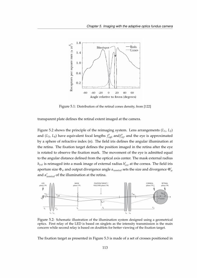
Chapter 5. Imaging with the adaptive optics fundus camera
Figure 5.1: Distribution of the retinal cones density, from [122]
transparent plate defines the retinal extent imaged at the camera.
Figure 5.2 shows the principle of the reimaging system. Lens arrangements (L1, L2)
and (L3, L4) have equivalent focal lengths f ′eq0 and f ′eq, and the eye is approximated
by a sphere of refractive index (n). The field iris defines the angular illumination at
the retina. The fixation target defines the position imaged in the retina after the eye
is rotated to observe the fixation mark. The movement of the eye is admitted equal
to the angular distance defined from the optical axis center. The mask external radius
hext is reimaged into a mask image of external radius h′ext at the cornea. The field iris
aperture size Φw and output divergence angle αwanted sets the size and divergence Φ′wand α′wanted of the illumination at the retina.
F’α'wanted
f’eq
φw/2
f4 f’4f3
(φw/2)’
f1 f’2
h0
αini
LEDplane (*P)
MASKplane (*P)
FIXATION TARGET /FIELD IRIS plane (*R)
CORNEALplane (*P)
RETINALplane (*R)
L4L3L2L1
f’eq0
Figure 5.2: Schematic illustration of the illumination system designed using a geometricaloptics. First relay of the LED is based on singlets as the intensity transmission is the mainconcern while second relay is based on doublets for better viewing of the fixation target.
The fixation target as presented in Figure 5.3 is made of a set of crosses positioned in
113
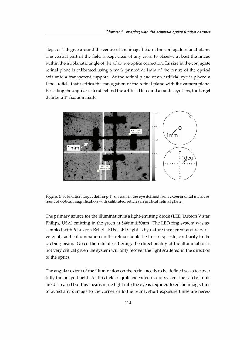
Chapter 5. Imaging with the adaptive optics fundus camera
steps of 1 degree around the centre of the image field in the conjugate retinal plane.
The central part of the field is kept clear of any cross to observe at best the image
within the isoplanatic angle of the adaptive optics correction. Its size in the conjugate
retinal plane is calibrated using a mark printed at 1mm of the centre of the optical
axis onto a transparent support. At the retinal plane of an artificial eye is placed a
Linos reticle that verifies the conjugation of the retinal plane with the camera plane.
Rescaling the angular extend behind the artificial lens and a model eye lens, the target
defines a 1 fixation mark.
22
22.54
X: 987 Y: 334RGB: 16, 16, 16
X: 516 Y: 875RGB: 24, 24, 24
0
50
100
150
200
250
1mm
1deg
1mm
Figure 5.3: Fixation target defining 1 off-axis in the eye defined from experimental measure-ment of optical magnification with calibrated reticles in artifical retinal plane.
The primary source for the illumination is a light-emitting diode (LED Luxeon V star,
Philips, USA) emitting in the green at 540nm±50nm. The LED ring system was as-
sembled with 6 Luxeon Rebel LEDs. LED light is by nature incoherent and very di-
vergent, so the illumination on the retina should be free of speckle, contrarily to the
probing beam. Given the retinal scattering, the directionality of the illumination is
not very critical given the system will only recover the light scattered in the direction
of the optics.
The angular extent of the illumination on the retina needs to be defined so as to cover
fully the imaged field. As this field is quite extended in our system the safety limits
are decreased but this means more light into the eye is required to get an image, thus
to avoid any damage to the cornea or to the retina, short exposure times are neces-
114

Chapter 5. Imaging with the adaptive optics fundus camera
sary. The LED activation and the camera acquisition are triggered using an electronics
board 8051 with software written to control the illumination power and flash dura-
tion. When the acquisition is not triggered with the illumination the camera acquires
the image with a light level averaged over time and thus presents an overall lower
intensity. Figure 5.4 shows the in-house heatsink built to prevent the burnout of the
LED junction in continuous operation, that is to improve the LED efficiency and life-
time. The mask used to block the central part of the illumination was also made at
the university.
(a)
CCD acquisitionPulse low controlled
LED illuminationPulse high dened
(b)
Figure 5.4: a. Condensed version of the 6-LED illumination system, with relay optics L1, L2and mask. b. Oscilloscope signals of single-source emission triggered with CCD cameraacquisition for a 4ms flash and image exposure.
From the average power Pavg measured at the corneal plane and the time of the pulse
∆t the pulse energy E illuminating the retina is calculated by :
Epulse = ∆t × Ppeak (5.4)
The illumination power Epulse in Equation 5.4 was designed so that its power at the
eye was at least 10× below the levels of Maximum Permissible Exposure (MPE) safety
levels defined by the EU Standard 60925-1:2007. Those calculations are presented in
Appendix B.
A calibration of the imaging system light collection efficiency was performed with a
paper target in the artificial eye retinal plane illuminated by the light source. A test
eye made of rubber was used with the maximal average power, which is equivalent
to the flash intensity. In such an object adaptive optics is required for deblurring the
initial high-resolution image. The rubber eye rear side structure is made of granulated
115

Chapter 5. Imaging with the adaptive optics fundus camera
structures which appear in the retinal image.
5.1.3 Experimental set up
Calibration of the image resolution and retinal imaging with adaptive optics has been
performed with the system presented in Figure 5.5. It is essentially identical to the
system described in Chapter 3 and Chapter 4, except that the probe beam system has
been implemented out of the Badal optometer. The probe beam diameter at the eye
was magnified from 0.9 mm at the aspheric collimator output to 1.05 mm at the pupil
plane of the eye. The 635 nm source of 3 µW power at the eye was replaced by an
infrared diode laser (Thorlabs S1FC780) of 10 µW power at the eye. Pre-correction of
the subject defocus was in turn impossible with this system. Calibration of the image
resolution was performed with the single-source system based on a Luxeon V Star
(Philips Lumileds, USA) flashing synchronously with the image acquisition. Reti-
nal imaging was performed with the 6-source system based on Luxeon Rebel diodes
(Philips Lumileds, USA) continuously illuminated.
5.2 Resolution targets imaged by the system
In the system considered here, the high magnification of the retina in the first con-
jugate retinal plane was also coupled with a good light efficiency provided by the
first lens small focal length. However the long optical path of the relay from the first
conjugate retinal plane to the science camera introduced some unwanted light from
the computer monitor or the desktop lamp. Isolation of the science camera optics
using black absorbing cardboard reduced noticeably this background signal. A large
amount of losses were due to the numerous optical elements and in particular due
to the beamsplitters separating the different system parts. To optimise the light cou-
pling to the science camera a dichroic beamsplitter (CVI Melles Griot Long Wave Pass
Unpolarised, 99 % reflective for 532 nm and 80 % transmittive for 633 nm) was placed
after the deformable mirror.
As all the lenses of the system were achromats, the optical design with the model eye
presented almost no difference in the focal plane position of the red wavelength and
of the green wavelength. This problem was different when observing the eye due to
the longitudinal and transverse chromatic aberrations [5,123]. The aberration pattern
corrected by the deformable mirror at the conjugate pupil plane was assumed to be
116
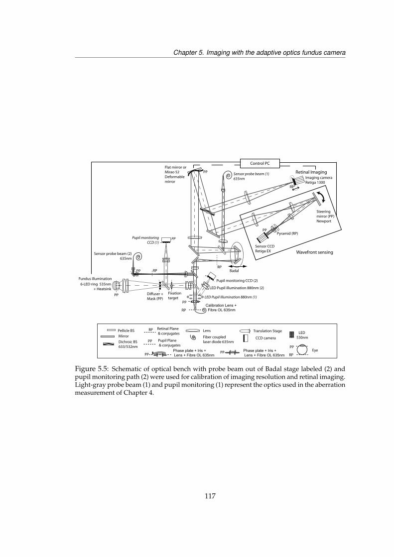
Chapter 5. Imaging with the adaptive optics fundus camera
LED Pupil illumination 880nm (2)
Pupil monitoring CCD (2)
RP
Control PC
Retinal Imaging
Wavefront sensing
Fundus illumination
LED Pupil Illumination 880nm (1)
Pupil monitoringCCD (1)
PP
RP
PPFlat mirror or Mirao 52 Deformable mirror
Steering mirror (PP)Newport
PPPyramid (RP)
Sensor probe beam (1)635nm
Sensor CCD Retiga EX
Imaging cameraRetiga 1300
RPCalibration Lens +
Fibre OL 635nm
PP
Mirror
Pellicle BS LensRP
PP
Retinal Plane & conjugates
Pupil Plane & conjugates
Translation Stage
Fiber coupled laser diode 635nm
CCD cameraDichroic BS 633/532nm
RP
PPEyePhase plate + Iris +
Lens + Fibre OL 635nmPPPhase plate + Iris +
Lens + Fibre OL 635nmPP
LED 530nm
Badal
6-LED ring 535nm+ Heatsink
Fixationtarget
Diffuser + Mask (PP)
PP
PP RP
Sensor probe beam (2)635nm
Figure 5.5: Schematic of optical bench with probe beam out of Badal stage labeled (2) andpupil monitoring path (2) were used for calibration of imaging resolution and retinal imaging.Light-gray probe beam (1) and pupil monitoring (1) represent the optics used in the aberrationmeasurement of Chapter 4.
117
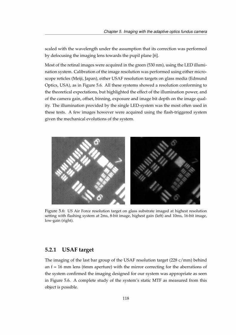
Chapter 5. Imaging with the adaptive optics fundus camera
scaled with the wavelength under the assumption that its correction was performed
by defocusing the imaging lens towards the pupil plane [6].
Most of the retinal images were acquired in the green (530 nm), using the LED illumi-
nation system. Calibration of the image resolution was performed using either micro-
scope reticles (Meiji, Japan), either USAF resolution targets on glass media (Edmund
Optics, USA), as in Figure 5.6. All these systems showed a resolution conforming to
the theoretical expectations, but highlighted the effect of the illumination power, and
of the camera gain, offset, binning, exposure and image bit depth on the image qual-
ity. The illumination provided by the single LED-system was the most often used in
these tests. A few images however were acquired using the flash-triggered system
given the mechanical evolutions of the system.
Figure 5.6: US Air Force resolution target on glass substrate imaged at highest resolutionsetting with flashing system at 2ms, 8-bit image, highest gain (left) and 10ms, 16-bit image,low-gain (right).
5.2.1 USAF target
The imaging of the last bar group of the USAF resolution target (228 c/mm) behind
an f = 16 mm lens (6mm aperture) with the mirror correcting for the aberrations of
the system confirmed the imaging designed for our system was appropriate as seen
in Figure 5.6. A complete study of the system’s static MTF as measured from this
object is possible.
118
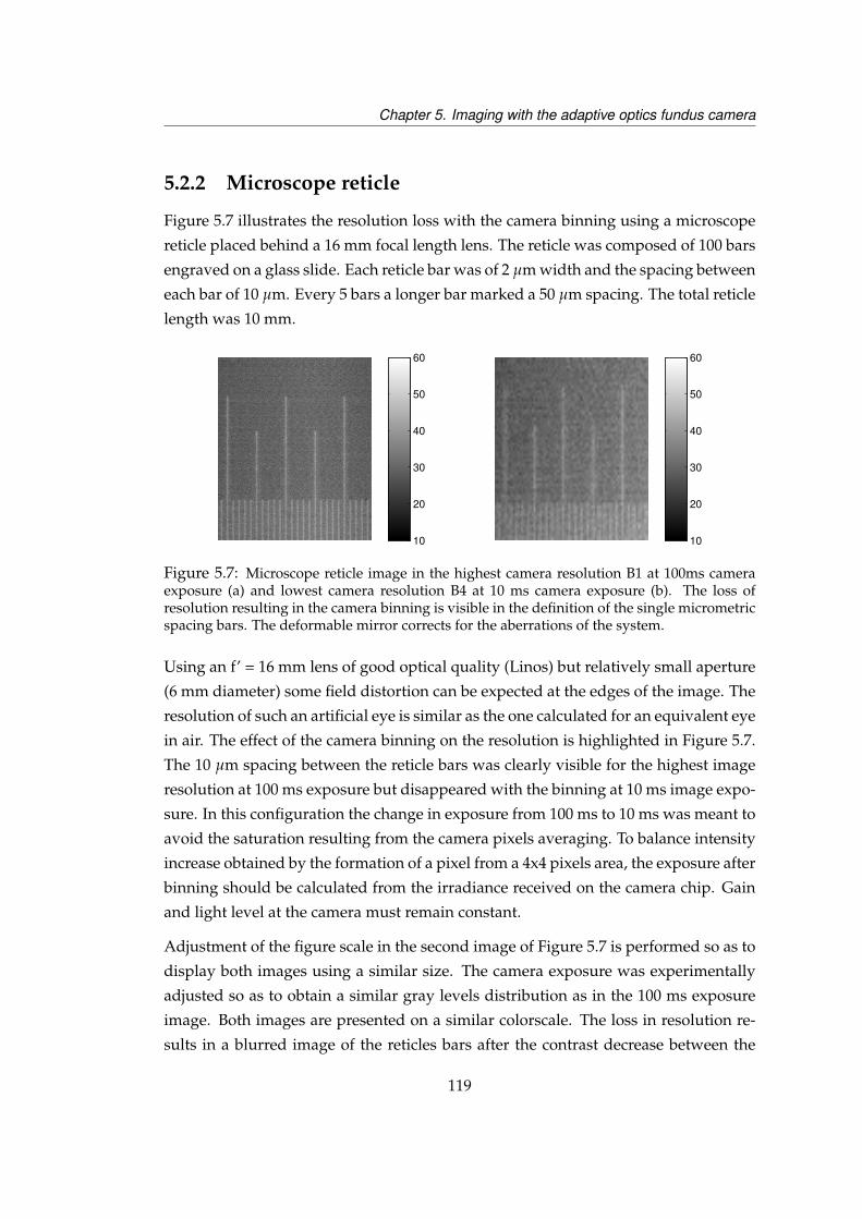
Chapter 5. Imaging with the adaptive optics fundus camera
5.2.2 Microscope reticle
Figure 5.7 illustrates the resolution loss with the camera binning using a microscope
reticle placed behind a 16 mm focal length lens. The reticle was composed of 100 bars
engraved on a glass slide. Each reticle bar was of 2 µm width and the spacing between
each bar of 10 µm. Every 5 bars a longer bar marked a 50 µm spacing. The total reticle
length was 10 mm.
10
20
30
40
50
60
10
20
30
40
50
60
Figure 5.7: Microscope reticle image in the highest camera resolution B1 at 100ms cameraexposure (a) and lowest camera resolution B4 at 10 ms camera exposure (b). The loss ofresolution resulting in the camera binning is visible in the definition of the single micrometricspacing bars. The deformable mirror corrects for the aberrations of the system.
Using an f’ = 16 mm lens of good optical quality (Linos) but relatively small aperture
(6 mm diameter) some field distortion can be expected at the edges of the image. The
resolution of such an artificial eye is similar as the one calculated for an equivalent eye
in air. The effect of the camera binning on the resolution is highlighted in Figure 5.7.
The 10 µm spacing between the reticle bars was clearly visible for the highest image
resolution at 100 ms exposure but disappeared with the binning at 10 ms image expo-
sure. In this configuration the change in exposure from 100 ms to 10 ms was meant to
avoid the saturation resulting from the camera pixels averaging. To balance intensity
increase obtained by the formation of a pixel from a 4x4 pixels area, the exposure after
binning should be calculated from the irradiance received on the camera chip. Gain
and light level at the camera must remain constant.
Adjustment of the figure scale in the second image of Figure 5.7 is performed so as to
display both images using a similar size. The camera exposure was experimentally
adjusted so as to obtain a similar gray levels distribution as in the 100 ms exposure
image. Both images are presented on a similar colorscale. The loss in resolution re-
sults in a blurred image of the reticles bars after the contrast decrease between the
119

Chapter 5. Imaging with the adaptive optics fundus camera
reticle bars and the background illumination is observed between two reticle bars.
A typical problem encountered by our system with glass and metallic supports is that
the image plane is much more reflective than the human eye, thus the experimental
parameters used during the calibration of the image quality need adjustment in the
eye. The deposited substrate in the case of the USAF target is also more reflective
than an engraved pattern such as the reticles bars. Over the image field we can also
see a non-uniform illumination distribution in those targets.
5.2.3 Rubber eye
The rubber eyeballs used in this demonstration are made of a soft plastic membrane
containing a transparent liquid meant to model the vitreous of the eye (n=1.44, from
the manufacturer’s specifications). The image is acquired from the front of the eye-
ball through a smooth plastic type that forms an artificial cornea and eye pupil. The
light backscattered by the plastic eyeball shows a network of artificial blood ves-
sels converging towards an equivalent artificial optic disk. The curvature and semi-
transparent nature of the artificial eyeball makes this object interesting for calibration
of the imaging system response to an absorbing and non-planar surface presenting
in-depth internal structures in a media of different refractive index than air.
A piece of white paper card placed at the back of the artificial retina is used to increase
the light return in the system. The result for a constant image field with and without
the reflector is presented in Figure 5.8 for a constant illumination level, camera ex-
posure and camera resolution. A sharp contrast improvement between the artificial
blood vessel network and the background retina results from the white paper imple-
mentation. The image acquisition range is filled in the second configuration which
means the white paper card replaces the choroid in the human eye. The static na-
ture of the object allows long exposures to be used without any blurring due to the
eye motion. The adaptive optics performance is also left free of constraints of speed
or dynamics. The initial 1.2 µm wavefront rms measured in open loop for the ocu-
lar aberration of the rubber eye is corrected down to 0.05 µm without the additional
reflective paper and down to 0.015 µm with the additional reflective paper as pre-
sented in Figure 5.9. The optical quality after closed loop is better when more light
is returned to the sensor. This seems to validate that for a static element formed by
a dense media, the correction of the ocular aberration is realized down to very low
120
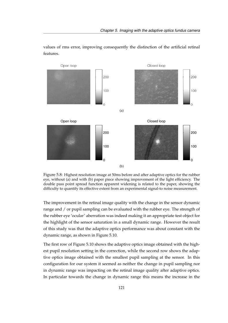
Chapter 5. Imaging with the adaptive optics fundus camera
values of rms error, improving consequently the distinction of the artificial retinal
features.
(a)
Open loop
0
100
200
Closed loop
0
100
200
(b)
Figure 5.8: Highest resolution image at 50ms before and after adaptive optics for the rubbereye, without (a) and with (b) paper piece showing improvement of the light efficiency. Thedouble pass point spread function apparent widening is related to the paper, showing thedifficulty to quantify its effective extent from an experimental signal-to noise measurement.
The improvement in the retinal image quality with the change in the sensor dynamic
range and / or pupil sampling can be evaluated with the rubber eye. The strength of
the rubber eye ‘ocular’ aberration was indeed making it an appropriate test object for
the highlight of the sensor saturation in a small dynamic range. However the result
of this study was that the adaptive optics performance was about constant with the
dynamic range, as shown in Figure 5.10.
The first row of Figure 5.10 shows the adaptive optics image obtained with the high-
est pupil resolution setting in the correction, while the second row shows the adap-
tive optics image obtained with the smallest pupil sampling at the sensor. In this
configuration for our system it seemed as neither the change in pupil sampling nor
in dynamic range was impacting on the retinal image quality after adaptive optics.
In particular towards the change in dynamic range this means the increase in the
121

Chapter 5. Imaging with the adaptive optics fundus camera
20 21 22 23 24 25 26 27 28 29 300
0.2
0.4
0.6
0.8
1
1.2
1.4
1.6
1.8
2
X: 28.64Y: 0.04803
Time (seconds)
RMS
ampl
itude
(µm
)
(a) RMS without reflecting paper
15 17 19 21 23 250
0.2
0.4
0.6
0.8
1
1.2
1.4
1.6
1.8
2
X: 23.34Y: 0.01538
Time (seconds)
RMS
ampl
itude
(µm
)
(b) RMS with reflecting paper
Figure 5.9: RMS timetrace for the rubber eye without and with the static reflector paperplaced behind the eye. More signal is beneficial to the closed loop as presented in the casethat has the reflector. Modulation 21λ/D, 20modes used in the correction, 7 pupil samples/actuator at the sensor
Figure 5.10: An increasing dynamic range (M3, M5, M7, M9 from left to right) and twosettings of pupil sampling (110µm/sample, top row and 430µm/sample, lower row) afteradaptive optics in a plastic eye at 50ms camera exposure. The lack of visual variation in thedefinition of the background rugosities means independence towards the sensor parametersfor this aberration.
122
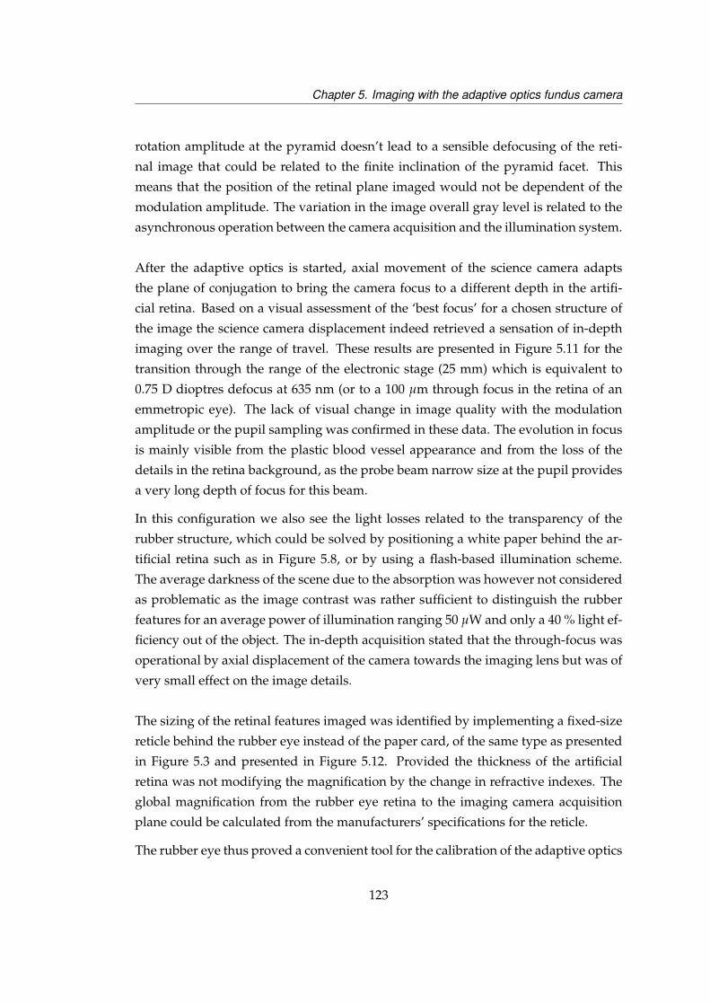
Chapter 5. Imaging with the adaptive optics fundus camera
rotation amplitude at the pyramid doesn’t lead to a sensible defocusing of the reti-
nal image that could be related to the finite inclination of the pyramid facet. This
means that the position of the retinal plane imaged would not be dependent of the
modulation amplitude. The variation in the image overall gray level is related to the
asynchronous operation between the camera acquisition and the illumination system.
After the adaptive optics is started, axial movement of the science camera adapts
the plane of conjugation to bring the camera focus to a different depth in the artifi-
cial retina. Based on a visual assessment of the ‘best focus’ for a chosen structure of
the image the science camera displacement indeed retrieved a sensation of in-depth
imaging over the range of travel. These results are presented in Figure 5.11 for the
transition through the range of the electronic stage (25 mm) which is equivalent to
0.75 D dioptres defocus at 635 nm (or to a 100 µm through focus in the retina of an
emmetropic eye). The lack of visual change in image quality with the modulation
amplitude or the pupil sampling was confirmed in these data. The evolution in focus
is mainly visible from the plastic blood vessel appearance and from the loss of the
details in the retina background, as the probe beam narrow size at the pupil provides
a very long depth of focus for this beam.
In this configuration we also see the light losses related to the transparency of the
rubber structure, which could be solved by positioning a white paper behind the ar-
tificial retina such as in Figure 5.8, or by using a flash-based illumination scheme.
The average darkness of the scene due to the absorption was however not considered
as problematic as the image contrast was rather sufficient to distinguish the rubber
features for an average power of illumination ranging 50 µW and only a 40 % light ef-
ficiency out of the object. The in-depth acquisition stated that the through-focus was
operational by axial displacement of the camera towards the imaging lens but was of
very small effect on the image details.
The sizing of the retinal features imaged was identified by implementing a fixed-size
reticle behind the rubber eye instead of the paper card, of the same type as presented
in Figure 5.3 and presented in Figure 5.12. Provided the thickness of the artificial
retina was not modifying the magnification by the change in refractive indexes. The
global magnification from the rubber eye retina to the imaging camera acquisition
plane could be calculated from the manufacturers’ specifications for the reticle.
The rubber eye thus proved a convenient tool for the calibration of the adaptive optics
123

Chapter 5. Imaging with the adaptive optics fundus camera
(a)
(b)
Figure 5.11: Axial translation of the science camera for the rubber eye retina. All imagesare 230×184arcmin in the rubber eye, at 50ms exposure image and highest image resolution.Sensor settings present an increasing dynamic range (M3, M5, M7, M9 from left to right)and two settings of pupil sampling (110µm/sample, top row and 430µm/sample, lower row)after adaptive optics. From Figure 5.10 in which the retina speckles are in focus the translationhighlights progressively the blood vessel structure in (a) then the focus is lost (b). The probebeam constant shape relates to its small diameter at the pupil of the eye and consequentlylengthened depth of focus.
Figure 5.12: 100ms and highest imaging camera resolution acquisition of the reticle of Fig-ure 5.3 placed behind the rubber eye retina after correction with adaptive optics.
124

Chapter 5. Imaging with the adaptive optics fundus camera
efficiency in a static configuration and to obtain an overview of the retinal image
quality improve resulting from the aberration correction.
5.3 Retinal imaging with adaptive optics in a real
eye
In the procedure for imaging the eye with adaptive optics the initial position of the
retinal camera was the one for which the calibration fibre point spread function was
best imaged. Given the chromatic aberration of the eye, even after adaptive optics an
axial displacement of the camera should be required between the plane of observation
for the ocular point spread function and the plane of observation of the retinal cells.
This displacement is equivalent to the application of a defocus in the image plane,
and has been quantified in Section 3.3.3.3 to be correctable by displacement of the
electronics translation stage [5].
In eyes with a good optical quality the adaptive optics performance is not obvious
but still the signal to noise ratio improvement is observed. In more aberrated eyes
the correction is obvious from the point of view of the observation of the point spread
function size before and after adaptive optics but overexposure of the camera image
rendered a saturated point spread function in the form of a white disk as presented
in Figure 5.16.
Retinal imaging in the eye with the first illumination system was performed with
adaptive optics but the source low illumination power resulted in a long exposure
image at the camera. Any possible observation of cellular structures was thus blurred
by the eye motion. Second, the resolution of this system in short exposures was mea-
sured not to be sufficient for resolving the retinal cells.
The system used for acquisition of the results presented in the following was de-
scribed in Figure 5.5, Section 4.2.2. A change in the first beamsplitter after the eye re-
sulted in an increase in light efficiency. The maximal power into the eye was reached
with the single-LED illumination system at 130 µW average power (530 nm) mea-
sured over a 10 mm-diameter circular sensor, which was under the safety limits for
the eye. Still, given the low light efficiency of the system from the eye to the camera
pixel, averaging, high camera gains and 8-bit image acquisition were required, which
resulted in signal artifacts in the form of diagonal fringes in the image. Basic image
125

Chapter 5. Imaging with the adaptive optics fundus camera
post-processing operations were applied to these images in the form of digital filter-
ing in order to extract some information on the retina structure.
Experimentally the effect of the adaptive optics on the double pass point spread func-
tion improvement was not very visible for the subjects which presented a refractive
error below±0.25 D dioptre. The subjects studied in the following are thus separated
into 2 groups which are noted "good eyes" for the eyes mentioned beforehand and
"very aberrated" for the eyes that had a refractive error above 1 D dioptres and which
were partially corrected with the Badal stage. In an absolute sense the refractive er-
ror in these eyes were below (-3) D diopters thus the system was tested only for low
myopia subjects.
5.3.1 Retinal imaging of eyes with refractive error <0.25D
In this case the mirror shape correcting for the aberrations of the system only (that is
the voltages set configuration ‘flat’) retrieved an image of the choroidal blood vessels
without requiring dynamic correction.
For these subjects the retinal image with or without adaptive optics is not very differ-
ent once the aberrations of the system are corrected. For subjects with a good fixation
images acquired at 20ms exposure retrieved a correct identification of choroidal blood
vessels. The lack of synchronization between the acquisition and the illumination sys-
tems resulted in the need for using 20 ms, 50 ms, 100 ms and 200 ms exposure times,
which are long exposures for the eye. Binning of the camera chip was necessary to
keep the light levels safe in the eye, which increased the size of a pixel at the retina
but the light levels were still too low to reduce the exposure time of the image.
The typical acquisition procedure started with the imaging of the double pass ocu-
lar point spread function before and after adaptive optics correction. The power of
the probe beam laser (780 nm) was 10 µW and the average power of the illumination
(535 nm) was 26 µW over a 5degree retinal area.
For the example presented in Figure 5.13, the ocular PSF was not extremely different
before and after adaptive optics thus again the correction was mainly effective on
the tip and tilt. Infrared laser at 780 nm was used here instead of red light as more
convenient for the viewing by the subject. The difference in wavelength between the
126
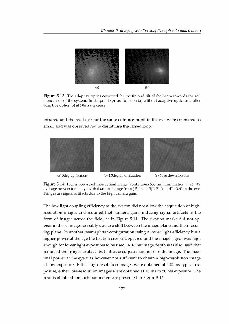
Chapter 5. Imaging with the adaptive optics fundus camera
(a) (b)
Figure 5.13: The adaptive optics corrected for the tip and tilt of the beam towards the ref-erence axis of the system. Initial point spread function (a) without adaptive optics and afteradaptive optics (b) at 50ms exposure.
infrared and the red laser for the same entrance pupil in the eye were estimated as
small, and was observed not to destabilise the closed loop.
(a) 3deg up fixation (b) 2.5deg down fixation (c) 5deg down fixation
Figure 5.14: 100ms, low-resolution retinal image (continuous 535 nm illumination at 26 µWaverage power) for an eye with fixation change from (-5) to (+3). Field is 4×3.6 in the eye.Fringes are signal artifacts due to the high camera gain.
The low light coupling efficiency of the system did not allow the acquisition of high-
resolution images and required high camera gains inducing signal artifacts in the
form of fringes across the field, as in Figure 5.14. The fixation marks did not ap-
pear in those images possibly due to a shift between the image plane and their focus-
ing plane. In another beamsplitter configuration using a lower light efficiency but a
higher power at the eye the fixation crosses appeared and the image signal was high
enough for lower light exposures to be used. A 16 bit image depth was also used that
removed the fringes artifacts but introduced gaussian noise in the image. The max-
imal power at the eye was however not sufficient to obtain a high-resolution image
at low-exposure. Either high-resolution images were obtained at 100 ms typical ex-
posure, either low-resolution images were obtained at 10 ms to 50 ms exposure. The
results obtained for such parameters are presented in Figure 5.15.
127
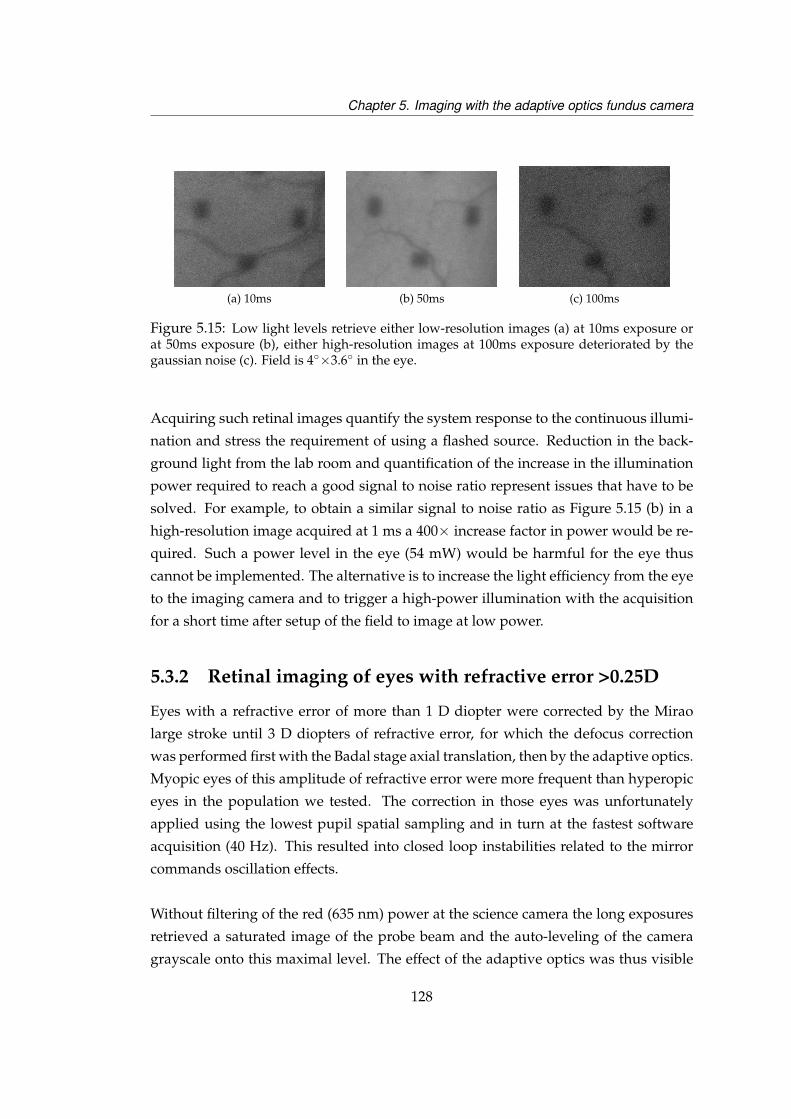
Chapter 5. Imaging with the adaptive optics fundus camera
(a) 10ms (b) 50ms (c) 100ms
Figure 5.15: Low light levels retrieve either low-resolution images (a) at 10ms exposure orat 50ms exposure (b), either high-resolution images at 100ms exposure deteriorated by thegaussian noise (c). Field is 4×3.6 in the eye.
Acquiring such retinal images quantify the system response to the continuous illumi-
nation and stress the requirement of using a flashed source. Reduction in the back-
ground light from the lab room and quantification of the increase in the illumination
power required to reach a good signal to noise ratio represent issues that have to be
solved. For example, to obtain a similar signal to noise ratio as Figure 5.15 (b) in a
high-resolution image acquired at 1 ms a 400× increase factor in power would be re-
quired. Such a power level in the eye (54 mW) would be harmful for the eye thus
cannot be implemented. The alternative is to increase the light efficiency from the eye
to the imaging camera and to trigger a high-power illumination with the acquisition
for a short time after setup of the field to image at low power.
5.3.2 Retinal imaging of eyes with refractive error >0.25D
Eyes with a refractive error of more than 1 D diopter were corrected by the Mirao
large stroke until 3 D diopters of refractive error, for which the defocus correction
was performed first with the Badal stage axial translation, then by the adaptive optics.
Myopic eyes of this amplitude of refractive error were more frequent than hyperopic
eyes in the population we tested. The correction in those eyes was unfortunately
applied using the lowest pupil spatial sampling and in turn at the fastest software
acquisition (40 Hz). This resulted into closed loop instabilities related to the mirror
commands oscillation effects.
Without filtering of the red (635 nm) power at the science camera the long exposures
retrieved a saturated image of the probe beam and the auto-leveling of the camera
grayscale onto this maximal level. The effect of the adaptive optics was thus visible
128
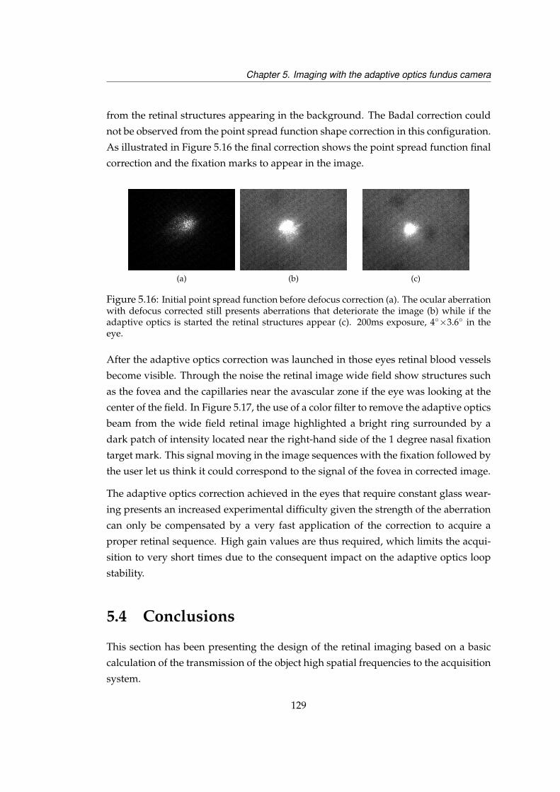
Chapter 5. Imaging with the adaptive optics fundus camera
from the retinal structures appearing in the background. The Badal correction could
not be observed from the point spread function shape correction in this configuration.
As illustrated in Figure 5.16 the final correction shows the point spread function final
correction and the fixation marks to appear in the image.
(a) (b) (c)
Figure 5.16: Initial point spread function before defocus correction (a). The ocular aberrationwith defocus corrected still presents aberrations that deteriorate the image (b) while if theadaptive optics is started the retinal structures appear (c). 200ms exposure, 4×3.6 in theeye.
After the adaptive optics correction was launched in those eyes retinal blood vessels
become visible. Through the noise the retinal image wide field show structures such
as the fovea and the capillaries near the avascular zone if the eye was looking at the
center of the field. In Figure 5.17, the use of a color filter to remove the adaptive optics
beam from the wide field retinal image highlighted a bright ring surrounded by a
dark patch of intensity located near the right-hand side of the 1 degree nasal fixation
target mark. This signal moving in the image sequences with the fixation followed by
the user let us think it could correspond to the signal of the fovea in corrected image.
The adaptive optics correction achieved in the eyes that require constant glass wear-
ing presents an increased experimental difficulty given the strength of the aberration
can only be compensated by a very fast application of the correction to acquire a
proper retinal sequence. High gain values are thus required, which limits the acqui-
sition to very short times due to the consequent impact on the adaptive optics loop
stability.
5.4 Conclusions
This section has been presenting the design of the retinal imaging based on a basic
calculation of the transmission of the object high spatial frequencies to the acquisition
system.
129

Chapter 5. Imaging with the adaptive optics fundus camera
(a) (b)
Figure 5.17: When the mirror is correcting for the system aberration only the retina doesnot appear (a) while if the adaptive optics is started the retinal structures appear (b). 200msexposure, 4×3.6 in the eye fixating at the 1 mark on the left side.
Experimental implementation of the illumination was described and experimental
testing of the image resolution using static objects in artificial eyes was presented
with and without adaptive optics. On a static object presenting an in-depth retinal
structure, the adaptive optics led to an improved image resolution, independently
of the wavefront sensor pupil sampling (‘B’ for the Binning parameter) and of the
modulation (‘M’ for the Modulation parameter).
In the human eye in-vivo, for refraction amplitudes of < 0.25 D the adaptive optics
could not be clearly distinguished from the cancellation of the aberration of the optical
system. The retinal image before and after the ocular aberrations were corrected did
not show a signal-to noise improve. For higher amplitudes of refraction, (remaining
below 3 D) the adaptive optics effect was clearer, despite the low quality of the final
image.
An overall need for improving the light collection efficiency of the system, by the use
of a flashed source at the retina synchronized with the image acquisition has been
observed. Imaging of the retina asking the subject to fixate at off-axis angles of higher
amplitude than 1 did not show ‘classical’ photoreceptors signals despite the cells size
expected at those retinal subtenses presence. Unexplained very weak intensity blobs
were present in some retinal images (Figure 5.14, left and Figure 5.15, center).
130
Chapter 6
Conclusion
6.1 General conclusions
In this work a pyramid sensor was implemented in an adaptive optics system dedi-
cated to the correction of ocular aberrations for use in a retinal imaging system for the
human eye. The lack of "nice" images of the retinal cells [meaning the cone photore-
ceptors response to light in an healthy retina] as a result of this work is believed to be
mainly related to the lack of power in the illumination of the eye, which resulted in
exposure times which were too large to overcome the motion of the eye.
Many assumptions were made in the design of the optical system, whose combined
errors might render impossible the imaging of the eye. The first was that a low-
coherence source would reduce the speckle observed in the retinal image point spread
function, for the part of the probe beam laser not used by the wavefront sensor. The
second was that a geometrical optics design would suffice to the description of the
propagation, and the third assumption was that the wavefront sensor signal was
based on the part of the probe beam light backreflected from the retina in the di-
rection of the sensor. We discuss in the following these assumptions and their relative
influences.
The range of the sensor was designed so as to provide the largest possible dynamic
range within the limits defined by the mechanical range of the steering mirror and by
the optics aperture. As a result, the maximal wavefront aberration detected should
131

Chapter 6. Conclusion
have allowed the measurement of keratoconic eyes [124], although no data were
specifically collected for this purpose. The maximal correction amplitude estimated
from the numerical simulations was experimentally verified using ophthalmic lenses
and phase plates. In the eye, it was observed for 3 eyes of spherical defocus ampli-
tude above 1.5 D diopter that the adaptive optics correction by the mirror only was
not sufficient. Complementary correction by the Badal optometer was then necessary.
The question of the adaptive optics reference arose after an experimental set acquired
in a low-aberrated eye presented a worse image quality with adaptive optics than
without.
The effect of the scattering by the retinal cells on the probe beam was visible by a
widening of the probe beam diameter image compared to its image after reflection
on a glass media or on a piece of paper. The use of a narrow probe beam diameter
for the eye was thought to minimize the propagation of unwanted backreflections
from the cornea into the system. The improve in the wavefront sensor light collection
efficiency provided by the spatial localization of the forward point spread function
using a wide-diameter probe beam [125] was expected to be compensated by the in-
sensitivity of a narrow probe beam to the ocular aberration [126,127]. In this view the
pre-correction of the spherical defocus by propagation through the Badal optometer
is not as powerful as it is on a wide diameter beam, and the parallel input of the probe
beam into the eye without pre-correction was then seen as equivalently efficient for
the wavefront sensing.
Assuming independence of the wavefront sensor light capture direction towards the
incoming direction of the wavefront sensor probe beam, the wavefront sensor light
was not only issued from the specular reflection at the outer nuclear segment of the
photoreceptors but from many retinal structure emitting in its collection cone. The
probe beam light that was not backscattered by the retina was lost for the sensing but
did not contribute to the closed loop wither, thus any type of quasi-monochromatic
source could have been used as long as the sensor detection plane was conjugated
with the pupil plane of the eye and with the correction plane formed by the de-
formable mirror. Even though this means a light loss for the wavefront sensor, the
high sensitivity of the sensing system still coped with very low light-levels. The
closed loop divergent regimes could never be attributed to the lack of light for the
sensor.
132

Chapter 6. Conclusion
At 50ms camera exposure for a static object such as a plastic-made eye, the narrow-
ing of the double-pass point spread function with adaptive optics corresponded to
an improvement in the retinal image definition. However, at 200 ms in the human
eye in-vivo with a low-power (20µW average power) illumination, the benefit of the
adaptive optics on the retinal image quality was not always obtained despite the re-
duction in the wavefront sensor probe beam narrowing. If hundreds of milliseconds
exposures are common for wavefront sensing in the eye, the order of the millisec-
ond is however required to outweigh the ocular microtremor effect in a fundus cam-
era [15]. The illumination power and the optical system light collection efficiency in
this system limited high resolution acquisition below 20ms exposure time. The data
collection presented nevertheless a certain consistency in the retinal image definition
for the wavelength used and the camera exposures considered after the change in the
deformable mirror. The comparison can be established with the data obtained at the
beginning of the thesis with 20µW average illumination power.
The adaptive optics correction seemed operational even when the sensor saturation
was reached - which shows the control system robustness to high amounts of aberra-
tion. This however becomes a limit for the global understanding of the system as it
means that the characterizarion of the aberration to correct by the sensor is not nec-
essary to obtain a closed loop regime. As expected from the numerical simulations,
the deformable mirror large stroke allowed full correction of a larger amplitude of
ocular aberration. The reference signal importance was highlighted in this regard,
as if the convergence to the ‘flat’ closed loop wavefront was defined by the user, the
wavefront correction ability given by the large stroke mirror could not be the limit to
obtain retinal images.
6.2 Recommendations for further work
Further work on this project would be first to increase the illumination power so as
to reach retinal acquisition at exposure times below 5 ms in a flashed sequence. In
the current configuration, high resolution cannot be achieved given this limit. It is
imperative that the illumination be triggered to the acquisition in a flashed sequence,
as high light levels continuously shone on the retina would be harmful for the eye. A
great emphasis was put on getting the closed loop working with the pyramid sensor
133
Chapter 6. Conclusion
and the high stroke deformable mirror. The sensor signal interpretation led to the
idea that the sensor variable sensitivity to the aberration could not be observed due
to the sensor noise. In this thesis it is possible that more attention should have been
devoted to the design of a high-quality fundus camera to which would have been
added an adaptive optics system afterwards applied to subjects imaging.
Second, it is generally accepted that the implementation of post processing techniques
is required to increase the signal to noise ratio after the acquisition of an image se-
quence in the eye. Evaluation of the raw data contents to guide the signal process-
ing steps are crucial for obtaining an image on which the clinician will assess the
stage of the disease. An initial image that presents the photoreceptor signal only after
image processing is susceptible to present signal artifacts related to the processing.
As shown by the implementation of Fourier deconvolution by the wavefront sen-
sor signal [13, 49], by pure signal processing [51, 128] dramatic improvements can be
obtained in the image quality. In some cases, image recentering and averaging algo-
rithms can still retrieve useful information on the retina after processing [129]. Algo-
rithms implemented for astronomy have shown that information could be extracted
from the long-exposure point spread function, but the turbulence statisics difference
with the eye prevents their application in this domain.
134

Appendix A
Acquisition software
A.1 Acquisition and processing interfaces
The wavefront reconstruction code calibration for the wavefront aberration in the
exit pupil was presented in Section 3.3.3. An upgrade in the operating systems was
required so as to synchronise both acquistions. The initial driver of the Mirao52
deformable mirror and the adaptive optics code were written respectively in Lab-
view 7 Express on a Dell Optiplex 260 (Windows XP) and in Labview 7.1 on a Dell
Optiplex GX260 (Windows 2000). The initial acquisition software for the science cam-
era was running onto a separate operating system (Windows 2000). The wavefront
sensor and the science camera acquisitions now run in parallel on a single machine
(Dell Optiplex GX745 using Windows XP Pro) using the dual input of the camera
graphics card (1394 port) via separate fireware cables. Two programmes have been
written in Labview 8.2, so as to separately control the adaptive optics acquisition pa-
rameters and the science acquisition parameters. We observed that the use of global
variables to control, for example, the science camera exposure was impacting on the
wavefront sensor camera exposure if this parameter was not defined explicitly. Sim-
ilarly, the global variable controlling for the acquisition of the cameras (‘Grab Abort’
control, which cancels the transfer of the camera buffer to the computer, but keeps
the camera recognized by the user software) once appropriately wired to each cam-
era, could be used to disable temporarily the science acquisition or the wavefront
135
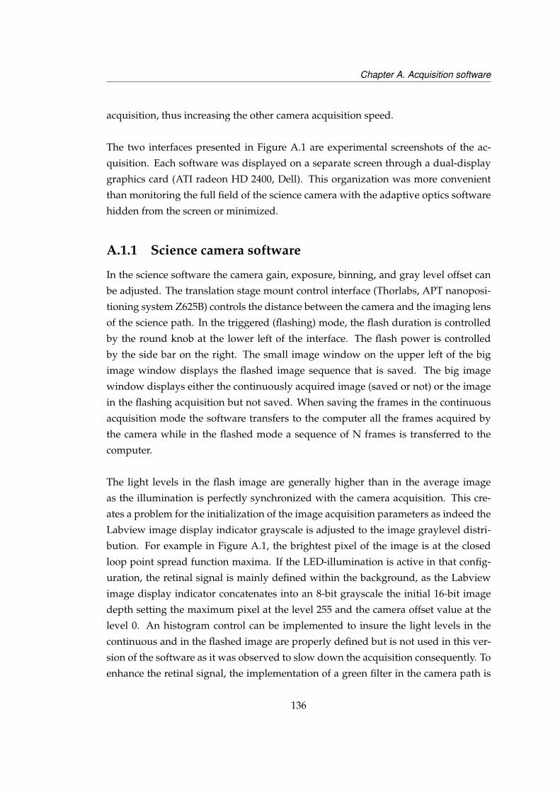
Chapter A. Acquisition software
acquisition, thus increasing the other camera acquisition speed.
The two interfaces presented in Figure A.1 are experimental screenshots of the ac-
quisition. Each software was displayed on a separate screen through a dual-display
graphics card (ATI radeon HD 2400, Dell). This organization was more convenient
than monitoring the full field of the science camera with the adaptive optics software
hidden from the screen or minimized.
A.1.1 Science camera software
In the science software the camera gain, exposure, binning, and gray level offset can
be adjusted. The translation stage mount control interface (Thorlabs, APT nanoposi-
tioning system Z625B) controls the distance between the camera and the imaging lens
of the science path. In the triggered (flashing) mode, the flash duration is controlled
by the round knob at the lower left of the interface. The flash power is controlled
by the side bar on the right. The small image window on the upper left of the big
image window displays the flashed image sequence that is saved. The big image
window displays either the continuously acquired image (saved or not) or the image
in the flashing acquisition but not saved. When saving the frames in the continuous
acquisition mode the software transfers to the computer all the frames acquired by
the camera while in the flashed mode a sequence of N frames is transferred to the
computer.
The light levels in the flash image are generally higher than in the average image
as the illumination is perfectly synchronized with the camera acquisition. This cre-
ates a problem for the initialization of the image acquisition parameters as indeed the
Labview image display indicator grayscale is adjusted to the image graylevel distri-
bution. For example in Figure A.1, the brightest pixel of the image is at the closed
loop point spread function maxima. If the LED-illumination is active in that config-
uration, the retinal signal is mainly defined within the background, as the Labview
image display indicator concatenates into an 8-bit grayscale the initial 16-bit image
depth setting the maximum pixel at the level 255 and the camera offset value at the
level 0. An histogram control can be implemented to insure the light levels in the
continuous and in the flashed image are properly defined but is not used in this ver-
sion of the software as it was observed to slow down the acquisition consequently. To
enhance the retinal signal, the implementation of a green filter in the camera path is
136
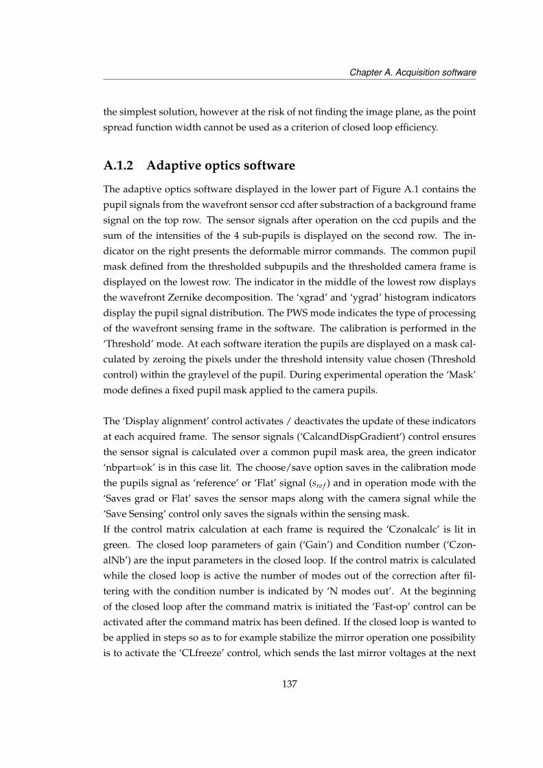
Chapter A. Acquisition software
the simplest solution, however at the risk of not finding the image plane, as the point
spread function width cannot be used as a criterion of closed loop efficiency.
A.1.2 Adaptive optics software
The adaptive optics software displayed in the lower part of Figure A.1 contains the
pupil signals from the wavefront sensor ccd after substraction of a background frame
signal on the top row. The sensor signals after operation on the ccd pupils and the
sum of the intensities of the 4 sub-pupils is displayed on the second row. The in-
dicator on the right presents the deformable mirror commands. The common pupil
mask defined from the thresholded subpupils and the thresholded camera frame is
displayed on the lowest row. The indicator in the middle of the lowest row displays
the wavefront Zernike decomposition. The ‘xgrad’ and ‘ygrad’ histogram indicators
display the pupil signal distribution. The PWS mode indicates the type of processing
of the wavefront sensing frame in the software. The calibration is performed in the
‘Threshold’ mode. At each software iteration the pupils are displayed on a mask cal-
culated by zeroing the pixels under the threshold intensity value chosen (Threshold
control) within the graylevel of the pupil. During experimental operation the ‘Mask’
mode defines a fixed pupil mask applied to the camera pupils.
The ‘Display alignment’ control activates / deactivates the update of these indicators
at each acquired frame. The sensor signals (‘CalcandDispGradient‘) control ensures
the sensor signal is calculated over a common pupil mask area, the green indicator
‘nbpart=ok’ is in this case lit. The choose/save option saves in the calibration mode
the pupils signal as ‘reference’ or ‘Flat’ signal (sre f ) and in operation mode with the
‘Saves grad or Flat’ saves the sensor maps along with the camera signal while the
‘Save Sensing’ control only saves the signals within the sensing mask.
If the control matrix calculation at each frame is required the ‘Czonalcalc’ is lit in
green. The closed loop parameters of gain (‘Gain’) and Condition number (‘Czon-
alNb’) are the input parameters in the closed loop. If the control matrix is calculated
while the closed loop is active the number of modes out of the correction after fil-
tering with the condition number is indicated by ‘N modes out’. At the beginning
of the closed loop after the command matrix is initiated the ‘Fast-op’ control can be
activated after the command matrix has been defined. If the closed loop is wanted to
be applied in steps so as to for example stabilize the mirror operation one possibility
is to activate the ‘CLfreeze’ control, which sends the last mirror voltages at the next
137
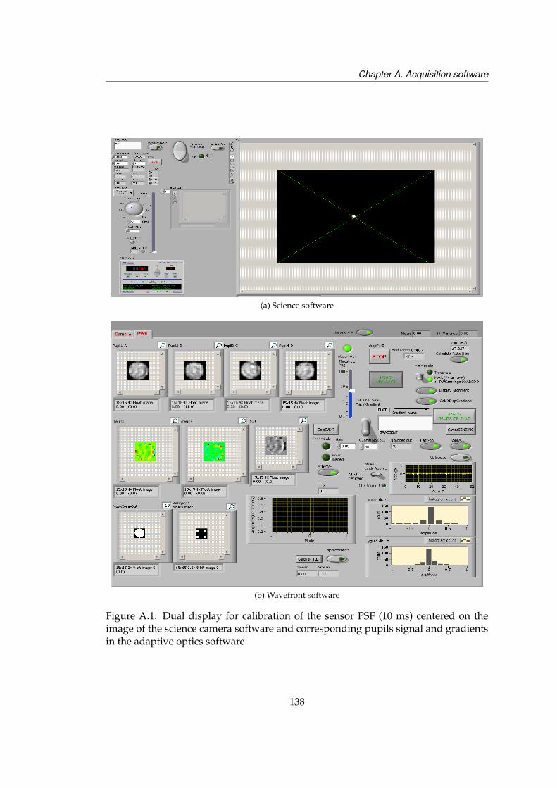
Chapter A. Acquisition software
(a) Science software
(b) Wavefront software
Figure A.1: Dual display for calibration of the sensor PSF (10 ms) centered on theimage of the science camera software and corresponding pupils signal and gradientsin the adaptive optics software
138

Chapter A. Acquisition software
loop iteration thus stabilizing the mirror commands for a short time.
Before activating the Zernike live reconstruction (‘activWF’) the control parameters
must be initialized ‘Rmat loaded ?’. The tip and tilt of the initial wavefront are deter-
mined for each direction under activation of the ‘calcTIP TILT’ button which displays
the associated values in the boxes ‘Xmean’ and ‘Ymean’. The tiptilt correction is pre-
ferrably activated after the closed loop is stabilised. If the user wants to obtain con-
vergence of the loop on another wavefront as the reference wavefront an additional
control (not displayed here) subtracts the reference signal from the sensor signals at
each loop iteration.
Control parameters such as the deformable mirror commands and the live Zernike
decomposition of the measured wavefront can be seen on the centre and on the upper-
right part of the interface. The same software is used for the calibration and for the
live operation, which probably induces losses in the acquisition speed.
During the acquisition the two programmes are operated in parallel. In the closed
loop control if the command matrix calculation is performed at each iteration of the
loop the closed loop is slowed down. The respective binnings of the cameras and the
definition of the region of interest for the wavefront sensing camera are the main pa-
rameters for the system speeds. For the optimal acquisition speed to be reached the
science camera image depth must be of 8 bit, the optional display of the ccd pupils
and gradients is cancelled. The optional Labview on-line Zernike reconstruction is
cancelled and the sensor signal maps saving system is disabled. When all displays
are updated and all the control parameters are saved the current system is indeed
keeping in memory the whole sequence of : mirror commands, sensor signals within
the pupil, sensor signals within the masks, and Zernike decomposition coefficients
when active. Still, the code suffers from some slowdown, as for example the setup
of the saving of the camera frames that necessitated the Labview code to create a
new image file at each frame acquired. This was however more appropriate for long
acquisition times than using the computer RAM memory which was progressively
saturating when long sequences of sensor data were acquired, eventually slowing
down the acquisition system.
All camera frames acquired in 8 bit or 16 bit were converted into a double precision
value so as to run additive and multiplicative operations on the pixels intensities. In
139

Chapter A. Acquisition software
open loop those operations were not very computationally intensive unless the live
wavefront reconstruction routines were active, as based on a Matlab node inserted
within the Labview code. In closed loop, the calculation of the control matrix was
the longest operation if operated at each frame acquisition. This calculation was thus
only initiated at the beginning of the adaptive optics then the same control matrix
was loaded in the live sensor operation for a parameter set. The display of the sensor
signals was also disabled and the closed loop stability was determined by observa-
tion of the point spread function at the science camera and of the mirror commands
only.
We verified separately that the binning of the science camera increases linearly with
the acquisition speed, and that the use of a 16 bit image depth divides it by almost
a factor 2. The science camera integration time is another dependency, as the speed
decreases with its increase, but not necessarily linearly over the exposures commonly
used in this work (1.6 ms, 10 ms, 50 ms, 100 ms and 200 ms). Over the whole thesis
the wavefront sensor camera parameters were constant at 10ms and 8 bit. Those pa-
rameters could have been changed but were fixed as providing a sufficient signal for
the calibration and for the operation of the system from the start of the thesis.
A.1.3 Reconstruction interface for results analysis
All the data are saved over a set of modulations and the post-processing of the sig-
nals is displayed in the form of a movie as in Figure A.2. The exact time the science
image is recorded and the exact time the sensor frame is acquired are noted during
the data acquisition. In the post-processing of the data, the time stamp of the sensor
and of the science are ordered in increasing order. Each point of the ordered timeline
is identified to a time stamp of the science timeline or of the sensor timeline, the cor-
responding data are imported and displayed in a new movie frame. The wavefront
sensor signal (k) or the science camera frame (ind) of the reconstruction interface thus
correspond to data acquired at a short intervals of time.
The full science camera image is displayed in the top-right corner of the movie frame.
A region of interest selected within the frame (typically near the center) is displayed
in the top-middle image of the frame. In the upper-right window is displayed the
wavefront rms at the time considered calculated from the decomposition into Zernike
terms. The wavefront surface reconstructed from the Zernike decomposition is dis-
played on the left in the middle-row. The Zernike coefficients of the decomposition
140
Chapter A. Acquisition software
are displayed in the central image of the middle row. The mirror commands are mon-
itored in the middle-right window of the display. In the last row the sensor signals of
the pixels within the pupil for the horizontal and vertical gradients are respectively
displayed in blue and black. This allowed to monitor the saturation when the signal
reached ±1.
Figure A.2: Offline reconstruction movie interface, closed loop operation in the eye
A.2 Open loop acquisition speed from code param-
eters
The magnification of the wavefront slope and of the camera pixel to the pupil of the
eye is calculated from geometrical optics in Table A.1. The wavefront sensor camera is
conjugated to the pupil of the eye through the artificial pupil of the mirror, of constant
size. The number of pixels across the pupil can be varied by the camera binning, that
is when 1 pixel of the display (i.e. a “super-pixel”) is the average of a 2× 2, 3× 3,
or 4× 4 pixels area on the camera chip. As fewer “super-pixels” describe the same
pupil area, the camera binning means a loss of spatial resolution for the wavefront
reconstruction. The advantage for the user is a gain in measurement speed as fewer
pixels of the camera chip are read.
141
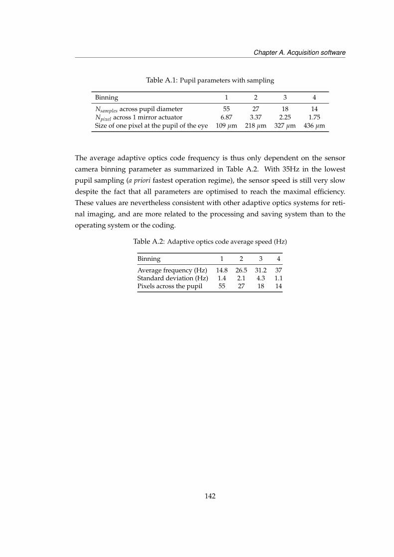
Chapter A. Acquisition software
Table A.1: Pupil parameters with sampling
Binning 1 2 3 4
Nsamples across pupil diameter 55 27 18 14Npixel across 1 mirror actuator 6.87 3.37 2.25 1.75Size of one pixel at the pupil of the eye 109 µm 218 µm 327 µm 436 µm
The average adaptive optics code frequency is thus only dependent on the sensor
camera binning parameter as summarized in Table A.2. With 35Hz in the lowest
pupil sampling (a priori fastest operation regime), the sensor speed is still very slow
despite the fact that all parameters are optimised to reach the maximal efficiency.
These values are nevertheless consistent with other adaptive optics systems for reti-
nal imaging, and are more related to the processing and saving system than to the
operating system or the coding.
Table A.2: Adaptive optics code average speed (Hz)
Binning 1 2 3 4
Average frequency (Hz) 14.8 26.5 31.2 37Standard deviation (Hz) 1.4 2.1 4.3 1.1Pixels across the pupil 55 27 18 14
142
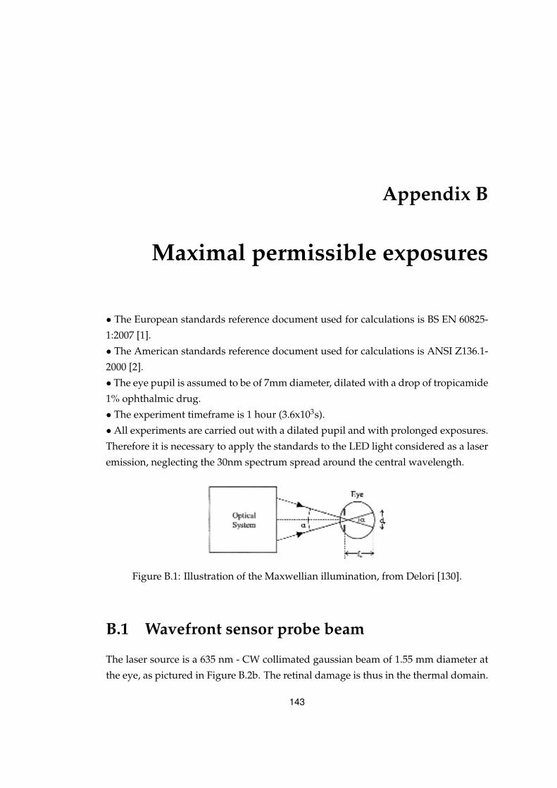
Appendix B
Maximal permissible exposures
• The European standards reference document used for calculations is BS EN 60825-
1:2007 [1].
• The American standards reference document used for calculations is ANSI Z136.1-
2000 [2].
• The eye pupil is assumed to be of 7mm diameter, dilated with a drop of tropicamide
1% ophthalmic drug.
• The experiment timeframe is 1 hour (3.6x10³s).
• All experiments are carried out with a dilated pupil and with prolonged exposures.
Therefore it is necessary to apply the standards to the LED light considered as a laser
emission, neglecting the 30nm spectrum spread around the central wavelength.
Figure B.1: Illustration of the Maxwellian illumination, from Delori [130].
B.1 Wavefront sensor probe beam
The laser source is a 635 nm - CW collimated gaussian beam of 1.55 mm diameter at
the eye, as pictured in Figure B.2b. The retinal damage is thus in the thermal domain.
143

Chapter B. Maximal permissible exposures
The angular subtense α of this beam is given considering the collimated input beam
at the entrance of the eye is focused on the retina by the eye’s optical elements (total
focal length = 17 mm) in the form of an Airy spot whos radius sets the height of the
angular subtense of the beam:
α = 2 * atan[ ( 1.22 * 0.635×10−6 * 17×10−3 / 1.55×10⁻³ ) * 1/17×10−3 ]
α = 2 * 0.49 mrad = 0.99 mrad
α ' 1 mrad
The maximal beam power at the cornea is measured at 1.3 µW for the 1.55 mm diam-
eter beam (of area 1.89x10⁻⁶ m2).
Hence the maximal corneal irradiance for the experimental input beam is :
1.3x10⁻⁶ / [π * (1.55x10⁻³)2 / 4] = 0.7689x10⁻³ W.m−2
A B
S
A’B’
α
α
(a) Retinal flood illu-mination with annualshape in corneal plane
AB
S
A’B’
α
B’A’
Airy Disk
(b) Airy disk radiusfor angular subtenseof AO beam
Figure B.2: Schematics for retinal irradiance in the wavefront sensor beacon and illumination
B.1.1 EU standard for AO beam
The Maximum Permissible Exposures (MPE) at the cornea given by the standard (An-
nex A, p.56 of [1]) is dependent on the parameter C6 which is given by Table 10 of
p.49, [1].
144
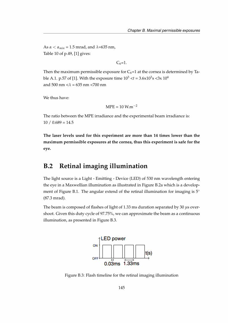
Chapter B. Maximal permissible exposures
As α < αmin = 1.5 mrad, and λ=635 nm,
Table 10 of p.49, [1] gives:
C6=1.
Then the maximum permissible exposure for C6=1 at the cornea is determined by Ta-
ble A.1. p.57 of [1]. With the exposure time 103 <t = 3.6x10³s <3x 10⁴
and 500 nm <λ = 635 nm <700 nm
We thus have:
MPE = 10 W.m−2
The ratio between the MPE irradiance and the experimental beam irradiance is:
10 / 0.689 = 14.5
The laser levels used for this experiment are more than 14 times lower than the
maximum permissible exposures at the cornea, thus this experiment is safe for the
eye.
B.2 Retinal imaging illumination
The light source is a Light - Emitting - Device (LED) of 530 nm wavelength entering
the eye in a Maxwellian illumination as illustrated in Figure B.2a which is a develop-
ment of Figure B.1. The angular extend of the retinal illumination for imaging is 5
(87.3 mrad).
The beam is composed of flashes of light of 1.33 ms duration separated by 30 µs over-
shoot. Given this duty cycle of 97.75%, we can approximate the beam as a continuous
illumination, as presented in Figure B.3.
Figure B.3: Flash timeline for the retinal imaging illumination
145
Chapter B. Maximal permissible exposures
The power of the source measured at the corneal plane with a powermeter is of
252µW over the 10mm-diameter aperture of the sensor head. The geometry of the
source in the corneal plane is annular, the internal ring is of 5 mm diameter and the
external ring is of 7 mm diameter. The consecutive area on the cornea is thus:
π*(7 x10⁻³)2 / 4 - π*(5 x10⁻³)2 / 4 = 18.8 x10⁻⁶ m2
And the resulting corneal irradiance for this source is:
252x10−6 / 18.8 x10−6 = 13.4 W.m−2
The duration of the experiment is set to 3.6x10³ s (1 hour).
B.2.1 EU standard for retinal illumination
B.2.1.1 EU Photochemical limit
For the retinal photochemical hazard, as the timeline is in the case:
102 s < t = 3.6x10³ s < 104 s
We must refer to Table A.2 of [1] with the system’s parameters :
MPEph(λ = 530 nm, α = 87.3 mrad, t = 3.6x10³ s) = 1 C3 W.m−2
With the limiting angle of acceptance γph defined by:
γph = 1.1 t0.5 mrad.
For our experiment duration t = 3.6x10³ s :
γph = 1.1 * (3.6x103)0.5 mrad = 66 mrad
Note:
As paragraph 3.50 of [1], p.14 and section A.4.3 of [1] p.61 specifies the definition of
γph. This angle must be taken into account for the calculation of the photochemical
limit :
“The angle γph is related to eye movements and is not dependent upon the angular
subtense of the source. If the angular subtense of the source is larger than the speci-
fied limiting angle of acceptance γph, the angle of acceptance γ is limited to γph and
the source is scanned for hotspots. If the measurement angle of acceptance γ is not
limited to the specified level, the hazard may be over-estimated.”
and:
“If the angular subtense of the source α is larger than the specified limiting angle of
acceptance γph, the angle of acceptance should not be larger than the values specified
146
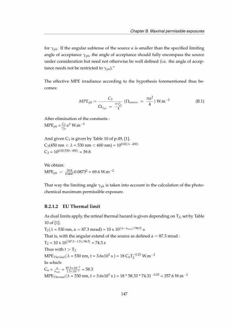
Chapter B. Maximal permissible exposures
for γph. If the angular subtense of the source α is smaller than the specified limiting
angle of acceptance γph, the angle of acceptance should fully encompass the source
under consideration but need not otherwise be well defined (i.e. the angle of accep-
tance needs not be restricted to γph).”
The effective MPE irradiance according to the hypothesis forementioned thus be-
comes:
MPEph =C3
Ωγph =πγ2
ph4
(Ωsource =πα2
4) W.m−2 (B.1)
After elimination of the constants :
MPEph = C3γ2
phα2 W.m−2
And given C3 is given by Table 10 of p.49, [1].
C3(450 nm < λ = 530 nm < 600 nm) = 100.02(λ−450)
C3 = 100.02(530−450) = 39.8
We obtain:
MPEph = 39.80.0662 0.08732 = 69.6 W.m−2
That way the limiting angle γph is taken into account in the calculation of the photo-
chemical maximum permissible exposure.
B.2.1.2 EU Thermal limit
As dual limits apply, the retinal thermal hazard is given depending on T2, set by Table
10 of [1].
T2(λ = 530 nm, α = 87.3 mrad) = 10 x 10[(α−αmin)/98.5] s
That is, with the angular extend of the source as defined α = 87.3 mrad :
T2 = 10 x 10[(87.3−1.5)/98.5] = 74.3 s
Thus with t > T2
MPEThermal(λ = 530 nm, t = 3.6x10³ s ) = 18 C6T−0.252 W.m−2
In which:
C6 = ααmin
= 87.5×10⁻³
1.5×10−3 = 58.3
MPEThermal(λ = 530 nm, t = 3.6x10³ s ) = 18 * 58.33 * 74.31−0.25 = 357.6 W.m−2
147
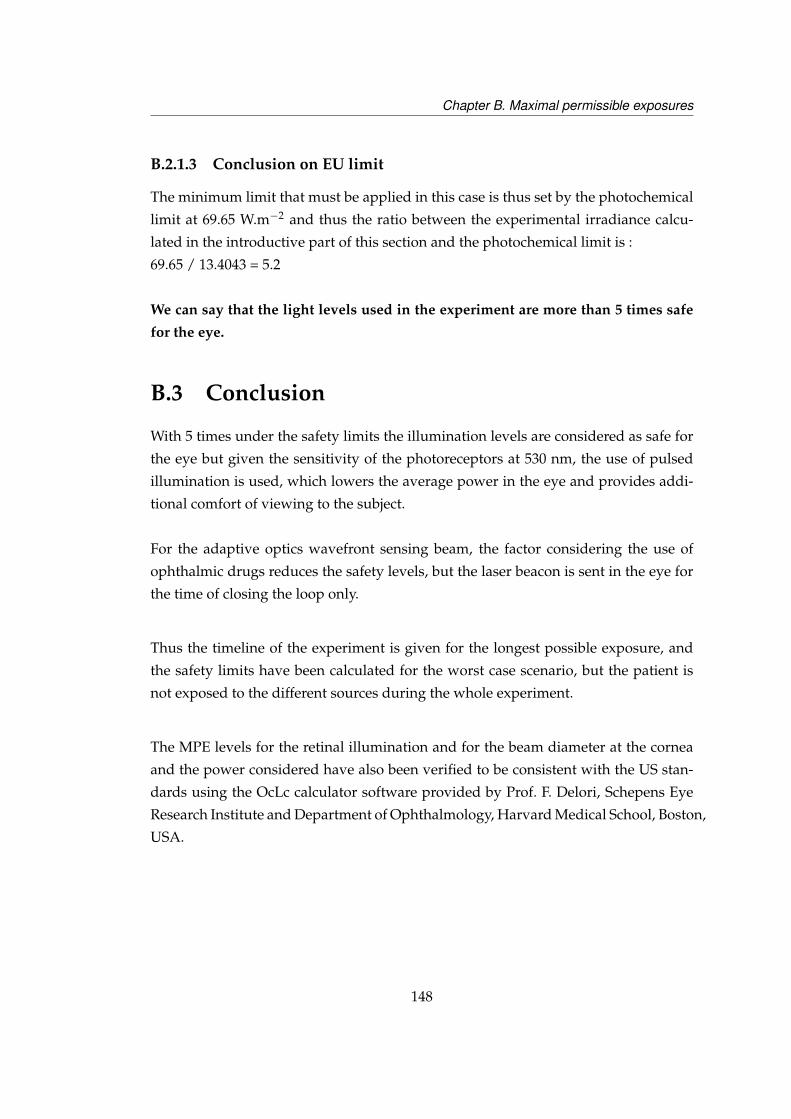
Chapter B. Maximal permissible exposures
B.2.1.3 Conclusion on EU limit
The minimum limit that must be applied in this case is thus set by the photochemical
limit at 69.65 W.m−2 and thus the ratio between the experimental irradiance calcu-
lated in the introductive part of this section and the photochemical limit is :
69.65 / 13.4043 = 5.2
We can say that the light levels used in the experiment are more than 5 times safe
for the eye.
B.3 Conclusion
With 5 times under the safety limits the illumination levels are considered as safe for
the eye but given the sensitivity of the photoreceptors at 530 nm, the use of pulsed
illumination is used, which lowers the average power in the eye and provides addi-
tional comfort of viewing to the subject.
For the adaptive optics wavefront sensing beam, the factor considering the use of
ophthalmic drugs reduces the safety levels, but the laser beacon is sent in the eye for
the time of closing the loop only.
Thus the timeline of the experiment is given for the longest possible exposure, and
the safety limits have been calculated for the worst case scenario, but the patient is
not exposed to the different sources during the whole experiment.
The MPE levels for the retinal illumination and for the beam diameter at the cornea
and the power considered have also been verified to be consistent with the US stan-
dards using the OcLc calculator software provided by Prof. F. Delori, Schepens Eye
Research Institute and Department of Ophthalmology, Harvard Medical School, Boston,
USA.
148

Appendix C
Aberration of subject S3
Figure C.1 displays the wavefront sensing data for the subject S3, which point spread
function with and without adaptive optics was displayed in Chapter 4, Section 4.4.2,
Figure 4.15. The dimensions of the uncorrected double pass point spread function let
expect an aberration of large amplitude, confirmed by the amplitude of the aberration
measurement by the sensor.
C.1 Wavefront reconstruction data for S3
Wavefront root mean squared (rms) error calculated from 35 coefficients including
and excluding tip and tilt are respectively presented in Figure C.1a and Figure C.1b.
In the usual representation, tip and tilt terms are not included in the calculation of the
rms. Given the influence of these terms on the aberration measurement was observed
in Section 3.3.3.4, Figure 3.14. Both rms calculations with and without tip and tilt
terms are presented. In other subjects, tip and tilt amplitudes were identified as the
source of the high rms values, but for this subject, the limit amplitudes for tip, tilt and
defocus are not reached. The aberration measurement is nevertheless not leveling,
that is that other terms could be at the origin of the rms increase.
Zernike wavefront coefficients (first 21 terms) are presented in Figure C.2. For each
dynamic range the coefficient is calculated from the average coefficient (100, 73 and
19 frames for dynamic ranges 12, 24 and 36λ/D respectively) after reconstruction of
the open-loop frames presented in the rms display Figure C.1a and Figure C.1b. The
149
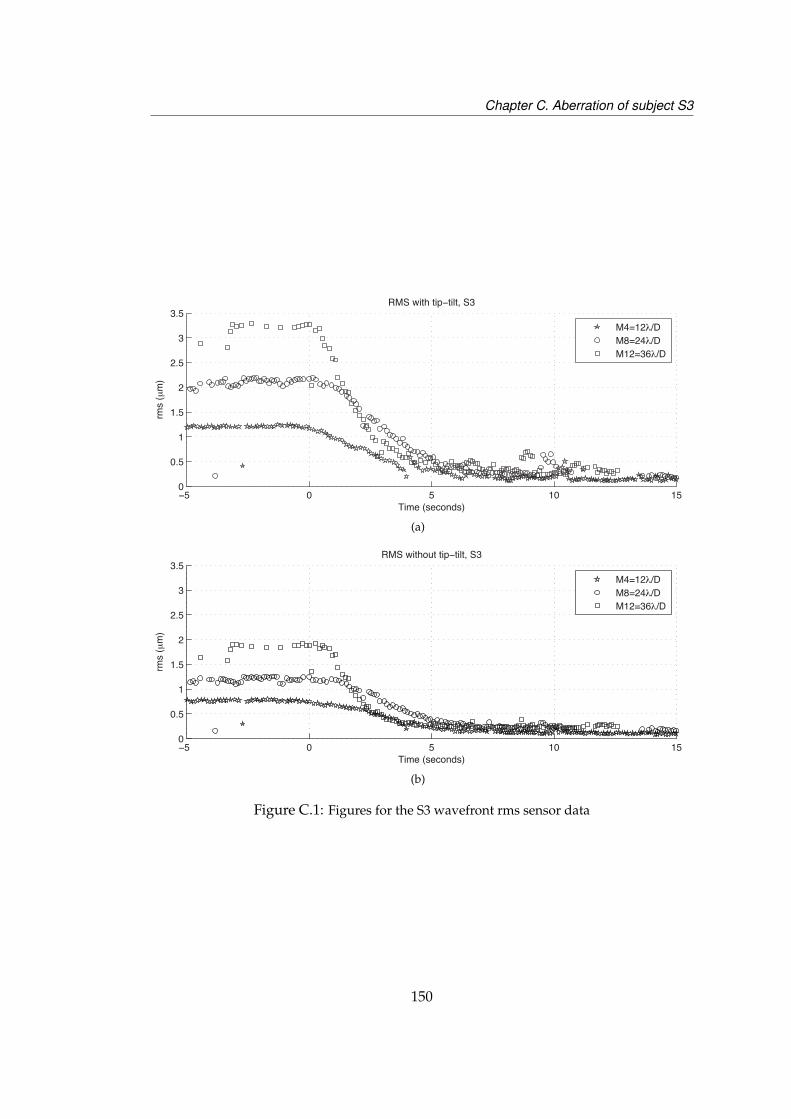
Chapter C. Aberration of subject S3
−5 0 5 10 150
0.5
1
1.5
2
2.5
3
3.5
Time (seconds)
rms
(μm
)
RMS with tip−tilt, S3
M4=12λ/DM8=24λ/DM12=36λ/D
(a)
−5 0 5 10 150
0.5
1
1.5
2
2.5
3
3.5
Time (seconds)
rms
(μm
)
RMS without tip−tilt, S3
M4=12λ/DM8=24λ/DM12=36λ/D
(b)
Figure C.1: Figures for the S3 wavefront rms sensor data
150
Chapter C. Aberration of subject S3
increase in a coefficient value with the increase in dynamic range is estimated as rep-
resentative of the sensor saturation for this term. Tip, Tilt and Defocus (j=1, 2, 4) terms
are identified as the main contributors for the wavefront error.
0 1 2 3 4 5 6 7 8 9 10 11 12 13 14 15 16 17 18 19 20 21−3
−2
−1
0
1
2
3
Term (j)
Ampli
tude
(μm
)
Open loop Zernike terms, with tip−tilt, S3
mean rms 12λ/D =0.7μmmean rms 24λ/D =1.3μmmean rms 36λ/D =1.8μm
Figure C.2: Zernike decomposition of open-loop aberration
Open loop and closed loop values of tip, tilt and defocus terms are displayed in Fig-
ure C.3a, Figure C.3b and Figure C.3c. Figure C.3a shows the contribution of tip
term is zero in the open-loop rms and does not require correction by the adaptive
optics. Figure C.3b shows a tilt term of (-0.9, -1.7 and -2.6 µm) amplitude for the re-
spective dynamic ranges (12, 24 and 36 λ/D), that is below the saturation values for
this Zernike aberration order. Figure C.3c displays a defocus term (j=4) of (0.6, 1 and
1.6µm) for the respective dynamic ranges (12, 24 and 36 λ/D) before adaptive optics,
meaning that the saturation amplitude of the sensor for this term is not obtained.
In conclusion, even though the aberration measurement for this subject in this ex-
perimental set is not saturated by tip, tilt and defocus terms, leveling of the ocular
wavefront rms is not observed. The saturation of the sensor by other Zernike orders
as presented in Section 3.3.3.2 is not necessarily avoided by the use of large dynamic
ranges. In addition noise constraints for a given order limit the accuracy of the aber-
ration measurement. Reconstruction of the aberration corrected by the mirror com-
mands might allow this quantification.
151
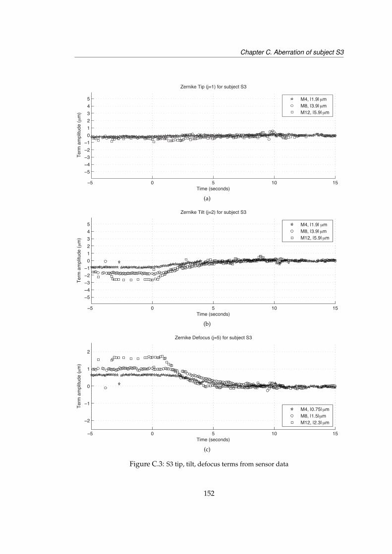
Chapter C. Aberration of subject S3
−5 0 5 10 15
−5−4−3−2−1
012345
Time (seconds)
Term
am
plitu
de (μ
m)
Zernike Tip (j=1) for subject S3
M4, |1.9|μmM8, |3.9|μmM12, |5.9|μm
(a)
−5 0 5 10 15Time (seconds)
Zernike Tilt (j=2) for subject S3
−5−4−3−2−1
012345
Term
am
plitu
de (μ
m)
M4, |1.9| μmM8, |3.9|μmM12, |5.9|μm
(b)
2
Zernike Defocus (j=5) for subject S3
−5 0 5 10 15
−2
−1
0
1
Time (seconds)
Term
am
plitu
de (μ
m)
M4, |0.75|μmM8, |1.5|μmM12, |2.3|μm
(c)
Figure C.3: S3 tip, tilt, defocus terms from sensor data
152

Bibliography
[1] S. R. Chamot, C. Dainty, and S. Esposito, “Adaptive optics for ophthalmic ap-plications using a pyramid wavefront sensor,” Opt. Express 14, 518–526 (2006).
[2] S. L. Polyak, The Retina (University of Chicago Press, Chicago, 1941).
[3] L. Diaz-Santana and J. C. Dainty, “Effects of retinal scattering in the oculardouble-pass process,” J. Opt. Soc. Am. A. 18, 1437–1444 (2001).
[4] M. Nowakowski, M. Sheehan, D. Neal, and A. V. Goncharov, “Investigation ofthe isoplanatic patch and wavefront aberration along the pupillary axis com-pared to the line of sight in the eye,” Biomed. Opt. Express pp. 240–258 (2012).
[5] L. Thibos, M. Ye, X. Zhang, and A. Bradley, “The chromatic eye: a new reduced-eye model of ocular chromatic aberration in humans,” Appl. Opt. 31, 3594–3600(1992).
[6] H. Hofer, L. Chen, G. Y. Yoon, B. Singer, Y. Yamauchi, and D. R. Williams, “Im-provement in retinal image quality with dynamic correction of the eye’s aber-rations,” Opt. Express 8, 631–643 (2001).
[7] K. Grieve, P. Tiruveedhula, Y. Zhang, and A. Roorda, “Multi-wavelength imag-ing with the adaptive optics scanning laser ophthalmoscope,” Opt. Express 14,12230–12243 (2006).
[8] D. De Brouwere, H. Ginis, G. Kymionis, I. Naoumidi, and I. Pallikaris, “For-ward scattering properties of corneal haze,” Opt. Vis. Science 85, 843–848(2008).
[9] J. M. Bueno, D. De Brouwere, H. Ginis, I. Sgouros, and P. Artal, “Purkinje imag-ing system to measure anterior segment scattering in the human eye,” Opt. Lett.32, 3447 (2007).
[10] D. A. Peyrot, F. Aptel, C. Crotti, F. Deloison, S. Lemaire, T. Marciano, S. Bancelin,F. Alahyane, L. Kowalczuk, M. Savoldelli, J.-M. Legeais, and K. Plamann, “Ef-
153
BIBLIOGRAPHY BIBLIOGRAPHY
fect of incident light wavelength and corneal edema on light scattering and pen-etration: Laboratory study of human corneas,” J. Refract. Surgery 26, 786–795(2010).
[11] J. M. Bueno and M. C. W. Campbell, “Confocal scanning laser ophthalmoscopyimprovement by use of Mueller-matrix polarimetry,” Opt. Lett. 27, 830–832(2002).
[12] S. Marcos, R. Navarro, and P. Artal, “Coherent imaging of the cone mosaic inthe living eye,” J. Opt. Soc. Am. A. 13, 897–905 (1996).
[13] D. Catlin and C. Dainty, “High-resolution imaging of the human retina with aFourier deconvolution technique,” J. Opt.Soc. Am. A 19, 1515–1523 (2002).
[14] J. Liang, D. Williams, and D. Miller, “Supernormal vision and high-resolutionretinal imaging through adaptive optics,” J. Opt. Soc. Am. A. 14, 2884–2892(1997).
[15] J. Rha, S. Jonnal, Ravi, K. E. Thorn, J. Qu, Y. Zhang, and D. T. Miller, “Adaptiveoptics flood-illumination camera for high speed retinal imaging,” Opt. Express14, 4552–4569 (2006).
[16] R. S. Jonnal, R. Jungtae, Y. Zhang, B. Cense, W. Gao, and D. T. Miller, “In vivofunctional imaging of human cone photoreceptors,” Opt. Express 15, 16141 –16160 (2007).
[17] M. Glanc, E. Gendron, F. Lacombe, D. Lafaille, J. F. Le Gargasson, and P. Léna,“Towards wide-field retinal imaging with adaptive optics,” Optics Communi-cations 230, 225–238 (2004).
[18] B. Xue, S. S. Choi, N. Doble, and J. Werner, “Photoreceptor counting and mon-taging of enface retinal images from an adaptive optics fundus camera,” J. Opt.Soc. Am. A. 24, 1364–1372 (2007).
[19] N. M. Putnam, H. J. Hofer, N. Doble, L. Chan, J. Caroll, and D. R. Williams,“The locus of fixation and the foveal cone mosaic,” Journal of Vision 5, 632–639(2005).
[20] N. Doble, S. S. Choi, J. L. Codona, J. Christou, J. M. Enoch, and D. R. Williams,“In-vivo imaging of the human rod photoreceptor mosaic,” Opt. Lett. (2010).
[21] D. Merino, J. C. Dainty, A. Bradu, and A. G. Podoleanu, “Adaptive optics en-hanced simultaneous en-face optical coherence tomography and scanning laserophthalmoscopy,” Opt. Express 14, 3345–3353 (2006).
[22] A. Roorda and D. R. Williams, “The arrangement of the three cone classes inthe living human eye,” Nature 397, 520–523 (1999).
[23] K. Grieve and A. Roorda, “Intrinsic signals from human cone photoreceptors,”Invest. Ophthalmol. Vis. Sci. 49, 713–719 (2008).
154
BIBLIOGRAPHY BIBLIOGRAPHY
[24] S. A. Burns, S. Wu, F. Delori, and A. E. Elsner, “Direct measurement of humancone photoreceptor alignment,” J. Opt. Soc. Am. A. 12, 2329–2338 (1995).
[25] S. A. Burns, S. Wu, J. C. He, and A. E. Elsner, “Variations in photoreceptordirectionality across the central retina,” J. Opt. Soc. Am. A. 14, 2033–2041 (1997).
[26] S. A. Burns, R. Tumbar, A. E. Elsner, D. Ferguson, and D. X. Hammer, “Large-field-of-view, modular, stabilized, adaptive-optics-based scanning laser oph-thalmoscope,” J. Opt. Soc. Am. A. 24, 1313–1326 (2007).
[27] D. C. Gray, W. Merigan, J. I. Wolfing, B. P. Gee, J. Porter, A. Dubra, T. H. Twiet-meyer, K. Ahmad, R. Tumbar, F. Reinholz, and D. R. Williams, “In vivo fluores-cence imaging of primate retinal ganglion cells and retinal pigment epithelialcells,” Opt. Express 14, 7144–7158 (2006).
[28] D. P. Biss, D. Sumorok, S. A. Burns, R. H. Webb, Y. Zhou, T. G. Bifano, D. Côté,I. Veilleux, P. Zamiri, and C. P. Lin, “In vivo fluorescent imaging of the mouseretina using adaptive optics,” Opt. Lett. 32, 659–661 (2007).
[29] A. Bindewald-Wittich, M. Han, S. Schmitz-Valckenberg, S. R. Snyder, G. Giese,J. F. Bille, and F. G. Holz, “Two-photon excited fluorescence imaging of humanRPE cells with a femtosecond Ti:Sapphire laser,” Investigative Ophthalmologyand Visual Science 47, 4553–4557 (2006).
[30] D. Malacara, Optical Shop Testing (Wiley-Interscience, 2006), 3rd ed.
[31] A. G. Podoleanu, J. A. Rogers, D. A. Jackson, and S. Dunne, “Three dimensionalOCT images from retina and skin,” Opt. Express 7, 292–298 (2000).
[32] R. G. Cucu, A. G. Podoleanu, J. A. Rogers, J. Pedro, and R. B. Rosen, “Combinedconfocal/en face t-scan-based ultrahigh-resolution optical coherence tomogra-phy in vivo retinal imaging,” Opt. Lett. 11, 1684–1686 (2006).
[33] Y. Zhang, J. Rha, R. Jonnal, and D. Miller, “Adaptive optics parallel spectral do-main optical coherence tomography for imaging the living retina,” Opt. Express13, 4792–4811 (2005).
[34] A. R. Tumlinson, B. Hermann, B. Hofer, B. Povazay, T. H. Margrain, A. M. Binns,and W. Drexler, “Techniques for extraction of depth-resolved in vivo humanretinal intrinsic optical signals with optical coherence tomography,” Jpn J. Oph-thalmol. 53, 315–326 (2009).
[35] W. Gao, B. Cense, Y. Zhang, R. S. Jonnal, and D. T. Miller, “Measuring reti-nal contributions to the optical Stiles-Crawford effect with optical coherencetomography,” Opt. Express 16, 6486–6501 (2008).
[36] Y. Zhang, B. Cense, J. Rha, S. Jonnal, Ravi, W. Gao, R. J. Zawadzki, J. S. Werner,S. Jones, S. Oliver, and D. T. Miller, “High-speed volumetric imaging of conephotoreceptors with adaptive optics spectral-domain optical coherence tomog-raphy,” Opt. Express 14, 4380–4395 (2006).
155
BIBLIOGRAPHY BIBLIOGRAPHY
[37] E. J. Fernández, B. Hermann, B. Povazay, A. Unterhuber, H. Sattmann, B. Hofer,P. K. Ahnelt, and W. Drexler, “Ultrahigh resolution optical coherence tomogra-phy and pancorrection for cellular imaging of the living human retina,” Opt.Express 16, 11083 (2008).
[38] C. Torti, B. Povazay, B. Hofer, A. Unterhuber, J. Carroll, P. K. Ahnelt, andW. Drexler, “Adaptive optics optical coherence tomography at 120,000 depthscans/s for non-invasive cellular phenotyping of the living human retina,” Opt.Express 17, 19382 (2009).
[39] R. Sabesan and G. Yoon, “Visual performance after correcting higher order aber-rations in keratoconic eyes,” Journal of Vision 9, 1–10 (2009).
[40] E. J. Fernandez, L. Vabre, B. Hermann, A. Unterhuber, B. Povazay, andW. Drexler, “Adaptive optics with a magnetic deformable mirror: Applicationsin the human eye,” Opt. Express 14, 18 (2006).
[41] D. T. Miller, D. R. Williams, G. M. Morris, and J. Liang, “Images of cone pho-toreceptors in the living human eye,” Vision Research 36, 1067 – 1079 (1996).
[42] A. Burvall, E. Daly, S. R. Chamot, and C. Dainty, “Linearity of the pyramidwavefront sensor,” Opt. Express 14, 11925–11934 (2006).
[43] L. N. Thibos, R. A. Applegate, J. T. Schwiegerling, R. Webb, and V. S. T. Mem-bers, “Standards for reporting the optical aberrations of eyes,” Conference Pa-per for Vision Science and its Applications (VSIA) pp. 232–244 (2000).
[44] E. Logean, E. Dalimier, and J. C. Dainty, “Measured double-pass intensity point-spread function after adaptive optics correction of ocular aberrations,” Opt. Ex-press 16, 17348–17357 (2008).
[45] E. Dalimier and C. Dainty, “Comparative analysis of deformable mirrors forocular adaptive optics,” Opt. Express 13, 4275–4285 (2005).
[46] T. Farrell, E. Daly, E. Dalimier, and C. Dainty, “Task-based assessment of de-formable mirrors,” Proc. of SPIE 6467, 64670F (2007).
[47] N. Devaney, E. Dalimier, T. Farrell, D. Coburn, R. Mackey, D. Mackey, F. Lau-rent, E. Daly, and C. Dainty, “Correction of ocular and atmospheric wavefronts:a comparison of the performance of various deformable mirrors,” Appl. Opt.47, 6550–6562 (2008).
[48] B. M. Welsh and M. C. Roggemann, “Signal-to-noise comparison of deconvolu-tion from wave-front sensing with traditional linear and speckle image recon-struction,” Appl. Opt. 34, 2111–2119 (1995).
[49] J. C. Christou, A. Roorda, and D. R. Williams, “Deconvolution of adaptive op-tics retinal images,” J. Opt. Soc. Am. A. 21, 1393–1401 (2004).
156

BIBLIOGRAPHY BIBLIOGRAPHY
[50] E. F. Y. Hom, F. Marchis, T. K. Lee, S. Haase, D. A. Agard, and J. W. Sedat,“AIDA: an adaptive image deconvolution algorithm with application to multi-frame and three-dimensional data,” J. Opt. Soc. Am. A. 24, 1580–1600 (2007).
[51] G. Chenegros, L. M. Mugnier, F. Lacombe, and M. Glanc, “3D phase diversity: amyopic deconvolution method for short-exposure images: application to retinalimaging,” J. Opt. Soc. Am. A. 24, 1349–1357 (2007).
[52] R. Ragazzoni, “Pupil plane wavefont sensing with an oscillating prism,” Jour-nal of Modern Optics 43, 289–293 (1996).
[53] M. C. Roggemann and T. J. Schulz, “Algorithm to increase the largest aberrationthat can be reconstructed from hartmann sensor measurements,” Appl. Opt. 37,4321–4329 (1998).
[54] L. A. Poyneer, D. T. Gavel, and J. M. Brase, “Fast wave-front reconstruction inlarge adaptive optics systems with use of the Fourier transform,” J. Opt. Soc.Am. A. 19, 2100–2111 (2002).
[55] R. Ragazzoni, A. Ghedina, A. Baruffolo, E. Marchetti, J. Farinato, T. Niero,G. Crimi, and M. Ghigo, “Testing the pyramid wavefront sensor on the sky,”Proc. of SPIE 4007, 423–430 (2000).
[56] F. Pérennès, M. Ghigo, M. Tormen, and S. Cabrini, “Production of identicalpyramid wavefront sensors for multi-conjugate adaptive optic systems usingthe LIGA process,” Proc. of SPIE, Microsystem Technologies 10, 552–555 (2004).
[57] A. Tozzi, P. Stefanini, E. Pinna, and S. Esposito, “The double pyramid wavefrontsensor for LBT,” Proc. SPIE 7015, 701558:1–9 (2008).
[58] A. Wang, J. Yao, D. Cai, and H. Ren, “Design and fabrication of a pyramidwavefront sensor,” Proc. of SPIE 49, 073401 (2010).
[59] B. Bauman, “Optical design for extremely large telescope adaptive optics sys-tems,” Ph.D. thesis, The University of Arizona (2003).
[60] L. Foucault, “Mémoire sur la construction des téléscopes en verre argenté,” An-nales de l’Observatoire de Paris 5, 197–237 (1859).
[61] M. A. Van Dam, “Measuring the centroid gain of a Shack-Hartmann quad-cellwavefront sensor by using slope discrepancy,” J. Opt. Soc. Am. A. 22, 1509–1514(2005).
[62] R. M. Clare and R. G. Lane, “Wave-front sensing from subdivision of the focalplane with a lenslet array,” J. Opt. Soc. Am. A. 22, 117–125 (2005).
[63] J. A. Johnson, R. Kupke, D. Gavel, and B. Bauman, “Pyramid wavefront sensing:theory and component technology development at LAO,” Proc. SPIE, Advancesin Adaptive Optics II 6272, 62724R (2006).
157
BIBLIOGRAPHY BIBLIOGRAPHY
[64] R. Kupke, D. Gavel, J. Johnson, and M. Reinig, “Implementation of the pyramidwavefront sensor as a direct phase detector for large amplitude aberrations,”Proc. SPIE, Adaptive Optics Systems 7015, 70155H (2008).
[65] J. Le Due, L. Jolissaint, J.-P. Véran, and C. Bradley, “Calibration and testingwith real turbulence of a pyramid sensor employing static modulation,” Opt.Express 17, 7186–7195 (2009).
[66] O. A. Feeney, “Theory and laboratory characterization of novel wavefront sen-sor for adaptive optics systems,” Ph.D. thesis, National University of Ireland,Galway (2001).
[67] S. Esposito and A. Riccardi, “Pyramid wavefront sensor behavior in partial cor-rection adaptive optic systems,” Astronomy and Astrophysics 369, 9–12 (2001).
[68] J. B. Costa, R. Ragazzoni, A. Ghedina, M. Carbillet, C. Verinaud, M. Feldt, S. Es-posito, E. Puga, and J. Farinato, “Is there need of any modulation in the pyramidwavefront sensor?” Proc. SPIE 4389 (2003).
[69] J. B. Costa, “Modulation effect of the atmosphere in a pyramid wave-front sen-sor,” Appl. Opt. 44, 60–67 (2005).
[70] D. Peter, M. Feldt, B. Dorner, T. Henning, S. Hippler, and J. Aceituno, “PYRA-MIR: Calibration and operation of a pyramid near-infrared wavefront sensor,”Publ. Astr. Soc. Pac. 120, 872–886 (2008).
[71] D. Peter, M. Feldt, T. Henning, S. Hippler, J. Aceituno, L. Montoya, J. Costa,and B. Dorner, “PYRAMIR: Exploring the on-sky performance of the world’sfirst near-infrared pyramid wavefront sensor,” Publ. Astr. Soc. Pac. 122, 63–70(2010).
[72] I. Iglesias, R. Ragazzoni, Y. Julien, and P. Artal, “Extended source pyramidwave-front sensor for the human eye,” Opt. Express 10, 10 (2002).
[73] V. Korkiakoski, C. Vérinaud, M. Le Louarn, and R. Conan, “Comparison be-tween a model-based and a conventional pyramid sensor reconstructor,” Appl.Opt. 46, 6176–6184 (2007).
[74] V. Korkiakoski, C. Vérinaud, and M. Le Louarn, “Improving the performanceof a pyramid wavefront sensor with modal sensitivity compensation,” Appl.Opt. 47, 79–87 (2008).
[75] R. Ragazzoni, E. Diolati, and E. Vernet, “A pyramid wavefront sensor with nodynamic modulation,” Optics Communications 208, 51–60 (2002).
[76] R. Ragazzoni, J. Farinato, and E. Marchetti, “Adaptive optics for 100-m-classtelescopes: new challenges require new solutions,” (2000), vol. 4007, pp. 1076–1087.
158

BIBLIOGRAPHY BIBLIOGRAPHY
[77] C. Arcidiacono, E. Diolaiti, M. Tordi, R. Ragazzoni, J. Farinato, E. Vernet, andE. Marchetti, “Layer-oriented simulation tool,” Appl. Opt. 43, 4288–4302 (2004).
[78] E. Diolaiti, A. Tozzi, R. Ragazzoni, D. Ferruzzi, E. Vernet-Viard, S. Esposito,J. Farinato, A. Ghedina, and A. Riccardi, “Some novel concepts in multipyra-mid wavefront sensing,” Proc. of SPIE, Adaptive Optical System TechnologiesII 4839, 299–306 (2003).
[79] C. Vérinaud, “On the nature of the measurements provided by a pyramid wave-front sensor,” Optics Communications 233, 27–38 (2004).
[80] M. Nicolle, T. Fusco, G. Rousset, and V. Michau, “Improvement of Shack-Hartmann wave-front sensor measurement for extreme adaptive optics,” Opt.Lett. 29, 2743–2745 (2004).
[81] L. A. Poyneer and B. Macintosh, “Spatially filtered wave-front sensor for high-order adaptive optics,” J. Opt. Soc. Am. A. 21, 810–819 (2004).
[82] C. Vérinaud, M. Le Louarn, V. Korkiakoski, and M. Carbillet, “Adaptive op-tics for high-contrast imaging: pyramid sensor versus spatially filtered Shack-Hartmann sensor,” Mon. Not. R. Astron. Soc. 357, 26–30 (2005).
[83] R. Ragazzoni and J. Farinato, “Sensitivity of a pyramidic wave front sensor inclosed loop adaptive optics,” AAP 350, L23–L26 (1999).
[84] S. Esposito, A. Tozzi, A. Puglisi, L. Fini, P. Stefanini, P. Salinari, D. Gallieni, andJ. Storm, “Development of the first-light AO system for the large binocular tele-scope,” Proc. SPIE, Astronomical Adaptive Optics Systems and Applications5169, 149–158 (2003).
[85] E. Pinna, A. T. Puglisi, F. Quiros-Pacheco, L. Busoni, A. Tozzi, S. Esposito,E. Aller-Carpentier, and M. Kasper, “The pyramid wavefront sensor for the highorder testbench (HOT),” Proc. SPIE 7015 (2008).
[86] E. Aller-Carpentier, M. Kasper, P. Martinez, E. Vernet, E. Fedrigo, C. Soenke,S. Tordo, N. Hubin, C. Verinaud, S. Esposito, E. Pinna, A. Puglisi, A. Tozzi,F. Quiros, A. G. Basden, S. J. Goodsell, G. D. Love, and R. M. Myers, “Highorder test bench for extreme adaptive optics system optimization,” Proc. SPIE,Adaptive Optics Systems 7015, 70153Z (2008).
[87] S. Esposito, E. Pinna, A. Tozzi, P. Stefanini, and N. Devaney, “Cophasing of seg-mented mirrors using the pyramid sensor,” Proc. SPIE, Astronomical AdaptiveOptics Systems and Applications 5169, 72–78 (2003).
[88] S. Esposito, E. Pinna, A. Puglisi, A. Tozzi, and P. Stefanini, “Pyramid sensor forsegmented mirror alignment,” Opt. Lett. 30, 2572–2574 (2005).
[89] B. Le Roux, “Pyramid wave-front sensing with a laser guide star for an ELT,”in “Adaptive Optics: Methods, Analysis and Applications,” (Optical Society ofAmerica, 2009), p. AOTuB3.
159
BIBLIOGRAPHY BIBLIOGRAPHY
[90] S. R. Chamot, S. Esposito, and J. C. Dainty, “Application of pyramid wavefrontsensing to ocular aberration measurements and corrections,” in “Frontiers inOptics,” (Optical Society of America, 2005), p. FThZ3.
[91] S. Chiesa, E. Daly, J. C. Dainty, and S. R. Chamot, “Adaptive optics system forretinal imaging based on a pyramid wavefront sensor,” in “Adaptive Optics forIndustry and Medicine,” Sixth International Workshop National University ofIreland (Imperial College Press, 2008), pp. 336–341.
[92] E. M. Daly and J. C. Dainty, “Measuring phase aberrations using a pyramidwave front sensor,” (2010), vol. 7726.
[93] E. M. Daly and J. C. Dainty, “Ophthalmic wavefront measurements using a ver-satile pyramid sensor,” Appl. Opt. 49, G67–G77 (2010).
[94] A. Riccardi, N. Bindi, R. Ragazzoni, S. Esposito, and P. Stefanini, “Labora-tory characterization of a "Foucault-like" wavefront sensor for adaptive optics,”3353, 941–951 (1998).
[95] D. A. Atchison, “Recent advances in measurement of monochromatic aberra-tions of human eyes,” Clinical and Experimental Optometry 88, 5–27 (2005).
[96] L. Thibos, X. Hong, A. Bradley, and X. Cheng, “Statistical variation of aberrationstructure and image quality in a normal population of healthy eyes,” J. Opt. Soc.Am. A. 19, 2329–2348 (2002).
[97] J. Porter, A. Guirao, I. G. Cox, and D. R. Williams, “Monochromatic aberrationsof the human eye in a large population,” J. Opt. Soc. Am. A. 18, 1793–1803(2001).
[98] R. Iskander, B. A. Davis, M. J. Collins, and R. Franklin, “Objective refractionfrom monochromatic wavefront aberrations via Zernike power polynomials,”Ophthal. Physiol. Opt. pp. 245–255 (2007).
[99] L. Thibos, “Handbook of visual optics,” (2008).
[100] R. J. Noll, “Zernike polynomials and atmospheric turbulence,” J. Opt. Soc. Am.66, 207–211 (1976).
[101] K. Hampson, “The higher-order aberrations of the human eye: relation to thepulse and effect on vision,” Ph.D. thesis, Imperial College, London (2005).
[102] D. R. Neal, D. M. Topa, and J. Copland, “Resolution effects on the dynamicrange and accuracy of ophthalmic wavefront sensing,” in “Vision Science andits Applications,” (Optical Society of America, 2001), p. SuD5.
[103] J. Schwiegerling, Field Guide to Visual and Ophthalmic Optics (SPIE Press book,Field guides, 2004).
160

BIBLIOGRAPHY BIBLIOGRAPHY
[104] R. Navarro, E. Moreno-Barriuso, S. Bará, and T. Mancebo, “Phase plates forwave-aberration compensation in the human eye,” Opt. Lett. 25, 236–238(2000).
[105] C. E. Leroux, A. Tzschachmann, and J. C. Dainty, “Pupil matching of Zernikeaberrations,” Opt. Express 18, 21567–21572 (2010).
[106] L. N. Thibos, “Retinal image quality for virtual eyes generated by a statisticalmodel of ocular wavefront aberrations,” Ophthalmic and Physiological Optics29, 288–291 (2009).
[107] T. Shirai, “Liquid-crystal adaptive optics based on feedback interferometry forhigh-resolution retinal imaging,” Appl. Opt. 41, 4013–4014 (2002).
[108] J. W. Hardy, Adaptive optics for astronomical telescopes (Oxford University Press,1998).
[109] E. Dalimier, “Adaptive Optics Correction of Ocular Higher-Order Aberrationsand the Effects on Functional Vision,” Ph.D. thesis, Department of Experimen-tal Physics, National University of Ireland, Galway (2007).
[110] W. Zou and S. A. Burns, “High-accuracy wavefront control for retinal imagingwith adaptive-influence-matrix adaptive optics,” Opt. Express 17, 20167–20177(2009).
[111] A. Dubra, “Wavefront sensor and wavefront corrector matching in adaptiveoptics,” Opt. Express 15, 2672–2769 (2007).
[112] E. Daly, C. Dainty, G. O’Connor, and T. Glynn, “Wave-front correction of a fem-tosecond laser using deformable mirrors,” Proc. SPIE 5708 (2005).
[113] E. Ödlund, H.-F. Raynaud, C. Kulcsar, F. Harms, X. Levecq, F. Martins,N. Château, and A. G. Podoleanu, “Control of an electromagnetic deformablemirror using high speed dynamics characterization and identification,” Appl.Opt. 49, G120–G128 (2010).
[114] R. K. Tyson, Principles of Adaptive Optics (Academic Press; 2 edition, 1998).
[115] G. Smith and D. A. Atchison, The eye and visual optical elements (Press syndicateof the University of Cambridge, 1997).
[116] C. A. Curcio, K. R. Sloan, O. Packer, A. E. Hendrickson, and R. E. Kalina, “Distri-bution of cones in human and monkey retina: Individual variability and radialasymmetry,” Science 236, 579–582 (1987).
[117] W. S. Stiles and B. H. Crawford, “The luminous efficiency of rays entering theeye pupil at different points,” Proceedings of the Royal Society of London, Se-ries B, Containing Papers of a Biological Character 112, 428 – 450 (1933).
[118] G. Smith and D. A. Atchison, Optics of the human eye (Elsevier Science, 2003).
161

BIBLIOGRAPHY BIBLIOGRAPHY
[119] J. W. Goodman, Speckle phenomena in optics (Roberts and Co., 2006).
[120] J. I. Yellot, “Spectral analysis of spatial sampling by photoreceptors: topologicaldisorder prevents aliasing,” Vision Res. (1982).
[121] K. Li and A. Roorda, “Automated identification of cone photoreceptors in adap-tive optics retinal images,” J. Opt. Soc. Am. A. 24, 1358–1363 (2007).
[122] G. Österberg, “Topography of the layer of rods and cones in the human retina,”Acta Ophthal. Suppl.6, 1–103 (1935).
[123] S. Marcos, S. A. Burns, E. Moreno-Barriusop, and R. Navarro, “A new ap-proach to the study of ocular chromatic aberrations,” Vision Research 39, 4309–23 (1999).
[124] R. Sabesan, K. Ahmad, and G. Yoon, “Correcting highly aberrated eyes usinglarge-stroke adaptive optics,” Journal of Refractive Surgery 23, 947–952 (2007).
[125] L. Diaz Santana Haro, “Wavefront sensing in the human eye with a Shack-Hartmann sensor,” Ph.D. thesis, University of London (2002).
[126] P. Artal, S. Marcos, R. Navarro, and D. R. Williams, “Odd aberrations anddouble-pass measurements of retinal image quality,” J. Opt. Soc. Am. A. 12,195–201 (1995).
[127] R. A. Applegate, W. J. Donnelly III, J. D. Marsack, and D. E. Koenig, “Three-dimensional relationship between high-order root-mean-square wavefront er-ror, pupil diameter, and aging,” J. Opt. Soc. Am. A. 24, 578 – 587 (2007).
[128] M. J. Booth, “Wavefront sensorless adaptive optics for large aberrations,” Opt.Lett. 32, 5–7 (2007).
[129] N. Meitav and E. N. Ribak, “Improving retinal image resolution with iterativeweighted shift-and-add,” J. Opt. Soc. Am. A. 28, 1395–1402 (2011).
[130] F. C. Delori, R. H. Webb, and D. H. Sliney, “Maximum permissible exposuresfor ocular safety (ANSI 2000), with emphasis on ophthalmic devices,” J. Opt.Soc. Am. A. 24, 1250–1266 (2007).
162


![PhdThesis Weizhong Fei[1]](https://static.fdocuments.net/doc/165x107/577cd7331a28ab9e789e567f/phdthesis-weizhong-fei1.jpg)
