
PhD thesis
335
The Pennsylvania State University The Graduate School Department of Aerospace Engineering ANALYSIS AND CONTROL OF THE TRANSIENT AEROELASTIC RESPONSE OF ROTORS DURING SHIPBOARD ENGAGEMENT AND DISENGAGEMENT OPERATIONS A Thesis in Aerospace Engineering by Jonathan Allen Keller 2001 Jonathan Allen Keller Submitted in Partial Fulfillment of the Requirements for the Degree of Doctor of Philosophy May 2001
-
Upload
jonathan-keller -
Category
Documents
-
view
22 -
download
1
Transcript of PhD thesis
The Pennsylvania State University
The Graduate School
Department of Aerospace Engineering
ANALYSIS AND CONTROL OF THE TRANSIENT AEROELASTIC RESPONSE
OF ROTORS DURING SHIPBOARD ENGAGEMENT AND
DISENGAGEMENT OPERATIONS
A Thesis in
Aerospace Engineering
by
Jonathan Allen Keller
2001 Jonathan Allen Keller
Submitted in Partial Fulfillmentof the Requirements
for the Degree of
Doctor of Philosophy
May 2001
We approve the thesis of Jonathan Allen Keller.
Date of Signature
Edward C. SmithAssociate Professor of Aerospace EngineeringThesis AdvisorChair of Committee
Farhan S. GandhiAssistant Professor of Aerospace Engineering
George A. LesieutreProfessor of Aerospace Engineering
Lyle N. LongProfessor of Aerospace Engineering
Kon-Well WangWilliam E. Diefenderfer Chaired Professor in
Mechanical Engineering
Dennis K. McLaughlinProfessor of Aerospace EngineeringHead of the Department of Aerospace Engineering
iii
ABSTRACT
An analysis has been developed to predict the transient aeroelastic response of a
helicopter rotor system during shipboard engagement and disengagement operations.
The coupled flap-lag-torsion equations of motion were developed using Hamilton’s
Principle and discretized spatially using the finite element method. Aerodynamics were
simulated using nonlinear quasi-steady or time domain nonlinear unsteady models. The
ship airwake environment was simulated with simple deterministic airwake distributions,
results from experimental measurements or numerical predictions. The transient
aeroelastic response of the rotor blades was then time-integrated along a specified rotor
speed profile.
The control of the rotor response for an analytic model of the H-46 Sea Knight
rotor system was investigated with three different passive control techniques. Collective
pitch scheduling was only successful in reducing the blade flapping response in a few
isolated cases. In the majority of cases, the blade transient response was increased. The
use of a discrete flap damper in the very low rotor speed region was also investigated.
Only by raising the flap stop setting and using a flap damper four times the strength of
the lag damper could the downward flap deflections be reduced. However, because the
flap stop setting was raised the upward flap deflections were often increased. The use of
extendable/retractable, gated leading-edge spoilers in the low rotor speed region was also
investigated. Spoilers covering the outer 15%R of the rotor blade were shown to
iv
significantly reduce both the upward and downward flap response without increasing
rotor torque.
Previous aeroelastic analyses developed at the University of Southampton and at
Penn State University were completed with flap-torsion degrees of freedom only. The
addition of the lag degree of freedom was shown to significantly influence the blade
response. A comparison of the two aerodynamic models showed that the nonlinear quasi-
steady aerodynamic model consistently yielded a larger blade response than the time
domain nonlinear unsteady model. The transient blade response was also compared
using the simple deterministic and numerically predicted ship airwakes for a frigate-like
ship shape. The blade response was often much larger for the numerically predicted ship
airwakes and was also much more dependent on deck location, wind speed and wind
direction. Fluctuating flow components in the range of frequencies measured in previous
ship airwake tests were shown to increase the blade response.
A separate analysis was developed to investigate the feedback control of
gimballed rotor systems using swashplate actuation. The equations of motion for a rigid,
three-bladed gimballed rotor system were derived and aerodynamic forces were
simulated with a simple, linear attached flow model. A time domain Linear Quadratic
Regulator optimal control technique was applied to the equations of motion to minimize
the transient rotor response. The maximum transient gimbal tilt angle was reduced by as
much as half within the current physical limits of the control system; further reduction
was achieved by increasing the limits.

v
TABLE OF CONTENTS
LIST OF TABLES ...................................................................................................ix
LIST OF FIGURES..................................................................................................x
LIST OF SYMBOLS................................................................................................xviii
ACKNOWLEDGMENTS ........................................................................................xxvii
Chapter 1 INTRODUCTION....................................................................................1
1.1 Background and Motivation.........................................................................11.2 Determination of Engagement and Disengagement Limits ...........................61.3 Related Research .........................................................................................9
1.3.1 Early Engagement and Disengagement Modeling ..............................101.3.1.1 Research at Westland Helicopters ............................................101.3.1.2 Research at Boeing Vertol........................................................12
1.3.2 Recent Engagement and Disengagement Modeling............................131.3.2.1 Research at the Naval Postgraduate School ..............................141.3.2.2 Research at NASA ...................................................................141.3.2.3 Research at McDonnell Douglas ..............................................151.3.2.4 Research at the University of Southampton..............................161.3.2.5 Research at Penn State University ............................................261.3.2.6 Multi-body Modeling Techniques ............................................33
1.4 Ship Airwake Modeling...............................................................................331.4.1 Research at the Naval Postgraduate School ........................................351.4.2 Research by The Technical Cooperation Programme .........................391.4.3 Research at Penn State University......................................................43
1.5 Summary of Related Research .....................................................................461.6 Objectives of the Current Research ..............................................................48
Chapter 2 MODELING AND ANALYSIS...............................................................51
2.1 Basic Considerations....................................................................................512.1.1 Coordinate Systems ...........................................................................52
vi
2.1.2 Nondimensionalization ......................................................................552.1.3 Ordering Scheme ...............................................................................56
2.2 Formulation Using Hamilton’s Principle......................................................582.2.1 Strain Energy.....................................................................................59
2.2.1.1 Blade Strain Energy .................................................................592.2.1.2 Flap Spring Strain Energy ........................................................602.2.1.3 Lag Spring Strain Energy.........................................................652.2.1.4 Control System Strain Energy ..................................................67
2.2.2 Kinetic Energy...................................................................................672.2.2.1 Blade Kinetic Energy ...............................................................68
2.2.3 Virtual Work......................................................................................722.2.3.1 Virtual Work due to Gravitational Forces.................................722.2.3.2 Virtual Work due to a Flap Hinge Damper ...............................732.2.3.3 Virtual Work due to a Lag Hinge Damper ................................732.2.3.4 Virtual Work due to Aerodynamic Forces ................................74
2.3 Blade Loads.................................................................................................1012.4 Finite Element Discretization.......................................................................104
2.4.1 Elemental Mass, Damping and Stiffness Matrices and Force Vector ..1062.4.2 Blade Mass, Damping and Stiffness Matrices and Force Vector.........1072.4.3 Rotor Mass, Damping and Stiffness Matrices and Force Vector .........108
2.5 Analysis Types ............................................................................................1102.5.1 Modal Analysis..................................................................................1112.5.2 Transient Time Integration.................................................................112
2.5.2.1 Initial Conditions .....................................................................1162.5.3 Engagement and Disengagement SHOL Analysis ..............................118
Chapter 3 BASELINE RESULTS ............................................................................120
3.1 Baseline Rotor System Properties ................................................................1203.2 Structural Modeling .....................................................................................121
3.2.1 Convergence Studies..........................................................................1213.2.1.1 Full Finite Element Space Convergence Study .........................1223.2.1.2 Modal Space Convergence Study.............................................127
3.2.2 Effect of Lag Motion .........................................................................1373.3 Aerodynamic Modeling ...............................................................................1393.4 Ship Airwake Modeling...............................................................................147
3.4.1 Effect of Numerically Computed Ship Airwakes................................1483.4.1.1 Effect of Fluctuating Flow Components ...................................154
3.4.2 Validation with Wind Tunnel Measurements .....................................1583.5 Initial Condition Modeling...........................................................................166
3.5.1 Effect of Blade Initial Deflection .......................................................1673.5.2 Effect of Blade Initial Azimuth Angle................................................169
3.6 Summary .....................................................................................................174

vii
Chapter 4 PASSIVE CONTROL METHODS FOR ARTICULATED ROTORS......176
4.1 H-46 Sea Knight Rotor System Properties ...................................................1764.2 Rotor Response with the Standard Configuration.........................................1784.3 Control of the Rotor Response with Collective Pitch Scheduling .................182
4.3.1 Feasibility Study................................................................................1844.3.2 Engagement SHOLs with Collective Pitch Scheduling.......................186
4.4 Control of the Rotor Response with a Flap Damper .....................................1924.4.1 Feasibility Study................................................................................1934.4.2 Engagement SHOLs with a Flap Damper...........................................197
4.5 Control of the Rotor Response with Extendable/Retractable Spoilers...........2064.5.1 Feasibility Study................................................................................2074.5.2 Engagement SHOLs with Extendable/Retractable Spoilers ................211
4.6 Summary .....................................................................................................218
Chapter 5 FEEDBACK CONTROL OF GIMBALLED ROTORS USINGSWASHPLATE ACTUATION.........................................................................221
5.1 Derivation of the Equations of Motion.........................................................2225.1.1 Optimal Control Theory.....................................................................2265.1.2 Control System Limits .......................................................................228
5.2 Results.........................................................................................................2295.2.1 Rigid Gimballed Rotor System Properties ..........................................2305.2.2 Optimal Control Results.....................................................................2315.2.3 Relaxation of Control System Limits .................................................2355.2.4 Sub-optimal Control Results ..............................................................238
5.2.4.1 Robustness to Anemometer Error.............................................2405.3 Summary .....................................................................................................243
Chapter 6 CONCLUSIONS AND RECOMMENDATIONS ....................................245
6.1 Conclusions .................................................................................................2456.2 Recommendations .......................................................................................248
Appendix A ADDITIONAL MODELING................................................................252
A.1 Coordinate Systems ....................................................................................252A.2 Strain Energy..............................................................................................258A.3 Unsteady Aerodynamic Modeling...............................................................260
A.3.1 Unsteady Attached Flow Modeling ...................................................261A.3.2 Nonlinear Separation Effects.............................................................265A.3.3 Dynamic Stall ...................................................................................268A.3.4 Flow Reattachment after Dynamic Stall ............................................270A.3.5 Total Unsteady Airloads....................................................................271
viii
Appendix B ROTOR SYSTEM MODELS ...............................................................272
B.1 Baseline Rotor System Model .....................................................................272B.2 Rigid Teetering Model Rotor System..........................................................274B.3 H-46 Sea Knight Rotor System Model ........................................................274B.4 Rigid Gimballed Model Rotor System Properties ........................................277
Appendix C SFS SHIP AIRWAKE PREDICTIONS ................................................278
Appendix D AERODYNAMIC MODELING FOR FEEDBACK CONTROL..........286
BIBLIOGRAPHY ....................................................................................................291
ix
LIST OF TABLES
Table 2.1: Nondimensionalization Parameters ..........................................................55
Table 2.2: Ordering Scheme .....................................................................................57
Table 3.1: Aerodynamic Environment and Control System Settings forConvergence Study............................................................................................122
Table 3.2: Full Finite Element Space Convergence Study.........................................123
Table 3.3: Modal Space Convergence Study Using the Fourth Order Runge-KuttaTime Integration Algorithm...............................................................................129
Table 3.4: Modal Space Convergence Study Using the Standard Newmark TimeIntegration Algorithm........................................................................................131
Table 3.5: Modal Space Convergence Study Using the Bossak-Newmark TimeIntegration Algorithm........................................................................................133
Table 3.6: Modal Space Convergence Study Using Modes Calculated at 100%NR...135
Table 3.7: Aerodynamic Model Study ......................................................................143
Table 3.8: Ship Airwake Study.................................................................................151
Table 3.9: Aerodynamic Environment and Control System Settings for ValidationStudy.................................................................................................................161
Table 4.1: Passive Control Methods Summary..........................................................220
Table B.1: Baseline Rotor System Properties ............................................................272
Table B.2: University of Southampton Teetering Model Rotor System Properties.....274
Table B.3: H-46 Rotor System Properties .................................................................275
Table B.4: Rigid Gimballed Rotor System Properties ...............................................277
x
LIST OF FIGURES
Figure 1.1: Illustration of an H-46 Tunnel Strike ......................................................2
Figure 1.2: Examples of USN Ship Types ................................................................4
Figure 1.3: Generic Engagement and Disengagement SHOLs ..................................7
Figure 1.4: H-46 Test Aircraft Outfitted with Greasy Board and Styrofoam Pegs .....8
Figure 1.5: Deterministic Airwake Distributions ......................................................10
Figure 1.6: Measured and Predicted AH-64 Rotor Engagement................................16
Figure 1.7: Measured and Deterministic Airwake Distributions................................19
Figure 1.8: Sea King and Lynx Rotor Engagements and Disengagements ................20
Figure 1.9: Model Helicopter/Ship Deck Configuration............................................22
Figure 1.10: Ship Airwake Survey Results ...............................................................23
Figure 1.11: Articulated Blade Sailing Results for Deck Position A .........................24
Figure 1.12: Articulated Blade Sailing Results for Deck Position B..........................24
Figure 1.13: Articulated Blade Sailing Results for Deck Position C..........................25
Figure 1.14: Articulated Blade Sailing Results for Deck Position D .........................25
Figure 1.15: Articulated Blade Sailing Results for Deck Position E..........................25
Figure 1.16: Comparison of Rotor Speed Profiles.....................................................27
Figure 1.17: Example Calculated SHOLs.................................................................29
Figure 1.18: Drop Test Time Histories .....................................................................30
Figure 1.19: Gimballed Rotor Schematic..................................................................31
Figure 1.20: 3D View of the Airflow Around a Cube ...............................................35
xi
Figure 1.21: Schematic of the Airwake Behind a DD Class Ship ..............................37
Figure 1.22: Schematic of the Airwake Behind an AOR Class Ship .........................38
Figure 1.23: Turbulence Intensities Behind an AOR Class Ship ...............................38
Figure 1.24: Velocity Spectra Behind a Generic Ship ...............................................39
Figure 1.25: Turbulence Intensities Behind a Generic Frigate...................................40
Figure 1.26: Velocity Spectra Behind a Generic Frigate ...........................................41
Figure 1.27: Frigate-like Ships .................................................................................42
Figure 1.28: Oil Flow Visualization of the Airwake Over the SFS............................45
Figure 1.29: NLDE Airwake Velocity Contours Over the SFS .................................45
Figure 1.30: PUMA Airwake Velocity Contours Over the SFS ................................45
Figure 1.31: Velocity Components for the SFS at 330º Yaw ....................................46
Figure 2.1: Ship and Vehicle Coordinate Systems ....................................................52
Figure 2.2: Deterministic Airwake Distributions ......................................................81
Figure 2.3: Shaft Plane Discretization ......................................................................83
Figure 2.4: Example Measured Spectrum Function ..................................................84
Figure 2.5: Definitions of Angle of Attack and Skew Angle.....................................88
Figure 2.6: Blade Section Aerodynamic Forces and Moments..................................89
Figure 2.7: Nonlinear Quasi-Steady Lift, Drag and Moment Coefficients.................93
Figure 2.8: Nonlinear Quasi-Steady Lift, Drag and Moment Coefficients in theSmall Angle of Attack Region ...........................................................................94
Figure 2.9: Spoiler Configurations ...........................................................................98
Figure 2.10: Measured NACA 4415 Lift and Drag Coefficients for SpoilersLocated at 15%c and with a Gate Spacing of 3%c .............................................98
Figure 2.11: Estimated NACA 0012 Lift and Drag Coefficients ...............................99
Figure 2.12: Beam Finite Element............................................................................105
xii
Figure 2.13: Comparison of Generic and Calculated SHOLs ....................................119
Figure 3.1: Baseline Rotor System Engagement and Disengagement Rotor SpeedProfiles..............................................................................................................121
Figure 3.2: Converged Time Histories in the Full Finite Element Space...................125
Figure 3.3: Schematic of Blade Deflections during Blade-Stop Contact ...................128
Figure 3.4: Converged Time Histories in Modal Space Using the Fourth OrderRunge-Kutta Time Integration Algorithm..........................................................130
Figure 3.5: Converged Time Histories in Modal Space Using the StandardNewmark Time Integration Algorithm...............................................................132
Figure 3.6: Converged Time Histories in Modal Space Using the Bossak-Newmark Time Integration Algorithm...............................................................134
Figure 3.7: Comparison of Mode Shapes and Natural Frequencies ...........................136
Figure 3.8: Effect of Lag Motion on Time Histories.................................................139
Figure 3.9: Comparison of the Time History of the Flap Tip Deflection usingQuasi-steady and Unsteady Aerodynamic Models .............................................141
Figure 3.10: Comparison of the Time Histories using Quasi-steady and UnsteadyAerodynamic Models ........................................................................................142
Figure 3.11: Effect of Aerodynamic Model on Engagement SHOLs for theHorizontal Airwake Distribution........................................................................144
Figure 3.12: Effect of Aerodynamic Model on Engagement SHOLs for theConstant Airwake Distribution ..........................................................................145
Figure 3.13: Effect of Aerodynamic Model on Engagement SHOLs for the StepAirwake Distribution .........................................................................................146
Figure 3.14: Effect of Aerodynamic Model on Engagement SHOLs for the LinearAirwake Distribution .........................................................................................146
Figure 3.15: Frigate-like Ship Types ........................................................................148
Figure 3.16: SFS Unstructured Grid and Landing Spots ...........................................149
Figure 3.17: SFS Ship Airwake Mean Velocities......................................................150
Figure 3.18: Engagement SHOLs for the SFS Airwake Distributions .......................152
xiii
Figure 3.19: Variation of Maximum Downward Flap Tip Deflection with WindOver Deck Direction for the SFS Airwake Distributions....................................154
Figure 3.20: Variation of Maximum Downward Flap Tip Deflection WithTurbulence Intensity for the SFS Spot #1 Airwake Distribution.........................155
Figure 3.21: Time Histories of Flap Tip Deflection at a Characteristic Frequencyof 0.1 Hz for the SFS Spot #1 Airwake Distribution ..........................................156
Figure 3.22: Time Histories of Flap Tip Deflection at a Characteristic Frequencyof 1.0 Hz for the SFS Spot #1 Airwake Distribution ..........................................157
Figure 3.23: Time Histories of Flap Tip Deflection at a Characteristic Frequencyof 10 Hz for the SFS Spot #1 Airwake Distribution ...........................................157
Figure 3.24: Results of Wand-Tuft Study for Model-scale Ship Airwake Tests ........159
Figure 3.25: Measured Mean Flow in Along-Freestream Direction for Model-scale Ship Airwake Tests...................................................................................160
Figure 3.26: Measured and Predicted Teeter Angle at Deck Position A ....................162
Figure 3.27: Measured and Predicted Teeter Angle at Deck Position B ....................163
Figure 3.28: Measured and Predicted Teeter Angle at Deck Position C ....................164
Figure 3.29: Measured and Predicted Teeter Angle at Deck Position D ....................165
Figure 3.30: Measured and Predicted Teeter Angle at Deck Position E.....................166
Figure 3.31: Time Histories of Flap Tip Deflection and Flap Hinge Angle withAssumed Initial Conditions................................................................................167
Figure 3.32: Effect of Initial Conditions on Time History of Flap Tip Deflection .....168
Figure 3.33: Effect of Initial Azimuth Angle on Engagement SHOLs for the SFSSpot #1 Airwake Distribution ............................................................................170
Figure 3.34: Effect of Blade Initial Azimuth Angle on Rotor Engagement for 40-knot 300° Winds................................................................................................171
Figure 3.35: Effect of Initial Azimuth Angle on Disengagement SHOLs for theSFS Spot #1 Airwake Distribution.....................................................................172
Figure 3.36: Effect of Blade Initial Azimuth Angle on Rotor Disengagement for40-knot 300° Winds...........................................................................................173
xiv
Figure 4.1: H-46 Engagement and Disengagement Rotor Speed Profiles ..................177
Figure 4.2: Engagement SHOLs for the Horizontal Airwake Distribution with theStandard Configuration......................................................................................178
Figure 4.3: Engagement SHOLs for the Linear Airwake Distribution with theStandard Configuration......................................................................................179
Figure 4.4: Engagement SHOLs for the SFS Spot #1 Airwake Distribution withthe Standard Configuration................................................................................180
Figure 4.5: Time Histories of the Flap Tip Deflection and Flap Hinge Angle forthe SFS Spot #1 Airwake Distribution ...............................................................181
Figure 4.6: Engagement SHOLs for the SFS Spot #2 Airwake Distribution withthe Standard Configuration................................................................................181
Figure 4.7: Engagement SHOLs for the SFS Spot #3 Airwake Distribution withthe Standard Configuration................................................................................182
Figure 4.8: Structural Stiffness Distributions............................................................183
Figure 4.9: Collective Pitch Scheduling Feasibility ..................................................185
Figure 4.10: Time Histories of Collective Pitch Setting and Flap Tip Deflection ......186
Figure 4.11: Engagement SHOLs for the Horizontal Airwake Distribution withCollective Pitch Scheduling...............................................................................187
Figure 4.12: Engagement SHOLs for the Linear Airwake Distribution withCollective Pitch Scheduling...............................................................................188
Figure 4.13: Engagement SHOLs for the SFS Spot #1 Airwake Distribution withCollective Pitch Scheduling...............................................................................189
Figure 4.14: Engagement SHOLs for the SFS Spot #2 Airwake Distribution withCollective Pitch Scheduling...............................................................................190
Figure 4.15: Engagement SHOLs for the SFS Spot #3 Airwake Distribution withCollective Pitch Scheduling...............................................................................191
Figure 4.16: HUP-2 Helicopter ................................................................................193
Figure 4.17: Flap Damper Feasibility .......................................................................194
Figure 4.18: Minimum and Maximum Flap Tip Deflections for Varying Flap StopAngles...............................................................................................................195
xv
Figure 4.19: Time Histories of Flap Tip Deflection and Flap Hinge Angle with aFlap Damper......................................................................................................197
Figure 4.20: Engagement SHOLs for the Horizontal Airwake Distribution with aFlap Damper......................................................................................................198
Figure 4.21: Engagement SHOLs for the Linear Airwake Distribution with a FlapDamper .............................................................................................................199
Figure 4.22: Engagement SHOLs for the SFS Spot #1 Airwake Distribution witha Flap Damper ...................................................................................................200
Figure 4.23: Minimum and Maximum Tip Deflections for the SFS Spot #1Airwake Distribution with a Flap Damper .........................................................201
Figure 4.24: Engagement SHOLs for the SFS Spot #2 Airwake Distribution witha Flap Damper ...................................................................................................202
Figure 4.25: Minimum and Maximum Tip Deflections for the SFS Spot #2Airwake Distribution with a Flap Damper .........................................................203
Figure 4.26: Engagement SHOLs for the SFS Spot #3 Airwake Distribution witha Flap Damper ...................................................................................................204
Figure 4.27: Minimum and Maximum Tip Deflections for the SFS Spot #3Airwake Distribution with a Flap Damper .........................................................205
Figure 4.28: Schematic of Blade with Extendable/Retractable Spoilers ....................207
Figure 4.29: Extendable/Retractable Spoiler Feasibility............................................208
Figure 4.30: Lift at 95%R and Flap Tip Deflection Time Histories...........................209
Figure 4.31: Lag Hinge Angle and Required Torque Time Histories ........................210
Figure 4.32: Engagement SHOLs for the Horizontal Airwake Distribution withExtendable/Retractable Spoilers ........................................................................211
Figure 4.33: Engagement SHOLs for the Linear Airwake Distribution withExtendable/Retractable Spoilers ........................................................................212
Figure 4.34: Engagement SHOLs for the SFS Spot #1 Airwake Distribution withExtendable/Retractable Spoilers ........................................................................213
Figure 4.35: Minimum and Maximum Tip Deflections for the SFS Spot #1Airwake Distribution with Extendable/Retractable Spoilers...............................214
xvi
Figure 4.36: Engagement SHOLs for the SFS Spot #2 Airwake Distribution withExtendable/Retractable Spoilers ........................................................................215
Figure 4.37: Minimum and Maximum Tip Deflections for the SFS Spot #2Airwake Distribution with Extendable/Retractable Spoilers...............................216
Figure 4.38: Engagement SHOLs for the SFS Spot #3 Airwake Distribution withExtendable/Retractable Spoilers ........................................................................217
Figure 4.39: Minimum and Maximum Tip Deflections for the SFS Spot #3Airwake Distribution with Extendable/Retractable Spoilers...............................218
Figure 5.1: Rigid Blade Free Body Diagram.............................................................222
Figure 5.2: Gimballed Rotor Fixed-Frame Degrees of Freedom ...............................223
Figure 5.3: Top View of Gimballed Rotor................................................................224
Figure 5.4: Swashplate Actuator Schematic..............................................................229
Figure 5.5: Assumed Gimballed Rotor Speed Variation ...........................................230
Figure 5.6: Time Histories for the Horizontal Airwake Distribution .........................232
Figure 5.7: Time Histories for the Constant Airwake Distribution ............................233
Figure 5.8: Time Histories for the Linear Airwake Distribution...............................234
Figure 5.9: Time Histories for the Constant Airwake Distribution with RelaxedControl System Limits.......................................................................................236
Figure 5.10: Time Histories for the Linear Airwake Distribution with RelaxedControl System Limits.......................................................................................237
Figure 5.11: Schematic of Ship Anemometer ...........................................................238
Figure 5.12: Time Histories for the Constant Airwake Distribution with Sub-optimal Control .................................................................................................239
Figure 5.13: Time Histories for the Linear Airwake Distribution with Sub-optimalControl ..............................................................................................................240
Figure 5.14: Time Histories for the Linear Airwake Distribution with Error in theWind Speed Measurement .................................................................................242
Figure 5.15: Time Histories for the Linear Airwake Distribution with Error in theWind Direction Measurement............................................................................243
xvii
Figure A.1: Undeformed and Deformed Blade Coordinate Systems..........................254
Figure A.2: Deformed Blade Cross Section ..............................................................255
Figure A.3: Blade Deformation in Terms of Euler Angles ........................................256
Figure B.1: Spanwise Variations of Generic Blade Properties...................................273
Figure B.2: Spanwise Variations of H-46 Blade Properties.......................................276
Figure C.1: Simple Frigate Shape (SFS) Top View ..................................................278
Figure C.2: SFS Ship Airwake Mean Velocities forψWOD = 0º.................................279
Figure C.3: SFS Ship Airwake Mean Velocities forψWOD = 330º.............................280
Figure C.4: SFS Ship Airwake Mean Velocities forψWOD = 300º.............................281
Figure C.5: SFS Ship Airwake Mean Velocities forψWOD = 270º.............................282
Figure C.6: SFS Ship Airwake Mean Velocities forψWOD = 240º.............................283
Figure C.7: SFS Ship Airwake Mean Velocities forψWOD = 210º.............................284
Figure C.8: SFS Ship Airwake Mean Velocities forψWOD = 180º.............................285
Figure D.1: Gimballed Rotor Schematic...................................................................286
Figure D.2: Blade Section Aerodynamic Model .......................................................287
xviii
LIST OF SYMBOLS
a 2-D lift curve slope
c Chord length
cel Elemental damping matrix
C Rotor damping matrix
Cc Chord force coefficient
Cc Constrained blade damping matrix
Cd Drag force coefficient
Cl Lift force coefficient
Cm Moment coefficient about the ¼ chord
Cn Normal force coefficient
Cu Transformed blade damping matrix
Cu Unconstrained blade damping matrix
vC Lag damper strength for hingeless rotors
wC Flap damper strength for hingeless rotors
Cβ Flap damper strength for articulated rotors
Cζ Lag damper strength for articulated rotors
D Blade section aerodynamic drag
e Modal amplitudes
xix
ec Blade section ¼ chord offset from elastic axis
eg Blade section center of gravity offset from elastic axis
eβ Flap hinge offset
eθ Pitch bearing offset
eζ Lag hinge offset
EB1, EB2 Blade pre-twist stiffnesses
EC1, EC2 Warping stiffnesses
EIyy, EIzz Normal and chordwise stiffnesses
fel Elemental force vector
F Rotor force vector
Fc Constrained blade force vector
Fr Transformed blade force vector
Fu Unconstrained blade force vector
g Gravitational acceleration
GJ Torsional stiffness
H Shape functions
ˆˆ ˆ, ,i j k Unit vectors in blade undeformed coordinate system
ˆˆ ˆ, ,i j kξ η ζ Unit vectors in blade deformed coordinate system
I Identity Matrix
ˆ ˆ ˆ, ,I J K Unit vectors in hub-fixed rotating coordinate system
ˆ ˆ ˆ, ,F F FI J K Unit vectors in vehicle-fixed coordinate system

xx
ˆ ˆ ˆ, ,H H HI J K Unit vectors in hub-fixed nonrotating coordinate system
ˆ ˆ ˆ, ,SHIP SHIP SHIPI J K Unit vectors in ship-fixed coordinate system
ˆ ˆ ˆ, ,I I ISHIP SHIP SHIPI J K Unit vectors in ship-fixed inertial coordinate system
kel Elemental stiffness matrix
K Rotor stiffness matrix
K c Constrained blade stiffness matrix
K r Transformed blade stiffness matrix
K u Unconstrained blade stiffness matrix
stopwK Rigid flap/lag stop spring stiffness for hingeless rotors
Kβ Flap hinge spring stiffness
stopKβ Rigid flap/lag stop spring stiffness for articulated rotors
ˆKφ Control system spring stiffness
Kζ Lag hinge spring stiffness
stopKζ Rigid flap/lag stop spring stiffness for articulated rotors
l Element length
L Blade section aerodynamic lift
m Blade section mass per unit length
m0 Blade uniform mass per unit length
mel Elemental mass matrix
1 2
2 2 2, ,m m mmk mk mk Polar, normal and chordwise mass moments of inertia
M Mach number

xxi
M Rotor mass matrix
M c Constrained blade mass matrix
/ 4cM Aerodynamic moment about the ¼ chord
M r Transformed blade mass matrix
M u Unconstrained blade mass matrix
Nb Number of blades
Ndof Number of degrees of freedom
Nel Number of finite elements
Nm Number of modes
q Rotor degrees of freedom
qel Elemental degrees of freedom
qc Constrained blade degrees of freedom
qr Transformed blade degrees of freedom
qu Unconstrained blade degrees of freedom
R Blade radius
s Distance within element
t Time
tf Final time
T Kinetic energy
Tship Ship roll period
u Axial deflection
U Strain energy
xxii
UR, UT, UP Blade section velocities
v Lag deflection
v Lag node displacements
vstop Lag stop deflection
vtip Lag tip deflection
V Blade section total velocity vector
, ,x y zV V V Ship airwake mean velocities
, ,x y zV V V′ ′ ′ Ship airwake fluctuating velocities
VWOD Wind over deck speed
w Flap deflection
w Flap node displacements
wstop Flap stop deflection
wtip Flap tip deflection
W External work
x Undeformed blade length coordinate
, ,x y z Blade undeformed coordinate system
x1, y1, z1 Distance from rotor hub to blade section
xnw, ynw, znw Distance from ship cg to helicopter nosewheel
xrh, yrh, zrh Distance from helicopter nosewheel to rotor hub
, ,x y zξ η ζ Blade undeformed coordinate system
, ,X Y Z Hub-fixed rotating coordinate system
, ,H H HX Y Z Hub-fixed nonrotating coordinate system
xxiii
, ,F F FX Y Z Vehicle fixed coordinate system
, ,SHIP SHIP SHIPX Y Z Ship-fixed coordinate system
, ,I I ISHIP SHIP SHIPX Y Z Ship-fixed inertial coordinate system
α Blade section angle of attack
α Mode shape
αs Longitudinal shaft angle
β1c Fixed frame rotor longitudinal tilt
β1s Fixed frame rotor lateral tilt
βhinge Flap hinge angle
βmax Maximum flap angle
βp Precone angle
βstop Flap/droop stop angle
δ Variational operator
ε Ordering scheme coefficient
εxx, εxη, εxζ Blade engineering strains
φ Elastic twist in undeformed blade coordinate system
φ Elastic twist in deformed blade coordinate system
φ Elastic twist node displacements
hingeφ Pitch bearing angle
shipφ Ship roll angle

xxiv
shipmaxφ Maximum ship roll angle
ΦΦΦΦ Modal matrix
γ Lock number
η Blade section chordwise coordinate
ηr Location of ¾ chord
κ Gust factor
λi Induced inflow
λT Blade section warping constant
Λ Blade section skew angle
νβ Nondimensional flap frequency
νθ Nondimensional torsion frequency
νζ Nondimensional lag frequency
Π Total energy
θ0 Geometric pitch angle
θ1 Total pitch angle
θ1c Lateral cyclic pitch angle
θ1s Longitudinal cyclic pitch angle
θ75 Collective pitch angle at 75%R
θtw Blade built-in twist
ρ Air density
ρs Blade mass density

xxv
, ,xx x xη ζσ σ σ Stress
, ,x y zσ σ σ Ship airwake turbulence intensities
Ω Rotor speed
Ω0 Full rotor speed
ψ Master blade azimuth angle
ψ Master blade azimuth angle at full rotor speed
ψ0 Initial master blade azimuth angle
ψmax Azimuth of maximum flap angle
ψWOD Wind over deck direction
ζ Blade section normal coordinate
ζhinge Lag hinge angle
ζstop Lead/lag stop angle
( ) = ψ∂
∂
( )′ = x∂
∂
( )AFContribution from aerodynamic forces
( )bContribution from blade motion
( )CContribution from circulatory effects
( )CSContribution from control system stiffness
( )f
Contribution from fuselage motion

xxvi
( )FDContribution from flap damper
( )FSContribution from flap stop
( )g
Contribution from gravity
( )iContribution from induced inflow
( )IContribution from inertial forces
( )LDContribution from lag damper
( )LSContribution from lag stop
( )NCContribution from noncirculatory effects
( )ship
Contribution from ship motion
( )wContribution from ship airwake

xxvii
ACKNOWLEDGMENTS
First and foremost, I would like to thank my advisor, Dr. Edward C. Smith, for
encouraging me to continue along my path in graduate school. He is a fine educator and
a wonderful advisor. I would also like to thank my other committee members for their
guidance and suggestions, which made this thesis much stronger. Thanks also to my
fellow graduate students for their many hours of encouragement.
I would like to thank the National Rotorcraft Technology Center for funding this
research and the Vertical Flight Foundation for extra financial assistance. Without either
I would not have been able to complete graduate school.
Many individuals were also invaluable in completing this research. I would like
to thank Dr. Lyle Long, Mr. Anirudh Modi, Dr. Jingmei Liu, Mr. Steven Schweitzer and
Mr. Robert Hansen for providing ship airwake predictions. Mr. Hao Kang provided
much help in the modeling of teetering and gimballed rotors. Dr. Simon J. Newman of
the University of Southampton provided access to the results of his own blade sailing
research. Dr. Robert Chen of NASA Ames made several suggestions on the use of
swashplate control of gimballed rotors. Mr. William Geyer, Mr. Larry Trick, Mr. Kurt
Long, and Mr. Charles Slade of the Dynamic Interface Group of the Naval Airwarfare
Center/Aircraft Division provided much technical assistance, experimental data, and
additional funding. Dr. Mark Nixon and Mr. David Piatak of NASA Langley provided
technical data and even mentored me for a summer. Mr. David Miller of Boeing

xxviii
Philadelphia, Mr. David Popelka of Bell Helicopter, and Mr. Robert Hansford of
Westland Helicopters made themselves available for technical discussions.
Chapter 1
INTRODUCTION
1.1 Background and Motivation
Helicopters have become a critical part of successful civilian and military
operations in maritime environments in the last half-century. For example, modern
navies use helicopters to fulfill attack, search and rescue, cargo and troop carrying,
antisubmarine, and mine sweeping missions; while oil companies use helicopters to
efficiently ferry crews to and from off shore oil rigs. Naval helicopter crews regularly
face hazardous flight conditions that land-based helicopter crews do not. High winds,
low visibility, sea-spray, a moving landing platform, and unusual airflow around ships
and oil rigs can increase the difficulty of naval helicopter operations, especially during
the takeoff and landing phases of the mission.
A less well-known problem can occur evenbeforethe helicopter takes off from or
evenafter it lands on a sea-based platform. At the beginning of every helicopter mission
the rotor must be accelerated from rest to full rotor speed and vice versa at the end of
every mission. This process is called the engagement and disengagement of the rotor
system and normally is a very mundane procedure. In calm winds, both the aerodynamic
lift and centrifugal stiffening forces increase proportionately with rotor speed. However
in a maritime environment, atmospheric wind speeds are often much higher than on land.
2
Furthermore, when most ships were designed their mission dependence on helicopters
was not foreseen. Little attention was paid to the aerodynamics of the superstructure,
resulting in an unusual airwake environment around the ship. Because of the high
atmospheric wind speeds and unusual flow patterns around the ship superstructure, the
rotor blades can occasionally generate appreciable aerodynamic forces. Combined with
low rotor speed and low centrifugal stiffening, excessive amounts of aeroelastic flapping
can occur during engagement or disengagement operations. This potentially dangerous
phenomenon has been termed "blade sailing" [1].
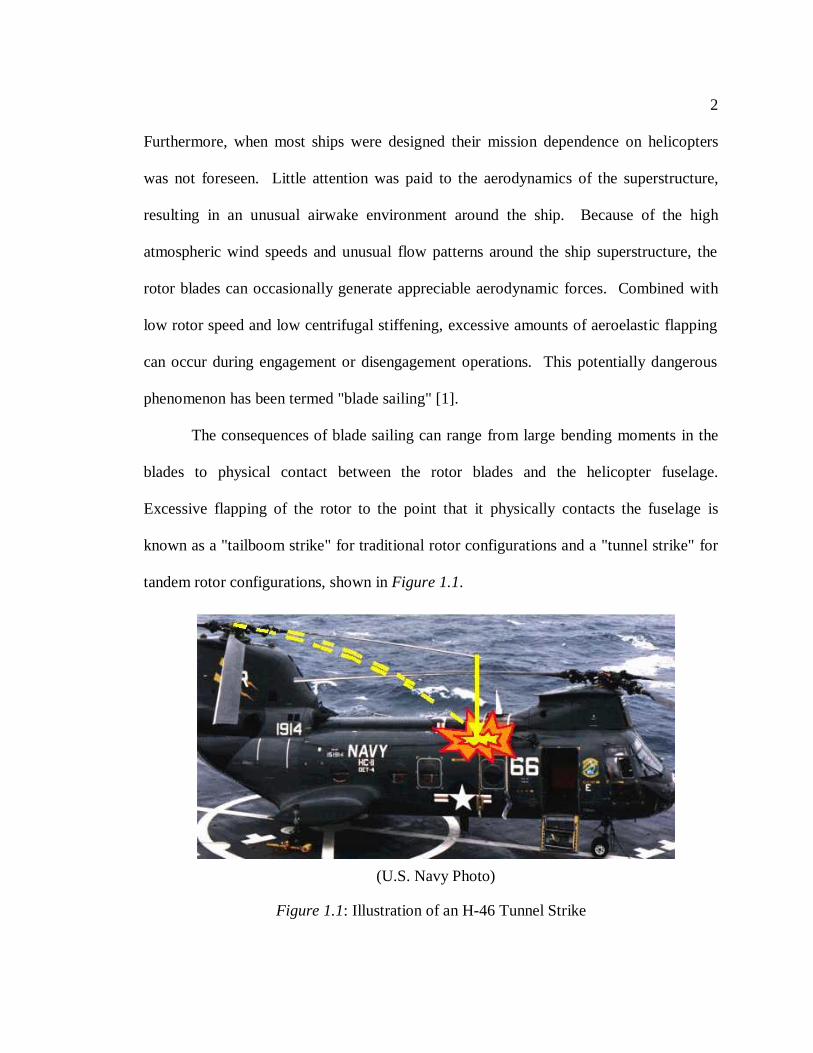
The consequences of blade sailing can range from large bending moments in the
blades to physical contact between the rotor blades and the helicopter fuselage.
Excessive flapping of the rotor to the point that it physically contacts the fuselage is
known as a "tailboom strike" for traditional rotor configurations and a "tunnel strike" for
tandem rotor configurations, shown inFigure 1.1.
(U.S. Navy Photo)
Figure 1.1: Illustration of an H-46 Tunnel Strike
3
Blade sailing most frequently occurs in severe weather conditions. North Sea oil
companies and the UK Royal Navy have documented examples of blade sailing. For
example, a commercially operated Boeing H-47 Chinook was reported having blade
sailing problems when operating from an oil rig [2]. Another Chinook operated by the
UK during the Falkland Islands conflict of 1982 could not disengage its rotors because of
continuous 70-knot winds. Until the winds dropped to an acceptable level, the rotor
system was kept turning with crew changes performed "on the fly". Some rescue
helicopters operating off the southwest coast of England have had to spin up their rotors
while remaining inside the ship's hangar because of extremely high wind speeds. Contact
between the blade tips and the tailboom, and even the ground in severe cases, have been
reported for the H-3 Sea King. In the most severe cases, fatalities have occurred in
connection with blade sailing events [1].
The phenomenon of blade sailing is familiar not just to North Sea oil companies
and the UK's military but also to the US Navy and Marines. The H-46 Sea Knight is a
tandem rotor helicopter that has been operated by the US Navy and Marines since 1964.
Since its introduction, there have been 114 documented H-46 tunnel strike incidents [3-
5]. These tunnel strikes, which typically occur at rotor speeds around 20% of the
nominal rotor speed, or 20%NR, pose a significant danger to both aircrew and ground
personnel. Physical damage can range from minor to the complete loss of the helicopter.
The dollar cost can range from just man-hour costs when inspections are required for
minor tunnel strikes, to upwards of $500,000 for a tunnel strike which involves the
sudden stoppage of the drive train system [6]. If the entire airframe is damaged beyond
4
repair, the true cost cannot be calculated because the H-46 is no longer in production.
Hidden costs of a tunnel strike can be even more expensive; for example, an interruption
in a ship's resupply schedule can lead to changes in the entire fleet schedule [7].
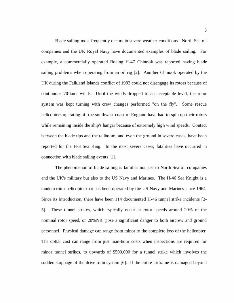
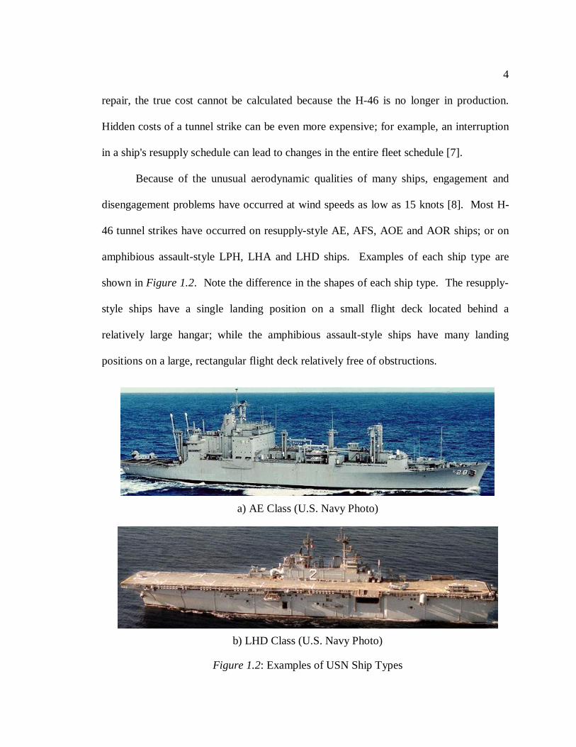
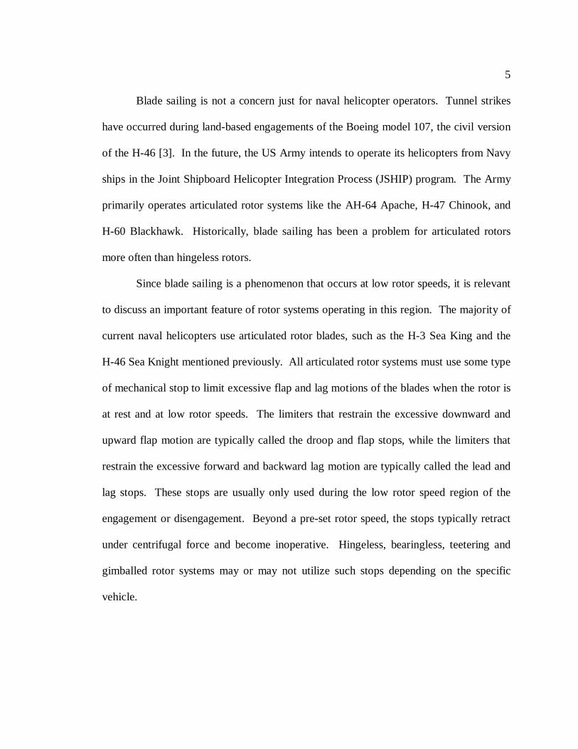
Because of the unusual aerodynamic qualities of many ships, engagement and
disengagement problems have occurred at wind speeds as low as 15 knots [8]. Most H-
46 tunnel strikes have occurred on resupply-style AE, AFS, AOE and AOR ships; or on
amphibious assault-style LPH, LHA and LHD ships. Examples of each ship type are
shown inFigure 1.2. Note the difference in the shapes of each ship type. The resupply-
style ships have a single landing position on a small flight deck located behind a
relatively large hangar; while the amphibious assault-style ships have many landing
positions on a large, rectangular flight deck relatively free of obstructions.
a) AE Class (U.S. Navy Photo)
b) LHD Class (U.S. Navy Photo)
Figure 1.2: Examples of USN Ship Types
5
Blade sailing is not a concern just for naval helicopter operators. Tunnel strikes
have occurred during land-based engagements of the Boeing model 107, the civil version
of the H-46 [3]. In the future, the US Army intends to operate its helicopters from Navy
ships in the Joint Shipboard Helicopter Integration Process (JSHIP) program. The Army
primarily operates articulated rotor systems like the AH-64 Apache, H-47 Chinook, and
H-60 Blackhawk. Historically, blade sailing has been a problem for articulated rotors
more often than hingeless rotors.
Since blade sailing is a phenomenon that occurs at low rotor speeds, it is relevant
to discuss an important feature of rotor systems operating in this region. The majority of
current naval helicopters use articulated rotor blades, such as the H-3 Sea King and the
H-46 Sea Knight mentioned previously. All articulated rotor systems must use some type
of mechanical stop to limit excessive flap and lag motions of the blades when the rotor is
at rest and at low rotor speeds. The limiters that restrain the excessive downward and
upward flap motion are typically called the droop and flap stops, while the limiters that
restrain the excessive forward and backward lag motion are typically called the lead and
lag stops. These stops are usually only used during the low rotor speed region of the
engagement or disengagement. Beyond a pre-set rotor speed, the stops typically retract
under centrifugal force and become inoperative. Hingeless, bearingless, teetering and
gimballed rotor systems may or may not utilize such stops depending on the specific
vehicle.
6
1.2 Determination of Engagement and Disengagement Limits
Due to the hazardous nature of maritime helicopter operations, limits must be
established on the atmospheric wind conditions and ship motions in which shipboard
helicopter operations can be safely performed. The shipboard helicopter operations,
including vehicle stowage, engagement/disengagement, launch/recovery, vertical
replenishment, and helicopter in-flight refueling operations, are usually referred to as
Dynamic Interface (DI) operations. The safe limits are called the Ship/Helicopter
Operational Limits (SHOLs). Naturally, larger SHOLs increase the helicopter's ability to
perform its mission in adverse weather conditions, which in turn increases the ship's
tactical flexibility.
The most important factor in determining the SHOLs for engagement and
disengagement operations is the relative speed and direction of the wind, or Wind-Over-
Deck (WOD), as it approaches the ship. In general, the faster the WOD speed, the more
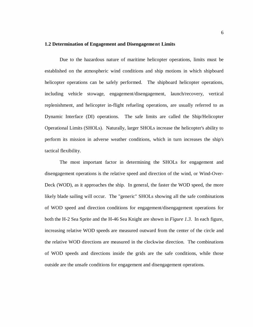
likely blade sailing will occur. The "generic" SHOLs showing all the safe combinations
of WOD speed and direction conditions for engagement/disengagement operations for
both the H-2 Sea Sprite and the H-46 Sea Knight are shown inFigure 1.3. In each figure,
increasing relative WOD speeds are measured outward from the center of the circle and
the relative WOD directions are measured in the clockwise direction. The combinations
of WOD speeds and directions inside the grids are the safe conditions, while those
outside are the unsafe conditions for engagement and disengagement operations.
7
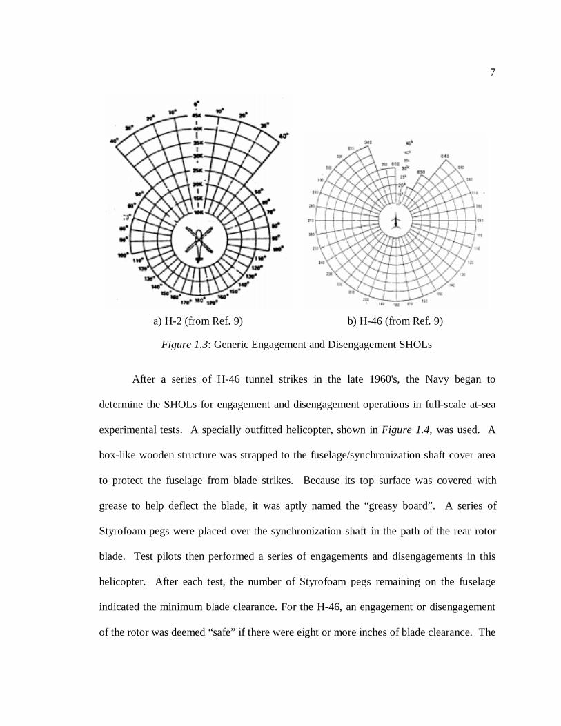
After a series of H-46 tunnel strikes in the late 1960's, the Navy began to
determine the SHOLs for engagement and disengagement operations in full-scale at-sea
experimental tests. A specially outfitted helicopter, shown inFigure 1.4, was used. A
box-like wooden structure was strapped to the fuselage/synchronization shaft cover area
to protect the fuselage from blade strikes. Because its top surface was covered with
grease to help deflect the blade, it was aptly named the “greasy board”. A series of
Styrofoam pegs were placed over the synchronization shaft in the path of the rear rotor
blade. Test pilots then performed a series of engagements and disengagements in this
helicopter. After each test, the number of Styrofoam pegs remaining on the fuselage
indicated the minimum blade clearance. For the H-46, an engagement or disengagement
of the rotor was deemed “safe” if there were eight or more inches of blade clearance. The
a) H-2 (from Ref. 9) b) H-46 (from Ref. 9)
Figure 1.3: Generic Engagement and Disengagement SHOLs
8
tests were then repeated, first in very calm winds and then in progressively more severe
winds for multiple wind directions, until a safe operational limit was reached. These tests
were conducted forevery helicopter/ship/landing spot combination. Typical DI test
reports are available in Refs. 10-18.
Unfortunately, this process of experimentally determining the SHOLs presented
several problems. First, it was very labor intensive and time consuming. The at-sea
portion of DI testing typically required four to five days and a crew of four pilots, two air
crewmen, four test engineers, and five maintenance personnel [19]. In 1985, a backlog of
11 helicopter types and 20 ship types required testing for DI characteristics. At that time,
this testing was to be completed in 15 years, primarily due to a lack of ship availability
[20]. Furthermore, DI testing was very expensive - a typical test cost approximately $75k
to $150kper ship/helicopter combination. One set of DI tests cost approximately $45k
and did not even yield useful data because the weather was calm during the entire test
(U.S. Navy Photo)
Figure 1.4: H-46 Test Aircraft Outfitted with Greasy Board and Styrofoam Pegs
9
period [21]. Finally, experience has shown that DI testing did not even consistently
produce safe results because of the variability of sea-state and wind conditions during the
test period. For example, a significant number of tunnel strikes occurred aboard AOR
type ships while operating inside of the "safe" envelope [7]. For these reasons, the Navy
ceased the portion of DI testing devoted to engagement and disengagement SHOL
determination in 1990.
The analytical determination of the SHOLs has been proposed as a viable
alternative to testing because it offers substantial benefits in terms of reducing cost,
improving safety, and developing larger operating envelopes [22]. The Technical Co-
operation Programme (TTCP) group, an international organization whose members
conduct DI testing, has led interest in analytic DI research. It is composed of the Defence
and Evaluation and Research Agency (DERA) in the United Kingdom, the National
Research Council - Institute for Aerospace Research (NRC - IAR) in Canada, the Naval
Air Warfare Center (NAWC) in the United States, and the Defence Science and
Technology Organisation (DSTO) in Australia.
1.3 Related Research
The following sections outlines the previous research related to the analytical and
experimental simulation of engagement and disengagement operations. The previous
research has been categorized into “early” research occurring from approximately the
mid 1960’s to the mid 1980’s and “recent” research conducted from the mid 1980’s to the
present.
10
1.3.1 Early Engagement and Disengagement Modeling
The earliest attempts at modeling the blade sailing phenomenon began in the early
1960's. Since this is before the advent of high-speed computing power, very simple
analytic solutions were sought. They are characterized by the assumptions that the rotor
speed is constant at some low value, typically 5% to 20%NR, and that the flow is fully
attached. Blade deformations were typically represented with single mode
approximations.
1.3.1.1 Research at Westland Helicopters
The British first initiated blade sailing research for the Westland Whirlwind and
Wasp [23]. Both helicopters featured articulated rotor systems. The blade was assumed
to remain in contact with the droop stop at all times; therefore, cantilevered blade modes
were used to approximate the blade shape. The reverse flow region was modeled by
assuming the entire retreating side of the rotor disk generated no lift. Three different ship
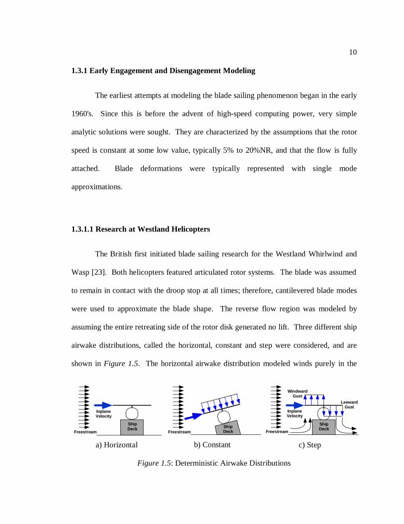
airwake distributions, called the horizontal, constant and step were considered, and are
shown inFigure 1.5. The horizontal airwake distribution modeled winds purely in the
ShipDeck
InplaneVelocity
Freestream
a) Horizontal
ShipDeckFreestream
b) Constant
ShipDeck
InplaneVelocity
WindwardGust
LeewardGust
Freestream
c) Step
Figure 1.5: Deterministic Airwake Distributions
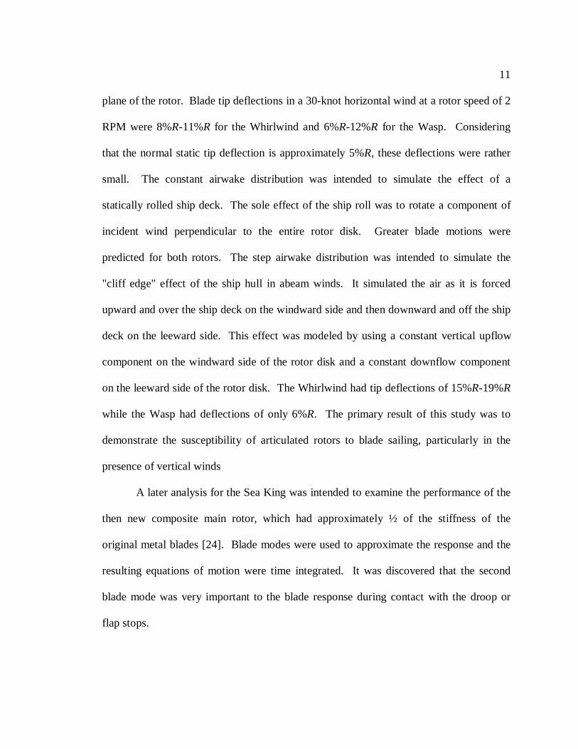
11
plane of the rotor. Blade tip deflections in a 30-knot horizontal wind at a rotor speed of 2
RPM were 8%R-11%R for the Whirlwind and 6%R-12%R for the Wasp. Considering
that the normal static tip deflection is approximately 5%R, these deflections were rather
small. The constant airwake distribution was intended to simulate the effect of a
statically rolled ship deck. The sole effect of the ship roll was to rotate a component of
incident wind perpendicular to the entire rotor disk. Greater blade motions were
predicted for both rotors. The step airwake distribution was intended to simulate the
"cliff edge" effect of the ship hull in abeam winds. It simulated the air as it is forced
upward and over the ship deck on the windward side and then downward and off the ship
deck on the leeward side. This effect was modeled by using a constant vertical upflow
component on the windward side of the rotor disk and a constant downflow component
on the leeward side of the rotor disk. The Whirlwind had tip deflections of 15%R-19%R
while the Wasp had deflections of only 6%R. The primary result of this study was to
demonstrate the susceptibility of articulated rotors to blade sailing, particularly in the
presence of vertical winds
A later analysis for the Sea King was intended to examine the performance of the
then new composite main rotor, which had approximately ½ of the stiffness of the
original metal blades [24]. Blade modes were used to approximate the response and the
resulting equations of motion were time integrated. It was discovered that the second
blade mode was very important to the blade response during contact with the droop or
flap stops.
12
A later analysis was intended as a "back of the envelope" calculation to predict
and compare the blade sailing behavior for the articulated Sea King and the hingeless
Lynx rotors [25]. A very simple expression for the flap equation of motion was derived
for a single, rigid blade. Blade element theory was used to solve for the steady state
response of the rotor. It was estimated that in a 60-knot horizontal wind with a 15-knot
vertical component, the articulated Sea King blade would have maximum flapping
excursions of 29%R, while the Lynx rotor system only 14%R. Once again, the
susceptibility of articulated rotors to blade sailing was displayed.
1.3.1.2 Research at Boeing Vertol
Boeing Vertol researched blade sailing of articulated rotors as early as 1964 [26].
Initially, this research was motivated by concerns of excessive flap bending moments at
the root of an articulated rotor blade during a droop stop impact. In this analysis, the flap
bending moment distribution along an articulated rotor blade during such an impact was
derived. Only the fundamental cantilevered mode was considered in the formulation.
The rotor speed was considered constant so a steady-state solution was obtained. Using a
full-scale aircraft operating at full rotor speed, an excessive cyclic pitch input was used to
cause a droop stop impact. Experimental measurements of the blade flapping motion and
root bending moment were recorded with an oscilloscope. Good agreement existed
between the predicted and the measured root bending moment.
A specific tunnel strike incident during an engagement of an H-46 helicopter
operating from the flight deck of the USS Kalamazoo, an AOR class ship, was also
13
modeled [27]. The strike incident was of the most severe type - all three aft rotor blades
struck the synchronization shaft and fuselage. Two of the blades were completely broken
off the rotor hub while the third shattered outboard of the blade attachment; and a hole 14
inches deep was torn in the fuselage. It was estimated that the tunnel strike occurred at
approximately 10%NR in 42-knot winds from 25° starboard of the ship's centerline. In
the analytic investigation, steady-state solutions for the flapping response at RPM values
of 2%NR to 20%NR were calculated. The maximum blade deflections were found to be
34%R upwards and 23%R downwards, occurring at a rotor speed of approximately
10%NR. The blade deflection required to contact the tunnel is 18%R for the H-46.
1.3.2 Recent Engagement and Disengagement Modeling
With the advent of faster computers, serious attention was paid to blade sailing
starting in the early 1980's. The blade equations of motion could be time integrated to
calculate the transient blade motion. Simple attached flow aerodynamic models yielding
analytic expressions were abandoned; instead, important nonlinear aerodynamic effects
such the reverse flow region and blade stall were included. Blade structural models were
also greatly improved. The use of a single mode approximation was no longer necessary;
instead, models with multiple elastic mode shapes were used.
14
1.3.2.1 Research at the Naval Postgraduate School
The Naval Postgraduate School attempted to model the tunnel strike problem for
the H-46 [28]. The aeroelastic rotor code, called the DYnamic System COupler program,
was an elastic flap-lag-torsion code. A converged solution using DYSCO was never
obtained so further study was abandoned.
1.3.2.2 Research at NASA
At NASA, research into disengagement behavior was motivated by a wind tunnel
test. It is common procedure to stop the rotor system as quickly as possible if a problem
is encountered. Normally, this would not pose any safety considerations. However, in
one set of tests the rotor shaft was tilted up to 30° to reduce ground effects. It was feared
that an emergency power shutdown of the rotor would induce a large blade lag response
leading to failure of structural components.
A rigid flap-lag blade analysis was developed to simulate a rotor in a wind tunnel
undergoing an emergency power shutdown [29]. Hub motion degrees of freedom in
longitudinal translation and pitch rotation were also considered. A linear, quasi-steady
aerodynamic model and a dynamic inflow model were used to represent the airloads.
The rotor speed profile was assumed to decay exponentially over a period of 40 seconds.
In the case of an emergency power shutdown, it was recommended that the collective
pitch and rotor shaft angle be quickly reduced to suppress the lag response.
15
1.3.2.3 Research at McDonnell Douglas
Engagement and disengagement research at McDonnell Douglas was motivated
not by aeroelastic flapping, but by concerns of excessive in-plane loads in the elastomeric
lead-lag dampers of the AH-64 Apache during brake-on startup operations [30]. In this
type of operation, the rotor brake is kept locked which prevents the rotor from turning
while the engine torque is increased. After the release of the rotor brake, the rotor is
essentially "jump started" and builds up speed very quickly. Applying a large impulsive
torque to the rotor tends to induce a large lag response. Accurate prediction of the lag
response is essential because it is a large contributor to the loads in the blade retention
system and because contact between the blade and the lag stops must be prevented.
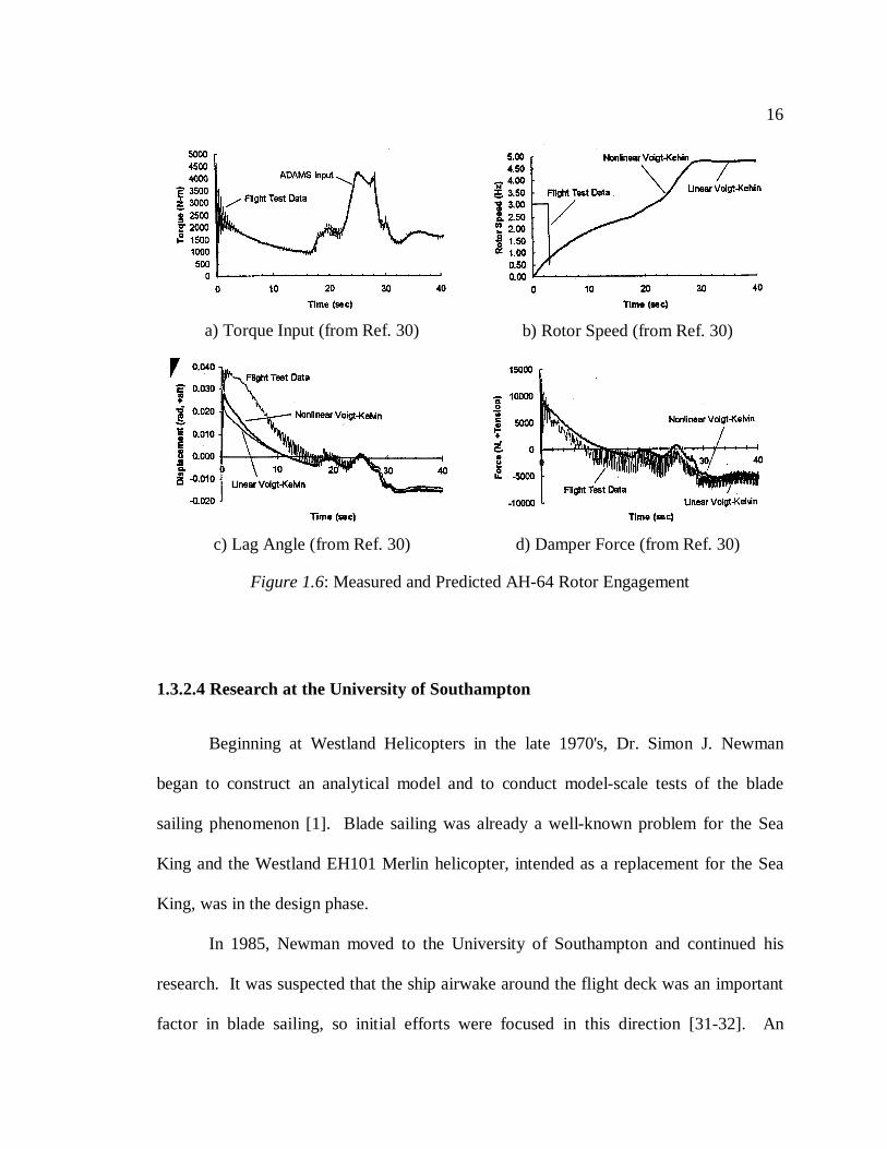
A full-scale experiment and an analytic simulation of an Apache brake-on rotor
engagement operation were conducted [30]. In the experiment, the time histories of the
rotor torque, rotor speed, lag response and damper loads were measured. In the
simulation, a nonlinear, rigid-blade, multi-body model of the Apache rotor was
constructed. A constant profile drag coefficient was used to model aerodynamic drag.
Linear and nonlinear models of a Voigt-Kelvin solid were used to simulate the
elastomeric lag dampers. Using the measured torque input, the rotor speed profile, lag
response and damper loads were predicted with both damper models. Results of the
analysis are shown inFigure 1.6. The predicted rotor speed profiles with both damper
models correlated very well with the experimentally measured profile. However, both
the predicted blade lag angles and loads were significantly different from their measured
counterparts, especially for rotor speeds less than 50% NR.
16
1.3.2.4 Research at the University of Southampton
Beginning at Westland Helicopters in the late 1970's, Dr. Simon J. Newman
began to construct an analytical model and to conduct model-scale tests of the blade
sailing phenomenon [1]. Blade sailing was already a well-known problem for the Sea
King and the Westland EH101 Merlin helicopter, intended as a replacement for the Sea
King, was in the design phase.
In 1985, Newman moved to the University of Southampton and continued his
research. It was suspected that the ship airwake around the flight deck was an important
factor in blade sailing, so initial efforts were focused in this direction [31-32]. An
a) Torque Input (from Ref. 30) b) Rotor Speed (from Ref. 30)
c) Lag Angle (from Ref. 30) d) Damper Force (from Ref. 30)
Figure 1.6: Measured and Predicted AH-64 Rotor Engagement
17
experimental investigation of the airflow about a model and full-scale RFA Rover Class
ship was performed without the presence of a helicopter. Mean, maximum and minimum
velocities, standard deviations and power spectral densities were measured for both
model-scale and full-scale flowfields. Two orthogonal velocity components, one along
the direction of the free stream air and one in the vertical direction, were taken over the
full-scale ship with golf ball and propeller anemometers. Data was taken for several
wind directions and speeds ranging from 15 to 30 knots. A 1/120th-scale ship was used
for the wind tunnel tests. No atmospheric boundary layer was simulated and the
turbulence intensity of the free stream air was 0.4%. A three-axis hot wire anemometer
was used to obtain the flow velocities over the same points and wind conditions on the
model flight deck as the full-scale tests. Comparisons of the mean flow components and
power spectral densities for both measurements showed satisfactory correlation.
Significant upwash and downwash velocities at the windward and leeward deck edges
were measured.
In addition to the airwake studies, a transient blade sailing model for hingeless
rotors was described [31-32]. The flapping equations of motion for a single blade were
derived and simulated with a modal superposition method. The effect of gravity and the
variation in centrifugal force with changing rotor speed were included. The ship airwake
was modeled with a step airwake distribution, which was based on the ship airwake tests.
A quasi-steady aerodynamic model, including trailing edge separation effects via a
Kirchoff method, was used to calculate the aerodynamic loads. The induced velocity was
assumed zero, since the nominal condition during rotor engagements and disengagements
18
is zero rotor thrust. The Westland Lynx was used as the helicopter for the study. The
aerodynamic properties of a NACA 0012 airfoil section were assumed instead of the
actual Lynx NPL 9615 airfoil section. Simple analytical expressions for the rotor speed
profile during the engagement and disengagement operations were used. Ship roll was
also simulated. No interaction between the ship motion and the rotor dynamics was
modeled since the rotor speed was typically much higher than the ship roll frequency.
Therefore, the sole effect of the ship motion was to rotate the plane of the rotor relative to
the ship airwake and to induce a lateral airflow component due to rotational motion about
the ship's center of gravity. A fourth order Runge-Kutta integrator was used to time
integrate the resulting equations of motion. The analysis showed the loads, calculated
from a curvature method, exceeded the blade fatigue limits in 50-knot winds with a 10-
knot vertical component and a 7.5° ship roll amplitude. Blade tailboom strike limits were
exceeded in 60-knot winds with a 15-knot vertical component and a ship roll amplitude
of 15°.
To obtain a greater understanding of the model-scale ship airwake, additional
measurements were taken with a laser Doppler anemometer [33]. Three orthogonal
velocity components were measured at 12 locations equally spaced around the 75%R
blade position and one at the rotor hub. Wind directions of 90° (from starboard), 135°,
and 180° (from astern) were examined. After examining the flow patters, it was
determined that the ship airwake could be specified with simple variations. The two
airwake types that most resembled the wind tunnel data were termed the step airwake and
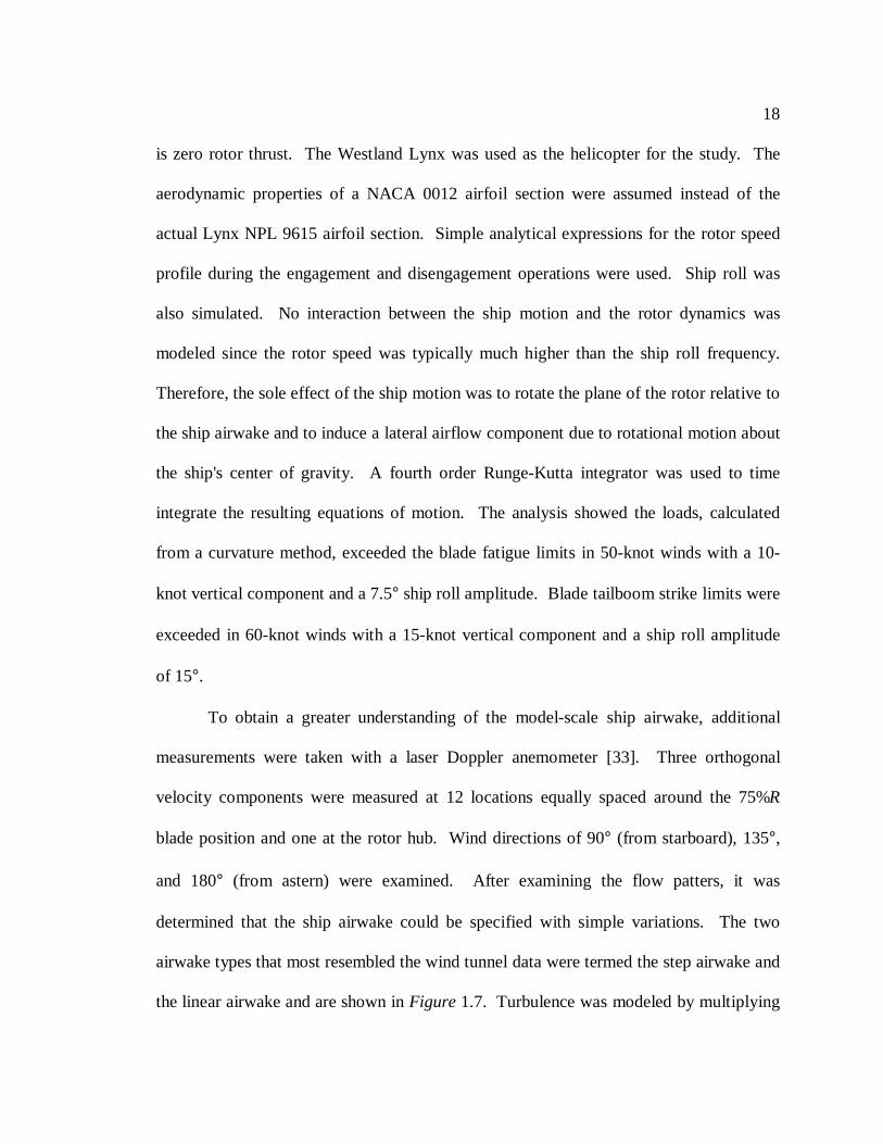
the linear airwake and are shown inFigure 1.7. Turbulence was modeled by multiplying
19
the measured flow standard deviation by a Gaussian distributed random number updated
at a Strouhal scaled frequency. The blade structural model was improved with flap-
torsion coupling. The largest rotor deflections occurred in 50-knot abeam winds. The
linear airwake model results consistently matched the original wind tunnel results much
better than the step airwake model results. Torsion was shown to increase tip deflections
by 30%. Extended engagement run-up times were shown to increase tip deflections by
10%. Ship roll effects were shown to increase blade deflections by 12%.
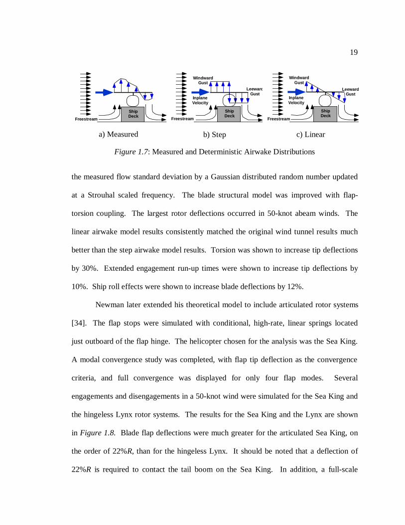
Newman later extended his theoretical model to include articulated rotor systems
[34]. The flap stops were simulated with conditional, high-rate, linear springs located
just outboard of the flap hinge. The helicopter chosen for the analysis was the Sea King.
A modal convergence study was completed, with flap tip deflection as the convergence
criteria, and full convergence was displayed for only four flap modes. Several
engagements and disengagements in a 50-knot wind were simulated for the Sea King and
the hingeless Lynx rotor systems. The results for the Sea King and the Lynx are shown
in Figure 1.8. Blade flap deflections were much greater for the articulated Sea King, on
the order of 22%R, than for the hingeless Lynx. It should be noted that a deflection of
22%R is required to contact the tail boom on the Sea King. In addition, a full-scale
ShipDeck
Freestream
a) Measured
ShipDeck
InplaneVelocity
WindwardGust
Leewar dGust
Freestream
b) Step
ShipDeck
InplaneVelocity
WindwardGust
Leewar dGust
Freestream
c) Linear
Figure 1.7: Measured and Deterministic Airwake Distributions
20
experimental run-up and run-down test with an SA330 Puma helicopter in a 10-knot
headwind was conducted and correlation with analytical results was performed. Blade
flap hinge angle deflections were measured and converted to tip deflections by assuming
a rigid blade. Since there was difficulty in accurately measuring the rotor speed,
collective pitch, and cyclic pitch at low rotor speed, a detailed investigation was not
warranted.
a) Sea King Rotor Engagement(from Ref. 34)
b) Sea King Rotor Disengagement(from Ref. 34)
c) Lynx Rotor Engagement(from Ref. 34)
d) Lynx Rotor Disengagement(from Ref. 34)
Figure 1.8: Sea King and Lynx Rotor Engagements and Disengagements
21
After the extension of the theoretical model to include articulated rotors, actual
experimental validation tests of model-scale radio-controlled helicopter engagements and
disengagements were undertaken [35-36]. The tests were intended to demonstrate blade
sailing and establish the effect of the ship airwake on the rotor behavior. In these tests, a
radio-controlled model helicopter was mounted atop a model ship deck. A Kalt Cyclone
kit was used because it had approximately the same rotor height/rotor diameter ratio as
the Westland Lynx. Only the main fuselage and rotor were used in the tests. The main
rotor system as originally provided in the kit was a two-bladed teetering rotor
configuration. The supplied gas engine was discarded and replaced with a ½ HP electric
motor. The main helicopter body was bolted to a sliding base plate on the ship's deck and
an electric motor was fitted below the deck. The ship deck itself consisted of nothing
more than a large rectangular box - all small details were omitted. The ship hull size was
scaled to approximate a Westland Lynx/RFA Rover Class ship combination.
The helicopter/ship combination was too large to be placed in the normal 5x7 foot
tunnel test section, so instead it was placed in the settling chamber. The ship deck was
placed in abeam wind conditions since previous work showed the greatest upwash and
downwash velocities were encountered in this situation. Engagements and
disengagements of the rotor system were then completed at a total of 5 locations on the
ship deck, from fully windward (A) to fully leeward (E), as shown inFigure 1.9. The
tunnel speed was set at 5 m/s, which represented a 47-knot full-scale wind. Tests were
performed in a teetering rotor configuration and in an articulated rotor configuration. For
each test, the rotor speed variation was a linear run-up followed by a constant period,
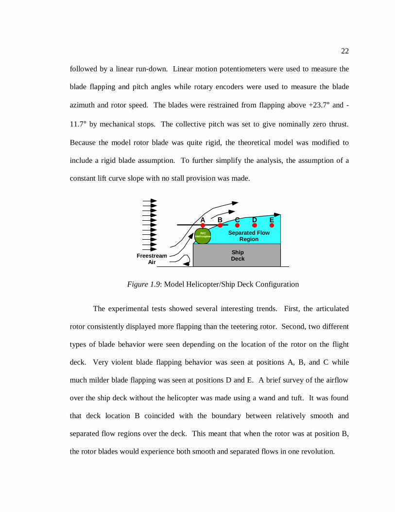
22
followed by a linear run-down. Linear motion potentiometers were used to measure the
blade flapping and pitch angles while rotary encoders were used to measure the blade
azimuth and rotor speed. The blades were restrained from flapping above +23.7° and -
11.7° by mechanical stops. The collective pitch was set to give nominally zero thrust.
Because the model rotor blade was quite rigid, the theoretical model was modified to
include a rigid blade assumption. To further simplify the analysis, the assumption of a
constant lift curve slope with no stall provision was made.
The experimental tests showed several interesting trends. First, the articulated
rotor consistently displayed more flapping than the teetering rotor. Second, two different
types of blade behavior were seen depending on the location of the rotor on the flight
deck. Very violent blade flapping behavior was seen at positions A, B, and C while
much milder blade flapping was seen at positions D and E. A brief survey of the airflow
over the ship deck without the helicopter was made using a wand and tuft. It was found
that deck location B coincided with the boundary between relatively smooth and
separated flow regions over the deck. This meant that when the rotor was at position B,
the rotor blades would experience both smooth and separated flows in one revolution.
R/CHelicopter
ShipDeckFreestream
Air
EA B C D
Separated FlowRegion
Figure 1.9: Model Helicopter/Ship Deck Configuration
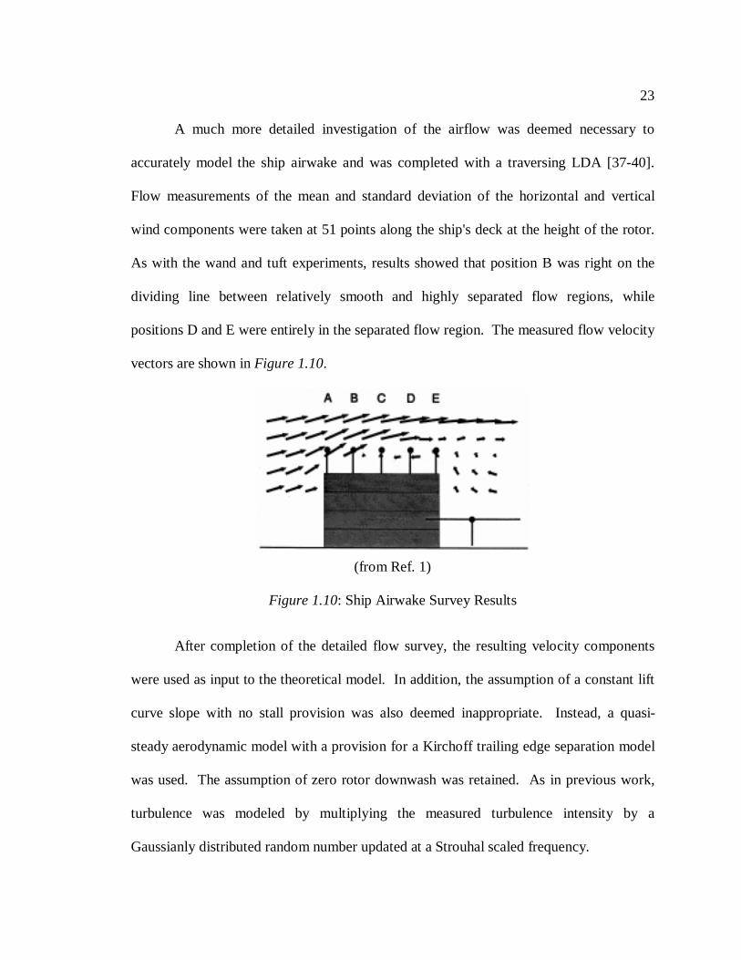
23
A much more detailed investigation of the airflow was deemed necessary to
accurately model the ship airwake and was completed with a traversing LDA [37-40].
Flow measurements of the mean and standard deviation of the horizontal and vertical
wind components were taken at 51 points along the ship's deck at the height of the rotor.
As with the wand and tuft experiments, results showed that position B was right on the
dividing line between relatively smooth and highly separated flow regions, while
positions D and E were entirely in the separated flow region. The measured flow velocity
vectors are shown inFigure 1.10.
After completion of the detailed flow survey, the resulting velocity components
were used as input to the theoretical model. In addition, the assumption of a constant lift
curve slope with no stall provision was also deemed inappropriate. Instead, a quasi-
steady aerodynamic model with a provision for a Kirchoff trailing edge separation model
was used. The assumption of zero rotor downwash was retained. As in previous work,
turbulence was modeled by multiplying the measured turbulence intensity by a
Gaussianly distributed random number updated at a Strouhal scaled frequency.
(from Ref. 1)
Figure 1.10: Ship Airwake Survey Results
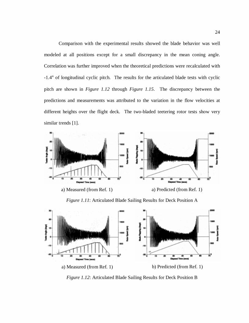
24
Comparison with the experimental results showed the blade behavior was well
modeled at all positions except for a small discrepancy in the mean coning angle.
Correlation was further improved when the theoretical predictions were recalculated with
-1.4° of longitudinal cyclic pitch. The results for the articulated blade tests with cyclic
pitch are shown inFigure 1.12 through Figure 1.15. The discrepancy between the
predictions and measurements was attributed to the variation in the flow velocities at
different heights over the flight deck. The two-bladed teetering rotor tests show very
similar trends [1].
a) Measured (from Ref. 1) a) Predicted (from Ref. 1)
Figure 1.11: Articulated Blade Sailing Results for Deck Position A
a) Measured (from Ref. 1) b) Predicted (from Ref. 1)
Figure 1.12: Articulated Blade Sailing Results for Deck Position B
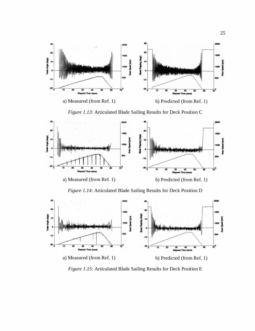
25
a) Measured (from Ref. 1) b) Predicted (from Ref. 1)
Figure 1.13: Articulated Blade Sailing Results for Deck Position C
a) Measured (from Ref. 1) b) Predicted (from Ref. 1)
Figure 1.14: Articulated Blade Sailing Results for Deck Position D
a) Measured (from Ref. 1) b) Predicted (from Ref. 1)
Figure 1.15: Articulated Blade Sailing Results for Deck Position E
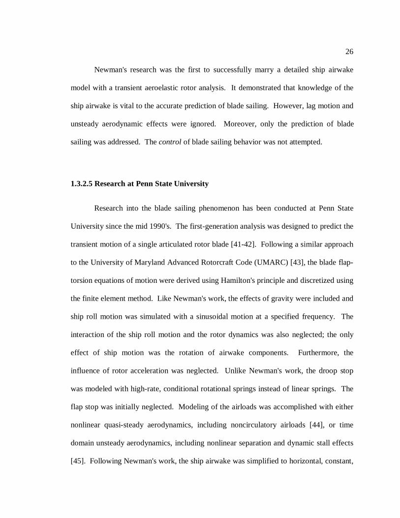
26
Newman's research was the first to successfully marry a detailed ship airwake
model with a transient aeroelastic rotor analysis. It demonstrated that knowledge of the
ship airwake is vital to the accurate prediction of blade sailing. However, lag motion and
unsteady aerodynamic effects were ignored. Moreover, only the prediction of blade
sailing was addressed. Thecontrol of blade sailing behavior was not attempted.
1.3.2.5 Research at Penn State University
Research into the blade sailing phenomenon has been conducted at Penn State
University since the mid 1990's. The first-generation analysis was designed to predict the
transient motion of a single articulated rotor blade [41-42]. Following a similar approach
to the University of Maryland Advanced Rotorcraft Code (UMARC) [43], the blade flap-
torsion equations of motion were derived using Hamilton's principle and discretized using
the finite element method. Like Newman's work, the effects of gravity were included and
ship roll motion was simulated with a sinusoidal motion at a specified frequency. The
interaction of the ship roll motion and the rotor dynamics was also neglected; the only
effect of ship motion was the rotation of airwake components. Furthermore, the
influence of rotor acceleration was neglected. Unlike Newman's work, the droop stop
was modeled with high-rate, conditional rotational springs instead of linear springs. The
flap stop was initially neglected. Modeling of the airloads was accomplished with either
nonlinear quasi-steady aerodynamics, including noncirculatory airloads [44], or time
domain unsteady aerodynamics, including nonlinear separation and dynamic stall effects
[45]. Following Newman's work, the ship airwake was simplified to horizontal, constant,
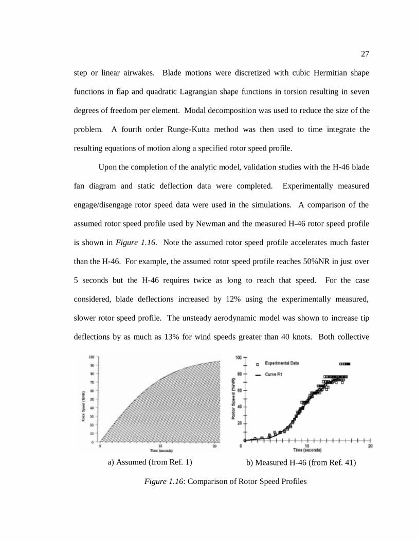
27
step or linear airwakes. Blade motions were discretized with cubic Hermitian shape
functions in flap and quadratic Lagrangian shape functions in torsion resulting in seven
degrees of freedom per element. Modal decomposition was used to reduce the size of the
problem. A fourth order Runge-Kutta method was then used to time integrate the
resulting equations of motion along a specified rotor speed profile.
Upon the completion of the analytic model, validation studies with the H-46 blade
fan diagram and static deflection data were completed. Experimentally measured
engage/disengage rotor speed data were used in the simulations. A comparison of the
assumed rotor speed profile used by Newman and the measured H-46 rotor speed profile
is shown inFigure 1.16. Note the assumed rotor speed profile accelerates much faster
than the H-46. For example, the assumed rotor speed profile reaches 50%NR in just over
5 seconds but the H-46 requires twice as long to reach that speed. For the case
considered, blade deflections increased by 12% using the experimentally measured,
slower rotor speed profile. The unsteady aerodynamic model was shown to increase tip
deflections by as much as 13% for wind speeds greater than 40 knots. Both collective
a) Assumed (from Ref. 1) b) Measured H-46 (from Ref. 41)
Figure 1.16: Comparison of Rotor Speed Profiles
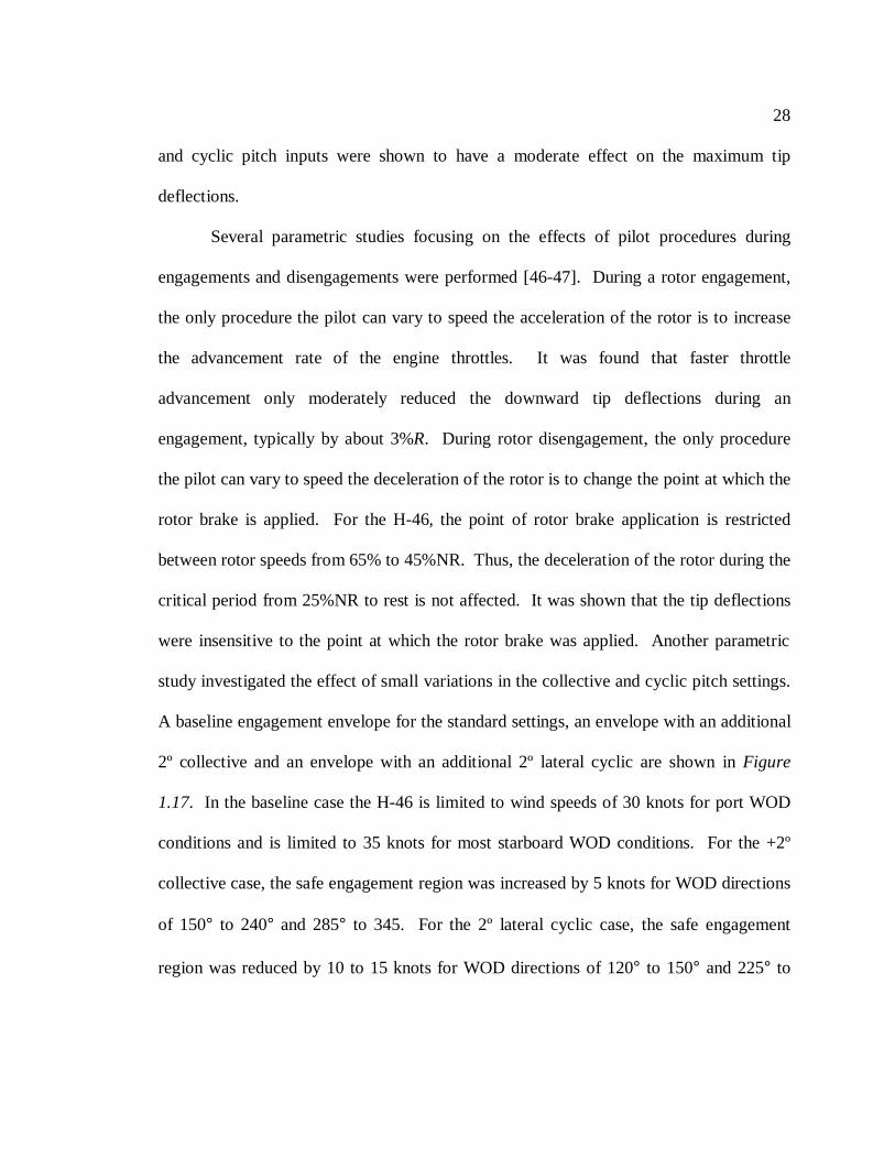
28
and cyclic pitch inputs were shown to have a moderate effect on the maximum tip
deflections.
Several parametric studies focusing on the effects of pilot procedures during
engagements and disengagements were performed [46-47]. During a rotor engagement,
the only procedure the pilot can vary to speed the acceleration of the rotor is to increase
the advancement rate of the engine throttles. It was found that faster throttle
advancement only moderately reduced the downward tip deflections during an
engagement, typically by about 3%R. During rotor disengagement, the only procedure
the pilot can vary to speed the deceleration of the rotor is to change the point at which the
rotor brake is applied. For the H-46, the point of rotor brake application is restricted
between rotor speeds from 65% to 45%NR. Thus, the deceleration of the rotor during the
critical period from 25%NR to rest is not affected. It was shown that the tip deflections
were insensitive to the point at which the rotor brake was applied. Another parametric
study investigated the effect of small variations in the collective and cyclic pitch settings.
A baseline engagement envelope for the standard settings, an envelope with an additional
2º collective and an envelope with an additional 2º lateral cyclic are shown inFigure
1.17. In the baseline case the H-46 is limited to wind speeds of 30 knots for port WOD
conditions and is limited to 35 knots for most starboard WOD conditions. For the +2º
collective case, the safe engagement region was increased by 5 knots for WOD directions
of 150° to 240° and 285° to 345. For the 2º lateral cyclic case, the safe engagement
region was reduced by 10 to 15 knots for WOD directions of 120° to 150° and 225° to
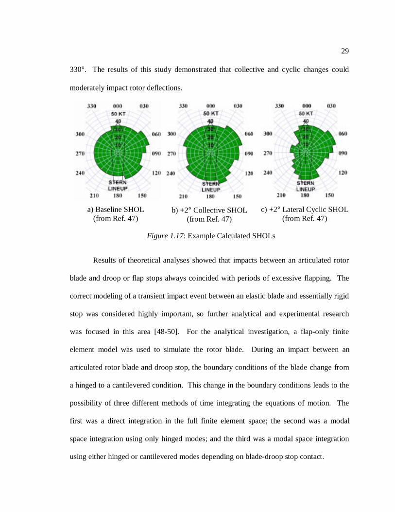
29
330°. The results of this study demonstrated that collective and cyclic changes could
moderately impact rotor deflections.
Results of theoretical analyses showed that impacts between an articulated rotor
blade and droop or flap stops always coincided with periods of excessive flapping. The
correct modeling of a transient impact event between an elastic blade and essentially rigid
stop was considered highly important, so further analytical and experimental research
was focused in this area [48-50]. For the analytical investigation, a flap-only finite
element model was used to simulate the rotor blade. During an impact between an
articulated rotor blade and droop stop, the boundary conditions of the blade change from
a hinged to a cantilevered condition. This change in the boundary conditions leads to the
possibility of three different methods of time integrating the equations of motion. The
first was a direct integration in the full finite element space; the second was a modal
space integration using only hinged modes; and the third was a modal space integration
using either hinged or cantilevered modes depending on blade-droop stop contact.
a) Baseline SHOL(from Ref. 47)
b) +2° Collective SHOL(from Ref. 47)
c) +2° Lateral Cyclic SHOL(from Ref. 47)
Figure 1.17: Example Calculated SHOLs
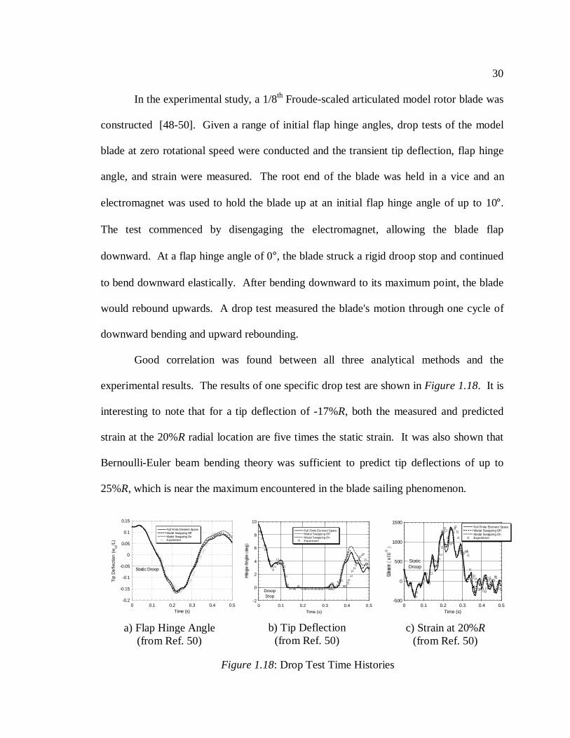
30
In the experimental study, a 1/8th Froude-scaled articulated model rotor blade was
constructed [48-50]. Given a range of initial flap hinge angles, drop tests of the model
blade at zero rotational speed were conducted and the transient tip deflection, flap hinge
angle, and strain were measured. The root end of the blade was held in a vice and an
electromagnet was used to hold the blade up at an initial flap hinge angle of up to 10°.
The test commenced by disengaging the electromagnet, allowing the blade flap
downward. At a flap hinge angle of 0°, the blade struck a rigid droop stop and continued
to bend downward elastically. After bending downward to its maximum point, the blade
would rebound upwards. A drop test measured the blade's motion through one cycle of
downward bending and upward rebounding.
Good correlation was found between all three analytical methods and the
experimental results. The results of one specific drop test are shown inFigure 1.18. It is
interesting to note that for a tip deflection of -17%R, both the measured and predicted
strain at the 20%R radial location are five times the static strain. It was also shown that
Bernoulli-Euler beam bending theory was sufficient to predict tip deflections of up to
25%R, which is near the maximum encountered in the blade sailing phenomenon.
-0.2
-0.15
-0.1
-0.05
0
0.05
0.1
0.15
0 0.1 0.2 0.3 0.4 0.5
Full Finite Element SpaceModal Swapping OffModal Swapping OnExperiment
Tip
De
flect
ion
(wtip
/L)
Time (s)
Static Droop
a) Flap Hinge Angle(from Ref. 50)
-2
0
2
4
6
8
10
0 0.1 0.2 0.3 0.4 0.5
Full Finite Element SpaceModal Swapping OffModal Swapping OnExperiment
Time (s)
DroopStop
b) Tip Deflection(from Ref. 50)
-500
0
500
1000
1500
0 0.1 0.2 0.3 0.4 0.5
Full Finite Element SpaceModal Swapping OffModal Swapping OnExperiment
Time (s)
StaticDroop
c) Strain at 20%R(from Ref. 50)
Figure 1.18: Drop Test Time Histories
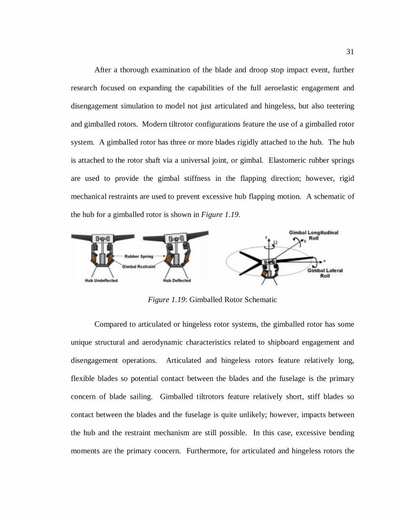
31
After a thorough examination of the blade and droop stop impact event, further
research focused on expanding the capabilities of the full aeroelastic engagement and
disengagement simulation to model not just articulated and hingeless, but also teetering
and gimballed rotors. Modern tiltrotor configurations feature the use of a gimballed rotor
system. A gimballed rotor has three or more blades rigidly attached to the hub. The hub
is attached to the rotor shaft via a universal joint, or gimbal. Elastomeric rubber springs
are used to provide the gimbal stiffness in the flapping direction; however, rigid
mechanical restraints are used to prevent excessive hub flapping motion. A schematic of
the hub for a gimballed rotor is shown inFigure 1.19.
Compared to articulated or hingeless rotor systems, the gimballed rotor has some
unique structural and aerodynamic characteristics related to shipboard engagement and
disengagement operations. Articulated and hingeless rotors feature relatively long,
flexible blades so potential contact between the blades and the fuselage is the primary
concern of blade sailing. Gimballed tiltrotors feature relatively short, stiff blades so
contact between the blades and the fuselage is quite unlikely; however, impacts between
the hub and the restraint mechanism are still possible. In this case, excessive bending
moments are the primary concern. Furthermore, for articulated and hingeless rotors the
Figure 1.19: Gimballed Rotor Schematic
32
hub is rigidly attached to the rotor shaft so the motion of each individual blade is
uncoupled from the others. For gimballed and teetering rotors, the hub is free to pivot on
the rotor shaft so the blade motions are coupled. Lastly, most articulated and hingeless
rotors have relatively small amounts of twist, on the order of 6° to 10°. The V-22 Osprey
tiltrotor has 45° of twist, which introduces significant structural flap-lag couplings.
An initial analysis was developed to model multi-bladed gimballed tiltrotors
during engagement and disengagement sequences [51-52]. A two-degree of freedom
model calculating the transient response of the gimbal pitch and roll resulted.
Satisfactory correlation with the two-bladed teetering rotor experimental wind tunnel
tests in Ref. 1 was displayed. The possibility of gimbal impacts for a gimballed rotor
similar to the V-22 was shown. A simple linear run-up and run-down rotor speed profile
was assumed requiring 100 seconds to reach full speed. Multiple impacts with the
gimbal restraint were seen for wind speeds as low as 30 knots.
The full aeroelastic simulation was then extended to model all three elastic blades
of a gimballed tiltrotor. Since the large amounts of blade twist result in significant flap-
lag coupling, lag degrees of freedom were added to the flap-torsion degrees of freedom
already included in the simulation. The capability to predict blade bending moments
using a curvature method was also added. The elastic code was first validated against
experimentally measured flap and lag bending moments for an aeroelastically scaled
model tiltrotor in hover and satisfactory correlation was observed. Engagements and
disengagements for the full scale V-22 in 35-knot winds were simulated. Several gimbal
restraint impacts were shown to occur.
33
1.3.2.6 Multi-body Modeling Techniques
Recently, a finite element based multi-body dynamics analysis was developed to
examine engagement and disengagement operations [53]. The multibody modeling
technique offers the advantage of easily modeling different rotor hub types with an
extensive library of pre-validated elements. In the technique, no modal reduction is
performed. Special implicit time integration techniques for nonlinear systems were used
containing high frequency numerical dissipation. The time integration scheme also
utilized a variable time step to maximize computational efficiency. The multi-body
analysis was first validated with the experimental rotor blade-droop stop impact tests
performed in Ref. 50 and good correlation was displayed. Engagements and
disengagements of an H-46 rotor system were then simulated in a constant airwake
distribution. Time histories of the flap tip deflection and pitch link loads were examined.
1.4 Ship Airwake Modeling
As seen in earlier blade sailing research, especially in the experimental wind
tunnel tests at the University of Southampton, the ship airwake environment plays a large
role in the aeroelastic response of the rotor. As such, it is relevant to review past efforts
in the measurement and prediction of the ship airwake environment. This review is by no
means comprehensive, but intended to introduce some of the most relevant research. In
general, the ship airwake is not considered during the design of ships. The boxy
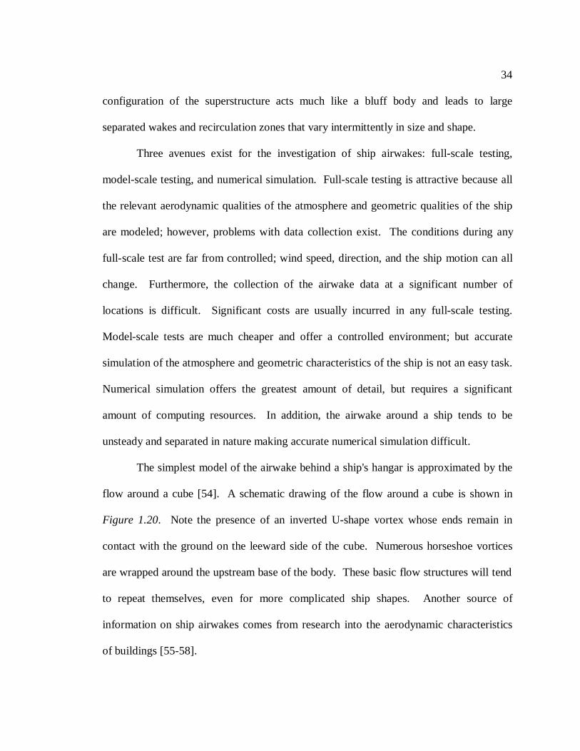
34
configuration of the superstructure acts much like a bluff body and leads to large
separated wakes and recirculation zones that vary intermittently in size and shape.
Three avenues exist for the investigation of ship airwakes: full-scale testing,
model-scale testing, and numerical simulation. Full-scale testing is attractive because all
the relevant aerodynamic qualities of the atmosphere and geometric qualities of the ship
are modeled; however, problems with data collection exist. The conditions during any
full-scale test are far from controlled; wind speed, direction, and the ship motion can all
change. Furthermore, the collection of the airwake data at a significant number of
locations is difficult. Significant costs are usually incurred in any full-scale testing.
Model-scale tests are much cheaper and offer a controlled environment; but accurate
simulation of the atmosphere and geometric characteristics of the ship is not an easy task.
Numerical simulation offers the greatest amount of detail, but requires a significant
amount of computing resources. In addition, the airwake around a ship tends to be
unsteady and separated in nature making accurate numerical simulation difficult.
The simplest model of the airwake behind a ship's hangar is approximated by the
flow around a cube [54]. A schematic drawing of the flow around a cube is shown in
Figure 1.20. Note the presence of an inverted U-shape vortex whose ends remain in
contact with the ground on the leeward side of the cube. Numerous horseshoe vortices
are wrapped around the upstream base of the body. These basic flow structures will tend
to repeat themselves, even for more complicated ship shapes. Another source of
information on ship airwakes comes from research into the aerodynamic characteristics
of buildings [55-58].
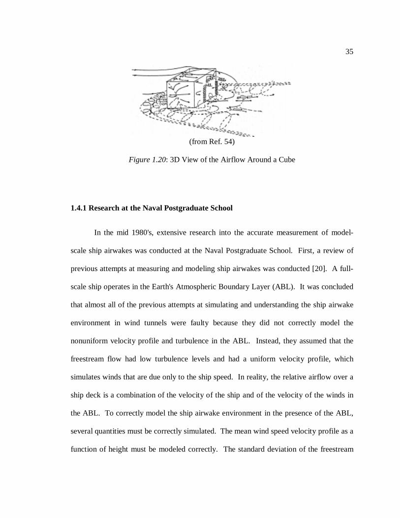
35
1.4.1 Research at the Naval Postgraduate School
In the mid 1980's, extensive research into the accurate measurement of model-
scale ship airwakes was conducted at the Naval Postgraduate School. First, a review of
previous attempts at measuring and modeling ship airwakes was conducted [20]. A full-
scale ship operates in the Earth's Atmospheric Boundary Layer (ABL). It was concluded
that almost all of the previous attempts at simulating and understanding the ship airwake
environment in wind tunnels were faulty because they did not correctly model the
nonuniform velocity profile and turbulence in the ABL. Instead, they assumed that the
freestream flow had low turbulence levels and had a uniform velocity profile, which
simulates winds that are due only to the ship speed. In reality, the relative airflow over a
ship deck is a combination of the velocity of the ship and of the velocity of the winds in
the ABL. To correctly model the ship airwake environment in the presence of the ABL,
several quantities must be correctly simulated. The mean wind speed velocity profile as a
function of height must be modeled correctly. The standard deviation of the freestream
(from Ref. 54)
Figure 1.20: 3D View of the Airflow Around a Cube
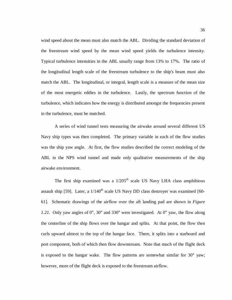
36
wind speed about the mean must also match the ABL. Dividing the standard deviation of
the freestream wind speed by the mean wind speed yields the turbulence intensity.
Typical turbulence intensities in the ABL usually range from 13% to 17%. The ratio of
the longitudinal length scale of the freestream turbulence to the ship's beam must also
match the ABL. The longitudinal, or integral, length scale is a measure of the mean size
of the most energetic eddies in the turbulence. Lastly, the spectrum function of the
turbulence, which indicates how the energy is distributed amongst the frequencies present
in the turbulence, must be matched.
A series of wind tunnel tests measuring the airwake around several different US
Navy ship types was then completed. The primary variable in each of the flow studies
was the ship yaw angle. At first, the flow studies described the correct modeling of the
ABL in the NPS wind tunnel and made only qualitative measurements of the ship
airwake environment.
The first ship examined was a 1/205th scale US Navy LHA class amphibious
assault ship [59]. Later, a 1/140th scale US Navy DD class destroyer was examined [60-
61]. Schematic drawings of the airflow over the aft landing pad are shown inFigure
1.21. Only yaw angles of 0°, 30° and 330° were investigated. At 0° yaw, the flow along
the centerline of the ship flows over the hangar and splits. At that point, the flow then
curls upward almost to the top of the hangar face. There, it splits into a starboard and
port component, both of which then flow downstream. Note that much of the flight deck
is exposed to the hangar wake. The flow patterns are somewhat similar for 30° yaw;
however, more of the flight deck is exposed to the freestream airflow.
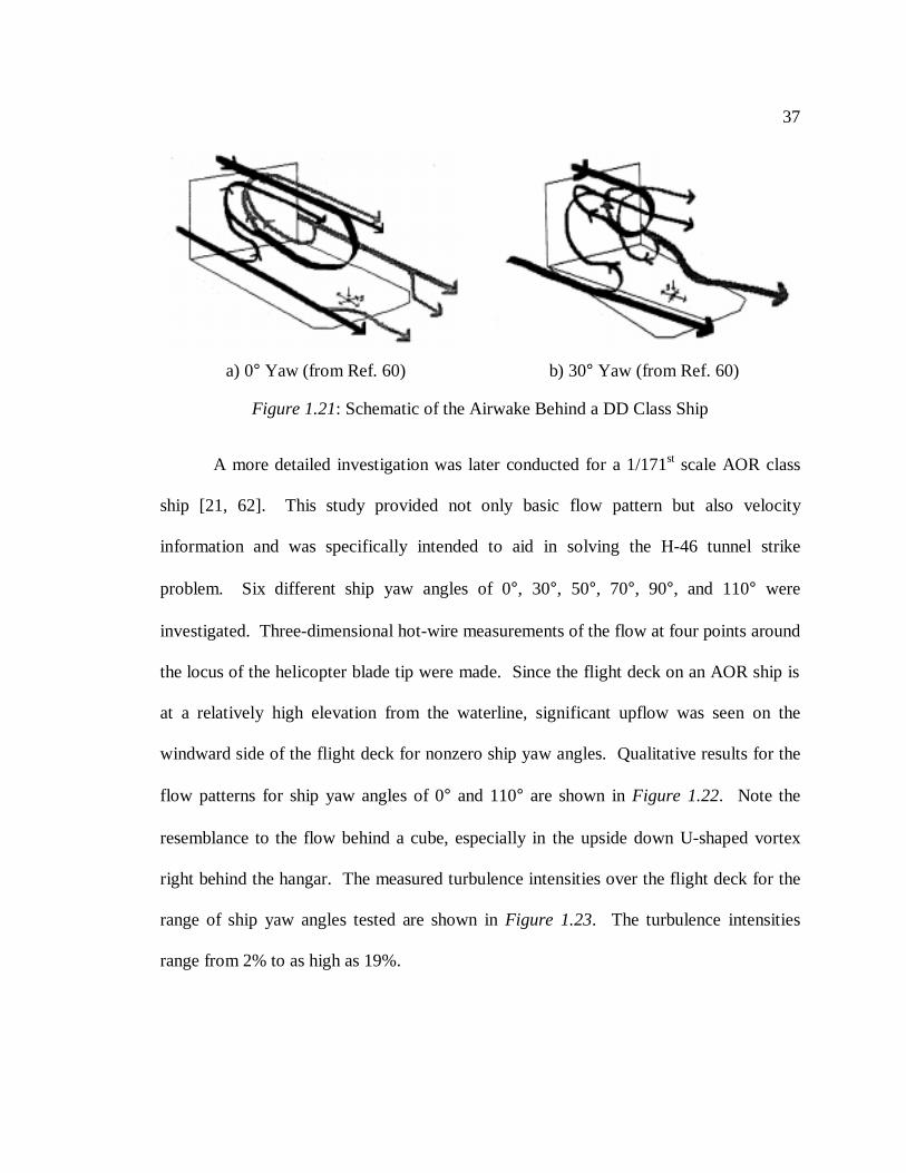
37
A more detailed investigation was later conducted for a 1/171st scale AOR class
ship [21, 62]. This study provided not only basic flow pattern but also velocity
information and was specifically intended to aid in solving the H-46 tunnel strike
problem. Six different ship yaw angles of 0°, 30°, 50°, 70°, 90°, and 110° were
investigated. Three-dimensional hot-wire measurements of the flow at four points around
the locus of the helicopter blade tip were made. Since the flight deck on an AOR ship is
at a relatively high elevation from the waterline, significant upflow was seen on the
windward side of the flight deck for nonzero ship yaw angles. Qualitative results for the
flow patterns for ship yaw angles of 0° and 110° are shown inFigure 1.22. Note the
resemblance to the flow behind a cube, especially in the upside down U-shaped vortex
right behind the hangar. The measured turbulence intensities over the flight deck for the
range of ship yaw angles tested are shown inFigure 1.23. The turbulence intensities
range from 2% to as high as 19%.
a) 0° Yaw (from Ref. 60) b) 30° Yaw (from Ref. 60)
Figure 1.21: Schematic of the Airwake Behind a DD Class Ship
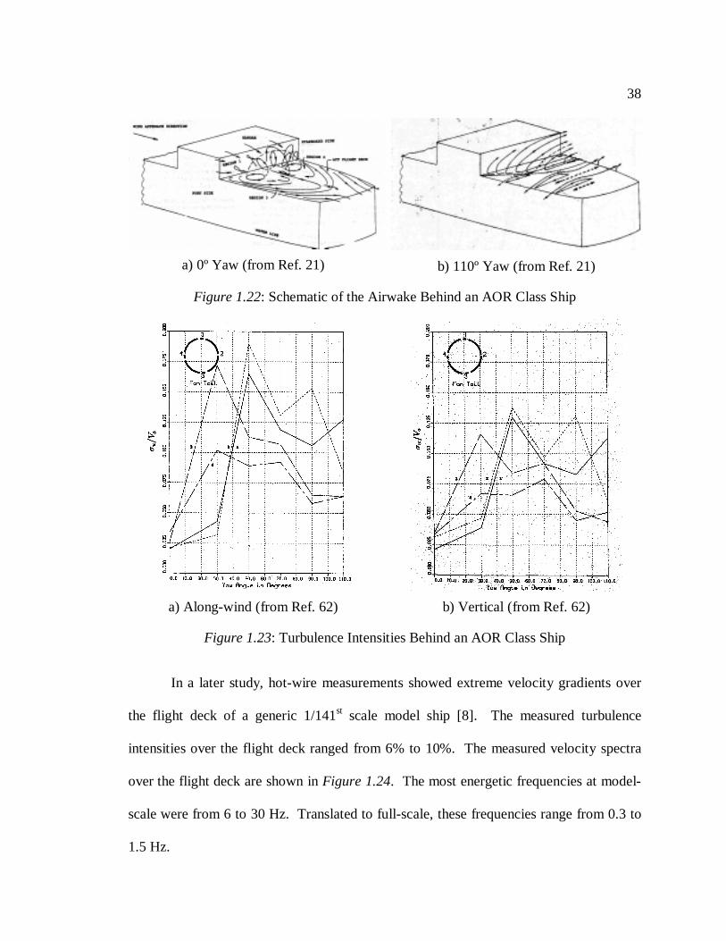
38
In a later study, hot-wire measurements showed extreme velocity gradients over
the flight deck of a generic 1/141st scale model ship [8]. The measured turbulence
intensities over the flight deck ranged from 6% to 10%. The measured velocity spectra
over the flight deck are shown inFigure 1.24. The most energetic frequencies at model-
scale were from 6 to 30 Hz. Translated to full-scale, these frequencies range from 0.3 to
1.5 Hz.
a) 0º Yaw (from Ref. 21) b) 110º Yaw (from Ref. 21)
Figure 1.22: Schematic of the Airwake Behind an AOR Class Ship
a) Along-wind (from Ref. 62) b) Vertical (from Ref. 62)
Figure 1.23: Turbulence Intensities Behind an AOR Class Ship
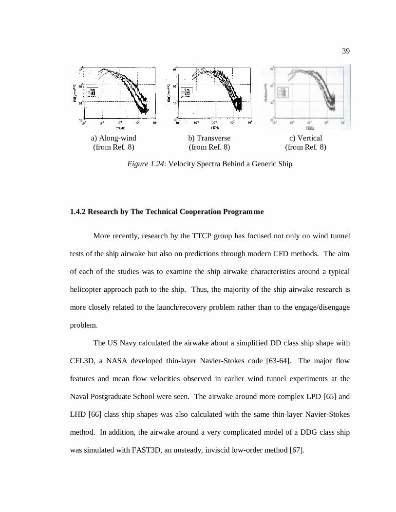
39
1.4.2 Research by The Technical Cooperation Programme
More recently, research by the TTCP group has focused not only on wind tunnel
tests of the ship airwake but also on predictions through modern CFD methods. The aim
of each of the studies was to examine the ship airwake characteristics around a typical
helicopter approach path to the ship. Thus, the majority of the ship airwake research is
more closely related to the launch/recovery problem rather than to the engage/disengage
problem.
The US Navy calculated the airwake about a simplified DD class ship shape with
CFL3D, a NASA developed thin-layer Navier-Stokes code [63-64]. The major flow
features and mean flow velocities observed in earlier wind tunnel experiments at the
Naval Postgraduate School were seen. The airwake around more complex LPD [65] and
LHD [66] class ship shapes was also calculated with the same thin-layer Navier-Stokes
method. In addition, the airwake around a very complicated model of a DDG class ship
was simulated with FAST3D, an unsteady, inviscid low-order method [67].
a) Along-wind(from Ref. 8)
b) Transverse(from Ref. 8)
c) Vertical(from Ref. 8)
Figure 1.24: Velocity Spectra Behind a Generic Ship
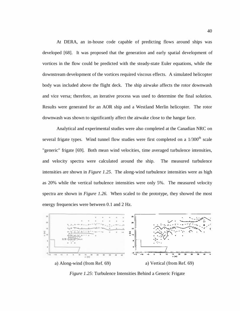
40
At DERA, an in-house code capable of predicting flows around ships was
developed [68]. It was proposed that the generation and early spatial development of
vortices in the flow could be predicted with the steady-state Euler equations, while the
downstream development of the vortices required viscous effects. A simulated helicopter
body was included above the flight deck. The ship airwake affects the rotor downwash
and vice versa; therefore, an iterative process was used to determine the final solution.
Results were generated for an AOR ship and a Westland Merlin helicopter. The rotor
downwash was shown to significantly affect the airwake close to the hangar face.
Analytical and experimental studies were also completed at the Canadian NRC on
several frigate types. Wind tunnel flow studies were first completed on a 1/300th scale
"generic" frigate [69]. Both mean wind velocities, time averaged turbulence intensities,
and velocity spectra were calculated around the ship. The measured turbulence
intensities are shown inFigure 1.25. The along-wind turbulence intensities were as high
as 20% while the vertical turbulence intensities were only 5%. The measured velocity
spectra are shown inFigure 1.26. When scaled to the prototype, they showed the most
energy frequencies were between 0.1 and 2 Hz.
a) Along-wind (from Ref. 69) a) Vertical (from Ref. 69)
Figure 1.25: Turbulence Intensities Behind a Generic Frigate
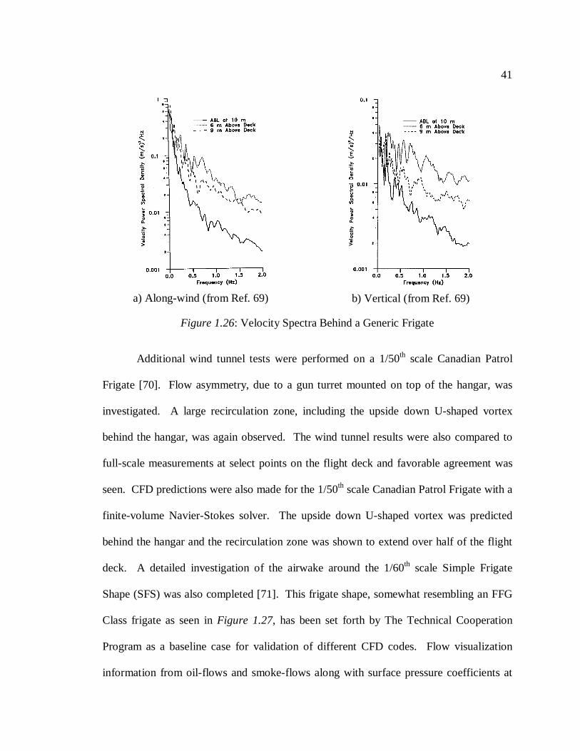
41
Additional wind tunnel tests were performed on a 1/50th scale Canadian Patrol
Frigate [70]. Flow asymmetry, due to a gun turret mounted on top of the hangar, was
investigated. A large recirculation zone, including the upside down U-shaped vortex
behind the hangar, was again observed. The wind tunnel results were also compared to
full-scale measurements at select points on the flight deck and favorable agreement was
seen. CFD predictions were also made for the 1/50th scale Canadian Patrol Frigate with a
finite-volume Navier-Stokes solver. The upside down U-shaped vortex was predicted
behind the hangar and the recirculation zone was shown to extend over half of the flight
deck. A detailed investigation of the airwake around the 1/60th scale Simple Frigate
Shape (SFS) was also completed [71]. This frigate shape, somewhat resembling an FFG
Class frigate as seen inFigure 1.27, has been set forth by The Technical Cooperation
Program as a baseline case for validation of different CFD codes. Flow visualization
information from oil-flows and smoke-flows along with surface pressure coefficients at
a) Along-wind (from Ref. 69) b) Vertical (from Ref. 69)
Figure 1.26: Velocity Spectra Behind a Generic Frigate
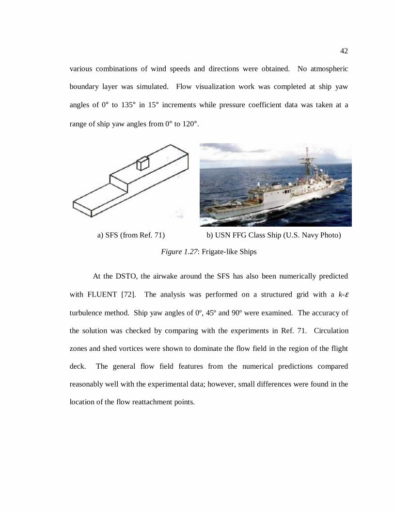
42
various combinations of wind speeds and directions were obtained. No atmospheric
boundary layer was simulated. Flow visualization work was completed at ship yaw
angles of 0° to 135° in 15° increments while pressure coefficient data was taken at a
range of ship yaw angles from 0° to 120°.
At the DSTO, the airwake around the SFS has also been numerically predicted
with FLUENT [72]. The analysis was performed on a structured grid with ak-ε
turbulence method. Ship yaw angles of 0º, 45º and 90º were examined. The accuracy of
the solution was checked by comparing with the experiments in Ref. 71. Circulation
zones and shed vortices were shown to dominate the flow field in the region of the flight
deck. The general flow field features from the numerical predictions compared
reasonably well with the experimental data; however, small differences were found in the
location of the flow reattachment points.
a) SFS (from Ref. 71) b) USN FFG Class Ship (U.S. Navy Photo)
Figure 1.27: Frigate-like Ships
43
1.4.3 Research at Penn State University
Ship airwake prediction through modern CFD methods has been the subject of
much research at Penn State University by Longet al. Two different solution methods
were tested. Initially, the method chosen to simulate the ship airwake used the Nonlinear
Disturbance Equations (NLDE) [73]. In this solution technique, the general Navier-
Stokes equations are written and the viscous terms are neglected. The resulting flowfield
variables (mass density, momentum, and energy) are then split into mean and fluctuating
parts. The mean flow terms can then be solved using an "off-the-shelf" CFD code such
as CFL3D or PUMA. These mean flow terms, in turn, can be used as a source term for
the unsteady part of the Navier Stokes equations, or the NLDE. The NLDE are then
solved numerically using a fourth order accurate Dispersion Relation Preserving scheme
and a fourth order accurate Runge-Kutta scheme. This method has several advantages - it
allows usage of the most effective algorithm and computational grid for the steady and
unsteady parts and it minimizes round-off error. Results were generated for the SFS for a
0° yaw angle [74-75]. The mean flow components were calculated with CFL3D, a
structured finite-difference flow solver. Indications of the upside-down U-shaped vortex
directly behind the hangar were observed. Comparison with oil-flow visualization
experiments showed that the attachment point of the U-shaped vortex was farther
outboard than measured, probably due to the inviscid assumption. Using the NLDE,
perturbation velocities were also predicted. Large magnitude longitudinal and vertical
turbulence intensities were measured aft of the bow and hangar.
44
Recently, a modified version of the Parallel Unstructured Maritime Aerodynamics
(PUMA) code was used to predict the flowfield around complex ship shapes [76-77].
PUMA, originally developed at Virginia Tech by Bruner, was designed to predict flows
over arbitrarily complex 3D geometries [78-79]. Based on the finite volume method
(FVM), it allows the use of unstructured grids and easily facilitates the mapping of
complex ship shapes.
After gaining confidence in PUMA through the validation studies, the Simple
Frigate Shape was again studied. Qualitative comparisons using the inviscid NLDE and
the viscous PUMA approaches were made with the wind tunnel oil-flow visualizations.
The results of these comparison studies are shown inFigure 1.28throughFigure 1.30.
Three locations on the SFS ship are shown: the bow, the exhaust stack, and the flight
deck. Figure 1.28shows the results for the oil flow visualizations,Figure 1.29shows the
results for the NLDE analysis andFigure 1.30shows the results for the PUMA analysis.
The viscous PUMA solution was better at predicting the separated flow aft of the bow
and hangar.
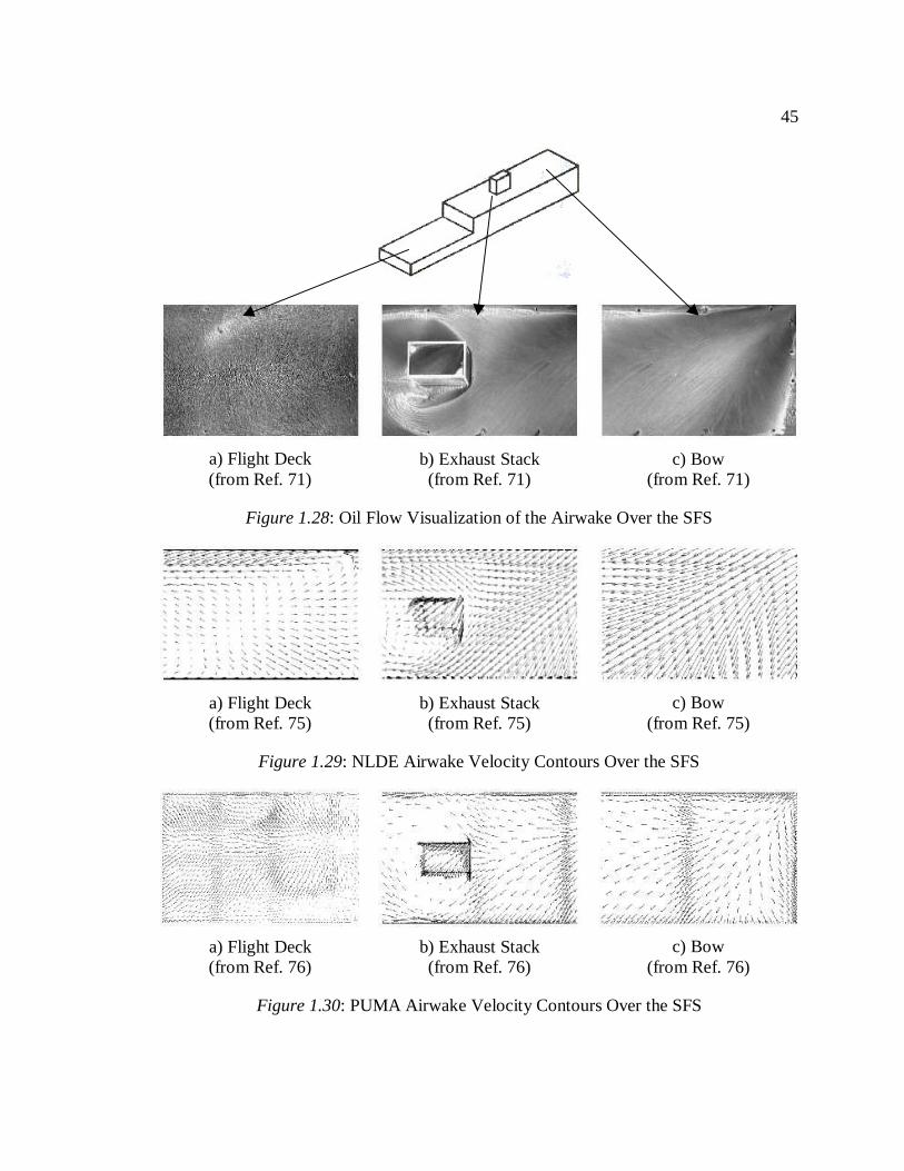
45
a) Flight Deck(from Ref. 71)
b) Exhaust Stack(from Ref. 71)
c) Bow(from Ref. 71)
Figure 1.28: Oil Flow Visualization of the Airwake Over the SFS
a) Flight Deck(from Ref. 75)
b) Exhaust Stack(from Ref. 75)
c) Bow(from Ref. 75)
Figure 1.29: NLDE Airwake Velocity Contours Over the SFS
a) Flight Deck(from Ref. 76)
b) Exhaust Stack(from Ref. 76)
c) Bow(from Ref. 76)
Figure 1.30: PUMA Airwake Velocity Contours Over the SFS
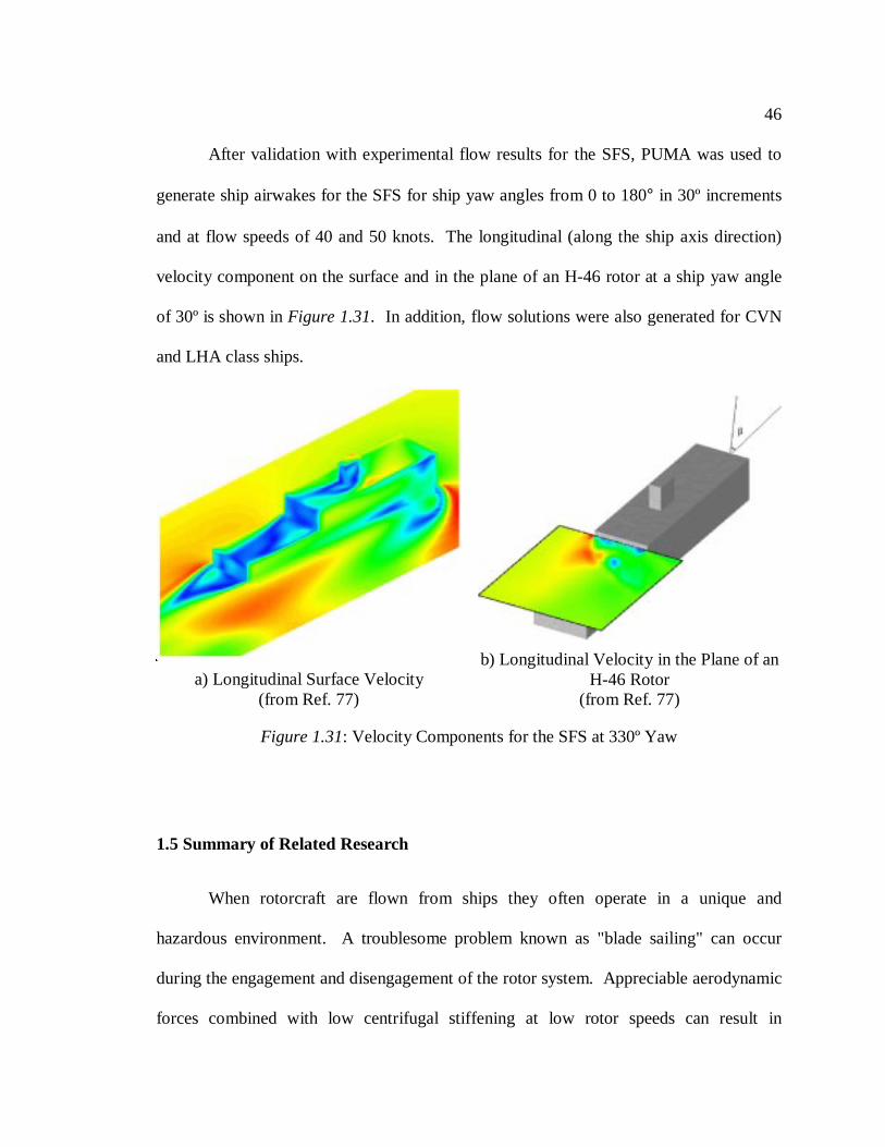
46
After validation with experimental flow results for the SFS, PUMA was used to
generate ship airwakes for the SFS for ship yaw angles from 0 to 180° in 30º increments
and at flow speeds of 40 and 50 knots. The longitudinal (along the ship axis direction)
velocity component on the surface and in the plane of an H-46 rotor at a ship yaw angle
of 30º is shown inFigure 1.31. In addition, flow solutions were also generated for CVN
and LHA class ships.
1.5 Summary of Related Research
When rotorcraft are flown from ships they often operate in a unique and
hazardous environment. A troublesome problem known as "blade sailing" can occur
during the engagement and disengagement of the rotor system. Appreciable aerodynamic
forces combined with low centrifugal stiffening at low rotor speeds can result in
a) Longitudinal Surface Velocity(from Ref. 77)
b) Longitudinal Velocity in the Plane of anH-46 Rotor
(from Ref. 77)
Figure 1.31: Velocity Components for the SFS at 330º Yaw
47
excessive aeroelastic flapping of the rotor. For articulated rotors, the blade tips may
contact the fuselage and endanger the airframe, flight crew, and anyone standing near the
helicopter. For teetering or gimballed rotors, excessive gimbal tilt angles may cause the
rotor hub to strike the gimbal stops resulting in potentially high bending moments in the
blade flexures.
Due to the potential of blade sailing, conservative limits are placed on the
conditions in which rotor systems can be engaged and disengaged on board ships, which
tends to severely limit the helicopter's operational capability. These limits are termed the
Ship/Helicopter Operational Limits (SHOLs) and in the past were determined in full-
scale, at-sea experimental tests. The tests had to be conducted forevery
helicopter/ship/landing spot combination because of the distinct performance
characteristics of helicopter types, the variability in size and shape of ship types, and the
various characteristics of landing spots on the ship's deck. Unfortunately, this process of
experimentally determining the SHOLs was very labor intensive, time consuming,
expensive, and somewhat unreliable. Because of these problems, the analytical
determination of SHOLs has been proposed as a viable alternative to experimental
testing. The use of modeling and simulation offers substantial benefits in terms of
reducing cost, improving safety, and developing larger operating envelopes.
Dr. Simon Newman at the University of Southampton was the first researcher to
conduct extensive blade sailing research. Model-scale, rigid blade, experimental tests
were conducted and successfully demonstrated blade sailing. Later, an aeroelastic flap-
torsion simulation code capable of predicting blade sailing for both hingeless and
48
articulated rotors was developed. The effect of the ship airwake on the rotor system
behavior was demonstrated.
Motivated by the H-46 Sea Knight tunnel strike problem, Geyeret al at Penn
State University have conducted research into blade sailing phenomenon. Initially, an
aeroelastic flap-torsion simulation code was developed and capable of simulating a single
hingeless or articulated rotor blade. The model was later modified to include lag degrees
of freedom and the capability of modeling multiple rotor blades for gimballed and
teetering rotors.
Substantial improvements in the modeling of ship airwakes have been made in the
past decade. Recently, Longet al at Penn State have modified PUMA, a CFD program
using unstructured grids and run on an inexpensive PC cluster, to predict the ship airwake
environment. Recent comparisons with experimental results for a generic frigate with
both viscid and inviscid models have increased confidence in the airwake predictions.
1.6 Objectives of the Current Research
Since 1995, substantial research has been completed and has been focused on
constructing and validating a finite-element based blade sailing model at Penn State
University to predict the transient aeroelastic response of rotorcraft during engagement
and disengagement operations. The subjects covered in the current research are
organized into thevalidation, the prediction, or the control of engagement and
disengagement behavior.

49
The first objective is to validate the analysis with the model-scale helicopter and
wind tunnel experiments conducted at the University of Southampton. The second
objective is to address recently added prediction capabilities including:
1. A comparison of the effects of the nonlinear quasi-steady and unsteady
aerodynamic models.
2. The effect of lag motion on the rotor response during engagement and
disengagement operations. Previous engagement and disengagement research at
the University of Southampton and Penn State University was completed with
flap-torsion only blade motion and its effect has yet to be assessed.
3. The effectiveness of recently added time integration techniques. The only time
integration technique used in previous engagement and disengagement
simulations was a fourth order Runge-Kutta method.
4. The effect of more realistic ship airwakes. The distribution of the steady airwake
components has been shown to substantially influence blade sailing behavior.
Recent work has made sophisticated ship airwake models more readily available
for use in engagement and disengagement research.
The third objective of this dissertation is to examine methods tocontrol blade
sailing behavior. Little research to date has seriously addressed the subject of reducing
excessive flapping. Each of the following control methods will be examined:
1. The simplest method to reduce flapping motion would be to introduce a discrete
flap damper. Such a flap damper could dissipate excessive flap motion as a lag
50
damper dissipates excessive lag motion. Naturally, such a flap damper would
have to become inactive in normal operating conditions.
2. Most articulated rotor blades are relatively elastic in the normal direction, but are
much stiffer in the chordwise direction. At high values of collective pitch, the
effective flapwise stiffness of the blade could be increased through the rotation of
the blade cross section. The effectiveness of a large change in collective pitch
setting during a short period in the engagement will be examined.
3. Blade sailing is caused by appreciable aerodynamic lift generated at low rotor
speeds. The simplest method of reducing blade flapping would be to reduce the
excessive lift. The effectiveness of reducing the excessive lift through spoilers
will be investigated. Naturally, the spoilers would only be used in the critical
rotor speed region and be inactive during normal operating conditions.
4. Future naval rotorcraft may have on-board control systems that allow feedback
from the blade motion to the control system inputs. The effectiveness of using a
control system to reduce blade flapping during rotor engagements will be
examined.
51
Chapter 2
MODELING AND ANALYSIS
In this chapter, the analytic model and transient analysis of rotors during
shipboard engagement and disengagement operations is presented. The ship is assumed
to be rolling about its centerline and the helicopter is assumed to be stationary on the ship
deck. The distribution of the ship airwake velocities over the rotor disk is modeled with
simple analytic expressions or with arbitrary spatially varying results from experimental
tests or numerical predictions. Only a single main rotor of the helicopter is modeled.
The rotor is, by definition, accelerating or decelerating in engagement and disengagement
operations. Each rotor blade is modeled as an isotropic elastic beam undergoing
moderate out-of plane (flap), in plane (lag), and twisting (torsion) motions. The
nonlinear governing equations of motion are derived using Hamilton’s Principle and are
spatially discretized using the finite element method. The formulation is applicable to
rotor hubs with articulated, hingeless, teetering and gimballed rotor blades.
2.1 Basic Considerations
In this section the coordinate systems, nondimensionalization and ordering
schemes used in the analysis are explained. They are based on the system used in Ref.
43, but have modifications specific to the simulation of engagement and disengagment
operations.
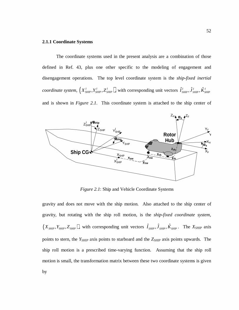
52
2.1.1 Coordinate Systems
The coordinate systems used in the present analysis are a combination of those
defined in Ref. 43, plus one other specific to the modeling of engagement and
disengagement operations. The top level coordinate system is theship-fixed inertial
coordinate system, ( ), ,I I ISHIP SHIP SHIPX Y Z , with corresponding unit vectors ˆ ˆ, ,I I I
SHIP SHIP SHIPI J K
and is shown inFigure 2.1. This coordinate system is attached to the ship center of
gravity and does not move with the ship motion. Also attached to the ship center of
gravity, but rotating with the ship roll motion, is theship-fixed coordinate system,
( ), ,SHIP SHIP SHIPX Y Z , with corresponding unit vectors ˆ ˆ, ,SHIP SHIP SHIPI J K . The XSHIP axis
points to stern, theYSHIP axis points to starboard and theZSHIP axis points upwards. The
ship roll motion is a prescribed time-varying function. Assuming that the ship roll
motion is small, the transformation matrix between these two coordinate systems is given
by
φφφφship
φφφφship
XSHIP
XSHIPI
ZSHIPI
ZSHIP YSHIPI
YSHIP
XF
YF
ZF
Ship CGxnw
ynw
znw
RotorHub XH
ZH ααααs
Y
ααααs
xrhyrh
zrh
Figure 2.1: Ship and Vehicle Coordinate Systems
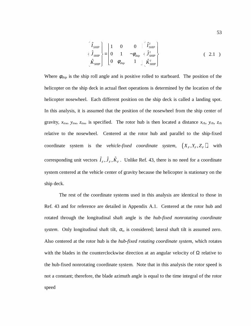
53
ˆ ˆ1 0 0ˆ ˆ0 1
ˆ ˆ0 1
ISHIP SHIP
ISHIP ship SHIP
IshipSHIP SHIP
I I
J J
K K
φφ
= −
( 2.1 )
Whereφship is the ship roll angle and is positive rolled to starboard. The position of the
helicopter on the ship deck in actual fleet operations is determined by the location of the
helicopter nosewheel. Each different position on the ship deck is called a landing spot.
In this analysis, it is assumed that the position of the nosewheel from the ship center of
gravity, xnw, ynw, znw, is specified. The rotor hub is then located a distancexrh, yrh, zrh
relative to the nosewheel. Centered at the rotor hub and parallel to the ship-fixed
coordinate system is thevehicle-fixed coordinate system, ( ), ,F F FX Y Z , with
corresponding unit vectors ˆ ˆ, ,F F FI J K . Unlike Ref. 43, there is no need for a coordinate
system centered at the vehicle center of gravity because the helicopter is stationary on the
ship deck.
The rest of the coordinate systems used in this analysis are identical to those in
Ref. 43 and for reference are detailed in Appendix A.1. Centered at the rotor hub and
rotated through the longitudinal shaft angle is thehub-fixed nonrotating coordinate
system. Only longitudinal shaft tilt,αs, is considered; lateral shaft tilt is assumed zero.
Also centered at the rotor hub is thehub-fixed rotating coordinate system, which rotates
with the blades in the counterclockwise direction at an angular velocity ofΩ relative to
the hub-fixed nonrotating coordinate system. Note that in this analysis the rotor speed is
not a constant; therefore, the blade azimuth angle is equal to the time integral of the rotor
speed
54
( ) 00
ftt dtψ ψ= Ω + ( 2.2 )
Where ψ0 is the azimuth angle of the blade at the start of the engagement or
disengagement. Theundeformed blade coordinate systemis inclined through the blade
precone angle,βp, from the hub-fixed rotating coordinate system. The final coordinate
system is thedeformed blade coordinate system. The deformed blade coordinate system
accounts for the axial displacementu, in plane displacementv, and out-of plane
displacementw of the blade. It is also rotated about the deformed elastic axis through the
total blade pitch angle. The total blade pitch angle,θ1, is defined by
1 0ˆθ θ φ= + ( 2.3 )
Whereθ0 is the rigid pitch angle due to the control system settings and blade pretwist and
φ is the elastic twist angle. Both angles are measured in the deformed blade coordinate
system. The rigid pitch angle is given by
( )0 75 1 1cos sinc s tw xθ θ θ ψ θ ψ θ θ= + + + + ∆ ( 2.4 )
Whereθ75 is the collective pitch at the 75% span location,θ1c andθ1s are the lateral and
longitudinal and cyclic pitch controls andθtw is the blade pretwist angle referenced to the
75% span location. In general, the blade pretwist angle is a nonlinear function. The
change in the pitch angle,∆θ, is due to pitch-flap or pitch-lag coupling from sources such
as skewed hinges, location of the pitch link, relative position of the hinges or composite
couplings.
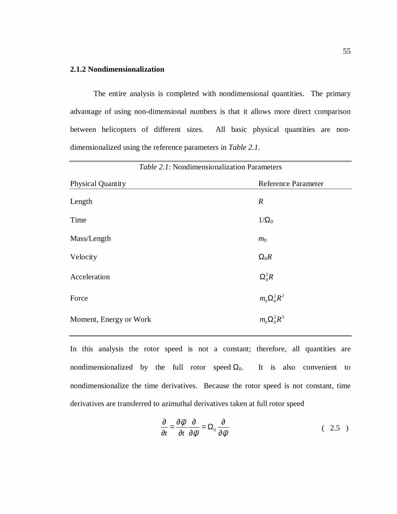
55
2.1.2 Nondimensionalization
The entire analysis is completed with nondimensional quantities. The primary
advantage of using non-dimensional numbers is that it allows more direct comparison
between helicopters of different sizes. All basic physical quantities are non-
dimensionalized using the reference parameters inTable 2.1.
In this analysis the rotor speed is not a constant; therefore, all quantities are
nondimensionalized by the full rotor speed Ω0. It is also convenient to
nondimensionalize the time derivatives. Because the rotor speed is not constant, time
derivatives are transferred to azimuthal derivatives taken at full rotor speed
0t t
ψψ ψ
∂ ∂ ∂ ∂= = Ω∂ ∂ ∂ ∂
( 2.5 )
Table 2.1: Nondimensionalization Parameters
Physical Quantity Reference Parameter
Length R
Time 1/Ω0
Mass/Length m0
Velocity Ω0R
Acceleration 20RΩ
Force 2 20 0m RΩ
Moment, Energy or Work 2 30 0m RΩ
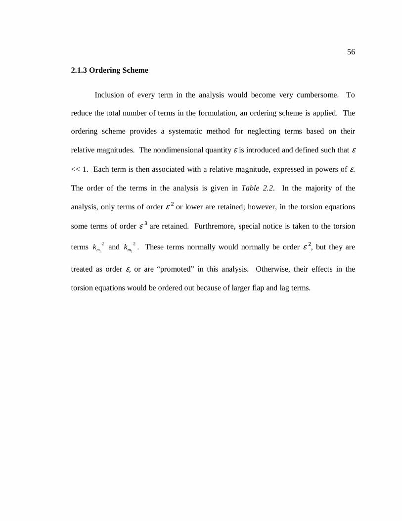
56
2.1.3 Ordering Scheme
Inclusion of every term in the analysis would become very cumbersome. To
reduce the total number of terms in the formulation, an ordering scheme is applied. The
ordering scheme provides a systematic method for neglecting terms based on their
relative magnitudes. The nondimensional quantityε is introduced and defined such thatε
<< 1. Each term is then associated with a relative magnitude, expressed in powers ofε.
The order of the terms in the analysis is given inTable 2.2. In the majority of the
analysis, only terms of orderε 2 or lower are retained; however, in the torsion equations
some terms of orderε 3 are retained. Furthremore, special notice is taken to the torsion
terms1
2mk and
2
2mk . These terms normally would normally be orderε 2, but they are
treated as orderε, or are “promoted” in this analysis. Otherwise, their effects in the
torsion equations would be ordered out because of larger flap and lag terms.
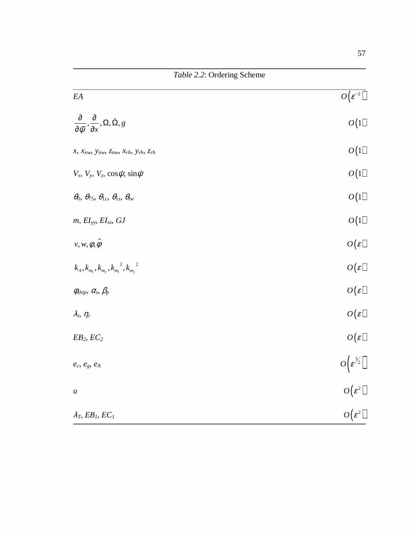
57
Table 2.2: Ordering Scheme
EA ( )2O ε −
, , , ,gxψ
∂ ∂ Ω Ω∂ ∂
( )1O
x, xnw, ynw, znw, xrh, yrh, zrh ( )1O
Vx, Vy, Vz, cosψ, sinψ ( )1O
θ0, θ75, θ1c, θ1s, θtw ( )1O
m, EIyy, EIzz, GJ ( )1O
ˆ, , ,v w φ φ ( )O ε
1 2 1 2
2 2, , , ,A m m m mk k k k k ( )O ε
φship, αs, βp ( )O ε
λi, ηr ( )O ε
EB2, EC2 ( )O ε
ec, eg, eA ( )32O ε
u ( )2O ε
λT, EB1, EC1 ( )2O ε
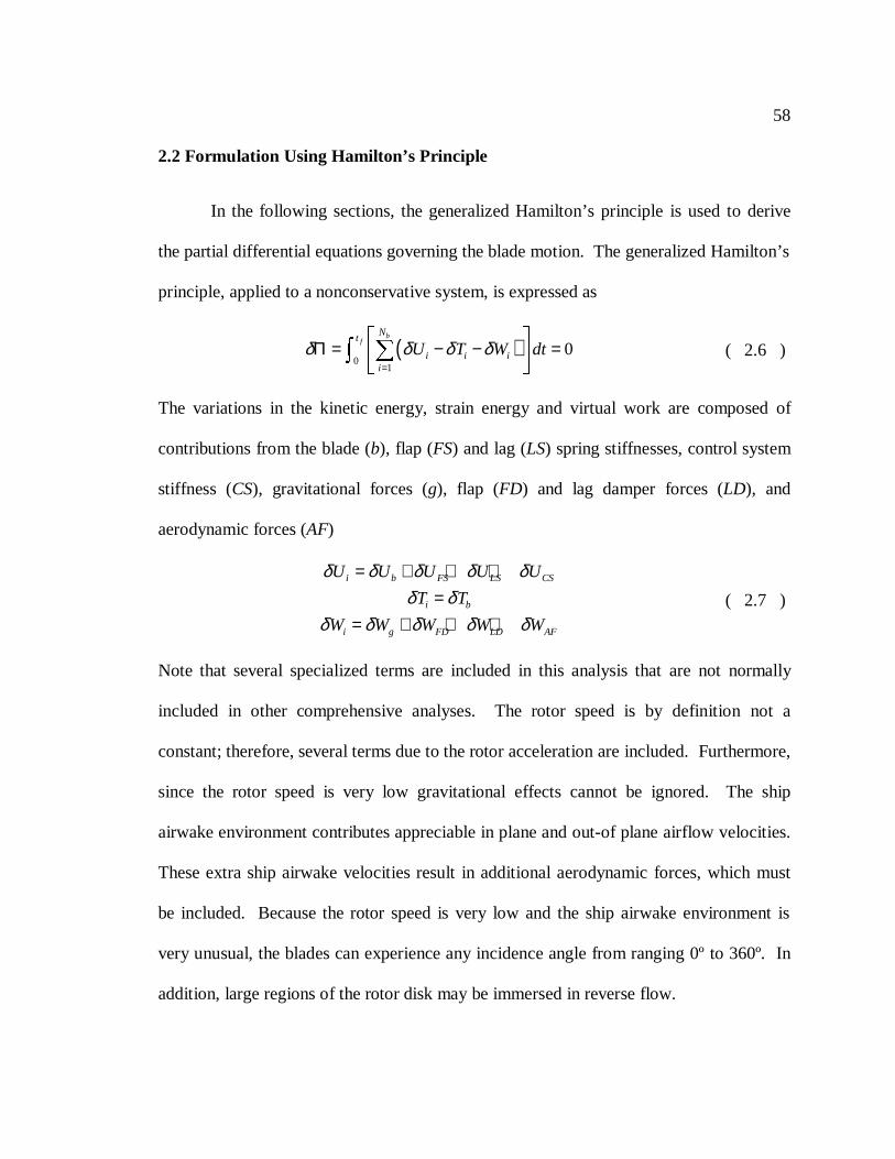
58
2.2 Formulation Using Hamilton’s Principle
In the following sections, the generalized Hamilton’s principle is used to derive
the partial differential equations governing the blade motion. The generalized Hamilton’s
principle, applied to a nonconservative system, is expressed as
( )0
1
0b
fN
t
i i ii
U T W dtδ δ δ δ=
Π = − − =
( 2.6 )
The variations in the kinetic energy, strain energy and virtual work are composed of
contributions from the blade (b), flap (FS) and lag (LS) spring stiffnesses, control system
stiffness (CS), gravitational forces (g), flap (FD) and lag damper forces (LD), and
aerodynamic forces (AF)
i b FS LS CS
i b
i g FD LD AF
U U U U U
T T
W W W W W
δ δ δ δ δδ δ
δ δ δ δ δ
= + + +=
= + + +( 2.7 )
Note that several specialized terms are included in this analysis that are not normally
included in other comprehensive analyses. The rotor speed is by definition not a
constant; therefore, several terms due to the rotor acceleration are included. Furthermore,
since the rotor speed is very low gravitational effects cannot be ignored. The ship
airwake environment contributes appreciable in plane and out-of plane airflow velocities.
These extra ship airwake velocities result in additional aerodynamic forces, which must
be included. Because the rotor speed is very low and the ship airwake environment is
very unusual, the blades can experience any incidence angle from ranging 0º to 360º. In
addition, large regions of the rotor disk may be immersed in reverse flow.

59
2.2.1 Strain Energy
In this section, expressions for the total strain energy of the system will be
derived. Contributions from the elastic deformation of the blade, the flap and lag spring
stiffnesses and the control system stiffness are also considered.
2.2.1.1 Blade Strain Energy
The expressions for the blade strain energy are derived in a manner similar to Ref.
43. The only difference is that the blade is assumed inelastic in the axial direction. The
variation in strain energy of each rotor blade is given by
( )1
0b xx xx x x x
A
U E G G d d dxη η ζ ζδ ε δε ε δε ε δε η ζ= + + ( 2.8 )
The strains are expressed as
( )( )( ) ( )
2 2 2 2 21 1 102 2 2
1 1 1 1cos sin sin cos
ˆ
ˆ
xx T
x
x
u v w
v w
η
ζ
ε λ φ η ζ θ φ φ
η θ ζ θ η θ ζ θ
ε ζφε ηφ
′ ′ ′ ′′ ′ ′= + + − + + +
′′ ′′− − − +
′= −′=
( 2.9 )
Taking the variation of each yields
( )( )( )( ) ( )( )
2 20
1 1 1 1 1 1cos sin sin cos
ˆ
ˆ
xx T
x
x
u v v w w
v w w v
η
ζ
δε δ δ δ λ δφ η ζ θ φ δφ
η θ ζ θ δ δθ η θ ζ θ δ δθ
δε ζδφδε ηδφ
′ ′ ′ ′ ′ ′′ ′ ′= + + − + + +
′′ ′′ ′′ ′′− − + − + −
′= −′=
( 2.10 )
Expressions for the axial deflection,u; the elastic twist in the undeformed blade
coordinate system,φ ; and the total blade pitch angle,θ1, are then substituted.
60
Appropriate structural quantities can then be easily defined. For reference, this process is
fully outlined in Appendix A.2.
2.2.1.2 Flap Spring Strain Energy
Depending on the type of rotor system, different means are employed to restrict
blade motions at rest and at low rotor speeds. The following sections describe the
formulas necessary to model the mechanical stops for articulated, hingeless, teetering,
and gimballed rotor types.
2.2.1.2.1 Articulated Rotors
Articulated rotors can have discrete rotational springs at the flap hinge. Such a
spring may be used to model friction in the hinge itself or the stiffness properties of a flap
damper. In the case of a continuous spring at the flap hinge, the strain energy is
212FS hingeU Kβ β= ( 2.11 )
Taking the variation yields
FS hinge hingeU Kβδ β δβ= ( 2.12 )
The flap hinge angle,βhinge, is defined as the difference in the flap slope,w′ , evaluated on
either side of the flap hinge
( )1tanhinge flap hingewβ − ′= ∆ ( 2.13 )
If the flap slope is small, the flap hinge angle simplies to
61
hinge flap hingewβ ′= ∆ ( 2.14 )
Articulated rotors also require rigid mechanical limiters to support the blade
weight when the rotor is at rest and to limit the blade flap angle at low rotor speeds.
These mechanical limiters are called droop and flap stops. In normal flight conditions,
the stops are not needed to restrain the blade motion. The stops are designed to retract
and become inactive above a certain rotor speed, usually about 50%NR. The stops are
also designed such that they may not retract if the blade is in contact with the stop.
Conversely, the stops are also designed such that they may not extend if the blade is
beyond the stop angle. An additional discrete rotational spring is used to simulate the
droop and flap stops; however, the spring stiffness is conditional on the blade rotation at
the flap hinge. If the blade is in between either stop, the spring stiffness is zero. If the
stops are extended and the flap hinge angle is sufficient to contact either stop, the spring
stiffness is equal to the stop stiffness. This stop stiffness is set arbitrarily large, so that
the blade rotation at the flap hinge is limited to less than 0.01º of rotation at the flap hinge
upon blade-stop contact. The strain energy for the flap stop spring is
( )212
0
stop
hinge stop
FS hinge stophinge stop
U K KKβ β
β
β ββ β β β
≤= − = >( 2.15 )
Whereβstop is the flap hinge angle at which contact between the blade and the stop is
made. Taking the variation yields
( ) 0
stop
hinge stop
FS hinge stop hingehinge stop
U K KKβ β
β
β βδ β β δβ β β
≤= − = >( 2.16 )
62
2.2.1.2.2 Hingeless Rotors
Hingeless rotors do not necessarily require rigid stops to support the blade weight
when the rotor is at rest; however, some models use them to limit the blade deflection at
low rotor speed. Like an articulated rotor, a discrete conditional spring is used to
simulate the droop and flap stops. However, the contact is based not upon the flap hinge
angle but upon the flap deflection at a point just beyond the flexbeam. The strain energy
for a hingeless rotor flap stop spring is
( )212
0
stop
hinge stop
FS w hinge stop ww hinge stop
w wU K w w K
K w w
≤= − = >( 2.17 )
Wherewhinge is the flap deflection at the flap stop location, andwstop is the flap deflection
at which contact between the blade and the stop is made. Taking the variation yields
( )0
stop
hinge stop
FS w hinge stop hinge ww hinge stop
w wU K w w w K
K w wδ δ
≤= − = >( 2.18 )
Like articulated rotors, in normal flight conditions, the stops are no longer needed to
restrain the blade motion.
2.2.1.2.3 Teetering Rotors
Teetering rotors have a rigid mechanical restraint that restricts the maximum
flapping angle of the rotor. Unlike articulated and hingeless rotors, this mechanical
restraint is usually always extended. The restraint is modeled with a conditional
rotational spring at the root of the rotor. The strain energy for such a spring is given by
63
( )212
0
stop
max stop
FS max stopmax stop
U K KKβ β
β
β ββ β
β β≤= − = >
( 2.19 )
Taking the variation yields
( )0
stop
max stop
FS max stop maxmax stop
U K KKβ β
β
β βδ β β δβ
β β≤= − = >
( 2.20 )
Where βmax is the maximum flap angle of the rotor. Because the blades are rigidly
attached to each other for a teetering rotor, the flapping of the entire rotor disk can be
referenced to any blade. In this analysis, the flapping of the rotor disk is referenced to
blade 1, also called the master blade. In terms of the motion of the master blade, the
fixed frame flap angles of a teetering rotor are given by
( )( )
11 1 1
11 1 1
tan cos
tan sin
c
s
w
w
β ψ
β ψ
−
−
′=
′=( 2.21 )
Where 1w′ is the master blade root flap slope. Assuming that the master blade root flap
slope is small, Eqn. 2.21 reduces to
1 1 1
1 1 1
cos
sinc
s
w
w
β ψβ ψ
′=′= ( 2.22 )
The azimuthal location of the maximum flapping angle,ψmax, is given by
1 1
1
tan smax
c
βψβ
− =
( 2.23 )
The maximum flap angle of the rotor is then given by
1 1cos sinmax c max s maxβ β ψ β ψ= + ( 2.24 )
Substituting Eqn. 2.22 into Eqn. 2.24 yields
64
1 1 1 1cos cos sin sinmax max maxw wβ ψ ψ ψ ψ′ ′= + ( 2.25 )
Taking the variation yields
1 1 1 1cos cos sin sinmax max maxw wδβ δ ψ ψ δ ψ ψ′ ′= + ( 2.26 )
2.2.1.2.4 Gimballed Rotors
Gimballed rotors also have a rigid restraint that restricts the tilt angle of the rotor.
Like the teetering rotor, this restraint is modeled with a conditional rotational spring at
the gimbal. The strain energy expression for such a flap spring is identical to Eqn. 2.19.
Unlike a teetering rotor, the maximum rotor flapping angle is a function of the master
blade root flap slopeand twist. In terms of the motion of the master blade, the fixed
frame flap angles of the rotor disk for a gimballed rotor are given by
( )( )
11 1 1 1 1
11 1 1 1 1
ˆtan cos sin
ˆtan sin cos
c
s
w
w
β ψ φ ψ
β ψ φ ψ
−
−
′= −
′= +( 2.27 )
Assuming that the master blade root flap slope is small, Eqn. 2.27 reduces to
1 1 1 1 1
1 1 1 1 1
ˆcos sin
ˆsin cos
c
s
w
w
β ψ φ ψ
β ψ φ ψ
′= −
′= +( 2.28 )
The position and tilt of the rotor disk in the rotating frame are still given by Eqns. 2.23
and 2.24. Substituting the new expressions for the fixed frame rotor motion yields
( ) ( )1 1 1 1 1 1 1 1ˆ ˆcos sin cos sin cos sinmax max maxw wβ ψ φ ψ ψ ψ φ ψ ψ′ ′= − + + ( 2.29 )
Taking the variation yields
( ) ( )1 1 1 1 1 1 1 1ˆ ˆcos sin cos sin cos sinmax max maxw wδβ δ ψ δφ ψ ψ δ ψ δφ ψ ψ′ ′= − + + ( 2.30 )
65
2.2.1.3 Lag Spring Strain Energy
Articulated and even some hingeless rotor designs must also employ mechanical
limiters to limit the blade lag motion at low rotor speeds. The following sections describe
the formulas necessary to model the mechanical stops for each rotor type.
2.2.1.3.1 Articulated Rotors
Articulated rotors can have discrete rotational springs at the flap hinge. Such a
spring may be used to model friction in the hinge itself or stiffness properties of a lag
damper. In the case of a continuous spring, the strain energy is
212LS hingeU Kζζ= ( 2.31 )
Taking the variation yields
LS hinge hingeU Kζδ ζ δζ= ( 2.32 )
The lag hinge angle,ζhinge, is defined as the difference in the lag slope,v′ , evaluated on
either side of the lag hinge
( )1tanhinge lag hingevζ − ′= ∆ ( 2.33 )
If the lag slope is small, the lag hinge angle simplifies to
hinge flap hingevζ ′= ∆ ( 2.34 )
Articulated blades also employ mechanical limiters to restrict the blade lag
motion at low rotor speeds. These limiters are called lag stops. Unlike the flap stops, the
66
lag stops typically never retract. For an articulated blade lag stop spring the strain energy
is given by
( )212
0
stop
hinge stop
LS hinge stophinge stop
U K KKζ ζ
ζ
ζ ζζ ζ ζ ζ
≤= − = >( 2.35 )
Whereζstop is the lag hinge angle at which contact between the blade and the stop is
made. Taking the variation yields
( ) 0
stop
hinge stop
LS hinge stop hingehinge stop
U K KKζ ζ
ζ
ζ ζδ ζ ζ δζ ζ ζ
≤= − = >( 2.36 )
Again, the stop stiffness is set arbitrarily large so that the lag hinge rotation is restricted
to less than 0.01º upon blade-stop contact.
2.2.1.3.2 Hingeless Rotors
Likewise, mechanical limiters can be used to limit the blade lag motion for a
hingeless rotor. A discrete conditional spring is used to simulate the lag stops; however,
the contact is based not upon the lag hinge angle but upon the lag deflection at a point
just beyond the flexbeam. The strain energy for a conditional linear lag stop spring is
( )2 0
stop
hinge stop
LS v hinge stop wv hinge stop
v vU K v v K
K v v
≤= − = >( 2.37 )
Wherevhinge is the lag deflection at the lag stop location, andvstop is the lag deflection at
which contact between the blade and the stop is made. Taking the variation yields
67
( )0
stop
hinge stop
LS v hinge stop hinge wv hinge stop
v vU K v v v K
K v vδ δ
≤= − = >( 2.38 )
2.2.1.4 Control System Strain Energy
Articulated, hingeless, teetering and gimballed rotors may all exhibit stiffness in
the control system. This stiffness can represent friction in the pitch bearing itself or
elastic stiffness in the pitch system linkages. A continuous rotational spring acting at the
pitch bearing is used to simulate the control system stiffness. The strain energy for such
a spring is
21ˆ2ˆ
CS hingeU Kφφ= ( 2.39a )
Taking the variation yields
ˆˆ ˆ
CS hinge hingeU Kφδ φ δφ= ( 2.40 )
Where the pitch bearing angle,hingeφ , is defined as the difference in the elastic twist angle
in the deformed blade coordinate system,φ , when evaluated on either side of the pitch
bearing
ˆ ˆhinge
pitch bearingφ φ= ∆ ( 2.41 )
2.2.2 Kinetic Energy
In this section, expressions for the total kinetic energy of the system are derived.
The blade motion is derived in terms of the flap, lag, torsion, and axial deformation of the

68
blade, although axial elastic dynamics are not included in the analysis. Axial
foreshortening resulting from flap and lag deflections is included. Much of the derivation
follows that in Ref. 43; however, in this analysis extra terms are included because of the
variable rotor speed.
2.2.2.1 Blade Kinetic Energy
The kinetic energy of the blade is dependent upon the total blade velocity and is
given by
112 0b s
A
T V V d d dxρ η ζ= ⋅ ( 2.42 )
Strictly speaking, the total velocity of the blade is due to the motion of the blade relative
to the hub and the motion of the hub itself( )b fV V V= + . In this analysis, it is assumed
that the contribution to the kinetic energy due to the motion of the hub is much smaller
than the contribution due to the motion of the blade relative to the hub. Therefore, the
kinetic energy simplifies to
112 0b s b b
A
T V V d d dxρ η ζ= ⋅ ( 2.43 )
Taking the variation yields
1
0b s b b
A
T V V d d dxδ ρ δ η ζ= ⋅ ( 2.44 )
The blade velocity can be written as
( )b b b brelV r rω= + ×
( 2.45 )
69
Where br is the position vector from the hub to a given point on the blade andbω is the
angular velocity. Using notation from Ref. 43, a pointP on the undeformed elastic axis
moves to a pointP′ on the deformed elastic axis. The vector from the hub toP′ is
1 1 1ˆˆ ˆ
br x i y j z k= + + ( 2.46 )
The angular velocity of the coordinate system is simply due to the rotor speed
ˆb HKω = Ω ( 2.47 )
Substitution of Eqn. 2.46 and 2.47 into Eqn. 2.45 yields
ˆˆ ˆx y zb b b bV V i V j V k= + + ( 2.48 )
Where
1 1
1 1 1
1 1
x
y
z
b
b p
b p
V x y
V y x z
V z y
β
β
= − Ω
= + Ω − Ω
= + Ω
( 2.49 )
Taking the variation yields
ˆˆ ˆx y zb b b bV V i V j V kδ δ δ δ= + + ( 2.50 )
Where
1 1
1 1 1
1 1
x
y
z
b
b p
b p
V x y
V y x z
V z y
δ δ δδ δ δ β δ
δ δ β δ
= − Ω
= + Ω − Ω
= + Ω
( 2.51 )
Substitution into the variation of kinetic energy, Eqn. 2.44, and integration by parts yields
( )1 1 1
1
1 1 10b x y z
A
T T x T y T z d d dxδ δ δ δ η ζ= + + ( 2.52 )
Where
70
1
1
1
2 21 1 1 1 1
21 1 1 1 1 1
22 21 1 1 1 1
2
2 2
2
x p
y p p
z p p p p
T x y y x z
T y y x x z z
T x z y y z
β
β β
β β β β
= − + Ω + Ω + Ω − Ω
= Ω − − Ω − Ω + Ω + Ω
= −Ω + Ω − Ω − Ω −
( 2.53 )
Note that the double underlined terms are due to the rotor acceleration and are unique to
this analysis. The deflections in the undeformed frame are given by
( ) ( )( )( )
1 1 1 1 1
1 1 1
1 1 1
cos sin sin cos
cos sin
sin cos
Tx x u v w
y v
z w
λ φ η θ ζ θ η θ ζ θη θ ζ θη θ ζ θ
′ ′ ′= + − − − − +
= + −
= + +( 2.54 )
Taking the variation yields
( ) ( )( ) ( )
( )( )
1 1 1 1 1
1 1 1 1 1
1 1 1 1
1 1 1 1
cos sin sin cos
sin cos cos sin
sin cos
cos sin
Tx u v w
v w
y v
z w
δ δ λ δφ δ η θ ζ θ δ η θ ζ θ
δθ η θ ζ θ η θ ζ θ
δ δ δθ η θ ζ θδ δ δθ η θ ζ θ
′ ′ ′= − − − − +
′ ′+ + − −
= − +
= + −
( 2.55 )
The expressions for the axial deformation,u, elastic twist in the undeformed blade
coordinate system,φ, and total blade pitch angle,θ1, are then substituted. Retaining
terms up to second order yields
( )1
ˆ0
ˆb v v w w FT T v T v T w T T T dxφδ δ δ δ δ δφ′ ′= + + + + + ( 2.56 )
Where
( )
( )
2 2 20 0 0 0
0 0 0 0
0 0
ˆcos sin sin 2
2 cos cos 2 sin sin
ˆ cos 2
v g g p p
g g g g
x
g
T m e v e w w
v e v e w e w e
v x e v v w w dx
θ θ θ φ θ β β
θ θ θ θ
φ θ
= Ω + + Ω − Ω + Ω + Ω
′ ′ ′ ′+ Ω + Ω + Ω + Ω
′ ′ ′ ′− − Ω + + Ω +
( 2.57a )
71
( )2 20 0 0 0
ˆcos sin 2 cos cosv gT m e x x v vθ φ θ θ θ′ = − Ω − Ω + Ω + Ω
( 2.57b )
( )20 0 0
ˆcos 2 cosw p g p p p gT m x e v v w eβ θ θ β β φ β θ = −Ω − − Ω − Ω − − + Ω
( 2.57c )
( )2 20 0 0 0
ˆsin cos 2 sin sinw gT m e x x v vθ φ θ θ θ′ = − Ω + Ω + Ω + Ω
( 2.57d )
( )( )
2 1
2 1
2 2 22 2 2ˆ 0 0 0 0
2 22 2 20 0 0 0
20 0 0 0
ˆ cos sin cos sin
ˆsin cos sin cos 2
ˆcos sin cos
m m m p g g
g g g m m
g m g g
T m k k k x e ve
v xe w xe ve k k
we k xe xe
φ φ θ θ β θ θ
θ θ θ φ θ
θ θ θ φ θ
= − − Ω − − Ω − Ω
′ ′+Ω − Ω + − Ω −
− − + Ω + Ω
( 2.57e )
( ) ( )2
02
x
FT m x v v v v w w dxδ δ ′ ′ ′ ′= − Ω + Ω + Ω +
( 2.57f )
The cross-sectional integrals are defined as
( )1 2
2 22 2
2 2 2
s g s
A A
m s m s
A A
m s
A
m d d me d d
mk d d mk d d
mk d d
ρ η ζ ρ η η ζ
ρ ζ η ζ ρ η η ζ
ρ η ζ η ζ
= =
= =
= +
( 2.58 )
Note that in the derivation of the blade kinetic energy, the blade cross-section has been
assumed symmetric about theξ-η plane. Therefore, all integrals of the form
( )A
d dζ η ζ are equal to zero.
72
2.2.3 Virtual Work
In this section, expressions for the virtual work due to both conservative and
nonconservative external forces are derived. The virtual work includes contributions
from gravity, flap and lag hinge dampers, and aerodynamic forces.
2.2.3.1 Virtual Work due to Gravitational Forces
Because the rotor speed can range from zero to full rotor speed in this analysis,
the centrifugal stiffening forces acting on the blade are not always large. Therefore, the
effects of gravity cannot necessarily be neglected as in most comprehensive rotor codes.
The virtual work due to gravitational forces is
1
0g s b
A
W g r d d dxδ ρ δ η ζ= ⋅ ( 2.59 )
Where the position vector,br , is given in Eqns. 2.46 and 2.54 and the gravitational
acceleration vector is
ˆ ISHIPg gK= − ( 2.60 )
Substituting the above expressions and retaining terms up to second order yields
1
00
ˆcosg gW mg w e dxδ δ θ δφ = − + ( 2.61 )
The second term in the preceding equation represents the offset of the mass center from
the shear center and statically twists the blade.
73
2.2.3.2 Virtual Work due to a Flap Hinge Damper
A discrete flap damper can be modeled in two manners, either with a linear or
rotational hydraulic damper, depending on the rotor system. For articulated blades, the
damper is assumed to provide a damping moment that resists the blade rotational velocity
at the flap hinge. The virtual work done by a discrete rotational flap damper is
FD hinge hingeW Cβδ β δβ= − ( 2.62 )
WhereCβ is the rotational flap damper strength.
For hingeless blades, the damper is assumed to provide a damping force that
resists the blade linear velocity at a specified point outboard of the flexbeam. The virtual
work done by a discrete linear flap damper is
FD w hinge hingeW C w wδ δ= − ( 2.63 )
WhereCw is the linear flap damper strength.
2.2.3.3 Virtual Work due to a Lag Hinge Damper
For an articulated blade, the virtual work done by a rotational lag damper is
LD hinge hingeW Cζδ ζ δζ= − ( 2.64 )
WhereCζ is the rotational flap damper strength. For a hingeless blade, the virtual work
done by a linear lag damper is
LD v hinge hingeW C v vδ δ= − ( 2.65 )
WhereCv is the linear lag damper strength.
74
2.2.3.4 Virtual Work due to Aerodynamic Forces
The virtual work done by the aerodynamic forces can be expressed as
ˆ
1
0
ˆv wAF AF AF AFW L v L w M dx
φδ δ δ δφ= + + ( 2.66 )
Naturally, the aerodynamic forces are proportional to the resultant velocity over the blade
section. The individual contributions of the blade section velocities will be derived first,
followed by a discussion of the modeling of the aerodynamic forces using both nonlinear
quasi-steady and unsteady aerodynamic models.
2.2.3.4.1 Blade Section Velocities
The velocity of the air flowing over the blade section includes contributions from
several sources. Airflow is due to the motion of the blade relative to the hub, the motion
of the hub (or ship), induced inflow and the airwake around the ship
b ship i wV V V V V= + − − ( 2.67 )
Each component of the resultant velocity will be discussed in the following sections.
Motion of the Blade Relative to the Hub
The motion of the blade relative to the hub was defined earlier in Eqns. 2.48 and
2.49. For convenience, it is restated here
ˆˆ ˆx y zb b b bV V i V j V k= + + ( 2.68 )
where
75
1 1
1 1 1
1 1
x
y
z
b
b p
b p
V x y
V y x z
V z y
β
β
= − Ω
= + Ω − Ω
= + Ω
( 2.69 )
For use in the aerodynamic model, the deflections in the undeformed reference frame
stated in Eqn. 2.54 are substituted into Eqn. 2.69. The only velocity of interest is the
velocity at the ¾ chord location, whereη = ηr andζ = 0. Making this substitution yields
( ) ( ) ( )( ) ( )
( )
1 1
1 1
1 1
1 1 1
1 1 1
1
cos sin
sin
cos
cos
cos sin sin
cos
x
y
z
b T r r
b r p
b r p
r
T r r r
r
V u
V v
V w
v w w v v
x u v w w
v
λ φ η θ η θ
θ η θ β
θ η θ β
θ θ η θ
λ φ η θ η θ η θ
η θ
′= − − − − Ω
= − + Ω − Ω
= + + Ω
′ ′ ′ ′+ + +
′ ′ ′+ − − − +
+
( 2.70 )
Ship Motion
Ship motion effects are accounted for by writing a vector from the ship center of
gravity to a given point on the blade section. Since the motion of the blade relative to the
hub was accounted for in the previous section and the helicopter fuselage is stationary
relative to the ship deck, the velocity due to ship motion can be expressed as
ship ship shipV rω= ×
( 2.71 )
Where shipr is the position vector from the ship center of gravity to a pointP′ on the
deformed elastic axis andshipω is the angular velocity of the ship. The position vector is
composed of contributions from the ship center of gravity to the rotor hub, defined in
Figure 2.1,and then from the rotor hub to the pointP′
ship nw rh br r r r= + + ( 2.72 )
76
The position vectorsnwr and rhr are
( ) ( ) ( )ˆ ˆ ˆnw rh nw rh SHIP nw rh SHIP nw rh SHIPr r x x I y y J z z K+ = + + + + + ( 2.73 )
The ship is assumed to roll only, so the ship angular velocity is simply
ˆship ship SHIPIω φ= −
( 2.74 )
Substitution of Equations 2.72 and 2.74 into Equation 2.71, and transferring to the blade
undeformed coordinate system yields
ˆˆ ˆx y zship ship ship shipV V i V j V k= + + ( 2.75a )
Where
( )( )[ ]
sin
cos
cos sin
x
y
z
ship ship nw rh
ship ship nw rh
ship ship nw rh
V z z w
V z z w
V y y v x
φ ψ
φ ψ
φ ψ ψ
= + +
= + +
= − + + +
( 2.75b )
The ship roll angle is also assumed to have a sinusoidal variation
sin 2maxship ship
ship
t
Tφ φ π
=
( 2.76 )
Both the maximum ship roll angle,maxshipφ , and the ship roll period,Tship, are dependent
upon the type of ship and the sea and wind states. Approximate values are 3° to 5° for
the maximum ship roll angle and 10 seconds for the ship roll period.
77
Induced Inflow
A complex calculation of the time-varying inflow distribution over a blade
moving at low rotor speed in the unusual ship airwake environment would be difficult at
best. Luckily, pilots are typically required to use a low collective pitch setting during
engagements and disengagements to ensure that the helicopter does not slip on a wet ship
deck. Even when the rotor finally reaches full speed the helicopter is not generating large
amounts of thrust, relative to hover or forward flight conditions, since the helicopter has
not lifted off the deck. The induced inflow, even in the high rotor speed portion of the
engagement or disengagement, is much lower than in hover or forward flight conditions.
Therefore, the induced inflow in this analysis is assumed zero.
However, it is occasionally necessary to model the induced inflow in hover or
forward flight conditions for validation purposes. In this case, the induced inflow is
modeled as constant across the rotor disk
ˆi i HV Kλ= − ( 2.77 )
Transforming to the blade undeformed coordinate system
ˆˆ ˆx y zi i i iV V i V j V k= + + ( 2.78 )
Where
0x
y
z
i p i
i
i i
V
V
V
β λ
λ
= −
=
= −( 2.79 )
78
Ship Airwake Components
The total ship airwake components are expressed in the inertial coordinate system
and are given by
ˆ ˆ ˆI I Iw x SHIP y SHIP z SHIPV V I V J V K= + + ( 2.80 )
Transferring to the blade undeformed coordinate system yields
ˆˆ ˆx y zw w w wV V i V j V k= + + ( 2.81 )
Where
( ) ( )( ) ( )
( )
cos sin
sin cos
cos sin
x
y
z
w x s z y ship z p z
w x s z y ship z
w p x p y z s x ship y
V V V V V V
V V V V V
V V V V V V
α ψ φ ψ β
α ψ φ ψ
β ψ β ψ α φ
= + + − +
= − + + −
= − − + − +
( 2.82 )
The total ship airwake componentsVx, Vy andVz vary with the direction and speed (VWOD,
ψWOD) of the ambient winds. Due to the nature of the flow around the ship, they are also
dependent upon the location of interest on the ship deck. Furthermore, even at a given
location on the ship deck they will vary spatially across the rotor disk. In general, the
ship airwake components are also time varying. Using the Reynolds Decomposition
principle [80], the total ship airwake components are split into mean (steady) and
fluctuating (unsteady) parts
x x x
y y y
z z z
V V V
V V V
V V V
′= +′= +
′= +
( 2.83 )
The airwake components can be modeled in two different manners - with simple
approximations calleddeterministic airwake distributions; or with results from detailed
79
numerical simulations or test data calledgeneral airwake distributions. The specification
of the airwake components for each method is discussed in the following sections.
Deterministic Airwake Distributions
In the initial blade sailing research conducted at the University of Southampton,
simple approximations of the ship airwake components were made. The approximations
were derived from model-scale measurements correlated with limited full-scale
measurements [31-32]. The distribution of the mean airwake components across the
rotor disk was originally specified with several simple analytic formulas, leading them to
be named deterministic airwake distributions. In this analysis, the fluctuating flow
components are assumed zero for the deterministic airwake distributions.
Four approximate distributions of the mean airwake components evolved - the
horizontal, constant, step, and linear airwake distributions. For each of the airwake
distributions, the mean flow velocities in the plane of the rotor can be expressed as
( )( )
cos
sin
x WOD WOD
y WOD WOD
V V
V V
ψψ
=
= −( 2.84 )
The approximations are differentiated by the airflowthroughthe plane of the rotor. The
horizontal distribution specifies no flow through the rotor disk
0zV = ( 2.85 )
The constant distribution specifies a constant vertical airflow through the plane of the
rotor disk

80
z WODV Vκ= ( 2.86 )
The parameterκ has been called the “gust” factor [1, 33, 41-42]. Normally, the term gust
is associated with atime varying velocity; but in this analysis it is meant to describe a
spatial distribution of the velocity. The last two airwake distributions are intended to
simulate the abeam wind condition, where the air is forced up over the windward side of
the ship deck and then down off the leeward side. The step distribution specifies a
constant upflow on the windward side of the rotor disk and a constant downflow on the
leeward side
( ) ( )( )2sgn sinz WOD hinge WODV V x πκ ψ ζ ψ = + − − ( 2.87 )
The linear airwake distribution specifies an upflow on the windward side of the rotor
transitioning linearly to a downflow on the leeward side
( ) ( )( )2sinz WOD i hinge WODV V x πκ ψ ζ ψ= + − − ( 2.88 )
Figure 2.2shows a schematic of each deterministic airwake distribution.
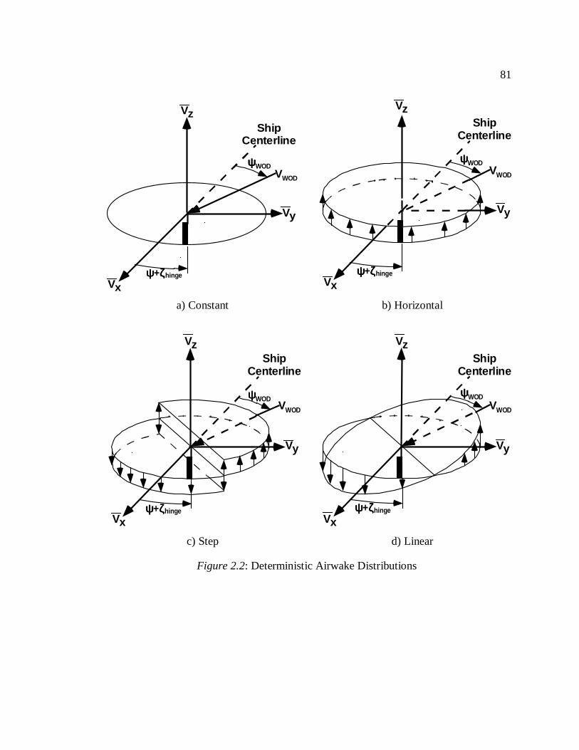
81
ShipCenterline
Vz
Vy
Vxψψψψ+ζζζζhinge
ψψψψWODVWOD
a) Constant
ShipCenterline
Vz
Vy
Vx
ψψψψWODVWOD
ψψψψ+ζζζζhinge
b) Horizontal
Vz
Vy
Vx
ShipCenterline
ψψψψWODVWOD
ψψψψ+ζζζζhinge
c) Step
Vz
Vy
Vx
ShipCenterline
ψψψψWODVWOD
ψψψψ+ζζζζhinge
d) Linear
Figure 2.2: Deterministic Airwake Distributions
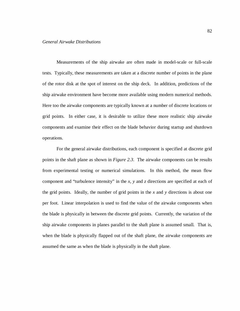
82
General Airwake Distributions
Measurements of the ship airwake are often made in model-scale or full-scale
tests. Typically, these measurements are taken at a discrete number of points in the plane
of the rotor disk at the spot of interest on the ship deck. In addition, predictions of the
ship airwake environment have become more available using modern numerical methods.
Here too the airwake components are typically known at a number of discrete locations or
grid points. In either case, it is desirable to utilize these more realistic ship airwake
components and examine their effect on the blade behavior during startup and shutdown
operations.
For the general airwake distributions, each component is specified at discrete grid
points in the shaft plane as shown inFigure 2.3. The airwake components can be results
from experimental testing or numerical simulations. In this method, the mean flow
component and “turbulence intensity” in thex, y andz directions are specified at each of
the grid points. Ideally, the number of grid points in thex andy directions is about one
per foot. Linear interpolation is used to find the value of the airwake components when
the blade is physically in between the discrete grid points. Currently, the variation of the
ship airwake components in planes parallel to the shaft plane is assumed small. That is,
when the blade is physically flapped out of the shaft plane, the airwake components are
assumed the same as when the blade is physically in the shaft plane.
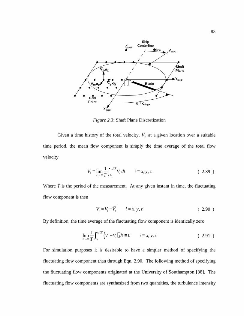
83
Given a time history of the total velocity,Vi, at a given location over a suitable
time period, the mean flow component is simply the time average of the total flow
velocity
0
0
1lim , ,
t T
i itTV V dt i x y z
T
+
→∞= = ( 2.89 )
WhereT is the period of the measurement. At any given instant in time, the fluctuating
flow component is then
, ,i i iV V V i x y z′= − = ( 2.90 )
By definition, the time average of the fluctuating flow component is identically zero
( )0
0
1lim 0 , ,
t T
i itTV V dt i x y z
T
+
→∞− ≡ = ( 2.91 )
For simulation purposes it is desirable to have a simpler method of specifying the
fluctuating flow component than through Eqn. 2.90. The following method of specifying
the fluctuating flow components originated at the University of Southampton [38]. The
fluctuating flow components are synthesized from two quantities, the turbulence intensity
Vz,σσσσz
Vy,σσσσyVx,σσσσx Blade
GridPoint
ShaftPlane
ShipCenterline
VWODψψψψWOD
ψψψψ + ζζζζhinge
XSHIPI
YSHIPI
ZSHIPI
Figure 2.3: Shaft Plane Discretization
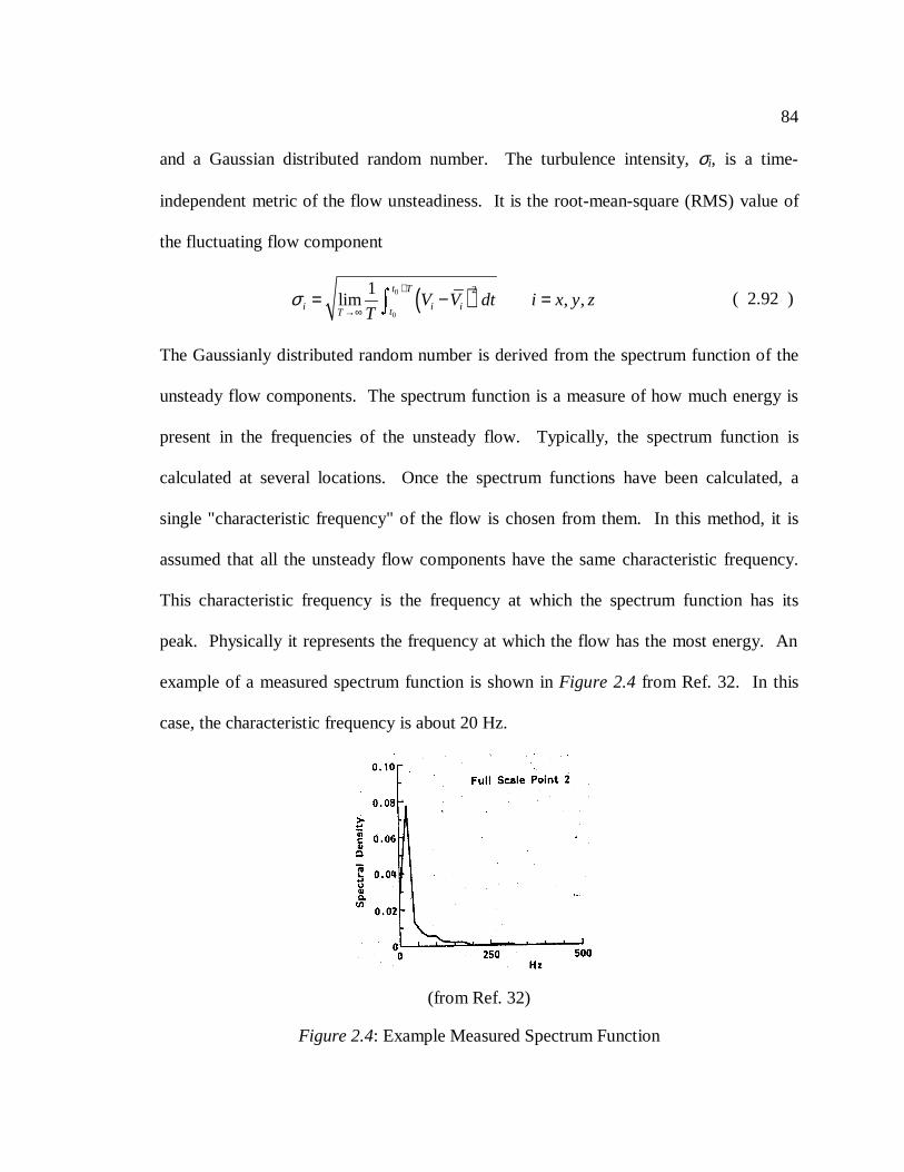
84
and a Gaussian distributed random number. The turbulence intensity,σi, is a time-
independent metric of the flow unsteadiness. It is the root-mean-square (RMS) value of
the fluctuating flow component
( )0
0
21lim , ,
t T
i i itTV V dt i x y z
Tσ
+
→∞= − = ( 2.92 )
The Gaussianly distributed random number is derived from the spectrum function of the
unsteady flow components. The spectrum function is a measure of how much energy is
present in the frequencies of the unsteady flow. Typically, the spectrum function is
calculated at several locations. Once the spectrum functions have been calculated, a
single "characteristic frequency" of the flow is chosen from them. In this method, it is
assumed that all the unsteady flow components have the same characteristic frequency.
This characteristic frequency is the frequency at which the spectrum function has its
peak. Physically it represents the frequency at which the flow has the most energy. An
example of a measured spectrum function is shown inFigure 2.4 from Ref. 32. In this
case, the characteristic frequency is about 20 Hz.
(from Ref. 32)
Figure 2.4: Example Measured Spectrum Function
85
Once the characteristic frequency is chosen, a Gaussian distributed random number,R(t),
is calculated [81]. The time-varying nature of the fluctuating flow components is
simulated by continually updatingR(t) at time intervals specified by the characteristic
frequency. The fluctuating flow component is then calculated from
( )( )( )
x x
y y
z z
V R t
V R t
V R t
σσσ
′ =
′ =
′ =( 2.93 )
The information on thespatial variation of the fluctuating flow components is contained
within the turbulence intensity,σi, and the information on thetime variation of the
fluctuating flow components is contained withinR(t). In this method, it is assumed that
the fluctuating flow components over the entire rotor disk all have the same characteristic
frequency. It is also assumed that the fluctuating flow components all have a Gaussian
distribution.
Resultant Velocities
Once the resultant velocities are known in the undeformed coordinate system,
they are transformed into the deformed coordinate system for use in the aerodynamic
model. The total velocity then becomes
ˆˆ ˆR P TV U i U j U kξ η ζ= + + ( 2.94 )
where

86
( ) ( )( ) ( )
( )( ) ( ) ( )
0
0 0
12
sin cos
cos sin 1 cos sin
ˆcos sin
cos sin
x
R x s z y ship z
s x ship y x y p s ship z
i z p r r
x y
U v v w w dx v v x V V V V
w V V V V w V
V w v w
v v w w V V
α ψ φ ψ
α φ ψ ψ β α ψ φ ψ
λ β η θ η θ φ
ψ ψ
′ ′ ′ ′ ′= − + − Ω + Ω + + − −
′ ′+ − − + − − +
′ ′ ′+ − + − Ω + + Ω −
′ ′+ + + +
( )( ) ( ) ( )
2 2
sin cos sinship nw rh nw rh nw rh
v w
z z w v z z w y y xφ ψ ψ ψ
′ ′+
′ ′+ + + + + − + +
( 2.95a )
( )
( )
( ) ( )
( )
2 210 2 0
212
0
ˆcos
sin cos 1
ˆcos sin cos sin
sin cos
sin
x
T p i s x ship y z
x y
x y p s ship p z
s ship z
U v v w dx w w V V V
vv x V V v
V V v w v V
V v v v w
w
θ β φ λ α φ
ψ ψ
ψ ψ φ β α ψ φ ψ β
α ψ φ ψ
θ
′ ′= − Ω + − Ω + + + − −
′ ′+Ω + Ω + − −
′ ′ ′+ + + + + − +
′ ′ ′ ′+ + + + +
+
( ) ( )( )( ) ( )
( )
( ) ( )
212
0
ˆcos sin
ˆsin cos cos sin
ˆ ˆsin cos
ˆcos cos sin
i s x ship y z p x y p
x y s ship p z
s ship z z
ship nw rh nw rh nw
V V V v w V V w v
x V V v w w V
V w V v w v w w
z z w v z z y y
λ α φ β ψ ψ β φ
ψ ψ φ α ψ φ ψ β
φ α ψ φ ψ φ
θ φ ψ ψ φ
′ ′ ′+ − − + Ω + + + + −
′ ′ ′− Ω + − + + − +
′ ′ ′ ′ ′− + + − + + +
′+ + − + − +
( ) ( ) ( ) ( ) 0
sin
ˆsin cos sin sin cos
rh
ship nw rh nw rh nw rh
x
y y v x w z z z z
ψ
θ φ ψ ψ ψ φ ψ
+ +
′− + + + − + − +
( 2.95b )
87
( )( ) ( )
( )
( )
0
212
2 210 2 0
ˆcos cos sin
ˆ ˆsin cos cos sin
ˆcos sin
ˆsin
P i s x ship y z p x y p
x y ship s z
p s ship z z
x
p
U w V V V v vw V V w v
x V V v w V
w V v w V
v v w dx vv w
θ λ α φ β ψ ψ β φ
ψ ψ φ φ φ ψ α ψ
β α ψ φ ψ φ
θ β
′ ′ ′= + + − − + Ω + Ω + + + −
′ ′− Ω + − + − +
′ ′+ + − − + +
′ ′ ′− + Ω + − Ω + Ω −
( ) ( )
( ) ( )
( ) ( ) ( )( )
212
0
0
ˆcos sin sin cos 1
sin cos cos sin
ˆ
ˆcos sin cos
i s x ship y z
x y p x y
s ship z p s ship z
r p
ship nw rh nw rh
w V V V
V V v w x V V v
V v V
w
y y x v z z
φ λ α φ
ψ ψ φ β ψ ψ
α ψ φ ψ β α ψ φ ψ
η θ φ β
θ φ ψ φ ψ
+ + − −
′ ′ ′− + + + − Ω + − −
′+ − − + − +
′+ + Ω + +
− + + − + +
( ) ( ) ( ) ( ) 0
sin
ˆsin cos sin sin
nw rh
ship nw rh nw rh nw rh
w z z
z z w y y x v z z
ψ
θ φ ψ φ ψ ψ
′− + +
′− + + + + − − +
( 2.95c )
The double underlined terms are unique to this analysis because they represent the
airwake components in the lateral (y) direction and through the plane of the rotor disk (z).
Normally the velocity due to the rotor speed,Ωx, dominates the tangential flow.
However, in this analysisΩ can be small so the airwake components are vital.
At very low rotor speeds large regions of the rotor disk can be in reverse flow.
Because of the unusual ship airwake environment and the low rotor speeds, the angles of
attack can vary from 0° to 360°. Once the blade section velocities are known, the local
blade section angle of attack is calculated from
1tan P
T
U
Uα − −=
( 2.96 )
Likewise, the local blade section skew angle is calculated from
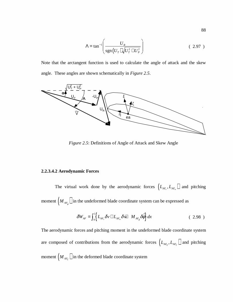
88
( )1
2 2tan
sgnR
T T P
U
U U U
− Λ = +
( 2.97 )
Note that the arctangent function is used to calculate the angle of attack and the skew
angle. These angles are shown schematically inFigure 2.5.
2.2.3.4.2 Aerodynamic Forces
The virtual work done by the aerodynamic forces( ),v wAF AFL L and pitching
moment( )ˆAFMφ
in the undeformed blade coordinate system can be expressed as
ˆ
1
0
ˆv wAF AF AF AFW L v L w M dx
φδ δ δ δφ= + + ( 2.98 )
The aerodynamic forces and pitching moment in the undeformed blade coordinate system
are composed of contributions from the aerodynamic forces( ),AF AFL Lη ζ
and pitching
moment( )AFMξ
in the deformed blade coordinate system
UT -UP
ααααΛΛΛΛ
URV
UT + UP2 2
η
ζ
ea
ξ
Figure 2.5: Definitions of Angle of Attack and Skew Angle
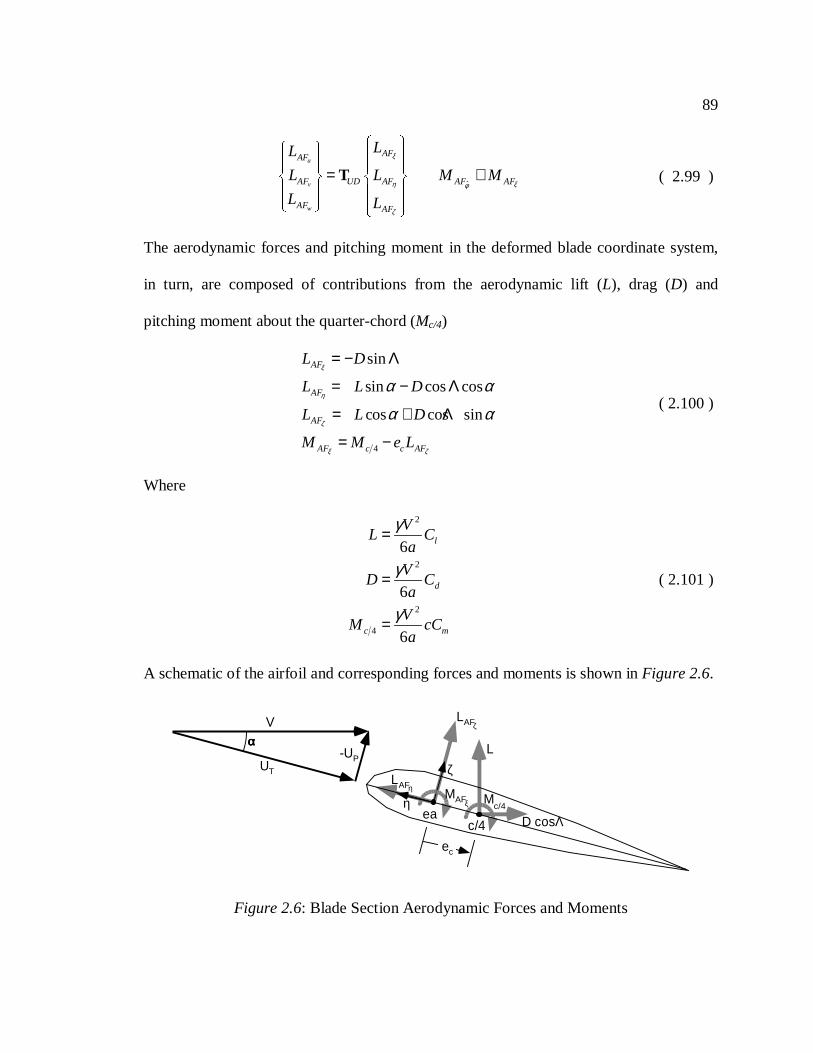
89
ˆ
u
v
w
AFAF
AF UD AF AF AF
AF AF
LL
L L M M
L L
ξ
η ξφ
ζ
= ≅
T ( 2.99 )
The aerodynamic forces and pitching moment in the deformed blade coordinate system,
in turn, are composed of contributions from the aerodynamic lift (L), drag (D) and
pitching moment about the quarter-chord (Mc/4)
4
sin
sin cos cos
cos cos sin
AF
AF
AF
AF c c AF
L D
L L D
L L D
M M e L
ξ
η
ζ
ξ ζ
α α
α α
= − Λ
= − Λ
= + Λ
= −
( 2.100 )
Where
2
2
2
4
6
6
6
l
d
c m
VL C
a
VD C
a
VM cC
a
γ
γ
γ
=
=
=
( 2.101 )
A schematic of the airfoil and corresponding forces and moments is shown inFigure 2.6.
Mc/4
L
LAFη
η
ζUT
-UP
eac/4
ec
αααα
D cosΛ
V ζLAF
ξMAF
Figure 2.6: Blade Section Aerodynamic Forces and Moments
90
Substituting Eqn. 2.101 into 2.100 yields
( )
( )
( )
( )( )
2
2
2
2
sin6
sin cos cos6
cos cos sin6
cos cos sin6
AF d
AF l d
AF l d
AF m c l d
VL C
a
VL C C
a
VL C C
a
VM cC e C C
a
ξ
η
ζ
ξ
γ
γ α α
γ α α
γ α α
= − Λ
= − Λ
= + Λ
= − + Λ
( 2.102 )
The aerodynamic lift, drag and pitching moment are always referenced to the quarter-
chord instead of the aerodynamic center because the angle of attack may range from 0° to
360°.
The aerodynamic lift, drag and pitching moment can be modeled using either
quasi-steady or unsteady aerodynamic models. Both models will be discussed in the
following sections. In either case, special provisions must be made to accommodate
situations in which the local angle of attack or skew angle becomes large. In addition, the
aerodynamic lift, drag, and pitching moment coefficients for a blade section with leading
edge spoilers will also be discussed.
Nonlinear Quasi-steady Aerodynamic Modeling
In the nonlinear quasi-steady aerodynamic model, the aerodynamic forces are
assumed functions of theinstantaneousvalues of the angle of attack and its time
derivatives. As the name implies, all the effects of unsteady forces are neglected.
91
Furthermore, the undeformed aerodynamic forces and pitching moment are split into
circulatory (C) and noncirculatory (NC) parts
( )( )( ) ( )( ) ( )ˆ ˆ ˆ
u u
v v
w w
AF AF C
AF AF C
AF AFw AFC NC
AF AF AFC NC
L L
L L
L L L
M M Mφ φ φ
=
=
= +
= +
( 2.103 )
The circulatory aerodynamic coefficients are modeled using curve fits to experimental
data from Prouty [82] and Critzoset al [83] while the noncirculatory aerodynamic forces
are modeled using an analysis similar to Johnson [44]. The circulatory aerodynamic
model will be discussed first, followed by the noncirculatory aerodynamic model. As
stated earlier, special provisions must be made for situations in which the angle of attack
or skew angle becomes large.
Circulatory Aerodynamic Forces
Sectional lift, drag, and moment coefficient data can easily be found from airfoil
data derived from wind tunnel measurements. The empirical relations for the lift and
drag coefficients are curve fits to experimentally measured data for angles of attack
ranging from 0° to 360° for a NACA 0012 airfoil [82]. Mach number effects on the stall
angle are modeled. It is important to note that the following relations are only strictly
applicable to a NACA 0012 airfoil section; other airfoils would require modification of
the relations. For angles of attack ranging from 0º to 360º, the lift coefficient is given by
92
( )( )
( )
( )
( )
2
2
1
1
0
20
1.15sin 2 20 161
0.70 161 173
0.10 180 173 187
0.70 187 201
1.15sin 2 201 340
360 360 340 360
360 360
l l
K
l l l
l
l
l
l
l
K
l l l
l
C a
C a K
C
C
C
C
C
C a K
C a
α α α
α α α α αα α
αα α
αα α
α α α α α
α
= < <
= − − < <= < <= − < <
= − < <
= + < <= < <
= − − − − − < < −
= − −
360lα α− < <
( 2.104 )
The parametersa , lα , 1K and 2K are Mach number dependent and are given by
2
7.151
2
0.10.01
115 16
0.0233 0.342
2.05 0.95
l
a MM
M
K M
K M
α
= −−
= −
= += −
( 2.105 )
In a similar manner, the drag coefficient is given by
( )( )
( )
4
4
3
3
0
20
1.03 1.02cos 2 20 340
360 340 360
360 360
i
i
i
i
d d d
K
d d d d
d
K
d d d d
d d d
C C
C C K
C
C C K
C C
α α
α α α αα α
α α α α
α α
= < <
= + − < <= − < <
= + − − < < −
= − < <
( 2.106 )
The parametersidC dα , 3K and 4K are given by
( )0
2 4 6 6
3
4
65.8 0.226 0.0046 10
17 23.4
0.00066
2.54
id d
d
C C x
M
K
K
α α α
α
−= + − +
= −==
( 2.107 )
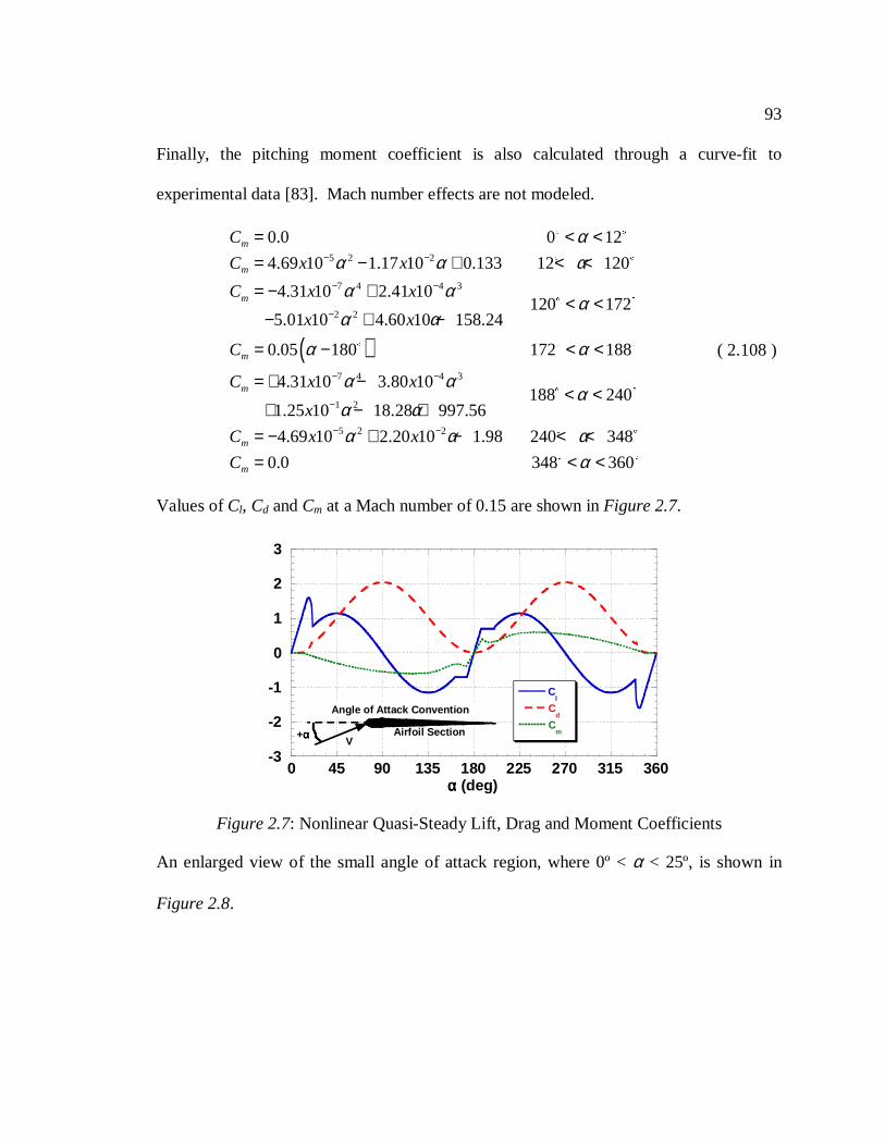
93
Finally, the pitching moment coefficient is also calculated through a curve-fit to
experimental data [83]. Mach number effects are not modeled.
( )
5 2 2
7 4 4 3
2 2
7 4 4 3
1 2
0.0 0 12
4.69 10 1.17 10 0.133 12 120
4.31 10 2.41 10120 172
5.01 10 4.60 10 158.24
0.05 180 172 188
4.31 10 3.80 1018
1.25 10 18.28 997.56
m
m
m
m
m
C
C x x
C x x
x x
C
C x x
x
αα α αα α
αα α
α α
α αα α
− −
− −
−
− −
−
= < <= − + < <= − +
< <− + −
= − < <
= + −
+ − +
5 2 2
8 240
4.69 10 2.20 10 1.98 240 348
0.0 348 360m
m
C x x
C
α
α α αα
− −
< <
= − + − < <= < <
( 2.108 )
Values ofCl, Cd andCm at a Mach number of 0.15 are shown inFigure 2.7.
An enlarged view of the small angle of attack region, where 0º <α < 25º, is shown in
Figure 2.8.
-3
-2
-1
0
1
2
3
0 45 90 135 180 225 270 315 360
Cl
Cd
Cm
αααα (deg)
+αααα Airfoil SectionV
Angle of Attack Convention
Figure 2.7: Nonlinear Quasi-Steady Lift, Drag and Moment Coefficients
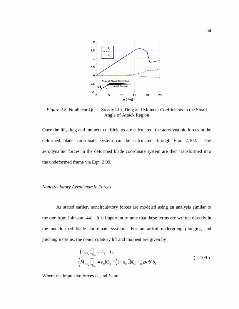
94
Once the lift, drag and moment coefficients are calculated, the aerodynamic forces in the
deformed blade coordinate system can be calculated through Eqn. 2.102. The
aerodynamic forces in the deformed blade coordinate system are then transformed into
the undeformed frame via Eqn. 2.99.
Noncirculatory Aerodynamic Forces
As stated earlier, noncirculatory forces are modeled using an analysis similar to
the one from Johnson [44]. It is important to note that these terms are written directly in
the undeformed blade coordinate system. For an airfoil undergoing plunging and
pitching motions, the noncirculatory lift and moment are given by
( )( ) ( )
ˆ
2 3
412 3 181
wAF NC
AF h hNC
L L L
M a bL a bL bφ
ρπ θ
= +
= − − −
( 2.109 )
Where the impulsive forcesL2 andL3 are
-1
-0.5
0
0.5
1
1.5
2
0 5 10 15 20 25
Cl
Cd
Cm
αααα (deg)
+αααα Airfoil SectionV
Angle of Attack Convention
Figure 2.8: Nonlinear Quasi-Steady Lift, Drag and Moment Coefficients in the SmallAngle of Attack Region
95
( )22 1
23 1
hL b w a b
L b V
ρπ θ
ρπ θ
= − −
=
( 2.110 )
And where
( )14
12
sin cosx y
h c
V x V V
a b e c
b c
ψ ψ= Ω + −
= − +=
( 2.111 )
Substitution of Eqns. 2.110 and 2.111 into Eqn. 2.109 yields
( ) ( )( ) ( )( ) ( ) ( ) ( ) ( ) ( )ˆ
14 0 0
21 1 1
4 4 32 20 0
ˆ ˆsin cos12
ˆ ˆsin cos12
wAF c x yNC
cAF c c c x y
NC
cL w e c x V V
a
cM e w e c c e c x V V
aφ
γπ θ φ ψ ψ θ φ
γπ θ φ ψ ψ θ φ
= − + + + + Ω + − +
= + − + + + − + Ω + − +
( 2.112 )
The double underlined terms are unique to this analysis and are not included in Ref. 44.
Special Provisions for the Nonlinear Quasi-steady Aerodynamic Model
The noncirculatory aerodynamic forces derived in the previous section are only
valid for small angles of attack and skew angles. In this analysis, it has been assumed
that the delineation between large and small angles occurs at 25º. Above this region,
where |α| < 25º and |Λ| < 25º, the noncirculatory forces are assumed zero.
Unsteady Aerodynamic Modeling
Even at full rotor speed, a helicopter blade encounters time-varying changes in the
angle of attack due to the control inputs, the motion of the blade and the complex three-
dimensional flowfield. This is especially true during the engagement and disengagement
96
of the rotor where the rate of change of the angle of attack can become very large.
Unsteady aerodynamic effects can result in increased lift and moment coefficients at
angles of attack above the static stall angle.
The unsteady aerodynamic model used in this analysis is taken from the model
originally developed by Leishman and Beddoes [45, 84]. It is a semi-empirical nonlinear
time-domain method suited for use in comprehensive rotorcraft analyses. Both
circulatory and noncirculatory effects are included. The effects of arbitrary time-varying
forces are derived using the superposition principle. For reference, the unsteady
aerodynamic model used in the analysis is fully detailed in Appendix A.3.
Special Provisions for the Unsteady Aerodynamic Model
Because of the unusual ship airwake environment, unsteady aerodynamic effects
are as likely to occur at negative angles of attack as at positive angles of attack.
Modifications to the unsteady aerodynamic model have been made that ensure unsteady
effects can be modeled for both situations. The unsteady aerodynamic model described
in the Appendix has only been validated for small to moderate angles of attack and skew
angles (|α| < 25º and |Λ| < 25º). If the angle of attack or the skew angle is large, then the
aerodynamic forces are calculated through the nonlinear quasi-steady aerodynamic
model. Lastly, the unsteady aerodynamic model is not valid for very low Mach numbers.
In this situation, the aerodynamic forces are also calculated with the nonlinear quasi-
steady aerodynamic model.
97
2.2.3.4.3 Spoiler Modeling
In this analysis, the effect of spoilers on the rotor blade behavior will be
investigated. Spoilers are aerodynamic devices commonly used to reduce lift and
increase drag on a body. Spoilers placed near the trailing edge of an airfoil section
simply increase the aerodynamic drag, while spoilers placed closer to the leading edge or
near the quarter-chord of an airfoil section will drastically reduce lift and increase drag.
Spoilers that extend continuously down the span of a wing, called full-span spoilers, are
also known to produce large hinge moments and vibration. Spoilers that are arranged in a
rake configuration, called gated spoilers, have significantly lower hinge moments and
buffeting problems than full-span spoilers while still having the same aerodynamic
effectiveness.
Gated, leading-edge spoilers were previously tested on the upper surface of a
model NACA 4415 wing section for application to tilt-wing V/STOL aircraft in the
transition phase [85]. The spoilers were mounted perpendicular to the wing surface in
several configurations. Two different chord locations of 5%c and 15%c; four different
spoiler heights of 2.5%c, 5%c, 7.5%c, and 10%c; and two different spoiler gate spacings
of 3%c and 6%c were tested. Schematics of the spoiler configurations are shown in
Figure 2.9. Sectional lift, drag, and moment coefficients were measured versus angle of
attack, ranging from 0° to 90°, with and without spoilers. The results for the lift and drag
coefficients for one configuration are shown inFigure 2.10. Note that essentially all the
lift in the attached flow region is eliminated. The lift curve slope was decreased 60% to
70% in the attached flow region and was essentially independent of gate spacing or for
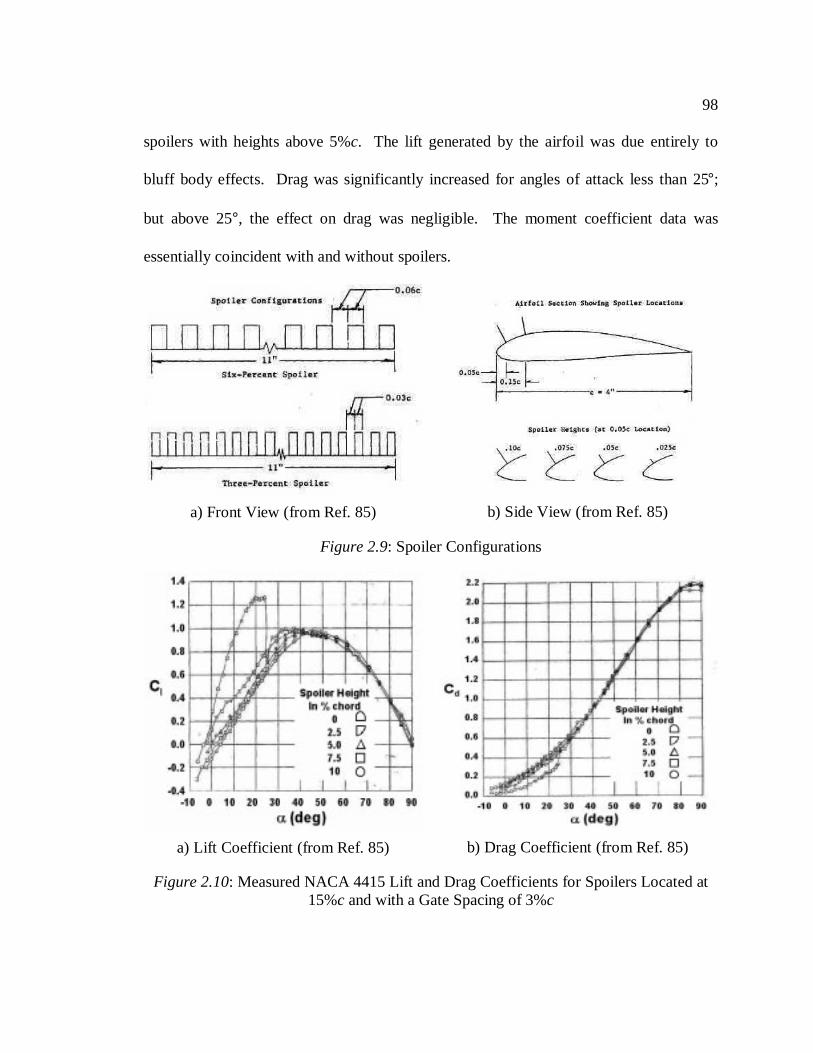
98
spoilers with heights above 5%c. The lift generated by the airfoil was due entirely to
bluff body effects. Drag was significantly increased for angles of attack less than 25°;
but above 25°, the effect on drag was negligible. The moment coefficient data was
essentially coincident with and without spoilers.
a) Front View (from Ref. 85) b) Side View (from Ref. 85)
Figure 2.9: Spoiler Configurations
a) Lift Coefficient (from Ref. 85) b) Drag Coefficient (from Ref. 85)
Figure 2.10: Measured NACA 4415 Lift and Drag Coefficients for Spoilers Located at15%c and with a Gate Spacing of 3%c
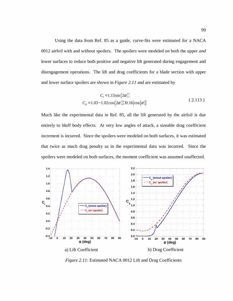
99
Using the data from Ref. 85 as a guide, curve-fits were estimated for a NACA
0012 airfoil with and without spoilers. The spoilers were modeled on both the upperand
lower surfaces to reduce both positive and negative lift generated during engagement and
disengagement operations. The lift and drag coefficients for a blade section with upper
and lower surface spoilers are shown inFigure 2.11and are estimated by
( )( ) ( )
1.15sin 2
1.03 1.02cos 2 0.16 cos
l
d
C
C
α
α α
=
= − +( 2.113 )
Much like the experimental data in Ref. 85, all the lift generated by the airfoil is due
entirely to bluff body effects. At very low angles of attack, a sizeable drag coefficient
increment is incurred. Since the spoilers were modeled on both surfaces, it was estimated
that twice as much drag penalty as in the experimental data was incurred. Since the
spoilers were modeled on both surfaces, the moment coefficient was assumed unaffected.
-0.4
-0.2
0.0
0.2
0.4
0.6
0.8
1.0
1.2
1.4
-10 0 10 20 30 40 50 60 70 80 90
Cl(w/out spoiler)
Cl(w/ spoiler)
Cl
αααα (deg)
a) Lift Coefficient
0.0
0.2
0.4
0.6
0.8
1.0
1.2
1.4
1.6
1.8
2.0
2.2
-10 0 10 20 30 40 50 60 70 80 90
Cd
(w/out spoiler)
Cd
(w/ spoiler)
Cd
αααα (deg)
b) Drag Coefficient
Figure 2.11: Estimated NACA 0012 Lift and Drag Coefficients
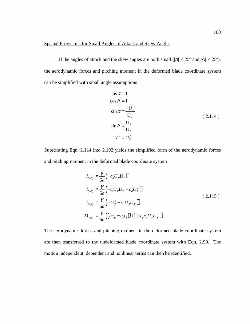
100
Special Provisions for Small Angles of Attack and Skew Angles
If the angles of attack and the skew angles are both small (|α| < 25º and |Λ| < 25º),
the aerodynamic forces and pitching moment in the deformed blade coordinate system
can be simplified with small angle assumptions
2 2
cos 1
cos 1
sin
sin
P
T
R
T
T
U
U
U
U
V U
α
α
=Λ =
−=
Λ =
=
( 2.114 )
Substituting Eqn. 2.114 into 2.102 yields the simplified form of the aerodynamic forces
and pitching moment in the deformed blade coordinate system
( )
( )
( )
( )( )
2
2
2
6
6
6
6
AF d R T
AF l P T d T
AF l T d P T
AF m c l T c d P T
L c U Ua
L cU U c Ua
L cU c U Ua
M cc e c U e c U Ua
ξ
η
ζ
ξ
γ
γ
γ
γ
= −
= − −
= −
= − +
( 2.115 )
The aerodynamic forces and pitching moment in the deformed blade coordinate system
are then transferred to the undeformed blade coordinate system with Eqn. 2.99. The
motion independent, dependent and nonlinear terms can then be identified.
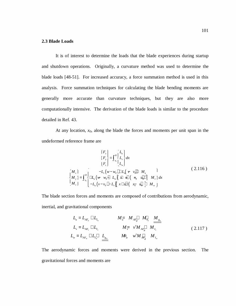
101
2.3 Blade Loads
It is of interest to determine the loads that the blade experiences during startup
and shutdown operations. Originally, a curvature method was used to determine the
blade loads [48-51]. For increased accuracy, a force summation method is used in this
analysis. Force summation techniques for calculating the blade bending moments are
generally more accurate than curvature techniques, but they are also more
computationally intensive. The derivation of the blade loads is similar to the procedure
detailed in Ref. 43.
At any location,x0, along the blade the forces and moments per unit span in the
undeformed reference frame are
( ) ( )( ) ( ) ( )( ) ( ) ( )
0
0
0 0
0 0 0
0 0 0
x uR
y vx
z w
x v w uR
y u w vx
z u v w
F L
F L dx
F L
M L w w L v v M
M L w w L x u x u M dx
M L v v L x u x u M
=
− − + − + = + − − + − − +
− − − + − − +
( 2.116 )
The blade section forces and moments are composed of contributions from aerodynamic,
inertial, and gravitational components
ˆ
ˆ
ˆ
u u u u
v v v
w w w w
u AF I u AF I g
v AF I v AF I
w AF I g w AF I
L L L M M M M
L L L M v M M
L L L L M w M M
φ
φ
φ
= + = + +
′= + = +
′= + + = +( 2.117 )
The aerodynamic forces and moments were derived in the previous section. The
gravitational forces and moments are
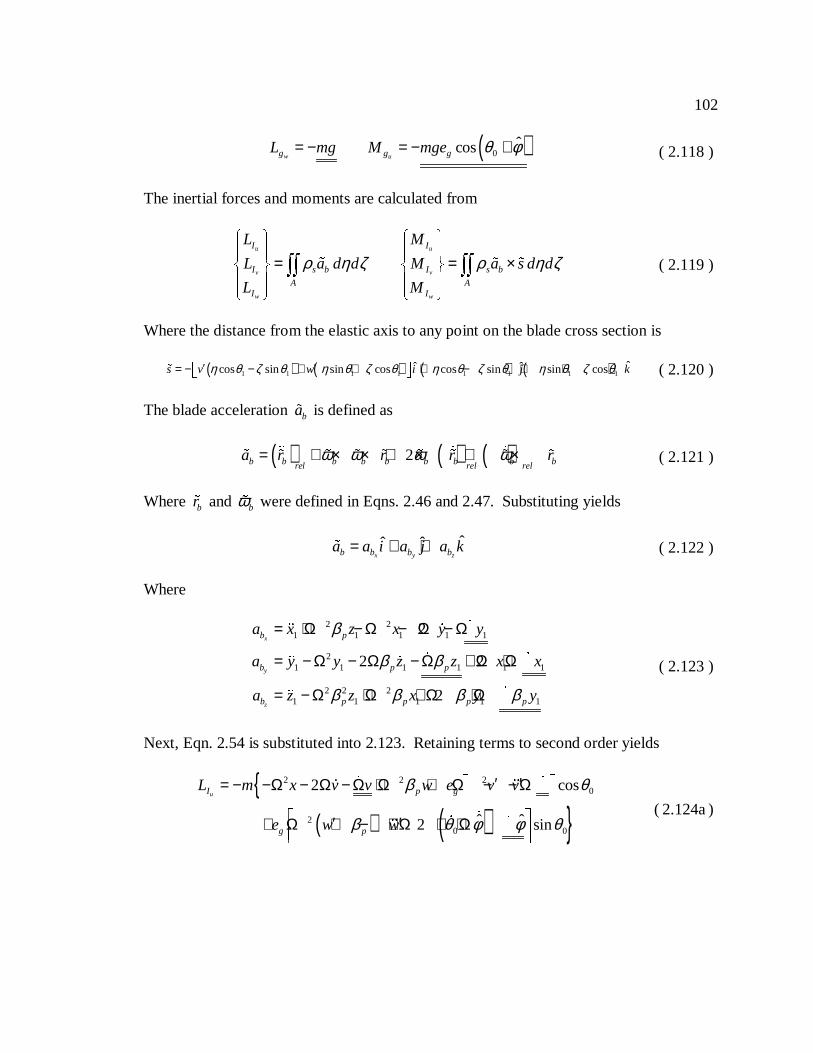
102
( )0ˆcos
w ug g gL mg M mge θ φ= − = − + ( 2.118 )
The inertial forces and moments are calculated from
u u
v v
w w
I I
I s b I s b
A AI I
L M
L a d d M a s d d
L M
ρ η ζ ρ η ζ = = ×
( 2.119 )
Where the distance from the elastic axis to any point on the blade cross section is
( ) ( ) ( ) ( )1 1 1 1 1 1 1 1ˆˆ ˆcos sin sin cos cos sin sin coss v w i j kη θ ζ θ η θ ζ θ η θ ζ θ η θ ζ θ′ ′= − − + + + − + + ( 2.120 )
The blade accelerationba is defined as
( ) ( ) ( )2b b b b b b b b brel rel rela r r r rω ω ω ω= + × × + × + ×
( 2.121 )
Where br and bω were defined in Eqns. 2.46 and 2.47. Substituting yields
ˆˆ ˆx y zb b b ba a i a j a k= + + ( 2.122 )
Where
2 21 1 1 1 1
21 1 1 1 1 1
2 2 21 1 1 1 1
2
2 2
2
x
y
z
b p
b p p
b p p p p
a x z x y y
a y y z z x x
a z z x y y
β
β β
β β β β
= + Ω − Ω − Ω − Ω
= − Ω − Ω − Ω + Ω + Ω
= − Ω + Ω + Ω + Ω
( 2.123 )
Next, Eqn. 2.54 is substituted into 2.123. Retaining terms to second order yields
( ) ( )
2 2 20
20 0
2 cos
ˆ ˆ2 sin
uI p g
g p
L m x v v w e v v
e w w
β θ
β θ φ φ θ
′ ′ = − −Ω − Ω − Ω + Ω + Ω − − Ω
′ ′+ Ω + − + Ω + + Ω
( 2.124a )

103
( )
( )
2
0
20
20 0
2 2
2 cos
ˆ ˆ 2 sin
v
x
I p p
g
g
L m v v v v w w dx w w x
e v v
e w w
β β
θ
θ φ φ θ
′ ′ ′ ′= − − Ω − Ω + − Ω −Ω + Ω
′ ′ − Ω + Ω + Ω
′ ′− + − Ω + Ω + Ω
( 2.124b )
( ) 2 20 0
ˆ2 coswI p p p p gL m w x v v w eβ β β β θ φ θ= − + Ω + Ω + Ω + Ω + +
( 2.124c )
( ) ( )( )( )( )( ) ( )
2 1
2 1
2 2 220 0 0
2 22 20 0
2 20 0
ˆ 2 cos sin
2 sin cos
cos sin
uI m p m m
m m
p g g
M m k v v k k
w w k k
x w e v v x e
θ φ β θ θ
θ θ
β θ θ
′ ′= − + + Ω + Ω + Ω + Ω −
′ ′+ Ω + Ω +
+ Ω + + Ω − − Ω
( 2.124d )
( )( )( ) ( )
( )
2 1
2 1
2 220 0
2 22 2 20 0 0
2 20 0
cos sin
ˆ2 sin cos
ˆ cos 2 sin
vI m m
p p m m
g g
M m v v k k
w w k k
x e x v v e
θ θ
β θ φ β θ θ
φ θ θ
′ ′= − Ω − − Ω −
′ ′+ Ω + − + Ω + + Ω +
−Ω − Ω + Ω + Ω
( 2.124e )
( ) ( )( )( )( ) ( )
2 1
2 1
2 22 20 0 0
2 22 2 20 0
2 20 0
ˆ2 cos sin
cos sin
ˆ2 cos sin
wI p m m
m m
g g
M m w w k k
v v k k
x v v xv e x xw e
θ φ β θ θ
θ θ
θ φ θ
′= − − Ω − Ω + − Ω −
′+ − Ω − Ω +
′ ′+ Ω + Ω + Ω − Ω − Ω + Ω
( 2.124f )
The double underlined terms are unique to this analysis and are not included in Ref. 43.
The aerodynamic, gravitational, and inertial moments are then summed and integrated
along the blade length via Eqn. 2.116. They are then transformed into the deformed
blade coordinate system.
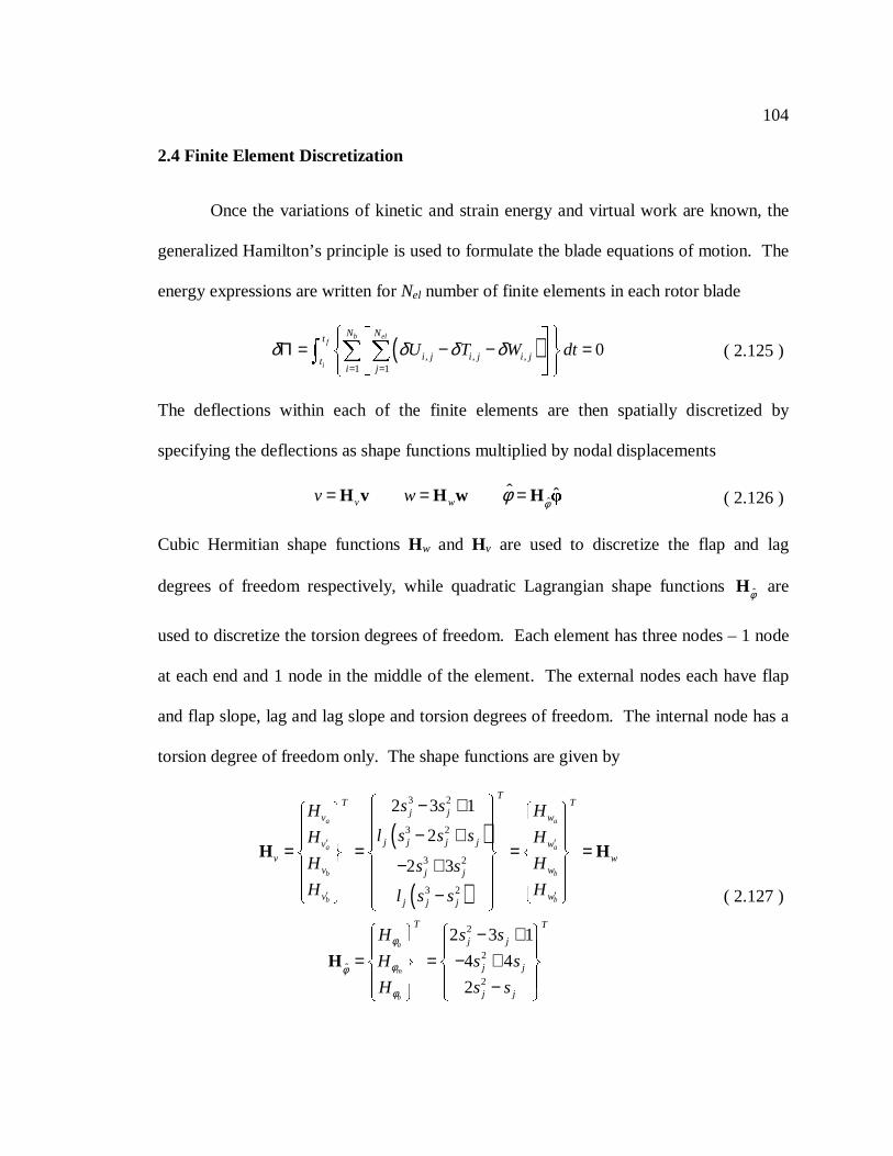
104
2.4 Finite Element Discretization
Once the variations of kinetic and strain energy and virtual work are known, the
generalized Hamilton’s principle is used to formulate the blade equations of motion. The
energy expressions are written forNel number of finite elements in each rotor blade
( ), , ,1 1
0b el
f
i
N Nt
i j i j i jti j
U T W dtδ δ δ δ= =
Π = − − = ( 2.125 )
The deflections within each of the finite elements are then spatially discretized by
specifying the deflections as shape functions multiplied by nodal displacements
ˆˆ ˆ
v wv w φφ= = =H v H w H φ ( 2.126 )
Cubic Hermitian shape functionsHw and Hv are used to discretize the flap and lag
degrees of freedom respectively, while quadratic Lagrangian shape functionsφH are
used to discretize the torsion degrees of freedom. Each element has three nodes – 1 node
at each end and 1 node in the middle of the element. The external nodes each have flap
and flap slope, lag and lag slope and torsion degrees of freedom. The internal node has a
torsion degree of freedom only. The shape functions are given by
( )
( )
3 2
3 2
3 2
3 2
2
2ˆ
2
2 3 1
2
2 3
2 3 1
4 4
2
a a
a a
b b
b b
a
m
b
TT T
j jv w
j j j jv w
v wv wj j
v wj j j
T T
j j
j j
j j
s sH H
l s s sH H
H Hs sH Hl s s
H s s
H s s
H s s
φ
φφ
φ
′ ′
′ ′
− + − + = = = =
− + −
− + = = − + −
H H
H
( 2.127 )
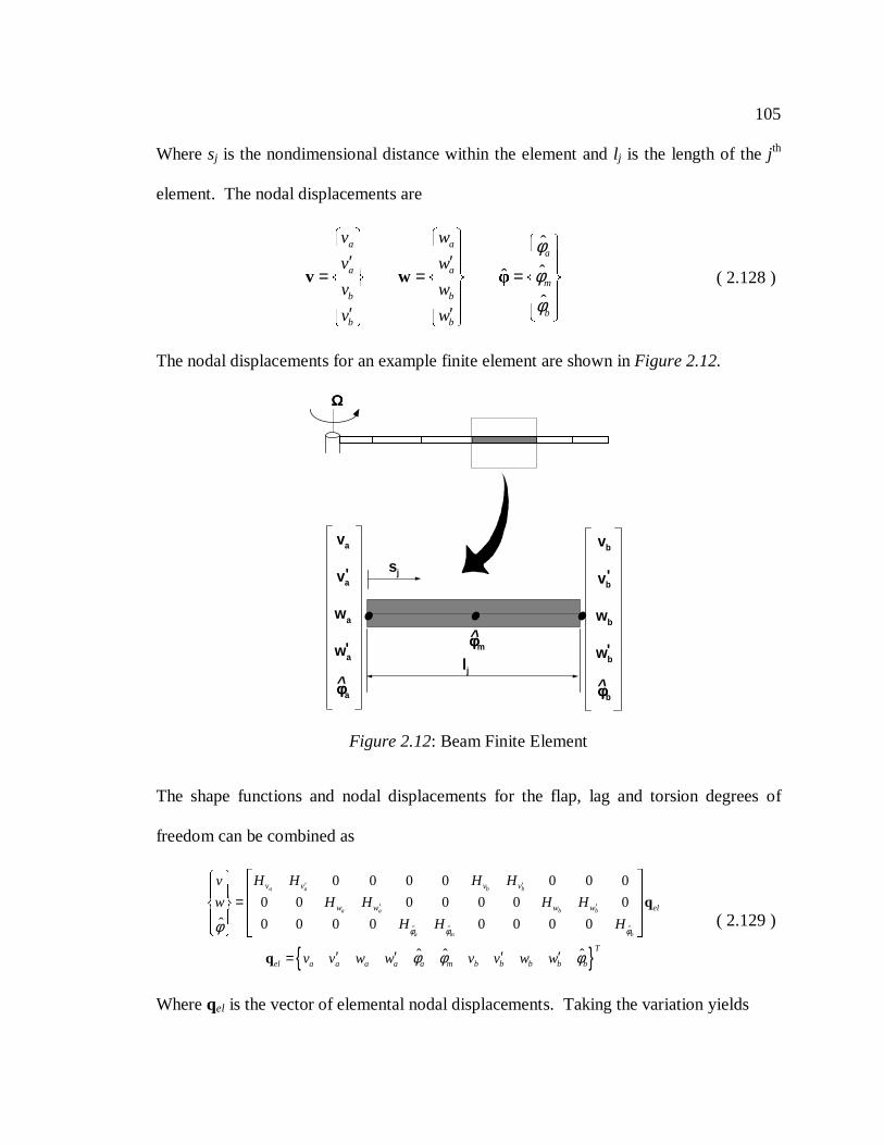
105
Wheresj is the nondimensional distance within the element andl j is the length of thej th
element. The nodal displacements are
ˆ
ˆˆ
ˆ
a aa
a am
b b
bb b
v w
v w
v w
v w
φ
φφ
′ ′ = = =
′ ′
v w φ ( 2.128 )
The nodal displacements for an example finite element are shown inFigure 2.12.
The shape functions and nodal displacements for the flap, lag and torsion degrees of
freedom can be combined as
ˆ ˆ ˆ
0 0 0 0 0 0 0
0 0 0 0 0 0 0
ˆ 0 0 0 0 0 0 0 0
ˆ ˆ ˆ
a a b b
a a b b
a m b
v v v v
w w w w el
T
el a a a a a m b b b b b
v H H H H
w H H H H
H H H
v v w w v v w w
φ φ φφ
φ φ φ
′ ′
′ ′
=
′ ′ ′ ′=
q
q
( 2.129 )
Whereqel is the vector of elemental nodal displacements. Taking the variation yields
• • •
sj
ΩΩΩΩ
l j
φφφφm
va
va
wa
wa
φφφφa^
'
'
vb
vb
wb
wb
φφφφb^
'
'^
Figure 2.12: Beam Finite Element
106
ˆ ˆ ˆ
0 0 0 0 0 0 0
0 0 0 0 0 0 0
ˆ 0 0 0 0 0 0 0 0
ˆ ˆ ˆ
a a b b
a a b b
a m b
v v v v
w w w w el
T
el a a a a a m b b b b b
v H H H H
w H H H H
H H H
v v w w v v w w
φ φ φ
δδ δ
δφ
δ δ δ δ δ δφ δφ δ δ δ δ δφ
′ ′
′ ′
=
′ ′ ′ ′=
q
q
( 2.130 )
Each flexible finite element then has eleven degrees of freedom - 4 in flap, 4 in lag, and 3
in torsion.
2.4.1 Elemental Mass, Damping and Stiffness Matrices and Force Vector
The shape functions and nodal displacements, Eqns. 2.129 and 2.130, are then
substituted into the discretized Hamilton’s principle, Eqn. 2.125. The shape functions are
then integrated within each element using a six-point Gaussian quadrature method. The
dependence of the variation in strain energy, variation in kinetic energy and virtual work
on the blade deflections is given by
( )( )( )
2, , , , ,
, , , , , ,
2, , , , , ,
, ,
, , ,
, , ,
i j i j i j i j i j
i j i j i j i j i j i j
i j i j i j i j i j i j
U U
T T
W W
δ δ δ
δ δ δ
δ δ δ
=
=
=
q q q
q q q q
q q q q
( 2.131 )
The variation in strain energy and virtual work contain nonlinear terms while the
variation in kinetic energy contains linear terms only. The energy expressions can then
be organized into motion dependent terms (, , ,, ,i j i j i jq q q ) and motion independent and
nonlinear ( 2,i jq ) terms. The discretized Hamilton’s principle then becomes
( )1 1
0b el
f
i
N Nt
Tel el el el el el el elt
i j
dtδ δ= =
Π = + + − = q m q c q k q f ( 2.132 )
107
Wheremel, cel and kel are the elemental mass, damping and stiffness matrices andqel is
the elemental displacement vector. The elemental force vector,fel, contains the motion
independent and nonlinear terms.
2.4.2 Blade Mass, Damping and Stiffness Matrices and Force Vector
The elemental mass, damping, and stiffness matrices and force vector are then
assembled for each blade
( )1
0b
f
i
Nt T
u u u u u u u uti
dtδ δ=
Π = + + − =
q M q C q K q F ( 2.133 )
WhereM u, Cu andK u are the unconstrained blade mass, damping and stiffness matrices;
Fu is the unconstrained blade force vector; andqu is the vector of unconstrained blade
displacements
1 1 1 1 1
el el el el elN N N N N
u el u el u el u el u elj j j j j= = = = =
= = = = = M m C c K k F f q q ( 2.134 )
The kinematic constraints must be applied to the unconstrained blade equation.
For an articulated or hingeless rotor, the boundary conditions are that the blade is purely
cantilevered at the root. In this case, the lag deflection, lag slope, flap deflection, flap
slope and twist at the root of the blade are set to zero
( ) ( ) ( ) ( ) ( ), 1 , 1 , 1 , 1 , 1
ˆ 0a a a a ai j i j i j i j i jv v w w φ
= = = = =′ ′= = = = = ( 2.135 )
It is assumed that the hinge offsets are not zero for an articulated rotor. For a teetering
rotor, the boundary conditions are that the blade is pinned in the flap degree of freedom
108
and cantilevered in the lag and twist degrees of freedom. The lag deflection, lag slope,
flap deflection and twist at the root are set to zero
( ) ( ) ( ) ( ), 1 , 1 , 1 , 1
ˆ 0a a a ai j i j i j i jv v w φ
= = = =′= = = = ( 2.136 )
For a gimballed rotor, the boundary conditions are that the blade is pinned in the flap and
twist degrees of freedom and cantilevered in the lag degree of freedom. The lag
deflection, lag slope and flap deflection at the root are set to zero
( ) ( ) ( ), 1 , 1 , 10a a ai j i j i j
v v w= = =
′= = = ( 2.137 )
After application of the kinematic constraints, Eqn. 2.133 becomes
( )1
0b
f
i
Nt T
c c c c c c c cti
dtδ δ=
Π = + + − =
q M q C q K q F ( 2.138 )
WhereM c, Cc andK c are the constrained blade mass, damping and stiffness matrices;Fc
is the constrained blade force vector; andqc is the vector of constrained blade
displacements.
2.4.3 Rotor Mass, Damping and Stiffness Matrices and Force Vector
The constrained blade mass, damping, and stiffness matrices and force vector
must be assembled for the entire rotor. In order to do this, the kinematic constraints must
be applied to the constrained blade matrices and force vector. For an articulated or
hingeless rotor, the forces and moments acting on one blade do not affect the other
blades. The blade motions are not coupled, so no modifications are necessary. For
teetering or gimballed rotors, the forces and moments acting on one blade do affect the
109
other blades. The blade motions are coupled, so the constrained blade matrices must be
modified. In the case of a teetering rotor, the modification is trivial. The flap slope at the
root of the second blade is simply the opposite of the flap slope at the root of the first
blade
( ) ( )2, 1 1, 1a ai j i jw w
= = = =′ ′= − ( 2.139 )
Taking the variation yields
( ) ( )2, 1 1, 1a ai i i iw wδ δ
= = = =′ ′= − ( 2.140 )
For a gimballed rotor, the modifications are more complex. Both the flap slope and twist
degrees of freedom at the root of each blade are coupled through the following relation
( ) ( ) ( )( ) ( ) ( )
, 1 1, 1 1, 1
1, 1, 1 1, 1
ˆcos sin1,
ˆ ˆsin cos
a a i a ii j i j i j
b
a a i a ii ji j i j
w wi N
w
ψ φ ψ
φ ψ φ ψ
= = = = =
= == = =
′ ′= ∆ + ∆=
′= − ∆ + ∆( 2.141 )
Taking the variation yields
( ) ( ) ( )( ) ( ) ( )
, 1 1, 1 1, 1
1, 1, 1 1, 1
ˆcos sin1,
ˆ ˆsin cos
a a i a ii j i j i j
b
a a i a ii ji j i j
w wi N
w
δ δ ψ δφ ψ
δφ δ ψ δφ ψ
= = = = =
= == = =
′ ′= ∆ + ∆=
′= − ∆ + ∆( 2.142 )
The azimuth angle between each blade,∆ψi, is given by
( )21i
b
iN
πψ∆ = − ( 2.143 )
After application of the kinematic constraints, Eqn. 2.138 becomes
( )1
0b
f
i
Nt T
r r r r r r r rti
dtδ δ=
Π = + + − =
q M q C q K q F ( 2.144 )
110
WhereM r, Cr andK r are the transformed blade mass, damping and stiffness matrices;Fr
is the transformed blade force vector; andqr is the vector of transformed blade
displacements.
The transformed blade mass, damping, and stiffness matrices and force vector are
then assembled
( ) 0f
i
tT
tdtδ δΠ = + + − = q Mq Cq Kq F ( 2.145 )
WhereM , C and K are the rotor mass, damping and stiffness matrices;F is the rotor
force vector; andq is the vector of rotor displacements
1 1 1 1 1
b b b b bN N N N N
r r r r ri i i i i= = = = =
= = = = = M M C C K K F F q q ( 2.146 )
The rotor virtual displacements are then arbitrary and the discretized equation of motion
becomes
FKqqCqM =++ ( 2.147 )
2.5 Analysis Types
Three different types of analyses - an eigenanalysis, an engagement or
disengagement operation, or an engagement or disengagement wind envelope - can be
performed on the discretized rotor equations of motion. In the first section, the reduction
of the full finite element equations of motion into modal space coordinates is presented.
In the second section, the methods used to time integrate the resulting modal equations of
111
motion to determine the rotor response is discussed. In the third section, the engagement
and disengagement envelope analysis used to determine the SHOLs is explained.
2.5.1 Modal Analysis
An eigenanalysis of the rotor equations of motion determines the natural
frequencies and mode shapes of the rotor. It is essential that the natural frequencies and
mode shape of the analytical model correlate well with experimental data to ensure that
the dynamic characteristics of the math model are representative of the actual rotor
system. Furthermore, a modal analysis permits the equations of motion to be transformed
into a generalized, or modal, coordinate system. The number of modes required to
accurately model the blade response are much less than the number of degrees of freedom
in the full finite element space model. Therefore, the modal transformation increases the
computational efficiency of the analysis.
To determine the natural frequencies and mode shapes of the rotor, the undamped,
free vibration response of the rotor is examined. It is important to note that for the modal
analysis, the rotor is assumed to be rotating at a constant speed. To examine the effects
of centrifugal force on the natural frequencies and mode shapes, the rotor speed can be
anywhere from 0%NR to 100%NR. Furthermore, all aerodynamic effects are ignored.
The discretized rotor equation of motion, Eqn. 2.9, then reduces to
s s+ =M q K q 0 ( 2.148 )
Where the matricesM s andK s refer to the mass and stiffness matrices composed from
structural quantities only. In general, they are different from the mass and stiffness
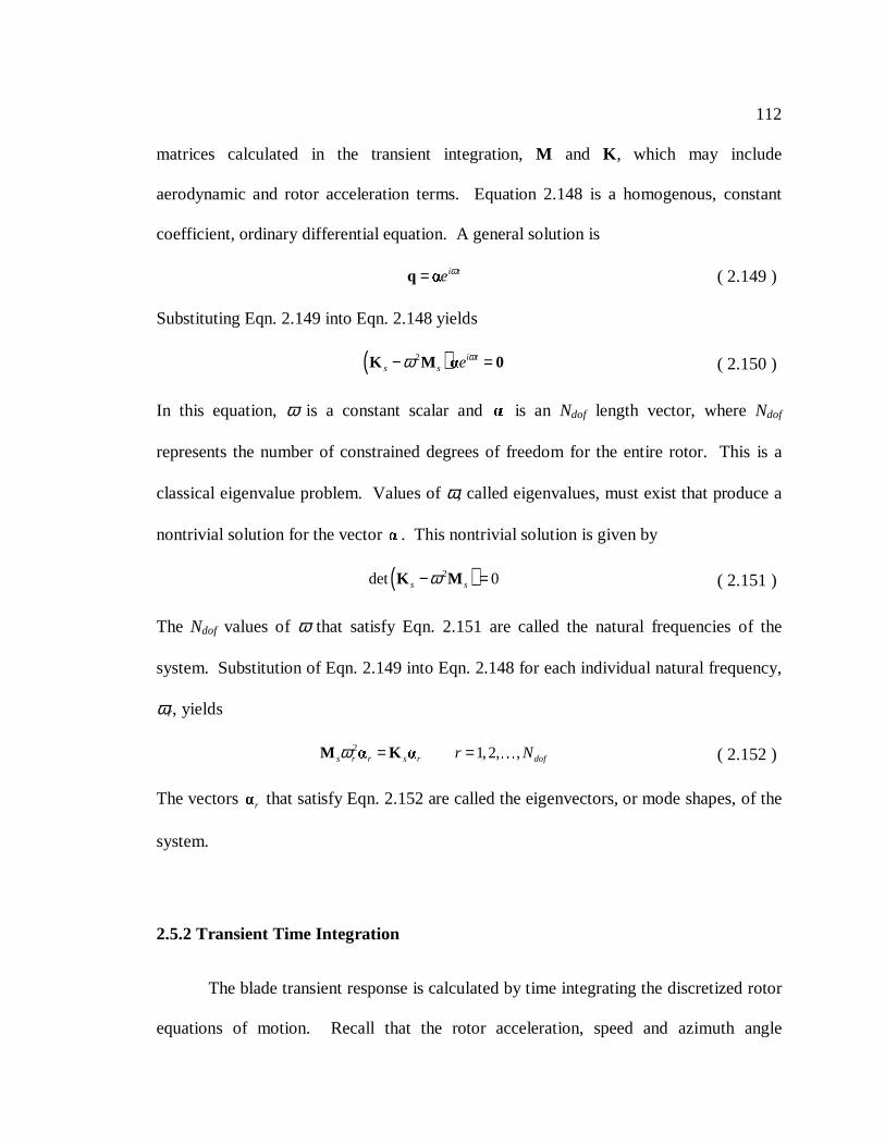
112
matrices calculated in the transient integration,M and K , which may include
aerodynamic and rotor acceleration terms. Equation 2.148 is a homogenous, constant
coefficient, ordinary differential equation. A general solution is
i teω=q α ( 2.149 )
Substituting Eqn. 2.149 into Eqn. 2.148 yields
( )2 i ts s eωω− =K M α 0 ( 2.150 )
In this equation,ω is a constant scalar andα is an Ndof length vector, whereNdof
represents the number of constrained degrees of freedom for the entire rotor. This is a
classical eigenvalue problem. Values ofω, called eigenvalues, must exist that produce a
nontrivial solution for the vectorα . This nontrivial solution is given by
( )2det 0s sω− =K M ( 2.151 )
The Ndof values ofω that satisfy Eqn. 2.151 are called the natural frequencies of the
system. Substitution of Eqn. 2.149 into Eqn. 2.148 for each individual natural frequency,
ωr, yields
2 1,2, ,s r r s r dofr Nω = =M α K α ( 2.152 )
The vectors rα that satisfy Eqn. 2.152 are called the eigenvectors, or mode shapes, of the
system.
2.5.2 Transient Time Integration
The blade transient response is calculated by time integrating the discretized rotor
equations of motion. Recall that the rotor acceleration, speed and azimuth angle
113
variations are prescribed non-periodic functions of time, so the equations of motion must
be recalculated at every single time step.
In this analysis, the transient time integration is permitted in the full finite element
space or modal space. A time integration in the full finite element space simply refers to
the time integration of Eqn. 2.9. A time integration in modal space refers to the time
integration of Eqn. 2.9 when transferred into the generalized coordinate system. In this
method, a modal matrix,ΦΦΦΦ, is assembled from the individual mode shapes calculated in
an eigenanalysis
1 2 mN m dofN N = ≤ Φ α α α ( 2.153 )
WhereNm is the total number of modes used in the analysis. The modal matrix can be
assembled using several methods. In earlier research presented in Refs. 49-50, a single
blade was articulated in flap only and utilized a nonzero flap stop angle. In this case, the
"modal swapping" technique was used with success. In the modal swapping technique,
two separate modal matrices were used. The first modal matrix was comprised of purely
articulated modes, representing the blade when not in contact with the flap stop. The
second modal matrix was comprised of purely cantilevered modes, representing the blade
when in contact with the flap stop. Depending upon blade/stop contact during the
transient time integration, the proper modal matrix was then used or "swapped". A
special procedure was required to adjust the modal amplitudes to maintain the physical
shape of the blade when swapping the modal matrices. In the current analysis, multiple
rotor blades can be articulated in both flap and lag directions. Furthermore for a real
articulated rotor blade, the flap and lag stop angles are usually nonzero. In this case, the
114
simplest method is to construct a single modal matrix comprised of a combination of
modes representing the blades when in contact with the flap/lag or gimbal stops, and
when not in contact with the stops. This method ensures that the physical shape of the
blades can be properly simulated when striking a nonzero flap/lag or gimbal stop angle.
Once the modal matrix is chosen, the response of each mode combines linearly to
approximate the rotor deflection according to the equation
≅q Φe ( 2.154 )
Where e is an Nm length vector representing the amplitudes of the mode shapes.
Substitution of Eqn. 2.154 into the discretized rotor equation of motion, Eqn. 2.9, and
premultiplying byΦΦΦΦT yields the equation of motion in modal space
+ + =Me Ce Ke F ( 2.155 )
The modal mass, damping and stiffness matricesM , C and K and force vectorF are
defined as
T T T T= = = =M Φ MΦ C Φ CΦ K Φ KΦ F Φ F ( 2.156 )
In the current analysis, the modal matrix is calculated at a predetermined rotor speed
before the transient time integration begins. Then during a transient time integration, the
modal matrix and the mode shapesare notrecalculated as the rotor speed and centrifugal
force change at every time step. However, the mass, damping and stiffness matrices and
force vectorare recalculated at every time step. This procedure is used because the
recalculation of the modal matrix at every time step throughout the time integration
would be computationally expensive.
115
Once the full finite element or modal spaces are chosen, the equations of motion
can be time integrated. The fourth order Runge-Kutta, Newmark, or Bossak-Newmark
integration schemes have been used in previous research. The fourth order Runge-Kutta
method was the time integration method used in the engagement and disengagement
analyses in Refs. 1, 32-42, and 46-47. Because it is widely used in structural dynamics
its specifics will not be discussed here, but a full description can be found in Ref. 86.
The Newmark integration scheme[87] is also widely used in structural dynamics to
integrate second order linear equations of motion. It is based on the assumption that the
acceleration of the system varies in a linear fashion between any two instants in time. It
is defined by the following equations
( )( )
2 211 12
1 1
1 1 1 1
1
n n n N n N n
n n N n N n
n n n n
t t t
t t
β βγ γ
+ +
+ +
+ + + +
= + ∆ + ∆ − + ∆
= + ∆ − + ∆+ + =
q q q q q
q q q q
Mq Cq Kq F
( 2.157 )
The parametersβN and γN determine how much the acceleration at the end of the time
interval enters into the velocity and displacement calculations. The parameters can be
chosen to obtain desired stability characteristics, but in this analysisβN = ¼ andγN = ½.
With those values, it is equivalent to assuming that the acceleration is a constant within
the time interval. UnlessγN = ½, spurious numerical damping is introduced, proportional
to (γN - ½). If (γN - ½) < 0 negative damping is introduced and a self-exciting oscillation
results; and if (γN - ½) > 0 positive damping is introduced and reduces the response even
without real damping in the system. The method is unconditionally stable for linear
systems for 12Nγ ≥ and ( )21 1
4 2N Nβ γ≥ + [88].
116
Very high frequencies are present in large finite element models. During a time
integration of such a system, artificial damping of the highest frequency modes can be
very beneficial. However, artificial damping of the high frequency modes in the
traditional Newmark method cannot be accomplished without reduced accuracy [89].
The Bossak-Newmark integration scheme [90], a modification of the original Newmark
method, remedies this situation. In this method, an additional parameter,αΒ, is used in
the third equation
( )( )
( )
2 211 12
1 1
1 1 1 1
1
1
n n n B n B n
n n B n B n
B n B n n n n
t t t
t t
β βγ γ
α α
+ +
+ +
+ + + +
= + ∆ + ∆ − + ∆
= + ∆ − + ∆
− + + + =
q q q q q
q q q q
Mq Mq Cq Kq F
( 2.158 )
The parameterαB permits positive artificial damping of only the higher modes. The
parameters can be chosen to obtain desired stability characteristics, but values of αB =
0.1, βB = 0.3025 andγB = 0.6 were shown to yield excellent results [90] and are the
values used in the current analysis.
2.5.2.1 Initial Conditions
To time integrate any differential equation, it is necessary to know the initial
conditions of the system. In this analysis, the discretized equations of motion are second
order so both the displacement and the velocity of the system are required. The initial
conditions are also different for engagement and disengagement operations.
For an engagement, the rotor initial displacement,q0, is found from the static
form of the discretized equation of motion
117
0 0 0=K q F ( 2.159 )
This equation is nonlinear because the aerodynamic forces acting on the rotor are
functions of the rotor initial displacement and initial azimuth
( ) ( )( )0 0 0 0 0 0 0 0, , ,ψ ψ= =K K q F F q . A Newton-Raphson iteration technique [86] is used to
solve for the initial displacementq0. A vector-valued functionG(q0) is defined as
( )0 0 0 0= − =G q K q F 0 ( 2.160 )
The functionG(q0) is then expressed as a first order Taylor series
( ) ( ) ( ) ( ) ( )1
20
i i
ii i
i
O−=
∂= − ∆ = − ∆ + ∆
∂q q
G qG q G q q G q q q
q( 2.161 )
Where the vectorqi is the approximation to the true initial conditionq0. Neglecting the
second order and higher terms yields an equation that can be solved for the increment in
the displacement vector∆q
( ) ( )1
1
i i
ii
i−
−
=
∂ ∆ =
∂ q q
G qq G q
q( 2.162 )
The next approximation in the total displacement vector is then
1i i −= − ∆q q q ( 2.163 )
This process is repeated until a sufficiently converged solution for is obtained. The initial
velocity for an engagement is simply assumed zero( )0 =q 0 . For integrations in modal
space, the initial modal amplitudes are given in terms of the physical displacements by
( ) 1
0 0T T
s s
−=e Φ M Φ Φ M q ( 2.164 )
118
For a disengagement operation, the initial displacement and velocity of the rotor
are not nearly as significant as for an engagement operation. As long as the rotor speed at
the beginning of a disengagement is above 50%NR, the rotor will reach a steady state
response long before the critical rotor speed region is reached. For this reason, the initial
conditions during a disengagement operation are simply assumed zero.
2.5.3 Engagement and Disengagement SHOL Analysis
The engagement and disengagement wind envelope analysis is a graphical tool
used to determine the atmospheric wind conditions conducive to safe engagement and
disengagement operations. An example of a “generic” SHOL is shown inFigure 2.13.
As stated in the introduction, increasing relative WOD speeds are measured outward
from the center of the circle and relative WOD directions are measured clockwise in the
azimuthal direction. The combinations of WOD speeds and directions inside the grid are
the safe conditions, while those outside are the unsafe. Usually, the maximum negative
tip deflection is compared to some metric to determine if the conditions have exceeded
the safe limits. For the H-46, the metric is the deflection required to strike the tunnel, or
55 inches. However, for other helicopters it could be the deflection determined to cause
excessively high bending loads in the blades.
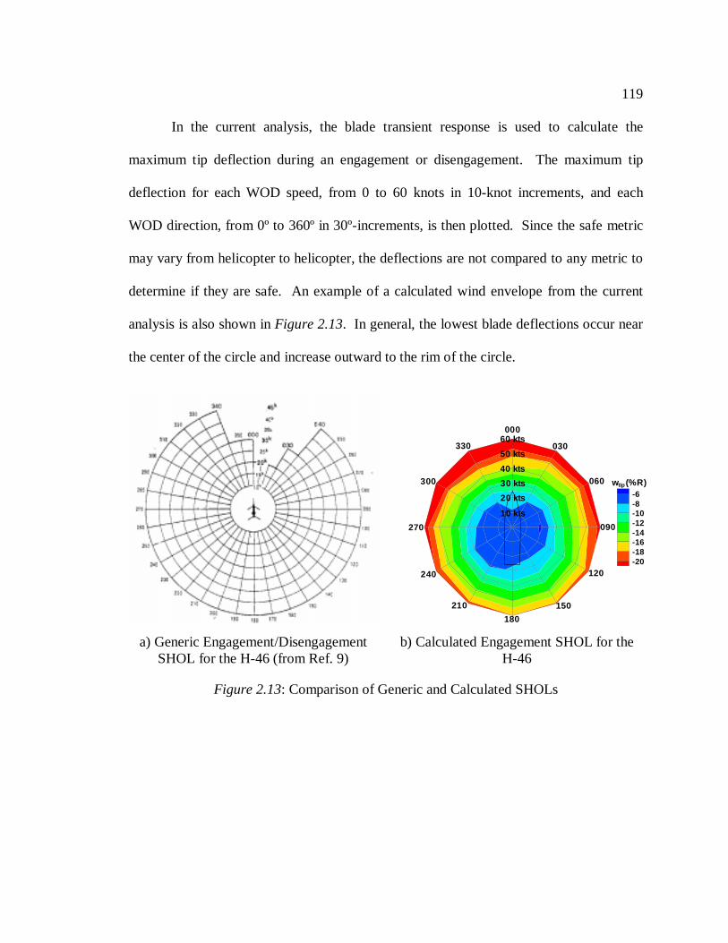
119
In the current analysis, the blade transient response is used to calculate the
maximum tip deflection during an engagement or disengagement. The maximum tip
deflection for each WOD speed, from 0 to 60 knots in 10-knot increments, and each
WOD direction, from 0º to 360º in 30º-increments, is then plotted. Since the safe metric
may vary from helicopter to helicopter, the deflections are not compared to any metric to
determine if they are safe. An example of a calculated wind envelope from the current
analysis is also shown inFigure 2.13. In general, the lowest blade deflections occur near
the center of the circle and increase outward to the rim of the circle.
a) Generic Engagement/DisengagementSHOL for the H-46 (from Ref. 9)
-6-8-10-12-14-16-18-20
w (%R)tip
10 kts
33050 kts
40 kts
30 kts
20 kts
60 kts000
060
030
090
120
150
180
210
240
270
300
b) Calculated Engagement SHOL for theH-46
Figure 2.13: Comparison of Generic and Calculated SHOLs
120
Chapter 3
BASELINE RESULTS
The purpose of this chapter is to determine the level of detail required in the
modeling of engagement and disengagement operations. This is accomplished by
examining the transient response of a generic, or “baseline”, rotor system during rotor
engagements and disengagements. There are four sections in this chapter. The level of
fidelity necessary in the structural model and the aerodynamic model are examined in the
first and second sections. The effect of ship airwakes and the blade initial conditions are
presented in the third and fourth sections.
3.1 Baseline Rotor System Properties
The structural properties of the baseline rotor system used in the simulations are
listed in Appendix B.1. The baseline rotor system is representative of an articulated rotor
system for a medium-sized naval helicopter. The rotor speed profile during both rotor
engagements and disengagements is assumed a simple offset sine wave
( ) ( )( )( ) ( )( )
12 20
12 20
cos 1
cos 1
t
t
t engagement
t disengagement
π π
π
Ω = + +
Ω = +( 3.1 )
Where time is measured in seconds and the rotor speed is nondimensional. The rotor
accelerates to or from full rotor speed in 20 seconds as shown inFigure 3.1. This rotor
speed profile is very similar to the H-46 rotor speed profile.
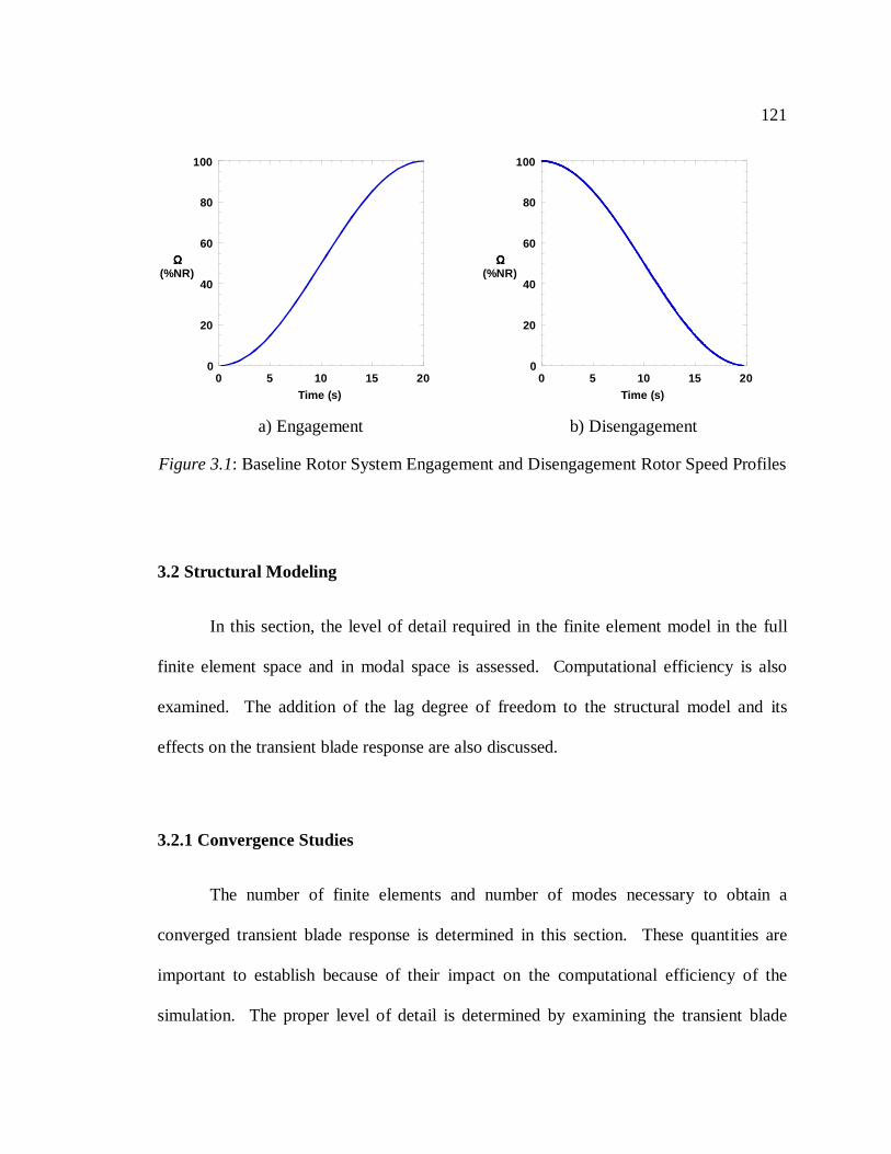
121
3.2 Structural Modeling
In this section, the level of detail required in the finite element model in the full
finite element space and in modal space is assessed. Computational efficiency is also
examined. The addition of the lag degree of freedom to the structural model and its
effects on the transient blade response are also discussed.
3.2.1 Convergence Studies
The number of finite elements and number of modes necessary to obtain a
converged transient blade response is determined in this section. These quantities are
important to establish because of their impact on the computational efficiency of the
simulation. The proper level of detail is determined by examining the transient blade
0
20
40
60
80
100
0 5 10 15 20
ΩΩΩΩ(%NR)
Time (s)
a) Engagement
0
20
40
60
80
100
0 5 10 15 20
ΩΩΩΩ(%NR)
Time (s)
b) Disengagement
Figure 3.1: Baseline Rotor System Engagement and Disengagement Rotor Speed Profiles
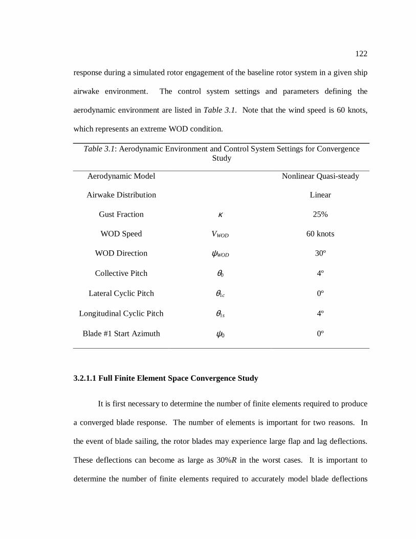
122
response during a simulated rotor engagement of the baseline rotor system in a given ship
airwake environment. The control system settings and parameters defining the
aerodynamic environment are listed inTable 3.1. Note that the wind speed is 60 knots,
which represents an extreme WOD condition.
3.2.1.1 Full Finite Element Space Convergence Study
It is first necessary to determine the number of finite elements required to produce
a converged blade response. The number of elements is important for two reasons. In
the event of blade sailing, the rotor blades may experience large flap and lag deflections.
These deflections can become as large as 30%R in the worst cases. It is important to
determine the number of finite elements required to accurately model blade deflections
Table 3.1: Aerodynamic Environment and Control System Settings for ConvergenceStudy
Aerodynamic Model Nonlinear Quasi-steady
Airwake Distribution Linear
Gust Fraction κ 25%
WOD Speed VWOD 60 knots
WOD Direction ψWOD 30º
Collective Pitch θ0 4º
Lateral Cyclic Pitch θ1c 0º
Longitudinal Cyclic Pitch θ1s 4º
Blade #1 Start Azimuth ψ0 0º
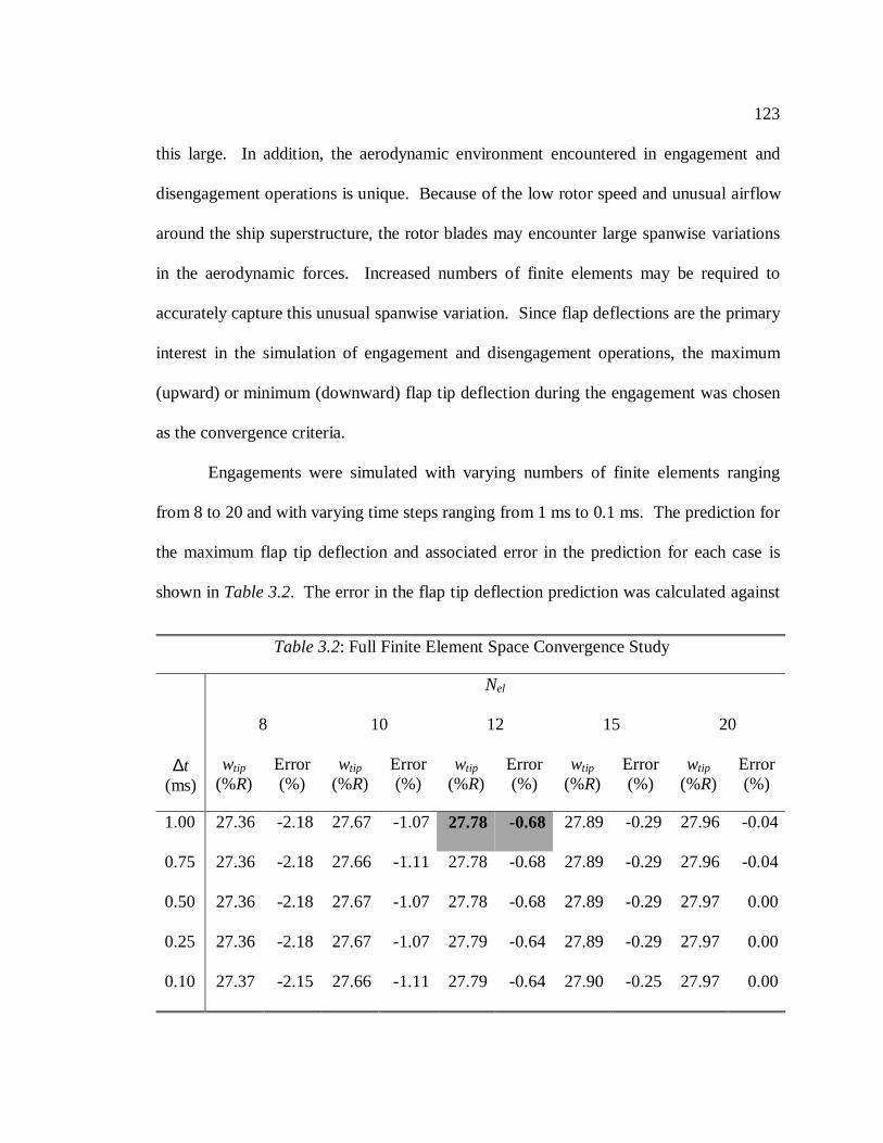
123
this large. In addition, the aerodynamic environment encountered in engagement and
disengagement operations is unique. Because of the low rotor speed and unusual airflow
around the ship superstructure, the rotor blades may encounter large spanwise variations
in the aerodynamic forces. Increased numbers of finite elements may be required to
accurately capture this unusual spanwise variation. Since flap deflections are the primary
interest in the simulation of engagement and disengagement operations, the maximum
(upward) or minimum (downward) flap tip deflection during the engagement was chosen
as the convergence criteria.
Engagements were simulated with varying numbers of finite elements ranging
from 8 to 20 and with varying time steps ranging from 1 ms to 0.1 ms. The prediction for
the maximum flap tip deflection and associated error in the prediction for each case is
shown inTable 3.2. The error in the flap tip deflection prediction was calculated against
Table 3.2: Full Finite Element Space Convergence Study
Nel
8 10 12 15 20
∆t(ms)
wtip
(%R)Error(%)
wtip
(%R)Error(%)
wtip
(%R)Error(%)
wtip
(%R)Error(%)
wtip
(%R)Error(%)
1.00 27.36 -2.18 27.67 -1.0727.78 -0.68 27.89 -0.29 27.96 -0.04
0.75 27.36 -2.18 27.66 -1.11 27.78 -0.68 27.89 -0.29 27.96 -0.04
0.50 27.36 -2.18 27.67 -1.07 27.78 -0.68 27.89 -0.29 27.97 0.00
0.25 27.36 -2.18 27.67 -1.07 27.79 -0.64 27.89 -0.29 27.97 0.00
0.10 27.37 -2.15 27.66 -1.11 27.79 -0.64 27.90 -0.25 27.97 0.00
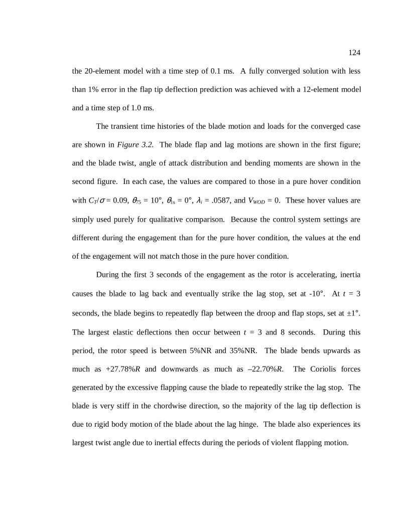
124
the 20-element model with a time step of 0.1 ms. A fully converged solution with less
than 1% error in the flap tip deflection prediction was achieved with a 12-element model
and a time step of 1.0 ms.
The transient time histories of the blade motion and loads for the converged case
are shown inFigure 3.2. The blade flap and lag motions are shown in the first figure;
and the blade twist, angle of attack distribution and bending moments are shown in the
second figure. In each case, the values are compared to those in a pure hover condition
with CT/σ = 0.09,θ75 = 10°, θ1s = 0°, λi = .0587, andVWOD = 0. These hover values are
simply used purely for qualitative comparison. Because the control system settings are
different during the engagement than for the pure hover condition, the values at the end
of the engagement will not match those in the pure hover condition.
During the first 3 seconds of the engagement as the rotor is accelerating, inertia
causes the blade to lag back and eventually strike the lag stop, set at -10°. At t = 3
seconds, the blade begins to repeatedly flap between the droop and flap stops, set at ±1°.
The largest elastic deflections then occur betweent = 3 and 8 seconds. During this
period, the rotor speed is between 5%NR and 35%NR. The blade bends upwards as
much as +27.78%R and downwards as much as –22.70%R. The Coriolis forces
generated by the excessive flapping cause the blade to repeatedly strike the lag stop. The
blade is very stiff in the chordwise direction, so the majority of the lag tip deflection is
due to rigid body motion of the blade about the lag hinge. The blade also experiences its
largest twist angle due to inertial effects during the periods of violent flapping motion.
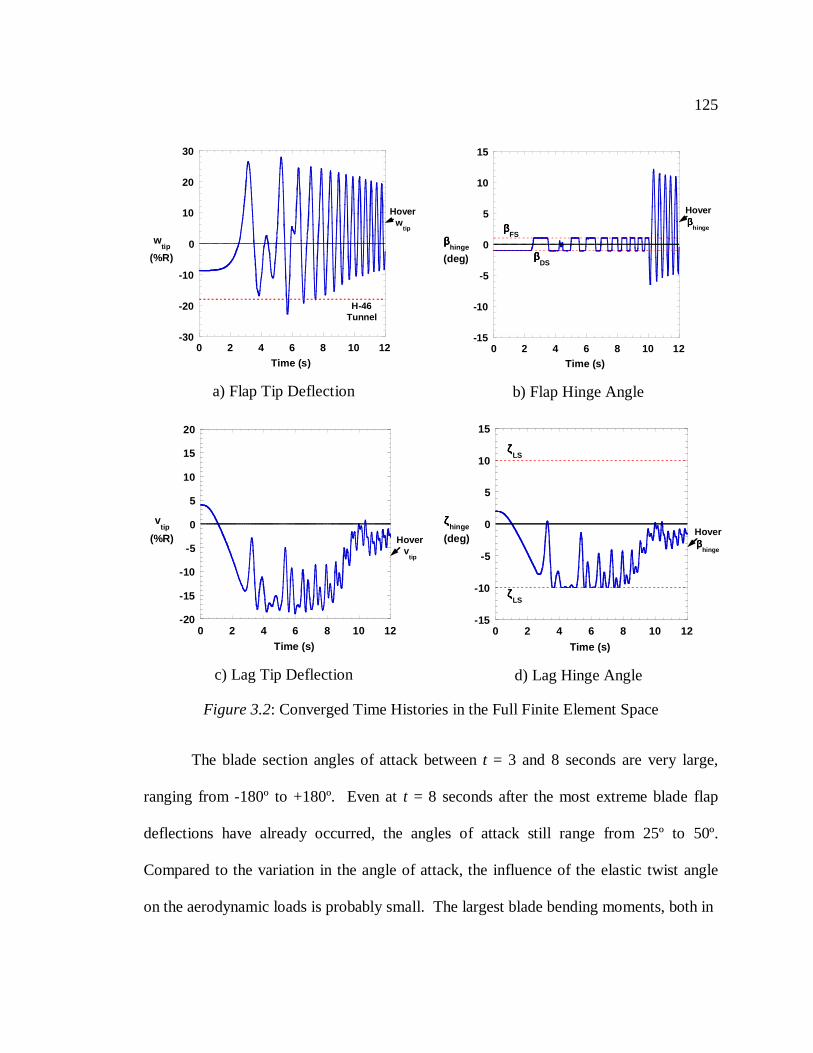
125
The blade section angles of attack betweent = 3 and 8 seconds are very large,
ranging from -180º to +180º. Even att = 8 seconds after the most extreme blade flap
deflections have already occurred, the angles of attack still range from 25º to 50º.
Compared to the variation in the angle of attack, the influence of the elastic twist angle
on the aerodynamic loads is probably small. The largest blade bending moments, both in
-30
-20
-10
0
10
20
30
0 2 4 6 8 10 12
wtip
(%R)
Time (s)
H-46Tunnel
Hoverw
tip
a) Flap Tip Deflection
-15
-10
-5
0
5
10
15
0 2 4 6 8 10 12
ββββhinge
(deg)
Time (s)
ββββDS
ββββFS
Hoverββββ
hinge
b) Flap Hinge Angle
-20
-15
-10
-5
0
5
10
15
20
0 2 4 6 8 10 12
vtip
(%R)
Time (s)
Hoverv
tip
c) Lag Tip Deflection
-15
-10
-5
0
5
10
15
0 2 4 6 8 10 12
ζζζζhinge
(deg)
Time (s)
ζζζζLS
ζζζζLS
Hoverββββ
hinge
d) Lag Hinge Angle
Figure 3.2: Converged Time Histories in the Full Finite Element Space
126
the normal and chordwise directions, also occur in this region. Flap bending moments
reach peak values of -21610 ft-lb at the blade root and -8196 ft-lb at the blade attachment
point. These transient values are 5.9 and 4.6 times higher than their values in hover of
-3678 ft-lb and -1787 ft-lb. Lag bending moments reach -16430 ft-lb at the blade root
and -11170 ft-lb at the blade attachment point. These transient values are 2.2 and 40
times higher than their values in hover of -7269 ft-lb and -280 ft-lb. As the blade
-2
-1
0
1
2
0 2 4 6 8 10 12
φφφφtip
(deg)
Time (s)
Hoverφφφφ
tip
e) Tip Twist Angle
-180
-135
-90
-45
0
45
90
135
180
0 2 4 6 8 10 12
50%R75%R95%R
αααα(deg)
Time (s)
f) Angle of Attack
-30000
-20000
-10000
0
10000
20000
30000
0 2 4 6 8 10 12
Blade Root (0%R)
Blade Attachment (25%R)
Mηηηη
(ft-lb)
Time (s)
HoverLoads
g) Normal Bending Moment
-30000
-20000
-10000
0
10000
20000
30000
0 2 4 6 8 10 12
Blade Root (0%R)Blade Attachment (25%R)
Mζζζζ
(ft-lb)
Time (s)
HoverLoads
h) Chordwise Bending Moment
Figure 3.2: Converged Time Histories in the Full Finite Element Space
127
continues to accelerate and centrifugal forces increase, the blade deflections decrease. At
t = 10 seconds, the rotor reaches 50%NR. At this point the flap stops retract, so the blade
is allowed to flap freely. However, enough centrifugal force has built up to prevent the
blade deflections from becoming larger than in the low rotor speed region. Centrifugal
force has also become large enough to rotate the blade forward off the lag stop. Blade
bending moments decrease substantially after impacts between the blade and the flap and
lag stops cease.
3.2.1.2 Modal Space Convergence Study
It is not always convenient to simulate engagement and disengagement operations
in the full finite element space. The transient integration process involves mathematical
manipulations of large matrices that are computationally expensive. A modal space
transformation is commonly used to reduce the size of the matrices and improve
computational efficiency. When using a modal transformation, it is necessary to
determine the number of modes that are necessary to approximate the blade transient
response. In this section, studies are conducted to determine the number of modes
required to obtain a converged solution in modal space. Furthermore, the efficiency of
the different time integration techniques discussed in Chapter 2 is also examined. In the
second section, the effect of the rotor speed at which the modal matrix and mode shapes
are calculated is discussed.
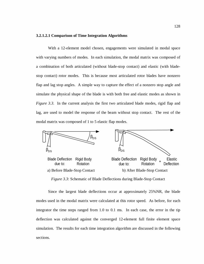
128
3.2.1.2.1 Comparison of Time Integration Algorithms
With a 12-element model chosen, engagements were simulated in modal space
with varying numbers of modes. In each simulation, the modal matrix was composed of
a combination of both articulated (without blade-stop contact) and elastic (with blade-
stop contact) rotor modes. This is because most articulated rotor blades have nonzero
flap and lag stop angles. A simple way to capture the effect of a nonzero stop angle and
simulate the physical shape of the blade is with both free and elastic modes as shown in
Figure 3.3. In the current analysis the first two articulated blade modes, rigid flap and
lag, are used to model the response of the beam without stop contact. The rest of the
modal matrix was composed of 1 to 5 elastic flap modes.
Since the largest blade deflections occur at approximately 25%NR, the blade
modes used in the modal matrix were calculated at this rotor speed. As before, for each
integrator the time steps ranged from 1.0 to 0.1 ms. In each case, the error in the tip
deflection was calculated against the converged 12-element full finite element space
simulation. The results for each time integration algorithm are discussed in the following
sections.
βDS
βDS
Blade Deflectiondue to:
Rigid BodyRotation
a) Before Blade-Stop Contact
βDS
Blade Deflectiondue to:
Rigid BodyRotation
ElasticDeflection+
b) After Blade-Stop Contact
Figure 3.3: Schematic of Blade Deflections during Blade-Stop Contact
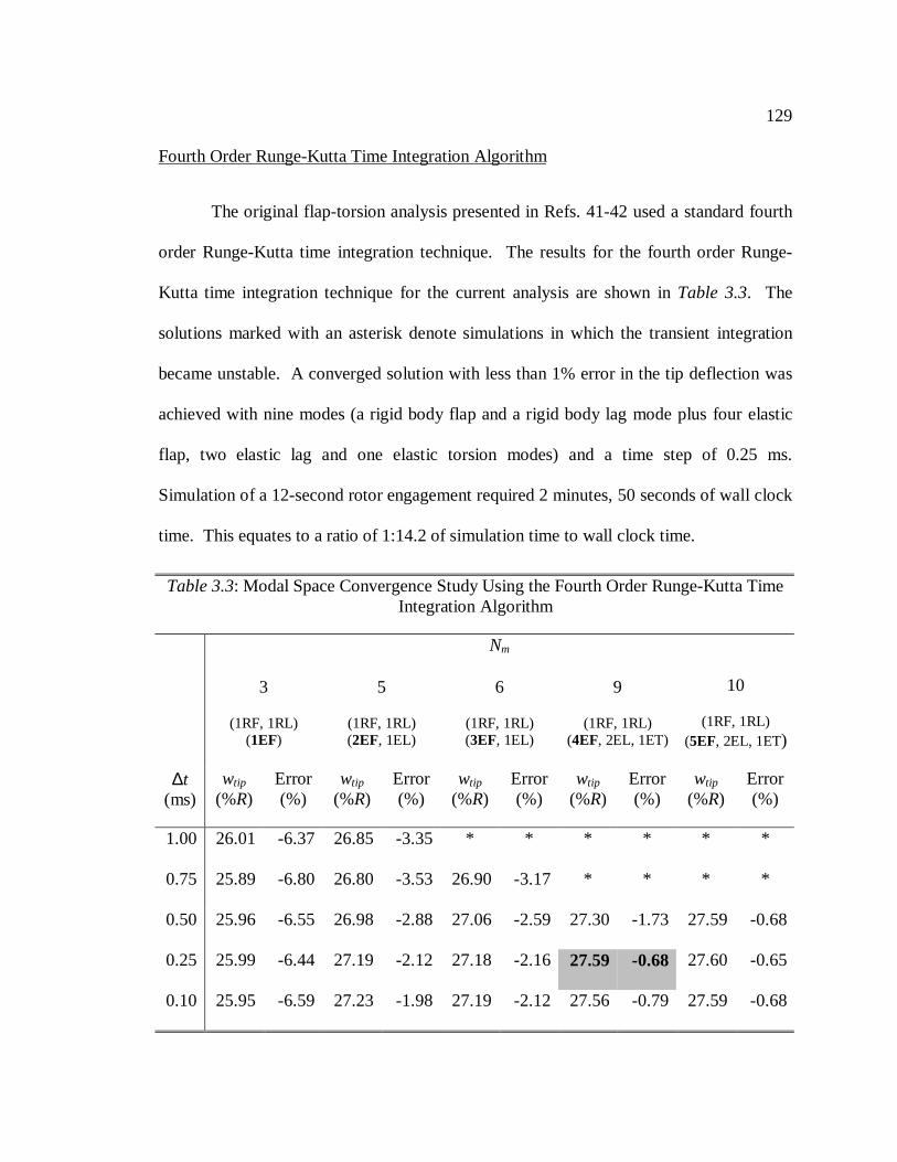
129
Fourth Order Runge-Kutta Time Integration Algorithm
The original flap-torsion analysis presented in Refs. 41-42 used a standard fourth
order Runge-Kutta time integration technique. The results for the fourth order Runge-
Kutta time integration technique for the current analysis are shown inTable 3.3. The
solutions marked with an asterisk denote simulations in which the transient integration
became unstable. A converged solution with less than 1% error in the tip deflection was
achieved with nine modes (a rigid body flap and a rigid body lag mode plus four elastic
flap, two elastic lag and one elastic torsion modes) and a time step of 0.25 ms.
Simulation of a 12-second rotor engagement required 2 minutes, 50 seconds of wall clock
time. This equates to a ratio of 1:14.2 of simulation time to wall clock time.
Table 3.3: Modal Space Convergence Study Using the Fourth Order Runge-Kutta TimeIntegration Algorithm
Nm
3
(1RF, 1RL)(1EF)
5
(1RF, 1RL)(2EF, 1EL)
6
(1RF, 1RL)(3EF, 1EL)
9
(1RF, 1RL)(4EF, 2EL, 1ET)
10
(1RF, 1RL)(5EF, 2EL, 1ET)
∆t(ms)
wtip
(%R)Error(%)
wtip
(%R)Error(%)
wtip
(%R)Error(%)
wtip
(%R)Error(%)
wtip
(%R)Error(%)
1.00 26.01 -6.37 26.85 -3.35 * * * * * *
0.75 25.89 -6.80 26.80 -3.53 26.90 -3.17 * * * *
0.50 25.96 -6.55 26.98 -2.88 27.06 -2.59 27.30 -1.73 27.59 -0.68
0.25 25.99 -6.44 27.19 -2.12 27.18 -2.1627.59 -0.68 27.60 -0.65
0.10 25.95 -6.59 27.23 -1.98 27.19 -2.12 27.56 -0.79 27.59 -0.68
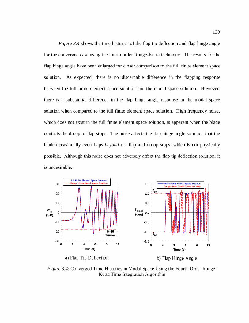
130
Figure 3.4shows the time histories of the flap tip deflection and flap hinge angle
for the converged case using the fourth order Runge-Kutta technique. The results for the
flap hinge angle have been enlarged for closer comparison to the full finite element space
solution. As expected, there is no discernable difference in the flapping response
between the full finite element space solution and the modal space solution. However,
there is a substantial difference in the flap hinge angle response in the modal space
solution when compared to the full finite element space solution. High frequency noise,
which does not exist in the full finite element space solution, is apparent when the blade
contacts the droop or flap stops. The noise affects the flap hinge angle so much that the
blade occasionally even flapsbeyondthe flap and droop stops, which is not physically
possible. Although this noise does not adversely affect the flap tip deflection solution, it
is undesirable.
-30
-20
-10
0
10
20
30
0 2 4 6 8 10
Full Finite Element Space SolutionRunge-Kutta Modal Space Soultion
wtip
(%R)
Time (s)
H-46Tunnel
a) Flap Tip Deflection
-1.5
-1.0
-0.5
0.0
0.5
1.0
1.5
0 2 4 6 8 10
Full Finite Element Space SolutionRunge-Kutta Modal Space Solution
ββββhinge
(deg)
Time (s)
ββββFS
ββββDS
b) Flap Hinge Angle
Figure 3.4: Converged Time Histories in Modal Space Using the Fourth Order Runge-Kutta Time Integration Algorithm
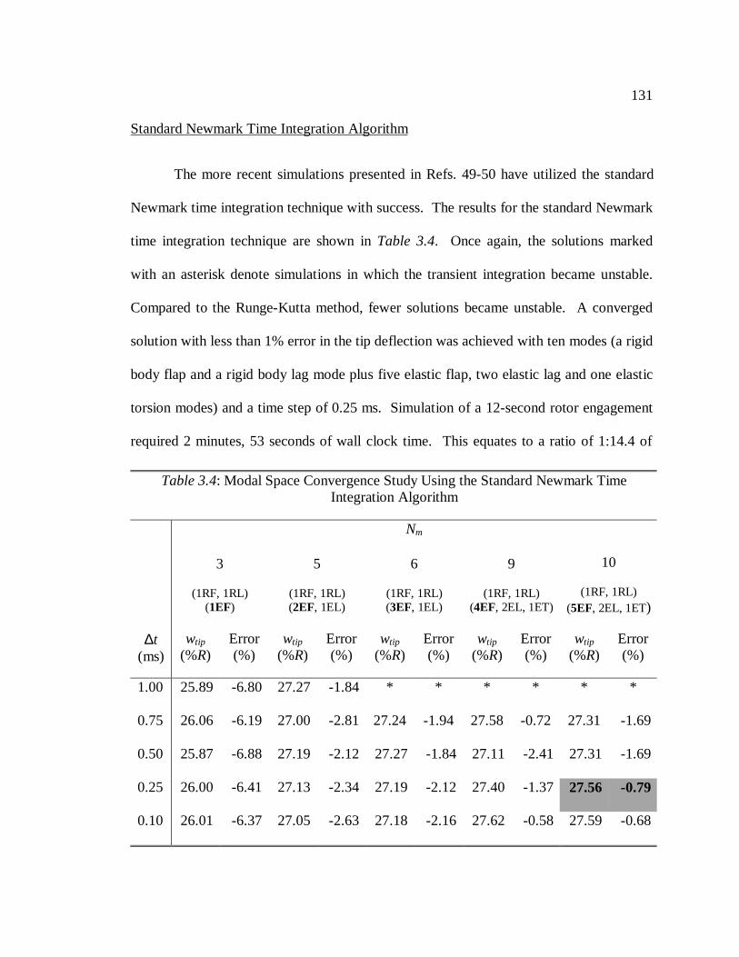
131
Standard Newmark Time Integration Algorithm
The more recent simulations presented in Refs. 49-50 have utilized the standard
Newmark time integration technique with success. The results for the standard Newmark
time integration technique are shown inTable 3.4. Once again, the solutions marked
with an asterisk denote simulations in which the transient integration became unstable.
Compared to the Runge-Kutta method, fewer solutions became unstable. A converged
solution with less than 1% error in the tip deflection was achieved with ten modes (a rigid
body flap and a rigid body lag mode plus five elastic flap, two elastic lag and one elastic
torsion modes) and a time step of 0.25 ms. Simulation of a 12-second rotor engagement
required 2 minutes, 53 seconds of wall clock time. This equates to a ratio of 1:14.4 of
Table 3.4: Modal Space Convergence Study Using the Standard Newmark TimeIntegration Algorithm
Nm
3
(1RF, 1RL)(1EF)
5
(1RF, 1RL)(2EF, 1EL)
6
(1RF, 1RL)(3EF, 1EL)
9
(1RF, 1RL)(4EF, 2EL, 1ET)
10
(1RF, 1RL)(5EF, 2EL, 1ET)
∆t(ms)
wtip
(%R)Error(%)
wtip
(%R)Error(%)
wtip
(%R)Error(%)
wtip
(%R)Error(%)
wtip
(%R)Error(%)
1.00 25.89 -6.80 27.27 -1.84 * * * * * *
0.75 26.06 -6.19 27.00 -2.81 27.24 -1.94 27.58 -0.72 27.31 -1.69
0.50 25.87 -6.88 27.19 -2.12 27.27 -1.84 27.11 -2.41 27.31 -1.69
0.25 26.00 -6.41 27.13 -2.34 27.19 -2.12 27.40 -1.3727.56 -0.79
0.10 26.01 -6.37 27.05 -2.63 27.18 -2.16 27.62 -0.58 27.59 -0.68
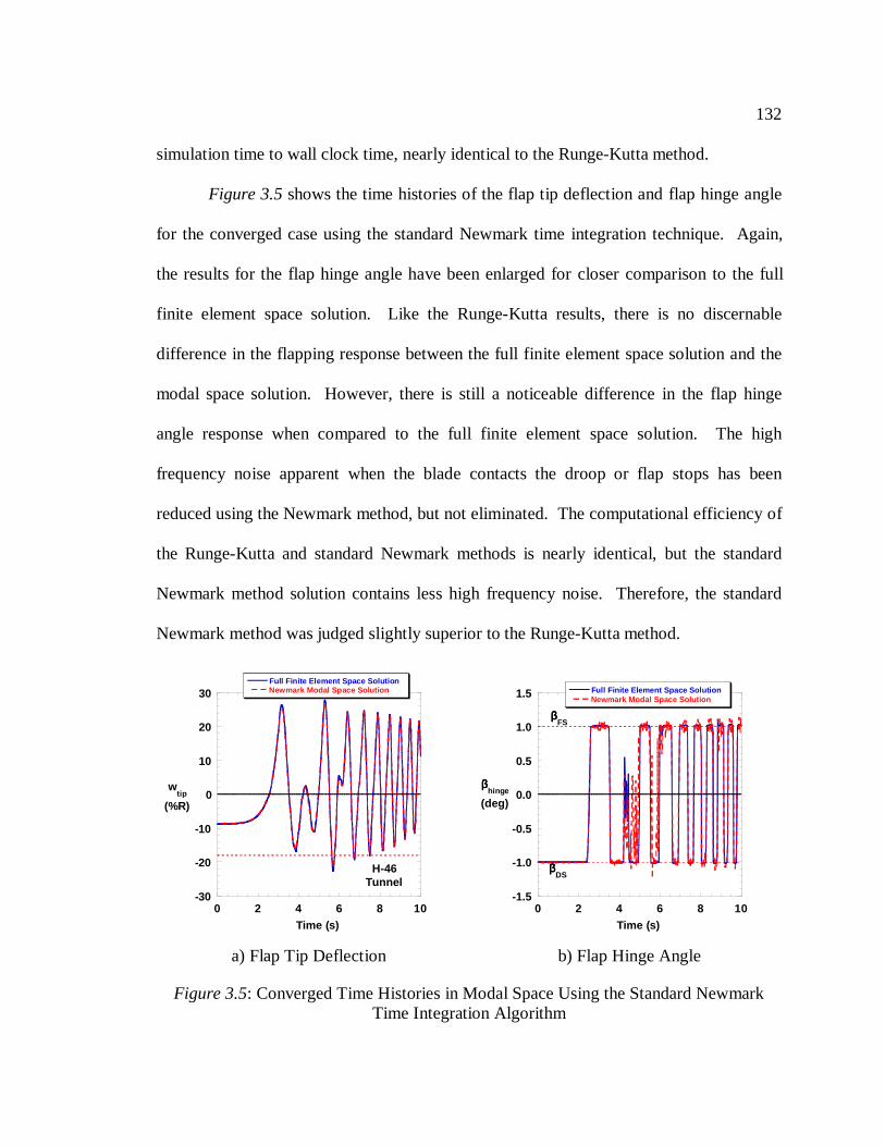
132
simulation time to wall clock time, nearly identical to the Runge-Kutta method.
Figure 3.5shows the time histories of the flap tip deflection and flap hinge angle
for the converged case using the standard Newmark time integration technique. Again,
the results for the flap hinge angle have been enlarged for closer comparison to the full
finite element space solution. Like the Runge-Kutta results, there is no discernable
difference in the flapping response between the full finite element space solution and the
modal space solution. However, there is still a noticeable difference in the flap hinge
angle response when compared to the full finite element space solution. The high
frequency noise apparent when the blade contacts the droop or flap stops has been
reduced using the Newmark method, but not eliminated. The computational efficiency of
the Runge-Kutta and standard Newmark methods is nearly identical, but the standard
Newmark method solution contains less high frequency noise. Therefore, the standard
Newmark method was judged slightly superior to the Runge-Kutta method.
-30
-20
-10
0
10
20
30
0 2 4 6 8 10
Full Finite Element Space SolutionNewmark Modal Space Solution
wtip
(%R)
Time (s)
H-46Tunnel
a) Flap Tip Deflection
-1.5
-1.0
-0.5
0.0
0.5
1.0
1.5
0 2 4 6 8 10
Full Finite Element Space SolutionNewmark Modal Space Solution
ββββhinge
(deg)
Time (s)
ββββFS
ββββDS
b) Flap Hinge Angle
Figure 3.5: Converged Time Histories in Modal Space Using the Standard NewmarkTime Integration Algorithm
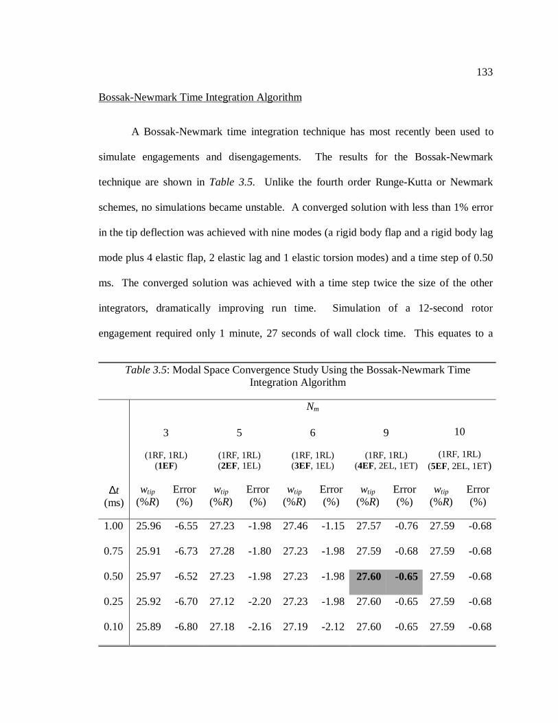
133
Bossak-Newmark Time Integration Algorithm
A Bossak-Newmark time integration technique has most recently been used to
simulate engagements and disengagements. The results for the Bossak-Newmark
technique are shown inTable 3.5. Unlike the fourth order Runge-Kutta or Newmark
schemes, no simulations became unstable. A converged solution with less than 1% error
in the tip deflection was achieved with nine modes (a rigid body flap and a rigid body lag
mode plus 4 elastic flap, 2 elastic lag and 1 elastic torsion modes) and a time step of 0.50
ms. The converged solution was achieved with a time step twice the size of the other
integrators, dramatically improving run time. Simulation of a 12-second rotor
engagement required only 1 minute, 27 seconds of wall clock time. This equates to a
Table 3.5: Modal Space Convergence Study Using the Bossak-Newmark TimeIntegration Algorithm
Nm
3
(1RF, 1RL)(1EF)
5
(1RF, 1RL)(2EF, 1EL)
6
(1RF, 1RL)(3EF, 1EL)
9
(1RF, 1RL)(4EF, 2EL, 1ET)
10
(1RF, 1RL)(5EF, 2EL, 1ET)
∆t(ms)
wtip
(%R)Error(%)
wtip
(%R)Error(%)
wtip
(%R)Error(%)
wtip
(%R)Error(%)
wtip
(%R)Error(%)
1.00 25.96 -6.55 27.23 -1.98 27.46 -1.15 27.57 -0.76 27.59 -0.68
0.75 25.91 -6.73 27.28 -1.80 27.23 -1.98 27.59 -0.68 27.59 -0.68
0.50 25.97 -6.52 27.23 -1.98 27.23 -1.9827.60 -0.65 27.59 -0.68
0.25 25.92 -6.70 27.12 -2.20 27.23 -1.98 27.60 -0.65 27.59 -0.68
0.10 25.89 -6.80 27.18 -2.16 27.19 -2.12 27.60 -0.65 27.59 -0.68
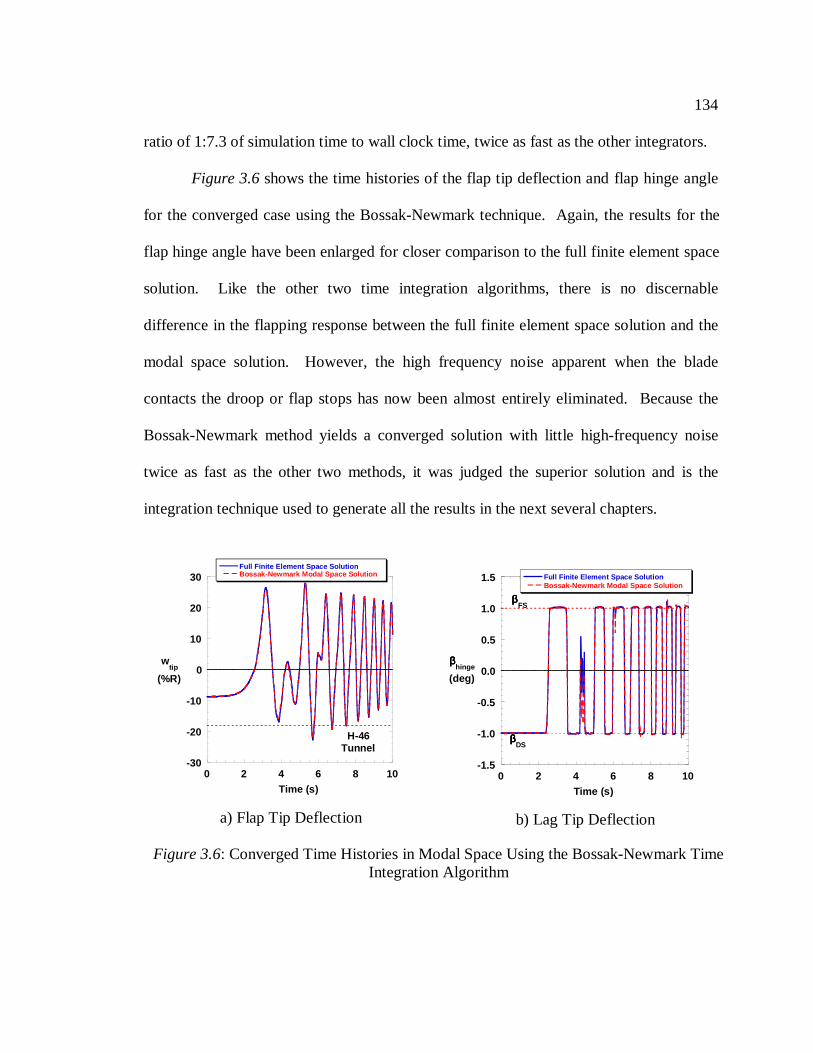
134
ratio of 1:7.3 of simulation time to wall clock time, twice as fast as the other integrators.
Figure 3.6shows the time histories of the flap tip deflection and flap hinge angle
for the converged case using the Bossak-Newmark technique. Again, the results for the
flap hinge angle have been enlarged for closer comparison to the full finite element space
solution. Like the other two time integration algorithms, there is no discernable
difference in the flapping response between the full finite element space solution and the
modal space solution. However, the high frequency noise apparent when the blade
contacts the droop or flap stops has now been almost entirely eliminated. Because the
Bossak-Newmark method yields a converged solution with little high-frequency noise
twice as fast as the other two methods, it was judged the superior solution and is the
integration technique used to generate all the results in the next several chapters.
-30
-20
-10
0
10
20
30
0 2 4 6 8 10
Full Finite Element Space SolutionBossak-Newmark Modal Space Solution
wtip
(%R)
Time (s)
H-46Tunnel
a) Flap Tip Deflection
-1.5
-1.0
-0.5
0.0
0.5
1.0
1.5
0 2 4 6 8 10
Full Finite Element Space SolutionBossak-Newmark Modal Space Solution
ββββhinge
(deg)
Time (s)
ββββFS
ββββDS
b) Lag Tip Deflection
Figure 3.6: Converged Time Histories in Modal Space Using the Bossak-Newmark TimeIntegration Algorithm
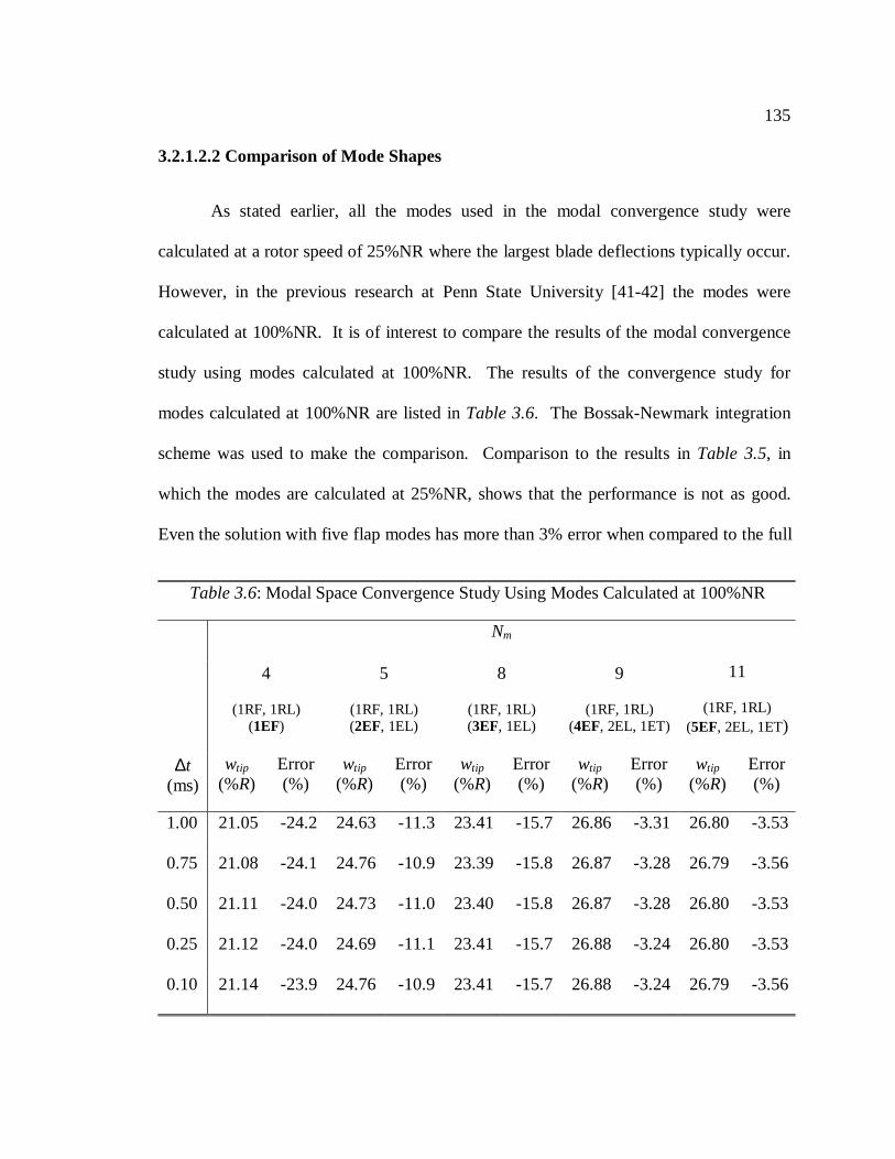
135
3.2.1.2.2 Comparison of Mode Shapes
As stated earlier, all the modes used in the modal convergence study were
calculated at a rotor speed of 25%NR where the largest blade deflections typically occur.
However, in the previous research at Penn State University [41-42] the modes were
calculated at 100%NR. It is of interest to compare the results of the modal convergence
study using modes calculated at 100%NR. The results of the convergence study for
modes calculated at 100%NR are listed inTable 3.6. The Bossak-Newmark integration
scheme was used to make the comparison. Comparison to the results inTable 3.5, in
which the modes are calculated at 25%NR, shows that the performance is not as good.
Even the solution with five flap modes has more than 3% error when compared to the full
Table 3.6: Modal Space Convergence Study Using Modes Calculated at 100%NR
Nm
4
(1RF, 1RL)(1EF)
5
(1RF, 1RL)(2EF, 1EL)
8
(1RF, 1RL)(3EF, 1EL)
9
(1RF, 1RL)(4EF, 2EL, 1ET)
11
(1RF, 1RL)(5EF, 2EL, 1ET)
∆t(ms)
wtip
(%R)Error(%)
wtip
(%R)Error(%)
wtip
(%R)Error(%)
wtip
(%R)Error(%)
wtip
(%R)Error(%)
1.00 21.05 -24.2 24.63 -11.3 23.41 -15.7 26.86 -3.31 26.80 -3.53
0.75 21.08 -24.1 24.76 -10.9 23.39 -15.8 26.87 -3.28 26.79 -3.56
0.50 21.11 -24.0 24.73 -11.0 23.40 -15.8 26.87 -3.28 26.80 -3.53
0.25 21.12 -24.0 24.69 -11.1 23.41 -15.7 26.88 -3.24 26.80 -3.53
0.10 21.14 -23.9 24.76 -10.9 23.41 -15.7 26.88 -3.24 26.79 -3.56
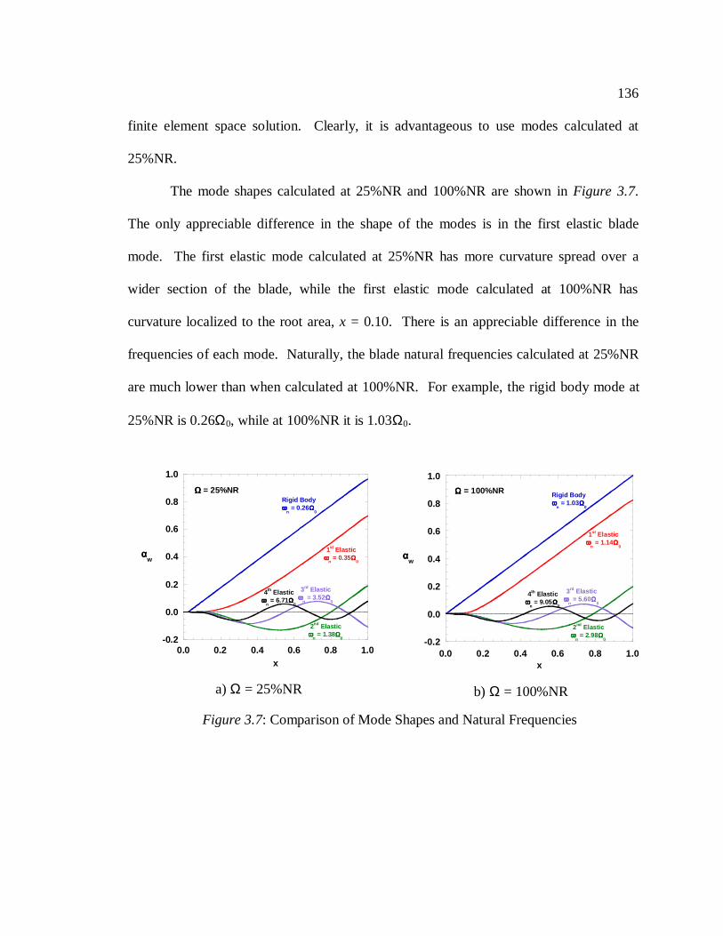
136
finite element space solution. Clearly, it is advantageous to use modes calculated at
25%NR.
The mode shapes calculated at 25%NR and 100%NR are shown inFigure 3.7.
The only appreciable difference in the shape of the modes is in the first elastic blade
mode. The first elastic mode calculated at 25%NR has more curvature spread over a
wider section of the blade, while the first elastic mode calculated at 100%NR has
curvature localized to the root area,x = 0.10. There is an appreciable difference in the
frequencies of each mode. Naturally, the blade natural frequencies calculated at 25%NR
are much lower than when calculated at 100%NR. For example, the rigid body mode at
25%NR is 0.26Ω0, while at 100%NR it is 1.03Ω0.
-0.2
0.0
0.2
0.4
0.6
0.8
1.0
0.0 0.2 0.4 0.6 0.8 1.0
ααααw
x
Rigid Bodyωωωω
n= 0.26ΩΩΩΩ
0
4th Elasticωωωω
n= 6.71ΩΩΩΩ
0
3rd Elasticωωωω
n= 3.52ΩΩΩΩ
0
2nd Elasticωωωω
n= 1.38ΩΩΩΩ
0
1st Elasticωωωω
n= 0.35ΩΩΩΩ
0
ΩΩΩΩ = 25%NR
a) Ω = 25%NR
-0.2
0.0
0.2
0.4
0.6
0.8
1.0
0.0 0.2 0.4 0.6 0.8 1.0
ααααw
x
Rigid Bodyωωωω
n= 1.03ΩΩΩΩ
0
4th Elasticωωωω
n= 9.05ΩΩΩΩ
0
3rd Elasticωωωω
n= 5.60ΩΩΩΩ
0
2nd Elasticωωωω
n= 2.98ΩΩΩΩ
0
1st Elasticωωωω
n= 1.14ΩΩΩΩ
0
ΩΩΩΩ = 100%NR
b) Ω = 100%NR
Figure 3.7: Comparison of Mode Shapes and Natural Frequencies
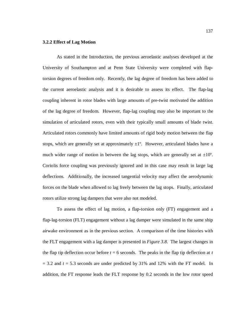
137
3.2.2 Effect of Lag Motion
As stated in the Introduction, the previous aeroelastic analyses developed at the
University of Southampton and at Penn State University were completed with flap-
torsion degrees of freedom only. Recently, the lag degree of freedom has been added to
the current aeroelastic analysis and it is desirable to assess its effect. The flap-lag
coupling inherent in rotor blades with large amounts of pre-twist motivated the addition
of the lag degree of freedom. However, flap-lag coupling may also be important to the
simulation of articulated rotors, even with their typically small amounts of blade twist.
Articulated rotors commonly have limited amounts of rigid body motion between the flap
stops, which are generally set at approximately ±1º. However, articulated blades have a
much wider range of motion in between the lag stops, which are generally set at ±10º.
Coriolis force coupling was previously ignored and in this case may result in large lag
deflections. Additionally, the increased tangential velocity may affect the aerodynamic
forces on the blade when allowed to lag freely between the lag stops. Finally, articulated
rotors utilize strong lag dampers that were also not modeled.
To assess the effect of lag motion, a flap-torsion only (FT) engagement and a
flap-lag-torsion (FLT) engagement without a lag damper were simulated in the same ship
airwake environment as in the previous section. A comparison of the time histories with
the FLT engagement with a lag damper is presented inFigure 3.8. The largest changes in
the flap tip deflection occur beforet = 6 seconds. The peaks in the flap tip deflection att
= 3.2 andt = 5.3 seconds are under predicted by 31% and 12% with the FT model. In
addition, the FT response leads the FLT response by 0.2 seconds in the low rotor speed
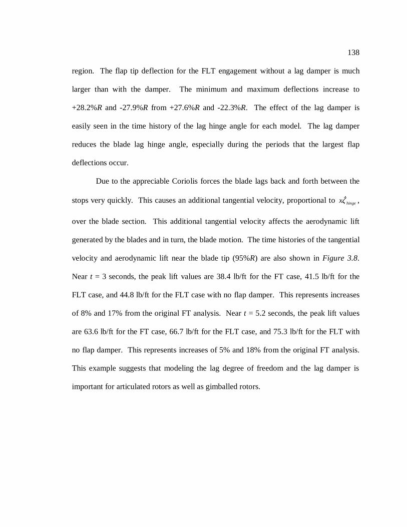
138
region. The flap tip deflection for the FLT engagement without a lag damper is much
larger than with the damper. The minimum and maximum deflections increase to
+28.2%R and -27.9%R from +27.6%R and -22.3%R. The effect of the lag damper is
easily seen in the time history of the lag hinge angle for each model. The lag damper
reduces the blade lag hinge angle, especially during the periods that the largest flap
deflections occur.
Due to the appreciable Coriolis forces the blade lags back and forth between the
stops very quickly. This causes an additional tangential velocity, proportional tohingexζ ,
over the blade section. This additional tangential velocity affects the aerodynamic lift
generated by the blades and in turn, the blade motion. The time histories of the tangential
velocity and aerodynamic lift near the blade tip (95%R) are also shown inFigure 3.8.
Near t = 3 seconds, the peak lift values are 38.4 lb/ft for the FT case, 41.5 lb/ft for the
FLT case, and 44.8 lb/ft for the FLT case with no flap damper. This represents increases
of 8% and 17% from the original FT analysis. Neart = 5.2 seconds, the peak lift values
are 63.6 lb/ft for the FT case, 66.7 lb/ft for the FLT case, and 75.3 lb/ft for the FLT with
no flap damper. This represents increases of 5% and 18% from the original FT analysis.
This example suggests that modeling the lag degree of freedom and the lag damper is
important for articulated rotors as well as gimballed rotors.
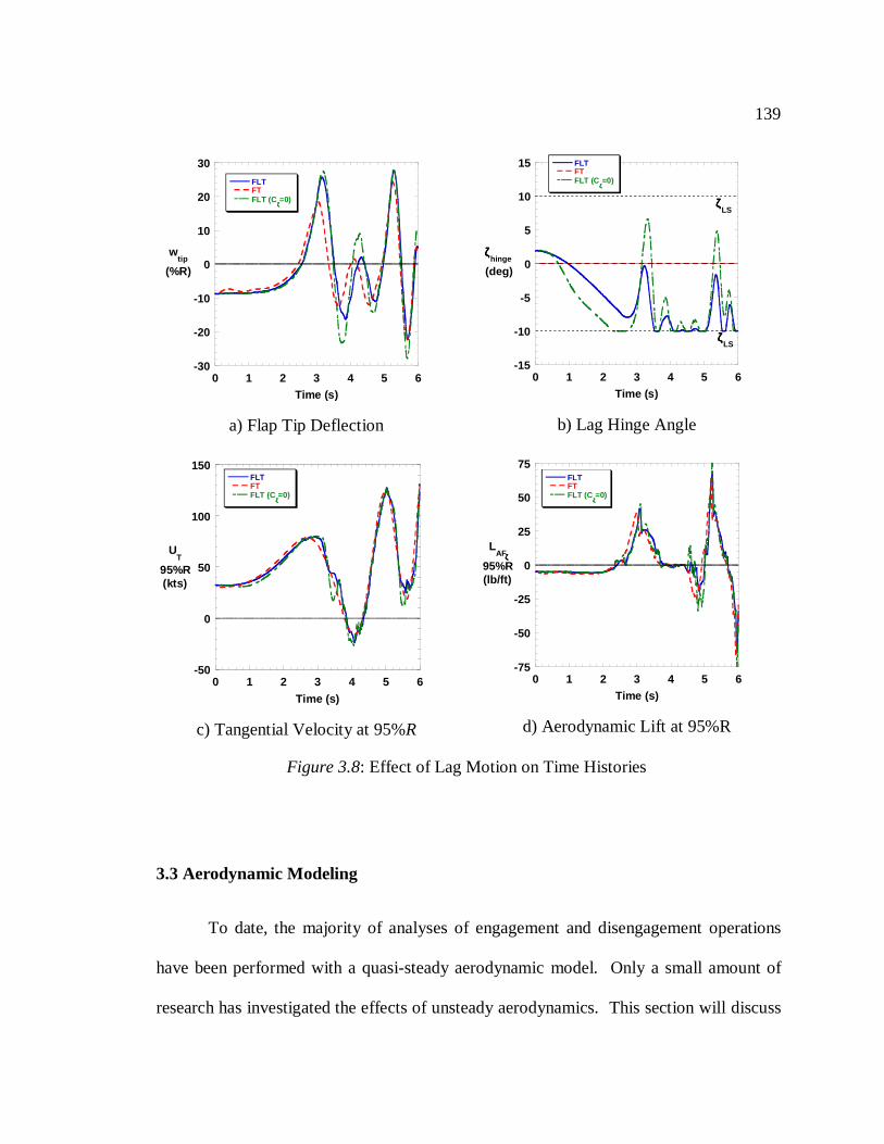
139
3.3 Aerodynamic Modeling
To date, the majority of analyses of engagement and disengagement operations
have been performed with a quasi-steady aerodynamic model. Only a small amount of
research has investigated the effects of unsteady aerodynamics. This section will discuss
-30
-20
-10
0
10
20
30
0 1 2 3 4 5 6
FLTFTFLT (C
ζζζζ=0)
wtip
(%R)
Time (s)
a) Flap Tip Deflection
-15
-10
-5
0
5
10
15
0 1 2 3 4 5 6
FLTFTFLT (C
ζζζζ=0)
ζζζζhinge
(deg)
Time (s)
ζζζζLS
ζζζζLS
b) Lag Hinge Angle
-50
0
50
100
150
0 1 2 3 4 5 6
FLTFTFLT (C
ζζζζ=0)
UT
95%R(kts)
Time (s)
c) Tangential Velocity at 95%R
-75
-50
-25
0
25
50
75
0 1 2 3 4 5 6
FLTFTFLT (C
ζζζζ=0)
LAF
95%R(lb/ft)
Time (s)
ζζζζ
d) Aerodynamic Lift at 95%R
Figure 3.8: Effect of Lag Motion on Time Histories
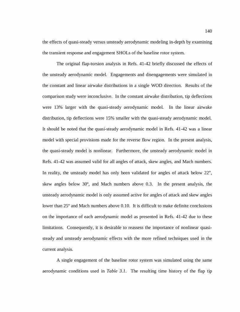
140
the effects of quasi-steady versus unsteady aerodynamic modeling in-depth by examining
the transient response and engagement SHOLs of the baseline rotor system.
The original flap-torsion analysis in Refs. 41-42 briefly discussed the effects of
the unsteady aerodynamic model. Engagements and disengagements were simulated in
the constant and linear airwake distributions in a single WOD direction. Results of the
comparison study were inconclusive. In the constant airwake distribution, tip deflections
were 13% larger with the quasi-steady aerodynamic model. In the linear airwake
distribution, tip deflections were 15% smaller with the quasi-steady aerodynamic model.
It should be noted that the quasi-steady aerodynamic model in Refs. 41-42 was a linear
model with special provisions made for the reverse flow region. In the present analysis,
the quasi-steady model is nonlinear. Furthermore, the unsteady aerodynamic model in
Refs. 41-42 was assumed valid for all angles of attack, skew angles, and Mach numbers.
In reality, the unsteady model has only been validated for angles of attack below 22°,
skew angles below 30º, and Mach numbers above 0.3. In the present analysis, the
unsteady aerodynamic model is only assumed active for angles of attack and skew angles
lower than 25º and Mach numbers above 0.10. It is difficult to make definite conclusions
on the importance of each aerodynamic model as presented in Refs. 41-42 due to these
limitations. Consequently, it is desirable to reassess the importance of nonlinear quasi-
steady and unsteady aerodynamic effects with the more refined techniques used in the
current analysis.
A single engagement of the baseline rotor system was simulated using the same
aerodynamic conditions used inTable 3.1. The resulting time history of the flap tip
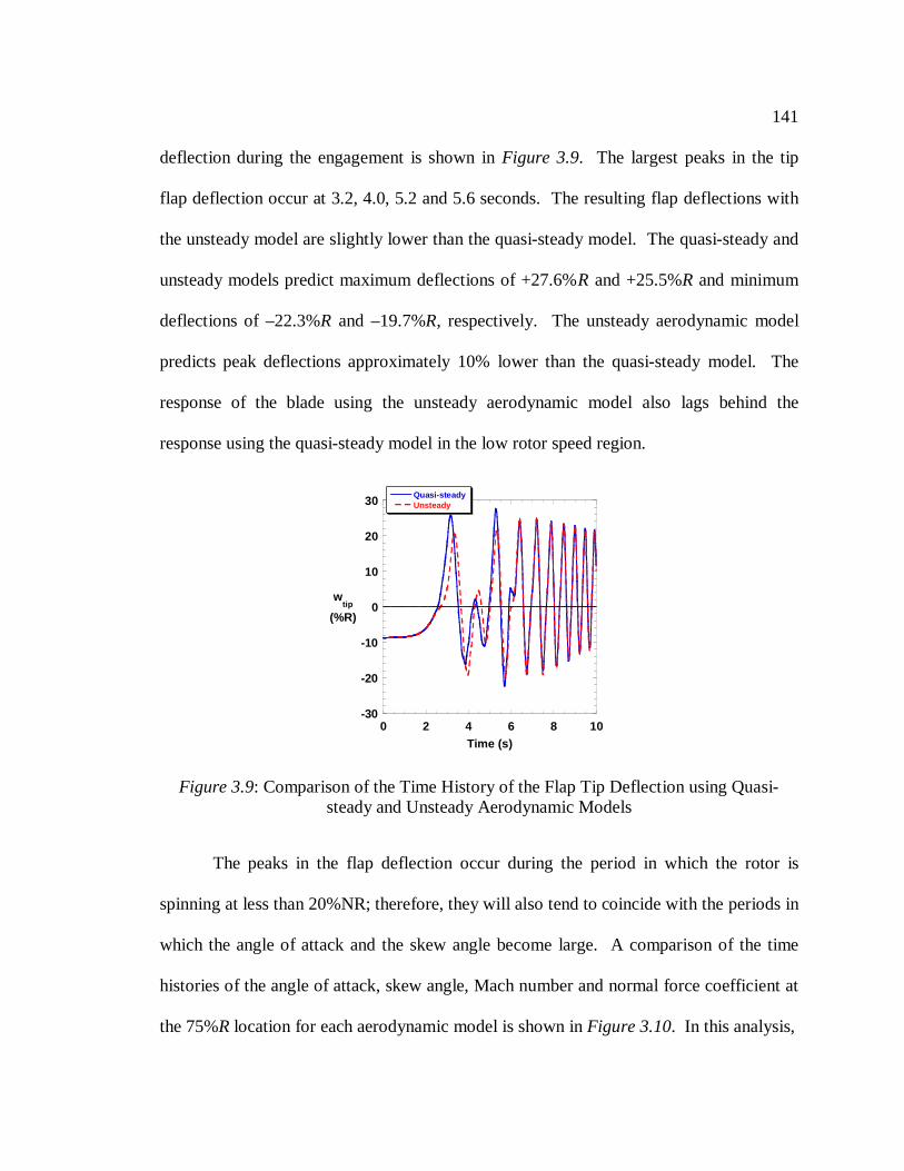
141
deflection during the engagement is shown inFigure 3.9. The largest peaks in the tip
flap deflection occur at 3.2, 4.0, 5.2 and 5.6 seconds. The resulting flap deflections with
the unsteady model are slightly lower than the quasi-steady model. The quasi-steady and
unsteady models predict maximum deflections of +27.6%R and +25.5%R and minimum
deflections of –22.3%R and –19.7%R, respectively. The unsteady aerodynamic model
predicts peak deflections approximately 10% lower than the quasi-steady model. The
response of the blade using the unsteady aerodynamic model also lags behind the
response using the quasi-steady model in the low rotor speed region.
The peaks in the flap deflection occur during the period in which the rotor is
spinning at less than 20%NR; therefore, they will also tend to coincide with the periods in
which the angle of attack and the skew angle become large. A comparison of the time
histories of the angle of attack, skew angle, Mach number and normal force coefficient at
the 75%R location for each aerodynamic model is shown inFigure 3.10. In this analysis,
-30
-20
-10
0
10
20
30
0 2 4 6 8 10
Quasi-steadyUnsteady
wtip
(%R)
Time (s)
Figure 3.9: Comparison of the Time History of the Flap Tip Deflection using Quasi-steady and Unsteady Aerodynamic Models
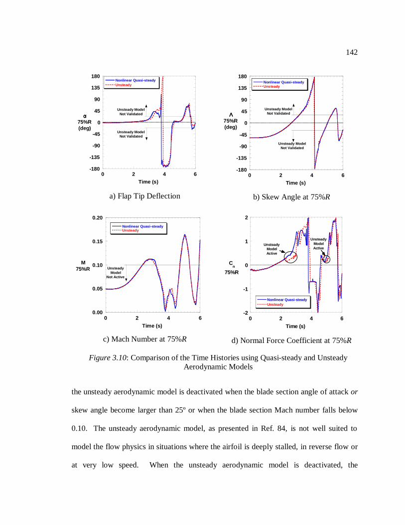
142
the unsteady aerodynamic model is deactivated when the blade section angle of attackor
skew angle become larger than 25º or when the blade section Mach number falls below
0.10. The unsteady aerodynamic model, as presented in Ref. 84, is not well suited to
model the flow physics in situations where the airfoil is deeply stalled, in reverse flow or
at very low speed. When the unsteady aerodynamic model is deactivated, the
-180
-135
-90
-45
0
45
90
135
180
0 2 4 6
Nonlinear Quasi-steadyUnsteady
αααα75%R(deg)
Time (s)
Unsteady ModelNot Validated
Unsteady ModelNot Validated
a) Flap Tip Deflection
-180
-135
-90
-45
0
45
90
135
180
0 2 4 6
Nonlinear Quasi-steadyUnsteady
ΛΛΛΛ75%R(deg)
Time (s)
Unsteady ModelNot Validated
Unsteady ModelNot Validated
b) Skew Angle at 75%R
0.00
0.05
0.10
0.15
0.20
0 2 4 6
Nonlinear Quasi-steadyUnsteady
M75%R
Time (s)
UnsteadyModel
Not Active
c) Mach Number at 75%R
-2
-1
0
1
2
0 2 4 6
Nonlinear Quasi-steadyUnsteady
Cn
75%R
Time (s)
UnsteadyModelActive
UnsteadyModelActive
d) Normal Force Coefficient at 75%R
Figure 3.10: Comparison of the Time Histories using Quasi-steady and UnsteadyAerodynamic Models
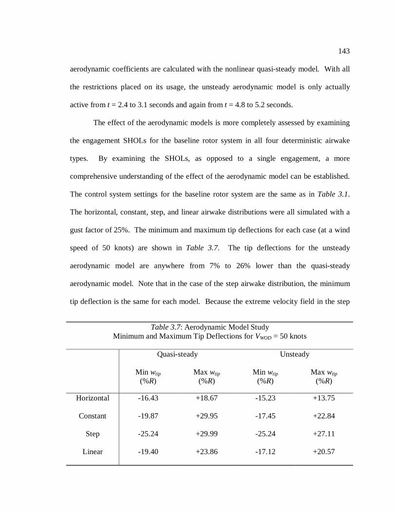
143
aerodynamic coefficients are calculated with the nonlinear quasi-steady model. With all
the restrictions placed on its usage, the unsteady aerodynamic model is only actually
active fromt = 2.4 to 3.1 seconds and again fromt = 4.8 to 5.2 seconds.
The effect of the aerodynamic models is more completely assessed by examining
the engagement SHOLs for the baseline rotor system in all four deterministic airwake
types. By examining the SHOLs, as opposed to a single engagement, a more
comprehensive understanding of the effect of the aerodynamic model can be established.
The control system settings for the baseline rotor system are the same as inTable 3.1.
The horizontal, constant, step, and linear airwake distributions were all simulated with a
gust factor of 25%. The minimum and maximum tip deflections for each case (at a wind
speed of 50 knots) are shown inTable 3.7. The tip deflections for the unsteady
aerodynamic model are anywhere from 7% to 26% lower than the quasi-steady
aerodynamic model. Note that in the case of the step airwake distribution, the minimum
tip deflection is the same for each model. Because the extreme velocity field in the step
Table 3.7: Aerodynamic Model StudyMinimum and Maximum Tip Deflections forVWOD = 50 knots
Quasi-steady Unsteady
Min wtip
(%R)Max wtip
(%R)Min wtip
(%R)Max wtip
(%R)
Horizontal -16.43 +18.67 -15.23 +13.75
Constant -19.87 +29.95 -17.45 +22.84
Step -25.24 +29.99 -25.24 +27.11
Linear -19.40 +23.86 -17.12 +20.57
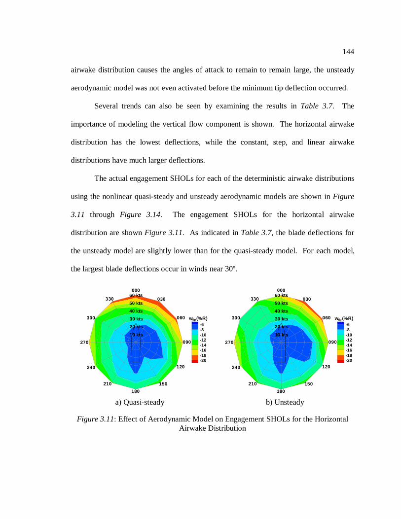
144
airwake distribution causes the angles of attack to remain to remain large, the unsteady
aerodynamic model was not even activated before the minimum tip deflection occurred.
Several trends can also be seen by examining the results inTable 3.7. The
importance of modeling the vertical flow component is shown. The horizontal airwake
distribution has the lowest deflections, while the constant, step, and linear airwake
distributions have much larger deflections.
The actual engagement SHOLs for each of the deterministic airwake distributions
using the nonlinear quasi-steady and unsteady aerodynamic models are shown inFigure
3.11 through Figure 3.14. The engagement SHOLs for the horizontal airwake
distribution are shownFigure 3.11. As indicated inTable 3.7, the blade deflections for
the unsteady model are slightly lower than for the quasi-steady model. For each model,
the largest blade deflections occur in winds near 30º.
-6-8-10-12-14-16-18-20
w (%R)tip
10 kts
33050 kts
40 kts
30 kts
20 kts
60 kts000
060
030
090
120
150
180
210
240
270
300
a) Quasi-steady
-6-8-10-12-14-16-18-20
w (%R)tip
10 kts
33050 kts
40 kts
30 kts
20 kts
60 kts000
060
030
090
120
150
180
210
240
270
300
b) Unsteady
Figure 3.11: Effect of Aerodynamic Model on Engagement SHOLs for the HorizontalAirwake Distribution
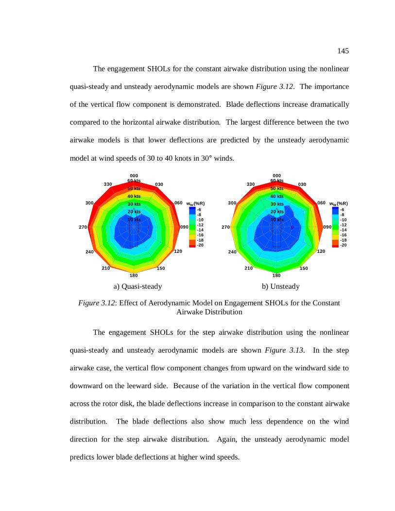
145
The engagement SHOLs for the constant airwake distribution using the nonlinear
quasi-steady and unsteady aerodynamic models are shownFigure 3.12. The importance
of the vertical flow component is demonstrated. Blade deflections increase dramatically
compared to the horizontal airwake distribution. The largest difference between the two
airwake models is that lower deflections are predicted by the unsteady aerodynamic
model at wind speeds of 30 to 40 knots in 30° winds.
The engagement SHOLs for the step airwake distribution using the nonlinear
quasi-steady and unsteady aerodynamic models are shownFigure 3.13. In the step
airwake case, the vertical flow component changes from upward on the windward side to
downward on the leeward side. Because of the variation in the vertical flow component
across the rotor disk, the blade deflections increase in comparison to the constant airwake
distribution. The blade deflections also show much less dependence on the wind
direction for the step airwake distribution. Again, the unsteady aerodynamic model
predicts lower blade deflections at higher wind speeds.
-6-8-10-12-14-16-18-20
w (%R)tip
10 kts
33050 kts
40 kts
30 kts
20 kts
60 kts000
060
030
090
120
150
180
210
240
270
300
a) Quasi-steady
-6-8-10-12-14-16-18-20
w (%R)tip
10 kts
33050 kts
40 kts
30 kts
20 kts
60 kts000
060
030
090
120
150
180
210
240
270
300
b) Unsteady
Figure 3.12: Effect of Aerodynamic Model on Engagement SHOLs for the ConstantAirwake Distribution
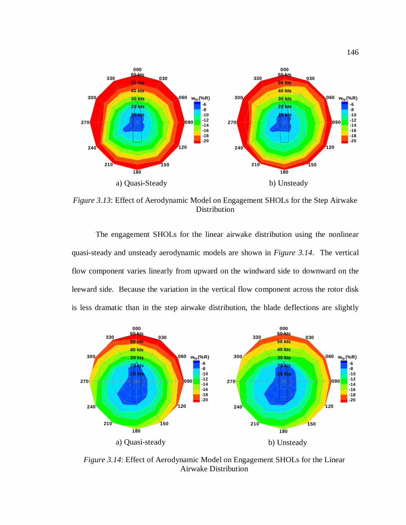
146
The engagement SHOLs for the linear airwake distribution using the nonlinear
quasi-steady and unsteady aerodynamic models are shown inFigure 3.14. The vertical
flow component varies linearly from upward on the windward side to downward on the
leeward side. Because the variation in the vertical flow component across the rotor disk
is less dramatic than in the step airwake distribution, the blade deflections are slightly
-6-8-10-12-14-16-18-20
w (%R)tip
10 kts
33050 kts
40 kts
30 kts
20 kts
60 kts000
060
030
090
120
150
180
210
240
270
300
a) Quasi-Steady
-6-8-10-12-14-16-18-20
w (%R)tip
10 kts
33050 kts
40 kts
30 kts
20 kts
60 kts000
060
030
090
120
150
180
210
240
270
300
b) Unsteady
Figure 3.13: Effect of Aerodynamic Model on Engagement SHOLs for the Step AirwakeDistribution
-6-8-10-12-14-16-18-20
w (%R)tip
10 kts
33050 kts
40 kts
30 kts
20 kts
60 kts000
060
030
090
120
150
180
210
240
270
300
a) Quasi-steady
-6-8-10-12-14-16-18-20
w (%R)tip
10 kts
33050 kts
40 kts
30 kts
20 kts
60 kts000
060
030
090
120
150
180
210
240
270
300
b) Unsteady
Figure 3.14: Effect of Aerodynamic Model on Engagement SHOLs for the LinearAirwake Distribution

147
lower. As with the other airwake distributions, the unsteady aerodynamic model results
in slightly lower blade deflections at the higher wind speeds.
These results suggest that a nonlinear quasi-steady aerodynamic model should be
used in engagement and disengagement modeling for two reasons. First, although
unsteady effects certainly exist, the current nonlinear unsteady aerodynamic model has
not been validated at the very high angles of attack and skew angles, or very low Mach
numbers encountered in these simulations. Second, since the prediction of large blade
deflections is of interest it is also more desirable to over predict blade deflections than
under predict them. In the remaining engagement and disengagement simulations, the
nonlinear quasi-steady aerodynamic model is utilized.
3.4 Ship Airwake Modeling
The majority of engagement and disengagement research completed with the
aeroelastic code described in this analysis has utilized the very simple deterministic
airwake types described in the previous sections. This section will explore the effects of
more realistic ship airwakes on the rotor behavior. An examination of the results for the
baseline rotor system in numerically computed full-scale ship airwakes is examined first.
In addition, a comparison of the results of the current analysis with the wind tunnel tests
completed at the University of Southampton is made. In each case, the role of the spatial
variation of the mean velocity components and the effect of the fluctuating velocity
components will be discussed.
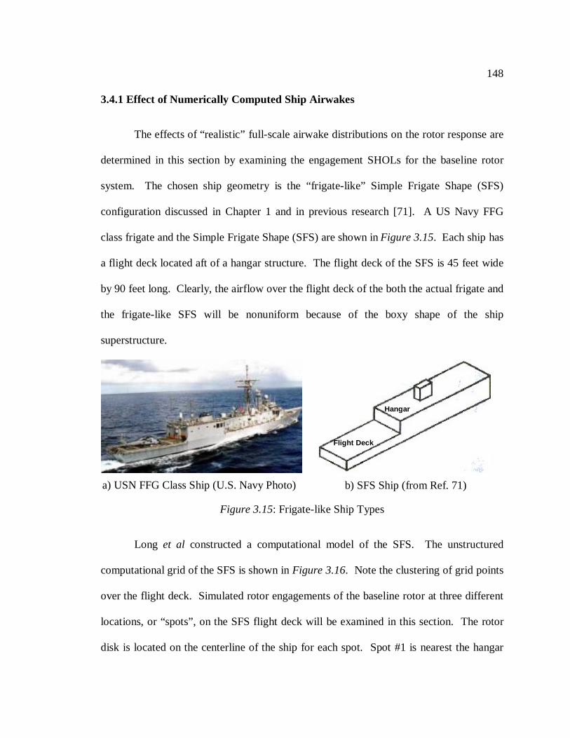
148
3.4.1 Effect of Numerically Computed Ship Airwakes
The effects of “realistic” full-scale airwake distributions on the rotor response are
determined in this section by examining the engagement SHOLs for the baseline rotor
system. The chosen ship geometry is the “frigate-like” Simple Frigate Shape (SFS)
configuration discussed in Chapter 1 and in previous research [71]. A US Navy FFG
class frigate and the Simple Frigate Shape (SFS) are shown inFigure 3.15. Each ship has
a flight deck located aft of a hangar structure. The flight deck of the SFS is 45 feet wide
by 90 feet long. Clearly, the airflow over the flight deck of the both the actual frigate and
the frigate-like SFS will be nonuniform because of the boxy shape of the ship
superstructure.
Long et al constructed a computational model of the SFS. The unstructured
computational grid of the SFS is shown inFigure 3.16. Note the clustering of grid points
over the flight deck. Simulated rotor engagements of the baseline rotor at three different
locations, or “spots”, on the SFS flight deck will be examined in this section. The rotor
disk is located on the centerline of the ship for each spot. Spot #1 is nearest the hangar
a) USN FFG Class Ship (U.S. Navy Photo) b) SFS Ship (from Ref. 71)
Figure 3.15: Frigate-like Ship Types
Hangar
Flight Deck
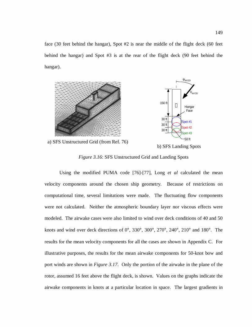
149
face (30 feet behind the hangar), Spot #2 is near the middle of the flight deck (60 feet
behind the hangar) and Spot #3 is at the rear of the flight deck (90 feet behind the
hangar).
Using the modified PUMA code [76]-[77], Longet al calculated the mean
velocity components around the chosen ship geometry. Because of restrictions on
computational time, several limitations were made. The fluctuating flow components
were not calculated. Neither the atmospheric boundary layer nor viscous effects were
modeled. The airwake cases were also limited to wind over deck conditions of 40 and 50
knots and wind over deck directions of 0°, 330°, 300°, 270°, 240°, 210° and 180°. The
results for the mean velocity components for all the cases are shown in Appendix C. For
illustrative purposes, the results for the mean airwake components for 50-knot bow and
port winds are shown inFigure 3.17. Only the portion of the airwake in the plane of the
rotor, assumed 16 feet above the flight deck, is shown. Values on the graphs indicate the
airwake components in knots at a particular location in space. The largest gradients in
a) SFS Unstructured Grid (from Ref. 76)
Spot #1
Spot #2
Spot #3
ψWOD
VW OD
HangarFace
150 ft
50 ft
30 ft
30 ft
30 ft
b) SFS Landing Spots
Figure 3.16: SFS Unstructured Grid and Landing Spots
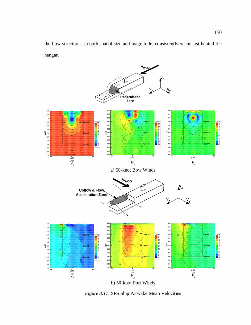
150
the flow structures, in both spatial size and magnitude, consistently occur just behind the
hangar.
RecirculationZone
VWOD
Vz
VyVx
-25
29
46
46 46
2 -3
40
46
y (ft)
x(f
t)
-50 0 50
150
160
170
180
190
200
210
220
230
240
250
260
270
514640352924181372
-3-9-14-20-25
V (kts)
Spot #3
Spot #1
Spot #2
xV
7
4
1
-24 19
16 -21
-54
-2
y (ft)
x(f
t)
-50 0 50
150
160
170
180
190
200
210
220
230
240
250
260
270
19161310741
-2-5-8-11-15-18-21-24
V (kts)
Spot #3
Spot #1
Spot #2
yV
23
-25-25
-8
-4
2
-1-1
y (ft)
x(f
t)
-50 0 50
150
160
170
180
190
200
210
220
230
240
250
260
270
23201613962
-1-4-8-11-15-18-22-25
V (kts)
Spot #3
Spot #1
Spot #2
zV
a) 50-knot Bow Winds
Vz
VyVx
VWOD
Upflow & FlowAcceleration Zone
30
12
8
8
3
3
3
-1
-10
-1
3
y (ft)
x(f
t)
-50 0 50
150
160
170
180
190
200
210
220
230
240
250
260
270
5248433935302621171283
-1-6-10
V (kts)
Spot #3
Spot #1
Spot #2
xV
71
17
71
65
65
59
53
53
53
59
53
59
53
y (ft)
x(f
t)
-50 0 50
150
160
170
180
190
200
210
220
230
240
250
260
270
7771655953474135292317115
-1-8
V (kts)
Spot #3
Spot #1
Spot #2
yV
31 -11
20
10
-1
-1
-1
15
-1
-1
-6
15
y (ft)
x(f
t)
-50 0 50
150
160
170
180
190
200
210
220
230
240
250
260
270
413631262015105
-1-6-11-16-21-27-32
V (kts)
Spot #3
Spot #1
Spot #2
zV
b) 50-knot Port Winds
Figure 3.17: SFS Ship Airwake Mean Velocities
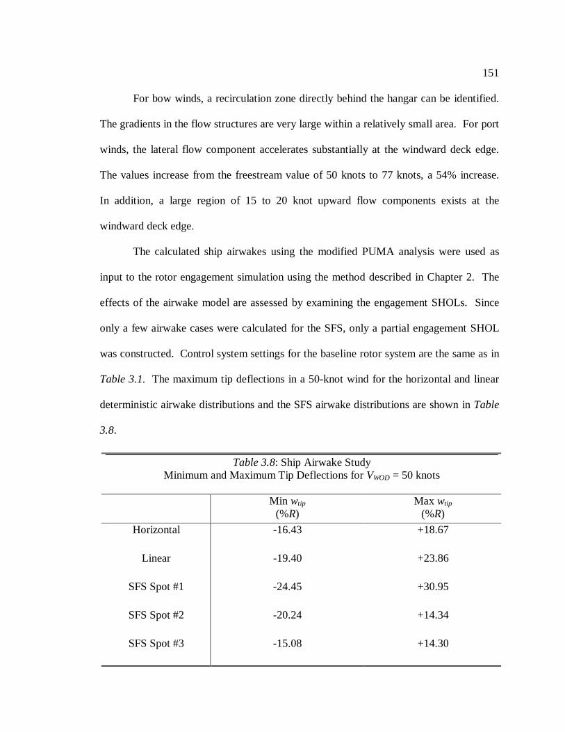
151
For bow winds, a recirculation zone directly behind the hangar can be identified.
The gradients in the flow structures are very large within a relatively small area. For port
winds, the lateral flow component accelerates substantially at the windward deck edge.
The values increase from the freestream value of 50 knots to 77 knots, a 54% increase.
In addition, a large region of 15 to 20 knot upward flow components exists at the
windward deck edge.
The calculated ship airwakes using the modified PUMA analysis were used as
input to the rotor engagement simulation using the method described in Chapter 2. The
effects of the airwake model are assessed by examining the engagement SHOLs. Since
only a few airwake cases were calculated for the SFS, only a partial engagement SHOL
was constructed. Control system settings for the baseline rotor system are the same as in
Table 3.1. The maximum tip deflections in a 50-knot wind for the horizontal and linear
deterministic airwake distributions and the SFS airwake distributions are shown inTable
3.8.
Table 3.8: Ship Airwake StudyMinimum and Maximum Tip Deflections forVWOD = 50 knots
Min wtip
(%R)Max wtip
(%R)
Horizontal -16.43 +18.67
Linear -19.40 +23.86
SFS Spot #1 -24.45 +30.95
SFS Spot #2 -20.24 +14.34
SFS Spot #3 -15.08 +14.30
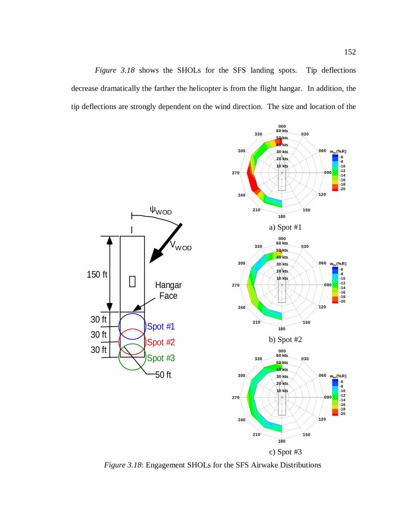
152
Figure 3.18 shows the SHOLs for the SFS landing spots. Tip deflections
decrease dramatically the farther the helicopter is from the flight hangar. In addition, the
tip deflections are strongly dependent on the wind direction. The size and location of the
-6-8-10-12-14-16-18-20
w (%R)tip
10 kts
33050 kts
40 kts
30 kts
20 kts
60 kts000
060
030
090
120
150
180
210
240
270
300
a) Spot #1
-6-8-10-12-14-16-18-20
w (%R)tip
10 kts
33050 kts
40 kts
30 kts
20 kts
60 kts000
060
030
090
120
150
180
210
240
270
300
b) Spot #2
Spot #1
Spot #2
Spot #3
ψWOD
VWOD
HangarFace
150 ft
50 ft
30 ft
30 ft
30 ft
-6-8-10-12-14-16-18-20
w (%R)tip
10 kts
33050 kts
40 kts
30 kts
20 kts
60 kts000
060
030
090
120
150
180
210
240
270
300
c) Spot #3
Figure 3.18: Engagement SHOLs for the SFS Airwake Distributions
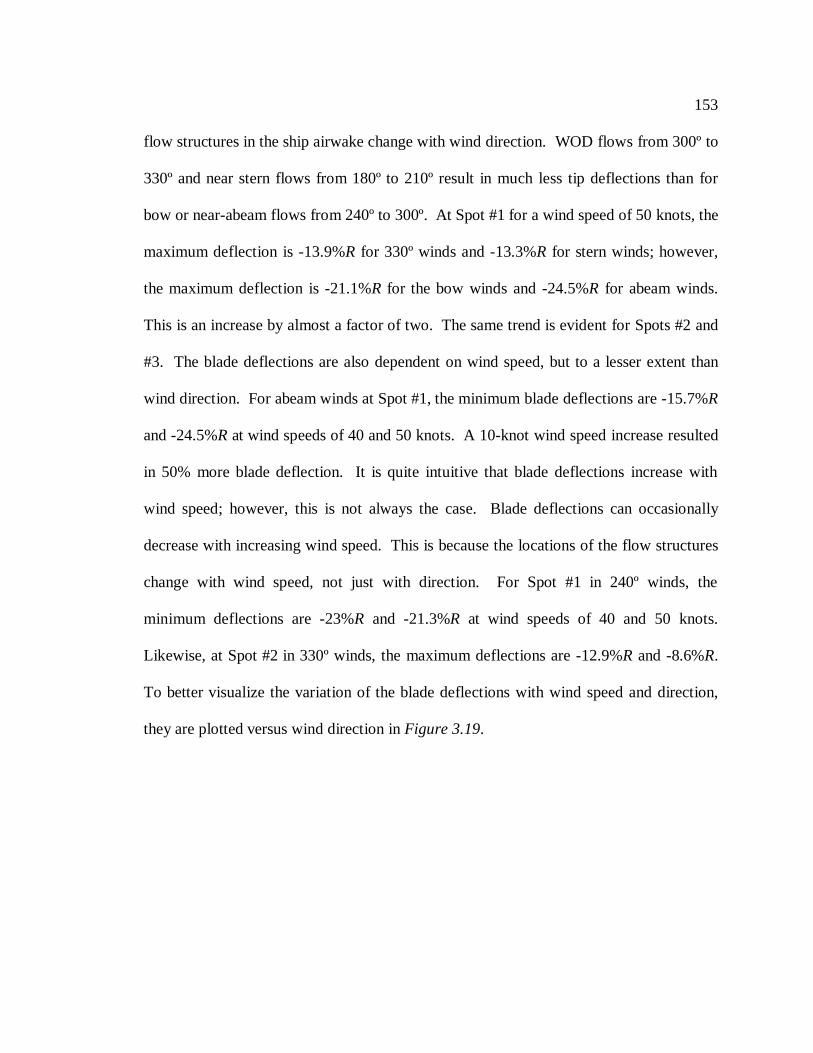
153
flow structures in the ship airwake change with wind direction. WOD flows from 300º to
330º and near stern flows from 180º to 210º result in much less tip deflections than for
bow or near-abeam flows from 240º to 300º. At Spot #1 for a wind speed of 50 knots, the
maximum deflection is -13.9%R for 330º winds and -13.3%R for stern winds; however,
the maximum deflection is -21.1%R for the bow winds and -24.5%R for abeam winds.
This is an increase by almost a factor of two. The same trend is evident for Spots #2 and
#3. The blade deflections are also dependent on wind speed, but to a lesser extent than
wind direction. For abeam winds at Spot #1, the minimum blade deflections are -15.7%R
and -24.5%R at wind speeds of 40 and 50 knots. A 10-knot wind speed increase resulted
in 50% more blade deflection. It is quite intuitive that blade deflections increase with
wind speed; however, this is not always the case. Blade deflections can occasionally
decrease with increasing wind speed. This is because the locations of the flow structures
change with wind speed, not just with direction. For Spot #1 in 240º winds, the
minimum deflections are -23%R and -21.3%R at wind speeds of 40 and 50 knots.
Likewise, at Spot #2 in 330º winds, the maximum deflections are -12.9%R and -8.6%R.
To better visualize the variation of the blade deflections with wind speed and direction,
they are plotted versus wind direction inFigure 3.19.
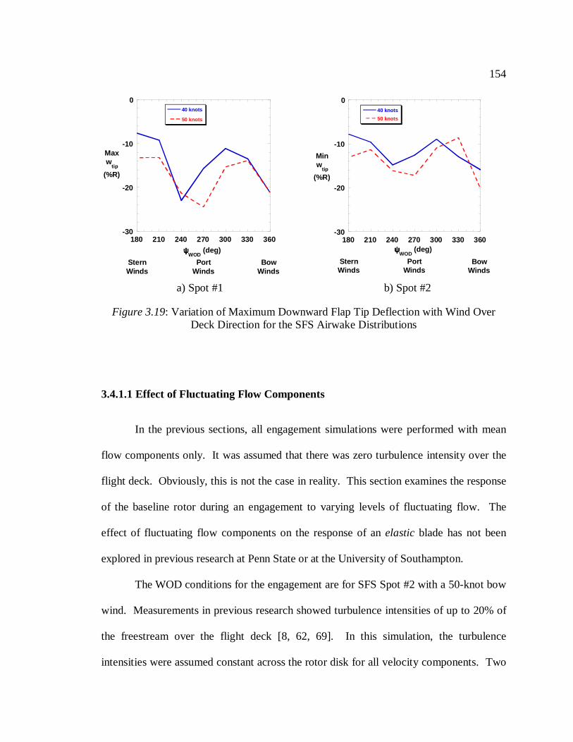
154
3.4.1.1 Effect of Fluctuating Flow Components
In the previous sections, all engagement simulations were performed with mean
flow components only. It was assumed that there was zero turbulence intensity over the
flight deck. Obviously, this is not the case in reality. This section examines the response
of the baseline rotor during an engagement to varying levels of fluctuating flow. The
effect of fluctuating flow components on the response of anelastic blade has not been
explored in previous research at Penn State or at the University of Southampton.
The WOD conditions for the engagement are for SFS Spot #2 with a 50-knot bow
wind. Measurements in previous research showed turbulence intensities of up to 20% of
the freestream over the flight deck [8, 62, 69]. In this simulation, the turbulence
intensities were assumed constant across the rotor disk for all velocity components. Two
-30
-20
-10
0
180 210 240 270 300 330 360
40 knots
50 knots
Maxw
tip
(%R)
ψψψψWOD
(deg)
BowWinds
PortWinds
SternWinds
a) Spot #1
-30
-20
-10
0
180 210 240 270 300 330 360
40 knots
50 knots
Minw
tip
(%R)
ψψψψWOD
(deg)
BowWinds
PortWinds
SternWinds
b) Spot #2
Figure 3.19: Variation of Maximum Downward Flap Tip Deflection with Wind OverDeck Direction for the SFS Airwake Distributions
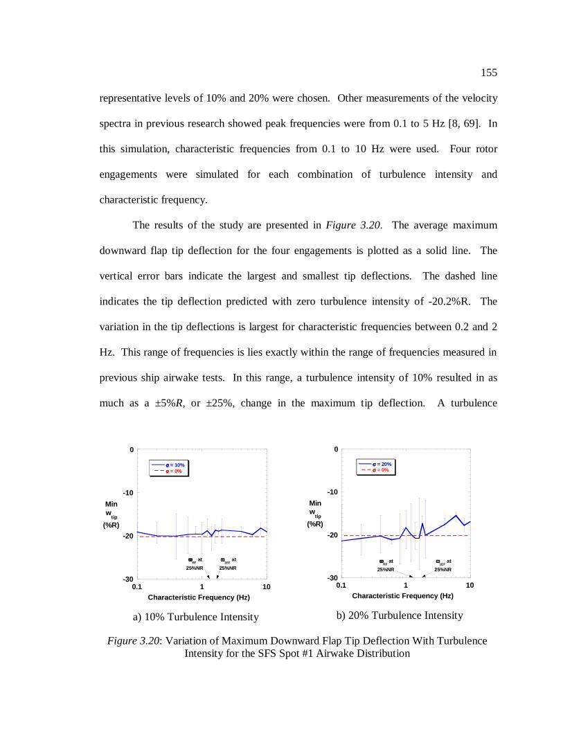
155
representative levels of 10% and 20% were chosen. Other measurements of the velocity
spectra in previous research showed peak frequencies were from 0.1 to 5 Hz [8, 69]. In
this simulation, characteristic frequencies from 0.1 to 10 Hz were used. Four rotor
engagements were simulated for each combination of turbulence intensity and
characteristic frequency.
The results of the study are presented inFigure 3.20. The average maximum
downward flap tip deflection for the four engagements is plotted as a solid line. The
vertical error bars indicate the largest and smallest tip deflections. The dashed line
indicates the tip deflection predicted with zero turbulence intensity of -20.2%R. The
variation in the tip deflections is largest for characteristic frequencies between 0.2 and 2
Hz. This range of frequencies is lies exactly within the range of frequencies measured in
previous ship airwake tests. In this range, a turbulence intensity of 10% resulted in as
much as a ±5%R, or ±25%, change in the maximum tip deflection. A turbulence
-30
-20
-10
0
0.1 1 10
σσσσ = 10%σσσσ = 0%
Minw
tip
(%R)
Characteristic Frequency (Hz)
ωωωωRF
at
25%NR
ωωωω1EF
at
25%NR
a) 10% Turbulence Intensity
-30
-20
-10
0
0.1 1 10
σσσσ = 20%σσσσ = 0%
Minw
tip
(%R)
Characteristic Frequency (Hz)
ωωωωRF
at
25%NR
ωωωω1EF
at
25%NR
b) 20% Turbulence Intensity
Figure 3.20: Variation of Maximum Downward Flap Tip Deflection With TurbulenceIntensity for the SFS Spot #1 Airwake Distribution
156
intensity of 20% resulted in as much as a ±9%R, or ±45%, change in the maximum tip
deflection. Also indicated on the plots are the natural frequencies of the blade at a rotor
speed of 25%NR, where the maximum tip deflections are most likely to occur. The rigid
body flap frequency at 1.23 Hz and the first elastic flap frequency at 1.67 Hz are within
the range of characteristic frequencies of interest. Above 2 Hz, the fluctuating flow
components have a much smaller effect on the blade response.
Example time histories of the flap tip deflection for characteristic frequencies of
0.1, 1.0 and 10 Hz are shown inFigure 3.21throughFigure 3.23. The response of the
baseline blade is influenced much more by characteristic frequencies of 0.1 and 1.0 Hz
than by the 10 Hz frequency. The fluctuating flow model used in this analysis, although
rudimentary, indicates that the fluctuating flow components can significantly affect the
blade response.
-30
-20
-10
0
10
20
30
0 2 4 6 8 10
σσσσ = 0%σσσσ = 10%, 0.1 Hz
wtip
(%R)
Time (s)
a) 10% Turbulence Intensity
-30
-20
-10
0
10
20
30
0 2 4 6 8 10
σσσσ = 0%σσσσ = 20%, 0.1 Hz
wtip
(%R)
Time (s)
b) 20% Turbulence Intensity
Figure 3.21: Time Histories of Flap Tip Deflection at a Characteristic Frequency of 0.1Hz for the SFS Spot #1 Airwake Distribution
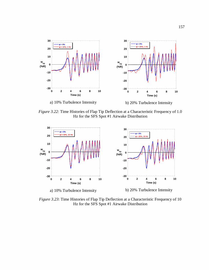
157
-30
-20
-10
0
10
20
30
0 2 4 6 8 10
σσσσ = 0%σσσσ = 10%, 1 Hz
wtip
(%R)
Time (s)
a) 10% Turbulence Intensity
-30
-20
-10
0
10
20
30
0 2 4 6 8 10
σσσσ = 0%
σσσσ = 20%, 1 Hz
wtip
(%R)
Time (s)
b) 20% Turbulence Intensity
Figure 3.22: Time Histories of Flap Tip Deflection at a Characteristic Frequency of 1.0Hz for the SFS Spot #1 Airwake Distribution
-30
-20
-10
0
10
20
30
0 2 4 6 8 10
σσσσ = 0%
σσσσ = 10%, 10 Hz
wtip
(%R)
Time (s)
a) 10% Turbulence Intensity
-30
-20
-10
0
10
20
30
0 2 4 6 8 10
σσσσ = 0%
σσσσ = 20%, 10 Hz
wtip
(%R)
Time (s)
b) 20% Turbulence Intensity
Figure 3.23: Time Histories of Flap Tip Deflection at a Characteristic Frequency of 10Hz for the SFS Spot #1 Airwake Distribution
158
3.4.2 Validation with Wind Tunnel Measurements
The deterministic ship airwake distributions described in Chapter 2 were
originally synthesized with limited model-scale wind tunnel measurements correlated
with a few full-scale measurements completed at the University of Southampton [31-32].
Later research at the University of Southampton focused on additional model-scale wind
tunnel tests [1, 38]. In these tests, engagements and disengagements of a radio-controlled
helicopter on board a model-scale ship were performed. The blade flapping response was
measured and predicted. This section compares the predictions of the current analysis
with these previous tests and analyses.
The wind tunnel tests at the University of Southampton were broken into two
parts. In the first part, a model-scale ship was inserted in a wind tunnel to simulate
abeam wind conditions. To obtain a general understanding of the flow characteristics,
the airwake across the width of the ship deck was examined with a wand-tuft study.
Flow measurements were concentrated at five locations spaced across the width of the
ship deck, called deck positions A through E. A schematic of the flow directions and a
characterization of the ship airwake are shown inFigure 3.24. Large amounts of upflow
exist at the windward deck positions A and B. The leeward deck positions C, D and E lie
within a recirculation zone. The tuft study showed that deck position B lied directly on
the boundary of the relatively undisturbed air and the recirculation zone.
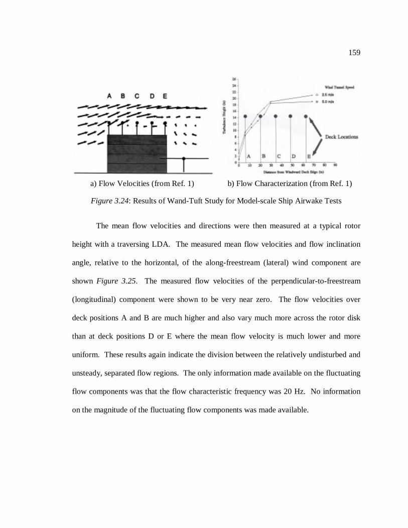
159
The mean flow velocities and directions were then measured at a typical rotor
height with a traversing LDA. The measured mean flow velocities and flow inclination
angle, relative to the horizontal, of the along-freestream (lateral) wind component are
shown Figure 3.25. The measured flow velocities of the perpendicular-to-freestream
(longitudinal) component were shown to be very near zero. The flow velocities over
deck positions A and B are much higher and also vary much more across the rotor disk
than at deck positions D or E where the mean flow velocity is much lower and more
uniform. These results again indicate the division between the relatively undisturbed and
unsteady, separated flow regions. The only information made available on the fluctuating
flow components was that the flow characteristic frequency was 20 Hz. No information
on the magnitude of the fluctuating flow components was made available.
a) Flow Velocities (from Ref. 1) b) Flow Characterization (from Ref. 1)
Figure 3.24: Results of Wand-Tuft Study for Model-scale Ship Airwake Tests
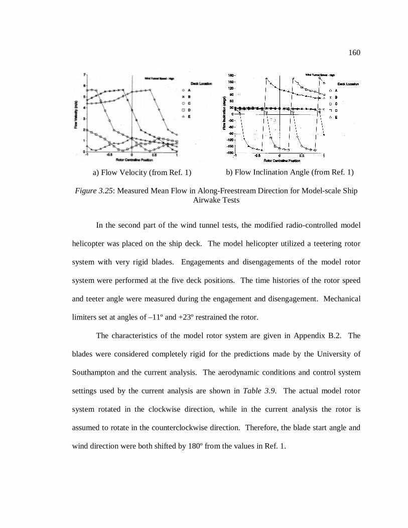
160
In the second part of the wind tunnel tests, the modified radio-controlled model
helicopter was placed on the ship deck. The model helicopter utilized a teetering rotor
system with very rigid blades. Engagements and disengagements of the model rotor
system were performed at the five deck positions. The time histories of the rotor speed
and teeter angle were measured during the engagement and disengagement. Mechanical
limiters set at angles of –11º and +23º restrained the rotor.
The characteristics of the model rotor system are given in Appendix B.2. The
blades were considered completely rigid for the predictions made by the University of
Southampton and the current analysis. The aerodynamic conditions and control system
settings used by the current analysis are shown inTable 3.9. The actual model rotor
system rotated in the clockwise direction, while in the current analysis the rotor is
assumed to rotate in the counterclockwise direction. Therefore, the blade start angle and
wind direction were both shifted by 180º from the values in Ref. 1.
a) Flow Velocity (from Ref. 1) b) Flow Inclination Angle (from Ref. 1)
Figure 3.25: Measured Mean Flow in Along-Freestream Direction for Model-scale ShipAirwake Tests
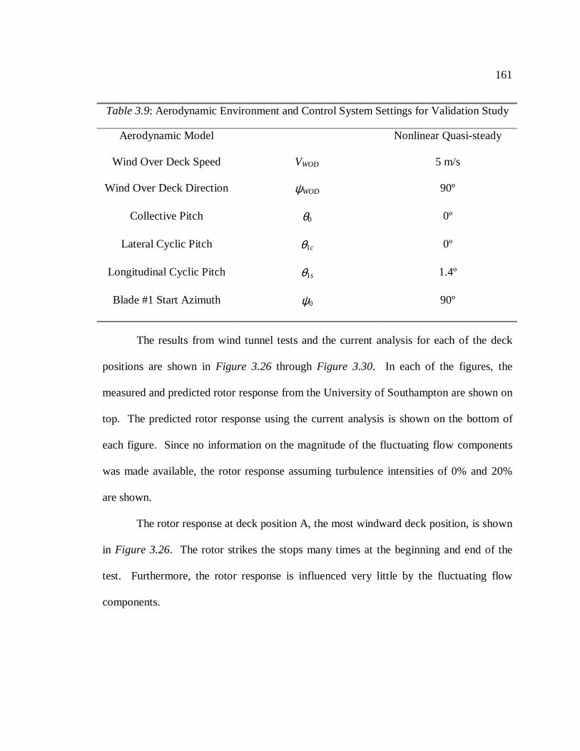
161
The results from wind tunnel tests and the current analysis for each of the deck
positions are shown inFigure 3.26 through Figure 3.30. In each of the figures, the
measured and predicted rotor response from the University of Southampton are shown on
top. The predicted rotor response using the current analysis is shown on the bottom of
each figure. Since no information on the magnitude of the fluctuating flow components
was made available, the rotor response assuming turbulence intensities of 0% and 20%
are shown.
The rotor response at deck position A, the most windward deck position, is shown
in Figure 3.26. The rotor strikes the stops many times at the beginning and end of the
test. Furthermore, the rotor response is influenced very little by the fluctuating flow
components.
Table 3.9: Aerodynamic Environment and Control System Settings for Validation Study
Aerodynamic Model Nonlinear Quasi-steady
Wind Over Deck Speed VWOD 5 m/s
Wind Over Deck Direction ψWOD 90º
Collective Pitch θ0 0º
Lateral Cyclic Pitch θ1c 0º
Longitudinal Cyclic Pitch θ1s 1.4º
Blade #1 Start Azimuth ψ0 90º
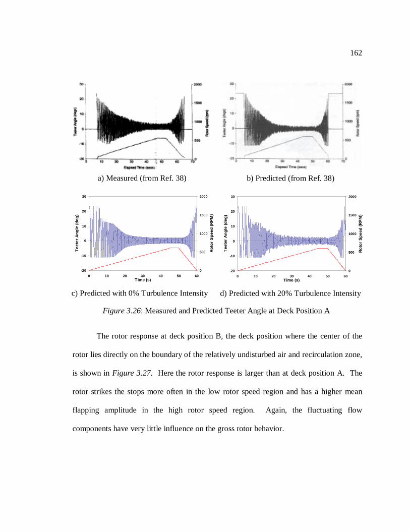
162
The rotor response at deck position B, the deck position where the center of the
rotor lies directly on the boundary of the relatively undisturbed air and recirculation zone,
is shown inFigure 3.27. Here the rotor response is larger than at deck position A. The
rotor strikes the stops more often in the low rotor speed region and has a higher mean
flapping amplitude in the high rotor speed region. Again, the fluctuating flow
components have very little influence on the gross rotor behavior.
a) Measured (from Ref. 38) b) Predicted (from Ref. 38)
-20
-10
0
10
20
30
0 10 20 30 40 50 60Time (s)
Tee
ter
Ang
le(d
eg)
0
500
1000
1500
2000
Rot
orS
peed
(RP
M)
c) Predicted with 0% Turbulence Intensity
-20
-10
0
10
20
30
0 10 20 30 40 50 60Time (s)
Tee
ter
Ang
le(d
eg)
0
500
1000
1500
2000
Rot
orS
pee
d(R
PM
)
d) Predicted with 20% Turbulence Intensity
Figure 3.26: Measured and Predicted Teeter Angle at Deck Position A
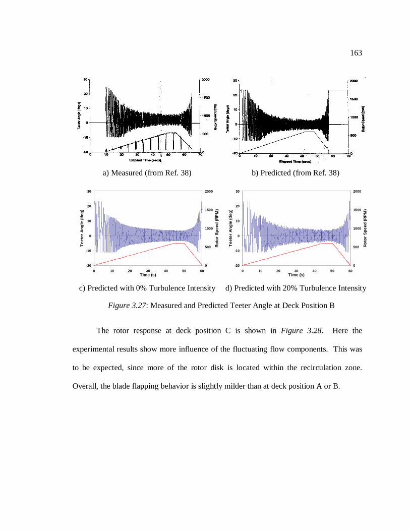
163
The rotor response at deck position C is shown inFigure 3.28. Here the
experimental results show more influence of the fluctuating flow components. This was
to be expected, since more of the rotor disk is located within the recirculation zone.
Overall, the blade flapping behavior is slightly milder than at deck position A or B.
a) Measured (from Ref. 38) b) Predicted (from Ref. 38)
-20
-10
0
10
20
30
0 10 20 30 40 50 60Time (s)
Tee
ter
Ang
le(d
eg)
0
500
1000
1500
2000
Rot
orS
pee
d(R
PM
)
c) Predicted with 0% Turbulence Intensity
-20
-10
0
10
20
30
0 10 20 30 40 50 60Time (s)
Tee
ter
An
gle
(deg
)
0
500
1000
1500
2000
Ro
tor
Spe
ed(R
PM
)
d) Predicted with 20% Turbulence Intensity
Figure 3.27: Measured and Predicted Teeter Angle at Deck Position B
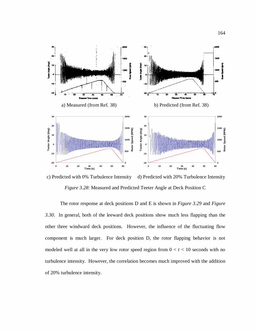
164
The rotor response at deck positions D and E is shown inFigure 3.29andFigure
3.30. In general, both of the leeward deck positions show much less flapping than the
other three windward deck positions. However, the influence of the fluctuating flow
component is much larger. For deck position D, the rotor flapping behavior is not
modeled well at all in the very low rotor speed region from 0 <t < 10 seconds with no
turbulence intensity. However, the correlation becomes much improved with the addition
of 20% turbulence intensity.
a) Measured (from Ref. 38) b) Predicted (from Ref. 38)
-20
-10
0
10
20
30
0 10 20 30 40 50 60Time (s)
Tee
ter
An
gle
(deg
)
0
500
1000
1500
2000
Ro
tor
Spe
ed(R
PM
)
c) Predicted with 0% Turbulence Intensity
-20
-10
0
10
20
30
0 10 20 30 40 50 60Time (s)
Tee
ter
Ang
le(d
eg)
0
500
1000
1500
2000
Rot
orS
pee
d(R
PM
)
d) Predicted with 20% Turbulence Intensity
Figure 3.28: Measured and Predicted Teeter Angle at Deck Position C
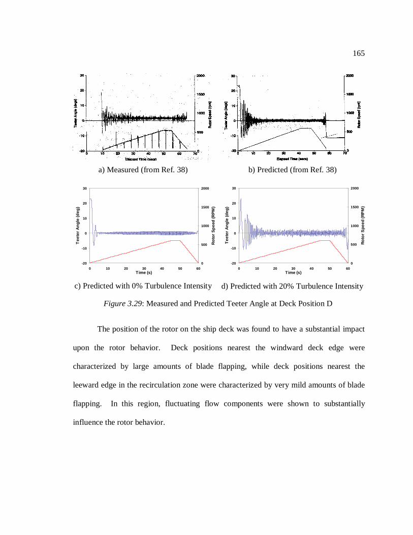
165
The position of the rotor on the ship deck was found to have a substantial impact
upon the rotor behavior. Deck positions nearest the windward deck edge were
characterized by large amounts of blade flapping, while deck positions nearest the
leeward edge in the recirculation zone were characterized by very mild amounts of blade
flapping. In this region, fluctuating flow components were shown to substantially
influence the rotor behavior.
a) Measured (from Ref. 38) b) Predicted (from Ref. 38)
-20
-10
0
10
20
30
0 10 20 30 40 50 60Time (s)
Tee
ter
Ang
le(d
eg)
0
500
1000
1500
2000
Rot
orS
pee
d(R
PM
)
c) Predicted with 0% Turbulence Intensity
-20
-10
0
10
20
30
0 10 20 30 40 50 60Time (s)
Tee
ter
Ang
le(d
eg)
0
500
1000
1500
2000
Rot
or
Spe
ed(R
PM
)
d) Predicted with 20% Turbulence Intensity
Figure 3.29: Measured and Predicted Teeter Angle at Deck Position D
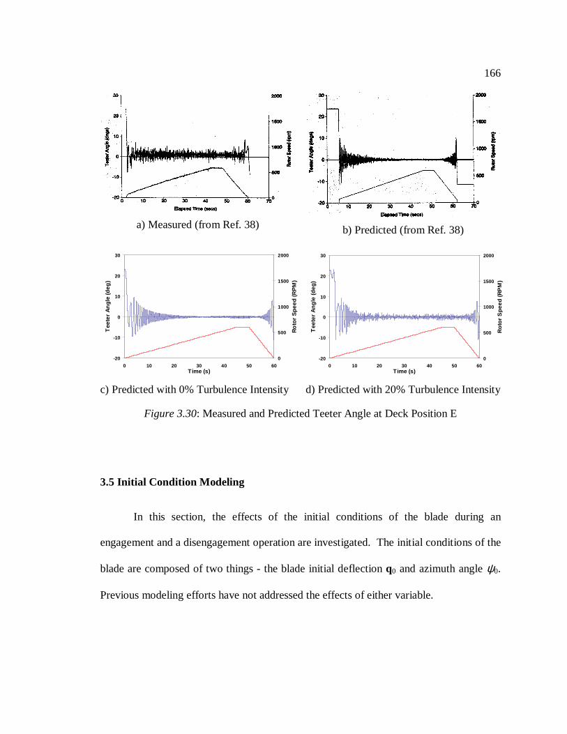
166
3.5 Initial Condition Modeling
In this section, the effects of the initial conditions of the blade during an
engagement and a disengagement operation are investigated. The initial conditions of the
blade are composed of two things - the blade initial deflectionq0 and azimuth angleψ0.
Previous modeling efforts have not addressed the effects of either variable.
a) Measured (from Ref. 38) b) Predicted (from Ref. 38)
-20
-10
0
10
20
30
0 10 20 30 40 50 60Time (s)
Tee
ter
An
gle
(deg
)
0
500
1000
1500
2000
Ro
tor
Spe
ed(R
PM
)
c) Predicted with 0% Turbulence Intensity
-20
-10
0
10
20
30
0 10 20 30 40 50 60Time (s)
Tee
ter
Ang
le(d
eg)
0
500
1000
1500
2000
Rot
orS
peed
(RP
M)
d) Predicted with 20% Turbulence Intensity
Figure 3.30: Measured and Predicted Teeter Angle at Deck Position E
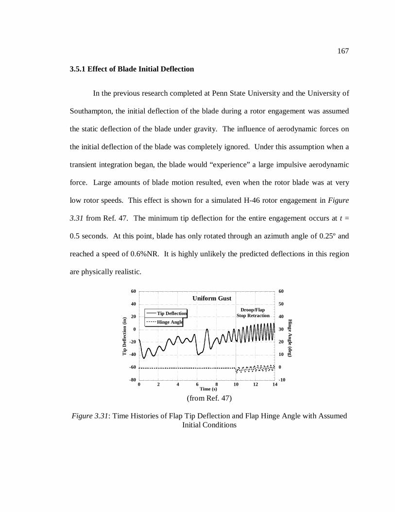
167
3.5.1 Effect of Blade Initial Deflection
In the previous research completed at Penn State University and the University of
Southampton, the initial deflection of the blade during a rotor engagement was assumed
the static deflection of the blade under gravity. The influence of aerodynamic forces on
the initial deflection of the blade was completely ignored. Under this assumption when a
transient integration began, the blade would “experience” a large impulsive aerodynamic
force. Large amounts of blade motion resulted, even when the rotor blade was at very
low rotor speeds. This effect is shown for a simulated H-46 rotor engagement inFigure
3.31 from Ref. 47. The minimum tip deflection for the entire engagement occurs att =
0.5 seconds. At this point, blade has only rotated through an azimuth angle of 0.25º and
reached a speed of 0.6%NR. It is highly unlikely the predicted deflections in this region
are physically realistic.
-80
-60
-40
-20
0
20
40
60
-10
0
10
20
30
40
50
60
0 2 4 6 8 10 12 14
Tip Deflection
Hinge Angle
Tip
Def
lect
ion
(in) H
inge
Angle
(deg)
Time (s)
Uniform Gust
Droop/FlapStop Retraction
(from Ref. 47)
Figure 3.31: Time Histories of Flap Tip Deflection and Flap Hinge Angle with AssumedInitial Conditions
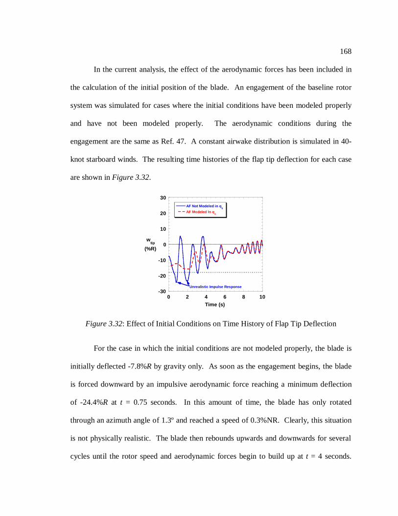
168
In the current analysis, the effect of the aerodynamic forces has been included in
the calculation of the initial position of the blade. An engagement of the baseline rotor
system was simulated for cases where the initial conditions have been modeled properly
and have not been modeled properly. The aerodynamic conditions during the
engagement are the same as Ref. 47. A constant airwake distribution is simulated in 40-
knot starboard winds. The resulting time histories of the flap tip deflection for each case
are shown inFigure 3.32.
For the case in which the initial conditions are not modeled properly, the blade is
initially deflected -7.8%R by gravity only. As soon as the engagement begins, the blade
is forced downward by an impulsive aerodynamic force reaching a minimum deflection
of -24.4%R at t = 0.75 seconds. In this amount of time, the blade has only rotated
through an azimuth angle of 1.3º and reached a speed of 0.3%NR. Clearly, this situation
is not physically realistic. The blade then rebounds upwards and downwards for several
cycles until the rotor speed and aerodynamic forces begin to build up att = 4 seconds.
-30
-20
-10
0
10
20
30
0 2 4 6 8 10
AF Not Modeled in q0
AF Modeled In q0
wtip
(%R)
Time (s)
Unrealistic Impulse Response
Figure 3.32: Effect of Initial Conditions on Time History of Flap Tip Deflection
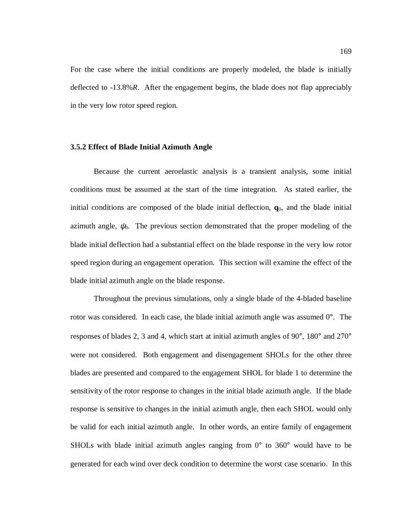
169
For the case where the initial conditions are properly modeled, the blade is initially
deflected to -13.8%R. After the engagement begins, the blade does not flap appreciably
in the very low rotor speed region.
3.5.2 Effect of Blade Initial Azimuth Angle
Because the current aeroelastic analysis is a transient analysis, some initial
conditions must be assumed at the start of the time integration. As stated earlier, the
initial conditions are composed of the blade initial deflection,q0, and the blade initial
azimuth angle,ψ0. The previous section demonstrated that the proper modeling of the
blade initial deflection had a substantial effect on the blade response in the very low rotor
speed region during an engagement operation. This section will examine the effect of the
blade initial azimuth angle on the blade response.
Throughout the previous simulations, only a single blade of the 4-bladed baseline
rotor was considered. In each case, the blade initial azimuth angle was assumed 0°. The
responses of blades 2, 3 and 4, which start at initial azimuth angles of 90°, 180° and 270°
were not considered. Both engagement and disengagement SHOLs for the other three
blades are presented and compared to the engagement SHOL for blade 1 to determine the
sensitivity of the rotor response to changes in the initial blade azimuth angle. If the blade
response is sensitive to changes in the initial azimuth angle, then each SHOL would only
be valid for each initial azimuth angle. In other words, an entire family of engagement
SHOLs with blade initial azimuth angles ranging from 0° to 360° would have to be
generated for each wind over deck condition to determine the worst case scenario. In this
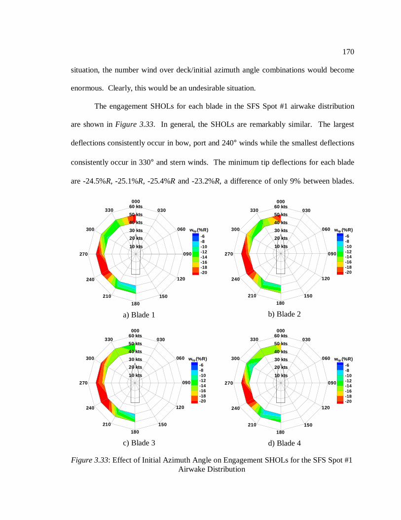
170
situation, the number wind over deck/initial azimuth angle combinations would become
enormous. Clearly, this would be an undesirable situation.
The engagement SHOLs for each blade in the SFS Spot #1 airwake distribution
are shown inFigure 3.33. In general, the SHOLs are remarkably similar. The largest
deflections consistently occur in bow, port and 240° winds while the smallest deflections
consistently occur in 330° and stern winds. The minimum tip deflections for each blade
are -24.5%R, -25.1%R, -25.4%R and -23.2%R, a difference of only 9% between blades.
-6-8-10-12-14-16-18-20
w (%R)tip
10 kts
33050 kts
40 kts
30 kts
20 kts
60 kts000
060
030
090
120
150
180
210
240
270
300
a) Blade 1
-6-8-10-12-14-16-18-20
w (%R)tip
10 kts
33050 kts
40 kts
30 kts
20 kts
60 kts000
060
030
090
120
150
180
210
240
270
300
b) Blade 2
-6-8-10-12-14-16-18-20
w (%R)tip
10 kts
33050 kts
40 kts
30 kts
20 kts
60 kts000
060
030
090
120
150
180
210
240
270
300
c) Blade 3
-6-8-10-12-14-16-18-20
w (%R)tip
10 kts
33050 kts
40 kts
30 kts
20 kts
60 kts000
060
030
090
120
150
180
210
240
270
300
d) Blade 4
Figure 3.33: Effect of Initial Azimuth Angle on Engagement SHOLs for the SFS Spot #1Airwake Distribution
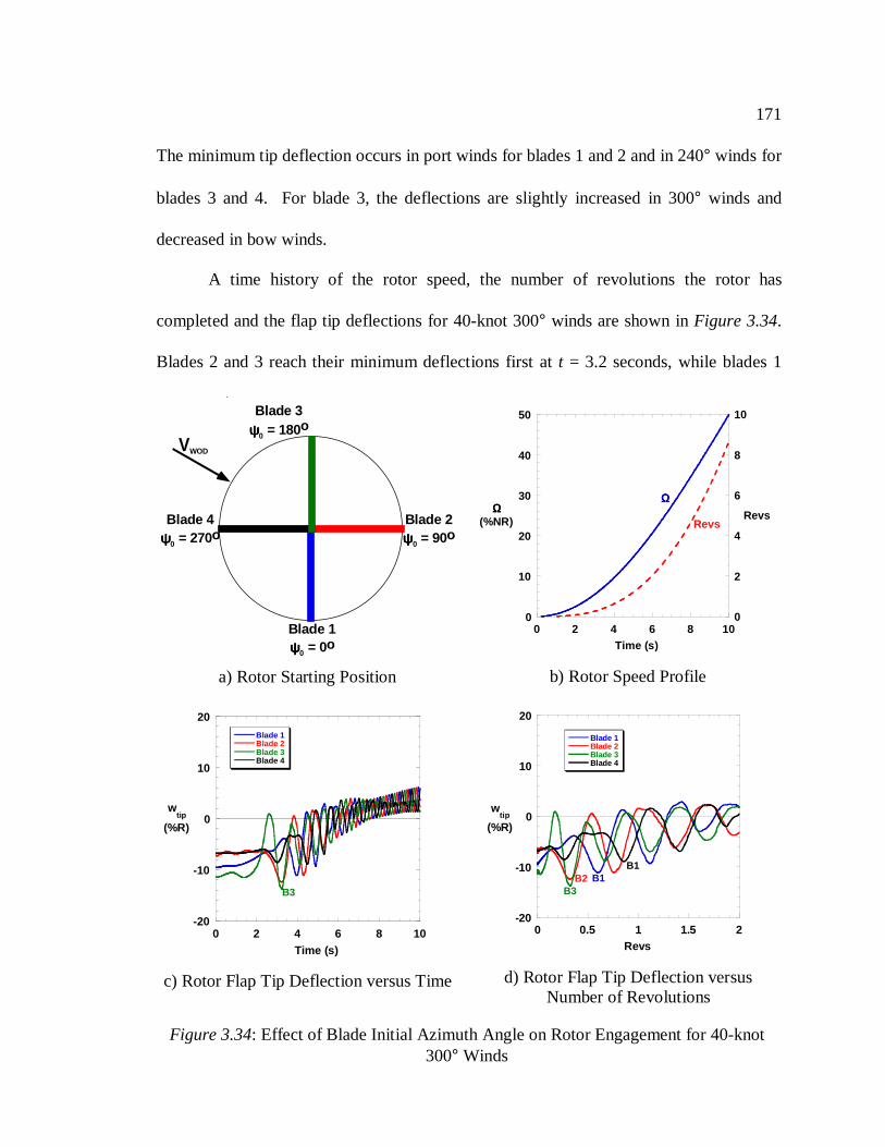
171
The minimum tip deflection occurs in port winds for blades 1 and 2 and in 240° winds for
blades 3 and 4. For blade 3, the deflections are slightly increased in 300° winds and
decreased in bow winds.
A time history of the rotor speed, the number of revolutions the rotor has
completed and the flap tip deflections for 40-knot 300° winds are shown inFigure 3.34.
Blades 2 and 3 reach their minimum deflections first att = 3.2 seconds, while blades 1
VWOD
Blade 1ψψψψ0 = 0o
Blade 2ψψψψ0 = 90o
Blade 3ψψψψ0 = 180o
Blade 4ψψψψ0 = 270o
a) Rotor Starting Position
0
10
20
30
40
50
0
2
4
6
8
10
0 2 4 6 8 10
ΩΩΩΩ(%NR) Revs
Time (s)
ΩΩΩΩ
Revs
b) Rotor Speed Profile
-20
-10
0
10
20
0 2 4 6 8 10
Blade 1Blade 2Blade 3Blade 4
wtip
(%R)
Time (s)
B3
c) Rotor Flap Tip Deflection versus Time
-20
-10
0
10
20
0 0.5 1 1.5 2
Blade 1Blade 2Blade 3Blade 4
wtip
(%R)
Revs
B3B2 B1
B1
d) Rotor Flap Tip Deflection versusNumber of Revolutions
Figure 3.34: Effect of Blade Initial Azimuth Angle on Rotor Engagement for 40-knot300° Winds
172
and 4 reach theirs att = 4.0 and 4.5 seconds, respectively. The flap tip deflections are
also plotted during the first two rotor revolutions. Blades 2 and 3 reach their minimum
deflection when the rotor has already rotated 0.33 revolutions or 120°. Blades 1 and 4
reach their minimum deflections at 0.60 and 0.86 revolutions, respectively.
The disengagement SHOLs for each blade in the SFS Spot #1 airwake distribution
are shown in Figure 3.35. The SHOLs are not nearly as similar for a rotor
disengagement as for a rotor engagement. For example, much smaller blade deflections
-6-8-10-12-14-16-18-20
w (%R)tip
10 kts
33050 kts
40 kts
30 kts
20 kts
60 kts000
060
030
090
120
150
180
210
240
270
300
a) Blade 1
-6-8-10-12-14-16-18-20
w (%R)tip
10 kts
33050 kts
40 kts
30 kts
20 kts
60 kts000
060
030
090
120
150
180
210
240
270
300
b) Blade 2
-6-8-10-12-14-16-18-20
w (%R)tip
10 kts
33050 kts
40 kts
30 kts
20 kts
60 kts000
060
030
090
120
150
180
210
240
270
300
c) Blade 3
-6-8-10-12-14-16-18-20
w (%R)tip
10 kts
33050 kts
40 kts
30 kts
20 kts
60 kts000
060
030
090
120
150
180
210
240
270
300
d) Blade 4
Figure 3.35: Effect of Initial Azimuth Angle on Disengagement SHOLs for the SFS Spot#1 Airwake Distribution
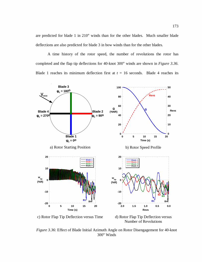
173
are predicted for blade 1 in 210° winds than for the other blades. Much smaller blade
deflections are also predicted for blade 3 in bow winds than for the other blades.
A time history of the rotor speed, the number of revolutions the rotor has
completed and the flap tip deflections for 40-knot 300° winds are shown inFigure 3.36.
Blade 1 reaches its minimum deflection first att = 16 seconds. Blade 4 reaches its
VWOD
Blade 1ψψψψ0 = 0o
Blade 2ψψψψ0 = 90o
Blade 3ψψψψ0 = 180o
Blade 4ψψψψ0 = 270o
a) Rotor Starting Position
0
20
40
60
80
100
0
10
20
30
40
50
0 5 10 15 20
ΩΩΩΩ(%NR) Revs
Time (s)
ΩΩΩΩ
Revs
b) Rotor Speed Profile
-20
-10
0
10
20
0 5 10 15 20
Blade 1Blade 2Blade 3Blade 4
wtip
(%R)
Time (s)
B1 B4
c) Rotor Flap Tip Deflection versus Time
-20
-10
0
10
20
0.00.51.01.52.0
Blade 1Blade 2Blade 3Blade 4
wtip
(%R)
Revs
B4B1
B2B3
d) Rotor Flap Tip Deflection versusNumber of Revolutions
Figure 3.36: Effect of Blade Initial Azimuth Angle on Rotor Disengagement for 40-knot300° Winds
174
minimum deflection att = 18.4 seconds, where the rotor speed is just under 2%NR. At
this point, the rotor is almost stopped. The flap tip deflections are also plotted during the
last two rotor revolutions. Blade 4 reaches its minimum deflection when the rotor is
within 0.04 revolutions, or 14°, of stopping.
In the case examined, the largest blade deflections occurred after the first one-
third rotor revolution for a rotor engagement. For a rotor disengagement, the largest
blade deflections occurredafter the last one-half revolution. Consequently, the initial
blade azimuth angle has a much smaller effect on the engagement SHOLs than on the
disengagement SHOLs.
3.6 Summary
This chapter detailed the level of detail necessary in the structural and
aerodynamic models required to accurately simulate a transient engagement or
disengagement operation. Convergence studies were performed in the full finite element
space and modal space. A 12-element, 9-mode blade model was shown to yield
converged results. The computational efficiency of different time integration techniques
was also examined. The Bossak-Newmark integration algorithm, using blade modes
calculated at 25%NR, was shown to yield the best results. Furthermore, the effect of lag
motion and the inclusion of aerodynamic forces in the initial conditions was shown to
more realistically predict the rotor response.
The quasi-steady nonlinear aerodynamic model was shown to predict larger blade
deflections than the unsteady aerodynamic model. Realistic ship airwake distributions
175
for a full-scale frigate-like shape resulted in much larger blade deflections compared to
the deterministic airwake distributions. The blade response was much more sensitive to
changes in wind speed and direction. The location of the rotor on the ship deck was also
shown to influence the blade response. Deck locations directly behind the hangar
resulted in much higher blade deflections. Fluctuating flow components were shown to
influence the blade response. Analysis of the response of all four blades of the rotor
system showed that the flapping response was relatively insensitive to the blade initial
azimuth angle for a rotor engagement, but highly sensitive for a rotor disengagement.
The current analysis was also correlated with previous model-scale wind tunnel tests
completed at the University of Southampton. Good correlation existed between the
measured and predicted rotor response. Once again, the position of the rotor on the ship
deck was shown to significantly affect the blade response.
176
Chapter 4
PASSIVE CONTROL METHODS FOR ARTICULATED ROTORS
The focus of this chapter is not on the prediction of the transient rotor response,
but on methods by which the rotor flapping response can be controlled or reduced. If
excessive flapping could be systematically reduced, the operational restrictions placed on
engagement and disengagement operations could be relaxed. Thus, helicopter operations
could be conducted in more adverse weather conditions increasing the helicopter's value.
Several methods to reduce the transient blade deflections are examined. Each method is
a passive control technique. The first control technique focuses on altering the
procedures the pilot follows during engagement and disengagement operations, while the
other two techniques focus on the addition of passive control devices to the rotor blades.
Instead of analyzing a generic articulated rotor system, the analysis will examine the
blade response for an analytic model of an H-46 Sea Knight rotor system.
4.1 H-46 Sea Knight Rotor System Properties
The relevant structural properties of the H-46 rotor system, derived from Ref. 91,
are given in Appendix B.3. The experimentally measured rotor speed profiles for an H-
46 Sea Knight engagement and disengagement are shown inFigure 4.1 from Ref. 41.
The rotor speed during the disengagement is shown versus the time before the rotor stops.
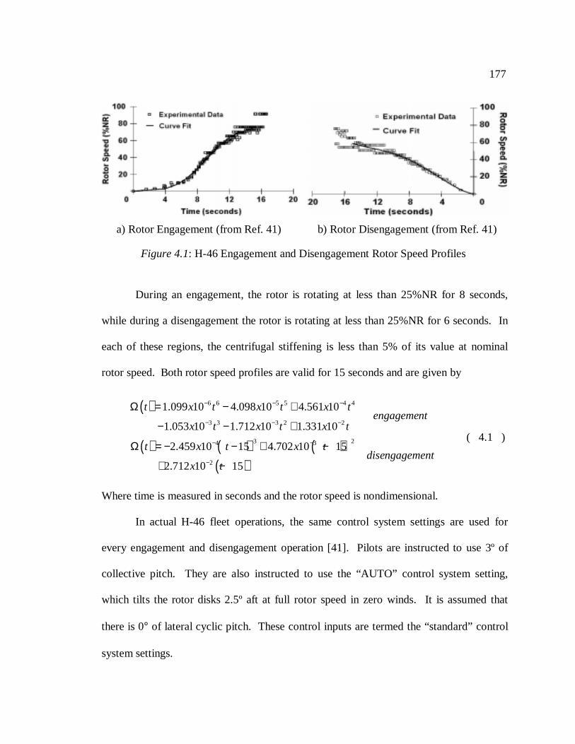
177
During an engagement, the rotor is rotating at less than 25%NR for 8 seconds,
while during a disengagement the rotor is rotating at less than 25%NR for 6 seconds. In
each of these regions, the centrifugal stiffening is less than 5% of its value at nominal
rotor speed. Both rotor speed profiles are valid for 15 seconds and are given by
( )
( ) ( ) ( )( )
6 6 5 5 4 4
3 3 3 2 2
3 24 3
2
1.099 10 4.098 10 4.561 10
1.053 10 1.712 10 1.331 10
2.459 10 15 4.702 10 15
2.712 10 15
t x t x t x tengagement
x t x t x t
t x t x tdisengagement
x t
− − −
− − −
− −
−
Ω = − +
− − +
Ω = − − + −
+ −
( 4.1 )
Where time is measured in seconds and the rotor speed is nondimensional.
In actual H-46 fleet operations, the same control system settings are used for
every engagement and disengagement operation [41]. Pilots are instructed to use 3º of
collective pitch. They are also instructed to use the “AUTO” control system setting,
which tilts the rotor disks 2.5º aft at full rotor speed in zero winds. It is assumed that
there is 0° of lateral cyclic pitch. These control inputs are termed the “standard” control
system settings.
a) Rotor Engagement (from Ref. 41) b) Rotor Disengagement (from Ref. 41)
Figure 4.1: H-46 Engagement and Disengagement Rotor Speed Profiles
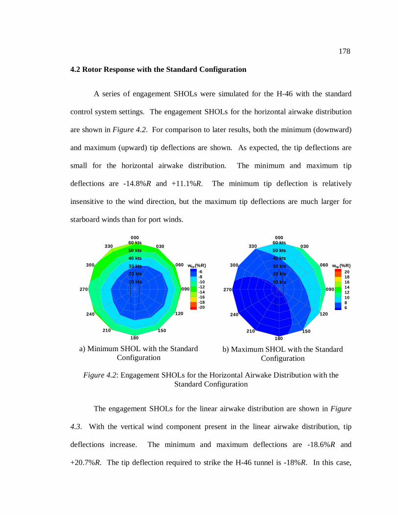
178
4.2 Rotor Response with the Standard Configuration
A series of engagement SHOLs were simulated for the H-46 with the standard
control system settings. The engagement SHOLs for the horizontal airwake distribution
are shown inFigure 4.2. For comparison to later results, both the minimum (downward)
and maximum (upward) tip deflections are shown. As expected, the tip deflections are
small for the horizontal airwake distribution. The minimum and maximum tip
deflections are -14.8%R and +11.1%R. The minimum tip deflection is relatively
insensitive to the wind direction, but the maximum tip deflections are much larger for
starboard winds than for port winds.
The engagement SHOLs for the linear airwake distribution are shown inFigure
4.3. With the vertical wind component present in the linear airwake distribution, tip
deflections increase. The minimum and maximum deflections are -18.6%R and
+20.7%R. The tip deflection required to strike the H-46 tunnel is -18%R. In this case,
-6-8-10-12-14-16-18-20
w (%R)tip
10 kts
33050 kts
40 kts
30 kts
20 kts
60 kts000
060
030
090
120
150
180
210
240
270
300
a) Minimum SHOL with the StandardConfiguration
20181614121086
w (%R)tip
10 kts
33050 kts
40 kts
30 kts
20 kts
60 kts000
060
030
090
120
150
180
210
240
270
300
b) Maximum SHOL with the StandardConfiguration
Figure 4.2: Engagement SHOLs for the Horizontal Airwake Distribution with theStandard Configuration
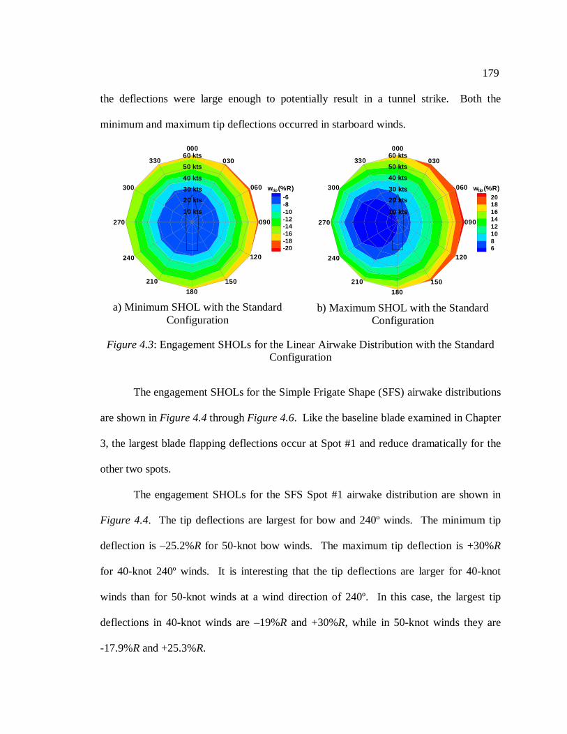
179
the deflections were large enough to potentially result in a tunnel strike. Both the
minimum and maximum tip deflections occurred in starboard winds.
The engagement SHOLs for the Simple Frigate Shape (SFS) airwake distributions
are shown inFigure 4.4throughFigure 4.6. Like the baseline blade examined in Chapter
3, the largest blade flapping deflections occur at Spot #1 and reduce dramatically for the
other two spots.
The engagement SHOLs for the SFS Spot #1 airwake distribution are shown in
Figure 4.4. The tip deflections are largest for bow and 240º winds. The minimum tip
deflection is –25.2%R for 50-knot bow winds. The maximum tip deflection is +30%R
for 40-knot 240º winds. It is interesting that the tip deflections are larger for 40-knot
winds than for 50-knot winds at a wind direction of 240º. In this case, the largest tip
deflections in 40-knot winds are –19%R and +30%R, while in 50-knot winds they are
-17.9%R and +25.3%R.
-6-8-10-12-14-16-18-20
w (%R)tip
10 kts
33050 kts
40 kts
30 kts
20 kts
60 kts000
060
030
090
120
150
180
210
240
270
300
a) Minimum SHOL with the StandardConfiguration
20181614121086
w (%R)tip
10 kts
33050 kts
40 kts
30 kts
20 kts
60 kts000
060
030
090
120
150
180
210
240
270
300
b) Maximum SHOL with the StandardConfiguration
Figure 4.3: Engagement SHOLs for the Linear Airwake Distribution with the StandardConfiguration
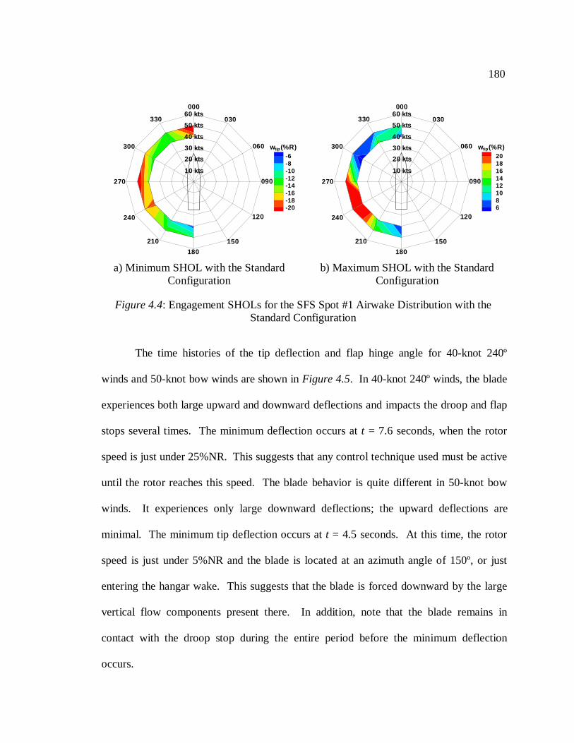
180
The time histories of the tip deflection and flap hinge angle for 40-knot 240º
winds and 50-knot bow winds are shown inFigure 4.5. In 40-knot 240º winds, the blade
experiences both large upward and downward deflections and impacts the droop and flap
stops several times. The minimum deflection occurs att = 7.6 seconds, when the rotor
speed is just under 25%NR. This suggests that any control technique used must be active
until the rotor reaches this speed. The blade behavior is quite different in 50-knot bow
winds. It experiences only large downward deflections; the upward deflections are
minimal. The minimum tip deflection occurs att = 4.5 seconds. At this time, the rotor
speed is just under 5%NR and the blade is located at an azimuth angle of 150º, or just
entering the hangar wake. This suggests that the blade is forced downward by the large
vertical flow components present there. In addition, note that the blade remains in
contact with the droop stop during the entire period before the minimum deflection
occurs.
-6-8-10-12-14-16-18-20
w (%R)tip
10 kts
33050 kts
40 kts
30 kts
20 kts
60 kts000
060
030
090
120
150
180
210
240
270
300
a) Minimum SHOL with the StandardConfiguration
20181614121086
w (%R)tip
10 kts
33050 kts
40 kts
30 kts
20 kts
60 kts000
060
030
090
120
150
180
210
240
270
300
b) Maximum SHOL with the StandardConfiguration
Figure 4.4: Engagement SHOLs for the SFS Spot #1 Airwake Distribution with theStandard Configuration
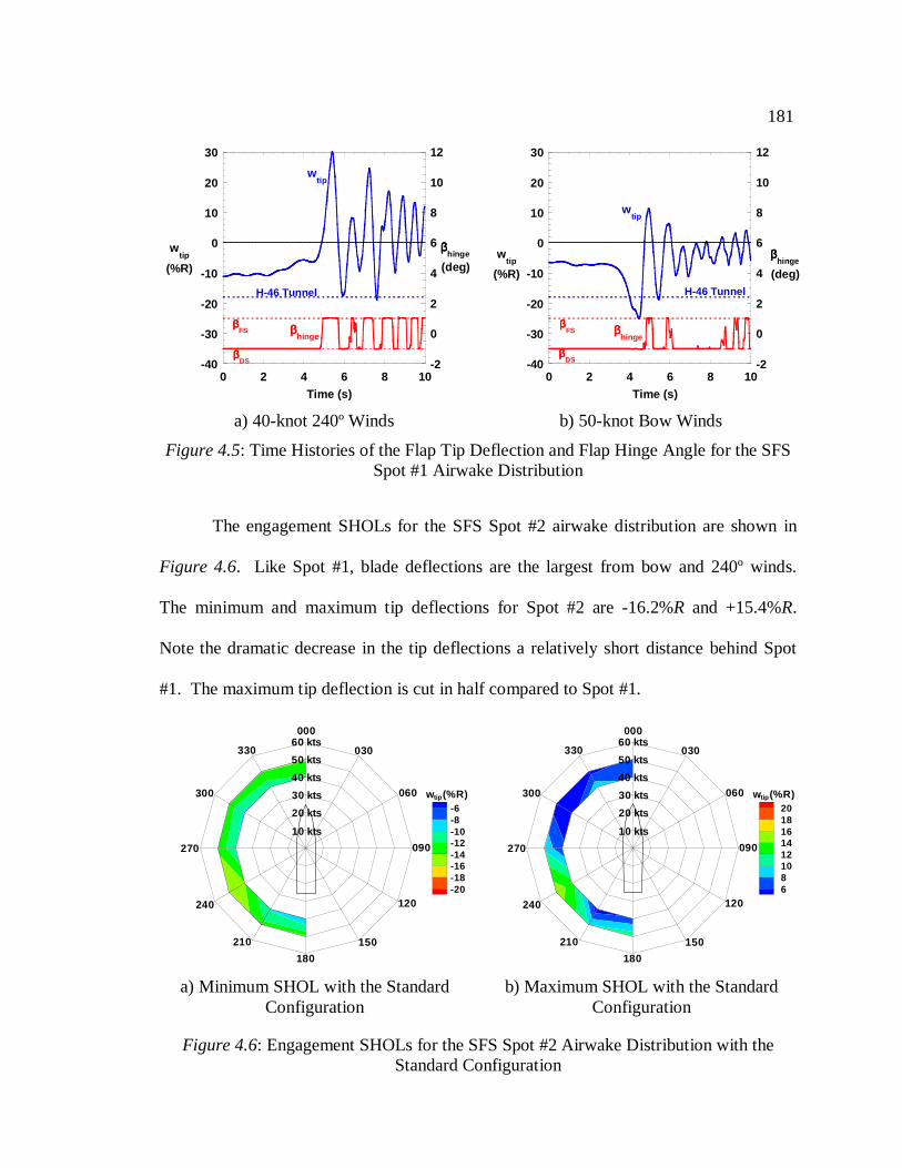
181
The engagement SHOLs for the SFS Spot #2 airwake distribution are shown in
Figure 4.6. Like Spot #1, blade deflections are the largest from bow and 240º winds.
The minimum and maximum tip deflections for Spot #2 are -16.2%R and +15.4%R.
Note the dramatic decrease in the tip deflections a relatively short distance behind Spot
#1. The maximum tip deflection is cut in half compared to Spot #1.
-40
-30
-20
-10
0
10
20
30
-2
0
2
4
6
8
10
12
0 2 4 6 8 10
wtip
(%R)
ββββhinge
(deg)
Time (s)
H-46 Tunnel
ββββDS
ββββFS
wtip
ββββhinge
a) 40-knot 240º Winds
-40
-30
-20
-10
0
10
20
30
-2
0
2
4
6
8
10
12
0 2 4 6 8 10
wtip
(%R)
ββββhinge
(deg)
Time (s)
wtip
ββββhinge
H-46 Tunnel
ββββFS
ββββDS
b) 50-knot Bow Winds
Figure 4.5: Time Histories of the Flap Tip Deflection and Flap Hinge Angle for the SFSSpot #1 Airwake Distribution
-6-8-10-12-14-16-18-20
w (%R)tip
10 kts
33050 kts
40 kts
30 kts
20 kts
60 kts000
060
030
090
120
150
180
210
240
270
300
a) Minimum SHOL with the StandardConfiguration
20181614121086
w (%R)tip
10 kts
33050 kts
40 kts
30 kts
20 kts
60 kts000
060
030
090
120
150
180
210
240
270
300
b) Maximum SHOL with the StandardConfiguration
Figure 4.6: Engagement SHOLs for the SFS Spot #2 Airwake Distribution with theStandard Configuration
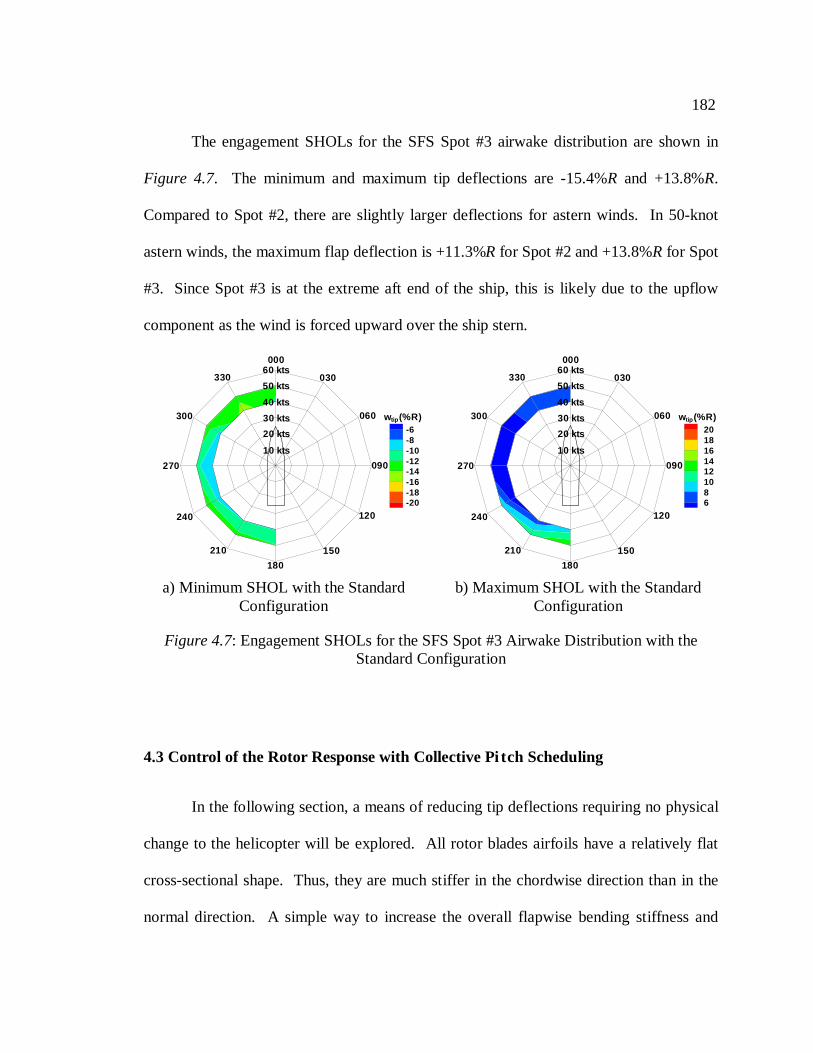
182
The engagement SHOLs for the SFS Spot #3 airwake distribution are shown in
Figure 4.7. The minimum and maximum tip deflections are -15.4%R and +13.8%R.
Compared to Spot #2, there are slightly larger deflections for astern winds. In 50-knot
astern winds, the maximum flap deflection is +11.3%R for Spot #2 and +13.8%R for Spot
#3. Since Spot #3 is at the extreme aft end of the ship, this is likely due to the upflow
component as the wind is forced upward over the ship stern.
4.3 Control of the Rotor Response with Collective Pi tch Scheduling
In the following section, a means of reducing tip deflections requiring no physical
change to the helicopter will be explored. All rotor blades airfoils have a relatively flat
cross-sectional shape. Thus, they are much stiffer in the chordwise direction than in the
normal direction. A simple way to increase the overall flapwise bending stiffness and
-6-8-10-12-14-16-18-20
w (%R)tip
10 kts
33050 kts
40 kts
30 kts
20 kts
60 kts000
060
030
090
120
150
180
210
240
270
300
a) Minimum SHOL with the StandardConfiguration
20181614121086
w (%R)tip
10 kts
33050 kts
40 kts
30 kts
20 kts
60 kts000
060
030
090
120
150
180
210
240
270
300
b) Maximum SHOL with the StandardConfiguration
Figure 4.7: Engagement SHOLs for the SFS Spot #3 Airwake Distribution with theStandard Configuration
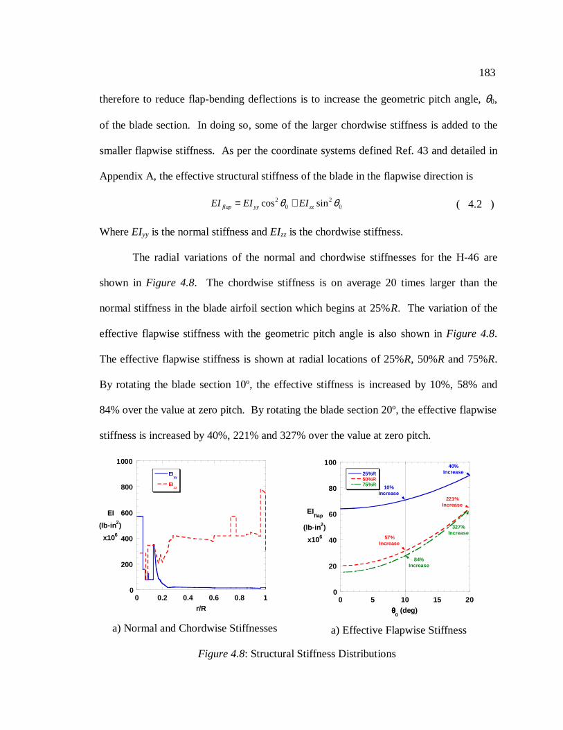
183
therefore to reduce flap-bending deflections is to increase the geometric pitch angle,θ0,
of the blade section. In doing so, some of the larger chordwise stiffness is added to the
smaller flapwise stiffness. As per the coordinate systems defined Ref. 43 and detailed in
Appendix A, the effective structural stiffness of the blade in the flapwise direction is
2 20 0cos sinflap yy zzEI EI EIθ θ= + ( 4.2 )
WhereEIyy is the normal stiffness andEIzz is the chordwise stiffness.
The radial variations of the normal and chordwise stiffnesses for the H-46 are
shown inFigure 4.8. The chordwise stiffness is on average 20 times larger than the
normal stiffness in the blade airfoil section which begins at 25%R. The variation of the
effective flapwise stiffness with the geometric pitch angle is also shown inFigure 4.8.
The effective flapwise stiffness is shown at radial locations of 25%R, 50%R and 75%R.
By rotating the blade section 10º, the effective stiffness is increased by 10%, 58% and
84% over the value at zero pitch. By rotating the blade section 20º, the effective flapwise
stiffness is increased by 40%, 221% and 327% over the value at zero pitch.
0
200
400
600
800
1000
0 0.2 0.4 0.6 0.8 1
EIyy
EIzz
EI
(lb-in 2)
x106
r/R
a) Normal and Chordwise Stiffnesses
0
20
40
60
80
100
0 5 10 15 20
25%R50%R75%R
EIflap
(lb-in 2)
x106
θθθθ0
(deg)
84%Increase
57%Increase
10%Increase
40%Increase
221%Increase
327%Increase
a) Effective Flapwise Stiffness
Figure 4.8: Structural Stiffness Distributions
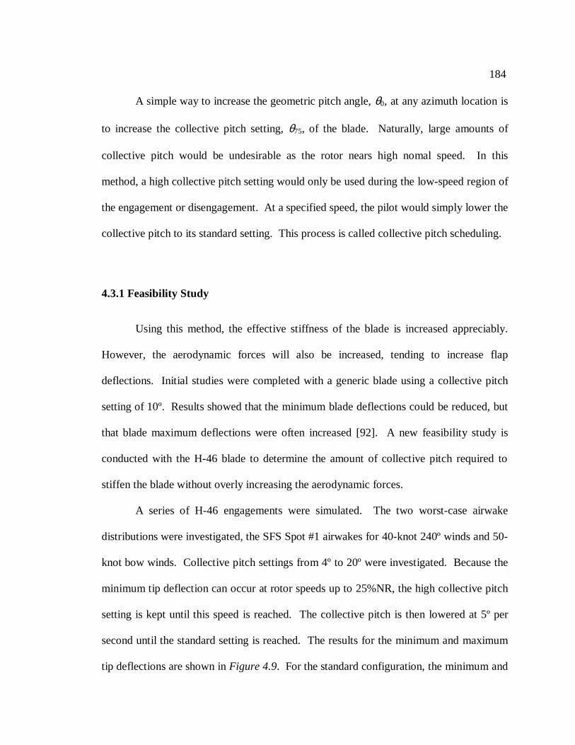
184
A simple way to increase the geometric pitch angle,θ0, at any azimuth location is
to increase the collective pitch setting,θ75, of the blade. Naturally, large amounts of
collective pitch would be undesirable as the rotor nears high nomal speed. In this
method, a high collective pitch setting would only be used during the low-speed region of
the engagement or disengagement. At a specified speed, the pilot would simply lower the
collective pitch to its standard setting. This process is called collective pitch scheduling.
4.3.1 Feasibility Study
Using this method, the effective stiffness of the blade is increased appreciably.
However, the aerodynamic forces will also be increased, tending to increase flap
deflections. Initial studies were completed with a generic blade using a collective pitch
setting of 10º. Results showed that the minimum blade deflections could be reduced, but
that blade maximum deflections were often increased [92]. A new feasibility study is
conducted with the H-46 blade to determine the amount of collective pitch required to
stiffen the blade without overly increasing the aerodynamic forces.
A series of H-46 engagements were simulated. The two worst-case airwake
distributions were investigated, the SFS Spot #1 airwakes for 40-knot 240º winds and 50-
knot bow winds. Collective pitch settings from 4º to 20º were investigated. Because the
minimum tip deflection can occur at rotor speeds up to 25%NR, the high collective pitch
setting is kept until this speed is reached. The collective pitch is then lowered at 5º per
second until the standard setting is reached. The results for the minimum and maximum
tip deflections are shown inFigure 4.9. For the standard configuration, the minimum and
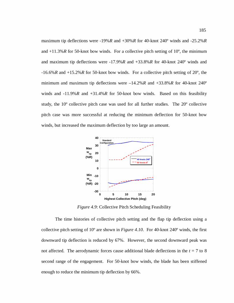
185
maximum tip deflections were -19%R and +30%R for 40-knot 240º winds and -25.2%R
and +11.3%R for 50-knot bow winds. For a collective pitch setting of 10º, the minimum
and maximum tip deflections were -17.9%R and +33.8%R for 40-knot 240º winds and
-16.6%R and +15.2%R for 50-knot bow winds. For a collective pitch setting of 20º, the
minimum and maximum tip deflections were –14.2%R and +33.8%R for 40-knot 240º
winds and -11.9%R and +31.4%R for 50-knot bow winds. Based on this feasibility
study, the 10º collective pitch case was used for all further studies. The 20º collective
pitch case was more successful at reducing the minimum deflection for 50-knot bow
winds, but increased the maximum deflection by too large an amount.
The time histories of collective pitch setting and the flap tip deflection using a
collective pitch setting of 10º are shown inFigure 4.10. For 40-knot 240º winds, the first
downward tip deflection is reduced by 67%. However, the second downward peak was
not affected. The aerodynamic forces cause additional blade deflections in thet = 7 to 8
second range of the engagement. For 50-knot bow winds, the blade has been stiffened
enough to reduce the minimum tip deflection by 66%.
-30
-20
-10
0
10
20
30
40
0 5 10 15 20
40 knots 240 o
50 knots 0 o
Maxw
tip
(%R)
Highest Collective Pitch (deg)
Minw
tip
(%R)
StandardConfiguration
Figure 4.9: Collective Pitch Scheduling Feasibility
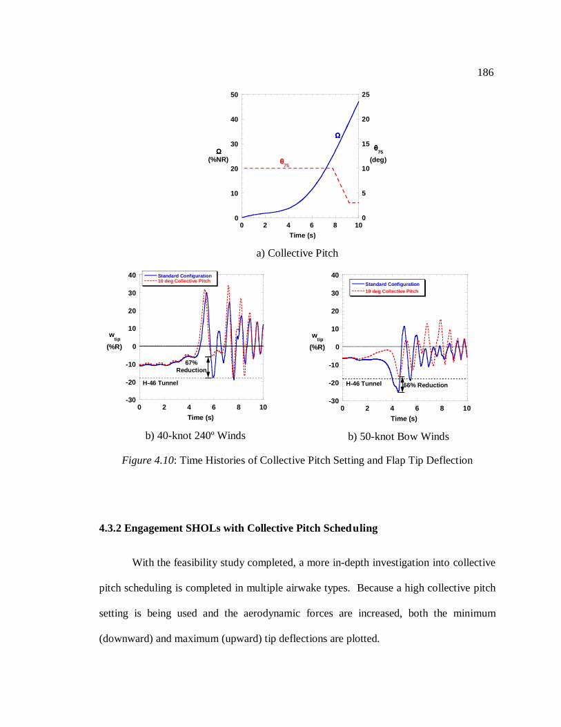
186
4.3.2 Engagement SHOLs with Collective Pitch Scheduling
With the feasibility study completed, a more in-depth investigation into collective
pitch scheduling is completed in multiple airwake types. Because a high collective pitch
setting is being used and the aerodynamic forces are increased, both the minimum
(downward) and maximum (upward) tip deflections are plotted.
0
10
20
30
40
50
0
5
10
15
20
25
0 2 4 6 8 10
ΩΩΩΩ(%NR)
θθθθ75
(deg)
Time (s)
ΩΩΩΩ
θθθθ75
a) Collective Pitch
-30
-20
-10
0
10
20
30
40
0 2 4 6 8 10
Standard Configuration10 deg Collective Pitch
wtip
(%R)
Time (s)
H-46 Tunnel
67%Reduction
b) 40-knot 240º Winds
-30
-20
-10
0
10
20
30
40
0 2 4 6 8 10
Standard Configuration10 deg Collective Pitch
wtip
(%R)
Time (s)
H-46 Tunnel 66% Reduction
b) 50-knot Bow Winds
Figure 4.10: Time Histories of Collective Pitch Setting and Flap Tip Deflection
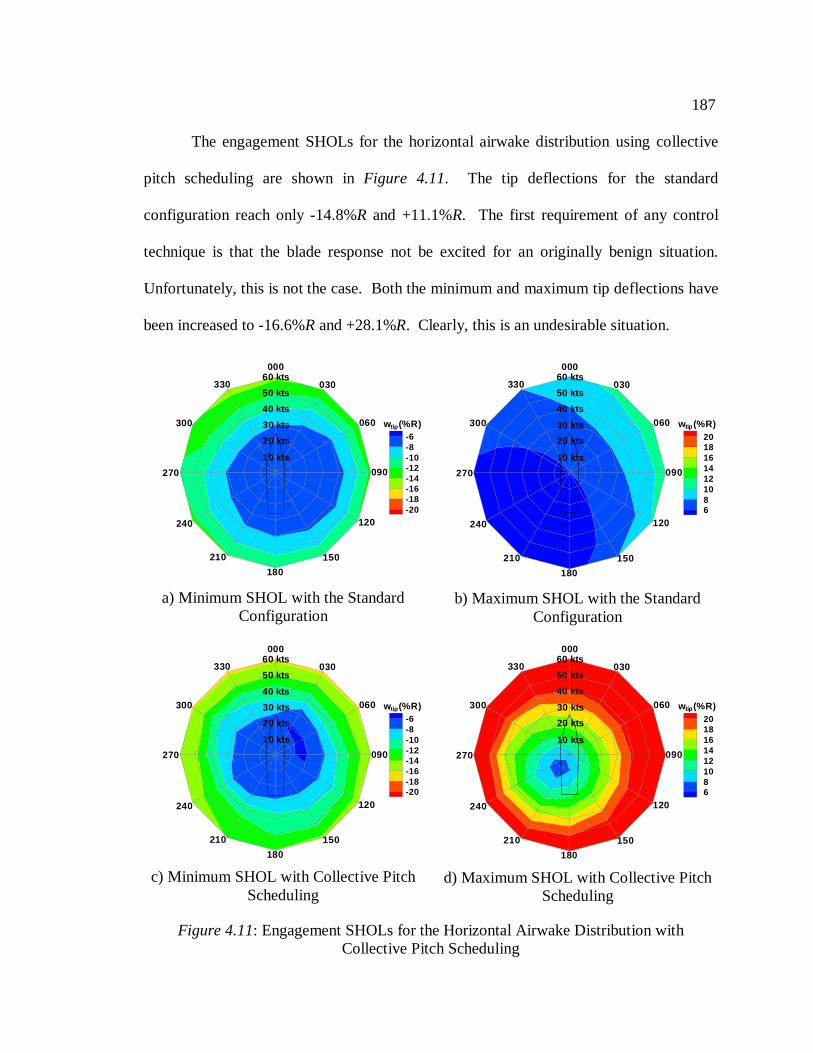
187
The engagement SHOLs for the horizontal airwake distribution using collective
pitch scheduling are shown inFigure 4.11. The tip deflections for the standard
configuration reach only -14.8%R and +11.1%R. The first requirement of any control
technique is that the blade response not be excited for an originally benign situation.
Unfortunately, this is not the case. Both the minimum and maximum tip deflections have
been increased to -16.6%R and +28.1%R. Clearly, this is an undesirable situation.
-6-8-10-12-14-16-18-20
w (%R)tip
10 kts
33050 kts
40 kts
30 kts
20 kts
60 kts000
060
030
090
120
150
180
210
240
270
300
a) Minimum SHOL with the StandardConfiguration
20181614121086
w (%R)tip
10 kts
33050 kts
40 kts
30 kts
20 kts
60 kts000
060
030
090
120
150
180
210
240
270
300
b) Maximum SHOL with the StandardConfiguration
-6-8-10-12-14-16-18-20
w (%R)tip
10 kts
33050 kts
40 kts
30 kts
20 kts
60 kts000
060
030
090
120
150
180
210
240
270
300
c) Minimum SHOL with Collective PitchScheduling
20181614121086
w (%R)tip
10 kts
33050 kts
40 kts
30 kts
20 kts
60 kts000
060
030
090
120
150
180
210
240
270
300
d) Maximum SHOL with Collective PitchScheduling
Figure 4.11: Engagement SHOLs for the Horizontal Airwake Distribution withCollective Pitch Scheduling
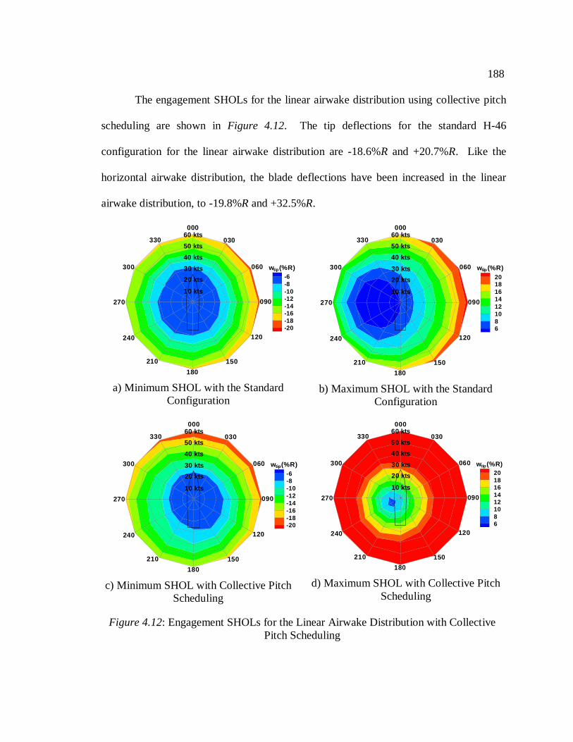
188
The engagement SHOLs for the linear airwake distribution using collective pitch
scheduling are shown inFigure 4.12. The tip deflections for the standard H-46
configuration for the linear airwake distribution are -18.6%R and +20.7%R. Like the
horizontal airwake distribution, the blade deflections have been increased in the linear
airwake distribution, to -19.8%R and +32.5%R.
-6-8-10-12-14-16-18-20
w (%R)tip
10 kts
33050 kts
40 kts
30 kts
20 kts
60 kts000
060
030
090
120
150
180
210
240
270
300
a) Minimum SHOL with the StandardConfiguration
20181614121086
w (%R)tip
10 kts
33050 kts
40 kts
30 kts
20 kts
60 kts000
060
030
090
120
150
180
210
240
270
300
b) Maximum SHOL with the StandardConfiguration
-6-8-10-12-14-16-18-20
w (%R)tip
10 kts
33050 kts
40 kts
30 kts
20 kts
60 kts000
060
030
090
120
150
180
210
240
270
300
c) Minimum SHOL with Collective PitchScheduling
20181614121086
w (%R)tip
10 kts
33050 kts
40 kts
30 kts
20 kts
60 kts000
060
030
090
120
150
180
210
240
270
300
d) Maximum SHOL with Collective PitchScheduling
Figure 4.12: Engagement SHOLs for the Linear Airwake Distribution with CollectivePitch Scheduling
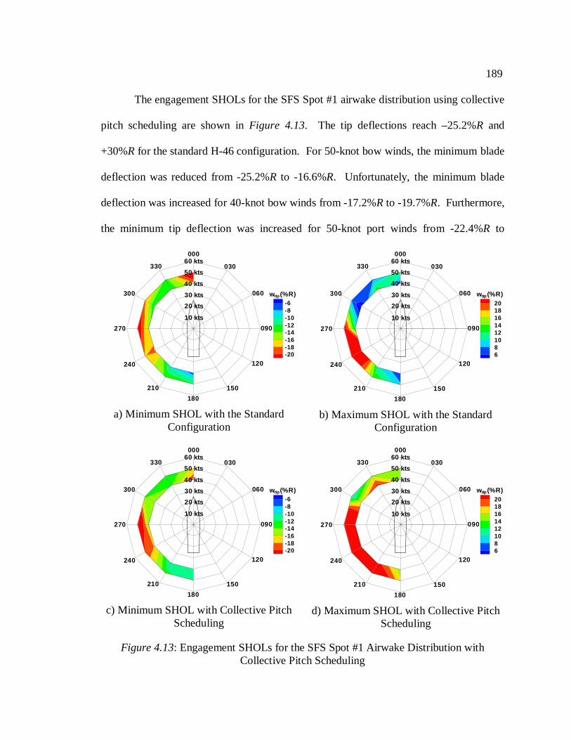
189
The engagement SHOLs for the SFS Spot #1 airwake distribution using collective
pitch scheduling are shown inFigure 4.13. The tip deflections reach –25.2%R and
+30%R for the standard H-46 configuration. For 50-knot bow winds, the minimum blade
deflection was reduced from -25.2%R to -16.6%R. Unfortunately, the minimum blade
deflection was increased for 40-knot bow winds from -17.2%R to -19.7%R. Furthermore,
the minimum tip deflection was increased for 50-knot port winds from -22.4%R to
-6-8-10-12-14-16-18-20
w (%R)tip
10 kts
33050 kts
40 kts
30 kts
20 kts
60 kts000
060
030
090
120
150
180
210
240
270
300
a) Minimum SHOL with the StandardConfiguration
20181614121086
w (%R)tip
10 kts
33050 kts
40 kts
30 kts
20 kts
60 kts000
060
030
090
120
150
180
210
240
270
300
b) Maximum SHOL with the StandardConfiguration
-6-8-10-12-14-16-18-20
w (%R)tip
10 kts
33050 kts
40 kts
30 kts
20 kts
60 kts000
060
030
090
120
150
180
210
240
270
300
c) Minimum SHOL with Collective PitchScheduling
20181614121086
w (%R)tip
10 kts
33050 kts
40 kts
30 kts
20 kts
60 kts000
060
030
090
120
150
180
210
240
270
300
d) Maximum SHOL with Collective PitchScheduling
Figure 4.13: Engagement SHOLs for the SFS Spot #1 Airwake Distribution withCollective Pitch Scheduling
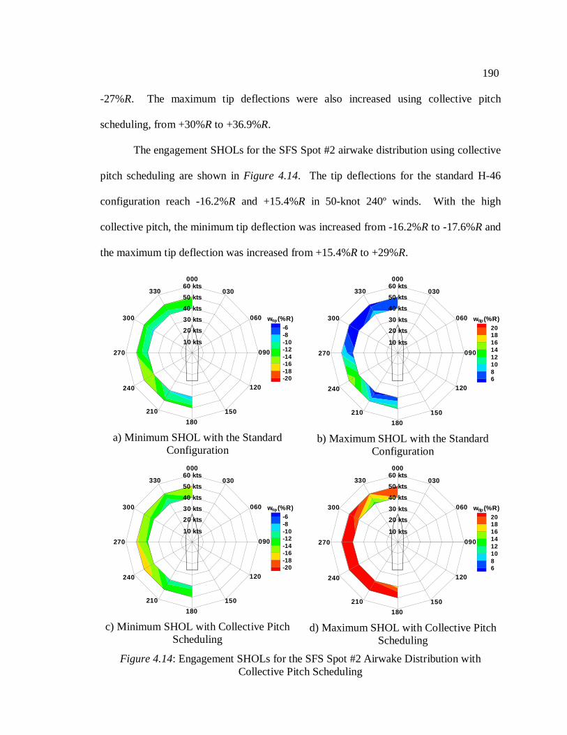
190
-27%R. The maximum tip deflections were also increased using collective pitch
scheduling, from +30%R to +36.9%R.
The engagement SHOLs for the SFS Spot #2 airwake distribution using collective
pitch scheduling are shown inFigure 4.14. The tip deflections for the standard H-46
configuration reach -16.2%R and +15.4%R in 50-knot 240º winds. With the high
collective pitch, the minimum tip deflection was increased from -16.2%R to -17.6%R and
the maximum tip deflection was increased from +15.4%R to +29%R.
-6-8-10-12-14-16-18-20
w (%R)tip
10 kts
33050 kts
40 kts
30 kts
20 kts
60 kts000
060
030
090
120
150
180
210
240
270
300
a) Minimum SHOL with the StandardConfiguration
20181614121086
w (%R)tip
10 kts
33050 kts
40 kts
30 kts
20 kts
60 kts000
060
030
090
120
150
180
210
240
270
300
b) Maximum SHOL with the StandardConfiguration
-6-8-10-12-14-16-18-20
w (%R)tip
10 kts
33050 kts
40 kts
30 kts
20 kts
60 kts000
060
030
090
120
150
180
210
240
270
300
c) Minimum SHOL with Collective PitchScheduling
20181614121086
w (%R)tip
10 kts
33050 kts
40 kts
30 kts
20 kts
60 kts000
060
030
090
120
150
180
210
240
270
300
d) Maximum SHOL with Collective PitchScheduling
Figure 4.14: Engagement SHOLs for the SFS Spot #2 Airwake Distribution withCollective Pitch Scheduling
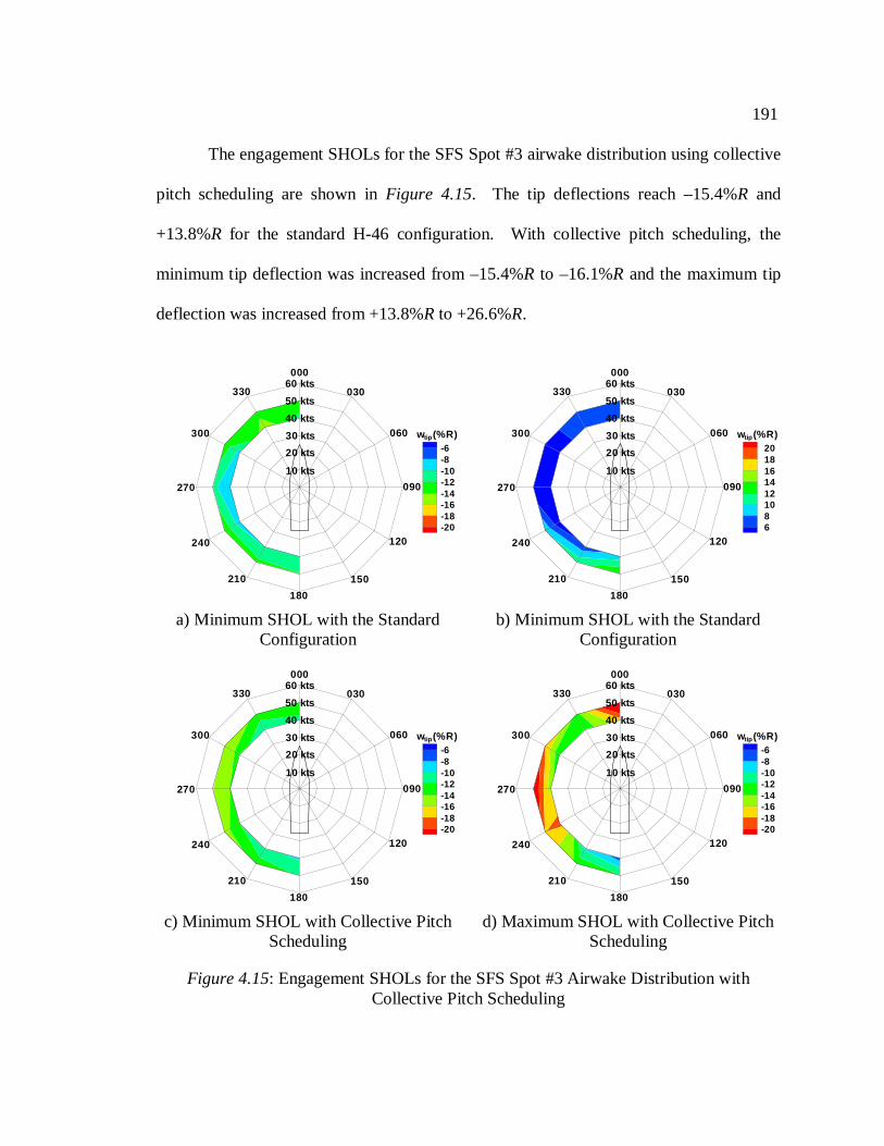
191
The engagement SHOLs for the SFS Spot #3 airwake distribution using collective
pitch scheduling are shown inFigure 4.15. The tip deflections reach –15.4%R and
+13.8%R for the standard H-46 configuration. With collective pitch scheduling, the
minimum tip deflection was increased from –15.4%R to –16.1%R and the maximum tip
deflection was increased from +13.8%R to +26.6%R.
-6-8-10-12-14-16-18-20
w (%R)tip
10 kts
33050 kts
40 kts
30 kts
20 kts
60 kts000
060
030
090
120
150
180
210
240
270
300
a) Minimum SHOL with the StandardConfiguration
20181614121086
w (%R)tip
10 kts
33050 kts
40 kts
30 kts
20 kts
60 kts000
060
030
090
120
150
180
210
240
270
300
b) Minimum SHOL with the StandardConfiguration
-6-8-10-12-14-16-18-20
w (%R)tip
10 kts
33050 kts
40 kts
30 kts
20 kts
60 kts000
060
030
090
120
150
180
210
240
270
300
c) Minimum SHOL with Collective PitchScheduling
-6-8-10-12-14-16-18-20
w (%R)tip
10 kts
33050 kts
40 kts
30 kts
20 kts
60 kts000
060
030
090
120
150
180
210
240
270
300
d) Maximum SHOL with Collective PitchScheduling
Figure 4.15: Engagement SHOLs for the SFS Spot #3 Airwake Distribution withCollective Pitch Scheduling
192
The results of this study indicate that the use of a high collective pitch setting is
not a feasible way to reduce blade flap deflections. Although the blade is stiffened
appreciably, the aerodynamic forces are also increased. Only a few cases were found
which resulted in decreased blade deflections. The blade deflections were more often
increased, especially in airwake distributions that exhibited mild flapping behavior with
the standard configuration.
4.4 Control of the Rotor Response with a Flap Damper
The second passive control technique examines the effect of a discrete flap
damper on the rotor response during engagements and disengagements. Such a flap
damper is intended to dissipate excessive flap motions much like a lag damper dissipates
excessive lag motions. This is not an entirely new idea. A special flap damper device
was used on the HUP-1 to HUP-4 series tandem naval helicopters as early as the 1950’s
to reduce excessive blade flapping during low rotor speed operations [93]. A picture of
the HUP-2 and a schematic of the flap damper are shown inFigure 4.16. Each rotor
blade had its own flap damper. Each flap damper was attached to a point just outboard of
the flap hinge at one end and to a mast above the rotor hub at the other end. The flap
damper was designed to become inactive above a specified rotor speed, by centrifugal
force pulling on a spring/counterweight combination and rotating a series of mechanical
linkages. The rotation of the mechanical linkages effectively made the flap damper
inactive.
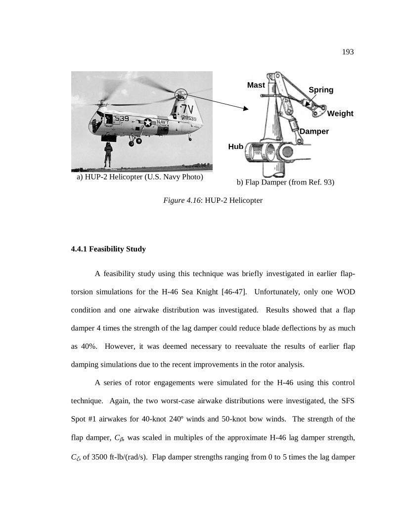
193
4.4.1 Feasibility Study
A feasibility study using this technique was briefly investigated in earlier flap-
torsion simulations for the H-46 Sea Knight [46-47]. Unfortunately, only one WOD
condition and one airwake distribution was investigated. Results showed that a flap
damper 4 times the strength of the lag damper could reduce blade deflections by as much
as 40%. However, it was deemed necessary to reevaluate the results of earlier flap
damping simulations due to the recent improvements in the rotor analysis.
A series of rotor engagements were simulated for the H-46 using this control
technique. Again, the two worst-case airwake distributions were investigated, the SFS
Spot #1 airwakes for 40-knot 240º winds and 50-knot bow winds. The strength of the
flap damper,Cβ, was scaled in multiples of the approximate H-46 lag damper strength,
Cζ, of 3500 ft-lb/(rad/s). Flap damper strengths ranging from 0 to 5 times the lag damper
a) HUP-2 Helicopter (U.S. Navy Photo)b) Flap Damper (from Ref. 93)
Figure 4.16: HUP-2 Helicopter
Hub
Weight
Spring
Damper
Mast
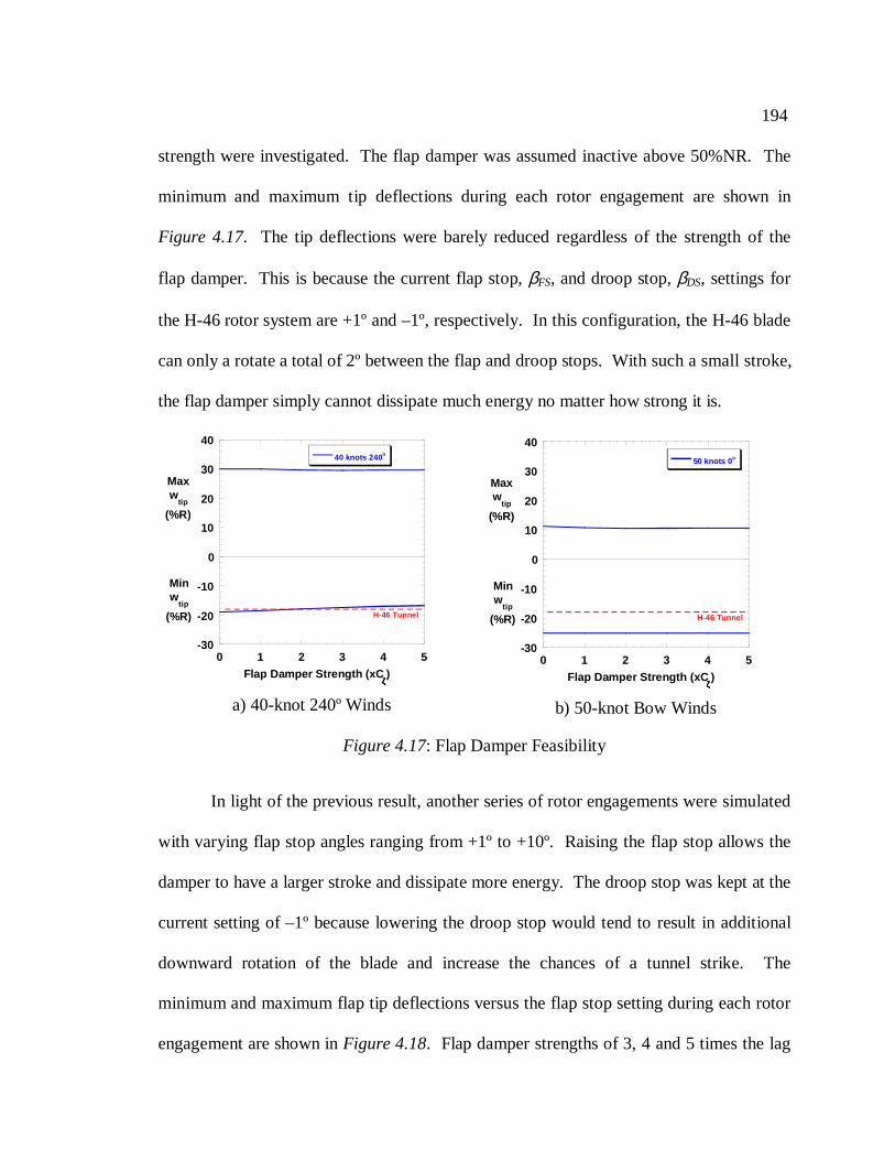
194
strength were investigated. The flap damper was assumed inactive above 50%NR. The
minimum and maximum tip deflections during each rotor engagement are shown in
Figure 4.17. The tip deflections were barely reduced regardless of the strength of the
flap damper. This is because the current flap stop,βFS, and droop stop,βDS, settings for
the H-46 rotor system are +1º and –1º, respectively. In this configuration, the H-46 blade
can only a rotate a total of 2º between the flap and droop stops. With such a small stroke,
the flap damper simply cannot dissipate much energy no matter how strong it is.
In light of the previous result, another series of rotor engagements were simulated
with varying flap stop angles ranging from +1º to +10º. Raising the flap stop allows the
damper to have a larger stroke and dissipate more energy. The droop stop was kept at the
current setting of –1º because lowering the droop stop would tend to result in additional
downward rotation of the blade and increase the chances of a tunnel strike. The
minimum and maximum flap tip deflections versus the flap stop setting during each rotor
engagement are shown inFigure 4.18. Flap damper strengths of 3, 4 and 5 times the lag
-30
-20
-10
0
10
20
30
40
0 1 2 3 4 5
40 knots 240 o
Maxw
tip
(%R)
Flap Damper Strength (xCζζζζ)
Minw
tip
(%R) H-46 Tunnel
a) 40-knot 240º Winds
-30
-20
-10
0
10
20
30
40
0 1 2 3 4 5
50 knots 0 o
Maxw
tip
(%R)
Flap Damper Strength (xCζζζζ)
H-46 Tunnel
Minw
tip
(%R)
b) 50-knot Bow Winds
Figure 4.17: Flap Damper Feasibility
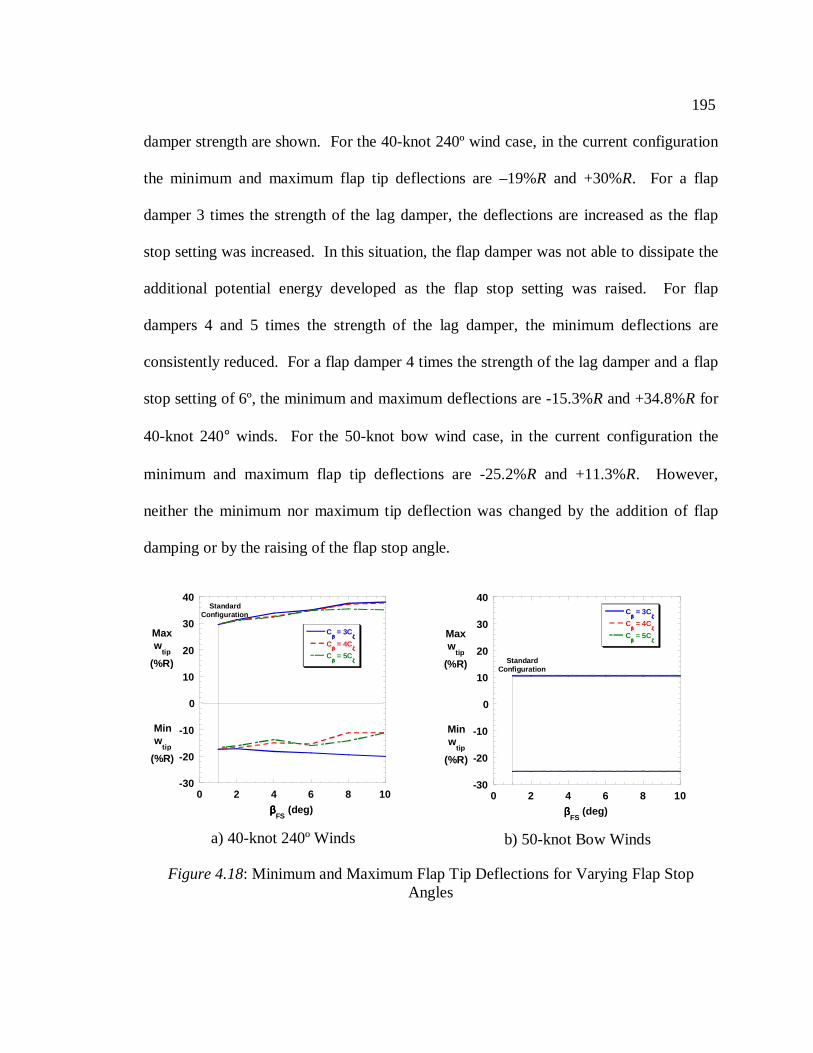
195
damper strength are shown. For the 40-knot 240º wind case, in the current configuration
the minimum and maximum flap tip deflections are –19%R and +30%R. For a flap
damper 3 times the strength of the lag damper, the deflections are increased as the flap
stop setting was increased. In this situation, the flap damper was not able to dissipate the
additional potential energy developed as the flap stop setting was raised. For flap
dampers 4 and 5 times the strength of the lag damper, the minimum deflections are
consistently reduced. For a flap damper 4 times the strength of the lag damper and a flap
stop setting of 6º, the minimum and maximum deflections are -15.3%R and +34.8%R for
40-knot 240° winds. For the 50-knot bow wind case, in the current configuration the
minimum and maximum flap tip deflections are -25.2%R and +11.3%R. However,
neither the minimum nor maximum tip deflection was changed by the addition of flap
damping or by the raising of the flap stop angle.
-30
-20
-10
0
10
20
30
40
0 2 4 6 8 10
Cββββ
= 3Cζζζζ
Cββββ
= 4Cζζζζ
Cββββ
= 5Cζζζζ
Maxw
tip
(%R)
ββββFS
(deg)
Minw
tip
(%R)
StandardConfiguration
a) 40-knot 240º Winds
-30
-20
-10
0
10
20
30
40
0 2 4 6 8 10
Cββββ
= 3Cζζζζ
Cββββ
= 4Cζζζζ
Cββββ
= 5Cζζζζ
ββββFS
(deg)
Maxw
tip
(%R)
Minw
tip
(%R)
StandardConfiguration
b) 50-knot Bow Winds
Figure 4.18: Minimum and Maximum Flap Tip Deflections for Varying Flap StopAngles

196
In choosing the correct flap damper/flap stop combination, it is desirable to use
the minimum flap damper strength and the smallest flap stop setting that have a
substantial effect of the tip deflections. Obviously, the flap damper 3 times the strength
of the lag damper was not strong enough. With minimal differences in the blade response
between flap damper strengths of 4 and 5 times the lag damper strength, use of the lower
strength flap damper is preferable. Flap stop settings higher than 6º resulted in increased
maximum tip deflections, while settings lower than 6º had only a minor effect on the
minimum tip deflection. Therefore, the combination of the flap damper 4 times the
strength of the lag damper and the 6º flap stop setting was chosen for the rest of the
simulations. It agrees well with the results from the original flap damping feasibility
analysis completed in Refs. 46-47.
The time histories of the flap tip deflection and flap hinge angle for this flap
damper/flap stop combination are shown inFigure 4.19. For 40-knot bow winds, both
the first and second minimum flap deflections are reduced. Note that for 50-knot bow
winds, the minimum tip deflection occurs before the blade ever lifts off the droop stop.
Therefore, the flap damping technique will be completely ineffective in reducing the
minimum tip deflection in this case.
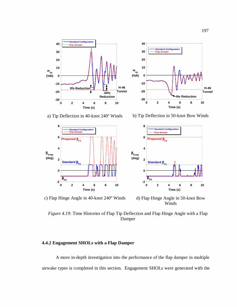
197
4.4.2 Engagement SHOLs with a Flap Damper
A more in-depth investigation into the performance of the flap damper in multiple
airwake types is completed in this section. Engagement SHOLs were generated with the
-30
-20
-10
0
10
20
30
40
0 2 4 6 8 10
Standard ConfigurationFlap Damper
wtip
(%R)
Time (s)
H-46Tunnel
9% Reduction
44%Reduction
a) Tip Deflection in 40-knot 240º Winds
-30
-20
-10
0
10
20
30
40
0 2 4 6 8 10
Standard ConfigurationFlap Damper
wtip
(%R)
Time (s)
H-46Tunnel
No Reduction
b) Tip Deflection in 50-knot Bow Winds
-2
0
2
4
6
8
0 2 4 6 8 10
Standard ConfigurationFlap Damper
ββββhinge
(deg)
Time (s)
ββββDS
Standard ββββFS
Proposed ββββFS
c) Flap Hinge Angle in 40-knot 240º Winds
-2
0
2
4
6
8
0 2 4 6 8 10
Standard Configuration
Flap Damper
ββββhinge
(deg)
Time (s)
Proposed ββββFS
Standard ββββFS
ββββDS
d) Flap Hinge Angle in 50-knot BowWinds
Figure 4.19: Time Histories of Flap Tip Deflection and Flap Hinge Angle with a FlapDamper
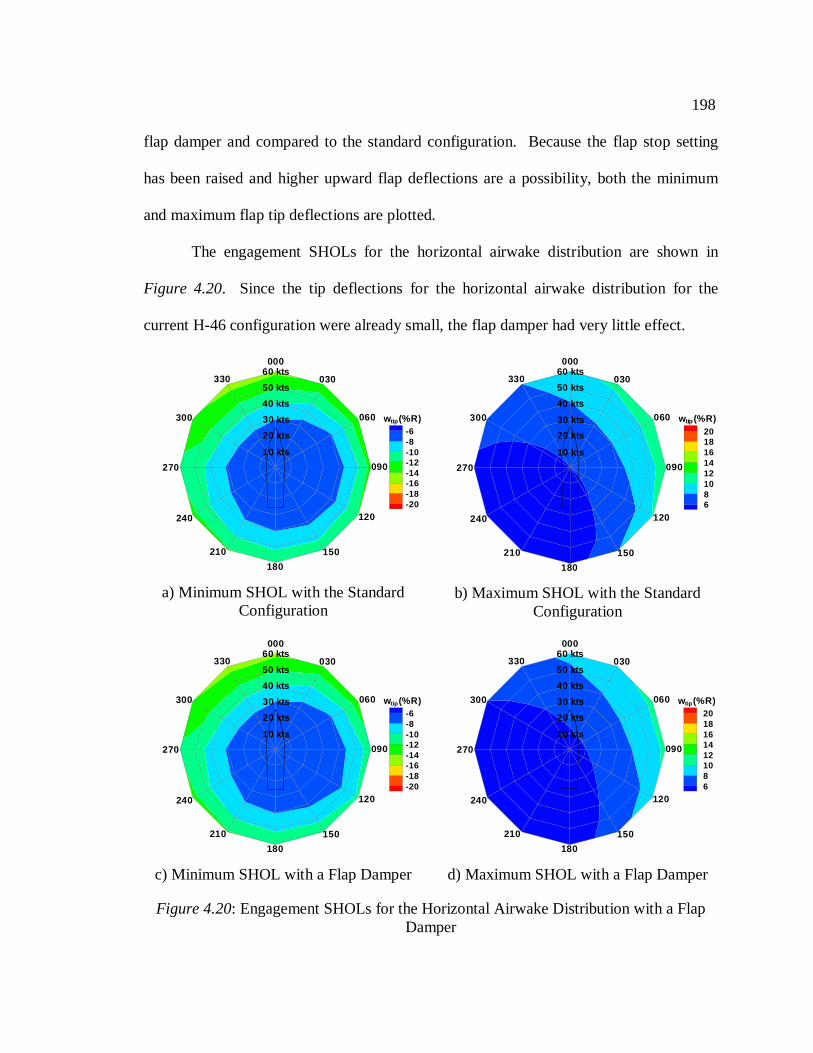
198
flap damper and compared to the standard configuration. Because the flap stop setting
has been raised and higher upward flap deflections are a possibility, both the minimum
and maximum flap tip deflections are plotted.
The engagement SHOLs for the horizontal airwake distribution are shown in
Figure 4.20. Since the tip deflections for the horizontal airwake distribution for the
current H-46 configuration were already small, the flap damper had very little effect.
-6-8-10-12-14-16-18-20
w (%R)tip
10 kts
33050 kts
40 kts
30 kts
20 kts
60 kts000
060
030
090
120
150
180
210
240
270
300
a) Minimum SHOL with the StandardConfiguration
20181614121086
w (%R)tip
10 kts
33050 kts
40 kts
30 kts
20 kts
60 kts000
060
030
090
120
150
180
210
240
270
300
b) Maximum SHOL with the StandardConfiguration
-6-8-10-12-14-16-18-20
w (%R)tip
10 kts
33050 kts
40 kts
30 kts
20 kts
60 kts000
060
030
090
120
150
180
210
240
270
300
c) Minimum SHOL with a Flap Damper
20181614121086
w (%R)tip
10 kts
33050 kts
40 kts
30 kts
20 kts
60 kts000
060
030
090
120
150
180
210
240
270
300
d) Maximum SHOL with a Flap Damper
Figure 4.20: Engagement SHOLs for the Horizontal Airwake Distribution with a FlapDamper
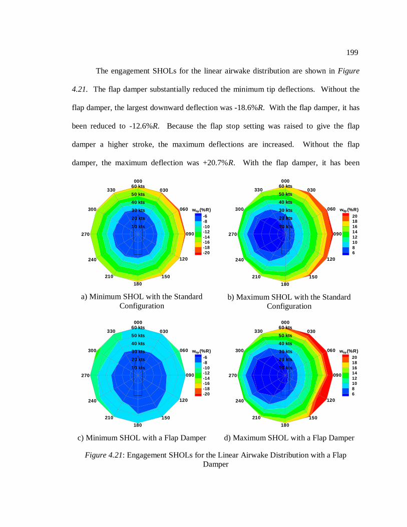
199
The engagement SHOLs for the linear airwake distribution are shown inFigure
4.21. The flap damper substantially reduced the minimum tip deflections. Without the
flap damper, the largest downward deflection was -18.6%R. With the flap damper, it has
been reduced to -12.6%R. Because the flap stop setting was raised to give the flap
damper a higher stroke, the maximum deflections are increased. Without the flap
damper, the maximum deflection was +20.7%R. With the flap damper, it has been
-6-8-10-12-14-16-18-20
w (%R)tip
10 kts
33050 kts
40 kts
30 kts
20 kts
60 kts000
060
030
090
120
150
180
210
240
270
300
a) Minimum SHOL with the StandardConfiguration
20181614121086
w (%R)tip
10 kts
33050 kts
40 kts
30 kts
20 kts
60 kts000
060
030
090
120
150
180
210
240
270
300
b) Maximum SHOL with the StandardConfiguration
-6-8-10-12-14-16-18-20
w (%R)tip
10 kts
33050 kts
40 kts
30 kts
20 kts
60 kts000
060
030
090
120
150
180
210
240
270
300
c) Minimum SHOL with a Flap Damper
20181614121086
w (%R)tip
10 kts
33050 kts
40 kts
30 kts
20 kts
60 kts000
060
030
090
120
150
180
210
240
270
300
d) Maximum SHOL with a Flap Damper
Figure 4.21: Engagement SHOLs for the Linear Airwake Distribution with a FlapDamper
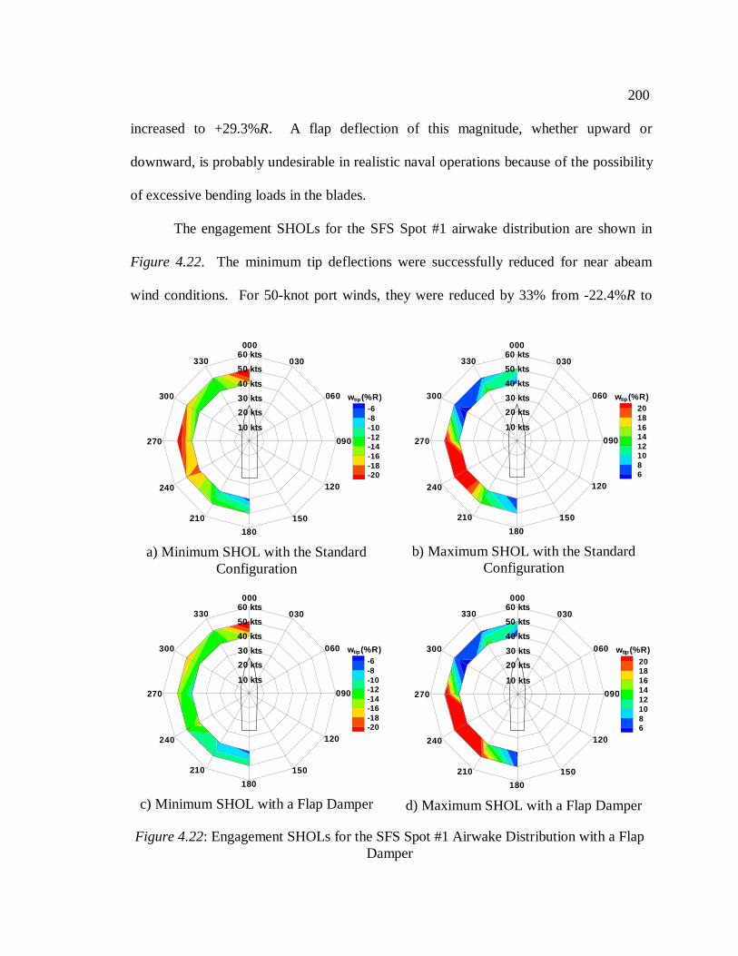
200
increased to +29.3%R. A flap deflection of this magnitude, whether upward or
downward, is probably undesirable in realistic naval operations because of the possibility
of excessive bending loads in the blades.
The engagement SHOLs for the SFS Spot #1 airwake distribution are shown in
Figure 4.22. The minimum tip deflections were successfully reduced for near abeam
wind conditions. For 50-knot port winds, they were reduced by 33% from -22.4%R to
-6-8-10-12-14-16-18-20
w (%R)tip
10 kts
33050 kts
40 kts
30 kts
20 kts
60 kts000
060
030
090
120
150
180
210
240
270
300
a) Minimum SHOL with the StandardConfiguration
20181614121086
w (%R)tip
10 kts
33050 kts
40 kts
30 kts
20 kts
60 kts000
060
030
090
120
150
180
210
240
270
300
b) Maximum SHOL with the StandardConfiguration
-6-8-10-12-14-16-18-20
w (%R)tip
10 kts
33050 kts
40 kts
30 kts
20 kts
60 kts000
060
030
090
120
150
180
210
240
270
300
c) Minimum SHOL with a Flap Damper
20181614121086
w (%R)tip
10 kts
33050 kts
40 kts
30 kts
20 kts
60 kts000
060
030
090
120
150
180
210
240
270
300
d) Maximum SHOL with a Flap Damper
Figure 4.22: Engagement SHOLs for the SFS Spot #1 Airwake Distribution with a FlapDamper
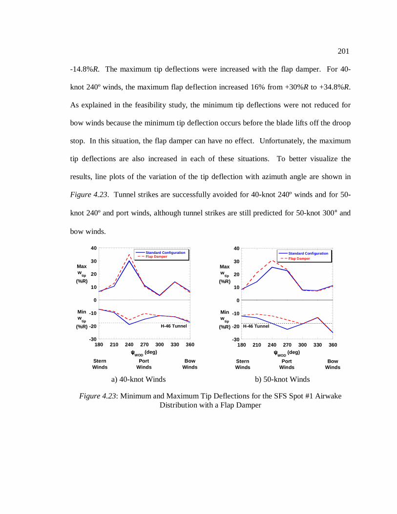
201
-14.8%R. The maximum tip deflections were increased with the flap damper. For 40-
knot 240º winds, the maximum flap deflection increased 16% from +30%R to +34.8%R.
As explained in the feasibility study, the minimum tip deflections were not reduced for
bow winds because the minimum tip deflection occurs before the blade lifts off the droop
stop. In this situation, the flap damper can have no effect. Unfortunately, the maximum
tip deflections are also increased in each of these situations. To better visualize the
results, line plots of the variation of the tip deflection with azimuth angle are shown in
Figure 4.23. Tunnel strikes are successfully avoided for 40-knot 240º winds and for 50-
knot 240º and port winds, although tunnel strikes are still predicted for 50-knot 300° and
bow winds.
-30
-20
-10
0
10
20
30
40
180 210 240 270 300 330 360
Standard ConfigurationFlap Damper
Maxw
tip
(%R)
ψψψψWOD
(deg)
Minw
tip
(%R)
BowWinds
PortWinds
SternWinds
H-46 Tunnel
a) 40-knot Winds
-30
-20
-10
0
10
20
30
40
180 210 240 270 300 330 360
Standard ConfigurationFlap Damper
Maxw
tip
(%R)
Minw
tip
(%R)
BowWinds
PortWinds
SternWinds
ψψψψWOD
(deg)
H-46 Tunnel
b) 50-knot Winds
Figure 4.23: Minimum and Maximum Tip Deflections for the SFS Spot #1 AirwakeDistribution with a Flap Damper
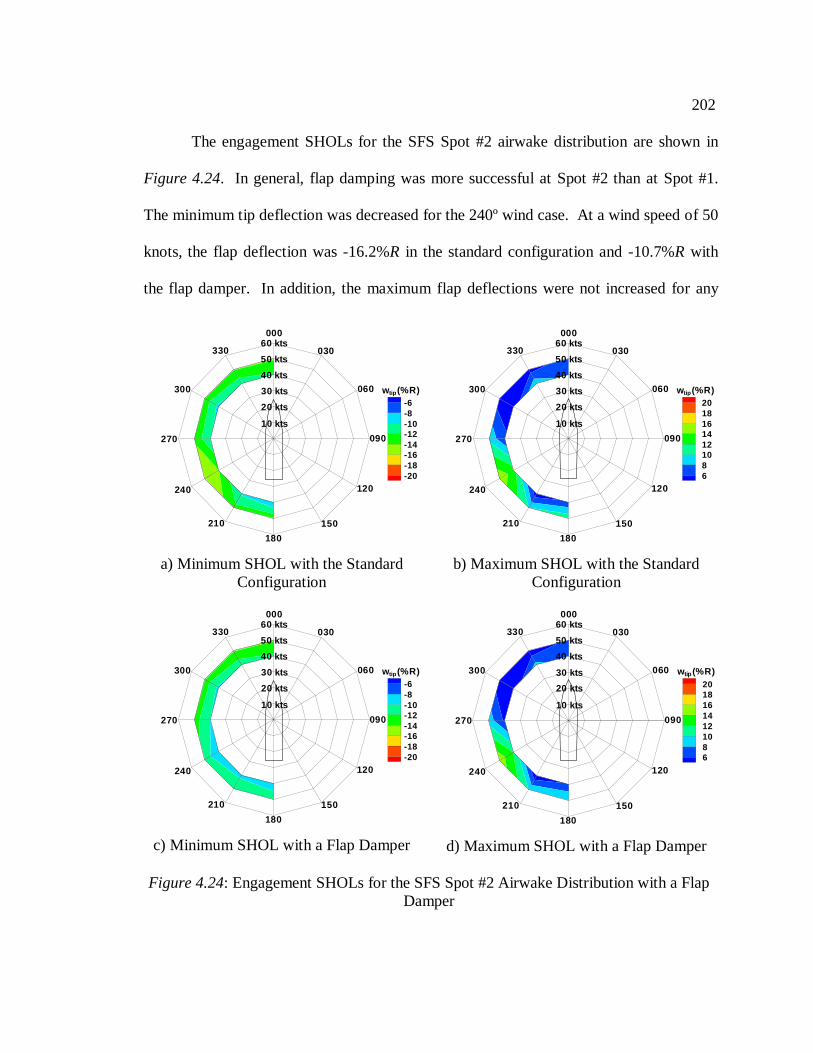
202
The engagement SHOLs for the SFS Spot #2 airwake distribution are shown in
Figure 4.24. In general, flap damping was more successful at Spot #2 than at Spot #1.
The minimum tip deflection was decreased for the 240º wind case. At a wind speed of 50
knots, the flap deflection was -16.2%R in the standard configuration and -10.7%R with
the flap damper. In addition, the maximum flap deflections were not increased for any
-6-8-10-12-14-16-18-20
w (%R)tip
10 kts
33050 kts
40 kts
30 kts
20 kts
60 kts000
060
030
090
120
150
180
210
240
270
300
a) Minimum SHOL with the StandardConfiguration
20181614121086
w (%R)tip
10 kts
33050 kts
40 kts
30 kts
20 kts
60 kts000
060
030
090
120
150
180
210
240
270
300
b) Maximum SHOL with the StandardConfiguration
-6-8-10-12-14-16-18-20
w (%R)tip
10 kts
33050 kts
40 kts
30 kts
20 kts
60 kts000
060
030
090
120
150
180
210
240
270
300
c) Minimum SHOL with a Flap Damper
20181614121086
w (%R)tip
10 kts
33050 kts
40 kts
30 kts
20 kts
60 kts000
060
030
090
120
150
180
210
240
270
300
d) Maximum SHOL with a Flap Damper
Figure 4.24: Engagement SHOLs for the SFS Spot #2 Airwake Distribution with a FlapDamper
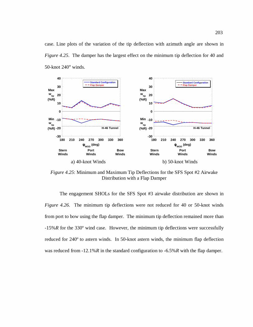
203
case. Line plots of the variation of the tip deflection with azimuth angle are shown in
Figure 4.25. The damper has the largest effect on the minimum tip deflection for 40 and
50-knot 240° winds.
The engagement SHOLs for the SFS Spot #3 airwake distribution are shown in
Figure 4.26. The minimum tip deflections were not reduced for 40 or 50-knot winds
from port to bow using the flap damper. The minimum tip deflection remained more than
-15%R for the 330º wind case. However, the minimum tip deflections were successfully
reduced for 240º to astern winds. In 50-knot astern winds, the minimum flap deflection
was reduced from -12.1%R in the standard configuration to -6.5%R with the flap damper.
-30
-20
-10
0
10
20
30
40
180 210 240 270 300 330 360
Standard ConfigurationFlap Damper
Maxw
tip
(%R)
Minw
tip
(%R)
BowWinds
PortWinds
SternWinds
H-46 Tunnel
ψψψψWOD
(deg)
a) 40-knot Winds
-30
-20
-10
0
10
20
30
40
180 210 240 270 300 330 360
Standard ConfigurationFlap Damper
Maxw
tip
(%R)
Minw
tip
(%R)
BowWinds
PortWinds
SternWinds
H-46 Tunnel
ψψψψWOD
(deg)
b) 50-knot Winds
Figure 4.25: Minimum and Maximum Tip Deflections for the SFS Spot #2 AirwakeDistribution with a Flap Damper
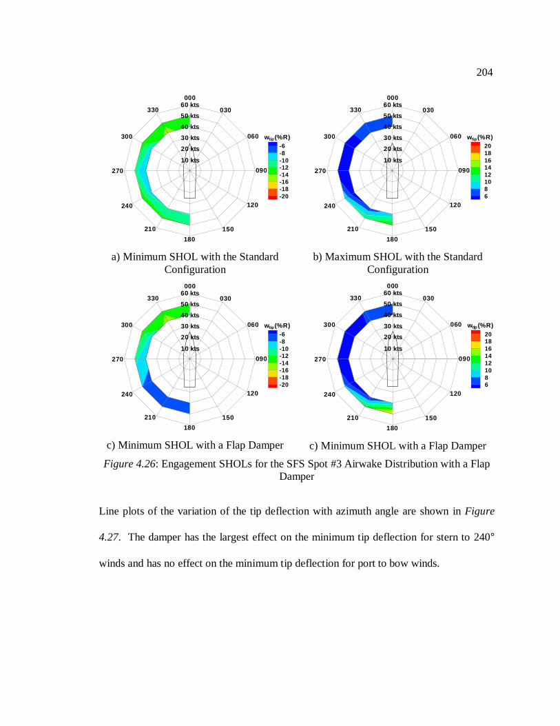
204
Line plots of the variation of the tip deflection with azimuth angle are shown inFigure
4.27. The damper has the largest effect on the minimum tip deflection for stern to 240°
winds and has no effect on the minimum tip deflection for port to bow winds.
-6-8-10-12-14-16-18-20
w (%R)tip
10 kts
33050 kts
40 kts
30 kts
20 kts
60 kts000
060
030
090
120
150
180
210
240
270
300
a) Minimum SHOL with the StandardConfiguration
20181614121086
w (%R)tip
10 kts
33050 kts
40 kts
30 kts
20 kts
60 kts000
060
030
090
120
150
180
210
240
270
300
b) Maximum SHOL with the StandardConfiguration
-6-8-10-12-14-16-18-20
w (%R)tip
10 kts
33050 kts
40 kts
30 kts
20 kts
60 kts000
060
030
090
120
150
180
210
240
270
300
c) Minimum SHOL with a Flap Damper
20181614121086
w (%R)tip
10 kts
33050 kts
40 kts
30 kts
20 kts
60 kts000
060
030
090
120
150
180
210
240
270
300
c) Minimum SHOL with a Flap Damper
Figure 4.26: Engagement SHOLs for the SFS Spot #3 Airwake Distribution with a FlapDamper
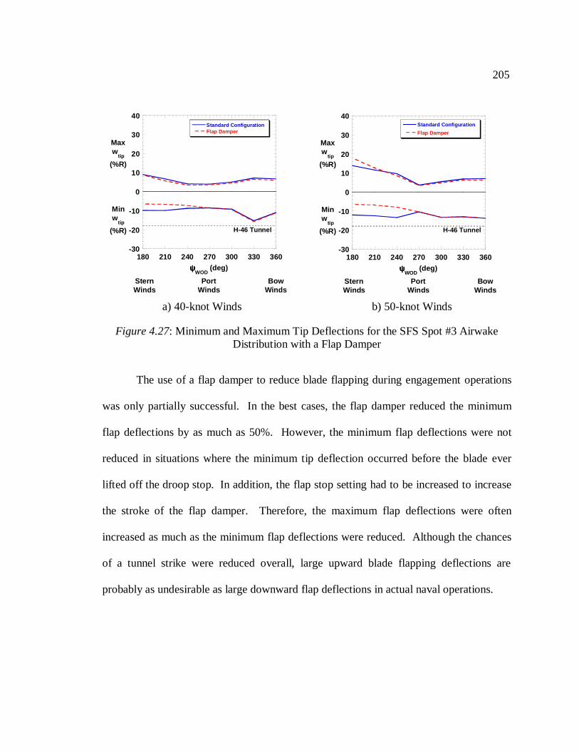
205
The use of a flap damper to reduce blade flapping during engagement operations
was only partially successful. In the best cases, the flap damper reduced the minimum
flap deflections by as much as 50%. However, the minimum flap deflections were not
reduced in situations where the minimum tip deflection occurred before the blade ever
lifted off the droop stop. In addition, the flap stop setting had to be increased to increase
the stroke of the flap damper. Therefore, the maximum flap deflections were often
increased as much as the minimum flap deflections were reduced. Although the chances
of a tunnel strike were reduced overall, large upward blade flapping deflections are
probably as undesirable as large downward flap deflections in actual naval operations.
-30
-20
-10
0
10
20
30
40
180 210 240 270 300 330 360
Standard ConfigurationFlap Damper
Maxw
tip
(%R)
Minw
tip
(%R)
BowWinds
PortWinds
SternWinds
H-46 Tunnel
ψψψψWOD
(deg)
a) 40-knot Winds
-30
-20
-10
0
10
20
30
40
180 210 240 270 300 330 360
Standard Configuration
Flap Damper
Maxw
tip
(%R)
Minw
tip
(%R)
BowWinds
PortWinds
SternWinds
H-46 Tunnel
ψψψψWOD
(deg)
b) 50-knot Winds
Figure 4.27: Minimum and Maximum Tip Deflections for the SFS Spot #3 AirwakeDistribution with a Flap Damper
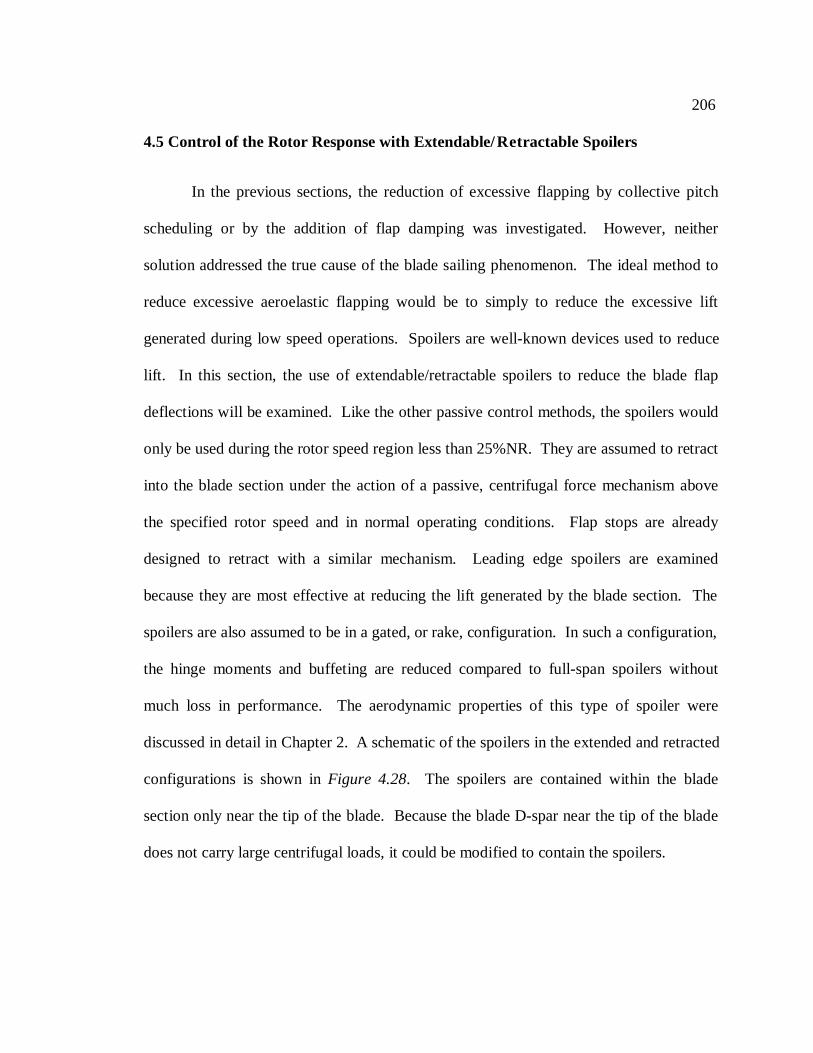
206
4.5 Control of the Rotor Response with Extendable/Retractable Spoilers
In the previous sections, the reduction of excessive flapping by collective pitch
scheduling or by the addition of flap damping was investigated. However, neither
solution addressed the true cause of the blade sailing phenomenon. The ideal method to
reduce excessive aeroelastic flapping would be to simply to reduce the excessive lift
generated during low speed operations. Spoilers are well-known devices used to reduce
lift. In this section, the use of extendable/retractable spoilers to reduce the blade flap
deflections will be examined. Like the other passive control methods, the spoilers would
only be used during the rotor speed region less than 25%NR. They are assumed to retract
into the blade section under the action of a passive, centrifugal force mechanism above
the specified rotor speed and in normal operating conditions. Flap stops are already
designed to retract with a similar mechanism. Leading edge spoilers are examined
because they are most effective at reducing the lift generated by the blade section. The
spoilers are also assumed to be in a gated, or rake, configuration. In such a configuration,
the hinge moments and buffeting are reduced compared to full-span spoilers without
much loss in performance. The aerodynamic properties of this type of spoiler were
discussed in detail in Chapter 2. A schematic of the spoilers in the extended and retracted
configurations is shown inFigure 4.28. The spoilers are contained within the blade
section only near the tip of the blade. Because the blade D-spar near the tip of the blade
does not carry large centrifugal loads, it could be modified to contain the spoilers.
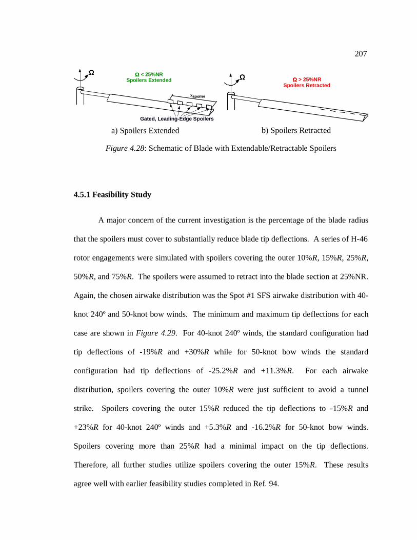
207
4.5.1 Feasibility Study
A major concern of the current investigation is the percentage of the blade radius
that the spoilers must cover to substantially reduce blade tip deflections. A series of H-46
rotor engagements were simulated with spoilers covering the outer 10%R, 15%R, 25%R,
50%R, and 75%R. The spoilers were assumed to retract into the blade section at 25%NR.
Again, the chosen airwake distribution was the Spot #1 SFS airwake distribution with 40-
knot 240º and 50-knot bow winds. The minimum and maximum tip deflections for each
case are shown inFigure 4.29. For 40-knot 240º winds, the standard configuration had
tip deflections of -19%R and +30%R while for 50-knot bow winds the standard
configuration had tip deflections of -25.2%R and +11.3%R. For each airwake
distribution, spoilers covering the outer 10%R were just sufficient to avoid a tunnel
strike. Spoilers covering the outer 15%R reduced the tip deflections to -15%R and
+23%R for 40-knot 240º winds and +5.3%R and -16.2%R for 50-knot bow winds.
Spoilers covering more than 25%R had a minimal impact on the tip deflections.
Therefore, all further studies utilize spoilers covering the outer 15%R. These results
agree well with earlier feasibility studies completed in Ref. 94.
xspoiler
ΩΩΩΩ < 25%NRSpoilers Extended
ΩΩΩΩ
Gated, Leadin g-Edge Spoilers
a) Spoilers Extended
ΩΩΩΩ > 25%NRSpoilers Retracted
ΩΩΩΩ
b) Spoilers Retracted
Figure 4.28: Schematic of Blade with Extendable/Retractable Spoilers
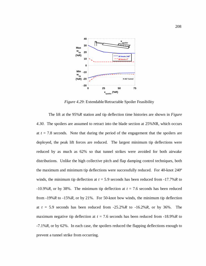
208
The lift at the 95%R station and tip deflection time histories are shown inFigure
4.30. The spoilers are assumed to retract into the blade section at 25%NR, which occurs
at t = 7.8 seconds. Note that during the period of the engagement that the spoilers are
deployed, the peak lift forces are reduced. The largest minimum tip deflections were
reduced by as much as 62% so that tunnel strikes were avoided for both airwake
distributions. Unlike the high collective pitch and flap damping control techniques, both
the maximum and minimum tip deflections were successfully reduced. For 40-knot 240º
winds, the minimum tip deflection att = 5.9 seconds has been reduced from -17.7%R to
-10.9%R, or by 38%. The minimum tip deflection att = 7.6 seconds has been reduced
from -19%R to -15%R, or by 21%. For 50-knot bow winds, the minimum tip deflection
at t = 5.9 seconds has been reduced from -25.2%R to -16.2%R, or by 36%. The
maximum negative tip deflection att = 7.6 seconds has been reduced from -18.9%R to
-7.1%R, or by 62%. In each case, the spoilers reduced the flapping deflections enough to
prevent a tunnel strike from occurring.
-30
-20
-10
0
10
20
30
40
0 25 50 75
40 knots 240 o
50 knots 0 o
Maxw
tip
(%R)
xspoiler
(%R)
Minw
tip
(%R)
xspoiler
H-46 Tunnel
Figure 4.29: Extendable/Retractable Spoiler Feasibility
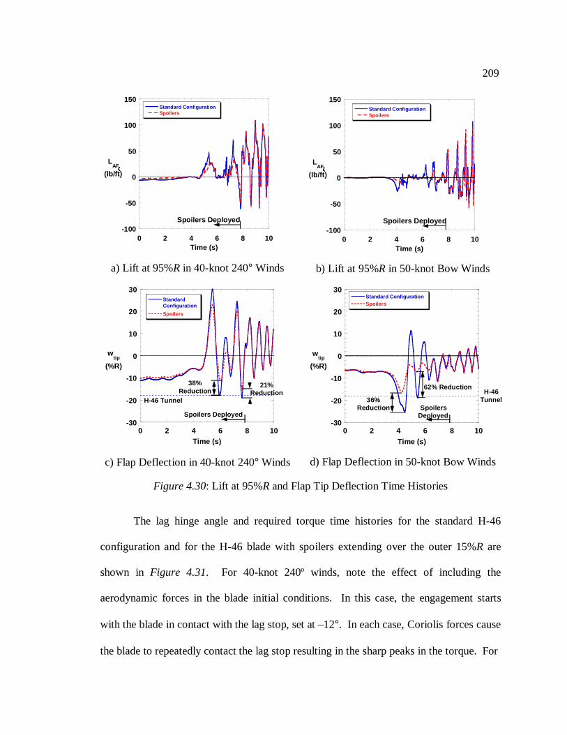
209
The lag hinge angle and required torque time histories for the standard H-46
configuration and for the H-46 blade with spoilers extending over the outer 15%R are
shown in Figure 4.31. For 40-knot 240º winds, note the effect of including the
aerodynamic forces in the blade initial conditions. In this case, the engagement starts
with the blade in contact with the lag stop, set at –12°. In each case, Coriolis forces cause
the blade to repeatedly contact the lag stop resulting in the sharp peaks in the torque. For
-100
-50
0
50
100
150
0 2 4 6 8 10
Standard ConfigurationSpoilers
LAF
(lb/ft)
Time (s)
Spoilers Deployed
ζζζζ
a) Lift at 95%R in 40-knot 240° Winds
-100
-50
0
50
100
150
0 2 4 6 8 10
Standard ConfigurationSpoilers
LAF
(lb/ft)
Time (s)
Spoilers Deployed
ζζζζ
b) Lift at 95%R in 50-knot Bow Winds
-30
-20
-10
0
10
20
30
0 2 4 6 8 10
StandardConfiguration
Spoilers
wtip
(%R)
Time (s)
Spoilers Deployed
H-46 Tunnel
38%Reduction
21%Reduction
c) Flap Deflection in 40-knot 240° Winds
-30
-20
-10
0
10
20
30
0 2 4 6 8 10
Standard ConfigurationSpoilers
wtip
(%R)
Time (s)
H-46Tunnel36%
Reduction
62% Reduction
SpoilersDeployed
d) Flap Deflection in 50-knot Bow Winds
Figure 4.30: Lift at 95%R and Flap Tip Deflection Time Histories
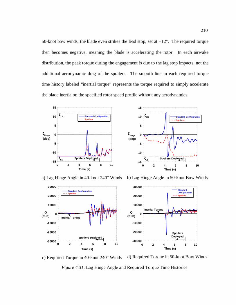
210
50-knot bow winds, the blade even strikes the lead stop, set at +12°. The required torque
then becomes negative, meaning the blade is accelerating the rotor. In each airwake
distribution, the peak torque during the engagement is due to the lag stop impacts, not the
additional aerodynamic drag of the spoilers. The smooth line in each required torque
time history labeled “inertial torque” represents the torque required to simply accelerate
the blade inertia on the specified rotor speed profile without any aerodynamics.
-15
-10
-5
0
5
10
15
0 2 4 6 8 10
Standard ConfigurationSpoilers
ζζζζhinge
(deg)
Time (s)
ζζζζLS
ζζζζLS Spoilers Deployed
a) Lag Hinge Angle in 40-knot 240° Winds
-15
-10
-5
0
5
10
15
0 2 4 6 8 10
Standard Configuration
Spoilers
ζζζζhinge
(deg)
Time (s)
ζζζζLS
ζζζζLS
Spoilers Deployed
b) Lag Hinge Angle in 50-knot Bow Winds
-30000
-20000
-10000
0
10000
20000
30000
0 2 4 6 8 10
Standard ConfigurationSpoilers
Q(ft-lb)
Time (s)
Inertial Torque
Spoilers Deployed
c) Required Torque in 40-knot 240° Winds
-30000
-20000
-10000
0
10000
20000
30000
0 2 4 6 8 10
StandardConfigurationSpoilers
Q(ft-lb)
Time (s)
SpoilersDeployed
Inertial Torque
d) Required Torque in 50-knot Bow Winds
Figure 4.31: Lag Hinge Angle and Required Torque Time Histories
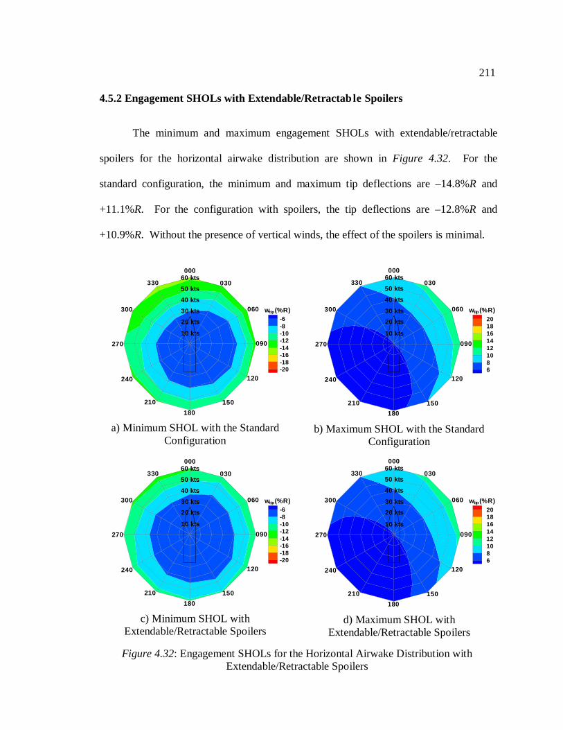
211
4.5.2 Engagement SHOLs with Extendable/Retractab le Spoilers
The minimum and maximum engagement SHOLs with extendable/retractable
spoilers for the horizontal airwake distribution are shown inFigure 4.32. For the
standard configuration, the minimum and maximum tip deflections are –14.8%R and
+11.1%R. For the configuration with spoilers, the tip deflections are –12.8%R and
+10.9%R. Without the presence of vertical winds, the effect of the spoilers is minimal.
-6-8-10-12-14-16-18-20
w (%R)tip
10 kts
33050 kts
40 kts
30 kts
20 kts
60 kts000
060
030
090
120
150
180
210
240
270
300
a) Minimum SHOL with the StandardConfiguration
20181614121086
w (%R)tip
10 kts
33050 kts
40 kts
30 kts
20 kts
60 kts000
060
030
090
120
150
180
210
240
270
300
b) Maximum SHOL with the StandardConfiguration
-6-8-10-12-14-16-18-20
w (%R)tip
10 kts
33050 kts
40 kts
30 kts
20 kts
60 kts000
060
030
090
120
150
180
210
240
270
300
c) Minimum SHOL withExtendable/Retractable Spoilers
20181614121086
w (%R)tip
10 kts
33050 kts
40 kts
30 kts
20 kts
60 kts000
060
030
090
120
150
180
210
240
270
300
d) Maximum SHOL withExtendable/Retractable Spoilers
Figure 4.32: Engagement SHOLs for the Horizontal Airwake Distribution withExtendable/Retractable Spoilers
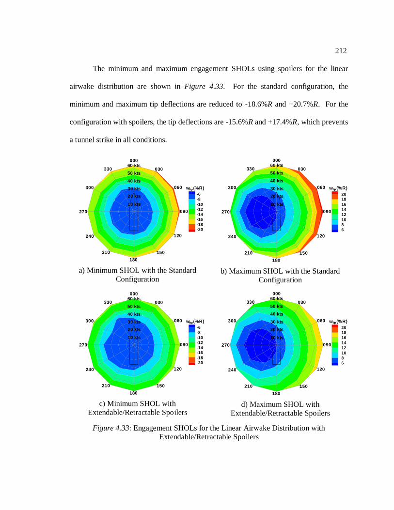
212
The minimum and maximum engagement SHOLs using spoilers for the linear
airwake distribution are shown inFigure 4.33. For the standard configuration, the
minimum and maximum tip deflections are reduced to -18.6%R and +20.7%R. For the
configuration with spoilers, the tip deflections are -15.6%R and +17.4%R, which prevents
a tunnel strike in all conditions.
-6-8-10-12-14-16-18-20
w (%R)tip
10 kts
33050 kts
40 kts
30 kts
20 kts
60 kts000
060
030
090
120
150
180
210
240
270
300
a) Minimum SHOL with the StandardConfiguration
20181614121086
w (%R)tip
10 kts
33050 kts
40 kts
30 kts
20 kts
60 kts000
060
030
090
120
150
180
210
240
270
300
b) Maximum SHOL with the StandardConfiguration
-6-8-10-12-14-16-18-20
w (%R)tip
10 kts
33050 kts
40 kts
30 kts
20 kts
60 kts000
060
030
090
120
150
180
210
240
270
300
c) Minimum SHOL withExtendable/Retractable Spoilers
20181614121086
w (%R)tip
10 kts
33050 kts
40 kts
30 kts
20 kts
60 kts000
060
030
090
120
150
180
210
240
270
300
d) Maximum SHOL withExtendable/Retractable Spoilers
Figure 4.33: Engagement SHOLs for the Linear Airwake Distribution withExtendable/Retractable Spoilers
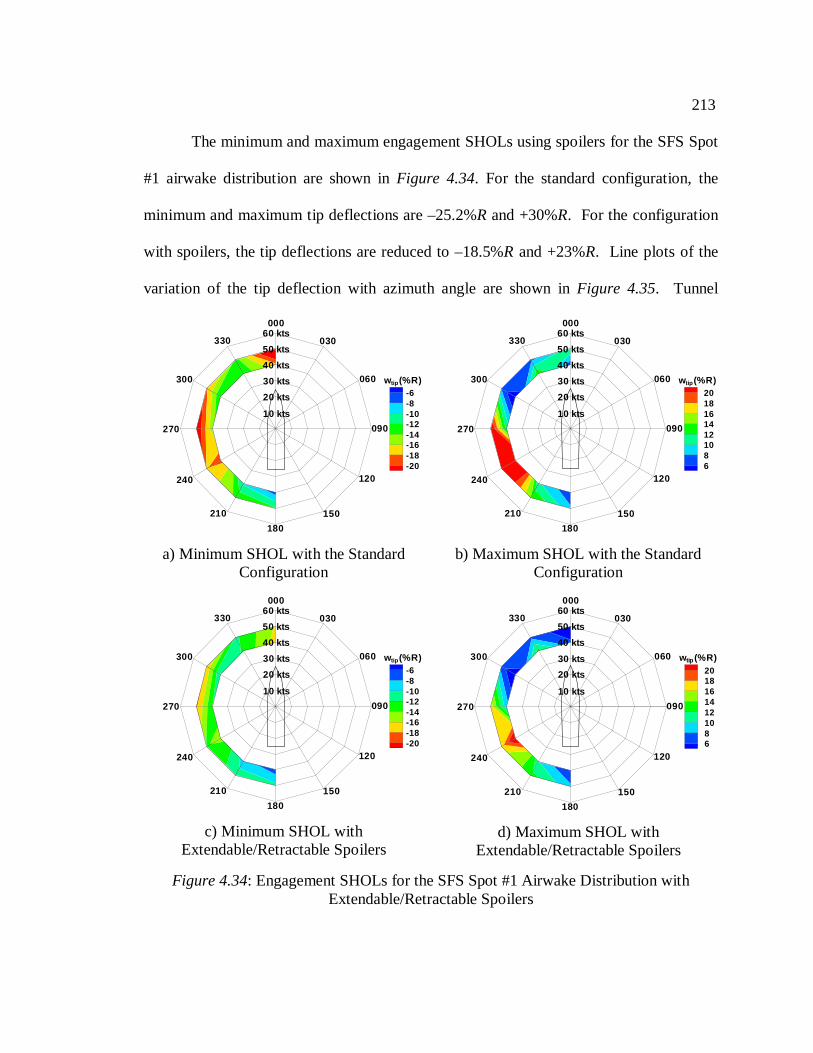
213
The minimum and maximum engagement SHOLs using spoilers for the SFS Spot
#1 airwake distribution are shown inFigure 4.34. For the standard configuration, the
minimum and maximum tip deflections are –25.2%R and +30%R. For the configuration
with spoilers, the tip deflections are reduced to –18.5%R and +23%R. Line plots of the
variation of the tip deflection with azimuth angle are shown inFigure 4.35. Tunnel
-6-8-10-12-14-16-18-20
w (%R)tip
10 kts
33050 kts
40 kts
30 kts
20 kts
60 kts000
060
030
090
120
150
180
210
240
270
300
a) Minimum SHOL with the StandardConfiguration
20181614121086
w (%R)tip
10 kts
33050 kts
40 kts
30 kts
20 kts
60 kts000
060
030
090
120
150
180
210
240
270
300
b) Maximum SHOL with the StandardConfiguration
-6-8-10-12-14-16-18-20
w (%R)tip
10 kts
33050 kts
40 kts
30 kts
20 kts
60 kts000
060
030
090
120
150
180
210
240
270
300
c) Minimum SHOL withExtendable/Retractable Spoilers
20181614121086
w (%R)tip
10 kts
33050 kts
40 kts
30 kts
20 kts
60 kts000
060
030
090
120
150
180
210
240
270
300
d) Maximum SHOL withExtendable/Retractable Spoilers
Figure 4.34: Engagement SHOLs for the SFS Spot #1 Airwake Distribution withExtendable/Retractable Spoilers
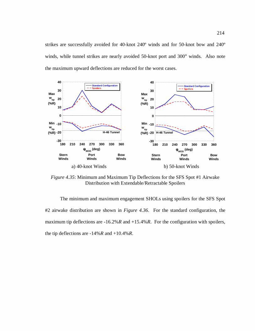
214
strikes are successfully avoided for 40-knot 240º winds and for 50-knot bow and 240º
winds, while tunnel strikes are nearly avoided 50-knot port and 300° winds. Also note
the maximum upward deflections are reduced for the worst cases.
The minimum and maximum engagement SHOLs using spoilers for the SFS Spot
#2 airwake distribution are shown inFigure 4.36. For the standard configuration, the
maximum tip deflections are -16.2%R and +15.4%R. For the configuration with spoilers,
the tip deflections are -14%R and +10.4%R.
-30
-20
-10
0
10
20
30
40
180 210 240 270 300 330 360
Standard ConfigurationSpoilers
Maxw
tip
(%R)
Minw
tip
(%R)
BowWinds
PortWinds
SternWinds
ψψψψWOD
(deg)
H-46 Tunnel
a) 40-knot Winds
-30
-20
-10
0
10
20
30
40
180 210 240 270 300 330 360
Standard ConfigurationSpoilers
Maxw
tip
(%R)
Minw
tip
(%R)
BowWinds
PortWinds
SternWinds
ψψψψWOD
(deg)
H-46 Tunnel
b) 50-knot Winds
Figure 4.35: Minimum and Maximum Tip Deflections for the SFS Spot #1 AirwakeDistribution with Extendable/Retractable Spoilers
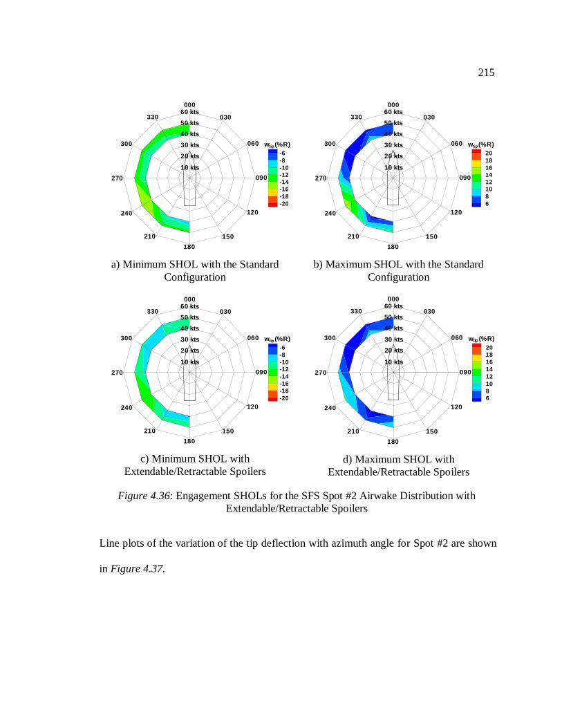
215
Line plots of the variation of the tip deflection with azimuth angle for Spot #2 are shown
in Figure 4.37.
-6-8-10-12-14-16-18-20
w (%R)tip
10 kts
33050 kts
40 kts
30 kts
20 kts
60 kts000
060
030
090
120
150
180
210
240
270
300
a) Minimum SHOL with the StandardConfiguration
20181614121086
w (%R)tip
10 kts
33050 kts
40 kts
30 kts
20 kts
60 kts000
060
030
090
120
150
180
210
240
270
300
b) Maximum SHOL with the StandardConfiguration
-6-8-10-12-14-16-18-20
w (%R)tip
10 kts
33050 kts
40 kts
30 kts
20 kts
60 kts000
060
030
090
120
150
180
210
240
270
300
c) Minimum SHOL withExtendable/Retractable Spoilers
20181614121086
w (%R)tip
10 kts
33050 kts
40 kts
30 kts
20 kts
60 kts000
060
030
090
120
150
180
210
240
270
300
d) Maximum SHOL withExtendable/Retractable Spoilers
Figure 4.36: Engagement SHOLs for the SFS Spot #2 Airwake Distribution withExtendable/Retractable Spoilers
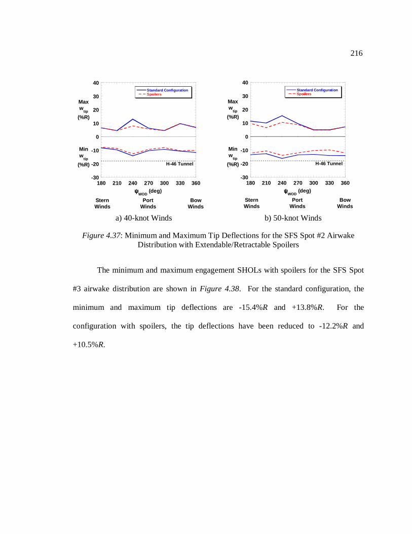
216
The minimum and maximum engagement SHOLs with spoilers for the SFS Spot
#3 airwake distribution are shown inFigure 4.38. For the standard configuration, the
minimum and maximum tip deflections are -15.4%R and +13.8%R. For the
configuration with spoilers, the tip deflections have been reduced to -12.2%R and
+10.5%R.
-30
-20
-10
0
10
20
30
40
180 210 240 270 300 330 360
Standard ConfigurationSpoilers
Maxw
tip
(%R)
Minw
tip
(%R)
BowWinds
PortWinds
SternWinds
ψψψψWOD
(deg)
H-46 Tunnel
a) 40-knot Winds
-30
-20
-10
0
10
20
30
40
180 210 240 270 300 330 360
Standard ConfigurationSpoilers
Maxw
tip
(%R)
Minw
tip
(%R)
BowWinds
PortWinds
SternWinds
ψψψψWOD
(deg)
H-46 Tunnel
b) 50-knot Winds
Figure 4.37: Minimum and Maximum Tip Deflections for the SFS Spot #2 AirwakeDistribution with Extendable/Retractable Spoilers
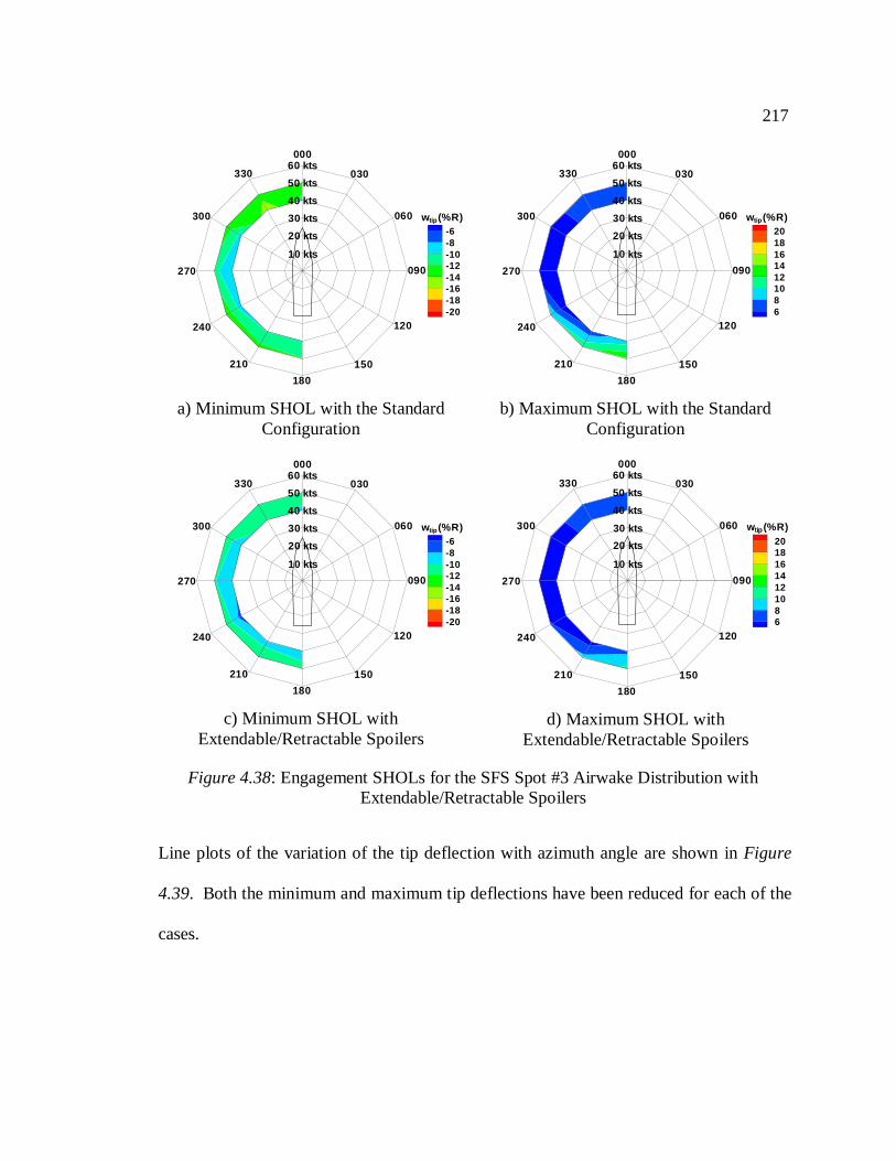
217
Line plots of the variation of the tip deflection with azimuth angle are shown inFigure
4.39. Both the minimum and maximum tip deflections have been reduced for each of the
cases.
-6-8-10-12-14-16-18-20
w (%R)tip
10 kts
33050 kts
40 kts
30 kts
20 kts
60 kts000
060
030
090
120
150
180
210
240
270
300
a) Minimum SHOL with the StandardConfiguration
20181614121086
w (%R)tip
10 kts
33050 kts
40 kts
30 kts
20 kts
60 kts000
060
030
090
120
150
180
210
240
270
300
b) Maximum SHOL with the StandardConfiguration
-6-8-10-12-14-16-18-20
w (%R)tip
10 kts
33050 kts
40 kts
30 kts
20 kts
60 kts000
060
030
090
120
150
180
210
240
270
300
c) Minimum SHOL withExtendable/Retractable Spoilers
20181614121086
w (%R)tip
10 kts
33050 kts
40 kts
30 kts
20 kts
60 kts000
060
030
090
120
150
180
210
240
270
300
d) Maximum SHOL withExtendable/Retractable Spoilers
Figure 4.38: Engagement SHOLs for the SFS Spot #3 Airwake Distribution withExtendable/Retractable Spoilers
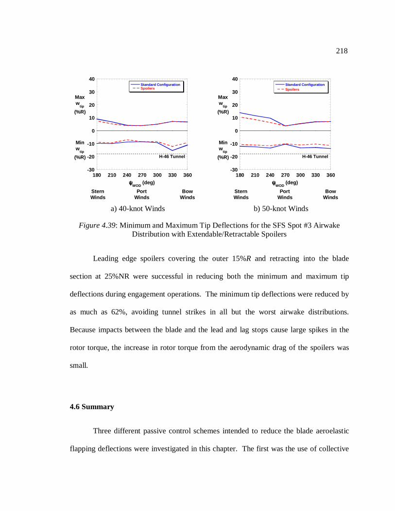
218
Leading edge spoilers covering the outer 15%R and retracting into the blade
section at 25%NR were successful in reducing both the minimum and maximum tip
deflections during engagement operations. The minimum tip deflections were reduced by
as much as 62%, avoiding tunnel strikes in all but the worst airwake distributions.
Because impacts between the blade and the lead and lag stops cause large spikes in the
rotor torque, the increase in rotor torque from the aerodynamic drag of the spoilers was
small.
4.6 Summary
Three different passive control schemes intended to reduce the blade aeroelastic
flapping deflections were investigated in this chapter. The first was the use of collective
-30
-20
-10
0
10
20
30
40
180 210 240 270 300 330 360
Standard Configur ationSpoilers
Maxw
tip
(%R)
Minw
tip
(%R)
BowWinds
PortWinds
SternWinds
ψψψψWOD
(deg)
H-46 Tunn el
a) 40-knot Winds
-30
-20
-10
0
10
20
30
40
180 210 240 270 300 330 360
Standard Configur ationSpoilers
Maxw
tip
(%R)
Minw
tip
(%R)
BowWinds
PortWinds
SternWinds
ψψψψWOD
(deg)
H-46 Tunn el
b) 50-knot Winds
Figure 4.39: Minimum and Maximum Tip Deflections for the SFS Spot #3 AirwakeDistribution with Extendable/Retractable Spoilers
219
pitch scheduling during the period of the engagement in which the rotor speed was less
than 25%NR. Collective pitch scheduling increases the effective flapwise stiffness of the
blade, which would tend to reduce blade deflections. However, it was found that in most
situations the aerodynamic forces were increased more than the blade was stiffened and
larger blade deflections resulted. The second method was the use of a discrete flap
damper that would also only be active during the low rotor speed region of the
engagement. Such a flap damper would dissipate excessive motion in the flapping
direction as a lag damper dissipates excessive motion in the lag direction. It was
determined that because the standard H-46 configuration only allows 2º of motion
between the flap and droop stops the flap stop setting had to be raised for the flap damper
to have an appreciable effect. Minimum blade deflections were successfully reduced in
this manner; however, because the flap stop setting was raised the maximum blade
deflections were often increased. The third method explored the effect of
extendable/retractable leading edge spoilers on the blade. It was found that spoilers
covering only the outer 15%R substantially reduced both the blade minimum and
maximum flapping deflections. It was also found that the torque required did not
increase appreciably because the maximum rotor torque was dominated by loads incurred
when the blade struck the lead or lag stops.
The numerical results of all three control techniques are summarized inTable 4.1.
The collective pitch scheduling method only reduced tip deflections for a few isolated
cases; in general, the blade deflections were increased. The flap damper control method
was more successful at reducing the minimum tip deflections for all airwake distributions
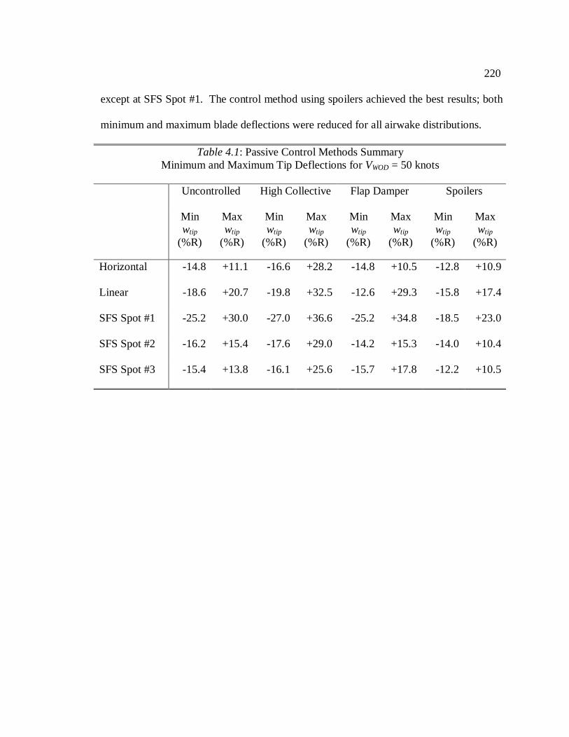
220
except at SFS Spot #1. The control method using spoilers achieved the best results; both
minimum and maximum blade deflections were reduced for all airwake distributions.
Table 4.1: Passive Control Methods SummaryMinimum and Maximum Tip Deflections forVWOD = 50 knots
Uncontrolled High Collective Flap Damper Spoilers
Minwtip
(%R)
Maxwtip
(%R)
Minwtip
(%R)
Maxwtip
(%R)
Minwtip
(%R)
Maxwtip
(%R)
Minwtip
(%R)
Maxwtip
(%R)
Horizontal -14.8 +11.1 -16.6 +28.2 -14.8 +10.5 -12.8 +10.9
Linear -18.6 +20.7 -19.8 +32.5 -12.6 +29.3 -15.8 +17.4
SFS Spot #1 -25.2 +30.0 -27.0 +36.6 -25.2 +34.8 -18.5 +23.0
SFS Spot #2 -16.2 +15.4 -17.6 +29.0 -14.2 +15.3 -14.0 +10.4
SFS Spot #3 -15.4 +13.8 -16.1 +25.6 -15.7 +17.8 -12.2 +10.5
221
Chapter 5
FEEDBACK CONTROL OF GIMBALLED ROTORS USING SWASHPLATEACTUATION
The previous chapter examined the control of the aeroelastic flapping response of
the rotor system during engagement and disengagement operations through passive
methods. The two more successful methods required that physical changes be made to
the rotor hub or the rotor blades. Although each method was successful at reducing the
rotor response, it is undesirable to make physical changes to the rotor system because
they could be expensive or maintenance intensive. Instead of controlling the rotor
flapping response using passive methods, this chapter will examine controlling the rotor
response using an active control technique.
Most rotorcraft utilize mechanical actuators to control the inputs to the rotor
system. Future rotorcraft may also have on-board devices that can measure the motion of
the rotor blades. Such systems could be combined to reduce the flapping response of the
rotor. The motion of the blades could be controlled through feedback from the measured
blade motions to the control system inputs. The V-22 Osprey already utilizes such a
control system to limit the flapping motion of the blades during forward flight conditions.
In this chapter, a feasibility study is conducted to determine the effectiveness of
using an active control system to reduce blade flapping during rotor engagements of a
gimballed rotor system. Naturally, this control system would only be used during the
critical rotor speed region and be shut off during normal operating conditions. Because
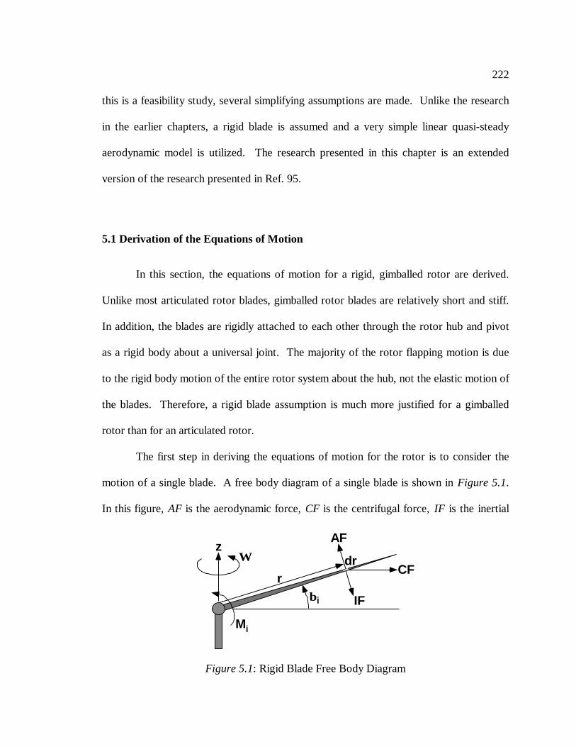
222
this is a feasibility study, several simplifying assumptions are made. Unlike the research
in the earlier chapters, a rigid blade is assumed and a very simple linear quasi-steady
aerodynamic model is utilized. The research presented in this chapter is an extended
version of the research presented in Ref. 95.
5.1 Derivation of the Equations of Motion
In this section, the equations of motion for a rigid, gimballed rotor are derived.
Unlike most articulated rotor blades, gimballed rotor blades are relatively short and stiff.
In addition, the blades are rigidly attached to each other through the rotor hub and pivot
as a rigid body about a universal joint. The majority of the rotor flapping motion is due
to the rigid body motion of the entire rotor system about the hub, not the elastic motion of
the blades. Therefore, a rigid blade assumption is much more justified for a gimballed
rotor than for an articulated rotor.
The first step in deriving the equations of motion for the rotor is to consider the
motion of a single blade. A free body diagram of a single blade is shown in Figure 5.1.
In this figure, AF is the aerodynamic force, CF is the centrifugal force, IF is the inertial
βi
ΩCF
AF
IF
r
zdr
Mi
Figure 5.1: Rigid Blade Free Body Diagram
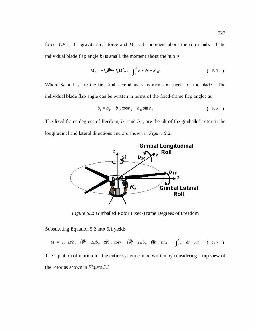
223
force, GF is the gravitational force and Mi is the moment about the rotor hub. If the
individual blade flap angle βi is small, the moment about the hub is
2
0
R
i b i b i z bM I I F r dr S gβ β= − − Ω + −∫&& ( 5.1 )
Where Sb and Ib are the first and second mass moments of inertia of the blade. The
individual blade flap angle can be written in terms of the fixed-frame flap angles as
1 1cos sini p c i s iβ β β ψ β ψ= + + ( 5.2 )
The fixed-frame degrees of freedom, β1c and β1s, are the tilt of the gimballed rotor in the
longitudinal and lateral directions and are shown in Figure 5.2.
Substituting Equation 5.2 into 5.1 yields
( ) ( )21 1 1 1 1 1 0
2 cos 2 sinR
i b p c s s i s c c i z bM I F r dr S gβ β β β ψ β β β ψ = − Ω + + Ω + Ω + − Ω + Ω + − ∫&& &&& & ( 5.3 )
The equation of motion for the entire system can be written by considering a top view of
the rotor as shown in Figure 5.3.
Figure 5.2: Gimballed Rotor Fixed-Frame Degrees of Freedom
β1c
β1s
Kβ
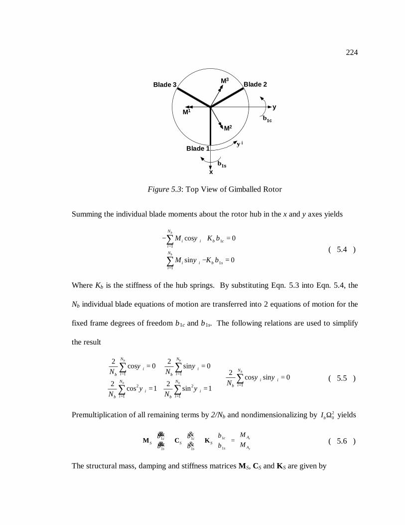
224
Summing the individual blade moments about the rotor hub in the x and y axes yields
11
11
cos 0
sin 0
b
b
N
i i ci
N
i i si
M K
M K
β
β
ψ β
ψ β
=
=
− + =
+ − =
∑
∑( 5.4 )
Where Kβ is the stiffness of the hub springs. By substituting Eqn. 5.3 into Eqn. 5.4, the
Nb individual blade equations of motion are transferred into 2 equations of motion for the
fixed frame degrees of freedom β1c and β1s. The following relations are used to simplify
the result
1 1
12 2
1 1
2 2cos 0 sin 0
2cos sin 0
2 2cos 1 sin 1
b b
b
b b
N N
i i Ni ib b
i iN Nib
i ii ib b
N NN
N N
ψ ψψ ψ
ψ ψ
= =
=
= =
= ==
= =
∑ ∑∑
∑ ∑( 5.5 )
Premultiplication of all remaining terms by 2/Nb and nondimensionalizing by 20bI Ω yields
11 1
11 1
x
y
Acc cS S S
Ass s
MM
ββ βββ β
+ + =
M C K&& &&& & ( 5.6 )
The structural mass, damping and stiffness matrices MS, CS and KS are given by
M1
M2
M3
x
y
β1c
β1s
ψ iBlade 1
Blade 2Blade 3
Figure 5.3: Top View of Gimballed Rotor
225
2
2
21 0 0 12
20 1 1 0S S Sβ
β
νν
Ω = = Ω = − Ω− M C K
&& ( 5.7 )
Where the nondimensional flap frequency of the rotor is defined as
220b b
KN I
ββν =
Ω ( 5.8 )
Note in this expression that the moment of inertia Ib is for a single blade while the gimbal
stiffness Kβ is for the entire rotor. The nondimensional moments about the rotor hub due
to aerodynamic forces, xAM and
yAM , are derived using a simple attached flow
aerodynamic model detailed in Appendix D. Using this approach, the nondimensional
moments can be written as
11
11
x
y
A ccA A A
A ss
MM
ββββ
= − − +
C K F&& ( 5.9 )
The final equations of motion are then
11 1
11 1
cc c
ss s
ββ βββ β
+ + =
M C K F&& &&& & ( 5.10 )
Where the global mass, damping and stiffness matrices M, C and K and force vector F
are given by
S S A S A A= = + = + =M M C C C K K K F F ( 5.11 )
Gimballed rotors typically have a mechanical restraint that prevents excessive
gimbal tilt angles. Because in this analysis the rotor is assumed rigid, this mechanical
restraint is not enforced.
226
5.1.1 Optimal Control Theory
Once the equations of motion have been written, they are transferred into state-
space form. Because the rotor acceleration, speed, and azimuth angles are non-periodic
functions of time, the resulting state-space equations are linear time-variant (LTV)
( ) ( ) ( )t t t= + +=
x A x B u d
y Cx
&( 5.1 )
The state vector, x, input vector, u, and output vector, y, are defined as
=
=
=s
c
s
c
s
c
s
c
1
1
1
1
75
1
1
1
1
ββ
θθθ
ββββ
yux
&& ( 5.2 )
The matrices A, B, C and the vector d are derived through the appropriate manipulations
of Eqn. 5.10. Note that there is an additional term d in the state equation. Typically, this
term is called the “disturbance” and is often used to represent external noise. That is not
the case in the current analysis. Here the disturbance term is a known quantity and arises
from aerodynamic forces generated by anything other than the pilot control inputs. It is
composed of contributions from the blade twist, blade precone and the vertical ship
airwake component zV .
Because the equations of motion are time-variant, traditional frequency domain
control approaches such as pole placement are ineffective. Instead, a time-domain Linear
Quadratic Regulator (LQR) control method is used [96]. Using this method, a quadratic
performance index, J, is defined as
227
( ) ( ) ( ) ( )1 12 2 0
ftT T Tf f fJ t t t dt= + +∫x S x x Qx u Ru ( 5.3 )
Where ( )ftS , Q and R are weighting matrices. It is assumed the matrices S and Q are
symmetric and positive semi-definite and R is symmetric and positive definite.
Minimization of the final state, ( )ftx , is achieved by setting ( )ftS large. Minimization
of the time history of the rotor response is achieved by setting Q larger than R, while
minimization of the time history of the control inputs is achieved by setting R larger than
Q. The matrices ( )ftS , Q and R are user-specified.
Assuming the final state ( )ftx is free, the Matrix Ricatti Equations (MRE) can
then be used to solve for the time variation of S
1T T−− = + − +S A S SA SBR B S Q& ( 5.4 )
Where ( )ftS is given. The MRE are then solved backward in time for ( )tS . The
Kalman gain matrix K is then given by
1 T−=K R B S ( 5.5 )
Since the weighting matrix S varies in time, so does the Kalman gain matrix. Due to the
disturbance term d in the state equation, an additional time-varying bias term exists in the
MRE. The time variation of the bias term, v, is given by
( )T− = − +v A BK v Sd& ( 5.6 )
Where ( )ftv is zero. This equation is also solved backward in time for ( )tv . The
closed-loop optimal control vector is then given by
1 T−= − −u Kx R B v ( 5.7 )
228
The second term in the equation is due to the disturbance term. The response of the
closed-loop system is then given by
( ) 1 T−= − − +x A BK x BR B v d& ( 5.8 )
With a given initial condition ( )0tx , this equation can be integrated forward in time for
the optimal state trajectory.
5.1.2 Control System Limits
Mechanical devices called swashplate actuators are often used to control the
movements of the swashplate, and hence the control system inputs. For many rotor
systems, several linear hydraulic actuators are used to move the swashplate. The relation
between the linear movement of the actuators and the control system inputs is given by
ac ac
ac ac
==
u T xu T x& & ( 5.1 )
Where xac is a Nac length vector of the displacement from a given reference of each
swashplate actuator, with Nac being the total number of actuators. The matrix Tac is a
3xNac-sized matrix that determines the control system inputs from the actuator
displacements. A schematic of the swashplate and actuators is shown in Figure 5.1. The
swashplate actuators used in rotorcraft control system typically have limits in magnitude
and rate. In the time integration of the closed-loop response, if any of the calculated
optimal control inputs are greater than the maximum allowable control inputs the
maximum allowable control inputs are simply used. Therefore, the feasibility study was
not conducted as a constrained optimization problem.
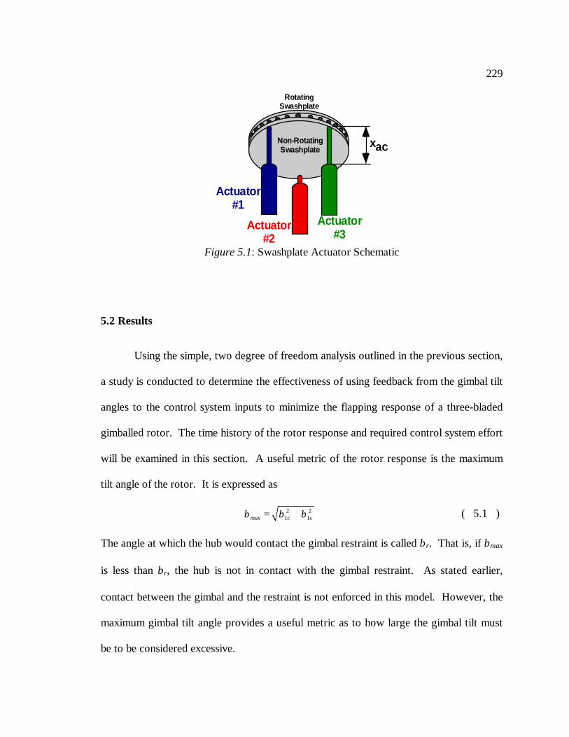
229
5.2 Results
Using the simple, two degree of freedom analysis outlined in the previous section,
a study is conducted to determine the effectiveness of using feedback from the gimbal tilt
angles to the control system inputs to minimize the flapping response of a three-bladed
gimballed rotor. The time history of the rotor response and required control system effort
will be examined in this section. A useful metric of the rotor response is the maximum
tilt angle of the rotor. It is expressed as
2 21 1max c sβ β β= + ( 5.1 )
The angle at which the hub would contact the gimbal restraint is called βr. That is, if βmax
is less than βr, the hub is not in contact with the gimbal restraint. As stated earlier,
contact between the gimbal and the restraint is not enforced in this model. However, the
maximum gimbal tilt angle provides a useful metric as to how large the gimbal tilt must
be to be considered excessive.
Non-RotatingSwashplate
RotatingSwashplate
Actuator#1
Actuator#2
Actuator#3
xac
Figure 5.1: Swashplate Actuator Schematic
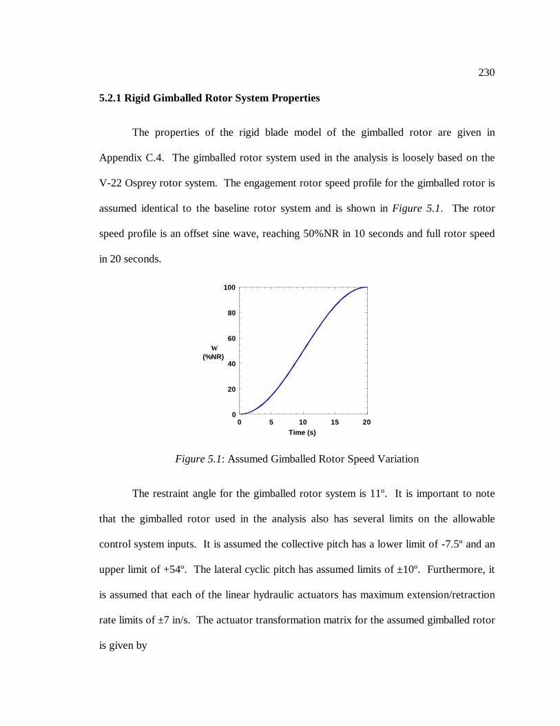
230
5.2.1 Rigid Gimballed Rotor System Properties
The properties of the rigid blade model of the gimballed rotor are given in
Appendix C.4. The gimballed rotor system used in the analysis is loosely based on the
V-22 Osprey rotor system. The engagement rotor speed profile for the gimballed rotor is
assumed identical to the baseline rotor system and is shown in Figure 5.1. The rotor
speed profile is an offset sine wave, reaching 50%NR in 10 seconds and full rotor speed
in 20 seconds.
The restraint angle for the gimballed rotor system is 11º. It is important to note
that the gimballed rotor used in the analysis also has several limits on the allowable
control system inputs. It is assumed the collective pitch has a lower limit of -7.5º and an
upper limit of +54º. The lateral cyclic pitch has assumed limits of ±10º. Furthermore, it
is assumed that each of the linear hydraulic actuators has maximum extension/retraction
rate limits of ±7 in/s. The actuator transformation matrix for the assumed gimballed rotor
is given by
0
20
40
60
80
100
0 5 10 15 20
Ω(%NR)
Time (s)
Figure 5.1: Assumed Gimballed Rotor Speed Variation
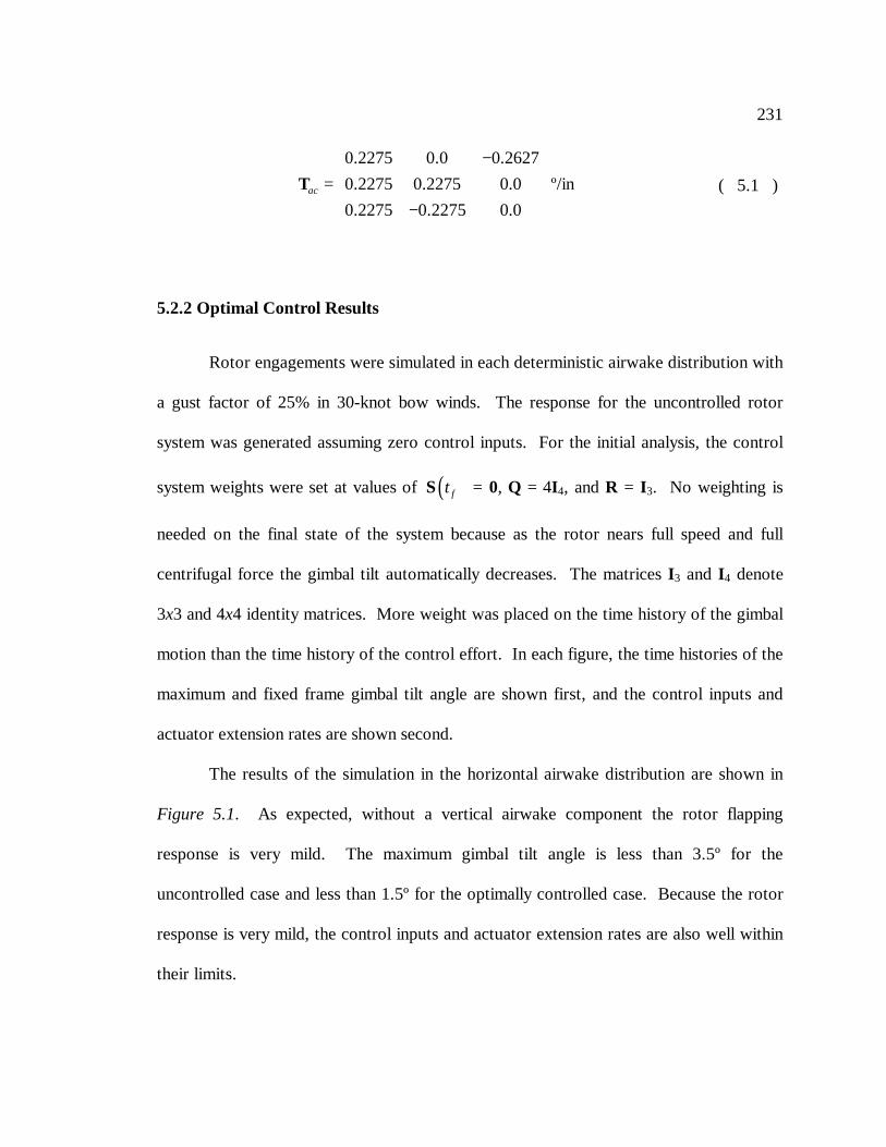
231
0.2275 0.0 0.26270.2275 0.2275 0.00.2275 0.2275 0.0
ac
− = −
T º/in ( 5.1 )
5.2.2 Optimal Control Results
Rotor engagements were simulated in each deterministic airwake distribution with
a gust factor of 25% in 30-knot bow winds. The response for the uncontrolled rotor
system was generated assuming zero control inputs. For the initial analysis, the control
system weights were set at values of ( )ftS = 0, Q = 4I4, and R = I3. No weighting is
needed on the final state of the system because as the rotor nears full speed and full
centrifugal force the gimbal tilt automatically decreases. The matrices I3 and I4 denote
3x3 and 4x4 identity matrices. More weight was placed on the time history of the gimbal
motion than the time history of the control effort. In each figure, the time histories of the
maximum and fixed frame gimbal tilt angle are shown first, and the control inputs and
actuator extension rates are shown second.
The results of the simulation in the horizontal airwake distribution are shown in
Figure 5.1. As expected, without a vertical airwake component the rotor flapping
response is very mild. The maximum gimbal tilt angle is less than 3.5º for the
uncontrolled case and less than 1.5º for the optimally controlled case. Because the rotor
response is very mild, the control inputs and actuator extension rates are also well within
their limits.
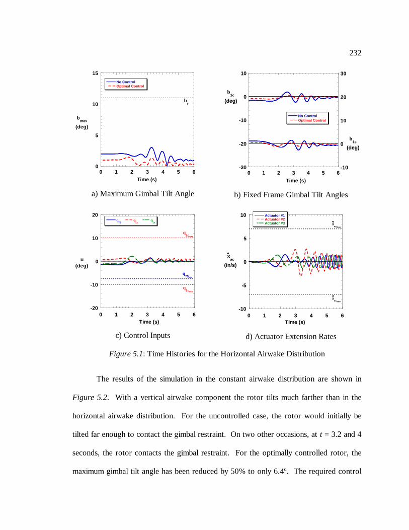
232
The results of the simulation in the constant airwake distribution are shown in
Figure 5.2. With a vertical airwake component the rotor tilts much farther than in the
horizontal airwake distribution. For the uncontrolled case, the rotor would initially be
tilted far enough to contact the gimbal restraint. On two other occasions, at t = 3.2 and 4
seconds, the rotor contacts the gimbal restraint. For the optimally controlled rotor, the
maximum gimbal tilt angle has been reduced by 50% to only 6.4º. The required control
0
5
10
15
0 1 2 3 4 5 6
No ControlOptimal Control
βmax
(deg)
Time (s)
βr
a) Maximum Gimbal Tilt Angle
-30
-20
-10
0
10
-10
0
10
20
30
0 1 2 3 4 5 6
No ControlOptimal Control
Time (s)
β1c
(deg)
β1s
(deg)
b) Fixed Frame Gimbal Tilt Angles
-20
-10
0
10
20
0 1 2 3 4 5 6
θ75
θ1c
θ1s
u(deg)
Time (s)
θ75min
θ1cmax
θ1cmin
c) Control Inputs
-10
-5
0
5
10
0 1 2 3 4 5 6
Actuator #1Actuator #2Actuator #3
xac
(in/s)
Time (s)
xacmax
xacmin
d) Actuator Extension Rates
Figure 5.1: Time Histories for the Horizontal Airwake Distribution
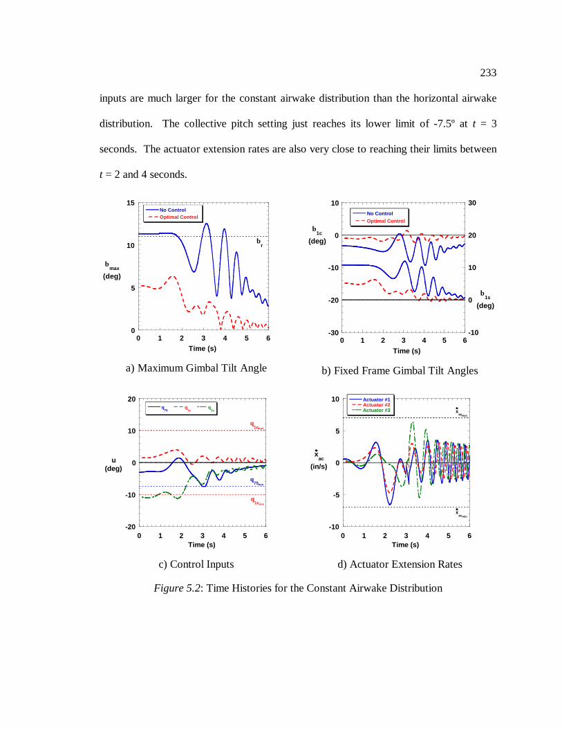
233
inputs are much larger for the constant airwake distribution than the horizontal airwake
distribution. The collective pitch setting just reaches its lower limit of -7.5º at t = 3
seconds. The actuator extension rates are also very close to reaching their limits between
t = 2 and 4 seconds.
0
5
10
15
0 1 2 3 4 5 6
No ControlOptimal Control
βmax
(deg)
Time (s)
βr
a) Maximum Gimbal Tilt Angle
-30
-20
-10
0
10
-10
0
10
20
30
0 1 2 3 4 5 6
No ControlOptimal Control
Time (s)
β1c
(deg)
β1s
(deg)
b) Fixed Frame Gimbal Tilt Angles
-20
-10
0
10
20
0 1 2 3 4 5 6
θ75
θ1c
θ1s
u(deg)
Time (s)
θ75min
θ1cmax
θ1cmin
c) Control Inputs
-10
-5
0
5
10
0 1 2 3 4 5 6
Actuator #1Actuator #2Actuator #3
xac
(in/s)
Time (s)
xacmax
xacmin
d) Actuator Extension Rates
Figure 5.2: Time Histories for the Constant Airwake Distribution
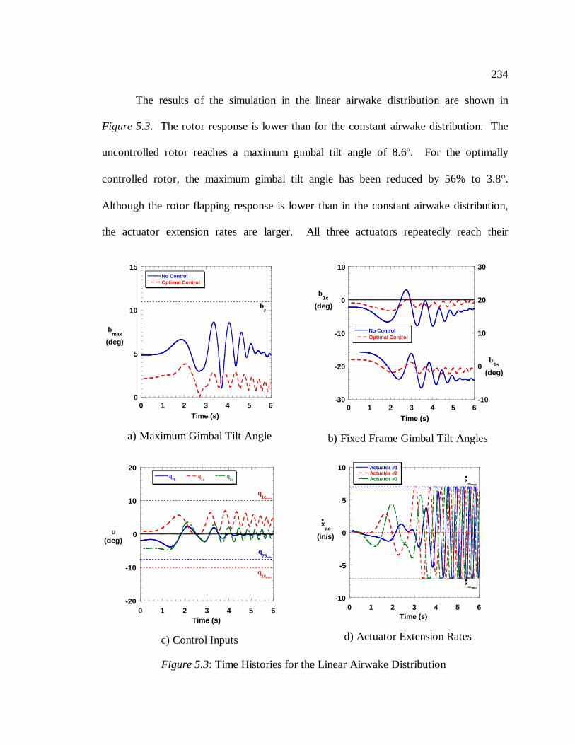
234
The results of the simulation in the linear airwake distribution are shown in
Figure 5.3. The rotor response is lower than for the constant airwake distribution. The
uncontrolled rotor reaches a maximum gimbal tilt angle of 8.6º. For the optimally
controlled rotor, the maximum gimbal tilt angle has been reduced by 56% to 3.8°.
Although the rotor flapping response is lower than in the constant airwake distribution,
the actuator extension rates are larger. All three actuators repeatedly reach their
0
5
10
15
0 1 2 3 4 5 6
No ControlOptimal Control
βmax
(deg)
Time (s)
βr
a) Maximum Gimbal Tilt Angle
-30
-20
-10
0
10
-10
0
10
20
30
0 1 2 3 4 5 6
No ControlOptimal Control
Time (s)
β1c
(deg)
β1s
(deg)
b) Fixed Frame Gimbal Tilt Angles
-20
-10
0
10
20
0 1 2 3 4 5 6
θ75
θ1c
θ1s
u(deg)
Time (s)
θ75min
θ1cmax
θ1cmin
c) Control Inputs
-10
-5
0
5
10
0 1 2 3 4 5 6
Actuator #1Actuator #2Actuator #3
xac
(in/s)
Time (s)
xacmax
xacmin
d) Actuator Extension Rates
Figure 5.3: Time Histories for the Linear Airwake Distribution
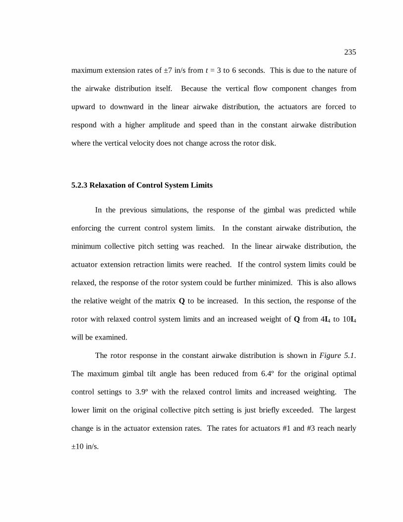
235
maximum extension rates of ±7 in/s from t = 3 to 6 seconds. This is due to the nature of
the airwake distribution itself. Because the vertical flow component changes from
upward to downward in the linear airwake distribution, the actuators are forced to
respond with a higher amplitude and speed than in the constant airwake distribution
where the vertical velocity does not change across the rotor disk.
5.2.3 Relaxation of Control System Limits
In the previous simulations, the response of the gimbal was predicted while
enforcing the current control system limits. In the constant airwake distribution, the
minimum collective pitch setting was reached. In the linear airwake distribution, the
actuator extension retraction limits were reached. If the control system limits could be
relaxed, the response of the rotor system could be further minimized. This is also allows
the relative weight of the matrix Q to be increased. In this section, the response of the
rotor with relaxed control system limits and an increased weight of Q from 4I4 to 10I4
will be examined.
The rotor response in the constant airwake distribution is shown in Figure 5.1.
The maximum gimbal tilt angle has been reduced from 6.4º for the original optimal
control settings to 3.9º with the relaxed control limits and increased weighting. The
lower limit on the original collective pitch setting is just briefly exceeded. The largest
change is in the actuator extension rates. The rates for actuators #1 and #3 reach nearly
±10 in/s.
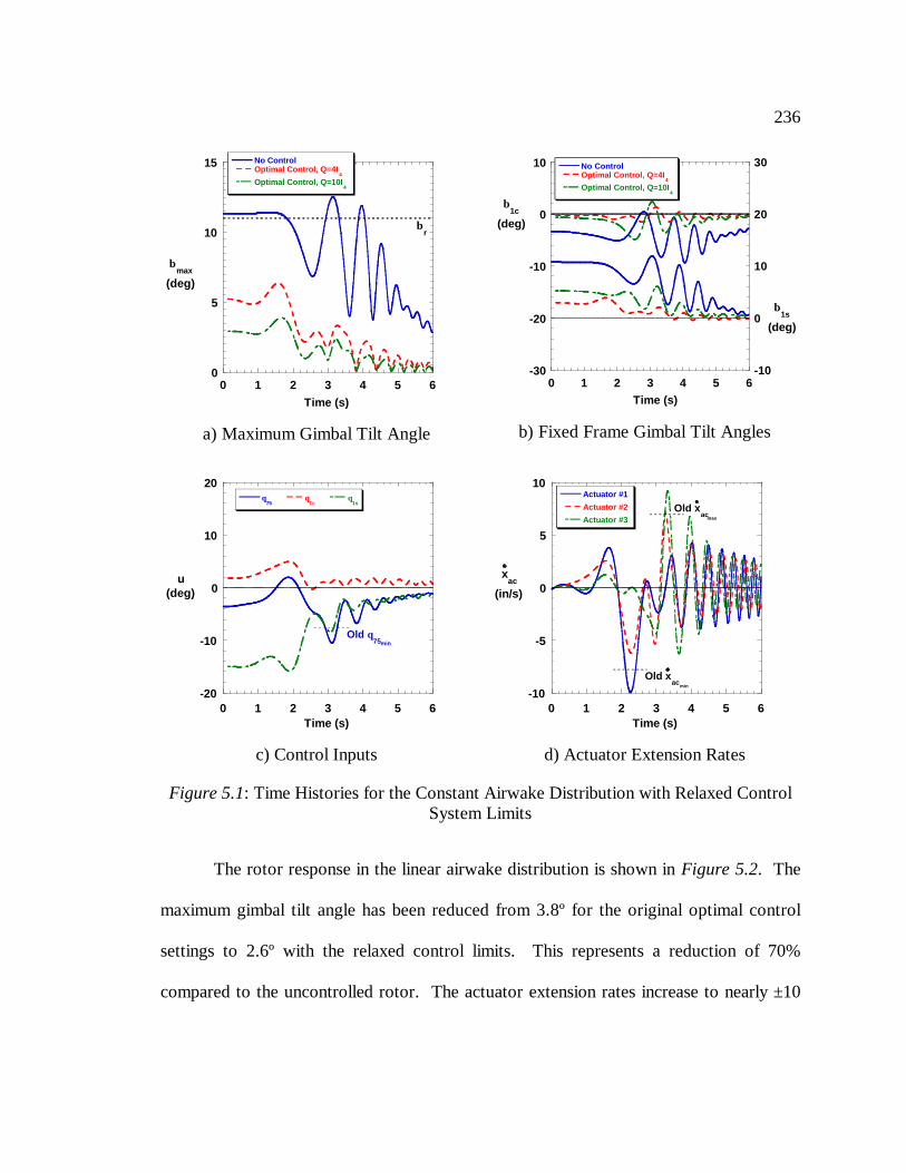
236
The rotor response in the linear airwake distribution is shown in Figure 5.2. The
maximum gimbal tilt angle has been reduced from 3.8º for the original optimal control
settings to 2.6º with the relaxed control limits. This represents a reduction of 70%
compared to the uncontrolled rotor. The actuator extension rates increase to nearly ±10
0
5
10
15
0 1 2 3 4 5 6
No ControlOptimal Control, Q=4I
4
Optimal Control, Q=10I4
βmax
(deg)
Time (s)
βr
a) Maximum Gimbal Tilt Angle
-30
-20
-10
0
10
-10
0
10
20
30
0 1 2 3 4 5 6
No ControlOptimal Control, Q=4I
4
Optimal Control, Q=10I4
Time (s)
β1c
(deg)
β1s
(deg)
b) Fixed Frame Gimbal Tilt Angles
-20
-10
0
10
20
0 1 2 3 4 5 6
θ75
θ1c
θ1s
u(deg)
Time (s)
Old θ75min
c) Control Inputs
-10
-5
0
5
10
0 1 2 3 4 5 6
Actuator #1Actuator #2Actuator #3
xac
(in/s)
Time (s)
Old xac
Old xacmax
min
d) Actuator Extension Rates
Figure 5.1: Time Histories for the Constant Airwake Distribution with Relaxed ControlSystem Limits
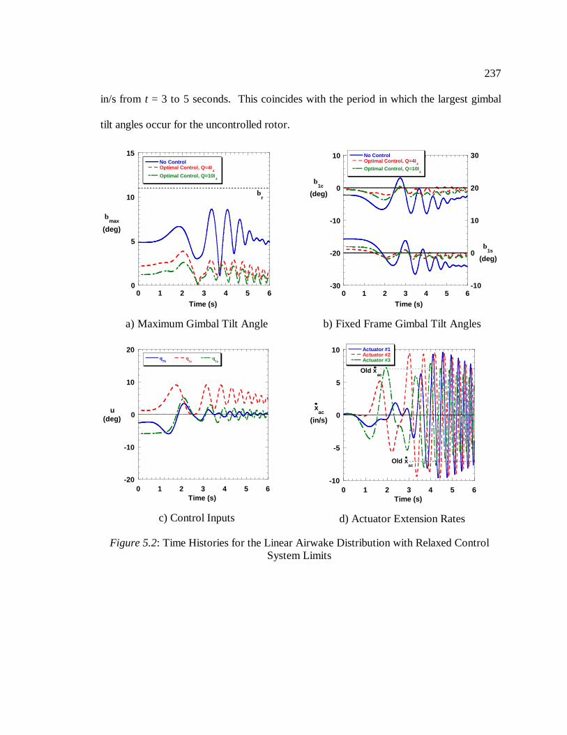
237
in/s from t = 3 to 5 seconds. This coincides with the period in which the largest gimbal
tilt angles occur for the uncontrolled rotor.
0
5
10
15
0 1 2 3 4 5 6
No ControlOptimal Control, Q=4I
4
Optimal Control, Q=10I4
βmax
(deg)
Time (s)
βr
a) Maximum Gimbal Tilt Angle
-30
-20
-10
0
10
-10
0
10
20
30
0 1 2 3 4 5 6
No ControlOptimal Control, Q=4I
4
Optimal Control, Q=10I4
Time (s)
β1c
(deg)
β1s
(deg)
b) Fixed Frame Gimbal Tilt Angles
-20
-10
0
10
20
0 1 2 3 4 5 6
θ75
θ1c
θ1s
u(deg)
Time (s)
c) Control Inputs
-10
-5
0
5
10
0 1 2 3 4 5 6
Actuator #1Actuator #2Actuator #3
xac
(in/s)
Time (s)
Old xac
Old xac
d) Actuator Extension Rates
Figure 5.2: Time Histories for the Linear Airwake Distribution with Relaxed ControlSystem Limits
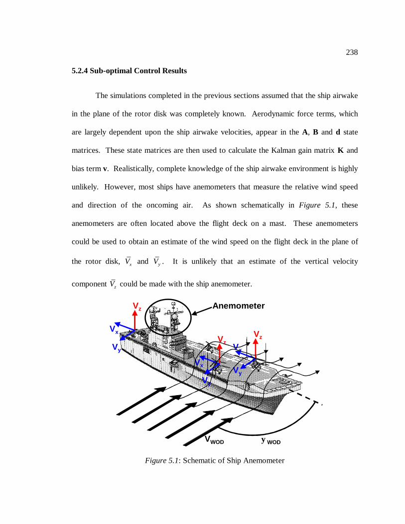
238
5.2.4 Sub-optimal Control Results
The simulations completed in the previous sections assumed that the ship airwake
in the plane of the rotor disk was completely known. Aerodynamic force terms, which
are largely dependent upon the ship airwake velocities, appear in the A, B and d state
matrices. These state matrices are then used to calculate the Kalman gain matrix K and
bias term v. Realistically, complete knowledge of the ship airwake environment is highly
unlikely. However, most ships have anemometers that measure the relative wind speed
and direction of the oncoming air. As shown schematically in Figure 5.1, these
anemometers are often located above the flight deck on a mast. These anemometers
could be used to obtain an estimate of the wind speed on the flight deck in the plane of
the rotor disk, xV and yV . It is unlikely that an estimate of the vertical velocity
component zV could be made with the ship anemometer.
Anemometer
Vx
Vy
Vz
Vx
Vz
Vx
Vy
Vz
VWOD ψ WOD
Vy
Figure 5.1: Schematic of Ship Anemometer
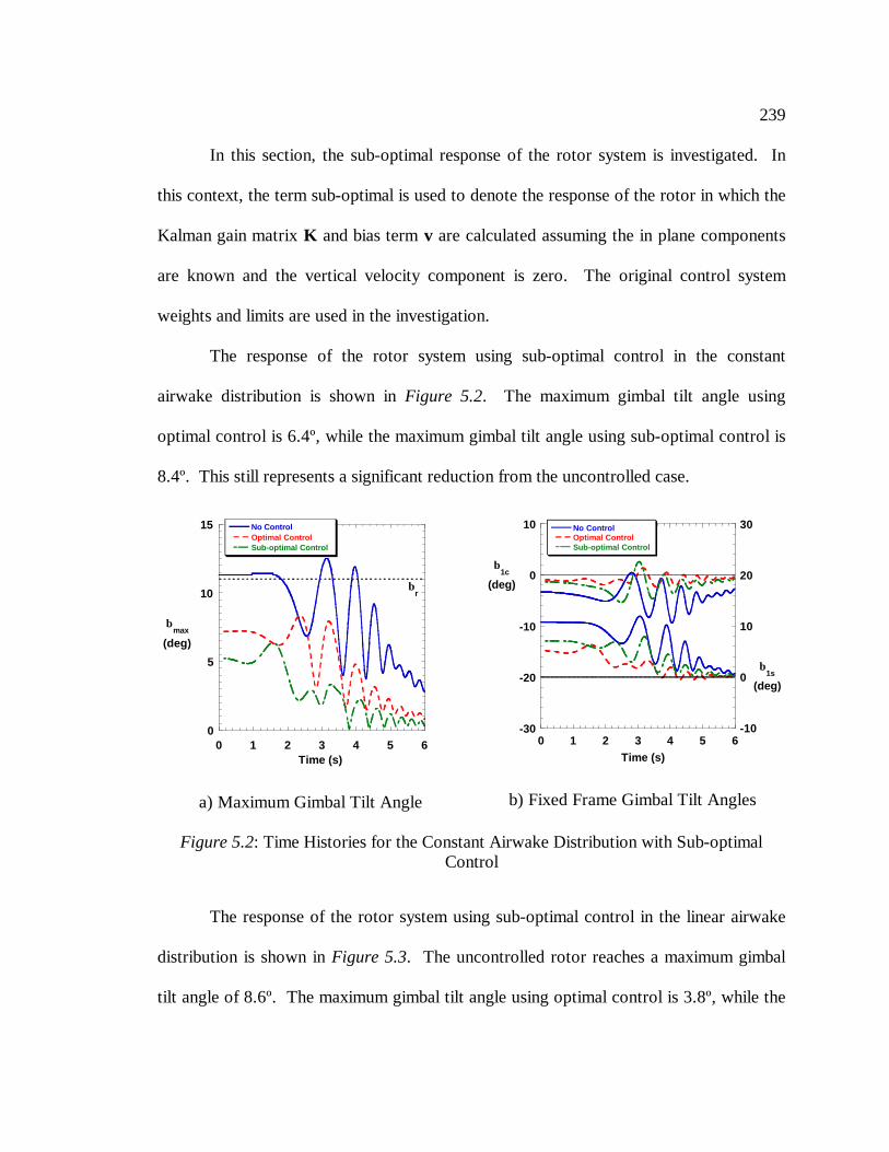
239
In this section, the sub-optimal response of the rotor system is investigated. In
this context, the term sub-optimal is used to denote the response of the rotor in which the
Kalman gain matrix K and bias term v are calculated assuming the in plane components
are known and the vertical velocity component is zero. The original control system
weights and limits are used in the investigation.
The response of the rotor system using sub-optimal control in the constant
airwake distribution is shown in Figure 5.2. The maximum gimbal tilt angle using
optimal control is 6.4º, while the maximum gimbal tilt angle using sub-optimal control is
8.4º. This still represents a significant reduction from the uncontrolled case.
The response of the rotor system using sub-optimal control in the linear airwake
distribution is shown in Figure 5.3. The uncontrolled rotor reaches a maximum gimbal
tilt angle of 8.6º. The maximum gimbal tilt angle using optimal control is 3.8º, while the
0
5
10
15
0 1 2 3 4 5 6
No ControlOptimal ControlSub-optimal Control
βmax
(deg)
Time (s)
βr
a) Maximum Gimbal Tilt Angle
-30
-20
-10
0
10
-10
0
10
20
30
0 1 2 3 4 5 6
No ControlOptimal ControlSub-optimal Control
Time (s)
β1c
(deg)
β1s
(deg)
b) Fixed Frame Gimbal Tilt Angles
Figure 5.2: Time Histories for the Constant Airwake Distribution with Sub-optimalControl
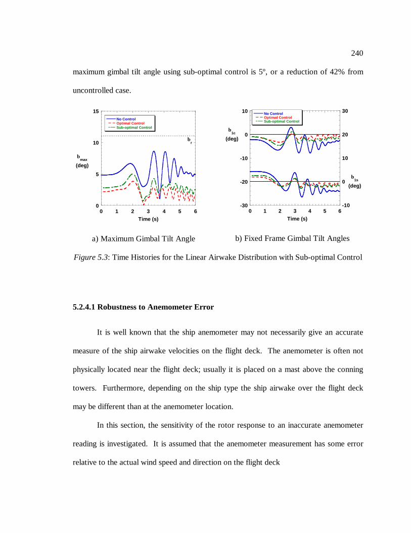
240
maximum gimbal tilt angle using sub-optimal control is 5º, or a reduction of 42% from
uncontrolled case.
5.2.4.1 Robustness to Anemometer Error
It is well known that the ship anemometer may not necessarily give an accurate
measure of the ship airwake velocities on the flight deck. The anemometer is often not
physically located near the flight deck; usually it is placed on a mast above the conning
towers. Furthermore, depending on the ship type the ship airwake over the flight deck
may be different than at the anemometer location.
In this section, the sensitivity of the rotor response to an inaccurate anemometer
reading is investigated. It is assumed that the anemometer measurement has some error
relative to the actual wind speed and direction on the flight deck
0
5
10
15
0 1 2 3 4 5 6
No ControlOptimal ControlSub-optimal Control
βmax
(deg)
Time (s)
βr
a) Maximum Gimbal Tilt Angle
-30
-20
-10
0
10
-10
0
10
20
30
0 1 2 3 4 5 6
No ControlOptimal ControlSub-optimal Control
Time (s)
β1c
(deg)
β1s
(deg)
b) Fixed Frame Gimbal Tilt Angles
Figure 5.3: Time Histories for the Linear Airwake Distribution with Sub-optimal Control
241
meas WOD WOD
meas WOD WOD
V V Vψ ψ ψ
= + ∆= + ∆ ( 5.1 )
The incorrect information from the anemometer is then used to form the incorrect state
matrices AE, BE and dE. These incorrect state matrices are used to calculated the
incorrect Kalman gain matrix, KE, and bias vector, vE
( )
1
1
T TE E E E E E E E E
TE E E
TE E E E E E E
−
−
− = + − +=
− = − +
S A S S A S B R B S Q
K R B S
v A B K v S d
&
&( 5.2 )
The incorrect optimal control vector, uE, is then calculated from
1 TE E E E E
−= − −u K x R B v ( 5.3 )
The rotor response is then calculated using the incorrect optimal control vector uE, but the
true state matrices A, B and d. In other words, the rotor response xE resulting from the
inaccurate anemometer reading is calculated from the time integration of the state
equation
E E E= + +x Ax Bu d& ( 5.4 )
The response of the rotor system with an error in the measurement of the wind
speed only is shown in Figure 5.1. The figure on the left examines the response of the
rotor system when the wind speed is underestimated and the figure on the right examines
the response of the rotor system when the wind speed is overestimated. In general, the
maximum gimbal tilt angle is increased when the wind speed is underestimated and is
decreased when the wind speed is overestimated. For a measurement underestimation of
20 knots, the maximum gimbal tilt angle increases from 5º to 6.2º. However, this still
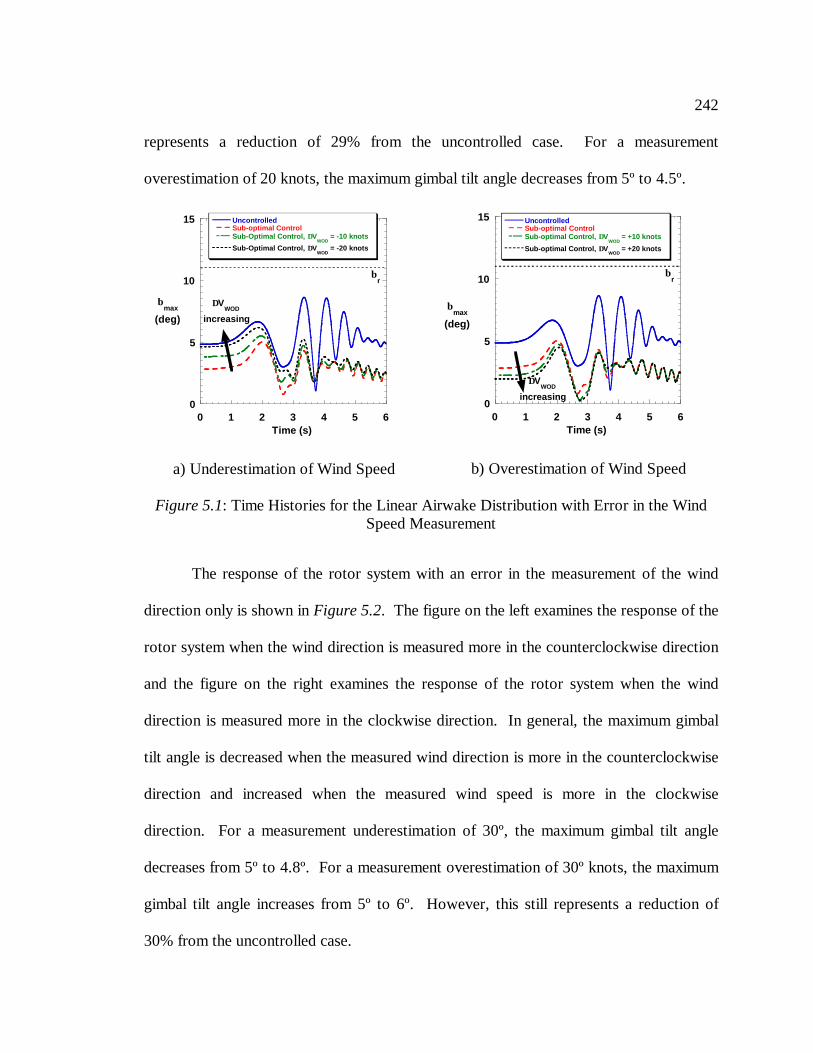
242
represents a reduction of 29% from the uncontrolled case. For a measurement
overestimation of 20 knots, the maximum gimbal tilt angle decreases from 5º to 4.5º.
The response of the rotor system with an error in the measurement of the wind
direction only is shown in Figure 5.2. The figure on the left examines the response of the
rotor system when the wind direction is measured more in the counterclockwise direction
and the figure on the right examines the response of the rotor system when the wind
direction is measured more in the clockwise direction. In general, the maximum gimbal
tilt angle is decreased when the measured wind direction is more in the counterclockwise
direction and increased when the measured wind speed is more in the clockwise
direction. For a measurement underestimation of 30º, the maximum gimbal tilt angle
decreases from 5º to 4.8º. For a measurement overestimation of 30º knots, the maximum
gimbal tilt angle increases from 5º to 6º. However, this still represents a reduction of
30% from the uncontrolled case.
0
5
10
15
0 1 2 3 4 5 6
UncontrolledSub-optimal ControlSub-Optimal Control, ∆V
WOD = -10 knots
Sub-Optimal Control, ∆VWOD
= -20 knots
βmax
(deg)
Time (s)
βr
∆VWOD
increasing
a) Underestimation of Wind Speed
0
5
10
15
0 1 2 3 4 5 6
UncontrolledSub-optimal ControlSub-optimal Control, ∆V
WOD = +10 knots
Sub-optimal Control, ∆VWOD
= +20 knots
βmax
(deg)
Time (s)
βr
∆VWOD
increasing
b) Overestimation of Wind Speed
Figure 5.1: Time Histories for the Linear Airwake Distribution with Error in the WindSpeed Measurement
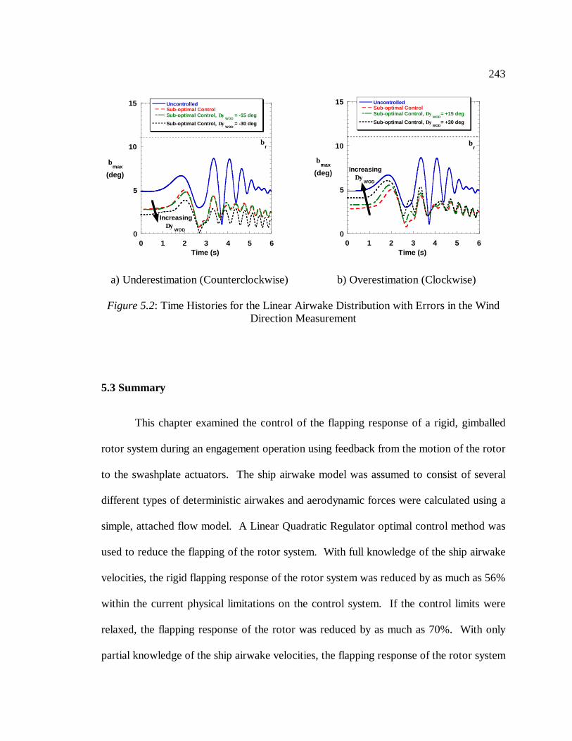
243
5.3 Summary
This chapter examined the control of the flapping response of a rigid, gimballed
rotor system during an engagement operation using feedback from the motion of the rotor
to the swashplate actuators. The ship airwake model was assumed to consist of several
different types of deterministic airwakes and aerodynamic forces were calculated using a
simple, attached flow model. A Linear Quadratic Regulator optimal control method was
used to reduce the flapping of the rotor system. With full knowledge of the ship airwake
velocities, the rigid flapping response of the rotor system was reduced by as much as 56%
within the current physical limitations on the control system. If the control limits were
relaxed, the flapping response of the rotor was reduced by as much as 70%. With only
partial knowledge of the ship airwake velocities, the flapping response of the rotor system
0
5
10
15
0 1 2 3 4 5 6
UncontrolledSub-optimal ControlSub-optimal Control, ∆ψ
WOD = -15 deg
Sub-optimal Control, ∆ψWOD
= -30 deg
βmax
(deg)
Time (s)
βr
Increasing∆ψ
WOD
a) Underestimation (Counterclockwise)
0
5
10
15
0 1 2 3 4 5 6
UncontrolledSub-optimal ControlSub-optimal Control, ∆ψ
WOD= +15 deg
Sub-optimal Control, ∆ψWOD
= +30 deg
βmax
(deg)
Time (s)
βr
Increasing∆ψ
WOD
b) Overestimation (Clockwise)
Figure 5.2: Time Histories for the Linear Airwake Distribution with Errors in the WindDirection Measurement

244
was reduced by as much as 42%. The sensitivity of the rotor response with errors in the
ship airwake measurements was also examined. The rotor response with the errors in the
ship airwake measurements of 20 knots and 30° was increased; however, this response
was still at least 30% lower than without any control.
245
Chapter 6
CONCLUSIONS AND RECOMMENDATIONS
6.1 Conclusions
Aeroelastic Flap-Lag-Torsion Analysis
An analysis has been developed to predict the transient aeroelastic response of a
helicopter rotor system during shipboard engagement and disengagement operations.
The blade coupled flap-lag-torsion equations of motion were developed using Hamilton’s
Principle and then discretized spatially using the finite element method. The analysis is
capable of simulating articulated, hingeless, teetering, or gimballed rotor systems.
Aerodynamics were simulated using both nonlinear quasi-steady and time domain
nonlinear unsteady models. The ship airwake environment was simulated with simple
deterministic airwake distributions, with results from experimental measurements or with
numerical predictions. The transient aeroelastic response of the rotor blades was then
time integrated along a specified rotor speed profile.
With the aeroelastic flap-lag-torsion analysis, the response of a generic articulated
rotor system was examined first. Using this model, it was shown that:
1) The Bossak-Newmark time integration method was shown to yield superior
results compared to Runge-Kutta or standard Newmark time integration techniques. A
246
converged transient response with less high frequency noise was achieved with a time
step twice as fast in terms of wall clock time as the other two integrators.
2) The addition of the lag degree of freedom was shown to significantly influence
the blade response. Tip deflections were under predicted by as much as 31% without lag
motion.
3) Predictions were made using both the nonlinear quasi-steady steady and unsteady
aerodynamic models. The nonlinear quasi-steady model was shown to consistently yield
a blade response approximately 10% larger than the unsteady model. Use of the unsteady
aerodynamic model at the high angles of attack, skew angles, and low Mach numbers
often encountered in engagement and disengagement operations is difficult.
4) The transient blade response was compared using the simple deterministic and
numerically predicted ship airwakes for a frigate-like ship shape. The blade response was
often much larger for the numerically predicted ship airwakes and was much more
dependent on deck location and wind speed and direction. Fluctuating flow components
in the range of frequencies measured in previous ship airwake tests were shown to
influence the blade tip deflections by as much as 45%.
5) Correlation with the wind tunnel tests performed at the University of
Southampton showed good correlation between the measured and the predicted blade
response. The position of the rotor on the deck was again shown to significantly affect
the blade response. Deck positions nearest the windward deck edge showed a larger
blade response than deck positions nearer the leeward deck edge. Fluctuating flow
247
components were shown to improve the correlation with the results for the blade response
at the leeward deck positions.
6) The proper modeling of the initial conditions was examined. The inclusion of
aerodynamic forces in the solution for the initial deflection was shown to significantly
affect the blade response in the low rotor speed region. Tip deflections were reduced by
as much as 43% in the very low rotor speed region with the inclusion of aerodynamic
forces. The effect of the initial azimuth angle was also examined. Engagement wind
envelopes were not sensitive to the initial azimuth angle because the minimum tip
deflections typically occurred during the first one-half to one rotor revolution. However,
disengagement wind envelopes were sensitive to the initial azimuth angle because the
minimum tip deflections typically occurred in the last half rotor revolution.
The control of the rotor response for an analytic model of the H-46 Sea Knight
rotor system was investigated with three different passive control techniques. It was
shown that:
1) The use of a high collective pitch setting in the rotor speed region below 25%NR
was not successful in reducing the blade flapping response. A collective pitch setting of
10º increased the effective flapwise stiffness of the blade by as much as 84%; however,
the increase in blade stiffness only reduced the flapping response of the rotor in a few
isolated cases. In the majority of the cases, the aerodynamic forces were often increased
enough to offset the increased stiffness and double the deflections.
2) The use of a discrete flap damper to damp excessive flap motions was
investigated. At the current H-46 flap stop setting of +1º, the flap damper was ineffective
248
in reducing the blade response regardless of its strength because the stroke of the damper
was too small. If the flap stop was raised to 6º and a flap damper 4 times the strength of
the lag damper was used, the downward blade deflections were typically reduced by
10%. However, because the blade flap stop setting was raised the blade upward
deflections were increased by as much as 40%.
3) The use of extendable/retractable, gated leading-edge spoilers was investigated.
The spoilers were assumed to be extended only in the region of the engagement or
disengagement where the rotor speed was less than 25%NR. Spoilers covering the outer
15%R of the rotor blade were shown to reduce both the downward and upward blade
flapping response by as much as 30% without an increase in the rotor torque.
Rigid Gimballed Rotor Analysis
Another separate analysis was developed to investigate the active control of
gimballed rotor systems. The equations of motion for a rigid, three-bladed gimballed
rotor system were derived using a Newtonian force balance approach. Aerodynamic
forces were simulated with a simple, linear attached flow model. The ship airwake was
assumed to consist of the deterministic airwake distributions. The resulting equations of
motion for the rigid roll and pitch of the rotor system were cast into state space form and
time integrated along an assumed rotor speed profile. A Linear Quadratic Regulator
optimal control technique was applied to the equations of motion to minimize the
transient rotor response. With this analysis, it was shown that:
249
1) With full knowledge of the ship airwake environment, the maximum transient
gimbal tilt angle was reduced by as much as 56% within the current physical limits of the
control system.
2) If the physical limits of the control system were relaxed, the maximum transient
gimbal tilt angle was reduced by as much as 70%.
3) With only partial knowledge of the ship airwake from a ship anemometer
measurement, the maximum transient gimbal tilt angle was still reduced by as much as
42%.
4) The control technique was even successful considering errors in the ship
anemometer measurements. Overestimating the wind speed on the flight deck minimized
the rotor response. The gimbal tilt angle was still reduced by 30% with a wind speed
measurement error of 20 knots and a wind direction measurement error of 30º.
6.2 Recommendations
1) Several interesting trends in the blade transient response were discovered when
using the numerically predicted airwakes for the Simple Frigate Shape. Additional
predictions of the SFS airwake, especially at the 30-knot wind speed, would be useful.
Ideally, predictions of the airwake around more realistic ship shapes, especially the LHA,
LHD, CVN, CV, AE or AOR, could be made and investigated. Prediction of the ship
airwake around more realistic ship types would allow correlation between the aeroelastic
code and actual historical tunnel strike events.
250
2) Currently, it is assumed that the rotor rotates in the counterclockwise direction
only. The analysis should be modified to simulate either clockwise or counterclockwise
rotation. This would improve the modeling of the rear rotor of tandem rotorcraft, the
second rotor of tiltrotors, or most European rotorcraft.
3) For gimballed rotors, such as the V-22 Osprey, the rotor pylon is not rigidly
attached to the wing structure. In the event of a gimbal restraint impact, the entire pylon-
wing structure bends as an elastic structure. Adding the pylon motion degrees of freedom
to the analysis would improve the modeling of gimballed tiltrotors.
4) Initial research has shown that the fluctuating flow components can significantly
impact the rotor response. This is because the range of frequencies present in actual ship
airwake measurements overlaps with the fundamental rotor frequencies when rotating at
low speed. However, the current fluctuating flow model is somewhat rudimentary and
should be improved.
5) In the current aeroelastic analysis, nonlinear structural terms are treated as an
additional linear force terms. As the blade response becomes large, the influence of these
nonlinear terms increases. Currently, the time integration techniques used in the analysis
are only unconditionally stable for linear systems. It is suspected that this is the reason
that the time integration can occasionally become unstable when the blade response
becomes large. The use of time integrator methods for nonlinear systems should be
investigated.

251
6) Blade and hub loads are currently predicted using a force summation technique.
This method can be computationally expensive. In the future, it is suggested that a
reaction force method be used to calculate blade loads.
7) Active control techniques with a rigid gimballed rotor system were shown to have
promise in reducing the rotor response. However, the aerodynamic model used in the
study was very simplified. The next step in the investigation of active control techniques
would be to include nonlinear aerodynamic effects. If the results are still promising, it
would be advantageous to incorporate the active control techniques into the aeroelastic
rotor analysis. In addition, a more rigorous examination of the stability of the system
should be undertaken.

252
Appendix A
ADDITIONAL MODELING
A.1 Coordinate Systems
The following coordinate systems are used to define the rotor blades and hub.
They are identical to those in Ref. 43 and are included here simply for reference. Rotated
through the shaft angle is thehub-fixed nonrotating coordinate system, ( ), ,H H HX Y Z ,
with corresponding unit vectors ˆ ˆ, ,H H HI J K . TheXH axis points to the rear of the rotor,
the YH axis points to the right side of the rotor and theZH axis points upwards parallel to
the rotor shaft. Note that only longitudinal shaft tilt,αs, is considered; lateral shaft tilt is
assumed zero. Assuming that the longitudinal shaft tilt angle is small, the transformation
matrix is given by
ˆ ˆ1 0ˆ ˆ0 1 0
ˆ ˆ0 1
H Fs
H F
sH F
I I
J J
K K
α
α
=
( A.1 )
Where the shaft tilt angle is positive nose down.
Also centered at the rotor hub is thehub-fixed rotating coordinate system,
( ), ,X Y Z , with corresponding unit vectors ˆ ˆ, ,I J K . The hub-fixed rotating coordinate
system rotates with the blades in the counterclockwise direction at an angular velocity of
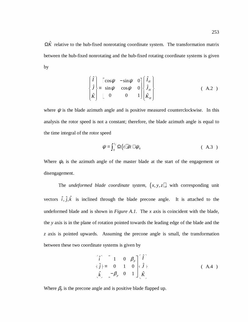
253
KΩ relative to the hub-fixed nonrotating coordinate system. The transformation matrix
between the hub-fixed nonrotating and the hub-fixed rotating coordinate systems is given
by
ˆ ˆcos sin 0ˆ ˆsin cos 0
ˆ ˆ0 0 1
H
H
H
I I
J J
K K
ψ ψψ ψ
− =
( A.2 )
whereψ is the blade azimuth angle and is positive measured counterclockwise. In this
analysis the rotor speed is not a constant; therefore, the blade azimuth angle is equal to
the time integral of the rotor speed
( ) 00
ftt dtψ ψ= Ω + ( A.3 )
Where ψ0 is the azimuth angle of the master blade at the start of the engagement or
disengagement.
The undeformed blade coordinate system, ( ), ,x y z , with corresponding unit
vectors ˆˆ ˆ, ,i j k is inclined through the blade precone angle. It is attached to the
undeformed blade and is shown inFigure A.1. The x axis is coincident with the blade,
they axis is in the plane of rotation pointed towards the leading edge of the blade and the
z axis is pointed upwards. Assuming the precone angle is small, the transformation
between these two coordinate systems is given by
ˆˆ 1 0ˆˆ 0 1 0
ˆ ˆ0 1
p
p
Ii
j J
Kk
β
β
=
−
( A.4 )
Whereβp is the precone angle and is positive blade flapped up.
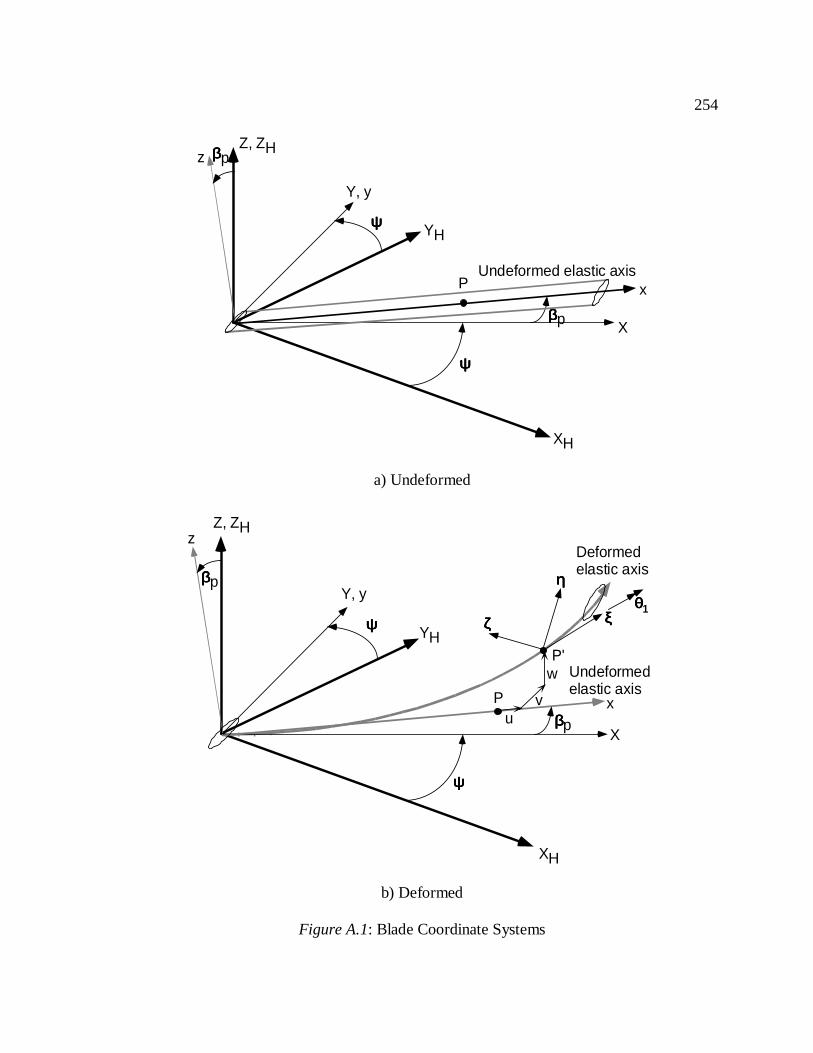
254
ββββpzZ, ZH
Y, y
ψψψψ
ψψψψ
X
xP
XH
YH
Undeformed elastic axis
ββββp
a) Undeformed
Deformedelastic axis
Undeformedelastic axis
ββββp
zZ, ZH
Y, y
ψψψψ YH
Pu
v
w
ηηηη
ξξξξζζζζ
P'
X
xββββp
ψψψψ
XH
θθθθ1
b) Deformed
Figure A.1: Blade Coordinate Systems
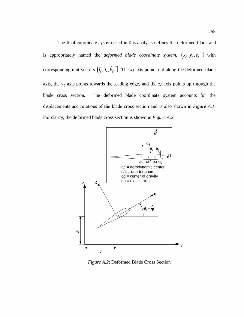
255
The final coordinate system used in this analysis defines the deformed blade and
is appropriately named thedeformed blade coordinate system, ( ), ,x y zξ η ζ , with
corresponding unit vectors( )ˆˆ ˆ, ,i j kξ η ζ . The xξ axis points out along the deformed blade
axis, theyη axis points towards the leading edge, and thezζ axis points up through the
blade cross section. The deformed blade coordinate system accounts for the
displacements and rotations of the blade cross section and is also shown inFigure A.1.
For clarity, the deformed blade cross section is shown inFigure A.2.
ac = aerodynamic centerc/4 = quarter chordcg = center of gravityea = elastic axis
ηηηη
ζζζζ
edeg
ac ea cg
θθθθ0 + φφφφ
ζζζζz
y
w
v
ηηηη
ec
c/4
Figure A.2: Deformed Blade Cross Section
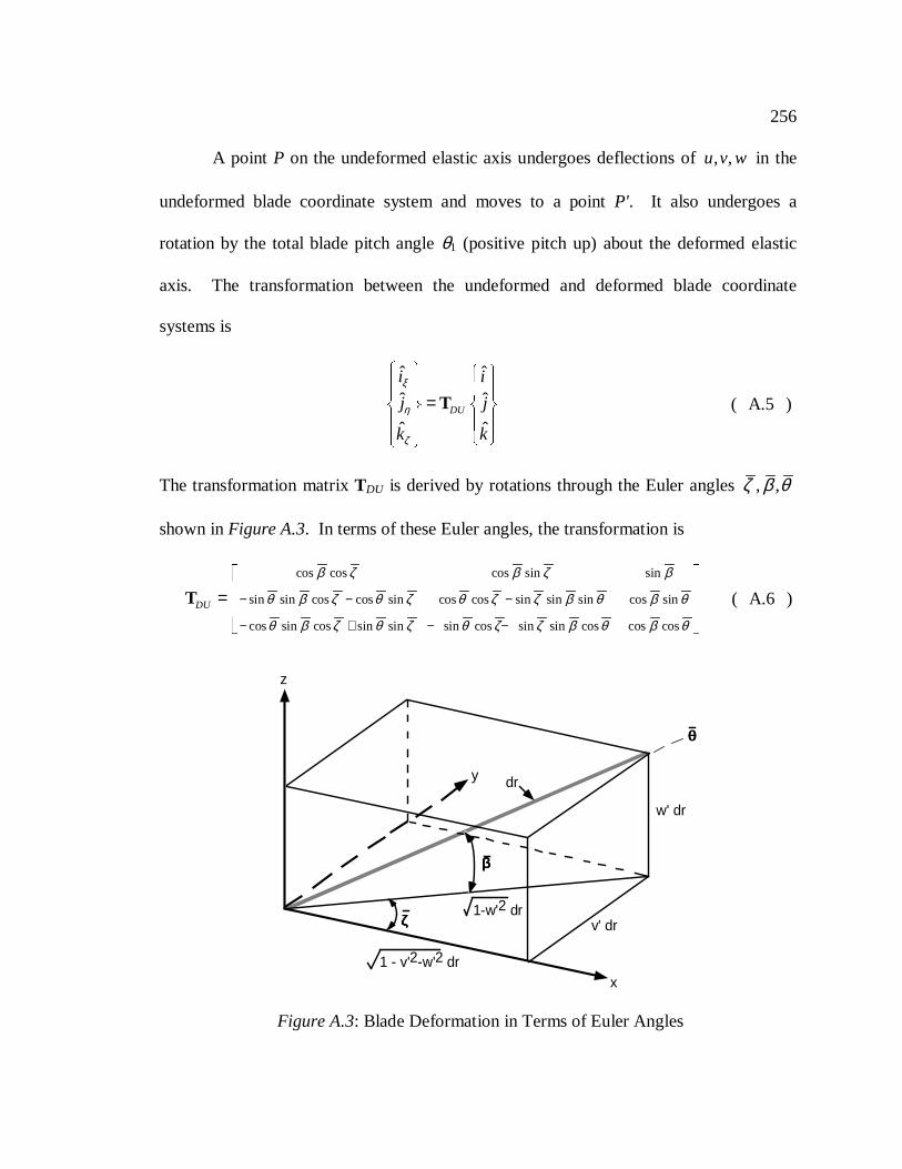
256
A point P on the undeformed elastic axis undergoes deflections of, ,u v w in the
undeformed blade coordinate system and moves to a pointP'. It also undergoes a
rotation by the total blade pitch angleθ1 (positive pitch up) about the deformed elastic
axis. The transformation between the undeformed and deformed blade coordinate
systems is
ˆ ˆ
ˆ ˆ
ˆ ˆDU
i i
j j
k k
ξ
η
ζ
=
T ( A.5 )
The transformation matrixTDU is derived by rotations through the Euler angles, ,ζ β θ
shown inFigure A.3. In terms of these Euler angles, the transformation is
cos cos cos sin sin
sin sin cos cos sin cos cos sin sin sin cos sin
cos sin cos sin sin sin cos sin sin cos cos cos
TDU
β ζ β ζ β
θ β ζ θ ζ θ ζ ζ β θ β θ
θ β ζ θ ζ θ ζ ζ β θ β θ
− − −
− + − −
=
( A.6 )
1 - v'2-w'2 dr
ββββ
w' dr
1-w'2 drv' dr
x
y
z
θθθθ
ζζζζ
dr
Figure A.3: Blade Deformation in Terms of Euler Angles
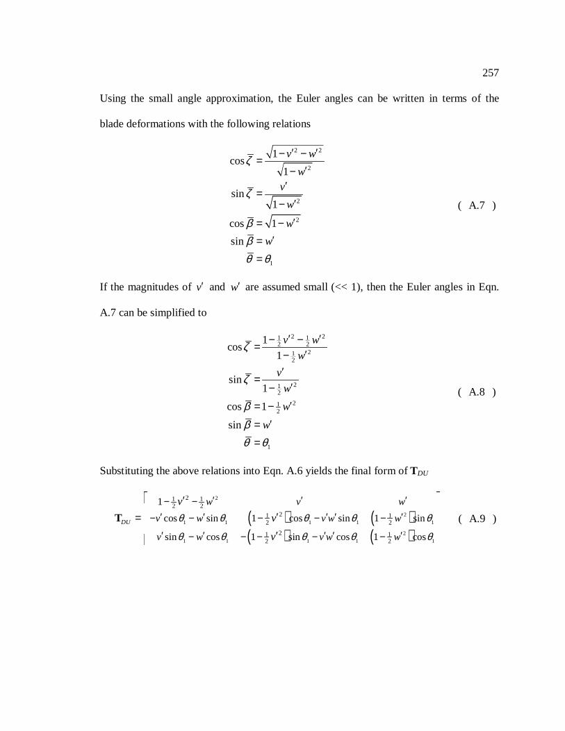
257
Using the small angle approximation, the Euler angles can be written in terms of the
blade deformations with the following relations
2 2
2
2
2
1
1cos
1
sin1
cos 1
sin
v w
wv
w
w
w
ζ
ζ
ββθ θ
′ ′− −=′−
′=
′−
′= −′=
=
( A.7 )
If the magnitudes ofv′ and w′ are assumed small (<< 1), then the Euler angles in Eqn.
A.7 can be simplified to
2 21 12 2
212
212
212
1
1cos
1
sin1
cos 1
sin
v w
w
v
w
w
w
ζ
ζ
ββθ θ
′ ′− −=′−
′=
′−′= −
′==
( A.8 )
Substituting the above relations into Eqn. A.6 yields the final form ofTDU
( ) ( )( ) ( )
2
2
1 1 1 1 1
2
1 1 1 1 1
21 12 2
21 12 2
21 12 2
1
cos sin 1 cos sin 1 sin
sin cos 1 sin cos 1 cos
DU
w v w
v w v w w
v w v w w
v
v
v
θ θ θ θ θ
θ θ θ θ θ
′ ′ ′− −′ ′ ′ ′ ′− − − − −
′ ′ ′ ′ ′− − − − −
′
′= ′
T ( A.9 )
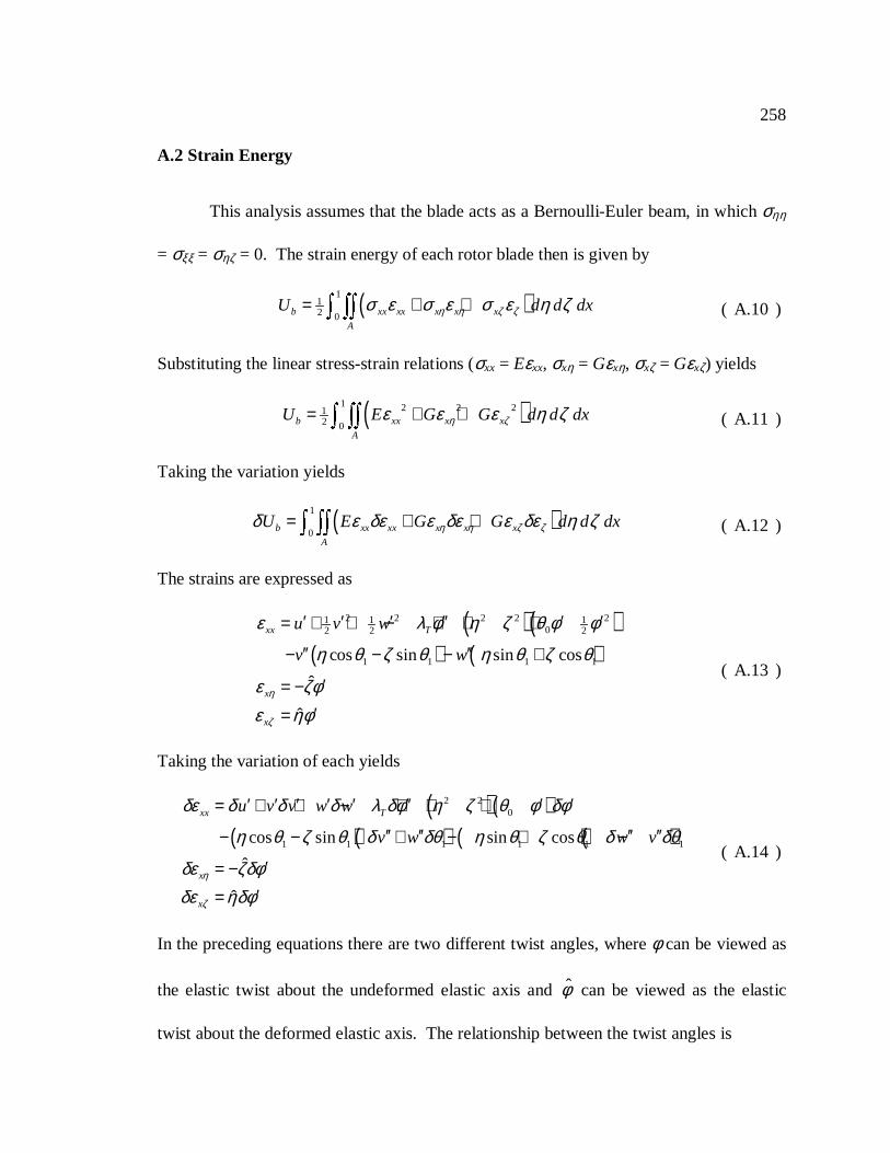
258
A.2 Strain Energy
This analysis assumes that the blade acts as a Bernoulli-Euler beam, in whichσηη
= σξξ = σηζ = 0. The strain energy of each rotor blade then is given by
( )112 0b xx xx x x x
A
U d d dxη η ζ ζσ ε σ ε σ ε η ζ= + + ( A.10 )
Substituting the linear stress-strain relations (σxx = Eεxx, σxη = Gεxη, σxζ = Gεxζ) yields
( )1 2 2 212 0b xx x x
A
U E G G d d dxη ζε ε ε η ζ= + + ( A.11 )
Taking the variation yields
( )1
0b xx xx x x x
A
U E G G d d dxη η ζ ζδ ε δε ε δε ε δε η ζ= + + ( A.12 )
The strains are expressed as
( )( )( ) ( )
2 2 2 2 21 1 102 2 2
1 1 1 1cos sin sin cos
ˆ
ˆ
xx T
x
x
u v w
v w
η
ζ
ε λ φ η ζ θ φ φ
η θ ζ θ η θ ζ θ
ε ζφε ηφ
′ ′ ′ ′′ ′ ′= + + − + + +
′′ ′′− − − +
′= −′=
( A.13 )
Taking the variation of each yields
( )( )( )( ) ( )( )
2 20
1 1 1 1 1 1cos sin sin cos
ˆ
ˆ
xx T
x
x
u v v w w
v w w v
η
ζ
δε δ δ δ λ δφ η ζ θ φ δφ
η θ ζ θ δ δθ η θ ζ θ δ δθ
δε ζδφδε ηδφ
′ ′ ′ ′ ′ ′′ ′ ′= + + − + + +
′′ ′′ ′′ ′′− − + − + −
′= −′=
( A.14 )
In the preceding equations there are two different twist angles, whereφ can be viewed as
the elastic twist about the undeformed elastic axis andφ can be viewed as the elastic
twist about the deformed elastic axis. The relationship between the twist angles is
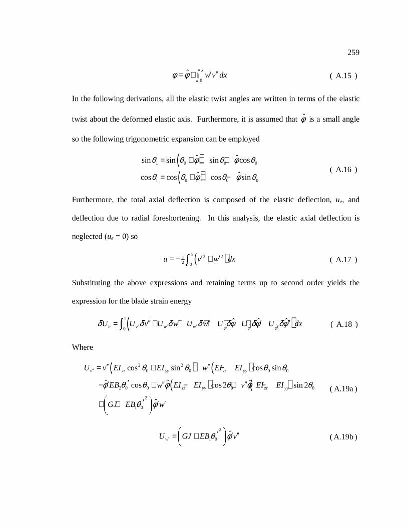
259
0
ˆ xw v dxφ φ ′ ′′= + ( A.15 )
In the following derivations, all the elastic twist angles are written in terms of the elastic
twist about the deformed elastic axis. Furthermore, it is assumed thatφ is a small angle
so the following trigonometric expansion can be employed
( )( )
1 0 0 0
1 0 0 0
ˆ ˆsin sin sin cos
ˆ ˆcos cos cos sin
θ θ φ θ φ θ
θ θ φ θ φ θ
= + ≅ +
= + ≅ −( A.16 )
Furthermore, the total axial deflection is composed of the elastic deflection,ue, and
deflection due to radial foreshortening. In this analysis, the elastic axial deflection is
neglected (ue = 0) so
( )2 212 0
xu v w dx′ ′= − + ( A.17 )
Substituting the above expressions and retaining terms up to second order yields the
expression for the blade strain energy
( )1
ˆ ˆ ˆ0
ˆ ˆ ˆb v w wU U v U w U w U U U dxφ φ φδ δ δ δ δφ δφ δφ′′ ′ ′′ ′ ′′
′′ ′ ′′ ′ ′′= + + + + + ( A.18 )
Where
( ) ( )( ) ( )
2 20 0 0 0
2 0 0 0 0
2
1 0
cos sin cos sin
ˆ ˆ ˆcos cos 2 sin 2
ˆ
v zz yy zz yy
zz yy zz yy
U v EI EI w EI EI
EB w EI EI v EI EI
GJ EB w
θ θ θ θ
φ θ θ φ θ φ θ
θ φ
′′ ′′ ′′= + + −
′′ ′′ ′′− + − + −
′ ′ ′+ +
( A.19a )
2
1 0ˆ
wU GJ EB vθ φ′ ′ ′ ′′= +
( A.19b )
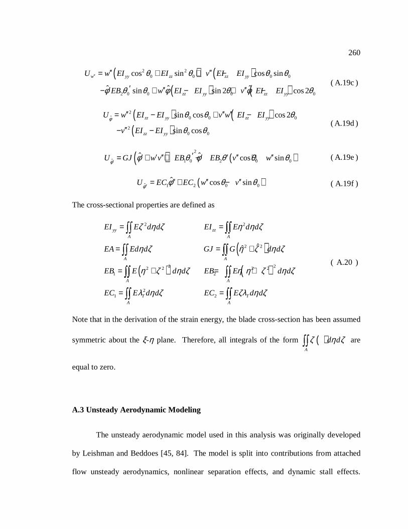
260
( ) ( )( ) ( )
2 20 0 0 0
2 0 0 0 0
cos sin cos sin
ˆ ˆ ˆsin sin 2 cos 2
w yy zz zz yy
zz yy zz yy
U w EI EI v EI EI
EB w EI EI v EI EI
θ θ θ θ
φ θ θ φ θ φ θ
′′ ′′ ′′= + + −
′′ ′′ ′′− + − + −( A.19c )
( ) ( )( )
2ˆ 0 0 0
20 0
sin cos cos 2
sin cos
zz yy zz yy
zz yy
U w EI EI v w EI EI
v EI EI
φ θ θ θ
θ θ
′′ ′′ ′′= − + −
′′− −( A.19d )
( ) ( )2
ˆ 1 0 2 0 0ˆ ˆ cos sinU GJ w v EB EB v wφ φ θ φ θ θ θ′
′′ ′ ′′ ′ ′ ′′ ′′= + + − + ( A.19e )
( )ˆ 1 2 0 0ˆ cos sinU EC EC w vφ φ θ θ′′′′ ′′ ′′= + − ( A.19f )
The cross-sectional properties are defined as
( )( ) ( )
2 2
2 2
2 22 2 2 21 2
21 2
ˆˆ
yy zz
A A
A A
A A
T T
A A
EI E d d EI E d d
EA Ed d GJ G d d
EB E d d EB E d d
EC E d d EC E d d
ζ η ζ η η ζ
η ζ η ζ η ζ
η ζ η ζ η η ζ η ζ
λ η ζ ζλ η ζ
= =
= = +
= + = +
= =
( A.20 )
Note that in the derivation of the strain energy, the blade cross-section has been assumed
symmetric about theξ-η plane. Therefore, all integrals of the form ( )A
d dζ η ζ are
equal to zero.
A.3 Unsteady Aerodynamic Modeling
The unsteady aerodynamic model used in this analysis was originally developed
by Leishman and Beddoes [45, 84]. The model is split into contributions from attached
flow unsteady aerodynamics, nonlinear separation effects, and dynamic stall effects.
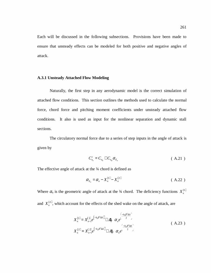
261
Each will be discussed in the following subsections. Provisions have been made to
ensure that unsteady effects can be modeled for both positive and negative angles of
attack.
A.3.1 Unsteady Attached Flow Modeling
Naturally, the first step in any aerodynamic model is the correct simulation of
attached flow conditions. This section outlines the methods used to calculate the normal
force, chord force and pitching moment coefficients under unsteady attached flow
conditions. It also is used as input for the nonlinear separation and dynamic stall
sections.
The circulatory normal force due to a series of step inputs in the angle of attack is
given by
0n n
cn n n EC C C
αα= + ( A.21 )
The effective angle of attack at the ¾ chord is defined as
( ) ( )1 2
nE n n nX Xα α= − − ( A.22 )
Whereαn is the geometric angle of attack at the ¾ chord. The deficiency functions( )1nX
and ( )2nX , which account for the effects of the shed wake on the angle of attack, are
( ) ( ) ( )
( ) ( ) ( )
21
21
22
22
21 11 1
22 21 2
b Sb S
n n n
b Sb S
n n n
X X e A e
X X e A e
ββ
ββ
α
α
− ∆ − ∆
−
− ∆ − ∆
−
= + ∆
= + ∆
( A.23 )
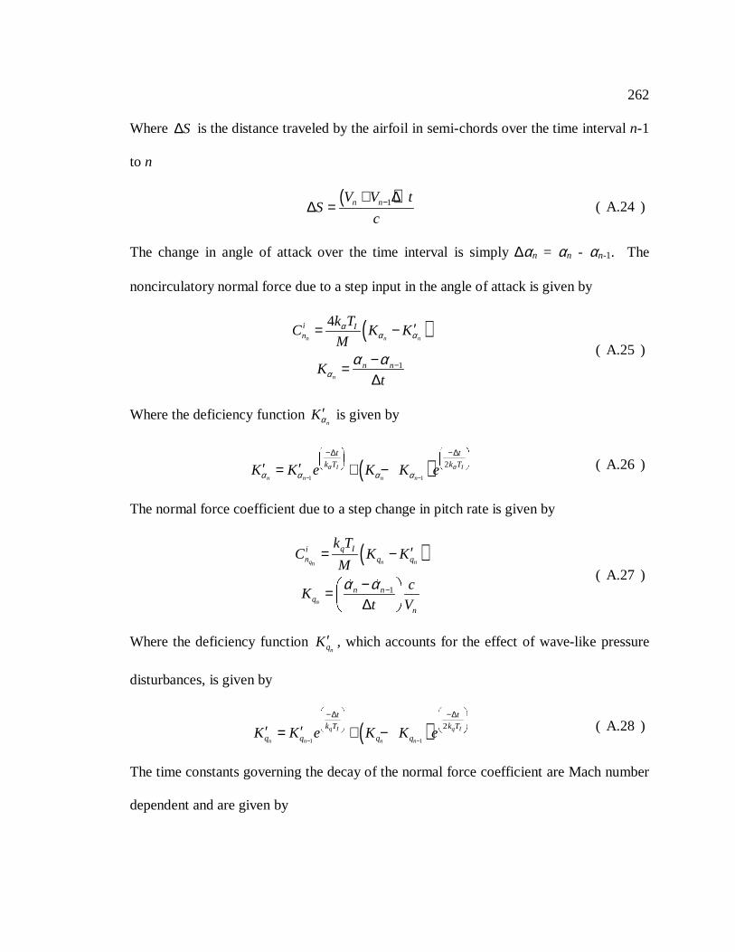
262
Where S∆ is the distance traveled by the airfoil in semi-chords over the time intervaln-1
to n
( )1n nV V tS
c−+ ∆
∆ = ( A.24 )
The change in angle of attack over the time interval is simply∆αn = αn - αn-1. The
noncirculatory normal force due to a step input in the angle of attack is given by
( )1
4n n n
n
i In
n n
k TC K K
M
Kt
αα α
αα α −
′= −
−=∆
( A.25 )
Where the deficiency functionn
Kα′ is given by
( )1 1
2I I
n n n n
t t
k T k TK K e K K eα αα α α α− −
−∆ −∆ ′ ′= + − ( A.26 )
The normal force coefficient due to a step change in pitch rate is given by
( )1
q n nn
n
q Iin q q
n nq
n
k TC K K
Mc
Kt V
α α −
′= −
− = ∆
( A.27 )
Where the deficiency functionnqK ′ , which accounts for the effect of wave-like pressure
disturbances, is given by
( )1 1
2q I q I
n n n n
t t
k T k T
q q q qK K e K K e− −
−∆ −∆ ′ ′= + − ( A.28 )
The time constants governing the decay of the normal force coefficient are Mach number
dependent and are given by
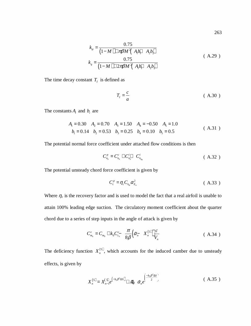
263
( ) ( )
( ) ( )
21 1 2 2
21 1 2 2
0.75
1
0.75
1 2q
kM M Ab A b
kM M A b A b
α πβ
πβ
=− + +
=− + +
( A.29 )
The time decay constantIT is defined as
I
cT
a= ( A.30 )
The constantsiA and ib are
1 2 3 4 5
1 2 3 4 5
0.30 0.70 1.50 0.50 1.0
0.14 0.53 0.25 0.10 0.5
A A A A A
b b b b b
= = = = − == = = = =
( A.31 )
The potential normal force coefficient under attached flow conditions is then
n n n qn
p c i in n n nC C C C= + + ( A.32 )
The potential unsteady chord force coefficient is given by
2
n
pc c n EC C
αη α= ( A.33 )
Whereηc is the recovery factor and is used to model the fact that a real airfoil is unable to
attain 100% leading edge suction. The circulatory moment coefficient about the quarter
chord due to a series of step inputs in the angle of attack is given by
( )( )0
50 8n n
c cm m c n n
n
cC C k C X
V
π αβ
= + − − ( A.34 )
The deficiency function ( )5nX , which accounts for the induced camber due to unsteady
effects, is given by
( ) ( ) ( )2
52
5 25 51 5
b Sb S
n n nX X e A e
ββ α
− ∆ − ∆
−= + ∆
( A.35 )
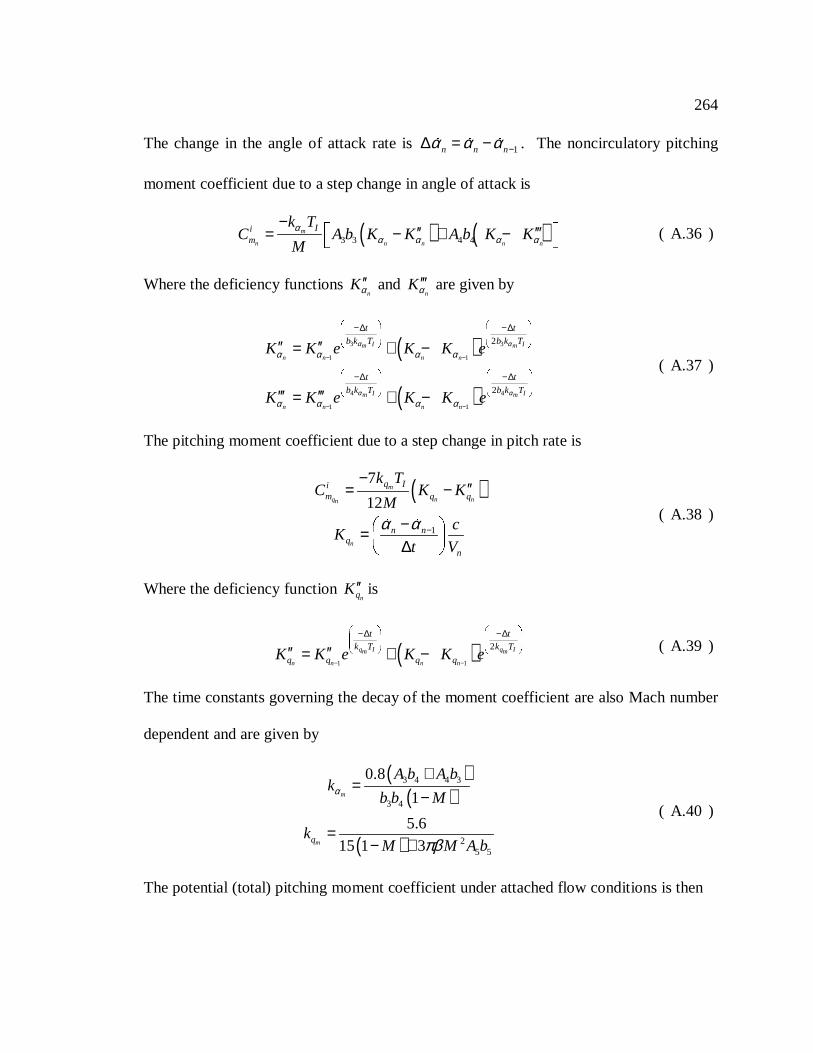
264
The change in the angle of attack rate is 1n n nα α α −∆ = − . The noncirculatory pitching
moment coefficient due to a step change in angle of attack is
( ) ( )3 3 4 4m
n n n n n
Iim
k TC A b K K A b K K
Mα
α α α α
− ′′ ′′′= − + −
( A.36 )
Where the deficiency functionsn
Kα′′ andn
Kα′′′ are given by
( )
( )
3 3
1 1
4 4
1 1
2
2
I Im m
n n n n
I Im m
n n n n
t t
b k T b k T
t t
b k T b k T
K K e K K e
K K e K K e
α α
α α
α α α α
α α α α
− −
− −
−∆ −∆
−∆ −∆
′′ ′′= + −
′′′ ′′′= + −
( A.37 )
The pitching moment coefficient due to a step change in pitch rate is
( )1
7
12m
q n nn
n
q Iim q q
n nq
n
k TC K K
Mc
Kt V
α α −
−′′= −
− = ∆
( A.38 )
Where the deficiency functionnqK ′′ is
( )1 1
2q I q Im m
n n n n
t t
k T k T
q q q qK K e K K e− −
−∆ −∆ ′′ ′′= + − ( A.39 )
The time constants governing the decay of the moment coefficient are also Mach number
dependent and are given by
( )( )
( )
3 4 4 3
3 4
25 5
0.8
1
5.6
15 1 3
m
mq
A b A bk
b b M
kM M A b
α
πβ
+=
−
=− +
( A.40 )
The potential (total) pitching moment coefficient under attached flow conditions is then
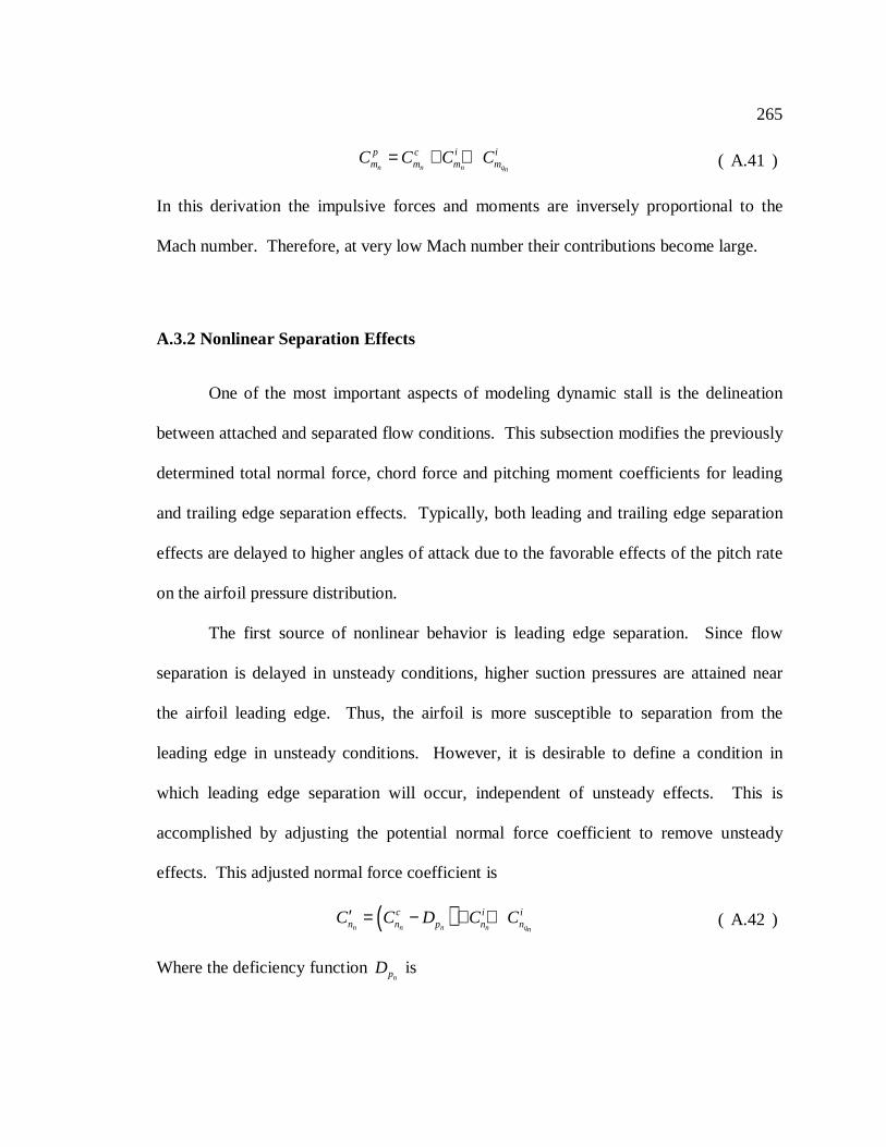
265
n n n qn
p c i im m m mC C C C= + + ( A.41 )
In this derivation the impulsive forces and moments are inversely proportional to the
Mach number. Therefore, at very low Mach number their contributions become large.
A.3.2 Nonlinear Separation Effects
One of the most important aspects of modeling dynamic stall is the delineation
between attached and separated flow conditions. This subsection modifies the previously
determined total normal force, chord force and pitching moment coefficients for leading
and trailing edge separation effects. Typically, both leading and trailing edge separation
effects are delayed to higher angles of attack due to the favorable effects of the pitch rate
on the airfoil pressure distribution.
The first source of nonlinear behavior is leading edge separation. Since flow
separation is delayed in unsteady conditions, higher suction pressures are attained near
the airfoil leading edge. Thus, the airfoil is more susceptible to separation from the
leading edge in unsteady conditions. However, it is desirable to define a condition in
which leading edge separation will occur, independent of unsteady effects. This is
accomplished by adjusting the potential normal force coefficient to remove unsteady
effects. This adjusted normal force coefficient is
( )n n n n qn
c i in n p n nC C D C C′ = − + + ( A.42 )
Where the deficiency functionnpD is
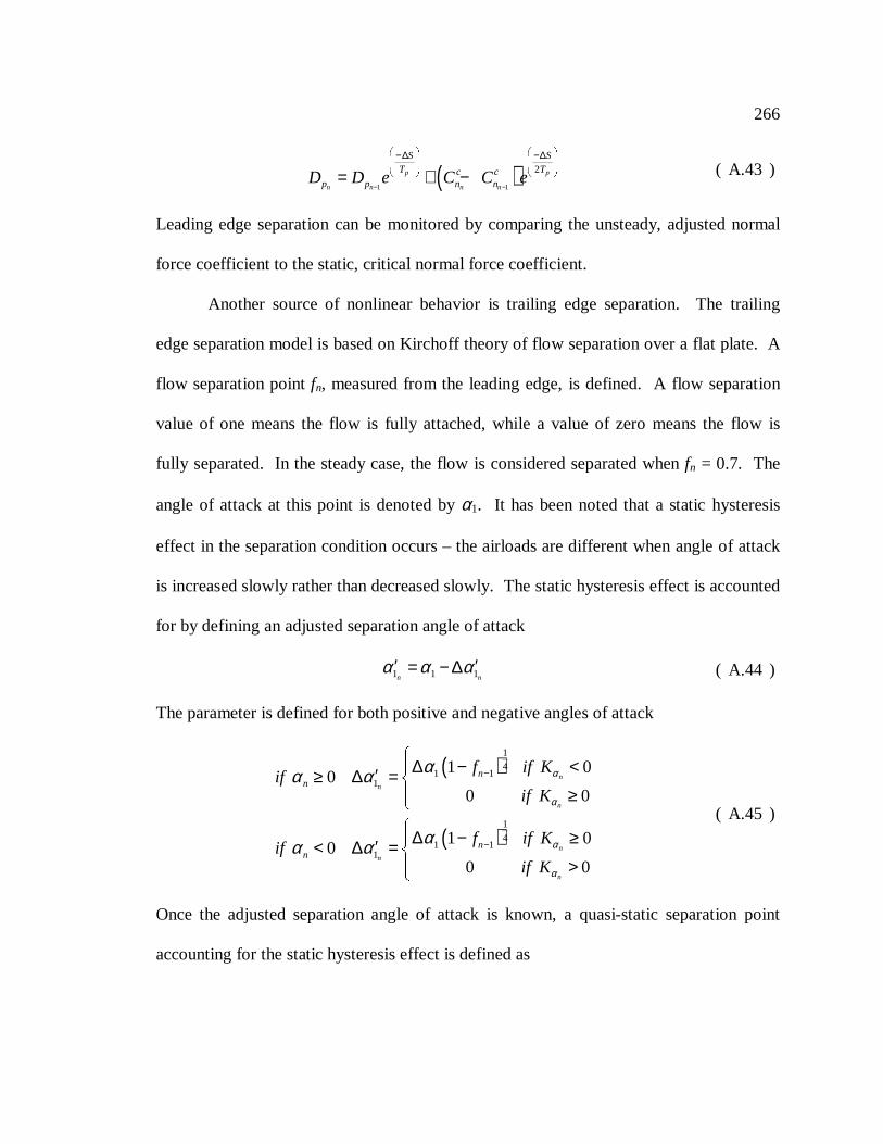
266
( )1 1
2p p
n n n n
S S
T Tc cp p n nD D e C C e
− −
−∆ −∆ = + − ( A.43 )
Leading edge separation can be monitored by comparing the unsteady, adjusted normal
force coefficient to the static, critical normal force coefficient.
Another source of nonlinear behavior is trailing edge separation. The trailing
edge separation model is based on Kirchoff theory of flow separation over a flat plate. A
flow separation pointfn, measured from the leading edge, is defined. A flow separation
value of one means the flow is fully attached, while a value of zero means the flow is
fully separated. In the steady case, the flow is considered separated whenfn = 0.7. The
angle of attack at this point is denoted byα1. It has been noted that a static hysteresis
effect in the separation condition occurs – the airloads are different when angle of attack
is increased slowly rather than decreased slowly. The static hysteresis effect is accounted
for by defining an adjusted separation angle of attack
1 1 1n nα α α′ ′= − ∆ ( A.44 )
The parameter is defined for both positive and negative angles of attack
( )
( )
14
1 11
14
1 11
1 00
0 0
1 00
0 0
n
n
n
n
n
n
nn
nn
f if Kif
if K
f if Kif
if K
α
α
α
α
αα α
αα α
−
−
∆ − <′≥ ∆ = ≥
∆ − ≥′< ∆ = >
( A.45 )
Once the adjusted separation angle of attack is known, a quasi-static separation point
accounting for the static hysteresis effect is defined as
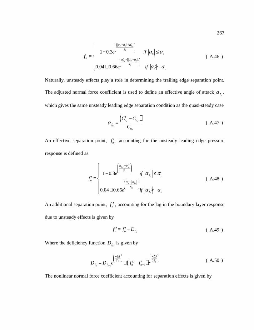
267
( )
( )
0 1
1
1 0
2
1
1
1 0.3
0.04 0.66
n n
nn
S
n
n
S
n
e iff
e if
α α α
α α α
α α
α α
′− −
′ − −
− ≤= + >
( A.46 )
Naturally, unsteady effects play a role in determining the trailing edge separation point.
The adjusted normal force coefficient is used to define an effective angle of attacknf
α ,
which gives the same unsteady leading edge separation condition as the quasi-steady case
( )0n
n
n n
fn
C C
Cα
α′ −
= ( A.47 )
An effective separation point, nf ′ , accounting for the unsteady leading edge pressure
response is defined as
1
1
1
2
1
1
1 0.3
0.04 0.66
fn n
n
fn n
n
S
f
n
S
f
e iff
e if
α α
α α
α α
α α
′−
′ −
− ≤′ = + >
( A.48 )
An additional separation point,nf ′′ , accounting for the lag in the boundary layer response
due to unsteady effects is given by
nn n ff f D′′ ′= − ( A.49 )
Where the deficiency functionnf
D is given by
( )1
2
1f f
n n
S S
T T
f f n nD D e f f e−
−∆ −∆
−′ ′= + − ( A.50 )
The nonlinear normal force coefficient accounting for separation effects is given by
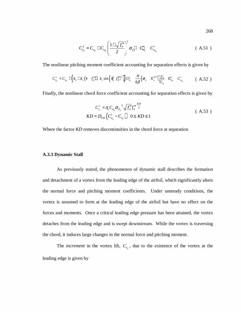
268
0
2
1
2n n n qn
nf i in n n E n n
fC C C C C
αα
′′+= + + +
( A.51 )
The nonlinear pitching moment coefficient accounting for separation effects is given by
( ) ( )( ) ( )( )0
2 5
0 1 21 sin8n n n qn
f c i i
m m n n n n m mnn
cC C k k f k f C X C C
U
ππ α
β′′ ′′= + − + − − + ++ ( A.52 )
Finally, the nonlinear chord force coefficient accounting for separation effects is given by
( )1
22
0 1
n n
n
fKD
c c n E n n
FD n n
C C f f
KD D C C KD
αη α= ′′ ′′
′= − ≤ ≤( A.53 )
Where the factorKD removes discontinuities in the chord force at separation.
A.3.3 Dynamic Stall
As previously stated, the phenomenon of dynamic stall describes the formation
and detachment of a vortex from the leading edge of the airfoil, which significantly alters
the normal force and pitching moment coefficients. Under unsteady conditions, the
vortex is assumed to form at the leading edge of the airfoil but have no effect on the
forces and moments. Once a critical leading edge pressure has been attained, the vortex
detaches from the leading edge and is swept downstream. While the vortex is traversing
the chord, it induces large changes in the normal force and pitching moment.
The incrementin the vortex lift,nvC , due to the existence of the vortex at the
leading edge is given by
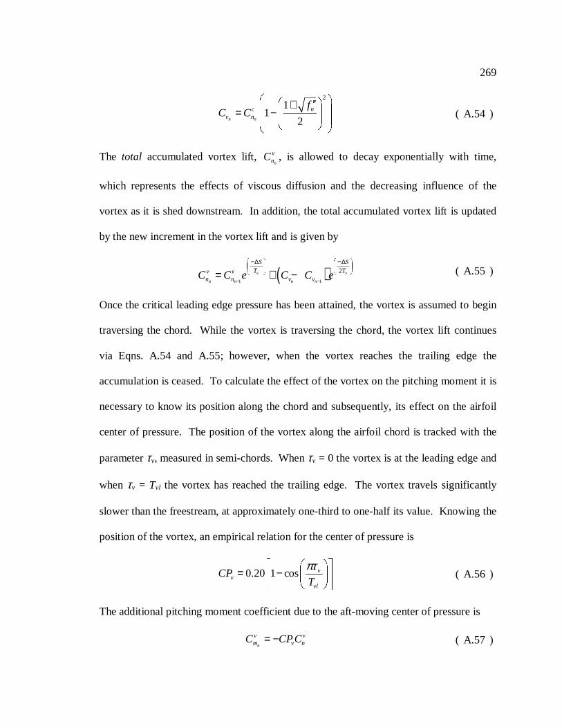
269
2
11
2n n
ncv n
fC C
′′+ = −
( A.54 )
The total accumulated vortex lift,n
vnC , is allowed to decay exponentially with time,
which represents the effects of viscous diffusion and the decreasing influence of the
vortex as it is shed downstream. In addition, the total accumulated vortex lift is updated
by the new increment in the vortex lift and is given by
( )1 1
2v v
n n n n
S S
T Tv vn n v vC C e C C e
− −
−∆ −∆ = + − ( A.55 )
Once the critical leading edge pressure has been attained, the vortex is assumed to begin
traversing the chord. While the vortex is traversing the chord, the vortex lift continues
via Eqns. A.54 and A.55; however, when the vortex reaches the trailing edge the
accumulation is ceased. To calculate the effect of the vortex on the pitching moment it is
necessary to know its position along the chord and subsequently, its effect on the airfoil
center of pressure. The position of the vortex along the airfoil chord is tracked with the
parameterτv, measured in semi-chords. Whenτv = 0 the vortex is at the leading edge and
whenτv = Tvl the vortex has reached the trailing edge. The vortex travels significantly
slower than the freestream, at approximately one-third to one-half its value. Knowing the
position of the vortex, an empirical relation for the center of pressure is
0.20 1 cos vv
vl
CPT
πτ = −
( A.56 )
The additional pitching moment coefficient due to the aft-moving center of pressure is
n
v vm v nC CP C= − ( A.57 )
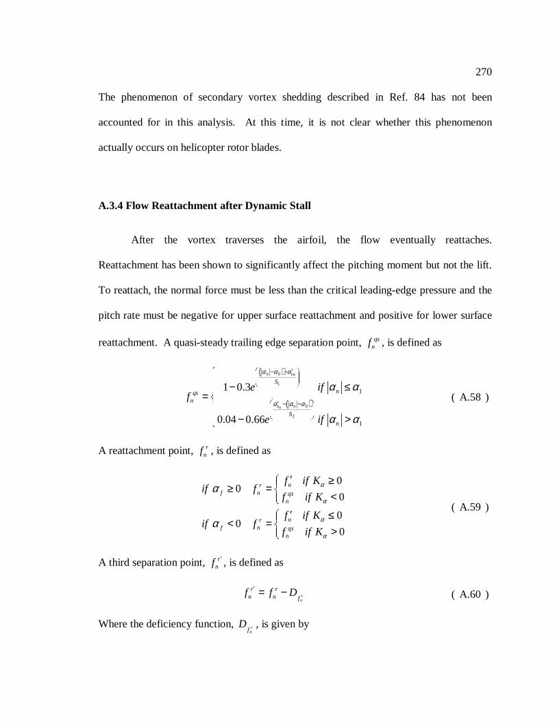
270
The phenomenon of secondary vortex shedding described in Ref. 84 has not been
accounted for in this analysis. At this time, it is not clear whether this phenomenon
actually occurs on helicopter rotor blades.
A.3.4 Flow Reattachment after Dynamic Stall
After the vortex traverses the airfoil, the flow eventually reattaches.
Reattachment has been shown to significantly affect the pitching moment but not the lift.
To reattach, the normal force must be less than the critical leading-edge pressure and the
pitch rate must be negative for upper surface reattachment and positive for lower surface
reattachment. A quasi-steady trailing edge separation point,qsnf , is defined as
( )
( )
0 1
1
1 0
2
1
1
1 0.3
0.04 0.66
n n
nn
S
nqsn
S
n
e iff
e if
α α α
α α α
α α
α α
′− −
′ − −
− ≤= − >
( A.58 )
A reattachment point, rnf , is defined as
00
0
00
0
nrf n qs
n
nrf n qs
n
f if Kif f
f if K
f if Kif f
f if K
α
α
α
α
α
α
′ ≥≥ = <
′ ≤< = >
( A.59 )
A third separation point, rnf
′ , is defined as
rn
r rn n f
f f D′ = − ( A.60 )
Where the deficiency function, rnf
D , is given by
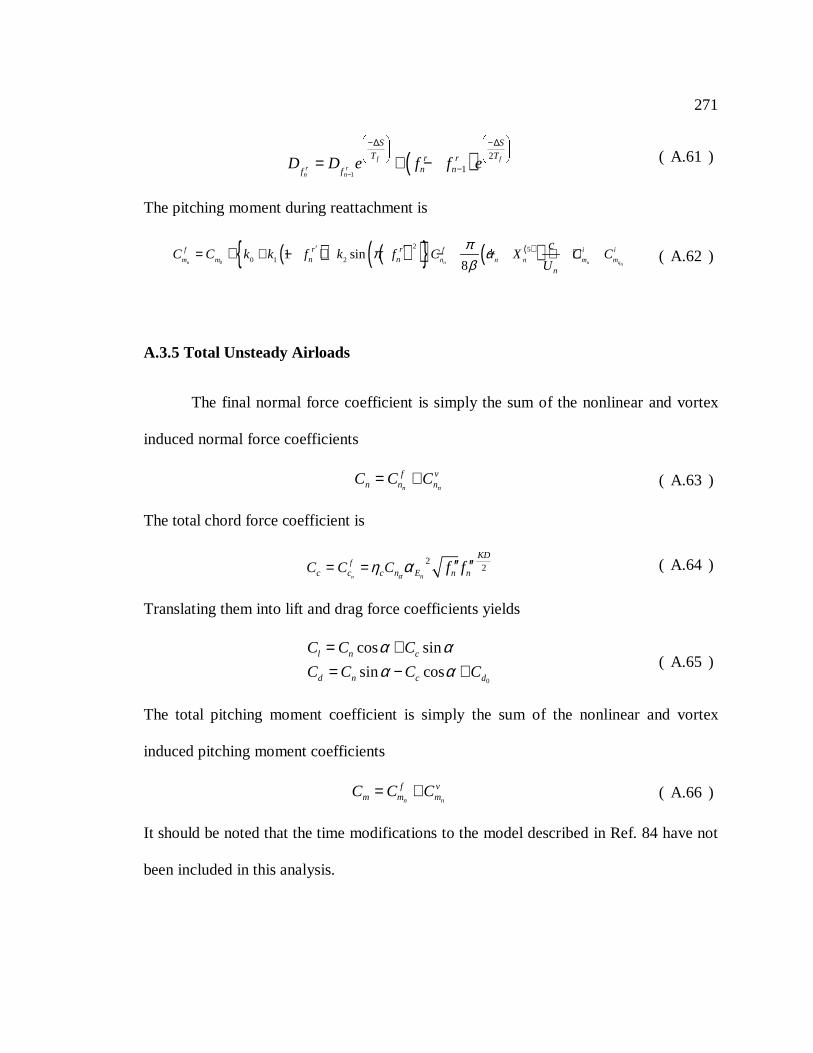
271
( )1
2
1f f
r rn n
S S
T Tr rn nf f
D D e f f e−
−∆ −∆
−= + − ( A.61 )
The pitching moment during reattachment is
( ) ( )( ) ( )( )0
2 5
0 1 21 sin8n n n qn
f f i i
m m n n n m m
r rn n
n
cC C k k f k f C X C C
U
ππ α
β′ ′= + − + − − + ++ ( A.62 )
A.3.5 Total Unsteady Airloads
The final normal force coefficient is simply the sum of the nonlinear and vortex
induced normal force coefficients
n n
f vn n nC C C= + ( A.63 )
The total chord force coefficient is
22
n n
fKD
c c c n E n nC C C f fα
η α= = ′′ ′′ ( A.64 )
Translating them into lift and drag force coefficients yields
0
cos sin
sin cosl n c
d n c d
C C C
C C C C
α αα α
= += − + ( A.65 )
The total pitching moment coefficient is simply the sum of the nonlinear and vortex
induced pitching moment coefficients
n n
f vm m mC C C= + ( A.66 )
It should be noted that the time modifications to the model described in Ref. 84 have not
been included in this analysis.
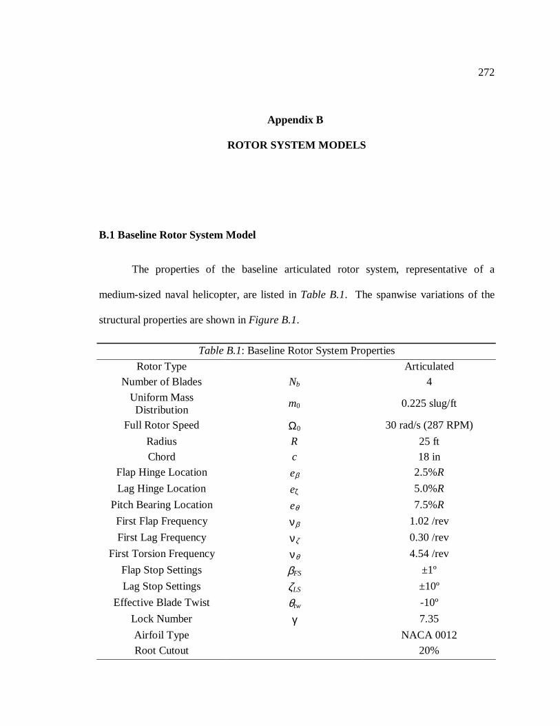
272
Appendix B
ROTOR SYSTEM MODELS
B.1 Baseline Rotor System Model
The properties of the baseline articulated rotor system, representative of a
medium-sized naval helicopter, are listed inTable B.1. The spanwise variations of the
structural properties are shown inFigure B.1.
Table B.1: Baseline Rotor System Properties
Rotor Type Articulated
Number of Blades Nb 4
Uniform MassDistribution
m0 0.225 slug/ft
Full Rotor Speed Ω0 30 rad/s (287 RPM)
Radius R 25 ft
Chord c 18 in
Flap Hinge Location eβ 2.5%R
Lag Hinge Location eζ 5.0%R
Pitch Bearing Location eθ 7.5%R
First Flap Frequency νβ 1.02 /rev
First Lag Frequency νζ 0.30 /rev
First Torsion Frequency νθ 4.54 /rev
Flap Stop Settings βFS ±1º
Lag Stop Settings ζLS ±10º
Effective Blade Twist θtw -10º
Lock Number γ 7.35
Airfoil Type NACA 0012
Root Cutout 20%
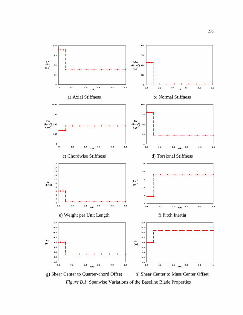
273
0
2 5
5 0
7 5
10 0
0.0 0 .2 0 .4 0.6 0 .8 1.0r /R
E A(lb )
x1 0 6
a) Axial Stiffness
0
2 50
5 00
7 50
1 0 00
0.0 0 .2 0.4 0.6 0 .8 1.0r /R
E Iyy
(lb -in 2)x 10 6
b) Normal Stiffness
0
25 0
50 0
75 0
1 00 0
0.0 0 .2 0 .4 0.6 0 .8 1.0r /R
E Izz
(lb -in 2)X 1 0 6
c) Chordwise Stiffness
0
25
50
75
1 00
0.0 0 .2 0.4 0.6 0 .8 1.0r /R
G J(lb -in 2)
x1 0 6
d) Torsional Stiffness
0
2
4
6
8
1 0
1 2
1 4
1 6
1 8
2 0
0 .0 0 .2 0 .4 0.6 0 .8 1.0r /R
w(lb /in )
e) Weight per Unit Length
0
5
10
15
20
25
0 .0 0.2 0 .4 0.6 0 .8 1.0r /R
k m 22
(in 2)
f) Pitch Inertia
-1 .0
-0 .8
-0 .5
-0 .3
0 .0
0 .3
0 .5
0 .8
1 .0
0 .0 0 .2 0 .4 0 .6 0 .8 1 .0r /R
e c
(in )
g) Shear Center to Quarter-chord Offset
-1 .0
-0 .8
-0 .5
-0 .3
0 .0
0 .3
0 .5
0 .8
1 .0
0 .0 0.2 0.4 0.6 0 .8 1 .0r /R
e g
(in )
h) Shear Center to Mass Center Offset
Figure B.1: Spanwise Variations of the Baseline Blade Properties
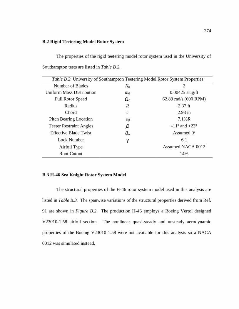
274
B.2 Rigid Teetering Model Rotor System
The properties of the rigid teetering model rotor system used in the University of
Southampton tests are listed inTable B.2.
B.3 H-46 Sea Knight Rotor System Model
The structural properties of the H-46 rotor system model used in this analysis are
listed inTable B.3.The spanwise variations of the structural properties derived from Ref.
91 are shown inFigure B.2. The production H-46 employs a Boeing Vertol designed
V23010-1.58 airfoil section. The nonlinear quasi-steady and unsteady aerodynamic
properties of the Boeing V23010-1.58 were not available for this analysis so a NACA
0012 was simulated instead.
Table B.2: University of Southampton Teetering Model Rotor System Properties
Number of Blades Nb 2
Uniform Mass Distribution m0 0.00425 slug/ft
Full Rotor Speed Ω0 62.83 rad/s (600 RPM)
Radius R 2.37 ft
Chord c 2.93 in
Pitch Bearing Location eθ 7.1%R
Teeter Restraint Angles βr -11º and +23º
Effective Blade Twist θtw Assumed 0º
Lock Number γ 6.1
Airfoil Type Assumed NACA 0012
Root Cutout 14%
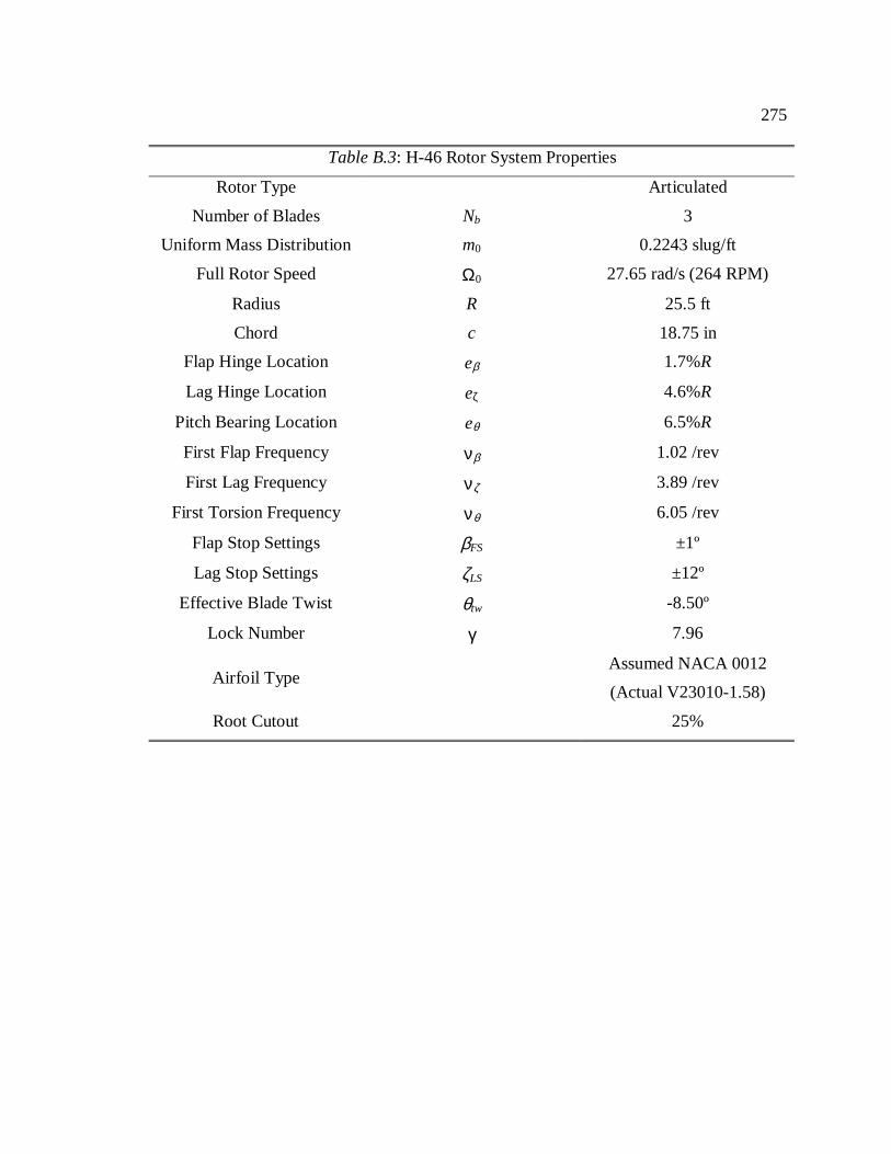
275
Table B.3: H-46 Rotor System Properties
Rotor Type Articulated
Number of Blades Nb 3
Uniform Mass Distribution m0 0.2243 slug/ft
Full Rotor Speed Ω0 27.65 rad/s (264 RPM)
Radius R 25.5 ft
Chord c 18.75 in
Flap Hinge Location eβ 1.7%R
Lag Hinge Location eζ 4.6%R
Pitch Bearing Location eθ 6.5%R
First Flap Frequency νβ 1.02 /rev
First Lag Frequency νζ 3.89 /rev
First Torsion Frequency νθ 6.05 /rev
Flap Stop Settings βFS ±1º
Lag Stop Settings ζLS ±12º
Effective Blade Twist θtw -8.50º
Lock Number γ 7.96
Airfoil TypeAssumed NACA 0012
(Actual V23010-1.58)
Root Cutout 25%
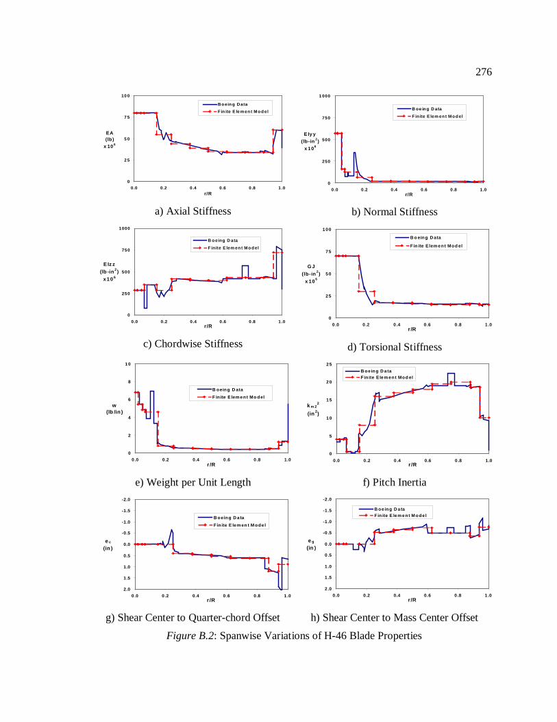
276
0
2 5
5 0
7 5
10 0
0.0 0.2 0.4 0.6 0 .8 1 .0r/R
EA(lb)
x 10 6
B o ein g D ata
F in ite E le m en t M o d el
a) Axial Stiffness
0
250
500
750
1 000
0 .0 0.2 0.4 0.6 0 .8 1.0r/R
E Iy y
(lb-in 2)
x 10 6
B oe in g D ata
F inite E lem en t M o d el
b) Normal Stiffness
0
250
500
750
1000
0.0 0.2 0.4 0.6 0.8 1 .0r/R
E Iz z(lb -in 2)
x 1 0 6
B o eing D ata
F inite E lem en t M o d el
c) Chordwise Stiffness
0
2 5
5 0
7 5
1 0 0
0 .0 0 .2 0 .4 0 .6 0 .8 1 .0r /R
G J
(lb- in 2)
x 10 6
B o ein g D ata
F in ite E lem e n t Mo d el
d) Torsional Stiffness
0
2
4
6
8
1 0
0 .0 0.2 0.4 0 .6 0 .8 1.0r /R
w(lb /in )
B o ein g D ata
F in ite E lem e n t Mo d el
e) Weight per Unit Length
0
5
1 0
1 5
2 0
2 5
0.0 0 .2 0 .4 0.6 0 .8 1.0r /R
k m 22
(in 2)
B o e in g D a taF in ite E le m e n t Mo d el
f) Pitch Inertia
-2.0
-1.5
-1.0
-0.5
0.0
0.5
1.0
1.5
2.0
0 .0 0 .2 0.4 0 .6 0.8 1 .0r /R
e c
(in )
B o ein g D a ta
F in ite E le m en t M o d e l
g) Shear Center to Quarter-chord Offset
-2 .0
-1 .5
-1 .0
-0 .5
0 .0
0 .5
1 .0
1 .5
2 .0
0 .0 0.2 0.4 0.6 0 .8 1 .0r /R
e g
(in )
B o e in g D a taF in ite E le m e n t M o d e l
h) Shear Center to Mass Center Offset
Figure B.2: Spanwise Variations of H-46 Blade Properties
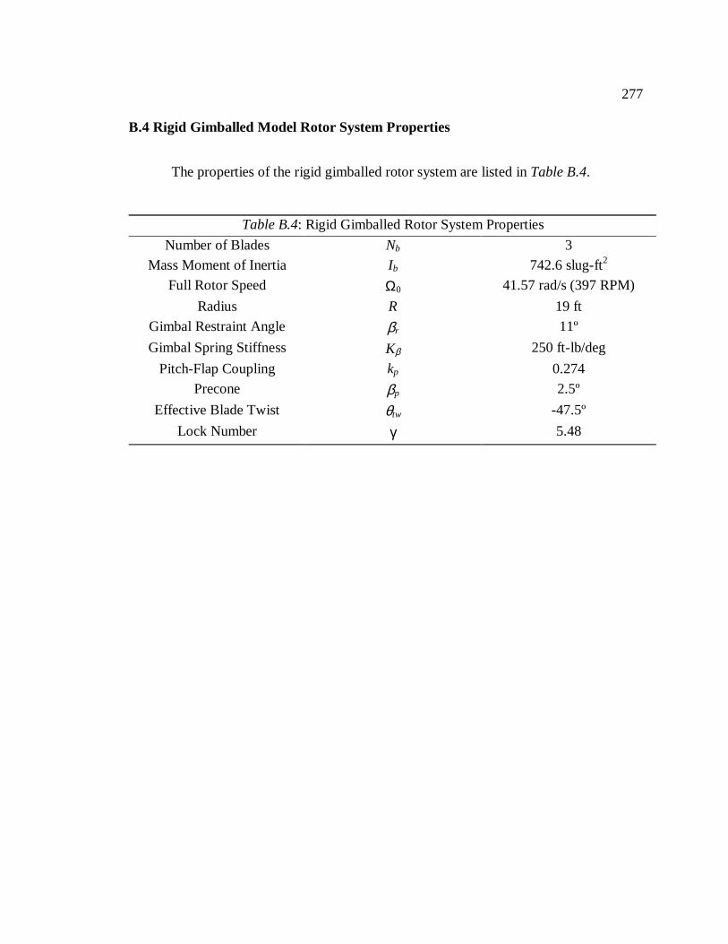
277
B.4 Rigid Gimballed Model Rotor System Properties
The properties of the rigid gimballed rotor system are listed inTable B.4.
Table B.4: Rigid Gimballed Rotor System Properties
Number of Blades Nb 3
Mass Moment of Inertia Ib 742.6 slug-ft2
Full Rotor Speed Ω0 41.57 rad/s (397 RPM)
Radius R 19 ft
Gimbal Restraint Angle βr 11º
Gimbal Spring Stiffness Kβ 250 ft-lb/deg
Pitch-Flap Coupling kp 0.274
Precone βp 2.5º
Effective Blade Twist θtw -47.5º
Lock Number γ 5.48
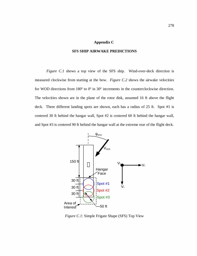
278
Appendix C
SFS SHIP AIRWAKE PREDICTIONS
Figure C.1 shows a top view of the SFS ship. Wind-over-deck direction is
measured clockwise from starting at the bow.Figure C.2shows the airwake velocities
for WOD directions from 180º to 0º in 30º increments in the counterclockwise direction.
The velocities shown are in the plane of the rotor disk, assumed 16 ft above the flight
deck. Three different landing spots are shown, each has a radius of 25 ft. Spot #1 is
centered 30 ft behind the hangar wall, Spot #2 is centered 60 ft behind the hangar wall,
and Spot #3 is centered 90 ft behind the hangar wall at the extreme rear of the flight deck.
Spot #1
Spot #2
Spot #3
ψWOD
VWOD
HangarFace
Vx
VyVz
150 ft
50 ft
30 ft
30 ft
30 ft
Area ofInterest
Figure C.1: Simple Frigate Shape (SFS) Top View
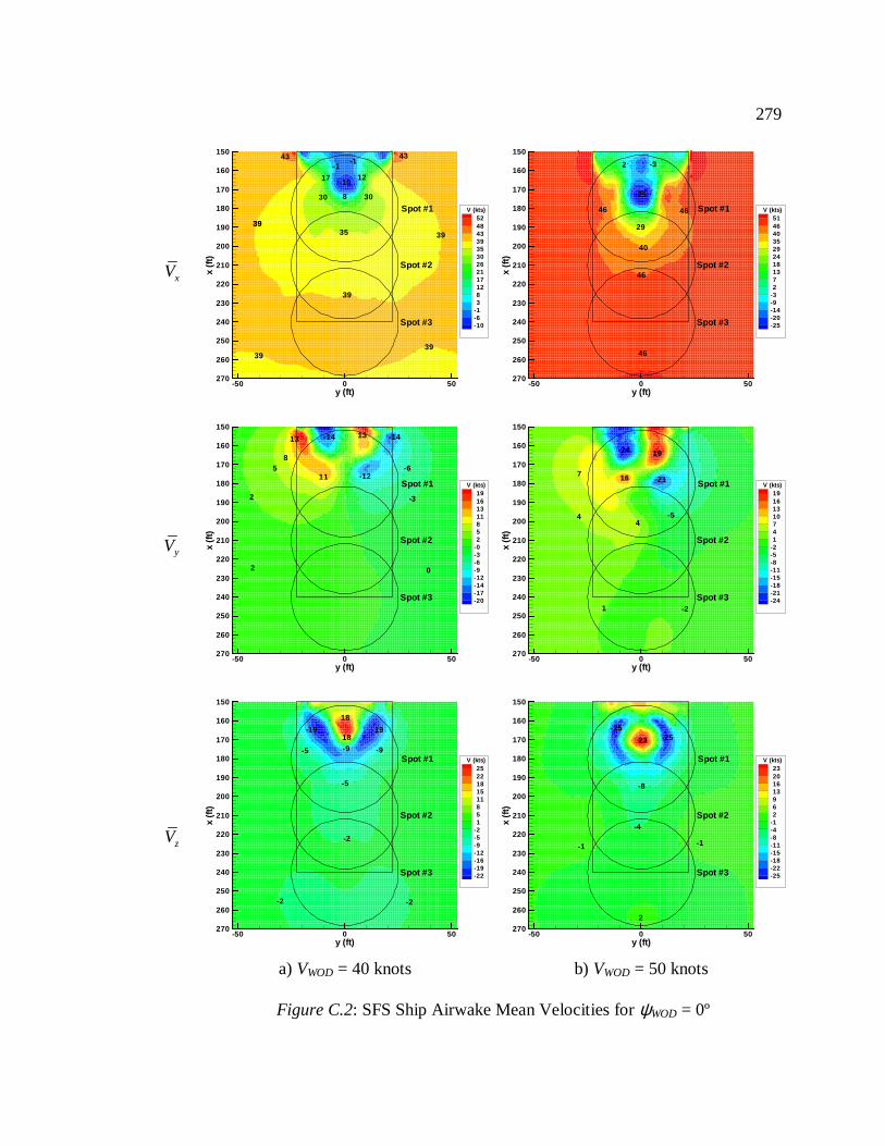
279
xV
3939
3939
39
43 43-1
-10
35
30
17
30
12
-1
39
8
y (ft)
x(ft
)
-50 0 50
150
160
170
180
190
200
210
220
230
240
250
260
270
5248433935302621171283
-1-6-10
V (kts)
Spot #3
Spot #1
Spot #2
-25
29
46
46 46
2 -3
40
46
y (ft)
x(ft
)
-50 0 50
150
160
170
180
190
200
210
220
230
240
250
260
270
514640352924181372
-3-9-14-20-25
V (kts)
Spot #3
Spot #1
Spot #2
yV
2
58
13
11 -12
-14-14 13
-3
-6
2 0
y (ft)
x(ft
)
-50 0 50
150
160
170
180
190
200
210
220
230
240
250
260
270
19161311852
-0-3-6-9-12-14-17-20
V (kts)
Spot #3
Spot #1
Spot #2
7
4
1
-24 19
16 -21
-54
-2
y (ft)
x(ft
)
-50 0 50
150
160
170
180
190
200
210
220
230
240
250
260
270
19161310741
-2-5-8-11-15-18-21-24
V (kts)
Spot #3
Spot #1
Spot #2
zV
-2 -2
-2
-5
-918
18
-19 -19
-5 -9
y (ft)
x(ft
)
-50 0 50
150
160
170
180
190
200
210
220
230
240
250
260
270
2522181511851
-2-5-9-12-16-19-22
V (kts)
Spot #3
Spot #1
Spot #2
a) VWOD = 40 knots
23
-25-25
-8
-4
2
-1-1
y (ft)
x(ft
)
-50 0 50
150
160
170
180
190
200
210
220
230
240
250
260
270
23201613962
-1-4-8-11-15-18-22-25
V (kts)
Spot #3
Spot #1
Spot #2
b) VWOD = 50 knots
Figure C.2: SFS Ship Airwake Mean Velocities forψWOD = 0º
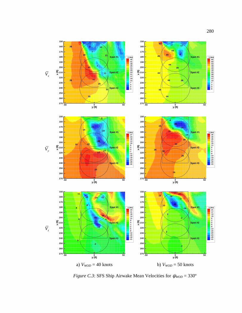
280
xV
38
38
7
387
14
41 7
41
35
31
35
0
21
11
y (ft)
x(ft
)
-50 0 50
150
160
170
180
190
200
210
220
230
240
250
260
270
4541383531282421171411740
-3
V (kts)
Spot #3
Spot #1
Spot #2
60
4960
44
44
44
39
39
-4
1217
44
44
44
y (ft)
x(ft
)
-50 0 50
150
160
170
180
190
200
210
220
230
240
250
260
270
656054494439332823171272
-4-9
V (kts)
Spot #3
Spot #1
Spot #2
yV
23
18
14-24
-2818
-19
6
1023
y (ft)
x(ft
)
-50 0 50
150
160
170
180
190
200
210
220
230
240
250
260
270
272318141062
-3-7-11-15-19-24-28-32
V (kts)
Spot #3
Spot #1
Spot #2
26
2630
351
-29
-24
26
26
26
30
-9
-14
y (ft)
x(ft
)
-50 0 50
150
160
170
180
190
200
210
220
230
240
250
260
270
35302621161161
-4-9-14-19-24-29-33
V (kts)
Spot #3
Spot #1
Spot #2
zV
8
11
-15
-18
-15
-2
24
5
14 -12
5
8
-8
y (ft)
x(ft
)
-50 0 50
150
160
170
180
190
200
210
220
230
240
250
260
270
2421181411851
-2-5-8-12-15-18-21
V (kts)
Spot #3
Spot #1
Spot #2
a) VWOD = 40 knots
-31
2113
2
2
-16
-2
-2
-2
10
-16
y (ft)
x(ft
)
-50 0 50
150
160
170
180
190
200
210
220
230
240
250
260
270
2117131062
-2-5-9-13-16-20-24-28-31
V (kts)
Spot #3
Spot #1
Spot #2
b) VWOD = 50 knots
Figure C.3: SFS Ship Airwake Mean Velocities forψWOD = 330º
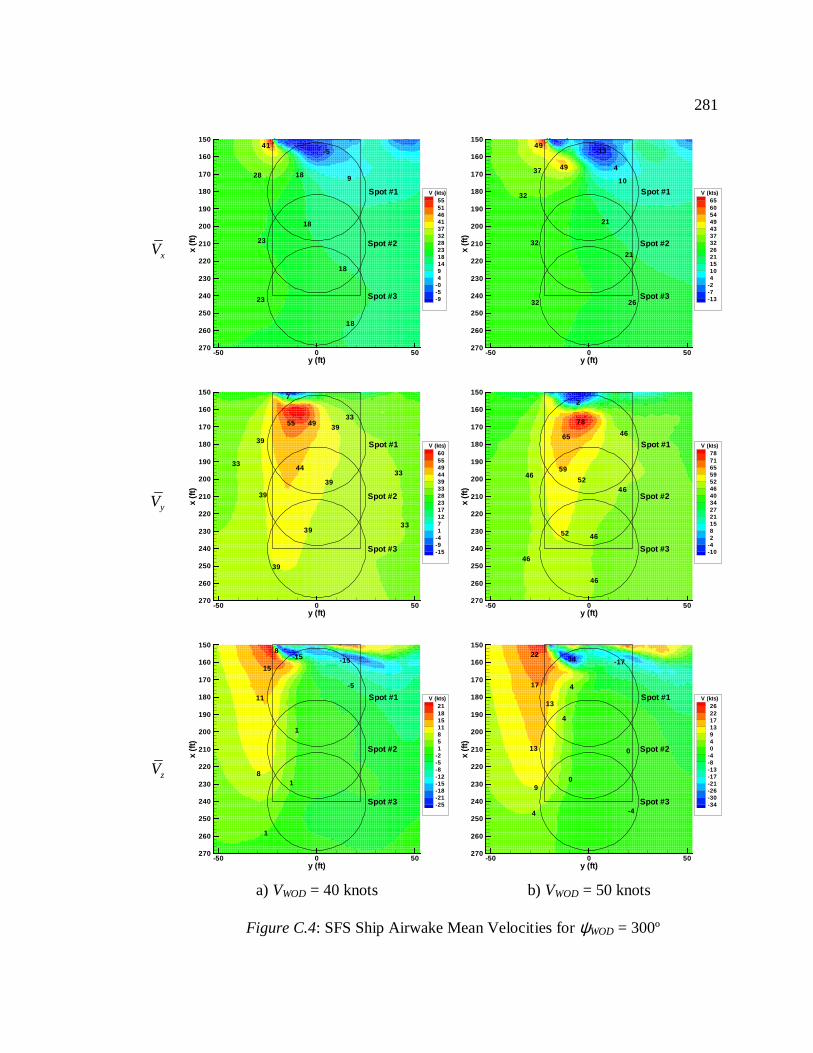
281
xV
41
28
18
18
18
18
9
-5
23
23
y (ft)
x(ft
)
-50 0 50
150
160
170
180
190
200
210
220
230
240
250
260
270
5551464137322823181494
-0-5-9
V (kts)
Spot #3
Spot #1
Spot #2
49
4937
32
32
21
-13
4
10
21
26
32
y (ft)
x(ft
)
-50 0 50
150
160
170
180
190
200
210
220
230
240
250
260
270
65605449433732262115104
-2-7-13
V (kts)
Spot #3
Spot #1
Spot #2
yV
39
39
39
33
55 49 3933
39
44
39
33
33
7
y (ft)
x(ft
)
-50 0 50
150
160
170
180
190
200
210
220
230
240
250
260
270
6055494439332823171271
-4-9-15
V (kts)
Spot #3
Spot #1
Spot #2
78
2
65
59
52
52 46
46
46
46
46
46
y (ft)
x(ft
)
-50 0 50
150
160
170
180
190
200
210
220
230
240
250
260
270
787165595246403427211582
-4-10
V (kts)
Spot #3
Spot #1
Spot #2
zV 8
11
15
-15 -15
-5
1
1
1
8
y (ft)
x(ft
)
-50 0 50
150
160
170
180
190
200
210
220
230
240
250
260
270
21181511851
-2-5-8-12-15-18-21-25
V (kts)
Spot #3
Spot #1
Spot #2
a) VWOD = 40 knots
22
17
13
9
4
4
-34
4
13
-17
0
-4
0
y (ft)
x(ft
)
-50 0 50
150
160
170
180
190
200
210
220
230
240
250
260
270
26221713940
-4-8-13-17-21-26-30-34
V (kts)
Spot #3
Spot #1
Spot #2
b) VWOD = 50 knots
Figure C.4: SFS Ship Airwake Mean Velocities forψWOD = 300º
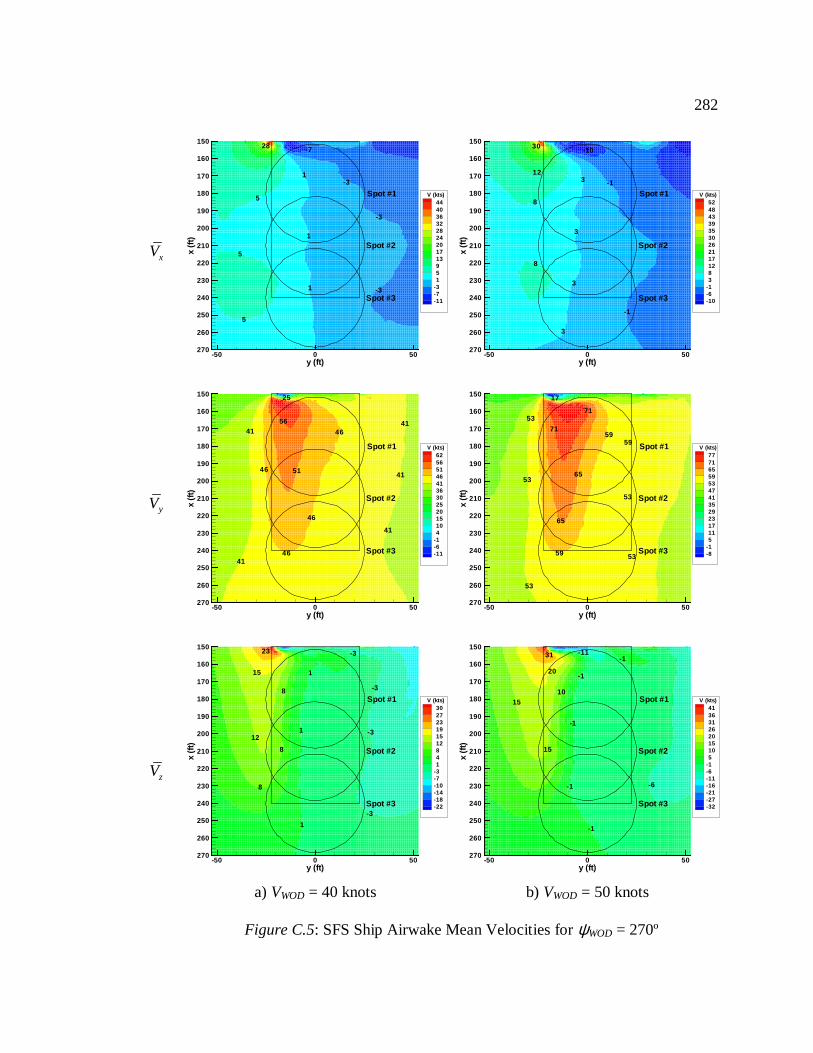
282
xV 5
5
5
28
1
1
1
-3
-3
-3
-7
y (ft)
x(ft
)
-50 0 50
150
160
170
180
190
200
210
220
230
240
250
260
270
444036322824201713951
-3-7-11
V (kts)
Spot #3
Spot #1
Spot #2
30
12
8
8
3
3
3
-1
-10
-1
3
y (ft)
x(ft
)
-50 0 50
150
160
170
180
190
200
210
220
230
240
250
260
270
5248433935302621171283
-1-6-10
V (kts)
Spot #3
Spot #1
Spot #2
yV
41
41
46
56
51
46
46
25
46
41
41
41
y (ft)
x(ft
)
-50 0 50
150
160
170
180
190
200
210
220
230
240
250
260
270
62565146413630252015104
-1-6-11
V (kts)
Spot #3
Spot #1
Spot #2
71
17
71
65
65
59
53
53
53
59
53
59
53
y (ft)
x(ft
)
-50 0 50
150
160
170
180
190
200
210
220
230
240
250
260
270
7771655953474135292317115
-1-8
V (kts)
Spot #3
Spot #1
Spot #2
zV
12
15
23
8
1
1
1
-3
-3
-3
-3
8
8
y (ft)
x(ft
)
-50 0 50
150
160
170
180
190
200
210
220
230
240
250
260
270
302723191512841
-3-7-10-14-18-22
V (kts)
Spot #3
Spot #1
Spot #2
a) VWOD = 40 knots
31 -11
20
10
-1
-1
-1
15
-1
-1
-6
15
y (ft)
x(ft
)
-50 0 50
150
160
170
180
190
200
210
220
230
240
250
260
270
413631262015105
-1-6-11-16-21-27-32
V (kts)
Spot #3
Spot #1
Spot #2
b) VWOD = 50 knots
Figure C.5: SFS Ship Airwake Mean Velocities forψWOD = 270º
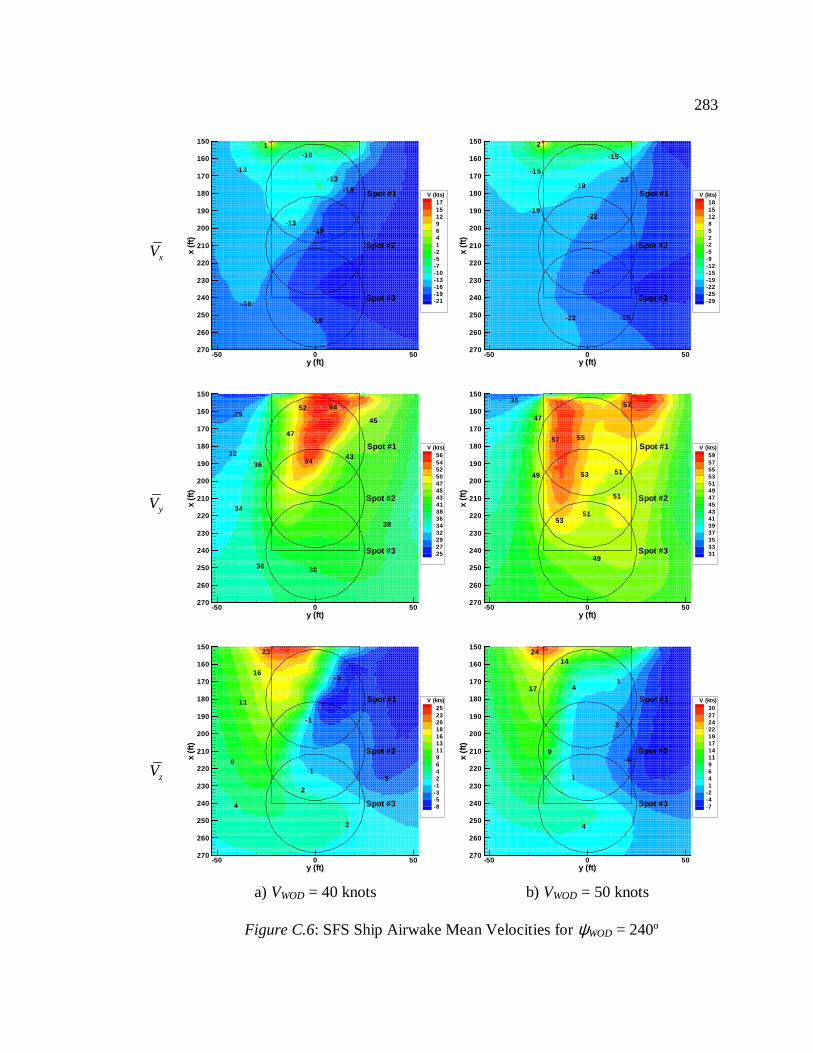
283
xV
-13
-16
-19
1-10
-13
-19
-19-13
y (ft)
x(ft
)
-50 0 50
150
160
170
180
190
200
210
220
230
240
250
260
270
1715129641
-2-5-7-10-13-16-19-21
V (kts)
Spot #3
Spot #1
Spot #2
2
-15
-19
-22
-22
-25
-25
-22
-15
-19
y (ft)
x(ft
)
-50 0 50
150
160
170
180
190
200
210
220
230
240
250
260
270
181512852
-2-5-9-12-15-19-22-25-29
V (kts)
Spot #3
Spot #1
Spot #2
yV
29
32
34
36
36
38
47
54
54
45
43
52
38
y (ft)
x(ft
)
-50 0 50
150
160
170
180
190
200
210
220
230
240
250
260
270
565452504745434138363432292725
V (kts)
Spot #3
Spot #1
Spot #2
47
49
53
57 55
57
51
51
51
53
35
49
y (ft)
x(ft
)
-50 0 50
150
160
170
180
190
200
210
220
230
240
250
260
270
595755535149474543413937353331
V (kts)
Spot #3
Spot #1
Spot #2
zV
4
11
16
23
2
-1
-1
-5
-5
6
2
y (ft)
x(ft
)
-50 0 50
150
160
170
180
190
200
210
220
230
240
250
260
270
252320181613119642
-1-3-5-8
V (kts)
Spot #3
Spot #1
Spot #2
a) VWOD = 40 knots
24
417
9
1
4
-2
14
1
-4
y (ft)
x(ft
)
-50 0 50
150
160
170
180
190
200
210
220
230
240
250
260
270
30272422191714119641
-2-4-7
V (kts)
Spot #3
Spot #1
Spot #2
b) VWOD = 50 knots
Figure C.6: SFS Ship Airwake Mean Velocities forψWOD = 240º
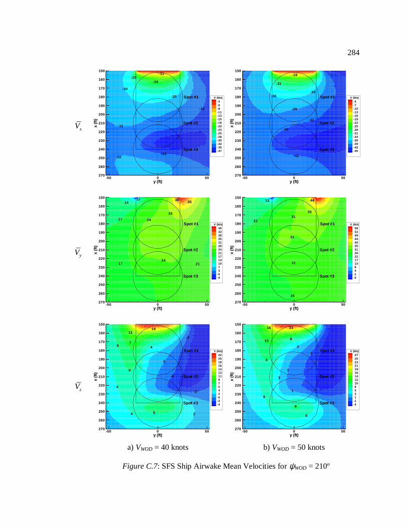
284
xV
-32-35
-32
-30
-25-20
-11
-30
-35
y (ft)
x(ft
)
-50 0 50
150
160
170
180
190
200
210
220
230
240
250
260
270
-3-6-8-11-13-15-18-20-23-25-28-30-32-35-37
V (kts)
Spot #3
Spot #1
Spot #2
-39
-36-36
-31
-16
-42
-42
-42
y (ft)
x(ft
)
-50 0 50
150
160
170
180
190
200
210
220
230
240
250
260
270
-4-7-10-13-16-19-22-25-28-31-34-36-39-42-45
V (kts)
Spot #3
Spot #1
Spot #2
yV
17
14
28
24
24
353810
17 21
y (ft)
x(ft
)
-50 0 50
150
160
170
180
190
200
210
220
230
240
250
260
270
454238353128242117141073
-0-4
V (kts)
Spot #3
Spot #1
Spot #2
13 44
3531
31
22
31
26
y (ft)
x(ft
)
-50 0 50
150
160
170
180
190
200
210
220
230
240
250
260
270
585349444035312622171384
-1-5
V (kts)
Spot #3
Spot #1
Spot #2
zV
5
4
5
1116
4
0
-2
-2
-2
2
5
4
7
y (ft)
x(ft
)
-50 0 50
150
160
170
180
190
200
210
220
230
240
250
260
270
2220181614131197542
-0-2-4
V (kts)
Spot #3
Spot #1
Spot #2
a) VWOD = 40 knots
16 23
8
3
-1
1
8
1
8
5
10
5
3
y (ft)
x(ft
)
-50 0 50
150
160
170
180
190
200
210
220
230
240
250
260
270
2725232119161412108531
-1-4
V (kts)
Spot #3
Spot #1
Spot #2
b) VWOD = 50 knots
Figure C.7: SFS Ship Airwake Mean Velocities forψWOD = 210º
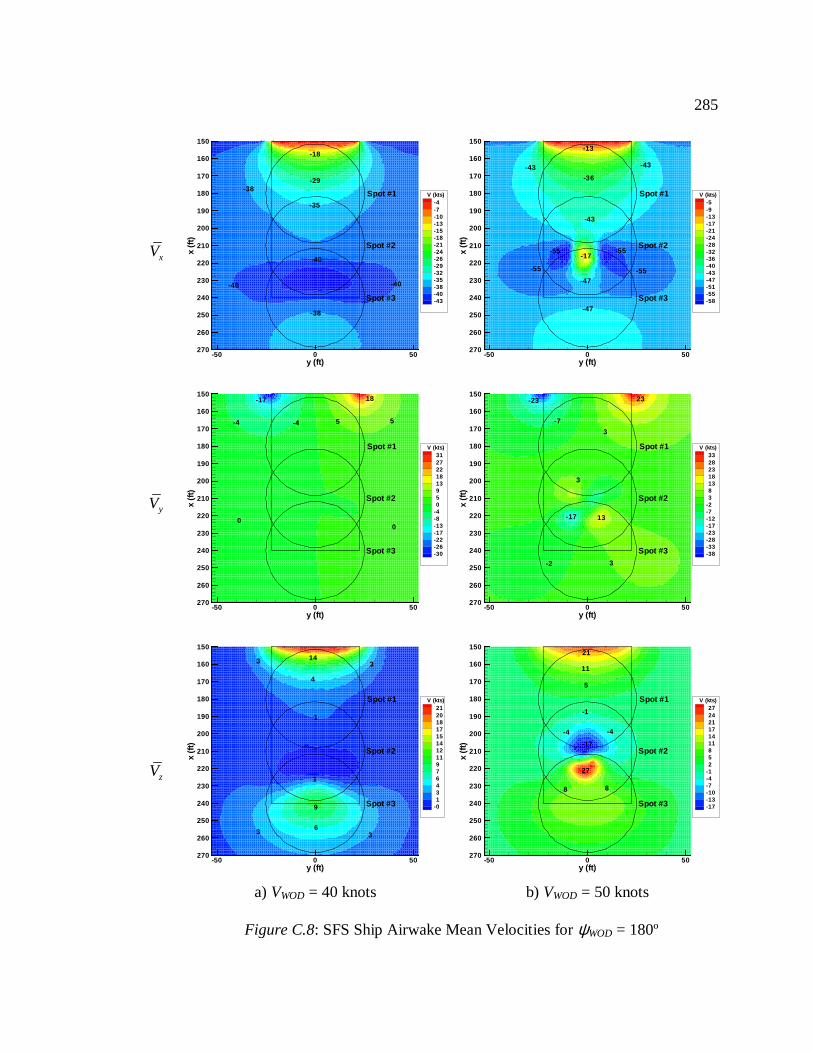
285
xV
-38
-40 -40
-38
-35
-29
-18
-40
y (ft)
x(ft
)
-50 0 50
150
160
170
180
190
200
210
220
230
240
250
260
270
-4-7-10-13-15-18-21-24-26-29-32-35-38-40-43
V (kts)
Spot #3
Spot #1
Spot #2
-13
-36
-43
-17-55 -55
-47
-47
-43 -43
-55 -55
y (ft)
x(ft
)
-50 0 50
150
160
170
180
190
200
210
220
230
240
250
260
270
-5-9-13-17-21-24-28-32-36-40-43-47-51-55-58
V (kts)
Spot #3
Spot #1
Spot #2
yV
-4 5
-17 18
-4 5
00
y (ft)
x(ft
)
-50 0 50
150
160
170
180
190
200
210
220
230
240
250
260
270
3127221813950
-4-8-13-17-22-26-30
V (kts)
Spot #3
Spot #1
Spot #2
-23 23
3
-7
3
-17 13
3-2
y (ft)
x(ft
)
-50 0 50
150
160
170
180
190
200
210
220
230
240
250
260
270
332823181383
-2-7-12-17-23-28-33-38
V (kts)
Spot #3
Spot #1
Spot #2
zV
9
63 3
1
1
4
1433
y (ft)
x(ft
)
-50 0 50
150
160
170
180
190
200
210
220
230
240
250
260
270
2120181715141211976431
-0
V (kts)
Spot #3
Spot #1
Spot #2
a) VWOD = 40 knots
-17
27
-1
11
5
21
88
-4-4
y (ft)
x(ft
)
-50 0 50
150
160
170
180
190
200
210
220
230
240
250
260
270
272421171411852
-1-4-7-10-13-17
V (kts)
Spot #3
Spot #1
Spot #2
b) VWOD = 50 knots
Figure C.8: SFS Ship Airwake Mean Velocities forψWOD = 180º
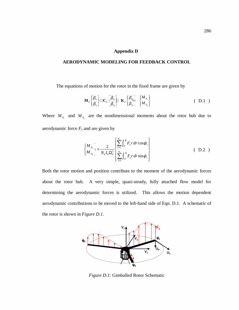
286
Appendix D
AERODYNAMIC MODELING FOR FEEDBACK CONTROL
The equations of motion for the rotor in the fixed frame are given by
11 1
11 1
x
y
Acc cS S S
Ass s
M
Mββ βββ β
+ + =
M C K
( D.1 )
WherexAM and
yAM are the nondimensional moments about the rotor hub due to
aerodynamic forceFz and are given by
01
20
01
cos2
sin
b
x
by
NR
z iA i
NRA b b
z ii
F r drM
M N IF r dr
ψ
ψ
=
=
= Ω
( D.2 )
Both the rotor motion and position contribute to the moment of the aerodynamic forces
about the rotor hub. A very simple, quasi-steady, fully attached flow model for
determining the aerodynamic forces is utilized. This allows the motion dependent
aerodynamic contributions to be moved to the left-hand side of Eqn. D.1. A schematic of
the rotor is shown inFigure D.1.
ψψψψ1ψψψψ2
ψψψψ3
Fz
Vx
Vy
Vz
UT
UP
Figure D.1: Gimballed Rotor Schematic
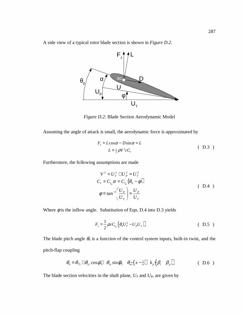
287
A side view of a typical rotor blade section is shown inFigure D.2.
Assuming the angle of attack is small, the aerodynamic force is approximated by
212
cos sinz
l
F L D L
L V cC
α αρ
= − ≈
=( D.3 )
Furthermore, the following assumptions are made
( )
T
P
T
P
lll
TPT
U
U
U
Utan
CCC
UUUV
≈
=
−==≈+=
−1
0
2222
φ
φθααα
( D.4 )
Whereφ is the inflow angle. Substitution of Eqn. D.4 into D.3 yields
( )20
1
2z l T P TF cC U U Uα
ρ θ= − ( D.5 )
The blade pitch angle θ0 is a function of the control system inputs, built-in twist, and the
pitch-flap coupling
( ) ( )30 75 1 1 4cos sinc i s i tw p i px kθ θ θ ψ θ ψ θ β β= + + + − − − ( D.6 )
The blade section velocities in the shaft plane,UT andUP, are given by
φ
θ0α
UT
UP
U
ac
FzL
D
Figure D.2: Blade Section Aerodynamic Model
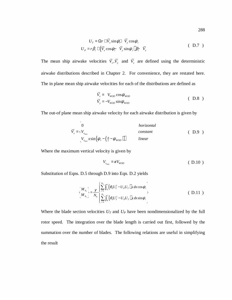
288
( )sin cos
cos sin
T x i y i
P i x i y i i z
U r V V
U r V V V
ψ ψ
β ψ ψ β
= Ω + +
= + − −
( D.7 )
The mean ship airwake velocities ,x yV V and zV are defined using the deterministic
airwake distributions described in Chapter 2. For convenience, they are restated here.
The in plane mean ship airwake velocities for each of the distributions are defined as
cos
sin
x WOD WOD
y WOD WOD
V V
V V
ψψ
=
= −( D.8 )
The out-of plane mean ship airwake velocity for each airwake distribution is given by
( )( )2
0
sinmax
max
z z
z i WOD
horizontal
V V constant
V x linearπψ ψ
= − −
( D.9 )
Where the maximum vertical velocity is given by
maxz WODV Vκ= ( D.10 )
Substitution of Eqns. D.5 through D.9 into Eqn. D.2 yields
( )
( )
1 200
1
1 200
1
cos
sin
b
x
by
N
T P T iA i
NA b
T P T ii
U U U x dxM
M NU U U x dx
θ ψγ
θ ψ
=
=
− =
−
( D.11 )
Where the blade section velocitiesUT andUP have been nondimensionalized by the full
rotor speed. The integration over the blade length is carried out first, followed by the
summation over the number of blades. The following relations are useful in simplifying
the result
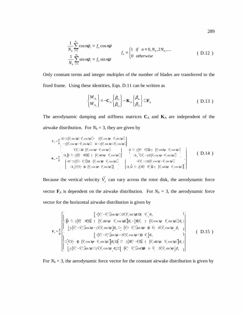
289
1
1
1cos cos
1 0, ,2 ,
01sin sin
b
b
N
i nib b b
nN
i nib
n f nN if n N N
fotherwise
n f nN
ψ ψ
ψ ψ
=
=
==
= =
( D.12 )
Only constant terms and integer multiples of the number of blades are transferred to the
fixed frame. Using these identities, Eqn. D.11 can be written as
11
11
x
y
A ccA A A
A ss
M
M
ββββ
= − − +
C K F
( D.13 )
The aerodynamic damping and stiffness matricesCA and K A are independent of the
airwake distribution. ForNb = 3, they are given by
( ) ( )( ) ( )
( )( ) ( )
( ) ( )
2 23 3
2 23 3
2 2 24 1 43 2 3
2 2 21 42 3
sin 3 cos 3 cos 3 sin 3
8 cos 3 sin3 sin 3 cos3
cos 3 sin3 sin3 cos3
3 sin 3 cos 3
8
x y x y
A
x y x y
x y x y x y x y
p x y x y p x
A
V V V V
V V V V
V V V V V V V V
k V V V V k V
ψ ψ ψ ψγψ ψ ψ ψ
ψ ψ ψ ψ
ψ ψγ
Ω + + − − = − − Ω − +
+ Ω − Ω + − + Ω +
+ Ω + + + Ω + + =
C
K( )
( ) ( )( )
( )( ) ( )
43
2 2 2 41 432 3
2 2 21 442 33
cos 3 sin3
cos3 sin 3sin3 cos3
3 sin 3 cos 3cos 3 sin3
y x y
x y x yx y x y
p x y x yp x y x y
V V V
V V V VV V V V
k V V V Vk V V V V
ψ ψ
ψ ψψ ψ
ψ ψψ ψ
− Ω −
− − Ω −−Ω + − + Ω +
+ Ω + + − Ω ++ − Ω −
( D.14 )
Because the vertical velocityzV can vary across the rotor disk, the aerodynamic force
vectorFA is dependent on the airwake distribution. ForNb = 3, the aerodynamic force
vector for the horizontal airwake distribution is given by
( )( ) ( ) ( )
( ) ( )
2 2 8753
2 2 21 4 41 12 3 3
2 2 2 21 1 412 6 3
cos3 2 sin 3
3 sin 3 cos3 cos3 sin 3
cos3 sin 3 sin 3 2 cos3
8
x y x y y
x y x y c x y x y s
x y x y tw x y x x y p
A
V V V V V
V V V V V V V V
V V V V V V V V V
V
ψ ψ θ
ψ ψ θ ψ ψ θ
ψ ψ θ ψ ψ βγ
− − + + Ω + Ω + + + Ω + + − Ω −
− − + − − − Ω − =−
F( )
( ) ( ) ( )( ) ( )
2 2 8753
2 2 24 1 41 13 2 3
2 2 2 21 1 412 6 3
sin 3 2 cos3
cos3 sin 3 3 sin 3 cos3
sin 3 cos3 cos3 2 sin 3
x y x y x
x y x y c x y x y s
x y x y tw x y y x y p
V V V V
V V V V V V V V
V V V V V V V V V
ψ ψ θ
ψ ψ θ ψ ψ θ
ψ ψ θ ψ ψ β
− − + Ω + − Ω − + Ω + + − Ω +
− + + + − + Ω −
( D.15 )
For Nb = 3, the aerodynamic force vector for the constant airwake distribution is given by
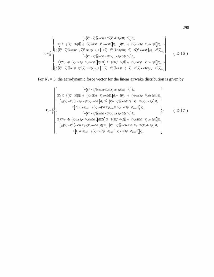
290
( )( ) ( ) ( )
( ) ( )
2 2 8753
2 2 21 4 41 12 3 3
2 2 2 21 1 412 6 3
cos3 2 sin 3
3 sin 3 cos3 cos3 sin 3
cos3 sin 3 sin 3 2 cos3 2
8
max
x y x y y
x y x y c x y x y s
x y x y tw x y x x y p y z
A
V V V V V
V V V V V V V V
V V V V V V V V V V V
ψ ψ θ
ψ ψ θ ψ ψ θ
ψ ψ θ ψ ψ βγ
− − + + Ω + Ω + + + Ω + + − Ω − − − + − − + Ω − + =F
( )( ) ( ) ( )
( ) ( )
2 2 8753
2 2 24 1 41 13 2 3
2 2 2 21 1 412 6 3
sin 3 2 cos3
cos3 sin 3 3 sin 3 cos3
sin 3 cos3 cos3 2 sin 3 2max
x y x y x
x y x y c x y x y s
x y x y tw x y y x y p x z
V V V V V
V V V V V V V V
V V V V V V V V V V V
ψ ψ θ
ψ ψ θ ψ ψ θ
ψ ψ θ ψ ψ β
− − − + Ω + − Ω − + Ω + + − Ω +
− + + + − + Ω − +
( D.16 )
For Nb = 3, the aerodynamic force vector for the linear airwake distribution is given by
( )( ) ( ) ( )
( ) ( )
2 2 8753
2 2 21 4 41 12 3 3
2 2 2 21 1 412 6 3
23
cos3 2 sin 3
3 sin 3 cos3 cos3 sin 3
cos3 sin 3 sin 3 2 cos3
cos s
8
x y x y y
x y x y c x y x y s
x y x y tw x y x x y p
WOD x
A
V V V V V
V V V V V V V V
V V V V V V V V V
V
ψ ψ θ
ψ ψ θ ψ ψ θ
ψ ψ θ ψ ψ β
ψγ
− − + + Ω
+ Ω + + + Ω + + − Ω −
− − + − − + Ω −
+ −Ω −=F
( ) ( )( )( )
( ) ( ) ( )( ) ( )
2 2 8753
2 2 24 1 41 13 2 3
2 2 2 21 112 6
in 3 cos 3
sin 3 2 cos3
cos3 sin 3 3 sin 3 cos3
sin 3 cos3
maxWOD y WOD z
x y x y x
x y x y c x y x y s
x y x y tw x y
V V
V V V V V
V V V V V V V V
V V V V V V
ψ ψ ψ ψ
ψ ψ θ
ψ ψ θ ψ ψ θ
ψ ψ θ
+ + +
− − − + Ω
+ − Ω − + Ω + + − Ω +
− + + + −
( ) ( )( )43
23
cos3 2 sin 3
sin cos 3 sin 3max
y x y p
WOD x WOD y WOD z
V V V
V V V
ψ ψ β
ψ ψ ψ ψ ψ
+ Ω − + Ω + + − +
( D.17 )
291
BIBLIOGRAPHY
1. Newman, S.J., An Investigation into the Phenomenon of Helicopter Blade Sailing,
Ph.D. Thesis, Department of Aeronautics and Astronautics, University of
Southampton, Highfield, Southampton, United Kingdom, Mar. 1995.
2. Porteous, T.C., “Commercial Chinook - First Year of Operation,”Proceedings of
the 26th Symposium of the Society of Experimental Test Pilots, Paper No. 5, Sept.
1982.
3. Anonymous, “107/H-46 Tunnel Strike Mishap History,” Boeing Vertol Company
Interoffice Memorandum #8-7930-0-366, Apr. 1983.
4. Trick, L.L., “H-46/CV Engage/Disengage DI Test,” NAVAIRTESTCEN Project
Test Plan, Naval Air Test Center, Patuxent River, MD, Aug. 1983.
5. Scheffler, W.W., “H-46 Tunnel Strike Mishap Data,” Naval Air Safety Center
Report #3750, Apr. 1994.
6. Naval Air Test Center Report, “H-46 Dynamic Interface Tests aboard the USS
Missouri (BB-63),” Dept. of the Navy, Naval Air Test Center, Patuxent River,
MD, Sept. 1988.
292
7. Narveson, M. L., Flow Modification Over a Backward Facing Step, M.S. Thesis,
Department of Aeronautical Engineering, Naval Postgraduate School, Monterey,
CA, Sept. 1990
8. Healey, J.V., “Establishing a Database for Flight in the Wake of Structures,”
Journal of Aircraft, Vol. 29, No. 4, July-Aug. 1992, pp. 559-564.
9. Naval Warfare Publication (NWP-42), “Shipboard Helicopter Operating
Procedures,” Dept. of the Navy, Washington, D.C., Dec. 1988.
10. White, B.T. and White, W.R., “H-46 Dynamic Interface Tests Aboard the USS
Cimarron (AO-177),” NAVAIRTESTCEN Report RW-52R-81, Naval Air Test
Center, Patuxent River, MD, Jul. 1981.
11. Heinle, D., O'Connor, J., VanderVliet, G., Steinbach, R., “H-46/T-AO 187
Dynamic Interface Tests,” NAVAIRTESTCEN Report RW-85R-87, Naval Air
Test Center, Patuxent River, MD, Sept. 1988.
12. Martin, P.W., Trick, L.L. and Fowler, J.E., “H-46 Dynamic Interface Tests
Aboard USS Wabash (AOR-5),” NAVAIRTESTCEN Report RW-94R-84, Naval
Air Test Center, Patuxent River, MD, Jun. 1985.
13. Madey, S.L. and Whitmer, L.D., “SH-2F/SH-3F Interface Tests Aboard the USS
Ticonderoga (CG-47),” Naval Air Test Center Report RW-14R-83, Nov. 1984.
293
14. Hurley, G.E., Pittman, C.W. and Trick, L.L., “HH-46A/CV-64 Rotor
Engage/Disengage Test,” NAVAIRTESTCEN Report RW-55R-84, Naval Air
Test Center, Patuxent River, MD, Oct. 1984.
15. Traasdahl, E.C. and Ruffa, S.A., “CH-46E/LHA Engage/Disengage Dynamic
Interface Test,” NAVAIRTESTCEN Report RW-58R-84, Naval Air Test Center,
Patuxent River, MD, Jan. 1985.
16. Carico, G.D., Groulx, J.W. and Vetter, D.R., “H-46 Rotor Engage/Disengage
Evaluation Aboard the USS Guadalcanal (LPH-7),” NAVAIRTESTCEN Report
FT-49R-74, Naval Air Test Center, Patuxent River, MD, Jun. 1974.
17. Moseley, R.P. and Allison, W.A., “H-46, HH-1K, and UH-1N Dynamic Interface
Tests Aboard the USS New Orleans (LPH-11),” NAVAIRTESTCEN Report RW-
24R-81, Naval Air Test Center, Patuxent River, MD, Jul. 1981.
18. Ball, J.C. and White, W.R., “H-46 Dynamic Interface Tests aboard USS Guam
(LPH-9),” NAVAIRTESTCEN Report RW-28R-83, Naval Air Test Center,
Patuxent River, MD, Mar. 1984.
19. Williams, S.L. and Long, K.R., “Dynamic Interface Tests and the Pilot Rating
Scale,”Proceedings of the 53rd Annual Forum of the American Helicopter Society
(Virginia Beach, VA), American Helicopter Society, Reston, VA, Apr. 1997, pp.
438-449.
294
20. Healey, J.V., “The Prospects for Simulating the Helicopter/Ship Interface,”Naval
Engineers Journal, Mar. 1987, pp. 45-63.
21. Rhoades, M.M., A Study of the Airwake Aerodynamics Over the Flight Deck of
an AOR Model Ship, M.S. Thesis, Department of Aeronautical Engineering,
Naval Postgraduate School, Monterey, CA, Sept. 1990.
22. Wilkinson, C.H., Zan, S.J., Gilbert, N.E. and Funk, J.D., “Modelling and
Simulation of Ship Airwakes for Helicopter Operations - A Collaborative
Venture,” Proceedings of the 83rd Fluid Dynamics Panel Symposium on Fluid
Dynamics Problems of Vehicles Operating Near or in the Air-Sea Interface
(Amsterdam, The Netherlands), Oct. 1998, 9-1 to 9-12.
23. Willmer, M.A.P., “The Motion of Helicopter Blades at Low Rotor Speeds in High
Winds,” RAE TM No. Naval 181, Sept. 1963.
24. Burton, K.W., “Blade Sailing,” Westland Helicopters Dynamics Department
Report GEN/DYN/146N, Westland Helicopters Ltd., Mar. 1978.
25. King, S.P., “An Analytical Investigation of Blade Sailing,” Westland Helicopters
Dynamics Department Report GEN/DYN/214N, Westland Helicopters Ltd., Jan.
1981.
26. Leone, P.F., “Theoretical and Experimental Study of the Flap Droop Stop Impact
Transient Aero-Elastic Response of a Helicopter Rotor Blade,”Journal of the
American Helicopter Society, Vol. 9, Jan. 1964, pp. 32-37.
295
27. Leone, P.F., “Analytic Correlation with Mishap Report of a CH-46D Aft Rotor
Blade Tunnel Strike Induced by a Wind Flow Up Through the Aft Rotor Disk
During a Startup Operation While Shipboard at Sea,” Boeing Vertol Company
Interoffice Memo, 8-7450-PFL-06, Apr. 1982.
28. Moran, R.D. Jr., Simulation of a Rotorcraft in Turbulent Flows, M.S. Thesis,
Department of Aeronautical Engineering, Naval Postgraduate School, Monterey,
CA, Sept. 1991.
29. Nguyen, K.Q., “Dynamic Analysis of Rotor Blade Undergoing Power Shutdown,”
NASA TM-102865, Dec. 1990.
30. Kunz, D.L., “Influence of Elastomeric Damper Modeling on the Dynamic
Response of Helicopter Rotors,”AIAA Journal, Vol. 35, No., 2, Feb. 1997, pp.
349-354.
31. Hurst, D.W. and Newman, S.J., “Wind Tunnel Measurements of Ship Induced
Turbulence and the Prediction of Helicopter Rotor Blade Response,”Proceedings
of the 11th European Rotorcraft Forum(London, England), Paper No. 99, Sept.
1985.
32. Hurst, D.W. and Newman, S.J., “Wind Tunnel Measurements of Ship Induced
Turbulence and the Prediction of Helicopter Rotor Blade Response,”Vertica, Vol.
12, No. 3, 1988, pp. 267-278.
296
33. Newman, S.J., “A Theoretical Model for Predicting the Blade Sailing Behaviour
of a Semi-Rigid Rotor Helicopter,”Vertica, Vol. 14, No. 4, 1990, pp. 531-544.
34. Newman, S.J., “The Application of a Theoretical Blade Sailing Model to Predict
the Behaviour of Articulated Helicopter Rotors,”The Aeronautical Journal of the
Royal Aeronautical Society, June/July 1992, pp. 233-239.
35. Newman, S., “An Investigation into the Phenomenon of Helicopter Blade
Sailing,” Proceedings of the Royal Aeronautical Society Conference on
Aerospace Vehicle Dynamics and Control(Cranfield Institute of Technology),
The Institute of Mathematics and its Applications on Aerospace Vehicle
Dynamics and Control, Sept. 1992, pp. 225-245.
36. Newman, S.J., “The Problems of Rotor Engagement and Disengagement of a
Shipborne Helicopter,”Journal of Naval Science, Vol. 20, No. 1, 1994, pp. 56-64.
37. Newman, S.J., “A Theoretical and Experimental Investigation Into the Rotor
Blade Aeroelastic Behaviour of a Shipborne Helicopter Rotor During Rotor
Engagement and Braking,”Proceedings of the AGARD FDP Symposium on
Aerodynamics of Rotorcraft(Berlin, Germany), Oct. 1994, pp. 32-1 to 32-10.
38. Newman, S.J., “The Verification of a Theoretical Helicopter Rotor Blade Sailing
Method by Means of Windtunnel Testing,”The Aeronautical Journal of the Royal
Aeronautical Society, Feb. 1995, pp. 41-50.
297
39. Newman, S.J. and Walker, W.R., “The Influence of Blade Flexibility on the
Sailing Behaviour of Helicopter Rotors,”Journal of Defense Science, Vol. 1, No.
4, 1996, pp. 498-507.
40. Newman, S.J., “The Phenomenon of Helicopter Rotor Blade Sailing,”
Proceedings of the Institution of Mechanical Engineers, Part G, Vol. 213, 1999,
pp. 347-363.
41. Geyer, W.P., Aeroelastic Analysis of Transient Blade Dynamics during Shipboard
Engage/Disengage Operations, M.S. Thesis, Department of Aerospace
Engineering, The Pennsylvania State University, University Park, PA, Aug. 1995.
42. Geyer, W.P. and Smith, E.C., “Aeroelastic Analysis of Transient Blade Dynamics
during Shipboard Engage/Disengage Operations,”Proceedings of the 2nd
International AHS Aeromechanics Specialists’ Meeting(Fairfield County, CT),
American Helicopter Society, Alexandria, VA, Oct. 1995, pp. 8-91 - 8-114.
43. Bir, G. and Chopra, I., University of Maryland Advanced Rotorcraft Code
(UMARC) Theory Manual, UM-AERO 94-18, University of Maryland, College
Park, MD, July 1994.
44. Johnson, W., Helicopter Theory, Dover Publications, Inc., New York, New York,
1994.
45. Leishman, J.G., Unsteady Aerodynamic Theory Manual for the Technology
Complex (TC) Airloads and Induced Velocity (ALIV) CPCI of the Second
298
Generation Comprehensive Helicopter Analysis (2GCHAS), UM-AERO90-30,
University of Maryland, College Park, MD, Jul. 1990.
46. Geyer, W.P., Smith, E.C. and Keller, J., “Validation and Application of a
Transient Aeroelastic Analysis for Shipboard Engage/Disengage Operations,”
Proceedings of the 52nd Annual National Forum of the American Helicopter
Society(Washington, D.C.), American Helicopter Society, Alexandria, VA, Jun.
1996, pp. 152-167.
47. Geyer, W.P., Smith, E.C. and Keller, J.A., “Aeroelastic Analysis of Transient
Blade Dynamics during Shipboard Engage/Disengage Operations,”Journal of
Aircraft, Vol. 35, No. 3, May-June 1998, pp. 445-453.
48. Keller, J.A., Smith, E.C. and Knarr, C.R., “Experimental/Theoretical Correlation
of Analysis for Helicopter Rotor Blade/Droop Stop Impacts,”Proceedings of the
38th AIAA/ASME/ASCE/AHS/ASC Structures, Structural Dynamics and Materials
Conference (Kissimmee, FL), American Institute of Aeronautics and
Astronautics, Inc., Reston, VA, Apr. 1997, pp. 345-357.
49. Keller, J.A., An Experimental and Theoretical Correlation of an Analysis for
Helicopter Rotor Blade and Droop Stop Impacts, M.S. Thesis, Department of
Aerospace Engineering, The Pennsylvania State University, University Park, PA,
Dec. 1997.
299
50. Keller, J.A. and Smith, E.C., “An Experimental and Theoretical Correlation of
Helicopter Rotor Blade-Droop Stop Impacts,”Journal of Aircraft,Vol. 36, No. 2,
Mar.-Apr. 1999, pp. 443-450.
51. Kang, H. and Smith, E.C., “Transient Response Analysis of Gimballed Tiltrotors
During Engage and Disengage Operations,”Proceedings of the 39th
AIAA/ASME/ASCE/AHS/ASC Structures, Structural Dynamics and Materials
Conference (Long Beach, CA), American Institute of Aeronautics and
Astronautics, Inc., Reston, VA, Apr. 1998.
52. Smith, E.C., Keller, J.A. and Kang, H., “Recent Developments in the Analytical
Investigation of Shipboard Rotorcraft Engage and Disegage Operations,”
Proceedings of the 83rd Fluid Dynamics Panel Symposium on Fluid Dynamics
Problems of Vehicles Operating Near or in the Air-Sea Interface(Amsterdam,
The Netherlands), Oct. 1998.
53. Bottasso, C.L. and Bauchau, O.A., "Mutibody Modeling of Engage and
Disengage Operations of Helicopter Rotors,"Proceedings of the American
Helicopter Society Aeromechanics Specialists Meeting(Atlanta, GA), American
Helicopter Society, Alexandria, VA, Nov. 2000.
54. Hunt, J.C.R., Abell, C.J., Peterka, J.A. and Woo, H., “Kinematic Studies of the
Flows Around Free or Surface Mounted Obstacles; Applying Topology to Flow
Visualization,”Journal of Fluid Mechanics, Vol. 86, 1978, pp. 179-200.
300
55. Frost, W., “Review of Data and Prediction Techniques for Wind Profiles Around
Manmade Surface Obstructions,”AGARD Conference Proceedings #140 on
Flight In Turbulence(Bedfordshire, England), 1973, pp. 4-1 to 4-18.
56. Cermak, J., “Aerodynamics of Buildings,”Annual Review of Fluid Mechanics,
Vol. 8, 1976, pp. 75-106.
57. Beranek, W.J., “General Rules for Determination of Wind Environment,”
Proceedings of the 5th International Conference on Wind Engineering(Fort
Collins, Colorado), Jul. 1979, pp. 225-234.
58. Castro, I.P. and Dianat, M., “Surface Flow Patterns on Rectangular Bodies in
Thick Boundary Layers,” Journal of Wind Engineering and Industrial
Aerodynamics, Vol. 11, 1983, pp. 107-119.
59. Daley, W.H., Flow Visualization of the Airwake Around a Model of a TARAWA
Class LHA in a Simulated Atmospheric Boundary Layer, M.S. Thesis,
Department of Aeronautical Engineering, Naval Postgraduate School, Monterey,
CA, Jun. 1988.
60. Johns, M. K., Flow Visualization of the Airwake Around a Model of a DD-963
Class Destroyer in a Simulated Atmospheric Boundary Layer, M.S. Thesis,
Department of Aeronautical Engineering, Naval Postgraduate School, Monterey,
CA, Sept. 1988.
301
61. Johns, M.K. and Healey, J.V., “The Airwake of a DD-963 Class Destroyer,”
Naval Engineer's Journal, Vol. 101, No. 3, 1989, pp. 36-42.
62. Rhoades, M.M. and Healey, J.V., “Flight Deck Aerodynamics of a Nonaviation
Ship,” Journal of Aircraft, Vol. 29, No. 4, Jul.-Aug. 1992, pp. 619-626.
63. Tai, T.C. and Carico, D., “Simulation of DD-963 Ship Airwake by Navier-Stokes
Method,” AIAA 24th Fluid Dynamics Conference(Orlando, FL), American
Institute of Aeronautics and Astronautics, Reston, VA, Jul. 1993.
64. Tai, T.C. and Carico, D., “Simulation of DD-963 Ship Airwake by Navier-Stokes
Method,”Journal of Aircraft, Vol. 32, No. 6, Nov.-Dec. 1995, pp. 1399-1401.
65. Tai, T.C., “Simulation of LPD Ship Airwake by Navier-Stokes Method,”
Proceedings of the 6th Asian Congress of Fluid Mechanics(Singapore), May
1995.
66. Tai, T.C., “Simulation and Analysis of LHD Ship Airwake by Navier-Stokes
Method,” Proceedings of the 83rd Fluid Dynamics Panel Symposium on Fluid
Dynamics Problems of Vehicles Operating Near or in the Air-Sea Interface
(Amsterdam, The Netherlands), Oct. 1998.
67. Landsberg, A.M., Young, T.R. and Boris, J.P., “An Efficient, Parallel Method for
Solving Flows in Complex Three-Dimensional Geometries,”32nd Aerospace
Sciences Meeting & Exhibit(Reno, NV), American Institute of Aerodynamics and
Astronautics, Reston, VA, Jan. 1994.
302
68. Tattersall, P., Albone, C.M., Soliman, M.M. and Allen, C.B., “Prediction of Ship
Airwake Over Flight Decks Using CFD,”Proceedings of the 83rd Fluid Dynamics
Panel Symposium on Fluid Dynamics Problems of Vehicles Operating Near or in
the Air-Sea Interface(Amsterdam, The Netherlands), Oct. 1998, 6-1 to 6-11.
69. Zan, S.J. and Garry, E.A., “Wind Tunnel Measurements of the Airwake Behind a
Model of a Generic Frigate,” NRC-CNRC Report LTR-AA-13, Jun. 1994.
70. Zan, S.J., Syms, G.F. and Cheney, B.T., “Analysis of Patrol Frigate Airwakes,”
Proceedings of the 83rd Fluid Dynamics Panel Symposium on Fluid Dynamics
Problems of Vehicles Operating Near or in the Air-Sea Interface(Amsterdam,
The Netherlands), Oct. 1998, 8-1 to 8-14.
71. Cheney, B.T. and Zan, S.J., “CFD Code Validation Data and Flow Topology for
The Technical Co-operation Program AER-TP2 Simple Frigate Shape,” NRC-
CNRC Report LTR-A-035, National Research Council Canada - Institute for
Aerospace Research, Apr. 1999.
72. Reddy, K.R., Toffoletto, R. and Jones, K.R.W., “Numerical Simulation of Ship
Airwake,” Computers & Fluids, Vol. 29, No. 4, May 2000, pp. 451-465.
73. Morris, P.J., Long, L.N., Bangalore, A. and Wang, Q., “A Parallel Three-
Dimensional Computational Aeroacoustics Method Using Non-Linear
Disturbance Equations,”Journal of Computational Physics, 1997.
303
74. Liu, J. and Long, L.N., “Higher Order Accurate Ship Airwake Predictions for the
Helicopter/Ship Interface Problem,”AHS 54th Annual National Forum
(Washington, D.C.), American Helicopter Society, Inc., Alexandria, VA, May
1998.
75. Liu, J., Long, L.N. and Modi, A., “Higher Order Accurate Solutions of Ship
Airwake Flow Fields Using Parallel Computer,”Proceedings of the 83rd Fluid
Dynamics Panel Symposium on Fluid Dynamics Problems of Vehicles Operating
Near or in the Air-Sea Interface(Amsterdam, The Netherlands), Oct. 1998.
76. Modi, A., Unsteady Separated Flow Simulations Using a Cluster of Workstations,
M.S. Thesis, Department of Aerospace Engineering, The Pennsylvania State
University, University Park, PA, May 1999.
77. Modi, A. and Long, L.N., “Unsteady Separated Flow Simulations Using a Cluster
of Workstations,”AIAA 38th Aerospace Sciences Meeting & Exhibit(Reno, NV),
American Institute of Aeronautics and Astronautics, Reston, VA, Jan. 2000.
78. Bruner, C.W.S., Parallelization of the Euler Equations on Unstructured Grids,
Ph.D. Dissertation, Department of Aerospace Engineering, Virginia Polytechnic
Institute and State University, May 1996.
79. Bruner, C.W.S. and Walters, R.W., “Parallelization of the Euler Equations on
Unstructured Grids,” AIAA Paper 97-1894, Jan. 1997.

304
80. Tennekes, H. and Lumley, J.L., A First Course in Turbulence, The MIT Press,
Cambridge, Massachusetts, 1972.
81. Press, W.H., Flannery, B.P., Teukolsky, S.A. and Vetterling, W.T., Numerical
Recipes – The Art of Scientific Computing, Cambridge University Press, 1986.
82. Prouty, R.W., Helicopter Performance, Stability, and Control, Robert E. Krieger
Publishing Co., Malabar, Florida, 1990.
83. Critzos, C.C., Heyson, H.H. and Boswinkle, R.W., “Aerodynamic Characteristics
of NACA 0012 Airfoil Section at Angles of Attack from 0° to 180°,” NACA TN-
3361, National Advisory Committee for Aeronautics, Langley Aeronautical
Laboratory, Jan. 1955.
84. Leishman, J.G. and Beddoes, T.S., “A Semi-Empirical Model for Dynamic Stall,”
Journal of the American Helicopter Society, Vol. 34, No. 3, Jul. 1989, pp. 3-17.
85. Brasseur, G.W., “A Preliminary Investigation to Study the Effect of Flat Spoilers
on the Aerodynamic Characteristics of Wings at Angles of Attack from 0° to
90°,” Report DTMB-2214, David Taylor Model Basin, Washington D.C., Apr.
1966.
86. Kreyszig, E., Advanced Engineering Mathematics, 6th Edition, John Wiley &
Sons, Inc., New York, New York, 1988.
305
87. Newmark, N.M., “A Method of Computation for Structural Dynamics,”Journal
of the Engineering Mechanics Division, Vol. 85, No. 3, Jul. 1959, pp. 67-94.
88. Rao, S.S., Mechanical Vibrations, 3rd Edition, Addison-Wesley, Reading MA,
1995.
89. Bauchau, O.A. and Joo, T., “Computational Schemes for Nonlinear Elasto-
Dynamics,” Proceedings of the 41st AIAA/ASME/ASCE/AHS/ASC Structures,
Structural Dynamics, and Materials Conference(Atlanta, GA), American
Institute of Aeronautics and Astronautics, Reston, VA, Apr. 2000, pp. 1-11.
90. Wood, W.L., Bossak, M. and Zienkiewicz, O.C., “An Alpha Modification of
Newmark’s Method,” International Journal for Numerical Methods in
Engineering, Vol. 15, 1981, pp. 1562-1566.
91. Gardner, B., “Theoretical Physical Properties of the A02R1702 Composite Rotor
Blade,” Boeing Report Number A02-SS-027-1, Boeing Vertol Company, March
1977.
92. Keller, J.A. and Smith, E.C., “Analysis and Control of the Transient Shipboard
Engagement Behavior of Rotor Systems,”Proceedings of the 55th Annual
National Forum of the American Helicopter Society(Montreal, Quebec),
American Helicopter Society, Alexandria, VA, May 1999, pp. 1064-1078.
93. Lemont, H.E., “Rotor Blade Flapping Control Mechanism,” Patent No. 2,946,391,
U.S. Patent Office, Washington, D.C., 1960.
306
94. Keller, J.A. and Smith, E.C., “Control of the Transient Aeroelastic Response of
Rotors During Shipboard Engagement Operations,”Proceedings of the American
Helicopter Society Aeromechanics Specialists Meeting(Atlanta, GA), American
Helicopter Society, Alexandria, VA, Nov. 2000.
95. Keller, J.A. and Smith, E.C., “Control of the Transient Response of Gimballed
Rotors During Shipboard Engagement Operations,”Proceedings of the American
Helicopter Society NE Region Active Controls Technology Conference
(Bridgeport, CT), American Helicopter Society, Alexandria, VA, Oct. 2000.
96. Lewis, F.L. and Syrmos, V.L., Optimal Control, 2nd Edition, John Wiley & Sons,
Inc., New York, NY, 1995.

VITA
Jonathan Allen Keller
Education:
B.S. in Aerospace Engineering, May 1995, The Pennsylvania State University
M.S. in Aerospace Engineering, December 1997, The Pennsylvania State University
Work Experience:
NASA Langley Research Center, LARSS Program Student, June 1998 - August 1998
Lockheed Martin Astro Space, Co-Op Student, January 1993 - August 1993
Student Member AIAA, AHS
Selected Publications:
Keller, J.A. and Smith, E.C., “Control of the Transient Aeroelastic Response of RotorsDuring Shipboard Engagement Operations,”Proceedings of the American HelicopterSociety Aeromechanics Specialists Meeting(Atlanta, GA), American Helicopter Society,Alexandria, VA, Nov. 2000.
Keller, J.A. and Smith, E.C., “Control of the Transient Response of Gimballed RotorsDuring Shipboard Engagement Operations,”Proceedings of the American HelicopterSociety NE Region Active Controls Technology Conference(Bridgeport, CT), AmericanHelicopter Society, Alexandria, VA, Oct. 2000.
Keller, J.A. and Smith, E.C., "Analysis and Control of the Transient ShipboardEngagement Behavior of Rotor Systems,"AHS 55th Annual Forum Proceedings(Montreal, Canada), May 1999, pp. 1064-1078.
Keller, J.A. and Smith, E.C., "An Experimental and Theoretical Correlation of HelicopterRotor Blade-Droop Stop Impacts,"Journal of Aircraft, Vol. 36, No. 2, Mar.-Apr. 1999,pp. 443-450.
Geyer, W.P., Smith, E.C. and Keller, J.A., "Aeroelastic Analysis of Transient BladeDynamics during Shipboard Engage/Disengage Operations,"Journal of Aircraft, Vol. 35,No. 3, May-June 1998, pp. 445-453.