UC DavisElectrical & Computer Engineering

TitleHigh-Performance Linear Algebra-based Graph Framework on the GPU

Permalinkhttps://escholarship.org/uc/item/37j8j27d

AuthorYang, Carl Y

Publication Date2019-05-31 Peer reviewed

eScholarship.org Powered by the California Digital LibraryUniversity of California

High-Performance Linear Algebra-based Graph Framework on the GPU

By

CARL YUE YANG

DISSERTATION

Submitted in partial satisfaction of the requirements for the degree of

DOCTOR OF PHILOSOPHY

in

Electrical and Computer Engineering

in the

OFFICE OF GRADUATE STUDIES

of the

UNIVERSITY OF CALIFORNIA, DAVIS

Approved:

Professor John D. Owens, Co-chair

Professor Aydın Buluc, Co-chair

Professor Chen-Nee Chuah

Committee in Charge

June 2019

Copyright © 2019 byCarl Yue Yang

All rights reserved.

ABSTRACT

High-Performance Linear Algebra-based Graph Framework on the GPU

By

Carl Yue Yang

Doctor of Philosophy in Electrical and Computer Engineering

University of California, Davis

Professor John D. Owens, Co-chairProfessor Aydın Buluc, Co-chair

High-performance implementations of graph algorithms are challenging to implement on newparallel hardware such as GPUs, because of three challenges: (1) difficulty of coming up withgraph building blocks, (2) load imbalance on parallel hardware, and (3) graph problems hav-ing low arithmetic ratio. To address these challenges, GraphBLAS is an innovative, on-goingeffort by the graph analytics community to propose building blocks based in sparse linear alge-bra, which will allow graph algorithms to be expressed in a performant, succinct, composableand portable manner. Initial research efforts in implementing GraphBLAS on GPUs has beenpromising, but performance still trails by an order of magnitude compared to state-of-the-artgraph frameworks using the traditional graph-centric approach of describing operations on ver-tices or edges.

This dissertation examines the performance challenges of a linear algebra-based approachto building graph frameworks and describes new design principles for overcoming these bottle-necks. Among the new design principles is making exploiting input sparsity a first-class citizenin the framework. This is an especially important optimization, because it allows users to writegraph algorithms without specifying certain implementation details thus permitting the softwarebackend to choose the optimal implementation based on the input sparsity. Exploiting outputsparsity allows users to tell the backend which values of the output in a single vectorized com-putation they do not want computed. We examine when it is profitable to exploit this outputsparsity to reduce computational complexity. Load-balancing is an important feature for bal-ancing work amongst parallel workers. We describe the important load-balancing features forhandling graphs with different characteristics.

The design principles described in the thesis have been implemented in GraphBLAST, anopen-source high-performance graph framework on GPU developed as part of this dissertation.It is notable for being the first graph framework based in linear algebra to get comparable orfaster performance compared to the traditional, vertex-centric backends. The benefits of designprinciples described in this thesis have been shown to be important for single GPU, and itwill grow in importance when it serves as a building block for distributed implementation inthe future and as a single GPU backend for higher-level languages such as Python. A graphframework based in linear algebra not only improves performance of existing graph algorithms,but in quickly prototyping new algorithms as well.

To my family

CONTENTS

List of Figures iv

List of Tables v

1 Introduction 11.1 Problem Statement . . . . . . . . . . . . . . . . . . . . . . . . . . . . . . . . 21.2 Thesis Organization . . . . . . . . . . . . . . . . . . . . . . . . . . . . . . . . 4

2 Background & Preliminaries 52.1 GPUs . . . . . . . . . . . . . . . . . . . . . . . . . . . . . . . . . . . . . . . 52.2 Sparse Matrix Formats . . . . . . . . . . . . . . . . . . . . . . . . . . . . . . 52.3 Breadth-first-search . . . . . . . . . . . . . . . . . . . . . . . . . . . . . . . . 62.4 Direction-optimized Breadth-first-search . . . . . . . . . . . . . . . . . . . . . 72.5 Notation . . . . . . . . . . . . . . . . . . . . . . . . . . . . . . . . . . . . . . 92.6 Traversal is Matrix-vector Multiplication . . . . . . . . . . . . . . . . . . . . . 9

3 Related Work 113.1 Literature survey . . . . . . . . . . . . . . . . . . . . . . . . . . . . . . . . . 113.2 Previous systems . . . . . . . . . . . . . . . . . . . . . . . . . . . . . . . . . 12

4 Fast Sparse Matrix and Sparse Vector Multiplication Algorithm on the GPU 144.1 Algorithms and Analysis . . . . . . . . . . . . . . . . . . . . . . . . . . . . . 144.2 Experiments and Results . . . . . . . . . . . . . . . . . . . . . . . . . . . . . 174.3 Conclusion . . . . . . . . . . . . . . . . . . . . . . . . . . . . . . . . . . . . 20

5 Implementing Push-Pull Efficiently in GraphBLAS 215.1 Types of Matvec . . . . . . . . . . . . . . . . . . . . . . . . . . . . . . . . . . 225.2 Relating Matvec and Push-Pull . . . . . . . . . . . . . . . . . . . . . . . . . . 265.3 Optimizations . . . . . . . . . . . . . . . . . . . . . . . . . . . . . . . . . . . 285.4 Implementation . . . . . . . . . . . . . . . . . . . . . . . . . . . . . . . . . . 325.5 Experimental Results . . . . . . . . . . . . . . . . . . . . . . . . . . . . . . . 365.6 Conclusion . . . . . . . . . . . . . . . . . . . . . . . . . . . . . . . . . . . . 39

6 Design Principles for Sparse Matrix Multiplication on the GPU 406.1 Design Principles . . . . . . . . . . . . . . . . . . . . . . . . . . . . . . . . . 406.2 Parallelizations of CSR SpMM . . . . . . . . . . . . . . . . . . . . . . . . . . 426.3 Experimental Results . . . . . . . . . . . . . . . . . . . . . . . . . . . . . . . 476.4 Conclusion . . . . . . . . . . . . . . . . . . . . . . . . . . . . . . . . . . . . 50

7 Design of GraphBLAST 517.1 GraphBLAS Concepts . . . . . . . . . . . . . . . . . . . . . . . . . . . . . . 527.2 Exploiting Input Sparsity (Direction-Optimization) . . . . . . . . . . . . . . . 607.3 Exploiting Output Sparsity (Masking) . . . . . . . . . . . . . . . . . . . . . . 66

-ii-

7.4 Load-balancing . . . . . . . . . . . . . . . . . . . . . . . . . . . . . . . . . . 677.5 Applications . . . . . . . . . . . . . . . . . . . . . . . . . . . . . . . . . . . . 717.6 Experimental Results . . . . . . . . . . . . . . . . . . . . . . . . . . . . . . . 74

8 Conclusion 798.1 Future Directions . . . . . . . . . . . . . . . . . . . . . . . . . . . . . . . . . 79

References 83

-iii-

LIST OF FIGURES

1.1 Mismatch in existing frameworks . . . . . . . . . . . . . . . . . . . . . . . . . 1

2.1 Matrix-graph duality . . . . . . . . . . . . . . . . . . . . . . . . . . . . . . . 10

4.1 Workload distribution of three SpMSpV implementations . . . . . . . . . . . . 194.2 Performance comparison of three SpMSpV implementations . . . . . . . . . . 19

5.1 SpMV vs. SpMSpV . . . . . . . . . . . . . . . . . . . . . . . . . . . . . . . . 255.2 BFS traversal in linear algebra . . . . . . . . . . . . . . . . . . . . . . . . . . 275.3 Direction-optimized BFS . . . . . . . . . . . . . . . . . . . . . . . . . . . . . 275.4 BFS traversal in detail . . . . . . . . . . . . . . . . . . . . . . . . . . . . . . . 295.5 SpMV vs. SpMSpV applied to BFS . . . . . . . . . . . . . . . . . . . . . . . 305.6 UML diagram of Vector interface . . . . . . . . . . . . . . . . . . . . . . . . . 365.7 BFS performance comparison . . . . . . . . . . . . . . . . . . . . . . . . . . 38

6.1 Aspect ratio vs. performance . . . . . . . . . . . . . . . . . . . . . . . . . . . 426.2 SpMV and SpMM load balance . . . . . . . . . . . . . . . . . . . . . . . . . 436.3 SpMM tiling scheme . . . . . . . . . . . . . . . . . . . . . . . . . . . . . . . 446.4 Aspect ratio vs. performance (this work) . . . . . . . . . . . . . . . . . . . . . 486.5 SpMM performance comparison (selected) . . . . . . . . . . . . . . . . . . . . 486.6 SpMM performance comparison (all) . . . . . . . . . . . . . . . . . . . . . . 49

7.1 Decomposition of key GraphBLAS operations . . . . . . . . . . . . . . . . . . 567.2 BFS running example . . . . . . . . . . . . . . . . . . . . . . . . . . . . . . . 577.3 Comparison of SpMV and SpMSpV. . . . . . . . . . . . . . . . . . . . . . . . 617.4 Where this work on direction-optimization fits in literature. . . . . . . . . . . . 637.5 Comparison with and without fused mask. . . . . . . . . . . . . . . . . . . . . 687.6 Graph algorithms using GraphBLAS . . . . . . . . . . . . . . . . . . . . . . . 717.7 Performance comparison for GraphBLAST. . . . . . . . . . . . . . . . . . . . 767.8 Hourglass design of GraphBLAST. . . . . . . . . . . . . . . . . . . . . . . . . 78

8.1 Scalability . . . . . . . . . . . . . . . . . . . . . . . . . . . . . . . . . . . . . 808.2 Direction-optimization . . . . . . . . . . . . . . . . . . . . . . . . . . . . . . 81

-iv-

LIST OF TABLES

4.1 BFS performance comparison . . . . . . . . . . . . . . . . . . . . . . . . . . 164.2 SpMSpV datasets . . . . . . . . . . . . . . . . . . . . . . . . . . . . . . . . . 184.3 Workload distribution of three SpMSpV implementations . . . . . . . . . . . . 194.4 Scalability of three SpMSpV implementations . . . . . . . . . . . . . . . . . . 20

5.1 Matrix-vector computational complexity . . . . . . . . . . . . . . . . . . . . . 245.2 BFS optimization summary . . . . . . . . . . . . . . . . . . . . . . . . . . . . 325.3 BFS datasets . . . . . . . . . . . . . . . . . . . . . . . . . . . . . . . . . . . . 37

6.1 ILP in SpMV and SpMM . . . . . . . . . . . . . . . . . . . . . . . . . . . . . 456.2 SpMM datasets . . . . . . . . . . . . . . . . . . . . . . . . . . . . . . . . . . 47

7.1 GraphBLAST matrix and vector methods . . . . . . . . . . . . . . . . . . . . 537.2 GraphBLAST operations . . . . . . . . . . . . . . . . . . . . . . . . . . . . . 547.3 GraphBLAST semirings and monoids . . . . . . . . . . . . . . . . . . . . . . 557.4 GraphBLAST descriptor settings . . . . . . . . . . . . . . . . . . . . . . . . . 567.5 Applicability of design principles. . . . . . . . . . . . . . . . . . . . . . . . . 607.6 Matrix-vector complexity and sparsity . . . . . . . . . . . . . . . . . . . . . . 627.7 Direction-optimization switching criteria . . . . . . . . . . . . . . . . . . . . . 657.8 GraphBLAST load-balancing . . . . . . . . . . . . . . . . . . . . . . . . . . . 697.9 GraphBLAST datasets . . . . . . . . . . . . . . . . . . . . . . . . . . . . . . 747.10 GraphBLAST performance comparison . . . . . . . . . . . . . . . . . . . . . 757.11 GraphBLAST lines of code . . . . . . . . . . . . . . . . . . . . . . . . . . . . 77

-v-

ACKNOWLEDGMENTS

Many people have contributed to making graduate career rewarding and enjoyable. First, I’dlike to thank my PhD advisors John D. Owens and Aydın Buluc. John taught me about GPUsand that the right way to do computer science research is not to be satisfied with getting a goodspeed-up, but being able to explain why a speed-up exists. Aydin taught me about sparse linearalgebra and pointed me to problems I was capable of solving. Chen-Nee Chuah, Zhaojun Baiand Venkatesh Akella formed the rest of my committee. Their insight and helpfulness improvedthe quality of this thesis.

I will be forever indebted to colleagues during my years at UC Davis. Yangzihao Wang,Yuechao Pan, Leyuan Wang, and Yuduo Wu have been great collaborators in the Gunrockproject. Yangzihao taught me a lot about graph processing and shared my excitement in discov-ering commonalities between the vertex-centric and linear algebra-based perspectives. Yuechaoprovided a deep understanding about optimizing algorithms on the GPU. Saman Ashkiani, Ja-son Mak, Afton Geil, Muhammad Osama, Shari Yuan, Weitang Liu, Vehbi Bayraktar, KerrySeitz, Collin Riffel, Andy Riffel, Shalini Venkataraman, Ahmed Mahmoud, Muhammad Awad,Yuxin Chen, Zhongyi Lin, and many others have also brightened up my life.

Thank you to all the people at the Department of Electrical and Computer Engineering at UCDavis, who helped me during my studies: Kyle Westbrook, Nancy Davis, Denise Christensen,Renee Kuehnau, Philip Young, Natalie Killeen, Fred Singh, Sacksith Ekkaphanh, and manymore. They kept the department running smoothly and were always there for me.

I am thankful of the generosity of ideas and willingness to help amongst the graph researchcommunity. Marcin Zalewski and Peter Zhang taught me much about writing beautiful code,especially when I was getting started. Scott McMillan continually teaches me new ways ofusing C++. Tim Mattson and Jose Moreira taught me much about how to design interfaces.

Finally, I am also grateful for my family’s support. It was with the help of Xinyan Xu that Iwas able to accomplish this. Her constant love and support make all this worthwhile.

-vi-

Chapter 1

Introduction

Graphs are a representation that naturally emerges when solving problems in domains includingbioinformatics [32], social network analysis [22], molecular synthesis [39], route planning [28].Problem sizes can be number in over a billion vertices, so parallelization has become a must.

The past two decades has seen the rise of parallel processors to a commodity product—bothgeneral-purpose processors in the form of graphic processor units (GPUs), as well as domain-specific processors such as tensor processor units (TPUs) and the graph processors developedunder the DARPA SDH (Software Defined Hardware) program. Research into developing par-allel hardware has succeeded in speeding up graph algorithms [61, 67]. However, the improve-ment in graph performance has come at the cost of a more challenging programming model.The result has been a mismatch between the high-level languages that users and graph algo-rithm designers would prefer to program in (e.g. Python) and the programming language forparallel hardware (e.g. C++, CUDA, OpenMP, MPI).

To address this mismatch, many initiatives including NVIDIA’s RAPIDS effort [59] havebeen launched in order to provide an open-source Python-based ecosystem for data science andgraphs on GPUs. One such initiative, GraphBLAS is an attractive open standard [18] that hasbeen released for graph frameworks. It promises standard building blocks for graph algorithmsin the language of linear algebra. This is exciting, because such a standard attempts to solve thefollowing problems:

Figure 1.1: Mismatch between existing frameworks targeting high-level languages and hard-ware accelerators

1

1.1 Problem StatementWhat is the right set of primitives for expressing graph algorithms? We will define the right setof primitives as one that fulfills the following goals:

1. Performance portability: Graph algorithm does not need modification to have high per-formance across hardware

2. Concise expression: Graph algorithms can be expressed in few lines of code

3. High-performance: Graph algorithms achieve state-of-the-art performance

4. Scalability: Framework is effective at small-scale and exascale

Firstly, the application code ought to require little to no change when targeting differentbackends. That is to say, the same application code ought to work just as well for single-threaded CPU as for GPU. Secondly, their application code ought to be concise. Thirdly, thegraph primitives ought to have high-performance meeting that of “hardwired” code written in alow-level language targeting a particular hardware. Finally, graph algorithms written using theframework should be effective across a wide range of problem scales.

Goal 1 (performance portability) is central to the GraphBLAS philosophy, and it has madeinroads in this regard with several implementations already being developed using this commoninterface [25, 53, 73]. Regarding Goal 2 (concise expression), GraphBLAS encourages usersto think in a vectorized manner, which yields an order-of-magnitude reduction in SLOC asevidenced by Table 7.11. Before Goal 4 (scalability) can be achieved, Goal 3 high-performanceon the small scale must first be demonstrated.

However, GraphBLAS has lacked high-performance implementations for GPUs. The Graph-BLAS Template Library [73] is a GraphBLAS-inspired GPU graph framework. The architec-ture of GBTL is C++ based and maintains a separation of concerns between a top-level interfacedefined by the GraphBLAS C API specification and the low-level backend. However, since itwas intended as a proof-of-concept in programming language research, it is an order of magni-tude slower than state-of-the-art graph frameworks on the GPU in terms of performance.

We identify several reasons graph frameworks are challenging to implement on the GPU:

Generalizability of optimization While many graph algorithms share similarities, the opti-mizations found in high-performance graph frameworks often seem ad hoc and difficultto reconcile with the goal of a clean and simple interface. What are the optimizationsmost deserving of attention when designing a high-performance graph framework on theGPU?

Load imbalance Graph problems have irregular memory access pattern that makes it hard toextract parallelism from the data. On parallel systems such as GPUs, this is further com-plicated by the challenge of balancing work amongst parallel compute units. How shouldthis problem of load-balancing be addressed?

2

Low compute-to-memory access ratio Graph problems emphasizes making multiple mem-ory accesses on the unstructured data instead of doing a lot of computations. Therefore,graph problems are often memory-bound rather than compute-bound. What can be doneto reduce the number of memory accesses?

In other words, we are interested in answering the following question: What are the de-sign principles required to build a GPU implementation based in linear algebra that matches thestate-of-the-art graph frameworks in performance? Towards that end, we have designed Graph-BLAST1: the first high-performance implementation of GraphBLAS for the GPU (graphicsprocessing unit). Our implementation is for single GPU, but given the similarity between theGraphBLAS interface we are adhering to and the CombBLAS interface [15], which is a graphframework for distributed CPU, we are confident the design we propose here will allow us toextend it to a distributed implementation with future work.

In order to perform a comprehensive evaluation of our system, we need to compare ourframework against the state-of-the-art graph frameworks on the CPU and GPU, and hard-wired GPU implementations, which are problem-specific GPU code that someone has hand-tuned for performance. The state-of-the-art graph frameworks we will be comparing againstare Ligra [61] for CPU and Gunrock [67] for the GPU, which we will describe in detail inSection 3.2. The hardwired implementations will be Enterprise (BFS) [47], delta-steppingSSSP [24], pull-based PR [43], and bitmap-based triangle counting [14]. The array of graphalgorithms we will be evaluating our system on are:

• Breadth-first-search (BFS)

• Single-source shortest-path (SSSP)

• PageRank (PR)

• Triangle counting (TC)

A description of these algorithms can be found in Section 7.5. We decided on these fourapplications, because based on a thorough literature survey by Beamer [9] they are consideredthe most common four applications across a variety of graph frameworks. Furthermore, theystress different facets of our framework. BFS and SSSP test how well we exploit input sparsity,PR tests sparse matrix-dense vector (SpMV) performance, and TC tests how well we exploitoutput sparsity.

Aside from these four algorithms, we have published elsewhere four algorithms built usingour framework: Graph Projections, Seeded Graph Matching and Local Graph Clustering areapplications built for the DARPA HIVE program [58], which is aimed at designing new graphprocessing hardware so our implementation on existing GPU hardware serves as a measure ofgoodness; Graph Coloring is a work where we compare our framework against Gunrock andhardwired implementations [57].

1https://github.com/gunrock/graphblast

3

1.2 Thesis OrganizationThe rest of the thesis will be organized as follows: Chapter 2 gives background information onmodern GPU architecture. Chapter 3 presents a survey of large-scale graph frameworks. Chap-ter 4 presents my work on exploiting input sparsity using column-based matrix multiplication todo breadth-first-search. Chapter 5 describes my work on exploiting output sparsity using row-based masked matrix multiplication and direction-optimized traversal to do breadth-first-search.Chapter 6 details my work on accelerating sparse matrix-dense matrix multiplication (SpMM).Chapter 7 leverages previous chapters to explain the design principles behind the architectureof GraphBLAST. Finally, Chapter 8 reviews future work that could be done in this area and theremaining research challenges to be solved.

4

Chapter 2

Background & Preliminaries

This section gives some background information on modern GPU architecture, sparse matrixformats, breadth-first-search, direction-optimized breadth-first-search, and introduces the dual-ity between graph traversal and sparse matrix-vector multiplication that forms a cornerstone toour work.

2.1 GPUsModern GPUs are throughput-oriented manycore processors that rely on large-scale multi-threading to attain high computational throughput and hide memory access time. The latestgeneration of NVIDIA GPUs have up to 80 streaming multiprocessors (SMs), each with up tohundreds of arithmetic logic units (ALUs). GPU programs are called kernels, which run a largenumber of threads in parallel in a single-program, multiple-data (SPMD) fashion.

The underlying hardware runs an instruction on each SM on each clock cycle on a warp of32 threads in lockstep. The largest parallel unit that can be synchronized within a GPU kernelis called a cooperative thread array (CTA), which is composed of warps. For problems thatrequire irregular data access, a successful GPU implementation needs to (1) ensure coalescedmemory access to external memory and efficiently use the memory hierarchy, (2) minimizethread divergence within a warp, and (3) maintain high occupancy, which is a measure of howmany threads are available to run on the implementation on the GPU.

CPUs use branch prediction, speculative fetching, and large caches to minimize latency. Bycontrast, GPUs are throughput-oriented processors, instead relying on thread-level parallelism(TLP) to hide stalls. This means that for running certain irregular computations such as SpMVand SpMM, the bottleneck can be how long a multiply instruction immediately following amemory access must wait. While traditional analyses such as the roofline model [68] focus oncompute-bound and memory-bound bottlenecks, we note GPU algorithms can also be latency-bound, which is when the GPU’s parallelism is insufficient to hide the instruction latency.

2.2 Sparse Matrix FormatsAnm×nmatrix is often called sparse if its number of nonzeroes nnz is small enough comparedto O(mn) such that it makes sense to take advantage of sparsity. The most straightforward

5

sparse matrix format is coordinate (COO) format. This format stores every nonzero as a triple(i, j,Aij). However, this format requires 3nnz memory for storage.

The compressed sparse row (CSR) format stores only the column indices and values ofnonzeroes within a row. The start and end of each row is then stored in terms of the columnindices and value in a row offsets (or row pointers) array. Hence, CSR only requires m+ 2nnzmemory for storage.

Similarly to sparse matrix-dense vector multiplication (SpMV), a desire to achieve goodperformance on SpMM has inspired innovation in matrix storage formatting [2, 56]. Thesecustom formats and encodings take advantage of the matrix structure and underlying machinearchitecture. Even only counting GPU processors, there exist more than sixty specialized SpMValgorithms and sparse matrix formats [31].

The vendor-shipped library cuSPARSE library provides two functions csrmm and csrmm2for SpMM on CSR-format input matrices [54]. The former expects a column-major input densematrix and generates column-major output, while the latter expects row-major input and gen-erates column-major output. Among many efforts to define and characterize alternate matrixformats for SpMM are a variant of ELLPACK called ELLPACK-R [56] and a variant of SlicedELLPACK called SELL-P [2]. However, there is a real cost to deviating from the standard CSRencoding. Firstly, the larger framework will need to convert from CSR to another format torun SpMM and convert back. This process may take longer than the SpMM operation itself.Secondly, the larger framework will need to reserve valuable memory to store multiple copiesof the same matrix—one in CSR format, another in the format used for SpMM.

Ortega explores doing SpMM on a specialized matrix storage format, which is a variant onELLPACK called ELLPACK-R [56]. Along with the usual two vectors that keep the nonzeroindex and value of standard ELLPACK, the -R variant keeps an additional vector that keeps thenonzero length of each row. Their insight is that by keeping the array in row-major format, theyare able to obtain ILP for each thread through loop unrolling.

Anzt, Tomov and Dongarra use another matrix storage format that is a variant of SlicedELLPACK called SELL-P to compute SpMM [2]. Their insight is that by forming row blocks,and padding (“P” stands for “padding”) them with the number of threads assigned to each row,memory savings can be had over standard ELLPACK. At the same time, most of the advantagesof ELLPACK over CSR are maintained.

2.3 Breadth-first-searchA common problem we are trying to solve is a breadth-first search on an unweighted directed orundirected graph G = (V,E). V is the set of vertices of G, and E is the set of all ordered pairs(u, v), with u, v ∈ V such that u and v are connected by an edge in G. A graph is undirected iffor all v, u ∈ V : (v, u) ∈ E ⇐⇒ (u, v) ∈ E. Otherwise, it is directed. For directed graphs,a vertex u is the child of another vertex v if (v, u) ∈ E and the parent of another vertex v if(u, v) ∈ E.

Given a source vertex s ∈ V , a BFS is a full exploration of graphG that produces a spanningtree of the graph, containing all the edges that can be reached from s, and the shortest path froms to each one of them. We define the depth of a vertex as the number of hops it takes to reach thisvertex from the root in the spanning tree. The visit proceeds in steps, examining one BFS level

6

at a time. It uses three sets of vertices to keep track of the state of the visit: frontier contains thevertices that are being explored at the current depth, next the vertices that can be reached fromfrontier, and visited the vertices reached so far.

Algorithm 1 Sequential breadth-first-search (BFS).1: procedure SEQUENTIALBFS(vertices, graph, source)2: frontier← {source}3: next← {}4: visited← {-1, -1, ..., -1}5: depth← 06: while frontier 6= {} do7: visited[i]← depth ∀ i s.t. frontier[i] = 08: for v ∈ frontier do9: for n ∈ neighbors[v] do

10: if visited[n] = -1 then11: next← next ∪ {n}12: end if13: end for14: end for15: frontier← next16: next← {}17: depth← depth + 118: end while19: return visited20: end procedure

2.4 Direction-optimized Breadth-first-searchPush is the standard textbook way of thinking about BFS. At the start of each push step, eachvertex in the frontier looks for its children and adds them to the next set if they have not beenvisited before. Once all children of the current frontier have been found, the discovered childrenare added to the visited array with the current depth, the depth is incremented, and the next setbecomes the frontier of the next BFS step.

Pull is an alternative algorithmic formulation of BFS, yielding the same results but comput-ing the next set in a different way. At the start of each pull step, each vertex in the unvisitedset of vertices looks for its parents. If at least one parent is part of the frontier, we include thevertex in the next set.

Because either push or pull is a valid option to compute each step, we can achieve betteroverall BFS performance if we make the optimal algorithmic choice at each step. This is thekey idea behind direction-optimized breadth-first-search (DOBFS), also known as push-pullBFS [10]. Push-pull can also be used for other traversal-based algorithms [13, 61]. DOBFSimplementations use a heuristic function after each step to determine whether push or pull willbe more efficient on the next step.

7

Algorithm 2 Direction-optimized BFS.1: procedure DIRECTIONOPTIMIZEDBFS(vertices, graph, source)2: frontier← {source}3: next← {}4: visited← {-1, -1, ..., -1}5: depth← 06: while frontier 6= {} do7: visited[i]← depth ∀i s.t. frontier[i] = 08: direction← COMPUTEDIRECTION()9: if direction=PUSH then

10: PUSHSTEP(vertices, graph, frontier, next, visited)11: else12: PULLSTEP(vertices, graph, frontier, next, visited)13: end if14: frontier← next15: next← {}16: depth← depth + 117: end while18: return visited19: end procedure

Algorithm 3 Sequential push.1: procedure PUSHSTEP(vertices, graph, frontier, next, visited)2: for v ∈ frontier do3: for n ∈ children[v] do4: if visited[n] = -1 then5: next← next ∪ {n}6: end if7: end for8: end for9: end procedure

8

Algorithm 4 Sequential pull.1: procedure PULLSTEP(vertices, graph, frontier, next, visited)2: for v ∈ vertices do3: if visited[n] = -1 then4: for n ∈ parents[v] do5: if n ∈ frontier then6: next← next ∪ {v}7: break8: end if9: end for

10: end if11: end for12: end procedure

2.5 NotationAt this point, we introduce some notation. We follow the MATLAB colon notation whereA(:, i) denotes the ith column, A(i, :) denotes the ith row, and A(i, j) denotes the element atthe (i, j)th position of matrix A. We use .∗ to denote the elementwise multiplication operator.For two frontiers u,v, their elementwise multiplication product w = u . ∗ v is defined asw(i) = u(i) ∗ v(i) ∀i.

For a set of nodes v, we will say the number of outgoing edges nnz(m+v ) is the sum of the

number of outgoing edges of all nodes that belong to this set. Outgoing edges are denoted bya superscript ‘+’, and incoming edges are denoted by a superscript ‘−’. That is, the number ofincoming edges for a set of nodes v is

nnz(m−v ) =∑

i: v(i)6=0

nnz(AT (i, :)). (2.1)

For matrix A, we will say the number of nonzero elements in it is nnz(A). For a vector v, wewill say the number of elements in the vector is nnz (v).

2.6 Traversal is Matrix-vector MultiplicationSince the start of graph theory, the duality between graphs and matrices has been establishedby the popular representation of a graph as an adjacency matrix [44]. After that time, it hasbecome well-known that a vector-matrix multiply in which the matrix represents the adjacencymatrix of a graph is equivalent to one iteration of breadth-first-search traversal. This is shownin Figure 2.1.

9

Figure 2.1: Matrix-graph duality. The adjacency matrix A is the dual of graph G. The currentfrontier (set of vertices we want to make a traversal from) is vertex 4. The next frontier isvertices 1 and 3, and is obtained by doing the matrix-vector multiplication. Therefore, thematrix-vector multiply (right) is the dual of the BFS graph traversal (left). Figure is based onKepner and Gilbert’s book [41].

10

Chapter 3

Related Work

Large-scale graph frameworks on multi-threaded CPUs, distributed memory CPU systems andmassively parallel GPUs fall into three broad categories: vertex-centric, edge-centric and linearalgebra-based.

3.1 Literature surveyIn this section, we will explain this categorization and the influential graph frameworks fromeach category.

3.1.1 Vertex-centricIntroduced by Pregel [48], vertex-centric frameworks are based on parallelizing by vertices.Vertex-centric frameworks follow an iterative convergent process (bulk synchronous program-ming model, or BSP) consisting of global synchronization barriers called supersteps. The com-putation in Pregel is inspired by distributed CPU programming model of MapReduce [27] and isbased on message passing. At the beginning of the algorithm, all vertices are active. At the endof a superstep, the runtime receives the messages from each sending vertex and computes the setof active vertices for the superstep. Computation continues until convergence or a user-definedcondition is reached.

Its programming model is good for scalability and fault tolerance. However, standard graphalgorithms in most Pregel-like graph processing systems suffer slow convergence on large-diameter graphs and load imbalance on scale-free graphs. Apache Giraph [21] is an open sourceimplementation of Google’s Pregel. It is a popular graph computation engine in the Hadoopecosystem initially open-sourced by Yahoo!.

3.1.2 Edge-centric (Gather-Apply-Scatter)First introduced by PowerGraph [34], the edge-centric or Gather-Apply-Scatter (GAS) modelis designed to address the slow convergence of vertex-centric models on power law graphs. Forthe load imbalance problem, it uses vertex-cut to split high-degree vertices into equal degree-sized redundant vertices. This exposes greater parallelism in real-world graphs. It supports bothBSP and asynchronous execution. Like Pregel, PowerGraph is a distributed CPU framework. Inthe linear algebraic model, edge-centric models are analogous to allocating to each processor an

11

even number of nonzeroes and computing matrix-vector multiply. For flexibility, PowerGraphalso offers vertex-centric programming model, which is efficient on non-power law graphs.

3.1.3 Linear algebra-basedLinear algebra-based graph frameworks are pioneered by the Combinatorial BLAS (Comb-BLAS) [15], a distributed me mory CPU-based graph framework. Algebra-based graph frame-works rely on the fact that graph traversal can be described as a matrix-vector product. Comb-BLAS offers a small, but powerful set of linear algebra primitives. Combined with algebraicsemirings, this small set of primitives can describe a broad set of graph algorithms. The ad-vantage of CombBLAS is that it is the only framework that can express a 2D partitioning ofadjacency matrix, which is helpful in scaling to large-scale graphs.

In the context of bridging the gap between vertex-centric and linear algebra-based frame-works, GraphMat [62] is groundbreaking work. Traditionally, linear algebra-based frameworkshave found difficulty gaining adoption, because they rely on users to understand how to expressgraph algorithms in terms of linear algebra. GraphMat addresses this problem by exposing avertex-centric interface ot the user, automatically converting such a program to a generalizedsparse matrix-vector multiply, and then performing the computation on a linear algebra-basedbackend.

nvGRAPH [30] is a high-performance GPU graph analytics library developed by NVIDIA.It views graph analytics problems from the perspective of linear algebra and matrix compu-tations [42], and uses semiring matrix-vector multiply operations to present graph algorithms.As of version 10.1, it supports five algorithms: PageRank, single-source shortest-path (SSSP),triangle counting, single-source widest-path, and spectral clustering. SuiteSparse [25] is no-table for being the first GraphBLAS-compliant library. However, it currently only supportssingle-threaded CPU implementation.

3.2 Previous systemsTwo systems that directly inspired our contribution are Gunrock and Ligra.

3.2.1 GunrockGunrock [67] is a state-of-the-art GPU-based graph processing framework. It is notable for be-ing the only high-level GPU-based graph analytics system, with support for both vertex-centricand edge-centric operations, as well as fine-grained runtime load balancing strategies, withoutrequiring any preprocessing of input datasets. However, since Gunrock has many performanceoptimizations, Gunrock provides much flexibility in terms of choosing kernel variants the userwants to use. In our work, we aim to extract the performance Gunrock optimizations providewhile delegating much of kernel selection work to the backend. This allows us to adhere toGraphBLAS’s compact and easy to use user interface, while maintaining state-of-the-art per-formance.

3.2.2 LigraLigra [61] is a CPU-based graph processing framework for shared memory. Its lightweightimplementation is targeted at shared memory architectures and uses CilkPlus for its multi-

12

threading implementation. It is notable for being the first graph processing framework togeneralize Beamer, Asanovic and Patterson’s direction-optimized BFS [10] to many graphtraversal-based algorithms. However, Ligra does not support multi-source graph traversals.In our framework, multi-source graph traversals find natural expression as BLAS 3 operations(matrix-matrix multiplications).

13

Chapter 4

Fast Sparse Matrix and Sparse VectorMultiplication Algorithm on the GPU

The motivating question for our work is given that the frontier vector (representing the set ofvertices we would like to perform graph traversal from) is typically sparse, can we performa sparse matrix-vector multiplication more efficiently than having to traverse the entire sparsematrix?

Before our work, there was research on sparse matrix-sparse vector in the CPU world [16,33] and by the traversal matrix-vector duality discussed in Section 2.6 it was typical for tra-ditional, graph-centric frameworks on the GPU. However, there were no sparse matrix-sparsevector implementations for the GPU, so we are the first to introduce this primitive to the GPUwhere the primitive is a cornerstone for any high-performance graph framework.

In this work, we show that a new primitive called sparse matrix-sparse vector multiplication(SpMSpV) is required in order to do graph algorithms efficiently. It performs favourably com-pared to sparse-matrix-dense vector multiplication (SpMV). Our contributions in this work areas follows:

1. We implement a promising algorithm for doing fast and efficient SpMSpV on the GPU.

2. We examine the various optimization strategies to solve the k-way merging problem thatmakes SpMSpV hard to implement on the GPU efficiently.

3. We provide a detailed experimental evaluation of the various strategies by comparing withSpMV and two state-of-the-art GPU implementations of breadth-first-search (BFS).

4.1 Algorithms and AnalysisAlgorithm 5 gives the high-level pseudocode of our parallel algorithm. The sparse vector x ispassed into the MULTIPLYBFS in dense representation. The STREAMCOMPACT consisting of

1This chapter substantially appeared as “Fast Sparse Matrix and Sparse Vector Multiplication Algorithm on theGPU” [70], for which I was responsible for most of the research and writing.

14

Algorithm 5 SpMSpV multiplication algorithm for BFS.Input: Sparse matrix G, sparse vector x (in dense representation)Output: Sparse vector w = GT × x

1: procedure MULTIPLYBFS(G, x)2: STREAMCOMPACT(x)3: ind⇐ GATHER(G, x)4: SORTKEYS(ind)5: w ⇐ SCATTER(ind)6: end procedure

a scan and scatter is used to put the sparse vector into a sparse representation. The natively-supported scatter operation here is a moving of elements from the original array x into a list ofnew indices given by scan.

This sparse vector representation can be considered an analogue of the CSR format, with thesimplification that since there is only one row, so the column-indices array C–which simplifiesto the array with two elements [0,m]–will be replaced by a single variable, m.

Since the vector is sparse, we use something akin to outer product rather than SpMV’s innerproduct. We do a linear combination on the rows of the matrix G. Even though the product weget is GT × x, we do not need to do a costly transposition in both memory storage and accesssince that is exactly the product we need for BFS. This way, we are only performing multiplica-tion when we know for certain the resulting product is nonzero. This is the fundamental reasonwhy SpMSpV is more work-efficient than SpMV.

To get the rows of G, we do a gather operation on the rows we are interested in and con-catenate them into one array. The use of this single array is our attempt of solving the multiwaymerging problem in parallel, which is mentioned in Buluc and Madduri [16]. By concatenatinginto a single array, we are able to avoid atomic operations, which are known to be costly.

Going into more detail about this gather operation, we use the sparse vector x to get anindex into graph G. (1) Then for all i ∈ ind we gather from the graph’s column-indices arrayobtaining two indices C[i] and C[i+1]. These two indices give us the beginning and end of rowi we are interested in. (2) Next, for all h ∈ [C[i], C[i+ 1]) we gather elements of row-offsetsarray R[h] and call this set indi. The first two gather operations are shown as a single gather inLine 3 of Algorithm 5 and Algorithm 6.

In the case of Algorithm 6, we perform a third gather. This is to obtain the correspondingvalue GVal[h] of node indexR[h] over the same interval [C[i], C[i+ 1]). We are now faced withthe problem of doing a k-way merge of different-sized indi within ind. We tried three differentapproaches:

1. No sort.

2. Merge sort.

3. Radix sort.

We first try no sorting. Since the array is unsorted, adjacent threads do not write adjacentvalues; we instead scatter outputs to their memory destinations. The result is uncoalesced writes

15

Runtime (ms) Dataset Description

Dataset SpMSpV Gunrock b40c Vertices Edges Max Degree Diameter

ak2010 1.686 0.932 0.104 45K 25K 199 15belgium osm 63.937 13.053 1.277 1.4M 1.5M 9 630

coAuthorsDBLP 4.530 2.829 0.452 0.30M 0.98M 260 36delaunay 13 1.085 0.820 0.117 8.2K 25K 10 142delaunay 21 11.511 2.207 0.259 2.1M 6.3M 17 230

soc-LiveJournal1 73.722 33.953 21.117 4.8M 68.9M 20333 16kron g500-log21 70.935 15.194 23.423 2.1M 90M 131503 6

Table 4.1: Dataset descriptions and performance comparison of our SpMSpV implementationagainst two state-of-the-art BFS implementations on a single GPU for seven datasets.

into GPU memory, with a resulting loss of memory bandwidth. Davidson et al. [24] use asimilar strategy when they remove duplicates in parallel in their single-source shortest-path(SSSP) algorithm.

Since we are skipping the sorting, we avoid the logarithmic time factor of merge sort men-tioned by Buluc et al. [16]. We scatter 1’s into a dense array using the concatenated arrayvalue as the index. This approach trades off less work in sorting for lower bandwidth fromuncoalesced memory writes.

Algorithm 6 Generalized SpMSpV multiplication algorithm.Input: Sparse matrix G, sparse vector x (in dense representation), operator ⊕, operator ⊗.Output: Sparse vector w = GT × x.

1: procedure MULTIPLY(G, x, ⊕, ⊗)2: STREAMCOMPACT(x)3: ind⇐ GATHER(G, x)4: GVal⇐ GATHER(G, ind)5: SORTPAIRS(ind, GVal)6: for each j ∈ ind in parallel do7: flag[j]⇐ 18: val[j]⇐ GVal[j]⊗ x[j]9: if ind[j] = ind[j − 1] then

10: flag[j]⇐ 011: end if12: end for13: wVal⇐ SEGREDUCE(val, flag, ⊕)14: w ⇐ SCATTER(wVal, ind)15: end procedure

To increase our achieved memory bandwidth, we could perform the k-way merge by sort-ing. We first try a merge sort, which does O(f log f) work, where f is the size of the frontier.Though this asymptotic complexity—which isO(m logm) in the worst case—sounds bad com-

16

pared to theO(m) work of SpMV, it is actually much faster in practice due to the nature of BFSon typical graph topologies, which rarely visits a large fraction of the graph’s vertices on asingle iteration.

We also try radix sort, which has O(kf) work, where k is the length of the largest key inbinary. We expect merge sort to be compute-bound; no-sorting to be memory-bound; and radixsort somewhere between the two. We investigate which is more efficient in practice.

Algorithm 6 is a generalized case of matrix multiplication parameterized by the two opera-tions (⊕,⊗). If we set those two operations to (∪, ∩), we obtain Algorithm 5. For low-diameter,power-law graphs, it is well-known that there are a few iterations when f becomes dense andthese are the iterations that dominate the overall running time. For the remainder of BFS itera-tions, it is wasteful to use a dense vector.

We will investigate whether this crossing point is a fixed number independent of the totalnumber of vertices or edges in the graph or whether it is determined by the percent of descen-dants f out of the total number of edges. The former would indicate a limit to SpMSpV’sscalability since it would only be interesting for a small number of cases, while the latter woulddemonstrate that SpMSpV could outperform SpMV for BFS calculations on graphs of any scaleprovided they have a topology similar to those we perform our scalability tests.

4.2 Experiments and ResultsWe ran all experiments in this paper on a Linux workstation with 2× 3.50 GHz Intel 4-coreE5-2637 v2 Xeon CPUs, 528 GB of main memory, and an NVIDIA K40c GPU with 12 GBon-board memory. The GPU programs were compiled with NVIDIA’s nvcc compiler (ver-sion 6.5.12). The C code was compiled using gcc 4.6.4. All results ignore transfer time (fromdisk-to-memory and CPU-to-GPU). The Gunrock code was executed using the command-lineconfiguration --src=0 --directed --idempotence --alpha=6. The merge sortis from the Modern GPU library [8]. The radix sort is from the CUB library [50].

The datasets used in our experiments are shown in Table 4.1. The graph topology of thedatasets varies from small-degree large-diameter to scale-free. The soc-LiveJournal1 (soc) andkron g500-logn21 (kron) datasets are two scale-free graphs with diameter less than 20 andunevenly distributed node degree. The belgium-osm dataset has a large diameter with small andevenly distributed node degree.

Performance summary Looking at the comparison with two state-of-the-art BFS implemen-tations, SpMSpV is between 2–4x slower. Nevertheless, this shows our implementation is areasonable implementation, with runtime results in the same ballpark. With some Gunrockoptimizations (that are not implemented in our system) turned off, the results are even closer.

One such BFS-specific optimization is direction-optimized traversal (discussed in detail inChapter 5). This optimization is known to be effective when the frontier includes a substantialfraction of the total vertices [10]. Another reason may be kernel fusion [52]: b40c is careful totake advantage of producer-consumer locality by merging kernels together whenever possible.This way, costly reads and writes to and from global memory are minimized. Apart from that,both b40c and Gunrock use load-balancing workload mapping strategies during the neighborlist expanding phase of the traversal. Compared to b40c, Gunrock implements the direction-optimized traversal and more graph algorithms than BFS.

17

Runtime (ms)

Dataset SpMSpV SpMV CPU

ak2010 1.686 0.427 0.00813belgium osm 63.937 97.280 0.0590

coAuthorsDBLP 4.530 6.213 5.507delaunay 13 1.085 0.568 0.00571delaunay 21 11.511 22.241 0.0128

soc-LiveJournal1 73.722 214.357 336.384kron g500-log21 70.935 230.609 753.737

Table 4.2: Performance comparison of our SpMSpV with SpMV for computing BFS on a singleGPU for seven datasets.

Comparison with SpMV Table 2 compares SpMSpV’s performance against SpMV. SpM-SpV is 1.26x faster than SpMV at performing BFS on average. The primary reason is simplythat SpMV does more work, performing multiplications on zeroes in the dense vector. Thespeed-up of SpMSpV is most prominent on scale-free graphs “soc” and “kron” where it is2.9x and 3.3x faster. This is likely because on larger graphs, the work-efficiency of SpMSpVbecomes prominent.

Such a conclusion is supported by the road network graph “belgium”. It has a large numberof edges, but both the average and max degrees are low while the diameter is high. In spite ofbeing a graph of similar size to “delaunay 21”, since not many edges need traversal every itera-tion there is not much difference in work-efficiency between the SpMSpV and SpMV. Perhapssuperior load-balancing in the SpMV kernel is the difference maker. In the same vein, it canbe seen that on the two smallest graphs “ak2010” and “delaunay 13”, SpMV is 3.9x and 1.9xfaster.

Figure 4.1 shows the impact of coalesced memory access on the scatter operation. With-out sorting, scatter write takes up a majority of computation time for large datasets, but be-comes neglible if prior sorting has been done. The only exception is for the road networkgraph belgium-osm, which has a high diameter and low node degree. This could be because theneighbor list is small every time and everything in the neighbor list is kept in sorted order, sothere is little gained from performing a costly sort operation. The unnormalized data is given inTable 4.3.

Some parts of our SpMSpV implementations are common to all three of our approaches.We see some variance in this common code across our tests. Some of this variance is due to themethod by which the execution times were measured, which was using the cudaEventRecordAPI. The rest of the variance is due to natural run-to-run variance of the GPU. This is whywhen possible, the runtimes taken were the average of ten iterations.

Figure 4.2 shows the runtime of BFS on a scale-free network (“kron”) plotted against thenumber of edges traversed. SpMSpV implemented using radix sort and merge sort scale lin-early, while SpMV (shown in Table 4.4 and SpMSpV with no sorting scale superlinearly. Fora small number of edges, it is faster to do SpMSpV without sorting. Since SpMSpV seemsto perform better than SpMV on bigger datasets, it seems that the answer as to whether the

18

ak2010

belgium_osm

coAuthorDBLP

delaunay_n13

delaunay_n21

Soc-LiveJournal1

kron-g500_n210.0

0.2

0.4

0.6

0.8

1.0

1.2

CommonScatterSort

No SortRadix SortMerge Sort

Figure 4.1: Workload distribution of threeSpMSpV implementations. Shown are nosorting, radix sort and merge sort for thedatasets listed in Table 1.

0 10 20 30 40 50 60 70 80 90Edges Traversed (millions)

0

20

40

60

80

100

120

140

Runt

ime

(ms)

No SortingRadix SortMerge Sort

Figure 4.2: Performance comparison ofthree SpMSpV implementations on sixdifferently-sized synthetically-generatedKronecker graphs with similar scale-freestructure. The raw data used to generatethis figure is given in Table 4.4. Each pointrepresents a BFS kernel launch from adifferent node. Ten different starting nodeswere used in this experiment.

Runtime (ms)

No Sort Radix Sort Merge Sort

Dataset Common Scatter Sort Common Scatter Sort Common Scatter Sort

ak2010 0.5979 0.0556 0 0.5349 0.05433 1.2820 0.5387 0.0499 0.1128belgium osm 64.60 4.1906 0 63.03 4.1906 0 62.85 4.1843 5.1752

coAuthorsDBLP 5.4573 0.4067 0 5.3658 0.4403 9.5211 5.3508 0.3984 1.6931delaunay 13 0.9395 0.0839 0 0.9146 0.0627 2.5720 0.9290 0.0573 0.2295delaunay 21 11.18 0.7558 0 11.00 0.7479 6.9629 11.02 0.7506 0.6574

soc-LiveJournal1 21.71 41.80 0 21.67 3.1452 50.40 21.67 3.1452 50.40kron-g500 n21 11.13 67.90 0 11.10 2.7280 58.24 11.12 2.7659 108.93

Table 4.3: Workload distribution of three SpMSpV implementations showing runtime (ms) ona single GPU for seven datasets. Common refers to time spent running the kernels common toall three implementations.

crossing point beyond which SpMV becomes more efficient than SpMSpV is governed not bya fixed frontier size, but rather as a function of both frontier size and the total number of edgesas well. This indicates that SpMSpV is competitive with SpMV not just on datasets of limitedsize, but large datasets as well.

To explain the superlinear scaling, we offer a few likely explanations. One is that congestiondegrades memory access latency [7]. As Figure 4.1 shows, the scatter writes are the differencebetween no sort and sort. One phenomenon that was observed was that if only a few iterationsof merge and radix sort were performed, there would be no effect on scatter time and therebyincrease the total execution time. Perhaps if a sorting algorithm that divides the array in a man-

19

Runtime (ms) Edge rate (MTEPS)

Dataset No Sorting SpMV Radix Sort Merge Sort No Sort SpMV Radix Sort Merge Sort

kron-16 1.37 2.21 4.74 3.81 1401.9 868.3 405.07 503.9kron-17 1.71 4.02 5.81 5.35 1923.5 819.6 567.3 615.2kron-18 2.85 7.70 9.79 11.37 2764.8 1022.8 804.7 692.4kron-19 6.79 19.94 16.85 22.31 2372.0 807.9 955.8 721.8kron-20 21.08 75.97 29.25 43.13 1469.0 407.7 1058.7 718.2kron-21 68.09 259.86 64.23 105.92 1087.7 285.0 1153.0 699.2

Table 4.4: Scalability of three SpMSpV implementations and one SpMV implementation (run-time and edges traversed per second) on a single GPU on six differently-sized synthetically-generated Kronecker graphs with similar scale-free structure. Radix sort and merge sort scalelinearly; no sorting and SpMV show non-ideal scaling.

ner like quick sort or bucket sort were used, more coalesced memory access could be attainedat the cost of additional computation.

Another way to express this idea is that there is an optimal compute to memory access ratiospecific for each particular GPU hardware model. It is possible that the no sort implementationreached peak compute to memory access for dataset “kron g500-logn18”, but for larger datasetsmemory access grew faster than the amount of gather operations, so memory accesses werebecoming degraded by congestion. The sorting methods may be closer to the compute-limitedside of the compute to memory access peak, so the increased memory accesses are bringingthem closer to peak performance.

4.3 ConclusionIn this paper we implement a promising algorithm for computing sparse matrix sparse vectormultiplication on the GPU. Our results using SpMSpV show considerable performance im-provement for BFS over the traditional SpMV method on power-law graphs. We also showthat our implementation of SpMSpV is flexible and can be used as a building block for a linearalgebra-based framework for implementing other graph algorithms.

An open research question now is how to optimize the compute to memory access ratioto maintain linear scaling. We showed merge sort and radix sort are good options, but it ispossible a partial quick sort or a hybrid k-way merge algorithm such as the one presentedby Leischner [46] can be used to obtain a better compute to memory access ratio, and betterperformance.

The SpMSpV algorithm used in this paper is generalizable to other graph algorithms throughAlgorithm 6. This algorithm is still being implemented in CUDA. By setting (⊕,⊗) to (+,×),one performs standard matrix multiplication. A direction may be using SpMSpV as a buildingblock for sparse matrix sparse matrix multiplication. Buluc and Gilbert’s work in simulatingparallel SpGEMM sequentially using SpMSpV has been promising [19]. Similarly, by setting(⊕,⊗) to (min,+), one performs single-source shortest path (SSSP).

In this chapter, we saw that direction-optimized BFS is one reason Gunrock attained suchhigh performance. In the next chapter, we address the problem of expressing direction-optimizedBFS using linear algebra.

20

Chapter 5

Implementing Push-Pull Efficiently inGraphBLAS

In the previous chapter, we saw that direction-optimized BFS was a reason why our system per-formed worse than Gunrock. In this chapter, we solve the problem of how to express direction-optimized BFS using linear algebra.

In order to do so, we needed to factor Beamer’s direction-optimized BFS [10] into 3 sep-arable optimizations, and analyze them independently—both theoretically and empirically—todetermine their contribution to the overall speed-up. This allows us to generalize these opti-mizations to other graph algorithms, as well as fit it neatly into a linear algebra-based graphframework. These 3 optimizations are, in increasing order of specificity:

1. Change of direction: Use push direction to take advantage of knowledge that the frontieris small, which we term input sparsity. When the frontier becomes large, go back to pulldirection.

2. Masking: In pull direction, there is an asymptotic speed-up if we know a priori the subsetof vertices to be updated, which we term output sparsity.

3. Early-exit: In pull direction, once a single parent has been found, the computation for thatundiscovered node ought to exit early from the search.

Previous work by Beamer et al. [11] and Besta et al. [13] have observed that push andpull correspond to column- and row-based matrix-vector multiplication (Opt. 1). However,this knowledge is not exploited in the sole GraphBLAS implementation in existence so far,namely SuiteSparse GraphBLAS [25]. In SuiteSparse GraphBLAS, the BFS executes in onlythe forward (push) direction.

The key distinction between our work and that of Shun, Besta and Beamer is that whilethey take advantage of input sparsity using change of direction (Opt. 1), they do not analyzeusing output sparsity through masking (Opt. 2), which we show theoretically and empirically

1This chapter substantially appeared as “Implementing Push-Pull Efficiently in GraphBLAS” [72], for which Iwas the first author and responsible for most of the research and writing.

21

(in Table 5.1 and 5.2 respectively) is critical for high performance. Furthermore, we submit thisspeed-up extends to all algorithms for which there is a priori information regarding the sparsitypattern of the output such as triangle counting and enumeration [5], adaptive PageRank [40],batched betweenness centrality [17], maximal independent set [18], and convolutional neuralnetworks [20].

Since the input vector can be either sparse or dense, we refrain from referring to this opera-tion as SpMSpV (sparse matrix-sparse vector) or SpMV (sparse matrix-dense vector). Instead,we will refer to it as matvec (short for matrix-vector multiplication and known in GraphBLASas GrB mxv). Our contributions in this paper are:

1. We provide theoretical and empirical evidence of the asymptotic speed-up from masking,and show it is proportional to the fraction of nonzeroes in the expected output, which weterm output sparsity.

2. We provide empirical evidence that masking is a key optimization required for BFS toattain state-of-the-art performance on GPUs.

3. We generalize the concept of masking to work on all algorithms where output sparsity isknown before computation.

4. We show that direction-optimized BFS can be implemented in GraphBLAS with minimalchange to the interface by virtue of an isomorphism between push-pull, and column- androw-based matvec.

5.1 Types of MatvecThe next sections will make a distinction between the different ways the matvec y ← Ax canbe computed. We define matvec as the multiplication of a sparse matrix with a vector on theright. This definition allows us to classify algorithms as row-based and column-based withoutambiguity. We draw a distinction between SpMV (sparse matrix-dense vector multiplication)and SpMSpV (sparse matrix-sparse vector multiplication). Our analysis differs from previouswork that focuses on the former, while we concentrate on the latter. Our novelty also comesfrom analysis of their masked variants, which is a mathematical formalism for taking advantageof output sparsity and to the best of our knowledge does not exist in the literature.

As mentioned in the introduction, we will henceforth refer to SpMV as row-based matvec,and SpMSpV as column-based matvec. We feel this is justified because although it is possibleto implement SpMV in a column-based way and SpMSpV in a row-based way, it is generallymore efficient to implement SpMV by iterating over rows of the matrix [65] and SpMSpV byfetching columns of the matrix A(:, i) for which x(i) 6= 0 [4]. Here, we are talking aboutSpMV and SpMSpV without direct dependence on graph traversal. Hence we use the common,untransposed problem description y← Ax instead of that specific to graph traversal case.

5.1.1 Row- and column-based matvecWe wish to understand, from a matrix point of view, which of row- and column-based matvecis more efficient. We quantify efficiency with the random-access memory (RAM) model ofcomputation. Since we assume the input vector must be read in both row- and column-basedmatvec, we will focus our attention on the number of random memory accesses into matrix A.

22

Row-based matvec The efficiency of row-based matvec is straightforward. For all rows i =0, 1, ...,M :

f ′(i) =∑

j: A(i,j) 6=0

A(i, j)× f(j) (5.1)

No matter what the sparsity of f , each row must examine every nonzero, so the number ofmemory accesses into the matrix required to compute Equation 5.1 is simply O(nnz(A)).

Column-based matvec However, computing matvec ought to be more efficient if the vectorf is all 0 except for just one element. We define such a situtation as input sparsity. Can wecompute a result without touching all elements in the entire matrix? This is the benefit ofcolumn-based matvec: if only f(i) is nonzero, then f ′ is simply the ith column of A i.e., A(:, i)× f(i).

f ′ =∑

i: f(i)6=0

A(:, i)× f(i) (5.2)

When f has more than one non-zero element (when nnz(f) > 1), we must access nnz(f)columns in A. How do we combine these multiple columns into the final vector? The necessaryoperation is a multiway merge of A(:, i)f(i) for all i where f(i) 6= 0. Multiway merge (alsoknown as k-way merge) is the problem of merging k sorted lists together such that the result issorted [3]. It arises naturally in column-based matvec from the fact that the outgoing edges ofa frontier do not form a set due to different nodes trying to claim the same child. Instead, oneobtains nnz(f) lists, and has to solve the problem of merging them together.

According to the literature, multiway merge takes n log k memory accesses where k is thenumber of lists and n is the length of all lists added together. For our problem where we havek = nnz(f) and n = nnz(m+

f ), so the multiway merge takes O(nnz(m+f ) log nnz(f)).

Summary The complexity of row-based matvec is a constant; we need to touch every elementof the matrix even if we want to multiply by a vector that is all 0’s except for one index. On theother hand, the complexity of column-based matvec scales with nnz(m+

f ). This matches ourintuition, as well as the result of previous work [61], that shows column-based matvec shouldbe more efficient when f is sparse.

5.1.2 Masked matvecA useful variant of matvec is masked matvec. The intuition behind masked matvec is that it isa mathematical formalism for taking advantage of output sparsity (i.e., when we know whichelements are zero in the output).

More formally, by masked matvec we mean computing f ′ = (Af). ∗m where vector m ∈RM×1 and .∗ represents the element-wise multiplication operation. This concept of maskinggives us two new definitions for row- and column-based masked matvec. By row-based maskedmatvec, we mean computing for all rows i = 0, 1, ...,M :

f ′(i) =

{∑j: A(i,j)6=0A(i, j)× f(j) if m(i) 6= 0

0 if m(i) = 0(5.3)

23

Operation Cost Expected Cost

Row- unmasked O(nnz(A)) O(dM)based masked O(nnz(m−m)) O(d nnz(m))Column- unmasked O(nnz(m+

f ) logM) O(d nnz(f) logM)based masked O(nnz(m+

f ) logM) O(d nnz(f) logM)

Table 5.1: Four sparse matvec variants and their associated cost, measured in terms of numberof memory accesses (actual and in expectation) into the sparse matrix A required.

Similarly for column-based masked matvec:

f ′ = m. ∗∑

i:f(i)6=0

A(:, i)× f(i) (5.4)

The intuition behind masked matvec is that if more elements are masked out (i.e., m(i) = 0for many indices i), then we ought to be doing less work. Looking at the definition above, weno longer need to go through all nonzeroes in A, but merely rows A(i, :) for which m(i) 6= 0.Thus as shown in Figure 5.3c where m = ¬v, the number of memory accesses decreases toO(nnz(m−m)).

For column-based masked matvec, the number of memory accesses is that of computingcolumn-based matvec, and doing an elementwise multiply with the mask, so the amount ofcomputation does not decrease compared to the unmasked version. At this time, we do notknow of an algorithm for column based matvec that can take advantage of the sparsity of m andthus reduce the number of memory accesses accordingly.

A summary of the complexity analysis above is shown in Table 5.1. We choose a matrix(‘kron g500-logn21’ from the 10th DIMACS challenge [6]) and perform a microbenchmarkto demonstrate the validity of this analysis. We will refer to it as ‘kron’ henceforth. We usethe experimental setup described in Section 5.5. We measure the runtime of four variants givenabove for increasing frontier sizes (for the two column-based matvecs), and increasing unvisitednode counts (for the two row-based matvecs):

1. Row-based: increase nnz(f), no mask

2. Row-based masked: nnz(f) =M , increase nnz(m)

3. Col-based: increase nnz(f), no mask

4. Col-based masked: increase nnz(f), increase mask at 23nnz(f)

Nodes were selected randomly to belong to the frontier and unvisited nodes. Here, we areusing frontier size nnz(f) as a proxy for nnz(mf ). The number of outgoing edges nnz(mf ) ≈d nnz(f), where d is the average number of outgoing edges per node. Similarly, we use nnz(m)as a proxy for nnz(mm).

The results are shown in Figure 5.1. They agree with our derivations above. For a givenmatrix, the row-based matvec’s runtime is independent of a varying frontier size and unvisited

24

0 500000 1000000 1500000 2000000Number of nonzeroes in Vector/Mask

0

50

100

150

200

250

Runt

ime

(ms)

Row-basedColumn-based (mask and no mask)Row-based mask

Figure 5.1: Runtime in milliseconds for row-based and column-based matvec in their maskedand unmasked variants for matrix ‘kron’ as a function of nnz(f) and nnz(m).

node count. The runtime of the column-based matvec and the masked row-based matvec bothincrease with frontier size and unvisited node count, respectively. For low values of eitherfrontier size or unvisited node count, doing either column-based matvec or masked row-basedmatvec is more efficient than row-based matvec. For high values of either frontier size orunvisited node count, doing the row-based matvec can be more efficient.

In Section 5.3, we will show that it is by staying in this region (low frontier size and low un-visited node count) through intelligent switching between column-based and row-based maskedmatvecs is what enables an entire BFS traversal to complete in less time than even a single row-based matvec.

5.1.3 Structural complementAnother useful concept is the structural complement. Recall the intuition behind masked matvecis that if the mask vector m is 1 at some index i, then it will allow the result of the computation tobe passed through to the output f ′(i). The structural complement operator ¬ is a user-controlledswitch that lets them invert this rule: all the indices i for which m were 1 will now prevent theresult of the computation to be passed through to the output f ′(i), while the indices that were 0will allow the result ot be passed through.

5.1.4 Generalized semiringsOne important feature that GraphBLAS provides is that it allows users to express differenttraversal graph algorithms such as BFS, SSSP (Bellman-Ford), PageRank, maximal indepen-dent set, etc. using matvec and matmul [41]. This way, the user can succinctly express thedesired graph algorithm in a way that makes parallelization easy. This is analogous to the keyrole Level 3 BLAS (Basic Linear Algebra Subroutines) plays in scientific computing; it is mucheasier to optimize for a set of standard operations than have scientists optimize every applica-tion all the way down to the hardware-level. The mechanism in which they are able to do so iscalled generalized semirings.

What generalized semirings do is allow the user to replace the standard matrix multipli-cation and addition operation over the real number field with zero-element 0 (R,×,+, 0) byany operation they want over arbitrary field D with zero-element I (D,⊗,⊕, I). We refer to

25

the latter as matvec over semiring (D,⊗,⊕, I). We also have the row-based and column-basedequivalents for all semirings. For example, row-based matvec over semiring (D,⊗,⊕, I) is:

f ′(i) =n⊕

A(i,j)6=Ij=0

A(i, j)⊗ f(j)

For row-based masked and column-based masked matvec over semirings, we generalize theelement-wise operation to be �: D × D2 → D where D2 is the set of allowable values of themask vector m and D is the set of allowable values of the matrix A and vector f . For example,row-based masked matvec over semiring (D,⊗,⊕, I) and element-wise multiply�: D×D2 → Dis:

f ′(i) = m.�n⊕

A(i,j) 6=Ij=0

A(i, j)⊗ f(j)

As an example, if the user wants to change from BFS to SSSP, they must specify a changeto the semiring from the Boolean semiring ({0, 1}, OR,AND, 0) to the tropical semiring (R ∪{∞},min,+,∞) and removing the masks from the GrB assign and GrB mxv. Then withthis simple change to 2 lines of code, the GraphBLAS application code would support high-performance SSSP code on any hardware backend for which there exists a GraphBLAS imple-mentation.

5.2 Relating Matvec and Push-PullIn this section, we discuss the connection between masked matvec and the three optimizationsinherent to DOBFS. Then, we discuss two closely related optimizations that were not in theinitial direction-optimization paper [10] by Beamer, Asanovic, and Patterson. In recent work,these authors looked at matvec in their row- and column-based variants for PageRank [11].They examine three blocking methods (cache, propagation and deterministic propagation) forcomputing matvec using row- and column-based approaches. Besta et al. also observed theduality between push-pull and row- and column-based matvec in the context of several graphalgorithms. They give a theoretical analysis on three parallel random access memory (PRAM)variants for differences between push-pull. We extend their push-pull analysis to include theconcept of masking, which is needed to take advantage of output sparsity and express earlyexit.

5.2.1 Connection with pushTo demonstrate the connection with push-pull, we consider the formulation of the problemusing f ′ = ATf . ∗ ¬v in the specific context of one BFS iteration. In graphical terms, this isvisualized as Figure 5.2a. Our current frontier is shown by nodes marked in orange. The visitedvector v indicates the already visited nodes A,B,C,D.

We will first consider the push case as shown in Figure 5.2d. We must examine all edgesleaving the current frontier. Doing so, we examine the children of B,C,D, and combine themusing a logical OR. This allows us discover nodes A,E, F . From these 3 nodes, we must filterusing the visited vector v and eliminate A from our frontier. This leaves us with the two nodes

26

(a) Graphical represen-tation.

(b) Linear algebraicrepresentation.

(c) Pull iteration: Startfrom unvisited vertices(in gray and green),then find their parents.Gray edges indicateones that need not bechecked due to earlyexit.

(d) Push iteration: Startfrom frontier (in or-ange), then find theirchildren (in green).

Figure 5.2: Simple example showing BFStraversal from the 3 nodes marked or-ange. There is a one-to-one correspon-dence between the graphical representation ofboth traversal strategies and their respectivematvec equivalents in Figure 5.3.

(a) Row-based matvec notable to take advantage of in-put sparsity or output spar-sity.

(b) Column-basedmatvec able to takeadvantage of inputsparsity.

(c) Row-based maskedmatvec able to take advan-tage of output sparsity.

(d) Column-basedmasked matvecable to take ad-vantage of inputsparsity, but notoutput sparsity.

(e) Row-based maskedmatvec able to take advan-tage of output sparsity andearly-exit.

(f) Column-basedmasked matveccannot early-exit.

Figure 5.3: The three optimizations knownas “direction-optimized” BFS. We are thefirst to generalize Optimization 2 by showingthat masking can achieve asymptotic speed-up over standard row-based matvec whenoutput sparsity is known before computation(i.e., a priori).

marked in green E,F as the newly discovered nodes. In matvec terms, our operation is thesame: we find the neighbors of the current frontier (represented by columns of AT) and mergethem together before filtering using v. This is a well-known result [16, 33].

5.2.2 Connection with pullNow let us consider the pull case shown in Figure 5.2c. Here, the traversal pattern is different,because we must take the unvisited vertices ¬v as our starting point (Opt. 2: masking). We startfrom each unvisited vertex E,F,G,H and look at each node’s parents. Once a single parenthas been found to belong in the visited vector, we can mark the node as discovered (Opt. 3:

27

early-exit). In matvec terms, we apply the unvisited vector v as a mask to our matrix to takeadvantage of output sparsity. Since we know that the first four nodes with values (0, 1, 1, 1) willbe filtered out anyways, we can skip computing matvec for them. For the rest, we will beginexamining each unvisited node’s parents until we find one that is in the frontier. Once we havefound one, this is sufficient to break the loop and early-exit.

In mathematical terms, performing the early-exit is justified inside an matvec inner loopas long as the addition operation of the matvec semiring is an OR that evaluates to true. Thisis the same principle by which C compilers allow short-circuit evaluation. This can easilybe implemented in the GraphBLAS underlying implementation by adding an if-statement thatchecks whether the matvec semiring is logical OR.

Algorithm 7 BFS using Boolean semiring ({0, 1}, OR,AND, 0) with equivalent GraphBLASoperations highlighted. For GrB mxv, the operations are changed from their standard matrixmultiplication meaning to become × = AND,+ = OR. GrB assign uses the standard matrixmultiplication meanings for the × and +.

1: procedure GRB BFS(Vector v, Graph A, Source s)2: Initialize d← 1

3: Initialize f(i)←

{1, if i = s

0, if i 6= s. GrB Vector new

4: Initialize v← [0, 0, ..., 0] . GrB Vector new5: Initialize c← 16: while c > 0 do7: Update v← f × d+ v . GrB assign8: Update f ← ATf . ∗ ¬v . GrB mxv9: Compute c←

∑ni=0 f(i) . GrB reduce

10: Update d← d+ 111: end while12: end procedure

What we propose is that the pull case can be expressed by the same formula f ′ = ATf . ∗ ¬vas the one in the GraphBLAS C API [18]. The full algorithm is shown in Algorithm 7. Thiswill allow the GraphBLAS backend to take the function call requested by the user and make aruntime decision as to whether to use the column-based matvec or the row-based matvec (Opt.1: change of direction).

5.3 OptimizationsIn this section, we discuss in-depth the five optimizations mentioned in the previous section. Wealso analyze their suitability for generalization to speeding up matvec for other applications.

1. Change of direction

2. Masking

3. Early-exit

28

1 2 3 4 5 6Iteration

0.0

0.2

0.4

0.6

0.8

1.0

1.2

1.4

1.6

Fron

tier/U

nvisi

ted

node

s c

ount

(Milli

ons)

Row-based maskColumn-based mask

(a) Frontier count and unvisited node count.

1 2 3 4 5 6Iteration

0

100

200

300

400

Runt

ime

(ms)

Row-based maskColumn-based mask

(b) Push and pull runtime.

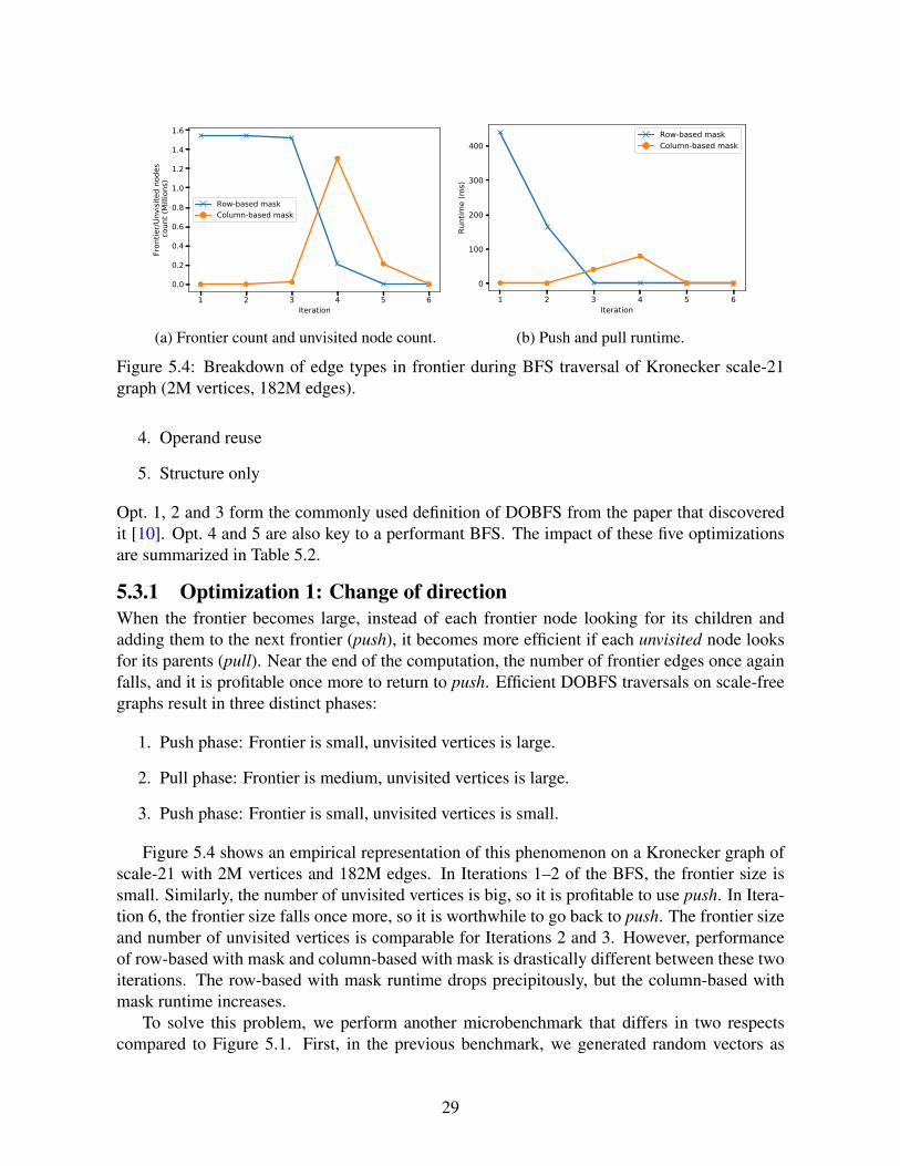
Figure 5.4: Breakdown of edge types in frontier during BFS traversal of Kronecker scale-21graph (2M vertices, 182M edges).

4. Operand reuse

5. Structure only

Opt. 1, 2 and 3 form the commonly used definition of DOBFS from the paper that discoveredit [10]. Opt. 4 and 5 are also key to a performant BFS. The impact of these five optimizationsare summarized in Table 5.2.

5.3.1 Optimization 1: Change of directionWhen the frontier becomes large, instead of each frontier node looking for its children andadding them to the next frontier (push), it becomes more efficient if each unvisited node looksfor its parents (pull). Near the end of the computation, the number of frontier edges once againfalls, and it is profitable once more to return to push. Efficient DOBFS traversals on scale-freegraphs result in three distinct phases:

1. Push phase: Frontier is small, unvisited vertices is large.

2. Pull phase: Frontier is medium, unvisited vertices is large.

3. Push phase: Frontier is small, unvisited vertices is small.

Figure 5.4 shows an empirical representation of this phenomenon on a Kronecker graph ofscale-21 with 2M vertices and 182M edges. In Iterations 1–2 of the BFS, the frontier size issmall. Similarly, the number of unvisited vertices is big, so it is profitable to use push. In Itera-tion 6, the frontier size falls once more, so it is worthwhile to go back to push. The frontier sizeand number of unvisited vertices is comparable for Iterations 2 and 3. However, performanceof row-based with mask and column-based with mask is drastically different between these twoiterations. The row-based with mask runtime drops precipitously, but the column-based withmask runtime increases.

To solve this problem, we perform another microbenchmark that differs in two respectscompared to Figure 5.1. First, in the previous benchmark, we generated random vectors as

29

0 500000 1000000 1500000 2000000Number of nonzeroes in Vector/Mask

0

100

200

300

400

Runt

ime

(ms)

Row-based, random input vectorColumn-based, random input vectorRow-based mask, random input vectorColumn-based mask, BFS input frontierRow-based mask, BFS input frontier

(a) Normal plot.

0 500000 1000000 1500000 2000000Number of nonzeroes in Vector/Mask

10 1

100

101

102

Runt

ime

(ms)

Push 1, Pull 5, Push 6, Pull 6Push 2

Push 3

Push 4

Push 5

Pull 1Pull 2

Pull 3

Pull 4

(b) Log-normal plot.

Figure 5.5: Runtime in milliseconds for row-based and column-based matvec in their maskedand unmasked variants for matrix ‘kron’ as a function of nnz(f) and nnz(m). Input vectorsand masks are generated using 2 methods: (1) random input vectors, (2) based on sampling BFSiterations from 1000 random sources on graph ‘kron g500-logn21’. Push 1 means Iteration 1 ofthe push-only BFS. Pull 1 means Iteration 1 of the pull-only BFS. For this graph, 2 iterationsof push followed by 3 of pull, then 1 iteration of push or pull, yields the best performance.

input and mask; here we launch BFS from 1000 different sources and plot the per-iterationruntime as a function of input frontier size (in the case of column-based) and unvisited nodes(in the case of row-based with mask), so the vectors have semantic meaning. Second, for row-based with mask we activate the early exit optimization. The result of the microbenchmark isshown in Figure 5.5. Interestingly, the runtimes of the row-based and column-based matvecslook very different depending on whether the input vector is random or whether it represents aBFS frontier.

We begin by analyzing the column-based-with-mask case (the red oval in Figure 5.5). Thisinteresting shape is characteristic of power-law graphs (of which ‘kron’ is a member) that havea small number of nodes with many edges (supernodes) but most nodes with only a few. Weexamined a few examples of the runtime data. Column-based-on-graph-data (push-based BFS)progresses with increasing iteration count in a clockwise-direction. In the first phase of the BFS,the algorithm quickly discovers a few supernodes, which dramatically increases its runtime.The BFS then reaches a peak in the frontier size (Iteration 4 of Figure 5.4a), at which pointthe frontier begins to fall. Its return to low frontier size corresponds to the bottom of the oval.Despite a comparable nonzero count in the input vector, this phase is notable for its lack ofsupernodes, which keeps runtime at a minimum.

Row-based mask has a different pattern. There, the pull-based BFS begins at the top of thebackwards ‘L’, then moves down and towards the left with increasing iteration count. Whenthere have only been one or two nodes visited, we most likely have not discovered a super nodeyet, so the runtime is high (around 1.5M in Figure 5.5). We found it took on average 79 parentchecks before a valid parent was found. After the first 20k or 30k nodes have been visited, itis with high probability that a supernode has been visited. In either case, we found that after2 BFS iterations, the average numbers of parents examined before a valid parent was found

30

dropped from 79 to 1.3. This concept of early-exit does not exist in the matvec of Figure 5.1,so there we get a different result. The line peaks around 1.5M, because that is the size of thelargest connected component.

In light of DOBFS, it becomes clear from looking at Figure 5.5b that at the start of the BFS,the push BFS is below the blue line around (0, 10−1), but the pull BFS is above the blue line, soit is more efficient to do push BFS for the first few iterations. By Iteration 3, the push-based hasincreased to above the blue line, while the pull-based has dropped sharply below. At this point,it is more efficient to do pull BFS. Near the end of the algorithm, both algorithms continue toimprove in efficiency, so either algorithm will suffice.

5.3.2 Optimization 2: MaskingAs described in Section 5.1, masking means computing only the rows whose value we know apriori must be updated. In Figure 5.3c, this means depending on the unvisited nodes (mask), wecan perform a matvec using just the latter four rows of the matrix. This yields the algorithmicspeed-up of O(nnz(m−m)) over O(nnz(A)).

5.3.3 Optimization 3: Early-exitIn the pull phase, an undiscovered node searches for a parent in the frontier. Once such aparent has been found, further computation for that undiscovered node is unnecessary and canpotentially halt. For the nodes who do not have parents that have been previously visited, early-exit has no benefit. According to Table 5.2, this optimization yielded the greatest speed-up.This optimization is only generalizable to semirings with Boolean operators that support short-circuiting.

5.3.4 Optimization 4: Operand reuseSince the set of the visited node list is always a superset of the frontier node list, we can simplyuse the visited node list in place of the frontier. Gunrock [67] notes that f ⊂ v and computesATv. ∗¬v instead of ATf . ∗¬v. This is a powerful optimization, because computing the lattermeans that during the iteration in which we are switching from push to pull; we get the costlysparse to dense frontier vector conversion for free because in the above expression, the frontierf is not required as part of the input.

5.3.5 Optimization 5: Structure onlyThe matrix values and sparse vector values do not need to be accessed for BFS. This optimiza-tion takes advantage of the fact for the purposes of a BFS, the matrix can be implicitly treated asa Boolean matrix, because we treat the existence of sparse matrix column indices as a Boolean1, and non-existence as Boolean 0. The majority of the speed-up comes during the multiwaymerge. In Section 5.4, we say that we implement this multiway merge using a radix sort. Thisradix sort is often the bottleneck of the algorithm, so if we use this optimization, we are reduc-ing a key-pair sort to a key-only sort, which will reduce the number of memory accesses by afactor of 2.

31

Optimization Performance (GTEPS) Speed-up

Baseline 0.874 —Structure only 1.411 1.62×

Direction-optimization 1.527 1.08×Masking 3.932 2.58×Early exit 15.83 4.02×

Operand reuse 42.44 2.68×

Table 5.2: Impact of the four optimizations described in this section on the performance mea-sured in billions of traversed edges per second on ‘kron g500-logn21’. These optimizations arecumulative, meaning the next optimization is stacked on top of the previous one. Speedups arestandalone.

5.3.6 GeneralityChange of direction can be generalized to other algorithms including betweenness centrality,personalized PageRank, and SSSP, with similar tradeoffs between row-based and column-basedapproaches (Table 5.1). In SSSP, for example, despite the workfront evolution (how the fron-tier changes between iterations) being completely different from Figure 5.4a, a simple 2-phasedirection-optimized traversal can be used where the traversal is begun using unmasked column-based matvec, and switches to row-based matvec when the frontier becomes large enough thatrow-based is more efficient.

Masking can be generalized to any algorithms where the output sparsity is known ahead ofcomputation. This includes algorithms such as triangle counting and enumeration [5], adap-tive PageRank [40], batched betweenness centrality [17], maximal independent set [18], andconvolutional neural networks [20]. In all of these algorithms, an optimal algorithm will wantto use the knowledge that some output elements will be zero (e.g., when the PageRank valuehas converged for a particular node). In these cases, our proposed elementwise multiply for-malism provides the mathematical theory to take advantage of this output sparsity yielding anasymptotic speed-up of O( dM

dnnz(m)) = O( M

nnz(m)).

Operand reuse is generalizable to any traversal-based algorithm for which computing ATvin place of ATf gives the correct result. We give SSSP and personalized PageRank as examplesfor which this holds true. However, early-exit and structure only are only generalizable tosemirings that operate on Booleans.

5.4 ImplementationThis section will discuss our implementation of row-based masked matvec, column-based matvec(masked and unmasked), and our direction-optimization heuristic. For simplicity in the follow-ing discussion, we use m(i) to denote checking whether the mask is nonzero, and if so, allowingthe value to pass through to the output if it is. ¬m(i), while not discussed, does the inverse.

5.4.1 Row-based masked matvec (Pull phase)Our parallel row-based masked matvec on the GPU is listed in Algorithm 8 and illustrated inFigure 5.3e. We parallelize over threads and have each thread check the m. If m(i) passes

32

the check, the thread i checks its neighbours j in the matrix AT (i, :) and tallies up the result ifand only if the v(j) is also nonzero. For semirings with Boolean operators that support short-circuiting such as the one used for BFS, namely the Boolean semi-ring ({0, 1}, AND,OR, 0),once a single non-zero neighbour j is discovered (meaning it has been visited before), the threadcan immediately write its result to the output vector and exit.

Algorithm 8 Masked row-based matrix multiplication over generalized semiring (D,⊗,⊕, I).The Boolean variable scmp controls whether or not m or ¬m is used.

1: procedure ROW MASKED MXV(Vector v, Graph AT , MaskVector m, MaskIdentity identity,Boolean scmp)

2: for each thread i in parallel do3: if m(i) 6= identity XOR scmp then4: value← I5: for index j in AT (i, :) do6: if v(j) 6= 0 then7: value← value ⊕AT (i, j)⊗ v(j)8: break (optional: early-exit opt. enables this break)9: end if

10: end for11: w(i)← value12: end if13: end for14: return w15: end procedure

5.4.2 Column-based masked matvec (Push phase)Our column-based masked matvec follows Gustavson’s algorithm for SpGEMM (sparse matrix-sparse matrix multiplication), but specialized to matvec [37]. The key challenge in parallelizingGustavson’s algorithm is solving the multiway merge problem [3]. For the GPU, our paral-lelization approach follows the scan-gather-sort approach outlined by Yang et al. [70] and isshown in Algorithm 9. Instead of doing the multiway merge by doingO(nnz(m+

f ) log nnz(f)),we concatenate all lists and use radix sort, because radix sort tends to have better performanceon GPUs. Our complexity then becomes O(nnz(m+

f ) logM), where M is the number of rowsin the matrix; an increase in M forces us to do a higher bit radix sort.

We begin by computing the requisite space to leave in the output frontier for each neighbourlist expansion. In compressed sparse row (CSR) format, node i computes its required spaceby taking the difference between the i-th and i+1-th row pointer values. Once each thread hasits requisite length, we perform a prefix-sum over these lengths. This is fed into a higher-levelabstraction, INTERVALGATHER, from the ModernGPU library [8]. On the prefix-sum array,INTERVALGATHER does a parallel search on sorted input to determine the indices from whicheach thread must gather. This gives us a load-balanced way of reading the column indices andvalues (Lines 6–9 in Algorithm 9).

During this process, the vector value of the corresponding thread v(i) is also gathered fromglobal memory. This will allow us to multiply all of i’s neighbours with v(i) using the ⊗ op-

33

erator. Once this is done, we write the column indices and multiplied values to global memory.Then we run a logM -bit radix sort, where M is the number of matrix rows. One advantageof the structure-only optimization is that it allows us to cut down on the runtime, because thisradix sort is often the bottleneck of the column-based masked matvec.

After the radix sort, a segmented reduction using the operator (⊕, I) gives us the temporaryvector. The unmasked column-based matvec ends here. The masked version additionally filtersout the values not in the mask by checking m(i).

Algorithm 9 Masked column-based matrix multiplication over generalized semiring(D,⊗,⊕, I). The Boolean variable scmp controls whether or not m or ¬m is used.

1: procedure COL MASKED MXV(Vector v, Graph AT , MaskVector m, MaskIdentity identity,Boolean scmp)

2: for each thread i in parallel do3: length[i]← row ptr(i+1)-row ptr(i+1) for all i such that v(i) 6= I4: end for5: scan← prefix-sum length6: addr[i]← INTERVALGATHER(scan, v)7: col← col ind j such that AT (j, i) 6= I from addr[i]8: val←AT (j, i) from addr[i]9: val← val ⊗v(i)

10: write (col, val) to global memory11: key-value sort (col, val)12: (optional: structure only opt. turns this into a key-only sort)13: segmented-reduction using (⊕, I) produces w′

14: for each thread i in parallel do15: ind← ind such that w′(ind) 6= I16: if m(ind) 6= identity XOR scmp then17: w(i) = w′(i)18: else19: w(i) = I20: end if21: end for22: return w23: end procedure

5.4.3 Direction-optimization heuristicImplementing an efficient DOBFS requires good decisions to switch between forward and re-verse. Beamer et al. compute the number of edges a column-based-with-mask implementationwould have to touch as nnz(mf ), and compare it with the number of edges a row-based-with-mask implementation would have to touch nnz(mu). If this ratio exceeds a constant determinedby the heuristic and the ratio has increased from before, then the implementation switches frompush to pull.

Beamer et al. proposed a heuristic to switch from push to pull when nnz(mf )nnz(mu)

< α for some

factor α, and to switch back when nnz(f)M

< β for some factor β [10]. We aim to match their

34

intent but face two difficulties: (1) GraphBLAS matvec calls do not pass in iteration counterinformation, and (2) we wish to avoid computing mf speculatively. Instead, our method relieson the fact that nnz(mf ) ≈ d nnz(f), where d is the average row length of the matrix and Mis the number of rows in the matrix. If we also assume that nnz(mu) ≈ nnz(A) ≈ dM whenwe desire to switch, we see that r = nnz(mf )

nnz(mu)≈ dnnz(f)

dM= nnz(f)

M. Our method thus reduces to

α = β; if it is increasing and α = β > r, we switch from push to pull, and if it is decreasingand α = β < r, then we switch from pull to push. In this paper, we use α = β = 0.01,which is optimal (defined by comparing with minimum of per-iteration push-only and pull-onlyBFS) for graphs we studied except ‘i04’ and the 3 non-scale free graphs, whose optimal BFS ispush-only for all iterations.

To decide which version of matvec to use, we call the CONVERT function on the input vec-tor f . Then the vector tests whether f is stored in DenseVector or SparseVector format. If theformer, then it checks whether the number of nonzeroes is low enough to warrant converting to aSparseVector using DENSE2SPARSE and whether it has decreased from the last time CONVERT

was called on it. If the latter, it checks whether the number of nonzeroes is high enough to war-rant converting to a DenseVector using SPARSE2DENSE and whether it has increased since thelast time CONVERT was called. The user can select this sparse/dense switching point by passingin a floating-point value through the Descriptor of the matvec call. The default switchpoint iswhen the ratio of nonzeroes in the sparse matrix exceeds 0.01. Another way of expressing thisis that once we have visited 1% of vertices in the graph in a BFS, we are sure to have hit asupernode.

As mentioned in Section 5.1, it is more efficient to store the input vector as a DenseVectorobject for row-based matvec. Similarly, it is efficient to store the frontier vector as a SparseVec-tor. Therefore switching from push-to-pull in our implementation means converting the inputvector from sparse to dense, and vice versa for pull-to-push. Using these SparseVector and Den-seVector objects, we have the function signatures of following operations, which correspond tothe four variants analyzed in Table 5.1:

1. ROW MXV( DenseVector w, GrB NULL, Matrix A, DenseVector v )

2. ROW MASKED MXV( DenseVector w, DenseVector mask, Matrix A, DenseVector v )

3. COL MXV( SparseVector w, GrB NULL, Matrix A, SparseVector v )

4. COL MASKED MXV( SparseVector w, DenseVector mask, Matrix A, SparseVector v )

There are already many efficient implementations of Operation (1) on the GPU [8, 12, 51],so we call ModernGPU’s SpmvCsrBinary, but we implemented the other 3 operations our-selves.

The UML (Unified Modeling Language) diagram for the relationship between the backendimplementation and the public interface is shown in Figure 5.6. The separation between thefrontend interface Vector and the backend interface backend::Vector is inspired by the workof Zhang et al. in their GraphBLAS Template Library (GBTL) work [73]. Our work differsfrom theirs in two ways in that: (1) their implementation was intended as a proof-of-conceptin programming language research rather than in performance; (2) our work demonstrates that

35

Figure 5.6: UML diagram showing the dynamic polymorphism we are using for Vector object.backend::SparseVector and DenseVector are two implementations of the backend::VectorGPU interface.

breaking up the Vector object into subclasses is necessary in order to take advantage of directionoptimization; and (3) we program directly in CUDA while they program using Thrust, so theyare limited by not being able to choose when to perform memory allocation. Our implementa-tion enjoys a 31.8x geomean speed-up over GBTL over 6 datasets listed in their paper.

5.5 Experimental Results5.5.1 Experimental setupWe ran all experiments in this paper on a Linux workstation with 2× 3.50 GHz Intel 4-coreE5-2637 v2 Xeon CPUs, 556 GB of main memory, and an NVIDIA K40c GPU with 12 GBon-board memory. The GPU programs were compiled with NVIDIA’s nvcc compiler (ver-sion 8.0.61). The C code was compiled using gcc 4.9.4. Ligra was compiled using icpc 15.0.1with CilkPlus. All results ignore transfer time (from disk-to-memory and CPU-to-GPU). Thegather, scan, row-based mxv (without mask) operations are from the Modern GPU library [8].The radix sort and reduce operations are from the CUDA UnBound library (CUB) [50]. AllBFS tests were run 10 times with the average runtime and MTEPS used for results.

The datasets we used are listed in Table 5.3. ‘soc-orkut’ (soc-ork), ‘soc-LiveJournal1’ (soc-lj), and ‘hollywood-09’ (h09) are three social-network graphs; ‘indochina-04’ (i04) is a crawledhyperlink graph from indochina web domains; and ‘kron g500-logn21’ (kron), ‘rmat s22 e64’(rmat-22), ‘rmat s23 e32’ (rmat-23), and ‘rmat s24 e16’ (rmat-24) are three generated R-MAT(Recursive-MATrix) graphs. These eight datasets are scale-free graphs with diameters of lessthan 30 and unevenly distributed node degrees (80% of nodes have degree less than 64). The‘rgg n 24’ (rgg), ‘roadNet CA’ (roadnet), and ‘road USA’ (road usa) datasets have large diam-eters with small and evenly distributed node degrees (most nodes have degree less than 12).

36

Dataset Vertices Edges Max Degree Diameter Type

soc-orkut 3M 212.7M 27,466 9 rssoc-Livejournal1 4.8M 85.7M 20,333 16 rs

hollywood-09 1.1M 112.8M 11,467 11 rsindochina-04 7.4M 302M 256,425 26 rs

kron g500-logn21 2.1M 182.1M 213,904 6 gsrmat s22 e64 4.2M 483M 421,607 5 gsrmat s23 e32 8.4M 505.6M 440,396 6 gsrmat s24 e16 16.8M 519.7M 432,152 6 gs

rgg n 24 16.8M 265.1M 40 2622 gmroadNet CA 2M 5.5M 12 849 rmroad USA 23.9M 577.1M 9 6809 rm

Table 5.3: Dataset Description Table. Graph types are: r: real-world, g: generated, s: scale-free,and m: mesh-like.

soc-ork is from Network Repository [60]; soc-lj, h09, i04, kron, roadNet CA, and road usa arefrom the UF Sparse Matrix Collection [26]; and rmat-22, rmat-23, rmat-24, and rgg are random-ized graphs we generated. All datasets have been converted to undirected graphs. Self-loopsand duplicated edges are removed.

5.5.2 Graph framework comparisonAs a baseline for comparison, we use the push-based BFS on the GPU by Yang et al. [70], be-cause it is based in linear algebra and is (relatively) free of graph-specific optimizations. It doesnot support DOBFS. We also compare against four other graph frameworks (1 linear-algebra-based, 3 native-graph). SuiteSparse is a single-threaded CPU implementation of GraphBLAS.It is notable for being the first GraphBLAS implementation that adheres closely to the spec-ification [25]. SuiteSparse performs matvecs by doing the column-based algorithm. CuShais a vertex-centric framework on the GPU using the gather-apply-scatter (GAS) programmingmodel [43]. Ligra is a CPU-based vertex-centric framework for shared memory [61]. It is thefastest graph framework we found on a multi-threaded CPU and was the first work that general-ized push-pull to traversal algorithms other than BFS. Gunrock is a GPU-based frontier-centricframework [67] that generated the fastest single-processor BFS in our experiments.

5.5.3 Discussion of resultsFigure 5.7 shows our performance results. In terms of runtime, we are 122×, 48.3×, 3.37×,1.16× faster in the geomean than SuiteSparse, CuSha, the baseline, and Ligra respectively. Weare 34.6% slower than Gunrock. Our implementation is relatively better on scale-free graphs,where we are 3.51× faster than Ligra on the scale-free datasets. In comparison, we are 3.2×slower than Ligra on the road maps and mesh graph. Our performance with respect to Gunrockis similar in that we do poorly on road maps (3.15× slower) compared with scale-free graphs(1.09× slower). This supports our intuition in Section 5.2 that DOBFS is helpful mainly onscale-free graphs.

The four biggest differences between Gunrock’s and our implementation is that on top of

37

Runtime (ms) [lower is better] Edge throughput (MTEPS) [higher is better]

Dataset SuiteSparse CuSha Baseline Ligra Gunrock This Work SuiteSparse CuSha Baseline Ligra Gunrock This Work

soc-ork 2165 244.9 122.4 26.1 5.573 7.280 98.24 868.3 1722 8149 38165 29217soc-lj 1483 263.6 51.32 42.4 14.05 14.16 57.76 519.5 1669 2021 6097 6049h09 596.7 855.2 23.39 12.8 5.835 7.138 188.7 131.8 4814 8798 19299 15775i04 1866 17609 71.81 157 77.21 80.37 159.8 22.45 4151 1899 3861 3709

kron 1694 237.9 108.7 18.5 4.546 4.088 107.5 765.5 1675 9844 40061 44550rmat-22 4226 1354 OOM 22.6 3.943 4.781 114.3 369.1 OOM 21374 122516 101038rmat-23 6033 1423 OOM 45.6 7.997 8.655 83.81 362.7 OOM 11089 63227 58417rmat-24 8193 1234 OOM 89.6 16.74 16.59 63.42 426.4 OOM 5800 31042 31327

rgg 230602 68202 9147 918 593.9 2991 1.201 3.887 30.28 288.8 466.4 92.59roadnet 342 288.5 284.9 82.1 130.9 214.4 16.14 14.99 19.38 67.25 42.18 25.75road usa 9413 36194 26594 978 676.2 7155 6.131 7.944 2.17 59.01 85.34 8.065

1

10

100

1000

soc-ork soc-lj h09 i04 kron rmat22 rmat23 rmat24 rgg roadnet road_usaSlow

downcomparedtoGunrock

Dataset

SuiteSparse CuSha Baseline Ligra ThisWork

Figure 5.7: The table compares our work to other graph libraries (SuiteSparse [25], CuSha [43],a baseline push-based BFS [70], Ligra [61], and Gunrock [67]) implemented on 1× Intel XeonCPU and 1× Tesla K40c GPU. Bold is fastest for that dataset. OOM means out of memory.The graph shows the same data presented as a slowdown compared to Gunrock.

the optimizations discussed in this paper, they also employ (1) local culling, (2) keeping sparsevector indices in unsorted order with possible duplicates, (3) kernel fusion, and (4) a differenttraversal strategy for road networks.

Local culling Instead of our write to global memory in Line 9 of Algorithm 9 which is fol-lowed by an expensive key-value sort, Gunrock’s filter step incorporates a series of inexpensiveheuristics [52] to reduce but not eliminate redundant entries in the output frontier. These heuris-tics include a global bitmask, a block-level history hashtable, and a warp-level hashtable. Thesize of each hashtable is adjustable to achieve the optimal tradeoff between performance and re-dundancy reduction rate. However, this approach may not be suitable for GraphBLAS, becausesuch an optimization may be too BFS-focused and would generalize poorly.

Unsorted order and redundant elements When performing the column-based masked matvecas in Figure 5.3d, our complexity is O(nnz(m+

f ) logM), so the bottleneck is in making the el-ements unique. If duplicate indices are tolerated, we can omit the multiway merge entirely, andget rid of the logarithmic factor leaving us with O(nnz(m+

f )). While redundant vertices im-pose an extra cost, BFS is an algorithm that can tolerate redundant vertices and in some cases, itmay be cheaper to allow a few extra vertices to percolate through the computation than to go tosignificant effort to filter them out. This approach may not be suitable for GraphBLAS, becausesuch an optimization may be too BFS-focused and would generalize poorly.

38

Kernel fusion Because launching a GPU kernel is relatively expensive, optimized GPU pro-grams attempt to fuse multiple kernels into one to improve performance (“kernel fusion”). Gun-rock fuses kernels in several places, for example, fusing Lines 7 and 8 in Algorithm 7 duringpull traversal. This optimization may be a good fit for a non-blocking implementation of Graph-BLAS, which would construct a task graph and fuse tasks when it deemed worth fusing toimprove performance.

Different traversal strategy for road networks For road networks, Gunrock uses the TWC(Thread Warp CTA) load-balancing mechanism of Merrill et al. [52]. TWC is cheaper to applythan other load-balancing mechanisms, which makes it a good match for road networks thathave many BFS iterations each with little work.

5.6 ConclusionIn this chapter we demonstrated that push-pull corresponds to the concept of column- and row-based masked matvec. We analyzed four variants of matvec, and show theoretically and em-pirically they have fundamentally different computational complexities. We presented evidencethat there is a difference in complexity between doing a matvec on arbitrary input comparedto doing matvec on a BFS frontier. We provided experimental evidence that the concept of amask to take advantage of output sparsity is critical for a linear-algebra based graph analyticframework to be competitive with state-of-the art vertex-centric graph frameworks on the GPUand multi-threaded CPU.

In the next chapter, we try to use our knowledge about SpMV in order to improve perfor-mance of mulitple column vectors (sparse matrix-dense matrix multiplication).

39

Chapter 6

Design Principles for Sparse MatrixMultiplication on the GPU

In this chapter, we take a turn to improve the state-of-the-art in sparse matrix-dense matrix(SpMM) multiplication.

Our main contributions in this work are:

1. We generalize two main classes of SpMV algorithms—(1) row splitting and (2) merge-based—for the SpMM problem and implement them on the GPU.

2. We introduce a simple heuristic that selects between the two kernels with an accuracy of95.9% compared to optimal.

3. Using our multi-algorithm and heuristic, we achieve a geomean speed-up of 23.5% andup to a maximum of 3.6x speed-up over state-of-the-art SpMM implementations over 195datasets from the SuiteSparse Matrix Collection [26].

6.1 Design PrinciplesWe discuss two design principles that every irregular problem on the GPU must follow for goodperformance. Ideally, we attain full utilization of the GPU hardware, where a ready warp canbe run on every cycle, all computational units are doing useful work on every cycle, and allmemory accesses are coalesced. Our principles for reaching this goal are (1) effective latency-hiding through a combination of thread- and instruction-level parallelism (TLP and ILP) and(2) efficient load-balancing. Then we will look at state-of-the-art SpMM implementations tounderstand their inefficiencies.

1. Load-balancing

2. Latency-hiding ability

(a) Thread-level parallelism (TLP)(b) Instruction-level parallelism (ILP)

2This chapter substantially appeared as “Design Principles for Sparse Matrix Multiplication on the GPU” [71],for which I was responsible for most of the research and writing.

40

6.1.1 Latency hiding with TLP and ILPMemory operations to a GPU’s main memory take hundreds of clock cycles. The GPU’s chiefmethod for hiding the cost of these long-latency operations is through thread-level parallelism(TLP). Effective use of TLP requires that the programmer give the GPU enough work so thatwhen a GPU warp of threads issues a memory request, the GPU scheduler puts that warp tosleep and another ready warp becomes active. If enough warps are resident on the GPU (if wehave enough TLP), switching between warps can completely hide the cost of a long-latencyoperation. We quantify the amount of TLP in a program as occupancy, the ratio of available(issued) warps to the maximum number of warps that can be supported by the GPU. Higheroccupancy yields better latency-hiding ability, which allows us to approach full utilization.

Another latency-hiding strategy is exploiting instruction-level parallelism (ILP) and its abil-ity to take advantage of overlapping the latency of multiple memory operations within a singlethread. Because the GPU’s memory system is deeply pipelined, a thread can potentially issuemultiple independent long-latency operations before becoming inactive, and those multiple op-erations will collectively incur roughly the same latency as a single operation. While this yieldsa significant performance advantage, it relies on the programmer exposing independent memoryoperations to the hardware. We can achieve this goal by assigning multiple independent tasksto the same thread (“thread coarsening”).

GPUs have a fixed number of registers. TLP requires many resident warps, each of which re-quires registers. ILP increases the work per thread, so each thread requires more registers. ThusTLP and ILP are in opposition, and attaining full utilization requires carefully balancing bothtechniques. While TLP is commonly used across all of GPU computing, ILP is a less exploredarea, with prior work limited to dense linear algebra [64] and microcode optimization [38].

6.1.2 Load-balancingWe now turn to the problem of ensuring that all computational units are doing useful workon every cycle, and that the memory accesses from those warps are coalesced to ensure peakmemory performance. In the context of SpMV and SpMM, this “load-balancing” problem hastwo aspects:

1. Load imbalance across warps. Some CTAs or warps may be assigned less work thanothers, which may lead to these less-loaded computation units being idle while the moreloaded ones continue to do useful work. In this paper, we term this “type 1” load imbal-ance.

2. Load imbalance within a warp, in two ways, which we collectively call “type 2” loadimbalance. (a) Some warps may not have enough work to occupy all 32 threads in thewarp. In this case, thread processors are idle, and we lose performance. (b) Some warpsmay assign different tasks to different threads. In this case, SIMD execution within athread means that some threads are idle while other threads are running; moreover, thedivergence in execution across the warp means memory accesses across the entire warpare unlikely to be coalesced.

For irregular matrices, we claim that SpMV and SpMM are fundamentally load-balancingproblems on the GPU. As evidence, Figure 6.1 shows load imbalance in a vendor-supplied im-

41

2 8 32 128

512

2048

8192

3276

8

1310

72

5242

88

2097

152

8388

608

Mean row length

0

10

20

30

40Sp

MV

Perfo

rman

ce (G

Flop

s)

SpMVSpMM

0

20

40

60

80

100

120

SpM

M P

erfo

rman

ce (G

Flop

s)

(a) SpMV and SpMM

2 8 32 128

512

2048

8192

3276

8

1310

72

5242

88

2097

152

8388

608

Mean row length

0.20

0.40

0.60

0.80

1.00

Achi

eved

Occ

upan

cy (I

deal

= 1

)

Achieved OccupancyWarp Efficiency

0.88

0.90

0.92

0.94

0.96

0.98

1.00

War

p Ef

ficie

ncy

(Idea

l = 1

)

(b) Occupancy and warp efficiency

Figure 6.1: Synthetic benchmark showing NVIDIA cuSPARSE SpMV and SpMM performanceas a function of matrix dimensions on a Tesla K40c, and SpMM’s achieved occupancy and warpefficiency (inverse of divergence).

plementation from a synthetic benchmark. The experimental setup is described in Section 5.5.The right side of the x-axis represents Type 1 load imbalance, where long matrix rows are notdivided enough, resulting in some computation resources on the GPU remaining idle while oth-ers are overburdened. The left size of the x-axis represents Type 2 load imbalance where toomany computational resources are allocated to each row, so some remain idle.

6.2 Parallelizations of CSR SpMMThis section reviews three existing parallelizations of SpMV through the lens of the designprinciples from Section 6.1. While our implementations of SpMM share some characteristicswith SpMV parallelizations, we also faced several different design decisions for SpMM, whichwe discuss below. The three SpMV variants are illustrated in Figure 6.2 and summarized here:

1. Row split [12]: Assigns an equal number of rows to each processor.

2. Merge based: Performs two-phase decomposition—the first kernel divides work evenlyamongst CTAs, then the second kernel processes the work.

(a) Nonzero split [8, 23]: Assign an equal number of nonzeroes per processor. Thendo a 1-D (1-dimensional) binary search on row offsets to determine at which row tostart.

(b) Merge path [51]: Assign an equal number of {nonzeroes and rows} per processor.This is done by doing a 2-D binary search (i.e., on the diagonal line in Figure 6.2c)over row offsets and nonzero indices of matrix A.

While row split focuses primarily on ILP and TLP, nonzero split and merge path focus onload-balancing as well. We consider nonzero split and merge path to be explicit load-balancingmethods, because they rearrange the distribution of work such that each thread must performT independent instructions; if T > 1, then explicit load-balancing creates ILP where there waspreviously little or none. Thus load-balance is closely linked with ILP, because if each thread is

42

(a) Row split (b) Nonzero split (c) Merge path

Figure 6.2: The three parallelizations for CSR SpMV and SpMM on matrix A. The orangemarkers indicate segment start for each processor (P = 4).

guaranteed T > 1 units of independent work (ILP), then each thread is doing the same amountof work (i.e., is load-balanced).

6.2.1 Algorithm I: Row-splitting SpMMRow split aims to assign each row to a different thread, warp, or CTA. Figure 6.3a shows thewarp assignment version. The typical SpMV row split is only the left-most column of matrixB with orange cells replaced by green cells. This gives SpMV 1 independent instruction anduncoalesced, random accesses into the vector. Although row-split is a well-known method forSpMV [12], we encountered three important design decisions when extending it to SpMM:1. Granularity. We assigned each row to a warp compared to the alternatives of assigning athread and a CTA per row. This leads to the simplest design out of the three options, sinceit gives us coalesced memory accesses into B. For matrices with few nonzeroes per row, thethread-per-matrix-row work assignment may be more efficient. This is borne out by Figure 6.4.2. Memory access pattern. This design decision had the greatest impact on performance. Toour knowledge, this is the first time in literature this novel memory access strategy has beendescribed. Our thread layout is shown in Figure 6.3c. For SpMM, we have two approaches wecould take: each thread is responsible for loading a column or a row of the matrix B.

We discovered the first approach is better, because the memory accesses into B are in-dependent and can be done in a coalesced manner (provided that B is in row-major order).In contrast, memory accesses into a column-major B would be independent but uncoalesced.Compared to the SpMV case, each thread now has 32 independent instruction and coalescedmemory accesses into B, which significantly amortizes the cost of memory accesses comparedto accessing a single vector. However, since we are forcing threads to pass a dummy columnindex if they are out of bounds within a row, the effective number of independent instructionand coalesced memory accesses is sensitive to row lengths that do not divide 32. For example,

43

if the row length is 33, then we will be doing 64 independent instruction and coalesced memoryaccesses into B. Whether or not they divide 32 does not matter for very long rows, becausethe cost is amortized by efficiently processing batches of 32. However, we would expect rowsplit to be negatively impacted by Type 2 load imbalances. The summary of this ILP analysis isshown in Table 6.1.3. Shared memory. The key component required is a round of 32 broadcasts (using the “shuffle”warp intrinsic shfl) by each thread to inform all other threads in the warp which B row oughtto be collectively loaded by the entire warp. This is required or otherwise each thread wouldbe responsible for loading its own row, which would result in uncoalesced access. We couldhave also implemented this using shared memory, but since all threads are within a single warp,there is no disadvantage to preferring warp intrinsics. That they are within a single warp is aconsequence of our decision to assign each row to a warp rather than a CTA.

4

A

B

C

32

m

k

n

k

m

n

Block.x 0

Block.x 1

Block.x 2

Block.x

Block.y 1Block.y 0

m4

.

.

.

(a) 2D block assignment of proposed rowsplit SpMM

(c) Step 2: Loaddense matrix B val-ues into registers.

Warp 0

Warp 1

Warp 2

Warp 3

0 0 0 0 0 00 0

ILP

TLP

(b) Step 1: Load sparse matrix A column indices intoregisters. Zeroes are marked as such.

Warp 0

Warp 1

Warp 2

Warp 3

(d) Step 3: Write to densematrix C.

Figure 6.3: Figure 6.3a shows the tiling scheme we use. Figures (b), (c), (d) represent the yellowblocks from Figure 6.3a. Row split SpMM ILP (orange) and TLP (green) are shown using warp1 with 8 threads per warp. In practice, we use 32 threads and 4 warps per GPU cooperativethread array (CTA). Matrix A is sparse in CSR format. Matrices B and C are both dense inrow-major format.

44

Table 6.1: This table shows the number of independent instructions per GPU thread for SpMVand SpMM with default value shown in brackets, as well as the register usage and the extranumber of memory accesses with respect to the row-split algorithm. T is the number of workitems per thread (typically specified as a tuning parameter to the algorithm). L is the numberof nonzeroes modulus 32 in the row of A that we are computing. B is the CTA size. Typicalvalues for T in SpMV and SpMM are 7 and 1 respectively, while a typical value for B is 128.T cannot be set arbitrarily high, because high register usage causes lower occupancy. A.nnzis the number of nonzeroes in the sparse matrix A. B.ncols is the number of columns of thedense matrix B.

SpMV SpMM

Operation Row-split Merge-based Row-split Merge-based

Read A.col ind and A.val 1 T (7) 1 T (1)Read x / Read B 1 T (7) 0 < L ≤ 32 32T (32)Write y / Write C 1 T (7) 1 32T (32)Register usage 2 2T (14) 64 64T (64)Memory access overhead 0 A.nnz

B×T 0 B.ncols×A.nnzB×T

(A.nnz896

) (2A.nnz )

6.2.2 Algorithm II: Merge-based SpMMThe essence of merge-based algorithms is to explicitly and evenly distribute the nonzeroesacross parallel processors. It does so by doing a two-phase decomposition: In the first phase(PARTITIONSPMM), it divides T work amongst all threads, and based on this deduces the start-ing indices of each CTA. Once coordinated thusly, work is done in the second phase. In theory,this approach should eliminate both Type 1 and Type 2 load imbalances, and performs well inrecent SpMV implementations [51]. We made the following design decisions when generalizingthis technique to SpMM:

1. Memory access pattern. For fetching B, we adapt the memory access pattern that wassuccessful in row-splitting. However, here, we must first apply the first phase (i.e., PARTITION-SPMM, Line 2 of Algorithm 10) to tell us the rows each CTA ought to look at if we want anequal number of nonzeroes per CTA. Then, we can apply the broadcast technique to retrieve Bvalues using coalesced accesses.2. Register usage. Since we opted for the coalesced memory access pattern explained in therow-splitting section, we require 32× the number of registers in order to store the values. Dueto this limitation, the number of independent instructions per thread T is limited to 1, so we seeno further latency-hiding gain from ILP over that of row-split.3. Memory access overhead. There are two sources of memory access overhead compared tothe row-splitting algorithm: (1) the additional GPU kernel that determines the starting rows foreach block (Line 3), and (2) the write of the carry-out to global memory for matrix rows of Cthat cross CTA boundaries (Lines 29 and 33). Since the user is unable to synchronize CTAsin CUDA, this is the only way the user can pass information from one CTA to another. Thefirst source of additional memory accesses is less of a problem for SpMM compared to SpMV,

45

Algorithm 10 The merge-based SpMM algorithm.Input: Sparse matrix in CSR A ∈ Rm×k and dense matrix B ∈ Rk×n.Output: C ∈ Rm×n such that C← AB.

1: procedure SPMMMERGE(A,B)2: limits[]← PARTITIONSPMM(A, blockDim.x) . Phase 1: Divide work and run

binary-search3: for each CTA i in parallel do . Phase 2: Do computation4: num rows← limits[i+ 1] − limits[i]5: shared.csr← GLOBALTOSHARED(A.row ptr + limits[i], num rows) . Read A

and store to shared memory6: end← min(blockDim.x, A.nnz - blockIdx.x × blockDim.x)7: if row ind < end then8: col ind← A.col ind[row ind] . Read A if matrix not finished9: valA← A.values[row ind]

10: else11: col ind← 0 . Otherwise do nothing12: valA← 013: end if14: for each thread j in parallel do15: for j = 0, 1, . . . , 31 do . Unroll this loop16: new ind[j]← Broadcast(col ind, j) . Each thread broadcasts17: new val[j]← Broadcast(valA, j) . col ind and valA18: valB[j]← B[col ind][j] × new val[j] . Read B19: end for20: end for21: terms← PREPARESPMM(shared.csr) . Flatten CSR-to-COO22: carryout[i]← REDUCETOGLOBALSPMM(C, valB, valB) . Compute partial of C

and save carry-outs23: end for24: FIXCARRYOUT(C, limits, carryout) . Carry-out fix-up (rows spanning across blocks)25: return C26: end procedure

46

Table 6.2: A selection of 20 datasets from the 195 SuiteSparse matrices used in our experiments.d is the mean row length of the matrix. nnz is the number of nonzeroes in the matrix. The leftdatasets have mean row length with arithmetic mean 7.92, while the right have 62.5.*: Despite having the same number of rows and nonzeroes, these two matrices differ in nonzerostructure and are treated as independent matrices in our experiments.

Dataset Description d nnz Dataset Description d nnz

wheel 601 combinatorial opt. 2.41 2.2M StocF-1465 CFD problem 13.3 19.5Mneos3 linear programming 4.01 2.1M ldoor structural problem 47.9 45.6Mc-big non-linear opt. 5.78 2M bmw3 2 structural problem 48.7 11.1Mins2 optimization problem 7.89 2.4M boneS10 3D trabecular bone 59.6 54.6MASIC 320k circuit simulation 8.19 2.6M bmwcra 1 stiffness matrix 70.5 10.5Mweb-Stanford* web graph 8.2 2.3M bone010 3D trabecular bone 71.6 70.7MStanford* web graph 8.2 2.3M inline 1 stiffness matrix 72.1 36.3McitationCiteseer citation network 8.62 2.3M F1 stiffness matrix 77.1 26.5MFullChip circuit simulation 8.9 26.7M audikw 1 structural problem 81.3 76.7Mcircuit5M circuit simulation 10.7 59.5M crankseg 2 structural problem 220 14.1M

because they are amortized by the increased work. The second source, however, scales withthe number of B columns. Thus we face a trade-off between having more efficient memoryaccess pattern (assign 32 columns per CTA so memory access is coalesced), and having lessmemory access overhead (assign 4 columns per CTA so T can be set higher resulting in fewerCTA boundaries that need to be crossed). The first approach resulted in better performance.

6.3 Experimental Results6.3.1 Experimental SetupWe ran all experiments in this paper on a Linux workstation with 2× 3.50 GHz Intel 4-coreE5-2637 v2 Xeon CPUs, 256 GB of main memory, and an NVIDIA K40c GPU with 12 GBon-board memory. The GPU programs were compiled with NVIDIA’s nvcc compiler (ver-sion 8.0.44). The C code was compiled using gcc 4.9.3. All results ignore transfer time (fromdisk-to-memory and CPU-to-GPU). The merge path operation is from the Modern GPU li-brary [8]. The version of cuSPARSE used was 8.0.

The 195 datasets mentioned in the previous section represent a random sample from theSuiteSparse sparse matrix collection. The topology of the datasets varies from small-degreelarge-diameter (road network) to scale-free. In the microbenchmark Figure 6.1a, dense matrices(varying from 2 rows with 8.3M nonzeroes per row to 8.3M rows with 2 nonzeroes per row)used in the micro-benchmark are generated to be nonzero, and converted to CSR sparse matrixstorage. We then multiply the matrix by a dense vector and a dense matrix with 64 columnsusing the vendor-supplied SpMV and SpMM implementations respectively.

6.3.2 Algorithm I: Row-splitFigure 6.5a shows the performance of our row split implementation on 10 SuiteSparse datasetswith long matrix rows (62.5 nonzeroes per row on average). We obtain a geomean speed-up of30.8% over the next fastest implementation and 39% peak improvement.

47

2 8 32 128

512

2048

8192

3276

8

1310

72

5242

88

2097

152

8388

608

Mean row length

0

25

50

75

100

125

150

175

Perfo

rman

ce (G

Flop

s)

cuSPARSE csrmm2Proposed Row Split

Figure 6.4: The performance of our proposed SpMM row split kernel vs. NVIDIA cuSPARSE’sSpMM as a function of aspect ratio on a Tesla K40c.

StocF-

1465

ldoor

bmw3_2

bone

S10 F1

inline

_1

bone

010

audik

w_1

bmwcra

_1

crank

seg_2

Dataset

0

20

40

60

80

100

120

140

160

Perfo

rman

ce (G

Flop

s)

cuSPARSE csrmmcuSPARSE csrmm2

MAGMA SELL-PProposed row-split

(a) Long rows (62.5 nonzeroes/row)

citati

onCite

web-St

anf

wheel_

601

c-big

FullC

hip

ASIC_32

0k

Stanfo

rd ins2

neos3

circui

t5M

Dataset

0

10

20

30

40

Perfo

rman

ce (G

Flop

s)

cuSPARSE csrmmRow-split

cuSPARSE csrmm2Proposed merge-based

(b) Short rows (7.92 nonzeroes/row)

Figure 6.5: Performance comparison between the proposed ILP-centric row split kernel andother state-of-the-art kernels on matrices with long and short row lengths on Tesla K40c usingsingle-precision floating-point. cuSPARSE csrmm and csrmm2 are from a vendor-suppliedlibrary [54]. MAGMA SELL-P is by Anzt, Tomov, and Dongarra [2].

We suspect our performance drop to the left in Figure 6.4 comes from the sensitivity toparameter L on row lengths that are significantly less than 32. This causes divergence anduncoalesced memory accesses. On the right hand side, we do much better than cuSPARSE. Webelieve this is due to the additional occupancy that we can get from superior ILP, which is betterat hiding latency. Using the profiler, we noted a 102% improvement in executed instructionsper cycle for the matrix sized 128-by-131072.

6.3.3 Algorithm II: Merge-basedFigure 6.5b shows the performance of our merge-based SpMM kernel on 10 SuiteSparse datasetswith short matrix rows (7.92 nonzeroes on average). We obtain a geomean speed-up of 53%over cuSPARSE csrmm2 and 237% peak improvement. We think the biggest reason that mergepath is doing better than the other methods is because it handles Type 2 load imbalances muchbetter. Other methods inevitably encounter warp efficiency degradation due to the divergence

48

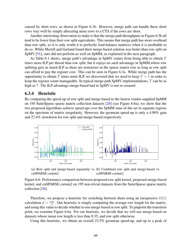
caused by short rows, as shown in Figure 6.1b. However, merge path can handle these shortrows very well by simply allocating more rows to a CTA if the rows are short.

Another interesting observation to make is that the merge path throughputs in Figure 6.5b alltend to be lower than their row split equivalents. This means that merge path has more overheadthan row split, so it is only worth it to perfectly load-balance matrices when it is profitable todo so. While Merrill and Garland found their merge-based solution was better than row split onSpMV [51], ours did not perform as well on SpMM, as explained in the next paragraph.

As Table 6.1 shows, merge path’s advantage in SpMV comes from being able to obtain Ttimes more ILP per thread than row split, but it enjoys no such advantage in SpMM,where rowsplitting gets as much ILP as there are nonzeroes in the sparse matrix row as long as row splitcan afford to pay the register cost. This can be seen in Figure 6.3a. While merge path has theopportunity to obtain T times more ILP, we discovered that we need to keep T = 1 in order tokeep the register count manageable. In typical merge path SpMV implementations, T can be ashigh as 7. The ILP advantage merge-based had in SpMV is not so assured.

6.3.4 HeuristicBy comparing the speed-up of row split and merge-based to the fastest vendor-supplied SpMMon 195 SuiteSparse sparse matrix collection datasets [26] (see Figure 6.6a), we show that thetwo proposed algorithms achieve speed-ups over the SpMM state-of-the-art in separate regionson the spectrum of matrix irregularity. However, the geomean speed-up is only a 4.98% gainand 27.4% slowdown for row split and merge-based respectively.

101 102 103

Mean row length

0.5

1.0

1.5

2.0

2.5

3.0

3.5

Spee

d-up

Row-splitMerge-based

(a) Row split and merge-based separately vs.cuSPARSE csrmm2.

101 102 103

Mean row length

0.5

1.0

1.5

2.0

2.5

3.0

3.5

Spee

d-up

(b) Combined row split and merge-based vs.cuSPARSE csrmm2.

Figure 6.6: Performance comparison between proposed row split kernel, proposed merge-basedkernel, and cuSPARSE csrmm2 on 195 non-trivial datasets from the SuiteSparse sparse matrixcollection [26].

Therefore, we propose a heuristic for switching between them using an inexpensive O(1)calculation d = nnz

n. Our heuristic is simply computing the average row length for the matrix,

and using this value to decide whether to use merge-based or row split. To pinpoint the transitionpoint, we examine Figure 6.6a. For our heuristic, we decide that we will use merge-based ondatasets whose mean row length is less than 9.35, and row split otherwise.

Using this heuristic, we obtain an overall 23.5% geomean speed-up, and up to a peak of

49

3.6×, over the vendor-supplied library cuSPARSE csrmm2. Over cuSPARSE csrmm, we obtaina 2.52× geomean speed-up and 22.4× peak speed-up. The result is shown in Figure 6.6. Usingthis heuristic as a binary classifier, we get 95.9% accuracy vs. an oracle that perfectly choosesthe fastest implementation.

6.4 ConclusionIn this paper we implement two promising algorithms for computing sparse matrix dense matrixmultiplication on the GPU. Our results using SpMM show considerable performance improve-ment over the vendor-supplied SpMM on a wide spectrum of graphs. One of the keys to ourhigh performance is our memory-access strategy that allows coalesced access into all 3 matrices(see Figure 6.3a).

In Figure 6.6, the points in the plot become sparser as the mean row length d gets larger.Greiner and Jacob have proven theoretically that as d exceeds some hardware threshold, namelymM

where m is the number of rows in the sparse matrix and M is the size of the fast memory ofthe device, that the tiling algorithm used in nearly every SpMM implementation will stop beingoptimal [36]. Instead, they claim that tiling both the sparse matrix A and B in a manner akin totiling dense matrix-matrix multiplication is optimal. In future work, it would be interesting tofind empirical evidence of such a transition.

In the next chapter, we put all the pieces together and describe general design principlesthat if heeded, can be used to build a high-performance linear-algebraic graph framework onthe GPU.

50

Chapter 7

Design of GraphBLAST

In this chapter, we are interested in answering the following question: What are the design prin-ciples required to build a GPU implementation based in linear algebra that matches the state-of-the-art graph frameworks in performance? Towards that end, we have designed GraphBLAST1:the first high-performance implementation of GraphBLAS for the GPU (graphics processingunit). Our implementation is for single GPU, but we believe the design we propose here willallow us to extend it to a distributed implementation with future work.

To perform a comprehensive evaluation of our system, we need to compare our frameworkagainst the state-of-the-art graph frameworks on the CPU and GPU, and hardwired GPU im-plementations, which are problem-specific GPU code that someone has handtuned for perfor-mance. The state-of-the-art graph frameworks we will be comparing against are Ligra [61] forCPU and Gunrock [67] for the GPU, which were described in detail in Chapter 3. The hardwiredimplementations will be Enterprise (BFS) [47], delta-stepping SSSP [24], pull-based PR [43],and bitmap-based triangle counting [14]. As described in Section 1, the graph algorithms wewill be evaluating our system on are:

• Breadth-first-search (BFS)

• Single-source shortest-path (SSSP)

• PageRank (PR)

• Triangle counting (TC)

Our contributions in this paper are as follows:

1. We give a brief introduction of GraphBLAS’s computation model (Section 7.1).

2. We demonstrate the importance of exploiting input sparsity, which means picking the al-gorithm that minimizes the number of computations and whose consequence is direction-optimization (Section 7.2).

1https://github.com/gunrock/graphblast

51

3. We show the importance of exploiting output sparsity, which is implemented as mask-ing and can be used to reduce the number of computations of several graph algorithms(Section 7.3).

4. We explain the load-balancing techniques required for high-performance on the GPU(Section 7.4).

5. We review how common graph algorithms are expressed in GraphBLAST (Section 7.5).

6. We show that enabled by the optimizations exploiting sparsity, masking, and proper load-balancing our system GraphBLAST gets 36× geomean (892× peak) over SuiteSparseGraphBLAS for sequential CPU and 2.14× geomean (10.97× peak) and 1.01× (5.24×peak) speed-up over state-of-the-art graph frameworks on CPU and GPU respectively onseveral graph algorithms (Section 7.6).

7.1 GraphBLAS ConceptsThe following section introduces GraphBLAS’s model of computation. A full treatment ofGraphBLAS is beyond the scope of this paper; we give a brief introduction to the reader, so thathe or she can better follow our contributions in later sections. We refer the interested reader tothe GraphBLAS C API spec [18] and selected papers [17, 42, 49] for a full treatment. At the endof this section, we give a running example (Section 7.1.9). In later sections, we will show howtaking advantage of input and output sparsity will, even in the small running example, allowcomputation to complete in much fewer memory accesses.

GraphBLAS’s model of computation consists Matrix, Vector, Operation, Semiring, Mask-ing and Descriptor. The programmer first defines Vector and Matrix objects (Lines 12-13 ofAlgorithm 11 (right)), interacts with these objects in order to perform useful computation, andextracts the data from these objects. During the process of computation, the Vector and Matrixobjects are assumed as being opaque to the user meaning no assumptions can be made regardingthe data structures behind them.

7.1.1 MatrixA Matrix is the adjacency matrix of a graph. A full list of methods used to interact with Matrixobjects is shown in Table 7.2. When referring to matrices in mathematical notation, we willindicate it by uppercase boldface i.e. A.

7.1.2 VectorA Vector is the set of vertices in a graph that are currently acting as starting points in the graphsearch. We call these vertices active. The list of methods used to interact with Vector objectsoverlaps heavily with the one for Matrix objects. When referring to vectors in mathematicalnotation, we will indicate it by a lowercase boldface i.e. x.

7.1.3 OperationAn Operation is a memory access pattern common to many graph algorithms. A full list ofoperations is shown in Table 7.2.

52

Operation Description Graph application

Matrix matrix constructor create graphVector vector constructor create vertex set

dup copy assignment copy graph or vertex setclear empty vector or matrix empty graph or vertex set

size no. of elements (vector only) no. of verticesnrows no. of rows (matrix only) no. of verticesncols no. of columns (matrix only) no. of verticesnvals no. of stored elements no. of active vertices or edges

build build sparse vector or matrix build vertex set or graph from tuplesbuildDense1 build dense vector or matrix build vertex set or graph from tuplesfill1 build dense vector or matrix build vertex set or graph from constant

setElement set single element modify single vertex or edgeextractElement extract single element read value of single vertex or edgeextractTuples extract tuples read values of vertices or edges

Table 7.1: A list of Matrix and Vector operations in GraphBLAST.Note 1: These are convenience operations not found in GraphBLAS specification, but wereadded by the authors for GraphBLAST.

7.1.4 SemiringA semiring is the computation on vertex and edge of the graph. In classical matrix multiplicationthe semiring used is the (+,×,R, 0) arithmetic semiring. However, this can be generalized to(⊕,⊗,D, I) in order to vary what operations are performed during the graph search. What the(⊕,⊗,D, I) represent are the following:

• ⊗: Semiring multiply

• ⊕: Semiring add

• D: Semiring domain

• I: Additive identity

Here is an example using the MinPlus semiring (also known as tropical semiring) (⊕,⊗,D, I) ={min,+,R ∪ {+∞},+∞}, which can used for shortest path calculation:

• ⊗: In MinPlus, ⊗ = +. The vector represents currently known shortest distancesbetween a source vertex s and vertices whose distance from s we want to update, say v.During the multiplication ⊗ = +, we want to add up distances from parents of v whosedistance from s is finite. This gives distances from s → u → v, potentially via manyparent vertices u.

53

Operation Math Equivalent Description Graph application

mxm C = AB matrix-matrix mult. multi-source traversalvxm w = Au matrix-vector mult. single-source traversalmxv w = vA vector-matrix mult. single-source traversal

eWiseMult C = A . ∗B element-wise mult. graph intersectionw = u . ∗ v vertex intersection

eWiseAdd C = A+B element-wise add graph unionw = u+ v vertex union

extract C = A(i, j) extract submatrix extract subgraphw = u((i)) extract subvector extract subset of vertices

assign C(i, j) = A assign to submatrix assign to subgraphw(i) = u assign to subvector assign to subset of vertices

apply C = f(A) apply unary op apply function to each edgew = f(u) apply function to each vertex

reduce w =∑

i A(i, :) reduce to vector compute out-degreesw =

∑j A(:, j) reduce to vector compute in-degrees

w =∑

w reduce to scalar

transpose C = AT transpose reverse edges in graph

Table 7.2: A list of operations in GraphBLAST.

• ⊕: In MinPlus, ⊕ = min. What this operation means is choosing the distance froms→ u→ v such that the distance is a minimum for all intermediate vertices u.

• D: In MinPlus, D = R∪{+∞}, which is the set of real numbers augmented by infinity(indicating unreachability).

• I: In MinPlus, I = +∞ representing that doing the reduction⊕ if there are no elementsto be reduced i.e. there is no parent u that reachable from s, the default output should beinfinity indicating v is unreachable from s as well.

The most frequently used semirings are shown in Table 7.3.

7.1.5 MonoidA monoid is the same as a semiring, but it only has one operation which must be associativeand an identity. A monoid should be passed in to GraphBLAS operations that only need oneoperation instead of two. As a rule of thumb, the only operations that require two operations (i.e.a semiring) are mxm, mxv and vxm. This means that for GraphBLAS operations eWiseMult,eWiseAdd, and reduce, a monoid should be passed in. A list of frequently used monoids isshown in Table 7.3.

54

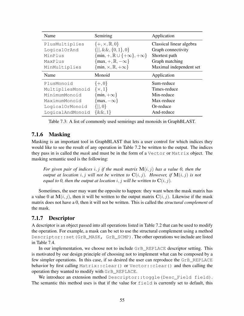
Name Semiring Application

PlusMultiplies {+,×,R, 0} Classical linear algebraLogicalOrAnd {||,&&, {0, 1}, 0} Graph connectivityMinPlus {min,+,R ∪ {+∞},+∞} Shortest pathMaxPlus {max,+,R,−∞} Graph matchingMinMultiplies {min,×,R,+∞} Maximal independent set

Name Monoid Application

PlusMonoid {+, 0} Sum-reduceMultipliesMonoid {×, 1} Times-reduceMinimumMonoid {min,+∞} Min-reduceMaximumMonoid {max,−∞} Max-reduceLogicalOrMonoid {||, 0} Or-reduceLogicalAndMonoid {&&, 1} And-reduce

Table 7.3: A list of commonly used semirings and monoids in GraphBLAST.

7.1.6 MaskingMasking is an important tool in GraphBLAST that lets a user control for which indices theywould like to see the result of any operation in Table 7.2 be written to the output. The indicesthey pass in is called the mask and must be in the form of a Vector or Matrix object. Themasking semantic used is the following:

For given pair of indices i, j if the mask matrix M(i, j) has a value 0, then theoutput at location i, j will not be written to C(i, j). However, if M(i, j) is notequal to 0, then the output at location i, j will be written to C(i, j).

Sometimes, the user may want the opposite to happen: they want when the mask matrix hasa value 0 at M(i, j), then it will be written to the output matrix C(i, j). Likewise if the maskmatrix does not have a 0, then it will not be written. This is called the structural complement ofthe mask.

7.1.7 DescriptorA descriptor is an object passed into all operations listed in Table 7.2 that can be used to modifythe operation. For example, a mask can be set to use the structural complement using a methodDescriptor::set(GrB_MASK, GrB_SCMP). The other operations we include are listedin Table 7.4.

In our implementation, we choose not to include GrB_REPLACE descriptor setting. Thisis motivated by our design principle of choosing not to implement what can be composed by afew simpler operations. In this case, if so desired the user can reproduce the GrB_REPLACEbehavior by first calling Matrix::clear() or Vector::clear() and then calling theoperation they wanted to modify with GrB_REPLACE.

We introduce an extension method Descriptor::toggle(Desc_Field field).The semantic this method uses is that if the value for field is currently set to default, this

55

Field Value Behavior

GrB_MASK (default) MaskGrB_SCMP Structural complement of mask

GrB_INP0 (default) Do not transpose first input parameterGrB_TRAN Transpose first input parameter

GrB_INP1 (default) Do not transpose second input parameterGrB_TRAN Transpose second input parameter

GrB_OUTP (default) Do not clear output before writing to masked indicesGrB_REPLACE Clear output before writing to masked indices

Table 7.4: A list of descriptor settings in GraphBLAST. Below the line are variants that are inthe GraphBLAS API specification that we do not support.

Figure 7.1: Decomposition of key GraphBLAS operations. Note that vxm is the same as mxvand setting the matrix to be transposed, so it is not shown.

method will set it to the non-default value and if it is currently set to non-default, it will set itto the default value. We found that if we want to reuse codepaths in our backend e.g. for AT fand fA, we can make the vector-matrix multiply call the matrix-vector codepath after callingDescriptor::toggle(GrB_INP1).

Another useful case is found in our code example (see Algorithm 11 (right)). Here, wewanted to use the same Descriptor object for several methods that required different GrB_MASKsettings. For example, the vector-matrix multiplication vxm requires the GrB_SCMP setting,but the assign requires the default setting. Instead of requiring the user to either: (1) use 2Descriptor objects, or (2) use a getter method and have the user implement using if-else state-ments how they want to change the Descriptor object using Descriptor::set, we simplifythe user experience by allowing them to call Descriptor::toggle(GrB_MASK).

7.1.8 Key GraphBLAS operationsLooking at Table 7.2, it is clear the most computationally intensive operations are the mxm,mxv, and vxm. We find empirically that these operations take over 90% of application runtime.For these operations, we will decompose them into constituent parts in order to better optimizetheir performance (see Figure 7.1).

56

7.1.9 Running example

(a) Graph representation (b) Linear algebraic representation

(c) Graph concepts and linear algebraic equivalents

Figure 7.2: Running example of breadth-first-search from source node 1. Currently, we are onlevel 2 and trying to get to level 3. To do so we need to do a graph traversal from current frontier(vertices 0, 2, 3) to their neighbors (vertices 4, 5, 7). This corresponds to the multiplication AT f .This is followed by filtering out of visited vertices (vertex 5), leaving us with the next frontier(vertices 4, 7). This corresponds to the elementwise multiply ¬v. ∗ (AT f).

57

As a running example in this paper, we will be talking about SpMV and SpMSpV with a directdependence on graph traversal. The key step we will be discussing is Line 8 of Algorithm 11,which is the matrix-formulation of parallel breadth-first-search. Illustrated in Figure 7.2b, thisproblem consists of a matrix-vector multiply followed by an elementwise multiplication be-tween two vectors: one is the output of the matrix-vector multiply and the other is the negation(or structural complement) of the visited vector.

Using the standard dense matrix-vector multiplication algorithm (GEMV), we would require8 × 8 = 64 memory accesses. However, if we instead treat the matrix not as a dense matrix,but as a sparse matrix in order to take advantage of input matrix sparsity, we can perform thesame computation in a mere 20 memory accesses into the sparse matrix. This number comesfrom counting the number of nonzeroes in the sparse matrix, which is equivalent to the numberof edges in the graph. Using this as the baseline, we will show in later sections how we can useoptimizations such as exploiting the input vector and output vector sparsity can further reducethe number of memory accesses required.

7.1.10 Code exampleHaving described the different components of GraphBLAST, we show a short code example ofhow to do breadth-first-search using the GraphBLAST interface alongside the linear algebra inAlgorithm 11. Before the while-loop, the vectors f and v representing the vertices currentlyactive in the traversal and the set of previously visited vertices are initialized.

Then in each iteration of the while-loop, the following steps take place: (1) vertices cur-rently active are added to the visited vertex vector, marked by the iteration they were first en-countered d, (2) the active vertices are traversed to find the next set of active vertices, and thenelementwise-multiplied by the negation of the set of active vertices (filtering out previouslyvisited vertices), (3) the number of active vertices of the next iterations is reduced as c, (4)the iteration number is incremented. This while-loop continues until there are no more activevertices (c reaches 0).

Our code example differs from the GraphBLAS spec in the following ways:

1. We require Matrix::build and Vector::build to use std::vector ratherthan C-style arrays. However, we will maintain compatibility with GraphBLAS C APIspecification by allowing C-style arrays too.

2. We pass in a template parameter specifying the type in place of: (1) passing a datatypeof GrB_Type to Matrix and Vector declaration, (2) specifying types used in thesemiring.

3. We have predefined semirings and monoids, whose naming scheme follows that of C++functors. As of May 2019, the latest version of GraphBLAS C API specification does nothave predefined semirings so users must construct semirings themselves.

4. We have convenience methods Vector::fill and Descriptor::toggle that arenot part of the GraphBLAS C API specification.

Regarding the use of template types, we plan to refactor our implementation to establishperfect compatibility with the GraphBLAS C API specification in the near future.

58

1: procedure MATRIXBFS(Graph A, Vector v, Source s)2: Initialize d← 1

3: Initialize f(i)←

{1, if i = s

0, if i 6= s

4: Initialize v← [0, 0, ..., 0]5: Initialize c← 16: while c > 0 do7: Update v← df + v8: Update f ← ATf .∗ ¬v . using Boolean semiring (see Table 7.3)9: Compute c←

∑ni=0 f(i) . using standard plus monoid (see Table 7.3)

10: Update d← d+ 111: end while12: end procedure

1 #include <graphblas/graphblas.hpp>2 using namespace graphblas;3

4 void bfs(Vector<float>* v,5 const Matrix<float>* A,6 Index s,7 Descriptor* desc) {8 Index A_nrows;9 A->nrows(&A_nrows);

10 float d = 1.f;11 Vector<float> f1(A_nrows);12 Vector<float> f2(A_nrows);13 std::vector<Index> indices(1, s);14 std::vector<float> values(1, 1.f);15 f1.build(&indices, &values, 1, GrB_NULL);16 v->fill(0.f);17 float c = 1.f;18 while (c > 0) {19 // Assign level d at indices f1 to visited vector v20 assign(v, &f1, GrB_NULL, d, GrB_ALL, A_nrows, desc);21 // Set mask to use structural complement (negation)22 desc->toggle(GrB_MASK);23 // Multiply frontier f1 by transpose of matrix A using visited vector24 // v as mask25 // Semiring: Boolean semiring (see Table 4)26 vxm(&f2, v, GrB_NULL, LogicalOrAndSemiring<float>(), &f1, A, desc);27 // Set mask to not use structural complement (negation)28 desc->toggle(GrB_MASK);29 f2.swap(&f1);30 // Check how many vertices of frontier f1 are active, stop when31 // number reaches 032 // Monoid: Standard addition (see Table 4)33 reduce(&c, GrB_NULL, PlusMonoid<float>(), &f1, desc);34 d++;35 }36 }

Algorithm 11: Matrix formulation of BFS (top) and example GraphBLAST code (bottom).

59

ApplicationMajor Feature Component BFS SSSP PR TC

Exploit input sparsityGeneralized direction-optimizationBoolean semiringAvoid sparse-to-dense conversion

Exploit output sparsity Masking

Load-balancingStatic mappingDynamic mapping (merge-based)

Table 7.5: Applicability of design principles.

As demonstrated in the code example, GraphBLAS has the advantage of being concise.Developing new graph algorithms in GraphBLAS requires modifying a single file and writingsimple C++ code. Provided a GraphBLAS implementation exists for a particular hardware,GraphBLAS code can be used with minimal change. Currently, we are working on a Pythonfrontend interface too, to allow users to build new graph algorithms without having to recom-pile. Over the next three sections, we will discuss the most important design principles formaking this code performant, which are exploiting input sparsity, output sparsity and goodload-balancing. Table 7.5 shows what applications our optimizations apply to.

7.2 Exploiting Input Sparsity (Direction-Optimization)In this section, we discuss our design philosophy of making exploiting input sparsity and one ofits consequences, direction-optimization, a first-class citizen of our implementation. Since thematrix represents a graph, the matrix will be assumed to be stored in sparse format. Therefore,by input sparsity, we are referring to the input vector being sparse and exploiting this fact toreduce the number of operations.

We provide quantitative data to support our conclusion that doing so is of the foremost im-portance in building a high-performance graph framework regardless of hardware. We presentthree seemingly unrelated challenges with implementing a linear algebra-based graph frame-work based on the GraphBLAS specification, but which we will show are actually facets of thesame problem:

1. Previous work [10, 61] has shown that direction-optimization is critical to achieving state-of-the-art performance on breadth-first-search. However, direction-optimization has beennotably absent in linear algebra-based graph frameworks and assumed only possible fortraditional, vertex-centric graph frameworks. How can direction-optimization be imple-mented as matrix-vector multiplication in a linear algebra-based framework like Graph-BLAS?

2. The GraphBLAS definition for mxv operation is underspecified. As Algorithms 12 and 13show, there are two ways to implement mxv. How should it be implemented?

60

(a) SpMV (20 memory accesses) (b) SpMSpV (8 memory accesses)

0 500000 1000000 1500000 2000000Number of nonzeroes in Vector/Mask

0

25

50

75

100

125

150

175

Runt

ime

(ms)

SpMV (cuSPARSE)SpMSpV (GraphBLAST)

(c) Algorithmic complexity of SpMV andSpMSpV as a function of vector sparsity.

0 25 50 75 100 125 150 175Millions of Edges

0

100

200

300

400

500

600

Runt

ime

(ms)

SpMV (cuSPARSE)SpMSpV (GraphBLAST)

(d) SpMV and SpMSpV runtime on Kroneckerscale-{16− 21} graphs.

Figure 7.3: Comparison of SpMV and SpMSpV.

3. The GraphBLAS definition for Matrix and Vector objects are underspecified. Whatshould the underlying data structure for these objects look like?

7.2.1 Two roads to matrix-vector multiplicationBefore we address the above challenges, we will draw a distinction between two different waysthe matrix-vector multiply y ← Ax can be computed. We distinguish between SpMV (sparsematrix-dense vector multiplication) and SpMSpV (sparse matrix-sparse vector multiplication).There is extensive literature focusing on SpMV for GPUs (a survey can be found in [31]).However, we concentrate on SpMSpV, because it is more relevant to graph search algorithmswhere the vector represents the subset of vertices that are currently active and is typically sparse.

Recall in the running example in Section 7.1.9 that by exploiting matrix sparsity (SpMV)in favor of dense matrix-vector multiplication (GEMV), we were able to bring the number ofmemory accesses down from GEMV’s 64 memory accesses down to SpMV’s 20. A naturalquestion to ask is whether it is possible to decrease the number of memory accesses furtherwhen the input vector is sparse? Indeed when we exploit input sparsity (SpMSpV) to get thesituation in Figure 7.3b, we can reduce the number of memory accesses from 20 down to 8.Similar how moving from GEMV to SpMV involved changing matrix storage format fromdense to sparse, moving from SpMV to SpMSpV similarly involves storing the vector in sparseformat. It is worth noting that the sparse vectors are assumed to be implemented as lists ofindices and values. A summary is shown in Table 7.6.

61

Matrix Input Vector Output VectorOperation Mask Expected Cost Sparsity (A) Sparsity (x) Sparsity (m)

GEMV no O(MN)SpMV (pull) no O(dM)SpMSpV (push) no O(d nnz(x) log nnz(x))

GEMV yes O(N nnz(m))SpMV (pull) yes O(d nnz(m))SpMSpV (push) yes O(d nnz(x) log nnz(x))

Table 7.6: Computational complexity of matrix-vector multiplication where d is the averagenumber of nonzeroes per row or column, and A is an M -by-N matrix. Top three rows indicatethe standard case y ← Ax, while the bottom three rows represent the masked case y ←Ax .∗m. Checkmarks indicate which form of sparsity each operation exploits.

Input: Sparse Matrix A, Dense Vector xOutput: Dense Vector y

1: procedure SPMV(A,x,y)2: for i = 0 to A.nrows −1 do3: y(i)←A(i, :)x4: end for5: end procedure

Algorithm 12: SpMV only exploits inputmatrix sparsity A(i, :).

Input: Sparse Matrix A, Sparse Vector xOutput: Sparse Vector y

1: procedure SPMSPV(A,x,y)2: for i s.t. x(i) 6= 0 do3: y←A(:, i)x(i)4: end for5: end procedure

Algorithm 13: SpMSpV exploits both inputvector sparsity (i s.t. x(i) 6= 0) and inputmatrix sparsity A(:, i).

7.2.2 Related workMirroring the dichotomy between SpMSpV and SpMV, there are two methods to perform oneiteration of graph traversal, which are called push and pull. They can be used to describe graphtraversals in a variety of graph traversal-based algorithms such as breadth-first-search, single-source shortest-path and PageRank.

In the case of breadth-first-search, push refers to starting from the current frontier (set ofvertices we are doing graph traversal from) and looking for children of this set of vertices.Then, out of this set of children, the previously visited vertices must be filtered out to generatethe next iteration’s frontier. On the other hand, pull refers to starting from the set of unvisitedvertices and looking back to find their parents. Those nodes who have a parent in the currentfrontier, we will add them to next iteration’s frontier. Beamer, Asanovic and Patterson [10]observed that in the middle iterations of a BFS on scale-free graphs, the frontier would get largeand each neighbor would be found many times leading to redundant work. In these iterations,they would switch to pull and in later iterations, back to push.

Many graph algorithms such as breadth-first-search, single-source shortest-path and PageR-ank involve multiple iterations of graph traversals. Switching between push and pull in dif-ferent iterations applied to the specific algorithm of breadth-first-search is called direction-

62

Figure 7.4: Where this work on direction-optimization fits in literature.

optimization or direction-optimized BFS, which was discovered by Beamer, Asanovic and Pat-terson. Sometimes, it is also known as push-pull. Building on this work, Shun and Blelloch [61]were able to generalize direction-optimization to graph traversal algorithms beyond BFS. Toavoid confusion with the BFS-specific instance, we refer to Shun and Blelloch’s discovery gen-eralized direction-optimization.

In Beamer, Asanovic and Patterson later work [11], they looked at matrix-vector multiplica-tion in the context of SpMV and SpMSpV-based implementations for PageRank. In both theirwork and that of Besta et al. [13], it was noted that switching between push/pull is the sameas switching between SpMSpV/SpMV. In both works, authors show there is a one-to-one cor-respondence between push and SpMSpV, and between pull and SpMV; they are two ways ofthinking about the same concept.

A summary of the work in this area is shown in Figure 7.4. Comparing with the workof Beamer, Asanovic and Patterson and of Besta et al., our work differs in several ways: (1)they emphasize graph algorithm research, whereas we focus on building a graph framework,(2) their work targets multithreaded CPU, while ours targets GPU, and (3) their interface isvertex-centric, but ours is linear algebra-based.

Building on our earlier work, our contribution in this work is being the the first to extend thegeneralized direction-optimization technique to linear algebra-based framework based on theGraphBLAS specification. This is in contrast to previous implementations to the GraphBLASspecification, GBTL [73] and SuiteSparse [25], which do not support generalized direction-optimization and in consequence, trail the state-of-art graph frameworks in performance.

63

In both implementations, the operation mxv is implemented as a special case of mxm whenone of the matrix dimensions is 1 (i.e. is a Vector). The mxm implementation is a variantof Gustavson’s algorithm [37], which takes advantage of both matrix sparsity and input vectorsparsity, so it has a similar performance characteristic as SpMSpV. Therefore, it shares SpM-SpV’s poor performance as the vector sparsity increases. In other words, neither GBTL andSuiteSparse automatically switch to pull when the input vector becomes large in middle iter-ations of graph traversal algorithms like BFS, and perform push throughout the entire BFS.In comparison, our graph framework balances exploiting input vector sparsity (SpMSpV) withthe efficiency of SpMV during iterations of high input vector sparsity. This helps us match orexceed the performance of existing graph frameworks (see Section 7.6).

7.2.3 ImplementationIn this subsection, we will revisit the three challenges we claimed boil down to different facetsof the same challenge: exploiting input sparsity.

Direction-optimization Backend automatically handles direction-optimization when mxv iscalled, by calling either the SpMV or SpMSpV routine, whichever one yields fewer mem-ory accesses based on an empirical cost model.

mxv: SpMV or SpMSpV Both routines are necessary for an efficient implementation of mxvin a graph framework.

Matrix and Vector storage format For Matrix store both CSR and CSC, but give users op-tion to save memory by using a memory efficient, performance inefficient solution by onlystoring one of two representations. For Vector, since dense vector and sparse vector arerequired for the two different routines SpMV and SpMSpV respectively, give backendresponsibility of switching between dense and sparse vector representations. Allow userto give hint as to the initial storage of the Matrix and Vector object.

7.2.3.1 Direction-optimizationBackend automatically handles direction-optimization when mxv is called, by calling either theSpMV or SpMSpV routine, whichever one yields fewer memory accesses based on an empiricalcost model.

Table 7.7 shows how our decision to change directions compares with existing literature.We make the following simplifying assumptions:

1. On GPUs, computing the precise number of neighbors |Ef | requires prefix-sum compu-tations. To avoid what in Beamer’s paper called a non-significant amount of overhead,we instead approximate the precise number of neighbors using the number of nonzeroesin the vector by assuming that in expectation, each vector has around the same number ofneighbors i.e. d|Vf | ≈ |Ef |. Gunrock makes this assumption too.

2. When the mask (representing the unvisited vertices) is dense, counting the number ofnonzeroes |Vu| requires an additional GPU kernel launch, which represents significantoverhead. Therefore, we make the assumption that the number of unvisited vertices is all

64

Work Direction Criteria Application

Beamer et al. [10] push→ pull |Ef | > |Eu|/14 and increasing BFS onlypush← pull |Vf | < |V |/24 and decreasing BFS only

Ligra [61] push→ pull |Ef | > |E|/20 generalizedpush← pull |Ef | < |E|/20 generalized

Gunrock [67] push→ pull |E∗f | > |E∗u|/1000 BFS onlypush← pull |E∗f | < |E∗u|/5 BFS only

This work push→ pull |E∗f | > |E|/10 generalizedpush← pull |E∗f | < |E|/10 generalized

Table 7.7: Direction-optimization criteria for four different works. |Vf | indicates number ofnonzeroes in frontier f . |Ef | indicates number of neighbors from frontier f . |Eu| indicatesnumber of neighbors from unvisited vertices. Superscript ∗ indicates the value is approximatedrather than precisely calculated.

vertices i.e. |Vu| ≈ |V | so |Eu| ≈ |E|. We find this is a reasonable assumption to make,because for scale-free graphs the optimal time to switch from push to pull is very earlyon, so |Vu| ≈ |V |. Ligra also makes this assumption.

7.2.3.2 mxv: SpMV or SpMSpVFollowing an earlier work by the authors [70], which showed that SpMV is not performantenough for graph traversal and that SpMSpV is necessary, we run our own microbenchmarkregarding GraphBLAS. In our microbenchmark, we benchmarked how using SparseVectorvariant of graphblas::mxv performed compared with DenseVector as a function ofVector sparsity for a synthetic undirected Kronecker graph with 2M vertices and 182M edges.For more details of the experiment setup, see Section 7.6.

As our microbenchmark in Figure 7.3 illustrates, the SpMSpV variant of graphblas::mxvscales with the sparsity of the input vector. However, SpMV variant is constant. This matchesthe theoretical complexity shown in Table 7.6, which shows that SpMV scales with O(dM),which is irrespective of input vector sparsity. However, SpMSpV is able to factor in the spar-sity of the input vector (i.e. nnz(x)) into the computational cost. Another observation is thatSpMSpV has an additional logarithmic factor compared to SpMV. This is because the columnsmust either be merged together in a multi-way merge, hash table or by using atomics.

7.2.3.3 Matrix and Vector storage formatOne of the most important design choices an implementer needs to make is whether Matrixand Vector objects ought to be stored in dense or sparse storage, and if sparse which type ofsparse matrix or vector storage?

For Matrix objects, the decision is clear-cut. Since graphs tend to have more than 99.9%sparsity and upwards of millions of vertices, storing them in dense format would be wastefuland in some cases impossible because it exceeds available device memory. We use the popularCSR (Compressed Sparse Row), because they are standard in graph analytics and in order tosupport fast row access required by SpMV. Similarly since we need to support SpMSpV, theCSC data structure is necessary to support fast column access (see Figure 7.3).

65

For Vector objects, we have both a dense storage and a sparse storage. The dense storageis a flat array of values. The sparse storage is a list of sorted indices and values for all nonzeroelements in the vector. Through additional Vector object methods Vector::buildDenseand Vector::fill as shown in Table 7.1, we allow the user to give the backend hints onwhether they want the object to initially be stored in dense or sparse storage.

7.2.4 Direction-optimization insightsExploiting input sparsity is a very useful and important strategy for high-performance in graphtraversals. This section showed that the GraphBLAS interface is at the right level of abstrac-tion that the user does not have to specify whether or not they want to exploit input sparsity;instead, they only need to write the code once using the mxv interface and both forms of SpMVand SpMSpV code are automatically generated for them by GraphBLAST. In the next section,we will show how the number of memory accesses can also be reduced by exploiting outputsparsity.

7.3 Exploiting Output Sparsity (Masking)The previous section discussed how important it is to reduce the number of memory accesses byusing input vector sparsity. This section deals with the mirror situation, which is output vectorsparsity (or output sparsity). Output vector sparsity can also be referred to as an output mask ormasking for short.

Masking allows GraphBLAS users to tell the framework they are planning to follow up amatrix-vector or matrix-matrix multiply with an elementwise product. This gives the backendopportunity to implement the fused mask optimization, which in some cases may reduce thenumber of computations needed. Alongside exploiting input sparsity, our design philosophywas to make exploiting output sparsity a first-class citizen in GraphBLAST with highly-efficientimplementations of masking. Masking raises the following implementation challenges.

1. Masking is a novel concept introduced by the GraphBLAS API to allow users to decidewhich output indices they do and do not care about computing. How can masking beimplemented efficiently?

2. When should the mask be accessed before the computation in out-of-order fashion andwhen should it be processed after the computation?

7.3.1 Motivation and applications of maskingFollowing the brief introduction to masking in Section 7.3, the reader may wonder why such anoperation is necessary. Masking can be thought of in two ways: (i) masking is a way to fuse anelement-wise operation with another operation from Table 7.2; and (ii) masking allows the userto express for which indices they do and do not require a value before the actual computation isperformed. We define this as output sparsity. The former means that masking is a way for theuser to tell the framework there is an opportunity for kernel fusion, while the latter is an intuitiveway to understand why masking can reduce the number of computations in graph algorithms.

There are several graph algorithms where exploiting output sparsity can be used to reducethe number of computations:

66

1. In breadth-first-search [18, 72] where the mask Vector represents the visited set ofvertices. Since in a breadth-first-search each vertex only needs to be visited once, theuser can let the software know that the output need not include any vertices from thevisited set.

2. In single-source shortest-path [24] where the mask Vector represents the set of verticesthat have seen their distances from source vertex change in this iteration. The mask canthus be used to zero out currently active vertices from the next traversal, because theirdistance information has already been taken into account in earlier traversal iterations.The mask can be used to help keep the active vertices Vector that would otherwise beincreasingly densifying sparse throughout the SSSP.

3. In adaptive PageRank (also known as PageRankDelta) [40, 61] where the mask Vectorrepresents the set of vertices that has converged already. The PageRank value for this setof vertices does not need to be updated in future iterations.

4. In triangle counting [5, 69] where the mask Matrix represents the adjacency matrixwhere a value 1 at M(i, j) indicates the presence of edge i → j, and 0 indicates a lackof an edge. Performing a dot product M ×M corresponds to finding for each index pair(i, j) the number of wedges i → k → j that can be formed for all k ∈ V . Adding themask Matrix then will yield M ×M. ∗M , which indicates the number of wedges thatare also triangles by virtue of the presence of edge i → j. The .∗ operation indicateselement-wise operation.

7.3.2 MicrobenchmarksSimilar to the earlier microbenchmark, we benchmark how using masked SpMV and SpMSpVvariants of graphblas::mxv performed compared with unmasked SpMV and SpMSpV as afunction of mask Vector sparsity for a synthetic undirected Kronecker graph with 2M verticesand 182M edges. For more details of the experiment setup, see Section 7.6.

As our microbenchmark in Figure 7.5 illustrates, the masked SpMV variant of graphblas::mxvscales with the sparsity of the mask Vector. However, the masked SpMSpV is unchangedfrom the unmasked SpMSpV. This too matches the theoretical complexity shown in Table 5.1,which shows that masked SpMV scales with O(d nnz(m)), where m is the mask Vector.However, masked SpMSpV only performs the elementwise multiply with the mask after theSpMSpV operation, so it is unable to benefit from the mask’s sparsity.

In the running example, recall in Figure 7.5a that standard SpMV, which performs thematrix-vector multiply followed by the elementwise product with the mask took 20 memoryaccesses. However, when we reverse the sequence of operations by loading the mask, seeingwhich elements of the mask are nonzero and then only doing the matrix-vector multiply forthose rows that map to a nonzero mask element, we see that the number of memory accessesdrops significantly from 20 down to 10.

7.4 Load-balancingIn this section, we discuss ways to implement the memory access patterns SpMV, SpMSpV,SpMM and SpGEMM in a way that tries to address the problem of load imbalance. We focus

67

(a) SpMV not fused with mask (20 memory ac-cesses)

(b) SpMV fused with mask (10 memory ac-cesses)

0 500000 1000000 1500000 2000000Number of nonzeroes in Vector/Mask

0

50

100

150

200

250

Runt

ime

(ms)

SpMV (cuSPARSE)SpMV fused mask (GraphBLAST)SpMSpV with and without mask (GraphBLAST)

(c) Algorithmic complexity of SpMSpV andSpMV with and without masking as a functionof vector sparsity.

0 25 50 75 100 125 150 175Millions of Edges

0

100

200

300

400

500

600

Runt

ime

(ms)

SpMV (cuSPARSE)SpMSpV (GraphBLAST)SpMSpV struconly (GraphBLAST)SpMSpV + SpMV fusedmask (GraphBLAST)

(d) SpMV and SpMSpV runtime on Kroneckerscale-{16− 21} graphs.

Figure 7.5: Comparison with and without fused mask.

on the backend implementations of these four patterns, because they are the implementationsbehind mxm, mxv and vxm, which are the most computationally intensive and important op-erations in GraphBLAS (see Table 7.2). These are the operations that make or break one’simplementation of GraphBLAS.

Recall in Section 7.1. we mentioned that an operation is a memory access pattern commonto many graph algorithms. A typical problem in graph algorithms is that most processing unitshave already completed their work, but a few are still working. This naturally emerges inalgorithms such as breadth-first-search on scale-free graphs, where it is common for there to bea few supernodes with thousands of neighbors, yet most nodes with only tens of neighbors. Insuch a situation, if one were to simply assign one GPU warp (a computing unit composed of 32threads) to each node in order to find its neighbors, the warps that got assigned these supernodeswould become the bottleneck of the computation.

This is a case of load imbalance. We try to address this problem in the context of the fouraforementioned memory access patterns. However, the problem or load imbalance cannot besolved completely. It often forces one to make tradeoffs in terms of the following:

• Graph traversal throughput (higher is better)

• Synchronizations (fewer is better)

68

Technique Description

Static workload mapping Assign thread, warp or CTA to matrix row or nonzero, but loadbalance could be arbitrarily bad depending on dataset

Dynamic workload mapping Divide computations evenly amongst threads, but need to payfor load-balance overhead (usually 2 additional kernel launchesand limited amount of global memory accesses)

Mask before multiply Get benefit of mask sparsity, but may require more irregularmemory access pattern such as binary search per thread

Mask after multiply Miss out on benefit of mask sparsity, but no need to take onirregular memory access pattern

Table 7.8: Summary of load-balancing techniques used in GraphBLAST.

• Kernel launches (fewer is better)

• Memory accesses (fewer is better)

The load-balancing techniques we consider fall into two categories—workload mappingstrategy and mask sparsity strategy (see Table 7.8). For masked variants of each memory ac-cess pattern, we must decide whether it is better to apply the mask (i.e. perform elementwisemultiply) before the matrix multiply or after the matrix multiply.

7.4.1 Matrix-vector multiplyIn matrix-vector multiply, the problem we are solving is y = Ax and for the masked varianty = Ax. ∗m.

7.4.1.1 SpMV: Sparse matrix-dense vectorFor unmasked SpMV, the dynamic workload mapping, also known as merge-based load-balancing(load-balancing based on merge path [29, 35], which is an algorithm for merging two lists inparallel) was pioneered by Baxter [8] and Dalton, Olson and Bell [23]. However, Merrill andGarland [51] noted that this was not a true merge path-based solution. provided a dataset hasan arbitrarily large number of empty rows. The difference between static and dynamic load-balancing schemes is shown in Figure 6.2.

Static workload mapping Assigns thread, warp or block to each matrix row.

Dynamic workload mapping We use the SpMV implementation from ModernGPU library [8]as our SpMV. We find that it outperforms static workload mapping in most circumstancesthat it can be used by default.

Masked variant Use static work mapping of assigning a warp per mask nonzero.

7.4.1.2 SpMSpV: Sparse matrix-sparse vectorStatic workload mapping We are planning to explore this approach in the future.

69

Dynamic workload mapping We use the multi-kernel approach described by the authors inan earlier paper [70]. One advantage of this approach is that it allows the SpMSpV to bedone without needing atomics. However, the disadvantage is that it requires |E| additionalmemory. This approach is suitable for scale-free graphs, but has a lot of kernel launchand memory access overhead, so it does not do so well on road network graphs.

Masked variant The mask is better to be applied afterwards, because there are typically muchmore nonzeroes in the mask compared to the input vector.

7.4.2 Matrix-matrix multiplyIn matrix-matrix multiply, the problem we are solving is C = AB and for the masked variantC = AB. ∗M.

7.4.2.1 SpMM: Sparse matrix-dense matrixIn this problem, we assume we are dealing with multiplying square sparse matrix by a tall-and-skinny dense matrix. This is due to the typical main memory of the GPU being limited to12 GB. We make the following assumptions: 1) floating point precision, 2) the 1M×1M sparsematrix takes up 2 GB, and 3) the input and output being 1M × N dense matrices taking 5 GBeach. These assumptions yieldd a value of N = 1250 for the number of columns, which meansin order to fit into GPU main memory the dense matrix must be a tall-and-skinny matrix.

Static workload mapping Assigns thread, warp or block to each matrix row.

Dynamic workload mapping We developed our own SpMM implementation [71] that is basedon the dynamic mapping SpMV variant. We use this when the number of nonzeroes perrow in A is less than 9.35.

Masked variant Typically, the mask can be assumed to be a sparse matrix, so the implementa-tion follows masked SpGEMM. The only difference is the right-hand-side matrix (in thiscase, dense) can be directly indexed skipping the binary search.

7.4.2.2 SpGEMM: Sparse matrix-sparse matrixStatic workload mapping We base our hash table-based SpGEMM on work by Naumov et

al. [55]. Following Naumov et al., we use a 2-step implementation of Gustavson’s algo-rithm [37]: 1) In the first step, we count how many nonzeroes there will be in the outputin order to populate the row pointers (deduplication done using the hash table, hash tablesize returns the number of nonzeroes), and 2) In the second step, we perform the multipli-cation. The memory access pattern in both steps is similar, and the only difference beingthe computation.

Dynamic workload mapping We are planning to explore this approach in the future.

Masked variant In our implementation, we use a generalization of this primitive where weassume we are solving the problem for three distinct matrices C = AB. ∗M. We usea straightforward static work mapping where we assign a warp per row of the mask M,and for every nonzero M(i, j) in the mask each warp loads the row of A(i, :) in order

70

(a) BFS (b) SSSP (Bellman-Ford)

(c) PR (d) TC

(e) SSSP (Bellman-Ford with sparsification)

Figure 7.6: Operation flowchart for different algorithms expressed in GraphBLAS. A loop in-dicates a while-loop that runs until the Vector is empty.

to perform the dot-product A(i, :)B(:, j). Using their A-element, thread in the warpperforms binary search on column B(:, j) and accumulates the result of the multiplication.After the row is finished, a warp reduction is done, and the output written to C(i, j).

7.5 ApplicationsOne of the main advantages of GraphBLAS is that the operations can be composable to developnew graph algorithms. For each application in this section, we describe the hardwired GPUimplementation and how our implementation can be expressed using GraphBLAS. Then thenext section will compare performance between hardwired and GraphBLAS implementations.Figure 7.6 shows the GraphBLAS algorithms required to implement each algorithm

7.5.1 Breadth-first-searchGiven a source vertex s ∈ V , a BFS is a full exploration of graph G that produces a spanningtree of the graph, containing all the edges that can be reached from s, and the shortest path froms to each one of them. We define the depth of a vertex as the number of hops it takes to reach

71

this vertex from the root in the spanning tree. The visit proceeds in steps, examining one BFSlevel at a time. It uses three sets of vertices to keep track of the state of the visit: the frontiercontains the vertices that are being explored at the current depth, next has the vertices that canbe reached from frontier, and visited has the vertices reached so far. BFS is one of the mostfundamental graph algorithms and serves as the basis of several other graph algorithms.

Hardwired GPU implementation The best-known BFS implementation of Merrill et al. [52]achieves its high performance through careful load-balancing, avoidance of atomics, andheuristics for avoiding redundant vertex discovery. Its chief operations are expand (togenerate a new frontier) and contract (to remove redundant vertices) phases. Enter-prise [47], a GPU-based BFS system, introduces a very efficient implementation thatcombines the benefits of direction optimization of Beamer, Asanovic and Patterson [10],adaptive load-balancing workload mapping strategy of Merrill et al., and not synchroniz-ing each BFS iteration which addresses the kernel launch overhead problem.

GraphBLAST implementation Merrill et al.’s expand and contract maps nicely to Graph-BLAST’s mxv operator with mask using a Boolean semiring. Like Enterprise, we im-plement efficient load-balancing (Section 7.4) and direction-optimization, which wasdescribed in greater detail in Section 7.2. We do not use Enterprise’s method of skip-ping synchronization between BFS iterations, but we use optimizations early-exit andstructure-only, that are consequences of the Boolean semiring that is associated with BFS.We also use operand reuse, which avoids having to convert from sparse to dense duringdirection-optimization. These optimizations are inspired by Gunrock and are describedin detail by authors in an earlier work [72].

7.5.2 Single-source shortest-pathGiven a source vertex s ∈ V , a SSSP is a full exploration of weighted graph G that produces adistance array of all vertices v reachable from s representing paths from s to each v such thatthe path distances are minimized.

Hardwired GPU Implementation Currently the highest performing SSSP algorithm imple-mentation on the GPU is the work from Davidson et al. [24]. They provide two keyoptimizations in their SSSP implementation: (1) a load balanced graph traversal method,and (2) a priority queue implementation that reorganizes the workload.

GraphBLAST implementation We take a different approach from Davidson et al. to solveSSSP. We show that our approach both avoids the need for ad hoc data structures such aspriority queues and wins in performance. The optimizations we use are: (1) generalizeddirection-optimization which is handled automatically within the mxv operation ratherthan inside the user’s application code, and (2) sparsifying the set of active vertices aftereach iteration, by comparing each active vertex to see whether or not they improved overthe stored distance in the distance array. The second step introduces two additional steps(compare Figures 7.6b and 7.6e).

72

7.5.3 PageRankThe PageRank link analysis algorithm assigns a numerical weighting to each element of a hy-perlinked set of documents, such as the World Wide Web, with the purpose of quantifying itsrelative importance within the set. The iterative method of computing PageRank gives each ver-tex an initial PageRank value and updates it based on the PageRank of its neighbors, until thePageRank value for each vertex converges. There are variants of the PageRank algorithm thatstop computing PageRank for vertices that have converged already and also remove it from theset of active vertices. This is called adaptive PageRank [40] (also known as PageRankDelta).In this paper, we do not implement or compare against this variant of PageRank.

Hardwired GPU Implementation One of the highest performing implementations of PageR-ank is written by Khorasani, Vora and Gupta [43]. In their system, they use solve theload imbalance and GPU underutilization problem with a GPU adoption of GraphChi’sParallel Sliding Window scheme [45]. They call this preprocessing step “G-Shard” andcombine it with a concatenated window method to group edges from the same source IDs.

GraphBLAST implementation In GraphBLAST, we rely on the merge-based load-balancingscheme discussed in Section 7.4. The advantage of the merge-based scheme is that unlikeKhorasani, Vora and Gupta, we do not need any specialized storage format; the GPU isefficient enough to do the load-balancing on the fly. In terms of exploiting input sparsity,we demonstrate that our system is intelligent enough to determine that we are doing re-peated matrix-vector multiplication where the vector does not get any sparser, it is moreefficient to use SpMV rather than SpMSpV.

7.5.4 Triangle countingTriangle counting is the problem of counting the number of unique triplets u, v, w in an undi-rected graph such that (u, v), (u,w), (v, w) ∈ E. Many important measures of a graph aretriangle-based, such as clustering coeffcient and transitivity ratio.

Hardwired GPU Implementation The best-performing implementation of triangle countingis by Bisson and Fatica [14]. There, they demonstrate the use of a static workload map-ping of thread, warp, block per matrix row together with using bitmaps is a very goodapproach to this problem.

GraphBLAST Implementation In GraphBLAST, we follow Azad and Buluc [5] and Wolf etal. [69] in modeling the TC problem as a masked matrix-matrix multiplication problem.Given an adjacency matrix of an undirected graph A, and taking the lower triangularcomponent L, it can be shown that the number of triangles is the reduction of the matrixB = LLT .∗L to a scalar. In our implementation, we use a generalization of this algorithmwhere we assume we are solving the problem for three distinct matrices A, B and Mby computing C = AB . ∗M. We use a straightforward static work mapping wherewe assign a warp per row of the mask M, and for every nonzero M(i, j) in the maskeach warp loads the row of A(i, :) in order to perform the dot-product A(i, :)B(:, j).Using their A-element, thread in the warp performs binary search on column B(:, j) and

73

Dataset Vertices Edges Max Degree Diameter Type

soc-orkut 3M 212.7M 27,466 9 rssoc-Livejournal1 4.8M 85.7M 20,333 16 rs

hollywood-09 1.1M 112.8M 11,467 11 rsindochina-04 7.4M 302M 256,425 26 rsrmat s22 e64 4.2M 483M 421,607 5 gsrmat s23 e32 8.4M 505.6M 440,396 6 gsrmat s24 e16 16.8M 519.7M 432,152 6 gs

rgg n 24 16.8M 265.1M 40 2622 gmroadnet USA 23.9M 577.1M 9 6809 rm

coAuthorsCiteseer 227K 1.63M 1372 31* rscoPapersDBLP 540K 30.6M 3299 18* rs

cit-Patents 3.77M 33M 793 24* rscom-Orkut 3.07M 234M 33313 8* rsroad central 14.1M 33.9M 8 4343* rm

Table 7.9: Dataset Description Table. Graph types are: r: real-world, g: generated, s: scale-free, and m: mesh-like. All datasets have been converted to undirected graphs. Self-loops andduplicated edges are removed. Datasets above the middle divide are used for BFS, SSSP andPR. Datasets below it are used for TC. An asterisk indicates the diameter is estimated usingsamples from 10,000 vertices.

accumulates the result of the multiplication. After the row is finished, a warp reduction isdone, and the output written to C(i, j). This is followed by a reduction of matrix C to ascalar returning the number of triangles in graph A.

7.6 Experimental ResultsWe first show overall performance analysis of GraphBLAST on nine datasets including bothreal-world and generated graphs; the topology of these datasets spans from regular to scale-free. Five additional datasets are used specifically for triangle counting, because they are theones typically used for comparison of triangle counting [14, 66].

We ran all experiments in this paper on a Linux workstation with 2×3.50 GHz Intel 4-core,hyperthreaded E5-2637 v2 Xeon CPUs, 528 GB of main memory, and an NVIDIA K40c GPUwith 12 GB on-board memory. GPU programs were compiled with NVIDIA’s nvcc compiler(version 8.0.44) with the -O3 flag. Ligra was compiled using icpc 15.0.1 with CilkPlus. SuiteS-parse was compiled using g++ 4.9.3. All results ignore transfer time (both disk-to-memoryand CPU-to-GPU). All Gunrock and GraphBLAST tests were run 10 times with the averageruntime and MTEPS used for results.

Datasets We summarize the datasets in Table 7.9. soc-orkut (soc-ork), com-Orkut (com-ork), soc-Livejournal1 (soc-lj), hollywood-09 (h09) are social graphs; indochina-04 (i04) is acrawled hyperlink graph from indochina web domains; coAuthorsCiteseer (coauthor), coPa-persDBLP (copaper), and cit-Patents (cit-pat) are academic citation and patent citation net-works; rmat s22 e64 (rmat-22), rmat s23 e32 (rmat-23), and rmat s24 e16 (rmat-24) are three

74

Runtime (ms) [lower is better] Edge throughput (MTEPS) [higher is better]SuiteSparse Hardwired Hardwired

Alg. Dataset GraphBLAS GPU Ligra Gunrock GraphBLAST SuiteSparse GPU Ligra Gunrock GraphBLASTB

FS

soc-ork 2165 25.81 26.1 5.573 7.230 98.24 12360 8149 38165 29217soc-lj 1483 36.29 42.4 14.05 14.16 57.76 5661 2021 6097 6049h09 596.7 11.37 12.8 5.835 7.138 188.7 14866 8798 19299 15775i04 1866 67.7 157 77.21 80.37 159.8 8491 1899 3861 3709

rmat-22 4226 41.81 22.6 3.943 4.781 114.3 17930 21374 122516 101038rmat-23 6033 59.71 45.6 7.997 8.655 83.81 12971 11089 63227 58417rmat-24 8193 270.6 89.6 16.74 16.59 63.42 1920 5800 31042 31327

rgg 230602 138.6 918 593.9 2991 1.201 2868 288.8 466.4 92.59road usa 9413 141 978 676.2 7155 6.131 1228 59.01 85.34 8.065

SSSP

soc-ork NI 807.2 595 981.6 676.7 NI 263.5 357.5 216.7 314.3soc-lj NI 369 368 393.2 256.3 NI 232.2 232.8 217.9 334.2h09 NI 143.8 164 83.2 109.123 NI 783.4 686.9 1354 1032i04 NI — 397 371.8 414.5 NI — 750.8 801.7 719.2

rmat-22 NI — 774 583.9 477.5 NI — 624.1 827.3 1011.7rmat-23 NI — 1110 739.1 680.0 NI — 455.5 684.1 743.6rmat-24 NI — 1560 884.5 905.2 NI — 333.1 587.5 574.0

rgg NI — 80800 115554 144291 NI — 3.28 2.294 1.84road usa NI 4860 29200 11037 144962 NI 11.87 1.98 5.229 0.398

Page

Ran

k

soc-ork 1230 52.54 476 173.1 64.22 173.0 4048 446.8 1229 3312soc-lj 1386 33.61 200 54.1 21.54 61.83 2550 428.5 1584 3978h09 386.8 34.71 77.4 20.05 8.12 33.10 368.8 165.4 638.4 1577i04 1390 164.6 210 41.59 19.16 217.3 1835 1438 7261 15763

rmat-22 5764 188.5 1250 304.5 115.6 83.79 2562 386.4 1586 4178rmat-23 7089 147 1770 397.2 161.3 71.32 3439 285.6 1273 3134rmat-24 8895 128 2180 493.2 211.5 58.42 4060 238.4 1054 2457

rgg 2991 53.93 247 181.3 34.58 88.64 4916 1073 1462 7665road usa 2746 — 209 24.11 26.91 210.2 — 2761 23936 21449

TC

coauthor 11.06 2.2 — 4.51 5.96 73.6 370 — 181 137copaper 103.8 64.4 — 197 246 309 498 — 163 130soc-lj 6322 295 490 896 1125 10.9 234 141 77.0 61.3cit-pat 1907 34.5 79.5 156 137 8.65 478 208 105 121

com-ork 27887 1626 1920 6636 5367 4.2 72.1 61.0 17.7 21.8road cent 895.2 5.6 — 61.4 78.7 18.9 3018 — 275 215

Table 7.10: GraphBLAST’s performance comparison (runtime and edge throughput) with othergraph libraries (SuiteSparse, Ligra, Gunrock) and hardwired GPU implementations on a TeslaK40c GPU. All PageRank times are normalized to one iteration. Hardwired GPU implementa-tions for each primitive are Enterprise (BFS) [47], delta-stepping SSSP [24], pull-based PR [43],and triangle counting [14]. NI means the algorithm is not implemented on a framework. Amissing data entry means either there is a runtime error.

generated R-MAT graphs. All seven datasets are scale-free graphs with diameters of less than 30and unevenly distributed node degrees (80% of nodes have degree less than 64). Both rgg n 24(rgg), road central (road cent) and roadnet USA (road usa) datasets have large diameters withsmall and evenly distributed node degrees (most nodes have degree less than 12). soc-ork andcom-Ork are from Network Repository [60]; soc-lj, i04, h09, road central, road usa, coauthor,copaper, and cit-pat are from University of Florida Sparse Matrix Collection [26]; rmat-22,rmat-23, rmat-24, and rgg are R-MAT and random geometric graphs we generated. The edgeweight values (used in SSSP) for each dataset are random values between 1 and 64.

Measurement methodology We report both runtime and traversed edges per second (TEPS)as our performance metrics. (In general we report runtimes in milliseconds and TEPS as mil-lions of traversals per second [MTEPS].) Runtime is measured by measuring the GPU kernelrunning time and MTEPS is measured by recording the number of edges visited during the run-ning (the sum of neighbor list lengths of all visited vertices) divided by the runtime. When alibrary does not report MTEPS, we use the following equation to compute it: |E|

twhere E is the

number of edges in the graph and t is runtime.

75

soc-or

ksoc

-lj h09 i04

rmat2

2

rmat2

3

rmat2

4 rgg

road_u

sa10−1

100

101

102

103

104

105

Perfo

rman

ce (M

TEPS

)BFS

soc-or

ksoc

-lj h09 i04

rmat2

2

rmat2

3

rmat2

4 rgg

road_u

sa

SSSP

soc-or

ksoc

-lj h09 i04

rmat2

2

rmat2

3

rmat2

4 rgg

road_u

sa

PR

coauth

or

copap

er

road_c

ent

soc-lj

cit-pa

t

com-or

k

TCSuiteSparseHardwiredLigraGunrockGraphBLAST

(a) Performance (MTEPS) [higher is better]

soc-or

ksoc

-lj h09 i04

rmat2

2

rmat2

3

rmat2

4 rgg

road_u

sa

101

102

103

104

105

Perfo

rman

ce (M

TEPS

)

BFS

soc-or

ksoc

-lj h09 i04

rmat2

2

rmat2

3

rmat2

4 rgg

road_u

sa

SSSP

soc-or

ksoc

-lj h09 i04

rmat2

2

rmat2

3

rmat2

4 rgg

road_u

sa

PR

coauth

or

copap

er

road_c

ent

soc-lj

cit-pa

t

com-or

k

TCSuiteSparseHardwiredLigraGunrockGraphBLAST

(b) Runtime (ms) [lower is better]

Figure 7.7: Performance in MTEPS and milliseconds for GraphBLAST vs. four other graphprocessing libraries and hardwired algorithms on nine different graph inputs. Data is fromTable 7.10.

7.6.1 Performance summaryTable 7.10 and Figure 7.7 compare GraphBLAST’s performance against several other graphlibraries and hardwired GPU implementations. In general, GraphBLAST’s performance ontraversal-based algorithms (BFS and SSSP) is better on the seven scale-free graphs (soc-orkut,soc-lj, h09, i04, and rmats) than on the small-degree large-diameter graphs (rgg and road usa).The main reason is our load-balancing strategy during traversal and particularly our emphasison high-performance for highly irregular graphs. Therefore, we incur certain amount of over-head for our merge-based load-balancing and requiring kernel launch in every iteration. Forthese types of graphs, asynchronous approaches pioneered by Enterprise [47] that do not re-quire exiting the kernel until the breakpoint has been met is a way to address the kernel launchproblem. However, this does not work for non-BFS solutions, so asynchronous approaches inthis area remains an open problem. In addition, graphs with uniformly low degree expose lessparallelism and would tend to show smaller gains in comparison to CPU-based methods.

7.6.2 Comparison with CPU graph frameworksWe compare GraphBLAST’s performance with two CPU graph libraries: the SuiteSparse Graph-BLAS library, the first GraphBLAS implementation for single-threaded CPU [25]; and Ligra [61],

76

Algorithm Ligra [61] Gunrock [67] This workFrontend Language C C++ C++

Breadth-first-search 29 2732 25Single-source shortest-path 55 857 25PageRank 74 2006 27Triangle counting 55 555 6

Table 7.11: Comparison of lines of C++ application code for three graph frameworks.

one of the highest-performing multi-core shared-memory graph libraries. Against SuiteSparse,the speedup of GraphBLAST on average on all algorithms is geomean 36× (892× peak). Com-pared to Ligra, GraphBLAST’s performance is generally comparable on most tested graph algo-rithms; note Ligra results are on a 2-CPU machine. We are 3.38× (1.35× peak) faster for BFSvs. Ligra for scale-free graphs, because we incorporate some BFS-specific optimizations suchas masking, early-exit and operand reuse as discussed in Section 7.5. However, we are 4.88×slower on the road network graphs. For SSSP, a similar picture emerges. Compared to Ligra forscale-free graphs, our Bellman-Ford with sparsification algorithm with Ligra’s Bellman-Fordalgorithm means we get 1.35× (1.72× peak) speed-up, but are 2.98× slower on the road net-works. For PR, we are 9.23× (10.96× peak) faster, because we use a highly-optimized merge-based load balancer that is suitable for this SpMV-based problem. With regards to TC, we are2.80× slower, because we have a simple algorithm for the masked matrix-matrix multiply.

7.6.3 Comparison with GPU graph frameworks and GPU hardwiredCompared to hardwired GPU implementations, depending on the dataset, GraphBLAST’s per-formance is comparable or better on BFS, SSSP, and PR with . For TC, GraphBLAST is 3.3xslower (geometric mean) than the hardwired GPU implementation due to fusing of the matrix-multiply and the reduce, which lets the hardwired implementation avoid the step of writing outthe output to the matrix-multiply. The alternative is having a specialized kernel that does afused matrix-multiply and reduce. This tradeoff is not typical of our other algorithms. Whilestill achieving high performance, GraphBLAST’s application code is smaller in size and clearerin logic compared to other GPU graph libraries.

Compared to Gunrock, the fastest GPU graph framework, GraphBLAST’s performance iscomparable on BFS and TC with Gunrock being 11.8% and 11.1% faster respectively in thegeomean. On SSSP, GraphBLAST is faster by 1.1× (1.53× peak). This can be attributedto GraphBLAST using generalized direction-optimization and Gunrock only doing push-basedadvance. On PR, GraphBLAST is significantly faster and gets speedups of 2.39× (5.24× peak).For PR, the speed-up again can be attributed to GraphBLAST automatically using generalizeddirection-optimization to select the right direction, which is SpMV in this case. Gunrock doespush-based advance.

77

Figure 7.8: Design of GraphBLAST: completed and planned components.

In addition to getting comparable or faster performance, GraphBLAST has the advantage ofbeing concise as shown by Table 7.11. Developing new graph algorithms in GraphBLAST re-quires modifying a single file and writing straightforward C++ code. Currently, we are workingon a Python frontend interface too, to allow users to build new graph algorithms without havingto recompile. Additional language bindings are being planned as well (see Figure 7.8). Simi-lar to working with machine learning frameworks, writing GraphBLAST code does not requireany parallel programming knowledge of OpenMP, OpenCL or CUDA, or even performanceoptimization know-how.

78

Chapter 8

Conclusion

In this paper, we set out to answer the question: What is needed for a high-performance graphframework that is based in linear algebra? The answer we propose is that it must: (1) exploitinput sparsity through direction-optimization, (2) exploit output sparsity through masking, and(3) have a good load-balancing scheme. In order to give empirical evidence for this hypothe-sis, using the above design principles we built a framework called GraphBLAST based on theGraphBLAS open standard. Testing GraphBLAST on four graph algorithms, we were able toobtain 36× geomean 892× peak) over SuiteSparse GraphBLAS (sequential CPU) and 2.14×geomean (10.97× peak) and 1.01× (5.24× peak) speed-up over Ligra and Gunrock respec-tively, which are state-of-the-art graph frameworks on CPU and GPU.

By construction, the GraphBLAS open standard establishes its first two goals—portableperformance and conciseness—the former by making implementers adhere to the same standardinterface, and the latter by basing the interface design around the language of mathematics,which is the most concise form of expression known to man. In this paper, we set out to meetthe third goal of high-performance, which is the first step towards the fourth goal of scalability.Having established that GraphBLAS is capable of effectiveness at the small scale, it remains forresearchers to determine whether it is also effective at the exascale. It is possible that expressingthe problem as matrix multiplication can more easily allow researchers to handle the graphpartioning in a rigorous rather than ad hoc fashion.

8.1 Future DirectionsScalability By construction, the GraphBLAS open standard establishes its first two goals—portable performance and conciseness—the former by making implementers adhere to the samestandard interface, and the latter by basing the interface design around the language of mathe-matics, which is one of the most concise forms of expression. In this paper, we set out to meetthe third goal of high-performance, which is the first step towards the fourth goal of scalability.Having established that GraphBLAS is capable of effectiveness at a single GPU scale, it re-mains for researchers to determine whether it is also effective at the exascale. It is possible thatexpressing the problem as matrix multiplication can more easily allow researchers to handle thegraph partioning in a rigorous rather than ad hoc fashion.

GPU-based implementations have typically found difficulty in scaling to as many nodes as

79

Figure 8.1: Data points from GraphBLAST and points representative of state-of-the-art in dis-tributed BFS. Dashed line indicates projected performance assuming perfect scaling from 1GPU. In random graph generation for each problem scale SCALE, the graph will have 2SCALE

vertices and 16× 2SCALE edges according to Graph500 rules.

CPU-based implementations, partly due to GPUs making the compute take less time, thus beingsensitive to waiting any amount of time for inter-node communication and partly because eachGPU has very limited main memory compared to CPUs. New GPU-based fat nodes such asthe DGX-2 may offer an interesting solution to both problems. By offering 16× GPUs with32GB memory each and by being connected using NVSwitch technology that offers a bisectionbandwidth of 2.4TB/s, the DGX-2 may be a contender for multiple GPU top BFS performance.For example in Figure 8.1, the dashed line and hollow point indicates the performance of DGX-2system assuming linear scalability from the 1× GPU GraphBLAST BFS would exceed currentGPU leaders on Graph-500.

Kernel fusion In this paper, we hinted at several open problems as potential directions ofresearch. One open problem is the problem of kernel fusion. In the present situation, aGraphBLAS-based triangle counting algorithm can never be as efficient as a hardwired GPUimplementation, because it requires a matrix-matrix multiply followed by a reduce. This bulk-synchronous approach forces the computer to write the output of the matrix-matrix multiply tomain memory before reading from main memory again in the reduce. A worthwhile area ofprogramming language research would be to use a computation graph to store the operationsthat must happen, do a pass over the computation graph to identify profitable kernels to fuse,generate the CUDA kernel code at runtime, and just-in-time (JIT) compile the code to machinecode, and execute the fused kernel.

Such an approach is what is done in machine learning, but with graph algorithms the re-searcher is faced with additional challenges. One such challenge is that the runtime of graphkernels is dependent on the input data, so in a multiple iteration algorithm such as BFS, SSSPor PR, it may be profitable to fuse two kernels in one iteration and two different kernels in a

80

Figure 8.2: Another possible generalization of direction-optimization.

different iteration. Another challenge is the problem of load-balancing. Typically code that isautomatically generated is not as efficient as hand-tuned kernels, and may not load-balance wellenough to be efficient.

Asynchronous execution model For road network graphs, asynchronous approaches pio-neered by Enterprise [47] that do not require exiting the kernel until the breakpoint has been metis a way to address the kernel launch problem. This opens the door to two avenues of research:(1) How can one detect whether one is dealing with a road network that will require thousandsof iterations to converge rather than tens of iterations? (2) How can such an asynchronous exe-cution model be reconciled with GraphBLAS, which is based on the bulk-synchronous parallelmodel? The first problem may turn out to be straightforward to solve, but the latter problemmay also have implications when scaling to distributed implementations.

Matrix-matrix generalization of direction-optimization Currently, direction-optimizationis only active for matrix-vector multiplication. However, in the future the optimization can beextended to matrix-matrix multiplication. The analogue is thinking of the matrix on the rightas not a single vector, but as composed of a many column vectors each representing a graphtraversal from a different source node. Applications include batched betweenness centralityand all-pairs shortest-path. Instead of switching between SpMV and SpMSpV, we could beswitching between SpMM (sparse matrix-dense matrix) and SpGEMM (sparse matrix-sparsematrix). This could be abstracted away from the user as shown in Figure 8.2.

Memory Allocator Memory on the GPU is a precious resource compared to CPUs. On GPUoperation timescales, memory allocation and deallocation can take significant portion of run-time. Three approaches are common:

1. Simple policy: This policy is to allocate and free GPU memory for each core opera-tion. This is the simplest method to implement, but may incur significant overhead forcompute-unintensive tasks. This method is used by the linear algebra library MAGMA [63].

81

2. Sophisticated policy: This policy will request all GPU memory at start-up. A sophisti-cated runtime then serves and recollects memory to and from data structures as necessary.This method is used by the deep learning library TensorFlow [1].

3. Greedy policy: This policy allocates temporary GPU memory required to do each coreoperation, and stores it in a buffer. This memory is not recollected after each operation.The memory is only freed when required temporary memory for a certain operation ex-ceeds what it has in the buffer, and a larger buffer size is allocated. The disadvantage isthis is not good software engineering practice, because it does not result in a clean separa-tion of concerns. The backend developer must keep in mind how to split up a single bufferinto multiple temporary arrays. This policy is what is currently implemented, and it canbe thought of as a middle-of-the-road approach in between the simple and sophisticatedpolicies.

82

REFERENCES

[1] Martın Abadi, Paul Barham, Jianmin Chen, Zhifeng Chen, Andy Davis, Jeffrey Dean,Matthieu Devin, Sanjay Ghemawat, Geoffrey Irving, Michael Isard, et al. TensorFlow: Asystem for large-scale machine learning. In Proceedings of the 12th USENIX Conferenceon Operating Systems Design and Implementation, pages 265–283. USENIX Association,2016.

[2] Hartwig Anzt, Stanimire Tomov, and Jack Dongarra. Accelerating the LOBPCG methodon GPUs using a blocked sparse matrix vector product. In Proceedings of the Symposiumon High Performance Computing (HPC), HPC ’15, pages 75–82, 2015.

[3] A. Azad, G. Ballard, A. Buluc, J. Demmel, L. Grigori, O. Schwartz, S. Toledo, andS. Williams. Exploiting multiple levels of parallelism in sparse matrix-matrix multipli-cation. SIAM Journal of Scientific Computing, 38(6):C624–C651, 2016.

[4] Ariful Azad and Aydin Buluc. A work-efficient parallel sparse matrix-sparse vector mul-tiplication algorithm. IPDPS ’17, pages 688–697. IEEE, 2017.

[5] Ariful Azad, Aydin Buluc, and John Gilbert. Parallel triangle counting and enumerationusing matrix algebra. In Proceedings of the IEEE International Parallel and DistributedProcessing Symposium Workshops (IPDPSW), pages 804–811. IEEE, 2015.

[6] D. A. Bader, H. Meyerhenke, P. Sanders, C. Schulz, A. Kappes, and D. Wagner. Bench-marking for graph clustering and partitioning. In Encyclopedia of Social Network Analysisand Mining, pages 73–82. Springer, 2014.

[7] Sara S. Baghsorkhi, Isaac Gelado, Matthieu Delahaye, and Wen-mei W. Hwu. Efficientperformance evaluation of memory hierarchy for highly multithreaded graphics proces-sors. In Proceedings of the ACM SIGPLAN Symposium on Principles and Practice ofParallel Programming (PPoPP), PPoPP ’12, pages 23–34, February 2012. ISBN 978-1-4503-1160-1. doi: 10.1145/2145816.2145820.

[8] Sean Baxter. Modern GPU Library. http://nvlabs.github.io/moderngpu/,2015. Accessed: 2015-02-22.

[9] Scott Beamer. Understanding and improving graph algorithm performance. PhD thesis,University of California, Berkeley, 2016.

[10] Scott Beamer, Krste Asanovic, and David Patterson. Direction-optimizing breadth-firstsearch. In Proceedings of the International Conference on High Performance Computing,Networking, Storage and Analysis (SC), SC ’12, pages 12:1–12:10, November 2012.

[11] Scott Beamer, Krste Asanovic, and David Patterson. Reducing Pagerank communicationvia propagation blocking. IPDPS ’17, pages 820–831. IEEE, May 2017.

[12] Nathan Bell and Michael Garland. Implementing sparse matrix-vector multiplication onthroughput-oriented processors. In Proceedings of the International Conference for HighPerformance Computing, Networking, Storage and Analysis (SC), pages 18:1–18:11, Nov.2009. doi: 10.1145/1654059.1654078.

[13] Maciej Besta, Michał Podstawski, Linus Groner, Edgar Solomonik, and Torsten Hoefler.To push or to pull: On reducing communication and synchronization in graph computa-tions. In Proceedings of the International Symposium on High-Performance Parallel andDistributed Computing (HPDC), HPDC ’17, pages 93–104. ACM, 2017.

[14] Mauro Bisson and Massimiliano Fatica. High performance exact triangle counting on

83

GPUs. IEEE Transactions on Parallel and Distributed Systems (TPDS), 28(12):3501–3510, 2017.

[15] Aydın Buluc and John R Gilbert. The combinatorial blas: Design, implementation, andapplications. The International Journal of High Performance Computing Applications, 25(4):496–509, 2011.

[16] Aydın Buluc and Kamesh Madduri. Parallel breadth-first search on distributed memorysystems. In Proceedings of the International Conference for High Performance Comput-ing, Networking, Storage and Analysis (SC), SC ’11, pages 65:1–65:12, November 2011.

[17] Aydin Buluc, Tim Mattson, Scott McMillan, Jose Moreira, and Carl Yang. Design of theGraphBLAS API for C. Proceedings of the IEEE International Parallel and DistributedProcessing Symposium Workshops (IPDPSW), pages 643–652. IEEE, 2017.

[18] Aydin Buluc, Timothy Mattson, Scott McMillan, Jose Moreira, and Carl Yang. The Graph-BLAS C API Specification, 11 2017. Rev. 1.1.

[19] Aydın Buluc and John R. Gilbert. On the representation and multiplication of hypersparsematrices. In Proceedings of the IEEE International Parallel and Distributed ProcessingSymposium (IPDPS), IPDPS ’08, April 2008.

[20] S. Changpinyo, M. Sandler, and A. Zhmoginov. The power of sparsity in convolutionalneural networks. arXiv preprint arXiv:1702.06257, 2017.

[21] Avery Ching. Giraph: Large-scale graph processing infrastructure on Hadoop. Proceed-ings of the Hadoop Summit, Santa Clara, 11(3):5–9, 2011.

[22] Avery Ching, Sergey Edunov, Maja Kabiljo, Dionysios Logothetis, and Sambavi Muthukr-ishnan. One trillion edges: Graph processing at Facebook-scale. Proceedings of the VLDBEndowment, 8(12):1804–1815, 2015.

[23] Steven Dalton, Luke Olson, and Nathan Bell. Optimizing sparse matrix-matrix multi-plication for the GPU. ACM Transactions on Mathematical Software (TOMS), 41(4):25,2015.

[24] Andrew Davidson, Sean Baxter, Michael Garland, and John D. Owens. Work-efficientparallel GPU methods for single source shortest paths. In Proceedings of the IEEE In-ternational Parallel and Distributed Processing Symposium (IPDPS), IPDPS ’14, pages349–359, May 2014. doi: 10.1109/IPDPS.2014.45.

[25] Tim Davis. SuiteSparse:GraphBLAS: Graph algorithms in the language of sparse linearalgebra. ACM Transactions on Mathematical Software (TOMS), 2018. Accessed: 2019-05-01.

[26] Timothy A Davis and Yifan Hu. The University of Florida sparse matrix collection. ACMTransactions on Mathematical Software (TOMS), 38(1):1, 2011.

[27] Jeffrey Dean and Sanjay Ghemawat. MapReduce: simplified data processing on largeclusters. Communications of the ACM, 51(1):107–113, 2008.

[28] Daniel Delling, Peter Sanders, Dominik Schultes, and Dorothea Wagner. Engineeringroute planning algorithms. In Algorithmics of Large and Complex Networks, pages 117–139. Springer, 2009.

[29] Narsingh Deo, Amit Jain, and Muralidhar Medidi. An optimal parallel algorithm formerging using multiselection. 1994.

[30] Joe Eaton. nvgraph. https://docs.nvidia.com/cuda/nvgraph/index.html, 2016. Accessed: 2018-01-18.

84

[31] Salvatore Filippone, Valeria Cardellini, Davide Barbieri, and Alessandro Fanfarillo.Sparse matrix-vector multiplication on GPGPUs. ACM Transactions on MathematicalSoftware (TOMS), 43(4):30, 2017.

[32] Evangelos Georganas, Rob Egan, Steven Hofmeyr, Eugene Goltsman, Bill Arndt, An-drew Tritt, Aydin Buluc, Leonid Oliker, and Katherine Yelick. Extreme scale de novometagenome assembly. In Proceedings of International Conference for High PerformanceComputing, Networking, Storage and Analysis (SC), page 10. ACM/IEEE, 2018. URLhttp://eecs.berkeley.edu/˜aydin/a10-georganas.pdf.

[33] John R. Gilbert, Steve Reinhardt, and Viral B. Shah. High-performance graph algorithmsfrom parallel sparse matrices. In Applied Parallel Computing: State of the Art in ScientificComputing, volume 4699 of LNCS, pages 260–269. Springer, March 2007.

[34] Joseph E. Gonzalez, Yucheng Low, Haijie Gu, Danny Bickson, and Carlos Guestrin. Pow-erGraph: Distributed graph-parallel computation on natural graphs. In Proceedings of the10th USENIX Conference on Operating Systems Design and Implementation, OSDI ’12,pages 17–30. USENIX Association, October 2012.

[35] Oded Green, Robert McColl, and David A Bader. GPU merge path: A GPU mergingalgorithm. In Proceedings of the ACM International Conference on Supercomputing (ICS),ICS ’12, pages 331–340. ACM, 2012.

[36] Gero Greiner and Riko Jacob. The I/O complexity of sparse matrix dense matrix multipli-cation. In LATIN, pages 143–156, 2010.

[37] Fred G Gustavson. Two fast algorithms for sparse matrices: Multiplication and permutedtransposition. ACM Transactions on Mathematical Software (TOMS), 4(3):250–269, 1978.

[38] James A Jablin, Thomas B Jablin, Onur Mutlu, and Maurice Herlihy. Warp-aware tracescheduling for GPUs. In ACM International Conference on Parallel Architectures andCompilation Techniques (PACT), PACT ’14, pages 163–174, 2014.

[39] Wengong Jin, Regina Barzilay, and Tommi Jaakkola. Junction tree variational autoencoderfor molecular graph generation. pages 2328–2337, 2018.

[40] Sepandar Kamvar, Taher Haveliwala, and Gene Golub. Adaptive methods for the compu-tation of pagerank. Linear Algebra and its Applications, 386:51–65, 2004.

[41] Jeremy Kepner and John Gilbert. Graph algorithms in the language of linear algebra.SIAM, 2011.

[42] Jeremy Kepner, Peter Aaltonen, David Bader, Aydin Buluc, Franz Franchetti, John Gilbert,Dylan Hutchison, Manoj Kumar, Andrew Lumsdaine, Henning Meyerhenke, et al. Math-ematical foundations of the GraphBLAS. In Proceedings of the IEEE High PerformanceExtreme Computing Conference (HPEC), pages 1–9. IEEE, 2016.

[43] Farzad Khorasani, Keval Vora, Rajiv Gupta, and Laxmi N Bhuyan. CuSha: Vertex-centricgraph processing on GPUs. In Proceedings of the IEEE International Parallel and Dis-tributed Processing Symposium (IPDPS), IPDPS ’14, pages 239–252. ACM, 2014.

[44] Denes Konig. Graphen und matrizen (Graphs and matrices). Matematikai Lapok, 38:116–119, 1931.

[45] Aapo Kyrola, Guy Blelloch, and Carlos Guestrin. GraphChi: Large-scale graph computa-tion on just a PC. In Proceedings of the 10th USENIX Conference on Operating SystemsDesign and Implementation, OSDI ’12, pages 31–46, Berkeley, CA, USA, 2012. USENIXAssociation. ISBN 978-1-931971-96-6. URL http://dl.acm.org/citation.

85

cfm?id=2387880.2387884.[46] Nikolaj Leischner. GPU algorithms for comparison-based sorting and merging based on

multiway selection. PhD thesis, Karlsruhe Institute of Technology, 2010.[47] Hang Liu and H. Howie Huang. Enterprise: Breadth-first graph traversal on GPUs. In

Proceedings of the International Conference for High Performance Computing, Network-ing, Storage and Analysis (SC), SC ’15, pages 68:1–68:12, New York, NY, USA, 2015.ACM. ISBN 978-1-4503-3723-6. doi: 10.1145/2807591.2807594.

[48] Grzegorz Malewicz, Matthew H Austern, Aart JC Bik, James C Dehnert, Ilan Horn, NatyLeiser, and Grzegorz Czajkowski. Pregel: a system for large-scale graph processing. InProceedings of the ACM SIGMOD International Conference on Management of Data,pages 135–146. ACM, 2010.

[49] Timothy G Mattson, Carl Yang, Scott McMillan, Aydin Buluc, and Jose E Moreira.GraphBLAS C API: Ideas for future versions of the specification. In Proceedingsof the IEEE High Performance Extreme Computing Conference (HPEC), 2017. URLhttp://eecs.berkeley.edu/˜aydin/GrB_futures_hpec17.pdf.

[50] Duane Merrill. CUB Library. http://nvlabs.github.io/cub, 2015. Accessed:2015-02-22.

[51] Duane Merrill and Michael Garland. Merge-based parallel sparse matrix-vector multipli-cation. In Proceedings of the International Conference for High Performance Computing,Networking, Storage and Analysis (SC), SC ’16, pages 678–689. IEEE, Nov. 2016.

[52] Duane Merrill, Michael Garland, and Andrew Grimshaw. Scalable GPU graph traversal.In ACM SIGPLAN Notices, volume 47, pages 117–128. ACM, 2012.

[53] Jose Moreira and Bill Horn. Ibm GraphBLAS. http://github.com/IBM/ibmgraphblas, 2018.

[54] M Naumov, LS Chien, P Vandermersch, and U Kapasi. CUSPARSE Library: A set ofbasic linear algebra subroutines for sparse matrices. In GPU Technology Conference,volume 2070, 2010.

[55] M Naumov, M Arsaev, P Castonguay, J Cohen, J Demouth, J Eaton, S Layton,N Markovskiy, I Reguly, Nikolai Sakharnykh, et al. AmgX: A library for GPU acceler-ated algebraic multigrid and preconditioned iterative methods. SIAM Journal on ScientificComputing, 37(5):S602–S626, 2015.

[56] Gloria Ortega, Francisco Vazquez, Inmaculada Garcıa, and Ester M Garzon. FastSpMM:An efficient library for sparse matrix matrix product on GPUs. The Computer Journal, 57(7):968–979, 2013.

[57] Muhammad Osama, Minh Truong, Carl Yang, Aydın Buluc, and John D. Owens. Graphcoloring on the GPU. In Proceedings of the Workshop on Graphs, Architectures, Program-ming, and Learning, GrAPL ’19, May 2019.

[58] John D. Owens. Hive applications. https://gunrock.github.io/docs/hive_year1_summary.html, 2018.

[59] Josh Patterson. RAPIDS: Open GPU data science. https://rapids.ai, 2018.[60] R. A. Rossi and N. K. Ahmed. The network data repository with interactive graph analytics

and visualization. In AAAI, 2015. URL http://networkrepository.com.[61] Julian Shun and Guy E. Blelloch. Ligra: A lightweight graph processing framework for

shared memory. In Proceedings of the ACM SIGPLAN Symposium on Principles and

86

Practice of Parallel Programming (PPoPP), PPoPP ’13, pages 135–146, New York, NY,USA, February 2013. ACM. ISBN 978-1-4503-1922-5.

[62] Narayanan Sundaram, Nadathur Satish, Md Mostofa Ali Patwary, Subramanya R Dul-loor, Michael J Anderson, Satya Gautam Vadlamudi, Dipankar Das, and Pradeep Dubey.GraphMat: High performance graph analytics made productive. Proceedings of the VLDBEndowment (VLDB), 8(11):1214–1225, 2015.

[63] Stanimire Tomov, Jack Dongarra, and Marc Baboulin. Towards dense linear algebra forhybrid GPU accelerated manycore systems. Parallel Computing, 36(5-6):232–240, June2010. ISSN 0167-8191. doi: 10.1016/j.parco.2009.12.005.

[64] Vasily Volkov and James W. Demmel. Benchmarking GPUs to tune dense linear alge-bra. In Proceedings of the International Conference for High Performance Computing,Networking, Storage and Analysis (SC), SC ’08, pages 31:1–31:11, Nov. 2008. doi:10.1145/1413370.1413402.

[65] Richard Wilson Vuduc. Automatic Performance Tuning of Sparse Matrix Kernels. PhDthesis, University of California, Berkeley, Fall 2003.

[66] Leyuan Wang, Yangzihao Wang, Carl Yang, and John D Owens. A comparative study onexact triangle counting algorithms on the GPU. In Proceedings of the ACM Workshop onHigh Performance Graph Processing (HPGP), pages 1–8. ACM, 2016.

[67] Yangzihao Wang, Yuechao Pan, Andrew Davidson, Yuduo Wu, Carl Yang, Leyuan Wang,Muhammad Osama, Chenshan Yuan, Weitang Liu, Andy T Riffel, et al. Gunrock: GPUgraph analytics. ACM Transactions on Parallel Computing (TOPC), 4(1):3, 2017.

[68] Samuel Williams, Andrew Waterman, and David Patterson. Roofline: An insightful visualperformance model for multicore architectures. Communications of the ACM, 52(4):65–76, 2009. ISSN 0001-0782. doi: 10.1145/1498765.1498785.

[69] Michael M Wolf, Mehmet Deveci, Jonathan W Berry, Simon D Hammond, andSivasankaran Rajamanickam. Fast linear algebra-based triangle counting with KokkosKer-nels. In Proceedings of the IEEE High Performance Extreme Computing Conference(HPEC), pages 1–7. IEEE, 2017.

[70] Carl Yang, Yangzihao Wang, and John D Owens. Fast sparse matrix and sparse vectormultiplication algorithm on the GPU. In Proceedings of the IEEE International Paral-lel and Distributed Processing Symposium Workshops (IPDPSW), pages 841–847. IEEE,2015.

[71] Carl Yang, Aydın Buluc, and John D. Owens. Design principles for sparse matrix multipli-cation on the GPU. August 2018. doi: 10.1007/978-3-319-96983-1_48. URLhttps://escholarship.org/uc/item/5h35w3b7.

[72] Carl Yang, Aydın Buluc, and John D. Owens. Implementing push-pull efficiently inGraphBLAS. In Proceedings of the International Conference on Parallel Processing(ICPP), ICPP 2018, pages 89:1–89:11, August 2018. doi: 10.1145/3225058.3225122.

[73] Peter Zhang, Marcin Zalewski, Andrew Lumsdaine, Samantha Misurda, and ScottMcMillan. GBTL-CUDA: Graph algorithms and primitives for GPUs. In Proceedingsof the IEEE International Parallel and Distributed Processing Symposium Workshops(IPDPSW), pages 912–920. IEEE, 2016.

87