PHASE TRANSFORMATIONS - Information and Library...

PHASE TRANSFORMATIONS

Nucleation & Growth

TTT and CCT Diagrams

APPLICATIONS

Transformations in Steel

Precipitation

Solidification & crystallization

Glass transition

Recovery, Recrystallization & Grain growth

Phase Transformations in Metals and AlloysDavid Porter & Kenneth Esterling

Van Nostrand Reinhold Co. Ltd., New York (1981)

When one phase transforms to another phase it is called phase transformation.

Often the word phase transition is used to describe transformations where there is no

change in composition.

In a phase transformation we could be concerned about phases defined based on:

Structure → e.g. cubic to tetragonal phase

Property → e.g. ferromagnetic to paramagnetic phase

Phase transformations could be classified based on (pictorial view in next page):

Kinetic: Mass transport → Diffusional or Diffusionless

Thermodynamic: Order (of the transformation) → 1st order, 2nd order, higher order.

Often subtler aspects are considered under the preview of transformations.

E.g. (i) roughening transition of surfaces, (ii) coherent to semi-coherent transition of

interfaces.

Phase Transformations: an overview

Diffusional


Diffusionless

1nd order

nucleation & growth


2nd (& higher) order

Entire volume transforms

Based on

Mass

transport

Based on

order

E.g. MartensiticInvolves long range mass transport

Phases Defects Residual stress

Transformations in Materials

Defect structures can changePhases can transform Stress state can be altered

Phase

Transformation

Defect Structure

Transformation

Stress-State

Transformation

Geometrical Physical

MicrostructurePhases

Microstructural TransformationsPhases Transformations

Structural Property

Phase transformations are associated with change in one or more properties.

Hence for microstructure dependent properties we would like to additionally ‘worry about’

‘subtler’ transformations, which involve defect structure and stress state (apart from

phases).

Therefore the broader subject of interest is Microstructural Transformations.

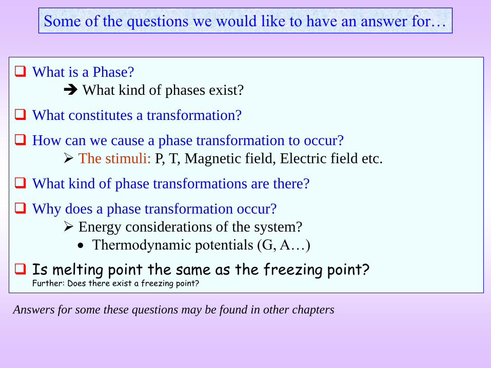
What is a Phase?

What kind of phases exist?

What constitutes a transformation?

How can we cause a phase transformation to occur?

The stimuli: P, T, Magnetic field, Electric field etc.

What kind of phase transformations are there?

Why does a phase transformation occur?

Energy considerations of the system?

Thermodynamic potentials (G, A…)

Is melting point the same as the freezing point?Further: Does there exist a freezing point?

Some of the questions we would like to have an answer for…

Answers for some these questions may be found in other chapters

Energies involved

Bulk Gibbs free energy ↓

Interfacial energy ↑

Strain energy ↑

Important in solid to solid transformations

Revise concepts of surface and interface energy before starting on these topics

When a volume of material (V) transforms three energies have to be considered :

(i) reduction in G (assume we are working at constant T & P),

(ii) increase in (interface free-energy),

(iii) increase in strain energy.

In a liquid to solid phase transformation the strain energy term can be neglected (as the

liquid can flow and accommodate the volume/shape change involved in the transformation-

assume we are working at constant T & P).

Volume of transformed material

New interface created

Energies involved



Strain energy ↑

The origin of the strain energy can be understood using the schematics as below. Eshelby

construction is used for this purpose.

In general a solid state phase transformation can involve a change in both volume and

shape. I.e. both dilatational and shear strains may be involved. For simplicity we consider

only change in volume of the material, leading to an increase in the strain energy of the

system (in future considerations).

Schematic of the Eshelby construction to understand the origin of the stresses due to phase transformation

of a volume (V): (a) region V before transformation, (b) the region V is cut out of the matrix and allowed to

transform (the transformation could involve both shape and volume changes), (c) the transformed volume

(V‘- shown to be larger in the figure) is inserted into the hole (here only volume change is shown for

simplicity), (c) the system is allowed to equilibrate. The continuity of the system is maintained during the

transformation. The system is strained as a larger volume V’ is inserted into the hole of volume V.

Only volume change

(a)

(b)(c) (d)

Considering only

volume change

Energies involved



Strain energy ↑ Solid-solid transformation

Let us start understanding phase transformations using the example of the solidification of

a pure metal. (This process is a first order transformation*. First order transformations

involve nucleation and growth**).

There is no change in composition involved as we are considering a pure metal. If we

solidify an alloy this will involve long range diffusion.

Strain energy term can be neglected as the liquid melt can flow to accommodate the

volume change (assume we are working at constant T & P).

The process can start only below the melting point of the liquid (as only below the melting

point the GLiquid < GSolid). I.e. we need to Undercool the system. As we shall note, under

suitable conditions (e.g. container-less solidification in zero gravity conditions), melts can

be undercooled to a large extent without solidification taking place.

Click here to know more about order of a phase transformation

Nucleation

of

phase

Trasformation

→

+

Growth till

is

exhausted=

1nd order

nucleation & growth

*

**

↑ t

“For sufficient Undercooling”

Cru

de

sch

emat

ic!

Liq

uid

→ S

oli

dphas

e tr

ansf

orm

atio

n:

Soli

dif

icat

ion

3

21

4

5 6

Liquid

Solid

Growth of Crystal

Two crystal going to join to

form grain boundary

Growth of nucleated crystal

Solidification complete

Video snap shots of

solidification of stearic acid

Grain boundary

Caution: here we are seeing an

increase time experiment and

soon we will be ‘talking of’

increasing undercooling

experiments

See video here

Liquid → Solid phase transformation

Liquid (GL)

TmT →

G

→

T

Gv

Liquid (L) stableSolid (S) stable

T - Undercooling

On cooling just below Tm solid becomes stable, i.e. GLiquid < GSolid.

But even when we are just below Tm solidification does not ‘start’.

E.g. liquid Ni can be undercooled 250 K below Tm.

We will try to understand Why?

The figure below shows G vs T curves for melt and a crystal.

The undercooling is marked as T and the ‘G’ difference between the liquid and the solid

(which will be released on solidification) is marked as Gv (the subscript indicates that the

quantity G is per unit volume). Hence, Gv is a function of undercooling (T)

GL→S → ve

GL→S → +ve

Solid (GS) Assume for now that

we are at a fixed T

below the Tm

Note that Tm is the melting point

of the bulk solid

In Homogenous nucleation the probability of nucleation occurring at point in the parent

phase is same throughout the parent phase.

In heterogeneous nucleation there are some preferred sites in the parent phase where

nucleation can occur

Homogenous

Heterogeneous

Nucleation

NucleationSolidification + Growth=

Heterogenous nucleation sites

Liquid → solid walls of container, inclusions

Solid → solid inclusions, grain boundaries,

dislocations, stacking faults

As pointed out before solidification is a first order phase transformation involving

nucleation (of crystal from melt) and growth (of crystals such that the entire liquid is

exhausted).

Nucleation is a ‘technical term’ and we will try to understand that soon.

In solid solid phase transformation, which involve strain energy, heterogeneous

nucleation (defined below) is highly preferred. Even in liquid solid transformations

heterogeneous nucleation plays an very important role.

of crystals from melt of nucleated crystals till liquid is exhausted

Homogenous nucleation

ΔG (Volume).( ) (Interface).( )VG

).(4 ).(3

4 ΔG 23 rGr v

r2

r3

1

)( TfGv

Free energy change on nucleation

Reduction in bulk free energy increase in interface energy increase in strain energy

r

( )f r

Neglected in L → S transformations

Let us consider LS transformation taking place by homogenous nucleation. Let the

system be undercooled to a fixed temperature (T held constant). Let us consider the formation of a

spherical crystal of radius ‘r’ from the melt. We can neglect the strain energy contribution.

Let the change in ‘G’ during the process be G. This is equal to the decrease in bulk free

energy + the increase in interface free energy. This can be computed for a spherical

nucleus as below.

Note that below a value of ‘1’ the lower power of ‘r’ dominates;

while above ‘1’ the higher power of ‘r’ dominates.

In the above equation these powers are weighed with other

‘factors/parameters’, but the essential logic remains.

Note that GV is negative

Let us start with a ‘text-book’ description of nucleation before taking up an alternate

perspective

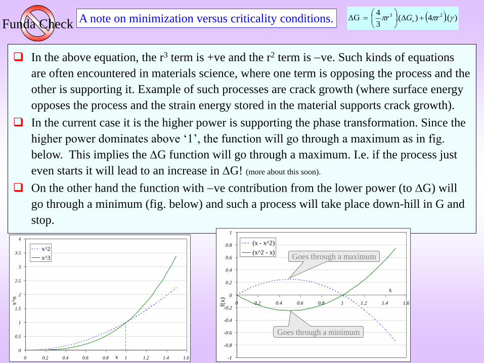
A note on minimization versus criticality conditions.Funda Check

In the above equation, the r3 term is +ve and the r2 term is ve. Such kinds of equations

are often encountered in materials science, where one term is opposing the process and the

other is supporting it. Example of such processes are crack growth (where surface energy

opposes the process and the strain energy stored in the material supports crack growth).

In the current case it is the higher power is supporting the phase transformation. Since the

higher power dominates above ‘1’, the function will go through a maximum as in fig.

below. This implies the G function will go through a maximum. I.e. if the process just

even starts it will lead to an increase in G! (more about this soon).

On the other hand the function with ve contribution from the lower power (to G) will

go through a minimum (fig. below) and such a process will take place down-hill in G and

stop.

).(4 ).(3

4 ΔG 23 rGr v

0

0.5

1

1.5

2

2.5

3

3.5

4

0 0.2 0.4 0.6 0.8 1 1.2 1.4 1.6x

x^n

x^2

x^3

-1

-0.8

-0.6

-0.4

-0.2

0

0.2

0.4

0.6

0.8

1

0 0.2 0.4 0.6 0.8 1 1.2 1.4 1.6

x

f(x)

(x - x^2)

(x^2 - x)Goes through a maximum

Goes through a minimum

).(4 ).(3

4 ΔG 23 rGr v

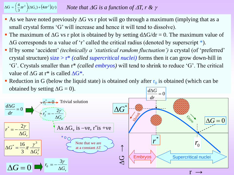
As we have noted previously G vs r plot will go through a maximum (implying that as a

small crystal forms ‘G’ will increase and hence it will tend to dissolve).

The maximum of G vs r plot is obtained by by setting dG/dr = 0. The maximum value of

G corresponds to a value of ‘r’ called the critical radius (denoted by superscript *).

If by some ‘accident’ (technically a ‘statistical random fluctuation’) a crystal (of ‘preferred’

crystal structure) size > r* (called supercritical nuclei) forms then it can grow down-hill in

‘G’. Crystals smaller than r* (called embryos) will tend to shrink to reduce ‘G’. The critical

value of G at r* is called G*.

Reduction in G (below the liquid state) is obtained only after r0 is obtained (which can be

obtained by setting G = 0).

0

dr

Gd0*

1 r

vGr

2*

2

Trivial solution

vGr

2*

2

3*

3

16

vGG

As Gv is ve, r*is +ve

r →

G

→

0G

0r

0G vGr

30

Supercritical nucleiEmbryos

Note that G is a function of T, r &

*r

0

dr

Gd

Note that we are

at a constant T

*G

r →

G

→

Decreasing r*

Dec

reas

ing

G*

Tm

23

2 2

16

3

mTG

T H

Using the Turnbull approximation (linearizing the G-T curve

close to Tm), we can get the value of G interms of the enthalpy

of solidification.

)( TfGv The bulk free energy reduction is a function of undercooling

What is the effect of undercooling (T) on r* and G*?

We have noted that GV is a fucntion of undercooling (T). At larger undercoolings GV

increases and hence r* and G* decrease. This is evident from the equations for r* and G*

as below (derived before).

At Tm GV is zero and r* is infinity!

That the melting point is not the same as the freezing point!!

This energy (G) barrier to nucleation is called the ‘nucleation barrier’.

vGr

2*

2

3*

3

16

vGG

T →

G →

Turnbull’s approximation

Tm

Solid (GS)

Liquid (GL)T

G

mf f

m m

T T TG H H

T T

fΔH heat of fusion

2

* 316

3

m

f

TG

H T

How are atoms assembled to form a nucleus of r* “Statistical Random Fluctuation”Quantum

Jump

To cause nucleation (or even to form an embryo) atoms of the liquid (which are randomly moving

about) have to come together in a order, which resembles the crystalline order, at a given instant of

time.

Typically, this crystalline order is very different from the order (local order), which exists in the liquid.

This ‘coming together’ is a random process, which is statistical in nature i.e. the liquid is exploring

‘locally’ many different possible configurations and randomly (by chance), in some location in the

liquid, this order may resemble the preferred crystalline order.

Since this process is random (& statistical) in nature, the probability that a larger sized crystalline

order is assembled is lower than that to assemble a smaller sized ‘crystal’.

Hence, at smaller undercoolings (where the value of r* is large) the chance of the formation of a

supercritical nucleus is smaller and so is the probability of solidification (as at least one nucleus is

needed which can grow to cause solidification). At larger undercoolings, where r* value is relatively

smaller, the chance of solidification is higher.

↑ T

r*

Tm

Ch

ance

s o

f n

ucl

eati

on

incr

ease

s

Here we try to understand: “What exactly is meant by the nucleation barrier?”.

It is sometime difficult to fathom out as to the surface energy can make freezing of a small

‘embryo’ energetically ‘infeasible’ (as we have already noted that unless the crystallite size is >

r0 the energy of the system is higher). Agreed that for the surface the energy lowering is not as

much as that for the bulk*, but even the surface (with some ‘unsaturated bonds’) is expected to

have a lower energy than the liquid state (where the crystal is energetically favoured). I.e. the

specific concern being: “can state-1 in figure below be above the zero level (now considered for

the liquid state)?” “Is the surface so bad that it even negates the effect of the bulk lowering?”

We will approach this mystery from a different angle by first asking the question: “what is

meant by melting point?” & “what is meant by undercooling?”.

What is meant by the ‘Nucleation Barrier’ an alternate perspective Funda Check

* refer to surface energy and surface tension slides.

surface_energy_and_surface_tension.ppt

The plot below shows melting point of Au nanoparticles, plotted as a function of the particle radius. It is to

be noted that the melting point of nanoparticles decreases below the ‘bulk melting point’ (a 5nm particle

melts more than 100C below Tmbulk). This is due to surface effects (surface is expected to have a lower

melting point than bulk!?*) actually, the current understanding is that the whole nanoparticle melts

simultaneously (not surface layer by layer).

Let us continue to use the example of Au. Suppose we are below Tmbulk (1337K=1064C, i.e. system is undercooled

w.r.t the bulk melting point) at T1 (=1300K T = 37K) and suppose a small crystal of r2 = 5nm forms in the liquid.

Now the melting point of this crystal is ~1200K this crystal will ‘melt-away’. Now we have to assemble a

crystal of size of about 15nm (= r1) for it ‘not to melt’. This needless to say is much less probable (and it is

better to undercool even further so that the value of r* decreases). Thus the mystery of ‘nucleation barrier’

vanishes and we can ‘think of’ melting point freezing point (for a given size of particle)!

Tm is in heating for the bulk material and in cooling if we take into account the size dependence of melting

point everything ‘sort-of’ falls into place .

Melting point, undercooling, freezing point (in the realm of homogenous nucleation)

Other materials like Pb, Cu, Bi,

Si show similar trend lines

* Surface atoms are loosely bound as compared to the bulk atoms.

T1

r1

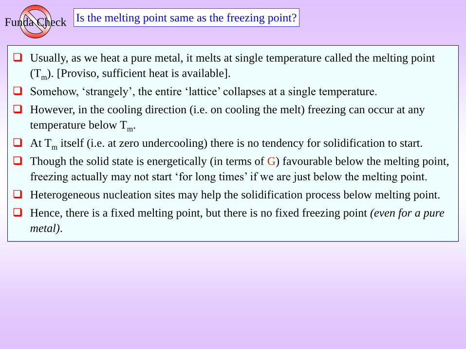
Is the melting point same as the freezing point?Funda Check

Usually, as we heat a pure metal, it melts at single temperature called the melting point

(Tm). [Proviso, sufficient heat is available].

Somehow, ‘strangely’, the entire ‘lattice’ collapses at a single temperature.

However, in the cooling direction (i.e. on cooling the melt) freezing can occur at any

temperature below Tm.

At Tm itself (i.e. at zero undercooling) there is no tendency for solidification to start.

Though the solid state is energetically (in terms of G) favourable below the melting point,

freezing actually may not start ‘for long times’ if we are just below the melting point.

Heterogeneous nucleation sites may help the solidification process below melting point.

Hence, there is a fixed melting point, but there is no fixed freezing point (even for a pure

metal).

The process of nucleation (of a crystal from a liquid melt, below Tmbulk) we have described so

far is a dynamic one. Various atomic configurations are being explored in the liquid state some

of which resemble the stable crystalline order. Some of these ‘crystallites’ are of a critical size

r*T for a given undercooling (T). These crystallites can grow to transform the melt to a

solid by becoming supercritical. Crystallites smaller than r* (embryos) tend to ‘dissolve’.

As the whole process is dynamic, we need to describe the process in terms of ‘rate’ the

nucleation rate [dN/dt number of nucleation events/volume/time].

Also, true nucleation is the rate at which crystallites become supercritical. To find the

nucleation rate we have to find the number of critical sized crystallites (N*) and multiply it by

the frequency/rate at which they become supercritical.

If the total number of particles (which can act like potential nucleation sites in homogenous

nucleation for now) is Nt , then the number of critical sized particles given by an Arrhenius type

function with a activation barrier of G*.

Atomic perspective of nucleation: Nucleation Rate

kT

G

t eNN

*

*

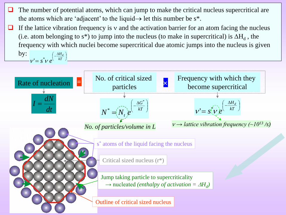
The number of potential atoms, which can jump to make the critical nucleus supercritical are

the atoms which are ‘adjacent’ to the liquid let this number be s*.

If the lattice vibration frequency is and the activation barrier for an atom facing the nucleus

(i.e. atom belonging to s*) to jump into the nucleus (to make in supercritical) is Hd , the

frequency with which nuclei become supercritical due atomic jumps into the nucleus is given

by:

No. of critical sized

particlesRate of nucleation

Frequency with which they

become supercritical=

dt

dNI

kT

G

t eNN

*

*

kT

Hd

es ' *

Critical sized nucleus (r*)

s* atoms of the liquid facing the nucleus

Outline of critical sized nucleus

Jump taking particle to supercriticality

→ nucleated (enthalpy of activation = Hd)

No. of particles/volume in L → lattice vibration frequency (~1013 /s)

kT

Hd

es ' *

T (

K)

→In

crea

sing

T

Tm

0 I →

T = Tm → G* = → I = 0

T = 0 → I = 0

kT

HG

t

d

esNI

*

*

G* ↑ I ↓

T ↑ I ↑

Note: G* is a function of T

The nucleation rate (I = dN/dt) can be written as a product of the two terms as in the equation

below.

How does the plot of this function look with temperature?

At Tm , G* is I = 0 (as expected if there is no undercooling there is no nucleation).

At T = 0K again I = 0

This implies that the function should reach a maximum between T = Tm and T = 0.

A schematic plot of I(T) (or I(T)) is given in the figure below.

An important point to note is that the nucleation rate is not a monotonic function of

undercooling.

Heterogenous nucleation

We have already talked about the ‘nucleation barrier’ and the difficulty in the nucleation

process. This is all the more so for fully solid state phase transformations, where the strain

energy term is also involved (which opposes the transformation).

The nucleation process is often made ‘easier’ by the presence of ‘defects’ in the system.

In the solidification of a liquid this could be the mold walls.

For solid state transformation suitable nucleation sites are: non-equilibrium defects such

as excess vacancies, dislocations, grain boundaries, stacking faults, inclusions and

surfaces.

One way to visualize the ease of heterogeneous nucleation

heterogeneous nucleation at a defect will lead to destruction/modification of the defect

(make it less “‘defective’”). This will lead to some free energy Gd being released → thus

reducing the activation barrier (equation below).

hetro,defectΔG (V) A ( )v s dG G G

Increasing Gd (i.e. decreasing G*)

Homogenous sites

Vacancies

Dislocations

Stacking Faults

Grain boundaries (triple junction…), Interphase boundaries

Free Surface

Heterogenous nucleation

Consider the nucleation of from on a planar surface of inclusion .

The nucleus will have the shape of a lens (as in the figure below).

Surface tension force balance equation can be written as in equation (1) below. The contact angle

can be calculated from this equation (as in equation (3)).

Keeping in view the interface areas created and lost we can write the G equation as below (2).

)( )()(A )(V ΔG lenslens circlecirclev AAG

Alens

Acircle

Acircle

Created

Created

Lost

CosSurface tension force balance

Interfacial Energies

Vlens = h2(3r-h)/3 Alens = 2rh h = (1-Cos)r rcircle = r Sin

Cos

(1)

(2)

is the contact angle

(3)

v

heteroG

r

2

*

3

2

3

* 323

4CosCos

GG

v

hetero

0

dr

Gd

3

homo

* 324

1CosCosGG *

hetero

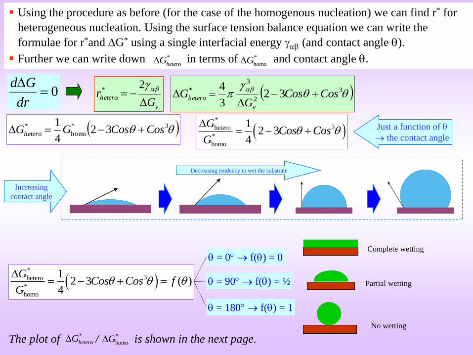
Using the procedure as before (for the case of the homogenous nucleation) we can find r* for

heterogeneous nucleation. Using the surface tension balance equation we can write the

formulae for r*and G* using a single interfacial energy (and contact angle ).

Further we can write down in terms of and contact angle . *

heteroG *

homoG

*

3hetero

homo

12 3

4*

GCos Cos

G

Just a function of

the contact angle

*

3hetero

homo

12 3 ( )

4*

GCos Cos f

G

= 0 f() = 0

= 90 f() = ½

= 180 f() = 1

The plot of / is shown in the next page.*

heteroG *

homoG

Increasing

contact angle

Complete wetting

No wetting

Partial wetting

Decreasing tendency to wet the substrate

0

0.25

0.5

0.75

1

0 30 60 90 120 150 180 (degrees) →

G

*het

ero

/

G*hom

o→

G*hetero (0o) = 0

no barrier to nucleation G*hetero (90o) = G*

homo/2

G*hetero (180o) = G*

homo

no benefit

Complete wetting No wettingPartial wetting

Cos

Plot of G*hetero/G*

homo is shown below. This brings out the benefit of heterogeneous nucleation vs homogenous nucleation.

If the phase nucleus (lens shaped) completely wets the substrate/inclusion (-phase) (i.e. = 0)

then G*hetero = 0 there is no barrier to nucleation.

On the other extreme if -phase does not we the substrate (i.e. = 180)

then G*hetero = G*

homo there is no benefit of the substrate.

In reality the wetting angle is somewhere between 0-180

Hence, we have to chose a heterogeneous nucleating agent with a minimum ‘’ value.

Choice of heterogeneous nucleating agent

How to get a small value of ? (so that ‘easy’ heterogeneous nucleation).

Choosing a nucleating agent with a low value of (low energy interface)

(Actually the value of ( ) will determine the effectiveness of the heterogeneous

nucleating agent → high or low )

Cos

Cos

How to get a low value of ?

We can get a low value of if:

(i) crystal structure of and are similar and

(ii) lattice parameters are as close as possible

Examples of such choices:

In seeding rain-bearing clouds → AgI or NaCl are used for nucleation of ice crystals

Ni (FCC, a = 3.52 Å) is used a heterogeneous nucleating agent in the production of

artificial diamonds (FCC, a = 3.57 Å) from graphite.

Heterogeneous nucleation has many practical applications.

During the solidification of a melt if only a few nuclei form and

these nuclei grow, we will have a coarse grained material (which

will have a lower strength as compared to a fine grained

material- due to Hall-Petch effect).

Hence, nucleating agents are added to the melt (e.g. Ti for Al

alloys, Zr for Mg alloys) for grain refinement.

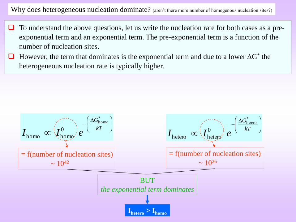
kT

G

eII

*homo

0

homohomo

kT

G

eII

*hetero

0

heterohetero

= f(number of nucleation sites)

~ 1042

= f(number of nucleation sites)

~ 1026

BUT

the exponential term dominates

Ihetero > Ihomo

To understand the above questions, let us write the nucleation rate for both cases as a pre-

exponential term and an exponential term. The pre-exponential term is a function of the

number of nucleation sites.

However, the term that dominates is the exponential term and due to a lower G* the

heterogeneous nucleation rate is typically higher.

Why does heterogeneous nucleation dominate? (aren’t there more number of homogenous nucleation sites?)

Heterogeneous nucleation in AlMgZn alloy

Nucleation of phaseTransformation

→ +

Growth of phase

till is exhausted*=

Diffusional transformations involve nucleation and growth. Nucleation involves the

formation of a different phase from a parent phase (e.g. crystal from melt). Growth

involves attachment of atoms belonging to the matrix to the new phase (e.g. atoms

‘belonging’ to the liquid phase attach to the crystal phase).

Nucleation we have noted is ‘uphill’ in ‘G’ process, while growth is ‘downhill’ in G.

Growth can proceed till all the ‘prescribed’ product phase forms (by consuming the parent

phase).

Growth

Hd – vatom Gv

Hd

phase

phase

At transformation temperature the probability of jump of atom from → (across the

interface) is same as the reverse jump

Growth proceeds below the transformation temperature, wherein the activation barrier for the

reverse jump is higher than that for the forward jump.

Growth

As expected transformation rate (Tr) is a function of nucleation rate (I) and growth rate

(U).

In a transformation, if X is the fraction of -phase formed, then dX/dt is the

transformation rate.

The derivation of Tr as a function of I & U is carried using some assumptions (e.g.

Johnson-Mehl and Avarami models).

Transformation rate

rate)Growth rate,on f(Nucleatiratetion Transforma

I, U, Tr →

T (

K)

→In

crea

sing

T

Tm

0

U

Tr

I

( , )r

dXT f I U

dt

Maximum of growth rate usually at higher

temperature than maximum of nucleation rate

We have already seen the curve for the nucleation rate (I) as a function of the

undercooling.

The growth rate (U) curve as a function of undercooling looks similar. The key difference

being that the maximum of U-T* curve is typically above the I-T curve*.

This fact that T(Umax) > T(Imax) give us an important ‘handle’ on the scale of the

transformed phases forming. We will see examples of the utility of this information later.

* The U-T curve is an alternate way of stating the U-T curve[rate sec1]

t →

X

→

0

1.0

0.5

3

t UI π

β

43

e 1X

Fraction of the product () phase forming with time the sigmoidal growth curve

Many processes in nature (etc.), e.g. growth of bacteria in a culture (number of bacteria

with time), marks obtained versus study time(!), etc. tend to follow a universal curve the

sigmoidal growth curve.

In the context of phase transformation, the fraction of the product phase (X) forming with

time follows a sigmoidal curve (function and curve as below).

Linear growth regime ~constant high growth rate

Incubation period slow growth (but with increasing growth rate with time)

Saturation phase decreasing growth rate with time

(region of law of diminishing returns)

Using ‘some’ model

From ‘Rate’ to ‘time’: the origin of Time – Temperature – Transformation (TTT) diagrams

A type of phase diagram

Tr (rate sec1) →

T (

K)

→

Tr

Tm

0

T (

K)

→

Tm

0

Time for transformation

Small driving

force for nucleation

Replot

( , )Rate f T t

Sluggish growth

The transformation rate curve (Tr-T plot) has hidden in it the I-T and U-T curves.

An alternate way of plotting the Transformation rate (Tr) curve is to plot Transformation

time (Tt) [i.e. go from frequency domain to time domain]. Such a plot is called the Time-

Temperature-Transformation diagram (TTT diagram).

High rates correspond to short times and vice-versa. Zero rate implies time (no transformation).

This Tt-T plot looks like the ‘C’ alphabet and is often called the ‘C-curve. The minimum

time part is called the nose of the curve.

Tt

Tt (time sec) →

Nose of the ‘C-curve’

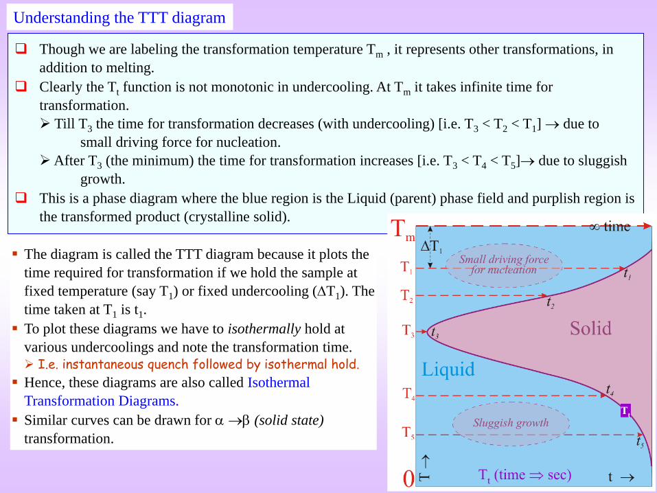
Understanding the TTT diagram

Though we are labeling the transformation temperature Tm , it represents other transformations, in

addition to melting.

Clearly the Tt function is not monotonic in undercooling. At Tm it takes infinite time for

transformation.

Till T3 the time for transformation decreases (with undercooling) [i.e. T3 < T2 < T1] due to

small driving force for nucleation.

After T3 (the minimum) the time for transformation increases [i.e. T3 < T4 < T5] due to sluggish

growth.

This is a phase diagram where the blue region is the Liquid (parent) phase field and purplish region is

the transformed product (crystalline solid).

The diagram is called the TTT diagram because it plots the

time required for transformation if we hold the sample at

fixed temperature (say T1) or fixed undercooling (T1). The

time taken at T1 is t1.

To plot these diagrams we have to isothermally hold at

various undercoolings and note the transformation time.

I.e. instantaneous quench followed by isothermal hold.

Hence, these diagrams are also called Isothermal

Transformation Diagrams.

Similar curves can be drawn for (solid state)

transformation.

Clearly the picture of TTT diagram presented before is incomplete transformations may

start at a particular time, but will take time to be completed (i.e. between the L-phase field

and solid phase field there must be a two phase region L+S!).

This implies that we need two ‘C’ curves one for start of transformation and one for

completion. A practical problem in this regard is related to the issue of how to define start

and finish (is start the first nucleus which forms? Does finish correspond to 100%?) . Since practically it is

difficult to find ‘%’ and ‘100%’, we use practical measures of start and finish, which can

be measured experimentally. Typically this is done using optical metallography and a

reliable ‘resolution of the technique is about 1% for start and 99% for finish.

Another obvious point: as x-axis is time any ‘transformation paths’ have to be drawn such

that it is from left to right (i.e. in increasing time).

t (sec) →T (

K)

→

99% = finish

Increasing % transformation

TTT diagram → phase transformation

1% = start

Fraction

transformed

f volume fractionof

volume fractionof at tf

final volumeof

How do we define the fractions transformed?

f(t,T) determined by

Growth rate

Density and distribution of nucleation sites

Nucleation rate

Overlap of diffusion fields from adjacent transformed volumes

Impingement of transformed volumes

How can we compute Tt(T) (transformation time for each T)

The ‘C’ curve depends on various factors as listed in diagram below.

Some common assumptions used in the derivation are: (i) constant number of nuclei, (ii)

constant nucleation rate, (iii) constant growth rate.

( , )f F number of nucleationsites growthrate growthrate withtime

Constant number of nuclei (these form at the beginning of the transformation)

One assumption to simplify the derivation is to assume that the number of nucleation sites

remain constant and these form at the beginning of the transformation.

This situation may be approximately valid for example if a nucleating agent (inoculant) is

added to a melt (the number of inoculant particles remain constant).

In this case the transformation rate is a function of the number of nucleation sites (fixed)

and the growth rate (U).

Growth rate is expected to decrease with time.

In Avrami model the growth rate is assumed to be constant (till impingement).

Parent phase has a fixed number of nucleation sites Nn per unit volume (and these sites are

exhausted in a very short period of time

Growth rate (U = dr/dt) constant and isotropic (as spherical particles) till particles impinge

on one another

Derivation of f(T,t): Avrami Model

2 3 224 4 4n n nr Utf N N N U t dtdr Udt

At time t the particle that nucleated at t = 0 will have a radius r = Ut

Between time t = t and t = t + dt the radius increases by dr = Udt

The corresponding volume increase dV = 4r2 dr

1

dXf

X

This fraction (f) has to be corrected for impingement. The corrected transformed volume

fraction (X) is lower than f by a factor (1X) as contribution to transformed volume

fraction comes from untransformed regions only:

Without impingement, the transformed volume fraction (f) (the extended transformed

volume fraction) of particles that nucleated between t = t and t = t + dt is:

3 24

1n

dXN U t dt

X

3 2

0 0

41

X t t

n

t

dXN U t dt

X

3 3n4π N U t

3

βX 1 e

Based on the assumptions note that the growth rate is not part of the equation it is only the

number of nuclei.

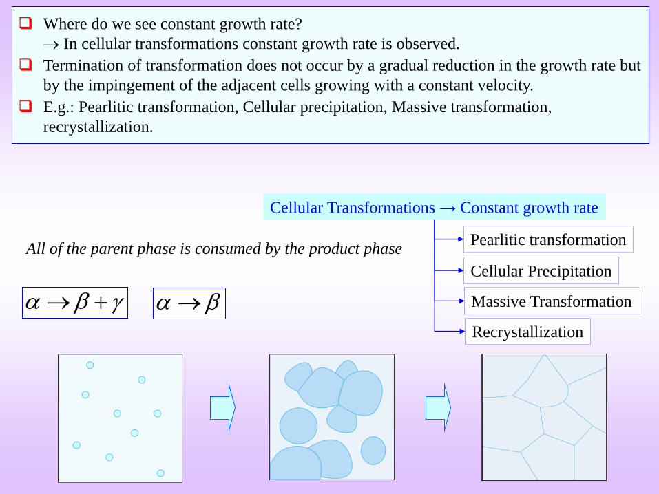
Cellular Transformations → Constant growth rate

Cellular Precipitation

Pearlitic transformation

Massive Transformation

Recrystallization

All of the parent phase is consumed by the product phase

Where do we see constant growth rate?

In cellular transformations constant growth rate is observed.

Termination of transformation does not occur by a gradual reduction in the growth rate but

by the impingement of the adjacent cells growing with a constant velocity.

E.g.: Pearlitic transformation, Cellular precipitation, Massive transformation,

recrystallization.

( , )f F nucleationrate growthrate

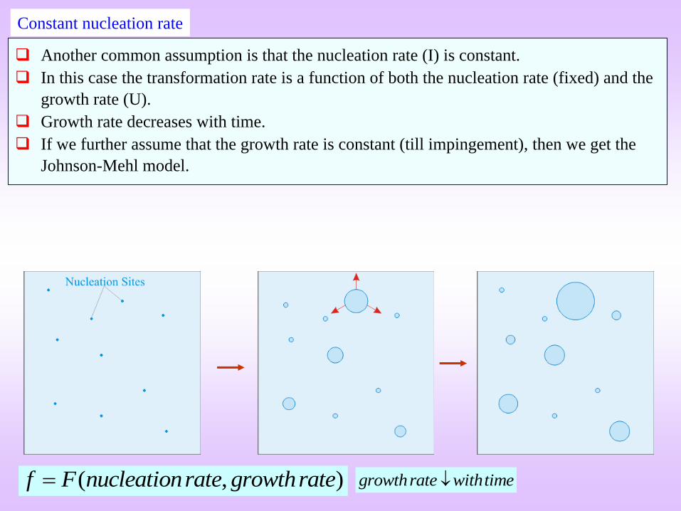
Constant nucleation rate

growthrate withtime

Another common assumption is that the nucleation rate (I) is constant.

In this case the transformation rate is a function of both the nucleation rate (fixed) and the

growth rate (U).

Growth rate decreases with time.

If we further assume that the growth rate is constant (till impingement), then we get the

Johnson-Mehl model.

Parent phase completely transforms to product phase ( → )

Homogenous Nucleation rate of in untransformed volume is constant (I)

Growth rate (U = dr/dt) constant and isotropic (as spherical particles) till particles impinge

on one another

Derivation of f(T,t): Johnson-Mehl Model

334 4

3 3( )r U t If Id d

At time t the particle that nucleated at t = 0 will have a radius r = Ut

The particle which nucleated at t = will have a radius r = U(t )

Number of nuclei formed between time t = and t = + d → Id

1

dXf

X

This fraction (f) has to be corrected for impingement. The corrected transformed volume

fraction (X) is lower than f by a factor (1X) as contribution to transformed volume

fraction comes from untransformed regions only:

Without impingement, the transformed volume fraction (f) (called the extended

transformed volume fraction) of particles that nucleated between t = and t = + d is:

334 4

1 3 3( )Idr U

dX

Xt Id

0 0

3(

4

1 3)

X t

U t IddX

X

3

t UI π

β

43

e 1X

t →

X

→

0

1.0

0.5

t →

X

→

0

1.0

0.5

3π I Uis a constant during isothermal transformation

3

For a isothermal transformation

Note that X is both a function of I and

U. I & U are assumed constant

APPLICATIONS

of the concepts of nucleation & growth

TTT/CCT diagrams

Phase Transformations in Steel

Precipitation

Solidification, Crystallization and Glass Transition

Recovery recrystallization & grain growth

As hyperlinks

Phase Transformations in Steel

Now we have the necessary wherewithal to understand phase transformations in steel

Phase diagram (Fe-Fe3C) and Concept of TTT diagrams

We shall specifically consider TTT and CCT diagrams for eutectoid, hypo- and hyper-

eutectoid steels.

Further we will consider the use of these diagrams to design heat treatments to get a

specific microstructure (each microstructure will give us a different set of properties).

%C →

T

→

Fe Fe3C

6.74.30.80.16

2.06

Peritectic

L + → Eutectic

L → + Fe3C

Eutectoid

→ + Fe3C

L

L +

+ Fe3C

1493ºC

1147ºC

723ºC

Fe-Cementite diagram

0.025 %C

0.1 %C

+ Fe3C

We have already seen the Fe-Fe3C phase diagram (please have a second look!)

Austenite

Pearlite

Pearlite + Bainite

Bainite

Martensite

100

200

300

400

600

500

800

723C

0.1 1 10 102 103 104 105

Eutectoid temperature

Ms

Mf

t (s) →

T

→

Eutectoid steel (0.8%C)

+ Fe3C

700

TTT diagram for


For every composition of steel we should draw a different TTT diagram.

To the left of the start C curve is the Austenite () phase field.

To the right of finish C curve is the ( + Fe3C) phase field.

Above Eutectoid

temperature there is no

transformation

Important points to be

noted:

The x-axis is log scale. ‘Nose’ of the ‘C’ curve is in

~sec and just below TE

transformation times may be

~day.

The starting phase has to

.

The ( + Fe3C) phase

field has more labels

included.

There are horizontal

lines labeled Ms and Mf.

‘Nose’ of ‘C’ curve

As pointed out before one of the important utilities of the TTT diagrams comes from the

overlay of microconstituents (microstructures) on the diagram.

Depending on the T, the ( + Fe3C) phase field is labeled with microconstituents like

Pearlite, Bainite.

We had seen that TTT diagrams are drawn by instantaneous quench to a temperature

followed by isothermal hold.

Suppose we quench below (~225C, below the temperature marked Ms), then Austenite

transforms via a diffusionless transformation (involving shear) to a (hard) phase known as

Martensite. Below a temperature marked Mf this transformation to Martensite is complete.

Once is exhausted it cannot transform to ( + Fe3C).

Hence, we have a new phase field for Martensite. The fraction of Martensite formed is not

a function of the time of hold, but the temperature to which we quench (between Ms and

Mf).

Austenite

Pearlite

Pearlite + Bainite

Bainite

Martensite

100

200

300

400

600

500

800

723C

0.1 1 10 102 103 104 105


Ms

Mf

t (s) →

T

→


+ Fe3C

700

How are these TTT diagrams drawn?

Samples are quenched into a salt bath maintained at

various temperatures (practical version of the

‘instantaneous quench’)

The samples are then quenched from this bath to room

temperature after various times.

Phase fraction of transformed phase is determined by

optical metallography.

Strictly speaking cooling curves (including finite quenching rates) should not be overlaid

on TTT diagrams (remember that TTT diagrams are drawn for isothermal holds!).

Isothermal hold at: (i) T1 gives us Pearlite, (ii) T2 gives Pearlite+Bainite, (iii) T3 gives

Bainite. Note that Pearlite and Bainite are both +Fe3C (but their morphologies are

different).

To produce Martensite we should quench at a rate such as to avoid the nose of the start ‘C’

curve. Called the critical cooling rate.

Austenite

Austenite

Pearlite

Pearlite + Bainite

Bainite

Martensite

100

200

300

400

600

500

800

723C

0.1 1 10 102 103 104 105


Not an isothermal

transformation

Ms

Mf

Coarse

Fine

t (s) →

T

→


700

T1

T2

T3

If we quench between Ms and Mf we

will get a mixture of Martensite and

(called retained Austenite).

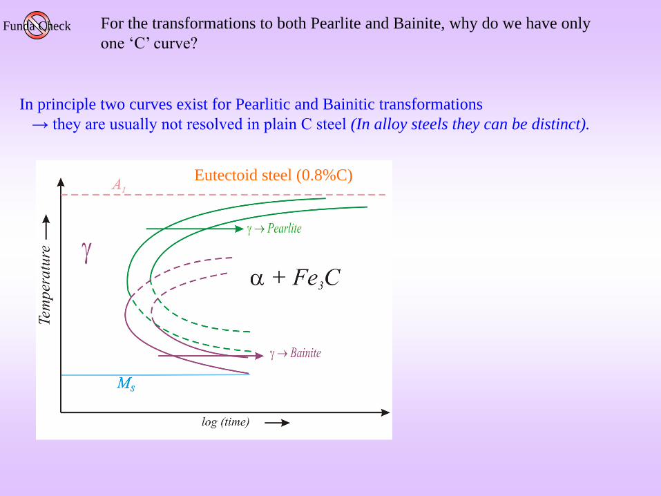
In principle two curves exist for Pearlitic and Bainitic transformations

→ they are usually not resolved in plain C steel (In alloy steels they can be distinct).


For the transformations to both Pearlite and Bainite, why do we have only

one ‘C’ curve?Funda Check

Atl

as

of

Iso

ther

ma

l T

ran

sfo

rma

tio

n a

nd

Co

oli

ng

Tra

nsf

orm

ati

on

Dia

gra

ms,

AS

M I

nte

rna

tio

na

l, M

eta

ls P

ark

, O

H,

19

77

.

TTT Diagram: hypoeutectoid steel

Hypo-Eutectoid steel

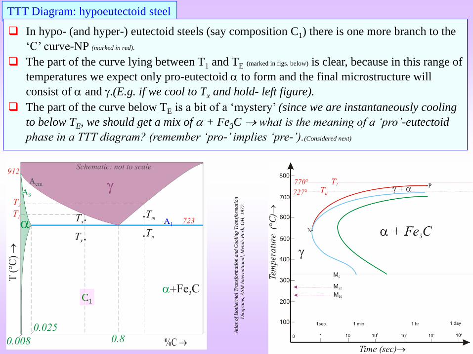
In hypo- (and hyper-) eutectoid steels (say composition C1) there is one more branch to the

‘C’ curve-NP (marked in red).

The part of the curve lying between T1 and TE (marked in figs. below) is clear, because in this range of

temperatures we expect only pro-eutectoid to form and the final microstructure will

consist of and .(E.g. if we cool to Tx and hold- left figure).

The part of the curve below TE is a bit of a ‘mystery’ (since we are instantaneously cooling

to below TE, we should get a mix of + Fe3C what is the meaning of a ‘pro’-eutectoid

phase in a TTT diagram? (remember ‘pro-’ implies ‘pre-’).(Considered next)

C1

Why do we get pro-eutectoid phase below TE?

Suppose we quench instantaneously an hypo-eutectoid composition (C1) to Tx we should expect the

formation of +Fe3C (and not pro-eutectoid first).

The reason we see the formation of pro-eutectoid first is that the undercooling w.r.t to Acm is more

than the undercooling w.r.t to A1. Hence, there is a higher propensity for the formation of pro-eutectoid

.

Undercooling wrt Acm

(formation of pro-eutectoid )undercooling wrt A1 line

(formation of + Fe3C)

C1

Funda Check

Hyper-Eutectoid steel

T2

TE

Similar to the hypo-eutectoid case, hyper-eutectoid compositions (e.g. C2 in fig. below) have a

+Fe3C branch.

For a temperature between T2 and TE (say Tm (not melting point- just a label)) we land up with +Fe3C.

For a temperature below TE (but above the nose of the ‘C’ curve) (say Tn), first we have the

formation of pro-eutectoid Fe3C followed by the formation of eutectoid +Fe3C.

C2

Continuous Cooling Transformation (CCT) Curves

The TTT diagrams are also called Isothermal Transformation Diagrams, because the

transformation times are representative of isothermal hold treatment (following a instantaneous quench).

In practical situations we follow heat treatments (T-t procedures/cycles) in which (typically)

there are steps involving cooling of the sample. The cooling rate may or may not be

constant. The rate of cooling may be slow (as in a furnace which has been switch off) or

rapid (like quenching in water).

Hence, in terms of practical utility TTT curves have a limitation and we need to draw

separate diagrams called Continuous Cooling Transformation diagrams (CCT), wherein

transformation times (also: products & microstructure) are noted using constant rate cooling

treatments. A diagram drawn for a given cooling rate (dT/dt) is typically used for a range of

cooling rates (thus avoiding the need for a separate diagram for every cooling rate).

However, often TTT diagrams are also used for constant cooling rate experiments keeping

in view the assumptions & approximations involved.

The CCT diagram for eutectoid steel is considered next. Blue curve is the CCT curve and

TTT curve is overlaid for comparison.

Important difference between the CCT & TTT transformations is that in the CCT case

Bainite cannot form.


Martensite

100

200

300

400

600

500

800

723

100

200

300

400

600

500

800

723

0.1 1 10 102 103 104105


Ms

Mf

t (s) →

T

→

Original TTT lines

Cooling curves

Constant rate

Pearlite

1T 2T

Continuous Cooling Transformation (CCT) Curves

Important points to be

noted:

As before the x-axis is

log scale.

Bainite cannot form by

continuous cooling.

Constant rate cooling

curves look like curves

due to log scale in x-

axis. The higher cooling

rate curve has a higher

(negative) slope.

As time is one of the

axes, no treatment curve

can be drawn where time

decreases or remains

constant.

dTT

dtConstant Cooling rate

1T 2T>

Start

Finish

CR1 CR2

CR1 CR2

A

B

C

D

E

F

G

CCT curvesCCT curves

The CCT curves are to the right of the corresponding TTT curves. Why?Funda Check

As the cooled sample has spent more time at higher temperature, before it intersects the

TTT curve (virtually superimposed) and the transformation time is longer at higher T

(above the nose) CCT curves should be to the right of TTT curves.


Martensite

100

200

300

400

600

500

800

723

100

200

300

400

600

500

800

723

0.1 1 10 102 103 104105


Ms

Mf

t (s) →T

→

Original TTT lines

Cooling curves

Constant rate

Pearlite

1T 2T

Further points to be noted:

Using CR1: the phase begins to transform to pearlite, but the transformation is not completed. The

remaining transforms to Martensite on crossing the Mf line (point C).

Using CR2: the phase completely transforms to pearlite (after point E). Hence, there is no significance

of the crossing of the CR2 line of the Ms (point F) and Mf lines (point G).

Common heat treatments involving cooling

Common cooling heat treatment labels (with increasing cooling rate) are:

Full anneal < Normalizing < Oil quench < Water quench

The microstructures produced for these treatments are:

Full Anneal (furnace cooling) Coarse Pearlite

Normalizing (Air cooling) Fine Pearlite

Oil Quench Matensite (M) + Pearlite (P)

Water Quench Matensite

To produce full martensite we have to avoid the ‘nose’ of the TTT diagram (i.e. the

quenching rate should be fast enough).

Within water or oil quench further parameters determine the actual quench rate (e.g. was the

sample shaken?).

Different cooling treatments

M = Martensite

P = Pearlite

M = Martensite

P = Pearlite


100

200

300

400

600

500

800

100

200

300

400

600

500

800

723

0.1 1 10 102 103 104 105

t (s) →

T

→

Water q

uen

ch

Oil quench

Norm

alizing

Full anneal

Coarse P

P M M + Fine P

It is important to note that for a single composition, different cooling treatments give

different microstructures these give rise to a varied set of properties.

After even water quench to produce Martensite, further heat treatment (tempering) can be

given to optimize properties like strength and ductility.

Note: this is ‘Microstructure

Engineering’ (changing properties

without changing the composition)

What are the typical cooling rates of various processes?

Process Cooling rate (K/s) Comments

Furnace cooling (Annealing) 105 – 103 Typically for solid samples

Air Cooling 1 – 10 “

Oil Quenching* ~100 “

Water Quenching* ~500 “

Splat Quenching 105 For molten material

Melt-Spinning 106 – 108 “

Evaporation, sputtering 109 (expected) Gaseous state involved

* Depends on conditions discussed later

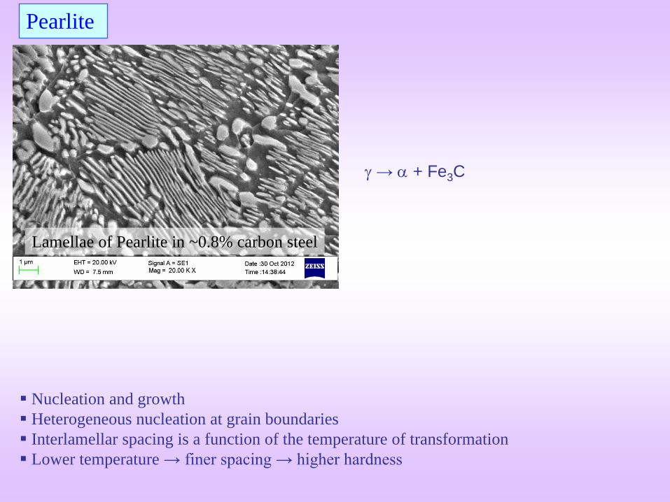
Pearlite

Nucleation and growth

Heterogeneous nucleation at grain boundaries

Interlamellar spacing is a function of the temperature of transformation

Lower temperature → finer spacing → higher hardness

→ + Fe3C

Lamellae of Pearlite in ~0.8% carbon steel

(100) || (111)C

Branching mechanismOrientation Relation:

Kurdyumov-Sachs (010) || (110)C

(001) || (112)C

1 Let us consider the heterogeneous nucleation of one of the phases of the pearlitic

microconstituent (say Fe3C), at a grain boundary of Austenite (). Further let this

precipitate be bound by a coherent interface on one side and a incoherent interface on the

other side. The incoherent interface will be glissile (mobile) and will grow into the

corresponding grain (2).

The orientation relation (OR) between and Fe3C is refered to as the Kurdyumov-

Sachs OR (as in fig. below).

2,3 The region surrounding this Fe3C precipitate will be depleted in Carbon and the

conditions will be right for the nucleation of adjacent to it.

4 The process is repeated to give rise to a pearlitic colony. Branching of an advancing

plate may also be observed.

Mechanism of Pearlitic transformation: arising of the lamellar microstructure

321 4

Bainite

Bainite formed at high temperature (~ 350C) has a feathery appearance and is called

‘Feathery Bainite’.

Bainite formed at lower temperature (~ 275C) has a needle-like appearance and is called

‘acicular Bainite’.

The process of formation of bainite involves nucleation and growth

Acicular, accompanied by surface distortions

** Lower temperature → carbide could be ε carbide (hexagonal structure, 8.4% C)

Bainite plates have irrational habit planes

Ferrite in Bainite plates possess different orientation relationship relative to the parent

Austenite than does the Ferrite in Pearlite

→ + Fe3C**

Micrograph courtesy: Prof. Sandeep Sangal

0.8% C steel, the sample was quenched

in a salt bath having 400°C temperature

and then it was held for 2 hours.

More images of Bainite

Micrograph courtesy: Prof. Sandeep Sangal, Swati Sharma

AFM image

Micrograph courtesy: Prof. Sandeep Sangal, Swati Sharma

Shape of the Martensite formed → Lenticular (or thin parallel plates)

Associated with shape change (shear)

But: Invariant plane strain (observed experimentally) → Interface plane between Martensite and

Parent remains undistorted and unrotated

This condition requires:

1) Bain distortion → Expansion or contraction of the lattice along certain crystallographic

directions leading to homogenous pure dilation

2) Secondary Shear Distortion → Slip or twinning

3) Rigid Body rotation

Characteristic of Martensitic transformations

Surface deformations caused by the Martensitic plate

MartensiteC

BCT

C

FCCQuench

% 8.0

)( '

% 8.0

)(

Martensitic transformation can be understood by first considering an alternate unit cell for the

Austenite phase as shown in the figure below.

If there is no carbon in the Austenite (as in the schematic below), then the Martensitic

transformation can be understood as a ~20% contraction along the c-axis and a ~12% expansion of

the a-axis → accompanied by no volume change and the resultant structure has a BCC lattice (the

usual BCC-Fe) → c/a ratio of 1.0.

Change in Crystal Structure

~20% contraction of c-axis

~12% expansion of a-axis

FCC → BCC

In Pure Fe after

the Matensitic transformation

c = a

FCC Austenite alternate choice of Cell

Martensite

In the presence of Carbon in the octahedral voids of CCP (FCC) -Fe (as in the schematic below) →

the contraction along the c-axis is impeded by the carbon atoms. (Note that only a fraction of the

octahedral voids are filled with carbon as the percentage of C in Fe is small).

However the a1 and a2 axis can expand freely. This leads to a product with c/a ratio (c’/a’) >1

→ 1-1.1.

In this case there is an overall increase in volume of ~4.3% (depends on the carbon content) → the

Bain distortion*.

C along the c-axis

obstructs the contraction

Tetragonal

MartensiteAustenite to Martensite → ~4.3 % volume increase

* Homogenous dilation of the lattice (expansion/contraction along crystallographic axis) leading to the formation of a new lattice is called

Bain distortion. This involves minimum atomic movements.

Martensite in 0.6%C steel

But shear will distort the lattice!

Slip Twinning

Average shape

remains undistorted

The martensitic transformation occurs without composition change.

The transformation occurs by shear without need for diffusion.

The atomic movements required are only a fraction of the interatomic spacing.

The shear changes the shape of the transforming region

→ results in considerable amount of shear energy

→ plate-like shape of Martensite.

The amount of martensite formed is a function of the temperature to which the sample is

quenched and not of time.

Hardness of martensite is a function of the carbon content

→ but high hardness steel is very brittle as martensite is brittle.

Steel is reheated to increase its ductility

→ this process is called TEMPERING.

Summary of characteristics of Martensitic transformation

% Carbon →

Har

dn

ess

(R

c) →

20

40

60

0.2 0.4 0.6

Harness of Martensite as a

function of Carbon content

Properties of 0.8% C steel

Constituent Hardness (Rc) Tensile strength (MN/m2)

Coarse pearlite 16 710

Fine pearlite 30 990

Bainite 45 1470

Martensite 65 -

Martensite tempered at 250C 55 1990

ROLE OF ALLOYING ELEMENTS

• + Simplicity of heat treatment and lower cost

• Low hardenability

• Loss of hardness on tempering

• Low corrosion and oxidation resistance

• Low strength at high temperatures

Plain Carbon Steel

Element Added

Segregation / phase separationSolid solution

Compound (new crystal structure)

• ↑ hardenability

• Provide a fine distribution of alloy carbides during tempering

• ↑ resistance to softening on tempering

• ↑ corrosion and oxidation resistance

• ↑ strength at high temperatures

• Strengthen steels that cannot be quenched

• Make easier to obtain the properties throughout a larger section

• ↑ Elastic limit (no increase in toughness)

Alloying elements

• Alter temperature at which the transformation occurs

• Alter solubility of C in or Iron

• Alter the rate of various reactions

Interstitial

Substitutional

P ►Dissolves in ferrite, larger quantities form iron phosphide → brittle (cold-shortness)

S►Forms iron sulphide, locates at grain boundaries of ferrite and pearlite poor ductility

at forging temperatures (hot-shortness)

Si ► (0.2-0.4%) increases elastic modulus and UTS

Cu►0.8 % soluble in ferrite, can be used for precipitation hardening

Pb►Insoluble in steel

Cr►Corrosion resistance, Ferrite stabilizer, ↑ hardness/strength, > 11% forms passive

films, carbide former

Ni► Austenite stabilizer, ↑ strength ductility and toughness,

Mo► Dissolves in & , forms carbide, ↑ high temperature strength,

↓ temper embrittlement, ↑ strength, hardenability

Sample elements and their role

Alloying Element (%) →

Bri

nel

l H

ard

nes

s→

v

0 2 4 6 8 1060

100

140

180

Cr

Cr + 0.1%C

Mn

Mn +0.1% C

Alloying elements increase hardenability but the major contribution to hardness comes from

Carbon

Mn, Ni are Austenite stabilizers

Cr is Ferrite stabilizer

Shrinking phase field with ↑ Cr

C (%) →

Tem

per

ature

→

0 0.4 0.8 1.61.2

5% Cr

12% Cr15% Cr

0% Cr

C (%) →

Tem

per

atu

re→

0 0.4 0.8 1.61.2

0.35% Mn

6.5% Mn

Outline of the phase field

Austenite Pearlite

Bainite

Martensite100

200

300

400

600

500

800

Ms

Mf

t →

T

→

TTT diagram for Ni-Cr-Mo low alloy steel

~1 min

TTT diagram of low alloy steel (0.42% C, 0.78% Mn,

1.79% Ni, 0.80% Cr, 0.33% Mo)U.S.S. Carilloy Steels, United States Steel Corporation, Pittsburgh, 1948)

0

100

200

300

400

500

600

700

800

900

1000

0 0.05 0.1 0.15 0.2 0.25 0.3 0.35

Engineering Strain (e)

En

gin

eeri

ng

Str

ess

(s)

[MP

a]

0.4% C - Slow cooled

0.8% C - Slow cooled

0.8% C - quenched

Effect of carbon content and heat treatment on properties of steel

150

200

250

300

350

400

450

0.5 0.6 0.7 0.8 0.9 1 1.1C %

Vik

ers

Ha

rdn

ess

Slowly cooled- 0.6%C

Quenched- 0.8% C

Slowly cooled- 0.8% C

Slowly cooled- 1.0% C

Hardness

Tensile Test

Precipitation

The presence of dislocations weakens the crystal → leading to easy plastic deformation.

Putting ‘hindrance’ to dislocation motion increases the strength of the crystal.

Fine precipitates dispersed in the matrix provide such an impediment.

Strength of Al → 100 MPa

Strength of Duralumin with proper heat treatment (Al + 4% Cu + other alloying elements)

→ 500 MPa.

Precipitation Hardening

If a high temperature solid solution is slowly cooled, then coarse (large sized) equilibrium

precipitates are produced. These precipitates have a large distance between them. These

precipitates have incoherent boundaries with the matrix (incoherent precipitates).

Such (coarse) precipitates, which have a large inter-precipitate distance, are ‘not the best’ in

terms of the increase in the hardness.

Hence, we device a 3 step process to obtain a fine distribution of precipitates, which have a

low inter-precipitate distance, to obtain a good increase in hardness.

Philosophy behind the process steps in Precipitation Hardening

Coarse incoherent

precipitates, with large inter-

precipitate distance

Click here to know more about: “how fine

precipitates can give rise to hardening”Multi-step process used to

obtain a fine distribution of

precipitates (with small

inter-precipitate distance)

../../e-book/Chapter_5b_Crystal_Imperfections_dislocations.ppt#76. Slide 76

Al-Cu phase diagram: the sloping solvus line and the design of heat treatments

The Al-Cu system is a model system to understand precipitation hardening (typical

composition chosen is Al-4 wt.% Cu).

Primary requirement (for precipitation hardening) is the presence of a sloping solvus line

(i.e. high solubility at high temperatures and decreasing solubility with decreasing

temperature). In the Al rich end, compositions marked with a shaded box can only be used

for precipitation hardening.

Sloping Solvus line:

high T → high solubility

low T → low solubility of Cu in Al

Al

Cu

4 % Cu

+

→ +

Slow equilibrium cooling gives rise to coarse

precipitates which is not good in impeding

dislocation motion.*

RT

Cu

TetragonalCuAl

RT

Cu

FCC

C

Cu

FCCcoolslow

o

% 52

)(

% 5.0

)(

550

% 4

)( 2

*Also refer section on Double Ended Frank-Read Source in the chapter on plasticity: max = Gb/L

C

A

B

Heat (to 550oC) → solid solution

Quench (to RT) →

Age (reheat to 200oC) → fine precipitates

4 % Cu

+

CA

B

To obtain a fine distribution of precipitates the cycle A → B → C is used

Note: Treatments A, B, C are for the same composition

Supersaturated solution

Increased vacancy concentration

Heat treatment steps to obtain a fine distribution of precipitates

Assume that we start with a material having coarse

equilibrium precipitates (which has been obtained by prior slow cooling of the

sample).

A: We heat the sample to the single phase region () in

the phase diagram (550C).

B: We quench (fast cooling) the sample in water to

obtain a metastable supersaturated solid solution (the amount

of Cu in the sample is more than that allowed at room temperature according to the

phase diagram).

C: We reheat the sample to relatively low temperature

(~180C/200C) get a fine distribution of precipitates. We

have noted before that at ‘low’ temperatures nucleation is dominant over growth.

Log(t) →

Har

dn

ess

→ 180oC

100oC

20oC

Higher temperature less time of aging to obtain peak hardness

Lower temperature increased peak hardness

optimization between time and hardness required

Schematic curves →

Real experimental curves

are in later slides

Note: Schematic curves shown- real curves considered later

Log(t) →

Har

dn

ess

→

180oC

T

OveragedUnderaged

Peak-aged

Region of solid solution

strengthening→ Hardness is higher than that of Al

(no precipitation hardening)

Region of precipitation

hardening

(but little/some solid solution

strengthening)

Dispersion of

fine precipitates

(closely spaced)

Coarsening

of precipitates

with increased

inter-precipitate spacing

Not zero of

hardness scale

Log(t) →

Har

dn

ess

→

180oC Peak-aged

Particle radius (r) →

CR

SS

Incr

ease

→

2

1

r r

1

Particle

shearingParticle

By-pass)(tfr

Section of GP zone parallel to (200) plane

Log(t) →

Har

dn

ess

→

T

Increasing size of precipitates with increasing interparticle (inter-precipitate) spacing

A complex set of events are happening in parallel/sequentially during the aging process

→ These are shown schematically in the figure below

Interface goes from coherent to semi-coherent to incoherent

Precipitate goes from GP zone → ’’ → ’ →

Cu rich zones fully coherent with the matrix → low interfacial energy

(Equilibrium phase has a complex tetragonal crystal structure which has incoherent

interfaces)

Zones minimize their strain energy by choosing disc-shape to the elastically soft <100>

directions in the FCC matrix

The driving force (Gv Gs) is less but the barrier to nucleation is much less (G*)

2 atomic layers thick, 10nm in diameter with a spacing of ~10nm

The zones seem to be homogenously nucleated (excess vacancies seem to play an

important role in their nucleation)

GP Zones

Atomic image of Cu layers in Al matrix

Bright field TEM micrograph of an Al-4% Cu alloy

(solutionized and aged) GP zones.

5nm

5nm

Selected area diffraction (SAD) pattern, showing

streaks arising from the zones.

Due to large surface to volume ratio the fine precipitates have a tendency to coarsen

→ small precipitates dissolve and large precipitates grow

Coarsening

↓ in number of precipitate

↑ in interparticle (inter-precipitate) spacing

reduced hindrance to dislocation motion (max = Gb/L)

Phase Transformations in Metals and Alloys, D.A. Porter and K.E. Easterling, Chapman & Hall, London, 1992.

''(001) || (001)

''[100] || [100]

'(001) || (001)

'[100] || [100]

10 ,100nmthick nmdiameter

Distorted FCC

Tetragonal

UC composition Al4Cu2 = Al2Cu

Becomes incoherent

as ppt. grows

BCT, I4/mcm (140),

a = 6.06Å, c = 4.87Å, tI12

''



'

Phase Transformations in Metals and Alloys, D.A. Porter and K.E. Easterling,Chapman & Hall, London, 1992.

Schematic diagram showing the lowering of the Gibbs free energy of the system on sequential transformation:

GP zones → ’’ → ’ →

Successive lowering if free

energy of the system

The activation barrier for

precipitation of equilibrium ()

phase is large

But, the free energy benefit in each step is small compared to the

overall single step process

Single step

(‘equilibrium’) process

Schematic plot

Precipitation processes in solids, K.C. Russell, H.I. Aaronson (Eds.), The Metallurgical Society of AMIE, 1978, p.87

In this diagram additionally information has

been superposed onto the phase diagram (which

strictly do not belong there- hence this diagram

should be interpreted with care)

The diagram shows that on aging at various

temperatures in the + region of the phase

diagram various precipitates are obtained first

At higher temperatures the stable phase is

produced directly

At slightly lower temperatures ’ is produced

first

At even lower temperatures ’’ is produced first

The normal artificial aging is usually done in

this temperature range to give rise to GP zones

first

Base Alloy Precipitation Sequence

Al Al-Ag GPZ (Spheres) ' (plates) (Ag2Al)

Al-Cu GPZ (Discs) '' (Discs) ' (Plates) (CuAl2)

Al-Cu-Mg GPZ (Rods) S' (Laths) S (Laths, CuMgAl2)

Al-Zn-Mg GPZ (Spheres) ' (Plates) (Plates/Rods, Zn2Mg)

Cu Cu-Be GPZ (Discs) ' (CuBe)

Cu-Co GPZ (Spheres) (Plates, Co)

Fe Fe-C -carbide (Discs) Fe3C (Plates)

Fe-N '' (Discs) Fe4N (Plates)

Ni Ni-Cr-Ti-Al ' (Cubes/Spheres)

Precipitation Sequence in some precipitation hardening systems

(Morphology and compound stoichiometry are given in brackets)

[1] J.M. Silcock, T.J. Heal and H.K. Hardy, J. Inst. Metal. 82 (1953-54) 239.

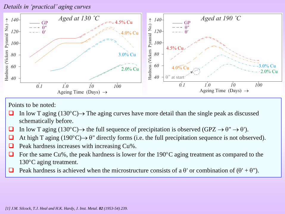
Details in ‘practical’ aging curves

Points to be noted:

In low T aging (130C) The aging curves have more detail than the single peak as discussed

schematically before.

In low T aging (130C) the full sequence of precipitation is observed (GPZ '' ').

At high T aging (190C) '' directly forms (i.e. the full precipitation sequence is not observed).

Peak hardness increases with increasing Cu%.

For the same Cu%, the peak hardness is lower for the 190C aging treatment as compared to the

130C aging treatment.

Peak hardness is achieved when the microstructure consists of a ' or combination of (' + '').

’’ at start

There will be a range of particle sizes due to time of nucleation and rate of

growth

As the curvature increases the solute concentration (XB) in the matrix adjacent to

the particle increases

Concentration gradients are setup in the matrix → solute diffuses from near the

small particles towards the large particles

small particles shrink and large particles grow

with increasing time * Total number of particles decrease

* Mean radius (ravg) increases with time

Particle/precipitate Coarsening

Gibbs-Thomson effect

Gibbs-Thomson effect

Rate controlling

factor

Interface diffusion rate

Volume diffusion rate

3 3

0avgr r kt

ek D X

r0 → ravg at t = 0

D → Diffusivity

Xe → XB (r = )

D is a exponential function of temperature

coarsening increases rapidly with T

2

avg

avg

dr k

dt r

small ppts coarsen more

rapidly

0r

avgr

t

3Linear versus relation maybreak down due todiffusionshort-circuits

or if theprocessisinterface controlled

avgr t

Rateof coarsening depends on (diffusion controlled)eD X

Precipitation hardening systems employed for high-temperature applications must

avoid coarsening by having low: , Xe or D

Nimonic alloys (Ni-Cr + Al + Ti)

Strength obtained by fine dispersion of ’ [ordered FCC Ni3(TiAl)] precipitate in FCC Ni

rich matrix

Matrix (Ni SS)/ ’ matrix is fully coherent [low interfacial energy = 30 mJ/m2]

Misfit = f(composition) → varies between 0% and 0.2%

Creep rupture life increases when the misfit is 0% rather than 0.2%

Low

Nimonic 90: Ni 54%, Cr 18-21%, Co 15-21%, Ti 2-3%, Al 1-2%

ThO2 dispersion in W (or Ni) (Fine oxide dispersion in a metal matrix)

Oxides are insoluble in metals

Stability of these microstructures at high temperatures due to low value of Xe

The term DXe has a low value

Low Xe

ThO2 dispersion in W (or Ni) (Fine oxide dispersion in a metal matrix)

Cementite dispersions in tempered steel coarsen due to high D of interstitial C

If a substitutional alloying element is added which segregates to the carbide → rate of

coarsening ↓ due to low D for the substitutional element

Low D

PHASE TRANSFORMATIONS - Information and Library...

Documents

Transcript of PHASE TRANSFORMATIONS - Information and Library...