Phase Inversion in dispersed liquid-liquid pipe flow

Kwun Ho Ngan

A thesis submitted to University College London in fulfillment of the requirements

for the degree of Doctor of Philosophy

Department of Chemical Engineering

University College London

London WC1E 7JE

October 2010

To my family and Ting Ting

1

Abstract

 

This thesis presents the experimental and theoretical investigations on the development of

phase inversion in horizontal pipeline flow of two immiscible liquids. It aims to provide

an understanding on the flow development across the phase inversion transition as well as

the effect on pressure drop.

Experimental investigation on phase inversion and associated phenomena were

conducted in a 38mm I.D. liquid pipeline flow facility available in the Department of

Chemical Engineering at University College London (UCL). Two sets of test pipelines

are constructed using stainless steel and acrylic. The inlet section of the pipeline has also

been designed in two different configurations – (1) Y-junction inlet to allow dispersed

flow to be developed along the pipeline (2) Dispersed inlet to allow formation of

dispersion immediately after the two phases are joined. Pressure drop along the pipeline

is measured using a differential pressure transducer and is studied for changes due to

redistribution of the phases during inversion. Various conductivity probes (ring probes,

wire probes, electrical resistance tomography and dual impedance probe) are installed

along the pipeline to detect the change in phase continuity and distribution as well as

drop size distribution based on the difference in conductivity of the oil and water phases.

During the investigation, the occurrence of phase inversion is firstly investigated and the

gradual transition during the process is identified. The range of phase fraction at which

the transition occurs is determined. The range of phase fraction becomes significantly

narrower when the dispersed inlet is used. The outcome of the investigation also becomes

the basis for subsequent investigation with the addition of glycerol to the water phase to

reduce the interfacial tension. Based on the experimental outcome, the addition of

glycerol does not affect the inversion of the oil phase while enhancing the continuity of

the water phase.

2

As observed experimentally, significant changes in pressure gradient can be observed

particularly during phase inversion. Previous literatures have also reviewed that phase

inversion occurs at the maximum pressure gradient. In a horizontal pipeline, pressure

gradient is primarily caused by the frictional shear on the fluid flow in the pipe and, in

turn, is significantly affected by the fluid viscosities. A study is conducted to investigate

on the phase inversion point by identifying the maximum mixture viscosity (i.e.

maximum pressure gradient) that an oil-in-water (O/W) and water-in-oil (W/O)

dispersion can sustain. It is proposed that the mixture viscosity will not increase further

with an increase in the initial dispersed phase if the inverted dispersion has a lower

mixture viscosity. This hypothesis has been applied across a wide range of liquid-liquid

dispersion with good results. This study however cannot determine the hysteresis effect

which is possibly caused by inhomogeneous inversion in the fluid system.

A mechanistic model is developed to predict the flow characteristics as well as the

pressure gradient during a phase inversion transition. It aims to predict the observed

change in flow pattern from a fully dispersed flow to a dual continuous flow during phase

inversion transition. The existence of the interfacial height provides a selection criterion

to determine whether a momentum balance model for homogeneous flow or a two-fluid

layered flow should be applied to calculate the pressure gradient. A friction factor is also

applied to account for the drag reduction in a dispersed flow. This developed model

shows reasonable results in predicting the switch between flow patterns (i.e. the

boundaries for the phase inversion transition) and the corresponding pressure gradient.

Lastly, computational fluid dynamic (CFD) simulation is applied to identify the key

interphase forces in a dispersed flow. The study has also attempted to test the limitation

of existing interphase force models to densely dispersed flow. From the study, it is found

that the lift force and the turbulent dispersion forces are significant to the phase

distribution in a dispersed flow. It also provides a possible explanation to the observed

flow distribution in the experiments conducted. However, the models available in CFX

are still unable to predict well in a dense dispersion (60% dispersed). This study is also

3

suggested to form the basis for more detailed work in future to optimize the simulation

models to improve the prediction of phase inversion in a CFD simulation.

4  

Acknowledgement

  I wish to firstly express my sincere gratitude to my supervisor at University College

London, Dr Panagiota Angeli, for offering me this valuable opportunity to learn about an

interesting topic of multiphase flow under her great guidance and experience. Her personal

devotion and passion on the investigation is always my greatest drive to push beyond the

boundaries for breakthrough. More importantly, I have to express my appreciation on her

personal care in every aspect of my life allowing me to pursue my research work in a worry free

environment. Her support for my participation in various conferences provides further

opportunities to interact with other expertise in the field. It is no doubt the most memorable

academic life I have pursued and a life changing experience I will never regret.

I would also like to thank Chevron Technology Company for the kind sponsorship on my

research project. In particular, I would like to thank Dr Lee Rhyne and Dr Karolina Ioannou for

their regular discussions during my course of studies. Their industrial experience has been a

valuable source of information for me to understand more about applying the outcome of the

investigation in the oil industry. I am also greatly appreciated about spending their precious time

to proof-read this work and making many constructive suggestions to it.

Thanks also to all the colleagues that have spent the past years with me. You are always

the best guides for my memorable student life in London. Without all of you, I would not have

appreciated the vibrant life in this metropolitan city. Thanks also to the staff in the mechanical

and electrical workshop. Your kind help to resolve every small issue that I encounter throughout

the course is what shapes the successful outcome in this work. I wish you all the best in your

future.

On a personal note, I have to express my special thanks to Ting Ting without whom I

would not have the strength and perseverance to pursue this challenging course in a top notched

university. Your continual care and support will always be remembered and appreciated. I wish

you all the success in life and continue to be my guiding light in my life.

Lastly, to my supportive family for always bringing me the feeling of home despite we

are miles apart. Thanks for all the advice and love to me.

5

Table of Contents

Abstract 1

Acknowledgement 4

Table of Contents 5

List of Figures 9

List of Tables 21

Nomenclature 23

Chapter 1: Introduction

1.1 Multiphase Flow in Petroleum Industry 28

1.2 Fundamentals of Multiphase Flow 29

1.2.1 The Occurrence of Phase Inversion 30

1.3 Objectives of Study 31

1.4 Structure of the Thesis 32

Chapter 2: Literature Review

2.1 Overview 34

2.2 Flow Development and Flow Pattern Maps 34

2.3 Phase Inversion 39

2.3.1 Phase Inversion in Stirred Vessels 41

2.3.2 Phase Inversion in Pipe Flow 44

2.3.3 Parametric Study on Phase Inversion 48

2.4 Phase Inversion Mechanisms and Prediction Models 53

2.4.1 Models based on Rate of Drop Break-Up and

Coalescence 53

2.4.1.1 Secondary Dispersions 56

2.4.2 Models based on Minimisation/Equal System and

Interfacial Energy 57

2.4.3 Models based on Zero Shear Stress at Interface 58

2.5 Drop Size Distribution and Characteristic Diameter 59

2.5.1 Types of Drop Size Distribution 60

2.5.2 Characteristic Diameter of Drop Size Distribution 62

6

2.6 Numerical Simulation on Dispersed Flow 63

2.6.1 Conservation Equations used in CFD 66

2.6.2 Models for Simulation of Liquid-Liquid

Dispersed Pipe Flow 69

2.7 Interphase Forces Models 72

2.7.1 Interphase Drag 72

2.7.1.1 Drag Force in Dense Dispersion 73

2.7.2 Lift Force 75

2.7.3 Turbulent Dispersion Force 75

2.7.3.1 Favre Averaged Drag Model 76

2.7.3.2 Lopez de Bertodano Model 76

2.8 Summary of Literature Review 77

Chapter 3: Facility and Instrumentation

3.1 Overview 79

3.2 Test Fluids 79

3.3 Experimental Flow Facility 80

3.4 Summary 100

Chapter 4: The Occurrence of Phase Inversion

4.1 Overview 101

4.2 Experimental Procedure 102

4.3 Visual Observations of Phase Inversion 103

4.4 Detection of Phase Inversion Occurrence 107

4.4.1 In-Situ Phase Distribution Measurements 107

4.4.2 Changes in Phase Continuity (Partial Phase

Inversion) 109

4.5 Effect of Dispersion Initialisation on Phase Inversion 112

4.6 Effect of Mixture Velocity on Phase Inversion 114

4.7 Pressure Gradient during Phase Inversion 116

4.7.1 Effect of Inversion Route on Pressure Gradient 118

4.7.2 Effect of Mixture Velocity on Pressure Gradient 118

4.8 Drop Size Distribution in Oil & Water Dispersion 121

4.8.1 Drop Size Distribution Measurement 122

7

4.9 Effect of Dispersion Inlet on Phase Inversion

126

4.10 Conclusion 130

Chapter 5: Effect of Interfacial Tension on Phase Inversion

5.1 Overview 134

5.2 Experimental Setup 136

5.3 Phase Inversion Results 138

5.4 Effect of Glycerol Addition on Pressure Gradient during

Phase Inversion 144

5.5 Effect of Glycerol on Drop Size Distribution in Oil and

Water Continuous Dispersions 146

5.6 Conclusion 149

Chapter 6: Prediction of Phase Inversion through Fluid Viscosities

6.1 Overview 150

6.2 Suggested Method for Determining the Phase Inversion

Point 151

6.3 Literature Mixture Viscosity Models 154

6.4 Comparison between Predicted Phase Inversion Points

and Experimental Results from Literature 156

6.5 Comparison of the Proposed Methodology with Literature

Correlations 161

6.6 Review on Prediction Model with an Experimental

Homogeneous Dispersed Flow 164

6.7 Conclusion 166

Chapter 7: Prediction of Pressure Gradient during Phase Inversion

7.1 Overview 168

7.2 Experimental Investigation 169

7.3 Development of Model for the Prediction of Pressure

Drop 171

7.3.1 Prediction of Flow Configuration 171

7.3.2 Entrainment Model 173

8

7.3.3 Two Fluid Model 174

7.3.4 Homogeneous Model 176

7.4 Comparison of Model Predictions with Experimental Data 176

7.5 Conclusion 179

Chapter 8: CFD Simulation of Horizontal Two-Phase Pipe Flow

8.1 Overview 180

8.2 Description of Ansys CFX Software Package 180

8.3 Model Geometry and Simulation Conditions 183

8.4 Results and Discussion 187

8.5 Conclusion 195

Chapter 9: Thesis Conclusion and Future Work

9.1 Overview 197

9.2 Conclusions 197

9.2.1 Conclusions from Experimental Studies 197

9.2.2 Conclusions from Theoretical Studies 199

9.3 Recommendations 200

Reference 203

Appendix A – Chord Length Measurement during Phase Inversion 214

Appendix B – Matlab Code for Pressure Gradient Prediction 217

Appendix C – Grid Sensitivity Test for CFD simulation 230

9

List of Figures

Chapter 1

Figure 1.1 Offshore production pipeline schematic from well centres to

production platforms and FPSO. 28

Chapter 2

Figure 2.1

(a) Flow regime map that is based on the fluid superficial

velocities.

(b) Flow regime map that is based on input water fraction and

mixture velocity.

35

Figure 2.2

(a) Stratified smooth flow (b) stratified wavy flow with the oil

phase on the top layer while the water phase on the bottom

layer. (Ngan et al., 2007)

37

Figure 2.3 Dual continuous flow with several oil drops entrained in the

water continuous layer. (Ngan et al., 2007) 38

Figure 2.4

Annular flow with an oil core and a water annulus. Small

amount of drops are also observed within the oil core in the

figure. (Ngan et al., 2007)

38

Figure 2.5

(a) Dispersed flow of oil drops in water. Drops observed are

polydispersed and highly deformable.

(b) Oil slug flow in water. (Ngan et al., 2007)

39

Figure 2.6 A schematic on the proposed phase inversion mechanism by

Arirachakaran et al. (1989). 40

Figure 2.7

The existence of ambivalent region between the aqueous and

organic continuous dispersion across the organic phase fraction

(Φo) (Noui-Mehidi et al., 2004).

41

Figure 2.8 Droplet in drop for a glycerol/water and chlorobenzene system

captured by Sony video printer (Pacek et al., 1994). 42

Figure 2.9

(a) Pressure gradient measurement of a Exxsol D80/water

system in a 60mm I.D. pipe.

(b) Pressure gradient measurement of a Marcol 52/water system

in a 60mm I.D. pipe (Ioannou, 2006).

45

10

Figure 2.10 Conductivity measurement conducted at the centre of a vertical

pipe across the phase inversion process (Hu, 2005). 47

Figure 2.11

Multiple dispersion of an oil/water system at a mixture velocity

of 1.5m/s and input oil fraction of 31%. The dark region

represents the oil phase and the light region represents the water

phase. (Liu et al., 2006)

47

Figure 2.12

Visual observations of (a) O/W/O and (b) W/O/W dispersions

using LIF technique. The oil phase is shown in black while the

water phase is shown in luminous green. (Liu et al., 2005)

57

Figure 2.13

Comparison between calculated drop size distribution and

experimental drop size data. Dotted line represents the

histogram at the circulation region and the solid line represents

the histogram at the impeller region. (Coulaloglou and

Tavlarides, 1977).

60

Figure 2.14

Comparison between experimental drop size data and selected

drop size distribution types in an horizontal pipe flow (Vso =

0.75m/s, Vsw=0.75m/s, oil drops). (Vielma et al., 2008).

62

Figure 2.15

Schematic representation on the modelling approaches for two-

phase flow: (a) Eulerian-Lagrangian approach and (b) Eulerian-

Eulerian approach. The number next to the blue arrow in (b)

represents the volume fraction of the dispersed phase within the

control volume. (Rusche, 2002)

65

Chapter 3

Figure 3.1 Schematic of the pilot scale facility. 81

Figure 3.2 Photograph of the pilot scale facility in stainless steel. 83

Figure 3.3 Stainless steel Y-inlet where the oil and water phases are joined

at the end. 83

Figure 3.4 Acrylic Y-inlet with a split plate to enhance stratification of the

oil and water. 84

Figure 3.5

Dispersion inlets with staggered nozzles. (a) The dispersed

phase flows within the stainless steel pipe while the continuous

phase flows in the acrylic pipe. (b) Dispersed phase is ejected

from the nozzles.

85

11

Figure 3.6 Junction effect of the coalescer that enhances separation.

(Information from manufacturer - KnitMesh Technologies). 86

Figure 3.7 Setup of the high speed video imaging unit, Kodak HS 4540

MX. 87

Figure 3.8

Section of pipe with quick closing valves in the 38mm stainless

steel pipeline. A viewbox is included to aid visual observation

and video capturing.

88

Figure 3.9 Conductivity ring probe for phase continuity measurement at

the pipe periphery. 89

Figure 3.10

Local conductive wire probe for phase continuity measurement

at the localized position. (a) Photo of wire probe (b) Schematic

of the interior (side view) of the wire probe.

90

Figure 3.11

(a) Stainless steel electrodes embedded across the pipe

periphery.

(b) Experimental setup of the ERT system with a PC for data

processing.

92

Figure 3.12

Sample ERT reconstructed image generated from ITS toolsuite.

The colour bar denotes the range of raw conductivity data with

respective to the reference frame.

93

Figure 3.13

In-situ liquid hold-up comparison between electrical resistance

tomography (ERT) and quick closing valves across a range of

input phase fractions.

94

Figure 3.14 (a) Photograph of the dual impedance probe setup. (b) Probe tip

configuration (Lovick, 2004). 95

Figure 3.15

A sample set of normalized signal from the two impedance

wires at a mixture velocity of 3m/s. Dispersed phase will be in

contact with probe 1 before it contacts with probe 2.

96

Figure 3.16

A sample frequency plot of the time delay between the two

impedance wires. The highest peak denotes the time delay

where most dispersed drop take to cross the two wires.

97

Figure 3.17 Pressure measuring port at stainless steel pipeline. Similar ports

are also found in the acrylic pipeline. 99

12

Chapter 4

Figure 4.1

Visual images are taken in a stainless steel pipe using an high

speed camera (Model: Vision Research Phantom V5.1) at 7m

away from the inlet. Mixture velocity is kept constant at 3m/s.

The percentage in the bracket represents the input water

fraction which the image is taken.

104

Figure 4.2

Visual images are taken in an acrylic pipe using an high speed

camera (Model: Kodak HS 4540) at 7m away from the inlet.

Mixture velocity is kept constant at 3m/s. The percentage in the

bracket represents the input water fraction at which the image is

taken. The arrows present samples of complex structures

observed in images.

106

Figure 4.3

Phase distribution in an acrylic pipe cross section during the

transition from a water continuous to an oil continuous mixture

at a mixture velocity of 3m/s. The percentages in brackets

represent the input water fraction.

108

Figure 4.4

Normalized conductivity data of the oil/water system in an

acrylic pipe at a mixture velocity of 3m/s from the ring and wire

probes as well as the ERT system. The vertical lines limit the

phase inversion transition region and are drawn at the first and

last near zero conductivity values recorded using the various

probes. The percentages represent the water fraction at which

the different probes show near-zero conductivity values.

110

Figure 4.5

Normalized conductivity data of the oil/water system in a

stainless steel pipe at a mixture velocity of 3m/s from the ring

and wire probes as well as the ERT system. The vertical lines

limit the phase inversion transition region and are drawn at the

first and last near zero conductivity values recorded using the

various probes. The percentages represent the water fraction at

which the different probes show near-zero conductivity values.

112

13

Figure 4.6

Normalized conductivity data for the oil/water system in an

acrylic pipe at a mixture velocity of 3m/s from the ring and the

wire probes for the two inversion routes (a) starting from oil

continuous (OC) and (b) starting from water continuous (WC)

mixture. The vertical lines limit the phase inversion transition

region and are drawn at the first and last near zero conductivity

values recorded from the two probes. The percentages represent

the water fraction at which the different probes show near-zero

conductivity values.

113

Figure 4.7

Phase distribution in a pipe cross section during the transition

from a water continuous to an oil continuous dispersion at a

mixture velocity of 4m/s. The percentages in brackets represent

the input water fraction.

115

Figure 4.8

Comparison of normalized conductivity data for the oil/water

mixture at a mixture velocity of 3m/s and 4m/s using the ring

probe and wire probe. The vertical lines determine the phase

inversion transition at which the first and last near zero

conductivity value are recorded using the various probes –

dotted lines for 3m/s and solid lines for 4m/s.

116

Figure 4.9

Experimental pressure gradients in an acrylic pipe at a mixture

velocity of 3m/s. The error bars represent the standard deviation

of the fluctuations at each specific phase fraction. The arrow

denotes the direction of experiment from water continuous to

oil continuous dispersion and the vertical lines represent the

boundaries of the phase inversion transition region.

117

Figure 4.10

Comparison of pressure gradient for the oil/water system in an

acrylic pipe at a mixture velocity of 3m/s between the two

inversion routes (a) starting from oil continuous dispersion

(OC) (b) starting from water continuous dispersion (WC). The

vertical lines represent the boundaries of the phase inversion

transition region.

119

Figure 4.11

Comparison of pressure gradient measurement between mixture

velocity of 3m/s and 4m/s in an acrylic pipe. The error bars

represent the standard deviation of the fluctuations at each

phase fraction. The arrow denotes the direction of experiment

from water continuous dispersion to oil continuous dispersion.

The vertical lines limit the boundaries for phase inversion

transition - dotted lines for 3m/s and solid lines for 4m/s.

120

14

Figure 4.12

Comparison of pressure gradient measurement between mixture

velocity of 3m/s and 4m/s in a stainless pipe. The arrow denotes

the direction of experiment from water continuous dispersion to

oil continuous dispersion.

120

Figure 4.13

Chord length distribution of oil drops in water (40% water

fraction) at a mixture velocity of 3m/s at (a) 6mm (b) 14mm (c)

20mm (d) 26mm (e) 32mm from the top wall of the pipe. The

distributions of the two inversion routes are given – starting

from a O/W dispersion (□) and from a W/O dispersion (■).

123

Figure 4.14

Sample drop size distribution is recorded at 14mm from the top

wall with a mixture velocity of 3m/s (a) oil-in-water dispersion

(60% water fraction). The experimental data is compared with a

log-normal distribution with a mean of 1.51mm and a variance

of 0.238. (b) water-in-oil dispersion (40% water fraction). The

experimental data is compared with a log-normal distribution

with a mean of 2.07mm and a variance of 0.451.

125

Figure 4.15

Sauter mean diameter at different input water fraction across

the phase inversion boundary (1). The phase in brackets

represents the initial continuous phase and the number in each

column represents the Sauter mean diameter at the specific

sample.

126

Figure 4.16

Normalized conductivity data for an oil/pure water mixture at a

mixture velocity of 3m/s using the ring probe and wire probe.

The letter in bracket represents initial dispersed phase – (W)

water (O) oil. The arrow denotes the direction of experiment

and the vertical line denotes the first input water fraction where

phase inversion occurs.

127

Figure 4.17

Normalized conductivity data for an oil/pure water mixture at a

mixture velocity of 3m/s using the ring probe and wire probe

through two initialization conditions – starting from water

continuous dispersion (empty symbols) and starting from oil

continuous dispersion (solid symbols). The dotted vertical line

represents the phase inversion point starting from water

continuous dispersion and the solid line represents the phase

inversion point starting from oil continuous dispersion.

128

15

Figure 4.18

Experimental pressure gradients for a dispersed inlet

configuration at a mixture velocity of 3m/s. The arrow denotes

the direction of experiment from water continuous to oil

continuous dispersion and the vertical line represents the phase

inversion point.

129

Figure 4.19

Comparison of chord length distribution at different input water

fraction (fraction in bracket) across the phase inversion process

at 3m/s mixture velocity.

130

Chapter 5

Figure 5.1

(a) Normalized conductivity data of the oil/water system at a

mixture velocity of 3m/s from the ring and wire probes and the

ERT system. The direction of the experiment from water to oil

continuous is shown by the arrow. The vertical lines denote the

boundaries of the phase inversion transition region and are

drawn at the first and last near zero conductivity values

recorded using the various probes. The percentages represent

the water fraction where conductivity approaches zero at the

various locations in the pipe cross section.

(b) Phase distribution in a pipe cross section during the

transition from a water continuous to an oil continuous

dispersion at a mixture velocity of 3m/s. The percentages in

brackets represent the input water fraction. Blue denotes the

region of the water phase and green denotes the region of the oil

phase. Last tomogram (i.e. water-in-oil dispersion) represents

the completion of phase inversion upon which ERT

measurement fails.

139

140

Figure 5.2

(a) Normalized conductivity data of the oil/1% glycerol solution

system at a mixture velocity of 3m/s from the ring and wire

probes and the ERT system. The direction of the experiment

from water to oil continuous is shown by the arrow. The

vertical lines denote the boundaries of the phase inversion

transition region and are drawn at the first and last near zero

conductivity values recorded using the various probes. The

percentages represent the water fraction where conductivity

approaches zero at the various locations in the pipe cross

section.

141

16

Figure 5.2

(b) Phase distribution in a pipe cross section during the

transition from a 1% aqueous continuous to an oil continuous

dispersion at a mixture velocity of 3m/s. The percentages in

brackets represent the input water fraction. Blue denotes the

region of the water phase and green denotes the region of the oil

phase. Last tomogram (i.e. water-in-oil dispersion) represents

the completion of phase inversion upon which ERT

measurement fails.

142

Figure 5.3

A comparison of the normalised conductivities in the middle of

the pipe and the pipe periphery between the 1% glycerol

solution and the pure water dispersions at a mixture velocity of

3m/s.

143

Figure 5.4

Normalized conductivity data of the oil/0.5% glycerol solution

system at a mixture velocity of 3m/s from the ring and wire

probes and the ERT system. The direction of the experiment

from water to oil continuous is shown by the arrow. The

vertical lines denote the boundaries of the phase inversion

transition region and are drawn at the first and last near zero

conductivity values recorded using the various probes. The

percentages represent the water fraction where conductivity

approaches zero at the various locations in the pipe cross

section.

144

Figure 5.5

Experimental pressure gradient for pure water, 0.5% 1%

glycerol solutions at different input water fractions at a mixture

velocity of 3m/s. The vertical lines indicate the boundaries of

the phase inversion transition region for pure water (solid lines)

and both glycerol solutions (dotted lines). The percentages

indicate the water fractions where pressure gradient shows a

minimum. The arrow denotes the direction of experiment from

aqueous to oil continuous dispersion.

145

Figure 5.6

Sauter mean diameter for pure water, 0.5% and 1% glycerol

solutions starting from (a) a water continuous dispersion and (b)

an oil continuous dispersion. The phase in the bracket

represents the initial continuous phase. The numbers on the

columns represent the d32 diameter of the respective sample in

mm.

148

17

Chapter 6

Figure 6.1

Prediction of phase inversion point for the Exxsol D140-water

dispersion. Phase inversion occurs at the phase fraction where

the difference in viscosity between the oil continuous and the

water continuous dispersions becomes 0. The Brinkman/Roscoe

(1952) model is used for calculating the viscosity of the

dispersions.

152

Figure 6.2

Predicted inversion points using different dispersion viscosity

models against the experimental phase inversion range for a

dispersion of water and (a) Exxsol D80 (1.7mPas), (b) Exxsol

D140 (5.5mPas), (c) Marcol 52 (11mPas) (data in stainless steel

pipe by Ioannou, 2006). Points in graph refer to the model

predictions while the lines represent the experimental phase

inversion region.

159

Figure 6.3

Predicted inversion points using different dispersion viscosity

models against the experimental phase inversion ranges in

stainless steel pipe obtained starting from oil continuous and

from water continuous dispersions for a water-Marcol 52

mixture. Points in graph refer to the model predictions while the

lines represent the experimental phase inversion region.

160

Figure 6.4

Predicted inversion points using different dispersion viscosity

models against the experimental phase inversion ranges in

stainless steel pipe obtained at different mixture velocities for a

water-Marcol 52 mixture. Points in graph refer to the model

predictions while the lines represent the experimental phase

inversion range.

160

Figure 6.5

Predicted inversion points using different dispersion viscosity

models against the experimental phase inversion ranges

obtained with different test sections for a water-Marcol 52

mixture. Points in graph refer to the model predictions while the

lines represent the experimental phase inversion range.

161

Figure 6.6 Comparison between proposed methodology (suggested best

models) and models for critical phase fraction from literature. 163

Figure 6.7

Application of proposed model on various systems from Yeh et

al. (1964) and Arirachakaran et al. (1989). The solid line

represents the prediction model by Yeh et al. (1964) (see

Equation 6.17) and the dotted line represents the prediction

model by Arirachakaran et al. (1989) (see Equation 6.15).

164

18

Figure 6.8

Comparison of pressure gradient at different phase fraction

between experimental data (□) and modeling outcome via

Brinkman/Roscoe (1952)’s mixture viscosity correlation. The

solid arrow (←) represents the direction for the experiment.

166

Chapter 7

Figure 7.1

Pressure gradient at mixture velocity (a) 3m/s and (b) 4m/s

measured experimentally. The solid lines represent the

boundaries of the transitional region between water continuous

and oil continuous fully dispersed flow. The arrow indicates the

direction of the experiment.

170

Figure 7.2

Experimental and predicted pressure gradient at (a) 3m/s and

(b) 4m/s predicted from two-fluid model. The lines represent

the boundaries of the transitional region between water

continuous and oil continuous fully dispersed flow, solid for

experimental and dotted for predicted fractions. The arrow

indicates the direction of the experiment.

178

Chapter 8

Figure 8.1 Schematic diagram on the iterative method for solving the

conservation equations. (Ansys CFX 11.0 Manual) 182

Figure 8.2

(a) Schematic diagram of the grid structure for the 2-D pipe

section for the CFD simulations.

(b) Part of the mesh of the 2-D pipe section with the thick lines

representing the smooth walls in the simulation.

184

Figure 8.3

Experimental oil phase distribution along a vertical pipe

diameter at a mixture velocity of 3m/s. Data is extracted from

ERT measurements at 7m from the inlet where flow is fully

developed.

187

Figure 8.4

Comparison between simulated (base) and experimental (ERT)

dispersed phase fractions at an input water fraction of 80% and

mixture velocity of 3m/s. The simulated data is extracted at 3m

from the inlet and the experimental data at 7m where the flow is

fully developed.

188

19

Figure 8.5

Effect of lift force on phase distribution at mixture velocity of

3m/s and input water fraction of 80%. LF in the legend

represents the lift coefficient applied to Equation 2.37.

189

Figure 8.6

Effect of lift force coefficient on the lift force term at a mixture

velocity of 3m/s and an input water fraction of 80%. ds

represents the drop size in mm and LF represents the lift force

coefficient applied to Equation 2.37.

190

Figure 8.7

Effect of drop size on phase distribution at a constant lift

coefficient (LF=0.5) at a mixture velocity of 3m/s and input

water fraction of 80%. ds represents the drop size in mm.

191

Figure 8.8

Effect of drop size on the lift force of a constant lift coefficient

(LF=0.5) at a mixture velocity of 3m/s and input water fraction

of 80%. ds represents the drop size in mm.

192

Figure 8.9

Effect of turbulent dispersion force coefficient on phase

distribution at a mixture velocity of 3m/s and input water

fraction of 80%. LB represents the coefficient for the Lopez de

Bertodano model in Equation 2.39.

193

Figure 8.10

Comparison between experimental and simulated phase fraction

distributions for 40% and 60% input water fractions at a

mixture velocity of 3m/s and drop size of 1mm. Oil is set to be

the dispersed phase in the simulation. The lift force coefficient

is 0.5 and the turbulent dispersion force coefficient is 2.

195

Appendix A

Figure A-1

Chord length distribution of oil drops in water (54% water

fraction) at various locations from the top wall of the pipe with

a mixture velocity of 3m/s. The distributions of the two

inversion routes are given – starting from a O/W dispersion (□)

and from a W/O dispersion (■).

214

Figure A-2

Chord length distribution of oil drops in water (50% water

fraction) at various locations from the top wall of the pipe with

a mixture velocity of 3m/s. The distributions of the two

inversion routes are given – starting from a O/W dispersion (□)

and from a W/O dispersion (■).

215

20

Figure A-3

Chord length distribution of oil drops in water (40% water

fraction) at various locations from the top wall of the pipe with

a mixture velocity of 3m/s. The distributions of the two

inversion routes are given – starting from a O/W dispersion (□)

and from a W/O dispersion (■).

216

Appendix C

Figure C-1 Sample schematics of simulation domain with a vertical height

consisting of 60 cells. 230

Figure C-2

Comparison of results on the dispersed phase fraction along a

vertical diameter at the end of the pipe with 3m in length. An

input dispersed phase fraction of 0.2 is chosen for all 3 cases.

231

21

List of Tables

Chapter 2

Table 2.1 Flow pattern classification suggested in various literature. 36

Table 2.2 Parameters affecting phase inversion in liquid-liquid pipeline

flow. 48

Table 2.3 Coefficients for k-ε turbulence model (Launder and Spalding,

1972). 70

Table 2.4 Coefficients for k-ε turbulence model (Ansys CFX Manual). 72

Table 2.5 Drag coefficient correlations for dense homogeneously

distributed dispersions. 74

Chapter 3

Table 3.1 Physical properties of working fluids. 79

Table 3.2

Comparison of phase distribution contour plot using single

impedance probe (red for oil and blue for water) and ERT

tomogram (green for oil and blue for water) at different input

phase fractions in a 3m/s oil/water mixture flow.

98

Chapter 5

Table 5.1

Properties of the glycerol solutions. The number in bracket

represents the percentage change in the value of the respective

physical property compared to that of pure water.

138

Chapter 6

Table 6.1 Literatures for dispersion viscosity models. 153

Table 6.2 Physical properties of fluids and pipes used in the phase

inversion experiments. 157

22

Table 6.3 Critical phase fraction models for phase inversion from

literature. 163

Chapter 7

Table 7.1

Flow patterns resulting from the application of a critical water

fraction for phase inversion (WFcritical) in each of the upper and

lower layers of a dual continuous flow configuration.

172

Appendix C

Table C-1 Number of grid points and cell elements in structures used in

the grid sensitivity test. 231

23

Nomenclature

Roman symbols

A cross sectional area

C coefficient in Equation 2.11

CD drag force coefficient

CL lift force coefficient

CLD chord length distribution

CTD turbulent dispersion force coefficient

(dP/dx) pressure drop

D pipe diameter

d drop diameter

dmax maximum drop diameter

d10 linear mean diameter

d32 (D32) Sauter mean diameter

d95 drop diameter of 95% percentile

DSD drop size distribution

E steady state entrainment fraction

Entl entrainment fraction at lower layer

Entu entrainment fraction at upper layer

Eo Eötvös number

ERT electrical resistance tomography

F force

FD drag force term

Flift lift force term

24

FM interphase force term

FTD turbulent dispersion force term

f friction factor

fDR friction factor with drag reduction used in Equation 7.8

Fr Froude number

g gravity

I turbulence intensity

K constant used in Equation 2.5.

k turbulent kinetic energy

k crowding factor in Equation 6.10

k1 coefficient used in Equation 2.11

k1 coefficient used in Table 2.5

k2 coefficient used in Equation 2.11

k2 coefficient used in Table 2.5

kD empirical deposition rate constant used in Equation 7.2

L turbulent length scale

N agitation speed

n number density

n coefficient used in Equation 2.11

n coefficient used in Equation 2.12

n coefficient used in Equation 7.8

O oil

OC oil continuous

O/W oil-in-water

ΔP pressure gradient

25

Pk shear production of turbulence

Q volumetric flowrate

QCV quick closing valve

r drop radius

Rb rate of drop break-up

Rc rate of drop coalescence

Rdep rate of deposition

Rent entrainment rate

Re Reynolds number

S perimeter

S source term

S slip ratio

Si length of interface

Sv slip ratio

T Reynolds stress tensor

Tcd Turbulence modulation terms used in Equation 2.30 and 2.31

t time

U velocity

U* frictional velocity used in Equation 7.3 and 7.4

Vcum cumulative volume fraction of drops

Vent volume of entrainment fraction

W water

WC water continuous

Wd mass flow rate of the dispersed phase used in Equation 7.2

We Weber number

26

WFcritical critical water fraction

W/O water-in-oil

Greek symbols

α volume fraction

Δ change

energy dissipation rate

viscosity

μφ effective viscosity used in Chapter 6

μr relative viscosity used in Table 6.1

pi

density

τ shear stress

interfacial tension

λ wavelength

Φ phase fraction

Φ dispersed phase fraction in Equation 6.1

Φmax maximum packing factor

φ phase fraction

δxy Kronecker delta

θ contact angle

υ viscosity

27

Subscripts

c continuous phase

d dipsersed phase

I interfacial

i interfacial

l lower

m mixture

o oil

s superficial

t turbulent

u upper

w water

Superscripts

I inversion

28

Chapter 1: Introduction

1.1 MULTIPHASE FLOW IN PETROLEUM INDUSTRY

In an offshore oil production operation, crude oil is pumped from the reservoirs through

the wellhead and pipelines to the processing platform or FPSO (floating platform, storage

and offloading) unit where phase separation will take place. Along the transportation

pipeline, the crude oil stream will tend to contain a percentage of water due to natural

inclusion of groundwater, leakage along the long pipeline, or deliberate injection of water

into the reservoir to enhance oil recovery. Water content tends to increase as the well

ages and, at some extreme situation, wells are still in operation with a production stream

of 98% of water or more. Gas may also be present especially at the riser when the

production stream undergoes a pressure reduction from the reservoir. As such, a mixture

of fluids is generally flowing simultaneously in the pipeline. This type of flow stream is

commonly known as multiphase flow.

Figure 1.1 Offshore production pipeline schematic from well centres to production

platforms and FPSO.

29

As oil exploitation has moved further from shore, hostile climate and greater water depth

threaten the construction of oil production platforms. Many satellite wells have to be

connected and relayed to existing platforms through long transportation pipelines. A

complex network of pipeline is thus developed. Maintaining the consistency of the fluid

flow becomes a technical challenge. The situation is worsened with depleting well where

the reservoir pressure is no longer sufficient to drive the flow.

In order to combat the increasing operating costs for offshore production while

maintaining high efficiency and consistency for oil recovery, technological advances

have been ongoing which have led to various technology commercialisation. For

example, multiphase boosting technology was introduced offshore to ensure that oil

recovery will not be disrupted by insufficient reservoir pressure and, preferably, can also

be enhanced by artificial boosting. The first commercial subsea multiphase boosting

system is the Shell multiphase underwater booster system (Smubs). A review on the

deployment of multiphase technology in the North Sea is presented in Leporcher et. al

(2001) with a focused case study on the DUNBAR project.

Currently, R&D in multiphase technology is still on high demand to tackle the continual

challenge on the demand for crude oil. Understanding the nature of these multiphase

flows has been complex and this is especially the case with oil/water mixture flow.

Literatures on the simultaneous flow of oil/water mixture has become more transparent

over the recent years. These literatures have primarily presented the different flow

regimes that can be observed across a wide range of operating conditions. Some authors

have extended the scope to review the effect of flow regime changes on pressure gradient

across pipeline (e.g. Angeli & Hewitt, 1998; Ioannou, 2006; Trallero, 1995; Pal 1993).

1.2 FUNDAMENTALS OF MULTIPHASE FLOW

In this thesis, multiphase flow refers to fluid flow with two immiscible phases. In

particular, oil/water flow will be focused to extend the investigation on this system. One

of the most significant differences between two-phase flow and single phase flow is the

presence of flow regimes (i.e. how the two phases are distributed). The development of

30

these flow regimes are determined by the change of operational condition (e.g. the input

flow velocities of the phases and the way they are introduced). Other influencing factors,

e.g. fluid rheological properties and pipe material, can also significantly affect the spatial

distribution of the phases. The effect of some of these influencing factors will be

investigated and presented in subsequent chapters.

1.2.1 THE OCCURRENCE OF PHASE INVERSION

As the flow rate increases or the Reynolds number is sufficiently high, one of the phases

may be broken up into dispersed drops in the continuum of the other phase. If the

concentration of the dispersed phase is gradually increased, this phase will become

closely packed and, at some point, the drops coalesce and the phase continuity will

switch. The initial continuous phase will on the other hand become dispersed as a result.

The change of phase continuity is generally referred to as phase inversion. The

corresponding phase fraction at which this change occurs is called the phase inversion

point. The occurrence of a catastrophic inversion process is however arguable.

Phase inversion investigation begins from work in agitated vessels where two immiscible

liquids are mixed. Experimental results showed that a hysteresis effect occurs between

the inversions from either phase as the continuous phase (i.e. the dispersed phase tends to

remain dispersed). This results in the formation of an ambivalent region (i.e. a range of

phase fractions) over which either phase can be continuous (Selker and Sleicher, 1965;

Luhning and Sawistowski, 1971; Arashmid and Jefferys, 1980). Literature reviews that

the width of the ambivalent region is dependent on the initial setup condition, viscosity

ratio of the two phases as well as the vessel wall material.

The occurrence of phase inversion will lead to changes in the system with different

rheology. Understanding the phase inversion process is thus important as its occurrence

can be beneficial (e.g. polymerisation) or catastrophic (e.g. significant changes in

pressure gradient in pipeline). Failure to account for the occurrence of phase inversion

can lead to reduced pipeline capacity and lower oil productivity.

31

In addition to the experimental investigation on the behaviour of the mixture flow during

phase inversion, research has also been conducted to predict the critical phase fraction at

which phase inversion occurs (e.g. Yeh et al., 1964; Luhning & Sawistowski, 1971;

Arashmid & Jefferys, 1980; Brauner & Ullman, 2002). However without a well

developed understanding on the actual mechanism for phase inversion, the suggested

models still have a wide discrepancy between the prediction and the actual experimental

results.

1.3 OBJECTIVES OF STUDY

The work presented in this thesis summarizes the work conducted at the University

College London (UCL). The main aim of the work is to gain further understanding on the

phase inversion process and subsequently evaluate the effects of various influencing

conditions on the change in phase inversion occurrence as well as the corresponding

impact on the flow. Prediction models for phase inversion and simulation of highly

concentrated dispersion will aim to identify improvement to better account for the phase

distribution and inversion especially for scenarios where experimental investigation is not

permitted.

The objectives for the experimental and theoretical investigations can be summarized as

follows:

Objectives for experimental investigation:

(1) To understand the flow development and the formation of flow regimes which

will eventually lead to the onset of phase inversion as the operating conditions are

changed.

(2) To investigate the occurrence of phase inversion using various measurement

techniques and account for the spatial distribution during the phase inversion

process. In addition, measurement of pressure gradient will be made as the

indication on the energy requirement for the fluid flow during phase inversion.

32

(3) To investigate the effect of various influencing factors (e.g. fluid rheology, pipe

materials, etc) on phase inversion occurrence. It will also be made available the

corresponding effect on pressure gradient due to the changes.

(4) To apply the developed technology of dual impedance probe for the investigation

on the changes in drop size distribution during phase inversion. This will aid in

the learning on the mechanism of phase inversion based on the drop coalescence

and break-up.

(5) To obtain the necessary data in the development of prediction models as well as

input conditions necessary for computational simulation of dense dispersed flow.

Objectives for numerical modelling:

(1) To apply the mechanism of momentum balance of the fluids and predict the

critical phase fraction for phase inversion to occur.

(2) To predict the flow conditions during phase inversion based on the momentum

balance of the fluid flow.

(3) To establish an understanding on the fluid motion of densely dispersed two-phase

flow through computational simulations.

1.4 STRUCTURE OF THE THESIS

In order to achieve the thesis objectives, the investigations described in this thesis is

organised as follows. A literature review is conducted in Chapter 2 to cover past studies

on the experimental conditions at which phase inversion occurs and the associated

phenomena. It also covers the theoretical studies on the mechanism causing the

occurrence of inversion. Lastly, literatures covering the application of computational

fluid dynamics are also reviewed to apply the necessary techniques for simulation

studies.

Chapter 3 presents the experimental facilities at which the occurrence of phase inversion

will be investigated. The instrumentations used in the experimental investigations will be

described in detail. The use of these instrumentation and the presentation of how phase

inversion is developed in an oil/water system is presented in Chapter 4. The associated

33

change in the drop size distribution of the dispersed phase and pressure gradient will also

be discussed. In Chapter 5, the effect of changing the interfacial tension of the oil/water

system is tested by the addition of glycerol. The investigation will provide an

understanding on the corresponding changes to the phase distribution, drop size and

associated pressure gradient.

In Chapter 6, a prediction model is developed to estimate the critical phase fraction at

which phase inversion will occur based on the criteria of momentum balance. This model

development was initiated due to the observation of a peak in pressure gradient at near to

the phase inversion point. Chapter 7 extends on the development in Chapter 6 and other

models developed in UCL (e.g. the entrainment model by Al-wahaibi and Angeli (2009))

to predict the phase distribution and corresponding pressure gradient based on the

momentum balance. A selection criterion is thus developed to select either the

homogenous mixture model or the two-fluid model for the determination of the pressure

gradient.

In Chapter 8, an attempt is made to establish an understanding on the fluid motion of a

densely dispersed two-phase system through computational fluid dynamics. Various

interphase forces are studied to identify their significance in distributing the two phases.

Current limitations of CFD for dense dispersion will also be discussed.

Lastly, an overview on the investigation outcome will be presented in Chapter 9 and

future works are recommended for review.

34

Chapter 2: Literature Review

2.1 OVERVIEW

This chapter presents a review of both experimental and theoretical studies on phase

inversion during oil-water flows. In Section 2.2, the liquid-liquid flow regimes in

pipelines and the relevant flow pattern maps will be reviewed. Section 2.3 discusses the

occurrence of phase inversion together with the effect of various parameters both in

stirred vessels and pipelines. Prediction models for phase inversion are then presented in

Section 2.4 based on several proposed inversion mechanisms. Among the model

parameters, drop size of the dispersed phase and its distribution is regarded to be

important. Observation of various types of drop size distributions in experiments are

presented in Section 2.5 and commonly used characteristic diameters for drop size will

also be introduced. In addition, understanding of the interaction between the fluid phases

in a dispersed flow is important but complex. In Section 2.6, the use of computational

fluid dynamics (CFD) simulations to predict the interactions of the fluid phases in an oil-

water mixture pipe flow will be discussed. Various closure equations and interphase force

correlations will be presented in Section 2.7. Section 2.8 discusses on the conclusions

from the reviews.

2.2 FLOW DEVELOPMENT AND FLOW PATTERN MAPS

When two immiscible fluids flow simultaneously in a pipeline (e.g. oil-water flow), a

number of different flow regimes will appear depending on how the phases are

distributed in a pipe cross section.

The identification of flow regimes is usually studied through visual observations and

image recording with high speed cameras. However, visual techniques do not always

offer a clear indication of regime transitions and of the oil-water interface especially at

high velocities. As such, flow regime transitions are also determined by indirect methods

based on the associated flow characteristics (e.g. pressure drop, conductivity, etc).

Pressure gradient, for example, will show significant changes during flow regime

35

transitions. Al-Sarkhi and Soleimani (2004) attributed the pressure gradient changes,

during transition from smooth stratified to slug flow, to the formation of interfacial waves

that cause significant increase in interfacial and wall shear stresses. Conductivity is also

widely used as an indicator for phase distribution if one of the phases is non-conductive.

The conductivity methods for detecting the distribution of the two phases also set the

foundation for the development of commercialized instruments such as electrical

capacitance tomography (ECT) and electrical resistance tomography (ERT).

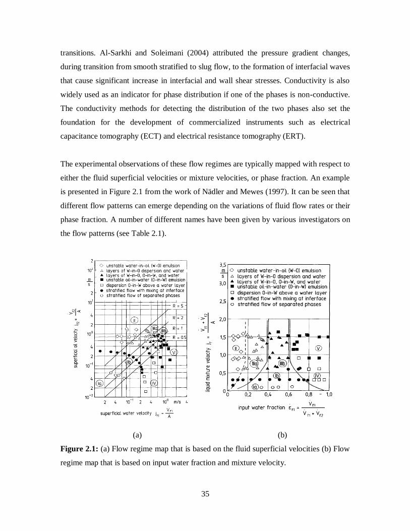
The experimental observations of these flow regimes are typically mapped with respect to

either the fluid superficial velocities or mixture velocities, or phase fraction. An example

is presented in Figure 2.1 from the work of Nädler and Mewes (1997). It can be seen that

different flow patterns can emerge depending on the variations of fluid flow rates or their

phase fraction. A number of different names have been given by various investigators on

the flow patterns (see Table 2.1).

(a) (b)

Figure 2.1: (a) Flow regime map that is based on the fluid superficial velocities (b) Flow

regime map that is based on input water fraction and mixture velocity.

36

Author Flow pattern classifications

Russell et al. (1959) Oil Bubbles in water

Stratified flow (SF)

Mixed Flow

Guzhov et al. (1973) Stratified flow

SF with mixing at the interface and a water lower layer

SF with mixing at the interface and a lower layer of oil/water dispersion

Water/oil and oil/water emulsions

w/o emulsion oil/water emulsion and a water lower layer

oil/water emulsion and a lower layer of oil/water dispersion

o/w emulsion

Oglesby (1979) Segregated

Semi-segregated

Semi-mixed (oil dominant, water dominant)

Mixed (oil dominant, water dominant)

Annular or concentric core of one phase within the phase (oil dominant,

water dominant)

Slug: Phases alternatively occupying the pipe as a free phase or as a

dispersion phase (oil dominant, water dominant)

Semi-dispersed (oil dominant, water dominant) Fully-dispersed: homogeneous mixture (oil dominant, water dominant)

Nädler & Mewes (1995) Stratified flow

SF with mixing at the interface and a water lower layer

SF oil/water dispersion and a water lower layer

o/w emulsion

SF water/oil dispersion, oil/water dispersion and a water lower layer

SF water/oil dispersion and a water lower layer w/o emulsion

Trallero (1995) Stratified flow

SF with mixing at the interface

o/w dispersion and free water layer

w/o dispersion and o/w dispersion

Full o/w emulsion

Full w/o emulsion

Brauner (2002) Stratified flow

SF with mixing at the interface

SF with a free liquid and a dispersion of another liquid (Do/w&w)

SF with a free liquid and a dispersion of another liquid (Dw/o&w)

w/o dispersion above o/w dispersion

w/o dispersion above o/w dispersion with pure oil at the top and pure

water at the bottom

Full o/w dispersion

Full w/o dispersion Core-annular flow (viscous oil in core and water in annulus)

Core-annular flow (water in core and oil in annulus)

Core-annular flow (dispersion of w/o in core and water in annulus)

Core-annular flow (dispersion of o/w in core and oil in annulus)

Core-annular flow (dispersion of one phase in core and dispersion of

another in annulus)

Intermittent flow

Elongated or spherical bubbles of one phase in a continuum of another

phase

Table 2.1: Flow pattern classification suggested in various literature.

The main ones are stratified flow, annular flow, dual continuous flow and dispersed flow

and are described in more detail below:

37

a) Stratified flow (ST) – (Figure 2.2a): Stratified flows are generally occurring at

low flow rates. Each of the oil and water layers flows as a continuum with a

distinct liquid-liquid interface. At the low flow rates, the flow is dominated by the

gravitational effect rather than inertia. As such, the separation of the two layers is

based on the density difference between the two phases. The oil phase (i.e. the

lighter phase) occupies the upper layer while the water phase occupies the lower

layer. As the flow rate is increased, waves of various lengths and amplitudes will

form at the interface and droplets of one phase may be entrained into the other

leading to a transition into the dual continuous flow pattern. A description of this

transition is presented by Al-Wahaibi et al. (2007).

(a)

(b)

Figure 2.2: (a) Stratified smooth flow (b) stratified wavy flow with the oil phase on the

top layer while the water phase on the bottom layer. (Ngan et al., 2007)

b) Dual continuous flow (DC) – (Figure 2.3): Dual continuous flow generally

occurs at intermediate mixture velocities between stratified and fully dispersed

flows. The oil and water phases retain their continuity and there is a distinct

interface between them. However, one or both phases are entrained into the other

as drops. The degree of entrainment varies according to the fluid velocities.

38

The transition into a dual continuous flow generally begins with wave formation

from a stratified flow. The interfacial waves are initially long compared to the

pipe diameter. As the fluid velocities increase, these waves become shorter.

Guzhov et al. (1973) reported that the relative movement of the two liquid phases

causes vortex motions due to the shear forces that penetrate the interface boundary.

This causes the formation of small droplets of one phase into the other (and is

regarded as the onset of entrainment). Once the drops are entrained, the

distribution of these drops will depend on the balance between inertial and

gravitational forces. At low flow rates, the entrained drops are few and gravity

tends to keep them near to the fluid interface. This flow pattern is sometimes

referred to as stratified flow with mixing dispersion at the interface. As the flow

rate increases, the degree of entrainment increases as drops are more evenly

distributed in the opposite layer due to the increased importance of the inertial

forces.

Figure 2.3: Dual continuous flow with several oil drops entrained in the water

continuous layer. (Ngan et al., 2007)

c) Annular flow (AN) – (Figure 2.4): A core of one phase is surrounded by an

annulus of the other. This flow pattern is common when the two phases have

equal densities or when one of the phases has a very high viscosity (Russell and

Charles, 1959).

Figure 2.4: Annular flow with an oil core and a water annulus. Small amount of drops

are also observed within the oil core in the figure. (Ngan et al., 2007)

39

d) Dispersed flow (D) – (Figure 2.5): One of the phases loses its continuity and

forms drops in the continuum of the other. This pattern occurs at high velocities.

There is usually a distribution of drop sizes which depends on the balance of drop

break-up and coalescence events. Drops can also be deformed and the deviation

from their sphericity can have significant impact on the mixture flow. In addition,

gravitational forces affect the vertical concentration of these drops leading to a

spatial distribution.

(a)

(b)

Figure 2.5: (a) Dispersed flow of oil drops in water. Drops observed are polydispersed

and highly deformable. (b) Oil slug flow in water (Ngan et al., 2007).

2.3 PHASE INVERSION

Phase inversion is a commonly observed phenomenon in dispersed liquid-liquid mixtures

(e.g. in pipe flow or in stirred vessels) but its mechanism is still not well understood. Two

types of dispersions are generally found (i.e. oil-in-water and water-in-oil) according to

the phase fraction and initial conditions. Phase inversion is generally found when the

mixture undergoes changes in the phase distribution as the phase fraction reaches certain

critical values (Yeh et al., 1964; Arirachakaran et al., 1989; Pal, 1993; Pacek et al., 1994;

Elseth, 2001; Ioannou et al., 2005; Hu, 2005; Piela et al., 2008). The critical phase

fraction where inversion occurs is known as phase inversion point. Coalescence and

break-up of the dispersed phase occur continuously in a dispersion. At low dispersed

40

phase fractions, this dynamic process can reach equilibrium. As the dispersed phase

fraction increases, the process may be unbalanced and coalescence becomes more

prominent due to the proximity of the dispersed drops. Eventually, phase inversion will

occur when the two phases switch their continuity. The occurrence of phase inversion and

the changes in phase continuity can lead to substantial changes in the mixture rheology

causing large fluctuations in pressure gradient during pipe flow (Angeli, 1996; Nädler

and Mewes, 1995).

Arirachakaran et al. (1989) has presented the development of the phase inversion process

as the initial water dispersed phase fraction is increased (see Figure 2.6). Some authors

have suggested that the inversion process is rapid and catastrophic (Smith and Lim, 1990;

Tyrode et al., 2005; Vaessen et al., 1996). However, other investigations suggest a

gradual inversion process particularly during pipe flow (e.g. Liu, 2005; Piela et al., 2008)

when partial inversion occurs at a certain location before the entire mixture is inverted.

The details of these observations will be discussed in the subsequent sections on phase

inversion in stirred vessels and pipe flow.

Figure 2.6: A schematic on the proposed phase inversion mechanism by Arirachakaran

et al. (1989).

41

2.3.1 PHASE INVERSION IN STIRRED VESSELS

Investigations on phase inversion have mainly been carried out in stirred vessels and the

outcomes from these works can provide valuable information on the phenomenon in pipe

flow. Reviews of literature available on phase inversion in stirred vessels can be found in

Yeo et al. (2000), Liu (2005) and Hu (2005).

One of the interesting findings in stirred vessel is the hysteresis effect observed when

inversion is approached from a water continuous or from an oil continuous dispersion.

The term ambivalent region has been introduced to define the region of phase fractions

where either dispersion can exist. Thus, either type of dispersion can only be clearly

defined beyond the ambivalent region. Figure 2.7 presents experimentally found

ambivalent region (Noui-Mehidi et al., 2004).

Figure 2.7: The existence of ambivalent region between the aqueous and organic

continuous dispersion across the organic phase fraction (Φo) (Noui-Mehidi et al., 2004).

Pacek et al. (1994) used video recording to capture the phase inversion process in a

stirred vessel and found that the drop size increased significantly near inversion while

secondary droplets (i.e. continuous phase drops within the dispersed phase) are formed

42

(Figure 2.8). Pacek et al. (1994) also found that secondary droplets only occur for

chlorobenzene in the dispersed glycerol/water phase but not in the opposite dispersion.

This difference in the formation of secondary droplets between the organic and the

aqueous continuous dispersions could be responsible for the appearance of the

ambivalent region. The formation of secondary droplet can have a significant widening in

the ambivalent region and hysteresis effect during phase inversion. According to them,

the coalescence of the dispersed phase is the most important mechanism controlling

phase inversion.

Figure 2.8: Droplet in drop for a glycerol/water and chlorobenzene system captured by

Sony video printer (Pacek et al., 1994).

Phase inversion and the ambivalent region are affected by many parameters. For example,

Selker and Sleicher (1965) found that the properties of the apparatus used (i.e. size and

materials of the vessel and impellers) and the operational conditions (i.e. agitation speed,

phase fraction) did not affect significantly the phase inversion. Deshpande & Kumar

(2003) also found that the limits of the ambivalent region reach asymptotic values at high

agitation speed and thus depend only on properties of the fluid system. According to

43

Selker and Sleicher (1965), fluid density would affect the ambivalent boundaries if the

agitation is slow and settling of the denser phase is prominent. The phase with higher

viscosity is also more likely to be the dispersed one. Viscosity also affects the ambivalent

region probably because of the lower coalescence rates caused by longer film drainage

time (Coulaloglou and Tavlarides, 1977). Interfacial tension has also been reported as an

important factor affecting phase inversion. Luhning & Sawistowski (1971) and Norato et

al. (1998), for example, showed that a decrease in interfacial tension can lead to a

widening of the ambivalent region.

Various empirical correlations have been developed from experiments to predict the

boundaries of the ambivalent region. The critical phase fraction of the organic phase, Φo,

was given by:

Luhning and Sawistowski (1971) for impeller speed between 600 to 1360 rpm:

(1) Φ for the upper inversion curve (w/o → o/w) (2.1)

(2) Φ for the lower inversion curve(o/w → w/o) (2.2)

Fakhr-Din (1973) for impeller speed below 680.85rpm:

(1) Φ

for the upper curve (2.3)

(2) Φ

for the lower curve (2.4)

where µc and µd are the continuous and dispersed phase viscosities (in Pa.s), Δ is the

density difference between phases (in kg/m3), FrI, ReI and WeI are the Froude number,

Reynolds number and Weber number at the impeller region.

The above equations demonstrate the importance of fluid properties on the width of the

ambivalent region. Fakhr-Din’s correlation also indicates the importance of the agitation

speed and impeller dimensions (in the Froude and Reynolds number terms). This may be

due to the low agitation speeds used where there may have been a separation of the

mixture.

44

Several mechanisms have been suggested by various investigators on the phase inversion

mechanism. According to Pacek et al. (1994), it is the imbalance between the break-up

and coalescence processes of the dispersed drop. This is also similarly suggested by

Arashmid & Jeffreys (1980) and Groeneweg et al. (1998). Phase inversion has also been

suggested to occur when the system free energy of the two possible dispersions (oil

continuous or water continuous) become equal (e.g. Luhning & Sawistowski, 1971;

Tidhar et al., 1986; Yeo, 2002). Yeh et al. (1964) have suggested that inversion occurs

when there is no shear between the two phases. However, it is difficult to measure

accurately the interfacial area close to and during inversion as well as the drop break-up

and coalescence rates. Further details about prediction of phase inversion based on these

mechanisms are presented in Section 2.4.

2.3.2 PHASE INVERSION IN PIPE FLOW

The investigation of phase inversion in pipelines can lead to better understanding on the

operating conditions and help to improve the pipe design to facilitate the transportation of

multiphase mixtures. This is particularly important as the presence of water is inevitable

and the mixture can only be separated after it has been transported over miles of pipeline

before processing. Inversion has been found to cause significant increase in pressure

gradient (Martinez et al., 1988; Angeli, 1996; Valle and Utvik, 1997; Nädler and Mewes,

1997 and Soleimani et al., 1997). A good understanding of the occurrence of phase

inversion is necessary to predict and control the pumping power required to transport the

mixture across and may lead to poor productivity. The exact relation between phase

inversion and pressure gradient is not well understood. For example, Ioannou (2006) has

shown that phase inversion occurs at the peak of the pressure gradient for Exxsol D80 but

not for Marcol 52 (see Figure 2.9). Exxsol D80 is less viscous (1.7 mPa.s) while Marcol

52 is more viscous (11mPa.s). Due to the high viscosity of Marcol 52, the high pressure

gradient caused during the oil continuous flow may have overshadowed the peak in

pressure gradient during phase inversion leading to an almost step change as a result.

45

(a)

(b)

Figure 2.9: (a) Pressure gradient measurement of a Exxsol D80/water system in a 60mm

I.D. pipe (b) Pressure gradient measurement of a Marcol 52/water system in a 60mm I.D.

pipe (Ioannou, 2006).

0.0

0.5

1.0

1.5

2.0

0 20 40 60 80 100

Input oil fraction, %

Pre

ssu

re g

rad

ien

t, k

Pa/m

Type I (o/w←w/o) Type II (o/w→w/o)

Phase

inversion

0.0

0.5

1.0

1.5

2.0

2.5

3.0

0 20 40 60 80 100

Input oil fraction, %

Pre

ssu

re g

rad

ien

t, k

Pa

/m

Type I (o/w←w/o) Type II (o/w→w/o)

Phase inversion

initiation

Phase inversion

completion

46

While changes in pressure gradient are direct consequences of the phase inversion

process, these changes cannot yet be accurately attributed to the point of phase inversion

and thus cannot be used to detect phase inversion. Other system parameters have been

used to detect the inversion process, e.g. conductivity. Conductivity measurements are

applicable to the flow of oil-water mixtures particularly as one phase is conductive and

the other is not. During phase inversion, the change is prominent with sharp changes in

conductivity. Conductivity measurements can be used to detect phase continuity at

locations where visual observations are not possible (e.g. at the centre of a pipe or in

highly concentrated dispersions). Such measurements have indicated that inversion may

not occur simultaneously across the whole pipe cross section. Soleimani et al. (2000)

reported that the spatial distribution of the two phases can be inhomogeneous due to

wetting effects of the pipe wall causing the water phase to concentrate towards the wall

and the oil phase concentrate in the pipe core. This inhomogeneity implies that phase

inversion may occur locally. Using laser induced fluorescence, Liu et al. (2006) showed

that zones of oil and water continuous dispersion appear within the pipe cross section

during inversion. This gradual phase inversion process has led to a transitional region

where phase inversion begins and completes over a range of phase fraction. An example

of such gradual inversion can be seen in Figure 2.10 (Hu, 2005) where oil continuous

dispersion begins to appear at one phase fraction until water becomes completely

dispersed at a higher dispersed phase fraction. Secondary droplets may also appear at

certain regions (see Figure 2.11 for example). Piela et al. (2006, 2008) have also reported

the formation of multiple dispersions and gradual inversion that spread over the cross

section in their pipe flow experiments.

47

Figure 2.10: Conductivity measurement conducted at the centre of a vertical pipe across

the phase inversion process (Hu, 2005).

Figure 2.11: Multiple dispersions of an oil/water system at a mixture velocity of 1.5m/s

and input oil fraction of 31%. The dark region represents the oil phase and the light

region represents the water phase. (Liu et al., 2006)

Secondary droplets

O/W W/O

Transitional Region

48

The effects of various parameters on phase inversion have been studied for pipe flow and

a summary of these parameters is presented in Table 2.2. It can be seen that fluid

properties, size and material of pipe used as well as operating conditions during the pipe

flow are of great importance. These parameters are similar to those observed in stirred

vessels.

Parameter investigated Author (Year)

1. Viscosity Arirachakaran et al.(1989); Luo et al. (1997); Nädler and

Mewes (1997)

2. Pressure drop Martinez et al.(1988); Angeli et. al (1996, 1998, 2000);

Valle and Utvik (1997); Luo et al. (1997); Nädler and

Mewes (1997); Soleimani (1999); Ioannou et al. (2004,

2005)

3. Velocity Luo et al.(1997); Angeli & Hewitt (1998 & 2000)

4. Phase Distribution Arirachakaran et al.(1989); Nädler and Mewes (1997);

Ioannou et al. (2004, 2005)

5. Pipe diameter & Material Arirachakaran et al.(1989); Ioannou et al.(2004, 2005)

6. Surfactant Pal (1993); Gillies et al. (2000)

7. Wettability Ioannou et al.(2004, 2005); Pettersen et al.(2001)

8. Conductivity Ioannou (2006); Hu (2005)

9. Drop size Liu et al. (2004) & Liu (2005); Hu (2005)

10. Interfacial tension Rodriguez and Bannwart (2006)

Table 2.2: Parameters affecting phase inversion in liquid-liquid pipeline flow.

2.3.3 PARAMETRIC STUDY ON PHASE INVERSION

The parameters which affect phase inversion in pipes are discussed in more detail here:

Agitation speed / Mixture velocity in pipe

The speed of agitation and the velocity of the mixture in the pipe flow have been reported

to enhance the mixing process and the dynamic processes of drop coalescence and break-

up. McClarey and Mansoori (1978) showed phase inversion occurs at a higher volume

fraction of the aqueous phase when the impeller speed is increased from 240RPM to

480RPM. However at high impeller speeds (beyond 480RPM), there is no effect of

49

agitation on the phase inversion hold up. Similar findings were also reported by Quinn

and Sigloh (1963), Luhning and Sawistowski (1971), and Deshpande and Kumar (2003).

Pacek et al. (1994) found that phase inversion will not occur under certain circumstances

if the agitation speed is very high but will occur if the agitation speed is reduced. On the

other hand, they also observed that phase inversion will not occur at very low speeds.

Efthimiadu and Moore (1994) suggested that the increase in agitation speed will increase

the shear rate and will lead to finer and more stable dispersions even at higher dispersed

phase fraction.

Similar experiments have been conducted in pipe flows by Arirachakaran et al. (1989)

who showed that mixture velocity has little effect on the occurrence of phase inversion.

However, Ioannou et al. (2005) found that an increase in mixture velocity increased the

fraction of oil continuous phase when inversion occurred.

Fluid Density

The effect of fluid density was previously found to be important in gas-liquid system

where the density difference is large. In liquid-liquid dispersed systems, Selker and

Sleicher (1965), McClarey and Mansoori (1978) and Norato et al. (1998) have shown that

the fluid densities have little effect on the ambivalent region in stirred vessels provided

that the difference in density is not large. However, large density difference can lead to

difficulty in maintaining the dispersion at low agitation speeds. Thus, more stirring power

is required to achieve an homogeneous dispersion. Other investigators have found that a

large density difference can increase the tendency for phase inversion (Rodger et al.,

1956; Kumar et al., 1991). Chiang and Chen (1994) found that inversion will occur at a

higher aqueous phase fraction when water is the dispersed phase for a fluid system with

large density difference.

Efthimiadu and Moore (1994) performed their phase inversion experiments in parallel

plates and found that the density of the aqueous continuous phase caused a small increase

in the volume fraction of the organic phase at inversion. However, these experiments

were conducted in conditions where effects of other fluid properties are coupled.

50

Fluid viscosity

Fluid viscosity has been reported in various investigations to be a significant factor

affecting phase inversion as well as the ambivalent region. Selker and Sleicher (1965)

reported that the viscosity ratio of the two phases in a stirred vessel can influence the

ambivalent boundaries. In addition, an increase in the viscosity of one phase will increase

its tendency to be the dispersed phase. However, Treybal (1963) suggested that the higher

viscosity of one phase will favour it to be the continuous phase. Efthimiadu and Moore

(1994) also found that the more viscous phase tends to become continuous in parallel

shearing plates (especially if the viscous phase tends to wet the surface). They attribute

this finding to be the increased dynamic stability of the dispersion when the viscous

phase is continuous. Similar results have also been reported by Norato et al. (1998), who

found that the upper and lower limit of the ambivalent region can be widened by

increasing the viscosity regardless of whether the phase is continuous or dispersed. The

widening behaviour is postulated to be caused by the lower coalescence rate due to longer

film drainage time which agrees with the findings from Groeneweg et al. (1998),

Coulaloglou and Tavlarides (1977) and Calabrese et al. (1986).

Arirachakaran et al. (1989) from literature data on inversion in pipelines with different

viscosity oils found that the more viscous oils tend to be dispersed. Similarly, Ioannou

(2006) showed that the more viscous Marcol 52 oil tended to invert at a higher oil

fraction. Nädler and Mewes (1997) however using oils with different viscosity (between

22 and 35 mPa.s) found no significant effect on inversion.

Interfacial tension

The effect of interfacial tension is the least well understood among the fluid properties on

phase inversion. According to Selker and Sleicher (1965), the magnitude of interfacial

tension is unlikely to influence the ambivalence region as the interfacial tension between

a pair of fluids is not a function of the interfacial curvature. Yeh et al. (1964) suggested

that interfacial tension plays a small role on phase inversion. In the absence of other

forces, the interfacial tension will cause inversion to occur at 50% volume fraction.

51

Luhning and Sawistowski (1971), on the other hand, found that interfacial tension can

affect the phase inversion since it affects drop size and interfacial area. Clarke and

Sawistowski (1978) later confirmed the change in interfacial area during phase inversion

and showed that the width of the ambivalent region is significantly affected by interfacial

tension. Lowering the interfacial tension will widen the width.

Norato et al. (1998) also found that decreasing the interfacial tension widens the

ambivalent region and makes it more difficult to cause an appearance of phase inversion.

According to Coulaloglou and Tavlarides (1977), decreasing the interfacial tension will

lead to an increase in drainage time for the film between drops leading to higher drop

breakage and lower drop coalescence and as such smaller drop size. A higher dispersed

phase fraction will thus be required for inversion to occur. This suggestion has been

confirmed by experiments. Efthimiadu and Moore (1994) found that lowering the

interfacial tension has a stabilising effect on the type of dispersion which depends also on

the other properties of the system. It was also experimentally found that the effect of

shear rate (i.e. rotational speed and gap width) is minimised with the decrease in

interfacial tension. The influence of the wettability of the contacting surfaces is also

reduced.

Surface wettability

The material of construction of the dispersion container (e.g. stirred vessel or pipe) has

been suggested to affect the type of dispersion formed and as a result phase inversion and

ambivalent region. McClarey and Mansoori (1978) suggested, through their experimental

outcome for an equal density and viscosity mixture, that the discrepancies in their

inversion curves can be attributed to the difference in wettability of the vessel surface

with the two liquids. However, the effect is only found to be significant at low agitation

speeds. Giulinger et al. (1988) changed the material used in the stirred vessel from water

to oil wetted and showed that the wetting phase was favoured to remain continuous. In

stirred vessels, drop break-up generally occurs within the impeller region and coalescence

at the other regions. However, Kumar et al. (1991) reported that the drops can coalesce

on the impeller and form a thin film if the impeller is preferably wetted by the dispersed

52

phase. The drops will subsequently be broken at the impeller or at its vicinity. The effects

on the coalescence and break-up process can significantly change the phase inversion

behaviour.

Efthimiadu and Moore (1994) investigated the effect of material on phase inversion of

liquid-liquid dispersions between parallel plates. Their experimental findings indicated

that the liquid which preferentially wets the surface of the plates tends to form the

continuous phase.

The effect of surface wettability is not well documented for pipeline flow. Angeli and

Hewitt (1998) conducted experiments in 24 mm I.D. pipe with Exxsol D80 as the oil

phase and water as the aqueous phase. They observed similar range of input water

fraction (at 37% - 40%) regardless of the material of the pipe (acrylic and stainless steel).

Pettersen et al. (2001) conducted experiments with the same type of oil in PVC and

stainless steel pipes of 100 mm I.D. and found that inversion is delayed to a higher oil

fraction in PVC compared to the steel one when experiments started from an oil

continuous mixture. Ioannou et al. (2005) found that acrylic is wetted more by the oil

phase than steel and thus phase inversion occurs at a higher oil fraction for acrylic pipe.

Inlet conditions

Inlet conditions are important as these determine how the two fluids are introduced into

the pipe and, coupled with other effects, can affect the phase inversion appearance. Piela

et al. (2006, 2008) discussed two approaches in introducing the phases into the test pipe.

In the continuous experiment, the continuous phase was introduced in the pipe loop and

wetted the pipe wall. The dispersed phase was then injected into the loop and a

corresponding volume of mixture was removed to ensure constant mixture velocity of

fluid in the system. The dispersed phase fraction was gradually increased with the

continuous injection of the dispersed phase until phase inversion occurred. In the direct

experiment, the two fluids were introduced as two separate continuous phases and

subsequently mixed within the test pipe. The input flow rates of the two phases were

adjusted to maintain a constant mixture velocity. From the experimental outcome, the

53

critical fraction of the dispersed phase for inversion can be significantly higher for the

continuous experiment than the direct one. The authors also suggested that the phase

inversion can be postponed or avoided by altering the inlet conditions.

Dispersion initialisation

The initialisation of the dispersion has been reported to have a strong effect on phase

inversion. For example, Selker and Sleicher (1965) found that the inversion point in

stirred vessels is strongly influenced by the initial type of dispersion (i.e. water

continuous or oil continuous) especially if the phase fraction is within the ambivalent

region.

The occurrence of ambivalent region as a direct effect of dispersion initialisation has

been seen mainly in stirred vessels but not studied systematically in pipes. Ioannou et al.

(2005) observed in their pipe flow experiments that the initial continuous phase will tend

to preserve its continuity leading to an hysteresis effect in the occurrence of phase

inversion according to the initial dispersion type. Hu and Angeli (2006), however,

observed no effect of dispersion initialisation in a vertical pipe flow based on their

experimental conditions studied.

2.4 PHASE INVERSION MECHANISMS AND PREDICTION

MODELS

Several types of prediction models based on different phase inversion mechanisms have

been reported in various literatures. These models will be discussed in detail in the

following sections.

2.4.1 MODELS BASED ON RATE OF DROP BREAK-UP AND

COALESCENCE

Phase inversion is commonly found in dispersion. Parameters affecting phase inversion

are known to also influence the drop coalescence and breakup (e.g. fluid properties,

agitation speed, wettability). This has led to various investigations to relate phase

54

inversion with the dynamic process of drop break-up and coalescence (Arashmid and

Jeffreys, 1980; Groeneweg et al., 1998). In a stable dispersion, e.g. O/W, the dynamic

process of drop break-up and coalescence is balanced. Increasing the dispersed phase (i.e.

oil) will lead to higher collision frequency and coalescence rate. Concurrently, more

drops of larger size will also be broken up. Thus, a new equilibrium of this dynamic

process will be formed.

According to Arashmid & Jeffreys (1980), collision of drops in a stirred vessel will lead

to some drops being coalesced. As the dispersed phase is increased under a constant

agitation speed, the chance of successful coalescence for each collision will increase. At

phase inversion, it is suggested that coalescence will occur for every collision. Thus, the

frequency of drop collision will be equal to the frequency of drop coalescence. Based on

Levich (1962)’s collision frequency model and Howarth (1967)’s coalescence frequency

model, the dispersed phase holdup (ΦdI) at inversion can be expressed as follows:

0.48

I

2

d

I

dNd

KΦ (2.5)

where K is a constant depending on the type of agitator, dd is the drop size and NI is the

agitation speed.

Vaessen et al. (1996) applied the idea from Arashmid & Jeffreys (1980) to determine

phase inversion. However, they suggested that drop break-up should be part of the

inversion process in addition to having coalescence occurring at each collision. At phase

inversion, drop break-up is dominated by the drop coalescence process and the

equilibrium drop size diverges.

To estimate the drop size at inversion, the following coalescence and break-up rate

equations are used.

55

Coalescence rate (based on Saffman and Turner, 1956):

21/31/3

c n(d)d6.87ε(d)R (2.6)

Break-up rate (based on Delichatsios and Probstein, 1976):

)n(d)d1.88ε

σexp(dε

π

21.37(d)R

5/32/3

2/31/3

b

(2.7)

where Rc(d) and Rb(d) are the rates of coalescence and break-up of drops with mean

diameter, d, ε is the turbulent energy dissipation rate, ζ is the interfacial tension, n(d) is

the number density of drops with diameter d.

It can be seen that the break-up process is proportional to the number of drops in a

volume while the coalescence process is proportional to the number of drops in a volume

squared. The coalescence rate will increase faster as the volume of dispersed phase

increases. This leads to phase inversion when the dynamic balance between the two rates

collapses.

Groeneweg et al. (1998) suggested that phase inversion is governed by the balance

between drop break-up and coalescence which can be altered in favour of coalescence by

the increase of the effective volume fraction of the dispersed phase on continuous stirring.

This results in the inclusion of the continuous phase into the drops of the dispersed phase

forming secondary droplets. The enclosed droplets can also be escaped back to the

continuous phase. The effective volume fraction of the dispersed phase will continue to

increase as long as the inclusion dominates over the escape. Inversion will start when the

effective volume fraction for inversion has been reached. At this point, the droplet size

increases significantly and inversion follows.

Desphande and Kumar (2003) proposed that drop break-up and coalescence do not occur

independently in high dispersed phase holdups. The ratio of the rates at which the two

events occur in turbulent flow field is determined by the average relative separation

between the drops and the physical properties of the fluids in the system. It is also

56

independent of the intensity of the turbulent flow field for sufficiently intense turbulent

flow.

Hu et al. (2004) applied the population balance model to predict the birth and death rates

of drops of specific size and account for the corresponding drop size distribution. The

birth and death of drops are associated with the drop break-up and coalescence. In order

to predict the phase inversion, the total volumetric break-up rate will be equal to the total

volumetric coalescence rate. With this approach, the ambivalent region can be found. It

agrees reasonably well with literature data except in high dispersed phase fraction. The

disagreement can be attributed to the coalescence efficiency correlations that are not

meant for dense dispersion.

2.4.1.1 SECONDARY DISPERSIONS

With the dynamic process of drop coalescence and break-up, secondary dispersions can

also arise in a dispersed flow as the continuous phase entrains in the dispersed phase (e.g.

O/W/O dispersion). The formation of secondary dispersions is found to be more likely

near the phase inversion point (Luhning and Sawistowski, 1971) and secondary

dispersions depend on the continuous phase. For example, Pacek and Nienow (1995)

have found that only O/W/O dispersion can exist in a water-kerosene mixture but not

W/O/W. Kumar (1996) suggested that secondary droplets are formed when successive

coalescence of drops leads to droplets entrained in them. However, two criteria must be

met (1) the coalescence efficiency should be high so that the drops can coalesce

simultaneously (2) the entrained droplets should be at a stable condition upon

entrainment. The absence of W/O/W dispersions could be due to the low coalescence

efficiency of the oil drops in water and the secondary water droplets, if any, will have

high coalescence efficiency leading to the water droplets escape to the water continuous

phase.

Liu et al. (2005) observed secondary droplets using laser induced florescence (LIF)

technique in pipe flow (Figure 2.12). The formation of secondary droplets will lead to a

higher effective dispersed phase fraction (i.e. the total volume fraction of the primary

57

drops and the secondary droplets) and would lead to an earlier occurrence of phase

inversion than that expected from the actual phase fractions of the two phases.

Figure 2.12: Visual observations of (a) O/W/O and (b) W/O/W dispersions using LIF

technique. The oil phase is shown in black while the water phase is shown in luminous

green (Liu et al., 2005).

2.4.2 MODELS BASED ON MINIMIZATION/EQUAL SYSTEM AND

INTERFACIAL ENERGY

Luhning and Sawistowski (1971) suggested that the total energy (including kinetic and

interfacial energy) of the system would reach a minimum value at phase inversion and the

change in total energy is caused by the fluid system itself. The measured impeller power

input in the stirred vessel was observed to remain constant throughout the inversion

process.

Other investigators (Tidhar et al., 1986; Decarre and Fabre, 1997; Yeo et al., 2002;

Brauner and Ullmann, 2002) have suggested that the surface energies (i.e. interfacial

energy and the surface energy of the fluids with the contacting wall) of the two possible

types of dispersion, O/W and W/O, should be balanced at phase inversion. To account for

the surface energy, the interfacial area can be calculated using Monte Carlo simulation

(Yeo et al., 2002) or Population Balance model (Hu, 2005). Brauner and Ullmann (2002)

expressed the interfacial area in terms of Sauter mean diameter and derived the following

equation for the oil volume fraction at phase inversion.

Primary drop

Secondary droplet

58

w/o32o/w32

o/w32IO

D/D/

cos6

sD/

(2.8)

where θ is the solid-liquid surface contact angle with 0 < 90 denoting a surface

preferentially wetted by water (hydrophilic surface) and 90 < 180 denoting a

surface wetted by oil (hydrophobic surface), s is the solid surface area per unit volume

where s=4/D and D is the pipe diameter, ζ is the interfacial tension and D32 is the Sauter

mean drop diameter.

Equation 2.8 can be simplified as follows when the solid-liquid surface energy is

neglected (Yeo et al., 2002):

O/W

W/O

32

32

IO

IO

D

D

1

(2.9)

While the correlations based on this approach does not account for the existence of

ambivalent region, Brauner and Ullmann (2002) suggested that ambivalent region can be

regarded as the change in interfacial tension when contaminant is present. Yeo et al.

(2002) use different correlations to calculate the Sauter mean drop diameter depending on

the dispersed phase fraction. The use of these correlations results in the presence of

ambivalent region according to the history of the system.

2.4.3 MODELS BASED ON ZERO SHEAR STRESS AT INTERFACE

Phase inversion has been previously mentioned to be influenced by the viscosities of the

liquid phases in the system. Yeh et al. (1964) developed a correlation for predicting the

critical phase fraction at inversion as a function of the viscosity ratio of the two phases

based on the assumption that the interfacial shear is zero at the point of the inversion (i.e.

no tendency to mix or create new surfaces). From the momentum balance of the two

phases, they suggested the following correlation for the phase inversion point which was

59

modified by replacing the viscosity of the continuous phase with the interfacial viscosity

( i) and was found to improve on the prediction:

2/1

i

d

Id

Id

1

(2.10)

where θdI is the dispersed phase fraction at phase inversion, d and i are the dispersed

phase and the interfacial viscosity respectively.

Nädler and Mewes (1995, 1997) also used the momentum balance of the phases and the

assumptions of zero interfacial shear and no slip between the two phases to develop the

following correlation for the initial water fraction at inversion.

2

ow

w

o

w

o

k/1

nnmn

w

no

)n1(w

)n1(o

w

o1

Iw

)DU(C

Ck1

1

(2.11)

where is the fluid density, subscripts o and w referring to the oil and water phases

respectively, D is the pipe diameter, and Um is the mixture velocity, and C and n are the

parameters used in the Blasius friction factor equation, CRe-n

, k1 and k2 are the empirical

parameters depending on the type of dispersion (O/W or W/O) and flow conditions. If

both phases are in laminar flow, k1 and k2 can be taken as 1 and 2 respectively and

equation 2.11 is equivalent to equation 2.10.

2.5 DROP SIZE DISTRIBUTION AND CHARACTERISTIC

DIAMETER

As discussed in the previous section, the drop size of the dispersed phase and its

distribution are important elements in the models of phase inversion prediction (e.g.

based on the dynamic process of drop break-up and coalescence, equal and minimization

60

of system/interfacial energy). Drop size distributions in liquid-liquid dispersions and the

various ways of expressing them are discussed in this section.

2.5.1 TYPES OF DROP SIZE DISTRIBUTION

Coulaloglou and Tavlarides (1977) developed a model for drop size distribution in a

stirred vessel based on the effects of drop break-up and coalescence in an isotropic

turbulent field. A break-up model was derived by considering drop deformation, break-up

under influence of local pressure fluctuation and the time needed for a critically deformed

drop to break-up in a locally isotropic field. A coalescence model was also derived based

on the assumption that the coalescence rate is proportional to the collision rate and the

coalescence frequency in the kinetic regime of locally isotropic turbulent fields. They

used a Gaussian probability density function of drop sizes in the feed and found good

agreement between the model and experimental distribution in the stirred vessel (see

Figure 2.13 for comparison).

Figure 2.13: Comparison between calculated drop size distribution and experimental

drop size data. Dotted line represents the histogram at the circulation region and the solid

line represents the histogram at the impeller region. (Coulaloglou and Tavlarides, 1977).

Collins and Knudsen (1970) investigated experimentally dilute O/W dispersions (up to 10%

by volume) in pipe flow using 3 different organic phases and did not observe coalescence.

61

They suggested that the drop size distribution in the pipe is a result of two superimposed

distributions – (1) produced by the injection nozzle and (2) produced by the turbulence of

the flow. The drop size distribution is nearly log-normal at the injection nozzle but

deviates from the log-normal type along the flow downstream due to the action of

turbulence.

Karabelas (1978) re-examined some of the experimental data from Collins and Knudsen

(1970) and compared that with his own experimental results in pipe flow using two

different organic phases. He found that the drop size distribution can be fitted with a

Rosin-Rammler or an upper limit log-probability distribution. While both distribution

types yield similar result, Rosin-Rammler distribution in Equation 2.12 is simpler for use.

n

95cum

d

d2.996expV1 (2.12)

where Vcum is the cumulative volume fraction of drops with diameter less than d, d is the

drop diameter and d95 is the drop size corresponding to 95% of drops smaller than d95. n

is a fitting parameter of the distribution.

Angeli and Hewitt (1998) investigated the drop size distribution experimentally in an

oil/water pipe flow. They observed that the drop size distribution is strongly influenced

by the pipe material with drops smaller in steel pipe than acrylic pipe and can be

reasonably fitted with a Rosin-Rammler distribution with parameter, n, in Equation 2.12

ranging from 2.1 to 2.8.

Simmons and Azzopardi (2001) also examined the drop size distribution experimentally

in a pipe flow. The backscatter technique applied in their experiments allows drop size

distribution to be obtained even at highly dense dispersion. From their results, the drop

size distribution of the mixture flow fits well with an upper-limit log-normal distribution.

62

Vielma et al. (2008) compared their experimental results in an horizontal pipe flow of

water and mineral oil with various dispersion types – Normal, Log-normal and Rosin-

Rammler. They conclude that log-normal distribution is the best probability distribution

for all their experimental results regardless of the type of dispersion (O/W or W/O).

Figure 2.14 presents one of comparisons of the oil drop size distribution at an oil and

water flow velocity of 0.75m/s.

Figure 2.14: Comparison between experimental drop size data and selected drop size

distribution types in an horizontal pipe flow (Vso = 0.75m/s, Vsw=0.75m/s, oil drops).

(Vielma et al., 2008).

2.5.2 CHARACTERISTIC DIAMETERS OF DROP SIZE DISTRIBUTION

Knowing the changes in drop size distribution is useful to understand the underlying

dynamics in the drop break-up and coalescence process. However, the distributions are

difficult to compare across different studies. An easier way to characterize a drop size

distribution is by using the characteristic mean diameters despite that some information

may be neglected. Two common characteristic diameters are the linear mean diameter,

d10, and the Sauter mean diameter, d32. They are defined in Equation 2.13 and 2.14

63

respectively. In this thesis, Sauter mean diameter will be used in general as this diameter

is commonly reported in prediction of mean drop size for liquid-liquid dispersions.

(1) Linear mean diameter, d10, which defines the number-averaged drop size.

n

d

d

n

1i

i

10

(2.13)

(2) Sauter mean diameter, d32, which defines the characteristic diameter that has the same

volume/area ratio as the distribution.

n

1i

2i

n

1i

3i

32

d

d

d (2.14)

where di is the diameter of the sample drop and n is the number of drops in the sample

distribution.

2.6 NUMERICAL SIMULATION ON DISPERSED FLOW

The occurrence of phase inversion is a direct consequence of the dynamic flow behaviour.

It involves the interaction of the fluid phases in the system and causes a spatial re-

distribution of the phases across the confined system (e.g. pipes). Phase inversion can be

influenced by many parameters and these parameters can themselves be inter-related. In

addition, empirical correlations on two-fluid flow usually provide global information on

the system. The important local information which can have great significance in

understanding dynamic phenomena such as phase inversion is neglected by such

correlations.

Information on the flow field would be important for understanding phase inversion. This

can be achieved by computational fluid dynamics (CFD) modelling. CFD is a

computational code for solving the continuity and Navier-Stokes equations using a

64

number of closure correlations. Various authors have attempted to improve the prediction

of multiphase flow and apply the development in simulating complex flows (Hill, 1998;

Rusche, 2002; Chesters and Issa, 2004; Liu, 2005; Krepper et al., 2005). While current

CFD simulation has been reported to achieve reasonable success in comparison with

experimental data, there are still a lot of developments required due to the uncertainty in

the actual mechanisms for the occurrence of fluid flow phenomenon (e.g. phase

inversion). The development of the CFD code should also be complemented with

improved experimental techniques for more detailed investigation on fluid flow.

While many process flows operate at high dispersed fraction, currently CFD handle dilute

dispersion with <10% dispersed fraction. This is due to the lack of information on terms

such as inter-phase momentum, turbulence effects as well as phenomenon such as phase

inversion at high dispersed phase fractions.

The common approaches used in CFD to simulate multiphase flows are (1) Eulerian-

Lagrangian, (2) Eulerian-Eulerian and (3) Volume of fluid (VOF). These approaches are

discussed below (more detailed discussion can be found in Hill (1998), Rusche (2002),

Ranade (2002)). In the Eulerian-Lagrangian (E-L) framework, the dispersed phase is

represented by individual dispersed elements (i.e. drops). The trajectories of these drops

are tracked by solving the appropriate momentum equations in a Lagrangian framework

(i.e. the dependent variables are functions of the properties of the tracked drop). At the

same time, the conservation equations for the continuous phase are expressed in the

Eulerian framework (i.e. the fluid properties are functions of space and time with respect

to the reference volume domain). This approach is good in capturing the flow dynamics

of the dispersed phase. The drop size distribution and inter-particle interactions can also

be accounted for. However, it is computational intensive especially at large numbers of

dispersed drops.

In the Eulerian-Eulerian (E-E) approach, the conservation equations of all the fluid

phases are expressed in the Eulerian framework. The fluid phases are assumed to share a

volume domain and interpenetrate during their motions. The presence of each phase is

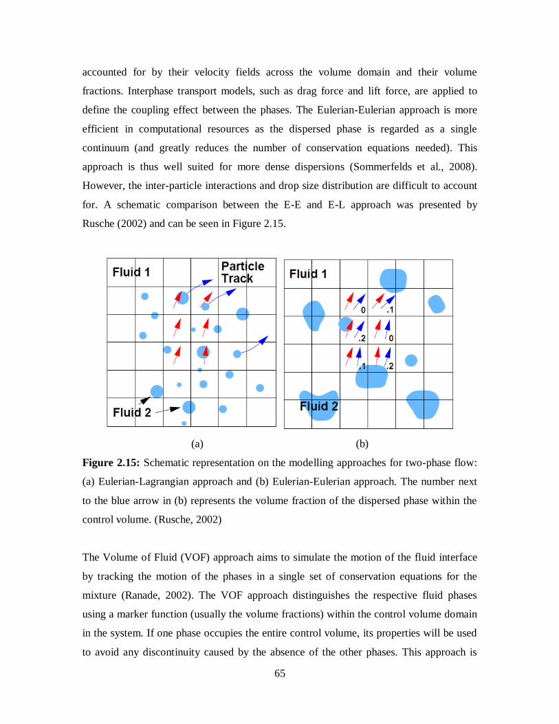
65

accounted for by their velocity fields across the volume domain and their volume

fractions. Interphase transport models, such as drag force and lift force, are applied to

define the coupling effect between the phases. The Eulerian-Eulerian approach is more

efficient in computational resources as the dispersed phase is regarded as a single

continuum (and greatly reduces the number of conservation equations needed). This

approach is thus well suited for more dense dispersions (Sommerfelds et al., 2008).

However, the inter-particle interactions and drop size distribution are difficult to account

for. A schematic comparison between the E-E and E-L approach was presented by

Rusche (2002) and can be seen in Figure 2.15.

(a) (b)

Figure 2.15: Schematic representation on the modelling approaches for two-phase flow:

(a) Eulerian-Lagrangian approach and (b) Eulerian-Eulerian approach. The number next

to the blue arrow in (b) represents the volume fraction of the dispersed phase within the

control volume. (Rusche, 2002)

The Volume of Fluid (VOF) approach aims to simulate the motion of the fluid interface

by tracking the motion of the phases in a single set of conservation equations for the

mixture (Ranade, 2002). The VOF approach distinguishes the respective fluid phases

using a marker function (usually the volume fractions) within the control volume domain

in the system. If one phase occupies the entire control volume, its properties will be used

to avoid any discontinuity caused by the absence of the other phases. This approach is

66

suited for investigations where the shape and fluid motion at near the interface are of

interest. While it offers better resolution close to the interface, computational resources

increase significantly if there is a dense dispersed phase. This approach is thus commonly

used to investigate, for example, deformation of single drop in a flow field and the

breakup and binary drop coalescence processes (Stover et al., 1997; Delnoij, 1997;

Krishna and van Baten, 1999).

2.6.1 CONSERVATION EQUATIONS USED IN CFD

As phase inversion tends to occur in dense dispersions, the simulation of such dispersion

will be a valuable source of information in addition to the experimental data. It will also

ease the investigation on the effects of various parameters especially with conditions that

are difficult to match with experiments. As suggested by Sommerfelds et al. (2008), the

numerical simulations used for intermediate and dense dispersion should be based on the

Eulerian-Eulerian framework. The Eulerian framework is based on volume-averaged

mass and momentum transport equations for the respective fluid phases. For an

incompressible multiphase system (e.g. oil/water), the phases are assumed to share the

space proportionally to their volume fractions such that:

αd + αc = 1.0 (2.15)

where α is the volume fraction of the respective phases and d, c represent the dispersed

and continuous phases respectively.

The continuity equation is:

0ut

kkk

(2.16)

The momentum transfer equation is:

Mkkkkkkkkkkkk Fgpuuut

(2.17)

67

From equations 2.16 and 2.17, the subscript k represents a specific phase (i.e. oil or water

in this study), is the mean fluid density, u is the velocity vector given by , u = [u, v, w],

g is the gravity, η is the phase shear stress tensor (ηk=-µk( uk + ( uk)T)) and FM is the

interphase force term.

For turbulent flow, the flow variables can be decomposed into two components: (1) a

steady mean, e.g. U, and (2) a fluctuating component that oscillates around the mean

value, u′(t). This is called the Reynolds decomposition (Hill, 1998; Elseth, 2001). The

flow variables of the turbulent flow can be expressed as follows:

u(t) = U + u′(t); v(t) = V + v′(t); w(t) = W + w′(t); p(t) = P + p′(t) (2.18)

By substituting equation 2.18 into equations 2.16 and 2.17, the effect of turbulence can be

accounted for in the conservation equations.

The continuity equation becomes:

0Uααt

kkk

(2.19)

The momentum equation becomes:

Mkkkkkkkkkkk FgpUUUt

(2.20)

where U is the volume averaged velocity in a turbulent flow, and Τ is the Reynolds stress

tensor given by:

zzzyzx

yzyyyx

xzxyxx

k (2.21)

68

The tensor creates six extra stress terms including three normal stresses

2

kkxx 'u 2

kkyy 'v 2

kkzz 'w (2.22)

and three shear stresses

'v'ukkyxxy 'w'ukkzxxz 'w'vkkzyyz (2.23)

These six extra stresses are called Reynolds stresses. The inclusion of these terms in

equation 2.21 requires a turbulence model to predict the Reynolds stresses. The k-ε model,

which will be used in this thesis, is by far one of the most widely used and validated

turbulence models. It is based on the assumption that there is an analogy between the

action of the viscous stresses and the Reynolds stresses on the mean flow.

According to Boussinesq (1877), the Reynolds stresses can be expressed in the following

way:

xykk

x

y

y

xtkyxxy k

3

2

x

U

x

U'u'u

(2.24)

where

)'w'v'u(2

1k 222 is the turbulence kinetic energy per unit mass, µt is known

as the turbulent or eddy viscosity. The Kronecker delta, δxy, becomes 1 if x=y and 0 if

x≠y. The other Reynolds stress terms can be expressed in the same form as Equation 2.24.

FM is a source term that accounts for the overall effect of various body forces – buoyancy

force, lift force, drag & turbulent dispersion force, virtual/added mass effects. Virtual

mass effects can be ignored unless the high frequency fluctuations of the relative velocity

occur. These high frequency fluctuations are generally not resolved in the CFD code and

also tend to be lost in the averaging process (Drew, 1983; Chen et al., 2005).

The conservation equations can be further simplified for the steady-state and

incompressible flow with no mass transfer encountered. In addition, the modeling of drop

69

dynamics and drop size distribution are not included in this thesis to reduce complexity of

the simulations and the required run time. With these assumptions, the continuity

equation becomes:

0Uα kk (2.25)

and the momentum transfer equation becomes:

force dispersionTurbulent & Drag

kint,F

forceLift

k,liftF

force Viscous

kk

force nalGravitatio

gkk

force Pressure

pk

convection todue momentum of Change

kUkUkk

(2.26)

In order to close the set of equations 2.26, appropriate models for the interphase drag, lift

and turbulent dispersion forces are needed.

2.6.2 MODELS FOR SIMULATION OF LIQUID-LIQUID DISPERSED

PIPE FLOW

Turbulence models

In order to achieve a balance between the level of accuracy expected from the CFD

simulations and the resources required to achieve it, turbulence models have been

proposed to simplify the numerical calculations needed to take into account the

turbulence. These models will be discussed with special focus on Ansys CFX which is

the CFD code used in this study.

Standard k-ε model

The k-ε model is a semi-empirical model based on the solution of two separate transport

equations for the mean turbulence kinetic energy, k, and the dissipation of this kinetic

energy, ε. The effect of turbulence is accounted for via the turbulence viscosity term (µt)

without modifying the effect of molecular viscosity (µk) in the conservation equations

(eddy viscosity hypothesis). Molecular viscosity refers to the viscosity effect caused by

the fluids while the turbulence viscosity is an imaginary viscosity effect caused by the

turbulence eddies proposed by Boussinesq (1877). The model assumes that the Reynolds

70

number of the flow is high and the turbulence across the domain is homogeneous. This is

valid for a fully developed turbulent flow in a pipe except at locations very near to the

wall.

The transport equations for k and ε are:

k ofon /destructiproduction of rateNet

)(k

diffusionby k ofTransport

c

c),(k

c,t

c

convectionby k ofTransport

cccc

k of change of Rate

ccc SkkU)k(t

(2.27)

ofon /destructiproduction of rateNet

diffusionby ofTransport

c

c,

c,t

c

convectionby ofTransport

cccc

of change of Rate

ccc SU)(t

(2.28)

where µt,c is the turbulence viscosity of the continuous phase. Among the terms, there are

several empirical parameters that have been evaluated through data fitting over a wide

range of turbulent flows. The set of constants given by Launder and Spalding (1972) is

the most widely used and is the default set of constants for CFX (see Table 2.3).

Model parameter Suggested value

Cµ

C1ε

C2ε

ζk(ε),c

ζε,c

0.09

1.44

1.92

1.00

1.30

Table 2.3: Coefficients for k-ε turbulence model (Launder and Spalding, 1972)

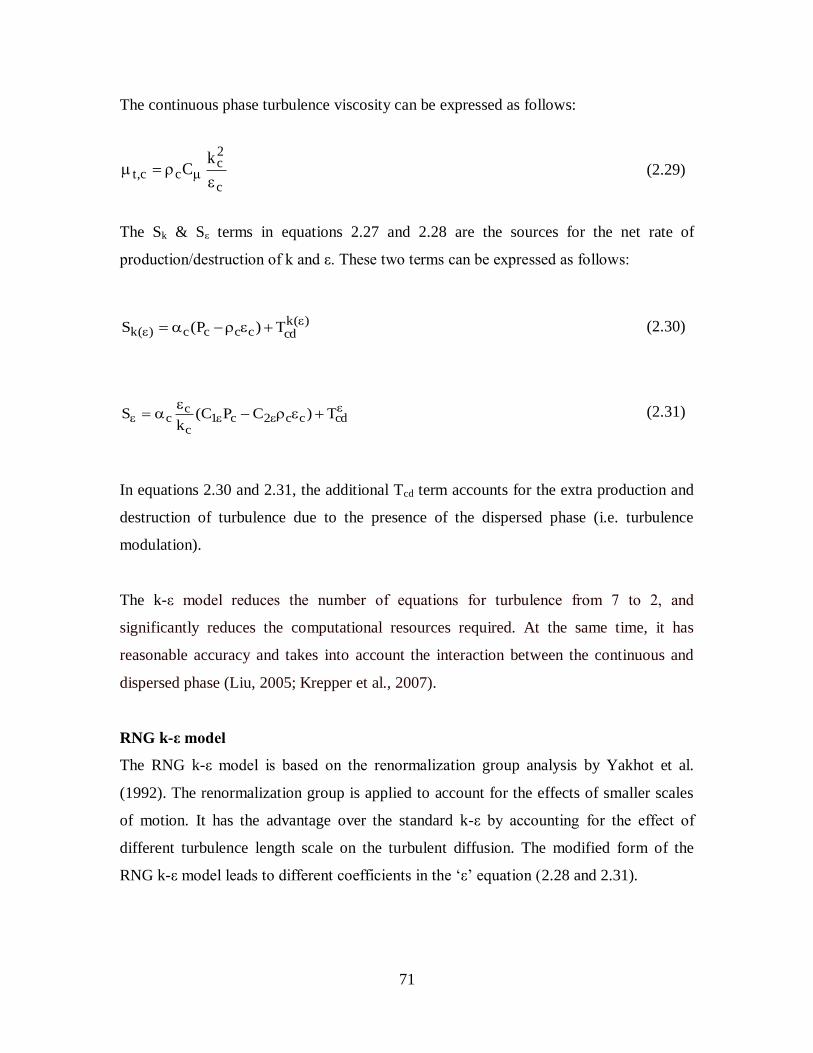
71

The continuous phase turbulence viscosity can be expressed as follows:

c

2c

cc,tk

C

(2.29)

The Sk & Sε terms in equations 2.27 and 2.28 are the sources for the net rate of

production/destruction of k and ε. These two terms can be expressed as follows:

)(kcdcccc)(k )P(S

(2.30)

cdcc2c1

c

cc )CPC(

kS (2.31)

In equations 2.30 and 2.31, the additional Tcd term accounts for the extra production and

destruction of turbulence due to the presence of the dispersed phase (i.e. turbulence

modulation).

The k-ε model reduces the number of equations for turbulence from 7 to 2, and

significantly reduces the computational resources required. At the same time, it has

reasonable accuracy and takes into account the interaction between the continuous and

dispersed phase (Liu, 2005; Krepper et al., 2007).

RNG k-ε model

The RNG k-ε model is based on the renormalization group analysis by Yakhot et al.

(1992). The renormalization group is applied to account for the effects of smaller scales

of motion. It has the advantage over the standard k-ε by accounting for the effect of

different turbulence length scale on the turbulent diffusion. The modified form of the

RNG k-ε model leads to different coefficients in the ‘ε’ equation (2.28 and 2.31).

72

Model parameter Suggested value

βRNG for eqn. 2.32 0.012

Cµ,RNG

C1ε,RNG

C2ε,RNG

ζk(ε),c,RNG

ζε,c,RNG

0.085

1.42-fη

1.68

0.7179

0.7179

Table 2.4: Coefficients for k-ε turbulence model (Adapted from Ansys CFX Manual).

For fη term in Table 2.4,

3

RNG1

38.41

f

and

RNG,

k

C

P (2.32)

2.7 INTERPHASE FORCES MODELS

In order to account for the interphase momentum interactions between the continuous and

dispersed phases in a turbulence model, various closure equations for the interphase

forces that contribute to the momentum balance are required. This section will discuss the

various interphase forces.

2.7.1 INTERPHASE DRAG

The interphase drag accounts for the resistance force encountered by one phase due to the

presence of the other phase. This force has always a direction opposite to the relative

velocity and the total drag force exerted on a single spherical drop can be given by:

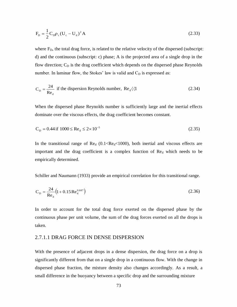
73

A)UU(C2

1F 2

dccDD (2.33)

where FD, the total drag force, is related to the relative velocity of the dispersed (subscript:

d) and the continuous (subscript: c) phase; A is the projected area of a single drop in the

flow direction; CD is the drag coefficient which depends on the dispersed phase Reynolds

number. In laminar flow, the Stokes’ law is valid and CD is expressed as:

d

DRe

24C if the dispersion Reynolds number, 1Red (2.34)

When the dispersed phase Reynolds number is sufficiently large and the inertial effects

dominate over the viscous effects, the drag coefficient becomes constant.

44.0CD if 5

d 102Re1000 (2.35)

In the transitional range of Red (0.1<Red<1000), both inertial and viscous effects are

important and the drag coefficient is a complex function of Red which needs to be

empirically determined.

Schiller and Naumann (1933) provide an empirical correlation for this transitional range.

687.0

d

d

D Re15.01Re

24C (2.36)

In order to account for the total drag force exerted on the dispersed phase by the

continuous phase per unit volume, the sum of the drag forces exerted on all the drops is

taken.

2.7.1.1 DRAG FORCE IN DENSE DISPERSION

With the presence of adjacent drops in a dense dispersion, the drag force on a drop is

significantly different from that on a single drop in a continuous flow. With the change in

dispersed phase fraction, the mixture density also changes accordingly. As a result, a

small difference in the buoyancy between a specific drop and the surrounding mixture

74

Authors Proposed correlation for drag coefficient

Ishii and Zuber

(1979)

Mixture viscosity: )()4.0(5.2

max

d

c

mcdcdmax

1

where Φd and Φmax are the dispersed phase fraction and

maximum packing factor respectively.

In viscous regime where drops are approximately spherical

(similar to Schiller Naumann correlation):

687.0

m

m

D Re15.01Re

24C

where m

dcdc

m

dUURe

In distorted fluid drop regime:

)(EEo3

2)ellipse(C dD

where )(f67.18

)(f67.171(E

d

76d

d

and

21d

m

cd 1)(f

In the regime where churn flow is dominant:

2dD 13

8)cap(C

Ansys CFX provides an automatic selection criterion for the

appropriate CD

)sphere(CC DD if )ellipse(C)sphere(C DD

)ellipse(CDmin(CD if )ellipse(C)sphere(C DD

Kumar and Hartland

(1985) 73.0

dD 56.41Re

2453.0C

Rusche and Issa (2000) 2

kd10DD dkexpCC where k1 and k2 are empirical

coefficient.

Table 2.5: Drag coefficient correlations for dense homogeneously distributed dispersions.

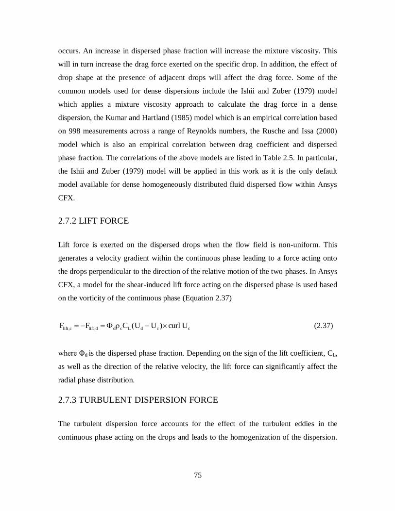
75

occurs. An increase in dispersed phase fraction will increase the mixture viscosity. This

will in turn increase the drag force exerted on the specific drop. In addition, the effect of

drop shape at the presence of adjacent drops will affect the drag force. Some of the

common models used for dense dispersions include the Ishii and Zuber (1979) model

which applies a mixture viscosity approach to calculate the drag force in a dense

dispersion, the Kumar and Hartland (1985) model which is an empirical correlation based

on 998 measurements across a range of Reynolds numbers, the Rusche and Issa (2000)

model which is also an empirical correlation between drag coefficient and dispersed

phase fraction. The correlations of the above models are listed in Table 2.5. In particular,

the Ishii and Zuber (1979) model will be applied in this work as it is the only default

model available for dense homogeneously distributed fluid dispersed flow within Ansys

CFX.

2.7.2 LIFT FORCE

Lift force is exerted on the dispersed drops when the flow field is non-uniform. This

generates a velocity gradient within the continuous phase leading to a force acting onto

the drops perpendicular to the direction of the relative motion of the two phases. In Ansys

CFX, a model for the shear-induced lift force acting on the dispersed phase is used based

on the vorticity of the continuous phase (Equation 2.37)

ccdLcdd,liftc,lift Ucurl)UU(CFF (2.37)

where Φd is the dispersed phase fraction. Depending on the sign of the lift coefficient, CL,

as well as the direction of the relative velocity, the lift force can significantly affect the

radial phase distribution.

2.7.3 TURBULENT DISPERSION FORCE

The turbulent dispersion force accounts for the effect of the turbulent eddies in the

continuous phase acting on the drops and leads to the homogenization of the dispersion.

76

Two models are included in Ansys CFX – the Favre averaged drag model and the Lopez

de Bertodano model (1991).

2.7.3.1 FAVRE AVERAGED DRAG MODEL

Favre averaging is an averaging operation for the turbulent terms using a density

weighted average of the turbulence terms. This is significant mainly for compressible

flow. In the Favre averaged drag model, an additional drag term is added into the

momentum equation by expressing the time averaged drag in terms of Favre averaged

velocities. The model is implemented in Ansys CFX as follows:

c

c

d

d

tc

tcc,DTDd,TDc,TD CCFF (2.38)

where CD,c is the coefficient of the interphase drag force, tc is the kinetic eddy viscosity,

ζtc is the turbulent Schmidt number for continuous phase volume fraction (default value:

0.9). CTD is the turbulent dispersion coefficient that is defined by the user where the

default value for CFX as 1.0.

2.7.3.2 LOPEZ DE BERTODANO MODEL

The Lopez de Bertodano model (1991) is one of the first models developed for the

turbulent dispersion force. It aims to physically account for the turbulent diffusion based

on the fluctuating components of the turbulent forces acting on the dispersed drops. The

model can be presented as follows:

cccTDdTD,cTD, ΦkρCFF (2.39)

Where kc is the turbulent kinetic energy and ÑΦc is the concentration gradient of the

continuous phase. CTD values between 0.1 and 0.5 have been used successfully for bubbly

flow with bubble diameters in the order of a few millimeters. However, much higher

values have been required in some situations (Lopez de Bertodano (1998) and Moraga et

al. (2003)).

77

2.8 SUMMARY OF LITERATURE REVIEW

Previous works on two-phase oil-water flows and particularly the phase inversion

phenomenon have been reviewed. Flow regime development and phase inversion were

found to depend on the properties of the fluids, pipe configuration, and operational

conditions in a pipeline. Phase inversion has been previously studied mainly in stirred

vessels but also increasingly on pipe flow. Among the pipe flow investigations, changes

in pressure drop have been used as an indication of phase inversion occurrence. However,

it is also known that these changes differ across different fluid systems. In addition, the

changes in pressure drop have not been clearly associated with the corresponding changes

in phase continuity. Inversion has been reported to occur across a range of phase fraction

before completion due to the presence of local phase inversion at certain locations within

the system. Thus, experimental investigations to understand the changes in phase

continuity and distribution (i.e. changes in flow regime) corresponding to that in pressure

drop during inversion will be conducted with results presented in Chapter 4. Successful

outcome from this investigation will also allow better prediction of the changes in

pressure drops as flow regime changes during inversion. A prediction method for these

changes in pressure drop is presented in Chapter 7.

From the literatures reviewed, various models have been developed based on mechanisms

including the dynamic process of drop coalescence and break-up, minimization/equal

system/interfacial energy of the mixture and zero shear stresses at the liquid-liquid

interface. While there is no definite mechanism for the occurrence of phase inversion,

these models provide important information about phase inversion. For example,

interfacial tension is found to be an important factor on the Weber number and phase

inversion in many of the correlations. However, the effects of interfacial tension on phase

inversion have not been previously established and thus will be studied in this work

(Chapter 5).

Momentum balance is regarded as the underlying principle behind the mechanism of zero

shear stresses at the interface. Pressure drop across a pipe is the direct effect of the shear

stresses at the interfaces in the system and these shear stresses in turn depend on the fluid

78

viscosities. A prediction model on phase inversion occurrence will be developed based on

this relation between viscosity and pressure drop and is presented in Chapter 6.

Computational Fluid Dynamics (CFD) simulation can offer some insight on the behavior

of dispersed systems and will be used in this work. A review on numerical simulations

using CFD has been presented. In particular, the k-ε model has been proposed for use in

subsequent chapter due to its good estimation of the system without a high demand on

computational resources. This is especially important at high concentration of the

dispersed phase. Closure equations for the interphase interactions are also presented.

Some of the more important interactive forces include the drag force, the turbulent

dispersion force and the lift force. The effect of these forces on the spatial distribution of

the phases in dispersed systems will be investigated in Chapter 8.

79

Chapter 3: Facility and Instrumentation

3.1 OVERVIEW

This chapter will introduce the flow facility and instrumentation used for the

experimental investigations of phase inversion during oil-water pipe flow. The

experimental facility has been constructed in the Department of Chemical Engineering,

UCL. There are two test sections made of steel and acrylic respectively and two types of

inlets, one that ensures minimum mixing of the fluid and the other creates a dispersion at

the beginning of the test section. Various measuring probes are used to measure phase

continuity and distribution, pressure drop and drop size distribution. This allows detailed

investigations of the flow parameters as the system approaches phase inversion.

3.2 TEST FLUIDS

The fluids used for the experimental investigations of the phase inversion phenomenon

are Exxsol D140 and tap water. Table 3.1 presents the physical properties of the two

fluids.

Exxsol D140 Tap Water

Density (kg/m3) 828 1000

Viscosity (mPa.s) @25oC 5.5 1.0

Interfacial Tension (mN/m) @ 25oC 37.04

Table 3.1: Physical properties of working fluids

The density of the oil phase is based on the data provided by the supplier (Exxon

Chemicals). The oil viscosity was measured using a Contraves 155 Rheometer over a

range of temperature. The oil-water interfacial tension was measured using the drop

volume method in a Krüss Drop Shape Analysis System (DSA100).

80

3.3 EXPERIMENTAL FLOW FACILITY

The schematic diagram of the flow facility used in the experiments is shown in Figure

3.1. It consists of three main sections – fluid storage, test pipeline and fluid separation

units. The test pipeline has been designed to accommodate various instrumentations and

inlet to investigate the development of dispersed flow and the occurrence of phase

inversion. These will be discussed in detail below.

Fluid Storage Section

This section consists of two fibre-glass storage tanks with a capacity of 880 liters each

for oil and water respectively. There are two acrylic baffles in each tank to prevent

vortices that may allow air to entrain in the fluids and be transported into the test section.

The baffles are also positioned in such a way to allow extra time for separation of the

fluids in case one phase enters the storage tank of the other phase. The tanks are similarly

connected to the centrifugal pumps on one end and to the separator on the other end.

Fresh fluids are manually put into the tanks while the fluid level in each tank is kept at

least ¾ of the tank height. Fluids can be recycled from the separator. In addition, fluid

from the recycle line of the pump is returned into the tank to regulate the outflow

through the pumps into the test pipeline. At high flowrates, water may enter into the oil

storage tank. In this case, the oil tank is drained into a spare separation tank from which

the oil is recycled bank to its storage tank and water is discarded. Fresh water is

consistently used if possible to ensure clean water stream is pumped into the pipeline

during experiments. Fresh water is also used to maintain the temperature of the fluid

mixture in the test section at approximately 20oC (+/- 5

oC).

81

Figure 3.1: Schematic of the pilot scale facility with adjustable sections in the test

pipeline.

82

The centrifugal pumps (Ingresoll-Dresser CPX200) are capable of generating a flow rate

of 240l/min. A recycle line back to the storage tank is used to regulate the flow rate of

each fluid in the flow meter. Good control over the regulation of the flow rate through

the pumps and the recycle streams is crucial in minimizing fluctuation of flow to the test

pipe section. This also avoids exceeding the designed capacity of the pumps and cause

overheating.

The flow rates of the respective fluids are monitored by two variable area flow meters

(ABB Instrumentation 10A5400) with maximum error of 1% of the full scale. The flow

meters measure a range between 20 – 240 l/min and are connected to a PC for data

logging.

Test Pipe Section

The test pipe has a total length of 16m with an internal diameter of 38mm and is split

into the front and back legs connected by an U-bend with a 150mm diameter curvature.

Two test pipes have been constructed from stainless steel and acrylic respectively. The

entire pipeline consists of sections of 1m and 2m long. This allows the various

instruments that are fitted in between two pipe sections to be installed at different axial

locations along the test pipe. The sections are either joined by tri-clamps (in the stainless

steel pipeline) or flanges (in the acrylic pipeline). These instruments are however fitted

away from the U-bend at the end of the first leg of the pipeline to avoid any influence on

the flow distribution. The probes can also be located at 7m (~184D) from the inlet when

the quick closing valves are not required.

83

Figure 3.2: Photograph of the pilot scale facility in stainless steel.

Figure 3.3: Stainless steel Y-inlet where the oil and water phases are joined at the end.

Storage Tank

Separator

Test Pipeline

Oil

Water

84

As observed in both Figures 3.2 and 3.3, oil and water are pumped through the inlet to

the test section. Two types of inlets were used. A Y-inlet (Figure 3.3 and 3.4) was used

to ensure that the fluids join with little mixing. The oil stream flows from the upper inlet

pipe and the water stream flows from the lower inlet pipe. The two pipes join with an

angle of approximately 15o. In addition in the acrylic inlet section, a splitting plate is

added where the two pipes join to further ensure minimum mixing of the two liquids (see

Figure 3.4).

Figure 3.4: Acrylic Y-inlet with a split plate to enhance stratification of the oil and water.

A dispersed inlet (Figure 3.5) was also constructed to create a dispersion from the

beginning of the test section and influence the type of dispersion formed. The inlet is

made from a steel pipe with a total of 1056 nozzles with heights 2mm and 4mm around

its periphery. Nozzles of the two heights are staggered so that the fluid jets from the

nozzles have more space to develop and do not coalesce with each other.

Split Plate Oil

Water

85

(a) (b)

Figure 3.5: Dispersion inlets with staggered nozzles. (a) The dispersed phase flows

within the stainless steel pipe while the continuous phase flows in the acrylic pipe. (b)

Dispersed phase is ejected from the nozzles.

Separation Section

A horizontal two phase separator is installed at the end of the test section (Figure 3.2)

with 800 litre in capacity. The separator contains a KnitMesh (DC 9201/SS/PPL)

coalescer to aid the separation process. The coalescer uses a composite of two materials

with different surface free energies (metallic and plastic). The junction effect from the

combination of the two materials increases the rate of coalescence when the droplets are

trapped and move towards the junction points of the coalescer as shown in Figure 3.6.

The separator is also used, at the end of each experimental session, for a more thorough

separation by gravity. This will generally take about 48 hours before the next

experimental run before the fluids are recycled into the storage tanks. In occasions when

there is water entrained in the oil storage tank, further separation will take place within

the tank and excess water will be removed.

Continuous

Phase

Dispersed

Phase

86

Figure 3.6: Junction effect of the coalescer that enhances separation. (Information from

manufacturer - KnitMesh Technologies).

Instrumentation

(a) Visual Observation

Visual observation of the flow development can be captured throughout the acrylic

pipeline or through a viewbox in the steel pipeline. Visual imaging is facilitated with

a high speed video camera (Kodak HS 4540 MX) which has a capturing rate of 4500

fps and a total recording time of 1.8 second. A monitor is connected for real time

visual observation. Figure 3.7 shows the setup of the video camera. The camera is

connected to the PC for data capture and storage. Video images can be saved and

individual frames extracted for further analysis. Background lighting (Spot light unit)

is used to enhance the contrast between the oil and water phases and improve the

quality of the images.

87

Figure 3.7: Setup of the high speed video imaging unit, Kodak HS 4540 MX.

(b) Fluid hold-up

Average volume fraction is measured using two quick closing valves (QCVs). Two

ball valves are fitted on both ends of a transparent pipe section of 1m in length to trap

fluid mixture with a volume of 1.13 litre (Figure 3.8). The pipe section is located at

7m (~184D) from the inlet (and also the last section before the U-bend in the setup).

Once the pipe section is closed, the mixture can be drained into a measuring cylinder

for separation. The respective volume fraction of the two phases can then be

identified. A manual hand pump is used to minimize any retention of the oil phase in

the pipe. The measurements are repeated several times with 2% deviation across

measurements. In the experiments, the two valves are closed simultaneously with the

pumps. The trapped mixture is drained in a measuring cylinder where the volume of

each phase is identified and recorded.

88

Figure 3.8: Section of pipe with quick closing valves in the 38mm stainless steel

pipeline. A viewbox is included to aid visual observation and video capturing.

(c) Instrumentation for phase continuity measurement

1) Conductivity Ring Probe

The ring probe consists of two metallic rings embedded on the pipe perimeter,

flush with the wall, and in contact with the fluid mixture. Each ring is 4mm wide

and the rings are 38mm apart (Figure 3.9). The conductivity ring probe is

generally located at about 7.0m (~184D) from the inlet where the flow is

considered as fully developed. The ring probe is normally paired with the

conductivity wire probe to measure the conductivity at the test section and

provide information on phase continuity and distribution. High conductivity

values indicate that a conductive water continuous mixture is in contact with the

probes, while low values denote an oil continuous mixture.

Quick Closing Valves

View Box

89

Figure 3.9: Conductivity ring probe for phase continuity measurement at the pipe

periphery.

2) Conductivity Wire Probe

Each wire probe consists of a pair of bended copper wires with a diameter of

0.5mm (Figure 3.10). The wires are 10mm apart and this gap is assumed to be

greater than the largest droplet of the dispersed phase. This will ensure that any

change in conductivity signal is due to a change of the continuous phase. It can

detect phase continuity at different locations in a pipe cross section using a

traversing mechanism. The wires are bent (Figure 3.10b) in L-shape at opposite

directions and only the horizontal portions of the wires are exposed to the flow.

This provides a large contact surface at particular height in the pipe cross section.

During experiments, the ring probe and the conductivity wire probe are used primarily to

detect the phase continuity at the pipe periphery and the centre of the pipe cross section

respectively unless otherwise stated. These locations are found to be critical during phase

inversion from previous experiments (i.e Hu, 2005, Ioannou, 2006). The electrical

resistance tomography will also be used to supplement on the phase continuity

investigation on other locations (e.g. top of pipe cross section). The application of the

tomographic system will be discussed in the next section.

90

(a)

(b)

Figure 3.10: Local conductive wire probe for phase continuity measurement at the

localized position. (a) Photo of wire probe (b) Schematic of the interior (side view) of the

wire probe.

91

3) Electrical resistance tomography (ERT)

Electrical resistance tomography provides information on the distribution of the

phases in a mixture through a series of electrodes arranged at regular intervals

within the boundary of the vessel investigated. A commercial ERT system

(Model: M3000 by Industrial Tomography Systems, ITS, plc) is used in the

current work. The tomographic sensor consists of 16 electrodes equally

distributed around the periphery of an acrylic pipe (Figure 3.11a). Each electrode

is made of a 4mm diameter circular stainless steel piece embedded on the acrylic

pipe wall and in contact with the mixture inside the pipe. Care is taken to ensure

that each electrode is flush with the interior pipe wall. Thus, ERT is considered to

be non-intrusive. The ERT can provide a signal as long as there are at least 2

electrodes in contact with the conductive phase (i.e. water) where one electrode

acts as a transmitter and the other as a receiver. The tomographic sensor provides

a resolution of 316 pixels over the 38mm pipe cross section with each pixel

representing approximately 2mm x 2mm.

Electrical signal is transmitted from a transmitting electrode and received by the

remaining 15 electrodes. The sample data transmission is repeated in sequence

until all 16 electrodes have acted as the transmitting electrode. All the received

data will be processed through a reconstruction algorithm to generate the phase

distribution through a cross-sectional image. The sampling frequency in this

study is set to be 10 images per second. The algorithm used in this study is the

Linear Back Projection (LBP) which allows quicker and less computational

resource intensive for the reconstruction. This is important in capturing the rapid

changes during phase inversion despite the compromise on the resolution of each

image. A software (ITS toolsuite) is used to present the reconstructed images

(Figure 3.12) for visualization and data analysis. Localised conductivity value at

each pixel across the pipe cross section can also be exported to Excel for further

data processing.

92

(a)

(b)

Figure 3.11: (a) Stainless steel electrodes embedded across the pipe periphery. (b)

Experimental setup of the ERT system with a PC for data processing.

93

Figure 3.12: Sample ERT reconstructed image generated from ITS toolsuite. The colour

bar denotes the range of raw conductivity data with respective to the reference frame.

From the phase distribution data, the fraction of each phase in a pipe cross section can be

found. This can be compared with the results from QCVs and an average difference of

5.6% is observed between the two methods. Figure 3.13 presents the results of the

comparison. An average deviation of 5.6% from the diagonal line can be found from the

ERT measurement while an average deviation of 3.6% from the QCV measurement. It

can thus be assumed that the mixture flow across the wide range of phase fraction to

have no slip (i.e. the input volume fractions of the oil and water equals to the in-situ

phase volume fractions). The ratio between the volume fractions is defined as the slip

ratio (S) presented in Equation 3.1 and the slip ratio is 1 when there is no slip.

wo

wo

/

/S

(3.1)

where βo and βw are the input volume fractions of the oil and the water phase respectively,

and εo and εw are the in-situ volume fractions of the oil and water phase respectively.

94

Figure 3.13: In-situ liquid hold-up comparison between electrical resistance tomography

(ERT) and quick closing valves across a range of input phase fractions at a mixture flow

velocity of 3m/s.

(d) Drop velocity and drop size distribution

The measurement of drop velocity and drop size distribution is made using the dual

impedance probe developed by Lovick (2004) at University College London (see

Figure 3.14). The details on the development and operation principles can be viewed

in his thesis (Lovick, 2004).

As shown in Figure 3.14, the dual impedance probe consists of two coaxial wires

which can work independently as sensors detecting the contacting phase at each of

the wire tips. Each tip is tapered with insulation in between the coaxial wires as

shown in Figure 3.14(b). The coaxial wires are placed at the same housing as the

conductivity wire probe presented in Section 3.3 Figure 3.10. The probe tips can thus

be moved to measure at different locations in the pipe cross section. The distance

0

20

40

60

80

100

0 10 20 30 40 50 60 70 80 90 100

In-S

itu O

il F

ract

ion

[%

]

Input Oil Fraction [%]

Quick Closing Valve

Electrical resistance tomography

95

between the two wires is again 10mm and this is assumed that no drop is larger than

this distance within the experimental flow conditions used in this work.

(a)

(b)

Figure 3.14: (a) Photograph of the dual impedance probe setup. (b) Probe tip

configuration (Lovick, 2004).

Measurements using the dual impedance probe are conducted at 7m from the test

section inlet. The impedance wires are set at the same height inside the pipe

perpendicular to the flow direction. It is assumed that drops that pass through the

first probe will also pass through the second probe. A single frequency regulator

controls the frequencies of the two probes to ensure that they are measuring at the

same cycle. The sampling frequency is set to 45kHz. At this high frequency, each

sampling cycle has a time span of 22μs, and this is capable of measuring a minimum

96

drop size of 66μm at 3m/s mixture velocity or 88μm at 4m/s mixture velocity. At

this high frequency, it is expected that each dispersed drop will cross each probe tip

over a succession of sampling cycles (see Lovick, 2004; Hu, 2005; Ioannou, 2006).

120,000 data points are captured at each location. An example of the normalized

signal data from the dual impedance probe is presented in Figure 3.15.

Figure 3.15: A sample set of normalized signal from the two impedance wires at a

mixture velocity of 3m/s. Dispersed phase will be in contact with probe 1 before it

contacts with probe 2.

The time delay (see highest peak of Figure 3.16) for the drops to pass through the

two probes is found by cross correlating the signals of the two probes with a fixed

distance of 10mm. By combining with the known distance between the probes, the

drop velocity can be found (Lovick, 2004). The chord lengths of the measured drops

can be estimated from the signal of either probe by multiplying the drop velocity

with the time duration of each drop passage. The duration of each drop passage is

obtained by converting the raw signals of the probe into square waves based on the

level and slope threshold values (Lovick, 2004 and Hu, 2005). It should also be

noted that measurements of chord length through this method tend to be biased

0.0

0.2

0.4

0.6

0.8

1.0

0 1 2 3 4 5

No

rmal

ised

Sig

nal

[-]

Time [ms]

Probe 1

Probe 2

97

towards the larger drops as they are more likely to pass through the probe tips than

the smaller drops.

Figure 3.16: A sample frequency plot of the time delay between the two impedance

wires. The highest peak denotes the time delay where most dispersed drop take to cross

the two wires.

Drop size distribution is then estimated from the chord length measurements. An

algorithm by Hu et al. (2006) provides the relationship between the chord length

distribution (CLD) and drop size distribution (DSD). In order to apply this algorithm,

the measured drops are assumed to be spherical. Sauter mean diameter (d32) can then

be calculated from the drop size distribution.

(e) Phase distribution measurements

Phase distribution measurements can be made using the same dual impedance probe

as described in the previous section. Only one impedance wire is required (generally

the first one to avoid any obstruction) for the measurement. Local phase distribution

measurements are made across 20 locations at 2mm intervals vertically across the

pipe cross section and diagonally at 45o and 10 locations horizontally. Phase

distribution is assumed to be mirrored at the vertical plane and thus the phase

-0.05

0.00

0.05

0.10

0.15

0.20

0.25

0.30

0.35

0.00 2.00 4.00 6.00 8.00 10.00

Fre

qu

ency

[-]

Time Delay [ms]

Time Delay

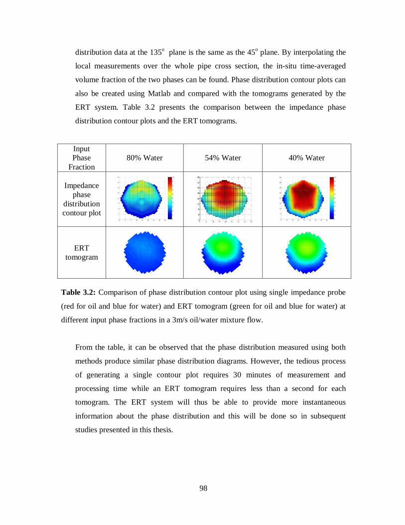
98

distribution data at the 135o plane is the same as the 45

o plane. By interpolating the

local measurements over the whole pipe cross section, the in-situ time-averaged

volume fraction of the two phases can be found. Phase distribution contour plots can

also be created using Matlab and compared with the tomograms generated by the

ERT system. Table 3.2 presents the comparison between the impedance phase

distribution contour plots and the ERT tomograms.

Input

Phase

Fraction

80% Water 54% Water 40% Water

Impedance

phase

distribution

contour plot

ERT

tomogram

Table 3.2: Comparison of phase distribution contour plot using single impedance probe

(red for oil and blue for water) and ERT tomogram (green for oil and blue for water) at

different input phase fractions in a 3m/s oil/water mixture flow.

From the table, it can be observed that the phase distribution measured using both

methods produce similar phase distribution diagrams. However, the tedious process

of generating a single contour plot requires 30 minutes of measurement and

processing time while an ERT tomogram requires less than a second for each

tomogram. The ERT system will thus be able to provide more instantaneous

information about the phase distribution and this will be done so in subsequent

studies presented in this thesis.

99

(f) Pressure gradient measurements.

Pressure gradient is measured by a FP2000 wet/wet differential pressure transducer

(RDP Electronics Ltd). The pressure transducer is connected to the test section via

nylon tubing and quick connect couplings. The first pressure measuring port is

located on the test section at 3.8m (~100D) from the inlet and the second port is

located 1.5m apart. The male adaptor of the quick connect couplings is connected to

the port while the female adaptor is fitted to the nylon tubing as shown in Figure

3.17. These quick connect couplings offer the flexibility to change the location of

pressure gradient measurements. During connection and disconnection, the

couplings are automatically shut off to avoid any air entrainment or leakage which

would affect the pressure gradient measurements. The dimensions of the ports were

carefully designed with the bore diameter of the port opening at the test section to be

no more than 1/8th of the pipe diameter (Perry, 1997). In addition, the pressure

transducer is connected to a transducer conditioner (type E308) which is calibrated

for pressure gradient data logging. The transducer conditioner has a capability of

measuring a maximum pressure of 22kPa and an accuracy of 0.25% of the full scale.

(a) (b)

Figure 3.17: (a) Pressure measuring port at stainless steel pipeline. Similar ports are also

found in the acrylic pipeline (b) Differential pressure transducer and control valves.

100

3.4 SUMMARY

In this chapter, the experimental facilities used for the experimental investigation of

phase inversion have been discussed. Two test sections were made from stainless steel

and acrylic, with 38mm I.D. had been used, and two inlets, a Y-junction and a dispersed

inlet, were developed to study their effect on flow patterns and phase inversion.

A number of instruments were used to study the phase continuity, drop size distribution,

average holdup and pressure drop. From the various conductivity probes used to detect

phase continuity in a pipe cross section, electrical resistance tomography provides faster

measurements. However, it cannot detect thin water layers that do not cover at least two

sensor electrode and also, in the case of an annular flow with oil in the annulus, it cannot

give measurements on phase continuity in the pipe core. A dual impedance probe will

also be used to investigate drop size distributions under different conditions. The probe

can also provide phase distribution data which is comparable with the ERT results.

Nonetheless, ERT has the advantage of quick measurement and will be used for the

purpose of accounting the phase distribution in the pipe cross section in experimental

studies.

101

Chapter 4: The occurrence of phase inversion

4.1 OVERVIEW

Phase inversion has been investigated in horizontal pipelines (in stainless steel and

acrylic) for mixture velocities between 3.0m/s and 4.0m/s where dispersed flow was

observed in previous investigations (Hu, 2005; Ioannou, 2006). Investigations have been

conducted for two inversion routes by (1) starting from a water continuous dispersion or

pure water phase if possible and increasing the oil input fraction at a constant mixture

velocity (o/w → w/o) and (2) starting from an oil continuous dispersion or pure oil phase

if possible (w/o → o/w) and increasing the water fraction at a constant mixture velocity.

In Section 4.2, a brief description of the experimental procedure is discussed. The applied

procedure is similar to the direct experiments by Piela et al. (2008) where specific phase

fractions of oil and water are introduced in the pipe at a constant mixture velocity to

allow for flow development along the pipeline. Measurements are conducted at the end of

the pipeline where the flow is developed.

Phase inversion is first observed through high speed images and the visual observations

are summarized in Section 4.3. Based on the visual observations, the various conductivity

probes are positioned and the change in phase continuity during inversion is discussed in

Section 4.4. Conductivity ring and wire probes detect the phase continuity of the

contacting phase at the pipe periphery and the centre of the pipe respectively. Electrical

resistance tomography is also used to support the investigation by identifying the phase

fraction at other locations as well as to provide visual images on how the phases are

distributed during phase inversion. The use of the various probes is then applied to

investigate the effect of inversion route and mixture velocities on the development of

phase inversion (Section 4.5 and 4.6).

102

The associated changes in pressure gradient are presented in Section 4.7 whereby a

change in phase distribution can have an impact on the corresponding pressure gradient.

Similar changes effected by the inversion route or mixture velocity are also discussed in

the section.

As phase inversion leads to significant change in drop size, Section 4.8 aims to

investigate the drop size distribution of the dispersed phase as well as a mechanism for

phase inversion based on the dynamic balance between drop coalescence and drop break-

up.

Lastly, similar investigation has been conducted in a dispersed inlet. The effect of the

dispersed inlet is presented in Section 4.9. It is observed in the section that the inversion

process is significantly different from the split inlet where the two fluid phases are

allowed to mix along the pipeline. With the outcome from this chapter, the results will

form the basis for further investigations in the investigation on the effect of interfacial

tension on phase inversion in Chapter 5 as well as the data set for comparison with

mechanistic models and CFD simulations in Chapter 7 and 8 respectively.

4.2 EXPERIMENTAL PROCEDURE

The experiments for the investigation of phase inversion occurrence were conducted in

the pilot scale facility discussed in Chapter 3 with a 38 mm ID test section. An acrylic

test section was made to allow visual observations of the flow along the pipeline

especially at the initial length when the flow pattern is still developing. A modified inlet

with a splitting plate is used to minimise any turbulent mixing caused by the Y-junction

inlet. Thus, any mixing along the pipe is assumed to be due to the turbulent flow. High

speed images are taken at approximately 7m (~184D) downstream the inlet to visually

observe the change in phase distribution as the dispersed phase fraction is increased.

Conductivity measurements are also taken to determine phase continuity (See Section

4.4). The conductivity ring probe, mounted on the pipe perimeter, indicates which phase

is in contact with the pipe wall. A conductivity wire probe, that can transverse along a

103

pipe diameter, is used to detect the local phase continuity; the probe tip is set at the centre

of the pipe during the current experiments. The probes are located at 7m from the inlet.

An electrical resistance tomographic (ERT) system is also used to complement the

conductivity probe measurements. In the results reported below, the ERT system is

primarily used to detect changes in phase continuity near the top of the pipe. The ERT

system is located at approximately the same position as the conductivity probes. Pressure

drop is recorded via a pressure transducer which is connected with two measuring ports

in the pipe, 1.5m apart, with the first port located at 3.8m (~100D) downstream the inlet.

The mixture velocity varies between 3.0 and 4.0 m/s. Previous work showed that the flow

is fully dispersed at this velocity range (Ioannou, 2006). Exxsol D140 and tap water are

used as the oil and water phase respectively with their properties shown in Table 3.1.

Two phase inversion routes are followed (1) starting from an oil-in-water dispersion, or

single phase water if possible (2) starting from a water-in-oil dispersion, or single phase

oil if possible. In both cases, the initial dispersed phase fraction is gradually increased

while the continuous phase fraction is reduced until phase inversion is reached and

beyond while maintaining a constant mixture velocity. This approach is similar to the

‘direct’ experiments conducted by Piela et al. (2008). The intervals in the input phase

fractions for measurements are smaller close to the inversion point (i.e. 20% - 60% water

fraction) than away from it (ie. below 20% and beyond 60% water fraction). At each

phase fraction in a particular mixture velocity (i.e. a single data point), the flow is

allowed to establish for approximately 5 minutes before any measurement is taken.

4.3 VISUAL OBSERVATIONS OF PHASE INVERSION

The use of the high speed camera provides the first indication on how the two phases are

distributed as they flow together along the test section. These images facilitate the

positioning of the various probes for detecting changes in phase continuity. Figure 4.1

shows images from the stainless steel pipe for 3m/s mixture velocity starting with high

water fractions where the mixture is water continuous and gradually reducing the water

fraction until phase inversion occurs and an oil continuous dispersion is obtained

(Camera model: Vision Research Phantom V5.1). The oil phase tends to appear white in

104

the images and the water phase appears transparent. While the oil drops in an oil-in-water

dispersion reflects light from the foreground lighting causing a sparkling appearance, a

water-in-oil dispersion tends to be dull white.

(60%) (53%) (40%)

(33%) (20%) (13%)

Figure 4.1: Visual images are taken in a stainless steel pipe using an high speed camera

(Model: Vision Research Phantom V5.1) at 7m away from the inlet. Mixture velocity is

kept constant at 3m/s. The percentage in the bracket represents the input water fraction

which the image is taken.

At 60% input water fraction, an oil-in-water dispersion can be seen with the oil drops

evenly distributed across the pipe. As the water fraction is reduced to 53%, the oil drops

105

tend to move towards the centre of the pipe (i.e. milky white region). The region close to

the bottom pipe wall appears to remain dominated by the water phase with oil drops

flowing within. Further reduction in water fraction to 40% and 33% shows dense

dispersions especially at the upper part of the pipe due to buoyancy of the oil drops.

Water continuous dispersion can only be identified visually near the bottom pipe wall. At

about 20% of water fraction and beyond, the whole pipe is completely dominated by the

oil continuous dispersion. With an oil continuous dispersion, water drops cannot be easily

seen.

Similar experiments were also carried out in the acrylic test section. The resolution of the

images captured in this set of experiments is lower than in the steel pipe because a high

speed camera (Model: Kodak HS 4540) with lower resolution and weaker lighting units

was used. The difference in appearance between the oil and water phase was still possible

to detect.

Figure 4.2 shows the images taken using a cold light unit that illuminates the image from

the back. Since water is transparent, light will be able to penetrate through an oil-in-water

dispersion (with an appearance of a light grey image). No light can get through a water-

in-oil dispersion leading to the appearance of an opaque black image. For example, the

oil-in-water dispersion at 60% water fraction has a bright appearance. As more oil is

added (34%, 40% and 54% water fraction), the upper part of the pipe becomes opaque as

oil drops concentrate here due to buoyancy. The lower region remains bright and

complex oil structures can clearly be observed flowing within the continuous water

phase. This water continuous region becomes thinner and closer to the bottom pipe wall

as more oil is added. From approximately 20% input water fraction and below, the entire

pipe is completely opaque indicating that oil is the continuous phase throughout.

106

(60%) (54%)

(40%) (34%)

(20%) (14%)

Figure 4.2: Visual images are taken in an acrylic pipe using an high speed camera

(Model: Kodak HS 4540) at 7m away from the inlet. Mixture velocity is kept constant at

3m/s. The percentage in the bracket represents the input water fraction at which the

image is taken. The arrows present samples of complex structures observed in images.

Homogeneous O/W dispersion Complex structure formed

Complex structure formed Complex structure formed

Homogeneous W/O Dispersion Homogeneous W/O Dispersion

107

In both pipes, it can be seen that oil will tend to occupy the upper part of the pipe due to

buoyancy as the oil fraction is increased. Phase inversion seems to occur at this part of

the pipe first. As more oil is added, phase inversion is completed when the water layer

near the bottom is completely consumed. The pipe material does not appear to have a

significant effect on how phase inversion occurs. The phase inversion process was also

studied in detail with the use of conductivity probes and ERT. The results will be

discussed in the following section.

4.4 DETECTION OF PHASE INVERSION OCCURRENCE

The investigation on the occurrence of phase inversion is conducted in both the stainless

steel and acrylic pipes. With the acrylic configuration, the Y-junction inlet is modified

with a splitting plate to minimise any turbulent mixing at the inlet. The two phases enter

the test pipe as stratified flow. The detection of phase inversion is investigated with

conductivity probes which provide information on the phase continuity at specific

locations. The spatial difference in changes of phase continuity across the pipe cross

section determines the phase inversion transition. In addition, the availability of an

electrical resistance tomographic system in the acrylic pipe test section provides

information about the phase distribution which can substantiate on the visual

observations made in the previous section. These conductivity measurements are

recorded at 7m downstream from the inlet where previous investigations have found that

the flow is fully developed (Ioannou, 2006). The results of measurements for phase

inversion occurrence will be presented at a mixture velocity of 3m/s but similar approach

of detection is also conducted at a higher velocity (i.e. 4m/s) which will be presented in a

later section on the effect of increasing the mixture velocity.

4.4.1 IN-SITU PHASE DISTRIBUTION MEASUREMENTS

As visual images do not provide clear information on the phase distribution especially in

the pipe core, an electrical resistance tomographic (ERT) system is used to reconstruct

the phase distribution across pipe cross section. For each mixture velocity, the mixture

108

flow is adjusted to the required input phase fraction and left for approximately 5 min to

run before any recordings are made. While the ERT system receives signals from the

sensors continuously, selected raw data are used for analysis. After the initial 5 min of

stabilisation time, the first 50 – 60 frames are ignored. The subsequent 50 frames are

captured which span a duration of approximately 30 sec of run time. This procedure is

repeated for all the input phase fractions used in a particular mixture velocity.

Type of dispersion Tomographic images

Oil-in-water

dispersion

(100%)

(80%)

(60%)

Phase inversion

transition

(54%)

(40%)

(26%)

Water-in-oil

dispersion

(18%)

(10%)

(0%)

Figure 4.3: Phase distribution in an acrylic pipe cross section during the transition from a

water continuous to an oil continuous mixture at a mixture velocity of 3m/s. The

percentages in brackets represent the input water fraction.

109

The tomograms during the phase inversion transition from an oil-in-water dispersion to a

water-in-oil dispersion are presented in Figure 4.3. The water phase is represented in blue

while the oil phase is represented in green. In the region that is reported as water

continuous dispersion (i.e. between 60% - 100% water fraction), it can be observed that

the oil drops accumulate near the pipe centre. During the phase inversion transition (i.e.

between 20% - 54%), part of the pipe cross section turns to be oil continuous as reflected

by the near-zero normalized conductivity in localized positions (e.g. pipe centre or near

top wall). With further increase in oil fraction, the wall contacting area by the water

phase will be reduced. Phase inversion is completed when the entire tomogram turns

green (i.e. water fraction below 20%). Due to the limitation of electrical resistance

tomography on non-conductive continuous phase, the distribution of the dispersed water

phase cannot be shown.

4.4.2 CHANGES IN PHASE CONTINUITY (PARTIAL PHASE

INVERSION)

Based on both the visual images and tomograms, the oil drops tends to move towards the

core of the pipe as the oil phase fraction is increased at a constant mixture velocity. As oil

starts to accumulate at this location, it seems to be a likely location where a local phase

inversion may occur (i.e. if starting from an oil-in-water dispersion). As such, an

adjustable wire probe is placed at the centre of the pipe to detect the phase continuity at

this location. The measurement of local phase continuity will allow better accountability

on whether the pipe core continues to be water continuous with a dense concentration of

oil drops or an inverted oil continuous dispersion. Similarly, a conductivity ring probe is

used to track on the continuity of the contacting phase with the pipe wall as previous

observations have indicated that a water layer remains until the water fraction is greatly

reduced (i.e. approximately 20%). The ERT system (where available with the acrylic test

section) can also provide local conductivity information at near to the top wall. This

allows the differentiation between a dual continuous flow from an annular flow.

110

The combined conductivity measurements, at different locations, can be used to map out

the change in phase continuity during the phase inversion transition. Figure 4.4 presents

the combined data in an acrylic pipe at 3 specific locations – near the top wall (4mm from

the top), centre of pipe (19mm from the top) and around the pipe periphery. Averaged

values over several experimental runs for each probe are presented here.

Figure 4.4: Normalized conductivity data of the oil/water system in an acrylic pipe at a

mixture velocity of 3m/s from the ring and wire probes as well as the ERT system. The

vertical lines limit the phase inversion transition region and are drawn at the first and last

near zero conductivity values recorded using the various probes. The percentages

represent the water fraction at which the different probes show near-zero conductivity

values.

From the figure starting from a pure water flow, the flow tends to be homogenous (at

about 90% water fraction) whereby the change in the normalized conductivity is linear to

the reduction in water fraction. As more oil is added, the value around the pipe periphery

is higher than at other locations. This is due to the formation of water layer at the bottom

W/O

Transition

O/W

○ 54% × 40% Δ 20%

Expt

111

as observed in the previous section. With further increase in oil fraction (at 60% water

fraction), the value at all three locations are different with the lowest value observed at

the centre of the pipe. This indicates that the oil drops are drawn towards the centre of the

pipe leaving other regions to have a higher presence of water. At 54% water fraction, the

conductivity at the centre of the pipe has reached a near-zero averaged value (i.e. less

than 3% deviation from zero). At this fraction, phase inversion has occurred at the centre

of the pipe. While the corresponding conductivity at the top is low, it still reflects more

than 5% of normalized conductivity. Thus, the flow pattern at 54% appears to resemble

an annular flow with an oil continuous core. The conductivity at the top falls to zero at

about 40% water fraction. From this phase fraction onwards, the flow pattern switches

into a dual continuous flow with an upper oil continuous layer and a lower water

continuous layer. This flow pattern persists until 20% water fraction. At 20% and beyond,

all three locations show a zero conductivity value. The phase inversion is completed with

a full water-in-oil dispersion. Based on the use of the different electrical techniques,

similar outcome have been found to observe the transitional stages during a phase

inversion process. This outcome agrees well with the observation from both the ERT and

visual images.

Similar combined data in stainless steel pipe is presented in Figure 4.5 without the

measurements from the ERT system. Nevertheless, previous measurements, by scanning

across the vertical pipe cross section using the conductivity wire probe, had found that

phase inversion occurs firstly from the centre of the pipe if starting from a water

continuous dispersion. As shown in Figure 4.5, the inversion at the centre occurs at 53%

water fraction while it completes at about 20% where the conductivity at the pipe

periphery falls to a near-zero value. By comparing between the two pipe materials, it is

observed that there is no significant difference between the limits on the phase inversion

transition and this finding supports what is observed from the visual images in Section

4.3.

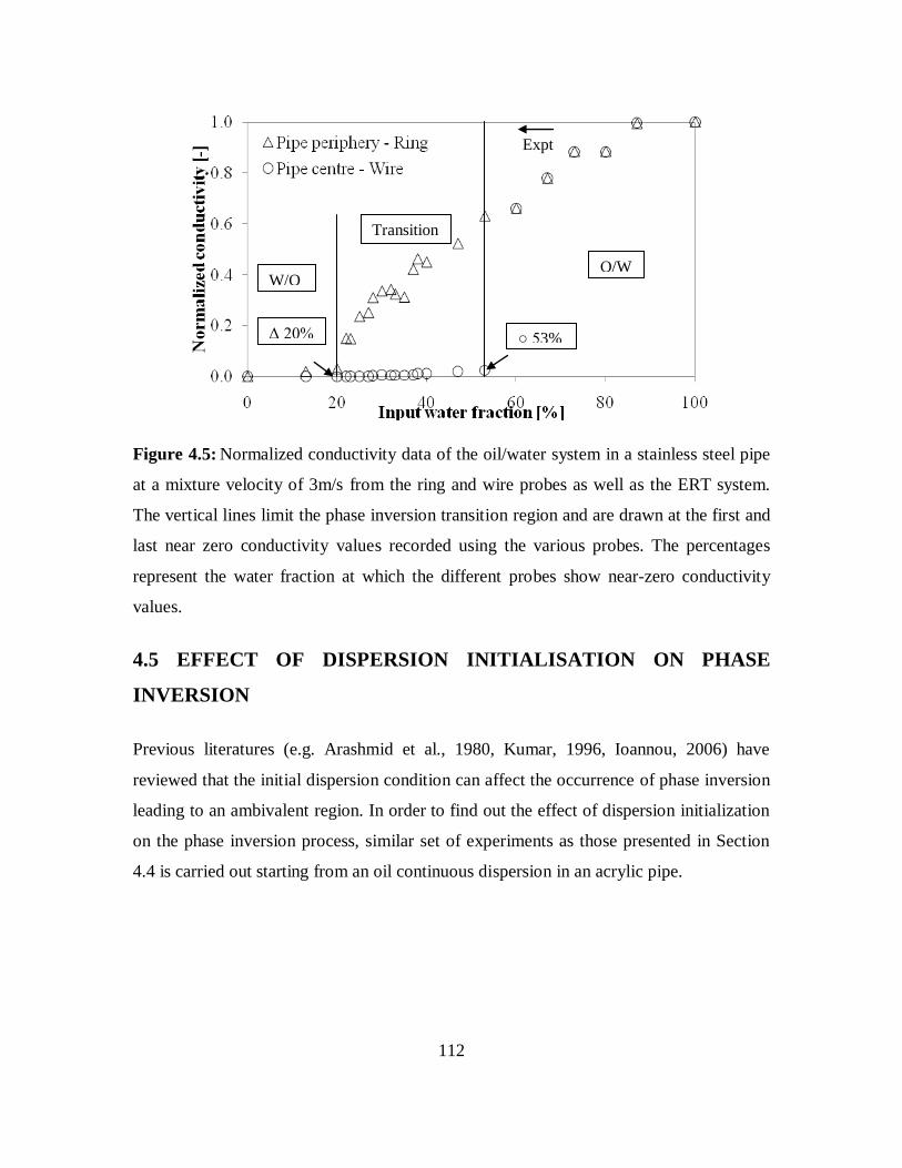
112

Figure 4.5: Normalized conductivity data of the oil/water system in a stainless steel pipe

at a mixture velocity of 3m/s from the ring and wire probes as well as the ERT system.

The vertical lines limit the phase inversion transition region and are drawn at the first and

last near zero conductivity values recorded using the various probes. The percentages

represent the water fraction at which the different probes show near-zero conductivity

values.

4.5 EFFECT OF DISPERSION INITIALISATION ON PHASE

INVERSION

Previous literatures (e.g. Arashmid et al., 1980, Kumar, 1996, Ioannou, 2006) have

reviewed that the initial dispersion condition can affect the occurrence of phase inversion

leading to an ambivalent region. In order to find out the effect of dispersion initialization

on the phase inversion process, similar set of experiments as those presented in Section

4.4 is carried out starting from an oil continuous dispersion in an acrylic pipe.

W/O

Transition

O/W

○ 53% Δ 20%

Expt

113

Figure 4.6: Normalized conductivity data for the oil/water system in an acrylic pipe at a

mixture velocity of 3m/s from the ring and the wire probes for the two inversion routes (a)

starting from oil continuous (OC) and (b) starting from water continuous (WC) mixture.

The vertical lines limit the phase inversion transition region and are drawn at the first and

last near zero conductivity values recorded from the two probes. The percentages

represent the water fraction at which the different probes show near-zero conductivity

values.

From Figure 4.6, the results from the wire and ring probes are shown since they represent

the pipe centre and periphery respectively where the phase inversion begins and ends. It

can be seen that the conductivity values from the ring and wire probes are very close for

both inversion routes. Only slight deviation is observed between 20-40% water fractions.

This is possibly because of the difference in the mechanism of the phase inversion

process. Starting from a water continuous dispersion, the water layer at the bottom of the

pipe is likely to have oil drops within it and the conductivity value of that layer will be

lower than in the case of pure water. Starting from an oil continuous dispersion, on the

other hand, the water layer at the bottom of the pipe is formed by the coalescence and

deposition of water drops. As such, there would probably be no oil drops present and the

W/O

Transition O/W

○ 54% Δ 20%

114

conductivity will be higher than in the water continuous route. Once the water layer has

reached a certain thickness, entrainment of oil drops can occur. In this case, it explains as

well the agreement of the data for the two routes beyond 40% water fractions. The wire

probe gives a higher conductivity value for the oil continuous route compared to the

water continuous route between 20% - 40% due to the opposite effect in the

concentration of water phase at the pipe centre.

4.6 EFFECT OF MIXTURE VELOCITY ON PHASE INVERSION

Phase inversion experiments were carried out at a mixture velocity of 4m/s starting from

a water continuous dispersion and the phase distribution at decreasing water fractions are

shown in Figure 4.7. At high water fraction when the flow is water continuous, the

dispersion appears more homogeneous than at 3m/s (comparing with Figure 4.3). At 40%

water fraction, the core of the pipe flow becomes oil continuous (green) while it remains

water continuous over the pipe annulus. A water layer still remains at the bottom of the

pipe but is thinner than the water layer at 3m/s with the same input water fraction

(compare 26% water fraction with Figure 4.3). Phase inversion is completed only when

this layer of water is also dispersed into the oil (i.e. at about 22% water fraction). Full oil

continuous dispersion is achieved at a water fraction below 22%.

The effect of mixture velocity on the changes in phase continuity in the pipe cross section

is shown in Figure 4.8. It can be observed that the mixture remains to be water

continuous in the pipe centre until a lower water fraction (>40%) at 4m/s compared to

54% at 3m/s. However, phase inversion is completed at approximately the same input

water fraction (20%) when the water layer at the bottom of the pipe is dispersed. Thus,

increasing the mixture velocity aids the homogenisation of the dispersion leading to a

narrower phase inversion transition.

115

Type of dispersion Tomographic images

Oil-in-water

dispersion

(80%)

(70%)

(60%)

Phase inversion

transition

(54%)

(40%)

(26%)

Water-in-oil

dispersion

(22%)

(20%)

(16%)

Figure 4.7: Phase distribution in a pipe cross section during the transition from a water

continuous to an oil continuous dispersion at a mixture velocity of 4m/s. The percentages

in brackets represent the input water fraction.

116

Figure 4.8: Comparison of normalized conductivity data for the oil/water mixture at a

mixture velocity of 3m/s and 4m/s using the ring probe and wire probe. The vertical lines

determine the phase inversion transition at which the first and last near zero conductivity

value are recorded using the various probes – dotted lines for 3m/s and solid lines for

4m/s.

4.7 PRESSURE GRADIENT DURING PHASE INVERSION

The pressure drop, across a 1.5m section of the pipeline, is also measured during the

conductivity measurements. Each data point at a specific phase fraction is an average of

3000 measurement points (taken in 30 seconds interval). The data points are then

normalized as pressure gradient. Figure 4.9 presents the average pressure gradient at 3m/s

mixture velocity starting from a water continuous dispersion across the phase inversion

transition.

Starting from 100% water fraction, an increase in the oil phase fraction will lead to a

reduction in pressure gradient. This can be attributed to the drag reduction effect due to

the presence of the dispersed oil drops in the water continuous phase and the effect has

been previously reported in literature (e.g. Arirachakaran et al., 1989, Pal, 1993, Nädler

and Mewes, 1997). The pressure gradient continues to reduce while water is still in

W/O Transition O/W

Expt

117

contact with the pipe wall. As the water fraction reaches about 40%, the pressure gradient

appears to fluctuate significantly especially within the transition region. The large

fluctuations are believed to be caused by the presence of both water continuous and oil

continuous dispersion co-existing as complex structures. Piela et al. (2008) has reported

similar findings where the friction factor is significantly affected by the changes in phase

continuity as the probes pass through the complex structures. As the presence of oil

continuous dispersion increases and upon the first contact of the oil phase with the pipe

wall, the pressure gradient starts to increase towards the single phase oil value as the

more viscous oil phase comes into contact with more of the pipe wall.

Figure 4.9: Experimental pressure gradients in an acrylic pipe at a mixture velocity of

3m/s. The error bars represent the standard deviation of the fluctuations at each specific

phase fraction. The arrow denotes the direction of experiment from water continuous to

oil continuous dispersion and the vertical lines represent the boundaries of the phase

inversion transition region.

Expt

W/O Transition O/W

118

Comparing between the water continuous and oil continuous dispersion, the drag

reduction is observed to be stronger in the oil continuous dispersion. Similar observation

has also been reported by both Ioannou, 2006 and Hu, 2005 when they conducted their

experiments in stainless steel pipes using Exxsol D140 as the oil phase. Pal (1993) has

also found that, in stainless steel pipe, unstable water-in-oil emulsions exhibit higher drag

reduction than oil-in-water emulsions. Ioannou (2006) has observed that the pipe material

has an effect on the drag reduction (when using Marcol 52 with viscosity at 11mPa s) of

which acrylic pipe will have a stronger drag reduction with oil-in-water dispersion.

However, this effect is not observed in the current experiments.

4.7.1 EFFECT OF INVERSION ROUTE ON PRESSURE GRADIENT

As the presence of oil at the pipe wall can have a significant effect on the changes in

pressure gradient, it is of interest to investigate whether the inversion route can influence

the pressure gradient by affecting the phase distribution. The pressure gradient results for

the two inversion routes are shown in Figure 4.10. In both cases, the minimum pressure

gradient falls within the phase inversion transition region. The inversion route does not

affect the pressure gradient significantly. This agrees with the phase continuity data that

showed changes in the continuity of phases in contact with the wall at similar phase

fractions for both inversion routes.

4.7.2 EFFECT OF MIXTURE VELOCITY ON PRESSURE GRADIENT

The results of the pressure gradient data with respect to the different mixture velocity are

presented in Figure 4.11 - 4.12. The pressure gradient increases with mixture velocity.

Similar to 3m/s, the pressure gradient at 4m/s initially decreases with decreasing water

fraction until about 40% and start increasing again towards the single phase oil value.

Large fluctuations are again observed between 26% and 54% water fraction. While the

absolute values for pressure gradient has increased across the whole range of phase

fraction, the difference in pressure gradient appear to be larger both below 20% and

beyond 60% water fraction. According to Ioannou (2006), drag reduction increases with

119

increasing velocity/turbulence as the increased occurrence of drop coalescence and

breakup event in the flow can cause a suppression of the velocity/turbulence in the

continuous phase. Thus, it is expected to have a wider difference in pressure gradient in a

dilute dispersion compared with a dense dispersion.

Figure 4.10: Comparison of pressure gradient for the oil/water system in an acrylic pipe

at a mixture velocity of 3m/s between the two inversion routes (a) starting from oil

continuous dispersion (OC) (b) starting from water continuous dispersion (WC). The

vertical lines represent the boundaries of the phase inversion transition region.

Similar trends in pressure gradient are also found for the stainless steel pipe. The

minimum in pressure gradient however appears at a lower water fraction indicating that

the water layer in the steel pipe persists till a lower water fraction than in the acrylic pipe.

Steel is a more hydrophilic pipe material than acrylic pipe (Ioannou, 2006) and this may

have aided the water layer to retain longer.

O/W Transition W/O

120

Figure 4.11: Comparison of pressure gradient measurement between mixture velocity of

3m/s and 4m/s in an acrylic pipe. The error bars represent the standard deviation of the

fluctuations at each phase fraction. The arrow denotes the direction of experiment from

water continuous dispersion to oil continuous dispersion. The vertical lines limit the

boundaries for phase inversion transition - dotted lines for 3m/s and solid lines for 4m/s.

Figure 4.12: Comparison of pressure gradient measurement between mixture velocity of

3m/s and 4m/s in a stainless pipe. The arrow denotes the direction of experiment from

water continuous dispersion to oil continuous dispersion.

Expt

Expt

121

4.8 DROP SIZE DISTRIBUTION IN OIL & WATER DISPERSION

In a liquid-liquid dispersion, the loss of balance between drop breakage and coalescence

rates has been considered as a possible mechanism for phase inversion (Coulaloglou &

Tavlarides, 1977; Kumar, 1996; Yeo et al., 2000). Breakage and coalescence rates

depend on drop size and dispersion phase fraction. Other criteria for phase inversion such

as equating the surface energy between water continuous dispersion and oil continuous

dispersion is also a relation with the drop size. In addition, the various forces that act on

the drops which determine their movements and placement in the flow field and

eventually the phase distribution also depend on the drop size. Thus, drop sizes and their

distribution are important in understanding phase inversion.

Drop size measurements are conducted with the dual impedance probe (see Chapter 3)

for a range of phase fractions. Measurements are taken for both inversion routes (starting

both from O/W and from W/O dispersions). Based on the conductivity probe experiments

(see Figure 4.4), it can be seen that the phase inversion region is within two boundaries (1)

the boundary at high water fraction beyond which the dispersion is water continuous and

(2) the boundary at low water fraction below which the dispersion is oil continuous. The

second boundary (2) involves an inversion of the water continuous layer at the bottom of

the pipe. Detection of drop size using the dual impedance probe can be difficult at that

location due to the possible interference of interfacial waves with the thin water layer.

Therefore, the investigation of drop size before and after inversion is focused on the first

inversion boundary (1) occurring at the pipe centre.

During the experiment, the drop velocity is calculated from the cross-correlation of

signals for the two dual impedance probe sensors (see Lovick, 2004 and Hu, 2005). The

calculated drop velocity together with the time duration of the drops in the signal of

either of the two impedance sensors will provide a drop chord length. The chord length

distribution from the measured drops can be further converted into drop size distribution

based on an algorithm developed by Hu et al. (2006).

122

4.8.1 DROP SIZE DISTRIBUTION MEASUREMENT

During the experiment, it was found that no cross correlation could be obtained at dilute

dispersions because of the small number of drops passing through the impedance sensors.

Therefore, drop size distributions are obtained from 60% water fraction across the first

inversion boundary and down to 40% water fraction at different locations along the

vertical pipe diameter. Drop size measurements are also conducted for the two inversion

routes (i.e. o/w → w/o and w/o → o/w).

Figure 4.13 represents a sample of chord length measurements an oil-in-water dispersion

(60% water fraction) at different locations along the vertical pipe diameter for a mixture

velocity of 3m/s and both inversion routes. Any chord length larger than 10mm has been

ignored since this exceeds the physical distance between the two impedance sensors. It

can be seen that the chord length distributions are similar for both inversion routes.

Larger drops can be seen at the centre of the pipe (see Figure 4.13 (c)) where, as

discussed before, the dispersed oil phase tends to accumulate. The higher fraction would

favour drop coalescence and increase the drop size. Data at other phase fractions are

given in Appendix A. As the dispersed oil fraction is increased, very few or no drop can

be captured at about 6mm from the top wall.

The probability density functions of an oil-in-water dispersion and a water-in-oil

dispersion are presented in Figure 4.14. For the same conditions as Figure 4.13 and at,

example, 14mm, it can be seen that a log-normal distribution fit the data well as this has

also been previously reported by other investigators for dispersed pipe flow (e.g.

Karabelas (1978), Simmons & Azzopardi (2001)). There is predominantly a large number

of small drops with approximately 1-2 mm in diameter. The long tail of large drops

(>5mm) may be caused by irregular drop structures but these large structures account for

less than 3% of the drop number. From the figure, the oil-in-water dispersion has a

narrower distribution than the water-in-oil dispersion which at the same time is shifted

towards smaller drop sizes. This has also been observed by Piela et al. (2008), Hu (2005)

and Liu et al. (2005). As suggested by Kumar (1996), the difference in drop size may be

123

(a) 6mm (b) 14mm

(c) 20mm (d) 26mm

(e) 32mm

Figure 4.13: Chord length distribution of oil drops in water (60% water fraction) at a

mixture velocity of 3m/s at (a) 6mm (b) 14mm (c) 20mm (d) 26mm (e) 32mm from the

top wall of the pipe. The distributions of the two inversion routes are given – starting

from a O/W dispersion (□) and from a W/O dispersion (■).

124

due to the different dielectric constants of the two phases. Oil drops in water experience

repulsive forces due to the overlapping of the electrical double layers forming in water

and thus have lower coalescence efficiencies whereas water drops in oil of low dielectric

constants (which applies to Exxsol D140) do not experience similar repulsion and

therefore have higher coalescence efficiencies. Coalescence efficiency also depends on

the continuous phase viscosity (Coulaloglou & Tavlarides, 1977; Tsouris & Tavlarides,

1994; Liu & Li, 1999). Based on the larger water drops in oil, it appears that the viscosity

of Exxsol D140 does not significantly affect the film drainage and lower the coalescence

efficiency in relation to other influencing factors.

The evolution of drop size during inversion can be seen in Figure 4.15. In terms of

average Sauter mean diameter, d32, for a mixture velocity of 3m/s and both inversion

routes. The results are from the core of the pipe (14mm from the top wall) where

inversion across boundary (1) occurs. It can be seen that the oil drops in water are smaller

than water drops in oil, regardless of the inversion route. The drop size, at 54% water

fraction, is higher than at either 40% or 60% water fraction. Based on previous

investigations, the large Sauter mean diameter is likely caused by the presence of

irregular complex structures as well as coalesced large drops especially at a location

where phase inversion is prominent. When comparing the effect of inversion route, no

significant difference can be seen on the drop size across the inversion boundary (1). This

may explain the reason for the same phase fraction when phase inversion occurs for

inversion boundary (1) reported in Figure 4.6.

125

(a) O/W

(b) W/O

Figure 4.14: Sample drop size distribution is recorded at 14mm from the top wall with a

mixture velocity of 3m/s (a) oil-in-water dispersion (60% water fraction). The

experimental data is compared with a log-normal distribution with a mean of 1.51mm and

a variance of 0.238. (b) water-in-oil dispersion (40% water fraction). The experimental

data is compared with a log-normal distribution with a mean of 2.07mm and a variance of

0.451.

126

Figure 4.15: Sauter mean diameter at different input water fraction across the phase

inversion boundary (1). The phase in brackets represents the initial continuous phase and

the number in each column represents the Sauter mean diameter at the specific sample.

4.9 EFFECT OF DISPERSION INLET ON PHASE INVERSION

With previous sections discussed on a split inlet where the flow is gradually developed,

phase inversion occurs across a transitional region due to partial inversion occurring at

different input water fraction. It is interesting to investigate the effect of phase inversion

if the two phases are introduced as a full dispersion straight from the inlet. Thus, a

dispersion inlet is developed and the design of the inlet was discussed in Chapter 3.

Figure 4.16 presents the conductivity data from the ring and wire probes. Measurements

are conducted at the centre of the pipe (with the conductivity wire probe) and at the

periphery of the pipe (with the ring probe) similar to the configuration as presented in

Section 4.4.2.

127

Figure 4.16: Normalized conductivity data for an oil/pure water mixture at a mixture

velocity of 3m/s using the ring probe and wire probe. The letter in bracket represents

initial dispersed phase – (W) water (O) oil. The arrow denotes the direction of experiment

and the vertical line denotes the first input water fraction where phase inversion occurs.

As can be seen in figure, the conductivity data from both probes are very close for all

input water fractions indicating that the flow is fully dispersed for all phase fractions at

the mixture velocity of 3m/s. As a result, the change from a water continuous dispersion

to an oil continuous dispersion (and vice versa) occurs throughout the pipe cross-section

and at a particular phase fraction rather than over a transitional region as in the case with

a split inlet. The decrease in conductivity is almost linearly proportional to the decrease

in the water phase. Phase inversion occurs at a single phase fraction of about 28% input

water fraction.

The effect of the dispersion initialization conditions is shown in Figure 4.17. There is

only very small difference on the phase inversion point between the two inversion routes,

28% input water fraction for an initial O/W dispersion and 26% water fraction for an

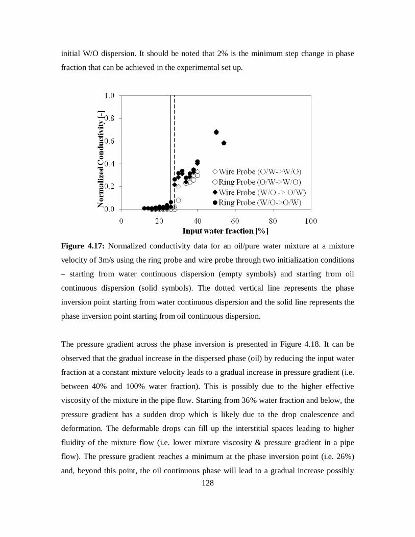
128

initial W/O dispersion. It should be noted that 2% is the minimum step change in phase

fraction that can be achieved in the experimental set up.

Figure 4.17: Normalized conductivity data for an oil/pure water mixture at a mixture

velocity of 3m/s using the ring probe and wire probe through two initialization conditions

– starting from water continuous dispersion (empty symbols) and starting from oil

continuous dispersion (solid symbols). The dotted vertical line represents the phase

inversion point starting from water continuous dispersion and the solid line represents the

phase inversion point starting from oil continuous dispersion.

The pressure gradient across the phase inversion is presented in Figure 4.18. It can be

observed that the gradual increase in the dispersed phase (oil) by reducing the input water

fraction at a constant mixture velocity leads to a gradual increase in pressure gradient (i.e.

between 40% and 100% water fraction). This is possibly due to the higher effective

viscosity of the mixture in the pipe flow. Starting from 36% water fraction and below, the

pressure gradient has a sudden drop which is likely due to the drop coalescence and

deformation. The deformable drops can fill up the interstitial spaces leading to higher

fluidity of the mixture flow (i.e. lower mixture viscosity & pressure gradient in a pipe

flow). The pressure gradient reaches a minimum at the phase inversion point (i.e. 26%)

and, beyond this point, the oil continuous phase will lead to a gradual increase possibly

129

because the deformed or coalesced drops are likely to be separated as the mixture is

diluted. This will result in a more narrowly distributed drop size and, thus, reducing the

fluidity of the mixture flow once again. The relatively higher pressure gradient by the oil

continuous dispersion is also due to the higher oil viscosity as the continuous phase.

Figure 4.18: Experimental pressure gradients for a dispersed inlet configuration at a

mixture velocity of 3m/s. The arrow denotes the direction of experiment from water

continuous to oil continuous dispersion and the vertical line represents the phase

inversion point.

In order to determine the change in drop size during the phase inversion process for the

dispersed inlet configuration, Figure 4.19 presents the chord length distribution at

different phase fractions. The chord length distribution can be seen to be narrow when the

input water fraction is higher than 36%. The distribution becomes broader with longer

chord length between 26% and 36% water fraction of which drop

deformation/coalescence was previously suggested to occur. The distribution is the

widest at about 26% where phase inversion is observed. At 20% water fraction (W/O

dispersion is formed), the distribution becomes narrower beyond the phase inversion

point. The corresponding drop size (by converting the chord length based on the method

by Hu (2005) of the W/O dispersion is also found to be higher than O/W dispersion.

Phase

inversion

130

Figure 4.19 Comparison of chord length distribution at different input water fraction

(fraction in bracket) across the phase inversion process at 3m/s mixture velocity.

4.10 CONCLUSION

The phase inversion transition of an oil-water dispersion was investigated in this chapter.

The ERT system revealed the distribution of the phases and the respective flow patterns

while the conductivity data from the ring and wire probes as well as the ERT provide

further information on the phase continuity in a pipe cross section. The following

mechanism for phase inversion is proposed based on the data from the split inlet

configuration.

131

For inversion starting from an oil-in-water dispersion:

(1) At low oil fraction, the added oil phase is initially dispersed in the continuous water

phase.

(2) As the oil fraction increases, the oil drops will accumulate at the pipe centre where

they coalesce and the mixture inverts.

(3) With the mixture also inverts at the top of the pipe, a dual continuous flow pattern is

formed with oil as the continuous phase at the top of the pipe and water as the continuous

phase at the bottom.

132

(4) At high oil fractions, the thin layer of water at the bottom of the pipe also disperses

and the flow becomes fully dispersed with oil as the continuous phase.

The change from a water continuous to an oil continuous dispersion occurs over a range

of volume fractions and is bounded by two lines: the first line is related to the inversion at

the pipe centre and the second line is related to the diminution/formation of the water

layer at the bottom of the pipe depending on the inversion route. However, no significant

difference was found in the phase inversion transition boundaries between the two

inversion routes. With increasing mixture velocity, the transitional region over which

phase inversion occurs reduces in size.

Change in phase distribution during the phase inversion transition is found to affect the

pressure gradient. Starting from a water continuous dispersion, the addition of dispersed

phase initially led to drag reduction. Pressure gradient continued to reduce even after

inversion has occurred at the centre of the pipe. When the water layer at the bottom of the

pipe eventually disperses and the viscous oil phase comes in contact with the whole pipe

wall, the pressure gradient starts to increase again. There is no significant difference in

pressure gradient between the two inversion routes. The V-shaped trend, which the

changes in pressure gradient exhibits, is similar regardless of mixture velocity and pipe

materials. The degree of changes is found to be higher at higher mixture velocity possibly

because of higher drag reduction. There is also observed, in the stainless pipe, a shift in

the minimum pressure gradient leftward with the increase in mixture velocity.

In addition to the change in flow conditions (e.g. mixture velocity, dispersion

initialization), the change in the inlet configuration (to a dispersed inlet) has led to a

133

significant change in the phase distribution in the mixture flow. This results in a

substantial difference in the phase inversion occurrence from a phase inversion transition

across a range of phase fraction into a phase inversion point. The pressure gradient

increases with the initial increase in the dispersed phase (i.e. oil) until drop

coalescence/deformation become prominent. During the rearrangement of the deformable

drops and until phase inversion has occurred, the pressure gradient has a sharp drop. The

higher oil viscosity will subsequently led the increase in pressure gradient beyond phase

inversion.

For the split inlet, drop size measurements are in accordance with the phase distribution

data. Larger drop sizes are found at the pipe core just before inversion from O/W to W/O

dispersion where the dispersed phase has concentrated. Differences are also seen between

the sizes of oil drops in water and water drops in oil regardless of the inlet configuration.

From the drop size measurement, it can also be concluded that drop coalescence and

deformation is a critical process during phase inversion.

The understanding on how phase inversion progresses during pipe flow will form the

basis of the investigation in the following chapters – effect of interfacial tension on phase

inversion (Chapter 5), prediction model of phase inversion based on flow regimes

(Chapter 7) and CFD simulation on the interaction of the dispersed and continuous phase

in a pipe flow (Chapter 8).

134

Chapter 5: Effect of interfacial tension on phase

inversion

5.1 OVERVIEW

The pipeline flow of two immiscible liquids, usually an aqueous and an organic, is

commonly encountered in process industries and during oil production. Depending on the

flow rates and phase fractions, dispersed flow can establish either the water (O/W) or the

oil (W/O) as being the continuous phase. At some critical operational conditions, phase

inversion occurs whereby the initial dispersed phase becomes continuous and the

continuous phase becomes dispersed. The change in phase continuity can have a

significant effect on the mixture rheology and on frictional pressure drop while the nature

of the continuous phase is related to pipeline corrosion and to the rate of the mixture

separation at the end of the process. It is important, therefore, to understand and be able

to predict the conditions under which inversion appears.

Many factors have been reported to affect phase inversion and the phase inversion point,

i.e. the volume fraction of the liquids at inversion. Experimental work has mainly been

carried out in stirred vessels (for a review see Yeo et. al, 2000) where it was found that

phase inversion is affected not only by the fluid properties such as viscosity, density and

interfacial tension, but also by the stirred vessel geometric configuration (e.g. type of

impeller), the vessel and impeller material wettability and the experimental set up (e.g.

the phase that the impeller is in at the beginning of the experiment). In contrast to stirred

vessels, there is less information available on the effect of various parameters on phase

inversion during pipeline flows. Apart from fluids properties, parameters such as mixture

velocity, rate at which the dispersed phase is added in the continuous, size of the pipe and

wettability of the pipe material have also been found to influence phase inversion (Angeli

and Hewitt, 2000; Ioannou et. al, 2005; Luo et. al, 1997; Piela et. al, 2008).

135

Among the fluid properties, viscosity is considered to have a significant impact on phase

inversion. Selker and Sleicher (1965) found that as the viscosity of one phase increases,

its tendency to be dispersed also increases, i.e. the minimum fraction that the phase can

be continuous will decrease and the maximum fraction that it can be dispersed will

increase. Notably, many models for the prediction of the phase inversion fraction are

based on the liquid viscosities (Arirachakaran et. al, 1989; Nädler and Mewes, 1995;

Ngan et al., 2009; Yeh et al., 1964). Density does not seem to affect inversion

significantly especially when the density difference between the two liquids is small but

it will influence the homogeneity of the dispersion (McClarey and Mansoori, 1978;

Selker and Sleicher, 1965). However, systems with large density difference between the

phases show an increased tendency to invert (Kumar et. al, 1991).

The effect of interfacial tension is the least understood. In agitated vessels, Selker and

Sleicher (1965) suggested that interfacial tension cannot affect the type of dispersion

since it is not a function of the sign of the interfacial curvature. However, the suggestion

was not further investigated. According to Yeh et. al (1964) interfacial tension will cause

inversion of a dispersion to occur at equal volumes of the two liquids in the absence of

other influencing parameters. Luhning and Sawistowski (1971), in contrast, stated that

interfacial tension is important and found that the limits of the ambivalent region were

correlated with the impeller Weber number (for Weber numbers between 350 and 4000).

A decrease in interfacial tension will make inversion more difficult to occur and will

widen the boundaries of the ambivalent region (Clarke and Sawistowski, 1978; Norato et.

al, 1998). Interfacial tension is also related to drop break up and coalescence

(Coulaloglou and Tavlarides, 1977; Luo and Svendsen, 1996; Prince and Blanch, 1990;

Sovová, 1981; Tsouris and Tavlarides, 1994) that define the size of the dispersed phase.

The evolution of the dispersed phase size and the departure from equilibrium between

break up and coalescence rates have been used to predict phase inversion in stirred

vessels (Arashmid and Jeffreys, 1980; Groeneweg et. al, 1998; Hu et. al, 2005), thus

indicating a strong dependence on interfacial tension. There is no reported work on the

effect of interfacial tension on phase inversion in pipeline flow of liquid-liquid

dispersions. This is not because interfacial tension was kept constant during

136

investigations of the fluid properties, rather that it was not monitored. It is actually quite

difficult to vary a liquid property without affecting at the same time to some extent the

interfacial tension. In this chapter, the interfacial tension of an oil-water mixture is varied

in a controlled way in order to investigate its effect on phase inversion during pipeline

flow while keeping all other fluid properties constant as shown in Table 5.1.

5.2. EXPERIMENTAL SETUP

The experimental investigations in this study were conducted in a pilot scale liquid-liquid

flow facility (See Chapter 3 for the detailed description of the experimental setup). A

38mm I.D acrylic test section will be used in all experiments during this study to

minimize any effect on phase inversion caused by the experimental configuration. In this

study, Exxsol D140 (density of 828 kgm-3

, viscosity of 5.5 mPa.s) is used as the oil phase

while tap water or a glycerol solution is used as the aqueous phase. The two fluids are

joined at the end of a Y-junction inlet to ensure that the two fluids join with minimum

mixing at the inlet.

For each experiment, simultaneous measurements of pressure gradient and phase

continuity were carried out. Pressure gradient was measured with a differential pressure

transducer between two ports 1.5m apart, with the first port located at 3.8m (~100D)

from the inlet. Two types of conductivity probes were used to detect phase continuity and

the appearance of phase inversion, namely a ring and a wire probe. These probes were

located at 7m (~184D) from the inlet. High conductivity values indicate that a

water/glycerol solution continuous mixture is in contact with the probes, while low

values denote an oil continuous mixture. The ring probe consists of a pair of metallic

rings, 4mm thick and 38mm apart, embedded on the pipe perimeter, flush with the wall,

and in contact with the fluid mixture. This probe provides information on the continuity

of the mixture adjacent to the pipe wall. The wire probe is made of two conducting wires

with 0.5 mm diameter set 10 mm apart. It detects the phase continuity at different

locations in a pipe cross section using a traversing mechanism. In this work, it was placed

in the middle of the pipe.

137

An Electrical Resistance Tomographic (ERT) imaging system was also used. ERT

tomograms were taken at the same axial location (i.e. 7m from the inlet) as the

measurements of the two conductivity probes. In addition, the conductivity data from the

ERT system were measured at 4mm from the top pipe wall in conjunction with the data

from the conductivity probes to study changes in the mixture continuity in a pipe cross

section at different phase volume fractions. Conductivity data for all three sensors were

time averaged when the conductivity measurements were stabilized and over a period of

30 seconds. The data were normalized with respect to the values of single phase water. It

was previously found that, at the same pipe cross section location, the normalized

conductivities from the different sensors differ by 1% and can be regarded to have

sufficient precision to relate the conductivity data from the various systems across a pipe

cross section for a given phase fraction.

A dual impedance probe using alternating current was also implemented to determine the

drop size distribution in the dispersion. During the experiment, the probe is positioned at

7 m downstream of the inlet. Sampling rate is set at 45kHz and a total number of 120,000

data points is collected. This high rate ensures that each dispersed drop is represented by

more than one data points in the probe output signal. The probe measures chord lengths

from which drop diameters can be calculated (Hu et. al, 2006).

The experiments were carried out at 3m/s mixture velocity and phase inversion was

investigated starting from the aqueous phase as being continuous as well as from the

organic phase. Each experiment started with a single phase flow of an initial continuous

phase where the flow rate of the dispersed phase was gradually increased while that of

the continuous phase was reduced to maintain a constant mixture velocity until phase

inversion has occurred and beyond. The same experimental run was repeated at least

three times and the averaged results are reported in Section 5.3.

The effect of glycerol addition on the physical properties of water and on the oil-water

interfacial tension is shown in Table 5.1. These measurements were conducted at ambient

temperature (~20oC±0.4

oC). Dilute glycerol solutions (0.5% and 1% v/v) were chosen to

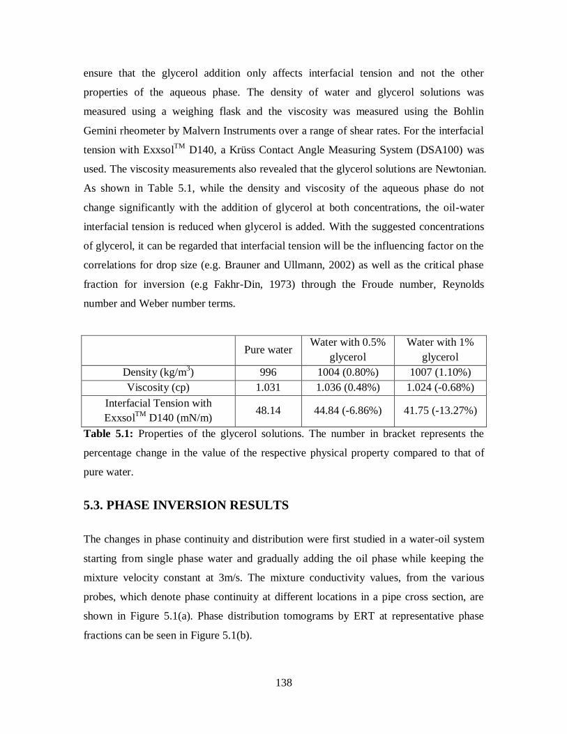
138

ensure that the glycerol addition only affects interfacial tension and not the other

properties of the aqueous phase. The density of water and glycerol solutions was

measured using a weighing flask and the viscosity was measured using the Bohlin

Gemini rheometer by Malvern Instruments over a range of shear rates. For the interfacial

tension with ExxsolTM

D140, a Krüss Contact Angle Measuring System (DSA100) was

used. The viscosity measurements also revealed that the glycerol solutions are Newtonian.

As shown in Table 5.1, while the density and viscosity of the aqueous phase do not

change significantly with the addition of glycerol at both concentrations, the oil-water

interfacial tension is reduced when glycerol is added. With the suggested concentrations

of glycerol, it can be regarded that interfacial tension will be the influencing factor on the

correlations for drop size (e.g. Brauner and Ullmann, 2002) as well as the critical phase

fraction for inversion (e.g Fakhr-Din, 1973) through the Froude number, Reynolds

number and Weber number terms.

Pure water Water with 0.5%

glycerol

Water with 1%

glycerol

Density (kg/m3) 996 1004 (0.80%) 1007 (1.10%)

Viscosity (cp) 1.031 1.036 (0.48%) 1.024 (-0.68%)

Interfacial Tension with

ExxsolTM

D140 (mN/m) 48.14 44.84 (-6.86%) 41.75 (-13.27%)

Table 5.1: Properties of the glycerol solutions. The number in bracket represents the

percentage change in the value of the respective physical property compared to that of

pure water.

5.3. PHASE INVERSION RESULTS

The changes in phase continuity and distribution were first studied in a water-oil system

starting from single phase water and gradually adding the oil phase while keeping the

mixture velocity constant at 3m/s. The mixture conductivity values, from the various

probes, which denote phase continuity at different locations in a pipe cross section, are

shown in Figure 5.1(a). Phase distribution tomograms by ERT at representative phase

fractions can be seen in Figure 5.1(b).

139

Figure 5.1: (a) Normalized conductivity data of the oil/water system at a mixture velocity

of 3m/s from the ring and wire probes and the ERT system. The direction of the

experiment from water to oil continuous is shown by the arrow. The vertical lines denote

the boundaries of the phase inversion transition region and are drawn at the first and last

near zero conductivity values recorded using the various probes. The percentages

represent the water fraction where conductivity approaches zero at the various locations

in the pipe cross section.

0.0

0.2

0.4

0.6

0.8

1.0

0 20 40 60 80 100

Norm

ali

zed

con

du

cti

vit

y [

-]

Input water fraction [%]

Pipe Periphery

Pipe Centre

Pipe Top Wall

O/W W/O

Transition

○ 54% × 40% Δ 20%

Expt

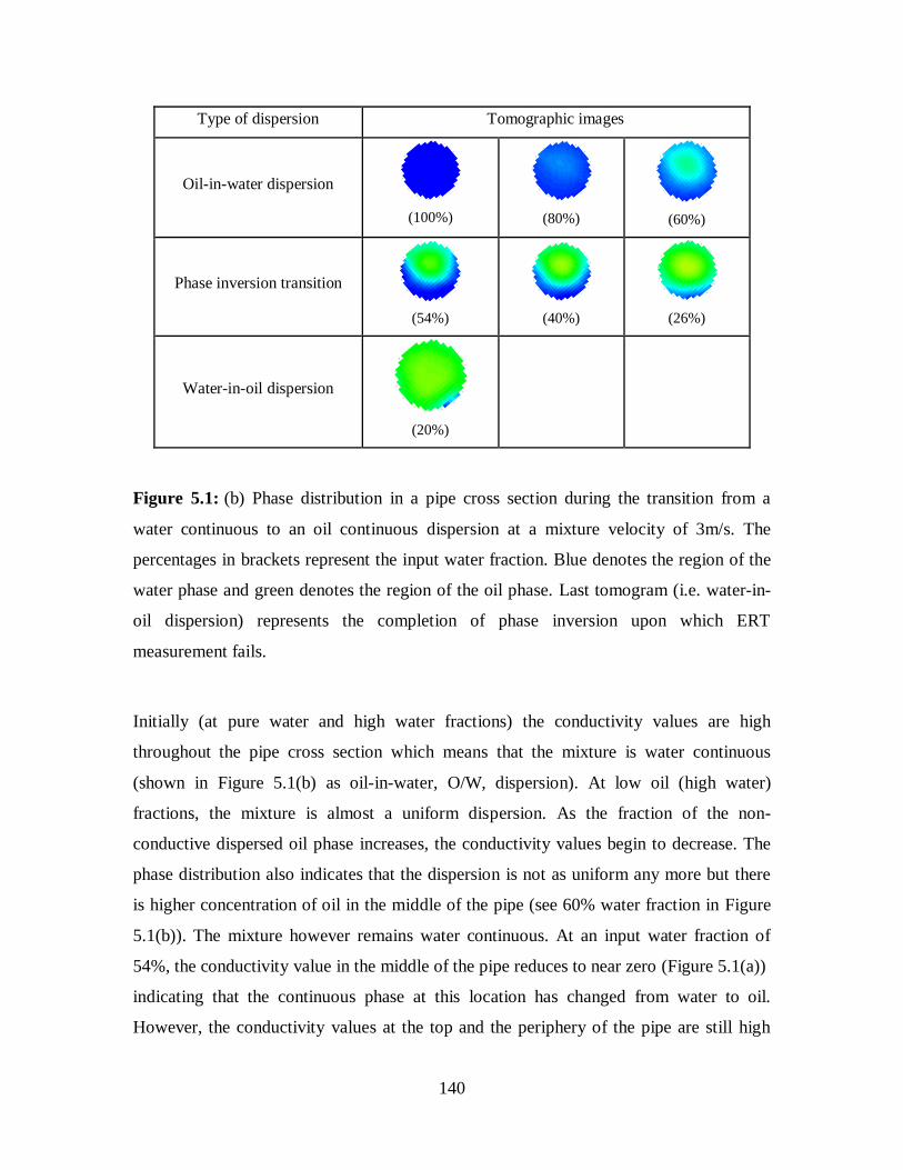
140

Type of dispersion Tomographic images

Oil-in-water dispersion

(100%)

(80%)

(60%)

Phase inversion transition

(54%)

(40%)

(26%)

Water-in-oil dispersion

(20%)

Figure 5.1: (b) Phase distribution in a pipe cross section during the transition from a

water continuous to an oil continuous dispersion at a mixture velocity of 3m/s. The

percentages in brackets represent the input water fraction. Blue denotes the region of the

water phase and green denotes the region of the oil phase. Last tomogram (i.e. water-in-

oil dispersion) represents the completion of phase inversion upon which ERT

measurement fails.

Initially (at pure water and high water fractions) the conductivity values are high

throughout the pipe cross section which means that the mixture is water continuous

(shown in Figure 5.1(b) as oil-in-water, O/W, dispersion). At low oil (high water)

fractions, the mixture is almost a uniform dispersion. As the fraction of the non-

conductive dispersed oil phase increases, the conductivity values begin to decrease. The

phase distribution also indicates that the dispersion is not as uniform any more but there

is higher concentration of oil in the middle of the pipe (see 60% water fraction in Figure

5.1(b)). The mixture however remains water continuous. At an input water fraction of

54%, the conductivity value in the middle of the pipe reduces to near zero (Figure 5.1(a))

indicating that the continuous phase at this location has changed from water to oil.

However, the conductivity values at the top and the periphery of the pipe are still high

141

which means that a flow pattern has formed with an oil continuous region in the middle

of the pipe and a water continuous region as an annulus around it. The water continuous

layer is thinner at the top of the pipe and finally it inverts as well at approximately 40%

water fraction. The flow regime then becomes dual continuous with an oil continuous

region at the upper part of the pipe and water continuous region at the lower part. The

respective tomogram in Figure 5.1(b) also shows the segregation of the phases at this

fraction. This transitional regime persists with a further decrease in the water fraction

until about 20% where the conductivity from the pipe periphery also reduces to zero

(Figure 5.1(a)) indicating that an oil continuous mixture is now established throughout

the pipe cross section.

Figure 5.2: (a) Normalized conductivity data of the oil/1% glycerol solution system at a

mixture velocity of 3m/s from the ring and wire probes and the ERT system. The

direction of the experiment from water to oil continuous is shown by the arrow. The

vertical lines denote the boundaries of the phase inversion transition region and are drawn

at the first and last near zero conductivity values recorded using the various probes. The

percentages represent the water fraction where conductivity approaches zero at the

various locations in the pipe cross section.

0.0

0.2

0.4

0.6

0.8

1.0

0 20 40 60 80 100

Norm

ali

sed

Con

du

cti

vit

y [

-]

Input Water Fraction [%]

Pipe PeripheryPipe CentrePipe Top Wall

Transition

W/O

Δ 10% × 26% ○ 54%

Expt

O/W

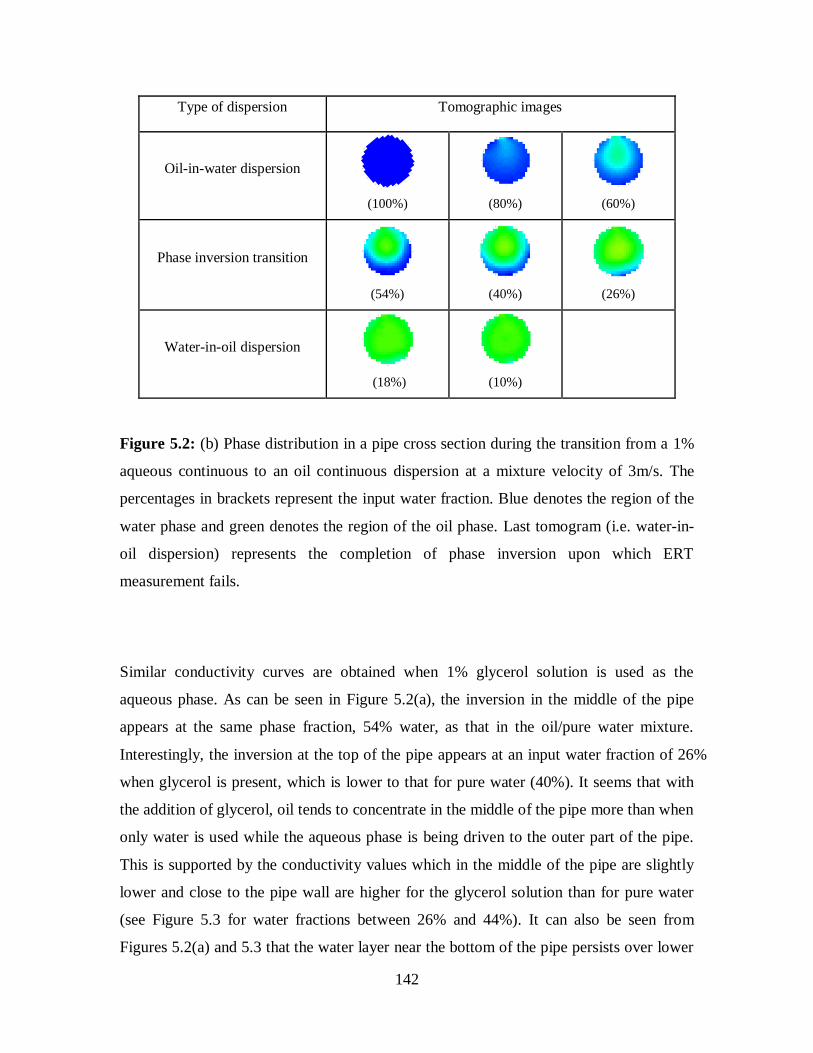
142

Type of dispersion Tomographic images

Oil-in-water dispersion

(100%)

(80%)

(60%)

Phase inversion transition

(54%)

(40%)

(26%)

Water-in-oil dispersion

(18%)

(10%)

Figure 5.2: (b) Phase distribution in a pipe cross section during the transition from a 1%

aqueous continuous to an oil continuous dispersion at a mixture velocity of 3m/s. The

percentages in brackets represent the input water fraction. Blue denotes the region of the

water phase and green denotes the region of the oil phase. Last tomogram (i.e. water-in-

oil dispersion) represents the completion of phase inversion upon which ERT

measurement fails.

Similar conductivity curves are obtained when 1% glycerol solution is used as the

aqueous phase. As can be seen in Figure 5.2(a), the inversion in the middle of the pipe

appears at the same phase fraction, 54% water, as that in the oil/pure water mixture.

Interestingly, the inversion at the top of the pipe appears at an input water fraction of 26%

when glycerol is present, which is lower to that for pure water (40%). It seems that with

the addition of glycerol, oil tends to concentrate in the middle of the pipe more than when

only water is used while the aqueous phase is being driven to the outer part of the pipe.

This is supported by the conductivity values which in the middle of the pipe are slightly

lower and close to the pipe wall are higher for the glycerol solution than for pure water

(see Figure 5.3 for water fractions between 26% and 44%). It can also be seen from

Figures 5.2(a) and 5.3 that the water layer near the bottom of the pipe persists over lower

143

water fractions in the presence of glycerol and the inversion to fully dispersed oil

continuous flow occurs at 10% water fraction compared to the 20% of the pure water

system.

Figure 5.3: A comparison of the normalised conductivities in the middle of the pipe and

the pipe periphery between the 1% glycerol solution and the pure water dispersions at a

mixture velocity of 3m/s.

Similar results are obtained with the 0.5% glycerol solution (Figure 5.4). As with the 1%

glycerol solution, the inversion in the middle of the pipe again occurs at 54%, the

inversion at the top occurs at 20% water fraction while fully dispersed oil continuous

flow establishes at 10% water fraction. The addition of glycerol seems to affect the

inversion behaviour of the oil-water mixture but, at least for the conditions tested, the

concentration of glycerol does not appear to play a significant role.

0.0

0.1

0.2

0.3

0.4

0.5

0 10 20 30 40 50

Norm

ali

sed

Con

du

cti

vit

y [

-]

Input Water Fraction [%]

3m/s (Pure Water) - Pipe Periphery

3m/s (Pure Water) - Pipe Centre

3m/s (Glycerol 1%) - Pipe Periphery

3m/s Glycerol 1%) - Pipe CentreExpt

144

Figure 5.4: Normalized conductivity data of the oil/0.5% glycerol solution system at a

mixture velocity of 3m/s from the ring and wire probes and the ERT system. The

direction of the experiment from water to oil continuous is shown by the arrow. The

vertical lines denote the boundaries of the phase inversion transition region and are drawn

at the first and last near zero conductivity values recorded using the various probes. The

percentages represent the water fraction where conductivity approaches zero at the

various locations in the pipe cross section.

5.4. EFFECT OF GLYCEROL ADDITION ON PRESSURE

GRADIENT DURING PHASE INVERSION

The changes in phase distribution and flow pattern during the inversion of the oil/water

dispersion, which were discussed in the previous section, are expected to affect the

frictional pressure gradient. The variation in pressure gradient as the oil fraction increases

(inversion from O/W to W/O) can be seen in Figure 5.5 for a mixture velocity of 3m/s

and for the three aqueous phases used, namely pure water, 0.5% and 1% glycerol

solutions.

0.0

0.2

0.4

0.6

0.8

1.0

0 20 40 60 80 100

Norm

ali

sed

Con

du

cti

vit

y [

-]

Input Water Fraction [%]

Pipe Periphery

Pipe Centre

Pipe Top Wall

O/W W/O

Transition

○ 54%

× 20%

Δ 10%

Expt

145

Figure 5.5: Experimental pressure gradient for pure water, 0.5% 1% glycerol solutions at

different input water fractions at a mixture velocity of 3m/s. The vertical lines indicate

the boundaries of the phase inversion transition region for pure water (solid lines) and

both glycerol solutions (dotted lines). The percentages indicate the water fractions where

pressure gradient shows a minimum. The arrow denotes the direction of experiment from

aqueous to oil continuous dispersion.

Pressure gradient is found to be the same for the single phase flow of either water or

glycerol solutions indicating that the addition of glycerol at these concentrations does not

affect the frictional pressure gradient because it does not alter significantly the density or

the viscosity of the aqueous phase. As the oil fraction increases, pressure gradient

remains the same for all fluid pairs used, while a drag reduction phenomenon is observed,

where the presence of the dispersed phase causes a decrease from the single phase value

of the continuous phase at the same as the mixture velocity (Pal, 1993). The initial

inversion in the middle of the pipe at 54% water fraction is the same for all three systems

and does not affect the pressure gradient possibly because the continuity of the phase in

contact with the pipe wall has not changed. Pressure gradient for pure water starts to

0.0

0.5

1.0

1.5

2.0

2.5

3.0

0 20 40 60 80 100

Pre

ssu

re G

rad

ien

t [k

Pa

/m]

Input water fraction [%]

Pure Water

0.5% glycerol

1% glycerol

O/W

Transition

36%

26% 18%

W/O

Expt

146

increase at about 36% water fraction after the mixture at the top of the pipe has inverted

(see Figure 5.1 (a)). Beyond this fraction, the more viscous oil phase comes in contact

with part of the pipe wall. The increase in pressure gradient for the two glycerol solutions

occurs at lower water fractions of about 18% and 26% for the 0.5% and 1% glycerol

solutions respectively. These changes again happen after the mixture at the top of the

pipe inverts from water to oil continuous. With further increase in the oil fraction

(decrease in water fraction), more oil contacts the pipe wall and the pressure gradient

continues to increase as phase inversion spreads across the pipe until all three systems

reach the single oil phase value. Similar results were found for the opposite experiment

starting from an oil continuous mixture.

5.5. EFFECT OF GLYCEROL ON DROP SIZE DISTRIBUTION IN

OIL AND WATER CONTINUOUS DISPERSIONS

Drop size distributions were measured using the dual impedance probe. The

measurements were conducted for both dispersion initialization conditions, i.e. starting

from oil continuous and from water continuous flows, and for the three aqueous solutions

considered, i.e. pure water, 0.5% and 1% glycerol. It was found that drop size

measurements in dilute solutions could not be obtained as the signals of the two sensors

of the dual impedance probe did not cross-correlate well probably because of the small

number of drops present. The same happened in the inversion transition region just after

the first inversion in the middle of the pipe when glycerol was present in the water phase.

Based on the tomographic images, the reason for this is probably the better separation

between the two phases in the transition region when glycerol is added which leaves a

lower concentration of the dispersed water phase in the middle where measurements are

taken. Drop size measurements were therefore conducted for input water fractions

between 40% and 60%. Measurements were carried out in the middle of the pipe

(approximately 14mm from the top pipe wall). This location was chosen because the

inversion at 54% allows both oil and water continuous dispersions to be investigated

while it is also away from the interface formed during the dual continuous flow that may

affect the measurements if any waves are present. Results are shown below for two

147

indicative fractions, 60% O/W and 40% W/O dispersion. To compare the drop sizes the

average Sauter mean diameter, d32, is used.

The Sauter mean diameters calculated for systems with pure water (PW), 0.5% and 1%

glycerol solutions can be seen in Figure 5.6(a) for an initial water continuous dispersion

and in Figure 5.6(b) for an initial oil continuous dispersion. In general, oil drops (at 60%

water fraction) are smaller than water drops (at 40% water fraction), and this difference is

more obvious for the pure water system. The addition of glycerol does not seem to affect

the oil drop size significantly, which may explain why the initial inversion in the middle

of the pipe from water to oil continuous mixture occurs at the same input phase fraction

for all the three aqueous solutions. In contrast, the size of water drops is reduced when

glycerol is added although the glycerol concentration does not seem to play an important

role. It has been found that water drops in oil tend to coalesce faster when glycerol is

added (Wang et. al, 2009); this would have resulted in larger drops when glycerol is

present which seems to contradict the current result. However, it is possible that these

larger drops will also tend to precipitate in the water layer that is still present at the

bottom of the pipe at 40% input water fraction. This agrees with the findings of the ERT

system which showed reduced concentration of water in the middle of the pipe and an

increase in the water layer at 40% water fraction when glycerol is present compared to

pure water (see Figures 5.1b, 5.2b and also the comparison of the conductivity values in

Figure 5.3). Similar results were found for the opposite experiment starting from an oil

continuous mixture (Figure 5.6(b)).

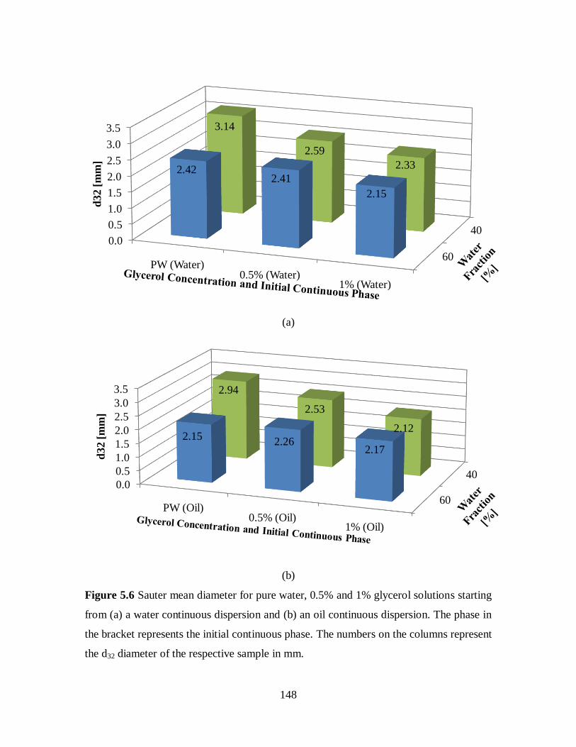
148

(a)

(b)

Figure 5.6 Sauter mean diameter for pure water, 0.5% and 1% glycerol solutions starting

from (a) a water continuous dispersion and (b) an oil continuous dispersion. The phase in

the bracket represents the initial continuous phase. The numbers on the columns represent

the d32 diameter of the respective sample in mm.

60

400.0

0.5

1.0

1.5

2.0

2.5

3.0

3.5

PW (Water)0.5% (Water)

1% (Water)

2.422.41

2.15

3.14

2.59

2.33

d32 [

mm

]

60

400.0

0.5

1.0

1.5

2.0

2.5

3.0

3.5

PW (Oil)0.5% (Oil)

1% (Oil)

2.152.26

2.17

2.94

2.53

2.12

d32 [

mm

]

149

5.6 CONCLUSION

The effect of interfacial tension on the phase inversion procedure of an oil-water mixture

in pipe flow was investigated in this paper. By adding small concentrations of glycerol to

water, the interfacial tension was reduced but the density and viscosity of the aqueous

phase were not significantly affected.

For all fluid pairs tested initially at low oil fractions, the dispersion was water continuous

with a fairly uniform distribution of the dispersed drops, as revealed by tomograms. As

the oil fraction increased for the same mixture velocity, the mixture at the centre of the

pipe inverted to become oil continuous. With a further increase in the oil fraction,

inversion spread to the top and finally the bottom of the pipe and the mixture became oil

continuous. It was found that while the addition of glycerol in water did not affect the

phase fraction where the first inversion in the middle of the pipe occurred, it delayed the

overall inversion at the rest of the pipe to higher oil (lower water) fractions. Drop size

measurements in the middle of the pipe revealed that the size of the oil drops before

inversion was not significantly affected by the addition of glycerol but the size of water

drops after inversion was reduced. Although with the addition of glycerol, larger water

drops are expected to form through coalescence; it is possible that these large drops also

separate more easily due to gravity leaving only the smaller ones in the pipe centre to be

measured. This settling would also explain the higher water concentration at the pipe

periphery which delays the inversion in these regions when glycerol is added.

A drag reduction phenomenon was seen and pressure drop decreased as the oil fraction

increased. Only when the mixture at the top of the pipe inverted and an oil continuous

phase came in contact with the top pipe wall did the trend reverse and the pressure drop

started to increase with further increase in the oil fraction.

150

Chapter 6: Prediction of phase inversion through

fluid viscosities

6.1 OVERVIEW

Dispersions of two immiscible liquids, usually an organic and an aqueous, where one

phase is in the form of drops within the continuum of the other, are very common in oil

production and transportation. One of the characteristic but least understood phenomena

in dispersions is phase inversion, where the dispersed phase changes to become

continuous and vice versa. Knowing the phase fraction where inversion occurs (phase

inversion point) is important for the processing of dispersions since such change results

to a mixture with different properties (e.g. rheology, drop size). The significant

consequence to the transportation of dispersions is the observed change in pressure

gradient that accompanies phase inversion (Arirachakaran et al., 1989; Angeli and Hewitt,

1998; Ioannou et al., 2005) which can have implications for the flow rate in pipelines.

Previous phase inversion studies have mainly focused on dispersions formed in

mechanically agitated batch or semi–batch vessels (see review by Yeo et al., 2000), but

are significantly less for dispersions in pipeline flows. Investigations of oil-water pipe

flows (Arirachakaran et al., 1989; Pal, 1993; Nädler and Mewes, 1997; Soleimani, 1999;

Liu et al., 2005; Ioannou et al., 2004 & 2005; Chakrabarti et al. 2006; Hu and Angeli,

2006) revealed that the phase inversion point is affected by phase viscosity ratio, velocity,

flow orientation and pipe diameter and material. It was also suggested that the change in

the mixture continuity does not happen at one particular volume fraction but over a range,

during which the flow is transitional.

Several physical mechanisms for phase inversion have been suggested in the literature.

These include instability of the dispersed phase drop size where drop coalescence

dominates over drop break up (Vaessen et al., 1996); minimum system energy or equal

surface energy of the two possible dispersions (oil-in-water and water-in-oil) at phase

151

inversion (Tidhar et al., 1986; Brauner and Ullmann, 2002); zero interfacial shear stress

(Yeh et al., 1964; Nädler and Mewes, 1997). It is, however, difficult to test these models

mainly due to lack of appropriate data.

From the various parameters that affect phase inversion, the viscosities of the phases in

particular, and consequently the dispersion mixture viscosity, appear to play a significant

role. As such, the aim of the chapter is to derive a method to identify phase inversion

based on the fluid viscosities. Section 6.2 presents the proposed method for determining

the phase inversion point. The various mixture viscosity models are listed in Section 6.3

which will be selected as the best model using the proposed methodology to identify the

phase inversion point. The prediction method is tested against 3 different oil/water

system presented by Ioannou (2006) (Section 6.4) and also tested against Yeh et al. (1964)

systems in Section 6.5. Comparison with other literature correlation on phase inversion

prediction is also conducted in Section 6.5. In addition, a dispersed experimental setup is

constructed to produce a homogeneous dispersion and the experimental outcome is tested

against the prediction method (Section 6.6). Lastly, a conclusion on the applicability of

the prediction method will be made in Section 6.7.

6.2. SUGGESTED METHOD FOR DETERMINING THE PHASE

INVERSION POINT

The methodology for identifying the phase inversion point is demonstrated in Figure 6.1

for a dispersion of oil with viscosity 5.5 mPa s and water. The viscosities of the two types

of dispersions, water continuous and oil continuous, are calculated from the viscosity

model by, for example, Brinkman/Roscoe (1952) given by Equation (6.7) in Table 6.1

(other viscosity models are discussed in the following section).

152

Figure 6.1: Prediction of phase inversion point for the Exxsol D140-water dispersion.

Phase inversion occurs at the phase fraction where the difference in viscosity between the

oil continuous and the water continuous dispersions becomes 0. The Brinkman/Roscoe

(1952) model is used for calculating the viscosity of the dispersions.

The mixture viscosities for oil and water continuous dispersions at dispersed phase

volume fractions from 0% to 100% are plotted together in Figure 6.1. The two viscosity

plots intercept at a point where the mixture viscosities of the two dispersions are the same.

Phase inversion is proposed to occur at this phase fraction where the two mixture

viscosities become equal. The mixture viscosity is related to the pressure gradient which

drives the dispersion. In the example of Figure 6.1 starting from an oil continuous

dispersion the mixture viscosity increases with the water fraction. If the mixture was to

remain oil continuous for water fractions above 34% then its viscosity (and in effect the

pressure drop) would be higher than if it inverted to water continuous. By inverting to

water continuous the mixture viscosity decreases with any further increase in the water

fraction. By adopting the continuous phase that results in the lower viscosity for a given

phase fraction therefore suggests that with inversion the mixture follows a more

favourable route. A similar change of viscosity of the dispersion with phase inversion

was found by Pal (1993).

0

5

10

15

20

0 20 40 60 80 100

Mix

ture

Vis

cosi

ty [

mP

a s

]

Water Fraction [%]

Oil Continuous

Water Continuous

Favourite

route

34%

W/O O/W

Phase

Inversion

Point

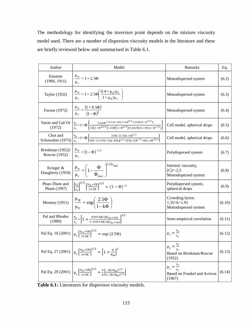
153

The methodology for identifying the inversion point depends on the mixture viscosity

model used. There are a number of dispersion viscosity models in the literature and these

are briefly reviewed below and summarised in Table 6.1.

Author Model Remarks Eq.

Einstein

(1906, 1911) 2.5Φ+1=

μ

μ

c

φ Monodispersed system (6.2)

Taylor (1932)

cd

cd

c

φ

/μμ+1

/μμ+0.42.5Φ+1=

μ

μ Monodispersed system (6.3)

Furuse (1972)

Monodispersed system (6.4)

Yaron and Gal-Or

(1972)

Cell model, spherical drops (6.5)

Choi and

Schowalter (1975)

- -

- - - -

Cell model, spherical drops (6.6)

Brinkman (1952)/

Roscoe (1952) 2.5

c

φΦ1=

μ

μ

Polydispersed system (6.7)

Krieger &

Dougherty (1959)

max

C

maxc

φ

Φ

Φ1=

μ

μ

Intrinsic viscosity,

[C]=-2.5

Monodispersed system

(6.8)

Phan-Thien and

Pham (1997)

Polydispersed system,

spherical drops (6.9)

Mooney (1951)

kΦ1

2.5Φexp=

μ

μ

c

φ

Crowding factor. 1.35<k<1.91

Monodispersed system

(6.10)

Pal and Rhodes

(1989)

Semi-empirical correlation (6.11)

Pal Eq. 16 (2001)

(6.12)

Pal Eq. 27 (2001)

Based on Brinkman/Roscoe

(1952)

(6.13)

Pal Eq. 29 (2001)

Based on Frankel and Acrivos

(1967)

(6.14)

Table 6.1: Literatures for dispersion viscosity models.

2c

φ

Φ1

0.5Φ+1=

μ

μ

154

6.3. LITERATURE MIXTURE VISCOSITY MODELS

Various models for calculating the viscosity of liquid-liquid dispersions can generally be

grouped into three main categories, namely linear, exponential and power function

models. A linear dispersion viscosity model was first suggested by Einstein (1906, 1911)

for an infinitely dilute suspension of small solid spheres (Equation (6.2), Table 6.1).

However, this theory would not account for non-spherical particles at high concentrations

or for particle size distributions. Still for near spherical drops and infinite dilution Taylor

(1932) extended Einstein's equation to fluid dispersions (Equation (6.3), Table 6.1) by

considering the internal circulation in the drops caused by the tangential stresses on the

drop surface. Equation (6.3) can be reduced to Einstein's model for solid particles

when d>> c while a corresponding lower limit is for gas bubbles where cd μ<<μ .

Attempts to extend Einstein's theory to high dispersion on entration, , fa ed many

challenges. Theoretical approaches based on a reflection technique led to power series

models, as generally described by Equation (6.1).

+ΦK+ΦK+ΦK+1=μ

μ3

32

21c

φ (6.1)

The contributions of the high order terms, though, in these models are extremely complex

to estimate and only the first order terms can be evaluated which result in equations

similar to that by Einstein (e.g. Guth and Gold, 1938). Furuse (1972) considered the

importance of the hydrodynamic effects of neighbouring particles in a concentrated

solution. By extending Einstein's model, a power law model was derived (Equation (6.4),

Table 6.1) to account for the higher order terms that were ignored by Einstein. An

alternative approach was the cell model (Yaron and Gal-Or, 1972, Equation (6.5), Table

6.1; Choi and Schowalter, 1975, Equation (6.6) Table 6.1) in which a certain number of

drops are confined within a representative cell to achieve a phase fraction that resembles

the concentration in the bulk surrounding the cell. However, Yaron & Gal-Or’s

expression failed to redu e to Taylor’s equation in the limit of → Pal,

155

Brinkman (1952) and Roscoe (1952) followed a slightly different approach by accounting

for the incremental change in viscosity caused by the addition of one extra solute particle

to a dispersion of known concentration (Equation (7), Table 1). As there is no assumption

on the shape and size of droplets, this model allows polydispersity but the interactions

between adjacent particles when they are closely packed are ignored. Krieger and

Dougherty (1959) applied Mooney's (1951) concept of crowding factor (which is

inversely proportional to the maximum drop packing fraction defined as the maximum

dispersed phase fraction in a confined space assuming monodispersed spherical drops) to

Brinkman's equation, in order to include the effect of close packing on the mixture

viscosity (Equation (6.8), Table 6.1). Pham-Thien and Pham 99 extended Brinkman’s

approach to evaluate the effect of a dispersed drop size distribution (Equation (6.9), Table

6.1).

In terms of exponential models, Vand (1948) developed a kinematic model by Couette

streaming of dispersion mixture. As the rate of shear is directly proportional to the

dispersion concentration, the mixture viscosity was found to be an exponential function

of the concentration. Mooney (1951) modified Vand's approach by including a crowding

factor (Equation (6.10), Table 6.1). Mooney's model was reported to correlate well with

various experimental data. This approach is similar to that by Arrhenius (1887). Barnea

and Mizrahi (1973) presented a generalised exponential equation, identical to that by

Mooney based on the empirical solution by Thomas (1965). The authors have

subsequently added a term to include the effect of internal drop circulation. From Vand to

Barnea and Mizrahi, these models have marked the development of exponential functions

for mixture viscosity.

Pal and Rhodes (1989) and Pal (2001) suggested a number of viscosity models (some are

given in Equations 6.11-6.14, Table 6.1). Pal (2001) evaluated various single parameter

viscosity models against experimental data and found that Yaron and Gal-Or (1972)

performed best for dispersed phase volume fractions up to about 55%. He also suggested

a number of new two parameter power and exponential function viscosity models but

found that, in overall, the model given by Equation 6.14 in Table 6.1 performed best.

156

Models used in the current study are presented in Table 6.1. Although all models were

tested using the proposed methodology for predicting phase inversion, only selected ones

are included in the graphs that follow. These were selected because (a) they are simple to

use (e.g. Brinkman/ Roscoe (1952)), (b) have been shown to give the best predictions of

dispersion viscosity (e.g. Yaron and Gal-Or (1972); Equation 6.14 by Pal (2001)) and (c)

represent a category of viscosity models (e.g. linear, exponential and power law).

6.4. COMPARISON BETWEEN PREDICTED PHASE INVERSION

POINTS AND EXPERIMENTAL RESULTS FROM LITERATURE

The phase inversion points predicted by the methodology described above are compared

against available experimental data from oil-water pipeline flows by Ioannou (2006).

Details of the properties of the three oils and of the test sections used can be found in

Table 6.2. Phase inversion was experimentally determined through conductivity

measurements obtained either at the flow perimeter with ring probes or at various

locations (e.g. pipe centre) within the pipe cross section with local conductivity wire

probes. At the operated range of mixture velocity, the liquid-liquid dispersion can be

inhomogeneous at high dispersed phase fraction close to phase inversion and phase

inversion may thus appear at certain parts of the pipe first before it spreads to the whole

pipe cross section. For example in an oil continuous dispersion in a horizontal pipe,

inversion would first occur at the bottom of the pipe where the dispersed water drops tend

to accumulate due to gravity (Ioannou et al., 2004). A hysteresis effect has also been

reported where the phase inversion point depends on the initial continuous phase (oil or

water) which results in an ambivalent range similar to that seen in stirred vessels

(Ioannou et. al., 2005). Some investigators have also found that inversion may not happen

at one particular volume fraction but is a transition occurring over a range of fractions

during which complex multiple dispersion structures form (Liu et al., 2005; Piela et. al.,

2008). Pipe material has also been found to affect the inversion point due to the

wettability of the fluid with the pipe wall. Thus for a given oil-water fluid pair in

dispersed pipe flow there is a range of phase volume fractions (phase inversion range)

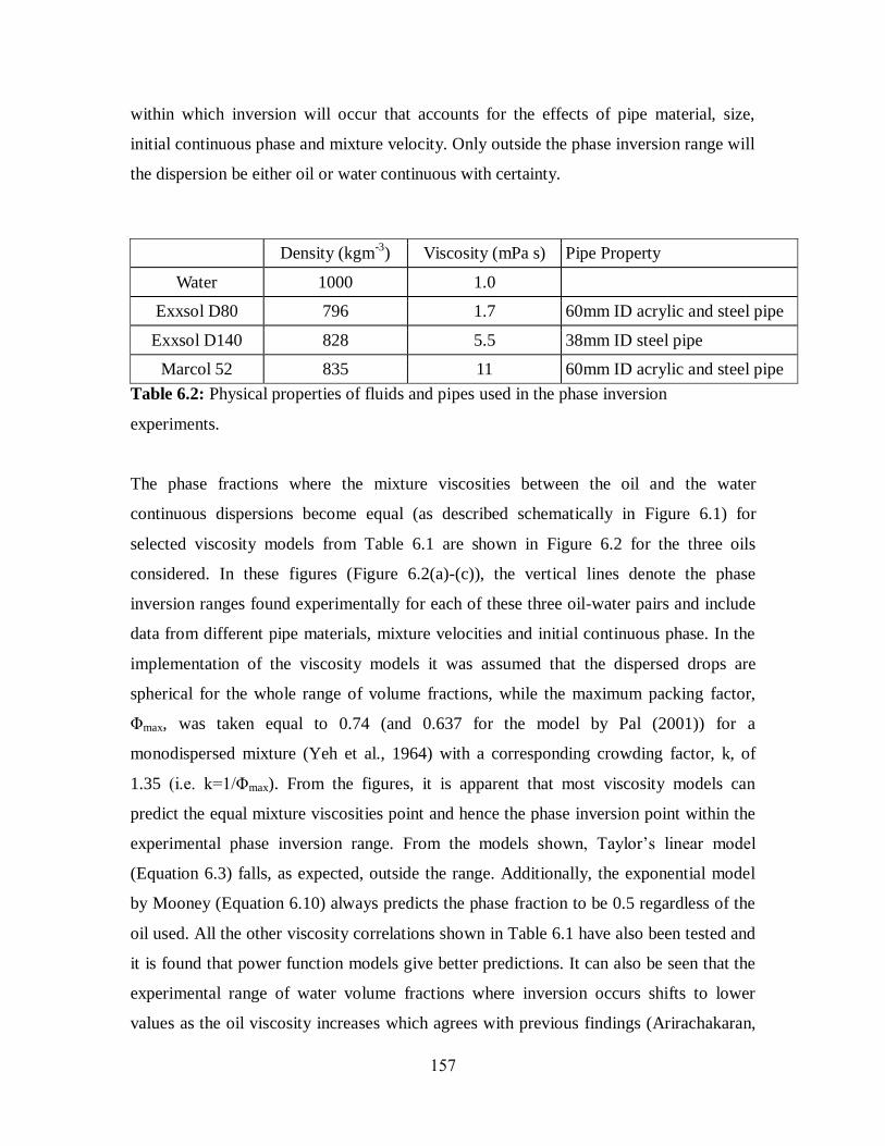
157

within which inversion will occur that accounts for the effects of pipe material, size,

initial continuous phase and mixture velocity. Only outside the phase inversion range will

the dispersion be either oil or water continuous with certainty.

Density (kgm-3

) Viscosity (mPa s) Pipe Property

Water 1000 1.0

Exxsol D80 796 1.7 60mm ID acrylic and steel pipe

Exxsol D140 828 5.5 38mm ID steel pipe

Marcol 52 835 11 60mm ID acrylic and steel pipe

Table 6.2: Physical properties of fluids and pipes used in the phase inversion

experiments.

The phase fractions where the mixture viscosities between the oil and the water

continuous dispersions become equal (as described schematically in Figure 6.1) for

selected viscosity models from Table 6.1 are shown in Figure 6.2 for the three oils

considered. In these figures (Figure 6.2(a)-(c)), the vertical lines denote the phase

inversion ranges found experimentally for each of these three oil-water pairs and include

data from different pipe materials, mixture velocities and initial continuous phase. In the

implementation of the viscosity models it was assumed that the dispersed drops are

spherical for the whole range of volume fractions, while the maximum packing factor,

max, was taken equal to 0.74 (and 0.637 for the model by Pal (2001)) for a

monodispersed mixture (Yeh et al., 1964) with a corresponding crowding factor, k, of

1.35 i e k / max). From the figures, it is apparent that most viscosity models can

predict the equal mixture viscosities point and hence the phase inversion point within the

experimental phase inversion range. From the models shown, Taylor’s linear model

(Equation 6.3) falls, as expected, outside the range. Additionally, the exponential model

by Mooney (Equation 6.10) always predicts the phase fraction to be 0.5 regardless of the

oil used. All the other viscosity correlations shown in Table 6.1 have also been tested and

it is found that power function models give better predictions. It can also be seen that the

experimental range of water volume fractions where inversion occurs shifts to lower

values as the oil viscosity increases which agrees with previous findings (Arirachakaran,

158

1989; Selker & Sleicher, 1965; Yeh et al., 1964); the predicted inversion points follow

the same trend.

The predicted phase inversion points for Marcol 52 are compared in Figures 6.3 - 6.5

against the phase inversion ranges obtained under different experimental conditions. The

effect of dispersion initialisation conditions is demonstrated in Figure 6.3, where it can be

seen that the inversion range depends on which phase is initially continuous. Mixture

velocity is also found to affect the boundaries of the phase inversion range and this is

demonstrated in Figure 6.4. With increasing flow velocity, the inversion region width

decreases as the dispersion becomes more homogeneous. While a transitional region in

the experimental outcome is maintained in the current operation conditions, a clear trend

of narrowing of this region to a specific phase fraction is observed if the mixture velocity

increases leading to higher turbulence and homogeneous dispersion (similar to Brauner

and Ullmann, 2002, and Chakrabarti et. al., 2006). Thus, the prediction of a phase

inversion point through the dispersion viscosity still valid as long as it falls within the

transitional region. The pipe material effect on the inversion range is shown in Figure. 6.5.

The phase inversion range is shifted to lower water fractions in the acrylic pipe compared

to the steel one. In all the above cases the predicted phase inversion points (equal mixture

viscosities), when the viscosity models by Brinkman/Roscoe (1952), Furuse (1972) and

Equation 6.14 by Pal (2001) are used, consistently fall within the phase inversion ranges.

Similar results were found for the other two oils investigated.

159

Figure 6.2: Predicted inversion points using different dispersion viscosity models against

the experimental phase inversion range for a dispersion of water and (a) Exxsol D80

(1.7mPas), (b) Exxsol D140 (5.5mPas), (c) Marcol 52 (11mPas) (data in stainless steel

pipe by Ioannou, 2006). Points in graph refer to the model predictions while the lines

represent the experimental phase inversion region.

160

Figure 6.3: Predicted inversion points using different dispersion viscosity models against

the experimental phase inversion ranges in stainless steel pipe obtained starting from oil

continuous and from water continuous dispersions for a water-Marcol 52 mixture. Points

in graph refer to the model predictions while the lines represent the experimental phase

inversion region.

Figure 6.4: Predicted inversion points using different dispersion viscosity models against

the experimental phase inversion ranges in stainless steel pipe obtained at different

mixture velocities for a water-Marcol 52 mixture. Points in graph refer to the model

predictions while the lines represent the experimental phase inversion range.

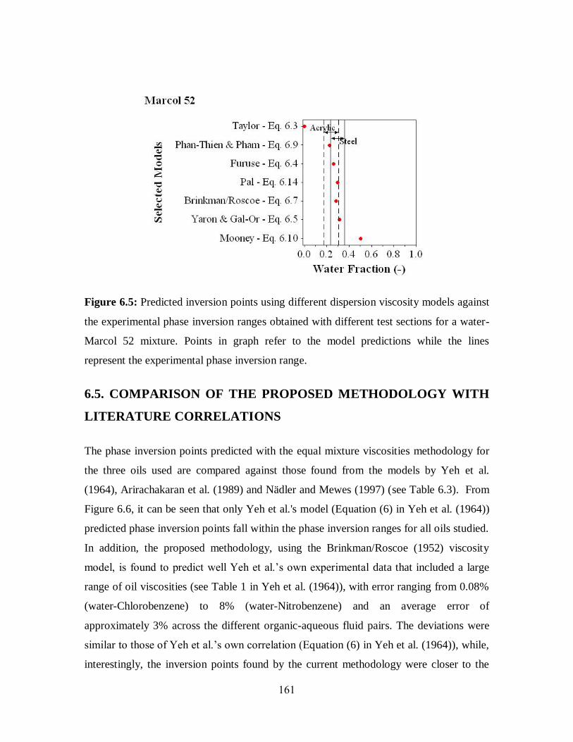
161

Figure 6.5: Predicted inversion points using different dispersion viscosity models against

the experimental phase inversion ranges obtained with different test sections for a water-

Marcol 52 mixture. Points in graph refer to the model predictions while the lines

represent the experimental phase inversion range.

6.5. COMPARISON OF THE PROPOSED METHODOLOGY WITH

LITERATURE CORRELATIONS

The phase inversion points predicted with the equal mixture viscosities methodology for

the three oils used are compared against those found from the models by Yeh et al.

(1964), Arirachakaran et al. (1989) and Nädler and Mewes (1997) (see Table 6.3). From

Figure 6.6, it can be seen that only Yeh et al.'s model (Equation (6) in Yeh et al. (1964))

predicted phase inversion points fall within the phase inversion ranges for all oils studied.

In addition, the proposed methodology, using the Brinkman/Roscoe (1952) viscosity

model, is found to predi t well Yeh et al ’s own experimental data that included a large

range of oil viscosities (see Table 1 in Yeh et al. (1964)), with error ranging from 0.08%

(water-Chlorobenzene) to 8% (water-Nitrobenzene) and an average error of

approximately 3% across the different organic-aqueous fluid pairs. The deviations were

similar to those of Yeh et al ’s own orrelation Equation (6) in Yeh et al. (1964)), while,

interestingly, the inversion points found by the current methodology were closer to the

162

predictions of a modified equation suggested by Yeh et al. (Equation (6a) in Yeh et al.

(1964)) where the interfacial viscosity is used instead of the water phase viscosity. To

develop his model, Yeh et al. assumed that there are no interfacial shear stresses at the

point of phase inversion indicating a momentum balance at the fluid interface. The

proposed methodology can also predict well with a wide range of oil/water system

reported in Arirachakaran et al. (1989).

In Figure 6.7, the proposed method is compared with the experimental data from both

Yeh et al. (1964) and Arirachakaran et al. (1989). It is also compared with the suggested

models proposed by the respective authors. From the figure, it can be shown that the

models from Yeh et al. (1964) and Arirachakaran et al. (1989) can only predict limited

range of viscosity ratio with Yeh et al. predicting well with the lower viscosity range and

Arirachakaran et al. (1989)’s at the higher viscosity range. In comparison, the proposed

method can predict very well across the wide range of viscosity ratio from an organic

viscosity of 0.235mPa.s and about 1500mPa.s. It demonstrates that the phase inversion

point is not a linear function of the logarithmic relation with the viscosity ratio. In fact, it

appears to reach an asymptote of about 0.23 for water fraction as the viscosity ratio

increases. This may be because the organic phase in the lower viscosity pairs can be

deformed more easily than that of the higher viscosity. This leads to the prediction of Yeh

et al. (1964)’s model to a lower water fra tion for phase inversion as it extrapolates

across the range of viscosity ratio tested. However, the increase in viscosity ratio is likely

to affect the deformation of the dispersed phase leading to a maximum packing that the

dispersed phase can sustain and beyond which a phase inversion will occur.

163

Figure 6.6: Comparison between proposed methodology (suggested best models) and

models for critical phase fraction from literature.

Author Model Eq.

Arirachakaran et al. (1989)

(6.15)

Nädler and Mewes (1997)

(6.16)

Yeh et al. (1964)

(6.17)

Yeh et al. (1964)

(6.18)

Table 6.3: Critical phase fraction models for phase inversion from literature.

164

Figure 6.7: Application of proposed model on various systems from Yeh et al. (1964)

and Arirachakaran et al. (1989). The solid line represents the prediction model by Yeh et

al. (1964) (see Equation 6.17) and the dotted line represents the prediction model by

Arirachakaran et al. (1989) (see Equation 6.15).

6.6. REVIEW ON PREDICTION MODEL WITH AN

EXPERIMENTAL HOMOGENEOUS DISPERSED FLOW

The proposed method for phase inversion prediction is now tested against the phase

inversion data obtained in the experimental facility using the dispersed inlet. As shown in

Chapter 4 with this inlet setup, the flow is fully dispersed for all phase fractions at the

mixture velocity of 3m/s. As a result, the change from a water continuous dispersion to

an oil continuous dispersion (and vice versa) occurs throughout the pipe cross section at a

particular phase fraction rather than over a transitional region as in the case of a split inlet.

The experimental phase inversion points from the dispersed inlet are therefore well suited

165

for comparison with the phase inversion prediction model since the mixture viscosity

models used are derived from homogeneously dispersed mixtures.

In order to compare with the prediction model, the pressure gradient from the prediction

model is firstly al ulated using Brinkman 9 ’s mixture vis osity equation and apply

that to a single phase mixture equation for pressure gradient (Equation 6.19).

D

Uf2

l

P2mm

(6.19)

where ∆P/l is the pressure gradient a ross a pipe, f is the fri tion fa tor f 6Rem-0.2

),

ρm is the mixture density, Um is the mixture velocity and D is the pipe diameter. The

calculated pressure gradient is then compared with the experimentally measured pressure

gradient together with the conductivity data on phase continuity switch.

From Figure 6.8, it can be observed that the experimental pressure gradient closely

resemble the trend deduced by the correlation (Equation 6.19) between 38% and 100%

water fraction. The difference between the experimental result and model outcome may

be due to the presence of drag reduction that is not accounted for in the correlation. There

is a sharper drop in pressure gradient for the experimental result between 26% and 38%

water fraction and subsequently an increase in pressure gradient below 26%.

Based on the prediction from the interception point in Figure 6.8, the predicted phase

inversion point (at 34%) falls in the phase fraction range where the pressure gradient is

decreasing. From the investigation outcome in Chapter 4, this lies at the range of phase

fraction where drop coalescence becomes prominent with likely formation of complex

structures. While the conductivity measurements detects a change in phase continuity at a

lower phase fraction (26%), the predicted phase inversion point can be considered to be

within close proximity because the process of drop coalescence can lead to the formation

of oil pockets (if starting from an O/W dispersion) as presented in Piela et al. 2008. These

oil pockets may not be easily detected by the conductivity wire and ring probe but

nonetheless an important stage in the onset of phase inversion. As such, the prediction

can be considered to have good prediction with the experiments conducted.

166

Figure 6.8: Comparison of pressure gradient at different phase fraction between

experimental data □ and modeling out ome via Brinkman/Ros oe 9 ’s mixture

vis osity orrelation The solid arrow ← represents the dire tion for the experiment and

the vertical line denotes the predicted phase inversion point.

6.7. CONCLUSION

A methodology has been introduced to identify the inversion point during oil-water

dispersed flow. It is suggested that inversion will occur at the phase fraction where the

mixture viscosities of the oil and the water continuous dispersions become equal. The

approach was tested against extensive available experimental data on phase inversion

where oil viscosity, pipe material, mixture velocity and dispersion initialisation

conditions were varied. From the available literature dispersion viscosity models tested,

the power function correlations by Brinkman (1952)/Roscoe (1952), Furuse (1972) and

Equation (14) by Pal (2001) always predicted inversion within the experimental phase

inversion range. The proposed methodology was also tested against the predictions of

literature correlations on phase inversion point. Very good agreement was found across a

wide range of two phase systems with organic viscosity of 0.235mPa.s and about

1500mPa.s from Yeh et al. (1964) and Arirachakaran et al. (1989).

0.0

0.5

1.0

1.5

2.0

2.5

3.0

3.5

4.0

0 20 40 60 80 100

Pre

ssu

re g

rad

ien

t [k

Pa/m

]

Input water fraction [%]

Model (Oil continuous)

Model (Water continuous)

Experimental

167

The suggested prediction method with Brinkman (1952)/Roscoe (1952) mixture viscosity

model was subsequently tested with experimental data of an homogeneous dispersed flow.

Similar increasing mixture viscosity can be observed as the dispersed phase fraction is

increased. The method shows closely at the phase fraction (i.e. 36% water fraction) where

the mixture viscosity is highest (and resulting in a corresponding maximum pressure

gradient). Below 34% water fraction, the dispersion appears to encounter drop

deformation/coalescence which leads to the complete change in phase continuity at 26%

water fraction. Pressure gradient of an inverted W/O system subsequently shows a

significant increase due to the higher viscosity by the continuous oil phase.

From this chapter, a conclusion can be drawn that the viscosity of the liquid-liquid

mixture is important for understanding phase inversion. The prediction method falls

within close proximity with the experimentally detected change in phase continuity.

Despite that there is a discrepancy within the two values, the predicted phase inversion

point highlights a point where drop coalescence/deformation becomes dominant in the

system and the coalescence process is a key factor for the inversion process. Further work

is needed to understand the changes in the mixture morphology as it approaches phase

inversion. Such studies will help to better describe the phase inversion phenomenon and

will also improve the model by including, for example, the drop packing and size

distribution.

168

Chapter 7: Prediction of pressure gradient

during phase inversion

7.1 OVERVIEW

Multiphase flow of two or more fluids is commonly encountered in the petroleum

industry during oil production and transportation. Water often appears in oil wells

particularly in the later years of production. At high velocities, the mixture of oil and

water is transported as a dispersion with either oil (water-in-oil, W/O) or water (oil-in-

water, O/W) as the continuous phase. The type of dispersion depends on the phase ratio,

rheological properties of the two fluids, wetting properties of the pipe material and the

operation initialisation conditions (Yeo et. al, 2000; Ioannou, 2006). Interestingly, the

continuous phase of the dispersion changes under certain conditions to become the

dispersed one and vice versa (phase inversion phenomenon). The phase fraction where

this change occurs is called the phase inversion point. During pipeline flow, however, it

has been found that inversion occurs over a range of input phase fractions. This

transitional range can be attributed to phenomena such as formation of multiple

dispersions (Liu et al., 2005) and partial or local inversion as the dispersed phase fraction

increases (Ioannou, 2006; Piela et al., 2008). Partial inversion results in stratification of

the flow with two layers that have different continuous phase.

The changes in the spatial distribution of the phases as their volume fractions change can

have significant impact on pressure drop and pose great challenges in its modelling. To

predict pressure drop in dispersed oil-water flows, the homogeneous model is often used

where the fluids are considered as one “pseudofluid” and single phase flow equations are

used with a weight averaged mixture density and an empirically determined mixture

viscosity (viscosity models by e.g. Brinkman, 1952; Yaron & Gal-Or, 1972; Choi &

Schowalter, 1975; Pal, 2001). However, the homogeneous model does not accurately

represent the phase distribution in horizontal pipelines where stratification due to gravity

can appear even at high mixture velocities. To account for the separation of the two fluids,

169

the two-fluid model (TFM), developed for stratified flows (e.g. Brauner & Moalem

Maron, 1989), can be applied.

In this chapter, experimental results on phase inversion and pressure drop during

horizontal oil-water dispersed flows are presented (Section 7.2). A methodology (see

Section 7.3) is developed based on a two layer flow configuration, in order to predict the

phase volume fractions where the mixture is completely dispersed or there is stratification

of the two fluids. The entrainment fractions in each layer are calculated from previously

developed correlations, while a phase inversion criterion is used to determine the

continuity of each continuous layer in the model. The outcome of the developed model

will be compared with experimental results in Section 7.4 and conclusions on the quality

of the model are made in Section 7.5.

7.2 EXPERIMENTAL INVESTIGATION

Experimental studies on phase inversion were conducted in the pilot scale liquid-liquid

flow facility (See Chapter 3). The test section is an acrylic pipe with 38mm ID. Exxsol

D140 oil (density of 828 kgm-3

, viscosity of 5.5mPa.s) and tap water were used as test

fluids. The two fluids were pumped from storage tanks via variable area flow meters into

the test section inlet where they were joined in a modified Y-junction to ensure minimum

mixing. Experiments were conducted at mixture velocities 3m/s and 4m/s where previous

work indicated that the flow was in the dispersed regime. At each velocity the

experiments were started with single phase water. Oil was then introduced into the pipe.

The oil flowrate was gradually increased while at the same time that of the water

decreased in order to increase the oil fraction while keeping the mixture velocity constant.

The experiments continued until phase inversion was observed and beyond until about 80%

input oil fraction. Pressure drop was measured via a differential pressure transducer

(Validyne DP103) between two measuring ports 1.5m apart, with the first port located at

3.8m (~100D) from the inlet. A conductivity wire probe was used to identify phase

continuity at different locations (i.e. every 2mm intervals) along the vertical diameter in a

pipe cross section and thus to understand the development of phase inversion. The probe

was located at 7m (~184D) from the inlet.

170

(a) 3m/s mixture velocity

(b) 4m/s mixture velocity

Figure 7.1: Pressure gradient at mixture velocity (a) 3m/s and (b) 4m/s measured

experimentally. The solid lines represent the boundaries of the transitional region

between water continuous and oil continuous fully dispersed flow. The arrow indicates

the direction of the experiment.

0.0

0.5

1.0

1.5

2.0

2.5

3.0

3.5

0 20 40 60 80 100

Pre

ssure

gra

die

nt (k

Pa)

Input water cut (%)

0.0

1.0

2.0

3.0

4.0

5.0

6.0

0 20 40 60 80 100

Pre

ssure

gra

die

nt (k

Pa)

Input water cut (%)

Full O/W

Dispersion

Full W/O

Dispersion Partial

Inversion

Full O/W

Dispersion Partial

Inversion

Full W/O

Dispersion

171

The pressure gradients measured at mixture velocities of 3m/s and 4m/s are depicted in

Figure 7.1 (a) & (b) respectively. At high water cuts the conductivity probe showed that

the mixture was water continuous in the whole pipe cross section. By gradually

increasing the oil fraction (as indicated by the direction of the arrow) the flow remains

fully dispersed with water as the continuous phase until about 60% water cut in both

mixture velocities, while the pressure gradient decreases. This indicates a drag reduction

phenomenon that has also been reported before (see Pal, 1993). Beyond this volume

fraction, partial inversion takes place at the top part of the pipe and the pattern is now

dual continuous with a water continuous layer at the bottom of the pipe and an oil

continuous layer at the top of the pipe, as indicated by the measurements of the

conductivity probe. At about 34% water cut, the pressure gradient reaches a minimum

and with further decrease in the water fraction it increases again. This increase coincides

with the change of the flow pattern from dual continuous to fully dispersed with oil as the

continuous phase. In these experiments inversion from the O/W to the W/O dispersion

occurs through a transitional region which is enclosed in Figure 7.1 between the solid

vertical lines.

7.3 DEVELOPMENT OF MODEL FOR THE PREDICITON OF

PRESSURE DROP

A methodology was developed to predict the flow configuration, dual continuous or fully

dispersed, as well as the pressure gradient during the flow of liquid-liquid mixtures.

7.3.1 PREDICTION OF FLOW CONFIGURATION

For each phase fraction it is assumed initially that the mixture has a dual continuous

configuration with a water continuous layer with oil drops dispersed in it at the bottom

and an oil continuous layer with water drops dispersed in it at the top of the pipe. A range

of interfacial heights is then considered with an interval of 0.1mm. At each interfacial

height, the dispersion in each layer is assumed to be homogeneously distributed. The

amount of dispersion of one phase into the other is calculated using the entrainment

model described in Section 7.3.2. By comparing the phase fractions in each layer with a

172

criterion for the phase inversion point, the continuous phase in that layer can be

determined. The phase inversion point (WFCritical) is calculated using the methodology

developed by Ngan et al. (2009) according to which phase inversion will occur at the

phase fraction where the viscosities of the two possible dispersions, oil continuous and

water continuous, are equal. For the Exxsol D140-water mixture used in this work, the

critical water fraction for phase inversion is found to be 34%. According to this, the

possible scenarios for the two layer mixture are:

Water entrainment in

upper (W/O) layer (Entu)

Oil entrainment in

lower (O/W) layer (Entl) Flow Pattern Valid

upper

layer

lower

layer

Entu<WFCritical Entl<(1- WFCritical) W/O O/W Yes

(1- WFCritical)<Entl<1 W/O W/O Yes

WFCritical<Entu<1 Entl<(1- WFCritical) O/W O/W Yes

(1- WFCritical)<Entl<1 O/W W/O No

Notes:

1) The entrainment fraction cannot be above 1.

2) The less dense oil cannot be continuous underneath the more dense water.

Table 7.1: Flow patterns resulting from the application of a critical water fraction for

phase inversion (WFcritical) in each of the upper and lower layers of a dual continuous

flow configuration.

A two-fluid model, as detailed in Section 7.3.3, is then applied for each interfacial height

only to the valid cases in Table 7.1. The model has a solution when the pressure gradients

of the upper and lower layers are the same within a 2% difference. If there is no solution

of the two fluid model for the entire range of interfacial heights for the particular phase

fraction, then the dual continuous flow configuration cannot exist and the mixture is fully

dispersed. This happens when the comparisons with the critical phase fraction have

indicated that both layers have the same continuity. In that case the homogeneous model

(see Section 7.3.4) is used to predict the pressure gradient.

173

7.3.2 ENTRAINMENT MODEL

To calculate the entrainment fraction in each layer of the dual continuous configuration,

the model developed by Al-Wahaibi and Angeli (2009) was used. According to the model,

drops will form from the crests of unstable waves at the oil-water interface when the drag

force on the waves exceeds the stabilising interfacial tension force. At steady state, the

rate of drop entrainment will be equal to the rate of drop deposition. According to Al-

Wahaibi and Angeli (2009), the rate of entrainment (Rent) can be calculated as follows:

2λi

S

oU

wU

dρ

entV

entR

(7.1)

where ρd is the density of the entrained phase, Vent is the volume of the entrained phase

from each wave crest, λ, is the wave length, which, based on experimental observations

and for simplicity is taken equal to the pipe diameter and Si is the length of the interface.

The rate of deposition (Rdep) is equal to:

vSQ

dW

Dk

depR (7.2)

where Wd is the mass flow rate of the dispersed phase in the layer, Q is the volumetric

flow rate of the mixture in a layer and Sv is the slip ratio between the dispersed drops and

the continuous phase. In this work, no slip is assumed between the dispersed and

continuous phases (i.e. Sv=1). kD is an empirically determined deposition rate constant

which was found by Al-Wahaibi (2006) to be equal to

*U

mU

soU

0.051D(O/W)

k

(7.3)

174

*U

mU

swU

0.077D(W/O)

k

(7.4)

where Us is the superficial velocity and U* is the frictional velocity. Subscripts, o and w,

represents the oil and water phases.

By equating the rates of entrainment and deposition, the entrainment fraction (W/W) in a

layer can be found as follows:

d

ρEc

ρE)(1ED

k2λ

iS

oU

wU

dρ

entV

(7.5)

where E is the steady state entrainment fraction, ρc and ρd are the densities of the

continuous and the dispersed phases respectively. The calculated entrainment fraction is

in w/w and for the application in the two-fluid model it is converted to v/v.

7.3.3 TWO FLUID MODEL

For a steady state, fully developed dual continuous flow configuration with an oil

continuous dispersed layer at the top and a water continuous dispersed layer at the bottom

the one-dimensional momentum equations for each layer are given by:

uA

iS

iτ

uA

uS

uτ

udx

dP (7.6)

lA

iS

iτ

lA

lS

lτ

ldx

dP (7.7)

175

where τ is the shear stress, S is the perimeter covered by the respective layer and A is the

pipe cross sectional area. In the above equations, subscripts “u” and “l” denotes the upper

and lower layers and subscript “i” denote the interface between the two layers.

The shear stresses in Equations (7.6) and (7.7) can be found as follows:

2

2u

Uu

ρ

uf

uτ

2

2l

Ul

ρ

lf

lτ

2

lU

uU)

lU

u(U

fρ

if

iτ

U is the in-situ velocity of the respective layer, ρ denotes the weight-averaged mixture

density, f is the frictional factor and ρf denotes the density of the faster layer. In all cases

investigated both upper and lower layers were in turbulent flow and the friction factors

were calculated from 0.046Re-0.2

, where Re is the Reynolds number of the respective

layer. The Reynolds number in each layer is calculated based on the mixture fluid

properties and velocity of that layer. The interfacial Reynolds number is calculated based

on the faster phase properties while the interfacial frictional factor is the maximum

between 0.014 and 0.046Rei-0.2

. To account for the drag reduction observed during fully

dispersed flow (dispersion pressure gradient less than that of the single phases at the same

mixture velocity) the following equation is used for calculating a modified friction factor

(Rozentsvaig, 1982).

nε1

originalf

DRf

(7.8)

where foriginal is the original friction factor (foriginal = 0.046Re-0.2

) and fDR is the modified

friction factor due to drag reduction, n is an empirical coefficient with a suggested value

of 1.125 and ε is the fraction of the dispersed phase in the layer.

176

The mixture density in each layer is equal to the weight averaged densities of the two

phases while for the calculation of the mixture viscosity Brinkman’s (1952) correlation is

used.

cρε)(1

dρε

mρ (7.9)

2.5ε)(1c

μm

μ (7.10)

7.3.4 HOMOGENEOUS MODEL

According to the homogeneous model the pressure gradient is found from:

D

2m

Um

2fρ

dx

dP (7.11)

where f is the friction factor (0.046Re-0.2

), ρm is a weight-averaged density (Equation

(7.9)), Um is the mixture velocity and D is the pipe diameter. Drag reduction is similarly

accounted for by Rozentsvaig’s equation (Equation (7.8)).

7.4. COMPARISON OF MODEL PREDICTIONS WITH

EXPERIMENTAL DATA

The model predictions on the flow pattern that establishes in the pipe and on pressure

drop for the different volume fractions at mixture velocities 3m/s and 4m/s are shown in

Figure 7.2 against the experimental results. Experimentally it was found that the flow at

3m/s is fully dispersed with water as the continuous phase for input water fraction above

62% and with oil as the continuous phase for input water fraction below 28%. In between

28-62% input water fraction there is stratification of the flow with an oil continuous

dispersed layer at the top of the pipe and a water continuous dispersed layer at the bottom,

as found by the conductivity probe. According to the model, flow stratification occurs

between 34-66% while below and above these fractions the mixture is oil and water

177

continuous respectively. Similarly, at 4m/s mixture velocity the experimental transitional

region between the two types of dispersion was between 32-60% input water fraction

while that predicted one was between 33-70% water fraction. The transitional regions for

phase inversion in both experimental and predicted results are within close range.

It can also be seen from Figure 7.2 that the predicted pressure gradients, calculated from

the two-fluid model in the transitional region and from the homogeneous model in the

fully dispersed regions, are in good agreement with the experimental data. The

experimental drag reduction is captured well by the model. The model is also able to

predict the increase in pressure gradient after the mixture becomes fully oil continuous.

Discrepancies between the experimental and predicted data appear at the oil continuous

region and particularly for the lower mixture velocity. It is believed that the discrepancies

are due to lack of uniform drop distribution as assumed in the homogeneous model,

because under the effect of gravity water drops would tend to accumulate closer to the

pipe bottom compared to the top. Dispersion inhomogeneity is expected to be more

pronounced in the oil continuous dispersion compared to the water one because the oil

viscosity is higher and the turbulent mixing will be less intense. In addition, it is more

apparent at the low mixture velocity tested compared to the high one where again mixing

is less intense.

178

(a) 3m/s mixture velocity

(b) 4m/s mixture velocity

Figure 7.2: Experimental and predicted pressure gradient at (a) 3m/s and (b) 4m/s

predicted from two-fluid model. The lines represent the boundaries of the transitional

region between water continuous and oil continuous fully dispersed flow, solid for

experimental and dotted for predicted fractions. The arrow indicates the direction of the

experiment.

0

1

2

3

4

0 20 40 60 80 100

Pre

ssu

re G

rad

ien

t (k

Pa)

Input Water Fraction (%)

Experiment

Prediction

0

1

2

3

4

5

0 20 40 60 80 100

Pre

ssu

re G

rad

ien

t (k

Pa)

Input Water Fraction (%)

Prediction

Experiment

Full W/O

Dispersion

Partial

Inversion

Full O/W

Dispersion

Full W/O

Dispersion Partial

Inversion

Full O/W

Dispersion

179

7.5. CONCLUSION

Phase inversion during horizontal oil-water flow was investigated experimentally with

the use of a local conductivity probe that identifies phase continuity. It was found that for

the mixture velocities studied there was a region of flow stratification between the fully

dispersed oil and water continuous flows. A methodology was suggested that predicted

the range of volume fractions where flow was separated and the pressure gradient. This

was based on the assumption of a two layer flow configuration, where the entrainment in

each layer was calculated and the continuity of the layer was decided based on a phase

inversion criterion. There was good agreement between the model predictions and the

experimental data apart from the oil continuous dispersed flow at the low mixture

velocity. This discrepancy was attributed to the inhomogeneous distribution of the

dispersed water drops in the pipe cross section.

180

Chapter 8: CFD simulation of horizontal two-

phase pipe flow

8.1 OVERVIEW

It was shown in the previous chapters that the spatial distribution of oil and water can be

significantly changed according to the input phase fractions. This consequently leads to a

change in flow regime (e.g. from a fully oil-in-water dispersion to a dual continuous

mixture). In this chapter, computational fluid dynamics (CFD) simulations will be

developed to predict phase distribution and flow characteristics for some of the

conditions used in experiments in Chapter 4. The results will be compared against the

experimental data. Use of CFD can provide information on flow characteristics that are

not easy in many cases to measure experimentally and thus offer insight on flow behavior

in combination with experiments. Validated CFD models can also be used for prediction

without the need to resort to experiments. Various commercial CFD codes have been

developed with multiphase flow capability (e.g. CFX, Fluent, Star-CD). In the current

study, CFX will be used. The outcome of the chapter will aim to have a better insight on

the effect of the different interphase force terms on the distribution of the mixture. The

chapter is organised in the following sections: description of CFX software package

(Section 8.2); description of the geometry and conditions simulated (Section 8.3);

comparison between the simulation and the experimental results (Section 8.4). In the

conclusions section, criteria in running a simulation of dense two-phase pipe flow will be

presented (Section 8.5).

8.2 DESCRIPTION OF ANSYS CFX SOFTWARE PACKAGE

The chosen CFD software, Ansys CFX, by Ansys Inc., is a commercial computational

fluid dynamics software package that has been widely used in solving a wide range of

fluid flow problems. The code has been applied to a number of multiphase flow systems

such as Krepper et al., 2005, Lucas et al., 2007 and Vallée et al., 2007. Many models

181

have been implemented to predict the various momentum transport terms allowing users

to predict the respective influence by the phases especially during dispersed flow.

Ansys CFX consists of four main modules:

Geometry construction and Meshing Module (via Ansys ICEM CFD)

Pre-processing Module (CFX-Pre)

Solver Module (CFX-Solver)

Post processing Module (CFX-Post)

The construction of the geometry (i.e. the pipe) and the creation of a computational grid

to define the points for computation (commonly known as meshing) are done via the

Ansys ICEM CFD module. The geometry is constructed in scale with the actual

construction process similar to the way a CAD package is used. Once the geometry is

constructed, the structure is subsequently divided into a grid with specified grid points

where the computation of the fluid motion is conducted. As the whole process is operated

interactively via the Graphical User Interface (GUI), the mesh can easily be refined at

specific locations (e.g. close to pipe wall) to improve predictions.

Through the CFX-Pre interface, the boundary and operation conditions of the simulation

are defined on the meshed structure (e.g. fluid properties, input phase fraction, phase

continuity, fluid velocities, wall roughness, and turbulence). A definition file with the

specified conditions and the system geometry will then be saved for the subsequent

calculations.

The solver module involves integrating the governing equations over the defined mesh

grid points using the finite volume method. This permits the mass, momentum and

energy terms to be conserved within each control volume. In Ansys CFX, a co-located

(non-staggered) grid layout is used whereby the control volumes for the pressure and

velocity transport equations are identical. Figure 8.1 presents the iterative method for

solving the governing equations for both transient and steady-state simulations.

182

Figure 8.1: Schematic diagram on the iterative method for solving the conservation

equations (Ansys CFX Manual).

183

The post processing module provides the environment to evaluate visually the results of

the simulation through vector, contour or streamline plots. Raw numerical data can also

be plotted into graphs (e.g. velocity profile, phase distribution profile). Numerical data

can be exported (as a whole domain or within specific region) to Excel for further

processing.

8.3 MODEL GEOMETRY AND SIMULATION CONDITIONS

Model Geometry

Due to the high computational effort for multiphase flow simulations, the geometry

adopted in this chapter is 2-dimensional. Due to the limitation of Ansys CFX in true 2D

simulation, the geometry used in this work is a rectangular slab with a width equal to 1%

of the pipe diameter. The final geometry of the 2D pipe is 3.0m in length and 19mm in

height (i.e. equivalent hydraulic diameter for a 38mm 3D pipe as according to Russell

and Charles (1959) and Agtersloot et al. (1996)). A length of 3.0m was chosen as

previous simulations for the same flow velocity showed that the flow is fully developed

beyond 2.5m. At the inlet, a splitting plate is used and located at the centre of the pipe

cross section with 100mm in length. This resembles the inlet configuration used in the

experimental setup. The grid points along the radial direction are non-uniform with more

grid points along the pipe wall. The shortest space between two grid points is 0.5mm and

the longest space is approximately 0.75mm (at the centre of the pipe). Figure 8.2 presents

the schematic of the pipe section with the boundaries used in the simulations. A total grid

size of 183000 is used after a grid sensitivity study (see Appendix C) was conducted by

adjusting the number of cells on the vertical height of the slab.

184

(a)

(b)

Figure 8.2: (a) Schematic diagram of the grid structure for the 2-D pipe section for the

CFD simulations. (b) Part of the mesh of the 2-D pipe section with the thick lines

representing the smooth walls in the simulation.

Oil

Water

Outlet

185

Boundary conditions

The following boundary conditions are used to define the solution domain:

1. Inlet: Two inlet sections are set up in the geometry separated by the plate – oil enters

the pipe from the top section and water from the bottom. The fluid velocity is set at the

boundary according to the relevant input phase fraction required. The inlet velocity is

uniform over the inlet cross section and normal to the inlet boundary. Equation 8.1

presents the inlet velocity of phase k (i.e. either oil or water).

kmkk AQαU

(8.1)

where U is the input velocity, α is the phase fraction and A is the occupied area of the

pipe by phase k. Qm is the total volumetric flow rate of the mixture.

2. Outlet: A pressure specific boundary condition is used in the simulation. A reference

pressure is set equal to the atmospheric pressure.

3. Wall: The wall boundary conditions include the wall surface of the pipe and the

splitting plate at the inlet. No slip conditions are set at the walls. The wall is also assumed

to be smooth.

4. Symmetry planes: The two side planes are assumed to be symmetric. This imposes

constraints on the conditions of flow on either side of the plane.

Inlet and initial conditions

The properties of the two fluids introduced used in the simulation are the same as those

used in the experiments (i.e. Exxsol D140 and water). The two fluids are regarded as

incompressible with constant density. The inlet phase fraction is set by adjusting the flow

velocities of the phases while maintaining the mixture velocity to be constant at 3m/s. As

an initial condition, the decision for the phase continuity is based on the phase inversion

point calculated in Chapter 6 (i.e. 34% water fraction). Below 34% water fraction, water

is regarded as the dispersed phase and vice versa. The dispersed phase will be introduced

186

into the simulation inlet despite that it is flown as a single phase through the inlet section

of the slab. The drop size for the dispersed phase is taken to be 1.0 mm (unless otherwise

stated) as it has the highest frequency in a drop size distribution based on previous

experiments (see Chapter 4). It is also assumed that the dispersed phase drops are

spherical with uniform size for simplicity in this study. In addition, all simulations are run

at a constant temperature and no thermal effect on the fluid will be considered.

The initial turbulence level is set by estimating the turbulence intensity. In all simulations,

the intensity is taken to be 5% (i.e. the default value in CFX) which is also close to the

calculated value for experimental results according to the following equation.

8/1mRe16.0I

(8.2)

From the initial turbulence intensity, the initial turbulent kinetic energy (k) and the

energy dissipation (ε) can be found.

2

c

c Iu

2

3k

and L

kC

2343

(8.3)

where L is the turbulent length scale that can be estimated by L=0.07D.

Convergence of solution

Convergence of the simulation is ensured by monitoring the residuals (i.e. the difference

in solution between the current step and the previous step) of the solutions of the

hydrodynamic equations. Convergence has been reached when the residuals are 10-6

or

less. The time step for each iteration is set to at least below 0.002s. With the current setup,

this ensures that the Courant number to be within 1 or less. This is suggested to be the

optimal configuration for numerical calculation with the current grid size.

187

8.4 RESULTS AND DISCUSSION

CFD simulations were carried out for a mixture velocity of 3m/s and three input water

fractions – 40% (dual continuous dispersion), 60% (dense O/W dispersion) and 80%

(dilute O/W dispersion). Results on phase distribution will be compared against the

experimental data (see Chapter 4). The phase distribution data along a vertical pipe

diameter for these water fractions obtained by the electrical resistance tomographic (ERT)

system are shown in Figure 8.3.

At 80% input water fraction, the dispersion is almost homogeneously distributed along

the whole vertical diameter. With the decrease in water fraction to 60%, inhomogenity

arises as the dispersed oil drops start accumulating at the core of the pipe. Further

decrease in water fraction (40%) leads to dual continuous.

Figure 8.3: Experimental oil phase distribution along a vertical pipe diameter at a

mixture velocity of 3m/s. Data is extracted from ERT measurements at 7m from the inlet

where flow is fully developed.

-1.0

-0.8

-0.6

-0.4

-0.2

0.0

0.2

0.4

0.6

0.8

1.0

0 20 40 60 80 100

Norm

ali

sed

dis

tan

ce f

rom

pip

e ce

ntr

e

Oil Fraction [%]

80%

60%

40%

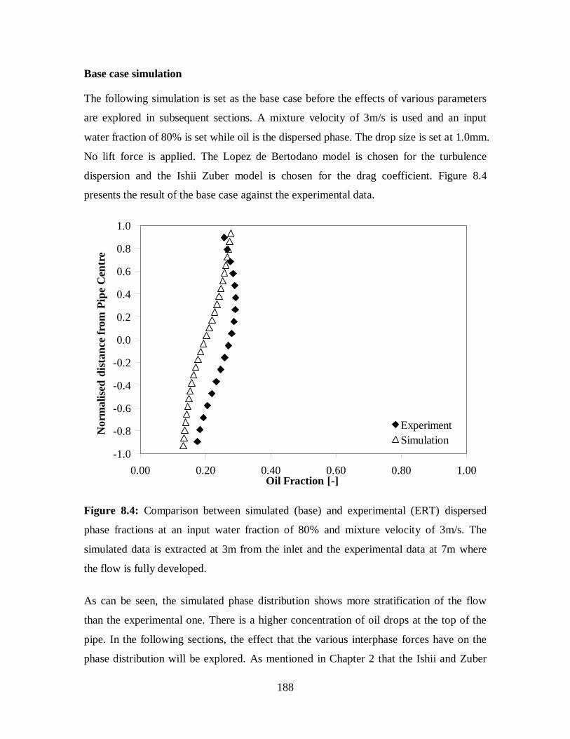
188

Base case simulation

The following simulation is set as the base case before the effects of various parameters

are explored in subsequent sections. A mixture velocity of 3m/s is used and an input

water fraction of 80% is set while oil is the dispersed phase. The drop size is set at 1.0mm.

No lift force is applied. The Lopez de Bertodano model is chosen for the turbulence

dispersion and the Ishii Zuber model is chosen for the drag coefficient. Figure 8.4

presents the result of the base case against the experimental data.

Figure 8.4: Comparison between simulated (base) and experimental (ERT) dispersed

phase fractions at an input water fraction of 80% and mixture velocity of 3m/s. The

simulated data is extracted at 3m from the inlet and the experimental data at 7m where

the flow is fully developed.

As can be seen, the simulated phase distribution shows more stratification of the flow

than the experimental one. There is a higher concentration of oil drops at the top of the

pipe. In the following sections, the effect that the various interphase forces have on the

phase distribution will be explored. As mentioned in Chapter 2 that the Ishii and Zuber

-1.0

-0.8

-0.6

-0.4

-0.2

0.0

0.2

0.4

0.6

0.8

1.0

0.00 0.20 0.40 0.60 0.80 1.00

Norm

ali

sed

dis

tan

ce f

rom

Pip

e C

entr

e

Oil Fraction [-]

Experiment

Simulation

189

(1979) model is the only model for dense dispersion within CFX, no investigation on the

effect of drag force will be conducted.

Effect of lift force coefficient on phase distribution

The effect of lift force on phase distribution will be investigated here. The lift force is

proportional to the cross product between the relative velocity and the curl of the

continuous phase velocity (Equation 2.37). A positive cross product will lead to an

upward lift force by the continuous phase on the dispersed drops and a negative cross

product will lead to a lift force in the opposite direction. Figure 8.5 presents the effect of

the lift force coefficient on phase distribution. With a negative lift force coefficient (LF_-

0.5), a stratification of the phases can be observed. However, the difference between the

case with no lift force (LF_0) and a positive lift force coefficient (LF_0.5) is not

significant except at the lower part of the pipe where some homogenization of the

dispersion can be observed.

Figure 8.5: Effect of lift force on phase distribution at mixture velocity of 3m/s and input

water fraction of 80%. LF in the legend represents the lift coefficient applied to Equation

2.37.

-1.0

-0.8

-0.6

-0.4

-0.2

0.0

0.2

0.4

0.6

0.8

1.0

0.00 0.05 0.10 0.15 0.20 0.25 0.30 0.35 0.40

Norm

ali

sed

dis

tan

ce f

rom

pip

e ce

ntr

e [-

]

Oil Fraction [-]

LF_-0.5

LF_0

LF_0.5

Experiment

190

To further understand the impact of lift force on phase distribution, Figure 8.6 presents

the lift force at different locations along the vertical diameter. The lift force is calculated

from Equation 2.37 assuming that the continuous phase is flowing only in the axial

direction. Other velocity components of the continuous phase are negligible and will not

affect the curl Uc term. A negative lift force coefficient (LF_-0.5) leads to a positive lift

force throughout the pipe. As a result, there is an upward force acting on the drops, which

is stronger near the walls that explains the stratification of the phases seen in Figure 8.5.

With a positive lift force coefficient (LF_0.5), the lift force is negative apart from the

region close to the lower pipe wall. This implies an inward drive of the dispersed drops

away from the bottom wall. The fact that the lift force acts on the opposite direction at the

lower part of the pipe can explain the greater homogenization of the flow at this region

(Figure 8.5).

Figure 8.6: Effect of lift force coefficient on the lift force term at a mixture velocity of

3m/s and an input water fraction of 80%. ds represents the drop size in mm and LF

represents the lift force coefficient applied to Equation 2.37.

-1.0

-0.8

-0.6

-0.4

-0.2

0.0

0.2

0.4

0.6

0.8

1.0

-0.4 -0.2 0 0.2 0.4 0.6 0.8

Norm

ali

sed

dis

tan

ce f

rom

pip

e ce

ntr

e [-

]

Lift force [N]

ds_1_LF_-0.5

ds_1_LF_0

ds_1_LF_0.5

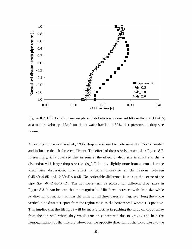
191

Figure 8.7: Effect of drop size on phase distribution at a constant lift coefficient (LF=0.5)

at a mixture velocity of 3m/s and input water fraction of 80%. ds represents the drop size

in mm.

According to Tomiyama et al., 1995, drop size is used to determine the Eötvös number

and influence the lift force coefficient. The effect of drop size is presented in Figure 8.7.

Interestingly, it is observed that in general the effect of drop size is small and that a

dispersion with larger drop size (i.e. ds_2.0) is only slightly more homogenous than the

small size dispersions. The effect is more distinctive at the regions between

0.4R<R<0.8R and -0.8R<R<-0.4R. No noticeable difference is seen at the centre of the

pipe (i.e. -0.4R<R<0.4R). The lift force term is plotted for different drop sizes in

Figure 8.8. It can be seen that the magnitude of lift force increases with drop size while

its direction of motion remains the same for all three cases i.e. negative along the whole

vertical pipe diameter apart from the region close to the bottom wall where it is positive.

This implies that the lift force will be more effective in pushing the large oil drops away

from the top wall where they would tend to concentrate due to gravity and help the

homogenization of the mixture. However, the opposite direction of the force close to the

-1.0

-0.8

-0.6

-0.4

-0.2

0.0

0.2

0.4

0.6

0.8

1.0

0.00 0.10 0.20 0.30 0.40

Norm

ali

sed

dis

tan

ce f

rom

pip

e ce

ntr

e [-

]

Oil fraction [-]

Experiment

ds_0.5

ds_1.0

ds_2.0

192

lower wall also prevents the drops from accumulating in that area. In addition, the

volume of a large 2mm drop is 64 times the volume of a small 0.5mm drop. This implies

that any movement of a large drop will lead to a much larger change in phase fraction

compared to a small drop. The large change in dispersed phase fraction will likely lead to

counteracting forces that are related to concentration gradient (such as the turbulent

dispersion forces) tend to keep the dispersion mixed.

Figure 8.8: Effect of drop size on the lift force of a constant lift coefficient (LF=0.5) at a

mixture velocity of 3m/s and input water fraction of 80%. ds represents the drop size in

mm.

-1.0

-0.8

-0.6

-0.4

-0.2

0.0

0.2

0.4

0.6

0.8

1.0

-0.4 -0.2 0 0.2 0.4

Norm

ali

sed

dis

tan

ce f

rom

th

e p

ipe

cen

tre

[-]

Lift force [N]

ds_0.5_LF_0.5

ds_1_LF_0.5

ds_2.0_LF_0.5

193

Effect of turbulent dispersion force on phase distribution

The changes in the lift force coefficient did not seem to homogenize the mixture to the

extent that it matches the experimental data. The effect of the turbulent dispersion force is

investigated as it can also act to homogenize the mixture.

Figure 8.9 presents the effect of increasing the turbulent dispersion force coefficient on

the phase distribution for a lift coefficient of 0.5 which gave the best results compared to

experimental data. As the coefficient is doubled, the distribution becomes more

homogeneous which agrees better with the experimental result. It is possible that the

deviations from the experimental data are due to the polydispersity of the real system

compared to the single drop size used in the simulations.

Figure 8.9: Effect of turbulent dispersion force coefficient on phase distribution at a

mixture velocity of 3m/s and input water fraction of 80%. LB represents the coefficient

for the Lopez de Bertodano model in Equation 2.39.

-1.0

-0.8

-0.6

-0.4

-0.2

0.0

0.2

0.4

0.6

0.8

1.0

0.00 0.20 0.40 0.60 0.80 1.00

Norm

ali

sed

dis

tan

ce f

rom

pip

e ce

ntr

e

Oil Fraction [-]

LB_1.0

LB_2.0

Experiment

194

Effect of lift and turbulent dispersion force on dispersion of different phase fraction

The force coefficients that were found in previous sections to give the best agreement

against the experimental data (i.e. lift force coefficient of 0.5 and turbulent dispersion

force coefficient of 2) are used here to simulate the flow for different input water

fractions at 40% and 60%. The results can be seen in Figure 8.10 against the

experimental data. The polydispersity of the experimental mixture may have accounted

for the deviation of the simulated results from experimental. Krepper et al. (2004)

demonstrated that a bimodal distribution can have a different phase fraction profile

compared to either mono-sized distribution.

The discrepancy is larger for 40% water fraction where the simulations show that the

flow is highly stratified while the experiments reveal a large concentration of oil drops at

the middle of the pipe. The high concentration of oil drops in the middle of the pipe

resulted in experiments is due to phase inversion (see Section 4.4). However, no

accounting of phase inversion is available in CFX. The available models in CFX are also

limited in simulating a very dense dispersion coupled with the occurrence of phase

inversion. As a result, the phase fraction distribution cannot be correctly modeled at this

fraction.

195

Figure 8.10: Comparison between experimental and simulated phase fraction

distributions for 40% and 60% input water fractions at a mixture velocity of 3m/s and

drop size of 1mm. Oil is set to be the dispersed phase in the simulation. The lift force

coefficient is 0.5 and the turbulent dispersion force coefficient is 2.

8.5 CONCLUSION

It was shown in previous chapters that the dispersed drops migrate towards the centre of

the pipe. The CFD simulations in this chapter offer some insight on the forces acting on

the dispersed drops and on how they influence drop movements. Lift and turbulent

dispersion forces can counteract the upward buoyancy acting on the dispersed oil drops.

Lift force depends on the velocity profile of the continuous phase and the relative

velocity of the dispersed phase. The turbulent dispersion force is driven by the

concentration gradient and tends to homogenize the dispersion.

-1.0

-0.8

-0.6

-0.4

-0.2

0.0

0.2

0.4

0.6

0.8

1.0

0.00 0.20 0.40 0.60 0.80 1.00

Norm

ali

sed

dis

tan

ce f

rom

pip

e ce

ntr

e

Oil Fraction [-]

Simulation (40%)

Simulation (60%)

Experiment (40%)

Experiment (60%)

196

For dilute dispersions (80% water fraction), the results showed that a positive lift force

coefficient (negative lift force) drives the drops away from the pipe wall, while the

magnitude of the force is larger for larger dispersed drops. This suggests that the larger

drops are more likely to be driven towards the centre of the pipe. An increase in the

turbulent dispersion force was also shown to improve the homogenization of the mixture.

Higher dispersed phase fractions (i.e. 40% and 60% water fraction) were also simulated.

There is a reasonable agreement between experimental and simulations for 20% and 40%

dispersed fraction. This may be further improved if a drop size distribution is taken into

account in the simulations (e.g. by using the MUSIG code) since it was found that the

magnitudes of the forces depend on drop size. However, the simulations fail to predict the

experimental results at 60%. This is probably because phase inversion has occurred

experimentally at this fraction which cannot be accounted for in CFX.

197

Chapter 9: Conclusions and Recommendations

9.1 OVERVIEW

Phase inversion in a dispersed pipe flow has been investigated experimentally using

various types of instrumentation. The effect of interfacial tension has also been studied as

it has been the least understood fluid property influencing the inversion process. Based on

the experimental outcome, prediction models have been developed to estimate the phase

fraction at which inversion will occur as well as the pressure gradient during the change

in phase fraction across an inversion process. Lastly, computational fluid dynamic

simulations were studied to understand the interactions between the fluid phases using

established models in Ansys CFX.

A summary of the main conclusions from the experimental and theoretical studies will be

given in Section 9.2, followed by recommendations for future studies in Section 9.3.

9.2 CONCLUSIONS

9.2.1 CONCLUSIONS FROM EXPERIMENTAL STUDIES

The occurrence of phase inversion

ERT tomography and other conductivity measurements reveal that the dispersion

in the pipe undergoes a change in flow regime from a fully dispersed flow to a

dual continuous flow during phase inversion. This transition is due to the

gravitational stratification of the fluid phases.

Phase inversion is also observed to be a gradual process across a range of phase

fraction. The range of phase fraction during inversion is regarded as the

transitional region. This transitional region narrows as the mixture velocity of the

fluids increases.

Phase inversion is observed to occur firstly at the centre of the pipe (if starting

from an O/W dispersion). The accumulation of oil continuous dispersion will

move towards the top of the pipe forming a dual continuous flow. Finally, phase

198

inversion is completed as the lower water layer is being dispersed into the oil

phase. The reverse process will occur starting from a W/O dispersion.

Pressure gradient along the pipe is found to be closely related to the distribution

of the phases contacting with the pipe wall. Drag reduction is first observed as the

dispersed phase is increased in an initial dispersion (e.g. O/W). As phase

inversion occurs at the centre of the pipe, no significant increase in pressure

gradient is observed. However, inversion will begin to increase once the oil

continuous dispersion is in contact with the pipe wall and before phase inversion

is completed across the pipe cross section.

The introduction of a dispersed inlet produces an homogeneous dispersion and

phase inversion occurs at a specific phase fraction (spontaneous inversion).

Pressure gradient is found to differ with an homogeneous dispersion. Pressure

gradient increases with the introduction of the dispersed phase. This is possibly

because of the increase in effective mixture viscosity. There is a suddenly drop at

36% water fraction likely due to drop coalescence and deformation of the closely

packed drops. Pressure gradient will fall to a minimum at the phase inversion

point before it gradually increases beyond inversion.

The drop size of the dispersion is found to fit well with a log-normal distribution.

It is also found that the O/W dispersion has a smaller drop size than the W/O

dispersion. The dispersed inlet also produces a narrower dispersion than the split

inlet.

The drop size distribution during phase inversion becomes wider due to the

dominance of coalescence of the dispersed phase.

Effect of interfacial tension on phase inversion

The addition of glycerol to the water phase has shown significant decrease in

interfacial tension while it does not significantly affect the density and viscosity

of the solution.

The presence of glycerol does not appear to affect the inversion of the dispersed

oil phase to become continuous. However, it retains the continuity of the water

phase before the water phase is inverted at a lower water fraction.

199

Changes on pressure gradient are similar to pure water system with an initial

decrease due to drag reduction and increases again once the more viscous oil

phase is in contact with the pipe wall.

Drop size measurements in the middle of the pipe reveals that the size of oil drops

before inversion is not significantly affected by the addition of glycerol while the

size of the water drops after inversion is reduced. While larger water drops are

expected with the addition of glycerol, the smaller size is possibly due to better

coalescence of the water drop and the formation of the water layer at the bottom

of the pipe.

9.2.2 CONCLUSIONS FROM THEORETICAL STUDIES

Prediction of phase inversion through fluid viscosities

Pressure gradient was previously reported to reach a peak at phase inversion. The

change of pressure gradient is primarily caused by the shear stress of the mixture

with the pipe wall which is related to the fluid viscosities. A prediction model for

phase inversion is thus proposed by assuming equal mixture viscosities of the oil

and water continuous dispersions during inversion.

Various correlations for mixture viscosities from literatures have been applied.

Brinkman (1952)/Roscoe (1952) is found to have the best agreement with

experimental data of oil/water systems of different oil viscosities regardless of its

mixture velocity, dispersion initialisation and pipe material.

The proposed model with Brinkman (1952)/Roscoe (1952) also agrees with

experimental data from Yeh et al. (1964) and Arirachakaran et al. (1989).

While the predicted phase fraction using the proposed model deviate from the

inversion point from the homogeneous dispersed flow, the predicted phase

fraction falls closely with the fraction at which maximum pressure gradient is

observed. The deviation with the inversion point maybe due to drop deformation

and coalescence which cannot be accounted by the applied mixture viscosity

correlations.

200

Prediction of pressure gradient during phase inversion

Based on the experimental observation during inversion, the change in flow

regime (from fully dispersed flow to dual continuous flow) forms the basis for the

development of a prediction model for pressure gradient during phase inversion.

The main difference in these two flow regimes is the presence of the interfacial

height during dual continuous flow. This is the selection criteria to choose

between the two layered flow model and the homogeneous flow model for the

prediction of pressure gradient. A phase inversion criteria is also set based on the

developed prediction model from fluid viscosities.

The proposed prediction model for pressure gradient agrees well with the

experimental data at two different mixture velocities apart from the oil continuous

dispersed flow at low mixture velocity. This discrepancy is attributed to the

inhomogenous distribution of the dispersed water drops in the pipe cross section.

CFD simulation of horizontal two-phase pipe flow

Lift force and turbulent dispersion force are found to be important to homogenize

the dispersion. The magnitude of the lift force is larger for larger dispersed drops

resulting larger drops move faster towards the centre of the pipe. An increase in

the magnitude of the turbulent dispersion force will also improve the

homogenization of the mixture.

Good agreement of the CFD simulation with experimental results can be

observed at lower dispersed phase fraction (i.e. 20% and 40%). However, the

simulation fails to predict at 60% dispersed phase fraction. This is probably due

to the limitation of the CFD code to account for the occurrence of phase

inversion.

9.3 RECOMMENDATIONS

The experimental and theoretical investigations in this work help towards a better

understanding on aspects affecting the phase inversion process in an horizontal pipe flow.

201

However, further work would be recommended to allow further depth into the existing

investigations.

Recommendations for experimental studies

At present, only one type of oil (Exxsol D140) is used throughout the whole

study. With existing instrumentation for phase inversion detection, it will be

beneficial to re-examine the oil/water system conducted by Angeli (1996) and

Ioannou (2006) using Exxsol D80 and Marcol 52. This will have a broader

understanding of the inversion process by having information about the changes

in phase distribution of different fluid mixtures during inversion using the ERT

tomography.

Investigation conducted at a different pipe size will lead to significant difference

in changes of flow regimes. Smaller pipes, for example, will lead to relatively

higher influence of the surface wettability at the pipe wall on the fluid

distribution. Thus, difference in the occurrence of phase inversion will be

expected.

More drop size results should be obtained at different location across the pipe

cross section to have a better understanding of the local drop size distributions

during inversion.

Measurement technique should be developed to account for the drop size of the

secondary droplets as the presence of secondary droplets can significantly affect

the occurrence of phase inversion.

Use of an oil-based surfactant to influence the interfacial tension and compare the

similarity/difference in the occurrence of phase inversion with the current use of

glycerol to the water phase.

Recommendations for theoretical studies

Mixture viscosity correlations should be modified to include dispersion packing

and drop size distribution of the dispersed phase. This aims to account for drop

deformation and polydispersity in a dense dispersion.

202

Pressure gradient prediction model should include the selection criteria from fully

dispersed flow to annular flow (when local inversion begins to appear at the

centre of the pipe) and from annular flow to dual continuous flow (due to the

gravitational stratification of the two continuous dispersions (O/W and W/O)).

Apply the pressure gradient prediction model to a wider range of experimental

conditions. This can help in improving the robustness of the model by using more

appropriate correlations.

Apply Multiple Size Group (MUSIG) model in CFD simulation to account for

the drop size distribution of the dispersed phase.

3-dimensional (3D) geometry for CFD simulation should be used to account for

the lateral forces exerted from the sides of the pipe. This may improve the

prediction of phase distribution between the dispersed and continuous phases in a

pipe cross section.

203

Reference

Agtersloot, R., Vuik, C., Zijlema, M. (1996). A comparison of two CFD packages

and engineering formulae for fluid flow problems. Report 96-93, Faculty of

Technical Mathematics and Informatics, Delft Univ. of Tech.

Al-Sarkhi, Soleimani, A. (2004). Effect of drag reducing polymer on two-phase

gas-liquid flows in a horizontal pipe. Trans IChemE., 82(Part A): 1583-1588.

Al-Wahaibi, T. (2006). Investigations on the transition between stratified and

non-stratified horizontal oil-water flows. Ph.D. thesis, UCL, UK.

Al-Wahaibi, T., Smith, M., Angeli, P. (2007). Effect of drag-reducing polymers

on horizontal oil-water flows. J. of Petroleum Sci. and Eng., 57(3-4): 334-346.

Al-Wahaibi, T., Angeli, P. (2009). Predictive model of the entrained fraction in

horizontal oil-water flows. Chem. Eng. Sci., 64(12): 2817-2825.

Ansys CFX reference guide Version 11.0. . (2006).

Angeli, P. (1996). Liquid-liquid dispersed flows in horizontal pipes. Ph.D. thesis,

Imperial College London, UK.

Angeli, P., Hewitt, G. F. (1998). Pressure gradient in horizontal liquid-liquid

flows. Int. J. Multiphase Flow, 24(7): 1183-1203.

Angeli, P., Hewitt, G. F. (2000). Flow structure in horizontal oil-water flow, Int. J.

Multiphase Flow, 26: 1117-1140.

Arashmid, M., Jeffreys, G. V. (1980). Analysis of phase inversion characteristics

of liquid-liquid dispersions. AIChE J., 26(1): 51-55.

Arirachakaran, S., Oglesby, K. D., Shoulam, O., Brill, J. P. (1989). An

investigation of oil water flow phenomena in horizontal pipes, Paper SPE 18836,

Society of Petroleum Engineers.

Arrhenius (1887). Zeits. f. physic. Chemie 1: 285.

Barnea, E., and Mizrahi, J. (1973). A generalized approach to the fluid dynamics

of particulate systems: Part 1. General correlation for fluidization and

sedimentation in solid multiparticle systems. Chem Eng. J., 5: 171-189.

204

Batchelor, G. K. (1956). The theory of homogeneous turbulence. Cambridge

University Press, Cambridge.

Boussinesq, J. (1877). Théorie de l’Écoulement Tourbillant. Mem. Présentés par

Divers Savants Acad. Sci. Inst. Fr., 23: 46-50.

Brauner, N., Moalem Maron, D. (1989). Two-phase liquid–liquid stratified flow.

Physico-Chem. Hydrodynam. 11, 487–506.

Brauner, N. (2002). Liquid-liquid two-phase flow systems. Modelling and control

of two-phase phenomena. V Bertola (Ed.), CISM Center, Udine, Italy.

Brauner, N., Ullmann, A. (2002). Modelling of phase inversion phenomenon in

two-phase pipe flow. Int. J. Multiphase Flow. 28(1): 55-68.

Brinkman, H. C. (1952). The viscosity of concentrated suspensions and solutions.

J. of Chem. Phy., 20(4): 571.

Calabrese, R. V., Chang, T. P. K., Dang, P. T. (1986). Drop breakup in turbulent

stirred-tank contactors. Part I: Effect of dispersed-phase viscosity. AIChE J.,

32(4): 667-676.

Chakrabarti, D. P., Das, G., Das, P. K. (2006). Transition from water continuous

to oil continuous flow pattern. AIChE J., 52(11): 3668-3678.

Chen, P., Dudukovic, M.P., Sanyal, J. (2005). Three-dimensional simulation of

bubble column flows with bubble coalescence and breakup. AIChE J., 51: 696-

712.

Chesters, A. K. (1991). The modeling of coalescence processes in fluid-liquid

dispersions: A review of current understanding. Chemical Engineering Research

& Design, Transaction IChemE (Part A), 69: 259-270.

Chesters, A. K., Issa, R. (2004). A framework for the modeling of phase inversion

in liquid-liquid systems. Proc. 5th

Int. Conf. on Multiphase Flow.

Chiang, C. L., Chen, C. M. (1994). Characteristics of phase inversion in a turbine-

type agitator. J. Chinese Inst. Chem. Eng., 25(6): 367-374.

Choi, S. J., Schowalter, W. R. (1975). Rheological properties of nondilute

suspensions of deformable particles. Physics of Fluids, 18(4): 420-427.

Clarke, S. I., Sawistowski, H. (1978). Phase inversion of stirred liquid/liquid

dispersions under mass transfer conditions, Trans. IChemE, 56: 50-55.

205

Collins, S. B., Knudsen, J. G. (1970). Drop-size distributions produced by

turbulent pipe flow of immiscible liquids. AIChE J., 16(6): 1072–1080.

Coulaloglou, C. A., Tavlarides, L. L. (1977). Description of interactions processes

in agitated liquid-liquid dispersions, Chem. Eng. Sci., 32: 1289-1297.

Delnoij, E., Kuipers, J. A. M., van Swaaij, W. P. M. (1997). Computational fluid

dynamics applied to gas-liquid contactors. Chem. Eng. Sci. 52: 3623-3638.

Delichatsios, M.A., Probstein, R.F. (1976). The effect of coalescence on the

average drop size in liquid–liquid dispersions. Ind. Eng. Chem. Fund., 14: 134-

138.

Deshphande, K. B., Kumar, S. (2003). A new characteristic of liquid-liquid

systems-inversion holdup of intensely agitated dispersions. Chem. Eng. Sci., 58:

3829-3925.

Drew, D.A (1983). Mathematical modeling of two phase flow. Annual review of

fluid mechanics. 15: 261 – 291.

Efthimiadu, I., Moore, I. P. T. (1994). Phase inversion of liquid-liquid dispersions

produced between parallel shearing plates. Chem. Eng. Sci., 49: 1439-1449.

Einstein, A. (1906). Eine neue bestimmung der moleküledimensionen, Annalen

Phys., 19: 289-306.

Einstein, A. (1911). Berichtigung zu meiner Arbeit: Eine neue bstimmung der

moleküledimensionen. Annalen Phys., 34: 591-592.

Elseth, G. (2001). An experimental study of oil/water flow in horizontal pipes.

Ph.D. thesis, NTNU Trondheim, Norway.

Fakhr-Din, S. M. (1973). Phase inversion and drop size measurements in agitated

liquid-liquid systems. Ph. D. thesis, University of Manchester, UK.

Furuse, H. (1972). Viscosity of concentrated solution. Jap. J. of Applied Physics,

11(10): 1537.

Gillies, R. G., Sun, R., Shook, C. A. (2000). Laboratory investigation of inversion

of heavy oil emulsion. Can. J. Chem. Eng., 78: 757-763.

Groeneweg, F., Agterof, W. G. M., Jaeger, P., Janssen, J. J. M., Wieringa, J. A.,

Klahn, J. K. (1998). On the mechanism of the inversion of emulsions. Trans

IChemE, 76 (Part A).

206

Guilinger, T. R., Grislingas, A. K., Erga, O. (1988). Phase inversion behavior of

water-kerosene dispersions. Ind. & Eng. Chem. Res., 27(6): 978-982.

Guth, E. and Gold, O. (1938). On the hydrodynamical theory of the viscosity of

suspensions. Phys. Rev. 53: 322.

Guzhov, A. I., Grishin, A. D., Medredev, V. F., Medredeva, O. P. (1973).

Emulsion formation during the flow of two liquids in a pipe. Neft Hhoz (in

Russian). 8: 58-61.

Hill, D. (1998). The computer simulation of dispersed two-phase flows. Ph.D.

thesis, Imperial College London, UK.

Hu, B. (2005). Experimental and theoretical investigation of phase inversion in

liquid-liquid dispersions. Ph.D. thesis, UCL, UK.

Hu, B., Matar, O.K., Hewitt, G.F., Angeli, P. (2005). Prediction of phase

inversion in agitated vessels using a two-region model. Chem. Eng. Sci., 60:

3487-3495.

Hu, B., Angeli, P. (2006). Phase inversion and associated phenomena in oil-water

vertical pipeline flow. Can. J. Chem. Eng., 84(1): 94-107.

Hu, B., Angeli, P., Matar, O. K., Lawrence, C. J., Hewitt, G. F. (2006). Evaluation

of drop size distribution from chord length measurements. AIChE J., 52(3): 931-

939.

Ioannou, K., Bin, H., Matar, O. K., Hewitt, G. F., Angeli, P. (2004). Phase

inversion in dispersed liquid-liquid pipe flows, Proc. 5th

Int. Conf. on Multiphase

Flow.

Ioannou, K., Nydal, O. J., Angeli, P. (2005). Phase inversion in dispersed liquid-

liquid flows. Experimental thermal and fluid science. 29(3): 331-339.

Ioannou, K. (2006). Phase inversion phenomenon in horizontal dispersed

oil/water pipeline flows. Ph.D. thesis, UCL, UK.

Ishii, M., Zuber, N. (1979). Drag coefficient and relative velocity in bubbly,

droplet or particulate flows. AIChE J., 25: 843-855.

Karabelas, A. J. (1978). Droplet size spectra generated in turbulent pipe flow of

dilute liquid/liquid dispersions. AIChE J., 24: 170–180.

Kennard, E. H. (1938). Kinetic theory of gases. McGraw-Hill, New York.

207

Krepper, E., Lucas, D., Prasser, H. M. (2005). On the modelling of bubbly flow in

vertical pipes. Nuclear Engineering and Design, 235: 597–611.

Krepper, E., Vanga, B. N. R., Zaruba, A., Prasser, H. M., Lopez de Bertodano, M.

A. (2007). Experimental and numerical studies of void fraction distribution in

rectangular bubble columns. Nuclear Engineering and Design. 237: 399-408.

Krieger, I. M., and Dougherty, T. J., 1959. A mechanism for non-Newtonian flow

in suspensions of rigid spheres. J. of Rheology, 3(1): 137-152.

Krishna, R., van Baten, J. M. (1999). Rise characteristics of gas bubbles in a 2D

rectangular column - VOF simulations vs Experiments. Int. Comm. in Heat and

Mass Transfer. 26: 965-974.

Kumar, A., Hartland, S. (1985). Gravity settling in Liquid/Liquid Dispersions.

Can. J. Chem. Eng., 63: 368-376.

Kumar, S., Kumar, R., Gandhi, K. S. (1991). Influence of the wetting

characteristics of the impeller on phase inversion. Chem. Eng. Sci., 46(9): 2365-

2367.

Kumar, S. (1996). On phase inversion characteristics of stirred dispersions. Chem.

Eng. Sci., 51(5): 831-834.

Launder, B. E., Spalding, D. B. (1972). Lectures in mathematical models of

turbulence. Academic Press, London, England.

Leporcher, E., Delaytermoz, A., Renault, J. F., Gerbier, A., Burger, O. (2001).

Deployment of multiphase pumps on a North Sea Field. Paper SPE 71536,

Society of Petroleum Engineers.

Levich, V. G. (1962). Physicochemical Hydrodynamics. Prentice-Hall,

Englewood Cliffs, New Jersey.

Liu, L. (2005). Optical and computational studies of liquid-liquid flows. Ph.D.

thesis, University of London, UK.

Liu, L., Matar, O.K., Perez de Ortiz, E.S., Hewitt, G.F. (2005). Experimental

investigation of phase inversion in a stirred vessel using LIF. Chem. Eng. Sci.,

60(1): 85-94.

208

Liu, L., Matar, O., Lawrence, C., Hewitt, G. (2006). Laser-induced fluorescence

(LIF) studies of liquid-liquid flows. Part I: Flow structures and phase inversion.

Chem. Eng. Sci., 61: 4007-4021.

Liu, S., Li, D. (1999). Drop coalescence in turbulent dispersions. Chem. Eng. Sci.,

54(23): 5667–5675.

Lopez de Bertodano, M., (1991). Turbulent Bubbly Two Phase Flow in a

Triangular Duct. Ph. D. Thesis, Rensselaer Polytechnic Institute, New York.

Lopez de Bertodano, M., (1998). Two fluid model for two-phase turbulent jet.

Nucl. Eng. Des., 179: 65 - 74.

Lovick, J. (2004). Horizontal oil-water flows in the dual continuous flow regime.

Ph.D. thesis, UCL, UK.

Lucas, D., Krepper, E., Prasser, H. M. (2007). Use of models for lift, wall and

turbulent dispersion forces acting on bubbles for poly-disperse flows. Chem. Eng.

Sci., 62(15): 4146 – 4157.

Luhning, R. W., Sawistowski, H. (1971). Phase inversion in stirred liquid-liquid

systems. Proceeding of the International Solvent Extraction Conference, The

Hague, 873-887, Society of Chemical Industry, London.

Luo, H., Svendsen, H. F. (1996). Theoretical model for drop and bubble breakup

in turbulent dispersions. AIChE J., 42(5): 1225-1233.

Luo, Y. S., Chen, T. K., Cai, J. Y. (1997). Frictional pressure loss and phase

inversion point for oil-water emulsion in vertical tube. Int. Symp on multiphase

fluid, non Newtonian fluid & physicochemical fluid flows. 3: 53-58.

Martinez, A. E., Intevep, S. A., Arirachakaran, S., Shoham, O., Brill, J. P. (1988).

Prediction of dispersion viscosity of oil/water mixture flow in horizontal pipes.

Paper SPE 18221: 427-438, Society of Petroleum Engineers.

McClarey, M., Mansoori, G. (1978). Factors affecting the phase inversion of

dispersed immiscible liquid-liquid mixtures. AIChE J., 74: 134-139.

Mooney, M. (1951). The viscosity of a concentrated suspension of spherical

particles. J. Colloid Sci, 6: 162.

209

Moraga, J. F., Larreteguy, A. E., Drew, D. A., Lahey, R. T. (2003). Assessment of

turbulent dispersion models for bubbly flows in the low Stokes number limit. Int.

J. multiphase flow, 29: 655.

Nädler, M., Mewes, D. (1995). Intermittent three-phase flow of oil, water and gas

in horizontal pipes. Proc. 5th

Int. Offshore and Polar Eng. Conf.

Nädler, M., Mewes, D. (1997). Flow induced emulsification in the flow of two

immiscible liquids in horizontal pipes. Int. J. Multiphase Flow, 23(1): 55-68.

Ngan, K. H., Linnenberg, S., Al-Wahaibi, T., Angeli, P. (2007). Effect of Drag

Reducing Polymers on Oil-Water Flows. Int. Conf. on Multiphase Flow, Germany.

Ngan, K.H., Ioannou, K., Rhyne, L.D., Wang, W., Angeli, P. (2009). A

methodology for predicting phase inversion during liquid-liquid dispersed

pipeline flow. Chem. Eng. Res. Des., 87:318-324.

Norato, M. A., Tsouris, C., Tavlarides, L. L. (1998). Phase inversion studies in

liquid-liquid dispersions, Can. J. Chem. Eng., 76: 486-494.

Noui-Mehidi, M., Wu, J., Zhu, Y. (2004). A few new findings on phase inversion

in a liquid/liquid system. AIChE J., 50: 3281-3283.

Oglesby, K. D. (1979) An experimental study on the effects of oil viscosity,

mixture velocity, and water fraction on horizontal oil-water flow. M.S. thesis,

University of Tulsa, Oklahoma.

Pacek, A. W., Moore, I. P. T., Nienow, A. W. (1994). Video technique for

measuring dynamics of liquid-liquid dispersion during phase inversion. AIChE J.,

40(12): 1940-1949.

Pacek, A. W., Nienow, A. W. (1995). A problem for the description of turbulent

dispersed liquid-liquid systems. Int. J. Multiphase Flow, 21(2): 323–328.

Pal, R., Rhodes, E. (1989). Viscosity/Concentration relationships for emulsions. J.

Rheol., 33(7): 1021-1045.

Pal, R. (1993). Pipeline flow of unstable and surfactant-stabilized emulsions.

AIChE J., 39 (11): 1754-1764.

Pal, R. (2001). Single-parameter and two-parameter rheological equations of state

for nondilute emulsions, Ind. Eng. Chem. Res., 40: 5666-5674.

210

Perry, R. H., Green, D. W. (1997). Perry’s Chemical Engineers’ Handbook. 7th

Ed.

McGraw-Hill, New York.

Pettersen, B.H., Langsholt, M., and Ødegård, J. (2001). Pressure drop and wall

wetting: the effect of pipe wall material in multiphase flow. Proc. 10th

International Conference of Multiphase Flow, Cannes, France.

Phan-Thein, N., Pham, D. C. (1997). Differential multiphase models for

polydispersed suspensions and particulate solids. J. Non-Newtonian Fluid Mech.,

72: 305.

Piela, K., Delfos, R., Ooms, G., Westerweel, J., Oliemans, R.V.A., Mudde, R.F.

(2006). Experimental investigation of phase inversion in an oil-water flow

through a horizontal pipe loop. Int. J. Multiphase Flow, 32(9): 1087-1099.

Piela, K., Delfos, R., Ooms, G., Westerweel, J., Oliemans, R.V.A. (2008). On the

phase inversion process in an oil-water pipe flow. Int. J. Multiphase Flow, 34(7):

665-677.

Prince, M., Blanch, H. W. (1990). Bubble coalescence and break-up in air-

sparged bubble columns. AIChE J., 36(10): 1485–1499.

Quinn, J. A., Sigloh, D. B. (1963). Phase inversion in the mixing of immiscible

liquids. Can. J. Chem. Eng., 41: 15-18.

Ranade, V. (2002). Computational flow modeling for chemical reactor

engineering. Process Systems Engineering Vol. 5. Academic Press, California.

Rodger, W. A., Trice, Jr., V. G., Rushton, J. H. (1956). The effect of fluid motion

on interfacial area dispersions. Chem. Eng. Prog., 52(12): 515-520.

Rodriguez, O. M. H., Bannwart, A. C. (2006). Analytical model for interfacial

waves in vertical core flow. J. of Petroleum Sci. and Eng., 54 (3-4).

Roscoe, R. (1952). The viscosity of suspensions of rigid spheres. British journal

of applied physics, 267-269.

Rotta, J. C. (1972). Turbulente Strömungen. B. G. Teubner, Stuttgart.

Rozentsvaig, A. K. (1982). Turublent pipe flow of concentrated emulsions with a

nonequilibrium disperse phase. Inzh.-Fiz. Zh., 42(3), 366-372.

211

Rusche, H., Issa, R. I. (2000). The Effect on voidage on the drag force on particles

in dispersed two-phase flow. Japanese-European two phase flow meeting,

Tsukuba, Japan.

Rusche, H. (2002). Computational fluid dynamics of dispersed two-phase flows at

high phase fractions. Ph.D. thesis, Imperial College London, UK.

Russell, T., Hodgsen, G., Govier, G. (1959). Horizontal pipeline flow of mixtures

of oil and water. Can. J. Chem. Eng., 37: 9-17.

Russell, T.W.F., Charles, M.E., (1959). The effect of the less viscous liquid in the

laminar flow of two immiscible liquids. Can. J. Chem. Eng. 37: 18–24.

Saffman, P. G., Turner, J. S. (1956). On the collision of drops in turbulent clouds.

J. Fluid Mech., 1: 16-30.

Schiller, L., Naumann, Z. (1933). Über die grundlegenden Berechungen bei der

Schwerkraftbereitung. Z. Ver. Deutsch. Ing., 77: 318 -320.

Schwartzberg, H.G., Treybal, R. E. (1968). Fluid and particle motion in turbulent

stirred tanks. Ind. & Eng. Chem. Res. Fund., 7: 1-6.

Seklker, A. H., Sleicher, Jr., C. A. (1965). Factors affecting which phase will

disperse when immiscible liquids are stirred together. Can. J. Chem. Eng.,

43:298-301.

Simmons, M. J. H., Azzopardi, B. J. (2001). Drop size distributions in dispersed

liquid-liquid pipe flow. Int. J. Multiphase Flow, 27: 843-859.

Smith, D. H., Lim, K. (1990). An experimental test of catastrophe and critical-

scaling theories of emulsion inversion. Langmuir, 6: 1071-1077.

Soleimani, A., Lawrence, C. J., Hewitt, G. F. (1997). Effect of mixers on flow

pattern and pressure drop on horizontal oil-water pipe flow. Int. Symp. on liquid-

liquid two phase flow and transportation phenomena, Turkey.

Soleimani, A. (1999). Phase distribution and associated phenomena in oil-water

flows in horizontal tubes. Ph.D. thesis, Imperial College London, UK.

Soleimani, A., Lawrence, C. J., Hewitt, G. F. (2000). Spatial distribution of oil

and water in horizontal pipe flow. SPE Journal, 5(4): 394-401.

212

Sommerfelds, M., Wachem, B.V., Oliemans, R.V.A (2008). Best practice

guidelines for computational turbulence dispersed multiphase flows. Seminar

presentation, SIAMUF, Chalmers University.

Sovová, H. (1981). Breakage and coalescence of drops in a batched stirred vessel

– II. Comparison of model and experiments. Chem. Eng. Sci., 36(9): 1567-1573.

Stover, R. L., Tobías, C. W., Denn, M. M. (1997). Bubble coalescence dynamics.

AIChE J., 43: 2385-2392.

Taylor, G. I. (1932). The viscosity of a fluid containing small drops of another

fluid. Proc. R. Soc., 138: 41.

Thomas, D. G. (1965). Transport characteristics of suspensions: VII. A note on

the viscosity of Newtonian suspensions of uniform spherical particles. J. Colloid

Sci., 20: 267-277.

Tidhar, M., Merchuk, J. C., Sembira, A. N., Wolf, D. (1986). Characteristics of a

motionless mixer for dispersion of immiscible fluids- Phase inversion of liquid-

liquid systems. Chem. Eng. Sci., 41(3): 457-462.

Tomiyama, A., Zun, I., Kanami, N., Sakaguchi, T. (1995). Effects of Eötvös

number and dimensionless liquid volumetric flux on lateral motion of a bubble in

a laminar duct flow. Adv. Multiphase Flow, 3-15.

Trallero, J. L. (1995). Oil water flow patterns in horizontal pipes. Ph.D. thesis,

University of Tulsa, Oklahoma.

Treybal, R. E. (1963). Liquid Extraction. 2nd

Edition, McGraw-Hill, New York.

Tsouris, C., Tavlarides, L. L. (1994). Breakup and coalescence models for drops

in turbulent dispersion. AIChE J., 40(3): 395-406.

Tyrode, E., Allouche, J., Choplin, L., Salager, J. (2005). Emulsion catastrophic

inversion from abnormal to normal morphology. 4. Following the emulsion

viscosity during three inversion protocols and extending the critical dispersed-

phase concept. Ind. & Eng. Chem. Res., 44: 67-74.

Vaessen, G. E. J., Visschers, M., Stein, H. N. (1996). Predicting catastrophic

phase inversion on the basis of droplet coalescence kinetics. Langmuir, 12: 875-

882.

213

Valentas, K.J., Bilous, O., Amundson, N.R. (1966). Analysis of breakage in

dispersed phase systems. Ind. Eng. Chem. Fundamentals, 5: 271–279.

Valle, A., Utvik, O. H. (1997). Pressure drop, flow pattern and slip for two phase

crude oil-water flow. Int. Symp. on liquid-liquid two phase flow and

transportation phenomena, Turkey

Vallée, C., Höhne, T., Prasser, H.M., Sühnel, T. (2007). Experimental

investigation and CFD simulation of slug flow in horizontal channels.

Forschungszentrum Dresden-Rossendorf, Report FZD-485, Dresden, Germany.

Vand, V. (1948). Viscosity of solutions and suspensions. I – Theory. J Phys Coll

Chem, 52: 277–299.

Vielma, M., Atmaca, S., Sarica, C., Zhang, H. (2008). Characterization of

Oil/Water Flows in Horizontal Pipes. Paper SPE 109591, Society of Petroleum

Engineers.

Wang, W., Gong, J., Ngan, K. H., Angeli, P. (2009). Effect of glycerol on the

binary coalescence of water drops in stagnant oil phase, Chem. Eng. Res. Des.,

87(12): 1640-1648.

Wilcox, D.C. (1986) Turbulence Modelling for CFD. DCW Industrie.

Yakhot, V., Smith, L.M. (1992). The renormalization group, the ε-expansion and

the derivation of turbulence models. J. Sci. Comp, 7: 35-61.

Yaron, I., Gal-Or, B. (1972). On viscous flow and effective viscosity of

concentrated suspensions and emulsions – Effect of particle concentration and

surfactant impurities. Rheologica Acta, Band 11, Heft 3/4: 245 – 252.

Yeh, G. C., Haynie Jr., F. H., Moses, R. A. (1964). Phase-volume relationship at

the point of phase inversion in liquid dispersions. AIChE J., 10(2): 260-265.

Yeo, L. Y., Matar, O. K., Perez de Ortiz, E. S., Hewitt, G. F. (2000). Phase

inversion and associated phenomena. Multiphase Science and Technology, 12(1):

51-116.

Yeo, L. Y. (2002). Modelling of phase inversion and associated phenomena in

liquid-liquid systems. Ph.D. thesis, University of London, UK.

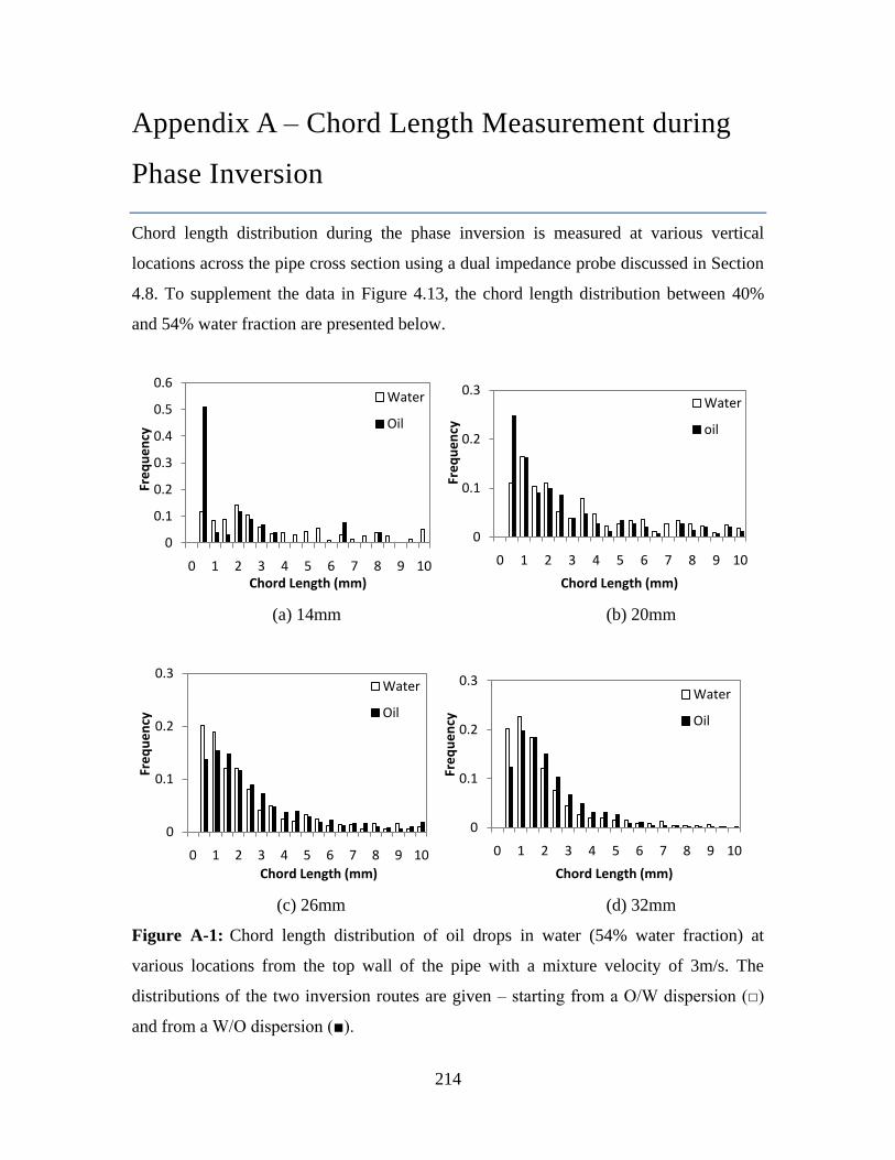
214

Appendix A – Chord Length Measurement during

Phase Inversion

Chord length distribution during the phase inversion is measured at various vertical

locations across the pipe cross section using a dual impedance probe discussed in Section

4.8. To supplement the data in Figure 4.13, the chord length distribution between 40%

and 54% water fraction are presented below.

(a) 14mm (b) 20mm

(c) 26mm (d) 32mm

Figure A-1: Chord length distribution of oil drops in water (54% water fraction) at

various locations from the top wall of the pipe with a mixture velocity of 3m/s. The

distributions of the two inversion routes are given – starting from a O/W dispersion (□)

and from a W/O dispersion (■).

0

0.1

0.2

0.3

0.4

0.5

0.6

0 1 2 3 4 5 6 7 8 9 10

Fre

qu

en

cy

Chord Length (mm)

Water

Oil

0

0.1

0.2

0.3

0 1 2 3 4 5 6 7 8 9 10

Fre

qu

en

cy

Chord Length (mm)

Water

oil

0

0.1

0.2

0.3

0 1 2 3 4 5 6 7 8 9 10

Fre

qu

en

cy

Chord Length (mm)

Water

Oil

0

0.1

0.2

0.3

0 1 2 3 4 5 6 7 8 9 10

Fre

qu

en

cy

Chord Length (mm)

Water

Oil

215

(a) 20mm (b) 26mm

(c) 32mm

Figure A-2: Chord length distribution of oil drops in water (50% water fraction) at

various locations from the top wall of the pipe with a mixture velocity of 3m/s. The

distributions of the two inversion routes are given – starting from a O/W dispersion (□)

and from a W/O dispersion (■).

0

0.1

0.2

0.3

0.4

0.5

0.6

0 1 2 3 4 5 6 7 8 9 10

Fre

qu

en

cy

Chord Length (mm)

Water

Oil

0

0.1

0.2

0.3

0.4

0.5

0.6

0 1 2 3 4 5 6 7 8 9 10

Fre

qu

en

cy

Chord Length (mm)

Water

Oil

0

0.1

0.2

0.3

0.4

0.5

0 1 2 3 4 5 6 7 8 9 10

Fre

qu

en

cy

Chord Length (mm)

Water

Oil

216

(a) 26mm (b) 32mm

Figure A-3: Chord length distribution of oil drops in water (40% water fraction) at

various locations from the top wall of the pipe with a mixture velocity of 3m/s. The

distributions of the two inversion routes are given – starting from a O/W dispersion (□)

and from a W/O dispersion (■).

From the above figures, only detectable chord length distributions are presented. At 54%

water fraction, it can be observed that the distribution becomes wider at 20mm (i.e. centre

of pipe) where it is previously found to be the beginning of phase inversion. As the water

fraction decreases, it can also be observed that the distribution becomes wide across all

the measured locations and the phenomenon spreads towards the bottom of the pipe cross

section. This supports the observation found using the ERT system in Figure 4.3 where

the phase inversion process has the same downward shift.

0

0.1

0.2

0.3

0.4

0.5

0 1 2 3 4 5 6 7 8 9 10

Fre

qu

en

cy

Chord Length (mm)

Water

Oil

0

0.1

0.2

0.3

0.4

0.5

0 1 2 3 4 5 6 7 8 9 10

Fre

qu

en

cy

Chord Length (mm)

Water

Oil

217

Appendix B – Matlab Code for Pressure Gradient

Prediction

A. MAIN EXECUTION CODE

%%%%%%%%%%%%%%%%%%

%Fluid properties%

%%%%%%%%%%%%%%%%%%

%density of oil (denso), density of water (densw)

denso=828; densw=1000;

%viscosity of oil (visco), viscosity of water (viscw)

visco=5.5*0.001; viscw=1.0*0.001;

%Interfacial tension (ST)

ST=39.6*0.001;

%%%%%%%%%%%%%%%%%

%Operation Input%

%%%%%%%%%%%%%%%%%

%gravity (g), pipe diameter (D)

g=9.81; D=0.038;

%Pipe area (A)

A=pi*D^2/4;

%Curvature (0-Flat Interface, 1-Curved Interface)

curve=0;

%%%%%%%%%%%%%%%%%%%%%%%%%%%%%%

%Critical amplitude at the onset of entrainment (Talal 2006)%

%%%%%%%%%%%%%%%%%%%%%%%%%%%%%%

a_oil=D/10;

a_water=D/10;

hwstart=min(a_oil,a_water);

%%%%%%%%%%%%%%%%%%%

%Flow rate (l/min) %

%%%%%%%%%%%%%%%%%%%

Flow_rates=[ ];

218

%%%%%%%%%%%%%%%

%flow rate conversion (m3/s)%

%%%%%%%%%%%%%%%

conversion=0.0000166667;

Q=conversion*Flow_rates;

%Friction factor mode (refer to fric.m for detail)

fric_no=2;

%Critical water fraction for phase inversion

wfc=0.34;

%Initialisation (Do Not Change)

N_hw=(D-2*hwstart)/0.0001;

N_fr=size(Q,1);

output=[];

output1=[];

output2=[];

%Execution Script (Do Not Change)

for m=1:N_fr

Qo=Q(m,2);

Qw=Q(m,1);

hwnew=hwstart;

fr=Qw/(Qw+Qo)*100

olddiff=6000;

count=0;

for i = 1:N_hw

if hwnew<D-hwstart

[Ento_w,Entw_o]=entrain1(Qo,Qw,hwnew,D,denso, densw, visco, viscw, ST,

a_oil, a_water, curve, fric_no);

if (Entw_o >=1)||(Ento_w>=1)||(imag(Ento_w) || imag(Entw_o))

elseif (Entw_o>=wfc)&&(Ento_w>=(1-wfc))

else

count=count+1;

[dPu,dPl, dPa,UL,LL,Entw,Ento, Reu, Rel, Au,Al]=dP1(hwnew, Qo, Qw,

denso, densw,Entw_o,Ento_w, visco, viscw, D, curve, fric_no, wfc);

if abs((dPu-dPl)/dPa*100)>=2 || ((UL==1)&&(LL==1))||((UL==2)&&(LL==2))

else

output=[output;fr hwnew UL LL dPa/1000 abs((dPu-dPl)/dPa*100)];

end

end

hwnew=hwnew+0.0001;

else

break

219

end

end

OP=isempty(output);

if (OP==1)

[dPa]=homo(Qo, Qw, denso, densw, visco, viscw, D, curve, fric_no);

output1=[output1;fr 0 0 0 dPa/1000 0];

else

output2=sortrows(output,[1,6]);

idx=find(min((output2(:,6))));

output1=[output1;output2(idx,:)];

output=[];

end

end

csvwrite('output.csv', output1)

B. ENTRAINMENT MODULE

function [Ento_w1,Entw_o1]=entrain(Qo,Qw,hwnew,D,denso, densw, visco, viscw, ST,

a_oil, a_water, curve, fric_no)

%Calculating entrainment fraction

%Entw_o is the entrainment fraction of water in oil

%Ento_w is the entrainment fraction of oil in water

%Um=mixture velocity

Entw_o=0;

Ento_w=0;

[Si,So,Sw,A,Ao,Aw,Hw,Ho]=geo(hwnew,D,curve);

Um=(Qo+Qw)/A;

Usw=Qw/A;

Uso=Qo/A;

hwinput=hwnew;

[Tw,To,Ti]=hwF(hwinput, Usw, Uso, D, denso, densw, visco, viscw, curve, fric_no);

Uw=Usw/Hw;

Uo=Uso/Ho;

if Uo/Uw>=0.98 && Uo/Uw<1.05

Dw=4*Aw/(Sw); Do=4*Ao/(So);

elseif Uo>Uw

Dw=4*Aw/(Sw); Do=4*Ao/(So+Si);

else

Dw=4*Aw/(Sw+Si); Do=4*Ao/(So);

end

220

%Reynolds number

Rew=Dw*Uw*densw/viscw;

Reo=Do*Uo*denso/visco;

%Drag coefficient

Cd=2.7e-7*Reo^(0.77)*Rew^(0.86);

%Wavelength (lamda)

lamda=1*D;

%Prediction of entrainment fraction of oil in water (Ento_w)

%Calculating the critical amplitude of oil waves at the new conditions

%amplitude (al)

al=0.00;

k=real((D-hwnew)/0.000001);

for m=1:k

al=al+0.000001;

hap=hwnew+al;

[Siap,Soap,Swap,A,Aoap,Awap,Hwap,Hoap]=geo(hap,D,curve);

Soapeak=Soap;

Siapeak=Siap;

Aoapeak=Aoap;

Awapeak=Awap;

hat=hwnew-al;

[Siat,Soat,Swat,A,Aoat,Awat,Hwat,Hoat]=geo(hat,D,curve);

Siatrough=Siat;

Soatrough=Soat;

Aoatrough=Aoat;

Awatrough=Awat;

Aw1=Awapeak;

Aw2=Awatrough;

Ao1=Aoapeak;

Ao2=Aoatrough;

Uo2=Uo*(Ao/Ao2);

Uw2=Uw*(Aw/Aw2);

%Drag force (Fd)

Fd=0.5*densw*(Aw-Aw2)*Cd*(Uw2-Uo2)^2;

%Surface tension force (Fst)

L=(al^2+(lamda/2)^2)^0.5;

Fst=2*Si*ST*(lamda/2)/L;

Total=Fd-Fst;

221

if Total>=0

break

end

end

%Amount of oil transfer to the water phase

Vent_o=0.5*((a_oil-al)*lamda*Si/(pi));

vdfo=0.051*(Uso/Um)^-2.08*(Tw/densw)^0.5;

%Calculation of the entrainment fraction of oil in water (Ento_w)

C_oil=Vent_o*denso*abs(Uw2-Uo2)/(Si*lamda^2*vdfo);

Ento_w=((densw)-((densw)^2-4*(densw-denso)*C_oil)^0.5)/(2*(densw-denso));

%Calculating the critical amplitude of water waves at the new condition

%amplitude (au)

au=0.00;

k=real((D-hwnew)/0.000001);

for m=1:k

au=au+0.000001;

hap2=hwnew+au;

[Siap2,Soap2,Swap2,A,Aoap2,Awap2,Hwap2,Hoap2]=geo(hap2,D,curve);

Soapeak=Soap2;

Siapeak=Siap2;

Aoapeak=Aoap2;

Awapeak=Awap2;

hat2=hwnew-au;

[Siat2,Soat2,Swat2,A,Aoat2,Awat2,Hwat2,Hoat2]=geo(hat2,D,curve);

Siatrough=Siat2;

Soatrough=Soat2;

Aoatrough=Aoat2;

Awatrough=Awat2;

Aw1=Awapeak;

Aw2=Awatrough;

Ao1=Aoapeak;

Ao2=Aoatrough;

Uo1=Uo*(Ao/Ao1);

Uw1=Uw*(Aw/Aw1);

%Drag force (Fd)

Fd=0.5*densw*(Aw1-Aw)*Cd*(Uw1-Uo1)^2;

%Surface tension force (Fst)

L=(au^2+(lamda/2)^2)^0.5;

222

Fst=2*Si*ST*(lamda/2)/L;

Total=Fd-Fst;

if Total>=0

break

end

end

%Amount of water transfer to the oil phase

Vent_w=0.5*((a_water-au)*lamda*Si/(pi));

vdfw=0.077*(Usw/Um)^-1.8*(To/denso)^0.5;

%Calculation of the entrainment fraction of oil in water (Ento_w)

C_water=Vent_w*densw*abs(Uw1-Uo1)/(Si*lamda^2*vdfw);

Entw_o=((denso)-((denso)^2-4*(denso-densw)*C_water)^0.5)/(2*(denso-densw));

Ento_w1=(Ento_w)/(1-Ento_w+densw/denso);

Entw_o1=(Entw_o)/(1-Entw_o+denso/densw);

C. SHEAR STRESS MODULE

function [Tw,To,Ti]=hwF(hwinput, Usw, Uso, D, denso, densw, visco, viscw, curve,

fric_no)

[Si,So,Sw,A,Ao,Aw,Hw,Ho]=geo(hwinput,D,curve);

Uw=Usw/Hw;

Uo=Uso/Ho;

if Uo/Uw>+0.98 && Uo/Uw<1.05

Dw=4*Aw/(Sw); Do=4*Ao/(So);

elseif Uo>Uw

Dw=4*Aw/(Sw); Do=4*Ao/(So+Si);

else

Dw=4*Aw/(Sw+Si); Do=4*Ao/So;

end

%Reynolds number

Rew=Dw*Uw*densw/viscw;

Reo=Do*Uo*denso/visco;

%Reynolds number of interface

if Uo>Uw

Rei=Si*Uo*denso/(pi*visco);

densf=denso;

else

Rei=Si*Uw*densw/(pi*viscw);

densf=densw;

end

223

%friction factors

[fw,fo,fi]=fric(Rew,Reo,Rei,Ho,Hw,Do,Dw,fric_no);

%shear stress

Tw=fw*densw*Uw*abs(Uw)/2;

To=fo*denso*Uo*abs(Uo)/2;

if Uo/Uw >= 0.98 && Uo/Uw<1.05

Ti=0;

else

Ti=fi*densf*(Uo-Uw)*abs(Uo-Uw)/2;

end

%Two Fluid Model

%Fhw=To*So/Ao+Ti*Si*(1/Aw+1/Ao)-Tw*Sw/Aw;

D. DIFFERENTIAL PRESSURE MODULE (LAYERED FLOW)

function [dPu,dPl, dPa,UL,LL,Entw,Ento, Reu, Rel, Au,Al]=dP1(hwinput, Qo, Qw,

denso, densw,Entw_o,Ento_w, visco, viscw, D, curve, fric_no, wfc)

%Geometry

[Si,Su,Sl,A,Au,Al,Hw,Ho]=geo(hwinput,D,curve);

%Error test for Input Entrainment

if (imag(Ento_w) | imag(Entw_o))~=0

Entw_o=NaN;

Ento_w=NaN;

end

%Error test for entrainment

if Ento_w==NaN

Ento1=NaN;

return

end

if Entw_o==NaN

Entw1=NaN;

return

end

%Phase Inversion

%Flow Pattern: 1-W/O, 2-O/W, 3-Pure oil, 4-Pure water

if Entw_o<wfc

if Ento_w<(1-wfc);

Entw=Entw_o;

224

viscu=visco;

Uo=Qo/(Au);

Ento=Ento_w;

viscl=viscw;

Uw=Qw/(Al);

UL=1;

LL=2;

elseif Ento_w<1

Entw=Entw_o;

viscu=visco;

Uo=Qo/(Au);

Ento=(1-Ento_w);

viscl=visco;

Uw=Qw/(Al);

UL=1;

LL=1;

else

%Invalid Scenario

Entw=Qw/(Qo+Qw);

viscu=visco;

Uo=Qo/(Au);

Ento=0;

viscl=visco;

Uw=Qw/(Al);

UL=1;

LL=3;

end

elseif Entw_o<1

if Ento_w<(1-wfc);

Entw=(1-Entw_o);

viscu=viscw;

Uo=Qo/(Au);

Ento=Ento_w;

viscl=viscw;

Uw=Qw/(Al);

UL=2;

LL=2;

elseif Ento_w<1

%Invalid Scenario

Entw=(1-Entw_o);

viscu=viscw;

Uo=Qo/(Au);

Ento=(1-Ento_w);

viscl=visco;

Uw=Qw/(Al);

UL=2;

225

LL=1;

else

%Invalid Scenario

Entw=(1-Entw_o);

viscu=visco;

Uo=Qo/(Au);

Ento=0;

viscl=visco;

Uw=Qw/(Al);

UL=2;

LL=3;

end

else

if Ento_w<(1-wfc);

%Invalid Scenario

Entw=0;

viscu=viscw;

Uo=Qo/(Au);

Ento=Ento_w;

viscl=viscw;

Uw=Qw/(Al);

UL=4;

LL=2;

elseif Ento_w<1

%Invalid Scenario

Entw=0;

viscu=viscw;

Uo=Qo/(Au);

Ento=(1-Ento_w);

viscl=viscw;

Uw=Qw/(Al);

UL=4;

LL=1;

else

%Invalid Scenario

Entw=0;

viscu=viscw;

Uo=Qo/(Au);

Ento=0;

viscl=viscw;

Uw=Qw/(Al);

UL=4;

LL=3;

end

end

226

%Mixture Density

densu=(Entw)*densw+(1-Entw)*denso;

densl=(Ento)*denso+(1-Ento)*densw;

%Mixture Viscosity

muu=viscu*(1-Entw)^-2.5;

mul=viscl*(1-Ento)^-2.5;

if Uo/Uw>+0.98 && Uo/Uw<1.05

Dw=4*Al/(Sl); Do=4*Au/(Su);

elseif Uo>Uw

Dw=4*Al/(Sl); Do=4*Au/(Su+Si);

else

Dw=4*Al/(Sl+Si); Do=4*Au/Su;

end

%Reynolds number

Rel=Dw*Uw*densl/mul;

Reu=Do*Uo*densu/muu;

%Reynolds number of interface

if Uo>Uw

Rei=Si*Uo*densu/(pi*muu); densf=densu;

else

Rei=Si*Uw*densl/(pi*mul);densf=densl;

end

%friction factors

[fw,fo,fi]=fric(Rel,Reu,Rei,Ho,Hw,Do,Dw,fric_no);

if LL==1

fl=fw/(1+1.125*Ento);

else

fl=fw/(1+1.125*Ento);

end

if UL==1

fu=fo/(1+1.125*Entw);

else

fu=fo/(1+1.125*Entw);

end

fi=fi;

%shear stress

Tl=fl*densl*Uw*abs(Uw)/2;

Tu=fl*densu*Uo*abs(Uo)/2;

227

if Uo/Uw >= 0.98 && Uo/Uw<1.05

Ti=0;

else

Ti=fi*densf*(Uo-Uw)*abs(Uo-Uw)/2;

end

%Two Fluid Model

if Uo>Uw

dPu=Tu*Su/Au-Ti*Si*(1/Au);

dPl=Tl*Sl/Al+Ti*Si*(1/Al);

else

dPu=Tu*Su/Au+Ti*Si*(1/Au);

dPl=Tl*Sl/Al-Ti*Si*(1/Al);

end

dPa=(dPu+dPl)/2;

Ento1=100*Ento;

Entw1=100*Entw;

E. PRESSURE GRADIENT MODULE (HOMOGENEOUS MODEL)

function [dPa]=homo(Qo, Qw, denso, densw, visco, viscw, D, curve, fric_no)

A=pi*D^2/4;

fr=Qo/(Qw+Qo)*100;

WF=Qw/(Qo+Qw);

OF=Qo/(Qo+Qw);

densm=denso*OF+densw*WF;

muw=visco*(1-WF)^-2.5;

muo=viscw*(1-OF)^-2.5;

if muw<=muo

mum=muw;

else

mum=muo;

end

Um=(Qo+Qw)/A;

Reh=densm*D*Um/mum;

[fh]=hfric(Reh,fric_no);

if muw<=muo

fh1=fh/(1+1.25*WF);

else

fh1=fh/(1+1.25*OF);

end

dPu=0;

228

dPl=0;

dPa=(2*fh1*densm*Um^2)/D;

F. GEOMETRY MODULE

function [Si,So,Sw,A,Ao,Aw,Hw,Ho]=geo(hwinput,D,curve)

if curve==0

%disp('flat interface');

hw=hwinput;

h=2*(hw/D)-1;

Si=D*((1-h^2)^(1/2));

So=D*acos(h);

Sw=D*pi-So;

A=pi*D^2/4;

Ao=D*((So)-(Si*h))/4;

Aw=A-Ao;

Hw=Aw/A;

Ho=Ao/A;

elseif curve==1

%disp('curved interface')

hw=hwinput;

X=(hw^2+4*(D/2)*hw)/(2*(D/2)+2*hw);

teta1=2*acos(((D/2)-X)/(D/2));

teta2=2*acos((2*(D/2)-(X-hw))/(2*(D/2)));

A=pi*D^2/4;

Aw=(0.5*((D/2)^2)*(teta1-sin(teta1)))-(0.5*(2*(D/2)^2)*(teta2-sin(teta2)));

Ao=A-Aw;

Sw=(D/2)*teta2;

So=pi*D-Sw;

Si=2*(D/2)*teta2;

Hw=Aw/A;

Ho=Ao/A;

end

G. FRICTION FACTOR MODULE (LAYERED FLOW)

function [fw,fo,fi]=fric(Rel,Reu,Rei,Hu,Hl,Do,Dw,fric_no)

%Friction factor for Upper Layer

%if Reu<4000

%fo=(1/(-

2*log10((0.015/3.70)+((4.518*log10(1/7*Reu))/(Reu*(1+1/29*Reu^0.52*(0.015)^0.7))))

))^2;

%fo=7e-10*(Reu)^2; %(S.W. Churchill (1973), AIChE J, 19(2):375)

229

%fo=sqrt(1/(-2*log10((0.0015/3.7065)-(5.0272/Reu)*log10((0.0015/3.827)-

(4.567/Reu)*log10((0.0015/7.7918)^0.9924+(5.3326/(208.815+Reu))^0.9345)))));

%fo=16*Reu^-1;

%else

if fric_no==1

fo=0.079*Reu^-0.25;

elseif fric_no==2

fo=0.046*Reu^-0.2; % Taitel & Dukler (1976)

elseif fric_no==3

fo=0.764*(Hu*Reu)^(-0.562); %Srichai (1994)

elseif fric_no==4

fo=(-3.6*log10((6.9/Reu)+(1*10^(-5)/(3.7*Do))^1.1))^(-2); %Haaland (1983);

Hadzlabdic & Oliemans (2007)

elseif fric_no==5

fo=(-4*log10((1*10^(-5)/(3.7*Do))-(5.02/Reu)*log10((1*10^(-5)/(3.7*Do))-

(5.02/Reu)*log10((1*10^(-5)/(3.7*Do))+(13/Reu)))))^(-2); %Zigrang & Sylvester (1982)

else

return

end

%end

H. FRICTION FACTOR MODULE (HOMOGENEOUS MODEL)

function [fh]=hfric(Reh,fric_no)

if fric_no==1

fh=0.079*Reh^-0.25;

elseif fric_no==2

fh=0.046*Reh^-0.2;

else

disp('No friction factor model chosen')

return

end

230

Appendix C – Grid Sensitivity Test for CFD

Simulation

A grid sensitivity test was conducted to define the optimal grid structure for the CFD

simulations conducted in Chapter 8. The optimal grid structure will be used to simulate a

pipe section of 3m in length and 38mm in internal diameter. The test was done by

changing the number of cells in the vertical height of a rectangular slab (see Figure C-1).

Three structures of different grid sizes are chosen – 40 cells (grid 40), 60 cells (grid 60)

and 80 cells (grid 80). The length of the slab is kept at 3100 cells including 100 cells to

represent the splitting inlet as introduced in Chapter 3. Table C-1 presents the total

number of grid points and elements in each structure.

Figure C-1: Sample schematics of simulation domain with a vertical height consisting of

60 cells.

The simulation was tested by running an oil/water flow at a mixture velocity of 3m/s. Oil

was inputted as the dispersed phase while the water being the continuous phase. Drop

size was set at 0.5mm (smallest drop size group found in experiment). An input dispersed

phase fraction of 0.2 was chosen. k-ε turbulence model was used. Ishii and Zuber (1979)

model was applied as the drag force for the dispersion. Lift force with coefficient of 0.5

231

was used together with Lopez de Bertodano model for the turbulent dispersion force

(coefficient: 1.0).

The calculations achieved convergence of less than 10-6

in approximately 2 hours (grid

40), 48 hours (grid 60) and 120 hours (grid 80) using a workstation having 4GB RAM

and 3.0GHz Pentium Core2Duo CPU processor.

Case Name Grid 40 Grid 60 Grid 80

Vertical Cell Size 40 60 80

Number of Grid Points 250282 372322 494362

Number of Cell Elements 122000 183000 244000

Table C-1: Number of grid points and cell elements in structures used in the grid

sensitivity test.

Figure C-2: Comparison of results on the dispersed phase fraction along a vertical

diameter at the end of the pipe with 3m in length. An input dispersed phase fraction of

0.2 is chosen for all 3 cases.

-1.0

-0.8

-0.6

-0.4

-0.2

0.0

0.2

0.4

0.6

0.8

1.0

0.00 0.20 0.40 0.60 0.80 1.00

Norm

ali

sed

dis

tan

ce f

rom

pip

e ce

ntr

e

Oil Fraction [-]

grid 40grid 60grid 80

232

Figure C-2 presents the comparison of oil fraction at the end of the grid structure (i.e. 3m

from end of split plate). While all 3 cases have shown mixing of the two phases, grid 40

deviates from the other cases. The results from grid 60 and grid 80 are comparable with

an average difference of 3.5%. A possible reason for the deviation of grid 40 is because

the grid size may be too large and fails to simulate the motion of the 0.5 mm drops.

In conclusion, grid 60 will be used for subsequent simulations in Chapter 8 as it offers the

optimal grid structure with a relatively short runtime compared with grid 80.