Phase field modeling of complex microstructure I....
54
5/23/2013 Computational Materials Science Group 1 Phase field modeling of complex microstructure I. Fundamentals Anter El-Azab School of Nuclear Engineering, School of Materials Engineering Purdue University CAMS Summer School on University of Florida, Gainesville May 19-24, 2013
Transcript of Phase field modeling of complex microstructure I....
5/23/2013Computational Materials Science Group 1
Phase field modeling of complex microstructure
I. Fundamentals
Anter El-AzabSchool of Nuclear Engineering, School of Materials Engineering
Purdue University
CAMS Summer School onUniversity of Florida, Gainesville
May 19-24, 2013

Acknowledgements
Karim Ahmed, Ph.D. student, CMSG, Purdue
Dr Srujan Rokkam, Advanced Cooling Technologies, Inc.
Prof Santosh Dubey, University of Petroleum and Energy Studies, India
Prof Thomas Hochrainer, Bremen University, Germany
5/23/2013Computational Materials Science Group 2
KarimSantosh Thomas Srujan
Acknowledgements
Dr. Jim Belak, Lawrence Livermore National Laboratory (solidification example)
Dr. Hui-Chia Yu, University of Michigan
Professor Yunzhi Wang, Materials Science, Ohio State University
Professor Marisol Koslowski, Mechanical Engineering, Purdue
Professor Long-Qing Chen, Penn State University
5/23/2013Computational Materials Science Group 3
Prof L-Q Chen Prof Yunzhi Wang Prof Marisol Koslowski Dr Hui-Chia Yu
Dr Jim Belak

Objectives of this lecture
This lecture covers the fundamentals and applications of phase field
modeling in materials science.
Phase field is a theory and simulation approach for micro chemical
and microstructure evolution in materials.
Fundamentals include basic concepts, governing equations,
numerical methods and connection to atomic scale models
Applications include virtually all diffusional, phase transformation
and interfacial dynamical processes in materials (i.e., chemical or
compositional evolution and microstructure evolution). Applications
include (but are not limited to): dislocation dynamics, solid state
phase changes, solidification, grain growth and radiation effects.
5/23/2013Computational Materials Science Group 4

Outline
5/23/2013Computational Materials Science Group 5
Part I
Basic Concepts
– Introduction to microstructure and composition evolution in materials
– Interfaces and diffuse interfaces in materials
– Free energy of heterogeneous materials systems
– Non-equilibrium thermodynamics and evolution
– The phase field method, phase field equations and numerical solution
Part II:
Two example problems
– Grain growth
– Void formation under irradiation
A survey of applications
Why is phase field modeling important?
5/23/2013Computational Materials Science Group 6
Materials Science and Engineering is the science field that focuses
on the structure and properties of materials.
Structure of materials
– Atomic/molecular structure (domain of all scientists chemists,
physicists, materials scientists, biologist, …)
– Mesoscale (hierarchical) structure of materials (mostly the domain of
materials scientists)
Microstructure science is the part of materials science that focuses
on understanding the hierarchical structure of materials and its
influence on materials performance.
Why is phase field modeling important?
5/23/2013Computational Materials Science Group 7
Microstructure is important in two contexts:
– Making materials (solidification, heat treatment, sintering, metal forming,
atomic and molecular deposition, plasma spray, …)
– Using materials (structural, chemical, physical, thermal, biological …
applications)
Microstructure changes during materials processing and utilization
Because microstructure dictates properties and because we care to
know properties all the time, we care about microstructure evolution.
Phase field approach is currently the most commonly used modeling
approach for microstructure evolution studies.
Microstructure science is mesoscale science
5/23/2013Computational Materials Science Group 8
In the context of modeling, the term mesoscale is often used to refer
to the microstructure scale.
And it implies models that capture details and the effects of
microstructure and composition fields, or
… models that tackle materials heterogeneity.
Outline
5/23/2013Computational Materials Science Group 9
Part I
Basic Concepts
– Introduction to microstructure and composition evolution in materials
– Interfaces and diffuse interfaces in materials
– Free energy of heterogeneous materials systems
– Non-equilibrium thermodynamics and evolution
– The phase field method, phase field equations and numerical solution
Part II:
Two example problems
– Grain growth
– Void formation under irradiation
A survey of applications

Grain structure of materials is the first example we encounter when
we look closer into the hierarchical structure of materials.
Microstructure and heterogeneity of materials
5/23/2013Computational Materials Science Group 10

The feature we see are grain boundary as interfaces between
misoriented single grains.
Boundaries are associated with an energy penalty; a rise in the
energy of the material.
The material would prefer to turn itself into a single grain if possible,
and, when possible, the material undergoes transitions to come to a
more preferred state.
Microstructure and heterogeneity of materials
5/23/2013Computational Materials Science Group 11

The term misorientation implies that there is some sort of a long
range order in the material, which if interrupted (changed) the
material forms domains separated by interfaces.
– The grain structure of the material is nothing but one example of such
partitioning of materials by interfaces.
– Other types of interfaces include ferroelectric domain boundaries,
ferromagnetic domain boundaries, order-disorder domain boundaries,
etc.
Interfaces appear in materials when they undergo phase transitions.
Interfaces are deliberately introduced into materials when we make
structure of dissimilar materials.
Microstructure and heterogeneity of materials
5/23/2013Computational Materials Science Group 12
Microstructure and heterogeneity of materials
5/23/2013Computational Materials Science Group 13
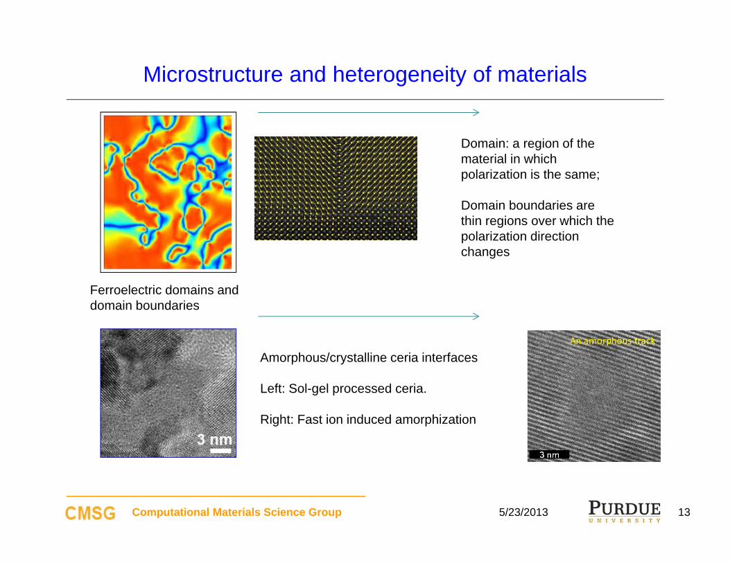
Ferroelectric domains and domain boundaries
Domain: a region of the material in which polarization is the same;
Domain boundaries are thin regions over which the polarization direction changes
Amorphous/crystalline ceria interfaces
Left: Sol-gel processed ceria.
Right: Fast ion induced amorphization
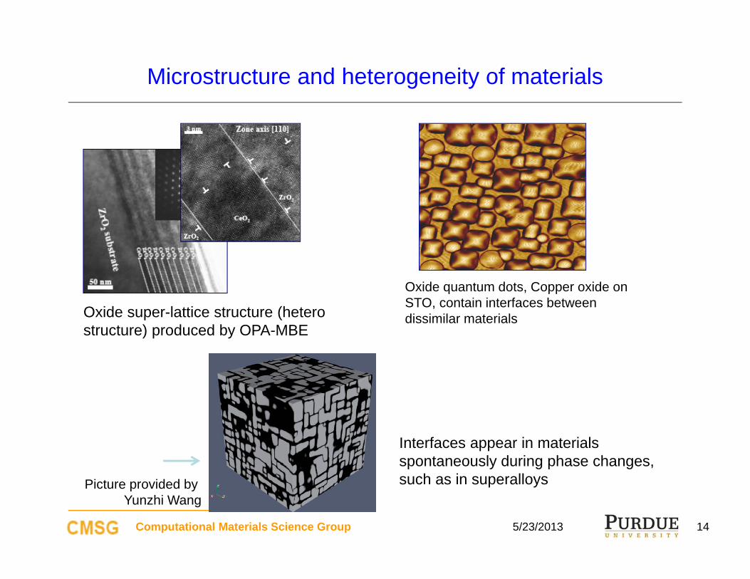
Microstructure and heterogeneity of materials
5/23/2013Computational Materials Science Group 14
Oxide super-lattice structure (hetero structure) produced by OPA-MBE
Oxide quantum dots, Copper oxide on STO, contain interfaces between dissimilar materials
Interfaces appear in materials spontaneously during phase changes, such as in superalloysPicture provided by
Yunzhi Wang
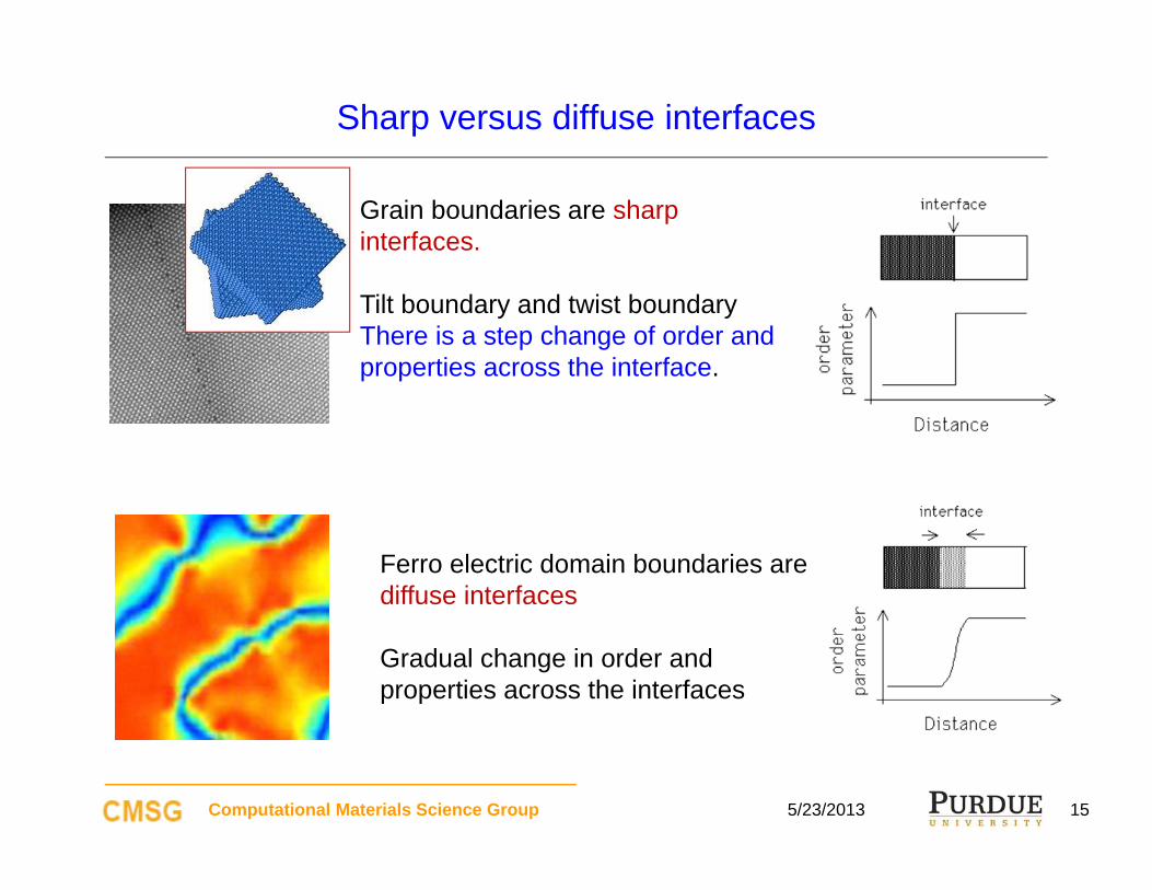
Sharp versus diffuse interfaces
5/23/2013Computational Materials Science Group 15
Grain boundaries are sharp interfaces.
Tilt boundary and twist boundaryThere is a step change of order and properties across the interface.
Ferro electric domain boundaries are diffuse interfaces
Gradual change in order and properties across the interfaces
Interfaces carry energy
Interfaces have energy associated with them
grain boundary energy
surface energy
hetero-phase interface energy (soli-solid interface, solid-liquid interface)
domain boundary energy
The energy of interfaces is often sensitive to chemical, mechanical
or physical state of the interface.
5/23/2013Computational Materials Science Group 16

What are transitions?
A transition is a process by which the material changes its energy state.
Transitions are thermally activated.
Transitions that are continuous in time are called kinetic processes.
5/23/2013Computational Materials Science Group 17
Outline
5/23/2013Computational Materials Science Group 18
Part I
Basic Concepts
– Introduction to microstructure and composition evolution in materials
– Interfaces and diffuse interfaces in materials
– Free energy of heterogeneous materials systems
– Non-equilibrium thermodynamics and evolution
– The phase field method, phase field equations and numerical solution
Part II:
Two example problems
– Grain growth
– Void formation under irradiation
A survey of applications
Microstructure and micro chemical evolution
5/23/2013Computational Materials Science Group 19
Microstructure change is a morphological evolution process that
occurs in order to lower the free energy of the material.
Micro chemical evolution is a composition change that occurs to also
lower the free energy.
Microstructure and micro chemical changes can be coupled in
certain material systems.
Sometimes, these changes occur while the free energy is not
decreasing – case of driven materials acted upon by external forces
of mechanical, thermal, chemical or physical nature.

The energy (or, in general, the thermodynamic) state of the material is fixed by the thermodynamic state variables and the material configuration.
The collection of energy states is called the energy landscape. Evolution is motion over this energy landscape under the action of thermodynamic forces.
5/23/2013Computational Materials Science Group 20
Energy state of a material
A material relaxing towards a local equilibrium state
A material at an equilibrium state
Material at a metastable state
A material driven away from equilibrium
State variables
Free
ene
rgy
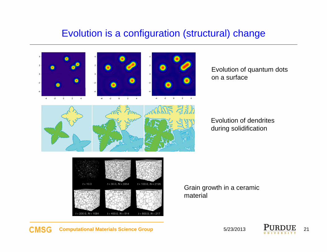
Evolution is a configuration (structural) change
5/23/2013Computational Materials Science Group 21
Evolution of quantum dots on a surface
Evolution of dendrites during solidification
Grain growth in a ceramic material

Micro chemical evolution
5/23/2013Computational Materials Science Group 22
Evolution of composition field in Cu-Au alloy under irradiation
This is also an example of a driven material system.

• Nucleation and growth of new phases.
• Continuous transformation
(spinodal instabilities, order-disorder transition)
• Nucleation and growth involve interface motion, coupled with diffusion (atomic/defect fluxes throughout the system)
• Not all phase changes involve diffusion
Motion of interfaces by atomic or molecular rearrangement locally (spin, polarization, …) or by short range diffusion
Motion of a grain boundary
Motion of a free surface
Etc
Phase Transformations Interface motion
Phase transformation versus interface motion
Computational Materials Science Group 5/23/2013 23

What makes things happen in a material?
The thermodynamic state
Current state
Equilibriumstate
?
Current state is an equilibrium state
Current state is not an equilibrium state
Nothing happens Something will happen
Phase transformation and microstructure evolution occurs to bring material from non-equilibrium states to equilibrium states.
The driving force for evolution
Computational Materials Science Group 5/23/2013 24

An equilibrium state is characterized by a minimum free energy. This energy
depends on the imposed physical, chemical, mechanical constraints (state
variables)
Gibbs free energy,
U, H, S and F are internal energy, enthalpy, entropy and Helmholtz free
energy.
If G can be made smaller by an internal change in the material keeping T ,
P fixed, then the material is in an unstable state.
If G cannot be made smaller, then it is at its global free energy minimum
and it is stable .
G U TS PVF PVH TS
Computational Materials Science Group 5/23/2013 25
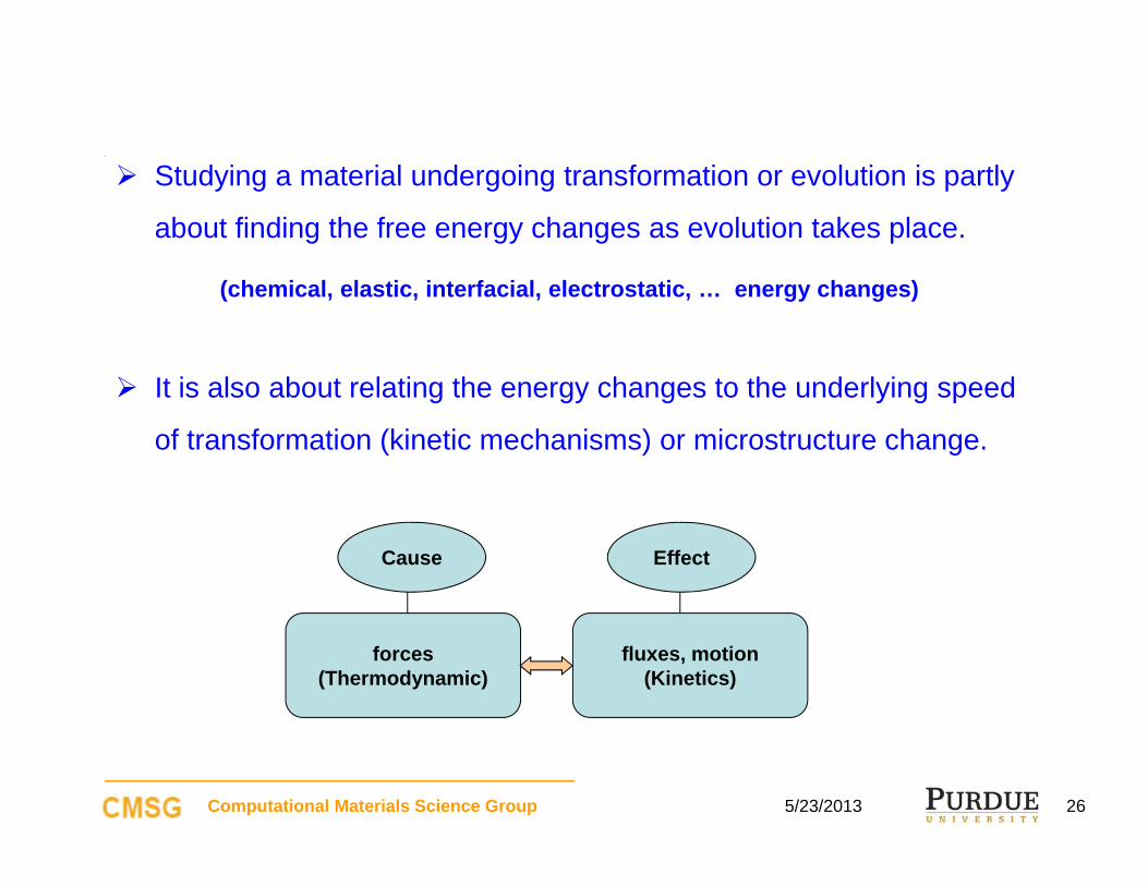
Studying a material undergoing transformation or evolution is partly
about finding the free energy changes as evolution takes place.
(chemical, elastic, interfacial, electrostatic, … energy changes)
It is also about relating the energy changes to the underlying speed
of transformation (kinetic mechanisms) or microstructure change.
Computational Materials Science Group 5/23/2013
forces(Thermodynamic)
fluxes, motion(Kinetics)
EffectCause
26

Modeling phase changes starts out by defining the appropriate order
parameters that describe the thermodynamic state of the material,
and by developing equations for the time and space evolution
(kinetic equations) of the order parameters.
The analysis is thus about the “ temporal evolution of a materials
initiated by variations in order parameters from equilibrium states”.
Computational Materials Science Group 5/23/2013 27
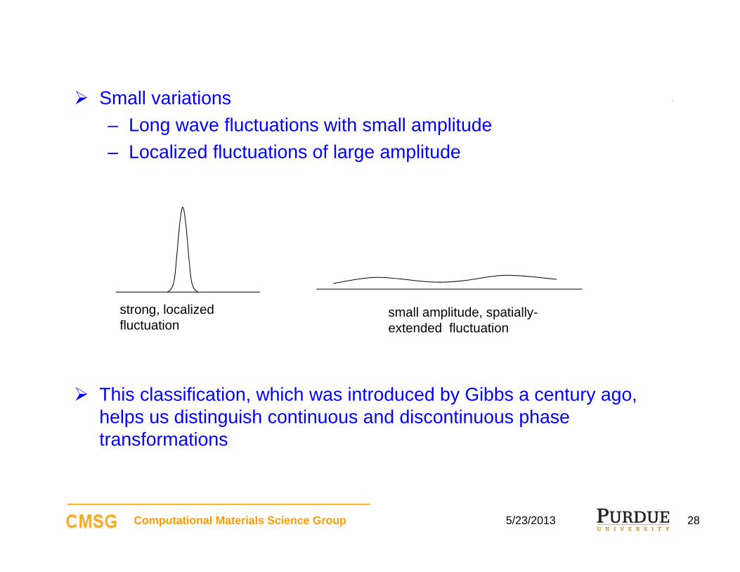
Small variations– Long wave fluctuations with small amplitude– Localized fluctuations of large amplitude
This classification, which was introduced by Gibbs a century ago, helps us distinguish continuous and discontinuous phase transformations
strong, localized fluctuation
small amplitude, spatially-extended fluctuation
Computational Materials Science Group 5/23/2013 28

We consider the molar free energy F and an internal variable for a one-component system at fixed volume. is an internal thermodynamic variable that cannot be controlled directly, and it is thus a characteristic of the transformation process.
Molar free energy as a function of T for a melting transition
Temperature-dependent order parameter
One component systems
Computational Materials Science Group 5/23/2013 29

For fixed V, the equilibrium value of F depends only on T.
The equilibrium value of , eq(T) can be found from:
At equilibrium , Feq (T, eq(T) )
((x) - eq(T)) is a local measure of departure from equilibrium.
21 2( , ) ( ) ( ) ( )oF T a T a T a T
(Landau expansion)
/ 0T
F
Computational Materials Science Group 5/23/2013 30

Order parameters may refer to the underlying crystal structure or
symmetry properties.
In a ferroelectric material, an ion is always displaced in some
direction or its opposite relative to center of the unit cell (both
directions are energetically equivalent). If we choose an order
parameter to describe this, the expression of the free energy
(molar Gibbs energy) will only include even powers of ,
2 4, , ( , ) ( )( ) ( )o cG T P G T P a P T T B P
Other types of order parameters
Computational Materials Science Group 5/23/2013 31
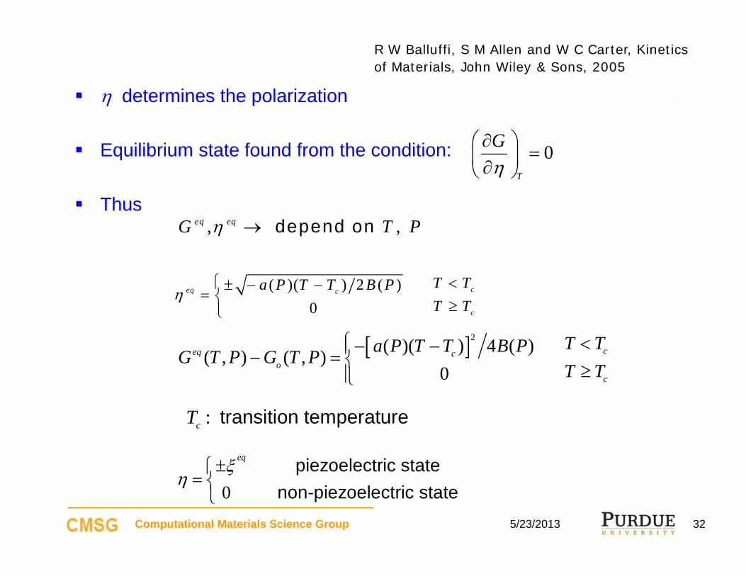
determines the polarization
Equilibrium state found from the condition:
Thus, ,depend on eq eqG T P
( )( ) 2 ( )0
ceq c
c
T Ta P T T B PT T
:cT transition temperature
2( )( ) 4 ( )( , ) ( , )0
ceq co
c
T Ta P T T B PG T P G T PT T
0piezoelectric state
non-piezoelectric state
eq
0T
G
R W Balluffi, S M Allen and W C Carter, Kinetics of Materials, John Wiley & Sons, 2005
Computational Materials Science Group 5/23/2013 32

The previous two examples refer to equilibrium of homogeneous
systems we worked with molar free energy functions.
In a heterogeneous system, we work with the corresponding free energy
functionals (the total free energy of the heterogeneous system).
Spatial dependence
comes into the picture
Computational Materials Science Group 5/23/2013 33

Outline
5/23/2013Computational Materials Science Group 34
Part I
Basic Concepts
– Introduction to microstructure and composition evolution in materials
– Interfaces and diffuse interfaces in materials
– Free energy of heterogeneous materials systems
– Non-equilibrium thermodynamics and evolution
– The phase field method, phase field equations and numerical solution
Part II:
Two example problems
– Grain growth
– Void formation under irradiation
A survey of applications

5/23/2013Computational Materials Science Group 35
The phase field approach
Phase field is an approach for modeling evolution in heterogeneous
materials.
The concept evolved from early work by theoretical physicists on
thermodynamics of heterogeneous systems (1950-70s).
Original name: field theoretic approach.
The approach focuses on the thermodynamics and kinetics of
heterogeneous systems, with a connection to the statistical
mechanical description of the underlying atomic systems.

5/23/2013Computational Materials Science Group 36
Phase field ‘cont.’
Field theoretic models start with a representation of the free energy functional of the heterogeneous material system in terms of order parameters
We do two things with free energy– Either minimize it to find the ‘shape’ of fields over a domain
– Or use non-equilibrium thermodynamics and develop kinetic equations, with driving forces defined from the free energy.
We thus have variational and evolutionary phase field formalisms.
[ , ] ( , ) ( , ) b iG c g c d g c d
,min [ , ]
cG c

Order parameters may by derived from extensive variables such as
mass or composition.
- Kinetic equations that apply to such order parameters must
satisfy the conservation principles that the extensive variables
satisfy.
Ferroelectric polarization, magnetic spin, crystal lattice orientation,
etc., are not subject to conservation principles.
– We call the corresponding variables non-conserved order parameters.
Conserved and non-conserved order parameters
5/23/2013Computational Materials Science Group 37

Random solid solutions:
- Use conserved order parameters (concentrations).
- Kinetic equations are generalized diffusion equations.
Solid solution that can developed ordered phases:
- Use conserved order parameters for concentrations and non-
conserved order parameters for long-range order.
- Two types of evolution equations.
Order parameters in two component solids
5/23/2013Computational Materials Science Group 38

In a binary alloy A-B in equilibrium at a molar concentrations XB , a small fluctuation of composition, , results in a change in the free energy G(XB) , which we write in terms of δXB as follows:
First order term is trivial (by equilibrium requirement), and the free erngychange is given by
The variation in molar free energy is proportional to (δXB)2, for conserved species.
If is positive, a barrier exists for the growth of localized fluctuations (nucleation). Otherwise, transformation is barrierless.
' oB B BX X X
2
2'2
1( ) ( )2o o
B B B B
oB B B B B
B BX X X X
G GG X G X X XX X
2
2'2
1( )2 o
B B
B BB X X
GG X XX
2 2/ BG X
Energy changes
5/23/2013Computational Materials Science Group 39

For non-conserved order parameters, the lowest-order term for change in molar free energy is,
o
GG
5/23/2013
R W Balluffi, S M Allen and W C Carter, Kinetics of Materials, John Wiley & Sons, 2005
Computational Materials Science Group 40
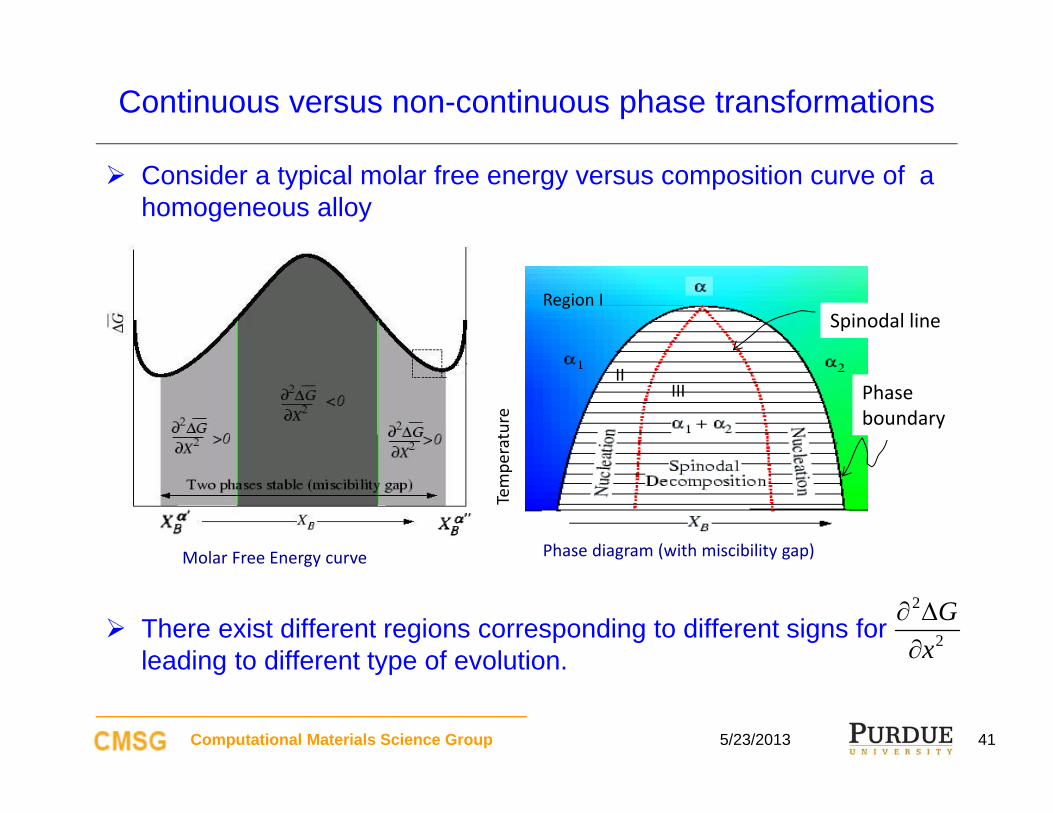
Consider a typical molar free energy versus composition curve of a homogeneous alloy
There exist different regions corresponding to different signs forleading to different type of evolution.
Molar Free Energy curve Phase diagram (with miscibility gap)
Spinodal line
Phase boundary
Tempe
rature
Region I
IIIII
2
2G
x
Continuous versus non-continuous phase transformations
5/23/2013Computational Materials Science Group 41

Consider a part of free energy where curvature is negative and suppose we have spatial fluctuations in composition.
Free energy change is negative for small fluctuation change. The system is thus inherently unstable and phase separation proceeds.
Condition for spinodal decomposition:
Uphill diffusion.
2
20
mixing
B
GX
Spinodal instability
5/23/2013
R W Balluffi, S M Allen and W C Carter, Kinetics of Materials, John Wiley & Sons, 2005
Computational Materials Science Group 42

Consider a region of free energy in which curvature is positive.
The system is stable (“meta-stable”) with respect to small fluctuations in composition.
And a large (localized) composition fluctuation is required to decrease the free energy.
The system separates as illustrated through a process of nucleation.
Note: the new phase must initiate with a composition that is not near that of the parent phase.
Nucleation and growth
5/23/2013
R W Balluffi, S M Allen and W C Carter, Kinetics of Materials, John Wiley & Sons, 2005
Computational Materials Science Group 43
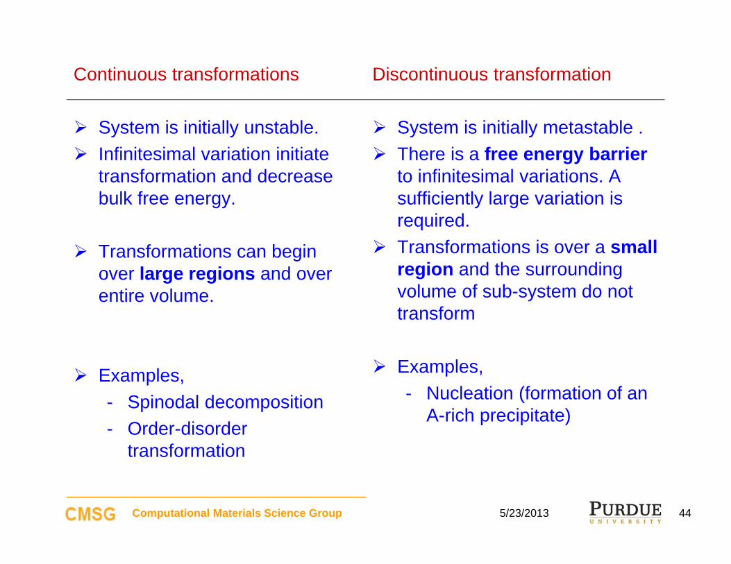
Continuous transformations
System is initially unstable. Infinitesimal variation initiate
transformation and decrease bulk free energy.
Transformations can begin over large regions and over entire volume.
Examples, - Spinodal decomposition- Order-disorder
transformation
Discontinuous transformation
System is initially metastable . There is a free energy barrier
to infinitesimal variations. A sufficiently large variation is required.
Transformations is over a small region and the surrounding volume of sub-system do not transform
Examples, - Nucleation (formation of an
A-rich precipitate)
5/23/2013Computational Materials Science Group 44

Cahn-Hilliard (generalized diffusion) equation applies. It accounts for concentration gradients in free energy construction.
is a matrix of mobility's of the conserved species
is the chemical potential of the species
The gradient energy coefficients account for inhomogeneities in the concentration field.
Substituting variational derivative, we get the kinetic equation,
( , )( , )
iciij fluct
j
c t FMt c t
r
r
2( , ) ( , ) ( , )ciij i
j
c t f tM c tt c
r r r
ijM
jj
Fc
ci
Kinetics of a conserved order parameter
5/23/2013Computational Materials Science Group 45

For formalism, see:
J W Cahn and J E Hilliard, Free enrgy of a nonuniform system. I. Interface free energy, J Chem Phys, 28 (1957) 258.
5/23/2013Computational Materials Science Group 46

Allen-Cahn (Ginsburg-Landau) equation applies to kinetics of nonconserved order parameters.
is the interfacial mobility matrix; it is related to microscopic rearrangement kinetics. The K.E. can be rewritten in the form:
is the gradient energy coefficient which accounts for the gradients in nonconserved field.
Depending on initial variations in η , a system may seek minima such that ηwill be attracted to local minima of .
( , )( , )
ppq
q
t FLt t
r
rpqL
q
homf
2( , ) ( , ) ( , )ppq q
q
t f tL tt
r r r
Kinetics of a non-conserved order parameter
5/23/2013
Bad notation;
F is used for G from now on.
Computational Materials Science Group 47

5/23/2013Computational Materials Science Group 48
The phase field approach is based on the kinetic equations for the conserved and non-conserved order parameters
,c FM tt c
x
,FL tt
x
Cahn-Hilliard Eq.
Allen-Cahn (G.L.) Eq.
Formally, is the variable called the phase field but nowadays the approach itself is called phase field …
5/23/2013Computational Materials Science Group 49
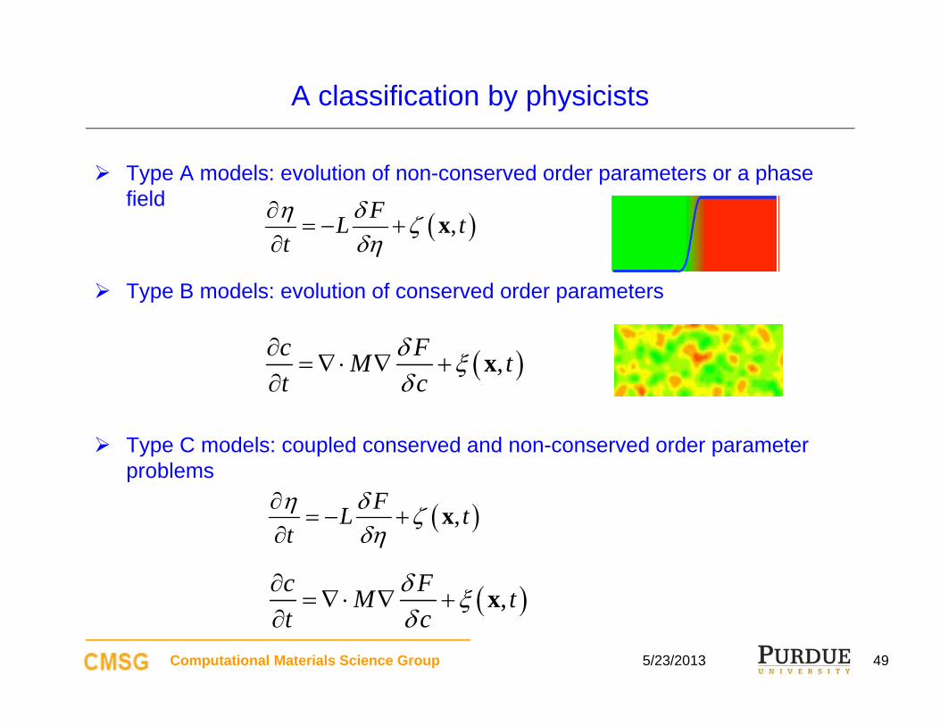
A classification by physicists
Type A models: evolution of non-conserved order parameters or a phase field
Type B models: evolution of conserved order parameters
Type C models: coupled conserved and non-conserved order parameter problems
,c FM tt c
x
,FL tt
x
,c FM tt c
x
,FL tt
x
5/23/2013Computational Materials Science Group 50
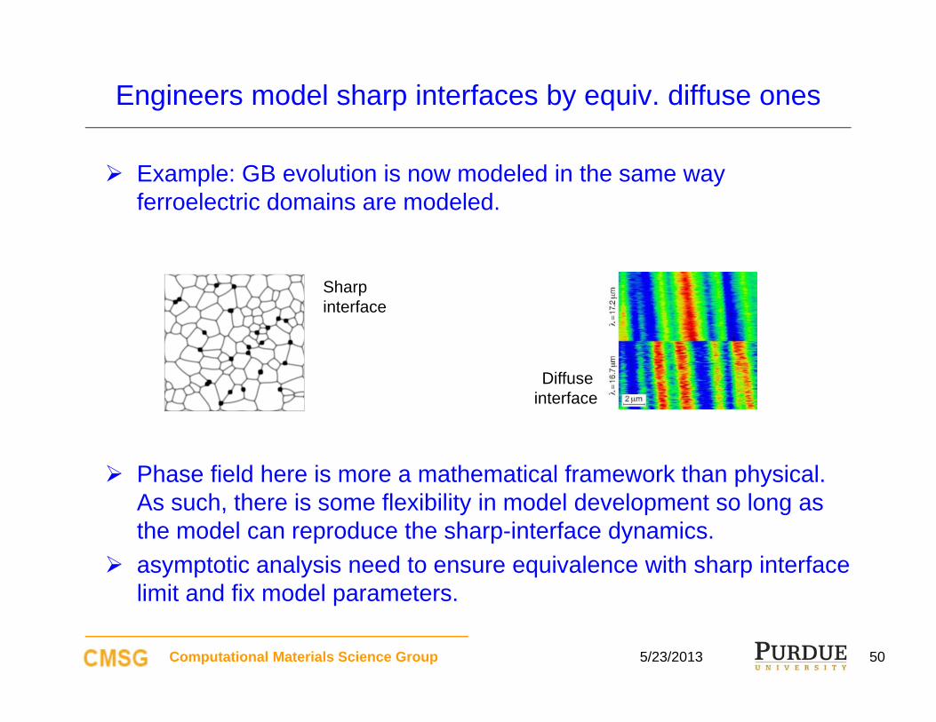
Engineers model sharp interfaces by equiv. diffuse ones
Example: GB evolution is now modeled in the same way ferroelectric domains are modeled.
Phase field here is more a mathematical framework than physical. As such, there is some flexibility in model development so long as the model can reproduce the sharp-interface dynamics.
asymptotic analysis need to ensure equivalence with sharp interface limit and fix model parameters.
Sharp interface
Diffuse interface
5/23/2013Computational Materials Science Group 51
Numerical solution
Phase field equations are often non-linear and strongly coupled.
They are also often spatially and temporally stiff.
All numerical machinery for PDE solution can work.
Methods used:– Spatial discretization: FD, FEM, FV, spectral– Time discretization: first order and higher order, explicit and implicit

5/23/2013Computational Materials Science Group 52
Constructing a phase field model
Determine phase field variables that fit the problem at hand
Develop a form for the free energy of the system in terms of these
variables
Determine the energy and kinetic parameters
Write the kinetic evolution equations and solve them
5/23/2013Computational Materials Science Group 53
Summary
Basic concepts of microstructure and micro chemical evolution in materials were given.
The underlying thermodynamics concepts were reviewed.
Application to heterogeneous materials led to the development of phase field approach.
5/23/2013Computational Materials Science Group 54
References
S M Allen and J W Cahn, A microscopic theory for antiphase boundary motion and its application in antiphase domain coarsening, Acta Metallurgica, 27 (1979) 1085
J W Cahn and J E Hilliard, Free enrgy of a nonuniform system. I. Interface free energy, J Chem Phys, 28 (1957) 258
Alexander Umantsev, Field Theoretic Method in Phase Transformation, Springer, 2012
R W Balluffi, S M Allen and W C Carter, Kinetics of Materials, John Wiley & Sons, 2005
Nikolas Provatas and Ken Elder, Phase field methods in materials science and engineering, Wiley-VCH