Phase 3A: HRA (Health Risk Assessment) …...Phase 3A: HRA (Health Risk Assessment) Concentration...
85
Meteorological and Dispersion Modelling Using TAPM for Wagerup Phase 3A: HRA (Health Risk Assessment) Concentration Modelling – Current Emission Scenario Final Report Prepared for Alcoa World Alumina Australia P. O. Box 252, Applecross, Western Australia, 6153 By CSIRO Atmospheric Research Private Bag 1 Aspendale, Vic 3195 Tel: (03) 9239 4400 Fax: (03) 9239 4444 Contact: E-mail: [email protected] Report C/0986 14 February 2005
Transcript of Phase 3A: HRA (Health Risk Assessment) …...Phase 3A: HRA (Health Risk Assessment) Concentration...

Meteorological and Dispersion Modelling Using
TAPM for Wagerup
Phase 3A: HRA (Health Risk Assessment) Concentration Modelling – Current Emission Scenario
Final Report
Prepared for
Alcoa World Alumina Australia P. O. Box 252,
Applecross, Western Australia, 6153
By CSIRO Atmospheric Research
Private Bag 1 Aspendale, Vic 3195
Tel: (03) 9239 4400 Fax: (03) 9239 4444
Contact: E-mail: [email protected]
Report C/0986 14 February 2005

This report has been prepared by CSIRO for its client and CSIRO (including its employees and consultants) unless otherwise agreed, makes no representations or warranties regarding merchantability, fitness for purpose or otherwise with respect to the Report. Any third party relying on the Report does so entirely at their own risk. CSIRO and all persons associated with it exclude all liability (including liability for negligence) in relation to any opinion, advice or information contained in this Report, including, without limitation, any liability which is consequential on the use of such opinion, advice or information to the full extent of the law, including, without limitation, consequences arising as a result of action or inaction taken by that person or any third parties pursuant to reliance on the Report. Project Team:
Mark Hibberd Peter Hurley Mary Edwards Ashok Luhar Ian Galbally Simon Bentley

PHASE 3A. FINAL REPORT
CSIRO Atmospheric Research Page 2 TAPM Modelling for Wagerup: Phase 3A. Current Refinery Modelling for HRA
Contents EXECUTIVE SUMMARY........................................................................................................................3
GLOSSARY................................................................................................................................................5
1. INTRODUCTION ............................................................................................................................12
2. TAPM ................................................................................................................................................15 2.1. TAPM SETTINGS.........................................................................................................................17
3. MODEL INPUTS .............................................................................................................................20 3.1. SOURCES .....................................................................................................................................20 3.2. SOURCES MODELLED...................................................................................................................23 3.3. EMISSION RATES .........................................................................................................................27 3.4. NOX TO NO2 CONVERSION ..........................................................................................................33 3.5. MODELLING SHORT-TERM PEAK CONCENTRATIONS...................................................................34
4. MODEL OUTPUTS .........................................................................................................................37 4.1. RECEPTOR LOCATIONS................................................................................................................37 4.2. UNCERTAINTY IN MODELLED CONCENTRATIONS.........................................................................38 4.3. QUALITY ASSURANCE RUNS .......................................................................................................42 4.4. CONCENTRATION STATISTICS (SORTED BY SPECIES) ...................................................................43 4.5. CONCENTRATION STATISTICS (SORTED BY RECEPTOR SITE) .......................................................55 4.6. CONCENTRATION CONTOURS......................................................................................................66 4.7. PEAK EVENTS..............................................................................................................................76
5. SUMMARY.......................................................................................................................................81
6. REFERENCES .................................................................................................................................82

PHASE 3A. FINAL REPORT
CSIRO Atmospheric Research Page 3 TAPM Modelling for Wagerup: Phase 3A. Current Refinery Modelling for HRA
Executive Summary The work presented in this report is part of a study entitled “Meteorological and Dispersion Modelling Using TAPM for Wagerup”.
The aspect addressed here is Phase 3A: Concentration Modelling for the Health Risk Assessment (HRA) for the Current Emissions Scenario of 6,600 tonnes per day of alumina.
The concentration modelling was carried out using TAPM (The Air Pollution Model) with the configuration determined by the evaluations of meteorology in Phase 1 of the Study and dispersion in Phase 2, which evaluated TAPM for air quality predictions at Wagerup using a database of emissions and observed ambient air concentrations.
The following emission sources are included in the modelling: • Liquor Burner Stack • Calciner stacks 1, 2, 3, 4 • Boiler stacks 1, 2, 3 • Gas Turbine 1 stack • Calciner 1, 2, 3 Vac Pump, 50B and Dorrco • Calciner 4 Vac Pump and Dorrco • 45K Cooling Tower 1 • 45K Cooling Towers 2 and 3 • 50 Cooling Towers 1 and 2 • Milling Vents • 25A Tank Vents • 35A Vents • 35J Tank Vents.
The following chemical species are included in the modelling: • 1,2,4, trimethylbenzene • 1,3,5 trimethylbenzene • 2-butanone • acetaldehyde • acetone • acrolein • ammonia • arsenic • benzo(a)pyrene equivalents • benzene • cadmium • carbon monoxide (CO) • chromium VI • dust • ethylbenzene • formaldehyde • manganese • mercury • methylene chloride

PHASE 3A. FINAL REPORT
CSIRO Atmospheric Research Page 4 TAPM Modelling for Wagerup: Phase 3A. Current Refinery Modelling for HRA
• nickel • nitrogen dioxide (NO2) • oxides of nitrogen(NOx) • selenium • styrene • sulphur dioxide (SO2) • toluene • vinyl chloride • xylenes.
Each of these species is released at different rates from one or more of the emission sources listed above. Modelling has been carried out for the Current Emissions Scenario (i.e. an Alumina production rate of 6,600 tonnes per day). Two sets of emissions have been considered – the Average emission rates and the Peak emission rates. The emission rates used have been provided by Alcoa World Alumina Australia. CSIRO has had no role in the development or verification of these emissions. The atmospheric concentrations modelled in this study are the direct consequence of the emissions included in the model. Different emission rates would produce different concentrations.
The following concentration statistics are tabulated at 15 receptor points located around and at distances up to 7 km from the Refinery:
• Annual average concentration (at average emission rates) • Maximum 1-hour average concentrations (at peak emission rates) • 95th percentile 1-hour average concentrations (at peak emission rates) • 95th percentile 24-hour average concentrations (at peak emission rates) • Maximum 10-minute average concentrations (at peak emission rates) • Maximum 3-minute average concentrations (at peak emission rates).
Concentrations were obtained from the model TAPM (version 2.6), which was run with four nested grid domains at 20-km, 7-km, 2-km, and 0.5-km resolution for meteorology (31 × 31 grid points). Similarly four nested domains of 53 × 53 horizontal grid points with resolutions of 10-km, 3.5-km, 1-km and 0.25-km were used for the pollutant dispersion modelling. The lowest ten of the 25 vertical levels were 10, 25, 50, 100, 150, 200, 250, 300, 400 and 500 m. The default databases of soil properties, topography, and the monthly sea-surface temperature and deep soil parameters (with a deep-soil moisture content of 0.15) were used. The Wagerup-specific land-use database and a refinery-generated surface heat flux value of 150 W m-2, both derived as part of the Phase 1 work (CSIRO, 2004b), were used. The runs included building wake effects with a total of 29 rectangular buildings included, ranging in height between 8 m and 42 m. In all the Phase 3 runs, the Lagrangian mode was used on the inner-most grid in the pollution dispersion calculations. The period modelled was one year from April 2003 to March 2004.
The uncertainty of the model predictions, based on consideration of results from a range of TAPM studies as well as uncertainties in the Wagerup region, is a factor of approximately 2 (i.e. the actual values lie in the range of +100% to -50% of the listed concentrations) at the 95% confidence level.

PHASE 3A. FINAL REPORT
CSIRO Atmospheric Research Page 5 TAPM Modelling for Wagerup: Phase 3A. Current Refinery Modelling for HRA
Glossary
Simple definitions of various technical terms are given here to assist the reader. If required, the reader should look to other sources for more formal and technical definitions.
ABL Atmospheric Boundary Layer. The ABL is the lowest 100 to 3000 m of the atmosphere modified by the earth’s surface. The ABL responds to surface forcings (i.e. heating, cooling, and roughness) with a time scale of about an hour or less, and its extent is deeper in the daytime and shallower in the nighttime. It is often turbulent and is capped by a temperature inversion (see definition below).
Aerosol A suspension of fine solid, liquid or mixed-phase particles in air.
AGL Height Above Ground Level
ANSTO Australian Nuclear Science and Technology Organisation (http://www.ansto.gov.au/)
AUSPLUME A simple, steady-state, Gaussian plume dispersion model used for predicting ground-level concentrations of pollutants from a variety of sources. It is a regulatory model developed and approved by EPA Victoria and other regulatory agencies. AUSPLUME requires input, which typically contains hourly values of temperature, wind speed, wind direction, stability, and mixing height.
BaP equivalents Benzo(a)pyrene equivalents. This species is used as a marker for a group of chemical compounds called Polycyclic Aromatic Hydrocarbons (PAH). The relative toxicities of the various PAHs have been assessed compared to BaP (e.g. Nisbet and LaGoy, 1992). Multiplying the concentration of each PAH by its relative toxicity yields a concentration for the total PAH mixture that is expressed in terms of an equivalent concentration (with regard to toxic potency) of BaP.
Buoyancy enhancement An increase in the effective buoyancy of a plume as a result of merging with another buoyant plume. This leads to greater plume rise of the combined plume than of the individual plumes.
CALMET A computer model providing the meteorological input for the dispersion model CALPUFF. It is driven by observed or large-scale model meteorology and is capable of calculating temporally and spatially varying wind fields.
CALPUFF An air pollution dispersion model developed by Earth Tech Inc. (USA). It simulates the transport and diffusion of a plume via the puff approach in which a plume is described as consisting of a series of puffs. CALPUFF

PHASE 3A. FINAL REPORT
CSIRO Atmospheric Research Page 6 TAPM Modelling for Wagerup: Phase 3A. Current Refinery Modelling for HRA
typically uses meteorological data generated by the processor CALMET. (http://www.src.com/calpuff/calpuff1.htm)
CAR CSIRO Atmospheric Research (http://www.dar.csiro.au)
CO Carbon monoxide
Combined source The representation of two or more closely-spaced emission sources (usually within the same stack) which have similar emission characteristics by a single source.
Convective mixed layer Also called the convective boundary layer, mixed layer or mixing layer. A type of atmospheric boundary layer (ABL) characterised by vigorous turbulence, generated by the solar heating of the ground, tending to stir and mix pollutants particularly in the vertical.
CSIRO Commonwealth Scientific and Industrial Research Organisation (http://www.csiro.au)
Diffusion In air pollution meteorology the words dispersion and diffusion are often used interchangeably. This is also the case in this report. However, strictly speaking the two words mean different things. Diffusion refers to dilution of pollutants by turbulent eddies in the atmosphere whose dimensions are smaller than that of a pollutant plume or a puff (see also Dispersion).
Dispersion Dispersion refers to the movement or transport of pollutants horizontally or vertically by the wind field and their dilution by atmospheric turbulence. Dispersion includes both transport and diffusion of pollutants (see also Diffusion).
Emission rate Specifies the rate at which gas or particles are emitted from a source. The quantity is expressed in units of grams per second.
EPAV Environment Protection Authority of Victoria (Australia) (http://www.epa.vic.gov.au)
Eulerian approach An approach to describing atmospheric diffusion in which the behaviour of species is described relative to a fixed coordinate system.
Exit temperature The temperature of the gas released from a source.
Exit velocity The velocity at which gases are emitted from source. For a stack, the volume flow rate from the stack is obtained by multiplying the exit velocity by the internal cross-sectional area of the top of the stack.
Exponential notation A notation used in scientific, engineering and computing applications to represent very large and small numbers without having to use a large number of zeros. For example, the value 4.8E-06 = 4.8×10-6 = 0.0000048.

PHASE 3A. FINAL REPORT
CSIRO Atmospheric Research Page 7 TAPM Modelling for Wagerup: Phase 3A. Current Refinery Modelling for HRA
GASP Global AnalySis and Prediction. A meteorological modelling system currently used by the Australian Bureau of Meteorology that can provide the large-scale (synoptic) meteorological input needed in the models TAPM and CALMET.
glc Ground-level concentration. Refers to pollutant concentrations at a height where it is detected by people standing on the ground. In modelling it is the concentration in the lowest model level, typically 0–10 m above the ground.
Inversion An atmospheric layer in which temperature increases with altitude (e.g. the layer above the atmospheric boundary layer). These layers are stable and resistant to vertical mixing and hence may restrict the dispersion of pollutants. Properly described as a temperature inversion.
Lagrangian approach An approach to describing atmospheric diffusion in which concentration changes are described relative to the moving fluid.
LAPS Limited Area Prediction System. A meteorological modelling system previously used by the Australian Bureau of Meteorology that can provide the large-scale (synoptic) meteorological input needed in the model TAPM.
mg Milligram (1 mg = 10-3 gram = 0.001 gram). One thousandth of a gram
mg m-3 Milligram per cubic metre. 1 mg m-3 = 1000 µg m-3
NBL Neutral Boundary Layer. A type of atmospheric boundary layer (ABL) that forms when winds are strong and/or when there is negligible heating or cooling of the ground (e.g. overcast conditions). The turbulence responsible for mixing under these conditions is generated by wind shear.
NO Nitric oxide
NOx Oxides of nitrogen (commonly NOx = NO + NO2)
NO2 Nitrogen dioxide
O3 Ozone
OU Odour Unit. The odour units are dimensionless and are effectively “dilutions to odour threshold.” An odour present at a concentration of 1 OU will be discerned as odourless by approximately half the population. 10 OU represents a mixture, which if diluted by 10 will then have an odour detected by 50% of the respondents and so forth.
Percentile The pth percentile is a value so that roughly p% of the data are smaller and (100-p)% of the data are larger than

PHASE 3A. FINAL REPORT
CSIRO Atmospheric Research Page 8 TAPM Modelling for Wagerup: Phase 3A. Current Refinery Modelling for HRA
this value; the 50th percentile is called the median. Quantile is a more general definition than percentile.
pg Picogram (1 pg = 10-12 gram = 0.000000000001 gram). One trillionth of a gram
pg m-3 Picogram per cubic metre. 1 pg m-3 = 0.000001 µg m-3
Pollutant Used in this report in the non-legal sense to refer to a chemical species being modelled by air pollution dispersion models, such as TAPM.
ppb Parts per billion (by volume): 1 ppb = 1/1000 ppm.
ppm Parts per million (by volume): a unit for the concentration of a gas in the atmosphere based on the mixing ratio approach. A concentration of 1 ppm is equivalent to a volume of 1 cubic metre of pure undiluted gas in 1 million cubic metres of air. The expression ppm (or ppb) is without dimensions. The ppm (or ppb) unit is useful because its value is unaffected by changes in temperature and pressure, and also because many sampling techniques are based on volume concentrations. Concentrations of gaseous compounds can be converted from mixing ratio units, e.g. ppm units (volumetric), to density units, e.g. mg m-3 (mass/volume), using the following formula:
,)15.273(4136.22
15.273)mmg( 3
TCM
C w
+×××
=−
where C is the concentration (ppm), Mw is the molecular weight of the gas, and T is the ambient temperature in degrees Celsius. At a temperature of 0 degrees Celsius, the conversion factor from 1 ppm to mg m-3 for nitrogen dioxide (NO2) is 2.050.
Prognostic equation Any equation governing a system that contains change with time of a quantity, and therefore can be used to determine the value of that quantity at a later time when the other terms in the equation are known.
Quantile The fraction (or percent) of points below the given value. That is, the 0.3 (or 30%) quantile is the point at which 30% percent of the data fall below and 70% fall above that value. Certain quantiles have special names. The 0.25-, 0.50-, and 0.75-quantiles are called the first, second and third quartiles. The 0.01-, 0.02-, 0.03-, ... , 0.98-, 0.99-quantiles are called the first, second, third, ... , ninety-eighth, and ninety-ninth percentiles.
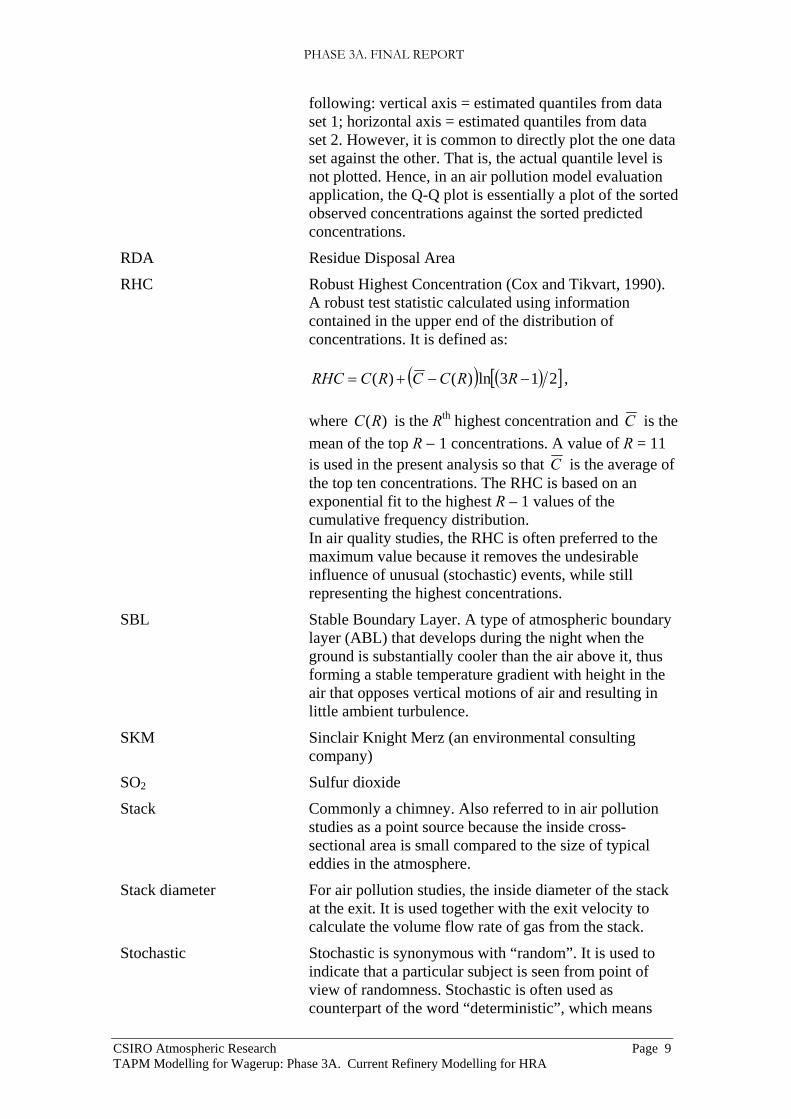
Q-Q plot A graphical data analysis technique for comparing the distributions of two data sets. The plot consists of the
PHASE 3A. FINAL REPORT
CSIRO Atmospheric Research Page 9 TAPM Modelling for Wagerup: Phase 3A. Current Refinery Modelling for HRA
following: vertical axis = estimated quantiles from data set 1; horizontal axis = estimated quantiles from data set 2. However, it is common to directly plot the one data set against the other. That is, the actual quantile level is not plotted. Hence, in an air pollution model evaluation application, the Q-Q plot is essentially a plot of the sorted observed concentrations against the sorted predicted concentrations.
RDA Residue Disposal Area
RHC Robust Highest Concentration (Cox and Tikvart, 1990). A robust test statistic calculated using information contained in the upper end of the distribution of concentrations. It is defined as:
( ) ( )[ ]213ln)()( −−+= RRCCRCRHC , where )(RC is the Rth highest concentration and C is the mean of the top R − 1 concentrations. A value of R = 11 is used in the present analysis so that C is the average of the top ten concentrations. The RHC is based on an exponential fit to the highest R – 1 values of the cumulative frequency distribution. In air quality studies, the RHC is often preferred to the maximum value because it removes the undesirable influence of unusual (stochastic) events, while still representing the highest concentrations.
SBL Stable Boundary Layer. A type of atmospheric boundary layer (ABL) that develops during the night when the ground is substantially cooler than the air above it, thus forming a stable temperature gradient with height in the air that opposes vertical motions of air and resulting in little ambient turbulence.
SKM Sinclair Knight Merz (an environmental consulting company)
SO2 Sulfur dioxide
Stack Commonly a chimney. Also referred to in air pollution studies as a point source because the inside cross-sectional area is small compared to the size of typical eddies in the atmosphere.
Stack diameter For air pollution studies, the inside diameter of the stack at the exit. It is used together with the exit velocity to calculate the volume flow rate of gas from the stack.
Stochastic Stochastic is synonymous with “random”. It is used to indicate that a particular subject is seen from point of view of randomness. Stochastic is often used as counterpart of the word “deterministic”, which means
PHASE 3A. FINAL REPORT
CSIRO Atmospheric Research Page 10 TAPM Modelling for Wagerup: Phase 3A. Current Refinery Modelling for HRA
that random phenomena are not involved.
TAPM The Air Pollution Model. A prognostic meteorological and air pollution dispersion model developed by CSIRO Atmospheric Research (http://www.dar.csiro.au/tapm). The meteorological component of TAPM predicts the local-scale flow, such as sea breezes and terrain-induced circulations, given the larger-scale synoptic meteorology. The air pollution component uses the model-predicted three-dimensional meteorology and turbulence, and consists of a set of species conservation equations and an optional particle trajectory module.
Temperature inversion see Inversion
TSP Total Suspended Particulates– all particles below about 50 µm in diameter suspended in the atmosphere.
US EPA United States Environmental Protection Agency (http://www.epa.gov)
Vent A short chimney or stack, usually located on top of a building to vent emissions from the building.
WA Western Australia
Wind data assimilation A technique in which at one or more locations in a meteorological model, the wind speed and wind direction in the model are adjusted towards those observed in the atmosphere. The model adjusts its airflow at this and surrounding locations to ensure that the model wind speed and direction at the location closely follow that observed.
µg Microgram (1 µg = 10-6 gram = 0.000001 gram). One millionth of a gram
µg m-3 Microgram per cubic metre: a unit for the concentration of a gas or particulate matter in the atmosphere based on the density approach (mass per unit volume of air). Concentrations of gaseous compounds can be converted from density units, e.g. mg m-3 (mass/volume), to mixing ratio units, e.g. ppm units (volumetric), using the following formula:
,15.273
)15.273(4136.22)ppm(wM
CTC×
×+×=
where C is the concentration (mg m-3), Mw is the molecular weight of the gas, and T is the ambient temperature in degrees Celsius. At a temperature of 0 degrees Celsius, the conversion factor from 1 mg m-3 to ppm for nitrogen dioxide (NO2) is 0.488.

PHASE 3A. FINAL REPORT
CSIRO Atmospheric Research Page 11 TAPM Modelling for Wagerup: Phase 3A. Current Refinery Modelling for HRA

PHASE 3A. FINAL REPORT
CSIRO Atmospheric Research Page 12 TAPM Modelling for Wagerup: Phase 3A. Current Refinery Modelling for HRA
1. Introduction
The Wagerup alumina refinery of Alcoa World Alumina Australia is located about 130 km south of Perth in Western Australia, 25 km inland from the coast and in the western foothills of the north-south Darling escarpment (Figure 1). The local communities in the proximity of the Refinery include Yarloop, a small town 15° west of south and 3 km away from the Refinery, and Hamel and Waroona, two small towns approximately 5 km and 8 km north of the Refinery (see Figure 1).
The work presented in this report forms Phase 3A of the project “Meteorological and Dispersion Modelling Using TAPM for Wagerup”. The larger project consists of the components:
• Phase 1: Meteorology Evaluation of the capability of CSIRO’s The Air Pollution Model (TAPM) to acceptably produce meteorological predictions matching available field observations at Wagerup (CSIRO, 2004b);
• Phase 2: Dispersion Evaluation of TAPM for air quality predictions at Wagerup using a database of emissions and observed ambient air concentrations (CSIRO, 2004c); and
• Phase 3: Concentration Modelling Use of TAPM to generate modelled concentrations as input for the Health Risk Assessment (HRA) and the Public Environmental Review Document concerning the Wagerup Refinery expansion plans.
The objective of Phase 3 is:
“To run TAPM with Wagerup specific input for four scenarios of emissions (Current-Average, Current-Peak, Expanded- Average, and Expanded-Peak) for agreed sources to produce selected concentration statistics at receptor points for input into the Health Risk Assessment and the Public Environmental Review Document. Investigate the temporal variation of concentration around, and mechanisms causing the modelled short-term peak concentrations.”
It has been agreed that the Phase 3 study be split into two parts; Phase 3A for the Current emission scenarios, and Phase 3B for the Expanded emissions scenarios. This report presents results from the Phase 3A modelling with the two emission scenarios corresponding to a production rate of 6,600 tonnes per day of alumina, namely Current-Average (average emission rates) and Current-Peak (peak emission rates).
The atmospheric concentrations modelled in this study are the direct consequence of the emissions included in the model. Different emission rates would produce different concentrations. The emissions used have been provided by Alcoa World Alumina Australia. CSIRO has had no role in the development or verification of these emissions.

PHASE 3A. FINAL REPORT
CSIRO Atmospheric Research Page 13 TAPM Modelling for Wagerup: Phase 3A. Current Refinery Modelling for HRA
Figure 1: A map of Wagerup area showing the Alcoa Wagerup Refinery, Bancell Road meteorological station, Residue Disposal Area (RDA) meteorological station, Boundary Road air quality monitoring station, and the Upper Dam monitoring site. The Yarloop monitoring site and the Waroona Monitor are non-operative. To the east of the Refinery is the north-south Darling escarpment (adapted from SKM, 2002).
Bancell Road met Station
Residue Disposal Area met station

PHASE 3A. FINAL REPORT
CSIRO Atmospheric Research Page 14 TAPM Modelling for Wagerup: Phase 3A. Current Refinery Modelling for HRA
The detailed objectives of Phase 3A are:
“Run the refined TAPM (as resolved in Phases 1 and 2) for the annual meteorological file (1 April 2003 to 31 March 2004) and agreed sources to produce estimates of the following parameters for 28 pollutants at 15 receptor points:
• Annual average concentration (at average emission rates) • Maximum 1-hour average concentrations (peak emissions) • 95th percentile 1-hour average concentrations (peak emissions) • 95th percentile 24-hour average concentrations (peak emissions) • Maximum 10-minute average concentrations (peak emissions) • Maximum 3-minute average concentrations (peak emissions).
The 28 pollutants are oxides of nitrogen(NOx), carbon monoxide (CO), sulphur dioxide (SO2), dust, arsenic, selenium, manganese, cadmium, chromium VI, nickel, mercury, ammonia, benzo(a)pyrene equivalents, acetone, acetaldehyde, formaldehyde, 2-butanone, benzene, toluene, xylenes, acrolein, ethylbenzene, methylene chloride, styrene, 1,2,4 trimethylbenzene, 1,3,5 trimethylbenzene, vinyl chloride, and nitrogen dioxide (NO2).
Produce contour plots of these six statistics for three example substances (NOx, Formaldehyde and Mercury) to indicate the different concentration distribution patterns for substances predominantly emitted from high and low level sources.
Calculate the conversion of NOx to NO2 using a simple titration algorithmic method.
Describe the best practice methods for deriving shorter time period (3 and 10-minute) maximum concentrations from the Wagerup hourly TAPM concentration fields.
Investigate the temporal variation of concentration around, and mechanisms causing the modelled 5 highest short-term peak concentrations for NOx and Formaldehyde for three receptors (at sites 1, 3, and 14) for the peak emission scenario.
Undertake separate quality assurance runs for selected pollutants to confirm the accuracy of the main modelling technique. Comment on the expected accuracy/level of confidence in model predictions, based on the work performed in Phases 1 and 2.”

PHASE 3A. FINAL REPORT
CSIRO Atmospheric Research Page 15 TAPM Modelling for Wagerup: Phase 3A. Current Refinery Modelling for HRA
2. TAPM The Phase 1 report of the present project (CSIRO, 2004b) provides a brief introduction to the various classes of air pollution models, and presents the advantages offered by the prognostic approach used by CSIRO’s The Air Pollution Model (TAPM) over some of the other commonly-used air pollution models. Although a brief description of TAPM has been given in the CSIRO (2004b) report, we describe TAPM here again for the sake of completeness.
TAPM is a three-dimensional, prognostic meteorological and air pollution model (see Hurley, 2002; http://www.dar.csiro.au/tapm/ for model details). The model uses a complete set of mathematical equations governing the behaviour of the atmosphere and the dispersion of pollutants. The global databases input to TAPM include terrain height (given at a resolution of about 300 m for Australia), land use, sea-surface temperature, and synoptic meteorological analyses. All input datasets, except emissions, accompany the TAPM software, and are easily transferred through a graphical user interface to nested grids for the region of interest.
The meteorological component of TAPM uses the large-scale weather information (synoptic analyses or, potentially, weather forecasts), typically obtained from the Bureau of Meteorology LAPS (Limited Area Prediction System) or GASP (Global Analysis and Prediction) analyses at a horizontal grid spacing of about 100 km at 6-hourly intervals as boundary conditions for the model outer grid. These synoptic data are for the horizontal wind components, temperature and moisture, and are obtained from the output of Bureau of Meteorology meteorological model(s) that assimilates meteorological observations from a network of stations. The vertical levels of the synoptic analyses are in a scaled pressure coordinate system. For the present application, the lowest of these correspond typically to 0, 75, 200, 425, 650, 875, 1100, 1325 and 1800 m above mean-sea level. TAPM then ‘zooms-in’ from the 100-km data to model local scales at a finer resolution using a one-way nested approach to improve efficiency and resolution, predicting local-scale meteorology (typically down to a resolution of 1 km), such as sea breezes and terrain induced flows.
The model solves a set of momentum equations for horizontal wind components, the incompressible continuity equation for the vertical velocity in a terrain-following coordinate system, and scalar equations for potential virtual temperature, specific humidity of water vapour, cloud water and rain water. Pressure is determined from the sum of hydrostatic and (when necessary) non-hydrostatic components, and a Poisson equation is solved for the non-hydrostatic component. Explicit cloud microphysical processes are included. Wind observations can optionally be assimilated into the momentum equations as nudging terms. The turbulence closure terms in the mean equations use a gradient diffusion approach, including a counter-gradient term for the heat flux, with eddy diffusivity determined using prognostic equations for turbulence kinetic energy and eddy dissipation rate. A weighted vegetative canopy, soil and urban land-use scheme is used to predict energy partitioning at the surface, while radiative fluxes, both at the surface and at upper levels, are also included. Boundary conditions for the turbulent fluxes are determined by Monin-Obukhov surface-layer scaling variables and parameterisations for stomatal resistance.
The air pollution component of TAPM consists of an Eulerian (fixed location) grid-based set of species conservation equations for determining a spatially explicit distribution of time varying ground-level pollutant concentrations, either using the Eulerian grid-based approach and/or a Lagrangian particle approach targeted at

PHASE 3A. FINAL REPORT
CSIRO Atmospheric Research Page 16 TAPM Modelling for Wagerup: Phase 3A. Current Refinery Modelling for HRA
important point sources. In the Lagrangian mode (where the model coordinates move with the flow), mass is represented as a puff in the horizontal direction and as a particle in the vertical direction. The Lagrangian option was used in the present work. The pollutants are transported and dispersed according to the air motions determined by the meteorological component.
Previous versions of TAPM have been used, for example, to model year-long meteorology and air pollution for the industrial area of Kwinana (Hurley et al., 2001) and the Pilbara (Physick and Blockley, 2001; Physick et al., 2002); to model year-long urban meteorology, photochemical smog and particulate matter in Melbourne (Hurley et al., 2003a); and to compare with international model validation data sets (Luhar and Hurley, 2003).
The performance of the meteorological component of TAPM is discussed in Section 10 of the Phase 1 report (CSIRO, 2004b) – for completeness, the main results are repeated here.
The Index of Agreement has been found to be the most useful measure of the degree to which the observed variable is accurately estimated by the model. It is defined as:
( )
( )2
1
2
11
∑
∑
=
=
−+−
−−=
N
imeanimeani
N
iii
OOOP
OPIOA , (1)
where N is the number of observations O and predictions P. An IOA value of 0 means no agreement whereas a value of 1 means perfect agreement. A value greater than 0.5 represents a good result for prediction of meteorology.
For the model comparisons presented in the Phase 1 report for Wagerup, the overall IOA for TAPM for the near-surface meteorology (with winds at 30 m AGL) at Bancell Road is 0.65 for wind speed, 0.79 for the U component, and 0.92 for the V component, 0.97 for temperature, 0.94 for net radiation, and 0.87 for relative humidity. For the winter months, when low to moderate winds are important from the point of view of point source emissions from the Refinery, the respective IOA values are 0.79, 0.86, 0.93, 0.89, and 0.81. The overall IOA for the near-surface meteorology at RDA is 0.73 for wind speed, 0.83 for the U component, and 0.90 for the V component. For the summer months, when high and variable winds are relevant from the point of view of dust emissions and management at RDA, the respective IOA values are 0.65, 0.79 and 0.84. In the summer months, the IOA values for net radiation and relative humidity at Bancell Road are 0.94 and 0.90, respectively.
The comparisons presented in the Phase 1 report indicate that TAPM’s overall performance is as good as and in some cases better than some of the other internationally used prognostic meteorological models such as MM5, RAMS, and CSU. The performance of TAPM at Wagerup is comparable to its performance elsewhere for the near-surface meteorology, except that TAPM generally predicts stronger wind speeds at Wagerup than the measurements. Its performance for wind speed at Wagerup is not as good as the best of TAPM modelling for other locations. This may be due to the complexity of the area being studied.

PHASE 3A. FINAL REPORT
CSIRO Atmospheric Research Page 17 TAPM Modelling for Wagerup: Phase 3A. Current Refinery Modelling for HRA
The uncertainty of the TAPM modelling of ground-level concentrations is discussed in more detail in Section 4.2 of this report. For the RHC (robust highest concentration, see Glossary) the ratio of modelled to observed values for a range of TAPM studies shows an average value of 1.07 with an uncertainty of ±40% at the 95% confidence level.
2.1. TAPM Settings Version 2.6 of TAPM was used for all the simulations presented in this report. This is the same version as used in Phases 1 and 2 (CSIRO, 2004b, c) of the present project. The most appropriate settings of TAPM for the Wagerup modelling have been described in Phase 1 (Meteorology) and Phase 2 (Dispersion), the latter of which evaluated TAPM using several different databases of emissions and observed ambient air concentrations at Wagerup.
The meteorological grids used here are the same as those used in Phase 2, but the pollution grids cover a larger area to include all the defined receptor points (Figure 2). Four nested domains of 31 × 31 horizontal grid points with resolutions of 20-km, 7-km, 2-km and 0.5-km are used for the meteorological modelling. Similarly four nested domains of 53 × 53 horizontal grid points with resolutions of 10-km, 3.5-km, 1-km and 0.25-km are used for the pollutant dispersion modelling. The pollution grid was selected to include all receptor points (Figure 2(d) and Figure 8) with the best possible combination of fine grid resolution and model computing time. The grids are all centred on the location 115°54′ E, 32°54.5′ S, which is equivalent to 397.133 km east and 6358.326 km north in the AMG84 (Australian Map Grid) coordinate system. The centre point is about 1 km north-west of the Refinery and was selected to optimise the locations of the grids with respect to the receptors. This centre point is situated 2 km north-northwest of the centre point used in the Phase 2 modelling and 3.8 km slightly west of north from the centre point used in the Phase 1 modelling. The lowest ten of the 25 vertical levels were 10, 25, 50, 100, 150, 200, 250, 300, 400 and 500 m, with the highest model level at 8000 m. The default databases of soil properties, topography, and the monthly sea-surface temperature and deep soil parameters (with a deep-soil moisture content of 0.15) were used. The Wagerup-specific land-use database and a refinery-generated surface heat flux value of 150 W m-2, both derived as part of the Phase 1 work (CSIRO, 2004b), were used. The change in the centre of the grids compared to Phases 1 and 2 produced slight changes in the apparent pattern of land-use because of the need to map the underlying complex pattern of land-use onto a single value for each grid square of the TAPM grids. However, the sensitivity tests reported in the Phase 2 report indicate that the model results at the receptor points change by less than 10% for runs with and without the Refinery heat flux. This is indicative of the sensitivity of the model to the slight changes caused by different grid centres. In all the Phase 3 runs, the Lagrangian mode was used on the inner-most grid in the pollution dispersion calculations and the Eulerian mode was used on the outer grid pollutant calculations.
The TAPM runs included building wake effects. A total of 29 rectangular buildings were considered, ranging in height between 8 m and 42 m. The locations and horizontal size of these buildings are shown in Figure 3, based on data supplied by Pitts (pers. comm. 20 Aug 2004). The figure also shows the locations of the Wagerup Refinery point sources modelled in this work, as supplied by Coffey (pers. comm. 7 Sep 2004).

PHASE 3A. FINAL REPORT
CSIRO Atmospheric Research Page 18 TAPM Modelling for Wagerup: Phase 3A. Current Refinery Modelling for HRA
(a) (b)
100 200 300 400 500 600 700AMG Easting (km)
6100
6200
6300
6400
6500
6600
AM
G N
orth
ing
(km
)
300 350 400 450 500
AMG Easting (km)
6250
6300
6350
6400
6450
AM
G N
orth
ing
(km
)
(c) (d)
370 380 390 400 410 420AMG Easting (km)
6330
6340
6350
6360
6370
6380
AMG
Nor
thin
g (k
m)
390 392 394 396 398 400 402 404
AMG Easting (km)
6352
6354
6356
6358
6360
6362
6364
6366
AM
G N
orth
ing
(km
)
1 2
3
4
5
6
7
8 9 10
11
13
14
15
16
Vegetation types
Pasture mid-dense (seasonal)
Refinery, Urban
Shrubland low mid-dense
Forest mid-dense
Water
Grassland mid-dense tussock
Figure 2: The horizontal grid domain used in TAPM for meteorology (31 × 31 grid points). The domains are successively nested with grid resolutions of (a) 20 km, (b) 7 km, (c) 2 km, and (d) 0.5 km. The dispersion grids are located within these grids and have higher resolutions of 53 × 53 grid points per domain. The resolutions for the dispersion grids are (a) 10 km, (b) 3.5 km, (c) 1 km, and (d) 0.25 km. The inner grid (d) shows the grid lines and the numbered receptor locations.

PHASE 3A. FINAL REPORT
CSIRO Atmospheric Research Page 19 TAPM Modelling for Wagerup: Phase 3A. Current Refinery Modelling for HRA
The period modelled was one year from 1 April 2003 to 31 March 2004. This is the same as the period used in Phases 1 and 2 and was selected for those phases because it had the best meteorological data available. This period was also used for Phase 3 to maintain consistency. In order to reduce run time for dispersion modelling of the many sources, the meteorological part of the model was only run once with the output stored at hourly intervals (in the TAPM *.m3d files) for use in all further pollution modelling runs.
398 398.5 399AMG Easting (km)
6357
6357.5
6358
AMG
Nor
htin
g (k
m)
Powerhouse BoilerMultiflue
Gas Turbine
Milling Vents
25A Vents
35A Vents
Calciner 4
100 m Multiflue
35J Vents
Cooling Towers (45)
Cooling Tower (50)
C4 Vac Pump
Figure 3: The locations and horizontal size of the buildings used in the TAPM runs (shown in aqua). The modelled point sources are shown – those in red are the higher stacks (40–100 m), those in blue are shorter than 25 m.
The TAPM runs presented here do not include wind data assimilation. The Phase 2 results on the effect of including data assimilation are mixed. The wind data available for assimilation were from 30 m at Bancell Road (18 July 2003 – 31 March 2004) and from 8 m at the RDA (1 April 2003 – 31 March 2004), although errors in the low wind speeds from the RDA meant that there were gaps where data from only one site were assimilated.
Comparisons with observed ground-level concentrations were limited by the available data: one year of NOx data from Bancell Road and Upper Dam, and 13 hours of ANSTO tracer data. The Bancell Road data were “contaminated” by NOx sources other than the Refinery (such as local traffic and Yarloop), which were not included in the TAPM modelling. While wind data assimilation will generally improve modelled concentrations close to the location where the wind data is recorded, it can worsen the accuracy of both the modelled winds and the modelled concentrations further afield. In

PHASE 3A. FINAL REPORT
CSIRO Atmospheric Research Page 20 TAPM Modelling for Wagerup: Phase 3A. Current Refinery Modelling for HRA
a topographically complex region such as Wagerup where there is significant influence of the escarpment on local wind fields, the radius of influence of 5 km for the assimilated winds means that the influence of these assimilated winds can extend into regions where the local wind fields differ from those at the wind data site, thus worsening the accuracy of the modelled winds in these regions. For example, wind direction data measured at the Bancell Road and RDA sites, which are less than 3 km apart, show that north-easterlies are much less frequent at Bancell Road than at the RDA (Phase 1 report; CSIRO, 2004b). Similarly, wind roses from Hamel and Yarloop for October/November 2003 show much more frequent easterlies and south-westerlies and much less frequent south-easterlies at Hamel than at Yarloop (WADEP, pers. comm.). As the aim of the Phase 3 modelling for the HRA is to provide the best model results for the whole 15 km × 15 km region around the Refinery (Figure 2(d), Figure 8), the modelling presented here did not include wind data assimilation. The sensitivity of the results to changes in the wind patterns is presented in Section 4.2 as part of the discussion of model uncertainty.
All model runs were carried out on a computer cluster using Intel Pentium IV processors running under the Linux operating system. The TAPM code was compiled using an Intel Fortran compiler version 8.0.
3. Model Inputs
3.1. Sources The stack (chimney) sources used in the modelling along with the relevant properties for the modelling were provided by Alcoa World Alumina Australia (pers. comm. 13 Sep 2004). They are listed in Table 1.
Some of the stacks (for example, the 100 m Multiflue and the 65 m Boilerhouse stacks) contain several closely-spaced flues which release buoyant plumes, i.e. the exit temperature of the gas emitted from the flue is greater than the temperature of the surrounding air. Buoyant plumes emitted from closely-spaced flues tend to merge quickly with one another after their release (Briggs, 1984; Manins et al, 1992; Anfossi et al, 1978; Overcamp and Ku, 1988). This plume merging results in an enhancement of the plume buoyancy, thus causing a greater plume rise of the combined plume than the individual plume rises that occur when the flues are treated as separate point sources. The enhancement of the plume buoyancy (and plume rise) can be understood by noting that as the hot air rises it mixes in (entrains) cooler surrounding air, which reduces the temperature of the rising plume. Eventually the temperature of the air in the plume is reduced to that of the surrounding air and the plume stops rising. If one buoyant plume is rising close to another buoyant plume, then some of the air entrained by the first plume will be warmer air from the second plume rather than the cooler surrounding air. The consequence of this is that it takes longer for the plume to cool to the temperature of the surrounding air so that both plumes together continue to rise higher than they would individually.
The emissions from the multiflue stacks are best modelled using a single combined source with its emission characteristics (stack height, diameter, exit temperature, exit velocity) chosen such that the buoyancy flux and momentum flux (defined below) of the combined source is equal to the sum of these quantities for the individual flues.
Merging of buoyant plumes can also occur for plumes that are released from stacks separated by some tens of metres or even a hundred metres. In this case, each of the

PHASE 3A. FINAL REPORT
CSIRO Atmospheric Research Page 21 TAPM Modelling for Wagerup: Phase 3A. Current Refinery Modelling for HRA
stacks is modelled separately but the buoyancy of each plume is increased by a buoyancy enhancement factor NE. This factor can be specified as an input parameter for each source in TAPM.
For a number of stacks with the same emission geometries and exit conditions, the buoyancy enhancement factor is defined as (e.g. Manins et al, 1992):
⎥⎦⎤
⎢⎣⎡++
=SSnN E 1
, (2)
where n is the number of stacks and S is the dimensionless separation factor, defined as
( ) 23
31
16 ⎥⎦⎤
⎢⎣⎡
∆⋅∆⋅−
⋅=znsnS , (3)
where ∆s is the stack separation and ∆z is the rise of an individual plume.
The plume rise ∆z depends on wind speed and other meteorological conditions. Figure 4 shows histograms of the plume rise from the individual Boiler 1 and Calciner 1 flues as modelled by TAPM for the annual model year considered in this report (April 2003 to March 2004). In most case the plume rise lies between 20 and 200 m. The median plume rise is 45 m for the Boiler 1 flue and 65 m for the Calciner 1 flue.
0 100 200 300Plume rise above stack top (m)
0
500
1000
1500
Freq
uenc
y (h
ours
per
yea
r)
Boiler 1 flue
0 100 200 300Plume rise above stack top (m)
0
500
1000
1500
Freq
uenc
y (h
ours
per
yea
r)
Calciner 1 flue

PHASE 3A. FINAL REPORT
CSIRO Atmospheric Research Page 22 TAPM Modelling for Wagerup: Phase 3A. Current Refinery Modelling for HRA
Figure 4: Histograms of plume rise modelled by TAPM for the year April 2003 to March 2004 for two separate flues, one in the 65 m Boilerhouse multiflue and one in the 100 m Multiflue stacks.
Figure 5 shows the results from equation (2) for the variation of NE with stack separation (and n = 2) for two typical values of plume rise. For two stacks, an enhancement factor of 2 is referred to as full buoyancy enhancement and is seen to occur for stacks separated by less than about 10 m. This corresponds to the case of the Wagerup multiflues where two or more flues are separated by much less than 10 m.
0 50 100 150 200Stack Separation, ∆s (m)
1
1.2
1.4
1.6
1.8
2
Buoy
ancy
enh
ance
men
t fac
tor,
NE
Plume rise ∆z = 65 m
Plume rise ∆z = 200 m
Figure 5: Buoyancy enhancement factor for two stacks as a function of stack separation for two values of plume rise ∆z = 65 m and ∆z = 200 m. Values for NE calculated using equations (2) and (3).
The merging of the buoyant plumes from each of the flues in the multiflue stacks can be taken into account in the modelling either by using the buoyancy enhancement factors or, equivalently, by treating them as a combined source.
If the buoyancy enhancement factors are used, then each flue is modelled separately and the appropriate buoyancy enhancement factor is included in the modelling, which increases the individual plume buoyancy by this factor. For two flues NE = 2 and for three flues NE = 3. In cases where each flue has the same emission geometry and exit conditions, then each of these enhanced plumes will be modelled as having the same plume rise and dispersion behaviour. Rather than modelling the same plume three times, it is computationally more efficient to model them as a combined source (single plume) that has its buoyancy flux (Fb) and momentum flux (Fm) equal to (or as close as possible to) the sum of these quantities for the individual flues. The pollution emission rate from the combined source is set equal to the sum of the pollution emission rates from the individual flues.
The quantities Fb (m4 s-3) and Fm (m4 s-2) are defined as:

PHASE 3A. FINAL REPORT
CSIRO Atmospheric Research Page 23 TAPM Modelling for Wagerup: Phase 3A. Current Refinery Modelling for HRA
21 sss
eb rwg
TTF ⎟⎟⎠
⎞⎜⎜⎝
⎛−= , (4)
22ss
s
em rw
TTF ⎟⎟⎠
⎞⎜⎜⎝
⎛= , (5)
where Te is the ambient temperature (K) of the environment, Ts is the stack exit temperature (K), rs is the stack top radius (m), ws is the stack exit velocity (m s-1), and g is the acceleration due to gravity (m s-2).
A common method for matching the fluxes is first to set the diameter of the combined source such that the exit area of the combined source is equal to the sum of the areas of the flues being combined. Then the combined source exit velocity and exit temperature are set equal to the averages of the values for the individual flues. Small adjustments to the exit velocity and temperature are then made to match the buoyancy and momentum fluxes of the combined source as closely as possible to the sums of these quantities for the individual flues. For cases where the buoyancy flux dominates the plume rise (such as for the Wagerup plumes), it is more important to match the buoyancy flux than the momentum flux.
For two flues with equal emission characteristics, the buoyancy flux of the combined source will be twice that from a single flue. This is equivalent to using a buoyancy enhancement factor of 2 for an individual flue. Thus the combined source approach is sometimes referred to as full plume buoyancy enhancement.
In contrast to these cases, there are some other sources such as the Milling Vents, where there are several sources with identical emission characteristics located near to each other but with very low buoyancy and not close enough for there to be any plume-rise enhancement. Within a few hundred to a thousand metres from these sources, the plumes overlap. Thus these sources can be modelled as a single source with the emission characteristics (stack height, diameter, exit temperature, exit velocity) of one of the sources and with the emission rate (in g/s) equal to the total from the sources being modelled by the single stack. The validity of this approach can be demonstrated by considering the case of two stacks, each with identical emission characteristics. If the pollutant emission rate from one stack is x g/s and this produces ground-level concentrations (glcs) of y µg/m3 at some point, say 1 km downwind, then two such stacks will produce glcs of 2y µg/m3 at the same point. The same glcs are achieved if just one stack is modelled with an emission rate of 2x g/s.
3.2. Sources modelled The properties of the stack sources included in the modelling are listed in Table 1. The sources shown in italics are the individual flues that are modelled as combined sources. The properties of the combined sources are listed directly above the data for each set of individual flues. These properties were calculated using the procedure outlined in the previous section. Combined sources were used for the Calciner 1–3 and the Boilerhouse 1–3 multiflues.
Flues from the Liquor Burner and the Calciner 1, 2, 3 Vacuum Pump and Dorrco are part of the 100 m Multiflue with the Calciner 1–3 flues but the former have not been included in the combined source because of their quite different emission characteristics, which lead to different plume trajectories.

PHASE 3A. FINAL REPORT
CSIRO Atmospheric Research Page 24 TAPM Modelling for Wagerup: Phase 3A. Current Refinery Modelling for HRA
The trajectory of a plume above its release point is given by the relation (Weil, 1988):
31
232 2.43.8 ⎟
⎠⎞
⎜⎝⎛ ⋅+⋅= x
UFx
UFz bm , (6)
where z is the height of the plume above the release point, x is the downwind distance, and U is the local wind speed at stack height.
The trajectories of the individual plumes from the 100 m Multiflue are shown in Figure 6 for a wind speed of 4 m s-1 and assuming no interaction between the plumes. Changes in the wind speed change the absolute heights of the plume but not the relativities between the trajectories of the plumes from the different flues. The similarity of the plume rise from the three Calciner flues reflects the similarities between their emission characteristics and justifies them being treated as a combined source. As expected, the trajectory for the combined Calciner source shows considerably more plume rise than the individual sources.
0 20 40 60 80 100Downwind distance from stack (m)
0
20
40
60
80
Plu
me
rise
from
top
of s
tack
(m)
Vac. Pump & Dorrco flue
Liquor Burner flue
Calciner 3 flue
Calciner 1 flue
Calciner 2 flueCombined Calciner 1-3 flues
Figure 6: Plume trajectories for the plumes from the flues in the 100 m Multiflue calculated according to equation (6) for a wind speed of 4 m s-1 assuming no interaction between the plumes (except for the Combined Source trajectory)
On the other hand, the trajectory of the Liquor Burner (LB) plume shows only one-third of the plume rise of the combined Calciner plume, and the Vacuum Pump/Dorrco (VPD) plume shows only one-quarter of the rise of the combined Calciner plume. The large differences between these trajectories make it unlikely that there will be much interaction between these plumes and so unlikely that there will be any buoyancy enhancement between either of these two plumes or with the combined Calciner plume. In the absence of information on the degree of such interaction, the LB and VPD plumes are modelled as separate plumes, i.e. without any buoyancy enhancement. If any buoyancy enhancement occurs, it will lead to lower ground-level concentrations from these sources.

PHASE 3A. FINAL REPORT
CSIRO Atmospheric Research Page 25 TAPM Modelling for Wagerup: Phase 3A. Current Refinery Modelling for HRA
The details of the assumptions made in modelling the other sources are listed below:
• Calciner 4 Vac Pump and Dorrco. There are two separate stacks but the emissions rates supplied by Alcoa are the total for both stacks. Because most of the volume flow (92%) occurs from the 50VAC4 stack and the stack heights are similar (40 m and 37 m), only the 50VAC4 stack was included in the modelling using the exit characteristics of this stack with the total emission rate attributed to this stack.
• Cooling Towers 1 and 2 (50CT). The two cooling towers are treated as one source with the diameter set to give the same effective area as the total of the two separate towers.
• Milling Vents. There are three separate Mill Vents, which are all low enough (12 m) to be affected by building wakes so that they rapidly effectively become volumes sources. As these are close to each other but not so close that they can be considered to produce a single plume, just one of these is modelled with the typical exit characteristics for a single vent. However, the total emission rate of the pollutants released from these vents is considered to all be discharged through the single modelled vent.
• 25A Tank Vents. There are two stacks 25A1 and 25A3. These have been treated in the same way as the Milling Vent stacks with just a single stack included in the modelling at the location of 25A1.
• 35A Vents. There are two separate vent stacks. These have been treated like the Milling Vents with just a single stack included in the modelling.
• 35J Vents. There are seven separate vent stacks. These have been treated like the Milling Vents with just a single stack included in the modelling.

PHASE 3A. FINAL REPORT
CSIRO Atmospheric Research Page 26 TAPM Modelling for Wagerup: Phase 3A. Current Refinery Modelling for HRA
Table 1. Relevant properties of the sources modelled in Phase 3A (location, stack height, exit temperature, stack diameter, and both average and peak exit velocities) for the Current Emissions Scenario (6,600 tpd) as supplied by Coffey (pers. comm. 13 Sep 2004).
Stacks modelled AMG84 Coordinates Current scenario East North Stack
height Stack
Diamet-er
Temper-ature
Average Exit
Velocity
Peak Exit
Velocity (km) (km) (m) (m) (K) (m/s) (m/s)
Liquor Burner (in Multiflue) 398.179 6357.052 100 0.925 338 27.9 28.7
Calciner 1–3 flues (modelled as combined source)
398.179 6357.052 100 3.44 450 20.6 24.2
Calciner1 flue (in Multiflue stack) 398.179 6357.052 100 1.9 432 21.6 24.7 Calciner2 flue (in Multiflue stack) 398.179 6357.052 100 1.9 433 20.8 24.3
Calciner 3 flue (in Multiflue stack) 398.179 6357.052 100 2.15 469 19.6 23.8
Calciner 4 stack 398.270 6356.955 48.8 2.35 430 20.1 23.8
Boiler 1–3 flues (modelled as combined source)
398.622 6357.512 65 3.71 390 14.6 21.8
Boiler 1 (in Boilerhouse Multiflue) 398.622 6357.512 65 2.4 374 14.5 20.2 Boiler 2 (in Boilerhouse Multiflue) 398.622 6357.512 65 2.0 397 16.2 25.0 Boiler 3 (in Boilerhouse Multiflue) 398.622 6357.512 65 2.0 404 13.7 20.6
Gas Turbine 1 stack 398.583 6357.395 40 3.03 371 22.4 30.7
Calciner 1,2,3 Vac Pump, 50B and Dorrco (in Multiflue)
398.179 6357.052 100 1.1 345 7.5 12.6
Calciner 4 Vac Pump and Dorrco (combined emission), use 50VAC4 stack details
398.245 6357.012 40 0.914 345 7.5 12.6
45K Cooling Tower 2 and 3 (1 duty, 1 standby cell)
398.504 6357.000 16.3 8 323 15.3 15.3
45K Cooling Tower 1 398.485 6357.000 8 7 323 13.7 13.7
50 Cooling Tower 1 and 2 398.228 6357.052 4 7.07 322 3.7 3.7
Milling Vents 398.142 6357.840 12 0.44 343 2.3 2.3
25A Tank Vents 398.131 6357.744 20 0.5 371 12.9 12.9
35A Vents 398.399 6357.415 19 0.6 370 1.3 1.8
35J Tank Vents 398.380 6357.540 9 0.49 357 1.7 2.0

PHASE 3A. FINAL REPORT
CSIRO Atmospheric Research Page 27 TAPM Modelling for Wagerup: Phase 3A. Current Refinery Modelling for HRA
3.3. Emission Rates In a typical TAPM run, all sources of a particular pollutant are included as input to TAPM, with the output being hourly modelled ground-level concentrations of that pollutant for each hour of the period modelled (in this case a full year).
However, because of the complexity and large computing time required to use this method for the 28 pollutant species and 2 emissions scenarios to be modelled in this Phase, separate model runs are undertaken for each stack source listed in Table 1 with separate runs for average and peak exit rates when these differed from each other. This required a total of 26 annual runs of TAPM. In each case the emission rate was assumed to be 1 g/s of a notional pollutant. The TAPM runs thus produced concentration fields for a nominal pollutant from each stack. The results from these runs were scaled according to the actual emission rates of each pollutant from each stack, as listed in Table 2, and then combined to derive concentration fields for each pollutant for both average and peak emission rates using the relation
nnspecies GLCeGLCeGLCeGLC ⋅++⋅+⋅= K2211 , (7)
where GLCspecies is the ground-level concentration for the species which is emitted at a rate ei (in g/s) from source i and GLCi is the modelled ground-level concentration for an emission rate of 1 g/s from source i.
The validity of this approach was verified by comparison of concentrations derived in this manner with those for the same species from a “typical” TAPM run where all sources of the particular pollutant were included, as described in Section 0.
The NO2 concentrations were derived from modelled NOx and representative O3 concentrations using the method described in Section 3.4.
The emissions listed as from “Boiler 2/3 (Non-condensables)” were split 50:50 between the Boiler 2 flue and Boiler 3 flue.
These emission rates from each source are as supplied by Alcoa World Alumina Australia on 7 September 2004 and updated for the Vent Stacks on 13 September 2004. CSIRO had no role in the development or verification of these emissions. The modelled concentrations are directly dependent on these emissions. If the emissions are different, then the modelled concentrations will be different.

PHASE 3A. FINAL REPORT
CSIRO Atmospheric Research Page 28 TAPM Modelling for Wagerup: Phase 3A. Current Refinery Modelling for HRA
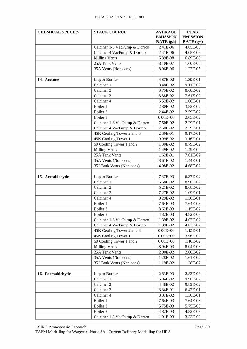
Table 2. Emission rates (Current Scenario with a production rate of 6,600 tonnes per day) as supplied by Alcoa World Alumina Australia from each of the sources for each of the 27 modelled species (Coffey, pers. comm. 13 Sep 2004, revised 16 Dec 2004). The 28th species (NO2) is modelled separately, as described in Section 3.4. Both the average and peak emission rates are listed. In the modelling, the emissions listed as from “Boiler 2/3 (Non-condensables)” were split 50:50 between the Boiler 2 and Boiler 3 flues. The numbers in the table are given using exponential notation which is commonly used in computing, for example, the value 4.81E-01 = 4.81×10-1 = 0.481.
CHEMICAL SPECIES STACK SOURCE AVERAGE EMISSION RATE (g/s)
PEAK EMISSION RATE (g/s)
1. NOx Liquor Burner 1.24E+00 4.20E+00 Calciner 1 2.16E+00 3.18E+00 Calciner 2 1.25E+00 4.47E+00 Calciner 3 3.60E+00 6.93E+00 Calciner 4 2.43E+00 4.28E+00 Boiler 1 7.61E+00 1.77E+01 Boiler 2 7.96E+00 1.65E+01 Boiler 3 2.64E+00 4.37E+00 Gas Turbine 1 3.00E+00 1.36E+01
2. CO Liquor Burner 7.65E+00 2.11E+01 Calciner 1 5.11E+00 1.11E+01 Calciner 2 8.89E+00 2.42E+01 Calciner 3 1.27E+00 3.69E+00 Calciner 4 2.29E+00 4.28E+00 Boiler 1 2.97E-01 2.31E+00 Boiler 2 2.47E-01 2.66E+00 Boiler 3 1.20E-01 8.37E-01 Gas Turbine 1 2.99E+00 7.83E+00
3. SO2 Liquor Burner 1.04E-01 4.33E-01 Calciner 1 3.22E-01 9.94E-01 Calciner 2 4.05E-01 9.17E-01 Calciner 3 2.34E-01 1.24E+00 Calciner 4 1.24E-01 3.32E-01 Boiler 1 1.96E-01 9.46E-01 Boiler 2 2.12E-01 1.38E+00 Boiler 3 1.79E-01 4.73E-01 Gas Turbine 1 4.27E-01 2.56E+00
4. Dust Liquor Burner 7.01E-02 5.33E-01 Calciner 1 5.94E-01 3.42E+00 Calciner 2 4.10E-01 2.40E+00 Calciner 3 4.19E-01 1.24E+00 Calciner 4 4.06E-01 7.97E-01
5. Arsenic Liquor Burner 1.42E-04 1.46E-04 Boiler 1 2.20E-03 3.03E-03 Boiler 2 9.84E-05 1.52E-04 Boiler 3 8.26E-05 1.25E-04 Boiler 2/3 (Non-condensables) 2.97E-06 2.97E-06 25A Tank Vents 2.08E-05 4.12E-05

PHASE 3A. FINAL REPORT
CSIRO Atmospheric Research Page 29 TAPM Modelling for Wagerup: Phase 3A. Current Refinery Modelling for HRA
CHEMICAL SPECIES STACK SOURCE AVERAGE EMISSION RATE (g/s)
PEAK EMISSION RATE (g/s)
6. Selenium Liquor Burner 8.50E-04 8.74E-04
Boiler 2 3.54E-05 5.47E-05 Boiler 3 2.97E-05 4.49E-05 Boiler 2/3 (Non-condensables) 2.76E-05 2.76E-05 Milling Vents 5.74E-06 5.74E-06 25A Tank Vents 7.27E-05 1.44E-04
7. Manganese Liquor Burner 7.08E-05 7.28E-05 Boiler 1 1.02E-03 1.41E-03 Boiler 2 5.81E-04 8.97E-04 Boiler 3 4.88E-04 7.36E-04 Boiler 2/3 (Non-condensables) 6.54E-04 6.54E-04 Milling Vents 1.15E-05 1.15E-05 25A Tank Vents 6.85E-03 1.35E-02
8. Cadmium Boiler 2/3 (Non-condensables) 2.23E-07 2.23E-07
9. Chromium VI Liquor Burner 3.17E-07 3.17E-07 Calciner 1 1.82E-06 1.82E-06 Calciner 2 1.82E-06 1.82E-06 Calciner 3 1.82E-06 1.82E-06 Calciner 4 1.82E-06 1.82E-06 Boiler 1 4.44E-06 4.44E-06 Boiler 2 4.44E-06 4.44E-06 Boiler 3 4.44E-06 4.44E-06
10. Nickel Boiler 2 1.01E-04 1.55E-04 Boiler 3 8.44E-05 1.27E-04 Boiler 2/3 (Non-condensables) 1.15E-04 1.15E-04 25A Tank Vents 2.15E-04 4.25E-04
11. Mercury Liquor Burner 3.05E-04 3.05E-04 Calciner 1 6.28E-05 6.28E-05 Calciner 2 6.28E-05 6.28E-05 Calciner 3 6.28E-05 6.28E-05 Calciner 4 6.28E-05 6.28E-05 Boiler 2/3 (Non-condensables) 3.55E-03 3.55E-03 Milling Vents 3.18E-05 3.18E-05 25A Tank Vents 2.77E-04 2.77E-04
12. Ammonia Boiler 2 1.19E-01 1.84E-01 Boiler 3 1.00E-01 1.51E-01 Milling Vents 3.56E-02 3.56E-02 25A Tank Vents 6.35E-02 1.25E-01
13. BaP Equivalents Liquor Burner 2.61E-06 2.68E-06 Calciner 1 5.09E-07 5.82E-07 Calciner 2 4.84E-07 5.64E-07 Calciner 3 5.71E-07 6.92E-07 Calciner 4 7.24E-07 7.97E-07
PHASE 3A. FINAL REPORT
CSIRO Atmospheric Research Page 30 TAPM Modelling for Wagerup: Phase 3A. Current Refinery Modelling for HRA
CHEMICAL SPECIES STACK SOURCE AVERAGE EMISSION RATE (g/s)
PEAK EMISSION RATE (g/s)
Calciner 1-3 VacPump & Dorrco 2.41E-06 4.05E-06 Calciner 4 VacPump & Dorrco 2.41E-06 4.05E-06 Milling Vents 6.89E-08 6.89E-08 25A Tank Vents 8.10E-07 1.60E-06 35A Vents (Non cons) 8.96E-06 1.22E-05
14. Acetone Liquor Burner 4.87E-02 1.39E-01 Calciner 1 3.48E-02 9.11E-02 Calciner 2 3.75E-02 8.68E-02 Calciner 3 3.38E-02 7.61E-02 Calciner 4 6.52E-02 1.06E-01 Boiler 1 2.80E-02 3.82E-02 Boiler 2 2.44E-02 2.59E-02 Boiler 3 0.00E+00 2.65E-02 Calciner 1-3 VacPump & Dorrco 7.50E-02 2.29E-01 Calciner 4 VacPump & Dorrco 7.50E-02 2.29E-01 45K Cooling Tower 2 and 3 2.89E-01 9.17E-01 45K Cooling Tower 1 9.99E-02 3.16E-01 50 Cooling Tower 1 and 2 1.30E-02 8.79E-02 Milling Vents 1.49E-02 1.49E-02 25A Tank Vents 1.62E-01 7.01E-02 35A Vents (Non cons) 8.61E-02 1.44E-01 35J Tank Vents (Non cons) 4.08E-02 4.68E-02
15. Acetaldehyde Liquor Burner 7.37E-03 6.37E-02 Calciner 1 5.68E-02 8.90E-02 Calciner 2 5.21E-02 8.68E-02 Calciner 3 7.27E-02 1.09E-01 Calciner 4 9.29E-02 1.30E-01 Boiler 1 7.64E-03 7.64E-03 Boiler 2 8.62E-03 1.15E-02 Boiler 3 4.82E-03 4.82E-03 Calciner 1-3 VacPump & Dorrco 1.39E-02 4.02E-02 Calciner 4 VacPump & Dorrco 1.39E-02 4.02E-02 45K Cooling Tower 2 and 3 0.00E+00 1.15E-01 45K Cooling Tower 1 0.00E+00 3.96E-02 50 Cooling Tower 1 and 2 0.00E+00 1.10E-02 Milling Vents 8.04E-03 8.04E-03 25A Tank Vents 2.00E-02 2.00E-02 35A Vents (Non cons) 1.28E-02 1.61E-02 35J Tank Vents (Non cons) 1.19E-02 1.38E-02
16. Formaldehyde Liquor Burner 2.83E-03 2.83E-03 Calciner 1 5.04E-02 9.96E-02 Calciner 2 4.48E-02 9.89E-02 Calciner 3 3.34E-01 6.42E-01 Calciner 4 8.87E-02 1.30E-01 Boiler 1 7.64E-03 7.64E-03 Boiler 2 5.75E-03 5.75E-03 Boiler 3 4.82E-03 4.82E-03 Calciner 1-3 VacPump & Dorrco 1.01E-03 3.22E-03

PHASE 3A. FINAL REPORT
CSIRO Atmospheric Research Page 31 TAPM Modelling for Wagerup: Phase 3A. Current Refinery Modelling for HRA
CHEMICAL SPECIES STACK SOURCE AVERAGE EMISSION RATE (g/s)
PEAK EMISSION RATE (g/s)
Calciner 4 VacPump & Dorrco 1.01E-03 3.22E-03 45K Cooling Tower 2 and 3 0.00E+00 1.15E-01 45K Cooling Tower 1 0.00E+00 3.96E-02 Milling Vents 1.15E-04 1.15E-04 25A Tank Vents 3.92E-04 4.88E-04 35A Vents (Non cons) 1.49E-04 1.73E-04 35J Tank Vents (Non cons) 1.38E-04 1.38E-04
17. 2-Butanone Liquor Burner 5.67E-03 1.27E-02 Calciner 1 4.95E-03 8.48E-03 Calciner 2 5.38E-03 8.07E-03 Calciner 3 1.66E-02 4.04E-02 Calciner 4 1.01E-02 1.81E-02 Boiler 1 7.64E-03 7.64E-03 Boiler 2 5.75E-03 5.75E-03 Boiler 3 4.82E-03 4.82E-03 Calciner 1-3 VacPump & Dorrco 4.36E-03 7.65E-03 Calciner 4 VacPump & Dorrco 4.36E-03 7.65E-03 45K Cooling Tower 2 and 3 0.00E+00 1.15E-01 45K Cooling Tower 1 0.00E+00 3.96E-02 Milling Vents 9.19E-04 9.19E-04 25A Tank Vents 5.29E-03 5.29E-03 35A Vents (Non cons) 2.97E-02 2.48E-02 35J Tank Vents (Non cons) 6.21E-03 7.57E-03
18. Benzene Liquor Burner 3.29E-02 5.24E-02 Calciner 1 4.98E-03 8.48E-03 Calciner 2 4.94E-03 8.07E-03 Calciner 3 2.38E-03 2.38E-03 Calciner 4 7.54E-03 9.05E-03 Boiler 1 4.78E-03 5.73E-03 Boiler 2 3.59E-03 4.31E-03 Boiler 3 3.01E-03 3.62E-03 Calciner 1-3 VacPump & Dorrco 4.69E-04 6.04E-04 Calciner 4 VacPump & Dorrco 4.69E-04 6.04E-04 45K Cooling Tower 2 and 3 0.00E+00 5.73E-02 45K Cooling Tower 1 0.00E+00 1.98E-02 Milling Vents 7.75E-05 7.75E-05 25A Tank Vents 0.00E+00 3.31E-04 35A Vents (Non cons) 0.00E+00 3.25E-05 35J Tank Vents (Non cons) 0.00E+00 2.06E-04
19. Toluene Liquor Burner 1.70E-03 4.25E-03 Calciner 1 1.91E-03 2.12E-03 Calciner 2 1.82E-03 2.02E-03 Calciner 3 2.14E-03 2.38E-03 Calciner 4 2.72E-03 3.02E-03 Boiler 1 3.82E-03 3.82E-03 Boiler 2 2.87E-03 2.87E-03 Boiler 3 2.41E-03 2.41E-03 Calciner 1-3 VacPump & Dorrco 4.02E-02 4.02E-02

PHASE 3A. FINAL REPORT
CSIRO Atmospheric Research Page 32 TAPM Modelling for Wagerup: Phase 3A. Current Refinery Modelling for HRA
CHEMICAL SPECIES STACK SOURCE AVERAGE EMISSION RATE (g/s)
PEAK EMISSION RATE (g/s)
Calciner 4 VacPump & Dorrco 4.02E-02 4.02E-02 45K Cooling Tower 2 and 3 0.00E+00 5.73E-02 45K Cooling Tower 1 0.00E+00 1.98E-02 50 Cooling Tower 1 and 2 0.00E+00 2.20E-04 Milling Vents 1.03E-04 1.03E-04 25A Tank Vents 3.19E-03 3.19E-03 35A Vents (Non cons) 6.79E-04 6.79E-04
20. Xylenes Liquor Burner 7.15E-04 9.49E-04 Calciner 1 6.89E-04 1.06E-03 Calciner 2 6.56E-04 1.01E-03 Calciner 3 7.73E-04 1.19E-03 Calciner 4 9.81E-04 1.51E-03 Calciner 1-3 VacPump & Dorrco 9.26E-03 9.26E-03 Calciner 4 VacPump & Dorrco 9.26E-03 9.26E-03 25A Tank Vents 3.55E-04 4.79E-04
21. Acrolein Calciner 1 8.48E-03 9.70E-03 Calciner 2 8.07E-03 9.41E-03 Calciner 3 9.51E-03 1.15E-02 Calciner 4 1.21E-02 1.33E-02
22. Ethylbenzene Liquor Burner 3.97E-04 4.08E-04 Calciner 1 2.12E-04 2.43E-04 Calciner 2 2.02E-04 2.35E-04 Calciner 3 2.38E-04 2.88E-04 Calciner 4 3.02E-04 3.32E-04 25A Tank Vents 1.16E-04 2.29E-04
23. Methylene Chloride Calciner 1 9.33E-03 1.07E-02 Calciner 2 8.88E-03 1.03E-02 Calciner 3 1.05E-02 1.27E-02 Calciner 4 1.33E-02 1.46E-02 Boiler 1 1.53E-02 2.10E-02 Boiler 2 1.15E-02 1.77E-02 Boiler 3 9.65E-03 1.46E-02 Calciner 1-3 VacPump & Dorrco 4.02E-02 6.75E-02 Calciner 4 VacPump & Dorrco 4.02E-02 6.75E-02 25A Tank Vents 3.14E-03 6.21E-03
24. Styrene Liquor Burner 5.24E-04 5.39E-04 Calciner 1 3.18E-04 3.64E-04 Calciner 2 3.03E-04 3.53E-04 Calciner 3 3.57E-04 4.32E-04 Calciner 4 4.53E-04 4.98E-04 45K Cooling Tower 2 and 3 3.65E-03 3.65E-03 45K Cooling Tower 1 1.26E-03 1.26E-03 50 Cooling Tower 1 and 2 1.64E-04 1.64E-04 25A Tank Vents 1.65E-05 3.27E-05
25. 1,2,4 Trimethylbenzene Liquor Burner 2.27E-04 2.33E-04

PHASE 3A. FINAL REPORT
CSIRO Atmospheric Research Page 33 TAPM Modelling for Wagerup: Phase 3A. Current Refinery Modelling for HRA
CHEMICAL SPECIES STACK SOURCE AVERAGE EMISSION RATE (g/s)
PEAK EMISSION RATE (g/s)
25A Tank Vents 4.79E-04 9.47E-04
26. 1,3,5 Trimethylbenzene Liquor Burner 5.67E-05 5.83E-05 Calciner 1 5.30E-05 6.06E-05 Calciner 2 5.05E-05 5.88E-05 Calciner 3 5.94E-05 7.21E-05 Calciner 4 7.54E-05 8.30E-05 25A Tank Vents 1.49E-04 2.94E-04
27. Vinyl Chloride Calciner 1 5.30E-05 6.06E-05 Calciner 2 5.05E-05 5.88E-05 Calciner 3 5.94E-05 7.21E-05 Calciner 4 7.54E-05 8.30E-05
3.4. NOx to NO2 Conversion The NOx (nitrogen oxides) emission rates were used to calculate NOx concentration fields. The NO2 (nitrogen dioxide) concentrations were derived using a simple titration algorithm for the conversion of nitric oxide (NO) to NO2 in the presence of ozone (O3):
NO + O3 NO2 + O2, (8)
which is approximately correct at night-time but is conservative (i.e. potentially over-estimates NO2) in the near field (less than 1 hour downwind of the source) during daylight hours when photochemical reactions become important.
This reaction equation shows that both compounds on the left-hand side (nitric oxide and ozone) are needed to produce nitrogen dioxide, NO2. The amount of NO2 produced is limited by the smaller of either the NO or the O3 concentration. If there is more O3 than NO then all of the NO will be converted to NO2. If, on the other hand, there is more NO than O3, then NO2 is only produced until all of the O3 is used up. Thus the NO2 concentration is taken to be the minimum of the NOx and the ozone concentration with both expressed in ppb. The NOx emission rates used in the TAPM modelling to generate NOx glcs are expressed in terms of NO2, as is standard practice in air pollution studies.
In the absence of hourly ozone data for the modelled period (April 2003 to March 2004), the average diurnal variation of ozone concentrations at the Upper Dam site for the period March 2002 to March 2003 reported by Johnson (2003) was used. These data are reproduced in Figure 7.
Capping of the peak 10-minute and 3-minute averages for NO2 due to the limited availability of ozone for titration of NO to NO2 is discussed at the end of Section 3.5. The affected peak NO2 concentrations are indicating by shading of the cells in the tables in Sections 4.4 and 4.5.

PHASE 3A. FINAL REPORT
CSIRO Atmospheric Research Page 34 TAPM Modelling for Wagerup: Phase 3A. Current Refinery Modelling for HRA
0 6 12 18 24Time of day (hours)
0
10
20
30
Ave
rage
Ozo
ne C
once
ntra
tion
(ppb
)
Figure 7. Average diurnal variation of ozone concentration used for deriving NO2 concentrations from modelled NOx concentrations (after Johnson, 2003). Concentrations are given in ppb (parts per billion).
3.5. Modelling Short-term Peak Concentrations It is well established in the literature that observed annual peak ground level concentrations for averaging times ranging from minutes to hours can be related through a power law expression of the form (e.g. Hibberd, 1998, NSW EPA, 2001):
p
ttcc ⎟⎟⎠
⎞⎜⎜⎝
⎛=
2
11max,2max, , (9)
where cmax,i is the maximum concentration for an averaging time ti and the value of the exponent p typically lies in the range 0.1 to 0.4 with lower values representative of stable conditions and larger values more appropriate for highly unstable (convective) conditions. The value of p also decreases with increasing distance from the source.
Provided that an appropriate value of p is used, this equation has been found to give good estimates of the highest concentrations likely to be observed in a year. For example, knowing the highest 1-hour average concentration in a year, it is possible to predict the highest 10-minute average or highest 3-minute average concentration.
Uncertainty in these estimates arises because the value of the exponent p depends on many factors, including: • the configuration of the source, e.g. point, area • atmospheric stability • the distance from the source. Table 3 lists commonly-used values of p with an indication of the origin of data used to derive these exponents.
In many cases, the maximum 1-hour average ground-level concentrations near tall stacks are observed during convective conditions and a value of p = 0.4 is used. This gives the peak 10-minute average as 2.0 × cmax,1hr and the peak 3-minute average as 3.3 × cmax,1hr. In cases where the maximum ground-level concentrations are observed at

PHASE 3A. FINAL REPORT
CSIRO Atmospheric Research Page 35 TAPM Modelling for Wagerup: Phase 3A. Current Refinery Modelling for HRA
night in stable conditions, for example as plume impact on nearby hills, a value of p = 0.2 is more commonly applied. This gives the peak 10-minute average as 1.4 × cmax,1hr and the peak 3-minute average as 1.8 × cmax,1hr.
Many modelling studies use a default value of p = 0.2, and this value is included in the commonly-used air quality models AUSPLUME and CALPUFF.
Table 3. Power-law exponents derived from a range of studies for different source configurations. After Katestone Scientific (1998).
Source type Power-law exponent
p
Types of studies F – field, L – laboratory N – numerical, T – theoretical
Area 0.10 – 0.15 L, N
Line 0.25 L, N, T
Surface point 0.15 – 0.2 F, L, N, T
Tall wake-free point 0.4 F, L, N, T
Wake-affected point 0.10 F, L
Volume 0.10 T
Although equation (9) is only valid for long data series such as year-long sets of data, it is often mis-applied to much shorter periods. For example, it is often applied to 1-hour average data for each hour of a year to calculate a maximum short-term peak during that hour, even though the actual “peak” may be much larger or much smaller than the calculated peak value. This discrepancy can easily be seen by considering two simple cases:
1. A pollutant concentration of 60 µg m-3 is observed for the first 3 minutes of an hour with a concentration of zero for the rest of the hour. The 1-hour average concentration is then 3 µg m-3 so that cmax,3-min = 20 × cmax,1hr.
2. A pollutant concentration of 10 µg m-3 is observed for each 3 minutes of a full hour. Both the maximum 3-minute average concentration and the 1-hour average concentration are 10 µg m-3. Thus cmax,3-min = 1 × cmax,1hr.
The factors of 1 and 20 are clearly much different from the factors obtained from the power-law model with p = 0.2 or 0.4, as given above. This occurs because the equation is based on properties of statistical extremes – it accurately predicts extreme statistics when there are a sufficiently large number of events, but it does not apply to data in any particular hour.
A consequence of this limitation is that the power-law method cannot be used to generate a time series of, for example, 10-minute average concentrations from modelled 1-hour average concentrations. It is only the annual peak 10-minute average concentration that can be obtained.
The most uncertain aspect of the power-law method is the selection of the correct value of p for calculating the peak values. In this study we determine the value of p from the magnitude of the concentration variance (a measure of the variability in the concentrations) calculated by the model, which accounts for its variability with

PHASE 3A. FINAL REPORT
CSIRO Atmospheric Research Page 36 TAPM Modelling for Wagerup: Phase 3A. Current Refinery Modelling for HRA
prevailing meteorological and dispersion conditions and hence for its variability with distance from the sources and time of day. The TAPM modelling for this study had the option switched on to calculate the concentration variance. In the processing step combining the model results from each stack source (represented by equation (7)), the variances contributed by each source is also taken into account. The larger the concentration variance, the larger the value was of p and vice versa, with values of p ranging between 0.1 and 0.4. Thus the most appropriate value of p was calculated for each hour of the day at each point on the modelled domain. Using equation (9) and the modelled 1-hour average concentration, a set of numbers was produced, from which the annual maximum 10-minute and 3-minute concentrations were derived at each point on the modelled domain. (As noted above, the individual values at each hour of the year are not realistic, but the annual maxima of these numbers do represent the extremes of the distribution.) A significant advantage of the technique is that the exponent chosen each hour more closely represents the dispersion conditions prevailing at that time. It can be more accurate than the simple AUSPLUME technique of applying a constant value of p = 0.2, as it correctly accounts for the larger exponent that applies for tall stack emissions into convective conditions and the smaller exponent for near-surface sources. This TAPM technique has been validated for peak 10-minute concentrations using emissions and ground-level monitoring data in the Kwinana region (Hurley, pers. comm.).
This TAPM approach represents the current state of knowledge for statistical modelling of extreme annual events.
The results obtained in this study for the maximum 1-hour, 10-minute and 3-minute concentrations show that at the 15 receptor points, the short-term peaks are equivalent to using exponents between 0.12 and 0.24 with the value varying across the grid.
The model results can be compared with observations of 6-minute average NOx concentrations at Upper Dam for the calendar year 2003, where the maximum observed 1-hour average concentration in 2003 was 76 µg m-3 and the maximum 6-minute average concentration was 102 µg m-3, corresponding to an exponent p = 0.13. The caveat on this calculation is that the numbers were derived from single points at the extreme end of the distribution of values and so are subject to some uncertainty, which cannot be quantified without a much more detailed analysis.
The modelled TAPM results for NOx obtained in this study for the Upper Dam site corresponds to an exponent of p = 0.24, which is somewhat larger than the observed value. This indicates that the results for the 10-minute and 3-minute peaks presented here may be conservative, i.e. they will tend to be over-predictions rather than under-predictions.
The peak-to-mean ratios for NO2 are affected by the capping of the 10-minute and 3-minute averages for NO2 due to the limited availability of ozone for titration of NO to NO2 (as described in Section 3.4). The ozone data used in this study do not include short-term (sub-hourly) variations (which in any case are small because of the nature and extent of ozone sources in the background air). On occasions when the 1-hour average NOx concentration exceeds the ozone concentration for that hour, then the modelled 10-minute and 3-minute NO2 concentrations will be the same as the 1-hour average NO2 and ozone concentration for that hour. This is equivalent to a power law exponent p = 0. On other occasions, just the modelled 10-minute or 3-minute NOx concentration will exceed the 1-hour average ozone concentration, so only these shorter term NO2 peaks will be capped (producing values of p between 0 and that for NOx). As

PHASE 3A. FINAL REPORT
CSIRO Atmospheric Research Page 37 TAPM Modelling for Wagerup: Phase 3A. Current Refinery Modelling for HRA
described above, the individual 10-minute and 3-minute concentrations calculated each hour are not realistic, but the annual peak values do represent the extreme values. The peak NO2 concentrations that are limited by the available ozone are highlighted by shading of the cells in which they occur in the tables in Sections 4.4 and 4.5.
4. Model Outputs
4.1. Receptor Locations Table 4 lists the coordinates and Figure 8 shows the locations of the 15 receptor sites at which the required concentration statistics of the 28 chemical species were extracted.
Table 4. Locations of each of the fifteen receptors used in the modelling study. (NB. Receptor 12 was not included in the selected sites.)
Receptor AMG84 Coordinates Location Eastings (km) Northings (km)
1 398.091 6354.834 Boundary Rd 2 399.393 6355.006 3 396.830 6352.949 Yarloop 4 397.138 6354.827 5 395.721 6352.503 6 399.650 6354.240 7 390.775 6358.733 Bremner Rd 8 392.360 6362.131 Somers/McClure Rds 9 396.099 6362.024
10 398.460 6362.000 Hamel 11 398.207 6360.331 13 400.520 6364.215 14 400.727 6360.830 Escarpment 15 400.726 6356.435 16 397.365 6359.285

PHASE 3A. FINAL REPORT
CSIRO Atmospheric Research Page 38 TAPM Modelling for Wagerup: Phase 3A. Current Refinery Modelling for HRA
Figure 8: Location of the receptors used in this modelling study overlaid on an aerial photograph of the site.
4.2. Uncertainty in modelled concentrations The performance statistics for the meteorological component of TAPM were presented in Section 2. The performance of the concentration (pollution) modelling component of TAPM has been evaluated using the robust highest concentration and is described here.
The robust highest concentration (Cox and Tikvart, 1990) is a robust test statistic calculated using information contained in the upper end of the distribution of concentrations. It is defined as:
( ) ( )[ ]213ln)()( −−+= RRCCRCRHC , (10)
where C(R) is the Rth highest concentration and C is the mean of the top R − 1 concentrations. A value of R = 11 is usually used in TAPM studies, in which case C is the average of the top ten concentrations. The RHC is based on an exponential fit to the highest R – 1 values of the cumulative frequency distribution. In air quality studies, the RHC is often preferred to the maximum value because it removes the undesirable influence of unusual (stochastic) events, while still representing the highest concentrations.
Table 5 lists the ratio of modelled-to-observed RHCs from the most recent studies undertaken using TAPM Version 2. The ratio ranges from 0.83 (a 17% underprediction) to 1.46 (a 46% over-prediction) with a mean of 1.07. The results indicate that in any particular modelling study, the uncertainty in the modelled RHCs is approximately ±40% at the 95% confidence level (i.e. two standard deviations). For more extreme statistics such as the annual maximum 1-hour average, 10-minute average or 3-minute average concentration, the uncertainty will be somewhat greater, and for less extreme statistics such as the annual average or 95th percentiles the uncertainty will be smaller, but the magnitude of these uncertainties have not been evaluated. Although it should be simple to evaluate the uncertainty in modelled annual averages, this is not the case. Measured concentrations are often confounded by zero offset problems, which can be of similar magnitude to the annual average, although much smaller than peak

PHASE 3A. FINAL REPORT
CSIRO Atmospheric Research Page 39 TAPM Modelling for Wagerup: Phase 3A. Current Refinery Modelling for HRA
concentrations. In addition, modelling often doesn’t include all sources of the particular pollutant (such as the vehicular and Yarloop sources of NOx in the current modelling).
Table 5. List of the ratio of modelled to observed robust highest concentrations (RHC) for a range of studies using TAPM.
Location Species Ratio of modelled to observed RHC
Reference
Kwinana, site 1 SO2 0.87 Hurley et al., 2002 Kwinana, site 2 SO2 0.91 Hurley et al., 2002 Kwinana, site 3 SO2 1.46 Hurley et al., 2002 Kwinana, site 4 SO2 0.83 Hurley et al., 2002 Kwinana, site 5 SO2 1.27 Hurley et al., 2002 Kwinana, site 6 SO2 1.13 Hurley et al., 2002 Pilbara, site 1 NOx 0.87 Hurley et al., 2003b Pilbara, site 2 NOx 1.06 Hurley et al., 2003b Anglesea, site 1 SO2 1.01 Hill and Hurley, 2003 Anglesea, site 2 SO2 1.29 Hill and Hurley, 2003 Kincaid (USA) SF6 1.19 Luhar and Hurley, 2003 Indianapolis SF6 0.92 Luhar and Hurley, 2003 Pilbara, site 1 NO2 1.27 Hurley et al., 2003b Pilbara, site 2 NO2 1.21 Hurley et al., 2003b Perth NO2 0.90 Hurley et al., 2002 Melbourne, site 1 NO2 1.12 Hurley et al., 2003a Melbourne, site 2 NO2 1.14 Hurley et al., 2003a Melbourne, site 3 NO2 1.20 Hurley et al., 2003a Melbourne, site 4 NO2 1.21 Hurley et al., 2003a Pilbara O3 1.05 Hurley et al., 2003b Perth O3 1.02 Hurley et al., 2002 Melbourne, site 1 O3 0.80 Hurley et al., 2003a Melbourne, site 2 O3 1.00 Hurley et al., 2003a Melbourne, site 3 O3 0.94 Hurley et al., 2003a Melbourne, site 4 O3 1.02 Hurley et al., 2003a Average ± standard deviation 1.07 ± 0.17
Factors contributing to the uncertainty in model results include the turbulent (random) nature of dispersion in the turbulent atmosphere, inaccuracies in the mathematical description of the physical processes that occur in the atmosphere, and uncertainties in the numerical solutions of the many equations in the model. A further factor is uncertainty or variability in the source emission rates. As mentioned above, the modelling of extreme events, such as annual maximum 1-hour average concentrations, has the highest level of uncertainty. The nature of the TAPM uncertainty is similar to the uncertainty in weather predictions of the timing and location of thunderstorms. Uncertainties are inherent in any modelling of the atmosphere. TAPM incorporates the best techniques for dispersion modelling consistent with the ability to do year-long model runs, albeit using large amounts of computing resources.

PHASE 3A. FINAL REPORT
CSIRO Atmospheric Research Page 40 TAPM Modelling for Wagerup: Phase 3A. Current Refinery Modelling for HRA
Two further analyses of uncertainty are undertaken. An analysis is presented of the year-to-year variation in synoptic wind directions at Wagerup and an analysis is made of the sensitivity of model results to wind data assimilation of the available wind data from Wagerup.
The annual variability in the large-scale synoptic weather pattern in the Wagerup region and the representativeness of the modelled year has been investigated by analysing the 6-hourly 10-m wind directions for the grid point closest to Wagerup in the Bureau of Meteorology’s GASP (Global Analysis and Prediction) analyses, which are used as the synoptic input to TAPM. The data have been sorted into 22.5º bins centred on the directions labelled on the axis of Figure 9.
The pattern shows that the winds are in the southerly quadrants (south-east and south-west) about two-thirds of the time, and in the northerly quadrants (north-east and north-west) about one-third of the time. The annual variability in the frequency of each wind direction is represented by the shaded vertical bar; it is typically ±30% about the mean (range 12% to 49%). The modelled year is seen to be a fairly average year with all frequencies within 20% of the median values, except for easterlies (33% less frequent than the median) and southerlies (24% more frequent than the median). Although ground-level concentrations are influenced by more meteorological conditions than just the wind directions, the inter-annual variability of ±30% in the frequency of wind in each sector would be expected to lead to similar sized variations in the annual average concentrations, but determining the effect on maximum concentrations is more complicated. In fact, a full comparison of the inter-annual variability would require repeat modelling for several years, which is currently beyond the scope of what is possible for such a complex set of modelling conditions. Even the current modelling for the Current and Expansion scenarios required more than 10,000 hours of CPU time.
N NE E SE S SW W NW NWind direction
0
2
4
6
8
10
12
Prob
abili
ty (%
) of w
ind
in g
iven
dire
ctio
ndu
ring
full
year
Modelled Year (Apr03-Mar04)20042003200220012000199919981997Range (1997-2004)
Figure 9. Probability distribution of 10-m wind directions at Wagerup for the years 1997–2004 compared with those for the modelled year (April 2003–March 2004) indicated by the solid line. Data are from the 6-hourly GASP (Global Analysis and Prediction) records that are used as the synoptic input to TAPM.

PHASE 3A. FINAL REPORT
CSIRO Atmospheric Research Page 41 TAPM Modelling for Wagerup: Phase 3A. Current Refinery Modelling for HRA
Some model runs for NOx were undertaken using wind data assimilation, as discussed in Section 2.1. The results from these runs provide an indication of the sensitivity of the model results to uncertainties in the wind direction and speed in the meteorological input to the model. The simulations were an annual run for NOx using the Current Scenario peak emission rates presented in Table 2 of the Phase 3A report (CSIRO, 2004d) with assimilation of available wind data from 30 m at Bancell Road and 8 m at the RDA. Table 6 lists the ratio at the receptor site of the concentration modelled with data assimilation to that without data assimilation.
For the maximum 1-hour average concentration, the bulk of the ratios are in the range from 0.4 to 2.0, with an outlier at site 3, where the ratio is 3.1. As can be seen from Figure 25, site 3 is in a region of low 1-hr average ground-level concentrations bordered by a steep concentration gradient to the west. A rotation of the modelled wind with wind data assimilation brings in the much higher ground-level concentrations from the west to receptor 3. Because the maximum 1-hour average concentration only occurs once per year, this difference between results with and without wind data assimilation at receptor 3 would not necessarily occur at that receptor if another year’s meteorology was used. The extreme sensitivity of this statistic (maximum concentration) is seen when comparing its ratios with the ratios of the 10th highest concentration in the table, which are all within the range 0.5 to 1.5, i.e. within ±50% of the runs without data assimilation.
Table 6. Ratio of modelled concentrations for NOx (Current Scenario – Peak Emissions) when TAPM was run with data assimilation compared to the results obtained without data assimilation.
Receptor cmax
(1-hr avg) RHC
(1-hr avg) 10th highest(1-hr avg)
Annual average
1 1.5 1.6 1.5 1.9 2 1.3 1.3 1.4 2.4 3 3.1 2.8 1.4 1.6 4 2.0 1.8 1.2 1.5 5 1.0 1.1 1.1 1.2 6 1.0 1.3 1.3 2.1 7 0.4 0.4 0.5 1.0 8 0.8 0.9 0.7 1.2 9 0.9 1.1 0.7 1.1
10 0.7 0.7 0.6 1.1 11 0.8 0.9 0.8 1.0 13 1.0 1.2 1.1 1.5 14 1.2 1.3 1.5 1.7 15 1.5 1.4 1.2 1.3 16 1.0 1.0 0.9 1.1
average 1.2 ± 0.7 1.2 ± 0.6 1.1 ± 0.3 1.4 ± 0.4
These results in Table 6 and Figure 9 indicate that the TAPM model uncertainty of ±40% derived from Table 5 from a range of studies is an underestimate for the topographically complex region of Wagerup with the significant influence of the escarpment on local wind fields. As mentioned elsewhere, wind direction data measured

PHASE 3A. FINAL REPORT
CSIRO Atmospheric Research Page 42 TAPM Modelling for Wagerup: Phase 3A. Current Refinery Modelling for HRA
at the Bancell Road and RDA sites, which are less than 3 km apart, show that north-easterlies are much less frequent at Bancell Road than at the RDA (Phase 1 report; CSIRO, 2004b). Similarly, wind roses from Hamel and Yarloop for October/November 2003 show much more frequent easterlies and south-westerlies and much less frequent south-easterlies at Hamel than at Yarloop (WADEP, pers. comm.). Although wind data assimilation will generally improve modelled concentrations close to the location where the wind data is recorded, this will not be the case to the north of the Refinery including at Hamel or for much of the 15 km × 15 km region considered in this modelling. The comparison of results with and without data assimilation is presented here to indicate the sensitivity of the model results to changes in the wind patterns.
Based on an analysis of all the above information, taking into account the occurrence of one outlier in Table 6, we conclude that the scenario model results for maximum 1-hour average concentrations presented in this report have an uncertainty of a factor of approximately 2 (i.e. the actual values lie in the range of +100% to -50% of the scenario model concentrations) at the 95% confidence level. We conclude that the same level of uncertainty also applies to the other reported scenario concentrations (annual averages, 95th percentiles, maximum 10-minute and maximum 3-minute average concentrations).
4.3. Quality Assurance Runs For two pollutants, NOx and formaldehyde, TAPM was run using all sources of the pollutant in a single input file to generate quality assurance runs. For example, for NOx, the method includes all the NOx sources with the associated emission rates (g/s) in a single TAPM run.
Table 7. Comparison of results from Quality Assurance (QA) run with results from the weighted sum method described in Section 3.3.
Max. 1-hr average (µg m-3) Max. 1-hr average (µg m-3) Site Species
Results using Eq(1)
QA run
Differ-ence
Species
Results using Eq(1)
QA run
Differ-ence
1 NOx 55.1 53.6 -3% Formaldehyde 0.86 0.83 -3% 2 NOx 68.9 67.5 -2% Formaldehyde 0.99 1.00 +1% 3 NOx 74.9 69.6 -7% Formaldehyde 0.95 0.92 -3% 4 NOx 84.5 73.9 -13% Formaldehyde 0.99 0.98 -1% 5 NOx 95.3 98.2 +3% Formaldehyde 1.06 1.05 -1% 6 NOx 89.2 85.7 -4% Formaldehyde 1.01 1.10 +9% 7 NOx 83.9 84.7 +1% Formaldehyde 0.66 0.62 -6% 8 NOx 36.2 33.0 -9% Formaldehyde 0.58 0.54 -7% 9 NOx 40.6 42.8 +5% Formaldehyde 0.58 0.57 -2% 10 NOx 42.1 45.7 +9% Formaldehyde 0.72 0.70 -3% 11 NOx 48.5 48.5 0% Formaldehyde 0.77 0.84 +9% 13 NOx 33.9 32.7 -4% Formaldehyde 0.46 0.45 -2% 14 NOx 85.0 86.1 +1% Formaldehyde 0.69 0.72 +4% 15 NOx 74.7 72.8 -3% Formaldehyde 1.35 1.34 -1% 16 NOx 52.0 52.6 +1% Formaldehyde 0.98 1.00 +2%

PHASE 3A. FINAL REPORT
CSIRO Atmospheric Research Page 43 TAPM Modelling for Wagerup: Phase 3A. Current Refinery Modelling for HRA
These results are compared with the results obtained from the method used in the rest of the modelling presented in this report, which is described by Equation (7). This combines the TAPM results from each point source with a weighting according to the emission rates from each source. The quality assurance runs were designed to test both the model and the post-processing steps.
Table 7 lists the results for the maximum 1-hour average concentrations at each of the receptor sites. (As the maximum 1-hour average concentration is a once in a year extreme event, it represents the most stringent test that can be used for this comparison. Other statistics will show smaller differences.) It compares the results obtained using the weighted sum method with those from the QA run and lists the differences as a percentage at each receptor point. The differences range from -13% to +9%.
These reflect uncertainties in TAPM modelling which arise from the numerical solutions of a large number of equations and the stochastic (Lagrangian) modelling technique used on the inner grid. Comparison of contour plots of the modelled concentration fields indicate similar agreement over the whole modelled domain (not shown). These results confirm the veracity of the weighted sum approach for computing the ground-level concentrations of a large number of species emitted from a large number of separate sources.
4.4. Concentration Statistics (sorted by Species) Table 8 lists the concentration statistics for all 28 chemical species modelled at each of the 15 receptor sites. The same results are shown in Table 9 sorted by receptor site. The results are shown to one decimal place as this represents an uncertainty of at most 10% in the results. As indicated in the previous section, results of many TAPM modelling studies indicate that it is not possible to obtain better accuracy than this, particularly for peak statistics.
The 95th percentile value represents a concentration where 95% of the data are smaller and 5% of the data are larger than this concentration. For the 24-hour averages, it represents the 18th highest concentration in a year of 365 24-hour averages, whereas for the 1-hour averages it represents the 440th highest concentration in a year of 8760 1-hour averages. Although on any particular day, the 24-hour average will always be smaller than (or equal to) the maximum 1-hour average for that day, for the 95th percentiles there is no simple relation. The 95th percentile 24-hour average can be either larger or smaller than the 95th percentile 1-hour average, as is observed in Table 8.

PHASE 3A. FINAL REPORT
CSIRO Atmospheric Research Page 44 TAPM Modelling for Wagerup: Phase 3A. Current Refinery Modelling for HRA
Table 8. Selected modelled concentration statistics sorted by chemical species for each of the 28 chemical species at each of the 15 receptor sites for the Current Emissions Scenario of 6,600 tonnes per day (as revised 16 Dec 2004 (Coffey, pers. comm.)). The annual averages are for the average emission rates, whereas all other statistics are for peak emission rates. The shaded NO2 cells indicate values that are limited by the available ozone, see Section 3.5. Chemical Species Site Annual
average
(µg m-3)
95th % 24-hr
average (µg m-3)
95th % 1-hr
average (µg m-3)
Max. 1-hr
average (µg m-3)
Max. 10-min average (µg m-3)
Max. 3-min
average (µg m-3)
NOx 1 2.6E-01 2.9E+00 1.4E+00 5.5E+01 8.4E+01 1.1E+02 NOx 2 2.9E-01 3.4E+00 2.0E+00 6.9E+01 1.0E+02 1.3E+02 NOx 3 2.0E-01 2.4E+00 5.8E-01 7.5E+01 1.1E+02 1.4E+02 NOx 4 2.5E-01 3.2E+00 8.7E-01 8.4E+01 1.3E+02 1.6E+02 NOx 5 1.9E-01 2.5E+00 4.5E-01 9.5E+01 1.4E+02 1.8E+02 NOx 6 2.8E-01 3.1E+00 2.1E+00 8.9E+01 1.2E+02 1.5E+02 NOx 7 2.5E-01 3.3E+00 1.3E+00 8.4E+01 1.2E+02 1.6E+02 NOx 8 1.7E-01 2.5E+00 1.5E+00 3.6E+01 5.4E+01 7.0E+01 NOx 9 2.7E-01 3.0E+00 3.0E+00 4.1E+01 6.3E+01 8.6E+01 NOx 10 2.3E-01 2.4E+00 2.1E+00 4.2E+01 6.2E+01 8.1E+01 NOx 11 3.8E-01 4.8E+00 4.9E+00 4.8E+01 7.7E+01 1.0E+02 NOx 13 1.4E-01 1.5E+00 1.2E+00 3.4E+01 5.2E+01 6.9E+01 NOx 14 3.7E-01 4.0E+00 3.5E+00 8.5E+01 1.3E+02 1.6E+02 NOx 15 4.4E-01 5.2E+00 3.3E+00 7.5E+01 1.1E+02 1.4E+02 NOx 16 5.4E-01 6.9E+00 8.3E+00 5.2E+01 8.1E+01 1.1E+02 CO 1 2.7E-01 3.4E+00 1.9E+00 5.6E+01 8.1E+01 1.0E+02 CO 2 3.2E-01 4.2E+00 2.4E+00 6.5E+01 9.7E+01 1.3E+02 CO 3 1.9E-01 2.7E+00 8.4E-01 7.7E+01 1.0E+02 1.3E+02 CO 4 2.3E-01 3.3E+00 1.3E+00 5.6E+01 8.3E+01 1.1E+02 CO 5 1.7E-01 2.5E+00 5.7E-01 6.5E+01 9.6E+01 1.2E+02 CO 6 2.9E-01 4.0E+00 2.5E+00 7.2E+01 9.7E+01 1.2E+02 CO 7 1.6E-01 2.4E+00 1.4E+00 3.4E+01 5.1E+01 6.7E+01 CO 8 1.5E-01 2.5E+00 1.7E+00 3.9E+01 5.8E+01 7.5E+01 CO 9 2.4E-01 3.1E+00 3.6E+00 4.1E+01 6.5E+01 8.7E+01 CO 10 2.1E-01 2.8E+00 2.5E+00 5.2E+01 8.1E+01 1.1E+02 CO 11 3.5E-01 4.2E+00 5.1E+00 5.2E+01 8.4E+01 1.2E+02 CO 13 1.6E-01 2.0E+00 2.2E+00 3.6E+01 5.5E+01 7.2E+01 CO 14 3.7E-01 4.3E+00 5.2E+00 1.1E+02 1.6E+02 2.1E+02 CO 15 4.7E-01 6.9E+00 3.4E+00 1.0E+02 1.6E+02 2.1E+02 CO 16 5.2E-01 8.1E+00 8.5E+00 5.0E+01 8.0E+01 1.1E+02 SO2 1 1.8E-02 3.7E-01 1.7E-01 6.5E+00 1.0E+01 1.4E+01 SO2 2 2.0E-02 4.2E-01 2.3E-01 7.8E+00 1.2E+01 1.5E+01 SO2 3 1.3E-02 3.1E-01 7.8E-02 9.8E+00 1.5E+01 1.9E+01 SO2 4 1.7E-02 4.0E-01 1.2E-01 1.1E+01 1.6E+01 2.2E+01 SO2 5 1.3E-02 3.0E-01 5.8E-02 1.1E+01 1.7E+01 2.2E+01

PHASE 3A. FINAL REPORT
CSIRO Atmospheric Research Page 45 TAPM Modelling for Wagerup: Phase 3A. Current Refinery Modelling for HRA
Chemical Species Site Annual average
(µg m-3)
95th % 24-hr
average (µg m-3)
95th % 1-hr
average (µg m-3)
Max. 1-hr
average (µg m-3)
Max. 10-min average (µg m-3)
Max. 3-min
average (µg m-3)
SO2 6 1.9E-02 3.9E-01 2.5E-01 1.0E+01 1.4E+01 1.7E+01 SO2 7 1.6E-02 4.1E-01 1.6E-01 9.2E+00 1.4E+01 1.8E+01 SO2 8 1.2E-02 3.1E-01 1.9E-01 3.9E+00 5.9E+00 7.7E+00 SO2 9 1.8E-02 3.9E-01 3.9E-01 4.7E+00 7.1E+00 9.3E+00 SO2 10 1.5E-02 3.1E-01 2.7E-01 5.1E+00 7.7E+00 1.0E+01 SO2 11 2.5E-02 5.5E-01 5.7E-01 5.3E+00 8.4E+00 1.1E+01 SO2 13 9.6E-03 1.8E-01 1.4E-01 4.1E+00 6.2E+00 8.2E+00 SO2 14 2.4E-02 4.8E-01 4.2E-01 1.0E+01 1.5E+01 2.0E+01 SO2 15 3.0E-02 7.1E-01 4.2E-01 9.1E+00 1.4E+01 1.8E+01 SO2 16 3.9E-02 8.7E-01 1.1E+00 6.4E+00 1.0E+01 1.4E+01 Dust 1 1.3E-02 2.5E-01 9.6E-02 4.9E+00 7.7E+00 1.0E+01 Dust 2 1.7E-02 2.9E-01 1.2E-01 6.4E+00 1.0E+01 1.3E+01 Dust 3 8.9E-03 1.8E-01 5.4E-02 5.5E+00 7.5E+00 9.3E+00 Dust 4 1.2E-02 2.5E-01 7.9E-02 5.2E+00 8.6E+00 1.2E+01 Dust 5 8.2E-03 1.7E-01 4.2E-02 3.8E+00 5.2E+00 6.3E+00 Dust 6 1.4E-02 2.4E-01 1.2E-01 5.9E+00 8.7E+00 1.1E+01 Dust 7 9.8E-03 1.6E-01 9.6E-02 3.1E+00 4.0E+00 4.8E+00 Dust 8 8.6E-03 1.8E-01 1.3E-01 3.0E+00 4.5E+00 5.8E+00 Dust 9 1.4E-02 2.5E-01 2.6E-01 4.1E+00 6.5E+00 8.7E+00 Dust 10 1.1E-02 2.4E-01 1.7E-01 5.5E+00 8.7E+00 1.2E+01 Dust 11 1.9E-02 3.6E-01 3.3E-01 5.9E+00 9.4E+00 1.3E+01 Dust 13 7.4E-03 1.5E-01 1.2E-01 3.2E+00 5.1E+00 6.9E+00 Dust 14 1.7E-02 3.6E-01 3.3E-01 4.9E+00 7.3E+00 9.5E+00 Dust 15 2.2E-02 4.2E-01 1.7E-01 7.7E+00 1.2E+01 1.6E+01 Dust 16 2.9E-02 7.3E-01 5.9E-01 5.3E+00 7.0E+00 8.4E+00 Arsenic 1 2.2E-05 1.4E-04 1.0E-04 2.5E-03 4.0E-03 5.5E-03 Arsenic 2 2.3E-05 1.3E-04 1.0E-04 3.6E-03 5.7E-03 7.7E-03 Arsenic 3 1.7E-05 1.1E-04 5.9E-05 2.8E-03 3.9E-03 4.9E-03 Arsenic 4 2.2E-05 1.4E-04 9.8E-05 3.0E-03 4.8E-03 6.6E-03 Arsenic 5 1.6E-05 1.0E-04 4.9E-05 4.0E-03 6.1E-03 8.1E-03 Arsenic 6 2.4E-05 1.2E-04 9.0E-05 4.5E-03 6.2E-03 7.8E-03 Arsenic 7 2.0E-05 1.3E-04 5.0E-05 4.8E-03 7.5E-03 1.0E-02 Arsenic 8 1.4E-05 9.2E-05 6.4E-05 2.2E-03 3.3E-03 4.4E-03 Arsenic 9 2.3E-05 1.3E-04 1.4E-04 2.4E-03 3.9E-03 5.5E-03 Arsenic 10 2.2E-05 1.2E-04 1.6E-04 2.0E-03 3.2E-03 4.6E-03 Arsenic 11 3.7E-05 2.5E-04 3.2E-04 3.8E-03 5.5E-03 7.0E-03 Arsenic 13 1.2E-05 7.1E-05 5.9E-05 1.5E-03 2.5E-03 3.5E-03 Arsenic 14 3.1E-05 1.9E-04 1.7E-04 3.5E-03 5.4E-03 7.3E-03 Arsenic 15 3.3E-05 2.2E-04 1.3E-04 3.7E-03 5.8E-03 7.8E-03

PHASE 3A. FINAL REPORT
CSIRO Atmospheric Research Page 46 TAPM Modelling for Wagerup: Phase 3A. Current Refinery Modelling for HRA
Chemical Species Site Annual average
(µg m-3)
95th % 24-hr
average (µg m-3)
95th % 1-hr
average (µg m-3)
Max. 1-hr
average (µg m-3)
Max. 10-min average (µg m-3)
Max. 3-min
average (µg m-3)
Arsenic 16 5.0E-05 2.9E-04 4.2E-04 4.0E-03 5.7E-03 7.2E-03 Selenium 1 2.3E-05 1.6E-04 1.2E-04 2.6E-03 3.9E-03 5.0E-03 Selenium 2 2.3E-05 1.5E-04 1.0E-04 2.7E-03 4.0E-03 5.2E-03 Selenium 3 1.6E-05 1.4E-04 8.2E-05 1.7E-03 2.3E-03 2.9E-03 Selenium 4 2.4E-05 2.0E-04 1.1E-04 4.6E-03 6.5E-03 8.3E-03 Selenium 5 1.2E-05 9.8E-05 6.8E-05 1.5E-03 2.1E-03 2.6E-03 Selenium 6 2.0E-05 1.4E-04 9.1E-05 2.4E-03 3.4E-03 4.2E-03 Selenium 7 9.2E-06 7.2E-05 4.9E-05 8.4E-04 1.2E-03 1.6E-03 Selenium 8 9.6E-06 7.4E-05 5.8E-05 1.0E-03 1.4E-03 1.7E-03 Selenium 9 1.9E-05 1.1E-04 1.5E-04 1.8E-03 2.6E-03 3.3E-03 Selenium 10 2.1E-05 1.7E-04 1.7E-04 4.2E-03 6.0E-03 7.8E-03 Selenium 11 4.2E-05 3.5E-04 3.1E-04 1.4E-02 2.0E-02 2.5E-02 Selenium 13 1.2E-05 7.3E-05 1.0E-04 9.5E-04 1.4E-03 1.9E-03 Selenium 14 2.6E-05 1.3E-04 2.2E-04 4.2E-03 6.2E-03 8.1E-03 Selenium 15 3.0E-05 2.1E-04 1.0E-04 4.1E-03 6.4E-03 8.7E-03 Selenium 16 6.2E-05 4.7E-04 5.2E-04 1.5E-02 2.1E-02 2.6E-02 Manganese 1 7.3E-04 7.3E-03 1.6E-03 2.4E-01 3.5E-01 4.6E-01 Manganese 2 4.7E-04 4.9E-03 1.3E-03 1.3E-01 2.0E-01 2.6E-01 Manganese 3 5.5E-04 6.1E-03 1.2E-03 1.4E-01 2.0E-01 2.7E-01 Manganese 4 1.1E-03 1.6E-02 2.1E-03 4.2E-01 6.0E-01 7.7E-01 Manganese 5 4.1E-04 5.4E-03 1.2E-03 1.3E-01 1.9E-01 2.3E-01 Manganese 6 3.3E-04 3.8E-03 9.7E-04 1.0E-01 1.5E-01 2.0E-01 Manganese 7 3.4E-04 3.6E-03 9.9E-04 7.6E-02 1.1E-01 1.5E-01 Manganese 8 2.9E-04 3.2E-03 1.3E-03 8.2E-02 1.2E-01 1.5E-01 Manganese 9 7.2E-04 6.8E-03 4.6E-03 1.5E-01 2.2E-01 2.8E-01 Manganese 10 9.6E-04 1.0E-02 5.7E-03 3.8E-01 5.5E-01 7.1E-01 Manganese 11 2.3E-03 2.3E-02 1.1E-02 1.3E+00 1.8E+00 2.3E+00 Manganese 13 2.4E-04 2.3E-03 1.9E-03 3.1E-02 4.4E-02 5.5E-02 Manganese 14 5.8E-04 4.6E-03 4.9E-03 8.5E-02 1.3E-01 1.8E-01 Manganese 15 3.5E-04 4.0E-03 8.5E-04 7.5E-02 1.2E-01 1.5E-01 Manganese 16 3.4E-03 3.8E-02 1.9E-02 1.3E+00 1.9E+00 2.4E+00 Cadmium 1 1.6E-09 7.4E-09 1.2E-09 1.7E-07 2.3E-07 2.8E-07 Cadmium 2 1.8E-09 7.5E-09 1.3E-09 2.4E-07 3.8E-07 5.2E-07 Cadmium 3 1.3E-09 6.0E-09 6.9E-10 1.7E-07 2.7E-07 3.7E-07 Cadmium 4 1.5E-09 7.2E-09 1.2E-09 2.0E-07 3.0E-07 4.1E-07 Cadmium 5 1.3E-09 5.8E-09 7.4E-10 2.6E-07 4.0E-07 5.3E-07 Cadmium 6 1.9E-09 6.7E-09 1.5E-09 2.9E-07 4.0E-07 5.0E-07 Cadmium 7 1.7E-09 7.0E-09 1.5E-09 3.2E-07 5.0E-07 6.8E-07

PHASE 3A. FINAL REPORT
CSIRO Atmospheric Research Page 47 TAPM Modelling for Wagerup: Phase 3A. Current Refinery Modelling for HRA
Chemical Species Site Annual average
(µg m-3)
95th % 24-hr
average (µg m-3)
95th % 1-hr
average (µg m-3)
Max. 1-hr
average (µg m-3)
Max. 10-min average (µg m-3)
Max. 3-min
average (µg m-3)
Cadmium 8 1.1E-09 5.1E-09 2.5E-09 1.4E-07 2.2E-07 2.9E-07 Cadmium 9 1.8E-09 8.2E-09 6.0E-09 1.6E-07 2.6E-07 3.7E-07 Cadmium 10 1.6E-09 7.2E-09 4.9E-09 1.3E-07 2.2E-07 3.1E-07 Cadmium 11 2.6E-09 1.3E-08 1.0E-08 1.8E-07 3.2E-07 4.5E-07 Cadmium 13 9.4E-10 4.3E-09 2.0E-09 9.5E-08 1.6E-07 2.3E-07 Cadmium 14 2.5E-09 1.1E-08 7.1E-09 2.2E-07 3.5E-07 4.8E-07 Cadmium 15 2.6E-09 1.3E-08 2.5E-09 2.5E-07 3.9E-07 5.3E-07 Cadmium 16 3.4E-09 1.6E-08 1.3E-08 1.7E-07 2.9E-07 4.3E-07 Chromium (VI) 1 1.5E-07 7.3E-07 2.6E-07 1.2E-05 1.9E-05 2.6E-05 Chromium (VI) 2 1.8E-07 8.0E-07 4.0E-07 1.8E-05 2.6E-05 3.4E-05 Chromium (VI) 3 1.2E-07 5.8E-07 1.2E-07 1.6E-05 2.1E-05 2.6E-05 Chromium (VI) 4 1.4E-07 7.1E-07 1.7E-07 1.6E-05 2.5E-05 3.3E-05 Chromium (VI) 5 1.1E-07 5.1E-07 1.1E-07 2.1E-05 3.0E-05 3.9E-05 Chromium (VI) 6 1.7E-07 7.6E-07 4.2E-07 2.2E-05 2.9E-05 3.6E-05 Chromium (VI) 7 1.4E-07 6.2E-07 2.6E-07 2.0E-05 2.9E-05 3.9E-05 Chromium (VI) 8 1.0E-07 5.6E-07 3.3E-07 8.9E-06 1.3E-05 1.7E-05 Chromium (VI) 9 1.6E-07 7.1E-07 7.5E-07 9.8E-06 1.5E-05 2.1E-05 Chromium (VI) 10 1.4E-07 6.2E-07 4.9E-07 9.7E-06 1.4E-05 1.9E-05 Chromium (VI) 11 2.3E-07 1.3E-06 1.2E-06 1.3E-05 2.0E-05 2.7E-05 Chromium (VI) 13 8.7E-08 3.9E-07 2.6E-07 8.9E-06 1.4E-05 1.8E-05 Chromium (VI) 14 2.2E-07 1.0E-06 7.7E-07 1.9E-05 2.8E-05 3.6E-05 Chromium (VI) 15 2.5E-07 1.2E-06 6.8E-07 2.0E-05 3.0E-05 3.9E-05 Chromium (VI) 16 3.2E-07 1.7E-06 2.0E-06 1.3E-05 1.7E-05 2.0E-05 Nickel 1 2.4E-05 2.3E-04 7.6E-05 7.5E-03 1.1E-02 1.4E-02 Nickel 2 1.6E-05 1.6E-04 6.2E-05 4.0E-03 6.1E-03 8.2E-03 Nickel 3 1.8E-05 1.9E-04 5.4E-05 4.3E-03 6.4E-03 8.4E-03 Nickel 4 3.7E-05 5.0E-04 1.0E-04 1.3E-02 1.9E-02 2.4E-02 Nickel 5 1.4E-05 1.7E-04 5.6E-05 4.1E-03 5.8E-03 7.4E-03 Nickel 6 1.2E-05 1.2E-04 5.1E-05 3.2E-03 4.9E-03 6.4E-03 Nickel 7 1.2E-05 1.2E-04 4.1E-05 2.4E-03 3.5E-03 4.6E-03 Nickel 8 1.0E-05 1.0E-04 5.5E-05 2.6E-03 3.7E-03 4.7E-03 Nickel 9 2.4E-05 2.3E-04 1.6E-04 4.7E-03 6.8E-03 8.8E-03 Nickel 10 3.1E-05 3.3E-04 2.0E-04 1.2E-02 1.7E-02 2.2E-02 Nickel 11 7.5E-05 7.4E-04 3.9E-04 4.0E-02 5.7E-02 7.2E-02 Nickel 13 8.5E-06 7.3E-05 7.7E-05 9.9E-04 1.4E-03 1.7E-03 Nickel 14 2.1E-05 1.6E-04 1.9E-04 2.7E-03 4.1E-03 5.5E-03 Nickel 15 1.3E-05 1.3E-04 3.9E-05 2.6E-03 4.0E-03 5.3E-03 Nickel 16 1.1E-04 1.2E-03 6.5E-04 4.2E-02 5.9E-02 7.4E-02

PHASE 3A. FINAL REPORT
CSIRO Atmospheric Research Page 48 TAPM Modelling for Wagerup: Phase 3A. Current Refinery Modelling for HRA
Chemical Species Site Annual average
(µg m-3)
95th % 24-hr
average (µg m-3)
95th % 1-hr
average (µg m-3)
Max. 1-hr
average (µg m-3)
Max. 10-min average (µg m-3)
Max. 3-min
average (µg m-3)
Mercury 1 6.4E-05 2.9E-04 2.7E-04 5.4E-03 7.9E-03 1.0E-02 Mercury 2 5.7E-05 2.5E-04 2.6E-04 4.0E-03 6.3E-03 8.5E-03 Mercury 3 4.9E-05 2.5E-04 1.7E-04 3.5E-03 4.8E-03 6.0E-03 Mercury 4 8.0E-05 4.0E-04 2.7E-04 9.0E-03 1.3E-02 1.6E-02 Mercury 5 4.2E-05 2.0E-04 1.6E-04 4.6E-03 7.1E-03 9.4E-03 Mercury 6 5.1E-05 2.3E-04 2.2E-04 5.2E-03 7.2E-03 9.0E-03 Mercury 7 4.5E-05 2.0E-04 1.4E-04 5.4E-03 8.4E-03 1.1E-02 Mercury 8 3.4E-05 1.5E-04 1.6E-04 2.8E-03 4.2E-03 5.6E-03 Mercury 9 6.6E-05 2.4E-04 3.5E-04 3.5E-03 5.0E-03 6.4E-03 Mercury 10 7.3E-05 3.7E-04 4.1E-04 8.6E-03 1.2E-02 1.6E-02 Mercury 11 1.5E-04 6.4E-04 8.3E-04 2.8E-02 4.0E-02 5.1E-02 Mercury 13 3.0E-05 1.2E-04 1.9E-04 1.9E-03 3.1E-03 4.4E-03 Mercury 14 7.3E-05 3.1E-04 4.8E-04 4.1E-03 6.3E-03 8.5E-03 Mercury 15 6.8E-05 3.5E-04 2.6E-04 4.9E-03 7.5E-03 1.0E-02 Mercury 16 2.2E-04 1.1E-03 1.1E-03 3.0E-02 4.2E-02 5.3E-02 Ammonia 1 1.2E-02 8.5E-02 4.3E-02 2.8E+00 4.0E+00 5.1E+00 Ammonia 2 8.0E-03 6.3E-02 3.4E-02 1.5E+00 2.2E+00 2.9E+00 Ammonia 3 8.9E-03 7.8E-02 3.2E-02 1.6E+00 2.3E+00 3.0E+00 Ammonia 4 1.8E-02 1.9E-01 6.0E-02 4.3E+00 6.1E+00 7.7E+00 Ammonia 5 7.0E-03 6.9E-02 3.1E-02 1.4E+00 1.9E+00 2.4E+00 Ammonia 6 6.1E-03 4.8E-02 2.9E-02 1.2E+00 1.8E+00 2.4E+00 Ammonia 7 6.9E-03 4.6E-02 2.5E-02 9.5E-01 1.4E+00 1.8E+00 Ammonia 8 5.8E-03 4.6E-02 3.0E-02 9.6E-01 1.4E+00 1.7E+00 Ammonia 9 1.3E-02 9.2E-02 8.4E-02 1.8E+00 2.6E+00 3.3E+00 Ammonia 10 1.6E-02 1.4E-01 9.5E-02 4.4E+00 6.4E+00 8.1E+00 Ammonia 11 3.8E-02 3.0E-01 2.0E-01 1.4E+01 2.0E+01 2.6E+01 Ammonia 13 4.3E-03 2.7E-02 3.8E-02 3.7E-01 5.1E-01 6.2E-01 Ammonia 14 1.0E-02 7.0E-02 9.8E-02 9.8E-01 1.5E+00 2.0E+00 Ammonia 15 6.9E-03 5.4E-02 2.3E-02 1.1E+00 1.6E+00 2.1E+00 Ammonia 16 6.1E-02 4.8E-01 3.6E-01 1.6E+01 2.2E+01 2.7E+01 BaP Equivalents 1 1.7E-06 1.4E-05 5.1E-06 1.7E-04 2.5E-04 3.2E-04 BaP Equivalents 2 1.1E-06 8.6E-06 3.8E-06 1.3E-04 2.0E-04 2.7E-04 BaP Equivalents 3 1.0E-06 8.1E-06 3.3E-06 1.3E-04 1.9E-04 2.4E-04 BaP Equivalents 4 1.8E-06 1.6E-05 6.8E-06 3.4E-04 5.0E-04 6.5E-04 BaP Equivalents 5 8.2E-07 8.3E-06 2.6E-06 1.1E-04 1.6E-04 2.0E-04 BaP Equivalents 6 7.5E-07 6.3E-06 2.6E-06 1.1E-04 1.6E-04 2.1E-04 BaP Equivalents 7 6.3E-07 4.8E-06 2.2E-06 1.1E-04 1.5E-04 1.9E-04 BaP Equivalents 8 5.2E-07 4.0E-06 2.5E-06 7.6E-05 1.1E-04 1.4E-04 BaP Equivalents 9 1.2E-06 8.1E-06 7.5E-06 1.4E-04 1.9E-04 2.4E-04

PHASE 3A. FINAL REPORT
CSIRO Atmospheric Research Page 49 TAPM Modelling for Wagerup: Phase 3A. Current Refinery Modelling for HRA
Chemical Species Site Annual average
(µg m-3)
95th % 24-hr
average (µg m-3)
95th % 1-hr
average (µg m-3)
Max. 1-hr
average (µg m-3)
Max. 10-min average (µg m-3)
Max. 3-min
average (µg m-3)
BaP Equivalents 10 1.4E-06 1.1E-05 7.7E-06 2.2E-04 3.2E-04 4.1E-04 BaP Equivalents 11 2.8E-06 2.0E-05 1.6E-05 4.0E-04 5.8E-04 7.4E-04 BaP Equivalents 13 4.3E-07 2.5E-06 2.9E-06 4.1E-05 5.5E-05 6.8E-05 BaP Equivalents 14 1.0E-06 6.5E-06 7.5E-06 8.6E-05 1.2E-04 1.5E-04 BaP Equivalents 15 8.3E-07 7.9E-06 3.3E-06 9.9E-05 1.5E-04 1.9E-04 BaP Equivalents 16 5.0E-06 3.3E-05 3.4E-05 7.4E-04 1.0E-03 1.3E-03 Acetone 1 5.8E-02 5.6E-01 4.8E-01 5.5E+00 8.1E+00 1.0E+01 Acetone 2 3.9E-02 4.0E-01 3.1E-01 6.5E+00 9.7E+00 1.3E+01 Acetone 3 3.9E-02 3.4E-01 2.9E-01 5.6E+00 8.3E+00 1.1E+01 Acetone 4 7.2E-02 7.0E-01 5.9E-01 7.1E+00 1.0E+01 1.3E+01 Acetone 5 3.3E-02 3.2E-01 2.1E-01 7.5E+00 1.1E+01 1.4E+01 Acetone 6 2.9E-02 3.2E-01 2.6E-01 5.4E+00 7.9E+00 1.0E+01 Acetone 7 2.7E-02 2.6E-01 1.7E-01 3.7E+00 5.2E+00 6.5E+00 Acetone 8 2.1E-02 1.8E-01 1.6E-01 3.1E+00 4.5E+00 5.7E+00 Acetone 9 4.7E-02 3.1E-01 4.0E-01 4.9E+00 6.8E+00 8.4E+00 Acetone 10 5.2E-02 3.9E-01 4.0E-01 9.4E+00 1.3E+01 1.7E+01 Acetone 11 1.1E-01 7.3E-01 8.2E-01 1.2E+01 1.7E+01 2.2E+01 Acetone 13 1.7E-02 1.2E-01 2.0E-01 1.3E+00 2.0E+00 2.6E+00 Acetone 14 3.9E-02 2.8E-01 4.5E-01 3.8E+00 5.3E+00 6.7E+00 Acetone 15 3.5E-02 4.5E-01 2.6E-01 7.8E+00 1.1E+01 1.5E+01 Acetone 16 1.9E-01 1.1E+00 1.5E+00 1.8E+01 2.5E+01 3.0E+01 Acetaldehyde 1 1.0E-02 9.4E-02 1.1E-01 1.1E+00 1.6E+00 2.1E+00 Acetaldehyde 2 8.2E-03 8.5E-02 7.0E-02 1.2E+00 1.7E+00 2.2E+00 Acetaldehyde 3 7.0E-03 6.5E-02 6.7E-02 1.1E+00 1.6E+00 2.0E+00 Acetaldehyde 4 1.3E-02 1.3E-01 1.4E-01 1.1E+00 1.7E+00 2.1E+00 Acetaldehyde 5 5.7E-03 6.3E-02 5.0E-02 1.1E+00 1.6E+00 2.0E+00 Acetaldehyde 6 6.1E-03 6.5E-02 6.4E-02 1.2E+00 1.8E+00 2.3E+00 Acetaldehyde 7 5.4E-03 5.9E-02 4.3E-02 7.4E-01 1.1E+00 1.4E+00 Acetaldehyde 8 4.5E-03 3.9E-02 4.4E-02 6.7E-01 9.6E-01 1.2E+00 Acetaldehyde 9 9.4E-03 6.8E-02 9.7E-02 9.6E-01 1.3E+00 1.6E+00 Acetaldehyde 10 9.9E-03 8.3E-02 9.6E-02 1.9E+00 2.7E+00 3.4E+00 Acetaldehyde 11 2.1E-02 1.6E-01 1.9E-01 2.6E+00 3.7E+00 4.6E+00 Acetaldehyde 13 3.6E-03 2.8E-02 5.0E-02 3.8E-01 5.6E-01 7.3E-01 Acetaldehyde 14 8.5E-03 6.6E-02 1.1E-01 8.8E-01 1.2E+00 1.6E+00 Acetaldehyde 15 7.9E-03 1.0E-01 7.0E-02 1.7E+00 2.5E+00 3.2E+00 Acetaldehyde 16 3.7E-02 2.4E-01 3.7E-01 4.3E+00 5.9E+00 7.3E+00 Formaldehyde 1 3.4E-03 4.9E-02 2.9E-02 7.1E-01 1.1E+00 1.4E+00 Formaldehyde 2 4.4E-03 4.2E-02 2.1E-02 9.5E-01 1.4E+00 1.8E+00

PHASE 3A. FINAL REPORT
CSIRO Atmospheric Research Page 50 TAPM Modelling for Wagerup: Phase 3A. Current Refinery Modelling for HRA
Chemical Species Site Annual average
(µg m-3)
95th % 24-hr
average (µg m-3)
95th % 1-hr
average (µg m-3)
Max. 1-hr
average (µg m-3)
Max. 10-min average (µg m-3)
Max. 3-min
average (µg m-3)
Formaldehyde 3 2.4E-03 3.3E-02 1.3E-02 9.0E-01 1.3E+00 1.7E+00 Formaldehyde 4 3.3E-03 4.9E-02 2.6E-02 9.5E-01 1.4E+00 1.8E+00 Formaldehyde 5 2.2E-03 3.5E-02 1.0E-02 8.8E-01 1.3E+00 1.7E+00 Formaldehyde 6 3.6E-03 3.7E-02 1.9E-02 9.8E-01 1.5E+00 1.9E+00 Formaldehyde 7 2.5E-03 4.3E-02 1.7E-02 6.4E-01 9.5E-01 1.2E+00 Formaldehyde 8 2.3E-03 3.3E-02 2.4E-02 5.8E-01 8.6E-01 1.1E+00 Formaldehyde 9 3.7E-03 4.3E-02 5.5E-02 5.8E-01 9.1E-01 1.2E+00 Formaldehyde 10 3.3E-03 3.6E-02 3.1E-02 7.1E-01 1.1E+00 1.6E+00 Formaldehyde 11 5.6E-03 5.5E-02 6.2E-02 7.0E-01 1.2E+00 1.6E+00 Formaldehyde 13 2.0E-03 2.1E-02 1.6E-02 4.5E-01 7.1E-01 9.7E-01 Formaldehyde 14 4.7E-03 4.9E-02 4.3E-02 6.8E-01 1.0E+00 1.3E+00 Formaldehyde 15 5.5E-03 7.0E-02 2.6E-02 1.2E+00 1.8E+00 2.4E+00 Formaldehyde 16 8.3E-03 1.1E-01 1.3E-01 7.3E-01 9.6E-01 1.2E+00 2-Butanone 1 6.6E-03 5.5E-02 4.8E-02 6.9E-01 1.0E+00 1.3E+00 2-Butanone 2 4.1E-03 3.8E-02 2.9E-02 7.6E-01 1.1E+00 1.5E+00 2-Butanone 3 4.0E-03 3.7E-02 2.8E-02 6.6E-01 9.8E-01 1.3E+00 2-Butanone 4 7.7E-03 7.2E-02 6.5E-02 8.6E-01 1.2E+00 1.6E+00 2-Butanone 5 3.4E-03 3.5E-02 2.2E-02 8.4E-01 1.2E+00 1.5E+00 2-Butanone 6 2.9E-03 2.8E-02 2.6E-02 5.4E-01 8.1E-01 1.1E+00 2-Butanone 7 2.8E-03 2.9E-02 1.8E-02 4.3E-01 6.4E-01 8.3E-01 2-Butanone 8 2.3E-03 2.0E-02 1.8E-02 3.2E-01 4.7E-01 6.1E-01 2-Butanone 9 5.1E-03 3.1E-02 4.3E-02 4.5E-01 6.2E-01 7.8E-01 2-Butanone 10 5.6E-03 4.2E-02 4.3E-02 7.9E-01 1.1E+00 1.4E+00 2-Butanone 11 1.2E-02 7.1E-02 8.8E-02 1.1E+00 1.5E+00 1.9E+00 2-Butanone 13 1.8E-03 1.1E-02 2.1E-02 1.5E-01 2.2E-01 2.9E-01 2-Butanone 14 4.3E-03 2.7E-02 4.5E-02 3.2E-01 4.6E-01 6.0E-01 2-Butanone 15 3.3E-03 4.3E-02 2.6E-02 7.5E-01 1.1E+00 1.5E+00 2-Butanone 16 2.2E-02 1.2E-01 1.6E-01 2.2E+00 3.1E+00 3.8E+00 Benzene 1 8.5E-04 1.6E-02 1.0E-02 3.0E-01 4.4E-01 5.8E-01 Benzene 2 1.0E-03 1.4E-02 7.2E-03 3.4E-01 5.2E-01 6.8E-01 Benzene 3 6.0E-04 1.1E-02 4.6E-03 3.4E-01 5.1E-01 6.6E-01 Benzene 4 6.9E-04 1.6E-02 8.5E-03 4.1E-01 6.1E-01 8.0E-01 Benzene 5 4.8E-04 9.3E-03 3.0E-03 4.3E-01 6.1E-01 7.8E-01 Benzene 6 9.0E-04 1.4E-02 7.1E-03 2.8E-01 4.1E-01 5.4E-01 Benzene 7 4.3E-04 1.4E-02 4.1E-03 2.0E-01 2.9E-01 3.8E-01 Benzene 8 4.1E-04 8.4E-03 5.0E-03 1.9E-01 2.8E-01 3.6E-01 Benzene 9 6.9E-04 1.2E-02 1.1E-02 1.8E-01 2.7E-01 3.4E-01 Benzene 10 6.2E-04 8.6E-03 8.8E-03 2.0E-01 2.9E-01 3.8E-01 Benzene 11 1.0E-03 1.3E-02 1.9E-02 2.3E-01 3.4E-01 4.4E-01

PHASE 3A. FINAL REPORT
CSIRO Atmospheric Research Page 51 TAPM Modelling for Wagerup: Phase 3A. Current Refinery Modelling for HRA
Chemical Species Site Annual average
(µg m-3)
95th % 24-hr
average (µg m-3)
95th % 1-hr
average (µg m-3)
Max. 1-hr
average (µg m-3)
Max. 10-min average (µg m-3)
Max. 3-min
average (µg m-3)
Benzene 13 4.8E-04 5.7E-03 5.9E-03 8.5E-02 1.3E-01 1.7E-01 Benzene 14 1.1E-03 1.1E-02 1.4E-02 2.8E-01 4.1E-01 5.3E-01 Benzene 15 1.5E-03 2.0E-02 7.4E-03 4.9E-01 7.2E-01 9.4E-01 Benzene 16 1.5E-03 2.7E-02 3.2E-02 2.7E-01 4.0E-01 5.2E-01 Toluene 1 5.8E-03 4.2E-02 2.8E-02 4.4E-01 6.7E-01 9.0E-01 Toluene 2 4.8E-03 2.9E-02 2.1E-02 4.4E-01 6.5E-01 8.6E-01 Toluene 3 3.8E-03 2.3E-02 1.7E-02 4.4E-01 6.5E-01 8.5E-01 Toluene 4 5.2E-03 3.7E-02 2.4E-02 5.6E-01 8.4E-01 1.1E+00 Toluene 5 2.8E-03 2.0E-02 1.1E-02 5.7E-01 8.2E-01 1.0E+00 Toluene 6 3.6E-03 2.5E-02 1.8E-02 4.0E-01 6.0E-01 7.8E-01 Toluene 7 1.8E-03 1.8E-02 8.1E-03 2.7E-01 3.9E-01 5.1E-01 Toluene 8 1.6E-03 1.2E-02 9.2E-03 2.4E-01 3.4E-01 4.4E-01 Toluene 9 3.7E-03 2.0E-02 2.2E-02 3.5E-01 5.0E-01 6.3E-01 Toluene 10 4.2E-03 2.4E-02 2.5E-02 8.5E-01 1.2E+00 1.6E+00 Toluene 11 7.9E-03 3.9E-02 4.1E-02 1.2E+00 1.8E+00 2.3E+00 Toluene 13 1.7E-03 9.5E-03 1.4E-02 1.0E-01 1.4E-01 1.8E-01 Toluene 14 4.1E-03 2.1E-02 3.1E-02 3.8E-01 5.4E-01 6.9E-01 Toluene 15 4.3E-03 3.6E-02 1.7E-02 6.3E-01 9.3E-01 1.2E+00 Toluene 16 1.3E-02 6.5E-02 7.3E-02 1.4E+00 1.9E+00 2.4E+00 Xylenes 1 1.3E-03 6.8E-03 3.0E-03 9.8E-02 1.5E-01 2.0E-01 Xylenes 2 1.1E-03 6.0E-03 2.8E-03 7.3E-02 1.1E-01 1.5E-01 Xylenes 3 8.2E-04 3.9E-03 2.3E-03 9.6E-02 1.4E-01 1.9E-01 Xylenes 4 1.1E-03 5.6E-03 2.8E-03 1.2E-01 1.8E-01 2.4E-01 Xylenes 5 6.1E-04 3.3E-03 1.3E-03 8.0E-02 1.2E-01 1.5E-01 Xylenes 6 8.0E-04 4.5E-03 2.4E-03 7.6E-02 1.1E-01 1.5E-01 Xylenes 7 3.8E-04 2.2E-03 1.1E-03 3.3E-02 4.5E-02 5.6E-02 Xylenes 8 3.4E-04 1.9E-03 1.3E-03 2.9E-02 4.2E-02 5.5E-02 Xylenes 9 8.0E-04 3.7E-03 3.5E-03 7.6E-02 1.1E-01 1.4E-01 Xylenes 10 8.8E-04 3.8E-03 3.6E-03 1.8E-01 2.6E-01 3.4E-01 Xylenes 11 1.6E-03 6.7E-03 6.5E-03 2.6E-01 3.9E-01 5.1E-01 Xylenes 13 3.8E-04 1.6E-03 2.2E-03 2.1E-02 2.8E-02 3.4E-02 Xylenes 14 9.0E-04 3.7E-03 5.2E-03 8.4E-02 1.2E-01 1.5E-01 Xylenes 15 9.6E-04 5.8E-03 2.2E-03 8.3E-02 1.2E-01 1.6E-01 Xylenes 16 2.7E-03 1.1E-02 1.1E-02 3.1E-01 4.4E-01 5.6E-01 Acrolein 1 2.8E-04 1.7E-03 4.7E-04 3.2E-02 5.2E-02 7.1E-02 Acrolein 2 3.8E-04 1.7E-03 5.5E-04 4.5E-02 6.9E-02 9.1E-02 Acrolein 3 2.0E-04 1.2E-03 2.5E-04 3.3E-02 5.1E-02 6.9E-02 Acrolein 4 2.6E-04 1.7E-03 4.3E-04 4.2E-02 6.5E-02 8.7E-02

PHASE 3A. FINAL REPORT
CSIRO Atmospheric Research Page 52 TAPM Modelling for Wagerup: Phase 3A. Current Refinery Modelling for HRA
Chemical Species Site Annual average
(µg m-3)
95th % 24-hr
average (µg m-3)
95th % 1-hr
average (µg m-3)
Max. 1-hr
average (µg m-3)
Max. 10-min average (µg m-3)
Max. 3-min
average (µg m-3)
Acrolein 5 1.9E-04 1.3E-03 2.2E-04 3.7E-02 5.6E-02 7.6E-02 Acrolein 6 3.1E-04 1.5E-03 5.2E-04 4.7E-02 7.1E-02 9.4E-02 Acrolein 7 2.4E-04 1.6E-03 5.9E-04 3.2E-02 4.8E-02 6.4E-02 Acrolein 8 1.9E-04 1.3E-03 8.8E-04 2.3E-02 3.4E-02 4.5E-02 Acrolein 9 3.0E-04 1.7E-03 1.8E-03 2.6E-02 4.1E-02 5.6E-02 Acrolein 10 2.4E-04 1.4E-03 8.7E-04 2.9E-02 4.6E-02 6.2E-02 Acrolein 11 4.0E-04 2.0E-03 1.8E-03 3.0E-02 4.8E-02 6.6E-02 Acrolein 13 1.5E-04 8.2E-04 6.0E-04 1.9E-02 2.9E-02 3.8E-02 Acrolein 14 3.6E-04 2.1E-03 1.6E-03 3.6E-02 5.4E-02 7.2E-02 Acrolein 15 4.9E-04 2.8E-03 8.6E-04 6.2E-02 9.6E-02 1.3E-01 Acrolein 16 6.3E-04 4.2E-03 3.8E-03 3.4E-02 5.4E-02 7.3E-02 Ethylbenzene 1 2.6E-05 1.9E-04 1.4E-04 4.1E-03 6.0E-03 7.7E-03 Ethylbenzene 2 2.5E-05 1.8E-04 1.3E-04 2.3E-03 3.5E-03 4.7E-03 Ethylbenzene 3 1.9E-05 1.7E-04 1.0E-04 2.3E-03 3.5E-03 4.5E-03 Ethylbenzene 4 3.0E-05 2.9E-04 1.4E-04 7.2E-03 1.0E-02 1.3E-02 Ethylbenzene 5 1.5E-05 1.3E-04 9.2E-05 2.2E-03 3.1E-03 4.0E-03 Ethylbenzene 6 2.0E-05 1.4E-04 1.1E-04 2.4E-03 3.5E-03 4.6E-03 Ethylbenzene 7 1.4E-05 1.1E-04 8.6E-05 1.3E-03 1.9E-03 2.5E-03 Ethylbenzene 8 1.2E-05 9.9E-05 8.7E-05 1.4E-03 2.0E-03 2.5E-03 Ethylbenzene 9 2.4E-05 1.6E-04 2.0E-04 2.6E-03 3.8E-03 4.9E-03 Ethylbenzene 10 2.6E-05 2.3E-04 2.1E-04 6.4E-03 9.3E-03 1.2E-02 Ethylbenzene 11 5.5E-05 4.9E-04 3.8E-04 2.1E-02 3.1E-02 3.9E-02 Ethylbenzene 13 1.2E-05 6.9E-05 1.2E-04 9.2E-04 1.4E-03 1.7E-03 Ethylbenzene 14 2.7E-05 1.6E-04 2.7E-04 2.2E-03 3.2E-03 4.2E-03 Ethylbenzene 15 3.0E-05 2.0E-04 1.4E-04 2.9E-03 4.3E-03 5.7E-03 Ethylbenzene 16 8.2E-05 7.2E-04 6.8E-04 2.2E-02 3.2E-02 4.0E-02 Methylene Chloride 1 6.1E-03 5.2E-02 2.8E-02 7.2E-01 1.1E+00 1.5E+00 Methylene Chloride 2 5.2E-03 4.6E-02 2.7E-02 5.3E-01 8.1E-01 1.1E+00 Methylene Chloride 3 4.0E-03 2.9E-02 2.1E-02 7.0E-01 1.1E+00 1.4E+00 Methylene Chloride 4 5.5E-03 4.2E-02 2.7E-02 8.9E-01 1.3E+00 1.8E+00 Methylene Chloride 5 3.1E-03 2.5E-02 1.3E-02 5.8E-01 8.6E-01 1.1E+00 Methylene Chloride 6 4.0E-03 3.3E-02 2.2E-02 5.6E-01 8.4E-01 1.1E+00 Methylene Chloride 7 2.2E-03 1.8E-02 1.1E-02 2.4E-01 3.3E-01 4.1E-01 Methylene Chloride 8 1.8E-03 1.5E-02 1.2E-02 2.2E-01 3.2E-01 4.2E-01 Methylene Chloride 9 4.1E-03 2.7E-02 3.1E-02 5.8E-01 8.2E-01 1.0E+00 Methylene Chloride 10 4.5E-03 3.1E-02 3.3E-02 1.4E+00 2.0E+00 2.6E+00 Methylene Chloride 11 8.3E-03 5.7E-02 5.7E-02 2.0E+00 3.0E+00 3.9E+00 Methylene Chloride 13 2.0E-03 1.2E-02 1.9E-02 1.6E-01 2.1E-01 2.6E-01 Methylene Chloride 14 4.7E-03 3.1E-02 4.7E-02 5.8E-01 8.4E-01 1.1E+00
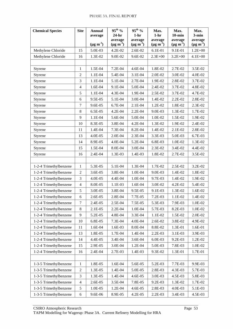
PHASE 3A. FINAL REPORT
CSIRO Atmospheric Research Page 53 TAPM Modelling for Wagerup: Phase 3A. Current Refinery Modelling for HRA
Chemical Species Site Annual average
(µg m-3)
95th % 24-hr
average (µg m-3)
95th % 1-hr
average (µg m-3)
Max. 1-hr
average (µg m-3)
Max. 10-min average (µg m-3)
Max. 3-min
average (µg m-3)
Methylene Chloride 15 5.0E-03 4.2E-02 2.6E-02 6.1E-01 9.1E-01 1.2E+00 Methylene Chloride 16 1.3E-02 9.0E-02 9.6E-02 2.3E+00 3.2E+00 4.1E+00 Styrene 1 1.5E-04 7.2E-04 4.6E-04 1.8E-02 2.7E-02 3.5E-02 Styrene 2 1.1E-04 5.4E-04 3.1E-04 2.0E-02 3.0E-02 4.0E-02 Styrene 3 1.1E-04 5.1E-04 2.7E-04 1.9E-02 2.8E-02 3.7E-02 Styrene 4 1.6E-04 9.1E-04 5.0E-04 2.4E-02 3.7E-02 4.8E-02 Styrene 5 1.1E-04 4.3E-04 1.9E-04 2.5E-02 3.7E-02 4.7E-02 Styrene 6 9.5E-05 5.1E-04 3.0E-04 1.4E-02 2.2E-02 2.8E-02 Styrene 7 9.6E-05 6.7E-04 2.1E-04 1.2E-02 1.8E-02 2.3E-02 Styrene 8 6.5E-05 4.2E-04 2.2E-04 9.0E-03 1.3E-02 1.7E-02 Styrene 9 1.1E-04 5.6E-04 5.0E-04 1.0E-02 1.5E-02 1.9E-02 Styrene 10 8.3E-05 3.8E-04 4.2E-04 1.3E-02 1.9E-02 2.4E-02 Styrene 11 1.4E-04 7.3E-04 8.2E-04 1.4E-02 2.1E-02 2.8E-02 Styrene 13 4.0E-05 2.0E-04 2.3E-04 3.3E-03 5.0E-03 6.7E-03 Styrene 14 8.9E-05 4.0E-04 5.2E-04 6.8E-03 1.0E-02 1.3E-02 Styrene 15 1.5E-04 8.0E-04 3.0E-04 2.3E-02 3.4E-02 4.4E-02 Styrene 16 2.4E-04 1.3E-03 1.4E-03 1.8E-02 2.7E-02 3.5E-02 1-2-4 Trimethylbenzene 1 5.3E-05 5.1E-04 1.3E-04 1.7E-02 2.5E-02 3.2E-02 1-2-4 Trimethylbenzene 2 3.6E-05 3.8E-04 1.0E-04 9.0E-03 1.4E-02 1.8E-02 1-2-4 Trimethylbenzene 3 4.0E-05 4.4E-04 1.0E-04 9.7E-03 1.4E-02 1.9E-02 1-2-4 Trimethylbenzene 4 8.0E-05 1.1E-03 1.6E-04 3.0E-02 4.2E-02 5.4E-02 1-2-4 Trimethylbenzene 5 3.0E-05 3.8E-04 9.5E-05 9.1E-03 1.3E-02 1.6E-02 1-2-4 Trimethylbenzene 6 2.6E-05 2.8E-04 7.7E-05 7.2E-03 1.1E-02 1.4E-02 1-2-4 Trimethylbenzene 7 2.4E-05 2.5E-04 7.5E-05 5.3E-03 7.9E-03 1.0E-02 1-2-4 Trimethylbenzene 8 2.1E-05 2.2E-04 1.0E-04 5.7E-03 8.2E-03 1.0E-02 1-2-4 Trimethylbenzene 9 5.2E-05 4.8E-04 3.3E-04 1.1E-02 1.5E-02 2.0E-02 1-2-4 Trimethylbenzene 10 6.8E-05 7.3E-04 4.0E-04 2.6E-02 3.8E-02 4.9E-02 1-2-4 Trimethylbenzene 11 1.6E-04 1.6E-03 8.0E-04 8.8E-02 1.3E-01 1.6E-01 1-2-4 Trimethylbenzene 13 1.8E-05 1.7E-04 1.4E-04 2.2E-03 3.1E-03 3.9E-03 1-2-4 Trimethylbenzene 14 4.4E-05 3.4E-04 3.6E-04 6.0E-03 9.2E-03 1.2E-02 1-2-4 Trimethylbenzene 15 2.9E-05 3.0E-04 1.2E-04 5.0E-03 7.8E-03 1.0E-02 1-2-4 Trimethylbenzene 16 2.4E-04 2.7E-03 1.4E-03 9.3E-02 1.3E-01 1.7E-01 1-3-5 Trimethylbenzene 1 1.8E-05 1.6E-04 5.6E-05 5.2E-03 7.7E-03 9.9E-03 1-3-5 Trimethylbenzene 2 1.3E-05 1.4E-04 5.0E-05 2.8E-03 4.3E-03 5.7E-03 1-3-5 Trimethylbenzene 3 1.3E-05 1.4E-04 4.6E-05 3.0E-03 4.5E-03 5.8E-03 1-3-5 Trimethylbenzene 4 2.6E-05 3.5E-04 7.8E-05 9.2E-03 1.3E-02 1.7E-02 1-3-5 Trimethylbenzene 5 1.0E-05 1.2E-04 4.6E-05 2.8E-03 4.0E-03 5.1E-03 1-3-5 Trimethylbenzene 6 9.6E-06 8.9E-05 4.2E-05 2.2E-03 3.4E-03 4.5E-03

PHASE 3A. FINAL REPORT
CSIRO Atmospheric Research Page 54 TAPM Modelling for Wagerup: Phase 3A. Current Refinery Modelling for HRA
Chemical Species Site Annual average
(µg m-3)
95th % 24-hr
average (µg m-3)
95th % 1-hr
average (µg m-3)
Max. 1-hr
average (µg m-3)
Max. 10-min average (µg m-3)
Max. 3-min
average (µg m-3)
1-3-5 Trimethylbenzene 7 8.8E-06 8.6E-05 4.0E-05 1.7E-03 2.5E-03 3.2E-03 1-3-5 Trimethylbenzene 8 7.6E-06 7.8E-05 4.7E-05 1.8E-03 2.5E-03 3.2E-03 1-3-5 Trimethylbenzene 9 1.8E-05 1.7E-04 1.3E-04 3.3E-03 4.7E-03 6.1E-03 1-3-5 Trimethylbenzene 10 2.2E-05 2.3E-04 1.4E-04 8.2E-03 1.2E-02 1.5E-02 1-3-5 Trimethylbenzene 11 5.3E-05 5.4E-04 2.8E-04 2.7E-02 3.9E-02 5.0E-02 1-3-5 Trimethylbenzene 13 6.6E-06 5.2E-05 5.8E-05 6.8E-04 9.6E-04 1.2E-03 1-3-5 Trimethylbenzene 14 1.5E-05 1.2E-04 1.4E-04 1.9E-03 2.9E-03 3.8E-03 1-3-5 Trimethylbenzene 15 1.2E-05 1.1E-04 6.5E-05 1.6E-03 2.4E-03 3.3E-03 1-3-5 Trimethylbenzene 16 7.7E-05 8.3E-04 4.8E-04 2.9E-02 4.1E-02 5.1E-02 Vinyl chloride 1 1.7E-06 1.1E-05 2.9E-06 2.0E-04 3.3E-04 4.5E-04 Vinyl chloride 2 2.4E-06 1.1E-05 3.5E-06 2.8E-04 4.3E-04 5.7E-04 Vinyl chloride 3 1.2E-06 7.4E-06 1.6E-06 2.1E-04 3.2E-04 4.3E-04 Vinyl chloride 4 1.6E-06 1.0E-05 2.7E-06 2.6E-04 4.1E-04 5.4E-04 Vinyl chloride 5 1.2E-06 7.8E-06 1.4E-06 2.3E-04 3.5E-04 4.7E-04 Vinyl chloride 6 1.9E-06 9.1E-06 3.2E-06 2.9E-04 4.4E-04 5.9E-04 Vinyl chloride 7 1.5E-06 1.0E-05 3.7E-06 2.0E-04 3.0E-04 4.0E-04 Vinyl chloride 8 1.2E-06 7.8E-06 5.5E-06 1.4E-04 2.2E-04 2.8E-04 Vinyl chloride 9 1.9E-06 1.1E-05 1.1E-05 1.6E-04 2.6E-04 3.5E-04 Vinyl chloride 10 1.5E-06 8.4E-06 5.4E-06 1.8E-04 2.9E-04 3.9E-04 Vinyl chloride 11 2.5E-06 1.2E-05 1.1E-05 1.9E-04 3.0E-04 4.1E-04 Vinyl chloride 13 9.6E-07 5.1E-06 3.7E-06 1.2E-04 1.8E-04 2.4E-04 Vinyl chloride 14 2.3E-06 1.3E-05 1.0E-05 2.2E-04 3.4E-04 4.5E-04 Vinyl chloride 15 3.1E-06 1.7E-05 5.4E-06 3.9E-04 6.0E-04 8.1E-04 Vinyl chloride 16 3.9E-06 2.7E-05 2.4E-05 2.1E-04 3.3E-04 4.6E-04 Shaded values limited by available ozone NO2 1 2.6E-01 2.9E+00 1.4E+00 5.0E+01 5.4E+01 5.4E+01 NO2 2 2.9E-01 3.4E+00 2.0E+00 5.1E+01 5.4E+01 5.4E+01 NO2 3 2.0E-01 2.4E+00 5.8E-01 5.4E+01 5.4E+01 5.4E+01 NO2 4 2.4E-01 2.9E+00 8.7E-01 5.3E+01 5.4E+01 5.4E+01 NO2 5 1.9E-01 2.3E+00 4.5E-01 5.0E+01 5.0E+01 5.4E+01 NO2 6 2.8E-01 3.1E+00 2.1E+00 5.1E+01 5.3E+01 5.4E+01 NO2 7 2.4E-01 3.3E+00 1.3E+00 3.8E+01 3.9E+01 4.7E+01 NO2 8 1.7E-01 2.5E+00 1.5E+00 3.6E+01 3.8E+01 4.3E+01 NO2 9 2.7E-01 3.0E+00 3.0E+00 4.1E+01 4.8E+01 5.1E+01 NO2 10 2.3E-01 2.4E+00 2.1E+00 4.2E+01 5.1E+01 5.4E+01 NO2 11 3.8E-01 4.8E+00 4.9E+00 4.5E+01 5.4E+01 5.4E+01 NO2 13 1.4E-01 1.5E+00 1.2E+00 3.4E+01 4.7E+01 4.8E+01 NO2 14 3.7E-01 4.0E+00 3.5E+00 5.4E+01 5.4E+01 5.4E+01 NO2 15 4.3E-01 5.0E+00 3.3E+00 5.4E+01 5.4E+01 5.4E+01 NO2 16 5.4E-01 6.9E+00 8.3E+00 4.4E+01 5.2E+01 5.4E+01

PHASE 3A. FINAL REPORT
CSIRO Atmospheric Research Page 55 TAPM Modelling for Wagerup: Phase 3A. Current Refinery Modelling for HRA
4.5. Concentration Statistics (sorted by Receptor Site) Table 9. Selected modelled concentration statistics sorted by receptor site for each of the 28 chemical species at each of the 15 receptor sites for the Current Emissions Scenario of 6,600 tonnes per day. The annual averages are for the average emission rates, whereas all other statistics are for peak emission rates. The shaded NO2 cells indicate values that are limited by the available ozone, see Section 3.5. Site Chemical Species Annual
average
(µg m-3)
95th % 24-hr
average (µg m-3)
95th % 1-hr
average (µg m-3)
Max. 1-hr
average (µg m-3)
Max. 10-min average (µg m-3)
Max. 3-min
average (µg m-3)
1 NOx 2.6E-01 2.9E+00 1.4E+00 5.5E+01 8.4E+01 1.1E+02 1 CO 2.7E-01 3.4E+00 1.9E+00 5.6E+01 8.1E+01 1.0E+02 1 SO2 1.8E-02 3.7E-01 1.7E-01 6.5E+00 1.0E+01 1.4E+01 1 Dust 1.3E-02 2.5E-01 9.6E-02 4.9E+00 7.7E+00 1.0E+01 1 Arsenic 2.2E-05 1.4E-04 1.0E-04 2.5E-03 4.0E-03 5.5E-03 1 Selenium 2.3E-05 1.6E-04 1.2E-04 2.6E-03 3.9E-03 5.0E-03 1 Manganese 7.3E-04 7.3E-03 1.6E-03 2.4E-01 3.5E-01 4.6E-01 1 Cadmium 1.6E-09 7.4E-09 1.2E-09 1.7E-07 2.3E-07 2.8E-07 1 Chromium (VI) 1.5E-07 7.3E-07 2.6E-07 1.2E-05 1.9E-05 2.6E-05 1 Nickel 2.4E-05 2.3E-04 7.6E-05 7.5E-03 1.1E-02 1.4E-02 1 Mercury 6.4E-05 2.9E-04 2.7E-04 5.4E-03 7.9E-03 1.0E-02 1 Ammonia 1.2E-02 8.5E-02 4.3E-02 2.8E+00 4.0E+00 5.1E+00 1 BaP Equivalents 1.7E-06 1.4E-05 5.1E-06 1.7E-04 2.5E-04 3.2E-04 1 Acetone 5.8E-02 5.6E-01 4.8E-01 5.5E+00 8.1E+00 1.0E+01 1 Acetaldehyde 1.0E-02 9.4E-02 1.1E-01 1.1E+00 1.6E+00 2.1E+00 1 Formaldehyde 3.4E-03 4.9E-02 2.9E-02 7.1E-01 1.1E+00 1.4E+00 1 2-Butanone 6.6E-03 5.5E-02 4.8E-02 6.9E-01 1.0E+00 1.3E+00 1 Benzene 8.5E-04 1.6E-02 1.0E-02 3.0E-01 4.4E-01 5.8E-01 1 Toluene 5.8E-03 4.2E-02 2.8E-02 4.4E-01 6.7E-01 9.0E-01 1 Xylenes 1.3E-03 6.8E-03 3.0E-03 9.8E-02 1.5E-01 2.0E-01 1 Acrolein 2.8E-04 1.7E-03 4.7E-04 3.2E-02 5.2E-02 7.1E-02 1 Ethylbenzene 2.6E-05 1.9E-04 1.4E-04 4.1E-03 6.0E-03 7.7E-03 1 Methylene Chloride 6.1E-03 5.2E-02 2.8E-02 7.2E-01 1.1E+00 1.5E+00 1 Styrene 1.5E-04 7.2E-04 4.6E-04 1.8E-02 2.7E-02 3.5E-02 1 1-2-4 Trimethylbenzene 5.3E-05 5.1E-04 1.3E-04 1.7E-02 2.5E-02 3.2E-02 1 1-3-5 Trimethylbenzene 1.8E-05 1.6E-04 5.6E-05 5.2E-03 7.7E-03 9.9E-03 1 Vinyl chloride 1.7E-06 1.1E-05 2.9E-06 2.0E-04 3.3E-04 4.5E-04 1 NO2 2.6E-01 2.9E+00 1.4E+00 5.0E+01 5.4E+01 5.4E+01
2 NOx 2.9E-01 3.4E+00 2.0E+00 6.9E+01 1.0E+02 1.3E+02 2 CO 3.2E-01 4.2E+00 2.4E+00 6.5E+01 9.7E+01 1.3E+02 2 SO2 2.0E-02 4.2E-01 2.3E-01 7.8E+00 1.2E+01 1.5E+01 2 Dust 1.7E-02 2.9E-01 1.2E-01 6.4E+00 1.0E+01 1.3E+01 2 Arsenic 2.3E-05 1.3E-04 1.0E-04 3.6E-03 5.7E-03 7.7E-03

PHASE 3A. FINAL REPORT
CSIRO Atmospheric Research Page 56 TAPM Modelling for Wagerup: Phase 3A. Current Refinery Modelling for HRA
Site Chemical Species Annual average
(µg m-3)
95th % 24-hr
average (µg m-3)
95th % 1-hr
average (µg m-3)
Max. 1-hr
average (µg m-3)
Max. 10-min average (µg m-3)
Max. 3-min
average (µg m-3)
2 Selenium 2.3E-05 1.5E-04 1.0E-04 2.7E-03 4.0E-03 5.2E-03 2 Manganese 4.7E-04 4.9E-03 1.3E-03 1.3E-01 2.0E-01 2.6E-01 2 Cadmium 1.8E-09 7.5E-09 1.3E-09 2.4E-07 3.8E-07 5.2E-07 2 Chromium (VI) 1.8E-07 8.0E-07 4.0E-07 1.8E-05 2.6E-05 3.4E-05 2 Nickel 1.6E-05 1.6E-04 6.2E-05 4.0E-03 6.1E-03 8.2E-03 2 Mercury 5.7E-05 2.5E-04 2.6E-04 4.0E-03 6.3E-03 8.5E-03 2 Ammonia 8.0E-03 6.3E-02 3.4E-02 1.5E+00 2.2E+00 2.9E+00 2 BaP Equivalents 1.1E-06 8.6E-06 3.8E-06 1.3E-04 2.0E-04 2.7E-04 2 Acetone 3.9E-02 4.0E-01 3.1E-01 6.5E+00 9.7E+00 1.3E+01 2 Acetaldehyde 8.2E-03 8.5E-02 7.0E-02 1.2E+00 1.7E+00 2.2E+00 2 Formaldehyde 4.4E-03 4.2E-02 2.1E-02 9.5E-01 1.4E+00 1.8E+00 2 2-Butanone 4.1E-03 3.8E-02 2.9E-02 7.6E-01 1.1E+00 1.5E+00 2 Benzene 1.0E-03 1.4E-02 7.2E-03 3.4E-01 5.2E-01 6.8E-01 2 Toluene 4.8E-03 2.9E-02 2.1E-02 4.4E-01 6.5E-01 8.6E-01 2 Xylenes 1.1E-03 6.0E-03 2.8E-03 7.3E-02 1.1E-01 1.5E-01 2 Acrolein 3.8E-04 1.7E-03 5.5E-04 4.5E-02 6.9E-02 9.1E-02 2 Ethylbenzene 2.5E-05 1.8E-04 1.3E-04 2.3E-03 3.5E-03 4.7E-03 2 Methylene Chloride 5.2E-03 4.6E-02 2.7E-02 5.3E-01 8.1E-01 1.1E+00 2 Styrene 1.1E-04 5.4E-04 3.1E-04 2.0E-02 3.0E-02 4.0E-02 2 1-2-4 Trimethylbenzene 3.6E-05 3.8E-04 1.0E-04 9.0E-03 1.4E-02 1.8E-02 2 1-3-5 Trimethylbenzene 1.3E-05 1.4E-04 5.0E-05 2.8E-03 4.3E-03 5.7E-03 2 Vinyl chloride 2.4E-06 1.1E-05 3.5E-06 2.8E-04 4.3E-04 5.7E-04 2 NO2 2.9E-01 3.4E+00 2.0E+00 5.1E+01 5.4E+01 5.4E+01
3 NOx 2.0E-01 2.4E+00 5.8E-01 7.5E+01 1.1E+02 1.4E+02 3 CO 1.9E-01 2.7E+00 8.4E-01 7.7E+01 1.0E+02 1.3E+02 3 SO2 1.3E-02 3.1E-01 7.8E-02 9.8E+00 1.5E+01 1.9E+01 3 Dust 8.9E-03 1.8E-01 5.4E-02 5.5E+00 7.5E+00 9.3E+00 3 Arsenic 1.7E-05 1.1E-04 5.9E-05 2.8E-03 3.9E-03 4.9E-03 3 Selenium 1.6E-05 1.4E-04 8.2E-05 1.7E-03 2.3E-03 2.9E-03 3 Manganese 5.5E-04 6.1E-03 1.2E-03 1.4E-01 2.0E-01 2.7E-01 3 Cadmium 1.3E-09 6.0E-09 6.9E-10 1.7E-07 2.7E-07 3.7E-07 3 Chromium (VI) 1.2E-07 5.8E-07 1.2E-07 1.6E-05 2.1E-05 2.6E-05 3 Nickel 1.8E-05 1.9E-04 5.4E-05 4.3E-03 6.4E-03 8.4E-03 3 Mercury 4.9E-05 2.5E-04 1.7E-04 3.5E-03 4.8E-03 6.0E-03 3 Ammonia 8.9E-03 7.8E-02 3.2E-02 1.6E+00 2.3E+00 3.0E+00 3 BaP Equivalents 1.0E-06 8.1E-06 3.3E-06 1.3E-04 1.9E-04 2.4E-04 3 Acetone 3.9E-02 3.4E-01 2.9E-01 5.6E+00 8.3E+00 1.1E+01 3 Acetaldehyde 7.0E-03 6.5E-02 6.7E-02 1.1E+00 1.6E+00 2.0E+00 3 Formaldehyde 2.4E-03 3.3E-02 1.3E-02 9.0E-01 1.3E+00 1.7E+00 3 2-Butanone 4.0E-03 3.7E-02 2.8E-02 6.6E-01 9.8E-01 1.3E+00

PHASE 3A. FINAL REPORT
CSIRO Atmospheric Research Page 57 TAPM Modelling for Wagerup: Phase 3A. Current Refinery Modelling for HRA
Site Chemical Species Annual average
(µg m-3)
95th % 24-hr
average (µg m-3)
95th % 1-hr
average (µg m-3)
Max. 1-hr
average (µg m-3)
Max. 10-min average (µg m-3)
Max. 3-min
average (µg m-3)
3 Benzene 6.0E-04 1.1E-02 4.6E-03 3.4E-01 5.1E-01 6.6E-01 3 Toluene 3.8E-03 2.3E-02 1.7E-02 4.4E-01 6.5E-01 8.5E-01 3 Xylenes 8.2E-04 3.9E-03 2.3E-03 9.6E-02 1.4E-01 1.9E-01 3 Acrolein 2.0E-04 1.2E-03 2.5E-04 3.3E-02 5.1E-02 6.9E-02 3 Ethylbenzene 1.9E-05 1.7E-04 1.0E-04 2.3E-03 3.5E-03 4.5E-03 3 Methylene Chloride 4.0E-03 2.9E-02 2.1E-02 7.0E-01 1.1E+00 1.4E+00 3 Styrene 1.1E-04 5.1E-04 2.7E-04 1.9E-02 2.8E-02 3.7E-02 3 1-2-4 Trimethylbenzene 4.0E-05 4.4E-04 1.0E-04 9.7E-03 1.4E-02 1.9E-02 3 1-3-5 Trimethylbenzene 1.3E-05 1.4E-04 4.6E-05 3.0E-03 4.5E-03 5.8E-03 3 Vinyl chloride 1.2E-06 7.4E-06 1.6E-06 2.1E-04 3.2E-04 4.3E-04 3 NO2 2.0E-01 2.4E+00 5.8E-01 5.4E+01 5.4E+01 5.4E+01
4 NOx 2.5E-01 3.2E+00 8.7E-01 8.4E+01 1.3E+02 1.6E+02 4 CO 2.3E-01 3.3E+00 1.3E+00 5.6E+01 8.3E+01 1.1E+02 4 SO2 1.7E-02 4.0E-01 1.2E-01 1.1E+01 1.6E+01 2.2E+01 4 Dust 1.2E-02 2.5E-01 7.9E-02 5.2E+00 8.6E+00 1.2E+01 4 Arsenic 2.2E-05 1.4E-04 9.8E-05 3.0E-03 4.8E-03 6.6E-03 4 Selenium 2.4E-05 2.0E-04 1.1E-04 4.6E-03 6.5E-03 8.3E-03 4 Manganese 1.1E-03 1.6E-02 2.1E-03 4.2E-01 6.0E-01 7.7E-01 4 Cadmium 1.5E-09 7.2E-09 1.2E-09 2.0E-07 3.0E-07 4.1E-07 4 Chromium (VI) 1.4E-07 7.1E-07 1.7E-07 1.6E-05 2.5E-05 3.3E-05 4 Nickel 3.7E-05 5.0E-04 1.0E-04 1.3E-02 1.9E-02 2.4E-02 4 Mercury 8.0E-05 4.0E-04 2.7E-04 9.0E-03 1.3E-02 1.6E-02 4 Ammonia 1.8E-02 1.9E-01 6.0E-02 4.3E+00 6.1E+00 7.7E+00 4 BaP Equivalents 1.8E-06 1.6E-05 6.8E-06 3.4E-04 5.0E-04 6.5E-04 4 Acetone 7.2E-02 7.0E-01 5.9E-01 7.1E+00 1.0E+01 1.3E+01 4 Acetaldehyde 1.3E-02 1.3E-01 1.4E-01 1.1E+00 1.7E+00 2.1E+00 4 Formaldehyde 3.3E-03 4.9E-02 2.6E-02 9.5E-01 1.4E+00 1.8E+00 4 2-Butanone 7.7E-03 7.2E-02 6.5E-02 8.6E-01 1.2E+00 1.6E+00 4 Benzene 6.9E-04 1.6E-02 8.5E-03 4.1E-01 6.1E-01 8.0E-01 4 Toluene 5.2E-03 3.7E-02 2.4E-02 5.6E-01 8.4E-01 1.1E+00 4 Xylenes 1.1E-03 5.6E-03 2.8E-03 1.2E-01 1.8E-01 2.4E-01 4 Acrolein 2.6E-04 1.7E-03 4.3E-04 4.2E-02 6.5E-02 8.7E-02 4 Ethylbenzene 3.0E-05 2.9E-04 1.4E-04 7.2E-03 1.0E-02 1.3E-02 4 Methylene Chloride 5.5E-03 4.2E-02 2.7E-02 8.9E-01 1.3E+00 1.8E+00 4 Styrene 1.6E-04 9.1E-04 5.0E-04 2.4E-02 3.7E-02 4.8E-02 4 1-2-4 Trimethylbenzene 8.0E-05 1.1E-03 1.6E-04 3.0E-02 4.2E-02 5.4E-02 4 1-3-5 Trimethylbenzene 2.6E-05 3.5E-04 7.8E-05 9.2E-03 1.3E-02 1.7E-02 4 Vinyl chloride 1.6E-06 1.0E-05 2.7E-06 2.6E-04 4.1E-04 5.4E-04 4 NO2 2.4E-01 2.9E+00 8.7E-01 5.3E+01 5.4E+01 5.4E+01

PHASE 3A. FINAL REPORT
CSIRO Atmospheric Research Page 58 TAPM Modelling for Wagerup: Phase 3A. Current Refinery Modelling for HRA
Site Chemical Species Annual average
(µg m-3)
95th % 24-hr
average (µg m-3)
95th % 1-hr
average (µg m-3)
Max. 1-hr
average (µg m-3)
Max. 10-min average (µg m-3)
Max. 3-min
average (µg m-3)
5 NOx 1.9E-01 2.5E+00 4.5E-01 9.5E+01 1.4E+02 1.8E+02 5 CO 1.7E-01 2.5E+00 5.7E-01 6.5E+01 9.6E+01 1.2E+02 5 SO2 1.3E-02 3.0E-01 5.8E-02 1.1E+01 1.7E+01 2.2E+01 5 Dust 8.2E-03 1.7E-01 4.2E-02 3.8E+00 5.2E+00 6.3E+00 5 Arsenic 1.6E-05 1.0E-04 4.9E-05 4.0E-03 6.1E-03 8.1E-03 5 Selenium 1.2E-05 9.8E-05 6.8E-05 1.5E-03 2.1E-03 2.6E-03 5 Manganese 4.1E-04 5.4E-03 1.2E-03 1.3E-01 1.9E-01 2.3E-01 5 Cadmium 1.3E-09 5.8E-09 7.4E-10 2.6E-07 4.0E-07 5.3E-07 5 Chromium (VI) 1.1E-07 5.1E-07 1.1E-07 2.1E-05 3.0E-05 3.9E-05 5 Nickel 1.4E-05 1.7E-04 5.6E-05 4.1E-03 5.8E-03 7.4E-03 5 Mercury 4.2E-05 2.0E-04 1.6E-04 4.6E-03 7.1E-03 9.4E-03 5 Ammonia 7.0E-03 6.9E-02 3.1E-02 1.4E+00 1.9E+00 2.4E+00 5 BaP Equivalents 8.2E-07 8.3E-06 2.6E-06 1.1E-04 1.6E-04 2.0E-04 5 Acetone 3.3E-02 3.2E-01 2.1E-01 7.5E+00 1.1E+01 1.4E+01 5 Acetaldehyde 5.7E-03 6.3E-02 5.0E-02 1.1E+00 1.6E+00 2.0E+00 5 Formaldehyde 2.2E-03 3.5E-02 1.0E-02 8.8E-01 1.3E+00 1.7E+00 5 2-Butanone 3.4E-03 3.5E-02 2.2E-02 8.4E-01 1.2E+00 1.5E+00 5 Benzene 4.8E-04 9.3E-03 3.0E-03 4.3E-01 6.1E-01 7.8E-01 5 Toluene 2.8E-03 2.0E-02 1.1E-02 5.7E-01 8.2E-01 1.0E+00 5 Xylenes 6.1E-04 3.3E-03 1.3E-03 8.0E-02 1.2E-01 1.5E-01 5 Acrolein 1.9E-04 1.3E-03 2.2E-04 3.7E-02 5.6E-02 7.6E-02 5 Ethylbenzene 1.5E-05 1.3E-04 9.2E-05 2.2E-03 3.1E-03 4.0E-03 5 Methylene Chloride 3.1E-03 2.5E-02 1.3E-02 5.8E-01 8.6E-01 1.1E+00 5 Styrene 1.1E-04 4.3E-04 1.9E-04 2.5E-02 3.7E-02 4.7E-02 5 1-2-4 Trimethylbenzene 3.0E-05 3.8E-04 9.5E-05 9.1E-03 1.3E-02 1.6E-02 5 1-3-5 Trimethylbenzene 1.0E-05 1.2E-04 4.6E-05 2.8E-03 4.0E-03 5.1E-03 5 Vinyl chloride 1.2E-06 7.8E-06 1.4E-06 2.3E-04 3.5E-04 4.7E-04 5 NO2 1.9E-01 2.3E+00 4.5E-01 5.0E+01 5.0E+01 5.4E+01
6 NOx 2.8E-01 3.1E+00 2.1E+00 8.9E+01 1.2E+02 1.5E+02 6 CO 2.9E-01 4.0E+00 2.5E+00 7.2E+01 9.7E+01 1.2E+02 6 SO2 1.9E-02 3.9E-01 2.5E-01 1.0E+01 1.4E+01 1.7E+01 6 Dust 1.4E-02 2.4E-01 1.2E-01 5.9E+00 8.7E+00 1.1E+01 6 Arsenic 2.4E-05 1.2E-04 9.0E-05 4.5E-03 76.2E-03 7.8E-03 6 Selenium 2.0E-05 1.4E-04 9.1E-05 2.4E-03 3.4E-03 4.2E-03 6 Manganese 3.3E-04 3.8E-03 9.7E-04 1.0E-01 1.5E-01 2.0E-01 6 Cadmium 1.9E-09 6.7E-09 1.5E-09 2.9E-07 4.0E-07 5.0E-07 6 Chromium (VI) 1.7E-07 7.6E-07 4.2E-07 2.2E-05 2.9E-05 3.6E-05 6 Nickel 1.2E-05 1.2E-04 5.1E-05 3.2E-03 4.9E-03 6.4E-03 6 Mercury 5.1E-05 2.3E-04 2.2E-04 5.2E-03 7.2E-03 9.0E-03 6 Ammonia 6.1E-03 4.8E-02 2.9E-02 1.2E+00 1.8E+00 2.4E+00

PHASE 3A. FINAL REPORT
CSIRO Atmospheric Research Page 59 TAPM Modelling for Wagerup: Phase 3A. Current Refinery Modelling for HRA
Site Chemical Species Annual average
(µg m-3)
95th % 24-hr
average (µg m-3)
95th % 1-hr
average (µg m-3)
Max. 1-hr
average (µg m-3)
Max. 10-min average (µg m-3)
Max. 3-min
average (µg m-3)
6 BaP Equivalents 7.5E-07 6.3E-06 2.6E-06 1.1E-04 1.6E-04 2.1E-04 6 Acetone 2.9E-02 3.2E-01 2.6E-01 5.4E+00 7.9E+00 1.0E+01 6 Acetaldehyde 6.1E-03 6.5E-02 6.4E-02 1.2E+00 1.8E+00 2.3E+00 6 Formaldehyde 3.6E-03 3.7E-02 1.9E-02 9.8E-01 1.5E+00 1.9E+00 6 2-Butanone 2.9E-03 2.8E-02 2.6E-02 5.4E-01 8.1E-01 1.1E+00 6 Benzene 9.0E-04 1.4E-02 7.1E-03 2.8E-01 4.1E-01 5.4E-01 6 Toluene 3.6E-03 2.5E-02 1.8E-02 4.0E-01 6.0E-01 7.8E-01 6 Xylenes 8.0E-04 4.5E-03 2.4E-03 7.6E-02 1.1E-01 1.5E-01 6 Acrolein 3.1E-04 1.5E-03 5.2E-04 4.7E-02 7.1E-02 9.4E-02 6 Ethylbenzene 2.0E-05 1.4E-04 1.1E-04 2.4E-03 3.5E-03 4.6E-03 6 Methylene Chloride 4.0E-03 3.3E-02 2.2E-02 5.6E-01 8.4E-01 1.1E+00 6 Styrene 9.5E-05 5.1E-04 3.0E-04 1.4E-02 2.2E-02 2.8E-02 6 1-2-4 Trimethylbenzene 2.6E-05 2.8E-04 7.7E-05 7.2E-03 1.1E-02 1.4E-02 6 1-3-5 Trimethylbenzene 9.6E-06 8.9E-05 4.2E-05 2.2E-03 3.4E-03 4.5E-03 6 Vinyl chloride 1.9E-06 9.1E-06 3.2E-06 2.9E-04 4.4E-04 5.9E-04 6 NO2 2.8E-01 3.1E+00 2.1E+00 5.1E+01 5.3E+01 5.4E+01
7 NOx 2.5E-01 3.3E+00 1.3E+00 8.4E+01 1.2E+02 1.6E+02 7 CO 1.6E-01 2.4E+00 1.4E+00 3.4E+01 5.1E+01 6.7E+01 7 SO2 1.6E-02 4.1E-01 1.6E-01 9.2E+00 1.4E+01 1.8E+01 7 Dust 9.8E-03 1.6E-01 9.6E-02 3.1E+00 4.0E+00 4.8E+00 7 Arsenic 2.0E-05 1.3E-04 5.0E-05 4.8E-03 7.5E-03 1.0E-02 7 Selenium 9.2E-06 7.2E-05 4.9E-05 8.4E-04 1.2E-03 1.6E-03 7 Manganese 3.4E-04 3.6E-03 9.9E-04 7.6E-02 1.1E-01 1.5E-01 7 Cadmium 1.7E-09 7.0E-09 1.5E-09 3.2E-07 5.0E-07 6.8E-07 7 Chromium (VI) 1.4E-07 6.2E-07 2.6E-07 2.0E-05 2.9E-05 3.9E-05 7 Nickel 1.2E-05 1.2E-04 4.1E-05 2.4E-03 3.5E-03 4.6E-03 7 Mercury 4.5E-05 2.0E-04 1.4E-04 5.4E-03 8.4E-03 1.1E-02 7 Ammonia 6.9E-03 4.6E-02 2.5E-02 9.5E-01 1.4E+00 1.8E+00 7 BaP Equivalents 6.3E-07 4.8E-06 2.2E-06 1.1E-04 1.5E-04 1.9E-04 7 Acetone 2.7E-02 2.6E-01 1.7E-01 3.7E+00 5.2E+00 6.5E+00 7 Acetaldehyde 5.4E-03 5.9E-02 4.3E-02 7.4E-01 1.1E+00 1.4E+00 7 Formaldehyde 2.5E-03 4.3E-02 1.7E-02 6.4E-01 9.5E-01 1.2E+00 7 2-Butanone 2.8E-03 2.9E-02 1.8E-02 4.3E-01 6.4E-01 8.3E-01 7 Benzene 4.3E-04 1.4E-02 4.1E-03 2.0E-01 2.9E-01 3.8E-01 7 Toluene 1.8E-03 1.8E-02 8.1E-03 2.7E-01 3.9E-01 5.1E-01 7 Xylenes 3.8E-04 2.2E-03 1.1E-03 3.3E-02 4.5E-02 5.6E-02 7 Acrolein 2.4E-04 1.6E-03 5.9E-04 3.2E-02 4.8E-02 6.4E-02 7 Ethylbenzene 1.4E-05 1.1E-04 8.6E-05 1.3E-03 1.9E-03 2.5E-03 7 Methylene Chloride 2.2E-03 1.8E-02 1.1E-02 2.4E-01 3.3E-01 4.1E-01 7 Styrene 9.6E-05 6.7E-04 2.1E-04 1.2E-02 1.8E-02 2.3E-02

PHASE 3A. FINAL REPORT
CSIRO Atmospheric Research Page 60 TAPM Modelling for Wagerup: Phase 3A. Current Refinery Modelling for HRA
Site Chemical Species Annual average
(µg m-3)
95th % 24-hr
average (µg m-3)
95th % 1-hr
average (µg m-3)
Max. 1-hr
average (µg m-3)
Max. 10-min average (µg m-3)
Max. 3-min
average (µg m-3)
7 1-2-4 Trimethylbenzene 2.4E-05 2.5E-04 7.5E-05 5.3E-03 7.9E-03 1.0E-02 7 1-3-5 Trimethylbenzene 8.8E-06 8.6E-05 4.0E-05 1.7E-03 2.5E-03 3.2E-03 7 Vinyl chloride 1.5E-06 1.0E-05 3.7E-06 2.0E-04 3.0E-04 4.0E-04 7 NO2 2.4E-01 3.3E+00 1.3E+00 3.8E+01 3.9E+01 4.7E+01
8 NOx 1.7E-01 2.5E+00 1.5E+00 3.6E+01 5.4E+01 7.0E+01 8 CO 1.5E-01 2.5E+00 1.7E+00 3.9E+01 5.8E+01 7.5E+01 8 SO2 1.2E-02 3.1E-01 1.9E-01 3.9E+00 5.9E+00 7.7E+00 8 Dust 8.6E-03 1.8E-01 1.3E-01 3.0E+00 4.5E+00 5.8E+00 8 Arsenic 1.4E-05 9.2E-05 6.4E-05 2.2E-03 3.3E-03 4.4E-03 8 Selenium 9.6E-06 7.4E-05 5.8E-05 1.0E-03 1.4E-03 1.7E-03 8 Manganese 2.9E-04 3.2E-03 1.3E-03 8.2E-02 1.2E-01 1.5E-01 8 Cadmium 1.1E-09 5.1E-09 2.5E-09 1.4E-07 2.2E-07 2.9E-07 8 Chromium (VI) 1.0E-07 5.6E-07 3.3E-07 8.9E-06 1.3E-05 1.7E-05 8 Nickel 1.0E-05 1.0E-04 5.5E-05 2.6E-03 3.7E-03 4.7E-03 8 Mercury 3.4E-05 1.5E-04 1.6E-04 2.8E-03 4.2E-03 5.6E-03 8 Ammonia 5.8E-03 4.6E-02 3.0E-02 9.6E-01 1.4E+00 1.7E+00 8 BaP Equivalents 5.2E-07 4.0E-06 2.5E-06 7.6E-05 1.1E-04 1.4E-04 8 Acetone 2.1E-02 1.8E-01 1.6E-01 3.1E+00 4.5E+00 5.7E+00 8 Acetaldehyde 4.5E-03 3.9E-02 4.4E-02 6.7E-01 9.6E-01 1.2E+00 8 Formaldehyde 2.3E-03 3.3E-02 2.4E-02 5.8E-01 8.6E-01 1.1E+00 8 2-Butanone 2.3E-03 2.0E-02 1.8E-02 3.2E-01 4.7E-01 6.1E-01 8 Benzene 4.1E-04 8.4E-03 5.0E-03 1.9E-01 2.8E-01 3.6E-01 8 Toluene 1.6E-03 1.2E-02 9.2E-03 2.4E-01 3.4E-01 4.4E-01 8 Xylenes 3.4E-04 1.9E-03 1.3E-03 2.9E-02 4.2E-02 5.5E-02 8 Acrolein 1.9E-04 1.3E-03 8.8E-04 2.3E-02 3.4E-02 4.5E-02 8 Ethylbenzene 1.2E-05 9.9E-05 8.7E-05 1.4E-03 2.0E-03 2.5E-03 8 Methylene Chloride 1.8E-03 1.5E-02 1.2E-02 2.2E-01 3.2E-01 4.2E-01 8 Styrene 6.5E-05 4.2E-04 2.2E-04 9.0E-03 1.3E-02 1.7E-02 8 1-2-4 Trimethylbenzene 2.1E-05 2.2E-04 1.0E-04 5.7E-03 8.2E-03 1.0E-02 8 1-3-5 Trimethylbenzene 7.6E-06 7.8E-05 4.7E-05 1.8E-03 2.5E-03 3.2E-03 8 Vinyl chloride 1.2E-06 7.8E-06 5.5E-06 1.4E-04 2.2E-04 2.8E-04 8 NO2 1.7E-01 2.5E+00 1.5E+00 3.6E+01 3.8E+01 4.3E+01
9 NOx 2.7E-01 3.0E+00 3.0E+00 4.1E+01 6.3E+01 8.6E+01 9 CO 2.4E-01 3.1E+00 3.6E+00 4.1E+01 6.5E+01 8.7E+01 9 SO2 1.8E-02 3.9E-01 3.9E-01 4.7E+00 7.1E+00 9.3E+00 9 Dust 1.4E-02 2.5E-01 2.6E-01 4.1E+00 6.5E+00 8.7E+00 9 Arsenic 2.3E-05 1.3E-04 1.4E-04 2.4E-03 3.9E-03 5.5E-03 9 Selenium 1.9E-05 1.1E-04 1.5E-04 1.8E-03 2.6E-03 3.3E-03 9 Manganese 7.2E-04 6.8E-03 4.6E-03 1.5E-01 2.2E-01 2.8E-01

PHASE 3A. FINAL REPORT
CSIRO Atmospheric Research Page 61 TAPM Modelling for Wagerup: Phase 3A. Current Refinery Modelling for HRA
Site Chemical Species Annual average
(µg m-3)
95th % 24-hr
average (µg m-3)
95th % 1-hr
average (µg m-3)
Max. 1-hr
average (µg m-3)
Max. 10-min average (µg m-3)
Max. 3-min
average (µg m-3)
9 Cadmium 1.8E-09 8.2E-09 6.0E-09 1.6E-07 2.6E-07 3.7E-07 9 Chromium (VI) 1.6E-07 7.1E-07 7.5E-07 9.8E-06 1.5E-05 2.1E-05 9 Nickel 2.4E-05 2.3E-04 1.6E-04 4.7E-03 6.8E-03 8.8E-03 9 Mercury 6.6E-05 2.4E-04 3.5E-04 3.5E-03 5.0E-03 6.4E-03 9 Ammonia 1.3E-02 9.2E-02 8.4E-02 1.8E+00 2.6E+00 3.3E+00 9 BaP Equivalents 1.2E-06 8.1E-06 7.5E-06 1.4E-04 1.9E-04 2.4E-04 9 Acetone 4.7E-02 3.1E-01 4.0E-01 4.9E+00 6.8E+00 8.4E+00 9 Acetaldehyde 9.4E-03 6.8E-02 9.7E-02 9.6E-01 1.3E+00 1.6E+00 9 Formaldehyde 3.7E-03 4.3E-02 5.5E-02 5.8E-01 9.1E-01 1.2E+00 9 2-Butanone 5.1E-03 3.1E-02 4.3E-02 4.5E-01 6.2E-01 7.8E-01 9 Benzene 6.9E-04 1.2E-02 1.1E-02 1.8E-01 2.7E-01 3.4E-01 9 Toluene 3.7E-03 2.0E-02 2.2E-02 3.5E-01 5.0E-01 6.3E-01 9 Xylenes 8.0E-04 3.7E-03 3.5E-03 7.6E-02 1.1E-01 1.4E-01 9 Acrolein 3.0E-04 1.7E-03 1.8E-03 2.6E-02 4.1E-02 5.6E-02 9 Ethylbenzene 2.4E-05 1.6E-04 2.0E-04 2.6E-03 3.8E-03 4.9E-03 9 Methylene Chloride 4.1E-03 2.7E-02 3.1E-02 5.8E-01 8.2E-01 1.0E+00 9 Styrene 1.1E-04 5.6E-04 5.0E-04 1.0E-02 1.5E-02 1.9E-02 9 1-2-4 Trimethylbenzene 5.2E-05 4.8E-04 3.3E-04 1.1E-02 1.5E-02 2.0E-02 9 1-3-5 Trimethylbenzene 1.8E-05 1.7E-04 1.3E-04 3.3E-03 4.7E-03 6.1E-03 9 Vinyl chloride 1.9E-06 1.1E-05 1.1E-05 1.6E-04 2.6E-04 3.5E-04 9 NO2 2.7E-01 3.0E+00 3.0E+00 4.1E+01 4.8E+01 5.1E+01
10 NOx 2.3E-01 2.4E+00 2.1E+00 4.2E+01 6.2E+01 8.1E+01 10 CO 2.1E-01 2.8E+00 2.5E+00 5.2E+01 8.1E+01 1.1E+02 10 SO2 1.5E-02 3.1E-01 2.7E-01 5.1E+00 7.7E+00 1.0E+01 10 Dust 1.1E-02 2.4E-01 1.7E-01 5.5E+00 8.7E+00 1.2E+01 10 Arsenic 2.2E-05 1.2E-04 1.6E-04 2.0E-03 3.2E-03 4.6E-03 10 Selenium 2.1E-05 1.7E-04 1.7E-04 4.2E-03 6.0E-03 7.8E-03 10 Manganese 9.6E-04 1.0E-02 5.7E-03 3.8E-01 5.5E-01 7.1E-01 10 Cadmium 1.6E-09 7.2E-09 4.9E-09 1.3E-07 2.2E-07 3.1E-07 10 Chromium (VI) 1.4E-07 6.2E-07 4.9E-07 9.7E-06 1.4E-05 1.9E-05 10 Nickel 3.1E-05 3.3E-04 2.0E-04 1.2E-02 1.7E-02 2.2E-02 10 Mercury 7.3E-05 3.7E-04 4.1E-04 8.6E-03 1.2E-02 1.6E-02 10 Ammonia 1.6E-02 1.4E-01 9.5E-02 4.4E+00 6.4E+00 8.1E+00 10 BaP Equivalents 1.4E-06 1.1E-05 7.7E-06 2.2E-04 3.2E-04 4.1E-04 10 Acetone 5.2E-02 3.9E-01 4.0E-01 9.4E+00 1.3E+01 1.7E+01 10 Acetaldehyde 9.9E-03 8.3E-02 9.6E-02 1.9E+00 2.7E+00 3.4E+00 10 Formaldehyde 3.3E-03 3.6E-02 3.1E-02 7.1E-01 1.1E+00 1.6E+00 10 2-Butanone 5.6E-03 4.2E-02 4.3E-02 7.9E-01 1.1E+00 1.4E+00 10 Benzene 6.2E-04 8.6E-03 8.8E-03 2.0E-01 2.9E-01 3.8E-01 10 Toluene 4.2E-03 2.4E-02 2.5E-02 8.5E-01 1.2E+00 1.6E+00

PHASE 3A. FINAL REPORT
CSIRO Atmospheric Research Page 62 TAPM Modelling for Wagerup: Phase 3A. Current Refinery Modelling for HRA
Site Chemical Species Annual average
(µg m-3)
95th % 24-hr
average (µg m-3)
95th % 1-hr
average (µg m-3)
Max. 1-hr
average (µg m-3)
Max. 10-min average (µg m-3)
Max. 3-min
average (µg m-3)
10 Xylenes 8.8E-04 3.8E-03 3.6E-03 1.8E-01 2.6E-01 3.4E-01 10 Acrolein 2.4E-04 1.4E-03 8.7E-04 2.9E-02 4.6E-02 6.2E-02 10 Ethylbenzene 2.6E-05 2.3E-04 2.1E-04 6.4E-03 9.3E-03 1.2E-02 10 Methylene Chloride 4.5E-03 3.1E-02 3.3E-02 1.4E+00 2.0E+00 2.6E+00 10 Styrene 8.3E-05 3.8E-04 4.2E-04 1.3E-02 1.9E-02 2.4E-02 10 1-2-4 Trimethylbenzene 6.8E-05 7.3E-04 4.0E-04 2.6E-02 3.8E-02 4.9E-02 10 1-3-5 Trimethylbenzene 2.2E-05 2.3E-04 1.4E-04 8.2E-03 1.2E-02 1.5E-02 10 Vinyl chloride 1.5E-06 8.4E-06 5.4E-06 1.8E-04 2.9E-04 3.9E-04 10 NO2 2.3E-01 2.4E+00 2.1E+00 4.2E+01 5.1E+01 5.4E+01
11 NOx 3.8E-01 4.8E+00 4.9E+00 4.8E+01 7.7E+01 1.0E+02 11 CO 3.5E-01 4.2E+00 5.1E+00 5.2E+01 8.4E+01 1.2E+02 11 SO2 2.5E-02 5.5E-01 5.7E-01 5.3E+00 8.4E+00 1.1E+01 11 Dust 1.9E-02 3.6E-01 3.3E-01 5.9E+00 9.4E+00 1.3E+01 11 Arsenic 3.7E-05 2.5E-04 3.2E-04 3.8E-03 5.5E-03 7.0E-03 11 Selenium 4.2E-05 3.5E-04 3.1E-04 1.4E-02 2.0E-02 2.5E-02 11 Manganese 2.3E-03 2.3E-02 1.1E-02 1.3E+00 1.8E+00 2.3E+00 11 Cadmium 2.6E-09 1.3E-08 1.0E-08 1.8E-07 3.2E-07 4.5E-07 11 Chromium (VI) 2.3E-07 1.3E-06 1.2E-06 1.3E-05 2.0E-05 2.7E-05 11 Nickel 7.5E-05 7.4E-04 3.9E-04 4.0E-02 5.7E-02 7.2E-02 11 Mercury 1.5E-04 6.4E-04 8.3E-04 2.8E-02 4.0E-02 5.1E-02 11 Ammonia 3.8E-02 3.0E-01 2.0E-01 1.4E+01 2.0E+01 2.6E+01 11 BaP Equivalents 2.8E-06 2.0E-05 1.6E-05 4.0E-04 5.8E-04 7.4E-04 11 Acetone 1.1E-01 7.3E-01 8.2E-01 1.2E+01 1.7E+01 2.2E+01 11 Acetaldehyde 2.1E-02 1.6E-01 1.9E-01 2.6E+00 3.7E+00 4.6E+00 11 Formaldehyde 5.6E-03 5.5E-02 6.2E-02 7.0E-01 1.2E+00 1.6E+00 11 2-Butanone 1.2E-02 7.1E-02 8.8E-02 1.1E+00 1.5E+00 1.9E+00 11 Benzene 1.0E-03 1.3E-02 1.9E-02 2.3E-01 3.4E-01 4.4E-01 11 Toluene 7.9E-03 3.9E-02 4.1E-02 1.2E+00 1.8E+00 2.3E+00 11 Xylenes 1.6E-03 6.7E-03 6.5E-03 2.6E-01 3.9E-01 5.1E-01 11 Acrolein 4.0E-04 2.0E-03 1.8E-03 3.0E-02 4.8E-02 6.6E-02 11 Ethylbenzene 5.5E-05 4.9E-04 3.8E-04 2.1E-02 3.1E-02 3.9E-02 11 Methylene Chloride 8.3E-03 5.7E-02 5.7E-02 2.0E+00 3.0E+00 3.9E+00 11 Styrene 1.4E-04 7.3E-04 8.2E-04 1.4E-02 2.1E-02 2.8E-02 11 1-2-4 Trimethylbenzene 1.6E-04 1.6E-03 8.0E-04 8.8E-02 1.3E-01 1.6E-01 11 1-3-5 Trimethylbenzene 5.3E-05 5.4E-04 2.8E-04 2.7E-02 3.9E-02 5.0E-02 11 Vinyl chloride 2.5E-06 1.2E-05 1.1E-05 1.9E-04 3.0E-04 4.1E-04 11 NO2 3.8E-01 4.8E+00 4.9E+00 4.5E+01 5.4E+01 5.4E+01
13 NOx 1.4E-01 1.5E+00 1.2E+00 3.4E+01 5.2E+01 6.9E+01 13 CO 1.6E-01 2.0E+00 2.2E+00 3.6E+01 5.5E+01 7.2E+01

PHASE 3A. FINAL REPORT
CSIRO Atmospheric Research Page 63 TAPM Modelling for Wagerup: Phase 3A. Current Refinery Modelling for HRA
Site Chemical Species Annual average
(µg m-3)
95th % 24-hr
average (µg m-3)
95th % 1-hr
average (µg m-3)
Max. 1-hr
average (µg m-3)
Max. 10-min average (µg m-3)
Max. 3-min
average (µg m-3)
13 SO2 9.6E-03 1.8E-01 1.4E-01 4.1E+00 6.2E+00 8.2E+00 13 Dust 7.4E-03 1.5E-01 1.2E-01 3.2E+00 5.1E+00 6.9E+00 13 Arsenic 1.2E-05 7.1E-05 5.9E-05 1.5E-03 2.5E-03 3.5E-03 13 Selenium 1.2E-05 7.3E-05 1.0E-04 9.5E-04 1.4E-03 1.9E-03 13 Manganese 2.4E-04 2.3E-03 1.9E-03 3.1E-02 4.4E-02 5.5E-02 13 Cadmium 9.4E-10 4.3E-09 2.0E-09 9.5E-08 1.6E-07 2.3E-07 13 Chromium (VI) 8.7E-08 3.9E-07 2.6E-07 8.9E-06 1.4E-05 1.8E-05 13 Nickel 8.5E-06 7.3E-05 7.7E-05 9.9E-04 1.4E-03 1.7E-03 13 Mercury 3.0E-05 1.2E-04 1.9E-04 1.9E-03 3.1E-03 4.4E-03 13 Ammonia 4.3E-03 2.7E-02 3.8E-02 3.7E-01 5.1E-01 6.2E-01 13 BaP Equivalents 4.3E-07 2.5E-06 2.9E-06 4.1E-05 5.5E-05 6.8E-05 13 Acetone 1.7E-02 1.2E-01 2.0E-01 1.3E+00 2.0E+00 2.6E+00 13 Acetaldehyde 3.6E-03 2.8E-02 5.0E-02 3.8E-01 5.6E-01 7.3E-01 13 Formaldehyde 2.0E-03 2.1E-02 1.6E-02 4.5E-01 7.1E-01 9.7E-01 13 2-Butanone 1.8E-03 1.1E-02 2.1E-02 1.5E-01 2.2E-01 2.9E-01 13 Benzene 4.8E-04 5.7E-03 5.9E-03 8.5E-02 1.3E-01 1.7E-01 13 Toluene 1.7E-03 9.5E-03 1.4E-02 1.0E-01 1.4E-01 1.8E-01 13 Xylenes 3.8E-04 1.6E-03 2.2E-03 2.1E-02 2.8E-02 3.4E-02 13 Acrolein 1.5E-04 8.2E-04 6.0E-04 1.9E-02 2.9E-02 3.8E-02 13 Ethylbenzene 1.2E-05 6.9E-05 1.2E-04 9.2E-04 1.4E-03 1.7E-03 13 Methylene Chloride 2.0E-03 1.2E-02 1.9E-02 1.6E-01 2.1E-01 2.6E-01 13 Styrene 4.0E-05 2.0E-04 2.3E-04 3.3E-03 5.0E-03 6.7E-03 13 1-2-4 Trimethylbenzene 1.8E-05 1.7E-04 1.4E-04 2.2E-03 3.1E-03 3.9E-03 13 1-3-5 Trimethylbenzene 6.6E-06 5.2E-05 5.8E-05 6.8E-04 9.6E-04 1.2E-03 13 Vinyl chloride 9.6E-07 5.1E-06 3.7E-06 1.2E-04 1.8E-04 2.4E-04 13 NO2 1.4E-01 1.5E+00 1.2E+00 3.4E+01 4.7E+01 4.8E+01
14 NOx 3.7E-01 4.0E+00 3.5E+00 8.5E+01 1.3E+02 1.6E+02 14 CO 3.7E-01 4.3E+00 5.2E+00 1.1E+02 1.6E+02 2.1E+02 14 SO2 2.4E-02 4.8E-01 4.2E-01 1.0E+01 1.5E+01 2.0E+01 14 Dust 1.7E-02 3.6E-01 3.3E-01 4.9E+00 7.3E+00 9.5E+00 14 Arsenic 3.1E-05 1.9E-04 1.7E-04 3.5E-03 5.4E-03 7.3E-03 14 Selenium 2.6E-05 1.3E-04 2.2E-04 4.2E-03 6.2E-03 8.1E-03 14 Manganese 5.8E-04 4.6E-03 4.9E-03 8.5E-02 1.3E-01 1.8E-01 14 Cadmium 2.5E-09 1.1E-08 7.1E-09 2.2E-07 3.5E-07 4.8E-07 14 Chromium (VI) 2.2E-07 1.0E-06 7.7E-07 1.9E-05 2.8E-05 3.6E-05 14 Nickel 2.1E-05 1.6E-04 1.9E-04 2.7E-03 4.1E-03 5.5E-03 14 Mercury 7.3E-05 3.1E-04 4.8E-04 4.1E-03 6.3E-03 8.5E-03 14 Ammonia 1.0E-02 7.0E-02 9.8E-02 9.8E-01 1.5E+00 2.0E+00 14 BaP Equivalents 1.0E-06 6.5E-06 7.5E-06 8.6E-05 1.2E-04 1.5E-04 14 Acetone 3.9E-02 2.8E-01 4.5E-01 3.8E+00 5.3E+00 6.7E+00

PHASE 3A. FINAL REPORT
CSIRO Atmospheric Research Page 64 TAPM Modelling for Wagerup: Phase 3A. Current Refinery Modelling for HRA
Site Chemical Species Annual average
(µg m-3)
95th % 24-hr
average (µg m-3)
95th % 1-hr
average (µg m-3)
Max. 1-hr
average (µg m-3)
Max. 10-min average (µg m-3)
Max. 3-min
average (µg m-3)
14 Acetaldehyde 8.5E-03 6.6E-02 1.1E-01 8.8E-01 1.2E+00 1.6E+00 14 Formaldehyde 4.7E-03 4.9E-02 4.3E-02 6.8E-01 1.0E+00 1.3E+00 14 2-Butanone 4.3E-03 2.7E-02 4.5E-02 3.2E-01 4.6E-01 6.0E-01 14 Benzene 1.1E-03 1.1E-02 1.4E-02 2.8E-01 4.1E-01 5.3E-01 14 Toluene 4.1E-03 2.1E-02 3.1E-02 3.8E-01 5.4E-01 6.9E-01 14 Xylenes 9.0E-04 3.7E-03 5.2E-03 8.4E-02 1.2E-01 1.5E-01 14 Acrolein 3.6E-04 2.1E-03 1.6E-03 3.6E-02 5.4E-02 7.2E-02 14 Ethylbenzene 2.7E-05 1.6E-04 2.7E-04 2.2E-03 3.2E-03 4.2E-03 14 Methylene Chloride 4.7E-03 3.1E-02 4.7E-02 5.8E-01 8.4E-01 1.1E+00 14 Styrene 8.9E-05 4.0E-04 5.2E-04 6.8E-03 1.0E-02 1.3E-02 14 1-2-4 Trimethylbenzene 4.4E-05 3.4E-04 3.6E-04 6.0E-03 9.2E-03 1.2E-02 14 1-3-5 Trimethylbenzene 1.5E-05 1.2E-04 1.4E-04 1.9E-03 2.9E-03 3.8E-03 14 Vinyl chloride 2.3E-06 1.3E-05 1.0E-05 2.2E-04 3.4E-04 4.5E-04 14 NO2 3.7E-01 4.0E+00 3.5E+00 5.4E+01 5.4E+01 5.4E+01
15 NOx 4.4E-01 5.2E+00 3.3E+00 7.5E+01 1.1E+02 1.4E+02 15 CO 4.7E-01 6.9E+00 3.4E+00 1.0E+02 1.6E+02 2.1E+02 15 SO2 3.0E-02 7.1E-01 4.2E-01 9.1E+00 1.4E+01 1.8E+01 15 Dust 2.2E-02 4.2E-01 1.7E-01 7.7E+00 1.2E+01 1.6E+01 15 Arsenic 3.3E-05 2.2E-04 1.3E-04 3.7E-03 5.8E-03 7.8E-03 15 Selenium 3.0E-05 2.1E-04 1.0E-04 4.1E-03 6.4E-03 8.7E-03 15 Manganese 3.5E-04 4.0E-03 8.5E-04 7.5E-02 1.2E-01 1.5E-01 15 Cadmium 2.6E-09 1.3E-08 2.5E-09 2.5E-07 3.9E-07 5.3E-07 15 Chromium (VI) 2.5E-07 1.2E-06 6.8E-07 2.0E-05 3.0E-05 3.9E-05 15 Nickel 1.3E-05 1.3E-04 3.9E-05 2.6E-03 4.0E-03 5.3E-03 15 Mercury 6.8E-05 3.5E-04 2.6E-04 4.9E-03 7.5E-03 1.0E-02 15 Ammonia 6.9E-03 5.4E-02 2.3E-02 1.1E+00 1.6E+00 2.1E+00 15 BaP Equivalents 8.3E-07 7.9E-06 3.3E-06 9.9E-05 1.5E-04 1.9E-04 15 Acetone 3.5E-02 4.5E-01 2.6E-01 7.8E+00 1.1E+01 1.5E+01 15 Acetaldehyde 7.9E-03 1.0E-01 7.0E-02 1.7E+00 2.5E+00 3.2E+00 15 Formaldehyde 5.5E-03 7.0E-02 2.6E-02 1.2E+00 1.8E+00 2.4E+00 15 2-Butanone 3.3E-03 4.3E-02 2.6E-02 7.5E-01 1.1E+00 1.5E+00 15 Benzene 1.5E-03 2.0E-02 7.4E-03 4.9E-01 7.2E-01 9.4E-01 15 Toluene 4.3E-03 3.6E-02 1.7E-02 6.3E-01 9.3E-01 1.2E+00 15 Xylenes 9.6E-04 5.8E-03 2.2E-03 8.3E-02 1.2E-01 1.6E-01 15 Acrolein 4.9E-04 2.8E-03 8.6E-04 6.2E-02 9.6E-02 1.3E-01 15 Ethylbenzene 3.0E-05 2.0E-04 1.4E-04 2.9E-03 4.3E-03 5.7E-03 15 Methylene Chloride 5.0E-03 4.2E-02 2.6E-02 6.1E-01 9.1E-01 1.2E+00 15 Styrene 1.5E-04 8.0E-04 3.0E-04 2.3E-02 3.4E-02 4.4E-02 15 1-2-4 Trimethylbenzene 2.9E-05 3.0E-04 1.2E-04 5.0E-03 7.8E-03 1.0E-02 15 1-3-5 Trimethylbenzene 1.2E-05 1.1E-04 6.5E-05 1.6E-03 2.4E-03 3.3E-03

PHASE 3A. FINAL REPORT
CSIRO Atmospheric Research Page 65 TAPM Modelling for Wagerup: Phase 3A. Current Refinery Modelling for HRA
Site Chemical Species Annual average
(µg m-3)
95th % 24-hr
average (µg m-3)
95th % 1-hr
average (µg m-3)
Max. 1-hr
average (µg m-3)
Max. 10-min average (µg m-3)
Max. 3-min
average (µg m-3)
15 Vinyl chloride 3.1E-06 1.7E-05 5.4E-06 3.9E-04 6.0E-04 8.1E-04 15 NO2 4.3E-01 5.0E+00 3.3E+00 5.4E+01 5.4E+01 5.4E+01
16 NOx 5.4E-01 6.9E+00 8.3E+00 5.2E+01 8.1E+01 1.1E+02 16 CO 5.2E-01 8.1E+00 8.5E+00 5.0E+01 8.0E+01 1.1E+02 16 SO2 3.9E-02 8.7E-01 1.1E+00 6.4E+00 1.0E+01 1.4E+01 16 Dust 2.9E-02 7.3E-01 5.9E-01 5.3E+00 7.0E+00 8.4E+00 16 Arsenic 5.0E-05 2.9E-04 4.2E-04 4.0E-03 5.7E-03 7.2E-03 16 Selenium 6.2E-05 4.7E-04 5.2E-04 1.5E-02 2.1E-02 2.6E-02 16 Manganese 3.4E-03 3.8E-02 1.9E-02 1.3E+00 1.9E+00 2.4E+00 16 Cadmium 3.4E-09 1.6E-08 1.3E-08 1.7E-07 2.9E-07 4.3E-07 16 Chromium (VI) 3.2E-07 1.7E-06 2.0E-06 1.3E-05 1.7E-05 2.0E-05 16 Nickel 1.1E-04 1.2E-03 6.5E-04 4.2E-02 5.9E-02 7.4E-02 16 Mercury 2.2E-04 1.1E-03 1.1E-03 3.0E-02 4.2E-02 5.3E-02 16 Ammonia 6.1E-02 4.8E-01 3.6E-01 1.6E+01 2.2E+01 2.7E+01 16 BaP Equivalents 5.0E-06 3.3E-05 3.4E-05 7.4E-04 1.0E-03 1.3E-03 16 Acetone 1.9E-01 1.1E+00 1.5E+00 1.8E+01 2.5E+01 3.0E+01 16 Acetaldehyde 3.7E-02 2.4E-01 3.7E-01 4.3E+00 5.9E+00 7.3E+00 16 Formaldehyde 8.3E-03 1.1E-01 1.3E-01 7.3E-01 9.6E-01 1.2E+00 16 2-Butanone 2.2E-02 1.2E-01 1.6E-01 2.2E+00 3.1E+00 3.8E+00 16 Benzene 1.5E-03 2.7E-02 3.2E-02 2.7E-01 4.0E-01 5.2E-01 16 Toluene 1.3E-02 6.5E-02 7.3E-02 1.4E+00 1.9E+00 2.4E+00 16 Xylenes 2.7E-03 1.1E-02 1.1E-02 3.1E-01 4.4E-01 5.6E-01 16 Acrolein 6.3E-04 4.2E-03 3.8E-03 3.4E-02 5.4E-02 7.3E-02 16 Ethylbenzene 8.2E-05 7.2E-04 6.8E-04 2.2E-02 3.2E-02 4.0E-02 16 Methylene Chloride 1.3E-02 9.0E-02 9.6E-02 2.3E+00 3.2E+00 4.1E+00 16 Styrene 2.4E-04 1.3E-03 1.4E-03 1.8E-02 2.7E-02 3.5E-02 16 1-2-4 Trimethylbenzene 2.4E-04 2.7E-03 1.4E-03 9.3E-02 1.3E-01 1.7E-01 16 1-3-5 Trimethylbenzene 7.7E-05 8.3E-04 4.8E-04 2.9E-02 4.1E-02 5.1E-02 16 Vinyl chloride 3.9E-06 2.7E-05 2.4E-05 2.1E-04 3.3E-04 4.6E-04 16 NO2 5.4E-01 6.9E+00 8.3E+00 4.4E+01 5.2E+01 5.4E+01

PHASE 3A. FINAL REPORT
CSIRO Atmospheric Research Page 66 TAPM Modelling for Wagerup: Phase 3A. Current Refinery Modelling for HRA
4.6. Concentration Contours Figure 5 to Figure 27 show the modelled concentration contour patterns for the six statistics (annual average, 95th percentile 24-hour average, 95th percentile 1-hour average, maximum 1-hour average, maximum 10-minute average, and maximum 3-minute average) for mercury, formaldehyde, and NOx. These were selected as representative of low-level, medium level and tall-stack releases from the Refinery for investigating the different patterns of ground-level concentrations. The mercury sources modelled here only include stack sources; the area source contributions are being modelled separately. The strongest mercury stack source is the Boilerhouse Mutiflue whereas the strongest formaldehyde stack source is the Calciner stacks.
For the annual average and 95th percentile 24-hour average, the highest concentrations in the spatial distribution all occur within the Refinery within a few hundred metres of the 100 m Multiflue stack. The same is true for the modelled maximum 1-hour average concentrations for formaldehyde and mercury although for formaldehyde there is a lobe with concentrations greater than 2 µg m-3 extending 4 km west-south-west from the Refinery.
For NOx, the modelled maximum 1-hour average concentrations (Figure 25) show a highest concentration in the spatial distribution of about 180 µg m-3 at a distance of 4 km approximately west-south-west of the 100 m Multiflue stack. Modelled maximum concentrations through Yarloop are lower (from 50 to 100 µg m-3) and less than 50 µg m-3 in Hamel. The NOx results differ from those for formaldehyde because most of the NOx emissions occur from the taller stacks that have significant plume rise because of the high temperature and volume of flow from the Calciner and Boilerhouse stacks. The highest ground-level concentrations from these stacks occur under convective or fumigation conditions. The maximum 10-minute and 3-minute average concentrations show similar patterns but with higher concentrations.
These yearly maximum 1-hour average concentrations represent the most extreme hour in the year with respect to ground-level concentrations. In a different year with different meteorology the location and magnitude of these yearly maximum 1-hour average concentrations could change. This is why the 9th highest concentration (99.9th perentile) or robust highest concentration (RHC) is often chosen as the key statistic to represent the extremes, rather than the modelled or observed maximum.

PHASE 3A. FINAL REPORT
CSIRO Atmospheric Research Page 67 TAPM Modelling for Wagerup: Phase 3A. Current Refinery Modelling for HRA
392 394 396 398 400 402AMG84 Easting (km)
6352
6354
6356
6358
6360
6362
6364
AM
G84
Nor
thin
g (k
m)
1 2
3
4
5
6
7
8 9 10
11
13
14
15
16
100 m Multiflue
Formaldehyde concentration (µg/m3)Annual average, Current scenario (6600 tpd) - Average emissions
Figure 10: Annual-average modelled formaldehyde concentrations for Current Emissions Scenario (6600 tpd)– Average Emissions.
392 394 396 398 400 402AMG84 Easting (km)
6352
6354
6356
6358
6360
6362
6364
AM
G84
Nor
thin
g (k
m)
1 2
3
4
5
6
7
8 9 10
11
13
14
15
16
100 m Multiflue
YARLOOP
HAMEL
Formaldehyde concentration (µg/m3)95th percentile 24-hour average, Current scenario (6600 tpd) - Peak emissions
Figure 11: 95th percentile 24-hour average modelled formaldehyde concentrations for Current Emissions Scenario (6600 tpd) – Peak Emissions.
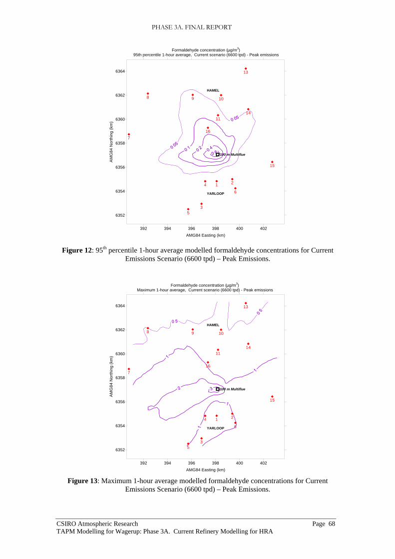
PHASE 3A. FINAL REPORT
CSIRO Atmospheric Research Page 68 TAPM Modelling for Wagerup: Phase 3A. Current Refinery Modelling for HRA
392 394 396 398 400 402AMG84 Easting (km)
6352
6354
6356
6358
6360
6362
6364
AM
G84
Nor
thin
g (k
m)
1 2
3
4
5
6
7
8 9 10
11
13
14
15
16
100 m Multiflue
YARLOOP
HAMEL
Formaldehyde concentration (µg/m3)95th percentile 1-hour average, Current scenario (6600 tpd) - Peak emissions
Figure 12: 95th percentile 1-hour average modelled formaldehyde concentrations for Current Emissions Scenario (6600 tpd) – Peak Emissions.
392 394 396 398 400 402AMG84 Easting (km)
6352
6354
6356
6358
6360
6362
6364
AM
G84
Nor
thin
g (k
m)
1 2
3
4
5
6
7
8 9 10
11
13
14
15
16
100 m Multiflue
YARLOOP
HAMEL
Formaldehyde concentration (µg/m3)Maximum 1-hour average, Current scenario (6600 tpd) - Peak emissions
Figure 13: Maximum 1-hour average modelled formaldehyde concentrations for Current
Emissions Scenario (6600 tpd) – Peak Emissions.

PHASE 3A. FINAL REPORT
CSIRO Atmospheric Research Page 69 TAPM Modelling for Wagerup: Phase 3A. Current Refinery Modelling for HRA
392 394 396 398 400 402
AMG84 Easting (km)
6352
6354
6356
6358
6360
6362
6364
AM
G84
Nor
thin
g (k
m)
1 2
3
4
5
6
7
8 9 10
11
13
14
15
16
100 m Multiflue
YARLOOP
HAMEL
Formaldehyde concentration (µg/m3)Maximum 10-minute average, Current scenario (6600 tpd) - Peak emissions
Figure 14: Maximum 10-minute average modelled formaldehyde concentrations for Current Emissions Scenario (6600 tpd) – Peak Emissions.
392 394 396 398 400 402AMG84 Easting (km)
6352
6354
6356
6358
6360
6362
6364
AM
G84
Nor
thin
g (k
m)
1 2
3
4
5
6
7
8 9 10
11
13
14
15
16
100 m Multiflue
YARLOOP
HAMEL
Formaldehyde concentration (µg/m3)Maximum 3-minute average, Current scenario (6600 tpd) - Peak emissions
Figure 15: Maximum 3-minute average modelled formaldehyde concentrations for Current Emissions Scenario (6600 tpd) – Peak Emissions.
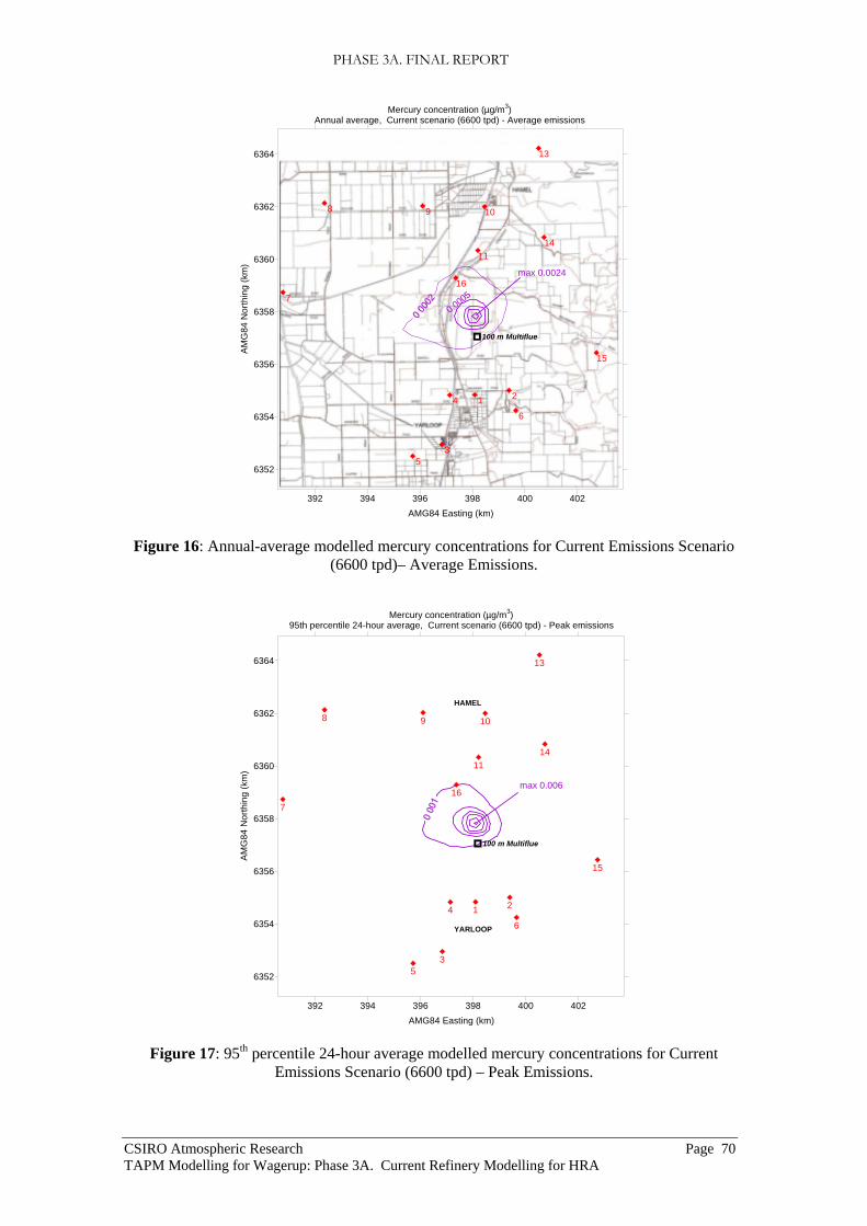
PHASE 3A. FINAL REPORT
CSIRO Atmospheric Research Page 70 TAPM Modelling for Wagerup: Phase 3A. Current Refinery Modelling for HRA
392 394 396 398 400 402AMG84 Easting (km)
6352
6354
6356
6358
6360
6362
6364
AM
G84
Nor
thin
g (k
m)
1 2
3
4
5
6
7
8 9 10
11
13
14
15
16
100 m Multiflue
Mercury concentration (µg/m3)Annual average, Current scenario (6600 tpd) - Average emissions
max 0.0024
0.0005
Figure 16: Annual-average modelled mercury concentrations for Current Emissions Scenario (6600 tpd)– Average Emissions.
392 394 396 398 400 402AMG84 Easting (km)
6352
6354
6356
6358
6360
6362
6364
AM
G84
Nor
thin
g (k
m)
1 2
3
4
5
6
7
8 9 10
11
13
14
15
16
100 m Multiflue
YARLOOP
HAMEL
Mercury concentration (µg/m3)95th percentile 24-hour average, Current scenario (6600 tpd) - Peak emissions
max 0.006
Figure 17: 95th percentile 24-hour average modelled mercury concentrations for Current Emissions Scenario (6600 tpd) – Peak Emissions.

PHASE 3A. FINAL REPORT
CSIRO Atmospheric Research Page 71 TAPM Modelling for Wagerup: Phase 3A. Current Refinery Modelling for HRA
392 394 396 398 400 402AMG84 Easting (km)
6352
6354
6356
6358
6360
6362
6364
AM
G84
Nor
thin
g (k
m)
1 2
3
4
5
6
7
8 9 10
11
13
14
15
16
100 m Multiflue
YARLOOP
HAMEL
Mercury concentration (µg/m3)95th percentile 1-hour average, Current scenario (6600 tpd) - Peak emissions
max 0.009
Figure 18: 95th percentile 1-hour average modelled mercury concentrations for Current Emissions Scenario (6600 tpd) – Peak Emissions.
392 394 396 398 400 402AMG84 Easting (km)
6352
6354
6356
6358
6360
6362
6364
AM
G84
Nor
thin
g (k
m)
1 2
3
4
5
6
7
8 9 10
11
13
14
15
16
100 m Multiflue
YARLOOP
HAMEL
Mercury concentration (µg/m3)Maximum 1-hour average, Current scenario (6600 tpd) - Peak emissions
Figure 19: Maximum 1-hour average modelled mercury concentrations for Current Emissions
Scenario (6600 tpd) – Peak Emissions.
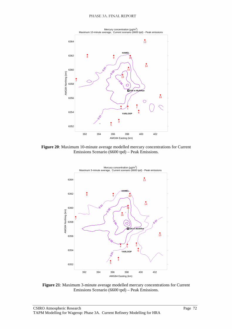
PHASE 3A. FINAL REPORT
CSIRO Atmospheric Research Page 72 TAPM Modelling for Wagerup: Phase 3A. Current Refinery Modelling for HRA
392 394 396 398 400 402
AMG84 Easting (km)
6352
6354
6356
6358
6360
6362
6364
AM
G84
Nor
thin
g (k
m)
1 2
3
4
5
6
7
8 9 10
11
13
14
15
16
100 m Multiflue
YARLOOP
HAMEL
Mercury concentration (µg/m3)Maximum 10-minute average, Current scenario (6600 tpd) - Peak emissions
Figure 20: Maximum 10-minute average modelled mercury concentrations for Current Emissions Scenario (6600 tpd) – Peak Emissions.
392 394 396 398 400 402AMG84 Easting (km)
6352
6354
6356
6358
6360
6362
6364
AM
G84
Nor
thin
g (k
m)
1 2
3
4
5
6
7
8 9 10
11
13
14
15
16
100 m Multiflue
YARLOOP
HAMEL
Mercury concentration (µg/m3)Maximum 3-minute average, Current scenario (6600 tpd) - Peak emissions
Figure 21: Maximum 3-minute average modelled mercury concentrations for Current Emissions Scenario (6600 tpd) – Peak Emissions.

PHASE 3A. FINAL REPORT
CSIRO Atmospheric Research Page 73 TAPM Modelling for Wagerup: Phase 3A. Current Refinery Modelling for HRA
392 394 396 398 400 402AMG84 Easting (km)
6352
6354
6356
6358
6360
6362
6364
AM
G84
Nor
thin
g (k
m)
1 2
3
4
5
6
7
8 9 10
11
13
14
15
16
100 m Multiflue
NOx concentration (µg/m3)Annual average, Current scenario (6600 tpd) - Average emissions
Figure 22: Annual-average modelled NOx concentrations for Current Emissions Scenario (6600 tpd) – Average Emissions.
392 394 396 398 400 402AMG84 Easting (km)
6352
6354
6356
6358
6360
6362
6364
AM
G84
Nor
thin
g (k
m)
1 2
3
4
5
6
7
8 9 10
11
13
14
15
16
100 m Multiflue
YARLOOP
HAMEL
NOx concentration (µg/m3)95th percentile 24-hour average, Current scenario (6600 tpd) - Peak emissions
Figure 23: 95th percentile 24-hour average modelled NOx concentrations for Current Emissions Scenario (6600 tpd) – Peak Emissions.

PHASE 3A. FINAL REPORT
CSIRO Atmospheric Research Page 74 TAPM Modelling for Wagerup: Phase 3A. Current Refinery Modelling for HRA
392 394 396 398 400 402AMG84 Easting (km)
6352
6354
6356
6358
6360
6362
6364
AM
G84
Nor
thin
g (k
m)
1 2
3
4
5
6
7
8 9 10
11
13
14
15
16
100 m Multiflue
YARLOOP
HAMEL
NOx concentration (µg/m3)95th percentile 1-hour average, Current scenario (6600 tpd) - Peak emissions
Figure 24: 95th percentile 1-hour average modelled NOx concentrations for Current Emissions Scenario (6600 tpd) – Peak Emissions.
392 394 396 398 400 402AMG84 Easting (km)
6352
6354
6356
6358
6360
6362
6364
AM
G84
Nor
thin
g (k
m)
1 2
3
4
5
6
7
8 9 10
11
13
14
15
16
100 m Multiflue
YARLOOP
HAMEL
NOx concentration (µg/m3)Maximum 1-hour average, Current scenario (6600 tpd) - Peak emissions
Figure 25: Maximum 1-hour average modelled NOx concentrations for Current Emissions
Scenario (6600 tpd) – Peak Emissions.

PHASE 3A. FINAL REPORT
CSIRO Atmospheric Research Page 75 TAPM Modelling for Wagerup: Phase 3A. Current Refinery Modelling for HRA
392 394 396 398 400 402AMG84 Easting (km)
6352
6354
6356
6358
6360
6362
6364
AM
G84
Nor
thin
g (k
m)
1 2
3
4
5
6
7
8 9 10
11
13
14
15
16
100 m Multiflue
YARLOOP
HAMEL
NOx concentration (µg/m3)Maximum 10-minute average, Current scenario (6600 tpd) - Peak emissions
Figure 26: Maximum 10-minute average modelled NOx concentrations for Current Emissions Scenario (6600 tpd) – Peak Emissions.
392 394 396 398 400 402AMG84 Easting (km)
6352
6354
6356
6358
6360
6362
6364
AM
G84
Nor
thin
g (k
m)
1 2
3
4
5
6
7
8 9 10
11
13
14
15
16
100 m Multiflue
YARLOOP
HAMEL
NOx concentration (µg/m3)Maximum 3-minute average, Current scenario (6600 tpd) - Peak emissions
100
Figure 27: Maximum 3-minute average modelled NOx concentrations for Current Emissions
Scenario (6600 tpd) – Peak Emissions.

PHASE 3A. FINAL REPORT
CSIRO Atmospheric Research Page 76 TAPM Modelling for Wagerup: Phase 3A. Current Refinery Modelling for HRA
These yearly maximum 1-hour average concentrations represent the most extreme hour in the year with respect to ground-level concentrations. In a different year with different meteorology the location and magnitude of these yearly maximum 1-hour average concentrations could change. This is why the 9th highest concentration or robust highest concentration (RHC) is often chosen as the key statistic to represent the extremes, rather than the modelled or observed maximum.
4.7. Peak Events Figure 28 to Figure 30 show the temporal variation of the modelled 1-hour average concentrations around the five highest concentration events for formaldehyde, NOx and NO2.
One-half of the model events occur at the same time for NOx and formaldehyde, though not always at the same site, with most of these events during the winter months (April to September).
For both formaldehyde and NOx the peaks at receptor 14 (Escarpment) all occur between 10:00 to 18:00, whereas at receptors 1 (Boundary Road) and 3 (Yarloop), peaks are observed both at night and during the day. Most of the peaks only last for one hour; the longest is a four-hour formaldehyde peak at site 1 from 19:00 to 23:00.
Figure 31 shows that the wind directions at the times of the peak concentrations correspond closely with the Refinery being directly upwind from the receptor except for one case at receptor 3 for both NOx and formaldehyde. This one case occurred on 9 Aug 2004 at 21:00 with a wind speed of 2 m s-1 and an inversion height of 34 m. It occurs with a more easterly component indicating some turning of the wind and flow from the escarpment towards the receptor. In the other cases, the wind speeds were higher, typically 4 to 8 m s-1. These features are similar to those identified in the Wagerup Air Quality Review (CSIRO, 2004a) when examining the peak NOx concentrations observed at Boundary Road and Upper Dam, except that the wind speeds in those cases tended to be lower, generally less than 4 m s-1. These features also closely match those identified in Section 6 of the Phase 2 report (CSIRO, 2004c), where most model events were identified as occurring with wind speeds from 2 to 6 m s-1 and at lower speeds under easterly flows. Night-time model events occurred with mixing heights less than 300 m, whereas daytime model events occur in strongly convective conditions with mixing heights up to 2000 m, similar to the results shown in Figure 31.
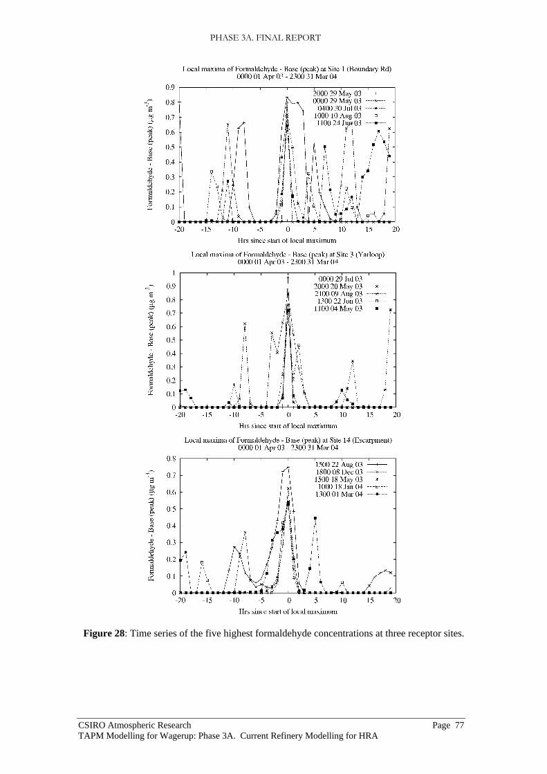
PHASE 3A. FINAL REPORT
CSIRO Atmospheric Research Page 77 TAPM Modelling for Wagerup: Phase 3A. Current Refinery Modelling for HRA
Figure 28: Time series of the five highest formaldehyde concentrations at three receptor sites.
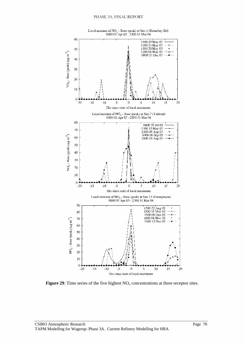
PHASE 3A. FINAL REPORT
CSIRO Atmospheric Research Page 78 TAPM Modelling for Wagerup: Phase 3A. Current Refinery Modelling for HRA
Figure 29: Time series of the five highest NOx concentrations at three receptor sites.

PHASE 3A. FINAL REPORT
CSIRO Atmospheric Research Page 79 TAPM Modelling for Wagerup: Phase 3A. Current Refinery Modelling for HRA
Figure 30: Time series of the five highest NO2 concentrations at three receptor sites.

PHASE 3A. FINAL REPORT
CSIRO Atmospheric Research Page 80 TAPM Modelling for Wagerup: Phase 3A. Current Refinery Modelling for HRA
0 90 180 270 360Wind direction (degrees)
0
200
400
600
800
1000
1200
Mix
ing
Hei
ght (
m)
NOx, Site 1NOx, Site 3NOx, Site 14Formaldehyde, Site 1Formaldehyde, Site 3Formaldehyde, Site 14
Figure 31: Modelled wind direction (at 25 m) and mixing height at Bancell Road for the 5 highest peak concentrations of NOx and formaldehyde at receptors 1, 3,
and 14.
The peaks at the Escarpment site all show a pattern of gradual build-up over two to three hours and then decay within an hour, whereas those at the other sites tend to be events that last just one hour.
The results for NO2 in Figure 30 are very similar to those for NOx in Figure 29. This reflects the fact that the daily maximum NOx concentration only rarely exceeds the maximum ozone concentration of 54 µg m-3 (28.2 ppb), which is used in the NO2 modelling (see Figure 7, Section 3.4).

PHASE 3A. FINAL REPORT
CSIRO Atmospheric Research Page 81 TAPM Modelling for Wagerup: Phase 3A. Current Refinery Modelling for HRA
5. Summary
The work presented in this report is part of a study entitled “Meteorological and Dispersion Modelling Using TAPM for Wagerup”, consisting of three closely defined objectives. This report deals with the third objective (Phase 3A: HRA Concentration Modelling), with the following objectives completed:
1. The refined TAPM (as resolved in Phases 1 and 2) has been run for the annual meteorological file (1 April 2003 to 31 March 2004) and the agreed sources listed in dot point 2 to produce estimates of the following parameters for 28 pollutants at 15 receptor points:
• Annual average concentration (at average emission rates) • Maximum 1-hour average concentrations (peak emissions) • 95th percentile 1-hour average concentrations (peak emissions) • 95th percentile 24-hour average concentrations (peak emissions) • Maximum 10-minute average concentrations (peak emissions) • Maximum 3-minute average concentrations (peak emissions).
2. The 28 pollutants are oxides of nitrogen, carbon monoxide, sulphur dioxide, dust, arsenic, selenium, manganese, cadmium, chromium VI, nickel, mercury, ammonia, benzo(a)pyrene equivalents, acetone, acetaldehyde, formaldehyde, 2-butanone, benzene, toluene, xylenes, acrolein, ethylbenzene, methylene chloride, styrene, 1,2,4, trimethylbenzene, 1,3,5 trimethylbenzene, vinyl chloride, and nitrogen dioxide.
3. Contour plots have been produced of these six statistics for three example substances (NOx, Formaldehyde and Mercury) to indicate the different concentration distribution patterns for substances predominantly emitted from high and low level sources.
4. A simple titration algorithmic method has been described and used to calculate the conversion of NOx to NO2 using available data on the diurnal variation in ozone concentrations at Wagerup.
5. The best practice method has been used for deriving shorter time period (3 and 10-minute) maximum concentrations from the Wagerup hourly TAPM concentration fields. A detailed description of this method has been presented.
6. The temporal variation of concentration around, and mechanisms causing, the modelled 5 highest short-term peak concentrations has been investigated for NOx and formaldehyde for the peak emission scenario at three receptors (sites 1, 3, and 14). The mechanisms identified as responsible for the highest short-term peak concentrations match those identified in Phase 2 of this work (CSIRO, 2004c) and in the Wagerup Air Quality review (CSIRO, 2004a).
7. Separate quality assurance runs have been undertaken for NOx and formaldehyde to confirm the accuracy of the main modelling technique.
8. The uncertainty of the model predictions has been determined from consideration of results from a range of TAPM studies and an analysis of the sensitivity of model results to wind data assimilation. We conclude that the results for the modelled concentrations

PHASE 3A. FINAL REPORT
CSIRO Atmospheric Research Page 82 TAPM Modelling for Wagerup: Phase 3A. Current Refinery Modelling for HRA
presented in this report have an uncertainty of a factor of approximately 2 (i.e. the actual values lie in the range of +100% to -50% of the listed concentrations) at the 95% confidence level.
6. References
Anfossi, D., Bonino, G., Bossa, F., and Richiardone, R.: 1978. Plume rise from multiple sources: a new model. Atmospheric Environment 12, 1821−1826.
Briggs, G.A., 1969. Plume Rise. US Atomic Energy Commission, Division of Technical Information, TID-25075.
Briggs, G.A., 1984. Plume rise and buoyancy effects. In: Randerson, D. (Ed), Atmospheric Science and Power Production. Publication No. DOE/TIC-27601, US Department of Energy, Washington, DC, pp. 327-366.
Cox, W. M., Tikvart, J. A.: 1990. A statistical procedure for determining the best performing air quality simulation model. Atmospheric Environment 24A, 2387−2395.
CSIRO (2004a), ‘Wagerup Air Quality Review’, Report to Alcoa World Alumina Australia, May 2004, 133 pp.
CSIRO (2004b), ‘Meteorological and Dispersion Modelling Using TAPM for Wagerup, Phase 1: Meteorology’, Report to Alcoa World Alumina Australia, November 2004.
CSIRO (2004c), ‘Meteorological and Dispersion Modelling Using TAPM for Wagerup, Phase 2: Dispersion’, Report to Alcoa World Alumina Australia, November 2004.
EPAV: 2000, ‘AUSPLUME Gaussian Plume Dispersion Model: Technical User Manual’, Environment Protection Authority of Victoria, Australia, http://www.epa.vic.gov.au.
Hibberd, M. F. (1998). Peak-to-mean ratios for isolated tall stacks (for averaging times from minutes to hours). In: Proceedings of the 14th International Clean Air and Environment Conference, Melbourne. Mitcham, Vic.: Clean Air Society of Australia and New Zealand. p. 255-260.
Hill, J. and Hurley, P., 2003. The use of TAPM at Anglesea. Proceedings of the 17th International Clean Air and Environment Conference, 23-27 November 2003, Newcastle, Australia.

PHASE 3A. FINAL REPORT
CSIRO Atmospheric Research Page 83 TAPM Modelling for Wagerup: Phase 3A. Current Refinery Modelling for HRA
Hurley P. (2002). ‘The Air Pollution Model (TAPM) Version 2. Part 1: Technical Description’, CSIRO Atmospheric Research Technical Paper No. 55. Available at www.dar.csiro.au/TAPM.
Hurley, P.J., Blockley, A., Rayner, K., 2001. Verification of a prognostic meteorological and air pollution model for year-long predictions in the Kwinana region of Western Australia. Atmospheric Environment 35, 1871−1880.
Hurley, P.J., Physick, W.L., and Luhar, A.K., 2002. The Air Pollution Model (TAPM) Version 2. Part 2: Summary of some verification studies. CSIRO Atmospheric Research Technical Paper No. 57. Available at www.dar.csiro.au/TAPM.
Hurley, P., Manins, P., Lee, S., Boyle, R., Ng, Y.L., Dewundege, P., 2003a. Year-long, hi-resolution, urban airshed modelling: verification of TAPM predictions of smog and particles in Melbourne, Australia. Atmospheric Environment 37, 1899−1910.
Hurley, P., Physick, W., Cope, M., Borgas, M. and Brace, P., 2003b. An evaluation of TAPM for photochemical smog applications in the Pilbara region of WA. Proceedings of the 17th International Clean Air and Environment Conference, 23-27 November 2003, Newcastle, Australia.
Johnson, S., 2003. Wagerup Ambient Air Quality Monitoring Report (December 2003, 1st edition), Alcoa World Alumina, 39 pp.
Katestone Scientific (1998). Peak-to-mean ratios for odour assessments, Report to the Environment Protection Agency New South Wales.
Luhar, A.K., and Hurley, P.J., 2003. Evaluation of TAPM, a prognostic meteorological and air pollution model, using urban and rural point-source data. Atmospheric Environment 37, 2795−2810.
Macdonald, R.W., Strom, R.K. and Slawson, P.R., 2002. Water flume study of the enhancement of buoyant rise in pairs of merging plumes. Atmospheric Environment, 36, 4603-4615.
Manins P., Carras J. and Williams D. (1992). ‘Plume rise from multiple stacks’, Clean Air, 26, 65-68.
Nisbet, I. C. T. and LaGoy, P. K., 1992. Toxic equivalency factors (TEFs) for polycyclic aromatic hydrocarbons (PAHs). Reg. Toxicol. Pharmacol. 16, 290-300.
NSW EPA, 2001. Approved methods and guidance for the modelling and assessment of air pollutants in New South Wales, 50 pp, www.epa.nsw.gov.au/air/amgmaap.pdf
Overcamp, T.J. and Ku, T. 1988: Plume rise from two or more adjacent stacks: Atmospheric Environment, 22, 625–637.

PHASE 3A. FINAL REPORT
CSIRO Atmospheric Research Page 84 TAPM Modelling for Wagerup: Phase 3A. Current Refinery Modelling for HRA
Physick, W.L., Blockley, A.: 2001. An evaluation of air quality models for the Pilbara region, CSIRO Division of Atmospheric Research. A Report to the Department of Environmental Protection, Western Australia, 98 pp, June 2001.
Physick, W. L., Blockley, A., Farrar, D., Rayner, K., Mountford, P.: 2002. Application of three air quality models in the Pilbara region, Proceedings of the 16th International Clean Air and Environment Conference, Christchurch, New Zealand, August 2002.
Pitts, O. (2004). ‘Wagerup Refinery – June and July 2003 Radio Sonde Data’, e-mail to P. Coffey of Alcoa, 11 May 2004, Air Assessments, Western Australia.
SKM (2002). ‘Wagerup Refinery Odour Assessment’, Final report, Sinclair Knight Merz, February 2002.
SKM (2003). ‘Alcoa World Alumina Australia: Wagerup weather station and ambient dust monitoring program review following implementation of audit findings. Sinclair Knight Merz, Bunbury, WA (Australia), 28 June 2004, pp. 27.
Weil, J.C (1988) Plume rise, in: Lecture on Air Pollution Modelling, American Meteorological Society, Boston, p. 119–166.