MCB 137 WINTER 2008

PHARMACOLOGY Introduction This chapter is a short tutorial on model building using the Berkeley Madonna FlowChart interface. We do this within the context of pharmacology because of the abundance of pharmacology models that are both simple and practical. Pharmacology models are designed to predict the time dependence of a drug's concentration in the body fluids following its administration, or to model the action of the drug once it reaches its target organ. The complexity of pharmacological models varies widely depending on the level of detail they encompass. We begin by representing the whole body as a single compartment; that is, a homogeneous volume. This simple model will provide us with an easy introduction to modeling with Madonna, and suffices to introduce the general concepts of steady state, exponential response, relaxation time, and the principle of superposition in linear systems.

Although the single compartment model yields useful results in many cases, it is not a very realistic representation of the body, especially if we are interested in the distribution of a drug into different tissues. So the next step up in complexity is to model a body as two interconnected compartments: a central compartment that includes the blood and tissues like the liver and kidney, that have a rapid and profuse blood circulation, and a second peripheral compartment that includes the more slowly perfused tissues. While more successful than a one compartment model, the abstract nature of the two compartment system makes it difficult to assign anatomical locations to the compartments, and to give physical interpretations to its parameters. These issues prompt us to move on to more precise and more elaborate physiologically based pharmacokinetic models which take explicit account of the blood supply to each represented tissue. Finally we conclude this chapter with an introduction to the more complex and more challenging problem of the action of drugs at their target site.

One Compartment Pharmacokinetics We begin with the simplest case where we infuse into the body the biologically inert polysaccharide, inulin. Inulin is infused into animals or humans to trace fluids; it is used to estimate the volume of extracellular fluids as well as the rate of filtration of blood plasma fluids into the kidney nephrons. This filtration rate, a fundamental parameter for investigation and evaluation of kidney function, is calculated from measurements of urinary flow and urinary and plasma concentrations. Interpretation of these measurements requires some notion of how the inulin concentration in the plasma changes following its administration by injection or infusion. Following the start of an inulin infusion, the plasma concentration rises rapidly. When will the concentration stabilize?

Model Summary

The model computes the inulin concentration in the plasma at any time. It does this by comparing the amounts entering the body with the amount leaving at each moment; any discrepancy must represent a gain or loss of inulin within the body. Adding all these gains (or losses) up to a particular time computes the amount and concentration of body inulin at that time.

PHARMACOLOGY

2

Before starting, verify that the flowchart editor is functioning properly. To do this, choose About Berkeley Madonna from the Help menu and look for text that reads “Flowchart version 8.0.1”. If it says “Java not loaded”, click the Load Java button. If Java fails to load, you need to install (or reinstall) Java™ support on your system.

Figure 1. Changes in the inulin body compartment depend on the entry and exit flow rates.

The results enable us to study and evaluate protocols for making measurements of extracellular volume and of renal filtration.

Model For The Accumulation Of Inulin In The Body Fluids

Building the Model --- Step by Step

In this section, we construct our inulin model graphically using the flowchart editor. The model consists of three dynamic elements: a reservoir icon (compartment) representing the mass [mg] of inulin in the body fluids, and two flow icons representing inulin entering and leaving the body [mg hr-1]. In addition we will employ supporting formula icons to represent the rate of rate of renal filtration [L hr-1], volume of body fluids L, and the concentration of inulin [mg L-1]. Begin: 1. Choose New Flowchart from the File menu. An empty flowchart window appears.

2. Position the mouse over the reservoir tool , press the mouse button, drag the reservoir to the flowchart, and release the mouse button. You’ve now placed a reservoir on the flowchart with the default name R1. Note that the reservoir is colored red which means it is selected.

3. Change the name of the reservoir to m by typing the new name. (It is not necessary to first click the reservoir since it is already selected.) This single reservoir represents the total mass in milligrams [mg] of inulin which we assume is uniformly dissolved in the extracellular fluid.

4. Click the flow tool , move the mouse over the mass reservoir, press the mouse button, drag the mouse to the right a few inches, and release the mouse button. This places a flow icon on the flowchart which drains the mass reservoir into an infinite sink.

5. Make sure the reservoir is connected to the flow. If the flow looks like this:

PHARMACOLOGY

3

You can remove an icon or arc from the flowchart by selecting it and choosing Clear (Macintosh) or Delete (Windows) from the Edit menu. You can also remove selected objects by holding down the Control key while pressing the delete or backspace key.

its source end is not connected to the reservoir. In this case, drag the infinite source on the left to the reservoir and drop it. This connects the flows input to the reservoir instead of an infinite source.

6. Change the name of the flow to Ex (for exit) by clicking the spherical part of the flow icon (if it is not already selected) and typing the new name.

7. Click the flow tool again and move the mouse an inch to the left of the mass reservoir, press the mouse button, drag the mouse to the right until the cursor is over the reservoir, and release the mouse button. This places a flow to inject inulin into the body fluids reservoir. Rename this icon Inj. As before, make sure you have connected the right hand side to the reservoir. If not drag the infinite sink on the right onto the reservoir and drop it by releasing the mouse button.

8. If you find that the icons are not positioned the way you want, they can be repositioned by clicking and dragging. Note that Berkeley Madonna maintains the connection between the reservoir, flow, and sink.

9. Place 3 formula icons on the flowchart near the Ex flow icon (use the same click and drag technique as you did for the reservoir). Change the names of the formula icons to V, C, and kc. V will represent the volume of extracellular . The units will be liters [L]. C is the concentration of inulin in the extracellular fluid in units of milligrams per liter [mg L-1]. kc is a proportionality constant [mL hr-1] relating the rate of inulin excretion to its concentration

10. Click the arc tool and create an arc going from the reservoir icon to the C icon (use the same technique as you did for the flow). This creates a dependency relationship between the concentration and the mass of inulin. Create another arc going from the V icon to the C icon. Now our diagram shows that C depends on both m and V. Finally, use an arc to connect C to Ex and use another arc to connect kc to Ex. These last two connections show that the rate of excretion of inulin by the kidney depends on how fast fluid flows into the renal nephron as well as the inulin concentration in the body fluids. Your flow chart should resemble Figure 2.

You can change the position of the icon labels by simply dragging them around. (Madonna will prevent you from straying too far from the icon.) You can also change the curvature of the dependency arcs by dragging their control points. To do this, first select an arc by clicking somewhere along its trajectory. The arc will turn red and a small square handle (control point) will appear. Click and drag the control point to change the arc’s trajectory.

Icons and arcs can be removed by selecting them and choosing Clear (Macintosh) or Delete (Windows) from the Edit menu. You can also remove selected objects by holding down the Control key while pressing the delete or backspace key. Try deleting the arc from the V icon to the C icon. Note that a question mark reappears in the C icon because the icon’s equation still shows that C depends on V, but this dependency is no longer shown on the flow chart. You can reestablish this dependency by drawing a new arc from the V to the C

PHARMACOLOGY

4

Figure 2. Inulin Model before setting the model parameter values.

11. So far we have not supplied the model with any numerical values. Madonna indicates this by the question marks on the icons. Double-clicking on any icon will open a dialog box asking for numerical data. For example, double-click on the C icon. The dialog box says that m and V are required inputs. This means that these variables must be used in the right-hand side of the equation defining the icon’s value. Enter m/V in the data box. You can type in the names from the keyboard or, more conveniently, simply double-click on the input’s name in the list. Click OK (or press Return) when done, and the dialog box will close; the question mark on the icon has disappeared indicating that Madonna is satisfied with your input to the flow icon. Next we must assign numerical values to V and k. The basis for these values is discussed in the Parameter Estimation box.

Parameter Estimation

The molecular weight of inulin is ~ 5000, so it is too large to pass through cell membrane channels, but it is small enough to easily pass through porous capillaries. There are no other significant transport pathways for inulin. Therefore, to a good approximation, we can assume inulin is uniformly dissolved in the extracellular fluid that makes up about 20% of the body weight. The extracellular volume for a 70 kg body is 14 liters [L] (20% body weight = 0.20 × 70 kg = 14 kg ≈ 14 L).

We calculate the rate constant k for excretion from the mass action relation Ex = kcC. Since inulin is biologically inert, its only escape from the body fluids is by renal excretion so Ex is easy to measure: simply collect the urine that flows over a given period of time, measure its inulin content and divide by the collection time. When C = 100 mg L-1 , typical values of Ex are around 720 mg hr-1. Using these figures, we estimate kc = Ex/C = 720/100 = 7.2 L hr-1.

PHARMACOLOGY

5

12. Double-click the kc icon and enter 7.2. Note that you can use the dialog’s calculator keypad to insert digits and common arithmetic operators. Double click the V icon and enter 14.

13. Double click the reservoir (m icon). In this dialog, you specify the reservoir’s initial value. Since there is normally no inulin in the extracellular fluids, we assume there is none at the beginning of the experiment, so enter 0 and close the box.

14. Now double click on the flow icon (click in the center circle with the question mark). kc and C are required, so enter their product, kc C, and click OK. (Flows are rates and have time in their dimensions. The dimensions of kc = [L⋅hr-1 ] while C = [mg⋅L-1] so that the dimensions of the product kc C = mg⋅hr-1, the rate that the reservoir is losing inulin.

15. Double click on the last unfilled icon, Inj. We will simulate a constant infusion at the rate 600 mg⋅hr-1. Enter 600 in the dialog and click OK

16. The model flowchart is now complete, and all question marks should have disappeared. Now run your model by choosing Run from the Compute menu. Berkeley Madonna runs your model and displays the results in a graph window. Click on the button labeled L located on top of the graph to insert a Legend on the graph. Click the button again to remove the legend. All buttons on the graph are toggle (on-off) buttons.

Figure 3. The graph window.

17. The graph shows the variables m, whose scale is on the left vertical axis, and Ex scaled on the right. (Madonna automatically plots the first two variables that were defined in the construction of the model window The first is scaled on the left axis, the second on the right.) There are 3 toggle buttons located on the left bottom margin of the graph window. Click on the C button. This will place a plot of C on the graph. Click on the Ex button to remove Ex. Both m and C are scaled on the same left hand axis. To scale one of them, say C, on the right, click on the C button while holding down the shift key.

PHARMACOLOGY

6

Madonna automatically places buttons for the first eight variables on graph window (we have only three). You can over-ride this default and completely control which buttons appear on the graph by double clicking anywhere in the Graph window to bring up the Choose Variables dialog (see Menu item Help>How Do I>Control Plotted Variables).

18. To see a tabular representation of the numerical results, click on the Table button . The graphical representation of our results is replaced by an equivalent numerical table. Relevant buttons on the table have the same function as on the graph. Also, double clicking in the middle of the table brings up the Choose Variable dialog. Click on the Table button once more to return to the graph.

19. To change parameters, select Parameter Window under the Parameters menu.

Figure 4. The Parameter Window obtained by selecting from the Parameter menu.

Select Inj in the list and then change the 600 that appears in the Edit box (above in the gray area) to 300. Click Run: the previous results are erased and the new simulation with Inj = 600 is plotted. The asterisk on the 300 in the parameter list indicates that the parameter has been changed from its original value. If you would like to restore the original, select the parameter and click the Reset button. If you would like to compare two simulations on the same plot, click on the Overlay button labeled O, and run once with Inf =300 and once with Inf =600. Activating the Overlay button stops Madonna from erasing the plot each time a new run is initiated. Like all graph buttons, Overlay is toggled on or off by clicking on it.

20. Now that you’ve created a useable model, you should take a look at the equations Berkeley Madonna generated. To do this, choose Equations from the Model menu. Position the equations along side the flowchart so that you can see both windows simultaneously.

PHARMACOLOGY

7

Figure 5. Equation Window obtained from the menu Model>Equations.

The model predicts an exponential response

Many experiments begin with a system in a steady state where all flows are constant and the reservoir levels are unchanging. The system is suddenly perturbed, for example by a sudden concentration change, after which the system moves to a new steady state. We can use the model to determine the new steady state and how long it took to get there.

The steady state

Whenever the flow into the body through injection is equal to the flow out through excretion the system is in a steady state condition; that is, the flow, Inj, into the reservoir m is equal the flow out Ex = kcC. Then the steady state concentration of inulin will be given by

Equation 1 steady state:

�

C = Inj /kc [mg/L]

When you select an icon in the flowchart, Berkeley Madonna highlights the corresponding equation(s) in the Equation window. This makes it easy to see an icon’s equations without opening its icon dialog. Conversely, you can show which icon corresponds to an equation in the equation window. Simply position the equation window’s insertion point (caret) within one of the equations, then choose Show Icon from the Edit menu. This activates the flowchart window and highlights the corresponding icon.

You can also open the icon dialog directly from the equation window by double-clicking an equation. For example, double-clicking anywhere within the line C =m/V opens the icon dialog for the C icon. Select the m reservoir, type Inulin and press return. The name of the icon changes and Berkeley Madonna updates the name in all equations that depend on it. To see this in action, change the name again and keep your eye on the equation window as you press the return key. Change the name back to m

PHARMACOLOGY

8

When Inj = 0, C = 0; this is our initial condition (a trivial result simply restating what we already knew: inulin is not a normal body constituent). When Inj = 600 mg/hr, the final steady state concentration is C = 600/7.2 = 83.3 mg L-1. You can verify this on the graph by ‘zooming in’ to view the last portion of your plot: click and drag the mouse to draw a rectangle over the relevant area. When you release the mouse, Berkeley Madonna adjusts the axis limits so that the portion that was in the rectangle now fills the window. To undo the effect of a zoom-in, click the Z button located in the toolbar on top of the plot. Now click the Readout button, on the Graph window toolbar

and place, the ‘crosshair’ cursor over a point on the plot; the coordinates are displayed in the information area at the top of the window. Alternatively, you could view the data in Table form and scroll down to the last time row.

More complex models will have more reservoirs, but the same considerations hold: in a steady state the inflow to each reservoir must equal its outflow. This can involve finding roots of a complicated set of simultaneous algebraic equations, but Madonna has provisions for finding the required numerical solutions.

Relaxation Time

Letting τ = V/kc, the mathematical solution for the inulin model as derived in the MATH NOTES box: The exponential response is:

Equation 2

�

C(t) = Injkc

1− e− tτ

⎛

⎝ ⎜

⎞

⎠ ⎟

C(t) approaches asymptotically (but never really reaches) the time independent steady state. So it makes no sense to ask how long it takes the system to reach its final destination. Instead, we ask how long it takes for C to reach a prescribed fraction of its final value, say 50%. In general, e- t/τ will reach the 50% mark when t ≈ 0.69⋅τ ( e-0.69 ≈ 1/2). The half-time, t1/2, is given by

Equation 3 t1/2 = 0.69⋅τ

Rather than carry around the numerical factor 0.69, we use τ itself as a measure of the time scale of an exponential process. τ is called the relaxation time or sometimes the time constant; it is the time required for the exponential to reach 63% of its final value.

In addition to the notational convenience, relaxation times are preferred because they have a physical interpretation: they measure the mean residence time of a molecule in the reservoir. In our inulin example each injected inulin molecule has a different fate. After an injection into the circulation some molecules travel to the kidneys and are excreted almost immediately. Others escape into tissue spaces and may meander around for long periods before entering the kidney. These molecules may have ‘life times’ of many hours. The mean residence time is the average lifetime of all the injected molecules, and this turns out to be equal to the relaxation time . This is derived in the MATH NOTES box: The mean residence time. Similar conclusions hold for any exponential process; for example, the relaxation time ( = t1/2 /0.69) for radioactive decay equals the average time that molecules persist before undergoing a radioactive disintegration.

PHARMACOLOGY

9

If the outflow of x from a reservoir is k⋅x, then the relaxation time = k-1

The outflow from any reservoir depends in some way on how much is in the reservoir—no contents means no outflow. The simplest assumption sets the outflow proportional to the contents and this turns out to be a good approximation in many cases. The proportionality constant is a rate constant, that governs how fast the contents are leaving the reservoir; it has the dimension time-1. It is shown in the Math Notes box that the mean residence time, or the relaxation time, is given by the reciprocal of this rate constant. If the quantity in the reservoir is denoted by x and the out flow is equal to k⋅x where k is a constant, then the relaxation (and mean residence) time is given by k-1.

MATH NOTES: EXPONENTIAL RESPONSE

During the time between t and t + dt, Inj•dt mg of inulin enter the body and Ex•dt leave. Letting dm represents the net gain of body inulin during that same time, we have dm = , Inj•dt – Ex•dt. Dividing both sides by dt leaves

�

dmdt

= Inj − Ex = Inj − k ∗C = Inj − k * mV

To integrate introduce a new variable x = Inj – k•m/V , and note that x = dm/dt. Then

dx/dt =- (k/V)•dm/dt=- (k/V)•x and

�

dxx

= − kVdt

Integrating both sides between the start time (t = 0 , m= 0 and x=x0 = Inj ) and some later time with t = t and x = Inj – k•m/V, we have

�

logn xx0= logn Inj − k ∗m /V

Inj= − k

Vt

Substituting m/V =C, k/V =τ, and solving for C yields Equation XXX:

�

C = Injk1− e

− tτ

⎛

⎝ ⎜

⎞

⎠ ⎟

At some arbitrary time after the injection begins it will be stopped and the inulin that has accumulated within the body will be excreted. At this time, reset the clock to t = 0 and let C0 and m0 denote the corresponding inulin concentration, and mass respectively. To find the concentration for t > 0, we use the same derivation, but now at t= 0 we have m = m0 , Inj =0, and x=x0 = – k•mo /V = – k•Co . Using the arguments above, we arrive at:

�

mmo

= CC0

= e− tτ

PHARMACOLOGY

10

Note that the relaxation times for the uptake and decay processes are identical

MATH NOTES: MEAN RESIDENCE TIME

Assume that at any arbitrary time we set t =0 and label the inulin molecules present in the body. Let there be N0 of these molecules and let us note the time each labeled molecule leaves the body. If ni= the number of labeled molecules that leave at time ti, then the average time a molecule spends in the body is given by

�

tmean = n1t1 + n2t2 + ...N0

=niti∑N0

We can calculate these times from our results . We begin with No molecules at t=0. Since the number of molecules at any time N is proportional to m, we have

�

N = N0e− tτ

and the number that leave in the time interval between ti and ti+dt is given by –dNi, (The minus sign occurs because we are counting the number of molecules that leave the body for the environment - each time the environment gains one, the body loses one)

�

−dNi = − dNi

dtdt = 1

τN0e

−tiτ

Using this result together with our expression for the mean, we have

�

tmean = 1No

−dNi( )tii=1

∞

∑ = 1τe−tiτ

⎛

⎝ ⎜

⎞

⎠ ⎟ tidt

i=1

∞

∑

As dt gets smaller, the sum approaches the following integral that we evaluate using standard integral tables:

�

tmean = tτe− tτ

0

∞

∫ dt = τ

Note that this result (tmean = τ) was derived entirely from the rate of disappearance of molecules. As long as this rate is independent of incoming molecules (e.g. when Ex is proportional to C), the result is also independent of incoming molecules.

PHARMACOLOGY

11

Dosage regimens In the inulin model the inulin plasma concentration is proportional to the amount of drug in the body (C =m/V) and its excretion rate is proportional to the plasma concentration (Ex = k⋅C) But unlike inulin, drugs are not inert. They are absorbed on plasma proteins, dissolve in fatty tissue, and enter cells where they may be metabolized. To model the fate of an injected drug we can use the same approach to compute C and Ex, but the constants of proportionality are now empirical quantities that may not have an explicit physical interpretation. We write formally as before

Equation 4

�

C =mVd

Equation 5

�

Ex = kcC

where Vd and kc are experimentally determined parameters. Vd is called the volume of distribution, and kc is called the clearance. Loosely speaking, Vd is a volume ‘corrected’ for absorption and solubility in different tissues, and kc accounts for metabolic destruction as well as excretion (see Empirically defined parameters box) These two parameters are very useful because their values for virtually any common drug are listed in tables found in textbooks and handbooks of pharmacology

Unlike inulin, drugs have biological effects, some desirable, some not. A common problem is to determine a dosage regimen (schedule) to produce plasma concentrations that are high enough to

Empirically defined parameters

The use of an empirical constant to correct for absorption and solubility is valid only over the range of drug concentrations where absorption and solubility are linear functions of concentration. For example, if the amount of drug absorbed = a⋅C and the amount dissolved in fatty tissue = bC, where a and b are proportionality constants. Then the total amount in the body = m = VC +aC +bC = (V+a+b)C. Solving for C leaves

�

C =m

V + a + b=mVd

so that Vd = V +a + b.

Similarly, if drug removal by metabolism and excretion are both linear then

�

Ex = kmetabC + kexcrC = kmetab + kexcr( )C = kcC

where kmetab and kexcr are constants. Thus, the clearance, kc = kmetab + kexcr.

PHARMACOLOGY

12

Under the Help menu is a file called Equation Help. It lists all of Berkeley Madonna’s built in functions. You can drag-and-drop a template onto the equation window. The PULSE function has the form:

PULSE(V, f, r) = Impulses of volume v, first time f, repeat interval r.

There is a bug in Berkeley Madonna that prevents using a pulse at t = 0, so use any value > 0.

produce the desired effect, but low enough to avoid toxic reactions. We illustrate this in the following example of the pharmacokinetics of the bronchodilator theophylline, a common ingredient in tea. It is used clinically to dilate the air passages and relieve the symptoms of chronic asthma. It is effective at plasma concentrations of 10−20 mg⋅L-1, but concentrations beyond this are considered toxic. Our problem is to develop a dose schedule that will maintain a steady concentration within the effective range and will not spill over beyond the toxic limits.

The theophylline clearance is kc, = 2.88 L⋅hr-1 and its distribution volume is Vd, = 35 L (Katzung, B. 1998. Basic and Clinical Pharmacology. Stamford CT: Appleton & Lange). Use this data to change your inulin model to a model for theophylline.

Begin by opening the inulin model and saving it with a new title. Change the labels so that V is replaced by Vd. Include formula icons for the magnitude of the dose and the interval between doses as shown in Figure 6.

Figure 6. Theophylline Model

To simulate discrete intravenous injections, click on Inj and replace the numerical figure with the following function that delivers a drug pulse of size Dose starting at time = 1 and repeating with interval Interval

PULSE(Dose,1,Interval)

Set Dose = 100 and Interval = 24. This specifies a series of injections of 100 mg starting at the beginning where time = 1 hour and repeating every 24 hours. The PULSE function rapidly and repetitively injects a specified amount at discrete intervals. Its general form is

PULSE(q, first, interval )

PHARMACOLOGY

13

Where q is the total amount that is delivered, first is the time of the first pulse, and interval is the interval between pulses.

You now have a generic one-compartment model that has been applied to hundreds of drugs whose parameters are tabulated in standard references.

To deliver a single pulse, use the PULSE function with an interval > STOPTIME. For example, set interval = STOPTIME +1. Select the Parameter Window under the Parameters menu to be certain that STOPTIME = 10 and run the model. You should get a single injection at the beginning.

Now change the STOPTIME in the Parameter Window to 240 (10 days), and run the model. Use the Pulse function to simulate different practical regimens (i.e. 1, 2, 3, and 4 times per day. The corresponding intervals are 24, 12, 8, and 6 hours.) Set the Interval and vary the Dose to find a dosage that, after a few days, will keep the concentration, C, within the safe-but-effective range of 10−20 mg L-1 Madonna’s sliders offer a convenient way do that.

Open the Define Sliders dialog (in the Parameters menu), double click on dose to add it to the Sliders list, and then click OK. Move the slider back and forth: when you release the mouse, Madonna automatically runs the program with the current parameter value shown on the slider. See Help>How Do I >Define and Use Sliders for details on how to tailor the slider to specific needs.

PHARMACOLOGY

14

Oral Ingestion

Figure 7. Theophylline Drug Model: Oral Ingestion

So far, we have used a single, well stirred, compartment to represent the entire body. Most drugs, including theophylline, are given orally, not injected directly into the veins. Thus they pass first into the GI tract and then into the circulatory system. To simulate oral administration, add an additional compartment, labeled GI, between the Dosage inflow and the m compartment. You will also need a new flow representing absorption (labeled Egm) between the GI and m compartments. Choose the flow icon, click on the GI reservoir and drag the mouse until it contacts the m reservoir. Set

�

Equation 6

�

Exgm = kgmm

where kgm is an absorption coefficient. Set kgm = 0.1 and run the model. Experiments with theophylline show that its plasma concentration reaches a peak value in about 2 hours following oral ingestion. Reset stoptime back to 10 so that you can see the details of a single injection. Then set up a slider to adjust the value of kabs so that the peak value in the model will appear at an appropriate time. Change stoptime to 240 and find the best dose to use at different dosage regimens (1, 2, 3,and 4 times per day).

Two Compartments Salicylic Acid

Although the last model includes an extra reservoir to accommodate oral ingestion, the lumen of the GI tract is essentially part of the delivery system; it is continuous with the external environment and is not considered part of the body. Following an intravenous drug injection, a single compartment model predicts that the drug plasma concentration will decay exponentially. In a number of cases

PHARMACOLOGY

15

this is a good approximation, but in many others it is not. For example, Figure 8 shows measured values of the plasma concentration of salicylic acid (an active derivative of ordinary aspirin) plotted as a function of time following an intravenous injection of 484 mg. The plot is not a simple exponential: it shows a relatively fast decay lasting about 25 min, followed by a much slower one, suggesting the presence of another body compartment, or reservoir.

Figure 8. Measured plasma concentration of salicylic acid (SA) following an iv injection of 484 mg in man. Plasma concentrations are normalized by the maximum value (at time = 0).

TIME (min.)0 50 100 150 200 250 300 350 400 450 500

0.1

0.2

0.3

0.4

0.5

0.6

0.7

0.8

0.9

1No runs

The single compartment approximation works only if the blood circulation distributes the drug very quickly to all tissues. However, the data in Table 1 shows that the efficiency of this distribution varies considerably from tissue to tissue. The liver, kidney, and heart have very large blood perfusion rates compared with resting muscle or skin or the rest of the body. Since tissues with larger rates can be expected to equilibrate faster, we associate these tissues with the fast phase in

Figure 8 while the other tissues account for the slower decline. (The brain presents a special case: although it has a rapid blood flow, it possesses a ‘blood–brain barrier’ that prevents most drugs from passing through its capillary walls at an appreciable rate.)

PHARMACOLOGY

16

Tissue Region Blood Flow mL/100g /min Liver 57.7 Kidneys 420.0 Brain 54.0 Skin 12.8 Skeletal Muscle 2.7 Heart Muscle 84.0 Rest of Body 1.4 Whole Body 8.6

Table 1. Regional Blood Flow Density (ml/100g tissue/min)

The fast and slow phase for salicylic acid can be modeled by defining two compartments (reservoirs) in series as shown in Figure 9. The first, central compartment, consists of the plasma together with all rapidly exchanging tissues that are assumed to be equilibrated at all times. The second, peripheral compartment is composed of the slowly exchanging compartments. Since drugs are generally eliminated by kidney excretion and by metabolic inactivation in the liver, the route of elimination emanates from the central compartment.

Figure 9. Two compartment model for salicylic acid (SA). The formula icon SA1norm represents the value of SA1 normalized by the Dose, i.e. its value equals the fraction of the original dose that appears in the central compartment at any time.

Although it is tempting to assign specific organs to each compartment, it is usually not feasible and the anatomical identity of the two compartments as well as their associated volumes are generally left as abstract elements of the model. The model shown in Figure 9 circumvents the ambiguity in the volumes by dealing explicitly with amounts (e.g. mg) rather than concentrations. There is no problem identifying quantities in the reservoirs as amounts; this is consistent with all of the models we have considered. However transfer between compartments as well as rates of elimination are determined by concentration, not by amount. This is easily resolved as follows:

We expect the transfer between compartments 1 and 2 to be proportional to the concentration difference, (C1 – C2) between the compartments. If the proportionality constant is denoted by k, and the distribution volumes of the two compartments are V1and V2, then the flow between 1 and 2, denoted jSA, will be given in terms of the drug masses SA as

PHARMACOLOGY

17

Equation 7

�

jSA = k C1 −C2( ) =kV1SA1 −

kV2SA2 = k12SA1 − k21SA2

where we have replaced k by two rate constants defined by k12 = k/V1 and k21 = k/V2. Similarly, we assume Ex = kex C1 to arrive at

Equation 8

�

Ex = k1xSA1

where k1x = kex/ V1.

Eliminating the concentrations has the advantage of reducing the number of unknown parameters; we have replaced four unknown parameters (k, kex, V1, and V2) with three (k12, k21, and k13).

Guess the Parameter Values

Using Equation 7 and Equation 8 together with initial conditions SA1 = SA2 = 0, set up the model illustrated in Figure 9. We will use the curve fitting routine in Madonna to find values for the rate constants from the experimental data shown in Figure 8. To do this, we will need initial guesses for these parameters. The time scale in the figure runs from 0 to 500 minutes suggesting that residence times of the order of 250 min ought to produce results that change within the required range, Set k12 = k21 = k13 = 1/250 = 0.004 min-1, and run the model. Your results should look like the blue curve in Figure 10.

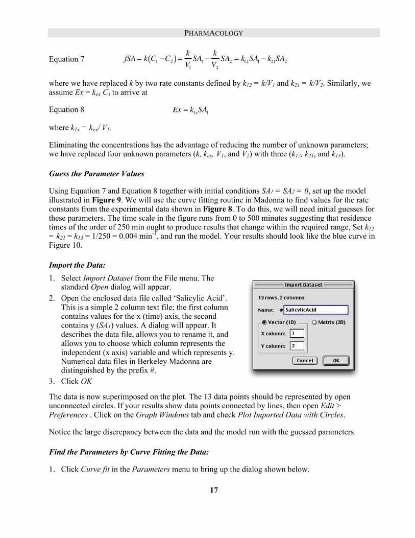
Import the Data: 1. Select Import Dataset from the File menu. The

standard Open dialog will appear. 2. Open the enclosed data file called ‘Salicylic Acid’.

This is a simple 2 column text file; the first column contains values for the x (time) axis, the second contains y (SA1) values. A dialog will appear. It describes the data file, allows you to rename it, and allows you to choose which column represents the independent (x axis) variable and which represents y. Numerical data files in Berkeley Madonna are distinguished by the prefix #.

3. Click OK

The data is now superimposed on the plot. The 13 data points should be represented by open unconnected circles. If your results show data points connected by lines, then open Edit > Preferences . Click on the Graph Windows tab and check Plot Imported Data with Circles.

Notice the large discrepancy between the data and the model run with the guessed parameters.

Find the Parameters by Curve Fitting the Data:

1. Click Curve fit in the Parameters menu to bring up the dialog shown below.

PHARMACOLOGY

18

2. Double click on the unknown parameters k12, k21, and k1x in the Available: list to move them over into the unknown Parameters list.

3. Use the Fit Variable pull down menu to select SA1norm.

4. Check that #SalicylicAcid is entered in To Dataset.

5. Click OK.

Madonna runs the model repetitively. New parameters are generated for each run until a “best fit” is found. The final run , using the best fit parameters, is then automatically displayed on the graph. (When comparing the curve fit to the data on the graph, be certain that both data points and curve fit are scaled on the same y axis.) Parameter values used in the plotted curve fit can be found in the current Parameter window. Or, as in Figure 10, simply click on the P button (on top of the graph) to place a moveable window that lists all parameters onto the graph.

These new parameter values provide a ready interpretation for the biphasic shape of Figure 8. The rate constants k12 and k21 for transfer between central and peripheral compartments are an order of magnitude larger than k1x ( the rate constant for elimination of the drug); in other words equilibration between compartments is much faster than elimination. The fast phase in Figure 8 reflects the rapid equilibration as the injected drug moves from central to peripheral compartments, while the later slow phase corresponds to the slow elimination.

PHARMACOLOGY

19

Figure 10

Aspirin

Our model for salicylic acid provides one part of the more complex model for aspirin (acetyl salicylic acid, ASA). When ASA enters the blood plasma it is rapidly hydrolyzed into salicylic (SA) and acetic acid by esterases contained in both blood and tissues. Both SA and ASA are effective analgesic, antipyretic, and anti-inflammatory drugs (see Error! Reference source not found.)

PHARMACOLOGY

20

Figure 11 Pharmacological Effects of SA and ASA

Our model for an iv injection of aspirin is shown in Figure 12. If ASA was not transformed into SA, their models would be almost identical. However, the transformation is rapid and irreversible; it provides the principal route J31 for elimination of ASA (elimination by other means, e.g. excretion, are negligible compared to J31 so they are left out of the model). Save a copy of your SA model and then use the original to build the aspirin model below.

PHARMACOLOGY

21

Figure 12

Fit the Two Curves Simultaneously

Import two files of experimental data entitled ASA.dat, and SA.dat from the CD. These data, resulting from a Dose = 650 mg, were not obtained from the same subject as the data of Figure 10. So parameters obtained from that data are not particularly applicable. Instead, we will employ the curve fitting routine to obtain all six unknown parameters. k12, k21, k34, k43, k1x, and k31. To acrry this out, set all initial values = 0, Dose = 650 mg, and use the same nominal guess of 0.004 min-1 for all six rate constants (k12= k21= k34= k43= k1x= k31 = 0.004). Run the model.

As in the salicylic acid model, bring up the Curve Fit dialog by clicking on Curve Fit in the Parameters menu, and load all six rate constants into the Parameters list. Since we will be looking for several parameters, it is a good idea to place restrictions on permissible values. In this case we will simply require all values to be positive by selecting each parameter in the list and setting its minimum value = 0 (upper right hand corner of dialog) . To fit more than one curve simultaneously check the box entitled Multiple Fits (center of the dialog). Then select ASAn from the Fit Variable popup and select the corresponding data, #ASAdat from the To Data Set.Click the ADD button to move the pair to the list on the right. Do the same for SAn and #SAdat . The Multiple Fits list should now show ASAn : #ASAdat followed on the next line by SAn : #Sadat. Click OK. After the program finds a best fit to the data, your results should look like. Figure 13. Again, make certain that the data and corresponding curve fit are scaled on the same axis (Use shift-click on the variable button qt the lower edge of the graph to toggle the scaling axis)

PHARMACOLOGY

22

Figure 13.

The model fits the data remarkably well. However this result is less impressive when we acknowledge that six independent parameters were adjusted to secure the best fit. This is but one example of a common dilemma: realistic biological models generally have large numbers of parameters whose values are not known; the larger the number of unknown parameters, the more difficult it is to establish validity or utility of the model. Confidence in the model increases when the range of data it accounts for increases. In our aspirin model, for example, it would be desirable if the same set of rate constants would predict the systems response to a wide range of doses. In addition, confidence increases when physiological rationalizations can be offered for the values of the fitted parameters. In the case of two compartment models, the abstract, ill defined, nature of the compartments precludes much success. Multi-compartment pharmacokinetic models that address these issues are known as physiologically based pharmacokinetic models.

PHARMACOLOGY

23

Physiologically Based Pharmacokinetics Physiologically based pharmacokinetic (PBPK) models model anatomical structures (usually organs) with compartments. This requires taking account of regional blood flow as well as the interaction of the drug with each tissue. We illustrate with a model of benzene, an industrial toxin. The most significant pharmacological features of benzene are:

1. It is volatile and its vapor gains access to the body via inspired air. 2. It is highly soluble in fat and tends to accumulate in fatty tissue. 3. It is removed from the body primarily through metabolism in the liver.

In the simplest model that accounts for these properties considers only 3 tissues in addition to the blood: fatty tissue, non-fatty tissue, and liver. The amount [in mg] of benzene within each of these tissues will be represented by a reservoir with a prescribed volume. Our task is to account for the flow of benzene into and out of each of these four compartments. First consider how the non-fatty compartment exchanges benzene with the blood compartment, as shown in Figure 14.

Figure 14 Benzene Flows from Blood to Non Fatty Tissue.

Blood flows from the blood compartment, B, to the non-fatty tissue compartment, NF, at a rate Qnf [L⋅hr-1]. Benzene, at blood concentration Cb [mg⋅L-1], flows into the NF tissue at rate Qnf *Cb. Benzene returns from non fatty tissue back to the blood at a rate Qnf * Cnfv, where Cnfv is the concentration at the venous end of the capillary. However, the lipid soluble benzene permeates membranes rapidly, so we can assume that by the time blood traverses a capillary, the benzene has equilibrated with the tissue. This means that Cnfv = Cnf where Cnf is the tissue concentration. Letting Jnf denote the net flow between blood and tissue:

Equation 9

�

Jnf = QnfCb −QnfCnfv = Qnf Cb − Cnf( )

Concentrations are computed by dividing the amount in the reservoir by the relevant volume as shown in Figure 14.

PHARMACOLOGY

24

We modify this basic element to model the other tissues, and connect them through the blood supply. This yields the four compartment model shown in Figure 15.

Figure 15 Four compartment benzene Model.

The structure for the fatty tissue compartment, F, is very similar to that of the non-fatty tissue compartment, NF, but modified to account for the high fat solubility of benzene as follows. If the concentration in venous blood ,Cfv, is in equilibrium with the tissue concentration Cf, then Cfv = Cf/Pf where Pf is the solubility of benzene in the fatty tissue.

The structure for the liver tissue compartment is similar to F, but with an additional outflow to account for the enzymatic processes that remove benzene from the liver. We shall model this rate by a saturating curve similar to that of a Michaelis-Menten enzyme:

Equation 10

�

Jmetab =vmaxCl

Km + Cl

PHARMACOLOGY

25

Finally, to represent the net uptake of benzene by respiration an inflow is added to the blood reservoir. Denote the ventilation rate by Qvent, and let Ci be the concentration of benzene in inspired air. Then benzene enters the lungs at a rate Qvent ⋅Ci. Assuming exhaled benzene is in equilibrium with blood, it will exit the lungs at a rate Qvent⋅Cb/Pb where Pb is the blood/air partition coefficient. The difference between entry and exit must represent the rate of uptake of benzene so that Jresp is given by

Equation 11

�

Jresp = Qp Ci −Cb

Pb

⎛ ⎝ ⎜

⎞ ⎠ ⎟

Typical parameter values for mice are given in Table 2 Qp 5.74 Alveolar ventilation rate [L hr-1] Ci 0.32 Benzene concentration in inspired air [mg L-1] Init B 0 Initial condition blood Init F 0 Initial condition fat Init L 0 Initial condition liver Init Nf 0 Initial condition non-fat Km 0.4 Michaelis-Menten constant [mg L-1] Pb 18 Blood/air partition coefficient Pf 28 Fat/blood partition coefficient Pl 2 Liver/blood partition coefficient Qf 0.517 Blood flow to fat [L hr-1] Ql 1.44 Blood flow to liver [L hr-1] Qnf 3.79 Blood flow to non-fat [L hr-1] Vb 0.024 Volume blood [L] Vf 0.027 Volume fat tissue [L] Vl 0.012 Volume liver tissue [L] vmax 1.42 Maximum velocity of metabolism [mg hr-1] Vnf 0.234 Volume non-fat tissue [L]

Table 2 Parameter for Benzene Model for Mice

Construct the model and simulate a 48 hour exposure of air containing 0.32 mg⋅L-1 of benzene. Compare the level of benzene as well as its equilibration times in the different tissues, and relate these to the tissue’s solubility and blood flow.

Simplifying the Flowchart: Aliases, Sub-models, and User Defined Icons As models grow, more complex, the flow chart becomes messy; the inevitable clutter obscures the simple elementary relations that generate the model. Berkeley Madonna uses several devices to simplify the flowchart, illuminate the basic structure of the model, and to make icons more reflective of their context. These devices include aliases, submodels, user defined icons, icon visibility, and user defined back-grounds.

PHARMACOLOGY

26

Aliases

Complex models begin to resemble a bowl of spaghetti when connections are required between two icons that are spaced far apart. Rearranging icons is time consuming and rarely produces a simpler flowchart. An alias icon is one solution to this problem. You create an alias for one of the icons and place it close to the otherwise distant icon, and then connect the alias to the target icon with a short connection. The alias icon looks like a ghost version of their original and it provides another way to access the original . Double-clicking an alias opens the icon dialog for the original. When connections are made to an alias, the effect is identical to that resulting from making the same connections to the original. The most important thing to remember is that an alias always refers to an original.(You can locate the original by selecting an alias and choosing Find Original from the Flowchart menu).

To create an alias, select one or more existing icons and click the alias button in the toolbar. Berkeley Madonna will create one alias for each icon you selected. However, note that aliases will only be created for reservoir, flow, and formula icons. You can create as many aliases for a particular original as you want by repeatedly clicking the alias button. These aliases can be placed anywhere in your flowchart. An alias always has the same name as the original. If you change the name of an alias, it changes the name of the original and all of its aliases. If you double-click an alias, it opens the icon dialog for the original.

Figure 16 shows a different representation of the benzene model shown in Figure 15. Here aliases have been used for B and for CB. The flowchart allows for easy comparison of the tissue variations involving solubility and metabolism. To add more tissues to the model simply select one of the tissue types (including all its connections) and copy and paste it into the diagram. (Be careful to reposition the pasted objects before de-selecting them.) Finally rename the icons where appropriate. Although the simplification in Figure 16 may not be dramatic, similar alias simplifications become very significant in more complex cases. Further, aliases are an essential component of sub-models described below.

PHARMACOLOGY

27

Figure 16 Benzene Model with Aliases.

Hierarchal Sub-models

Although aliases can help make complex models easier to construct, as models continue to grow, there simply isn’t enough room in a single flowchart window to contain all elements. And even if it were possible to cram an entire model into one full-screen window, it would difficult to see its overall structure through the forest of arcs, flow lines and icons.

Berkeley Madonna allows you to break your model down into functional parts by placing them in submodels just as you would place related groups of files into a folder or directory on your computer. Submodels appear as icons in your flowchart. The flowchart containing a submodel icon is referred to as the submodel’s parent flowchart. When you double-click a submodel icon, a separate flowchart window is opened showing the contents of that submodel. Figure 17 shows an application of sub-models to the Benzene Model of Figure 15.

PHARMACOLOGY

28

Figure 17 Benzene Model with Submodels. Clicking on a submodel opens it’s window.

Notice that submodels can be imbedded in each other; i.e. a submodel can serve as the ‘parent’ for a deeper level submodel.

Creating Submodels

You will find that Flowchart models with more than a few reservoirs and functions quickly become a spaghetti whose structure is obscured by the clutter. The answer is to use Submodels, which are analogous to subroutines in a programming language. Submodels can be created in several ways. To create a

new, empty submodel, you can click the submodel tool on the toolbar, drag the mouse over the flowchart and release it. Berkeley Madonna places a new submodel icon on the flowchart.

More often, new submodels are created from icons that already exist on the flowchart. This is accomplished by selecting the icons and choosing Group from the Flowchart menu. Berkeley Madonna creates a submodel icon on the flowchart and places the previously selected icons inside that submodel. When icons are moved into a submodel, aliases are created in order to preserve the connections that existed before the submodel was created. Double- clicking the submodel icon allows the user to edit its contents in the same way as the top-level flowchart.

Try transforming your model as depicted in Figure 15 into the model shown in Figure 17. A simple way is to begin by selecting the NF reservoir and then choosing Group from the Flowchart menu. Name the sub-model icon Non Fatty Tissue and then, one by one, drag the associated icons JNF,

PHARMACOLOGY

29

CNF, VolNF, and QNF and drop them on the sub-model. You can accomplish the same task in one operation by choosing Group after selecting all the relevant icons (either by shift-clicking or by drawing a marquee around them with the selection tool)

Deleting a submodel icon, deletes not only the icon but also all of the icons it contains. However, it is possible to delete a submodel icon while preserving the icons and connections it contains by selecting one or more submodel icons and choosing Ungroup from the Flowchart menu. Berkeley Madonna removes the submodel icon and moves all the icons it contained into the parent flowchart.

Making Connections between Submodels

Icons may be moved from one submodel to another in two ways: First, you can move a set of icons from a flowchart into one of its submodels (children) by dragging the icons to the submodel icon and dropping them inside. Second, you can move a set of icons from a submodel into its parent flowchart (the flowchart containing that submodel ’s icon) by selecting the icons and choosing Move To Parent from the Flowchart menu Try moving some of the icons back and forth from parent (main) to child (submodel) window.

User Designed Icons

Flowcharts can be made even more intuitive by replacing the default, generic icons with icons that are designed to reflect the object that each represents. This is illustrated in Figure 18 which shows a customized version of the our benzene model. Note that the new images are not simple paste- overs, they are bona fide icons with the same functionality as the originals. They can be moved about freely and functional connections can be added or removed. Double clicking on the icon initiates the same action as clicking on the original.

Icon replacement is implemented by first preparing an icon in a paint/draw program and saving it in either GIF or JPEG format. Next select the icon in your model to be replaced, and then select the Import Icon Image command (Flowchart menu). An ordinary open dialog will appear allowing you to select any GIF or JPEG image . Clicking Open in the dialog will replace your selected model icon with the new custom image (selected in the dialog) from an external file. (The Import Icon Image command is available only when one or more model icons are selected.)

Figure 19 shows a more elaborate model of the same problem. Here, the visual advantages provided by context sensitive images are even more apparent. They allow the features of a complex model to be grasped with a single glance. In this version we have combined the flows and associated icons into submodels (replacing their image with faucets) while keeping the reservoirs intact (but , replacing the generic icons with anatomical ones).

A set of Icons designed for PBPK models is contained within a folder on the Madonna disk.

PHARMACOLOGY

30

Figure 18 Benzene Model with User Defined Icons

Figure 19 PBPK Model with User Defined Icons.

Applications and Limitations of PBPK models

Defining a detailed and explicit physiological basis for the distribution of drugs is more satisfying than a more formal abstract compartment approach. It is particularly useful and has found wide application in cases where the location of the drug is critical, e.g. models for anticancer drugs as well as in toxicology studies. In some cases, e.g. when dealing with CNS drugs, the permeability of the vascular bed is also taken into account. However the models are complex and depend on large numbers of parameters. Many of these parameters are only measured with invasive techniques,

PHARMACOLOGY

31

which are not applicable to humans. In these cases we rely on extrapolating data obtained from animal studies. Guidelines and empirical rules for interpolating or extrapolating PKPB parameters between species are reviewed by REF XXX.

Population Pharmacokinetics (Monte Carlo Simulations)

Even when we have good “normal” values for the parameters, we still may want to account for individual variations. Environmental Toxicologists, for example, are continually confronted with problems that require some estimates of risk associated with pollutants. These are often expressed in statistical terms – e.g. what percentage of the population can be expected to have high levels of pollutant in specific organs when they are exposed to a given pattern of pollutants. We can attack this problem by running the same model over and over while each repetition draws a random estimate of each parameter. We illustrate with the benzene model:

Pharmacodynamics Receptors

Computing the concentration of a drug at its target site (pharmacokinetics) is a first step. It solves the drug delivery problem, but it does not address the mechanism of drug action. A more complete theory would integrate the action of the drug with a model of the physiology of its target cell (e.g. See chapter xxx on the action of a local anesthetic). But cellular models is a diverse subject, and so, unlike pharmacokinetics, pharmacodynamics does not lend itself to a simple general treatment. However, most pharmacodynamic models consider the binding of ligands (e.g. drugs or hormones) with receptors as the first step. The relation between free and bound ligand concentrations follows simple chemical principles. Letting L represent free ligand, R free receptor, and LR ligand -receptor complex, we write L + R→ LR.

Here, we make the simple assumption that the ligand receptor reaction is so fast that it is virtually in equilibrium at all times. More general cases will be discussed later. Let K50 denote the equilibrium (dissociation) constant, then

Equation 12

�

K50 =L[ ] R[ ]LR[ ]

Letting [RT] denote the total concentration of both free, R, and occupied, LR , receptors

Equation 13

�

RT[ ] = R[ ] + LR[ ]

Eliminating [R] from the last two expressions, we can solve for [LR]. Then letting C = [L], and defining p = [LR] / [RT] as the fraction of receptors occupied by the ligand we have

Equation 14

�

p =C

K50 + C

The value of p varies between 0 (all receptors free) to 1 (all receptors occupied)

PHARMACOLOGY

32

Note that in the special case where 50% of the receptors are occupied, p = 1/2 and C = K50. Hence the notation: aside from being a dissociation constant, K50 is numerically equal to the concentration where 50% of the receptors are occupied.

Just how the physiological response of the ligand depends on the number of occupied receptors will differ from case to case. In the simplest examples, the physiological effect E is proportional to the number of occupied receptors. If a is the proportionality constant then, since the actual concentration of occupied receptors is [RT] p,

Equation 15

�

E = a RT[ ]p

If the maximal physiological activity, Emax, occurs when all receptors are occupied, i.e. when p =1, then Emax = a [RT] and

Equation 16

�

E = Emax p = EmaxC

K50 + C (activation)

Equation 16 implies that the drug is stimulatory, i.e. it enhances the activity. On the contrary, many drugs are inhibitory; they work by blocking receptors. In this case we assume that E is proportional to the unoccupied receptors. The fraction of unoccupied receptors is given by 1-p and in place of (12) we now have

Equation 17

�

E = Emax 1− p( ) =EmaxK50K50 + C

(inhibition)

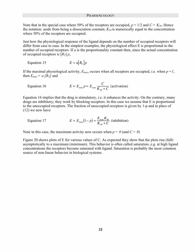
Note in this case, the maximum activity now occurs when p = 0 (and C = 0)

Figure 20 shows plots of E for various values of C. As expected they show that the plots rise (fall) asymptotically to a maximum (minimum). This behavior is often called saturation, e.g. at high ligand concentrations the receptors become saturated with ligand. Saturation is probably the most common source of non-linear behavior in biological systems.

PHARMACOLOGY

33

Figure 20 Plots of Equation 16 (solid line) and Equation 17 (dashed line with Emax = 100% and K50 = 2. Note that both plots cross the 50% level at C = K50 = 2.

Sigmoidal Response

The curves depicted in Figure 20 are rectangular hyperbolae; they rise (fall) abruptly with the steepest slope at the origin. When activation or inhibition of a receptor requires binding of more than one ligand, this behavior changes and the curves assume an S or sigmoidal shape where the curve is flatter near the origin (see Figure 21 and Figure 22). If we change the stoichiometry in our reaction by requiring n ligands for each receptor: nL + R → Ln⋅R. Using the same arguments as before, we arrive at the following analogous expressions for activation and inhibition respectively.

Equation 18

�

E =EmaxC

n

K50n + Cn

Equation 19

�

E =EmaxK50

n

K50n + Cn

These are plotted in Figure 21 and Figure 22. Again, Emax and K50 indicate the maximum effect and the concentration where E = 1/2 Emax.

PHARMACOLOGY

34

Figure 21 Plot of Equation 18 with K50 = 2, Emax =100 and n = 1, 3, 5. Again, all plots cross the 50% level at C = K50 = 2.

Figure 22 Plot of Equation 19 with K50 = 2, Emax =100 and n = 1, 3, 5. All plots cross the 50% level at C = K50 = 2.

The reaction implies that n molecules of L react simultaneously with R. Even with n =2, this is highly unlikely. A more accurate formulation would characterize the reaction taking place in stages i.e.

L + R –––> L1R

L1R + R –––> L2R

…

Ln-1R + R –––> LnR

Our simplification of writing the reaction in a single step essentially assumes that intermediates are short lived with only negligible amounts present at equilibrium. This appears to be the case in many proteins which bind ligands cooperatively, e.g. hemoglobin binding of oxygen (refXXX).

PHARMACOLOGY

35

Combining Pharmacokinetics and Dynamics Steroid Regulation of Cell Trafficking: A Direct Response

Once a pharmacodynamic system is constructed, it is fairly easy to add a pharmacokinetic regime for a more complete model. To illustrate we consider models developed by Jusko et.al. to describe some physiological responses to doses exogenous steroids (refsXXX) The simplest describes the movements of histamine containing white blood cells (basophils) between vascular and extra-vascular (tissue) spaces. Basophils are assumed to enter the blood stream at a constant rate and to leave at a rate proportional to the number contained within the circulatory tree. Exogenous steroids are assumed to inhibit the rate of entry by reacting with a steroid receptor.

Following the injection of the steroid, methylprednisolone, data were obtained from measurements of methylprednisolone and histamine in the blood. Since more than 97% of blood histamine resides within basophils, it follows that blood histamine concentration is proportional to basophil count. Rather than following basophils directly, it is more convenient to measure histamine and this is reflected in the model shown in Figure 23.

Figure 23 Cell Trafficking Model

PHARMACOLOGY

36

The lower sequence is a simplest model for passage of basophils between vascular and extra-vascular spaces. It is assumed that the extra-vascular space is an infinite source for basophils so that we need only account for the basophils ( amount of histamine ) in the vascular compartment. This is represented by the H reservoir which, as usual, reflects the initial amount present as well as the Enter and Exit flows. The Exit flow is proportional to the histamine concentration (density of vascular basophils). If Ch= H/Vb denotes the histamine concentration and kh denotes the proportionality constant, then

Equation 20

�

Exit = kh ∗Ch .

But, the Enter flow contains the link to the steroid concentration Cs. It is assumed that this rate is inhibited by drug interacting with an unspecified receptor. Let p represent the fraction of receptor sites occupied by the drug and let baseRate denote the rate of entry in the absence of inhibitor, then (see occupied by the ligand we have

Equation 14 and Equation 17 with Emax = baseRate)

Equation 21

�

p =Cs

K50 + Cs

Equation 22

�

Enter = baseRate 1− p( )

The top sequence in Figure 23 is a one compartment pharmacokinetic model with parameters listed in Table 3. Flows are similar to earlier one compartment models e.g. Figure 6.

Steroid Init Steroid 0 Exogenous Steroid (µg) Dose 4E04 Injection dose (µg) Interval IE06 Time for “second injection” (hr) k 24 Steroid clearance (L hr-1) Vd 90 Volume of distribution (L)

Histamine Init H Ho Initial histamine content (µg) Ho 90 Initial histamine content (µg) baseRate 30.6 Uninhibited rate of histamine entry (µg hr-1) kh 1.7 Clearance rate constant for histamine leaving the circulation (L hr-1) K50 3 Dissociation constant for Steroid-Receptor (µg hr-1)

�

Vb 5 Blood Volume (L)

Table 3. Cell Trafficking Model: Parameters for 70 kg Human

Set up the model and run it, plotting Ch (scaled on the left) and p (scaled on the right). Overlay each response for dose levels of 10, 20, 40, and 80 E04 µg. Note how the proportionality between dose

PHARMACOLOGY

37

level and response that was evident in the earlier models has disappeared as receptor becomes saturated at higher doses.

To compare the time course of drug dose remaining in the body with its effect on histamine content of the blood, it is convenient to normalize the plots and define the effect more precisely in terms of histamine depression. To do this, place two new formula icons on the flowchart, label one steroidPercent, the other hIinhibition. Connect an arrow from Steroid and another from a Dose to the first icon. Connect an arrow from H and Ho to the second icon. Remembering that initially H =Ho mg L-1, double click on the icons and enter the following:

Equation 23

�

steroidPercent =100 ∗ SteroidDose

Equation 24

�

hInhibition =100* H0 −HH0

⎛

⎝ ⎜

⎞

⎠ ⎟

Reset the Dose to 4E04 and run the program. Replace the plotted variables with steroidPercent and hIinhibition. Note the discrepancy between the two curves; by the time the inhibition is at its maximum of about 92% (i.e. at about 10 hours), the steroid has fallen to less than 10 % of the original dose. Plotting p shows a major reason for this large discrepancy. At 10 hours, the receptors are still nearly saturated. The saturation which is apparent at the beginning persists because the large injected dose created an initial concentration (Dose/Vd = 4E04/90 =440 µg L-1 ) much larger than K50= 3 µg L-1, so even though C declines rapidly there is still enough to keep the receptors near saturation. Receptor occupancy will decrease to 50% only when C falls to 3 µg L-1.

But, even if the original dosage were reduced, there would still be a discrepancy because the steroid does not act directly on the vascular H pool. Rather, it acts on how fast the pool is replenished from extra-vascular sources, and it takes time for any rate change to exert its full effects on the pool. There is an inevitable delay whenever a dynamic process intervenes between cause and effect. The next model provides a more dramatic example.

Steroid Regulation of Enzyme Synthesis: A Gene Mediated Delayed Response with Down Regulation

Glucocorticoids, secreted by the adrenal cortex, are essential steroid hormones with diverse functions: They facilitate the action of other hormones, or they take part in the long term adaptation to stress. These latter functions include the mobilization of amino acids from labile protein reserves, the synthesis of gluconeogenic enzymes to promote the conversion of proteins to glucose, and the trafficking of white cells. In chronic stress, excess glucocorticoids can be harmful causing atrophy of lymphatic nodes, decreased immunity, hypertension, and other vascular disorders.

Glucocorticoids are used in higher concentrations as drugs because of their immunosuppressive and anti-inflammatory actions. Some administered glucocorticoid effects (e.g. synthesis of enzymes) are gene mediated and, following a single dose, may only appear after the drug has dissipated. The following model (ref XXXX) accounts for the gene mediated effects of the glucocorticoid drug. methylprednisolone, on the synthesis of a gluconeogenic enzyme called TAT (tyrosine-amino transferase, an enzyme that catalyzes the cleavage of amino groups from tyrosine making the residue

PHARMACOLOGY

38

available for glucose synthesis.) In addition to exhibiting a delayed response, the system becomes desensitized to repeated doses, a behavior attributed to receptor down-regulation. Both of these features, delay and desensitization, are accounted for in model of Figure 24.

Figure 24 . Basic Scheme of Steroid Model (REF). Symbols are: D = Drug (methylprednisolone), R = Receptor (cytosolic), DR=Drug/Receptor complex(cytosolic), DRn = Drug/Receptor complex(nuclear), mRNA-R = messenger RNA for Receptor, mRNA-TAT = messenger RNA for TAT, TAT = enzyme (final product of gene medziated response to steroid) DRn is assumed to stimulate production of mRNA-TAT, and to feedback and inhibit production of mRNA-R. Downward pointing arrows represent normal degradation.

R

DR

DRnD

mRNA-R

mRNA-TAT TAT

+

+

—

Steroids, in general, are lipid soluble and easily pass through cell membranes. When the steroid D enters the cytosol it reacts with a receptor protein R forming a complex DR that is transported into the nucleus where it has two effects:

1. It binds to DNA control sequences adjacent to the target gene. Transcription is stimulated producing more mRNA-TAT to be transported to the cytosol where translation and production of the final protein TAT increases.

2. It inhibits transcription of mRNA-R thereby cutting back on the rate of synthesis of new receptors. This negative feedback will reduce the rate that DRn can be formed and accounts, in part, for the receptor down regulation.

The model takes into account that both mRNA-TAT and mRNA-R are perturbed from their normal steady state by the action of DRn. In turn this perturbs the steady state of both TAT and R. To accomplish this it is necessary to account for rates of production and degradation of the messenger RNA variables mRNA-R, and mRNA-TAT, as well as R, DR, DRn, and TAT.

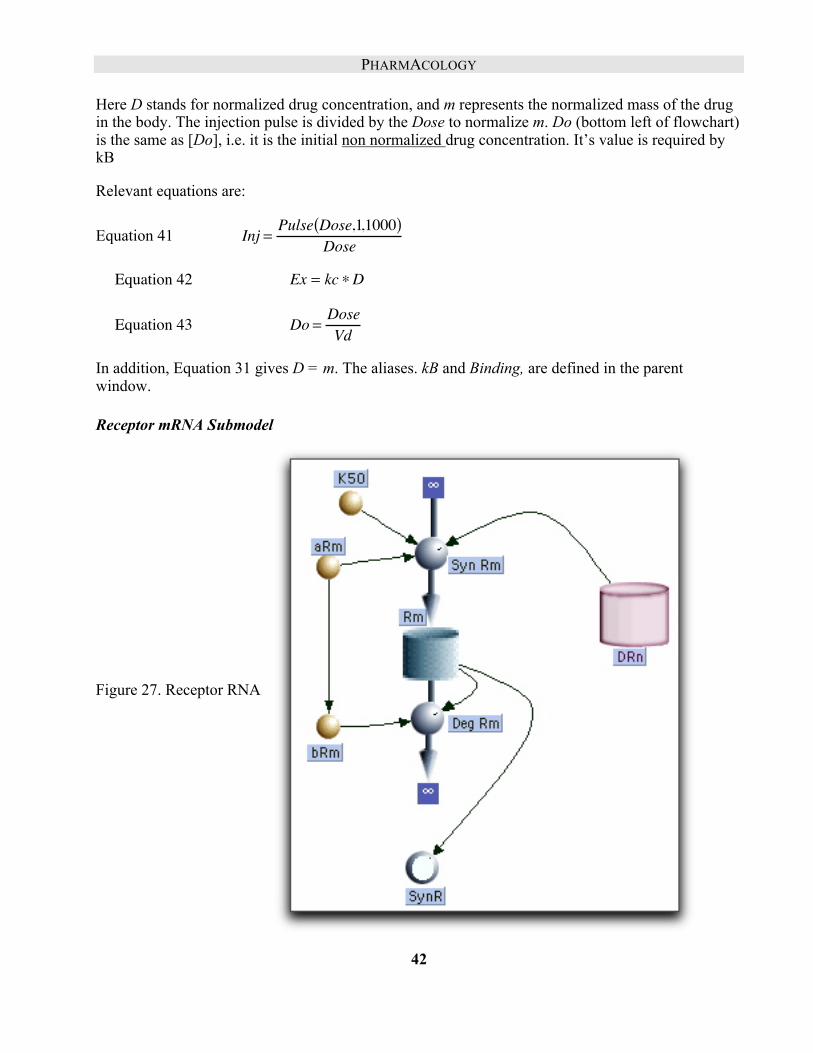
Parent Window

Implementation of the model in Madonna is shown in Figure 25 to Figure 28. It contains a main parent window with the D-R cycle (shown in black Figure 24) and three submodels (shown in blue) for Steroid pharmacokinetics, Receptor mRNA synthesis, and TAT synthesis.

The model can be constructed by duplicating Figure 25, dragging each submodel icon from the toolbar. To make connections to the submodel icons, make an alias of the icon to be linked and drag the alias into the submodel icon. Then double click on the submodel icon to open its window and duplicate its contents as shown in the figures below.

PHARMACOLOGY

39

Figure 25. Steroid Model in Madonna: Parent Window.

Normalize the Variables

To get a good overview of the model it will be expedient to plot and compare behavior of the major variables D, R, DR, DRn, TATm, and TAT on the same graph. Using concentrations, this is not feasible because the variables do not have a common scaling. Some are in the fmole range while others are measured in nmoles. We can provide a workable scaling by normalizing variables to their initial concentrations. Denoting concentrations with conventional square brackets, and letting the subscript o denote initial values, we define our new normalized variables as:

Equation 25

�

TAT =TAT[ ]TATo[ ]

Equation 26

�

TATm =TATm[ ]TATmo[ ]

Equation 27

�

Rm =Rm[ ]Rmo[ ]

The Drug-Receptor complexes DR and DRn have initial values equal to zero. However they are simply different forms of R, so we use Ro for all three

Equation 28

�

R =R[ ]Ro[ ]

�

DR =DRRo

�

DRn =DRn[ ]Ro[ ]

PHARMACOLOGY

40

The drug concentration, D, is also zero at starttime, so we normalize D by it’s concentration Do immediately following the injection. At that time the drug mass ,mDo, is equal to Dose, making

Equation 29

� � � �

[Do] =mDoVd

=DoseVd

and

Equation 30

�

D =D[ ]Do[ ] =

Vd∗ D[ ]Dose

Note that for normalized variables. the distinction between concentration and mass vanishes. This follows because they are proportional i.e. if mD is the mass of drug, then initially we have mDo = [Do]*Vd, and at any later time we have mD = [D]*Vd. Dividing the first equation into the second leaves

Equation 31

�

D =D[ ]Do[ ] =

mDmDo

= m

where m is the normalized mass.

Finally it will be helpful to keep track of all receptor molecules, regardless of their location or the presence of bound ligand. We define this total as

Equation 32

�

Rtot = R + DR + DRn

Normalized variables requires redefinition of parameters

Our normalized variables have no dimensions, they are pure numbers. Yet, we use them in model building as though they are the original non-normalized variable. For example, the law of mass action relates the rate of a reaction to the product of concentrations, not the product of numbers. In our model we apply this law to the binding of D to R with the binding rate given by

Equation 33

�

rate= k ∗ D[ ] ∗ R[ ]

In terms of our normalized variables this becomes

Equation 34

�

rate= k ∗ Do[ ]∗ Ro[ ]∗ D[ ]Do[ ] ∗

R[ ]Ro[ ] = k1∗D ∗R

where k1 = k*[Do]*[Ro].

In general, by multiplying and dividing individual terms by the same number, we can always use normalized variables as though they were the original non-normalized quantity provided we absorb normalization factors within the parameters. (Sometimes normalization factors will occur on both sides of an equation and cancel so that some parameters may not change - see pp XXX.) The parameters in Table 4 have been adjusted for normalizations defined by Equation 25 to Equation 32.

PHARMACOLOGY

41

Define the Model Flow Rates

Flow rates in the cycle of the parent chart (Figure 25) are calculated from the law of mass action. In the equations that follow. all parameters beginning with k are rate constants for the cycle, all beginning with a are synthesis rate constants, and those that begin with b are degradation rate constants. The flows in Figure 25 are given by:

Equation 35

�

Binding = kB ×D × R

Equation 36

�

Transport = kT ×DR

Equation 37

�

Re cycle = fR ∗ kre∗DRn

Equation 38

�

DegDRn = 1- fR( ) × kre× DRn

Equation 39

�

DegR= bR× R

Equation 40

�

SynR = aR× Rm

where, fR is the fraction of dissipating DRn that gets recycled to the cytosol as free R, and Rm is the amount of messenger RNA coded for R as calculated in the subprogram Receptor mRNA (see below).

Numerical values for parameters are listed inTable 4.

Steroid Submodel

The submodel entitled Steroid is a simple generic one compartment model:

Figure 26 One compartment model for steroid pharmacokinetics. It is linked to the parent window with its attachment to the alias for the Binding flow as well an attachment of Do to kB .

PHARMACOLOGY

42

Here D stands for normalized drug concentration, and m represents the normalized mass of the drug in the body. The injection pulse is divided by the Dose to normalize m. Do (bottom left of flowchart) is the same as [Do], i.e. it is the initial non normalized drug concentration. It’s value is required by kB

Relevant equations are:

Equation 41

�

Inj =Pulse Dose,1,1000( )

Dose

Equation 42

�

�

Ex = kc ∗D

Equation 43

�

Do =DoseVd

In addition, Equation 31 gives D = m. The aliases. kB and Binding, are defined in the parent window.

Receptor mRNA Submodel

Figure 27. Receptor RNA

PHARMACOLOGY

43

It is assumed that Rm is normally produced at a constant rate that is inhibited by DRn. Binding of DRn to this control site occurs with dissociation constant = K50 so that

Equation 44

�

SynRm = aRm × 1− DRnK50 + DRn

⎛ ⎝ ⎜

⎞ ⎠ ⎟ .

Degradation of Rm is assumed proportional to Rm:

Equation 45

�

DegRm = bRm × Rm

TAT Synthesis Submodel

Figure 28. TAT Synthesis

Equation 46

�

SynTAT = aTAT ∗ TATm( )g

The exponent g is an “amplification factor” introduced because the TAT synthesis rate is very sensitive to TATm , rising faster than a simple linear dependence on TATm.

Equation 47

�

DegTAT = bTAT × TAT

We assume TATm is normally produced at a constant rate aTm that is stimulated by DRn, and stimulation is proportional DRn with proportionality constant, s.

Equation 48

�

SynTm = aTm × 1+ s× DRn( )

Equation 49

�

DegTm = bTm × TATm

PHARMACOLOGY

44

Getting Parameters from the Steady State

This model has its share of parameters, but they are not all independent. Before the first injection takes place, we assume our system is not changing ; it is at “rest”. More precisely the system is in a steady state where variables such as R or TAT remain constant because their rates of production are balanced by their rates of degradation. In our terms the flows in equal the flows out.

Beginning with R, we find three relevant flows Binding, SynR and DegR . At time = 0 (starttime), Binding = 0 because D = 0, so the SynR inflow has to equal the DegR outflow. But, using the initial normalized values (Equation 27 and Equation 28) we have R = 1 and Rm = 1. It follows from Equation 39 and Equation 40, that

Equation 50

�

aR = bR

Now consider Rm. At time = 0, DRn =0 and Rm =1. Setting the inflow, SynRm, equal to the out flow, DegRm,, we have from Equation 44 and Equation 45,

Equation 51

�

aRm = bRm

Flows for TAT and TATm are handled the same way. At time = 0, both TAT and TATm equal 1 and DRn = 0. Setting inflow = outflow for both, we use Equation 46 to Equation 49 to arrive at

Equation 52

�

aTAT = bTAT

Equation 53

�

aTm = bTm

The assumption of a steady state at time = 0 is a common practice for reducing the number of independent parameters. We will use it repeatedly.

VARIABLE VALUE DEFINITION AND UNITS INIT R 1 Initial Receptor Conc. ( number) INIT DR 0 Initial cytosolic Drug-Receptor Conc. (number) INIT DRn 0 Initial nuclear Drug-Receptor Conc. (number) kB 0.0039*Do Binding rate constant ( hr-1 ) kre 0.57 nuclear Drug-Receptor recycling/degradation constant ( hr-1 ) rF 0.49 Fraction of disappearing DRn that is recycled to free R (number) kT 0.63 Transport rate constant for DR from cytosol to nucleus (hr-1) aR = bR Rate constant for R synthesis (hr-1) --obtained from steady state bR 0.0572 Rate constant for R degradation ( hr-1 )

STEROID subprogram kc 1.32 Normalized Steroid Clearance (hr-1) Vd 0.27 Volume of distribution (L) Dose 5E03 Amount injected (nmole) Interval 1000 Time for second injection (hr)

RECEPTOR mRNA subprogram

PHARMACOLOGY

45

INIT Rm 1 Initial Rm concentration (number) a Rm 2.9 Rate constant for Rm synthesis (hr-1) b Rm = = a Rm Rate constant for Rm degradation (hr-1 ) --obtained from steady

state K50 0.062 Dissociation constant for DRn binding to control site for R

synthesis (number) TAT subprogram

INIT TATm 1 Initial TAT mRNA concentration (number) INIT TAT 1 Initial TAT concentration (number) S 12.1 Proportionality constant for DRn stimulation of TATm (number) g 1.804 “Amplification “exponent for TATm stimulation of TAT (number) aTm = bTm rate constant for synthesis Tm (hr-1) -- from steady state bTm 0.383 rate constant for degradation Tm ( hr-1) aTAT = bTAT rate constant for synthesis TAT (hr-1 ) -- from steady state bTAT 0.6904 rate constant for degradation TAT ( hr-1 )

Table 4. Steroid (Methylprednisolone) Model: Normalized Parameters for 380 g Rat.

Set Stoptime = 25 hours and run the model.

Double click in the middle of the plotting window to bring up the Choose Variables dialog. Remove all variables and add those defined in Equation 25 through Equation 31. Keep all variables scaled on the left except TATm and TAT; scale these two on the right.

1. Plot the first two D, and DR. D rises instantaneously, reflecting the instantaneous injection. Drug binding to receptor is nearly instantaneous, reaching its peak, where it binds 84% of the receptor, at 0.2 hours. But, the DR curve decays much slower than the D curve because of the difference in relaxation times The average lifetime (relaxation time) of a D molecule in the body is given by (kc/Vd)-1 = 0.2 hours while that for DR is kT

-1 = 1.6 hr.

2. Now add DRn the drug receptor in the nucleus. Here we see the first significant delay in the chain. It rises to a peak and then, as DR declines, DRn decays with a relaxation time of 1.75 hours. By the time the DRn peak occurs (about 1 3/4 hours after injection, D has disappeared.

3. Next add TATm and note that it is scaled on the right hand axis. It rises to approximately 4 times its resting concentration about 4 hours after injection.

4. Now add TAT; this final response peaks at 10 times its normal activity several hours after the drug has disappeared. Moreover an enhanced enzyme activity persists for the better part of the day.

5. The status of free cytosolic receptors can be seen by plotting R. (It’s a good idea to toggle TAT and TATm off the graph to reduce clutter.) Almost immediately after injection, R drops precipitously as it binds D to become DR. As D declines R builds back up slowly toward its normal value. There are two sources of this build up 1. recycling from the nucleus, and 2. synthesis of new R. You can evaluate both contributions by plotting SynR and Recycle. (You

PHARMACOLOGY

46

will have to select these in the Choose Variables dialog and then re-run the model). As you might expect recycling is only important in the early phase, while synthesis maintains a fairly steady supply and is responsible for the slow recovery in the later part of the run.

6. To examine the consequences of receptor down regulation, set Stoptime = 40 and Interval = 24, This will give an additional injection one day after the first. Run the model and toggle all plotting variables off the graph except D (the stimulus) and TAT (the response). Although the injections are identical, the second response is lower than the first. The system has been de-sensitized by receptor down regulation. This is shown when you add Rtot to the plot. Soon after the drug is applied there is a drop in the total amount of receptors to about 75% of normal followed by a slow rise back towards normal as the DRn declines. Rtot has not fully recovered by the time of the next injection; as a result, its responds to the new injection by falling lower than it did to the first.

7. Down regulation caused by the negative feedback feed-back of DRn (Figure 24) is seen if the mRNA coded for R, Rm, is added to the plot. It’s decline and rise correlates with Rtot. To see the effect of this feedback more clearly, toggle the O (overly) button and run the model with the feedback removed by setting K50 equal to a number much greater than DRn, say K50 = 1E10. This essentially removes the feed back term , DRn /( K50 + DRn), in Equation 44 by making it close to zero. The results show that Rm no longer shows any dip; it remains in a steady state. On the other hand both Rtot and TAT still show evidence of a substantial, down regulation . Evidently there is a second cause. Since, under these conditions, the synthesis of R remains constant this extra factor must involve the degradation terms, and indeed, when their relaxation times are compared we find that the mean lifetime of a DRn molecule is kre-1 =1.75 hours, while that of an R molecule is ten times larger (bR-1 =17.5 hours ). Thus, even though half of DRn will recycle its R, the nuclear receptor drug complex is much more susceptible to degradation than cytosolic free R. Exposure to the drug produces DRn which has an enhanced rate of degradation so that R is reduced and the tissue becomes desensitized.

8. A small bump on the Rtot curve occurs just after injection. It rises when substantial DR has formed .but before much has been transported into the nucleus. In contrast to DRn, cytosolic DR is “protected”, it is transported, but not degraded. Movement from cytosol to nucleus does not reduce Rtot, while the diminished degradation due to DR formation increases Rtot. You can verify this by showing that the size of the bump varies inversely with kT.