Pharmaceutical Crystallization Design Using Micromixers ...

Pharmaceutical Crystallization Design Using Micromixers,

Multiphase Flow, and Controlled Dynamic Operations

by

Mo Jiang

B.S. Biology, Tsinghua University, 2006

M.S. Chemical Engineering, University of Illinois at Urbana-Champaign, 2008

SUBMITTED TO THE DEPARTMENT OF CHEMICAL ENGINEERING IN PARTIAL

FULFILLMENT OF THE REQUIREMENTS FOR THE DEGREE OF

Doctor of Philosophy

at the

MASSACHUSETTS INSTITUTE OF TECHNOLOGY

June 2015

© 2015 Massachusetts Institute of Technology. All rights reserved.

Signature of Author: ____________________________________________________________

Department of Chemical Engineering

March 20, 2015

Certified by: ___________________________________________________________________

Richard D. Braatz

Edwin R. Gilliland Professor of Chemical Engineering

Thesis Supervisor

Accepted by: __________________________________________________________________

Richard D. Braatz

Edwin R. Gilliland Professor of Chemical Engineering

Chairman, Committee for Graduate Students

2

Pharmaceutical Crystallization Design Using Micromixers,

Multiphase Flow, and Controlled Dynamic Operations

by

Mo Jiang

Submitted to the Department of Chemical Engineering on March 20, 2015 in Partial Fulfillment of

the Requirements for the Degree of Doctor of Philosophy in Chemical Engineering

ABSTRACT

Crystallization is a key unit operation in the pharmaceutical industry. Control of crystallization

processes can be challenging when undesirable phenomena such as particle attrition and

breakage occur. This thesis describes the controlled crystallization of pharmaceuticals and amino

acids for more efficient manufacturing processes and better efficacy of products. Crystallization

equipment is designed so that (1) the undesirable phenomena do not occur at all, and/or (2) the

phenomena that do occur are carefully controlled.

One key strategy is to exploit dual-impinging jets and multiphase flow to decouple nucleation

and growth so that they can be individually controlled. Various configurations of micromixers

were designed to provide controlled nucleation. Based on the dual-impinging-jet (DIJ)

configuration, a physical explanation was provided for the discovery that a cooling micromixer

can generate small crystals of uniform size and shape. An alternative design replaces the

micromixing with the application of ultrasonication to decouple nucleation and flow rates. Based

on these nucleation methods, a novel continuous crystallizer is designed where the slurry flow is

combined with an air flow to induce a multiphase hydrodynamic instability that spontaneously

generates slugs where the crystals continue to grow. These slugs are well-mixed without having

the mixing blades in traditional crystallizer designs that induce undesirable uncontrolled

crystallization phenomena.

Another key strategy is to increase the degrees of freedom in the dynamic operation of the

crystallizers. In the slug-flow continuous crystallizer, extra degrees of freedom for control of the

crystal growth are created by spatially varying the temperature profile along the tube. In a semi-

continuous crystallizer configuration, continuous seeding using a DIJ mixer is combined with

growth rate control in a stirred tank to experimentally demonstrate the manufacture of uniform-

sized crystals. In addition, temperature-cycling experiments are designed in batch crystallizers to

substantially change crystal shape with only a small number of cycles.

Experimental validation confirms that the proposed crystallizer designs reduce production time

and equipment cost by orders of magnitude while suppressing secondary nucleation, attrition,

3

and aggregation/agglomeration—dominant but undesired phenomena that worsen the ability to

control the properties of crystals produced by most existing crystallizer designs.

Thesis Supervisor:

Prof. Richard D. Braatz

Title: Edwin R. Gilliland Professor of Chemical Engineering

Thesis Committee Members:

Prof. Allan S. Myerson

Title: Professor of the Practice of Chemical Engineering

Prof. Bernhardt L. Trout

Title: Raymond F. Baddour, ScD, (1949) Professor of Chemical Engineering

4

ACKNOWLEDGEMENTS

I feel lucky that I chose Prof. Richard D. Braatz as my Ph.D. advisor. He not only transfers

knowledge of process control, systems engineering, and particulate processes to us, but also

cultivates self-motivation through patient mentoring and conveying a systems perspective that

will aid our future success almost anywhere.

For beginning students, he spares no effort in encouraging their research and career interests,

together with providing detailed knowledge and technical support. When I joined the group, Prof.

Braatz gave a warmup mini-project to implement industrial-grade data-archiving software for a

laboratory apparatus. To work properly, the project involved a large number of precise steps that

had to be correct for the implementation to work. He decomposed the problem and explained

each step in detail. Although unfamiliar with computer systems administration and computer-

equipment communication (my background was experimental biology), I was able to accomplish

the project goal within a week, after talking to experts and experimenting with frequent feedback

from Prof. Braatz. He helped build up confidence in a natural way, not by words, but from

gaining experience.

After Prof. Braatz provided a smooth and efficient start on research, I became more deeply

involved in, fond of, and knowledgeable in my research area. When I designed a novel

continuous-flow crystallizer that provided an unprecedented degree of control of the crystal size

distribution, all previous knowledge of semi-continuous crystallizers and relevant analysis

methods readily came to mind. Although most students mature to the point of becoming very

independent in carrying out their research in their later years, we know that he is always there,

happy to spend time in face-to-face discussion of data analysis and career options.

5

I also thank other committee members, Profs. Allan S. Myerson and Bernhardt L. Trout, and

other professors for their valuable input and helpful interactions over the course of my thesis

work. For example, a thesis committee member pointed out that it was not just enough to

develop a new crystallization technology, and pushed the importance of precisely characterizing

the class of crystallizations that would benefit from the technology (in the particular case, in

question, the answer was “for fast-growing materials in the final crystallization step”). Through

interactive teaching, Prof. Myerson also provided a solid systematic knowledge of

pharmaceutical engineering and crystallization technology. The inspiration, guidance, and

recommendations of my thesis committee members no doubt contributed to my eventual delivery

of invited talks at more than a half dozen universities and conferences while I have been a Ph.D.

student.

I thank Braatz Group members, past and present, especially: Dr. Mitsuko Fujiwara for the

patient instruction and guidance for concentration control data collection experiments and data

analysis coding; Dr. J. Carl Pirkle, Jr., Michael L. Rasche, Min Hao Wong, Zhilong Zhu, Mark C.

Molaro, Dr. Xiaoxiang Zhu, and Dr. Jeremy VanAntwerp for helpful technical contribution and

discussion; and Wenqing Tian, Lucas Foguth, Dr. Jingcai Cheng, Dr. Lixian Zhang, Dr. Eranda

Harinath, Dr. Ali Mesbah, Dr. Ashlee N. Ford Versypt, Dr. Kwang-Ki Kim, Jang Hong, Benben

Jiang, and Dr. Davide M. Raimondo for their support and company over all these years.

I also thank Yuran Wang, Yunzhi Gao, Chen Gu, Guolong Su, Jianjian Wang, Zeyuan Zhu,

Dr. Jun Fu, Dr. Haitao Zhang, Dr. Keith Chadwick, Li Tan, Dr. Jun Xu, Mark Kebler, Dr. Patrick

Heider, Christopher Testa, Andrew Ryan, Stephen K Wetzel, Ron Wiken, Wenzhen Yuan,

Xiaodan Jia, Dr. Zhenya Zhu, Dr. Ying Diao, Dr. Liang Su, Brandon Reizman, Dr. Fei Guo, and

Mike Healy for technical support and helpful discussions on experimental technique and coding,

6

and everyone else who have helped me in one way or another for my thesis work. All of these

individuals went beyond the responsibilities of their jobs in their interactions with others.

My funding resources are acknowledged for financial support, namely, OSIsoft LLC, Abbott

Laboratories (now AbbVie), Novartis Pharmaceuticals, and Takeda Pharmaceuticals.

Last but not least, I take this opportunity to express my gratitude to my family and friends

who have supported me throughout my Ph.D., at the beginning of a challenging but wonderful

journey.

7

TABLE OF CONTENTS

LIST OF FIGURES .........................................................................................................................9

LIST OF TABLES .........................................................................................................................15

1. INTRODUCTION TO CSD AND SHAPE CONTROL .........................................................16

1.1. Introduction to control of CSD with existing crystallizers ...............................................16

1.2. Enhanced control of crystal shape using well-designed temperature cycling ..................17

1.3. Enhanced control of CSD using a semi-continuous crystallizer design ...........................18

1.4. Enhanced control of CSD using a novel continuous-flow crystallizer design..................19

2. THE ROLE OF AUTOMATIC PROCESS CONTROL IN QUALITY BY DESIGN ...........22

2.1. Introduction .......................................................................................................................22

2.2. The design of robust control strategies .............................................................................30

2.3. Some example applications of automatic feedback control ..............................................35

2.4. The role of kinetics modeling ...........................................................................................45

2.5. An example idea for a deeper QbD approach ...................................................................49

2.6. Summary ...........................................................................................................................55

3. MODIFICATION OF CRYSTAL SIZE AND SHAPE USING DEEP TEMPERATURE

CYCLING ................................................................................................................................57

3.1. Introduction .......................................................................................................................57

3.2. Experimental and numerical methods ...............................................................................58

3.3. Results and discussion ......................................................................................................70

3.4. Summary ...........................................................................................................................93

4. ENHANCED CSD CONTROL IN SEMI-CONTINUOUS CRYSTALLIZERS BY

COMBINING CONTINUOUS SEEDING AND CONTROLLED GROWTH……………. 94

4.1. Introduction…………………………………………………………………………… ...94

4.2. Experimental methods………………………………………………………………….. 96

4.3. Results and discussion………………………………………………………………… 108

4.4. Summary………………………………………………………………………………. 115

5. MATHEMATICAL MODELING AND ANALYSIS OF COOLING CRYSTALLIZATION

WITHIN DUAL-IMPINGING JET MIXERS.......................................................................117

5.1. Introduction .....................................................................................................................117

5.2. Theory .............................................................................................................................119

5.3. Results and discussion ....................................................................................................128

5.4. Summary .........................................................................................................................143

6. CONTINUOUS-FLOW TUBULAR CRYSTALLIZATION IN SLUGS

SPONTANEOUSLY INDUCED BY HYDRODYNAMICS ...............................................145

6.1. Introduction .....................................................................................................................145

6.2. Experimental methods and equipment setup ..................................................................147

6.3. Results and discussion ....................................................................................................159

6.4. Summary .........................................................................................................................170

8

7. INDIRECT ULTRASONICATION IN CONTINUOUS SLUG-FLOW

CRYSTALLIZATION ...........................................................................................................172

7.1. Introduction .....................................................................................................................172

7.2. Experimental Materials and Methods .............................................................................174

7.3. Results and Discussion ...................................................................................................178

7.4. Summary .........................................................................................................................192

8. CONCLUSIONS....................................................................................................................194

8.1. Enhancing control of crystal shape in a batch crystallizer ..............................................194

8.2. Enhancing control of CSD in a semi-continuous crystallizer .........................................195

8.3. Enhancing control of CSD in a slug-flow continuous crystallizer .................................196

8.4. Overall conclusion and future perspective ......................................................................196

9. REFERENCES ......................................................................................................................198

9

LIST OF FIGURES

Figure 2.1. A photograph of a bench-scale crystallizer with a jacket for temperature control.

Supersaturation in pharmaceutical crystallizers is usually induced by cooling and/or antisolvent

addition. .........................................................................................................................................24

Figure 2.2. A photograph of some pharmaceutical crystals produced from a crystallizer that was

inadequately controlled, showing potential variations in size and shape ......................................24

Figure 2.3. (a) α polymorph (metastable form, prismatic shape) and (b) β polymorph (stable

form, needlelike platelet shape) crystals of L-glutamic acid .........................................................25

Figure 2.4. An example of a potential target crystal size distribution and polymorphic form ......26

Figure 2.5. Example simulation results of the spatial distribution of turbulent Reynolds number

in a confined dual impinging jet mixer ..........................................................................................26

Figure 2.6. A microfluidic platform that uses evaporation to generate supersaturation in 2–10

microliter-sized droplets in microwells .........................................................................................27

Figure 2.7. A comparison of induction times measured in wells in a microfluidic platform

(crosses) with predictions of a first-principles model (circles) with nucleation kinetics estimated

from the microfluidic data at high supersaturation ........................................................................28

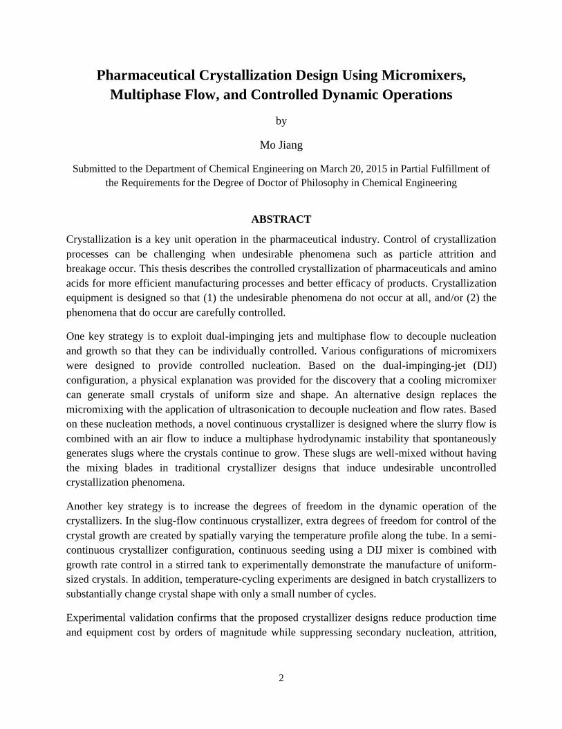
Figure 2.8. A high-throughput microfluidic chip for protein and pharmaceutical crystallization

that enables 144 induction time experiments to be conducted in parallel with different

precipitants and different solute concentrations: (a) a micrograph of the microfluidic chip, which

contains 8 inlets for pressurized control lines, 48 inlets for different precipitants, and one inlet for

the target protein or pharmaceutical, (b) a micrograph of the microfluidic components used for

metering solutions and controlling evaporation of solvent [1] ......................................................29

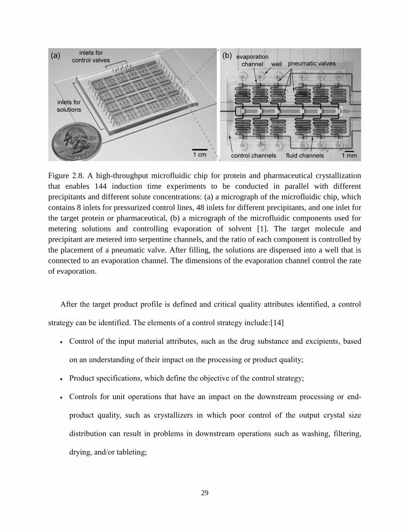
Figure 2.9. Temperature profiles for seeded cooling crystallizations. Optimal control that ignores

uncertainties predicts a 21% improvement in n/s (from 10.7 to 8.5) that can be completely lost

due to uncertainties (from 10.7 to 14.6). ........................................................................................32

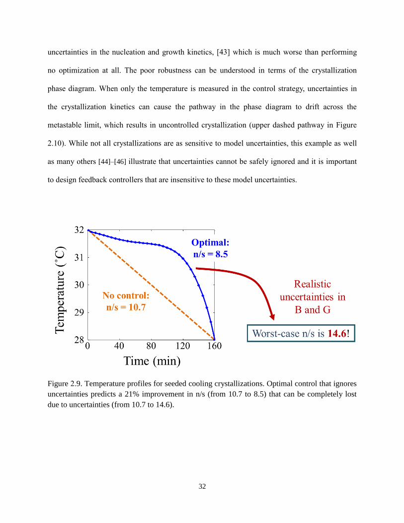
Figure 2.10. Phase diagram for crystal dissolution, growth, and uncontrolled nucleation showing

robust and non-robust operational trajectories ...............................................................................33

Figure 2.11. (a) A photograph and (b) a schematic of crystallization laboratory setup with state-

of-the-art in situ sensor technologies that enable the development of robust control strategies ...34

Figure 2.12. Automatic feedback control of the batch crystallization of a Merck compound: (a)

concentration control at constant absolute and relative supersaturation; (b) secondary nucleation

monitored by FBRM total counts per second ................................................................................36

Figure 2.13. Powder X-ray diffraction patterns for the metastable α (upper curve) and stable β

(lower curve) polymorphic forms of L-glutamic acid ...................................................................39

Figure 2.14. Crystallization phase diagram for L-glutamic acid ...................................................40

Figure 2.15. Crystallization phase diagram for L-glutamic acid, showing metastable limits at

various cooling rates (0.1, 0.5, and 1.0 °C/min) with corresponding polymorphic portions of

nuclei ..............................................................................................................................................41

10

Figure 2.16. Controlled operations to manufacture the L-glutamic acid stable β-polymorph .......42

Figure 2.17. Controlled operations to manufacture a pure batch of metastable α-form crystals of

L-glutamic acid ..............................................................................................................................43

Figure 2.18. Implementations of (a) temperature control and (b) concentration feedback control

for cooling crystallization ..............................................................................................................44

Figure 2.19. A manufacturing-scale crystallizer couples phenomena (micromixing, macromixing,

nucleation, and growth) over a wide range of length scales (sub-micron to meter scale) .............47

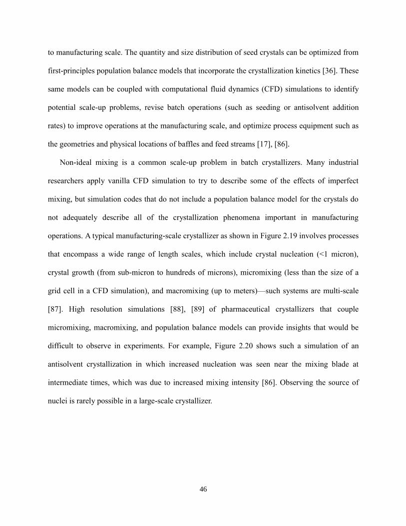
Figure 2.20. Simulation results for antisolvent crystallization in a stirred-tank crystallizer with

imperfect mixing. (a) The grid cells at the start of the simulation, with increased number of cells

near the blade and the feed position shown, with the topmost cells increasing in size as

antisolvent raises the level of slurry in the tank. (b) Supersaturation and (c) nucleation rate spatial

distributions within the crystallizer at 1, 8, and 15 minutes after the start of antisolvent addition48

Figure 2.21. A schematic of antisolvent crystallization occurring within a confined DIJ mixer

operating at high supersaturation that continuously produces seed crystals that enter a stirred tank

........................................................................................................................................................50

Figure 2.22. A free-surface cooling DIJ mixer forms crystals by combining hot and cold

saturated solutions. The entire system is located within a humidity chamber to minimize

evaporation .....................................................................................................................................51

Figure 2.23. (a) Comparison of a unimodal target CSD (line) with the CSD (dash star) achieved

by optimization of continuously varying inlet velocities to a DIJ mixer coupled to an stirred tank

(simulation results). (b) The time profile of inlet jet velocities for the simulated achievable CSD,

with the jets constrained to have the same inlet velocity ...............................................................52

Figure 2.24. (a) Comparison of a uniform target CSD (line) with the CSD (dash star) achieved by

optimization of continuously varying inlet velocities to a DIJ mixer coupled to an aging tank


with the jets constrained to have the same inlet velocity ...............................................................54

Figure 3.1. (a) Representative FTIR spectra of MSG aqueous samples used for calibration. (b)

Regression coefficients of the calibration model relating absorbances to solute concentration ....63

Figure 3.2. The temperature profile for the estimation temperature-cycling experiment (5 cycles) .

........................................................................................................................................................66

Figure 3.3. Mean chord length for various length weightings (none, length, square, and cubic) for

the estimation temperature-cycling experiment .............................................................................72

Figure 3.4. Microscopy images (with polarizers) of MSG slurry for samples collected at 35°C in

the estimation temperature-cycling experiment at (a) cycle 1a, (b) cycle 3b, and (c) cycle 5c. The

timing of the sampling points is shown in Fig. 3.2. .......................................................................72

Figure 3.5. PVM images of MSG slurry at 35°C in the estimation temperature-cycling

experiment at (a) cycle 1a, (b) cycle 3b, and (c) cycle 5c. The timing of the measurement points

is shown in Fig. 3.2. .......................................................................................................................74

11

Figure 3.6. G400 FBRM (macro mode, which was called ‘coarse mode’ in earlier versions of the

FBRM software) counts/sec statistics and temperature for the validation temperature-cycling

experiment with samples collected at the end of the first, second, third, and seventh cycles (at

35°C, timing of the four sampling points shown with cycle numbers) .........................................76

Figure 3.7. Microscopy images (with polarizers) of slurry of MSG crystals in aqueous solution

for the validation temperature-cycling experiment at the end of (a) cycle 1, (b) cycle 3, and (c)

cycle 7 ............................................................................................................................................76

Figure 3.8. Solute concentration profile over time for the estimation temperature-cycling

experiment......................................................................................................................................79

Figure 3.9. Comparison between experimental data and model predictions using the kinetic

parameters in Table 3.2 for the estimation temperature-cycling experiment for (a) solute

concentration and absolute supersaturation, and (b) mean crystal length and width.....................80


parameters in Table 3.2 for the estimation in the validation temperature-cycling experiment (7

cycles) for the mean crystal length and width ...............................................................................85

Figure 3.11. Crystal size distributions of MSG slurry from model simulation using the kinetic

parameters in Table 3.2 for the 5-cycle estimation temperature-cycling experiment, with the

points as in Fig. 3.2: (a) 1a; (b) 2f; (c) 3b; (d) 4d; (e) 5c ...............................................................86

Figure 3.12. Crystal size distributions of MSG slurry from model simulation using the kinetic

parameters in Table 3.2 for the 7-cycle validation temperature-cycling experiment at the end of

cycles, with the points as in Fig. 3.6: (a) cycle 1; b) cycle 2; c) cycle 3; d) cycle 7......................88

Figure 3.S1. Differential Scanning Calorimetry (DSC) of MSG crystals .....................................60

Figure 3.S2. Thermogravimetric Analysis (TGA, Q5000 V3.8 Build 256) of MSG crystals .......61

Figure 3.S3. DSC data of MSG crystals before and after milling .................................................65

Figure 4.1. Photograph (a) and schematic (b) of stirred-tank crystallizer instrumented with in situ

ATR-FTIR immersion probe, FBRM probe, and thermocouple ...................................................97

Figure 4.2. (a) Representative ATR-FTIR spectra of LAM aqueous samples used for calibration

(units: g LAM/g water). (b) Regression coefficients of the calibration model relating absorbances

to solute concentration .................................................................................................................100

Figure 4.3. (a) LAM solubility curve compared to reference data from Greenstein and Winitz

(1986). (b) Representative experimental solute concentrations and temperatures obtained during

concentration feedback control for a constant supersaturation level of 0.0074 g/g and a seeding

point at 55.5°C .............................................................................................................................101

Figure 4.4. (a) Size distribution of LAM seeds (based on the largest dimension) and product

crystals after concentration feedback control at two different values of constant supersaturation,

measured from off-line optical microscopy. (b) FBRM counts during concentration feedback

control at constant supersaturation of 0.0074 g LAM/g water ....................................................104

12

Figure 4.5. Photograph of DIJ configuration for continuous seeding coupled to a stirred-tank

crystallizer ....................................................................................................................................105

Figure 4.6. LAM crystals generated by DIJs (scale bar = 20 µm) (a) Microscopy image (with

polarizers) and (b) Size distribution measured from off-line microscopy images .......................105

Figure 4.7. van’t Hoff equation, 1

0ln 9973.791 86.14549ln 56.68014C T T , fit to solubilities

for LAM in aqueous solution obtained from ATR-FTIR spectroscopy (red triangles). A van’t

Hoff equation was also fit to previously published solubility data [2] that are shown as blue

asterisks. .......................................................................................................................................109

Figure 4.8. Microscope image of a batch of LAM seed crystals after sieving for the range of 125

to 180 µm (scale bar = 200 µm) ...................................................................................................110

Figure 4.9. Microscope images of LAM product crystals produced by concentration feedback

control experiments with constant supersaturation of (a) 0.0074 g LAM/g water and (b) 0.0037 g

LAM/g water (scale bar = 200 µm) .............................................................................................111

Figure 4.10. Comparison of optimal uniform CSD (green plot, from [3]) and experimental CSD

measured by off-line optical microscopy (blue histogram) .........................................................114

Figure 4.11. Microscopy image (with polarizers) of LAM product crystals at the end of

concentration control after continuous DIJ seeding (scale bar = 100 µm) ..................................115

Figure 5.1. (a) Schematic of a free-surface cooling DIJ mixer. (b) Streamlines of the hot (red,

right side) and cold jets (blue, left side) of the cooling DIJ mixer in (a), from the analytical

solutions of the flow field (5.3) and (5.4) ....................................................................................120

Figure 5.2. (a) Schematic for scaling analysis and defining the region of interest (only the hot jet

side is shown due to symmetry). (b) Time and length scales of heat transfer (blue) and mass

transfer (pink) for liquid near to the jet centreline .......................................................................130

Figure 5.3. Temperature field: (a) computed by 2D simulation using the finite element method

implemented in COMSOL, at the full length range with the dimensions being the nozzle-to-

nozzle distance and the contact area diameter; (b) computed by 2D simulation using the finite

element method implemented in COMSOL, very near the impingement plane (small range of z,

as if ‘stretching’ Fig. 5.3a horizontally); (c) 1D analytical solution near the impingement plane,

with the streamlines shown in black ............................................................................................132

Figure 5.4. Concentration field: (a) computed by 2D simulation using the finite element method

implemented in COMSOL, at the full length range (same as in Fig. 5.3a); (b) computed by 2D

simulation using the finite element method implemented in COMSOL, very near the

impingement plane; (c) 1D analytical solution near the impingement plane, with the streamlines

shown in black .............................................................................................................................136

Figure 5.5. Temperature (blue) and concentration (red) profiles (solid lines) and edges of the

boundary layers (dashed lines), based on the 1D approximation (Figs. 5.3c and 5.4c) along the jet

centreline ......................................................................................................................................139

Figure 5.6. Supersaturation spatial field for the cooling DIJ mixer based on the 1D analytical

solutions (Figs. 5.3c and 5.4c) .....................................................................................................140

13

Figure 5.7. Concentration (blue curve), solubility (dark orange curve) and supersaturation (red

curve) profiles along the jet centerline based on the 1D analytical solutions ..............................141

Figure 5.S1. (a) Liquid flows for a free-surface cooling DIJ mixer. (b) Microscope image (with

polarizers) of LAM crystals generated by a DIJ mixer [4] ..........................................................122

Figure 6.1. Schematic of slug-flow cooling crystallization .........................................................148

Figure 6.2. Photographs and schematics of setup for nucleation induced by cooling: (a) laminar

flow tube; (b) coaxial mixer, the inner diameters of the two inlets are 3.1 mm (hot) and 0.26 mm

(cold), respectively; (c) radial mixer, the inner diameters of the two inlets are 2 mm (hot) and 0.3

mm (cold), respectively ...............................................................................................................151

Figure 6.3. Schematics of hydrodynamically stable flow patterns of a gas (white color) and liquid

(blue color) mixture in a horizontal round tubing ........................................................................153

Figure 6.4. (a) Slug formation from streams of LAM slurry and air through a T mixer. (b) Slurry-

containing slugs in the growth stage. (c) Crystals in the funnel after filtration obtained under

operations of high solids density in each slug .............................................................................154

Figure 6.5. (a) Photograph of stable water slugs (aspect ratio about 1) separated by air slugs

(aspect ratio about 4) in packed silicone tube, with black background to improve contrast. (b)

Microscope image of water slug (slug in the center) and parts of air slugs (dark regions at both

edges) inside a silicone tube. (c) Horizontal wrapping of silicone tube around a cylinder of the

same diameter ..............................................................................................................................156

Figure 6.6. Photograph of the experimental setup with two temperature baths ..........................159

Figure 6.7. Microscope (with polarizers) images of product crystals from the preliminary

experiment (after laminar flow nucleation and growth in slugs) with (a) no heating; (b) heating to

50°C followed by natural cooling in the tubing; (c) heating to 50°C followed by two temperature

baths of set temperatures (39°C and 22°C) ..................................................................................161

Figure 6.8. Stereomicroscope images of product crystals with nucleation induced by coaxial

mixing in slug number (a) 21, (b) 81, (c) 141, (d) 201, (e) 261, (f) 311 (last slug) .....................162

Figure 6.9. Seed crystals generated by cooling nucleation in a coaxial mixer. The flow setups are

in Fig. 6.2b ...................................................................................................................................163

Figure 6.10. In-line stereomicroscope images of crystals in slugs with an aspect ratio of about (a)

4 (the slug is too long to fit into the image and is off to the left) and (b) almost 1 .....................166

Figure 6.11. Stereomicroscope images of product crystals with nucleation by radial mixing in

slug number (a) 16–18, (b) 106–108, (c) 286–288, (d) 466–468, (e) 646–648, (f) 726–728 (last

slug)..............................................................................................................................................169

Figure 6.S1. X-ray powder diffraction (XRPD) of LAM starting material (black) and product

crystals with nucleation from coaxial mixing (red, Fig. 6.8) and radial mixing (cyan, Fig. 6.11)149

Figure 6.S2. Seed crystals generated by cooling nucleation in laminar flow ..............................164

Figure 7.1. (a) Schematic of the slug-flow cooling crystallizer with ultrasonication-assisted

nucleation. (b) Photograph of the experimental setup for ultrasonication ...................................174

14

Figure 7.2. Microscope (with polarizers) images of seed crystals generated by cooling nucleation

with ultrasonication (before slug formation in Fig. 7.1a) at different ultrasonication amplitude

setpoints (values listed in Table 7.1): (a) Experiment #1, (b) Experiment #2, (c) Experiment #3,

(d) Experiment #4, (e) Experiment #5, and (f) Experiment #6 ....................................................179

Figure 7.3. Stereomicroscope images of product crystals obtained by cooling nucleation without

ultrasonication followed by slug flow in a 15.2 m long tube (Experiment #1, with conditions in

Table 7.1) for slug numbers (a) 106–109, (b) 170–173, (c) 234–237, and (d) 298–301 .............184

Figure 7.4. Stereomicroscope images of product crystals obtained at an ultrasonication power

amplitude setpoint of 50% followed by slug flow in a 15.2 m long tube (Experiment #4, with

conditions in Table 7.1) for slug numbers (a) 108–110, (b) 180–182, (c) 252–254, and (d) 324–

326................................................................................................................................................186

Figure 7.5. Comparison of the cumulative product crystal size distribution on a mass basis

(labeled as Q3) obtained using the nucleation conditions in Experiment #4 of Table 7.1 (blue

square, with representative images of crystals in Fig. 7.4d) with product crystals reported in Fig.

7.4b of [5].....................................................................................................................................191

Figure 7.S1. Mean crystal length (blue circle) and width (red square) of seed crystals at various

ultrasonication power amplitudes ................................................................................................182

15

LIST OF TABLES

Table 3.1. ReactIR calibration samples for in-situ solute concentration measurement .................62

Table 3.2. Kinetic parameters estimated from fitting data from the estimation temperature-

cycling experiment or set with justifications .................................................................................68

Table 3.3. Mean aspect ratio and standard deviations from microscope measurements for the 5-

cycle experiment ............................................................................................................................71

Table 3.4. Parameters used in the numerical simulation of the population balance model (3.2) in

the estimation temperature-cycling experiment .............................................................................82


the validation temperature-cycling experiment .............................................................................83


cycle experiment ............................................................................................................................84

Table 3.7. Crystal length and width measurement from the 7-cycle validation experiment .........84

Table 3.8. Estimated confidence intervals for each parameter estimate in ...............................91

Table 3.9. The standard deviation of the mean crystal length and width predicted by the model

with its uncertainty description, with the time points being the same as in Fig. 3.12 ...................92

Table 4.1. ATR-FTIR calibration samples for in situ solute concentration measurement ............98

Table 5.1. Experimental parameters for the cooling crystallization of L-asparagine monohydrate

(LAM, from Sigma Aldrich) in a free-surface DIJ mixer with aligned centreline ......................123

Table 5.2. Physical constants associated with the crystallization of glycine in water [6] ...........124

Table 6.1. Main experimental conditions for cooling nucleation ................................................150

Table 6.2. Experimental conditions for slug formation and growth by cooling ..........................157

Table 6.3. Product crystal size and shape statistics for slug-flow crystallization, for nucleation

using coaxial mixing (corresponding to the experimental results reported in Fig. 6.8) ..............165


using radial mixing (corresponding to the experimental results reported in Fig. 6.11) ...............167

Table 6.S1. Mean size for seed crystals by cooling nucleation in laminar flow (corresponding to

the experimental results reported in Fig. 6.S2) ............................................................................168

Table 7.1. Experimental conditions and size and shape statistics for the ultrasonication-assisted

nucleation of seed crystals ...........................................................................................................176

Table 7.2. Comparison of product crystals obtained using the nucleation conditions in

Experiment #4 of Table 7.1, with representative images of crystals in Fig. 7.4d, with product

crystals produced in past similar study [7] ..................................................................................189

16

1. INTRODUCTION TO CSD AND SHAPE CONTROL

Crystallization is a key unit operation in the pharmaceutical industry. The crystal size

distribution (CSD) and shape can affect the efficacy of drug products (such as the amount of

drug reaching the lungs from a nasal spray) as well as the efficiency of downstream processes

such as filtration and milling. CSD control can be challenging when multiple simultaneous

crystallization phenomena occur, such as growth, particle attrition and breakage, agglomeration,

and primary and secondary heterogeneous nucleation.

After an introduction to the control of CSD (Section 1.1, details in Chapter 2), this thesis

demonstrates the enhanced control of crystal size distribution and shape in the batch, semi-

continuous, and continuous pharmaceutical crystallizers (Sections 1.2-1.4, details in Chapters 3-

7). Each project started from the perspective of the whole system, whose configuration was

designed based on requirements for the final product quality (Quality-by-Design). The system

was then decomposed into subsystems that were understood in detail before adding more

functionality and complexity.

1.1. Introduction to control of CSD with existing crystallizers

Successful Quality by Design (QbD) requires good comprehension and implementation of

robust automatic process control. Chapter 2 discusses the role and application of control in QbD,

with a primary emphasis on the crystallization of pharmaceuticals. Some successful industrial

applications of automatic process control strategies are reviewed, as well as alternative control

strategies that have been proposed for providing various tradeoffs between model fidelity, sensor

inaccuracies, and robust performance. These strategies include feedback controllers based on

solution concentration measurement via ATR-FTIR spectroscopy as well as measurements of

particles in crystallizers based on in-process laser backscattering. The use of models for

17

crystallization kinetics to improve crystallizer designs, increase product quality, and reduce

scale-up risk is also discussed, which is followed by simulation and experimental results that

demonstrate how a target crystal size distribution can be obtained by combining continuous

seeding with controlled crystal growth. [8] More detailed analysis of CSD control in advanced

crystallizers is described in Chapters 3-7.

1.2. Enhanced control of crystal shape using well-designed temperature cycling

The evolution of particle shape is an important consideration in many industrial

crystallization processes. Bad crystal shapes can cause operational problems downstream from

the crystallizer (e.g., filtration, granulation, tableting). To monitor and optimize the shape of

crystals, population balance models have been used which require the estimation of 2D growth

and dissolution rates. Most past studies that estimated kinetics along multiple crystal axes in

mixed-tank crystallizers were based on frequently sampling the slurry during crystallization, or

employing imaging technology that only applies for low crystal number densities [9][10]. In

contrast, Chapter 3 designs a single experiment (with temperature cycling) that substantially

changes crystal shape with only a small number of cycles and allows the estimation of kinetic

parameters in a two-dimensional PBM demonstrated to predict the crystal size and shape in

another temperature cycling experiment.

The growth and dissolution of monosodium glutamate crystals of varying shapes are

monitored using in-process Attenuated Total Reflection-Fourier Transform Infrared

Spectroscopy, Focused Beam Reflectance Measurement (FBRM), Particle Vision and

Measurement (PVM), and off-line optical microscopy. The growth and dissolution kinetics are

estimated in a multidimensional population balance model (PBM) based on solute concentration

and crystal dimension measurements. This model fitted the experimental data with a limited

18

number of parameters of small uncertainty. In addition, with the estimated kinetic parameters,

the model was used to predict the crystal size and shape distribution in a different temperature-

cycling experiment. In contrast to previous studies that have estimated kinetics along multiple

crystal axes in mixed-tank crystallizers, this study implements dissolution terms in the

multidimensional population balance model along multiple axes [11].

1.3. Enhanced control of CSD using a semi-continuous crystallizer design

Control of the size distribution (not necessarily the narrowest) of crystals is desired in the

pharmaceutical industry to meet bioavailability requirements. The controllability of CSD is

limited in industrial batch crystallizations, where seed crystals are added near the start of the

batch. A theoretical study [3] predicted that the controllability of the crystal size distribution

could be greatly increased by employing continuous seeding, where crystals are continuously fed

to a well-mixed tank crystallizer at any time during the batch. Since uniform CSD is very

difficult to achieve with batch cooling crystallization, this distribution was the target in Chapter 4

of an experimental demonstration of the crystallizer configuration with continuous seeding.

To experimentally demonstrate the enhanced control of CSD in a semi-continuous

crystallizer, I combined continuous crystal seeding from a dual impinging jet (DIJ) mixer with a

batch crystallizer operating under feedback control of the crystal growth rate. To generate seed

crystals with a narrow size distribution, I developed a DIJ configuration that combines hot and

cold saturated solutions. These seed crystals were further grown to a desired size in the stirred

tank with suppressed nucleation that was instrumented with attenuated total reflection-Fourier

transform infrared (ATR-FTIR) spectroscopy and FBRM. An automated system that followed

preset supersaturation profiles by using feedback control was based on the construction of

calibration models and the measurement of solubility and metastable limit [4].

19

Crystallization within DIJ mixers is useful, but not expected to be applicable to all

combinations for all conditions, especially because the average supersaturation for a cooling DIJ

mixer is usually not very high. Currently, whether any particular compound/solvent combination

is suitable for use in a DIJ mixer has to be assessed by trial-and-error experimentation aided with

experience. It would be useful at the early stage of research and development to be able to

quickly identify compound-solvent combinations that cannot nucleate crystals within DIJ mixers,

based on their physicochemical properties.

Chapter 5 develops a mathematical model for crystallization in a DIJ mixer that combines

thermodynamics, kinetics, fluid dynamics, and heat and mass transfer [12]. The mathematical

model is in the form of partial differential equations, simplified by exploiting symmetries and

employing scaling analysis to generate one-dimensional analytical solutions for physical

insights. Two-dimensional energy and molar balances are solved using COMSOL input with an

analytical solution for the velocity field, to generate spatial distributions of temperature,

concentration, and supersaturation near the hot-cold interface within a cooling DIJ mixer. The

mathematical model provides guidance for modifying solvent and jet flow rates to increase the

likelihood of continuously generating seed by mixing hot and cold saturated solutions in a DIJ

mixer.

1.4. Enhanced control of CSD using a novel continuous-flow crystallizer design

Compared to batch and semibatch crystallizers, continuous-flow crystallizers have the

potential for higher reproducibility, process efficiency, and flexibility, as well as lower capital

and production cost. For higher process efficiency and reproducibility, many new continuous-

flow crystallizer designs have been developed in recent years, including continuous oscillatory

baffled crystallizers and continuous-flow tubular crystallizers. However, most of these

20

crystallizers are not specifically designed to provide many degrees of freedom for the control of

crystal shape, size distribution, and polymorphic identity in the presence of process disturbances

and variations in crystallization kinetics due to possible changes in the contaminant profile in the

feed streams. Chapters 6 and 7 design a continuous-flow crystallizer that achieves maximum

yield and controlled CSD with continuous cooling crystallization in the presence of process

disturbances and variations in kinetics.

In order to achieve both maximum crystal yield and CSD control with high spatial and

temporal uniformities, a novel continuous slug-flow crystallizer is operated in a

hydrodynamically stable flow regime in which slugs of slurry are separated by slugs of gas in a

tube. The residence time distribution of the slugs is equivalent to a set of small completely

segregated batch reactors moving from the feed location to the exit. Each slug is well mixed

through nondestructive liquid recirculation, rather than by a regular solid mixer, to reduce crystal

attrition. Past knowledge of batch crystallizers is applied to continuously generate high-quality

drug crystals, which enhanced the control of product CSD with properly tuned parameters within

the design space. Unlike most other continuous-flow crystallizers that employ slugs, the

proposed slug-flow crystallizer does not require a solvent/solvent separation operation afterwards,

which further improves crystal product purity and process energy efficiency [7].

The crystallizer is designed so that nucleation and growth processes are decoupled to

enhance the individual control of each phenomenon. Stable slugs will be generated with

approximately uniform target sizes by mixing slurry and gas streams at proper flow rates for the

specific mixer configuration in use. Nucleation methods are developed and implemented before

slug formation (e.g., radial/coaxial mixers [7] and ultrasonication [13]) to generate seeds

continuously with a controlled number density. After slug formation, an optimal cooling profile

21

can be applied to control the crystal growth rate, with temperature zones set up using peristaltic

pumps and Proportional-Integral (PI) controllers.

22

2. THE ROLE OF AUTOMATIC PROCESS CONTROL IN QUALITY BY DESIGN

2.1. Introduction

The U.S. Food and Drug Administration defines Quality by Design (QbD) as “a systematic

approach to pharmaceutical development that begins with predefined objectives and emphasizes

product and process understanding and process control, based on sound science and quality risk

management.”[14] Pharmaceutical development includes the following elements: [14]

Defining the target product profile while taking into account quality, safety, and efficacy

of the drug compound. This profile considers the method of drug delivery, the form of the

drug compound when delivered, the bioavailability of the drug once delivered, the dosage

of the drug compound to maximize therapeutic benefits while minimizing side effects, and

the stability of the product.

Identifying potential critical quality attributes of the drug product. All of the drug product

characteristics that have an impact on product quality must be determined so these

attributes can be studied and controlled.

Determining the critical quality attributes of the components (e.g., drug compound,

excipients) needed for the drug product to be of desired quality.

Selecting a process capable of manufacturing the drug product and its components;

Identifying a strategy for controlling the process to reliably achieve the target product

profile.

Most pharmaceuticals manufacturing processes include at least one crystallizer for

purification of intermediates or the final active pharmaceutical ingredient (Figure 2.1), and

usually for producing crystals to be compacted with excipients to form a tablet. The

bioavailability and tablet stability depend on the crystal structure, size, and shape distribution

23

(Figure 2.2). Typical objectives in the operation of intermediate and final crystallizations are to

maximize chemical purity and yield and to produce crystals that do not cause operations

problems in downstream processing. An important consideration in many crystallization

concerns polymorphism, which occurs when a chemical compound can adopt different crystal

structures. Polymorphs are the same molecular species but have different packing of molecules

within the crystal structure (see Figure 2.3 for an example) [15], [16]. Another common

occurrence is solvatomorphism or pseudo-polymorphism, which is when varying amounts of

solvent molecules can be incorporated within the crystal structure, to form crystal solvates of

different composition. Different polymorphs or solvatomorphs can have very different physical

properties (e.g., solubility, bioavailability, shelf-life), and hence very different efficacy. The

control of crystal polymorphism is required for the manufacturing process to achieve the QbD

objectives and for regulatory compliance. The most stable polymorph is typically achievable

with sufficient process time and suitable crystallization conditions. Metastable polymorphs are

more challenging to manufacture reliably with a key challenge being to prevent transformation to

more stable forms.

A QbD approach for the development of pharmaceutical crystallization processes involves

two consecutive steps:

1. Design of a target crystal size distribution (CSD) and polymorphic form based on

bioavailability and delivery needs (Figure 2.4);

2. Design a manufacturing-scale crystallizer to produce the target CSD based on simulation

models that account for all potential scale-up issues such as non-ideal mixing (Figure 2.5)

[17].

24

Figure 2.1. A photograph of a bench-scale crystallizer with a jacket for temperature control.

Supersaturation in pharmaceutical crystallizers is usually induced by cooling and/or antisolvent

addition.

Figure 2.2. A photograph of some pharmaceutical crystals produced from a crystallizer that was

inadequately controlled, showing potential variations in size and shape.

25

(a)

(b)

Figure 2.3. (a) α polymorph (metastable form, prismatic shape) and (b) β polymorph (stable

form, needlelike platelet shape) crystals of L-glutamic acid. The two polymorphs show different

crystal morphologies.

26

Figure 2.4. An example of a potential target crystal size distribution and polymorphic form.

Figure 2.5. Example simulation results of the spatial distribution of turbulent Reynolds number

in a confined dual impinging jet mixer. Such mixers can be used to generate sub 10-micron

crystals for many solute/solvent systems.

Many crystallizer designs for Step 2 are based on the creation of a highly intense mixing

zone operating at high supersaturation to produce crystal seeds for subsequent growth [3], [18]–

[24]. Step 1 requires first finding all of the polymorphs by crystallizing the pharmaceutical

compounds in many different solvents with many different supersaturation methods and

trajectories, and the identification of crystallization kinetics from the small quantity of

27

pharmaceutical compounds available for process development. Such investigations can be

facilitated by high-throughput microfluidics platforms that can provide information on

polymorphism, solubility, and kinetics even at very high supersaturation difficult to achieve in

other systems (Figures 2.6 and 2.7) [1], [25]–[33]. A more advanced version of the high-

throughput platform in Figures 2.6 and 2.7 allows information to be collected in parallel using

chips comprised of 144 wells (each 30 nanoliters in volume) with crystal detection performed

using optical spectroscopy (Figure 2.8). Further developed versions of these microfluidic array

chips allow for in situ identification of polymorph identity via Raman spectroscopy or X-ray

diffraction.

Figure 2.6. A microfluidic platform that uses evaporation to generate supersaturation in 2–10

microliter-sized droplets in microwells. The rate of evaporation (J), and thereby the

28

supersaturation profile, is set by the dimensions of the channel (cross-sectional area A and length

L) that connects the well with the ambient environment.

Figure 2.7. A comparison of induction times measured in wells in a microfluidic platform

(crosses) with predictions of a first-principles model (circles) with nucleation kinetics estimated

from the microfluidic data at high supersaturation. A detailed study demonstrated that these

nucleation kinetic parameters resulted in accurate predictions of induction times in subsequent

experiments.

29

Figure 2.8. A high-throughput microfluidic chip for protein and pharmaceutical crystallization

that enables 144 induction time experiments to be conducted in parallel with different

precipitants and different solute concentrations: (a) a micrograph of the microfluidic chip, which

contains 8 inlets for pressurized control lines, 48 inlets for different precipitants, and one inlet for

the target protein or pharmaceutical, (b) a micrograph of the microfluidic components used for

metering solutions and controlling evaporation of solvent [1]. The target molecule and

precipitant are metered into serpentine channels, and the ratio of each component is controlled by

the placement of a pneumatic valve. After filling, the solutions are dispensed into a well that is

connected to an evaporation channel. The dimensions of the evaporation channel control the rate

of evaporation.

After the target product profile is defined and critical quality attributes identified, a control

strategy can be identified. The elements of a control strategy include:[14]

Control of the input material attributes, such as the drug substance and excipients, based

on an understanding of their impact on the processing or product quality;

Product specifications, which define the objective of the control strategy;

Controls for unit operations that have an impact on the downstream processing or end-

product quality, such as crystallizers in which poor control of the output crystal size

distribution can result in problems in downstream operations such as washing, filtering,

drying, and/or tableting;

30

A monitoring program such as regular testing of intermediates and product for verifying

drug product quality and the accuracy of multivariate prediction models.

The controls for unit operations include not only the design of feedback controllers but also

other considerations associated with the integration of sensors, process design, and control

required to move from input materials to optimized process design, such as:[34]

Sensors, experimental design, and data analysis;

Process automation;

First-principles modeling and simulation;

Design of operations to form a consistent product.

The remainder of this chapter provides a more detailed description of the QbD approach for

the development of pharmaceutical crystallization processes, namely,

The design of robust control strategies;

Some example applications of automatic feedback control;

The role of kinetics modeling;

An example idea for a deeper QbD approach.

2.2. The design of robust control strategies

A well-studied control objective in crystallization is to minimize the secondary nucleation of

crystals that may cause potential problems in downstream filtering operations by minimizing the

ratio of nucleation mass to seed mass (n/s) over the temperature profile [35]–[38]

( )

nucleation massmin

seed massT t

(2.1)

The control objective is related to the temperature profile through a population balance

model [39][40] for the crystals in the slurry:

31

( , ) ( , ) ( )

f fG C T B C T L

t L (2.2)

where f (L,t) is the crystal size distribution which is a function of the crystal size L and time t, G

is the growth rate and B is the nucleation rate which are assumed to be functions of the solute

concentration C and the temperature T, and δ is the Dirac delta function. The solute

concentration is described by its mass balance

0

d3 ( , ) ( , )

d

C

G C T f L t dLt

(2.3)

where α is a conversion factor. The temperature profile must satisfy constraints due to equipment

limitations

min max

min max

( )

d ( )

d

T T t T

T tR R

t

(2.4)

where Tmin, Tmax, Rmin, and Rmax are user-specified scalars. The crystallization must also satisfy a

constraint to ensure a high enough batch yield:

final final,max( ) C t C (2.5)

where tfinal is the time in which the batch ends and Cfinal,max is the limit on the concentration at

tfinal. A common practice in the crystallization control literature is to solve optimizations (2.1) to

(2.5) while ignoring uncertainties in the nucleation and growth kinetics [37], [41], [42].

This example shows that the robustness of the control strategy can be very strongly affected

by uncertainties. A linear cooling profile results in n/s = 10.7, while numerical solution of the

optimization (2.1) to (2.5) improves the n/s to 8.5, which is a 21% reduction in the nucleation

mass to seed mass (Figure 2.9). All of the improvements due to optimization can be lost due to

uncertainties in crystallization kinetics. In particular, the n/s can be as large as 14.6 for realistic

32

uncertainties in the nucleation and growth kinetics, [43] which is much worse than performing

no optimization at all. The poor robustness can be understood in terms of the crystallization

phase diagram. When only the temperature is measured in the control strategy, uncertainties in

the crystallization kinetics can cause the pathway in the phase diagram to drift across the

metastable limit, which results in uncontrolled crystallization (upper dashed pathway in Figure

2.10). While not all crystallizations are as sensitive to model uncertainties, this example as well

as many others [44]–[46] illustrate that uncertainties cannot be safely ignored and it is important

to design feedback controllers that are insensitive to these model uncertainties.

Figure 2.9. Temperature profiles for seeded cooling crystallizations. Optimal control that ignores

uncertainties predicts a 21% improvement in n/s (from 10.7 to 8.5) that can be completely lost

due to uncertainties (from 10.7 to 14.6).

33

Figure 2.10. Phase diagram for crystal dissolution, growth, and uncontrolled nucleation showing

robust and non-robust operational trajectories. A control strategy that is insensitive to model

uncertainties must keep the operational trajectory between the solubility curve and metastable

limit.

State-of-the-art in situ sensor technologies [47]–[74] (Figure 2.11) provide additional

information that can be employed in real-time to produce more robust control strategies. For

example, a strategy that is much less sensitive to uncertainties in the kinetics employs feedback

control based on in situ solute concentration measurement obtained by ATR-FTIR spectroscopy

to follow the desired pathway in the crystallization phase diagram (lower dashed pathway in

Figure 2.10). Detailed theoretical analyses indicate that this feedback control strategy more

robustly operates the crystallizer at constant growth and low nucleation rates [75], [76], which

34

has been demonstrated in numerous experimental implementations at universities and

pharmaceutical companies [4], [7], [75], [77]–[79].

(a)

35

(b)

Figure 2.11. (a) A photograph and (b) a schematic of crystallization laboratory setup with state-

of-the-art in situ sensor technologies that enable the development of robust control strategies.

ATR-FTIR refers to Attenuated Total Reflection FTIR spectroscopy, FBRM refers to Focused

Beam Reflectance Measurement (laser backscattering), and PVM refers to Particle Vision and

Measurement (in situ video microscopy).

2.3. Some example applications of automatic feedback control

Figure 2.12 shows some sample results in which automatic feedback control was applied to a

Merck pharmaceutical with very high secondary nucleation kinetics [78]. The feedback control

system tracks any desired trajectory in the crystallization phase diagram, including constant

absolute or relative supersaturation (Figure 2.12a). The extent of nucleation was simultaneously

monitored by tracking the total counts/sec measured in real-time using in situ laser

backscattering (Figure 2.12b). The input to the feedback control system was the solubility curve

36

and the metastable limit obtained by an automated system with software implemented in Visual

Basic and Matlab, using a similar crystallizer and sensor technology as shown in Figure 2.11

(without the PVM).

(a)

37

(b)

Figure 2.12. Automatic feedback control of the batch crystallization of a Merck compound: (a)

concentration control at constant absolute and relative supersaturation; (b) secondary nucleation

monitored by FBRM total counts per second.

The initial three runs at constant supersaturation were run automatically, followed by

inspection of the total counts/sec that indicated different secondary nucleation levels at different

absolute supersaturation. An absolute supersaturation ΔC = 30 mg/ml resulted in excessive

nucleation within an hour whereas ΔC = 20 mg/ml resulted in excessive nucleation after 70 min.

An absolute supersaturation ΔC = 10 mg/ml resulted in a long batch time with slow increase in

nucleation near the end of the batch. These observations motivated the selection of a pathway in

the crystallization phase diagram with a constant relative supersaturation of 0.15, which has a

similar supersaturation as ΔC = 20 mg/ml in the early portion of the batch in which no nucleation

38

was observed, and a somewhat lower supersaturation at 10 mg/ml near the end of the batch to

suppress nucleation then. The constant relative supersaturation pathway resulted in about half of

the batch time as the ΔC = 10 mg/ml pathway while also having less nucleation. The automated

system enabled a rapid convergence to controlled batch crystallization operations with minimum

user input. The temperature time profile resulting from the feedback control of concentration can

be implemented subsequently using simple temperature controllers.

Another demonstration of automatic feedback control is for the crystallization of polymorphs

of L-glutamic acid (Figures 2.3 and 2.13). The α-polymorph is easier to process in downstream

operations, whereas manufacture of the stable β-polymorph crystals is more reliably produced by

operating between the solubility curves of the two polymorphs (Figure 2.14). Operating an

unseeded crystallizer at various cooling rates produced crystals of both polymorphs, with widely

varying proportions (Figure 2.15). This objective of this experimental study was to produce

crystals of pure single polymorphic form.

39

Figure 2.13. Powder X-ray diffraction patterns for the metastable α (upper curve) and stable β

(lower curve) polymorphic forms of L-glutamic acid.

40

Figure 2.14. Crystallization phase diagram for L-glutamic acid. For such a monotropic system, β-

form crystals grow and α-form crystals dissolve in the region between the solubility curves of the

α- and β-forms.

41

Figure 2.15. Crystallization phase diagram for L-glutamic acid, showing metastable limits at

various cooling rates (0.1, 0.5, and 1.0 °C/min) with corresponding polymorphic portions of

nuclei.

Pure stable β-polymorph crystals in an unseeded crystallizer can be achieved at any cooling

rate, as long as the operations in the last portion of the batch remain for a long enough time

between the two solubility curves (Figure 2.16). The batch time can be reduced by maximizing

the supersaturation while operating between the two solubility curves, by increasing the

temperature after the initial mixture of α- and β-polymorph crystals are produced by rapid

cooling. The products were large β-polymorph crystals (Figure 2.16).

42

Figure 2.16. Controlled operations to manufacture the L-glutamic acid stable β-polymorph. The

operation begins with a quick cooling from 65°C to 25°C to generate nuclei, followed by holding

the temperature at 25°C for 1 hour to deplete supersaturation to maximize surface area of crystals,

then a quick heating to 50°C (while operating between the two solubility curves) to reach a much

higher temperature to increase the growth rate of the β-form crystals. The last step is to apply

concentration feedback control (solid lines) to grow larger β-form product crystals.

The manufacture of the metastable α-polymorph crystals requires operation above the

solubility curves for both forms (Figure 2.14), but not at such a high supersaturation that

nucleation of the stable β-polymorph crystals occurs. The most reliable operation is to seed with

the metastable crystals while cooling to operations above the solubility of the α-polymorph while

remaining below the metastable limit (Figure 2.17). Seeding with α-polymorph crystals is

required because the initial unseeded operation produced a mixture of α- and β-polymorph

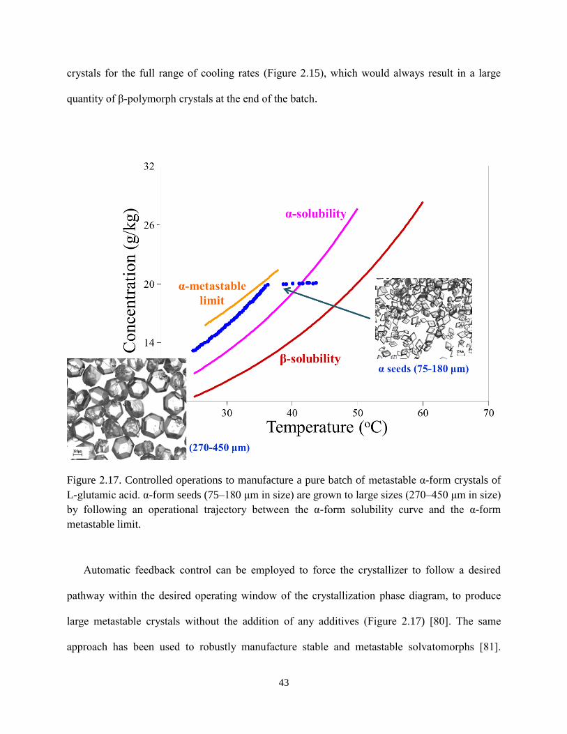
43

crystals for the full range of cooling rates (Figure 2.15), which would always result in a large

quantity of β-polymorph crystals at the end of the batch.

Figure 2.17. Controlled operations to manufacture a pure batch of metastable α-form crystals of

L-glutamic acid. α-form seeds (75–180 μm in size) are grown to large sizes (270–450 μm in size)

by following an operational trajectory between the α-form solubility curve and the α-form

metastable limit.

Automatic feedback control can be employed to force the crystallizer to follow a desired

pathway within the desired operating window of the crystallization phase diagram, to produce

large metastable crystals without the addition of any additives (Figure 2.17) [80]. The same

approach has been used to robustly manufacture stable and metastable solvatomorphs [81].

44

These experimental implements also demonstrate how in situ sensor technologies can be used to

design and implement a robust control strategy.

The feedback control of concentration to follow a target pathway in the crystallization phase

diagram (Figure 2.18b) has several advantages over the application of a pre-determined

temperature or antisolvent addition profile (Figure 2.18a): [75], [76], [82]

Lower costs and process development times;

Lower trial-and-error experimentation;

Insensitivity to most variations in kinetics and most disturbances.

(a)

(b)

45

Figure 2.18. Implementations of (a) temperature control and (b) concentration feedback control

for cooling crystallization. The implementations for antisolvent crystallization are similar, with T

replaced by % solvent.

Concentration feedback control can result in high variability in the batch time, which is

indirectly used as an extra degree of freedom to produce the reduced sensitivity. A drawback of

both control approaches in Figure 2.18, as well as nearly all other crystallization control

approaches described in the literature, is sensitivity to variations in the solubility due to

impurities. The simplest way to deal with impurities is to have fine control of the input material

attributes, which is one of the tenets of the QbD approach [14]. Unfortunately, often the chemical

feed streams for pharmaceutical production are outsourced and suppliers are switched or remain

the same but modify their operations, which results in a change in the impurity profile for the

input materials to the crystallizer. For pharmaceutical-solvent combinations in which only one

form occurs, alternative feedback control strategies have been developed that employ in situ laser

backscattering measurements so as to be insensitive to variations in the solubility as well as other

disturbances [82]–[85]. It will be interesting to see whether such approaches can be modified to

reduce their weaknesses, such as reduced molecular purity of the product crystals, and how well

these approaches can be extended to various types of polymorphic crystallizations.

2.4. The role of kinetics modeling

The aforementioned robust control strategies are insensitive to variations in crystallization

kinetics and actually did not require a determination of explicit expressions for the crystallization

kinetics. Instead, information on nucleation and growth kinetics were incorporated implicitly

through the position of the metastable limit within the crystallization phase diagram (Figure 2-

10). Explicit models for the crystallization kinetics can still be very useful, in particular, in

improving the characteristics of the seed crystals and in reducing risk during scale-up from bench

46

to manufacturing scale. The quantity and size distribution of seed crystals can be optimized from

first-principles population balance models that incorporate the crystallization kinetics [36]. These

same models can be coupled with computational fluid dynamics (CFD) simulations to identify

potential scale-up problems, revise batch operations (such as seeding or antisolvent addition

rates) to improve operations at the manufacturing scale, and optimize process equipment such as

the geometries and physical locations of baffles and feed streams [17], [86].

Non-ideal mixing is a common scale-up problem in batch crystallizers. Many industrial

researchers apply vanilla CFD simulation to try to describe some of the effects of imperfect

mixing, but simulation codes that do not include a population balance model for the crystals do

not adequately describe all of the crystallization phenomena important in manufacturing

operations. A typical manufacturing-scale crystallizer as shown in Figure 2.19 involves processes

that encompass a wide range of length scales, which include crystal nucleation (<1 micron),

crystal growth (from sub-micron to hundreds of microns), micromixing (less than the size of a

grid cell in a CFD simulation), and macromixing (up to meters)—such systems are multi-scale

[87]. High resolution simulations [88], [89]

of pharmaceutical crystallizers that couple

micromixing, macromixing, and population balance models can provide insights that would be

difficult to observe in experiments. For example, Figure 2.20 shows such a simulation of an

antisolvent crystallization in which increased nucleation was seen near the mixing blade at

intermediate times, which was due to increased mixing intensity [86]. Observing the source of

nuclei is rarely possible in a large-scale crystallizer.

47

Figure 2.19. A manufacturing-scale crystallizer couples phenomena (micromixing, macromixing,

nucleation, and growth) over a wide range of length scales (sub-micron to meter scale).

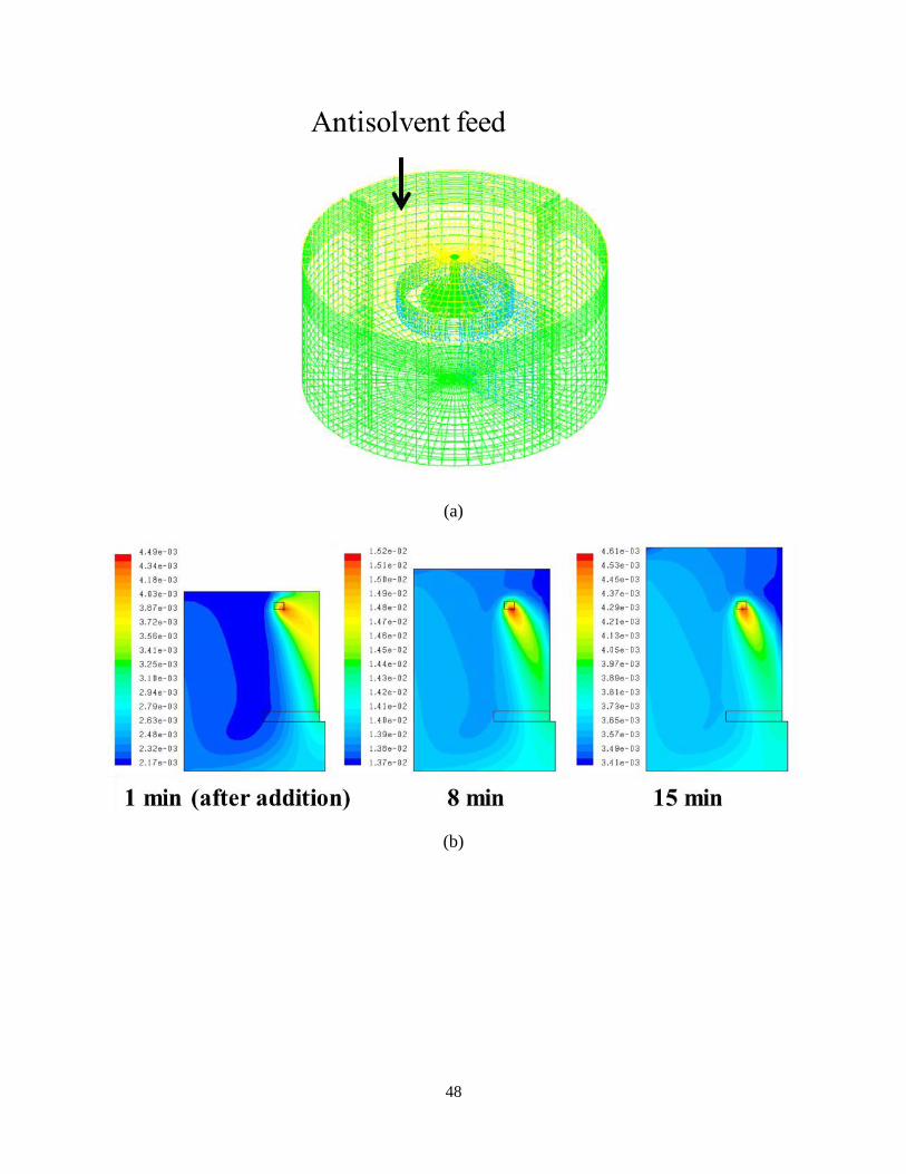
48

(a)

(b)

49

(c)

Figure 2.20. Simulation results for antisolvent crystallization in a stirred-tank crystallizer with

imperfect mixing. (a) The grid cells at the start of the simulation, with increased number of cells

near the blade and the feed position shown, with the topmost cells increasing in size as

antisolvent raises the level of slurry in the tank. (b) Supersaturation and (c) nucleation rate spatial

distributions within the crystallizer at 1, 8, and 15 minutes after the start of antisolvent addition.

The highest supersaturation level exists close to the upper right corner for all three time spots.

The highest nucleation rate happens at similar places as the supersaturation ones for 1 and 15

minutes, but very close to the mixing blade (on the lower right edge) for 8 minutes.

2.5. An example idea for a deeper QbD approach

The above discussions were mostly focused on the design of a crystallizer that manufacture

large uniform-sized crystals while minimizing nucleation, which is motivated by the fact that

large crystals are easier to wash, filter, and dry. Most crystallizers in the pharmaceutical industry

add seeds at the beginning of batch, with the remainder of the control strategy specified by

optimization of cooling and/or antisolvent addition.

An idea that has been explored has been the continuous addition of seed crystals during a

batch, to provide extra degrees of freedom to enable the manufacture of crystals with a targeted

size distribution that is not necessarily large uniform-size crystals [3]. For many pharmaceutical-

50

solvent combinations, the application of high supersaturation enables the manufacture of very

small seed crystals with a narrow size distribution, which can be coupled with a jacketed stirred-

tank crystallizer to subsequently grow these crystals to a desired size (Figure 2.21). For some

systems, high quality seed crystals can be manufactured by performing cooling crystallization

within a DIJ mixer, in which the fluids in the two jets are saturated solutions of the same solvent

at two different temperatures (Figure 2.22).

Figure 2.21. A schematic of antisolvent crystallization occurring within a confined DIJ mixer

operating at high supersaturation that continuously produces seed crystals that enter a stirred

tank. The high supersaturation in the DIJ mixer is generated in a mixing zone where opposing

streams from two jets (containing saturated solution and antisolvent, respectively) collide. A

feedback control system operates the stirred-tank crystallizer at lower supersaturation so that

only crystal growth (no nucleation) occurs.

51

Figure 2.22. A free-surface cooling DIJ mixer forms crystals by combining hot and cold

saturated solutions. The entire system is located within a humidity chamber to minimize

evaporation.

For either mode of supersaturation generation, many target CSDs can be achieved by

manipulating seed generation continuously using a DIJ mixer [3]. The slurry exiting the DIJ

mixer is directed into the aging vessel with crystal growth rate optimally controlled to get as

close as possible to the target size distribution. A unimodal crystal size distribution is easily

obtained by continuously manipulating the inlet jet velocities of the DIJ mixer throughout the

batch, to continuously vary the seeding (Figure 2.23). The inlet velocities were computed by

solution of the optimization

target finaljet

min ( ) ( , )( )

f L f L tv t

(2.6)

where ftarget is the target crystal size distribution, vjet is the inlet velocities for the two jets, and || ||

is the integral of the square of its argument over the crystal dimension L. This optimization was

numerically solved subject to the constraints

jet jet

( , ) ( , )( , ; ( ))

f L t f L tG f L t v t

t L (2.7)

52

jet,min jet jet,max( ) v v t v (2.8)

where fjet is the CSD of the crystals existing the DIJ mixer, which was computed using a coupled

model for micromixing, macromixing, and population balance within the DIJ mixer [3], and

vjet,min and vjet,max are user-specified scalars set to satisfy constraints on the DIJ mixer operation.

Equation (2.7) is the population balance model for the stirred tank operating under a constant

growth rate by using feedback control of the concentration.

(a)

53

(b)

Figure 2.23. (a) Comparison of a unimodal target CSD (line) with the CSD (dash star) achieved

by optimization of continuously varying inlet velocities to a DIJ mixer coupled to an stirred tank


with the jets constrained to have the same inlet velocity.

The largest deviation between the target CSD and the nearest achievable CSD in Figure 2.23

occurs at the largest crystal size where the CSD drops to zero. Simulation results for other target

CSDs also show the largest deviation occurring wherever the target CSD is sharp. The most

challenging unimodal target CSD is a uniform distribution, with the optimal inlet jet velocities

being close to a uniform distribution–a constant value of particle numbers per unit length

between some minimum and maximum size (Figure 2.24). Theoretical analysis [3] indicates that

the proposed control strategy is reasonably robust to variations in the inlet jet velocity profiles,

which was tested experimentally by attempting to achieve a nearly uniform CSD by using a

constant inlet jet velocity followed by a sharp drop to zero, to approximate the profile in Figure

2.24b. The experimental implementation resulted in a CSD very close to the CSD determined by

simulations to most closely match a uniform distribution. Similar to the simulated achievable

54

CSD, the experimentally achieved CSD also has the largest deviation with the target uniform

distribution at the largest crystal size (sharp side). In addition to the inlet jet velocity (Figures

2.23b and 2.24b), the supersaturation trajectory can be optimized over time, to take advantage of

the ability to robustly control the supersaturation (e.g., Figure 2.12a and 2.17) [4].

(a)

55

(b)

Figure 2.24. (a) Comparison of a uniform target CSD (line) with the CSD (dash star) achieved by

optimization of continuously varying inlet velocities to a DIJ mixer coupled to an aging tank


with the jets constrained to have the same inlet velocity.

2.6. Summary

This chapter discusses the role and application of automatic control in Quality by Design

with examples taken from pharmaceutical crystallization. Microfluidic platforms were discussed

as a technology for early-stage pharmaceutical process development to screen for polymorphs,

identify desirable process parameters such as choice of solvents, and to rapidly determine key

properties such as solubility and crystallization kinetics. Throughout the drug development and

manufacturing processes, automatic feedback control can be employed together with

microfluidic platforms and/or process sensor technology to reduce process/product sensitivity to

uncertainties and disturbances for control of such properties as crystal size distribution [4], [7],

56

[11] and polymorphism. The key points were illustrated by simulation results and experimental

implementations. Kinetics modeling was described as a step towards improving process designs,

especially for reducing risk during scale-up by quantifying the effects of non-ideal mixing on

product quality. A deeper QbD approach to pharmaceutical crystallization was described that

designs controlled operations to obtain a target product CSD. Other advanced approaches are

described in details in later chapters.

57

3. MODIFICATION OF CRYSTAL SIZE AND SHAPE USING DEEP TEMPERATURE

CYCLING

3.1. Introduction

A large proportion of crystallizations from solution produce rod-like crystals, which can

cause problems in downstream process operations. One effective method for modifying the

crystal shape and size is to introduce molecular additives [90]–[92], which have the potential

problem of contaminating the product. An alternative method of shape modification is to

optimally control the supersaturation trajectory or by cycling between positive and negative

supersaturations to take advantage of different relative dependencies along the crystal axes of

growth and dissolution [93]–[100]. A very large change in the crystal shape has been reported

with 20 to 80 temperature cycles, both theoretically and experimentally [97], [101]. This article

experimentally demonstrates that a large change in crystal size and aspect ratio is possible with a

reduced number of temperature cycles (e.g., 3 to 6).

Many efforts have been directed towards the construction of multidimensional population

balance models suitable for the design of process operations to optimize crystal shape [58], [98],

[102]–[110]. These models require the estimation of growth kinetics along multiple axes, with

most methods based on sampling the slurry during crystallization, or on employing imaging

technology [9], [10], [55], [56], [60], [93], [111]–[115]. A commercial instrument that has been

used for in-situ measurement of the crystal shape distribution is Particle Vision and

Measurement (PVM) [67]. Focused Beam Reflectance Measurement (FBRM) is commonly

available in crystallization laboratories, but it is not possible to construct an arbitrary two-

dimensional crystal size distribution (2D CSD) from measurements of the chord length

distribution (CLD) obtained by an FBRM. The CLD data is not sufficiently informative for

58

accurate quantitative correlation to a 2D CSD, even with a design limiting the variety of CSDs

with a set seed mass and supersaturation profile.

To identify dissolution and growth kinetic parameters in a 2D population balance model

(PBM), this article uses solute concentrations determined using ATR-FTIR spectroscopy [53],

[64], [116] and mean crystal lengths and widths from microscope images [88], [89], [105], [117],

[118]. Trends in mean crystal width, length, and aspect ratio in intermediate times were

measured using FBRM. The initial crystal size distributions in the PBM were determined from

PVM measurements. Compared to the previously published multidimensional PBMs, the PBM

in this article includes dissolution kinetics. The PBM is used to predict the crystal size and shape

distribution in a temperature-cycling experiment with a different supersaturation profile.

3.2. Experimental and numerical methods

This section summarizes experimental methods for characterization of the solute

concentration and mean length and width for monosodium glutamate (MSG) crystals in aqueous

solution by attenuated total reflection-Fourier transform infrared (ATR-FTIR) spectroscopy,

chemometrics, Focused Beam Reflectance Measurement® (FBRM), Particle Vision and

Measurement® (PVM), and optical microscopy. Then we describe a two-dimensional population

balance model for the growth and dissolution of rod-like crystals, and the numerical algorithms

for simulation of the model and for estimation of the growth and dissolution kinetics along the

length and width dimensions of the crystals.

3.2.1. Experimental setup

The solute was monosodium glutamate (MSG, from Ajinomoto, with DSC and TGA data in

Figs. 3.S1 and 3.S2), whose crystals are rod-like in shape. The solvent was deionized (DI) water.

Within the experimental temperature range and solvent, MSG crystallizes as a monohydrate

59

[119]. Crystallizations were carried out in two 100-ml cylindrical glass vessels were placed side

by side in an EasyMax crystallization platform. Due to the inability to place all probes within

one vessel due to space limitations, one vessel had PVM (Lasentec V819L) and S-series FBRM

probes and the other vessel had ReactIR and G-series FBRM probes. This study utilized chord

length data measured every 10 seconds with the G-series (G400) FBRM probe and iC FBRM

4.2.65 Beta software. Infrared spectra for MSG in DI water were collected once every minute in

a stirred crystallizer by an in-situ ReactIR™ probe with iC IR 4.2 software (ReactIR™ 15 FTIR

reaction analysis system) with 256 scans collected for each spectrum and DI water at 25°C used

for the background spectrum. Metal overhead stirrers were continuously operated at rotational

speed of 150–200 rpm, which was just enough to well suspend the crystals. The temperatures of

both crystallizers were measured every 2 seconds and adjusted through the solid-state thermostat

embedded in the EasyMax platform controlled with iControl EasyMax 4.1 software. Off-line

optical images were taken of the crystal slurry or crystals obtained by vacuum filtration by

polarized microscopes (Leica DM2500 and Zeiss Axiovert 200) with a digital camera (Leica

DFC 400 Color).

60

Figure 3.S1. Differential Scanning Calorimetry (DSC) of MSG crystals. The red line is for the

original MSG crystals with two characteristic peaks. After heating to 180°C, holding, and then

cooling to 25°C, the MSG loses the peak at about 162°C (green line), which provides evidence

that the peak at about 162°C was associated with water incorporated into the crystals.

61

Figure 3.S2. Thermogravimetric Analysis (TGA, Q5000 V3.8 Build 256) of MSG crystals. The

ratio of solid weight loss (10%) after 160°C (green line) coincides with the loss of one mole of

combined water from the monohydrate form of MSG (with molecular weight = 187.11 g/mol).

3.2.2. Microscope images for measuring mean crystal length and width

During two temperature-cycling experiments, slurry samples of 2 ml were collected from the

crystallizer at certain times during the cycles when the slurry was at the lowest temperature so as

to reduce potential size changes during the off-line measurement of the mean crystal length and

width by optical microscope. The mean length and width of crystals were measured from the

microscope images.

3.2.3. IR calibration for solute concentration

The two crystallizers were cooled at a constant rate of 0.5 °C/min for different known MSG

concentrations (Table 3.1) in 120 grams of aqueous solution, while being measured with in-situ

62

ReactIR spectroscopy and FBRM. Each decrease in the solute concentration was achieved by

dosing solvent followed by equilibration after measurements were taken for a higher

concentration, all controlled with a procedure pre-set in the EasyMax software. The FBRM total

counts/sec were at very low level throughout the calibration experiments, confirming that

nucleation was negligible during these IR calibration experiments (that is, the metastable limit

was not crossed).

Table 3.1. ReactIR calibration samples for in-situ solute concentration measurement.

Calibration

sample

Solute concentration

(g/g solvent)

Temperature

range (°C)

Number

of spectra

Cs1 0.7937 65.0–48.3 34

Cs2 0.7576 55.0–37.9 35

Cs3 0.7246 44.9–32.1 26

Cs4 0.6944 35.0–22.7 25

IR absorbance spectra after DI water background subtraction and baseline offset were

exported from the iC IR 4.2 software. Five chemometrics methods detailed by Togkalidou et al.

[116] were applied to the absorbance spectra in the range 1200–1800 cm–1

with known solute

concentrations and temperatures to construct a linear calibration model for measurement of the

solute concentration:

1800

0

1200

j j T

j

C w a w T w

(3.1)

where C is the solute concentration (g MSG/g water), aj is the absorbance at frequency j

(cm–1

), T is the temperature (°C), and wj, wT, and w0 are regression coefficients. Representative

infrared spectra and the regression coefficients are in Fig. 3.1, with the equipment and

procedures being the same as for other solute-solvent systems [54], [77]. The calculations were

63

carried out using in-house Matlab 5.3 code (The Mathworks, Inc.). Standard Principal

Component Regression with a noise level of 0.015 gave the smallest 95% prediction interval of

0.0055 g/g solvent. The regression coefficient plot in Fig. 3.1b does not show any spikes that

would indicate overfitting, and is relatively flat except for frequencies where there are large

peaks, as expected.

(a)

64

(b)

Figure 3.1. (a) Representative FTIR spectra of MSG aqueous samples used for calibration. (b)

Regression coefficients of the calibration model relating absorbances to solute concentration.

3.2.4. Temperature-cycling experiments for kinetics estimation and model validation

The cycling experiment that produced the measurements of mean crystal length and width

and solute concentration used for kinetics estimation followed this procedure (Fig. 3.2):

1. Add 66.6 g MSG (milled with IKA mill Werke MP 10) to 60 ml DI water.

2. Stir at 25ºC for 5 minutes.

3. Heat to 65ºC at a rate of 2 ºC/min.

4. Hold for one hour to fully equilibrate.

5. Cool to 35ºC at a rate of 10 ºC/hour.

6. Hold at 35ºC for 30 minutes.

7. Heat to 65ºC at a rate of 2 ºC/min.

65

8. Repeat the cooling/hold/heating cycle in Steps 5 to 7 three more times before end of

experiment.

The milling of the seed crystals to produce more surface area for growth did not change the

hydration state of the MSG crystals (Fig. 3.S3). The heating rate in Fig. 3.2 was set high because

dissolution kinetics are much faster than growth kinetics, which was observed in the preliminary

experiments by observing the infrared spectra abruptly stop changing when the temperature was

held at a constant value after heating. The cooling rate was set to be just slow enough to suppress

nucleation based on analysis of PVM and optical microscopy images collected during

preliminary experiments.

Figure 3.S3. DSC data of MSG crystals before (red line) and after (green line) milling. The

characteristic peak associated with MSG did not change, and the peak associated with combined

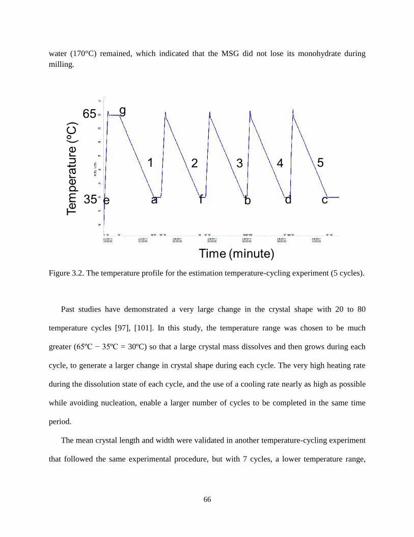
66

water (170°C) remained, which indicated that the MSG did not lose its monohydrate during

milling.

Figure 3.2. The temperature profile for the estimation temperature-cycling experiment (5 cycles).

Past studies have demonstrated a very large change in the crystal shape with 20 to 80

temperature cycles [97], [101]. In this study, the temperature range was chosen to be much

greater (65ºC − 35ºC = 30ºC) so that a large crystal mass dissolves and then grows during each

cycle, to generate a larger change in crystal shape during each cycle. The very high heating rate

during the dissolution state of each cycle, and the use of a cooling rate nearly as high as possible

while avoiding nucleation, enable a larger number of cycles to be completed in the same time

period.

The mean crystal length and width were validated in another temperature-cycling experiment

that followed the same experimental procedure, but with 7 cycles, a lower temperature range,

67

and no solute concentration measurement. These different experimental conditions were

expected to lead to different amounts of change in crystal size and shape for the two experiments.

3.2.5. Simulation and optimization codes for kinetics estimation and CSD prediction

Experimental data (e.g., size of time step, number of time steps, initial liquid concentration

and solvent mass) were input to a Matlab simulation-optimization code that estimated kinetic

parameters based on an initial estimate obtained from an initial set of simulation runs in which

one parameter was changed at a time based on physical intuition on the effect of each parameter

on the solute concentration and mean crystal length and width profiles. The 2D population

balance model included size-dependent dissolution and growth terms,

0, for 0

0, for 0

L W

L W

fG f G f S

t L W

fD f D f S

t L W

(3.2)

where f is the 2D population density, S is the absolute supersaturation, t is time, the growth

and dissolution rates in the length L and width W directions are assumed to be 2D generalizations

of the 1D equations [120], i.e.,

0

0

exp (1 )

exp (1 )

( )

( )

L

W

L

W

g

L GL GL

g

W GW GW

d

DLL

d

DWW

EG k S L

RT

EG k S W

RT

k SD

L

k SD

W

(3.3)

and the δij and γ define size-dependencies. The two-dimensional population balance model (3.2)

was combined with a solute mass balance and solved using a multidimensional method of

characteristics algorithm [121], [122]. All but six of the kinetic parameters were set to fixed

68

values as described in the caption to Table 3.2, with the remaining six parameters determined by

applying successive quadratic programming to minimize the sum-of-squared-deviations between

the model predictions and experiments,

42 2

2 21 1 ,

42

21 ,

1 1min ( ) ( ; ) ( ) ( ; )

1( ) ( ; )

CN

measured i model i measured k model k

i kC L k

measured k model k

k W k

C t C t L t L t

W t W t

(3.4)

where

T

0 0ln ln ln lnGW GL W L DW DLk k g g k k (3.5)

is the vector of fitted model parameters, NC is the number of concentration measurements, σ is

the standard deviation of each measurement error, and the subscripts C, L, and W refer to the

solute concentration and mean crystal length and width, respectively. These coefficients weigh

the relative confidence in the measurements of solute concentration and mean crystal length and

width, to produce parameter estimates that are unbiased with minimum variance assuming that

the errors have zero expectation and are uncorrelated with each other and the independent

variables [123].

Table 3.2. Kinetic parameters estimated from fitting data from the estimation temperature-

cycling experiment or set with justifications.a

Parameters Optimal values Units Fitted or fixed parameter

0GLk 136.4 10 2 2(μm)(g water) /(min)(g MSG) Fitted

Lg 2.00 Dimensionless Fitted

GL 0 1/μm Fixed

0GWk 132.3 10 2 2(μm)(g water) /(min)(g MSG) Fitted

Wg 2.00 Dimensionless Fitted

69

GW 0 1/μm Fixed

DLk 64.4 10 2(μm) (g water)/(min)(g MSG) Fitted

DWk 61.6 10 2(μm) (g water)/(min)(g MSG) Fitted

Ld 1 dimensionless Fixed

Wd 1 dimensionless Fixed

γ 1 dimensionless Fixed

ΔE 71.24 kJ/mol Fixed

aThe lower and upper bounds for the growth exponents

Lg and Wg were 1 and 2, as specified by

theory [41]. The dissolution exponents Ld and

Wd were set equal to 1 to be consistent with the

assumption of mass-transfer-limited dissolution [124], and the size-dependencies in the growth

rates, GL and

GW were set to zero as nonzero values did not significantly improve the fit to data.

The average activation energy 71.24 kJ/mol in WG and

LG expressions was estimated from [53].

The value of γ was selected to capture the trends in the increase in mean crystal length and width

(Fig. 3.9b). Varying the value of the dependency of the dissolution rate on the crystal dimensions,

γ in (3.3), above 1 did not affect the quality of fit much (comparison not shown). Although it

could be argued from physical grounds that the dissolution rate in the length direction should be

better modeled as being dependent on the size in the width direction and vice versa, swapping

these dependencies did not improve the quality of the model’s fit to data.

Uncertainties in the parameter estimates were quantified using standard methods whose

applications to crystallization are well established [41]. With the vector of predicted variables

T

1 2 1 2 3 4 1 2 3 4CNY C C C L L L L W W W W , (3.6)

the sensitivity matrix for this system is

70

1 1 1 1 1 1

0 0

2 2 2 2 2 2

0 0

0 0

1 1 1 1

0 0

ln ln ln ln

ln ln ln ln

ln ln ln ln

ln ln

C C C C C C

GW GL W L DW DL

GW GL W L DW DL

N N N N N N

GW GL W L DW DL

GW GL W

C C C C C C

k k g g k k

C C C C C C

k k g g k k

C C C C C C

k k g g k k

L L L LY

F k k g

1 1

4 4 4 4 4 4

0 0

1 1 1 1 1 1

0 0

4 4 4 4 4 4

0 0

ln ln

ln ln ln ln

ln ln ln ln

ln ln ln ln

L DW DL

GW GL W L DW DL

GW GL W L DW DL

GW GL W L DW DL

L L

g k k

L L L L L L

k k g g k k

W W W W W W

k k g g k k

W W W W W W

k k g g k k

(3.7)

where is the vector of optimal parameter estimates (values listed in Table 3.2). Each element

of F was calculated by the two-point central finite difference formula and used to construct an

estimate of the parameter covariance matrix

T1 1V FV F

, (3.8)

given the measurement error covariance matrix

2 2 2 2 2 2 2 2 2

,1 ,2 ,3 ,4 ,1 ,2 ,3 ,4diag( , , , , , , , , )CC N L L L L W W W WV I . (3.9)

3.3. Results and discussion

3.3.1. Evolution of crystal dimensions for the temperature-cycling experiments

In the estimation temperature-cycling experiment, the FBRM statistics had not converged to

a stable oscillation even after five cycles (Fig. 3.3), with the square-weighted mean chord length

at the end of each cycle increasing with cycle number, indicating that each cycle continues to

increase the size of the crystals. The increase in the ratio of the mean cube-weighted and square-

weighted mean chord length (blue line in Fig. 3.3) is associated with a change in the mean aspect

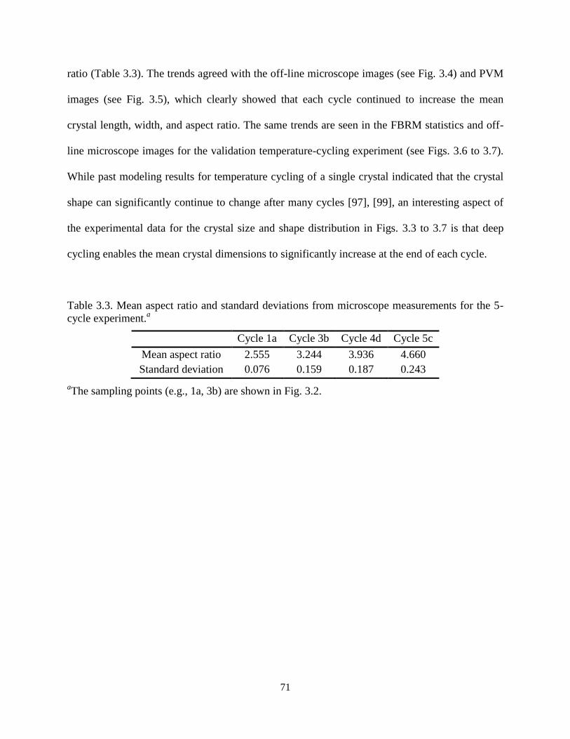
71

ratio (Table 3.3). The trends agreed with the off-line microscope images (see Fig. 3.4) and PVM

images (see Fig. 3.5), which clearly showed that each cycle continued to increase the mean

crystal length, width, and aspect ratio. The same trends are seen in the FBRM statistics and off-

line microscope images for the validation temperature-cycling experiment (see Figs. 3.6 to 3.7).

While past modeling results for temperature cycling of a single crystal indicated that the crystal

shape can significantly continue to change after many cycles [97], [99], an interesting aspect of

the experimental data for the crystal size and shape distribution in Figs. 3.3 to 3.7 is that deep

cycling enables the mean crystal dimensions to significantly increase at the end of each cycle.


cycle experiment.a

Cycle 1a Cycle 3b Cycle 4d Cycle 5c

Mean aspect ratio 2.555 3.244 3.936 4.660

Standard deviation 0.076 0.159 0.187 0.243

aThe sampling points (e.g., 1a, 3b) are shown in Fig. 3.2.

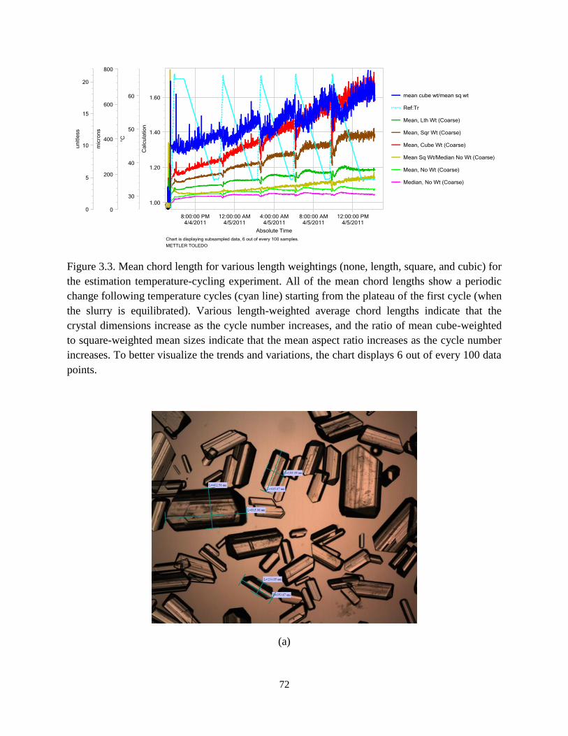
72

Figure 3.3. Mean chord length for various length weightings (none, length, square, and cubic) for

the estimation temperature-cycling experiment. All of the mean chord lengths show a periodic

change following temperature cycles (cyan line) starting from the plateau of the first cycle (when

the slurry is equilibrated). Various length-weighted average chord lengths indicate that the

crystal dimensions increase as the cycle number increases, and the ratio of mean cube-weighted

to square-weighted mean sizes indicate that the mean aspect ratio increases as the cycle number

increases. To better visualize the trends and variations, the chart displays 6 out of every 100 data

points.

(a)

73

(b)

(c)

Figure 3.4. Microscopy images (with polarizers) of MSG slurry for samples collected at 35°C in

the estimation temperature-cycling experiment at (a) cycle 1a, (b) cycle 3b, and (c) cycle 5c. The

timing of the sampling points is shown in Fig. 3.2.

74

(a)

(b)

75

(c)

Figure 3.5. PVM images of MSG slurry at 35°C in the estimation temperature-cycling

experiment at (a) cycle 1a, (b) cycle 3b, and (c) cycle 5c. The timing of the measurement points

is shown in Fig. 3.2. The PVM images show that crystals grow larger as the cycle number

increases, with some crystals growing larger than the image frame of PVM, such as in the fifth

cycle. No secondary nuclei were observed in any of the PVM images collected during the

experiments.

76

Figure 3.6. G400 FBRM (macro mode, which was called ‘coarse mode’ in earlier versions of the

FBRM software) counts/sec statistics and temperature for the validation temperature-cycling

experiment with samples collected at the end of the first, second, third, and seventh cycles (at

35°C, timing of the four sampling points shown with cycle numbers). The validation experiment

shows periodic changes in FBRM statistics as the temperature cycles, with a decrease in the

measured number of smaller chord lengths (< 300 μm) and an increase in mean square-weight

size with cycle number.

(a)

77

(b)

(c)

Figure 3.7. Microscopy images (with polarizers) of slurry of MSG crystals in aqueous solution

for the validation temperature-cycling experiment at the end of (a) cycle 1, (b) cycle 3, and (c)

cycle 7.

78

We will see in the solute concentration measurements in Section 3.3.2 that the solute

concentration at the lowest temperature, when the slurry samples are collected, increases little

from one cycle to the next. Since the total quantity of solute molecules is constant, the total mass

of crystals when samples are collected changes slowly with cycle number, which suggests that

the increase in the crystal dimensions after each cycle is mostly explained by a reduction in the

total number of crystals during each dissolution step. For this reduction to occur, a significant

fraction of the crystals becomes small enough to completely dissolve in each cycle. This

observation implies that the CSD must become broader during each cycle, which can only occur

in the PBM (3.2) if the growth and/or dissolution rates are size dependent. Most reported

dissolution rate expressions are size-dependent [120] whereas most reported growth rates are

size-independent [41], so these assumptions were made in this article.

3.3.2. Evolution of crystal dimensions and solute concentration for the estimation

temperature-cycling experiment

The solute concentration during the estimation temperature-cycling experiment is shown in

Fig. 3.8. For the first cycle, the temperature was held constant immediately after the first heating

ramp, to enable a qualitative assessment of the dissolution rate. The solution concentration

reaches a constant value shortly after the temperature is held constant, indicating that the

dissolution rate is fast enough for the solute concentration to quickly reach steady-state (and

hence the saturated concentration).

The solute concentration at the highest temperature (~65°C) is almost the same for each cycle

(Fig. 3.8, where each narrow peak arises from overshooting of the temperature at each transition

between heating to cooling), and the supersaturation is largely consumed before the next heating

stage (Fig. 3.9a). Given that the solute conditions are essentially the same at the start of each

79

cooling stage, the increase of solute concentration at the end of each cooling stage (35°C, see Fig.

3.8), must be associated with a decrease in the overall crystal mass grown during each cycle. As

the average supersaturation during each cooling stage increases (thus the growth rate increases

[40]) with cycle number (Fig. 3.9a), the decrease in the overall crystal mass grown is explained

by a reduction in the amount of crystal surface area in each subsequent cycle. This analysis is

consistent with a decrease in the total number of crystals at the end of each cycle, as the crystals

become larger, as seen in the FBRM statistics and PVM and optical microscopy images (Figs.

3.3 to 3.5).

Figure 3.8. Solute concentration profile over time for the estimation temperature-cycling

experiment. The time range covers the first four cycles. Beyond that time range (after point 4g in

Fig. 3.2), there was no FTIR equipment available. The distance along the vertical axis between

80

red and black lines is C in (3.4), which is the predicted standard deviation of solute

concentration.

(a)

81

(b)


parameters in Table 3.2 for the estimation temperature-cycling experiment for (a) solute

concentration and absolute supersaturation (the solubility, which is computed based on the

implemented temperature, uses the same vertical axis as the solute concentration), and (b) mean

crystal length (experiment: black circle; model: blue line) and width (experiment: green square;

model: red line).

The use of the in-situ measurements of the solute concentration and crystal mean length and

width to estimate the dissolution and growth kinetics is described next.

3.3.3. Simulation and prediction of CSDs with estimated kinetic parameters

The two-dimensional dissolution and growth kinetic parameters determined by the

application of least-square estimation to the data from the estimation temperature-cycling

82

experiment are reported in Table 3.2, with comparisons between model predictions and

experiments in Fig. 3.9. The estimated parameters for the growth and dissolution rates in Table

3.2 have values that are consistent with theory [40], [120]. About half of the model parameters

were set based on theory or experimental studies by other groups, as described in the caption of

Table 3.2, and the simulation parameters are in Table 3.4. The solute concentration from the

population balance model (3.2) tracks the experimental value, including the slow increase in the

minimum solute concentration in each cycle (Fig. 3.9a). The mean crystal length and widths

from the model also track the optical microscopy measurements quite closely through all of the

cycles, with somewhat larger deviations for the ratio of the mean length and mean width (Fig.

3.9b).


the estimation temperature-cycling experiment.

Variable Description Values Units

Δt Time step 0.05 minute

ΔW mesh size for the width 5.0 μm

ΔL mesh size for the length 5.0 μm

C(0) initial solute

concentration 1.0558 g MSG/g water

Ms mass of solvent (water) begins with 60.0 g

times that slurry

sample was collected

215, 645,

875, 1145 minute

T real-time temperature 35.0 to 65.0 °C

number of temperature

points 1162 dimensionless

The kinetic parameters in Table 3.2 were used to predict the mean crystal length and width

(Fig. 3.10) in another temperature-cycling experiment (e.g., the 7-cycle validation experiment,

83

detailed in Section 3.2.4 and Table 3.5). The predictions closely track the experimental data

throughout the temperature cycles (Fig. 3.10), except at the 7th

cycle, which is consistent with the

accumulation of the effects of model uncertainties on model predictions that would be expected

in any process that has states whose values continue to drift over time. The mean crystal length

prediction is especially accurate, with negligible prediction error for cycles 1, 2, and 3 and <10%

prediction error at Cycle 7. The mean crystal width and the ratio of length to width have larger

deviations. The crystal size distributions at the sampling times were also calculated (Figs. 3.11 to

3.12) based on the estimated kinetic parameters (Table 3.2). The CSDs from the PBM grow

wider with cycle number, which is consistent with having size-dependent dissolution rates in the

model, and consistent with experimental measurements (Table 3.7). The trends in mean width,

length, and aspect ratio in Fig. 3.10 and Table 3.6 agree with FBRM CLD data (Fig. 3.6).


the validation temperature-cycling experiment.

Variable Description Values Units

Δt Time step 0.05 minute

ΔW mesh size for the width 5.0 μm

ΔL mesh size for the length 5.0 μm

C(0) initial solute

concentration 1.0024

g MSG/g

water

Ms mass of solvent (water) begins with

60.0 G

times that slurry

sample was collected

199, 379,

567, 1297 Minute

T real-time temperature 35.0 to 60.0 °C

number of temperature

points 1318 dimensionless

84


cycle experiment.a

Cycle 1 Cycle 2 Cycle 3 Cycle 7

Mean aspect ratio 2.349 2.399 2.622 2.835

Standard deviation 0.064 0.050 0.059 0.053

aThe sampling points are defined in Fig. 3.6.

Table 3.7. Crystal length and width measurement from the 7-cycle validation experiment.a

Cycle

number

Minimum

width

(μm)

Maximum

width

(μm)

Minimum

length

(μm)

Maximum

length

(μm)

Range

of width

(μm)

Range

of length

(μm)

Number

of

crystals

1 17.0 345.3 38.0 1056.5 328.3 1018.5 201

2 25.6 389.8 36.9 1295.5 364.2 1258.6 287

3 26.8 474.8 81.0 1176.7 448.0 1095.7 138

7 40.2 651.2 160.5 1505.2 611.0 1344.7 187

aThe cycle numbers are defined in Fig. 3.3.

85


parameters in Table 3.2 for the estimation in the validation temperature-cycling experiment (7

cycles) for the mean crystal length (experiment: black circle; model: blue line) and width

(experiment: green square; model: red line). The model expected errors in the mean crystal

length and width are reported in Table 3.9. The measurement error bars in the plot are the sample

standard deviations computed by resampling the crystal size measurements.

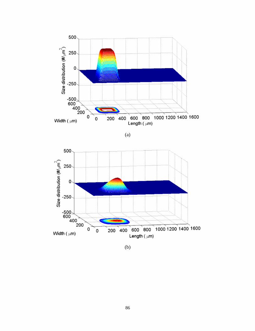
86

(a)

(b)

87

(c)

(d)

88

(e)

Figure 3.11. Crystal size distributions ( , , )f L W t of MSG slurry from model simulation using the

kinetic parameters in Table 3.2 for the 5-cycle estimation temperature-cycling experiment, with

the points as in Fig. 3.2: (a) 1a; (b) 2f; (c) 3b; (d) 4d; (e) 5c.

(a)

89

(b)

(c)

90

(d)

Figure 3.12. Crystal size distributions ( , , )f L W t of MSG slurry from model simulation using the

kinetic parameters in Table 3.2 for the 7-cycle validation temperature-cycling experiment at the

end of cycles, with the points as in Fig.3.6: (a) cycle 1; b) cycle 2; c) cycle 3; d) cycle 7.

3.3.4. Parameter estimation and accuracy quantification for the population balance model

The parameter error estimates in Table 3.8 were obtained from (3.4) to (3.9) using C = 0.01

g MSG/g water and L and W in Fig. 3.9b, based on the experimental data from the single

temperature-cycling estimation experiment. Such parameter error estimates should always be

taken as being underestimates, since the statistical assumptions that the errors have zero

expectation and are uncorrelated with each other and the independent variables [123] almost

never exactly hold in practice. In particular, the derivation of a first-principles model always

includes some simplifying assumptions that do not exactly hold, such as perfect spatially-

uniform mixing, in which case the statistical assumptions will not hold exactly. Such parameter

uncertainty estimates have been found to be useful in past crystallization studies [41], [100], and

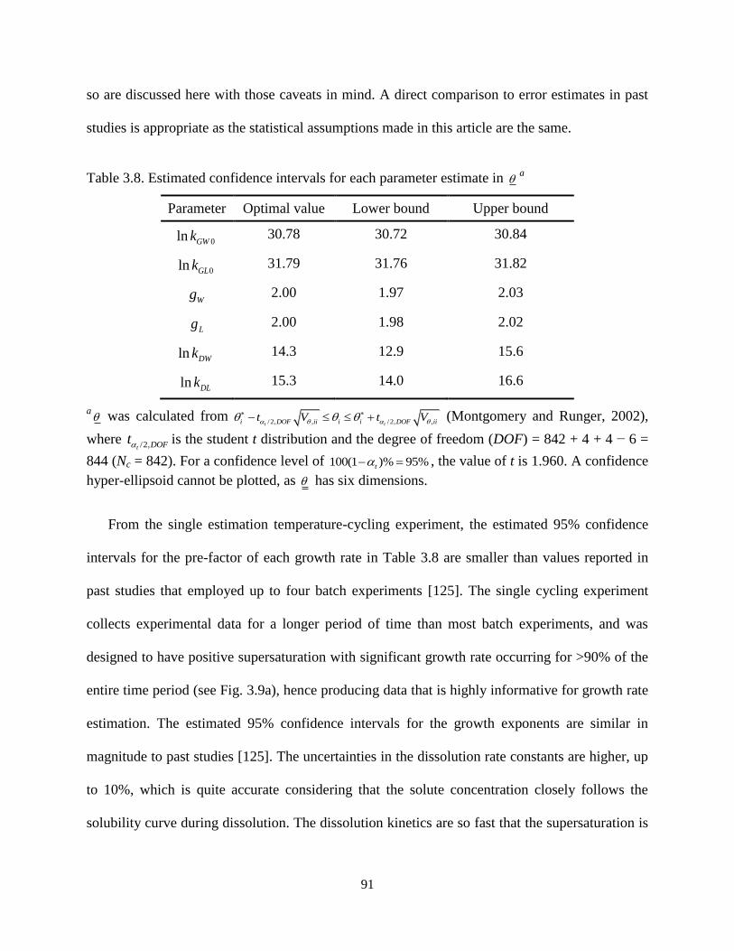
91

so are discussed here with those caveats in mind. A direct comparison to error estimates in past

studies is appropriate as the statistical assumptions made in this article are the same.

Table 3.8. Estimated confidence intervals for each parameter estimate in a

Parameter Optimal value Lower bound Upper bound

ln 0GWk 30.78 30.72 30.84

ln 0GLk 31.79 31.76 31.82

Wg 2.00 1.97 2.03

Lg 2.00 1.98 2.02

ln DWk 14.3 12.9 15.6

ln DLk 15.3 14.0 16.6

a was calculated from

/2, , /2, ,t ti DOF ii i i DOF iit V t V (Montgomery and Runger, 2002),

where /2,t DOFt is the student t distribution and the degree of freedom (DOF) = 842 + 4 + 4 − 6 =

844 (Nc = 842). For a confidence level of 100(1 )% 95%t , the value of t is 1.960. A confidence

hyper-ellipsoid cannot be plotted, as has six dimensions.

From the single estimation temperature-cycling experiment, the estimated 95% confidence

intervals for the pre-factor of each growth rate in Table 3.8 are smaller than values reported in

past studies that employed up to four batch experiments [125]. The single cycling experiment

collects experimental data for a longer period of time than most batch experiments, and was

designed to have positive supersaturation with significant growth rate occurring for >90% of the

entire time period (see Fig. 3.9a), hence producing data that is highly informative for growth rate

estimation. The estimated 95% confidence intervals for the growth exponents are similar in

magnitude to past studies [125]. The uncertainties in the dissolution rate constants are higher, up

to 10%, which is quite accurate considering that the solute concentration closely follows the

solubility curve during dissolution. The dissolution kinetics are so fast that the supersaturation is

92

never far from zero during dissolution, so the uncertainties in the dissolution rate constants are

larger than for the parameters in the growth rate expressions.

3.3.5. Comparison of population balance model predictions with data from validation

experiment

The small parametric uncertainties in Table 3.8 provide some confidence that the model

predictions could be accurate enough to be used for design purposes. To make a more informed

assessment, the parameter covariance matrix was also used to estimate the accuracy of the model

predictions for the validation 7-cycle experiment. The parameter covariance matrix V remains

the same, while the sensitivity matrix is specific for each experiment. The sensitivity matrix for

the 7-cycle experiment 7F was calculated using the same central finite difference method. The

prediction error covariance matrix YV was calculated from T

7 7YV F V F . The diagonal elements

of YV include the standard deviations of mean crystal length ( 7L ) and width ( 7W ) from the

model prediction, all of which are listed in Table 3.9. The 95% prediction intervals for the

predicted mean crystal length and width are estimated to be ±12.5 μm and ±2.5 μm, respectively,

at Cycle 7, suggesting that the difference between the model predictions and experimental data in

Fig. 3.10 is more likely to be due to uncertainties in the measurements rather than uncertainties

in the model predictions.

Table 3.9. The standard deviation of the mean crystal length and width predicted by the model

with its uncertainty description, with the time points being the same as in Fig. 3.12.a

Time

points

Standard deviation of the mean

crystal length ( 7L ), μm

Standard deviation of the mean

crystal width ( 7W ), μm

Cycle 1 1.7249 0.4516

Cycle 2 2.8045 0.4993

93

Cycle 3 3.0404 0.4663

Cycle 7 6.2465 1.2851

aThe prediction errors are much smaller than the noise in the mean crystal length and width

measurements, so only bars on the estimated experimental measurement noise are shown in Figs.

3.9 and 3.10.

3.4. Summary

Temperature-cycling experiments were designed in which the mean crystal dimensions and

aspect ratio significantly increased at the end of each cycle, in a much smaller number of cycles

than in previous studies [97], [101]. FBRM, a commercial instrumentation that is readily

available in pharmaceutical laboratories, was used for the in-situ simultaneous measurement of

crystal shape and size for rod-like crystals during a temperature cycling experiment. The

temperature-cycling experimental design may also be applied to semi-continuous and continuous

crystallizers to modify crystal shape.

Dissolution and growth kinetics in a population balance model were estimated along the

length and width directions for rod-shaped crystals based on experimental data from commercial

instrumentation applied to a single experiment in which the temperature cycles. For the first time,

both the growth and dissolution rates along multiple crystal axes were estimated from a

multidimensional population balance model with a limited number of minimum-variance kinetic

parameter estimates, based on solute concentration and crystal dimension measurements in a

single experiment. The model outputs tracked well the experimentally measured mean crystal

dimensions and solute concentrations. With the same parameter estimates, the model predicted

the crystal dimensions for another temperature-cycling experiment reasonably well (Fig. 3.10).

Both this observation and uncertainty analysis suggested that growth and dissolution rates

estimated in a single temperature-cycling experiment might be suitable for designing a

temperature-cycling protocol for optimizing the size and shape of the product crystals.

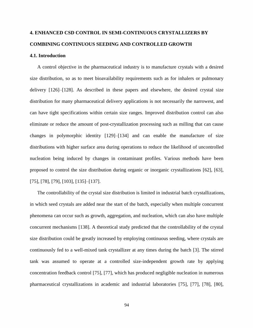
94

4. ENHANCED CSD CONTROL IN SEMI-CONTINUOUS CRYSTALLIZERS BY

COMBINING CONTINUOUS SEEDING AND CONTROLLED GROWTH

4.1. Introduction

A control objective in the pharmaceutical industry is to manufacture crystals with a desired

size distribution, so as to meet bioavailability requirements such as for inhalers or pulmonary

delivery [126]–[128]. As described in these papers and elsewhere, the desired crystal size

distribution for many pharmaceutical delivery applications is not necessarily the narrowest, and

can have tight specifications within certain size ranges. Improved distribution control can also

eliminate or reduce the amount of post-crystallization processing such as milling that can cause

changes in polymorphic identity [129]–[134] and can enable the manufacture of size

distributions with higher surface area during operations to reduce the likelihood of uncontrolled

nucleation being induced by changes in contaminant profiles. Various methods have been

proposed to control the size distribution during organic or inorganic crystallizations [62], [63],

[75], [78], [79], [103], [135]–[137].

The controllability of the crystal size distribution is limited in industrial batch crystallizations,

in which seed crystals are added near the start of the batch, especially when multiple concurrent

phenomena can occur such as growth, aggregation, and nucleation, which can also have multiple

concurrent mechanisms [138]. A theoretical study predicted that the controllability of the crystal

size distribution could be greatly increased by employing continuous seeding, where crystals are

continuously fed to a well-mixed tank crystallizer at any times during the batch [3]. The stirred

tank was assumed to operate at a controlled size-independent growth rate by applying

concentration feedback control [75], [77], which has produced negligible nucleation in numerous

pharmaceutical crystallizations in academic and industrial laboratories [75], [77], [78], [80],

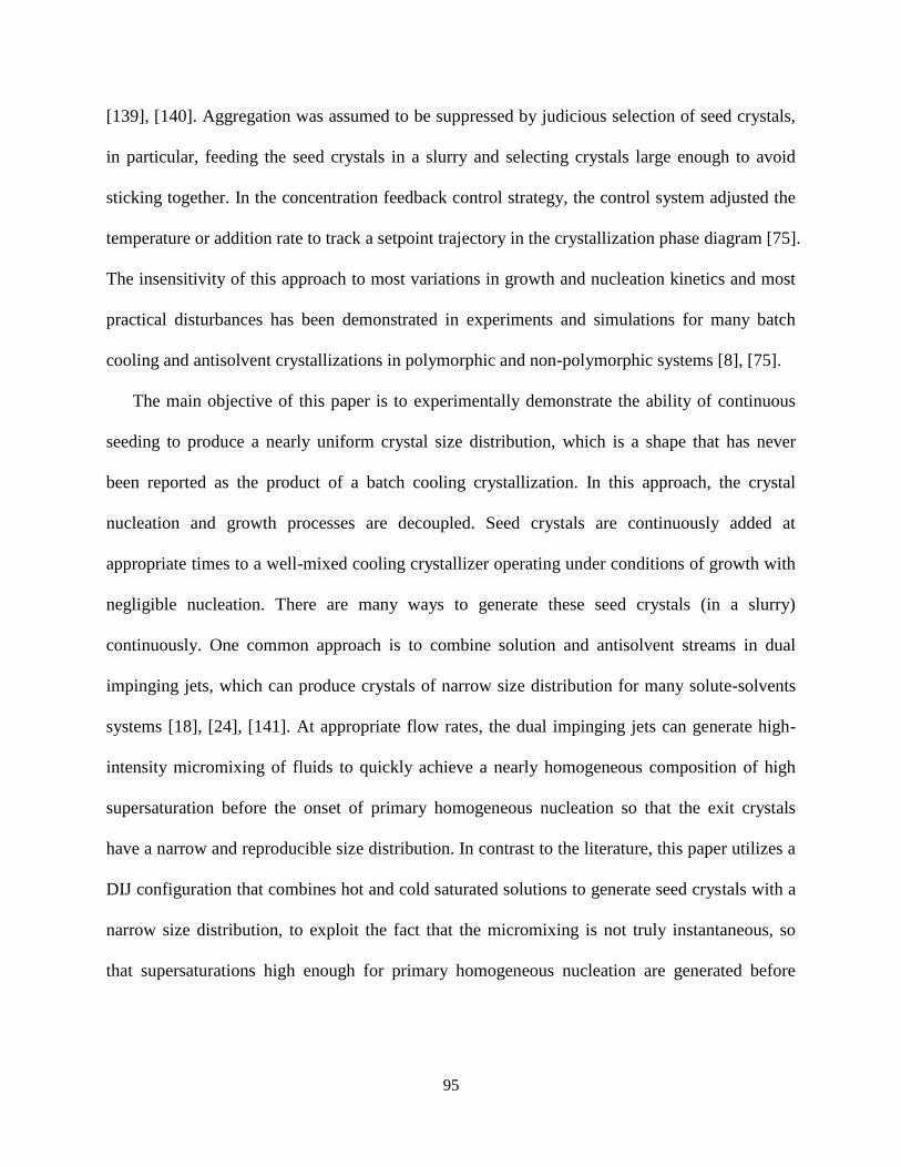
95

[139], [140]. Aggregation was assumed to be suppressed by judicious selection of seed crystals,

in particular, feeding the seed crystals in a slurry and selecting crystals large enough to avoid

sticking together. In the concentration feedback control strategy, the control system adjusted the

temperature or addition rate to track a setpoint trajectory in the crystallization phase diagram [75].

The insensitivity of this approach to most variations in growth and nucleation kinetics and most

practical disturbances has been demonstrated in experiments and simulations for many batch

cooling and antisolvent crystallizations in polymorphic and non-polymorphic systems [8], [75].

The main objective of this paper is to experimentally demonstrate the ability of continuous

seeding to produce a nearly uniform crystal size distribution, which is a shape that has never

been reported as the product of a batch cooling crystallization. In this approach, the crystal

nucleation and growth processes are decoupled. Seed crystals are continuously added at

appropriate times to a well-mixed cooling crystallizer operating under conditions of growth with

negligible nucleation. There are many ways to generate these seed crystals (in a slurry)

continuously. One common approach is to combine solution and antisolvent streams in dual

impinging jets, which can produce crystals of narrow size distribution for many solute-solvents

systems [18], [24], [141]. At appropriate flow rates, the dual impinging jets can generate high-

intensity micromixing of fluids to quickly achieve a nearly homogeneous composition of high

supersaturation before the onset of primary homogeneous nucleation so that the exit crystals

have a narrow and reproducible size distribution. In contrast to the literature, this paper utilizes a

DIJ configuration that combines hot and cold saturated solutions to generate seed crystals with a

narrow size distribution, to exploit the fact that the micromixing is not truly instantaneous, so

that supersaturations high enough for primary homogeneous nucleation are generated before

96

complete mixing occurs. To our knowledge, this is the first time that experimental data have

been reported for such a cooling DIJ.

4.2. Experimental methods

This section summarizes the experimental methods for characterization of the solubility,

metastable limit, and growth kinetics for L-asparagine monohydrate (LAM) in aqueous solution

by attenuated total reflection-Fourier transform infrared (ATR-FTIR) spectroscopy,

chemometrics, and focused beam reflectance measurement (FBRM). Also discussed are the

operations of the cooling DIJ and mixing-tank crystallizers that are coupled for the purposes of

generating a target crystal size distribution.

4.2.1. Materials and instrumentation

Infrared spectra for L-asparagine monohydrate (LAM, from Sigma Aldrich) in de-ionized

(DI) water were collected in a 2-liter stirred tank by an in situ Dipper-210 ATR immersion probe

(Axiom Analytical) with ZnSe as the internal reflectance element attached to a Nicolet 6700

FTIR spectrophotometer, 64 scans collected for each spectrum, and DI water at 25°C used for

the background (see Fig. 4.1). This solute-solvent system has selected because its solubility vs.

temperature relationship is very similar to many pharmaceutical compounds.

97

(a)

(b)

Figure 4.1. Photograph (a) and schematic (b) of stirred-tank crystallizer instrumented with in situ

ATR-FTIR immersion probe, FBRM probe, and thermocouple. The PVM and pump was not

used in this study.

98

During crystallization, the temperature of the slurry in the stirred tank was controlled by

ratioing hot and cold water to the jacket of a round-bottom or cylindrical flask with a control

valve using a proportional-integral control system designed via internal model control [80] and

was measured every 2 seconds using a Teflon-coated thermocouple attached to a Data

Translation 3004 data acquisition board via a Fluke 80TK thermocouple module [81]. The total

counts/second of LAM crystals in solution were measured every 10 seconds using Lasentec

FBRM with version 6.0b12 of the FBRM control interface software [80]. Images of crystal

slurries were taken with a polarized microscope (Leica DMI 4000B) with cameras Qimaging

ReRIGA 2000R (black and white) and Leica DFC 420 (color). Both FBRM and microscope can

measure characteristic sizes in the range of about 1-2000 microns. Experimental data were

archived and DIJ inlet flows specified using PI software from OSIsoft.

4.2.2. Calibration of ATR-FTIR for solute concentration

A bench-scale stirred-tank crystallizer was cooled at a constant rate of 0.5 °C/min for

different known LAM concentrations (Table 4.1) in about 400 grams of aqueous solution, while

being measured with in situ ATR-FTIR spectroscopy and FBRM, until an increase in the total

counts/s indicated that the metastable limit was reached (the detailed experimental procedures

are described elsewhere [77]. The width of the metastable zone at this cooling rate depended on

solute concentration, so that a different number of infrared spectra was collected for each

temperature.

Table 4.1. ATR-FTIR calibration samples for in situ solute concentration measurement.

Calibration

sample

Solute concentration

(g/g solvent)

Temperature

range (°C)

Number

of spectra

Cs1 0.0300 30.4-18.0 27

Cs2 0.0567 42.9-25.1 38

99

Cs3 0.0834 50.9-34.5 35

Cs4 0.1101 59.4-46.9 27

Cs5 0.1368 63.9-57.1 16

Several chemometrics methods were applied to the absorbance spectra (in the range 1200-

1800 cm–1

) with known solute concentrations and temperatures to construct a linear calibration

model for measurement of the solute concentration (see Fig. 4.2 for representative data and the

regression coefficients, with the equipment and procedures being the same as for other solute-

solvent systems [54], [77]. The calculations were carried out using in-house MATLAB 5.3 (The

Mathworks, Inc.) code except for partial least-squares (PLS) regression, which was from the PLS

Toolbox 2.0 (Eigenvector Research, Inc.). The correlation Forward Selection 2 PCR method with

a noise level of 0.004 gave the smallest prediction interval of 0.00579 g/g solvent while being

consistent with the accuracy of the solubility data. The calibration model had the form

1800

0

1200

j j T

j

C w a w T w

, (4.1)

where C is the solute concentration (g LAM/g water), aj is the absorbance at frequency j (cm–1

),

T is the temperature (°C), and wj, wT, and w0 are regression coefficients.

100

(a)

(b)

Figure 4.2. (a) Representative ATR-FTIR spectra of LAM aqueous samples used for calibration

(units: g LAM/g water). (b) Regression coefficients of the calibration model relating absorbances

1200 1300 1400 1500 1600 1700 1800

0

0.05

0.1

0.15

0.2

0.25

0.3

wavenumber (cm-1)

abso

rbance

0.0300 g/g at 24.93 C

0.0567 g/g at 33.78 C

0.0834 g/g at 45.02 C

0.1101 g/g at 51.32 C

0.1368 g/g at 58.09 C

13001400150016001700

-0.02

0

0.02

0.04

0.06

0.08

wavenumber (cm-1)

regression coefficients

IR spectrum (absorbances)

12001800

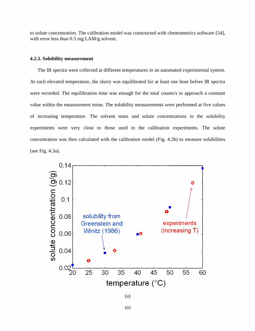
101

to solute concentration. The calibration model was constructed with chemometrics software [54],

with error less than 0.5 mg LAM/g solvent.

4.2.3. Solubility measurement

The IR spectra were collected at different temperatures in an automated experimental system.

At each elevated temperature, the slurry was equilibrated for at least one hour before IR spectra

were recorded. The equilibration time was enough for the total counts/s to approach a constant

value within the measurement noise. The solubility measurements were performed at five values

of increasing temperature. The solvent mass and solute concentrations in the solubility

experiments were very close to those used in the calibration experiments. The solute

concentration was then calculated with the calibration model (Fig. 4.2b) to measure solubilities

(see Fig. 4.3a).

(a)

102

(b)

Figure 4.3. (a) LAM solubility curve compared to reference data from Greenstein and Winitz

(1986). Reference data are slightly higher than solute concentrations determined from the

calibration model, probably due to use of different grades of water. (b) Representative

experimental solute concentrations and temperatures obtained during concentration feedback

control for a constant supersaturation level of 0.0074 g/g and a seeding point at 55.5°C. Also

shown is the unseeded metastable limit that defines the highest solute concentration for which

the calibration model was valid, which is much higher than the solute concentrations used in the

concentration feedback control experiments.

4.2.4. Seeded batch crystallizations

An initial set of seeded batch crystallizations were carried out to (i) verify that concentration

feedback control could reliably track a constant absolute supersaturation with negligible

nucleation and (ii) estimate average growth kinetics. An undersaturated solution with solute

concentration 0.122 g LAM/g water was cooled at 0.5 °C/min from 65°C to below the saturation

temperature (55.5°C, see Fig. 4.3b). The stirring conditions were very similar to the calibration

experiments. Then seed crystals of LAM with mass 6.44% of the expected crystal yield were

103

added to the solution. The seed crystals (Fig. 4.4a) were generated from crash cooling of high

temperature LAM-saturated solution, followed by filtration and vacuum drying at room

temperature and then sieving. Crash cooling usually produces a wide size distribution of crystals;

to make full use of material, dry seeds of adjacent sieve ranges were combined for the

concentration control experiments.

During continuous seeding, the product CSD is a function of the supersaturation [3]. For each

batch cooling crystallization, the control algorithm to follow a preset supersaturation profile

started shortly after seeding, and continued throughout the rest of crystallization experiment

(until the system cooled to about 18°C) [80]. The supersaturation set point profiles were selected

within the metastable zone at different constant absolute supersaturations (ΔC = C – Csat) where

Csat denotes the solubility (g LAM/g water). In addition to visual inspection by optical

microscopy after each experiment, FBRM data collected during each experiment confirmed that

negligible nucleation occurred (see Fig. 4.4b).

These experiments with seeds obtained by crash cooling serve to demonstrate good

concentration feedback control for the system and, at same time, estimation of temperature-

averaged growth rates (For example, as used by [35], [142], [143]. As dry seed crystals have a

tendency to agglomerate, slurry seed crystals were used in subsequent experiments. More

specifically, for implementation towards the production of a target crystal size distribution, slurry

seeds manufactured by dual impinging jets (Fig. 4.5, details below) with size less than 20 µm

(Fig. 4.6) were fed to the stirred tank through the crystallizer neck (with residence time of about

1 second). The total mass of seeds added in slurry form was 3.39% of the total expected crystal

yield. Similarly, the feedback control algorithm started shortly after seeding, and continued

throughout the cooling crystallization experiment.

104

(a)

(b)

Figure 4.4. (a) Size distribution of LAM seeds (based on the largest dimension) and product

crystals after concentration feedback control at two different values of constant supersaturation,

measured from off-line optical microscopy. (b) FBRM counts during concentration feedback

control at constant supersaturation of 0.0074 g LAM/g water.

nu

mb

er

of

cry

sta

ls

crystal size (µm)

crash-

cooled

seedsS = 0.0074 g/g

S = 0.0037 g/g

0 20 40 60 80 100 120 140 160 1800

10

20

30

40

50

60

70

time (min)

#/s

ec fro

m F

BR

M

total counts

(29.286-85.77)um

(10-23.263)um

(100-251.189)um

(1-5.012)um

(292.864-1000)um

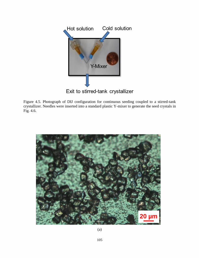
105

Figure 4.5. Photograph of DIJ configuration for continuous seeding coupled to a stirred-tank

crystallizer. Needles were inserted into a standard plastic Y-mixer to generate the seed crystals in

Fig. 4.6.

(a)

20 µm

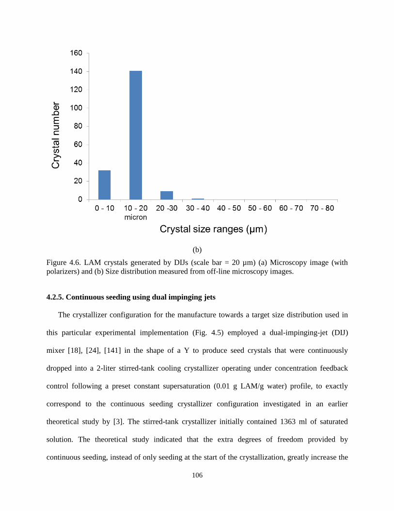
106

(b)

Figure 4.6. LAM crystals generated by DIJs (scale bar = 20 µm) (a) Microscopy image (with

polarizers) and (b) Size distribution measured from off-line microscopy images.

4.2.5. Continuous seeding using dual impinging jets

The crystallizer configuration for the manufacture towards a target size distribution used in

this particular experimental implementation (Fig. 4.5) employed a dual-impinging-jet (DIJ)

mixer [18], [24], [141] in the shape of a Y to produce seed crystals that were continuously

dropped into a 2-liter stirred-tank cooling crystallizer operating under concentration feedback

control following a preset constant supersaturation (0.01 g LAM/g water) profile, to exactly

correspond to the continuous seeding crystallizer configuration investigated in an earlier

theoretical study by [3]. The stirred-tank crystallizer initially contained 1363 ml of saturated

solution. The theoretical study indicated that the extra degrees of freedom provided by

continuous seeding, instead of only seeding at the start of the crystallization, greatly increase the

107

controllability of the crystal size distribution. A uniform size distribution was selected for

experimental validation of the approach as its shape is very different from the product size

distributions produced by cooling crystallizations that only seed at the beginning of the batch. As

the optimal jet velocity profile for producing the flattop CSD was nearly constant, to simplify the

implementation the experiments employed a constant jet velocity of 1.9 m/s, with a volumetric

flow rate of 5.8 ml/min and jet inner diameter of 0.254 mm. The total slurry volume added

during the experiment was 88.5 ml. For crystallization with neither nucleation nor aggregation,

multiplying the supersaturation and/or mass flow rate of seeds by a constant changes the height

and width of the flattop distribution with negligible effect on its shape (for detailed mathematical

expressions, see [3], so the theoretically optimal distribution shape can be directly compared to

the experimentally obtained distribution for a different solute-solvent system (see Fig. 4.10,

measured manually from off-line microscope images of hundreds of crystals). Due to the limited

volume limit of the stirred-tank crystallizer, for proof-of-concept purposes, the continuous

seeding was allowed to cover a 4.4% volume ratio of the reactor. The seeding time duration

could also help tune the width of the product CSD.

Unlike antisolvent/reaction DIJ crystallizations, this experimental implementation generated

seed crystals by mixing hot and cold saturated streams (solution concentrations of 0.20 g LAM/g

water at 70 C and 0.03 g LAM/g water at 25 C ). If the micromixing were perfect, then it is

straightforward to show from a mass balance and Fig. 3a that the solute concentration of the

well-mixed stream for this solute-solvent system would be near saturated conditions, with

supersaturation too low ((C – Csat )/Csat = 1.4) to generate nuclei by primary homogeneous

nucleation. Crystals nucleate easily from this cooling DIJ configuration, suggesting that the

108

micromixing is sufficiently slow in this system that high enough supersaturation is generated

near the interfaces between the two streams to induce nucleation.


4.3.1. Solubility

The solubility curve of LAM in aqueous solution was fit to a quadratic function to give

2 3 5 23.084 10 1.373 10 5.214 10satC T T (4.2)

(see Fig. 4.3b). The maximum deviation of the experimental data points from the fitted solubility

curves (0.0021 g LAM/g water) was within the prediction intervals. The solubility data were also

fit to a van’t Hoff equation [144]:

1

0ln ( / ) ( / ) lnC a R T b R T c (4.3)

where R is the ideal gas constant, T is in units of Kelvin, and C0 is in units of mole fraction (see

Fig. 4.7). The solubility data are in good agreement with [2]; the differences can be attributed to

differences in the purity of water in the two sets of experiments. From the coefficients of the

solubility curve, the apparent enthalpy of solution [144], *H a bT of LAM in aqueous

solution was calculated to be 35.66 kJ/mol at 298.15 K, and apparent heat capacity as *

pC = b =

86 J/(mol-K). This calculated enthalpy of solution is in good agreement with calculation by

applying the same method to the reference [2] (35.45 kJ/mol) and directly from measurement

(33.89 kJ/mol).

109

Figure 4.7. van’t Hoff equation, 1

0ln 9973.791 86.14549ln 56.68014C T T , fit to solubilities

for LAM in aqueous solution obtained from ATR-FTIR spectroscopy (red triangles). A van’t

Hoff equation was also fit to previously published solubility data [2] that are shown as blue

asterisks.

4.3.2. Initial seeded batch crystallizations.

Batch crystallizations seeded with dry crystals generated by crash cooling (Fig. 4.8) to follow

preset constant absolute supersaturation profiles within the metastable zone were implemented

using concentration feedback control with cooling rate based on the in situ measurement of the

solute concentration (Fig. 4.3b). The solute concentration very closely tracked the setpoint

trajectory in the phase diagram as has been observed for many other pharmaceutical compounds

(e.g., [77], [80]).

290 300 310 320 330 340 350-2.5

-2

-1.5

-1

-0.5

0

0.5

1Ln c

once

ntr

ation

(m

ole

of L a

spa

rag

ine

mo

no

hyd

rate

/Lite

r o

f D

I w

ate

r)

Temperature (K)

solubility curve from experiments

(temperature upward)

solubility data

from Greenstein

and Winitz (1986)

110

Figure 4.8. Microscope image of a batch of LAM seed crystals after sieving for the range of 125

to 180 µm (scale bar = 200 µm).

Two sets of supersaturation profiles were applied. Run 1 was implemented at a constant

supersaturation (ΔC = 0.0074 g LAM/g water) that was very close to the middle of the

metastable zone and Run 2 was implemented for half of this absolute supersaturation (ΔC =

0.0037 g LAM/g water). Microscope images of the product crystals are very similar between the

two runs (see Fig. 4.9ab). Inspection of the microscope images and FBRM data (Fig. 4.4)

indicated that that negligible nucleation occurred in the stirred-tank.

200 µm

111

(a)

(b)

Figure 4.9. Microscope images of LAM product crystals produced by concentration feedback

control experiments with constant supersaturation of (a) 0.0074 g LAM/g water and (b) 0.0037 g

LAM/g water (scale bar = 200 µm).

112

The change in the mean crystal length during each experiment operating under constant

absolute supersaturation in Fig. 4.4a was divided by the batch time to determine the average

growth rate for each supersaturation. The estimated average growth rate G was plotted vs.

supersaturation S to estimate the kinetic parameters in the power-law growth rate expression G =

kgSg for LAM crystals in aqueous solution, closely following a procedure described in [139],

which determined that g ≈ 1 and average kg = 6.353 μm/s. The relationship between the average

growth rate and absolute supersaturation implies that the concentration feedback control provides

control of the average growth rate in the stirred-tank crystallizer.

The crystals shown in Fig. 4.8 were produced by crash cooling followed by vacuum drying

and sieving, which caused some aggregation. Slurry seeds were used in the subsequent

continuous seeding experiment because (i) they have a reduced potential for aggregation, and (ii)

using a carrier fluid makes it easier to reliably deliver seed crystals at a smoothly controlled rate

to a stirred-tank crystallizer.

4.3.3. Continuous seeding by dual impinging jets

Seed crystals produced by the DIJ mixer were highly uniform and smaller than 20 microns

(Fig. 4.6). It is unlikely that the nucleation of these seed crystals occur under conditions of

perfect mixing (that is, conditions in which the two liquids are mixed at the molecular scale

before nucleation occurs). The temperature achieved by complete mixing would be about 47.5°C,

which is the average of the two inlet stream temperatures of 25°C and 70°C in a 1:1 volume ratio,

and the solubility at that temperature is about 0.082 g LAM/g water (see Fig. 4.3a). If the solute

concentrations were perfectly mixed, the well-mixed concentration would be (0.2 + 0.03)/2 =

0.115 g LAM/g water, which is just above the unseeded metastable limit in Fig. 4.3b measured

for a large-volume stirred-tank crystallizer at a low cooling rate. Smaller volumes and higher

113

cooling rates produce much higher metastable limits than for large volumes at low cooling rates

(the former effect is described in papers on nucleation in microscale droplets, e.g., [25], and the

latter effect is described in any textbook or paper that discusses metastable limits in some detail,

e.g., [77]), which implies that the seed crystals were not nucleated under conditions of perfect

mixing (which is defined in this context as the crystals nucleating after the fluids have perfectly

mixed).

The ratio of the Prandtl to the Schmidt number, D/α, specifies the relative thickness of the

concentration boundary layer to the thermal boundary layer, which is about 1/100, where D is the

diffusivity of LAM in solution and α is the thermal diffusivity of the solution. This value

indicates that the thermal boundary layer is much thicker than the concentration boundary layer.

This implies that the temperature in the high concentration fluid side of the interface can drop

while the concentration remains high, to produce a highly supersaturated solution. If symmetry

about the interface between the two fluids is assumed, then the temperature near the interface is

about equal to 47.5°C, and a solute concentration of 0.2 g LAM/g water is far enough above the

metastable limit measured in Fig. 4.3b to indicate that primary homogenous nucleation can occur

within the 1 second of residence time before the mixture enters the mixed-tank crystallizer.

Collectively, this analysis provides evidence that the two liquids were not mixed at the molecular

scale before crystal nucleation occurred.

The seeds in slurry generated by the DIJ mixer were continuously added to the

experimentally validated concentration-controlled stirred-tank crystallizer (Fig. 4.1) for

manufacturing the product crystal size distribution. For this experimental validation, the use of a

flattop size distribution as the target enabled a direct comparison to the previously published

theoretical results [3] (see Fig. 4.10 for the optimal CSD for some realistic seed crystals). Most

114

of the product crystals are within the size range of 50 to 150 µm, with similar smoothing at high

and low sizes as predicted by theory for a seed distribution with nonzero width (Fig. 4.10). The

experimental product crystal size distribution has very similar deviations from the target size

distribution as predicted by theory. The theory of Woo et al. [3] assumed no growth rate

dispersion and that the crystallizer was perfectly well-mixed, and the experimentally observed

longer tail at large crystal sizes in Fig. 4.10 could be due to growth rate dispersion or some non-

ideal mixing in the crystallizers. A microscope image in Fig. 4.11 shows crystals with a highly

uniform shape with minimum aggregation and no fine crystals as would be produced by

nucleation. These results provide an experimental validation of the increased controllability of

the size distribution obtainable by continuous seeding.

Figure 4.10. Comparison of optimal flattop CSD (green plot, from [3]) and experimental CSD

measured by off-line optical microscopy (blue histogram).

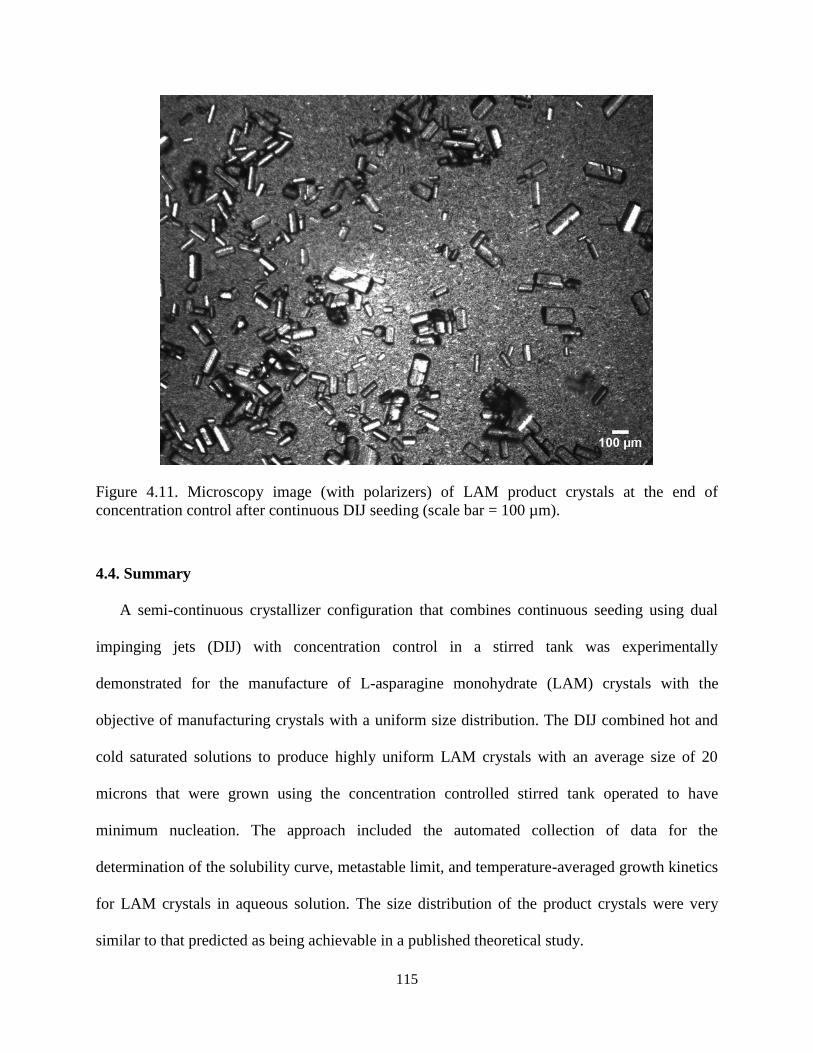
115

Figure 4.11. Microscopy image (with polarizers) of LAM product crystals at the end of

concentration control after continuous DIJ seeding (scale bar = 100 µm).

4.4. Summary

A semi-continuous crystallizer configuration that combines continuous seeding using dual

impinging jets (DIJ) with concentration control in a stirred tank was experimentally

demonstrated for the manufacture of L-asparagine monohydrate (LAM) crystals with the

objective of manufacturing crystals with a uniform size distribution. The DIJ combined hot and

cold saturated solutions to produce highly uniform LAM crystals with an average size of 20

microns that were grown using the concentration controlled stirred tank operated to have

minimum nucleation. The approach included the automated collection of data for the

determination of the solubility curve, metastable limit, and temperature-averaged growth kinetics

for LAM crystals in aqueous solution. The size distribution of the product crystals were very

similar to that predicted as being achievable in a published theoretical study.

116

The experiments confirm that greatly enhanced control of the crystal size distribution can be

achieved by using continuous seeding. In this approach, the DIJ crystallizer can be replaced by

any alternative technique for the continuous generation of seeds, as long as the rate of production

of seed crystals can be specified and the seed crystals are uniform and smaller than the desired

length resolution in the target product size distribution. Examples of alternative continuous

seeding equipment include vortex mixers and wet milling crystals from a previous batch. Dual-

impinging-jet and vortex mixers generate crystals of high uniformity of size and shape and

produce a higher overall crystal yield per batch than wet milling crystals from a previous batch.

By keeping a low supersaturation for the entire time history of each crystal, using wet milling

crystals from a previous batch as seed may generate product crystals of higher average molecular

purity.

117

5. MATHEMATICAL MODELING AND ANALYSIS OF COOLING

CRYSTALLIZATION WITHIN DUAL-IMPINGING JET MIXERS

5.1. Introduction

A key objective in pharmaceutical crystallization is to control the crystal size distribution

(CSD), to improve process efficiency and product quality. An effective way to improve the

control of CSD is through combining continuous seeding and growth with concentration control

[3]. One well-studied approach for continuous seeding is to combine solution and anti-solvent

streams in a dual-impinging jet (DIJ) mixer [3], [18], [20], [141], [145]. The underlying principle

is that, at appropriate flow rates, such a DIJ mixer can generate high-intensity micro-mixing of

fluids to quickly achieve a nearly spatially homogeneous composition of high supersaturation

before the onset of primary nucleation. An inexpensive DIJ mixer can be used to rapidly generate

a large amount of small crystals and remove any need for post-crystallization milling, which

simplifies the overall manufacturing process and avoids a potential route for the generation of an

undesirable polymorphic transformation [18], [141].

Rather than anti-solvent crystallization as commonly used, a cooling DIJ mixer was recently

demonstrated that combined hot and cold saturated solutions to generate small uniform seed

crystals [4]. All of the crystals from the cooling DIJ mixer were about 10 microns in length,

placing them in the approximate size range for direct application in inhalers [127]. Theoretically,

if the mixing was perfect (that is, solution concentrations and temperature were completely

mixed at the molecular scale in the mixer), the average supersaturation level would be too low to

nucleate crystals in a cooling DIJ mixer. The surprising result of nucleating crystals by

combining hot and cold saturated solutions in a DIJ mixer motivates the theoretical analysis of

the system in this article. Also, it would be useful at the early stage of research and development

118

to be able to quickly decide on compound-solvent combinations for DIJ mixers without time-

consuming trial-and-error as is currently used in process development [145]. These two

motivations lead to the main objectives of this article: (1) to improve the understanding of

primary nucleation in a free-surface cooling DIJ mixer, and (2) to develop design criteria for

cooling DIJ mixers to quickly rule out unsuitable compound-solvent combinations based on their

physicochemical properties. The primary emphasis is on the free-surface DIJ mixer configuration,

as it is simple and flexible to implement experimentally, although the results are relevant to other

DIJ mixer configurations.

A mathematical model is developed for crystallization in a DIJ mixer that combines

thermodynamics, kinetics, fluid dynamics, and heat and mass transfer. The mathematical model

is in the form of partial differential equations, simplified by exploiting symmetries and

employing scaling analysis. The theoretical analysis is supported with process simulation. The

two-dimensional energy and molar balances are solved using COMSOL input with an analytical

solution for the velocity field, to generate spatial distributions of temperature, concentration, and

supersaturation near the hot-cold interface within a cooling DIJ mixer. Compared to past work

with similar DIJ geometries (e.g., confined dual jets) that mainly used numerical simulations to

investigate flow and heat/mass transfer characteristics [3], [146]–[149], analytical expressions

are derived that are composed of simple functions that provide physical insight, which are

compared and supported with numerical results. Based on these analytical solutions of velocity,

temperature, and concentration spatial distributions, design criteria are developed to increase the

probability of primary nucleation in cooling DIJ mixers.

119

5.2. Theory

An analytical solution for the local flow field near the interface between two impinging jets

can be derived for a partial differential equation that is simplified by exploiting symmetries.

Assumptions are also presented and justified that are subsequently used to determine temperature

and concentration spatial distributions via analytical and numerical approaches.

5.2.1. Assumptions with justifications for deriving an analytical solution of the DIJ local

velocity field

A schematic of a DIJ mixer is in Fig. 5.1a, with an example set of operating parameters in

Table 5.1 and the analytically computed jet shape and example set of crystal results in Fig. 5.S1).

Nucleation can only occur very close to the interface between the two jets, since the

supersaturation is zero far from the interface and can only increase when the jets are close

enough to transfer heat and solute with each other. The region with the highest potential of

nucleation is of most interest, which is where the residence time is the longest, shown as an

orange box in Fig. 5.1a and referred to as ‘local’ here. Like some past studies that have

mathematically modeled similar geometries (e.g., single free-surface jet impingement on a

normal plane [150]–[152] or dual-impinging jets [153]), three assumptions are made to simplify

the analysis:

(i) The fluid is assumed to be irrotational and in steady state.

(ii) The flow is assumed to be axisymmetric and the two impinging jets are assumed to have

the same velocity field but in opposing directions.

(iii) The flow is assumed to be incompressible with constant values of density and viscosity.

120

(a)

121

(b)

Figure 5.1. (a) Schematic of a free-surface cooling DIJ mixer. The centerlines of hot (70°C, red,

right side) and cold (25°C, blue, left side) jets align. Both jets have the same volumetric flow rate,

so the impingement plane is a symmetry plane perpendicular to the jet centerline. (b) Streamlines

of the hot (red, right side) and cold jets (blue, left side) of the cooling DIJ mixer in (a), from the

analytical solutions of the flow field (5.3) and (5.4).

122

(a)

(b)

Figure 5.S1. (a) Liquid flows for a free-surface cooling DIJ mixer. Liquid from the cold jet (blue)

is on the left side and hot jet (red) on the right side. The flow rates from the two opposite jets are

the same, so the liquid flow at the impingement plane has circular cross-sections along the z axis.

(b) Microscope image (with polarizers) of LAM crystals generated by a DIJ mixer [4].

123

In a past study that demonstrated the nucleation of crystals by mixing hot and cold saturated

solutions [4], the Reynolds number indicates that the flow was in a laminar regime, which is the

regime of interest in this article. As an example, the Reynolds number at the exit, Re =𝜌𝑈𝐿

𝜇, is on

the order of 600 (using jet velocity 𝑣𝑧 and inner diameter 2𝑟0 , with density and dynamic

viscosity values in Table 5.2) or smaller [154]. No splattering is expected at such a low Reynolds

number [155].

Table 5.1. Experimental parameters for the cooling crystallization of L-asparagine monohydrate

(LAM, from Sigma Aldrich) in a free-surface DIJ mixer with aligned centreline.a

Physical properties Values

Molecular weight (g

mol) 150.13

Hot jet temperature, 𝑇ℎ𝑜𝑡 (°C) 70

Hot jet concentration, 𝑐ℎ𝑜𝑡 (g LAM

g water) 0.20 (slightly supersaturated)

Cold jet temperature, 𝑇𝑐𝑜𝑙𝑑 (°C) 25

Cold jet concentration, 𝑐𝑐𝑜𝑙𝑑 (g LAM

g water) 0.03 (saturated)

Area-average jet velocity, 𝑣𝑧 (m

s) 1.9 (or slightly higher)

Inner diameter of the jet nozzle, 2𝑟0 (μm) 254

Jet nozzle-to-interface distance, 𝑧0 (μm) 5000

The largest distance away from the centerline

at interface, 𝑅 (μm) 5000

aThe relation between the solubility of LAM in deionized (DI) water (𝑐𝑠𝑎𝑡, in g LAM/g water)

and temperature (𝑇 , in °C) is 𝑐𝑠𝑎𝑡 = 3.084 × 10−2 − 1.373 × 10−3𝑇 + 5.214 × 10−5𝑇2 [4].

Thus the solubility of LAM at the average mixing temperature (approximately 47.5°C, the

average of the temperatures of two streams) is about 0.08 g LAM/g water.

124

Table 5.2. Physical constants associated with the crystallization of glycine in water [6].

Physical properties Values

Density, ρ (kg

m3) 977.8 (70°C), 997.1 (25°C)

Dynamic viscosity, μ (N∙s

m2)

0.4 × 10−3 (70°C), 0.58 × 10−3

(47.5°C), 0.9 × 10−3 (25°C)

Thermal conductivity, k (mW

m∙K) 663.1 (70°C), 607.2 (25°C)

Heat capacity, 𝐶𝑝 (kJ

kg∙K) 4.19 (70°C), 4.18 (25°C)

thermal diffusivity, 𝛼 =𝑘

𝜌𝐶𝑝 (m2

s)

1.6 × 10−7 (70°C), 1.5 × 10−7

(25°C)

Diffusion coefficient of glycine in

water at infinite dilution, D (cm2

s)

1.05 × 10−5 (25°C)

Acceleration due to gravity, g (m

s2) 9.81

The axisymmetric assumption simplifies the analysis while being a good approximation for

free liquid (unconfined) opposed-jet DIJ configuration with a flow rate ratio of 1:1. The two jet

flows are considered symmetric with respect to the impingement plane (aka contact plane

between the low temperature/low concentration fluid and the high temperature/high

concentration fluid), with each side of the impingement plane similar to a circular jet

perpendicular to a flat surface of radius 𝑅 (Figs. 5.1ab). The symmetry allows the convenient use

of cylindrical coordinates (Fig. 5.1a), where the 𝑧 direction is that of jet centerline (positive

direction on the right side of the impingement plane), and the 𝑟 direction is perpendicular to 𝑧,

pointed outward from the centerline. The angular velocity parallel to the interface (𝑣θ) is zero.

The assumption of spatially uniform density simplifies the analysis while being a good

approximation for the impingement of two saturated solutions containing the same solute and

solvent. As a specific example, the density of LAM aqueous solution (or slurry with very small

125

amount of nuclei) in Table 5.1 is a weak function of temperature and concentration, so the

densities for cold, hot, or mixed LAM solutions/slurries are nearly identical, and of similar

magnitude as the density of water at the average temperature. Liquid flow with uniform density

is incompressible by definition. The dynamic viscosity of LAM aqueous solution is a stronger

function of solute concentration and temperature compared to density, but in this cooling DIJ

mixer, the viscosity difference between hot and cold streams does not affect the velocity field.

The temperature and concentration variations are small are do not affect the velocity field.

5.2.2. Analytical solution of the DIJ local velocity field

Under the assumptions, an analytical solution for the velocity field can be derived using

streamline analysis [153]. A derivation of the analytical solution is given here for completeness.

For an axisymmetric irrotational flow, the continuity equation can be written as 𝐸2𝜓 = 0, which

in cylindrical coordinates is

𝜕2𝜓

𝜕𝑟2−1

𝑟

𝜕𝜓

𝜕𝑟+𝜕2𝜓

𝜕𝑧2= 0 (5.1)

with boundary conditions

(i) No penetration: 𝑣𝑧(𝑟,0) = 0, so 1

𝑟

𝜕𝜓

𝜕𝑟(𝑟, 0) = 0

(ii) Symmetry: 𝜕𝜓

𝜕𝑧(0, 𝑧) = 0

Note that the symmetry plane z = 0, and the axis r = 0 are both streamlines.

Assuming a trial solution of the form 𝜓(𝑟, 𝑧) = 𝑓(𝑟)𝑔(𝑧), then 𝜕𝜓

𝜕𝑟= 𝑓′𝑔,

𝜕2𝜓

𝜕𝑟2= 𝑓′′𝑔,

𝜕𝜓

𝜕𝑧=

𝑓𝑔′,𝜕2𝜓

𝜕𝑧2= 𝑓𝑔′′ which can be plugged into the continuity equation (1) to give 𝑓′′𝑔 −

𝑓′𝑔

𝑟+

𝑓𝑔′′ = 0. Divide by 𝑓𝑔 on both sides to give

𝑓′′

𝑓−𝑓′

𝑟𝑓= −

𝑔′′

𝑔 (5.2)

126

Because the left-hand side is a function of r while the right-hand side is a function of z, both

sides must equal the same constant for the trial solution to be valid. For the simplest solution

satisfying this condition, begin with the constant 0, and solve for f and g [153].

For the right-hand side of (5.2), 𝑔′′ = 0 implies that 𝑔(𝑧) = 𝑏𝑧 + 𝑑 where 𝑏 and 𝑑 are

unknown constants. The boundary condition (i), 1

𝑟

𝜕𝜓

𝜕𝑟(𝑟, 0) = 0, implies that 𝑓′(𝑟)𝑔(0) = 0 for

all 𝑟, so 𝑑 = 0. For the left-hand side of (5.2), 𝑓′′

𝑓−𝑓′

𝑟𝑓= 0 implies that 𝑓′′ =

𝑓′

𝑟. Once way to

solve this equation is to insert the trial solution 𝑓 = ∑𝑎𝑛𝑟𝑛 into 𝑓′′ =

𝑓′

𝑟 and match terms, which

gives that 𝑓(𝑟) = 𝐵𝑟2. The boundary condition (ii), 𝜕𝜓

𝜕𝑧(0, 𝑧) = 0, implies that 𝑓(0)𝑔′(𝑧) = 0

for all 𝑧 , so 𝑓(0) = 0, which is satisfied by 𝑓(𝑟) = 𝐵𝑟2 . Hence the trial solution 𝜓(𝑟, 𝑧) =

𝑓(𝑟)𝑔(𝑧) = 𝑏𝐵𝑟2𝑧 satisfies the continuity equation (5.1) and both boundary conditions.

Having the fluid flow move towards the impingement plane and moving radially outward

implies that the one independent constant 𝐶 = −𝑏𝐵 > 0, so the stream function is 𝜓(𝑟, 𝑧) =

−𝐶𝑟2𝑧 [153]. Then the velocity components are

𝑣𝑟 = −1

𝑟

𝜕𝜓

𝜕𝑧= 𝐶𝑟 (> 0) (5.3)

𝑣𝑧 =1

𝑟

𝜕𝜓

𝜕𝑟= −2𝐶𝑧 (< 0 for 𝑧 > 0) (5.4)

As an example of the determination of the constant 𝐶, consider an experimental system with a

nozzle-to impingement plane distance of 𝑧 = 𝑧0 = 5 mm with a jet velocity along the jet

centerline of 𝑣𝑧0 = −1.9 m/s ; then the constant 𝐶 determined from equation (5.4) is 𝐶 =

−𝑣𝑧0

2𝑧0= 190 s−1.

127

5.2.3. Assumptions for calculation of temperature and concentration spatial fields

The temperature and concentration spatial distribution of liquid within a DIJ mixer is

calculated via both analytical and numerical approaches. The governing equations of heat and

mass transfer are

𝑣𝑟𝜕𝑇

𝜕𝑟+ 𝑣𝑧

𝜕𝑇

𝜕𝑧= 𝛼 [

1

𝑟

𝜕

𝜕𝑟(𝑟

𝜕𝑇

𝜕𝑟) +

𝜕2𝑇

𝜕𝑧2] (5.5)

𝑣𝑟𝜕𝑐

𝜕𝑟+ 𝑣𝑧

𝜕𝑐

𝜕𝑧= 𝐷 [

1

𝑟

𝜕

𝜕𝑟(𝑟

𝜕𝑐

𝜕𝑟) +

𝜕2𝑐

𝜕𝑧2] (5.6)

where 𝛼 is thermal diffusivity and D is the molecular diffusivity. The boundary conditions for

the temperature 𝑇(𝑟, 𝑧) are

𝜕𝑇

𝜕𝑟(0, 𝑧) = 0, 𝑇(𝑟, 𝑧0) = 𝑇ℎ𝑜𝑡 = 70℃, 𝑇(𝑟, −𝑧0) = 𝑇𝑐𝑜𝑙𝑑 = 25℃,

where some example temperature values are given. For the experimental configurations of

interest, the boundary conditions can be approximated to very high accuracy by

𝜕𝑇

𝜕𝑟(0, 𝑧) = 0, 𝑇(𝑟,∞) = 𝑇ℎ𝑜𝑡 = 70℃, 𝑇(𝑟, −∞) = 𝑇𝑐𝑜𝑙𝑑 = 25℃.

The corresponding boundary conditions for concentration 𝑐(𝑟, 𝑧) are

𝜕𝑐

𝜕𝑟(0, 𝑧) = 0 , 𝑐(𝑟,∞) = 𝑐ℎ𝑜𝑡 = 0.20 g LAM/g water , 𝑐(𝑟, −∞) = 𝑐𝑐𝑜𝑙𝑑 = 0.03 g LAM/

g water,

where some example concentration values are given.

For both the heat and mass transfer equations (5.5)–(5.6), assume that (i) the analytical

solution for the velocity field (5.3)–(5.4) is valid for the region of interest (Fig. 5.1a); (ii) the

air/liquid interfaces are assumed to be streamlines from the analytical solution for the velocity

field, starting from the edge of the inlet nozzles; (iii) the thermal diffusivity 𝛼 is approximated as

a constant. Assumption (iii) is a very accurate approximation for most systems; for example, 𝛼

128

varies by less than ±3.5% and the molecular diffusivity 𝐷 is constant over a wide range of

temperature for the system in Table 5.2.

All numerical simulations were made using the finite element method as implemented in

COMSOL V4.3, using two additional assumptions:

(i) Uniform temperature and concentration at the nozzle inlets

(ii) No mass or heat flux at the air/liquid interfaces (including very far from centerline)

The latter assumption holds because air is an excellent insulator. Analytical solutions involve

additional approximations described in the next section, where the analytical solutions are

derived and compared to the numerical simulations.


In this section, scaling analysis is applied to simplify the heat and mass transfer equations

from two dimensional (2D) to one dimensional (1D) so that relatively simple analytical solutions

can be derived. For the region of interest, the 1D analytical solutions is shown to be comparable

to the 2D numerical solutions except near the outlet flows. Based on the analytical solutions for

the temperature and concentration spatial fields, the supersaturation profile is analyzed for

regions of high potential for nucleation, which leads to design criteria for inducing nucleation in

cooling DIJ mixers.

5.3.1. Flow field and residence time

A good understanding of the velocity field is a prerequisite for the analysis of heat and mass

transfer. The liquid gets decelerated as it approaches the impingement plane (hot/cold interface)

(Fig. 5.1a). Then the fluid flow is diverted radially and accelerated, due to the fluid mass balance

and finite volume of the region of interest (orange box in Fig. 5.1a, with small r and z).

129

Equations (5.3) and (5.4) are analytical solutions for the velocity field that are valid for the

region of interest.

The liquid velocity in the z-direction is very small near the impingement plane, making the

residence time very large for liquid moving along the jet centerline (Fig. 5.1b). According to (5.3)

and (5.4), the residence time is infinity exactly on the jet centerline. In reality, liquid will not

flow exactly along the centerline (due to fluid elements having finite size, fluctuation, etc.), so

the residence time of a fluid element in the zone of interest is finite but still much longer than

any other area. Consider that, for liquid that starts at a distance of 𝑅1 from centerline, its

residence time up to radial position 𝑅 is 𝑡𝑟 = ∫𝑑𝑟𝑣𝑟⁄

𝑅

𝑅1=ln

𝑅

𝑅1

𝐶. Even slightly away from

centerline (e.g., 𝑅1 = 1 μm, much smaller than the jet nozzle diameter), the total residence time

decreases significantly (𝑡𝑟 = 44.8 ms).

5.3.2. Scaling analysis for the temperature and concentration spatial fields

The independence of the heat and mass transfer governing equations (5.5)–(5.6) enables

independent analysis of the heat and mass transfer. In the region of interest (Fig. 5.2a), the

temperature gradient along impingement plane (𝜕𝑇

𝜕𝑟) is negligible compared to along the

centerline (𝜕𝑇

𝜕𝑧), because the dominating direction of heat transfer (conduction) is from hot jet to

cold jet [153]. In this way, the two-dimensional energy conservation equation (5.5) can be

simplified to a one-dimensional equation,

𝑣𝑧𝜕𝑇

𝜕𝑧= 𝛼

𝜕2𝑇

𝜕𝑧2, (5.7)

along the centerline. This simplified equation (5.7) has the unique analytical solution

𝑇−𝑇𝑐𝑜𝑙𝑑

𝑇ℎ𝑜𝑡−𝑇𝑐𝑜𝑙𝑑=1

2(erf (

𝑧

𝑧𝑟𝑒𝑓ℎ) + 1) (5.8)

130

where 𝑧𝑟𝑒𝑓ℎ = √𝛼

𝐶. For the system in Table 5.2, 𝑧𝑟𝑒𝑓ℎ = 28.1 μm.

(a)

(b)

z

e𝛼,𝑧 =𝑣𝑧𝑧

𝛼

e ,𝑧 =𝑣𝑧𝑧

𝐷

e𝛼,𝑧 > 10 e𝛼,𝑧 0.1 0.1 e𝛼,𝑧 10

e ,𝑧 > 100.1 e ,𝑧 10 e ,𝑧 0.1

𝑧ℎ𝑣 =64 μm

𝑡ℎ𝑣 = 11.5 ms

𝑧ℎ𝑑 =6.4 μm

𝑡ℎ𝑣𝑑 = 6.06 ms𝑡ℎ𝑑 +∞

𝑧 𝑣 =5.3 μm

𝑡 𝑣 = 18 ms

𝑧 𝑑 =0.53 μm

𝑡 𝑣𝑑 = 6.06 ms𝑡 𝑑 +∞

𝑧0 =5000 μm

131

Figure 5.2. (a) Schematic for scaling analysis and defining the region of interest (only the hot jet

side is shown due to symmetry). The z axis is the jet centerline. The blue region (large r and z) is

air, which is not in the control volume. Temperatures and concentrations in the purple (large r,

small z) and brown (large z, small r) regions are approximately spatially uniform, serving as

boundary conditions (with values listed). The green region (small r, small z) of low velocity and

long residence time is of interest for nucleation. (b) Time and length scales of heat transfer (blue)

and mass transfer (pink) for liquid near to the jet centerline. The leftmost vertical line is the

impingement plane, which is in the direction of the r axis, and the rightmost vertical line is the

hot jet inlet (e.g., 5 mm away from the impingement plane). The residence time is denoted by t.

The length of each regime are not drawn to linear scale, so as to show the small regimes with low

Pe clearly (e.g., for heat transfer, 𝑧 ≤ 𝑧ℎ𝑣 = 6.4 μm). Example numerical values are given to

show how to calculate the length scales and residence times: When liquid is far away from the

impingement plane, the convection term dominates, 𝑈𝐿

𝛼≥ 10 , and 2𝐶𝑧2 ≥ 10𝛼 , which is

equivalent to 𝑧 ≥ 𝑧ℎ𝑣 = 64 μm. The residence time in this regime is 𝑡ℎ𝑣 = ∫𝑑𝑧(−𝑣𝑧)⁄

𝑧0

𝑧ℎ𝑣=

ln 𝑧0𝑧ℎ𝑣

2𝐶= 11.5 ms.

This analytical solution (5.8) is in the form of an error function, indicating a sharp

temperature gradient at the impingement plane (z = 0) and nonlinear along the z axis (Fig. 5.3c).

The error function also indicates temperature gradient drops to nearly zero at a distance of

around 𝑧𝑟𝑒𝑓ℎ from the impingement plane (supported by Figs. 5.3abc). For the region of interest

(near r = z = 0), the 1D analytical model (Fig. 5.3c) generates a very similar temperature profile

to the 2D simulation from COMSOL (Fig. 5.3b).

132

(a)

133

(b)

134

(c)

Figure 5.3. Temperature field: (a) computed by 2D simulation using the finite element method

implemented in COMSOL, at the full length range with the dimensions being the nozzle-to-

nozzle distance and the contact area diameter; (b) computed by 2D simulation using the finite

element method implemented in COMSOL, very near the impingement plane (small range of z,

as if ‘stretching’ Fig. 5.3a horizontally); (c) 1D analytical solution near the impingement plane,

with the streamlines shown in black. The temperature is indicated by color (red indicates high

temperature, and blue indicates low temperature), in unit of °C, and the black lines are

streamlines. The cold impinging jet is on the left, and the hot impinging jet on the right. The

white color shows air at room temperature. The edges between air and liquid are streamlines

starting from the edge of the inlet nozzles.

Similar scaling analysis applies for the concentration field, to give

𝑣𝑧𝜕𝑐

𝜕𝑧= 𝐷

𝜕2𝑐

𝜕𝑧2 (5.9)

135

Similar to the temperature equation, the simplified concentration equation (5.9) has the unique

analytical solution

𝑐−𝑐𝑐𝑜𝑙𝑑

𝑐ℎ𝑜𝑡−𝑐𝑐𝑜𝑙𝑑=1

2(erf (

𝑧

𝑧𝑟𝑒𝑓𝑚) + 1) (5.10)

where 𝑧𝑟𝑒𝑓 = √

𝐶. For the system in Table 5.2, 𝑧𝑟𝑒𝑓 = 2.35 μm.

The assumptions and governing equations for heat and mass transfer are very similar, and

heat transfer is decoupled from mass transfer, thus the analytical solutions for the temperature

and concentration profiles (5.8) and (5.10) are expected to be very similar. The trend of the

concentration variation is very similar to the temperature, with sharp gradient at the impingement

plane and nonlinear gradient along the z axis) as shown in Figs. 5.3 and 5.4. For the region of

interest, the 1D analytical model (Fig. 5.4c) generates a very similar concentration profile to the

2D simulation from COMSOL (Fig. 5.4b). Thus for assessing the potential of primary nucleation,

the analytical model is sufficiently accurate.

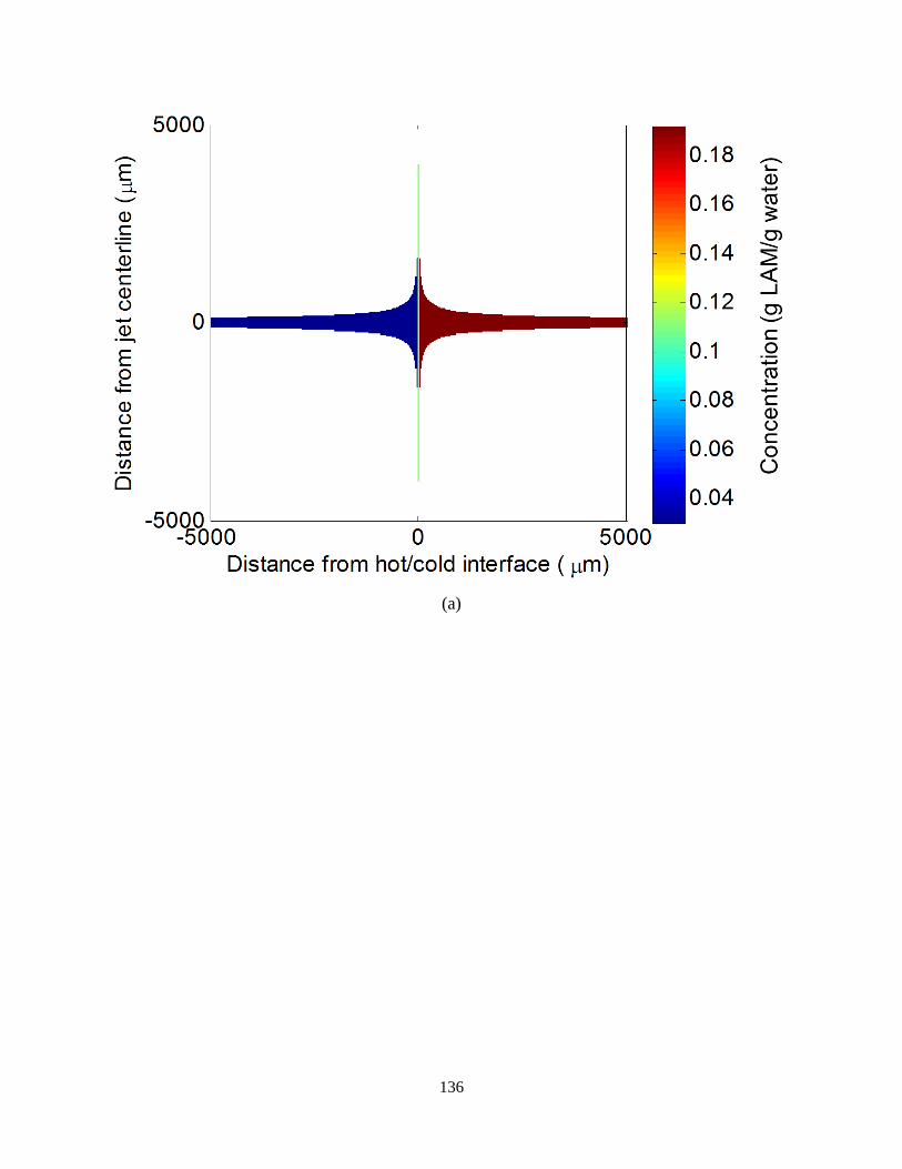
136

(a)

137

(b)

138

(c)

Figure 5.4. Concentration field: (a) computed by 2D simulation using the finite element method

implemented in COMSOL, at the full length range (same as in Fig. 5.3a); (b) computed by 2D

simulation using the finite element method implemented in COMSOL, very near the

impingement plane; (c) 1D analytical solution near the impingement plane, with the streamlines

shown in black. The concentration is indicated by color (red indicates high concentration, and

blue indicates low concentration), in unit of g LAM/g water. As in Fig. 5.3, the cold impinging

jet is on the left and the hot impinging jet on the right, and the edges between air and liquid are

streamlines starting from the edge of the inlet nozzles. The streamlines in 5.4c (black) are the

same as in Fig. 5.3c.

The difference between heat and mass transfer exists in the length scale along centerline (in

the example system, 𝑧𝑟𝑒𝑓ℎ = 28.1 μm for the temperature gradient change, and 𝑧𝑟𝑒𝑓 = 2.35 μm

for the concentration gradient change, as shown in Figs. 5.3–5.5), which comes from the

difference in heat and mass transfer rates. This difference can be indicated by the large value of

139

Lewis number (Le = 143), which is the ratio between thermal diffusivity and mass diffusivity

(α/D), and also the ratio of the Schmidt to the Prandtl numbers.

Figure 5.5. Temperature (blue) and concentration (red) profiles (solid lines) and edges of the

boundary layers (dashed lines), based on the 1D approximation (Figs. 5.3c and 5.4c) along the jet

centerline. The black line is the impingement plane.

5.3.3. Supersaturation spatial distribution and design criteria

The supersaturation spatial distribution was calculated (Figs. 5.5 and 5.6) based on the

analytical solutions for the temperature and concentration profiles in the region of interest (Figs.

5.3c and 5.4c). Due to the different rates of heat and mass transfer, the temperature of the hot

solution can drop towards the average temperature of the two solutions before its solution

concentration has significantly changed (Fig. 5.5). Supersaturation can be much higher than the

140

spatially averaged supersaturation (e.g., 0.035 g LAM/g water) close to the impingement plane at

the hot stream side (e.g., 0.10 g LAM/g water, from Fig. 5.6 or Region A in Fig. 5.7), where the

temperature is low (thus the solubility) while the concentration remains high (Figs. 5.5 and 5.7).

Between the impingement plane and Region A on the hot stream side (Region B in Fig. 5.7), the

residence time is very high (due to low velocity) with positive supersaturation (though not as

high as in Region A).

Figure 5.6. Supersaturation spatial field for the cooling DIJ mixer based on the 1D analytical

solutions (Figs. 5.3c and 5.4c). The streamlines in black are the same as in Figs. 5.3c and 5.4c,

with an additional streamline at the edges between air and liquid. The absolute supersaturation is

indicated by color (red indicates high supersaturation, and blue indicates low supersaturation), in

unit of g LAM/g water.

141

Figure 5.7. Concentration (blue curve), solubility (dark orange curve) and supersaturation (red

curve) profiles along the jet centerline based on the 1D analytical solutions. Region A (dark

purple) is the high supersaturation region, located between the thermal and concentration

boundary layers, closer to the latter. Region A is just above the metastable limit for cooling DIJ,

which is higher than the metastable limit in a cooling bath (dark green dashed line) due to

smaller volume and faster cooling rate. Region B (light purple) is a long residence time region

with slow velocity, located very near the jet centerline and the impingement plane.

As long as one of these two regions (high local supersaturation or long local residence time)

exists for the solute/solvent system at operating conditions, the nucleation of crystals in a DIJ

mixer may be feasible by combining hot and cold saturated solutions. This analysis leads to two

design considerations for preferentially nucleating in a cooling DIJ mixer:

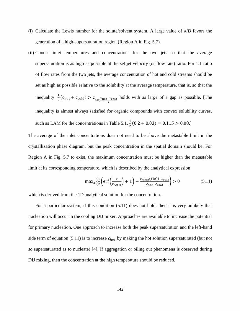
142

(i) Calculate the Lewis number for the solute/solvent system. A large value of α/D favors the

generation of a high-supersaturation region (Region A in Fig. 5.7).

(ii) Choose inlet temperatures and concentrations for the two jets so that the average

supersaturation is as high as possible at the set jet velocity (or flow rate) ratio. For 1:1 ratio

of flow rates from the two jets, the average concentration of hot and cold streams should be

set as high as possible relative to the solubility at the average temperature, that is, so that the

inequality 1

2(chot + ccold) > csat,Thot+Tcold

2 holds with as large of a gap as possible. [The

inequality is almost always satisfied for organic compounds with convex solubility curves,

such as LAM for the concentrations in Table 5.1, 1

2(0.2 + 0.03) = 0.115 > 0.08.]

The average of the inlet concentrations does not need to be above the metastable limit in the

crystallization phase diagram, but the peak concentration in the spatial domain should be. For

Region A in Fig. 5.7 to exist, the maximum concentration must be higher than the metastable

limit at its corresponding temperature, which is described by the analytical expression

max𝑧 {1

2(erf (

𝑧

𝑧𝑟𝑒𝑓𝑚) + 1) −

𝑐𝑚𝑒𝑡𝑎(𝑇(𝑧))−𝑐𝑐𝑜𝑙𝑑

𝑐ℎ𝑜𝑡−𝑐𝑐𝑜𝑙𝑑} > 0 (5.11)

which is derived from the 1D analytical solution for the concentration.

For a particular system, if this condition (5.11) does not hold, then it is very unlikely that

nucleation will occur in the cooling DIJ mixer. Approaches are available to increase the potential

for primary nucleation. One approach to increase both the peak supersaturation and the left-hand

side term of equation (5.11) is to increase 𝑐ℎ𝑜𝑡 by making the hot solution supersaturated (but not

so supersaturated as to nucleate) [4]. If aggregation or oiling out phenomena is observed during

DIJ mixing, then the concentration at the high temperature should be reduced.

143

A second approach to facilitate primary nucleation is to reduce the inlet jet velocity (but not

so low that the jets no longer impinge). The lower the jet velocity (thus a smaller 𝐶 in Eq. 5.3

and larger 𝑧𝑟𝑒𝑓 in Eq. 5.11), the longer the residence time.

Another approach is to increase the nozzle-to-impingement plane distance 𝑧0 to decrease 𝐶

and increase 𝑧𝑟𝑒𝑓 . The use of this approach is limited as longer distance will make the jet

centerline alignment more difficult. When using the second and third approaches, one has to be

reminded that 𝑐 𝑒𝑡𝑎 is also a function of z.

5.4. Summary

The primary nucleation of crystals by combining saturated hot and cold solutions in a cooling

DIJ mixer is analyzed, mostly in terms of derived analytical expressions for the velocity,

temperature, concentration, and supersaturation fields. The analytical solutions with a 1D

approximation of the temperature and concentration fields are accurate in the region of interest,

as confirmed by 2D numerical solutions by the finite element method.

Design criteria were developed to provide guidance for achieving or for ruling out conditions

not suitable for nucleation within a cooling DIJ mixer: (i) The Lewis number α/D >> 1, so that

the heat transfer is much faster than mass transfer, and (ii) The solute concentration on the hot

side of the interface should be higher than the metastable limit. Several approaches were

suggested to facilitate nucleation: (i) increase the concentration of the hot inlet stream, (ii)

decrease the inlet jet velocity; and (iii) increase the distance between the two jets. The design

criteria provide guidance, at the early stage of process development, for researchers to quickly

identify compound-solvent combinations that will not nucleate crystals within DIJ mixers, based

on their physicochemical properties.

144

The analysis of the cooling DIJ mixer may be extended to other free-surface DIJ mixer

configurations such as use of oblique angles between the inlet nozzles or flow rate ratios other

than 1:1. In the latter case, the symmetry analysis and flow field calculation will be different

[150], [152], [156], [157], which will, together with jet geometry (nozzle-to-interface distance)

[150], affect the constant 𝐶 in the velocity field expressions. The design criteria may also shed

light on analysis of other devices that generate small uniform-sized crystals through mixing hot

and cold streams, such as radial or coaxial mixers [7].

145

6. CONTINUOUS-FLOW TUBULAR CRYSTALLIZATION IN SLUGS

SPONTANEOUSLY INDUCED BY HYDRODYNAMICS

6.1. Introduction

Compared to batch and semibatch crystallizers, continuous-flow crystallizers have the

potential for higher reproducibility, process efficiency, and flexibility, as well as lower capital

and production cost [158]–[165]. Many continuous-flow crystallizer designs have been proposed

in recent years with the goals of improving pharmaceutical processing or control of crystal

product properties. For example, a continuous oscillatory baffled crystallizer has been proposed

that employs a piston to agitate the crystal slurry in a long pipe with baffles [159]. Such a

crystallizer can typically operate at lower shear rates than a single stirred-tank crystallizer, but is

limited to lower solids densities and effective viscosities and has limited degrees of freedom for

feedback control. An alternative design that employed laminar flow through a tube was

demonstrated for paracetamol crystallization, but it was warned that inducing crystallization in a

continuous slurry undergoing laminar flow in a tube by cooling through its walls was very prone

to clogging for some solute-solvent systems [163]. With the notion that the best control of crystal

size distribution should be obtained in a continuous-flow design that has negligible back-mixing

with a residence time distribution approaching that of an ideal plug-flow crystallizer, several

designs have tried to generate plug flow-like conditions. One continuous crystallizer design

consists of slurry flowing through a tube with Kenics-type static mixers through its length to

induce a more uniform velocity profile, with improved controllability obtained by introducing

antisolvent at multiple points along the tube length [158]. A tubular crystallizer less prone to

clogging ensured plug-flow behavior by forcibly segmenting the flow into liquid slugs separated

by an immiscible fluid [160]–[162], [166]. Due to recirculation, the slurry in each slug is mixed

146

even in the absence of any static mixer [167], [168]. However, the separation of immiscible

solvent takes additional process time when multiple liquids are used, and the slug production

devices, usually with more than three channels, were relatively complicated. A significant

advantage of all of these continuous-flow crystallizer designs is the lack of a stirring blade,

resulting in negligible attrition compared to the mixed-suspension mixed-product-removal

crystallizers widely employed for inorganic crystallization [169].

Most existing continuous-flow crystallizers are not specifically designed to provide many

degrees of freedom for the control of crystal shape and size distribution in the presence of

process disturbances and variations in crystallization kinetics associated with changes in

contaminant profile of the feed streams. An improved continuous-flow crystallizer design would

minimize operational problems while retaining the advantages of the best previous continuous

crystallizers. At the same time, there are advantages to continuous-flow designs that enable the

direct application of best-practices operations developed for the optimal control of batch and

semi-batch crystallization.

Towards these goals, this chapter describes the design and implementation of a slug-flow

crystallizer in which a multiphase mixture of liquid and gas in a tube spontaneously separates

into slugs of liquid or slurry separated by slugs of gas [170]–[176]. The slug-flow crystallizer has

all the advantages of a segmented-flow crystallizer, but does not require any specialized

equipment to induce slug formation and avoids the use of liquid/liquid separators. In the

proposed design, hydrodynamically stable slugs form spontaneously immediately upon the

contact of the liquid/slurry and the gas. The crystallizer is designed so that nucleation and growth

processes are decoupled to enhance the individual control of each phenomenon. This chapter

demonstrates the crystallizer design for a cooling crystallization, which is inherently more

147

challenging than antisolvent crystallization due to the latter's easier nucleation to generate seed

crystals.

6.2. Experimental methods and equipment setup

For better control of product CSD, the cooling crystallization process is decoupled into three

parts: crystal nucleation, slug formation, and crystal growth (Fig. 6.1). Nuclei were generated

within laminar flow by direct cooling, or within a coaxial or radial jet mixer by mixing hot and

cold solutions. The slurry stream containing nuclei acting as seed crystals are combined with an

air stream at flow rates selected to spontaneously form stable slugs. The motion of the slug

through the tube mixes the solution without requiring any of the stirring blades that cause

attrition in mixed-tank crystallizers. With each slug going through the tube with the same

residence time, and with no stirring blades to cause attrition, the crystals in the slugs would be

expected to grow to a large uniform size. The following experimental methods and equipment

setup were selected to demonstrate the feasibility of this process design.

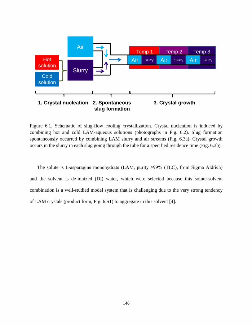
148

Figure 6.1. Schematic of slug-flow cooling crystallization. Crystal nucleation is induced by

combining hot and cold LAM-aqueous solutions (photographs in Fig. 6.2). Slug formation

spontaneously occurred by combining LAM slurry and air streams (Fig. 6.3a). Crystal growth

occurs in the slurry in each slug going through the tube for a specified residence time (Fig. 6.3b).

The solute is L-asparagine monohydrate (LAM, purity ≥99% (TLC), from Sigma Aldrich)

and the solvent is de-ionized (DI) water, which were selected because this solute-solvent

combination is a well-studied model system that is challenging due to the very strong tendency

of LAM crystals (product form, Fig. 6.S1) to aggregate in this solvent [4].

1. Crystal nucleation 3. Crystal growth

Temp 3Temp 2Temp 1

Slurry

Air

Air Slurry Air Slurry Air SlurryHot

solution

Cold

solution

2. Spontaneous

slug formation

149

Figure 6.S1. X-ray powder diffraction (XRPD) of LAM starting material (black) and product

crystals with nucleation from coaxial mixing (red, Fig. 6.8) and radial mixing (cyan, Fig. 6.11).

The X-ray equipment was a Bruker D8 diffractometer using Cu Kα radiation (40kV, 40 mA). The

angle (2θ) is from 10º to 41º, at a step size of 0.02º. The diffractogram was also compared to a

published diffractogram for LAM [177] to further confirm the crystal structure.

6.2.1 Nuclei generation

In a preliminary experiment, a high solids amount (high initial concentration, 0.16 g LAM/g

DI, as shown in Table 6.1) in each slug was used to demonstrate slug stability and CSD

improvement in the growth stage. In another preliminary experiment, a low solids amount (low

initial concentration, 0.09 g LAM/g DI, as shown in Table 6.1) was applied to facilitate in-line

and off-line imaging and to compare the nucleation obtained from coaxial and radial mixers, to

identify the most promising mixer type for subsequent experiments.

Crystals (coaxial nucleation)

Crystals (radial nucleation)

2θ ( )

Counts

LAM (starting material)

150

Table 6.1. Main experimental conditions for cooling nucleation.a

Experiment Preliminary Coaxial Radial

Concentration of hot stream (g LAM/g DI) 0.16 or 0.09 0.16 0.16

Concentration of cold stream (g LAM/g DI) N/A 0.02 0.02

Temperature of hot stream (°C) 65 or 44 65 66

Temperature of cold stream (°C) N/A 23 22

Pump for hot stream Peristaltic Peristaltic Peristaltic

Pump for cold stream N/A Peristaltic Syringe

Tubing for hot and cold streams Tygon Tygon BioPharm

Volumetric flow rate of hot stream (ml/min) 23.5 7.2 3.7

Volumetric flow rate of cold stream

(ml/min) N/A 6.8 3.3

Average velocity of hot stream (m/s) 0.05 0.02 0.02

Average velocity of cold stream (m/s) N/A 2.14 0.78

Nucleation site (mixer) Fig. 6.2a Fig. 6.2b Fig. 6.2c

Mixer inner diameter of hot inlet (mm) 3.1 3.1 2

Mixer inner diameter of cold inlet (mm) N/A 0.26 0.3

aThe preliminary experiment did not have a cold stream (the hot stream was directly cooled in an

ice bath, see Fig. 6.2a). ‘Peristaltic’ refers to a peristaltic pump (Masterflex pump drive 7521-40,

Easy Load II pump head with Model # 77200-50), and ‘Syringe’ refers to a syringe pump

(Model NE-4000, from New Era Pump Systems, Inc.). ‘Tygon’ refers to Masterflex Tygon

tubing, and ‘BioPharm’ refers to Masterflex BioPharm Plus platinum-cured silicone tubing. The

volumetric flow rate reported for the syringe pump was pre-calibrated, and the volumetric flow

rate reported for the peristaltic pump was estimated from the mass flow rate and temperature

measured right before or after the experiment. The average velocities are calculated from the

volumetric flow rates and mixer inner diameters.

The nucleation experimental conditions are listed in Table 6.1. For the radial mixing

experiment (LAM nuclei were generated by combining hot and cold saturation solutions (66°C,

0.16 g LAM/g DI; and 22°C, 0.02 g LAM/g DI, respectively) through a coaxial or radial jet

mixer (Figs. 6.2bc). This approach, first demonstrated in Ref. [4], contrasts with other

continuous tubular cooling crystallizations that require a separate batch crystallizer to produce

seed crystals to feed into the continuous crystallizer. Peristaltic pumps enable simple operation of

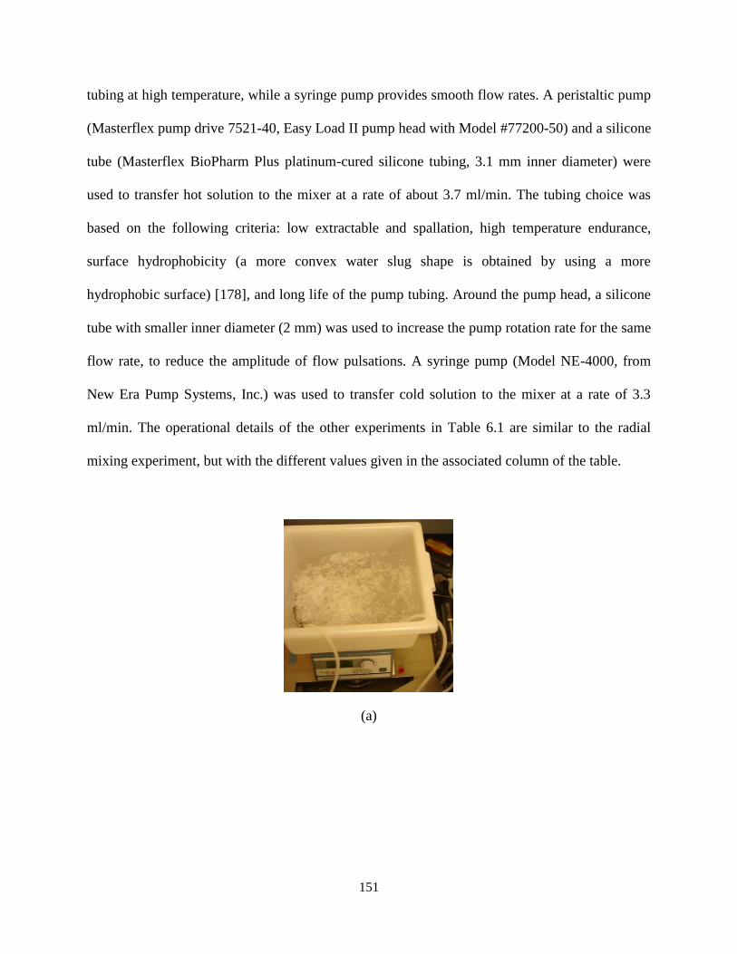
151

tubing at high temperature, while a syringe pump provides smooth flow rates. A peristaltic pump

(Masterflex pump drive 7521-40, Easy Load II pump head with Model #77200-50) and a silicone

tube (Masterflex BioPharm Plus platinum-cured silicone tubing, 3.1 mm inner diameter) were

used to transfer hot solution to the mixer at a rate of about 3.7 ml/min. The tubing choice was

based on the following criteria: low extractable and spallation, high temperature endurance,

surface hydrophobicity (a more convex water slug shape is obtained by using a more

hydrophobic surface) [178], and long life of the pump tubing. Around the pump head, a silicone

tube with smaller inner diameter (2 mm) was used to increase the pump rotation rate for the same

flow rate, to reduce the amplitude of flow pulsations. A syringe pump (Model NE-4000, from

New Era Pump Systems, Inc.) was used to transfer cold solution to the mixer at a rate of 3.3

ml/min. The operational details of the other experiments in Table 6.1 are similar to the radial

mixing experiment, but with the different values given in the associated column of the table.

(a)

152

(b)

(c)

Figure 6.2. Photographs and schematics of setup for nucleation induced by cooling: (a) laminar

flow tube; (b) coaxial mixer, the inner diameters of the two inlets are 3.1 mm (hot) and 0.26 mm

(cold), respectively; (c) radial mixer, the inner diameters of the two inlets are 2 mm (hot) and 0.3

mm (cold), respectively.

6.2.2 Slug generation

A key element in the proposed crystallizer design is to exploit the hydrodynamically stable

spontaneous generation of slugs. Many hydrodynamically stable flow regimes can occur when a

liquid and gas are combined in a tube [172], [173], [179], as shown in Fig. 6.3, with the stability

of the flow regimes determined by the ranges of inlet gas and liquid flow rates, tubing diameter,

and fluids properties. For crystallization from liquid solution, most of the flow regimes have

relatively poor spatial mixing of the liquid and allow liquid solution to remain close to the tube

Hot

solution

Cold

solution 65 C

23 C

Hot

solution

Cold

solution

65 C22 C

153

walls for long periods of time, which would encourage crystallization on the surface of the inner

tube (aka fouling), eventually clogging the tube. In contrast, slug flow has an internal circulation

of liquid [168] that limits the time that liquid stays close to the tube wall, which results in the

fluid dynamics within each slug operating like a small well-mixed crystallizer, with limited

fouling.

Figure 6.3. Schematics of hydrodynamically stable flow patterns of a gas (white color) and liquid

(blue color) mixture in a horizontal round tubing. The notations and images of the flow were

based on [179]. The air and liquid in slug flow can swap places depending on the affinity of the

liquid for the material on the inner surface of the tube, e.g., a water slug with a strongly

hydrophobic surface would appear as shown, with convex/roundish water slugs moving through

the tube. For a strongly hydrophilic surface with water as the liquid, the air slugs would be

convex. Regardless of surface affinities, the slugs become asymmetric at sufficiently high

velocities, as observed in Fig. 6.10.

Plug

Stratified

Wavy

Slug

Dispersed

bubble

Annular

154

Fig. 6.4a shows an experimental demonstration of the spontaneous formation of

hydrodynamically stable slugs after streams of slurry and air are passed through two branches of

a T mixer that had a similar inner diameter as the tubes. Stable slugs were maintained throughout

crystallization within each slug as it transports through the tubing to its exit. Air was transferred

to the mixer through the same peristaltic pump with dual pump heads, with flow oscillation

suppressed by offsetting their rollers, and a silicone tube with filters (pore sizes 3 μm and 0.2

μm) to prevent dust particles from getting into the tubes at the pump heads, and from contacting

slurry at the mixer, respectively. Within a large hydrodynamically stable regime [173] for slugs

in a 3.1 mm (inner diameter) tube, the length ratio of liquid and gas slugs was adjustable by

specifying the flow rates (or pump rotation rates) between slurry and air. A pump rpm ratio of

1:1 between hot solution and air was used to generate stable liquid slugs of similar sizes with all

aspect ratios of about 1 (Figs. 6.5ab). A horizontal wrapping of tubing around a bucket produced

hydrodynamically stable slugs with no combination or partitioning (Figs. 6.4b and 6.5ac).

(a)

LAM slurry

Air Slug

155

(b)

(c)

Figure 6.4. (a) Slug formation from streams of LAM slurry and air through a T mixer. The white

slugs contain LAM-aqueous slurry, and the transparent slugs are air. (b) Slurry-containing slugs

in the growth stage. The white slugs have high solids densities in this photograph. (c) Crystals in

the funnel after filtration obtained under operations of high solids density in each slug.

156

(a)

(b)

(c)

Figure 6.5. (a) Photograph of stable water slugs (aspect ratio about 1) separated by air slugs

(aspect ratio about 4) in packed silicone tube, with black background to improve contrast. (b)

Microscope image of water slug (slug in the center) and parts of air slugs (dark regions at both

GasWaterGas

157

edges) inside a silicone tube. The flow direction is from left to right. The front of the water slug

is less curved towards the flow direction than the back [171], as indicated from the thickness of

black shades at water/air interfaces. At higher flow rates, the shape of the water slug would be

dominated by the velocity (e.g., the drag from wall) rather than the hydrophobicity of the tubing

material. (c) Horizontal wrapping of silicone tube around a cylinder of the same diameter. The

photograph (a) is a close-up of (c) indicated by the edge of the black background.

6.2.3 Crystal growth

The growth experimental conditions were reported in Table 6.2. Again the radial mixing

experiment was used to justify the optimized design. The residence time after slug formation was

on the order of 5 minutes (to prevent generation of large amount of waste materials) in 15.2

meter of transparent hydrophobic silicone tube (Dow Corning Pharma-80 tubing, 3.1 mm inner

diameter). While the slugs were moving inside the silicone tube towards the exit, videos of them

were recorded under an in-line trinocular stereomicroscope (Microscope model #XV331AC20C,

from Cyber Scientific Corp.; Camera model #DFK 22BUC03, from The Imaging Source, LLC)

at 1 meter before the exit. After the slurry slugs exited the end of tube, they were collected one

by one into polystyrene wells (1.5 cm diameter, with the aqueous slugs covered with corn oil

after collection to suppress evaporation) for off-line imaging under the stereomicroscope.

Table 6.2. Experimental conditions for slug formation and growth by cooling.a

Experiment Preliminary Coaxial Radial

Pump for air stream Peristaltic Peristaltic Peristaltic

Pump rotation rate for air stream (rpm) 66 78 53.4 (dual head)

Tubing for slug movement Tygon Tygon Pharma-80

Tubing length (m) 15.2 15.2 15.2

Residence time (min) 1.7 2.9 5.0

Tube inner diameter (mm) 3.1 3.1 3.1

158

a‘Peristaltic’ and ‘Tygon’ are the same terms as in Table 6.1, and ‘Pharma-80’ refers to Dow

Corning Pharma-80 tubing. Residence time counts the time between when the hot solution

reaches the mixer and the exit of the tubing.

Crystallizations are generally more poorly mixed for higher solids densities. Since each slug

operates as a small well-mixed batch crystallizer, each slug will not be as well mixed for a high

solids density, in which case a fines dissolution step can be inserted into the crystal growth stage

to enlarge the final product crystals and reduce aggregation. The end stage of the preliminary

experiment had fines dissolution implemented as a fast heating of the slurry slugs to 50°C,

followed by going through 2 meters of tubing in each of the two temperature baths at 39°C and

22°C, respectively, and then to room temperature (Fig. 6.6). The temperature in each bath was

held constant using peristaltic pumps (same model as before) and hot and cold water reservoirs

(Fig. 6.6), controlled with Proportional-Integral controller tuned as in past studies [77]. The

temperature baths were not used in experiments with coaxial and radial mixing, as the product

crystals from those experiments were uniformly large without fines dissolution.

159

Figure 6.6. Photograph of the experimental setup with two temperature baths. The hot reservoir

is in a temperature-controlled bath (lower right), and the cold reservoir is in an ice bucket at the

lower left (not shown in the picture). Each of the two temperature baths at the top of the

photograph is controlled with only one dual-head peristaltic pump using Proportional-Integral

controllers tuned by Internal Model Control [180][181]. The dual head transfers both inlet and

outlet water, keeping the water level of the reservoir constant. The temperature of the slugs in the

tube increases or decreases relatively slowly due to the low thermal conductivity of the tube wall.

Only one temperature bath is needed for coarse temperature control; additional temperature baths

enable finer tuning of the spatial temperature profile of the slugs as they move through the tube.


Below are results and discussion from the experimental demonstrations of the slug-flow

crystallizer that include (1) a nonmonotonic spatial temperature profile to reduce aggregation and

promote growth, (2) a comparison of coaxial and radial mixers for in-situ generation of seed

crystals, and (3) the improvement of hydrodynamics for reducing variations in product quality.

Hot reservoir

Cold reservoir

Temperature baths

Peristaltic pumps

Controller box

160

6.3.1 Preliminary Experiment with Temperature Baths to Reduce Aggregation and

Promote Growth

After crystal nucleation in a tube under laminar flow (no mixer, Re number of about 150, see

Fig. 6.2a) and slug formation (Fig. 6.4a), the solids amount increases in the slugs as they move

along the tube length, indicated by the whiter color of slurry slugs (Fig. 6.4b, top) observed

visually after a short period of growth. Under high initial solute concentrations, the slugs were

able to carry 12.3 wt% crystals in the slurry, with crystals nearly occupying the whole slug (Fig.

6.4b) at a reasonably fast flow rate (Table 6.1). The total yield (mass of product crystals/total

mass of solute) from this preliminary experiment was 87%, close to the theoretical yield of a

batch cooling experiment from the same hot solution (87.5%).

The final product crystals after growth from laminar flow nucleation were small and

aggregated (Fig. 6.7a) (LAM has a strong tendency towards aggregation [4]). Heating followed

by natural cooling in the tubing after the first stage of growth was expected to increase the

crystal size [97][11], which was observed experimentally (Fig. 6.7b). Heating followed by

cooling in two baths of controlled temperatures was able to further increase the average crystal

size and reduce aggregation (Fig. 6.7c). Some small crystals remained, which motivated the

implementation of mixers to provide better control of nucleation, which is described next.

161

(a)

(b)

(c)

Figure 6.7. Microscope (with polarizers) images of product crystals from the preliminary

experiment (after laminar flow nucleation and growth in slugs) with (a) no heating; (b) heating to

50°C followed by natural cooling in the tubing; (c) heating to 50°C followed by two temperature

baths of set temperatures (39°C and 22°C).

162

6.3.2 Improved Hydrodynamics (e.g., Coaxial Mixing) to Improve Nucleation from

Laminar Flow

The product crystals obtained when nucleation was induced by coaxial mixing (Fig. 6.8)

improved the seed crystal quality (Fig. 6.9), with less aggregation and narrower CSD in each

slug, compared to nucleation in laminar flow (Figs. 6.7a and 6.S2). Crystals nucleated by

impinging a hot and a cold solution at an approximately equimolar ratio (Table 6.1) in a small

volume can be more uniform in size than crystals nucleated by cooling from a single solution, as

high local supersaturation (much higher than the average supersaturation) can be obtained near

the interface between hot and cold solutions when the thermal diffusivity is much larger than the

molecular diffusivity, as experimentally demonstrated and explained in a previous study [4]. By

combining two streams, the coaxial mixer also has more intense mixing than would be obtained

using one stream [182], with a Re ~ 600, which is expected to lead to more uniform-sized

crystals due to more crystals following a similar supersaturation trajectory in the crystal phase

diagram.

(a) (b)

1 mm 1 mm

163

(c) (d)

(e) (f)

Figure 6.8. Stereomicroscope images of product crystals with nucleation induced by coaxial

mixing in slug number (a) 21, (b) 81, (c) 141, (d) 201, (e) 261, (f) 311 (last slug). The scale bar =

1 mm. Detailed experimental conditions are provided in the coaxial experiment column in Tables

6.1 and 6.2.

Figure 6.9. Seed crystals generated by cooling nucleation in a coaxial mixer. The background is a

membrane filter with a pore size of 10 μm. The flow setups are in Fig. 6.2b. Although the

1 mm 1 mm

1 mm 1 mm

164

quantitative size of measured seed crystals is a combination of both nucleation and growth (with

local supersaturation not easy to measure at fine spatial resolution), this image does qualitatively

show the coaxial mixing reduces crystal aggregation and CSD width compared to laminar flow.

Figure 6.S2. Seed crystals generated by cooling nucleation in laminar flow. The starting

concentration is 0.09 g LAM/g DI (the rest of experimental conditions are also listed in Table 6.1,

in the preliminary experiment column). Although the quantitative size of measured seed crystals

is a combination of both nucleation and growth (with local supersaturation not easy to measure

within small-diameter tubes), this image does show the qualitative extent of aggregation.

While each slug obtained using the coaxial mixer (Fig. 6.8) had orders-of-magnitude less

aggregation than the preliminary experiment (Fig. 6.7), the crystal number per unit volume and

mean crystal size were variable from one slug to another (Fig. 6.8). With nucleation using a

coaxial mixer, the crystal size distribution was narrow within nearly each slug (Fig. 6.8a-f). The

variation in size of crystals before slug formation (Fig. 6.9) is similar to that within a single slug

(Fig. 6.8, Table 6.3), which suggests that the mixing within each slug (from internal recirculation

[176]) may be sufficient for maintaining a spatially uniform environment of temperature and

concentration after nucleation. In particular, if the mixing had not been sufficient, there would

have been a small number of crystals much larger than shown in Fig. 6.8, such as observed at the

bottom of poorly mixed batch crystallizers. The slug-to-slug variability suggested that some

165

experimental component was inducing oscillations to the experimental system, which led to an

effort to reduce flow pulsations from the peristaltic pumps (the experimental details are in

Sections 6.2.1 and 6.2.2, with the results discussed in next section).


using coaxial mixing (corresponding to the experimental results reported in Fig. 6.8).a

Slug number 21 81 141 201 261 311 All

Crystal image Fig.

6.8a

Fig.

6.8b

Fig.

6.8c

Fig.

6.8d

Fig.

6.8e

Fig.

6.8f

Figs.

6.8a-f

Crystal mean length

(µm) 442 205 231 279 341 318 303

Standard deviation,

length (µm) 100 62 107 81 132 96 99

Crystal mean width

(µm) 316 136 144 184 217 222 203

Standard deviation,

width (µm) 82 46 58 52 69 76 65

Correlation

coefficient of length

and width

0.43 0.21 0.72 0.58 0.65 0.54 0.52

Coefficient

of variation

in length

0.23 0.30 0.46 0.29 0.39 0.30 0.34

Coefficient of

variation in width 0.26 0.34 0.40 0.28 0.32 0.34 0.33

Mean aspect ratio 1.47 1.60 1.65 1.56 1.61 1.62 1.59

aThe correlation coefficient of length and width varies widely from slug to slug, which indicates

a wide range of crystal aspect ratios among different slugs (a correlation coefficient of length and

width of one would correspond to all crystals having exactly the same aspect ratio).

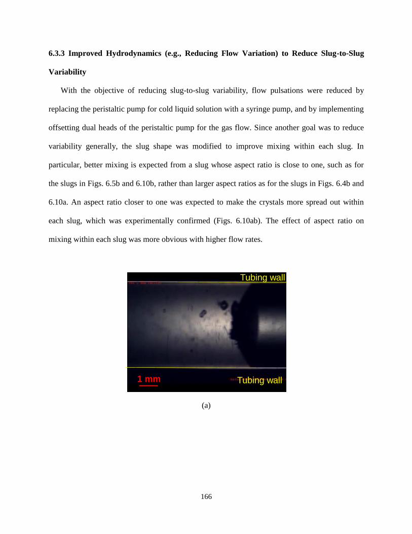
166

6.3.3 Improved Hydrodynamics (e.g., Reducing Flow Variation) to Reduce Slug-to-Slug

Variability

With the objective of reducing slug-to-slug variability, flow pulsations were reduced by

replacing the peristaltic pump for cold liquid solution with a syringe pump, and by implementing

offsetting dual heads of the peristaltic pump for the gas flow. Since another goal was to reduce

variability generally, the slug shape was modified to improve mixing within each slug. In

particular, better mixing is expected from a slug whose aspect ratio is close to one, such as for

the slugs in Figs. 6.5b and 6.10b, rather than larger aspect ratios as for the slugs in Figs. 6.4b and

6.10a. An aspect ratio closer to one was expected to make the crystals more spread out within

each slug, which was experimentally confirmed (Figs. 6.10ab). The effect of aspect ratio on

mixing within each slug was more obvious with higher flow rates.

(a)

Tubing wall

Tubing wall

1 mm

167

(b)

Figure 6.10. In-line stereomicroscope images of crystals in slugs with an aspect ratio of about (a)

4 (the slug is too long to fit into the image and is off to the left) and (b) almost 1. The scale bar ≈

1 mm. Relatively low solids density was used in both experiments so that the crystals could be

clearly imaged.

In addition, the coaxial mixer was replaced by a radial mixer, which provides much better

mixing for systems of comparable velocities [183]. Compared with the coaxial mixer (Fig. 6.8a-

f, Table 6.3), the radial mixer experiment produced similar mean aspect ratios and coefficient of

variations in length and width (Fig. 6.11a-f, Table 6.4) within each slug but larger mean crystal

dimensions and much lower slug-to-slug variability in mean crystal shape (i.e., aspect ratio). The

reduction of slug-to-slug variability of the product crystal shape in the radial mixer experiment

may be attributed to its reduced flow variability. The use of either coaxial or radial mixers

reduced aggregation by orders-of-magnitude compared to laminar flow (compare Figs. 6.8 and

6.11 with Fig. 6.7).


using radial mixing (corresponding to the experimental results reported in Fig. 6.11).a

Slug number 16-18 106-108 286-288 466-468 646-648 726-728 All

Tubing wall

Tubing wall1 mm

168

Crystal image Fig. 11a Fig. 11b Fig. 11c Fig. 11d Fig. 11e Fig. 11f Figs. 11a-f

Crystal mean

length (µm) 225 479 588 545 502 325 444

Standard

deviation,

length (µm)

103 146 202 160 181 92 152

Crystal mean

width (µm) 176 388 471 371 330 220 326

Standard

deviation,

width (µm)

90 152 181 146 173 71 142

Correlation

coefficient

of length

and width

0.92 0.86 0.90 0.81 0.74 0.76 0.83

Coefficient

of variation

in length

0.46 0.30 0.34 0.29 0.36 0.28 0.34

Coefficient

of variation

in width

0.51 0.39 0.39 0.39 0.52 0.32 0.43

aThe correlation coefficient of length and width is near one for each slug, which indicates a high

consistency in aspect ratio among different slugs (a correlation coefficient of length and width of

one would correspond to all crystals having exactly the same shape).

Table 6.S1. Mean size for seed crystals by cooling nucleation in laminar flow (corresponding to

the experimental results reported in Fig. 6.S2).a

Crystal image Fig. A2

Crystal mean length (µm) 48

Standard deviation, length (µm) 16

Crystal mean width (µm) 34

Standard deviation, width (µm) 15

Correlation coefficient of length and width 0.71

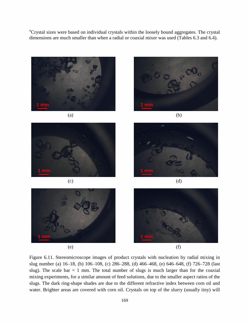
169

aCrystal sizes were based on individual crystals within the loosely bound aggregates. The crystal

dimensions are much smaller than when a radial or coaxial mixer was used (Tables 6.3 and 6.4).

(a) (b)

(c) (d)

(e) (f)

Figure 6.11. Stereomicroscope images of product crystals with nucleation by radial mixing in

slug number (a) 16–18, (b) 106–108, (c) 286–288, (d) 466–468, (e) 646–648, (f) 726–728 (last

slug). The scale bar = 1 mm. The total number of slugs is much larger than for the coaxial

mixing experiments, for a similar amount of feed solutions, due to the smaller aspect ratios of the

slugs. The dark ring-shape shades are due to the different refractive index between corn oil and

water. Brighter areas are covered with corn oil. Crystals on top of the slurry (usually tiny) will

1 mm 1 mm

1 mm 1 mm

1 mm 1 mm

170

tend to align at the interface between the oil and water. Detailed experimental conditions are

provided in the radial experiment column in Tables 6.1 and 6.2.

6.4. Summary

High-quality non-aggregating LAM crystals were produced in a continuous-flow cooling

crystallizer that employed alternating slugs of slurry and air moving through a tube with a

residence time of 2 to 5 minutes. The most novel aspects of the experimental system are that (1)

the crystals were nucleated by mixing hot and cold solutions in coaxial and radial mixers instead

of rapid cooling of a single solution [161], [163]

or feeding seeds obtained by batch

crystallization as done in many past continuous-flow cooling crystallization studies [184], and

(2) the slugs were spontaneously induced by hydrodynamic forces rather than by alternating the

feed between the two inlet flows [162]. As used in some past studies [160], [162], air was

employed as the separating fluid so that no liquid-liquid separations are needed downstream

from the crystallization.

The slugs generated spontaneously by hydrodynamic forces were highly uniform in size and

shape, and the slugs maintained that uniformity during crystallization as the slugs moved through

the tubular crystallizer. The slug size and shape were controllable by just changing the ratio of

volumetric flows rates of the inlet streams of slurry and air. An in-line imaging system was

employed to study the effect of slug aspect ratio, which confirmed the expectation that aspect

ratios near one produced better mixing than larger aspect ratios. The size uniformity of the

product crystals was enhanced by the introduction of the coaxial or radial jet mixers to improve

nucleation, and by employing in-line fines dissolution involving a nonmonotonic spatial

temperature profile (cooling, then heating, then cooling). The crystals grown from nuclei

produced in a radial mixer were more uniform in size compared to a coaxial mixer (compare

171

Figs. 6.11 and 6.8). The high degree of mixing and small size of each slug promoted high spatial

uniformity of temperature within each slug.

The experimental system can be used to simplify scale-up as the slug volume can be selected

as the same volume as the batch crystallizer used in bench-scale experiments for initial process

development. The residence time of 2 to 5 minutes is orders of magnitude shorter than the hours

taken in a stirred-tank crystallization, enabled by the much higher supersaturations that can be

generated within a slug while maintaining pure-growth conditions (the slug does not have a

stirring blade, which is the primary source of secondary nuclei and attrition particles in a mixed-

tank crystallizer). With further optimization, it is likely that the residence time could be brought

down to less than one minute. The slug-flow crystallizer has higher equipment utilization, as the

experimental system can generate crystals with narrow CSD with orders-of-magnitude higher

supersaturation and growth rate than obtainable using a stirred tank of the same volume. Instead

of scale-up, throughput can be further increased by scale-out, that is, using more slugs. While

scale-out has already been discussed many times in the literature for microscale systems [185],

this approach is much more industrially relevant for the length scales considered in this article, at

least for the typical production rate for a pharmaceutical compound.

172

7. INDIRECT ULTRASONICATION IN CONTINUOUS SLUG-FLOW

CRYSTALLIZATION

7.1. Introduction

In the pharmaceutical industry, the continuous generation of crystals of target size

distribution has the potential to simplify and/or reduce post-crystallization operations [186],

[187]. Crystal growth can be effectively controlled in a segmented/slug flow [5], [161], [167],

[184] that can be operated at low enough supersaturation to remove or greatly suppress

secondary nucleation [7], but the control of primary nucleation to generate the initial seed

crystals is more limited [188]. The joining of two streams in dual impinging jet, coaxial, or radial

micromixers has been demonstrated to produce seed crystals of uniform crystal size distribution

(CSD) [4], [7], but with a nucleation rate that depends on the liquid flow rate [4], [7], [18], [189].

In addition, the primary nucleation rate in many micromixer designs is very sensitive to inlet

flow alignment, and clogging can potentially occur in low velocity regions of the micromixers.

Ultrasonication is a technology for facilitating primary nucleation that has been useful in

various industrial and academic studies [21], [190]–[193]. The nucleation rate is a function of

ultrasonication parameters rather than just liquid flow rate, which provides extra degrees of

freedom for controlling the CSD. Ultrasonication-assisted crystallization seldom has clogging

problems, and actually has the opposite effect and is commonly used to remove particles from

containers for cleaning purposes [191]. Ultrasonication facilitates primary nucleation by

inducing acoustic cavitation in the liquid solution using high-frequency mechanical vibrations

from converters (connected sonication generator) [194].

The effect of ultrasonication operation parameters on crystallization process and crystal size

has been widely studied (e.g., see [191], [194]–[197] and citations there), which indicates that

173

the primary nucleation rate is sensitive to the power amplitude. This observation suggests that

the power amplitude is a good choice for control of the primary nucleation rate in a continuous

crystallization, which is the approach taken in this article.

In most studies of sonocrystallization, an ultrasonication probe (or horn) is in direct contact

with the liquid solution, which may induce secondary nucleation from metal contact or

contaminate the solution with metal after long time of use [191], [198]. The closer the liquid

solution is to the probe tip, the more ultrasonication energy per unit volume is transferred to the

solution, which is more spatially localized than when a sonication bath is used. This article uses

an ultrasonication horn and so has spatial localization of ultrasonication energy, but does not

directly contact the horn with the liquid solution. The ultrasonication probe tip is placed close

enough to the liquid solution so as to transfer significant power and induce primary nucleation,

but the tip and liquid solution are separated by a thin wall of plastic.

This article describes the implementation of this indirect ultrasonication-assisted primary

nucleation into a slug-flow cooling crystallizer to demonstrate rapid generation of a large amount

of crystals of larger size than the nuclei. The most closely related study is described in a high

quality paper published by Khinast and co-workers [5] that also employs indirect ultrasonication

and crystal nucleation and growth in a liquid solution flowing through a plastic tubing. The main

differences compared to [5] is that this article (1) uses an ultrasonic probe focused on a small

spatial location instead of placing a long tube in a sonication bath, (2) has order of magnitude

lower time in which the solution is in contact with ultrasonication, (3) uses a simpler

experimental system, and (4) uses horizontal instead of vertical coils of tubing. The pros and

cons of the different configurations are discussed at the end of the Results and Discussion section.

174

7.2. Experimental Materials and Methods

7.2.1. Materials. The solute is L-asparagine monohydrate (LAM, purity ≥99%, from Sigma

Aldrich), which forms crystals in the solvent, de-ionized (DI) water, that have a strong tendency

to aggregate [4].

7.2.2. Equipment. A slug-flow cooling crystallizer that decouples crystal nucleation, slug

formation, and crystal growth to allow control of the individual processes is shown in Fig. 7.1.

The main differences with past similar experimental systems are described in the Introduction

section.

(a)

Nucleation Growth

Sonication

bath

Air

Air Slurry Air Slurry Air SlurryHot

solution

Slug formation

Sonication

probe

175

(b)

Figure 7.1. (a) Schematic of the slug-flow cooling crystallizer with ultrasonication-assisted

nucleation. (b) Photograph of the experimental setup for ultrasonication. For maximum acoustic

energy transmitted from the ultrasonication probe to the solution inside silicone tubing, the probe

was placed in direct contact with the outer wall of silicone tubing, in water whose temperature

was kept constant. The water outside the tubing is used to draw thermal energy generated by the

ultrasonication away from the ultrasonication zone. The right background shows downstream

tubing whose temperature can be controlled by placement in a temperature-controlled water bath

[7].

The ultrasonication equipment for nucleation (Sonics® VCX 750,

Fig. 7.1b) is composed of a

generator, a converter, and a probe. Its generator has a working frequency of 20 kHz (widely

used for sonocrystallization studies, such as [191], [194], [195], [197], [199]) and an input

electric power of 750 Watt. The generator’s output power to the probe (Sonics® 630-0597)

increases as the amplitude increases (Table 7.1). Different amplitude values are set on the control

panel of the generator keypad. The probe tip diameter is 13 mm, which is large enough for the

center of the tip to cover the outer diameter (6 mm) of the silicone tubing.

176

Table 7.1. Experimental conditions and size and shape statistics for the ultrasonication-assisted

nucleation of seed crystals.a

Experiment number 1 2 3 4 5 6

Ultrasonication amplitude

setpoint (% maximum) 0 20 40 50 60 80

Ultrasonication power output

(Watts) 0 9 26 39 45 68

Image of generated

seed crystals

Fig.

7.2a

Fig.

7.2b

Fig.

7.2c

Fig.

7.2d

Fig.

7.2e

Fig.

7.2f

Mean length (µm) 34 53 42 24 20 20

Standard deviation, length (µm) 20 25 20 8 12 11

Standard error, length (µm) 2.3 1.6 1.3 0.5 0.8 0.9

Mean width (µm) 23 33 27 15 12 13

Standard deviation, width (µm) 18 18 16 6 8 8

Standard error, width (µm) 2.1 1.2 1.0 0.4 0.5 0.7

Coefficient of variation

in length 0.60 0.46 0.47 0.32 0.59 0.54

Coefficient of variation in width 0.79 0.54 0.56 0.41 0.65 0.65

Mean aspect ratio 1.87 1.84 1.69 1.83 1.82 1.66

aThe ultrasonicator vendor recommended that the ultrasonication be operated at or below a

setpoint of 80% maximum amplitude (the power reading takes a few seconds to reach stable

counts) continuously for our experimental time of 7 minutes or longer, thus continuous

ultrasonication at 100% maximum amplitude was not carried out. The power output was

calculated, as suggested by the vendor, to be the difference in power reading from the generator

screen between when probe is in solution and in air at the same amplitude. The mean length and

width are on a number basis. The standard errors are estimates of the uncertainties in the mean

width and length measurements determined using Monte Carlo sampling [200].

A T-mixer of 2.7 mm inner diameter was employed for slug generation with its two inlets

connected to the slurry and air. A peristaltic pump (Masterflex pump drive 7521-40, Easy Load

II pump head with Model #77200-50) was used to transfer hot slurry to the T-mixer through a

silicone tube (Masterflex BioPharm Plus platinum-cured silicone tubing, 3.1 mm inner diameter).

Filtered air at room temperature was transferred to the T-mixer through the same peristaltic

177

pump with dual pump heads (their rollers were offset to suppress flow oscillation). Downstream

of the T-mixer was 15.2 m of silicone tubing (Dow Corning Pharma-80 tubing, 3.1 mm inner

diameter) in room-temperature air used for downstream crystal growth [7].

Product crystals were characterized using a stereomicroscope (microscope model

#XV331AC20C from Cyber Scientific Corporation and camera model #DFK 22BUC03 from

The Imaging Source, LLC).

7.2.3. Procedure. Nucleation from a supersaturated liquid solution is induced by the

ultrasonication probe, which is followed by the formation of alternating slugs of air and slurry.

The inlet air and liquid flow rates are selected so that the slugs form spontaneously as the

hydrodynamically stable multiphase flow [1]. The supersaturated liquid solution was generated

by slowly cooling a solution of 0.09 g LAM/g DI from 52°C to 45°C, which was the temperature

of the bath in which the ultrasonication probe tip was placed (Fig. 7.1b). It is well established

that ultrasonication reduces the width of the metastable zone [190], and the resulting absolute

supersaturation of 0.015 g LAM/g DI at 45°C was selected to be lower than but close to the

unseeded metastable limit of cooling nucleation observed in past experiments [4] so that primary

nucleation is induced in the solution in front of the ultrasonication probe only when the probe is

in operation. The mass flow rate of the inlet liquid solution was 4.03 g/min, and the

ultrasonication residence time, that is, the time in which the liquid solution experiences

cavitation as observed by eye, is 3 seconds.

LAM nuclei generated from ultrasonication of supersaturated LAM solution traversed the

tubing for 0.7 m before slug formation. The distance of 0.7 m was selected to be long enough

that the presence of air downstream in the tube does not significantly dampen the energy

transferred to the liquid by the ultrasonication probe. The slug generation experimental setup is

178

the same as in a previous slug-flow experiment that used a radial mixer [7], except that the

experimental system in this article also uses slugs of water before and after the LAM-containing

slugs so that the pressure drops from the inlets to the tube outlet are nearly constant, so that the

velocities of the slugs are constant throughout the entire experiment instead of having time

periods during startup and shutdown with higher slug velocities. The crystals grow in the slugs of

slurry while traversing through the tubing, for a residence time of ~8.5 minutes between slug

formation and outlet. At the outlet of the tubing, slurry slugs were collected into polystyrene

wells (1.5 cm in diameter) for off-line imaging under the stereomicroscope [7].


The nuclei from indirect ultrasonication-assisted cooling nucleation at different amplitudes

are compared in Section 7.3.1 to determine good values for subsequent crystal growth in the

slug-flow crystallization process in Section 7.3.2.

7.3.1. Sonication-assisted continuous seed generation by cooling crystallization

For the same experimental system, inlet steams, and operating conditions, more nuclei were

formed with ultrasonication than without (see Fig. 7.2), which is consistent with past studies that

indicate a shortened induction time with ultrasonication [192]. For Experiment #1 at zero

ultrasonication power (Table 7.1), most of the membrane filter contained no crystals, which is

consistent with the average supersaturation of 0.015 g LAM/g DI being below the metastable

limit for this experimental system under these operating conditions (e.g., at 45°C) [4]. Fig. 7.2a

shows the few images that contained any crystals, with the seed crystals that were obtained

having over an order of magnitude variation in crystal size. Crystals were consistently nucleated

for the experiments with ultrasonication (Figs. 7.2b to 7.2f), with the crystals becoming smaller

with increasing ultrasonication power (Table 7.1, Figure 7.S1). Some abnormally large crystals

179

were observed for an ultrasonication power amplitude setpoint of 40% and less (Figs. 7.2a to

7.2c), but not for 50% and higher ultrasonication power (Figs. 7.2d to 7.2f), indicating that the

higher power should be used in this experimental system if the objective is to manufacture

uniformly sized crystals.

(a)

(b)

200 µm 200 µm

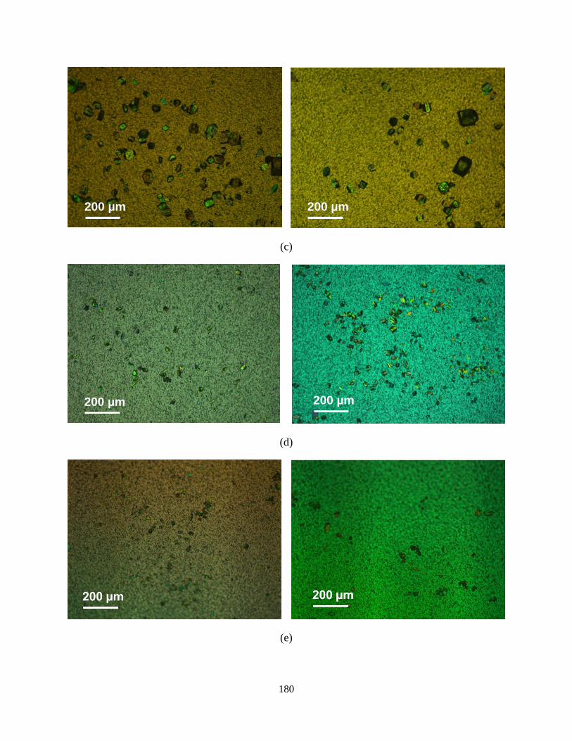
180

(c)

(d)

(e)

200 µm 200 µm

200 µm 200 µm

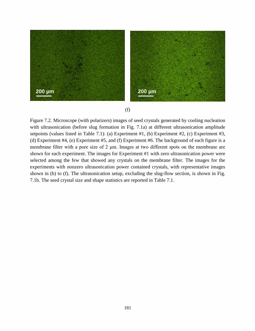
181

(f)

Figure 7.2. Microscope (with polarizers) images of seed crystals generated by cooling nucleation

with ultrasonication (before slug formation in Fig. 7.1a) at different ultrasonication amplitude

setpoints (values listed in Table 7.1): (a) Experiment #1, (b) Experiment #2, (c) Experiment #3,

(d) Experiment #4, (e) Experiment #5, and (f) Experiment #6. The background of each figure is a

membrane filter with a pore size of 2 μm. Images at two different spots on the membrane are

shown for each experiment. The images for Experiment #1 with zero ultrasonication power were

selected among the few that showed any crystals on the membrane filter. The images for the

experiments with nonzero ultrasonication power contained crystals, with representative images

shown in (b) to (f). The ultrasonication setup, excluding the slug-flow section, is shown in Fig.

7.1b. The seed crystal size and shape statistics are reported in Table 7.1.

200 µm200 µm

182

Figure 7.S1. Mean crystal length (blue circle) and width (red square) of seed crystals at various

ultrasonication power amplitudes. The power input and crystal length and width statistics (e.g.,

standard errors for the error bars) are reported in Table 7.1.

Ultrasonication increased the nuclei number and size uniformity (compare coefficient of

variations for Experiments 1 with 2 to 6 in Table 7.1). In the range of ultrasonication power

amplitude setpoint from 20% to 50%, higher ultrasonication power reduced the size of the seed

crystals (Figs. 7.2d to 7.2f, Table 7.1), which is consistent with sonocrystallization results

published for other compounds [194]–[197], [199]. This observation is consistent with a higher

ultrasonication power generating more bubbles that can act as direct or indirect sites for

nucleation, so that the solute crystalizes on a larger number of nuclei. Increased ultrasonication

183

power would be expected to increase the nucleation rate as long as the fluid inside and outside of

the tubing has a high enough mass flow rate and heat capacity to draw enough thermal energy

away from the ultrasonication zone. No clear trend was observed in the mean aspect ratio with

varying ultrasonication power (Table 7.1). The lowest coefficient of variations for the mean and

length of crystals occurred for ultrasonication power amplitude setpoint of 50%.

When the amplitude was 60% or 80% of the maximum (Figs. 7.2e and 7.2f), no evident

increases in the size uniformity were observed (Table 7.1). A possible explanation is that the

mass flow rate and heat capacity of the water were insufficient to draw enough thermal energy

away from the ultrasonication zone, so the local temperature increased, which increased the

solubility and lowered the supersaturation and nucleation rate per nucleation site, which

counteracted the increasing number of nucleation sites generated by the larger power input. The

images showed more aggregation for the 60% or 80% power amplitude, which could be

associated with increased particle-particle contacts resulting from increased cavitation. Based on

having the lowest coefficient of variation and low aggregation (Table 7.1), the ultrasonication

power amplitude setpoint of 50% was selected to provide seeds in subsequent slug-flow

crystallization experiments to manufacture product crystals.

7.3.2. Product crystals obtained after growth in slugs

The product crystals generated without ultrasonication showed a high variability in size (see

Fig. 7.3), which is consistent with the large variability in the size of crystals observed

immediately before the slug formation zone (Fig. 7.2a and associated caption). In contrast,

crystals from ultrasonication-assisted nucleation are much more uniform in size, while also

having a small degree of aggregation (Fig. 7.4), which is consistent with the higher size

uniformity of seed crystals continuously generated by ultrasonication (Fig. 7.2d). The unimodal

184

character of the crystal size distribution within each slug (Fig. 7.4) indicates that secondary

nucleation was small in the slug growth zone (Fig. 7.1), which is consistent with a past

observation [7] that recirculation within each slug provides sufficient mixing without requiring

the use of any mixing blade that would induce secondary nucleation [201]. This operation allows

the slug-flow crystallization to occur at orders of magnitude higher supersaturation and shorter

residence times than traditional crystallizers, without inducing significant secondary nucleation

[7].

(a)

1 mm

185

(b)

(c)

1 mm

1 mm

186

(d)

Figure 7.3. Stereomicroscope images of product crystals obtained by cooling nucleation without

ultrasonication followed by slug flow in a 15.2 m long tube (Experiment #1, with conditions in

Table 7.1) for slug numbers (a) 106–109, (b) 170–173, (c) 234–237, and (d) 298–301.

(a)

1 mm

1 mm

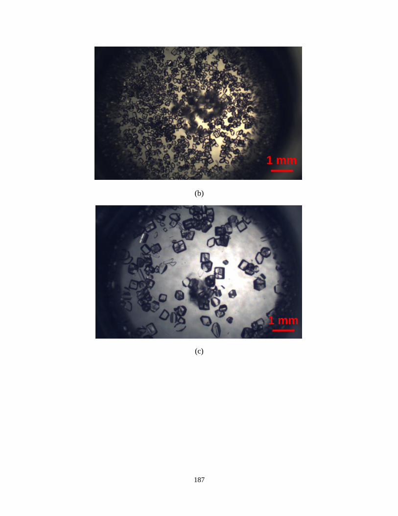
187

(b)

(c)

1 mm

1 mm

188

(d)

Figure 7.4. Stereomicroscope images of product crystals obtained at an ultrasonication power

amplitude setpoint of 50% followed by slug flow in a 15.2 m long tube (Experiment #4, with

conditions in Table 7.1) for slug numbers (a) 108–110, (b) 180–182, (c) 252–254, and (d) 324–

326. The product crystal size and shape statistics are reported in Table 7.1.

By first selecting the ultrasonication power amplitude for nucleation and then combining

with slug flow for crystal growth, product crystals were obtained with high size uniformity,

comparable with the best results from past experiments that combined ultrasonication with

subsequent growth in slugs [5]. Compared to a past study [5], this design requires simpler

experimental configuration for the slug-flow section, with no fines dissolution equipment, by

instead generating tunable seed size with spatially localized ultrasonication. The one ultrasonic

probe can be replaced by two ultrasonic probes in series along the tubing with only one probe in

ultrasonic mode and the other in rest mode, alternating between the modes of the two probes, to

extend their lifetime. This two-probe design does not significantly increase the complexity of

operation while facilitating scale-up, which is a typical problem in ultrasonication-associated

research [193].

1 mm

189

Table 7.2 compares the product crystals with seeds generated by spatially localized

ultrasonication with seeds generated using a radial micromixer for the same conditions as

Experiment 4. The product crystals generated by spatially localized ultrasonication are about

28%–35% smaller in mean length and width and have 15%–23% narrower crystal size

distributions based on smaller coefficients of variation. The mean aspect ratios are similar.

Table 7.2. Comparison of product crystals obtained using the nucleation conditions in

Experiment #4 of Table 7.1, with representative images of crystals in Fig. 7.4d, with product

crystals reported in [7].a

Nucleation method for slug flow

crystallization

Micromixer

(radial mixer)

Spatially localized

ultrasonication

Crystal image Fig. 11 in Ref [7] Fig. 7.4d

Mean length (µm) 444 321

Standard deviation, length (µm) 152 92

Standard error, length (µm) 13.0 6.4

Mean width (µm) 326 211

Standard deviation, width (µm) 142 69

Standard error, width (µm) 12.0 4.8

Coefficient of variation in length 0.34 0.29

Coefficient of variation in width 0.43 0.33

Mean aspect ratio 1.46 1.60

aThe mean width and length are on a number basis.

An advantage of using ultrasonication to generate nuclei is that the nucleation rate can be

manipulated by the ultrasonication power, which is a control variable that can be changed

independently from the mass flow rate through the tubular crystallizer. The nuclei generation rate

produced by a micromixer cannot be varied independently from the mass flow rates of the inlet

streams, regardless of whether the micromixer is radial, coaxial, or dual-impinging-jet type. In a

190

crystallizer that uses a micromixer, any operating variable that affects the nuclei generation rate

also affects the crystal production rate. The nuclei generation rate can be affected by changing

the design of the micromixer, but such equipment design parameters are then fixed during

operation.

The measured process yield (mass of product crystals/total inlet mass of solute) for the slug-

flow crystallizer with ultrasonication nucleation (73.8%) was close to the theoretical maximum

yield of a batch cooling crystallizer of the same initial concentrations (74.4%). In contrast to

employing micromixers that combine hot and cold inlet solutions, applying ultrasonication to a

single hot inlet solution in a continuous crystallizer can better approach the maximum yield

obtainable in a batch cooling crystallizer. For the slug-flow crystallizer, the maximum yield is

obtained by having a sufficiently long tube near the exit held at the desired exit cooling

temperature.

Another advantage of employing ultrasonication over micromixers is that the former is less

likely to clog. By using a consistent inner diameter of tubing in the slug-flow crystallizer, as in

Fig. 7.1, there are no constrictions available to induce clogging. Although the potential for

clogging in micromixers can be reduced by employing computational fluid dynamics simulations

to improve the micromixer design [17], a surer approach to avoid clogging is to replace the

micromixer by employing ultrasonication instead.

In a past study [5] that also employed indirect ultrasonication and crystal nucleation and

growth in a liquid solution flowing through a plastic tubing, primary nucleation occurs within 3

meters of plastic tubing placed inside of a sonication bath. The ultrasonication power per unit

volume varies widely with spatial position inside of a sonication bath, and having crystals

nucleate throughout a long tubing length means that the crystals leaving the sonication bath have

191

widely varying residence time and sizes. In particular, crystals that nucleate near the inlet of the

tubing enters the sonication bath have much more time to grow in size than crystals that nucleate

near the tubing outlet. This article uses a sonication probe tip focused in a small spatial location,

which enables primary nucleation to occur within a small section of tubing. The much narrower

side distribution that results is shown in Fig. 7.5, which compares product crystal size

distributions (CSDs) obtained in [5] with the product CSD obtained in this study.

Figure 7.5. Comparison of the cumulative product crystal size distribution on a mass basis

(labeled as Q3) obtained using the nucleation conditions in Experiment #4 of Table 7.1 (blue

square, with representative images of crystals in Fig. 7.4d) with product crystals reported in Fig.

4b of [3]. A mass basis was used to allow a direct comparison with the results of this manuscript

with Fig. 4b of [3]. The CSD for the product crystals in this manuscript is much narrower even

192

though the crystals are grown much larger and have a greater opportunity to be affected by

growth dispersion.

Another difference with a past study [5] is that the experimental system in this article uses a

simpler single solution stream instead of two streams, and so has one less pump and less tubing,

and does not require a mixer to combine two liquid streams. The experimental apparatus in [5]

has higher flexibility of operation but also has higher complexity. Instead of applying

ultrasonication to liquid solution for a half minute or more as in past studies [191], this article

subjects the liquid solution to ultrasonication for a much shorter time (e.g., a few seconds), to

reduce heating of the solution and widening of the CSD. Another difference with a past study [5]

is that this article uses horizontal coils of tubing, as in [7], instead of vertical coils. The

advantage of a horizontal coils is that the slug velocities are much more spatially uniform and the

advantage of vertical coils is that the crystals are forced to opposite sides of the slug during each

coil [184].

7.4. Summary

This article presents a slug-flow crystallizer that employs indirect ultrasonication to

continuously generate seed crystals. The ultrasonication probe is pressed up against a tube to

generate a localized ultrasonication zone within supersaturated solution in the tube for the

generation of crystal nuclei (Fig. 7.1). The ultrasonication design with an intermediate power

amplitude (Fig. 7.2d) continuously generated a larger number of uniform-sized seed crystals than

using micromixers or direct cooling in a past study [7], with minimal aggregation for a solute-

solvent combination known to have a high tendency towards aggregation. The ultrasonication

design also enables the seed generation rate to be varied in real time independently of the

193

production rate, providing an additional degree of freedom that can be used in feedforward

and/or feedback control design.

The ultrasonication-assisted nucleation design was implemented into a continuous slug-flow

crystallization process to generate uniform-sized product crystals within each slug (Fig. 7.4). The

ultrasonication-assisted slug-flow crystallizer was operated at sufficiently high supersaturation

for the entire crystallization to have a residence time of only ~8.5 min, without inducing

significant secondary nucleation. The overall production rate can be increased by operating at a

higher inlet mass flow rate while using a longer tube for crystal growth. The crystallizer can be

operated continuously for a long time period with equipment of similar complexity, such as by

placing two ultrasonic probes in series along the tubing with only one probe in ultrasonic mode

and the other in rest mode, alternating between the modes of the two probes, so as to extend the

probe lifetimes.

By increasing size uniformity, the indirect ultrasonication-assisted slug-flow crystallizer has

potential as a final crystallization step to produce crystals for use in direct compression tableting

[202], which would remove the need for milling and/or granulation steps from the drug product

manufacturing process chain. The use of indirect ultrasonication, as demonstrated for segmented-

flow crystallization in a past study [5], avoids the potential for sample contamination from

metals detaching from the ultrasonication equipment [198], which can be a significant concern in

pharmaceutical applications. The use of an ultrasonication probe, in contrast to an ultrasonication

bath used in a past study [5], allows the ultrasonication zone to be more spatially localized,

which can produce a narrower size distribution of seed crystals (Figure 7.S1, Table 7.2), and

hence narrower product crystal size distribution (Figure 7.5, Table 7.2).

194

8. CONCLUSIONS

My Ph.D. research is on the design and experimental validation of batch, semi-continuous,

and continuous crystallizers with controlled crystal shape and size distribution. Each project

started from the perspective of the whole system, whose configuration was designed based on

requirements for the final product quality. The system was then decomposed into subsystems that

were understood in detail before adding more functionality and complexity. One key strategy is

to exploit dual-impinging jets and multiphase flow to decouple nucleation and growth so that the

phenomena can be individually controlled. Another key strategy was to increase the degrees of

freedom in the dynamic operation of the crystallizers.

8.1. Enhancing control of crystal shape in a batch crystallizer

In Chapter 3, temperature-cycling experiments in batch crystallizers were designed to

alternate between positive and negative supersaturations to substantially change crystal shape

with only a small number of cycles. FBRM, a readily available commercial instrumentation, was

paired with ATR-FTIR spectroscopy and PVM to monitor the crystallization growth and

dissolution during the temperature-cycling experiment.

The growth and dissolution kinetics were estimated in a multidimensional population balance

model based on solute concentration and crystal dimension measurements. This model fitted the

experimental data with a limited number of parameters of small uncertainty. In addition, with the

estimated kinetic parameters, the model predicted the crystal size and shape distribution in a

different temperature-cycling experiment reasonably well. The results suggested that growth and

dissolution rates estimated in a single temperature-cycling experiment might be suitable for

designing a temperature-cycling protocol for optimizing the size and shape of the product

195

crystals. This method may be suitable for guiding the design of temperature-cycling experiments

to change particle shape in a wide variety of systems.

8.2. Enhancing control of CSD in a semi-continuous crystallizer

In Chapter 4, a semi-continuous crystallizer configuration that combines continuous seeding

using a dual impinging jet with growth rate control in a stirred tank was experimentally

demonstrated for the challenging problem of obtaining a target uniform product CSD. Uniform

seed crystals generated by DIJ were further grown to a desired size in the stirred tank with

suppressed nucleation. The construction of calibration models and the measurement of solubility

and metastable limit were obtained by an automated system that followed preset supersaturation

profiles by using feedback control. The experiments confirm that greatly enhanced control of the

crystal size distribution can be achieved by using continuous seeding. The same approach works

for other seed generation methods, such as a rotor stator or wet milling.

The results in Chapter 4 appear to be the first report of using a DIJ mixer to nucleate crystals

by cooling. Chapter 5 provides a physical explanation for this discovery that a cooling DIJ mixer

can generate small crystals of uniform size and shape by combining hot and cold saturated

solutions. The surprising result of nucleating crystals even at a low average supersaturation in a

DIJ mixer led to the analysis of the system that showed that nucleation was enabled by having

much faster energy transfer than mass transfer rates, resulting in a local supersaturation

sufficiently high to nucleate crystals.

The cooling DIJ mixer may work for some compounds that are not suitable with anti-solvent

operations. Design criteria were developed for cooling DIJ mixers to quickly identify suitable

compound-solvent combinations based on their physicochemical properties. These criteria could

196

save time and material by avoiding or reducing trial-and-error experiments, which is helpful at

the early stage of pharmaceutical process development (details in Chapter 5).

8.3. Enhancing control of CSD in a slug-flow continuous crystallizer

Chapter 6 presents the design of a slug-flow continuous crystallizer that exploits multi-phase

hydrodynamics to experimentally demonstrate the generation of large uniform crystals of LAM

in less than five minutes. Temperature and concentration are uniform inside each slug due to

recirculation, without using a mixing blade. Coaxial or radial mixers were developed to combine

liquid streams and continuously generate uniform seed crystals immediately upstream of the

growth zone. Scale up of slug flow crystallization process is straightforward—run the process

continuously and sustainably for a longer time. In addition, in-situ imaging and analysis methods

were developed for sub-millimeter flowing crystals inside millimeter-size moving slugs in

tubular crystallizers and a simple but effective syringe heater was designed to keep solutions at a

constant elevated temperature while pumping with minimum pulsing (details in Chapter 6).

An alternative nucleation design that can decouple nucleation and flow rates (thus product

rate) is to replace the micromixer with the application of an ultrasonication probe through the

tube wall. The nucleation design allows fast tuning of nuclei number by sonication power

amplitude. This sonication-assisted nucleation design may be implemented in other advanced

continuous slug-flow crystallizers to generate product crystals of target uniform size (details in

Chapter 7).

8.4. Overall conclusion and future perspective

Experimental validation has confirmed that the proposed designs suppress secondary

nucleation, attrition, and aggregation/agglomeration—phenomena that worsen the ability to

control the CSD but are dominant in most existing crystallizer designs. My experiments are

197

supported by mathematical modeling and analysis. The technologies and strategies developed for

successful pharmaceutical crystallization may shed light on advancing other areas such as

biopharmaceutical development and manufacturing.

198

REFERENCES

[1] S. Talreja, D. Y. Kim, A. Y. Mirarefi, C. F. Zukoski, and P. J. A. Kenis, “Screening and

optimization of protein crystallization conditions through gradual evaporation using a

novel crystallization platform,” J. Appl. Crystallogr., vol. 38, pp. 988–995, 2005.

[2] J. P. Greenstein and M. Winitz, Chemistry of the Amino Acids. Malabar, FL: Robert. E.

Krieger Publishing Company, 1986.

[3] X. Y. Woo, R. B. H. Tan, and R. D. Braatz, “Precise tailoring of the crystal size

distribution by controlled growth and continuous seeding from impinging jet

crystallizers,” CrystEngComm, vol. 13, no. 6, pp. 2006–2014, 2011.

[4] M. Jiang, M. H. Wong, Z. Zhu, J. Zhang, L. Zhou, K. Wang, A. N. Ford Versypt, T. Si, L.

M. Hasenberg, Y. E. Li, and R. D. Braatz, “Towards achieving a flattop crystal size

distribution by continuous seeding and controlled growth,” Chem. Eng. Sci., vol. 77, pp.

2–9, 2012.

[5] R. J. P. Eder, S. Schrank, M. O. Besenhard, E. Roblegg, H. Gruber-Woelfler, and J. G.

Khinast, “Continuous sonocrystallization of acetylsalicylic acid (ASA): Control of crystal

size,” Cryst. Growth Des., vol. 12, no. 10, pp. 4733–4738, 2012.

[6] W. M. Haynes, Ed., CRC Handbook of Chemistry and Physics, 95th ed. Boca Raton, FL:

CRC Press/Taylor and Francis, 2015.

[7] M. Jiang, Z. Zhu, E. Jimenez, C. D. Papageorgiou, J. Waetzig, A. Hardy, M. Langston,

and R. D. Braatz, “Continuous-flow tubular crystallization in slugs spontaneously induced

by hydrodynamics,” Cryst. Growth Des., vol. 14, no. 2, pp. 851–860, 2014.

[8] M. Jiang, X. Y. Woo, N. C. S. Kee, L. M. Goh, J. D. Tice, L. Zhou, R. B. H. Tan, C. F.

Zukoski III, M. Fujiwara, Z. K. Nagy, P. J. A. Kenis, and R. D. Braatz, “The role of

automatic process control in Quality by Design,” in Comprehensive Quality by Design for

Pharmaceutical Product Development and Manufacture, G. V Reklaitis, Ed. Chichester:

John Wiley & Sons Ltd., in press.

[9] J. De Calderon Anda, X. Z. Wang, and K. J. Roberts, “Multi-scale segmentation image

analysis for the in-process monitoring of particle shape with batch crystallisers,” Chem.

Eng. Sci., vol. 60, no. 4, pp. 1053–1065, 2005.

[10] M. Oullion, F. Puel, G. Févotte, S. Righini, and P. Carvin, “Industrial batch crystallization

of a plate-like organic product. In situ monitoring and 2D-CSD modelling: Part 1:

Experimental study,” Chem. Eng. Sci., vol. 62, no. 3, pp. 820–832, 2007.

[11] M. Jiang, X. Zhu, M. C. Molaro, M. L. Rasche, H. Zhang, K. Chadwick, D. M. Raimondo,

K.-K. K. K. Kim, L. Zhou, Z. Zhu, M. H. Wong, D. O’Grady, D. Hebrault, J. Tedesco,

199

and R. D. Braatz, “Modification of crystal shape through deep temperature cycling,” Ind.

Eng. Chem. Res., vol. 53, no. 13, pp. 5325–5336, 2014.

[12] M. Jiang, C. Gu, and R. D. Braatz., “Mathematical modeling and analysis of cooling

crystallization within dual impinging jet mixers,” final manuscript under review by

Novartis Pharmaceuticals.

[13] M. Jiang, C. D. Papageorgiou, J. Waetzig, A. Hardy, M. Langston, and R. D. Braatz,

“Indirect ultrasonication in continuous slug-flow crystallization,” Cryst. Growth Des., in

press. DOI: 10.1021/acs.cgd.5b00263.

[14] R. A. Lionberger, S. L. Lee, L. Lee, A. Raw, and L. X. Yu, “Quality by design: Concepts

for ANDAs,” AAPS J., vol. 10, no. 2, pp. 268–276, 2008.

[15] H. G. Brittain, Polymorphism in Pharmaceutical Solids, 2nd ed. London and New York:

Informa Healthcare, 2009.

[16] J. Bernstein, Polymorphism in Molecular Crystals. Chester, England: International Union

of Crystallography, 2008.

[17] X. Y. Woo, R. B. H. Tan, and R. D. Braatz, “Modeling and computational fluid

dynamics−population balance equation−micromixing simulation of impinging jet

crystallizers,” Cryst. Growth Des., vol. 9, no. 1, pp. 156–164, 2009.

[18] M. Midler Jr., E. L. Paul, E. F. Whittington, M. Futran, P. D. Liu, J. Hsu, and S. H. Pan,

“Crystallization Method to Improve Crystal Structure and Size,” U.S. Patent 5314506 A,

May 24, 1994.

[19] D. J. am Ende, T. C. Crawford, and N. P. Weston, “Reactive Crystallization Method to

Improve Particle Size,” U.S. Patent 6558435, May 6, 2003.

[20] R. Dauer, J. E. Mokrauer, and W. J. Mckeel, “Dual Jet Crystallizer Apparatus,” U.S.

Patent 5578279, Nov 26, 1996.

[21] M. D. Lindrud, S. Kim, and C. Wei, “Sonic Impinging Jet Crystallization Apparatus and

Process,” U.S. Patent 6302958 B1, Oct. 16, 2001.

[22] C. Lindenberg and M. Mazzotti, “Experimental characterization and multi-scale modeling

of mixing in static mixers. Part 2. Effect of viscosity and scale-up,” Chem. Eng. Sci., vol.

64, no. 20, pp. 4286–4294, 2009.

[23] H. Chiou, H.-K. Chan, R. K. Prud’homme, and J. A. Raper, “Evaluation on the use of

confined liquid impinging jets for the synthesis of nanodrug particles,” Drug Dev. Ind.

Pharm., vol. 34, no. 1, pp. 59–64, 2008.

200

[24] A. J. Mahajan and D. J. Kirwan, “Nucleation and Growth Kinetics of Biochemicals

Measured at High Supersaturations,” J. Cryst. Growth, vol. 144, no. 3–4, pp. 281–290,

1994.

[25] L. Goh, K. Chen, V. Bhamidi, G. He, N. C. S. Kee, P. J. A. Kenis, C. F. Zukoski, and R.

D. Braatz, “A stochastic model for nucleation kinetics determination in droplet-based

microfluidic systems,” Cryst. Growth Des., vol. 10, no. 6, pp. 2515–2521, 2010.

[26] M. J. Anderson, C. L. Hansen, and S. R. Quake, “Phase knowledge enables rational

screens for protein crystallization,” Proc. Natl. Acad. Sci. U. S. A., vol. 103, no. 45, pp.

16746–16751, 2006.

[27] C. L. Hansen, E. Skordalakest, J. M. Berger, and S. R. Quake, “A robust and scalable

microfluidic metering method that allows protein crystal growth by free interface

diffusion,” Proc. Natl. Acad. Sci. U. S. A., vol. 99, no. 26, pp. 16531–16536, 2002.

[28] A. J. Alvarez, A. Singh, and A. S. Myerson, “Polymorph screening: Comparing a semi-

automated approach with a high throughput method,” Cryst. Growth Des., vol. 9, no. 9,

pp. 4181–4188, 2009.

[29] K. Kim, I. S. Lee, A. Centrone, T. A. Hatton, and A. S. Myerson, “Formation of nanosized

organic molecular crystals on engineered surfaces,” J. Am. Chem. Soc., vol. 131, no. 51,

pp. 18212–18213, 2009.

[30] L. Li and R. F. Ismagilov, “Protein crystallization using microfluidic technologies based

on valves, droplets, and slipChip,” Annu. Rev. Biophys., vol. 39, no. 1, pp. 139–158, 2010.

[31] G. He, R. B. H. Tan, P. J. A. Kenis, and C. F. Zukoski, “Generalized phase behavior of

small molecules and nanoparticles,” J. Phys. Chem. B, vol. 111, no. 43, pp. 12494–12499,

2007.

[32] S. Talreja, P. J. A. Kenis, and C. F. Zukoski, “A kinetic model to simulate protein crystal

growth in an evaporation-based crystallization platform,” Langmuir, vol. 23, no. 8, pp.

4516–4522, 2007.

[33] S. Talreja, S. L. Perry, S. Guha, V. Bhamidi, C. F. Zukoski, and P. J. A. Kenis,

“Determination of the phase diagram for soluble and membrane proteins,” J. Phys. Chem.

B, vol. 114, no. 13, pp. 4432–4441, 2010.

[34] L. X. Yu, R. A. Lionberger, A. S. Raw, R. D’Costa, H. Wu, and A. S. Hussain,

“Applications of process analytical technology to crystallization processes,” Adv. Drug

Deliv. Rev., vol. 56, no. 3, pp. 349–369, 2004.

[35] H. B. Matthews and J. B. Rawlings, “Batch crystallization of a photochemical: Modeling,

control, and filtration,” AIChE J., vol. 44, no. 5, pp. 1119–1127, 1998.

201

[36] S. H. Chung, D. L. Ma, and R. D. Braatz, “Optimal seeding in batch crystallization,” Can.

J. Chem. Eng., vol. 77, no. 3, pp. 590–596, 1999.

[37] J.-P. Corriou and S. Rohani, “A new look at optimal control of a batch crystallizer,”

AICHE J., vol. 54, no. 12, pp. 3188–3206, 2008.

[38] D. Sarkar, S. Rohani, and A. Jutan, “Multi-objective optimization of seeded batch

crystallization processes,” Chem. Eng. Sci., vol. 61, no. 16, pp. 5282–5295, 2006.

[39] H. M. Hulburt and S. Katz, “Some problems in particle technology. A statistical

mechanical formulation,” Chem. Eng. Sci., vol. 19, no. 8, pp. 555–574, 1964.

[40] A. D. Randolph and M. A. Larson, Theory of Particulate Processes: Analysis and

Techniques of Continuous Crystallization, 2nd ed. New York: Academic Press, 1974.

[41] J. B. Rawlings, S. M. Miller, and W. R. Witkowski, “Model identification and control of

solution crystallization processes: a review,” Ind. Eng. Chem. Res., vol. 32, no. 7, pp.

1275–1296, 1993.

[42] R. D. Braatz and S. Hasebe, “Particle size and shape control in crystallization processes,”

in Sixth International Conference on Chemical Process Control, AIChE Symposium

Series, J. B. Rawlings, B. A. Ogunnaike, and J. W. Eaton, Eds. New York: AIChE Press,

2002, pp. 307–327.

[43] Z. K. Nagy and R. D. Braatz, “Distributional uncertainty analysis using power series and

polynomial chaos expansions,” J. Process Control, vol. 17, no. 3, pp. 229–240, 2007.

[44] M. W. Hermanto, M. S. Chiu, X. Y. Woo, and R. D. Braatz, “Robust optimal control of

polymorphic transformation in batch crystallization,” AIChE J., vol. 53, no. 10, pp. 2643–

2650, 2007.

[45] Z. K. Nagy and R. D. Braatz, “Worst-case and distributional robustness analysis of finite-

time control trajectories for nonlinear distributed parameter systems,” IEEE Trans.

Control Syst. Technol., vol. 11, no. 5, pp. 694–704, 2003.

[46] Z. K. Nagy and R. D. Braatz, “Open-loop and closed-loop robust optimal control of batch

processes using distributional and worst-case analysis,” J. Process Control, vol. 14, no. 4,

pp. 411–422, 2004.

[47] G. Févotte, “In situ Raman spectroscopy for in-line control of pharmaceutical

crystallization and solids elaboration processes: A review,” Chem. Eng. Res. Des., vol. 85,

no. 7, pp. 906–920, 2007.

[48] D. R. Thompson, E. Kougoulos, A. G. Jones, and M. W. Wood-Kaczmar, “Solute

concentration measurement of an important organic compound using ATR-UV

spectroscopy,” J. Cryst. Growth, vol. 276, no. 1–2, pp. 230–236, 2005.

202

[49] D. D. Dunuwila, L. B. Carroll, and K. A. Berglund, “An investigation of the applicability

of attenuated total reflection infrared spectroscopy for measurement of solubility and

supersaturation of aqueous citric acid solutions,” J. Cryst. Growth, vol. 137, no. 3–4, pp.

561–568, 1994.

[50] L. Feng and K. A. Berglund, “ATR-FTIR for determining optimal cooling curves for

batch crystallization of succinic acid,” Cryst. Growth Des., vol. 2, no. 5, pp. 449–452,

2002.

[51] P. Billot, M. Couty, and P. Hosek, “Application of ATR-UV spectroscopy for monitoring

the crystallisation of UV absorbing and nonabsorbing molecules,” Org. Process Res. Dev.,

vol. 14, no. 3, pp. 511–523, 2010.

[52] G. Févotte, “New perspectives for the on-line monitoring of pharmaceutical crystallization

processes using in situ infrared spectroscopy,” Int. J. Pharm., vol. 241, no. 2, pp. 263–

278, 2002.

[53] H. Gron, P. Mougin, A. Thomas, G. White, D. Wilkinson, R. B. Hammond, X. Lai, and K.

J. Roberts, “Dynamic in-process examination of particle size and crystallographic form

under defined conditions of reactant supersaturation as associated with the batch

crystallization of monosodium glutamate from aqueous solution,” Ind. Eng. Chem. Res.,

vol. 42, no. 20, pp. 4888–4898, 2003.

[54] T. Togkalidou, M. Fujiwara, S. Patel, and R. D. Braatz, “Solute concentration prediction

using chemometrics and ATR-FTIR spectroscopy,” J. Cryst. Growth, vol. 231, no. 4, pp.

534–543, 2001.

[55] J. Calderon De Anda, X. Z. Wang, X. Lai, and K. J. Roberts, “Classifying organic crystals

via in-process image analysis and the use of monitoring charts to follow polymorphic and

morphological changes,” J. Process Control, vol. 15, no. 7, pp. 785–797, 2005.

[56] X. Z. Wang, J. Calderon De Anda, and K. J. Roberts, “Real-time measurement of the

growth rates of individual crystal facets using imaging and image analysis: A feasibility

study on needle-shaped crystals of L-glutamic acid,” Chem. Eng. Res. Des., vol. 85, no. 7,

pp. 921–927, 2007.

[57] A. R. Parsons, S. N. Black, and R. Colling, “Automated measurement of metastable zones

for pharmaceutical compounds,” Chem. Eng. Res. Des., vol. 81, no. 6, pp. 700–704, 2003.

[58] R. Gunawan, L. David, M. Fujiwara, and D. B. Richard, “Identification of kinetic

parameters in multidimensional crystallization processes,” Int. J. Mod. Phys. B, vol. 16,

no. 1–2, pp. 367–374, 2002.

[59] S. W. Wong, C. Georgakis, G. D. Botsaris, K. Saranteas, and R. Bakale, “Online

estimation and monitoring of diastereomeric resolution using FBRM, ATR-FTIR, and

Raman spectroscopy,” Ind. Eng. Chem. Res., vol. 47, no. 15, pp. 5576–5584, 2008.

203

[60] K. Pöllänen, A. Häkkinen, S.-P. Reinikainen, M. Louhi-Kultanen, and L. Nyström, “A

study on batch cooling crystallization of sulphathiazole: Process monitoring using ATR-

FTIR and product characterization by automated image analysis,” Chem. Eng. Res. Des.,

vol. 84, no. 1, pp. 47–59, 2006.

[61] T. Togkalidou, R. D. Braatz, B. K. Johnson, O. Davidson, and A. Andrews, “Experimental

design and inferential modeling in pharmaceutical crystallization,” AIChE J., vol. 47, no.

1, pp. 160–168, 2001.

[62] J. Worlitschek and M. Mazzotti, “Model-based optimization of particle size distribution in

batch-cooling crystallization of paracetamol,” Cryst. Growth Des., vol. 4, no. 5, pp. 891–

903, 2004.

[63] P. A. Larsen, D. B. Patience, and J. B. Rawlings, “Industrial crystallization process

control,” IEEE Control Syst. Mag., vol. 26, no. 4, pp. 70–80, 2006.

[64] T. Togkalidou, H.-H. Tung, Y. Sun, A. T. Andrews, and R. D. Braatz, “Parameter

estimation and optimization of a loosely bound aggregating pharmaceutical crystallization

using in situ infrared and laser backscattering measurements,” Ind. Eng. Chem. Res., vol.

43, no. 19, pp. 6168–6181, 2004.

[65] F. Lewiner, G. Févotte, J. P. Klein, and F. Puel, “Improving batch cooling seeded

crystallization of an organic weed-killer using on-line ATR FTIR measurement of

supersaturation,” J. Cryst. Growth, vol. 226, no. 2–3, pp. 348–362, 2001.

[66] P. Barrett, B. Smith, J. Worlitschek, V. Bracken, B. O’Sullivan, and D. O’Grady, “A

review of the use of process analytical technology for the understanding and optimization

of production batch crystallization processes,” Org. Process Res. Dev., vol. 9, no. 3, pp.

348–355, 2005.

[67] M. Kempkes, J. Eggers, and M. Mazzotti, “Measurement of particle size and shape by

FBRM and in situ microscopy,” Chem. Eng. Sci., vol. 63, no. 19, pp. 4656–4675, 2008.

[68] H. M. Alatalo, H. Hatakka, M. Louhi-Kultanen, J. Kohonen, and S. P. Reinikainen,

“Closed-loop control of reactive crystallization. Part I: Supersaturation-controlled

crystallization of L-glutamic acid,” Chem. Eng. Technol., vol. 33, no. 5, pp. 743–750,

2010.

[69] Z. P. Chen, J. Morris, A. Borissova, S. Khan, T. Mahmud, R. Penchev, and K. J. Roberts,

“On-line monitoring of batch cooling crystallization of organic compounds using ATR-

FTIR spectroscopy coupled with an advanced calibration method,” Chemom. Intell. Lab.

Syst., vol. 96, no. 1, pp. 49–58, 2009.

[70] A. Borissova, S. Khan, T. Mahmud, K. J. Roberts, J. Andrews, P. Dallin, Z.-P. Chen, and

J. Morris, “In situ measurement of solution concentration during the batch cooling

204

crystallization of L-glutamic acid using ATR-FTIR spectroscopy coupled with

Chemometrics,” Cryst. Growth Des., vol. 9, no. 2, pp. 692–706, 2008.

[71] L. L. Simon, Z. K. Nagy, and K. Hungerbuhler, “Endoscopy-based in situ bulk video

imaging of batch crystallization processes,” Org. Process Res. Dev., vol. 13, no. 6, pp.

1254–1261, 2009.

[72] L. L. Simon, Z. K. Nagy, and K. Hungerbuhler, “Comparison of external bulk video

imaging with focused beam reflectance measurement and ultra-violet visible spectroscopy

for metastable zone identification in food and pharmaceutical crystallization processes,”

Chem. Eng. Sci., vol. 64, no. 14, pp. 3344–3351, 2009.

[73] L. L. Simon, K. A. Oucherif, Z. K. Nagy, and K. Hungerbuhler, “Bulk video imaging

based multivariate image analysis, process control chart and acoustic signal assisted

nucleation detection,” Chem. Eng. Sci., vol. 65, no. 17, pp. 4983–4995, 2010.

[74] K. Chow, H. H. Y. Tong, S. Lum, and A. H. L. Chow, “Engineering of pharmaceutical

materials: An industrial perspective,” J. Pharm. Sci., vol. 97, no. 8, pp. 2855–2877, 2008.

[75] Z. K. Nagy, J. W. Chew, M. Fujiwara, and R. D. Braatz, “Comparative performance of

concentration and temperature controlled batch crystallizations,” J. Process Control, vol.

18, no. 3–4, pp. 399–407, 2008.

[76] M. Fujiwara, Z. K. Nagy, J. W. Chew, and R. D. Braatz, “First-principles and direct

design approaches for the control of pharmaceutical crystallization,” J. Process Control,

vol. 15, no. 5, pp. 493–504, 2005.

[77] M. Fujiwara, P. S. Chow, D. L. Ma, and R. D. Braatz, “Paracetamol crystallization using

laser backscattering and ATR-FTIR spectroscopy: Metastability, agglomeration, and

control,” Cryst. Growth Des., vol. 2, no. 5, pp. 363–370, 2002.

[78] H. Grön, A. Borissova, and K. J. Roberts, “In-process ATR-FTIR spectroscopy for closed-

loop supersaturation control of a batch crystallizer producing monosodium glutamate

crystals of defined size,” Ind. Eng. Chem. Res., vol. 42, no. 1, pp. 198–206, 2003.

[79] V. Liotta and V. Sabesan, “Monitoring and feedback control of supersaturation using

ATR-FTIR to produce an active pharmaceutical ingredient of a desired crystal size,” Org.

Process Res. Dev., vol. 8, no. 3, pp. 488–494, 2004.

[80] N. C. S. Kee, R. B. H. Tan, and R. D. Braatz, “Selective crystallization of the metastable

alpha-form of L-glutamic acid using concentration feedback control,” Cryst. Growth Des.,

vol. 9, no. 7, pp. 3044–3051, 2009.

[81] N. C. S. Kee, P. D. Arendt, R. B. H. Tan, and R. D. Braatz, “Selective crystallization of

the metastable anhydrate form in the enantiotropic pseudo-dimorph system of L-

205

phenylalanine using concentration feedback control,” Cryst. Growth Des., vol. 9, no. 7,

pp. 3052–3061, 2009.

[82] Z. K. Nagy and R. D. Braatz, “Advances and new directions in crystallization control,”

Annu. Rev. Chem. Biomol. Eng., vol. 3, pp. 55–75, 2012.

[83] N. Doki, H. Seki, K. Takano, H. Asatani, M. Yokota, and N. Kubota, “Process control of

seeded batch cooling crystallization of the metastable α-form glycine using an in-situ

ATR-FTIR spectrometer and an in-situ FBRM particle counter,” Cryst. Growth Des., vol.

4, no. 5, pp. 949–953, 2004.

[84] X. Y. Woo, Z. K. Nagy, R. B. H. Tan, and R. D. Braatz, “Adaptive concentration control

of cooling and antisolvent crystallization with laser backscattering measurement,” Cryst.

Growth Des., vol. 9, no. 1, pp. 182–191, 2009.

[85] M. R. A. Bakar, Z. K. Nagy, A. N. Saleemi, and C. D. Rielly, “The impact of direct

nucleation control on crystal size distribution in pharmaceutical crystallization processes,”

Cryst. Growth Des., vol. 9, no. 3, pp. 1378–1384, 2009.

[86] X. Y. Woo, R. B. H. Tan, P. S. Chow, and R. D. Braatz, “Simulation of mixing effects in

antisolvent crystallization using a coupled CFD-PDF-PBE approach,” Cryst. Growth Des.,

vol. 6, no. 6, pp. 1291–1303, 2006.

[87] R. D. Braatz, R. C. Alkire, E. Seebauer, E. Rusli, R. Gunawan, T. O. Drews, X. Li, and Y.

He, “Perspectives on the design and control of multiscale systems,” J. Process Control,

vol. 16, no. 3, pp. 193–204, 2006.

[88] D. L. Ma, D. K. Tafti, and R. D. Braatz, “High-resolution simulation of multidimensional

crystal growth,” Ind. Eng. Chem. Res., vol. 41, no. 25, pp. 6217–6223, 2002.

[89] R. Gunawan, I. Fusman, and R. D. Braatz, “High resolution algorithms for

multidimensional population balance equations,” AIChE J., vol. 50, no. 11, pp. 2738–

2749, 2004.

[90] A. S. Michaels and A. R. Colville Jr., “The effect of surface active agents on crystal

growth rate and crystal habit,” J. Phys. Chem., vol. 64, no. 1, pp. 13–19, 1960.

[91] C. Sano, N. Nagashima, T. Kawakita, and Y. Iitaka, “Effects of additives on the crystal

habit of monosodium L-glutamate monohydrate,” J. Cryst. Growth, vol. 99, no. 1–4 pt 2,

pp. 1070–1075, 1990.

[92] I. Weissbuch, L. Addadi, M. Lahav, and L. Leiserowitz, “Molecular recognition at crystal

interfaces,” Science, vol. 253, no. 5020, pp. 637–645, 1991.

[93] D. L. Ma and R. D. Braatz, “Worst-case analysis of finite-time control policies,” IEEE

Trans. Control Syst. Technol., vol. 9, no. 5, pp. 766–774, 2001.

206

[94] F. Lewiner, G. Févotte, J. P. Klein, and F. Puel, “An online strategy to increase the

average crystal size during organic batch cooling crystallization,” Ind. Eng. Chem. Res.,

vol. 41, no. 5, pp. 1321–1328, 2002.

[95] H. Takiyama, K. Shindo, and M. Matsuoka, “Effects of undersaturation on crystal size

distribution in cooling type batch crystallization,” J. Chem. Eng. Japan, vol. 35, no. 11,

pp. 1072–1077, 2002.

[96] G. Yang, N. Kubota, Z. Sha, M. Louhi-Kultanen, and J. Wang, “Crystal shape control by

manipulating supersaturation in batch cooling crystallization,” Cryst. Growth Des., vol. 6,

no. 12, pp. 2799–2803, 2006.

[97] R. C. Snyder, S. Studener, and M. F. Doherty, “Manipulation of crystal shape by cycles of

growth and dissolution,” AIChE J., vol. 53, no. 6, pp. 1510–1517, 2007.

[98] J. Wan, X. Z. Wang, and C. Y. Ma, “Particle shape manipulation and optimization in

cooling crystallization involving multiple crystal morphological forms,” AIChE J., vol. 55,

no. 8, pp. 2049–2061, 2009.

[99] N. Bajcinca, V. de Oliveira, C. Borchert, J. Raisch, and K. Sundmacher, “Optimal control

solutions for crystal shape manipulation,” Comput. Aided Chem. Eng., vol. 28, pp. 751–

756, 2010.

[100] Z. K. Nagy, M. Fujiwara, and R. D. Braatz, “Monitoring and advanced control of

crystallization processes,” in Handbook of Industrial Crystallization, 3rd ed., A. Myerson

and D. Erdemir, Eds. Cambridge University Press, in press.

[101] M. A. Lovette, M. Muratore, and M. F. Doherty, “Crystal shape modification through

cycles of dissolution and growth: Attainable regions and experimental validation,” AIChE

J., vol. 58, no. 5, pp. 1465–1474, 2012.

[102] D. B. Patience and J. B. Rawlings, “Particle-shape monitoring and control in

crystallization processes,” AIChE J., vol. 47, no. 9, pp. 2125–2130, 2001.

[103] K. Lee, J. H. Lee, M. Fujiwara, D. L. Ma, and R. D. Braatz, “Run-to-run control of

multidimensional crystal size distribution in a batch crystallizer,” Proc. Am. Control

Conf., vol. 2, pp. 1013–1018, 2002.

[104] F. Puel, G. Févotte, and J. P. Klein, “Simulation and analysis of industrial crystallization

processes through multidimensional population balance equations. Part 1: A resolution

algorithm based on the method of classes,” Chem. Eng. Sci., vol. 58, no. 16, pp. 3715–

3727, 2003.

[105] H. Briesen, “Simulation of crystal size and shape by means of a reduced two-dimensional

population balance model,” Chem. Eng. Sci., vol. 61, no. 1, pp. 104–112, 2006.

207

[106] C. Y. Ma, X. Z. Wang, and K. J. Roberts, “Multi-dimensional population balance

modeling of the growth of rod-like L-glutamic acid crystals using growth rates estimated

from in-process imaging,” Adv. Powder Technol., vol. 18, no. 6, pp. 707–723, 2007.

[107] C. Y. Ma and X. Z. Wang, “Crystal growth rate dispersion modeling using morphological

population balance,” AIChE J., vol. 54, no. 9, pp. 2321–2334, 2008.

[108] C. Y. Ma, X. Z. Wang, and K. J. Roberts, “Morphological population balance for

modeling crystal growth in face directions,” AIChE J., vol. 54, no. 1, pp. 209–222, 2008.

[109] J. J. Liu, C. Y. Ma, Y. D. Hu, and X. Z. Wang, “Effect of seed loading and cooling rate on

crystal size and shape distributions in protein crystallization-A study using morphological

population balance simulation,” Comput. Chem. Eng., vol. 34, no. 12, pp. 1945–1952,

2010.

[110] J. J. Liu, C. Y. Ma, Y. D. Hu, and X. Z. Wang, “Modelling protein crystallisation using

morphological population balance models,” Chem. Eng. Res. Des., vol. 88, no. 4, pp. 437–

446, 2010.

[111] J. De Calderon Anda, X. Z. Wang, X. Lai, K. J. Roberts, K. H. Jennings, M. J. Wilkinson,

D. Watson, and D. Roberts, “Real-time product morphology monitoring in crystallization

using imaging technique,” AIChE J., vol. 51, no. 5, pp. 1406–1414, 2005.

[112] J. Eggers, M. Kempkes, and M. Mazzotti, “Measurement of size and shape distributions of

particles through image analysis,” Chem. Eng. Sci., vol. 63, no. 22, pp. 5513–5521, 2008.

[113] P. A. Larsen, J. B. Rawlings, and N. J. Ferrier, “An algorithm for analyzing noisy, in situ

images of high-aspect-ratio crystals to monitor particle size distribution,” Chem. Eng. Sci.,

vol. 61, no. 16, pp. 5236–5248, 2006.

[114] F. Puel, P. Marchal, and J. Klein, “Habit transient analysis in industrial crystallization

using two dimensional crystal sizing technique,” Chem. Eng. Res. Des., vol. 75, no. 2, pp.

193–205, 1997.

[115] X. Z. Wang, K. J. Roberts, and C. Ma, “Crystal growth measurement using 2D and 3D

imaging and the perspectives for shape control,” Chem. Eng. Sci., vol. 63, no. 5, pp. 1173–

1184, 2008.

[116] T. Togkalidou, H.-H. Tung, Y. Sun, A. Andrews, and R. D. Braatz, “Solution

concentration prediction for pharmaceutical crystallization processes using robust

chemometrics and ATR FTIR spectroscopy,” Org. Process Res. Dev., vol. 6, no. 3, pp.

317–322, 2002.

[117] D. L. Ma, D. K. Tafti, and R. D. Braatz, “Optimal control and simulation of

multidimensional crystallization processes,” Comput. Chem. Eng., vol. 26, no. 7–8, pp.

1103–1116, 2002.

208

[118] S. Qamar, S. Noor, Q. U. Ain, and A. Seidel-Morgenstern, “Bivariate extension of the

quadrature method of moments for batch crystallization models,” Ind. Eng. Chem. Res.,

vol. 49, no. 22, pp. 11633–11644, 2010.

[119] C. Sano, N. Nagashima, T. Kawakita, and Y. Iitaka, “Crystal and molecular structures of

monosodium L-glutamate monohydrate,” Anal. Sci., vol. 5, no. 1, pp. 121–122, 1989.

[120] M. Shoji, T. Eto, and H. Takiyama, “A kinetic study of the influence of modulated

undersaturation operation on crystal size distribution in cooling-type batch

crystallization,” J. Chem. Eng. Japan, vol. 44, no. 3, pp. 191–196, 2011.

[121] S. Qamar, S. Mukhtar, and A. Seidel-Morgenstern, “Efficient solution of a batch

crystallization model with fines dissolution,” J. Cryst. Growth, vol. 312, no. 20, pp. 2936–

2945, Jan. 2010.

[122] Z. K. Nagy, E. Aamir, and C. D. Rielly, “Internal fines removal using population balance

model based control of crystal size distribution under dissolution, growth and nucleation

mechanisms,” Cryst. Growth Des., vol. 11, no. 6, pp. 2205–2219, 2011.

[123] J. V Beck and K. J. Arnold, Parameter Estimation in Engineering and Science. New

York: Wiley, 1977.

[124] S. M. Miller and J. B. Rawlings, “Model identification and control strategies for batch

cooling crystallizers,” AIChE J., vol. 40, no. 8, pp. 1312–1327, 1994.

[125] J. N. Sherwood and R. I. Ristic, “The influence of mechanical stress on the growth and

dissolution of crystals,” Ind. Cryst., vol. 56, no. 7, pp. 2267–2280, 2001.

[126] L. M. Nagao, S. Lyapustina, M. K. Munos, and M. D. Capizzi, “Aspects of particle

science and regulation in pharmaceutical inhalation drug products,” Cryst. Growth Des.,

vol. 5, no. 6, pp. 2261–2267, 2005.

[127] N. Rasenack, H. Steckel, B. W. Muller, and B. W. Müller, “Micronization of anti-

inflammatory drugs for pulmonary delivery by a controlled crystallization process,” J.

Pharm. Sci., vol. 92, no. 1, pp. 35–44, 2003.

[128] B. Y. Shekunov and P. York, “Crystallization processes in pharmaceutical technology and

drug delivery design,” J. Cryst. Growth, vol. 211, no. 1–4, pp. 122–136, 2000.

[129] M. Alleso, F. Tian, C. Cornett, and J. Rantanen, “Towards effective solid form screening,”

J. Pharm. Sci., vol. 99, no. 9, pp. 3711–3718, 2010.

[130] D. J. am Ende and S. J. Brenek, “Strategies to control particle size during crystallization

processes,” Am. Pharm. Rev., vol. 7, no. 3, pp. 98–104, 2004.

209

[131] M. Descamps, J. F. Willart, E. Dudognon, and V. Caron, “Transformation of

pharmaceutical compounds upon milling and comilling: The role of Tg,” J. Pharm. Sci.,

vol. 96, no. 5, pp. 1398–1407, 2007.

[132] S.-Y. Lin, C.-H. Hsu, and W.-T. Ke, “Solid-state transformation of different gabapentin

polymorphs upon milling and co-milling,” Int. J. Pharm., vol. 396, no. 1–2, pp. 83–90,

2010.

[133] J. Linol, T. Morelli, M. N. Petit, and G. Coquerel, “Inversion of the relative stability

between two polymorphic forms of (±) modafinil under dry high-energy milling:

Comparisons with results obtained under wet high-energy milling,” Cryst. Growth Des.,

vol. 7, no. 9, pp. 1608–1611, 2007.

[134] F. Tian, H. Qu, M. Louhi-Kultanen, and J. Rantanen, “Insight into crystallization

mechanisms of polymorphic hydrate systems,” Chem. Eng. Technol., vol. 33, no. 5, pp.

833–838, 2010.

[135] E. Aamir, Z. K. Nagy, and C. D. Rielly, “Optimal seed recipe design for crystal size

distribution control for batch cooling crystallisation processes,” Chem. Eng. Sci., vol. 65,

no. 11, pp. 3602–3614, 2010.

[136] S. Rohani, S. Horne, and K. Murthy, “Control of product quality in batch crystallization of

pharmaceuticals and fine chemicals. Part 2: External control,” Org. Process Res. Dev.,

vol. 9, no. 6, pp. 873–883, 2005.

[137] C. Wibowo, W. C. Chang, and K. M. Ng, “Design of integrated crystallization systems,”

AIChE J., vol. 47, no. 11, pp. 2474–2492, 2001.

[138] J. D. Ward, D. A. Mellichamp, and M. F. Doherty, “Choosing an operating policy for

seeded batch crystallization,” AIChE J., vol. 52, no. 6, pp. 2046–2054, 2006.

[139] N. C. S. Kee, P. D. Arendt, L. M. Goh, R. B. H. Tan, and R. D. Braatz, “Nucleation and

growth kinetics estimation for L-phenylalanine hydrate and anhydrate crystallization,”

CrystEngComm, vol. 13, pp. 1197–1209, 2011.

[140] G. X. Zhou, M. Fujiwara, X. Y. Woo, E. Rusli, H.-H. Tung, C. Starbuck, O. Davidson, Z.

Ge, and R. D. Braatz, “Direct design of pharmaceutical antisolvent crystallization through

concentration control,” Cryst. Growth Des., vol. 6, no. 4, pp. 892–898, 2006.

[141] B. K. Johnson and R. K. Prud’homme, “Chemical Processing and Micromixing in

Confined Impinging Jets,” AIChE J., vol. 49, no. 9, pp. 2264–2282, 2003.

[142] R. J. Farrell and Y.-C. Tsai, “Modeling, simulation and kinetic parameter estimation in

batch crystallization processes,” AIChE J., vol. 40, no. 4, pp. 586–593, 1994.

210

[143] Y. Qiu and Å. Rasmuson, “Estimation of crystallization kinetics from batch cooling

experiments,” AIChE J., vol. 40, no. 5, pp. 799–812, 1994.

[144] D. J. W. Grant, M. Mehdizadeh, A. H.-L. Chow, and J. E. Fairbrother, “Non-linear van’t

Hoff solubility-temperature plots and their pharmaceutical interpretation,” Int. J. Pharm.,

vol. 18, no. 1–2, pp. 25–38, 1984.

[145] H.-H. Tung, E. L. Paul, M. Midler, and J. A. McCauley, Crystallization of

Pharmaceuticals: An Industrial Perspective. Hoboken, NJ: Wiley, 2009.

[146] Y. Wu, Impinging Streams: Fundamentals, Properties, Applications. New York: Elsevier,

2007.

[147] Y. Liu and R. O. Fox, “CFD Predictions for Chemical Processing in a Confined

Impinging-Jets Reactor,” AIChE J., vol. 52, no. 2, pp. 731–744, 2006.

[148] D. L. Marchisio, L. Rivautella, and A. A. Barresi, “Design and scale-up of chemical

reactors for nanoparticle precipitation,” AIChE J., vol. 52, no. 5, pp. 1877–1887, 2006.

[149] S. M. Hosseinalipour and A. S. Mujumdar, “Flow and thermal characteristics of steady

two dimensional confined laminar opposing jets: Part I. Equal jets,” Int. Commun. Heat

Mass Transf., vol. 24, no. 1, pp. 27–38, 1997.

[150] B. W. Webb and C. F. Ma, “Single-phase liquid jet impingement heat transfer,” Adv. Heat

Transf., vol. 26, pp. 105–217, 1995.

[151] D. J. Phares, G. T. Smedley, and R. C. Flagan, “The inviscid impingement of a jet with

arbitrary velocity profile,” Phys. Fluids, vol. 12, no. 8, pp. 2046–2055, 2000.

[152] C. duP Donaldson and R. S. Snedeker, “ Study of free jet impingement. Part 1. Mean

properties of free and impinging jets,” J. Fluid Mech., vol. 45, pp. 281–319, 1971.

[153] W. M. Deen, Analysis of Transport Phenomena, 2nd ed. New York: Oxford University

Press, 2012.

[154] J. M. Bergthorson, K. Sone, T. W. Mattner, P. E. Dimotakis, D. G. Goodwin, and D. I.

Meiron, “Impinging laminar jets at moderate Reynolds numbers and separation distances,”

Phys. Rev. E, vol. 72, no. 6, p. 66307, 2005.

[155] J. H. Lienhard V., “Heat Transfer by Impingement of Circular Free-Surface Liquid Jets,”

in 18th National and 7th ISHMT-ASME Heat and Mass Transfer Conference, IIT

Guwahati, India, January 2006. Available online at

http://web.mit.edu/lienhard/www/jets.pdf.

211

[156] S. Devahastin and A. S. Mujumdar, “A numerical study of flow and mixing characteristics

of laminar confined impinging streams,” Chem. Eng. J., vol. 85, no. 2–3, pp. 215–223,

2002.

[157] D. A. Johnson, “Experimental and numerical examination of confined laminar opposed

jets part I. Momentum imbalance,” Int. Commun. Heat Mass Transf., vol. 27, no. 4, pp.

443–454, 2000.

[158] A. J. Alvarez and A. S. Myerson, “Continuous plug flow crystallization of pharmaceutical

compounds,” Cryst. Growth Des., vol. 10, no. 5, pp. 2219–2228, 2010.

[159] S. Lawton, G. Steele, P. Shering, L. Zhao, I. Laird, and X.-W. Ni, “Continuous

crystallization of pharmaceuticals using a continuous oscillatory baffled crystallizer,” Org.

Process Res. Dev., vol. 13, no. 6, pp. 1357–1363, 2009.

[160] R. Vacassy, J. Lemaître, H. Hofmann, and J. H. Gerlings, “Calcium carbonate

precipitation using new segmented flow tubular reactor,” AIChE J., vol. 46, no. 6, pp.

1241–1252, 2000.

[161] J. Schiewe and B. Zierenberg, “Process and Apparatus for Producing Inhalable

Medicaments,” U.S. Patent 20030015194 A1, Jan 23, 2003.

[162] J. Lemaître, N. Jongen, R. Vacassy, and P. Bowen, “Production of Powders,” U.S. Patent

6458335 B1, Oct 1, 2002.

[163] J. R. Méndez del Río and R. W. Rousseau, “Batch and tubular-batch crystallization of

paracetamol: Crystal size distribution and polymorph formation,” vol. 6, no. 6, pp. 1407–

1414, 2006.

[164] R. J. P. Eder, S. Radl, E. Schmitt, S. Innerhofer, M. Maier, H. Gruber-Woelfler, and J. G.

Khinast, “Continuously seeded, continuously operated tubular crystallizer for the

production of active pharmaceutical ingredients,” Cryst. Growth Des., vol. 10, no. 5, pp.

2247–2257, 2010.

[165] S. Ferguson, G. Morris, H. Hao, M. Barrett, and B. Glennon, “In-situ monitoring and

characterization of plug flow crystallizers,” 18th Int. Symp. Ind. Cryst., vol. 77, pp. 105–

111, 2012.

[166] S. Guillemet-Fritsch, M. Aoun-Habbache, J. Sarrias, A. Rousset, N. Jongen, M. Donnet,

P. Bowen, and J. Lemaître, “High-quality nickel manganese oxalate powders synthesized

in a new segmented flow tubular reactor,” Solid State Ionics, vol. 171, no. 1–2, pp. 135–

140, 2004.

[167] C. J. Gerdts, V. Tereshko, M. K. Yadav, I. Dementieva, F. Collart, A. Joachimiak, R. C.

Stevens, P. Kuhn, A. Kossiakoff, and R. F. Ismagilov, “Time-controlled microfluidic

212

seeding in nl-volume droplets to separate nucleation and growth stages of protein

crystallization,” Angew. Chemie - Int. Ed., vol. 45, no. 48, pp. 8156–8160, 2006.

[168] M. N. Kashid, I. Gerlach, S. Goetz, J. Franzke, J. F. Acker, F. Platte, D. W. Agar, and S.

Turek, “Internal circulation within the liquid slugs of a liquid−liquid slug-flow capillary

microreactor,” Ind Eng Chem Res, vol. 44, no. 14, pp. 5003–5010, 2005.

[169] A. S. Myerson, Handbook of Industrial Crystallization, 2nd ed. Woburn, MA:

Butterworth-Heinemann, 2002.

[170] T. Yonemoto, M. Kubo, T. Doi, and T. Tadaki, “Continuous synthesis of titanium dioxide

fine particles using a slug flow ageing tube reactor,” Chem. Eng. Res. Des., vol. 75, no. 4,

pp. 413–419, 1997.

[171] M. Kubo and T. Yonemoto, “Continuous synthesis of TiO2 fine particles and increase of

particle size using a two-stage slug flow tubular reactor,” Chem. Eng. Res. Des., vol. 77,

no. 4, pp. 335–341, 1999.

[172] A. E. Dukler, D. Moalem Maron, and N. Brauner, “A physical model for predicting the

minimum stable slug length,” Chem. Eng. Sci., vol. 40, no. 8, pp. 1379–1385, 1985.

[173] K. A. Triplett, S. M. Ghiaasiaan, S. I. Abdel-Khalik, and D. L. Sadowski, “Gas–liquid

two-phase flow in microchannels Part I: two-phase flow patterns,” Int. J. Multiph. Flow,

vol. 25, no. 3, pp. 377–394, 1999.

[174] C.-X. Zhao and A. P. J. Middelberg, “Two-phase microfluidic flows,” Microfluid. Eng.,

vol. 66, no. 7, pp. 1394–1411, 2011.

[175] M. Gopal and W. P. Jepson, “The study of dynamic slug flow characteristics using digital

image analysis—Part I: Flow visualization,” J. Energy Resour. Technol., vol. 120, no. 2,

pp. 97–101, 1998.

[176] A. Günther, M. Jhunjhunwala, M. Thalmann, M. A. Schmidt, and K. F. Jensen,

“Micromixing of miscible liquids in segmented gas-liquid flow,” Langmuir, vol. 21, no. 4,

pp. 1547–1555, 2005.

[177] A. S. de Menezes, F. M. Ardito, A. O. dos Santos, A. J. D. Moreno, R. J. C. Lima, M. A.

Hayashi, and L. P. Cardoso, “Characterization of the time-dependent L-asparagine

monohydrate crystal phase transition,” J. Appl. Crystallogr., vol. 44, pp. 954–957, 2011.

[178] S. Kuhn, R. L. Hartman, M. Sultana, K. D. Nagy, S. Marre, and K. F. Jensen, “Teflon-

coated silicon microreactors: Impact on segmented liquid-liquid multiphase flows,”

Langmuir, vol. 27, no. 10, pp. 6519–6527, 2011.

[179] A. J. Ghajar, “Non-boiling heat transfer in gas-liquid flow in pipes - A tutorial,” J.

Brazilian Soc. Mech. Sci. Eng., vol. 27, no. 1, pp. 46–73, 2005.

213

[180] M. Morari and E. Zafiriou, Robust process control. Englewood Cliffs, N.J.: Prentice Hall,

1989.

[181] W. S. Levine, Ed., The Control Handbook. Boca Raton, Florida: CRC Press/IEEE Press,

1996.

[182] J. Baldyga and W. Orciuch, “Barium sulphate precipitation in a pipe - An experimental

study and CFD modelling,” Chem. Eng. Sci., vol. 56, no. 7, pp. 2435–2444, 2001.

[183] K. Mahesh, “The interaction of jets with crossflow,” Annu. Rev. Fluid Mech., vol. 45, pp.

379–407, 2013.

[184] R. J. P. Eder, E. K. Schmitt, J. Grill, S. Radl, H. Gruber-Woelfler, and J. G. Khinast,

“Seed loading effects on the mean crystal size of acetylsalicylic acid in a continuous-flow

crystallization device,” Cryst. Res. Technol., vol. 46, no. 3, pp. 227–237, 2011.

[185] N. Jongen, M. Donnet, P. Bowen, J. Lemaître, H. Hofmann, R. Schenk, C. Hofmann, M.

Aoun-Habbache, S. Guillemet-Fritsch, J. Sarrias, A. Rousset, M. Viviani, M. T.

Buscaglia, V. Buscaglia, P. Nanni, A. Testino, and R. Herguijuela, “Development of a

continuous segmented flow tubular reactor and the ‘Scale-out’ concept - In search of

perfect powders,” Chem. Eng. Technol., vol. 26, no. 3, pp. 303–305, 2003.

[186] D. McCormick, “Evolutions in direct compression,” Pharm. Technol., vol. 29, no. 4, pp.

52–62, 2005.

[187] Z. Sun, N. Ya, R. C. Adams, and F. S. Fang, “Particle size specifications for solid oral

dosage forms: A regulatory perspective,” Am. Pharm. Rev., vol. 13, no. 4, pp. 68–73,

2010.

[188] A. S. Myerson and B. L. Trout, “Nucleation from Solution,” Science, vol. 341, no. 6148,

pp. 855–856, 2013.

[189] A. J. Mahajan and D. J. Kirwan, “Micromixing effects in a two-impinging-jets

precipitator,” AIChE J., vol. 42, no. 7, pp. 1801–1814, 1996.

[190] N. S. Deora, N. N. Misra, A. Deswal, H. N. Mishra, P. J. Cullen, and B. K. Tiwari,

“Ultrasound for improved crystallisation in food processing,” Food Eng. Rev., vol. 5, no.

1, pp. 36–44, 2013.

[191] J. R. G. Sander, B. W. Zeiger, and K. S. Suslick, “Sonocrystallization and

sonofragmentation,” Ultrason. Sonochem., vol. 21, no. 6, pp. 1908–1915, 2014.

[192] G. Ruecroft, D. Hipkiss, T. Ly, N. Maxted, and P. W. Cains, “Sonocrystallization: The use

of ultrasound for improved industrial crystallization,” Org. Process Res. Dev., vol. 9, no.

6, pp. 923–932, 2005.

214

[193] D. Ensminger and L. J. Bond, “Applications of high- intensity ultrasonics: Basic

mechanisms and effects,” in Ultrasonics: Fundamentals, Technologies, and Applications,

3rd ed., New York: CRC Press, 2011.

[194] E. Miyasaka, S. Ebihara, and I. Hirasawa, “Investigation of primary nucleation

phenomena of acetylsalicylic acid crystals induced by ultrasonic irradiation-ultrasonic

energy needed to activate primary nucleation,” J. Cryst. Growth, vol. 295, no. 1, pp. 97–

101, 2006.

[195] S. Devarakonda, J. M. B. Evans, and A. S. Myerson, “Impact of ultrasonic energy on the

crystallization of dextrose monohydrate,” Cryst. Growth Des., vol. 3, no. 5, pp. 741–746,

2003.

[196] I. Nishida, “Precipitation of calcium carbonate by ultrasonic irradiation,” Ultrason.

Sonochem., vol. 11, no. 6, pp. 423–428, 2004.

[197] M. D. Luque de Castro and F. Priego-Capote, “Ultrasound-assisted crystallization

(sonocrystallization),” Ultrason. Sonochem., vol. 14, no. 6, pp. 717–724, 2007.

[198] H. M. Santos, C. Lodeiro, and J.-L. Capelo-Martínez, “The power of ultrasound,” in

Ultrasound in Chemistry: Analytical Applications, J.-L. Capelo-Martínez, Ed. KGaA,

Weinheim, Germany: Wiley, 2008.

[199] N. Amara, B. Ratsimba, A. M. Wilhelm, and H. Delmas, “Crystallization of potash alum:

Effect of power ultrasound,” Ultrason. Sonochem., vol. 8, no. 3, pp. 265–270, 2001.

[200] G. Bohm and G. Zech, Introduction to Statistics and Data Analysis for Physicists.

Hamburg, Germany: Verlag Deutsches Elektronen-Synchrotron, 2010.

[201] S. K. Bermingham, A Design Procedure and Predictive Models for Solution

Crystallisation Processes, Ph.D. thesis, Delft University of technology, The Netherlands,

2003.

[202] C. Sun and D. J. W. Grant, “Effects of initial particle size on the tableting properties of L-

lysine monohydrochloride dihydrate powder,” Int. J. Pharm., vol. 215, no. 1–2, pp. 221–

228, 2001.

Pharmaceutical Crystallization Design Using Micromixers ...

Documents

Transcript of Pharmaceutical Crystallization Design Using Micromixers ...