PH 805.897.3800 Memorandum · jurisdictions (shown in the “Normalized CPI” column, also...

924 Anacapa Street, Suite 4A Santa Barbara, CA 93101

PH 805.897.3800 www.geosyntec.com

M e mo r a n d u m

Date: 15 April 2015

To: Cathleen Garnand, County of Santa Barbara, Project Clean Water

From: Avery Blackwell, P.E., Brandon Steets, P.E., and Stacey Schal Geosyntec Consultants

Subject: Program Effectiveness Assessment and Improvement Plan Load, Prioritization, Reduction (LPR) Model Guidance Document

INTRODUCTION

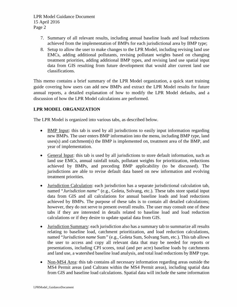
The Load, Prioritization, and Reduction (LPR) Model was developed to aid the County of Santa Barbara, and the Cities of Buellton, Solvang, Goleta, and Carpinteria (jurisdictions) in quantifying existing (baseline) runoff volume and pollutants loads within the jurisdictional MS4 Permit areas, prioritizing catchments for BMP implementation, and estimating the anticipated load reductions resulting from implementation of the Program Effectiveness Assessment and Improvement Plans (PEAIPs). The LPR Model fulfills the requirements specified by the 2013 California Phase II General Municipal Separate Storm Sewer System (MS4) Permit (MS4 Permit) and the July 25, 2014, Central Coast Regional Water Quality Control Board (Regional Board) “Effectiveness Assessment and Monitoring” guidance letter. The LPR Model was created based on the approach outlined in the PEAIP Approach to Quantify Pollutant Loads and Pollutant Load Reductions Memorandum (Modeling Approach Memo). Key features of the LPR Model include:

1. Utilization of spatial data from GIS to estimate average annual runoff and pollutant loads for up to 15 pollutants;

2. Analysis of runoff volumes and pollutant loads by watershed (i.e., all land uses and jurisdictions within the major County watersheds) and the relative contribution of loading from the MS4 Permit areas to the receiving waters;

3. Catchment prioritization based on multiple pollutants weighted by jurisdictional-specific treatment priorities for BMP implementation;

4. Visual representation of pollutant loading by land use in order to prioritize treatment of non-structural BMPs by land use;

5. User-friendly BMP input menu that allows the user to easily input information describing a BMP, including BMP type and the catchment(s), land use(s), treatment area for BMP implementation, and year of implementation;

6. Estimation of the annual runoff volume and pollutant load reductions achieved by the implementation of BMPs;

LPR Model Guidance Document 15 April 2016

LPRModel_GuidanceDocument

7. Summary of all relevant results, including annual baseline loads and load reductions achieved from the implementation of BMPs for each jurisdictional area by BMP type;

8. Setup to allow the user to make changes to the LPR Model, including revising land use EMCs, adding additional pollutants, revising pollutant weights based on changing treatment priorities, adding additional BMP types, and revising land use spatial input data from GIS resulting from future development that would alter current land use classifications.

This memo contains a brief summary of the LPR Model organization, a quick start training guide covering how users can add new BMPs and extract the LPR Model results for future annual reports, a detailed explanation of how to modify the LPR Model defaults, and a discussion of how the LPR Model calculations are performed.

LPR MODEL ORGANIZATION

The LPR Model is organized into various tabs, as described below.

• BMP Input: this tab is used by all jurisdictions to easily input information regarding new BMPs. The user enters BMP information into the menu, including BMP type, land uses(s) and catchment(s) the BMP is implemented on, treatment area of the BMP, and year of implementation.

• General Input: this tab is used by all jurisdictions to store default information, such as land use EMCs, annual rainfall totals, pollutant weights for prioritization, reductions achieved by BMPs, and preceding BMP applicability (to be discussed). The jurisdictions are able to revise default data based on new information and evolving treatment priorities.

• Jurisdiction Calculation: each jurisdiction has a separate jurisdictional calculation tab, named “Jurisdiction name” (e.g., Goleta, Solvang, etc.). These tabs store spatial input data from GIS and all calculations for annual baseline loads and load reductions achieved by BMPs. The purpose of these tabs is to contain all detailed calculations; however, they do not serve to present overall results. The user may consult one of these tabs if they are interested in details related to baseline load and load reduction calculations or if they desire to update spatial data from GIS.

• Jurisdiction Summary: each jurisdiction also has a summary tab to summarize all results relating to baseline load, catchment prioritization, and load reduction calculations, named “Jurisdiction name Sum” (e.g., Goleta Sum, Solvang Sum, etc.). This tab allows the user to access and copy all relevant data that may be needed for reports or presentations, including CPI scores, total (and per acre) baseline loads by catchments and land use, a watershed baseline load analysis, and total load reductions by BMP type.

• Non-MS4 Area: this tab contains all necessary information regarding areas outside the MS4 Permit areas (and Caltrans within the MS4 Permit areas), including spatial data from GIS and baseline load calculations. Spatial data will include the same information



shown in the Jurisdiction Calculation tab, but will also include a description of the area, such as “Goleta Slough watershed Non-MS4 area” or “Caltrans” in the Goleta MS4 Permit area. This tab is only utilized to estimate watershed baseline pollutant loading analyses. Therefore, it is not necessary for this area to be divided by catchments.

• IGP Parcels: similar to the Non-MS4 Area tab, this tab contains all necessary information regarding IGP Parcels (which are excluded from each MS4 Permit area but included in total watershed loading calculations), including spatial data from GIS and baseline load calculations. This tab is only utilized to estimate watershed baseline pollutant loading analyses, it is not necessary for this area to be divided by catchments.

• Watershed MS4 Area: several jurisdictions have a portion of the MS4 Permit area located within a major watershed. Because the entire MS4 Permit area is not located within the watershed, this tab (named “Watershed name MS4”) is necessary to store spatial data and baseline loading calculations for the MS4 Permit area located within the given watershed. This tab is only utilized to estimate watershed baseline pollutant loading analyses. Therefore, it is not necessary for this area to be divided by catchments.

QUICK START TRAINING GUIDE

The LPR Model is initially setup to calculate baseline runoff volume and pollutant loads based on GIS input data and to evaluate initial runoff volume/pollutant load reductions resulting from BMPs implemented since the new MS4 Permit and PEAIP was established. However, the user may also add newly implemented BMPs in the future and extract updated summary data for use in reports and presentations. The procedures outlined in the following sections (broken up by the LPR Model tabs) will guide the user in entering data for new BMPs and accessing relevant summary information.

BMP Input Tab

The BMP Input tab can be used by all jurisdictions to enter data for newly implemented BMPs. An overall view of this tab is shown in Figure 1 and details of each step in the BMP input procedure are provided below.



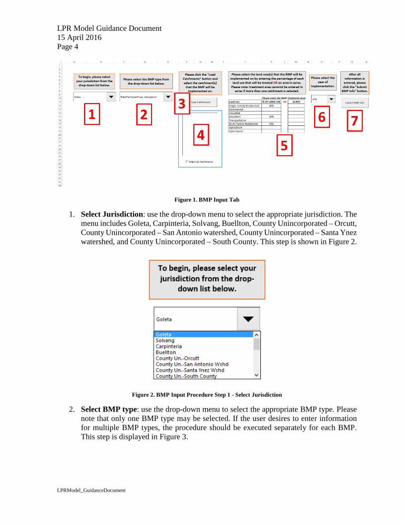
Figure 1. BMP Input Tab

1. Select Jurisdiction: use the drop-down menu to select the appropriate jurisdiction. The menu includes Goleta, Carpinteria, Solvang, Buellton, County Unincorporated – Orcutt, County Unincorporated – San Antonio watershed, County Unincorporated – Santa Ynez watershed, and County Unincorporated – South County. This step is shown in Figure 2.

Figure 2. BMP Input Procedure Step 1 - Select Jurisdiction

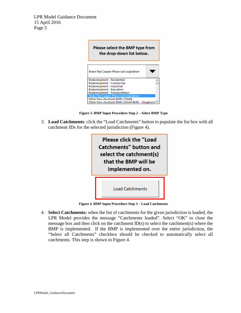
2. Select BMP type: use the drop-down menu to select the appropriate BMP type. Please note that only one BMP type may be selected. If the user desires to enter information for multiple BMP types, the procedure should be executed separately for each BMP. This step is displayed in Figure 3.



Figure 3. BMP Input Procedure Step 2 – Select BMP Type

3. Load Catchments: click the “Load Catchments” button to populate the list box with all catchment IDs for the selected jurisdiction (Figure 4).

Figure 4. BMP Input Procedure Step 3 – Load Catchments

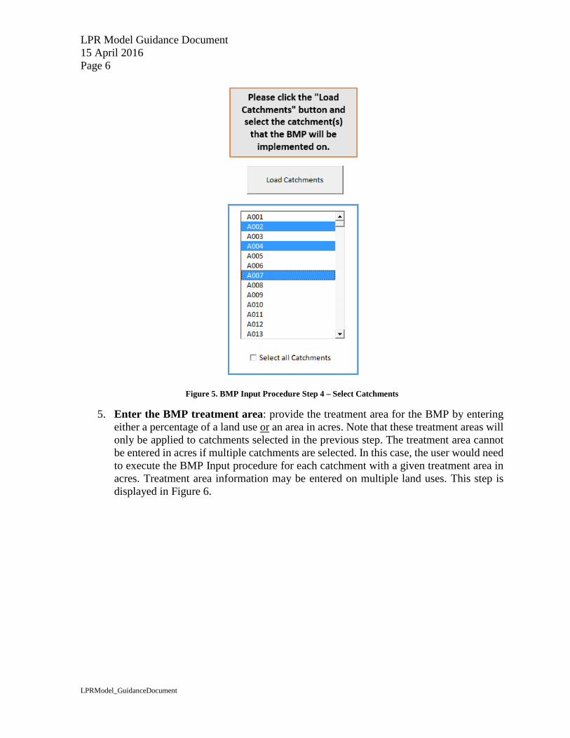
4. Select Catchments: when the list of catchments for the given jurisdiction is loaded, the LPR Model provides the message “Catchments loaded”. Select “OK” to close the message box and then click on the catchment ID(s) to select the catchment(s) where the BMP is implemented. If the BMP is implemented over the entire jurisdiction, the “Select all Catchments” checkbox should be checked to automatically select all catchments. This step is shown in Figure 4.



Figure 5. BMP Input Procedure Step 4 – Select Catchments

5. Enter the BMP treatment area: provide the treatment area for the BMP by entering either a percentage of a land use or an area in acres. Note that these treatment areas will only be applied to catchments selected in the previous step. The treatment area cannot be entered in acres if multiple catchments are selected. In this case, the user would need to execute the BMP Input procedure for each catchment with a given treatment area in acres. Treatment area information may be entered on multiple land uses. This step is displayed in Figure 6.



Figure 6. BMP Input Procedure Step 5 – BMP Treatment Area by Land Use

6. Enter the Year for BMP Implementation: Select the year that the BMP was first implemented from the drop-down list (this assumes that ongoing BMP reductions will result). Note that only one year may be selected at a time. This step is shown in Figure 7.

Figure 7. BMP Input Procedure Step 6 – BMP Implementation Year

7. Submit Info: After all data has been accurately entered, click the “Submit BMP Info” button (Figure 8). This will transfer BMP information to the appropriate Jurisdiction Calculation tab.



Figure 8. BMP Input Procedure Step 7 – Submit BMP Info

Jurisdiction Summary Tabs

As previously outlined, the LPR Model contains a calculation and summary tab for each jurisdiction. While the Jurisdiction Calculation tab contains detailed calculations related to annual baseline runoff volume and pollutant load estimates and reductions achieved by each implemented BMP, the Jurisdiction Summary tab is most helpful in providing the user with a summary of all relevant data. A brief summary of all data included in the Jurisdiction Summary tab is outlined in the following sections.

Runoff Volume/Pollutant Loads by Catchment

Each Jurisdiction Summary tab displays the runoff volume and pollutant loading by catchment. Table 1 in the LPR Model presents total runoff volume and pollutant loading per catchment, while Table 2 shows these values per acre for each catchment. An example of this LPR Model output is shown in Figure 9 and Figure 10.

Figure 9. Baseline Loads by Catchment Example Table



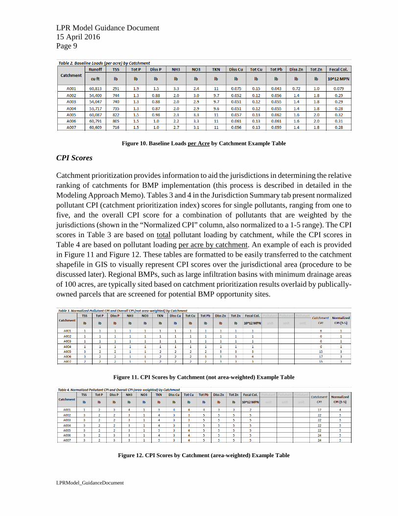
Figure 10. Baseline Loads per Acre by Catchment Example Table

CPI Scores

Catchment prioritization provides information to aid the jurisdictions in determining the relative ranking of catchments for BMP implementation (this process is described in detailed in the Modeling Approach Memo). Tables 3 and 4 in the Jurisdiction Summary tab present normalized pollutant CPI (catchment prioritization index) scores for single pollutants, ranging from one to five, and the overall CPI score for a combination of pollutants that are weighted by the jurisdictions (shown in the “Normalized CPI” column, also normalized to a 1-5 range). The CPI scores in Table 3 are based on total pollutant loading by catchment, while the CPI scores in Table 4 are based on pollutant loading per acre by catchment. An example of each is provided in Figure 11 and Figure 12. These tables are formatted to be easily transferred to the catchment shapefile in GIS to visually represent CPI scores over the jurisdictional area (procedure to be discussed later). Regional BMPs, such as large infiltration basins with minimum drainage areas of 100 acres, are typically sited based on catchment prioritization results overlaid by publically-owned parcels that are screened for potential BMP opportunity sites.

Figure 11. CPI Scores by Catchment (not area-weighted) Example Table

Figure 12. CPI Scores by Catchment (area-weighted) Example Table



MS4 Permit Area Baseline Loads by Land Use

Each Jurisdiction Summary tab summarizes total runoff volume and pollutant loads over the entire jurisdictional area by land use. Table 5 in the LPR Model presents total runoff volume and pollutant loading by land use, while Table 6 shows runoff volume and pollutant loading per acre of each land use. Pie charts are also included for these tables to represent runoff volume and pollutant loading by land use. An example of the LPR Model Table 5 is displayed in Figure 13, and an example of Table 6 is shown in Figure 14. An example pie chart for baseline loading per acre by land use is shown in Figure 15.

The jurisdictions can utilize these baseline loadings per acre results, along with land use maps of the MS4 Permit areas, to target implementation of distributed structural BMPs and plan for land use-based non-structural BMPs. The jurisdictions can then select BMPs that target specific pollutants in areas that will result in the greatest load reduction of the targeted pollutants.

Figure 13. Baseline Loads by Land Use Example Table

Figure 14. Baseline Loads by Land Use Acre Example Table



Figure 15. Baseline Loads for MS4 Permit Areas by Land Use Acre Example Chart

Watershed Baseline Load Analysis

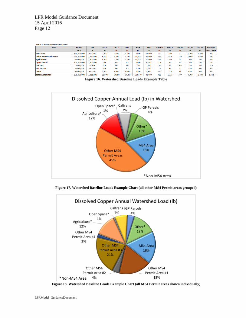
The LPR Model Tables 7 and 8 in the Jurisdiction Summary tabs provide an analysis of watershed baseline loads. Table 7 sums the runoff volume and pollutant loading for each MS4 Permit area located within the corresponding watershed. For LPR Model calculations, all analyzed jurisdictional areas are shown in Table 7, but only jurisdictions located within the given watershed are shown with black text, while all others are shown with light gray text. Several MS4 Permit areas not participating in development of the LPR Model are also quantified in this table. The LPR Model Table 8 summarizes runoff volume and pollutant loading within the appropriate watershed, separating the total watershed loads by the MS4 Permit area for the specific jurisdiction, all other MS4 areas, non-MS4 agriculture, non-MS4 open space, Caltrans, IGP Parcels, and other non-MS4 areas (non-MS4 area that is not classified as agriculture or open space). Pie charts are also provided to display the breakdown of annual runoff and pollutant loading within the watershed. The first set of pie charts shows the MS4 Permit area runoff volume or pollutant load contribution separated by the MS4 area in question and all other MS4 areas, while the second set of plots displays contributions from each MS4 Permit area separately. An example of Table 8 is shown in Figure 16. An example pie chart, where all other MS4 Permit areas are grouped, is displayed in Figure 17, and an example pie chart where each MS4 Permit area is shown individually is displayed in Figure 18

This analysis provides each jurisdiction information regarding the runoff volume and pollutant loading that their MS4 Permit area is contributing to the watershed, relative to other contributing areas. These results provide prospective on the impact of the MS4 Permit area to the watershed.



Figure 16. Watershed Baseline Loads Example Table

Figure 17. Watershed Baseline Loads Example Chart (all other MS4 Permit areas grouped)

Figure 18. Watershed Baseline Loads Example Chart (all MS4 Permit areas shown individually)

MS4 Area18%Other MS4

Permit Areas45%

Agriculture*12%

Open Space*1%

Caltrans7%

IGP Parcels4%

Other*13%

Dissolved Copper Annual Load (lb) in Watershed

*Non-MS4 Area

MS4 Area18%

Other MS4 Permit Area #1

18%


4%


21%


2%

Agriculture*12%

Open Space*1%

Caltrans7%

IGP Parcels4%

Other*13%

Dissolved Copper Annual Watershed Load (lb)

*Non-MS4 Area



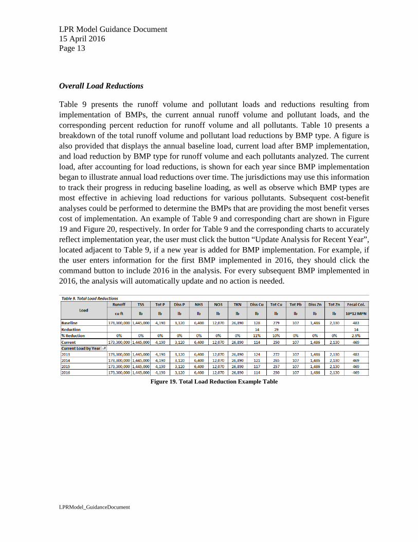
Overall Load Reductions

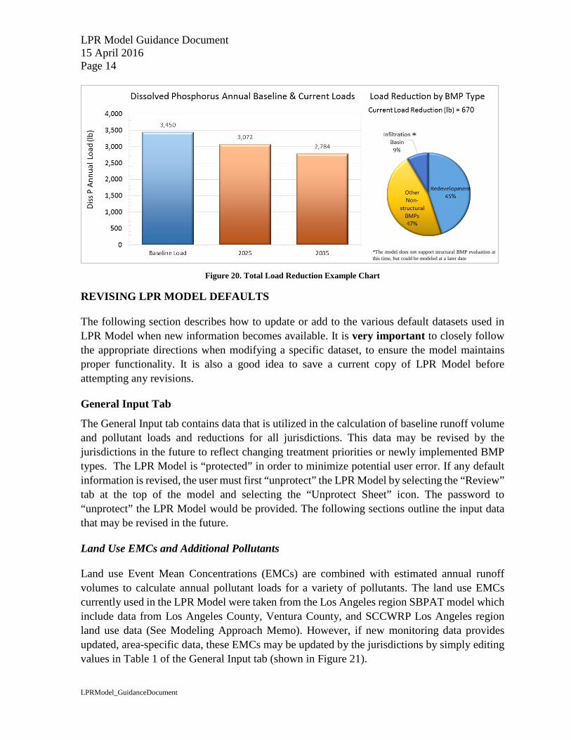
Table 9 presents the runoff volume and pollutant loads and reductions resulting from implementation of BMPs, the current annual runoff volume and pollutant loads, and the corresponding percent reduction for runoff volume and all pollutants. Table 10 presents a breakdown of the total runoff volume and pollutant load reductions by BMP type. A figure is also provided that displays the annual baseline load, current load after BMP implementation, and load reduction by BMP type for runoff volume and each pollutants analyzed. The current load, after accounting for load reductions, is shown for each year since BMP implementation began to illustrate annual load reductions over time. The jurisdictions may use this information to track their progress in reducing baseline loading, as well as observe which BMP types are most effective in achieving load reductions for various pollutants. Subsequent cost-benefit analyses could be performed to determine the BMPs that are providing the most benefit verses cost of implementation. An example of Table 9 and corresponding chart are shown in Figure 19 and Figure 20, respectively. In order for Table 9 and the corresponding charts to accurately reflect implementation year, the user must click the button “Update Analysis for Recent Year”, located adjacent to Table 9, if a new year is added for BMP implementation. For example, if the user enters information for the first BMP implemented in 2016, they should click the command button to include 2016 in the analysis. For every subsequent BMP implemented in 2016, the analysis will automatically update and no action is needed.

Figure 19. Total Load Reduction Example Table



Figure 20. Total Load Reduction Example Chart

REVISING LPR MODEL DEFAULTS

The following section describes how to update or add to the various default datasets used in LPR Model when new information becomes available. It is very important to closely follow the appropriate directions when modifying a specific dataset, to ensure the model maintains proper functionality. It is also a good idea to save a current copy of LPR Model before attempting any revisions.

General Input Tab

The General Input tab contains data that is utilized in the calculation of baseline runoff volume and pollutant loads and reductions for all jurisdictions. This data may be revised by the jurisdictions in the future to reflect changing treatment priorities or newly implemented BMP types. The LPR Model is “protected” in order to minimize potential user error. If any default information is revised, the user must first “unprotect” the LPR Model by selecting the “Review” tab at the top of the model and selecting the “Unprotect Sheet” icon. The password to “unprotect” the LPR Model would be provided. The following sections outline the input data that may be revised in the future.

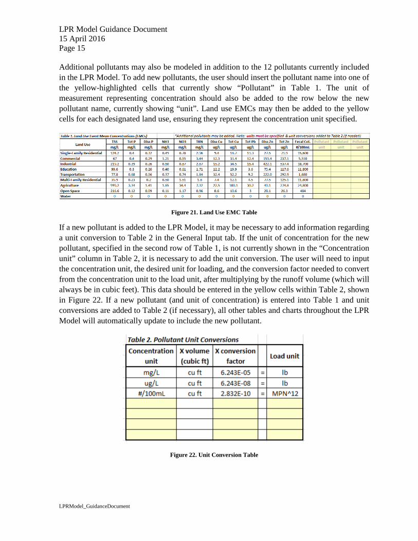
Land Use EMCs and Additional Pollutants

Land use Event Mean Concentrations (EMCs) are combined with estimated annual runoff volumes to calculate annual pollutant loads for a variety of pollutants. The land use EMCs currently used in the LPR Model were taken from the Los Angeles region SBPAT model which include data from Los Angeles County, Ventura County, and SCCWRP Los Angeles region land use data (See Modeling Approach Memo). However, if new monitoring data provides updated, area-specific data, these EMCs may be updated by the jurisdictions by simply editing values in Table 1 of the General Input tab (shown in Figure 21).

*

*The model does not support structural BMP evaluation at this time, but could be modeled at a later date



Additional pollutants may also be modeled in addition to the 12 pollutants currently included in the LPR Model. To add new pollutants, the user should insert the pollutant name into one of the yellow-highlighted cells that currently show “Pollutant” in Table 1. The unit of measurement representing concentration should also be added to the row below the new pollutant name, currently showing “unit”. Land use EMCs may then be added to the yellow cells for each designated land use, ensuring they represent the concentration unit specified.

Figure 21. Land Use EMC Table

If a new pollutant is added to the LPR Model, it may be necessary to add information regarding a unit conversion to Table 2 in the General Input tab. If the unit of concentration for the new pollutant, specified in the second row of Table 1, is not currently shown in the “Concentration unit” column in Table 2, it is necessary to add the unit conversion. The user will need to input the concentration unit, the desired unit for loading, and the conversion factor needed to convert from the concentration unit to the load unit, after multiplying by the runoff volume (which will always be in cubic feet). This data should be entered in the yellow cells within Table 2, shown in Figure 22. If a new pollutant (and unit of concentration) is entered into Table 1 and unit conversions are added to Table 2 (if necessary), all other tables and charts throughout the LPR Model will automatically update to include the new pollutant.

Figure 22. Unit Conversion Table



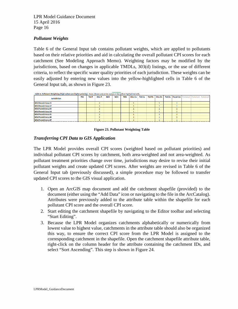
Pollutant Weights

Table 6 of the General Input tab contains pollutant weights, which are applied to pollutants based on their relative priorities and aid in calculating the overall pollutant CPI scores for each catchment (See Modeling Approach Memo). Weighting factors may be modified by the jurisdictions, based on changes in applicable TMDLs, 303(d) listings, or the use of different criteria, to reflect the specific water quality priorities of each jurisdiction. These weights can be easily adjusted by entering new values into the yellow-highlighted cells in Table 6 of the General Input tab, as shown in Figure 23.

Figure 23. Pollutant Weighting Table

Transferring CPI Data to GIS Application

The LPR Model provides overall CPI scores (weighted based on pollutant priorities) and individual pollutant CPI scores by catchment, both area-weighted and not area-weighted. As pollutant treatment priorities change over time, jurisdictions may desire to revise their initial pollutant weights and create updated CPI scores. After weights are revised in Table 6 of the General Input tab (previously discussed), a simple procedure may be followed to transfer updated CPI scores to the GIS visual application.

1. Open an ArcGIS map document and add the catchment shapefile (provided) to the document (either using the “Add Data” icon or navigating to the file in the ArcCatalog). Attributes were previously added to the attribute table within the shapefile for each pollutant CPI score and the overall CPI score.

2. Start editing the catchment shapefile by navigating to the Editor toolbar and selecting “Start Editing”.

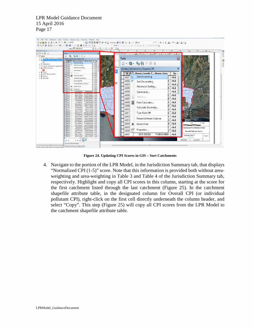
3. Because the LPR Model organizes catchments alphabetically or numerically from lowest value to highest value, catchments in the attribute table should also be organized this way, to ensure the correct CPI score from the LPR Model is assigned to the corresponding catchment in the shapefile. Open the catchment shapefile attribute table, right-click on the column header for the attribute containing the catchment IDs, and select “Sort Ascending”. This step is shown in Figure 24.



Figure 24. Updating CPI Scores in GIS – Sort Catchments

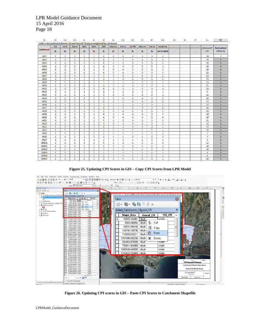
4. Navigate to the portion of the LPR Model, in the Jurisdiction Summary tab, that displays “Normalized CPI (1-5)” score. Note that this information is provided both without area-weighting and area-weighting in Table 3 and Table 4 of the Jurisdiction Summary tab, respectively. Highlight and copy all CPI scores in this column, starting at the score for the first catchment listed through the last catchment (Figure 25). In the catchment shapefile attribute table, in the designated column for Overall CPI (or individual pollutant CPI), right-click on the first cell directly underneath the column header, and select “Copy”. This step (Figure 25) will copy all CPI scores from the LPR Model to the catchment shapefile attribute table.



Figure 25. Updating CPI Scores in GIS – Copy CPI Scores from LPR Model

Figure 26. Updating CPI scores in GIS – Paste CPI Scores to Catchment Shapefile



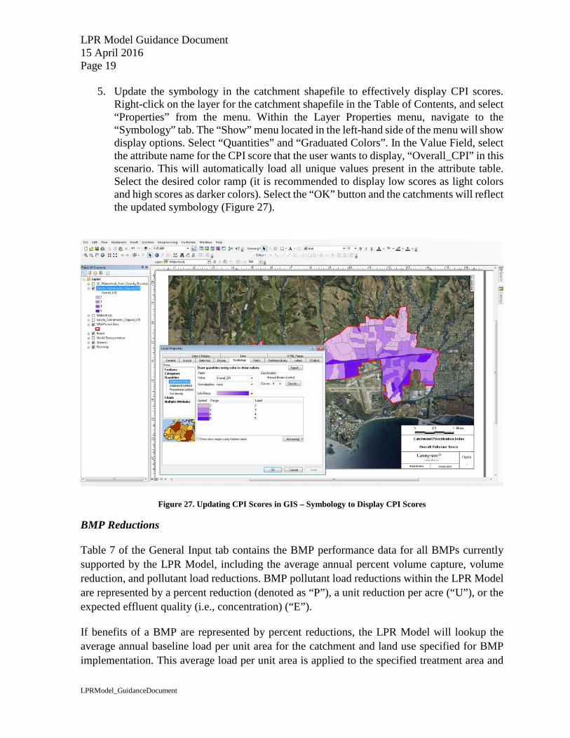
5. Update the symbology in the catchment shapefile to effectively display CPI scores. Right-click on the layer for the catchment shapefile in the Table of Contents, and select “Properties” from the menu. Within the Layer Properties menu, navigate to the “Symbology” tab. The “Show” menu located in the left-hand side of the menu will show display options. Select “Quantities” and “Graduated Colors”. In the Value Field, select the attribute name for the CPI score that the user wants to display, “Overall_CPI” in this scenario. This will automatically load all unique values present in the attribute table. Select the desired color ramp (it is recommended to display low scores as light colors and high scores as darker colors). Select the “OK” button and the catchments will reflect the updated symbology (Figure 27).

Figure 27. Updating CPI Scores in GIS – Symbology to Display CPI Scores

BMP Reductions

Table 7 of the General Input tab contains the BMP performance data for all BMPs currently supported by the LPR Model, including the average annual percent volume capture, volume reduction, and pollutant load reductions. BMP pollutant load reductions within the LPR Model are represented by a percent reduction (denoted as “P”), a unit reduction per acre (“U”), or the expected effluent quality (i.e., concentration) (“E”).

If benefits of a BMP are represented by percent reductions, the LPR Model will lookup the average annual baseline load per unit area for the catchment and land use specified for BMP implementation. This average load per unit area is applied to the specified treatment area and



is then adjusted by the appropriate percent reduction for the applicable pollutants. It should be noted that runoff volume reductions (which are also specified as percent reductions, in this case) are also applied to pollutant load reductions if a separate pollutant load reduction is not specified. For example, if a particular BMP achieves a 10 percent reduction in runoff volume, but does not provide any extra pollutant load reduction, the LPR Model will also calculate a 10 percent load reduction for each pollutant to account for the pollutant load reduction resulting from the overall reduction in runoff volume.

BMPs can also be represented as unit load reductions, where a specified quantity of load is anticipated to be removed for each unit area of BMP implementation. The LPR Model applies this load removal per unit area to the specified implementation area to calculate the total load removal resulting from BMP implementation. It should be noted that the units specified for each pollutant in Table 7 of the General Input tab reflect units of concentration only. BMP reduction values specified in Table 7 for BMPs represented by unit load reductions must be in load units, which are specified in relation to concentration units in Table 2 of the General Input tab. Runoff volume reduction is also specified as a unit load reduction (in cubic feet) per acre for this type of BMP reduction. For BMPs represented as unit load reductions, runoff volume reductions are computed separately from pollutant load reductions. Therefore, a corresponding pollutant load reduction must be specified for BMPs that achieve a reduction in runoff volume, to account for the reduced pollutant load resulting from the reduction in runoff volume.

Lastly, the LPR Model supports BMP reductions in the form of effluent concentrations. Effluent concentrations should be utilized if structural BMPs are added to the LPR Model in the future. They are also used to calculate load reductions for redevelopment BMPs in the current LPR Model. Percent capture refers to the long-term average percentage of influent runoff volume that the BMP is designed to capture and then retain or treat. A value for percent capture should be specified for each BMP supported by the LPR Model, but will simply be set to 100% for most non-structural BMPs. If structural BMPs are added in the future, a hydrologic analysis should be conducted (typically done using SWMM for continuous simulation) to derive an average annual percent capture for the given BMP.

The specified volume reduction in Table 7 of the General Input tab, always represented as a percent reduction for BMPs with load reductions measured by effluent concentrations, refers to the decrease in the captured runoff volume due to infiltration or evapotranspiration through the BMP. Removing runoff volume from the BMP discharge will also remove all associated pollutants. The effluent concentration shown in Table 7 (specified in the unit of concentration shown under the pollutant name) represents the effluent concentration of runoff that is captured and treated by the BMP. Treated runoff is considered runoff that is captured by the BMP but not infiltrated through the BMP, as specified by the runoff volume reduction. Runoff volume that is bypassed, as represented by the percent capture, is considered untreated. For example, if a BMP with a percent capture of 80% has an influent runoff volume of 10,000 cubic feet, 8,000 cubic feet will enter the BMP and 2,000 cubic feet will bypass the BMP untreated. If the percent



volume reduction of the BMP is specified as 20%, 1,600 cubic feet of runoff will be infiltrated and 6,400 cubic feet will be treated by the BMP. The effluent concentration for a given pollutant will be applied to the 6,400 cubic feet to find the effluent pollutant load, which is subtracted by the influent load (also taking into account the bypassed runoff volume and loading) to determine the total load reduction. Therefore, the reduction in runoff volume achieved by this type of BMP is accounted for in calculating the associated pollutant load reductions.

A new BMP can easily be added to the BMP list in Table 7 (shown in Figure 28) of the General Input tab. The user should specify the name of the new BMP type, whether it is characterized by a percent load reduction, unit load reduction, or effluent concentration, by entering a “P”, “U”, or “E”, respectively, the percent capture (100% for most non-structural BMPs), and the associated reductions for runoff volume and each pollutant. As previously noted, runoff volume should be entered as a percent reduction for BMPs characterized as “P” or “E”, while BMPs specified by “U” should represent runoff volume reductions as unit reductions (cubic feet per acre). In terms of pollutant reductions, percent reduction BMPs (“P”) should specify load reductions as a percentage of the influent load, effluent concentration BMPs (“E”) should include effluent concentrations of the treated volume in the units of concentration shown under the pollutant name in Table 7, and BMPs characterized by unit load reductions (“U”) should show pollutant unit load reductions in load units (specified in Table 2 of the General Input tab based on concentration units) per acre. If structural BMPs are added to the LPR Model in the future, BMP effluent concentrations from the SBPAT User’s Manual (Geosyntec, 2012) can be combined with new BMP performance data from the International Stormwater BMP Database (www.bmpdatabase.org), to ensure that water quality modeling efforts utilize the most current BMP performance summary statistics.

Figure 28. BMP Reduction Table

Preceding BMPs

For each BMP type included, the LPR Model is able to specify one other BMP type that will act as a “preceding BMP”, which is taken into account so estimated load reductions are not double-calculated. A “preceding BMP” is defined as a BMP that treats the same source and treatment area of another BMP. The preceding BMP is the BMP that first treats the treatment area in question. A BMP with a treatment area upstream of another BMP, but the BMPs do not treat the same source or the treatment areas do not overlap, is not considered a preceding BMP.



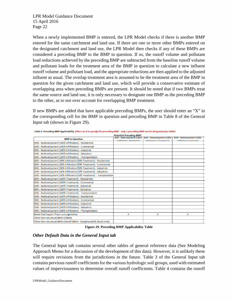
When a newly implemented BMP is entered, the LPR Model checks if there is another BMP entered for the same catchment and land use. If there are one or more other BMPs entered on the designated catchment and land use, the LPR Model then checks if any of these BMPs are considered a preceding BMP to the BMP in question. If so, the runoff volume and pollutant load reductions achieved by the preceding BMP are subtracted from the baseline runoff volume and pollutant loads for the treatment area of the BMP in question to calculate a new influent runoff volume and pollutant load, and the appropriate reductions are then applied to the adjusted influent as usual. The overlap treatment area is assumed to be the treatment area of the BMP in question for the given catchment and land use, which will provide a conservative estimate of overlapping area when preceding BMPs are present. It should be noted that if two BMPs treat the same source and land use, it is only necessary to designate one BMP as the preceding BMP to the other, as to not over account for overlapping BMP treatment.

If new BMPs are added that have applicable preceding BMPs, the user should enter an “X” in the corresponding cell for the BMP in question and preceding BMP in Table 8 of the General Input tab (shown in Figure 29).

Figure 29. Preceding BMP Applicability Table

Other Default Data in the General Input tab

The General Input tab contains several other tables of general reference data (See Modeling Approach Memo for a discussion of the development of this data). However, it is unlikely these will require revisions from the jurisdictions in the future. Table 3 of the General Input tab contains pervious runoff coefficients for the various hydrologic soil groups, used with estimated values of imperviousness to determine overall runoff coefficients. Table 4 contains the runoff



coefficient adjustment factor, derived from a hydrologic calibration that compared calculated annual discharge volumes predicted by LPR Model to streamflow gage observed annual discharge volumes at Atascadero Creek. Table 5 contains average annual precipitation data for each jurisdictional area (and watershed). It is unlikely the data in Table 3, Table 4, and Table 5 of the General Input tab will require revisions by the jurisdictions in the future.

Jurisdiction Calculation Tab

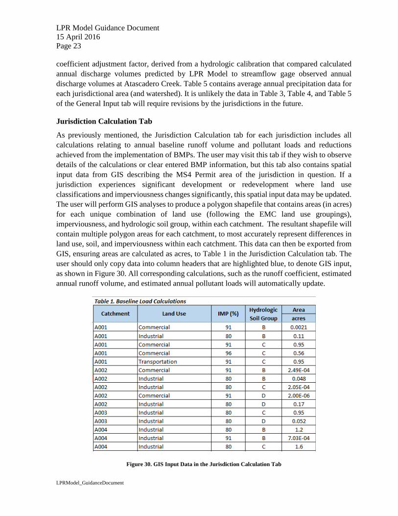
As previously mentioned, the Jurisdiction Calculation tab for each jurisdiction includes all calculations relating to annual baseline runoff volume and pollutant loads and reductions achieved from the implementation of BMPs. The user may visit this tab if they wish to observe details of the calculations or clear entered BMP information, but this tab also contains spatial input data from GIS describing the MS4 Permit area of the jurisdiction in question. If a jurisdiction experiences significant development or redevelopment where land use classifications and imperviousness changes significantly, this spatial input data may be updated. The user will perform GIS analyses to produce a polygon shapefile that contains areas (in acres) for each unique combination of land use (following the EMC land use groupings), imperviousness, and hydrologic soil group, within each catchment. The resultant shapefile will contain multiple polygon areas for each catchment, to most accurately represent differences in land use, soil, and imperviousness within each catchment. This data can then be exported from GIS, ensuring areas are calculated as acres, to Table 1 in the Jurisdiction Calculation tab. The user should only copy data into column headers that are highlighted blue, to denote GIS input, as shown in Figure 30. All corresponding calculations, such as the runoff coefficient, estimated annual runoff volume, and estimated annual pollutant loads will automatically update.

Figure 30. GIS Input Data in the Jurisdiction Calculation Tab



CALCULATIONS OF BASELINE LOADS AND REDUCTIONS

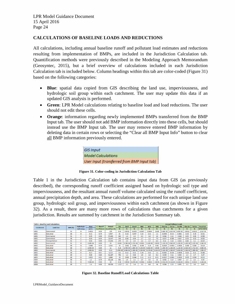
All calculations, including annual baseline runoff and pollutant load estimates and reductions resulting from implementation of BMPs, are included in the Jurisdiction Calculation tab. Quantification methods were previously described in the Modeling Approach Memorandum (Geosyntec, 2015), but a brief overview of calculations included in each Jurisdiction Calculation tab is included below. Column headings within this tab are color-coded (Figure 31) based on the following categories:

• Blue: spatial data copied from GIS describing the land use, imperviousness, and hydrologic soil group within each catchment. The user may update this data if an updated GIS analysis is performed.

• Green: LPR Model calculations relating to baseline load and load reductions. The user should not edit these cells.

• Orange: information regarding newly implemented BMPs transferred from the BMP Input tab. The user should not add BMP information directly into these cells, but should instead use the BMP Input tab. The user may remove entered BMP information by deleting data in certain rows or selecting the “Clear all BMP Input Info” button to clear all BMP information previously entered.

Figure 31. Color-coding in Jurisdiction Calculation Tab

Table 1 in the Jurisdiction Calculation tab contains input data from GIS (as previously described), the corresponding runoff coefficient assigned based on hydrologic soil type and imperviousness, and the resultant annual runoff volume calculated using the runoff coefficient, annual precipitation depth, and area. These calculations are performed for each unique land use group, hydrologic soil group, and imperviousness within each catchment (as shown in Figure 32). As a result, there are many more rows of calculations than catchments for a given jurisdiction. Results are summed by catchment in the Jurisdiction Summary tab.

Figure 32. Baseline Runoff/Load Calculations Table



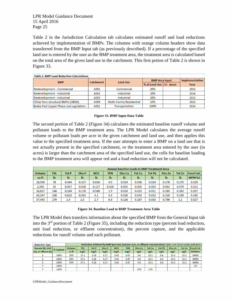
Table 2 in the Jurisdiction Calculation tab calculates estimated runoff and load reductions achieved by implementation of BMPs. The columns with orange column headers show data transferred from the BMP Input tab (as previously described). If a percentage of the specified land use is entered by the user as the BMP treatment area, the treatment area is calculated based on the total area of the given land use in the catchment. This first potion of Table 2 is shown in Figure 33.

Figure 33. BMP Input Data Table

The second portion of Table 2 (Figure 34) calculates the estimated baseline runoff volume and pollutant loads to the BMP treatment area. The LPR Model calculates the average runoff volume or pollutant loads per acre in the given catchment and land use, and then applies this value to the specified treatment area. If the user attempts to enter a BMP on a land use that is not actually present in the specified catchment, or the treatment area entered by the user (in acres) is larger than the catchment area of the specified land use, the cells for baseline loading to the BMP treatment area will appear red and a load reduction will not be calculated.

Figure 34. Baseline Load to BMP Treatment Area Table

The LPR Model then transfers information about the specified BMP from the General Input tab into the 3rd portion of Table 2 (Figure 35), including the reduction type (percent load reduction, unit load reduction, or effluent concentration), the percent capture, and the applicable reductions for runoff volume and each pollutant.



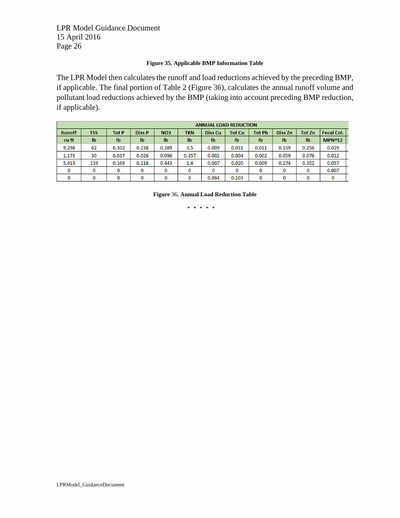
Figure 35. Applicable BMP Information Table

The LPR Model then calculates the runoff and load reductions achieved by the preceding BMP, if applicable. The final portion of Table 2 (Figure 36), calculates the annual runoff volume and pollutant load reductions achieved by the BMP (taking into account preceding BMP reduction, if applicable).

Figure 36. Annual Load Reduction Table

* * * * *



REFERENCES

Geosyntec Consultants, 2012a. A User’s Guide for the Structural BMP Prioritization and Analysis Tool. November 2012. Geosyntec Consultants, 2015. Memorandum: Program Effectiveness Assessment and

Improvement Plan Approach to Quantify Pollutant Loads and Pollutant Load Reductions. October 2015.

PH 805.897.3800 Memorandum · jurisdictions (shown in the “Normalized CPI” column, also...

Documents

Transcript of PH 805.897.3800 Memorandum · jurisdictions (shown in the “Normalized CPI” column, also...