Petro-electric modeling for CSEM reservoircharacterization and monitoring

Alireza Shahin1, Kerry Key2, Paul Stoffa3, and Robert Tatham4

ABSTRACT

The controlled-source electromagnetic (CSEM) method hasbeen successfully applied to petroleum exploration; however,less effort has been made to highlight the applicability of thistechnique for reservoir monitoring. This work appraises theability of time-lapse CSEM data to detect the changes in fluidsaturation during water flooding into an oil reservoir. We si-mulated a poorly consolidated shaly sandstone reservoir basedon a prograding near-shore depositional environment. Startingwith an effective porosity model simulated by Gaussian geos-tatistics, dispersed clay and dual water models were efficientlycombined with other well-known theoretical and experimentalpetrophysical correlations to consistently simulate reservoirproperties. The constructed reservoir model was subjected

to numerical simulation of multiphase fluid flow to predictthe spatial distributions of fluid pressure and saturation. Ageologically consistent rock physics model and a modifiedArchie’s equation for shaly sandstones were then used to si-mulate the electrical resistivity, showing up to 60% decreasesin electrical resistivity due to changes in water saturation dur-ing 10 years of production. Time-lapse CSEM data were si-mulated at three production time steps (zero, five, and tenyears) using a 2.5D parallel adaptive finite element algorithm.Analysis of the time-lapse signal in the simulated multicom-ponent and multifrequency data set demonstrates that a detect-able time-lapse signal after five years and a strong time-lapsesignal after ten years of water flooding are attainable usingcurrent CSEM technology.

INTRODUCTION

The CSEM method has been recently applied to petroleumexploration as a direct hydrocarbon detector. The contrast betweenthe low electrical conductivity of hydrocarbon-saturated rocks andthe higher conductivity of the surrounding water-saturated rocksleads to an anomaly in the magnetic and electric fields emittedin the vicinity of the sea floor by electric dipole transmitters andrecorded by ocean bottom EM receivers. Successful applicationsare documented in several studies (e.g., Ellingsrud et al., 2002;Eidesmo et al., 2002; Constable and Srnka, 2007).Time-lapse CSEM data consist of two or more repeat surveys

recorded at different calendar times over a depleting reservoir.The main objective is to detect and estimate production-inducedtime-lapse changes in subsurface rock and fluid properties. In doingso, changes in observations, i.e., the amplitude and phase of

magnetic and electric fields, or inverted attributes, e.g., rock resis-tivity, can be associated to changes in fluid saturation assuming anoncompacting isothermal reservoir.Time-lapse CSEM has been considered by several authors in the

literature. Wright et al. (2002) present time-lapse transient EM sur-veys over a shallow underground gas storage reservoir and demon-strated that the data are repeatable enough to detect the reservoir andmonitor the evolution of the gas and water content. Lien andMannseth (2008) conduct a feasibility study of time-lapse CSEMdata to monitor the water flooding of an oil reservoir. Utilizing 3Dintegral equation modeling, they find that time-lapse signals exhibitdetectable changes even in the presence of measurement errors.Orange et al. (2009) utilize 2D finite element modeling to simulatetime-lapse CSEM data for several simplified water flooding scenar-ios. Through a set of 2D modeling studies, they show that a data

Manuscript received by the Editor 11 October 2010; revised manuscript received 11 July 2011; published online 3 February 2012.1Formerly University of Texas at Austin, Institute for Geophysics, Austin, Texas, USA. Presently BP North America Inc., Reservoir Geophysics R&D,

Houston, Texas, USA. E-mail: alireza.shahin@bp.com.2Scripps Institution of Oceanography, University of California, San Diego, California, USA. E-mail: kkey@ucsd.edu.3University of Texas, Institute for Geophysics, Austin, Texas, USA. E-mail: pauls@ut.ig.utexas.edu.

© 2012 Society of Exploration Geophysicists. All rights reserved.

E9

GEOPHYSICS. VOL. 77, NO. 1 (JANUARY-FEBRUARY 2012); P. E9–E20, 14 FIGS., 1 TABLE.10.1190/GEO2010-0329.1

Downloaded 05 Feb 2012 to 72.37.249.68. Redistribution subject to SEG license or copyright; see Terms of Use at http://segdl.org/

repeatability of 1%–2% relative error is required to detect the smalltime-lapse signals. Zach et al. (2009) conduct 3D time-lapse model-ing by perturbing conductivity over a large reservoir (10 × 10 km2)and report changes of 30% to 50% in relative amplitudes of base andmonitor surveys. Black et al. (2009) models the time-lapse CSEMresponse over a realistic geologic model for a simplified flood geo-metry, but without fluid flow simulation and rock-physics modeling.They show that marine CSEM data are able to locate the position ofthe oil-water contact if the complicating effects from the back-ground, bathymetry, and a salt dome are taken into account.These previous studies used direct perturbation of electrical-

conductivity under the reasonable assumption that reservoir deple-tion will give substantial resistivity variations, rather than usingreservoir simulation and rock-physics modeling to determine theexpected resistivity changes. Ziolkowski et al. (2010) publisheda time-domain EM repeatability experiment over the North SeaHarding field where fluid flow simulation and resistivity modelingby Archie’s equation for clay-free sandstone were combined byintegral equation modeling to simulate the observed EM data. Theyconcluded that the production-induced time-lapse changes in reser-

voir resistivity would be observable provided that a signal to noiseratio of greater than 100, i.e., 40 dB, is obtained.Here, we generate a 2D geological reservoir model that exhibits a

realistic spatial distribution of petrophysical properties. Fluid flowsimulation and a geologically consistent rock-physicsmodel are thenemployed to convert the petrophysical properties of the shalysandstone to electrical resistivity. The representative time-dependentresistivity model developed here shows an accurate front geometryduring water flooding. To simulate the surrounding rocks, we burythe reservoir into a 1D background resistivity model. We thennumerically acquire 2.5D time-lapse CSEM data over the reservoirto assess the value of EM data in monitoring a complicated water-flooding scenario.

CONSTRUCTING A SYNTHETICRESERVOIR MODEL

Geological reservoir model

A stacked sand-rich strandplain reservoir architecture is consid-ered in this study to simulate a realistic geological framework.

Strandplains are mainly marine-dominated de-positional systems generated by seaward accre-tion of successive, parallel beach ridges weldedonto the subaerial coastal mainlands. They are in-herently progradational features and are presenton wave-dominated microtidal coasts (Tylerand Ambrose, 1986; Galloway and Hobday,1996). This sand-rich beach-ridge reservoir archi-tecture is inferred to be originally deposited as aclay-free geobody. However, due to postdeposi-tional diagenesis, dispersed clay is producedand it is themain factor reducing porosity and per-meability of the reservoir. This model, generatedusing a Gaussian simulation technique, is part ofthe Comparative Solution Project, a widely used,large geostatistical model for research on upgrid-ding and upscaling approaches (Christie andBlunt, 2001). We worked with the top 35 layersof the model, which are representative of the Tar-bert formation, a part of the Brent sequence ofmiddle Jurassic age and one of the major produ-cers in the North Sea. By changing the grid sizeand imposing smoothness, wemodified this mod-el to meet the objectives of this research. Next, weassigned geologically consistent petrophysics in-formation and add facies characterization todevelop a more realistic reservoir model compar-able to complicated models in the petroleum in-dustry. The model is described on a regularCartesian grid. The model size is 220 × 60 × 35

cells in the X (east-west), Y (north-south), andZ (depth) directions, respectively. The grid sizeis 10 × 10 × 10m, giving total model dimensionsof 2200 × 600 × 350 m.The reservoir consists of three facies

(Figure 1). Facies A is a fine grained sandstonewith mean grain size distribution of 80 μm. Thisfacies simulates a low porous and permeablesandstone reservoir with high clay content.Facies C is a course grained sandstone with mean

Wid

th(m

)

Effective porosityAll facies

200

400

600 0

0.2

0.4

Wid

th(m

)

Facies A

200

400

600 0

0.2

0.4

Wdt

h(m

)

Facies B

200

400

600 0

0.2

0.4

Length(m)

Wid

th(m

)

Facies C

500 1000 1500 2000

200

400

600 0

0.2

0.4

Figure 1. Map view of the first upper layer of the 3D reservoir (Christie and Blunt,2001) showing petrophysical facies (A, B, and C) overlaid on the distribution of effec-tive porosity model. Color scale is effective porosity and the same for all panels. Themodel is associated with synthetic geologic model and used for the numerical simulationof multiphase fluid flow, rock physics, and CSEM modeling. The model is defined on aregular Cartesian grid of 10 × 10 × 10m cells, with 220 × 60 × 35 cells in X (east-west),Y (north-south), and Z (depth) directions, respectively, for a total dimension of 2200 ×600 × 350 m A 2D cross section from the middle of this 3D model has been selected forthis study.

E10 Shahin et al.

Downloaded 05 Feb 2012 to 72.37.249.68. Redistribution subject to SEG license or copyright; see Terms of Use at http://segdl.org/

grain size distribution of 500 μm. This facies is associated with asandstone with high porosity and permeability and low clay content.Facies B is a transition facies between facies A and C and corre-sponds to a medium grained sandstone with mean grain size distri-bution of 250 μm. It is worth noting that a strong correlationbetween grain size and clay content is reported by several authors(e.g., Saner et al., 1996), so this knowledge has been accordinglyincorporated into the model by assigning clay-dependent grain sizesto the three facies, i.e., the higher the clay content, the lower themean grain size distribution.

Petrophysics model

The geological model described above is used to populate thepetrophysical properties, assuming a meaningful petrophysics mod-el. A petrophysics model includes the theoretical and experimentalcorrelations among various sets of petrophysical properties. Themodel is required to be validated using available well log and coredata. Here, the effective porosity model was firstgenerated using Gaussian geostatistics and claycontent, and total porosity models were thencomputed assuming a dispersed clay distribution(Thomas and Stieber, 1975; Marion et al., 1992),as shown in Figure 2a. Horizontal permeabilityin the X and Y directions are equal and calculatedbased on the extension of the dispersed claymodel for permeability introduced by Reviland Cathles, 1999 (Figure 2b and 2c). It is worthmentioning that permeability fields depend onporosity, clay content, grain size distribution,and the degree of cementation; subsequentlyfacies A, B, and C were assigned different trendsin permeability-clay content and permeability-porosity domains based on their grain sizes(Table 1). The vertical permeability field wastaken as 25% of the horizontal permeability fieldfor the entire reservoir. It is worth mentioningthat the joint relationship of permeability and re-sistivity has been taken into account by assigningthree different cementation factors to the threefacies.So far, the effective and total porosities,

clay content and directional permeabilities aremodeled using geostatistics and theoretical corre-lations according to the dispersed clay distribu-tion. Next, we initialize the reservoir for watersaturation and pore pressure. An experimentalcorrelation (Uden et al., 2004) between water

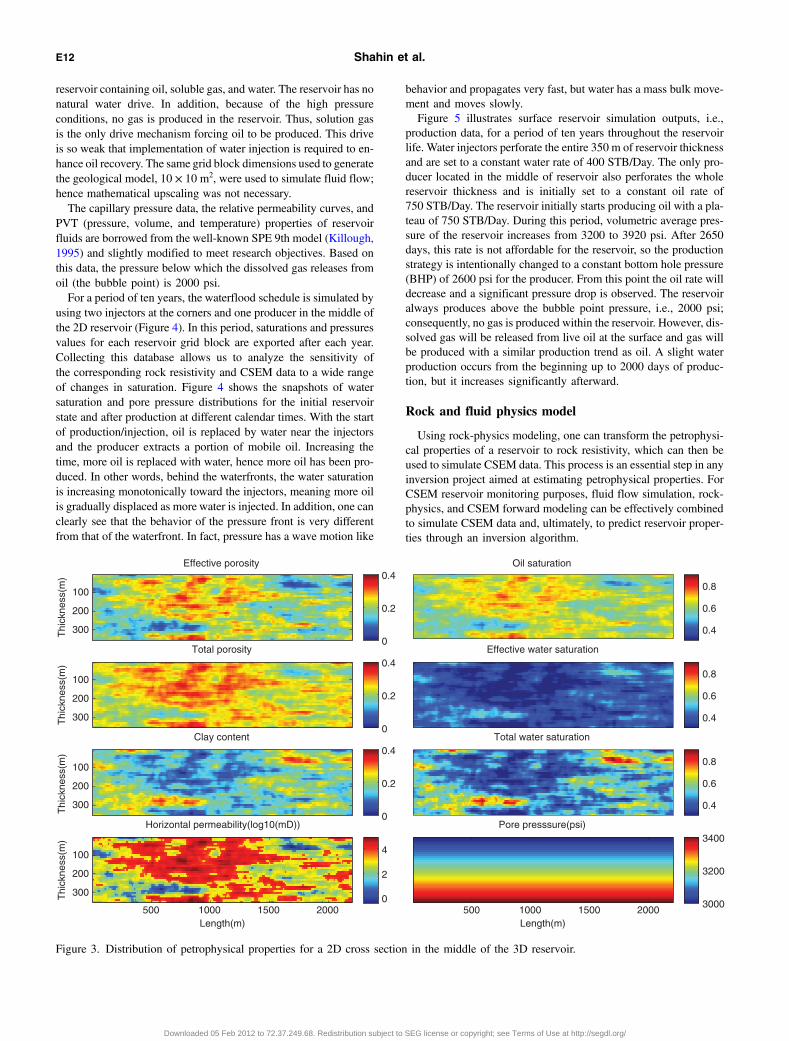
saturation and clay content was combined with the dual water model(Best et al., 1980; Dewan, 1983; Clavier, 1984) to compute claybound-water (Swb), effective water saturation (Swe), total water sa-turation (Swt), and oil saturation (So) (Figure 2d and Table 1). Initialreservoir pore pressure was simulated assuming a linear hydrostaticgradient from the top to the bottom of the reservoir. Figure 3 sum-marizes the distribution of petrophysical properties for a 2D crosssection in the middle of the 3D reservoir. This 2D reservoir has beenused for the numerical simulation of multiphase fluid flow, rock phy-sics, and CSEM modeling in this paper.

Reservoir simulation

Fluid flow simulation combines three fundamental laws governingfluid motions in porous media. These laws are based on conservationof mass, momentum, and energy (Aziz and Settari, 1979). In thisresearch, the commercial finite difference reservoir simulator,Eclipse 100, is utilized to replicate a water flooding plan on a 2D

0 0.1 0.2 0.30

0.1

0.2

0.3

0.4

0.5

Clay content Clay content

Por

osity

Effective porosity

Total porosity

0.05 0.1 0.15 0.2 0.25 0.3 0.35

Per

mea

bilit

y(m

D)

0.05 0.1 0.15 0.2 0.25 0.3 0.35

Effective porosity

Per

mea

bilit

y(m

D)

0 0.1 0.2 0.30

0.2

0.4

0.6

0.8

1

Clay content

Sat

urat

ion

SweSoSwbSwt

10−2

100

102

104

106

10−2

100

102

104

106a) b)

c) d)

Figure 2. Petrophysics model. Panel (a) shows the dispersed clay model for porosityreduction due to increasing of clay. Panel (b) displays horizontal permeability versusclay content. Panel (c) is permeability vs. effective porosity. In panels (a), (b), and(c), three colors are associated with three facies A (in blue), B (in green), and C (inred). Black dots in panels (b) and (c) are projected reservoir points. Note that the highconcentration of projected points looks like a continuous curve. Panel (d) shows fluidsaturations vs. clay content. Swe, So, Swb, and Swt are effective water saturation, oilsaturation, clay bound-water saturation, and total water saturation, respectively. Notethat the summation of effective water saturation (red curve) and oil saturation (greencurve) is always one.

Table 1. Facies petrophysical properties associated with the synthetic reservoir model.

Facies Total porosityEffectiveporosity

Claycontent

Effective watersaturation

Mean grainsize(micron)

Horizontalpermeability (mD)

A 0.11–0.18 0.01–0.12 0.25–0.34 0.45–0.62 80 0.37–10B 0.18–0.25 0.12–0.22 0.15–0.25 0.27–0.45 250 68–1400C 0.25–0.37 0.22–0.37 0.0–0.15 0.15–0.27 500 6800–91,000

E11

Downloaded 05 Feb 2012 to 72.37.249.68. Redistribution subject to SEG license or copyright; see Terms of Use at http://segdl.org/

reservoir containing oil, soluble gas, and water. The reservoir has nonatural water drive. In addition, because of the high pressureconditions, no gas is produced in the reservoir. Thus, solution gasis the only drive mechanism forcing oil to be produced. This driveis so weak that implementation of water injection is required to en-hance oil recovery. The same grid block dimensions used to generatethe geological model, 10 × 10 m2, were used to simulate fluid flow;hence mathematical upscaling was not necessary.The capillary pressure data, the relative permeability curves, and

PVT (pressure, volume, and temperature) properties of reservoirfluids are borrowed from the well-known SPE 9th model (Killough,1995) and slightly modified to meet research objectives. Based onthis data, the pressure below which the dissolved gas releases fromoil (the bubble point) is 2000 psi.For a period of ten years, the waterflood schedule is simulated by

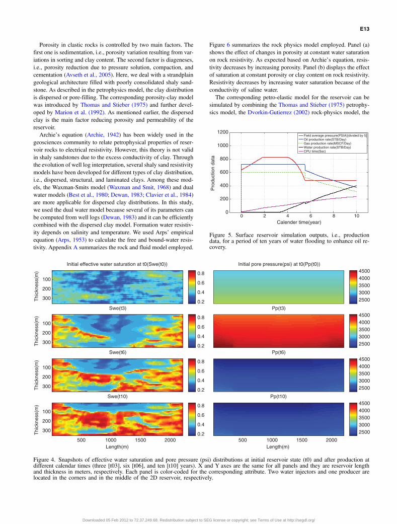
using two injectors at the corners and one producer in the middle ofthe 2D reservoir (Figure 4). In this period, saturations and pressuresvalues for each reservoir grid block are exported after each year.Collecting this database allows us to analyze the sensitivity ofthe corresponding rock resistivity and CSEM data to a wide rangeof changes in saturation. Figure 4 shows the snapshots of watersaturation and pore pressure distributions for the initial reservoirstate and after production at different calendar times. With the startof production/injection, oil is replaced by water near the injectorsand the producer extracts a portion of mobile oil. Increasing thetime, more oil is replaced with water, hence more oil has been pro-duced. In other words, behind the waterfronts, the water saturationis increasing monotonically toward the injectors, meaning more oilis gradually displaced as more water is injected. In addition, one canclearly see that the behavior of the pressure front is very differentfrom that of the waterfront. In fact, pressure has a wave motion like

behavior and propagates very fast, but water has a mass bulk move-ment and moves slowly.Figure 5 illustrates surface reservoir simulation outputs, i.e.,

production data, for a period of ten years throughout the reservoirlife. Water injectors perforate the entire 350 m of reservoir thicknessand are set to a constant water rate of 400 STB/Day. The only pro-ducer located in the middle of reservoir also perforates the wholereservoir thickness and is initially set to a constant oil rate of750 STB/Day. The reservoir initially starts producing oil with a pla-teau of 750 STB/Day. During this period, volumetric average pres-sure of the reservoir increases from 3200 to 3920 psi. After 2650days, this rate is not affordable for the reservoir, so the productionstrategy is intentionally changed to a constant bottom hole pressure(BHP) of 2600 psi for the producer. From this point the oil rate willdecrease and a significant pressure drop is observed. The reservoiralways produces above the bubble point pressure, i.e., 2000 psi;consequently, no gas is produced within the reservoir. However, dis-solved gas will be released from live oil at the surface and gas willbe produced with a similar production trend as oil. A slight waterproduction occurs from the beginning up to 2000 days of produc-tion, but it increases significantly afterward.

Rock and fluid physics model

Using rock-physics modeling, one can transform the petrophysi-cal properties of a reservoir to rock resistivity, which can then beused to simulate CSEM data. This process is an essential step in anyinversion project aimed at estimating petrophysical properties. ForCSEM reservoir monitoring purposes, fluid flow simulation, rock-physics, and CSEM forward modeling can be effectively combinedto simulate CSEM data and, ultimately, to predict reservoir proper-ties through an inversion algorithm.

Thi

ckne

ss(m

)

Effective porosity

100

200

3000

0.2

0.4

Thi

ckne

ss(m

)

Total porosity

100

200

3000

0.2

0.4

Thi

ckne

ss(m

)

Clay content

100

200

3000

0.2

0.4

Length(m) Length(m)

Thi

ckne

ss(m

)

Horizontal permeability(log10(mD))

500 1000 1500 2000

100

200

3000

2

4

Oil saturation

0.4

0.6

0.8

Effective water saturation

0.4

0.6

0.8

Total water saturation

0.4

0.6

0.8

Pore presssure(psi)

500 1000 1500 20003000

3200

3400

Figure 3. Distribution of petrophysical properties for a 2D cross section in the middle of the 3D reservoir.

E12 Shahin et al.

Downloaded 05 Feb 2012 to 72.37.249.68. Redistribution subject to SEG license or copyright; see Terms of Use at http://segdl.org/

Porosity in clastic rocks is controlled by two main factors. Thefirst one is sedimentation, i.e., porosity variation resulting from var-iations in sorting and clay content. The second factor is diageneses,i.e., porosity reduction due to pressure solution, compaction, andcementation (Avseth et al., 2005). Here, we deal with a strandplaingeological architecture filled with poorly consolidated shaly sand-stone. As described in the petrophysics model, the clay distributionis dispersed or pore-filling. The corresponding porosity-clay modelwas introduced by Thomas and Stieber (1975) and further devel-oped by Marion et al. (1992). As mentioned earlier, the dispersedclay is the main factor reducing porosity and permeability of thereservoir.Archie’s equation (Archie, 1942) has been widely used in the

geosciences community to relate petrophysical properties of reser-voir rocks to electrical resistivity. However, this theory is not validin shaly sandstones due to the excess conductivity of clay. Throughthe evolution of well log interpretation, several shaly sand resistivitymodels have been developed for different types of clay distribution,i.e., dispersed, structural, and laminated clays. Among these mod-els, the Waxman-Smits model (Waxman and Smit, 1968) and dualwater models (Best et al., 1980; Dewan, 1983; Clavier et al., 1984)are more applicable for dispersed clay distributions. In this study,we used the dual water model because several of its parameters canbe computed from well logs (Dewan, 1983) and it can be efficientlycombined with the dispersed clay model. Formation water resistiv-ity depends on salinity and temperature. We used Arps’ empiricalequation (Arps, 1953) to calculate the free and bound-water resis-tivity. Appendix A summarizes the rock and fluid model employed.

Figure 6 summarizes the rock physics model employed. Panel (a)shows the effect of changes in porosity at constant water saturationon rock resistivity. As expected based on Archie’s equation, resis-tivity decreases by increasing porosity. Panel (b) displays the effectof saturation at constant porosity or clay content on rock resistivity.Resistivity decreases by increasing water saturation because of theconductivity of saline water.The corresponding petro-elastic model for the reservoir can be

simulated by combining the Thomas and Stieber (1975) petrophy-sics model, the Dvorkin-Gutierrez (2002) rock-physics model, the

Thi

ckne

ss(m

)

Initial effective water saturation at t0(Swe(t0))

100

200

3000.2

0.4

0.6

0.8

Thi

ckne

ss(m

)

Swe(t3)

100

200

3000.2

0.4

0.6

0.8

Thi

ckne

ss(m

)

Swe(t6)

100

200

3000.2

0.4

0.6

0.8

Length(m)

Thi

ckne

ss(m

)

Swe(t10)

500 1000 1500 2000

100

200

3000.2

0.4

0.6

0.8

Initial pore pressure(psi) at t0(Pp(t0))

25003000350040004500

Pp(t3)

25003000350040004500

Pp(t6)

25003000350040004500

Length(m)

Pp(t10)

500 1000 1500 2000

25003000350040004500

Figure 4. Snapshots of effective water saturation and pore pressure (psi) distributions at initial reservoir state (t0) and after production atdifferent calendar times (three [t03], six [t06], and ten [t10] years). X and Y axes are the same for all panels and they are reservoir lengthand thickness in meters, respectively. Each panel is color-coded for the corresponding attribute. Two water injectors and one producer arelocated in the corners and in the middle of the 2D reservoir, respectively.

0 2 4 6 8 100

200

400

600

800

1000

1200

Calender time(year)

Pro

duct

ion

data

Field average pressure(PSIA)[divided by 5]Oil production rate(STB/Day)Gas production rate(MSCF/Day)Water production rate(STB/Day)CPU time(Sec)

Figure 5. Surface reservoir simulation outputs, i.e., productiondata, for a period of ten years of water flooding to enhance oil re-covery.

E13

Downloaded 05 Feb 2012 to 72.37.249.68. Redistribution subject to SEG license or copyright; see Terms of Use at http://segdl.org/

fluid physics model (Batzle and Wang, 1992),and a modified Gassmann theory (Dvorkin et al.,2007) for shaly sandstones. The joint modelingof the elastic and electrical properties of reservoirrocks will lead to the consistent forward model-ing algorithm for joint inversion of seismic andCSEM data and is a topic for future research.Further applications of using the petro-elasticmodel can be found in Shahin et al. (2010, 2011).The surrounding offshore sedimentary basin in

which the reservoir is buried is replicated using a1D resistivity model generated by correlating theP-wave velocity and resistivity based on the mod-ified Faust equation (Hacikoylu et al., 2006).Because the fine detailed structure of the over-burden is irrelevant to the time-lapse studies con-

sidered here, we then simplified this into a two layer model with 1.5and 2.5 ohm-m layers separated by a contact at 2350 m below seasurface (the same depth as the base of the reservoir). A 1 km thick,0.33 ohm-m layer represents the overlying conductive ocean.Figure 7 compares the seismic and CSEM rock-physics models

in terms of their time-lapse signals due to changes in effective watersaturation. By increasing the effective water saturation, rock resis-tivity (Rt) changes significantly, about 100%, but elastic parametersincluding P-wave velocity (VP), S-wave velocity (VS), and density(Rho) are all less affected, e.g., at most 14%.Figure 8 illustrates three resistivity logs extracted from the mid-

dle of the 2D reservoir in the vicinity of the producer. These arerelated to the base case (t0) before water flooding and two monitorsurveys (t05 and t10, i.e., after five and ten years of water flooding,respectively). As expected, resistivity decreases as injected salinewater replaces oil. Note that the absolute values of the resistivity,less than 10 ohm-m, are significantly lower than that of the simple“canonical” reservoir considered in many previous studies (e.g.,Constable and Weiss, 2006; Key, 2009), in which reservoirs of100 ohm-m electrical resistivity and 100 m thickness are investi-gated. This fact is due to the excess conductivity of clay and makesour reservoir seemingly a more difficult-exploration target. How-ever it is also worth noting that CSEM is predominantly sensitiveto the resistivity-thickness product of the reservoir (e.g., Constableand Weiss, 2006). While the reservoir considered here has a resis-tivity of only 10 ohm-m, its thickness of 300 m results in a resis-tivity-thickness product only about a factor of three lower than forthe canonical reservoir, therefore making it a good exploration tar-get. Now, the key question is whether or not the time-lapse reservoirchanges are also a good target for monitoring.Figure 9 displays the percentage of time-lapse changes in effec-

tive water saturation and the associated changes in rock resistivityand seismic acoustic impedance. Here, for any parameter the basesurvey value is subtracted from that of the monitor survey and thennormalized using that of the base survey. For plotting the changes inresistivity, a minus sign is applied to have a consistent color displayfor flood geometry between saturation, acoustic impedance, and re-sistivity models. As confirmed in Figure 7, resistivity is much moresensitive to water saturation than acoustic impedance.

CSEM MODELING

The changes in the reservoir resistivity shown in Figure 9 aresubstantial; however, we expect the corresponding changes in

0

a) b)

0.1 0.2 0.3 0.425

30

35

40

45

50

55

Porosity

Res

istiv

ity(o

hm−

m)

Total porosityEffective porosity

0 0.2 0.4 0.6 0.8 10

5

10

15

20

25

30

35

Water saturation

Res

istiv

ity(o

hm−

m)

Total water saturationEffective water saturation

Figure 6. Rock physics model displaying the effects of porosity at constant effectivewater saturation of 0.5 (a) and saturation at constant effective porosity of 0.2 (b) onrock resistivity.

0 0.1 0.2 0.3 0.4 0.5 0.6−100

−80

−60

−40

−20

0

20

Change in effective water saturation

Cha

nge

in p

aram

eter

s(%

)

VpVsRhoRt

Figure 7. Comparison of seismic and CSEM rock-physics model interms of time-lapse signal due to changes in effective water satura-tion. Elastic parameters including P-wave velocity (VP), S-wave ve-locity (VS), and density (Rho) are less affected than rock resistivity(Rt).

100

101

102

1900

2000

2100

2200

2300

2400

Dep

th(m

)

Rt(ohm−m)

Base surveyMonitor survey05Monitor survey10

Figure 8. Resistivity logs extracted from the middle of the 2D re-servoir for base survey (blue), the first monitor survey after fiveyears of water flooding (dashed red), and the second monitor surveyafter ten years of water flooding (dashed black).

E14 Shahin et al.

Downloaded 05 Feb 2012 to 72.37.249.68. Redistribution subject to SEG license or copyright; see Terms of Use at http://segdl.org/

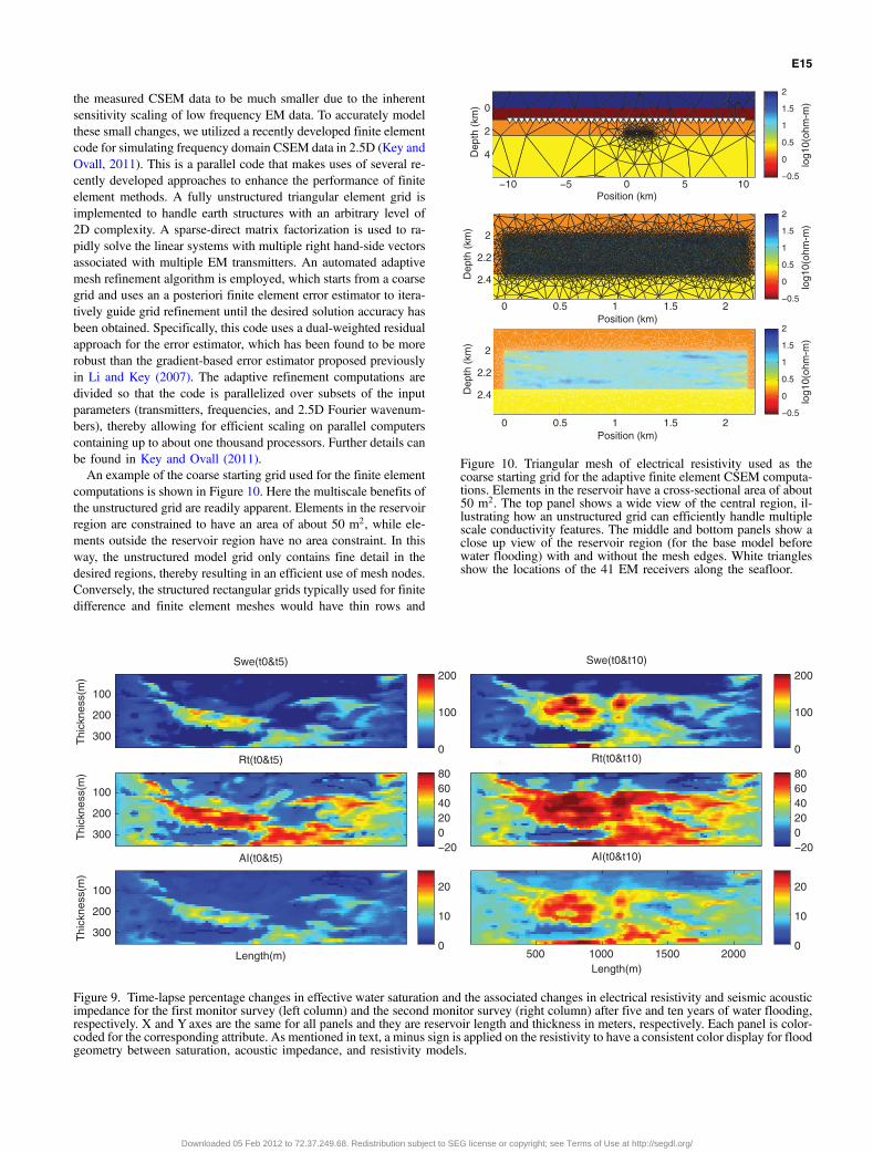
the measured CSEM data to be much smaller due to the inherentsensitivity scaling of low frequency EM data. To accurately modelthese small changes, we utilized a recently developed finite elementcode for simulating frequency domain CSEM data in 2.5D (Key andOvall, 2011). This is a parallel code that makes uses of several re-cently developed approaches to enhance the performance of finiteelement methods. A fully unstructured triangular element grid isimplemented to handle earth structures with an arbitrary level of2D complexity. A sparse-direct matrix factorization is used to ra-pidly solve the linear systems with multiple right hand-side vectorsassociated with multiple EM transmitters. An automated adaptivemesh refinement algorithm is employed, which starts from a coarsegrid and uses an a posteriori finite element error estimator to itera-tively guide grid refinement until the desired solution accuracy hasbeen obtained. Specifically, this code uses a dual-weighted residualapproach for the error estimator, which has been found to be morerobust than the gradient-based error estimator proposed previouslyin Li and Key (2007). The adaptive refinement computations aredivided so that the code is parallelized over subsets of the inputparameters (transmitters, frequencies, and 2.5D Fourier wavenum-bers), thereby allowing for efficient scaling on parallel computerscontaining up to about one thousand processors. Further details canbe found in Key and Ovall (2011).An example of the coarse starting grid used for the finite element

computations is shown in Figure 10. Here the multiscale benefits ofthe unstructured grid are readily apparent. Elements in the reservoirregion are constrained to have an area of about 50 m2, while ele-ments outside the reservoir region have no area constraint. In thisway, the unstructured model grid only contains fine detail in thedesired regions, thereby resulting in an efficient use of mesh nodes.Conversely, the structured rectangular grids typically used for finitedifference and finite element meshes would have thin rows and

Thi

ckne

ss(m

)

Swe(t0&t5)

100

200

3000

100

200

Thi

ckne

ss(m

)

Rt(t0&t5)

100

200

300−20020406080

Length(m)

Thi

ckne

ss(m

)

AI(t0&t5)

100

200

3000

10

20

Swe(t0&t10)

0

100

200

Rt(t0&t10)

−20020406080

Length(m)

AI(t0&t10)

500 1000 1500 20000

10

20

Figure 9. Time-lapse percentage changes in effective water saturation and the associated changes in electrical resistivity and seismic acousticimpedance for the first monitor survey (left column) and the second monitor survey (right column) after five and ten years of water flooding,respectively. X and Y axes are the same for all panels and they are reservoir length and thickness in meters, respectively. Each panel is color-coded for the corresponding attribute. As mentioned in text, a minus sign is applied on the resistivity to have a consistent color display for floodgeometry between saturation, acoustic impedance, and resistivity models.

−10 −5 0 5 10

0

2

4

Position (km)

Dep

th (

km)

0 0.5 1 1.5 2

2

2.2

2.4

Position (km)

Dep

th (

km)

log1

0(oh

m-m

)

−0.5

0

0.5

1

1.5

2

log1

0(oh

m-m

)

−0.5

0

0.5

1

1.5

2

log1

0(oh

m-m

)

−0.5

0

0.5

1

1.5

2

0 0.5 1 1.5 2

2

2.2

2.4

Position (km)

Dep

th (

km)

Figure 10. Triangular mesh of electrical resistivity used as thecoarse starting grid for the adaptive finite element CSEM computa-tions. Elements in the reservoir have a cross-sectional area of about50 m2. The top panel shows a wide view of the central region, il-lustrating how an unstructured grid can efficiently handle multiplescale conductivity features. The middle and bottom panels show aclose up view of the reservoir region (for the base model beforewater flooding) with and without the mesh edges. White trianglesshow the locations of the 41 EM receivers along the seafloor.

E15

Downloaded 05 Feb 2012 to 72.37.249.68. Redistribution subject to SEG license or copyright; see Terms of Use at http://segdl.org/

columns that extend laterally and vertically away from the reservoirregion all the way to the model edges, thereby resulting in a sig-nificant increase in the number of mesh nodes and hence an unne-cessarily larger linear system to solve. After the finite element gridwas generated, the resistivity of each triangle in the reservoir regionwas assigned to the nearest 10 × 10 m cell from the correspondingreservoir modeling grid, resulting in CSEM modeling grids for thebase case and for five and ten years of water flooding.In the numerical simulations, we employed 41 inline electric

dipole transmitters positioned 20 m above the sea bed, and 41 re-ceivers located on the sea bed, all equally spaced every 500 m. SinceCSEM data are typically collected using a transmitter waveformcontaining a broad bandwidth of discrete frequency harmonics(e.g., Myer et al., 2011), we modeled frequencies of 0.1, 0.3,0.5 and 0.7 Hz. While the code outputs all field components, herewe only examine the three fundamental components for an inlinetransmitter (the crossline magnetic field, and the inline and verticalelectric fields). As demonstrated by previous studies, employingmulticomponent and multifrequency measurements in interpreta-tion and inversion of CSEM data can lead to better reservoir char-acterization (e.g., Um and Alumbaugh, 2007; Key, 2009).The adaptive finite element procedure was set to run until the

solution obtained an estimated accuracy no worse than 0.3%

relative error. The coarse starting grid used 13,826 mesh nodeswhile the finally refined grids required between 70,000–110,000nodes to achieve the requested 0.3% accuracy, depending on thespecific parameters of the parallel refinement tasks. Computationswere performed using 960 processors on a parallel cluster computer,taking about 90 s total per time-lapse model. For comparison, only55 s was required to obtain 1% accuracy and 34 s was required for10% accuracy.Figure 11 shows an example of the CSEM responses for the base

case before any water flooding. To establish a baseline signal of thereservoir signal (c.f., the time-lapse signal) responses are shown fora “reference” off-target receiver at position −10 km and a targetreceiver near the edge of the reservoir at −1 km position. Asexpected, the target receiver has significantly larger amplitudes thanthe off-target receiver. The CSEM anomalies (relative differencebetween the target and off-target responses) for all field componentsare largest at the highest frequency (0.7 Hz) with 50%–150%anomalies, whereas at the lowest frequency (0.1 Hz) the anomaliesare only about 10%–20%, depending on the particular fieldcomponent.The amplitude decay curves show that the fields intersect typical

CSEM acquisition system noise floors of 10−19 − 10−18 T∕Am and10−16 − 10−15 V∕Am2 (e.g., Constable and Weiss, 2006; Hoversten

et al., 2006) at ranges of about 7 km for 0.7 Hz togreater than 12 km for 0.1 Hz. The peak anoma-lies occur at 3–7 km ranges. An exception is thelarge second peak in the inline electric field atabout 8 km range. Examination of the amplitudeplot shows that this secondary peak is related tothe arrival of the airwave, which results in a localamplitude minimum where the upward anddownward traveling energy have similar magni-tudes but opposite phase, leading to a field can-cellation (e.g., Orange et al., 2009). Whilefundamentally interesting from a physical stand-point, this phenomenon occurs at amplitudesaround the system noise level and we thereforeconsider it less relevant than the primary anoma-lies at 3–7 km range. The crossline magneticfield also shows a change in decay rate at longerranges associated with the airwave but does notcontain the local amplitude minimum; the verti-cal electric field shows no signs of the airwave,as expected based on previous studies.Now that we have established the baseline

reservoir signal of 10%–50% anomalies, we cancompare that to the time-lapse signals generatedfrom water flooding. Instead of showing lineplots, we condense the data from all 41 transmit-ters and receivers into simple 2D sections. This isaccomplished by plotting the anomaly (here therelative difference between the water-floodedmodel and the base model) horizontally at thetransmitter-receiver midpoint and vertically atthe transmitter-receiver offset (range). Since theCSEM fields generally become more sensitiveto depth with increasing offset, the vertical axiscan be thought of as relative depth scale. Theseanomaly midpoint-offset sections are shown in

10−19

10−18

10−17

10−16

10−15

10−14

10−13

Am

plitu

de (

T/A

m)

−50

0

50

100

150

Ano

mal

y (%

)

Crossline B

0.7 Hz

0.7 Hz

0.1 Hz0.1 Hz

system noise floor

system noise floor

system noise floor

Crossline B

10−16

10−15

10−14

10−13

10−12

10−11

10−10

Am

plitu

de (

V/A

m2 )

−50

0

50

100

150

Ano

mal

y (%

)

0 5 10

10−16

10−15

10−14

10−13

10−12

10−11

10−10

Range (km)

Am

plitu

de (

V/A

m2 )

0 5 10−100

−50

0

50

100

150

Range (km)

Ano

mal

y (%

)

Inline E Inline E

Vertical E Vertical E

Figure 11. CSEM responses of the base model (before water flooding) shown in Fig-ure 10 for various frequencies (0.1, 0.3, 0.5, and 0.7 Hz). The left column shows themagnetic and electric field amplitude responses for the three fundamental components(crossline, inline, and vertical) for a receiver located far off the reservoir at position−10 km (dashed line) and near the edge of the reservoir at position −1 km (solid line).Responses are shown for transmitter tows to the right of the receiver. The right columnshows the anomaly (relative difference) between the two receivers.

E16 Shahin et al.

Downloaded 05 Feb 2012 to 72.37.249.68. Redistribution subject to SEG license or copyright; see Terms of Use at http://segdl.org/

Figures 12, 13, and 14 for the crossline magnetic field and the inlineand vertical electric fields, computed for five and ten years flooding.Again we see that the peak anomalies occur for the highest fre-

quency, but now we can see that the anomalies are largely confinedto data with transmitter-receiver midpoints located over the reser-voir (position 0–2.2 km). Since the water flooding leads to a de-crease in resistivity, the anomalies are generally negative. Thelocation and shape of the anomalies is fairly similar among the threefield components, yet the vertical electric field has a significant po-sitive anomaly at shorter offsets. This is likely due to a change in thevertical electrical impedance of the reservoir during water flooding,leading to a galvanic distortion of electric current flowing normal tothe top boundary. This is supported by the observation that thiseffect is largest at the lowest frequency, where galvanic effectsare expected to be more significant than inductive effects. Contoursof the system noise floor show that most of the anomalies are pre-sent at shorter offsets and are therefore observable with existing sur-vey gear.After five years of flooding, the negative anomalies are only

about −1% at 0.1 Hz and about −5% at 0.7 Hz. After ten years offlooding much larger anomalies are observed: about −5% at 0.1 Hzand −10% at 0.7 Hz. Given the 50% anomaly for the base reservoirwhen compared with an off-target receiver, these 5%–10% time-lapse signals represent fairly significant anomalies. Since the datarepeatability for a real survey is likely to be at best about 1%–2%using currently available nodal CSEM receivers and a deep-towedtransmitter, the −5% anomaly associated with five years of waterflooding would be just detectable, but the −10% anomaly after tenyears of water flooding should be more readily detectable withexisting CSEM survey technology. Future improvements to acqui-

sition technology for time-lapse monitoring, such as permanentlydeployed sensors or sea-bottom cable systems could be used to re-duce the measurement uncertainties, particularly those associatedwith navigation of the transmitter, to well below 1%, making this2D anomaly an appreciable target for monitoring purposes.It is worth noting that during these time-lapse surveys cumula-

tively 1.33 and 2.29 million stock tank barrels (STB) of oil and 1.1and 1.89 million standard cubic feet (MSCF) of gas is produced dueto injection of 1.44 and 2.9 million STB of water after five and tenyears, respectively. This information in conjunction with other para-meters, e.g., reservoir depth, water depth, reservoir lithology type,oil-gas-water electrical properties, etc., can be used to developcriteria for detectability of other reservoirs located at comparableconditions.The results presented here suggest that for a realistic reservoir to

be monitored at a short time lag, i.e., less than five years, a datarepeatability of much less than 1% is required for the basic CSEMmeasurements. As reported by Orange et al. (2009), this is likely tobe impractical using the current CSEM technology that employsfree-falling receivers and towed streamers. Beside, several other fac-tors could obscure the small time-lapse signals. Some of the majorconsiderations are errors in navigation of transmitters and receivers,an inhomogeneous near surface, effects of time-varying ocean con-ductivity, and changes in onsite field instruments and their sensorcalibration corrections during production. All these issues have tobe addressed and appropriately modeled to make time-lapse CSEMapplicable for shorter time intervals through the reservoir’s life.Our 2D study is a first step in the direction of modeling the effects

of exquisitely detailed reservoir production scenarios; however, it isworth considering how the 2D results are relevant for finite-length

5 years

Offs

et (

km)

0.1 Hz

5

10

15

−18Offs

et (

km)

0.3 Hz

5

10

15

−19

−18

Offs

et (

km)

0.5 Hz

5

10

15

−19

−18

Midpoint (km)

Offs

et (

km)

0.7 Hz

−10 −5 0 5 10

5

10

15

10 years

0.1 Hz −10

0

10

−18 0.3 Hz −10

0

10

−19

−18

0.5 Hz −10

0

10

−19

−18

Midpoint (km)

0.7 Hz

−10 −5 0 5 10

−10

0

10

Ano

mal

y (%

)A

nom

aly

(%)

Ano

mal

y (%

)A

nom

aly

(%)

Crossline B: Figure 12. CSEM time-lapse responses computedfor the crossline magnetic field as a function offrequency after five years (left column) and tenyears (right column) of water flooding. Anomaliesare computed as the relative difference betweenthe water-flooded reservoir and the unflooded basereservoir. Anomalies are shown as a function ofthe transmitter-receiver midpoint and transmit-ter-receiver offset. Only positive offsets (transmit-ter to the right of the receiver) are shown. Blacklines show amplitude contours at 10−18 and10−19 T∕Am, which roughly correspond to thesystem noise levels of existing CSEM instrumen-tation.

E17

Downloaded 05 Feb 2012 to 72.37.249.68. Redistribution subject to SEG license or copyright; see Terms of Use at http://segdl.org/

−15

5 years

Offs

et (

km)

0.1 Hz

5

10

15

−16

−15

Offs

et (

km)

0.3 Hz

5

10

15

−16−15

Offs

et (

km)

0.5 Hz

5

10

15

−16−15

Midpoint (km)

Offs

et (

km)

0.7 Hz

−10 −5 0 5 10

5

10

15

−15

10 years

0.1 Hz −10

0

10

−16

−15

0.3 Hz −10

0

10

−16−15

0.5 Hz −10

0

10

−16−15

Midpoint (km)

0.7 Hz

−10 −5 0 5 10

−10

0

10

Ano

mal

y (%

)A

nom

aly

(%)

Ano

mal

y (%

)A

nom

aly

(%)

Vertical E:Figure 14. CSEM time-lapse responses computedfor the vertical electric field as a function of fre-quency after five years (left column) and ten years(right column) of water flooding. Black lines showamplitude contours at 10−15 and 10−16 V∕Am2,which roughly correspond to the system noiselevels of existing CSEM instrumentation.

5 years

Offs

et (

km)

0.1 Hz

5

10

15

−15Offs

et (

km)

0.3 Hz

5

10

15

−15

Offs

et (

km)

0.5 Hz

5

10

15

−16

−15

Midpoint (km)

Offs

et (

km)

0.7 Hz

−10 −5 0 5 10

5

10

15

10 years

0.1 Hz −10

0

10

−15 0.3 Hz −10

0

10

−15

0.5 Hz −10

0

10

−16

−15

Midpoint (km)

0.7 Hz

−10 −5 0 5 10

−10

0

10

Ano

mal

y (%

)A

nom

aly

(%)

Ano

mal

y (%

)A

nom

aly

(%)

Inline E :Figure 13. CSEM time-lapse responses computedfor the inline horizontal electric field as a functionof frequency after five years (left column) and tenyears (right column) of water flooding. Blacklines show amplitude contours at 10−15 and10−16 V∕Am2, which roughly correspond to thesystem noise levels of existing CSEM instrumen-tation.

E18 Shahin et al.

Downloaded 05 Feb 2012 to 72.37.249.68. Redistribution subject to SEG license or copyright; see Terms of Use at http://segdl.org/

3D reservoirs. Constable (2010) performed a 3D resolution kernelstudy that showed the region of highest CSEM sensitivity is largelyconfined to a narrow vertical zone between the source and receiver.While certainly there will be cases were 3D modeling is essential,this narrow sensitivity region suggests that the results from our 2Dstudy will be relevant to 3D reservoirs as long as the survey profilespans the middle of an elongate 3D reservoir. Another concern isthat the small-scale 3D heterogeneity within the reservoir and the3D changes during production have not been captured by the 2Dmodeling scenarios. While such issues are best addressed by future3D model studies of similarly detailed reservoirs, we expect that thevolume averaging of the EM fields will likely act to smooth theeffects of this variability, so that 3D time-lapse responses will besimilar to the 2D responses when the survey profile is over the re-gion where the largest changes in resistivity occur; for example,between the injection and production wells.

CONCLUSIONS

The geologically consistent petroelectric model developed in thispaper explicitly relates petrophysical properties to rock resistivity.As a model, it can be generalized to other geological scenarios and,ultimately, applied to quantitative CSEM reservoir characterizationand monitoring.Our example application simulated three sets of 2D resistivity

models corresponding to the initial reservoir state, and after fiveand ten years of water flooding of a 2200-m wide by 350-m thickoil reservoir. In these intervals, time-lapse changes in effective watersaturation led to −20% − 60% decreases in electrical resistivity. Abase and two monitor CSEM surveys were simulated via a highlyaccurate 2.5D adaptive finite element algorithm numerical algo-rithm. The CSEM responses show a 1%–5% time-lapse signal afterfive years and a stronger 5%–10% time-lapse signal after ten yearsof water flooding. Although small, these changes could be detectedwith the careful application of currently available CSEM acquisitiontechnology. Signal levels at much shorter time intervals (a year orless) would be significantly smaller and not possible to detect withexisting nodal CSEM receivers and deep-towed transmitters.Furthermore, factors restricting the repeatability of CSEMmeasure-ments, e.g., errors in positioning of transmitters and receivers, in-homogeneities in the near surface, effect of time-varying oceanconductivity, and changes in field instruments during productionhave to be addressed properly to preserve these relatively smalltime-lapse signals. Finally, more detailed and 3D time-lapse CSEMsynthetic modeling and inversion, as well as time-domain CSEMsimulation may shed light on complications probably not seen inour 2.5D frequency domain analyses.

ACKNOWLEDGMENTS

We would like to thank the sponsors of the UT-Austin EDGERForum and the Jackson School of Geosciences at the University ofTexas at Austin for their support of this research. K. Key was sup-ported by the Seafloor Electromagnetic Methods Consortium atScripps Institution of Oceanography. Alireza Shahin sincerelythanks Carlos Verdin, Jack Dvorkin, Larry Lake, and William Gal-loway for enlightening discussion on reservoir modeling. Specialthanks to Anton Ziolkowski and three reviewers for critically re-viewing the manuscript and suggesting many improvements. A noteof special gratitude goes to Schlumberger for providing reservoir

simulation software. The San Diego Supercomputer Center atUCSD provided access to the Triton Compute Cluster.

APPENDIX A

PETROPHYSICS AND ROCK-FLUID PHYSICSMODEL TO COMPUTE ELECTRICAL

RESISTIVITY

As described in the petrophysics model, the clay distribution isdispersed or pore-filling. The corresponding porosity-clay modelwas introduced by Thomas and Stieber (1975) and further devel-oped by Marion et al. (1992). Total φt and effective φe porosityin shaly sand domain is calculated as follows

φt ¼ φss − Cshð1 − φshÞ Csh ≤ φss (A.1)

φe ¼ φt − φshCsh (A.2)

where φsh is pure shale porosity, φss is the clean sandstone porosity,and Csh is the volumetric shale concentration of the rock.Dual water models (Best, 1980; Dewan, 1983; Clavier, 1984) are

applicable for dispersed clay distributions. In this study, we use thedual water model because several of its parameters can be computedfrom well logs (Dewan, 1983) and it can be efficiently combinedwith the dispersed clay model. Based on this model, electrical-conductivity or inverse of rock resistivity (Rt) is computed asfollows

1

Rt¼ φm

t Snwta

�1

Rwþ Swb

Swt

�1

Rwb−

1

Rw

��(A.3)

Where a, m, n are tortuosity factor, cementation factor, and sa-turation exponent, respectively, Swb and Swt are clay bound-watersaturation and total water saturation, respectively and are computedusing

Swb ¼Cshϕsh

ϕt(A.4)

Swt ¼ SwbSwsϕe

ϕt(A.5)

The terms Rw and Rwb are free and bound-water resistivity whichdepends on salinity and temperature. We use Arps’ empirical equa-tion (Arps, 1953) to calculate these quantities:

Rw ¼�0.0123 þ 3647.5

NaClðppmÞ0.995���

81.77

TðoFÞ þ 6.77

�

(A.6)

Where the concentration of NaCl in particle per million (ppm)and temperature (T) in Fahrenheit degree are required to computefluid resistivity.

E19

Downloaded 05 Feb 2012 to 72.37.249.68. Redistribution subject to SEG license or copyright; see Terms of Use at http://segdl.org/

REFERENCES

Archie, G. E., 1942, The electrical resistivity of log as an aid in determiningsome reservoir characteristics: Petroleum Transactions, AIME, 146, 54–61.

Arps, J. J., 1953, The effect of temperature on the density and electricalresistivity of sodium chloride solutions: Petroleum Transactions, AIME,198, 327–328.

Avseth, P., T. Mukerji, and G. Mavko, 2005, Quantitative seismicinterpretation: Cambridge University Press.

Aziz, K., and A. Settari, 1979, Petroleum reservoir simulation: AppliedScience Publishers LTD.

Batzle, M., and Z. Wang, 1992, Seismic properties of pore fluids:Geophysics, 57, 1396–1408, doi: 10.1190/1.1443207.

Best, D. L., J. S. Gardner, and J. L. Dumanoir, 1980, A computer-processedwellsite log interpretation: SPE, 9039.

Black, N., and M. S. Zhdanov, 2009, Monitoring of hydrocarbon reservoirsusing marine CSEM method: 79th Annual International Meeting, SEG,Expanded Abstracts, 850–854.

Christie, M. A., and M. J. Blunt, 2001, Tenth society of petroleum engineerscomparative solution project: A comparison of upscaling techniques:Reservoir Simulation Symposium, SPE, 72469.

Clavier, C., G. Coates, and J. Dumanoir, 1984, Theoretical and experimentalbases for the dual water model for interpretation of shaly sands: SPE6859.

Constable, S., 2010, Ten years of marine CSEM for hydrocarbon explora-tion: Geophysics, 75, no 5, 75A67–75A81, doi: 10.1190/1.3483451.

Constable, S., and L. J. Srnka, 2007, An introduction to marine controlled-source electromagnetic methods for hydrocarbon exploration:Geophysics, 72, WA3–WA12, doi: 10.1190/1.2432483.

Constable, S., and C. J. Weiss, 2006, Mapping thin resistors and hydrocar-bons with marine EM methods: Insights from 1D modeling: Geophysics,71, no. 2, G43–G51, doi: 10.1190/1.2187748.

Dewan, J. T., 1983, Essentials of modern open-hole log interpretation:PennWell Books.

Dvorkin, J., and M. Gutierrez, 2002, Grain sorting, porosity, and elasticity:Petrophysics, 43, 185–196.

Dvorkin, J., G. Mavko, and B. Gurevich, 2007, Fluid substitution in shalysediments using effective porosity: Geophysics, 72, no. 3, O1–O8, doi:10.1190/1.2565256.

Eidesmo, T., S. Ellingsrud, L. M. MacGregor, S. Constable, M. C. Sinha,S. Johansen, F. N. Kong, and H. Westerdahl, 2002, Seabed logging (SBL),a new method for remote and direct identification of hydrocarbon filledlayers in deepwater areas: First Break, 20, 144–152.

Ellingsrud, S., T. Eidesmo, S. Johansen, M. C. Sinha, L. M. MacGregor, andS. Constable, 2002, Remote sensing of hydrocarbon layers by seabedlogging (SBL): Results from a cruise offshore Angola: The Leading Edge,21, 972–982, doi: 10.1190/1.1518433.

Galloway, W. E., and D. K. Hobday, 1996, Terrigenous clastic depositionalsystems: Applications to fossil fuel and groundwater resources, 2ndedition, Springer-Verlag.

Hacikoylu, P., J. Dvorkin, and G. Mavko, 2006, Resistivity-velocitytransforms revisited: The Leading Edge, 25, 1006–1009, doi: 10.1190/1.2335159.

Hoversten, G. M., F. Cassassuce, E. Gasperikova, G. A. Newman, J. Chen,Y. Rubin, Z. Hou, and D. Vasco, 2006, Direct reservoir parameterestimation using joint inversion of marine seismic AVA and CSEM data:Geophysics, 71, no. 3, C1–C13, doi: 10.1190/1.2194510.

Key, K., 2009, 1D inversion of multicomponent, multifrequency marineCSEM data: Methodology and synthetic studies for resolving thinresistive layers: Geophysics, 74, F9–F20, doi: 10.1190/1.3058434.

Key, K., and J. Ovall, 2011, A parallel goal-oriented adaptive finite elementmethod for 2.5D electromagnetic modeling: Geophysical JournalInternational, 186, 137–154, doi: 10.1111/gji.2011.186.issue-1.

Killough, J. E., 1995, Ninth SPE comparative solution project: A reexami-nation of black-oil simulation: SPE Reservoir Simulation Symposium,29110, 135–147.

Li, Y., and K. Key, 2007, 2D marine controlled-source electromagnetic mod-eling: Part 1 — An adaptive finite-element algorithm: Geophysics, 72,WA51–WA6, doi: 10.1190/1.2432262.

Lien, M., and T. Mannseth, 2008, Sensitivity study of marine CSEM data forreservoir production monitoring: Geophysics, 73, no. 4, F151–F163, doi:10.1190/1.2938512.

Marion, D., A. Nur, H. Yin, and D. Han, 1992, Compressional velocity andporosity in sand-clay mixtures: Geophysics, 57, 554–563, doi: 10.1190/1.1443269.

Myer, D., S. Constable, and K. Key, 2011, Broad-band waveforms androbust processing for marine CSEM surveys: Geophysical Journal Inter-national, 184, 689–698, doi: 10.1111/gji.2011.184.issue-2.

Orange, A., K. Key, and S. Constable, 2009, The feasibility of reservoirmonitoring using time-lapse marine CSEM: Geophysics, 74, no. 2F21–F29, doi: 10.1190/1.3059600.

Revil, A., and L. M. Cathles, 1999, Permeability of shaly sands: WaterResources Research, 35, 516–662, doi: 10.1029/98WR02700.

Saner, S., M. N. Cagatay, and A. M. A1 Sanounah, 1996, Relationships be-tween shale content and grain-size parameters in the Safaniya sandstonereservoir, NE Saudi Arabia: Journal of Petroleum Geology, 19, 3, 305–320, doi: 10.1111/jpg.1996.19.issue-3.

Shahin, A., P. L. Stoffa, R. H. Tatham, and R. Seif, 2011, Accuracy requiredin seismic modeling to detect production-induced time-lapse signatures:81st Annual International Meeting, SEG, 2860–2864.

Shahin, A., R. H. Tatham, P. L. Stoffa, and K. T. Spikes, 2010, Comprehen-sive petro-elastic modeling aimed at quantitative seismic reservoir char-acterization and monitoring: 80th Annual International Meeting, SEG,Expanded Abstracts, 2245–2250.

Thomas, E. C., and S. J. Stieber, 1975, The distribution of shale insandstones and its effect upon porosity, paper T in the 16th AnnualLogging Symposium Transactions: Society of Professional Well LogAnalysts.

Tyler, N., and W. A. Ambrose, 1986, Facies architecture and productioncharacteristics of strand-plain reservoirs on north Markham-North BayCity Field, Frio formation, Texas: AAPG Bulletin, 70, 809–829.

Uden, R., J. Dvorkin, J. Walls, and M. Carr, 2004, Lithology substitution in asand/shale sequence, Extended Abstracts, ASEG 17th GeophysicalConference and Exhibition, Sydney.

Um, E. S., and D. L. Alumbaugh, 2007, On the physics of the marinecontrolled-source electromagnetic method: Geophysics, 72, no. 2,WA13–WA26, doi: 10.1190/1.2432482.

Waxman, M. H., and L. J. M. Smits, 1968, Electrical conductivities in oil-bearing shaly sands: SPE Journal, 8, 107–12, doi: 10.2118/1863-A.

Wright, D., A. Ziolkowski, and B. Hobbs, 2002, Hydrocarbon detection andmonitoring with a multicomponent transient electromagnetic (MTEM)survey: The Leading Edge, 21, 852–864, doi: 10.1190/1.1508954.

Zach, J. J., M. A. Frenkel, D. Ridyard, J. Hincapie, B. Dubois, andJ. P. Morten, 2009, Marine CSEM time-lapse repeatability for hydrocar-bon field monitoring: 79th Annual International Meeting, SEG, ExpandedAbstracts, 820–823.

Ziolkowski, A., R. Parr, D. Wright, V. Nockles, C. Limond, E. Morris, andJ. Linfoot, 2010, Multi-transient electromagnetic repeatability experimentover the North Sea Harding field: Geophysical Prospecting, 58, no. 6,1159–1176.

E20 Shahin et al.

Downloaded 05 Feb 2012 to 72.37.249.68. Redistribution subject to SEG license or copyright; see Terms of Use at http://segdl.org/