Perturbation Theory for Linear Operators
643
C L A S S I C S I N M A T H E M AT I C S Tosio Kato Perturbation Theory for Linear Operators Springer
-
Upload
luftbahnfahrer -
Category
Documents
-
view
130 -
download
7
description
Tosio KatoSecond Edition (Classics in Mathematics)-Springer (1995)
Transcript of Perturbation Theory for Linear Operators
C L A S S I C S I N M A T H E M AT I C S
Tosio Kato
Perturbation Theoryfor Linear Operators
Springer
Tosio Kato
Perturbation Theory
for Linear Operators
Reprint of the 1980 Edition
Springer
Tosio KatoDepartment of Mathematics, University of CaliforniaBerkeley, CA 94720-3840USA
Originally published as Vol. 132 of theGrundlehren der mathematischen Wissenschaften
Mathematics Subject Classification (1991): 46BXX, 46CXX, 47AXX, 47BXX,47D03, 47E05, 47F05, 81Q10, 81Q15, 81UXX
ISBN 3-540-58661-X Springer-Verlag Berlin Heidelberg New York
CIP data applied for
This work is subject to copyright. All rights are reserved, whether the whole or part of the material isconcerned, specifically the rights of translation, reprinting, reuse of illustration, recitation, broadcasting,reproduction on microfilm or in any other way, and storage in data banks. Duplication of this publicationor parts thereof is permitted only under the provision of the German Copyright Law of September 9, 1965,in its current version, and permission for use must always be obtained from Springer-Verlag. Violations areliable for prosecution under the German Copyright Law.
a Springer-Verlag Berlin Heidelberg 1995Printed in Germany
The use of general descriptive names, registered names, trademarks, etc. in this publication does not imply,even in the absence of a specific statement, that such names are exempt from the relevant protective lawsand regulations and therefore free for general use.
SPIN 10485260 41/3140 - 54 3 210 - Printed on acid-free paper
Tosio Kato
Perturbation Theoryfor Linear Operators
Corrected Printing of the Second Edition
Springer-VerlagBerlin Heidelberg New York 1980
Dr. Tosio KatoProfessor of Mathematics, University of California, Berkeley
AMS Subject Classification (1970): 46Bxx, 46Cxx, 47Axx, 47Bxx, 47D05,47Exx, 47Fxx, 81A09, 81A10, 81A45
ISBN 3-540-07558-5 2. Auflage Springer-Verlag Berlin Heidelberg New York
ISBN 0-387-07558-5 2nd edition Springer-Verlag New York Heidelberg Berlin
ISBN 3-540-03526-5 1. Auflage Berlin Heidelberg New York
ISBN 0-387-03526-5 1st edition New York Heidelberg Berlin
Library of Congress Cataloging in Publication Data. Kato, Tosio, 1917-Perturbationtheory for linear operators. (Grundlehren der mathematischen Wissenschaften;132). Bibliography: p. Includes indexes. 1. Linear operators. 2. Perturbation(Mathematics). I. Title. II. Series: Die Grundlehren der mathematischen Wissen-schaften in Einzeldarstellungen; Bd. 132.QA329.2.K37 1976. 515'.72. 76-4553.
This work is subject to copyright. All rights are reserved, whether thewhole or part of
the material is concerned, specifically those of translation, reprinting, re-use of
illustrations, broadcasting, reproduction by photocopying machine or similar means,and storage in data banks. Under § 54 of the German Copyright Law where
copies are made for other than private use, a fee is payable to thepublisher,
the amount of the fee to be determined by agreement with the publisher.
© by Springer-Verlag Berlin Heidelberg 1966, 1976Printed in Germany.Typesetting, printing and binding: Briihlsche Universit5tsdruckerei Giellen
To the memory
of my patents

Preface to the Second Edition
In view of recent development in perturbation theory, supplementarynotes and a supplementary bibliography are added at the end of the newedition. Little change has been made in the text except that the para-graphs V-§ 4.5, VI-§ 4.3, and VIII-§ 1.4 have been completely rewritten,and a number of minor errors, mostly typographical, have been corrected.The author would like to thank many readers who brought the errors tohis attention.
Due to these changes, some theorems, lemmas, and formulas of thefirst edition are missing from the new edition while new ones are added.The new ones have numbers different from those attached to the oldones which they may have replaced.
Despite considerable expansion, the bibliography is not intended tobe complete.
Berkeley, April 1976 Tosio KATO
Preface to the First EditionThis book is intended to give a systematic presentation of perturba-
tion theory for linear operators. It is hoped that the book will be usefulto students as well as to mature scientists, both in mathematics and inthe physical sciences.
Perturbation theory for linear operators is a collection of diversifiedresults in the spectral theory of linear operators, unified more or lessloosely by their common concern with the behavior of spectral propertieswhen the operators undergo a small change. Since its creation by RAY-LEIGH and SCHRODINGER, the theory has occupied an important place inapplied mathematics; during the last decades, it has grown into amathematical discipline with its own interest. The book aims at a mathe-matical treatment of the subject, with due consideration of applications.
The mathematical foundations of the theory belong to functionalanalysis. But since the book is partly intended for physical scientists,who might lack training in functional analysis, not even the elements ofthat subject are presupposed. The reader is assumed to have only a basicknowledge of linear algebra and real and complex analysis. The necessarytools in functional analysis, which are restricted to the most elementarypart of the subject, are developed in the text as the need for them arises(Chapters I, III and parts of Chapters V, VI).
An introduction, containing a brief historical account of the theory,precedes the main exposition. There are ten chapters, each prefaced by a
VIII Preface
summary. Chapters are divided into sections, and sections into para-graphs. I-§ 2.3, for example, means paragraph three of section two ofchapter one; it is simply written § 2.3 when referred to within the samechapter and par. 3 when referred to within the same section. Theorems,Corollaries, Lemmas, Remarks, Problems, and Examples are numberedin one list within each section: Theorem 2.1, Corollary 2.2, Lemma 2.3,etc. Lemma 1-2.3 means Lemma 2.3 of chapter one, and it is referredto simply as Lemma 2.3 within the same chapter. Formulas are numberedconsecutively within each section; I-(2.3) means the third formula ofsection two of chapter one, and it is referred to as (2.3) within the samechapter. Some of the problems are disguised theorems, and are quotedin later parts of the book.
Numbers in [ ] refer to the first part of the bibliography containingarticles, and those in Q JI to the second part containing books and mono-graphs.
There are a subject index, an author index and a notation index at theend of the book.
The book was begun when I was at the University of Tokyo andcompleted at the University of California. The preparation of the bookhas been facilitated by various financial aids which enabled me to pursueresearch at home and other institutions. For these aids I am gratefulto the following agencies: the Ministry of Education, Japan; Com-missariat General du Plan, France; National Science Foundation,Atomic Energy Commission, Army Office of Ordnance Research, Officeof Naval Research, and Air Force Office of Scientific Research, U.S.A.
I am indebted to a great many friends for their suggestions duringthe long period of writing the book. In particular I express my heartythanks to Professors C. CLARK, K. O. FRIEDRICHS, H. FUJITA, S. GOLD-BERG, E. HILLE, T. IKEBE, S. KAKUTANI, S. T. KURODA, G. NEUBAUER,R. S. PHILLIPS, J. and O. TODD, F. WOLF, and K. YOSIDA. I am especiallyobliged to Professor R. C. RIDDELL, who took the pains of going throughthe whole manuscript and correcting innumerable errors, mathematicalas well as linguistic. I am indebted to Dr. J. HOWLAND, Dr. F. McGRATH,Dr. A. MCINTOSH, and Mr. S.-C. LIN for helping me in proofreadingvarious parts of the book. I wish to thank Professor F. K. SCHMIDT whosuggested that I write the book and whose constant encouragementbrought about the completion of the book. Last but not least mygratitudes go to my wife, MIZUE, for the tedious work of typewritingthe manuscript.
Berkeley Tosio KATO
August, 1966
Contentspage
Introduction . . . . . . . . . . . . . . . . . . . . . . . . . . . XVII
§ 1.
Chapter OneOperator theory in finite-dimensional vector spaces
Vector spaces and normed vector spaces . . . . . . . . . . . . . I1. Basic notions . . . . . . . . . . . . . . . . . . . . . . . . 1
2. Bases . . . . . . . . . . . . . . . . . . . . . . . . . . . 23. Linear manifolds . . . . . . . . . . . . . . . . . . . . . . 34. Convergence and norms . . . . . . . . . . . . . . . . . . . 45. Topological notions in a normed space . . . . . . . . . . . . . 66. Infinite series of vectors . . . 77. Vector-valued functions . . . . . . . . . . . . . . . . . . . 8
§ 2. Linear forms and the adjoint space . . . . . . . . . . . . . . . . 101. Linear forms . . . . . . . . . . . . . . . . . . . . . . . . 102. The adjoint space . . . . . . . . . . . . . . . . . . . . . . 113. The adjoint basis . . . . . . . . . . . . . . . . . . . . . . 124. The adjoint space of a normed space . . . . . . . . . . . . . . 135. The convexity of balls . . . . . . . . . . . . . . . . . . . . 146. The second adjoint space . . . . . . . . . . . . . . . . . . . 15
§ 3. Linear operators . . . . . . . . . . . . . . . . . . . . . . . . 161. Definitions. Matrix representations . . . . . . . . . . . . . . 162. Linear operations on operators . . . . . . . . . . . . . . . . 183. The algebra of linear operators . . . . . . . . . . . . . . 194. Projections. Nilpotents . . . . . . . . . . . . . . . . . . . . 205. Invariance. Decomposition . . . . . . . . . . . . . . . . . . 226. The adjoint operator . . . . . . . . . . . . . . . . . . . . . 23
§ 4. Analysis with operators . . . . . . . . . . . . . . . . . . . . . 251. Convergence and norms for operators . . . . . . . . . . . . . 252. The norm of T" . . . . . . . . . . . . . . . . . . . . . . . 273. Examples of norms . . . . . . . . . . . . . . . . . . . . . 284. Infinite series of operators . . . . . . . . . . . . . . . . . . 295. Operator-valued functions . . . . . . . . . . . . . . . . . . 316. Pairs of projections . . . . . . . . . . . . . . . . . . . . . 32
§ 5. The eigenvalue problem . . . . . . . . . . . . . . . . . . . . . 341. Definitions . . . . . . . . . . . . . . . . . . . . . . . . . 342. The resolvent . . . . . . . . . . . . . . . . . . . . . . . . 363. Singularities of the resolvent . . . . . . . . . . . . . . . . . 384. The canonical form of an operator . . . . . . . . . . . . . . . 405. The adjoint problem . . . . . . . . . . . . . . . . . . . . . 436. Functions of an operator . . . . . . . . . . . . . . . . . . . 447. Similarity transformations . . . . . . . . . . . . . . . . . . 46
X Contents
§ 6. Operators in unitary spaces . . . . . . . . . . . . . . . . . . . 471. Unitary spaces . . . . . . . . . . . . . . . . . . . . . . . 472. The adjoint space . . . . . . . . . . . . . . . . . . . . . . 483. Orthonormal families . . . . . . . . . . . . . . . . . . . . 494. Linear operators . . . . . . . . . . . . . . . . . . . . . . 515. Symmetric forms and symmetric operators . . . . . . . . . . . 526. Unitary, isometric and normal operators . . . . . . . . . . . . 547. Projections . . . . . . . . . . . . . . . . . . . . . . . . . 558. Pairs of projections . . . . . . . . . . . . . . . . . . . . . 569. The eigenvalue problem . . . . . . . . . . . . . . . . . . . 58
10. The minimax principle . . . . . . . . . . . . . . . . . . . . 60
Chapter TwoPerturbation theory in a finite-dimensional space 62
§ 1. Analytic perturbation of eigenvalues . . . . . . . . . . . . . . . 631. The problem . . . . . . . . . . . . . . . . . . . . . . . . 632. Singularities of the eigenvalues . . . . . . . . . . . . . . . . 653. Perturbation of the resolvent . . . . . . . . . . . . . . . . . 664. Perturbation of the eigenprojections . . . . . . . . . . . . . . 675. Singularities of the eigenprojections . . . . . . . . . . . . . . 696. Remarks and examples . . . . . . . . . . . . . . . . . . . . 707. The case of T (x) linear in x . . . . . . . . . . . . . . . . . 728. Summary . . . . . . . . . . . . . . . . . . . . . . . . . 73
§ 2. Perturbation series . . . . . . . . . . . . . . . . . . . . . . . 741. The total projection for the A-group . . . . . . . . . . . . . . 742. The weighted mean of eigenvalues . . . . . . . . . . . . . . . 773. The reduction process . . . . . . . . . . . . . . . . . . . . 814. Formulas for higher approximations . . . . . . . . . . . . . . 835. A theorem of MOTZKIN-TAUSSxv . . . . . . . . . . . . . . . 856. The ranks of the coefficients of the perturbation series . . . . . . 86
§ 3. Convergence radii and error estimates . . . . . . . . . . . . . . 881. Simple estimates . . . . . . . . . . . . . . . . . . . . . . 882. The method of majorizing series . . . . . . . . . . . . . . . . 893. Estimates on eigenvectors . . . . . . . . . . . . . . . . . . 914. Further error estimates . . . . . . . . . . . . . . . . . . . 935. The special case of a normal unperturbed operator . . . . . . . . 946. The enumerative method . . . . . . . . . . . . . . . . . . . 97
§ 4. Similarity transformations of the eigenspaces and eigenvectors . . . . 981. Eigenvectors . . . . . . . . . . . . . . . . . . . . . . . . 982. Transformation functions . . . . . . . . . . . . . . . . . . . 993. Solution of the differential equation . . . . . . . . . . . . . . 1024. The transformation function and the reduction process . . . . . . 1045. Simultaneous transformation for several projections . . . . . . . 1046. Diagonalization of a holomorphic matrix function . . . . . . . . 106
§ 5. Non-analytic perturbations . . . . . . . . . . . . . . . . . . . 1061. Continuity of the eigenvalues and the total projection . . . . . . 1062. The numbering of the eigenvalues . . . . . . . . . . . . . . . 1083. Continuity of the eigenspaces and eigenvectors . . . . . . . . . 1104. Differentiability at a point . . . . . . . . . . . . . . . . . . 111
Contents XI
5. Differentiability in an interval . . . . . . . . . . . . . . . . 1136. Asymptotic expansion of the eigenvalues and eigenvectors . . . . 1157. Operators depending on several parameters . . . . . . . . . . . 1168. The eigenvalues as functions of the operator . . . . . . . . . . 117
§ 6. Perturbation of symmetric operators . . . . . . . . . . . . . . . 1201. Analytic perturbation of symmetric operators . . . . . . . . . . 1202. Orthonormal families of eigenvectors . . . . . . . . . . . . . . 1213. Continuity and differentiability . . . . . . . . . . . . . . . . 1224. The eigenvalues as functions of the symmetric operator . . . . . 1245. Applications. A theorem of LIDSKII . . . . . . . . . . . . . . 124
Chapter ThreeIntroduction to the theory of operators in Banach spaces
§ 1. Banach spaces . . . . . . . . . . . . . . . . . . . . . . . . . 1271. Normed spaces . . . . . . . . . . . . . . . . . . . . . . . 1272. Banach spaces . . . . . . . . . . . . . . . . . . . . . . . 1293. Linear forms . . . . . . . . . . . . . . . . . . . . . . . . 1324. The adjoint space . . . . . . . . . . . . . . . . . . . . . . 1345. The principle of uniform boundedness . . . . . . . . . . . . . 1366. Weak convergence . . . . . . . . . . . . . . . . . . . . . . 1377. Weak* convergence . . . . . . . . . . . . . . . . . . . . . 1408. The quotient space . . . . . . . . . . . . . . . . . . . . . 140
§ 2. Linear operators in Banach spaces . . . . . . . . . . . . . . . . 1421. Linear operators. The domain and range . . . . . . . . . . . . 1422. Continuity and boundedness . . . . . . . . . . . . . . . . . 1453. Ordinary differential operators of second order. . . . . . . . . . 146
§ 3. Bounded operators . . . . . . . . . . . . . . . . . . . . . . . 1491. The space of bounded operators . . . . . . . . . . . . . . . 1492. The operator algebra .1 (X) . . . . . . . . . . . . . . . . . . 1533. The adjoint operator . . . . . . . . . . . . . . . . . . . . . 1544. Projections . . . . . . . . . . . . . . . . . . . . . . . . . 155
§ 4. Compact operators . . . . . . . . . . . . . . . . . . . . . . . 1571. Definition . . . . . . . . . . . . . . . . . . . . . . . . . 1572. The space of compact operators . . . . . . . . . . . . . . . . 1583. Degenerate operators. The trace and determinant . . . . . . . . 160
§ 5. Closed operators . . . . . . . . . . . . . . . . . . . . . . . . 1631. Remarks on unbounded operators . . . . . . . . . . . . . . . 1632. Closed operators . . . . . . . . . . . . . . . . . . . . . . . 1643. Closable operators . . . . . . . . . . . . . . . . . . . . . . 1654. The closed graph theorem .. . . . . . . . . . . . . . . . . . 1665. The adjoint operator . . . . . . . . . . . . . . . . . . . . . 1676. Commutativity and decomposition . . . . . . . . . . . . . . . 171
§ 6. Resolvents and spectra . . . . . . . . . . . . . . . . . . . . . 1721. Definitions . . . . . . . . . . . . . . . . . . . . . . . . . 1722. The spectra of bounded operators . . . . . . . . . . . . . . . 1763. The point at infinity . . . . . . . . . . . . . . . . . . . . . 1764. Separation of the spectrum . . . . . . . . . . . . . . . . . . 178
XII Contents
5. Isolated eigenvalues . . . . . . . . . . . . . . . . . . . . . 1806. The resolvent of the adjoint . . . . . . . . . . . . . . . . . 1837. The spectra of compact operators . . . . . . . . . . . . . . . 1858. Operators with compact resolvent . . . . . . . . . . . . . . . 187
Chapter Four
Stability theorems
§ 1. Stability of closedness and bounded invertibility . . . . . . . . . . 1891. Stability of closedness under relatively bounded perturbation . . . 1892. Examples of relative boundedness . . . . . . . . . . . . . . . 1913. Relative compactness and a stability theorem . . . . . . . . . . 1944. Stability of bounded invertibility . . . . . . . . . . . . . . . 196
§ 2. Generalized convergence of closed operators . . . . . . . . . . . . 1971. The gap between subspaces . . . . . . . . . . . . . . . . . . 1972. The gap and the dimension . . . . . . . . . . . . . . . . . . 1993. Duality . . . . . . . . . . . . . . . . . . . . . . . . . . 2004. The gap between closed operators . . . . . . . . . . . . . . . 2015. Further results on the stability of bounded invertibility . . . . . 2056. Generalized convergence . . . . . . . . . . . . . . . . . . . 206
§ 3. Perturbation of the spectrum . . . . . . . . . . . . . . . . . . 2081. Upper semicontinuity of the spectrum . . . . . . . . . . . . . 2082. Lower semi-discontinuity of the spectrum . . . . . . . . . . . 2093. Continuity and analyticity of the resolvent . . . . . . . . . . . 2104. Semicontinuity of separated parts of the spectrum . . . . . . . . 2125. Continuity of a finite system of eigenvalues . . . . . . . . . . . 2136. Change of the spectrum under relatively bounded perturbation . 2147. Simultaneous consideration of an infinite number of eigenvalues 2158. An application to Banach algebras. Wiener's theorem . . . . . . 216
§ 4. Pairs of closed linear manifolds . . . . . . . . . . . . . . . . . 2181. Definitions . . . . . . . . . . . . . . . . . . . . . . . . . 2182. Duality . . . . . . . . . . . . . . . . . . . . . . . . . . 2213. Regular pairs of closed linear manifolds . . . . . . . . . . . . 2234. The approximate nullity and deficiency . . . . . . . . . . . . 2255. Stability theorems . . . . . . . . . . . . . . . . . . . . . . 227
§ 5. Stability theorems for semi-Fredholm operators . . . . . . . . . . 2291. The nullity, deficiency and index of an operator . . . . . . . . . 2292. The general stability theorem . . . . . . . . . . . . . . . . . 2323. Other stability theorems . . . . . . . . . . . . . . . . . . . 2364. Isolated eigenvalues . . . . . . . . . . . . . . . . . . . . . 2395. Another form of the stability theorem . . . . . . . . . . . . . 2416. Structure of the spectrum of a closed operator . . . . . . . . . 242
§ 6. Degenerate perturbations . . . . . . . . . . . . . . . . . . . . 2441. The Weinstein-Aronszajn determinants . . . . . . . . . . . . . 2442. The W-A formulas . . . . . . . . . . . . . . . . . . . . . . 2463. Proof of the W-A formulas . . . . . . . . . . . . . . . . . . 2484. Conditions excluding the singular case . . . . . . . . . . . . . 249
Contents XIII
Chapter FiveOperators in Hilbert spaces
§ 1. Hilbert space . . . . . . . . . . . . . . . . . . . . . . . . 2511. Basic notions . . . . . . . . . . . . . . . . . . . . . . . . 2512. Complete orthonormal families . . . . . . . . . . . . . . . . 254
§ 2. Bounded operators in Hilbert spaces . . . . . . . . . . . . . . . 2561. Bounded operators and their adjoints . . . . . . . . . . . . . 2562. Unitary and isometric operators . . . . . . . . . . . . . . . . 2573. Compact operators . . . . . . . . . . . . . . . . . . . . . 2604. The Schmidt class . . . . . . . . . . . . . . . . . . . . . . 2625. Perturbation of orthonormal families . . . . . . . . . . . . . . 264
§ 3. Unbounded operators in Hilbert spaces . . . . . . . . . . . . . . 2671. General remarks . . . . . . . . . . . . . . . . . . . . . . 2672. The numerical range . . . . . . . . . . . . . . . . . . . . 2673. Symmetric operators . . . . . . . . . . . . . . . . . . . . 2694. The spectra of symmetric operators . . . . . . . . . . . . . . 2705. The resolvents and spectra of selfadjoint operators . . . . . . . 2726. Second-order ordinary differential operators . . . . . . . . . . 2747. The operators T*T . . . . . . . . . . . . . . . . . . . . . 2758. Normal operators . . . . . . . . . . . . . . . . . . . . . . 2769. Reduction of symmetric operators . . . . . . . . . . . . . . 277
10. Semibounded and accretive operators . . . . . . . . . . . . . 27811. The square root of an m-accretive operator . . . . . . . . . . 281
§ 4. Perturbation of selfadjoint operators . . . . . . . . . . . . . . . 2871. Stability of selfadjointness . . . . . . . . . . . . . . . . . . 2872. The case of relative bound 1 . . . . . . . . . . . . . . . . . 2893. Perturbation of the spectrum . . . . ... . . . . . . . . . . . 2904. Semibounded operators . . . . . . . . . . . . . . . . . . . 2915. Completeness of the eigenprojections of slightly non-selfadjoint
operators . . . . . . . . . . . . . . . . . . . . . . . . . . 293
§ 5. The Schr6dinger and Dirac operators . . . . . . . . . . . . . . . 2971. Partial differential operators . . . . . . . . . . . . . . . . . 2972. The Laplacian in the whole space . . . . . . . . . . . . . . . 2993. The Schr6dinger operator with a static potential . . . . . . . . 3024. The Dirac operator . . . . . . . . . . . . . . . . . . . . . 305
Chapter SixSesquilinear forms in Hilbert spaces and associated operators
§ 1. Sesquilinear and quadratic forms . . . . . . . . . . . . . . . . . 3081. Definitions . . . . . . . . . . . . . . . . . . . . . . . . . 3082. Semiboundedness . . . . . . . . . . . . . . . . . . . . . . 3103. Closed forms . . . . . . . . . . . . . . . . . . . . . . . . 3134. Closable forms . . . . . . . . . . . . . . . . . . . . . . . 3155. Forms constructed from sectorial operators . . . . . . . . . . . 3186. Sums of forms . . . . . . . . . . . . . . . . . . . . . . . 3197. Relative boundedness for forms and operators . . . . . . . . . . 321
§ 2. The representation theorems . . . . . . . . . . . . . . . . . . 3221. The first representation theorem . . . . . . . . . . . . . . . . 3222. Proof of the first representation theorem . . . . . . . . . . . . 3233. The Friedrichs extension . . . . . . . . . . . . . . . . . . . 3254. Other examples for the representation theorem . . . . . . . . . 326
XIV Contents
§ 3.
§ 4.
§ 5.
§ 1.
§ 2.
§ 3.
§ 4.
5. Supplementary remarks . . . . . . . . . . . . . . . . . . . 3286. The second representation theorem . . . . . . . . . . . . . . 3317. The polar decomposition of a closed operator . . . . . . . . . . 334
Perturbation of sesquilinear forms and the associated operators . . . 3361. The real part of an m-sectorial operator . . . . . . . . . . . . . 3362. Perturbation of an m-sectorial operator and its resolvent . . . . . 3383. Symmetric unperturbed operators . . . . . . . . . . . . . . . 3404. Pseudo-Friedrichs extensions . . . . . . . . . . . . . . . . . 341
Quadratic forms and the Schrodinger operators . . . . . . . . . . 3431. Ordinary differential operators . . . . . . . . . . . . . . . . 3432. The Dirichlet form and the Laplace operator . . . . . . . . . . 3463. The Schrodinger operators in R3 . . . . . . . . . . . . . . . . 3484. Bounded regions . . . . . . . . . . . . . . . . . . . . . . 352
The spectral theorem and perturbation of spectral families . . . . . 3531. Spectral families . . . . . . . . . . . . . . . . . . . . . . 3532. The selfadjoint operator associated with a spectral family . . . . 3563. The spectral theorem . . . . . . . . . . . . . . . . . . . . 3604. Stability theorems for the spectral family . . . . . . . . . . . . 361
Chapter SevenAnalytic perturbation theory
Analytic families of operators . . . . . . . . . . . . . . . . . . 3651. Analyticity of vector- and operator-valued functions . . . . . . . 3652. Analyticity of a family of unbounded operators . . . . . . . . . 3663. Separation of the spectrum and finite systems of eigenvalues . . . 3684. Remarks on infinite systems of eigenvalues . . . . . . . . . . . 3715. Perturbation series . . . . . . . . . . . . . . . . . . . . 3726. A holomorphic family related to a degenerate perturbation . . . . 373
Holomorphic families of type (A) . . . . . . . . . . . . . . . . 3751. Definition . . . . . . . . . . . . . . . . . . . . . . . . . 3752. A criterion for type (A) . . . . . . . . . . . . . . . . . . . 3773. Remarks on holomorphic families of type (A) . . . . . . . . . . 3794. Convergence radii and error estimates . . . . . . . . . . . . . 3815. Normal unperturbed operators . . . . . . . . . . . . . . . . 383
Selfadjoint holomorphic families . . . . . . . . . . . . . . . . . 3851. General remarks . . . . . . . . . . . . . . . . . . . . . . . 3852. Continuation of the eigenvalues . . . . . . . . . . . . . . . . 3873. The Mathieu, Schrodinger, and Dirac equations . . . . . . . . . 3894. Growth rate of the eigenvalues . . . . . . . . . . . . . . . . 3905. Total eigenvalues considered simultaneously . . . . . . . . . . 392
Holomorphic families of type (B) . . . . . . . . . . . . . . . . 3931. Bounded-holomorphic families of sesquilinear forms . . . . . . . 3932. Holomorphic families of forms of type (a) and holomorphic families
of operators of type (B) . . . . . . . . . . . . . . . . . . . 3953. A criterion for type (B) . . . . . . . . . . . . . . . . . . . 3984. Holomorphic families of type (13) . . . . . . . . . . . . . . . 4015. The relationship between holomorphic families of types (A) and (B) 4036. Perturbation series for eigenvalues and eigenprojections . . . . . 4047. Growth rate of eigenvalues and the total system of eigenvalues . . . 4078. Application to differential operators . . . . . . . . . . . . . . 4089. The two-electron problem . . . . . . . . . . . . . . . . . . 410
Contents XV
§ 5. Further problems of analytic perturbation theory . . . . . . . . . 4131. Holomorphic families of type (C) . . . . . . . . . . . . . . . 4132. Analytic perturbation of the spectral family . . . . . . . . . . 4143. Analyticity of IH (x) and IH (x) Ie . . . . . . . . . . . . . . . 416
§ 6. Eigenvalue problems in the generalized form . . . . . . . . . . . 4161. General considerations . . . . . . . . . . . . . . . . . . . . 4162. Perturbation theory . . . . . . . . . . . . . . . . . . . . . 4193. Holomorphic families of type (A) . . . . . . . . . . . . . . . 4214. Holomorphic families of type (B) . . . . . . . . . . . . . . . 4225. Boundary perturbation . . . . . . . . . . . . . . . . . . . . 423
Chapter EightAsymptotic perturbation theory
§ 1. Strong convergence in the generalized sense . . . . . . . . . . . . 4271. Strong convergence of the resolvent . . . . . . . . . . . . . . 4272. Generalized strong convergence and spectra . . . . . . . . . . . 4313. Perturbation of eigenvalues and eigenvectors . . . . . . . . . . 4334. Stable eigenvalues . . . . . . . . . . . . . . . . . . . . . . 437
§ 2. Asymptotic expansions . . . . . . . . . . . . . . . . . . . . . 4411. Asymptotic expansion of the resolvent . . . . . . . . . . . . . 4412. Remarks on asymptotic expansions . . . . . . . . . . . . . . 4443. Asymptotic expansions of isolated eigenvalues and eigenvectors . . 4454. Further asymptotic expansions . . . . . . . . . . . . . . . . 448
§ 3. Generalized strong convergence of sectorial operators . . . . . . . . 4531. Convergence of a sequence of bounded forms . . . . . . . . . . 4532. Convergence of sectorial forms "from above" . . . . . . . . . . 4553. Nonincreasing sequences of symmetric forms . . . . . . . . . . 4594. Convergence from below . . . . . . . . . . . . . . . . . . . 4615. Spectra of converging operators . . . . . . . . . . . . . . . . 462
§ 4. Asymptotic expansions for sectorial operators . . . . . . . . . . . 4631. The problem. The zeroth approximation for the resolvent . . . . . 4632. The 1/2-order approximation for the resolvent . . . . . . . . . 4653. The first and higher order approximations for the resolvent . . . . 4664. Asymptotic expansions for eigenvalues and eigenvectors . . . . . 470
§ 5. Spectral concentration . . . . . . . . . . . . . . . . . . . . . 4731. Unstable eigenvalues . . . . . . . . . . . . . . . . . . . . . 4732. Spectral concentration . . . . . . . . . . . . . . . . . . . . 4743. Pseudo-eigenvectors and spectral concentration . . . . . . . . . 4754. Asymptotic expansions . . . . . . . . . . . . . . . . . . . . 476
Chapter NinePerturbation theory for semigroups of operators
§ 1. One-parameter semigroups and groups of operators . . . . . . . . . 4791. The problem . . . . . . . . . . . . . . . . . . . . . . . . 4792. Definition of the exponential function . . . . . . . . . . . . . 4803. Properties of the exponential function . . . . . . . . . . . . . 4824. Bounded and quasi-bounded semigroups . . . . . . . . . . . . 4865. Solution of the inhomogeneous differential equation . . . . . . . 4886. Holomorphic semigroups . . . . . . . . . . . . . . . . . . . 4897. The inhomogeneous differential equation for a holomorphic semi-
group . . . . . . . . . . . . . . . . . . . . . . . . . . . 4938. Applications to the heat and Schrodinger equations . . . . . . . 495
XVI Contents
§ 2.
§ 3.
§ 1.
§ 2.
§ 3.
§ 4.
§ 5.
Perturbation of semigroups . . . . . . . . . . . . . . . . . . . 4971. Analytic perturbation of quasi-bounded semigroups . . . . . . . 4972. Analytic perturbation of holomorphic semigroups . . . . . . . . 4993. Perturbation of contraction semigroups . . . . . . . . . . . . 5014. Convergence of quasi-bounded semigroups in a restricted sense . . . 5025. Strong convergence of quasi-bounded semigroups . . . . . . . . 5036. Asymptotic perturbation of semigroups . . . . . . . . . . . . 506Approximation by discrete semigroups . . . . . . . . . . . . . . 5091. Discrete semigroups . . . . . . . . . . . . . . . . . . . . 5092. Approximation of a continuous semigroup by discrete semigroups . 5113. Approximation theorems . . . . . . . . . . . . . . . . . . . 5134. Variation of the space . . . . . . . . . . . . . . . . . . . . 514
Chapter Ten
Perturbation of continuous spectra and unitary equivalenceThe continuous spectrum of a selfadjoint operator . . . . . . . . . 5161. The point and continuous spectra . . . . . . . . . . . . . . . 5162. The absolutely continuous and singular spectra . . . . . . . . . 5183. The trace class . . . . . . . . . . . . . . . . . . . . . . . 5214. The trace and determinant . . . . . . . . . . . . . . . . . . 523
Perturbation of continuous spectra . . . . . . . . . . . . . . . . 5251. A theorem of WEYL-voN NEUMANN . . . . . . . . . . . . . . 5252. A generalization . . . . . . . . . . . . . . . . . . . . . . . 527Wave operators and the stability of absolutely continuous spectra . . . 5291. Introduction . . . . . . . . . . . . . . . . . . . . . . . . 5292. Generalized wave operators . . . . . . . . . . . . . . . . . . 5313. A sufficient condition for the existence of the wave operator . . . 5354. An application to potential scattering . . . . . . . . . . . . . 536Existence and completeness of wave operators . . . . . . . . . . . 5371. Perturbations of rank one (special case) . . . . . . . . . . . . 5372. Perturbations of rank one (general case) . . . . . . . . . . . . 5403. Perturbations of the trace class . . . . . . . . . . . . . . . . 5424. Wave operators for functions of operators . . . . . . . . . . . 5455. Strengthening of the existence theorems . . . . . . . . . . . . 5496. Dependence of Wt (H2, Hl) on Hl and H9 . . . . . . . . . . . . 553
A stationary method . . . . . . . . . . . . . . . . . . . . . . 5531. Introduction . . . . . . . . . . . . . . . . . . . . . . . . 5532. The r operations . . . . . . . . . . . . . . . . . . . . . . 5553. Equivalence with the time-dependent theory . . . . . . . . . . 5574. The r operations on degenerate operators . . . . . . . . . . . 5585. Solution of the integral equation for rank A = I . . . . . . . . 5606. Solution of the integral equation for a degenerate A . . . . . . . 5637. Application to differential operators . . . . . . . . . . . . . . 565
Supplementary Notes
Chapter I . . . . . . . . . . . . . . . . . . . . . . . . . . . . . 568Chapter I I . . . . . . . . . . . . . . . . . . . . . . . . . . . . 568Chapter III . . . . . . . . . . . . . . . . . . . . . . . . . . . . 569Chapter IV . . . . . . . . . . . . . . . . . . . . . . . . . . . . 570Chapter V . . . . . . . . . . . . . . . . . . . . . . . . . . . . 570

Contents XVII
Chapter VI . . . . . . . . . . . . . . . . . . . . . . . . . . . . 573Chapter VII . . . . . . . . . . . . . . . . . . . . . . . . . . . 574Chapter VIII . . . . . . . . . . . . . . . . . . . . . . . . . . . 574Chapter IX . . . . . . . . . . . . . . . . . . . . . . . . . . . . 575Chapter X . . . . . . . . . . . . . . . . . . . . . . . . . . . . 576
Bibliography . . . . . . . . . . . . . . . . . . . . . . . . . . . 583Articles . . . . . . . . . . . . . . . . . . . . . . . . . . . . 583Books and monographs . . . . . . . . . . . . . . . . . . . . . 593
Supplementary Bibliography . . . . . . . . . . . . . . . . . . . . 596Articles . . . . . . . . . . . . . . . . . . . . . . . . . . . 596
Notation index . . . . . . . . . . . . . . . . . . . . . . . . . . . 606Author index . . . . . . . . . . . . . . . . . . . . . . . . . . . 608Subject index . . . . . . . . . . . . . . . . . . . . . . . . . . . 612

IntroductionThroughout this book, "perturbation theory" means "perturbation
theory for linear operators". There are other disciplines in mathematicscalled perturbation theory, such as the ones in analytical dynamics(celestial mechanics) and in nonlinear oscillation theory. All of themare based on the idea of studying a system deviating slightly from asimple ideal system for which the complete solution of the problemunder consideration is known; but the problems they treat and the toolsthey use are quite different. The theory for linear operators as developedbelow is essentially independent of other perturbation theories.
Perturbation theory was created by RAYLEIGH and SCHRODINGER(cf. Sz.-NAGY [1]). RAYLEIGH gave a formula for computing the naturalfrequencies and modes of a vibrating system deviating slightly from asimpler system which admits a complete determination of the frequenciesand modes (see RAYLEIGH Q1)J, §§ 90, 91). Mathematically speaking,the method is equivalent to an approximate solution of the eigenvalueproblem for a linear operator slightly different from a simpler operatorfor which the problem is completely solved. SCHRODINGER developed asimilar method, with more generality and systematization, for theeigenvalue problems that appear in quantum mechanics (see SCHRODIN-GER (1), [1]).
These pioneering works were, however, quite formal and mathe-matically incomplete. It was tacitly assumed that the eigenvalues andeigenvectors (or eigenfunctions) admit series expansions in the smallparameter that measures the deviation of the "perturbed" operatorfrom the "unperturbed" one; no attempts were made to prove that theseries converge.
It was in a series of papers by RELLICH that the question of con-vergence was finally settled (see RELLICH [1]-[5]; there were someattempts at the convergence proof prior to RELLICH, but they were notconclusive; see e. g. WILSON [1]): The basic results of RELLICH, whichwill be described in greater detail in Chapters II and VII, may be statedin the following way. Let T (m) be a bounded selfadjoint operator in aHilbert space H, depending on a real parameter x as a convergent powerseries
(1) T(x)= T+xTM +x2T(2)+" .
Suppose that the unperturbed operator T = T (0) has an isolated eigen-value A (isolated from the rest of the spectrum) with a finite multi-plicity m. Then T (x) has exactly m eigenvalues y j (x), j = 1, ..., m
XX Introduction
(multiple eigenvalues counted repeatedly) in the neighborhood of 2 forsufficiently small I44, and these eigenvalues can be expanded into con-vergent series
(2) Fay (x) + x 1u} + x2 2) + ... = 1, ..., m .
The associated eigenvectors 4p3 (x) of T (x) can also be chosen as con-vergent series
(3) p, (x) = 99j + x _(I) + x2 99(2) + ... j = 1, ..., m ,
satisfying the orthonormality conditions
(4) (9'1(x), 997, (x)) = be k
where the q., form an orthonormal family of eigenvectors of T for theeigenvalue A.
These results are exactly what were anticipated by RAYLEIGH,SCHRODINGER and other authors, but to prove them is by no meanssimple. Even in the case in which H is finite-dimensional, so that theeigenvalue problem can be dealt with algebraically, the proof is not atall trivial. In this case it is obvious that the E.c; (x) are branches of al-gebroidal functions of x, but the possibility that they have a branchpoint at x = 0 can be eliminated only by using the selfadjointness ofT (x). In fact, the eigenvalues of a selfadjoint operator are real, but afunction which is a power series in some fractional power xl/¢ of x cannotbe real for both positive and negative values of x, unless the series reducesto a power series in x. To prove the existence of eigenvectors satisfying(3) and (4) is much less simple and requires a deeper analysis.
Actually RELLICH considered a more general case in which T (x) is anunbounded operator; then the series (1) requires new interpretations,which form a substantial part of the theory. Many other problems relatedto the one above were investigated by RELLICH, such as estimates for theconvergence radii, error estimates, simultaneous consideration of all theeigenvalues and eigenvectors and the ensuing question of uniformity, andnon-analytic perturbations.
Rellich's fundamental work stimulated further studies on similarand related problems in the theory of linear operators. One new develop-ment was the creation by FRIEDRICHS of the perturbation theory ofcontinuous spectra (see FRIEDRICHS [2]), which proved extremelyimportant in scattering theory and in quantum field theory. Here anentirely new method had to be developed, for the continuous spectrumis quite different in character from the discrete spectrum. The mainproblem dealt with in Friedrichs's theory is the similarity of T (x) to T,that is, the existence of a non-singular operator W (m) such that T (m)= W (x) T W (x)-'.
Introduction XXI
The original results of RELLICH on the perturbation of isolatedeigenvalues were also generalized. It was found that the analytic theorygains in generality as well as in simplicity by allowing the parameter xto be complex, a natural idea when analyticity is involved. However,one must then abandon the assumption that T(m) is selfadjoint for all x,for an operator T (m) depending on x analytically cannot in general beselfadjoint for all x of a complex domain, though it may be selfadjointfor all real x, say. This leads to the formulation of results for non-self-adjoint operators and for operators in Banach spaces, in which the use ofcomplex function theory prevails (SZ.-NAGY [2], WOLF [1], T. KATO [6]).It turns out that the basic results of RELLICH for selfadjoint operatorsfollow from the general theory in a simple way.
On the other hand, it was recognized (TITCHMARSH [1], [2], T. KATO[1]) that there are cases in which the formal power series like (2) or (3)diverge or even have only a finite number of significant terms, and yetapproximate the quantities ,u; (x) or 99 (x) in the sense of asymptoticexpansion. Many examples, previously intractable, were found to liewithin the sway of the resulting asymptotic theory, which is closelyrelated to the singular perturbation theory in differential equations.
Other non-analytic developments led to the perturbation theory ofspectra in general and to stability theorems for various spectral propertiesof operators, one of the culminating results being the index theorem(see GOHBERG and KREIN [1]).
Meanwhile, perturbation theory for one-parameter semigroups ofoperators was developed by HILLE and PHILLIPS (see PHILLIPS [1],HILLE and PHILLIPS Q11). It is a generalization of, as well as a mathe-matical foundation for, the so-called time-dependent perturbation theoryfamiliar in quantum mechanics. It is also related to time-dependentscattering theory, which is in turn closely connected with the perturba-tion of continuous spectra. Scattering theory is one of the subjects inperturbation theory most actively studied at present.
It is evident from this brief review that perturbation theory is nota sharply-defined discipline. While it incorporates a good deal of thespectral theory of operators, it is a body of knowledge unified more byits method of approach than by any clear-cut demarcation of its province.The underpinnings of the theory lie in linear functional analysis, and anappreciable part of the volume is devoted to supplying them. Thesubjects mentioned above, together with some others, occupy theremainder.

Chapter One
Operator theory in finite-dimensional vector spacesThis chapter is preliminary to the following one where perturbation theory for
linear operators in a finite-dimensional space is presented. We assume that thereader is more or less familiar with elementary notions of linear algebra. In thebeginning sections we collect fundamental results on linear algebra, mostly withoutproof, for the convenience of later reference. The notions related to normed vectorspaces and analysis with vectors and operators (convergence of vectors and opera-tors, vector-valued and operator-valued functions, etc.) are discussed in somewhatmore detail. The eigenvalue problem is dealt with more completely, since this willbe one of the main subjects in perturbation theory. The approach to the eigenvalueproblem is analytic rather than algebraic, depending on function-theoreticaltreatment of the resolvents. It is believed that this is a most natural approach in viewof the intended extension of the method to the infinite-dimensional case in laterchapters.
Although the material as well as the method of this chapter is quite elementary,there are some results which do not seem to have been formally published elsewhere(an example is the results on pairs of projections given in §§ 4.6 and 6.8).
§ 1. Vector spaces and normed vector spaces1. Basic notions
We collect here basic facts on finite-dimensional vector spaces,mostly without proof'. A vector space X is an aggregate of elements,called vectors, u, v, . . ., for which linear operations (addition u + v oftwo vectors u, v and multiplication a u of a vector u by a scalar a) aredefined and obey the usual rules of such operations. Throughout thebook, the scalars are assumed to be complex numbers unless otherwisestated (complex vector space). a u is also written as u a wheneverconvenient, and a-' u is often written as u/a. The zero vector is denotedby 0 and will not be distinguished in symbol from the scalar zero.
Vectors u1, ..., u, are said to be linearly independent if their linearcombination al u1 + - - - + cc u is equal to zero only if a1= ... = a,,= 0;otherwise they are linearly dependent. The dimension of X, denoted bydim X, is the largest number of linearly independent vectors that exist inX. If there is no such finite number, we set dim X = oo. In the presentchapter, all vector spaces are assumed to be finite-dimensional (0 5S dim X < oo) unless otherwise stated.
' See, e. g., GELFAND (11, HALMOS 12)J, HOFFMAN and KUNZE 11).
2 I. Operator theory in finite-dimensional vector spaces
A subset M of X is a linear manifold or a subspace if M is itself avector space under the same linear operations as in X. The dimensionof M does not exceed that of X. For any subset S of X, the set M of allpossible linear combinations constructed from the vectors of S is alinear manifold; M is called the linear manifold determined or spannedby S or simply the (linear) span of S. According to a basic theorem onvector spaces, the span M of a set of n vectors u1...., u,, is at mostn-dimensional; it is exactly n-dimensional if and only if ul, ..., u arelinearly independent.
There is only one 0-dimensional linear manifold of X, which consistsof the vector 0 alone and which we shall denote simply by 0.
Example 1.1. The set X = CN of all ordered N-tuples u =of complex numbers is an N-dimensional vector space (the complex euclideanspace) with the usual definition of the basic operations a u + fl v. Such a vectoru is called a numerical vector, and is written in the form of a column vector (in ver-tical arrangement of the components $1) or a row vector (in horizontal arrangement)according to convenience.
Example 1.2. The set of all complex-valued continuous functions u : x- u (x)defined on an interval I of a real variable z is an infinite-dimensional vector space,with the obvious definitions of the basic operations a u + fi v. The same is truewhen, for example, the u are restricted to be functions with continuous derivativesup to a fixed order n. Also the interval I may be replaced by a region' in the m-dimensional real euclidean space R.
Example 1.3. The set of all solutions of a linear homogeneous differentialequation
u(n) + a, (x) ucn-n + ... + an (x) u = 0
with continuous coefficients a, (z) is an n-dimensional vector space, for any solutionof this equation is expressed as a linear combination of n fundamental solutions,which are linearly independent.
2. Bases
Let X be an N-dimensional vector space and let x1, ..., XN be afamily2 of N linearly independent vectors. Then their span coincideswith X, and each it E X can be expanded in the form
N(1.1) u= jxs
in a unique way. In this sense the family {x;} is called a basis8 of X,and the scalars j are called the coefficients (or coordinates) of u withrespect to this basis. The correspondence it --+ is an isomorphism
1 By a region in R" we mean either an open set in R"" or the union of an openset and all or a part of its boundary.
2 We use the term "family" to denote a set of elements depending on a para-meter.
3 This is an ordered basis (cf. HoFFMAN and Kuxzx (1), p. 47).
§ 1. Vector spaces and normed vector spaces 3
of X onto CN (the set of numerical vectors, see Example 1.1) in the sensethat it is one to one and preserves the linear operations, that is, u -+and v -). (rlf) imply a u + fi v (o: j + 9 rl;)
As is well known, any family x1, ..., x, of linearly independentvectors can be enlarged to a basis x1, ..., xy, x9t1, ..., xN by addingsuitable vectors x9+1, . . ., X.
Example 1.4. In CN the N vectors xi = (..., 0, 1, 0, ...) with 1 in the j-thplace, j = 1, ..., N, form a basis (the canonical basis). The coefficients of u = (ii)with respect to the canonical basis are the r themselves.
Any two bases {x;} and {xi} of X are connected by a system of linearrelations(1.2) xk= Yjkx,', k=1,...,N.
The coefficients ; and j' of one and the same vector u with respect to thebases {x;} and {x'} respectively are then related to each other by
(1.3) fyj7, k , j = 1, ..., N.h
The inverse transformations to (1.2) and (1.3) areat
(1.4) x1 =fYk,xk, Sk= rYkik 9
where (y; k) is the inverse of the matrix (y; k) :
(1.5)
(1.6)
i
Y;iYikYjiYi70 bih=idet (y; k) det (y j7,) = 1 .
J1 (j=k)0 (j+k)
Here det (y; k) denotes the determinant of the matrixThe systems of linear equations (1.3) and (1.4) are conveniently
expressed by the matrix notation
(1.7) (u)' = (C) (u) , (u) = (C)-1(u)'
where (C) is the matrix (yfk), (C)-1 is its inverse and (u) and (u)' standfor the column vectors with components f and ee respectively. It shouldbe noticed that (u) or (u)' is conceptually different from the "abstract"vector u which it represents in a particular choice of the basis.
3. Linear manifoldsFor any subset S and S' of X, the symbol S + S' is used to denote
the (linear) sum of S and S', that is, the set of all vectors of the formu + u' with u E S and WE S'1. If S consists of a single vector u, S + S'
I S + S' should be distinguished from the union of S and S', denoted by S 11 S'.The intersection of S and S' is denoted by S r S'.
4 I. Operator theory in finite-dimensional vector spaces
is simply written u + S'. If M is a linear manifold, u + M is called theinhomogeneous linear manifold (or linear variety) through u parallel to M.The totality of the inhomogeneous linear manifolds u + M with afixed M becomes a vector space under the linear operation
(1.8) a(u+M)+P(v+M)=(au+Pv)+M.This vector space is called the quotient space of X by M and is denotedby X/M. The elements of X/M are also called the cosets of M. The zerovector of X/M is the set M, and we have u + M = v + M if and only ifit - v E M. The dimension of X/M is called the codimension or deficiencyof M (with respect to X) and is denoted by codim M. We have
(1.9) dim M + codimM = dim X .
If M1 and M. are linear manifolds, M1 + M2 and M1 n M2 are againlinear manifolds, and
(1.10) dim (M1 + M2) + dim (M1 n M2) = dim M1 + dim M2 .
The operation M1 + M. for linear manifolds (or for any subsets of X)is associative in the sense that (M1 + M2) + M3 = M1 + (M2 + M3),which is simply written M1 + M2 + M3. Similarly we can define M1 ++ M2 + + M8 for s linear manifolds M;.
X is the direct sum of the linear manifolds M1, ..., M8 if X = M1 ++ . + M8 and Z u; = 0 (u; E M,,) implies that all the u; = 0. Then wewrite
(1.11) X=M1®...®M8.
In this case each u E X has a unique expression of the form
(1.12) uu;, u;EM;, j=1,...,s.Also we have
(1.13) dim X = dim M, .
Problem 1.5. If X = M19 M, then dim M. = codim M1.
4. Convergence and norms
Let {x1} be a basis in a finite-dimensional vector space X. Let {un},n = 1, 2, ..., be a sequence of vectors of X, with the coefficients s1with respect to the basis {x1}. The sequence {un} is said to converge to 0or have limit 0, and we write un -> 0, n -> oo, or lim un = 0, if
-P. 00
(1.14) lim n9=0, j= 1,...,N.n-00
§ 1. Vector spaces and normed vector spaces 5
If u - u --> 0 for some u, {u is said to converge to u (or have limit u),in symbol u,, -* u or limun = u. The limit is unique when it exists.
This definition of convergence is independent of the basis {x,}employed. In fact, the formula (1.3) for the coordinate transformationshows that (1.14) implies limb;,,, = 0, where the ; are the coefficientsof un with respect to a new basis {x;}.
The linear operations in X are continuous with respect to this notionof convergence, in the sense that an -> a, ton --> fi, un -> u and v,, --> vimply anun+ Nnun -->au+ fl v.
For various purposes it is convenient to express the convergence ofvectors by means of a norm. For example, for a fixed basis {x,} of X, set
(1.15) (lull = maxi
where the f are the coefficients of u with respect to {x1}. Then (1.14)shows that un --> u is equivalent to llun - ull - 0. hull is called the normof U.
(1.15) is not the only possible definition of a norm. We could as wellchoose
(1.16) hull =vor
(lull = (2r' 1$112)1'2
In each case the following conditions are satisfied:
(1.18) hull z 0; hull = 0 if and only if u = 0.
Ila ull = lal hull (homogeneity) .
1ku + vil 5 hull + jIviI (the triangle inequality)
Any function Ilull defined for all u E X and satisfying these conditions iscalled a norm. Note that the last inequality of (1.18) implies
(1.19) 1 Ilull - hjvII 1 s llu - vii
as is seen by replacing u by u - v.A vector u with llull = 1 is said to be normalized. For any u + 0,
the vector uo = llulh-1 u is normalized; uo is said to result from u bynormalization.
When a norm 11 Ii is given, the convergence un -> u can be defined in anatural way by Ilun - ulI -> 0. This definition of convergence is actuallyindependent of the norm employed and, therefore, coincides with theearlier definition. This follows from the fact that any two norms 11 11
6 I. Operator theory in finite-dimensional vector spaces
and II II' in the same space X are equivalent in the sense that
(1.20) a'Ilull s Ilull's P'IIull, uEX,
where a', X are positive constants independent of u.We note incidentally that, for any norm Il
Iland any basis {x5},
the coefficients ep of a vector u satisfy the inequalities
j=1,...,N,(lulls y' max I&&I ,i
where y, y' are positive constants depending only on the norm IIIl andthe basis {x;}. These inequalities follow from (1.20) by identifying thenorm Il ' with the special one (1.15).
A norm 'lull is a continuous function of u. This means that un - uimplies unll -- Ilull, and follows directly from (1.19). It follows from thesame inequality that un --> u implies that {un} is a Cauchy sequence,that is, the Cauchy condition
(1.23) llun - umll ->0, m,n -* oo,
is satisfied. Conversely, it is easy to see that the Cauchy condition issufficient for the existence of limun.
The introduction of a norm is not indispensable for the definitionof the notion of convergence of vectors, but it is a very convenientmeans for it. For applications it is important to choose a norm mostsuitable to the purpose. A vector space in which a norm is defined iscalled a normed (vector) space. Any finite-dimensional vector space canbe made into a normed space. The same vector space gives rise to dif-ferent normed spaces by different choices of the norm. In what followswe shall often regard a given vector space as a normed space by intro-ducing an appropriate norm. The notion of a finite-dimensional normedspace considered here is a model for (and a special case of) the notionof a Banach space to be introduced in later chapters.
5. Topological notions in a normed space
In this paragraph a brief review will be given on the topologicalnotions associated with a normed space'. Since we are here concernedprimarily with a finite-dimensional space, there is no essential differencefrom the case of a real euclidean space. The modification needed in theinfinite-dimensional spaces will be indicated later.
1 We shall need only elementary notions in the topology of metric spaces. As ahandy textbook, we refer e. g. to RoYDEN [1).
§ 1. Vector spaces and normed vector spaces 7
A normed space X is a special case of a metric space in which thedistance between any two points is defined. In X the distance betweentwo points (vectors) u, v is defined by 11u - v11. An (open) ball of X is theset of points u E X such that Ilu - uuii < r, where uo is the center andr > 0 is the radius of the ball. The set of u with 1ju - u,11 s r is a closedball. We speak of the unit ball when uo = 0 and r = 1. Given a u E X,any subset of X containing a ball with center u is called a neighborhoodof u. A subset of X is said to be bounded if it is contained in a ball. Xitself is not bounded unless dim X = 0.
For any subset S of X, u is an interior point of S if S is a neighborhoodof u. u is an exterior point of S if u is an interior point of the complementS' of S (with respect to X). u is a boundary point of S if it is neither aninterior nor an exterior point of S. The set d S of all boundary points of Sis the boundary of S. The union S of S and its boundary is the closureof S. S is open if it consists only of interior points. S is closed if S' is open,or, equivalently, if S = S. The closure of any subset S is closed: _ S.Every linear manifold of X is closed (X being finite-dimensional).
These notions can also be defined by using convergent sequences.For example, S is the set of all u E X such that there is a sequence u,, E Swith un --> u. S is closed if and only if u,,, E S and u,. -# u imply u E S.
We denote by dist (u, S) the distance of u from a subset S :
(1.24) dist(u, S) = inf 11 u - v11vES
If S is closed and u I S, then dist (u, S) > 0.An important property of a finite-dimensional normed space X is
that the theorem of BOLZANO-WEIERSTRASS holds true. From eachbounded sequence {un} of vectors of X, it is possible to extract a sub-sequence {vn} that converges to some v E X. This property is expressed bysaying that X is locally compact'. A subset S C X is compact if any sequenceof elements of S has a subsequence converging to an element of S.
6. Infinite series of vectorsThe convergence of an infinite series
00
(1.25) X U.na1
of vectors u,,E X is defined as in the case of numerical series. (1.25)is said to converge to v (or have the sum v) if the sequence {vn} consisting
of the partial sums v _ uk converges (to v). The sum v is usuallyk=1
denoted by the same expression (1.25) as the series itself.
1 The proof of (1.20) depends essentially on the local compactness of X.
8 I. Operator theory in finite-dimensional vector spaces
A sufficient condition for the convergence of (1.25) is
(1.26) F. Ilunll < oo .n
If this is true for some norm, it is true for any norm in virtue of (1.20).In this case the series (1.25) is said to converge absolutely. We have
(1.27) unll <n n
Problem 1.6. If u and v have respectively the coefficients $nr and 77, with respectto a basis {x1}, (1.25) converges to v if and only if E 1 = 77j, j = 1, ..., N. (1.25)
converges absolutely if and only if the N numerical series Ej = 1, ..., N,n
converge absolutely.
In an absolutely convergent series of vectors, the order of the termsmay be changed arbitrarily without affecting the sum. This is obviousif we consider the coefficients with respect to a basis (see Problem 1.6).For later reference, however, we shall sketch a more direct proof withoutusing the coefficients. Let f u,, be a series obtained from (1.25) bychanging the order of terms. It is obvious that 2 11un11 = T' 1lunll < oo.
00
For any 8>0, there is an integer m such that Z jjunjj< e. Let p be son=m+1
large that ul, . . ., u,m are contained in ui, ..., up. For any n > m and1 q n 00
q > p, we have then u; - uk < e, and goingj=1 k=1 k=m+1
9 00
to the limit n -> oo we obtain u1 s for q > p. Thisj=1 k=1
proves that ' ub = f un.This is an example showing how various results on numerical series
can be taken over to series of vectors. In a similar way it can be proved,for example, that an absolutely convergent double series of vectors maybe summed in an arbitrary order, by rows or by columns,or by trans-formation into a simple series.
7. Vector-valued functionsInstead of a sequence {un} of vectors, which may be regarded as a
function from the set {n} of integers into X, we may consider a functionut = u (t) defined for a real or complex variable t and taking values in X.The relation lim u (t) = v is defined by 11 u (t) - v 0 for t -> a (with
t-sathe usual understanding that t + a) with the aid of any norm. u (t) iscontinuous at t = a if lim u (t) = u (a), and u (t) is continuous in a region E
t-.aof t if it is continuous at every point of E.
§ 1. Vector spaces and normed vector spaces 9
The derivative of u (t) is given by
(1.28) u' (t)a a( t)
= h o h ' (u (t + h) - u (t))
whenever this limit exists. The formulas
dt (u (t) + v (t)) = u' (t) + v' (t) ,
(1.29)
at 0 (t) u (t) _ 0 (t) u' (t) + 0' (t) u (t)
are valid exactly as for numerical functions, where 0 (t) denotes a complex-valued function.
The integral of a vector-valued function u (t) can also be defined asfor numerical functions. For example, suppose that u (t) is a continuous
b
function of a real variable t, a c t s b. The Riemann integral f it (t) d ta
is defined as an appropriate limit of the sums f (t; - t; _1) u (ti) con-structed for the partitions a = to < t1 < < t,, = b of the interval[a, b]. Similarly an integral f u(t) dt can be defined for a continuous
cfunction is (t) of a complex variable t and for a rectifiable curve C. Theproof of the existence of such an integral is quite the same as for numericalfunctions; in most cases it is sufficient to replace the absolute value of acomplex number by the norm of a vector. For these integrals we havethe formulas
(1.30)f (a u (t) + jI v (t)) d t= a f u (t) d t+ j9 f v (t) d t,
IIf u(t) dtIl s f IIu(t)II Idtl .
There is no difficulty in extending these definitions to improper integrals.We shall make free use of the formulas of differential and integralcalculus for vector-valued functions without any further comments.
Although there is no difference in the formal definition of the deriva-tive of a vector-valued function u (t) whether the variable t is real orcomplex, there is an essential difference between these two cases just aswith numerical functions. When u (t) is defined and differentiable every-where in a domain D of the complex plane, u (t) is said to be regular(analytic) or holomorphic in D. Most of the results of complex functiontheory are applicable to such vector-valued, holomorphic functions'.
1 Throughout this book we shall make much use of complex function theory,but it will be limited to elementary results given in standard textbooks such asKNOPP 11, 21. Actually we shall apply these results to vector- or operator-valuedfunctions as well as to complex-valued functions, but such a generalization usuallyoffers no difficulty and we shall make it without particular comments. For thetheorems used we shall refer to Knopp whenever necessary.
10 I. Operator theory in finite-dimensional vector spaces
Thus we have Cauchy's integral theorem, Taylor's and Laurent's expan-sions, Liouville's theorem, and so on. For example, if t = 0 is an isolatedsingularity of a holomorphic function u (t), we have
(1.31) u(t)= t"`an, an= 2ni f t-n-1u(t)dt,C
where C is a closed curve, say a circle, enclosing t = 0 in the positivedirection. t = 0 is a regular point (removable singularity) if a = 0 forn < 0, a Pole of order k > 0 if a_,, + 0 whereas an = 0 for n < - k, andan essential singularity otherwise.
Problem 1.7. If t = 0 is a pole of order k, then 11u(t)IJ = 0 (Its-k) for t-+ 0.Problem 1.8. Let (t) be the coefficients of u (t) with respect to a basis of X.
u(t) is continuous (differentiable) if and only if all the $; (t) are continuous (dif-ferentiable). u' (t) has the coefficientsf (t) for the same basis. Similarly, f u (t) dthas the coefficients f $; (t) d t.
2. Linear forms and the adjoint space1. Linear forms
Let X be a vector space. A complex-valued function / [u] defined foru E X is called a linear form or a linear functional if
(2.1) f[au-I-#v]af[u]-h[v]for all u, v of X and all scalars a,
Example 2.1. If X = CN (the space of N-dimensional numerical vectors),a linear form on X can be expressed in the form
N(2.2) l [u] = E a; ej for u =
i-rIt is usual to represent / as a row vector with the components a;, when u is representedas a column vector with the components ;. (2.2) is the matrix product of these twovectors.
Example 2.2. Let X be the space of continuous functions u = u (x) consideredin Example 1.2. The following are examples of linear forms on X:
(2.3) f [u] = u (xo) , x0 being fixed.b
(2.4) f [u] f 0 (x) u (x) dx , 0 (x) being a given function.a
Let {xf} be a basis of X (dim X = N < oo). If u = Z j x5 is theexpansion of it, we have by (2.1)
(2.5) f[u] =E a; i
where a; = f [x;]. Each linear form is therefore represented by a numericalvector (aj) with respect to the basis and, conversely, each numerical
1 See KNOP? (1), p. 117.
§ 2. Linear forms and the adjoint space 11
vector (a;) determines a linear form / by (2.5). (2.5) corresponds exactlyto (2.2) for a linear form on CN.
The same linear form / is represented by a different numericalvector for a different basis {xi}. If the new basis is connected with theold one through the transformation (1.2) or (1.4), the relation betweenthese representations is given by
a'=f[xi]= 'Yk31[xn]_fPhiakA k
ak=Lr y91 a).i
In the matrix notation, these may be written
(2.7) (f)' = (f) (C)-1, (f) = (f)' (C)
where (C) is the matrix (y; k) [see (1.7) ] and where (f) and (/)' stand forthe row vectors with components (a;) and (ay) respectively.
2. The adjoint space
A complex-valued function / [u] defined on X is called a semilinear(or conjugate-linear or anti-linear) form if
(2.8) f[au+#v]=af[u] +9/[v],where & denotes the complex conjugate of a. It is obvious that f [u] is asemilinear form if and only if f [u] is a linear form. For the sake of acertain formal convenience, we shall hereafter be concerned with semi-linear rather than with linear forms.
Example 2.3. A semilinear form on CN is given by (2.2) with the r on the rightreplaced by the Tj, where u = (a;).
Example 2.4. Let X be as in Example 2.2. The following are examples of semi-linear forms on X:
(2.9) flu] = u (xo)b _
(2.10) f [u] = f 0 (x) u (x) d x.a
The linear combination a / + f3 g of two semilinear forms f, g definedby(2.11) (a f -I- #g) [u] = a f [u] + fl g [u]
is obviously a semilinear form. Thus the set of all semilinear forms on Xbecomes a vector space, called the adjoint (or conjugate) space of X anddenoted by X*. The zero vector of X*, which is again denoted by 0,is the zero form that sends every vector u of X into the complex numberzero.
12 I. Operator theory in finite-dimensional vector spaces
It is convenient to treat X* on the same level as X. To this end wewrite(2.12) [u] u)
and call (/, u) the scalar product off E X* and u E X. It follows from thedefinition that (/, u) is linear in / and semilinear in u :
(af+flg,u)=a(f,u)+j3(g,u),(2.13)
(f,au+Pv)=a(f,u)+fl(f,v).Example 2.5. For X = CN, X* may be regarded as the set of all row vectors
f = (a;) whereas X is the set of all column vectors u = (s). Their scalar product isgiven by(2.14) (f, u) _ ar r
Remark 2.6. In the algebraic theory of vector spaces, the dual spaceof a vector space X is defined to be the set of all linear forms on X.Our definition of the adjoint space is chosen in such a way that theadjoint space of a unitary space (see § 6) X can be identified with Xitself1.
3. The adjoint basisLet {x;} be a basis of X. As in the case of linear forms, for each
numerical vector ((xk) there is an / E X* such that (f, xk) = al, In particu-lar, it follows that for each j, there exists a unique e; E X* such that
(2.15) (e;, xk) = S; 7, j, k = 1, . . ., N.It is easy to see that the e; are linearly independent. Each f E X* can beexpressed in a unique way as a linear combination of the e;, according to
(2.16) f = aj el where of = (f , xf) .
In fact, the difference of the two members of (2.16) has scalar productzero with all the xk and therefore with all u E X ; thus it must be equalto the zero form.
Thus the N vectors of form a basis of X*, called the basis adjointto the basis {xf} of X. Since the basis {ef} consists of N elements, we have
(2.17) dim X* = dim X = N.
For each u E X we have
(2.18) u =' j xf where 3 = (e;, u) .i
! See e. g. HALMOS (2). Sometimes one defines X* as the set of all linear forms fon X but defines a f by (a f) [u] = a f [u], so that f [u] is linear in u and semilinearin f (see e. g. LORCH fll ). Our definition of X* is the same as in Riasz and Sz.-NAGYIII in this respect.
§ 2. Linear forms and the adjoint space 13
It follows from (2.16) and (2.18) that
(2.19) (f, u) = f of = f (/, xj) (e;, u)
Let {x;} and {x'} be two bases of X related to each other by (1.2).Then the corresponding adjoint bases {ef} and {ee} of X* are relatedto each other by the formulas
(2.20) ej = rYjkeFurthermore we have
(2.21)
k j
Yak = (ej, xk) , Y7,1 = (ek, xj)
4. The adjoint space of a normed spaceSince X* is an N-dimensional vector space with X, the notion of
convergence of a sequence of vectors of X* is defined as in § 1.4. For thesame reason a norm could be introduced into X*. Usually the norm in X*is not defined independently but is correlated with the norm of X.
When a norm IIuII in X is given so that X is a normed space, X* is bydefinition a normed space with the norm IIfII defined by'
(2.22) 11 /11 = supI (f' u) I = sup W, u)
O+uEX dull Jkp=1
That IIfII is finite follows from the fact that the continuous functionI(/, u) I of u attains a maximum for Iull = 1 (because X is locally compact).It is easily verified that the norm IfII thus defined satisfies the conditions(1.18) of a norm. There is no fear of confusion in using the same symbolII
II for the two norms.Example 2.7. Suppose that the norm in X is given by (1.15) for a fixed basis {x1}.
If {e!} is the adjoint basis in X+, we have I(f, u) I (E Iafl) lull by (2.19). But theequality holds if u is such that 11I = %J = = and all of Ts are real andnonnegative. This shows that(2.23) IIfII = k1Similarly it can be shown that, when the norm in X is given by (1.16), the norm inX" is given by(2.24) IItIl = maxla, .Thus we may say that the norms (1.15) and (1.16) are adjoint to each other.
(2.22) shows that
(2.25) I(f.u)I SII/IIIIull, IEX*, uEX.This is called the Schwayz inequality in the generalized sense. As we havededuced it, it is simply the definition of II/II and has an essential meaningonly when we give IIfII some independent characterization (as, forexample, in the case of a unitary space; see § 6).
1 Here we assume dimX > 0; the case dimX = 0 is trivial.
14 I. Operator theory in finite-dimensional vector spaces
(2.25) implies that JJuJJ I(/, u)1/11/11. Actually the following strongerrelation is true':
(2.26) 11 uII = sup 1(f, u) I = sup IV, u)0+/EX * Ilfll 111i1-1
This follows from the fact that, for any uo E X, there is an / E X* such that
(2.27) V'uo) = lluoll , 11/11 = 1 .
The proof of (2.27) requires a deeper knowledge of the nature of a normand will be given in the following paragraph.
Problem 2.8. (/, u) = 0 for all u E X implies f = 0. (f, u) = 0 for all f E X*implies u = 0.
A simple consequence of the Schwarz inequality is the fact that thescalar product (f, u) is a continuous function o l / and u. In fact 2,
1(f', u') - (f, u) I = I W - f, u) + (f, u' - u) + (f' - f, u' - u)(2.28)
5 11/'- AAA 'lull + I1/I1 11u'-,U11 + 11/'- /11 11u'- u(j
In particular, u -> it implies (/, u,,) --> (/, it) for every / E X* andfn - / implies (1,,, u) - (/, u) for every it E X. Similarly, the convergenceof a series ' u,,, = is implies the convergence ,' (/, u,,) = (f, u) for every/ E X* (that is, term by term multiplication is permitted for the scalarproduct). Conversely, (f, u,,,) (f, u) for all / E X* implies is,, - u ; thiscan be seen by expanding is,, and u by a fixed basis of X.
5. The convexity of ballsLet S be an open ball of X. S is a convex set: for any two points
(vectors) is, v of S, the segment joining is and v belongs to S. In otherwords,(2.29) Au+(1-A)vES if u,vES and 0<-A<-1.In fact, denoting by uo the center and by r the radius of S, we have11Au+(1-A)v-u011 =(IA(u-uo)+(1-A) (v - uo)ll < Ar+(1-A)r= r, which proves the assertion. In what follows we assume S to be theunit ball (uo = 0, r = 1).
Since X is isomorphic with the N-dimensional complex euclideanspace CN, X is isomorphic with the 2N-dimensional real euclideanspace R2N as a real vector space (that is, when only real numbers areregarded as scalars). Thus S may be regarded as a convex set in R2N.
It follows from a well-known theorem3 on convex sets in R"a that, for
1 Again dim X* = dim X > 0 is assumed.2 The continuity of (f, u) follows immediately from (2.19). But the proof in
(2.28) has the advantage that it is valid in the oo-dimensional case.3 See, e. g., EGGLESTON Ill.
§ 2. Linear forms and the adjoint space 15
each vector ue lying on the boundary of S (that is, IIu0II = 1), there isa support hyperplane of S through u0. This implies that there exists areal-linear form g [u] on X such that
(2.30) g [u0] = 1 whereas g [u] < 1 for u E S.
That g is real-linear means that g [u] is real-valued and g [a u + fl v]= a g [u] + fl g [v] for all real numbers a, fi and u, v E X.
g is neither a linear nor a semilinear form on the complex vectorspace X. But there is an / E X* related to g according to'
(2.31) (f, u) = f [u] = g [u] + i g [i u] .
To see that this / is in fact a semilinear form on X, it suffices to verifythat / [(a + i fl) u] = (a - i fl) / [u] for real a, fi, for it is obvious thatf [u + v] = / [u] + f [v]. This is seen as follows:
/[(a+ifi)u]=g[au+iflu]+ig[iau- flu]=ag[u]+ flg[iu]+iag[iu]-iflg[u]= (a- i fl) (g [u] +ig[iu]) _ (a- i /9) / [u] .
Now this / has the following properties :
(2.32) (f, uo) = 1 , II/II = 1
To see this, set (f, u) = Re", 0 real and R z 0. It follows from whatwas just proved that (f, ed a u) = e°(/, u) = R and hence that I(/, u) I= R = Re(/, e'B u) = g [e{8 u] < 1 if Ile" ull = lull < 1. This shows thatIIfII S 1. In particular we have I(/, ua) 15 1. But since Re(/, u0) = g [uo]= 1, we must have (f, uo) = 1. This implies also IIfII = 1.
Note that (2.32) is equivalent to (2.27) in virtue of the homogeneityof the norm.
6. The second adjoint spaceThe adjoint space X** to X* is the aggregate of semilinear forms
on X*. An example of such a semilinear form F is given by F [/] = (f, u)where u E X is fixed. With each u E X is thus associated an element Fof X**. This correspondence of X with X** is linear in the sense thata u + /9 v corresponds to a F + /9 G when u, v correspond to F, G,respectively. The fact that dim X** = dim X* = dim X shows that thewhole space X** is exhausted in this way; in other words, to eachF E X** corresponds a u E X. Furthermore when X and therefore X*,X** are normed spaces, the norm in X** is identical with the norm inX : IIFII = IIuII, as is seen from (2.26). In this way we see that X** can beidentified with X, not only as a vector space but as a normed space.
I i is the imaginary unit.
16 I. Operator theory in finite-dimensional vector spaces
In this sense we may write F U] ] as u U] ] = (u, f), so that
(2.33) (u, /) = (f, u) .
It should be noted that these results are essentially based on theassumption that dim X is finite.
Problem 2.9. If {e1} is the basis of X* adjoint to the basis {xr} of X, {x5} is thebasis of X** = X adjoint to {e,}.
We write / L u or u L f when (/, u) = 0. When f L u for all u of asubset S of X, we write f L S. Similarly we introduce the notation u L S'for u E X and S' C X*. The set of all f E X* such that f L S is called theannihilator of S and is denoted by SJ-. Similarly the annihilator S'J-of a subset S' of X* is the set of all u E X such that u L S'.
For any S C X, SL is a linear manifold. The annihilator S11 of S1is identical with the linear span M of S. In particular we have Ml 1 = Mfor any linear manifold M of X.
Problem 2.10. codimM = dimMl.
§ 3. Linear operators1. Definitions. Matrix representations
Let X, Y be two vector spaces. A function T that sends every vectoru of X into a vector v = T u of Y is called a linear transformation or alinear operator on X to Y if T preserves linear relations, that is, if
(3.1) T (al ul + a2 u2) = al T ul + a2 T u2'
for all ul, u2 of X and all scalars al, a2. X is the domain space and Yis the range space of T. If Y = X we say simply that T is a linear operatorin X. In this book an operator means a linear operator unless otherwisestated.
For any subset S of X, the set of all vectors of the form T u withu E S is called the image under T of S and is denoted by TS; it is a subsetof Y. If M is a linear manifold of X, TM is a linear manifold of Y. Inparticular, the linear manifold TX of Y is called the range of T and isdenoted by R (T). The dimension of R (T) is called the rank of T ; wedenote it by rank T. The deficiency (codimension) of R (T) with respectto Y is called the deficiency of T and is denoted by def T. Thus
(3.2) rank T + def T = dim Y .
For any subset S' of Y, the set of all vectors u E X such that T u E S'is called the inverse image of S' and is denoted by T-1 S'. The inverseimage of 0 C Y is a linear manifold of X; it is called the kernel or null space
§ 3. Linear operators 17
of T and is denoted by N (T). The dimension of N (T) is called thenullity of T, which we shall denote by nul T. We have
(3.3) rank T + nulT = dim X.
To see this it suffices to note that T maps the quotient space X/N (T)(which has dimension dim X - nul T) onto R (T) in a one-to-one fashion.
If both nul T and def T are zero, then T maps X onto Y one to one.In this case the inverse operator T-1 is defined; T-1 is the operator on Yto X that sends Tu into u. Obviously we have (T-1)-1 = T. T is said tobe nonsingular if T-1 exists and singular otherwise. For T to be non-singular it is necessary that dim X = dim Y. If dim X = dim Y, each ofnul T = 0 and def T = 0 implies the other and therefore the non-singularity of T.
Let {xk} be a basis of X. Each u E X has the expansion (1.1), so thatN
(3.4) T u = f k Txk , N =dim X .
k=1
Thus an operator T on X to Y is determined by giving the values ofTxk, k = 1, ..., N. Furthermore, these values can be prescribed ar-bitrarily in Y; then it suffices to define T by (3.4) to make T linear.
'if {y,} is a basis of Y, each Txk has the expansionM
(3.5) Txk=' 2,7,y;, M=dimY.i=1
Substituting (3.5) into (3.4), we see that the coefficients 77; of v = T uwith respect to the basis {y,} are given by
(3.6) 77J= j= 1,...,M.I&
In this way an operator T on X to Y is represented by an M x N matrix(rjk) with respect to the bases {xk}, {yj} of X, Y, respectively. Conversely,to each M X N matrix (rj k) there is an operator T on X to Y representedby it with respect to the given bases.
Let (rj'k) be the matrix representing the same operator T with respectto a new pair of bases {xk}, {y, }. The relationship between the matrices(rj'k) and (rfk) is obtained by combining (3.5) and a similar expression forTxk in terms of {y1'} with the formulas (1.2), (1.4) of the coordinatetransformation and the corresponding formulas in Y. The result is
(3.7) iik = Yii rsk ykki, k
Thus the matrix (rj'k) is the product of three matrices (y;7,), (r,,%) and(Yjk)
18 I. Operator theory in finite-dimensional vector spaces
If T is an operator on X to itself, it is usual to set y, = x5 and y; = xwe have then(3.8) (40 = (Yjk) (T9k) (Yjk)
It follows by (1.6) that
(3.9) det (xk) = det (i5 k) .
Thus det (t k) is determined by the operator T itself and does not dependon the basis employed. It is called the determinant of T and is denoted bydet T. Similarly, the trace' r of the matrix (r, ) does not depend onthe basis; it is called the trace of T and is denoted by tr T.
Problem 3.1. If {f;} is the basis of Y* adjoint to {y,}, then
(3.10) a; A = (T za, fs)
Problem 3.2. Let {xt} and {e5} be the bases of X and X*, respectively, which areadjoint to each other. If T is an operator on X to itself, we have
(3.11) trT=_'(Tz;,e5)j
2. Linear operations on operatorsIf T and S are two linear operators on X to Y, their linear combination
a S + fi T is defined by
(3.12) (aS+fT)u=a(Su)+19(Tu)for all u E X, and is again a linear operator on X to Y. Let us denote byR (X, Y) the set of all operators on X to Y; 2 (X, Y) is a vector spacewith the linear operations defined as above. The zero vector of thisvector space is the zero operator 0 defined by 0 u = 0 for all u E X.
Problem 3.3. rank (S + T) 5 rank S + rank T.
The dimension of the vector space 2 (X, Y) is equal to N M, whereN = dim X and M = dim Y. To see this, let {xk} and {y5} be bases of Xand Y, respectively, and let Pfk be the operator on X to Y such that
(3.13) P1kxn=8kny5, k,h=1,...,N; j=1,...,M.These M N operators P11, are linearly independent elements of . (X, Y),and we have from (3.5)
(3.14) T=f ijkPjkThus {P5k} is a basis of R(X, Y), which proves the assertion. {Pfk} willbe called the basis of 9 (X, Y) associated with the bases {xk} and { y,}of X and Y, respectively. (3.14) shows that the matrix elements rik arethe coefficients of the "vector" T with respect to the basis {PJk}, and(3.7) or (3.8) is the formula for coordinate transformation in 69(X, Y).
§ 3. Linear operators 19
The product TS of two linear operators T, S is defined by
(3.15) (TS) u = T (S u)
for all u E X, where X is the domain space of S, provided the domainspace of T is identical with the range space Y of S. The following relationshold for these operations on linear operators :
(TS) R = T (SR), which is denoted by T S R ,
(3.16)((x T) S = T (a S) = a(TS), denoted by a TS ,
(T1 + T2) S = T1S + T2S,
T(S1+S2)=TS1+TS2.Problem 3.4. rank (T S) s max (rank T, rank S).Problem 3.5. If S, T have the matrices (a, k), (ti k) with respect to some fixed
bases, S + T and T S have the matrices (ai k) + (t1 k), (t; k) (a; k) respectively(whenever meaningful). If T-1 exists, its matrix is the inverse matrix of (t; k).
3. The algebra of linear operators
If S and T are operators on X to itself, their product TS is definedand is again an operator on X to itself. Thus the set . (X) = .9 (X, X)of all linear operators in X is not only a vector space but an algebra.9 (X) is not commutative for dim X z 2 since T S = S T is in general nottrue. When T S = S T, T and S are said to commute (with each other).We have TO = OT = 0 and TI = 1 T T for every T E RN, where 1denotes the identity operator (defined by 1 u = u for every u E X). Thus 1is the unit element of .4 (X) 1. The operators of the form a 1 are calledscalar operators 2 and in symbol will not be distinguished from thescalars a. A scalar operator commutes with every operator of R(X).
We write T T = T2, T T T = T3 and so on, and set TO = 1 bydefinition. We have
(3.17) TmTn=Tm+n (Tm)n=Tmn m,n=0,1,2,...For any polynomial p (z) = ao + a1 z + + a zn in the indeterminatez, we define the operator
(3.18) p(T)=ao+al T+...+an Tn.
The mapping p (z) -+ p (T) is a homomorphism of the algebra of poly-nomials to 69 (X) ; this means that p (z) + q (z) = r (z) or p (z) q (z) = r (z)
1 Note that 1 + 0 if (and only if) dim X Z 1.2 This should not be confused with the notion of scalar operators in the theory
of spectral operators due to DUNFORD (see DUNFORD [1]).

20 I. Operator theory in finite-dimensional vector spaces
inplies p (T) + q (T) = r (T) or p (T) q (T) = r (T) respectively. Inparticular, it follows that p (T) and q (T) commute.
Problem 3.6. The operators P, k E 9 (X) given by (3.13) with Y = X, y5 = z,satisfy the relations
(3.19) PJkPih=Sk(PJh, j,k,i,h=1,...,N.Problem 3.7. Set R. = R(T") and N. = N (Ta), n = 0, 1, 2, ... . The sequence
{R,,} is nonincreasing and {Na} is nondecreasing. There is a nonnegative integerny < dim X such that R. + Ra+i for n < m and R. = Ra+i for n Z in.
If T E -4 (X) is nonsingular, the inverse T-1 exists and belongs to9 (X) ; we have
(3.20) T-1 T= T T-1 = 1.
If T has a left inverse T' (that is, a T' E 9 (X) such that T' T = 1), T hasnullity zero, for T u = 0 implies u = T' T u = 0. If T has a right inverseT" (that is, T T" = 1), T has deficiency zero because every u E X liesin R (T) by u = T T" u. If dim X is finite, either of these facts impliesthat T is nonsingular and that T' = T-1 or T" = T-1, respectively.
If S and T are nonsingular, so is TS and
(3.21) (TS)-1= S-1 T-1 .
For a nonsingular T, the negative powers T-n, n = 1, 2, ..., can bedefined by T-n = (T-1)". In this case (3.17) is true for any integers m, n.
The following relations on determinants and traces follow directlyfrom Problem 3.5:
det T S = (det T) (det S) ,
(3.22) tr (a S + f3 T) = a tr S -I- fl tr T ,
trST=tr TS.Problem 3.8. The last formula of (3.22) is true even when S E 2 (X, Y) and
T E. (Y, X) so that S T E R (Y) and T S E R(X).
4. Projections. NilpotentsLet M, N be two complementary linear manifolds of X; by this we
mean that(3.23) X=M®N;see § 1.3. Thus each u E X can be uniquely expressed in the form u= u' + u" with u' E M and u" E N. u' is called the projection of u on Malong N. If v = v' + v" in the same sense, a u + jI v has the projectiona u' + 9 v' on M along N. If we set u' = Pu, it follows that P is a linearoperator on X to itself. P is called the projection operator (or simply theprojection) on M along N. i - P is the projection on N along M. We have
§ 3. Linear operators 21
Pu = it if and only if u E M, and Pu = 0 if and only if u E N. The range ofP is M and the null space of P is N. For convenience we often writedim P for dim M = dim R (P). Since Pu E M for every u E X, we havePPu = Pu, that is, P is idempotent:
(3.24) P2= P.Conversely, any idempotent operator P is a projection. In fact, set
M = R (P) and N = R (1 - P). u' E M implies that u' = P u for some uand therefore Pu' = P2u = Pu = u'. Similarly u" E N implies Pu" = 0.Hence u E M n N implies that u = Pu = 0, so that M n N = 0. Eachit F X has the expression it = u' + u" with u'= Pu E M and u" _ (1- P) itE N. This shows that P is the projection on M along N.
Problem 3.9. If P is a projection, we have
(3.25) trP = dim P .
The above results can be extended to the case in which there are
several linear manifolds M1, ..., M3 such that
(3.26)
X u E
in a unique way. The operator P; defined by P; u = u; isthe projection on Mi along N, = M1® .Furthermore, we have
® Mf_1® Mf+1® ® M,.
(3.27) P; = 1
(3.28) Ph Pi = 65, P5 .
Conversely, let P1...., P, be operators satisfying the conditions (3.27)and (3.28)1. If we write Mi = R (P3), it is easily seen that (3.26) is satisfiedand the Pf are the projections defined as above. In particular considerthe case s=3andsetP=P1+P2.Then P1=P1P=PP1=PP1P;P1 is a projection commuting with P and with R (Pl) C R (P). Such a P1will be called a subprojection of P (a proper subprojection if P1 + P inaddition), in symbol P1 S P.
A basis {x5} of X#is said to be adapted to the decomposition (3.26)if the first several elements of {x;} belong to M1, the following several onesbelong to M2, and so on. With respect to such a basis {x3}, each Pf isrepresented by a diagonal matrix with diagonal elements equal to 0or 1, the number of l's being equal to dim Mi. Conversely, such a matrixalways represents a projection.
1 Such a family is sometimes called a .complete orthogonal family of projections.We do not use this term to avoid a possible confusion with the notion of an ortho-gonal projection to be introduced in a unitary or. Hilbert space.
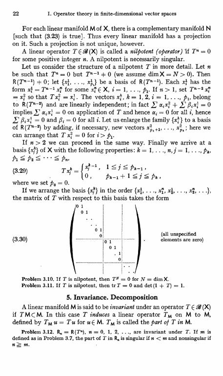
22 I. Operator theory in finite-dimensional vector spaces
For each linear manifold M of X, there is a complementary manifold N[such that (3.23) is true]. Thus every linear manifold has a projectionon it. Such a projection is not unique, however.
A linear operator T E R (X) is called a nilpotent (operator) If T"a = 0for some positive integer n. A nilpotent is necessarily singular.
Let us consider the structure of a nilpotent T in more detail. Let nbe such that Tn = 0 but T4-I * 0 (we assume dimX = N > 0). ThenR(Tn-1) $ 0; let {xi, ..., x1i,,} be a basis of R(Tn-1). Each x; has theform x; = Tn-1 xi for some xn E X, i = 1, ..., p1. If n > 1, set Tn-2 xn= xi so that Tx = x,' . The vectors x; , k = 1, 2, i = 1, ..., p1, belongto R (Tn-2) and are linearly independent ; in fact I ai xi + I fli x; = 0implies ai xi = 0 on application of T and hence ai = 0 for all i, hence
ixi = 0 and Ni = 0 for all i. Let us enlarge the family {xi } to a basisof R (Tn-2) by adding, if necessary, new vectors x22,+1, ..., x,, ; here wecan arrange that T xi = 0 for i > p1.
If n > 2 we can proceed in the same way. Finally we arrive at abasis {,vi} of X with the following properties: k = 1, . . ., n, j = 1, ..., PA,PI sp2' spn,
l = 7 = pk-1(3.29) T xk = 10,xk
1' pk-1+ 1 5 pk,
where we set po = 0.If we arrange the basis {xk} in the order {xi, . . ., xi, x2, ..., x2, ...},
the matrix of T with respect to this basis takes the form
0 1I0
(3.30)
0 1(all unspecifiedelements are zero)
0------------------------------------
Problem 3.10. If T is nilpotent, then TN = 0 for N = dim X.Problem 3.11. If T is nilpotent, then tr T = 0 and det (1 + T) = 1.
5. Invariance. DecompositionA linear manifold M is said to be invariant under an operator T E a (X)
if T M C M. In this case T induces a linear operator TM on M to M,defined by TM u = T u for u E M. TM is called the part of T in M.
Problem 3.12. R = R (T°), n = 0, 1, 2, ..., are invariant under T. If m isdefined as in Problem 3.7, the part of T in R. is singular if n < m and nonsingular ifn Z M.
§ 3. Linear operators 23
Problem 3.13. If M is invariant under T, M is also invariant under p (T) forany polynomial p (z), and p (T)M = p (TM).
If there are two invariant linear manifolds M, N for T such thatX = M ® N, T is said to be decomposed (or reduced) by the pair M, N.More generally, T is said to be decomposed by the set of linear manifoldsM1, ..., M, if (3.26) is satisfied and all the Mf are invariant under T[or we say that T is decomposed according to the decomposition (3.26)].In this case T is completely described by its parts TM,, j = 1, ..., s.T is called the direct sum of the TM5. If {P,} is the set of projectionscorresponding to (3.26), T commutes with each P;. In fact we have,successively, Pi u E M;, T P; u E M;, P, T P; u = 6j, T P; u, and theaddition of the last equalities for j = 1, ..., s gives Pk T u = T Pk u orPk T = T Pk. Conversely, it is easy to see that T is decomposed byM1, ..., M, if T commutes with all the Pf.
If we choose a basis {x;} adapted to the decomposition (3.26), T isrepresented by a matrix which has non-zero elements only in s smallersubmatrices along the diagonal (which are the matrices of the TMJ).Thus the matrix of T is the direct sum of the matrices of the TM..
Problem 3.14. With the above notations, we have
(3.31) det T = jj det TK, tr T = X' tr TM2 .i i
Remark 3.15. The operator P; T = T P5 = Pi T P1 coincides with Tand also with TM, when applied to a u E M; ; it is sometimes identifiedwith TM, when there is no possibility of misunderstanding.
6. The adjoint operator
Let T E 2(X, Y). For each 9E Y* and u E X, the scalar product(g, T u) is defined and is a semilinear form in u. Therefore, it can bewritten as / [u] = (f, u) with an / E X*. Since / is determined by g,a function T* on Y* to X* is defined by setting f = T* g. Thus thedefining equation of T* is
(3.32) (T * g, u) = (g, T u) , g E Y* , u E X .
T* is a linear operator on Y* to X*, that is, T* E 6W (Y*, X*). In fact,we have (T* (a g1 + a2 g2), u) _ (al g1 + a2 g2, Tu) = al (g1, T u) ++ a2 (g2, T u) = al (oT* gl, u) + a2 (T* 92, u) = (al T* g1 + a2 T * g2, u)so that T* (al g1 + a2 g2) = al T* g1 + as T* g2. T* is called the adjoint(operator) of T.
The operation * has the following properties:
(3.33) (aS+fT)*=aS*+flT*, (TS)*=S*T*.
24 I. Operator theory in finite-dimensional vector spaces
In the second formula it is assumed that T E -4 (Y, Z) and S E R (X, Y)so that T S is defined and belongs to .4E1 (X, Z) ; note that S* E .4 (Y*, X*)and T* E 9 (Z*, Y*) so that S* T* E 9 (Z*, X*). The proof of (3.33) issimple; for example, the second formula follows from ((TS)* h, u)_ (h, T S u) = (T* h, S u) _ (S* T* h, u) which is valid for all h E Z*and u E X.
Problem 3.16. 0* = 0, 1 * = 1 (the 0 on the left is the zero of 9 (X, Y) while the 0on the right is the zero of 9 (Y*, X*) ; similarly for the second equality, in which wemust set Y = X).
If T E .47(X, Y), we have T* E .1(Y*, X*) and T** E . (X**, Y**).If we identify X** and Y** with X and Y respectively (see § 2.6), itfollows from (3.32) that
(3.34) T** = T.
If we take bases {xk} and {y;} in X and Y respectively, an operatorT E 6R (X, Y) is represented by a matrix (r; k) according to (3.5) or (3.6).If {ek} and {f;} are the adjoint bases of X* and Y*, respectively, theoperator T* E R (Y*, X*) can similarly be represented by a matrixThese matrix elements are given by -r;, = (Txk, f;) and tk*i = (T* f;, xk)= (f;, Txk) in virtue of (3.10) . Thus
(3.35) r* -z k= 1,...,N=dimX,ky- 3k+ j= 1,...,M=dimY,
and T and T* are represented by mutually adjoint (Hermitian conjugate)matrices with respect to the bases which are adjoint to each other.
Problem 3.17. If T E .4 (X), we have
(3.36) detT* = det T , trT* = tr T .
Let T E 2 (X, Y). A g E Y* belongs to the annihilator of R (T) ifand only if (g, T u) = 0 for all u E X. (3.32) shows that this is equivalentto T* g = 0. Thus the annihilator of the range of T is identical with thenull space of T*. In view of (3.34), the same is true when T and T* areexchanged. In symbol, we have
(3.37) N(T*) = R(T)1 , N(T) = R(T*)1 .
It follows that [see (3.2), (3.3) and (2.17)]
(3.38) nul T * = def T , nul T = def T * , rank T * = rank T .
If in particular Y = X, (3.38) shows that T* is nonsingular if and only ifT is; in this case we have(3.39) (T*)-l = (T-1)* .
For the proof it suffices to note that T* (T-')* = (T-1 T)* = 1* = 1.
§ 4. Analysis with operators 25
Problem 3.18. If T E l (X), we have
(3.40) nulT*= nulT , defT* = defT.
If PE PE7(X) is a projection, the adjoint P*E -4 (X*) is likewise aprojection, for P2 = P implies P*2 = P*. The decompositions of thespaces X and X*
(3.41) X=M®N, M= R(P), N= R(1-P),(3.42) X*=M*e N*, M*= R(P*), N*= R(1-P*),are related to each other through the following equalities :
(3.43) N* = Ml , M* = N' , dimM* = dimM , dimN* = dimN ,
as is seen from (3.37) and (3.40).Similar results hold when there are several projections. If {P;} is a
set of projections in X satisfying (3.27-3.28), {P*} is a similar set ofprojections in X*. The ranges M, = R (P), W- = R (P*) are related by
(3.44) dimM*=dimM,, j= 1,2,...,(3.45) M1 = (M2 ®...)1 Mi = (M2 ®...) i , etc.
Problem 3.19. Let {xj} be a basis of X adapted to the decomposition X = M,® ® M and let {ej} be the adjoint basis of X*. Then {e;} is adapted to thedecomposition X* = Ml ® ... ® M,*. For any u E X we have
(3.46) P1 u = £ (u, e5.) x1i ,r=1
where {xj,, ..., xj1} is the part of {x5} belonging to M5 and m5 = dim M5.
§ 4. Analysis with operators1. Convergence and norms for operators
Since the set R(X, Y) of all linear operators on X to Y is an MN-dimensional vector space, where N = dim X < oo and M = dim Y < oo,the notion of convergence of a sequence {T,n} of operators of R(X, Y) ismeaningful as in the case of a sequence of vectors of X. If we introducethe matrix representation (r r k) of T. with respect to fixed bases {xk},{yf} of X, Y, respectively, T,,--> T is equivalent to rJ k y rj k for each j, k,for the rngk are the coefficients of T,,, for the basis {P;k} of R(X, Y)(see § 3.2). But the are the coefficients of Txk with respect to thebasis {y;}; hence T. -> T is equivalent to T. xk -> Txk for all k andtherefore to T u -+ T u for all u E X. This could have been used as thedefinition of T,,, -> T.
As it was convenient to express the convergence of vectors by meansof a norm, so it is with operators. But an operator-norm is usually
26 I. Operator theory in finite-dimensional vector spaces
introduced only in correlation with the vector-norms. More precisely,when X and Y are normed spaces 9 (X, Y) is defined to be a normed spacewith the norm given by
(4.1) 11 T11 = sup Mull = sup IITull = sup IITull , T E -4 (X, Y) .
O+uEx Ilull IIulI= 1 (lulls'
The equality of the various expressions in (4.1) is easily verified'. Wecan replace "sup" by "max" in (4.1) because the set of u with 'lull = 1or IIull s 1 is compact (see a similar remark for the norm of an /E X*in § 2.4) ; this shows that II TII is finite. It is easy to verify that II TII definedon P,R (X, Y) by (4.1) satisfies the conditions (1.18) of a norm. Hence itfollows that T,,, --> T is equivalent to II T,, - TII --> 0. A necessary andsufficient condition that {Tu} converge to some T is given by the Cauchycondition II T,,, - Tm!I 0, n, m -+ oo.
Another convenient expression for 11 T11 is2
(4.2) 11 T11
=sup
I(TIIf)
= sup I(Tu,o
1)Iac
iO +tEY*
The equivalence of (4.2) with (4.1) follows from (2.26).. If we introduce different norms in the given vector spaces X and Y,
.Q (X, Y) acquires different norms accordingly. As in the case of normsin X, however, all these norms in 9 (X, Y) are equivalent, in the sensethat for any two norms II II and II II', there are positive constants a',such that(4.3) « II TII s II TII' s fl' II TII
This is a special case of (1.20) applied to 9 (X, Y) regarded as a normedspace. Similarly, the inequalities (1.21) and (1.22) give the followinginequalities :(4.4) ltfkl < y IITII , j = 1, ..., M; k = 1, ..., N,(4.5) IITII s y'maxlrskl
where (tf k) is the matrix of T with respect to the bases of X and Y.The constants y and y' depend on these bases and the norm employed,but are independent of the operator T.
As in the case of vectors, a S + 8 T is a' continuous function of thescalars a, P and the operators S, T E 69 (X, Y), and II TII is a continuousfunction of T. As a new feature of the norm of operators, we should notethe inequality
(4.6) II TSII s II TII IIuII for T E V (Y, Z) and S E RN Y) .
1 The second and third members of (4.1) do not make sense if dimX = 0;in this case we have simply 11 1 = 0.
2 Here we assume dim X 1, dim Y Z 1.
§ 4. Analysis with operators 27
This follows from IITSuII < 11 T11 IISuII < IITII IISIIIIuII; note also that(4.6) would not be valid if we chose arbitrary norms in 1(X, Y) etc.regarded simply as vector spaces.
Problem 4 . 1 .1 1 1 1 1 = 10 E 9 (X) is the identity operator, dim X > 0). If P ERNis a projection and P $ 0, then IITII Z I.
TS is a continuous function of S and T. In other words, Tn --> Tand Sn -+ S imply Tn Sn -+ TS. The proof is similar to (2.28) ; it sufficesto use (4.6). In the same way, it can be shown that Tu is a continuousfunction of T and u. In particular un -+ u implies Tun --> T u. In thissense a linear operator T is a continuous function. It is permitted, forexample, to operate with T term by term on a convergent series ofvectors:(4.7) T(Zun)=ZTun.
1n 1 n
If X is a normed space, .9 (X) = -4 (X, X) is a normed algebra (or ring)with the norm given by (4.2). In particular, (4.6) is true for T, S E . (X).
If T E 9(X, Y), then T* _ -4 (Y*, X*) and
(4.8) IIT*II=IITII
This follows from (4.2), according to which II T*II = sup I(T* f, u) I= sup I(f, Tu) I =IITII where u E X** = X, IIu!I = 1 and / E X*, IITII = 1.
2. The norm of T"As an example of the use of the norm and also with a view to later
applications, we consider the norm II T"11 for T E 2 (X). It follows from(4.6) that
(4.9) 11 T-+1111 S 11 T-11 IITnII , 11 T'411 S IITII"`, m,n=0, 1,2,... .
We shall show that lim II T11II'1n exists and is equal to inf II T"`Ill/n This
limit is called the spectral radius of T and will be denoted by spr T. As isseen later, spr T is independent of the norm employed in its definition.
Set an = log 11T''II. What is to be proved is that
(4.10) an/n -* b - inf an/n .n = 1,2,...
The inequality. (4.9) gives(4.11) am+n s am + an .
(Such a sequence {an} is said to be subadditive.) For a fixed positiveinteger m, set n = mq + r, where q, r are nonnegative integers with0 S r < m. Then (4.11) gives an s q am + a, and
n n an+ ar.
28 I. Operator theory in finite-dimensional vector spaces
If n -> oo for a fixed m, q/n -+ 1/m whereas r is restricted to one of thenumbers 0, 1, ..., m - 1. Hence lim sup an/n s am/m. Since m is arbi-
n-r 00trary, we have lim sup an/n < b. On the other hand, we have an/n _>_ band so lim inf an/n z b. This proves (4.10)1.
Remark 4.2. The above result may lead one to conjecture that II T"IIII" is mono-tone nonincreasing. This is not true, however, as is seen from the following example.Let X = C2 with the norm given by (1.17) (X is a two-dimensional unitary space,see § 6). Let T be given by the matrix
T=(0a2)
, a>b>0.b2 0
It is easily seen that (1 is the unit matrix)
Ten=a2nb2n1 T2"+I= a2"b2"T IIT2"II=/2n=ab
TII = a2 II Ten+llllI(2n+1) = a b (a/b)1I(2n+I) > a b .
Next let us consider II T-1I1 and deduce an inequality estimatingII T-1II in terms of II TII and det T, assuming that T is nonsingular. Therelation T u = v is expressed by the linear equations (3.6). Solving theseequations for k, we obtain a fractional expression of which the denomina-tor is det T and the numerator is a linear combination of the qk withcoefficients that are equal to minors of the matrix (r; k). These minors arepolynomials in the -r27, of degree N - 1 where N = dim X. In virtue ofthe inequalities IIuII < y' max [see (1.22)], Ir;>,I s y" 11 T11 [see
(4.4)] and ItI;I s y... IIvII [see (1.21)], it follows that there is a constanty such that lull s y IIvII IITIIN-1/IdetTI or
(4.12) II T- 111 s y IIIdet Tl
The constant y is independent of T, depending only on the normemployed2.
3. Examples of normsSince the norm II TII of an operator T is determined in correlation with the norms
adopted in the domain and the range spaces X, Y, there is not so much freedom inthe choice of TII as in the choice of the norms for vectors. For the same reasonit is not always easy to compute the exact value of II TII. It is often required, how-ever, to estimate an upper bound of II TII. We shall illustrate by examples how such anestimate is obtained.
Most commonly used among the norms of vectors is the p-norm defined by
(4.13) IIuII = Ilulln = E I iV )1/D
with a fixed p Z 1, where the , are the coefficients of u with respect to a fixedbasis {xi} (which will be called the canonical basis). The conditions (1.18) for a
1 See P6LYA and SZEG6 (l), p. 17. Cf. also HILLE and PHILLIPS 11), pp. 124, 244.2 We can set y = I if X is a unitary space; see T. KATO [13].
§ 4. Analysis with operators 29
norm are satisfied by this p-norm [the third condition of (1.18) is known as theMinkowski inequality']. The special cases p = 1 and 2 were mentioned before;see (1.16) and (1.17). The norm lull = given by (1.15) can be regarded asthe limiting case of (4.13) for p = oo.
Suppose now that the p-norm is given in X and Y with the same p. We shallestimate the corresponding norm IITII of an operator T on X to Y in terms of thematrix (r; k) of T with respect to the canonical bases of X and Y. If v = T u, thecoefficients $k and 17; of u and v, respectively, are related by the equations (3.6). Let
(4.14) T; = E IT, hl , Tk = G l ti hl 'k j
be the row sums and the column sums of the matrix (1T;7,1). (3.6) then gives
Ir/mI < IT,kI l$klT; k T;
Since the nonnegative numbers IT, Al/T; for k = 1, ..., N with a fixed j have thesum 1, the right member is a weighted average of the Ie5I. Since A9 is a convexfunction of A Z 0, the p-th power of the right member does not exceed the weightedaverage of the with the same weights2. Thus
(lrli!) < E IT1-I
T; .) k Tf
and we have successively
I'MP E IT; "I IssIDC (maxrfD-'L ITi kl k1sV.
IIVII' Im; XT1\1D-1. Tk
1$7,lD
S (maxTT-1 (maxTk1 llullp
hence
(4.15)
This shows thate
(4.16)
II Tull = IIvII 5 (maxTJ11 n (mkaxala IIulI
11Th I S (maxTT)1-r (mhaxT'A' .
4 1If p = 1, the first factor on the right of ( .16) is equal to I and does not depend onthe Tj. On letting p -+ oo, it is seen that (4.16) is true also for p = oo ; then thesecond factor on the right is 1 and does not depend on the Tg.
Problem 4.3. If (T; k) is a diagonal matrix (r; k = 0 for j + k), we have for any p
(4.17) 11 T11 S -ax IT; ;Ij
4. Infinite series of operatorsThe convergence of an infinite series of operators E T. can be
defined as for infinite series of vectors and need not be repeated here.Similarly, the absolute convergence of such a series means that the series
1 The proof may be found in any textbook on real analysis. See e. g. HARDY,LITTLEWOOD and P6LYA 11), p. 31; ROYDEN 111, p. 97.
9 For convex functions, see e. g. HARDY, LITTLEWOOD and P6LYA (1), p. 70.8 Actually this is a simple consequence of the convexity theorem of M. RIEsz
(see HARDY, LITTLEWOOD and P6LYA (1), p. 203).
30 I. Operator theory in finite-dimensional vector spaces
f II TnII is convergent for some (and hence for any) norm IIII
In thiscase Z Tn is convergent with IIE TnII s ' II TnII.
Owing to the possibility of multiplication of operators, there arecertain formulas for series of operators that do not exist for vectors.For example, we have
(4.18) S(S'T.)=ZST.n, (?T.)STnS,
whenever ' Tn is convergent and the products are meaningful. Thisfollows from the continuity of S T as function of S and T. Two absolutelyconvergent series can be multiplied term by term, that is
(4.19) (L Sm) (' Tn) = T' S. T.if the products are meaningful. Here the order of the terms on the rightis arbitrary (or it may be regarded as a double series). The proof is notessentially different from the case of numerical series and may be omitted.
Example 4.4 (Exponential function)
o(4.20) etT = exp(tT) = T' to Tn , T E °.,8(X) .
This series is absolutely convergent for every complex number t, for then-th term is majorized by Itln IITIInIn! in norm. We have
(4.21) IIetTII 5 eltl IITII
Example 4.5 (Neumann series)00
(4.22) (1 - T)-1 = ' Tn, 11 (1 - T)-111 S (1 - 11 T11)-1, TERN.n=0
This series is absolutely convergent for II TII < 1 in virtue of II TnII < II T II nDenoting the sum by S, we have TS = S T = S - 1 by term by termmultiplication. Hence (1 - T) S = S(1 - T) = 1 and S = (1 - T)-1.It follows that an operator R E R (X) is nonsingular if 111 - RII < 1.
It should be noted that whether or not II TII < 1 (or 11 1 - RII < 1)may depend on the norm employed in X; it may well happen thatIl TII < 1 holds for some norm but not for another.
Problem 4.6. The series (4.22) is absolutely convergent if 11 Tm1I < 1 for somepositive integer m or, equivalently, if spr T < 1 (for spr T see § 4.2), and the sum isagain equal to (1 - T)-1.
In the so-called iteration method in solving the linear equationn
(1 - T) u = v for u, the partial sums S,, = r Tk are taken as ap-k=0
proximations for S = (1 - T)-1 and un = S. v as approximations forthe solution u = S v. The errors incurred in such approximations can be
§ 4. Analysis with operators 31
estimated by
(4.23) IIS - S-II =00 00
s IlTllk = IITIIn}1
k=n+1 l - IITIIf Tk
k=n+1
For n = 0 (4.23) gives 11(1 -T)-1 - III 5 IITII (1 - IITII)-1 With
R = 1 - T, this shows that R -+ 1 implies R-1-> 1. In other words,R-1 is a continuous function of R at R = 1. This is a special case of thetheorem that T-1 is a continuous function o l T. More precisely, ifT E .4 (X, Y) is nonsingular, any S E -4 (X, Y) with sufficiently smallIIS - TII is also nonsingular, and IIS-1 - T-111 -> 0 for II T - SII -1 0. Inparticular, the set of all nonsingular elements of -4 (X, Y) is open. [Of courseX and Y must have the same dimension if there exist nonsingularelements of .4E1 (X, Y).]
To see this we set A = S - T and assume that IIAII < 1III T-111. ThenIIA T-1II s IIAII II T-1II < 1, and so 1 + A T-1 is a nonsingular operator of.1 (Y) by the above result. Since S = T + A = (1 + A T-1) T, S is alsononsingular with S-1= T-1 (1 + A T-1)-1.
Using the estimates for II (1 + A T-1)-1II and II (1 + A T-1)-1- IIIgiven by (4.22) and (4.23), we obtain the following estimates for IIS-111and IIS-1- T-111:
(4.24) IIS-111 s l - IIIAII IIIT-111' IIS-1- T-1II s I IIAIIA1 II TI8111
forS=T+A, IIAII<1/IIT-111.
Remark 4.7. We assumed above that IIAII < II T-1II to show theexistence of S-1. This condition can be weakened if X = Y and TS = S T.In this case A commutes with T and hence with T-1. Therefore
(4.25)sprA T-1= limIi(A T--1)nII1/n = limIIA% T-nII1/n s
[limIIAnII1/n] Dim 11T-n9I1/n] _ (sprA) (sprT-1) .
It follows that S-1= T-1(1 + A T-1) -1 exists if
(4.26) sprA < (sprT-1)-1.
5. Operator-valued functionsOperator-valued functions Tt = T (t) defined for a real or complex
variable t and taking values in .1 (X, Y) can be defined and treated justas vector-valued functions u (t) were in § 1.7. A new feature for T (t)appears again since the products T (t) u (t) and S (t) T (t) are defined.Thus we have, for example, the formulas
dt T (t) u (t) = T' (t) u (t) + T (t) u' (t) ,
(4.27)at
T (t) S (t) = T' (t) S (t) + T (t) S' (t) ,
32 I. Operator theory in finite-dimensional vector spaces
whenever the products are meaningful and the derivatives on the rightexist. Also we have
(4.28) at T (t)-1 T (t)-1 T' (t) T(t)-1
whenever T (t)-1 and T' (t) exist. This follows from the identity
(4.29) S-1 - T-' = - S-' (S - T) T-1and the continuity of T-1 as function of T proved in par. 4.
For the integrals of operator-valued functions, we have formulassimilar to (1.30). In addition, we have
f S u (t) d t= S f u (t) d t, f T (t) u d t= (f T (t) d t) u,(4.30)
f S T (t) d t= S f T (t) d t, f T (t) S d t= (f T (t) d t) S.
Of particular importance again are holomorphic functions T (t) of acomplex variable t; here the same remarks apply as those given forvector-valued functions (see § 1.7). It should be added that S (t) T (t) andT (t) u (t) are holomorphic if all factors are holomorphic, and that T (t) -1is holomorphic whenever T (t) is holomorphic and T (t)-1 exists [thelatter follows from (4.28)].
Example 4.8. The exponential function ell' defined by (4.20) is anentire function of t (holomorphic in the whole complex plane), with
(4.31) dt etT = TetT = etTT.
Example 4.9. Consider the Neumann seriesCo
(4.32) S(t) = (1 - tT)-1= to Tnn=0
with a complex parameter t. By Problem 4.6 this series is absolutelyconvergent for Itl < 1/sprT. Actually, the convergence radius r of (4.32)is exactly equal to 1/spr T. Since S (t) is holomorphic for It < r, theCauchy inequality gives 11 T' S M,,, r'-n for all n and r' < r as in the caseof numerical power series' (Mr is independent of n). Hence spr T= lim 11 Tn II1/n 5 Y'-' and, going to the limit r' r, we have spr T s r-1
or r 5 1/spr T. Since the opposite inequality was proved above, thisgives the proof of the required result. Incidentally, it follows that spr Tis independent of the norm used in its definition.
6. Pairs of projectionsAs an application of analysis with operators and also with a view to
later applications, we shall prove some theorems concerning a pair of
1 We have To = (2n i)-1 f t-"-1 S (t) dt and so 11 T"II 5 (2n)-1 fItl = r' Ill
II S (t) II I dtl s y' -" where M,. = max II S (t) iI < oo.
§ 4. Analysis with operators 33
projections (idempotents)1. As defined in § 3.4, a projection P is anoperator of .4 (X) such that P2 = P. 1 - P is a projection with P.
Let P, Q E °..d (X) be two projections. Then
(4.33) R=(P-Q)2=P+Q-PQ-QPcommutes with P and Q; this is seen by noting that PR = P - P Q P= R P and similarly for Q. For the same reason (1 - P - Q) 2 commuteswith P and Q because 1 - P is a projection. Actually we have theidentity
(4.34) (P-Q)2+(1-P-Q)2=1as is verified by direct computation. Another useful identity is
(4.35) (PQ - QP)2 = (P-Q)4- (P-Q)2=R2-R,
the proof of which is again straightforward and will be left to the reader.Set
(4.36) U'=QP+(1-Q) (1-P), V'=PQ+(1-P) (1-Q).U' maps R(P) = P X into Q X and (1 - P) X into (1 - Q) X, whereasV' maps Q X into P X and (1 - Q) X into (1 - P) X. But these mappingsare not inverse to each other; in fact it is easily seen that
(4.37) V' U' = U' V' = 1 - R.
A pair of mutually inverse operators U, V with the mapping propertiesstated above can be constructed easily, however, since R commuteswith P, Q and therefore with U', V' too. It suffices to set
U= U'(1 - R)-I/z = (1 - R)-1/2 U1,(4.38)
V = V'(1 - R)-I/2 = (1 - R)-1/2 V' ,
provided the inverse square root (1 - R)-1/2 of 1 - R exists. A naturaldefinition of this operator is given by the binomial series
(4.39) (1 - R)-1/2 = 'o ( 1/2) (-R)-.
This series is absolutely convergent if I1R1I < 1 or, more generally, if
(4.40) sprR < 1 ,
1 The following results, which are taken from T. KATO [9], are true even when Xis an co-dimensional Banach space. For the special case of projections in a unitary(Hilbert) space, see § 6.8. For related results cf. AKHIZzER and GLAZMAN (1),SZ.-NAGY [1], [2], WOLF [1].
34 I. Operator theory in finite-dimensional vector spaces
and the sum T of this series satisfies the relation Ts = (1 - R)-1 justas in the numerical binomial series. Thus'(4.41) VU=UV=1, V=U-', U = V-1.
Since U' P = Q P = Q U' and P V' = P Q = V' Q as is seen from(4.36), we have UP = QU and PV = VQ by the commutativity of Rwith all other operators here considered. Thus we have
(4.42) Q= UPU-', P= U-1QU.Thus P and Q are similar to each other (see § 5.7). They are isomorphicto each other in the sense that any linear relationship such as v = Pugoes over to v' = Qu' by the one-to-one linear mapping U : u' = Uu,v'= Uv. In particular their ranges PX, QX are isomorphic, beingmapped onto each other by U and U-'. Thus
(4.43) dim P = dim Q , dim (1 - P) = dim (1 - Q) .
An immediate consequence of this result isLemma 4.10. Let P (t) be a projection depending continuously on a
parameter t varying in a (connected) region of real or complex numbers.Then the ranges P (t) X for different t are isomorphic to one another. Inparticular dim P (t) X is constant.
To see this, it suffices to note that 11 P (t') - P (t") 11 < I for suf-ficiently small It' - t" ( so that the above result applies to the pairP(t'), P(t").
Problem 4.11. Under the assumption (4.40), we have PQ X = P X, Q P X = Q X[hint: PQ =.PV' = PU-'(1 - R)lia].
Problem 4.12. For any two projections P, Q, we have(4.44) (1- P -{- QP) (1 - Q + PQ) = 1 - R [R is given by (4.33)],(4.45) (1-P+QP)-'_(1-R)-'(l-Q-{-PQ) if sprR<1.If spr R< 1, W= 1- P+ Q P maps P X onto Q X and W u= u for u E (1 - P) X,while W-' maps Q X onto P X and W-' u = u for u E (1 - P) X, and we haveX=QX®(1-P)X.
Problem 4.13. For any two projections P, Q such that spr (P - Q) 2 < 1,there is a family P (t), 0 < t S 1, of projections depending holomorphically on tsuch that P(O) =P, P(l) = Q. [hint: set 2P(t) = 1 +(2P- 1 +21(Q-P%)-- (1 - 41(1 - t) R)-11Z.]
§ 5. The eigenvalue problem1. Definitions
In this section X denotes a given vector space with 0 < dim X= N < oo, but we shall consider X a normed space whenever convenientby introducing an appropriate norm.
' As is shown later (§ 6.7), U and V are unitary if X is a unitary space and P, Qare orthogonal projections. The same U appears also in Sz.-NAGY [1] and WOLF [1]with a different expression; its identity with the above U was shown in T. KATO [9].
§ S. The eigenvalue problem 35
Let T E R (X). A complex number A is called an eigenvalue (propervalue, characteristic value) of T if there is a non-zero vector uE X such that(5.1) Tu=Au.u is called an eigenvector (proper vector, characteristic vector) of T belongingto (associated with, etc.) the eigenvalue A. The set NA of all u E X suchthat T u = A u is a linear manifold of X; it is called the (geometric)eigenspace of T for the eigenvalue A, and dim NA is called the (geometric)multiplicity of 2. NA is defined even when A is not an eigenvalue; then wehave N2 = 0. In this case it is often convenient to say that NA is theeigenspace for the eigenvalue 2 with multiplicity zero, though this is notin strict accordance with the definition of an eigenvalue'.
Problem 5.1. A is an eigenvalue of T if and only if A - Z is an eigenvalue ofT - C. NA is the null space of T - A, and the geometric multiplicity of the eigen-value A of T is the nullity of T- A. T- A is singular if and only if A is an eigenvalue of T.
It can easily be proved that eigenvectors o l T belonging to differenteigenvalues are linearly independent. It follows that there are at most Neigenvalues of T. The set of all eigenvalues of T is called the spectrumof T; we denote it by E (T). Thus E (T) is a finite set with not morethan N points.
The eigenvalue problem consists primarily in finding all eigenvaluesand eigenvectors (or eigenspaces) of a given operator T. A vector u + 0is an eigenvector of T if and only if the one-dimensional linear manifold[u] spanned by u is invariant under T (see § 3.5). Thus the eigenvalueproblem is a special case of the problem of determining all invariantlinear manifolds for T (a generalized form of the eigenvalue problem).
If M is an invariant subspace of T, the part TM of T in M is defined.As is easily seen, any eigenvalue [eigenvector] of TM is an eigenvalue[eigenvector] for T. For convenience an eigenvalue of TM is called aneigenvalue o l T in M.
If there is a projection P that commutes with T, T is decomposedaccording to the decomposition X = M e N, M = PX, N = (1 - P) X(see § 3.5). To solve the eigenvalue problem for T, it is then sufficientto consider the eigenvalue problem for the parts of T in M and in N Z.
i There are generalized eigenvalue problems (sometimes called nonlineareigenvalue problems) in which one seeks solutions of an equation T (A) u = 0, whereT (A) is a linear operator depending on a parameter A; for example, T (A) = To ++ A Tl -{- + A" T. In general a solution u + 0 will exist only for some particu-lar values of A (eigenvalues). A special problem of this kind will be considered later(VII, § 1.3).
8 If T u = A u, then T Pu = P T u = APu so that Pu E M is, if not 0, aneigenvector of T (and of TM) for the eigenvalue A, and similarly for (1 - P) u.Thus any eigenvalue of T must be an eigenvalue of at least one of TM and TN,and any eigenvector of T is the sum of eigenvectors of TM and TN for the sameeigenvalue. The eigenspace of T for A is the direct sum of the eigenspaces of TMand TN for A.
36 I. Operator theory in finite-dimensional vector spaces
The part TM of T in M may be identified with the operator P T = T P= P T P in the sense stated in Remark 3.15. It should be noticed,however, that T P has an eigenvalue zero with the eigenspace N andtherefore with multiplicity N - m (where m = dim P X) in addition to theeigenvalues of TM 1
Problem 5.2. No eigenvalue of T exceeds 11 T11 in absolute value, where 1111
is the norm of .4 (X) associated with any norm of X.Problem 5.3. If T has a diagonal matrix with respect to a basis, the eigenvalues
of T coincide with (the different ones among) all its diagonal elements.
2. The resolventLet T E M (X) and consider the inhomogeneous linear equation
(5.2) (T-C)it =v,where 4 is a given complex number, v E X is given and u ( X is to befound. In order that this equation have a solution u for every v, it isnecessary and sufficient that T - C be nonsingular, that is, 4 be differentfrom any eigenvalue 2,, of T. Then' the inverse (T - 4)-1 exists and thesolution u is given by
(5.3) u = (T - C)-1 v .
The operator-valued function
(5.4) R(C, T) = (T -
is called the resolvent2 of T. The complementary set of the spectrum E (T)(that is, the set of all complex numbers different from any of the eigen-values of T) is called the resolvent set of, T and will be denoted by P (T).The resolvent R is thus defined for C E P (T).
Problem 5.4. R commutes with T. R (C) has exactly the eigenvalues (RA - y)'
An important property of the resolvent is that it satisfies the (first)resolvent equation
(5.5) R (CI) - R (C2) = (Cl - U R (Cl) R (C2)
This is seen easily if one notes that the left member is equal to R(T - 2) R (C2) - R (C,1) (T - C1) R (T2). In particular, (5.5) implies that
R (Cl) and R (C2) commute. Also we have R (Cl) = [1 - (C2 - ) R (C1)]
1 Strictly speaking, this is true only when TM has no eigenvalue 0. If TM hasthe eigenvalue 0 with the eigenspace L, the eigenspace for the eigenvalue 0 of TPis N ® L.
2 The resolvent is the operator-valued function C -+ R (c). It appears, however,that also the value R (C) of this function at a particular t' is customarily called theresolvent. Sometimes (C - T)-1 instead of (T - C)-1 is called the resolvent. Inthis book we follow the definition of STONE M.
§ 5. The eigenvalue problem 37
R (C,2). According to the results on the Neumann series (see Example 4.5),this leads to the expansion
(5.6) R [1 - (C - o) R -1 R (Co) = G ( - Co)n R (Co)n+1n=0
the series being absolutely convergent at least if
(5.7) 1. - oI < IIR(Co)II-1
for some norm. We shall refer to (5.6) as the first Neumann series for theresolvent.
(5.6) shows that R (C) is holomorphic in C with the Taylor series'shown on the right; hence
(5.8) n = 1,2,3,... .
According to Example 4.9, the convergence radius of the series of (5.6)is equal to 1/sprR(Co). Hence this series is convergent if and only if
(5.9) IC - Col < 1/sprR(Co) = (limIIR(Co)nII1/n)-1
For large ICI, R(C) has the expansionM
(5.10) R(C)=-C,-'(1-C,-'T)-'=- E C-n-1 Tn,n=o
which is convergent if and only if IC I > sprT; thus R (T) is holomorphicat infinity.
Problem 5.5. We have(5.11) IIR (C)II S (ICI - IITII)-1, IIR (C) + C-111;9 ICI-1(ICI - IITII)-1II TII
for ICI > II TII
The spectrum E (T) is never empty; T has at least one eigenvalue.Otherwise R (C) would be an entire function such that R (C) -+ 0 for C -+ 00[see (5.11) ] ; then we must have R (C) = 0 by Liouville's theorem 2. Butthis gives the contradiction I = (T - R (C) = 0 8.
It is easily seen that each eigenvalue of T is a singularity4 of theanalytic function R (C). Since there is at least one singularity of R (C)on the convergence circles ICI = spr T of (5.10), spr T coincides with the
1 This is an example of the use of function theory for operator-valued functions;see KNOPP (1), p. 79.
8 See Kr oPP [1D, p. 113. Liouville's theorem implies that R (C) is constant;since R (C) -+ 0 for C oo, this constant is 0.
8 Note that we assume dim X > 0.4 Suppose A is a regular point (removable singularity) of the analytic function
R (C). Then limR (C) = R exists and so (T - A) R = lim (T - C) R (C) = 1. Thus
(T - A)-1 = R exists and A is not an eigenvalue.5 See KNoPP 111, p. 101.
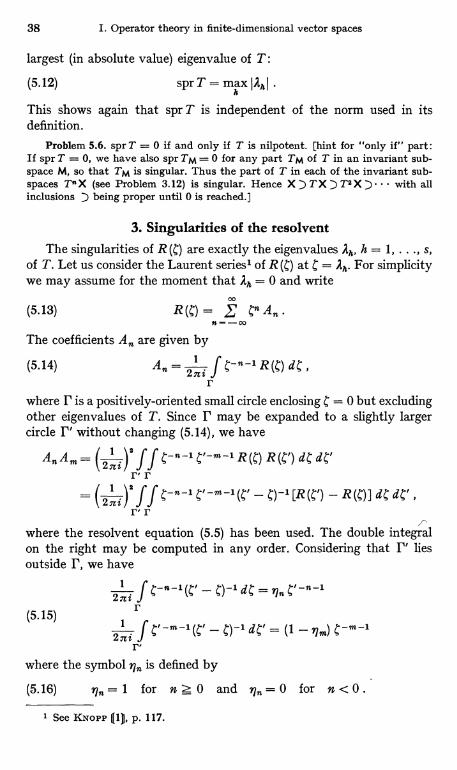
38 1. Operator theory in finite-dimensional vector spaces
largest (in absolute value) eigenvalue of T:
(5.12) spr T = max JRh .h
This shows again that spr T is independent of the norm used in itsdefinition.
Problem 5.6. spr T = 0 if and only if T is nilpotent. [hint for "only if" part:If spr T = 0, we have also spr TM = 0 for any part TM of T in an invariant sub-space M, so that TM is singular. Thus the part of T in each of the invariant sub-spaces To X (see Problem 3.12) is singular. Hence X) T X) T2 X) . with allinclusions ) being proper until 0 is reached.]
3. Singularities of the resolventThe singularities of R (C) are exactly the eigenvalues 2h, h = 1, ..., s,
of T. Let us consider the Laurent series' of R at C = 2h. For simplicitywe may assume for the moment that 1h = 0 and write
00
(5.13) R (g) _ E A. .
The coefficients A,,, are given byr
(5.14) A,n. =2 i J C-"i-1 R (C) dC ,
rwhere r is a positively-oriented small circle enclosing = 0 but excludingother eigenvalues of T. Since r may be expanded to a slightly largercircle r' without changing (5.14), we have
AnAm- = ( 1 )8 f f C-n-1 R(C) R(g') dC dC'2nir, r
2rzi)efr, r
where the resolvent equation (5.5) has been used. The double integralon the right may be computed in any order. Considering that r' liesoutside r, we have
27Li
r(5.15)
1 f b)-1 dC' = (1 -'7m) b-m-1
2ni
where the symbol q,,, is defined by
(5.16) T = 1 for n z 0 and ,n = 0 for n <
1 See KxoPP 111, p. 117.
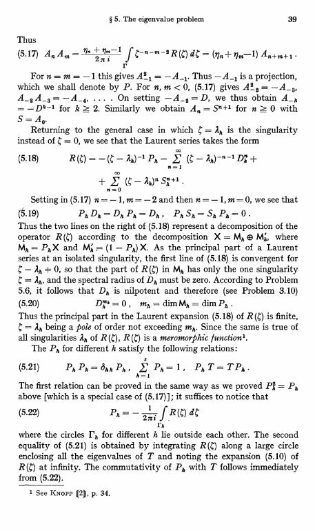
§ 5. The eigenvalue problem 39
Thusr(5.17) An A.= J C-n-m-2R(C)dC=(yln+7Jm 1)An+m+1
rFor n = m = -1 this gives A21 = -A_1. Thus -A_1 is a projection,
which we shall denote by P. For n, m < 0, (5.17) gives A22 = -A-s,A_2 A_3 = -A_4, ... . On setting -A-2=D, we thus obtain A_h= -Dk-1 for k z 2. Similarly we obtain An = Sn+1 for n > 0 withS=A0.
Returning to the general case in which C = a.h is the singularityinstead of = 0, we see that the Laurent series takes the form
(5.18)cc
R(S) _ -(y - Ah)-1 Ph -' (C - a'h)-n-sDh +n=1
co
+ f (S - 2h)n Sh+1n=0
Setting in (5.17) n = -1, m = - 2 and then n = -1, m = 0, we see that(8.19) PhDh=DhPh=Dh, PhSh=ShPh=O.Thus the two lines on the right of (5.18) represent a decomposition of theoperator R (C) according to the decomposition X = Mh ® Mh, whereMh = PhX and M;, ; (1 - Ph) X. As the principal part of a Laurentseries at an isolated singularity, the first line of (5.18) is convergent for
- Ah + 0, so that the part of R (C) in Mh has only the one singularityAh, and the spectral radius of Dh must be zero. According to Problem
5.6, it follows that Dh is nilpotent and therefore (see Problem 3.10)(5.20) Dk e = 0 , mh = dim Mh = dim Ph .Thus the principal part in the Laurent expansion (5.18) of R (C) is finite,l; = Ah being a pole of order not exceeding mh. Since the same is true ofall singularities 2h of R (c), R (C) is a meromoyphic functions.
The Ph for different h satisfy the following relations:S
(5.21) PhPh=ShhPh, f Ph= 1, PhT=TPh.h=1
The first relation can be proved in the same way as we proved Ph = Phabove [which is a special case of (5.17))]; it suffices to notice that
(5.22) Ph = - 22nai f R(T) dCrh
where the circles Th for different h lie outside each other. The secondequality of (5.21) is obtained by integrating R(C) along a large circleenclosing all the eigenvalues of T and noting the expansion (5.10) ofR (C) at infinity. The commutativity of Ph with T follows immediatelyfrom (5.22).
1 See KNoPP Q21, p. 34.
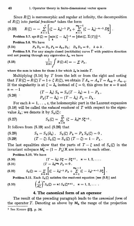
40 I. Operator theory in finite-dimensional vector spaces
Since R is meromorphic and regular at infinity, the decompositionof into partial fractions' takes the form
(5.23) R (C) 2h)-1 Ph + 2h)-n -' DR]h=1 n=1
Problem 5.7. sprR (C) = rmin I - [dist (Z , E (T))]-1.
Problem 5.8. We have [ f
(5.24) PhDh-D,,Ph=ahhDh; DhDh=O, h+k.Problem 5.9. For any simple closed (rectifiable) curve r with positive direction
and not passing through any eigenvalue Ah, we have
(5.25) 2ni f R() _P P,,,r
where the sum is taken for those h for which Ah is inside r.
Multiplying (5.14) by T from the left or from the right and notingthat T R R (g) T = 1-I- R (C), we obtain TA, = An T = ano + A,-,.If the singularity is at = Ah instead of C = 0, this gives for n = 0 andn= -1(5.2Ei)
(T - Ah.) Sh. = S, (T - 2 ) = 1 - P,, .
Ph (T - ).h) _ (T - 2h) Ph = Dh .For each h = 1, . . ., s, the holomorphic part in the Laurent expansion
(5.18) will be called the reduced resolvent of T with respect to the eigen-value 2h; we denote it by Sh (c) :
00
(5.27) Sh(b) _ (S - 2h)n S-+1n=0
It follows from (5.19) and (5.26) that
(5.28) Sh = Sh ()h) , Sh () Ph = Ph Sh () = 0(5.29) (T-C)Sh(C)=Sh(b) (T-C)= 1-Ph.The last equalities show that the parts of T - C and of Sh (C) in theinvariant subspace Mh = (1 - Ph) X are inverse to each other.
Problem 5.10. We have(5.30) (T-Ah)D4=DA+i, n 1,2.....(5.31) (T - Ah)Mh Ph = 0.
mg-i(5.32) Sx) E [(C - Ah)-1 Ph E ( - Ah)-"-1 Dk]
h+h n=1Problem 5.11. Each lSh(C) satisfies the resolvent equation [see (5.5)] and
(5.33) \ d /Sh(C) = n ! Shn = 1 , 2, ... .
4. The canonical form of an operatorThe result of the preceding paragraph leads to the canonical form of
the operator T. Denoting as above by Mh the range of the projection
i See KNOPP 121, p. 34.
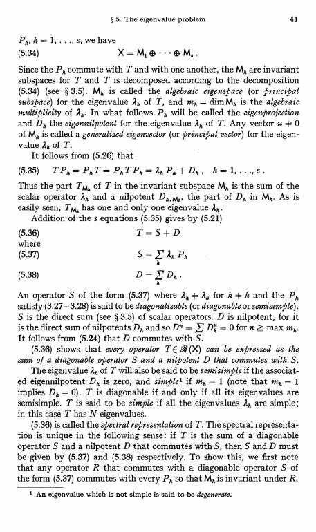
§ 5. The eigenvalue problem 41
Ph, h= 1, ..., s, we have(5.34) M,.
Since the Ph commute with T and with one another, the Mh are invariantsubspaces for T and T is decomposed according to the decomposition(5.34) (see § 3.5). Mh is called the algebraic eigenspace (or principalsubspace) for the eigenvalue Ah of T, and mh = dim Mh is the algebraicmultiplicity of Ah. In what follows Ph will be called the eigenprojectionand Dh the eigennilpotent for the eigenvalue Ah of T. Any vector u $ 0of Mh is called a generalized eigenvector (or principal vector) for the eigen-value Ah of T.
It follows from (5.26) that
(5.35) T P, = Ph T = Ph TPh = Ah Ph + Dh, h = 1, ..., S.
Thus the part TMh of T in the invariant subspace Mh is the sum of thescalar operator Ah and a nilpotent Dh, Mh, the part of Dh in Mh. As iseasily seen, TMh has one and only one eigenvalue Ah.
Addition of the s equations (5.35) gives by (5.21)
(5.36)where(5.37)
T=S+D
S=G AhPhh
(5.38) DDh.h
An operator S of the form (5.37) where Ah + Ak for h + k and the Phsatisfy (3.27-3.28) is said to be diagonalizable (or diagonable or semisimple).S is the direct sum (see § 3.5) of scalar operators. D is nilpotent, for itis the direct sum of nilpotents Dh and so Dn = D;, = 0 for n z max mh.It follows from (5.24) that D commutes with S.
(5.36) shows that every operator T E .°d (X) can be expressed as thesum o l a diagonable operator S and a nilpotent D that commutes with S.
The eigenvalue Ah of T will also be said to be semisimple if the associat-ed eigennilpotent Dh is zero, and simple' if mh = 1 (note that mh = 1implies Dh = 0). T is diagonable if and only if all its eigenvalues aresemisimple. T is said to be simple if all the eigenvalues Ah are simple;in this case T has N eigenvalues.
(5.36) is called the spectral representation of T. The spectral representa-tion is unique in the following sense: if T is the sum of a diagonableoperator S and a nilpotent D that commutes with S, then S and D mustbe given by (5.37) and (5.38) respectively. To show this, we first notethat any operator R that commutes with a diagonable operator S ofthe form (5.37) commutes with every Ph so that Mh is invariant under R.
' An eigenvalue which is not simple is said to be degenerate.
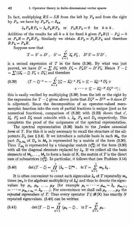
42 I. Operator theory in finite-dimensional vector spaces
In fact, multiplying RS = SR from the left by Ph and from the rightby Ph, we have by PhPh = ahh
AhPhRPk=AhPhRPh or PhRP,=0 for h+-k.Addition of the results for all k + h for fixed h gives PhR (1 - Ph) = 0or PhR = PhRPh. Similarly we obtain R Ph = PhRPh and thereforeRP, = PhR.
Suppose now thats
T=S'+D', S'= f AhPh, D'S'=S'D',h=1
is a second expression of T in the form (5.36). By what was justproved, we have D' _ Z Dh with Dh = PhD' = D' Ph. Hence T -
[(Ah - ) Ph + Dh] and thereforeS' . p
(5.39) (T - Ah)-1 Ph + (b - Ah)-2 Dh +h=1 + ... (S - All DhN-1] ,
this is easily verified by multiplying (5.39) from the left or the right bythe expression for T - C given above (note that Dhly = DIN = 0 since D'is nilpotent). Since the decomposition of an operator-valued mero-morphic function into the sum of partial fractions is unique (just as fornumerical functions), comparison of (5.39) with (5.23) shows that s',Ah, Ph and Dh must coincide with s, Al, Ph and Dh respectively. Thiscompletes the proof of the uniqueness of the spectral representation.
The spectral representation (5.36) leads to the Jordan canonicalform of T. For this it is only necessary to recall the structure of the nil-potents Dh (see § 3.4). If we introduce a suitable basis in each Mh, thepart Dh,M1 of Dh in Mh is represented by a matrix of the form (3.30).Thus TMh is represented by a triangular matrix (i$hk) of the form (3.30)with all the diagonal elements replaced by Ah. If we collect all the basiselements of M1, . . ., M, to form a basis of X, the matrix of T is the directsum of submatrices (r}' ). In particular, it follows that (see Problem 3.14)
S
(5.40) det (T - C) (Ah - C)mh , tr T = Z mh Ah .h=1 h-1
It is often convenient to count each eigenvalue Ah of T repeatedly mhtimes (mh is the algebraic multiplicity of Ah) and thus to denote the eigen-values by ,u1, p2, ..., IAN (for example ,uz = = lum1
=A1, Pm,+1
= _ Pmt+m, = A2, ...). For convenience we shall call p1, ..., ,uN therepeated eigenvalues of T. Thus every operator TE. (X) has exactly Nrepeated eigenvalues. (5.40) can be written
N N(5.41) det(T - t;) = fl trT = Iph .
h-1 h-1

§ 5. The eigenvalue problem 43
Problem 5.12. The geometric eigenspace Nh of T for the eigenvalue A,, is asubset of the algebraic eigenspace Mh. Nh = MI, holds if and only if Ah is semisimple.
Problem 5.13. Ah is semisimple if and only if C = A,, is a simple pole (pole oforder 1) of R(C).
Problem 5.14. If n is sufficiently large (n > m, say), rank T" is equal to N - m,where m is the algebraic multiplicity of the eigenvalue 0 of T (it being agreed toset m = 0 if 0 is not an eigenvalue of T, see § 1.1).
Problem 5.15. We have(5.42) Itr TI s (rank T) II T1I s N II TII
Problem 5.16. The eigenvalues Ah of T are identical with the roots of thealgebraic equation of degree N (characterictic equation)(5.43) det(T - C) = 0.The multiplicity of Ah as the root of this equation is equal to the algebraic multi-plicity of the eigenvalue Ah.
Let (r; k) be an N x N matrix. It can be regarded as the representationof a linear operator Tin a vector space X, say the space CN of N-dimension-al numerical vectors. This means that the matrix representing T withrespect to the canonical basis {x;} of X coincides with (rfk). Let (5.36)be the spectral representation of T, and let {xf } be the basis of X used inthe preceding paragraph to bring the associated matrix (r; k) of T intothe canonical form.
The relationship between the bases {x;} and {xj'} is given by (1.2)and (1.4). Since the xk are eigenvectors of T in the generalized sense,the numerical vectors (pi k, ..., Y1vk), k = 1, ..., N, are generalizedeigenvectors of the matrix (rfk). The relationship between the matrices(rfk) and (tj'k) is given by (3.8). Thus the transformation of (r;,) into thesimpler form (rrk) is effected by the matrix (p,,), constructed from thegeneralized eigenvectors of (rjk), according to the formula (rj'k) _
_ (Pi k)-'(r3k) (Y1 P) -
If the eigenvalue Ak is semisimple, the h-th submatrix of (ilk) is adiagonal matrix with all diagonal elements equal to Ak. If T is diagon-able, (tj'k) is itself a diagonal matrix with the diagonal elements Al,..., A8, where Ak is repeated mk times (that is, with the diagonal elements,ul, ..., ,AN, where the ,uf are the repeated eigenvalues). In this case(pi k' , pNk), k = 1, ..., N, are eigenvectors of (rfk) in the proper sense.
Problem 5.17. (yjl, ..., y1 y), j = 1, ..., N, are generalized eigenvectors of thetransposed matrix of (r5 h)
5. The adjoint problemIf T E 2 (X), then T* E 2 (X*). There is a simple relationship between
the spectral representations of the two operators T, T*. If (5.36) is thespectral representation of T, then that of T* is given by
(5.44) T*=S*+D*= £ +Dr,),h=1
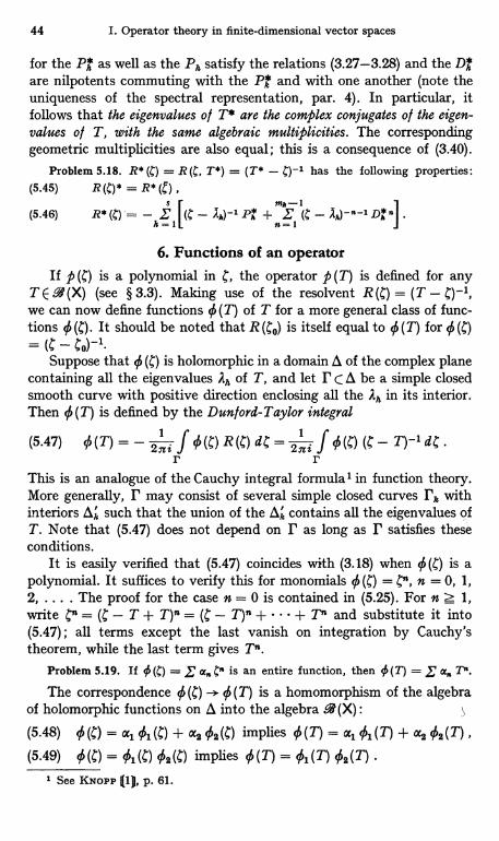
44 I. Operator theory in finite-dimensional vector spaces
for the Pi*, as well as the Ph satisfy the relations (3.27-3.28) and the D,*,are nilpotents commuting with the Ph and with one another (note theuniqueness of the spectral representation, par. 4). In particular, itfollows that the eigenvalues of T* are the complex conjugates of the eigen-values of T, with the same algebraic multiplicities. The correspondinggeometric multiplicities are also equal; this is a consequence of (3.40).
Problem 5.18. R* (C) = R (C, T*) = (T* - a)-1 has the following properties:(5.45) R (C) * = R* () ,
(5.46) R* P, + D. "1 .h= n=1
6. Functions of an operatorIf p is a polynomial in C, the operator p (T) is defined for any
T E -4 (X) (see § 3.3). Making use of the resolvent R (C) = (T - C)-1,we can now define functions (T) of T for a more general class of func-tions q (c). It should be noted that R (Co) is itself equal to 0 (T) for q
Suppose that q is holomorphic in a domain 0 of the complex planecontaining all the eigenvalues 2), of T, and let r C d be a simple closedsmooth curve with positive direction enclosing all the 2h in its interior.Then 0(T) is defined by the Dunford-Taylor integral
(5.47) q(T) = - 2ni ,f 0(C) R(C) dC = 2n% ,f 0(C) (C - T)-1 dC.r r
This is an analogue of the Cauchy integral formulas in function theory.More generally, P may consist of several simple closed curves Ph withinteriors A h' such that the union of the A' contains all the eigenvalues ofT. Note that (5.47) does not depend on r as long as r satisfies theseconditions.
It is easily verified that (5.47) coincides with (3.18) when 0(c) is apolynomial. It suffices to verify this for monomials 0 (C) = c", n = 0, 1,2, .... The proof for the case n = 0 is contained in (5.25). For n z 1,write bn = (C - T + T)n = (C - T)n + + Tn and substitute it into(5.47) ; all terms except the last vanish on integration by Cauchy'stheorem, while the last term gives Tn.
Problem 5.19. If 0 (g) _' ac Co is an entire function, then 0 (T) = E ac" T°.
The correspondence 0 (c') -> 0 (T) is a homomorphism of the algebraof holomorphic functions on 0 into the algebra i(X) :
(5.48) 0 (C) = aal 01(C) + a202(C) implies 0 (T) = al 0, (T) + a2 02(T) ,
(5.49) 0(C) = 01(C) 02(C) implies 0(T) = 0,(T) 02(T)1 See KNOPP (1), p. 61.
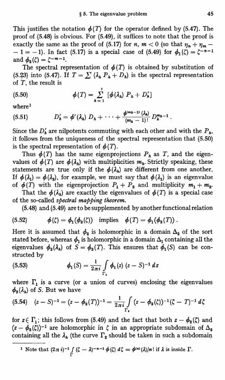
§ 5. The eigenvalue problem 45
This justifies the notation q (T) for the operator defined by (5.47). Theproof of (5.48) is obvious. For (5.49), it suffices to note that the proof isexactly the same as the proof of (5.17) for n, m < 0 (so that r/ + r/m -- I = -1). In fact (5.17) is a special case of (5.49) forand q2M = C-m-1.
The spectral representation of O (T) is obtained by substitution of(5.2,3) into (5.47). If T = ' (Ah Ph + Dh) is the spectral representationof T, the result is
(5.50) (T) _ [0 (Ah) Ph + Da]h=1
where'
(5.51)(mh-1)
Dh'_0'(Ah)Dh+...+ mh-(),)D,h-1
Since the Dh are nilpotents commuting with each other and with the Ph,it follows from the uniqueness of the spectral representation that (5.50)is the spectral representation of 0(T).
Thus O (T) has the same eigenprojections Ph as T, and the eigen-values of 0 (T) are 0 (Ah) with multiplicities mh. Strictly speaking, thesestatements are true only if the O (Ah) are different from one another.If 0 (Al) = 0 (A2), for example, we must say that ¢ (A,) is an eigenvalueof 0 (T) with the eigenprojection P1 + P2 and multiplicity m1 + m2.
That the 0 (Ah) are exactly the eigenvalues of 0 (T) is a special caseof the so-called spectral mapping theorem.
(5.48) and (5.49) are to be supplemented by another functional relation
(5.52) 0 M = 01(02 (0) implies 0 (T) = 01(02 (T))
Here it is assumed that 02 is holomorphic in a domain I2 of the sortstated before, whereas 0, is holomorphic in a domain ., containing all theeigenvalues 02 (Ah) of S = 02 (T). This ensures that 01 (S) can be con-structed by
/'(5.53) 0, (S) ,/= 01(z) (z - S)-1 dz
r,where r, is a curve (or a union of curves) enclosing the eigenvalues02 (Ah) of S. But we have
(5.54) (z - S)-1 = (z - 02(T))-1= 2aii,f (z - 02(x))-1(b - T)-1 dl;
r,for z E r1; this follows from (5.49) and the fact that both z - 02'M and(z - 02 (C))-1 are holomorphic in C in an appropriate subdomain of i 2
containing all the Ah (the curve r2 should be taken in such a subdomain
1 Note that (2n i)-1 f (C - '(C) dC if A is inside I'.r
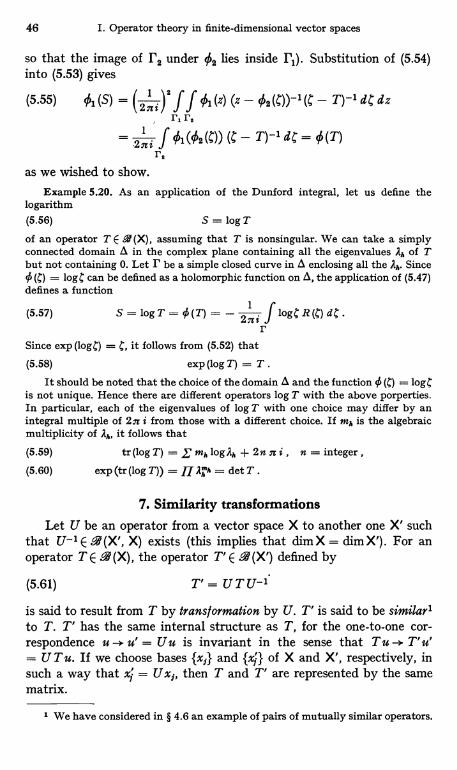
46 I. Operator theory in finite-dimensional vector spaces
so that the image of F2 under 4 lies inside F1). Substitution of (5.54)into (5.53) gives
(5.55) 01 (S) _(2ni)' .lci(z)(z-02('))-1('-T)-1dCdz
r re
2ni f 01(020)) (C - T)-1 dC _ O(T)r,
as we wished to show.
Example 5.20. As an application of the Dunford integral, let us define thelogarithm(5.56) S = log T
of an operator T E .°,d (X), assuming that T is nonsingular. We can take a simplyconnected domain A in the complex plane containing all the eigenvalues Ak of Tbut not containing 0. Let r be a simple closed curve in A enclosing all the Ak. Since0 (C) = loge can be defined as a holomorphic function on A, the application of (5.47)defines a function
(5.57) S = logT 2aci J logCR(C) dC.r
Since exp (loge) = C, it follows from (5.52) that
(5.58) exp (log T) = T.
It should be noted that the choice of the domain A and the function 0 (C) =logeis not unique. Hence there are different operators log T with the above porperties.In particular, each of the eigenvalues of log T with one choice may differ by anintegral multiple of 2n i from those with a different choice. If ml, is the algebraicmultiplicity of Ak, it follows that
(5.59) tr (log T) = Emk log Ak + 2 n n i , n = integer,(5.60) exp (tr (log T)) = jj AA k = det T .
7. Similarity transformationsLet U be an operator from a vector space X to another one X' such
that U-1 E .4 (X', X) exists (this implies that dim X = dim X'). For anoperator T E . (X), the operator T' E .4(X') defined by
(5.61) T'= UT U-1
is said to result from T by transformation by U. T' is said to be similar'to T. T' has the same internal structure as T, for the one-to-one cor-respondence u -> u' = Uu is invariant in the sense that T u -> T' u'= U T u. If we choose bases {xf} and {xj'} of X and X', respectively, insuch a way that xj' = Ux,, then T and T' are represented by the samematrix.
1 We have considered in § 4.6 an example of pairs of mutually similar operators.

§ 6. Operators in unitary spaces 47
If(5.62) T = ' (2h Ph + Dh)
is the spectral representation of T, then
(5.63) T' = ' (Ah Pk + Dl',) , Ph = UP4U-1 , Dh = UDhU-1 ,
is the spectral representation of T'.
§ 6. Operators in unitary spaces1. Unitary spaces
So far we have been dealing with general operators without introduc-ing any special assumptions. In applications, however, we are oftenconcerned with Hermitian or normal operators. Such notions are definedonly in a special kind of normed space H, called a unitary space, in whichis defined an inner product (u, v) for any two vectors u, v. In this sectionwe shall see what these notions add to our general results, especially ineigenvalue problems. We assume that 0 < dim H < oo.
The inner product (u, v) is complex-valued, (Hermitian) symmetric:
(6.1) (u, v) = (v, u)
and sesquilineay, that is, linear in u and semilinear in v. (6.1) impliesthat (u, u) is always real; it is further assumed to be positive-definite:
(6.2) (u, u) > 0 for u + 01 .
We shall see in a moment that the inner product (u, v) may be regardedas a special case of the scalar product defined between an element of avector space and an element of its adjoint space. This justifies the useof the same symbol (u, v) for the two quantities.
Since a unitary space H is a vector space, there could be defineddifferent norms in H. There exists, however, a distinguished norm in H(unitary norm) defined in terms of the inner product, and it is this onewhich is meant whenever we speak of the norm in a unitary space.[Of course any other possible norms are equivalent to this particularnorm, see (1.20).] The unitary norm is given by
(6.3) lull _ (u, u)1/2 .
Obviously the first two of the conditions (1.18) for a norm are satisfied.Before verifying the third condition (triangle inequality), we note theSchwarz inequality(6.4) I(u, v)I s (lull Ilvll
1 In any finite-dimensional vector space X, one can introduce a positive-definitesesquilinear form and make X into a unitary space.
48 I. Operator theory in finite-dimensional vector spaces
where equality holds if and only if u and v are linearly dependent.(6.4) follows, for example, from the identity
(6.5)II Ilvjl2
u - (u, v) v112 = (IIu112 IIv112 - I(u, V) I2) IIv1I2
The triangle inequality is a consequence of (6.4) : JJU + VI12 = (u + v,u + v) = IIul12+2 Re(u, v) + IIv112 < IIu112 + 21lulI IIvII + 110112 = (IIull + IIvlI)2.
Example 6.1. For numerical vectors u = (1, ..., N) and v = (111, ..., 17N) set(6.6) (u,v)=_F a, l1, Ilull2=E1$,12_
With this inner product the space CN of N-dimensional numerical vectors becomesa unitary space.
Problem 6.2. The unitary norm has the characteristic property(6.7) llu + vll$ + Ilu -- vll$ = 2llull$ + 21lvll2 .
Problem 6.3. The inner product (u, v) can be expressed in terms of the norm by
(6.8) (u, v) __4 (Ilu+v112-Ilu-v112+=llu+ivlla-=Ilu-Zvll')
Problem 6.4. For any pair ($,), (iii) of numerical vectors, we have1 1
IE $, ail < E iktl2)2 (E lnil2)2 ,(s.9)1 1 1
(E l $f +'il$)2 s (E (E Imrl$)a .
2. The adjoint spaceA characteristic property of a unitary space H is that the adjoint
space H* can be identified with H itself: H* = H.For any u E H set fu [v] _ (u, v). fu is a semilinear form on H so that
fu E H*. The mapu - ff is linear, for if u = al u1 + a2 u2 then fu [v]_ (u, v) = al (u1, v) + «2 (u2, v) = al ful [v] + «2 fu' [v] so that fu = «1 fu1 ++ a2 fu,. Thus u- fu = Tu defines a linear operator T on H to H*.
T is isometric: I1Tull = Dull. In fact 1ITull = llfuil = supI(u,v)IIIIvllv
_ hull by (2.22) [note the Schwarz inequality and (u, u) = hIull2]. Inparticular T is one to one. Since dim H* =dim H, it follows that Tmaps H onto the whole of H* isometrically. This means that every/ E H* has the form fu with a uniquely determined u E H such thatII/I1 = hull. It is natural to identify / with this u. It is in this sense thatwe identify H* with H.
Since (u, v) = / [v] = (f, v), the inner product (u, v) is seen to coincidewith the scalar product (f, v).
We can now take over various notions defined for the scalar productto the inner product (see § 2.2). If (u, v) = 0 we write u 1 v and saythat u, v are mutually orthogonal (or perpendicular). u is orthogonal to asubset S of H, in symbol u 1 S, if u l v for all v E S. The set of all u E Hsuch that u L S is the annihilator of S and is denoted by S. Two subsetsS, S' of H are orthogonal, in symbol S I S', if every u E S and every v E S'are orthogonal.
§ 6. Operators in unitary spaces 49
Problem 6.5. (u, v) is a continuous function of u, v.Problem 6.6. The Pythagorean theorem:
(6.10) Ilu + vpa = lk112 + 110112 if ulv .Problem 6.7. u 1 S implies u,1 M where M is the span of S. S 1 is a linear manifold
and Sl = Ml.Consider two unitary spaces H and H'. A complex-valued function
t [u, u'] defined for u E H and WE H' is called a sesquilinear form onH x H' if it is linear in u and semilinear in u'. If in particular H' = H,we speak of a sesquilinear form on H. The inner product of H is a specialcase of a sesquilinear form on H. For a general sesquilinear form t [u, v]on H, there is no relation between t [u, v] and t [v, u] so that the quadraticform t [u] = t [u, u] need not be real-valued. In any case, however, wehave the relation (polarization Principle)
(6.11) t[u,v]= 4 (t[u+v]-t[u-v]+it[u+iv]-it[u-iv])similar to (6.8). Thus the sesquilinear form t [u, v] is determined by theassociated quadratic form t [u]. In particular t [u, v] = 0 identically ift [u] = 0 identically. t [u, v] is called the Polar form of t [u].
Problem 6.8. If it [u] S MI1u1I2 for all u E H, then It [u, v] 1 S 2MIlull IIvII.Problem 6.9. If T is a linear operator on H to H', 11 T uI12 is a quadratic form on H
with the polar form (T u, T v).
Remark 6.10. The validity of (6.11) is closely related to the existenceof the scalar i. The quadratic form t [u] does not determine t[u, v] in areal vector space.
3. Orthonormal families
A family of vectors x1, ..., X. E H is called an orthogonal family ifany two elements of this family are orthogonal. It is said to be ortho-normal if, in addition, each vector is normalized :
(6.12) (x,,xk)=alk-As is easily seen, the vectors of an orthonormal family are linearlyindependent. An orthonormal family {x1, ..., is complete if n = N= dim H. Thus it is a basis of H, called an orthonormal basis.
Let M be the span of an orthonormal family {x1, ..., For anyu E H, the vector
(6.13) (u, x,) x,,i=1
has the property that u' E M, u - u' E Ml. u' is called the orthogonalprojection (or simply the projection) of u on M. The Pythagorean theorem
50 I. Operator theory in finite-dimensional vector spaces
(6.10) gives
(6.14) I1ull2-Ilu'll2+llu-ull2= Ly I(u,x,)I2+Ilu-u'112,j=1
and hencen
(6.15) f I (u, x1) 12 I1 ull2 (Bessel's inequality)i=1
For any linearly independent vectors u1, ..., un, it is possible toconstruct an orthonormal family x1, ..., xn such that for each k = 1,..., n, the k vectors x1, ..., x71 span the same linear manifold as the kvectors u1...., U. This is proved by induction on k. Suppose that x1,..., x71_1 have been constructed. If Mk_, denotes the span of x1...., x71_11then by hypothesis M71_i is identical with the span of u1, ..., u71-1Set uk = u7, -uk where uk' is the projection of u71 on M, -1 (if k = 1 setui = u1). The linear independence of the of implies that uk + 0. Setx71 = Ilu II-i uk . Then the vectors x1, ..., x, satisfy the required condi-tions. The construction described here is called the Schmidt orthogonaliza-tion process.
Since every linear manifold M of H has a basis {u1}, it follows that Mhas an orthonormal basis {x1}. In particular there exists a completeorthonormal family in H. An arbitrary vector x1 with Ilxlll = 1 can be thefirst element of an orthonormal basis of H.
It follows also that any u E H has an orthogonal projection u' on agiven linear manifold M. u' is determined uniquely by the property thatu' E M and u" = u - U' E Ml. Thus H is the direct sum of M and M-L :
(6.16) H = Me M-L .
In this sense M-L is called the orthogonal complement of M. We have
(6.17) M1.L = M , dim M L = N - dim M .
When N ( M, Mn N 1 is also denoted by M CO N; it is the set of all u E Msuch that u ..L N.
In the particular case M = H, we have M-L = 0 and so u" = 0.Thus (6.13) gives
N(6.18) u = ,' (u, x,) x5 .
j=1This is the expansion of u in the orthonormal basis {x1}. Multiplicationof (6.18) from the right by v gives
(6.19) (u, v) = ' (u, x,,) (x f, v) (u, x1) (v, x1)
In particular(6.20) I1 ull2 = E I (u, x1) I2 (Parseval's equality)
j
§ 6. Operators in unitary spaces 51
The following lemma will be required later.Lemma 6.11. Let M, M' be two linear manifolds of H with dimensions
n, n' respectively. Then dim (M' n M-L) z n' - n.This follows from (1.10) in view of the relations dim M' = n', dim MI
= N - n, dim (M' + M-L) s N.Let {x1} be a (not necessarily orthonormal) basis of H. The adjoint
basis {e1} is a basis of H* = H satisfying the relations
(6.21) (e5, x,) = bjk
(see § 2.3). {x5} and {e1} are also said to form a biorthogonal family ofelements of H. The basis {x f} is self adjoint if e1 = x5, j = 1, ..., N. Thusa basis of H is self adjoint if and only if it is orthonormal.
4. Linear operatorsConsider a linear operator T on a unitary space H to another unitary
space H'. We recall that the norm of T is defined by II T11 = sup II T uII /IIuII
= sup I (T u, u') I/IIuII IIuII [see (4.1), (4.2)].The function
(6.22) t [u, u'] = (T u, u')
is a sesquilinear form on H x H'. Conversely, an arbitrary sesquilinearform t [u, u'] on H x H' can be expressed in this form by a suitablechoice of an operator T on H to H'. Since t [u, u'] is a semilinear form onH' for a fixed u, there exists a unique w' E H' such that t [u, u'] = (w', u')for all U' E H'. Since w' is determined by u, we can define a function Tby setting w' = T u. It can be easily seen that T is a linear operatoron H to H'. If in particular t is a sesquilinear form on H(H'= H), then Tis a linear operator on H to itself.
In the same way, t [u, u'] can also be expressed in the form
(6.23) t [u, u'] = (u, T* u') ,
where T* is a linear operator on H' to H, called the adjoint (operator)of T. T* coincides with the adjoint operator defined in § 3.6 by theidentification of H*, H'* with H, H' respectively.
T*T is a linear operator on H to itself. The relation
(6.24) (u, T*Tv) = (T*Tu, v) = (Tu, Tv)
shows that T*T is the operator associated with the sesquilinear form(T u, T v) on H. Note that the first two members of (6.24) are the innerproduct in H while the last is that in H'. It follows from (6.24) and (4.2)that 11 T* TII = sup I (Tu, Tv) I/IIuII IIuII ? supll Tuii2/IIuii2 = 11 TII2 Since,
52 I. Operator theory in finite-dimensional vector spaces
on the other hand, II T* T11 s II T*II II TII = II TII2, we have
(6.25) II T*TII = II TII 2
In particular, T*T = 0 implies T = 0.Problem 6.12. N (T* T) = N (T).Problem 6,13. We have the polarization principle for an operator T on H to H
(6.26) (T u, v) = 4 [(T (u + v), u + v) - (T (u - v), u - v) +
+i(T(u+iv),u+iv)-i(T(u-iv),u-iv)]Problem 6.14. If T is an operator on H to itself, (Tu, u) = 0 for all u implies
T=0.The matrix representation of an operator is related to a pair of
adjoint bases in the domain and range spaces [see (3.10)]. This suggeststhat the choice of selfadjoint (orthonormal) bases is convenient for thematrix representation of operators between unitary spaces.
Let T be an operator from a unitary space H to another one H' andlet {xk}, {X'I be orthonormal bases of H, H', respectively. The matrixelements of T for these bases are then
(6.27) rik = (Txk, xi) = (xk T* xi)
as is seen from (3.10) by setting I j = xi . More directly, (6.27) follows fromthe expansion(6.28) T x7, = (T x7, xi) xi .
Recall that if H' = H it is the convention to take x, = xf.Problem 6.15. If {zk} is an orthonormal basis of H and if T is an operator on H
to itself,(6.29) trT =' (Tzk, xk) .
The matrix of T* with respect to the same pair of bases N1}1 {xk}is given by a,*q = (T* xi, xk). Comparison with (6.27) gives
(6.30) ski-f1kThus the'matrices of T and T* (for the same pair of orthogonal bases)are Hermitian conjugate to each other.
5. Symmetric forms and symmetric operatorsA sesquilinear form t [u, v] on a unitary space H is said to be sym-
metric if
(6.31) t [v, u] = t [u, v] for all u, v E H .
If t [u, v] is symmetric, the associated quadratic form t [u] is real-valued.The converse is also true, as is seen from (6.11).
§ 6. Operators in unitary spaces 53
A symmetric sesquilinear form (or the associated quadratic form) t isnonnegative (in symbol t z 0) if t [u] 0 for all u, and positive if t [u] > 0for u $ 0. The Schwarz and triangle inequalities are true for any non-negative form as for the inner product (which is a special positive ses-quilinear form) :
It [u, v] 1 s t [u]1/2 t [v]1/2 < 2 (t [u] + t [v])
(6.32) t [u + v]1/2 t [u]1/2 + t [v]1/2 ,
t [u + v] 2t [u] + 2t [v]
Note that strict positivity was not used in the proof of similar inequalitiesfor the inner product.
The lower bound y of a symmetric form t is defined as the largest realnumber such that t [u] ull2. The upper bound y' is defined similarly:We have
(6.33) It[u,v]1 sMHHul11Iv1I, Mmax(Iyl.ly'I)
To see this, we note that the value t [u, v] under consideration may beassumed to be real, for (6.33) is unchanged by multiplying u with ascalar of absolute value one. Since t [u] is real-valued, we see from (6.11)that t [u, v] = 4-1 (t [u + v] - t [u - v]). Since jt[U]I S M11u112 for allu, it follows that It[u,v]1s4-1M(Ilu+vI12+IIu-vI12)=2-1M(IIuII2+IIv112).Replacement of u, v respectively by a u, v/a, with a2 = lIvII/iluIl, yields(6.33).
The operator T associated with a symmetric form t [u, v] accordingto (6.22) has the property that
(6.34) T* = T
by (6.22), (6.23) and (6.31). An operator T on H to itself satisfying (6.34)is said to be (Hermitian) symmetric or sel f adjoint. Conversely, a sym-metric operator T determines a symmetric form t [u, v] = (T u, v) on H.Thus (T u, u) is real for all u E H i f and only i f T is symmetric. A sym-metric operator T is nonnegative (positive) if the associated form isnonnegative (positive). For a nonnegative symmetric operator T we havethe following inequalities corresponding to (6.32) :
(6.35) /I (T u, v) 1 S (T u, u)1/2 (TV, V)1/2,
(T (u + v), u + v)1/2 S (T u, u)1/2 + (T v, v)1/2 .
We write T z 0 to denote that T is nonnegative symmetric. Moregenerally, we write
(6.36) T z S or S< T
54 I. Operator theory in finite-dimensional vector spaces
if S, T are symmetric operators such that T - S z 0. The upper andlower bounds of the quadratic form (Tu, u) are called the upper andlower bounds of the symmetric operator T.
Problem 6.16. If T is symmetric, a T + P is symmetric for real at, 9. Moregenerally, p (T) is symmetric for any polynomial p with real coefficients.
Problem 6.17. For any linear operator Ton H to H' (H, H' being unitary spaces),T* T and T T* are nonnegative symmetric operators in H and H', respectively.
Problem 6.18. If T is symmetric, then T2 0; T2 = 0 if and only if T=O.If T is symmetric and T" = 0 for some positive integer n, then T = 0.
Problem 6.19. R:< S and S:!' T imply R g' T. S:< T and S Z T imply S= T.
6. Unitary, isometric and normal operatorsLet H and H' be unitary spaces. An operator T on H to H' is said to be
isometric' if(6.37) IITuII = IIull for every u E H .
This is equivalent to ((T* T - 1) u, u) = 0 and therefore (see Problem6.14)
(6.38) T*T = 1 .This implies that(6.39) (T u, T v) = (u, v) for every u, v E H .
An isometric operator T is said to be unitary if the range of T is the wholespace H'. Since (6.37) implies that the mapping by T is one to one, it isnecessary for the existence of a unitary operator on H to H' that dim H'= dim H. Conversely, if dim H' = dim H < oo any isometric operator onH to H' is unitary. As we shall see later, this is not true for infinite-dimensional spaces.
Problem 6.20. A T E R (H, H') is unitary if and only if T-1 E R (H', H) exists and
(6.40) T-1 = T*.
Problem 6.21. T is unitary if and only if T* is.Problem 6.22. If T E 9 (H', H") and S E R (H, H') are isometric, TS E R (H, H")
is isometric. The same is true if "isometric" is replaced by "unitary".
Symmetric operators and unitary operators on a unitary space intoitself are special cases of normal operators. T E .(H) is said to be normalif T and T* commute :(6.41) T*T = T T* .
This is equivalent to (again note Problem 6.14)
(6.42) IIT*ull=IITull for all uEH.
1 Isometric operators can be defined more generally between any two normedspaces, but we shall have no occasion to consider general isometric operators.
§ 6. Operators in unitary spaces 55
An important property of a normal operator T is that
(6.43) IIT"11 =IITIIn, n= 1,2,....This implies in particular that (spr denotes the spectral radius, see § 4.2)
(6.44) spr T = II TII
To prove (6.43), we begin with the special case in which T is sym-metric. We have then II T2II = II TII2 by (6.25). Since T2 is symmetric,we have similarly II T4II = II T2II2 = II TII4. Proceeding in the same way,we see that (6.43) holds for n = 2"", m = 1, 2, ... . Suppose now that Tis normal but not necessarily symmetric. Again by (6.25) we have II T n II 2= IITn*TnII. But since Tn*Tn = (T*T)n by (6.41) and T*T is sym-metric, we have II T"112 = II (T*T)n9I = II T *T II n = II T II2n for n=2-.This proves (6.43) for n = 2'n. For general n, we take an m such that2m - n = r z 0. Since (6.43) has been proved for n replaced by n + r= 2"", we have IITIIn+s = IITn+TII < IITnnI 11 T"11 s IIT"`II 11TH" or IITIIn s
II TnII. But since the opposite inequality is obvious, (6.43) follows.Problem 6.23. If T is normal, p (T) is normal for any polynomial p.Problem 6.24. T-1 is normal if T is normal and nonsingular.Problem 6.25. If T is normal, P' = 0 for some integer n implies T = 0. In other
words, a normal operator T is nilpotent if and only if T = 0.
7. ProjectionsAn important example of a symmetric operator is an orthogonal
projection. Consider a subspace M of H and the decomposition H = M® Ml [see (6.16)]. The projection operator P = PM on M along Ml iscalled the orthogonal projection on M. P is symmetric and nonnegative, for(with the notation of par. 3)
(6.45) (Pu, u) = (u', u' + u") _ (u', u') z 0
in virtue of u' 1 u". Thus
(6.46) P*=P, Pz0, P2=P.Conversely, it is easy to see that a symmetric, idempotent operatorPE °.,8(H) is an orthogonal projection on M = R(P).
Problem 6.26. 1 - P is an orthogonal projection with P. If P is an orthogonalprojection, we have(6.47) 0S PS 11, J!PII=1 if P + 0.
Problem 6.27. 11 (1 - PM) UI! = dist (u, M) , u E H.
1 The notation 0:< P:< 1, which is used to denote the order relation definedfor symmetric operators [see (6.36)], does not conflict with the notation introducedearlier for projections (see § 3.4).
56 I. Operator theory in finite-dimensional vector spaces
Problem 6.28. M I N is equivalent to PM PN = 0. The following three conditionsare equivalent: M ) N, PM Z PN, PM PN = PN.
Let P1, ..., Pn be orthogonal projections such that
(6.48)
Then their sumP1 P, =BfkP5.
n(6.49) P = ' P,
i=1is also an orthogonal projection, of which the range is the direct sum ofthe ranges of the P;.
Orthogonal projections are special kinds of projections. We can ofcourse consider more general "oblique" projections in a unitary space H.Let H = M ® N with M, N not necessarily orthogonal, and let P be theprojection on M along N. Then P* is the projection on N-i along Ml[see (3.43)].
Problem 6.29. IIPII > I for a projection P r 0; IIPII = I holds if and only if Pis an orthogonal projection. [hint for "only if" part: Let u E NJ-. Then u,1(1 - P) u.Apply the Pythagorean theorem to obtain IIPUII' = II'II2 + II(1 - P) ulla. Fromthis and IIPII = 1 deduce N1( M. Consider P* to deduce the opposite inclusion.]
Problem 6.30. A normal projection is orthogonal.Problem 6.31. If P is a projection in a unitary space with 0 + P + 1, then
IIPII=III - Pill.8. Pairs of projections
Let us now consider a pair P, Q of projections in H and recall theresults of § 4.6 that R (P) and R (Q) are isomorphic if P - Q is suf-ficiently small. A new result here is that the operator U given by (4.38)is unitary i f P, Q are orthogonal projections. This is seen by noting thatU' * = V' and R* = R [see (4.36) and (4.33)], which imply U* = V = U-1.Thus
Theorem 6.32. Two orthogonal projections P, Q such that 11 P- Q11 < 1are unitarily equivalent, that is, there is a unitary operator U with theproperty Q = UP U-1.
Problem 6.33. 11P - QII 5 1 for any pair P, Q of orthogonal projections [see(4.34)].
A similar but somewhat deeper result is given by the followingtheorem.
Theorem 6.34. 2 Let P, Q be two orthogonal projections with M = R (P),N = R (Q) such that(6.50) 11(1 - Q) P11 = 8 < 1 .
1 See T. KAxo [13].2 See T. KATO [12], Lemma 221. This theorem is true even for dim H = oo.
A similar but slightly weaker result was given earlier by AKHIEZER and GLAZMANQi), § 34.
§ 6. Operators in unitary spaecs 57
Then there are the following alternatives. Eitheri) Q maps M onto N one to one and bicontinuously, and
(6.51) IIP'-QII=II(1-P)QII=11(1-Q)PII=6; or
ii) Q maps M onto a proper subspace No of N one to one and biconti-nuously and, if Q0 is the orthogonal projection on No,
IIP-Q0I1=11(1-P)QoII=11(1-Qo)PII=II(i-Q)PII=a(6.52)
IIP-QII=11(1 -P) QII=1.Proof. For any u E M, we have 11 u - Qu11 = 11(1 - Q) Pull 5 6llu11
so that IIQuII G (1 - a) 11u11 Thus the mapping u--* Qu of M into N isone to one and bicontinuous (continuous with its inverse mapping).Therefore, the image QM = No of this mapping is a closed subspace of N.Let Q0 be the orthogonal projection on No.
For any w E H, Qow is in No and hence Q0 w = Qu for some u E M.If Qow + 0 then u + 0 and, since (1 - P) u = 0,
11(1 - P) Qow!1 = 11(1 - P) QoII = 11(1 - P) (Qu - IIQuII2IIuil-2 u)II53)(6.
Hences II(Qu - IIQu11211u11-2 u)II
(6.54) 11(1 - P) Qow112 IIQuII2 - IIQuI14 IIuil-2 =
= 11Qu112 1Iu1I-2(11u112 - IIQu112) = 11u11-2 IIQow112 11(1 - Q) U112 S
11u11-2 11w11211(1 - Q) PuI12 6211w112.
This inequality is true even when Qow = 0. Hence
(6.55) 11(1-P)Q011Sa=11(1-Q)P11For any w E H, we have now
(6.56) 11(P-Q0)w112=11(1-Q0) Pw-Q0(1-P)w112=11(1-Q0)Pw112+11Q0(1-P)w112
since the ranges of 1 - Q0 and Q0 are orthogonal. Noting that P = P2and 1 - P = (1 - P)2, we see from (6.56) that
(6.57) 11(P-Q0)Will 11(i-Qo)P112IIPwll2+11Q0(1-P)112II(1-P)w112.
Since Qo P = Q0Q P = Q P by the definition of Q0, we have 11(1 - Q0) P11=11(1-Q)P11=a, and11Qo(1-P)11=11(Qo(1-P))*II=11(1-P)Q011 sS 6 by (6.55). Hence
(6.58) I1(P-Q0)Will 5 62(11Pw112+11(1-P)w112)=6211w112.
This gives 11 P - Q011 s a. Actually we have equality here, for
(6.59) 6=11(1-Q)PI1=11(1-Qo)P11=11(P-Q0)PII s IIP-Q011S6.
58 I. Operator theory in finite-dimensional vector spaces
The fact that lip - QOII = a < 1 implies that P maps NO = R (Q0) onto Mone to one (see Problem 4.11). Applying the above result (6.55) to thepair P, Q replaced by QO, P, we thus obtain II (1 - Q0) PII S II (1 - P)QO IIComparison with (6.59) then shows that we have equality also in (6.55).
If NO = N, this completes the proof of i). If NO $ N, it remains toprove the last equality of (6.52). Let v be an element of N not belongingto N0. Since PNO = M as noted above, there is a v0 ENO such thatPv0=Pv.Thus w=v-v0EN,w+0 andPw=0, sothat(P-Q)w= -w and Q(1 - P) w = Qw = w. Thus IIP - QIIz 1 and11(1-P)QII= II Q (1 - P) II z 1. Since we have the opposite inequalities (see Problem6.33), this gives the desired result.
As an application of Theorem 6.34, we deduce an inequality concern-ing pairs of oblique and orthogonal projections.
Theorem 6.35. Let P', Q' be two oblique projections in H and let M='R(P'), N = R(Q'). Let P, Q be the orthogonal Projections on M, Nrespectively. Then(6.60) IIP - QII s IIP' - Q'II
Proof. Since IIP - QII never exceeds 1 (see Problem 6.33), it sufficesto consider the case 11 P' - Q'II = 6' < 1. For any u E H, we have (seeProblem 6.27) II (1 - Q) Pull = dist (Pu, N) S II Pu - Q' Pull = II (P' -- Q') Pull s a'IIPuII s S'IIuII. Hence p(1- Q) PII s a' < 1. Similarlywe have 11(1 - P) Q11 S a' < 1. Thus Theorem 6.34 is applicable, wherethe case ii) is excluded, so that 11P - Q11 = II (1 - P) Q II s a' = II P' - Q'11
by (6.51).
Problem 6.36. If P', Q' are oblique projections with JJP' - Q'11 < 1, then thereis a unitary operator U such that UM = N, U-1 N = M, where M = R(P'),N = R(Q'). (This proposition can be extended directly to the infinite-dimensionalcase, in which it is not trivial.)
Problem 6.37. Let P'(x) be an oblique projection depending continuously on xfor 0:< x:5, 1, and let P (x) be the orthogonal projection on M (x) = R (P' (x)). ThenP (x) is also continuous in x, and there is a family of unitary operators U (x), depend-ing continuously on x, such that U (x) M (0) = M (x), U (x)-1 M (x) = M (0).
9. The eigenvalue problemWe now consider the eigenvalue problem for an operator in a unitary
space H. For a general operator T, there is not much simplification to begained by the fact that the underlying space is unitary; this is clear ifone notes that any vector space may be made into a unitary space byintroducing an inner product, whereas the eigenvalue problem can beformulated without reference to any inner product, even to any norm.The advantage of considering a unitary space appears when the operatorT has some special property peculiar to the context of a unitary space,such as being symmetric, unitary or normal.
§ 6. Operators in unitary spaces 59
Theorem 6.38. A normal operator is diagonable, and its eigenprojectionsare orthogonal projections.
Proof. Let T be normal. Since T and T* commute, we have
(6.61) (T - C) (T* - C') (T* - C') (T - C)
If C is not an eigenvalue of T and C' is not an eigenvalue of T*, theinverse of (6.61) exists and we have
(6.62) R* (c') R (C) = R (C) R* (c')
where R (C) and R* (C) are the resolvents of T and T* respectively.(6.62) shows that these resolvents commute. In view of the expression(5.22) for the eigenprojection Ph associated with the eigenvalue 2h of T,a double integration of (6.62) along appropriate paths in the C andplanes yields the relation
(6.63) P h * Ph = Ph P h *, h, k = 1, ..., s ;
recall that T* has the eigenvalues h and the associated eigenprojectionsP,* (§ 5.5). In particular Ph and Ph commute, which means that the Phare normal. This implies that the Ph are orthogonal projections (seeProblem 6.30) :
1, ..., s .(6.64) P'=PA, h=The eigennilpotents are given by Dh = (T - 2h) Ph and D` = (T* -
- Ah) Ph = (T* - Ah) Ph by (5.26). Since Ph and T commute, Ph = P:commutes with T* and T* commutes with T, it follows that Dh commuteswith D:, that is, Dh is normal. As a normal nilpotent DA must be zero(Problem 6.25). Thus T is diagonable.
The spectral representation of a normal operator T thus takes theform
(6.65)
s s
T= Z,''hPh, T* f 1hPh,h=1 h=1
P x =Ph, PhPA=64APh, £, Ph= 1.h=1
T and T* have the same set of eigenspaces, which are at the same timealgebraic and geometric eigenspaces and which are orthogonal to oneanother. It follows further from (6.65) that
(6.66) T*T=TT*= ' I2AI'Ph.h_1
HenceIITull2=(T*Tu,u) = f IAII2(Phu,u) s (maxIAAI2)E(Phu,u)_
A
_ (max IAAI2) 11 ul12 ,
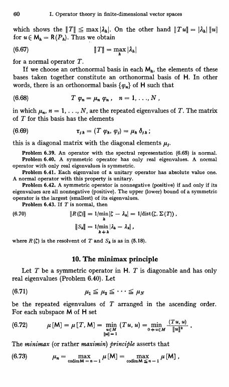
60 I. Operator theory in finite-dimensional vector spaces
which shows the 11 T11 s maxlAkl. On the other hand llTull = IAkl (lullfor u E Mk = R (Ph). Thus we obtain
(6.67) II TII = mkax lAhl
for a normal operator T.If we choose an orthonormal basis in each Mk, the elements of these
bases taken together constitute an orthonormal basis of H. In otherwords, there is an orthonormal basis {(p,,} of H such that
(6.68) T99n=Yn9'n, n=1,...,N,in which un, n = 1, ..., N, are the repeated eigenvalues of T. The matrixof T for this basis has the elements
(6.69) Z1 k = (T (pk, 99s) _ ,uk 61h;
this is a diagonal matrix with the diagonal elements ,u1.Problem 6.39. An operator with the spectral representation (6.65) is normal.Problem 6.40. A symmetric operator has only real eigenvalues. A normal
operator with only real eigenvalues is symmetric.Problem 6.41. Each eigenvalue of a unitary operator has absolute value one.
A normal operator with this property is unitary.Problem 6.42. A symmetric operator is nonnegative (positive) if and only if its
eigenvalues are all nonnegative (positive). The upper (lower) bound of a symmetricoperator is the largest (smallest) of its eigenvalues.
Problem 6.43. If T is normal, then
(6.70) IIR(C)II = l/minIC - AkI = 1/dist(C, E(T)),k
IISkII = 1/min IA,, - AkIk4k
where R (C) is the resolvent of T and Sh is as in (5.18).
10. The minimax principleLet T be a symmetric operator in H. T is diagonable and has only
real eigenvalues (Problem 6.40). Let
(6.71) Y1SF2S ...5YNbe the repeated eigenvalues of T arranged in the ascending order.For each subspace M of H set
(6.72) ,u [M] _ ,u [T, M] = minM
(T u, u) =o min a (Tu, u)
IIuII$Iinll =1
The minimax (or rather maximin) principle asserts that
(6.73) ,un = max ,u [M] = max ,u [M] ,codim M= n- 1 codim M i n -1
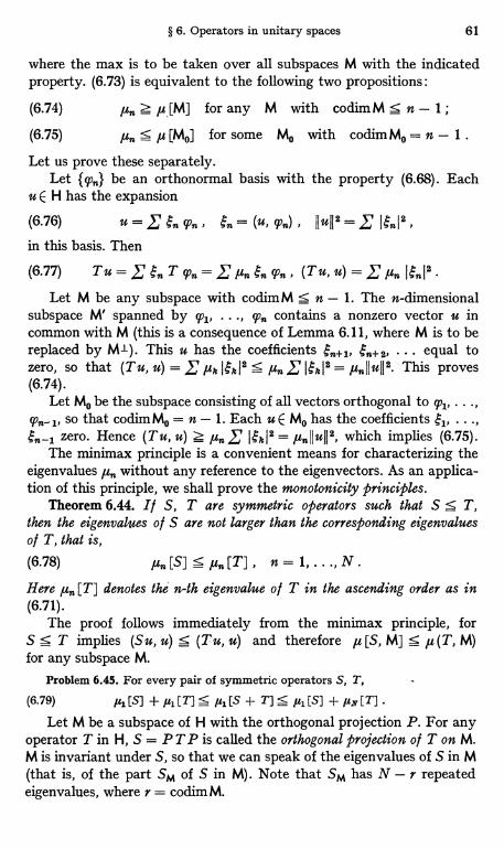
§ 6. Operators in unitary spaces 61
where the max is to be taken over all subspaces M with the indicatedproperty. (6.73) is equivalent to the following two propositions:
(6.74) ,un z It [M] for any M with codimM s n - 1;(6.75) ,un S u [Me] for some Mo with codim Mo = n - 1 .
Let us prove these separately.Let {q,,} be an orthonormal basis with the property (6.68). Each
u E H has the expansion
(6.76) u = .I Sn (P., (u, Pn) , Il u ll 2 = 2' I sn 12 ,
in this basis. Then
(6.77) (Tu,u)=G,un ISnJ2.
Let M be any subspace with codim M s n - 1. The n-dimensionalsubspace M' spanned by 4pl, ..., qqn contains a nonzero vector u incommon with M (this is a consequence of Lemma 6.11, where M is to bereplaced by M1). This u has the coefficients n+1, $n+2, ... equal tozero, so that (T u, u) = f ,u7, 1E 7 ' 1 2 s ,un 2' I S k 12 = ,un lI ull2. This proves(6.74).
Let Mo be the subspace consisting of all vectors orthogonal to %, ...,g9n_ 1, so that codim Mo = n - 1. Each u E Mo has the coefficients $1, ...,$n-1 zero. Hence (Tu, u) z ,un 2' ,un!Iull2, which implies (6.75).
The minimax principle is a convenient means for characterizing theeigenvalues ,un without any reference to the eigenvectors. As an applica-tion of this principle, we shall prove the monotonicity principles.
Theorem 6.44. If S, T are symmetric operators such that S 5 T,then the eigenvalues of S are not larger than the corresponding eigenvaluesof T, that is,
(6.78) ,un [S] S pn [T] , n = 1, ..., N .
Here ,u, [T] denotes the n-th eigenvalue of T in the ascending order as in(6.71).
The proof follows immediately from the minimax principle, forS S T implies (Su, u) S (Tu, u) and therefore a [S, M] S ju (T, M)for any subspace M.
Problem 6.45. For every pair of symmetric operators S, T,
(6.79) ,u1 [S] + ,u1 [T];5 ,u1 [S + T] 5 ,s1 [S] + ,um [T]
Let M be a subspace of H with the orthogonal projection P. For anyoperator T in H, S = P T P is called the orthogonal projection of T on M.M is invariant under S, so that we can speak of the eigenvalues of S in M(that is, of the part SM of S in M). Note that SM has N - r repeatedeigenvalues, where r = codim M.
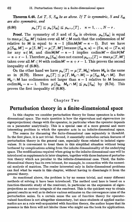
62 II. Perturbation theory in a finite-dimensional space
Theorem 6.46. Let T, S, SM be as above. If T is symmetric, S and SMare also symmetric, and
(6.80) 4n [T] < 4n [SM] S /A.+, [T] , n = 1, ..., N - Y.
Proof. The symmetry of S and of SM is obvious. ,un [SM] is equalto max,u [SM, M'] taken over all M' C M such that the codimension of M'relative to M is equal to n - 1 (dimM/M' = n - 1). But we have,u [SM, M'] = ,u [S, M'] = ,u [T, M'] because (SM u, u) = (Su, u) = (Tu, u)for any u E M, and dim M/M' = n - 1 implies codim M'= dim H/M'= n + r - 1. Therefore,un [SM] does not exceed,un+, [T] = max,u [T, M']taken over all M' C H with codim M' = n + r - 1. This proves the secondinequality of (6.80).
On the other hand we have ,un [T] = ,u [T, M0] where Mo is the sameas in (6.75). Hence ,un [T] S u [T, Mo n M] = ,u [SM, Mo n M]. ButMo n M has codimension not larger than n - 1 relative to M becausecodimMo = n - 1. Thus 4u [SM, Mo n M] ,un [SM] by (6.74). Thisproves the first inequality of (6.80).
Chapter Two
Perturbation theory in a finite-dimensional spaceIn this chapter we consider perturbation theory for linear operators in a finite-
dimensional space. The main question is how the eigenvalues and eigenvectors (oreigenprojections) change with the operator, in particular when the operator dependson a parameter analytically. This is a special case of a more general and moreinteresting problem in which the operator acts in an infinite-dimensional space.
The reason for discussing the finite-dimensional case separately is threefold.In the first place, it is not trivial. Second, it essentially embodies certain features ofperturbation theory in the general case, especially those related to isolated eigen-values. It is convenient to treat them in this simplified situation without beingbothered by complications arising from the infinite dimensionality of the underlyingspace. The modifications required when going to the infinite-dimensional case will beintroduced as supplements in later chapters, together with those features of perturba-tion theory which are peculiar to the infinite-dimensional case. Third, the finite-dimensional theory has its own interest, for example, in connection with the numeri-cal analysis of matrices. The reader interested only in finite-dimensional problemscan find what he wants in this chapter, without having to disentangle it from thegeneral theory.
As mentioned above, the problem is by no means trivial, and many differentmethods of solving it have been introduced. The method used here is based on afunction-theoretic study of the resolvent, in particular on the expression of eigen-projections as contour integrals of the resolvent. This is the quickest way to obtaingeneral results as well as to deduce various estimates on the convergence rates of theperturbation series. In a certain sense the use of function theory for operator-valued functions is not altogether elementary, but since students of applied mathe-matics are as a rule well-acquainted with function theory, the author hopes that itspresence in this form will not hinder those who might use the book for applications.
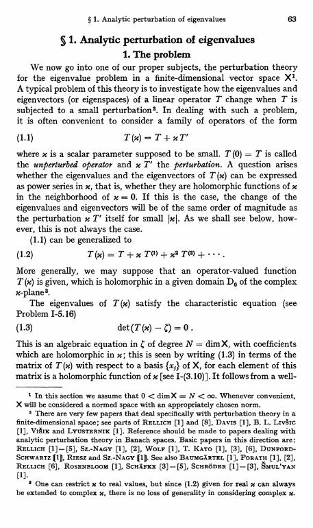
§ 1. Analytic perturbation of eigenvalues 63
§ 1. Analytic perturbation of eigenvalues1. The problem
We now go into one of our proper subjects, the perturbation theoryfor the eigenvalue problem in a finite-dimensional vector space X1.A typical problem of this theory is to investigate how the eigenvalues andeigenvectors (or eigenspaces) of a linear operator T change when T issubjected to a small perturbation. In dealing with such a problem,it is often convenient to consider a family of operators of the form
(1.1) T (m) = T + x T'
where x is a scalar parameter supposed to be small. T (0) = T is calledthe unperturbed operator and x T' the Perturbation. A question ariseswhether the eigenvalues and the eigenvectors of T (m) can be expressedas power series in x, that is, whether they are holomorphic functions of xin the neighborhood of x = 0. If this is the case, the change of theeigenvalues and eigenvectors will be of the same order of magnitude asthe perturbation x T' itself for small Ixl. As we shall see below, how-ever, this is not always the case.
(1.1) can be generalized to
(1.2) T(x)=T+ cT(')+x2T(2)+...More generally, we may suppose that an operator-valued functionT (x) is given, which is holomorphic in a given domain Do of the complexx-plane 8.
The eigenvalues of T (x) satisfy the characteristic equation (seeProblem 1-5.16)
(1.3) det (T (x) - C) = 0.
This is an algebraic equation in C of degree N = dim X, with coefficientswhich are holomorphic in x; this is seen by writing (1.3) in terms of thematrix of T (m) with respect to a basis {x;} of X, for each element of thismatrix is a holomorphic function of x [see I-(3.10)]. It follows from a well-
1 In this section we assume that 0 < dimX = N < oo. Whenever convenient,X will be considered a normed space with an appropriately chosen norm.
1 There are very few papers that deal specifically with perturbation theory in afinite-dimensional space; see parts of RELLICH [1] and [8], DAvis [1], B. L. LIv§Ic[1], VI§IK and LYUSTERNIK [1]. Reference should be made to papers dealing withanalytic perturbation theory in Banach spaces. Basic papers in this direction are:RELLICH [1]-[5], SZ.-NAGY [1], [2], WOLF [1], T. KATO [1], [3], [6], DUNFORD-SCHWARTZ (1), RIEsz and SZ.-NAGY (1). See also BAUMGXRTEL [1], PORAT22GHG [1], [2],RELLICH [6], ROSENBLOOM [1], SCHXFKE [3]-[5], SCHRSDER [1]-[3], DMUL'YAN[1].
® One can restrict x to real values, but since (1.2) given for real x can alwaysbe extended to complex x, there is no loss of generality in considering complex x.
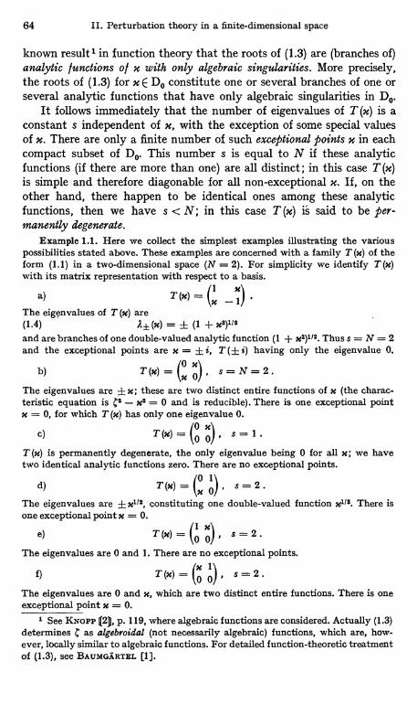
64 II. Perturbation theory in a finite-dimensional space
known results in function theory that the roots of (1.3) are (branches of)analytic functions of x with only algebraic singularities. More precisely,the roots of (1.3) for xE Do constitute one or several branches of one orseveral analytic functions that have only algebraic singularities in Do.
It follows immediately that the number of eigenvalues of T (m) is aconstant s independent of x, with the exception of some special valuesof x. There are only a finite number of such exceptional Points x in eachcompact subset of Do. This number s is equal to N if these analyticfunctions (if there are more than one) are all distinct; in this case T(u)is simple and therefore diagonable for all non-exceptional X. If, on theother hand, there happen to be identical ones among these analyticfunctions, then we have s < N; in this case T (m) is said to be per-inanently degenerate.
Example 1.1. Here we collect the simplest examples illustrating the variouspossibilities stated above. These examples are concerned with a family T (x) of theform (1.1) in a two-dimensional space (N = 2). For simplicity we identify T (X)with its matrix representation with respect to a basis.
a)T (x) = (x 1)
The eigenvalues of T (x) are(1.4) A} (x) (1 + x2)118
and are branches of one double-valued analytic function (1 + x8)118. Thus S = N = 2and the exceptional points are x = ± i, T (± i) having only the eigenvalue 0.
b) T(x)=(x 0)' s=N=2.The eigenvalues are ± x; these are two distinct entire functions of x (the charac-teristic equation is Cs - xe =0 and is reducible). There is one exceptional pointx = 0, for which T (x) has only one eigenvalue 0.
c) T(x)=(0 0)' s=1.T (m) is permanently degenerate, the only eigenvalue being 0 for all x; we havetwo identical analytic functions zero. There are no exceptional points.
d)T (m) = (x 0) ' s = 2 .
The eigenvalues are ±xiI2, constituting one double-valued function x116. There isone exceptional point x = 0.
e) T(x)=(0 0), s=2.The eigenvalues are 0 and 1. There are no exceptional points.
f) T(x)=(0 0)' s=2.The eigenvalues are 0 and x, which are two distinct entire functions. There is oneexceptional point x = 0.
1 See KNOPP 121, p. 119, where algebraic functions are considered. Actually (1.3)determines C as algebroidal (not necessarily algebraic) functions, which are, how-ever, locally similar to algebraic functions. For detailed function-theoretic treatmentof (1.3), see BAUMGXRTEL [1].
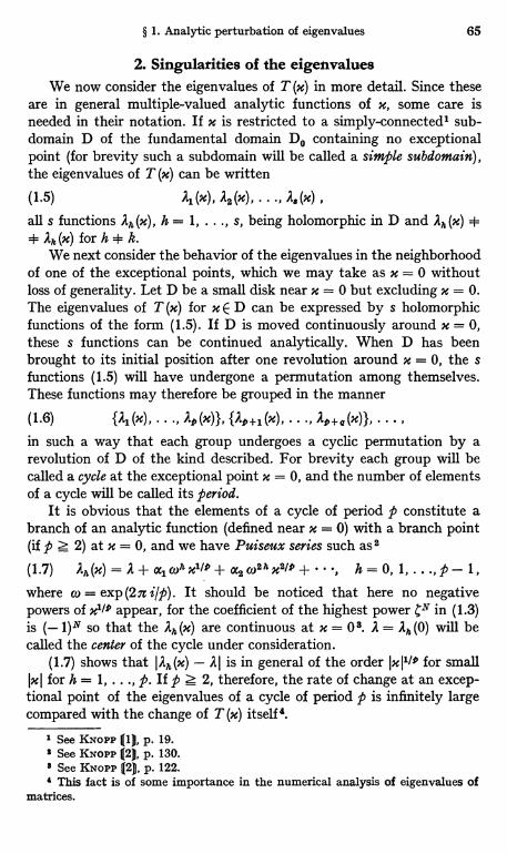
§ 1. Analytic perturbation of eigenvalues 65
2. Singularities of the eigenvaluesWe now consider the eigenvalues of T (m) in more detail. Since these
are in general multiple-valued analytic functions of x, some care isneeded in their notation. If x is restricted to a simply-connected' sub-domain D of the fundamental domain Do containing no exceptionalpoint (for brevity such a subdomain will be called a simple subdomain),the eigenvalues of T (m) can be written
(1.5) Al (x), A2 (x), ..., A, (x)
all s functions Ah (x), h = 1, ..., s, being holomorphic in D and Ah (x) ++ Ah (x) for h + k.
We next consider the behavior of the eigenvalues in the neighborhoodof one of the exceptional points, which we may take as x = 0 withoutloss of generality. Let D be a small disk near x = 0 but excluding x = 0.The eigenvalues of T (x) for x E D can be expressed by s holomorphicfunctions of the form (1.5). If D is moved continuously around x = 0,these s functions can be continued analytically. When D has beenbrought to its initial position after one revolution around x = 0, the sfunctions (1.5) will have undergone a permutation among themselves.These functions may therefore be grouped in the manner
(1.6) {Al (x), ..., Ap (x)}, {Ay+, (x), ..., A,+a (x)}, ... ,
in such a way that each group undergoes a cyclic permutation by arevolution of D of the kind described. For brevity each group will becalled a cycle at the exceptional point x = 0, and the number of elementsof a cycle will be called its period.
It is obvious that the elements of a cycle of period p constitute abranch of an analytic function (defined near x = 0) with a branch point(if p ? 2) at x = 0, and we have Puiseux series such as 2
(1.7) Ah (x) = A + al CO" xl/Q + a2 w2 h x2/P + ..., h = 0, 1, ..., p - 1,where co = exp (2a i/p). It should be noticed that here no negativepowers of x'1' appear, for the coefficient of the highest power CN in (1.3)is (- 1)N so that the Ah(x) are continuous at x = 08. A = A,,(0) will becalled the center of the cycle under consideration.
(1.7) shows that I Ah (x) - A I is in general of the order jx I'/p for smallIxI for h = 1, . . ., p. If p z 2, therefore, the rate of change at an excep-tional point of the eigenvalues of a cycle of period p is infinitely largecompared with the change of T (x) itself'.
1 See KNOPP 1l1, p. 19.' See KNOPP (2), p. 130.L See KNOPP (2), p. 122.' This fact is of some importance in the numerical analysis of eigenvalues of
matrices.
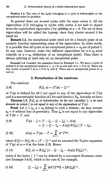
66 II. Perturbation theory in a finite-dimensional space
Problem 1.2. The sum of the Ah (x) belonging to a cycle is holomorphic at theexceptional point in question.
In general there are several cycles with the same center A. All theeigenvalues (1.7) belonging to cycles with center A are said to departfrom the unperturbed eigenvalue A by splitting at x = 0. The set of theseeigenvalues will be called the A -group, since they cluster around A forsmall Iki.
Remark 1.3. An exceptional point need not be a branch point of ananalytic function representing some of the eigenvalues. In other words,it is possible that all cycles at an exceptional point x = xo are of period 1.In any case, however, some two different eigenvalues for x + xo mustcoincide at x = xo (definition of an exceptional point). Thus there isalways splitting at (and only at) an exceptional point.
Example 1.4. Consider the examples listed in Example 1.1. We have a cycle ofperiod 2 at the exceptional points x = ± i in a) and also at x = 0 in d). There aretwo cycles of period I at x = 0 in b) and f). There are no exceptional points in c)and e).
3. Perturbation of the resolventThe resolvent
(1.8) R x) _ (T
of T (x) is defined for all C not equal to any of the eigenvalues of T (x)and is a meromorphic function of C for each fixed x E Do. Actually we have
Theorem 1.5. R (C, x) is holomorphic in the two variables C, x in eachdomain in which is not equal to any of the eigenvalues of T (x).
Proof. Let C _ Co, x = xo belong to such a domain; we may assumexo = 0 without loss of generality. Thus Co is not equal to any eigenvalueof T (O) = T, and
(1.9) T(x)-C=T-CO-(C-Co)+A(x)= [1 - (C-C0-A(x))R(Q] (T-C0)
00
(1.10) A(x)=T(x)-T= E x"TOln=1
where R R (C, 0) _ (T - and we assumed the Taylor expansionof T (m) at x = 0 in the form (1.2). Hence
(1.11) R (C, x) = R (CO) [1 - (. - CO - A (x)) R
exists if the factor [ ]-1 can be defined by a convergent Neumann series(see Example 1-4.5), which is the case if, for example,
00
(1.12) IC - Col + E IkIn IIT(")II < IIR(C0)II-1,n-1
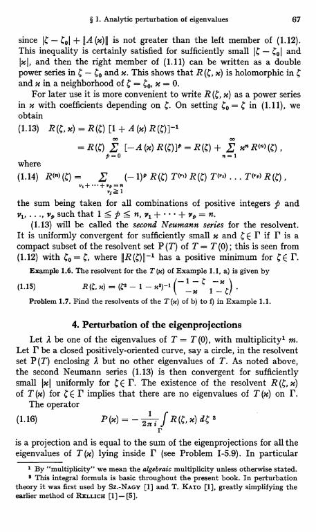
§ 1. Analytic perturbation of eigenvalues 67
since IC - oI + CIA (x)JJ is not greater than the left member of (1.12).This inequality is certainly satisfied for sufficiently small IC - Q andI4I4 and then the right member of (1.11) can be written as a doublepower series in C - Co and x. This shows that R x) is holomorphic in Cand x in a neighborhood of C _ Co, x = 0.
For later use it is more convenient to write R (C, x) as a power seriesin x with coefficients depending on . On setting Co = C in (1.11), weobtain(1.13) R (C, x) = R (C) [1 + A (x) R (C) ]-'
M 00
= R (C) E [- A (x) R (C) ]¢ = R (C) + E xn R(n) (C)P=0 n=]
where(1.14) R(n) (C) _ (-1)fl R (c') T(") R (C) T(V2) ... T &.') R (C)
yl+...+yy=nvJ I
the sum being taken for all combinations of positive integers p andvl, ..., v9 such that 1 S p S n, vl + + v, = n.
(1.13) will be called the second Neumann series for the resolvent.It is uniformly convergent for sufficiently small x and C E P if P is acompact subset of the resolvent set P (T) of T = T (0) ; this is seen from(1.12) with Co = C, where 11 R (C) 11 -' has a positive minimum for C E P.
Example 1.6. The resolvent for the T (x) of Example 1.1, a) is given by
(1.15) R 1
Problem 1.7. Find the resolvents of the T (x) of b) to f) in Example 1.1.
4. Perturbation of the eigenprojectionsLet A be one of the eigenvalues of T = T (0), with multiplicity' m.
Let r be a closed positively-oriented curve, say a circle, in the resolventset P (T) enclosing A but no other eigenvalues of T. As noted above,the second Neumann series (1.13) is then convergent for sufficientlysmall Ix I uniformly for C E P. The existence of the resolvent R (C, X)of T (x) for C E r implies that there are no eigenvalues of T (x) on P.
The operator
(1.16) P(X)=- 2 I R (C, x) d C 2r
is a projection and is equal to the sum of the eigenprojections for all theeigenvalues of T (x) lying inside I' (see Problem 1-5.9). In particular
By "multiplicity" we mean the algebraic multiplicity unless otherwise stated.This integral formula is basic throughout the present book. In perturbation
theory it was first used by Sz.-NAGY [1] and T. KATO [1], greatly simplifying theearlier method of RZLLicx [1]-[5].
68 II. Perturbation theory in a finite-dimensional space
P(0) = P coincides with the eigenprojection for the eigenvalue A of T.Integrating (1.13) term by term, we have
(1.17)
with
(1.18)
W
P(x)=P-1- 'E X- P(-)n=1
p(n) = - Zn a Rll (C) dCr
The series (1.17) is convergent for small Ix so that P(m) is holomorphicnear x = 0. It follows from Lemma I-4.10 that the range M (m) of P (M)is isomorphic with the (algebraic) eigenspace M = M (0) = PX of T forthe eigenvalue A. In particular we have
(1.19) dim P (x) = dim P = m.
Since (1.19) is true for all sufficiently small Ix I, it follows that theeigenvalues of T (x) lying inside r form exactly the A-group. For brevitywe call P (m) the total projection, and M (m) the total eigenspace, for theA-group.
If x = 0 is not an exceptional point, there is no splitting at x = 0of the eigenvalue A in question. In this case there is exactly one eigen-value A (x) of T (x) in the neighborhood of A, and P (x) is itself the eigen-projection for this eigenvalue A(x). (1.19) shows that the multiplicity ofA (x) is equal to m. Similar results hold when x = 0 is replaced by anyother non-exceptional point x = xo.
Now consider a simple subdomain D of the x-plane and the set (1.5)of the eigenvalues of T (x) for x E D, and let P,% (m) be the eigenprojectionfor the eigenvalue A7, (m), Is = 1, . . ., s. The result just proved shows thateach Ph (x) is holomorphic in D and that each A,, (x) has constant multi-plicity mh. Here it is essential that D is simple (contains no exceptionalpoint) ; in fact, P, 1(x0) is not even defined if, for example, Al (x0) = A2 (x0)which may happen if xo is exceptional.
Let M,, (x) = P1, (x) X be the (algebraic) eigenspace of T (x) for theeigenvalue A,(x). We have [see I-(5.34)]
(1.20)
dimMA(x)=mn, f mn=N, xED.j-1
The eigennilpotent DA(m) for the eigenvalue A7, (m) is also holomorphic forxED, for
(1.21) DA (x) _ (T (x) - A,r (x)) Ph (x)
by I-(5.26).
§ 1. Analytic perturbation of eigenvalues 69
5. Singularities of the eigenprojectionsLet us now consider the behavior of the eigenprojections Ph(x)
near an exceptional point, which we may again assume to be x = 0.As was shown above, each eigenvalue A of T splits in general into severaleigenvalues of T (m) for x + 0, but the corresponding total projection isholomorphic at x = 0 [see (1.17)]. Take again the small disk D nearx = 0 considered in par. 2; the eigenvalues Ah(x), the eigenprojectionsPh (x) and the eigennilpotents Dh (x) are defined and holomorphic forx E D as shown above. When D is moved around x = 0 and brought to theinitial position in the manner described in par. 2, each of the families{Ah (x)}, {Ph (x)} and {Dh (x)} is subjected to a permutation by the analyticcontinuation. This permutation must be identical for the three families,as is seen from the following consideration.
The resolvent R (C, x) of T (x) has the partial-fraction expression
Dh (x)` h-1J
(1.22) R' $( Pi. (x) Dh (x) . . . +.x) (x) + (C - h (x))$ ( - Rh (x))'"hh=1
[see I-(5.23)], where is assumed to be somewhere distant from thespectrum of T so that E P(T (x)) for all x considered. If Al (x), ..., A, (x)constitute a cycle (see par. 2) of eigenvalues, the permutation mentionedabove takes Ah (x) into Ah+1(x) for 1 s h : p - 1 and A. (x) into Al (x).But as R (C, x) should be unchanged by the analytic continuation underconsideration, the permutation must take Ph (x) into Ph+1(x) for1 S h S P - 1 and P. (x) into P1 (x) 1; the possibility that Ph (x) = Ph (x)for some h + k is excluded by the property Ph (x) Ph (x) = 84 h Ph (x).Similar results hold for the eigennilpotents Dh(x) by (1.21), except thatsome pair of the Dh (x) may coincide [in fact all Dh (x) can be zero).
We shall now show that Ph (x) and Dh (x) have at most algebraicsingularities. Since DA(m) is given by (1.21), it suffices to prove this forPh(x). To this end we first note that
(1.23) II Ph (x) II(I 2
a f R(1, x) d'II s eh (x) {mahx) IIR (C, x) II
rh (x)
where rh (x) is a circle enclosing Ah (x) but excluding all other Ah (x)and where ph (x) denotes the radius of rh (x). On the other hand, we seefrom I-(4.12) that
(1.24) IIR(C,x)II = (T (m) - C) -'II
s Y II T (x) - CIIN-1/ Idet (T (x) - ) I s
Y(IIT(x)II + IRI)N-1/17 IC- Ah(M )I""h'h -$I
1 This is due to the uniqueness of the partial-fraction representation of R (C, x)as a function of C. A similar argument was used in I-§ 5.4.
70 II. Perturbation theory in a finite-dimensional space
where y is a constant depending only on the norm employed. Hence
(1.25) II Ph(x)II s ICI)N_' 17IC-A,(x)Im"
Suppose that x -3 0, assuming again that x = 0 is an exceptionalpoint. Then we have to choose the circle Ph (x) smaller for smaller Ix Iin, order to ensure that it encloses Ah (x) but no other Ah (x), for the Ah (x)of the A-group will approach Ah (x) indefinitely. But we know that thedistances I Ah (x) - Ah (x) I between these eigenvalues tend to zero forx --* 0 at most with some definite fractional order of Ix I because allAh (x) have at most algebraic singularities at x = 0 [see (1.7)]. By choosingeh(m) = Ix I,, with an appropriate a> 0, we can therefore ensure that17I y - 2 (x) Imk y' IxIaN for C E Ph(x) with some constant y' > 0.Then we have(1.26) II P,(x)II < const. IxI-(N-1)a
This shows that, when Ph (x) is represented by a Laurent series in x'1Q,the principal part is finite.
These results may be summarized inTheorem 1.8. The eigenvalues Ah (x), the eigenprojections Ph (x) and the
eigennilpotents Dh (x) of T (x) are (branches of) analytic functions forx E Do with only algebraic singularities at some (but not necessarily all)exceptional points. Ah (x) and Ph (x) have all branch points in common(including the order of the branch points), which may or may not be branchpoints for Dh (x) . I/ in particular Ah (x) is single-valued near an exceptionalpoint x = xo (cycle of period 1), then Ph (x) and Dh (x) are also single-valued there.
6. Remarks and examplesAlthough the Ph (x) and Dh (x) have algebraic singularities as well
as the Ah (x), there are some important differences in their behavior at thesingular points. Roughly speaking, Ph (x) and DA (x) have strongersingularities than Ah (x).
We recall that these singular points are exceptional points, thoughthe converse is not true. As we have already noted, the Ah (x) are conti-nuous even at exceptional points and, therefore, have no poles. ButPh (x) and Dh (x) are in general undefined at exceptional points. Inparticular they may be single-valued and yet have a pole at an excep-tional point (see Example 1.12 below).
Even more remarkable is the following theorem'.Theorem 1.9. 1/ x = xo is a branch point of Ah (x) (and therefore also
of Ph (x)) of order p - 1 z 1, then Ph (x) has a pole there; that is, the
1 This theorem is due to BUTLER [1].
§ 1. Analytic perturbation of eigenvalues 71
Laurent expansion of Ph (x) in powers of (x - xo)1/Q necessarily containsnegative powers. In particular II Ph (x) II -> oo for x --> xo.
Proof. Suppose that this were not the case and let
Ph(n)=Ph+x1I Ps+..., h=1,...,p,
be the Laurent expansions of the Ph (x) belonging to the cycle underconsideration. Here we again assume for simplicity that xo = 0. When xis subjected to a revolution around x = 0, Ph (x) is changed into Ph+1 (x)for 1 S h <- p - 1 and Pfl (x) into P, (m). Hence we must have Ph+1 = Phfor 1 h 5 p - 1. On the other hand, the relation Ph (x) Ph+l (x) = 0for x-.0 gives Ph Ph+1 = 0, and the idempotent character of Ph(n)gives Pk = Ph. Hence Ph = P' = Ph Ph+1 = 0. But this contradicts thefact that dim Ph (x) X = mh > 0, which implies that II Ph (x) II z 1 (seeProblem 1-4.1).
As regards the order p - 1 of the branch point x = go for Ah (x) or,equivalently, the period p of the cycle {2 (u), . . ., A, (x)}, we have thefollowing result. An eigenvalue A of T with multiplicity m does not giverise to a branch point of order larger than m - 1. This is an obviousconsequence of the fact that such an eigenvalue can never split intomore than m eigenvalues [see (1.19)].
Theorem 1.10. Let X be a unitary space. Let xo E Do (possibly anexceptional point) and let there exist a sequence {xa} converging to xo suchthat T (x,,) is normal for n = 1, 2, ... . Then all the Ah (x) and Ph (x) areholomorphic at x = xo, and the Dh (x) = 0 identically.
Proof. We have II Ph (xn) II = 1 since T (x,,,) is normal [see I-(6.64)].Thus x;= xo is not a branch point for any Ah(x) by Theorem 1.9. Con-sequently the Ah (x) are holomorphic at x = xo. Then the Ph (x) are single-valued there and, since they cannot have a pole for the same reason asabove, they must be holomorphic. Then the Dh (x) vanish identically,since the holomorphic functions Dh (x) = (T (x) - Ah (x)) Ph (x) vanishat x = x,, --> xo.
Remark 1.11. In general the Ph (x) and Dh (x) are not defined at anexceptional point xo. But they can have a removable singularity at xoas in Theorem 1.10. In such a case Ph (xo) and Dh (xo) are well-defined,but they need not be the eigenprojection and eigennilpotent for theeigenvalue Ah (xo) of T (xo). If, for example, Al (xo) = A2 (xo) + Ah (xo),k z 3, then Pl (xo) + P2 (xo) (and not P1(xo)) is the eigenprojection forAl (xo). Again, the eigennilpotent for Ah (xo) need not vanish even ifDA(m) = 0, as is seen from Example 1.12 a), d), f) below.
Example 1.12. Consider the eigenprojections and eigennilpotents of T(x) forthe operators of Example I.I.
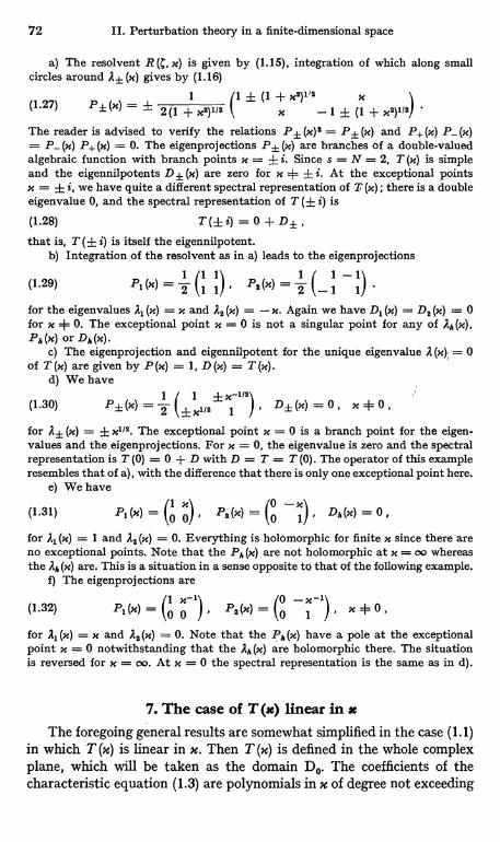
72 II. Perturbation theory in a finite-dimensional space
a) The resolvent R (C, x) is given by (1.15), integration of which along smallcircles around A± (x) gives by (1.16)
1
(1
± (1+ x2)1 2
x /(1.27) P± (x) = ± 2 (1 + x2)112 x - 1 ± (1 + x2)112
The reader is advised to verify the relations P± (x) 2 = P± (x) and P+ (x) P_ (x)= P-(%) P+(x) = 0. The eigenprojections P±(%) are branches of a double-valuedalgebraic function with branch points x = ± i. Since s = N = 2, T (x) is simpleand the eigennilpotents D ± (x) are zero for x 4 ± i. At the exceptional pointsx = ± i, we have quite a different spectral representation of T (x) ; there is a doubleeigenvalue 0, and the spectral representation of T (f i) is
(1.28) T(f i) = 0 -I- D±that is, T (± i) is itself the eigennilpotent.
b) Integration of the resolvent as in a) leads to the eigenprojections
(1.29) P1 (x) = 2 (1 1)' P2(x) = 2 (-1 1)
for the eigenvalues Al (x) = x and A2 (x) x. Again we have D1 (x) = D2 (x) = 0for x = 0. The exceptional point x = 0 is not a singular point for any of A,, (X),Pr, (x) or Dh (x).
c) The eigenprojection and eigennilpotent for the unique eigenvalue A(x)) = 0of T (x) are given by P (x) = 1, D (x) = T (x).
d) We have1 1 x-112\
(1.30) P± (x) =2 (+x1/s i f . D± (x) = 0, x + 0,
for A± (x) = t x112. The exceptional point x = 0 is a branch point for the eigen-values and the eigenprojections. For x = 0, the eigenvalue is zero and the spectralrepresentation is T (0) = 0 + D with D = T = T (0). The operator of this exampleresembles that of a), with the difference that there is only one exceptional point here.
e) We have
(1.31) P1(x) _ (0 0) ' P. (x) _ (0 1) . DH (x) = 0 .
for Al (x) = 1 and A2 (x) = 0. Everything is holomorphic for finite x since there areno exceptional points. Note that the Ph (x) are not holomorphic at x = oo whereasthe AA (x) are. This is a situation in a sense opposite to that of the following example.
f) The eigenprojections are
(1.32) P1(x) _ (0 0-1) ' P2(') = (01
x + 0 .
for Al (x) = x and A2 (x) = 0. Note that the Pa, (x) have a pole at the exceptionalpoint x = 0 notwithstanding that the A,,(x) are holomorphic there. The situationis reversed for x = oo. At x = 0 the spectral representation is the same as in d).
7. The case of T (x) linear in xThe foregoing general results are somewhat simplified in the case (1.1)
in which T (x) is linear in x. Then T (x) is defined in the whole complexplane, which will be taken as the domain Do. The coefficients of thecharacteristic equation (1.3) are polynomials in x of degree not exceeding
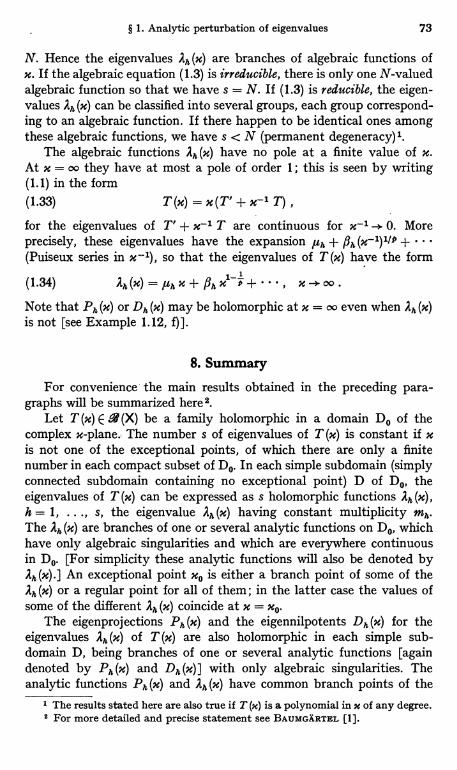
§ 1. Analytic perturbation of eigenvalues 73
N. Hence the eigenvalues Ah (x) are branches of algebraic functions ofx. If the algebraic equation (1.3) is irreducible, there is only one N-valuedalgebraic function so that we have s = N. If (1.3) is reducible, the eigen-values Ah (x) can be classified into several groups, each group correspond-ing to an algebraic function. If there happen to be identical ones amongthese algebraic functions, we have s < N (permanent degeneracy)'.
The algebraic functions Ah (x) have no pole at a finite value of x.At x = co they have at most a pole of order 1; this is seen by writing(1.1) in the form(1.33) T (m) = m (T' + x-1 T) ,
for the eigenvalues of T' + x-1 T are continuous for x-1-+ 0. Moreprecisely, these eigenvalues have the expansion ,uh + Ph (x-1) 1/11 + .. .(Puiseux series in x--1), so that the eigenvalues of T (m) have the form
(1.34)I_ 1
Ah (x) = 1Zh x flh x 9 +... , X__>00'
Note that Ph (x) or Dh (x) may be holomorphic at x = oo even when Ah (x)is not [see Example 1.12, f)].
8. Summary
For convenience the main results obtained in the preceding para-graphs will be summarized here2.
Let T (x) E 9 (X) be a family holomorphic in a domain Do of thecomplex x-plane. The number s of eigenvalues of T (m) is constant if xis not one of the exceptional points, of which there are only a finitenumber in each compact subset of Do. In each simple subdomain (simplyconnected subdomain containing no exceptional point) D of Do, theeigenvalues of T (m) can be expressed as s holomorphic functions Ah (x),h = 1, ..., s, the eigenvalue Ah (x) having constant multiplicity mh.The Ah (x) are branches of one or several analytic functions on Do, whichhave only algebraic singularities and which are everywhere continuousin Do. [For simplicity these analytic functions will also be denoted byAh(x).] An exceptional point xo is either a branch point of some of theAh (x) or a regular point for all of them ; in the latter case the values ofsome of the different Ah (x) coincide at x = xo.
The eigenprojections P,, (x) and the eigennilpotents D,, (x) for theeigenvalues Ah (x) of T (;c) are also holomorphic in each simple sub-domain D, being branches of one or several analytic functions [againdenoted by Ph (x) and Dh (x) ] with only algebraic singularities. Theanalytic functions Ph (x) and Ah (x) have common branch points of the
1 The results stated here are also true if T (x) is a polynomial in x of any degree.2 For more detailed and precise statement see BAUMGARTEL [1].
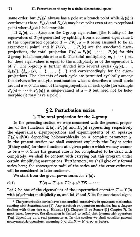
74 II. Perturbation theory in a finite-dimensional space
same order, but Ph (x) always has a pole at a branch point while Ah (x) iscontinuous there. Ph (x) and Dh (x) may have poles even at an exceptionalpoint where Ah (x) is holomorphic.
If A, (x), ..., A, (x) are the A-group eigenvalues [the totality of theeigenvalues of T (x) generated by splitting from a common eigenvalue Aof the unperturbed operator T = T (0), x = 0 being assumed to be anexceptional point] and if P, (x), . . ., P, (x) are the associated eigen-projections, the total projection P (x) = P, (x) + + P, (x) for thisA-group is holomorphic at x = 0. The total multiplicity m1 + + m,for these eigenvalues is equal to the multiplicity m of the eigenvalue Aof T. The A-group is further divided into several cycles {A, (m), ...,A9(x)}, {A,+1 (x), ...}, ..., {...} and correspondingly for the eigen-projections. The elements of each cycle are permuted cyclically amongthemselves after analytic continuation when x describes a small circlearound x = 0. The sum of the eigenprojections in each cycle [for exampleP1 (x) + + Pt, (x) ] is single-valued at x = 0 but need not be holo-morphic (it may have a pole).
§ 2. Perturbation series1. The total projection for the A-group
In the preceding section we were concerned with the general proper-ties of the functions Ah (x), Ph (x) and Dh (x) representing respectivelythe eigenvalues, eigenprojections and eigennilpotents of an operatorT (x) E .4 (X) depending holomorphically on a complex parameter M.In the present section we shall construct explicitly the Taylor series(if they exist) for these functions at a given point x which we may assumeto be x = 0. Since the general case is too complicated to be dealt withcompletely, we shall be content with carrying out this program undercertain simplifying assumptions. Furthermore, we shall give only formalseries here; the convergence radii of the series and the error estimateswill be considered in later sections'.
We start from the given power series for T (m):
(2.1) T(x)=T+xTM +x2T(2)+...Let A be one of the eigenvalues of the unperturbed operator T = T (0)with (algebraic) multiplicity m, and let P and D be the associated eigen-
1 The perturbation series have been studied extensively in quantum mechanics,starting with ScxxoDINGER [1]. Any textbook on quantum mechanics has a chapterdealing with them (see e. g. KEMBLE (1), Chapter 11 or ScxiFF (lU Chapter 7). Inmost cases, however, the discussion is limited to selfadjoint (symmetric) operatorsT (m) depending on a real parameter x. In this section we shall consider generalnonsymmetric operators, assuming 0 < dimX = N < oo as before.
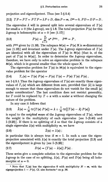
§ 2. Perturbation series 75
projection and eigennilpotent. Thus (see I-§ 5.4)
(2.2) TP=PT= PTP=AP+D, dime=m, Dm=O, PD=DP=D.The eigenvalue A will in general split into several eigenvalues of T (M)for small x $ 0 (the A-group), see § 1.8, The total projection P (x) for thisA-group is holomorphic at x = 0 [see (1.17) ]
(2.3) P (x) = Mn p(n) , p(O) = P ,n=0
with P(n) given by (1.18). The subspace M (x) = P (x) X is m-dimensional[see (1.19)] and invariant under T (x). The A-group eigenvalues of T (x)are identical with all the eigenvalues of T (x) in M (x) [that is, of thepart of T (m) in M (m)]. In order to determine the A-group eigenvalues,therefore, we have only to solve an eigenvalue problem in the subspaceM (x), which is in general smaller than the whole space X.
The eigenvalue problem for T (x) in M (x) is equivalent to the eigen-value problem for the operator
(2.4) T, (x) = T (m) P (m) = P (m) T (m) = P (m) T (m) P (m) ,
see I-§ 5.1. Thus the A-group eigenvalues of T (x) are exactly those eigen-values of T, (x) which are different from zero, provided that JAI is largeenough to ensure that these eigenvalues do not vanish for the small IxIunder consideration'. The last condition does not restrict generality,for T could be replaced by T + a with a scalar a without changing thenature of the problem.
In any case, it follows that
(2.5) 1 (x) = m tr(T (x) P (x)) = A + m tr((T (x) - A) P (x))
is equal to the weighted mean of the A-group eigenvalues of T (x), wherethe weight is the multiplicity of each eigenvalue [see I-(5.40) andI-(3.25)]. If there is no splitting of A so that the A-group consists of asingle eigenvalue A (x) with multiplicity m, we have
(2.6) - A (M) = A (x) ;
in particular this is always true if m = 1. In such a case the eigen-projection associated with A (x) is exactly the total projection (2.3) andthe eigennilpotent is given by [see I-(5.26)]
(2.7) D (m) = (T (x) - A (m)) P (m) .
These series give a complete solution to the eigenvalue problem for theA-group in the case of no splitting, A (m), P (m) and D (m) being all holo-morphic at x = 0.
1 Note that T,(x) has the eigenvalue 0 with multiplicity N - m, with theeigenprojection 1 - P(x). Cf. also footnote 1 on p. 36.
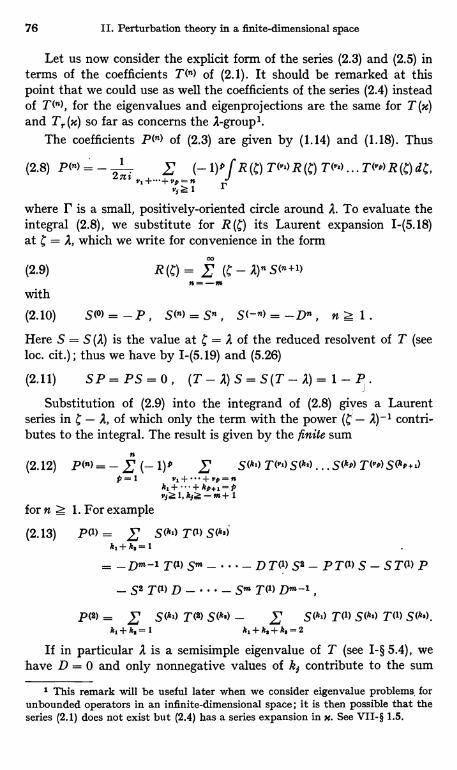
76 II. Perturbation theory in a finite-dimensional space
Let us now consider the explicit form of the series (2.3) and (2.5) interms of the coefficients T(n) of (2.1). It should be remarked at thispoint that we could use as well the coefficients of the series (2.4) insteadof T(n), for the eigenvalues and eigenprojections are the same for T (M)and T, (x) so far as concerns the 2-group'.
The coefficients P(n) of (2.3) are given by (1.14) and (1.18). Thus
(2.8) P(n) = - 22 a (-1)Q, f R T (y=) R T (y=) ... TOP) R (C) dC,VP n ry, 1
where IF is a small, positively-oriented circle around A. To evaluate theintegral (2.8), we substitute for R (C) its Laurent expansion I-(5.18)at C = A, which we write for convenience in the form
M
(2.9) R (C) = f (C - A)" S("+1)n=-mwith
(2.10) S(°) P , S(n) = Sn , S(-n) _ -Dn
Here S = S (2) is the value at C = 2 of the reduced resolvent of T (seeloc. cit.) ; thus we have by I-(5.19) and (5.26)
(2.11) SP=PS=0, (T - A) S = S (T - A) = 1-P.j
Substitution of (2.9) into the integrand of (2.8) gives a Laurentseries in C - A, of which only the term with the power (C - A)-' contri-butes to the integral. The result is given by the finite sum
(2.12) P(") _ - (- 1)p ' S(k,) P14 SO') ... SOP) T(vp) SOP +1)P-1 vi+...+vp=n
k,+...+kp+l=pvlZ1,kj -m+1
for n z 1. For example
(2.13) P(1) S(ki) T(1) S(k.)
=_Dm-1T(1)S"i_...-DT(1)S2-PT(')S-ST(')P
-S2T(1)D-..._SmT(t)Dm-1,
P(2) _ Ski) T(2) S(k.) _ S(k1) T(') S(k$) T(1) S(k.).k1 k, = 1 k, + k, + k. = 2
If in particular A is a semisimple eigenvalue of T (see I-§ 5.4), wehave D = 0 and only nonnegative values of kf contribute to the sum
1 This remark will be useful later when we consider eigenvalue problems, forunbounded operators in an infinite-dimensional space; it is then possible that theseries (2.1) does not exist but (2.4) has a series expansion in x. See VII-§ 1.5.
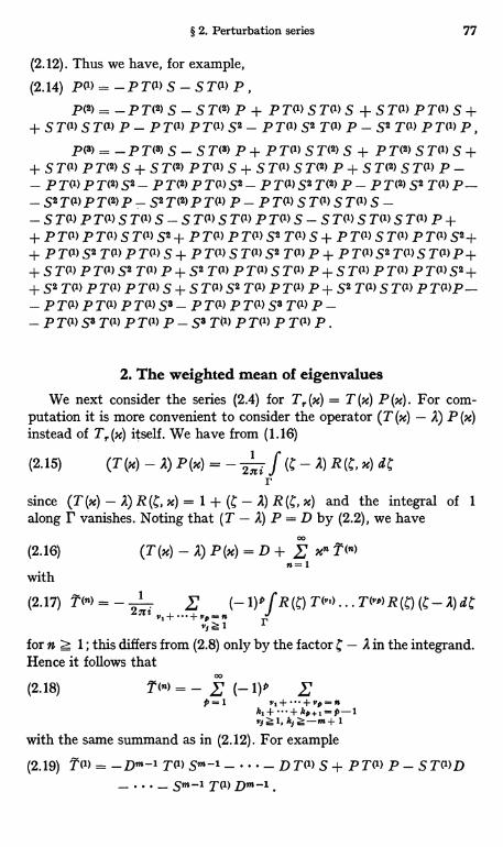
§ 2. Perturbation series 77
(2.12). Thus we have, for example,
(2.14) P('>=-PT('>S-ST(')P,P(2)=-PT(2) S-ST(2) P+ PT('>ST('>S+ST('>PT('>S+
+ST('>ST('>P-PT('>PT('>S2-PT(')S2T('>P-S2T(')PT('>P,PM = - P T(3) S - ST(8> P + PT(') S T(2) S + P T(2) ST(') S +
+ST('>PT(2) S+ST(2) PT('>S+ST('>ST(2) P+ST(2)ST('>P-- PT('>PT(2) S2-PT(2) PT('>S2-PT(')S2T(2) P-PT(2)S2T('>P--S2T('>PT(2) P-S2T(2)PT('>P-PT(')ST(')ST('>S--ST('>PT('>ST('>S-ST(')ST(')PT('>S-ST(')ST(')ST(')P++ PT(') PT('> ST(') S2 + PT('> PT(') S2 T(') S + PT(') ST('> PT('> S2++PT('>S2T('>PT('>S+PT('>ST(')S2T('>P+PT('>S2T('>ST(')P++ ST(') PT(') S2 T(') P + S2 T(') PT(') ST(') P+ST(') PT(') PT(')S2++S2T('>PT('>PT('>S+ST('>S2T(')PT('>P+S2T(')ST('>PT('>P-- PT('> PT('> PT(') Ss- PT('> PT('> S8 T(') P -- PT(') S8 T('> PT(') P - S3 T(') PT(') P T(') P.
2. The weighted mean of eigenvalues
We next consider the series (2.4) for T,.(x) = T (m) P (x) . For com-putation it is more convenient to consider the operator (T (x) - A) P (x)instead of T, (x) itself. We have from (1.16)
(2.15) (T(x)-A)P(x)=-2niJ (C -A)R(C,x)dCrsince (T (x) - A) R (C, x) = 1 + (C - A) R x) and the integral of 1
along r vanishes. Noting that (T - A) P = D by (2.2), we haveCo
(2.16) (T (x) - A) P (m) = D + E x" T (n>n=1
with/'(2.17) T(n) =- 2nivi+
1)9J)R(C)(C-A)dCVir
for n 1; this differs from (2.8) only by the factor C - A in the integrand.Hence it follows that
00
(2.18) T (n) E (- 1)p Epal vl+...+vy><Isk,+...+kp+j=p-1vj*a:l,kZ-m+l
with the same summand as in (2.12). For example
(2.19)-...-Sm_1T(')Dm-'.
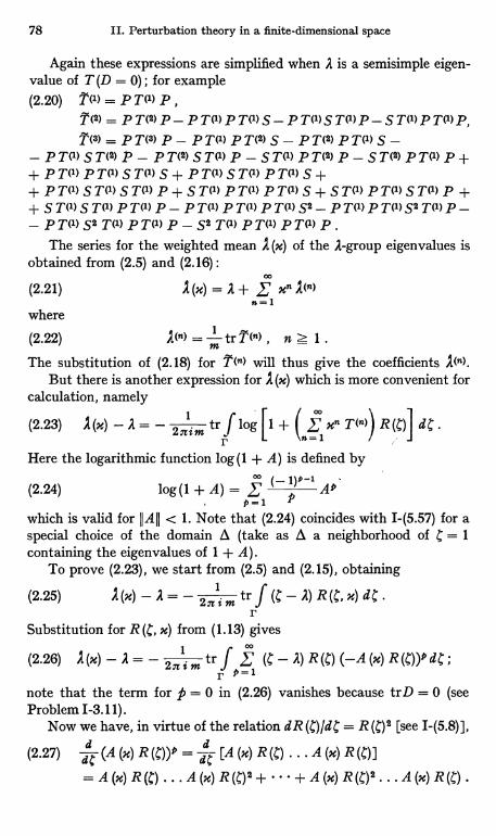
78 II. Perturbation theory in a finite-dimensional space
Again these expressions are simplified when A is a semisimple eigen-value of T (D = 0) ; for example(2.20) T(1) = PT(1) P ,
T(2) = PT(2)P-PT(1)PT(1)S-PT(1)ST(M)P-ST(1)PTM P,T(3) = PT(3) P - PT(1) P T(2) S - P T(2) PT(1) S -
- PT(1) S T(2) P - P T(2) ST(1) P - ST(1) P T(2) P - S T(2) PT(1) P ++ P TM P TM S TM S + P TM S TM P T(1) S ++ P TM S T(1) S T(1) P+ S TM P TM P TM S+ S TM P TM S TM P ++ S T(1) S T(1) P TM P - P TM P TM P T(1) S2 - P TM P TM S2 TM P -- PT(1) S2 T(1) PT(1) P - S2 T(1) PT(1) PT(1) P .
The series for the weighted mean A (x) of the A-group eigenvalues isobtained from (2.5) and (2.16) :
(2.21)
where
(2.22)
M
A (M) = A+ z xn )(n)n=1
1(n) = m trT(n) , n 1 .
The substitution of (2.18) for T(n) will thus give the coefficients 1(n).But there is another expression for A (x) which is more convenient for
calculation, namely
(2.23) trJ log 1 (,Z xn TO) I R(C) dC.2nim n 1rHere the logarithmic function log (I + A) is defined by
(2.24) log (1 + A) AApffi1
which is valid for IjAII < 1. Note that (2.24) coincides with I-(5.57) for aspecial choice of the domain i (take as A a neighborhood of C = 1containing the eigenvalues of 1 + A).
To prove (2.23), we start from (2.5) and (2.15), obtaining
(2.25) A(x)-A=-2nimtr (.l (C- A)R(C,x)dCr
Substitution for R(C, x) from (1.13) gives
(2.26) 1(x) - _ - 2 i m tr A) R (C) (-A (x) R (C))9 d Cr p-1
note that the term for $ = 0 in (2.26) vanishes because trD = 0 (see
Problem 1-3.11).Now we have, in virtue of the relation dR(C)/dg = R(C)2 [see I-(5.8)],
(2.27)dd (A (x) R (C))' = dg [A (x) R (C) ... A (x) R(C)]
= A (x) R (C) ... A (x) R (C) 2 + ... + A (x) R (b)2 ... A (x) R (C)
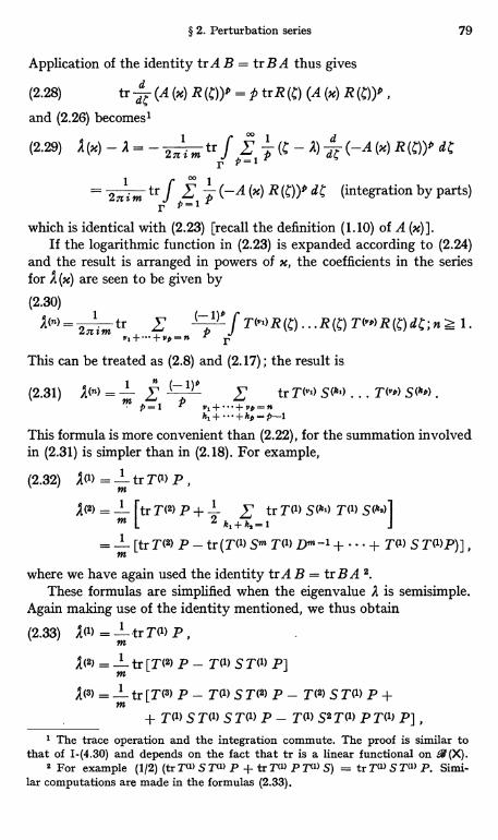
§ 2. Perturbation series 79
Application of the identity trA B = tr B A thus gives
(2.28) tr dg (A (x) R p trR (A (x) R (g))p ,
and (2.26) becomes'
(2.29) (x) - 2 = - 2 i m :r1p1+ (-A (x) R d
2,c i m tr f z' (-A (x) R (C))A d C (integration by parts)r p=1P
which is identical with (2.23) [recall the definition (1.10) of A (x)].If the logarithmic function in (2.23) is expanded according to (2.24)
and the result is arranged in powers of x, the coefficients in the seriesfor A (x) are seen to be given by
(2.30)1(n)=
27r1im tr (-1)D f R(C)dC;nz 1.
vl VDp r
This can be treated as (2.8) and (2.17) ; the result is
(2.31) 1(-) =.. (-1)n f trT(v=) SO') ... T(vo) S(kr)M ?=1 p vl+...+vD=n
k,+...+kP=¢-1This formula is more convenient than (2.22), for the summation involvedin (2.31) is simpler than in (2.18). For example,
(2.32) 1(') = m tr TM P ,
1(2) = m [tr T(2) P + 2 E tr T(1) S(ki) T(1) S(ke)Jk,+k,=1 f1
=
m
[tr T(2) P - tr (T(') Sm T(1) Dm-1 + ... + T(1) S T(1)P)]
where we have again used the identity trA B = tr BA 2.These formulas are simplified when the eigenvalue 2 is semisimple.
Again making use of the identity mentioned, we thus obtain
(2.33) I(') =1 tr T(') P ,m
A(2) = 1tr[T(2) P - T(') ST(') P]M
A(2> =1 tr [T(3) P - TM S T(2) P - T(2) S TM P +M
+ T(') ST(') ST(') P - T(1) S2 T(1) PT(1) P] ,1 The trace operation and the integration commute. The proof is similar to
that of I-(4.30) and depends on the fact that tr is a linear functional on . (X).2 For example (1/2) (tr Tu) S Tu) P + tr Tu) P T(2) S) = tr Tu) S T(l) P. Simi-
lar computations are made in the formulas (2.33).
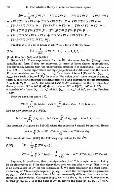
80 II. Perturbation theory in a finite-dimensional space
A14>= tr[Tl4)P-T(')STc3)P-T(2)ST(2)P-T(3)STM)P+ TM S TM S T(2) P + TM S T(2) S TM P + T(2) S TM S TM) P-- TM S2 TM PT(2) P - TM S2T(2) PTM1) P - T(2) S2 TM PTA) P-- TM S T(') S TM S TM P + TM S2 TM S TM P TM P ++ T(1) S TM S2 T(') P TM P + TM S2 TM P TM S TM P -- TM) S3 TM PTA) PTM1) P] .
Problem 2.1. If T (x) is linear in x (T") = 0 for n 2), we have
(2.34) 2"> = Mntr(T(1) Pc"-')) n=1,2,3 .... .
[hint: Compare (2.8) and (2.30).]Remark 2.2. These expressions for the AW take more familiar (though more
complicated) form if they are expressed in terms of bases chosen appropriately.For simplicity assume that the unperturbed operator T is diagonable. Let Ah, Ph,h = 1, 2, ..., be the eigenvalues and eigenprojections of T different from the ones A,P under consideration. Let {x1, ..., x",} be a basis of M = R (P) and let {xh', ...,zhh} be a basis of Mh = R(P5) for each h. The union of all these vectors z5 and zh1forms a basis of X consisting of eigenvectors of T and adapted to the decompositionX = M ® M, ® ... of X. The adjoint basis of X* is adapted to the correspondingdecomposition X* = M* ® M,* ® , where M* = R (P*), M; = R (Pl ), .. ,
it consists of a basis {e,...., em} of M*, {ell, ..., el,,,,} of M,*, etc. (see Problem1-3.19).
Now we have, for any u E X,
m mhPu= (u,ei)xt, Phu= E (u,ehi)xh9, h = 1,2,.. ,
j=1and for any operator A E -' (X),
m mhtrAP= E (Ax9,ej), trAPh= , (Axhj,ehi), h = 1,2.... .
j®1 j=1
The operator S is given by I-(5.32) where the subscript h should be omitted. Hence
Su=E(A,, -A)-1Phu=Eh h, j
Thus we obtain from (2.33) the following expressions for the A-):
(2.35) i(l) = m E (Tcu xi, e9) ,i
1(2) = 1 (T() xs, e,) - m E (Ah - A)-' (T(l) x j, eha) (T(1) xhq, er)Th
Suppose, in particular, that the eigenvalue A of T is simple: m = 1. Let 9,be an eigenvector of T for this eigenvalue; then we can take x, = 97. Then el = y7is an eigenvector of T* for the eigenvalue A. We shall renumber the other eigen-vectors xhj of T in a simple sequence qi,, q7a, ..., with the corresponding eigenvalues/tl, /t ... which are different from A but not necessarily different from one another(repeated eigenvalues). Correspondingly, we write the eh, in a simple sequence y79so that {gyp, tp,, y7 ...} is the basis of X* adjoint to the basis {q7, 971, 97%, ...} of X.
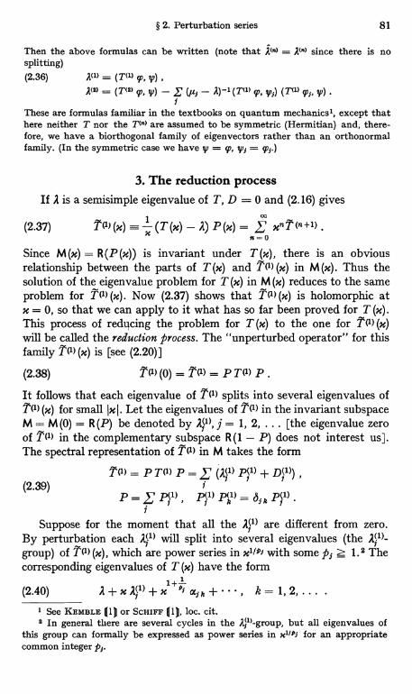
§ 2. Perturbation series 81
Then the above formulas can be written (note that A(") = A(") since there is nosplitting)(2.36) 2' = (Tcu q,, v')
Acs) = (T(2) 9) W) - E (u - A) -I (TO)p 'W7)
(T(vi
These are formulas familiar in the textbooks on quantum mechanics', except thathere neither T nor the T(") are assumed to be symmetric (Hermitian) and, there-fore, we have a biorthogonal family of eigenvectors rather than an orthonormalfamily. (In the symmetric case we have V = q), y,, = T;.)
3. The reduction processIf A is a semisimple eigenvalue of T, D = 0 and (2.16) gives
(2.37) T(l) (M) 1 (T (x) - A) P (m) = f xnT (n+1) .n=0
Since M (x) = R (P (x)) is invariant under T (x), there is an obviousrelationship between the parts of T (x) and T(I) (x) in M (x). Thus thesolution of the eigenvalue problem for T (x) in M (x) reduces to the sameproblem for T(1) (x). Now (2.37) shows that T(') (n) is holomorphic atx = 0, so that we can apply to it what has so far been proved for T (x).This process of reducing the problem for T (x) to the one for T(I) (x)will be called the reduction process. The "unperturbed operator" for thisfamily T(1) (x) is [see (2.20)]
(2.38) TM (0) = TM = P TM P .
It follows that each eigenvalue of T(1) splits into several eigenvalues ofT(1) (x) for small Ix 1. Let the eigenvalues of T(1) in the invariant subspaceM = M (0) = R (P) be denoted by A}1), j = 1, 2, ... [the eigenvalue zeroof T(1) in the complementary subspace R(1 - P) does not interest us].The spectral representation of T(1) in M takes the form
T(1) = PT(1) P = f (A2(1) P(1) + D(1)) ,(2.39) PPI1), P'1)k)=B;kP'1>
Suppose for the moment that all the AM are different from zero.By perturbation each A,(1) will split into several eigenvalues (thegroup) of T (l) (x), which are power series in x1/¢i with some ji; z 1.2 Thecorresponding eigenvalues of T (m) have the form
1+ 1(2.40) A--xA}1)-I x °' a;a- , k= 1,2,... .
1 See KEMBLE 11) or SCHIFF 11), loc. cit.2 In general there are several cycles in the AM-group, but all eigenvalues of
this group can formally be expressed as power series in c')ni for an appropriatecommon integer p9.
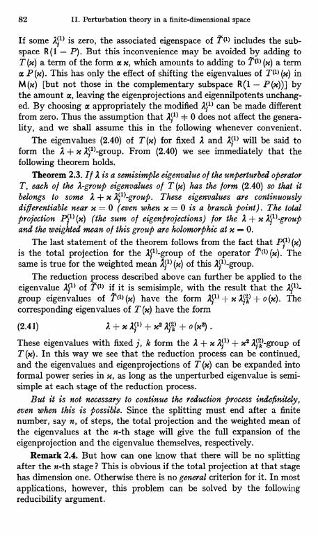
82 II. Perturbation theory in a finite-dimensional space
If some V) is zero, the associated eigenspace of TM includes the sub-space R(1 - P). But this inconvenience may be avoided by adding toT (x) a term of the form a x, which amounts to adding to TM (x) a terma P (x). This has only the effect of shifting the eigenvalues of TM (x) inM(x) [but not those in the complementary subspace R(1 - P(x))] bythe amount a, leaving the eigenprojections and eigennilpotents unchang-ed. By choosing a appropriately the modified can be made differentfrom zero. Thus the assumption that A(.1) * 0 does not affect the genera-lity, and we shall assume this in the following whenever convenient.
The eigenvalues (2.40) of T (m) for fixed A and AM will be said toform the A + x A'1)-group. From (2.40) we see immediately that thefollowing theorem holds.
Theorem 2.3. If A is a semisimple eigenvalue of the unperturbed operatorT, each of the A-group eigenvalues of T (x) has the form (2.40) so that itbelongs to some A + x 2(1)-group. These eigenvalues are continuouslydifferentiable near x = 0 (even when x = 0 is a branch point). The totalprojection Pi(t) (x) (the sum of eigenprojections) for the A + x groupand the weighted mean of this group are holomorphic at x = 0.
The last statement of the theorem follows from the fact that P(1) (x)is the total projection for the A}1)-group of the operator 7(1) (x). Thesame is true for the weighted mean (x) of this Al l>-group.
The reduction process described above can further be applied to theeigenvalue 2}1> of TM if it is semisimple, with the result that thegroup eigenvalues of TM (n) have the form A21> + X A} k) + o (m). Thecorresponding eigenvalues of T (x) have the form
(2.41) A+xA(1) +x2Ak +o(x2).
These eigenvalues with fixed j, k form the A + x A,(1) + x2 2w-group ofT (x). In this way we see that the reduction process can be continued,and the eigenvalues and eigenprojections of T (x) can be expanded intoformal power series in x, as long as the unperturbed eigenvalue is semi-simple at each stage of the reduction process.
But it is not necessary to continue the reduction process indefinitely,even when this is possible. Since the splitting must end after a finitenumber, say n, of steps, the total projection and the weighted mean ofthe eigenvalues at the n-th stage will give the full expansion of theeigenprojection and the eigenvalue themselves, respectively.
Remark 2.4. But how can one know that there will be no splittingafter the n-th stage? This is obvious if the total projection at that stagehas dimension one. Otherwise there is no general criterion for it. In mostapplications, however, this problem can be solved by the followingreducibility argument.
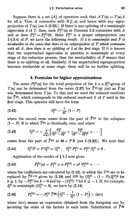
§ 2. Perturbation series 83
Suppose there is a set {A} of operators such that A T (x) = T (x) Afor all x. Then A commutes with R (C, x) and hence with any eigen-projection of T (x) [see I-(5.22)]. If there is any splitting of a semisixpleeigenvalue A of T, then, each P(1) (x) in Theorem 2.3 commutes with Aand so does P(1) = P1(1; (0). Since P(1) is a proper subprojection (seeI-§ 3.4) of P, we have the following result : If A is semisimple and P isirreducible in the sense that there is no subprojection o l P which commuteswith all A, then there is no splitting of A at the first stage. If it is knownthat the unperturbed eigenvalue in question is semisimple at everystage of the reduction process, then the irreducibility of P means thatthere is no splitting at all. Similarly, if the unperturbed eigenprojectionbecomes irreducible at some stage, there will be no further splitting.
4. Formulas for higher approximationsThe series Pi) (x) for the total projection of the A + x A')-group of
T (x) can be determined from the series (2.37) for TM (x) just as P (x)was determined from T (m). To this end we need the reduced resolventfor TM, which corresponds to the reduced resolvent S of T used in thefirst stage. This operator will have the form
(2.42)1
(1-P)S7)-,uwhere the second term comes from the part of TM in the subspace(1 - P) X in which T(1) is identically zero, and where
(2.43 S((1) = - rP"' D
k+fApp
comes from the part of 7) in M = PX [see I-(5.32)]. We note that
(2.44) S$1)P = PS7) = S7) S,c1) P7) = P7) S,c1) = 0 .
Application of the results of § 1.1 now gives
(2.45) (x) = P(1) + x x2 p$12) + ..
where the coefficients are calculated by (2.12), in which the TMv) are to bereplaced by 1("+x) given by (2.18) and S(k) by (1 - fork z 1, by - for k = 0 and by - (D7))-k fork 5 -1. If, for example,41) is semisimple (D,(1) = 0), we have by (2.14)
(2.46) P;11) P(1) 7(2) 4i, (1 - P)) + (inv)
where (inv) means an expression obtained from the foregoing one byinverting the order of the factors in each term. Substitution of
y1 (2)
84 II. Perturbation theory in a finite-dimensional space
from (2.20) gives
p(il) P7) T(2) S(1) - f P(1) T(i) P T(1) S + P(1) T(1) S T(1) S(1)+ (inv).
But we have P T(1) A(1) because 27) is asemisimple eigenvalue of P TM P. Hence
(2.47) p(11) _ -P7) T(2) S(1) - P7) T(1) S + PM T(1) ST(1) S7) + (inv).
Note that the final result does not contain 27) explicitly. Similarlycan be calculated, though the expression will be rather complicated.
The weighted mean A(1) (x) for the A,(1)-group eigenvalues of TM (m) isgiven by
q(2.48) (x) = A'1) + x 112) + x2 113) + ..
where the coefficients 2(") are obtained from (2.31) by replacing m,P, S, TO by m11) = dimP(1)X, (2.42) and T(v}1) respectively. Forexample, assuming that A7) is semisimple,
(2.49) 1(12) _ y1 trT(2) P(1)
I tr [T (2) Pi(1) - TM S TM P1(1>]In, ,
( l113) _ Jl) tr I T(3) P(1) - T(2) \S}l) - u (1 - P)l/
T(2). 1)]
_ )1) tr E TM Pi1) - TM S T(2) P7) - T(2) S TM P7) +
+ T(1) ST(') ST(1) Pj(1) - 27) T(1> S2 T(1) P7) -
- T(2) S7) T(2) P'1) + T(1) S T(1) S7) T(2)
T(2) S'1) T(?) S T(1) P(1) - T(1) S TM S7) T(1) S T(1) P'1)] .
Here we have again used the identity tr A B = tr B A and the relations(2.44) and (2.11). The weighted mean of the A + x A'1)-group eigenvaluesof T (x) is given by
(2.50) 1s (x) = A + x /lyl) (x)
= A + x A,(1).+ x2 1(12) + x3
If there is no splitting in the A + x 27)-group (that is, if this groupconsists of a single eigenvalue), (2.50) is exactly this eigenvalue. Inparticular this is the case if mil) = 1.
Remark 2.5. At first sight it might appear strange that the third order coefficienti$13) of (2.49) contains a term such as - (1/mi(l)) tr Tc2) Sf1) TX3) Ps1) which is quadraticin T3). But this does not involve any contradiction, as may be attested by the
§ 2. Perturbation series 85
following example. Let N = 2 and let
T = 0, T(l) = (01
Tcs) = (a0) ,
T(' = 0 for n Z 3.
The eigenvalues of T (x) are
)l
±X (I + a2 x2)1/2 = ± (x +2
as xs + ...) ,
in which the coefficient of the third order term is a2/2 and is indeed quadratic in or(that is, in T(2)).
5. A theorem of MoTZxnv-TAUSSKYAs an application of Theorem 2.3, we shall prove some theorems
due to MOTZKIN and TAUSSKY [1], [2].Theorem 2.6. Let the operator T (x) = T + xT' be diagonable for
every complex number x. Then all eigenvalues of T (x) are linear in x(that is, of the form Ah + x ah), and the associated eigenprojections areentire functions of x.
Proof. The eigenvalues Ah (x) of T (x) are branches of algebraic func-tions of x (see § 1.7). According to Theorem 2.3, on the other hand, theAh (x) are continuously differentiable in x at every (finite) value of M.Furthermore, we see from (1.34) that the dAh(x)/dx are bounded atx = no. It follows that these derivatives must be constant (this is a simpleconsequence of the maximum principle for analytic functions'). Thisproves that the Ah (x) are linear in x.
Since Ah (x) has the form Ah + x ah, the single eigenvalue A. (x)constitutes the Ah + x ah-group of T (x). Thus the eigenprojection Ph (x)associated with A,, (x) coincides with the total projection of this groupand is therefore holomorphic at x = 0 (see Theorem 2.3). The same istrue at every x since T (x) and A. (x) are linear in x. Thus Ph (x) is anentire function.
Ph(x) may have a pole at x = no [see Example 1.12, e)]. But if T'is also diagonable, Ph (x) must be holomorphic even at x = no becausethe eigenprojections of T (x) = x (T' + x-' T) coincide with those ofT' + x-' T, to which the above results apply at x = no. Hence eachPh (x) is holomorphic everywhere including x = oo and so must be aconstant by Liouville's theorem 2. It follows that T and T' have commoneigenprojections [namely Ph (0) = Ph (oo) ] and, since both are diagonable,they must commute. This gives
Theorem 2.7. If T' is also diagonable in Theorem 2.6, then T and T'commute.
1 Since ,u (x) = d A,, (x)/dx is continuous everywhere (including x = no), l, t (x) I
must take a maximum at some x = no (possibly no = oo). Hence /t (x) must beconstant by the maximum principle; see KNOPP 111, p. 84. [If no is a branch pointof order p - 1, apply the principle after the substitution (x - xo)1/P = x'; if no = no,apply it after the substitution x-1 = x'.]
2 See KNOPP 111, p. 112.
86 II. Perturbation theory in a finite-dimensional space
These theorems can be given a homogeneous form as follows.Theorem 2.8. Let A, BE 9 (X) be such that their linear combination
aA + 9B is diagonable for all ratios a: 9 (including oo) with Possibly asingle exception. Then all the eigenvalues of aA + 9B have the forma An + fly, with A,,, It, independent of a, P. If the said exception isexcluded, then A and B commute.
Remark 2.9. The above theorems are global in character in the sensethat the diagonability of T(x) (aA + 3B) for all finite x (all ratiosa : 9 with a single exception) is essential. The fact that T (x) is diagonablemerely for all x in some domain D of the x-plane does not even implythat the eigenvalues of T (x) are holomorphic in D, as is seen from thefollowing example.
Example 2.10. Let N = 3 and0 x 0
(2.51) T (x) = 0 0 x .
x 0 1
It is easy to see that T (x) is diagonable for all x with the exception of three valuessatisfying the equation xe = - 4/271. Thus T (x) is diagonable for all x in a certainneighborhood of x = 0. But the Puiseux series for the three eigenvalues of T (n)for small x have the forms(2.52) + x3/2 + .. 1 + xs + . .
two of which are not holomorphic at x = 0.Remark 2.11. Theorem 2.6 is not true in the case of infinite-dimensional spaces
without further restrictions. Consider the differential operatorda
T (x) d 9 + x$ + 2 x z
regarded as a linear operator in the Hilbert space L2 (- oo, + oo) (such differentialoperators will be dealt with in detail in later chapters). T (x) has the set of eigen-values A. (x) and the associated eigenfunctions op. (x, x) given by
n=0,1,2,...,op. (z, x) = exp I - 2 x2 - x x\I H. (x + x) ,
where the H. (x) are Hermite `polynomials. The eigenfunctions gl form a completeset in the sense that every function of L$ can be approximated with arbitraryprecision by a linear combination of the 97.. This is seen, for example, by noting thatthe set of functions of the form exp(- (x + Re x)1/2) x (polynomial in x) iscomplete and that multiplication of a function by exp (- i x Imx) is a unitaryoperator. Therefore, T'(x) may be regarded as diagonable for every finite x. Never-theless, the A. (x) are not linear in x.
6. The ranks of the coefficients of the perturbation seriesThe coefficients PO'") and T(n) of the series (2.3) and (2.16) have
characteristic properties with respect to their ranks. Namely
1 The characteristic equation for T (x) is I'e - I'$ - ms = 0. This cubic equationhas 3 distinct roots so that T (x) is diagonable, except when x = 0 or 0 ° 4/27.But T (0) is obviously diagonable (it has already a diagonal matrix).
§ 2. Perturbation series 87
(2.53) rank P(n> S (n + 1) m, rank T (n) S (n + 1) m ,
n = 1,2, .. .
This follows directly from the following lemma.Lemma 2.12. Let P (x) E R (X) and A (x) E 9 (X) depend on x holo-
morphically near x = 0 and let P (x) be a projection for all x. Let A (x) P (x)have the expansion
(2.54) A (x) P (x) = L' Mn B,n .
n=0Then we have
(2.55) rankBn S (n + 1) m, n = 0, 1, 2, ....where m = dim P (0). Similar results hold when the left member of (2.54)is replaced by P (x) A (x).
Proof. Let
(2.56) P (x) _ I Mn Pn .00
=0
The coefficients Pn satisfy recurrence formulas of the form
(2.57) Pn=POPn-I-QniPoPn-1-I-...-I-QnnPo, n=0,1,2,...,where Qnk is a certain polynomial in PO, Pi, ..., P,. (2.57) is proved byinduction. The identity P (x) 2 = P (x) implies that
(2.58) Pn=POPn+P1Pn-1+...+PnPO,
which proves (2.57) for n = 1. If (2.57) is assumed to hold with n replacedby 1, 2, . . ., n - 1, we have from (2.58)
Pn=POPn+Pi(POPn-1+Qn-1,1POPn-2+...+Qn-1,n-1P0)++P2(P0Pn-2+Qn-2,1POPn-s+...+Qn-2,n-2P0)+...+Pn PO
= PoPn+ P1 PoPn-1+ (P1Qn-1,1+ P2) PoPn-2+...+
+ (PI Q--I,--l + P2 Qn-2,n-2 + ... + Pn) PO,which is of the form (2.57). This completes the induction.
Now if A (x) .,f xn An is the expansion of A (x), we have from (2.54),(2.56) and (2.57)
(2.59) Bn=AOPn+A,Pn-1+...+AnPo=AO POPn+ (AOQni+A,) POPn-1+ (AOQn2+A,Qn-1,1+
+ A2) POPn-2+'''+ (AoQnn+A1Qn-1,n-1+"'+ An) Po.Thus Bn is the sum of n + 1 terms, each of which contains the factor P.and therefore has rank not exceeding rank PO (see Problem 1-3.4). Thisproves the required inequality (2.55). It is obvious how the aboveargument should be modified to prove the same results for P (x) A (x)instead of A (x) P (x).
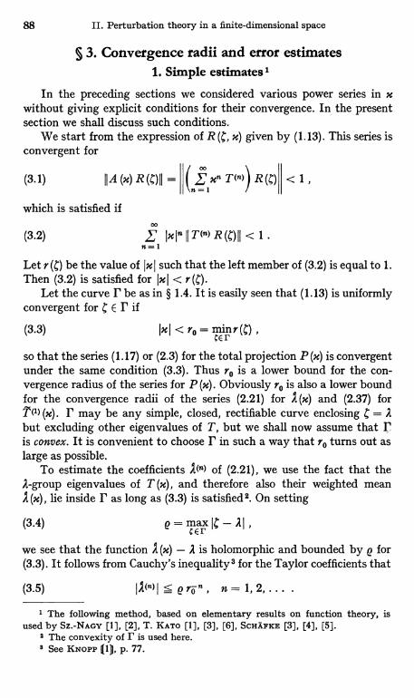
88 H. Perturbation theory in a finite-dimensional space
§ 3. Convergence radii and error estimates1. Simple estimates'
In the preceding sections we considered various power series in xwithout giving explicit conditions for their convergence. In the presentsection we shall discuss such conditions.
We start from the expression of R (C, x) given by (1.13). This series isconvergent for
(3.1) 11A (x) R (I) 11 =n=1
<1,
which is satisfied if00
(3.2) 'n=1
Let r (C) be the value of Ix I such that the left member of (3.2) is equal to 1.Then (3.2) is satisfied for I m I < r (C).
Let the curve P be as in § 1.4. It is easily seen that (1.13) is uniformlyconvergent for C E P if
(3.3) IHI < ro = mr
so that the series (1.17) or (2.3) for the total projection P (x) is convergentunder the same condition (3.3). Thus ro is a lower bound for the con-vergence radius of the series for P (x). Obviously ro is also a lower boundfor the convergence radii of the series (2.21) for A(x) and (2.37) forT11) (x). P may be any simple, closed, rectifiable curve enclosing C = Abut excluding other eigenvalues of T, but we shall now assume that I',is convex. It is convenient to choose r in such a way that ro turns out aslarge as possible.
To estimate the coefficients J (n) of (2.21), we use the fact that theA-group eigenvalues of T (x), and therefore also their weighted meanA (m), he inside r as long as (3.3) is satisfied 2. On setting
(3.4) marxIC - A
we see that the function A (x) - A is holomorphic and bounded by e for(3.3). It follows from Cauchy's inequality3 for the Taylor coefficients that
I1(n) I < err , n = 1, 2, ... .
1 The following method, based on elementary results on function theory, isused by Sz.-NAGY [1], [2], T. KATO [1], [3], [6], SCHXFKE [3], [4], [5].
9 The convexity of r is used here.8 See KNOPP (l), p. 77.
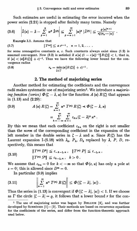
§ 3. Convergence radii and error estimates 89
Such estimates are useful in estimating the error incurred when thepower series (2.21) is stopped after finitely many terms. Namely
(3.6) (x) - ' - xp A p)P=1
yI IxI' 11(p) I sp=n+I ° (
I° I"I'xl)
Example 3.1. Assume that(3.7) II V011 < a c' 1, n = 1, 2, ... .
for some nonnegative constants a, c. Such constants always exist since (1.2) isassumed convergent. Now (3.2) is satisfied if a IxI (1 - c IxI)-hII R (C)II < 1, that is,
if IxI < c)-1. Thus we have the following lower bound for the con-vergence radius(3.8) r° = min(aIIR(C)II + c)-i.
CE r
2. The method of majorizing seriesAnother method for estimating the coefficients and the convergence
radii makes systematic use of majorizing series'. We introduce a majoriz-ing function (series) ch (C - A, x) for the function A (x) R (C) that appearsin (1.13) and (2.29) :
(3.9) A (x) R u xn T (n) R (C) 0 ( - A, x)n=1
o0
f I Ckn(b "- A)knk=-ao n=1
By this we mean that each coefficient ckn on the right is not smallerthan the norm of the corresponding coefficient in the expansion of theleft member in the double series in C - A and x. Since R (C) has theLaurent expansion I-(5.18) with Ak, Pk, Dh replaced by A, P, D, re-spectively, this means that
(3.10)II T(n) Dk!I < C-k-I,n , IIT(n) PII s c-I, n ,
II DO S9II S ck -l, n , k > 0 .
We assume that ckn = 0 for k < - m so that 0 (z, x) has only a pole atz = 0; this is allowed since Dm = 0.
In particular (3.9) implies00
(3.11) 11 Z xn T(n) R(I)II < O(IC, - Al, IxI)n=1
Thus the series in (1.13) is convergent if 0 (It - A I, Ix I) < 1. If we chooseas r the circle IC Al = e, it follows that a lower bound r for the con-
1 The use of majorizing series was begun by RELLICH [4], and was furtherdeveloped by SCHR6DER [1] - [3]. Their methods are based on recurrence equationsfor the coefficients of the series, and differ from the function-theoretic approachused below.

90 H. Perturbation theory in a finite-dimensional space
vergence radius of the series for P (x) as well as for ). (x) is given by thesmallest positive root of the equation
(3.12) O (Q, r) = 1.
It is convenient to choose a so as to make this root r as large as possible.Also 0 can be used to construct a majorizing series for R (x) - A.
Such a series is given by
(3.13) P (x) = 21 log(1 - 0 (g - A, x)) dC .
IC-Al = e
To see this we first note that, when the integrand in (2.29) is expandedinto a power-Laurent series in x and C - A using (2.9), only those termswhich contain at least one factor P or D contribute to the integral.Such terms are necessarily of rank S m and, therefore, their traces donot exceed m times their norms [see I-(5.42)]. Thus a majorizing seriesfor ) (x) - A is obtained if we drop the factor l1 m and the trace sign on theright of (2.29) and replace the coefficients of the expansion of the inte-grand by their norms. Since this majorizing function is in turn majorizedby (3.13), the latter is seen to majorize ) (x) - A.
As is well known in function theory, (3.13) is equal to the sum of thezeros minus the sum of the poles of the function 1 - 0 (z, x) containedin the interior of the circle Iz I = e I. But the only pole of this function isz = 0 and does not contribute to the sum mentioned. In this way wehave obtained
Theorem 3.2. A majorizing series for A (x) - A is given by (the Taylorseries representing) the sum of the zeros of the function 1 - 0 (z, x) (as afunction of z) in the neighborhood of z = 0 when x -- 0, multiple zeros beingcounted repeatedly. This majorizing series, and a fortiori the series forP (x) and A (x), converge for Ix I < r, where r is the smallest positive root of(3.12); here 0 is arbitrary as long as the circle I - Al = P encloses noeigenvalues of T other than A.
Example 3.3. Consider the special case in which T"> = 0 for n Z 2 and A is asemisimple eigenvalue of T (D = 0). From (3.10) we see that we may take c-1,1= II T(" PIi, ckl Z II TI) Sk}1II, k Z 0, all other ck being zero. For the choice ofck1, we note that Sk+l = S(S - a P)k for any a because SP = PS = 0. Thuswe can take ck1 = II T(" SII II S - a PII k and obtain
(3.14) (P +1 4 s x )
as a majorizing series, where
(3.15) p=IIT'1'PII, 4=IIT1'Sp, s=IIS - aPII for any a.
1 See KNoPP (1), p. 134; note that f log/ (z) dz f f'(z),f(z)-1 zdz byintegration by parts.
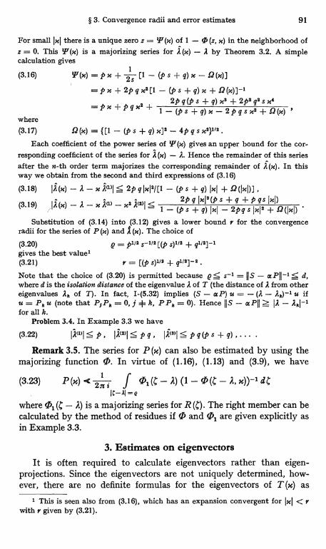
§ 3. Convergence radii and error estimates 91
For small lxl there is a unique zero z ='P(x) of 1 -' (z, x) in the neighborhood ofz = 0. This 1P (x) is a majorizing series for A(x) - A by Theorem 3.2. A simplecalculation gives
(3.16)1
'I'(x) = p x + 2s [1 - (P s + q) x - D(x)]
=px+2pgx2[l - (ps+q)x+Q(x)]-l
=px+pgx2 -f- 2pq(Ps +q)x1 +2p2g2sx`1 - (ps +q)x-2pgsx2+Q(x) '
where(3.17) S2(x) _ {[1 - (p s + q) x]2 - 4p q s x2}1'2 .
Each coefficient of the power series of PP (x) gives an upper bound for the cor-responding coefficient of the series for A (x) - A. Hence the remainder of this seriesafter the n-th order term majorizes the corresponding remainder of i(n). In thisway we obtain from the second and third expressions of (3.16)
(3.18) lA (x) - A - x Au)l 5 2p q IxI2/[1 - (1's + q) Ixi + D (l xl )]
193 2 2(2) S 2p q Ix12 (P s + q + p qs 1-1)AMAA( . ) - x- x(x) -1 1 - (p s + q) I xl - 2pq s 1x12 + .(lxl)Substitution of (3.14) into (3.12) gives a lower bound r for the convergence
radii for the series of P (x) and Ar (x). The choice of
(3.20)gives the best value'
(3.21)
e = pl/2 s-112 [(p S)112 + ql/2]-1
r = [(p s)'12 + g112]-2
Note that the choice of (3.20) is permitted because o;5 s-' = 11 S - a Pll -' < d,where d is the isolation distance of the eigenvalue A of T (the distance of A from othereigenvalues Ak of T). In fact, I-(5.32) implies (S - aP) u = - (A - Ak)-' u ifu = Pk u (note that PIP5 , = 0, j + k, PPk = 0). Hence JIS - aP11 Z lA - Akl-1
for all k.Problem 3.4. In Example 3.3 we have
(3.22) 11a/l S p l;l,c2el S p g i' >l S p q (p s + q) .... .
Remark 3.5. The series for P (x) can also be estimated by using themajorizing function 0. In virtue of (1.16), (1.13) and (3.9), we have
-CI
(3.23) P (x) 2a i f 01(C - A) (1 - O (C - A, x))-1 dCIC-11=e
where fil (C - A) is a maj orizing series for R (c). The right member can becalculated by the method of residues if 0 and 01 are given explicitly asin Example 3.3.
3. Estimates on eigenvectorsIt is often required to calculate eigenvectors rather than eigen-
projections. Since the eigenvectors are not uniquely determined, how-ever, there are no definite formulas for the eigenvectors of T (m) as
1 This is seen also from (3.16), which has an expansion convergent for ixl < rwith r given by (3.21).
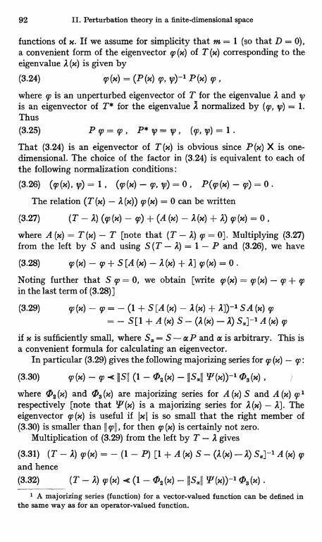
92 II. Perturbation theory in a finite-dimensional space
functions of x. If we assume for simplicity that m = 1 (so that D = 0),a convenient form of the eigenvector (p (x) of T (x) corresponding to theeigenvalue A (x) is given by
(3.24) 99 (x) = (P (x) 99, vi)-1 P (x) 99
where 9, is an unperturbed eigenvector of T for the eigenvalue A and ,
is an eigenvector of T* for the eigenvalue A normalized by (99, y,) = 1.Thus(3.25) P9,=99, P*V =y,, (9,,P)=1.That (3.24) is an eigenvector of T (x) is obvious since P (x) X is one-dimensional. The choice of the factor in (3.24) is equivalent to each ofthe following normalization conditions:
(3.26) (w (x), V) =1, (99 (x) - 99, ip) = 0 , P(99 (x) - 99) = 0 .
The relation (T (x) - A (x)) 99 (x) = 0 can be written
(3.27) (T - A) (99 (x) - 99) + (A (x) - A (x) + A) 99 (x) = 0
where A (x) = T (x) - T [note that (T - A) 99 = 0]. Multiplying (3.27)from the left by S and using S (T - A) = 1 - P and (3.26), we have
(3.28) 99 (x) - 99 + S [A (x) - A (x) + A] 99 (x) = 0 .
Noting further that S 99 = 0, we obtain [write 9' (x) = q (x) - 9' + 99in the last term of (3.28)]
(3.29) 97 (x) - 97 (1 + S [A (x) - A (x) + A])-1 S A (x) 92
S [ 1 + A (x) S - (A (x) - A) S]-1 A (x) 92
if x is sufficiently small, where Sa = S - a P and a is arbitrary. This isa convenient formula for calculating an eigenvector.
In particular (3.29) gives the following majorizing series for 92 (x) - ip:
(3.30) 9' (x) - 99 _< IISII (1 - '2(x) - IIS«p fi(x))-1 03(x) 1
where 02 (x) and 03 (x) are majorizing series for A (x) S and A (x) 97 1respectively [note that Y¶(x) is a majorizing series for A(x) - A]. Theeigenvector 99(m) is useful if In I is so small that the right member of(3.30) is smaller than 119911, for then 97 (x) is certainly not zero.
Multiplication of (3.29) from the left by T - A gives
(3.31) (T - A) p (x) (1 - P) [1 + A (x) S - (A (x) -A) Sa]-1 A (x) 97
and hence(3.32) (T - A) 99(x) _c (1 - 02(x) - JISa11 fi(x))-1 (3(x)
1 A majorizing series (function) for a vector-valued function can be defined inthe same way as for an operator-valued function.
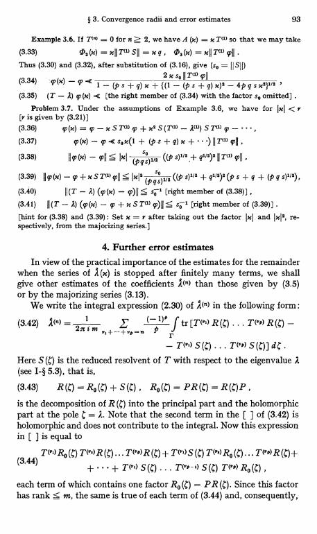
§ 3. Convergence radii and error estimates 93
Example 3.6. If T") = 0 for n Z 2, we have A (x) = x T1) so that we may take
(3.33) 02(x) = x II T(1) S = x q , 0, (x) = x II 711) cII
Thus (3.30) and (3.32), after substitution of (3.16), give (so = IISII)
0 11 T11) 9,11(3.34) (x) -
2 x s1- (p s+q)x+{(1-(ps+q)x)a-4pgsxiff_
(3.35) (T - A) 4' (x) -c [the right member of (3.34) with the factor so omitted] .
Problem 3.7. Under the assumptions of Example 3.6, we have for[r is given by (3.21)]
IxI <r
(3.36) (p(x)=q'-xST1)9'+%IS(T(1)-Aa))ST)9,-...(3.37) 9,(x) - op .C sox(1 + (p s + q) x + ...) II T1) q,H ,
3 38 s 112 112 2 T1( . ) ,+ g )IIm(x) - c'II 9'IIIIIxI(pgs)112
((p s)
3 39 a
sohIz 2 112ST1) S 1"2( . ) + g ) ),(p s + q + (p 9 s)II9'(x) - +x us ((p s)9'II Ixl
(p q s)(3.40) II (T - A) (q) (x) - p) II S so 1 [right member of (3.38)],
(3.41) II(T - A) (qq(x) - c + x ST1) q')II S so-' [right member of (3.39)].
[hint for (3.38) and (3.39) : Set x = r after taking out the factor IxI and Ixla, re-spectively, from the majorizing series.]
4. Further error estimatesIn view of the practical importance of the estimates for the remainder
when the series of A (m) is stopped after finitely many terms, we shallgive other estimates of the coefficients I(n) than those given by (3.5)or by the majorizing series (3.13).
We write the integral expression (2.30) of I('") in the following form:
(3.42) 1(n)= 2nim f (-1)D
f tr[T(y')R(C)...T(ID)R(C)-y1+...+yD=n p r
- T(") S(g) ... PIP) S(C)] dC
Here S (C) is the reduced resolvent of T with respect to the eigenvalue A(see I-§ 5.3), that is,
(3.43) R(C) = Ro (C) + S (C) , R0() = PR (C) = R (C) P ,
is the decomposition of R (C) into the principal part and the holomorphicpart at the pole C = A. Note that the second term in the [ ] of (3.42) isholomorphic and does not contribute to the integral. Now this expressionin [ ] is equal to
(3.44)T(14 Ro (C) T (I-) R (C)... T(11)R(C) + T (y1) S (C) T (y') Ro (r) ... T (vP) R M+
+ ... + T(v,) S(g) ... T(yr-1) S(C) T(&P) Ro(C) ,
each term of which contains one factor Ro (C) = PR (c). Since this factorhas ranks m, the same is true of each term of (3.44) and, consequently,
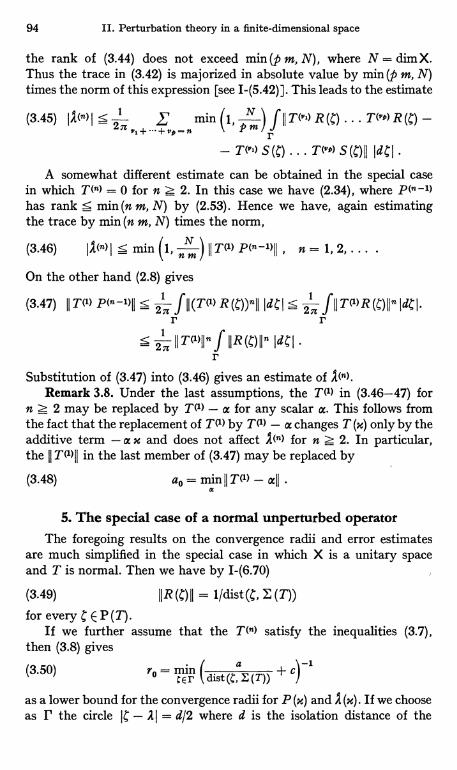
94 II. Perturbation theory in a finite-dimensional space
the rank of (3.44) does not exceed min (p m, N), where N = dim X.Thus the trace in (3.42) is majorized in absolute value by min (p m, N)times the norm of this expression [see I-(5.42)]. This leads to the estimate
(3.45) IA(n) 15 2 Vj --4' min 1,
pm) f h D "O R (C) ... T(la) R
r- T("") S(C) ... T(""P) S(C)II IdCI
A somewhat different estimate can be obtained in the special casein which T(n) = 0 for n __> 2. In this case we have (2.34), where P(n-1)has rank S min (n m, N) by (2.53). Hence we have, again estimatingthe trace by min (n m, N) times the norm,
(3.46) I1(0I S min \1, nm) I I T(1) P(n-1)II , n = 1, 2, ... .
On the other hand (2.8) gives
(3.47) II T(1) P(--1)11 < f 11 (T(1) R IdCI S 2ac f II T(1)R IdCjr r
S2 IIT(1)IInf IIR(C)IIlIdCIr
Substitution of (3.47) into (3.46) gives an estimate of Il(n).Remark 3.8. Under the last assumptions, the T(1) in (3.46-47) for
n 2 may be replaced by T(1) - a for any scalar a. This follows fromthe fact that the replacement of TM by TM - a changes T (x) only by theadditive term - a x and does not affect AN for n z 2. In particular,the II T(1)II in the last member of (3.47) may be replaced by
(3.48) ao = min II T(1) - aIIa
5. The special case of a normal unperturbed operatorThe foregoing results on the convergence radii and error estimates
are much simplified in the special case in which X is a unitary spaceand T is normal. Then we have by I-(6.70)
(3.49) 11R II = 1/dist(C, E (T))
for every C E P (T).If we further assume that the T(n) satisfy the inequalities (3.7),
then (3.8) gives
(3.50) ro = mr (diet(g,aE (z))
+c
1
as a lower bound for the convergence radii for P (x) and A (m). If we chooseas r the circle IC - AI = d/2 where d is the isolation distance of the
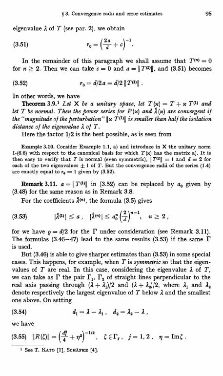
§ 3. Convergence radii and error estimates 95
eigenvalue A of T (see par. 2), we obtain
(3.51) ro = (da -I- c)-1.
In the remainder of this paragraph we shall assume that T (n) = 0for n z 2. Then we can take c = 0 and a = II T MII , and (3.51) becomes
(3.52) ro = d/2a = d/2 II T(1)II
In other words, we haveTheorem 3.9.1 Let X be a unitary space, let T (x) = T + x Tel) and
let T be normal. Then the power series for P (x) and A (x) are convergent ifthe "magnitude of the perturbation" 11m T(l)II is smaller than half the isolationdistance of the eigenvalue A of T.
Here the factor 1/2 is the best possible, as is seen from
Example 3.10. Consider Example 1.1, a) and introduce in X the unitary normI-(6.6) with respect to the canonical basis for which T (x) has the matrix a). It isthen easy to verify that T is normal (even symmetric), 11 VD11 = I and d = 2 foreach of the two eigenvalues ± 1 of T. But the convergence radii of the series (1.4)are exactly equal to ro = 1 given by (3.52).
Remark 3.11. a = II T (')II in (3.52) can be replaced by ao given by(3.48) for the same reason as in Remark 3.8.
For the coefficients )fin), the formula (3.5) gives
2 n-1(3.53) I,AJAM I S a, 110) I S
a0
(d , n z 2,
for we have p = d/2 for the P under consideration (see Remark 3.11).The formulas (3.46-47) lead to the same results (3.53) if the same Pis used.
But (3.46) is able to give sharper estimates than (3.53) in some specialcases. This happens, for example, when T is symmetric so that the eigen-values of T are real. In this case, considering the eigenvalue A of T,we can take as r the pair rl, r2 of straight lines perpendicular to thereal axis passing through (A + Al)/2 and (A + A2)/2, where Al and A2denote respectively the largest eigenvalue of T below A and the smallestone above. On setting
(3.54) d1=A-Al, d2=A2-A,we have
(3.55) IIR(C)II=(4 -t-rl2)-1hI2, CEI',s, j=1,2, rl=ImC.
1 See T. KATO [1], SCHAFKE [4].
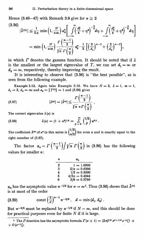
96 II. Perturbation theory in a finite-dimensional space
Hence (3.46-47) with Remark 3.8 give for n Z 2
(3.56)
2
_ n _ n(' /'(< --!-min (1, m)ao J 41 ad's+ f(4 +n2) add]
=min (1' m) 'r(n2'n) ae 2 {(di)n-1+ (da)n-1]Y r(2)in which I' denotes the gamma function. It should be noted that if Ais the smallest or the largest eigenvalue of T, we can set d1 = oo ord2 = oo, respectively, thereby improving the result.
It is interesting to observe that (3.56) is "the best possible", as isseen from the following example.
Example 3.12. Again take Example 3.10. We have N = 2, A = 1, m = 1,dl = 2, d2 = oo and ao = 11 VD11 = 1 and (3.56) gives
r(n-1)(3.57) IAcn>I = Acn <
2
yn nr(2)The correct eigenvalue A (x) is
(3.58) A(x) _ (1 + x2)1/2 = Z (1/2) n2np=0 P
The coefficient A(n) of xn in this series is (1n/2) for even n and is exactly equal to the
right member of (3.57).
The factor an = T (n2
) I T (2) in (3.56) has the followingvalues for smaller n :
to an
2 1 = 1.00003 2/n = 0.63664 1/2 = 0.50005 4/3n = 0.42446 3/8 = 0.3750
an has the asymptotic value n-1/2 for n -+ col. Thus (3.56) shows that A(n)is at most of the order
2 n-1(3.59) const d n-3/2, d = min (d1, d2) .
But n-3/2 must be replaced by n-1/2 if N = oo, and this should be donefor practical purposes even for finite N if it is large.
1 The r-function has the asymptotic formula r (x + 1)= (2n)1/2 xx } 1/2 e-(1 ++ 0 (z-1)).
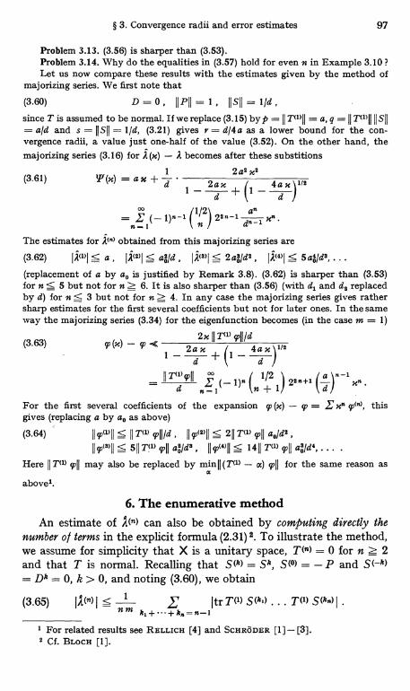
§ 3. Convergence radii and error estimates 97
Problem 3.13. (3.56) is sharper than (3.53).Problem 3.14. Why do the equalities in (3.57) hold for even n in Example 3.10 ?Let us now compare these results with the estimates given by the method of
majorizing series. We first note that
(3.60) D = 0, IIpII=1, IISII=l/d,since T is assumed to be normal. If we replace (3.15) byp = II T'>II = a, q = II T11II II SII= ald and s = 11 S11 = 1/d, (3.21) gives r = d/4a as a lower bound for the con-vergence radii, a value just one-half of the value (3.52). On the other hand, themajorizing series (3.16) for A(x) - A becomes after these substitions
(3.6,1) Vf(x) =ax+ d .2a2 x2
tax+4a \2I2d
1/2 dxax-1
xn._ (- 1)1-1 ( n ) 22x-1n=1The estimates for i(l) obtained from this majorizing series are
(3.62) 1;1n>1 < a , 12(2>I S ag/d , IAcs>I S 2ag/d2 , IAc4>I S 5a$ /d3, .. .(replacement of a by ao is justified by Remark 3.8). (3.62) is sharper than (3.53)for n G 5 but not for n Z 6. It is also sharper than (3.56) (with d, and d2 replacedby d) for n:< 3 but not for n > 4. In any case the majorizing series gives rathersharp estimates for the first several coefficients but not for later ones. In the sameway the majorizing series (3.34) for the eigenfunction becomes (in the case m = 1)
(3.63) (x) - 9' -C2x 11 211> y,II/d
1 - six +\1
- 4x`12
v
/II
n-1
d
n / 1 22n+1 xnd
1)n (n + 11
For the first several coefficients of the expansion 97 (x) - q' = E xx 971n>, thisgives (replacing a by ao as above)
(3.64) I197u>II S 11711) 97II/d , 1197(2)11 S 211 T'> 9,11 colds
119,(111115 511 Tu> 9,11 ao/ds , 119,(1111 S 1411 Ta> 9>II ao/d4, ... .
Here 11TH) 9711 may also be replaced by min11(T(') - a) 9711 for the same reason as
above'.
6. The enumerative methodAn estimate of J(n) can also be obtained by computing directly the
number of terms in the explicit formula (2.31) 2. To illustrate the method,we assume for simplicity that X is a unitary space, TM = 0 for n z 2and that T is normal. Recalling that S() = Sk, S(°) P and S(-k)= Dk = 0, k > 0, and noting (3.60), we obtain
(3.65) I1(n) 15 1 ! Itr T(I) SO-) ... TM S00I .nm kid ... kn.n-I
1 For related results see RELLICH [4] and SCHRODER [1]- [3].2 Cf. BLOCH [1].
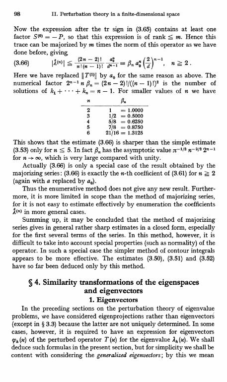
98 II. Perturbation theory in a finite-dimensional space
Now the expression after the tr sign in (3.65) contains at least onefactor S(°) = - P, so that this expression is of rank f,- in. Hence thistrace can be majorized by m times the norm of this operator as we havedone before, giving
(2n - 2)! a" 2 -1(3.66) 11(")1 s n!(n-1)! \a/ , n2.Here we have replaced 11 T(1)IJ by a° for the same reason as above. Thenumerical factor 2' ' n fi" _ (2n - 2) !/((n - 1) 1)2 is the number ofsolutions of k1 + + k, = n - 1. For smaller values of n we have
nfl.
2 1 = 1.00003 1/2 = 0.50004 5/8 = 0.62505 7/8 = 0.87506 21/16 = 1.3125
This shows that the estimate (3.66) is sharper than the simple estimate(3.53) only for n < 5. In fact j" has the asymptotic value -1/2 n-3/2 2"-1
for n -* oo, which is very large compared with unity.Actually (3.66) is only a special case of the result obtained by the
majorizing series: (3.66) is exactly the n-th coefficient of (3.61) for n z 2(again with a replaced by a°).
Thus the enumerative method does not give any new result. Further-more, it is more limited in scope than the method of majorizing series,for it is not easy to estimate effectively by enumeration the coefficientsIN in more general cases.
Summing up, it may be concluded that the method of majorizingseries gives in general rather sharp estimates in a closed form, especiallyfor the first several terms of the series. In this method, however, it isdifficult to take into account special properties (such as normality) of theoperator. In such a special case the simpler method of contour integralsappears to be more effective. The estimates (3.50), (3.51) and (3.52)have so far been deduced only by this method.
§ 4. Similarity transformations of the eigenspacesand eigenvectors
1. EigenvectorsIn the preceding sections on the perturbation theory of eigenvalue
problems, we have considered eigenprojections rather than eigenvectors(except in § 3.3) because the latter are not uniquely determined. In somecases, however, it is required to have an expression for eigenvectorsq,, (x) of the perturbed operator T (m) for the eigenvalue Ah (x). We shalldeduce such formulas in the present section, but for simplicity we shall becontent with considering the generalized eigenvectors; by this we mean
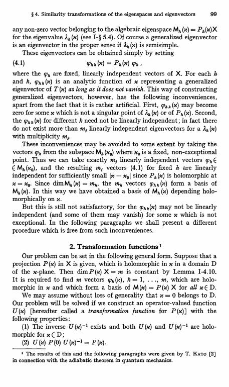
§ 4. Similarity transformations of the eigenspaces and eigenvectors 99
any non-zero vector belonging to the algebraic eigenspace Mh (x) = Ph(x)Xfor the eigenvalue 1h (x) (see I-§ 5.4). Of course a generalized eigenvectoris an eigenvector in the proper sense if Ah (x) is semisimple.
These eigenvectors can be obtained simply by setting(4.1) 99h h (x) = Ph (x) 99h ,
where the 99k are fixed, linearly independent vectors of X. For each hand k, 99h, (x) is an analytic function of x representing a generalizedeigenvector of T (x) as long as it does not vanish. This way of constructinggeneralized eigenvectors, however, has the following inconveniences,apart from the fact that it is rather artificial. First, gghh(x) may becomezero for some x which is not a singular point of 2h (x) or of Ph (x). Second,the 99hh(x) for different k need not be linearly independent; in fact theredo not exist more than mf linearly independent eigenvectors for a 2h (x)with multiplicity mf.
These inconveniences may be avoided to some extent by taking thevectors o, from the subspace Mh (xo) where xo is a fixed, non-exceptionalpoint. Thus we can take exactly mf linearly independent vectors 99h EE Mh(xo), and the resulting m; vectors (4.1) for fixed h are linearlyindependent for sufficiently small Ix - xoI since Ph(x) is holomorphic atx = xo. Since dim Mh (x) = mh, the mh vectors 9,h h (x) form a basis ofMh (x). In this way we have obtained a basis of Mh (x) depending holo-morphically on x.
But this is still not satisfactory, for the 47hh(x) may not be linearlyindependent (and some of them may vanish) for some x which is notexceptional. In the following paragraphs we shall present a differentprocedure which is free from such inconveniences.
2. Transformation functions'Our problem can be set in the following general form. Suppose that a
projection P (x) in X is given, which is holomorphic in x in a domain Dof the x-plane. Then dim P (x) X = m is constant by Lemma I-4.10.It is required to find m vectors 997, (x), k = 1, ..., m, which are holo-morphic in x and which form a basis of M (x) = P (x) X for all x E D.
We may assume without loss of generality that x = 0 belongs to D.Our problem will be solved if we construct an operator-valued functionU (x) [hereafter called a transformation function for P (x) ] with thefollowing properties :
(1) The inverse U(m)-1 exists and both U(x) and U(m)-1 are holo-morphic for x E D ;
(2) U (x) P (0) U (x)-1 = P (x).
1 The results of this and the following paragraphs were given by T. KATO [2]in connection with the adiabatic theorem in quantum mechanics.
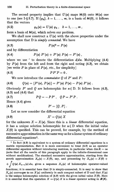
100 II. Perturbation theory in a finite-dimensional space
The second property implies that U (x) maps M (0) onto M (x) oneto one (see I-§ 5.7). If {q, }, k = 1, ..., m, is a basis of M (0), it followsthat the vectors(4.2) 991,(x) = U (m) 991, , k = 1, ..., m ,
form a basis of M(x), which solves our problem.We shall now construct a U (m) with the above properties under the
assumption that D is simply connected. We have
(4.3) P (x)' = P (x)and by differentiation(4.4) P (x) P' (x) + P' (x) P (x) = P' (x)
where we use ' to denote the differentiation d/dx. Multiplying (4.4)by P (x) from the left and from the right and noting (4.3), we obtain[we write P in place of P(x), etc., for simplicity]
(4.5) PPP = 0.We now introduce the commutator Q of P and P:
(4.6) Q (x) _ [P'`(x), P (x) ] = P' (x) P (x) - P (x) P' (x) .
Obviously P and Q are holomorphic for x E D. It follows from (4.3),(4.5) and (4.6) that(4.7) PQ=-PP', QP=P'P.Hence (4.4) gives(4.8) P' = [Q, P] .
Let us now consider the differential equation
(4.9) X' = Q (X) X
for the unknown X = X (x). Since this is a linear differential equation,it has a unique solution holomorphic for x E D when the initial valueX (O) is specified. This can be proved, for example, by the method ofsuccessive approximation in the same way as for a linear system of ordinarydifferential equations'.
' In fact (4.9) is equivalent to a system of ordinary differential equations in amatrix representation. But it is more convenient to treat (4.9) as an operatordifferential equation without introducing matrices, in particular when dimX = 00(note that all the results of this paragraph apply to the infinite-dimensional casewithout modification). The standard successive approximation, starting from thezeroth approximation X. (x) = X (0), say, and proceeding by X (x) = X (0) +
X
+ f Q(x) dx, gives a sequence of holomorphic operator-valued0
functions; it is essential here that D is simply-connected. It is easy to show thatX. (x) converges to an X (x) uniformly in each compact subset of D and that X (x)is the unique holomorphic solution of (4.9) with the given initial value X (0). Hereit is essential that the operation X -+ Q (x) X is a linear operator acting in R (X).
§ 4. Similarity transformations of the eigenspaces and eigenvectors 101
Let X (x) = U (x) be the solution of (4.9) for the initial conditionX (O) = 1. The general solution of (4.9) can then be written in the form
(4.10) X (M) = UM X (O) .In fact (4.10) satisfies (4.9) and the initial condition ; in view of theuniqueness of the solution it must be the required solution.
In quite the same way, the differential equation
(4.11) Y' = - YQ (x)
has a unique solution for a given initial value Y (0). Let Y = V (x) be thesolution for Y (0) = 1. We shall show that U (x) and V (x) are inverseto each other. The differential equations satisfied by these functionsgive (V U)' = V' U + V U' = -VQU +VQU = 0. Hence VU is aconstant and(4.12) V (x) U (x) = V (0) U (0) = 1 .
This proves that V = U-1 and, therefore, we have also
(4.13) U (M) V (X) = 1 .
We shall give an independent proof of (4.13), for later reference,for (4.13) is not implied by (4.12) if the underlying space is of infinitedimension. We have as above
(4.14) (UV)' = QUV - UVQ = [Q, UV].
This time it is not obvious that the right member of (4.14) is zero.But (4.14) is also a linear differential equation for Z = U V, and theuniqueness of its solution can be proved in the same way as for (4.9)and (4.11). Since Z (x) = 1 satisfies (4.14) as well as the initial conditionZ (0) = 1 = U (0) V (0), U V must coincide with Z. This proves (4.13) 1.
We now show that U(x) satisfies the conditions (1), (2) requiredabove. (1) follows from U(x)-1= V (x) implied by (4.12) and (4.13).To prove (2), we consider the function P (x) U (x). We have
(4.15) (PU)'=P'U+PU'=(P'+PQ)U=QPUby (4.9) and (4.8). Thus X = P U is a solution of (4.9) with the initialvalue X (0) = P (0) and must coincide with U (x) X (0) = U (x) P (0) by(4.10). This is equivalent to (2).
Remark 4.1. In virtue of (4.7), the Q in the last member of (4.15)can be replaced by P'. Thus the function W (x) = U (x) P (0) = P (x) U (x)satisfies the differential equation
(4.16) W' = P' (x) W,
1 (4.13) can also be deduced from (4.12) by a more general argument based onthe stability of the index; cf. X-§ 5.5.
102 II. Perturbation theory in a finite-dimensional space
which is somewhat simpler than (4.9). Similarly, it is seen that Z(x)= P (O) U (x)-' satisfies
(4.17) Z' = Z P, (x)
Remark 4.2. U (x) and U (x)-1 can be continued analytically as longas this is possible for P (x). But it may happen that they are not single-valued even when P (x) is, if the domain of x is not simply connected.
Remark 4.3. The construction of U (x) can be carried out even if xis a real variable. In this case P (m) need not be holomorphic ; it sufficesthat P (x) exists and is continuous (or piecewise continuous). Then U(x)has a continuous (piecewise continuous) derivative and satisfies (1), (2)except that it is not necessarily holomorphic in x.
Remark 4.4. The transformation function U (x) is not unique for agiven P (x). Another U (x) can be obtained from the result of I-§ 4.6, atleast for sufficiently small Ix I. Substituting P (O), P (m) for the P, Q ofI-§ 4.6, we see from I-(4.38) that'(4.18)
U (x) = [1 - (P (x) - P (0))21-1/2 [P (x) P (0) + (1 - P (x)) (1 - P (0))]
is a transformation function if Ix I is so small that 11 P (x) - P (0) 11 < 1.(4.18) is simpler than the U (x) constructed above in that it is an algebraicexpression in P (x) and P (0) while the other one was defined as thesolution of a differential equation. But (4.18) has the inconvenience thatit may not be defined for all x E D.
3. Solution of the differential equationSince we are primarily interested in the mapping of M (0) onto M (x)
by the transformation function U (x), it suffices to consider W (x)= U (x) P (0) instead of U (x). To determine W it suffices to solve thedifferential equation (4.16) for the initial condition W (0) = P (0).
Let us solve this equation in the case where P (x) is the total projec-tion for the A-group eigenvalues of T (x). P (x) has the form (2.3), so that
00
(4.19) P' (x) = E (n + 1) Mn p(n+1)n=0
Since W (0) = P (0) = P, we can write
(4.20)00
W (x) = P + _Y Mn W (n) .
n.1
Substitution of (4.19) and (4.20) into (4.16) gives the following recur-rence formulas for W(n):
(4.21) nW(n) = nP(n) P + (n - 1) P(n-1) W(') ..}.... + P(1) W(n-1) ,
n = 1, 2, .. .
1 (4.18) was given by Sz.-NAGY [1] in an apparently different form.
§ 4. Similarity transformations of the eigenspaces and eigenvectors 103
The W(n) can be determined successively from (4.21) by making useof the expressions (2.12) for P(n). In this way we obtain
(4.22) WMl> = PM P,
W(2) = P(2) P + [P(i)]2 P
WM3> = P3> P + 3 P(2) P(1) P + P(i) (2) P + 6 [P(1)]3P.
If the eigenvalue 2 of T is semisimple, we have by (2.14)
(4.23) W(i) = - S T (l> P ,
W(2) =-ST(2) P+STMI>STMI>P-S2TM1>PTMI>P-
- PTMI> S2 TM P .
In case the 2-group consists of a single eigenvalue (no splitting),M (m) = P (m) X is itself the algebraic eigenspace of T (m) for this eigen-value, and we have a set of generalized eigenvectors
(4.24) k (x) = W (x) k , k = 1, ..., m ,
where {q9k}, k = 1, . . ., m, is a basis of M (0). According to the propertiesof W (x), the m vectors (4.24) form a basis of M (x).
The function Z (x) = P (0) U (x)-1 can be determined in the same way.Actually we need not solve the differential equation (4.17) independently.(4.17) differs from (4.16) only in the order of the multiplication of theunknown and the coefficient P(x). Thus the series E Mn Z(') for Z (x) isobtained from that of W (x) by inverting the order of the factors in eachterm. This is true not only for the expression of Z(n) in terms of the p(n)but also in terms of P, S, TM, T(2), . . . as in (4.23). This is due to thefact that the expressions (2.12) for the POn> are invariant under theinversion of the type described. This remark gives, under the sameassumption that 2 is semisimple,
(4.25) Z(l> = - P TM S ,
Z(2) = -P T(2) S + PTMI> STMl> S - PTM1> PTMI> S2
- 2 PTMI>S2TM1>P.
Remark 4.5. The other transformation function U (x) given by (4.18)can also be written as a power series in x under the same assumptions.As is easily seen, the expansion of U (m) P coincides with that of W (M)deduced above up to the order x2 inclusive.
104 II. Perturbation theory in a finite-dimensional space
4. The transformation function and the reduction processThe transformation function U (m) for the total projection P(M) for
the A-group constructed above can be applied to the reduction processdescribed in § 2.3. Since the A-group eigenvalues are the eigenvalues ofT (x) in the invariant subspace M (x) = R (P (x)) and since U (x) has theproperty P (m) = U (n) P U (x)-1, the eigenvalue problem for T (m) inM (m) is equivalent to the eigenvalue problem for the operator
(4.26) U()-' T (m) U (m)
considered in the subspace M = M (0) = R (P) (which is invariant underthis operator). In fact, (4.26) has the same set of eigenvalues as T(M),whereas the associated eigenprojections and eigennilpotents of (4.26)are related to those of T (x) by the similarity transformation with U (x)-1.Since we are interested in the A-group only, it suffices to consider theoperator(4.27) P U (x)-1 T (m) U (m) P= Z (x) T (m) W (m)
with the Z and W introduced in the preceding paragraphs.(4.27) is holomorphic in x and in this sense is of the same form as the
given operator T (x). Thus the problem for the A-group has been reducedto a problem within a fixed subspace M of X. This reduction of the originalproblem to a problem in a smaller subspace M has the advantage that Mis independent of x, whereas in the reduction process considered in § 2.3the subspace M (x) depends on x. For this reason the reduction to (4.27)is more complete at least theoretically, though it has the practicalinconvenience that the construction of U (m) is not simple.
In particular it follows that the weighted mean A (x) of the A-groupeigenvalues is equal to m-1 times the trace of (4.27) :
(4.28) 1 (x) = m-1 trZ (x) T (x) W (x)= A + m-1 trZ(x) (T (x) - A) W (m) .
Substitution of (4.23) and (4.25) for the coefficients of W (M) and Z (x)leads to the same results as in (2.33).
Problem 4.6. Verify the last statement.
5. Simultaneous transformation for several projectionsThe U (x) considered in par. 2 serves only for a single projection P (n).
We shall now consider several projections Ph (u), h = 1, . . ., s, satisfyingthe conditions(4.29) Ph (x) Ph (x) = 6hh Ph (x)
and construct a transformation function U (x) such that
(4.30) UM PAM UN' = Ph (x) , h = 1 , ..., s .
§ 4. Similarity transformations of the eigenspaces and eigenvectors 105
As a consequence, we can find a basis {phi (x), ..., Ph.m (x)} of eachsubspace Mh (x) = R (Ph (x)) by setting
(4.31) Thf(x) = U(x) Thl,
where {Th1, ..., Th.,} is a basis of Mh = Mh (0).As before we assume that the Ph (x) are either holomorphic in a
simply-connected domain D of the complex plane or continuouslydifferentiable in an interval of the real line. We may assume that theset {Ph(x)} is complete in the sense that
(4.32) Ph (x) = 1 .h=1
s
Otherwise we can introduce the projection Po (x) = 1 - Ph (x) ;h=1
the new set {Ph (x)}, h = 0, 1, ..., s, will satisfy (4.29) as well as thecompleteness condition, and U (x) satisfies (4.30) for the old set if andonly if it does the same for the new set.
The construction of U (x) is similar to that for a single P (x). Wedefine U (x) as the solution of the differential equation (4.9) for theinitial value X (0) = 1, in which Q (x) is to be given now by
(4.33) Q (x) = 2 Z,' [P1" (x), Ph (x)] _ ' PA' (x) Ph (x)h h=1
Ph (x) Pk (x) .h=1
The equality of the three members of (4.33) follows from (4.32), whichimplies that E Pk Ph + E Ph Pk = E'(Ph)' = E' Pk = 0. Note also thatthis Q (x) coincides with (4.6) in the case of a single P (m); the apparentdifference due to the presence in (4.33) of the factor 1/2 arises from thefact that in (4.33) we have enlarged the single P (x) to the pair {P (x),1 - P(x)} so as to satisfy the completeness condition (4.32).
The argument of par. 2 [in particular (4.15)] shows that (4.30) isproved if we can show that
(4.34) Pk(x) = [Q(x), Ph(x)] , h = 1, ..., S .
To prove this we differentiate (4.29), obtaining
(4.35) Pk Ph + Ph Pk = 670, Pk .
Multiplication from the left by Ph gives Ph Pk Ph + Ph Pk = bhh Ph Ph'
= Ph Ph Pk, which may be written
(4.36) - [Ph Pk, Ph] = Ph PA'.
Summation over h = 1, ..., s gives (4.34) in virtue of (4.33).
106 H. Perturbation theory in a finite-dimensional space
Obviously a simultaneous transformation function U (x) can beconstructed in this way for the set of all eigenprojections Ph (x) of T (M)in any simply connected domain D of the x-plane in which the Ph (x)are holomorphic1.
6. Diagonalization of a holomorphic matrix functionLet (t;h(x)) be an N X N matrix whose elements are holomorphic
functions of a complex variable x. Under certain conditions such amatrix function can be diagonalized, that is, there is a matrix (y;h (x))with elements holomorphic in x such that
(4.37) (4h(x)) = (Yjh(x))-I(tjh(x)) (Yjh(x))is a diagonal matrix for every x considered.
This problem can be reduced to the one considered in this section.It suffices to regard the given matrix as an operator T (m) acting in thespace X = CN of numerical vectors and apply the foregoing results.If the value of x is restricted to a simply-connected domain D containingno exceptional points, we can construct the U(x) and therefore a basis(4.31) consisting of vector functions holomorphic for x E D and adaptedto the set {Ph (x)} of eigenproj ections of T (x). With respect to such a basis,the matrix representation of T (x) takes the simple form described inI-§ 5.4. In particular it is a diagonal matrix with diagonal elementsAh (x) if the Dh (x) are all identically zero [which happens, for example, ifall mh = 1 or T (x) is normal for real x, say]. As is seen from I-§ 5.4,this is equivalent to the existence of a matrix function (y; h (x)) with therequired property (4.37). Note that the column vectors (y,h (x), ...,YNI(s)) are eigenvectors of the given matrix (a;h(n)).
S 5. Non-analytic perturbations1. Continuity of the eigenvalues and the total projection
In the preceding sections we considered the eigenvalue problem foran operator T (x) E . (X) holomorphic in x and showed that its eigen-values and eigenprojections are analytic functions of x. We now askwhat conclusions can be drawn if we consider a more general type ofdependence of T (m) on n 2.
First we consider the case in which T (x) is only assumed to becontinuous in x. x may vary in a domain Do of the complex plane or in
1 The transformation function U (x) has important applications in the adiabatictheorem in quantum mechanics, for which we refer to T. KATO [2], GARRIDO [1],GARRIDO and SANCHO [1].
9 This question was discussed by RELLICH [1], [2], [8] (in greater detail in [8])for symmetric operators.
§ S. Non-analytic perturbations 107
an interval I of the real line. Even under this general assumption, someof the results of the foregoing sections remain essentially unchanged.
The resolvent R (C, x) = (T (x) - is now continuous in C and xjointly in each domain for which C is different from any eigenvalue ofT (x). This is easily seen by modifying slightly the argument given in§ 1.3; we need only to note that the A (x) = T (x) - T in (1.11) is nolonger holomorphic but tends to zero for x --k 0 (T = T (0)).
It follows that R (C, x) exists when C is in the resolvent set P (T) of Tprovided that Ix I is small enough to ensure that
(5.1) IIT(x) - TII < IIR(C)II-1 R(C, 0));
see (1.12). Furthermore, R x) -+ R for x -* 0 uniformly for belong-ing to a compact subset of P(T).
Let A be one of the eigenvalues of T, say with (algebraic) multiplicitym. Let r be a closed curve enclosing A but no other eigenvalues of T.II R II -1 has a positive minimum 6 for C E P, and R x) exists for allC E P if II T (x) - TII < 6. Consequently the operator P (x) is againdefined by (1.16) and is continuous in x near x = 0. As in the analyticcase, P(x) is the total projection for the eigenvalues of T (M) lyinginside P. The continuity of P (x) again implies that
(5.2) dim M (x) = dim M = m , M(x)=P(x)X, M = M (0) = PX ,
where P = P (0) is the eigenprojection of T for the eigenvalue A. (5.2)implies that the sum of the multiplicities of the eigenvalues of T (x)lying inside r is equal to m. These eigenvalues are again said to form theA-group.
The same results are true for each eigenvalue Ah of T. In any neigh-borhood of Ah, there are eigenvalues of T (m) with total multiplicityequal to the multiplicity mh of Ah provided that Ix I is sufficiently small.Since the sum of the mh is N, there are no other eigenvalues of T (x).This proves (and gives a precise meaning to) the proposition that theeigenvalues of T (x) are continuous in x.
We assumed above that T (x) is continuous in a domain of x. Butthe same argument shows that the eigenvalues of T (x) and the totalprojection P (x) are continuous at x = 0 if T (x) is continuous at x = 0.To see this it suffices to notice that R x) --- R (4), x -> 0, uniformly forC E P. We may even replace T (x) by a sequence such that T ->. T,n --> oo. Then it follows that the eigenvalues as well as the total projec-tions of T tend to the corresponding ones of T for n -- oo.
Summing up, we haveTheorem 5.1. Let T (x) be continuous at x = 0. Then the eigenvalues of
T (x) are continuous at x = 0. 11 A is an eigenvalue of T = T (0), the
108 II. Perturbation theory in a finite-dimensional space
2-group is well-defined for sufficiently small Ix and the total projectionP (x) for the 2-group is continuous at x = 0. If T (x) is continuous in adomain of the x plane or in an interval of the real line, the resolventR x) is continuous in C and x jointly in the sense stated above.
2. The numbering of the eigenvaluesThe fact proved above that the eigenvalues of T (x) change contin-
uously with x when T (x) is continuous in x is not altogether simplesince the number of eigenvalues of T (x) is not necessarily constant.It is true that the same circumstance exists even in the analytic case,but there the number s of (different) eigenvalues is constant for non-exceptional x. In the general case now under consideration, this numbermay change with x quite irregularly; the splitting and coalescence ofeigenvalues may take place in a very complicated manner.
To avoid this inconvenience, it is usual to count the eigenvaluesrepeatedly according to their (algebraic) multiplicities as described inI-§ 5.4 (repeated eigenvalues). The repeated eigenvalues of an operatorform an unordered N-tuple of complex numbers. Two such N-tuples6 = (,ul, ..., ,uN) and 6' = (/4, ..., ,u') may be considered close to eachother if, for suitable numbering of their elements, the are smallfor all n = 1, ..., N. We can even define the distance between such twoN-tuples by
(5.3) dist (6, 6') = min max ,u;,I
where the min is taken over all possible renumberings of the elements ofone of the N-tuples. For example, the distance between the triples(0, 0, 1) and (0, 1, 1) is equal to 1, though the set {O, 1} of their elementsis the same for the two triples. It is easy to verify that the distance thusdefined satisfies the axioms of a distance function.
The continuity of the eigenvalues of T (x) given by Theorem 5.1can now be expressed by saying that the N-tuple a (x) consisting of therepeated eigenvalues of T (x) changes with x continuously. This means thatthe distance of 6 (x) from 6 (,D) tends to zero for x -> xo for each fixed xo.
The continuity thus formulated is the continuity of the repeatedeigenvalues as a whole. It is a different question whether it is possible todefine N single-valued, continuous functions ,un (x), n = 1, ..., N, whichfor each x represent the repeated eigenvalues of T (u). Such a para-metrization is in general impossible. This will be seen from Example1.1, d), in which the two eigenvalues are ±x1/2; here it is impossible todefine two single-valued 'continuous functions representing the twoeigenvalues in a domain of the complex plane containing the branchpoint x=0.
§ 5. Non-analytic perturbations 109
A parametrization is possible if either i) the parameter x changesover an interval of the real line or ii) the eigenvalues are always real.In case ii) it suffices to number the eigenvalues ,u,, (x) in ascending (ordescending) order :
(5.4) Y1 (9) S J Z2 (x) S ... < JZN (x)
It should be noted, however, that this way of numbering is not alwaysconvenient, for it can destroy the differentiability of the functions whichmay exist in a different arrangement.
The possibility of a parametrization in case i) is not altogetherobvious. This is contained in the following theorem.
Theorem 5.2. Let 6 (x) be an unordered N-tuple of complex numbers,depending continuously on a real variable x in a (closed or open) interval I.Then there exist N single-valued, continuous functions ,u,, (x), n = 1, ..., N,the values of which constitute the N-tuple 6 (x) for each x E I. [(4u,, (x))
is called a representation of 6(x).]Proof. For convenience we shall say that a subinterval Io of I has
property (A) if there exist N functions defined on Io with the propertiesstated in the theorem. What is required is to prove that I itself hasproperty (A). We first show that, whenever two subintervals It, I2 withproperty (A) have a common point, then their union Io = I1 v I2 alsohas the same property. Let (M11) (x)) and (u ) (x)) be representations of6 (x) in It and 12, respectively, by continuous functions. We may assumethat neither I1 nor I2 contains the other (otherwise the proof is trivial) andthat It lies to the left of 12. For a fixed xo lying in the intersection of It andI2, we have ,u(t) (x°) = ,u;,2) (x°), n = 1, ..., N, after a suitable renumberingof (,u;,2)), for both (,u;,tl (x°)) and (,u;,2> (x°)) represent the same 6 (xo). Thenthe functions u;°> (x) defined on Io by
(5.5) (x)
,unl (x) , x 5 xo
Y. (M) x z x°n l
are continuous and represent e (x) on I°.It follows that, whenever a subinterval I' has the property that each
point of I' has a neighborhood with property (A), then I' itself hasproperty (A).
With these preliminaries, we now prove Theorem 5.2 by induction.The theorem is obviously true for N = 1. Suppose that it has beenproved for N replaced by smaller numbers and for any interval I. Let rbe the set of all x E I for which the N elements of 6 (x) are identical,and let i be the complement of r in I. P is closed and A is open relativeto I. Let us now show that each point of i has a neighborhood havingproperty (A). Let x° E A. Since the N elements of 6 (x°) are not all
110 II. Perturbation theory in a finite-dimensional space
identical, they can be divided into two separate groups with Nl and N2elements, where Nl + N2 = N. In other words, 6 (xa) is composed of anN1-tuple and an N2-tuple with separate elements ("separate" meansthat there is no element of one group equal to an element of the other).The continuity of 0 (x) implies that for sufficiently small Ix - x,1, 0 (x)consists likewise of an N1-tuple and an N2 tuple each of which is con-tinuous in x. According to the induction hypothesis, these Nl and NZtuples can be represented in a neighborhood A' of xo by families ofcontinuous functions (p., (m), ..., JUN, (x)) and (µN,+1(x), ..., ,uN (x)),respectively. These N functions taken together then represent 0 (x) in A'.In other words, A' has property (A).
Since A is open in I, it consists of at most countably many sub-intervals I, I2, ... . Since each point of A has a neighborhood withproperty (A), it follows from the remark above that each componentinterval I., has property (A). We denote by p(P) (x), n = 1, ..., N, the Nfunctions representing e (x) in Ii,. For x E F, on the other hand, 0 (x)consists of N identical elements ,u (x). We now define N functions ,u,, (x),n= 1, . . ., N, on I by
(5.6) Jun (x) _A.") (x) , x E Ifl , p = 1, 2, ... ,,u(x), xEP.
These N functions represent e (x) on the whole interval I. It is easy toverify that each ,u (x) is continuous on I. This completes the inductionand the theorem is proved.
3. Continuity of the eigenspaces and eigenvectorsEven when T (x) is continuous in x, the eigenvectors or eigenspaces
are not necessarily continuous. We have shown above that the totalprojection P (m) for the A-group is continuous, but P (m) is defined onlyfor small IkI for which the A-group eigenvalues are not too far from A.
If T (x) has N distinct eigenvalues Ah (x), h = 1, ..., N, for all xin a simply connected domain of the complex plane or in an interval ofthe real line, we can define the associated eigenprojections P,(x) eachof which is one-dimensional. Each Ph (x) is continuous since it is identicalwith the total projection for the eigenvalue Ah (x). But Ph (x) cannot ingeneral be continued beyond a value of x for which Ah (x) coincides withsome other A, (m). In this sense the eigenprojections behave more sin-gularly than the eigenvalues. It should be recalled that even in theanalytic case Ph (x) may not exist at an exceptional point where Ah (x)is holomorphic [Example 1.12, f) ] ; but Ph (x) has at most a pole in thatcase (see § 1.8). In the general case under consideration, the situation ismuch worse. That the eigenspaces can behave quite singularly even for a
§ 5. Non-analytic perturbations 111
very smooth function T (x) is seen from the following example due toRELLICH'.
Example 5.3. Let N = 2 and2 2cos - sin -
(5.7) T (x) = exj
x x
2 2sin - - cos -x x
T (O) = 0.
T (m) is not only continuous but is infinitely differentiable for all real values of x,and the same is true of the eigenvalues of T (x), which are ±,e-11s' for x = 0 andzero for x = 0. But the associated eigenprojections are given for x + 0 by
1 1 1 1 1 1cosy 1 cos -sin - sin2 1 -cos -sin -
x x x x x x
cos x sin x sing x - cos x sin % cost % IThese matrix functions are continuous (even infinitely differentiable) in anyinterval not containing x = 0, but they cannot be continued to x = 0 as continuousfunctions. Furthermore, it is easily seen that there does not exist any eigenvector ofT (x) that is continuous in the neighborhood of x = 0 and that does not vanish atx=0.
It should be remarked that (5.7) is a symmetric operator for each real x (actingin C2 considered a unitary space). In particular it is normal and, therefore, theeigenprojections would be holomorphic at x = 0 if T (x) were holomorphic (Theorem1.10). The example is interesting since it shows that this smoothness of the eigen-projections can be lost completely if the holomorphy of T (x) is replaced by infinitedifferentiability.
4. Differentiability at a pointLet us now assume that T (x) is not only continuous but differentiable.
This does not in general imply that the eigenvalues of T (x) are dif-ferentiable; in fact they need not be differentiable even if T (x) is holo-morphic [Example 1.1, d)]. However, we have
Theorem 5.4. Let T (x) be differentiable at x = 0. Then the total projec-tion P (x) for the A-group is differentiable at x = 0:
(5.9) P (x) = P -I- M PM -I- o (x) ,
where2 P(1) P T'(0) S - S T' (0) P and S is the reduced resolvent o l Tfor A (see I-§ 5.3). If d is a semisimple eigenvalue of T, the A -group eigen-values of T (x) are differentiable at x = 0:
(5.10) ,ue (x) = d -I- x u1(il -I- o (x) , j = 1, ..., m ,where the µf (x) are the repeated eigenvalues of the A-group and the ,u(l)are the repeated eigenvalues of PT'(0) P in the subspace M = PX (P is
1 See RELLICH [1]; for convenience we modified the original example slightly.2 Here o(x) denotes an operator-valued function F(x) such that 11F(xA = 0W
in the ordinary sense.
112 ' II. Perturbation theory in a finite-dimensional space
the eigenprojection of T for A). If T is diagonable, all the eigenvalues aredifferentiable at x = 0.
Remark 5.5. The above theorem needs some comments. That theeigenvalues of T (x) are differentiable means that the N-tuple 0 (x)consisting of the repeated eigenvalues of T (m) is differentiable, andsimilarly for the differentiability of the A-group eigenvalues. That an(unordered) N-tuple 6 (x) is differentiable at x = 0 means that 6 (x)can be represented in a neighborhood of x = 0 by N functions ,u (u),n = 1, ..., N, which are differentiable at x = 0. The N-tuple 0'(0)consisting of the ,u;, (0) is called the derivative of .S (x) at x = 0. It can beeasily proved (by induction on N, say) that e' (0) is thereby definedindependently of the particular representation (,q,, (x)) of e (m). If e (m)is differentiable at each x and Cam' (x) is continuous, 0 (x) is said to becontinuously differentiable.
Note that .S (0) and V(0) together need not determine the behaviorof e (x) even in the immediate neighborhood of x = 0. For example,e1(x) = (x, 1 - x) and e2 (x) = (- x, 1 + x) have the common value(0, 1) and the common derivative (1, - 1) at x = 0.
Proof of Theorem 5.4. We first note that the resolvent R x) isdifferentiable at x = 0, for it follows from I-(4.28) that
(5.11) [ax R(C, x)]xo= -R (g) T'(0) R(C)
Here it should be noted that the derivative (5.11) exists uniformly for Cbelonging to a compact subset of P (T), for R (C, x) -> R (C), x -+ 0, holdsuniformly (see par. 1). Considering the expression (1.16) for P (M), itfollows that P (x) is differentiable at x = 0, with
(5.12) P'(0) 21 J [ax R(C,x)]x=odC= 2s f R(C) T'(0)R(C)dCr r= - P T' (0) S - S T' (0) P = P(1) [cf. (2.14) ] .
This proves (5.9).As in the analytic case, if A is semisimple the A-group eigenvalues of
T (n) are of the form
(5.13) 14100 = A + x 41) (x) , j = 1, ..., m ,
where the pi(l) (x) are the (repeated) eigenvalues of the operator
(5.14) 1 > (x) = x-1(T (x) - A) P (x) _ - 2n i J (C- A) R (C, x) dr
in the subspace M (x) = P (x) X [see (2.37) ]. Since T (x) and P (x) aredifferentiable at x = 0 and (T - A) P = 0 if A is semisimple, TM (x) is
§ 5. Non-analytic perturbations 113
continuous at x = 0 if we set
(5.15) To) (0) = T'(0) P + (T - 2) P'(0) = P T'(0) P
where we have used (5.12) and (T - A) S = 1 - P [see (2.11)]. Hencethe eigenvalues of TM (x) are continuous at x = 0. In particular, theeigenvalues ,u,(') (x) of TM (x) in the invariant subspace M (x) are contin-uous at x = 0 (see Theorem 5.1), though they need not be continuousfor x + 0. In view of (5.13), this proves (5.10).
5. Differentiability in an intervalSo far we have been considering the differentiability of the eigenvalues
and eigenprojections at a single point x = 0. Let us now consider thedifferentiability in a domain of x, assuming that T (m) is differentiablein this domain. If this is a domain of the complex plane, T (x) is neces-sarily holomorphic; since this case has been discussed in detail, we shallhenceforth assume that T (m) is defined and differentiable in an interval Iof the real line'.
According to Theorem 5.4, the N-tuple 9 (x) of the repeated eigen-values of T (x) is differentiable for x E I provided that T (x) is diagonablefor x E I. However, it is by no means obvious that there exist N functions,u (x), n = 1, . . ., N, representing the repeated eigenvalues of T (x),which are single-valued and differentiable on the whole of I Actuallythis is true, as is seen from the following general theorem.
Theorem 5.6. Let a (x) be an unordered N-tuple of complex numbersdepending on a real variable x in an interval I, and let 6 (x) be differentiableat each HE I (in the sense of Remark 5.5). Then there exist N complex-valued functions 1u,, (x), n = 1, . . ., N, representing the N-tuple a (x) forx E I, each of which is differentiable /or x E I.
Proof. A subinterval of I for which there exist N functions of thekind described will be said to have property (B) ; it is required to provethat I itself has property (B). It can be shown, as in the proof of Theorem5.2, that for any overlapping2 subintervals Il, I2 with property (B),their union Il U I2 has also property (B). The only point to be noted isthat care must be taken in the renumbering of the u(2) (x) to make surethat the continuation (5.5) preserves the differentiability of the functionsat x = xo; this is possible owing to the assumption that 6 (x) is differen-tiable at x = xo.
1 The differentiability of eigenvalues was investigated in detail in RELLICH [8]in the case when T (x) is symmetric for each real x. It should be noted that theproblem is far from trivial even in that special case.
8 Here "overlapping" means that the two intervals have common interiorpoints.
114 II. Perturbation theory in a finite-dimensional space
With this observation, the proof is carried out in the same way asin Theorem 5.2. A slight modification is necessary at the final stage,for the functions defined by (5.6) may have discontinuities of derivativesat an isolated point of P. To avoid this, we proceed as follows. An isolatedpoint no of r is either a boundary point of I or a common boundary ofan I,, and an I. In the first case we have nothing to do. In the secondcase, it is easy to "connect" the two families (x)) and (P(q) (x))"smoothly" by a suitable renumbering of the latter, for these twofamilies of differentiable functions represent e (x) at the different sidesof x = no and 6 (x) is differentiable at x = xo. It follows that the intervalconsisting of Ip, IQ and xa has property (B).
Let r' be the set of isolated points of P. d u r, is relatively openin I and consists of (at most) countably many subintervals I. Each Ikconsists in turn of countably many subintervals of the form 1p joinedwith one another at a point of r, in the manner stated above. By repeatedapplications of the connection process just described, the functionsrepresenting 6 (x) in these I,, can be connected to form a family of Nfunctions differentiable on I. This shows that each Ik has property (B).
The construction of N differentiable functions ,u (x) representing6 (x) on the whole interval I can now be carried out by the method (5.6),in which the I p and r should be replaced by the Ik and r,' respectively,r' being the complement of r, in P. The differentiability at a point no ofr,, of the Fin (x) thus defined follows simply from the fact that the deri-vative 6' (xo) consists of N identical elements, just as does 6 (no). Thiscompletes the proof of Theorem 5.6.
Theorem 5.7. I l in Theorem 5.6 the derivative Cam' (x) is continuous,the N functions ,u (x) are continuously differentiable on I.
Proof. Suppose that the real part of ,u;, (x) is discontinuous at x = xo.According to a well-known result in differential calculus, the valuestaken by Re,u;, (x) in any neighborhood of xo cover an interval of lengthlarger than a fixed positive number'. But this is impossible if Cam' (x) iscontinuous, for any value of ,un (x) is among the N elements of S' (x) . Forthe same reason Im u (u) cannot be discontinuous at any point.
Remark 5.8. We have seen (Theorem 5.4) that the eigenvalues of T (x)are differentiable on I if T (x) is differentiable and diagonable for x E I.
' Let a real-valued function f (t) of a real variable t be differentiable fora S 1S b ; then f' (t) takes in this interval all values between a = f' (a) and P = f' (b) .To prove this, we may assume or < P. For any y E (a, P) set g (t) = f (t) - y t.Then g' (a) = a - y < 0, g' (b) = # - y > 0, so that the continuous function g (t)takes a minimum at a point t = c E (a, b). Hence g' (c) = 0 or f' (c) = y.If /'(1) is discontinuous at t = to, then there is e > 0 such that, in anyneighborhood of to, there exist t,, t$ with 11'%) - f' (t2) > e. It follows from theabove result that /' (t) takes all values between )' (t,) and /' (t2). Hence the valuesof /'(1) in any neighborhood of to covers an interval of length larger than e.
§ 5. Non-analytic perturbations 115
It is quite natural, then, to conjecture that the eigenvalues are continuouslydifferentiable if T (x) is continuously differentiable and diagonable.But this is not true, as is seen from the following example'.
Example 5.9. Let N = 2 and
xla Ixla - kIP 2 + sin(5.16) T (X) _ TxT x 40 ; T (O) = 0 .
- Ixla .Ixla
T (x) is continuously differentiable for all real x if a > 1 and fi > 2. The two eigen-values of T(m) are
«+R t
(5.17) fif (x) = f x -12P (2 + sin1
ICI f I-, x + 0, Fit (0) = 0 .
Since the ,ut (x) are different from each other for x + 0, T (x) is diagonable, andT (0) = 0 is obviously diagonable. The ,u± (x) are differentiable everywhere, as thegeneral theory requires. But their derivatives are discontinuous at x = 0 if a ++ #S 4. This simple example shows again that a non-analytic perturbation can berather pathological in behavior.
Remark 5.10. If T (x) is continuously differentiable in a neighborhoodof x = 0 and 2 is a semisimple eigenvalue of T (O), the total projectionP (x) for the 2-group is continuously differentiable and Ta) (x) is contin-uous in a neighborhood of x = 0, as is seen from (5.12) and (5.14).
6. Asymptotic expansion of the eigenvalues andeigenvectors
The differentiability of the eigenvalues considered in the precedingparagraphs can be studied from a somewhat different point of view.Theorem 5.4 may be regarded as giving an asymptotic expansion of theeigenvalues u5 (x) up to the first order of x when T (x) has the asymptoticform T (x) = T + x T' + o (m), where T' = T'(0). Going to the secondorder, we can similarly inquire into the asymptotic behavior of theeigenvalues when T (x) has the asymptotic form T + x T(')+ xs T (2) ++ o (xa). In this direction, the extension of Theorem 5.4 is rather straight-forward.
Theorem 5.11. Let T(x) = T + x T (') + x2 T (2) + 0 (x2) for x --)- 0.Let A be an eigenvalue of T with the eigenprojection P. Then the totalprojection P (x) for the 2-group eigenvalues of T (x) has the form
(5.18) P (x) = P + x P(') + x2 P(2) + o (x$)
where P, P(1) and P(2) are given by (2.13). If the eigenvalue d of T issemisimple and if A(') is an eigenvalue of P TO) P in P X with the eigen-
' The operator of this example is not symmetric. For symmetric operatorsbetter behavior is expected; see Theorem 6.8.
116 II. Perturbation theory in a finite-dimensional space
projection P(i), then T (x) has exactly m(,') = dim P}) repeated eigenvalues(the A + x A,I' group) of the form A + x A,(I) + o (x). The total eigenprojec-tion P(i) (x) for this group has the form
(5.19) Pit) (x) = pill) + x Pill) + o (x)
If, in addition, the eigenvalue A(') of P TM P is semisimple, then P(li)is given by (2.47) and the m,(2) repeated eigenvalues of the A + x 2')-grouphave the form(5.20) /j,,k (x) = A + x 2' + x2 IU(2 + 0 (x2) , k
where ,u} k, k = 1, ..., mil>, are the repeated eigenvalues of P(I) TM P,1= Phi) T(2) Pj(') - p) T (') S TM P}) in the subspace PEI) X.
Proof. The possibility of the asymptotic expansion of T (x) up to thesecond order implies the same for the resolvent :
(5.21) R (g, x) = R (C) - R (C) (T (x) - T) R (g) + R (C) (T (x) - T) xx R(C)(T(x)-T)R(g)+...+
= R x R (C) TM R x2 [- R (C) T(2) R (C) +
+ R (C) T(1) R (C) TM R (4) j + o (x2) .
Here o (x2) is uniform in C in each compact subset of P (T). Substitutionof (5.21) into (1.16) yields (5.18), just as in the analytic case.
It follows that if A is semisimple, the T(l) (x) of (5.14) has the form
(5.22) TM (x) = P TM P + x T(2) + o (x)
where T(2) is given by (2.20). The application of Theorem 5.4 to TAI) (x)then leads to the result of the theorem. Again the calculation of theterms up to the order x2 is the same as in the analytic case.
7. Operators depending on several parametersSo far we have been concerned with an operator T (x) depending on a
single parameter x. Let us now consider an operator T (xl, x2) dependingon two variables x2, x2 which may be complex or real.
There is nothing new in regard to the continuity of the eigenvalues.The eigenvalues are continuous in xl, x2 (in the sense explained in par. 1,2)if T (xl, x2) is continuous. Again, the same is true for partial differen-tiability (when the variables xl, x2 are real). But something singularappears concerning total differentiability. The total differentiability ofT (xl, x2) does not necessarily imply the same for the eigenvalues even ifT (xl, x2) is diagonable (cf. Theorem 5.4).
Example 5.12.1 Let N = 2 and
(5.23) T (x1, x2) = (MI x)1 See RELLIcn [1].
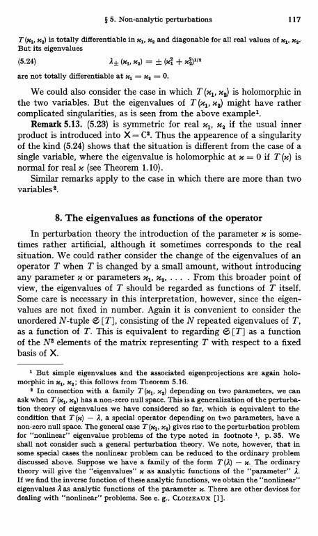
§ 5. Non-analytic perturbations 117
T (xl, x2) is totally differentiable in xl, x2 and diagonable for all real values of xl, xQ:But its eigenvalues
(5.24) R f (MI, xa) (xi + x22)1/2
are not totally differentiable at xl = xQ = 0.
We could also consider the case in which T (xl, x2) is holomorphic inthe two variables. But the eigenvalues of T (x1, x2) might have rathercomplicated singularities, as is seen from the above example'.
Remark 5.13. (5.23) is symmetric for real xl, x2 if the usual innerproduct is introduced into X = C2. Thus the appearence of a singularityof the kind (5.24) shows that the situation is different from the case of asingle variable, where the eigenvalue is holomorphic at x = 0 if T (x) isnormal for real x (see Theorem 1.10).
Similar remarks apply to the case in which there are more than twovariables 2.
8. The eigenvalues as functions of the operator
In perturbation theory the introduction of the parameter x is some-times rather artificial, although it sometimes corresponds to the realsituation. We could rather consider the change of the eigenvalues of anoperator T when T is changed by a small amount, without introducingany parameter x or parameters xl, x2, ... . From this broader point ofview, the eigenvalues of T should be regarded as functions of T itself.Some care is necessary in this interpretation, however, since the eigen-values are not fixed in number. Again it is convenient to consider theunordered N-tuple a [T], consisting of the N repeated eigenvalues of T,as a function of T. This is equivalent to regarding 6 [T] as a functionof the N2 elements of the matrix representing T with respect to a fixedbasis of X.
1 But simple eigenvalues and the associated eigenprojections are again holo-morphic in xl, xa; this follows from Theorem 5.16.
9 In connection with a family T (xl, x2) depending on two parameters, we canask when T (xl, x9) has a non-zero null space. This is a generalization of the perturba-tion theory of eigenvalues we have considered so far, which is equivalent to thecondition that T (m) - R, a special operator depending on two parameters, have anon-zero null space. The general case T (%I, x9) gives rise to the perturbation problemfor "nonlinear" eigenvalue problems of the type noted in footnote 1, p. 35. Weshall not consider such a general perturbation theory. We note, however, that insome special cases the nonlinear problem can be reduced to the ordinary problemdiscussed above. Suppose we have a family of the form T (A) - x., The ordinarytheory will give the "eigenvalues" x as analytic functions of the "parameter" A.If we find the inverse function of these analytic functions, we obtain the "nonlinear"eigenvalues A as analytic functions of the parameter x. There are other devices fordealing with "nonlinear" problems. See e. g., CLOIZEAUX [1].
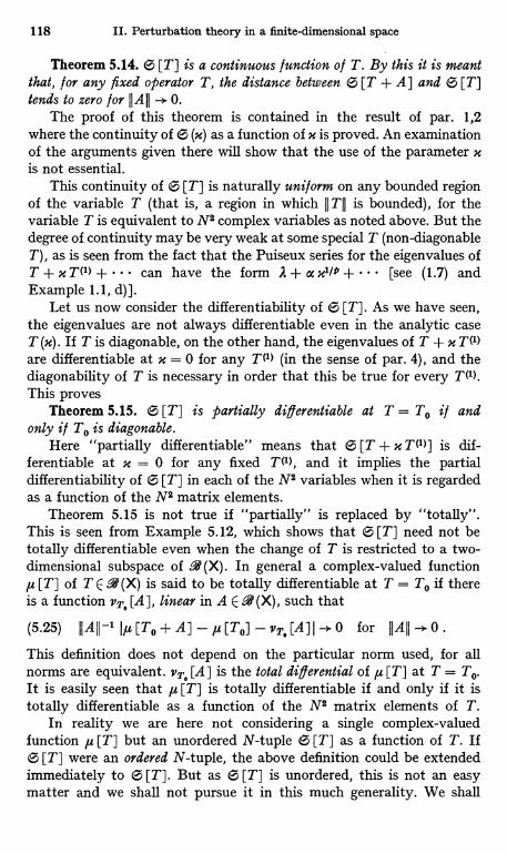
118 II. Perturbation theory in a finite-dimensional space
Theorem 5.14. 6 [T] is a continuous function of T. By this it is meantthat, for any fixed operator T, the distance between 6 [T + A] and 6 [T]tends to zero for 11 All -+ 0.
The proof of this theorem is contained in the result of par. 1,2where the continuity of 6 (x) as a function of x is proved. An examinationof the arguments given there will show that the use of the parameter xis not essential.
This continuity of e [T] is naturally uniform on any bounded regionof the variable T (that is, a region in which 11 T11 is bounded), for thevariable T is equivalent to N2 complex variables as noted above. But thedegree of continuity may be very weak at some special T (non-diagonableT), as is seen from the fact that the Puiseux series for the eigenvalues ofT + x TM + can have the form 2 + a xl/Q + [see (1.7) andExample 1.1, d) ].
Let us now consider the differentiability of e [T]. As we have seen,the eigenvalues are not always differentiable even in the analytic caseT (x). If T is diagonable, on the other hand, the eigenvalues of T + x TMare differentiable at x = 0 for any T(') (in the sense of par. 4), and thediagonability of T is necessary in order that this be true for every TM.This proves
Theorem 5.15. e [T] is partially differentiable at T = To if andonly if To is diagonable.
Here "partially differentiable" means that 6 [T + x TM] is dif-ferentiable at x = 0 for any fixed TM, and it implies the partialdifferentiability of 6 [T] in each of the N2 variables when it is regardedas a function of the N2 matrix elements.
Theorem 5.15 is not true if "partially" is replaced by "totally".This is seen from Example 5.12, which shows that 6 [T] need not betotally differentiable even when the change of T is restricted to a two-dimensional subspace of gi(X). In general a complex-valued function,u [T] of T E 9 (X) is said to be totally differentiable at T = To if thereis a function vTa [A], linear in A E 9 (X), such that
(5.25) IIAII-1Iu[To+A]-p[To]-VT,[A]I-+0 for IIAil--0.This definition does not depend on the particular norm used, for allnorms are equivalent. vTa [A] is the total differential of ,u [T] at T = To.It is easily seen that y [T] is totally differentiable if and only if it istotally differentiable as a function of the N2 matrix elements of T.
In reality we are here not considering a single complex-valuedfunction u [T] but an unordered N-tuple e [T] as a function of T. If6 [T] were an ordered N-tuple, the above definition could be extendedimmediately to 6 [T]. But as 6 [T] is unordered, this is not an easymatter and we shall not pursue it in this much generality. We shall
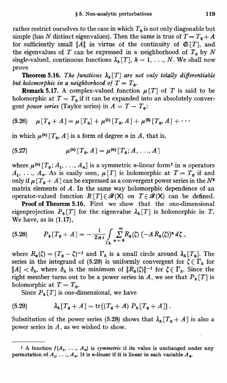
§ 5. Non-analytic perturbations 119
rather restrict ourselves to the case in which T. is not only diagonable butsimple (has N distinct eigenvalues). Then the same is true of T = To+ Afor sufficiently small IIAII in virtue of the continuity of e [T], andthe eigenvalues of, T can be expressed in a neighborhood of T. by Nsingle-valued, continuous functions Ah [T], h = 1, ..., N. We shall nowprove
Theorem 5.16. The functions Ah [T] are not only totally differentiablebut holomorphic in a neighborhood of T = To.
Remark 5.17. A complex-valued function ,u [T] of T is said to beholomorphic at T = To if it can be expanded into an absolutely conver-gent power series (Taylor series) in A = T - To:
(5.26) µ[T0+A]=µ[To]+µ(')[To,A]+µ(2)[To,A]+...
in which p(n) [To, A] is a form of degree n in A, that is,
(5.27) p0"l [TO, A] = µ("l [TO; A, ..., A]
where ,u(') [To; A,, ..., An] is a symmetric n-linear form' in n operatorsA,, ..., An. As is easily seen, ,u [T] is holomorphic at T = To if andonly if ,u [To + A] can be expressed as a convergent power series in the N2matrix elements of A. In the same way holomorphic dependence of anoperator-valued function R [T] E M (X) on TERN can be defined.
Proof of Theorem 5.16. First we show that the one-dimensionaleigenprojection Ph [T] for the eigenvalue Ah [T] is holomorphic in T.We have, as in (1.17),
(5.28) Ph[To+A] f £Ro(C) (-ARo(C))ndC,I,h n=0
where R0(C) = (To - C)-' and Ph is a small circle around Ah [To]. Theseries in the integrand of (5.28) is uniformly convergent for C E Ph forII A ( I < 6h, where Sh is the minimum of I I Ro (C) I I -1 for C E Ph. Since theright member turns out to be a power series in A, we see that Ph [T] isholomorphic at T = To.
Since Ph [T] is one-dimensional, we have
(5.29) A,[To+A]=tr{(To+A) Ph[To+A]}.
Substitution of the power series (5.28) shows that Ah [To + A] is also apower series in A, as we wished to show.
1 A function I (A, ..., is symmetric if its value is unchanged under anypermutation of A1, ..., A. It is n-linear if it is linear in each variable Ax.
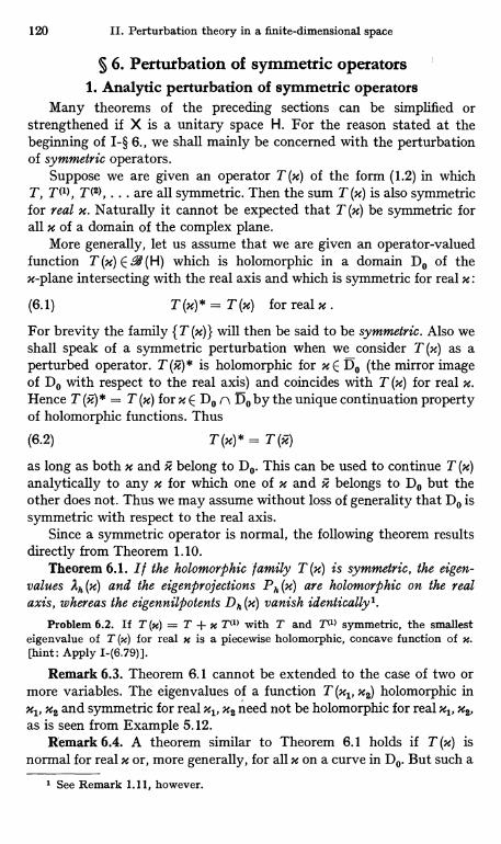
120 II. Perturbation theory in a finite-dimensional space
§ 6. Perturbation of symmetric operators1. Analytic perturbation of symmetric operators
Many theorems of the preceding sections can be simplified orstrengthened if X is a unitary space H. For the reason stated at thebeginning of I-§ 6., we shall mainly be concerned with the perturbationof symmetric operators.
Suppose we are given an operator T (m) of the form (1.2) in whichT, TO'), T(2), ... are all symmetric. Then the sum T (m) is also symmetricfor real x. Naturally it cannot be expected that T (m) be symmetric forall x of a domain of the complex plane.
More generally, let us assume that we are given an operator-valuedfunction T (x) E . (H) which is holomorphic in a domain Do of thex-plane intersecting with the real axis and which is symmetric for real x:
(6.1) T (x)* = T (m) for real x .
For brevity the family {T (x)} will then be said to be symmetric. Also weshall speak of a symmetric perturbation when we consider T (m) as aperturbed operator. T (x)* is holomorphic for x E Do (the mirror imageof Do with respect to the real axis) and coincides with T (m) for real x.Hence T (r.) * = T (x) for x E Do n Do by the unique continuation propertyof holomorphic functions. Thus
(6.2) T()* = T (R)
as long as both x and x belong to Do. This can be used to continue T (x)analytically to any x for which one of x and x belongs to Do but theother does not. Thus we may assume without loss of generality that Do issymmetric with respect to the real axis.
Since a symmetric operator is normal, the following theorem resultsdirectly from Theorem 1.10.
Theorem 6.1. I l the holomorphic family T (x) is symmetric, the eigen-values Ah (x) and the eigenprojections Ph (x) are holomorphic on the realaxis, whereas the eigennilpotents Dh (x) vanish identically'.
Problem 6.2. If T (m) = T + x Tx'> with T and Ti1> symmetric, the smallesteigenvalue of T (m) for real x is a piecewise holomorphic, concave function of X.[hint: Apply I-(6.79)].
Remark 6.3. Theorem 6.1 cannot be extended to the case of two ormore variables. The eigenvalues of a function T (xl, x2) holomorphic inxl, x2 and symmetric for real xl, xa need not be holomorphic for real x,, x2,as is seen from Example 5.12.
Remark 6.4. A theorem similar to Theorem 6.1 holds if T (m) isnormal for real x or, more generally, for all x on a curve in Do. But such a
1 See Remark 1.11, however.
§ 6. Perturbation of symmetric operators 121
theorem is of little practical use, since it is not easy to express the condi-tion in terms of the coefficients T(') of (1.2).
The calculation of the perturbation series given in § 2 is also simplifiedin the case of a symmetric perturbation. Since the unperturbed operator Tis symmetric, any eigenvalue . of T is semisimple (D = 0) and thereduction process described in § 2.3 is effective. The operator functionTM (u) given by (2.37) is again symmetric, for P (x) is symmetric andcommutes with T (x). The reduction process preserves symmetry. Therefore,the reduction can be continued indefinitely. The splitting of the eigen-values must come to an end after finitely many steps, however, and theeigenvalues and the eigenprojections are finally given explicitly by theformulas corresponding to (2.5) and (2.3) in the final stage of the reduc-tion process where the splitting has ceased to occur. In this way thereduction process gives a complete recipe for calculating explicitly theeigenvalues and eigenprojections in the case of a symmetric perturbation.
Remark 6.5. Again there is no general criterion for deciding whetherthere is no further splitting of the eigenvalue at a given stage. But thereducibility principle given in Remark 2.4 is useful, especially for sym-metric perturbations. Since the unperturbed eigenvalue at each stage isautomatically semisimple, there can be no further splitting if the un-perturbed eigenprojection at that stage is irreducible with respect to aset {A} of operators.
In applications such a set {A} is often given as a unitary group underwhich T (x) is invariant. Since the eigenprojection under considerationis an orthogonal projection, it is irreducible under {A} if and only ifthere is no proper subspace of the eigenspace which is invariant under allthe unitary operators A.
Remark 6.6. The general theory is simplified to some extent even ifonly the unperturbed operator T is symmetric or even normal. Forexample, all the eigenvalues 2h (x) are then continuously differentiable atx = 0 in virtue of the diagonability of T (Theorem 2.3). The estimatesfor the convergence radii and the error estimates are also simplified if theunperturbed operator T is symmetric or normal, as has been shown in§ 3.5.
Remark 6.7. The estimate (3.52) is the best possible of its kind evenin the special case of a symmetric perturbation, for Example 3.10 belongsto this case.
2. Orthonormal families of eigenvectorsConsider a holomorphic, symmetric family T (x). For each real x
there exists an orthonormal basis {97.(u)} of H consisting of eigenvectorsof T (m) [see I-(6.68)]. The question arises whether these orthonormaleigenvectors cvri (x) can be chosen as holomorphic functions o l x. The answeris yes for real x.
122 II. Perturbation theory in a finite-dimensional space
Since the eigenvalues ;Lh (x) and the eigenprojections Ph (x) areholomorphic on the real axis (Theorem 6.1), the method of § 4.5 can beapplied to construct a holomorphic transformation function U (M)satisfying (4.30). Furthermore, U (x) is unitary for real x. To see thiswe recall that U (x) was constructed as the solution of the differentialequation U' = Q (x) U with the initial condition U (0) = 1, where Q (x)is given by (4.33). Since the Ph (x) are symmetric, we have Ph (x) * = Ph (x)as in (6.2) and so the same is true of P n (x) . Hence Q (x) is skew-symmetric :Q (x) * _ - Q (x) and U (x) * satisfies the differential equation
(6.3) ax UN)* U(9)* QM
On the other hand, V(x) = U(m)-1 satisfies the differential equationV' = - V Q (x) with the initial condition V (0) = 1. In view of theuniqueness of the solution we must have
(6.4) U (x) * = U (M)_1 .
This shows that U (x) is unitary for real x.It follows that the basis qh h (x) = U (M) Th h as given by (4.31) is
orthonormal for real x if the 9hh form an orthonormal basis (which ispossible since T is symmetric). It should be noted that the g7hk(x) are(not only generalized but proper) eigenvectors of T (m) because T (m)is diagonable. The existence of such an orthonormal basis dependingsmoothly on x is one of the most remarkable results of the analyticperturbation theory for symmetric operators. That the analyticity isessential here will be seen below.
3. Continuity and differentiabilityLet us now consider non-analytic perturbations of operators in H.
Let T (x) E .4 (H) depend continuously on the parameter x, which willnow be assumed to be real. The eigenvalues of T (n) then depend on xcontinuously, and it is possible to construct N continuous functionsyn (x), n = 1, ..., N, representing the repeated eigenvalues of T (x)(see § 5.2). In this respect there is nothing new in the special case whereT (x) is symmetric, except that all Iu (x) are real-valued and so a simplenumbering such as (5.4) could also be used.
A new result is obtained for the differentiability of eigenvalues.Theorem 6.8.1 Assume that T (m) is symmetric and continuously
differentiable in an interval I of x. Then there exist N continuously dif-ferentiable functions 4u,,(x) on I that represent the repeated eigenvalues ofT (x).
1 This theorem is due to RELUcx [8]. Recall that the result of this theoremis not necessarily true for a general (non-symmetric) perturbation (see Remark 5.8).
§ 6. Perturbation of symmetric operators 123
Proof. The proof of this theorem is rather complicated'. Consider afixed value of x; we may set x = 0 without loss of generality. Let A beone of the eigenvalues of T = T (O), m its multiplicity, and P the as-sociated eigenprojection. Since A is semisimple, the derivatives at x = 0of the repeated eigenvalues of T (x) belonging to the A-group are given bythe m repeated eigenvalues of P T' (0) P in the subspace M = P X(Theorem 5.4). Let A,, ..., Ap be the distinct eigenvalues of PT'(0) Pin M and let Pl, ..., P, be the associated eigenprojections. The M; = Pf Hare subspaces of M. It follows from the above remark that the A-group(repeated) eigenvalues of T (x) for small Ix I + 0 are divided into psubgroups, namely the A + x A;-groups, j = 1, ..., p. Since each of thesesubgroups is separated from other eigenvalues, the total projections P, (x)for them are defined. Pi (x) is at the same time the total projection forthe A;-group of the operator TM (x) given by (5.14). But TV') (x) iscontinuous in a neighborhood of x = 0 as was shown there (the continuityfor x + 0 is obvious). Hence P, (x) is continuous in a neighborhood ofx = 0 by Theorem 5.1, and the same is true of
(6.5) T; (x) = P; (x) T' (x) P; (x)
because T' (x) = d T (x)/dx is continuous by hypothesis.The A + x A;-group of T (x) consists in general of several distinct
eigenvalues, the number of which may change 'discontinuously with xin any neighborhood of x = 0. Let A (xo) be one of them for x = xo + 0and let Q (xo) be the associated eigenprojection. This A (xo) may furthersplit for small Ix - xoI + 0, but the derivative of any of the resultingeigenvalues must be an eigenvalue of Q (xo) T' (xo) Q (xo) in the subspaceQ (xo) H (again by Theorem 5.4). But we have Q (xo) H c P; (xo) H becauseA (xo) belongs to the A + x A;-group, so that Q (xo) T' (xo) Q (xo)= Q (xo) Tf (xo) Q (xo). Therefore, the derivatives under consideration areeigenvalues of the orthogonal projection (in the sense of I-§6.10) of theoperator T; (xo) on a certain subspace of M5 (xo) = PS (xo) H. Since T5 (xo)is symmetric, it follows from Theorem 1-6.46 that these eigenvalues liebetween the largest and the smallest eigenvalues of T5 (xo) in the subspaceM5 (xo). But as T; (x) is continuous in x as shown above, the eigenvaluesof T; (xo) in M5 (xo) tend for xo --> 0 to the eigenvalues of PS T' (0) P; in M5,which are all equal to A;. It follows that the derivatives of the A + X A;-group eigenvalues of T (x) must also tend to A; for x --> 0. This provesthe required continuity of the derivatives of the eigenvalues ,U,, (x) con-structed by Theorem 5.6. [In the above proof, essential use has been madeof the symmetry of T (x) in the application of Theorem 1-6.46. This ex-plains why the same result does not necessarily hold in the general case].
1 The original proof due to RELLICH is even longer.
124 II. Perturbation theory in a finite-dimensional space
Remark 6.9. As in the general case, the eigenprojections or eigen-vectors have much less continuity than the eigenvalues even in the caseof a symmetric perturbation, once the assumption of analyticity isremoved. Example 5.3 is sufficient to illustrate this; here the functionT (x) is infinitely differentiable in x and symmetric (by the usual innerproduct in C2), but it is impossible to find eigenvectors of T (M) that arecontinuous at x = 0 and do not vanish there.
4. The eigenvalues as functions of the symmetric operatorAs in § 5.8, we can regard the eigenvalues of a symmetric operator T
as functions of T itself. As before, the eigenvalues are continuous func-tions of T in the sense explained there. The situation is however muchsimpler now because we can, if we desire, regard the repeated eigenvaluesas forming an ordered N-tuple by arranging them in the ascending order
(6.6) lq [T] < u2 [T] < ... < fcN [ T]
This defines N real-valued functions of T, T varying over all symmetricoperators in H. The continuity of the eigenvalues is expressed by thecontinuity of these functions (T' - T implies u [T'] --- 4u,, [T]).
The numbering (6.6) of the eigenvalues is very simple but is notalways convenient, for the ,u [T] are not necessarily even partiallydifferentiable. This is seen, for example, by considering the u [T + x T']as functions of x, where T, T' are symmetric and n is real. The eigenvaluesof T + x T' can be represented as holomorphik functions of x (Theorem6.1). The graphs of these functions may cross each other at some valuesof x (exceptional points). If such a crossing takes place, the graph of,u,, [T + x T'] jumps from one smooth curve to another, making a cornerat the crossing point. In other words, the ,u,, [T + x T'] are continuousbut not necessarily differentiable. In any case, they are piecewise holo-morphic, since there are only a finite number of crossing points (excep-tional points) in any finite interval of x.
Thus it is sometimes more convenient to return to the old point ofview of regarding the repeated eigenvalues of T as elements of an un-ordered N-tuple 6 [T]. Then it follows from the result of the precedingparagraph that 6 [T] is partially continuously differentiable. But 6 [T]is totally differentiable only at those T with N distinct eigenvalues(again Example 5.12). In the neighborhood of such a T, however, thefunctions (6.6) are not only differentiable but holomorphic in T.
5. Applications. A theorem of LmsKnPerturbation theory is primarily interested in small changes of the
various quantities involved. Here we shall consider some problems
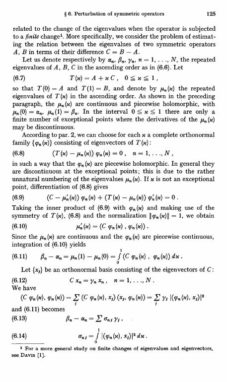
§ 6. Perturbation of symmetric operators 125
related to the change of the eigenvalues when the operator is subjectedto a finite change'. More specifically, we consider the problem of estimat-ing the relation between the eigenvalues of two symmetric operatorsA, B in terms of their difference C = B - A.
Let us denote respectively by an, fl, yn, n = 1, ..., N, the repeatedeigenvalues of A, B, C in the ascending order as in (6.6). Let
(6.7) T(x)=A+xC, 0<x< 1,so that T (0) =A and T (1) = B, and denote by 1u,a(x) the repeatedeigenvalues of T (m) in the ascending order. As shown in the precedingparagraph, the µn (x) are continuous and piecewise holomorphic, withµ5(0) = an, µn(1) = Nn. In the interval 0 < x <_ 1 there are only afinite number of exceptional points where the derivatives of the µn (x)may be discontinuous.
According to par. 2, we can choose for each x a complete orthonormalfamily {qqn (x)} consisting of eigenvectors of T (x) :
(6.8) (T (x) - ,un (x)) 99n (x) = 0 , n = 1, ..., N,in such a way that the 99n (x) are piecewise holomorphic. In general theyare discontinuous at the exceptional points; this is due to the ratherunnatural numbering of the eigenvalues µ,, (x). If x is not an exceptionalpoint, differentiation of (6.8) gives
(6.9) (C - Jun (x)) wn (x) + (T (x) - µn (x)) 92n (x) = 0 .
Taking the inner product of (6.9) with qn (x) and making use of thesymmetry of T(x), (6.8) and the normalization (x) = 1, we obtain
(6.10) run (x) = (C 9qn (x) , 92n (x))
Since the µn (x) are continuous and the 99n (x) are piecewise continuous,integration of (6.10) yields
Q i
(6.11) Nn - an = lun(1) - gun(0) = f (C Tn(x) , 9gn(x)) dx .0
Let {x5} be an orthonormal basis consisting of the eigenvectors of C :
(6.12) Cxn=ynxn, n= 1,...,N.We have
(C 99n (x), 9?n (x)) _ (C Tn (x), x1) (x1, 99n (x)) _ Ys 1(99n (x), xs) I'i i
and (6.11) becomes(6.13) fin - an= r a'nJYJ,
1
(6.14) 1=f I(9pn(x),x1)1adx0
1 For a more general study on finite changes of eigenvalues and eigenvectors,see DAvis [1].
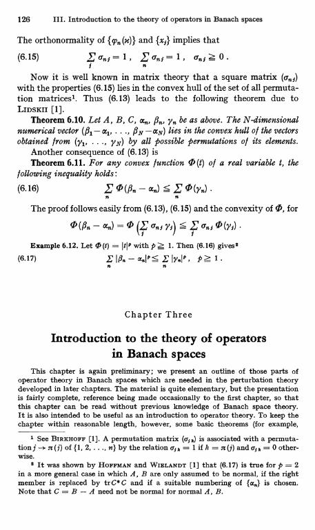
126 III. Introduction to the theory of operators in Banach spaces
The orthonormality of {'p (u)} and {xj} implies that
(6.15) anj=1, L.'anj=1, anjz0.j n
Now it is well known in matrix theory that a square matrix (anj)with the properties (6.15) lies in the convex hull of the set of all permuta-tion matrices'. Thus (6.13) leads to the following theorem due toLIDSKII [1].
Theorem 6.10. Let A, B, C, an, fl, yn be as above. The N-dimensionalnumerical vector (f31-al, ..., NN-aN) lies in the convex hull of the vectorsobtained from (y,,, ..., yN) by all possible permutations of its elements.
Another consequence of (6.13) isTheorem 6.11. For any convex function 0(t) of a real variable t, the
following inequality holds :
(6.16) E 0 (QQtin. - an) S (Yn)n
The proof follows easily from (6.13), (6.15) and the convexity of 0, for
an)anjYjf S I anj0 (y1)Example 6.12. Let 0 (t) = ItIo with p Z 1. Then (6.16) gives2
(6.17) I7n19. pz i.n
Chapter Three
Introduction to the theory of operatorsin Banach spaces
This chapter is again preliminary; we present an outline of those parts ofoperator theory in Banach spaces which are needed in the perturbation theorydeveloped in later chapters. The material is quite elementary, but the presentationis fairly complete, reference being made occasionally to the first chapter, so thatthis chapter can be read without previous knowledge of Banach space theory.It is also intended to be useful as an introduction to operator theory. To keep thechapter within reasonable length, however, some basic theorems (for example,
1 See BIRKHOFF [1]. A permutation matrix (ajI,) is associated with a permuta-tion j .- n (j) of {1, 2, ..., n} by the relation aj n = 1 if k = n (j) and aj R = 0 other-wise.
2 It was shown by HOFFMAN and WIELANDT [1] that (6.17) is true for p = 2in a more general case in which A, B are only assumed to be normal, if the rightmember is replaced by trC* C and if a suitable numbering of is chosen.Note that C = B - A need not be normal for normal A, B.
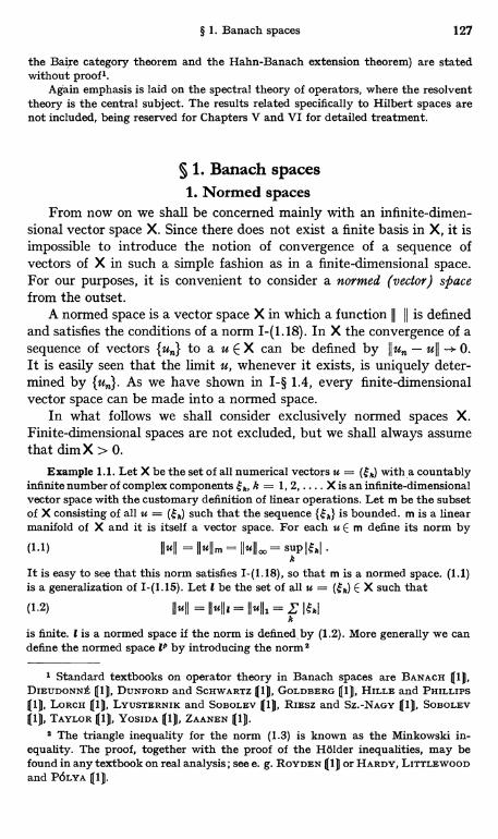
§ 1. Banach spaces 127
the Baire category theorem and the Hahn-Banach extension theorem) are statedwithout proof I.
Again emphasis is laid on the spectral theory of operators, where the resolventtheory is the central subject. The results related specifically to Hilbert spaces arenot included, being reserved for Chapters V and VI for detailed treatment.
§ 1. Banach spaces1. Normed spaces
From now on we shall be concerned mainly with an infinite-dimen-sional vector space X. Since there does not exist a finite basis in X, it isimpossible to introduce the notion of convergence of a sequence ofvectors of X in such a simple fashion as in a finite-dimensional space.For our purposes, it is convenient to consider a normed (vector) spacefrom the outset.
A normed space is a vector space X in which a function is definedand satisfies the conditions of a norm I-(1.18). In X the convergence of asequence of vectors {un} to a u E X can be defined by Iiu,, - ull -* 0.It is easily seen that the limit u, whenever it exists, is uniquely deter-mined by {u,,}. As we have shown in I-§ 1.4, every finite-dimensionalvector space can be made into a normed space.
In what follows we shall consider exclusively normed spaces X.Finite-dimensional spaces are not excluded, but we shall always assumethat dim X > 0.
Example 1.1. Let X be the set of all numerical vectors u = (gk) with a countablyinfinite number of complex components gk, k = 1, 2, .... X is an infinite-dimensionalvector space with the customary definition of linear operations. Let m be the subsetof X consisting of all u = such that the sequence {ik} is bounded. m is a linearmanifold of X and it is itself a vector space. For each u E m define its norm by
(1.1) IIuII = 11'11M = IIHIIoo = sup Iklk
It is easy to see that this norm satisfies I-(1.18), so that m is a normed space. (1.1)is a generalization of I-(1.15). Let l be the set of all u = (6') E X such that
(1.2) IIuDI = IIUIII = IIuII1 = L+ INk
is finite. I is a normed space if the norm is defined, by (1.2). More generally we candefine the normed space P by introducing the norm2
1 Standard textbooks on operator theory in Banach spaces are BANACH Qlf,DIEUDONNE Q11, DUNFORD and SCHWARTZ Q11, GOLDBERG 111, HILLE and PHILLIPS(1), LORCH (1), LYUSTERNIK and SOBOLEV 111, RIESZ and Sz.-NAGY 111, SOBOLEV(1), TAYLOR (11, YOSIDA 111, ZAANEN (1).
2 The triangle inequality for the norm (1.3) is known as the Minkowski in-equality. The proof, together with the proof of the HSlder inequalities, may befound in any textbook on real analysis; see e. g. RoYDEN Ql) or HARDY, LITTLEWOODand PGLYA 11).

128 III. Introduction to the theory of operators in Banach spaces
(1.3) IIuII = Ilullzp =IIuII, = ILr 1U11 \1"D
where p is a fixed number with p > 1. m can b` a regarded as the limiting case of lDfor p -+ oo, and is also denoted by 1°O. P is a proper subset of IQ if p < q.
Example 1.2. The most important examples of normed spaces are functionspaces. The simplest example of a function space is the set C [a, b] of all complex-valued, continuous functions u = u (x) on a finite closed interval [a, b]1 of a realvariable (see Example 1-1.2). C [a, b] is a normed space if the norm is defined by(1.4) IIuII = IIuIIC[a,b] = IIuII =as x lu(x)I
More generally, the set C (E) of all continuous functions u = u (x) = u (x1, ..., xm)defined on a compact region E in the m-dimensional space R"' (or, more generally,on any compact topological space E) is a normed space if the norm is defined by(1.5) (lull = IIuIIc(E) = IIuII = m E Iu(x)I
Example 1.3. We could introduce other norms in C [a, b], for example(1.6) (lull =IIUIIt,=IIuII,=(flu(x)lldx)1I1 pz 1.This would make C [a, b] into a different normed space. Actually a wider class offunctions can be admitted when the norm (1.6) is used. We denote by LP (a, b) theset of all complex-valued, Lebesgue-measurable functions u = u (x) on a finite orinfinite interval (a, b) for which the integral (1.6) is finite. It can be shown thatL1 (a, b) is a normed space by the customary definition of linear operations and bythe norm (1.6). It should be remarked that in L1 (a, b), any two functions u, vare identified whenever they are equivalent in the sense that u (x) = v (x) almosteverywhere in (a, b) ; this convention makes the first condition of I-(1.18) satisfied 2.
More generally, for any measurable subset E of R" the set L9 (E) of all Lebesgue-measurable functions u = u (x) = u (x1, ..., xm) on E such that (1.6) is finite is anormed space if the norm is defined by (1.6). Again two equivalent functions shouldbe identified. In the limiting case p --> oo, L1 (E) becomes the space L°O (E) = M (E)consisting of all essentially bounded functions on E with the norm(1.7) Ilull = IIuJIM(E) = IIulh = ess s plu(x)I
zEEIn other words, IIuII. is the smallest number M such that lu(x)I S M almost every-where in E.
In the same way, we can define the space L9 (E, d µ) over any set E on which a(x)1111.measure d y is defined $, the norm being given by (flu (x) 11 d y
E IExample 1.4. Let C' [a, b] be the set of all continuously differentiable functions
on a finite closed interval [a, b]. C' [a, b] is a normed space if the norm is defined by(1.8) hull = (lull. + Ilu'll.where llull°° is given by (1.4) and u' = du/dx.
1 We denote by [a, b] a closed interval, by (a, b) an open interval, by [a, b)a semi-closed interval, etc.
9 In this sense L1 is a set of equivalence classes of functions rather than a setof functions. But it is customary to represent an element of L1 by a function, withthe identification stated in the text.
8 When we consider function spaces like L1, we have to assume that thereader is familiar with the basic facts on real analysis, including Lebesgue integra-tion, for which we may refer to standard textbooks (e. g., ROYDEN (11). In mostcases, however, it is restricted to examples, and the main text will be readablewithout those prerequisites.
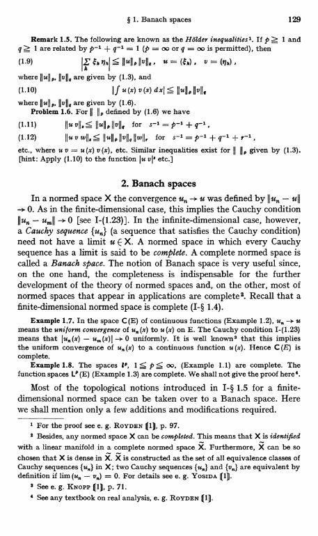
§ 1. Banach spaces 129
Remark 1.5. The following are known as the Holder inequalities 1. If p > 1 andq Z 1 are related by p-1 + q-1 = 1 (p = no or q = no is permitted), then
(1.9) IL k nkl S Hull Hulls , u = ( k) , v = (17k)
where llulln+ llvll5 are given by (1.3), and
(1.10) I f u (x) v (x) dxl 5 Ilully Ilv1IQ
where Only, Ilvl15 are given by (1.6).Problem 1.6. For 11 Ilp defined by (1.6) we have
(1.11) Ilu vll. S (lull., llvllc for s-1 = p-1 + q-1,
(1.12) Il u v -11. :&- llulln IlvllQ llwll, for s-1 = p-1 + q-1 + -I,etc., where u v = u (x) v (x), etc. Similar inequalities exist for Il IID given by (1.3).[hint: Apply (1.10) to the function lu vl' etc.]
2. Banach spacesIn a normed space X the convergence u,, -+ u was defined by lIu - ull
- 0. As in the finite-dimensional case, this implies the Cauchy conditionl1u,, - u,nll -;,. 0 [see I-(1.23)]. In the infinite-dimensional case, however,a Cauchy sequence {u,,} (a sequence that satisfies the Cauchy condition)need not have a limit u E X. A normed space in which every Cauchysequence has a limit is said to be complete. A complete normed space iscalled a Banach space. The notion of Banach space is very useful since,on the one hand, the completeness is indispensable for the furtherdevelopment of the theory of normed spaces and, on the other, most ofnormed spaces that appear in applications are complete2. Recall that afinite-dimensional normed space is complete (I-§ 1.4).
Example 1.7. In the space C (E) of continuous functions (Example 1.2), u -+ umeans the uniform convergence of u. (%) to u (x) on E. The Cauchy condition I-(1.23)means that 1u. (x) - u, (x) I -a 0 uniformly. It is well known3 that this impliesthe uniform convergence of u (x) to a continuous function u(%). Hence C (E) iscomplete.
Example 1.8. The spaces l9, 1S PS no, (Example 1.1) are complete. Thefunction spaces L9 (E) (Example 1.3) are complete. We shall not give the proof here4.
Most of the topological notions introduced in I-§ 1.5 for a finite-dimensional normed space can be taken over to a Banach space. Herewe shall mention only a few additions and modifications required.
1 For the proof see e. g. ROYDEN Q11, p. 97.8 Besides, any normed space X can be completed. This means that X is identified
with a linear manifold in a complete normed space X. Furthermore, X can be sochosen that X is dense in X. X is constructed as the set of all equivalence classes ofCauchy sequences in X; two Cauchy sequences and are equivalent bydefinition if lim (u - 0. For details see e. g. YOSIDA 11).
8 See e. g. KxoPp (1), p. 71.See any textbook on real analysis, e. g. RoYDEN (1).
130 III. Introduction to the theory of operators in Banach spaces
A linear manifold M of a Banach space X need not be closed. A closedlinear manifold M of X is itself a Banach space. In this sense it is asubspace of X. The closure of a linear manifold is a closed linear manifold.
Lemma 1.9. 1/ M is a closed linear manifold, the linear manifold M'spanned by M and a finite number of vectors ul, ..., u," is closed.
Proof. It suffices to consider the case m = 1; the general case isobtained by successive application of this special case. If ul E M, we haveM' = M so that M' is closed. If ul I M, we have dist (ul, M) = d > 0,because M is closed. M' is the set of all u' of the form u' _ ul + v,v E M. We have(1.13) IEI s Il u'IVd .
In fact, u'll = 1lul + -1 v d if r 0 while (1.13) is trivial ifE=0.
Suppose now that u;, E M', u;, -+ u', n - oo; we have to show thatu' E M'. Let u,, _ " u1 + vn, v a E M. Application of (1.13) to u' = u, - u;,,gives 11 u;, - u' 11 Id -+ 0. Hence for some E, andv = u;, - ul - u' - ul. Since M is closed and v,, E M, v = u' -- ul E M. Hence u' _ ul + v E M' as required.
For any subset S of X, there is a smallest closed linear manifoldcontaining S (that is, a closed linear manifold M such that any closedlinear manifold M'D S contains M). It is equal to the closure of the(linear) span of S, and is called the closed linear manifold spanned by Sor simply the closed span of S.
Example 1.10. In E9 the set of all u = (fix) with sl = 0 is a closed linear manifold.In 100 the set c of all u = ($x) such that lim $,, _ $ exists is a closed linear manifold.The subset co of c consisting of all u such that $ = 0 is a closed linear manifold of100 and of c. In C [a, b] the set of all functions u (x) such that u (a) = 0 is a closedlinear manifold. The same is true of the set of u such that u (a) = u (b) = 0. C [a, b]itself may be considered a closed linear manifold of L00 (a, b).
A subset S of X is (everywhere) dense if the closure S coincides with X.In this case each u E X can be approximated by an element of S, in thesense that for any e > 0 there is a v E S such that 1ju - vjj < e. Moregenerally, for two subsets S1, Sa of X, S1 is dense with respect to S2 ifg1) S2 (or dense in S2 if S1 C S2 in addition). Then each u E S2 can beapproximated by an element of S1. If S1 is dense with respect to S2 and S2is dense with respect to S3, then S1 is dense with respect to S3.
Example 1.11. In C [a, b] (finite interval) the set of all polynomials is every-where dense (theorem of WEIERSTRASS)1. The same is true for L9 (a, b) for 1 <p <oo.In L9 (a, b) (not necessarily finite interval) the set Co (a, b) of all infinitely differen-tiable functions with compact supports is everywhere dense. If E is an open set of
1 See e. g. RoYDEN (1), p. 150.2 A function has compact support if it vanishes outside a compact set. Thus
u E Co (a, b) if all the d"u/d x" exist and u (x) = 0 except for a < a' S z < b' < b(where a', b' depend on u).
§ 1. Banach spaces 131
R'", the set of all infinitely differentiable functions with compact support in E isdense in LP (E), 1 s p < ool.
Unlike a finite-dimensional normed space, an infinite-dimensionalBanach space X is not locally compact (see I-§ 1.5). Thus X contains abounded sequence {un} that contains no convergent subsequence.{un} is such a sequence if
(1.14) llunll=l, llun - umll z1 for n$m.{un} can be constructed by induction. Suppose that u1, . . ., un have beenconstructed. Let Mn be their span. Then there is a u E X such that1lull = 1 and dist(u, Mn) = 1, as is seen from Lemma 1.12 proved below.It suffices to set un+1 = u.
Lemma 1.12. For any closed linear manifold M + X o l X and anye > 0, there is a u E X such that 1lull = 1 and dist (u, M) > 1 - s. We caneven achieve dist (u, M) = 1 if dim M < oo.
Proof. There is a uo E X not belonging to M, so that dist (uo, M)= d > 0. Hence there is a vo E M such that 11uo - vo11 < d/(1 - --)-Set u1= uo - vo. Then 11u111 < d/(1 - c) and dist (u1, M) = rinf lu1 - vll
= mM 11 uo - vll = dist (uo, M) = d > (1 - c) 11 u111. The required u is obtain-
ed by normalizing ul : u = u1/11u111. If dim M < oo, let uo be as above andlet X. be the linear manifold spanned by M and uo. We can apply theresult, just obtained to the subspace M of X0. Thus there exists a un E Xosuch that 11 unll = 1 and dist (un, M) > 1 - n-1. Since dim Xo < oo,X0 is locally compact and there is a convergent subsequence of {un}.It is easy to see that its limit u satisfies 1lu11 = 1 and dist (u, M) = 1.
A subset S C X is said to be fundamental if the closed span of S is X(in other words, if the span of S is everywhere dense). S is separable if Scontains a countable subset which is dense in S. For the separabilityof X, it is sufficient that X contain a countable subset S' which is funda-mental; for the set of all linear combinations of elements of S' withrational coefficients is a countable set dense in X. A subset of a separableset is separable z.
Example 1.13. C [a, b] is separable; this is a consequence of the theorem ofWEIERSTRASS, for the set of monomials u" (x) = x°, n = 0, 1, ..., is fundamental inC [a, b] (see Example 1.11). i9 is separable if 1 S p < no. The canonical basisconsisting of u = (S" x), n = 1, 2, ..., is fundamental in P. L9 (a, b) is also separableif 1 S p < oo. The set of functions u(,. (z), which is equal to 1 on (a', b') andzero otherwise, is fundamental when a' and b' vary over all rational numbers in(a, b) 8. Similarly L9 (Rm) is separable for 1:5, p < oo. It then follows that L9 (E) is alsoseparable if E is any measurable subset of Rm, for L'(E) may be regarded as thesubspace of L9 (Rm) consisting of all functions vanishing outside E.
1 For the proof see e. g. SOBOLEV (1), p. 13.8 See DUNFORD and SCHWARTZ (1), p. 21.3 This follows from the properties of the Lebesgue integral; see ROYDEN M.
132 III. Introduction to the theory of operators in Banach spaces
An important consequence of the completeness of a Banach spaceis the category theorem of BAIRE':
Theorem 1.14. I l X is the union o l a countable number o l closed subsetsS,,, n = 1, 2, . . ., at least one of the S contains interior points (that is,contains a ball).
In spite of some essential differences in topological structure betweena general Banach space X and a finite-dimensional space, most of theresults regarding sequences infinite series E u and vector-valuedfunctions u (t) stated in I-§ 1.6-7 remain valid in X. Such results will beused freely without comment in the sequel. It should be noted that thecompleteness of X is essential here. For example, the existence of thesum of an absolutely convergent series E u depends on it, and similarlyfor the existence of the integral f u (t) dt of a continuous function u (t).Also we note that the analyticity of a vector-valued function u (t) isdefined and the results of complex function theory are applicable tosuch a function (see loc. cit.). On the other hand, results of I-§ 1 basedon the explicit use of a basis are in general not valid in the general case.
3. Linear formsA linear form f [u] on a Banach space X can be defined as in I-§ 2.1.
But we here consider also linear forms f [u] that are defined only on acertain linear manifold D of X. Such a form f will be called a linearform in X, and D = D (f) will be called the domain of f. f is an extension ofg (and g is a restriction of f) if D (f) ) D (g) and f [u] = g [u] for u E D (g) ;
we write f)gorg(f.f [u] is continuous at u = uo E D if II u - uolJ - . 0, u E D, implies
f f [uo]. Since / [u - u0], it follows that f [u] iscontinuous everywhere in D if and only if it is continuous at u = 0. Suchan f is simply said to be continuous.
In a finite-dimensional space every linear form is continuous. Thisis not true in the general case, though it is not easy to give an exampleof a discontinuous linear form defined everywhere on a Banach space X.
If a linear form f is continuous, there is a S > 0 such that hull < 6implies If [u] I S 1. By homogeneity, it follows that
(1.15) If[u]I S MIIuII for every u E D(f)
where M = 1/6. A linear form / with the property (1.15) is said to bebounded. The smallest number M with this property is called the boundoff and is denoted by 11 /11. It is easy to see that, conversely, (1.15) impliesthat f is continuous. Thus a linear form is continuous if and only if it isbounded.
1 See e. g. RoYDEN (1), p. 121, or any textbook on functional analysis.2 See footnote 3 of p. 133.
§ 1. Banach spaces 133
Lemma 1.15. A bounded linear form / is determined if its values aregiven in a subset D' dense in D (f ).
Proof. For each u E D (f ), there is a sequence un E D' such that un - u.Thus / [u] = lim f [un] by continuity.
Theorem 1.16 (Extension principle). A bounded linear form withdomain D can be extended to a bounded linear form with domain D (theclosure of D). This extension is unique and the bound is preserved in theextension.
Proof. The uniqueness of the extension follows from Lemma 1.15.To construct such an extension, let u ED and let un E D be such thatu,, - u. The f [un] form a Cauchy sequence since I/ [u,,] - / [um] I == I1 [un - um] 11/11 11 un - umll - 0, n, m -+ oo. Let the limit of f [un]be denoted by /'[u]. f' [u] is determined by u independently of thechoice of the sequence {un}, for un u and vn -+ u imply un - vn -+ 0and hence f [u.] - f [v.] = f [u, - vn] -+ 0. It is now easy to show thatf'[u] is a linear form with domain 6. That IIfII = II/II follows from theinequality 1/'[u] I s II/II IIull, which is the limit of 1/[u,,] I < II/II IIunjI.
Example 1.17. In 1P, I S p S oo, consider a linear form f given by(1.16) f [u] = E ak k for u = (k)
k
If we take as D (/) the set of all u E l such that only a finite number of the Sk arenot zero, the coefficients ak are arbitrary. But such an f is in general not bounded.f is bounded if(1.17) M = (Z' Iakla)11c < oo where p-1 + q-1 = 1 .
Then we have if [u]1;5 MIIuJI by the Holder inequality (1.9). In this case we cantake D (f) = 1'; then it can easily be shown that 11 /11 = M. It is further known thatif p < oo any bounded linear form on t9 can be expressed in the form (1.16) with theak satisfying (1.17)1.
Example 1.18. Let X = C [a, b] ; set / [u] = u (xo) for every u E X, with a fixedxo, a S x0 S b [see I-(2.3)]. / is a bounded linear form with domain X. More ge-nerally, let I (x) be a complex-valued function of bounded variation over [a, b].Then the Stieltjes integral
b
(1.18) f [u] = f u (x) d f (x)a
defines a linear form on C [a, b]. / is bounded, for I / [u]I: M IIull where M is thetotal variation off. Hence IIfII S M. Actually it is known that II f II = M, and that anybounded linear form on C [a, b] can be expressed by a function / of bounded varia-tion in the form (1.18) $.
Example 1.19. For each u E C' [a, b] (see Example 1.4) set f [u] = u' (xo).f is a bounded linear form on C' [a, b]. f can also be regarded as a linear form inX = C [a, b] with D (f) = C' [a, b] C X. In this interpretation f is not bounded, forI u' (xo) I may be arbitrarily large for II ull = max Iu (x) I = 1-.
1 See e. g. ROYDEN 111, p. 103, TAYLOR (1), p. 193, YOSIDA 11), p. 117.2 See e. g. TAYLOR (1), p.382.® This f is a simple example of an unbounded linear form, but D(f) is not the
whole space X = C [a, b]. An unbounded linear form with domain X could beobtained by extending f, but it would require the use of the axiom of choice.
134 III. Introduction to the theory of operators in Banach spaces
Example 1.20. For u E L9 (E) and f E Lc (E), P-1 + q-1 = 1, set
(1.19) f [u] = f f (x) u (x) d x.E
For a fixed f, t [u] is a bounded linear form on L9(E) with IIfII S IIfIIc by (1.10).It is known that IIfII = IIfIIc and that any bounded linear form on L9(E), p < oo,can be expressed in the form (1.19) in terms of an f E Lc (E) 1.
4. The adjoint spaceSemilinear forms and bounded semilinear forms in a Banach space X
can be defined in the same way as above (cf. I-§ 2.2). The adjoint space X*of X is defined as the set of all bounded semilinear forms on X, and X*is a normed vector space if the norm of f E X* is defined as the bound11111 of f. As before we introduce the scalar product (f, u) = / [u] for every/ E X* and u E X. The generalized Schwarz inequality I-(2.25) is again aconsequence of the definition of 11/11. Other notions and obvious results ofthe finite-dimensional case will be taken over without further comment.
X* is a Banach space. To prove the completeness of X*, consider aCauchy sequence {fn} in X*. Then
(1.20) I(1n-fm,u)1 < Ilfn-1mlJ (lull -0, n,m -* oo,for every u E X so that lim(fn, u) = / [u] exists. It is easily seen thatf [u] is a semilinear form in u. On letting n -* oo in I (1n, u) 1 S 11&1111 ull
we have I/ [u] 1 < M ll ull, where M = lim 111,2 II < oo since the 111,211 form aCauchy sequence of positive numbers. Thus / is bounded with 11111 < M.Now (1.20) shows for m-. no that l(fn - f, u) 1 s lim 111,2 - fmhI hull or
m-r oo
I11n -1II S lim Il/n -lmll . Hence lim 111,, - fII lim 1I 1n - fmll = 0. Thusm-+oo n--roo n,m-+oo
fn --> / and X* is complete.All these considerations would be of little use if there were no bounded
semilinear forms on X except the trivial form 0. For this reason theHahn-Banach theorem, which assures the existence of "sufficientlymany" bounded linear (or equivalently, semilinear) forms on X, is basicin Banach space theory. We shall state this theorem in a rather restrictedform convenient for our use.
Theorem 1.21. Any bounded linear form in a Banach space X (withdomain D C X) can be extended to a bounded linear form on the whole of Xwithout increasing the bound.
We do not give the proof of this theorems, but we add the followingcomments. If this theorem has been proved for real Banach spaces, thecomplex case can be dealt with by using the method of I-§ 2.5. In thecase of a real space, the theorem admits the following geometric inter-pretation. Let S be the open unit ball of X. The intersection So of S
1 See e. g. ROYDEN (1), p. 103, TAYLOR Q11, p. 382, YOSIDA (11, p. 115.ss See e. g. ROYDEN Q11, p. 162, or any book on functional analysis.
§ 1. Banach spaces 135
with D is the unit ball of D. If there is in D a support hyperplane Moto So (see I-§ 2.5), then there is in X a support hyperplane M to S contain-ing Mo 1.
A consequence of Theorem 1.21 isTheorem 1.22. Let M be a closed linear manifold of X and let u0 E X
not belong to M. Then there is an f E X* such that (/, u0) = 1, (f, u) = 0for u E M and II/II = 1/dist (uo, M).
Proof. Let M' be the span of M and u0. As in the proof of Lemma 1.9,each u E M' has the form u = uo + v, v E M. E is determined by u,so that we can define a function f [u] = on M'. f is obviously semilinearand bounded by (1.13), with IIfII 1/d where d = dist (u0, M). Actually wehave IIfII = 1/d, for there is a u E M' for which IIull = 1 and dist (u, M) >> I - e (apply Lemma 1.12 with X replaced by M') ; for this u we have1 - s < dist (u, M) = dist ( uo + v, M) = 1 I dist (uo, M) = I I d or If [u] I> (1 - e) IIuII/d. This / can now be extended to X preserving the bound.Denoting again by / the extended form, we see easily that the assertionsof the theorem are satisfied.
Corollary 1.23. For any two vectors u v of X, there is an f E X*such that (f, u) + (f, v). Thus X* contains sufficiently many elements todistinguish between elements of X.
Corollary 1.24. For any uo E X, there is an f E X* such that (/, u0)= Iluoll, IIfII =1 [see I-(2.27)].
A consequence of Corollary 1.24 is that I-(2.26) is valid in a generalBanach space:
(1.21) (lull = sup I (t, u) I = sup V, u) I = sup IV, u) IO+/EX* Iltll 1 fl/l=I
Example 1.25. Let u = (k) E P and f = (aA) E It with p-1 + q-1 = 1, 1 < p < oo.For a fixed f, f [u] = £ ak , is a bounded semilinear form on X, and any boundedsemilinear form on X is expressed in this form by an f E 1Q (Example 1.17). For thisreason the adjoint space of P is identified with If, and we write (f, u) = E ak Th.Similarly, the adjoint space of L' (E), 1:!9 p < oo, is identified with LQ (E) wherep-1 + q-1 = 1. We write(1.22) (/,u) = f t (x) T dx , u E L' (E) , t E LQ (E) .
E
The adjoint space of C [a, b] is the space BV [a, b] of all functions / (x) of boundedvariation properly normalized, with the norm IIfII equal to the total variation of f.The scalar product is
b
(1.23) (1,u)= fi(x)df(x), uEC[a,b], fEBV[a,b].a
Problem 1.26. Each finite-dimensional linear manifold M of X has a com-plementary subspace N : X = M $ N. [hint : It suffices to consider the case dim M= 1. Let 0 4 u E M and let f E X*, (f, u) = 1. Let N be the set of all v E X such that(f, v) = 0.]
1 The same is true if the open unit ball is replaced by any open convex subsetof X.

136 III. Introduction to the theory of operators in Banach spaces
The adjoint space X** of X* is again a Banach space. As in thefinite-dimensional case, each u E X may be regarded as an element ofX** (see I-§ 2.6). In this sense we may again write (u, f) = (f, u foru E X and / E X*. This does not imply, however, that X** can be identifiedwith X as in the finite-dimensional case, for there may be semilinear formsF [f] on X* that cannot be expressed in the form (f, u) with a u E X.If there are no such forms F, X is said to be reflexive and X is identifiedwith X**. In general X is identified with a certain subspace of X**.
The results of I-§ 2.6 on annihilators should be modified and sup-plemented accordingly. For any subset S of X, the annihilator Sl is aclosed linear manifold of X* (since the scalar product is a continuousfunction of its arguments). The annihilator S 11 of S 1 is a closed linearmanifold of X** but need not be a subset of X (under the identificationstated above). In any case we have
(1.24) S1I n X = [S]where [S] is the closed span of S. Since S1 1-) S is clear, we have S1 I)
[S]. To prove (1.24), it is therefore sufficient to show that any u E Xnot belonging to [S] does not satisfy (f, u) = 0 for all / E S-L = [S]l.But this is implied by Theorem 1.21.
5. The principle of uniform boundednessThe following are among the basic theorems in Banach space theory.
In what follows X denotes a Banach space.Theorem 1.27. Let {u} be a sequence of vectors of X such that the
numerical sequence {(f, is bounded for each fixed f E X*. Then {u} isbounded: IIunII S M.
Theorem 1.28. Let be a sequence of vectors of X* such that thenumerical sequence {(f,,, u)} is bounded for each fixed u E X. Then isbounded: IIfnII S M.
These are special cases of the following theorem.Theorem 1.29. Let {fix [u]} be a family of nonnegative continuous
functions defined for all u E X such that
(1.25) px [u' + u"] S px [u'] + px [u"]
I/ {px [u]} is bounded for each fixed u, then it is uniformly bounded forIIul! 1.
Proof. Let S. be the set of all u E X such that px [u] S n andpx [-u] S n for all A. The S. are closed since the Px [u] are continuous inu. The assumption implies that for each u E X there is an n such thatPA [u] S n and PA [-u] ;S n for all A. Hence u E S, and X is the union ofthe S,,, n = 1, 2, .... It follows from the category theorem (Theorem 1.14)that at least one S contains a ball K, say with center uo and radius r.
§ 1. Banach spaces 137
Any u E X with IIuII s 2r can be written in the form u = u' - u"with u', u" E K; it suffices to set u' = uo + u/2, u" = ua - u/2. HencePA [u] s PA [u'] + px[-u"] s n -{- n = 2n by (1.25). Thus {P;L [u]} isuniformly bounded for IIull < 2r. If 2r Z 1, this proves the assertion.If 2r < 1, let m be an integer larger than 1/2r. Then lull < 1 impliesllu/mll S 2r so that px [u/m] 5 2n. Repeated application of (1.25) thengives px [u] < 2m n for lull < 1.
To deduce Theorem 1.28 from Theorem 1.29, it suffices to takeP. [u] = I(/., u) I. To deduce Theorem 1.27, we replace the X of Theorem1.29 by X* and set pn [l] = I(/, un) I [note (1.21)].
Problem 1.30. Let f E X* be such that lim (f,,, u) = / [u] exists for all u E X.
Then f E X* and 11f 11 < lim infllt,ll < oo.
6. Weak convergenceA sequence un E X is said to converge weakly if (un, f) converges for
every / E X*. If this limit is equal to (u, f) for some u E X for every f,then {un} is said to converge weakly to u or have weak limit u. We denotethis by the symbol un W u or u = w-limun. It is easily seen that asequence can have at most one weak limit'. To distinguish it from weakconvergence, the convergence un u defined earlier by llun - ull -+ 0is called strong convergence. To stress strong convergence, we sometimeswrite un u or u = s-limun. But in this book convergence will meanstrong convergence unless otherwise stated.
It is obvious that strong convergence implies weak convergence.The converse is in general not true unless X is finite-dimensional.Furthermore, a weakly convergent sequence need not have a weaklimit. If every weakly convergent sequence has a weak limit, X is saidto be weakly complete.
A weakly convergent sequence is bounded. This is an immediate con-sequence of Theorem 1.27. Also we note that
(1.26) lull s lim infllunll for u = w-limun .
This follows from (u, f) = limun, /) where / E X* is such that ll/II = 1,(u, f) = (lull (see Corollary 1.24).
Lemma 1.31. Let un E X be a bounded sequence. In order that un con-verge weakly (to u), it suffices that (un, f) converge (to (u, f)) for all / of afundamental subset S* of X*.
1 Weak convergence is related to the weak topology of X, as strong convergenceis related to the norm topology. In this book we do not need the deeper results onweak topology; the use of the simple notion of weak convergence is sufficient for ourpurposes.
138 III. Introduction to the theory of operators in Banach spaces
Proof. Let D* be the span of S*; D* is dense in X*. Obviously (un, f )converges [to (u, f)] for all / E D*. Let g E X* and s > 0. Since D* isdense in X*, there is an / E D* such that IIg - /11 < e. Since (un, /) con-verges, there is an N such that I (un - un, /) I < e for n, m > N. ThusI (un, g) - (um, g) I s I (un, g - l) I + I (un - um., l) I + I (um, l- g) 1;5 (2M+ 1) sfor n, m > N, where M = sup II unli This shows that (un, g) converges forall g E X*. When (un, /) - (u, /) for / E D*, we can apply the same ar-gument with un - um replaced by un - u to conclude that (un, g) - (u, g)for all g E X*.
The relationship between strong and weak convergence is given byTheorem 1.32. A sequence un E X converges strongly it and only if
{(un, f)} converges uniformly for II/II s 1, / E X*.Proof. The "only if" part follows directly from I (un, f) - (um, f) I s
< II un - umll II/II < 11u,, - umll To prove the "if" part, suppose that (un, f)converges uniformly for II/II < 1. This implies that for any e >,0, thereexists an N such that I (un - um, f) I <--_ a if n, m > N and 11 /11 S 1. Hence
Ilun - umll = supl(un-um,/)I S eforn,m>Nby(1.21).11t;I S 1
Remark 1.33. In Theorem 1.32, it suffices to assume the uniformconvergence of (u,,, f) for all / of a set dense in the unit ball of X*, for(un - u,n, f) I < e for such / implies the same for all / of the unit ball.
Problem 1.34. Let M be a closed linear manifold of X. Then u E M and u --+ uw
imply is E M. [hint: Theorem 1.22.] '
Let us now consider vector-valued functions u (t) of a real or complexvariable t. We have already noticed that the notions of strong continuity,strong differentiability, and strong analyticity of such functions, andthe integrals f u (t) dt of continuous functions u (t), can be defined as inthe finite-dimensional case (see par. 2).
u (t) is weakly continuous in t if (u (t), f) is continuous for each / E X*.Obviously strong continuity implies weak continuity. u (t) is weaklydifferentiable if (u (t), f) is differentiable for each / E X*. If the derivativeof (u (t), f) has the form (v (t), /) for each /, v (t) is the weak derivativeof u(t).
If u (t) is weakly continuous at t = to, II u (t) II is bounded near t = to;this follows from Theorem 1.27. If u (t) is weakly continuous on a compactset of t, then II u (t) II is bounded there.
Lemma 1.35. If u (t) is weakly differentiable for a < t < b with weakderivative identically zero, then u (t) is constant.
Proof. The assumption implies that (u (t), f) has derivative zero,so that (u (t'), f) = (u (t"), /) for any t', t" and f E X*. Hence u (t') = u (t")by Corollary 1.23.
Lemma 1.35 implies that u (t) is constant if u (t) is strongly differen-tiable with du (t)/dt = 0. It is desirable, however, to have a direct proof
§ 1. Banach spaces 139
of this fact, for the proof of Lemma 1.35 is not altogether elementarysince it is based on the Hahn-Banach theorem. We shall give a directproof in a slightly generalized case.
Lemma 1.36. It u (t) is strongly continuous for a s t < b and has thestrong right derivative D+u (t) = 0, then u (t) is constant.
Proof. D+u (t) is defined as the strong limit of h-1 [u (t + h) - u (t) ]for h \ 01. We may assume without loss of generality that a = 0 andu (0) = 0. We shall prove that II u (t) II s c t for any e > 0; then u (t) = 0follows on letting c -+ 0. Suppose c is given. Since D+u (0) = 0, we have11u (t) II < e t for sufficiently small t. Let [0, c) be the maximal subintervalof [0, b) in which II u (t) II < e t is true ; we shall show that c = b. If c < b,
we have II u (c) II s e c by continuity. Then it follows from D+u (c) = 0that II u (c + h) II = II u (c) II + o (h) < s c + o (h) < c (c + h) for sufficientlysmall h > 0. But this contradicts the definition of c.
We can also define a weakly holomorphic function u (t) of a complexvariable t. But such a function is necessarily strongly holomorphic:Namely, we have
Theorem 1.37. Let u (C) E X be defined in a domain A o l the complexplane and let (u (C), f) be holomorphic in A for each f E X*. Then u (C) isholomorphic in the strong sense (strongly differentiable in C).
Proof. Let P be a positively-oriented circle in A. We have the Cauchyintegral formula for the holomorphic function (u (C), f) :
(u (C) f) = 1f (u dC'
2ni Cr
for C inside P. It follows that
(1.27) (u (c -I- rl) - UM' fl - (u (c), fl
11 f (u (0 ,
rBut u (C) is bounded on r because it is weakly continuous, so thatI(u(C'), f I s MIIfII for C' E P. Hence (1.27) is majorized by a number ofthe form I I M'11111 for small I, I. This shows that 27-1(u (C + rl) - u (C), f)converges as 71 -+ 0 to d(u (C), f)/dC uniformly for IIfII S I. It follows fromTheorem 1.32 that r7-1(u (C + rl) - u (rl)) converges strongly. This provesthat u (C) is strongly differentiable and hence holomorphic.
Remark 1.38. If II u (C) II is assumed to be locally bounded, it sufficesin Theorem 1.37 to assume that (u (C), f) is holomorphic for all f of afundamental subset of X* (note Remark 1.33).
1 h \Omeans h>0and hi0.
140 III. Introduction to the theory of operators in Banach spaces
7. Weak* convergenceIn the adjoint space X* there is another notion of convergence called
weak* convergence'. A sequence fn E X* is said to converge to / weak* if(u, fn) - (u, /) for each u E X. Weak* convergence is weaker than weakconvergence considered in the Banach space X*, for the latter requiresthe convergence of (F, fn) for all F E X**. We use the notations /, : /or w*-lim fn = / for weak* convergence.
w
A weak* convergent sequence is bounded. This follows immediatelyfrom Theorem 1.28.
It should be noted that if (u, fn) converges for each u E X, thenw*-lim fn = / E X* exists (see Problem 1.30). In this sense X* is weak*complete.
The following results can be proved in the same way as for weakconvergence.
{fn} converges strongly if and only if {(u, fn)} converges uniformly forlull s 1, u E X.
If {fn} is bounded, it suffices for the weak* convergence of {fn} that{(u, fn)} converge for all u of a fundamental subset of X.
If I M E X* is holomorphic in a domain A of the complex plane inthe weak* sense [that is, if (f (a), u) is holomorphic in A for each u E X),then I (C) is holomorphic in the strong sense.
Problem 1.39. Let u, u E X, fR, f E X*. Then (un, (u, f) if (i) u -+ u andf ---' f or (ii) u - u and fn --> f.
W* w
8. The quotient spaceIf M is a linear manifold of a vector space X, the quotient space
X = X/M is defined as the set of all cosets u" = u + M modulo M (or allinhomogeneous linear manifolds parallel to M) with the linear operationsdefined by I-(1.8). If X is a normed space and M is closed, X becomes anormed space by the introduction of the norm(1.28) (lull = inullvll = EMllu - zil = dist(u, M) .
E
It is easy to verify that (1.28) satisfies the conditions I-(1.18) of a norm.Recall that u" = u"' if and only if u - u' E M.
X is a Banach space if X is a Banach space. To prove this, let (ii.) bea Cauchy sequence in X. Let n (k) be an integer such that 11u"n - umlIS 2-k for n, m Z n (k). We may further assume that n (1) < n (2) SSet vk = un(k+1) - un(k), k = 1, 2. ... .
Then Jjt Jj 5 2-k, and we can choose a vk E vk for each k in such a way0
that Ilvkll 5 lkvklI + 2-k s 2'-k. Set u = u,,(1) + X v.; this seriesh-1
1 Again we shall not consider the deeper notion of weak* topology.
§ 1. Banach spaces 141
converges absolutely and defines a vector of X since X is complete.Denoting by wk the partial sums of this series, we have iv-1, = un(k+ilSince Ilivk - uII s Ilwk - uII - 0 as k -+ oo, we have II Un(k) - all -* 0.Choose k so large that Ilun(k) - u"11 < e as well as 2-7, < e; then Ilun - uII << Thin - un (k) 11 + Il un (k) - uII < 2 e for n >- n (k). This shows that {u}has the limit u E X and completes the proof of the completeness of X.
The codimension or deficiency of a linear manifold M of X is defined bycodimM = dimX/M as before (I-§ 1.3).
Lemma 1.40. If M is closed, then codim M = dim Ml and codimMl= dim M.
Proof. Suppose that codimM = m < oo. Then there is a finite basis{z;}, j = 1, ..., m, of X = X/M. Let x; E z;. For any u E X, iZ can beexpressed uniquely in the form iZ = 1 zl + + m zm. Hence u admitsa unique expression(1.29) vEM.Let M; be the span of M and xl, ..., x;_1, x;+1, ..., xm. M1 is closed byLemma 1.9, so that there exists an f; E X* such that f; E Mj and (f;, x;) =1(Theorem 1.22). In other words f; E M1 and (f;, xk) = S;k. It is easily seenthat the f; are linearly independent.
Let f E M1 and a; = (f, x;). Then f - a, fl - - am fm has scalarproduct 0 with all the xk and v E M, hence with all u E X by (1.29).Hence it is 0 and f = al f1 + + am fm. Thus M1 is spanned by f1, ...,fm: dim M1 = m.
If codim M = oo, then there exists an infinite sequence Mn of closedlinear manifolds such that M C M, C M, C , all inclusions being proper.Thus MJ- D M1 D M2 D with all inclusions proper [cf. (1.24)]. ThusdimM1 = 00.
If dimM = m < oo, let {x1, ..., xm} be a basis of M. As above we canconstruct f; E X*, j = 1, ..., m, with (f;, xk) = 8;k. Each / E X* can be
m
expressed in the form / = I (f, xk) fk + /'with (f, x;) = 0, j = 1, . . ., m,k=1
that is, /'E M1. Hence I is a linear combination of the 1h, where I and the!k are elements of X*/M1. Since the !k are linearly independent, thisproves that codimMl = m.
If dim M = oo, there is an infinite sequence Mn of finite-dimensionallinear manifolds such that M, C M, C C M, all inclusions being proper.Thus M1 ) M21) M1 with all inclusions proper. This proves thatcodimMl = oo.
Corollary 1.41. 1/ M is a finite-dimensional linear manifold, thenM-L1=M.
Problem 1.42. If codim M < dim N (which implies that codim M = m < oo),then dim (M r N) > 0. [hint: u E M is expressed by the m conditions (u, f;) = 0,where the f; are as in the first part of the proof of Lemma 1.40.1
142 III. Introduction to the theory of operators in Banach spaces
§ 2. Linear operators in Banach spaces1. Linear operators. The domain and range
-In what follows X, Y, Z, ... will denote Banach spaces unless other-wise stated. The definition of a linear operator (or simply an operator) issimilar to that given in the finite-dimensional case (I-§ 3.1). But thereare some generalizations of definition that we have to make for laterapplications.
We find it necessary to consider operators T not necessarily definedfor all vectors of the domain space. Thus we define an operator T from Xto Y as a function which sends every vector u in a certain linear manifoldD of X to a vector v = T u E Y and which satisfies the linearity conditionI-(3.1) for all u1, u, E D. D is called the domain of definition, or simply thedomain, of T and is denoted by D (T). The range R (T) of T is defined asthe set of all vectors of the form T u with u E D (T). X and Y are re-spectively called the domain and range spaces'. If D (T) is dense in X,T is said to be densely defined. If D (T) = X, T is said to be defined onX. If Y = X, we shall say that T is an operator in X. The null space N (T)of T is the set of all u E D (T) such that Tu = 0.
The consideration of operators not necessarily defined on the wholedomain space leads to the notion of extension and restriction of operators,as in the case of linear forms. If S and T are two operators from X to Ysuch that D(S) C D (T) and Su = T u for all u E D (S), T is called anextension of S and S a restriction of T; in symbol
(2.1) T ) S, S c T .
T is called a finite extension of S and S a finite restriction of T if T D Sand [T/S] = dim D (T)/D (S) = m < oo. m is the order of the extension orrestriction. If m = 1, we shall say that T is a direct extension of S and Sis a direct restriction of T.
For any subset S of the domain space X of T, we denote by TS theimage of S n D (T), that is, the set of all v = T u with is E S n D (T) ;TS is a subset of the range space Y. For any subset S' of Y, the inverseimage T-1 S' is the set of all u E D (T) such that T u E S12.
1 It might appear that one need not complicate the matter by introducingoperators not defined everywhere in the domain space, for T could be regarded as anoperator on D (T) to Y or to R (T). We do not take this point of view, however,for D (T) is in general not closed in X and hence is not a Banach space (with thenorm of X). In particular when X = Y, it is often convenient and even necessary toregard T as an operator in X rather than as an operator between different spacesD(T) and X.
8 The inverse image T-1 S' is defined even if the inverse T-1 (see below) doesnot exist. When T-1 exists, T-1 S' coincides with the image of S' under T-1.

§ 2. Linear operators in Banach spaces 143
The inverse T-1 of an operator T from X to Y is defined if andonly if the map T is one to one, which is the case if and only if T u = 0implies u = 0. T-1 is by definition the operator from Y to X that sendsT u into u. Thus
(2.2) D(T-1) = R(T) , R(T-1) = D(T) .
(2.3) T-1(Tu)=u, uED(T); T(T-ly)=v, vER(T).T is said to be invertible if T-1 exists. Any restriction of an invertibleoperator is invertible.
Example 2.1. A linear form in X is an operator from X to C (the one-dimensionalspace of complex numbers).
Example 2.2. When the domain and range spaces X, Y are function spacessuch as C (E), L9 (E), an operator T defined by multiplication by a fixed functionis called a multiplication operator. For example, let X = LP (E), Y = La (E) anddefine T by T u (x) = f (x) u (x), where f (x) is a fixed complex-valued measurablefunction defined on E. D (T) must be such that u E D (T) implies f u E Lt. If D (T)is maximal with this property [that is, D (T) consists of all u E L9 (E) such thatfu E LQ (E)], T is called the maximal multiplication operator by f (x). T is invertibleif and only if / (x) $ 0 almost everywhere in E. If in particular p = q, the maximalmultiplication operator T is defined on the whole of L9 (E) if and only if f (x) is es-sentially bounded on E.
Example 2.3. An infinite matrix (itk)f,k =1.2..... can be used to define anoperator T from X to Y, where X, Y may be any of the sequence spaces c and l9,15 p S oo. Formally T is given by Tu = v, where u = and v = (77j) arerelated by
(2.4)
00
m=Etek j=1,2,....k=1
D (T) ( X must be such that, for any u E D (T), the series (2.4) is convergent forevery j and the resulting vector v belongs to Y. T is called the maximal operatordefined by (sfk) and X, Y if D (T) consists exactly of all such u. How large D (T)is depends on the property of the given matrix.
Assume for instance that there are finite constants M', M" such that
(2.5) t;=EItrkISM',j=1,2.. :ix=Ikttkl:!c_: M", k = 1,2,....k=1 j=1
If we choose X = Y = l9, 1 S p:9 oo, the same calculation as in I-(4.15) showsthat T u exists for any u E X and that
(2.6) 1ITUII = IlvlV s M') '-P Hull s max(M', M") Ilull
Thus the maximal operator T is defined on the whole of P. In particular this is thecase if (r, k) is a diagonal matrix with bounded diagonal elements.
Example 2.4. An operator of the form'
(2.7) Tu(y)=v(y)= ft(y,x)u(x)dx, yEF,E
' For simplicity we write T u (y) in place of (T u) (y). There is no possibility ofconfusion, for T[u(y)] does not make sense [u(y) is a complex number, T is anoperator].
144 III. Introduction to the theory of operators in Banach spaces
is called an integral operator with the kernel t (y, x). t (y, x) is a complex-valuedmeasurable function defined for x E E, Y E F (E, F being, for example, subsets ofeuclidean spaces, not necessarily of the same dimension). If X and Y are functionspaces defined over E and F respectively, say X = If (E) and Y = LQ (F), then (2.7)defines an operator T from X to Y by an appropriate specification of D (T). D (T)must be such that for u E D (T), the integral on the right of (2.7) exists (in a suitablesense) for almost every y and the resulting v (y) belongs to y. If D (T) consistsexactly of all such u, T is called the maximal integral operator defined by the givenkernel and X, Y.
For example, assume that there exist finite constants M', M" such that
(2.8) f It(y,x)Idx<M',YEF; f It(y,x)IdysM", xEE.E F
If we choose X = If (E) and Y = LP (F), the maximal operator T is defined onthe whole of X, and we have the inequality
(2.9) II Tu1I = IIvII s M'1-, M"; (lulls max (M', M") (lullThis can be proved as in I-(4.15) by using the inequalities for integralsinstead of those for series. One has to invoke Fubini's theorems, however, to proverigorously the existence of the integral of (2.7) for almost all y.
If, in particular, E, F are compact regions and t(y, x) is continuous in x, y,(2.8) is obviously satisfied. In this case T can also be regarded as an operator fromX = C (E) or any Ln (E) to Y = C (F) defined on X, for T u (y) is continuous for allintegrable u (x).
Problem 2.5. Let f f It (yo x)12 dx dy = M2 < oo. ThenF E
Tu(y)=v(y)= rt(y,x)u(x)dx
defines an operator T from X = L2 (E) to Y = L2 (F) with domain X, andIITull S MllulJ. [hint: Iv(y)12 s IIuJI21 It(y, x)12 dx by the Schwarz inequality.]
Example 2.6. One is led to the notion of extension and restriction for operatorsin a natural way by considering differential operators. The simplest example of adifferential operator T is
(2.10) T u (x) = u' (x) =du(x)
d z
To be more precise, set X = C [a, b] for a finite interval and regard T as an operatorin X. Then D (T) must consist only of continuously differentiable functions. If D (T)comprises all such functions, T is the maximal operator given by (2.10) in X.D (T) is a proper subset of X = C [a, b]. Let Ds be the subset of D (T) consisting ofall u E D (T) satisfying the boundary condition u (a) = 0. Then the operator Ts in Xdefined by D (Ti) = Ds and Tsu = u' is a direct restriction of T. Similarly, a directrestriction T2 of T is defined by the boundary condition u (b) = 0. Another possibleboundary condition is u (b) = k u (a) with a constant k; the resulting direct re-striction of T will be denoted by T8, with domain D3. Furthermore, the boundarycondition u (a) = u (b) = 0 gives another restriction To (with domain D0) of T oforder 2. To is a direct restriction of each of Ts, T8, Ts. All these operators are simpleexamples of differential operators. The maximal differential operator T is notinvertible, for T u = 0 if u (x) = const. Ts, T2, T. are invertible. D (Ti 1) = R (T")
xis the whole space X = C [a, b] and Tr' v (z) = f v (t) d t for every v E X ; thus Ti -1
a1 See, e. g., ROYDEN (1), p. 233.
§ 2. Linear operators in Banach spaces 145
is an integral operator with domain X. To is invertible as a restriction of T, or T3,but the domain of To-1 is not the whole space X; it is the set of all v E X such that
b
f v (x) dx = 0. T. is invertible if and only if k + 1; in this case Ti 1 has domain Xaand
(2.11) TSlv(x) =k
1 1 ( k f v(t) dt + f v(t) dt) .
It should be noted that T is densely defined but the T,,, n = 0, 1, 2, 3, are not.Example 2.7. The differential operator (2.10) can be considered in other function
spaces, X = L9 (a, b), say. Then T u (x) = u' (x) need not be continuous, and it isconvenient to interpret the differentiation in a slightly generalized sense: u' (x)is supposed to exist if u (x) is absolutely continuous [that is, u (X) is an indefiniteintegral of a locally Lebesgue-integrable function v (x) ; then u' = v by definition].Thus the maximal differential operator defined from (2.10) in X = LP (a, b) has thedomain D (T) consisting of all absolutely continuous functions u (x) E If (a, b)such that u' (x) E If (a, b). The various boundary conditions considered in the preced-ing example can also be introduced here, leading to the restrictions To, ..., Teof the maximal operator T defined in a similar way. All the operators T, To, ..., T,are densely defined if I 5 p < oo. As in Example 2.6, the inverses of T,, T8, T,exist and are integral operators.
So far we have assumed that (a, b) is a finite interval. The operator (2.10)can also be considered on the whole real line (- no, oo) or on a semi-infinite intervalsuch as (0, oo), with some modifications. The maximal operator T can be defined inexactly the same way as above. It is convenient to define also the minimal operator tas the restriction of T with D (D) = Co (a, b) C X (see Example 1.11). [fi can alsobe defined when (a, b) is finite.] In the case of a semi-infinite interval (0, oo), we canagain define Tiff T with the boundary condition u(0) = 0.
When we consider boundary conditions such as u (a) = 0 for T defined inL9 (a, b), it is important to see what u (a) means. u (a) has no meaning for a generalu E If (a, b), for equivalent functions are identified in If (a, b) (see Example 1.3).But u (a) can be given a meaning if u is equivalent to a continuous function, as thevalue at x = a of this (necessarily unique) continuous function. Actually eachu E D (T) is equivalent to a function continuous on [a, b) if a > - no, as is easilyseen from the condition u' E If (a, b).
2. Continuity and boundedness
An operator T from X to Y is continuous at it = uo E D (T) if IIu,, - uoll0, u E D (T), implies II T u,, - T uoll -* 0. As in the case of a linear form
(§ 1.3), T is continuous everywhere in its domain if it is continuous atu = 0. Again, T is continuous if and only if T is bounded : II T ull S M II ull ,it E D (T). The smallest number M with this property is called the boundof T and is denoted by II T11. An unbounded operator is sometimes said tohave bound no.
The extension principle proved for a linear form (Theorem 1.16) canbe taken over to a bounded operator from X to Y. The only point to benoted in the proof is that the completeness of Y is to be used in showingthat {T has a limit v E Y if it,, is a convergent sequence in X.
146 III. Introduction to the theory of operators in Banach spaces
Problem 2.8. An operator with a finite-dimensional domain is bounded.Problem 2.9. Let T be bounded with R (T) dense in Y. If D' ( D (T) is dense in
D (T), T D' is dense in Y.Problem 2.10. T-1 exists and is bounded if and only if there is an m > 0 such that
(2.12) IlTullZmllull, -ED(T).Example 2.11. The maximal multiplication operator T of Example 2.2 for
q = p is bounded if and only if f (x) is essentially bounded on E; we have Il Tll= it f Il , The operator T of Example 2.3 defined from a matrix (af k) is bounded if(2.5) is assumed; we have Il Til < M"-1/9 M"'1" by (2.6). The integral operator Tof Example 2.4 is bounded under the condition (2.8) ; we have 11 Til 5 M"-'/o M"1by (2.9). The integral operator T of Problem 2.5 is also bounded with 11 Tl) 5 M.
Example 2.12. The differential operators considered in Examples 2.6-2.7 are allunbounded, for llu'll can be arbitrarily large for Mull = 1; this is true whetherX = C [a, b] or LP (a, b) and whether boundary conditions are imposed or not'.But the inverses TR' are bounded; this follows, for example, from the precedingexample since these inverses are simple integral operators.
3. Ordinary differential operators of second orderWe considered very simple differential operators in Examples 2.6-2.7. Let us
consider here in some detail second order ordinary differential operators and theirinverses2. Let
(2.13) L u = p0 (x) u" + p, (x) u' + p2 (x) u
be a formal differential operator defined on a finite interval a < x < b. We assumethat p0, pl and P. are real-valued, po , Al p2 are continuous on [a, b] and P. (x) < 0.From the formal operator L various operators in (or between) different functionspaces can be constructed.
First take the space X = C [a, b]. Let D be the set of all functions u with u"continuous on [a, b]. By(2.14) Tu=Lu, uED,we define an operator T in X with D (T) = D. Restriction of the domain of T bymeans of boundary conditions gives rise to different operators. We shall not considerall possible boundary conditions but restrict ourselves to several typical ones,namely,(2.15) TI, D (TI) = Dl : u (a) = 0, u (b) = 0
(zero boundary conditions) .(2.16) T9 , D (T$) = D9 : u' (a) - h, u (a) = 0 , u' (b) + hb u (b) = 0
(elastic boundary conditions) .(2.17) Ts , D (T$) = D3 : u (a) = 0 , u' (a) = 0
(zero initial conditions) .(2.18) To, D (Tb) = Db : u (a) = u' (a) = u (b) = u' (b) = 0 .
T is the maximal operator in X constructed from the formal operator L. T,, T2, T3are restrictions of T of order 2 and also extensions of T. of order 2.
' But T = d 1d x is bounded if it is regarded as an operator on C' [a, b] toC [a, b].
9 For more details on ordinary differential operators, see CODDINGTON andLavINsoN (1), GOLDBERG 111, NAIMARK (1), STONE 11).
§ 2. Linear operators in Banach spaces 147
T is not invertible, for Tu = 0 has two linearly independent solutions u1, usbelonging to X. The other operators T5, k = 0, 1, 2, 3, are invertible, possiblyunder certain additional conditions. T$' always exists and has domain X, sincean initial-value problem is always solvable in a unique way; it is an integraloperator of the Volterra type', given by
Y
(2.19) Ts'y(Y) = f [u,(Y) U2 (-v) - us(Y) ui(x)] _W(x)dx
() po (x)a
where u,, us are any two linearly independent solutions of Tu = 0 and W (x) is theWronshian
(2.20) W (x) = u, (z) ua (x) - us (x) ui (x) = const. exp \-fpu
d z) .
To is also invertible since it is a restriction of Ts.Tl' is also an integral operator
b
(2.21) Ti'v(y) = f g(y, x) v(x) dx,a
where g (y, x), the Green functions for the zero boundary conditions, is given by
(2.22) g (Y x)(Y) us (x) z ; = us (Y) ui (x)
Y> X.
po (x) W (x)yS
- po (x) W (x)
Here ul, us are the nontrivial solutions of L u = 0 such that ul (a) = 0, us (b) = 0and W is their Wronskian given by (2.20). g is well-defined if u, (b) + 0, for thenW (b) + 0 and hence W (x) is nowhere zero. This is the case if, for example, ps > 0on [a, b]. In fact if ul (b) = ul (a) = 0, ul (x) takes either a positive maximum or anegative minimums. If ul (xe) is a positive maximum, xo E (a, b) and we must haveui (x0) = 0, ui (x0) S 0, which is a contradiction since L u, (xe) = 0, po (x0) < 0,p, (xa) > 0. A negative minimum is excluded in the same way. Thus T, is invertibleif ps > 0 on [a, b], and Tl' is the integral operator (2.21) defined on the whole of X[note that g (y, x) is continuous in x and y].
Similarly it can be shown that Ti' exists, has domain X and is an integraloperator of the form (2.21) with an appropriate Green function g under someadditional conditions (for example P. > 0 on [a, b] and ha, hb 0).
Problem 2.13. The domain of To' is not the whole of X; it is the set of allv E X satisfying the conditions
b
(2.23) f r(z)ub(z)v(z)dx=0, k= 1, 2,a
pi= 1 (fdx).r (x)- po (x)
exp
Let us estimate 11 Ti-111 explicitly, assuming p2 > 0. We note that g (y, x) Z 0 andb
(2.24) f g (y, x) d x S c_' , c = minps (z) > 0 .a x
' A kernel t (y, x) (or the associated integral operator) is of Volterra type ift (y, x) = 0 identically for y < x (or for y > x).
e See, e. g., CODDINGTON and LEVINSON (lA for the Green functions and otherelementary results used below.
s Since L has real coefficients, ul (x) may be assumed to be real without loss ofgenerality.
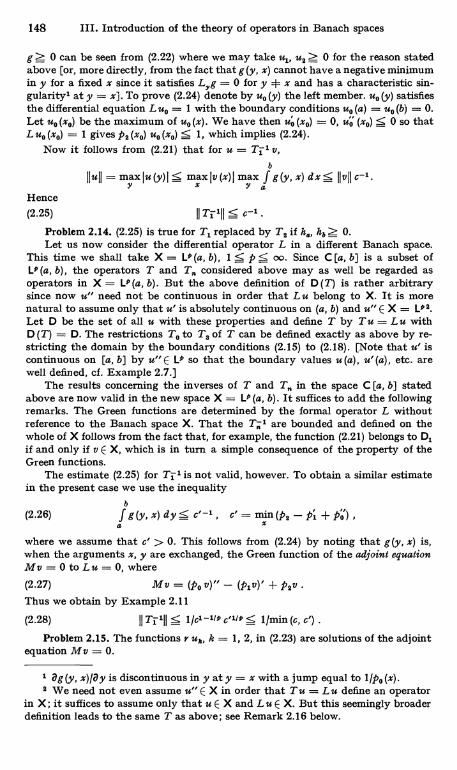
148 III. Introduction of the theory of operators in Banach spaces
g Z 0 can be seen from (2.22) where we may take u1, u2 Z 0 for the reason statedabove [or, more directly, from the fact that g (y, x) cannot have a negative minimumin y for a fixed x since it satisfies L,,g = 0 for y + x and has a characteristic sin-gularity' at y = x]. To prove (2.24) denote by uo (y) the left member. ua (y) satisfiesthe differential equation L uo = 1 with the boundary conditions ub (a) = ua (b) = 0.Let uo (xo) be the maximum of ua (x). We have then uo (xo) = 0, u' (x0) S 0 so thatL ua (xo) = 1 gives p2 (x0) uo (x0) S 1, which implies (2.24).
Now it follows from (2.21) that for u = TI -1 v,b
11ull=myxlu(y)IS mxaxlv(x)lmyx f g(y,x)dx< 1lv11c-1.
Hence(2.25) 11 Ti 111 c-1
Problem 2.14. (2.25) is true for T, replaced by T2 if h0, hb Z 0.Let us now consider the differential operator L in a different Banach space.
This time we shall take X = LP (a, b), I S P< oo. Since C [a, b] is a subset ofL9 (a, b), the operators T and T. considered above may as well be regarded asoperators in X = LP (a, b). But the above definition of D (T) is rather arbitrarysince now u" need not be continuous in order that L u belong to X. It is morenatural to assume only that u' is absolutely continuous on (a, b) and u" E X = LPs.Let D be the set of all u with these properties and define T by T u = L u withD (T) = D. The restrictions To to T. of T can be defined exactly as above by re-stricting the domain by the boundary conditions (2.15) to (2.18). [Note that u' iscontinuous on [a, b] by u" E L9 so that the boundary values u (a), u' (a), etc. arewell defined, cf. Example 2.7.]
The results concerning the inverses of T and T. in the space C [a, b] statedabove are now valid in the new space X = L9 (a, b). It suffices to add the followingremarks. The Green functions are determined by the formal operator L withoutreference to the Banach space X. That the T;1 are bounded and defined on thewhole of X follows from the fact that, for example, the function (2.21) belongs to D,if and only if v E X, which is in turn a simple consequence of the property of theGreen functions.
The estimate (2.25) for Ti.' is not valid, however. To obtain a similar estimatein the present case we use the inequality
b
(2.26) f g (y, x) d y S c'-1 , c' = min (ps - p', + po )a
where we assume that c' > 0. This follows from (2.24) by noting that g (y, x) is,when the arguments x, y are exchanged, the Green function of the adjoint equationMv = 0 to Lu = 0, where(2.27) My = ('0 vY" - (plv)' + pavThus we obtain by Example 2.11
(2.28) 11 Ti 111 S 1/cl-lir cntn < 1/min (c, c') .
Problem 2.15. The functions r u2, k = 1, 2, in (2.23) are solutions of the adjointequation My = 0.
1 2g(y, x)/2y is discontinuous in y at y = x with a jump equal to 1/po(x).8 We need not even assume u" E X in order that Tu = Lu define an operator
in X; it suffices to assume only that u E X and Lu E X. But this seemingly broaderdefinition leads to the same T as above; see Remark 2.16 below.

§ 3. Bounded operators 149
Remark 2.16. We assumed above that (a, b) is a finite interval, po , pi, p2 arecontinuous on the closed interval [a, b] and that po < 0. In such a case L is said to beregular. Let us now consider singular cases in which these conditions are notnecessarily satisfied; we assume only that po, pi and p2 are continuous in the openinterval (a, b) and po + 0. The pk may even be complex-valued, and the interval(a, b) may be finite or infinite.
In a singular case we cannot define all the operators T and Tk given above.But we can define at least the maximal operator T and the minimal operator Tin X = L9 (a, b), 1 < p < oo. T is defined by T u = L u where D (T) is the set of allu E X such that u (x) is continuously differentiable in (a, b), u' (x) is absolutelycontinuous in (a, b) [so that u" (x) is defined almost everywhere] and L u E X. T is therestriction of T with D(T) = Co (a, b) (see Example 1.11). T and T are denselydefined.
In a singular case it is in general not easy to define restrictions of T with "good"boundary conditions such as the Tk considered in the regular case. But T is oftena "good" operator itself, in a sense to be explained later.
It should also be remarked that, when applied to the regular case, the maximaloperator T just defined is apparently different from the T defined earlier, for theearlier definition requires u" E X whereas the new one only L u E X. Actually,however, these two definitions are equivalent, for L u E X implies u" E X in theregular case. This is due to the basic property of a solution of the ordinary dif-ferential equation L u = f E X, namely, that u is continuous with u' on [a, b] inthe regular case.
§ 3. Bounded operators
1. The space of bounded operatorsWe denote by .4 (X, Y) the set of all bounded operators on X to Y.
This corresponds to the set of all operators on X to Y, denoted by thesame symbol, in the finite-dimensional case (see I-§ 3.2). We write.4 (X) for 2 (X, X).
Since every operator belonging to .4 (X, Y) has domain X and rangein Y, the meaning of the linear combination a S + 9 T of S, T E.4(X, Y)is clear (I-§ 3.2). The resulting operator is again linear and bounded.Thus .°4 (X, Y) is a normed space with the norm 11 TI! defined as the boundof T (see I-§ 4.1). Similarly, the product TS is defined for T E. (Y, Z),S E -4 (X, Y) by I-(3.15) and belongs to -4 (X, Z).
Example 3.1. Consider the operator T of Example 2.3 defined from a matrix.As a maximal operator from X = P to itself, T is defined everywhere on X and isbounded if (2.5) is assumed (see Example 2.11). Thus T E a (X). The set of alloperators of this type is a linear manifold of a (X). If T, S are operators of this typedefined by the matrices (rs k), (at k) respectively, T S E 9 (X) is again of the sametype and is defined by the matrix which is equal to the product of the two matrices.
Example 3.2. Consider an integral operator of the form (2.7). Regarded as amaximal integral operator from X = L9 (E) to Y = L9 (F), T is defined on X and isbounded with 11 TICS M'1-111 M"1/s if the condition (2.8) is satisfied. Thus Tbelongs to .4 (X, Y). The set of all integral operators of this type is a linear manifoldof .' (X, Y).
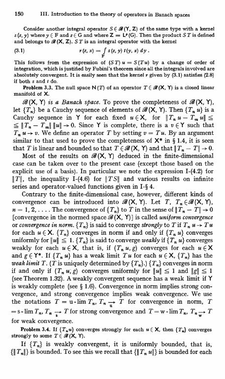
150 III. Introduction to the theory of operators in Banach spaces
Consider another integral operator S E R (Y, Z) of the same type with a kernels (z, y) where y E F and z E G and where Z = LP (G). Then the product S T is definedand belongs to 9 (X, Z). S T is an integral operator with the kernel
(3.1) r(z,x)= fs(z,y)t(y,x)dy.F
This follows from the expression of (S T) u = S (T u) by a change of order ofintegration, which is justified by Fubini's theorem since all the integrals involved areabsolutely convergent. It is easily seen that the kernel r given by (3.1) satisfies (2.8)if both s and t do.
Problem 3.3. The null space N (T) of an operator T E -4 (X, Y) is a closed linearmanifold of X.
R (X, Y) is a Banach space. To prove the completeness of R (X, Y),let {T,,} be a Cauchy sequence of elements of .6 (X, Y). Then {T u} is aCauchy sequence in Y for each fixed u E X, for II T,, u - T,,n '4ll ss II T. - T mlI II ull - . 0. Since Y is complete, there is a v E Y such thatT. u -+ v. We define an operator T by setting v = T u. By an argumentsimilar to that used to prove the completeness of X* in § 1.4, it is seenthat T is linear and bounded so that T E 9 (X, Y) and that II T. - TII - 0.
Most of the results on R (X, Y) deduced in the finite-dimensionalcase can be taken over to the present case (except those based on theexplicit use of a basis). In particular we note the expression I-(4.2) forII T (I , the inequality I-(4.6) for II T SII and various results on infiniteseries and operator-valued functions given in I-§ 4.
Contrary to the finite-dimensional case, however, different kinds ofconvergence can be introduced into .4 (X, Y). Let T, T E.4 (X, Y),n = 1, 2, .... The convergence of to Tin the sense of II T - TII --* 0[convergence in the normed space -4 (X, Y) ] is called uniform convergenceor convergence in norm. is said to converge strongly to T if T u -* T ufor each u E X. converges in norm if and only if {T u} convergesuniformly for lull 5 1. is said to converge weakly if {T u} convergesweakly for each u E X, that is, if (T u, g) converges for each u E Xand g E Y*. If {T u} has a weak limit T u for each u E X, has theweak limit T. (T is uniquely determined by converges in normif and only if (T u; g) converges uniformly for IIull s 1 and IIgll S 1(see Theorem 1.32). A weakly convergent sequence has a weak limit if Yis weakly complete (see § 1.6). Convergence in norm implies strong con-vergence, and strong convergence implies weak convergence. We usethe notations T = u - lim T., T - T for convergence in norm, T
u= s - lim T, T. -. T for strong convergence and T = w - lim T,,, T -, T
W
for weak convergence.Problem 3.4. If converges strongly for each u E X, then converges
strongly to some T E 2 (X, Y).
If is weakly convergent, it is uniformly bounded, that is,{II Tnll} is bounded. To see this we recall that {II T ull} is bounded for each
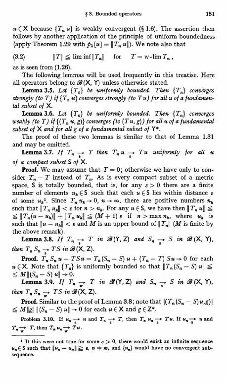
§ 3. Bounded operators 151
u E X because IT,, u} is weakly convergent (§ 1.6). The assertion thenfollows by another application of the principle of uniform boundedness(apply Theorem 1.29 with px [u] = II T,, ujj ). We note also that
(3.2) II TII s lim inf II T,II for T = w-lim T ,
as is seen from (1.26).The following lemmas will be used frequently in this treatise. Here
all operators belong to . (X, Y) unless otherwise stated.Lemma 3.5. Let {TJ be uniformly bounded. Then converges
strongly (to T) if { T,, u} converges strongly (to T u) for all u of a fundamen-tal subset of X.
Lemma 3.6. Let {TJ be uniformly bounded. Then {T,,} convergesweakly (to T) if {(T,, u, g)} converges (to (T u, g)) for all u of a fundamentalsubset of X and for all g of a fundamental subset of Y*.
The proof of these two lemmas is similar to that of Lemma 1.31and may be omitted.
Lemma 3.7. If T,, - T then T,, u -+ T u uniformly for all us
S
of a compact subset S of X.Proof. We may assume that T = 0; otherwise we have only to con-
sider T,, - T instead of T.. As is every compact subset of a metricspace, S is totally bounded, that is, for any e > 0 there are a finitenumber of elements uk E S such that each u E S lies within distance eof some ukl. Since T. uk -* 0, n -* oo, there are positive numbers nksuch that II T,, ukll < e for n > nk. For any u E S, we have then II T,, ull 5s II T. (u - uk) II + II T ukll 5 (M + 1) a if n > max nk, where uk issuch that Ilu - ukll < e and M is an upper bound of 11 T.11 (M is finite bythe above remark).
Lemma 3.8. If T,, T in .4 (Y, Z) and S,, -S . S in .4 (X, Y),then T,, S T S in .4 (X, Z).
Proof. T,, S u - T S u = T,, (S - S) u + (T,, - T) S u -> 0 for eachu E X. Note that is uniformly bounded so that II T,, (S,, - S) ull S
MII (Sri - S) uII - 0.Lemma 3.9. If T. T in .4 (Y, Z) and S g S in .1 (X, Y),
then T. S -, TS in B(X, Z).W
Proof. Similar to the proof of Lemma 3.8; note that S)u,g)IMIIgII II(S.-S)ujj-*0foreach uEXand9EZ*.Problem 3.10. If u -- u and T. --+ T, then T. is,, --> T u. If is,, - u and
S s s s
T. ---p T, then T. u - Tu.W W
1 If this were not true for some e > 0, there would exist an infinite sequenceu E S such that 11u - u.11 Z e, n + m, and would have no convergent sub-sequence.

152 III. Introduction to the theory of operators in Banach spaces
For an operator-valued function t -+ T (t) E 2 (X, Y) of a real orcomplex variable t, we can introduce different kinds of continuity accord-ing to the different kinds of convergence considered above. T (t) iscontinuous in norm if II T (t + h) - T (t) 11 -+ 0 for h -+ 0. T (t) is stronglycontinuous if T (t) u is strongly continuous for each u E X. T (t) is weaklycontinuous if T (t) u is weakly continuous for each u E X, that is, if(T (t) u, g) is continuous for each u E X and g E Y*.
II T (t) II is continuous if T (t) is continuous in norm. II T (t) II is notnecessarily continuous if T (t) is only strongly continuous, but II T (t) IIis locally bounded and lower semicontinuous if T (t) is weakly continuous.The local boundedness follows from the fact that {II T (tl.)II } is bounded fort -+ t, and the lower semicontinuity follows from (3.2).
Similarly, different kinds of differentiability can be introduced.T (t) is differentiable in norm if the difference coefficient h-1 [T (t + h) -- T (t)] has a limit in norm, which is the derivative in norm of T (t).The strong derivative T' (t) = d T (t)/dt is defined by T' (t) u = limh-1 [T (t + h) u - T (t) u], and similarly for the weak derivative.
Problem 3.11. If u (t) E X and T (t) E -4 (X, Y) are strongly differentiable, thenT (t) u (t) E Y is strongly differentiable and (did t) T (t) u (t) = T' (t) u (t) + T (t) u' (t).
We can also define different kinds of integrals f T (t) dt for anoperator-valued function T (t) of a real variable t. If T (t) is continuous innorm, the integral f T (t) dt can be defined as in the finite-dimensionalcase (or as for numerical-valued functions). If T (t) is only stronglycontinuous, we can define the integral v = f T (t) u dt for each u E X.ThenIIvII s f IIT(t) uli dt s hull f IIT(t)II dt;note that IIT(t)II need not becontinuous but is bounded and lower semicontinuous and henceintegrable1. Thus the mapping u -; v = S u defines an operator S EE R (X, Y) with bound 5 f II T (t) II d t. If we write S = f T (t) d t, we havedefined a "strong" integral f T (t) dt for a strongly continuous functionT (t), with the properties
(3.3) (f T(t)dt)u= f T(t)udt, 11f T(t)dill < f IIT(t)Ildt,t
(3.4) dtf T (s) d s = T (t) (strong derivative!) .
Similarly, the integral of a function T (C) of a complex variable alonga curve can be defined.
When we consider holomorphic operator-valued functions, thereis no distinction among uniform, strong and weak holomorphy, as invector-valued functions. More precisely, we have
Theorem 3.12. Let T M E -4 (X, Y) be defined on a domain A of thecomplex plane and let (T (C) u, g) be holomorphic in 4 E A for each u E X
1 If a real-valued function f is lower-semicontinuous, the set of all t such thatf (t) > at is open for any a. Hence / is Lebesgue-measurable.
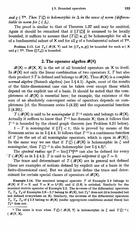
§ 3. Bounded operators 153
and g E Y*. Then T (l;) is holomorphic in A in the sense of norm (differen-tiable in norm /or C E A) .
The proof is similar to that of Theorem 1.37 and may be omitted.Again it should be remarked that if II T (C) II is assumed to be locallybounded, it suffices to assume that (T (C) u, g) be holomorphic for all uof a fundamental subset of X and for all g of a fundamental subset of Y*.
Problem 3.13. Let T. E -4 (X, Y) and let {(T u, g)} be bounded for each u E Xand g E Y*. Then {1I T.11) is bounded.
2. The operator algebra V (X)9 (X) = .4 (X, X) is the set of all bounded operators on X to itself.
In -4 (X) not only the linear combination of two operators S, T but alsotheir product S T is defined and belongs to. (X). Thus 9(X) is a completenonmed algebra (Banach algebra) (see I-§ 4.1). Again, most of the resultsof the finite-dimensional case can be taken over except those whichdepend on the explicit use of a basis. It should be noted that the com-pleteness of .(X) is essential here; for example, the existence of thesum of an absolutely convergent series of operators depends on com-pleteness [cf. the Neumann series I-(4.22) and the exponential functionI-(4.20)].
T E.°47(X) is said to be nonsingular if T-1 exists and belongs to -4 (X).Actually it suffices to know that T-1 has domain X; then it follows thatT-1 is bounded by the closed graph theorem (see Problem 5.21 below).
1 - T is nonsingular if II TII < 1; this is proved by means of theNeumann series as in I-§ 4.4. It follows that T-1 is a continuous functionof T [on the set of all nonsingular operators, which is open in .4 (X)].In the same way we see that if T (C) E Q (X) is holomorphic in C andnonsingular, then T (C)-1 is also holomorphic (see I-§ 4.5)1.
The spectral radius spr T = lim II T nlll/n can also be defined for everyT E .4 (X) as in I-§ 4.2. T is said to be quasi-nilpotent if spr T = 0.
The trace and determinant of T E.V(X) are in genera] not defined(these are examples of notions defined by explicit use of a basis in thefinite-dimensional case). But we shall later define the trace and deter-minant for certain special classes of operators of P.11 (X).
Example 3.14. The maximal integral operator T of Example 2.4 belongs toa (X) if F = E and Y = X = L' (E) and if (2.8) is satisfied. Similarly for themaximal matrix operator of Example 2.3. The inverses of the differential operatorsT1, T9, T. of Examples 2.6-2.7 belong to . (X), but Ti- 1 does not (it is bounded butnot defined everywhere on X). Similarly, the inverses of the differential operatorsT1, T8, T. of § 2.3 belong to 9 (X) (under appropriate conditions stated there) butTi 1 does not.
1 The same is true when T (C) E a (X, Y) is holomorphic in C and T (0-1 EE 9i (Y, X).
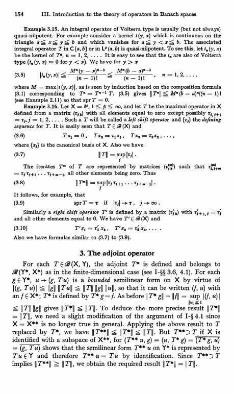
154 III. Introduction to the theory of operators in Banach spaces
Example 3.15. An integral operator of Volterra type is usually (but not always)quasi-nilpotent. For example consider a kernel t (y, x) which is continuous on thetriangle a< x S y< b and which vanishes for a 5 y < x 5 b. The associatedintegral operator Tin C [a, b] or in L° (a, b) is quasi-nilpotent. To see this, let t (y, x)be the kernel of T", n = 1, 2. .... It is easy to see that the t are also of Volterratype (t. (y, x) = 0 for y < x). We have for y > x
)n-1 n )n-1Mn _M(3.5) It.(y,x)Is (ny- 1)! S (n_ 1)! , n
where M = max It (y, x) I, as is seen by induction based on the composition formula(3.1) corresponding to TO = T"-1 T. (3.5) gives 11 P111 S M° (b - a)"I(n - 1)!(see Example 2.11) so that spr T = 0.
Example 3.16. Let X = P, 1 < PS oo, and let T be the maximal operator in Xdefined from a matrix (rr k) with all elements equal to zero except possibly r3 i+1= ri, j = 1, 2. .... Such a T will be called a left shift operator and {rr} the definingsequence for T. It is easily seen that T E -4 (X) and
(3.6) Tx1=0, Txs=rlxl, Txs=r$xs,...where {xj} is the canonical basis of X. Also we have
(3.7) II TII = sup IrrIi
The iterates Tm of T are represented by matrices (i R)) such that= rt rj+1 rj+m-1, all other elements being zero. Thus
(3.8) II Tmli = sup Ir, r1+1 ... ri+m-1Ii
TAm)l.9tm
It follows, for example, that(3.9) spr T = r if Ii4i --- r , j --- oo .
Similarly a right shift operator T' is defined by a matrix (r! k) with rj+ 1, 9 =t!and all other elements equal to 0. We have PE 9 (X) and
(3.10) T'x1=r1xs, T'xs=rax3,... .Also we have formulas similar to (3.7) to (3.9).
3. The adjoint operatorFor each T E-4 (X, Y), the adjoint T* is defined and belongs to
.4 (Y*, X*) as in the finite-dimensional case (see I-§§ 3.6, 4.1). For eachg E Y*, u -*. (g, T u) is a bounded semilinear form on X by virtue ofI(g, Tu)I <- IIgII IITuII s 11 T11 IIgII IIull, so that it can be written (f, u) withan f E X*; T* is defined by T* g= f. As before II T* gli = 11 /11 = sup I(/, u) I
IlulslII TII IIgVI gives II T *II 5 II T11. To deduce the more precise result II T *II
= II TII, we need a slight modification of the argument of I-§ 4.1 sinceX = X** is no longer true in general. Applying the above result to Treplaced by T*, we have II T**II s II T*II S II TII. But T**:) T if X isidentified with a subspace of X**, for (T** u, g) = (u, T* g) _g, u= (g, T 7u shows that the semilinear form T** u on Y* is represented byTu E Y and therefore T** u = Tu by identification. Since T**:) Timplies 11 T**II ? 11 TII, we obtain the required result 11 T*II =T h .11
I
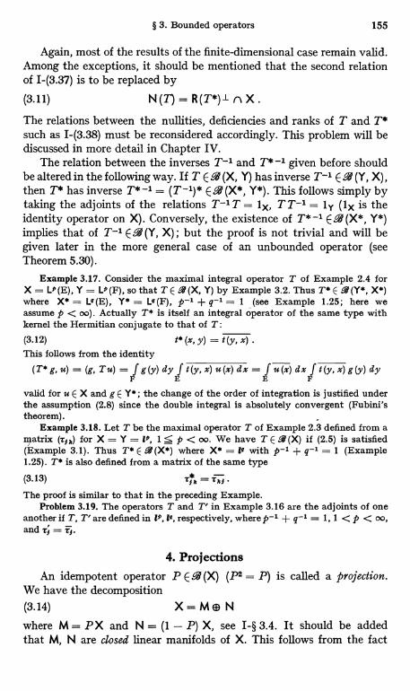
§ 3. Bounded operators 155
Again, most of the results of the finite-dimensional case remain valid.Among the exceptions, it should be mentioned that the second relationof I-(3.37) is to be replaced by
(3.11) N (T) = R (T*)1 n X.
The relations between the nullities, deficiencies and ranks of T and T*such as I-(3.38) must be reconsidered accordingly. This problem will bediscussed in more detail in Chapter IV.
The relation between the inverses T-1 and T* -1 given before shouldbe altered in the following way. If T E 9 (X, Y) has inverse T-1 ER (Y, X),then T* has inverse T*-1= (T-1)* E.9 (X*, Y*). This follows simply bytaking the adjoints of the relations T-1T = lx, TT-1 = ly (lX is theidentity operator on X). Conversely, the existence of T* -1 E -4 (X*, Y*)implies that of T-1 E.9 (Y, X); but the proof is not trivial and will begiven later in the more general case of an unbounded operator (seeTheorem 5.30).
Example 3.17. Consider the maximal integral operator T of Example 2.4 forX = L9 (E), Y = L9 (F), so that T E R (X, Y) by Example 3.2. Thus T* E .1 (Y*, X*)where X* = LQ(E), Y* = LQ(F), p-1 + q-1 = 1 (see Example 1.25; here weassume p < oo). Actually T* is itself an integral operator of the same type withkernel the Hermitian conjugate to that of T:(3.12) t* (x, y) = t (y, x) .This follows from the identity
(T*g,u)=(g,Tu) f g (y) dy ft(y,x)u(x)dx= fu(z)dx ft (y, x) g (y) dyF E E F
valid for u E X and g E Y*; the change of the order of integration is justified underthe assumption (2.8) since the double integral is absolutely convergent (Fubini'stheorem).
Example 3.18. Let T be the maximal operator T of Example 2.3 defined from an}atrix (TI m) for X = Y = 1P, 1 S p < oo. We have T E .9 (X) if (2.5) is satisfied(Example 3.1). Thus T* E 9(X*) where X* = is with p-1 + q-1 = 1 (Example1.25). T* is also defined from a matrix of the same type
(3.13) fIm=fki.The proof is similar to that in the preceding Example.
Problem 3.19. The operators T and T' in Example 3.16 are the adjoints of oneanother if T, T' are defined in 19, l*, respectively, where p-1 + q-1 = 1, 1 < p < oo,andfi=ai.
4. ProjectionsAn idempotent operator P E 9 (X) (P2 = P) is called a projection.
We have the decomposition(3.14) X= Me N
where M = PX and N = (1 - P) X, see I-§ 3.4. It should be addedthat M, N are closed linear manifolds of X. This follows from the fact
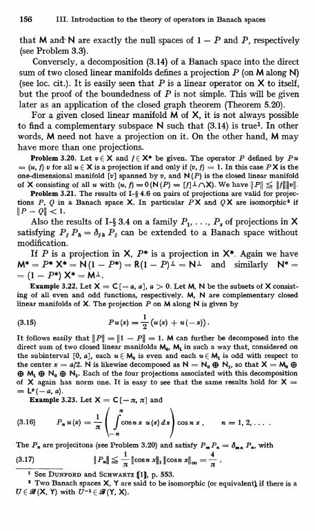
156 III. Introduction to the theory of operators in Banach spaces
that M and- N are exactly the null spaces of 1 - P and P, respectively(see Problem 3.3).
Conversely, a decomposition (3.14) of a Banach space into the directsum of two closed linear manifolds defines a projection P (on M along N)(see loc. cit.). It is easily seen that P is a linear operator on X to itself,but the proof of the boundedness of P is not simple. This will be givenlater as an application of the closed graph theorem (Theorem 5.20).
For a given closed linear manifold M of X, it is not always possibleto find a complementary subspace N such that (3.14) is true'. In otherwords, M need not have a projection on it. On the other hand, M mayhave more than one projections.
Problem 3.20. Let v E X and / E X* be given. The operator P defined by Pu_ (u, f) v for all u E X is a projection if and only if (v, f) = 1. In this case P X is theone-dimensional manifold [v] spanned by v, and N (P) is the closed linear manifoldof X consisting of all u with (u, f) =0(N(P) _ [f]1r\X). We have 11 P11 S II/IIIIvII.
Problem 3.21. The results of I-§ 4.6 on pairs of projections are valid for projec-tions P, Q in a Banach space X. In particular P X and Q X are isomorphic 2 ifIII'-QII<1.
Also the results of I-§ 3.4 on a family P1, ..., P8 of projections in Xsatisfying Pf P, = b;7, P; can be extended to a Banach space withoutmodification.
If P is a projection in X, P* is a projection in X*. Again we haveM* = P* X* = N (I - P*) = R (1 - P)1 = NJ- and similarly N*=_ (1 - P*) X* = M1.
Example 3.22. Let X = C [- a, a], a > 0. Let M, N be the subsets of X consist-ing of all even and odd functions, respectively. M, N are complementary closedlinear manifolds of X. The projection P on M along N is given by
(3.15) Pu(x) =2
(U (X) + u(-x))
It follows easily that II PII = III - PII = 1. M can further be decomposed into thedirect sum of two closed linear manifolds M0, M1 in such a way that, considered onthe subinterval [0, a], each u E Mo is even and each u E M1 is odd with respect tothe center x = a/2. N is likewise decomposed as N = No ® N1, so that X = Mo® M1 ® No ® N1. Each of the four projections associated with this decompositionof X again has norm one. It is easy to see that the same results hold for X == L'(-a, a).
Example 3.23. Let X = C [- n, n] andI n
(3.16) P, u (x) = n ( J cos n x u (x) dx) cos n X, n = 1, 2, ... .
_ n
The P. are projecitons (see Problem 3.20) and satisfy P.P. P,,, with
(3.17) IIPnll S Ilcosn xlli Ilcosn xII. =
1 See DUNFORD and SCHWARTZ Q1), p. 553.s Two Banach spaces X, Y are said to be isomorphic (or equivalents if there is a
U E. (X, Y) with U-1 E a (Y, X).
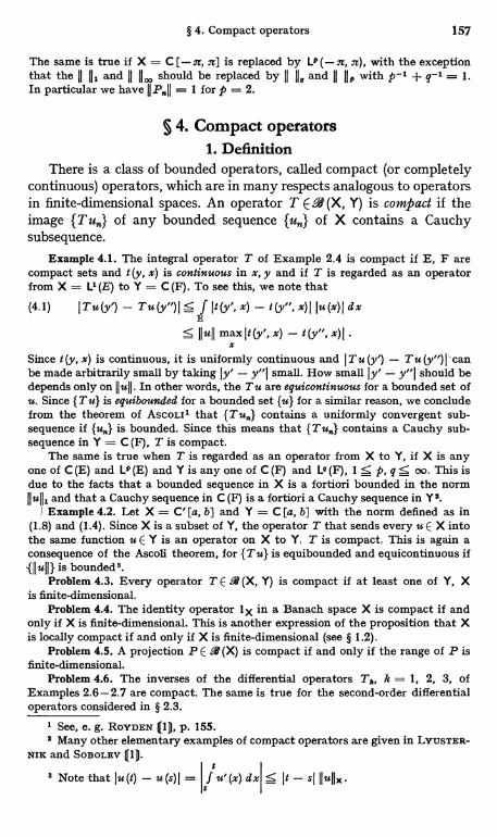
§ 4. Compact operators 157
The same is true if X = C [- ar, n] is replaced by L9 (- n, n), with the exceptionthat the 11 11. and 11 11. should be replaced by II IIQ and II III with p-1 + q-1= 1.In particular we have II P*II = 1 for p = 2.
§ 4. Compact operators1. Definition
There is a class of bounded operators, called compact (or completelycontinuous) operators, which are in many respects analogous to operatorsin finite-dimensional spaces. An operator T E. (X, Y) is compact if theimage {T u,,} of any bounded sequence {u,,} of X contains a Cauchysubsequence.
Example 4.1. The integral operator T of Example 2.4 is compact if E, F arecompact sets and t (y, x) is continuous in x, y and if T is regarded as an operatorfrom X = L' (E) to Y = C (F). To see this, we note that
(4.1) ITu(y') - Tu(y")l S f It(y, x) - t(y", x)I Iu(x)I dxE
s (lull max I t (y', x) - t (y", x)Ix
Since t(y, x) is continuous, it is uniformly continuous and ITu(y') - Tu(y")I"canbe made arbitrarily small by taking ly' - y"I small. How small l y' - y"I should bedepends only on (lull. In other words, the Tu are equicontinuous for a bounded set ofu. Since {Tu} is equibounded for a bounded set {u} for a similar reason, we concludefrom the theorem of AscoLI1 that contains a uniformly convergent sub-sequence if is bounded. Since this means that contains a Cauchy sub-sequence in Y = C (F), T is compact.
The same is true when T is regarded as an operator from X to Y, if X is anyone of C (E) and LP (E) and Y is any one of C (F) and Le (F), 1 S p, q;5 oo. This isdue to the facts that a bounded sequence in X is a fortiori bounded in the norm(lull, and that a Cauchy sequence in C (F) is a fortiori a Cauchy sequence in Y8.
1 Example 4.2. Let X = C' [a, b] and Y = C [a, b] with the norm defined as in(1.8) and (1.4). Since X is a subset of Y, the operator T that sends every u E X intothe same function u E Y is an operator on X to Y. T is compact. This is again aconsequence of the Ascoli theorem, for {Tu} is equibounded and equicontinuous ifJllull} is boundeds.
Problem 4.3. Every operator T E .4 (X, Y) is compact if at least one of Y, Xis finite-dimensional.
Problem 4.4. The identity operator IX in a Banach space X is compact if andonly if X is finite-dimensional. This is another expression of the proposition that Xis locally compact if and only if X is finite-dimensional (see § 1.2).
Problem 4.5. A projection P E .9 (X) is compact if and only if the range of P isfinite-dimensional.
Problem 4.6. The inverses of the differential operators Ty,, k = 1, 2, 3, ofExamples 2.6-2.7 are compact. The same is true for the second-order differentialoperators considered in § 2.3.
1 See, e. g. RoYDEN [I), p. 155.S Many other elementary examples of compact operators are given in LYUSTER-
NIE and SOBOLEV W.e
3 Note that lu(t) - u(s)I = sf u'(x) dxl 5 It - sI llullx.
158 III. Introduction to the theory of operators in Banach spaces
2. The space of compact operators
We denote by -40 (X, Y) the set of all compact operators of R (X, Y).Theorem 4.7. -4o (X, Y) is a closed linear manifold of the Banach space
9 (X, Y). Thus .40 (X, Y) is itself a Banach space with the same norm as in-4 (X, Y).
Proof. 69o (X, Y) is a linear manifold. Since it is obvious that a T iscompact with T, it suffices to show that T' + T" is compact wheneverT', T" are. Let {un} be a bounded sequence in X. Take a subsequence{u;,} of {un,} such that {T' is a Cauchy sequence in Y, and then take asubsequence of {u,'} such that {T" u } is Cauchy. Then {(T' ++ T") un } is a Cauchy sequence. Hence T' + T" is compact.
To prove that °9o (X, Y) is closed, let {Tk} be a sequence of compactoperators such that II T h - TII 0, k - oo, for some T E -4 (X, Y) ; wehave to show that T is also compact. Let {un} be a bounded sequencein X. As above, take a subsequence {u;; )} of {u,,} such that {T1 u(')} isCauchy, then a subsequence {un2)} of {u;,"} such that {T2 un2)} is Cauchy,and so on. Then the diagonal sequence {u(n) = vn} has the property that{Tvn} is Cauchy. In fact, since {vn} is a subsequence of every sequence{unk)}, each {Tk vn} is Cauchy for fixed k. For any s > 0, take a k solarge that II Tk - TII < e and then take N so large that II Tk vn - Tkvn+,Il<eforn>N,p>0.Then(4.2) IITvn - Tvn+,II < 11(T - Tk) (vn - vn+,)II + IITk(vn - vn+,)II <
<(2M+1)e,where M = supllunll < oo. Since (4.2) is true whenever n > N, {Tvn} isCauchy. This proves that T is compact.
Theorem 4.8. The product of a compact operator with a bounded operatoris compact. More precisely, let T Ego (X, Y) and A E.4 (Y, Z), B E °..8 (W, X),W, X, Y, Z being Banach spaces. Then A TEgo (X, Z) and T B E go (W, Y):
Proof. Let {un} be a bounded sequence in X. Take a subsequence{u;,} of {un} such that {T is a Cauchy sequence in Y. Then {A T u,,'}is a Cauchy sequence in Z; this shows that A T is compact. Again, let{vn} be a bounded sequence in W. Then B vn is bounded in X and thereforecontains a subsequence {Bv;,} such that {T Bv;,} is Cauchy. This showsthat TB is compact.
If in particular Y = X, it follows from Theorem 4.8 that the product(in either order) of operator of °Ro (X) = °Qo (X, X) with any operator ofR(X) is again compact. This is expressed by saying that go (X) is aclosed two-sided ideal of the Banach algebra .4 (X).
Problem 4.9. If dim X = oo, every T E . (X) is singular [T-1 E 2 (X) is im-possible].
§ 4. Compact operators 159
Theorem 4.10. The adjoint of a compact operator is compact, that is,T E9o(X, Y) implies T* E-'o(Y*, X*).
Proof. We begin by proving that the range of a compact operator T isseparable. To this end it suffices to show that the image TS of the unitball S of X is separable, for R (T) is the union of T S, 2 T S, 3 T S, .. .each of which is similar to TS. For any positive integer n, there are afinite number p,, of elements of T S such that any point of T S is withinthe distance 1/n from some of these p,, points. Otherwise there wouldexist an infinite number of points Tun (u,,E S) separated from oneanother with distance larger than 1/n; these points would form a sequencecontaining no Cauchy sequence, contrary to the assumption that T iscompact and S is bounded. Now the assembly of these pn points for alln = 1, 2, 3, ... is countable and dense in T S, which shows that T S isseparable.
Returning to the proof of the theorem, let T E -4o (X, Y). ThenT* E.6(Y*, X*). We have to show that, from any bounded sequence {gn}in Y*, we can extract a subsequence such that {T* is a Cauchysequence in X*. Let {vk} be a sequence dense in R (T) C Y; the existenceof such a sequence was just proved. Since every numerical sequence{(g, vk)} with fixed k is bounded, the "diagonal method" can be appliedto extract a subsequence of {g,,} such that {(fn, vk)} is a Cauchysequence for every fixed k. Since {vk} is dense.in R (T), it follows that{(f,,, v)} is Cauchy for every v E R(T). (The arguments are similar tothose used in the proof of Theorem 4.7.)
Set lim (f,,, v) = / [v]. f is a semilinear form on_ R (T) and is boundedbecause {fn} is bounded. f can be extended to a bounded semilinearform on Y (the Hahn-Banach theorem), which will again be denoted by f .
Thus we have (f,,, v) - (f, v), f E Y*, for every v E R(T), that is,
(4.3) (f n, T u) - (/, T u) , n -s oo , for all u E X X.
We shall now show that T* fn -- T* /. Since {fn} is a subsequence ofS
{gn}, this will complete the proof. Set fn - f = h,,; we have to showthat T* h - 0. If this were not true, there would exist a S > 0 such that
II T* hnIJ z S for an infinite number of subscripts n. We may assumethat it is true for all n, for otherwise we need only to replace {hn} by asuitable subsequence. Since 11 T* hnIl = sup I(T* h,,, u) I for 11u = 1,there is for each n a u,, E X such that
(4.4) (he, Tun) (T* he, un) I 6/2, II unll = 1
The compactness of T implies that {Tun} has a Cauchy subsequence.Again replacing {Tun} by a suitable subsequence if necessary, we may,assume that {Tun} is itself Cauchy. For any e > 0, there is thus an N
160 III. Introduction to the theory of operators in Banach spaces
such that m, n > N implies 11 T u,, - T u< e. Then it follows from (4.4)that
6/2 < I (hn, Tun) 1 c I (hn, Tun - T um) I + I (hn, T um) i
<- M e + i (hn, T um) i , M = sup ii hhI i .
Going to the limit n - no for a fixed m gives 6/2 S M e, for (4.3) implies(hn, T u) 0. But since e > 0 was arbitrary, this contradicts S > 0.
3. Degenerate operators. The trace and determinant
An operator T E .4 (X, Y) is said to be degenerate if rank T is finite,that is, if R (T) is finite-dimensional. This range is necessarily closed.Since a finite-dimensional space is locally compact (I-§ 1.5), a degenerateoperator is compact. It is easy to see that the set of all degenerate operatorsis a linear manifold in -4 (X, Y), but it is in general not closed.
Also it is easily verified that the product of a degenerate operator Twith a bounded operator is degenerate, with its rank not exceedingrank T (a more precise formulation should be given in a form similar toTheorem 4.8). In particular, the set of all degenerate operators of .9 (X)is a (not necessarily closed) two-sided ideal of the algebra -4 (X).
Problem 4.11. T E a (X, Y) is degenerate if and only if the codimension of thenull space N (T) is finite (dim X/N (T) < oo).
Problem 4.12. Let T. be degenerate and let 11 T. - T11 --> 0. Then T is compact,though not necessarily degenerate.
A degenerate operator T E 9 (X, Y) can he described convenientlyby making use of a basis y1, ..., ym of R (T), where m = rank T. SinceT u E R (T) for every u E X, we can write
m
(4.5) T u = E 17jy5 .i=1
The coefficients i?f are uniquely determined by u and are obviouslylinear in u. Furthermore, these linear forms are bounded, for 11?mi S
S y11 Tu11 5 y11 T11 Hull by I-(1.21). Hence we can write ?7m = (e;, u)_ (u, ef) with some e; E X*, and (4.5) becomes
m
(4.6) T u = E (u, ef) y, .f=1
It is convenient to write, in place of (4.6),
(4.7) T =' ( , ej) y5
For any g E Y* we have
(4.8) (T*g, u) = (g, T u) _ ' (e1, u) (g, y5) _ (g, y5) e;, u) .
§ 4. Compact operators 161
Since this is true for all u E X, we have
(4.9) T* g (g, yj) e1 or T* _ ( , yj) eji=I
This shows that R (T*) is spanned by m vectors el, ..., em. Thus T*is also degenerate with rank T* S rank T. Application of this result to Treplaced by T* shows that T** is also degenerate with rank T** S<_ rank T. Since, however, T may be regarded as a restriction of T**(see § 3.3), we have also rank T 5 rank T**. Thus we have proved
Theorem 4.13. T is degenerate i f and only i f T* is. I l T is degenerate,we have
(4.10) rank T* = rank T .
(4.10) is true for all T E.9 (X, Y) if oo is allowed as a value of rank T.m
Problem 4.14. An integral operator with a kernel of the form E fJ (x) gj (y) isi=I
degenerate (jj E X*, gj E Y).Problem 4.15. In (4.9) the ej form a basis of R (T*), which is correlated to the
basis {yj} of R (T). If we take an arbitrary basis {ej} of R (T*), then we have theexpressions T = E aj 1, ( , ej) yl,, T* = E o x ( , yk) ej
An important property of degenerate operators T Ed (X) is thatthe dete4minant can be defined for 1 + T and the trace can be definedfor T'. R (T) is finite-dimensional and invariant under T. Let TR be thepart of Tin R = R (T). We define the determinant of 1 + T by
(4.11) det(1 + T) = det(1R+ TO
where 1R is the identity operator in R. [For det (1R + TO see I-§ 3.1.]Any subspace M of X containing R is likewise invariant under T.
If M is finite-dimensional, det (1M + TM) is defined. We have
(4.12) det (1M + TM) = det (1 + T) .
This can proved by introducing into R a basis and extending it to abasis of M; the associated matrix for TM has the property that all rowscorresponding to the basis elements not in R contain only zero elements.Thus the determinant of this matrix is equal to det (1R + TR), which isequal to det (1 + T) by definition.
If T has the form (4.7) where the yj = xj form a basis of R, thematrix elements of TR for this basis are given by (x,, ej). Hence
(4.13) det(1 + T) = det(Sjk + (xi, ek)) .
1 There is a wider class of operators than that of degenerate operators for whichthe trace or the determinant can be defined; see RUSTON (1), GROTHENDIECK Ell(for operators in Hilbert space see X-§ 1.4).
162 III. Introduction to the theory of operators in Banach spaces
Note that this is true even if T is defined by (4.7) with y1= xf E Xwhich are not necessarily linearly independent. This can be proved by anappropriate limiting procedure.
The determinant thus defined for degenerate operators has theproperty
(4.14) det((1 + S) (1 + T)) = det(1 + S) det(1 + T) .
Note that (1 + S) (1 + T) = 1 + R where R = S + T + ST is de-generate if S, T are. To prove (4.14), let M be a finite-dimensional sub-space containing both R (S) and R (T). Then R (R) C M and det ((1 + S)(1+T))=det(1+R)=det(1M+RM)=det(1M+SM+TM+SMTM)
= det ((1 M + SM) (1M + TM)) = det (1 M + SM) det (1M + TM) = det (1 + S) .det (1 + T) by (4.12).
It follows from (4.13) that det (1 + x T) is a polynomial in x withdegree not exceeding rank T = dim R. The coefficient of x in this poly-nomial is by definition the trace of T. Thus we have
(4.15) tr T = tr TR = tr TM
with the same notations as obove. If T is given by (4.7) with x = y, wehave from (4.13)
(4.16) tr T = (xf, e,) .j=1
The trace has the property
(4.17) trTA = trAT
where T is a degenerate operator of .i (X, Y) and A is any operatrr ofR (Y, X). Note that TA is a degenerate operator in Y and A T is adegenerate operator in X. To prove (4.17), let R = R (T) C Y andS = A R C X. R and S are finite-dimensional and R (A T) = A R (T) = Swhile R (T A) C R (T) = R. Therefore, it suffices by (4.15) to show thattr(TA)R = tr(A T) S. But it is obvious that (A T) S = A' T' where T'is the operator on S to R induced by T (that is, T' u = T u for u E S)and A' is the operator on R to S induced by A, and similarly (TA)R= T' A'. Thus what we have to show is reduced to tr T' A' = tr A' T', afamiliar result in the finite-dimensional case (Problem 1-3.8)
Problem 4.16. det (1 + T*) = det(l + T), tr T' = tr T.Problem 4.17. det(1 + TS) = det(1 + ST) [where one of T E .4(X,Y) and
S E a (Y, X) is degenerate].Problem 4.18. Generalize I-(3.25) and I-(5.42) to the case of a degenerate
operator.Problem 4.19. If T E . (X) is degenerate and nilpotent, then tr T = 0, det (1 + T)
= 1.
§ 5. Closed operators 163
§ 5. Closed operators1. Remarks on unbounded operators
We have seen in the preceding sections that most of the importantresults of the operator theory developed for finite-dimensional spacesapply without essential modification to operators of 9(X, Y) [or -4 (X)].For unbounded operators with domain not identical with the wholedomain space, the situation is quite different and we encounter variousdifficulties.
For such operators, the construction of linear combinations andproducts stated in § 3.1 needs some modifications. The linear combina-tion aS + PT of two operators S, T from X to Y is again defined byI-(3.12), but the domain of this operator is by definition the intersectionof the domains of S and of T:
(5.1) D (aS + #T) = D (S) n D (T) .
In fact, aS u + fi T u would be meaningless if u did not belong to thisintersection. It may happen that (5.1) consists of a single element u = 0;in such a case aS + fiT is a trivial operator whose domain consists of0 E X alone (its range also consists of 0 E Y alone).
Problem 5.1. 0 T C 0, 0 + T = T + 0 = T for any operator T.Problem 5.2. For any three operators R, S, T from X to Y, we have (R + S) + T
= R + (S + T), which will be written R + S + T, and also S + T = T + S,but we have only (S + T) - T C S (the inclusion cannot in general be replaced byequality).
The product TS of an operator T from Y to Z and an operator Sfrom X to Y is again defined by I-(3.15), but the domain of TS is bydefinition the set of all u E D (S) such that S u E D (T) ; otherwise theright member of this defining equation is meaningless. Thus
(5.2) D(TS) = S-1 D(T) .
Again it, is possible that D (TS) consist of the single element 0.
Problem 5.3. Let S, T be as above and let R be a third operator with rangespace X. Then we have (T S) R = T (SR), which will be written T SR. Also we have(a T) S = T (a S) = a (T S) for a scalar a + 0, but this is not true for a = 0; itshould be replaced by (0 T) S = 0 (T S) C T (0 S), for the domains of (0 T) S and0 (TS) are the same as (5.2) while that of T (0 S) is equal to D (S). Again, we have(TL + T$) S = TLS + T2S but T (SL + S,) ) TSL + TS2, where ) cannot ingeneral be replaced by =. If IX denotes the identity operator in X, we have ly T= T IX = T. Compare these results with I- (3.16).
Problem 5.4. If T is an invertible operator from X to Y, then T-1T C 1X,TT-1 C 1y.
Remark 5.5. These results show that one must be careful in theformal manipulation of operators with restricted domains. For suchoperators it is often more convenient to work with vectors rather than
with operators themselves. For example, we write T-1(T u) = u, u ED(T),instead of T-1 T C 1X. As a rule, we shall make free use of the variousoperations on operators themselves only for operators of the class °.,A (X, Y)
2. Closed operatorsAmong unbounded operators there are certain ones, called closed
operators, which admit rather detailed treatment and which are alsoimportant for application.
Let T be an operator from X to Y. A sequence u E D (T) will be saidto be T-convergent (to u E X) if both {un} and {Tun} are Cauchy sequences(and u,, - u). We shall write un T u to denote that {un} is T-convergent
to u. T is said to be closed if un T u implies u E D (T) and T u = lim Tun;
in other words if, for any sequence un E D (T) such that un- u and T un-*-* v, u belongs to D (T) and T u = v. In appearance closedness resemblescontinuity, but in reality the two notions are quite different.
The set of all closed operators from X to Y will be denoted by ' (X, Y)1.Also we write le (X, X) = W (X).
A bounded operator T is closed i f and only i f D (T) is closed. In fact,un -+ u with un E D (T) implies automatically the existence of lim Tun = v.Therefore, the closedness of T is equivalent to the condition that un u,un E D (T), implies u E D (T).
In particular, every T E 9 (X, Y) is closed : -4 (X, Y) c ' (X, Y).Problem 5.6. T + A is closed if T is closed and A is bounded with D (A) D 'D (T).Problem 5.7. If T E 'B (Y, Z), S E T (X, Y) and T-1 E .4 (Z, Y), then TS E %(X, Z).
In dealing with closed operators, it is convenient to consider thegraph of the operator. Consider the product space X X Y consisting of all(ordered) pairs {u, v} of elements u E X and v E Y. X X Y is a vectorspace if the linear operation is defined by(5.3) oc1{u1, v1} + a2{u2, v2} = {a1 u1 + a2 u2, % v1 + a2 v2}
Furthermore, X X Y becomes a normed space if the norm is defined by 2
(5.4) Hu, v}li = (IJuH2 + iIvii2)1t2.
1 In IV-§ 2 we shall introduce a metric in %(X, Y) so as to make it into a metricspace.
2 Other choices of the norm are possible; for example, II{u, v}11 = 1111 + iivii ormax(Iiuii, 11vii) We employ (5.4) mainly because it ensures that (X X Y)* = X* X Y*(as Banach spaces), whereas this is not true for other norms unless different choicesare made for X X Y and X* X Y*. (X x Y)* = X* X Y* means the following:(i) each element { f, g} E X* X Y* defines an element F E (X X Y)* by ({u, v}, F)= (u, t) + (v, g) and, conversely, each F E (X X Y) * is expressed in this form by aunique {f, g} E X*'X Y*; (ii) the norm of the above F E (X X Y)* is exactly equal toii{f, g}II = (11/112 + 11g112)1". It is easy to see that (i) is true. To prove (ii), it sufficesto note that I ({u, v}, {/, g})i s i(u, /)I + I(v, g)1;5 11ull 1if11 + 11vi11IgII s (I1ui1' ++ IIvii°)1'°(11tii2 + Iighi2)1/2 = II{u, v}1111{t, g}11 and that, for fixed {/, g} and any e > 0,there is a {u, v} such that 1111=11/11, 11vii =11g11, (u, l) ? (1- 8)11 f 11 (v, g)Z? (1 - e)11g1I' so that 1({u, v}, {t, g})1 z (1 - e) (11/11' + 11x11').
It is easily seen that X x Y is complete and hence is a Banach space.The graph G (T) of an operator T from X to Y is by definition the
subset of X x Y consisting of all elements of the form {u, T u} withu E D (T). G (T) is a linear manifold of X x Y. Now it is clear that asequence of vectors of X is T-convergent if and only if {u, T u,,}is a Cauchy sequence in X x Y. It follows that T is closed i f and only i fG (T) is a closed linear manifold o l X x Y.
Problem 5.8. S C T is equivalent to G (S) C G (T).Problem 5.9. If T E W (X, Y), the null space N (T) of T is a closed linear manifold
of X.Problem 5.10. In order that a linear manifold M of X X Y be the graph of an
operator from X to Y, it is necessary and sufficient that no element of the form{0, v} with v = 0 belong to M. Hence a linear submanifold of a graph is a graph.
Problem 5.11. A finite extension (see § 2.1) of a closed operator is closed. [hint:Lemma 1.9.]
Problem 5.12. Let T E' (X, Y).. If u E D (T), u, --. u E X and T u - v E Y,w w
then u E D (T) and Tu = v. [hint: Apply Problem 1.34 to G (T)].
If S is an operator from Y to X, the graph G (S) is a subset of Y X X.Sometimes it is convenient to regard it as a subset of X x Y. Moreprecisely, let G' (S) be the linear manifold of X x Y consisting of allpairs of the form IS v, v} with v E D (S). We shall call G' (S) the inversegraph of S. As in the case of the graph, G' (S) is a closed linear manifoldif and only if S is closed.
If an operator T from X to Y is invertible, then clearly
(5.5) G (T) = G' (T-1) .
Thus T-1 is closed i f and only i f T is.
Problem 5.13. A linear manifold M of X X Y is an inverse graph if and only ifM contains no element of the form {u, 0} with u + 0.
Example 5.14. The differential operators considered in Examples 2.6-2.7 areall closed. In fact, Tl is closed because Tl 1 E 9 (X) is closed. The same is true of Tsand T8. To is closed since it is the largest common restriction of Tl and Ts [in otherwords, G (To) = G (T1) (' G (T2)]. In the same way, we see that all the differentialoperators of § 2.3 are closed.
Problem 5.15. T is closed if R (T) is closed and there is an m > 0 such that11 Tull z m1lu11 for all u E D (T).
3. Closable operatorsAn operator T from X to Y is said to be closable if T has a closed
extension. It is equivalent to the condition that the graph G (T) is asubmanifold of a closed linear manifold which is at the same time agraph. It follows that T is closable i f and only if the closure G (T) of G (T)is a graph (note Problem 5.10). We are thus led to the criterion: T isclosable if and only if no element of the form {0, v}, v + 0, is the limit ofelements of the form {u, T u}. In other words, T is closable i f and only i f
(5.6) u, E D (T), u - 0 and T u,, -+ v imply v = 0 .

166 III. Introduction to the theory of operators in Banach spaces
When T is closable, there is a closed operator T with G (T) = G (T).T is called the closure of T. It follows immediately that T is the smallestclosed extension of T, in the sense that any closed extension of T is alsoan extension of T. Since u E D (T) is equivalent to {u, T u} E v,u E X belongs to D (T) i f and only if there exists a sequence that isT-convergent to u. In this case we have T u = lim T u,
Let T be a closed operator. For any closable operator S such that3 = T, its domain D (S) will be called a core of T. In other words, alinear submanifold D of D (T) is a core of T if the set of elements {u, T u}with u E D is dense in G (T). For this it is necessary (but not sufficientin general), that D be dense in D (T).
Problem 5.16. If T is bounded and closed, any linear submanifold D of D (T)dense in D (T) is a core of T.
Problem 5.17. Every bounded operator is closable (the extension principle, see§ 2.2).
Problem 5.18. Every closable operator with finite rank is bounded. (Thus anunbounded linear form is never closable.)
Problem 5.19. Let T be an operator from X to Y' with T-1 E el (Y, X). ThenD'C D (T) is a core of T if and only if T D' is dense in Y.
4. The closed graph theorem
We have seen above that a bounded operator with domain X isclosed. We now prove a converse of this proposition.
Theorem 5.20. A closed operator T from X to Y with domain X isbounded. In other words, T E ' (X, Y) and D (T) = X imply T E -4 (X, Y).
Proof. Let S be the inverse image under T of the unit open ball of Y(it is not yet known whether S is open or not). Since D (T) = X, X is theunion of S, 2 S, 3 S, .... It follows by an argument used in the proof ofTheorem 1.29 that the closure S of S contains a ball K, say withcenter uo and radius r.
Any u E X with IIuII < 2r can be written in the form u = u' - u"with u', u" E K (loc. cit.). Since K C 5, there are sequences u,,, u E Ssuch that u; -+ u', u ' -+ u". II T (u,, - un) II S II T u,',11 + II T un II < 2 showsthat u - u E 2 S. Thus u = lim (u;, - E S. It follows by homo-geneity that for any d > 0, the ball lull < d r of X is a subset of TS.
Now take an arbitrary u E X with IIuII < r and an arbitrary a with0 < e < 1. Since u E S as remarked above, there is a u1 E S within distancee r of u, that is, II u - ujil < E r and II T ulll < 1. Hence u - ul E _e Sby the same remark and, therefore, there is a u2 E e S within distance e2 rof u - u1, that is, 11U - u1 - u211 < E2 r, II Tu2II < e. Proceeding in thisway, we can construct a sequence {un} with the properties
Ilu-ul-...-u,ll <Enr, IlTunll <En-1, n= 1,2,... .
§ 5. Closed operators 167
If we set wn = u1 + + u, we have Ilu - wnll < En r - 0, n -+ oo, andn+'p
IITwn-Twn+DII r IlTukll<En+En+1+...S 0.k=n+I
This implies that wnz u. Since T is closed, we must have T u = lim Twn.
But since II TwnII < 1 + E + Es + _ (1 - E)-1, we conclude thatII T ull s (1 - E)-1. Since this is true for every u E X with (lull < r, T isbounded with II TII s (1 - E)-1 Y-1. Since E was arbitrary, it follows that11TIISIfy.
As an application of Theorem 5.20, we shall prove the bounded-ness of the projection P on M along N defined by (3.14). It suffices toshow that P is closed, for P is defined everywhere on X and linear.Let {un} be a P-convergent sequence: u, -+ u, Pun -+ v. Since Pun E Mand M is closed, we have v E M. Since (1 - P) u,, E N and N is closed,u - v = lim(un - Pu,,) E N. Thus Pu = v by definition and P is closed.
Problem 5.21. Let T E cf (X, Y) with R (T) = Y. If T is invertible, then T-1 EE R (Y, X).
Problem 5.22. Let T E .4 (X, Y) and let S be a closable operator from Y to Zwith D (S) ) R (T). Then S T E .4 (X, Z). [hint : S T is closable with domain X,hence closed.]
5. The adjoint operator
Consider an operator T from X to Y and an operator S from Y*to X*. T and S are said to be adjoint to each other if
(5.7) (g, T u) = (Sg, u), u E D (T), g E D (S) .
For each operator T from X to Y, there are in general many operatorsfrom Y* to X* that are adjoint to T. If T is densely defined, however,there is a unique maximal operator T* adjoint to T. This means that T*is adjoint to T while any other S adjoint to T is a restriction of T*.T* is called the adjoint (operator) of T.
T* is constructed in the following way. D (T*) consists of all g E Y*such that there exists an f E X* with the property
(5.8) (g, Tu) = (/, u) for all u E D(T) .
The f E X* is determined uniquely by g, for (/, u) = (/', u) for all u E D (T)implies f = /' because D (T) is dense in X by assumption. Therefore, anoperator T* from Y* to X* is defined by setting T* g = f. Obviously T*is a linear operator, and comparison of (5.7) with (5.8) shows that S C T*holds for any S adjoint to T while T* itself is adjoint to T.
The adjointness relation (5.7) admits a simple interpretation interms of the graphs. Consider the product Banach space X X Y introducedin par. 2. Now (5.7) can be written (-Sg, u) + (g, T u) = 0, which
168 III. Introduction to the theory of operators in Banach spaces
implies that {u, T u} E X X Y is annihilated by {- Sg, g} E X* X Y*= (X x Y)*1. In other words, T and S are adjoint to each other if andonly if the graph of T and the inverse graph of - S annihilate each other :G(T)1G'(-S).
Similarly (5.8) shows that the inverse graph of - T* is the annihilatorof the graph of T:
(5.9) G'(- T*) =G(T)J- .
The assumption that T is densely defined guarantees that G (T) L isindeed an inverse graph. Since an annihilator is closed (see § 1.4), itfollows that T* is a closed operator. Note that this is true even if T is notclosed or closable, but it may happen that T* is trivial (has domain 0).
Problem 5.23. If T E 9(X, Y), the above definition of T* coincides with thatof § 3.3.
Problem 5.24. If T and S are adjoint to each other and T is closable, then Tand S are also adjoint. In particular we have T* = (T)*.
Problem 5.25. TC T' implies T* )T'* (if T is densely defined).Problem 5.26. If T is from Y to Z, S is from X to Y and if TS is densely defined
in X, then (TS)* D S* T*. Here ) may be replaced by = if T E .4 (Y, Z).Problem 5.27. For any densely defined T, we have
(5.10) N(T*) = R(T)1 .
The notion of adjointness gives a very convenient criterion forclosability, namely
Theorem 5.28. Let T from X to Y and S from Y* to X* be adjoint toeach other. If one of T, S is densely defined, the other is closable.
Proof. If T is densely defined, T* exists, is closed and T* ) S. HenceS is closable. If S is densely defined, G'(-S)-'- is a graph in X** X Y**[just as G (T)1 is an inverse graph in X* x Y* if T is densely defined].Since G (T) annihilates G' (- S), it is a subset of G' (- S)1 and the sameis true of its closure G (T) (regarded as a subset of X** x Y**). HenceG-(7T is a graph and T is closable.
Theorem 5.29. Let X, Y be reflexive. If an operator T from X to Y isdensely defined and closable, then T* is closed and densely defined andT**=T.
Proof. Since X, Y are reflexive, we have G (T) L L = G (T) = G (T)by (1.24) (we idenitfy X**, Y** with X, Y respectively). Hence G (T)= G' (- T*)- L, which implies that T* is densely defined; otherwise therewould exist a v E Y such that 0* v 1 D (T*), hence {0, v} E G'(- T*) -L= G (T), contradicting the fact that G (T) is a graph. Thus T** is definedas an operator from X** = X to Y** = Y, and G (T**) = G'(- T*)1= G (T), which implies T** = T.
1 See footnote 2 of p. 164.
§ 5. Closed operators 169
Theorem 5.30. Let T C e (X, Y) be densely defined. I/ T-1 existsand belongs to -4 (Y, X), then T* -1 exists and belongs to -4 (X*, Y*), with
(5;11) T*-1= (T-1)*Conversely, if T* -1 exists and belongs to R (X*, Y*), then T-1 exists andbelongs to 9(Y, X) and (5.11) holds.
Proof. Assume T-1 E -4 (Y, X). Then (T-1) * E -4 (X*, Y*). For eachg E D (T*) C Y* and v E Y, we have ((T-1)* T* g, v) _ (T* g, T-1 v)= (g, T T-1 v) = (g, v) ; hence (T-1)* T* g = g. On the other hand, foreach / E X* and u E D (T) C X we have ((T-1)* f, T u) = (f, T-1 T u)= (/, u) ; hence (T-1)* / E D (T*) and T* (T-1) * / = f by the definitionof T* given above. The two relations thus proved show that T*-'exists and equals (T-1)*.
Conversely, assume T*-1 E-4(X*, Y*). For each f E X* and u E D(T)we have (T* -1 f, Tu) _ (T* T* -1 /, u) = (/, u). For any u E X, how-ever, there exists an f E X* such that II/I1 = 1 and (f, u) = lull (seeCorollary 1.24). For this / we have Dull = (T*-1 f, Tu) S IIT*-hll IITullThis implies that T is invertible with II T-1II < II T* -111. Since T-1 is thusbounded and closed, R (T) is closed. It remains to be shown that thisrange is the whole space Y. For this it suffices to show that no g + 0 ofY* annihilates R (T). But this is obvious from (5.10) since T* g = 0implies g = 0 by the invertibility of T*.
Example 5.31. Let us determine the adjoints of the T, T,,, n = 0, 1, 2, 3, ofExample 2.7 defined from the formal differential operator L = d)d x in X = LP (a, b).We denote by S, S. the same operators defined in X* = Ls(a, b), p-1 + g-1 = 1,assuming 1 S p < oo. It is easily seen that T and - So are adjoint to each other.We shall show that TO _ - So. To this end let g E D (T*), f = T* g; then
b b
(5.12) f fudx=(f,u)=(T*g,u)=(9,Tu)= fgu'dxa a
xfor every u E D (T). Set h (x) = f f dx. Then f = h' and h (a) = 0 so that (5.12)
agives, after integration by parts,
b
(5.13) f (g + h) u' d x - h (b) W (F) = 0 .a
For any v E X, there is a u E X such that u' = v and u (b) = 0. Hence g + h E X*annihilates all v E X and so g + h = 0. Then (5.13) gives h (b) u (b) = 0. But sincethere are u E D (T) with u (b) + 0, we have h (b) = 0. Hence g = - h is absolutelycontinuous with g' = - h' _ - f E X* and g (a) = g (b) = 0, so that g E D (So)with T*g = f = - Sog. This proves the desired result T* _ - So, since T* ) - Soas noted above.
In the same way it can be proved that To = - S, Tl = - Ss, TT -Si,Ts (k) * = - S8 (IjN). Similarly, we have t* = - S in the general case where (a, b)need not be finite (T is the minimal operator, see Example 2.7).
Example 5.32. Consider the operators of § 2.3 constructed from the formalsecond-order differential operator L [(2.13)]. First we consider the general (singular)
170 III. Introduction to the theory of operators in Banach spaces
case (Remark 2.16) and define the maximal and minimal operators T, T in X= L9 (a, b), 1 < p < oo. Similarly we define the maximal and minimal operatorsS, S from the formal adjoint M to L [see (2.27)]. A basic result in this connection is
(5.14) T*=S.The fact that t and S are adjoint to each other is easily seen from the Lagrange
identity
(5.15) f (Lu-uMv)dx= [pou'v-u(p(, v)'+Piuv]a
where u E D (T) = Co (a, b), v E D (S) and u (x) = 0 outside of the finite interval(a, P)
To prove the stronger result (5.14), we introduce an integral operator K = K8with the kernel
(5.16) k(y,x)=ly-x1 rl(y-x),where , (t) is an infinitely differentiable function of the real variable i such thati (t) = 1 identically for - e/2 G t S e/2 and i (t) = 0 identically for Itl > e,e being a sufficiently small positive constant. h (y, x) is infinitely differentiableexcept for y = x and k (y, x) = 0 for ly - xJ Z e.
Let w (x) be an infinitely differentiable function vanishing identically outsidethe interval (a + 2 e, b - 2 e) and let u = Kw. Since the kernel k (y, x) vanishesfor I y - xl > e, u (x) vanishes outside the interval (a + e, b - e). Since k (y, x) iscontinuous at y = x, it follows that u' = K'w where K' is the integral operatorwith the kernel k' (y, x) = a k (y, x)/ay. Since k' (y, x) has a discontinuity at y = xwith a jump of 2, the second derivative u" cannot be obtained simply by dif-ferentiation under the integral sign; the correct expression for u" is
(5.17) u" = 2w + K"w
where K" is the integral operator with the kernel k" (y, x) = aek(y, x)/aye. Notethat k" is infinitely differentiable everywhere. Thus u is infinitely differentiable andvanishes identically outside (a + e, b - e), so that u E D (1`') and
(5.18) Tu=Lu=2pow+p0K"w+p1K'w+p.Kw.Now let g E D (T*) and / = T* g. We have (g, t u) = (f, u) for all u of the
above form, so that
(5.19) (2po g + K"* po g + K'* pig + K* peg, w) = (K* f, w)
Note that K, K', K" are bounded operators on X to X (since the kernels k, k', k"are bounded functions; see Examples 2.4, 2.11), and their adjoints are again integraloperators with the Hermitian conjugate kernels (Example 3.17). (5.19) is true forevery infinitely differentiable function w vanishing outside (a + 2 e, b - 2 e).Since such functions form a dense set in L9 (a + 2e, b - 2e), it follows that
(5.20) g (x) = 72-Po (x)
[K* / (x) - K* ps g (x) - K' * pi g (x) - K" * po g (x) ]
for almost all x E (a + 2e, b - 2e).Since it is known that /, g E X* = L*, the right member of (5.20) is a
continuous function of x (note that the kernels h, k', k" are smooth or piecewisesmooth functions). Hence g (x) is continuous for x E (a + 2e, b - 2e). But sincee > 0 is arbitrary, g (x) is continuous on (a, b). Returning to (5.20) we then see that
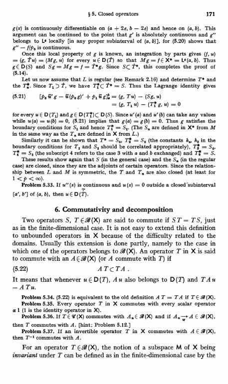
§ 5. Closed operators 171
g(x) is continuously differentiable on (a + 2e, b - 2s) and hence on (a, b). Thisargument can be continued to the point that g' is absolutely continuous and g"belongs to LQ locally [in any proper subinterval of (a, b)], for (5.20) shows thatg" - f1p0 is continuous.
Once this local property of g is known, an integration by parts gives (/, u)_ (g, Tu) = (Mg, u) for every u E D(T) so that Mg = f E X* = LQ(a, b). ThusgE D(S) and Sg = Mg = f = T*g. Since SC T*, this completes the proof of(5.14).
Let us now assume that L is regular (see Remark 2.16) and determine T* andthe T. Since Ti) t, we have Ti C T* = S. Thus the Lagrange identity gives
(5.21) [po u' g - u (po g)' -I- p1 u g]6. = (g, T u) - (Sg, u)=(g,T1u)-(Tig,u)=0
for every u E D (T1) and g E D (Ti) ( D (S). Since u' (a) and u' (b) can take any valueswhile u (a) = u (b) = 0, (5.21) implies that g (a) = g (b) = 0. Thus g satisfies theboundary conditions for S1 and hence T1 = S1. (The S. are defined in X* from Min the same way as the T. are defined in X from L.)
Similarly it can be shown that T* = So, Ta = S2 (the constants hQ, kb in theboundary conditions for T2 and S2 should be correlated appropriately), T9 = S41T4 = Ss (the subscript 4 refers to the case 3 with a and b exchanged) and To = S.
These results show again that S (in the general case) and the S. (in the regularcase) are closed, since they are the adjoints of certain operators. Since the relation-ship between L and M is symmetric, the T and T. are also closed (at least for1 <P < oo).
Problem 5.33. If u" (x) is continuous and u (x) = 0 outside a closed-subinterval
[a', b'] of (a, b), then u E D (T).
6. Commutativity and decompositionTwo operators S, T E.4 (X) are said to commute if S T = T S, just
as in the finite-dimensional case. It is not easy to extend this definitionto unbounded operators in X because of the difficulty related to thedomains. Usually this extension is done partly, namely to the case inwhich one of the operators belongs to .4 (X). An operator T in X is saidto commute with an A E .4 (X) (or A commute with T) if
(5.22) A T c_ TA.
It means that whenever u E D (T), A u also belongs to D (T) and TA u=ATu.
Problem 5.34. (5.22) is equivalent to the old definition A T = TA if T E 9N.Problem 5.35. Every operator T in X commutes with every scalar operator
at 1 (1 is the identity operator in X).Problem 5.36. If T E W (X) commutes with A. E . (X) and if A. w A E 6W (X),
then T commutes with A. [hint: Problem 5.12.]Problem 5.37. If an invertible operator T in X commutes with A E 6W (X),
then T-1 commutes with A.
For an operator T E .4 (X), the notion of a subspace M of X beinginvariant under T can be defined as in the finite-dimensional case by the
172 III. Introduction of the theory of operators in Banach spaces
condition TM C M. It is difficult to extend this notion to unboundedoperators in X, for T M C M would be satisfied whenever M has only 0in common with D (T) (see § 2.1 for the notation TM).
However, the notion of the decomposition of T by a pair M, N ofcomplementary subspaces [see (3.14)] can be extended. T is said to bedecomposed according to X = M ® N if
(5.23) PD(T)CD(T), TMCM, TNCN,where P is the projection on M along N (see § 3.4). Note that the firstcondition excludes the singular case mentioned above.
(5.23) is equivalent to the condition that T commutes with P:
(5.24) TP) PT .In fact, (5.23) implies that for any u E D (T), Pu E D (T) and T Pu E M,T(1-P)uEN. Hence (1-P) TPu=O and PT(1-P)u=O sothat T P u = P T P u = P T u, which implies (5.24). Similarly, it iseasy to verify that (5.24) implies (5.23).
When T is decomposed as above, the parts TM, TN of T in M, N,respectively, can be defined. TM is an operator in the Banach space Mwith D (TM) = D (T) n M such that TM u = T u E M. TN is definedsimilarly. If T is closed, the same is true of TM and TN, for G (TM) is theintersection of G (T) with the closed set M x M (regarded as a subset ofXX X)
The notion of decomposition can be extended to the case in whichthere are several projections P1, . . ., P. satisfying P,Pk = BhkPk,with the associated decomposition of the space X = M1® ... ® M8where Mk = Ph X. T is decomposed according to this decomposition of Xif T commutes with all the Ph. The part TMh of Tin Mk can be defined asabove.
Problem 5.38. Let T be densely defined in X. If T is decomposed as describedabove, the part TMh is densely defined in Mh.
§ 6. Resolvents and spectra1. Definitions
The eigenvalue problem considered in I-§ 5 in the finite-dimensionalcase requires an essential modification when we deal with operators Tin a Banach space X1. Again, an eigenvalue of T is defined as a complexnumber A such that there exists a nonzero u E D (T) C X, called aneigenvector, such that T a = d u. In other words, A is an eigenvalue if
1 Recall that we always assume dim X > 0.
§ 6. Resolvents and spectra 173
the null space N (T - A) is not 0; this null space is the geometric eigen-space for A and its dimension is the geometric multiplicity of the eigen-value A.
These definitions are often vacuous, however, since it may happenthat T has no eigenvalue at all or, even if T has, there are not "suf-ficiently many" eigenvectors.
To generalize at least partly the results of the finite-dimensionalcase, it is most convenient to start from the notion of the resolvent.In what follows T is assumed to be a closed operator in X. Then the sameis true of T - C for any complex number C. If T - C is invertible with
(6.1) R (C) = R (C, T) = (T - 0-1 E °. (X)
C is said to belong to the resolvent set of T. The operator-valued functionR (C) thus defined on the resolvent set P (T) is called the resolvent of T.Thus R (C) has domain X and range D (T) for any C E P (T). This definitionof the resolvent is in accordance with that given in the finite-dimensionalcase (I-§ 5.2)'.
Problem 6.1. C E P (T) if and only if T - t has inverse with domain X (seeTheorem 5.20).
Problem 6.2. If E P (T), we have
(6.2) R (C) T C T R (C) = 1+ C R (C) E-1 (X)
Thus T commutes with R (C) (see § 5.6).Problem 6.3. If P (T) is not empty, D'C D (T) is a core of T if and only if (T- C) D'
is dense in X for some (or all) C E P (T) (see Problem 5.19).Problem 6.4. If A is a closable operator from X to Y with D (A) ) D (T), then
A R (C, T) E -1 (X, Y) for every C E P (T). [hint: Problem 5.22.]
Theorem 6.5. Assume that P (T) is not empty. In order that T commutewith A E -4 (X), it is necessary that
(6.3) R (g) A = AR(C)
for every C E P (T), and it is sufficient that this hold /or some C E P (T).Proof. This follows directly from Problem 5.37.Problem 6.6. The R (C) for different C commute with each other.
The resolvent R (C) satisfies the resolvent equation I-(5.5) for everyC1, Ca E P (1). The proof is the same as before; it should only be observedthat TR (C) is defined everywhere on X [see (6.2) ]. From this it followsagain that the Neumann series I-(5.6) for the resolvent is valid, but theproof is not, trivial. Denote for the moment by R' (C) the right member
1 We have defined P (T) and E (T) only for closed operators in X. They can bedefined for more general linear operators T in X. If T is closable, we set P (T)= P (T), E (T) = E (T). If T is not closable, P (T) is empty and E (T) is the wholeplane.
174 III. Introduction to the theory of operators in Banach spaces
of I-(5.6), which exists for small IC - Col. Then we have R' (4) (T - C) u= u for every u E D (T), since R (Co) (T - C) u = u - (C - Co) R (CO) u.Similarly, we have formally (T - C) R' (C) v = v for every v E X. Theassumed closedness of T then ensures that actually R' (C) v E D (T) andthe result is correct. This shows that C E P (T) and R' (C) = R (C) for any Cfor which the series converges. We have thus proved
Theorem 6.7. P (T) is an open set in the complex plane, and R (C) is(piecewise) holomorphic for C E P (T). ("Piecewise" takes into accountthat P (T) need not be connected.) Each component of P (T) is the naturaldomain of R (4) (R (C) cannot be continued analytically beyond the boundaryof P(T)).
The complementary set E (T) (in the complex plane) of P (T) iscalled the spectrum of T. Thus C E E (T) if either T - C is not invertibleor it is invertible but has range smaller than X. In the finite-dimensionalcase E (T) consisted of a finite number of points (eigenvalues of T), butthe situation is much more complicated now. It is possible for E (T) to beempty or to cover the whole plane. Naturally we are interested in themoderate case nearer to the situation in the finite-dimensional case,but it happens frequently that the spectrum is an uncountable set.
Example 6.8. Consider the differential operators T and T. of Example 2.6.E (T) is the whole plane. In fact, the equation (T - t u =
u (x) = eCx, which belongs to X. The restriction T1of T with the boundary condition u (a) = 0, on the other hand, has an emptyspectrum. In fact the resolvent R1 (C) = R (C, T1) exists for every C and is given by
v(6.4) Rj(C)v(y)=eCY fe-Cxv(x)dx.
aSimilarly E (T2) is empty. The spectrum of Ts consists of a countable number ofisolated points A. (which are exactly the eigenvalues of T3) given by
(6.5) An= b1
a (logk+2nni), n= 0,±1,±2,...If C is different from any of the A,,, the resolvent R. R (C, T3) exists and isgiven by the integral operator [cf. (2.11)]
Y b
(6.6) R3(C) v(1') = k -eeb -a)C [kfe_xv(x) dx +ecb -a)Cfe-Cxv(x) dx I.a r J
Finally, E(TO) is again the whole plane. It is true that (To - c)-1 exists and isbounded for every C but its domain is not the whole space X. In fact, eachv E D ((To - c)-1) = R (To - C) has the form v = u' - C u with u satisfying theboundary conditions u (a) = u (b) = 0, so that v is subjected to the condition
b
(6.7) f e-Cx v (x) dx = 0.a
These results remain true when the differential operator d/dx is considered inX = LP (a, b) for a finite (a, b) (Example 2.7).
In these examples, R (C, T) does not exist since the domain of T is too largewhile R (C, To) does not exist since D (To) is too small. In a certain sense T1, Te, TSare "reasonable" operators.
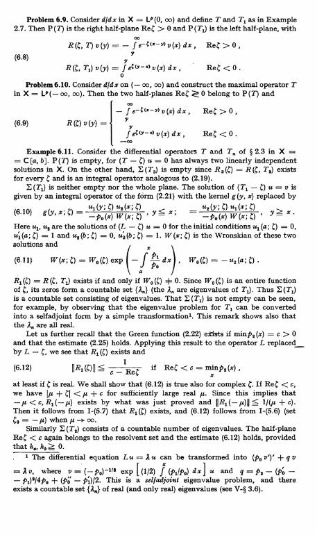
Problem 6.9. Consider dldx in X = L9 (0, oo) and define T and T, as in Example2.7. Then P (T) is the right half-plane ReC > 0 and P (T,) is the left half-plane, with
R(C, T) v(y) = - f e-C(x-Y v(x) dx, ReC> 0,Y
Y
R(C, T1) v(y) = f eC(Y-x)v(x) dx, ReC < 0.0
Problem 6.10. Consider dldx on (- oo, oo) and construct the maximal operator Tin X = L9(- oo, oo). Then the two half-planes ReC C 0 belong to P(T) and
- f e-C(x-y) v (x) dx, ReC > 0,(6.9) R (C) v (y) = 7Y
f eC(Y-x) v (x) dx, ReC<0.co-00
Example 6.11. Consider the differential operators T and T. of § 2.3 in X == C [a, b]. P (T) is empty, for (T - C) u = 0 has always two linearly independentsolutions in X. On the other hand, E (T$) is empty since R 3 (C) = R (g, T3) existsfor every C and is an integral operator analogous to (2.19).
E (T,) is neither empty nor the whole plane. The solution of (T, - C) u = v isgiven by an integral operator of the form (2.21) with the kernel g(y, x) replaced by
(6.10) g (Y, X; C) =ui (y; C) us (x; C)
y< x . = ua (y; C) ul (x; C)
y > x .-po(x) W (x; C) -po(x) W (x; C)
Here u1, ue are the solutions of (L - C) u = 0 for the initial conditions u, (a; C) = 0,u'1 (a; C) = 1 and u2 (b; C) = 0, u'5 (b; C) = 1. W (x; C) is the Wronskian of these twosolutions and
(6,11) W (x; C) = Wo (C) exp (_fiP_tld x) ,
WO (C) _ - uQ (a; C)a
R, (g) = R (C, T,) exists if and only if Wo (C) + 0. Since Wo (C) is an entire functionof C, its zeros form a countable set (the A. are eigenvalues of T,). Thus E (Ti)is a countable set consisting of eigenvalues. That E (T,) is not empty can be seen,for example, by observing that the eigenvalue problem for T, can be convertedinto a selfadjoint form by a simple transformation'. This remark shows also thatthe A. are all real.
Let us further recall that the Green function (2.22) ex sts if minpe (x) = c > 0and that the estimate (2.25) holds. Applying this result to the operator L replacedby L - C, we see that R, (C) exists and
(6.12) IIR,(C)11 < c - ReC if ReC < c = minp2(x) ,X
at least if C is real. We shall show that (6.12) is true also for complex C. If ReC < c,we have l,u + Cl < y + c for sufficiently large real ,u. Since this implies that-,u < c, R,(-,u) exists by what was just proved and 11 R,(-,u)p 5 11(,u + c).Then it follows from I-(5.7) that Rl (C) exists, and (6.12) follows from I-(5.6) (setCo = -,u) when u -+ co.
Similarly E (T2) consists of a countable number of eigenvalues. The half-planeReC < c again belongs to the resolvent set and the estimate (6.12) holds, providedthat h hb Z 0.
' The differential equation L u = A u can be transformed into (po v')' + q vz
= A v, where v = (- po)-'IS exp [ (112) f (pljpo) dx u and q = pa - (po -- pi)$14po + (po - p')/2. This is a selfadjoint eigenvalue problem, and thereexists a countable set {Aa} of real (and only real) eigenvalues (see V-§ 3.6).
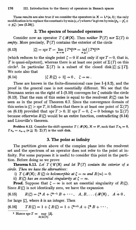
176 III. Introduction to the theory of operators in Banach spaces
These results are also true if we consider the operators in X = L9 (a, b) ; the onlymodification is to replace the constant c by min (c, c') where c' is given by min (p1- pi ++ po) [see (2.26)]-
2. The spectra of bounded operatorsConsider now an operator T E 9 (X). Then neither P (T) nor E (T) is
empty. More precisely, P (T) contains the exterior of the circle
(6.13) ICI =sprT= li IITnI111"=nniIIT"II1,n
(which reduces to the single point C = 0 if and only if spr T = 0, that is,T is quasi-nilpotent), whereas there is at least one point of E (T) on thiscircle'. In particular E (T) is a subset of the closed disk ICI ;5'11 T11.We note also that(6.14) IICR(C)+1II->0, 4-* oo.
These are known in the finite-dimensional case (see I-§ 5.2), and theproof in the general case is not essentially different. We see that theNeumann series on the right of I-(5.10) converges for C outside the circle(6.13). That the sum of this series is equal to the resolvent R (T) can beseen as in the proof of Theorem 6.7. Since the convergence domain ofthis series is ICI > spr T, it follows that there is at least one point of E (T)on (6.13) provided that spr T > 0. If spr T = 0, C = 0 belongs to E (T)because otherwise R (C) would be an entire function, contradicting (6.14)and Liouville's theorem.
Problem 6.12. Consider the shift operator T E 9 (X), X = lp, such that Tx1= 0,Tx = (n Z 2). E(T) is the unit disk.
3. The point at infinityThe partition given above of the complex plane into the resolvent
set and the spectrum of an operator does not refer to the point at in-finity. For some purposes it is useful to consider this point in the parti-tion. Before doing so we prove
Theorem 6.13. Let T E ' (X) and let P (T) contain the exterior of acircle. Then we have the alternatives :
i) T E -4 (X) ; R (C) is holomorphic at = oo and R (oo) = 0.ii) R (C) has an essential singularity at = oo.Proof. Suppose that C = oo is not an essential singularity of R (c).
Since R (C) is not identically zero, we have the expansion
(6.15) R(g)=CkA+Ck-'B+... A,B,...E.1(X), A+O,for large ICI, where k is an integer. Then
(6.16) TR(C) = 1+1;R(C)= 1+C11+1A+]kB+..1 Hence spr T = sup I Rl
.EE(T)
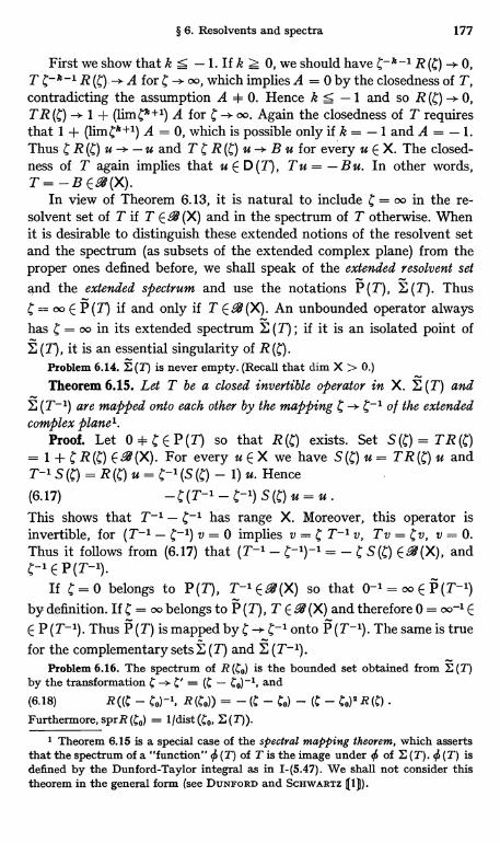
§ 6. Resolvents and spectra 177
First we show that k S -1. If k ? 0, we should have C-k -1 R 0,T C-k-1 R (C).-> A for 4 oo, which implies A= 0 by the closedness of T,contradicting the assumption A + 0. Hence k 5 -1 and so R (C) -> 0,T R (C) -> 1 + (lim Ck +1) A for C -> oo. Again the closedness of T requiresthat 1 + (limCk+1) A = 0, which is possible only if k = -1 and A = -1.Thus C R (C) u -> - u and T C R (C) u B u for every u E X. The closed-ness of T again implies that u E D (T), Tit = - B u. In other words,T=-BEPb`(X).
In view of Theorem 6.13, it is natural to include 4 = oo in the re-solvent set of T if T E 9 (X) and in the spectrum of T otherwise. Whenit is desirable to distinguish these extended notions of the resolvent setand the spectrum (as subsets of the extended complex plane) from theproper ones defined before, we shall speak of the extended resolvent setand the extended spectrum and use the notations P (T), >3 (T). ThusC = oo E P(T) if and only if T E. (X). An unbounded operator alwayshas C = oo in its extended spectrum E (7); if it is an isolated point ofE (T), it is an essential singularity of R (c).
Problem 6.14.E (T) is never empty. (Recall that dim X > 0.)
Theorem 6.15. Let T be a closed invertible operator in X. E (T) andE (T-1) are mapped onto each other by the mapping C -> C-1 o l the extendedcomplex plane'.
Proof. Let 0 + C E P (T) so that R (C) exists. Set S (C) = TR (C)= 1 + C R (C) E R(X). For every U E X we have S(C)u= T R (C) u andT-1 S (C) = R (C) u = C-1(S (C) - 1) u. Hence
(6.17) -(T-' - c-1) S() u = u.This shows that T-1 - C-1 has range X. Moreover, this operator isinvertible, for (T-1- C-1) v = 0 implies v = C T-1 v, Tv = Cv, v = 0.Thus it follows from (6.17) that (T-1 - C-1)-1 = - C SM E. (X), andC-1 E P (T-1).
If C = 0 belongs to P (T), T-1 E P4 (X) so that 0-1= oo E P (T-1)by definition. If 4 = oo belongs to P (T), T E -4 (X) and therefore 0 = o0-1 EE P (T-1). Thus P (T) is mapped by C C-1 onto f (T-1). The same is truefor the complementary sets E (T) and E (T-1).
Problem 6.16. The spectrum of R (CO) is the bounded set obtained from E (T)by the transformation C - C' = (C - Co)-', and(6.18) R ((C - Co)-', R (Co)) = - (C - Co) - (C - Co)a R (C)Furthermore, sprR (Co) = l/dist(CO, E (T)).
1 Theorem 6.15 is a special case of the spectral mapping theorem, which assertsthat the spectrum of a "function" 0 (T) of T is the image under 0 of E (T). 0 (T) isdefined by the Dunford-Taylor integral as in I-(5.47). We shall not consider thistheorem in the general form (see DUNFORD and SCHWARTZ Q4).
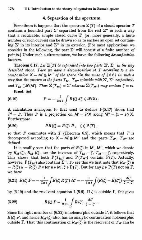
178 III. Introduction to the theory of operators in Banach spaces
4. Separation of the spectrum
Sometimes it happens that the spectrum E (T) of a closed operator Tcontains a bounded part E' separated from the rest E" in such a waythat a rectifiable, simple closed curve r (or, more generally, a finitenumber of such curves) can be drawn so as to enclose an open set contain-ing E' in its interior and E" in its exterior. (For most applications weconsider in the following, the part E' will consist of a finite number ofpoints.) Under such a circumstance, we have the following decompositiontheorem.
Theorem 6.17. Let E (T) be separated into two parts E', E" in the waydescribed above. Then we have a decomposition o l T according to a de-composition X = M' (D M" of the space (in the sense of § 5.6) in such away that the spectra of the parts TM" coincide with E', E" respectively
and TM E -4 (M'). Thus (TM.) = E' whereas E may contain 4 = oo.Proof. Set
(6.19) P=-2nif R(C)dCE°.,8(X).
rA calculation analogous to that used to deduce I-(5.17) shows thatPa = P. Thus P is a projection on M' = PX along M" _ (1 - P) X.Furthermore
(6.20) PR (C) = R (C) P , CEP (T) ,
so that P commutes with T (Theorem 6.5), which means that T isdecomposed according to X = We M" and the parts TM,, aredefined.
It is readily seen that the parts of R (C) in M', M", which we denoteby RM (C), RM" (c), are the inverses of TM - C, TM,, - C, respectively.This shows that both P and P contain P (T). Actually,however, P (TM') also contains E". To see this we first note that RM. (C) u= R() u = R() Pu for u EM', E P(T). But for any E P(T) not onwe have
(6.21) R(C)P=- 2ni l 2nzr rby (6.19) and the resolvent equation I-(5.5).-If C is outside IF, this gives
(6.22) R(C) P = 2ni ,f R(c').d
rSince the right member of (6.22) is holomorphic outside r, it follows thatR (C) P, and hence RM. (C) also, has an analytic continuation holomorphicoutside P. That this continuation of RM. (C) is the resolvent of TM. can be
§ 6. Resolvents and spectra 179
seen from Theorem 6.7. Thus P (TM.) contains the exterior of P andtherefore E (TM.) C E'.
Similarly, it follows from (6.21) that
(6.23) R (C) P = R (C) + 2 n i ,f R (C')d
C.
rif C is inside P. This shows that R (C) (1 - P) has an analytic continuationholomorphic inside P. As above, this leads to the conclusion thatE (TM") ( E
On the other hand, a point 4 E E cannot belong to both P (TM.)and P (TM..) ; otherwise it would belong to P (T) because RM. (C) P ++ RM" (C) (1 - P) would be equal to the inverse of T - C. This showsthat we have E (TM.) = E', E (TM") = E
Finally we shall show that
(6.24) PTCTP=-2I TR(C)dC=-2I CR(C)dCE-V(X).r r
P T C T P expresses the known fact that T commutes with P. Thesecond equality of (6.24) is obvious since TR (C) = 1 + C R (c). The firstequality is obtained by a formal multiplication of (6.19) from the leftby T. This multiplication is justified by the closedness of T [approxi-mate (6.19) by a finite sum and use the boundedness of TR (C) = 1 ++ C R (C)].
(6.24) implies that TM. E 9 (M'). This completes the proof.We note the following facts proved above. R (C) can be written in the
form
(6.25)R (C) = R' (C) + R" (C)
R'(C) = R(C)P, R"(C) = R(C) (1 - P) .
R' (C) is holomorphic outside E' and coincides with RM (C) when restrictedto M' while it vanishes on M"; similarly R" (C) is holomorphic outside E"and coincides with RM.. (C) on M" while vanishing on M'.
Theorem 6.17 can easily be extended to the case in which E (T) isseparated into several parts El, ..., E, and Eo, where each E,, with1 5 h S s is bounded and is enclosed in a closed curve (or a system ofclosed curves) P,, running in P (T) and lying outside one another,whereas E may be unbounded and is excluded by the P,,. Then theoperators P,, defined by (6.19) with P = P,, satisfy P,, Pk = 6, 1, P,,,h, k = 1, ..., s. T commutes with every P,, so that T is decomposedaccording to the decomposition X = M, ® ® M, ® M0, M,, = P,, X,where P0 = 1 - P, - - P,. The part TMe of T in M,, has spectrumE,,, and TMh E .4 (M,,) for h 1.
180 III. Introduction to the theory of operators in Banach spaces
5. Isolated eigenvalues 1Suppose that the spectrum E (T) of T E '(X) has an isolated point A.
Obviously E (T) is divided into two separate parts E', E" in the senseof the preceding paragraph, where E' consists of the single point A;any closed curve enclosing A but no other point of E (T) may be chosenas 1'. The operator TM, described in Theorem 6.17 has spectrum consistingof the single point A. Therefore, TM. - A is quasi-nilpotent (see par. 2).The Neumann series I-(5.10) applied to TM. - A beomes
00
(6.26) RM, (C) (C - A)---1(TM, - A)-
and converges except for C = A. (6.26) is equivalent to
I D-(6.27) R' (t) = R (C) P = - _
_A - z ( . )n+1n-1
where
(6.28) 27zf (4-A)R(C)dCEP'8(X)r
is likewise quasi-nilpotent and
(6.29) D=DP=PD.On the other hand RM" (C) is holomorphic at C = A and admits the Taylorexpansion I-(5.6) with Co = A. This is equivalent to
(6.30) R" (C) = R (C) (1 - P) = , ' (C, - A)?' S" +1n=0
where(6.31) S = RM. (A) (1 - P) = ;limR (C) (1 - P).
(Note that R (A) does not exist.) R" (C) will be called the reduced resolventof T for the eigenvalue A.
It follows from (6.27) and (6.30) that
00 "(6.32) R (C) = -
PA -
f1 ( DA)^+ f (C - A)n Sn+1n=0
This is the Laurent series for R (C) at the isolated singularity C = A.S has properties similar to those of the operator S, introduced
in the finite-dimensional case (I-§ 5.3), namely
(6.33)S=
2nz ,f R(C) EQ(X),r
(6.34) STCTSEP(X), (T-A)S=1-P, SP=PS=O.1 The expression "an isolated eigenvalue" is somewhat ambiguous. We mean
by it an eigenvalue which is an isolated point of the spectrum (not just an isolatedpoint in the set of eigenvalues).
§ 6. Resolvents and spectra 181
The Laurent expansion (6.32) is similar to I-(5.18) in the finite-dimensional case, with the sole difference that the principal part (withnegative powers of 4 - A) may be an infinite series. The principal part isfinite, however, if M' is finite-dimensional, for DM. = TM. - A is thennilpotent (see Problem 1-5.6) and the same is true of D. In this case A is aneigenvalue of T. In fact, since A belongs to the spectrum of the finite-dimensional operator TM., it must be an eigenvalue of TM, and hence of T.In this case dim M' is again called the (algebraic) multiplicity of theeigenvalue A of T, and P and D are the eigenprojection and the eigen-nilpotent associated with A. A may or may not be an eigenvalue of T ifdim M' = oo.
These results can be extended to the case in which we consider severalisolated points Al, . . ., A. of E (T). The remark at the end of par. 4 leadsimmediately to
(6.35) R (C)h8 [
Ph'+ 1 (1 - Ah)"+i, + R. (C)
Here the Ph are projections and the D. are quasi-nilpotents such that
(6.36) Ph Ph = bhh Ph Ph Dh = Dh Ph = Dh , (T - Ah) Ph = Dh .
Ro (C) is holomorphic at = A,,, h = 1, . . ., s, and
(6.37) Ro (C) = R (C) Po , PO = 1 - (P1 + ... + Ps)
Again Ah is an eigenvalue of T if M,, = Ph X is finite-dimensional, andPh and D,, are respectively the associated eigenprojection and eigen-nilpotent. We have further
5
(6.38) T P = Z; (Ah P, + D,,) , P = Pl + ... + P8 .
h=1
Here we have a spectral representation of T in a restricted sense.This is not so complete as the one in the finite-dimensional case (I-§ 5.4),since the isolated points do not in general exhaust the spectrum E (T)and, even if this is the case, there are in general an infinite number ofpoints Ah. Nevertheless, it gives a fairly complete description of theoperator T if one is interested only in a limited portion of the complexplane where there are only a finite number of points of E (T) which areeigenvalues with finite multiplicities. For brevity a finite collectionAl, . . ., A. of such eigenvalues will be called a finite system o l eigenvalues.For a finite system of eigenvalues, the situation is much the same asin the finite-dimensional case discussed in detail in 1-§5. Most of theresults deduced there can now be taken over, and this will be done in thesequel without further comment whenever there is no particular dif-ficulty.
182 III. Introduction to the theory of operators in Banach spaces
Problem 6.18. Suppose that dim M' = m < oo in Theorem 6.17. Then E'consists of a finite system of eigenvalues with the total multiplicity in.
Example 6.19. Consider the differential operator T. of Example 2.6 (or 2.7).The spectrum of Ts consists of the isolated points A. given by (6.5). Let us find theassociated eigenprojections P,,. Integrating the resolvent R, (C) given by (6.6)along a small circle around C = A. (which is a zero of k - 0 -')C), we have by (6.19)
b
1 eon y(6.39) P. v (Y)
2 n ti Rs v (Y) d= b- a f e-2n x v (x) d x,
a
where a simple calculation of the residue has been made'. P. is a degenerate integraloperator of rank one with the kernel
(6.40) P. (Y' x) = 1b a e4(v-x).-
Each A. is an isolated eigenvalue of T. with multiplicity one (simple eigenvalue),and the associated eigennilpotent is zero.
Example 6.20. Consider the differential operator T, of § 2.3. E (T,) consists ofisolated points A. which are the zeros of the entire function W. (j), see Example 6.11.The eigenprojections P. can be calculated in the same way as above: the resolventR, (C) is an integral operator with the kernel g (y, x; C) given by (6.10), and P. isobtained by (6.19) as in (6.39). Since there is a constant k such that us (x,
k ul (x, An) in virtue of the vanishing of the Wronskian at = An, a simplecalculation of the residue gives
a
b
f01 dx
(6.41) Pn v (Y) =k gin (Y) gin (x) v (x) ea pa dxWo (An) f po (x)
a
(x) = ul (x, An)
q' (x) is an eigenfunction of T1 for the eigenvalue A,,. P is a degenerate integraloperator with rank one. Incidentally, we note that Pp = P is equivalent to
(6.42)
arb
( 2
/'Po
T W. (An) _,/ ;, () ea dx
a
which can also be verified directly from the differential equation satisfied by q,,(x).(6.42) implies that Wo (An) + 0, for 9ia (x) is real because A. is real s (see Example6.11).
1 Strictly speaking, the validity of relations such as (6.39) or (6.41) needs aproof, for the integral in (6.19) is an integral of an operator-valued function R (C)whereas (6.39) or (6.41) is concerned with the values of functions. For X = C [a, b]this proof is trivial since u (y) for each fixed y is a bounded linear form in u E X.It is not so simple for X = LP (a, b). In this case we first note, for example, that (6.19)implies (Pv, f) = - (2n i)-1 f (R (C) v, f) dC for v E X and f E X* = La (a, b),p-' + q-' = 1. On calculating the right member and noting that f E X* is arbitrary,we see that (6.39) or (6.41) holds for almost all y.
2 W"o may be zero if some of P0, p1, P2 are not real or if we consider non-realboundary conditions. If W, (An) = 0, P. is no longer of rank 1 and R (C) may havea pole of order higher than 1.
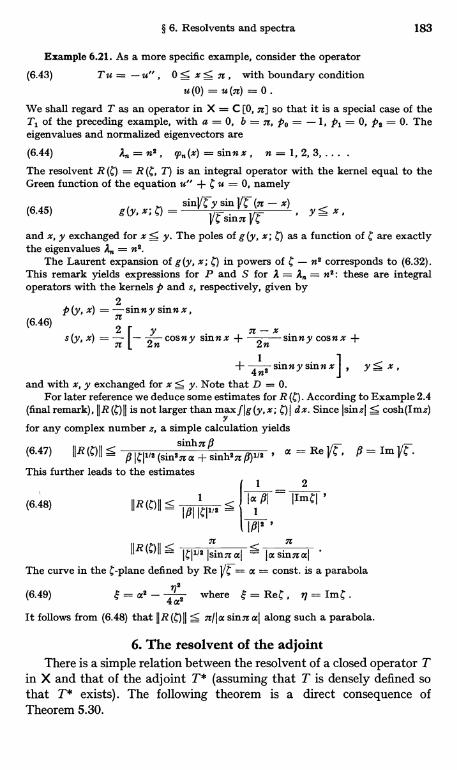
§ 6. Resolvents and spectra 183
Example 6.21. As a more specific example, consider the operator
(6.43) T u u", 0:-< x S 7r, with boundary conditionU (O) = U (n) = 0 .
We shall regard T as an operator in X = C [0, n] so that it is a special case of theTl of the preceding example, with a = 0, b = n, po = -1, Pi = 0, pe = 0. Theeigenvalues and normalized eigenvectors are
(6.44) n" n=1,2,3,... .The resolvent R R (C, T) is an integral operator with the kernel equal to theGreen function of the equation u" + c u = 0, namely
sinVy sin I/--C (n - x)(6.45) g(Y,x;0= y sinny , YS x,
and x, y exchanged for x:< y. The poles of g (y, x; C) as a function of C are exactlythe eigenvalues A. =.n2.
The Laurent expansion of g(y, x; C) in powers of C - n2 corresponds to (6.32).This remark yields expressions for P and S for A = A. = n2: these are integraloperators with the kernels p and s, respectively, given by
2p(y, x) = -sinny sinnx,(6.46)
n
s(y,x) = n I- 2n cosny sinnx + n2n sinnycosnx +LLL
+ One sinnysinnx] , y5 x,and with x, y exchanged for x S y. Note that D = 0.
For later reference we deduce some estimates for R (c). According to Example 2.4(final remark), 11R (C) 11 is not larger than max f lg(y,x; C) I dx. Since jsinzl S cosh(Imz)
for any complex number z, a simple calculation yields
(6.47) IIR (C) 11 S ireesinhn s
a ile at = Re y . $ = Im ytP ICI (sin n a + sinh n fl)
This further leads to the estimates1 2
1
A IImCI(6.48) IjR(C)jI S 1 ire S IaICI ICI
I$Ien
IIR ( I ' 1C1h12sinn al Ia sinnalThe curve in the c-plane defined by Re 1/t7= at = const. is a parabola
(6.49) = ae - 4ne where = Re C , fj = Im C .
It follows from (6.48) that IIR (C)II S n1la sinn al along such a parabola.
6. The resolvent of the adjointThere is a simple relation between the resolvent of a closed operator T
in X and that of the adjoint T* (assuming that T is densely defined sothat T* exists). The following theorem is a direct consequence ofTheorem 5.30.
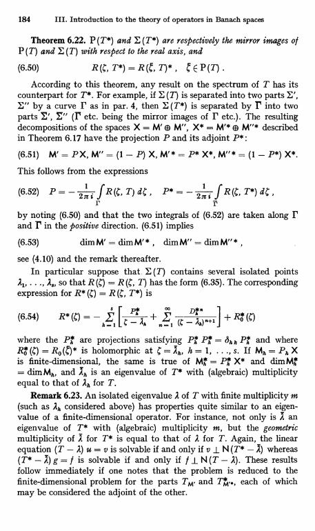
184 III. Introduction to the theory of operators in Banach spaces
Theorem 6.22. P (T*) and E(T*) are respectively the mirror images ofP (T) and E (T) with respect to the real axis, and
(6.50) R (C, T*) = R T)* , C E P (T) .
According to this theorem, any result on the spectrum of T has itscounterpart for T*. For example, if E (T) is separated into two parts E',E" by a curve r as in par. 4, then E (T*) is separated by I' into twoparts M', S" (IT etc. being the mirror images of r etc.). The resultingdecompositions of the spaces X = WED M", X* = M'* ® M"* describedin Theorem 6.17 have the projection P and its adjoint P*:
(6.51) M'=PX,M"=(1-P)X,M'*P*X*,M"*=(1-P*)X*.This follows from the expressions
(6.52) P = - /'-- R(C,T)dC, P*2nifR(C,T*)dC,2ni
rby noting (6.50) and that the two integrals of (6.52) are taken along rand I' in the positive direction. (6.51) implies
(6.53) dim M' = dim M' * , dim M" = dim M" * ,
see (4.10) and the remark thereafter.In particular suppose that, E (T) contains several isolated points
Al, ..., A., so that R (C) = R (C, T) has the form (6.35). The correspondingexpression for R* (C) = R (C, T*) is
+ Ro*(6.54) R* (C) hI [P
,r + DAh) 0+11
where the Ph are projections satisfying Ph Ph = Shh Ph and whereRo (C) = R0(C)* is holomorphic at C = /lh, h = 1, ..., s. If Mh = Ph Xis finite-dimensional, the same is true of Ph X* and dimMh= dim Mh, and 2h is an eigenvalue of T* with (algebraic) multiplicityequal to that of Ah for T.
Remark 6.23. An isolated eigenvalue A of T with finite multiplicity m(such as Ah considered above) has properties quite similar to an eigen-value of a finite-dimensional operator. For instance, not only is A aneigenvalue of T* with (algebraic) multiplicity m, but the geometricmultiplicity of A for T* is equal to that of A for T. Again, the linearequation (T - A) u = v is solvable if and only if v L N (T* - .I) whereas(T* - 1) g = / is solvable if and only if / 1 N (T - A). These resultsfollow immediately if one notes that the problem is reduced to thefinite-dimensional problem for the parts TM, and TM.., each of whichmay be considered the adjoint of the other.
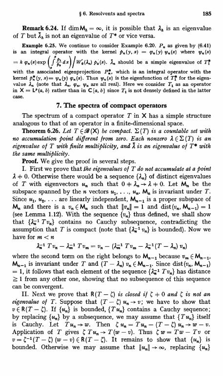
§ 6. Resolvents and spectra 185
Remark 6.24. If dim Mh = oo, it is possible that 2, is an eigenvalueof T but 1h is not an eigenvalue of T* or vice versa.
Example 6.25. We continue to consider Example 6.20. P. as given by (6.41)is an integral operator with the kernel P. (y, x) = q, (y) V,, (x) where V. (x)
= k q,, (x) exp\
f o dxl/Wo(A.) P0 (x). should be a simple eigenvalue of Tla
with the associated eigenprojection P*, which is an integral operator with thekernel p* (y, x) = V. (y) q' (x). Thus yi (x) is the eigenfunction of Tl for the eigen-value A. (note that An, q,,,, V. are all real). Here we consider T1 as an operatorin X = L9 (a, b) rather than in C [a, b] since T1 is not densely defined in the lattercase.
7. The spectra of compact operatorsThe spectrum of a compact operator T in X has a simple structure
analogous to that of an operator in a finite-dimensional space.Theorem 6.26. Let T E -4 (X) be compact. E (T) is a countable set with
no accumulation point di9erent from zero. Each nonzeyo A E E (T) is aneigenvalue of T with finite multiplicity, and A is an eigenvalue of T* withthe same multiplicity.
Proof. We give the proof in several steps.I. First we prove that the eigenvalues of T do not accumulate at a point
A + 0. Otherwise there would be a sequence {An} of distinct eigenvaluesof T with eigenvectors un such that 0 + An -> A + 0. Let M,, be thesubspace spanned by the n vectors u1, ..., u,,. Mn is invariant under T.Since u1, u2, ... are linearly independent,M is a vn E Mn such that 1lv, D = 1 and dist(vn, 1
(see Lemma 1.12). With the sequence {vn} thus defined, we shall showthat {A,-, 1 T vn} contains no Cauchy subsequence, contradicting theassumption that T is compact (note that {An 1 vn} is bounded). Now wehave for m < n
where the second term on the right belongs to Mn_1 because V. E Mn_1,Mn_1 is invariant under T and (T - An) v, E Mn_1. Since dist(vn, Mn-1)= 1, it follows that each element of the sequence T vn} has distancez 1 from any other one, showing that no subsequence of this sequencecan be convergent.
II. Next we prove that R (T - C) is closed if C = 0 and C is not aneigenvalue of T. Suppose that (T - un -* v; we have to show thatv E R (T - C). If {un} is bounded, {Tun} contains a Cauchy sequence ;by replacing {un} by a subsequence, we may assume that {Tun} itselfis Cauchy. Let Tun w. Then C un = Tun - (T - C) un -* w - v.Application of T gives C T un T (w - v). Thus C w = T w - T v orv = C-1(T - l;) (w - v) E R (T - ). It remains to show that {un} isbounded. Otherwise we may assume that 11 unil oo, replacing {un}
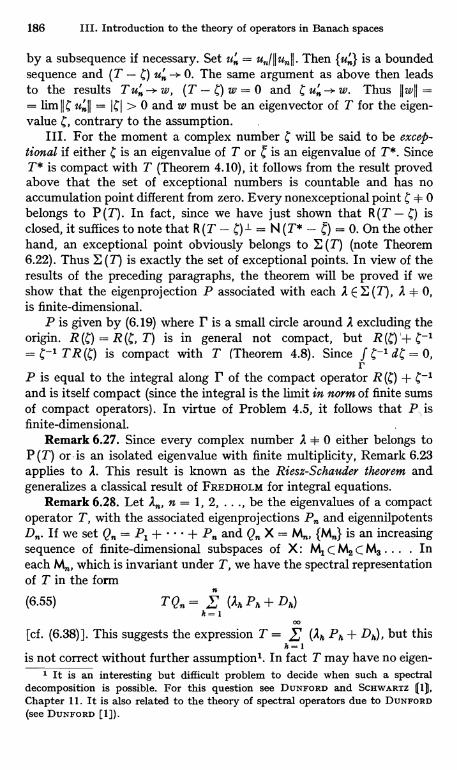
186 III. Introduction to the theory of operators in Banach spaces
by a subsequence if necessary. Set u,, = unll. Then is a boundedsequence and (T - T) u ->. 0. The same argument as above then leadsto the results T u,, -- w, (T - C) w = 0 and C u ->. w. Thus II wil == limlIC unll = ICI > 0 and w must be an eigenvector of T for the eigen-value C, contrary to the assumption.
III. For the moment a complex number C will be said to be excep-tional if either C is an eigenvalue of T or is an eigenvalue of T*. SinceT* is compact with T (Theorem 4.10), it follows from the result provedabove that the set of exceptional numbers is countable and has noaccumulation point different from zero. Every nonexceptional point C + 0belongs to P (T). In fact, since we have just shown that R (T - C) isclosed, it suffices to note that R (T - c) 1 = N (T* - ) = 0. On the otherhand, an exceptional point obviously belongs to E (T) (note Theorem6.22). Thus E (T) is exactly the set of exceptional points. In view of theresults of the preceding paragraphs, the theorem will be proved if weshow that the eigenprojection P associated with each A E E (T), A + 0,is finite-dimensional.
P is given by (6.19) where P is a small circle around A excluding theorigin. R (T) = R (C, T) is in general not compact, but R (4)'+ C-1_ C-1 TR(C) is compact with T (Theorem 4.8). Since f C-1 dt = 0,
rP is equal to the integral along r of the compact operator R (C) + C-1and is itself compact (since the integral is the limit in norm of finite sumsof compact operators). In virtue of Problem 4.5, it follows that P, isfinite-dimensional.
Remark 6.27. Since every complex number A + 0 either belongs toP (T) or -is an isolated eigenvalue with finite multiplicity, Remark 6.23applies to A. This result is known as the Riesz-Schauder theorem andgeneralizes a classical result of FREDHOLM for integral equations.
Remark 6.28. Let A,,, n = 1, 2, . . ., be the eigenvalues of a compactoperator T, with the associated eigenprojections P and eigennilpotents
and Q. X = M, {M} is an increasingsequence of finite-dimensional subspaces of X : Ml C M2 C M3 ... . Ineach M, which is invariant under T, we have the spectral representationof T in the form
(6.55) TQn = £ (Ah Ph + Dh)h=1
[cf. (6.38)]. This suggests the expression T = I (Ah Ph + DJ, but thish - I
is not correct without further assumption'. In fact T may have no eigen-1 It is an interesting but difficult problem to decide when such a spectral
decomposition is possible. For this question see DUNFORD and SCHWARTZ (1),Chapter 11. It is also related to the theory of spectral operators due to DUNFORD(see DuNFORD [1]).
§ 6. Resolvents and spectra 187
values at all (for example, a quasi-nilpotent operator has no nonzeroeigenvalue and an integral operator of Volterra type is usually quasi-nilpotent, see Example 3.15). We shall see, however, that the suggestedexpansion is valid if T is a normal compact operator in a Hilbert space(Theorem V-2. 10).
8. Operators with compact resolventAnother class of operators which have spectra analogous to the
spectra of operators in a finite-dimensional space is provided by operatorswith compact resolvent. Let T be a closed operator in X such thatR (C) = R (C, T) exists and is compact at least for some C = Co. Accordingto the result of the preceding paragraph, E (R (To)) is a countable sethaving no accumulation point different from zero. Since E (R (Co)) is theimage of E (T) under the map 4 -* (C - So)-1 (see Problem 6.16), itfollows that E (T) also consists of isolated points alone (with no accumula-tion point different from oo). The eigenprojection P for each A E E (T)is identical with the eigenprojection for the eigenvalue 4u = (A - C0)-1 ofR (Q, as is seen from (6.18) and (6.19) by transformation of the integra-tion variable. In particular we have dim P < oo so that A is an eigenvalueof T with finite multiplicity. Furthermore, for any 4 E P (T) the relationR (C) = R (C.) (1 + (C - Co) R (c)) implied by the resolvent equation showsthat R (C) is again compact. Thus we have proved
Theorem 6.29. Let T be a closed operator in X such that the resolventR exists and is compact for some C. Then the spectrum o l T consistsentirely o l isolated eigenvalues' with finite multiplicities, and R (C) iscompact for every C E P (T).
Such an operator T will be called an operator with compact resolventand a spectrum of the kind described will be said to be discrete. Anoperator with compact resolvent has a discrete spectrum. Operatorswith compact resolvent occur frequently in mathematical physics. Itmay be said that most differential operators that appear in classicalboundary problems are of this type.
Problem 6.30. If an operator in X with compact resolvent is bounded, X must befinite-dimensional.
Example 6.31. The differential operators of Examples 2.6-2.7 and of § 2.3for which the resolvent set is not empty are all operators with compact resolvent,for their resolvents are integral operators with continuous kernels (Example 4.1).This immediately leads to the result that the spectra of these operators consist ofisolated eigenvalues with finite multiplicities (cf. Examples 6.19-6.20).
In connection with operators with compact resolvent, the followinglemmas and their corollary are useful.
1 See footnote 1 of p. 180.
188 III. Introduction to the theory of operators in Banach spaces
Lemma 6.32. Let T1 T2 E'f(X, Y) have the properties: i) T1 and T2are extensions of a common operator To, the order of extension for T1 beingfinite; ii) T1 1 and Ti 1 exist and belong to . (Y, X). Then A = Ti -1 - T2 1is degenerate, and N (A) ) R (To) where codim R (To) < oo. The orders ofthe extensions T1 and T2 of T. are equal (so that T2 is also a finite extensionof To)
Proof. Set D1= D (T1), D2 = D (TO), Do = D (TO), Ro = R (To). Eachv E Ro is of the form v = To u = T1 u so that Ti 1 v = u and similarlyTZ 1 v = u. Hence A v = 0 and RocC N (A). Since the mapping by T1 aswell as by T2 is one to one, we have dim (Y/Ro) =dim (T1 Dl/ T1 Do)= dim (D1/Do) and similarly dim (Y/Ro) = dim (D2/Do). Hence dim(Y/ N (A)) S dim (Y/ R.) = dim (D2/ Do) = dim (D1/ Do) < oo and A is de-generate by Problem 4.11.
Lemma 6.33. Let T1, T2 E 'f(X, Y) have the properties: i) T1 and T2are restrictions of a common operator T, the order of restriction for T1 beingfinite; ii) T11 and Ti 1 exist and belong to-4 (Y, X). Then A = T11 - Tatis degenerate, and R (A) C N (T) where dim N (T) < oo. The orders of therestrictions T1, T2 of T are equal.
Proof. For any v E Y, T Ti v= Ti T1 1 v = v and similarly T TS 1 v= v. Hence T A v = 0 and R (A) c N (T). But since T is a finite extensionof T1 and T1 maps D1 = D (T1) onto Y, we have dim N (T) = dim (D/ D1)where D = D (T). Similarly dim N (T) = dim (D/ D2). Hence dim R (A)s dim N (T) = dim (D/D2) = dim (D/D1) < oo.
Corollary 6.34. Let T1, T2 E T (X) have non-empty resolvent sets.Let T1, T2 be either extensions of a common operator T. or restrictions of acommon operator T, with the order of extension or restriction for T1 beingfinite. Then T1 has compact resolvent if and only if T2 has compact resolvent.
Example 6.35. The result of Example 6.31 that the operators considered therehave compact resolvents is not accidental. For these operators are finite extensionsof a common operator denoted by To and, at the same time, finite restrictions of acommon operator denoted by T.
For convenience we add another lemma related to the lemmasproved above.
Lemma 6.36. Let the assumptions of both Lemmas 6.32, 6.33 be satisfied.Then A = T11 - Ta 1 has the form
m
(6.56) A X (.g,) u,, u3EN(T), g1ER(To)l.f=1
Proof. Since R (A) c N (T) by Lemma 6.33, we may write A vm
I gi [v] u5 where the uj are linearly independent vectors of N (T). Ob-i-1
viously the g1 [v] are bounded linear forms on Y and vanish for v E R (To)by Lemma 6.32. Hence we may write g1 [v] = (v, g5) with g5 E R (To)t .
§ 1. Stability of closedness and bounded invertibility 189
Chapter Four
Stability theorems
In this chapter we investigate the stability, under small perturbations, ofvarious spectral properties of linear operators acting between Banach spaces. Thebasic problems to be treated are the stability or instability of the spectrum andthe perturbation of the resolvent. The results will be fundamental for the furtherdevelopment of perturbation theory given in the following chapters. Other subjectsdiscussed include the stability of the Fredholm or semi-Fredholm property, of thenullity, deficiency, index, etc. The endeavor is to treat these problems for unboundedoperators and for the most general perturbations.
One of the basic problems here is how to define a "small" perturbation forunbounded operators. One rather general definition useful in applications is basedon the notion of a relatively bounded perturbation. But it is still too restricted in ageneral theory. The most natural and general definition of smallness of a perturba-tion is given in terms of a metric in the space %(X, Y) of all closed linear operatorsfrom one Banach space X to another one Y. Such a metric has long been known,but so far no systematic use of it has been made in perturbation theory. In thischapter we base the main part of the theory on it.
Since the metric is defined in terms of the graphs of operators, which are closedsubspaces of the product space X x Y, the technique is equivalent to introducing ametric in the set of all closed subspaces of a Banach space. For this reason, a con-siderable part of the chapter is devoted to the theory of a metric on subspaces and torelated problems. In this way, for example, we are led to define such notions as theFredholm or semi-Fredholm property and the nullity, deficiency and index for apair of subspaces. The results obtained for them lead in a natural way to the cor-responding results for operators.
§ 1. Stability of closedness and boundedinvertibility
1. Stability of closedness under relatively boundedperturbation
Let T E WK Y), where X, Y are Banach spaces. ['f(X, Y) is the setof all closed operators from X to Y.] We have already noted (Problem111-5.6) that T + A is also closed if A E .4 (X, Y). This expresses thefact that closedness is stable under a bounded perturbation A. We nowtry to extend this stability theorem to a not necessarily bounded perturba-tion.
190 IV. Stability theorems
An immediate extension of this kind can be made to the case of arelatively bounded perturbation. Let T and A be operators with thesame domain space X (but not necessarily with the same range space)such that D (T) C D (A) and
(1.1) IIAujl sahIuhI +b1ITull , uED(T)
where a, b are nonnegative constants. Then we shall say that A is relativelybounded with respect to T or simply T-bounded. The greatest lower boundbo of all possible constants b in (1.1) will be called the relative bound of Awith respect to T or simply the T-bound of A. If b is chosen very closeto b0, the other constant a will in general have to be chosen very large;thus it is in general impossible to set b = bo in (1.1).
Obviously a bounded operator A is T-bounded for any T withD (T) C D (A), with T-bound equal to zero.
The extension of the stability theorem for closedness mentionedabove is now given by
Theorem 1.1. Let T and A be operators from X to Y, and let A beT-bounded with T-bound smaller than 1. Then S = T + A isclosable if and only if T is closable ; in this case the closures o l T and S havethe same domain. In particular S is closed if and only if T is.
Proof. We have the inequality (1.1) in which we may assume thatb < 1. Hence
(1.2) -aIIuII+(1-b)IITull sjhSuII salluli+(1 +b)IITull, uED(T).
Applying the second inequality of (1.2) to u replaced by un - um, wesee that a T-convergent sequence {un} (that is, a convergent sequence{un} for which Tun is also convergent, see III-§ 5.2) is also S-convergent.Similarly we see from the first inequality that an S-convergent sequence{un} is T-convergent. If {un} is S-convergent to 0, it is T-convergent to 0so that Tun -+ 0 if T is closable [see III-(5.6) ] ; then it follows from thesecond inequality of (1.2) that Sun --> 0, which shows that S is closable.Similarly, T is closable if S is.
Let T, 9 be the closures of T, S, respectively. For any u E D (.S),there is a sequence {un} S-convergent to u (see III-§ 5.3). Since this {un}is also T-convergent to u as remarked above, we have u E D (T) so thatD (.) C D (T). The opposite inclusion is proved similarly.
Problem 1.2. (1.1) with b < 1 implies
(1.3) IIA ull s a (lull + b II TuII s (1 - b)-1(a lull + b IlSull)
In particular A is S-bounded with S-bound not exceeding b (1 - b)-1. More generally,any operator that is T-bounded with T-bound fi is also S-bounded with S-boundS # (1 - b)-1.
§ 1. Stability of closedness and bounded invertibility 191
The assumptions of Theorem 1.1 are not symmetric with respect to Tand S, although the assertions are symmetric. In this connection, thefollowing symmetrized generalization of Theorem 1.1 is of some interest:
Theorem 1.3. Let T, S be operators from X to Y such that
(1.4) IlSu - Tull 5 a IIuII + b'IITull + b"IISuII , u E D(T) = D(S) .
where a, b', b" are nonnegative constants and b' < 1, b" < 1. Then theconclusions of Theorem 1.1 are true.
Proof. Set A=S- T, T(x) = T + xA, 0 S x ;51. T(n) hasconstant domain D (T), and T (0) = T, T (1) = S. Since T u = T (x) u --xAu and Su= T(x)u+ (1 -x)Au, (1.4) gives IIA uII SaIlull ++ (b' + b") II T (x) u11 + b 11A uII , where b = max (b', b"). Hence
(1.5) IIAuji s T' b (aIIull+(b'+b")IIT(x) uII).This shows that A is T (n)-bounded with T (x)-bound not exceeding#= (1 - b)-1(b' + b"). Hence (x' - x) A is T (x)-bounded with T (x)-bound less than 1 provided Ix' - ml < 1/#, so that by Theorem 1.1,T (x') is closable if and only if T (x) is. This observation leads immediatelyto the proof of the theorem; for example, the closability of T (x) propagat-es from x = 0 to x = 1 in a finite number of steps if T is closable.
Remark 1.4. Let T E '(X, Y). Set
(1.6) IIIuIII=IIuII+IITull, uED(T).It is easily seen that D (T) becomes a Banach space X if
III III is chosenA
as the norm ; the completeness of X is a direct consequence of theclosedness of T. If A is an operator from X to Y' with D (A) ) D (T),the restriction of A to D (T) can be regarded as an operator A on X to Y'.It is easily seen that A is T-bounded if and only if A is bounded.
Remark 1.5. If T is closed and A is closable, the inclusion D (T) CC D (A) already implies that A is T-bounded. To see this define X and .Aas in the preceding remark. Then A is closable, for an A-convergentsequence in X is an A-convergent sequence in X. Since A is defined onthe whole of X, A is closed and therefore bounded by Theorem 111-5.20.Thus A is T-bounded by Remark 1.4.
2. Examples of relative boundednessSince the notion of relative boundedness is important in perturbation theory,
let us consider several examples'.Example 1.6. Let X = C [a, bJ or X = LP (a, b) for a finite interval (a, b) and
let T and A be the maximal operators defined by T u = - u" and A u = u' (see
' The inequalities deduced below are special cases of the Sobolev inequalities;see SOBOLEV (1), GOLDBERG (1).

192 IV. Stability theorems
Examples 2.6-2.7 and § 2.3 of Chapter III). We shall show that A is T-boundedwith T-bound 0. To this end we use the identity
(1.7) u'=Gu"+Huwhere G and H are integral operators with the kernels g (y, x) and h (y, x), respec-tively, given by
*+1 _ " 1
6'(Y.x)=(b xa)(Y-a)"' h(y'x) (b-a)(Y-a)" aSx<ySb,
(1.8) - (b - x)"+1 n (n + 1) (bg(Y.x)= (b - a) (b-y)"' h(Y' - (b - a) (b-y)" a5Y<xSb,
where n is any positive number. (1.7) can be verified easily by carrying out appro-priate integrations by parts. The operators G and H are bounded, for
b b-a(1.9) f n+2
(1.10)
ab
f Ih(y.x)I dxS 2(n + 1)b - a 'a
b
f I g (Y, x) I dY S n- 1a
b
f Ih(y x) I dyS 2n (n + l)(n-1)(b-a)
a
where we assumed n > 1 for simplicity. It follows from III-(2.9) that
(1.11)
Hence (1.7) gives
b-a 2n(n+1)IIGIi n-1' IIHIIS (n-1)(b-a)
(1.12) Ilu'Il n -1
IIu..IIP + (n - 1) (1)a) Ilulln. n > 1
Since the factor of llu"IIy can be made arbitrarily small by taking n large, this givesthe desired result.
Incidentally we note that only the first inequality in each of (1.9) and (1.10) isneeded in the case of X = LO0 or X = C. In this case (1.12) may be replaced by
(1.13) Ilu'll s nb
+ 22bn ±a1)
Iluli n z 0 .
Note that in (1.12) or (1.13) no boundary conditions are imposed on u(x).Suppose now that both u and u" belong to LP (0, oo). Then (1.12) is true with
a = 0 and any b > 0, and the IIull, and IIu"IIb may be replaced by the correspondingnorms taken on the interval (0, oo). Now choose n = bah for a fixed k > 0 andlet b -* no. We see then that Ilu'IIs taken on (0, b) is bounded for b -- no so thatu' E L9 (0, oo) also, with
(1.14) 11U,11- :5 hllu"Iln + k IIuII"
The same inequality holds for the interval (- oo, oo). Since h > 0 is arbitrary,A = dldx is T-bounded with T-bound zero also in the case of an infinite interval.
Problem 1.7. From (1.14) deduce
(1.15) IIu'IIs S 2 y2(IIuIIn Ilu"IIy)"a (an infinite interval) .
Example 1.8. Let X = LP (a, b) with finite (a, b) and let T u = u', A u = u (c),where c E [a, b]. A is a linear form and is unbounded if p < on. We shall show that Ais T-bounded with T-bound 0 if p > 1 and with a positive T-bound if p = 1.We start from the identity
(1.16) u (c) = (u', g) + (u, h)
§ 1. Stability of closedness and bounded invertibility 193
where(x - a)n+i h (n + 1) (x -
a)nS Sg(x) =
(b - a) (c - a)n(x) =
(b - a) (c - a)n '
a x c ,
(1.17)- (b -
x)n+1 (n + 1) (b - x)"h S bg (x) _ (b-a)(b-c)' (x) (b-a)(b-c)" c < x ,
where n is any positive number. (1.16) can be verified by integration by parts.A straightforward calculation gives the inequalities
b - a 'It n+1(1.18) IIgIl nq + q + 1 P11.5- (b - a)'-"a (nq + 1)'19
for any q Z 1. Hence we obtain from (1.16) and the Holder inequalities(1.19) Iu(c)I 5 IIglIaII''II,, + IIh1I1IIuII,S
b-a lea n..{_1S(nq-f-q+I) IIu'II0+ (b-a)i"P(nq+1)" llulln,P' q'=1.If p > 1, then q < co and the coefficients of IIu'II9 on the right of (1.19) can be madearbitrarily small by taking n large; thus A is T-bounded with T-bound 0. If p = 1,then q = co and (1.19) gives for n --* 0(1.20) Iu(c)I s Iiu'll, + IIulI,/(b - a)This shows that A is T-bounded with T-bound not larger than 1. For c = a andc = b, the T-bound is exactly equal to 1; this follows from the existence of asequence {u,} such that u,%(b) = 1, IIuaII1 = 1 and IIuklIi -* 0 for k -* oo. An exampleof such a sequence is given by uk(x) = (x - a)a/(b - a)k. For a < c < b, theT-bound of A is equal to 1/2. In fact we have
(1.21) Iu(c)I S Z IIu1Ii+ 2 max(c 1 a, b 1 C)IIuIIithis can be proved by noting that (1.16) is true also for g, h given by
(1.22) g (x) = 2(c -a) ,h (x) = 2 (c a) , for a S x < c ,
and similarly for c < x S b, for which IIgLIoo = 1/2 and IIhiI = max((c - a)-1,(b - c)-1)/2. That the T-bound of A in this case cannot be smaller than 1/2 is seenfrom the example u1(x) = (x - a)71/(c - a)" for a:5-. x S c and = (b - x)1/(b - c)°for c S x S b so that u,(c) = 1, IIuxtlj = 2 and IIuRII, -* 0 for k - on.
Example 1.9. Let X = LP (a, b) for finite (a, b), let T u = u' (regarded as anoperator in X as above) and let A u = u be an operator from X to Y = C [a, b].Since every u E D (T) is a continuous function, we have D (T) ( D (A). Furthermore,since (1.19) is true for every c E [a, b] while the right member of this inequality isindependent of c, 11A ull = IIuDIoo satisfies the same inequality. This shows that A isT-bounded, with T-bound 0 if p > 1 and T-bound 1 if p = 1. Note that (1.21)is useless here since the right member is not bounded for varying c. But thisinequality is useful if A is regarded as an operator from Ll (a, b) to Y' = C [a', b']for a < a' < b' < b; then (1.21) shows that the T-bound of A is 1/2.
Example 1.10. Consider the maximal differential operator T of III-§ 2.3 con-structed from the formal operator (2.13). Consider another formal differentialoperator obtained from (2.13) by replacing the coefficients po(x), p,(x), p,(x) byother functions qo (x), q, (x), q2 (x), respectively, and construct the correspondingoperator S. S and T have the same domain, consisting of all u E X such that u',u" E X. We shall show that S is T-bounded and estimate its T-bound. For anyu E D (T) we have(1.23) IISuII 5 NoIIu II + NjIIu'II + NoIIulI , N, = max Ige(x)I , j = 0, 1, 2.
a: z: b
194 IV. Stability theorems
But we have the inequality (1.12), which may be written
(1.24) llu'll 5 8 Ilu1l + Cellullwhere e > 0 is arbitrary if C. is chosen appropriately. Hence
(1.25) IISull s (No + e N1) (C8 N. + N2) Ilull
On the other hand, setting mo = min Ipo (x) I and M, = max I p, (x) l , j = 1, 2, wehave
(1.26) IITull z mollu"ll - Millu'll - MSIIuJI (mo - 6 MI)-(C8M1+M$)Ilull
If a is chosen so small that mo > e M1, it follows that
(1.27) IISuIIs No-+- eN, llTull+r(CeM1+M2)(No+eNI)
mo - em, mo - eMlLetting 8 we see that the T-bound of S is not larger than Nolmo. It should benoted that the coefficients of 11 T-11 and (lull in (1.27) become arbitrarily small ifN = max (No, N1, N2) is taken sufficiently small. We note also that q0 (x) need notbe positive in the above arguments.
If we consider the restrictions T1, T2, etc. of T (see loc. cit.) and define S,, S,etc. from S by the same boundary conditions, it follows from the above result thatS. is T,; bounded.
3. Relative compactness and a stability theoremA notion analogous to relative boundedness is that of relative com-
pactness. Again let T and A be operators with the same domain space X(but not necessarily with the same range space). Assume that D (T) CC D (A) and, for any sequence u ED (T) with both {un} and {Tun}bounded, {Aun} contains a convergent subsequence. Then A is said to berelatively compact with respect to T or simply T-compact'.
If A is T-compact, A is T-bounded. For if A is not T-bounded, thereis a sequence u E D (T) such that II T unll = 1 but 11A unIl z n,n = 1, 2,3 ..... It is obvious that {Aun} has no convergent subsequence.
Theorem 1.11. Let T, A be operators from X to Y and let A be T-compact 2. 1/ T is closable, S = T + A is also closable, the closures of Tand S have the same domain and A is S-compact. In particular S is closedif T is closeds.
Proof. First we prove that A is S-compact if T is closable. Assumethat {un} and {Sun} are bounded sequences; we have to show that {Aun}contains a convergent subsequence. Since A is T-compact, it sufficesto show that {Tun} contains a bounded subsequence. Suppose this is not
1 For examples of relatively compact operators for ordinary differentialoperators see BALSLEV [1].
2 Here we make no assumption on the "size" of A, in contrast to Theorem 1.1.S The assertions of this theorem are not symmetric in T and S (unlike Theorem
1.1). It is possible that T is not even closable while S is closed. A simple exampleis given by choosing T = - A = / as an unbounded linear form on X, Y being theone-dimensional space C (see footnote 3 of III-p. 133). T is not closable (see Problem111-5.18) and A is T-compact, but S = 0 is closed.
§ 1. Stability of closedness and bounded invertibility 195
true so that 11 T unll - oo. Set u' = u./II T unll . Then u -> 0, S u,' 0 and{T is bounded. Hence {A contains a convergent subsequence.Replacing un by a suitable subsequence, we may assume that A U'. -->. w.
Then T U.' = S u,, - A u,, -+ - w. Since u -> 0 and T is closable, we musthave w = 0. But this contradicts the fact that - w is the limit of T u.'where 11 Tu,,11 = 1.
Next we prove that S is closable. Let un -> 0 and S un v ; we haveto show that v = 0. Since A is S-compact, {A un} contains a convergentsubsequence. Again we may assume that A un -> w. Then Tun = Sun -- A un v - w. Since un 0 and T is closable, we have Tun -> v - w= 0. Since A is T-bounded, we have A u,, 0. Hence v = w = 0.
Let T, 9 be the closures of T, S, respectively. If u E D (T), there is asequence {un} which is T-convergent to u. Since S as well as A is T-bounded, {un} is also S-convergent to u so that u E D (9). Suppose,conversely, that u E D (9). Then there is a sequence {un} which is S-convergent to u. Then {Tun} is bounded; this can be proved exactlyin the same way as in the first part of this proof. Hence we may assume,as before, that A un w and Tun = Sun - A un -> v - w. Thus un isT-convergent to u and u E D (T). This proves that D (T) = D (. ).
Remark 1.12. Let T be closed and D (A) ) D (T). Define X and A as inRemark 1.4. Then A is T-compact if and only if A is compact.
Remark 1.13. We can also define relatively degenerate operators asspecial cases of relatively compact operators. A is T-degenerate if A isT-bounded and R (A) is finite-dimensional. It is easy to see that a T-degenerate operator is T-compact.
We shall give an explicit form of a T-degenerate operator. Let Tbe from X to Y and consider the product space X x Y (see III-§ 5.2).Since the T-boundedness of A implies that 11 A ull S const. 11 {u, T u} 11,
A may be regarded as a bounded operator from X x Y to Y' (the rangespace of A), with domain G (T) (the graph of T). Since R (A) is finite-dimensional, A u can be written in the form
(1.28) Augi[u]yi, yiEY'.
f=1where the gj, are linear forms defined on G (T). Since Ig; [u] 1 5 const.IIA ull by I-(1.21), it follows that the gi are bounded forms in X x Y with
domain G (T). According to the Hahn-Banach theorem, the gi can beextended to bounded forms on X x Y. Since (X x Y)* = X* x Y*, theextended forms can be written in the form {u, v} -> (u, f,) + (v, g,) withfj E X* and gi E Y*. Restricting {u, v} to G (T), we have gj [u] = (u, ff) ++ (Tu, g,). In this way we arrive at the following expression for aT-degenerate operator from X to Y':
m
(1.29) Au= E [(u,f/)+ (Tu,ge)]yi , f,EX*, g1EY*, yi EY'.f-1
196 IV. Stability theorems
Problem 1.14. Assume that there is a densely defined operator S from Y* to X*adjoint to T [see III-(5.7)]. Then a T-degenerate operator A has T-bound zero.[hint: Approximate the gi of (1.29) by elements of D (S).]
Example 1.15. In Example 1.6, A is T-compact if (a, b) is a finite interval.In fact if is a sequence such that T u u;; is bounded, then A u = u isequicontinuous. If in addition is bounded, {u;, (x)} is uniformly bounded in xand n. Thus it follows from the Ascoli theorem that {u;,} contains a uniformlyconvergent subsequence, which is a Cauchy sequence in X. A is not T-compact forthe interval (0, oo) or (- oo, oo), although A is T-bounded with T-bound zero [see(1.14)]. In Example 1.8, A is not only T-compact but T-degenerate. This is obvioussince A is T-bounded and the range space of A is one-dimensional.
4. Stability of bounded invertibilityLet T E ' (X, Y). We shall now show that the property T-1 E 9 (Y, X)
is stable under a small perturbation.Theorem 1.16.1 Let T and A be operators from X to Y. Let T-1 exist
and belong to M(Y, X) (so that T is closed). Let A be T-bounded, with theconstants a, b in (1.1) satisfying the inequality
(1.30) aJIT-1II +b<1.Then S = T + A is closed and inveytible, with S-1 E .1 (Y, X) and
(1.31) IIS-111;5 1 - 11TT 1 H - b , IIS-1- T-1II s it 1-111(aIilT
1111
±b)
If in addition T-1 is compact, so is S-1.Proof. Since (1.30) implies b < 1, S is closed by Theorem 1.1. The
proof of other assertions of the theorem is not essentially different fromthe finite-dimensional case (see the end of I-§ 4.4) : first we note that
(1.32) S = T + A = (1+AT-1) T, AT-1EM(Y),
for A T-1 is an operator on Y to Y and is bounded by 11A T-1 v II 5 all T-1 v II
+bIIvII 5 (aJIT-III+b)IIvIl.Thus
(1.33) 11AT-111 saIIT-1II+b<1
and 1 + A T-1 maps Y onto Y one to one, and the argument of I-§ 4.4is applicable without essential change. The only change required is theuse of (1.33) instead of the simple estimate IIA T-1II 5 IIAII IIT-111 usedthere.
If T-1 is compact, S-1= T-1 (1 + A T-1)-1 is compact by TheoremIII-4.8.
Remark 1.17. If A is bounded in Theorem 1.16, we can take a = IIAIIb = 0 and (1.31) reduces to I-(4.24). If, furthermore, A is assumed tocommute with T (Y = X being assumed), then we can prove the existenceof S-1 under a weaker assumption, namely,
1 This theorem will be generalized in the following section (see Theorem 2.21).
§ 2. Generalized convergence of closed operators 197
Theorem 1.18. Let T be an operator in X with T-1 E 9 (X). LetA E .' (X) commute with T. If sprA < 1/spr T-I, then (T + A)-I existsand belongs to 9(X).
Proof. The commutativity of A with T is equivalent to A T-I= T-I A (see Problem 111-5.37). Thus the proof is essentially the sameas the proof of a similar result in the finite-dimensional case (Remark1-4.7).
§ 2. Generalized convergence of closed operators1. The gap between subspaces
When we consider various perturbation problems related to closedoperators, it,,is necessary to make precise what is meant by a "small"perturbation. In the previous section we considered a special kind,namely a relatively bounded perturbation. But this notion is still restrict-ed, and we want to have a more general definition of the smallness of aperturbation for closed operators.
This can be done in a most natural way by introducing a metric inthe set W (X, Y) of all closed operators from X to Y. If T, S E ' (X, Y),their graphs G (T), G (S) are closed linear manifolds in the product spaceX x Y. Thus the "distance" between T and S can be measured by the"aperture" or "gap" between the closed linear manifolds. G (T), G (S).In this way we are led to consider how to measure the gap of two closedlinear manifolds of a Banach space.
In this paragraph we shall consider closed linear manifolds M, N, .. .of a Banach space Z.
We denote by SM the unit sphere of M (the set of all u E M withlull = 1). For any two closed linear manifolds M, N of Z, we set
(2.1) 6 (M, N) = sup dist (u, N) ,g UESM
(2.2) 6(M, N) = max[8(M, N), 6(N, M)]'.(2.1) has no meaning if M = 0; in this case we define 8 (0, N) = 0 forany N. On the other hand 6 (M, 0) = 1 if M + 0, as is seen from thedefinition.
6 (M, N) can also be characterized as the smallest number 6 such that
(2.3) dist (u, N) 5 6 j ull for all u E M .
8(M, N) will be called the gap between M, N.The following relations follow directly from the definition.
(2.4) 6 (M, N) = 0 if and only if M c N .(2.5) 8(M, N) = 0 if and only if M=N.(2.6) b (M, N) = b (N, M) .
(2.7) 056(M,N) 51, 0S8(M,N) 51.1 See GOHBERG and KREIN [1], T. KATO [12], CORDES and LABROUSSE [1].
198 IV. Stability theorems
(2.5) and (2.6) suggest that 8 (M, N) could be used to define a distancebetween M and N. But this is not possible, since the function 3 does notin general satisfy the triangle inequality required of a distance function'.
This incovenience may be removed by slightly modifying the defini-tion (2.1-2.2). Set(2.8) d (M, N) = sup dist (u, SN) ,
CESM
(2.9) d (M, N) = max [d (M, N), d (N, M) ] 2.
(2.8) does not make sense if either M or N is 0. In such cases we set(2.10) d (O, N) = 0 for any N ; d (M, 0) = 2 for M +-0.Then all the relations (2.4-2.7) are again satisfied by 6, 8 replacedby d, d, respectively if I is replaced by 2 in (2.7). Furthermore, d and dsatisfy the triangle inequalities :(2.11) d(L,N) sd (L, M) + d (M, N) , d(L,N) (L, M) +d(M,N).
The second inequality of (2.11) follows from the first, which in turnfollows easily from the definition. The proof will be left to the reader.[The case when some of L, M, N are 0 should be considered separately;note (2.10).]
The set of all closed linear manifolds of Z becomes a metric spaceif the distance between M, N is defined by J (M, N). A sequence ofclosed linear manifolds converges to M if J (M, M) -+ 0 for n -> oo. Thenwe write M,, -> M or lim M,, = M.
Although the gap 8 is not a proper distance function, it is moreconvenient than the proper distance function d for applications since itsdefinition is slightly simpler. Furthermore, when we consider the topologyof the set of all closed linear manifolds, the two functions give the sameresult. This is due to the following inequalitiess:
6 (M, N) S d (M, N) s 2 6 (M, N) ,(2.12)
8(M,N) scl(M,N) s28(M,N).The second set of inequalities follows directly from the first. Also the
first inequality of the first set is trivial. To prove the second inequalityd (M, N) S 2 6 (M, N), it suffices to assume N + 0 and show that
(2.13) dist (u, SN) S 2 dist (u, N) for any u E Z with 1juDD = 1 .
1 4 does satisfy the triangle inequality if Z is a Hilbert space. This followsfrom the relation 3 (M, N) =11 P - QII, where P, Q are the orthogonal projections onM, N, respectively, which follows from Theorem 1-6.34. In this case 6 is a moreconvenient metric than the d to be introduced below.
2 See GOHBERG and MARKUS [1]. A different but equivalent metric is introducedby NEWBURGH [2]. d is the Hausdorff distance defined on the set of all SM (exceptfor M = 0) ; see HAUSDORFF (1), p. 145. d (M, N) is equal to Q (SM, SN) in the notationof HAUSDORFF. For the discussion of various metrics see BERKSON [1].
8 Cf. GOHBERG and MARKUS [1].
§ 2. Generalized convergence of closed operators 199
For any e > 0, there is a v E N such that 11u - v11 < dist (u, N) + e.We may assume that v + 0, for otherwise we can change v slightlywithout affecting the inequality. Then vo = v111 I E SN and dist (u, SN) 5Sllu - volt Sllu - vII+IIv - volt. But IIv-v.11=IIIvil-11=111vIl-- (lull! 5 IIv - ull, so that dist(u, SN) 5 211u - vii < 2 dist(u, N) + 2s.Since e > 0 is arbitrary, this proves (2.13).
(2.12) shows that c$(M,,, M) 0 is equivalent to 8(M,,, M) 0.Thus the convergence M,, M can be defined by 8 (M,,, M) 0 withoutreference to the d function. In what follows we shall use almost exclusivelythe gap 3 rather than the distance J.
Remark 2.1. The metric space of all closed linear manifolds of Zdefined above is complete; if is a Cauchy sequence (c$(Ma, M.) + 0for n, m oo), then there is a closed linear manifold M such thatc$(M,,, M) 0. Since we do not need this theorem, we shall not prove ithere.
The following lemma will be needed later.Lemma 2.2. For any closed linear manifolds M, N of Z and any u E Z,
we have
(2.14) (1 + 6 (M, N)) dist (u, M) z dist (u, N) - (lu116 (M, N) .
Proof. For any e > 0 there is a v E M such that 11u - v11 < dist (u, M) ++ e, and for this v there is a w E N such that 11v - wil < dist(v, N) + e.Hence dist (u, N) 5 11u - wll 5 dist (u, M) + dist (v, N) + 2e 5 dist (u,M) + llvll 8(M, N) + 2e. But lvIl <_ hull + llu - vii 5 (lull + dist(u, M) + S.Hence dist(u, N) _< (1 + 6(M, N)) dist(u, M) + lull b (M, N) + 2e ++ e 6 (M, N). On letting a -+ 0 we obtain (2.14).
2. The gap and the dimensionThe following lemma is basic in the study of the gaps between closed
linear manifolds.Lemma 2.3.1 Let M, N be linear manifolds in a Banach space Z.
I/ dim M> dim N, there exists a u E M such that
(2.15) dist(u, N) = 11ull > 0 .
Remark 2.4. If the quotient space Z = Z/N is introduced (see III-§ 1.8), (2.15) can be written
(2.16) 1I411=1lull > 0 .
Note that N is closed since dim N < co by hypothesis.
1 See KREIN, KRASNOSEL'sxII and MIL'MAN [1], GOHBERG and KREIN [1],T. KATO [12].
200 IV. Stability theorems
Proof of Lemma 2.3. We may assume that both M and N are finite-dimensional, for dim N < oo and we may replace M by any of its finite-dimensional subspaces with dimension equal to dim N + 1. Hence Zitself may also be assumed to be finite-dimensional, for it suffices toconsider the problem in the subspace M + N.
For the moment assume that Z is strictly convex, by which we meanthat Ilu + vJJ < llull + Ilvil whenever u, v are linearly independent. Thenit is easily seen that each u E Z has a unique nearest point v = A u in Nand that the map u -->. A u is continuous 1. The operator A is in generalnonlinear, but it has the property that A (- u) = - A u. According to atheorem by Borsuk2, there exists a u E M such that lull = 1 and Au = 0.This u satisfies the requirements of the lemma.
In the general case we regard Z as a real Banach space and choose abasis fl, ..., fm of the real adjoint space of Z. Then
Ilulln = {11u112+ n [(u, f1)2 + ... + (u,fm)2]}1/2
defines a new norm in Z and converts Z into a strictly convex space.For each n = 1, 2, . . ., there exists a u,, E M such that dist,, (u,,, N)
= 1, where dist,, denotes the distance in the sense of the normSince 11u.11 5 1, the sequence {u,,,} contains a convergent
subsequence. The limit u of this subsequence is easily seen to satisfy therequirements of the lemma.
Remark 2.5. The nonlinearity of the operator A used above givesthe lemma a non-elementary character. If Z is a unitary space, A issimply the orthogonal projection on N, and the proof of the lemma isquite elementary.
Corollary 2.6. Let M, N be closed linear manifolds. S (M, N) < i impliesdim M s dim N. S (M, N) < 1 implies dim M = dim N.
Remark 2.7. The last corollary shows that the space of closed linearmanifolds of Z is the union of disjoint open sets, each of which consists ofclosed linear manifolds with a fixed dimension.
3. DualityThere is a simple relationship between the gap function in a Banach
space Z and that in the adjoint space Z*. For any closed linear manifoldM Z, Ml denotes the annihilator of M; M1 is the closed linear manifoldof Z* consisting of all / E Z* such that / 1 M (see III-§ 1.4).
1 The existence of a nearest point v in N to u follows from the local compactnessof N. The uniqueness of v and its continuous dependence follows from the strictconvexity of Z.
2 See ALEXANDROFF and HOPF [11, p. 483.
§ 2. Generalized convergence of closed operators 201
Lemma 2.8. Let M be a closed linear manifold o l Z, 0 + M + Z. Then
(2.17) dist (f, M1) = sup I(u, /)I = II/MII /E Z*uESM
(2.18) dist(u, M) = sup I (u, f) I , u E Z ,1 E SM
where fM is the restriction o l / to M.Proof. Let / E Z*. By the Hahn-Banach theorem, there is a g E Z*
which is an extension of /M with IIgII = 11/mil. Then h = / - g E M1 since(u, f) = (uc g) for u E M. Thus dist (f, M1) s II/ - hII = IIgII = II/MII= sup I (u. /) I
uESMOn the other hand, for any h E M J- we have I (u, f) I = I (u, f - h) I Slit - hII if u E SM. Hence I (u, f) I < dist (t, M J- ), which gives the
opposite inequality to the above and completes the proof of (2.17).Let u E Z. For each / E SM- we have I (u, f) I = l (u - v.1)! s II u - v II
for any v E M. Hence I (u, f) 15 dist (u, M) and so sup I (u, f) I < dist (u,IESM-
M). The opposite inequality follows from the fact that there exists an/ E SM- such that I (u, /)I = dist (u, M) (which is a direct consequence ofTheorem 111-1.22).
Theorem 2.9. For closed linear manifolds M, N of Z, we have
(2.19) 8(M,N)=S(N1,M!), S(M,N)=8(M-L,N-i).Proof. The second equality follows from the first, which in turn
follows from Lemma 2.8, for
b (M, N) = sup dist (u, N) = sup sup I (u, g) IUESM uESM gESN'
= sup sup I (u, g) I = sup dist (g, M 1) = S (N 1, M J-) .
gESN- uESM gESN'
[The above proof applies to the case where M + 0 and N + Z. If M = 0,then M-L = Z* so that 8(M, N) = 0 = S(NJ-, MJ-). If N = Z, thenN1=0sothat O(M,N)=0= S(Ni-,MJ-).]
4. The gap between closed operatorsLet us consider the set '(X, Y) of all closed operators from X to Y.
If T, S E T (X, Y), their graphs .G (T), G (S) are closed linear manifoldsof the product space X x Y. We set(2.20) S (T, S) = 6(G (T), G (S)) , 8 (T, S) = 8(G (T), G (S))
= max [S (T, S), 8 (S, T) ] .
(T, S) will be called the gap between T and S1 A similar notion is introduced, and some of the theorems given below are
proved, in NEWBURGH [2]. In the special case where X, Y are Hilbert spaces, mostof the following results are simplified and strengthened; see CORDES and LABROUSSE[1].
202 IV. Stability theorems
Similarly we can define the distance J (T, S) between T and S asequal to d(G (T), G (S)). Under this distance function '(X, Y) becomesa metric space. In this space the convergence of a sequence T E W (X, Y)to a T E e (X, Y) is defined by d (T,,, T) 0. But since S (T, S) S5 d (T, S) s 28 (T, S) in virtue of (2.12), this is true if and only if8 (T., T) --> 0. In this case we shall also say that the operator T con-verges to T (or T T) in the generalized sense.
It should be remarked that earlier we defined the convergence ofoperators only for operators of the class 9 (X, Y). Actually we introducedseveral different notions of convergence: convergence in norm, strongand weak convergence. We shall show in a moment that the notion ofgeneralized convergence introduced above for closed operators is ageneralization of convergence in norm for operators of 9(X, Y).
Remark 2.10. When T varies over f (X,Y), G (T) varies over a propersubset of the set of all closed linear manifolds of X x Y. This subsetis not closed and, consequently, ' (X, Y) is not a complete metric space(assuming, of course, that dimX 1, dimY ? 1). It is not trivial to seethis in general, but it is easily seen if Y = X. Consider the sequence {nI}where I is the identity operator in X. G(nI) is the subset of X x Xconsisting of all elements {n-1 u, u}, u E X, and it is readily seen thatlimG (nI) exists and is equal to the set of all elements of the form {0, u},u E X. But this set is not a graph. -Thus {nI) is a Cauchy sequence inT (X) = ' (X, X) without a limit.
Lemma 2.11. Let T E.4 (X, Y). If S E8(X, Y) and S(S, T) << (1 + II T11 2) - 1/1, then S is bounded (so that D (S) is closed).
Proof. Let 92 be an element of the unit sphere of G (S) : 99 = {u, Su} EE G (S), u E D (S) and(2.21) IIuII2 + IISull2 = II9wI12 = 11
Let 6' be any number such that S (S, T) < 6' < (1 + II T11 2) -1/2 . Then99 has distance smaller than S' from G (T), so that there exists ap = {v, T v} E G (T) such that 11 99 - 1VII < X:
(2.22) I1 u-v1I2+IISu- Tv112= Ilm- VII2<6'2
Set A = S - T; we have llAull2= IlSu- Tv - T(u-v)II2 <(IISu -- T vll + II T11 Ilu - vjj)2 s 612 (1 + II T112) by the Schwarz inequalityand (2.22). Since
I = IIuII2+ IITu+ Au112 s (1 + IITII2) IIuII2+ 211TII (lull IIAuII + 11A U112,
by (2.21), we have
IIAuII2 6'2(1 + JITII2) [(1 + IITI12) IIuII2 + 2 IITII (lull IIAuII + IIAuII2]
It should be recalled that we defined the norm in X x Y by lI{u, v}11 = Olull, ++ I!vjI2)h12.
§ 2. Generalized convergence of closed operators 203
Solving this inequality for IIA ujI, we obtain
(2.23) IlAullE'(1
411 T112) [(9 - 612)1/2+ 6'11 T111
(lull s1-s (1+IITII8)
6'(1 + IITII1)Ilull1-a(1+IITII)1.2
note that the denominators are positive.Since (2.23) is homogeneous in u, it is true for every u E D (S) without
any normalization. Thus A is bounded and so is S = T + A.Lemma 2.12. Let T E .. (X, Y). If S E ' (X, Y) and 6(T, S) <
< (1 + 11 TI1 2)-1/2, then S is densely defined'.Proof. Let v be any vector of X so normalized that _ {v, Tv} has
norm 1:(2.24) Ilvli2+ IITvjj2= II,I12= 1 .
Let 6' be such that S (T, S) < 6' < (1 + it TII2)-1/2. Then there is a 99_ {u, Su} satisfying (2.22) [but not necessarily (2.21)]. Hence Ilv - uli << 6' and so dist (v, M) < 6' where M is the closure of D (S). But since1 S (1 + II TI12) IIvjl2 by (2.24), dist (v, M) < 6' (1 + II TI12)1/2 IIvII. The lastinequality is homogeneous in v and therefore true for every v E X.Since 6'(1 + II TI12)1/2 < 1, it follows that M = X; otherwise there wouldexist a v + 0 such that dist (v, M) > 6' (l + II TII2)1/2 Ilvii, see LemmaIII-1.12. Thus D (S) is dense in X.
Theorem 2.13. Let T E.4 (X, Y). It S E ' (X, Y) is so close to T that8 (S, T) < (1 +IITII 2) -1/2 then S E P4 (X, Y) and 2
(2.25) it S - Tli s(1 + II TII2) 6 (S, T)
1 - (1 + II T112)1,2 6 (S. T)
Proof. It follows from Lemmas 2.11 and 2.12 that S is bounded,D(S) is closed and dense in X. Hence D(S) = X and S E °..d+ (X, Y).Then (2.25) follows from (2.23) since 6' can be chosen arbitrarily close to6 (S, T).
Theorem 2.14. Let T E ' (X, Y) and let A be T-bounded with relativebound less than 1, so that we have the inequality (1.1) with b < 1. ThenS= T+ A E W (X, Y) and
(2.26) 8 (S, T) S (1 - b)-' (a2 + b2)1/2.
In Particular if A E9 (X, Y), then
(2.27) 3(T+A,T) SIIAII.Proof. S E T (X, Y) was proved in Theorem 1.1. To prove (2.26), let
4P = {u, Su} E G (S) with 11 9911 = 1, so that we have (2.21). Setting
1 Actually we have a stronger result that S E 9 (X, Y) ; see Problem 5.21.2 In (2.25) 6 (S, T) may be replaced by 6 (T, S) ; see Problem 5.21.
204 IV. Stability theorems
y' _ {u, T u} E G (T), we have 11 9? - 'VII = II (S - T) ull = IIA ull 55 (1 - b)-1(a IIull + b IISuhi) by (1.3). It follows by the Schwarz inequa-lity and (2.21) that II T - y'II 5 (1 - b)-1(a2 + b2)1/2. Hence dist (T, G (T))
S (1 - b)-1(a2 + b2)1/2 and, since 9' is an arbitrary element of the unitsphere of G (S), 6 (S, T) = S(G (S), G (T)) S (1 - b)-1(a2 + b2)1/2.
6 (T, S) can be estimated similarly, using (1.1) rather than (1.3) ;the result is 6 (T, S) S (a2 + b2)1/2. Thus we obtain the estimate (2.26)for 6 (S, T) = max [S (S, T), 6 (T, S) ].
Problem 2.15. If we assume (1.4) with b = max (b', b") < 1, then
(2.28) S (S, T):5 (1 - b)-' [a2 + (b' + b")2]1/2
Remark 2.16. Theorem 2.13 shows that 9 (X, Y) is an open subset of' (X, Y). (2.25) and (2.27) show that within this open subset 9 (X, Y),
the topology defined by the distance function d (or, equivalently, by thegap function S) is identical with the norm topology.
Theorem 2.17. Let T, S E ' (X, Y) and A E R (X, Y). Then
(2.29) S (S + A, T + A) 5 2 (1 + 11A II2) S (S, T) .
Proof. T E ' (X, Y) implies that T + A C e (X, Y) with D (T + A)= D (T). Similarly S + A E '(X, Y).
Let 92 E G (S + A) with II 9?II = 1. Then there is a u E D (S) such that99={u,(S+A)u}and(2.30) IIuII2+ II (S+ A) uII2 = 1199112 = 1.
Set JIu1I2+ IISuII2 = y2, y> 0. r-1{u, Su) is an element of the unit sphereof G (S). For any 6' > S (S, T) = S (G (S), G (T)), therefore, r-1 {u, S u}has distance < S' from G (T). Hence there is a v E D (T) such that 11u - V11 2+ IISu - TvII2 < r2 6". Then, setting , _ {v, (T + A) v}, we have
(2.31) IIA-'WII2= IIu-uII2+II(S+A)u-(T+A)v1I2s IIu - uII2 + 2IISu - TvII2 + 2IIAII2
11U - uII2 s
s2(1+IIAII2)r28'2.
On the other hand r2 = IIuII2 + IISuII2 = IIuII2 +11(S+ A) u - Au1I2 s5 IIuII2 + 211(S + A) U112 + 211A 112 IIuII2 s 2 + 211A 112 IIuII2 s 2 + 211A 11 2by(2.30). Hence 1192 - y1II2 S 4 (1 + IIAII2)2 612. Since V E G (T + A), thisimplies that dist(T, G (T + A)) S 2(1 + IIAII2) 6' and, since 99 is anarbitrary element of the unit sphere of G (S + A), that S (S + A, T + A)= S(G (S + A), G (T + A)) 5 2 (1 + IIAII2) 6'. Since S and T may beexchanged in the above argument and since 6' may be arbitrarily closeto S (S, T), we obtain (2.29).
Theorem 2.18. Let T, S E ' (X, Y) be densely defined. Then 6 (T, S)= 6 (S*, T*) and 3 (T, S) = 6 (T*, S*).
§ 2. Generalized convergence of closed operators 205
Proof. b(S*, T*) = b(G (S*), G (T*)) = E(G' (S*), G' (T*))= 6 (G(-S)1, G(-T)1) = E(G(-T), G(-S)) = 6(G(T), G(S))= S (T, S), where G (T) X x Y is the graph of T and G' (T*) C X* x Y*is the inverse graph of T* E ' (Y*, X*) ; note that G' (T*) = G (- T)1by III-(5.9) and that 6 (N1, M') = 5 (M, N) by (2.19). E(G (S*), G (T*))= E(G' (S*), G' (T*)) is due to the special choice of the norm in theproduct space (see par. 5 below).
Problem 2.19. Let T E'(X, Y). T is bounded if and only if 6(T, 0) < 1.T E a (X, Y) if and only if a (T, 0) < 1.
5. Further results on the stability of bounded invertibilityThe graph G (R) of an R E ' (Y, X) is a closed linear manifold of
Y x X, and the inverse graph G' (R) of R is a closed linear manifold ofX x Y obtained as the image of G (R) under the map {y, x} -> {x, y}(see III-§ 5.2). Since this map preserves the norm and hence the gapbetween two closed linear manifolds, S (R1, R2) = S(G (R1), G (R2))= S(G' (R1), G' (R2)) and the same is true with S replaced by E, d or J.Thus in the discussion of the gap or distance between operators of'(Y, X), we can replace their graphs by their inverse graphs.
If T E '(X, Y) is invertible, T-1 E '(Y, X) and G'(T-1) = G (T)[see III-(5.5)]. The following theorem is an immediate consequence ofthese observations.
Theorem 2.20. I l T, S E T (X, Y) are invertible, then
(2.32) S (S-1, T-1) = S (S, T) , S (S-1, T-1) = S (S, T) .
If we denote by ,(X, Y) the subset of '(X, Y) consisting of allinvertible operators, Theorem 2.20 means that T -- T-1 is an isometricmapping of c' (X, Y) onto T; (Y, X). In general the structure of Tt (X, Y)in IF (X, Y) would be quite complicated. We shall show, however, thatthe set of T E W{ (X, Y) such that T-1 E.4 (Y, X) is open in T (X, Y).This is the principle o l stability o l bounded invertibility in its most generalform.
Theorem 2.21. Let T E'f (X, Y) be invertible with T-1 E -V(Y, X).11 S E ' (X, Y) with 8 (S, T) < (1 + 11 T-1112)-1/2, then S is invertible and
S-1 E R (Y, X).
Proof. If S is known to be invertible, then S (S-1, T-1) = S (S, T) <<(1 + II T-1112)-1/2 so that S-1 E R(Y, X) by Theorem 2.13 (appliedto the pair S-1, T-1). Thus it suffices to show that S is invertible.
Suppose that Su = 0, Hull = 1. Then {u, 0} is on the unit sphere ofG (S), so that there is a {v, Tv} E G (T) such that IIu - v112 + 11 Tv112 < 612,where 6' is a number such that 8 (S, T) < S' < (i + 11 T-1112)-1/2. Then
206 IV. Stability theorems
1= Ilull2 s (Ilu - vll + llvll)2 s (Ilu - vll + II T-111II Tvll)2 s (1+ II T-1II2) a'2 <
< 1, a contradiction.Remark 2.22. The theorems proved in this and the preceding para-
graphs are not very strong from the quantitative point of view, for manycrude estimates have been used in their proof. For example, Theorems 2.14and 2.21 give the result that (T + A)-1 E 9 (Y, X) exists if 11 All <
< (1 + II T-1112)-1/2. But this condition is unnecessarily strong, for weknow that it is sufficient to assume (IAII < II T-111-1 (a special case ofTheorem 1.16).
It is easy to improve this unsatisfactory result by an auxiliaryargument. If we apply the result just obtained to the pair cc T, aA witha > 0, we see that a(T + A) has an inverse in °.,fl (Y, X) if a11A11 <
< (1 + a-2 11 T-1112)-1/2 that is, if IIAII < (a2 + 11 T-1112)-1/2. Since a canbe chosen arbitrarily small, it follows that (T + A)-' E . (Y, X) ifIIAII < II T-111-1. In this way we regain the specific result from generaltheorems. In many cases this kind of auxiliary argument can be used toimprove the numerical results.
6. Generalized convergenceWe recall that Tn converges to T (Tn T) in the generalized sense
if 3 (Tn, T) -> 0. The following theorem is a direct consequence ofRemark 2.16, Theorems 2.17, 2.18 and 2.20.
Theorem 2.23. Let T, Tn E '(X, Y), n = 1, 2, ... .
a) I/ T E -4 (X, Y), Tn -> T in the generalized sense i f and only i fTn E 2 (X , Y) for sufficiently large n and II Tn - T11 - 0.
b) I l T-1 exists and belongs to J (Y, X), Tn - T in the generalizedsense i f and only i f Tn-1 exists and belongs to 2 (Y, X) for sufficiently large nand 11 Tn 1- T-1110.
c) I/ Tn -+ T in the generalized sense and i f A E . J (X, Y), then Tn + AT + A in the generalized sense.d) I l Tn, T are densely defined, Tn -> T in the generalized sense it
and only i f Tn* T* in the generalized sense. .
Another sufficient condition for generalized convergence is obtainedfrom Theorem 2.14.
Theorem 2.24. Let T E '(X, Y). Let An, n = 1, 2, ..., be T-boundedso that IlAnull sanllull+bnl1Tull for uED(T)CD(An). If an-0 andbn -> 0, then Tn = T + An E ' (X, Y) for sufficiently large n and Tn -+ Tin the generalized sense.
The conditions b), c) of Theorem 2.23 lead to a very convenientcriterion for generalized convergence in case Y = X.
Theorem 2.25. Let T E '(X) have a non-empty resolvent set P(T). Inorder that a sequence Tn E'(X) converge to T in the generalized sense, it is
§ 2. Generalized convergence of closed operators 207
necessary that each 4 E P (T) belong to P for sufficiently large n and
(2.33) R (C, R (4, T) II -' 0 ,
while it is sufficient that this be true for some 4 E P (T).This theorem is useful since most closed operators that appear
in applications have non-empty resolvent sets. It follows also from thistheorem that if (2.33) is true for some C E P (T), then it is true for every4 E P (T). We shall come back to this question in later sections.
Theorem 2.26. Let T, T E T (X) and let T T in the generalizedsense. If all the T have compact resolvents and if T has non-empty re-solvent set, then T has compact resolvent.
Proof. Let C E P (T). Then we have (2.33) where R (C, T,,,) is compact.Hence R(C, T) is compact (see Theorem 111-4.7).
Remark 2.27. The converse of Theorem 2.26 is not true: T. need not havecompact resolvent even if T has. A simple counter-example: let X = In and letS E . (X) be defined by a diagonal matrix with diagonal elements Ilk, k = 1, 2, ...,and let S. be a similar operator with diagonal elements (n + k)ln k, k = 1, 2, ... .Let T = S-1, T. = which exist and belong to %(X). It is easily verified that 0belongs to the resolvent sets of all the T. and of T, R (0, S. -- R (0, T) = S
uand that T has compact resolvent (because S is compact). But the resolvent of T.is not compact for any n = 1, 2.... (since S. is not compact). It should be noted,however, that the converse of Theorem 2.26 is true if T. - T is T-bounded; for amore precise statement see Theorem 3.17. See also Theorem VI-3.6.
Problem 2.28. Let T E ' (X, Y). Under what conditions does n-1 T [resp.(1 + n-1) T] converge to 0 [resp. T] in the generalized sense?
Finally we give another sufficient condition for generalized conver-gence'.
Theorem 2.29. Let T,,, T E V (X, Y). Let there be a third Banach space Zand operators U,,, U E .4 (Z, X) and V,,, V E 2 (Z, Y) such that U,,, Umap Z onto D (T ), D (T), respectively, one-to-one and T U = V,,,T U = V. 1/ II U,, - UII -+ 0 and 11 V - V11 .- 0, n .- oo, then T -+ Tin the generalized sense.
Proof. The mapping z 99 = {Uz, Vz} _ {Uz, T Uz} is a one-to-one, bounded linear operator on Z onto G (T). Since G (T) is closed,this operator has a bounded inverse :
(2.34) 11x111 s ca119911 1 = c2(II UzIia + II Vzi11)
Let 99 = {Uz, Vz} be an arbitrary element of G (T). Then99n = E G and
(2.35) 1199 - 99.111 s (II U - Unit $ + II V - VVII2) Ilzila s c 6,1,11 li$
where Sn = 11 U - U.112 + 11 V - Vn1I2. This implies that dist (99, G (T )) s5 c6,1i9911 and hence S(T, S(G(T), S n-* oo.
1 This is a discrete version of the definition, due to RELricx [3], of the analyticdependence of a family T (x) of operators on the parameter x.
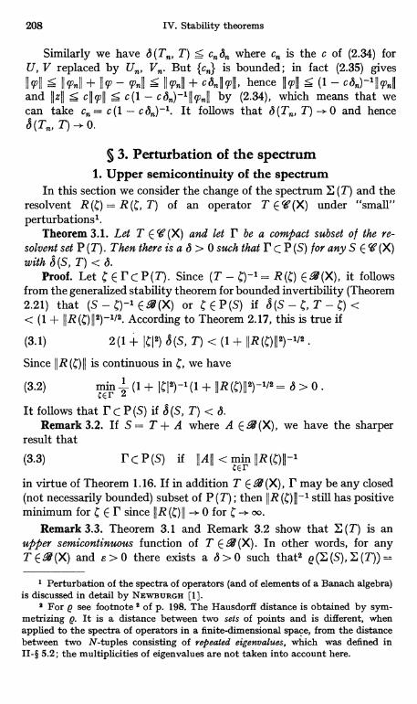
208 IV. Stability theorems
Similarly we have 6 (Tn, T) S c,,6,, where cn is the c of (2.34) forU, V replaced by U,,, V. But {c} is bounded; in fact (2.35) givesIImII < I199nll + IIq - Tnli s 1199.11 + c&&II99j1, hence 119,11 < (1 - cbn)-1IIT.11and j zjj S c119911 5 c (I - c bn)-11199n.I1 by (2.34), which means that wecan take cn = c (1 - can)-1. It follows that 6 (Tn, T) -+ 0 and henceS(Tn, T)--0.
§ 3. Perturbation of the spectrum1. Upper semicontinuity of the spectrum
In this section we consider the change of the spectrum E (T) and theresolvent R (4) = R (C, T) of an operator T E ' (X) under "small"perturbations'.
Theorem 3.1. Let T E le (X) and let r be a compact subset of the re-solvent set P (T). Then there is a b > 0 such that PCP (S) for a n y S E ' (X)with E (S, T) < b.
Proof. Let C E P c P (T). Since (T - C)-1= R M E .°.l! (X), it followsfrom the generalized stability theorem for bounded invertibility (Theorem2.21) that (S-0-' E(X) or CEP(S) if 5(S - 4, T - 4) << (1 + 11R(C)1I2)-1/2. According to Theorem 2.17, this is true if
(3.1) 2(1 + ICI2) b(S, T) < (1 + IIR(C)II2)-1/2
Since 11 R (C) 11 is continuous in g, we have
(3.2) Ti 2 (1 + IC12)-1 (1 + JJR(C)II2)-1/2= > 0.
It follows that r C P (S) if S (S, T) < 6.Remark 3.2. If S = T + A where A E °& (X), we have the sharper
result that
(3.3) PCP(S) if IIAII <mr IJR(C)II-1
in virtue of Theorem 1.16. If in addition T E -4 (X), P may be any closed(not necessarily bounded) subset of P (T) ; then 11 R still has positiveminimum for C E P since 11 R (C)11-+ 0 for -+ oo.
Remark 3.3. Theorem 3.1 and Remark 3.2 show that E (T) is anupper semicontinuous function of T E .4 (X). In other words, for anyT E 2 (X) and s > 0 there exists a 6 > 0 such that2 e (I (S), E (T)) =
1 Perturbation of the spectra of operators (and of elements of a Banach algebra)is discussed in detail by NEwBURGH [1].
2 For p see footnote' of p. 198. The Hausdorff distance is obtained by sym-metrizing p. It is a distance between two sets of points and is different, whenapplied to the spectra of operators in a finite-dimensional space, from the distancebetween two N-tuples consisting of repeated eigenvalues, which was defined inII-§ 5.2; the multiplicities of eigenvalues are not taken into account here.
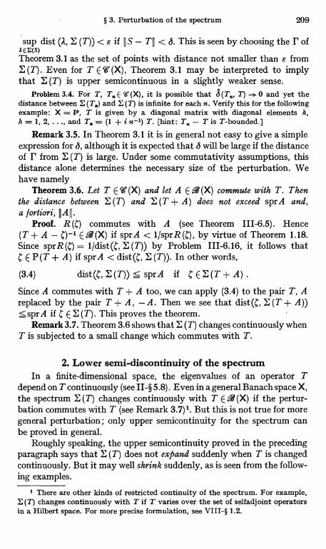
§ 3. Perturbation of the spectrum 209
sup dist (A, E (T)) < s if 11S - T11 < S. This is seen by choosing the r of2 E E(S)
Theorem 3.1 as the set of points with distance not smaller than s fromE (T). Even for T E ' (X), Theorem 3.1 may be interpreted to implythat E (T) is upper semicontinuous in a slightly weaker sense.
Problem 3.4. For T, T. E T (X), it is possible that 3 (T,,, T) 0 and yet thedistance between E and E (T) is infinite for each n. Verify this for the followingexample: X = I P, T is given by a diagonal matrix with diagonal elements k,k = 1, 2, ..., and T. = (1 + i n-1) T. [hint: T. - T is T-bounded.]
Remark 3.5. In Theorem 3.1 it is in general not easy to give a simpleexpression for S, although it is expected that S will be large if the distanceof r from E (T) is large. Under some commutativity assumptions, thisdistance alone determines the necessary size of the perturbation. Wehave namely
Theorem 3.6. Let T E le (X) and let A E P2 (X) commute with T. Thenthe distance between E (T) and .E (T + A) does not exceed sprA and,a /ortiori, 11 All.
Proof. R (C) commutes with A (see Theorem 111-6.5). Hence(T + A - 0)-1 E .4 (X) if sprA < 1/sprR (C), by virtue of Theorem 1.18.Since sprR (4) = 1/dist(C, E (T)) by Problem 111-6.16, it follows thatC E P(T + A) if sprA < dist(C, E (T)). In other words,
(3.4) dist(C, E (T)) 5 sprA if C E E (T + A) .
Since A commutes with T + A too, we can apply (3.4) to the pair T, Areplaced by the pair T + A, - A. Then we see that dist (C, E (T + A))SsprA if C E E (T). This proves the theorem.
Remark 3.7. Theorem 3.6 shows that E (T) changes continuously whenT is subjected to a small change which commutes with T.
2. Lower semi-discontinuity of the spectrumIn a finite-dimensional space, the eigenvalues of an operator T
depend on T continuously (see II-§ 5.8). Even in a general Banach space X,the spectrum E (T) changes continuously with T E 2 (X) if the pertur-bation commutes with T (see Remark 3.7)1. But this is not true for moregeneral perturbation ; only upper semicontinuity for the spectrum canbe proved in general.
Roughly speaking, the upper semicontinuity proved in the precedingparagraph says that E (T) does not expand suddenly when T is changedcontinuously. But it may well shrink suddenly, as is seen from the follow-ing examples.
1 There are other kinds of restricted continuity of the spectrum. For example,E (T) changes continuously with T if T varies over the set of selfadjoint operatorsin a Hilbert space. For more precise formulation, see VIII-§ 1.2.
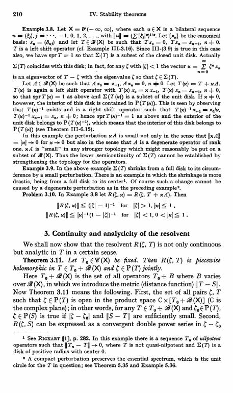
210 IV. Stability theorems
Example 3.8. Let X = l9 (- co, co), where each u E X is a bilateral sequenceu = (g,), j = , -1, 0, 1, 2,..., with (lull = Let be the canonicalbasis: x = (4,) and let T E 9(X) be such that Tx0 = 0, Tx = x,,_1, n + 0.T is a left shift operator (cf. Example 111-3.16). Since III-(3.9) is true in this casealso, we have spr T = 1 so that E (T) is a subset of the closed unit disk. Actually
ao
E (T) coincides with this disk; in fact, for any C with ICI < 1 the vector u = _P C° X.n=0
is an eigenvector of T - C with the eigenvalue C so that C E E (T).Let A E Q (X) be such that A xo = x_1, A x = 0, n + 0. Let T (m) = T + x A.
T (x) is again a left shift operator with T (x) xo = x x_1, T (x) x = n + 0,so that spr T (x) = 1 as above and E (T (x)) is a subset of the unit disk. If x + 0,however, the interior of this disk is contained in P (T (x)). This is seen by observingthat T (x)-1 exists and is a right shift operator such that T (x)-1 x_1 = xoJx,T (x)-1 x,,, n = 0; hence spr T (x)-1 = 1 as above and the exterior of theunit disk belongs to P (T (x)-1), which means that the interior of this disk belongs toP (T (x)) (see Theorem III-6.15).
In this example the perturbation xA is small not only in the sense that 11-Alllxl -+ 0 for x -+ 0 but also in the sense that A is a degenerate operator of rank
one. xA is "small" in any stronger topology which might reasonably be put on asubset of ..(X). Thus the lower semicontinuity of E (T) cannot be established bystrengthening the topology for the operators.
Example 3.9. In the above example E (T) shrinks from a full disk to its circum-ference by a small perturbation. There is an example in which the shrinkage is moredrastic, being from a full disk to its center'. Of course such a change cannot becaused by a degenerate perturbation as in the preceding example z.
Problem 3.10. In Example 3.8 let R (C, x) = R (C, T + xA). Then
OR (C, x)ll s (ICI -1)-' for ICI > 1, Ixl s 1,
IIR(C, x) II s 1-1-1(1 - ICI)-1 for ICJ < 1, 0 < Ixl s 1.
3. Continuity and analyticity of the resolventWe shall now show that the resolvent R (C, T) is not only continuous
but analytic in T in a certain sense.Theorem 3.11. Let To E T (X) be fixed. Then R T) is piecewise
holomorphic in T E To + .4 (X) and C E P (T) jointly.Here To + .4 (X) is the set of all operators To + B where B varies
over 9 (X), in which we introduce the metric (distance function) 11 T - S11.Now Theorem 3.11 means the following. First, the set of all pairs C, Tsuch that I E P (T) is open in the product space C x [To + .4 (X)] (C isthe complex plane) ; in other words, for any T E To + . (X) and Co E P (T),C E P(S) is true if IC - and HIS - TII are sufficiently small. Second,R (C, S) can be expressed as a convergent double power series in C - Cu
1 See RICKART [1D, p. 282. In this example there is a sequence T. of nilpotentoperators such that 11 T. - T11 -+ 0, where T is not quasi-nilpotent and E (T) is adisk of positive radius with center 0.
8 A compact perturbation preserves the essential spectrum, which is the unitcircle for the T in question; see Theorem 5.35 and Example 5.36.
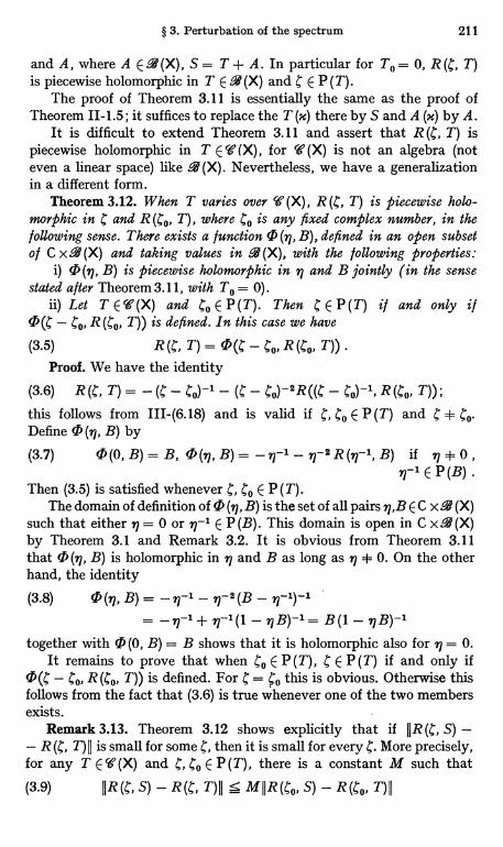
§ 3. Perturbation of the spectrum 211
and A, where A E -4 (X), S = T + A. In particular for To = 0, R (C, T)is piecewise holomorphic in T E .4 (X) and C E P (T).
The proof of Theorem 3.11 is essentially the same as the proof ofTheorem 11-1.5; it suffices to replace the T (m) there by S and A (x) by A.
It is difficult to extend Theorem 3.11 and assert that R (C, T) ispiecewise holomorphic in T Es' (X), for '(X) is not an algebra (noteven a linear space) like -1 (X). Nevertheless, we have a generalizationin a different form.
Theorem 3.12. When T varies over 'f(X), R(C, T) is piecewise holo-morphic in C and R (Co, T), whereto is any fixed complex number, in thefollowing sense. There exists a function 0 (9J, B), defined in an open subsetof C x. (X) and taking values in 2(X), with the following properties:
i) 0 (97, B) is piecewise holomorphic in 77 and B jointly (in the sensestated after Theorem 3.11, with To = 0).
ii) Let T E' (X) and Co E P (T). Then 4 E P (T) if and only if0(C - Co, R(Co, T)) is defined. In this case we have
(3.5) R (4, T) = 0(C - C R (Co, T))Proof. We have the identity
(3.6) R(C, T) = - (C - C0)-1 - (4 - Co)-2R((C - Co)-', R(CO, T));
this follows from III-(6.18) and is valid if C, Co E P (T) and C $ Co.Define 0 (97, B) by
(3.7) 0 (0, B) = B, 0 (97, B) 77-1 - 77-2 R (97-1, B) if 17 4 0 ,9l-1EP(B).
Then (3.5) is satisfied whenever C, C, E P (T).The domain of definition of 0 (97, B) is the set of all pairs 97,B E C x 9 (X)
such that either 97 = 0 or 97-1 E P (B). This domain is open in C x.46' (X)by Theorem 3.1 and Remark 3.2. It is obvious from Theorem 3.11that 0 (97, B) is holomorphic in 77 and B as long as 77 + 0. On the otherhand, the identity
(3.8) 0(n, B) _ - rl-1 - 71-'(B - 97-1)-1197-1(1 - 97B)-1= B(1 - 97B)-1
together with 0 (0, B) = B shows that it is holomorphic also for 97 = 0.It remains to prove that when go E P (T), C E P (T) if and only if
(l; - Co, R (Co, T)) is defined. For C = Co this is obvious. Otherwise thisfollows from the fact that (3.6) is true whenever one of the two membersexists.
Remark 3.13. Theorem 3.12 shows explicitly that if 11R (C, S) -- R (l;, T) 11 is small for some l;, then it is small for every C. More precisely,for any T E ' (X) and C, Co E P (T), there is a constant M such that(3.9) IIR(C, S) - R(C, T)II S MIIR(Co, S) - R(Co, T)II
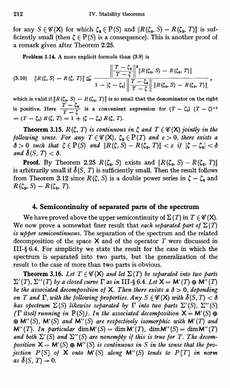
212 IV. Stability theorems
for any S E W (X) for which Cu E P (S) and 11 R (Co, S) - R (Co, T) 11 is suf-ficiently small (then 4 E P (S) is a consequence). This is another proof ofa remark given after Theorem 2.25.
Problem 3.14. A more explicit formula than (3.9) is
T - .'oII R (Co, S) - R (Co, T) lI
(3.10) II R (C, S) - R (C, T) 11 SCO
1 - 1C - ColO
11R (Co, S) - R (CO, T)11
T 1
which is valid if JJR (CO, S) - R (CO, T) 11 is so small that the denominator on the right
is positive. Here TT -. is a convenient expression for (T - Co) (T - C)-1
_ (T - Co) R(C, T) = 1 -I- (C - Co) R(C, T)
Theorem 3.15. R(4, T) is continuous in C and T E '(X) jointly in thefollowing sense. For any T E `' (X), Co E P (T) and e > 0, there exists a6>0 such that CEP (S) and IJR (C, S) - R (Co, T) 11 <8 if IC-CJ <6and S (S, T) < 6.
Proof. By Theorem 2.25 R (CO, S) exists and 11 R (Co, S) - R (Co, T) 11is arbitrarily small if 8 (S, T) is sufficiently small. Then the result followsfrom Theorem 3.12 since R (4, S) is a double power series in C - Co andR (Co, S) - R (Co, T).
4. Semicontinuity of separated parts of the spectrumWe have proved above the upper semicontinuity of E (T) in T E ' (X).
We now prove a somewhat finer result that each separated part of E (T)is upper semicontinuous. The separation of the spectrum and the relateddecomposition of the space X and of the operator T were discussed inIII-§ 6.4. For simplicity we state the result for the case in which thespectrum is separated into two parts, but the generalization of theresult to the case of more than two parts is obvious.
Theorem 3.16. Let T E W (X) and let E (T) be separated into two partsE' (T), E" (T) by a closed curve r as in III-§ 6.4. Let X = M' (T) ® M" (T)be the associated decomposition of X. Then there exists a 6 > 0, dependingon T and r, with the following properties. Any S E ' (X) with 8 (S, T) < 6has spectrum E (S) likewise separated by r into two parts E' (S), E" (S)(r itself running in P (S)). In the associated decomposition X = M' (S) ®® M" (S), M' (S) and M" (S) are respectively isomorphic with M' (T) andM" (T). In particular dim M' (S) = dim M' (T), dim M" (S) = dim M" (T)and both E' (S) and E" (S) are nonempty i f this is true for T. The decom-position X = M' (S) ® M" (S) is continuous in S in the sense that the pro-jection P [S] o l X onto M' (S) along M" (S) tends to P [T] in normas 3 (S, T) -> 0.
T - C
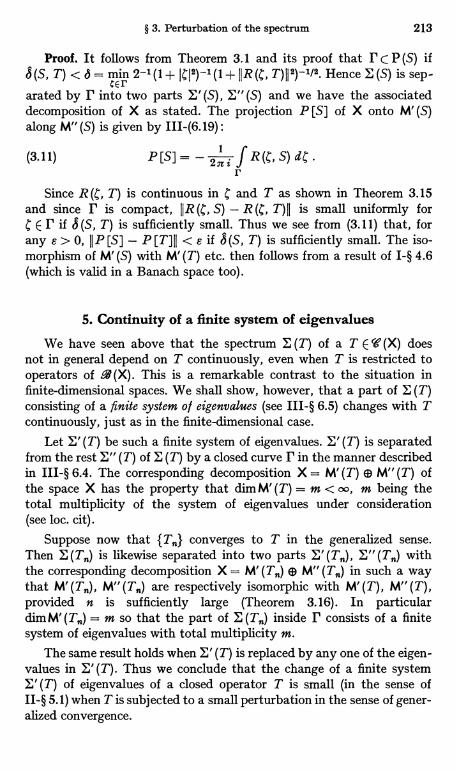
§ 3. Perturbation of the spectrum 213
Proof. It follows from Theorem 3.1 and its proof that P C P (S) ifS (S, T) < 6= min 2-1(1+ IC12)-1 (1 + JJR (C, T) 112)-1/2. Hence E (S) is sep-
arated by r into two parts E' (S), E" (S) and we have the associateddecomposition of X as stated. The projection P [S] of X onto M' (S)along M" (S) is given by III-(6.19) :
(3.11) P[S] _ - .12ni R(C' S) dCr
Since R (C, T) is continuous in C and T as shown in Theorem 3.15and since r is compact, 11R (C, S) - R (C, T) 11 is small uniformly forC E P if S(S, T) is sufficiently small. Thus we see from (3.11) that, forany s > 0, II P [S] - P [T] 11 < e if S (S, T) is sufficiently small. The iso-morphism of M' (S) with M' (T) etc. then follows from a result of I-§ 4.6(which is valid in a Banach space too).
5. Continuity of a finite system of eigenvalues
We have seen above that the spectrum E (T) of a T E le (X) doesnot in general depend on T continuously, even when T is restricted tooperators of 9(X). This is a remarkable contrast to the situation infinite-dimensional spaces. We shall show, however, that a part of E (T)consisting of a finite system of eigenvalues (see III-§ 6.5) changes with Tcontinuously, just as in the finite-dimensional case.
Let E' (T) be such a finite system of eigenvalues. E' (T) is separatedfrom the rest E" (T) of E (T) by a closed curve r in the manner describedin III-§ 6.4. The corresponding decomposition X = M' (T) ® M" (T) ofthe space X has the property that dim M' (T) = m < oo, m being thetotal multiplicity of the system of eigenvalues under consideration(see loc. cit).
Suppose now that {T} converges to T in the generalized sense.Then E is likewise separated into two parts E' (T ), E" withthe corresponding decomposition X = M' M" (Ta) in such a waythat M' (T,,), M" are respectively isomorphic with M' (T), M" (T),provided n is sufficiently large (Theorem 3.16). In particulardim M' m so that the part of E (Ta) inside r consists of a finitesystem of eigenvalues with total multiplicity m.
The same result holds when E' (T) is replaced by any one of the eigen-values in E' (T). Thus we conclude that the change of a finite systemE' (T) of eigenvalues of a closed operator T is small (in the sense ofII-§ 5.1) when T is subjected to a small perturbation in the sense of gener-alized convergence.

214 IV. Stability theorems
Not only is the system E' (T) continuous in T in this sense, but thetotal projection P [T] of X on M' (T) along M" (T) changes with T contin-uously, as is seen easily from Theorem 3.16.
Summing up, the behavior of a finite system of eigenvalues of aclosed operator under a small perturbation is much the same as in thefinite-dimensional case. We may pursue this analogy further by intro-ducing the unordered m-tuple 6'(T) of repeated eigenvalues to representthe finite system E' (T), as described in II- §5.2. Then the distance between(5'(T,,) and Cam' (T) converges to zero if T,, converges to T in the gener-alized sense.
6. Change of the spectrum under relatively boundedperturbation
The results on the upper semicontinuity of the spectrum E (T)and analyticity of the resolvent R (C, T) as functions of C and R (Co, T)given in par. 3 are rather general but not very convenient for application.Here we shall give a theorem which is less general but more directly useful.
Theorem 3.17. Let T be a closed operator in X and let A be an operatorin X which is T-bounded, so that D (A) D D (T) and the inequality (1.1)holds. If there is a point C o l P (T) such that
(3.12) ajIR(C, T)II + bjlTR(C, T)II < 1
then S = T + A is closed and C E P (S), with
(3.13) IIR(C, S)II 5 IIR(C, T)II (1- aIIR(C, T)II - bIITR(C, T)11)-1
I/ in particular T has compact resolvent, S has compact resolvent.This theorem follows easily from Theorem 1.16. It is convenient
since (3.12) gives an explicit condition for C to belong to P (S). For example,it can be used to deduce
Theorem 3.18. Let T, S and A be as in the preceding theorem. LetE (T) be separated into two parts by a closed curve r as in Theorem 3.16.if .(3.14) sup (aIIR(C, T) 11 + bIITR(C, T)II) < 1
CEP -
then E (S) is likewise separated by r and the results of Theorem 3.16 hold.Proof. The proof is similar to that of Theorem 3.16; only the follow-
ing points should be noted. We see from (3.11) and II-(1.11) thatII P [S] - P[T]II is arbitrarily small if II A R (C, T)11 is sufficiently smallfor all C E P, which is the case if a, b are sufficiently small. In this casethe results follow as in the proof of Theorem 3.16. Actually a, b neednot be too small but the condition (3.14) suffices. To see this, it is con-venient to introduce a parameter x and set T (x) = T + xA, 0 5 x 5 1.
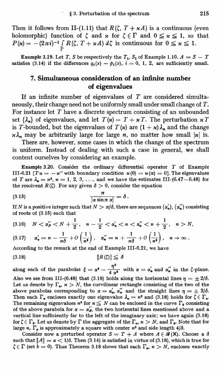
§ 3. Perturbation of the spectrum 215
Then it follows from II-(1.11) that R(C, T + xA) is a continuous (evenholomorphic) function of C and x for C E P and 0 S x S 1, so thatP(x) (2ni)-1 f R (T, T + xA) dC is continuous for 0:5 x 5 1.
rExample 3.19. Let T, S be respectively the T1, S1 of Example 1.10. A = S - T
satisfies (3.14) if the differences q, (x) - P, (x), i = 0, 1, 2, are sufficiently small.
7. Simultaneous consideration of an infinite numberof eigenvalues
If an infinite number of eigenvalues of T are considered simulta-neously, their change need not be uniformly small under small change of T.For instance let T have a discrete spectrum consisting of an unboundedset of eigenvalues, and let T (x) = T + x T. The perturbation x Tis T-bounded, but the eigenvalues of T (x) are (1 + x) A and the changexA may be arbitrarily large for large n, no matter how small 1xI is.
There are, however, some cases in which the change of the spectrumis uniform. Instead of dealing with such a case in general, we shallcontent ourselves by considering an example.
Example 3.20. Consider the ordinary differential operator T of Example111-6.21 [T u = - u" with boundary condition u (0) = u (n) = 0]. The eigenvaluesof T are A. = n2, n = 1, 2, 3, ..., and we have the estimates III-(6.47-6.48) forthe resolvent R (a). For any given 6 > 0, consider the equation
(3.15) la sine «l - 8
If N is a positive integer such that N > n16, there are sequences {a;,}, {ax} consistingof roots of (3.15) such that
(3.16) N<a4<N-{ 2 n-2 <a;,<n<a;;<n+2 n>N,(3.17) an=n-n + n6 +o(- ) n_*m.According to the remark at the end of Example 111-6.21, we have
(3.18) 11R(C)II5 aa
along each of the parabolas = a8 - 4a8
with a = a;, and or in the c-plane.Also we see from III-(6.48) that (3.18) holds along the horizontal lines 216.Let us denote by ra, n > N, the curvilinear rectangle consisting of the two of theabove parabolas corresponding to at = a;; and the straight lines rl = ± 216.Then each r, encloses exactly one eigenvalue A = n2 and (3.18) holds for C E r,,.The remaining eigenvalues n2 for n < N can be enclosed in the curve ro consistingof the above parabola for a = cc , the two horizontal lines mentioned above and avertical line sufficiently far to the left of the imaginary axis; we have again (3.18)for C E ro. Let us denote by r the aggregate of the r, n > N, and ro. Note that forlarge n, r is approximately a square with center n2 and side length 416.
Consider now a perturbed operator S = T + A where A E .1 (X). Choose a asuch that h All = a < 116. Then (3.14) is satisfied in virtue of (3.18), which is true forC E r (set b = 0). Thus Theorem 3.18 shows that each r,,, n > N, encloses exactly
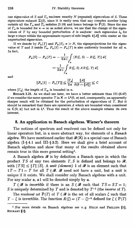
216 IV. Stability theorems
one eigenvalue of S and ro encloses exactly N (repeated) eigenvalues of S. Theseeigenvalues exhaust E (S), since it is easily seen that any complex number lyingoutside all the r and ro satisfies (3.18) and hence belongs to P (S). Since the sizeof r is bounded for n on as noted above, we see that the change of the eigen-values of T by any bounded perturbation A is uniform: each eigenvalue 2 forlarge n stays within the approximate square of side length 411 All with center at theunperturbed eigenvalue.
If we denote by P. [T] and P. [S], n > N, the eigenprojections for the eigen-value of T and S inside r,,, P. [S] - P [T] is also uniformly bounded for all n.In fact,
P. [S] - P.[T] = - 2ni f [R (C, S) - R(C, T)] dC
=1
2 n if R S) A R T) d
and
(11 P. [S] -
jrn18
Il- `4IIlAll)
C2n 6(where the length of is bounded in n.
Remark 3.21. As we shall see later, we have a better estimate than III-(6.47)if we consider the same operator T in X = L$ (0, n) and, consequently, an apparentlysharper result will be obtained for the perturbation of eigenvalues of T. But itshould be remarked that there are operators A which are bounded when consideredin C [0, n] but not in L2. Thus the result of the above example retains its owninterest.
8. An application to Banach algebras. Wiener's theorem
The notions of spectrum and resolvent can be defined not only forlinear operators but, in a more abstract way, for elements of a Banachalgebra. We have mentioned earlier that 9 (X) is a special case of Banachalgebra (I-§ 4.1 and III-§ 3.2). Here we shall give a brief account ofBanach algebras and show that many of the results obtained aboveremain true in this more general setting'.
A Banach algebra .4 is by definition a Banach space in which theproduct TS of any two elements T, S is defined and belongs to M,with 11 T S11 S 11 T11 JIS11. A unit (element) 1 of .4 is an element such that1 T = Ti = T for all T E M..4 need not have a unit, but a unit isunique if it exists. We shall consider only Banach algebras with a unit.For any scalar a, a 1 will be denoted simply by a.
T E -4 is invertible if there is an S E 9 such that TS = S T = 1;S is uniquely determined by T and is denoted by T-' (the inverse of T).
The resolvent set P (T) of T E.9' is the set of all scalars C such thatT - C is invertible. The function R (C) = (T - C,)-' defined for C E P (T)
1 For more details on Banach algebras see e. g. HILLS and PHILLIPS Q1D,RICKART Q1).
§ 3. Perturbation of the spectrum 217
is the resolvent of T. The complementary set E (T) ,(in the complex plane)of P (T) is the spectrum of T.
Many other notions introduced for 9 (X) can be taken over withoutchange to the case of an abstract Banach algebra 9 and many theoremsfor 9 (X) remain true for -4. As a rule, this is the case if such notions ortheorems can be defined or proved without explicit reference to theunderlying space X. For example: the spectral radius spr T can be definedfor T E .°.l! exactly as in I-§ 4.2. The Neumann series I-(4.22) is valid forT E 9 and 1 - T is invertible if spr T < 1. In particular we have thefirst Neumann series I-(5.6) for the resolvent, from which it follows thatP (T) is open and E (T) is closed, etc.
Most of the results on the perturbation of spectra are again validin -4, but we have to restrict ourselves to those results which are relatedto operators belonging to .°.l! (X), for an unbounded operator has noanalogue in -4. For example, E (T) is an upper semicontinuous functionof T E-4, but it is in general not lower semicontinuous. It is continuous,however, for a restricted change of T in a sense similar to Remark 3.7.
Here we have something new and interesting which did not existin 9 (X). It is possible that a Banach algebra 6` is commutative, whichmeans that all elements of -4 commute with one another, whereas thisis not true for -V(X) if dim X >- 2. If A is commutative, Theorem 3.6and Remark 3.7 are valid without any restriction. Thus E (T) is continuousin T E . it .4 is commutative.
Example 3.22. A typical example of a Banach algebra is the Banach space l(the set of all sequences T = (ax) with 11 T11 = E lv I < oo, see Example III-1.1)
kin which the product TS of two elements T= (th), S= (o,,) is defined by con-volution:
(3.19) TS=(Ps), Qk=EzjaA_j.i
It is easy to verify that 11 TS11S 11 T11 JIS11. Also it is easily seen that l is commutative.In the definition of 1 given in Example III-1.1 the index h runs from 1 to 00; inthis case I has no unit element. If we modify this slightly and assume that h runseither from 0 to oo or from - oo to co, then I has the unit I = (S 0). In whatfollows we take the latter case and set 69 = 1.
With each T E 9 we can associate a complex-valued function00
(3.20) T(ete) _ r5eike
defined on the unit circle (for real 0) ; note that the Fourier series on the right of(3.20) is absolutely convergent. It follows directly from (3.19) that
(3.21) TS(ere) = T(ere) S(e{B).We shall now show that
(3.22) Z (T) is exactly the range of T (ete) .
This implies, in particular, that T is invertible if T (e'8) + 0. If we set S = T-1,then S(e'0) = 1/T(et0). But S(e'8) has an absolutely convergent Fourier series by
218 IV. Stability theorems
definition. Hence the stated result implies the following theorem by Wiener: If acomplex-valued function T (e'0) with an absolutely convergent Fourier series does notvanish anywhere, 11T (et e) has also an absolutely convergent Fourier series'.
To prove the proposition (3.22), we first note that it is true if T (e{B) has ananalytic continuation T (z) in a neighborhood of the unit circle K. In fact, let Cbe a complex number not in the range of T(00). Then$ (T - C) (z) = T (z) -does not vanish anywhere in some neighborhood of K, so that R (z) = (T (z) -is again analytic in a neighborhood of K. It follows from the Cauchy inequalitiesfor the Laurent coefficients that R (et e) has an absolutely convergent Fourier series.If the sequence of the Fourier coefficients of R (e'0) is denoted by R, we have R E -4and R (T - C) = (T - C) R = 1, so that T - C is invertible. On the other hand,it is easily seen from (3.21) that T - C is not invertible if C lies in the range of T (e'°).
Now (3.22) is a simple consequence of the theorem stated above that E(T)is continuous in T (note that -4 is commutative). It suffices to note that for anyT = (ak) E A there is a sequence such that 11 T,, - T11 -a 0 and each T. (00)has an analytic continuation in a neighborhood of K. Such a sequence is given, for
nexample, by setting T.(et0) _ ak e{ k0. Since E is the range of T.(et0),
k=-nE (T) = lim E must be the range of T (ete) = lim T. (ete).
§ 4. Pairs of closed linear manifolds,1. Definitions
This section is intended to be preliminary to the following one, whereperturbation theory for the nullity, deficiency and index of an operatoris developed. But the subject will probably have its own interest.
The problems to be considered are related to pairs M, N of closedlinear manifolds in a Banach space Z. The results obtained will be appliedin the following section to operators of the class '9 (X, Y), with Z = X x Ythe product space of X, Y. Some of the basic results in this direction havebeen obtained in § 2, but we need more results for later applications.
Let Z be a Banach space and let M, N be closed linear manifoldsof Z. Then M n N is also a closed linear manifold. We shall define thenullity of the pair M, N, in symbol nul (M, N), by
(4.1) nul (M, N) = dim (M n N) .
M + N is a linear manifold (not necessarily closed) ; we define thedeficiency of the pair M, N, in symbol def (M, N), by
(4.2) def (M, N) = codim (M + N) = dim Z/(M + N) 8 .
1 Cf. RiESZ and Sz.-NAGY 11)1, p. 434.
2 Note that 1(ete) = 1 for the unit element 1.8 A different definition of def (M, N) is to use the closure of M + N instead of
M + N in (4.2). But the two definitions coincide for semi-Fredholm pairs.
§ 4. Pairs of closed linear manifolds 219
The index of the pair M, N, in symbol ind (M, N), is defined by
(4.3) ind (M, N) = nul (M, N) - def (M, N)
if at least one of nul (M, N) and def (M, N) is finite.The pair M, N will be said to be Fredholm [semi-Fredholm] if M + N
is a closed linear manifold and both of [at least one of] nul (M, N) anddef (M, N) are [is] finite.
Finally we define the quantity
(4.4) (M, N) = inf dist(u, N) (< 1)uEM,u4N dist(u, Mn N)
By this formula y (M, N) is defined only when M Q N. If M C N we sety (M, N) = 1. Obviously y (M, N) = 1 if M ) N. y (M, N) is not symmetricwith respect to M, N. We set
(4.5) y (M, N) = min [y (M, N), y (N, M)]
and call it the minimum gap between M and N.Problem 4.1. y (M, N) < 6 (M, N) except for M C N. [hint: dist (u - z, N)
= dist(u, N) for u E M, z E Mn N].
Although y (M, N) and y (N, M) are not in general equal, they are notcompletely independent. We have namely
(4.6) y (N, M) 1 +(MM )N)
The proof of (4.6) will be given in a moment.Theorem 4.2. In order that M + N be closed, it is necessary and su f -
ficient that y (M, N) > 0.Proof. First consider the special case M n N = 0. If M + N = Zo
is closed, Zo is a Banach space and each u E Zo has a unique expressionu = v + w, v E M, W EN. Thus Pu = v defines the projection P of Zoonto M along N. P is bounded by a remark after Theorem 111-5.20. But11P11 = sup IIPuII/IIuII = sup IIvII/IIv + wII = sup IvII/dist (v, N)
uEZo vEM, WEN vEM
= 1/y(M, N) since dist(v, M n N) = IIvII by M n N = 0. Thus
(4.7) y(M, N) = 1/IIPII > 0.
The above argument is not correct if M = 0. In this case y (M, N) = 1 > 0by definition, but it is not equal to IIPII-1= oo.
Suppose, conversely, that y (M, N) > 0; we shall show that M + Nis closed. We may assume that M + 0. Let vn + w -+ u, vn E M, w E N.Then Iv - vmll S dist(v,, - vm, N)/Y(M, N) S iv,, - vm + w - wmll//y (M, N)- 0. Hence lim v,, = v exists and w _ (v,, + v,, -+ u - v.Since M, N are closed, v E M, u -v E N and hence u E M + N.
220 IV. Stability theorems
In this case (4.6) follows from (4.7) and the corresponding formulay (N, M) = 1/11 1 - PII, noting that 11 1 - PII 5 1 + II P11. The proof is notvalid in the exceptional case M = 0 or N = 0, but it is clear that (4.6)is true in these cases too.
In the general case M n N + 0 set L = M n N and introduce thequotient space Z = Z/L. Since L is closed, Z is a Banach space (seeIII-§ 1.8). Let M be the set of all u E Z such that u c: M; note that thewhole coset ii is contained in M if there is one element u of u containedin M. Similarly we define N. It is easily seen that M, N are closed linearmanifolds of Z with M n N = 0. Furthermore, M + N is closed in Zif and only if M + N is closed in Z.
Thus the proof of the theorem in the general case is reduced to thespecial case considered above if we show that
(4.8) y (M, N) = y (M, N) .
But this follows from the identity
(4.9) dist (u, M) = dist (u, M)
and similar identities with M replaced by N and L. To show (4.9) itsuffices to note that dist (u, M) = inf IIu - vII = inf inf II u - v - z1I
;E FA vEM aEL
= EM 11u - v11 = dist(u, M). Again the exceptional case MC N in (4.8)
should be treated independently, but the proof is trivial.Remark 4.3. In view of (4.8), (4.7) is true even in the general case if
M + 0 and P is the projection of M + N onto M along N. Also we notethat (4.6) is true in the general case if M + N is closed. It is true evenwhen M + N is not closed, for then we have y (M, N) = y (N, M) = 0by Theorem 4.2.
Lemma 4.4. Let M + N be closed. Then we have for any u E Z
(4.10) dist (u, M) + dist (u, N) z 2 y (M, N) dist (u, M n N) .
Proof. In view of (4.8) and (4.9), it suffices to prove (4.10) in whichu, M, N are replaced by u, M, N, respectively. Changing the notation,we may thus prove (4.10) assuming that M n N = 0 (so that dist (u, M n N)
= IIuII)For any s > 0, there exists a v E M and w E N such that dist (u, M) >
>IIu - vII - e, dist(u,N)>Ilu-w1l - s.If IIvII S IuII/2, we have dist(u, M) > IIuII -IvII - e Z IuII/2 - e.
If IIvII z IIuII/2, then dist(u, M) + dist(u, N) z IIu - vII + IIu - wII - 2ez.Ilv-wII-2e z dist(v,N)-2ez IIvlly(M,N)-2e? a IIuIIy(M,N)-2e.
§ 4. Pairs of closed linear manifolds 221
In either case the left member of (4.10) is not smaller than2 jjujj y(M, N) - 2s. Since 6>0 is arbitrary, this proves (4.10).
Problem 4.5. ind (M, 0) = - codim M, ind (M, Z) = dim M.Problem 4.6. Let M' ) M with dim M'/M = m < oo. Then ind (M', N)
= ind (M, N) + m.Problem 4.7. If def (M, N) < oo, then M + N is closed. [hint: There is an M'such
that M') M, M' n N = M n N, M' + N = Z, dim M'/M < oo. Then 0 < y (M', N)S y(M,
2. DualityFor any subset S of Z, the annihilator S1 is a closed linear manifold
of Z* consisting of all / E Z* such that f .1 S. For any closed linear mani-folds M, N of Z, it is easily seen that
(4.11) (M+ N)1 = MJ- n N1 .
The dual relation MJ- + N 1 = (M n N) J- is not always true, for thesimple reason that (M n N)1 is always closed but MJ- + NJ- need notbe closed. We shall show, however, that it is true if and only if M + Nis closed.
Theorem 4.8. Let M, N be closed linear manifolds of Z. Then M + Nis closed in Z if and only if MJ- + N1 is closed in Z*. In this case we have,in addition to (4.11),
(4.12) M1+N1= (MnN)1,(4.13) nul(M1, N1) = def(M, N), def(M1, N1) = nul(M, N) ,
(4.14) (M 1, N1) = y(N M), (M1 N1) = (M, N)
[(4.14) is true even if M + N is not closed.]The proof of this theorem will be given in several steps.Lemma 4.9. If M + N is closed, then (4.12) is true. In Particular
M1 + N1 is closed.Proof. It is easily seen that M1 + N1 C (M n N) 1. Thus it suf-
fices to prove the opposite inclusion.Let / E (M n N)1 and consider (f, u) for u E M + N. u has a form
u = v + w, v E M, w E N, but such an expression may not be unique.If u = v' + w' is another expression of this kind, we have v - v' = w' --wEMnN so that (f,v-v')= (1,w-w')=0. Thus (f, v)= (f, v')and (f, v) is determined uniquely by u. The functional g [u] _ (f, v)thus defined for u E M + N is obviously semilinear. Similarly we defineh [u] = (f, w). We note that
(4.15) g [u] = 0 for U E N and h [u] = 0 for , u E M.
g and h are bounded. In fact we have Ig [u] =I(/, v)1:5 11/11 jjvjj, where vmay be replaced by v - z for any z E L = M n N. Hence Ig [u] S
222 IV. Stability theorems
II/II dist (v, L). Since lull = IIv + wII _>_ dist (v, N) y (M, N) dist (v, L), itfollows that Ig[u]I S II/II IIuII/y (M, N). In other words, g is bounded with
(4.16) IIuII 5 11/11/y (M, N) .
g can be extended to a bounded semilinear form on Z by the Hahn-Banach theorem, preserving the bound (4.16) ; we shall denote thisextension by the same symbol g. Similarly h can be extended to anelement of Z*, denoted again by h. Then (4.15) shows that
(4.17) g E NJ-, h E M1 .
Since (f, u) v) + (f, w) = g [u] + h [u] = (g, u) + (h, u) foru E M + N, the forms / and g + h coincide on M+ N. Thus f - g - h= k E (M+ N)1 CM1. Hence h+k E M1 and /=g+(h+k) E M1 + N1.This proves the lemma.
Lemma 4.10. If M + N is closed, then y (M, N) S y (N1, M1).Proof. For any go E N1 and hoEM1 set f =go+ho. Then /EM1 +N1
_ (M n N)1 by Lemma 4.9. According to the proof of Lemma 4.9, /can be written as f = g + h, g E N1, h E M1, in such a way that (4.16) istrue. But since g-go=ho-h E M1nN1, we have IIglj=Ilgo+g-golf>- dist (go, M1 n Nl). Thus (4.16) implies dist (go, M1 n N1)s Ilgo + hoill y (M, N). Since this is true for any ho E M1, we havedist(go, M1 n Ni) S dist (go, Ml)/y(M, N). Since this is true for anygo E N1, we obtain the desired result. (Again the exceptional caseM C N needs separate discussion but it is trivial.)
Lemma 4.11. If M + N is closed, then y (N1, M1) s y (M, N).Proof. Again the exceptional case is trivial and we assume that
M C N. For simplicity we write y (M, N) = y and M n N = L.By definition, for any e > 0 there exists a v E M such that
(4.18) 0 < dist (v, N) < (y + e) dist (v, L) .
For this v, there exists a f E Z* such that f E L 1 and 0 < (f, v) =IIfII dist (v, L)(see Theorem 111-1.22). Since L1 = M1 + N1 by Lemma 4.9, f can bewritten as f = g + h with g E N1, h E M1. Thus II/II dist (v, L) = (f, v)=(g+h,v)_ (g,v)= (g,v-w)= (g-k, v-w) IIg - kilIIv - wII,where w E N and k E M1 n N1 are arbitrary. Hence 0 < II/II dist (v, L) Ss dist (g, M1 n NJ-) dist (v, N). But since dist (g, M1) s IIg+hII = II/II,we obtain(4.19) dist(g, M1) dist(v, L) s dist(v, N) dist(g, M1 n N1) .
It follows from (4.18) and (4.19) that dist (g, M1) S (y + s)dist(g, M1 n N1). Since g E N1, this shows that y (N1, M1) s y + e.
Since e > 0 is arbitrary, this proves the Lemma.Lemma 4.12. If M 1+ Ni is closed, then M + N is closed.
§ 4. Pairs of closed linear manifolds 223
Proof. Let Zo be the closure of M + N. Let BM, BN be the unit ballsof M, N, respectively. We shall first show that the closure S of the setS = BM + BN contains a ball of Zo.
Let uo E Zo be outside S. Since S is a closed convex set, there exists aclosed hyperplane of Zo separating uo from S. In other words, thereexists an to E Zo such that'
(4.20) Re (f o, v + w) < Re (f o, uo) for all v E BM, w E BN .
to can be extended to an element of Z*, denoted again by to, preservingthe bound.
Since in (4.20) v and w may be multiplied by arbitrary phase factors(complex numbers with absolute value one), the left member can bereplaced by 1 (/o, v) + 1 (/ o, w) . But sup I (to, v) = dist (to, M 1) by (2.17)
aE BM
and similarly for I (f o, w) 1. Hence
(4.21) dist(/o, M1) + dist(/o, N1) 5 Re(/o, uo) S 11uoll 11/oil
But the left member of (4.21) is not smaller than y' dist(/o, M1 n NJ-)by Lemma 4.4, where y' = y (M1, N1)/2 > 0. Furthermore, we have
J-) = (bound ofdist (f o, M1 n N 1) = dist (/o, (M + N) 1) = dist (f o, Z0f o restricted to Zo) _ 11/o 11 by the definition of f o. Hence we obtain Iluoll
This means that any u E Zo with llul < y' belongs to S. In other words,contains the ball of Zo with center 0 and radius y'. Then an argument
similar to the one used in the proof of the closed graph theorem (Theorem111-5.20) can be applied to show that S itself contains a ball of Zo.Since M + N is a linear set containing S, it must be identical with Zoand therefore closed.
Lemmas 4.9 to 4.12 put together prove Theorem 4.8. Note that(4.13) follows immediately from (4.11) and (4.12) (see Lemma III-1.40).
Corollary 4.13. A pair M, N of closed linear manifolds is Fredholm[semi-Fredholm] it and only if the pair M1, N1 is Fredholm[semi-Fred-holm]. In this case we have
(4.22) ind(M, N) _ -ind(M1, N1) .
3. Regular pairs of closed linear manifolds
We have remarked above that in general y (M, N) + y (N, M),although these two quantities are both zero or both non-zero (see (4.6)).If y (M, N) = y (N, M), we shall say that the pair M, N is regular.
1 Let d = dist (uo, S) > 0 and let S' be the set of all u E Zo such that dist (u, S) << d/2. S' is an open convex set not containing uo. Thus the existence of to followsfrom the Hahn-Banach theorem (see footnote 1 of p. 135).
224 IV. Stability theorems
It is known that any pair M, N is regular if Z is a Hilbert space'.Another example of a regular pair is given by the pair X, Y in the prod-uct space Z = X x Y. Here X is identified with the closed linear mani-fold of Z consisting of all elements of the form {u, 0} with u varyingover X, and similarly for Y. It is easy to see that y (X, Y) = y (Y, X) = 1.
It is interesting, however, to notice that there are other nontrivialregular pairs in the product space Z = X x Y. In fact, there are closedlinear manifolds N of Z such that M, N is a regular pair for any M C Z.Such an N will be called a distinguished closed linear manifold.
Theorem 4.14. In Z = X x Y, X is a distinguished closed linearmanifold. Similarly for Y.
Proof. According to our definition, the norm in Z is given by
(4.23) II{x, y}112 = Ilxll2 + llyll2, x E X, y E Y .
Let M be a closed linear manifold of Z. We have to show thaty (M, X) = y (X, M). We set L = M n X.
First let us compute y (M, X). Let u = {x, y} E M. Then dist (u, X)2= inf (llx - x'll2 + lyll2) = Ilyll2, and dist(u, L)2 =xi f (IIx - x1ll2+ Ilyll2)
= Ilxll2 + Ilyll2 where x E X = X/L. Hence
(4.24) y (M, X) ={x,YnEM
II YII Y
(IIxII2 +IIY112)l1s = (1 + y2)1"2
where(4.25) y = {xynf 11Y11/11911
inf (Il
y(X, M) =inf dist(x, M) = inf {x',}EMx - x'll' + IIY'll')1"
xEX dist(x, L) xEX 11911
= (IIz11II2 + IIy'II2)"2 (Iiz"It2 + lly'IIe)112{xy'}EM IIx' + x"II Y') EM Ilx' + x"lIx"EXx'EJC
For a given {x', y'} E M, there is an x" E X with 119'+ x"ll = Il x' II + 11 x"" lland with an arbitrary IIx" II . Hence
(4.26) y (X, M) yinf'} M
(II'I' I'lI + IIt. "III)l,s
;"ER
inf f 1 + Y2 2 e 1-1/2 = Y/(1 + V2)1/2 ,{x',Y'}EM IIY'II'
where the Schwarz inequality was used. (4.24) and (4.26) show thaty (M, X) = y (X, M). [The above computations do not make sense ifM C X or X C M. But in these exceptional cases y (M, X) = y (X, M) = 1.]
1 This is due to the identity III - PII = IIPII which is valid for any (oblique)projection P, 0 + P + 1, in a Hilbert space; see Problem 1-6.31.
§ 4. Pairs of closed linear manifolds 225
4. The approximate nullity and deficiencyLet M, N be closed linear manifolds of a Banach space Z. We define
the approximate nullity of the pair M, N, in symbol nul' (M, N), as theleast upper bound (actually the greatest number, as will be shownbelow) of the set of integers m (m = no being permitted) with the propertythat, for any e > 0, there is an m-dimensional closed linear manifoldM,(Mwith 6(ML1 N) <e.
Problem 4.15. nul'(M, N) > nul (M, N).
We define the approximate deficiency of the pair M, N, denoted bydef'(M, N), by(4.27) def'(M, N) = nul'(M1, N1) .
It should be remarked that nul (M, N) and def (M, N) have beendefined in a purely algebraic fashion, without referring to any topology.The definition of nul' (M, N) and def' (M, N), on the other hand, dependsessentially on the topology of the underlying space.
As mentioned above, nul' (M, N) is not only the least upper boundbut the greatest number m with the properties stated above. This isobvious if nul'(M, N) is finite. When nul'(M, N) = no, this remark isequivalent to the following lemma.
Lemma 4.16. Suppose that for any e > 0 and any finite in, there existsan m-dimensional M, M with 6 (M,, N) < E. Then for any e > 0 thereexists an oo-dimensional M, C M with 6 (Me, N) < E.
Proof. For any closed linear manifold M' c M with dim M/M' < no,there is an M, r_ M with dim M, > dim M/M' and 6 (M,, N) < E. Thendim (M' n Me) > 0 (see Problem 111-1.42), so that there is a u = 0 in M'such that dist (u, N) < e 11 u 1I . Thus Lemma 4.16 is a consequence of thefollowing lemma.
Lemma 4.17. Assume that for any e > 0 and any closed linear manifoldM' C M with dim M/M' < no, there exists a u + 0 in M' such that dist (u, N) << e II u II . Then there is, for any e > 0, an oo-dimensional M, r_ M such that6 (Me, N) < e. In particular nul' (M, N) = no.
Proof. We construct two sequences u, , fn with the following prop-erties.
u.EM, f,EZ*, IIunII=1, IIffII=1,(4.28) (u,,, fn) = 1 , (un, fk) = 0 for k < n ,
dist (u,,, N) 5 3-n e .
Supposing that u, fk have been constructed for k = 1, 2, ..., n - 1,u,, and fn can be found in the following way. Let M' be the set of allu E M such that (u, fk) = 0 for k = 1, ..., n - i. Since M' is a closedlinear manifold with dim M/M' S n - 1, there is a un E M' such that
226 IV. Stability theorems
11unll = i and dist (u,,, N) S 3-n e. For this u there is an / E Z* suchthat 11/nll = i and (u,,, 1 (see Corollary 111-1.24).
It follows from (4.28) that the u are linearly independent, so thattheir span M' is infinite-dimensional. Each u E M,' has the form
(4.29)
with some integer n. We shall show that the coefficients k satisfy theinequalities(4.30) S 21-1 (lull , k = 1, 2, ..., n.
To prove this we note that by (4.29) and (4.28)
(4.31) (u, /,) = $1(ul, /,) + ... + $J-1(u, -1, /,) + $j
If we assume that (4.30) has been proved for k < j, (4.31) gives
1 11 I(ul, MI + ... + ICJ-11 I(ui-v /,)1
< 1jull+Ilull+...+2'-211ull=2'-' hull,
completing the proof of (4.30) by induction.From (4.28-4.30) we obtain
dist (u, N) < 1$11 dist (ul, N) + + l$,l dist (u,,, N) s
s (3-1+2.3-2+...+2n-i'3J'')e1lull s ellull
The same inequality is true for all u in the closure M. (M of M. Hence(M,, N) < e.
Theorem 4.18. I/ M + N is closed, then
(4.32) nul' (M, N) = nul (M, N) , def' (M, N) = def (M, N) .
Proof. Ml + Nl is closed if and only if M + N is closed, by Theorem4.8. In view of (4.13) and (4.27), therefore, it suffices to prove the firstequality of (4.32).
Suppose that there is an M, M such that dim M. > nul (M, N)= dim (M n N) and S (M,, N) < e. Then there is a u E M, such thatdist (u, M n N) = hull = i (see Lemma 2.3). Then dist (u, N) Z y dist (u,M n N) = y, where y = y (M, N) > 0 by Theorem 4.2. On the otherhand, dist (u, N) 5 hull 6 (M,, N) < e. Hence a cannot be smaller than Y.This shows that nul' (M, N) S nul (M, N). Since the opposite inequalityis also true (Problem 4.15), we have the required equality.
Theorem 4.19. 1/ M + N is not closed, then
(4.33) nul' (M, N) = def' (M, N) = oo.
Proof. Again it suffices to prove nul' (M, N) = oo. For any M' Mwith dim M/M' < oo, M' + N is not closed (otherwise M + N would be
§ 4. Pairs of closed linear manifolds 227
closed by Lemma 111-1.9). Thus y (M', N) = 0 by Theorem 4.2. Hence forany e > 0, there is a nonzero u E M' with dist (u, N) < e dist (u, M' n N)5 e 1lull. Thus the assumptions of Lemma 4.17 are satisfied.
Problem 4.20. nul'(M, N), def'(M, N) are symmetric in M, N.Problem 4.21. def'(M, N) def (M, N).Problem 4.22. nul'(M, N) = def'(Ml, NI-).
Finally we add a simple criterion for nul' (M, N) = oo.Theorem 4.23. We have nul' (M, N) = oo if and only i f there is a
sequence u E M with Ilunli = 1 and dist (u,,, N) -+ 0 which contains noconvergent subsequence.
Proof. Suppose that nul' (M, N) = oo. We shall construct a sequenceu E M such that 11 1, dist (u,,, N) s 1/n and 11u - u,,J Z 1 forn + in. Assume that u1...., u have already been constructed, and letM. be their span. Since nul' (M, N) = oo, there is an (n + 1)-dimensionallinear manifold M' c: M such that S (M', N) S 1/(n + 1). Since dim M'>> dim M, there is a u E M' such that dist (u, M) = 11ull = 1 (Lemma 2.3).u = satisfies all the requirements for
Suppose, conversely, that nul' (M, N) < oo and u E M is a sequencewith 11 1 and dist (u,,, N) -+ 0. We shall show that contains aconvergent subsequence. Since M + N is closed by Theorem 4.19,y (M, N) = y > 0 by Theorem 4.2 and nul (M, N) < oo by Theorem 4.18.Thus dist (u,,, M n N) S y-1 dist (u,,, N) --> 0. This means that there is asequence z E M n N such that u - z -+ 0. Since is thus boundedand dim (M n N) = nul (M, N) < oo, contains a convergent sub-sequence. The same is true of by u - z -+ 0.
5. Stability theorems
Let us now show that nul (M, N), def (M, N), ind (M, N) and theclosedness of M + N have a certain stability when M is subjected to asmall perturbation.
Theorem 4.24. Let M, N, M' be closed linear manifolds o l Z and letM + N be closed. Then 8 (M', M) < y (N, M) implies nul'(M', N) s5 nul (M, N), and 6 (M, M') < y (M, N) implies def'(M', N) 5 def (M, N).[Note that 6 (M, N) and y (M, N) are in general not symmetric in M, N.]
Proof. Assume that 6 (M', M) < y (N, M). Suppose that there is aclosed linear manifold N, C N such that dim N. > nul (M, N) = dim (M nn N) ; we shall show that 6 (N,, M') cannot be too small. Then we shallhave nul' (M', N) = nul' (N, M') 5 nul(M, N) (see Problem 4.20).
dim N, > dim (M n N) implies that there exists a u E N, C N suchthat dist (u, M n N) = 11 ull = 1 (Lemma 2.3). Hence dist (u, M) ? y (N, M)by (4.4). If we make the substitutions N -+ M, M -* M' in (2.14), we
228 IV. Stability theorems
thus obtain dist (u, M') > [1 + 6 (M', M)]-1 [y (N, M) - 6 (M', M)]. Thisshows that dist (u, M') and, a fortiori, 6 (NE, M') cannot be arbitrarilysmall.
The second assertion of the theorem follows from the first by con-sidering Ml, N', M'-L; note (2.19), (4.13), (4.14) and (4.27).
Corollary 4.25. Let M, N be a Fredholm [semi-Fredholm] pair. Thenthe same is true of the pair M', N it S (M', M) < y (M, N), and we havenul (M', N) < nul (M, N), def (M', N) s def (M, N).
Proof. The assumption implies that both of the two conditions ofTheorem 4.24 are satisfied. Hence both of the two conclusions are true.If M, N is a semi-Fredholm pair, at least one of nul (M, N) and def (M, N)is finite. Hence at least one of nul' (M', N) and def' (M', N) is finite.Then M' + N is closed by Theorem 4.19, and at least one of nul (M', N)= nul' (M', N) and def (M', N) = def' (M', N) is finite (see Theorem 4.18).Thus M', N is a semi-Fredholm pair. If M, N is a Fredholm pair, bothnul (M, N) and def (M, N) are finite and hence both nul (M', N) anddef (M', N) are finite.
Remark 4.26. In Theorem 4.24, M' + N need not be closed if nul (M, N)= def (M, N) = oo. There is an example of a pair M, N for which there isan M' with arbitrarily small 3 (M', M) such that M' + N is not closed.
Remark 4.27. In Corollary 4.25, y (M', N) > 0 since M', N is a semi-Fredholm pair. But it is in general difficult to estimate y (M', N) frombelow in terms of y (M, N) and b (M', M). In other words, y (M, N) canchange discontinuously when M is changed slightly. This discontinuity isdue to the discontinuity of M n N that appears in the definition ofy (M, N) [see (4.4) ]. But there is lower semicontinuity of y (M, N) ifM n N = 0 or M + N = Z. In such a case we have more detailed resultsgiven by the following lemmas.
Lemma 4.28. Let M + N be closed with nul (M, N) = 0. It 6 (M', M) << y (N, M)/ [2 + y (N, M) ] , then M' + N is closed, nul (M', N) = 0 anddef (M', N) = def (M, N).
Proof. In view of (4.6), we have 3 (M', M) < min [y (M, N), y (N, M)]= y (M, N). Hence M' + N is closed and nul (M', N) = 0, def (M', N) 5def (M, N) by Corollary 4.25. It remains to be shown that def (M, N) 5S def (M', N).
To this end it suffices to show that 6 (M', M) < y (M', N), for then wecan apply the second part of Theorem 4.24 with M and M' exchanged.
Let u E N. Then dist (u, M) ->_ y (N, M) dist (u, M n N) = y (N, M) lullsince M n N = 0. It follows from (2.14) (with the substitution N -+ M,M -+ M') that dist (u, M') [1 + 6 (M', M)]-1 [y (N, M) - 6 (M', M)] hull.Since this is true for any u E N, we have
(4.34) y (N, M') z y (N 4-M
) &(W6
(M,M)
§ 5. Stability theorems for semi-Fredholm operators 229
Application of the inequality (4.6) then gives the desired inequality:
(4.35) y (M'. N) z y (N,M') __ y (N. M) - S (M', M)
> 6 (M', M)1+y(N,M') 1+y(N,M)since 6 (M', M) < y (N, M)/ [2 + y (N, M)] by hypothesis.
Lemma 4.29. Let M + N = Z (so that def (M, N) = 0). I/ S (M', M) << y (M, N)/ [2 + y (M, N) ], then M' + N = Z (so that def (M', N) = 0)and nul(M', N) = nul(M, N).
Proof. It suffices to apply Lemma 4.28 to M, N, M' replaced by theirannihilators. Note Theorems 4.8 and 2.9.
Theorem 4.30. Let M, N be a Fredholm [semi-Fredholm] pair. Thenthere is a 6 > 0 such that S (M', M) < 6 implies that M', N is a Fredholm[semi-Fredholm] pair and ind (M', N) = ind (M, N).
Proof. It suffices to consider the semi-Fredholm case, for thenind(M', N) = ind(M, N) implies that the pair M', N is Fredholm if andonly if the pair M, N is. Furthermore, we may assume that def (M, N) < oo ;the case nul (M, N) < oo can be reduced to this case by considering theannihilators.
If def (M, N) = m < oo, we can find an No ) N such that dim No/N= m, No n M = N n M and M + No = Z. According to Lemma 4.29,there is a 6 > 0 such that S (M', M) < 6 implies that def (M', No) = 0 andnul (M', No) = nul (M, No) = nul (M, N). Hence ind (M', No) = nul (M, N),and it follows from Problem 4.6 that ind(M', N) = ind(M', No) - m= nul (M, N) - def (M, N) = ind (M, N).
Remark 4.31. Theorem 4.30 shows that the index of a semi-Fredholmpair M, N is stable under a small perturbation of M. It could be shownthat the same is true for simultaneous perturbation of M and N, but theproof would be more complicated. Also it is not easy to give a simpleestimate of 6 in Theorem 4.30. In particular, it is in general not known'whether ind(M', N) is constant for all M' considered in Corollary 4.25,except that this is true if Z is a Hilbert space2.
5. Stability theorems for semi-Fredholm operators1. The nullity, deficiency and index of an operator
In this section we define the nullity, deficiency, index, etc. of alinear operator T E `' (X, Y) and establish several stability theorems forthese quantities3. The general results follow from the corresponding
1 Cf. NEUBAUER [1].2 Cf. T. KATO [9].8 General references for this section are ATKINSON [1], [2], BROWDER (1],
[2], [3], CORDES and LABROUSSE [1], DTEUDONNA [1], GOHBERG and KREIN [1],KAASHOEK [1], KANIEL and SCHECHTER [1], T. KATO [12], KREIN and KRASNO-SEL'SKII [1], SZ.-NAGY [3], NEUBAUER [1], [2], YOOD [1].
230 IV. Stability theorems
results for pairs of closed linear manifolds studied in the precedingsection'. But these will be supplemented by more specific results pertain-ing to, operators.
As in the finite-dimensional case (I-§ 3.1), the nullity, nut T, of anoperator T from X to Y is defined as the dimension of N (T). Since N (T)is the geometric eigenspace of T for the eigenvalue zero, nul T is thegeometric multiplicity of this eigenvalue. The deficiency, def T, of T isthe codimension in Y of R (T) : def T = dim Y/ R (T) 2. Each of nul Tand def T takes values 0, 1, 2, . or oo. The index of T is defined by3
(5.1) ind T = nut T - def T
if at least one of nul T and def T is finite. -
The notions of nullity and deficiency involve certain arbitrariness.An operator T from X to Y could as well be regarded as an operatorfrom X to a space Y' containing Y as a subspace; then def T would beincreased by dim Y'/Y. Again, T could be regarded as an operator from aspace X' to Y, where X' is the direct sum X ® Xo of X and anotherspace X0, with the stipulation that T u = 0 for u E X0; then nul T wouldbe increased by dim X0. Once the domain and range spaces have beenfixed, however, nul T and def T are well-defined quantities with importantproperties to be discussed below.
In what follows we assume that X, Y are two fixed Banach spaces.The stability of bounded invertibility (Theorem 2.21) is the stabilityof the property of T E ' (X, Y) that nul T = def T = 0. We are nowgoing to generalize this stability theorem to other values of def T andnul T under some additional conditions.
One of these additional conditions will be that R (T) be closed.This condition is automatically satisfied if def T < oo, but, should beassumed independently in the general case. An operator T E `' (X, Y)is said to be Fredholm 4 if R (T) is closed and both nul T and def T arefinite. T is said to be semi-Fredholm if R (T) is closed and at least one ofnul T and def T is finite. The index (5.1) is well-defined for a semi-Fredholm operator T. The main result to be proved in this sectionis that the property of being Fredholm [semi-Fredholm] is stableunder small perturbations.
1 This method of deducing the results for operators from those for pairs ofsubspaces seems to be new. It has the advantage of being able to make full use ofduality theorems for subspaces. The corresponding theorems for operators arerestricted to densely defined operators for which the adjoints are defined.
8 Sometimes def T is defined as equal to dim Y/l-(T, when R M is the closureof R (T). The two definitions coincide for semi-Fredholm operators.
8 Some authors choose the opposite sign for the index.' It should be noted that there is quite a different use of the term "Fredholm";
see e. g. GROTHENDIECK M.
§ 5. Stability theorems for semi-Fredholm operators 231
To this end it is necessary to study the properties of closed operatorswith closed range.
For any T E `' (X, Y), the null space N = N (T) is a closed linearmanifold of X. Therefore, the quotient space X = X/N is a Banach spacewith the norm defined by (see III-§1.8)
(5.2) lllill = inf Mull = inf Ihu - zll = dist (u, N) , u E a
If u E D (T), all u' E u" belong to D (T) by u' - u E N C D (T). Moreover,we have T u = T u' since N is the null space of T. Thus we can definean operator T from X to Y by(5.3) Tu=Tu.The domain D(T) of T is the set of all d E X such that every u E u"belongs to D (T).
It is obvious that T is linear. Furthermore T is closed. To see thislet iZ, be a T-convergent sequence in X: u" E D (T), u,, , iZ E X, T4" - -- v E Y. Let u,, E u,,, u E u. u" ->. u implies that dist (u - u, N) -+ 0.Hence there are z E N such that u - u - z -> 0. Since T (u -
T u,, = T a,, ->. v, the u - z form a sequence , T-convergent to u.It follows from the closedness of T that u E D (T) and T u = v. Henceu E D (T) and T u = T u = v. This proves that T is closed.
T is invertible. In fact T u= 0 implies T u= 0, hence u E N andu" = N ; but N is the zero element of X.
We now define a number y (T) by V (T) = 1/11 T-lll ; it is to be under-stood that y (T) = 0 if T-1 is unbounded and y (T) = oo if T-1= 0.It follows from (5.3) that y (T) is the greatest number y such that
(5.4) 11 Tull z yllull = y dist (u, N) for all u E D (T) .
It should be noted that y(T) = oo occurs if and only if T is a trivialoperator with both D(T) and R(T) 0-dimensional, and this is the caseif and only if T C 0 [T u = 0 for all u E D (T) ]. To make the statement(5.4) correct even for this case, one should stipulate that oo x 0 = 0.
We shall call y(T) the reduced minimum modulus of T. If N (T) = 0,y (T) is equal to the minimum modulus' of T, which is defined' as inf 11 T ull /hullfor 0+uED(T).
Problem 5.1. y (T) = y (T).
Theorem 5.2. T E `' (X, Y) has closed range it and only it y (T) > 0.Proof. By definition y (T) > 0 if and only if T-1 is bounded, and
this is true if and only if D (T-1) = R (T) = R (T) is closed (see III-§ 5.4).Example 5.3.2 Let X = lQ and let {xT} be the canonical basis of X. Let T E . (X)
be such that Tx1 = 0, Tx2 = x1, Tx3 = xe, .... T is a shift operator (see Example1 See GINDLER and TAYLOR [1].2 y (T) for differential operators T is discussed in detail in GOLDBERG QlD.
232 IV. Stability theorems
111-3.16). As is easily verified, N (T) is the one-dimensional subspace spanned by x1,and R (T) = X. Thus nul T = 1, def T = 0, ind T = 1. For any u we have
IIuII=dist(u, N(T)) =i 2
IITull. Hence IITuII/IIuiI = 1 for every uEX=
so that y(T) = 1. T is a Fredholm operator.Example 5.4. Let X and x, be as above and let T E .4 (X) be such that Tx1 = x2,
Tx2 = x3, .... This T is the adjoint of the T of Example 5.3 for an appropriate p.It is easily verified that N (T) = 0, and that R (T) is the subspace spanned byx2, x2, .. Hence nul T = 0, def T = 1, ind T = - 1. In this case X = X, T = T,II TuII = IIuII so that y (T) = 1. T is Fredholm.
Example 5.5. Let X be as above but write each u E X in the form of a bilateralsequence u = (.... _ 1, $(,, $1....). Let {xi} be the canonical basis of X and let T E 9 (X)be such that Tx0 = 0, T x1 = x, _1 (j = ± 1, ± 2, ...). N (T) is the one-dimensionalsubspace spanned by x0 and R (T) is the subspace spanned by all the x1 exceptx_1. Hence nul T = 1, def T = 1, ind T = 0. A consideration similar to that inExample 5.3 shows that y (T) = 1. T is Fredholm (cf. Example 3.8).
Problem 5.6. Let T E (e (X, Y). Then C E P (T) if and only if nul (T -=def(T-C)=0.
2. The general stability theoremThe nullity, deficiency and the closed range property can be expressed
conveniently in terms of the graph of the operator. Such expressionswill be important in perturbation theory since a "small" change of aclosed operator is expressed by means of its graph.
Consider the product space Z = X x Y. For convenience we shallidentify each u E X with {u, 0} E Z and each v E Y with {0, v} E Z. Then Xis identified with the subspace X x 0 of Z and similarly for Y. Z is identicalwith the direct sum X ® Y. Similarly, any subset of X or of Y is identifiedwith a subset of Z.
Let T E `' (X, Y). The graph G (T) of T is the closed linear manifoldof Z consisting of all elements {u, T u} where u E D (T). u E X belongsto N (T) if and only if {u, 0} E G (T). According to the identification justintroduced, this means that
(5.5) N(T)=G(T)nX.Also we have
(5.6) R(T)+X=G(T)+X.In fact R (T) + X is the set of all {v, T u} where u E D (T) and v E X,while G (T) + X is the set of all {u + v, T u} where u E D (T) and v E X.Obviously these two sets are identical.
It follows from (5.5) and (5.6) that [see (4.1) and (4.2)]
(5.7)nut T = dim (G (T) n X) = nul (G (T), X) ,
def T = codim (G (T) + X) = def (G (T), X) .
§ 5. Stability theorems for semi-Fredholm operators 233
Thus the nullity and deficiency of T are exactly equal to the correspond-ing quantities for the pair G (T), X of closed linear manifolds of Z.
Furthermore, it is easily seen that R (T) is closed in Y if and only ifX + R (T) is closed in Z. According to (5.6), therefore, R (T) is closed ifand only if G (T) + X is closed.
Even the reduced minimum modulus y (T) of T is related in a simpleway to the minimum gap y (G (T), X) of the pair G (T), X. By (5.4),y(T) is equal tou in T)jjTulj/jlijl ={u,vml llvil/llull where u E X = X/N (T).
In view of (5.5), this is exactly equal to they of (4.25) for M = G (T).Hence, by (4.24) and (4.26), we have
(5.8) y(G (T), X) = y(X, G (T)) = y(T) 2[1 +y(T)]ire
In this way we see that all the important quantities introduced for Tcan be expressed in terms of the pair G (T), X of closed linear manifoldsof Z.
To complete this correspondence, we shall define the approximatenullity and approximate deficiency of T by
(5.9) nul' T = nul' (G (T), X) , def' T = def' (G (T), X) .
The following results are direct consequences of the correspondingones for pairs of closed linear manifolds proved in the preceding para-graph.
Problem 5.7. Let T E V (X, Y). Then def T < oo implies y (T) > 0 (see Problem4.7).
Problem 5.8. If T1 is an extension of T of order m < oo, ind T1 = ind T + m(see Problem 4.6).
Theorem 5.9. nul' T is the greatest number m S oo with the followingproperty : for any e > 0 there exists an m-dimensional closed linear manifoldN, C D (T) such that 11 Tull S e 11 ull for every u E N, (see the definition in§ 4.4).
Theorem 5.10. nul'T >_ nul T, def'T > def T for any T E `I (X, Y).The equalities hold if R (T) is closed. If R (T) is not closed, then nul' T= def' T = oo (see Problem 4.15, Theorems 4.18 and 4.19).
Theorem 5.11.1 nul' T = oo if and only if there is a sequence u,,, E D (T)with Ilu,,Il = 1 and Tu 0 which contains no convergent subsequence(see Theorem 4.23).
Problem 5.12. nul' (a T) = nul' T, def' (a T) = def' T for at + 0. [hint: Theorem5.10].
Let us now assume that T is densely defined so that the adjointoperator T* exists and belongs to '(Y*, X*). For convenience we
1 This theorem is due to WOLF [4].
234 IV. Stability theorems
consider the inverse graph G' (T*) of T* rather than the graph G (T*) ;G' (T*) is the closed linear manifold of X* x Y* = Z* consisting of allelements {T* g, g} where g varies over D (T*) c Y*. As was shown inIII-§ 5.5, we have the basic relation
(5.10) G'(- T*) = G (T) 1 .
Since G' (T*) is simply the image of G (T*) under the map {g, f} -+{f, g} of Y* x X* onto X* X Y*, the properties of G (T*) correspond
to those of G' (T*) in an obvious manner. Thus we have, corresponding to(5.7) to (5.9),
(5.11) N (T*) = N (- T*) = G'(- T*) n Y* = G (T)1 n X1 ,(5.12) R(T*)+Y*= R(-T*)+Y*= G'(-T*)+Y*= G(T)1+X1,
(nulT* = dim(G(T)1 n X1) = nul(G(T)1, X1) ,(5.13)
defT* = codim(G(T)1 + X1) = def (G(T)1, X1) ,
(5.14) Y(G (T)1, X1) = y(X1, G (T) 1) = [1 +yy(T))a]11a
(5.15) nul' T* = nul'(G (T)1, X1) , def' T* = def'(G (T)1, X1) .
Here G (T)1 and X1 = Y* are considered as linear manifolds of Z*= X* x Y* [for (5.15) note Problem 5.12].
Thus Theorem 4.8 givesTheorem 5.13.1 Assume that T* exists. R (T) is closed if and only it
R (T*) is closed. In this case we have 2
(5.16) R(T)1 = N(T*) , N(T)1 = R(T*) ,
(5.17) nul T * = def T , def T * = nul T ,
(5.18) Y(T*) = y(T)
(5.18) is true even when R (T) is not closed.Corollary 5.14. Assume that T* exists. T is Fredholm [semi-Fredholm]
if and only if T* is. In this case we have
(5.19) ind T* _ - ind T.Problem 5.15. null T* = def' T, def' T* = nul' T.
1 This theorem is given in Banach (1) for bounded T. For unbounded T it isproved by several authors; see BROWDER [1], [3], JoicHi [1], T. KATO [12], ROTA[1]. In view of (5.16), a densely defined T E' (X, Y) with closed range is also saidto be normally solvable.
R Here N (T), R (T), N (T*), R (T*) are- regarded as subsets of X, Y, Y*, X*,respectively. To prove (5.16), for example, we note that (R (T) + X) 1 = (G (T) ++ X)1 = G (T) 1 n X1 = G (- T*) nY* = N (T*) by (4.11), where all membersare regarded as subsets of Z* = X* x Y*. It follows that R(T)1 = N(T*) whereboth members are regarded as subsets of Y*. Similarly, the second relation of (5.16)follows from (4.12) applied to the pair G (T), X.
§ 5. Stability theorems for semi-Fredholm operators 235
Finally, the stability theorems for closed linear manifolds provedin par. 4 immediately give stability theorems for operators (see Theorems4.24, 4.30 and Corollary 4.25).
Theorem 5.16. Let T, S E `' (X, Y) and let R (T) be closed (so thaty (T) = y > 0). Then 6 (S, T) < y (1 + y2) -1/2 implies nul'S s nut T,and 6 (T, S) < y (1 + y2) -1/2 implies def'S < def T.
Theorem 5.17.1 Let T, S ET (X, Y) and let T be Fyedholm [semi-Fyedholm]. If S (S, T) < y (1 + y2)-1/2 where y = y (T), then S is Fredholm[semi-Fredholm] and nul S S nul T, def S 5 def T. Furthermore, thereis a & > 02 such that E (S, T) < 6 implies ind S = ind T 3.
The above results have been deduced by considering the pair ofsubspaces G.(T) and X of the product space X x Y and the pair of theirannihilators. It is interesting to see what is obtained by considering thepair G (T) and Y. It turns out that the results are related to boundedoperators rather than to Fredholm operators. We shall state some of theresults in the form of problems, with hints for the proofs.
Problem 5.18. Let T E W (X, Y). Then y (G (T), Y) > 0 [y (Y, G (T)) > 0] ifand only if T is bounded. If T E 9 (X, Y), then y (G (T), Y) = y,(Y, G (T))
(1 + 11 T112)-1"2 (cf. Theorem 4.14).
Problem 5.19. Let T E T (X, Y). Then nul (G (T), Y) = 0. T is bounded if and onlyif G (T) + Y is closed. T E 2 (X, Y) if and only if def (G (T), Y) = 0. [hint :G(T)+Y=D(T)+Y.]
Problem 5.20. Let T E' (X, Y) be densely defined. Then T E a (X, Y) if andonly if T* is bounded4. [hint: Apply the preceding problem to T*.]
1 It appears that this stability theorem for nul T, def T and ind T is new in thegeneral form given here. For T, S E 69 (X, Y) and small 11S - TIC, this theorem haslong been known (ATKINSON [1], DIEUDONNL [1], KREIN and KRASNOSEL'SKII [l]).Sz.-NAGY [3] extended the results to unbounded T and relatively bounded pertur-bations S - T. GOHBERG and KREIN [1] and T. KATO [12] have similar results,with quantitative refinements. CORDES and LABROUSSE [1] consider a moregeneral kind of perturbation like the one in Theorem 5.17 but assume X = Y to be aHilbert space. Recently, NEUBAUER [1] proved a theorem similar to Theorem5.17.
2 We can choose S = y (1 + y2)-1"2 if X, 'Y are Hilbert spaces. In general it isdifficult to give a simple estimate for 6 (but see NEUBAUER [1]).
2 This stability theorem for the index is important in many respects. In particularit is one of the most powerful methods for proving the existence of solutions offunctional equations. As an example we refer to the proof of Lemma X-5.14. Herewe have two families of operators W (x), Z (x) E .4 (X), depending on a parameter xholomorphically, such that Z (x) W (x) = 1 and W (0) = Z (0) = 1. Application ofthe stability theorem shows that W (x) maps X onto X [i. e., W (x) u = v has asolution u for any v E X].
4 This is a nontrivial result and aroused some interest recently; see BROWN [1],NEUBAUER [1 ], GOLDBERG Q1D. There is a close relationship between this proposition,the closed range theorem (Theorem 5.13) and Theorem 4.8. We have deduced the firsttwo from the last. BROWN [1] deduces the second from the first. BROWDER gave adeduction of the last from the second (oral communication).
236 IV. Stability theorems
Problem 5.21. Let T E .l (X, Y). If SE '(X, Y) and a(T, S)< (1 +ll Tll2)-1j2
then S E R (X, Y) and (2.25) holds with S (S, T) replaced by S (T, S) 1. [hint: SeeTheorem 4.24 and Problem 5.19.]
3. Other stability theoremsTheorem 5.17 may be called the general stability theorem since the
only assumption involved is that 3 (S, T) be small; there is no assumptionon the relationship between the domains of S and T. If we add such anassumption, however, we can deduce a somewhat stronger result.
Theorem 5.22. Let T E ' (X, Y) be semi-Fredholm (so that y = y (T) >> 0). Let A be a T-bounded operator from X to Y so that we have the inequali-ty (1.1), where
(5.20) a<(1-b)y.Then S = T + A belongs to ' (X, Y), S is semi-Fredholm and
(5.21) nu1S s nul T , def S s def T , indS = ind T .
Proof. (5.20) implies b < 1, so that S E '(X, Y) by Theorem 1.1.First we shall show that the problem can be reduced to the case in whichT and A are bounded.
Let us introduce a new norm in D (T) by
(5.22) IlluIll = (a + e) (lull + (b + e) 11Tull llull
where e > 0 is fixed. Under this norm D (T) becomes a Banach space,which we shall denote by X (see Remark 1.4), and we can regard T and A[or rather the restriction of A to D (7)] as operators from X to Y ; in thissense they will be denoted by T and .A respectively (Remark 1.5). Thesebelong to .4 (X, Y) and
(5.23) . II TII s (b + e)-1, IIA II s 1
in virtue of (1.1) and (5.22).Since R(T) = R(T), T has closed range. Furthermore, we have the
obvious relationsA A A
(5.24) nul T = nul T, def T = def T, nul S = nul S ,
def S = def S , R (S) = R (S) where S = T + A.1 This partly strengthens Theorem 2.13. To prove that (2.25) is true with
S (S, T) replaced by S (T, S), we note that for any v E X there is a u E X satisfying(2.22), where S' is any number such that a (T, S) < S' < (1 + lI T11 2)-1/2 (see theproof of Lemma 2.12). Then we have IIA ull < a' (1 + it T11 2)1/2 as in the proof ofLemma 2.11. Hence llA vll s IlA ull + IIAII llu - oil < 6'(1 + II TIl2)"2 + IIAII 6',since llu - vIl < 6' by (2.22). Since I1v1I2(1 + llTll2) Z 1 by (2.24), it follows thatIIAII s 6'(1 + IITII2) + IIAII a'(1 + IITII2)112 or IIAII s a'(1 + IITII2) [l - a'(1 ++ 11 TII2)112]-1 which gives the required result when 6' -> 6 (T, S).
§ 5. Stability theorems for semi-Fredholm operators 237
Hence T is semi-Fredholm, and it suffices to show that S is semi-Fred-A
holm and (5.21) holds with S, T replaced by S, T.A
Let us express y (T) in terms of y = y (T). By definition y (T)A A
= inf11 Tull/IIIuIIl = inf 11Tull/IIIuIII where u E X/N, N = N (T) = N (T) (N isA
closed both in X and in X). But
(5.25) IIIuIII = l IIIu - zIII = N [(a + E) 11u - zHI + (b + E) II T(u-z)II ]
= (a+E) IIuII+ (b+e) IITuIIby Tz = 0. Hence
(5.26) y (T) °uED(T) II TuII(a + e) IIuII + (b + e) II Tull (a + E) + (b + e) v
by the definition y = inf II T uII/IIuII .
It follows from (5.20) and (5.26) that we can make y (T) > 1 bychoosing e sufficiently small. Since IIAII < 1 by (5.23), we have IIAII << y (T). Rewriting T, A, S as T, A, S, respectively, we see that itsuffices to prove the theorem in the special case in which all T, A, Sbelong to a (X, Y) and II A II < y (T) = y.
In this special case, however, the theorem follows immediately fromthe general stability Theorem 5.17. In fact let a > 0 be chosen suf-ficiently small so that IIAII < y/ (1 + a2 y2)1/2. Then II a A II = a II A II << y(aT)/(1 + y(ctT)2)1/2 since a y(T) = y(aT). Since, on the otherhand, O(aS, 0T) < IIaAII by (2.27), we see that the assumptions ofTheorem 5.17 are satisfied for the pair S, T replaced by 0S, ocT. Itfollows that aS, and hence S, is semi-Fredholm and nu1S = nulaS 5<_ nul a T = nul T and similarly for def S.
It remains to show that indS = ind T. It follows from Theorem 5.17that this is true at least if 11 All is sufficiently small. Now we can connect Sand T by a continuous path; it suffices to consider the family T (M)= T + xA, 0 s x S 1. Since IIaAII s IIAII < y, T (x) is semi-Fredholmfor each x. It follows from Theorem 5.17 that ind T (x) is continuous in M.Since it is an integer (including ± oo), it must be constant for 0 S x 1,
showing that ind S = ind T.Remark 5.23. Let T and A be operators in a finite-dimensional
space X to itself. Then ind (T + A) is always zero so that the thirdformula of (5.21) is true without restriction [see I-(3.2), (3.3)]. Supposethat nul T = def T > 0 and that A = - C. Then nul (T - C) = def (T - C)= 0 for sufficiently small ICI + 0, for the eigenvalues of T are isolated. Thisshows that in the first two inequalities of (5.21), the equalities cannot beexpected in general.
Example 5.24. Consider the T of Example 5.3 and set A Let us computenul (T + A) = nul (T - C). Let u = (k) E N (T - ). Then $1, +1 = pp so thatSk = k-1 y1, If ICI < 1, this determines u for any 1. If ICI > 1, we have to set
238 IV. Stability theorems
, = 0 in order that u E X (we assume 1 < p < oo for simplicity). Thusnul(T - C) = 1 for ICI< l and nul(T - C) = 0 for ICIs 1.
A similar consideration applied to T* (which is the T of Example 5.4) showsthat nul (T* - C) = 0 for any C. On the other hand T - C has closed range forICI + I; this follows from the general result of Theorem 5.22 since y (T) = y (1) = 1.Thus T - C is Fredholm for ICI + 1 and nul(T - C) = 1, def(T - C) = 0,ind (T - C) =1 for ICI < 1 while nul (T - C) = def (T - C) = ind (T - C) = 0for ICI > 1.
It should be noted that T - C is semi-Fredholm for no C with ICI = 1. In fact,if T - Co were semi-Fredholm for some Co with ICoI = 1, ind (T - C) would have to beconstant in some neighborhood of Co, contrary to the above result. This shows thatthe assumption (5.20) of Theorem 5.22 cannot in general be replaced by a weaker one.
Problem 5.25. Let T be as in Example 5.5. If ICI < 1, T - is Fredholm withnul (T - C) = def (T - C) = 1, ind (T - C) = 0. If ICI > 1, T - C is Fredholmwith nul (T - C) = def (T - C) = ind (T - C) = 0. (Check these results directlywhenever possible.) T - C is not semi-Fredholm if IcI = I.
Theorem 5.22 (or the more general Theorem 5.17) is sometimescalled the first stability theorem. The second stability theorem is concernedwith a perturbation which need not be restricted in "size" [as in (5.20)]but which is assumed to be relatively compact'.
Theorem 5.26. Let T E W (X, Y) be semi-Fredholm. I l A is a T-compactoperator from X to Y, then S = T + A E 'e (X, Y) is also semi-Fredholmwith ind S = ind T.
Proof. S E ' (X, Y) by Theorem 1.11. Again the theorem can bereduced to the special case where T, A E .l (X, Y) and A is compact. Tothis end it suffices to introduce the space X and the operators T, A, Sas in the proof of Theorem 5.22 [here we have nothing to do with the con-stants a, b, so we set a = b = 1 and e = 0 in (5.22)]. Then the T-com-pactness of A implies that A is compact (see Remark 1.12).
Assume, therefore, that T, A E 9 (X, Y) and A is compact.First we assume that nul T < oo and prove that nul' S < oo ; then it,
follows from Theorem 5.10 that S is semi-Fredholm. To this end it isconvenient to apply the result of Theorem 5.11. Suppose that there is asequence u E X such that 11 uj = 1 and S u -) 0', we have to show that
has a convergent subsequence. Since A is compact, there is a sub-sequence of such that A v - w E Y. Then T v,, = (S - A) v-+ - w. Since R (T) is closed, - w E R (T). Thus there is a u E X suchthat - w = T u. Then T (v,, - u) -; 0. Since nul' T < m, Theorem 5.11shows that {v - u} contains a convergent subsequence. Hence the sameis true of as required.
1 For the second stability theorem, see ATKINSON [1], FRIEDMAN [1], GOHBERGand KREIN [1], Sz.-NAGY [3], YooD [1]. This theorem has also been generalized toperturbations by not necessarily relatively compact but "strictly singular" opera-tors; see T. KATO [12], GOHBERG, MARKUS and FEL'DMAN [1], GOLDBERG (1), andother papers cited by GOLDBERG.
§ 5. Stability theorems for semi-Fredholm operators 239
Next suppose that def T < oo. Then nul T* < oo. Since T* is semi-Fredhoim and A* is compact, it follows from what was just proved thatS* = T* + A*, and therefore S too, is semi-Fredholm.
Once it is known that S is semi-Fredholm, it is easy to prove thatindS = ind T. Again introduce the family T (x) = T + xA, 0 x 5 1.Since xA is compact with A, T (x) is semi-Fredholm for every x. Henceind T (x), being continuous by the first stability theorem, must beconstant.
Example 5.27. Let T be as in Example 5.5, namely Tx0 = 0, Txf = xi_l,j = ± 1, ± 2, .... We have seen (Problem 5.25) that T - C is Fredholm for 41and
(527)nul (T - C) = def (T - C) = 1, JCI< 1,nul(T - C) = def(T-C) =0, JCS >1.
Let A E 9 (X) be such that A x0 = x1, A x, = 0, j + 0. A is compact; it is evendegenerate with rank one. Thus it follows from Theorem 5.26 that T (x) - C isFredholm for every complex x and J41 + 1, where T (m) = T + xA. But we knowthat E (T (x)) is the unit circle I4I = 1 for x + 0 (see Example 3.8). Hence
(5.28) nul (T (x) - 4) = def (T (x) - 4) = 0, J41 + 1, x + 0 .
4. Isolated eigenvaluesLet T E '(X) and let A be an isolated point of the spectrum E (T).
Let P be the projection associated with A (see III-§ 6.5).Theorem 5.28. Let T, A, P be as above. If dim P < oo, T - A is Fred-
holm and we have nul'(T - A) = nul (T - A) S dim P, def'(T - A)= def (T - A) 5 dim P. I l dim P = oo, we have nul' (T - A) = def' (T - A)
00.
Proof. T is decomposed according to the decomposition X = M' ® M",M' = P X, M" = (1 - P) X (see III-§ 6.4-6.5), and A E P so thatnul' (TM.. - A) = def' (TM.. - A) = 0. On the other hand, TM - A isbounded and quasi-nilpotent. If dim P < oo, M' is finite-dimensional andthe approximate nullity and deficiency of TM. - A cannot exceed dim P.If dimP = oo, we have nul' (TM. - A) = def' (TM. - A) = oo by Theorem5.30 to be proved below. Theorem 5.28 follows easily from these propertiesof the parts TM, and
T E 'e (X, Y) have closed range with nul T < oo.Then TM is closed for any closed linear manifold M of X.
Proof. Define X_= X/N, N = N (T), and T as before (par. 1). ThenTM = TM, where M is the set of all u E X such that the coset u containsat least one element of M. Since T has bounded inverse (Theorem 5.2),it suffices to show that M is closed in X.
Suppose that u a E M, u - u E X. This implies that dist (un - u, N) -* 0,and there are zn E N with un - u - z -'. 0. Since we may assume that
240 IV. Stability theorems
un E M and M + N is closed by dimN < oo (Lemma 111-1.9), it followsthat u E M + N or u E M. This proves that M is closed.
Theorem 5.30. Let T E 9 (X) be quasi-nilpotent. If dim X = oo, thennul' T = def' T = oo.
Proof. In view of Theorem 5.10, it suffices to show that we havenecessarily dim X < oo if R (T) is closed and nul T < oo or if R (T) isclosed and def T < oo. Since the latter case can be reduced to the formerby considering T* instead of T (T* is quasi-nilpotent with T), it suf-fices to prove that dim X < oo if R (T) is closed and nul T < oo.
Since R = R (T) = T X is closed, it follows from Lemma 5.29 suc-cessively that all Tn X are closed, n = 1, 2, ... .
Since X ) T X ) T2 X ) , the intersections of the Tn X with N = N (T)also form a descending sequence. Since the latter are subspaces of thefinite-dimensional space N, No = N n Tn X must be independent of nfor sufficiently large n, say for n > m. Set Xo = TmX. Since Xo is aclosed linear manifold of X and T Xo C Xo, the part To of T in Xo isdefined. We have N (To) = N n Xo = No. Furthermore, No C T- +n X= Tn Xo = To Xo for all it = 1, 2, .... Thus N (To) is contained in allR (To).
This in turn implies that N (To) R (To)1 for all n. Let us prove thisby induction. Since this is known for n = 1, assume that it has beenproved for n and let To }1 u = 0; we have to show that u E R (To).To +1 u = 0 implies To u E No C R (7"0 "+') or To u = To }1 v for somev E X0. Then u - To V E N (To) C R (To), which implies u E R (To).
Since dim No < oo, there is a complementary subspace Mo of No inXo : X0 = No ® Mo. To maps Mo onto R (To) = Ro one to one. Let Sobe the inverse map of Ro onto Mo; So is bounded by Problem 111-5.21.(Note that Ro = To Xo = T Xo = T- +1 X is closed.)
Let uo E No. Since No C R0, u1= So uo is defined. Since To u1 = To uo= 0, u1 E N (To) C Ro. Hence u2 = So u1 is defined. Since To u2 = To u1= 0,u2 E N (To) C Ro and u$ = So u2 is defined. In this way we see that thereis a sequence un E Ro such that u,, = So u, _1, n = 1, 2, .... Thus un = So uo
and Ilunll < IISoiln Iluoll. On the other hand, we have uo = To un = Tn u,,and so Iluoll S II TnII IISolln Iluoll. But as limll TnIl1/n = 0 by hypothesis,we have II Tnll II SoIIn < 1 for sufficiently large n. This gives that uo = 0.Since uo E No was arbitrary, we conclude that No = 0, Mo = Xo.
This implies that T5-1 exists and is equal to So. Hence (lulls IISolI II Toullfor any u E X0 and so llull IISohIn II To ull. Since II To ull s 11 1"'11 (lull asabove, the same argument as above leads to the result that u = 0,Xo = 0, that is, TmX = 0.
1 The sequences of subspaces N(T") and R(T") have been studied in variousproblems. See DUNFORD and SCHWARTZ 111, p. 556, HUKUHARA [1], KANIEL andSCHECHTER [I].
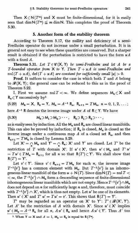
§ 5. Stability theorems for semi-Fredholm operators 241
Then X C N (Tm) and X must be finite-dimensional, for it is easilyseen that dim N (Tm) S m dim N. This completes the proof of Theorem5.30.
5. Another form of the stability theoremAccording to Theorem 5.17, the nullity and deficiency of a semi-
Fredholm operator do not increase under a small perturbation. It is ingeneral not easy to see when these quantities are conserved. But a sharperresult is obtained if the perturbation is restricted to have the form MAwith a fixed A.
Theorem 5.31. Let T C e (X, Y) be semi-Fredholm and let A be aT-bounded operator from X to Y. Then T + xA is semi-Fredholm andnul(T+xA), def(T+xA) are constant for sufficiently small IxI > 0.
Proof. It suffices to consider the case in which both T and A belongto R (X, Y) ; the general case can be reduced to this as in the proof ofTheorem 5.22.
I. First we assume nul T < oo. We define sequences Mn C X andRn C Y successively by'
;(5.29) Mo = X, Ro = Y, M,, = A-1 Rn, R,i+1= T Mn, n = 0, 1, 2....
here A-1 R denotes the inverse image under A of R C Y. We have
(5.30) Mo)M1)M2)..., Ro)R1)R2)...as is easily seen by induction. All the Mn and Rn are closed linear manifolds.This can also be proved by induction; if Rn is closed, Mn is closed as theinverse image under a continuous map A of a closed set R, and thenRn+1= T Mn is closed by Lemma 5.29.
Let X' = n Mn and Y' = nn Rn; X' and Y' are closed. Let T' be therestriction of T with domain K. If u' E X', then u' E Mn and T' u'= T u' E T Mn = Rn+1 for all n so that R (T') C Y'. We shall show thatR (T') = Y'.
Let v' E Y'. Since v' E Rn+1 = T M,, for each n, the inverse imageT-1{v'} has a common element with Mn. But T-1{v'} is an inhomo-geneous linear manifold of the form u + N (T). Since dim N (T) = nul T << oo, the T-1{v'} n M,, form a descending sequence of finite-dimensionalinhomogeneous linear manifolds which are not empty. Hence T-1 {v'} n Mndoes not depend on n for sufficiently large n and, therefore, must coincidewith T-1 {v'} n X', which is thus not empty. Let u' be one of its elements.Then u' E X' and T' u' = T u' = v'. This shows that R (T') = Y'.
T' may be regarded as an operator on X' to Y': T' E 69 (X', Y').Let A' be the restriction of A with domain K. Since u' E X' impliesu' E M,, = A-1 R. for all n, A u' E Rn and hence A U' E Y'. Thus A' too
1 When Y = X and A = 1. M. = R. is equal to R (TT).
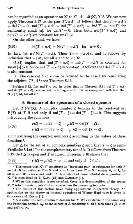
242 IV. Stability theorems
can be regarded as an operator on X' to Y': A' E 9 (X', Y') 1. We can nowapply Theorem 5.17 to the pair T', xA'. It follows that def (T' + MA')= def T' = 0, nul (T' + xA') = ind (T' + x A') = ind T' = nul T' forsufficiently small Ix4, for def T' = 0. Thus both nul(T' + xA') anddef (T' + xA') are constant for small jxj.
On the other hand, we have
(5.31) N(T+xA)=N(T'-1,-HA') for x+0.In fact, let u E N (T + xA). Then Tu = -x Au, and it follows byinduction that u E M for all n and so u E X'.
(5.31) implies that nul(T -f- xA) = nul(T' + xA') is constant forsmall jxj > 0. Since ind (T + xA) is constant, it follows that def (T + xA)is also constant.
II. The case def T < no can be reduced to the case I by consideringthe adjoints T*, A*; see Theorem 5.13.
Problem 5.32. Let nul T < no. In order that in Theorem 5.31 nul (T + xA)and def (T + xA) be constant including x = 0, it is necessary and sufficient thatN(T)(M.foralln.2
6. Structure of the spectrum of a closed operatorLet T E ' (X). A complex number belongs to the resolvent set
P (T) of T if and only if nul (T - ) = def (T - ) = 0. This suggestsintroducing the functions
v (C) = nul (T - C) , u (C) = def (T - C) ,(5.32)
v' (C) = nul' (T - C) , /z' (C) = def' (T - C) ,
and classifying the complex numbers C according to the values of thesefunctions 8.
Let A be the set of all complex numbers C such that T - C is semi-Fredholm 4. Let r be the complementary set of A. It follows from Theorem5.17 that A is open and r is closed. Theorem 5.10 shows that
(5.33) v'() = ,u' (C) = oo if and only if C E P .
1 This means that X', Y' constitute an "invariant pair" of subspaces for both Tand A. If in particular Y = X and A = 1, we have Y' = X' because M. = R forall n, and X' is invariant under T. A similar but more detailed decomposition ofX, Y is considered in T. KATO [12] and GAMEI,IN [1].
8 When this condition is not satisfied, there is a decomposition of the spacesX, Y into "invariant pairs" of subspaces; see the preceding footnote.
8 The results of this section have many applications in spectral theory. Anapplication to the theory of integral equations of Wiener-Hopf type is given inGOHBERG and KREIN [1].
6 A is called the semi-Fredholm domain for T. We can define in the same waythe Fredholm domain ,p as the subset of A consisting of all C such that v(C) < ooand ,u (C) < oo.
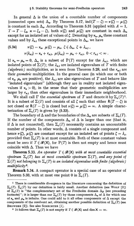
§ 5. Stability theorems for semi-Fredholm operators 243
In general A is the union of a countable number of components(connected open sets) A,,. By Theorem 5.17, ind (T - C) = v (C) - u (C)is constant in each A. According to Theorem 5.31 (applied with A = 1,T -+ T - CO, x = Co - C), both v (C) and ,u (() are constant in each A.except for an isolated set of values of C. Denoting by v, /z,, these constantvalues and by A,,s these exceptional points in A,,, we have
(5.34) v (C,) = vn, /u (C) = /un, C E An, C + An 1 ,
v(2n1)=v+Yrj, I'(An1)=tun+'Yn1, O<Yn2<0o.
If vn = a,, = 0, A,, is a subset of P (T) except for the A. , which areisolated points of E (T) ; the An; are isolated eigenvalues of T with finite(algebraic) multiplicities, as is seen from Theorem 5.28, and the Y,,j aretheir geometric multiplicities. In the general case (in which one or bothof vn, y,, are positive), the A, ,j are also eigenvalues of T and behave like"isolated eigenvalues" (although they are in reality not isolated eigen-values if v > 0), in the sense that their geometric multiplicities arelarger by Y,nj than other eigenvalues in their immediate neighborhood.
We shall call r the essential spectrum of T and denote it by Ee (T) 1.It is a subset of E (T) and consists of all C such that either R (T - C) isnot closed or R (T - ) is closed but v (C) = ,u (C) = c. A simple charac-terization of 1,(T) is given by (5.33).
The boundary of A and the boundaries of the An are subsets of Ee (T).If the number of the components A,, of A is larger than one (that is,if A is not connected), then 1,(T) necessarily contains an uncountablenumber of points. In other words, A consists of a single component andhence v (C), ,u (C) are constant except for an isolated set of points C = Aj,provided that Z,(7) is at most countable. Both of these constant valuesmust be zero if T E -4 (X), for P (T) is then not empty and hence mustcoincide with A. Thus we have
Theorem 5.33. An operator T E -4 (X) with at most countable essentialspectrum Z. (T) has at most countable spectrum E (T), and any point ofE(T) not belonging to Z.(T) is an isolated eigenvalue with finite (algebraic)multiplicity 2.
Remark 5.34. A compact operator is a special case of an operator ofTheorem 5.33, with at most one point 0 in Ee(T).
1 There is considerable divergence in the literature concerning the definition ofEe(T). Ee(T) by our definition is fairly small. Another definition (see WOLF [3])of Ee(T) is "the complementary set of the Fredholm domain AF (see precedingfootnote)"; it is larger than our E. (T) by those components A. of A for which oneof v and u is infinite. One could add to it all other components of A except thecomponents of the resolvent set, obtaining another possible definition of Z. (T) (seeBROWDER [2]). See also SCHECHTER [1].
2 It follows that Ee (T) is not empty if T E .4 (X) and dim X = oo.
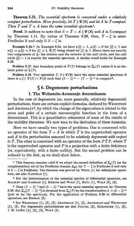
244 IV. Stability theorems
Theorem 5.35. The essential spectrum is conserved under a relativelycompact perturbation. More precisely, let T E ' (X) and let A be T-compact.Then T and T + A have the same essential spectrum I.
Proof. It suffices to note that S = T + A E W (X) and A is S-compactby Theorem 1.11. By virtue of Theorem 5.26, then, T - C is semi-Fredholm if and only if S - C is.
Example 5.36.2. In Example 5.24, we have v 1, y 0 for ICJ < I andv (C) = µ 0 for ICI > 1, R (T) being closed for ICI * 1. Hence there are exactlytwo components of A: the interior and the exterior of the unit circle, and the unitcircle ICI = 1 is exactly the essential spectrum. A similar result holds for Example5.25.
Problem 5.37. Any boundary point of P (T) belongs to Z. (T) unless it is an iso-lated point of E (T).
Problem 5.38. Two operators T, S E ' (X) have the same essential spectrum ifthere is a t E P (T) r1 P (S) such that (S - C)-1 - (T - C)-1 is compacts.
§ 6. Degenerate perturbations1. The Weinstein-Aronszajn determinants
In the case of degenerate (or, more generally, relatively degenerate)perturbations, there are certain explicit formulas, deduced by WEINSTEINand ARONSZAJN4, by which the change of the eigenvalues is related to thezeros and poles of a certain meromorphic function in the form of adeterminant. This is a quantitative refinement of some of the results ofthe stability theorems. We now turn to the derivation of these formulas.
Here we have usually two types of problems. One is concerned withan operator of the form T + A in which T is the unperturbed operatorand A is the perturbation assumed to be relatively degenerate with respectto T. The other is concerned with an operator of the form P T P, where Tis the unperturbed operator and P is a projection with a finite deficiency(or, equivalently, with a finite nullity). But the second problem can bereduced to the first, as we shall show below.
1 This theorem remains valid if we adopt the second definition of Ee(T) (as thecomplementary set of the Fredholm domain AF), for T - t' is Fredholm if and onlyif S - C is Fredholm. The theorem was proved by WEYL [1] for selfadjoint opera-tors; see also HARTMAN [1].
2 For the determination of the essential spectra of differential operators, seeBALSLEV and GAMELIN [1], KREITH and WOLF [1], ROTA [1], WOLF [3], [4].
8 Then (T - C)-1 and (S - C)-1 have the same essential spectrum by Theorem5.35. But Ee((T - C)-1) is obtained from Ee(T) by the transformation A -+ (A - )-1(just as for the spectrum). For the application of Problem 5.38 to differentialoperators, see BIRMAN [5].
4 See WEINSTEIN [1], [2], [3], ARONSZAJN [1], [2], ARONSZAJN and WEINSTEIN[1], [2]. For degenerate perturbations see also FOGUEL [2], KLEINECKE [1], [2],I. M. LIFAIC [1], [2], [3], WOLF [2].
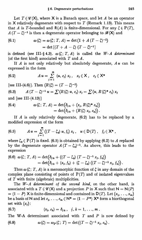
§ 6. Degenerate perturbations 245
Let T E ' (X), where X is a Banach space, and let A be an operatorin X relatively degenerate with respect to T (Remark 1.13). This meansthat A is T-bounded and R (A) is finite-dimensional. For any C E P (T),A (T - is then a degenerate operator belonging to 9 (X) and
(6.1) w co (C; T, A) = det (1 + A (T - )-1)
=det[(T+A-C) (T -C)-1]is defined (see III-§ 4.3). o.) (C; T, A) is called the W-A determinant(of the first kind) associated with T and A.
If A is not only relatively but absolutely degenerate, A u can beexpressed in the form
m
(6.2) Au= (u,ef)x;, x;EX, e;EX*=1
[see III-(4.6)]. Then (R(C) _ (T - C)-1)
(6.3) A (T - u = E (R u, e,) x; = £ (u, R e;) xj
and [see III-(4.13)]
(6.4) co (C; T, A) = det(S; k + (x1, R (C) * ek))
= det (6j k + (R (C) x ek))
If A is only relatively degenerate, (6.2) has to be replaced by amodified expression of the form
(6.5) Au= E((T -CO)u,ff)xf, uED(T), f1EX*,1=1
where Co E P (T) is fixed. (6.5) is obtained by applying (6.2) to A replacedby the degenerate operator A (T - Co)-'. As above, this leads to theexpression
(6.6) w (C; T, A) = det(S1k + ((T - CO) (T - C)-1 x5, fk))= det(85k + (xi, fk) + (pS
- CO) ((T - C)-1 X1, fk))
Thus co (C; T, A) is a meromorphic function of C in any domain of thecomplex plane consisting of points of P (T) and of isolated eigenvaluesof T with finite (algebraic) multiplicities.
The W- A determinant o t the second kind, on the other hand, isassociated with a T E ' (X) and a projection P in X such that N = N (P)= (1 - P) X is finite-dimensional and contained in D (T). Let {x1, . . ., x,,,}
be a basis of N and let e1, . . ., em E N* _ (1 - P*) X* form a biorthogonalset with {x5} :
(6.7) (x1, ek) = 89k k = 1, . . ., m .
The W-A determinant associated with T and P is now defined by(6.8) w (C) = wp (C; T) = det ((T - (,)-1 x5, ek) .
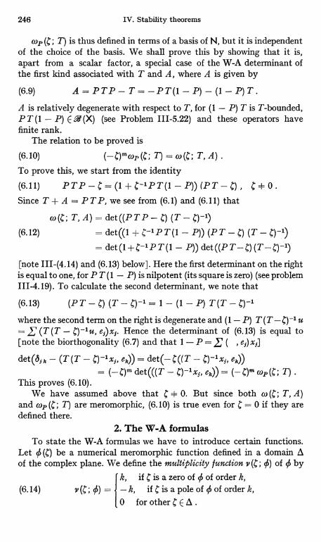
246 IV. Stability theorems
wp (C; T) is thus defined in terms of a basis of N, but it is independentof the choice of the basis. We shall prove this by showing that it is,apart from a scalar factor, a special case of the W-A determinant ofthe first kind associated with T and A, where A is given by
(6.9) A=PTP-T=-PT(1-P)-(1-P)T.A is relatively degenerate with respect to T, for (1 - P) T is T-bounded,P T (1 - P) E .4 (X) (see Problem 111-5.22) and these operators havefinite rank.
The relation to be proved is
(6.10) (-S)mwp(C; T) = a) (C; T, A)
To prove this, we start from the identity
(6.11) PTP-C=(1+C-1PT(1Since T + A = PTP, we see from (6.1) and (6.11) that
w(4; T, A) = det((PTP - (T - C) -1)
(6.12) = det((1 + s-1PT(1 - P)) (PT - (T - C)-1)
= det(1+C-1PT(1 - P)) det ((P T - C) (T - C) -1)
[note III-(4.14) and (6.13) below]. Here the first determinant on the rightis equal to one, for P T (1 - P) is nilpotent (its square is zero) (see problem111-4.19). To calculate the second determinant, we note that
(6.13) (PT-a) (T-1,)-1= 1-(1-P) T(T-C)-1where the second term on the right is degenerate and (1- P) T (T -t,)-1 u= E (T (T - C)-'u, e,)x,. Hence the determinant of (6.13) is equal to[note the biorthogonality (6.7) and that 1- P = E ( , e5) x5]
det(S;k - (T (T - C)-1x5, ek)) = det(-C((T - C)-1x5, ek))_ (-C)m det(((T - C)-1x e7,)) _ (-C)m wP(pS; T)
This proves (6.10).We have assumed above that C + 0. But since both w (C; T, A)
and cop (C; T) are meromorphic, (6.10) is true even for C = 0 if they aredefined there.
2. The W-A formulasTo state the W-A formulas we have to introduce certain functions.
Let O (C) be a numerical meromorphic function defined in a domain Aof the complex plane. We define the multiplicity function v(C; 0) of 0 by
k, if C is a zero of 0 of order k,(6.14) v(; 0) = -k, if C is a pole of 0 of order k,
0 for other CEi .
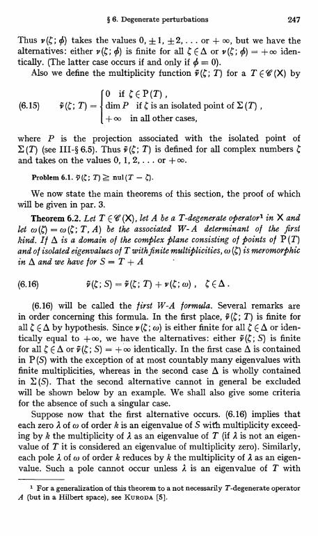
§ 6. Degenerate perturbations 247
Thus v(C; 0) takes the values 0, ± 1 , ±2, ... or + oo, but we have thealternatives : either v (C; 0) is finite for all E A or v (C; + co iden-tically. (The latter case occurs if and only if - 0).
Also we define the multiplicity function T) for a T E'(X) by
0 if C E P (T) ,
(6.15) v T) = dim P if C is an isolated point of E (T)+ co in all other cases,
where P is the projection associated with the isolated point ofE (T) (see III-§ 6.5). Thus f (C; T) is defined for all complex numbers Cand takes on the values 0, 1, 2.... or +oo.
Problem 6.1. 9 T) Z nul (T - ).
We now state the main theorems of this section, the proof of whichwill be given in par. 3.
Theorem 6.2. Let T E '' (X), let A be a T-degenerate operator' in X andlet co (C) = co (C; T, A) be the associated W- A determinant of the firstkind. If A is a domain of the complex plane consisting of points of P (T)and of isolated eigenvalues of T with finite multiplicities, co (4) is meromorphicin Aand we have forS= T+A
(6.16) i(C;S)=v"(C;T)+v(C;co), CEA.
(6.16) will be called the first W-A formula. Several remarks arein order concerning this formula. In the first place, v" (C; T) is finite forall C E A by hypothesis. Since v (C; co) is either finite for all C E A or iden-tically equal to +oo, we have the alternatives: either f(C; S) is finitefor all C E A or v" (C; S) = +oo identically. In the first case A is containedin P (S) with the exception of at most countably many eigenvalues withfinite multiplicities, whereas in the second case A is wholly containedin E (S). That the second alternative cannot in general be excludedwill be shown below by an example. We shall also give some criteriafor the absence of such a singular case.
Suppose now that the first alternative occurs. (6.16) implies thateach zero A of co of order k is an eigenvalue of S with multiplicity exceed-ing by k the multiplicity of A as an eigenvalue of T (if A is not an eigen-value of T it is considered an eigenvalue of multiplicity zero). Similarly,each pole A of co of order k reduces by k the multiplicity of A as an eigen-value. Such a pole cannot occur unless A is an eigenvalue of T with
1 For a generalization of this theorem to a not necessarily T-degenerate operatorA (but in a Hilbert space), see KURODA [5].
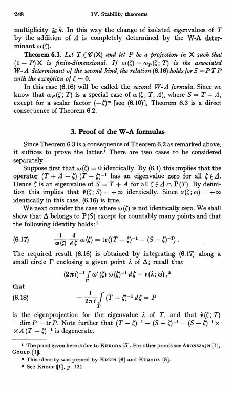
248 IV. Stability theorems
multiplicity z k. In this way the change of isolated eigenvalues of Tby the addition of A is completely determined by the W-A deter-minant co (4).
Theorem 6.3. Let T E '(X) and let P be a projection in X such that(1 - P) X is finite-dimensional. If (o (C) = (op (C; T) is the associatedW- A determinant of the second kind, the relation (6.16) holds for S = P T Pwith the exception of C = 0.
In this case (6.16) will be called the second W-A formula. Since weknow that (op (C; T) is a special case of w T, A), where S = T + A,except for a scalar factor [see (6.10)], Theorem 6.3 is a directconsequence of Theorem 6.2.
3. Proof of the W-A formulas
Since Theorem 6.3 is a consequence of Theorem 6.2 as remarked above,it suffices to prove the latter.' There are two cases to be consideredseparately.
Suppose first that w (C) = 0 identically. By (6.1) this implies that theoperator (T + A - C) (T - a)-' has an eigenvalue zero for all C E A.Hence l ; is an eigenvalue of S = T + A for all C E A n P (T). By defini-tion this implies that v" (C; S) _ +oo identically. Since (0) = +ooidentically in this case, (6.16) is true.
We next consider the case where co (C) is not identically zero. We shallshow that A belongs to P (S) except for countably many points and thatthe following identity holds : 2
(6.17)w (C) , co (C) = tr((T - C)-' - (S - C)-')
The required result (6.16) is obtained by integrating (6.17) along asmall circle r enclosing a given point A of i ; recall that
(2rci)-1 f co'(C) co(C)-' dC=v(A; co),ar
that(6.18) - 2I if (T -C)-1dC=P
ris the eigenprojection for the eigenvalue A of T, and that v" (C; T)= dim P = trP. Note further that (T - c)-' - (S - a)-' = (S - C)-lxx A (T - C) -1 is degenerate.
1 The proof given here is due to KURODA [5]. For other proofs see ARONSZAJN [1],GOULD 111.
2 This identity was proved by KREIN [6] and KURODA [5].3 See KNOPP (1), p. 131.
§ 6. Degenerate perturbations 249
To prove (6.17) we consider a C E P (T) such that co (4) + 0. We have[see I-(5.60)1]
(6.19) w (C) = det (1 + B (4)) = exp(tr log(1 + B (C))), B (C) = A (T - C)-1.
That co (C) + 0 implies that B (4) has no eigenvalue - 1, and the logarith-mic function in (6.19) is defined by
(6.20) log (I + B (C)) = 2 i f log (1 + z) (z - B (C))-1 d z ,
c
where C is a closed curve enclosing all the eigenvalues of the degenerateoperator B (C) but excluding the point -1 [see I-(5.57)].
It follows from (6.19) and (6.20) that (' = d/dC)
(6.21)d
w W tr log(1 + B (C))
2 1 i f tr [log (1 + z) (z - B (C))-1 B' (C) (z - B (C))-1] dz
c [see I-(4.28)]
2i f tr[log(l+z)(z-B(C))-zB'(C)]dz= 'c
2 1 iitr f (1 + z)-1 (z - B (C))-1 B' P dz
c= tr [(1 + B (C))-1 B'(0 ] [see I-(5.53)]
Here we have used the formula tr A B = tr B A, done an integration byparts, and changed the order of the integral and trace signs whenpossible. Substituting B (C) = A (T - C)-1 and B' (C) = A (T - C)-E,the last member of (6.21) becomes
tr [(T - a)-1(1 + B (C))-'A (T- c)-1] = tr [(T + A - C)-' A (T - a)-1]= tr [(T - C)-1 - (S - a)-1] .
This completes the proof of (6.17). Note that (S - C)-1 = (T - c)-1 xx (1 + B(0)-1 E . (X) so that CE P(S).
4. Conditions excluding the singular caseAs mentioned before, the possibility is in general not excluded
that co (C) = 0 identically in (6.16) so that i (C; S) = + oo identically[this is equivalent to A E E (S)].
1' The results of Chapter I can be applied tow (C) since A (T - C)-1 is degenerate;see III-§ 4.3.
250 IV. Stability theorems
Example 6.4. Consider the operators discussed in Example 3.8. If we change thenotation by T -* S, A - A, T + A S - A = T, the open unit disk A belongsto P (T) so that v" (C; T) - 0 in A. But since A E E (S), we have v (t'; S) - oo in A.In view of (6.16) this implies v w) - co, hence w (C) - 0. This can also be verifieddirectly as follows. A is of rank one (m = 1) and the x1, e1 of (6.2) should be replacedby - x_1, eo, respectively (e0 is the vector xo regarded as an element of X*). Hencew w T, A) = 1 - ((T - 0)-1x_1, e0). But since it is easily verified that
(T - 1x_1 = E Ix5 for C E A, we have indeed w(C) = 0 identically in A.i=o
Theorem 6.5. In order that the w of Theorem 6.2 not be identicallyzero for C E A, it is necessary and sufficient that at least one C of i belongto P (S).
This is obvious from Theorem 6.2 and the remarks thereafter.We shall now give several sufficient conditions for co (C) not to be
identically zero.a) co (C) * 0 if 11A (T - C)-'II < I for some C E A. For then we have
E P (S) because (S - a)-1 can be constructed by the Neumann seriesas in II-(1.13).
b) w (C) E# 0 if T* exists and is densely defined in X* and if thereexists a sequence C,, E A such that IC.I - and {ICnI II (T - Cn.)-1II}is bounded. To see this it suffices by a) to show that IIA (T - C,,)-1II 0.But we have by (6.5)
A (T - C.)-lu =,f ((T - Co) (T - gym.)-1u, f,)xj == ' (u, (T* - o) (T* - C.)-lf,) x,
so that
(6.22) IIA (T - C)-'Ih s E II (T'" - o) (T* - fin)-1f,Il IIxjhI
Now the sequence of operators Bn* = (T* - Co) (T* -acting inX* is uniformly bounded since the B71= I + (C,, - Co) (T - C,,)-1 areuniformly bounded by hypothesis. Furthermore, f = (T* - n)-1 XX (T*-fo)f, 0 if f ED(T*) since II(T*-C)-III=II(T-Cn)-III-+0.It follows (see Lemma 111-3.5) that converges strongly to zero, andthe right member of (6.22) tends to zero for n -+ oo, as we wished to show.
c) co (C) * 0 if T E .4 (X) and there is a E A such that ICJ Z II TII.In this case A can be extended so as to include the whole exterior of thecircle ICI = II TII. Then it is easy to see that b) is satisfied in the extendeddomain A'. Hence co (C) * 0 in A' and, a fortiori, in A.
Remark 6.6. The condition b) is satisfied if X is a Hilbert space andT is selfadjoint (see Chapter V).
§ 1. Hilbert space 251
Chapter Five
Operators in Hilbert spacesHilbert space is a special case of Banach space, but it deserves separate con-
sideration because of its importance in applications. In Hilbert spaces the generalresults deduced in previous chapters are strengthened and, at the same time, newproblems arise.
The salient feature of Hilbert space is the existence of an inner product and theensuing notion of orthogonality. For linear operators this leads to the notions ofsymmetric, selfadjoint and normal operators. Also there is a more general class ofaccretive (or dissipative) operators, the importance of which has been recognizedin application to differential operators. In perturbation theory, these new notionsgive rise to such problems as perturbation of orthonormal families, perturbationof selfadjoint operators (with applications to the Schrodinger and Dirac operators),etc., which will be discussed in this chapter.
This chapter is again partly preliminary, beginning with an elementary expositionof the specific results in the operator theory of Hilbert spaces which are not coveredin the general theory of Banach spaces. Accretive and sectorial operators are givenspecial attention in view of later applications to analytic and asymptotic perturbationtheory.
§ 1. Hilbert space1. Basic notions
Hilbert space is a generalization of the unitary space consideredin I-§ 6 to the infinite-dimensional case'.
A Hilbert space H is a Banach space in which the norm is definedin terms of an inner product (u, v) defined for all pairs u, v of vectorsand satisfying the conditions stated in I-§ 6.1. The norm lull is definedby I-(6.3). H is assumed to be complete with respect to this norms.
Most of the results of I-§ 6 can be taken over to the Hilbert space H,and we shall do this freely without comment whenever it is obvious.But there are also results that need modification or at least some com-ments. These will be given in this and the following paragraphs. It shouldbe remarked at this point that the Schwarz inequality I-(6.4) is validand that (u, v) is continuous in u and v jointly, exactly as before.
1 General references to Hilbert space theory are AKHIEZER and GLAZMAN QlD,DUNFORD and SCHWARTZ (1), {2D, HALMOS (11, SZ.-NAGY 111, RIEsz and SZ.-NAGY(1), STONE 111, YOSIDA Q1D, ZAANEN (1).
I A vector space H with an inner product, which is not necessarily complete,is called a pre-Hilbert space. Such a space can be completed to a Hilbert space H.Again H can be defined as the set of equivalence classes of Cauchy sequences {un}in H (see footnote2 of p. 129). The inner product of two elements of H represented bythe Cauchy sequences {un}, {vn} is then defined by lim (uv, vn).
252 V. Operators in Hilbert spaces
Example 1.1. la is a Hilbert space (see Example III-1.1) if the inner product isdefined by(1.1) (u, v) _ ' k Y7k for u = (R) and v = (ilk)
k
L$ (E) is a Hilbert space (see Example 111-1.3) if the inner product is defined by
(1.2) (u, v) = f u (x) R(7) d x .E
If H is a Hilbert space, the adjoint space H* can be identified with H.In particular H** = H* = H and H is reflexive. The proof of this factgiven in I-§ 6.2, depending essentially on the finite dimensionality,cannot be applied to the general case.
For the proof we start with the projection theorem: every subspace(closed linear manifold) M of H has an orthogonal (perpendicular) projec-tion. In other words, we have the decomposition of H
(1.3) H=M®MI ,where Ml is the orthogonal complement of M (the set of all u E Hsuch that (u, v) = 0 for all v E M). Note that Ml is also a closed sub-space of H ; this is a direct consequence of the continuity of the innerproduct.
For any u E H, set d = dist (u, M) and take a sequence un E M suchthat llu,, - ujl -+ d. We have
(1.4)I I 2
(un+ um) - u l z + (un - um)I 2 Ilun - uII2+ Ilum - ull2
by I-(6.7). For n, m -+ no the right member tends to d2, whereas the firstterm on the left is not smaller than d2 because (un + um)/2 E M. ThusII un - umll --* 0 and there exists a u' E H such that u,, -+ u'(completenessof H). The closedness of M then implies that u' E M. Moreover, we haveIlu-u'll=limllu-unll=d.
We shall now show that u" = u - u' E M. For this it suffices toshow that (u", x) = 0 for any x E M with IIxii = 1. But this follows from
d2 = Ilu - (u x) x112+ I(u x)I2 z d2 + I(u11' X)12
[set u u", v = x in I-(6.5)].The possibility of the decomposition u = u' + u" proves (1.3),
for the uniqueness of this decomposition can easily be proved.(1.3) implies that
(1.5) Ml.i = Mas in the finite-dimensional case. Also (1.3) defines the orthogonal pro-jection P = PM on M by Pu = u' as before.
Now the possibility of the identification of H* with H can be proved.Let / E H*; / is a bounded semilinear form on H. Let N = N (/), the nullspace of /. N is a closed linear manifold of H. If / + 0, N + H so thatNJ- + 0. Let v E N J-, v + 0. We may assume / [v] = 1. For any w E H,
§ 1. Hilbert space 253
w'= w - f [ w ] v E N since f [w'] = 0. Hence 0= (v, w') _ (v, w) -- 1[w] IIvjI2 or 1[w] = (u, w) with u = v/IIvII2. Thus any / E H* can beidentified with a u E H (Theorem of RIESZ). Other arguments necessaryto complete the proof are quite the same as in I-§ 6.2.
As in general Banach spaces, we can define in H the notion of weakconvergence (see III-§ 1.6) besides the ordinary (strong) convergence.In virtue of the identification H* = H, un u is equivalent to (un, v) -+
W
(u, v) for every v E H.Lemma 1.2. If un w u and lim supllunll S Hull, then u,, g U.
Proof. IIu, - uII2 = IIuuII2 - 2Re (us, u) + Ilull2. But (u,, u) -+ (u, u)= IIu1I2 and`lim supItu,'II2 - IIull2. Hence limllun - ull = 0.
Lemma 1.3. H is weakly complete : i f {u,,} is weakly convergent, thenu,, , u for some u E H.
W
Proof. Since {u,,} is bounded (see III-§ 1.6), lim (un, v) = f [v] defines abounded semilinear form /. Hence / [v] = (u, v) for some u E H andu --.u.
W
Lemma 1.4. H is sequentially weakly compact. In other words: ifun E H is a bounded sequence, then there is a subsequence {vn} o l {un} suchthat vn v for some v E H.
Proof. Since I(un,ul)I 5 IIunll IIuiII is bounded in n, there is a sub-sequence of {un} such that u1) is convergent. Since u2) issimilarly bounded in n, there is a subsequence of {ul,} such that
u2) is convergent. Proceeding in the same way, we can construct asequence of subsequences {u'} of {un} such that {u +1}n
= 1, 2, ... is asubsequence of {u }n = 1, 2,... and lim (u,,, um) exists. Then the diagonal
sequence {vn}, vn = unn, has the property that lim (vn, u,n) exists for all m.
Since IIvnII is bounded in n, it follows (cf. Lemma 111-1.31) that lim (vn, u)exists for any u in the closed span M of the set {un}.
On the other hand lim (vn, u) exists for any u E Ml since (vn, u) = 0.Thus {vn} is weakly convergent, hence vn -, v for some v (Lemma 1.3).
W
A sesquilinear form t [u, u'] on H x H', where H and H' are Hilbertspaces, can be defined as in I-§ 6.2, and we have again the formulaI-(6.11). t is said to be bounded if there is a constant M such that
.(1.6) It [u, u']I 5 MIIuII lull
We denote by IItII the smallest M with this property. A bounded ses-quilinear form t [u, u'] is continuous in u and u' jointly; the proof is thesame as that of the continuity of the inner product. The converse is alsotrue. A sesquilinear form t [u, u'] is bounded i f it is continuous in u for eachfixed u' and also in u' for each fixed u. This is a consequence of the prin-ciple of uniform boundedness (III-§ 1.5).
254 V. Operators in Hilbert spaces
Problem 1.5. Prove the last statement.Problem 1.6. Let be a sequence of bounded sesquilinear forms on H X H'
and let {t [u, u']} be bounded for n = 1, 2, ... for each fixed u E H, WE H'. Then thesequence {I1tn1I} is bounded. [hint: Another application of the principle of uniformboundedness.]
2. Complete orthonormal familiesWe did not define the notion of a basis in a general Banach space.
In a Hilbert space, however, a complete orthonormal family plays therole of a basis.
A family {xx} of vectors of H, with the index y running over a certainset, is orthonormal if
(1.7) (x x ) = =N, y y0 rlt v
For any u E H, the scalars(1.8)N = (u, xN)
are the coefficients of u with respect to {xN}. Since any finite subfamily{xNl, ..., x,,} of {xN} is also orthonormal, it follows from I-(6.15) that
X l Nkl2 < llull2. Since this is true for any choice of It,, ..., µn, we havek=Ithe Bessel inequality ((1.9) Lr I NIy = (u, XN)I2 IIulI2
N
This implies, in particular, that.for each u, only a countable number ofthe coefficients µ are different from zero.
(1.9) implies also thatf(1.10) U, _ SN xN - Lr (u, xN) xN
N N
exists. In fact, the right member of (1.10) contains only a countablenumber of non-vanishing coefficients. Let these be denoted by Nk,
k = 1, 2, ..., in an arbitrary order. Then the u;, _Nk xNk form ak=1
Cauchy sequence because
ll un - umll2 - E lµkl2 -> 0, m, n -> oo ,k=m+1
in virtue of (1.9). It is easy to see that the limit u' of the sequencedoes not depend on the way in which the sequence {,u,} is numbered.
u' is equal to the orthogonal projection Pu of u on the closed span Mof {xN}. For it is obvious that u' E M, whereas u" = u - u' E Ml because(u", xN) = (u - u', xN) _ N - (Z x, xN) = 0 for every Fc. In particularwe have
(1.11) ilu1ll2 = E IENl2 = E I(u, xN) 12 , llu"H2 = 0ull2 - llu'll2 .N N
§ 1. Hilbert space 255
The orthonormal family {x,,} is said to be complete if M = H. Anecessary and sufficient condition for completeness is that u" = 0 forall u E H, and this is equivalent to the Parseval equality
(1.12) 7 Ru, x,4)12 = 1Jul12K K
for every u E H. In this case we have also
(1.13) u = Z ,, x,, _ Z (u, x,,) x,,A is
which is the expansion of u in terms of the complete orthonormal family{x,,}.
If H is separable (see III-§ 1.2), any orthonormal family of Hconsists of at most a countable number of elements. To see this, letbe a countable subset of H which is dense in H. For each ,u there is a usuch that jjx,, - u,,11 < 1/2. Since jjxµ - x,11 = V2 for ,u + v, the index n isdifferent for different u. Thus {x,,} can be put in correspondence with asubset of the set of positive numbers {n}.
Conversely, H is separable if there is a complete orthonormal familyconsisting of a countable number of elements. For the set of all
(finite) linear combinations of the x with rational coefficients is countableand dense in H.
If H is separable, a complete orthonormal family can be constructedby the Schmidt orthogonalization procedure (see I-§ 6.3) applied to anysequence which is dense in H. A similar construction could be used evenin a non-separable space by using the axiom of choice, but we shall notgo into details since we are mostly concerned with separable spaces.
Problem 1.7. An orthonormal family {x,} is complete if and only if there isno nonzero vector orthogonal to all x,,.
Example 1.8. A complete orthonormal family of 12 is given by the canonicalbasis consisting of x =
Example 1.9. The set of trigonometric functions (2n)-112 ei"Z, n = 0, ± 1, ± 2, ... ,forms a complete orthonormal family in L2 (a, a + 2;r), where a is any real number".
Example 1.10. Let 4pk (x), apr (y) be two sequences of functions on E and F,constituting complete orthonormal families in L2 (E) and L2 (F), respectively. Thenthe functions xkr (x, y) _ 4px (x) zpf (y) form a complete orthonormal family inL2 (E x F), the space of all measurable functions w (x, y) defined for x E E, Y E F
Esuch that 11w112 = f Fw(x, y) 12 dx dy is finite. The orthonormality of xkr is obvious
from (xkr. xn{) = (42k, TI) (pr, zpi) =SkiBrr. To prove the completeness, it suffices toshow that (w, xkr) = 0 for all k, j implies w = 0 (Problem 1.7). Set
(1.14) wk(y) = f w(x, y) q, (x) dx;E
then we have wk E L2 (F) since Jwk (y) 12 S j 1w (x, y) 12 d x by the Schwarz inequality
and f Iwk(y)12 dy s f Jw(x, y) 12 dx dy = 11 w11 s. This enables one to write (w, xkr)F ExF1 See any textbook on Fourier series, or on Hilbert space, e. g. STONE Qli.
256 V. Operators in Hilbert spaces
_ (w, tpkyri) _ (wk, W,). Thus (w, X1, j) = 0 for all k, j implies that (wk, ap) = 0 andhence wk = 0 by the completeness of {apf}. On the other hand, wk (y) is defined foralmost every y E F and this value must be zero for every k and almost every y. Invirtue of the completeness of qqk, (1.14) shows that w (x, y) = 0 for almost every xfor almost every y. Thus w = 0 as an element of L2 (E x F).
§ 2. Bounded operators in Hilbert spaces1. Bounded operators and their adjoints
A (linear) operator T from a Hilbert space H to another one H' isdefined as in general Banach spaces. There are, however, some propertiespeculiar to operators in (or between) Hilbert spaces. We begin withbounded operators T E -4 (H, H').
First we note that
(2.1) T** = T ;
this is true since H is reflexive (see III-§ 3.3).An operator T E -4 (H, H') is closely related to a bounded sesquilinear
form t on H x H' by
(2.2) t [u, u'] _ (Tu, u') = (u, T* u')
note that T* E 9 (H', H) because H* = H, H'* = H'. The relationship (2.2)gives a one-to-one correspondence between the set of all bounded sesqui-linear forms t on H x H', the set of all T E °.,8 (H, H') and the set of allT* E 9 (H', H). This can be proved in the same way as in the finite-dimensional case (I-§ 6.4). That (Tu, u') is a bounded form is obvious byI(Tu, u') I s IITuII Ilu'll s IITII IIuII IIuII. Conversely, a bounded sesqui-linear form t [u, u'] can be written in the form (v', u'), v' E H', since it is abounded semilinear form in u' for fixed u. Setting v' = T u defines alinear operator T on H to H', and the boundedness of T follows fromIITII = supI(Tu, u')IIIIuhi Ilu'll = suplt[u, u']I/IIuhi IIuII = IItDI.
Problem 2.1. Let T. E R (H, H') be such that (T u, u') is bounded for eachfixed pair u E H, u' E H'. Then is uniformly bounded (that is, {11 T,11} is bounded).[hint: The principle of uniform boundedness.]
For an operator T E . (H, H'), a matrix representation is possiblein the same fashion as in the finite-dimensional case (I-§ 6.4). Forsimplicity assume that H and H' are separable and let {xk}, {xj'} becomplete orthonormal families in H, H', respectively. The matrix of T isthen defined exactly by I-(6.27) and the expansion I-(6.28) holds true(where we have in general an infinite series on the right).
Remark 2.2. For an unbounded operator T from H to H', (Tu, u') isalso a sesquilinear form, which is, however, not necessarily defined forall u E H. The relationship between an operator and a sesquilinear formin this general case is rather complicated. Later we shall consider it indetail in the special case of a so-called sectorial operator.
§ 2. Bounded operators in Hilbert spaces 257
A symmetric sesquilinear form t [u, v] in a Hilbert space H is definedby t [v, u] = t [u, v] as in I-§ 6.5. If in addition t is assumed to be bounded,all the results stated there are valid. The operator T E .4 (H) associated by(2.2) with a bounded symmetric sesquilinear form t has the property that
(2.3) T*= T;T is said to be symmetric. The notion of a positive (or non-negative)symmetric operator or form and the order relation S < T for symmetricS, T E . (H) are defined as before (see loc. cit.).
The results of I-§ 6.7 on projections are also valid without modifica-tion; here we are concerned with a P E 9 (H) such that P2 = P. Comparealso the results of III-§ 3.4 on projections in Banach spaces. We add thefollowing lemma.
Lemma 2.3. Let {Pn} be a sequence of orthogonal Projections in H00
such that P. P. = Smn P. Then Pn = P exists in the strong sense andn=1
P is an orthogonal Projection. The range of P is the closed span of the unionof the ranges of all the P.
n nProof. For any u E H we have £ II Pk uII2 = II Pk uII2 IIull2
A-1 k=1n Co
since Z Pk is an orthogonal projection [see I-(6.49)]. Hence Z IIPk uII2k=1 k=1
n+Q +p 00
is convergent and II' Pk u1I2 = E 11P1, uII2 ; 0, n -+ co. Thus Pn= Pk=n k=n n=1
is strongly convergent. It is easy to see that the P thus defined has theproperties stated.
We shall say that the {Pn} of Lemma 2.3 is complete if E Pn = 1.A normal operator T E 9(H) is defined by the property T* T = T T*,
and the results of I-§ 6.6 remain valid. For example
(2.4) spr T = II TII if T is normal.Problem 2.4. A quasi-nilpotent normal operator is zero.Example 2.5. Consider the integral operator T of Example 111-2.4, with the
kernel t (x, y). If E = F and i (x, y) = t (y x) (Hermitian symmetric kernel), T is asymmetric operator in H = L2 (E) (see Example 111-3.17). The same is true of theoperator T of Example 111-2.3, defined from a given matrix (ti k), if consideredin H = 12 and if (tfk) is Hermitian symmetric (tkf = zek), see Example111-3.18.
Unbounded symmetric and normal operators will be dealt with indetail in later sections.
2. Unitary and isometric operatorsAn operator T E. (H, H') is said to be isometric if it preserves the norm :
(2.5) II T u ll = lull for every u E H .
258 V. Operators in Hilbert spaces
As in the finite-dimensional case (I-§ 6.6), this implies that T* T = 1H(the identity operator in H) and (Tu, Tv) = (u, v) for all u, v E H.
An isometric operator T is invertible, for T u = 0 implies u = 0.But T-1 need not belong to °.,11(H', H) since its domain may not be thewhole space H'. Note that this may happen even when H' = H, in contra-distinction to the finite-dimensional case.
An isometric operator T is said to be unitary if T-1 has domain H',that is, if T has range H'. Then T-1 belongs to R(H', H) and is itselfunitary. Thus a T E -4 (H, H') is unitary if and only if
(2.6) T* T = 1H and T T* = 1H' ,which is in turn equivalent to
(2.7) T-1= T* .
The existence of a unitary operator T on H to H' implies that Hand H' have identical structure as Hilbert spaces, for T preserves thelinear relations and inner products. An operator A' in H' is said to beunitarily equivalent to an operator A in H if there is a unitary operator Tfrom H to H' such that
(2.8) A'T= TA or A'= TAT-1= TA T*.This means that D (A') is exactly the image of D (A) under the unitarymap T and A' T u = TA u holds for every u E D (A). A' and A have thesame internal structure, for the correspondence u H u' = T u is unchangedunder the operators A and A' in virtue of the relation A u E-+ TA u=A'Tu=A'u'.
Let T E 9(H, H') be an isometric operator and let M' = R(T). Theisometry implies that M' is a closed linear manifold of H'. The operatorT* E -4 (H', H) is an extension of T-1 as is readily seen from T* T = 1H,whereas T*u' = 0 if and only if u' E M'J- [see III-(5.10)]. Thus T* is notisometric unless T is unitary; it is partially isometric.
An operator W E 2(H, H') is Partially isometric if there is a closedlinear manifold M of H such that II W uII = lull for u E M while W u = 0for u E M. M is called the initial set and M'= W M the final set of W ;M' is a closed linear manifold. An equivalent definition is
(2.9) II Wull = IIPull for every uEH,
where P is the orthogonal projection of H on M. (2.9) is in turn equivalentto
(2.10) W*W = P.
For any uEH we have W(1 - P) u = 0 since (1 - P) u E Ml. Hence
(2.11) W= WP.
§ 2. Bounded operators in Hilbert spaces 259
We have W*u' = 0 for u' E M'1, as in the case of an isometric operator.Furthermore, IIW*WuII = 11 Pull = IIWuII shows that IIW*u'II = IIu'II foru' E M'. Hence W* is likewise partially isometric with the initial set M'.Application of this result to W replaced by W* shows that the final setof W* is identical with the initial set M of W** = W. Thus there iscomplete symmetry between W and W*. The following relations aredirect consequences of these considerations (P' is the orthogonal pro-jection of H' on M').
W*W= P, WP= P'W= W, WW*W_ W,(2.12) WW*= P', W*P'= PW*= W*, W*WW*= W*.
Problem 2.6. W E . (H, H') is partially isometric if and only if W = W W* W.[hint: W = WW*W implies W*W = W*WW*W. Thus P = W*W is an ortho-gonal projection of H on some subspace M.]
Example 2.7. Let H = L2 (E) and H = L2 (E'), where both E and E' are thereal n-dimensional euclidean space (so that they may be identified), the points ofwhich will be denoted respectively by x = (x1, ..., x") and k = (k1, ..., k"). TheFourier transformation 12 = Tu given by
(2.13) d(k) = (2 n)-n/2 f e- ik.x u (x) dxE
k.x=k1x1+... +k"x".
defines a unitary operator T on H to'H. The inverse operator T-1 it = u is given by
(2.14) u(x) = (2a)-12 t' eik.' d(k) dkE'
These results are known as the Fourier-Plancherel theorem. Actually, these integralsshould be taken in the sense of limit in mean: the integral (2.13) is first to be takenover a bounded subset K of E, the resulting function converging in the norm II
II
of H to the required transform d when K expands to the whole space El. Thus Tor T-1 is not an integral operator in the sense of Example 111-2.4.
Example 2.8. Let H = L2 (- n, n). For any u E H the Fourier coefficients
(2.15) (2n)-112 fu(z)e-i"Idx, n=0,±1,±2,...,,i
are defined. The operator T that sends u into the vector v = (i") is a unitaryoperator on H to H' = 12. The inverse T-1 assigns to each v = (") E H' the functionu (x) defined by the Fourier series
(2.16) u (x) = (2a)-112 -' et":
which is convergent in norm IIII
These results are another expression of the com-pleteness of the family of trigonometric functions ei"x. Similar results hold whenit is replaced by any complete orthonormal family of H = L2 (- n, n) or of anyabstract Hilbert space.
Example 2.9. An example of an isometric operator that is not unitary is givenby a shift operator (cf. Example 111-3.16). Let {x"}"a1.2.... be a complete ortho-normal family in a Hilbert space H and let T E .4 (H) be such that T x, = x"+ 1. T isisometric and T* is partially isometric, with T* x"+1 = x" and T* x1 = 0. Theinitial set of T is H and the final set is the subspace of H spanned by x2, x2, ... .
1 For details see e. g. STONE [1)1.
260 V. Operators in Hilbert spaces
3. Compact operatorsLet T E I (H) be a compact operator. We know that the spectrum
E (T) consists of at most a countable number of eigenvalues with finitemultiplicities, possibly excepting zero (Theorem 111-6.26). Let Al, A, .. .be these nonzero eigenvalues arranged, say, in decreasing order ofmagnitude, and let P1, P2, ... be the associated eigenprojections. Wenote that IAJ J is equal to the spectral radius of T:
(2.17) IAII = spr T = lim 11 T' '/nn->oo
(see III-§ 6.2; read 0 for 1AII if there is no nonzero eigenvalue).Suppose, in addition, that T is normal. Then the Ph are orthogonal
projections as in the finite-dimensional case (see I-§ 6.9), and the as-sociated eigennilpotents are zero. On setting Qn = Pl + P2 + + Pn,we see from 111-(6.55) that T Qn = A, Pi + + An Pw Since Q,, com-mutes with T, T (l - Q,) is normal and has the eigenvalues An+i,An+2, and possibly 0. For a normal operator, however, the spectralradius coincides with the norm [see (2.4)]. In view of (2.17), we havetherefore JIT (1 - Qn) JI = spr T (1 - Q,) = I An+, I -+ 0, n -> oo. This gives'
(2.18) IIT-(AlPl+A2P2+...+AnPn)11-+0, n oo.
We have thus proved the spectral theorem, analogous to the one obtainedin the finite-dimensional case [I-(6.65)].
Theorem 2.10. If T E 9 (H) is normal and compact, we have the spectralrepresentation(2.19) T= Ah Ph, Ph = Ph, dim Ph < o0,
h
in the sense of convergence in norm. The projections Ph form a completeorthogonal family together with the orthogonal projection Po on the null spaceN (T).
Proof. Only the last statement remains to be proved. Let Q be theorthogonal projection on the subspace of H spanned by all the Ph H ;we have Q = s-limQn (see Lemma 2.3). Q commutes with T since allthe Qn do. Thus Q H and (1 - Q) H are invariant under T. But the part Taof T in (1 - Q) H has no nonzero eigenvalue, for Tou = Au withu E (1 - Q) H, A + 0, would imply T u = A u, hence A = Ah for some hand u E PhH, so that u = Ph u = PhQu = 0 by Ph = PhQ and Qu = 0.Since To is normal too, it follows from (2.19) applied to To that To = 0.This means that (1 - Q) H C N (T). Since, on the other hand, T has, nozeros in QH, we obtain (1 - Q) H = N (T).
It is possible that T has only a finite number n of eigenvalues; then (2.18)
should be interpreted to mean T = E A,, Pk. Similar modification will be needed inh=1
some of the following formulas.
§ 2. Bounded operators in Hilbert spaces 261
Sometimes it is convenient to consider the eigenvectors of T ratherthan the eigenprojections. From each subspace PhH choose an arbitraryorthonormal basis consisting of mh = dim Ph vectors. These vectorstogether form an orthonormal basis {(ph} of the subspace QH, and (2.19)may be written
m
(2.20) T = ,uk (, 99k) 99kk=1
where the It, are the repeated eigenvalues of T with the eigenvectors 99k(eigenvalues 2; each counted repeatedly according to its multiplicity).[For the notation (2.20) cf. III-(4.7).]
Let us now consider an arbitrary compact operator T E . 0 (H, H')where H' is another Hilbert space. Since T* T is a nonnegative sym-metric, compact operator in H, we have the spectral expression (notethat the eigenvalues of T* T are nonnegative)
(2.21)00
T* T = f, ak ( , 9'k) 9q1, , (T;,k=1
where T*T99k=ahTk,k= 1,2,...and al> a2 > 0. Set
(2.22) 99k= ak 1 T 9 9 , k= 1,2,... .
The 99k form an orthonormal family in H', for (Ti', 99k) = (a; ah)-1(T 99j,T Tk) = (aj ak)-1 (T* T 99;, 9'1,) = a; ak 1(9,j, 99k) = s;,% We now assertthat
w(2.23) T
k=1
Since {qqk}, {99k} are orthonormal and ak -+ 0, the series on the rightof (2.23) converges in norm. In fact,
n(+ p
OCR (u, 9911) 9911k=n
2 n+p n+p
= G ak I (u, 9qk) I2 S an 1(u, 9gk)'I2 a Hull 2k=» k=n
n+pso that ' ak (, 99k) 9911 S an -+ 0 for n -+ oo. Therefore, it suffices to
k=nshow that (2.23) is true when applied to vectors u of a dense subset of H.For this it suffices, in turn, to consider u = 99n and u = yin,, where {yin}is an orthonormal basis of N (T) = N (T* T) (eigenvectors of T* T for theeigenvalue zero). But this is obvious by (2.22) and 99n 1'V,
(2.23) is called the canonical expansion of T. Strictly speaking, it isnot unique since the choice of {qqk} is not unique when there are degenerateeigenvalues a2 of T* T. al, a2, ... are called the (repeated) nonzerosingular values' of T.
1 In an obvious way we can define the set of non-repeated singular values of Tand their multiplicities. 0 should be included in this set if T* T has the eigenvalue 0.
262 V. Operators in Hilbert spaces
It follows from (2.23) that
(2.24)00
T* = xk( , -ph) 99kk=1
is the canonical expansion of T*. Also we have
(2.25) T T* = E.ah ( , 99k) 99k
Hence the repeated nonzero eigenvalues of T T* are exactly theIn other words, T and T* have the same nonzero singular values.
Also we define
ak.
(2.26) 1 T I = v ak ( , 99k) 99k , I T* I = X ak (, 99k) qk
Note that I TI is determined by T, independently of the particular choiceof the qk.
Problem 2.11. Any compact operator of -4 (H, H') is the limit in norm of a sequenceof degenerate operators.
Problem 2.12. If T is compact and symmetric, the singular values of T are theabsolute values of the eigenvalues of T.
Problem 2.13. For any unitary operators U, V, the two operators T and U T Vhave the same singular values.
4. The Schmidt classOne of the most important classes of compact operators of R(H, H')
is the Schmidt class. In this paragraph we assume for simplicity thatboth H and H' are separable, though the results are valid in the generalcase.
Let T E 9 (H, H') and define
(2.27)1,2
II T 112 = it T 99kIl2k=1
where {qqk} is a complete orthonormal family in H. If the series on theright of (2.27) does not converge, we set II T11 2 = co. 11 Tit 2 is called theSchmidt norm of T.
The Schmidt norm is independent of the choice of the family {997jemployed in the definition. To see this we note that
(2.28) EIITwkll2=E I (T 99A, 99,1)12 T* 99j') I'k k j j k
where {99j'} is a complete orthonormal family in H'; the change of orderof summation in (2.28) is permitted because all terms involved are non-negative. The left member of (2.28) is independent of the particularfamily {99j'}, while the right member is independent of the particularfamily {,pk}. Hence both members are independent of the choice of{qqk} or {T1}.

§ 2. Bounded operators in Hilbert spaces 263
Incidentally, we have proved that
(2.29) IITI1 2= IIT*112
The subset of M (H, H') consisting of all T with II TII2 < co is calledthe Schmidt class; it will be denoted by 92(H, H').
We have the inequalities
(2.30) IIS TII2 IISII IITII2 IITS112 s IITII21ISII
These should be read in the following sense: if T E A (H, H') andS E . (H', H"), then S T E M2 (H, H") and the first inequality holds;and similarly for the second.
Problem 2.14.'42 (H, H') is a vector space, that is, a T + fiS belongs to 92 (H, H')whenever S, T do.
Problem 2.15. II T11 < II T112-
We can introduce an inner product (S, T) for S, T E R2(H, H')so that -42 (H, H') becomes a Hilbert space with the Schmidt norm as itsnorm. We set
(2.31) (S, T) (S (pk, T 99k)
The series converges absolutely since 2 I (S 9'7, T 99,)l < 11 S 99kII2 + II T99,112
and IISII2, II T112 are finite. In virtue of the polarization principle I-(6.8),we have
(2.32) (S, T) = 4 (IIS + TII2 -IIS - Tl122 + ills + I T112 - iIIS - i T112)2 2
which shows that (S, T) is independent of the choice of {q9k} used in thedefinition (2.31). It is easy to see that (S, T) satisfies all the requirementsof an inner product and that
(2.33) II Tl122 = (T, T) .
This in turn shows that II 112 has indeed the properties of a norm.To see that -12(H, H') is a complete space, let {T,,} be a Cauchy
sequence in -42 (H, H') : II T. - T,,1I2 ->'0, m, n, --> oo. Then 11 T. - Tnil 0by Problem 2.15, so that there is a T E 9 (H, H') such that II T,, - TII -' 0.Since
II (T. - Tm) s II T. - Tm112 < e22k=1
for sufficiently large m, n, and any s, we have for m --> oos
f 11(T.-T)99kII25e2k=1
for sufficiently large n and any s. Hence II T,,- T II2 S e for sufficientlylarge n. This implies that T,, - T E 12 (H, H'), hence T E 22 (H, H'),and II T,,- TII2-0.
264 V. Operators in Hilbert spaces
We note that °R2 (H, H') C ,Vo (H, H') : each operator of 92 (H, H') is00
compact. To see this let n be so large that ' II T 991,11 I< s'. Setk=n+1
T q97, = T 99k forks n and Tn qqk = 0 for k > n. Clearly T can beextended to a degenerate linear operator, and II T. - T11 < II Tn - T112 < e.Hence T, as the limit in norm of {Tn}, is compact (see Theorem III-4.7).
Problem 2.16. If ak are the repeated singular values of T,
(2.34) II TI12 =(E ak )112
Problem 2.17. If T E '42 (H, H'), the canonical expansion (2.23) of T convergesin the norm 11112-
Problem 2.18. T E .A2 (H, H') if and only if T* E . 2 (H', H) and
(2.35) (S, T) = (T*, S*) .
Example 2.19. Integral operators of Schmidt type. Let t (y, x) be a kernel definedfor x E E, Y E F, where E, F are measurable sets in euclidean spaces, and let
(2.36) 111112= f f I1(y,x)I2dxdy<oo.ExF
Then the integral operator with kernel t (y, x) defines an operator T E °..A2 (H, H')where H = L2(E) and H' = L2(F).
To see this we first note that the formal expression III-(2.7) for Tu defines anoperator T E °..A (H, H') (see Problem 111-2.5). To show that T E .°42 (H, H'), let{ggk(x)} and be complete orthonormal families in H and H', respectively.We have by (2.27) and (2.28)
(2.37) 11TI122 = E I(Ttpk,,;)I2 = E ff t(y.x) qk(x) j(y) dxdyl2j,k j,k ExF
=Ef f It(y,x)12dxdy=11t112,
where we have used the fact that the functions 4pk (x) 9'(y) forma complete ortho-normal family in the Hilbert space L2 (E x F) (see Example 1.10).
Let s (y, x), t (y, x) E L2 (E x F) and define the associated integral operatorsS, T E .42 (H, H') as above. Then
(2.38) (S, T) = f f s (y, x) t (y, x) dx dy ;ExF
this follows from (2.37) by polarization. (2.38) shows that t --> T is an isometrictransformation from L2 (E x F) to 22 (H, H'). Actually this transformation isunitary: every T E 812 (H, H') is obtained in this way from a kernel t E L2 (E x F).To see this it suffices to recall the canonical expansion (2.23) of T, which convergesin the norm 11 112 (Problem 2.17). Since the partial sum of this expansion is an integraloperator with the kernel
n n(2.39) to (y, x) = E ak q, (.y) (x) with 11tn112 = E as,
k=1 k=1it follows that T is the integral operator with the kernel t (y, x) which is the limitin L2 (E x F) of t. (y, x).
5. Perturbation of orthonormal familiesAs an application of the theory of the Schmidt class, let us consider
perturbation of complete orthonormal families in a separable Hilbert
§ 2. Bounded operators in Hilbert spaces 265
space H. Let {qq,}, j = 1, 2, ..., be a complete orthonormal family in H.Let {Vf} be a sequence of vectors of H, not necessarily orthonormal, suchthat the differences ipj - qqj are small in some sense or other. The questionis under what conditions {Vj} is fundamental (complete) or is a basis of H.We recall that {o} is fundamental if the set of all linear combinationsof the ip3 is dense in H. {ip;} is called a basis of H if every vector u of Hcan be expressed in the form
M n(2.40) u = E rl; Vj = s-lim m'J1=1
by means of a unique sequence {j;} of complex numbers. For a sequence{o}, being a basis is a stronger property than being fundamental.
A convenient measure of the smallness of the zp - qqj is given by00
(2.41) r2 = E 11 Vs - 99ill, .j=1
Theorem 2.20.1 Let {qq;} be a complete orthonormal family in H and let{V,} be a sequence such that r2 < oo. Then {yo;} is a basis of H if (2.40)with u = 0 implies that all rj; = 02.
Proof. We define a linear operator T in H by00 00
(2.42) T u = E j Vj for u= l: f qq; .i=1 i=1
To see that this definition is possible, it suffices to note that any u E Hhas a unique series expansion as in (2.42) with E 1,12 = JJu112 and thatthe series T u - u = E 1('Ws - qq5) converges absolutely by the Schwarzinequality:(2.43) IITu - u1I2 (Ell jws - mjll2) = r211u112.
On setting 1:1= aek in (2.42), we see that Tqk = yak, k = 1, 2, ... .Hence(2.44) ii'T- 1112=Ell(T-1) 99j112=EIIw1- 99,112=r2<oo
so that A = T - 1 E -12 (H) with II A II 2 5 r. In particular A is compactand so T = 1 + A has an inverse T-' E a (H), for 0 is not an eigenvalueof T (see Theorem 111-6.26). In fact T u = 0 implies E l j ipe = 0, andhence all j = 0 by hypothesis, so that u = 0.
Thus the range of T is the whole space H, and (2.42) shows that anyelement v = T u of H has an expansion E 1 ip;. The uniqueness of thisexpansion follows from the last assumption of the theorem.
It is easily seen that this assumption is satisfied if r is sufficientlysmall; for example, r < 1 is sufficient, as is seen from the above proof bynoting that T = 1 + A has a bounded inverse because 11A11 5 11A112 5
1 See BARY [1], KREIN [4].2 The last condition is expressed by saying that the y/4 are w-linearly independent.

266 V. Operators in Hilbert spaces
< r < 1 (Neumann series for T-1). A somewhat weaker condition isgiven by
Theorem 2.21. Let {T1} be a complete orthonormal family in H. Thena sequence { V1} of nonzero vectors of H is a basis if
(2.45) (11 w1- Till2 -I(W1
III II
Vi)IE)< 1 .
E
Proof. As is readily seen from the definition, {V1} is a basis if andonly if {,o, ip1} is a basis, where the O, are any nonzero complex numbers.Therefore, {tp1} is a basis if we can choose the P1 in such a way thatf 1l e1 V1 - T1112 < 1 (see the above remark). Naturally the best choiceof the o1 is obtained by minimizing each IIPj'V, - Till. If P; is the orthog-onal projection on the one-dimensional subspace spanned by zV1, thisminimum rr is given by ri 2 = 11(1 - P1) X1112 = 11(1 - P1) (9'1 - VJ)112
= 119'1 - w1II2 - 11 P1(9'1 - V1) 112 = II 9'1 - w1112 - I (9'1 - y'1, w1)12/II w1112.(2.45) is exactly the condition that ' rI 2 < 1. Note that, under (2.45),the minimizing P1 are not zero because rj' < 1.
Corollary 2.22.1 Each of the following conditions is sufficient for { p,}to be a basis, where we write 11 ''V; - 9';11 = r1
r4<1.ii) 11 u'; 11= 1 for all j and Z rr (i - rz) < 1 .
iii) (y11, q,1) = 1 for all j and ! rj / (1 + r;:) < 1.
Proof. It is trivial that i) implies (2.45). To deal with the cases ii)and iii), we set x1= y'1 - q,; then, if 11Vill = 1, 1 = 119'1112 = II ?w1 - x,1l2= 1 - 2 Re(xii V1) + Ilxlll2, hence I(x1' V1)I z Re(x1' y'1) = IIx1Il212= r?/2 and ii) implies (2.45). If (y11, q91) = 1, then (x1, q91) = 0 so that(y'1 - 991' V1) = (x1' 9'1 + x1) = 1 1 x1112 = y z and 11 Vill2 = 119'1 + x1112 = 1 ++ 11 x1112 = 1 + r2. Thus iii) implies (2.45).
Corollary 2.23.2 Let {q,} be a complete orthonormal family and let {y11}
be an orthonormal family. Then { tp1} is complete if E j2 (1 - 4 r, ) < oo,
where r1= II '1 - Till.Proof. As in the proof of Corollary 2.22, the assumption implies that11 e1 V1- 9'1112 converges for a suitable sequence N1 of complex numbers.
It may happen that some of the P1 are zero, but there are only a finitenumber of such P1 since II 9'111 = 1. Hence we can replace these vanishingn1 by O1= 1, say, with the series £ 11 e1 'W1 - 9'ill2 still converging with alle1 + 0. Furthermore, £ i71 L1 y'1 = 0 implies qj = 0 since the y11 areorthogonal and nonvanishing. Hence the P1 v'1 form a basis of H byTheorem 2.20 and the same is true of the ip1.
1 See HILDING [1].2 See ISEKI [1], BIRKHOFF and ROTA [1].
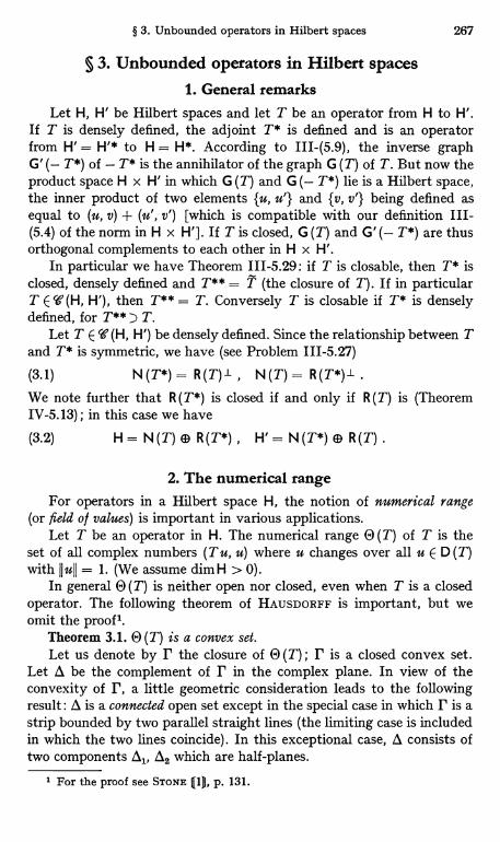
§ 3. Unbounded operators in Hilbert spaces 267
§ 3. Unbounded operators in Hilbert spaces1. General remarks
Let H, H' be Hilbert spaces and let T be an operator from H to H'.If T is densely defined, the adjoint T* is defined and is an operatorfrom H' = H'* to H = H*. According to III-(5.9), the inverse graphG' (- T*) of - T* is the annihilator of the graph G (T) of T. But now theproduct space H x H' in which G (T) and G (- T*) lie is a Hilbert space,the inner product of two elements {u, u'} and {v, v'} being defined asequal to (u, v) + (u', v') [which is compatible with our definition III-(5.4) of the norm in H x H']. If T is closed, G (T) and G' (- T*) are thusorthogonal complements to each other in H x H'.
In particular we have Theorem 111-5.29: if T is closable, then T* isclosed, densely defined and T** = T (the closure of T). If in particularT E '(H, H'), then T** = T. Conversely T is closable if T* is denselydefined, for T** D T.
Let T E ' (H, H') be densely defined. Since the relationship between Tand T* is symmetric, we have (see Problem 111-5.27)
(3.1) N(T*)= R(T)1, N(T)= R(T*)1.We note further that R (T*) is closed if and only if R (T) is (TheoremIV-5.13) ; in this case we have
(3.2) H = N (T) ® R (T*) , H' = N (T*) ® R (T) .
2. The numerical rangeFor operators in a Hilbert space H, the notion of numerical range
(or field o l values) is important in various applications.Let T be an operator in H. The numerical range 0 (T) of T is the
set of all complex numbers (T u, u) where u changes over all u E D (T)with lull = 1. (We assume dimH > 0).
In general 0 (T) is neither open nor closed, even when T is a closedoperator. The following theorem of HAUSDORFF is important, but weomit the proof 1.
Theorem 3.1. 0 (T) is a convex set.Let us denote by r the closure of 0 (T) ; r is a closed convex set.
Let 0 be the complement of r in the complex plane. In view of theconvexity of r, a little geometric consideration leads to the followingresult : 0 is a connected open set except in the special case in which r is astrip bounded by two parallel straight lines (the limiting case is includedin which the two lines coincide). In this exceptional case, 0 consists oftwo components A, 02 which are half-planes.
1 For the proof see STONE Q1], p. 131.
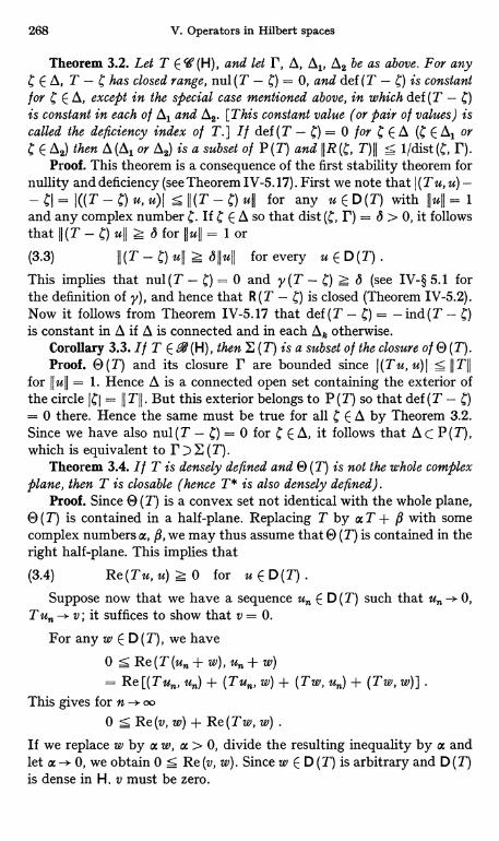
268 V. Operators in Hilbert spaces
Theorem 3.2. Let T E W(H), and let P, A, All A2 be as above. For anyC E A, T - C has closed range, nul (T - C) = 0, and def (T - C) is constantfor C E A, except in the special case mentioned above, in which def (T - C)is constant in each of A and A2. [This constant value (or pair of values) iscalled the deficiency index of T.] I/ def (T - C) = 0 toy C E A (C E A orC E A2) then A(A or A2) is a subset of P(T) and T) 11 S 1/dist(C, P).
Proof. This theorem is a consequence of the first stability theorem fornullity and deficiency (see Theorem IV-5.17). First we note that I (T u, u) -- Cl= I((T-C)u,u)I SII(T - C)ull for any u E D(T) with (lull= 1and any complex number C. If Z' E A so that dist r) = 6 > 0, it followsthatII(T - C)ull z (5 for lull for(3.3) 11 (T - C) u11 z bllull for every u E D(T) .
This implies that nul (T - C) = 0 and y (T - C) > S (see IV-§ 5.1 forthe definition of y), and hence that R (T - r;) is closed (Theorem IV-5.2).Now it follows from Theorem IV-5.17 that def (T - C) = - ind (T - C)is constant in A if A is connected and in each Ak otherwise.
Corollary 3.3. If T E 9 (H), then E (T) is a subset of the closure of 0 (T).Proof. 0 (T) and its closure r are bounded since I (T u, u) I s 11 T11
for (lull = 1. Hence A is a connected open set containing the exterior ofthe circle ICI = II T11. But this exterior belongs to P (T) so that def (T - I')= 0 there. Hence the same must be true for all r; E A by Theorem 3.2.Since we have also nul (T - l;) = 0 for C E A, it follows that A C P (T),which is equivalent to r D E (T).
Theorem 3.4. If T is densely defined and 0 (T) is not the whole complexplane, then T is closable (hence T* is also densely defined).
Proof. Since 0 (T) is a convex set not identical with the whole plane,0 (T) is contained in a half-plane. Replacing T by a T + P with somecomplex numbers a, 9, we may thus assume that 0 (T) is contained in theright half-plane. This implies that
(3.4) Re (T u, u) z 0 for u E 0 (T) .
Suppose now that we have a sequence u E D (T) such that u 0,T u,, --> v ; it suffices to show that v = 0.
For any w E D (T), we have
0 sRe w) + (Tw, (T w, w)] .
This gives for n --> oo
0 S Re (v, w) + Re (T w, w) .
If we replace w by a w, a > 0, divide the resulting inequality by at andlet a -* 0, we obtain 0 5 Re (v, w). Since w E D (T) is arbitrary and D (T)is dense in H. v must be zero.
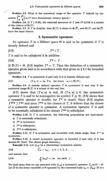
§ 3. Unbounded operators in Hilbert spaces 269
Problem 3.5. What is the numerical range of the operator T defined by the
matrix I o I in C2 (two dimensional unitary space) ?Y 11
Problem 3.6. If T E ' (H), the essential spectrum of T (see IV-§ 5.6) is a subsetof the closure of O (T).
Problem 3.7. If T is closable, then O (T) is dense in e (T), and E) (T) and O (T)have the same closure.
3. Symmetric operatorsAn operator T in a Hilbert space H is said to be symmetric if T is
densely defined and
(3.5) T* D T.
T is said to be selfadjoint if in addition
(3.6) T* = T.If D (T) = H, (3.5) implies T* = T. Thus the definition of a symmetricoperator given here is in accordance with that given in § 2.1 for boundedoperators.
Problem 3.8. T is symmetric if and only if it is densely defined and
(3.7) (Tu, v) = (u, Tv) for every u, v E D(T) .
Problem 3.9. A densely defined operator T is symmetric if and only if thenumerical range 0 (T) is a subset of the real line.
(3.7) shows that (Tu, u) is real. If (Tu, u) 0, the symmetricoperator T is said to be nonnegative (in symbol T 0). (3.5) shows thata symmetric operator is closable, for T* is closed. Since (3.5) impliesT*** ) T** and since T** is the closure of T, it follows that the closureo l a symmetric operator is symmetric. A symmetric operator T is saidto be essentially selfadjoint if its closure T** is selfadjoint.
Problem 3.10. If T is symmetric, the following propositions are equivalent:a) T is essentially selfadjoint.b) T* is symmetric.c) T* is selfadjoint.d) T** is selfadjoint.Problem 3.11. If T is symmetric and invertible with dense range, then T-1 is
symmetric.Problem 3.12. A closed symmetric operator is bounded if and only if it has
domain H. [hint: The closed graph theorem.]Example 3.13. Let (r!k) be a (Hermitian) symmetric matrix:
(3.8) zik=ska, j,h=1,2,3,...,and assume that
(3.9) .L' IZlkl2 < oo for each j.k
We shall show that we can associate with (rf k) a symmetric operator To in H = Is.Let D be the linear manifold of H spanned by the canonical basis x = (3m,,). D is a
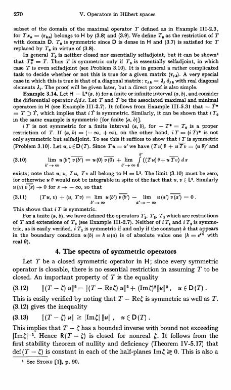
270 V. Operators in Hilbert spaces
subset of the domain of the maximal operator T defined as in Example 111-2.3,for T x, = (v ,,) belongs to H by (3.8) and (3.9). We define To as the restriction of Twith domain D. T. is symmetric since D is dense in H and (3.7) is satisfied for Treplaced by To in virtue of (3.8).
In general To is neither closed nor essentially selfadjoint, but it can be shown'that To = T. Thus T is symmetric only if T. is essentially selfadjoint, in whichcase T is even selfadjoint (see Problem 3.10). It is in general a rather complicatedtask to decide whether or not this is true for a given matrix (r5 ). A very specialcase in which this is true is that of a diagonal matrix : tf u = A, 611, with real diagonalelements A,. The proof will be given later, but a direct proof is also simple.
Example 3.14. Let H = L2 (a, b) for a finite or infinite interval (a, b), and considerthe differential operator d/dx. Let T and t be the associated maximal and minimaloperators in H (see Example 111-2.7). It follows from Example 111-5.31 that - T*= T ) T, which implies that i t is symmetric. Similarly, it can be shown that i Toin the same example is symmetric [for finite (a, b)].
i T is not symmetric for a finite interval (a, b), for - T* = T. is a properrestriction of T. If (a, b) = (- oo, + oo), on the other hand, i T = (i t)* is notonly symmetric but selfadjoint. To see this it suffices to show that i T is symmetric(Problem 3.10). Let u, v E D (T). Since T u = u' we have (T u) v + u 27-v = (u v)' and
b'(3.10) lim u (b') v (b') = u (0) v (0) + lim f ((T u) v + u T v) d x
b'-aoo b'-*m 0
exists; note that u, v, T u, T v all belong to H = L2. The limit (3.10) must be zero,for otherwise u v would not be integrable in spite of the fact that u, v E L2. Similarlyu (x) v (x) -. 0 for x -. - no, so that
(3.11) (T u, v) + (u, T v) = lim u (b') v (b') - lim a (a') v (a') = 0 .b'-a oo a'--,.- co
This shows that i T is symmetric.For a finite (a, b), we have defined the operators T1, Ts, Ts which are restrictions
of T and extensions of T. (see Example 111-2.7). Neither of i T1 and i T. is symme-tric, as is easily verified. i T. is symmetric if and only if the constant h that appearsin the boundary condition u (b) = k u (a) is of absolute value one (k = e4 8 withreal 0).
4. The spectra of symmetric operatorsLet T be a closed symmetric operator in H ; since every symmetric
operator is closable, there is no essential restriction in assuming T to beclosed. An important property of T is the equality
(3.12) II (T -C) u1I2 = II (T - Ret) ull2 + (ImC)2IIulj2 , u E D (T)
This is easily verified by noting that T - ReC is symmetric as well as T.(3.12) gives the inequality
(3.13) II (T - C) ull > IImCI'lull , u E D (T)
This implies that T - C has a bounded inverse with bound not exceedingIImCI-1. Hence R(T - C) is closed for nonreal . It follows from the
first stability theorem of nullity and deficiency (Theorem IV-5.17) thatdef (T - C) is constant in each of the half-planes ImC 0. This is also a
1 See STONE 111, p. 90.
§ 3. Unbounded operators in Hilbert spaces 271
direct consequence of Theorem 3.2; note that the numerical range 0 (T)of T is a subset of the real axis and therefore A of Theorem 3.2 either is aconnected set or consists of the two half-planes mentioned. The pair(m', m") of the constant values of def (T - C) for Imp < 0 is called thedeficiency index of the symmetric operator T. If T is not closed, thedeficiency index of T is defined as equal to that of T, the closure of T.
According to (3.1) (applied to T - C), T* - C = (T - )* has range Hand nullity m" or m' according as ImC c 0.
If m'= 0, R (T - C) for ImC > 0 is H and R (C, T) = (T - 0-1 ER(H)exists. In other words, the upper half-plane belongs to the resolvent setP(T). If m' > 0, no C in the upper half-plane belongs to P(T). Similarresults hold for m" and C with ImC < 0. Thus there are the followingalternatives :
i) m' = m" = 0. All nonreal numbers belong to P (T) ; the spectrumE (T) is a subset of the real axis.
ii') m' = 0, m" > 0. P (T) is the open upper half-plane ImC > 0 andE (T) is the closed lower half-plane Im C S 0.
ii") m' > 0, m" = 0. "upper" and "lower" exchanged in ii').iii) m' > 0, m" > 0. P (T) is empty and E (T) is the whole plane.Problem 3.15. The case i) occurs whenever P (T) contains at least one real
number.
A closed symmetric operator is said to be maximal if at least one of m',m" is zero [the case i), ii') or ii")]. A maximal symmetric operator has noproper symmetric extension. To show this, we may assume that m' = 0.Let Tl be a symmetric extension of T; T1 may be assumed to be closed(otherwise take the closure). For any u E D (Ti), there is a v E D (T) suchthat (T - i) v = (Tl - i) u because R (T - i) = H. Since T Tl, we maywrite (T1 - i) (u - v) = 0. Since Tl is symmetric, this gives u - v = 0.This implies that D (Ti) C D (T) and hence T1= T.
If both m' and m" are zero [case i)], T is selfadjoint. We have namelyTheorem 3.16. A closed symmetric operator T has deficiency index (0, 0)
if and only it T is self adjoint. In this case the resolvent R (C, T) = (T - ts)-1exists for Im C + 0 and
(3.14) JJR(C, T) 11 5 1 ImCI-1 , 11(T - Re C) R(C, T) 11 s 1 .
Proof. Assume that T has deficiency index (0, 0). Then both T ± ihave range H, so that for each u E D (T*) there is a v E D (T) such that(T - i) v = (T* - i) u. Since T ( T*, this may be written (T* - i)(u - v) = 0. But T* - i has nullity zero by m" = 0, so that u - v = 0.
This shows that D (T*) ( D (T) and hence T* = T.Conversely assume that T* = T. Then T* is also symmetric and the
nullities of T* ± i must be zero. Since these nullities are the deficienciesof T i, the deficiency index of T is (0, 0).
272 V. Operators in Hilbert spaces
(3.14) follows directly from (3.12).Problem 3.17. In order that a symmetric operator T be essentially selfadjoint,
each of the following conditions is necessary and sufficient (cf. also Problem 3.10) :a) T* has no nonreal eigenvalue.b) R (T - C) is dense in H for every nonreal C.c) R (T - 4) is dense in H for some C with ImC' > 0 and also for some
=C"with ImC"<0.Problem 3.18. If T is selfadjoint and invertible, T-1 is also selfadjoint. [hint:
Use, for example, Problem 3.11 and Theorem 111-6.15. Note that T-1 is denselydefined since u E R (T) J- implies that T u = T* u = 0, u = 0. ]
Problem 3.19. If T is a closed symmetric operator with finite deficiency index,then T* is a finite extension of T (see III-§ 2.1).
Problem 3.20. Let T, S be closed symmetric operators and let S be a finiteextension of T of order r. If T has deficiency index (m', m"), then S has deficiencyindex (m' - r, m" - r).
Example 3.21. Let us determine the deficiency index of the closed symmetricoperator i T. of Example 3.14. Since (i TO)* = i T, it suffices to solve the equationsi T u = ± i u, that is, u' = ± u. The solutions of these differential equations areu (x) = c e± x (c is a constant). If (a, b) is finite, these solutions belong to D (T) forany c and satisfy i T u = f i u. Thus both i T i have nullity one; the deficiencyindex of i To is (1, 1).
If (a, b) = (- oo, + oo), the above solutions do not belong to H unless c = 0.Thus the nullity of i T + i is zero and the deficiency index of i t is (0, 0)1. This is inconformity with the result stated in Example 3.14 that i T = (i t) * is in this caseselfadjoint.
Next consider the case of a semi-infinite interval (a, b), say a = 0, b = oo.Then the function e-x belongs to D (T) but ex does not. Thus the nullity of i T - iis zero whereas that of i T + i is one, and the deficiency index of i t is (1, 0). Theclosure of i t is maximal symmetric but not selfadjoint and has no selfadjointextension. (Actually T = T1.)
Finally consider the symmetric operator i T8 (i T for a finite (a, b), with theboundary condition u (b) = e4 e u (a). Since i T8 is symmetric and a direct extensionof i T. and since i T. has deficiency index (1, 1), i T. has deficiency index (0, 0)and is therefore selfadjoint.
Problem 3.22. Let H = L2 (E) and let T be the maximal multiplication operatorby a real-valued measurable function j(x) (see Example 111-2.2). T is selfadjoint.
5. The resolvents and spectra of selfadjoint operatorsLet T be a selfadjoint operator in H. Its spectrum E (T) is a subset
of the real axis, and the resolvent R (C) = R (C, T) _ (T - c)-1 is definedat least for all nonreal We have from III-(6.50)
(3.15) R (C) * = R
It follows that R (C) is normal, for the R (C) for different C commute witheach other.
In particular, we have IIR (C) II = sprR (C) by (2.4) and hence byProblem 111-6.16
(3.16) IIR(C)II = 1/dist(C, Y-(T)) S IImCI-1.
1 Note that i I' is not closed.
§ 3. Unbounded operators in Hilbert spaces 273
In the same way we have
(3.17) II TR (C)II = sup JAI IA - CI-1AEE(T)
for T R (4) = 1+ C R (C) so that II T R (;) II = spr(l + CR(C)) = sup I 1 ++ C(A - sup IA(A - 1
the of 1 + C (A - C)-1.]If a real number a belongs to the resolvent set P (T), P (T) contains
a neighborhood of a; we say then that E (T) has a gap at a. Note thatP (T) is a connected set if E(T) has at least one gap.
Suppose that E (T) has gaps at a and 9, a < P. Let r be a closedcurve passing through a, 9 and enclosing the part of E (T) between aand P. Further we assume that r is symmetric with respect to the realaxis [for example we may take as r a circle with the segment (a, 9)as a diameter]. Then E (T) is separated by r into two parts, onebeing in the interval (a, 9) and the other E" outside this interval. Let(3.18) H=M'®M"be the associated decomposition of H (see III-§ 6.4). Here M', M" areorthogonal complements to each other, for the projection P on M' alongM" is orthogonal:(3.19) P*= P,as is seen from the expressions for P and P* given by III-(6.52), whichcoincide in virtue of T* = T and the symmetry of r with respect to thereal axis.
If (T) has an isolated point A (which is necessarily real), we havethe Laurent expansion III-(6.32) for R (l;) = R (l;, T). Here not only Pbut D and S are also symmetric (and bounded). D* = D follows fromIII-(6.28) and S* = S from III-(6.31). But D as a symmetric quasi-nilpotent operator must be zero (see Problem 2.4). Hence (T - A) P = 0and A is an eigenvalue of T with the associated eigenspace M' = PH.Note that, in this case, M' is the geometric as well as the algebraiceigenspace. We have further
(3.20) IISII = 1/d with d = dist (A, E")
where E" is the spectrum of T with the single point A excluded. We shallcall d the isolation distance of the eigenvalue A. (3.20) can be proved as in(3.16), noting that S may be regarded as the value at A of the resolventof the part TM" of T, of which the spectrum is exactly E" [see III-(6.31)]and that M' 1 M".
Similar results hold when there are several isolated points Al, ..., A,of E (T). We have [see III-(6.35)]
PA(3.21) R (C) = - Z,' + Ro (C),
274 V. Operators in Hilbert spaces
where the Ph have the properties(3.22) Ph = Ph , Ph Pk = ah k Phand where Ro (C) is holomorphic at C _ Ah, h = 1, ..., s. Again the .h areeigenvalues of T with the associated eigenspaces Mh = Ph H, which areorthogonal to one another.
6. Second-order ordinary differential operatorsConsider the formal differential operator
d du(3.23) Lu=-dxp(x) dx +q(x)u, a<x<b,where p (x) is positive and continuously differentiable and q (x) is real and contin-uous, both in the open interval (a, b). L is formally selfadjoint: M = L where Mis the formal adjoint to L defined by III-(2.27). Thus we have
b
(3.24) f ((Lu)v-uLv)dx=[puv'-pu'v]o;, a<a'<b'<b.a'
Let us consider the linear operators T, t, etc. constructed from L in III-§ 2.3,choosing now X = H = La (a, b) (see also Example 111-5.32). We have t* = T ) T'by III-(5.14), so that the minimal operator t is symmetric. T is essentially sell-adjoint it and only if the maximal operator T is symmetric (see Problem 3.10).Whether or not this is true depends on the properties of the coefficients p (x), q (x).
It is certainly not true if (a, b) is finite and p (x), q (x) are continuous on theclosed interval [a, b] with p > 0 (the regular case). In this case T is not symmetric;the closure of t is exactly the operator To with the boundary condition u (a)= u' (a) = u (b) = u' (b) = 0 and To has deficiency index (2, 2). This is obvious sinceTo* = T and the equation (T ± i) u = 0 has two linearly independent solutions(belonging to H). There are infinitely many selfadjoint operators H such thatTo (H C T. Without trying to determine all such H', we note only that the T3,T2 and Ts of III-§ 2.3 are examples of H; this follows immediately from the lastresults of Example 111-5.32 in view of S = T.
As a typical case of a singular differential operator, let us now consider the casewith (a, b) = (- oo, + oo). We shall show that t is essentially selfadjoint (and T isselfadjoint if p (x) > 0 is bounded and q (x) is bounded from below on (-oo, +oo).To this end we may assume without loss of generality that q (x) Z 1, for the additionof a real scalar to T does not affect its selfadjointness. Then
co(3.25) (Tu, u) = f (p Ju'12 + qjuj2) dx> 11u112 , u E D(T),_,o
so that the numerical range 0 (T) of T lies to the right of C = 1, and the same istrue of O (T') (see Problem 3.7). It follows that the exterior of O (T) is a connectedopen set containing the origin. To show that t is selfadjoint, it is therefore sufficientto show that R (T) has deficiency 0 or, equivalently, that T = T'* has nullity zero(see par. 3 and 4).
Suppose now that T u = 0. Take any smooth real-valued function w (x) thatvanishes outside of a finite interval. Then v = w u belongs to D (T) (see Problem111-5.33), and a direct calculation gives
11Tv=Lv=wLu - (p w')'u - 2pw'u'.
1 For a complete determination of the H see STONE (1}.
§ 3. Unbounded operators in Hilbert spaces 275
Since L u = T u = 0, it follows that
"r 00
(3.26) (Tv,v)=- f (pw')'wlul%dx-2 f pw'wu'u,dxM 00 _f pw'%IuI%dx+ f pw'w(uu'-u'u)dx
00 M
(integration by parts). Since (Tv, v) is real while the first term on the right of (3.26)
is real and the second pure imaginary, this last term must vanish. Since (T v, v)IIvII%, we thus obtain
(3.27) f w%IuI%dx = IIvII% s f p w'%Iu!%dx S c f w'%Iuj%dx
where p (x) S c by assumption.It is easy to deduce from (3.27) that u = 0. To this end let w (x) be equal to one
for Ixj 5 r with Iw'I S s everywhere. Then (3.27) givesr 00 00
(3.28) f IuI%dxS f w%IuI%dxSc f w12 Iu12dx<cs2 f Iztl%dx.-r -00 -00It is possible to choose r as large as we please while s is fixed. On letting r ---> 00 for
ma fixed s, we obtain f Iu12 dx = 0 since it is known that u E L2. This gives the
-00desired result u = 0.
Problem 3.23. The assumption made above that p (x) is bounded can be replacedby the weaker one that the integrals of p (x)-112 on the intervals (- oo, 0) and(0, oo) both diverge.
Finally let us consider the case (a, b) = (0, oo) and assume that p (x) is positiveand bounded and q (x) is bounded from below on [0, 00)'. An argument similarto that given above shows that T has deficiency index (1, 1). A typical selfadjointextension T, of T is obtained by restricting T with the boundary condition u (0) = 0.
00
Again the assumption that p (x) be bounded may be weakened to f p (x)-1/% dx = no.0
Details may be left to the reader.
7. The operators T* TThe following theorem due to VON NEUMANN is of fundamental
importance.Theorem 3.24. Let H, H' be Hilbert spaces. Let T E W (H, H') be densely
defined. Then T* T is a selfadjoint operator in H, and D (T* T) is a core of T.Proof. As noted in par. 1, the graphs G (T) and G' (- T*) are com-
plementary subspaces of the Hilbert space H x H'. This implies that anyvector {u, u'} of H x H' can be expressed in the form {v, Tv} + {- T* v', v'}with some v E D (T) and V' E D (T*). If in particular u' = 0, we haveu=v-T*v' and 0= Tv+v'. Hence Tv=-v'ED(T*) andu = (1 + T* T) v. Since u E H was arbitrary, it follows that S = 1 + T* Thas range H. But it is easily seen that S-1 is symmetric and JIS-11I -, 1.
1 p (x) may tend to 0 and q (x) may go to + oo for x oo.
276 V. Operators in Hilbert spaces
Thus S-1 is symmetric and belongs to .(H) so that it is selfadjoint.Hence S and T* T are also selfadjoint (see Problem 3.18). Note that thisimplies that T* T is densely defined, which is by no means obvious.
To prove that D = D (T* T) is a core of T, it suffices to show thatthe set of all elements {v, Tv} with v E D is dense in G (T) (see III-§ 5.3).Thus we need only to show that an element {u, T u} with u E D (T)orthogonal to all {v, Tv) with v E D must be zero. But this orthogonalityimplies that 0 = (u, v) + (Tu, Tv) = (u, (1 + T* T) v) = (u, Sv). SinceS v fills the whole space H when v varies over D, this gives u = 0 asrequired.
Example 3.25. Consider the operators T, To, etc. of Example 3.14 for a finiteinterval (a, b). We know that Tp* T, Tl = - T2, T2* = - T1, T* To(see also Example 111-5.31). Thus we have T* T = - To T; it is the differentialoperator - d2/d x2 with the boundary condition T u E D (T(,), that is, u' (a) = u' (b)= 0. (This is identical with the T2 of III-§ 2.3 in the special case po = - 1, p, = p$= 0, ho = hb = 0.) Next we have To To = - T To; this is the same differentialoperator - d2/dx2 with the boundary condition u (a) = u (b) = 0 (and coincideswith the Tl of the same example). Again, Ti Tl = - T2 Tl is the same differentialoperator with the boundary condition u (a) = u' (b) = 0, and Ta T2 =- Tl T2is obtained from it by exchanging a and b. That these differential operators are allselfadjoint is a direct consequence of Theorem 3.24.
Example 3.26. A construction similar to the above one applied to the second-order differential operators of III-§ 2.3 for X = H = L2 will give rise to variousdifferential operators of fourth order which are selfadjoint.
8. Normal operatorsSelfadjoint operators are special cases of normal operators. The
definition of a not necessarily bounded normal operator T in a Hilbertspace H is formally the same as that of a normal operator of -V(H) :T is normal if T is closed, densely defined and
(3.29) T*T= TT*;note that both T* T and T T* are selfadjoint (preceding paragraph).The implication of (3.29) is rather complicated, however, on account ofthe domain relations involved.
(3.29) implies that II Tu1I = 11 T* u11 for u E D - D (T* T) = D (T T*).Since D is a core for both T and T*, it follows that D (T) = D (T*)
Dl(:) D) and 11 TuII =IIT*ull for any u E D1.For any complex numbers C', we have then D [(T* - C') (T -c)]
= D. In fact, u E D [(T* - C") (T - C)] implies u E D1 and Tu - 1 u E D1,hence T u E D1, hence u E D. The opposite implication is obvious. SinceD [(T - l;) (T* - c')] = D similarly, we see from (3.29) that (T* -- C') (T - C) = (T - C) (T* - a'). If in particular C E P(T) and V EE P (T*), it follows that [we write R (C) = R (ts, T), R* R (C, T*)]
(3.30) R* (C') R (C) = R (C) R* (C') .
§ 3. Unbounded operators in Hilbert spaces 277
(3.30) means simply that the resolvents R (C) and R* (c') commute.Since R* (a') = R (y') * by III-(6.50), it follows that R (C) is also normal.As in (3.16) and (3.17), we have
IJR(C, T)II = 1/dist(C, E(T)) = sup IC - AI-1(3.31) AEE(T)
IITR(C, T)II = sup IA(C - A)-'I .2EE(T)
Suppose now that the spectrum Z (T) of a normal operator T isseparated into two parts E', E". The projection P associated with thisdecomposition and its adjoint P* are again given by III-(6.52). Itfollows from (3.30) that P and P* commute so that P is normal. As inthe finite-dimensional case, this implies that P is an orthogonal projection[see Problem 1-6.30]. If E' consists of a single point, the associatedquasi-nilpotent operator D is similarly seen to be normal, which impliesthat D = 0 (see Problem 2.4). Thus we are led to the same expression(3.21) for R(C) as for a selfadjoint operator T whenever E(T) containsisolated eigenvalues Al, ..., A3, with the only difference that the eigen-values Ah need not be real.
Problem 3.27. If T is normal, T and T* have the same null space.
Let T be a normal operator with compact resolvent (see III-§ 6.8).Application of (2.19) to the resolvent R (C) = R (C, T) leads to the formula
00
R (C) _ Ph Ph, where the Huh are the eigenvalues of R (C) and Ph -> 0,h=1
h oo, and where the Ph are the associated eigenprojections. Theorthogonal family {Ph} is complete since R (C) has the null space 0 (seeTheorem 2.10). But R (C) and T have the same set of eigenprojections,and the eigenvalues Ah of T are related to the Ph by Ph = (AhThus we have
(3.32) R (C) = h2 h 1 'h , Ah °O , h -->. oo
00
(3.33) , Ph = 1 (strong convergence) .h=1
Example 3.28. (3.32) is true for all selfadjoint restrictions of the i T of Example3.21. The same is true of all selfadjoint restrictions of the T of par. 6 in the regularcase (see Example 111-6.31). All these operators have discrete spectra consisting ofreal eigenvalues with finite multiplicities (which do not exceed the order m of thedifferential operator in question, since a differential equation of order m has atmost m linearly independent solutions).
9. Reduction of symmetric operatorsSuppose that a symmetric operator T is decomposed according to the
decomposition H = M ® M1 of H into the direct sum of mutually orthog-onal subspaces M and M1. According to III-(5.24), this is the case
278 V. Operators in Hilbert spaces
if and only if T commutes with the orthogonal projection P on M:
(3.34) PTCTP.In this case we say simply that T is reduced by M. Since 1 - P is theprojection on Ml, T is reduced by M if and only if it is reduced by M-L.
A symmetric operator T is reduced by M if and only if u E D (T) impliesPu E D (T) and TPu E M. The "only if" part of this theorem is obviousfrom (3.34), so it suffices to prove the "if" part. The assumption impliesthat TPu= PTPu foreveryu E D(T). Hence(u, PTPv) = (PTPu,v)= (TPu, v) _ (u, PTv) for all u, v E D(T), which gives PTPv = PTv.Thus TPu = PTPu = P T u for u E D (T), which is equivalent to (3.34).
Problem 3.29. Let H = Ml ® M2 ® .. ® M, be a decomposition of H intothe direct sum of mutually orthogonal subspaces. If a symmetric operator T isreduced by each M1, then T is decomposed according to the above decomposition ofH in the sense of III-§ 5.6.
10. Semibounded and accretive operatorsA symmetric operator T is said to be bounded from below if its
numerical range (which is a subset of the real axis) is bounded frombelow, that is, if
(3.35) (T u, u) z y (u, u) , u E D (T) .
In this case we simply write T > y. The largest number y with thisproperty is the lower bound of T. Similarly one defines the notions ofboundedness from above and the upper bound. A symmetric operatorbounded either from below or from above is said to be semibounded.
If T is bounded both from below and from above, then T is bounded,with the bound equal to the larger one of the absolute values of thelower and upper bounds. The proof is the same as in the finite-dimensionalcase [I-(6.33)]. In this case T E9 (H) if T is closed.
If T is selfadjoint, T is bounded from below (with lower bound VT)if and only if E(T) is bounded from below (with lower bound yE).In fact, suppose that T is bounded from below. Then the open set Acomplementary to the closure of 0 (T) is connected, including realnumbers C such that C < YT, and is contained in the resolvent set P (T)(see Theorem 3.2). Thus E(T) is bounded below with lower boundyE z VT Conversely suppose that E (T) is bounded below with lowerbound yE. Set T' = T - yE. T' has its spectrum on the nonnegativereal axis, and for any a > 0 we have II(T' + a) -111 = o e-1 by (3.16).For any u E D (T), we have therefore Hull S a-1 11 (T' + a) ull and so
(3.36) 11ull2 a-111 T'uhI2+ 2a-1(T'u u) + 1lull2
or 0 5 a-' 11 T' u I12 + 2 (T' u, u). On letting a -> oo we have (T' u, u) Z 0,that is, T' z 0, T z yE. Thus T is bounded from below with YT z yE.
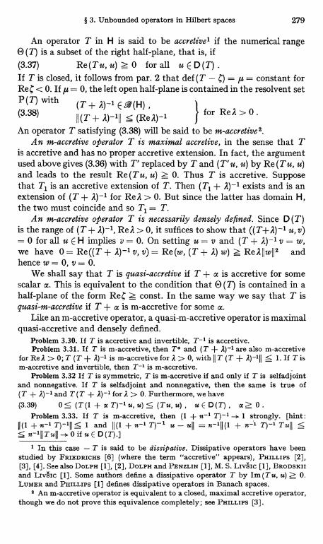
§ 3. Unbounded operators in Hilbert spaces 279
An operator T in H is said to be accyetive) if the numerical range0 (T) is a subset of the right half-plane, that is, if(3.37) Re (T u, u) z 0 for all u E D (T) .If T is closed, it follows from par. 2 that def (T - C) = ,u = constant forReC < 0. If /u = 0, the left open half-plane is contained in the resolvent setP(T)with (T+A)-'E2(H), l(3.38) II (T + A)-III < (ReA)_1
for ReA > 0.
An operator T satisfying (3.38) will be said to be m-accretive2.
An m-accretive operator T is maximal accretive, in the sense that Tis accretive and has no proper accretive extension. In fact, the argumentused above gives (3.36) with T' replaced by T and (T' u, u) by Re (T u, u)and leads to the result Re (T u, u) >- 0. Thus T is accretive. Supposethat T, is an accretive extension of T. Then (T, + A)-' exists and is anextension of (T + A)-' for ReA > 0. But since the latter has domain H,the two must coincide and so T, = T.
An m-accretive operator T is necessarily densely defined. Since D (T)is the range of (T + A)-', ReA > 0, it suffices to show that ((T+A)-' u, v)= 0 for all u E H implies v = 0. On setting u = v and (T + A)-' v = w,we have 0,= Re((T+ A)-1 v, v) = Re(w, (T + A) w) > ReAIIwIIz andhence w = 0, v = 0.
We shall say that T is quasi-accyetive if T + a is accretive for somescalar a. This is equivalent to the condition that 0 (T) is contained in ahalf-plane of the form ReC > const. In the same way we say that T isquasi-m-accretive if T + a is m-accretive for some a.
Like an m-accretive operator, a quasi-m-accretive operator is maximalquasi-accretive and densely defined.
Problem 3.30. If T is accretive and invertible, T-' is accretive.Problem 3.31. If T is m-accretive, then T* and (T + A)-' are also m-accretive
for ReA > 0; T (T + A)-' is m-accretive for A > 0, with II T (T + A)-'II S 1. If T ism-accretive and invertible, then T-' is m-accretive.
Problem 3.32 If T is symmetric, T is m-accretive if and only if T is selfadjointand nonnegative. If T is selfadjoint and nonnegative, then the same is true of(T + A)-' and T (T + A)-' for A > 0. Furthermore, we have(3.39) 0S(T(1+aT)-'u,u)S(Tu,u), uED(T), a>0.
Problem 3.33. If T is m-accretive, then (1 + n-' T)-' 1 strongly. [hint:II (1 + n-' T)-1II 5 1 and 11(1 + n-' T)-1 u - uII = n-1II (1 + n-1 T)-' TuIIS n-1 11 TuII 0 if u E D (T).]
' In this case - T is said to be dissipative. Dissipative operators have beenstudied by FRIEDRICHS [6] (where the term "accretive" appears), PHILLIPS [2],[3], [4]. See also DOLPH [1], [2], DOLPH and PENZLIN [1], M. S. LIvsic [1], BRODSKIIand LIv§Ic [1]. Some authors define a dissipative operator T by Im(Tu, u) > 0.LUMER and PHILLIPS [1] defines dissipative operators in Banach spaces.
2 An m-accretive operator is equivalent to a closed, maximal accretive operator,though we do not prove this equivalence completely; see PHILLIPS [3].
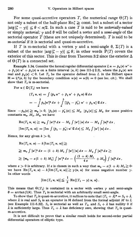
280 V. Operators in Hilbert spaces
For some quasi-accretive operators T, the numerical range 0 (T) isnot only a subset of the half-plane ReC const. but a subset of a sectorI arg (C - y) 15 0 < 7r/2. In such a case T is said to be sectorially-valuedor simply sectorial; y and 0 will be called a vertex and a semi-angle of thesectorial operator T (these are not uniquely determined). T is said to bem-sectorial if it is sectorial and quasi-m-accretive.
If T is m-sectorial with a vertex y and a semi-angle 0, E (T) is asubset of the sector I arg (C - y) I < 0; in other words P (T) covers theexterior of this sector. This is clear from Theorem 3.2 since the exterior Aof 0 (T) is a connected set.
Example 3.34. Consider the formal regular differential operator L u = p0 (x) u"++ p1(x) u' + p2 (x) u on a finite interval [a, b] (see III-§ 2.3), where the pk (x) arereal and p0 (x) < 0. Let Tl be the operator defined from L in the Hilbert spaceH = L2 (a, b) by the boundary condition u (a) = u (b) = 0 (see loc. cit.). We shallshow that T1 is m-sectorial.
For u E D (T1) we have
(T1u,u)= f (pou"+P1u'+P2u)udxb b
f P. JUT dx + f [(p1 - po) u' + p2 u] u dx .a a
Since - pu (x) > mo > 0, IN (x) - po (x) I S M1, I p2 (x) 15 M2 for some positiveconstants mo, Ml, M2, we have
Re(T1u,u)Z No f Iu1I2dx-M1 f Iu'i Jul dx - M2 f Iu12dx,
IIm(Ti u, u)I = IIm f (P1 - po) u' u dxl s M1 f lu'I Jul dx .
Hence, for any given k > 0,
Re(T1 u, u) - kIIm(Tj u, u)I
MO f lu'12 dx - (1 + k) M1 Jul l ul dx - M2 f lu12 dx >
[m0 - e(1 + k) Ml] f Iu1I2 dx - ((1±1)M1
+ M2) f Iuls dx,
where e > 0 is arbitrary. If a is chosen in such a way that mo - e (1 + k) M1 Z 0,we have Re (T1 u, u) - k I Im (Tl u, u) I Z y (u, u) for some negative number y.In other words
IIm(T1u,u)IS T Re ((T, - V) u, u)
This means that 0 (T1) is contained in a sector with vertex y and semi-angle0 = arctan(l/k). Thus T1 is sectorial with an arbitrarily small semi-angle.
To show that T1 is quasi-m-accretive, it suffices to note that (T1 + A) * = S1 + A,where A is real and S1 is an operator in H defined from the formal adjoint M to L(see Example 111-5.32). S1 is sectorial as well as T1, and S1 + A has nullity 0 ifA is sufficiently large. Thus T1 + A has deficiency zero, showing that T1 is quasi-m-accretive.
It is not difficult to prove that a similar result holds for second-order partialdifferential operators of elliptic type.
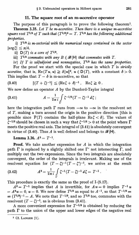
§ 3. Unbounded operators in Hilbert spaces 281
11. The square root of an m-accretive operatorThe purpose of this paragraph is to prove the following theorem'.Theorem 3.35. Let T be m-accretive. Then there is a unique m-accretive
square soot T'l2 o f T such that (T'/2)2 = T. T'/2 has the following additionalproperties.
i) T'/2 is m-sectorial with the numerical range contained in the sectorIargCI S ;r/4.
ii) D (T) is a core of T'/2.
iii) T'12 commutes with any B E -4 (H) that commutes with T.iv) If T is selfadjoint and nonnegative, T'/2 has the same properties.For the proof we start with the special case in which T is strictly
accretive, that is, Re(Tu, u) > 6IIuII2, u E D(T), with a constant 6 > 0.This implies that T - 6 is m-accretive, so that
(3.40) II(T+ C)-111 s (Re '+ 6)-' , ReC z 0 .
We now define an operator A b(y' the Dunford-Taylor integral
(3.41) A = 2' - C-1/2(T-a)-'dC;r
here the integration path r runs from -oo to -oo in the resolvent setof T, making a turn around the origin in the positive direction [this ispossible since P(T) contains the half-plane ReC < 6]. The values ofC-1/2 should be chosen in such a way that C-1/2 > 0 at the point where rmeets the positive real axis. The integral of (3.41) is absolutely convergentin virtue of (3.40). Thus A is well defined and belongs to . (H).
Lemma 3.36. A 2 = T.
Proof. We take another expression for A in which the - integrationpath r is replaced by a slightly shifted one r' not intersecting r, andmultiply out the two expressions. Since the two integrals are absolutelyconvergent, the order of the integrals is irrelevant. Making use' of theresolvent equation for (T - C)-' (T - we arrive at the result
(3.42) A2 = 2 if C-1(T - C)-1 dC = T-1
rr
This procedure is exactly the same as the proof of I-(5.17).A2 = T-' implies that A is invertible, for Au = 0 implies T-' u
= A2u = 0, u = 0. We now define T'/2 as equal to A-', so that T-'/2(P/2) -I = A. We note that T-'12, and so T'/2 too, commutes with the
resolvent (T - C)-', as is obvious from (3.41).A more convenient expression for T-'12 is obtained by reducing the
path r to the union of the upper and lower edges of the negative real
1 Cf. LANGER [1].
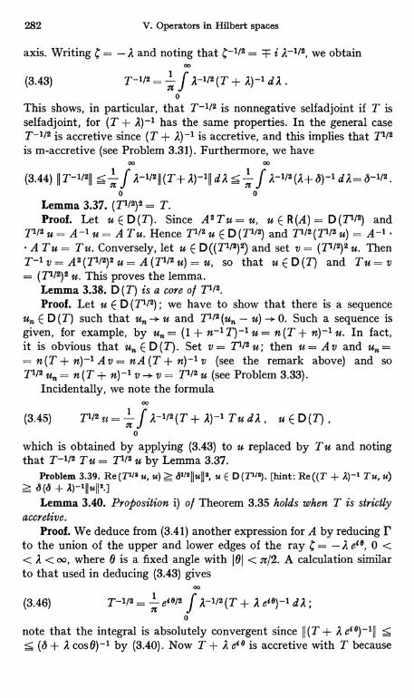
282 V. Operators in Hilbert spaces
axis. Writing C = - A and noting that C-1/2 = T- i A-1/2we obtainM
(3.43) T-1/2 =
a
f A-1/2 (T + A)-1 d A.0
This shows, in particular, that T-1/2 is nonnegative selfadjoint if T isselfadjoint, for (T + A)-1 has the same properties. In the general caseT-1/2 is accretive since (T + A)-1 is accretive, and this implies that T1/2is m-accretive (see Problem 3.31). Furthermore, we have
00 00
(3.44) I! T-1/211 SJ A-1/211
(T+ A)-111 d A f A-1/2 (A+ 6)-1 d A= 6-1/2.0 0
Lemma 3.37. (Tl/2)2 = T.Proof. Let it E D (T). Since A2 T u = u, u E R (A) = D (T1/2) and
T1/2 u = A-1 u = A Tit. Hence T1/2 u E D (TI/2) and T1/2 (TI/2 U) = A-1 .A Tit = Tit. Conversely, let u E D((T1/2)2) and set v = (T1/2)2 u. Then
T-1 v = A2 (T1/2)2 u = A (T1/2 u) = u, so that u E D (T) and Tu = v_ (T'/2)2 u. This proves the lemma.
Lemma 3.38. D(T) is a core of T1/2.
Proof. Let u E D (T1/2) ; we have to show that there is a sequenceu E D (T) such that u -> u and T1/2 (un - u) - 0. Such a sequence isgiven, for example, by u,, _ (1 + n-1 T) -1 u = n (T + n) -1 u. In fact,it is obvious that un E D (T). Set v = T1/2 u; then u = Av and u _= n(T + n)-1 Av = nA (T + n)-1 v (see the remark above) and soP/2 u a = n (T + n) -1 v -*- v = T1/2 u (see Problem 3.33).
Incidentally, we note the formula00
(3.45) T1/2 a= f A-1/2 (T + A)-1 Tit d A, u E D (T) ,0
which is obtained by applying (3.43) to u replaced by Tit and notingthat T-1/2 Tit = T1/2 u by Lemma 3.37.
Problem 3.39. Re (7'1/2 u, u) Z 61/21ju112, u E D (T1/2). [hint: Re((T + A)-1 Tu, u)6(6 + A)-111u112.1
Lemma 3.40. Proposition i) o l Theorem 3.35 holds when T is strictlyaccretive.
Proof. We deduce from (3.41) another expression for A by reducing rto the union of the upper and lower edges of the ray C = -A ete, 0 << A < oo, where 0 is a fixed angle with 101 < n/2. A calculation similarto that used in deducing (3.43) gives
00
(3.46) T-1/2 = ete/2 f A-1/2(T+ A e{6)-1 dA;
0
note that the integral is absolutely convergent since 11 (T + A el0)-1II
S (8 + A cos0)-1 by (3.40). Now T + A et0 is accretive with T because
§ 3. Unbounded operators in Hilbert spaces 283
ReA eie= A cosO > 0, so that (T+ Aei°)-1 is also accretive. Hencee-i0/2(T-1/2 u, u) has nonnegative real part by (3.46). Since this is truefor 101 < n/2, it follows that (T-1/2,U, u) lies in the sector IargCI n/4.This result can be written(3.47) I Im (T1/2 u, u) ( S Re (Tl/2 u, u) , u E D (TI/2)
Proposition iii) follows from (3.41), which shows that A = T-1/2commutes with B. Summing up the results obtained so far, we haveproved the theorem in the special case of a strictly accretive T exceptfor the uniqueness of T1/2. We now prove this uniqueness under somerestrictions.
Lemma 3.41. Assuming that T is strictly accretive, suppose there is anm-accretive operator S such that S-1= B E -4 (H) and S2 = T. ThenS = Tl/2.
Proof. B = S-1 commutes with B2 = T-1, hence with T and alsowith the resolvent (T - a)-1 (see Theorem 111-6.5). It follows from (3.41)that BA = A B. Since A2 = T-1= B2, we have (A + B) (A - B)= A2 - B2 = 0. For any u E H, we have therefore (A + B) v = 0 forv= (A - B) u. Then Re (A v, v) + Re (B v, v) = Re ((A + B) v, v) = 0.But both (A v, v) and (Bv, v) have nonnegative real parts since A, B areaccretive. Thus Re (A v, v) = 0 or Re (w, T'/2 w) = 0 for w = A v. SinceRe (w, T1/2 w) > 61/2 11 wII 2 by Problem 3.39, we conclude that w = 0,(A - B) u = v = T112 w = 0. Since u was arbitrary, this proves B = Aland hence S = T112.
We shall now remove the assumption made above that T is strictlyaccretive. Let T be m-accretive. For any e > 0, T, = T + e is strictlyaccretive, so that Tell= Se can be constructed as above. We shall showthat lim Se = S exists in a certain sense.
e-s0
For any u E D(Ti) = D (T), we have the expression (3.45) for Se uwhere T is to be replaced by T. Since (Te + A)-1 Te u = u - A(T, + A)-'u
= u - A(T + e + A)-lu, we have e (Te + A)-' Te u = A(T + e + A)-2u
= A(Te + A)-2 u = - A d A (Te + A)-1 u. Hence00
(3.48) de Se u = i f A1/2 T1 (TB + A)-1 u dA0
00
,/ A-1/2 (Te + 2)-' u d2 = 2 T.-1/2U,0
where we made an integration by parts and used (3.43) for TB 112. Integrat-ing (3.48) between 97 and e, where 0 < 27 < e, we obtain S, u - S,, U
1 The argument used here is a generalization of that of RIEsz and Sz.-NAGY 111)1,p. 264, where symmetric operators T > 0 are considered.
284 V. Operators in Hilbert spaces
= 1 f Te 112 u d e. Making use of the estimate 11 TQ 112 S e-1/2, whichzfollows from (3.44), we have then
e e
(3.49) S. u - Sn u S2
f 1jTe 112 ull de s f e-1/2 Ilull den n
_ (el/2 - 171/2) IIuII
This shows that lim S. it = S' u exists for it E D (T) and that6- 0
(3.50) IISeu - S'ull el/211ull, uED(T).Thus the operator S' - S. [with domain D(T)] is bounded with bound<e1/2. Since D (T) = D (T.) is a core of S, (see Lemma 3.38), it followsfrom the stability theorem of closedness (Theorem IV-1.1) that S' isclosable and the closure S = 9' has the same domain as S. [which implies,in turn, that D (Se) is independent of e]. At the same time (3.50) isextended to all u E D (S) with the S' on the left replaced by S. Thus wemay write(3.51) S, = S + Be , Be E 4(H) , 11Be11 5 e1/2 .
Since (Se u, u) - (S u, u), e -> 0, u E D (S) = D (Se), S is sectorialwith 0 (S) contained in the sector largCl 5 r/4, for this is true for Se.Furthermore, any C outside of this sector belongs to the resolvent set of S,as is seen by constructing R (C, S) by the Neumann series from S = S, -- Be, in which a is chosen so small that e1/2 is smaller than the distanceof C from that sector. This shows that S is m-accretive.
Lemma 3.42. S2 = T.Proof. Let u E D (T) and set v, = S, u. We have v, - Su, e > 0.
Since we know that S2 = Te, v6 E D (Se) = D (S) and S, v, = T, u. HenceS v, = (Se - Be) ve = Te u - Be ve T u, e -+ 0. It follows from theclosedness of S that S u E D (S) and S S u = T u. Thus we have provedthat T C S2 This implies that T + 1S2+1= (S + i) (S - i) and so(T + 1) -1 c (S - i)-1 (S + i) -1. But (T + 1) -1 and (S +i)-1 belong toR(H). Hence we must have equality instead of the last inclusion, andthis in turn implies that T = S2.
On writing S = T1/2, we have thus proved that i), ii) of Theorem 3.35are satisfied [ ii) is implied by S = 3']. iv) is also clear, for Se and S aresymmetric and hence selfadjoint if T is selfadjoint.
Lemma 3.43. (3.45) is true in the general case.Proof. The integral in (3.45) is absolutely convergent, for IIA-1/2.
(T+ A)-III S A-3/2 for A-+oo and IIA-112(T+ A)-1 Tull S 2 A-1/2j ulfor A -+ 0. The corresponding integral expression for Te12 u has the sameproperties, the estimate being independent of e. Since (T, + A)-1 Te it -- (T+A)-1Tu= -A[(T,+A)-1u- (T+A)-1u]-+0 for a-.0 for
§ 3. Unbounded operators in Hilbert spaces 285
each A > 0, it follows by the principle of dominated convergence thatT812 u converges to the right member of (3.45). Since Te"2 u T112 U,
T1/2 u must be equal to the right member of (3.45).Lemma 3.44. iii) of Theorem 3.35 is satisfied.Proof. B commutes with Te = T + e, hence with S. = Ts12 by what
was already proved. Since it is easily seen that (Se + 1)-1 -. (S + 1)-1,S
e 0, B commutes with (S + 1)-1, hence with S = T1/2 (see Theorem111-6.5).
Lemma 3.45. Let R be any m-accretive square root of T : R2 = T.Then R commutes with the resolvent of T and D (T) is a core of R.
Proof. Let A + 0 be real. Then (R - i A) (R + i A) = R2 + A2 = T + A2has range H and so does R - i A. On the other hand R - i A has nullityzero, for R u= i A u implies T u= R2 u= i A R u=- A2 u, (T + A2) u= 0, u= 0. Thus f i A E P (R) and (T + A2)-1= (R - i A)-' (R + i A) -1.Hence R commutes with (T'+ A2)-1. It follows also that D (R) D D (T) and(R - i A) D (T) = R [(R - i A) (T + A2)-1] = R [(R + i A)-'] = D (R) isdense in H, so that D (T) is a core of R.
Lemma 3.46. An m-accretive square root of T is unique'Proof. Let R be any m-accretive square root of T. Then R + e is
strictly m-accretive for any s > 0, and (R + 8)2 = R2 + 2 s R + e2= T + 2e R + e2 = Qe is also strictly accretive. In fact it is also m-accretive; to see this it suffices to note that R is relatively bounded withrespect to T because D (R) D D (T) (see Remark IV-1.5), so that (Qe ++ 1)-1 E.V(H) for sufficiently small e (see Theorem IV-1.16). Accordingto Lemma 3.41, R + e must be identical with the unique square rootQe112
Let u E D (T). Then it E D (R) and (R + e) u -+ Ru, s -+ 0. On theother hand, we have Q'12 U T1/2 u as we shall prove in a moment.Thus we obtain Ru = T1/2 u for it E D (T). Since D (T) is a core for both Rand T1/2 (see Lemma 3.45), it follows that R = T1/2, as we wished to show.
To prove that Q812 it -+ T1/2 u, e -+ 0, for u E D (T), we make use of(3.45) and a similar expression for Qe12 u (see Lemma 3.43). Since(T + A)-1 T u = u - A (T + A)-1 u, we have
(3.52) Qe12 u - T1/2 u = - f A1/2 [(Q. + A)-1 u - (T + A)-1 u] dA0
00
e f A1/2 (Qe + A)-' (2R + e) (T + A)-' u d A .
0
To estimate this integral, it is convenient to split it into two parts
f and f and to use the integrand in the form of the middle member of0 6
286 V. Operators in Hilbert spaces
(3.52) in the first part and in the form of the last member in the secondpart. Thus, noting the commutativity of R with (T + A)-1 (see Lemma3.45), we obtain
E
aIIQe12 u - Tl/2uII < f A"' [11(Q0+ A)-'II + II(T+ A)-'I!] IIuII dA +0
00
+ e f A112II (QE + A)-'II II (T + A)-1II II (2R + e) uII dA <C
(_ii2d2)IIuII+e(fA-3/2d2)II(2R+e)uII
o \E
= 4 e1/2II uII + 2e/211(2R+ e) uII -> 0 , s -> 0 .
Problem 3.47. If T E .4 (H) is symmetric and nonnegative, then II T11211 = II TII112.
Problem 3.48. If T is m-accretive, the following conditions on u are equivalent:a) Tu = 0, b) T112 u = 0, c) (A + T)-1 u = A-1 u, A > 0.
Theorem 3.49. Let T be m-accretive. T has compact resolvent i f andonly if Tl/2 has.
Proof. Set S = T1/2. The formula (T + 1)-1 = (S + i)-1 (5 - i)-1proved above (in the proof of Lemma 3.42) shows that T has compactresolvent if S has. To prove the converse statement, define TE = T + eand S. = T812 as above. S,-' is given by (3.43) with T replaced by TEon the right. Since the integral converges in norm and since (TE + A)-1 iscompact for all A > 0, it follows that SB 1 is compact. Thus SE has compactresolvent, so that (1 + SE)-1 is compact. Now II (1 + Se)-1 - (1 + S)-1IM
= II (1 + SE)-1(1 + S)-1(S - SE) II 5 II BEII < el/2 -. 0 for e -* 0 by (3.51).Hence (1 + S)-1 is compact and S has compact resolvent.
Remark 3.50. More generally we can define the fractional powers T",0 < oc < 1, for an m-accretive operator T by a construction similar tothat given above for T1/2. If T is strictly m-accretive, we have simply toreplace C-1/2 by C-" in (3.41) to obtain T. The formula correspondingto (3.43) is
Co
(3.53) T-" = sin= a f A-"(T + A)-1 dA.0
The general case can be dealt with by the method of this paragraph.It will be noted that T" can be defined for a more general class of operatorsacting in a Banach space.
Problem 3.51. Let T,,, T be m-accretive operators such that T. --.>, T in thegeneralized sense. Then (T + e)-1/2 -+ (T+ e)-112 in norm for any e > 0.
Problem 3.52. Let T,,, T be m-accretive and (T + (T + A)-1 for alls
A > 0. Then (T + e)-1/2 (T + e)-112 for any e > 0.
§ 4. Perturbation of selfadjoint operators 287
§ 4. Perturbation of selfadjoint operators1. Stability of selfadjointness
Since the selfadjoint operators form the most important class of oper-ators that appear in applications, the perturbation of selfadjoint operatorsand the stability of selfadjointness is one of our principal problems'.
The first question is under what conditions the selfadjointness ispreserved under a "small" perturbation. A fundamental result in thisdirection is given by
Theorem 4.1. Let T be a selfadjoint operator. Then there is a S > 0such that any closed symmetric operator S with 8(S, T) < S is selfadjoint,where S (S, T) denotes the gap between S and T.
Proof. Since ± i belong to P (T), it follows from Theorem IV-3.15that there is a S > 0 such that 6 (S, T) < b implies + i E P (S). Then S isselfadjoint by Theorem 3.16.
Corollary 4.2. Let T, T. be closed symmetric operators and let {Tn}converge to T in the generalized sense (see IV-§ 2.4). If T is selfadjoint,then T,, is selfadjoint for sufficiently large n.
Although this theorem is rather general, it is not very convenientfor application since the definition of the gap 6 (S, T) is complicated.A less general but more convenient criterion is furnished by relativelybounded perturbations.
We recall that an operator A is relatively bounded with respect to T(or T-bounded) if D (A) D D (T) and(4.1) IIAull S alluil + b11 TuII , u E D(T) ;see IV-(1.1). An equivalent condition is(4.2) IIAuII2 S a'allull'+ b'2IITuII', u E D(T) ,where the constants a', b' are, of course, in general different from a, b.As is easily seen, (4.2) implies (4.1) with a = a', b = b', whereas (4.1)implies (4,2) with a12 = (1 + e-') a2 and b' 2 = (1 + e) b2 with an arbitrarye > 0. Thus the T-bound of A (defined as the greatest lower bound of thepossible values of b) may as well be defined as the greatest lower boundof the possible values of Y.
Theorem 4.3.2 Let T be selfadjoint. If A is symmetric and T-boundedwith T-bound smaller than 1, then T + A is also selfadjoint. In particularT + A is selfadjoint if A is bounded and symmetric with D (A) ) D (T).
1 In this section all operators are assumed to act in a Hilbert space H, unlessotherwise stated.
2 Theorems 4.3 and 4.4 are due to RELLICH [3]. See also T. KATO [3], [4].These theorems have been found to be convenient for establishing the selfadjointnessor essential selfadjointness of various operators that appear in applications. Theapplications to the Schrodinger and Dirac operators will be discussed in § 5. Forthe applications to the quantum theory of fields, see Y. KATO [1], Y. KATO andMUGIBAYASHI [1]; Cf. also COOK [2].
288 V. Operators in Hilbert spaces
Proof. Obviously T + A has domain D (T) and is symmetric. Wemay assume without loss of generality that (4.2) holds with constantsa', b' such that a' > 0, 0 < b' < 1. In view of the identity (3.12), (4.2)can be written(4.3) 1 1 A ulI s 11 (b' T + i a') ull , u E D (T)
With (T + i c') u = v, this gives(4.4) IIAR(+i c') v11 < b'I1 v11 c' = a'lb'where R (C) = R (4, T) is the resolvent of T. Since T is selfadjoint,v changes over the whole space H when u changes over D (T), so that wehave(4.5) IIB±II Sb'.Since b' < 1, (1 - Bf)-1 exists and belongs to M(H) (the Neumannseries), so that 1 - Bt maps H onto itself one to one. But T + A + i c'= (1 - B±) (T + i c') and T + i c' has range H because T is selfadjoint.Hence T + A + i c' also has range H, which proves that T + A isselfadjoint. Note that the proof given here is essentially the same as theproof of Theorem IV-3.17.
Theorem 4.4. Let T be essentially selfadjoint. If A is symmetric andT-bounded with T-bound smaller than 1, then T + A is essentially self-adjoint and its closure
(T+A)-
is equal to T+A. In particular this is trueif A is symmetric and bounded with D (A) ) D (T).
Proof. We first prove that A is T-bounded, that is,(4.6) D (A)) D (T) and 11AujI2 S a" 11uIl2 + b' 2117uII2, u E D (T),
if (4.2) is assumed. For any u E D (T), there is a sequence which isT-convergent to u (that is, u,, - u and Tu -+ T u). (4.2) shows thatis also A-convergent so that u E D (A) and A u -+ A u. (4.6) is now ob-tained as the limit of (4.2) with u replaced by u.. Incidentally we havealso (T+ A) u,, -->(T+A)u, so that u E D ((T + A)-) and (T+A)-u_ (T + A) u. This shows that(4.7) (T+A)-DT+A.Note that we have so far not used the fact that b' < 1, which may beassumed as in the proof of Theorem 4.3.
On the other hand, it follows from Theorem 4.3 applied to the pairT, A that T + A is selfadjoint (here we use the assumption b' < 1).Thus T + A is a closed extension of T + A and therefore also of (T + A)Combined with (4.7), this gives T + A = (T + A) "' and completes theproof.
Theorems 4.3 and 4.4 are not symmetric with respect to T andS = T + A. The following symmetrized version generalizes thesetheorems. The proof is similar to that of a corresponding theorem for thestability of closedness (Theorem IV-1.3) and may be omitted.
§ 4. Perturbation of selfadjoint operators 289
Theorem 4.5. Let T, S be two symmetric operators such that D (T)= D (S) = D and
(4.8) II(S- T)uII sallull+b(IITuII+IISuII), u E D,
where a, b are nonnegative constants with b < 1. Then S is essentiallyselfadjoint if and only if T is; in this case .S' and T7 have the same domain.In particular, S is selfadjoint i f and only i f T is.
2. The case of relative bound 1
In the theorems proved in the preceding paragraph, the assumptionthat the relative bound be smaller than 1 cannot be dropped in general(at least in the "selfadjoint" case). This is seen from the simple examplein which T is unbounded and selfadjoint and A = - T ; here A is T-bounded with T-bound 1, but T + A is a proper restriction of theoperator 0 and is not selfadjoint.
In this connection the following theorem is of interest, which isconcerned with the case of relative bound 1 (but which does not cover allsuch cases).
Theorem 4.6. Let T be essentially selfadjoint and let A be symmetric.If A is T-bounded and (4.2) holds with b' = 1, then T + A is essentiallyselfadjoint.
Proof. First we assume that T is selfadjoint and define the operatorsB, as in the proof of Theorem 4.3. We have then IIB±II 5 1 by (4.5),and the ranges of 1 - B2. need not be the whole space H. Neverthelesswe can show that these ranges are dense in H; then the argument givenbefore will show that the ranges of T + A F i c' are dense in H andtherefore T + A is essentially selfadjoint [see Problem 3.17, c)].
To see that the range of 1 - B+ is dense in H (1 - B_ can be dealtwith in the same way), it suffices to show that a v E H orthogonal to thisrange must be zero. Now such a v satisfies B*_ v = v. According to Lemma4.7 proved below, this implies also that B+ v = v, that is, A R (i a') v ++ v = 0 (note that c' = a' by b' = 1). Setting u = R (i a') v E D (T),we have (T + A - i a') u = 0. But since T + A is symmetric anda' > 0 (as assumed before), this gives u = 0 and hence v = 0. Thisproves the theorem under the strengthened assumption that T is self-adjoint.
We now consider the general case in which T is assumed only es-sentially selfadjoint. In this case we have the inclusion (4.7); recall thatthis has been proved without the assumption b' < 1. Now 7 is self-adjoint and (4.6) is satisfied with b' = 1. Applying what was provedabove to the pair 7, A, we see that 7 + A is essentially selfadjoint.(4.7) thus shows that the closed symmetric operator (T + A) "' is an exten-
290 V. Operators in Hilbert spaces
sion of an essentially selfadjoint operator. Thus (T + A) - is selfadjoint,that is, T + A is essentially selfadjoint.
Lemma 4.7. Let B E 9 (H) and J I B II 5 1. Then B u = u is equivalentto B*u = u. (Such an operator B is called a contraction.)
Proof. Since B** = B and IIB*II = IIBII 5 1, it suffices to show thatBu = u implies B*u = u. But this is obvious from
IIB*u - uII2= IIB*uII2+ IIulI2- 2Re(B*u, u) s 2IIulI2-2Re(u, Bu) = 0.
3. Perturbation of the spectrum
The results of IV-§ 3 on the perturbation of the spectra of closedlinear operators apply to selfadjoint operators, often with considerablesimplifications. As an example, let us estimate the change of isolatedeigenvalues.
Let T be selfadjoint and let A be T-bounded, with T-bound smallerthan 1; thus we have the inequality (4.1) with b < 1. In general we neednot assume that A is symmetric; thus S is closed by Theorem IV-1.1but need not be symmetric. Let us ask when a given complex numberbelongs to P (S).
A sufficient condition for this is given by IV-(3.12). Since T is self-adjoint, however, we have [see (3.16)-(3.17)]
(4.9) IIR(C, T)II= sup JA'-CI-1, IITR(C, T)II= sup IA'IIA'-CI-1x'E£(T) x'EE(T)
Hence S E P (S) if
(4.10) a sup JA' - CI-1 + b sup IA'I JA' - CI-1 < 1.x'E£(T) XE£(T)
In particular suppose that T has an isolated eigenvalue A withmultiplicity m < oo and with isolation distance d (see § 3.5). Let r' be thecircle with center A and radius d/2. If C E P, we have then JA' - CI-1 5 2/dand IA'(A' - C)-'I s 1 + (IC - Al + JAI) JA' - CI-1 5 2 + 2IAI/d. Hence(4.10) is satisfied if
(4.11) a + b (JAI + d) < d/2.
It follows from Theorem IV-3.18 that P encloses exactly m (repeated)eigenvalues of S = T + A and no other points of E (S). If, in addition,A is symmetric, then S is selfadjoint and any eigenvalue of S must bereal. Thus S has exactly m repeated eigenvalues [and no other points of
E (S) ] in the interval I A - 2, A + 2) provided (4.11) is satisfied.
The condition(4.1\1)
is not always very general; a weaker sufficientcondition may be deduced by a more direct application of TheoremIV-3.18.
§ 4. Perturbation of selfadjoint operators 291
Problem 4.8. Let T be normal and A E . (H). Let d (C) = E (T)). Thend(C) > IIAII implies C E P(T + A) and IIR(C, T + A)11;5 l/(d(C) - IIAII)
Remark 4.9. We have seen in IV-§ 3.1-3.2 that the spectrum of aclosed operator T is upper semicontinuous in T but not necessarily lowersemicontinuous. If T is restricted to vary over the set of selfadjointoperators, however, it can be shown that E (T) is also lower semi-continuous so that it is continuous in T. Here the lower semicontinuityof E (T) means that any open set of the complex plane containing a pointof E (T) contains also a point of E (T,,) for sufficiently large n, if T and Tare all selfadjoint and {TJ converges to T in the generalized sense.This lower semicontinuity of the spectrum will be proved later underweaker conditions. Here we content ourselves with proving the followingweaker theorem, which however expresses the stated continuity of thespectrum very clearly.
Theorem 4.10. Let T be selfadjoint and A E 9(H) symmetric. ThenS = T + A is selfadjoint and dist (E (S), E (T)) 5 IIAll, that is,
(4.12) sup dist (C, E (T)) 5 II A II , sup dist E (S)) IIA IILEE(S) CEE(T)
Proof. Since S is selfadjoint as well as T, it suffices by symmetry toshow the first inequality. For this it suffices in turn to show that any Csuch that dist (C, E (T)) > II A II belongs to P (S). But this is obvious sinceII R (C, T) II < II A II -1 by (4.9) and the second Neumann series for R (C, T + A)converges [see II-(1.13)].
4. Semibounded operators
An important property of a relatively bounded symmetric perturba-tion is that it preserves semiboundedness. More precisely, we have
Theorem 4.11. Let T be selfadjoint and bounded from below. Let Abe symmetric and relatively bounded with respect to T with relative boundsmaller than 1. Then S = T + A is selfadjoint and bounded from below.I/ the inequality (4.1) holds with b < 1, the following inequality holds for thelower bounds VT, ys of T and S, respectively:
(4.13) Ys? YT-max(1 a b , a +b IYTI).
Proof. Since the selfadjointness of S is known by Theorem 4.3, itsuffices to show that any real number 4 smaller than the right member of(4.13) (which we denote by y) belongs to the resolvent set P (S) (see§ 3.10). Considering the second Neumann series for R (l;, S) = R (l;, T + A),we have only to show that 11 A R (C) 11 < I for C < y, where R (l;) = R (C, T).
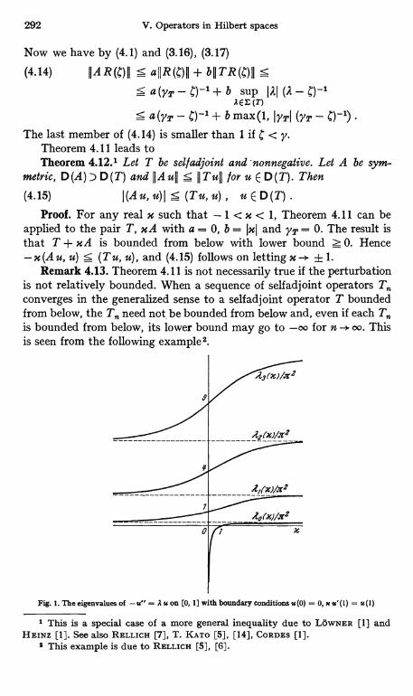
292 V. Operators in Hilbert spaces
Now we have by (4.1) and (3.16), (3.17)
(4.14) IIAR(C)II 5 aIIR(C)II + bIITR(C)II ss a (YT - C)-1 + b sup I2I (2 - )-I
xEE(T)
a(YT - C)-'+ b max(1, IYTI (VT - 0-1)The last member of (4.14) is smaller than 1 if C < y.
Theorem 4.11 leads toTheorem 4.12.1 Let T be sel/adjoint and nonnegative. Let A be sym-
metric, D(A) ) D(T) and IIAul! 5 IITull /or u E D(T). Then
(4.15) I(Au, u)I s (Tu, u) , u E D(T) .
Proof. For any real x such that - 1 < x < 1, Theorem 4.11 can beapplied to the pair T, xA with a = 0, b = IxI and YT = 0. The result isthat T + xA is bounded from below with lower bound Z 0. Hence- x (A u, u) 5 (T u, u), and (4.15) follows on letting x -* ± 1.
Remark 4.13. Theorem 4.11 is not necessarily true if the perturbationis not relatively bounded. When a sequence of selfadjoint operators T,,converges in the generalized sense to a selfadjoint operator T boundedfrom below, the T,, need not, be bounded from below and, even if each Tis bounded from below, its lower bound may go to -oo for n -+ oo. Thisis seen from the following example'.
20(x)/x2--------------r---- ---
x
Fig. 1. The eigenvalues of -u" - x u on (0, 1] with boundary conditions u(0) = 0, u u'(1) = u(1)
1 This is a special case of a more general inequality due to LSWNER [1] andHEINZ [1]. See also RELLICH [7], T. KATO [5], [14], CORDES [1].
2 This example is due to RELLICH [5], [6].

§ 4. Perturbation of selfadjoint operators 293
Example 4.14. Let H = L2 (0, 1) and let T (x) be the differential operator- d2/d x2 with the boundary condition u (0) = 0, x u' (1) - u (1) = 0. It is easilyseen that T (x) is selfadjoint for any real x [cf. § 3.6; note that the boundary condi-tion at x = 0 is of type III-(2.15) while that at x = 1 is of type III-(2.16)]. Theresolvent R (C, x) = R (C, T (x)) can be represented by an integral operator with thekernel (Green function)
sin CI12 y(4.16) [C-uasin llls(1-x)-xcosCi/a (1-x)]
for O< y5 x5 1 (and x, y exchanged for x5 y). This resolvent exists exceptfor those C for which the denominator vanishes; the exceptional values of l: areexactly the eigenvalues of T (x). As is easily seen, there is one and only one negativeeigenvalue AO (x) of T (x) for 0 < x < 1, and this AO (x), which is at the same timethe lower bound of T (x), tends to - oo for x " 0, whereas T (0) is nonnegative;see Fig. 1. Nevertheless, T (x) converges for x -+ 0 to T (0) in the generalized sense;this is seen from the fact that g (y, x; C, x) --> g (y, x; C, 0), x -+ 0, uniformly for afixed nonreal , which implies that R (C, x) R (C, 0) in norm. (The verificationof these results is left to the reader. Cf. also Example VII-1.11.)
5. Completeness of the eigenprojections of slightlynon-selfadjoint operators
In IV-§ 3.7 we mentioned the difficulties encountered when all theeigenvalues or the eigenprojections of a perturbed operator S = T + Aare considered simultaneously, and then gave an example of a perturbedoperator in a Banach space in which uniform estimates can be given toall perturbed eigenvalues and eigenprojections. Here we shall considerthe completeness of the eigenprojections of a non-selfadjoint operator Sin a Hilbert space as a perturbation problem for a selfadjoint operator T.Actually we shall go a little further and deduce a sufficient condition forS to be a spectral operator.
Theorem 4.15 a. Let T be a self adj oint operator with compact resolvent,with simple eigenvalues Al < AZ < . Let Ph, h = 1,2, ... , be theassociated eigenprojections (so that Ph Ph = bh k Ph, P)*, = Ph, dim Ph = 1).Assume further that Ah - Ah_1 -> oo as h -+ oo. Let A E -4 (H) (not neces-sarily symmetric). Then S = T + A is closed with compact resolvent, andthe eigenvalues and eigenprojections o l S can be indexed as {,a k, uh} and{Qok, Qh}, respectively, where k = 1, ... , m < oo and h = n + 1, n + 2, .. .
with n z 0, in such a way'that the following results hold. i) I AUh - Ahl isbounded as h -+ oo. ii) There is a W E .4 (H) with W-1 E .4 (H) such that
m (', Ph) W , Qh = W-' Ph W for h> n .L' Qo k = W`ksl ASn
294 V. Operators in Hilbert spaces
Remark 4.16 a. (a) ii) implies that S is a spectral operator'. In parti-cular, {Qok, Qh} is a complete family in the sense that
(4.29) Z Qok + ' Qh = 1,k=i h>n
where the series converges strongly and unconditionally (with an arbitraryorder of summation). This is easily seen by noting that the system
Qok, Qn+1, Qn+2, is similar to (' Ph, Pn+1, Pn+2, .. , thek llhSn
latter being complete because T is selfadjoint.(b) The assumption that T be bounded from below is not essential.
The proof given below can be modified in an obvious way to deal withthe case in which T has simple eigenvalues < A-1 < Ao < A,< . .
such that Ah - Ah-1-+ oo as h ± oo .(c) The theorem can be generalized to the case in which A is not
bounded but relatively bounded with respect to T or some fractionalpower of T, with a corresponding assumption on the growth rate ofAh - Ah-1 as h 00 2.
The proof of Theorem 4.15a is based on the following lemma3.
Lemma 4.17a. Let {Pj}j-o,l,... be a complete family of orthogonalprojections, and let {Q1}1= 0,1.... be a family o l (not necessarily orthogonal)projections such that QJQk = 61kQ1. Assume that
(4.30) dim P0 = dim Q0 = m< oo ,
00
(4.31) 'E II P1 (Q1 - P,)uJJ2S c hJuh12 for every u E H,j=1
where c is a constant smaller than 1. Then there is a WE 9(H) withW' E . (H) such that Q, = W-'P1W for j = 0,1,2.....
Proof. First we shall show that00
(4.32) W = E Pi Q, E -4 (H)j-0exists in the strong sense. Since ' P, = 1 by the completeness of {P,}[see (3.33)], it suffices to show that (P, - Pi Q,) = Li Pi (P, - Q,)converges strongly. But this is true since
k+p
E P,(P1-Q1)uj=k
2 k+p
=E IIP,(P,-Q1)uhh2- 0, k-+oo,j=k
1 For spectral operators, see DUNFORD [1], DUNFORD-SCHWARTZ (2).2 See CLARK [1], H. KRAMER [1], SCHWARTZ [1], TURNER [1, 2, 3].
See T. KATO [20].
§ 4. Perturbation of selfadjoint operators 295
by (4.31). Also (4.31) shows that IIBII S c1/2 < 1 if
(4.33) B= I Pf (P9 - Q1) = 1 - Po - I P J Qt-1 i=1
Now (4.32) implies that W Q5 = Pj Qs = P; W, j = 0, 1,2, .... Thusthe lemma is proved if we show that W-1 E -4 (H) exists.
To this end we define
00
(4.34) W1='E P5Q5=W-P000=1-Po-B.i=1
Since Po is an orthogonal projection with dim PO = m < oo, 1 - PO is aFredholm operator with nul (1- Po) = m, ind (1 - Po) = 0, and y (1 - Po)= 1 (y is the reduced minimum modulus, see IV-§ 5.1). Since 11 B11 < 1= y (1 - Po), it follows that W1 is also Fredholm, with
(4.35) nul Yi 1 < nul (1 - Po) = m , ind W1 = ind (1 - Po) = 0
(see IV-Theorem 5.22). Since W = PoQo + W1, where PoQo is compactby dim PO < oo, W is also Fredholm with ind W = ind W1 = 0 (see IV-Theorem 5.26). To show that W-1 E .4(H) exists, therefore, it suffices toshow that nut W = 0 .
To this end we first prove that
(4.36) N (W1) = Qo H .
Indeed, we have W,Q0 = 0 by (4.34) so that N (Wl) D Qo H. But sincedim Q0 = m z nul W1, we must have (4.36).
Suppose now that W u = 0. Then 0 = Po W u = PoQou and W1 u == W u - PoQou = 0. Hence u = Qou by (4.36) and so Pou = PoQou = 0.Thus (1 - B)u = Wlu + Pou = 0. Since IIBII < 1, we obtain u = 0. Thisshows that nut W = 0 and completes the proof.
Proof of Theorem 4.15 a. Let dh = max{Ah - Ah_1, Ah+1- Ah} be theisolation distance of the eigenvalue Ah; then dh -> oo as h -* oo. Hencethere is an integer N and S > 0 such that 11 All < S s dh/2 for h > N. Forthese h let Ph be the circle with center Ah and radius 6, and let Po be thecircle with a diameter [A1 - S, AN + S]. Then each Ph with h > N enclosesexactly one eigenvalue 'uh of S, Po encloses exactly N repeated eigen-values of S, and these eigenvalues exhaust the spectrum of S. This is seenby the same argument as was used in par. 3; note that all the circlesconsidered are outside one another and IIR(C, T)II < 1/6 < IIAII-1 if C is onone of the circles or outside all of them, so that R (C, S) exists for such C.
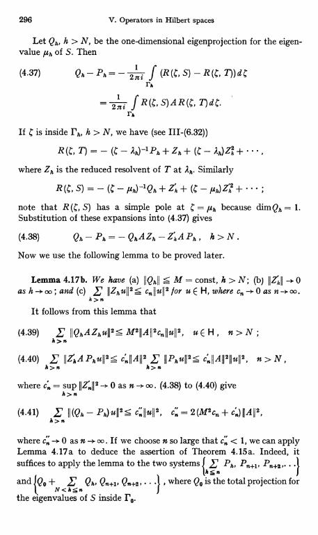
296 V. Operators in Hilbert spaces
Let Qh, h > N, be the one-dimensional eigenprojection for the eigen-value 4uh of S. Then
(4.37) Qh - Ph = - 2.ni f (R (C, S) - R(C, T))drh
2ni f R(C, S)AR(C, T)dC.rIf C is inside N, we have (see III-(6.32))
R(S,+)=- (S-Ah)-'Ph+Zh+(S-Ah)Zh+...
where Zh is the reduced resolvent of T at Ah- Similarly
R (C, S) = - (C - ,uh)-'Qh + ZZh + (pS - ,llh) Zh + ... ;
note that R (C, S) has a simple pole at C _ ,uh because dim Q. = 1.Substitution of these expansions into (4.37) gives
(4.38) Qh-Ph=-QhAZh-ZhAPh, h>N.Now we use the following lemma to be proved later.
Lemma 4.17b. We have (a) IIQaII M = const, h > N; (b) IIZ'hJJ -+ 0
as h oo ;and (c) ,' IIZhuII2 s cnIIuII2 for u E H, where cn 0 as n-+ oo.h>n
It follows from this lemma that
(4.39) E I I QhAZhuII2s MZIIA[I2cnjIuII2, u E H, n > Nh>n
(4.40) E IIZZAPhuII2< cnJIAII2 L IIPhuJI2s c'IIAIIZIIuJI2, n > N,h>n h>n
where c;, = sup IIZJ 2 -+ 0 as n -+ oo. (4.38) to (4.40) giveh>n
(4.41) E II(QA - cnllufl2, cn = 2(M2cn + cn) IIAII2,h>n
where cK -+ 0 as n -s oo. If we choose n so large that c < 1, we can applyLemma 4.17a to deduce the assertion of Theorem 4.15a. Indeed, itsuffices to apply the lemma to the two systems { E Ph, Pn+2 . .
k n
and Q0+ E Qh, Qn+i' Qn+2, . , where Q0 is the total projection forN<h5n
the eigenvalues of S inside P0.
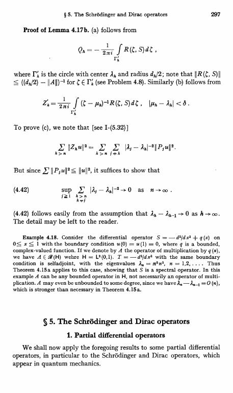
§ 5. The Schrodinger and Dirac operators 297
Proof of Lemma 4.17b. (a) follows from
Qh= -1
2Ici ,f R(C, S)dC ,
where rh is the circle with center Ah and radius dh/2; note that llR(C, S)lI((dh/2) - IIAli)-' for C E rh (see Problem 4.8). Similarly (b) follows from
142n% ,f `S - Ph)-1R (S, S)dS, JjUh - Ahl < 6.
r;
To prove (c), we note that [see I-(5.32)]
. r llZhull2 = f !' Ia5 - a ,hl-ZIIP9ull2.h>n h>nj$h
But since 2' ll Pj u lI 2 s Il u lI 2, it suffices to show that
(4.42) sup I IAj - A,I-2 -' 0 as n ->. aojZl h>nhj
(4.42) follows easily from the assumption that Ah - Ah_1-+ 0 as h -)- oo.The detail may be left to the reader.
Example 4.18. Consider the differential operator S = - d2ldx2 + q (x) on0 < x < 1 with the boundary condition u (0) = u (1) = 0, where q is a bounded,complex-valued function. If we denote by A the operator of multiplication by q (x),we have A E . (H) wehre H = L$(0,1). T = -d2ldx$ with the same boundarycondition is selfadjoint, with the eigenvalues A. = 'ant, n = 1,2..... ThusTheorem 4.15a applies to this case, showing that S is a spectral operator. In thisexample A can be any bounded operator in H, not necessarily an operator of multi-plication. A may even be unbounded to some degree, since we have A. - 0 (n),which is stronger than necessary in Theorem 4.15 a.
§ 5. The Schrodinger and Dirac operators
1. Partial differential operators
We shall now apply the foregoing results to some partial differentialoperators, in particular to the Schrodinger and Dirac operators, whichappear in quantum mechanics.
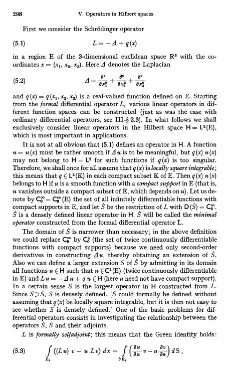
298 V. Operators in Hilbert spaces
First we consider the Schrodinger operator
(5.1) L = - d + q (x)
in a region E of the 3-dimensional euclidean space R3 with the co-ordinates x = (x1, x2, x3). Here d denotes the Laplacian
(5.2)_ a2 a2 a2
.72 +axa+ax2
and q (x) = q (x1, x2, x3) is a real-valued function defined on E. Startingfrom the formal differential operator L, various linear operators in dif-ferent function spaces can be constructed (just as was the case withordinary differential operators, see III-§ 2.3). In what follows we shallexclusively consider linear operators in the Hilbert space H = L2 (E),which is most important in applications.
It is not at all obvious that (5.1) defines an operator in H. A functionu = u (x) must be rather smooth if d u is to be meaningful, but q (x) u (x)may not belong to H = L2 for such functions if q (x) is too singular.Therefore, we shall once for all assume that q (x) is locally square integrable;this means that q E L2 (K) in each compact subset K of E. Then q (x) u (x)belongs to H if u is a smooth function with a compact support in E (that is,u vanishes outside a compact subset of E, which depends on u). Let us de-note by Co = Co (E) the set of all infinitely differentiable functions withcompact supports in E, and let S be the restriction of L with D (S) = Ca°°.S is a densely defined linear operator in H. S will be called the minimaloperator constructed from the formal differential operator L.
The domain of S is narrower than necessary; in the above definitionwe could replace Co by Co (the set of twice continuously differentiablefunctions with compact supports) because we need only second-orderderivatives in constructing d u, thereby obtaining an extension of S.Also we can define a larger extension S of S by admitting in its domainall functions u E H such that u E C2 (E) (twice continuously differentiablein E) and L u = - A u + q u E H (here u need not have compact support).In a certain sense S is the largest operator in H constructed from L.Since S D S, S is densely defined. [S could formally be defined withoutassuming that q (x) be locally square integrable, but it is then not easy tosee whether S is densely defined.] One of the basic problems for dif-ferential operators consists in investigating the relationship between theoperators S, S and their adjoints.
L is formally sel f adjoint ; this means that the Green identity holds :
(5.3) f ((Lu) v - uLv) dx f (an v - uan)dS,BE,
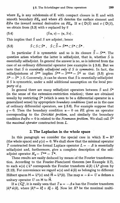
§ 5. The Schrodinger and Dirac operators 299
where Ea is any subdomain of E with compact closure in E and withsmooth boundary aEo and where dS denotes the surface element anda/an the inward normal derivative on aEo. If u E D (S) and v E D (S),we obtain from (5.3) with v replaced by v
(5.4) (S u, v) _ (u, S V) .
This implies that S and S are adjoint; hence
(5.5) S(Scs*, SCS=S**CS*CS*.In particular S is symmetric and so is its closure S = S**. The
question arises whether the latter is selfadjoint, that is, whether S isessentially selfadjoint. In general the answer is no, as is inferred from thecase of an ordinary differential operator (see examples in § 3.6). But wenote that S is essentially selfadjoint only if S is symmetric. In fact, theselfadjointness of S** implies S** = S*** = S* so that (5.5) givesS* = S* ) S. Conversely, it can be shown that S is essentially selfadjointif S is symmetric, under a mild additional assumption on the local pro-perty of q.
In general there are many selfadjoint operators between S and S*(in the sense of the extension-restriction relation) ; these are obtainedusually by restricting S* (which is seen to be a differential operator in ageneralized sense) by appropriate boundary conditions (just as in the caseof ordinary differential operators, see § 3.6). For example suppose thatq = 0. Then the boundary condition u = 0 on aE gives an operatorcorresponding to the Diyichlet Problem, and similarly the boundarycondition au/an = 0 is related to the Neumann Problem. We shall callthe maximal operator constructed from L.
2. The Laplacian in the whole spaceIn this paragraph we consider the special case in which E = R3
(the whole space) and q (x) = 0. We shall show that the minimal operatorT constructed from the formal Laplace operator L = - d is essentiallyselfadjoint and, furthermore, give a complete description of the self-adjoint operator Ha = T** = T*.
These results are easily deduced by means of the Fourier transforma-tion. According to the Fourier-Plancherel theorem (see Example 2.7),to each u (x) E L2 corresponds the Fourier transform u (k) E La given by(2.13). For convenience we regard u (x) and u (k) as belonging to differentHilbert spaces H = La (x) and H = LZ (k). The map u u = U u defines aunitary operator U on H to H.
If u E Co , it is easily seen that P u = - d u has the Fourier transformJkJa u (k), where JkJa = k1 + k2 + h . Now let K2 be the maximal multi-
300 V. Operators in Hilbert spaces
A
plication operator by IkI2 in the Hilbert space H (see Example 111-2.2).K2 is selfadjoint (see Problem 3.22). We denote by Ha the operator K2transformed by U-1:
(5.6) Ha = U-1 K2 U .
Ha is a selfadjoint operator in H, being a unitary image of the selfadjointA
operator K2 in H, with D (Ha) = U-1 D (K2). In other words, D (Ha) isthe set of all u E L2 (x) whose Fourier transforms belong to L2 (k) after multi-plication by 1k12. It follows from the remark given above that H0) T.That T is essentially selfadjoint is therefore equivalent to the assertionthat T has closure Ho, that is, D (T) = Co is a core of Ho (see III-§ 5.3).
Before giving the proof of this proposition, we note that there areother subsets of D (Ho) that can be easily seen to be cores of Ha. Forexample, the set S of all functions of the form
(5.7) e- IxI'/2 P (x) [P (x) are polynomials in x,, x2, x3]A
is a core of Ha. To see this, it suffices to show that the set S of the Fouriertransforms of the functions (5.7) forms a core of K2. Since K2 is non-
A
negative, this is true if K2 + 1 maps S onto a set dense in H (see Problem111-6.3). But the Fourier transforms of the functions (5.7) have a similarform with x replaced by k. Noting that (JkJ2 + 1) e-"k1'/4 = 1(k) isbounded, we see that (K2 + 1)
A
S is the image under F [the maximalA
multiplication operator by f (k)] of the set S' of all functions of the form
(5.8) e-jkj'/4 P(k) .
But the set of functions of the form (5.8) is dense in L2 (k) since it includesthe whole set of Hermite functions'. Since F is a bounded symmetricoperator with nullity zero and, consequently, R (F) is dense in H, (K2 +
A
+ 1) S is dense in H (see Problem 111-2.9).
We can now prove that T = Ho. Let T, be the restriction of Ho withthe set (5.7) as the domain. Since we have shown above that 7, = H0,it suffices to show that T ) T1 (which implies TD 71= Ha). To this endwe shall construct, for each u of the form (5.7), a sequence u,, E Co°° suchthat u, - u and Tu. = -A u,, -,J u = T, u. Such a sequence is
8 8
given, for example, by
1 For the completeness of the orthonormal family of Hermite functions, seeCOURANT and HILBERT (1), 95. The three-dimensional Hermite functions consideredhere are simply products of one-dimensional ones.
§ 5. The Schrodinger and Dirac operators 301
where w (x) is a real-valued function of Co such that 0 5 w (x) 5 1everywhere and w (x) = 1 for lxl 5 1. It is obvious that u E Co andu,, u. Also
(5.10) A u.(x) = w (n) A U (X) + n (grad w) (n) grad u (x) +
+ n2 (d w) (n) u (x)
shows that A u --. A u.S
Apart from a constant factor and a unit of length, Ha is the Hamilto-nian operator for a free particle in non-relativistic quantum mechanicsand K2 is its representation in momentum space.
Problem 5.1. Let T be the operator S of par. 1 in the special case LT is symmetric and essentially selfadjoint with T = H.. Also prove directly that(Tu, u) is real for each u E D (T).
Remark 5.2. The selfadjoint operator Ha is not a differential operatorin the proper sense, for a function u (x) of D (Ho) need not be differentiableeverywhere. But it (x) has derivatives in the generalized sense up to thesecond order, all belonging to L2. The generalized derivative au/ax,is the inverse Fourier transform of i kf i (k), as a natural generalizationfrom the case of a "smooth" u, and similarly the generalized 82 it/8x1 axtis the inverse Fourier transform of - k1 kt s (k). Since u E D (Ha) implies(1 + Ikl2) 12(k) E L2, all these generalized derivatives belong to L21.
In virtue of this generalized differentiability, functions of D (Ha) aremore "regular" than general functions of L2. In fact every u E D (Ha) is(equivalent to) a bounded, uniformly continuous function. To see this wenote that
(5.11) (f 14(k)I dk)2 5 f (Ikla+ a2)2f (1k12 + a2)2 Iei(k)12 dk
a 11 (Ha + a2) ull2 <
where a > 0 is arbitrary. But it is a well known (and easily verifiable)fact that a function u (x) whose Fourier transform it (k) is integrable isbounded and continuous, with
(5.12) l u (x) l 5 (2 n)-g/2 f 14 (k) I d k s c a-1/ell (HO + a2) ull
S c (a-1/2IIHO ull + as/2llull) ,
where c is a numerical constant. In particular the value u (x) of u at anyfixed point x is relatively bounded with respect to Ho with relative boundzero.
1 These generalized derivatives are special cases of derivatives in the theory ofgeneralized functions (or distributions). For generalized functions see e. g. YOSIDA (1) .
302 V. Operators in Hilbert spaces
A similar calculation gives
(5.13) Iu(x) - u(y)I < Cvlx - AV \a 2 _yJ 11,1o u11 + a 2+v
Hull/
where y is any positive number smaller than 1/2, C., is a numericalconstant depending only on y and a is any positive constant. In deducing(5.13) we note the following facts. I ei k x - ei k - y l = I ei k (x -Y) - 11 doesnot exceed 2 or IkJ Ix - yI, hence it does not exceed 21-YjkIyIx - yly.And f Ikly Ii(k)I dk is finite if 0 < y < 1/2, with an estimate similar to(5.11). (5.13) means that u (x) is Holder continuous with any exponentsmaller than 1/2.
(5.12) and (5.13) are special cases of the Sobolev inequalities'.Remark 5.3. The above results can be extended to the case of n
variables x1...., x. instead of 3, with the exception of (5.12) and (5.13)which depend essentially on the dimension 3 of the space.
3. The Schrodinger operator with a static potentialWe now consider the Schrodinger operator (5.1) in the whole space
E = R3. Here we assume that q (x) is not only locally square integrablebut can be expressed as
(5.14) q= qo + q, where qo E L°° (R3) , q, E L2 (R3)
As before we consider the minimal operator S and the "larger" operator Sconstructed from L = -,J + q. Let T be the minimal operator for q = 0investigated in the preceding paragraph. Then S can be written
(5.15) S=T+Q=T+Qo+Q1where Q, Q0 and Q, denote the maximal multiplication operators byq (x), qo(x) and q,(x) respectively; note that S and T have the same domainCo (R3). S cannot be put into a similar form, however, for there is nosimple relationship between the domains of S and T (the correspondingoperator for q = 0).
We shall now prove that S is essentially selfadjoint. To this end itsuffices to apply Theorem 4.4, regarding S as obtained from T by addingthe perturbing term Q and showing that Q is relatively bounded withrespect to T with relative bound 0. Denoting by H and Ho the selfadjointclosures of S and P respectively, we shall further show that
(5.16) H = Ho + Q , D (H) = D (Ho) C D (Q) .
Each u (x) E D (Ho) is a bounded function in virtue of (5.12). Therefore
Qi u belongs to L2, with I! Q, u!I S IIq,II2II uII. 5c jj g1II2 (a-1"2II Ho uII + a3/2IIuII)
1 See SosoLEV M.
§ 5. The Schrodinger and Dirac operators 303
Also Qo u E L2 and IIQo u11 s JIgoLJIu11. Hence
(5.17) D(Q) ) D(Ho) ) D(T) , IIQ uIl s allull + bIIHO uII
with b = c a-1/2IIg1II2 , a = c a312IIg1II2 + IIg0II.
Since a may be chosen as large as one pleases, (5.17) shows that Q isHo bounded (and T-bounded a fortiori) with relative bound 0. Thus wesee from Theorem 4.3 that Ho + Q is selfadjoint and from Theorem 4.4that . = 1' + Q is essentially selfadjoint. Since Ho + Q) S is obvious,Ho + Q coincides with the closure of .. Thus the Perturbed operator Hhas the same domain as the unperturbed operator Ho. Finally we note that His bounded from below by virtue of Theorem 4.11. Summing up, we haveproved
Theorem 5.41. 1/ (5.14) is satisfied, S is essentially sel f adjoint. Thesel f adjoint extension H o l S is equal to Ho + Q with D (H) = D (Ho) andis bounded from below.
Problem 5.5. The Coulomb potential q (x) = e jxj-1 satisfies (5.14). For whatvalues of # is (5.14) satisfied for q (x) = e lxl -S ?
Remark 5.6. The results obtained above can be extended to theSchrodinger operator for a system of s particles interacting with eachother by Coulomb forces. In this case the formal Schrodinger operatorhas the form (5.1) in which d is the 3s-dimensional Laplacian and thepotential q (x) has the form
S
(5.18) q (x) = fe1 + E e",i=I r5 7 <k rJA
where e1 and e1,% are constants and
r1 = (x31-2 + x31-1 + x31)1/2 ,
r1k= [(x31-2 - x31-2)2+ (x31-1 - x31-1)2+ (x31 - x31)211/2
It can be proved that the minimal operator T constructed from the formaloperator -d is essentially selfadjoint with the selfadjoint closure Ho(Remark 5.3) and that Q is relatively bounded with respect to Ho as wellas to T with relative bound 0. The proof given above for s = 1 is notdirectly applicable, for (5.12) is no longer true, but it can be modified
1 The proof given here is due to T. KATO [4]. This result is, however, not verystrong, although the proof is quite simple. Many stronger results have since beenobtained (see STUMMEL [I], WIENHOLTZ [1], BROWNELL [1], IKEBE and KATO [1],ROHDE [1], G. HELLWIG [I], B. HELLWIG [I], JORGENS [1]), but most of theseworks take into account special properties of differential operators. BABBITT [1] andNELSON [1] deduce interesting results in this direction using Wiener integrals infunction spaces.
304 V. Operators in Hilbert spaces
by taking into account the fact that q (x) consists of terms each of whichdepends essentially only on 3 variables'.
Regarding the spectrum of H, we have a more detailed result if weassume slightly more on q.
Theorem 5.7. In addition to (5.14) assume that qo (x) -> 0 for jxj -> 00.Then the essential spectrum of H is exactly the nonnegative real axis.(Thus the spectrum of H on the negative real axis consists only of isolatedeigenvalues with finite multiplicities.) 2
Proof. It is easy to see that the spectrum of Ho is exactly the non-negative real axis, which is at the same time the essential spectrum of Ho.In view of Theorem IV-5.35, therefore, it suffices to prove the followinglemma.
Lemma 5.8. Under the assumptions o l Theorem 5.7, Q is relativelycompact with respect to Ho.
Proof. First we consider the special case q0 = 0. Let be a boundedsequence in H such that {Hour} is also bounded; we have to show that{Q,,uj contains a convergent subsequence. According to (5.12) and (5.13),the u (x) are uniformly bounded in x and n and are equicontinuous.According to the Ascoli theorem, contains a subsequence {vn} thatconverges uniformly on any bounded region of R3. Let v be the limitfunction; v is bounded, continuous and belongs to H. Hence we have
Ql vn = ql v,,. -- ql v in H
by the dominated convergence theorem.
The general case q0 + 0 can be reduced to the above case by ap-proximating qo uniformly by a sequence {qo } of bounded functionswith compact support; for example set qo (x) = q0 (x) for I x nand = 0 for I x I > n. If Qo denotes the operator of multiplication by q0",we obtain IIQo - Q011 -> 0. But Q1 + Qo is Ho compact by what wasproved above, since q1 + qo" E L2 (RS). Hence (Q1 + Qa) (Ho + 1)-' is com-pact. Since 11 (Q0 - Q0) (Ho + 1) -111 s 11 Qo - Q011--> 0, it follows fromTheorem 111-4.7 that (Q1 + Q0) (Ho + 1)-' is compact. This implies thatQ = Q1 + Q0 is Ha compact.
Remark 5.9. In the theorems proved above we assumed that q (x)is real-valued, but this is not essential in a certain sense. Of course Sis not symmetric if q is not real-valued, and the essential selfadjointnessof S is out of the question. Nevertheless we can consider the spectrum
I For details see T. KATO [4].S For the spectrum of the SchrOdinger operators, see T. KATO [4], [4 a], POVZNER
[1], BIRMAN [5], BROWNELL [2], 2ISLIN [1], IKEBE [1].
§ 5. The Schrodinger and Dirac operators 305
of and, for example, Theorem 5.7 is true if H is replaced by Eventhe proof is not changed; it is only essential that Qe and Q, are relativelycompact with respect to He, which is true whether or not qo and ql arereal-valued.
4. The Dirac operator
It is of some interest to consider the Dirac operator in conjunctionwith the Schrodinger operator'. For a particle moving freely in space,this operator has the form (apart from a numerical factor and unit oflength) 2
(5.19) L = i-' a grad -f- fi .
L is again a formal differential operator, but it acts on a vector-valued(or, rather, spiny-valued) function u (x) = (u, (x), ..., u4 (x)), with 4components, of the space variable x = (x,, x2, x,). We denote by C4the 4-dimensional complex vector space in which the values of u (x) lie.a is a 3-component vector a = (al, a2, a,) with components aA which areoperators in C4 and may be identified with their representations by 4 x 4matrices. Similarly j9 is a 4 x 4 matrix. Thus L u = v = (v,...., v4) hascomponents
3 4 4
(5.20) v9 (x) = t-' E E (al)!A au,, +a E N9h ulh (x)1=1 h=1 ; h=1
The matrices aA and 9 are Hermitian symmetric and satisfy the com-mutation relations
(5.21) a1 al, + al, a5 = 2bfh 1 , j, h = 1, 2, 3, 4 ,
with the convention of writing 04 = f (1 is the unit 4 x 4 matrix). Itis known that such a system of matrices af, f exists; it is not necessaryfor our purpose to give their explicit form.
Since L is a formal differential operator, we can construct from Lvarious operators in the basic Hilbert space H = (L2 (R$))4 consistingof all C4-valued functions such that
4
(5.22) 11u112= f ju(x)I2dx <oo, Iu(x)I2= E IuJ(x)I2.f=1
The associated inner product is4
(5.23) (u, v) = f u (x) -v (x7 d x , u (x) v x = ' u, (x) v, x .
j=1
I For the selfadjointness of the Dirac operator, see T. KATO [4], PROSSER [1].See e. g. SCHIFF M.
306 V. Operators in Hilbert spaces
In particular we denote by T the minimal operator T u = L u withdomain D (T) = (CO)4 consisting of all u (x) with the components %(x)lying in Co (R').
T is essentially self adjoint. The proof is again easily carried out byusing the Fourier transformation. Let 4 (k) be the Fourier transformof u (x) ; this means that 2 (k) has 4 components 2, (k) which are theFourier transforms of the u; (x). The mapping u -* Il = Uu defines againa unitary operator on H to H = (L2 (k))4. It is now easily verified that foru E D (T), T u = L u = v has the Fourier transform(5.24) v(k)_ 19)iu(k)_ (k,al+k2a2+ksa,+ f)9(k).Let us now define an operator K in H as the maximal multiplicationoperator by k a + f ; here we use the term "multiplication operator"in a generalized sense, for k cc + f is not a scalar but a 4 x 4 matrix foreach fixed k. Since this matrix is of finite order, it can easily be shownthat K is selfadjoint (just as for ordinary multiplication operators).Let Ho be the transform of K by the unitary operator U-1:(5.25) Ho = U-1 K U .
Ho is a selfadjoint operator in H with D (Ho) = U-1 D (K), and D (K)is by definition the set of all is E (L2) 4 such that (k a + j9) 11(k) E (L2)4.Since the matrix k a + f is Hermitian symmetric and(5.26) (k a + f )2 = (k2 + 1) 1in virtue of (5.21), 2E E D (K) is equivalent to
(5.27) f (k2+ 1) Iil(k)I2dk= IIKii1I2<oo.It follows from the remark given above that P c: Ho. Thus P is essentially
selfadjoint if and only if T = Ho.To prove the essential selfadjointness of T, it is convenient to show
that K is a direct sum of 4 operators, two of which are isomorphic to themultiplication operator by (1 + k2)'/2 and two by - (1 + k2)1/2. To seethis we need only to introduce, for each k, a new orthonormal basis of C4consisting of eigenvectors of the Hermitian matrix k a + P. In view of(5.26), the only eigenvalues of this matrix are ± (k2 + 1)1/2, and it isknown that there are indeed two eigenvectors for each sign forming anorthonormal set of 4 eigenvectors. With the introduction of such abasis (which is by no means unique owing to the degeneracy of theeigenvalues) for each k, the Hilbert space H is seen to be decomposedinto the direct sum of 4 subspaces in each of which K acts simply as amultiplication by (k2 + 1)1/2 or - (k2 + 1)1/2. The proof of the essentialselfadjointness of T can be effected, then, as in the case of the Schrodingeroperator for a free particle. Details may be left to the reader'.
1 Cf. PROSSER [1].
§ 5. The Schrodinger and Dirac operators 307
The Dirac operator for a particle in a static field with potential q (x)is given by(5.28) L= i-1 a- grad + f+ Qwhere Q is the multiplication operator by q (x) 1. If q (x) is real andlocally square integrable, the minimal operator S with domain (Co )4constructed from (5.28) is densely defined and symmetric (cf. par. 1).To ensure that S is essentially selfadjoint, however, we need a furtherassumption. Without aiming at generality, we shall content ourselves byshowing that the Coulomb potential(5.29) q (x) = ell xl , I xI = (Al + x2 + x32)111,
is sufficient for the essential selfadjointness of . provided lel is not toolarge. To see this it suffices to verify that Q is relatively bounded withrespect to He with relative bound smaller than 1 (see a similar argumentin the preceding paragraph). But it is well known that [see VI-(4.24)]
(5.30) f lxI-2lu(x)I2dx 5 4 f Igradu(x)12dx= 4 f k2Nl(k)12dk
at least for a scalar-valued function u E Co ; the same inequality for avector-valued function u E (Co°°)4 follows by simply adding the resultsfor the components u5 (x). In virtue of (5.29) and (5.27), this gives
(5.31) IlQuII 5 21el lIK4II = 2Iel IIHouIlfor u E D (T), and it can be extended to all u E D (Ho) since Ho is theclosure of T as proved above. Thus Q is Ho bounded with relative bound
2l el. In this way we have proved (note Theorems 4.4 and 4.6)Theorem 5.10. If q (x) = e/lxl with a real e such that lel S 1/2, then
the minimal Dirac operator . is essentially selfadjoint. If lel < 1/2 theclosure of S has the same domain as Ho.
Problem 5.11. A similar result is also valid if
(5.32) q (x) = E eall x - ail + qo (x)i
where ai, j = 1, 2, . . ., are points of Re, qo (x) is a bounded function and Z l eil 5 1/2.
Remark 5.12. Theorem 5.10 is unsatisfactory inasmuch as thecondition lel S 1/2 is too strong to cover all interesting cases of thehydrogen-like atoms. Returning to the ordinary system of units, Iel S 1/2corresponds to the condition IZI S 137/2 = 68.5, where Z is the atomicnumber and 1/137 is the fine structure constant. In this connection it isof some interest to note that the condition Iel s 1/2 can be slightlyimproved if we use Theorem VI-3.11 (to be proved in Chapter VI). Infact, it is easily seen that IHoI = (H20)1/2 is just the multiplication operatorby (k2 + 1)1/2 in H. But we have
(5.33) f IxI-llu(x)I2 dx S 2 f IkI Ila (k) 12 dk S 2 (IHoI u, u) ;
308 VI. Sesquilinear forms in Hilbert spaces and associated operators
this can be proved by using the transform by U of the operator JxJ-1which is an integral operator with kernel 1/2,r21k - k'J 2. It follows fromthe cited theorem that i f
(5.34) Jel < 2/n = 1/1.57,
S has a selfadjoint extension with domain contained in D(JH01'/2). Thecondition (5.34) corresponds to JZJ S 137/1.57 = 87.
It should be further remarked that, although Theorem VI-3.11 doesnot assert the uniqueness of the selfadjoint extension of S for each fixed e,the extension considered is "analytic" in e and it is a unique extensionwith the analytic property. This remarkable result follows from TheoremVII-5.1 to be proved in Chapter VII.
Chapter Six
Sesquilinear forms in Hilbert spacesand associated operators
In a finite-dimensional unitary space, the notion of a sesquilinear form and thatof a linear operator are equivalent, symmetric forms corresponding to symmetricoperators. This is true even in an infinite-dimensional Hilbert space as long asone is concerned with bounded forms and bounded operators. When we have toconsider unbounded forms and operators, however, there is no such obvious rela-tionship. Nevertheless there exists a closed theory on a relationship between semi-bounded symmetric forms and semibounded selfadjoint operators'. This theory canbe extended to non-symmetric forms and operators within certain restrictions.Since the results are essential in applications to perturbation theory, a detailedexposition of them will be given in this chapter 2. Some of the immediate applicationsare included here, and further results will be found in Chapters VII and VIII.
The final section of this chapter deals with the spectral theorem and perturbationof spectral families. The subjects are not related to sesquilinear forms in anyessential manner, though the proof of the spectral theorem given there dependson some results in the theory of forms. In view of the fact that the spectral theoremis of a rather special character, we have avoided its use whenever possible. But sincethere are problems in perturbation theory which require it in their very formulation,the theorem cannot be dispensed with altogether; and the end of our preliminarytreatment of Hilbert space seems an appropriate place to discuss it.
§ 1. Sesquilinear and quadratic forms1. Definitions
In V-§ 2.1 we considered bounded sesquilinear forms defined on theproduct space H x H'. We shall now be concerned with unbounded formst [u, v] but restrict ourselves to forms defined for u, v both belonging to a
' This theory is due to FRIEDRICHS [1]. See also T. KATO [8].2 For other approaches to this problem see ARONSZAJN [4], LIONS 11).
§ 1. Sesquilinear and quadratic forms 309
linear manifold D of a Hilbert space H. Thus t [u, v] is complex-valuedand linear in u E D for each fixed v E D and semilinear in v E D for eachfixed u E D. D will be called the domain of t and is denoted by D (t).t is densely defined if D (t) is dense in H.
t [u] = t [u, u] will be called the quadratic form associated witht [u, v]. t [u] determines t [u, v] uniquely according to I-(6.11), namely
(1.1) t[u,v]= 4 (t[u+v]-t[u-v]+it[u+iv]-it[u-iv]).We repeat the remark that (1.1) is true only in a complex Hilbert space(Remark 1-6.10). We shall call t [u, v] or t [u] simply a form when thereis no possibility of confusion.
Two forms t and t' are equal, t = t', if and only if they have the samedomain D and t [u, v] = t' [u, v] for all pairs u, v in D. Extensions andrestrictions of forms (t' t or t c: t' in symbol) are defined in an obviousway as in the case of operators.
The situation that the domain of a form need not be the whole spacemakes the operations with forms rather complicated, just as for operators.The sum t = t1 + t2 of two forms t1, t2 will be defined by
(1.2) t [u, v] = t1 [u, v] + t2 [u, v] , D (t) = D (t1) n D (t2) .
The product a t of a form t by a scalar a is given by
(1.3) (a t) [u, v] = a t [u, v] , D (a t) = D (t) .
The unit form 1 [u, v] is by definition equal to the inner product (u, v)and the zero form 0 [u, v] takes the value zero for all u, v, both formshaving the domain H. Thus we have 0 t c 0 for any form t, and t + at= t + at 1 is defined for any form t by
(1.4) (t + a) [u, v] = t [u, v] + a (u, v) , D(t+a)= D(t).A form t is said to be symmetric if
(1.5) t [u, v] _ [v, u] , u, v E D (t) .
As is seen from (1.1), t is symmetric if and only if t [u] is real-valued.With each form t is associated another form t* defined by
(1.6) t* [u, v] = [v, u7, D (t*) = D (t) .
t* is called the adjoint form of t. t is symmetric if and only if t* = t.We have the identity//
(1.7) (a1 t1 + a2 t2) * = al tl + a2 t2
For any form t, the two forms 0, f defined by
(1.8) h = 2 (t + t*) f = 2d (t - t*) ,
310 VI. Sesquilinear forms in Hilbert spaces and associated operators
are symmetric and
(1.9) t=h+ie.h and t will be called the real and imaginary parts of t, respectively, andbe denoted by Re t, t = Im t. This notation is justified by
(1.10) 1 [u] = Re t [u] , t [u] = Im t [u] ,
although h [u, v] and E [u, v] are not real-valued and have nothing to dowith Re (t [u, v]) and Im (t [u, v]).
2. SemiboundednessA symmetric form h is said to be bounded from below if the set of
(real) values h [u] for (lull = 1 is bounded from below or, equivalently,
(1.11) h[u] z yllull2, uED(h)This will be written simply
(1.12) hzy.The largest number y with this property is called the lower bound ofand will be denoted by Y4. If h z 0, t is said to be nonnegative. Similarlywe define the notions of boundedness from above, upper bound, non-positiveness, etc. Since we are mostly concerned with forms boundedfrom below, the symbol y4 will be used exclusively for the lower bound.
If 4 is a nonnegative symmetric form, we have the inequalitiesI-(6.32). If a symmetric form h is bounded from below as well as fromabove, then h is bounded with bound equal to the larger one of theabsolute values of the upper and lower bounds. In other words, 10 [u] 155 MIIu112 for all u E D(h) implies 10 [u, v]I 5 Mllull Ilv11 for all u, v E D(ID).The proof is the same as in the finite-dimensional case [see I-(6.33)].It should be remarked that, more generally, I E [u] 1 5 MO [u] for allu E D = D (0) = D (E) implies I E [u, v] I S MO [u]1/2 h [v]1/2 for all u, v E D,
provided both h and E are symmetric and h is nonnegative.Let us now consider a nonsymmetric form t. The set of values of t [u]
for u E D (t) with hull = 1 is called the numerical range of t and will bedenoted by 0 (t). As in the case of operators, 0 (t) is a convex set in thecomplex plane (cf. Theorem V-3.1). A symmetric form h is boundedfrom below if and only if 0 (y) is a finite or semi-infinite interval of thereal axis bounded from the left. Generalizing this, we shall say that aform t is bounded from the left if 0(t) is a subset of a half-plane of theform Re I z y. In particular, t will be said to be sectorially boundedfrom the left (or simply sectorial) if 0 (t) is a subset of a sector of the form
(1.13) I arg ( I - y) 1 5 0 , 0 5 0 < 2 , y real.
§ 1. Sesquilinear and quadratic forms 311
This means that
(1.14) 0Z y and If [u] I S (tan 0) (0-y) [u], u E D (t) ,
where h = Re t, f = Im t. The numbers y and 0 are not uniquely deter-mined by t; we shall call y a vertex and 0 a corresponding semi-angle ofthe form t. It follows from a (remark given above that
(+/ - Y) [u, v] 15 (h - Y) [u]l/2 (h - Y) [v]1/2 ,(1.15) It [u, v] 15 (tan 0) (h - y) [u]1/2 (h - Y) [V]1/2'
I (t - Y) [u, v] I s (1 + tan 0) (h - Y) [u]112 (h - y) [v]'I2
In the following sections we shall be concerned mostly with sectorialforms.
Problem 1.1. It follows further from (1.15) that
(h - y) [u] 5 I (t - y) [u] 15 (sec 0) (, - y) [u](1.16) I(t - V) [u + v]1112 S (sec 0)1/2 {I (t - Y) [u]11/2 + I(t - Y) [v]11/2} ,
I(t - y) [u + vii 5 2(secO) {I(t - y) Lull + I(t - y) [v]l}.Example 1.2. Let T be an operator in H and set
(1.17) t[u, v] = (Tu, v) , D(t) = D(T) .T and t have the same numerical range. In particular, t is symmetric if T is sym-metric, and t is bounded from below if T is bounded from below; t is bounded fromthe left if T is quasi-accretive; t is sectorial if T is sectorial (see V-§ 3.10).
Example 1.3. Let S be an operator from H to another Hilbert space H' (whichmay be identical with H) and set
(1.18) 0 [u, v] = (Su, Sv) , D D (S) ,
where the inner product is, of course, that of H'. is a nonnegative symmetric form.Example 1.4. Let H= 12 and
M
(1.19) t [u, v] = E ai r 11 for u = (gf) and v = (qi) ,9=1
where {ai} is a sequence of complex numbers. D (t) is by definition the set of allu = (fir) E H such that Flail oo. Let t be the restriction of t with D(t)consisting of all u E H with a finite number of nonvanishing components. t is denselydefined and so is t a fortiori. t is symmetric if and only if all the a, are real. t issectorial with a vertex y and a semi-angle 0 if and only if all the a, lie in the sector(1.13).
A further restriction tl oft is obtained by requiring each u E D (tl) to satisfy thecondition [in addition to u E D(t)]
(1.20) E lei = 0'i=1
where {#,} is a given sequence of complex numbers not all equal to zero. tl is denselydefined if and only if E I &Q 2 = oo. To see this, let w = (c,) E H be orthogonal toD (tl). Since the vector 1Yk, 0, ..., - N1, 0, ...) with - fl, in the k-th componentbelongs to D (t1), we have fl k C1 - #1 Ck = 0. Since this is true for all h, we have

312 VI. Sesquilinear forms in Hilbert spaces and associated operators
C1: C2: ... = fl1 : fl2 : . . . . If E I flil2 = oo, we must have all C, = 0 so that w = 0.This shows that D (f1) is dense in H. If E Ifl,I2 < oo, (ai) = b belongs to H and (1.20)implies that D (f1) is orthogonal to b. Hence D (t1) is not dense in H.
Example 1.5. Let H = L2 (E) and
(1.21) t [u, v] = f f (x) u (x) vv (x) d x ,E
where f (x) is a complex-valued measurable function on E. D (t) is by definition theset of all u E H such that f It (x) I j u (x) 12 d x < oo. t is densely defined (as in the caseof a maximal multiplication operator, see Example 111-2.2). t is symmetric if f (x)is real-valued. t is sectorial with a vertex y and a semi-angle 0 if the values of f (x)lie in the sector (1.13).
Suppose that E is a bounded open set. Then the restriction i of t with domainD (t) = Cp (E) is also densely defined. Let t1 be a restriction of i with D (t1) consistingof all u E D(t) such that
(1.22) f g (x) u (x) d x= 0E
where g (x) is a locally integrable function. Then t1 is densely defined if g j L2 (E)and not densely defined if 0 + g E L2 (E). The proof is similar to that in the precedingexample.
Example 1.6. Let H = L2(0, 1) and
(1.23) 0 [u,v]=u(0)v.D (O) is by definition the set of all u (x) continuous (more exactly, equivalent to acontinuous function) on the closed interval [0, 1] ; then u (0) is well defined foru E D (h). 4 is densely defined, symmetric and nonnegative. Actually [j is a specialcase of (1.18) in which Su = u (0), S being an operator from H into a one-dimensionalspace C.
Example 1.7. Let H = L2 (a, b) where (a, b) is a finite interval and setb
(1.24) t [u, v] = f {p (x) u' (x) + q (x) u (x) v z +a
+ r (x) u' (x) -v -(7x + s (x) u (x) v' (x) d x +
+ h, u (a) -v (7a + hb u (b) _v T .
where P (x), q (x), r (x), s (x) are given complex-valued functions and h hb areconstants. Suppose that p, q, r, s are continuous on the closed interval [a, b] (regularcase), and let D (t) be the set of all u E H such that u (x) is absolutely continuous on[a, b] with u' (x) E H [so that the right member of (1.24) is meaningful for u, v E D (t)].t is densely defined. t is symmetric if p, q are real-valued, r-(x-) = s (x) and h hbare real. If we restrict D (t) to the set of all u (x) with u (a) = u (b) = 0, we obtain arestriction to of t. to is densely defined. We define a further restriction i of to byD (i) = Co (a, b)
t is sectorial if p (x) > 0 on [a, b]. To see this we note that there are positiveconstants S and M such that P (x) Z S, I q (x) I s M, I r (x) I S M, Is (x) I S M. Thus
Re t [u] z f {o J U112 - M (Iu12 + 2 Iu u'I )} dx - Ih.1 Iu (a) 12 - I hbl Iu (b) I2 .
Since 2Iu u'I S s Iu'I2 + e-1IuI2, we obtain, making use of IV-(1.19) with p = 2,the inequality
(1.25) 4 [u] = Re t [u] z 61lu'II2 - MIIuII2
§ 1. Sesquilinear and quadratic forms 313
in which the positive constants 6 and M need not be the same as above. Similarlywe have, noting that p (x) is real,
(1.26) IE[u]I = !Imt[u]I S eIIu1II2 + MBIIUII2.
where e > 0 may be chosen arbitrarily small. Thus it is easy to see that we have aninequality of the form (1.14) with appropriate constants y and 0; 0 can even bechosen arbitrarily small if - y is taken sufficiently large.
Problem 1.8. The t of the above example is sectorial even if p (x) is not real-valued, provided Rep (x) > 0 [the continuity of p (x) being assumed as above].
Example 1.9. Let H = L$ (Re) and
(1.27) t [u, v] = f [grad u (x) grad v (x) + q (x) u (x) v (x) ] d x ,
where q (x) is a given function assumed to be locally integrable. As D (t) we may takeC'(R3) (the set of continuously differentiable functions with compact supports).t is densely defined, and symmetric if q (x) is real-valued. We may restrict D (t) byrequiring more differentiability of u (x), v (x) (for example, D (t) = Co (R3)) withoutlosing these properties of t; or we could extend D(t) somewhat so as to includefunctions with non-compact supports.
3. Closed forms
Let t be a sectorial form. A sequence {un} of vectors will be said to bet-convergent (to u E H), in symbol
(1.28) un! u, n-+oo,
if un E D (t), un -+ u and t [un - u n] -+ 0 for n, m - no. Note that u mayor may not belong to D (t). Compare also the notion of T-convergencewhere T is an operator (see III-§ 5.2).
It follows immediately from the definition that t-convergence is equi-valent to t + at-convergence for any scalar at. Also, t-convergence is equivalentto t-convergence where 4 = Re t; this follows from (1.16) by which(h - y) [un - um] - 0 if and only if (t - y) [un - u n] -* 0. Again,un i u and v,, i v imply at u,, + l9 v,, ! at u + 9 v. For the proof it suf-fices to note that t may be assumed to be symmetric and nonnegative bythe above remark; then the result follows from I-(6.32).
A sectorial form t is said to be closed if un t u implies that u E D (t)
and t [un - u] 0. It follows from the above remark that t is closed ifand only if Re t is closed. t is closed if and only if t + at is closed.
Problem 1.10. A bounded form is closed if and only if its domain is a closedlinear manifold.
Let h be a symmetric nonnegative form and set
(1.29) (u, v)4 = (0 + 1) [u, v] = 0 [u, v] + (u, v) , u, v E D (h) .

314 VI. Sesquilinear forms in Hilbert spaces and associated operators
(u, v)4 may be regarded as an inner product in D (h), since it is symmetricand strictly positive:
(1.30) IIuII2'O ° (u, u)q = (h + 1) [u] = h [u] + 11 UP IIul12
D (0) will be denoted by H, when it is regarded as a pre-Hilbert spacewith the inner product ( , ) 0.
When a sectorial form t is given, we define a pre-Hilbert space Htas equal to HO, with h' = Re t - y z 0 where y is a vertex of t. Ht willbe called a pre-Hilbert space associated with t. Ht is identical with D (t)as a vector space, but the inner product (, )t = (, )g, of Ht depends onthe choice of y so that Ht is not uniquely determined by t. In any case,the following are immediate consequences of (1.30). A sequence u E D (t)is t-convergent i f and only i f it is a Cauchy sequence in Ht. When u E D (t),un i u is equivalent to II U. - ullt - 0.
From (1.15) and (1.30) we have
(1.31) It [u, v]I s Iv! I(u, v)I + (1 + tang) 0'[u]'/' 0'[v]1/25lyl lull IIvII + (1 + tan8) IIuJIt IIvIIt 5 (I 'j + 1 .f tang) IIuIIt IIvIIt
This shows that t [u, v] is a bounded sesquilinear form on Ht.Theorem 1.11. A sectorial form t in H is closed i f and only i f the pre-
Hilbert space Ht is complete.Proof. Since t is closed if and only if h' = Re t - y is closed, we may
assume that t = h is symmetric and nonnegative and the inner productof Ht = HO is given by (1.29). Suppose that h is closed, and let {un} be aCauchy sequence in Hi,: Ilun - urjI4 0. Then is also Cauchy in Hby (1.30), so that there is a u E H such that un u. Since [u, - um] - 0by (1.30), {un} is ,-convergent and the closedness of implies thatu E D (h) = H4 and h [u - u] 0. Hence Il un - ull -- 0 by (1.30),which shows that HO is complete.
Suppose, conversely, that H4 is complete. Let u 4 u. This implies
that 1, [un - u n] -* 0 and llu,, - umll -' 0 so that llu,, - umljD -* 0 by (1.30).By the completeness of HO there is a uo E H4 = D (y) such that II un -- uoII4 0. It follows from (1.30) that h [u,, - uo] - 0 and Il un - uoll -* 0.Hence we must have u = uo E D (h) and h [u,, - u] 0. This proves thatis closed.
Theorem 1.12. Let t be a sectorial form. If u,i u and vi v,
then limt [un, exists. I/ t is closed, this limit is equal to t [u, v].Proof. We have it [un, vn] - t [um, vm] 15 It [un - um, vu] I + It [um,
vn - vm]I S (1 + tan 0) {h [un - um]1/2 4 [V.]112 + h [u,,]112 h [vn - vm]1/2}where we have assumed y = 0 [see (1.15)]. Since u t u implies thath [un - um] -- 0 and 0 [un] is bounded and similarly for vn, lim t [un, vn]
§ 1. Sesquilinear and quadratic forms 315
exists. The second part of the theorem can be proved in the same wayby considering t [un, t [u, v].
Example 1.13. Consider the symmetric nonnegative form 4 [u, v] _ (Su, Sv)of Example 1.3. 0 is closed if and only if S is a closed operator. To see this, it sufficesto note that u 4 u is equivalent to u S u and 4 [u - u] - 0 is equivalentto Su -- Su (see III-§ 5.2).
Example 1.14. Consider the form t [u, v] = E as 1 q, defined in Example 1.4and assume that all the of lie in the sector (1.13) so that t is sectorial. Thent is closed. In fact we have ]lull' = E(1 + Rea, - y) l$sl' for u = ($,). ButHt = D (t) is the set of all u E H such that E la,] l$,l' < oo, and it is easily seen that,under the assumptions made, this condition is equivalent to llullt < oo. Thus Htcomprises all u = with llullt < oo and therefore it is complete (just as is is).
Example 1.15. Consider the form t [u, v] = f I (x) u (x) vv (x) dx defined inExample I.S. If the values of f (x) are assumed to lie in the sector (1.13) so that t issectorial, t is closed; the proof is similar to that in the preceding example.
Before closing this paragraph, we state a theorem which is importantin deciding whether a given u E H belongs to the domain of a closedform t. We know from the definition of closedness that u E D (t) if thereis a sequence u E D (t) such that un --->. u and t [u,, - u,n] -> 0. Actually,however, a weaker condition is sufficient, namely,
Theorem 1.16. Let t be a closed sectorial form. Let un E D (t), u,, -> uand let It [u ]} be bounded. Then u E D (t) and Re t [u] S lim inf Re t
The proof will be given later, after the representation theorem hasbeen proved (see § 2.2).
4. Closable formsA sectorial form is said to be closable if it has a closed extension.Theorem 1.17. A sectorial form t is closable if and only if u t 0
implies t [un] - 0. When this condition is satisfied, t has the closure (thesmallest closed extension) i defined in the following way. D(f) is the set ofall u E H such that there exists a sequence {un} with u t u, and
(1.32) [u, v] = lim t [un, vn] for any un t u, vt v .
Any closed extension of t is also an extension of f.Proof. Let tl be a closed extension of t. un! 0 implies un ! 0 so
that t [un] = tl [un] = tl [u,, - 0] - 0 by the, closedness of t1. This provesthe necessity part.
To prove the sufficiency part, let D (f) be defined as in the theorem.Then the limit on the right of (1.32) exists by Theorem 1.12. We shallshow that this limit depends only on u, v and not on the particularsequences {vn}. Let {un}, be other sequences such that u,, t u,v i v. Then u - ui 0, v - vn -t. 0 (see par. 3) so that t [un - un]
316 VI. Sesquilinear forms in Hilbert spaces and associated operators
0, t [v - vn] -- 0 by the assumption. Hence t [u,,, t [un, vn]= t [u - un, v;,] + t [un, vn - vn] 0 as in the proof of Theorem 1.12.
We note that
(1.33) [un - u] - 0 if un t u .
In fact, lim f [un - u] = lim lim t [un - u n] by (1.32) and this isn-s oo n-s oo m-r oo
zero by u,, t U.
We have defined a form i with domain D (t). Obviously f is sectorialand f t. Let us show that f is closed. Consider the pre-Hilbert space Hiassociated with f; it suffices to show that Ht is complete (see Theorem1.11).
Since t, Ht is a linear manifold of H. The construction of t givenabove shows that Ht is dense in Ht and that any Cauchy sequence in Hthas a limit in Ht [see (1.33)]. As is well known, this implies that Hi iscomplete'.
That f is the smallest closed extension of t follows also from theconstruction, for if t1 D t is closed and un t u, then un t u and sou E D (t1). Hence D (f) D (t1) and f [u, v] = t1 [u, v] by (1.32) and Theorem1.12.
Theorem 1.18. Let t, f be as above. The numerical range 0 (t) of t is adense subset of the numerical range 0 (Y) of L.
Proof. For any u E D (t) with (lull = 1, there is a sequence un E D (t)such that u,, t u. We may assume that II unll = 1; otherwise we needonly to replace u,, by un/ll unll. Since t [u,,] -+ [u], the result followsimmediately.
Corollary 1.19. A vertex y and a semi-angle 0 for i can be chosen equalto the corresponding quantities for t. If h is a closable symmetric formbounded from below, h and have the same lower bound.
Theorem 1.20. A closable sectorial form t with domain H is bounded.Proof. t is necessarily closed, for t and i have the same domain H
and hence t = L. We may again assume that t has a vertex zero. Thecomplete Hilbert space Ht associated with t coincides with H as a vectorspace, with the norm Ilulit z (lull. According to the closed graph theorem,these two norms are equivalent, that is, there is a constant M such thatII ull t 5 M II uli (For the proof consider the operator T on Ht to H definedby T u = u ; T is bounded with II T II 5 1 and maps Ht onto H one to one,hence T-1 is bounded by Problem 111-5.21.) Hence 0 s 0 [u] s M2IIu1I2and It [u, v]l s (1 + tang) M2IIuJI IIvII by (1.45).
1 Let be a Cauchy sequence in H. Since Ht is dense in Ht, there is a sequencevn E Ht such that lIvn - unjj S 1/n. Then is Cauchy, so that v -# v for somev E H. Then u,, -+ v, and Ht is complete.
§ 1. Sesquilinear and quadratic forms 317
When t is a closed sectorial form, a linear submanifold D' of D (t) iscalled a core of t if the restriction t' of t with domain D' has the closuret : t' = t. (Cf. the corresponding notion for an operator, III-§ 5.3.)Obviously D' is a core oft if and only if it is a core oft + a for any scalara. If t is bounded, D' is a core of t if and only if D' is dense in D (t) [notethat D (t) is then a closed linear manifold].
The next two theorems follow directly from the proof of Theorem 1.17.Theorem 1.21. Let t be a closed sectorial form. A linear submani f old D'
of D (t) is a core of t if and only if D' is dense in the Hilbert space H t as-sociated with t.
Theorem 1.22. Let t', t" be two sectorial forms such that t' Ct". Let Ht,and Ht., be the associated pre-Hilbert spaces'. I/ t" is closed, t' is closed ifand only if Ht, is a closed subspace of Ht... When t" is closable, if andonly if Ht, is dense in Ht...
Example 1.23. Consider the form 4 [u, v] = (Su, Sv) of Examples 1.3 and 1.13.is closable if and only if S is closable. In fact, u 0 and 0 0 are equivalent
to u S 0 and Su - 0, respectively. When S is closable, we have
(1.34) [u, v] = (Su, Sv) with D(()) = D(S)
We know also that is closed if and only if S is closed; in this case a subset D' ofD (q) = D (S) is a core of 4 if and only if it is a core of S.
Example 1.24. Consider the form t [u, v] = E of $s i of Examples 1.4 and 1.14.Assume that all the as lie in the sector (1.13) so that t is sectorial and closed. t isclosable with t = t; this follows from the fact that D (t) is dense in Ht, which canbe easily verified. Next let us consider the closure of t1. The additional condition(1.20) can be written in the form E (1 + Re a1 - y) 3 ! = 0 where #,(I ++ Real - y)-1. Noting the expression llullt = E(1 + Reas - y) given inExample 1.14, we see that D%) is dense in Ht if and only if E (I + Re a1 - y) 1 fl§12= oo (see a similar argument in Example 1.4). As is easily seen, this condition isequivalent to
(1.35) E(laal + 1)-1 IPJ12 = oo .
Thus we have t1 = t if and only if (1.35) is satisfied. If the left member of (1.35) isconvergent, on the other hand, D (t1) is a dense subset of the orthogonal complementM in Ht of the one-dimensional subspace spanned by the vector (flf), which belongs
to Ht, and D (t1) is identical with M. Thus u E D (t1) is characterized by E (la,I ++ 1) oo and .Z' $1 = 0 [note that Z j! r is absolutely convergent foru E D (t), as is seen by applying the Schwarz inequality].
Example 1.25. Considei the form t [u, v] = j' f (x) u (x) vv (z) dx of Examples 1.5and 1.15 and assume that the values of f (x) lie in the sector (1.13) so that t is sectorialand closed. By an argument similar to that of the preceding example, it can beshown that t = t, and that t1 = t if and only if
(1.36) f (It(x)I + 1)-I g(x) 12 dx = ooE
I Here we assume that a common vertex y is chosen for t', t" and the norms inHt', Ht,, are respectively given by (Re t' - y) [u] + 11u112, (Re t" - y) [u] + (13112.
318 VI. Sesquilinear forms in Hilbert spaces and associated operators
Example 1.26. An example of a densely defined, sectorial (even symmetricand nonnegative) form which is not closable is given by the form 4 [u, v] = u (0) v (0)of Example 1.6. To see this, it suffices to note that u 0 implies that 0
and limun(0) = at exists (where is a sequence of continuous functions); but thisdoes not imply or = 0.
5. Forms constructed from sectorial operatorsLet us recall that an operator T in H is said to be sectorial if its
numerical range is a subset of a sector of the form (1.13) (see V-§ 3.10).Let T be sectorial and set (see Example 1.2)(1.37) t [u, v] = (T u, v) with D (t) = D (T)
The form t is obviously sectorial with a vertex y and semi-angle 0.Theorem 1.27.1 A sectorial operator T is f orm-closable 2, that is, the
form t defined above is closable.Proof. We may assume without loss of generality that T has a vertex 0
so that h = Re t >_ 0. Let u,, E D (t) = D (T) be t-convergent to 0: un -- 0and t [u, - u n] -> 0; we have to show that t [un] -. 0.
We have by (1.15)
1138)It [un] I S It [un, U. - um] I + It [un, um] 15
5 (1 + tan 0) h [un]1/2 [un - un]1/2 + I (Tun, u+n) I
For any e > 0 there is an N such that [itn - um] S 62 for n, m z N,for 4 [un - um] - Q. Since 4 [u,,] is bounded in n for the same reason,it follows from (1.38) that
(1.39) It [un] I s M e+ I (Tun, un,.) I, n, m z N,where M is a constant. On letting m -* oo, we obtain It [un] I S Me forn z N, which proves the required result t [u,,] -+ 0.
Corollary 1.28 A symmetric operator bounded from below is f orm-closable.
Problem 1.29. In Theorem 1.27 we have { [u, v] _ (T u, v) for every u E D (T)and v E DO).
Example 1.30. Consider the t of III-§ 2.3 for X = H = L' (a, b), which is theminimal operator in H constructed from the formal differential operator L u = po u"+ pl u' + p$ u. An integration by parts gives
b
(1.40) (Tu,v) f{-pou'v + (p1-po)u'v+p$uv}dz.a
This is of the same form as the form t considered in Example 1.7, and defines asectorial form if po(r) < 0 and p,,, po, p,. and ps are continuous on the closed finiteinterval [a, b]. Hence t is form-closable.
I This theorem is due to M. SCHECHTER [3]. The author originally proved itonly when 0 < n/4; cf. T. KATO [15].
' Note that a sectorial operator is closable as an operator if it is densely defined(see Theorem V-3.4).
§ 1. Sesquilinear and quadratic forms 319
6. Sums of forms
Theorem 1.31 Let t,. ..., t, be sectorial forms in H and let t = t, ++ + t8 [with D(t) = D (tl) n n D(Q]. Then t is sectorial. I/ allthe t, are closed, so is t. I/ all the t; are closable, so is t and
(1.41) f Cf1+...+I,,Proof. Without loss of generality all the t1 may be assumed to have a
vertex zero. Let 01 be a semi-angle oft; for vertex zero. Since the numer-ical range of t1 is a subset of the sector largCl S 01 < a/2, the numericalrange of t is a subset of the sector largCl S 0 = max 01 < n/2. Thus t issectorial with a vertex zero and semi-angle 0.
Suppose that all the t1 are closed and let u i u. Then u, u for
Re t = 01 + + t , h1= Re t1, which implies that h [u - 0,n, m -> oo. Since h1 z 0, it follows that t [u - u,,,] --->. 0 for each j.Thus un --* u and hence u, u, so that u E D (t1) and t1 [u - u] -- 0
br tjfor each j. Hence u E D (t) and t [u - u] -- 0. This proves that t is closed.
Next suppose that all the t1 are closable. Then f1 + + f3 is closedby what was just proved and is an extension of t. Therefore t is closableand (1.41) holds.
Remark 1.32. The inclusion C in (1.41) cannot in general be replacedby equality, even when all the t1 are symmetric'. Theorem 1.31 can beextended to the case in which there are an infinite number of forms to besummed, with certain assumptions to ensure the convergence and thesectorial boundedness of the sum.
Let t be a sectorial form in H. A form t' in H, which need not besectorial, is said to be relatively bounded with respect to t, or simply t-bounded, if D (t') ) D (t) and
(1.42) It' [u] 15 a ll ull2 + bit [u] I , u E D (t) ,
where a, b are nonnegative constants. The greatest lower bound for allpossible values of b will be called the t-bound of V.
Obviously t-boundedness is equivalent to (t + oc)-boundedness forany scalar a. Also t-boundedness is equivalent to h-boundedness for4 = Ret, for (1.42) is equivalent to [see (1.16)]
(1.43) It' [u] 15 a JIU112 + b0 [u] , u E D (t) = D (0) ,
with a, b not necessarily equal to the a, b of (1.42).If both t and t' are sectorial and closable, (1.42) is extended to all
u E D () with the same constants a, b and with t, t' replaced by f, ',respectively [D (i') D D () being a consequence]. To see this it suffices
1 For a counter-example see T. KATO [8].
320 VI. Sesquilinear forms in Hilbert spaces and associated operators
to consider, for each u E D (i), a sequence {un) such that u t u and use
an appropriate limiting argument.For symmetric forms we can define relative semiboundedness. Let
be a symmetric form bounded from below. A symmetric form y', whichneed not be semibounded, is said to be relatively semibounded from belowwith respect to 0, or simply lj-semibounded from below, if D (0') D D (0) and
(1.44) 0' [u] z - a'llullI - b' h [u] , u E D(0) ,
where a', b' are nonnegative constants. Similarly, h' is 0-semiboundedfrom above if D (0') D D (0) and
(1.45) 0'[u] s a" II ull a + b" h [u] , u E D (h)
If h' is h-semibounded both from below and from above, t,' is h-bounded.Note that h-semiboundedness from above and from below are not quiteparallel since h is assumed to be semibounded from below.
Theorem 1.33 Let t be a sectorial form and let t' be t-bounded withb < 1 in (1.43). Then t + t' is sectorial. t + t' is closed if and only if t isclosed. t + t' is closable i f and only i f t is closable; in this case D (t + t')
D ().Proof. We have D (t + t') = D (t) since D (t') D D (t). We may assume
without loss of generality that t has a vertex zero so that h = Re t z 0;note that replacement of h by 4 - y does not change the b of (1.43)though it may change a. Denoting the semi-angle oft by 0 and settingf = Im t, h' = Re t', f' = Im t', we have(1.46) (1+ t') [u]I s If[u]I+ If'[u]I s If[u]I+ It'[u]I s
s (tan 0+b)0[u]+allulI2,(1.47) (h + h') [u] z h [u] -14' [u]I z (1- b) h [u] - allulla .
Hence
(1.48) (f + f') [u] I S (1 - b)--1 (tan 0 + b) ((h + h') [u] + a) + a
for lull = 1. This shows that the numerical range of t + t' is a subset ofthe sector Iarg (C + R) 1 s 0' with sufficiently large R and 0' < 3/2:t + t' is sectorial.
It follows from (1.42) that u i u implies ui u and henceu,, t+i u. Conversely, it follows from (1.47) that u i- , u (which isequivalent to u t+i u) implies u 4 u (which is equivalent to ut u).
Similarly we see that t [u - u] -+ 0 and (t + t') [u - u] -+ 0 are equi-valent. The remaining statements of the theorem are direct consequencesof these equivalences. We note, incidentally, that all the above inequali-ties are extended to u E D (t) with t, t + t', etc. replaced by f, (t+ t') -, etc.when t is closable.
§ 1. Sesquilinear and quadratic forms 321
Remark 1.34. If t' is also sectorial and closable in Theorem 1.33,then D (') D D (i) and (t + t')_= i + '. In fact, we have (t + t')- C i+ 'by Theorem 1.31 but also D ((t + t') = D (f) by Theorem 1.33.
Remark 1.35. If t, t' are symmetric in Theorem 1.33, it suffices toassume that t' is t-semibounded from below and from above with b' < 1in (1.44).
Example 1.36. Consider the form t of Example 1.7. t can be expressed ast = t1 + t$ + ty with
t1[u,v]= fp(x)u'v dx,(1.49) to [u, v] = f {q (x) u v + r (x) u' D + s (x) u F} d x ,
t3 [u, v] = he u (a) a (a) + ha u (b) v 1"1
and D (tl) = D (tg) = D (t8) = D (t). If we assume that p (x) > 0 as before, tl may bewritten as t1[u, v] _ (Su, Sv) where S is a linear operator defined by Su(x)= p (x)1/2 u' (x) with D (S) = D (t). With the D (t) described in Example 1.7, S is aclosed operator in H [see Example 111-5.14 and Problem 111-5.7; note that p (x)-1 isbounded]. Hence t1 is nonnegative and closed by Example 1.13.
On the other hand ty and t8 are tl-bounded with tl-bound 0; in effect thiswas proved in Example 1.7. Thus we see from Theorem 1.33 that t is closed. Simi-larly, the restriction to of t mentioned in Example 1.7 is closed; this is due to thefact that the corresponding restriction So of S is closed (see Example 111-5.14).
Problem 1.37. Let t, t' be sectorial, t closed and t' closable. If D (t') ) D (t), then t'is t-bounded [hint: Theorem 1.20].
7. Relative boundedness for forms and operatorsWe have introduced the notions of relative boundedness, which are
important in perturbation theory, for operators and for quadratic forms(the latter only in Hilbert spaces). Both notions can be applied tosectorial operators S and S': on the one hand S' may be bounded relativeto S and, on the other, the sectorial form (S' u, u) may be boundedrelative to the form (Su, u). Under appropriate assumptions on closednessand the smallness of the relative bound, S + S' and S have the samedomain in the first case, and the corresponding closed forms have thesame domain in the second case.
In general it is not clear whether there is any relationship betweenthese two kinds of relative boundedness. If we restrict ourselves toconsidering only symmetric operators S, S', however, form-relativeboundedness is weaker than operator-relative boundedness. Moreprecisely, we have
Theorem 1.38. Let T be selfadjoint and bounded from below, let A besymmetric and T-bounded with T-bound b. Then the form (A u, u) isrelatively bounded with respect to the form (T u, u) with relative bound S b,and the same is true of their closures'.
I This theorem is essentially the same as Theorem V-4.11.

322 VI. Sesquilinear forms in Hilbert spaces and associated operators
Proof. We have the inequality 11 A ull 5 a' ll ull + b' ll T ull , u E D (T),where b' may be chosen arbitrarily close to b. It follows from TheoremV-4.11 that T (x) = T + xA is selfadjoint and bounded from below forreal x with IxI < b'-1, the lower bound y (x) of T (x) satisfying
(1.50) Y M z YT - lxl max (1 b, N , a' + b'lyTl) .
That y (x) is the lower bound of T (x) implies that
(1.51) -x(Au, u) < -y(x) (u, u) + (Tu,u), uED(T).Since ±x can be taken arbitrarily near b'-1, and hence to b-1, (1.51)shows that the form (A u, u) is relatively bounded with respect to (T u, u)with relative bounds b. The last assertion of the theorem follows froma remark in par. 6.
§ 2. The representation theorems1. The first representation theorem
If t [u, v] is a bounded form defined everywhere on H, there is abounded operator T E 9 (H) such that t [u, v] = (T u, v) (see V-§ 2.1).We can now generalize this theorem to an unbounded form t, assumingthat t is densely defined, sectorial and closed. The operator T thatappears will be sectorial as is expected from the sectorial boundednessof t. Actually T turns out to be m-sectorial (see V-§ 3.10), which impliesthat T is closed and the resolvent set P (T) covers the exterior of 0 (T).In particular T is selfadjoint and bounded from below if t is symmetric.The precise result is given by
Theorem 2.1. (The first representation theorem) 1. Let t [u, v] be a denselydefined, closed, sectorial sesquilinear form in H. There exists an m-sectorialoperator T such that
i) D (T) C D (t) and
(2.1) t [u, v] = (Tu, v)
for every u E D (T) and v E D (t);ii) D(T) is a core of t;
iii) if u E D (t), w EH and
(2.2) t [u, v] = (w, v)
holds for every v belonging to a core of t, then u E D (T) and T u = w. Them-sectorial operator T is uniquely determined by the condition i).
1 Whent is symmetric, this theorem is due to FRIEDRICHS [1]. The generalizationto nonsymmetric t appears to have been given by many authors, at least implicitly;a systematic treatment may be found in LIONS [1)J, where the theorem is given in asomewhat different form.
§ 2. The representation theorems 323
Corollary 2.2. If a form to is defined from the T of Theorem 2.1 byto [u, v] = (T u, v) with D (to) = D (T), then t = L.
Corollary 2.3. The numerical range E) (T) of T is a dense subset of thenumerical range 0 (t) of t.
Corollary 2.4. If S is an operator such that D (S) C D (t) and t [u, v]_ (Su, v) for every u E D (S) and every v belonging to a core of t, thenS C T.
T will be called the m-sectorial operator (or simply the operator)associated with t. We shall often write T = Tt to express this correspon-dence.
Theorem 2.5. 1/ T = Tt, then T* = Tt.. In other words, if T is theoperator associated with a densely defined, closed sectorial form t, then T* isassociated in the same way with t*, the adjoint form of t (which is alsodensely defined, sectorial and closed).
Theorem 2.6. If h is a densely defined, symmetric closed form boundedfrom below, the operator T = TO associated with h is self adjoint and boundedfrom below. T and h have the same lower bound.
Theorem 2.7. t -> T = Tt is a one-to-one correspondence between theset of all densely defined, closed sectorial forms and the set of all m-sectorialoperators. t is bounded if and only if T is bounded. t is symmetric it andonly if T is sel f adjoint.
Remark 2.8. These results will show that the closed sectorial formsare convenient means for constructing m-sectorial operators (in particularselfadjoint operators bounded from below), for such forms are easy toconstruct owing to the fact that there are no "maximal" sectorial forms.
2. Proof of the first representation theorem
In the proof of Theorems 2.1 and 2.5, we may assume without lossof generality that t has a vertex zero so that h = Re t z 0. Let Ht be theassociated (complete) Hilbert space into which D (t) is converted byintroducing the inner product (u, v)t = (u, v)4 given by (1.29).
Consider the form t, = t + 1. t1 as well as t is a bounded form on Ht.Hence there is an operator B E 2 (Ht) such that
(2.3) t1 [u, v] _ (Bu, v)t, u, v E Ht = D (t) .
Since JIuIIt = (h + 1) [u] = Ret1 [u] = Re(Bu, u)t S JIBuIIt I!ullt, we haveIlulit 5 IlBuIlt. Hence B has a bounded inverse B-1 with closed domainin H. This domain is the whole of Ht so that B-1 E M(Ht) with JIB-lilt S 11.To see this, it suffices to show that a u E Ht orthogonal in Ht to D (B-1)= R(B) is zero. This is obvious from JIuI1r = Re(Bu, u)t= 0.
1 This result is known as the Lax-Milgram theorem, see LAX-MILGRAM [1].
324 VI. Sesquilinear forms in Hilbert spaces and associated operators
For any fixed u E H, consider the semilinear form v -+ lu [v] = (u,v)defined for v E Ht. l,, is a bounded form on Ht with bound 5 1lull, sinceIlu[v]l 5 Hull Ilvii 5 lull JIvilt By the Riesz theorem (see V-§ 1.1), thereis a unique u' E Ht such that (u, v) = lu [v] = (u', v)t, llu'IIt 5 hull. We nowdefine an operator A by A u = B-1 W. A is a linear operator with domainH and range in Ht. Regarded as an operator in H, A belongs to M(H)with 11A 11 s 1, for IIA ull = 11B-1 u'll s 11B-1 wilts llu'llt s dull. It followsfrom the definition of A that
(2.4) (u, v) _ (u', v)t = (BAu, v)t = t1 [Au, v] _ (t -F 1) [Au, v] .
Hence
(2.5) t[Au,v]= (u-Au,v), uEH, vEHt= D(t).A is invertible, for A u = 0 implies by (2.4) that (u, v) = 0 for all
v E D (t) and D (t) is dense in H. On writing w = A u, u = A-1 w in (2.5),we get t [w, v] _ ((A-' - 1) w, v) = (T w, v), where T = A-' - 1, forevery w E D (T) = R (A) C D (t) and v E D (t). This proves i) of Theorem2.1.
T is a closed operator in H since A E 2 (H). T is sectorial, for 0 (T) CC 0 (t) because (T u, u) = t [u] by (2.1). T is m-sectorial, for R (T + 1)= R (A-1) = D (A) = H (see V-§ 3.10).
To prove ii) of Theorem 2.1, it suffices to show that D (T) = R (A)is dense in Ht (see Theorem 1.21). Since B maps Ht onto itself bi-continuously, it suffices to show that B R (A) = R (BA) is dense in Ht.Let v E Ht be orthogonal in Ht to R (B A). Then (2.4) shows that (u, v) = 0for all u E H and so v = 0. Hence R(BA) is dense in Ht.
Corollary 2.2 is another expression of ii) just proved, and Corollary 2.3follows from it by Theorem 1.18.
To prove further results of the theorems, it is convenient at thispoint to consider t*, the adjoint form oft. Since t* is also densely defined,sectorial with a vertex zero, and closed, we can construct an associatedm-sectorial operator T' in the same way as we constructed T from t.For any u E D (t*) = D (t) and v E D (T'), we have then
(2.6) t* [v, u] _ (T' v, u) or t [u, v] _ (u, T' v) .
In particular let u E D (T) C D (t) and v E D (T') C D (t). (2.1) and (2.6)give (Tu, v) = (u, T'v). This implies that T' c: T*. But since T* and T'are both m-sectorial (which implies that they are maximal accretive,see V-§ 3.10), we must have T' = T* and hence T'* = T too.
This leads to a simple proof of iii) of Theorem 2.1. If (2.2) holds forall v of a core of t, it can be extended to all v E D (t) by continuity.Specializing v to elements of D (T'), we have then (u, T' v) = t [u, v]= (w, v). Hence U E D (T' *) = D (T) and w = T' * u = T u by the
§ 2. The representation theorems 325
definition of T'*. Corollary 2.4 is a direct consequence of iii), and theuniqueness of an m-sectorial operator T satisfying i) follows from thisCorollary. This completes the proof of Theorem 2.1.
Theorem 2.5 follows immediately from T' = T* proved above.Theorem 2.6 results from it since t = t* implies T = T*; the assertionon the lower bounds of t and T follows from Corollary 2.3.
Proof of Theorem 2.7. We first note that the mapping t -+ T = Ttis one to one; this is a direct consequence of Theorem 2.1 and Corollary2.2. It remains to show that any m-sectorial operator T is associated inthis way with a densely defined, closed sectorial form t. As is suggestedby Corollary 2.2, such a t is obtained as the closure of the form
(2.7) to [u, v] = (T u, v) , D (to) = D (T) .
to is densely defined and sectorial; it is closable by Theorem 1.27. Lett = fo and define the associated operator Tt; then Tt D T by Corollary 2.4.But since both T and Tt are m-sectorial, we must have T = Tt.
Proof of Theorem 1.16. We can now give the promised proof of Theorem1.16. By hypotheses the sequences and {(Re t - y) [u.]} are bounded.Since h' = Re t - y is closed with t and since u,,i u is equivalent tou,, u (see § 1.3), we may assume without loss of generality thatt = lj is symmetric and nonnegative.
Consider the Hilbert space H4 defined before. Since {IIu ll} and[u,,]} are bounded, forms a bounded sequence in H. Consequently,
there exists a subsequence of which is weakly convergent in H4(see Lemma V-1.4). Let v E H4 be the weak limit of {vn}, and let H = T.For any w E D (H), we have
(v., (H + 1) w) + 1) [v., w] = (v., w)D -+
--> (v, w)o = (h + 1) [v, w] _ (v, (H + 1) w) .
Since we have (v,,, (H + 1) w) --> (u, (H + 1) w) on the other hand, wehave (u - v, (H + 1) w) = 0. But (H + 1) w varies over the whole ofH when w varies over D (H). This gives u = v so that u E H4 = D (h).
We have also Iluk, = IlvllD 5 lim in view of (1.30),equivalent to h [u] 5 lim inft, [v,,]. Since we could have replacedby any subsequence, this gives h [u] S lim info
3. The Friedrichs extensionIn this paragraph we denote by S a densely defined, sectorial operator.
Define the form s by s [u, v] = (Su, v) with D (s) = D (S). Then s isclosable by Theorem 1.27. Let t = s and let T = Tt be the associatedm-sectorial operator. It follows from Corollary 2.4 that T ) S, for D (S)= D (s) is a core of t. T will be called the Friedrichs extension of S.
326 VI. Sesquilinear forms in Hilbert spaces and associated operators
Originally the Friedrichs extension was defined for a semiboundedsymmetric operator S, in which case T is selfadjoint by Theorem 2.61.
Theorem 2.9. If S is m-sectorial, the Friedrichs extension of S is Sitself. In particular, the Friedrichs extension of the Friedrichs extension Tof a densely defined, sectorial operator is T itself.
This is clear since an m-sectorial operator has no proper sectorialextension (see V-§ 3.10).
The following two theorems characterize the Friedrichs extension.Here S, s, t, T are as above.
Theorem 2.10. Among all m-sectorial extensions T' of S, the Friedrichsextension T has the smallest form-domain (that is, the domain of the as-sociated form t is contained in the domain of the form associated with anyother T').
Proof. Define the form t' by t' [u, v] = (T' u, v) with D (t') = D (T').Then T' is associated with the form ' (see Theorem 2.7). But sinceT' D S, we have t' D s and so PD s = t. This implies D (f') D D (t).
Theorem 2.11. The Friedrichs extension of S is the only m-sectorialextension of S with domain contained in D (t) 2.
Proof. Let T' be any m-sectorial extension of S with D (T') < D (t).Let t' be as above. For any u E D (T') and v E D (t), we have (T' u, v)= P [u, v] = t [u, v] since T' = Ti., l' ) t, and u E D (T') C D (t). It followsfrom Corollary 2.4 that T' C T. But since T' and T are both m-sectorial,we must have T' = T.
Remark 2.12. The importance of the Friedrichs extension lies in thefact that it assigns a special m-sectorial extension to each densely defined,sectorial operator S, even when the closure 3 of S is not m-sectorial.
4. Other examples for the representation theoremExample 2.13. Consider the form 4 [u, v] = (Su, Sv) studied in Examples 1.3,
1.13 and 1.23. Assume that S is densely defined and closed so that 4 has the sameproperties. Let T = T4. Since (Su, Sv) = (Tu, v) for all u E D(T) and v E D(0)= D(S), it follows that TC S* S. Since S* S is obviously symmetric and T isselfadjoint, we must have T = S* S. Also D (T) is a core oft and hence of S byTheorem 2.1 and Example 1.23. This gives another proof of the facts that S* S is aselfadjoint operator in H whenever S is a densely defined, closed operator from H toH' and that D (S* S) is a core of S (see Theorem V-3.24).
1 See FRIEDRICHS [1], FREUDENTHAL [1]. For the generalization of the Fried-richs extension to operators from a Banach space X to its adjoint space X* seeBIRMAN [2].
2 Cf. FREUDENTHAL [1]. We do not consider the problem of determining allm-sectorial extensions of S. For semibounded selfadjoint extensions of a semi-bounded symmetric S, this problem is solved by KREIN [1], [2]. See also BIRMAN [1],VIAIK [1].
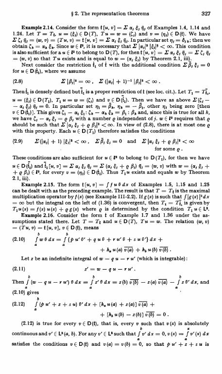
§ 2. The representation theorems 327
Example 2.14. Consider the form t [u, v] = E a; $1 ; of Examples 1.4, 1.14 and1.24. Let T = Tt, u = E D (T), T u = w = (C;) and v = (71;) E D (t). We haveE C, , = (w, v) _ (T u, v) = t [u, v] = E a; ; al;. In particular set 77; = S; b; then weobtain jk = a,, sek. Since w E 12, it is necessary that E la4 l$;la < oo. This conditionis also sufficient for a u E 12 to belong to D (T), for then t [u, v] = E a; se, , = E Ca la_ (w, v) so that Tu exists and is equal to w = (a; ;) by Theorem 2.1, iii).
Next consider the restriction t1 of t with the additional condition E 0for u E D (t1), where we assume
(2.8) E 1#iI2 = oo . E (Ia3I + 1)-1 I#rla < oo .
Then t1 is densely defined but t1 is a proper restriction oft (see loc. cit.). Let T, = Tt,,
u = (;) E D (TI), T, u = w = (C;) and v E D (t1). Then we have as above E- a; ;) & = 0. In particular set 771 = 9r, 711, = - #1, other r7; being zero [thenv E D (t1)]. This gives C, - a1 $1 : CA - aA $k = fl1: ftk and, since this is true for allk,we have C; - a; ; = Q fl; with a number e independent of j. w E 12 requires that Qshould be such that E la; ; + 8 &12 < oo. In view of (2.8), there is at most one 8with this property. Each u E D (TI) therefore satisfies the conditions
(2.9) E(Iajl+1)I$5I2<0O, E#,$,=0 and Ela;se,+et,I2<00for some Q .
These conditions are also sufficient for u E 12 to belong to D (TI), for then we have
u E D (t1) and t1 [u, v] = Ear a a = E (aa a + p & , = (w, v) with w = (a, .sea -i-+ e f4,) E 12, for every v = (71;) E D (t1). Thus T, u exists and equals w by Theorem2.1, iii).
Example 2.15. The form t [u, v] = J f u v dx of Examples 1.5, 1.15 and 1.25can be dealt with as the preceding example. The result is that T = Tt is the maximalmultiplication operator by f (x) (see Example 111-2.2). If g (x) is such that f Ig (x) isdx= oo but the integral on the left of (1.36) is convergent, then T, = Tt, is given byT1 u (x) = f (x) u (x) + B g (x) where 8 is determined by the condition T, u E L2.
Example 2.16. Consider the form t of Example 1.7 and 1.36 under the as-sumptions stated there. Let T = Tt and u E D (T), Tu = w. The relation (w, v)= (T u, v) = t [u, v], v E D (t), means
6 b
(2.10) Jw6dx= J{pu'0'+qu6+ru'6+sufl'}dx+a a
+ h, u (a) v (a) + hb u (b) v '_(b) .
Let z be an indefinite integral of w - q u - r u' (which is integrable) :
(2.11) z'=w-qu-ru'.b b 6
Then J(w-qu-ru')0dx= f z'vdx=z(b)v(b) -z(a)v(a) - Jz0'dx,anda a a
(2.10) givesb _
(2.12) f (p u' + z + s u) O' dx + [ha u (a) + z (a)] v (a) +0
+ [hb u (b) - z (b) ] v (b) = 0 .
(2.12) is true for every v E D (t), that is, every v such that v (x) is absolutelyb x
continuous and v' E L2 (a, b). For any v' E L2 such that f v' d x = 0, v (x) = f v'(x) d xa a
satisfies the conditions v E D (t) and v (a) = v (b) = 0, so that p u' + z + s u is
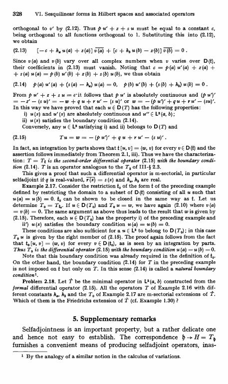
328 VI. Sesquilinear forms in Hilbert spaces and associated operators
orthogonal to v' by (2.12). Thus p u' + z + s u must be equal to a constant c,being orthogonal to all functions orthogonal to 1. Substituting this into (2.12),we obtain
(2.13) [- c + ho u (a) + z (a) ] v (a) + [c + hb u (b) - z(b) ] v (b) = 0 .
Since v (a) and v (b) vary over all complex numbers when v varies over D (t),their coefficients in (2.13) must vanish. Noting that c = p (a) u' (a) + z (a) ++ s (a) u (a) = p (b) u' (b) + z (b) + s (b) u (b), we thus obtain
(2.14) p (a) u' (a) + (s (a) - ho) u (a) = 0, 1' (b) u' (b) + (s (b) + ha) u (b) = 0 .
From p u' + z + s u = c it follows that p u' is absolutely continuous and (p u')'= - z' - (s u)' = - w + q u + r u' - (s u)' or w = - (p u')' + q u + r u' - (su)'.In this way we have proved that each u E D (T) has the following properties:
i) u (x) and u' (x) are absolutely continuous and u" E La (a, b) ;ii) u (x) satisfies the boundary condition (2.14).Conversely, any u E L8 satisfying i) and ii) belongs to D (T) and
(2.15) Tu=w= -(pu')'+qu+ru'- (su)'.In fact, an integration by parts shows that t [u, v] = (w, v) for every v E D (t) and theassertion follows immediately from Theorem 2.1, iii). Thus we have the characteriza-tion: T = Tt is the second-order differential operator (2.15) with the boundary condi-tion (2.14). T is an operator analogous to the T. of III-§ 2.3.
This gives a proof that such a differential operator is m-sectorial, in particularselfadjoint is real-valued, r(x) = s(x) and h hb are real.
Example 2.17. Consider the restriction to of the form t of the preceding exampledefined by restricting the domain to a subset of D (t) consisting of all u such thatu (a) = u (b) = 0. to can be shown to be closed in the same way as t. Let usdetermine To = T. If U E D (To) and To u = w, we have again (2.10) where v (a)= v (b) = 0. The same argument as above thus leads to the result that w is given by(2.15). Therefore, each u E D (To) has the property i) of the preceding example and
ii') u (x) satisfies the boundary condition u (a) = u (b) = 0.These conditions are also sufficient for a u E L$ to belong to D (TO); in this case
To u is given by the right member of (2.15). The proof again follows from the factthat to [u, v] = (w, v) for every v E D (to), as is seen by an integration by parts.Thus To is the differential operator (2.15) with the boundary condition u (a) = u (b) = 0.
Note that this boundary condition was already required in the definition of to.On the other hand, the boundary condition (2.14) for T in the preceding exampleis not imposed on t but only on T. In this sense (2.14) is called a natural boundarycondition'.
Problem 2.18. Let t be the minimal operator in La (a, b) constructed from theformal differential operator (2.15). All the operators T of Example 2.16 with dif-ferent constants h hb and the To of Example 2.17 are m-sectorial extensions of T.Which of them is the Friedrichs extension of t (cf. Example 1.30) ?
5. Supplementary remarksSelfadjointness is an important property, but a rather delicate one
and hence not easy to establish. The correspondence h -. H = Tofurnishes a convenient means of producing selfadjoint operators, inas-
' By the analogy of a similar notion in the calculus of variations.
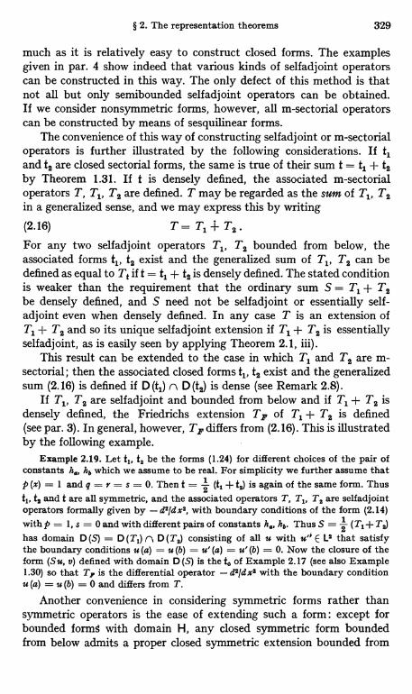
§ 2. The representation theorems 329
much as it is relatively easy to construct closed forms. The examplesgiven in par. 4 show indeed that various kinds of selfadjoint operatorscan be constructed in this way. The only defect of this method is thatnot all but only semibounded selfadjoint operators can be obtained.If we consider nonsymmetric forms, however, all m-sectorial operatorscan be constructed by means of sesquilinear forms.
The convenience of this way of constructing selfadjoint or m-sectorialoperators is further illustrated by the following considerations. If t1and t2 are closed sectorial forms, the same is true of their sum t = t1 + t2by Theorem 1.31. If t is densely defined, the associated m-sectorialoperators T, T1, T2 are defined. T may be regarded as the sum of T1, T2in a generalized sense, and we may express this by writing
(2.16) T=T1-I-T2.For any two selfadjoint operators T1, T2 bounded from below, theassociated forms t1, t2 exist and the generalized sum of T1, T2 can bedefined as equal to Tt if t = t1 + t2 is densely defined. The stated conditionis weaker than the requirement that the ordinary sum S = T1 + T2be densely defined, and S need not be selfadjoint or essentially self-adjoint even when densely defined. In any case T is an extension ofT1 + T2 and so its unique selfadjoint extension if T1 + T2 is essentiallyselfadjoint, as is easily seen by applying Theorem 2.1, iii).
This result can be extended to the case in which T1 and TZ are m-sectorial; then the associated closed forms t1, t2 exist and the generalizedsum (2.16) is defined if D (t1) n D (t2) is dense (see Remark 2.8).
If T1, T2 are selfadjoint and bounded from below and if T1 + T2 isdensely defined, the Friedrichs extension TF of T1 + T2 is defined(see par. 3). In general, however, TF differs from (2.16). This is illustratedby the following example.
Example 2.19. Let t1, to be the forms (1.24) for different choices of the pair ofconstants he, hb which we assume to be real. For simplicity we further assume thatp (x) = 1 and q = r = s = 0. Then t = 2 (tl + t2) is again of the same form. Thusti, t9 and t are all symmetric, and the associated operators T, T1, T$ are selfadjointoperators formally given by - d2/dx2, with boundary conditions of the form (2.14)with p = 1, s = 0 and with different pairs of constants he, hb. Thus S =
2
(T1+T2)has domain D (S) = D (T1) n D (T2) consisting of all u with u't E L2 that satisfythe boundary conditions u (a) = u (b) = u' (a) = u' (b) = 0. Now the closure of theform (Su, v) defined with domain D (S) is the to of Example 2.17 (see also Example1.30) so that Tr is the differential operator - d2/d x$ with the boundary conditionu (a) = u (b) = 0 and differs from T.
Another convenience in considering symmetric forms rather thansymmetric operators is the ease of extending such a form : except forbounded forms with domain H, any closed symmetric form boundedfrom below admits a proper closed symmetric extension bounded from

330 VI. Sesquilinear forms in Hilbert spaces and associated operators
below ; there is no such thing as a maximal symmetric form, whereasmaximal symmetric operators do exist (selfadjoint operators are maximalsymmetric). Similar remarks can be made for more general, sectorialforms on the one hand and m-sectorial operators on the other.
A question arises: what is the relationship between the m-sectorialoperators H1, Ha associated with two forms 0, 02 such that hl C h2 ?The answer is not straightforward; there is no simple relationship bet-ween the domains of H1 and H2. Later we shall give a partial answer tothis question.
Another question concerns the relationship between the selfadjointoperators H1, H2 associated with two symmetric forms Hl, h2 such that01 > h2. We find it convenient to define the order relation 01 z h2 forany two symmetric forms 01, h2 bounded from below by
(2.17) D (01) (: D (h2) and 01 [u] z h2 [u] for u E D (hi) .
Note that according to this definition, if 01, 02 are symmetric and boundedfrom below, then 01 C 02 implies 01 h2
Problem 2.20. 01 Z 42 implies 61 Z 4a
Let H1, H2 be the selfadjoint operators bounded from below associatedrespectively with closed symmetric forms 01, h2 bounded from below.We write H1 z H2 if hl z h2 in the sense defined above. This notationis in accordance with the usual one if H1, H2 are symmetric operatorsbelonging to M(H).
Theorem 2.21. Let H1, H2 be selfadjoint operators bounded from'belowwith lower bounds yl, ya, respectively. In order that H1 z H2, it is necessarythat yl L Y2 and R (C, H1) 5 R (C, H2) for every real C < y2, and it issufficient that R (C, H1) 5 R (C, H2) for some C < min (y, y2) (R denotesthe resolvent).
Proof. Necessity. Let 01, h2 be the associated symmetric formsbounded from below. Hl z H2 is equivalent to hl z h2 by definition,which implies y4, z y4,. Since y1= y4,, y2 = y4, by Theorem 2.6, itfollows that yl z y$. Thus the resolvents R (C, H1) and R (C,'H2) exist forC < y2. Replacing hl - C, h2 - C, H1 - -, H2 - C by 01, h2, H11 H2 re-spectively, it suffices to show that H1 z H2 z a > 0 implies H1 -1 5 Hit[where Hit, Hat E.i(H)].
For any u E H, set v1= HT' u, v2 = Hi' u. Then we have
(HT 1 u, u)2 = (v1, H2 v2)2 = h2 [v1, v2]2 5 h2 [v1] h2 [v2]
5 01 [vl] h2 [v2] = (H1 v1, v1) (H2 v2, v2) _ (u, HT I u) (u, Ha 1 u) ,
which gives the desired result (Hl 1 u, u) (Hi' u, u). Note thatv1 E D (H1) C D (01) C D (02), and that H1, H2, Hi 1, Hi 1 are all symmetricand nonnegative.
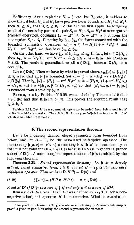
§ 2. The representation theorems 331
Sufficiency. Again replacing H, - C, etc. by Hl, etc., it suffices toshow that, if both H, and H2 have positive lower bounds and Hi 1 5 HZthen Hl z H2, that is, h1 z 02 To this end we first apply the foregoingresult of the necessity part to the pair S1= Hi 1, S2 = HZ 1 of nonnegativebounded operators, obtaining (S1 + a)-1 > (S2 + a)-1, a > 0, from theassumption S1 5 S2. Denoting by 0111, hen the forms associated with thebounded symmetric operators (S1 + w-1)-1 = H, (1 + 11-1 H,)-1 andH2(1 + n-1 H2)-1, we thus have 0111 ? 0211.
On the other hand we have 0111 5 01, 0211 5 02. In fact, let u E D (H,) ;then 01, [u] = (H, (1 + w-1 H,)-1 u, u) 5 (H1 u, u) = 0, [u] by ProblemV-3.32. The result is generalized to all u E 'D (01) because D (H,) is acore of 01
Let u E D (01). Then we have by what is proved above 02n [u] 5 0111 [u]5 01 [u] so that 02- [u] is bounded. Set un = (1 + 11-1 H2)-1 u E D (H2) CC D/(02). Then 02- [u] = (H2(I+ n-i H2)-1 u, u) _ (H2un, (1 + n-1 H2) un)
/(H2 u11, un) + n-111H2 unJJ2 Z (H2 un, u11) so that (H2 u11, u11) = 02 [un]is bounded from above by 01 [u].
Since un -> u by Problem V-3.33, we conclude by Theorem 1.16 thatu E D (02) and that 02 [u] 5 01 [u]. This proves the required result thath1zh2 '-
Problem 2.22. Let K be a symmetric operator bounded from below and let Hbe its Friedrichs extension. Then H Z H' for any selfadjoint extension H' of Kwhich is bounded from below.
6. The second representation theoremLet 0 be a densely defined, closed symmetric form bounded from
below, and let H = To be the associated selfadjoint operator. Therelationship 0 [u, v] _ (Hu, v) connecting 0 with H is unsatisfactory inthat it is not valid for all u, v E D (0) because D (H) is in general a propersubset of D(0). A more complete representation of 0 is furnished by thefollowing theorem.
Theorem 2.23. (Second representation theorem). Let 0 be a denselydefined, closed symmetric form, 0 z 0, and let H = To be the associatedsel f adjoint operator. Then we have D (H1/2) = D (0) and
(2.18) 0 [u, v] = (H1/2 u, H1/2 v) , u, v E D(0)
A subset D' of D (0) is a core of 0 if and only if it is a core of H1/2.Remark 2.24. We recall that H1/2 was defined in V-§ 3.11, for a non-
negative selfadjoint operator H is m-accretive. What is essential in
1 The proof of Theorem 2.21 given above is not simple. A somewhat simplerproof is given in par. 6 by using the second representation theorem.
332 VI. Sesquilinear forms in Hilbert spaces and associated operators
Theorem 2.23 is that H1/2 is selfadjoint, nonnegative, (H'!2)2 = H andthat D (H) is a core of H1/2 (see Theorem V-3.35).
Proof of Theorem 2.23. Let us define the symmetric form 0'[u, v]_ (H'!2 u, H1/2 v) with D (lj') = D (Hl/2). Since H1/2 is densely defined, andclosed (because it is selfadjoint), the same is true of h' (see Example 1.13).Since D (H) is a core of H1/2, it is also a core of h' (see Example 1.23).On the other hand, D (H) is a core of h by Theorem 2.1. But the two formsh and h' coincide on D (H), for we have
(2.19) h [u, v] = (Hu, v) = (HI/2 u, Hl/a v) , u, v E D (H) .
Thus h and h' must be identical, being the closure of one and the sameform - the restriction of h to D(H). This proves (2.18). The last statementof the theorem follows from h = h' and Example 1.23.
Problem 2.25. Let 4 be a densely defined, symmetric, closed form boundedfrom below with lower bound y and let H = To. For any y, we have thenD (4) = D ((H - S)1/2), l, [u, v] ((H - )112 u, (H - )1/2 v) + $ (u, v)
Theorem 2.26. Let h, H be as in Theorem 2.23 and, in addition, let hhave a positive lower bound. Then a subset D' o l D (h) is a core o l t i f andonly if HOOD' is dense in H.
Proof. This follows from Theorem 2.23 and Problem 111-5.19 [notethat Hl/z has positive lower bound, as is seen from Theorem 2.23, so thatits inverse belongs to M(H)].
Corollary 2.27. Let h be a densely defined, symmetric form, h ? 0,and let H be the self adjoint operator associated with its closure h. Then D (0)is a core o t H1/2. 1/ 4 has a positive lower bound, H1/2 D (h) is dense in H.
Remark 2.28. In Corollary 2.27, D (h) need not be a core of H evenwhen it is a subset of D (H).
Remark 2.29. The second representation theorem was proved onlyfor symmetric forms. A corresponding theorem for nonsymmetric formsis not known. A natural generalization of that theorem to a nonsym-metric form t would be that t [u, v] _ (T'!2 u, T#1/2 v) with D (t) _= D (Tl/$) = D (T*1/2) where T = Tt; but the question is open whetherthis is true for a general closed sectorial form t (with a vertex z 0),although the operators T1/2 and T* 1/2 are well-defined (V-§ 3.11) 1.
As an application of the second representation theorem, we shall giveanother formulation of the order relation H, z H2 for two selfadjointoperators bounded from below. In the preceding paragraph this wasdefined as equivalent to h, z ha for the associated closed forms 0l, tea,which means that D (hl) C D (p2) and 01 [u] z h2 [u] for all u E D (Ih).According to Theorem 2.23, this is in turn equivalent to
(2.20) D (Hi/$) C D (H$/2) and 11H,1/2 uII z IIH21/2 uII for u E D (Hr/r),
1 For this question see Lioxs [1], T. KATO [16].
§ 2. The representation theorems 333
if we assume that both H, and H2 are nonnegative (which does notrestrict the generality, for H1 z H2 is equivalent to H1 + a z H2 + a).If we further assume that H, has a positive lower bound so that Hl 1/2= (Hi/2)-1 E-4 (H), then (2.20) is equivalent to
(2.21) 1 2 1 2 Hi 1/2 E . (H) , 11H$/2 HI-1/211 S 1
We could have chosen (2.21) as the definition of H, z H. in the caseunder consideration.
We can now give a simpler proof of Theorem 2.21. As noted in theproof of this theorem given before, the essential point is that H, z H2is equivalent to H1 -1 HQ 1 when both H, and H2 have positive lowerbounds. In view of the equivalence of H1 z H2 with (2.21), what is to beproved is contained in the following lemma.
Lemma 2.30. Let S, T be densely defined closed operators in H suchthat their adjoints S*, T* are invertible. I/ D (S):) D (T) and IISuII 5 II T uIIfor all u E D (T), then D (T*-1) ) D (S#-1) and II T* -1 ull 5 IIS*-1 uII for allu E D(S*-1).
Proof. Let u E D (S* -1) = R (S*) ; u = S* g for some g E D (S*). Forany v E D (T) C D (S), we have then (u, v) = (S* g, v) = (g, S v) and soI(u, v)I s IIgHI IISuII s IIgII II Tv!I. Thus Tv = 0 implies (u, v) = 0 andT v, = T V2 implies (u, v1) = (u, v2) . Therefore, (u, v) may be regarded as afunction of w = T v and as such it is semilinear in w. Since R (T)1 = N (T*)= 0, w varies over a dense linear manifold of H when v varies over D (T).Since this semilinear form is bounded with bound 5 IIgII as is seen fromthe inequality given above, it can be extended by continuity to all w E H.Then it can be represented in the form (f, w) with a uniquely determined/ E H such that 11/11 :5 IIg!I. Thus we obtain (u, v) = (f, w) = (f, T v) for allv E D (T), which implies that f E D (T*) and u = T* /. Thus u ER(T*)= D(T*-1) and IIT*-1 ull = II/II s IIgII = IIS#-1 uII, as we wished to show.
Example 2.31. Consider the form t [u, v] of Examples 1.4, 1.14, 1.24 and 2.14.Assume that all the as are real and nonnegative, so that t is symmetric and non-negative. Let T = Tt; T has been characterized in Example 2.14. It is now easyto see that T1j2 is the maximal diagonal-matrix operator (r4'2). Similarly, for theform t [u, v] = f f u v dx of Examples 1.5, 1.15, 1.25, and 2.15, Tl/2 is the maximal
Emultiplication operator by / (x)i12, provided we assume that / (x) Z 0 so that t isnonnegative symmetric.
Remark 2.32. Except in simple examples such as those given above,the operator T1/2 is hard to describe in elementary terms, even when Tcan be easily described. In particular this is the case for differentialoperators T as in Example 2.16. In this sense, the expression (2.18) is oftheoretical rather than of practical interest. As we shall see later, how-ever, there are some results of practical significance that can be deducedmore easily from (2.18) than by other methods.

334 VI. Sesquilinear forms in Hilbert spaces and associated operators
7. The polar decomposition of a closed operator
Let T be a densely defined, closed operator from a Hilbert space Hto another one H'. Consider the symmetric form h [u, v] = (Tu, Tv).As we have seen in Example 2.13, h is nonnegative and closed, with theassociated selfadjoint operator To = H = T* T. Let G = H1/2. Thesecond representation theorem gives
(2.22) (Tu, Tv) = (Gu, Gv) , IITuII = IIGuII , u, v E D(T) = D(G) .
This implies that G u --> T u defines an isometric mapping U of R (G) C Honto R (T) C H': T u = UG u. By continuity U can be extended to anisometric operator on R [the closure of R (G)] onto 1 ((TT). Furthermore,U can be extended to an operator of -4 (H, H'), which we shall denoteagain by U, by setting Uu = 0 for u E R (G)1 = N (G). Thus defined, U ispartially isometric with the initial set RT) and the final set R(T) (seeV-§ 2.2), and we have
(2.23) T= UG, D (T) = D (G) .
(2.23) is called the polar decomposition of T ; here G is nonnegativeselfadjoint and U is partially isometric. If U is required as above to haveinitial set W), the decomposition (2.23) is unique. In fact it is easilyseen from (2.23) that
(2.24) T*= GU*
[which implies that D (T*) is the inverse image of D (G) under U*],and so T* T = G U* UG = G2 because U* Uu = u for u in the initialset of U. Thus G must be a nonnegative square root of T* T, whichdetermines G uniquely (see V-§ 3.11). Then (2.23) determines U on R (G)and hence completely since U = 0 on R (G)1 by hypothesis.
By analogy with the case of complex numbers, G is called the absolutevalue,of T and is denoted by I TI. Thus I TI is defined for any denselydefined closed operator from H to H' and is a nonnegative selfadjointoperator in H ; of course it should be distinguished from the scalar II T11.
Similarly, I T* I is a nonnegative selfadjoint operator in H'; it isrelated to I TI by
(2.25) IT*I = UITI U* .
To see this set G'= U I T I U* = UGU*. Then G' u = 0 for u E R (T)1since U* u = 0, and R (G') C R (U) = RM. Thus G' is zero on R (T) 1, andon R-(7)- it is unitarily equivalent to the part in R_(G of G. Hence G'is selfadjoint and nonnegative. But G12= UG U* UG U* = UGGU*= T T*. Hence G' must be equal to IT* I by the uniqueness of the squareroot.
§ 2. The representation theorems 335
From (2.23), (2.24), (2.25) we obtain the following relations:
(2.26) T= UITI= IT*IU = UT* U, T* = U* IT*I= ITIU* = U*TU*.ITI= U*T= T*U= U*IT*IU, IT*I= UT*= TU*= UITIU*.
In particular T* = U* IT* I is the polar decomposition of T*.Problem 2.33. N(T) = N(ITI), R(T) = R(IT*I).Example 2.34. The canonical expansion of a compact operator T E a (H, H')
discussed in V-§ 2.3 is a special case of the polar decomposition. Let U q' = lpR,k = 1, 2, ..., in V-(2.23). If {qpk} is not complete, set Uu = 0 for u L op", k = 1,2, .... Then I TI = L' ak ( qpk) pl, [see V-(2.26)] and V-(2.23) is exactly identicalwith T = UITI.
Let us now consider the special case in which T = H is selfadjoint:H* = H. Let H = U IHI be its polar decomposition. Since H = H*= U* IH*I = U* IHI is the polar decomposition of the same operator,we must have U* = U by the uniqueness proved above. Furthermore,the initial set R I ) and the final set RH) of U coincide by Problem 2.33;we denote by R this common subspace of H. We have U2u = U* Uu = ufor u E R and Uu = 0 for u E R. Any u E R can be written as u = u+ + u_where Uu+= u+ and Uu_ = -u_; it suffices to set u}= (1 ± U) u/2.Moreover, it is easy to see that such a decomposition is unique. Let M±be the subspaces of R consisting of all u such that Uu = +u. We havethus the decomposition
(2.27) H=M+eM_eMO, MO =R1,
the three subspaces being orthogonal to one another.It follows also from (2.26) that UH = U* H = IHI = IH*I = H U*
= H U; hence H commutes with U. Similarly CHI commutes with U.From the definition of R, Mt, it then follows that H as well as IHI isdecomposed according to the decomposition (2.27). For U E Mo, we haveHu = IHI u = 0, for Me = R (IHI)1 = N (IHI) = N (H) (see Problem 2.33).For U E M+ we have Hu = H Uu = IHI u, and similarly Hu = - IHI ufor u E M_. Since IHI is positive in R, it follows that the part of H in M+is positive and that in M_ is negative. Thus (2.27) gives a decompositionof H into positive, negative and zero parts and the associated decomposi-tion of IHI.
In particular it follows that H and IHI commute, because this isobviously true in each of the three subspaces. [By this we mean that theresolvents R (C, H) and R (c', IHI) commute, for the commutativity of twounbounded operators has not been defined.]
Problem 2.35. If H is selfadjoint, D (H) = D (IHI) and for u E D (H)
«)II IHI -11,(2.28)
II H-11
s II(IHII(Hu,
Ill(IHI
(IH+ual u, u) s ((IHI + laI) u, u)[hint for the last inequality: V-(4.15).]
336 VI. Sesquilinear forms in Hilbert spaces and associated operators
Problem 2.36. The orthogonal projections onto the three subspaces M+, M_and M. are respectively given by
(2.29) P+ = (U2 + U)12, P_ _ (U2 - U)/2, Po = l - U2.Lemma 2.37. If A E 9 (H) commutes with H, then A commutes with
IHJand U.Proof. A commutes with the resolvent of H, hence also with the
resolvent of H2 in virtue of (H2 - c)-1= (H - C1/2)-1(H+ C1/2)-1. Hence Acommutes with IHI = (H2)1/2 by Theorem V-3.35. To show that A com-mutes with U, we note that A U I HI = A H C HA and UA IHI C U I HI A= HA. Hence A Uu = UA u for u E R. If u E R1 = M,= N (H), on theother hand, we have A Uu = 0 = UA u since Hu = 0 implies HA u= A Hu = 0. Hence A U = UA.
Lemma 2.38. The decomposition (2.27) of H into positive, negative andzero parts for H is unique in the following sense. Suppose that H is reducedby a subspace M' and (Hu, u) z 0 [(Hu, u) S 0] for every u E M' n D (H).Then M' must be a subspace of M+ ® M, = Ml (M_ (D M, = M+).
Proof. Let P' be the orthogonal projection on M'. Since M' reducesH, P' commutes with H. It follows from Lemma 2.37 and (2.29) that P'commutes with U and P±, Po. Thus P'P_ = P_ P' is the projection onM' n M_. But this subspace is 0, for u E D' = D (H) n M' n M_ impliesu = 0 [otherwise we have the contradiction that (Hu, u) z 0 and(Hu, u) < 0] and D' is dense in M' n M_ because the latter reduces H.This proves that P' P_ = P_ P' = 0 and hence that M' C M 1.
§ 3. Perturbation of sesquilinear forms and theassociated operators
1. The real part of an m-sectorial operatorIn this section we shall consider the perturbation of an m-sectorial
operator T when the associated form t undergoes a small perturbation.Lemma 3.1. Let i be a densely defined, symmetric, nonnegative closed
form with the associated nonnegative sel f adjoint operator H = To. Let abe a form relatively bounded with respect to h, such that
(3.1) Ia[u]I s bh[u], uED(h)
Then there is an operator C E.4 (H) with 11 C11 S e b (where e = 1 or 2according as a is symmetric or not) such that
(3.2) a [u, v] = (CGu, Gv) , G = H1/2 , u, v E D (O) = D (G) .
Proof. (3.1) implies that
(3.3) Ia [u, v]I S e b o [u]1/2 0 [v]1/2 = E bIIGuJJ IIGvhI
§ 3. Perturbation of sesquilinear forms and the associated operators 337
as. is seen by applying (1.15) to Re a and Im a and noting that h [u] = Il'Gu112by the second representation theorem. (3.3) implies that the value ofa [u, v] is determined by Gu, Gv, for Gu = Gu', Gv = Gv' implies thata[u',v']-a[u,v]=a[u'-u,v']+a[u,v'-v]=0. Thus a [u, v] maybe regarded as a bounded sesquilinear form in x = G u, y = G v, and itcan be extended to all x, y in the closure M of the range of G. It followsthat there exists a bounded operator C on M to itself such that 11C11 < e band a [u, v] = (Cx, y). For convenience C may be extended, withoutincreasing the bound, to an operator of 2 (H) by setting Cx = 0 forx E Ml.
As an application of this lemma, we shall deduce an expressionconnecting an m-sectorial operator T with its real part H. Let T beassociated with a closed, densely defined sectorial form t by Theorem 2.7.Let H = To where the symmetric form h = Re t is also closed. H is bydefinition the real part of T, H = Re T in symbol. It is obvious thatH = 2 (T + T*) if T is bounded, but this is in general not true. Itfollows directly from Theorem 2.5 that Re T* = Re T.
Theorem 3.2. Let T be an m-sectorial operator with a vertex 0 and semi-angle 0. Then H = Re T is nonnegative, and there is a symmetric operatorB E -4 (H) such that JIB11 5 tan 0 and
(3.4) T = G (1 + i B) G , G = H1/2.
Proof. Let T = Tt and h = Re t, f = Im t. Since f [u] 5 (tan 0) h [u]by hypothesis, we have f [u, v] = (BGu, Gv) by Lemma 3.1, whereB is symmetric and 11 B11 S tan 0. Hence
(3.5) t[u,v]= (0+ if) [u, v]=((1+iB)Gu,Gv).
Now let u E D (T). We have t [u, v] = (T u, v) for all v E D (t) = DD (G) by the definition of T. Comparing this with (3.5) and noting
that G is selfadj oint, we see that G (1 + i B) G u exists and is equal to T u.This shows that T c G (1 + i B) G. But it is easy to see that G (1 + i B) Gis accretive. In view of the fact that T is m-accretive, we must haveequality instead of inclusion. This proves (3.4).
Theorem 3.3. Let T be m-sectorial with H = Re T. T has compactresolvent if and only if H has.
Proof. We may assume without loss of generality that T has apositive vertex, so that C = 0 belongs to the resolvent sets of T and of H[that is, T-1 and H-1 belong to M(H)]. Suppose that H has compactresolvent. Then the same is true of G = H1/2 (see Theorem V-3.49).Since T-1= G-1(1 + i B)-1 G-1 by (3.4), it follows that T-1 is compact,which implies that T has compact resolvent. The proof of the converse
338 VI. Sesquilinear forms in Hilbert spaces and associated operators
proposition is somewhat complicated. It is known that G T-" E 9 (H)for 1/2 < a < 11 and that T- (1-") is compact if T has compact resolvent 2.Hence G T-1= G T-" T-(1-11) is compact and so is G-1= (1 + iB) G T-1.Thus H-1= G-2 is compact, and H has compact resolvent.
2. Perturbation of an m-sectorial operator and its resolventLet t be a densely defined, closed sectorial form and let T = Tt
be the associated m-sectorial operator. Let us ask how T is changed whent is subjected to a "small" perturbation. We shall consider this problemin the case in which the perturbation of t is relatively bounded.
We recall that t + a = s is also sectorial and closed if a is relativelybounded with respect to t with relative bound smaller than 1 (Theorem1.33). It is not easy to compare the associated operator S = TB directlywith the unperturbed operator T, for S and T need not have the samedomain. But we can compare the resolvents R (C, S) and R (C, T) andestimate their difference in terms of the relative bound of a with respectto t.
Theorem 3.4. Let t be a densely defined, closed sectorial form with= Re t z 0 and let T = Tt be the associated m-sectorial operator. Let a
be a form relatively bounded with respect to t, with
(3.6) Ia [u]J s aIIuJI2 + b h [u] , u E D (h) = D(t) C D(a) ,
where a, b are nonnegative constants and b < 1. Then s = t + a is alsosectorial and closed. Let S = TB be the associated m-sectorial operator. Ifb < 1/2, the resolvents R (t;, T) and R (C, S) exist, with
(3.7) IIR(C, S) - R(C, T)II s
(-Re-2a)(-Re) for - < Ret; < -2a ,b
2b a(1 - 2b) (-Reg) for Re C S -
b
(if b = 0 read no for alb) . If T has compact resolvent, the same is true of S.Proof. The closedness of s was proved in Theorem 1.33. Let e > 0
(to be determined later) and t' = t + Q h' = Re t' = h + Q, and letT' = T + Q, H' = H + Q z e > 0 be the associated operators. By (3.5)we have t' [u, v] = ((1 + iB') G'u, G'v) with G' = H'1/$ and B' * = B' EE 9 (H). On the other hand, (3.6) can be written
(3.8) 1 a [u]J 5 k h' [u] with k = max (b, a/Q) .
1 See T. KATO [15], [16].See Theorem V-3.49 and Remark V-3.50.
§ 3. Perturbation of sesquilinear forms and the associated operators 339
Hence a [u, v] = (CG'u, G'v), 11 C11 5 2k, by Lemma 3.1. For the forms' = s + e, we have the expression s' [u, v] = (t' + a) [u, v] = ((1 ++ i B' + C) G' u, G' v). As in the proof of (3.4), this leads to
(3.9) S + e = S'= G'(1 + iB'+ C) G', IICII 52k.
We nowhave S-C= S'-C.= G'(1 -C'H'-1 +iB'+C)G'whereC'= C + e, so that(3.10) R(C, S) = R(C', S') = G'-1(1 - C' H'-1+ iB'+ C)-1 G'-1 ,
provided the middle factor on the right exists and belongs to 9(H).But (1 - H' -1 + i B')-1 E 9 (H) exists and has norm 5 1 if e is chosenso that Re C' = Re C + e;5 0, for then 1 -C'H'-'+ i B' E M (H) hasnumerical range in the half-plane Re z z 1. It follows [see I-(4.24)]that the factor in question exists and
(3.11) 11(1-l;'H'-1+iB'+C)-1- (1 -C'H'-1+iB)-1II 5S 2k(1 - 2k)-1
if 2 k < 1. Then we see from (3.10) and a similar expression for R (C, T)obtained by setting C = 0 in (3.10) that
(3.12) IIR(t, S) - R(5, T)II 5 2k(1 - 2k)-1 e-1,
where we have also used the fact that IIG'-1II 5 P-1/2. If we set e = - Re l;,(3.12) gives the desired result (3.7), by the definition (3.8) of k.
If T has compact resolvent, the same is true of H, H' and G' byTheorems 3.3 and V-3.49. Hence G'-1 is compact and so is R(l;, S) by(3.10).
Remark 3.5. Theorem 3.4 shows that IIR(C, S) - R(l;, T) 11 is smallif a, b are sufficiently small. (3.7) shows this explicitly only for C withRe l: < 0. According to Remark IV-3.13, however, it is true for anyC E P (T) ; an explicit formula estimating R (C, S) - R (l;, T) could beobtained by using IV-(3.10), though we shall not write it down. Such aformula will be given in the next paragraph in the special case of asymmetric T, since it is then particularly simple.
Theorem 3.6. Let t be a densely defined, closable sectorial form, and letbe a sequence of forms with D D (t) such that
(3.13) I(t - tn) [u]I 5 anlluII2 + b , [u] , u E D (t)
where h = Re t and the constants a,,, b > 0 tend to zero as n -> oo. Thenthe t are also sectorial and closable for sufficiently large n. Let f, f berespectively the closures of t, t and let T, T,, be the associated m-sectorialoperators. Then converges to T in the generalized sense (of IV-§ 2.4).If T has compact resolvent, the same is true of T. for sufficiently large n.
340 VI. Sesquilinear forms in Hilbert spaces and associated operators
Proof. That t is sectorial and closable follows from Theorem 1.33.We note also that (3.13) holds with t, to replaced by respectively.
We may assume without loss of generality that fj z 0; otherwisewe need only to add a common constant to t and t,,. We may further as-sume that an = b1,; otherwise it suffices to replace a and b by the com-mon constant max(a,,, Then it follows from (3.7) that
1, T) 11 5 2 a (1 - 2 -1 -+ 0, which proves that T convergesto T in the generalized sense. The last assertion of the theorem alsofollows from Theorem 3.4.
Remark 3.7. Theorem 3.6 gives a convenient criterion for a sequenceof operators T to converge to T in the generalized sense. Compare asimilar criterion, related to a relatively bounded perturbation of anoperator, given by Theorem IV-2.24.
Remark 3.8. All the results pertaining to a sequence of operatorsconverging in the generalized sense can be applied to the T of Theorem3.6. For instance, we note that the spectrum of T does not expandsuddenly and, in particular, any finite system of eigenvalues is stablewhen T is changed to T (see IV-§ 3.5).
3. Symmetric unperturbed operators
Theorem 3.9. Let h be a densely defined, closed symmetric form boundedfrom below and let a be a (not necessarily symmetric) form relatively boundedwith respect to h, so that D (a) ) D (h) and
(3.14) la[u] 5alIull 2+b0 [u],
where 0 5 b < 1 but a may be positive, negative or zero. Then s = h + ais sectorial and closed. Let H, S be the operators associated with s, re-spectively. I/ C E P (H) and
(3.15) a 11(a + b H) R (C, H) II < 1 ,
then C E P (S) and
(3.16) hIR(C, S) - R(C, H)11 5 (14e 11
Ia + bH)RR(CHH)II)$ IIR(C, H)II
Here e = 1 or 2 according as a is symmetric or not.Proof. First we assume that b > 0 and set h' = h + a b=' + 6,
s' = s + a b-' + 8 with a 6 > 0 to be determined later. s' is closed aswell as s by Theorem 1.33. The operators associated with h' and s' arerespectively H' = H + a b-1 + 6 and S' = S + a b-1 + 6.
We have h + a b-1 z 0 by (3.14) so that y' Z 6. (3.14) impliesalso I a [u] I 5 b 0'[u]. We can now apply the same argument that wasused in the proof of Theorem 3.4; we note that a [u, v] may be written
§ 3. Perturbation of sesquilinear forms and the associated operators 341
in the form (C G' u, G' v) with II CII S s b, where s = 1 or 2 accordingas a is symmetric or not (see Lemma 3.1), and that G' z 6'/2 or II G`111S 6-1/2. In this way we obtain
(3.17) IIR(C,S)-R(C,H)IISsbM2(1-ebM)-1b-1 if 6 bM<1,
where M = II (1 - C' H`1) -1II for C' = C + a b-' + S (note that here B'= 0 because T = H is symmetric). Thus
(3.18) M = II (H' (H' - C')-1II = II (H + a b-1 + S) (H - C)-1II
5 b-1II (a + b H) R H) II + b II R H) II
The desired inequality (3.16) follows from (3.17) by substituting for Mfrom (3.18) and setting 6 = a(l - a) (1 + a)-1 N-1 where a= ejl (a ++ bH) H) 11 and 9 = s bljR(g, H)II ; note that 1 - s bM = (1 - a)(1+a)-1>Oif z<1.
The case b = 0 can be dealt with by going to the limit b --> 0.Remark 3.10. The condition (3.15) for C E P (S) is fairly satisfactory,
but the estimate (3.16) is not very sharp, as is seen by considering thespecial case b = 0; in this case one has a sharper estimate with theright member s ajIRII2(1 - e aIIRII)-1 by I-(4.24) (R = R(C, H)), for
Ia [u]I = I(s - h) [u]I 5 allull2 implies Ia [u, v]I 5 s aIIuII IIvii so thata [u, v] = (Cu, v), S = H + C with II CII <_ s a. But the merit of Theorem3.9 lies rather in the fact that a may be negative. A more satisfactoryresult could be obtained by using the lower bound y z 0 of a + b Hexplicitly in the estimate.
4. Pseudo-Friedrichs extensionsThe Friedrichs extension was defined for a densely defined, sectorial
operator; it is thus inherently connected with sectorial boundedness.We shall now introduce a new kind of extension, similar to the Friedrichsextension, which can be applied to a not necessarily sectorial operatorand which produces a selfadjoint operator when applied to a symmetricoperator'.
Theorem 3.11. Let H be a selfadjoint operator and let A be an operatorsuch that D = D (A) C D (H) and
(3.19) I(Au, u)I S aIIuII$+ b(IHI u, u) , u E D(A) ,
where 0 5 b < 1 or 0 5 b < 1/2 according as A is symmetric or not.If D (A) is a core of I HI'/2, there is a unique closed extension T of H + A
1 The results of this paragraph are not related to sesquilinear forms in anyessential way. We consider them here simply because the techniques used in theproofs are similar to those of the preceding paragraphs.
342 VI. Sesquilinear forms in Hilbert spaces and associated operators
such that D (T) C D (IHI'/a), D (T*) c D (IHII/a) and in E P (T) for all real ,with sufficiently large I, . T is selfadjoint if A is symmetric. (T will becalled the pseudo-Friedrichs extension of H + A.)
Proof. Recall that IHI = (H2)1/2 is selfadjoint with D (IHI) = D (H)and commutes with H in the sense stated in § 2.71.
We may assume b > 0 without loss of generality. Set H' = IHI ++ a b-1 + b with a b > 0. (3.19) implies I (A u, u) I s b (H' u, u) == bIIG' uII2, where G' = H'1/2. Since D(A) is a core of IHI1/2, D(A) isalso a core of G' and the last inequality implies that (A u, v) can beextended to a form a [u, v] with D (a) = D (G') such that Ia [u, v] I s< e bll G' uII II G' v ll , where e = 1 or 2 according as a is symmetric or not(see the preceding paragraph). This gives (see par. 1)
(3.20) a[u,v]= (CG'u,G'v), CEM(H), IICII s e b.
We now claim that the operator T defined by
(3.21) T = G' (HH' -1 + C) G'
has the properties stated in the theorem. It is clear that D (T) C D (G')= D (I H11/2). Let u E D (A). Then G' HH'-1 G' u exists and equals Husince H' = G' 2 and G'- I and H commute. Since, furthermore, (A u, v)= a [u, v] = (CG' u, G' v) for all v E D (A) where D (A) is a core of G',G' C G' u exists and equals A u. Thus T u exists and equals (H + A) u,that is, T ) H + A.
Let C E P (H). Then T- C= G' [(H - C) Hl-'+ C] G' since 1 D
G' H' -1 G', so that
(3.22) (T - c)-1= G'-1 [(H - C) H'-' + C]-1 G'-'provided (H - C) H'-' + C has an inverse in 69 (H). This is true ifC [(H - C) H' -1]-1 = CH' (H - C)-1 has norm less than 1 (the Neumannseries), or if
(3.23) 11 C11 II (IHI + a b-1 + 6) (H - C)-III < 1
Recalling that II CII 5 e b, we see that this condition is satisfied if
(3.24) ell (a + b I HI + b 6) (H - C)-111 < 1 .
Since j a + b 61 11 (H - i r1)-III can be made arbitrarily small andII IHI (H - i 71)-III = 11H (H - i ?7)-Ill S 1 by choosing q real and verylarge, (T - i r1)-1 E.V(H) exists if e b < 1 and I,qI is sufficiently large.Thus T is closed with non-empty P (T) .
If A is symmetric, then C is symmetric and so is T (note that HH'-1is symmetric). Hence T must be selfadjoint.
1 This commutativity is essential in the proof; this is the reason why H must beassumed selfadjoint.
§ 4. Quadratic forms and the Schrbdinger operators 343
It follows from (3.22) that (T* - C)-' = G'-1 [(H - C) H' -1 ++ C*]-1 G'-1; note that [(H - C) H'-1 + C*] -1 exists as above in virtueof IIC*II = IICII It follows that D(T*) = R((T* - C)-1) C R(G'-1) = D(G')and
(3.25) T* = G'(HH'-1+ C*) G' .
Finally we prove the uniqueness of T. Suppose T, is a closed exten-sion of H + A with the properties stated in the theorem. Let u E D (T,*)and v E D (A). Then u E D (G') and (Ti u, v) = (u, T, v) = (u, (H + A) v)= (u, T v) = (u, G' (H H' -1 + C) G' v) = ((H H' -1 + C*) G' u, G' v). Sincethis is true for all v E D (A) and since D (A) is a core of G', T* u == G' (HH' -1 + C*) G' u exists and is equal to Tl u. This shows thatTl C T*, hence T,) T and T, - ) T - . But since l; = i q belongsto both P(T) and P(T1) for sufficiently large Iq1, we must have T1 - C=T - Cor T1=T.
Corollary 3.12. Let H be selfadjoint and let A, n = 1,2, ..., satisfy(3.19) for A with constants a, b replaced by a, b,, such that a,, - 0, b,, - 0,n -> 00, where it is assumed that D (As) C D (H) is a core o l IHI'/2 for each n.Then the pseudo-Friedrichs extension T,,, o l H + A,, is defined for su f -ficiently large n and T,, - H in the generalized sense.
Proof. First we note that we may assume a,, = b1, > 0. We can applythe proof of Theorem 3.11 with H' = IHI + 1 (set b = 0). (3.24) is truefor any C E P (H) if a, b are replaced by a, b,, and n is sufficiently large.For such n the resolvent (T,, - C)-1 exists and converges to (H - C)-1 innorm, for
[(H - C) H'-1 + Cn]-1-+ [(H - C)H'-1]-1
by II C,,11 -> 0 (with the obvious definition of Cu). Thus T,, --* H in thegeneralized sense (see Theorem IV-2.25).
Remark 3.13. Since D (IHI) = D (H) and I (Hu, u) 15 (IHI u, u) by(2.28), (3.19) is satisfied if
(3.26) I(Au, u)I 5 aIIujI2+ bI(Hu, u)I , u E D(A) .
Problem 3.14. Let H be selfadjoint and A symmetric with D (A) = D (H).If A is H-bounded with JjAuJJ25 a2IIuI1$ + b2jjHujj2, then A satisfies (3.19). [hint:Note that jjA ujl S 11 (a + bIHI) ull and use Theorem V-4.12.]
§ 4. Quadratic forms and the Schrodinger operators1. Ordinary differential operators
Since the simple types of regular differential operators have beendealt with in several examples above (see Examples 2.16, 2.17), we
344 VI. Sesquilinear forms in Hilbert spaces and associated operators
consider here a singular differential operator of the form'
(4.1) L=-d2/dx2+q(x), 0<x<oo.For simplicity we assume that q (x) is real-valued, though this is notnecessary. For the moment we further assume that q (x) z 0 and thatq (x) is locally integrable on the open interval (0, oo).
As in V-§ 5, we are mainly interested in constructing from the formaldifferential operator L a selfadjoint operator acting in H = L2(0, 00).It should be remarked at this point that, under the rather weak assump-tion made on q (x), the "minimal" operator such as the 1' of III-§ 2.3or V-§ 5.1 cannot be defined, for Lu need not belong to L2 for u E Co[because q (x) is not assumed to be locally L2].
Instead we consider the sesquilinear form
(4.2)
where
(4.3)
h=ho+h',
00 [u, v] = f u' v' d x = (u', v') , u (0) = v (0) = 0 ,0
Co
(4.4) 0'[u, v] = f q(x) u v dx .
0
D (00) is by definition the set of all u E H such that u (x) is absolutelycontinuous, u' E H and u (0) = 0. As before (cf. Example 1.36) 0o issymmetric, nonnegative and closed. D (h') is the set of all u E H such thatf q (x) J ul2 d x < oo ; t,' is also symmetric, nonnegative and closed (Example1.15). Thus 4 = 00 + h' is symmetric, nonnegative and closed by Theorem1.31. Moreover, h is densely defined since Co (0, oo) c D (h) = D (h0) nr D (1,').
According to the representation theorem, there is a nonnegativeselfadjoint operator H = TO associated with the form h. As in Example2.16, H can be described as follows : u E D (H) is characterized by theconditions that i) u and u' are absolutely continuous on (0, oo) and belong
00
to H, ii) u (O) = 0, iii) f q (u12 dx <oo, and iv) L u = -u"+ q u E H ; for0
such u we have Hu = Lu. In deducing this result, one should note thefollowing points. In the proof of the necessity of the conditions i) to iv),we consider an identity similar to (2.12) in which v E Co and the boundaryterms are absent and in which an indefinite integral z of w - q u is used(set r = s = 0) ; note that w - q u is locally integrable because w = Hu EE L2, u E D (H) C D (h) is continuous and q is locally integrable. In the
1 We take the semi-infinite interval (0, oo) because it is more important forapplications than the whole interval (- oo, oo). The latter case can be dealt within a similar way.
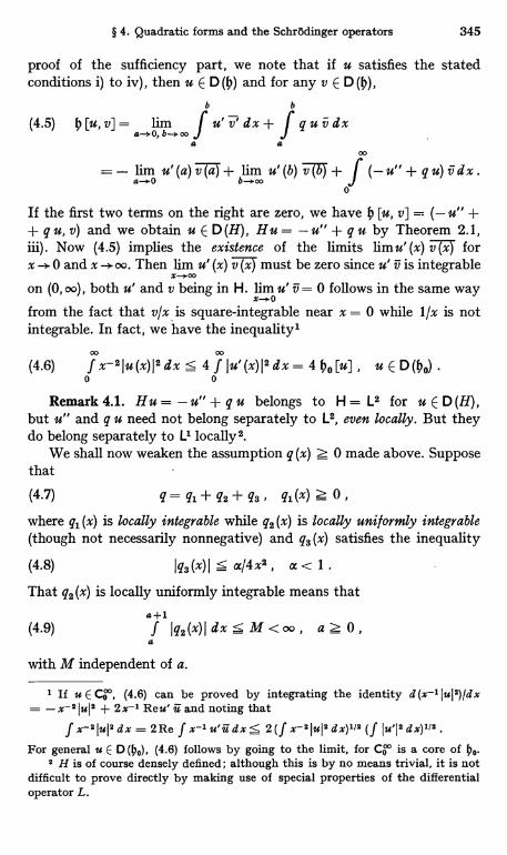
§ 4. Quadratic forms and the Schrodinger operators 345
proof of the sufficiency part, we note that if u satisfies the statedconditions i) to iv), then u E D (h) and for any v E D (h),
fu'J'dx+ fquidx(4.5) 0[u,v]= lima->0, b-roo
a aw
lim u'(a)v(a m u'(b) v(b + u"+qu)vdx.0
If the first two terms on the right are zero, we have t [u, v] _ (- u" ++ q u, v) and we obtain u E D (H), Hu = - u" + q u by Theorem 2.1,iii). Now (4.5) implies the existence of the limits limn' (x) -v-(7x forx -> 0 and x - oo. Then lim u' (x) v (x must be zero since u' v is integrable
X-±oo
on (0, oo), both u' and v being in H. lim u' v = 0 follows in the same wayx-r0
from the fact that v/x is square-integrable near x = 0 while l/x is notintegrable. In fact, we have the inequality'
(4.6) f x-21u(x)I2dx < 4 f lu'(x)12dx= 400[u] , u E D(lI0) .0 0
Remark 4.1. Hu = - u" + q u belongs to H = L2 for u ED (H),but u" and q u need not belong separately to L2, even locally. But theydo belong separately to L' locally2.
We shall now weaken the assumption q (x) 0 made above. Supposethat(4.7) q=q1+q2+q3, g1(x)0,where q1 (x) is locally integrable while q2 (x) is locally uniformly integrable(though not necessarily nonnegative) and q3 (x) satisfies the inequality
(4.8) l q3 (x) 1 5 a/4x2 , a< 1.That q2 (x) is locally uniformly integrable means that
a+1
(4.9) f lg2(x)l dx_M<oo, az0,a
with M independent of a.
If u E CO', (4.6) can be proved by integrating the identity d (x-1IuI2)/dx_ -x-2IuI2 + 2x-1 Reu' u and noting that
f x-2IuJ2 dx = 2Re f x-1 u'u dx 5 2 (f x-21u12 dx)112 (f Iu,I2 dx)112.
For general u E D (00), (4.6) follows by going to the limit, for C4 is a core of 1, .
2 H is of course densely defined; although this is by no means trivial, it is notdifficult to prove directly by making use of special properties of the differentialoperator L.
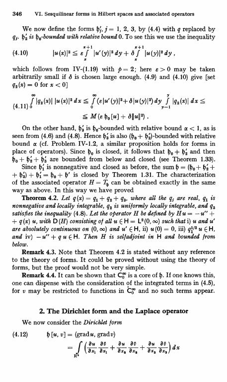
346 VI. Sesquilinear forms in Hilbert spaces and associated operators
We now define the forms j = 1, 2, 3, by (4.4) with q replaced byq5. 0' is 0,-bounded with relative bound 0. To see this we use the inequality
x+1 x+1(4.10) Iu(x)I2sef Iu'(y)I2dy+6f Iu(y)I2dy,
x
which follows from IV-(1.19) with p = 2; here e > 0 may be takenarbitrarily small if S is chosen large enough. (4.9) and (4.10) give [setq2 (x) = 0 for x < 0]
00 00 y
(4.11)f Ig2(W )I Iu(x)I2dx f (eIu'(y)I2+8Iu(y)I2)dyy f Jg2(x)I dx 5
M(e ho [u] + o1Iu1I2)
On the other hand, 03 is ho bounded with relative bound a < 1, as isseen from (4.6) and (4.8). Hence 03 is also (00+ h2)-bounded with relativebound a (cf. Problem. IV-1.2, a similar proposition holds for forms inplace of operators). Since he is closed, it follows that h0 + 02 and thenho + hz + hs are bounded from below and closed (see Theorem 1.33).
Since 0' is nonnegative and closed as before, the sum h = (he + ha ++ 03) + hi = 0o + h' is closed by Theorem 1.31. The characterizationof the associated operator H = TO can be obtained exactly in the sameway as above. In this way we have proved
Theorem 4.2. Let q (x) = ql + q2 + q3, where all the qj are real, ql isnonnegative and locally integrable, q2 is uniformly locally integrable, and q3satisfies the inequality (4.8). Let the operator H be defined by Hu = - u" ++ q (x) u, with D (H) consisting of all u E H = L2 (0, oo) such that i) u and u'are absolutely continuous on (0, oo) and u' E H, ii) u (0) = 0, iii) q1/2 u E H,and iv) - u" + q u E H. Then H is sel f adjoint in H and bounded frombelow.
Remark 4.3. Note that Theorem 4.2 is stated without any referenceto the theory of forms. It could be proved without using the theory offorms, but the proof would not be very simple.
Remark 4.4. It can be shown that Co is a core of If one knows this,one can dispense with the consideration of the integrated terms in (4.5),for v may be restricted to functions in Co and no such terms appear.
2. The Dirichlet form and the Laplace operatorWe now consider the Dirichlet form
(4.12) [u, v] = (grade, grade)=2U 20 au av au a
( 2x1 2x3 + axe axe + axe axe) dxR'
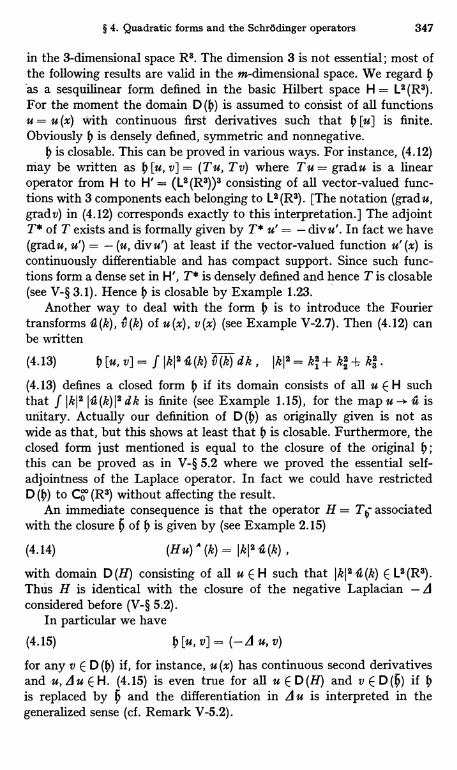
§ 4. Quadratic forms and the Schrodinger operators 347
in the 3-dimensional space R3. The dimension 3 is not essential; most ofthe following results are valid in the m-dimensional space. We regard has a sesquilinear form defined in the basic Hilbert space H = L2 (R3).For the moment the domain D (h) is assumed to consist of all functionsu = u (x) with continuous first derivatives such that h [u] is finite.Obviously h is densely defined, symmetric and nonnegative.
h is closable. This can be proved in various ways. For instance, (4.12)may be written as h [u, v] = (T u, T v) where T u = grade is a linearoperator from H to H'= (L2 (R3))3 consisting of all vector-valued func-tions with 3 components each belonging to L2 (R3). [The notation (grad u,grade) in (4.12) corresponds exactly to this interpretation.] The adjointT* of T exists and is formally given by T* u' = - divu'. In fact we have(gradu, u') = - (u, divu') at least if the vector-valued function u' (x) iscontinuously differentiable and has compact support. Since such func-tions form a dense set in H', T* is densely defined and hence T is closable(see V-§ 3.1). Hence h is closable by Example 1.23.
Another way to deal with the form h is to introduce the Fouriertransforms l (k), v (k) of u (x), v (x) (see Example V-2.7). Then (4.12) canbe written
(4.13) h[u,v]= f JkJsis(k)v"(k)dk, IkI2=ki+ka-}; k3.
(4.13) defines a closed form 4 if its domain consists of all u E H suchthat f JkJ2 111(k) 12 dk is finite (see Example 1.15), for the map u -+ is isunitary. Actually our definition of D (h) as originally given is not aswide as that, but this shows at least that h is closable. Furthermore, theclosed form just mentioned is equal to the closure of the original 0;this can be proved as in V-§ 5.2 where we proved the essential self-adjointness of the Laplace operator. In fact we could have restrictedD (h) to Co (R3) without affecting the result.
An immediate consequence is that the operator H = T4 associatedwith the closure 5 of 4 is given by (see Example 2.15)
(4.14) (H U) A (k) = JkJ2 4(k) ,
with domain D(H) consisting of all u E H such that I k 1 2 i1 (k) E L2(R3).
Thus H is identical with the closure of the negative Laplacian -Aconsidered before (V-§ 5.2).
In particular we have
(4.15) h [u, v] = (-d u, v)
for any v E D(0) if, for instance, u (x) has continuous second derivativesand u, A u E H. (4.15) is even true for all u E D (H) and v E D (5) if 4is replaced by 5 and the differentiation in d u is interpreted in thegeneralized sense (cf. Remark V-5.2).
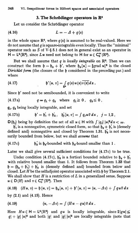
348 VI. Sesquilinear forms in Hilbert spaces and associated operators
3. The Schrodinger operators in R3Let us consider the Schrodinger operator
(4.16) L=-d+q(x)in the whole space R3, where q (x) is assumed to be real-valued. Here wedo not assume that q is square-integrable even locally. Thus the "minimal"operator such as S of V-§ 5.1 does not in general exist as an operator inH = L2 (R8), since L u need not belong to H for u E Co (R8).
But we shall assume that q is locally integrable on R8. Then we canconstruct the form h = ho + 0', where ho [u] = grad u112 is the closedDirichlet form (the closure of the h considered in the preceding par.) andwhere
(4.17) 0'[u, v] = f q (x) u (x) v (x) dx .PIG
Since ij' need not be semibounded, it is convenient to write
(4.17 a) q = q1 + q2 where q1 0, q2 s 0,
q1, q2 being locally integrable, and set
(4.17b) h'=h,+hz, hj[u,v]= fgfuvdx, j=1,2,D (01) being by definition the set of all u E H with f I qai I u I $ d x < oo .
h, is a nonnegative, symmetric closed form, so that 40 + 0, is (denselydefined and) nonnegative and closed by Theorem 1.31. hz is not neces-sarily bounded from below, but we shall assume that
(4.17c) 42 is 0, -bounded with ho bound smaller than 1 .
Later we shall give several sufficient conditions for (4.17c) to be true.Under condition (4.17c), ha is a fortiori bounded relative to ho + hl
with relative bound smaller than 1. It follows from Theorem 1.33 thath = (bo + hl) + ha is (densely defined and) bounded from below andclosed. Let H be the selfadjoint operator associated with h by Theorem 2.1.We shall show that H is a restriction of L in a generalized sense. Supposeu E D (H) and v E Co (R8). Then
(4.18) (Hu, v) = h [u, v] = Oo [u, v] + h' [u, v] = (u, -d v) + f quv dx
by (2.1) and (4.15). Hence
(4.19) (u, -d v) = f (Hu - qu) v dx .
Here Hu E H = L2(R8) and qu is locally integrable, since 2IquI SqI + IqI Iui2 and both IqI and IqI Iui2 are locally integrable (note that
§ 4. Quadratic forms and the SchrOdinger operators 349
u E D(h;) n D(h2)). Hence Hu - qu is locally integrable, and (4.19)implies
(4.20) -du=Hu-qu or Hu=-Au+qu=Lu,the differentiation A u being interpreted in the generalized sense'.
This shows that H is indeed a restriction of L. But we want to go onestep further and obtain a characterization of D (H). The result is given bythe following theorem.
Theorem 4.6 a. Let q = ql + q2 be as above. Let D be the set of allu E H such that i) the generalized derivative grad u belongs to H' = (L2 (R3))3,ii) f ql (x) Ju12 d x < oo, and iii) the generalized derivative A u exists andL u = -A u + q u belongs to H. Define the operator H by H u = L u withD (H) = D. Then H is selfadjoint in H and is bounded from below. (Notethat ii) implies that qu E as shown above.)
The operator H we have constructed above was already shown tosatisfy D (H) C D. Thus it only remains to show that D C D (H). To thisend let u E D. Then u E D (fjo) C D (,2) by i) and u E D (01) by ii). Henceu E D (h) and we have for each v E Co (R3)
(4.22) t,[u,v]=00[u,v]+0'[u,v]
(u,-Av)+ f quvdx=(Lu,v)since Lu exists and belongs to H. According to Theorem 2.1, (4.22)implies that u E D (H) with Hu = L u provided we know that Co (R3) is acore of h. Thus the proof is reduced to
Lemma 4.6b. Co (R3) is a core of h.
Proof. Since h = (ho + 0,) + 02 in which the second term is boundedrelative to the first term, a simple consideration reduces Lemma 4.6b to
Lemma 4.6c Co (R3) is a core of ho + 0
Proof. ho + h is nonnegative and closed as shown above. Hence itsuffices to show that Co is dense in the Hilbert space D (ho + 0,)D (00) n D (01) equipped with the inner product (ho + h, + 1) [u, v] (seeTheorem 1.21). Suppose that u is orthogonal to Co in this space:
(4.22a) (ho + 0', + 1) [u, v] = 0 for all v E Ca (R3)
we have to show that u = 0.An argument similar to the one used to deduce (4.20) from (4.18)
shows that (4.22 a) implies
(4.22b) A u = (ql + 1) u
i This is exactly the definition of d in the generalized sense; see e. g. YosIDA Ui).
350 VI. Sesquilinear forms in Hilbert spaces and associated operators
in the generalized sense, where q,u is locally integrable. Now it can beshown that the only function u E H that satisfies (4.22b) is u = 0. This isa nontrivial result in partial differential equations, and we shall notprove it here'.
Remark 4.7 a. Although we have characterized D (H), the questionremains whether or not there are other restrictions of L that are self-adjoint. It is known that if q2 is bounded, then there are no selfadjointrestrictions of L other than H. To see this we may assume g2 = 0 (by chang-ing L into L + const. if necessary). It suffices to show that if u E H and ifLu exists (by which is implied that qu is locally integrable) and belongsto H, then u E D (H). Let v = (H + 1)-' (L + 1) u E D (H). Since H C L,it follows that (L + 1) (u - v) = 0. Thus u - v E H satisfies (4.22b) andhence must vanish as above. This shows that u = v E D (H), as required.It can be shown that the same result holds if q2 is locally square-integrablewith local square-integrals not growing too rapidly at infinity.
We shall now give several sufficient conditions for (4.17c) to be met.A simple potential satisfying (4.17c) is given by
(4.23 a) q2 (x) = E e; Ix - a;I-2 with E ej > - 1/4 ,
i
where the as are fixed points in R3. (Here it suffices to consider onlynegative e5, for the terms with positive e3 can be absorbed into q1.)(4.23 a) implies (4.17c) by the well-known inequality
(4.24) f Ix-al-2lu(x)I2dxs 4 f Igraduj2dxs 40,[u],
which can be proved in the same way as (4.6) (use the polar coordinateswith origin at x = a).
Another sufficient condition for (4.17c) is given in terms of thefunction
(4.25 a) Me, (x; r) = f Ix-yI-'lg2(y)I dyI x-yl <.
Lemma 4.8 a. Assume that M., (x; r) -+ 0 as r -+ 0, uniformly inx E R3. Then (4.17c) is true.
Proof. We have to show that II Ig2I1/2UII2 = Ih2 [u]I 5 b(00 [u] + k2IIuII2)= b II (Ho + k2)'/2uII2 for an arbitrarily small b > 0 if k2 is chosen ap-propriately. Thus it suffices to show that
(4.25b) II Tk1I -- 0 as k -* oo , where Tk = Ig2I1/2 (Ho + k2)-1/2 .
1 For the proof see T. KATO [25].
§ 4. Quadratic forms and the Schrodinger operators 351
Since II TkII = II Tk T,*t111/2, it suffices in turn to show that II Tk TA*. 11-> 0
as k -+ oo. But Tk Tr) Ig211/2 (HO + k2)-l Ig2I 1/2, where (H0 + k2)-l is anintegral operator with the kernel
(4.25c) g(y, x; k) = e-klr-x1/4;rly - xI
[see IX-(1.67) ]. Let us estimate 11 T,, Tk* vII. If v E D (Ig2I1/2) and
w = (Ho + k2)-I Ig2I1/2v, we have
w(Y) = f g(Y, x; k) Ig2(x)11/2v(x)dx .
By the Schwarz inequality we obtain
Iw (Y) I2 < ck f g (Y, x; k) IV (x) I2dx ,
where
(4.25d) ck = sup f g(y, x; k) Ig2(x)I dx .YER
Since TkTr v = Ig2I1/2w, we have (anticipating that it is in H)
IITkTkv112=
IIIg2I1/2w112< ckff Ig2(Y)Ig(Y,x; k)IIv(x)I2dxdy
Ck f Iv(x)I2dx = ckIIvII2.
Hence 11 Tk Tk 11 5 ck. Thus the lemma will be proved if we show thatck -+O as k -+oo.
To this end, let e > 0 and choose r > 0 so small that the integral in(4.25d) taken on Ix - yl < r is smaller than e; this is possible by theassumption that M.. (x; r) -+ 0 as r -+ 0 uniformly in x. The remainingpart of the integral can be made smaller than e by choosing k sufficientlylarge, uniformly in y. We may leave the detail to the reader.
Lemma 4.8b. (4.17c) is true i/ q2 E L3/2(R3).
Proof. We may assume that the L3/2-norm of q2 is as small as weplease, since q2 may be approximated in L3/2-norm by a bounded func-tion, which contributes to 02' only a bounded form. Then the desiredresult follows from the Sobolev embedding theorem', which shows thatu E D (h0) implies u E LB (R3) with IIuII2. const. 40 [u], combined withthe Holder inequality
f I q2I I u 12 d x< const. I I g2II L.,1I I U
II L-
Remark k 4.9 a. Theorem 4.6a and the lemmas given above can beextended without essential change to the case of Schrodinger operators inRm with m > 3. The only changes required are to replace: - 1/4 in
1 See NIRENBERG [1].
352 VI. Sesquilinear forms in Hilbert spaces and associated operators
(4.23 a) by - (m - 2)2/4, 4 in (4.24) by 4/(m - 2)2, Ix - yj-1 in (4.25 a) byIx - yl'" - 2, and L3/2 (R3) in Lemma 4.8b by Lm/2 (R'"). Lemma 4.8a isstill true for m = 2 if in the definition of M9, (x; r), Ix - yI-1 is replacedby -logIx - yj.
4. Bounded regionsIf the region E of R3 or R" in which the differential operator (4.16) is to be
considered is bounded, there are complications arising from the possibility ofimposing various boundary conditions. To simplify the matter, let us assume that Eis open and has a smooth boundary a E and that q (x) is a smooth function in theclosed region E. Then the minimum operator . in H = L2(E) can be defined as inV-§ 5.1, and it would seem that one need not invoke the theory of forms in con-structing selfadjoint operators from L. Nevertheless considering a form h = hU + h',such as the one discussed in the preceding paragraph (the integrations should nowbe taken over E), is a convenient way to obtain various selfadjoint extensions of S.
First let us assume that D (h) = Co (E), the set of infinitely differentiablefunctions with compact supports in E; as before it can be shown that h is denselydefined, symmetric, bounded from below and closable. We denote this form by 01and set H1 = Ti,. Next we extend the domain of h and include in D (h) all functionscontinuously differentiable in the closed region r; the resulting form, which wedenote by 02, is densely defined, symmetric, bounded from below and closable.We set H. = T. Obviously 01C h3 and so 01C ha. According to the definition of theorder relation for selfadjoint operators given in § 2.5, this implies that 61 Z 62 andH1 Z H3,
We define a third form 03 by
(4.35) h3 Cu. v] = h3 [u, v] +a f a u v d S , D (h3) = D (43) ,
where the integral is taken on the boundary aE and a is a given smooth functiondefined on aE. It can be shown that the additional term in (4.35) is relatively boundedwith respect to 03 with relative bound 0. The proof is omitted, but the assertioncorresponds to the fact, in Example 1.36, that t3 is t1-bounded.
We set H3 = r,. Note that 03 Do, and so 63 )fj1, for the boundary term in(4.35) vanishes for u E D %). Again this implies that 63 S 61 and H. S H1.
It can now be shown that H1, H31 H. are all selfadjoint extensions of the minimaloperator S and restrictions of the maximal operator S*. Roughly speaking, theseare the formal differential operator L = -A + q (x) with the following boundaryconditions on aE:
(4.36)
u=0 for H1,aulan = 0 for H3 ,
au/an - a u = 0 for H3 ,
where a/an denotes the inward normal derivative, as is suggested by comparisonwith ordinary differential operators (see Example 2.16). But this statement needssome comments. A function u in the domain of any of these operators need not bedifferentiable in the ordinary sense, and the operator Lu must be interpreted in ageneralized sense; also the boundary conditions (4.36) must be interpreted accord-ingly. In any case it is easily seen that a function u with continuous second deri-vatives in E and satisfying the boundary condition au/an = 0 belongs to D(H2)
§ 5. The spectral theorem and perturbation of spectral families 353
and Hau = Lu. For this we need only to verify that 0.[u, v] = (Lu, v) for allv E D (p2) (see Theorem 2.1) ; here we are dealing only with smooth functions andthere is no difficulty.
These results can be generalized to the form
3 au av(4.37) 0 [u, v] = bh I [pr a (x) ax axk + q(.) u v] dx + f a u v d S ,
aEwhere (p, k (x)) is a symmetric 3 X 3 matrix whose elements are real-valued smoothfunctions of x, and it is assumed that the matrix is uniformly positive definite; thismeans that there exist constants a, ft > 0 such that
(4.38) Z Pk
for all complex vectors (1,a. s) (4.38) is equivalent to the condition that theeigenvalues of the symmetric matrix (Pi k (x)) lie between a and fl. Incidentally,these eigenvalues are continuous functions of x; this is a consequence of the pertur-bation theory for symmetric operators (see II-§ 5.5).
(4.38) implies that the 0 of (4.37) is comparable with the old 4 in the sensethat the two are relatively bounded with respect to each other, so that the twohave the same domain as do their closures. (As before we have to distinguish threedifferent forms h,,, n = 1, 2, 3.) Thus we are led to the selfadjoint operators H,,,n = 1, 2, 3, which are formally the same differential operator
(4.39) L u= 'E a zzj Pi k (x) a k 14 (x) u
but with distinct boundary conditions. These are similar to (4.36) but differ in thata/an means differentiation in the direction of the conormal, which is determined by(pa k (x))
The fact stated above - that the domain of the closure of 0. is identical withthat !of the special case pi k (x) = 6 f k and so independent of the coefficients p, k (x),q (x) and a (x) as long as (pi k (x)) is uniformly positive definite and q (x), a (x) aresmooth - is one of the merits in considering the forms 0,,. There are in generalno simple relationships between the domains of the H. for different choices ofcoefficients.
A deeper theory of differential operators' shows, however, that the dependenceof the domain of H. on p, k (x) etc. is due exclusively to the change of the boundarycondition. The interior properties of functions u of D are the same for all n andindependent of pi k (x) ; the main point is that u should have generalized derivativesof second order that belong to L2. Among the various boundary conditionsconsidered above, the Dirichlet condition (u = 0 on aE) is independent of pik(x)and q (x). Hence it follows that D (H3) is independent of the coefficients p, k (x) and q (x).
5. The spectral theorem and perturbation ofspectral families1. Spectral families
Let H be a Hilbert space, and suppose there is a nondecreasingfamily {M (A)} of closed subspaces of H depending on a real parameter A,-oo < A < +oo, such that the intersection of all the M (A) is 0 and their
' See e. g. LIONS M.
354 VI. Sesquilinear forms in Hilbert spaces and associated operators
union is dense in H. By "nondecreasing" we mean that M (A') C M (A") forAt < All.
For any fixed A, then, the intersection M (A+ 0) of all M (A') withA' > A contains M (A). Similarly we have M (A) D M (A - 0), where M (A - 0)is the closure of the union of all M (A') with A' < A. We shall say that thefamily {M (A)} is right continuous at A if M (A + 0) = M (A), left continuousif M (A - 0) = M (A) and continuous if it is right as well as left continuous.As is easily seen, {M (A + 0)} has the same properties as those required of{M (A)} above and, moreover, it is everywhere right continuous.
These properties can be translated into properties of the associatedfamily {E (A)} of orthogonal projections on M(A). We have:
(5.1) E (A) is nondecreasing: E (A') 5 E (A") for A' < A".
(5.2) s-lim E (A) = 0, s-lim E (A) = 1.
(5.1) is equivalent to
(5.3) E (A) E (,u) = E(y) E (A) = E (min (A, 'u)) .
A family {E (A)} of orthogonal projections with the properties (5.1), (5.2)is called a spectral family or a resolution o l the identity.
The projections E (A ± 0) on M (A ± 0) are given by
(5.4) E(A ± 0) = s-lmE(A ± e) .
Thus {M (A)} is right (left) continuous if and only if {E (A)} is stronglyright(left) continuous. Usually a spectral family is assumed to be rightcontinuous everywhere :
(5.5) E (A + 0) = E (A) , -oo < A < -I-oo ,
and we shall follow this convention. In any case the family {E (A + 0)}is right continuous everywhere.
{E (A)} will be said to be bounded from below if E (eu) = 0 for somefinite 4u [then E (A) = 0 for A < y a fortiori] ; the least upper bound ofsuch ,u is the lower bound of {E (A)}. Similarly, {E (A)} is bounded fromabove if E (y) = 1 for some finite ,u and the upper bound is defined ac-cordingly. Note that E (A) need not be zero when A is equal to the lowerbound, while E (A) = 1 if A is equal to the upper bound; this is due to theconvention (5.5).
For any semiclosed interval I = (A', A"] of the real line we set
(5.6) E (I) = E (A") - E (A') ;
E (I) is the projection on the subspace M (I) = M (A") e M (A') 1. Iftwo such intervals I,, 12 have no point in common, M (I,) and M (12) are
1 M e N = M r Nl is the orthogonal complement of N in M (see I-§ 6.3).
§ 5. The spectral theorem and perturbation of spectral families 355
orthogonal; for, if Il is to the left of 12, M (I2) = M (Aa) e M (2) 11 M (Aa) ) M (A") ) M (Ii). The corresponding relation for the projec-tions is(5.7) E(11) E (I2) = E (I2) E (I1) = 0 for disjoint 111,21
which can also be verified directly by using (5.3)The projection on M (A) A M (A - 0) is
(5.8) P (A) = E (A) - E (A - 0) .As above we have
(5.9) P(A)P(1z)=P(1z)P(A)=O for A +,u .
P (A) + 0 if and only if E (A) is discontinuous at 2. If H is separable,an orthogonal set of nonzero projections is at most countable. Hencethere are at most countably many points of discontinuity of E (A) in aseparable space.
If S is the union of a finite number of intervals (open, closed or semi-closed) on the real line, S can be expressed as the union of disjoint setsof the form I or {A} stated above. If we define E (S) as the sum of thecorresponding E (I) or P (A), it is easily seen that E (S) has the propertythat E (S') E (S") = E (S' n S"). E (S) is called a spectral measure on theclass of all sets S of the kind described. This measure E (S) can thenbe extended to the class of all Borel sets S of the real line by a standardmeasure-theoretic construction.
For any u E H, (E (A) u, u) is a nonnegative, nondecreasing functionof A and tends to zero for A-> -oo and to IIull2 for A - . +oo. For anyu, v E H, the polar form (E (A) u, v) can be written as a linear combinationof functions of the form (E (A) w, w) by I-(6.26). Hence the complex-valued function (E (A) u, v) of A is o l bounded variation. This can be seenmore directly as follows. For any I = (A', A"] we have
(5.10) I (E (A") u, v) - (E (A') u, v)I = I (E (I) u, v)I
= I (E (I) u, E (I) v)I s IIE (I) ull IIE (I) vll
If I,, ..., I. is a set of disjoint intervals of the above form, we have
(5.11) P I (E (Ii) u, v)I s EIIE (Is) ull IIE (Is) vjl s
s (EIIE(I1) u1I$)1'2(EIIE(I,) v112)1,2
= [E(E (Ii) u, u)]'/2 [E(E (Ii) v, v)]'12
= (EE(Ii) u, u)111(EE(It) v, v)1/1:_!5 IluII lIvil
Thus the total variation of (E (A) u, v) does not exceed hull Ilvll.A = a is called a point of constancy with respect to {E (A)} if E (A) is
constant in a neighborhood of a: E (a + e) = E (a - e), 8 > 0. a is then
356 VI. Sesquilinear forms in Hilbert spaces and associated operators
an internal point of a maximal interval in which E (A) is constant. Theset of all points which are not points of constancy is called the supportof {E (A)} [or of the spectral measure E (S)]. {E (A)} is bounded frombelow (above) if and only if the support of E (A) is.
2. The selfadjoint operator associated with a spectral familyTo any spectral family {E (A)}, there is associated a selfadjoint
operator H expressed by+00
(5.12) H= f A dE (A) ._00
D (H) is the set of all u E H such that1+D
(5.13) f A2 d (E (A) u, u) < oo .
For such u, (Hu, v) is given by+00
(5.14) (Hu, v) = f A d(E (A) u, v) , v E H .-00
The convergence of the integral in (5.14) follows from the estimate(5.10), which maybe written jd (E (A) u, v)1;5 [d (E (A) u, u) d(E (A) v, v)]1/aand from (5.13) by means of the Schwarz inequality. That H is symmetricis obvious. The selfadjointness of H will be proved below. We note that
+00(5.15) IIHU112 = (Hu, Hu) = f A d (E (A) u, Hu)
-00+00 +00
= f A dx f ,u d,, (E (A) u, E (,u) u)M -00+00 z +00
= f A dx f ,ud(E (u) u, u) = f Aa d(E (A) u, u)_W -M -00
for u E D (H), where (5.3) has been used.More generally, we can define the operators
+00(5.16) O(H) = f O(A) dE(A)
-00
in a similar way. (5.14) corresponds to the special case (A) = A. 0 (A)may be any complex-valued, continuous function z. If 0 (A) is boundedon the support E of {E (A)}, the condition corresponding to (5.13) is
1 The integrals in (5.13) and (5.14) are Stieltjes integrals. These are quiteelementary since the integrands A and A2 are continuous functions.
2 More general functions tS can be allowed, but then the integral (0 (H) u, v)= f 0 (A) d (E (A) u, v) must be taken in the sense of the Radon-Stieltjes integral.For details see e. g. STONE Ill.
§ 5. The spectral theorem and perturbation of spectral families 357
always fulfilled, so that D (ci (H)) = H and 0 (H) is bounded [cf. (5.15) ] :
(5.17) I10(H)II s sup Ic(A)IAE E
Thus 0 (H) belongs to 2 (H). Furthermore it is normal. This follows fromthe general relations
(5.18) O(H)* _ (H) if
(5.19) 0 (H) = 01 (H) 02 (H) if 0 (A) = 01 (A)'02 (A)
(5.20) 0 (H) = ai 01 (H) + as fit (H) if 0 (A) = ai fil (A) + as 0a (A)
where 0, 01 and 02 are assumed to be bounded on E. The proofs of(5.18) and (5.20) are simple. (5.19) can be proved by a calculation similarto that given in (5.15). These relations justify the notation 0 (H) for theoperator (5.16).
An important special case is 0 (A) = (A - c)-' for a nonreal constantThe corresponding O(H) is seen to be the resolvent (H - c)-', whichshows that H is selfadj oint. To prove this, we first note that 0 (H) (H - C) u= u for all u E D (H) ; again this is easily proved by a calculation similarto (5.15). This implies that 0(H) ) (H - On the other hand, anyu E R (qi (H)) satisfies the condition (5.13) ; this is due to the fact thatA(A - c)-' is a bounded function [again a calculation similar to (5.15) isto be used here]. It follows that (H - c)-' = 0 (H) as we wished to show.
(H - C)-' = f (A - C)-' dE (A) is defined and belongs to -V(H) notonly for nonreal C but also for any real C which is a point of constancy forE (A), for (A - c)-' is bounded for A E E. Hence such a C belongs to theresolvent set P (H). This implies that E (H) C E. Actually we have E (H)= E. To show this we note that
+00(5.21) II(H-#)uIIB= f (A- y)'d(E(A)u,u), uED(H),
as is seen by applying (5.15) to H - ,u. If ,u E E, E' = E (,u + e) -- E (,u - e) + 0 for any e > 0. Hence there is a u + 0 such that E' u = u,which implies E (,u - e) u = 0 and E (,u + e) u = u. Then it follows
/4+8from (5.21) that II (H - u) U112 = f S 82 11 u II 2. Since such a u exists for
each e > 0, a does not belong to P (H). This implies E C- E (H) and henceE= E(H).
It follows also from (5.21) that (H - u) u = 0 if and only if (E (A)u, u)is constant except for a discontinuity at A = ju so that E (,u) u = u,E (,u - 0) u = 0. Hence ,u is an eigenvalue of H if and only if P (,u) + 0,and u is an associated eigenvector if and only if P (,u) u = U.
358 VI. Sesquilinear forms in Hilbert spaces and associated operators
An operational calculus can be developed for the operators 0 (H).(H) is in general unbounded if 0 (A) is unbounded; D (0 (H)) is the
set of all u E H such that f I 0 (A) I 2 d (E (A) u, u) < no. When 0 or 01,02 are unbounded, it can be shown that (5.18) is still true but (5.19),(5.20) must be replaced in general by
(5.22) 0 (H)) 01(H) 02 (H) , 0 (H) D a, 0, (H) + a2 02 (H)respectively. But (5.19) remains true if both 02 and 01 02 = 0 arebounded on E.
Problem 5.1. All the E (A) and E (A - 0) commute with H. Equivalently, all theM (A) and M (A - 0) reduce H.
Problem 5.2. The union of the ranges M (y) e M (A) of E (y) --E (A) for all A,,u with - oo < A <,u < oo is a core of H.
Problem 5.3. H > y if and only if E (y - 0) = 0.W
Problem 5.4. If H z 0, then H""2 = f A1/2 dE(A).0
Problem 5.5. If H1 Z H2 in the sense of § 2.5, then dim El (A) 5 dimE2 (A)(a generalization of Theorem I-6.44)1.
We have shown that any spectral family {E (A)} determines a self-adjoint operator H by (5.12). We shall now show that different spectralfamilies lead to different selfadjoint operators. To this end, it sufficesto give an explicit formula for determining E (A) from H.
Define the operator+00 +00 0
(5.23) IHI = f JAI dE(A) = f AdE(A) - f AdE(A) .
01 -00
D (IHI) is the same as D (H). It is easily seen that IHI is selfadjoint andnonnegative, and that N (IHI) = N (H) = R(P(0)). Also it is easy to seethat IHI u= Hu if E (O) u= O and IHI u = -Hu if u= E (- 0) u. Hence
(5.24) H= [1 - E(0) - E(-0)] CHI .But U = 1 - E (0) - E (- 0) has the properties that Uu = 0 foru E N (H) = R (P (0)) and II UuII = IIull if P (0) u = 0. Thus (5.24) isexactly the polar decomposition of H (see § 2.7), which determines IHIand U uniquely from H.
Applying the same argument to H replaced by H - A, we see that
(5.25) U (A) = 1 - E (A) - E (A - 0)
is the unique partially isometric operator that appears in the polardecomposition H - A = U (A) IH - Al of H - A. Since (5.25) implies
(5.26) E(A) = 1 - 2 [U(A) + U(A)2] ,
E (A) is determined by H.1 If H is finite-dimensional, E(A) is purely discontinuous in A; the points of
discontinuity are exactly the eigenvalues of H.
§ 5. The spectral theorem and perturbation of spectral families 359
The determination of U (A) given above is not explicit, however.An explicit formula is given by
Lemma 5.6. We have
(5.27)
where
(5.28)
sdlimUere(A) = U(A)= 1 - E(A) - E(A-0)e +m
r -e Q
Ud,e(A)_ f +f (H-A-i27)-1dt)-Q e
e
= 2 f (H - A) [(H - A)2 + q2]-' d t .
Proof. (5.27) is obviously true if applied to any u E R (P (A)) = N (H- A),for then Ue,e (A) u = 0 identically and (1 - E (A) - E (A - 0)) u = 0.Thus it suffices to prove that (5.27) is true when applied to any u EM(A-0)or u E M (A)1. Since the two cases can be treated similarly, we mayassume u E M (A)1, that is, E (A) u = 0, and prove
(5.29) U,5,, (A) u u = (1 - E (A) - E (A - 0)) u .
Now it is easy to see that
(5.30)
whereU0,e(A) = 0e,e,z(H) ,
/e
(5.31) 00,e,z(,u) n J ( -'u AA)2 + rl' d
a
[arctanA]- Q
for u + A.
Thus 1c6 , e, z (7.c) I s 1, which implies IIU(2) II S 1. To prove (5.29) forE (A) u = 0, it is therefore sufficient to prove it for any u such thatE (A + e) u = 0 for some e > 0 [such u form a dense subset of M (A)1 ].We have
00
(Ua, a (A) u, u) = f 0a, e, z (,u) d (E (,u) u, u) -++M
f d (E (y) u, u) = (u, u) , 8 --> 0, e - oo ,z+8
since Oa,Q,z(,u) -+ 1 uniformly for u ? A+ e. Hence 11Ua,a(A) u - u11 2= II Ud,e(A) u112+ I1 u112 - 2Re(U6,e(A) u, u) s 21Iu112 - 2Re(Ua,e(A) u, u) ->
0, which proves (5.29).
Problem 5.7. For any real A and ,u such that A <,u, we have
(5.32)
2
[E (,u) + E (Fi - 0) ] - 2 [E (A) + E (A - 0) ] = slim 2 n i f (H - C) -1 d ,
e
360 VI. Sesquilinear forms in Hilbert spaces and associated operators
where FE is the union of the two rectifiable curves r+ and r defined in the followingway: r is any curve in the upper half-plane beginning at it + i e and ending atA + i e, and r is any curve in the lower half-plane beginning at A - i e andending at ,u - i e.
Problem 5.8. A E R (H) commutes with H, if and only if A commutes withE (A) for all A. In particular a subspace M of H reduces H if and only if the orthogonalprojection P on M commutes with all E (A). This is in turn true if and only if M isinvariant under all E (A).
Problem 5.9. Let H = f A dE (A). A E P (H) if and only if E (A + e) - E (A - e)
= 0 for some e > 0, and A E E (H) if and only if E (A + e) - E (A - e) + 0 for anye>0.
3. The spectral theorem
We have shown above that every spectral family {E (A)} determines aselfadjoint operator by (5.12). The spectral theorem asserts that everyselfadjoint operator H admits an expression (5.12) by means of a spectralfamily {E (A)} which is uniquely determined by H.
A natural proof of the spectral theorem is obtained by reversing theorder of the argument given in the preceding paragraph. We define E (A)by (5.26), where U(A) is the partially isometric operator that appearsin the polar decomposition H - A = U (A) JH - Al of H - A. We haveto show that the E (A) form a spectral family and that the H determinedby (5.12) coincides with the given H.
First we note that E (A) = 1- P+ (A) = P_ (A) + PO (A), where P± (A),P0(A) are the Pt, P. of (2.29) corresponding to H replaced by H - A.Hence ((H - A) u, u) S 0 for u E D (H) n M (A) where M (A) = R (E (A)).If i > A, ((H - ,u) u, u) 5 0 a fortiori for such a u. Since M (A) reducesH (see § 2.7), it follows from Lemma 2.38 that M (A) C M (,u). This isequivalent to (5.1).
Since {E(A)} is thus a monotonic family of projections, the stronglimits E (± oo) = s-lim E (A) exist [cf. (5.4) ]. Since all the M (A) reduce
a-.t 00H, M (±oo) = R (E (±oo)) also reduce H and D (H) n M (±oo) is dense inM (± oo). Let u E D (H) n M(-oo). Then U E M (A) for all A and so((H'- A) u, u) S 0 for all A < 0. Hence (u, u) S A-'(Hu, u) for allA < 0 and u must be 0. This proves M (-oo) = 0 or E (-oo) = 0. Similarlywe can prove E (oo) = 1.
Thus {E (A)} has been shown to form a spectral family. It remainsto show that E (A) is right continuous. E (A + 0) is the projection onM (A + 0), which is the intersection of all the M (,u) for ,u > A. Since theM(;u) reduce H, the same is true of M (A + 0). For every u E D (H) nn M (A + 0), we have (Hu, u) S 4u (u, u) for all ,u > A so that (Hu, u) sS A (u, u). It follows from Lemma 2.38 that M (A + 0) c M (A). Thisshows that E (A + 0) 5 E (A). Since the opposite inequality is true, itfollows that E (A + 0) = E (A).
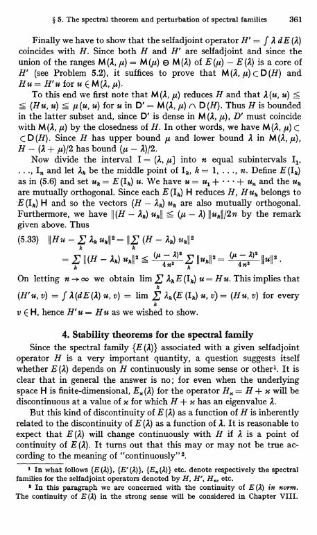
§ 5. The spectral theorem and perturbation of spectral families 361
Finally we have to show that the selfadjoint operator H' = f A dE (A)coincides with H. Since both H and H' are selfadjoint and since theunion of the ranges M (A, ,u) = M (,u) e M (A) of E (,u) - E (A) is a core ofH' (see Problem 5.2), it suffices to prove that M (A, ,u) C D (H) andHu = H' u for u E M (A, A.
To this end we first note that M (A, ,u) reduces H and that A (u, u)(Hu, u) s ,u (u, u) for u in D' = M (A, ,u) n D (H). Thus H is bounded
in the latter subset and, since D' is dense in M (A, 1u), D' must coincidewith M (A, ,u) by the closedness of H. In other words, we have M (A, ,u) CC D (H). Since H has upper bound ,u and lower bound A in M (A, ,u),H - (A + ,u)/2 has bound (,u - A)/2.
Now divide the interval I = (A, ,u] into n equal subintervals I,I,,, and let Ak be the middle point of Ik, k = 1, ..., n. Define E (Ik)
as in (5.6) and set uk = E (Ik) u. We have u = ul + + un and the upare mutually orthogonal. Since each E (Ik) H reduces H, Huk belongs toE (Ik) H and so the vectors (H - Ak) uk are also mutually orthogonal.Furthermore, we have II (H - Ak) ukll <__ (a - A) IIukII/2n by the remarkgiven above. Thus
(5.33) II Hu - E AP ukII2 = 11Z (H - Ak) ukII2k
= G II (H - 2k) uk112 4.n2 )2 IIukII2 = 0A4-n2 )2 IIuII2 .
A;
On letting n -s oo we obtain lim Ak E (Ik) u = Hu. This implies thatk
(H'u, v) = f A(dE(A) u, v) = lim A,, (E (Ik) u, v) _ (Hu, v) for everyk
v E H, hence H'u = Hu as we wished to show.
4. Stability theorems for the spectral familySince the spectral family {E (A)} associated with a given selfadjoint
operator H is a very important quantity, a question suggests itselfwhether E (A) depends on H continuously in some sense or other'. It isclear that in general the answer is no; for even when the underlyingspace H is finite-dimensional, Ex (A) for the operator H,, = H + x will bediscontinuous at a value of x for which H + x has an eigenvalue A.
But this kind of discontinuity of E (A) as a function of H is inherentlyrelated to the discontinuity of E (A) as a function of A. It is reasonable toexpect that E (A) will change continuously with H if A is a point ofcontinuity of E (A). It turns out that this may or may not be true ac-cording to the meaning of "continuously".
' In what follows {E (A)}, {E, (A)} etc. denote respectively the spectralfamilies for the selfadjoint operators denoted by H, H', H,,, etc.
9 In this paragraph we are concerned with the continuity of E (A) in norm.The continuity of E (A) in the strong sense will be considered in Chapter VIII.
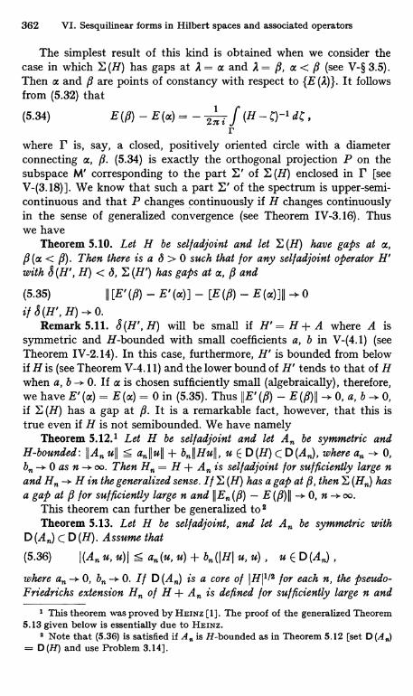
362 VI. Sesquilinear forms in Hilbert spaces and associated operators
The simplest result of this kind is obtained when we consider thecase in which E (H) has gaps at A = a and A = f4, a < fi (see V-§ 3.5).Then a and fi are points of constancy with respect to {E (A)}. It followsfrom (5.32) that
(5.34) E(19)-E(a)=-2nif (H-C)-1dCr
where r is, say, a closed, positively oriented circle with a diameterconnecting a, P. (5.34) is exactly the orthogonal projection P on thesubspace M' corresponding to the part E' of E (H) enclosed in r [seeV-(3.18)]. We know that such a part E' of the spectrum is upper-semi-continuous and that P changes continuously if H changes continuouslyin the sense of generalized convergence (see Theorem IV-3.16). Thuswe have
Theorem 5.10. Let H be self adjoint and let E (H) have gaps at a,(a < j9). Then there is a 6 > 0 such that for any self adjoint operator H'
with S (H', H) < 6, E (H') has gaps at a, ,B and
(5.35) II [E' (19) - E(a)] - [E (19) - E (or)] 11 -> 0if 6(H',H)-.0.
Remark 5.11. S (H', H) will be small if H' = H +A where A issymmetric and H-bounded with small coefficients a, b in V-(4.1) (seeTheorem IV-2.14). In this case, furthermore, H' is bounded from belowif H is (see Theorem V-4.11) and the lower bound of H' tends to that of Hwhen a, b -> 0. If at is chosen sufficiently small (algebraically), therefore,we have E' (a) = E (a) = 0 in (5.35). Thus II E' (f3) - E (fl) II -+ 0, a, b -+ 0,if E (H) has a gap at j9. It is a remarkable fact, however, that this istrue even if H is not semibounded. We have namely
Theorem 5.12.1 Let H be sel f adjoint and let A,, be symmetric andH-bounded: II A uIi 5 anIIu1I + b,, 11 Hull, u E D(H) c D(A,,), where a -+ 0,b -+ 0 as n -* oo. Then H,,, = H + A is sel f adjoint for sufficiently large nand H,,, -- H in the generalized sense. If E (H) has a gap at f3, then E hasa gap at fi for sufficiently large n and II E,, (f4) - E (f4) II -* 0, n -+ oo.
This theorem can further be generalized to 2Theorem 5.13. Let H be selfadjoint, and let A be symmetric with
D (A,,,) C D (H). Assume that
(5.36) (An u, u) 15 a (u, u) + b (I HI u, u) , u E D (A,,.) ,
where a --I 0, b -+ 0. If D (A,,) is a core of IHII/2 for each n, the pseudo-Friedrichs extension H,,, of H + A,,, is defined for sufficiently large n and
I This theorem was proved by HEINZ [1]. The proof of the generalized Theorem5.13 given below is essentially due to HEINZ.
8 Note that (5.36) is satisfied if A. is H-bounded as in Theorem 5.12 [set D (A.)= D (H) and use Problem 3.14].
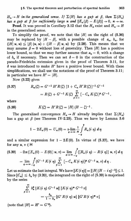
§ 5. The spectral theorem and perturbation of spectral families 363
H. -> H in the generalized sense. It E (H) has a gap at 9, then E (H,, )has a gap at j9 for sufficiently large n and II E (P) - E (19) II - 0, n - oo.
Proof. It was proved in Corollary 3.12 that the H,n exist and H,n Hin the generalized sense.
To simplify the proof, we note that the IHI on the right of (5.36)may be replaced by IH - #I, with a possible change of a, bn, for(IHI u, u) s I flI (u, u) + (IH - #1 u, u) by (2.28). This means that wemay assume fl = 0 without loss of generality. Then IHI has a positivelower bound, so that we may further assume that an = 0, with a changeof bn if necessary. Then we can set 6 = 0 in the construction of thepseudo-Friedrichs extension given in the proof of Theorem 3.11, forS was introduced to make H' have a, positive lower bound. With thesesimplifications, we shall use the notations of the proof of Theorem 3.11;in particular we have H' = IHI.
Now (3.22) gives
(5.37) R. (C) = G'-1 H'R(C) [1 + C. H'R(C)]-1 G'-100
E [-C.K(C)]pG'-1,p=1
where
(5.38) K (C) = H'R (C) = IHI (H -The generalized convergence H,, -* H already implies that E (H,,)
has a gap at /1 (see Theorem IV-2.25). Thus we have by Lemma 5.6e
1 - 2E,, (0) = U (0) = s-lim 1 f R,, (in) d rle-+OO n
-eand a similar expression for 1 - 2E(0). In virtue of (5.37), we havefor any u, v E H
e(5.39) E(0)] u, v) = lim f rl) - R(i rl)] u, v) d9J
e-* °° -eQ
00= lim f (G'-1 K(i q) ,' [-C K(i rl)]Q G'-1 u, v) d9l .
e->M_e p=1
Let us estimate the last integral. We have IIK(i r1)II = II IHI (H - i r1)-iII S 1.Since IIC,II s bn by (3.20), the integrand on the right of (5.39) is majorizedby the series
CO
' b IIK(i n) G'-1 uII II K(i 9)* G'-1 vIIP=1
1 b*bn 11 G' R(i 9l) uhi IIG'R(i 97)* vII
(note that IHI = H'= G12).
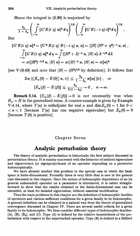
364 VII. Analytic perturbation theory
Hence the integral in (5.39) is majorized by
b1 - b
But
i/z
fG'R(_1V2d97)112.fG'R(i)uII2d- 00 - 00
(H2+92)_'u,u),00 00
IIIG'R(i ii) ullzdii= f ((H2+ A) u, IHI u)2-'/2d2-00 0
_r((H2)-'lzu,IHI u)=n(IHL'u,IHIu)_;IIIuIIZ
[see V-(3.43) and note that IHI = (H2)'/2 by definition]. It follows that
2n I([En(o) - E(0)] u, v) I s1 IIvii , or
IIEn(Y)-E(N)II5 2(1-bn)-> 0, n
Remark 5.14. II En (,9) - E (9) II 0 is not necessarily true whenH - H in the generalized sense. A counter-example is given by ExampleV-4.14, where T(x) is selfadjoint for real x and dimEx(0) = 1 for 0 << x < 1 [because T (x) has one negative eigenvalue] but Ee (0) = 0[because T (0) is positive].
Chapter Seven
Analytic perturbation theoryThe theory of analytic perturbation is historically the first subject discussed in
perturbation theory. It is mainly concerned with the behavior of isolated eigenvaluesand eigenvectors (or eigenprojections) of an operator depending on a parameterholomorphically.
We have already studied this problem in the special case in which the basicspace is finite-dimensional. Formally there is very little that is new in the generalcase discussed in this chapter. Once the notion of holomorphic dependence of an (ingeneral unbounded) operator on a parameter is introduced, it is rather straight-forward to show that the results obtained in the finite-dimensional case can beextended, at least for isolated eigenvalues, without essential modification.
Thus the main problems in this chapter are the definition of holomorphic familiesof operators and various sufficient conditions for a given family to be holomorphic.A general definition can be obtained in a natural way from the theory of generalizedconvergence discussed in Chapter IV. There are several useful criteria for a givenfamily to be holomorphic. We thus consider different types of holomorphic families:(A), (B), (B0), and (C). Type (A) is defined by the relative boundedness of the per-turbation with respect to the unperturbed operator. Type (B) is defined in a Hilbert
§ 1. Analytic families of operators 365
space in terms of a holomorphic family of sesquilinear forms, where the perturbingform is relatively bounded with respect to the unperturbed form. Type (Bo) is aspecial case of (B) and is related to the notion of Friedrichs extension. Type (C) isformally similar to (B0) but differs from it in many respects. It is a matter of coursethat each of these special types has its own special properties.
§ 1. Analytic families of operators1. Analyticity of vector- and operator-valued functions
In what follows we are concerned with a family u (x) of vectors in aBanach space X or a family T (x) of operators from X to another Banachspace Y, and we are particularly interested in the case in which u (x) orT (x) is holomorphic in x in a domain D of the complex plane. We havealready defined u (x) to be holomorphic if it is differentiable at eachx E D; it is immaterial whether the differentiation is taken in the strongor weak sense (see III-§ 1.6). Thus u (x) is holomorphic if and only if(u (x), f) is holomorphic in x for every / E X*. For applications, thefollowing criterion is often convenient : u (x) is holomorphic in x if andonly if each x E D has a neighborhood in which 1Iu (x) 11 is bounded and(u (x), f) is holomorphic for all fin a fundamental subset of X* (see RemarkIII-1.38).
Sometimes we consider a family u (x) depending on a real parameter x,a < x < b. u (x) is real-holomorphic if u (x) admits a Taylor expansion ateach x. In such a case u (x) can be extended by the Taylor series tocomplex values of x in some neighborhood D of the real axis. The extendedu (x) is a holomorphic family for x E D.
Example 1.1. Let X = Ln(0, oo), 1:5 p < oo, and let u(x) = u(x; x) = e-"x.In order that u (x) E X, x must be restricted to the half-plane Re x > 0. Sincedu (x)ldx = - x u (x) E X, u (x) is holomorphic for Re x > 0. If we take X = LP (a, b)
for a finite interval (a, b), u (x) = e-x F is holomorphic for all x. Next set u (x)= u (x; x) _ (x - x)-' and X = LP (a, b), (a, b) being finite or infinite. u (x) isholomorphic in the domain obtained from the whole plane by removing the pointsa:5' x5 b on the real axis.
In considering an operator-valued holomorphic function T (X),we first restrict ourselves to the case T (x) E 9 (X, Y). T (x) is holomorphicif it is differentiable in norm for all in a complex domain. Again wehave the criterion : T (x) E 69 (X, Y) is holomorphic if and only if each xhas a neighborhood in which T (x) is bounded and (T (x) u, g) is holomorphicfor every u in a fundamental subset of X and every g in a fundamentalsubset of Y* (see III-§ 3.1).
We note also that if T (x) E 2K Y) is holomorphic and T (xo) E
E -V(Y, X) exists, then T (x)-1 exists, belongs to M(Y, X) and is holo-morphic for sufficiently small Ix - xoj. This is a consequence of thestability theorem for bounded invertibility (see the Neumann series
366 VII. Analytic perturbation theory
expansion of the inverse in Theorem IV-1.16) ; we have (d/dx) T (x)-11_ - T (x)-1(d T (x)/dx) T (x)-1 by I-(4.28).
A real-holomorphic family T (x) can be defined as in the case of avector-valued, real-holomorphic family u (x) ; T (x) can be extendedto a holomorphic family on some domain D of the complex.plane.
2. Analyticity of a family of unbounded operatorsFor applications it is not sufficient to consider bounded operators
only, and the notion of analytic dependence of a family of operators on aparameter needs to be generalized to unbounded operators. In order todistinguish the current sense of holomorphy from the extended sense tobe introduced in a moment, we shall say T(m) is bounded-holomorphic ifT (x) E 2 (X, Y) and T (x) is holomorphic in the sense so far considered.
The extension to unbounded operators is suggested by the notion ofgeneralized convergence introduced in IV-§ 2.4. A family of operatorsT (x) E ' (X, Y) defined in a neighborhood of x = 0 is said to be holo-morphic at x = 0 (in the generalized sense) if there is a third Banachspace Z and two families of operators U (x) E 9 (Z, X) and V (x) E 9 (Z, Y)which are bounded-holomorphic at x = 0 such that U (x) maps Z ontoD(T(x)) one to one and
(1.1) T (m) U (m) = V (x)1 .
T (m) is holomorphic in a domain D of the complex plane if it is holo-morphic at every x of D. If T (x) is holomorphic, then it is continuous in xin the generalized sense: T (x) -+ T (xo) in the generalized sense if x -+ xo,as is seen from Theorem IV-2.29.
The new notion is a generalization of the old one: T (n) E -4 (X, Y) isholomorphic in the new sense if and only if it is bounded-holomorphic.To prove the "only if" part, it suffices to note that the U(x) of (1.1)maps Z onto X so that U(x)-' E -4 (Y, X) (see Problem III-5.21). ThenU (x) is bounded-holomorphic (see par. 1), and the same is true of T (x)= V (x) U(x)-1.
We note also that if T (x) is holomorphic and T (xo) E -4 (X, Y), thenT (x) E 9 (X, Y) for sufficiently small Ix - xol [so that T (x) is bounded-holomorphic for such x]. This is a- consequence of Theorem IV-2.23, 'forT (x) is continuous in x in the sense of generalized convergence.
The notion of a real-holomorphic family T (m) could be defined inthe same way by requiring only that U(m), V(x) be real-holomorphic.
1 This definition corresponds to Theorem IV-2.29, which gives a sufficientcondition for generalized convergence. It is a formal generalization of a definitiongiven by RELLlcx [3], in which Z = X = Y is assumed.
§ 1. Analytic families of operators 367
But it is in general impossible to extend a real-holomorphic family to acomplex-holomorphic family. It is true that U (x) and V (x) can beextended to complex x, but U(x) may not be a one-to-one mapping fornonreal x 1.
Problem 1.2. If T (x) is holomorphic and A (x) is bounded-holomorphic, T (x) ++ A (x) is holomorphic.
Theorem 1.3.2 Let T (x) E V (X) be defined in a neighborhood of x = 0and let c E P(T (0)). Then T (x) is holomorphic at x = 0 if and only if
E P(T (x)) and the resolvent R (C, x) = (T (x) - c)-1 is bounded-holo-morphic for sufficiently small jxj. R (C, x) is even bounded-holomorphic in thetwo variables on the set of all , x such that E P(T(0)) and 1XI is sufficientlysmall (depending on C).
Proof. The proof is similar to the corresponding one for generalizedconvergence (see IV-§ 2.6). Suppose T (x) is holomorphic and let U(x),V (x) be as in (1.1). We have (T (x) - ) U(x) = V (x) - C U (m), andV (0) - C U (0) maps Z onto X one to one. Therefore its inverse belongsto R (X, Z) and [V (x) - C U (x) ]-1 is bounded-holomorphic near x = 0(see a similar argument above). Thus (T (x) - )-1= U(x) [V (x) -- U(x)]-1 is bounded-holomorphic. Conversely, suppose that x)is bounded-holomorphic in x. We need only to set Z = X, U (x) = R (c, x),V (x) = I + C U(x) to satisfy (1.1). That R x) is holomorphic in thetwo variables follows from Theorem IV-3.12, according to which R (C, x)is holomorphic in C and R(C0, x).
The holomorphy of T (m) as defined here is peculiar in that a T (M)may be holomorphic for all complex x, including x = oo 8, without beingconstant. An example is given by
Example 1.4. Let T (m) be the ordinary differential operator on the interval(0, 1) given by T (x) u = - u" with the boundary condition u (0) = 0, u'(1) + x u (1)= 0. T (x) depends on x only through the boundary condition at x = 1. It is definedeven for x = oo; then the boundary condition is u (1) = 0 by definition. The resolv-ent R (C, x) is an integral operator with kernel (the Green function) g (y, x; C, x)given by
siniy[cosCT(1-x) +xC`$sinC(1 -x)]j cos Cg + x sin Cyl
1 For example let T (x) = (U - x) -1 for real x, where U E 6W (X). Suppose Uhas a set of nonreal eigenvalues dense in a complex neighborhood of 0. Then T (x) isreal-holomorphic [as is seen by taking U (x) = U - x, V (x) = 1], but it cannot beextended to complex x. In fact 0 E P (T (0)) since T (0) = U E 61 (X) ; hence0 E P (T (x)) and T (x)-1 is bounded-holomorphic for sufficiently small Ixl if such anextension exists (Theorem 1.3). Then we must have T (x)-1 = U - x since this istrue for real x. But this is a contradiction since U - x is not invertible if x is aneigenvalue.
2 This theorem is due to RELLICH [3] when T (x) is a selfadjoint family (see § 3).8 As usual, T (x) is holomorphic at x = oo if T (lax) is holomorphic at x = 0
with a suitable definition of T (oo).
368 VII. Analytic perturbation theory
for 0 5 y;5 x :!g 1, with x, y exchanged if x5 y. For a fixed C. (1.2) is holomorphicin x with the single exception of a pole at x = -C1/2 cot Y,l/s. For any given x,, a Ican be found such that x is not a pole if it is near enough to xo. According to Theorem1.3, therefore, T (x) is holomorphic in the whole complex plane including x = oo.
Example 1.5. Similarly, let T (m) be the operator T (m) u = - u" with theboundary condition u(0) = 0, x u'(1) - u(1) = 0. T(x) is identical with theT (-x'1) of Example 1.4 and is holomorphic for all x. R (C, x) is given by theGreen function V-(4.16).
Remark 1.6. Does the holomorphic function T (x) defined abovepossess the unique continuation Property? In other words, let T, (x) andT2 (x) be holomorphic in a (connected) domain D and let T, T2 (x.)for a sequence {x,,} converging to a point xo E D different from any ofthe x,,. Then is it true that T, (x) = T2 (x) for all x E D ? It is not clearwhether this is true in general. But it is if Y = X and T, (x), T2 (x) havenonempty resolvent sets for every x E D.
To see this, we first note that T, (x,,) = T2 T1, implies T, (xo)= T2 (xo) = To in virtue of the uniqueness of the generalized limit. LetCo E P (To) ; then R (Co, T, (x)) and R (Co, T2 (x)) exist and are bounded-holomorphic in a neighborhood of xo by Theorem 1.3. Since the uniquecontinuation theorem holds for bounded-holomorphic functions justas for numerical functions [it is sufficient to consider the function(R (CO, T, (x)) u, /) for fixed u E X and / E X*], we conclude thatR(Co, T, (x)) = R (Co, T2 (x)), and therefore T, (x) = T2 (x), in this neigh-borhood.
It is now easy to show that T, (x) = T2 (x) holds for all x E D. Thisextension of the domain of validity of T1 (x) = T2 (x) from a neighborhoodto the whole D follows the standard pattern' and may be omitted.
3. Separation of the spectrum and finite systems ofeigenvalues
Theorem 1.7. If a family T (x) E ' (X) depending on x holomorphicallyhas a spectrum consisting of two separated parts, the subspaces of X cor-responding to the separated parts also depend on x holomorphically.
Comment and proof. To be precise, this theorem means the following.Let T (x) be holomorphic in x near x = 0 and let E (0) = E (T (0)) beseparated into two parts E' (0), E" (0) by a closed curve r in the mannerdescribed in III-§ 6.4. Since T (x) converges to T (0) as x 0 in thegeneralized sense, it follows from Theorem IV-3.16 that r c P (x)= P(T (x)) for sufficiently small Ixl and E (x) = E (T (x)) is likewiseseparated by r into two parts 1'(x), E" (x) with the associated decom-position X = M' (x) ® M" (x) of the space. The projection on M' (x) along
1 See KNOPP (l), p. 87.
§ 1. Analytic families of operators 369
M" (x) is given by
(1.3) P (x) _- 2, i ,l R (C, x) d Cr
by IV-(3.11). Since R (C, x) is bounded-holomorphic in C and x jointlyby Theorem 1.3, it follows from (1.3) that P (x) is bounded-holomorphicnear x = 0. This is what is meant by saying that the subspaces M' (x),M" (x) depend on x holomorphically.
When E (x) is separated as in Theorem 1.7, the eigenvalue problemfor T (x) is reduced to the eigenvalue problems for the parts of T (x) inthe two subspaces M' (x), M" (x). But it is somewhat inconvenient thatthese subspaces depend on x. This inconvenience can be avoided by thefollowing device.
Since the projection P (x) on M' (x) is holomorphic in x, there exists atransformation function U (x) E -4 (X) which is bounded-holomorphictogether with its inverse U (x) i E R (X) and which transforms P (0)into P (x) :
(1.4) P(x) = U(x) P(0) U(x)-';
see II-§ 4.2, the results of which are valid in a Banach space X as well.Since T (m) commutes with P (x) (see 111-§ 6.4), it follows that theoperator
(1.5) T (x) = U (x)-1 T (x) U (x)
commutes with P (0). Thus the pair M'(0) = P (0) X and M" (0) = (1 -- P (0)) X decomposes T (x) for all x. But the eigenvalue problem for thepart of T (x) in M' (x) is equivalent to that for the part of T (x) in M' (0),for the eigenvalues (if any) are the same for the two parts and the eigen-projections and eigennilpotents for them are related with each otherthrough transformation by U (x).
Let us describe this relationship in more detail under the assumptionthat Z'(0) consists of a finite system of eigenvalues (III-§ 6.5). ThenM' (0) is finite-dimensional and the same is true of M' (x) by (1.4). Let
(1.6) T (x) Ph (x) = Ah (x) Ph (x) + Dh (x) , h = 1, ..., s ,
be the solution of the eigenvalue problem for the part of T (x) in M' (0),where
(1.7)Ph (x) P (0) P (0) Ph (x) Ph (x)
Dh (x) P (0) = P (0) Dh (x) = Dh (x)
[see 1-(5.35)]. Then the solution for T (m) in M' (x) is given by
(1.8) T (m) Ph (x) = 2h (x) Ph (x) + Dh (x) , h= 11 ..., s ,
370 VII. Analytic perturbation theory
with(1.9) Ph (x) = U k Ph (x) U()-1, Dh (x) = U (M) Dh (x) U(m)-l.
Now all the results of Chapter II on the analytic perturbation theoryin a finite-dimensional space can be applied to the eigenvalue problemfor T (x) in the fixed subspace M' (0). In this way the study of a finitesystem of eigenvalues for T (m) has been reduced to that of a problemin a finite-dimensional space. Note that the part of T (m) in M'(0) isequal to the part in M' (0) of the bounded-holomorphic function T (m) P (0)= U (x)-1 T (x) P (x) U (m); T (x) P (x) is bounded-holomorphic as is seenfrom III-(6.24).
Recalling the results of II-§ 1.8, we have thus provedTheorem 1.8.1 I/ T (x) is holomorphic in x near x = 0, any finite
system of eigenvalues 2, (x) of T (x) consists of branches of one or severalanalytic functions which have at most algebraic singularities near x = 0.The same is true of the corresponding eigenprojections P, (m) and eigen-nilpotents Dh (x).
More detailed properties of these functions can be read from the resultsof II-§ 1, all of which are valid as long as we are concerned with a finitesystem of eigenvalues.
As an application, let us prove some theorems on "nonlinear eigen-value problems" a.
Theorem 1.9. Let T (x) be a family o l compact operators in X holo-morphic for x E Do. Call x a singular point i f 1 is a an eigenvalue o t T (x).Then either4 all x E Do are singular points or there are only a finite number ofsingular points in each compact subset o l Do.
Proof. Let xo ED,. If xa is not singular, 1 E P(T (xa)) since T (xo) iscompact. Then 1 E P(T (x)) for sufficiently small Ix - xoj, by Theorem 1.3.If xa is singular, 1 is an isolated eigenvalue of T (xa) with finite multi-plicity (see III-§ 6.7). It follows from Theorem 1.8 that T (x) has only afinite system of eigenvalues in some neighborhood of 1 if Ix - xa1 issmall and that these eigenvalues have at most an algebraic singularityat x = xo. If some of these eigenvalues are identically equal to 1, all the xnear xo are singular. Otherwise there is no singular point x + xa if Ix - xojis sufficiently small.
1 This theorem was proved by Sz.-NAGY [2], WOLF [1], T. KATO [6]. See alsoBAUMGARTEL [1] (which contains the most complete description of the analyticfunctions Ar,(x) etc.), SCHAFKE [1]-[5].
8 See footnote 1 of p. 35. If T (x) = x T where T is compact, a singular point xin Theorem 1.9 is the reciprocal of an eigenvalue of T. This is the reason why wespeak of a "nonlinear eigenvalue problem". Theorem 1.9 is due to ATKINSON [2](see also Sz. -NAGY [4]) where T (x) is assumed to be a polynomial in x.
8 The value 1 has no particular meaning; it can be replaced by any a = 0.' The first alternative is excluded if 11 T (xo) 11 < 1 for some xo E Do.
§ 1. Analytic families of operators 371
Summing up, for each x, E Da there is a neighborhood D such thateither every x E D is singular or no x E D is singular except xo. Theresult follows immediately.
Theorem 1.10. Let T (x) E ' (X) be a holomorphic family for x ED,and let T (x) have compact resolvent for each x. Call x a singular Point i f 0is' an eigenvalue o l T (x). Then the same result holds as in Theorem 1.9.
Proof. For each xo, there is a nonzero u E P(T (xa)) and Cu R (C,0, x)is compact and holomorphic in x near xa. A singular point x is a singularpoint for the compact family - a R (Ca, x) in the sense of Theorem 1.9.Hence the result follows at least in some neighborhood of xo. But sincexo E Do is arbitrary, the same is true in the whole of Do.
4. Remarks on infinite systems of eigenvaluesWhen an infinite, number of eigenvalues of T (m) are considered
simultaneously, various complications arise2. To make the situationsimpler, suppose that T (x) has compact resolvent for each x ED,.For convenience assume that x = 0 belongs to Do. Then each eigenvalueA (0) of T (0) is isolated with finite multiplicity and can be continued toone or several eigenvalues A (x) of T (x), each of which is analytic in acertain domain D' C Do. D' may be large for some A (x) and small forothers. Furthermore, these A (x) need not exhaust all the eigenvalues ofT (x), no matter how small jxj is. In an extreme case T (0) may have noeigenvalue at all (empty spectrum) while T (x) for x + 0 has an infinitenumber of eigenvalues. Thus it is in general impossible to speak of "theset of all eigenvalues of T (x) as analytic functions of x."
Example 1.11. Consider the family T (x) of Example I.S. Here T (x) is holo-morphic in the whole extended complex plane and has compact resolvent. For afixed x, the eigenvalues of T (x) are given as the zeros of the entire function
C-1/2 sinV2 - x cost'/5
that appears in V-(4.16) as the denominator of the Green function. The eigenvaluesfor x = 0 are A = ns n8, n = 1, 2, ... and the associated eigenfunctions j sinn n xform a complete orthonormal family in H = L2 (0, 1). Since each of these eigen-values is simple, the corresponding eigenvalue A. (x) of T (m) is holomorphic in aneighborhood of x = 0. For real x, it is evident from Fig. 1 (see p. 292) thatA. (x) - A grows with n for fixed x, suggesting that the convergence of the powerseries of A (x) becomes worse with increasing n.
There is another peculiarity in this example. It is easily verified that the A. (x)are the only eigenvalues of T (x) for x S 0, but another eigenvalue AO (x) exists forx > 0. If 0 < x < 1, AO (x) is given by AO (x) = - Q (x)$ where e (x) is determined asthe unique positive root of the equation tanh Q = x Q. Ao (x) is holomorphic on and
1 Again the value 0 may be replaced by any complex number.2 See RELLICR [5], which contains Example 1.11 below and other examples.
372 VII. Analytic perturbation theory
near the positive real axis, and Ao (x) -* - oo when x ' 0; it cannot be continued tox < 0 as long as x is confined to a real neighborhood of x = 01.
If complex values of x are considered, it turns out that all the A. (x), includingn = 0, have analytic continuations and constitute a single analytic function A (x),which is exactly the inverse function of the meromorphic function C-1/2This analytic function A(x) behaves in a very complicated way near x = 0; thereare branch points which accumulate at x = 0. This explains the absence of thegraph of AO (x) for x < 0; within any neighborhood of x = 0, it is possible to gofrom the branch AO (x) to any A. (x) with sufficiently large n by circling around anappropriate branch point.
The convergence radii of the series expansion of the A. (x) could be determinedif these branch points were computed.
Example 1.12. As a simpler example than the preceding one, consider thefirst order differential operator T (x) _ - i d(dx, 05 x S 1, with the boundarycondition (1 + i x) u(0) _ (1 - i x) u(1). As in the preceding example, it is easilyseen that T (m) is holomorphic for all complex x including x = oo. The eigenvaluesof T(m) are
(1.10) : L
T(e) is selfadjoint for real x if considered in the Hilbert space L2(0, 1), and theeigenvalues A. (x) are real for real x. It is seen from (1.10) that the Taylor series foreach has the convergence radius 1. If x is unrestricted, all the form asingle analytic function 2 arctanx, which has logarithmic singularities at x = ± i.
It is instructive to inquire what these singularities mean with respect to T (m).The answer is that T (± i) have no eigenvalues at all : their spectra are empty.If T (i) is regarded as the unperturbed operator with the perturbation parameterx' = x - i, there is no perturbation series for T (x) = T (i + x') to be considered(hence there is no contradiction to the general result that the perturbation seriesfor simple eigenvalues are convergent Taylor series).
Remark 1.13. In the above examples, T(m) is holomorphic butD (T (x)) varies with x. Better behavior may be expected of the eigen-values in the case where T (x) has a constant domain. We shall discussthis question later (see §§ 3.5, 4.7).
5. Perturbation seriesThe formal series in powers of x for the eigenvalues etc. of T (m) in a
finite system, as considered in par. 3, can be obtained by the method ofII-§§ 2, 3 applied to the operator
(1.11) Tr (x) = T (x) P (x) = Tr + x Ty1) + xa T;$) + .. .
which is bounded-holomorphic in x. The following remarks should beadded.
1 For real x, T (m) is selfadjoint and its eigenvectors 97.(x) form a completeorthonormal family. If x > 0, this family contains the eigenvector quo (x) for theeigenvalue AO (x). Thus if one starts from the complete family {q/ (0)}, n 1, forT (0) and considers the perturbed family {p (x)}, n > 1, one sees that the latteris not complete for x > 0.
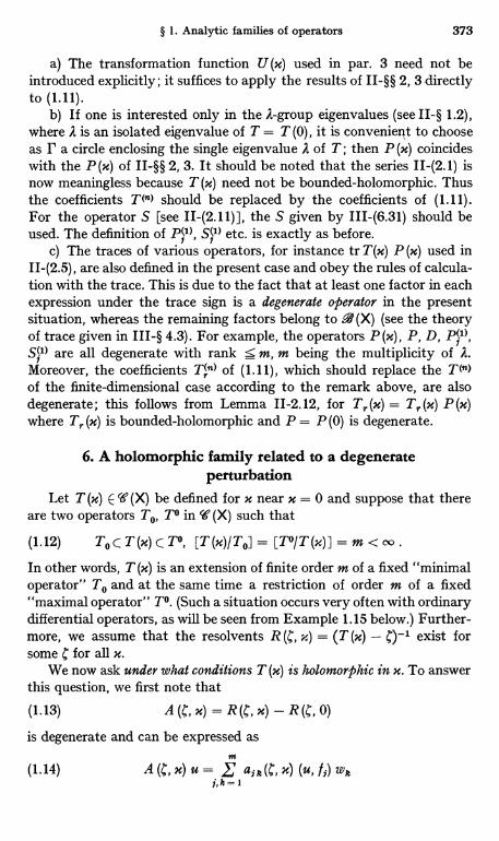
§ 1. Analytic families of operators 373
a) The transformation function U (x) used in par. 3 need not beintroduced explicitly; it suffices to apply the results of II-§§ 2, 3directlyto (1.11).
b) If one is interested only in the R-group eigenvalues (see II-§ 1.2),where 2 is an isolated eigenvalue of T = T (0), it is convenient to chooseas P a circle enclosing the single eigenvalue R of T ; then P (x) coincideswith the P(x) of II-§§ 2, 3. It should be noted that the series II-(2.1) isnow meaningless because T (m) need not be bounded-holomorphic. Thusthe coefficients T() should be replaced by the coefficients of (1.11).For the operator S [see II-(2.11)], the S given by III-(6.31) should beused. The definition of P(l), SJ(i> etc. is exactly as before.
c) The traces of various operators, for instance tr T (x) P (m) used inII-(2.5), are also defined in the present case and obey the rules of calcula-tion with the trace. This is due to the fact that at least one factor in eachexpression under the trace sign is a degenerate operator in the presentsituation, whereas the remaining factors belong to .4 (X) (see the theoryof trace given in III-§ 4.3). For example, the operators P(x), P, D, P(10,S(') are all degenerate with rank < m, m being the multiplicity of R.Moreover, the coefficients T"> of (1.11), which should replace the T011of the finite-dimensional case according to the remark above, are alsodegenerate; this follows from Lemma 11-2.12, for T,. (x) = T,. (x) P (m)where T,. (x) is bounded-holomorphic and P = P (0) is degenerate.
6. A holomorphic family related to a degenerateperturbation
Let T (x) E (f (X) be defined for x near x = 0 and suppose that thereare two operators T°, TO in ' (X) such that
(1.12) To c T (m) c TO, [T (x)I T°] = [T°/T()] = m < co.
In other words, T (x) is an extension of finite order m of a fixed "minimaloperator" To and at the same time a restriction of order m of a fixed"maximal operator" TO. (Such a situation occurs very often with ordinarydifferential operators, as will be seen from Example 1.15 below.) Further-more, we assume that the resolvents R (C, x) = (T (x) - C)-1 exist forsome C for all x.
We now ask under what conditions T (x) is holomorphic in x. To answerthis question, we first note that
(1.13) A (C, x) = R (C, x) - R (C, 0)
is degenerate and can be expressed as
(1.14) A (C, x) u = ask (C, x) (u, f9) wk9,k=1
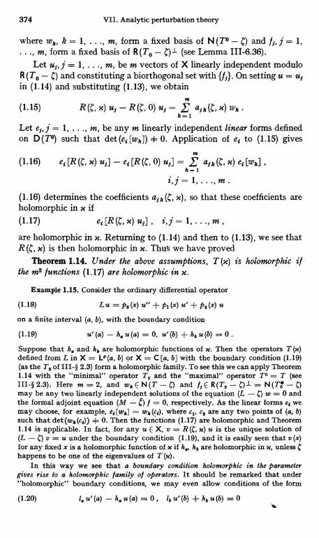
374 VII. Analytic perturbation theory
where wk, k = 1, ..., in, form a fixed basis of N (T° - C) and f;, j = 1,., m, form a fixed basis of R (T° - )1 (see Lemma 111-6.36).Let j = 1, ..., m, be m vectors of X linearly independent modulo
R (T° - and constituting a biorthogonal set with {f}. On setting u = usin (1.14) and substituting (1.13), we obtain
(1.15) R(C, x) u; - R(C, 0) is, a, k (C, x) wk .k=1
Let e,, j = 1, ..., in, be any m linearly independent linear forms definedon D (T°) such that det (ei [wk]) + 0. Application of ej to (1.15) gives
m
(1.16) ej [ R (C, x) u;] - ei [R (C, 0) u,] = a , , x) ej [wk] ,k=1
ij =1, M.
(1.16) determines the coefficients a, x), so that these coefficients areholomorphic in x if(1.17) ei[R(C,x)u;], i,j=1,...,m,are holomorphic in x. Returning to (1.14) and then to (1.13), we see thatR (C, x) is then holomorphic in x. Thus we have proved
Theorem 1.14. Under the above assumptions, T (x) is holomorphic ifthe m2 functions (1.17) are holomorphic in x.
Example 1.15. Consider the ordinary differential operator
(1.18) L u = p° (x) u" + p, (x) u' + p, (x) u
on a finite interval (a, b), with the boundary condition
(1.19) u' (a) - h, u (a) = 0, u' (b) + ho u (b) = 0 .
Suppose that h, and h, are holomorphic functions of x. Then the operators T (M)defined from L in X = LP (a, b) or X = C [a, b] with the boundary condition (1.19)(as the T. of III-§ 2.3) form a holomorphic family. To see this we can apply Theorem1.14 with the "minimal" operator To and the "maximal" operator TO = T (seeIII-§ 2.3). Here m = 2, and wk E N (T - C) and t j E R (T° - C)1 = N (To - C)
may be any two linearly independent solutions of the equation (L - C) w = 0 andthe formal adjoint equation (M - f) f = 0, respectively. As the linear forms ej wemay choose, for example, ej [wk] = wk (ci), where c1, c$ are any two points of (a, b)such that det (w,, (cr)) + 0. Then the functions (1.17) are holomorphic and Theorem1.14 is applicable. In fact, for any is E X, v = R (g, x) is is the unique solution of(L - C) v = u under the boundary condition (1.19), and it is easily seen that v (x)for any fixed x is a holomorphic function of x if h hb are holomorphic in x, unless Chappens to be one of the eigenvalues of T (x).
In this way we see that a boundary condition holomorphic in the parametergives rise to a holomorphic family of operators. It should be remarked that under"holomorphic" boundary conditions, we may even allow conditions of the form
(1.20) 1, u' (a) - h, u (a) = 0 , lb u' (b) + hb u (b) = 0
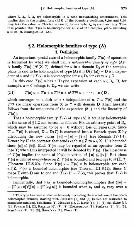
§ 2. Holomorphic families of type (A) 375
where d h la, hb are holomorphic in x with nonvanishing determinant. Thisimplies that, in the original form (1.19) of the boundary condition, h, (x) and hb (x)may take the value oo. This is the case if, for example, h hb are linear in X. Thusit is possible that T (x) is holomorphic for all x of the complex plane includingx = oo (cf. Examples 1.4, 1.5).
§ 2. Holomorphic families of type (A)1. Definition
An important special case of a holomorphic family T (m) of operatorsis furnished by what we shall call a holomorphic family of type (A)'.A family T (x) E ' (X, Y), defined for x in a domain Da of the complexplane, is said to be holomorphic of type (A) if i) D (T (x)) = D is indepen-dent of x and ii) T (x) u is holomorphic for x E Do for every u E D.
In this case T (m) u has a Taylor expansion at each x E D0. If, forexample, x = 0 belongs to Do, we can write
(2.1) T(x)u= Tu+xTl')u+x2T(2)u+... uED,
which converges in a disk I ml < r independent of u. T = T (0) and theT(') are linear operators from X to Y with domain D [their linearityfollows from the uniqueness of the expansion (2.1) and the linearity ofT (x)].
That a holomorphic family T (x) of type (A) is actually holomorphicin the sense of § 1.2 can be seen as follows. Fix an arbitrary point of D0,which may be assumed to be x = 0 without loss of generality. SinceT = T (0) is closed, D = D (T) is converted into a Banach space Z byintroducing the new norm IIIuIII = IIuII + IITull (see Remark IV-1.4).Denote by U the operator that sends each u E Z to u E X; U is boundedsince lull s IIIuIII Each T (x) may be regarded as an operator from Zinto Y; when thus interpreted it will be denoted by V (x). The closednessof T (x) implies the same of V (x) in virtue of lull S IIIuIII. But sinceV (x) is defined everywhere on Z, V (x) is bounded and belongs to a (Z, Y)(Theorem 111-5.20). Since V (x) u = T (x) u is holomorphic for eachu E Z, V (x) is bounded-holomorphic (see Theorem 111-3.12). Since Umaps Z onto D one to one and T (x) U = V (x), this proves that T (x) isholomorphic.
Incidentally, that V (x) is bounded-holomorphic implies that (IIuII ++ II V (xI) ubb)/(IIuII + II V (x2) uhi) is bounded when xl and x2 vary over a
1 This type has been studied extensively, including the special case of bounded-holomorphic families, starting with RELLICH [1] and [3] (which are restricted toselfadjoint families). See HEINZ [1], HOLDER [1], T. KATO [1], [3], [6], SZ.-NAGY [1],[2], PORATH [1], [2], RELLICH [6], [7], [8], ROSENBLOOM [1], SCHAFKE [3], [4], [5],SCHRODER [1], [2], [3], AMUL'YAN [1], WOLF [1].
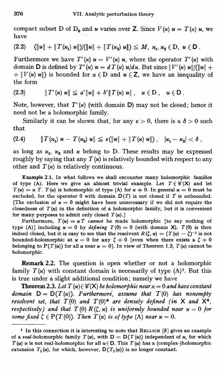
376 VII. Analytic perturbation theory
compact subset D of Da and u varies over Z. Since V (x) u = T (x) u, wehave
(2.2) (Ilull + II T (xl) ull)/(Ilull + II T (x2) ull) s M, xi, x2 E D, u E D.
Furthermore we have T' (x) u = V' (x) u, where the operator T' (x) withdomain D is defined by T' (x) u = d T (x) u/dx. But since 11 V' (x) uIl/(Ijull ++ 11 V (x) u11) is bounded for x E D and u E Z, we have an inequality ofthe form
(2.3) 11 T'(x) ull S a'jjujj +b'11 T(x) ull , xED, uED.Note, however, that T' (x) (with domain D) may not be closed; hence itneed not be a holomorphic family.
Similarly it can be shown that, for any e > 0, there is a 6 > 0 suchthat(2.4) IIT (xl) u - T(x2) ull s s(Ilull + I!T (x) uIU , Ixl - x21 < 6,
as long as x, x2 and x belong to D. These results may be expressedroughly by saying that any T (x) is relatively bounded with respect to anyother and T (m) is relatively continuous.
Example 2.1. In what follows we shall encounter many holomorphic familiesof type (A). Here we give an almost trivial example. Let T E W (X) and letT (x) = x T. T (x) is holomorphic of type (A) for x $ 0. In general x = 0 must beexcluded, for, the operator 0 with domain D(T) is not closed if T is unbounded.The exclusion of x = 0 might have been unnecessary if we did not require the
closedness of T (m) in the definition of a holomorphic family, but it is convenientfor many purposes to admit only closed T (m).]
Furthermore, T (x) = x T cannot be made holomorphic [to say nothing oftype (A) ] including x = 0 by defining T (O) = 0 (with domain X). T (O) is thenindeed closed, but it is easy to see that the resolvent R (C, x) = (T (x) - C)-' is notbounded-holomorphic at x = 0 for any C + 0 [even when there exists a C + 0belonging to P (T (x)) for all x near x = 0]. In view of Theorem 1.3, T (m) cannot beholomorphic.
Remark 2.2. The question is open whether or not a holomorphicfamily T (x) with constant domain is necessarily of type (A)1. But thisis true under a slight additional condition; namely we have
Theorem 2.3. Let T (x) E '(X) be holomorphic near x = 0 and have constantdomain D = D (T (x)). Furthermore, assume that T (0) has nonemptyresolvent set, that T (O) and T (O)* are densely defined (in X and X*,respectively) and that T (0) R (C, x) is uniformly bounded near x = 0 forsome fixed C E P (T (0)). Then T (x) is of type (A) near x = 0.
1 In this connection it is interesting to note that RELLlcx [5] gives an exampleof a real-holomorphic family T (x), with D = D (T (x)) independent of x, for whichT (x) u is not real-holomorphic for all u E D. This T (x) has a (complex-)holomorphicextension T, (x), for which, however, D (Ti (x)) is no longer constant.
§ 2. Holomorphic families of type (A) 377
Proof. Before giving the proof, we note that D (T (0)) = D (T (x))already implies that T (0) R x) and T (x) R (C, 0) belong to -4 (X)(see Problem 111-5.22). The essential assumption is that T (0) R (C, x)be uniformly bounded near x = 0.
For the proof we may assume = 0 for simplicity. Then R (0, x) isbounded-holomorphic by Theorem 1.3. Hence 0 (x; f) = (T (0) R (0, x) u, f)= (R (0, x) u, T (0) * f) is holomorphic near x = 0 for each it E X and/ E D (T (0)*) = D* E X*. Since D* is dense and II T (0) R (0, x)II is boundedin x by hypothesis, it follows from Theorem 111-3.12 and a remarkfollowing it that T (0) R (0, x) is bounded-holomorphic. Hence the sameis true of the inverse (T (0) R (0, x))-1 = T (x) R (0, 0) (see the remarkat the end of § 1.1). This implies that T (x) u is holomorphic for everyu E D (T (0)).
A holomorphic family of type (A) has many properties not shared bygeneral holomorphic families, as we shall see in the course of the followingsections. Here we note
Theorem 2.4. Let T (x) E `'(X) be holomorphic of type (A) and have nonemp-ty resolvent set for each x. Then T (x) has compact resolvent either for all xor for no x.
Proof. Let D' be the set of all x such that T (x) has compact resolvent ;we have to show that D' is open and closed relative to Do, the domainof definition of the family T (x). That D' is open follows from TheoremIV-3.17, for T (x2) is relatively bounded with respect to T (x1) if Ixs - X1I issufficiently small [see (2.4)]. On the other hand, Theorem IV-2.26shows that D' is closed relative to Do [here T (x) need not be of type (A)].
Example 2.5. An example opposite, in a certain sense, to Example 2.1 is furnish-ed by a family T (x) = (U + x)-1, where U E 2 (X) is quasi-nilpotent but invertible.Then D (T (x)) = X for x * 0 while D (T (0)) = R (U) is a proper subset of X. T (x)is holomorphic of type (A) for x +_ 0; in fact it is even bounded-holomorphic. It isinteresting to note that T (x) is holomorphic even when x = 0 is included, thoughit is no longer of type (A). This is verified by writing T (x) U (x) = 1, U (x) = U + X.
Suppose now that U is in addition compact. Then T (0) = U-1 has compactresolvent, for T(O)-1 = U is compact. But T (m) does not possess this property ifx + 0. This remark shows that Theorem 2.4 is not true for a general holomorphicfamily T (m).
2. A criterion for type (A)
Theorem 2.6.1 Let T be a closable operator from X to Y with D (T) = D.Let TO), is = 1, 2, ..., be operators from X to Y with domains containing D,and let there be constants a, b, c z 0 such that
(2.5) IITHull 5 c"'-1(a llull+b11Tull), u E D, n = 1, 2, . . . .
1 This theorem is essentially due to RELLICH [3] (where it is restricted to self-adjoint families).
378 VII. Analytic perturbation theory
Then the series (2.1) defines an operator T (x) with domain D for IxI < 1/c.If IxI < (b + c)-1, T (x) is closable and the closures T (x) for such x form aholomorphic family of type (A).
Remark 2.7. The form of the condition (2.5) is so chosen as to beparticularly convenient when T(2) = T(M) _ = 0. In this case we canchoose c = 0 if
(2.6) IIT(1)ullcallull+bIITull, uED.
Note also that the required constants a, b, c exist if the series (2.1) isfinite and the T(n) are T-bounded (see IV-§ 1.1).
Proof of Theorem 2.6. T(x) is well defined by (2.1) if IxI < c-1, for
Ilxn T(n) u + ... + xn+rT(n+?) uII <(cn-1IxIn + ... + cn+r-l Ixln+p) (allull + bIITull) <
s cn-llxln(1-clxl)-1(allull+bIITull)->0, n -aoo
and the series on the right of (2.1) converges.If we write (2.1) in the form T (x) u = T u + A (x) u, it follows from
the above inequality that
(2.7) IIA (x) uII s IxI (1- clxi)-1(aIluii + b11 Tull) , it E D .
Thus A (x) is T-bounded with T-bound not exceeding b IxI (1 - c IxI)-1,which is smaller than 1 if IxI < (b + c)-1. It follows from TheoremIV-1.1 that T (x) is closable for such x. Incidentally we note the followinginequality, which follows from IV-(1.3):
(2.8) allull + bII TuII s (1 - clxl) (1- (b + c) IxI)-1(aIIuII + bII T (x)uII).
Let T be the closure of T, with domain D ) D. D is converted into aBanach space Z by introducing the norm IIIuIII = (a + e) (lull + bIITullwhere e > 0. That T is the closure of T implies that D is dense in Z.Let V(n) be the operator T(n) regarded as an operator from Z to Y; V(n)is densely defined and II V(") uII 5 cn -1 IIIuIII Hence V M has closureV(n) E 9 (Z, Y) with II r(n)II S cn-1. If we denote by V (x) and V the T (x)and T, respectively, as operators from Z to Y, we have
(2.9) V (x) = V + x V(1) + x2 V(2) + . ,
and V (x) obviously has the closure V (x) obtained by replacing V and theV(n) by r and the 7(n) on the right of (2.9). Thus T (x) u = V (x) u isholomorphic for each u E D if IxI < (b + c)-1.
Remark 2.8. The inequalities (2.5) are also necessary for T (x) to beholomorphic of type (A), in the following sense. If T(m) is holomorphicof type (A) in a neighborhood of x = 0, we have the expansion (2.1) with
§ 2. Holomorphic families of type (A) 379
the coefficients TO) satisfying (2.5). This follows from the fact that theV (x) used above is bounded-holomorphic near x = 0 and, consequently,developable into a power series of the form (2.9). Then we have II M011 <s Mr-n where r is any positive number smaller than the convergenceradius of this series (Cauchy's inequality). Hence II T (n) U11 = II
V (n) U11 S
s Mr-nlllulll, which is equivalent to (2.5).
3. Remarks on holomorphic families of type (A)The results concerning a holomorphic family T (x) of operators are
simplified and become more explicit when T (x) is of type (A). Here wecollect such results in a series of remarks.
Remark 2.9. Suppose the spectrum E = E (T) of T is separated intotwo parts by a closed curve P. Then E (x) = E (T (x)) is likewise separatedby r for sufficiently small x by Theorem 1.7. Here we can estimate howsmall IxI should be. According to Theorem IV-3.18, it suffices thatIV-(3.14) be satisfied for all C E P, with the constants a, b replaced byalxl (1 - c Ixl)-1, blxl (1 - c IxI)-' in view of (2.7). This means thatseparation of the spectrum occurs at least if
(2.10) IxI < ro = min (a IIR (C, 7)11 + b 1l TR (C, T)11 + c)-1.
Then the projection P(x) given by (1.3) is holomorphic in x. If the partof E inside r is a finite system of eigenvalues, it follows that the eigen-values, eigenprojections and eigennilpotents of T (x) in question areanalytic for (2.10) with only algebraic singularities (see § 1.3).
Remark 2.10. The existence of the formal power series for T (x),which did not occur in the case of a general holomorphic family, makes itpossible to take over directly the results of II-§§ 1, 2 without replacingT(n) by T;n) (see § 1.5). This is due to the fact that II-(1.13) is valid inspite of the unboundedness of the TO); in fact, these operators appear inthe formulas there only in such combinations as T (n) R (c), TM S,TO) P, TO) D = TO) PD which all belong to .4 (X) (by Problem 111-5.22).In this way we see that all formulas of II-§§ 1, 2 are valid in the presentcase.
There is one important point to be noticed, however. The use of thetrace in a formula such as II-(2.28) is not justified here, for the operatorsthat appear under the trace sign are in general not degenerate. Never-theless the final result II-(2.29) (or similar formulas that follow) is true,in which all operators under the trace sign are degenerate because theycontain at least one factor P. This is easily seen by calculating theintegral explicitly in the fashion of II-(2.18) ; then it becomes a poly-nomial in operators of ,1 (X) each term of which contains, as just men-tioned, at least one degenerate factor. When one takes the trace of such a
380 VII. Analytic perturbation theory
monomial, the order of the factors can be changed cyclically. As iseasily verified, this amounts to the validity of II-(2.30).
Remark 2.11. For applications it is often convenient to generalize(2.5) tot
(2.11) IIT(n) uIl < cn-1 z(IIull, IITuJI) , u E D , n = 1, 2, ... .
Here x (s, t) is a nonnegative function of two variables s, t z 0 with thefollowing properties: i) x (s, t) is positive-homogeneous of order 1:x (k s, k t) = k x (s, t) fork > 0; ii) x (s, t) is monotonically increasing in s,t: x (s, t) x (s', t') for 0 _<_ s <_ s', 0 <_ t s t'. We can now generalizeTheorem 2.6 by replacing (2.5) by (2.11), the conclusion being that 7(x)is holomorphic o l type (A) for I.I < (x (+ 0, 1) + c)-1. Also (2.10) should bereplaced by
(2.12) ro = min(x(II T) 11 , II T)iI) + c)-1 .
Examples of the function x (s, t) are :
(2.13) as+bt, a(st)1/2, (as2+bt2)1/2,
It should be noticed that (2.11) actually implies (2.5) with appro-priate constants a, b. The point is that by strengthening the assumption,the conclusions are also strengthened.
Example 2.12. Consider the formal differential operator
(2.14) L (x) u = po (x, x) u" + pi (x. x) u' -}- pa (x. x) u
on a finite interval [a, b], in which the coefficients p, (x, x) are assumed to be holo-morphic in x near x = 0 (uniformly with respect to x) and real-valued for real x,with appropriate continuity properties with respect to z. Furthermore, let- p0 (x, x) Z 6 > 0 for real x. Let T (x) be the operator in X = C [a, b] orX = L9 (a, b) constructed from L (x) as the T1 of III-§ 2.3 [boundary condition u (a)= u (b) = 0]. T (x) satisfies the assumptions of Theorem 2.6. In fact T (x) can bewritten in the form (2.1) with T(n) u = L(n) u (T = T(0)) with the same boundarycondition as above, where(2.15) D' u = p(On) (x) u" + p( In) (x) u' + p2) (x) u
and the p(P) (x) are the coefficients of xn in the Taylor expansion of p, (x, x). Sincethese coefficients satisfy inequalities of the form jp() (x) 5 K Nn, the inequalities(2.5) follow from IV-(1.27). Recalling that the spectrum of T = T (O) consists ofisolated eigenvalues of multiplicity one (see Example 111-6.20), we see fromTheorem 2.6 that these eigenvalues are holomorphic in x near x = 0 together withthe associated eigenprojections.
Example 2.13. Consider the Schr6dinger operator
(2.16) L(x)u=-du+q(x)u+xq(i)(x)uin R3. Assume that the potential q (x) is real-valued and can be written in the formq = q0 + q1 where q1 E L2 (R') and q0 is bounded. Then there is a selfadjointrestriction H of L (0) [acting in H = L$ (R')] which is defined as the closure of the
1 See SCHR6DER [1], SCHAFKE [4], PORATH [1].
§ 2. Holomorphic families of type (A) 381
minimal operator (see V-§ 5.3). Actually D (H) is identical with D (Ho), where Hois the special case of H for q = 0, the multiplication operator Q = q (x) beingHo-bounded with relative bound zero. It follows that QM = 01) (x) is also Ho-bounded and hence H-bounded with relative bound zero if q(l) is likewise the sumof two real-valued functions of La and of L°°. Hence the operators T (M) definedas the closure of the minimal operators for the L (x) form a selfadjoint family oftype (A) defined for all complex x. It follows that the isolated eigenvalues andeigenprojections of T (m) are holomorphic in x at least in a neighborhood of thereal axis'.
4. Convergence radii and error estimatesThe estimates of the convergence radii and the errors for the perturba-
tion series given in the finite-dimensional case (see II-§ 3) can be takenover to the case of type (A) without essential modification. The projectionP (m) as given by (1.3) is holomorphic for Ixi < ro, where ro is givenby (2.10) or (2.12) as the case may be. In particular this is true for thetotal projection P (x) for the A-group eigenvalues of T (m) when A is anisolated eigenvalue of T with finite multiplicity m; then r should bechosen as a closed curve around C = A in such a way that ro becomes aslarge as possible. The weighted mean A (x) of these eigenvalues is alsoholomorphic for IxI < ro, so that the power series for P (x) and A (x) haveconvergence radii not smaller than ro. If the A-group consists of a singleeigenvalue A (x) (no splitting), which is certainly the case if m = 1, thenA (x) itself is a power series convergent for I ml < ro.
The results of II-§ 3.2-3 on majorizing series hold true withoutmodification; note that the operators in II-(3.10) are bounded in thecase under consideration (see Remark 2.10).
Other results of II-§ 3 are also useful in the present case. Naturallywe have to set N = oo in general in the formula II-(3.45) and the follow-ing ones in which the demension N of the underlying space X appearsexplicitly. These estimates may in general not be very sharp, butmost of them are still the best possible of their kind, since this was trueeven in the finite-dimensional case (see II-§ 3.5, in particular).
The estimate I I-(3.32) for (T - A) 99(x), which is also valid here,deserves special attention. Since T - A is in general an unboundedoperator, this estimate is rather strong. Combined with the estimateII-(3.30) for 92 (x) itself, it makes possible an error estimate of p (x) withrespect to a norm such as
(2.17) Iiiuiil = aIIuII + #II(T - A) ull
which is stronger than the original norm IIuII. In this way one is able toestimate, for example, the error of the eigenfunction in L°°-norm in a
' Here we used some results on selfadjoint families (see § 3).
382 VII. Analytic perturbation theory
theory within an L2-space, or estimate even the error of the derivativesof the eigenfunction.
Example 2.14. Let X = C [0, n] 1. Consider the family T (x) = T + x 2'(1)where T is the differential operator T u = - u" on the interval 0 5 x 5 n withthe boundary condition u (0) = u (n) = 0 (see Examples 111-6.21 and IV-3.20)and where T'1> is a bounded operator. Each eigenvalue An = n2 of T is isolatedand simple, so that the corresponding eigenvalue 2,, (x) of T (x) is holomorphic atleast for small IxI. Let us estimate the convergence radius for the Taylor series of
To this end we consider a closed curve r. similar to the IF, used in ExampleIV-3.20 but larger in size: IF. consists of the two parabolas = a$ - 1)$/400
1[see III-(6.49)] corresponding to a = n ± 2 and the two horizontal lines _
_1f (2n - 1)/n. It follows then from III-(6.48) that IIR(C)II < n - 2)forC E I. Since r. encloses exactly one eigenvalue A. of T, a lower bound for theconvergence radius of A. (x) is given by (2.10) with b = c = 0 and a = II T°'IIIn this way we obtain
(2.18) ro ? n - 2 I n a where a = II Vl>II
The coefficients An''> in the Taylor series of A (x) can be estimated, for example,by II-(3.5). For this we need the maximum distance o of A. = ne from r.. A straight-forward calculation gives the inequality o < (1 + 4 r 2)112 n S 1.2n, so that
(2.19) IA:)IC1.2n7ra l° n,v=1,2,...
(W.
- 1/2 J
This estimate is not very sharp, at least for small v. A better estimate can be obtainedfrom the method of majorizing series. For this we need the quantities p, q, s ofII-(3.15) for A = n2. Now the operator S = S. is an integral operator with the
nkernels (y, x) given by III-(6.46), so that 11 S11 is estimated by 11 S11 S sup f Is (y, x) I dx
0(see Example 111-2.11; note that X = C [0, n] here and the estimate for p = 00is applicable). Thus we have 2 IISII < 1.7/n and IIS - P/4n2II S j/2 /n. Sincewe knowthat IIPII = 4/n < 1.3 (see Example 111-3.23), p, q, s are estimated by II-(3.15) as
(2.20) p < 1.3 a, q < 1.7 a/n , s < 1.5/n .
Substitution of (2.20) into II-(3.21) gives a lower bound for the convergence radiusin question:(2.21) r > 0.136 n/a ,
which is not so sharp as (2.18) obtained above. But II-(3.22) gives
(2.22) IA;,1>I < 1.3 a, 2.3 a2/n , IA;,s>I < 8.1 ae/n$ ,
which are much sharper than (2.19). Similarly, the remainder for after thefirst order term is given by II-(3.18) :
(2.23) I A (x) - ne - x 22>I S 8.8 IxI $ ae/n for IxI S 0.136 n/a.
1 We shall later consider the same problem in X = L2 (0, n) ; see Example 2.17.S See RosENBLOOM [1], where the same example is treated by a different
method. Note that S - P/4n2 has the kernel represented by the first two terms inthe kernel of S.
§ 2. Holomorphic families of type (A) 383
Note that the coefficient 8.8 on the right of (2.23) depends on the range of x con-sidered; it can be reduced if this range is narrowed. If, for example, we restrict IxIto the range 0.12 n/a, II-(3.18) gives
(2.24) IA. (c) - n2 - x 5 4.9 Ixla ae/n for IxI < 0.12 n/a .
The eigenfunction normalized according to II-(3.26) is estimated by II-(3.38) as
(2.25) II9,. (x) - sinn xII S 3.7 IxI a/n for IxI < 0.12 n/a ,
where sinn x is the unperturbed eigenfunction with norm 1. Note that, in II-(3.26),we have V(x) = 2x1 sinn x so that the normalization implies that 4Tn(x) - sinn xshould be orthogonal to sin n x.
The estimates for (T - 2,,) qp (x) (x) - n2 qp (x) are given by II-(3.40).Since its right member is the same as that of II-(3.38) with one factor so omitted, wehave (for the same range of x as above)
(2.26) II,pri (x) + na 92. (x) II < 2.2 IxI a .
(2.25) and (2.26) give
(2.27) II d2/dx2 (pn (x) - sinn #1 < (2.2 + 3.7 n) IxI a
and, on integration,
(2.28) sinn x)II < n(2.2 + 3.7 n) IxI a;
note that the function i'n (x) - sinn x vanishes at x = 0 and n and so its derivativevanishes somewhere in (0, x).
Remark 2.15. The estimate (2.28) is rather crude. A better result can be obtainedby using the formula
(2.29) T. (x) - sin -n x = S. (T - (qp (x) - sin -n x) ;
note that S. (T - 1 - P. and P. (q,, (x) - sinn x) = 0 by the normalizationof 97. (x) employed. Since S. is the integral operator with the kernel s = s (y, x)mentioned above, we have by differentiatix£g (2.29)
(2.30) dx sinn x] = S (T - An) (97. (m) - sinn x),
where S, is the integral operator with the kernel ay s (y, x), which is piecewise
continuous in x, y. Hence
[97. (m) - sinn x](2.31) < 2.2I a aIISnII
na s (y, x) dx, which can be shown to be boundedHere IISpii is majorized by sup flay
Q
for n -)- oo. Thus (2.31) would lead to a sharper result than (2.28).Problem 2.16. In Example 2.14, estimate by II-(3.19) and (3.41) the remainders
after the second-order term of A. (x) and after the first-order term of q,, (x).
5. Normal unperturbed operatorsIf X = H is a Hilbert space and T = T (0) is a normal operator, the
foregoing results are considerably simplified. The situation is similar tothe finite-dimensional case (see I I-§ 3.5), and few modifications are needed.
384 VII. Analytic perturbation theory
In virtue of the inequalities V-(4.9), (2.12) becomes
(2.32) ro = min [x( sup IA' - I-1 , sup IA'I JA' - CI-1) + CJ-1CEr WEE(T)
if (2.11) is assumed. If we consider an isolated eigenvalue A of T withisolation distance d, it is convenient to take P as the circle IC - Al = d/2.Then IA' - CI-1 <= 2/d and IA'I IAA - CI-1 5 1 + ICI IAA - CI-1 1 ++ (JAI + 2-1 d) 2d-1 = 2 + 2 JAI d-1 for A' EE(T) and4 Er. Hence
(2.33) To >= 1/[x l d , 2 + 2dAI + c]
If (2.5) is assumed, we have
(2.34) ro> 1/[2(a dbJAI) +2b+c,
corresponding to II-(3.51).For majorizing series discussed in the preceding paragraph, we can
take over the results of II-§ 3.2-3 by setting
(2.35) '=II TO)PII, q = II TMSII, s=IISII=1/d
[see II-(3.15) and V-(3.20)]. If TM is bounded, we can use
(2.36) p = II T(1)II , q = II T(1)II/d , s =1/d
since II PII = 1.Example 2.17. Let us consider the problem of Example 2.14 in the Hilbert space
H = Le (0, n). Now the operator T is selfadjoint; it has the eigenvalues A. = n'as before, but the normalized eigenfunctions 97. = (2/n)1/e sinn z have differentfactors due to the different norm employed. The resolvent R (C) of T is again givenby the integral operator with the kernel s (y, z), but R (C) has a different norm fromthe former case. In particular, the norm of the reduced resolvent S for the eigenvalueA = n2 is now given by IISII = 1/d [see (2.35)], where the isolation distance d = dfor A is
(2.37) for n>2 and d1=3.Consider now a perturbed operator T (x) = T + x T° where Ta) is T-bounded
as in (2.6). The convergence radius for the n-th eigenvalue A (x) of T (x) is estimatedby (2.34) with c = 0. If, in particular, 211) is bounded, we can set a = II T1l>II, b = 0and obtain
(2.38) ro Z d/2a = (n - 1/2)/a (replace n - 1/2 by 3/2 for n = 1)
as a lower bound for the convergence radius. This is apparently sharper by a factor nthan the corresponding estimate (2.18) obtained in the case X = C [0, n], but itmust be noticed that an operator TM bounded in C need not be bounded in L2, andneed not have the same bound even if bounded. If 111) is a multiplication operatorby a function q (x), however, 112'(1) 11 = sup Iq (z) I is the same whether considered in Cor in L2; in such a case the L$-theory certainly gives a sharper estimate for ro.
In this connection it is instructive to calculate various estimates furnished bythe method of majorizing series. Substituting the value of d = d from (2.37) into
§ 3. Selfadjoint holomorphic families 385
(2.36) and using II-(3.21), we get r = (n - 1/2)/2a as a lower bound for the con-vergence radius, which is less sharp by a factor 2 than (2.38). On the other hand, thefollowing estimates are obtained in the same way as in Example 2.14:
a2 xa
(2.39) A. (x) - A -c ' P ( x ) m a x +n - 1/2
1
ax/ +\
2a m \1/2n-12 1 n-121
1\ 2ax 1/2 2axn-21 1- n-12] 2ax
/ 1 } I1- n-1/2>
(2.40) IA»1'l S a, IA(.2)l 5 a2/2 (n - 1/2), IA2)1 S a3/2(n - 1/2)$, .. ,
(2.41) IA. (m) - n2 - x A( .1)1 < 2 IM12 a2/(n - 1/2) for lxl <n - 1/2
2a
(2.42) qn(x) - V a sinnxll S N2-1/2 , IHI S n 2a /2
In all these formulas n - 1/2 should be replaced by 3/2 for n = 1. The resultsshould be compared with the corresponding results of Example 2.14. It must beborne in mind that the norm 11 11 used here is the L2-norm whereas that in the formerexample is the maximum norm, but the eigenvalues are the same in both cases andeigenfunctions differ only in the normalization factor. It will be seen that theL2-theory as a rule gives sharper results than the C-theory, at least if II Pull is thesame in both cases (as for a multiplication operator).
In estimating the eigenvectors the C-theory has its own interest, for the C-normis stronger than the L2-norm. However, we can even use the result of the L$-theoryin the C-estimate of the eigenfunctions. In fact, in deducing the majorizing function(in C-norm) II-(3.30) for the eigenfunction, we have made use of the majorizingfunction W(x) of the eigenvalue A(x) - A, but this TV(x) can be taken from theresult of L2-theory if convenient (because the eigenvalue is the same for the twotheories).
Finally it 'should be noted that estimates for the eigenfunctions in C-norm canbe deduced in the framework of pure L2-theory. To this end we first estimate (T -
_2 C2(fin (x) - sinn x) by II-(3.32) and then use (2.29) I in which a factor
should be attached to sinn x owing to the different normalization) . If we calculate
the /bound of S. as an operator from L2 to C, we can estimate the C-norm of 97n (x) -2
- V sinn x. Such a bound for S. can be estimated by sup Is (y, ) II. in terms of the
kernel s(y, x) of S. [lls(y, -)II, means the L$-norm of s(y, x) as a function of,x fora fixed y].
§ 3. Selfadjoint holomorphic families1. General remarks
When we consider a holomorphic family T (m) of operators in aHilbert space H, the most important case is the one in which T (m) isselfiadjoint for real x. More specifically, suppose that T(x) E'(H) isholomorphic for x in a domain Do of the complex plane symmetric with
386 VII. Analytic perturbation theory
respect to the real axis, T (x) is densely defined for each x and thatT (x) * = T (x). Then we shall call T (x) a self adjoint holomorphic family.It is clear that T (x) is selfadjoint for each real x E D0.
The selfadjointness of T (m) permits much simplification in thegeneral results on a holomorphic family given in the preceding sections.For example, suppose that for some real xo E Do the spectrum E (xe)= E (T (xo)) has gaps at a and P. Let r be a closed curve passing througha, 6, such as considered in V-§ 3.5, with the resulting decomposition ofthe space H = M' (x0) ® M" (xo). According to the general results of § 1.3,E (x) = E (T (x)) is also separated by r into two parts E' (x), E" (x) withthe associated decomposition H = M' (x) ® M" (x) if x is sufficientlyclose to xo. In particular the spectrum E (x) of the selfadjoint operatorT (x) for real x close to xa has gaps at a and P. The projections P (x) onM' (x) along M" (x) form a selfadjoint family:
(3.1) P (x) * = P (R) .
To see this, it suffices to note that (3.1) is true for real x because T (x)is then selfadjoint and so P (x) is an orthogonal projection. Then (3.1)is extended to all x by the unique continuation theorem [which is heretrivial since P (x) is bounded-holomorphic].
The part of T (m) in the invariant subspace M' (x) may be identifiedwith T,. (x) = T (x) P (x) = P (x) T (x) P (x), which is bounded-holo-morphic and selfadjoint. To avoid the inconvenience that M' (x) dependson x, we could introduce the transformation function U (x) as in § 1.3.This operator U(x) is now unitary for real x, as in the finite-dimensionalcase (II-§ 6.2). Thus the T(x) of (1.5) form a selfadjoint family, and itmay be considered a selfadjoint bounded-holomorphic family in the(fixed) Hilbert space M' (xo) [which is invariant under f (x)]. In particularif M' (xo) is of finite dimension in, the same is true of M' (x), and the results
of II-§ 6 can then be applied directly to T (x).These considerations lead to the following results. If T (xo) has a finite
system of eigenvalues for a real xo, these eigenvalues change with xholomorphically in a neighborhood of xo. There may be splitting of eigen-values, but they have no singularities. The associated eigenprojectionsare also holomorphic in x and the eigennilpotents are identically zero.In short, there is nothing different from the situation in the finite-dimensional case as long as we are concerned with a limited part of thespectrum E (x) for x close to xo.
Concerning the general properties of the perturbation series for aselfadjoint holomorphic family T (x), we refer to the results of § 1.5 andII-§ 2. The selfadjointness insures that the reduction process, startingfrom an isolated eigenvalue A of T with multiplicity m < oo, can be
§ 3. Selfadjoint holomorphic families 387
continued indefinitely (as in the finite-dimensional case, see II-§ 6.1),until a stage is finally reached after which there is no more splitting andtherefore the weighted mean of the group of eigenvalues at that stage isthe eigenvalue itself. This indefinite reducibility is due to the fact that,at each stage, the operator T('') (0) is a (finite-dimensional) selfadjointoperator. We need not repeat the details, for there is nothing newcompared with the results of II-§ 6.1 once we start from the bounded-holomorphic family T, (x) = T (x) P(x), which is essentially the partof T (x) in the m-dimensional subspace M (x) = P (x) H.
Problem 3.1. A necessary condition for no splitting of A (x) is that Tai (0) be ascalar operator. [When T (x) is defined by (2.1), TM (0) is equal to P TX') P.]
If T (m) is a selfadjoint holomorphic family in a neighborhood ofx = 0 and, in addition, is of type (A), T (m) has the expression (2.1),in which T is selfadjoint and all the T(n) are symmetric [because (TO'') u, u)must be real]. Conversely, the family T (x) defined by (2.1) is selfadjointand of type (A) if T is selfadjoint, the T() are symmetric and satisfythe conditions (2.5) or (2.11) ; this is a direct consequence of Theorems 2.6and V-4.4.
2. Continuation of the eigenvaluesIf T (m) is a selfadjoint holomorphic family, every isolated eigen-
value A of T = T (0) with finite multiplicity splits into one or severaleigenvalues of T (x) which are holomorphic at x = 0 [assuming that x = 0is in the domain of definition Do of the family T (x)]. Each one A (x) ofthese holomorphic functions, together with the associated eigenprojec-tion P(x), can be continued analytically along the real axis, and theresulting pair represents an eigenvalue and an eigenprojection of T (M).This is true even when the graph of 2 (x) crosses the graph of another sucheigenvalue, as long as the eigenvalue is isolated and has finite multi-plicity. In this way there is determined a maximal interval I of the realaxis in which A (x) and P (x) are holomorphic and represent an eigenvalueand an eigenproj ection of T (x) 1.
In general this maximal interval I differs from one A (x) to another.At one or the other end of I, A(x) can behave in various ways: it maytend to infinity or be absorbed into the continuous spectrum 2. Weshall illustrate this by some examples.
Example 3.2. An example in which A (x) -* - on at the end of the maximalinterval is furnished by the Ao (x) of Example 1.11. Here the maximal interval is(0, oo) and A (x) -a - oo as x -* + 0 (see Fig. 1 on p. 292).
1 Then the transformation function U (x) exists and is unitary for x E I, so thatan orthonormal basis {q7, (x)} of P (x) H exists such that each 97, (x) is holomorphic forxEI;see§1.3andII-§6.2.
2 Exact definition of the continuous spectrum is given in X-§ 1.
388 VII. Analytic perturbation theory
Example 3.3. An example of absorption of the eigenvalue by the continuousspectrum is given by the Schrodinger operator with the so-called square-wellpotential. Consider the differential operator T (x) = - d2/dx2 + x q (x) in H == L2 (0, co) with the boundary condition u (0) = 0, where q (x) is assumed to havethe form(3.2) q(x)=-1, 0<x<b; q(x)=0, xZb.As is seen from the remark at the end of par. 1, T (x) is a selfadjoint holomorphicfamily of type (A) ; here we have even a bounded perturbation since the multiplica-tion operator by q (x) is bounded. Suppose that T (x) has a negative eigenvalueA = A (x), with the eigenfunction 97 (x) = q' (x ; x). 92 is a solution of the differentialequation
(3.3) q""-{-(A+x)4p=0 for 0<x<b and p"-}-A4p=0 for xZb.Hence p = a sin (A + x)'" x for x < b and 97 = f e-(_A)ii': for x > b. The constantsA, a, fi should be determined in such a way that 92 (x) and 4p' (x) are continuous atx = b, for any function in D (T (x)) = D must satisfy these conditions. This leadsto the following equation to be satisfied by It = - A (x) > 0:
(3.4) Vx - u cot(vx -u b)It can be shown without difficulty that (3.4) has exactly N positive roots ,u if
(3.5) xN < x < xN+i , where xN =N--L)2
n2 b-2,
and that each of these roots is an increasing function ofx, starting with 0 at thevalue of x where it appears (see Fig. 2).
Fig. 2. The spectrum of - u" + x q (x) u = A u on (0, oo), with boundary condition u (0) - 0, for a"square-well" potential a; qtx) with width n and depth x
On the other hand it is known that T (m) has no nonnegative eigenvalue, thespectrum of T (x) consisting of negative isolated eigenvalues and a continuousspectrum covering exactly the positive real axis'.
Suppose now that x is increased continuously from x = - oo. There is noeigenvalue of T (x) if x < xl, the first eigenvalue Al (x) appears at x = ,e + 0 and
' A rigorous proof of this fact will be given in Chapter X; see footnote S ofp. 546.
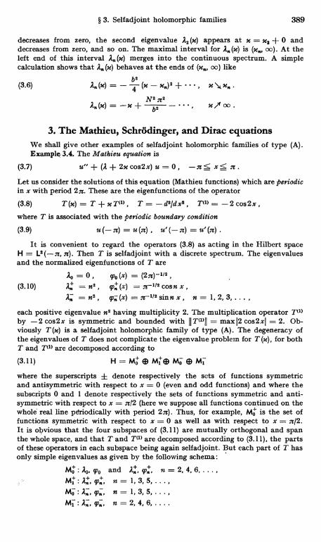
§ 3. Selfadjoint holomorphic families 389
decreases from zero, the second eigenvalue AE (x) appears at x = x, + 0 anddecreases from zero, and so on. The maximal interval for is (x,,, oo). At theleft end of this interval A (x) merges into the continuous spectrum. A simplecalculation shows that A. (x) behaves at the ends of (x,,, oo) like
E
(3.6)A.
(x) _ - (x - xn) E + ... X\ X. .
-x+Nb2E- x/"oo.
3. The Mathieu, Schrodinger, and Dirac equationsWe shall give other examples of selfadjoint holomorphic families of type (A).Example,, 3.4. The Mathieu equation is
(3.7) u" + (A + 2xcos2x) u = 0, -nS x< n.Let us consider the solutions of this equation (Mathieu functions) which are periodicin x with period 2n. These are the eigenfunctions of the operator
(3.8) T (m) = T -{- x V'), T = - dE/d xE , T'> _ - 2 cos 2 x ,
where T is associated with the periodic boundary condition
(3.9) u (- n) = u (a) , u' (- n) = u' (n)
It is convenient to regard the operators (3.8) as acting in the Hilbert spaceH = L2 (-a, n). Then T is selfadjoint with a discrete spectrum. The eigenvaluesand the normalized eigenfunctions of T are
Ao = 0, q'o (x) = (2n)-IIE
(3.10) =n2, 97.+(X) = n-ICE cosn x ,= nE 97;
(x) = n-112 sinn x, n = 1, 2, 3, . .
each positive eigenvalue n2 having multiplicity 2. The multiplication operator T'>by -2 cos2x is symmetric and bounded with 11T'>11 = max12 cos2xl = 2. Ob-viously T (m) is a selfadjoint holomorphic family of type (A). The degeneracy ofthe eigenvalues of T does not complicate the eigenvalue problem for T (x), for bothT and T<'> are decomposed according to
(3.11) H = Mo a M1+9 Mo a Mi
where the superscripts ± denote respectively the sets of functions symmetricand antisymmetric with respect to x = 0 (even and odd functions) and where thesubscripts 0 and 1 denote respectively the sets of functions symmetric and anti-symmetric with respect to x = n/2 (here we suppose all functions continued on thewhole real line periodically with period 2n). Thus, for example, Mo is the set offunctions symmetric with respect to x = 0 as well as with respect to x = 7F/2.It is obvious that the four subspaces of (3.11) are mutually orthogonal and spanthe whole space, and that T and T'> are decomposed according to (3.11), the partsof these operators in each subspace being again selfadjoint. But each part of 2' hasonly simple eigenvalues as given by the following schema:
Ma : Ao, q7o and An, q>n, it = 2, 4, 6, .. ,
Mi:A,q'n, n=1,3,5,. ,
n=1,3,5,.. ,
n=2,4,6.....
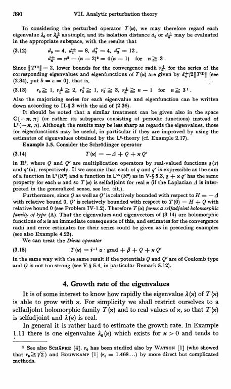
390 VII. Analytic perturbation theory
In considering the perturbed operator T (m), we may therefore regard eacheigenvalue Ao or An as simple, and its isolation distance do or dA may be evaluatedin the appropriate subspace, with the results that
(3.12) do = 4, dl = 8, d2 = 4, da = 12,do =us-(n-2)z=4(n-1) for nZ3.
Since II TMII = 2, lower bounds for the convergence radii rA for the series of thecorresponding eigenvalues and eigenfunctions of T (x) are given by df/211 T(I)II [see(2.34), put b = c = 0], that is,
(3.13) ro Z 1, rl Z 2, ra > 1, ra > 3, rn Z n - 1 for n Z 3 I .
Also the majorizing series for each eigenvalue and eigenfunction can be writtendown according to II-§ 3 with the aid of (2.36).
It should be noted that a similar treatment can be given also in the spaceC [- n, n] (or rather its subspaces consisting of periodic functions) instead ofL2 (-n, n). Although the results may be less sharp as regards the eigenvalues, thosefor eigenfunctions may be useful, in particular if they are improved by using theestimates of eigenvalues obtained by the L2-theory (cf. Example 2.17).
Example 3.5. Consider the Schrodinger operator
(3.14) T(x)=-d+Q+xQ'in R3, where Q and Q' are multiplication operators by real-valued functions q (x)and q' (x), respectively. If we assume that each of q and q' is expressible as the sumof a function in Lz (R3) and a function in L°O (R3) as in V-§ 5.3, q + x q' has the sameproperty for each x and so T (x) is selfadjoint for real x (if the Laplacian d is inter-preted in the generalized sense, see loc. cit.).
Furthermore, since Q as well as Q' is relatively bounded with respect to H = - dwith relative bound 0, Q' is relatively bounded with respect to T (0) = H + Q withrelative bound 0 (see Problem IV-1.2). Therefore T (x) forms a selfadjoint holomorphicfamily of type (A). That the eigenvalues and eigenvectors of (3.14) are holomorphicfunctions of x is an immediate consequence of this, and estimates for the convergenceradii and error estimates for their series could be given as in preceding examples(see also Example 4.23).
We can treat the Dirac operator
(3.15) +fl+Q+xQ'in the same way with the same result if the potentials Q and Q' are of Coulomb typeand Q is not too strong (see V-§ 5.4, in particular Remark 5.12).
4. Growth rate of the eigenvaluesIt is of some interest to know how rapidly the eigenvalue A (x) of T (x)
is able to grow with x. For simplicity we shall restrict ourselves to aselfadjoint holomorphic family T (x) and to real values of x, so that T (M)is selfadjoint and A(x) is real.
In general it is rather hard to estimate the growth rate. In Example1.11 there is one eigenvalue A, (x) which exists for x > 0 and tends to
I See also SCHAFKE [4]. ro has been studied also by WATSON [1] (who showedthat ro Z V2-) and BOUWKAMP [1] (ro = 1.468...) by more direct but complicatedmethods.
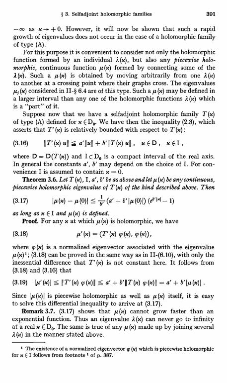
§ 3. Selfadjoint holomorphic families 391
- oo as x -* + 0. However, it will now be shown that such a rapidgrowth of eigenvalues does not occur in the case of a holomorphic familyof type (A).
For this purpose it is convenient to consider not only the holomorphicfunction formed by an individual A (m), but also any piecewise holo-morphic, continuous function ,u (x) formed by connecting some of theA (m). Such a p (m)(x) is obtained by moving arbitrarily from one A (X)to another at a crossing point where their graphs cross. The eigenvalues,u; (x) considered in II-§ 6.4 are of this type. Such a It (x) may be defined ina larger interval than any one of the holomorphic functions A (x) whichis a "part" of it.
Suppose now that we have a selfadjoint holomorphic family T (M)of type (A) defined for x E Do. We have then the inequality (2.3), whichasserts that T' (x) is relatively bounded with respect to T (x) :
(3.16) IIT'(x)ullsa'Ilull+b'IIT(x)ull, uED, xEI,where D = D (T (x)) and I ( Do is a compact interval of the real axis.In general the constants a', b' may depend on the choice of I. For con-venience I is assumed to contain x = 0.
Theorem 3.6. Let T (x), I, a', b' be as above and let,u (x) be any continuous,piecewise holomorphic eigenvalue of T (x) of the kind described above. Then
(3.17) Iy (x) - u (0) I s (a' + b' Iu (0) I) (eb I'll - 1)
as long as x E I and ,u (x) is defined.Proof. For any x at which ,u (x) is holomorphic, we have
(3.18) y' (x) = (T' (x) 9, (x), 9, (x)),
where 99 (x) is a normalized eigenvector associated with the eigenvalue,u (x)1; (3.18) can be proved in the same way as in II-(6.10), with only theinessential difference that T' (x) is not constant here. It follows from(3.18) and (3.16) that
(3.19) I,u' (x) I < II T' (x) '()II s a' + b' II T (x) 99(x)II = a' + b' I u (x) I
Since I4u (x) l is piecewise holomorphic as well as ,u (x) itself, it is easyto solve this differential inequality to arrive at (3.17).
Remark 3.7. (3.17) shows that ,u (x) cannot grow faster than anexponential function. Thus an eigenvalue A (m) can never go to infinityat a real x E D0. The same is true of any ,u (x) made up by joining severalA (x) in the manner stated above.
1 The existence of a normalized eigenvector ip (x) which is piecewise holomorphicfor x E I follows from footnote 1 of p. 387.
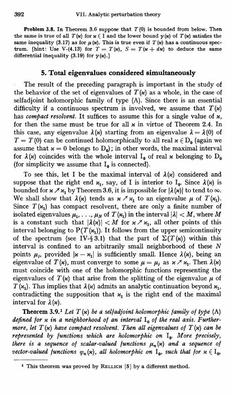
392 VII. Analytic perturbation theory
Problem 3.8. In Theorem 3.6 suppose that T (O) is bounded from below. Thenthe same is true of all T (x) for x E I and the lower bound y (x) of T (x) satisfies thesame inequality (3.17) as for ,u (x). This is true even if T (x) has a continuous spec-trum. [hint: Use V-(4.13) for T = T (m), S = T (m + dx) to deduce the samedifferential inequality (3.19) for y(x).]
5. Total eigenvalues considered simultaneously
The result of the preceding paragraph is important in the study ofthe behavior of the set of eigenvalues of T (x) as a whole, in the case ofselfadjoint holomorphic family of type (A). Since there is an essentialdifficulty if a continuous spectrum is involved, we assume that T (x)has compact resolvent. It suffices to assume this for a single value of x,for then the same must be true for all x in virtue of Theorem 2.4. Inthis case, any eigenvalue A (x) starting from an eigenvalue A = A (0) ofT = T (0) can be continued holomorphically to all real x E Da (again weassume that x = 0 belongs to D0) ; in other words, the maximal intervalfor A (m) coincides with the whole interval Io of real x belonging to Do(for simplicity we assume that Io is connected).
To see this, let I be the maximal interval of A (m) considered andsuppose that the right end x, say, of I is interior to I. Since A (x) isbounded for x /1' x, by Theorem 3.6, it is impossible for I A (x) I to tend to oo.We shall show that A (x) tends as x /' x, to an eigenvalue ,u of T (xl).Since T (xl) has compact resolvent, there are only a finite number ofisolated eigenvalues ,ul, . . ., IuN of T (xl) in the interval I Al < M, where Mis a constant such that IA (x) I < M for x / x,, all other points of thisinterval belonging to P(T (x,)). It follows from the upper semicontinuityof the spectrum (see IV-§ 3.1) that the part of E(T (x)) within thisinterval is confined to an arbitrarily small neighborhood of these Npoints ,uj, provided Ix - xlI is sufficiently small. Hence A (x), being aneigenvalue of T (x), must converge to some ,u = ,uj as x >' xl. Then A (x)must coincide with one of the holomorphic functions representing theeigenvalues of T (x) that arise from the splitting of the eigenvalue ,u ofT (x,). This implies that A (x) admits an analytic continuation beyond xl,contradicting the supposition that x, is the right end of the maximalinterval for A (x).
Theorem 3.9.1 Let T (x) be a sel f adjoint holomorphic family of type (A)defined for x in a neighborhood of an interval Io of the real axis. Further-more, let T (x) have compact resolvent. Then all eigenvalues of T (x) can berepresented by functions which are holomorphic on I. More precisely,there is a sequence of scalar-valued functions ,u (x) and a sequence ofvector-valued functions q,n (x), all holomorphic on I0, such that for x E Io,
1 This theorem was proved by RELLICH [5] by a different method.
§ 4. Holomorphic families of type (B) 393
the un (x) represent all the repeated eigenvalues of T (x) and the q,, (x) form acomplete orthonormal family of the associated eigenvectors of T (x).
Proof. The first half of the theorem has already been proved above 1It remains to show that the eigenvectors form a complete set. But this isanother expression of the fact that all the eigenprojections of a self-adjoint operator with compact resolvent form a complete set (see V-§ 3.8).
Remark 3.10. Each A,, (x) is holomorphic in a complex neighborhoodof To, but this neighborhood will depend on n, so that it will be in generalimpossible to find a complex neighborhood in which all the A,, (x) exist.
Remark 3.11. The assumption in Theorem 3.9 that T (x) has compactresolvent is rather crucial. A similar result might be expected for aselfadjoint holomorphic family T (m) of compact operators, but theexistence of the limit point 0 of the eigenvalues of a compact operatorcauses some difficulty. Every eigenvalue A (m) of T (m) can indeed becontinued analytically as long as it does not reach the value 0. OnceA (x) = 0 for some x, A (x) may have no further' analytic continuation.There is a sufficient condition that A (m) never equals 0 unless it is iden-tically zero; then the result of Theorem 3.9 remains true if the systemq (x) is supplemented with the eigenvectors belonging to the eigen-value A (x) = 0 (if any) of T (x). An example of such a sufficient condition 2is that there exist positive constants in, M such that for real x
(3.20) m!IT(0)uII 5 IIT(x)uII 5 MIIT(0)uII, uEH.
In fact, (3.20) implies that the null space N of T (x) is independent of xfor any real x. Thus any orthonormal family of N can be a part of{T (x)} with 1 (x) = 0. Since T (x) is selfadjoint for real x, it is decompos-ed according to H = N ® N -L. In the subspace N -L, T (x) has no eigen-value 0 so that the result of Theorem 3.9 is true.
§ 4. Holomorphic families of type (B)1. Bounded-holomorphic families of sesquilinear forms
Let {t (x)} be a family of sesquilinear forms in a Hilbert space H.Suppose that t (x) is a bounded sesquilinear form with domain H for eachx E Do, where Do is a domain in the complex plane, and that t (x) [u]is holomorphic in Do for each fixed u E H. Then the family {t (x)} is saidto be bounded-holomorphic.
1 For the existence of an orthonormal family {q7 (x)} of eigenproj ections seefootnote 1 on p. 387.
2 Another sufficient condition is 0 < m T (0) S T (x) S M T (0) ; the proof isthe same as for (3.20). These conditions are essentially given by RELLicx [5].
394 VII. Analytic perturbation theory
It follows by polarization that t (x) [u, v] is holomorphic in Do foreach fixed u, v E H [see VI-(1.1)]. The family of operators T (x) E -4 (H)defined by (T (x) u, v) = f (m) [u, v] is a bounded-holomorphic family ofoperators; this follows from Theorem 111-3.12. In particular it followsthat t (x) is uniformly bounded in each compact subset of Do.
A similar result holds for a family t (x) originally defined for real x.Suppose t (x) is defined for - r < x < r and t (x) [u] has a power seriesexpansion convergent for - r < x < r. Then the family T (x) of theassociated operators can be extended to all complex x with Ixl < r so asto form a bounded-holomorphic family.
To see this, it suffices to show that t (x) can be continued analyticallyto all x with jxj < r, preserving its property of being a bounded form. Let
(4.1) t (x) [u, v] = t [u, v] + x t1> [u, v] + x2 t(2) [u, v] +
be the Taylor expansion of the numerical function t (x) [u, v] of the realvariable x, - r < x < r, obtained by polarization from the expansionof the t (x) [u]. t = t (0) is obviously a bounded sesquilinear form. Weshall show that all the t(') are also bounded sesquilinear forms. Thesesquilinearity of t('') is a simple consequence of that of t (x) and theuniqueness of the Taylor expansion (4.1).
(4.1) implies that t(1) [u, v] = lim x-11 (t (x) - t) [u, v]. Since this
limit exists for every u, v E H and since t (x) - t is a bounded form forevery real x, it follows from the principle of uniform boundedness thatt(') is bounded (Problem 111-1.30). Then we have from (4.1) that t(2) [u, v]= Jim x-2(t (x) - t - x t()) [u, v], and a similar argument shows that t(2)
33 +0
is bounded, and so on.Thus there are operators T() E .4 (H) such that t() [u, v] = (T (n) u, v),
and (4.1) can be written
(4.2) (T (x) u, v) = (T u, v) + x (TM u, v) + x2 (TM u, v) + .
This series converges for jxj < r for all u, v E H. Hence r'n (T(3) u, v) -a 0,n -* oo, for all u, v and any r' < r. Again the principle of uniform bound-edness (see Problem 111-3.13) shows that {r' n llT (n) IJ } is bounded asn -> oo. Hence(4.3) TM = T + x TM + x2 TM +
is absolutely convergent (in norm) for IxI <r and defines TM E.4(H).Thus t (x) [u, v] = (T (x) u, v), valid for real x, has been extended to allx with IxI < r, T (x) forming a bounded-holomorphic family.
Remark 4.1. Let t (x) be a family of sesquilinear forms with domain Hand let t (x) [u] be holomorphic for x E Do for every u E H. Then t (x)is a bounded-holomorphic family of forms if there is a sequence xn E Do,
§ 4. Holomorphic families of type (B) 395
converging to a xo E Do different from any x,,, such that t is a boundedform for every n = 1, 2, ... .
The point is that the assumptions imply that t (x) is bounded forevery x E Do. This is seen again by invoking the principle of uniformboundedness. We may assume xo = 0, x,, + 0. The existence of lim
n-* 00(T u, v) = lim t [u, v] = t [u, v] implies that T is uniformlybounded and hence t is bounded with the associated T. Then t(') [u, v]= t) [u, v] shows that t(1) is bounded, and so on as above.Thus we see that t (x) is bounded near x = 0, and this property propagatesto all x E Do.
2. Holomorphic families of forms of type (a) andholomorphic families of operators of type (B)
We now consider a family t (x) of (not necessarily bounded) ses-quilinear forms defined for x ED,. t (x) will be called a holomorphicfamily of type (a) if i) each t (x) is sectorial and closed with D (t (x)) = Dindependent of x and dense in H, and ii) t (x) [u] is holomorphic forx E Do for each fixed u E D. Note that ii) implies, by polarization, thatt (x) [u, v] is holomorphic in x for each fixed pair u, v E D. (For sectorialforms see Chapter VI.)
Theorem 4.2. Let t (x) be a holomorphic family of forms of type (a).For each x let T (x) = Tt (.,) be the associated m-sectorial operator (seeTheorem VI-2.7). Then the T(x) form a holomorphic family of operators,and the T (x) are locally uniformly sectorial.
A holomorphic family of m-sectorial operators associated with aholomorphic family of forms of type (a) according to Theorem 4.2 willbe called a holomorphic family of type (B) 1.
Proof of Theorem 4.2. We may assume that x = 0 belongs to Do andRe t Z 1, t = t (0) ; otherwise this situation can be attained by
shifting the origin of the x-plane and adding a suitable constant to t (x).Let H = To z 1 be the selfadjoint operator associated with the
closed form t Z 1 [H is by definition the real part of T = T (0), seeVI-§ 3.1 ], and consider the forms to (x) [u, v] = t (x) [G-1 u, G-1 v] whereG = HI/2. Since G-1 u E D (G) = D (0) = D by the second representationtheorem (Theorem VI-2.23), to(x) is a'sectorial form defined everywhereon H. Since to (x) is closable as is easily verified, it follows from TheoremVI-1.20 that to (x) is bounded. Since to (x) [u, v] is obviously holomorphicfor x E Do for each fixed u, v E H, to (x) forms a bounded-holomorphicfamily of forms. Thus we have the expression to (x) [u, v] = (To (x) u, v),where {T0 (x)} is a bounded-holomorphic family of operators (see the
1 A special case (selfadjoint) of this type was introduced in T. KATO [8].
396 VII. Analytic perturbation theory
preceding paragraph). Replacing u, v respectively by Gu, Gv, we thusobtain the expression
(4.4) t(x) [u, v] = (To(x) Gu, Gv) , u, v E D, G = H1/2.
An argument similar to that used in deducing VI-(3.4) then gives
(4.5) T (m) = G To (x) G,
(4.6) T (m)-l' = G-1 To (x)-1 G-1.
Here G-1 E V (H) and To(x)-1 is bounded-holomorphic near x = 0,for To (x) is bounded-holomorphic and To (0)-1 E V (H) exists becauseTo(0) is of the form 1 + iB, B* = B [see VI-(3.4)]. Therefore T(x)is holomorphic near x = 0 by Theorem 1.3. Since x = 0 is not distinguish-ed from other points, T (x) is holomorphic for x E Do. Finally it is clearfrom (4.4) that the t (x) are uniformly sectorial near x = 0, for To (0)= 1 + i B and the To (x) are uniformly bounded near x = 0. Hence thesame is true of the T (x).
Theorem 4.3. Let T (x) be a holomorphic family of operators of type (B).T (x) has compact resolvent either for all x or for no x.
The proof is similar to that of Theorem 2.4; we need only replaceTheorem IV-3.17 used there by Theorem VI-3.4. (Note that an m-sectorial operator has a non-empty resolvent set.)
Remark 4.4. In the definition of a holomorphic family t (x) of formsof type (a), it suffices to require in i) the closedness of t (x) onlyfor a sequence x = x converging to a xo E Do different from any ofthe x,,. To see this we note that, in the proof of Theorem 4.2, to (x) isfirst seen to be bounded for x = x,,. Then we see by Remark 4.1 that to (x)is bounded for all x = Do and the proof of Theorem 4.2 is valid. Then itfollows from (4.4) that t (x) is closed for sufficiently small I4I4 and then wecan generalize this to all x E Do.
This remark is useful since we need to verify that t (x) is closed,say, only for real x when Do meets the real axis.
Remark 4.5. For a holomorphic family t (x) - of type (a) we have thefollowing inequalities, which correspond to similar inequalities (2.2)-(2.4)for a family of operators of type (A). (Here we assume that h z 1, as inthe proof of Theorem 4.2.)
it(x1) [u] I s bIt(x) [u](4.7) It'(xl) [u, v] 1 s b'It(x) [u]11/21 It (X) [v]11/2,
I(t (x1) - t (x2)) [u, v] I S e It (x) [u] 11/2 It (x) [v] 11/2
Here u E D and a, b, a', b' are constants as long as x and x1 remain ina compact subset of Do; a may be made arbitrarily small if Ixl - x21
§ 4. Holomorphic families of type (B) 397
is sufficiently small. (4.7) can be easily proved by making use of (4.4).Also we note that the it (x) [u] I on the right of these inequalities may bereplaced by h (x) [u] = Re t (x) [u] with possible change of the constantsa, b, etc. [see VI-(1.42)-(1.43)]. (4.7) expresses that, roughly speaking, thet (m) are relatively bounded with respect to one another and the changeof t (x) is relatively continuous with respect to t (x).
Remark 4.6. There are several useful identities for the resolventR (C, x) of T (x). Assuming t 1 as in the proof of Theorem 4.2, we have
(4.8) ((T (xi)-1- T(2)-') u, v) = - (t (xl) - t (x2)) [T (xi) -1 u, T (x2) *-1 v] .
This follows from t (x1) [T (x,) -l u, g] _ (u, g) and t (x2) [f, T (x2) * -1 v]= t(x2)* [T (X2)*-' v, f] _ (v, v), where f = T (xl)-1 u E D,9ET(x2)*-1vED.
Letting xl - x2 in (4.8), we obtain
(4.9) (x T (x)-l u, v) t' (x) [T (x)-1 u, T (x) * -1 v] ,
since T (m)-l' u is continuous (even holomorphic) in the norm IIwlit = IIGwIIin virtue of (4.6).
If we replace t (x) and T (x) by t (x) - C and T (x) - C, respectively,(4.8) and (4.9) give
(4.10) ((R (C, x1) - R (C, x2)) u, v) = - (t (xl) - t (x2)) [R (C, x1) u, R (C, x2) * v] ,
(4.11) (M R (C, x) u, v) t' (x) [R (C, x) u, R (C, x) * v] .
In view of (4.7), we obtain from (4.11)
(a R (C, x) u, v) I s b' It (x) [R (C, x) u] I1/2 It (X)* [R (C, X)* v] Iu/2
= b' I (T (x) R (C, x) u, R (C, x) u)I1/2 I (T* (x) R (C, x)* v, R (C, x) * V)11/2.
But II T (x) R (C, x) II 5 1 if C < 0 (Problem V-3.31) and II T (x) * R (C, x) *II
S 1 similarly. Hence
(4.12)I dx R(C, x)II s b'IIR(C, x)II1/2IIR(C, x)*II1/2
=b'IIR(C,x)IIl-C, C<0.Remark 4.7. If t (x) is a holomorphic family of forms of type (a)
and if t (x) [u] is real for real x (assuming that Do intersects the realaxis), then it is easily seen that t (x) * = t (x) ; in this sense t (x) is a self -adjoint family. Then T (x) * = T (p), and T (x) forms a selfadjoint familyof operators (see § 3.1) ; in particular T (x) is a selfadjoint operator forreal x.
In this case (T (x) + A)1/2 has constant domain D for real x andlarge A, by the second representation theorem. But it is not clear whether
398 VII. Analytic perturbation theory
the same is true for complex x, though (T (x) + 2)1/2 is well defined byV-§ 3.11. Thus we do not know whether (T (x) + 2)1/2 forms a holo-morphic family of type (A) when T (m) is of type (B), even when it is aselfadjoint family.
In any case, however, (T (x) + 2)1/2 is a holomorphic family. Tosee this we note that
00
(4.13) (T (x) + 2)-1/2 f u-1/2(T (x) +A+ 1u)-1 du0
by V-(3.43). (4.13) can be differentiated under the integral sign, forwe have the estimate II d(T (x) + 2 + ,u)-1/dxll s b' (2 + ,u)-1 by (4.12);so that the resulting integral converges absolutely. This shows that(T (x) + 2)-1/2 is bounded-holomorphic in x. Thus (T (x) + 2)1/2 is holo-morphic by Theorem 1.3.
3. A criterion for type (B)
Theorem 4.8. Let t(n), n = 0, 1, 2, . . ., be a sequence o/ sesquilinearforms in H. Let t = t(O) be densely defined, with D (t) = D, sectorial andclosable. Let t('), n Z 1, be relatively bounded with respect to t so thatD (t(n") D D and
(4.14) It(n)[u]Iscn-1(aJIuII2+bh[u]), uED, n 1,
where h = Re t and a, b 0. Then the /orm00
(4.15) t (x) [u] = E xn t(n) [u] , D (t (x)) = D ,n=0
and the associated polar form t (x) [u, v] are defined for Ixj < 1/c. t (m) issectorial and closable for lxl < 1/(b + c). Let f(x) be its closure. {f (x)} is aholomorphic family of forms of type (a) for Ixj < 1/(b + c). The operatorT (x) associated with i (x) forms a holomorphic family of type (B).
Proof. The right member of (4.15) converges for Ixl < 1/c and definesa quadratic form. By polarization the sesquilinear form t (x) [u, v] isdefined also for Ixl < 1/c. We have
(4.16) #(x) - t) Cull S 1 I xI(all u112 + b h [u]) , Ixl < 1/c.
By Theorem VI-1.33, t (x) is sectorial and closable if b lxl/(1 - c IxI) < 1,that is, if lxl < 1/(b + c). It follows also from the same theorem that theclosure i (x) has the same domain b = D () as L. What remains is toshow that f (x) [u] has a power series similar to (4.15) for every u E D :
00
(4.17) i (x) [u] = X xn fi''') [u] , u E D ;n=0
§ 4. Holomorphic families of type (B) 399
here f(°) = i and i(n) is an extension of t(n) with domain b (not neces-sarily the closure of t(71)), for which the same inequality (4.14) holds with hreplaced by 6 = Ref. J(n) [u] is defined for u E D by (n) [u] = lim t(o ') [uk]
where {uk} is a sequence such that uk i u and the existence of thislimit is insured by (4.14). (4.17) follows from (4.15) with u replaced by ukon going to the limit k -* oo.
Since T (x) is holomorphic in x in Theorem 4.8, the resolvent R (C, X)= R(C, T (x)) is holomorphic in and x jointly in an appropriate regionof the variables. Let us estimate this region and the convergence radiusand errors for the Taylor series. Such estimates can be obtained from theproof of Theorem VI-3.4. For simplicity assume 4 = Ret > 0 and a 0.It suffices to replace the S of VI-(3.10) by T(); then the C on the rightof this formula should be replaced by the operator C (x) defined by(i (x) - f) [u, v] = (C (x) G' u, G' v). Recall that G' = H'1/2, H' = H ++ e z 0. In view of (4.17), C (x) has the form
00
(4.18) C (x) C(' , C(') E °,$ (H) , (CO) G' u, G' v) = J(n) [u, V].n=1
We have
(4.19) IIC(n)II 20 -1 k , k = max(b, ale)
[see VI-(3.8)-(3.9)]. Thus R (C, S) = R(C, T (m)) = R (C, x) becomes
(4.20) R x) = G' -1(1 - ' H' -1 + i B' + C (x))-1 G' -100
= R (C) + G'-1 E J (C) (- C (x) J (C))' G'-1 ,P-1
where
(4.21) R.(C) =R(C,0) =R(C, T), J(C) = (1-C'H'-1+iB')-1, C'=4+e,if IxI is so small that
(4.22) IIC(x)II IIJM II s IIJM II E Ik!nIIC(n)II < 100n=1
In view of (4.19), (4.22) is satisfied if,
(4.23) IxI < (2kIIJ(C)II + c)-l.
Here it has been tacitly assumed that J M E .Q (H) ; in generalit is not easy to see when this is satisfied, but it is certainly the caseif Red'' S 0, for we have then IIJ(C)II 5 1 (see loc. cit.). and (4.23) issatisfied if
(4.24) IxI<(2k+c)-1, ReC'=ReC+eos 0.
400 VII. Analytic perturbation theory
In particular if -Red' > a/b, we can choose e > alb without violating thecondition Re C' _< 0; then we have k = b and (4.24) becomes IxI < (2b ++ c) -1. In other words x) is a convergent power series in x for IxI << (2 b + c) -1 i f - Re > 0 is sufficiently large. This gives another proofthat T (x) is holomorphic at x = 0.
These results admit some refinements if the unperturbed form t = his symmetric so that the associated operator T = H is selfadjoint. Thenwe need not assume h >_ 0, the constant a may be negative and J P EE -4 (H) is true for any C E P (H). To see this we need only make thefollowing modifications. We set o = a b-1 + 6, 6 > 0; then H' = H ++ e z 6 > 0 by (4.14), and (4.19) is true with k = b and R (C, x) con-verges as a power series in x for IxI < (2bljJ(C)II + c)-1 [see (4.23)]. Sincewe have B' = 0 now, J (1 - C'H'-1)-1 = H'(H' - c')-1 = (H ++ a b-1 + S) (H - )-1 = b-1 (a + bH + b 6) R(C). Since 6 > 0 is arbi-trary, we conclude that R (C,x) converges as a power series in x if IxI << (211(a + b H) R (C) II + c)-1. Here even the factor 2 can be dropped ifall the t(n) are symmetric, for then I t(n) [u] I < b 0'[u] implies It(,,) [u, v] I <S b II G' ull II G' v11. The case b = 0 can be dealt with by going to the limit.These modifications yield
Theorem 4.9. In Theorem 4.8 let t = 1 be symmetric (with the associatedoperator T = H selfadjoint) and let a in (4.14) be not necessarily non-negative. For any C E P (H), the resolvent R (C, x) o l T (x) exists and is aconvergent power series in x for
(4.25) IxI < (eII (a + bH) R(C, H)II + c)-1
where e = 1 or 2 according as all the t(') are symmetric or not.Remark 4.10. Not only the convergence radius but R (C, x) itself
can be estimated as in VI-(3.16), in which a and b must now be replacedby appropriate functions of x. We omit the details.
Example 4.11. Consider the form
b b
(4.26) f (m) [u, v] = f P (x) u' v' d z + J [q (z) + x q(1)(z) ] u V d x +a a
+ (ho + x h () ) u (a) v (a) + (hb + x h') u (b) vv (8) ,
where p (x), q (x), q(l) (x) are continuous on a :!g x:!-, b and p (x) < 0 [see ExampleVI-1.7; here we have set r (x) = s (z) = 0 for simplicity, but we could have retainedthem without affecting the following results]. As we have seen in Example VI-1.36,t(x) satisfies the assumptions of Theorem 4.8 with an arbitrarily small b because allforms on the right of (4.26) except the first are relatively bounded with respect tothe first term, with relative bound 0. The operator T (x) associated with t (x) is givenby (see Example VI-2.16)
(4.27) T (x) u = - (p u')' + (q + x q(1)) u
§ 4. Holomorphic families of type (B) 401
with the boundary condition
(4.28) p (a) u' (a) - (h, + x h( ") u (a) = 0, p (b) u' (b) + (ha + x ha'") u (b) = 0 .
Thus the T (m) form a holomorphic family of type (B) defined for all complex X.If we start from the restriction to (x) of t (x) with domain restricted by the
boundary condition
(4.29) u (a) = 0, u (b) = 0,
we get another holomorphic family To (x), which is given formally by (4.27) withboundary condition (4.29) (see Example VI-2.17). But this is rather trivial, forTo (x) has a constant domain and the perturbing term x q(1) in (4.26) is a boundedoperator, so that To (x) is actually of type (A).
By restricting the domain oft (x) by the condition u (a) = 0 only, we arrive at athird family of operators (4.27) with the boundary condition: (4.28) at x = b and(4.29) at x = a, which is again holomorphic of type (B).
4. Holomorphic families of type (Bo)In Theorem 4.8, the unperturbed form t may not be closed. If t is
closed, the perturbed form t (m) is closed too, for we have then D (I (x))= D. But it is convenient to have the theorem in its generality withoutassuming t to be closed.
As an important application, suppose we are given a family ofoperators S (x) of the form
(4.30) S (M) = S + MS(1) + x2S(2) + .. .
where S is densely defined and sectorial, D (S (n)) ) D (S) and
(4.31) I(S(n) u, u)I s c"-1(aIIujI2 + b Re(Su, u)) , u E D(S)
with constants a, b such that a z 0, 0 5 b < 1.Then the assumptions of Theorem 4.8 are satisfied by setting t [u, v]
_ (Su, v) and t(n) [u, v] = (S(n) u, v), for the form t is closable (see TheoremVI-1.27). The resulting operator T (x) is the Friedrichs extension of S (x)(see VI-§ 2.3). Thus we have
Theorem 4.12. Let S (x) be as above. The Friedrichs extension T (x)of S (x) exists and forms a holomorphic family of type (B) for Ixj < (b + c)-1.
A family T (x) as in Theorem 4.12 will be called a holomorphicfamily of type (BO)1. It is a special case of type (B), and the domains ofthe T (x) for different x have a dense common part D (S), which is nottrue for a general family of type (B).
T (x) is a closed extension of S (x) but it may or may not be identicalwith the closure of S (x). If not, it is possible that there is another familyT1 (x) consisting of m-sectorial extensions of S (x). In this connection,the following theorem, essentially due to RELLICH [3], is remarkable.
1 A special case (selfadjoint) of type (Bo) was introduced by RELLicH [3].
402 VII. Analytic perturbation theory
Theorem 4.13. I l the closure . o l S is m-sectorial, the family T (x) o tTheorem 4.12 is the unique holomorphic family 1 defined near x = 0consisting o l extensions o l S (x) such that T (0) = 9.
Proof. We have T = T (0) = . since T is an m-sectorial extensionof S. Suppose that T, (x) is a holomorphic family such that T, (x) D S (x)near x = 0 and T, = T, (0) = . = T. Then P (T,) is not empty. IfC E P(T,),
(4.32) R + x R, + x2R2 +
is bounded-holomorphic near x = 0 by Theorem 1.3. For any u E D (S),we have R(g, Tl (x)) (S (x) - C) u = u since T, (x) D S (x). Hence
(4.33) (R+xR,+x2R2+...) (S-C+xS(')+x2$(2)+...)u=u
and comparison of coefficients gives
R(S-C)u=u,(4.34). R, (S - u = -RS(') u,
R2(S-u=-RS(2)it-R,SMu,
for any u E D (S). These equations determine the operators R, R,,R2, ... E .1(H) uniquely, for (S - C) D (S) = (T - C) D (S) is dense in Hbecause T = . ' (see Problem 111-6.3).
Remark 4.14. The essential point in Theorem 4.13 is that the closureof S (x) need not coincide with T (x) for x + 0 and yet T (x) is the uniquefamily with the stated property. In many problems in applications T (x)is actually the closure of S (x) or even T (x) = S (x). Even in such a case,application of Theorem 4.8, in particular the estimate (4.25) whenT = H is selfadjoint, often leads to an improvement of results obtainedotherwise.
Example 4.15. Consider the formal differential operator
(4.35) L (m) u = _U11 + x z-$ u , 0 < x < oo .
Let t (x) be the minimal operator in H = L2 (0, oo) constructed from (4.35), withD (T (x)) = Co (0, oo), t (x) is symmetric for real x; it is sectorial for every complex x
00
with Re x > - 1/4 in virtue of the inequality VI-(4.6) and - (u", u) =J
1u'1$ dx.0
Thus the family t (x) satisfies the assumptions for S (x) in Theorem 4.12, and theFriedrichs extension T (x) of t (x) forms a holomorphic family of type (B0).
Is T (m) the unique holomorphic family consisting of m-sectorial extensions ofT (x) ? The answer depends on the region Do of x considered. It is yes if Do contains
1 As is seen from the proof, the uniqueness holds even if T (x) is assumed to beonly real-holomorphic.
§ 4. Holomorphic families of type (B) 403
x = 3/4. In fact, it is known that t(3/4) is essentially selfadjointl; thus we have thesituation of Theorem 4.13 if x = 0 is replaced by x = 3/4 (see also Remark 1.6).It is interesting to note that for x < 3/4, 2` (x) is not essentially selfadjoint and,consequently, T (m) is not the only selfadjoint extension of t (m). Nevertheless it isunique as a holomorphic extension of the family t (x).
This unique family T (x) is characterized by the condition D (T (x)) C D (t),where t is the closure of the form t = t (3/4) associated with T (3/4), namely, t [u]
_ (u', u') (3/4) f xa Ju12 dx, u E Co . In view of VI-(4.6), it is easy to see that D ('t)0
is the set of all u E H such that u' E H and u (0) = 0 (cf. Problem VI-2.18). Therefore,T (x) must be the restriction of L (x) such that u E D (T (x)) implies u' E H andU (O) = 0.
5. The relationship between holomorphic families oftypes (A) and (B)
It is natural to ask whether there is any relationship between aholomorphic family of type (A) and one of type (B). In general there isno such relation, for the former is defined in any Banach space whilethe latter is defined only in Hilbert spaces. If we restrict ourselves toselfadjoint families of sectorial operators, however, the families of type (B)form a wider class than those of type (A). More precisely, we have
Theorem 4.16. A self adjoint holomorphic family T (x) o l type (A) isalso o l type (B0), at least in a neighborhood o l the real axis, if T (x) isbounded from below for some real x (whereupon T (x) is bounded frombelow for all real x).
Proof. We may assume that x = 0 belongs to the domain Do in whichthe family is defined and that T = T (0) is selfadjoint and nonnegative.Then we have the expression (2.1) for T (x) u, u E D = D (T (x)), wherethe coefficients TM are symmetric and satisfy inequalities of the form(2.5) (see Remark 2.8). Noting that aIlull + b11Tulj V211(a+ bT) ull,we see from Theorem V-4.12 that
(4.36) I (T("') u, u) s y2 c"'-1((a + bT) u, u) , it = 1, 2, ... .
Let Tp(x) be the Friedrichs extension of T(x). In view of (4.36),we. see from Theorem 4.12 that T p (x) exists in a neighborhood of x = 0and forms a holomorphic family of type (B). But we have T p (x) = T (x)for real x, . since T (x) is selfadjoint and T7 (x) is a selfadjoint extensionof T (x). Since both T (x) and T p (x) are holomorphic families, it follows
i At x = 0, the differential equation (4.35) is in the limit point case if x 3/4and in the limit circle case if x < 3/4 (cf. CODDINGTON and LEViNSON (1J, p. 225).In fact, L (x) u = 0 has two linearly independent solutions u± = x5±, where 2 at= 1 +(1 + 4x)1"8; both u± belong to L$(0, 1) if 4x <-3 but u_ does not belong toL2 (0, 1) if 4x Z 3. It follows that for real x, t (x) is essentially selfadjoint if (andonly if) x> 3/4 (at x = oo the equation is in the limit point case for any real x).
404 VII. Analytic perturbation theory
from the unique continuation property (Remark 1.6) that T (M) = TF (x)for all x in the common region of definition of T (m) and TF (x) . Thisproves that T (x) is of type (B) in a neighborhood of x = 0; note thatthis implies that T (x) is sectorial and, in particular, bounded from belowfor real x.
To complete the proof of the theorem by showing that the sameresult holds in a neighborhood of any real x, it suffices to prove that T (x)is bounded from below for every real x E DO where T (x) is defined.Suppose T (x0) is bounded from below for a real x.,. Since by (2.4) T (x) -- T (xo) is relatively bounded with respect to T (xo) with relative bound< 1 for sufficiently small Ix - xol, it follows from Theorem V-4.11 thatT (x) is bounded from below for real x near xo. Since the required small-ness of Ix - xol is uniform in any compact subset of Do, the semibound-edness of T (x) propagates from x = 0 to all real x E Do.
6. Perturbation series for eigenvalues and eigenprojectionsThe general results of § 1.3 on finite systems of eigenvalues of T (X)
apply to a holomorphic family T (m) of type (B). We collect here someresults that are peculiar to this type. For simplicity we restrict ourselvesto dealing with the case of Theorem 4.9.
Consider an isolated eigenvalue A of H with the eigenprojection P,00
dim P = m < oc. The total projection P (x) = P + x" P(n) for the"=1
A-group eigenvalues of T(x) is holomorphic in x, being given by (1.3).Substitution of (4.20) gives [cf. 11-(2.8)]
(4.37) P(") = - ' (-1)°P=1 vl+... Fvy=n r
' J (C) ... J (C) Cc"nl J (C) G'-1 d.C
Here G' = H'1/2, H' = H + e = H + a b-1 + 6 and J(g) is given by(4.21) where B' = 0 since we assumed t to be symmetric:
(4.38) J() = H' (H' - C')-1= H'R (C) , R(C)=(H-C)-1.
The CM are given by (4.18). The power series for the weighted meanof the eigenvalues under consideration can be obtained as in II-§ 2.2.It should be remarked, however, that the expression II-(2.23) cannot beused now, for the operators TM are not defined. Instead we have
(4.39) ,Z (x) - A = - 2n i m tr f log (1 +`
x" C") J (C)1 d C .
r \ " /This can be proved by using the property of the trace trAB = trBAand by integration by parts, starting from the expression II-(2.25)
§ 4. Holomorphic families of type (B) 405
where we substitute R (C, x) from (4.20). The integration by parts makesuse of the fact that J G'-'J(C) = H' R (C) 2 = (d/d ) H' R (C) .The useof the formal equality trAB = trBA under the integration sign is notdirectly justified, but it can be justified by the consideration given in§ 2.3 in the case of a family of type (A).
(4.39) gives the following expressions for the coefficients of the series(x) = A + E xn AN [cf. 11-(2.30)]:
(4.40)
AN = 2nim trE (_1)9 E fC(°')J(C)C(I-)...J(C)C(°Q)J(C)dCP=1 vl+...+vP=nr
If the reduced resolvent S of H for the eigenvalue A is introducedaccording to R (C) = - ( - A)-1 P + S + (C - A) S2 + [see I-(5.18)and III-(6.32)], (4.37) and (4.40) reduce to [cf. II-(2.12, 31)]
(4.41) P(n) _ -f (- 1)P ' G'-1 J(k,) C(vi) ... J(ho) C(vo) J(k,+i) G'-1,
P
(4.42) 1('1) = 1 f'(-1)r
trC(vl) J(k,) ... C(VP) J(kP)'IfM P P v,+...+vy=n
where
(4.43) J(°)=-H'P=-(A+ab-1+6)P, JO)=H'Sk, kz 1.It is desirable to express these results in terms of the given forms t(n)
alone, without using such auxiliary quantities as H', G', C('i), etc. Thisis not simple in general, but can be done without difficulty at least forthe first few coefficients. For example,
(4.44) A()= - m trC(1) J(°) =
m
trC(1) H'P = m E (C(1) H' 9, 91j)9=1
1= '(1) [G' 99s G'-1 9f] =m (1) [91AM y=1 i=1
where 99f, j = 1, ..., m, form an orthonormal basis of the eigenspace PH[note that G' - q23 = (A + a b-1 + 6) ± 1/2 99f].
Problem 4.17. (4.37) and (4.40) are formally identical with II-(2.8) and II-(2.30),respectively, after substitution of (4.38) for J(C) and of C1°) = G'-1 V^) G'-1.
Let us now estimate the convergence radius of the series for P (m).According to (4.25), a lower bound for this convergence radius is given by
(4.45) re = inf (ell (a + bH)R II + c)-1tof
a
+b p I+
C)-1,ErpEE(H)
where e = 1 or 2 according as all the t(") are symmetric or not. As before,the knowledge of r0 will lead to estimates for the convergence radius, thecoefficients and the remainders for the series of A (x).
406 VII. Analytic perturbation theory
If r is chosen to be the circle IC - Al = d/2 where d is the isolationdistance of the eigenvalue A of H, we have IIR II < 2/d and II (H -- A) R (C) II < 2 for E P (see § 2.5). Hence
(4.46) II (a + b H) R II 5 (a + b A) 11R (C) II + b II (H - A) R II
==
d(a+bA)+2b
(note that, although a need not be nonnegative, a + b A > 0 sincea + bH >- 0 and A is an eigenvalue of H). Thus (4.45) gives
(4.47) ro> 1/r28(ad+bA) +2sb+c].
It is interesting to note the similarity and the difference between (4.47)and the estimate (2.34) for the case of type (A).
Of course a more careful choice of r will lead to an improvement of(4.47) (see the examples below).
Remark 4.18. The reduction process used in determining the seriesfor the eigenvalues and eigenprojections should start from the operatorTr(x) given by (1.11). The process is rather complicated since T(x) isnot given directly in the form of a power series [as in the case of type (A)].
This inconvenience can be avoided to some extent by consideringthe eigenvalues and eigenprojections of the operator R (C,x) = (T (x) -- C)-1 for a fixed C. Since R (C, x) is bounded-holomorphic in x with theTaylor expansion (4.20), its eigenvalues and eigenprojections can becalculated by the reduction process described in the finite-dimensionalcase. Since these quantities are in a simple relationship with those ofT (x), we obtain in this way the required perturbation series for T (x)'.
For example, the repeated eigenvalues of R (C, x) correspondingto the eigenvalue (A - C,)-1 of the "unperturbed" operator R (0,= R (C) have the form
(4.48) j = 1 , . . m,
where the v1 are the eigenvalues of the operator
(4.49) PG'-1 J(C) Ca) J(C) G'-1 P = A +ab-1$
s PCi') P(A-0regarded as an operator in the finite-dimensional space P H. But PC(1) Pis the bounded operator associated with the bounded form (PC(') Pu, v)= (C(')Pu,Pv) _ail) [G'-1Pu, G'-1 Pv] = (A + a b-1+6)-1f(1) [Pu, Pv].Hence we have v = (A - ,)-214 where the ,uy are the m repeatedeigenvalues of the m-dimensional operator associated with the formf(l) [u, v] restricted to the m-dimensional space P H. It follows from (4.48),
I The use of the family T (x)-1 instead of T (m) itself was made by T. KATO[3], [7] and V. KRAMER [1], [2] (mainly for asymptotic perturbation theory).
§ 4. Holomorphic families of type (B) 407
then, that the eigenvalues of T (x) must have the form
(4.50) A + x ,u' '+ .
Note that this refines (4.44), which gives only the mean of the m eigen-values ,uj'. Higher order coefficients of the series for the eigenvalues canbe computed in a similar fashion.
Problem 4.19. A necessary condition that there be no splitting at the first orderis that t"1> [u, v] = A' (u, v) for u, v E PH with a constant A'. This constant is equalto the common value ui = . . . = ,um.
Example 4.20. Consider the differential eigenvalue problem
(4.51) -u"+xq(x)u=A(x)u, u(0)=u(n)=0, 0SxSn.Assume, for simplicity, that q (x) is continuous on [0, n]. This problem is a specialcase of Example 2.17 in which T1 is the multiplication operator by q (x), so thatthe results of that example are applicable with II TW II = IIg1Ioo = max Iq (x) I. But theestimates for the convergence radii or other quantities may be quite crude ifmax I q (x) I is very large while I q (x) I is not very large on the average. In such acase the results of this paragraph may be useful. Note that here we have a familyT (m) = T + x T1> of type (A) and (B) simultaneously; this is obvious since TW isbounded.
Let s (x) be an indefinite integral of q (x). We haven n n
(4.52) 1f glul3dxl = I .f s'Iu12dxI = I f s(u'u+uu')dxI<0 0 0
< (maxlsl) 2IIu1I Ilu'll < ailulI2 + b(Tu, u)
where a, b > 0 are arbitrary if a b = (maxlsl)$ [note that Ilu'llI = (Tu, u)]. Anestimate for the convergence radius for the unperturbed eigenvalue A = A. = n$is then given by (4.47) with c = 0, d = 2n - 1 (d = 3, if n = 1) (see loc. cit.).The best choice of a under the restriction stated above is a = (n2 + 2n - 1)1/2 .
(max Is 1) ; then (set e = 1 if q (x) is real)2n - 1
(4.53) roZ 4e (0 + 2n - 1)1/a(maxlsl)x
The indefinite additive constant in s (x) = f q (x) d x should be chosen so as tominimize maxlsl. Since maxlsl may be small while maxlgI is very large (eveninfinite), the estimate (4.53) is independent of the ones given in Example 2.17 [suchas (2.35)] in which II Tl'II = max Igl was used.
The same method could be applied to the Mathieu equation (see Example 3.4).But the coefficient q(x) = cos2x is too smooth for (4.53) to give an improvementover the former results.
7. Growth rate of eigenvalues and the total system of eigenvaluesFor a selfadjoint family T (x) of type (B), we can estimate the growth
rate of the eigenvalues in the same way as in the case of type (A) (see§ 3.4). We use the inequality [see (4.7)]
(4.54) It' (x) [u] s a' (u, u) + b' t (x) [u] , u E D , x E I ,
where D = D(t(x)) = const. and I is an interval of the real axis, whichis assumed to contain x = 0. Again we consider a piecewise holomorphic
408 VII. Analytic perturbation theory
function a (x) formed by connecting several isolated eigenvalues of T (x)in the manner described in § 3.4.
Theorem 4.21. Let ,u (x) be as above. Then
(4.55) ly (x) - u (0) f b'(a' + b' u (0)) (eb" I' - 1) .
Proof. (4.55) is similar to the corresponding estimate (3.17) for type(A), with the slight difference that here ,u (0) appears in place of j u (0) j.The proof of (4.55) is also similar to that of Theorem 3.6, but somemodification is needed since T' (x) 99 (x) does not make sense here. Insteadwe use the result of Problem 4.19, which shows that
(4.56) ,u' (x) = t' (x) [99 (x) ]
for any x at which no crossing of ,u (x) with other eigenvalues occurs.Hence
(4.57) ,u' (x) < a' + b' t (x) [99(m)] = a' + b' (T (x) 99(m), 99(m))
=a'+b',u(n).This differs from (3.19) only in the lack of the absolute value signs.Solution of this differential inequality leads to (4.55).
Remark 4.22. As in § 3.5, it follows from Theorem 4.21 that Theorem3.9 is true also for a selfadjoint family T (m) of type (B) with compactresolvent [again T (x) has compact resolvent for all x if this is the casefor some x, see Theorem 4.3]. Thus there exists a complete family of nor-malized eigenvectors and the associated eigenvalues of T (x) which areholomorphic on the whole interval of x being considered'.
8. Application to differential operatorsThe theory of holomorphic families of operators of type (B) has wide application
in the perturbation theory of differential operators. Simple examples were given inExamples 4.11 and 4.20 for regular ordinary differential operators. Here we addsome further examples related to regular partial differential operators and certainsingular differential operators, both ordinary and partial.
Example 4.23. Consider the formal differential operator
(4.58) L (x) u=- E aps 7, (x, x)
8 u+q (x, x) u
9,k=1 axf axA
in a bounded region E of R. The coefficients p, m (x, x) and q (x, x) are assumed to besufficiently smooth functions of z in the closed region 1Z and to depend on the realparameter x holomorphically. Furthermore, it is assumed that p (x, x) and q (x, x) arereal-valued and the matrix (pi)(z, x)) is symmetric and positive definite uniformlywith respect to x and x.
As we have seen in VI-§ 4.4, several selfadjoint operators in H = L2 (E) can beconstructed from the formal differential operator L (x) by considering the quadratic
1 Cf. RELLICH [5], where this is proved for families of type (B0).
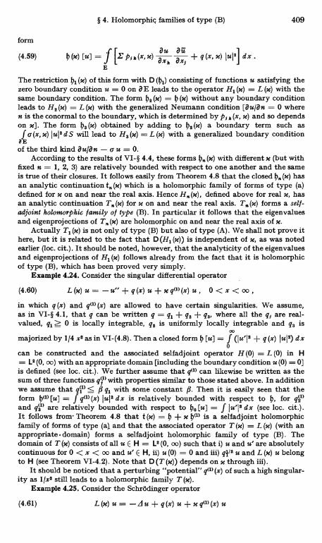
§ 4. Hooomorphie families of type (B) 409
form
(4.59) h (x) [u] = f . ps s (x, x)au au +
q (x, x) lull ] dx .axR axjE
The restriction hl (x) of this form with D (01) consisting of functions u satisfying thezero boundary condition u = 0 on a E leads to the operator HI (x) = L (x) with thesame boundary condition. The form 03 (x) = 4 (x) without any boundary conditionleads to H3 (x) = L (x) with the generalized Neumann condition [au(an = 0 wheren is the conormal to the boundary, which is determined by p, k (x, x) and so dependson x]. The form 0,(m) obtained by adding to h3 (x) a boundary term such asf a (x, x) JuI3 d S will lead to H3 (x) = L (x) with a generalized boundary condition
aEof the third kind aufan - a u = 0.
According to the results of VI-§ 4.4, these forms h,, (x) with different x (but withfixed n = 1, 2, 3) are relatively bounded with respect to one another and the sameis true of their closures. It follows easily from Theorem 4.8 that the closed 0. (x) hasan analytic continuation t (x) which is a holomorphic family of forms of type (a)defined for x on and near the real axis. Hence H. (x), defined above for real x, hasan analytic continuation T. (x) for x on and near the real axis. T. (x) forms a self-adjoint holomorphic family of type (B). In particular it follows that the eigenvaluesand eigenprojections of T. (x) are holomorphic on and near the real axis of X.
Actually Tl (x) is not only of type (B) but also of type (A). We shall not prove ithere, but it is related to the fact that D (Hl (x)) is independent of x, as was notedearlier (loc. cit.). It should be noted, however, that the analyticity of the eigenvaluesand eigenprojections of Hl (x) follows already from the fact that it is holomorphicof type (B), which has been proved very simply.
Example 4.24. Consider the singular differential operator
(4.60) L (x) u = - u" + q (x) u -}- x q(I) (x) u , 0 < x < oo ,
in which q (x) and qa> (x) are allowed to have certain singularities. We assume,as in VI-§ 4.1, that q can be written q = ql + qs + q3, where all the qj are real-valued, qr Z 0 is locally integrable, q2 is uniformly locally integrable and q3 is
mmajorized by 1/4 x2 as in VI-(4.8). Then a closed form I) [u] = f (lu'13 + q (x) 1u12) dx
0can be constructed and the associated selfadjoint operator H (0) = L (0) in H= L2 (0, oo) with an appropriate domain [including the boundary condition u (0) = 0]is defined (see loc. cit.). We further assume that q(I) can likewise be written as thesum of three functions qu with properties similar to those stated above. In additionwe assume that qll) < ig qr with some constant P. Then it is easily seen that theform Ou)[u] = f q( (x) Ju13dx is relatively bounded with respect to h, for &and q3 are relatively bounded with respect to 40 [u] = f lu'I3 dx (see loc. cit.).It follows from- Theorem 4.8 that t (x) = 4 + x O(1) is a selfadjoint holomorphicfamily of forms of type (a and that the associated operator T (x) = L (x) (with anappropriate .domain) forms a selfadjoint holomorphic family of type (B). Thedomain of T (x) consists of all u E H = L2 (0, oo) such that i) u and u' are absolutelycontinuous for 0 < x < oo and u' E H, ii) u (0) = 0 and iii) q}'3 u and L (x) u belongto H (see Theorem VI-4.2). Note that D (T (x)) depends on x through iii).
It should be noticed that a perturbing "potential" q(I) (x) of such a high singular-ity as 1/x3 still leads to a holomorphic family T (x).
Example 4.25. Consider the Schrodinger operator
(4.61) L(x)u=-du+q(x)u+xgl>(x)u
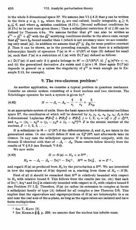
410 VII. Analytic perturbation theory
in the whole 3-dimensional space R3. We assume (see VI-§ 4.3) that q can be writtenin the form q = q1 + q2, where the qk are real-valued, locally integrable, q1 Z 0,q2S 0, and where q2 satisfies condition (4.17c). [Several sufficient conditions for(4.17c) to be met were given there.] Then a selfadjoint restriction H of L (0) can bedefined by Theorem 4.6a. We assume further that q(1) can also be written asqc1) = gj11 + q(2') with the qk 1 satisfying conditions similar to the above ones, exceptthat q2) have 4o bound smaller than 1 (which is not necessary since we are consider-ing only small IxI). In addition we assume that g111 5 13g1 for some positive constantfl. Then it can be shown, as in the preceding example, that there is a selfadjointholomorphic family of operators T (x) in H = L2 (R3) of type (B) defined for smallIxl, such that T (x) is a restriction of L (x) with D (T (x)) defined as follows:
u E D (T (x)) if and only if i) gradu belongs to H' = (L3 (R3))3, ii) f g1lu12dx < oo,and iii) the generalized derivative zl u exists and L (x) u E H. Here again D (T (x))depends in general on x unless the singularity of ge11 is weak enough (as in Ex-ample 2.13, for example).
9. The two-electron problem 1As another application, we consider a typical problem in quantum mechanics.
Consider an atomic system consisting of a fixed nucleus and two electrons. TheSchrodinger operator for such a system is given by 3
(4.62) H=-d1-z2-? -? + 2
r1 r2 Zr1E
in an appropriate system of units. Here the basic space is the 6-dimensional euclideanspace R6, the coordinates of which will be denoted by x1, y1, z1, x2, ,y2, z2; LI is the3-dimensional Laplacian a304 + a3/ay; + a3/azq, j = 1, 2; r, = (4 + y, + z2)1/2,and r12 = [(x1 - x2)2 + (y1 - y2)2 + (z1 - z$)2]1/2. Z is the atomic number of thenucleus, Z = 1, 2, 3. ... .
H is selfadjoint in H = L2 (Re) if the differentiations z11 and A. are taken in thegeneralized sense. Or one could define H first on Co (R6) and afterwards take itsclosure. In any case the selfadjoint operator H is determined uniquely, with thedomain D identical with that of -d1 - d2. These results follow directly from theresults of V-§ 5.3 (see Remark V-5.6).
We now write
(4.63) H = H (x) = Ho + x Hat,
Ho=-d1-d2-2r11-2ra1, HM =2rla, x=Z-1,and regard H (x) as produced from Ho by the perturbation x H11. We are interestedin how the eigenvalues of H (x) depend on x, starting from those of Ho = H (0).
First of all it should be remarked that HIM is relatively bounded with respectto Ho with relative bound 0. This follows from the results (see loc. cit.) that eachof 2ri 1, 2ra 1 and 2ri91 is relatively bounded with respect to Ho with relative bound 0(see Problem IV-1.2). Therefore, H (x) (or rather its extension to complex x) formsa selfadjoint family of type (A) defined for all complex x (see Theorem 2.6). Thisimplies that the eigenvalues and eigenprojections of H(x) are holomorphic in x onand near the real axis of the x-plane, as long as the eigenvalues are isolated and havefinite multiplicities.
1 See T. KATO [3].3 See KEMBLE 111, p. 209; we assume that the nucleus has infinite mass.
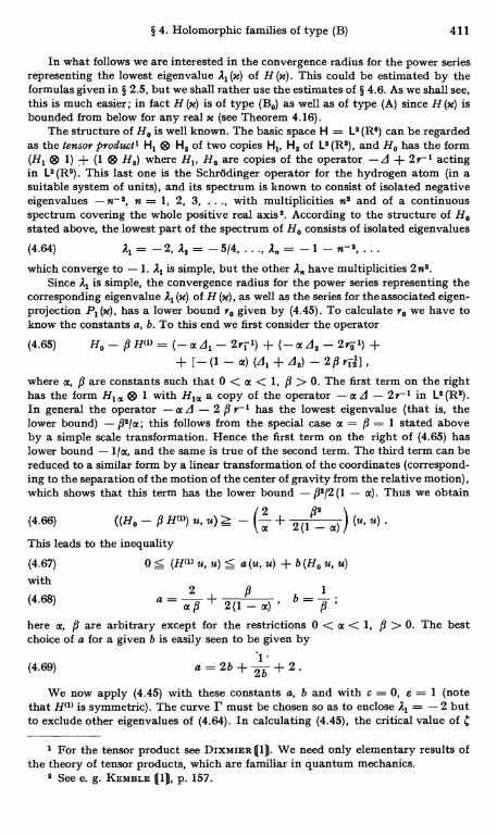
§ 4. Holomorphic families of type (B) 411
In what follows we are interested in the convergence radius for the power seriesrepresenting the lowest eigenvalue AI (x) of H (x). This could be estimated by theformulas given in § 2.5, but we shall rather use the estimates of § 4.6. As we shall see,this is much easier; in fact H (x) is of type (Bo) as well as of type (A) since H (x) isbounded from below for any real x (see Theorem 4.16).
The structure of H. is well known. The basic space H = L2 (Ro) can be regardedas the tensor product' H, 0 H2 of two copies Hl, H. of L2 (R3), and Ho has the form(HI 0 1) + (1 0 He) where HI, H2 are copies of the operator -d + 2r-' actingin L2 (R'). This last one is the Schrodinger operator for the hydrogen atom (in asuitable system of units), and its spectrum is known to consist of isolated negativeeigenvalues - n- 8, n = 1, 2, 3, ..., with multiplicities n2 and of a continuousspectrum covering the whole positive real axis $. According to the structure of Hostated above, the lowest part of the spectrum of Ho consists of isolated eigenvalues
(4.64) AI = -2, Ae = -514, ..., A. = - 1 - n- 2, .. .which converge to - 1. AI is simple, but the other A. have multiplicities 2n2.
Since AI is simple, the convergence radius for the power series representing thecorresponding eigenvalue AI (x) of H (x), as well as the series for the associated eigen-projection PI (x), has a lower bound ro given by (4.45). To calculate ro we have toknow the constants a, b. To this end we first consider the operator
(4.65) Ho-PH(')=(-adl-2ri')+(-adz-2ra')++ C-(1 - a) (di +d2) - 2Pr'i217
where a, # are constants such that 0 < a < 1, > 0. The first term on the righthas the form H, a 0 1 with H,, a copy of the operator - a A - 2r-' in L' (R').In general the operator - a d - 2 fl r-I has the lowest eigenvalue (that is, thelower bound) - f2/a; this follows from the special case a = i3 = 1 stated aboveby a simple scale transformation. Hence the first term on the right of (4.65) haslower bound -1(a, and the same is true of the second term. The third term can bereduced to a similar form by a linear transformation of the coordinates (correspond-ing to the separation of the motion of the center of gravity from the relative motion),which shows that this term has the lower bound - p2/2(1 - a). Thus we obtain
s(4.66) ((Ho - Hay) it, u)
a + fl l - 00(u, u) .
This leads to the inequality
(4.67) 0 S (HU) it, u) S a (u, u) + b (Ho it, u)with
2 l4 1(4.68) a= ap + 2(1
a), b= ;
here a, fl are arbitrary except for the restrictions 0 < a < 1, fi > 0. The bestchoice of a for a given b is easily seen to be given by
1 '(4.69) a=2b-} 2b
+2.We now apply (4.45) with these. constants a, b and with c = 0, e = 1 (note
that H>'> is symmetric). The curve r must be chosen so as to enclose AI = - 2 butto exclude other eigenvalues of (4.64). In calculating (4.45), the critical value of C
1 For the tensor product see DIXMIER (1). We need only elementary results ofthe theory of tensor products, which are familiar in quantum mechanics.
2 See e. g. KEMBLE (1), p. 157.
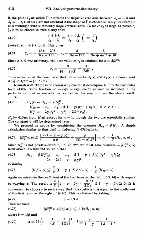
412 VII. Analytic perturbation theory
is the point Co at which r intersects the negative real axis between k = - 2 andd$ = - 5/4; other C are not essential if the shape of r is chosen suitably, for exampleas a rectangle with sufficiently large vertical sides. To make ro as large as possible,Co is to be chosen in such a way that
(4.70)a+b21 a+bAs= lCo - Al As - Co ro
(note that a + b A, > 0). This gives13a - 20b 3 3
(4.71) Co=- 8a-13b ' r0 8a-13b_
3b+4b-1+16Since b > 0 was arbitrary, the best value of ro is attained for b = 2/31/2:
3 1
ro = = 7.6416+41/3Thus we arrive at the conclusion that the series for 1 (x) and P1 (x) are convergentif Ixl < 1/7.7 or I21 > 7.7.
Remark 4.26. There is no reason why one must decompose H into the particularform (4.63). Some fraction of - 2ri 1 - 2ra 1 could as well be included in theperturbation. Let us see whether we can in this way improve the above result.
Set(4.73) Hy (x) =Hoy + x Hy ) ,
Hoy=-41-A2-2(l-Y)(ril+rz'), 0<y<l.Hy)=-2Y(ri1+r21)+2Z-1r14
Hy (x) differs from H (x) except for x = 1, though the two are essentially similar.The constant y will be determined later.
We proceed as above by considering the operator Hoy - fi Hy3. A simplecalculation similar to that used in deducing (4.67) leads to
s(4.74) (H y u, u) <
L
(1
aP
Y) + 2 (1 - a) Ze ] (u. u) + (Ho y u, u) .
Since Hy 3 is not positive-definite, unlike Ha3, we must also estimate - (Hy D u, u)from above. To this end we note that
(4.75) Hoy+fH, ZZ -2(1-Y+fly)$.
obtaining
(4.76) - (Hy u, u) S (I + P V) l (u, u) + (Hoy u, u)
Again we minimize the coefficient of the first term on the right of (4.74) with respect
to varying a. The result is 11 - y - fl y + z ZZ if 1 - y - i4 y 0. It isconvenient to choosey in such a way that this coefficient is equal to the coefficientof the first term on the right of (4.76). This is attained by taking
(4.77) y = 1/4Z .
Then we have
(4.78) ((HY u, u) S a (u, u) + b (Hoy u, u)
where b = 1/# and
'j-b-)',b.1, y = 1
(4.79) a=2bI1- 4Z1+
4 1 - y 4Z - 1
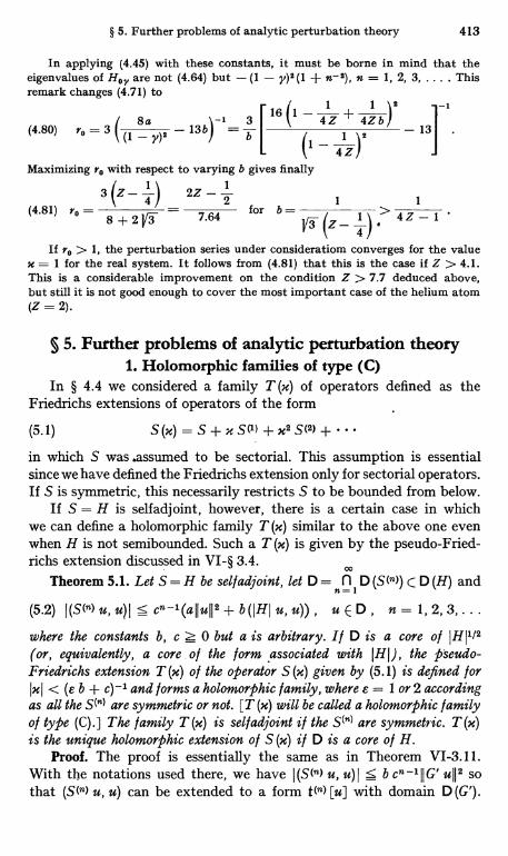
§ 5. Further problems of analytic perturbation theory 413
In applying (4.45) with these constants, it must be borne in mind that theeigenvalues of H0 are not (4.64) but - (1 - y) 2 (1 + n-8), n = 1, 2, 3, .... Thisremark changes (4.71) to
r__/. 1 1 \2 --ii8a 3
(4.80) ro=3 (1 -y)2 - 13b=b
- 13$
(1
1
4Z)Maximizing ro with respect to varying b gives finally
3(Z- 4) 2Z- 11 1
(4.81) ro =7.64
for b =3
(Z - 1 > 4 7_ - 18+213 V- 4).If ro > 1, the perturbation series under consideration converges for the value
x = 1 for the real system. It follows from (4.81) that this is the case if Z > 4.1.This is a considerable improvement on the condition Z > 7.7 deduced above,but still it is not good enough to cover the most important case of the helium atom(Z = 2).
§ 5. Further problems of analytic perturbation theory1. Holomorphic families of type (C)
In § 4.4 we considered a family T (x) of operators defined as theFriedrichs extensions of operators of the form
(5.1) S(x) = S+xS(1)+x2S(2)+...
in which S was assumed to be sectorial. This assumption is essentialsince we have defined the Friedrichs extension only for sectorial operators.If S is symmetric, this necessarily restricts S to be bounded from below.
If S = H is selfadjoint, however, there is a certain case in whichwe can define a holomorphic family T (x) similar to the above one evenwhen H is not semibounded. Such a T (x) is given by the pseudo-Fried-richs extension discussed in VI-§ 3.4.
Theorem 5.1. Let S = H be sel f adjoint, let D = fl1 D (S(")) C D (H) and
(5.2) I(S(") u,u)I s cn-1(aIIuII2+b(IHI u, u)), uED, n= 1,2,3,.
where the constants b, c >,= 0 but a is arbitrary. If D is a core of IHI1/2(or, equivalently, a core, of the form associated with I HI) , the pseudo-Friedrichs extension T (x) of the operator S (x) given by (5.1) is defined forIxI < (e b + c) -1 and forms a holomorphic family, where e = 1 or 2 accordingas all the S(") are symmetric or not. [T (x) will be called a holomorphic familyof type (C).] The family T (x) is selfadjoint if the S(") are symmetric. T (x)is the unique holomorphic extension of S (x) if D is a core of H.
Proof. The proof is essentially the same as in Theorem VI-3.11.With the notations used there, we have I (S (n) u, u) I S b c" -1 II G' u1I 2 sothat (S(") u, u) can be extended to a form t(") [u] with domain D (G').
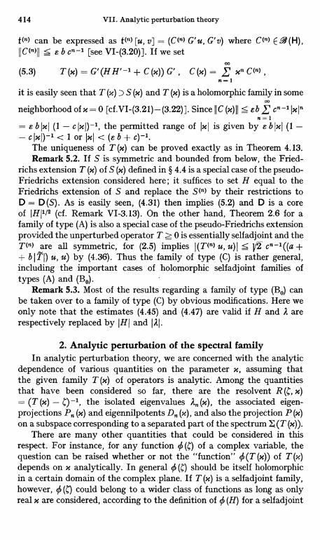
414 VII. Analytic perturbation theory
t(n) can be expressed as t(nl [u, v] = (CO G'u, G'v) where CO E _q (H),IIC(n)II <- s b cn-1 [see VI-(3.20)]. If we set
00
(5.3) T(x)=G'(HH'-1+C(x))G', C(x)_ Z xnC(),n=1
it is easily seen that T (x) > S (x) and T (x) is a holomorphic family in some00
neighborhood of x = 0 [cf.VI-(3.21)-(3.22)]. Since 11C (m) 11 < eb f cn-1lxlnn=1
= s b Iml (1 - c Ixl)-1, the permitted range of Iml is given by e b Iml (1 -- c lxl)-1 < I or Iml < (e b + c)-1.
The uniqueness of T (x) can be proved exactly as in Theorem 4.13.Remark 5.2. If S is symmetric and bounded from below, the Fried-
richs extension T (x) of S (x) defined in § 4.4 is a special case of the pseudo-Friedrichs extension considered here; it suffices to set H equal to theFriedrichs extension of S and replace the S(n) by their restrictions toD = D (S). As is easily seen, (4.31) then implies (5.2) and D is a coreof IH11/2 (cf. Remark VI-3.13). On the other hand, Theorem 2.6 for afamily of type (A) is also a special case of the pseudo-Friedrichs extensionprovided the unperturbed operator T z 0 is essentially selfadjoint and theT (n) are all symmetric, for (2.5) implies I (T (n) u, u) J < VT cn -1((a ++ b I TI) u, u) by (4.36). Thus the family of type (C) is rather general,including the important cases of holomorphic selfadjoint families oftypes (A) and (B0).
Remark 5.3. Most of the results regarding a family of type (Bo) canbe taken over to a family of type (C) by obvious modifications. Here weonly note that the estimates (4.45) and (4.47) are valid if H and A arerespectively replaced by IHI and IAI.
2. Analytic perturbation of the spectral familyIn analytic perturbation theory, we are concerned with the analytic
dependence of various quantities on the parameter x, assuming thatthe given family T (x) of operators is analytic. Among the quantitiesthat have been considered so far, there are the resolvent R (r;, x)= (T (x) - 4) -1, the isolated eigenvalues An (x), the associated eigen-projections Pn (x) and eigennilpotents D. (x), and also the projection P (x)on a subspace corresponding to a separated part of the spectrum F (T (x)).
There are many other quantities that could be considered in thisrespect. For instance, for any function of a complex variable, thequestion can be raised whether or not the "function" O(T (x)) of T (x)depends on x analytically. In general 0 should be itself holomorphicin a certain domain of the complex plane. If T(x) is a selfadjoint family,however, 0 (C) could belong to a wider class of functions as long as onlyreal x are considered, according to the definition of 0 (H) for a selfadjoint
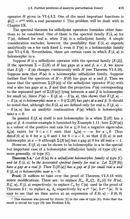
§ 5. Further problems of analytic perturbation theory 415
operator H given in VI-§ 5.2. One of the most important functions isei E c with a real parameter t. This problem will be dealt with in
Chapter IX.The spectral theorem for selfadjoint operators furnishes other func-
tions to be considered. One of them is the spectral family E (A, x) forT (x), defined for real x, when T (x) is a selfadjoint family. A simpleconsideration excludes, however, the possibility that E (A, x) dependsanalytically on x for each fixed A, even if T (x) is a holomorphic family(see VI-§ 5.4). Nevertheless, there are certain cases in which E (A, x) isholomorphic in x.
Suppose H is a selfadjoint operator with the spectral family {E (A)}.If the spectrum E = E (H) of H has gaps at a and fl, a < j3, we knowthat E (f1) - E (a) changes continuously with H (see Theorem VI-5.10).Suppose now that H (x) is a holomorphic selfadjoint family. Supposefurther that the spectrum of H = H (0) has gaps at a and j3. Then weknow that the spectrum E (H (x)) of the selfadjoint operator H (x) withreal x also has gaps at a, fi and that the projection P(x) correspondingto the separated part of E (H (x)) lying between a and j3 is holomorphicfor small I44. Since P (x) = E (fl, x) - E (a, x), this shows that E (fl, x) -- E (a, x) is holomorphic near x = 0 if E (H) has gaps at a and P. It shouldbe noted that, although the E (A, x) are defined only for real x, E (j3, x) -- E (a, x) has an analytic continuation P (x) which is holomorphicnear x = 0.
In general E (fl, x) itself is not holomorphic in x when E (H) has agap at j9. A counter-example is furnished by Example 1.11; here E (H (x))is a subset of the positive real axis for x 5 0 but a negative eigenvalueAo (x) exists for 0 < x < I such that Ao (x) -+ - oo for x -, 0. ThusdimE (0, x) is 0 for n :50 and 1 for 0 < x < 1, so that E (0, x) is notholomorphic at x = 0 although E (H (x)) has a gap at 0 for all real x < 1.
However, E (fl, x) can be shown to be holomorphic in x in the specialbut important case of a holomorphic selfadjoint family of type (A) or,more generally, of type (C).
Theorem 5.4.1 Let H (x) be a selfadjoint holomorphic family of type (C)and let E (A, x.) be the associated spectral family for real x. Let E (H (0))have a gap at a real P. Then E (H (x)) has a gap at 9 for small real x andE (fl, x) is holomorphic near x = 0.
Proof. It suffices to take over the proof of Theorem VI-5.13 withminor modifications. These are: to replace H,,, R. E. (2) by H (x),R x), E (A, x) respectively; to replace C by C (x) used in the proof ofTheorem 5.1; to replace a,,, b respectively by a cn-1Ix1, b cn-1 jxI. It iseasy to see that we then arrive at an expression of E (0, x) - E (0, 0)
1 This theorem was proved by HEINZ [2] in the case of type (A). Note that theresult is trivial for type (B) (see Problem 5.5).
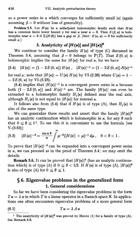
416 VII. Analytic perturbation theory
as a power series in x which converges for sufficiently small Ixl (againassuming 9 = 0 without loss of generality).
Problem 5.5. Let H (x) be a selfadjoint holomorphic family such that H (x)has a common finite lower bound y for real x near x = 0. Then E (i$, x) is holo-morphic near x = 0 if E (H (0)) has a gap at P. [hint: E (a, x) = 0 for sufficientlysmall a.]
3. Analyticity of IH(x)I and IH(x)I0We continue to consider the family H (m) of type (C) discussed in
Theorem 5.4, assuming that fi = 0 belongs to P (T). That E (0, x) isholomorphic implies the same for IH (x) I for real x, for we have
(5.4) IH(x)I = (1 - 2E(0, x)) H(x) , IH(x)1-1 = (1 - 2E(0, x)) H(x)-1
for real x ; note that I H (x) I = U (x) H (x) by VI-(2.26) where U (x) = 1 -- 2E(0, x) by VI-(5.25).
(5.4) implies that IH (x) I-1 is a convergent power series in x becauseboth (1 - 2E(0, x)) and H (x)-1 are. The family IH (x) I can even beextended to a holomorphic family H1(x) defined near the real axis,although H1 (x) is not equal to J H (x) I for nonreal x.
It follows also from (5.4) that if H (x) is of type (A), then H1 (x) isalso of the same type.
We can generalize these results and assert that the family I H (x)10
has an analytic continuation which is holomorphic in x, for any 0 suchthat 0 S 0 5 11. To see this it is convenient to use the formula [seeV-(3.53)]
00
(5.5) IH(x)I-0=sinxO /1U_0(IH(x)I+'u)-' du, 0<0<1.
79
0
To prove that IH (x) I - 0 can be expanded into a convergent power seriesin x, we can proceed as in the proof of Theorem 5.4; we may omit thedetails.
Remark 5.6. It can be proved that IH (x)10 (has an analytic continua-tion which) is of type (A) if 0 5 0 < 1/2. If H (m) is of type (A), IH (x)10is also of type (A) for 0 5 0 5 1.
§ 6. Eigenvalue problems in the generalized form1. General considerations
So far we have been considering the eigenvalue problems in the formT u = A u in which T is a linear operator in a Banach space X. In applica-tions one often encounters eigenvalue problems of a more general form
(6.1) Tu = AAu
1 The analyticity of IH(x)10 was proved by HEINZ [1] for a family of type (A).See Remark 5.6.
§ 6. Eigenvalue problems in the generalized form 417
where T and A are operators in X or, more generally, operators from Xto another Banach space Y.
There are several ways of dealing with this general type of eigenvalueproblem. For instance, (6.1) may be transformed into
(6.2) A-'Tu=Auif A-' exists. (6.2) has the standard form so far considered in detail,for A-' T is an operator in X. Or (6.1) may be written
(6.3) TA-'v=Av, v=Au;then we have again a standard form, this time the operator TA -I actingin the space Y.
A transformation into a more symmetric form is given by
(6.4) A-1/2 TA-112 w= A w, w = A1/2 U.
This is particularly convenient when T and A are symmetric operatorsin a Hilbert space. In any case the construction of A11/2 would requirethat Y = X.
In each transformation given above, however, it appears that there issomething arbitrary involved; there is no reason to choose one over theother. Besides, the relationship between the original eigenvalue problemand the spectra of the operators A-' T or TA-1 is not clear. It is truethat any eigenvalue A of (6.1) is at the same time an eigenvalue of (6.2)or (6.3) and that any eigenvector of (6.1) is also an eigenvector of (6.2),the eigenvector of (6.3) being related to that of (6.1) by the transforma-tion v = A u. But it is not clear what is meant by an isolated eigenvalueof (6.1) or the algebraic multiplicity of such an eigenvalue; for it mighthappen that A is an isolated eigenvalue of (6.2) but not of (6.3) and viceversa.
A more natural generalization of the results obtained for the standardproblem T u = A u to the general problem (6.1) would consist in thestudy of the generalized resolvent (T - CA)-' and the generalized spectrumassociated with it. Of course several modifications would be required ofthe former results when one considers such a generalization. For example,the resolvent equation should read
(6.5) (T -C'A)-1- (T -C"A)-1= (T-C'A)-1A (T-CAA)-1
Furthermore, there is in general no sense in speaking of the commutati-vity of the resolvents for different C, for the resolvent is an operatorfrom Y to X.
In this book, however, we shall not pursue this problem in anygenerality. Instead we shall content ourselves with considering some
418 VII. Analytic perturbation theory
special cases in which it suffices to consider the problem in the form(6.2) or (6.3).
Let us assume that T E'' (X, Y), A E -4 (X, Y) and A-1 E .4 (Y, X).Then A-' T E W (X) and TA-1 E W (Y), and (6.1) is equivalent to eitherof (6.2) and (6.3).
Let A be an isolated eigenvalue of A-1 T with a finite algebraicmultiplicity in, with the eigenprojection P and the eigennilpotent D.We have [see III-(6.28)-(6.29)]
(6.6) PA-1TCA-1TP=AP+D, D=DP=PD.Q = A PA-1 is a projection in Y, for Q E .V (Y) and Q2 = Q. SimilarlyG = A D A-1 is a nilpotent in Y. On multiplying (6.6) by A from the left,we obtain
(6.7) QTCTP=AAP+AD=AQA+GA, G=GQ=QG.
The consideration of the eigenvalue A of TA-1 leads to the same results;in fact, Q is exactly the eigenprojection associated with the eigenvalue Aof TA-1 and G is the associated eigennilpotent.
The resolvent (A-1 T - C,)-1 of A-1 T has the expansion
(6.8) (A-1 T - C)-1
_ - ( - A)-1 P - I (C - Dn -f- A)n Sn+1n=1 n=0
near = A [see 111-(6.32) ]. Here S is the reduced resolvent of A-' Tat C = A. Multiplication from the right by A-1 gives
00
(6.9) (T - CA)-1= - (C - A)-1 PA-1 - Y ( - A)-n-1 Dn A-' +n=1
00
+ A)n Sn+l A-1nl== O
00
n=100
+ f (C - A)n A-' Un+1,n=0
where U = A S A-1 is the reduced resolvent of TA-1.If we consider a system Ah, h = 1, . . ., s, of isolated eigenvalues of
A-' T, with the associated eigenprojections Ph and eigennilpotents Dh,we have (Qh = A PhA-1, Gh = A Dh A-1)
(6.10) QhTCTPh=AhAPh+ADh=A,,Q,,A+G,,A,Dh=DhP,,= PhD,,, Gh=GhQh=Q,,G,,, P,,Pk=BhhPh,
QhQk = ahkQh
§ 6. Eigenvalue problems in the generalized form 419
Suppose, in particular, that both T and A are symmetric operatorsin a Hilbert space X = Y = H. In this case neither A-1 T nor TA-1 issymmetric in general. But A-1 T becomes a symmetric operator if thenew inner product
(6.11) ((u, v)) = (Au, v)
is introduced, assuming in addition that A is positive. Note that His also a complete Hilbert space with this new inner product under thestated assumptions on A. Consequently, A or the Ah must be real and Por the Ph are orthogonal projections (and therefore have bounds 1) in thenew metric, and D or the Dh must be zero. Returning to the old metric,we see that P or the Ph are bounded with bounds not exceeding a fixednumber depending only on A. In fact, it can easily be seen that
(6.12) IIPII < IIA-1IV1/2lIAII1/2.
We also note that (in the symmetric case)
(6.13) Q=P*, P=Q*.The proof depends on the observation that, since P is the eigenprojectionfor A of A-1 T, P* is the eigenprojection for 1 = A of (A-' T) * = TA-1.
An alternative way of dealing with the symmetric case is to use thetransformation to (6.4). A-1/2 TA-1112 is symmetric and similar to A-' Tand to TA-1. It is therefore selfadjoint if it (or A-1 T or TA-1) has atleast one isolated eigenvalue. The associated eigennilpotent must be zeroand the associated orthogonal projection is identical with A1/2 PA-112.
2. Perturbation theory
Here we are mainly interested in the eigenvalue problems of the form
(6.14) T (x) u= A (x) A (x) u,
where T (x) as well as A (x) is a holomorphic family of closed operatorsfrom X to Y defined near x = 0. We inquire whether or not the eigen-values A (x) and the associated eigenvectors can be expressed as holo-morphic functions of x.
According to the restrictions introduced in the preceding paragraph,we shall assume that A (x) is bounded-holomorphic, so that it can beexpressed as a convergent power series
(6.15) A(x)=A+xA(1)+x2A(2)+..., A,A(n)Ei(X,Y).
Furthermore, A will be assumed to have an inverse A-1 E .4 (Y, X),so that A (x)-1 also exists and belongs to l(Y, X) for small Ixl, with the
420 VII. Analytic perturbation theory
expansion
(6.16) A(m)-l= A-1 - xA-1 A(1) A-1 + x2(A-1 A(1) A-1 A(1) A-1 --A-'A(2)A-1)+...
(6.14) is now equivalent to the eigenvalue problem
(6.17) Ta (x) u = A (x)-1 T (x) u = A (m) u.
Here Ta (x) is a closed operator acting in X and forming a holomorphicfamily, as is easily verified from the property of T (m). Thus theanalytic perturbation theory developed in this chapter can be applied toTa (x). It follows, for example, that any isolated eigenvalue of theunperturbed operator T. = T. (0) = A-1 T (0) can be continued as ananalytic function 2 (x) of x, which is an eigenvalue of T. (x) for each M.Similar results hold for the associated eigenprojection P(x) and theeigennilpotent D(x) for the operator Ta(x), and for the eigenprojectionQ (x) = A (x) P (x) A (x)-1 and eigennilpotent G (x) = A (x) D (x) A (x)-1for the operator Tb(x) = T (x) A (x)-1 = A (x) Ta(x) A (x)-1 (cf. thepreceding paragraph).
There is another transformation of (6.14) [which is particularlyconvenient when T (m) and A (x) are selfadjoint]. We write (6.15) in theform
(6.18) A (x) = (1 + x C2 (x)) A = (1 + x C2 (x))1/2 A (1 + x C, (x))1/2 ,
where00 00
(6.19) C2 (x) = fxn A (n +1) A-1 E -V(Y) , C, (x) = Zxn A -1 A (n +1) E ,off (X)n=0 n=0
are bounded-holomorphic. The validity of the first equality of (6.18) isobvious. The second is a consequence of the general formula
(6.20) (1 + BA-1)k A = A (1 + A-1 B)k , A, B E .9 (X, Y) ,
which holds for any number k and any B with sufficiently small II BIITo verify (6.20) one need only to develop both sides into binomial series.
(6.18) permits the transformation of (6.14) into
(6.21) (1 + x C2 (x))-1/2 T (m) (1 + x C1 (n))-1/2 w = 2 (x) A w
where
(6.22) w = (1 + x C, (x))1/2 u .
It should be noted that the operator on the left of (6.21) forms a self-adjoint family if both T (x) and A (x) are selfadjoint families.
The operator A on the right of (6.21) can be eliminated, if desired,by a further transformation of the form (6.4). This is not necessary,however, since A is independent of x. In the selfadjoint case with A > 0,
§ 6. Eigenvalue problems in the generalized form 421
it suffices to introduce the new metric (6.11) so that the operator on theleft of (6.21) becomes selfadjoint after multiplication from the left by A-',thus reducing the problem to the standard form. The procedure describedhere is particularly convenient inasmuch as no fractional powers (suchas Al/2) of operators are needed except those which can be calculated bybinomial series.
Problem 6.1. Let T (x) and A (x) be selfadjoint families with A > 0. Then 2 (x)is real for real x, 2 (x) and P (x) are holomorphic near the real axis, and D (x) = 0.
3. Holomorphic families of type (A)
Suppose that the T (x) of (6.14) is holomorphic of type (A) nearx = 0, with the expansion (2.1). Then Ta(x) = A (x)-1 T (x) has the sameproperty, and we have
(6.23) Ta(x) u = A-' Tu + x(A-1 T(1) - A-' A(1) A-' T) u + .
The series for the eigenvalues A; (x) that arise by splitting from anisolated eigenvalue A of T. (0) = A-1 T and for the associated eigen-projections P5(x) can then be calculated by application of the formulasof II-§ 2 to Ta(x). We shall write only the series for the averaged eigen-value A (x) :
(6.24) (x) = A + x P) + .. .
P) = 1 tr(A-1 T(1) - A-' A(1) A-' T) PM
= m tr (A-1 T(1) - A A-1 AM) P,
where P is the eigenprojection for A of A-' T, m = dim P and the as-sociated eigennilpotent is assumed to be zero.
If {uk}, k = 1, . . ., m, is a basis of the eigenspace PX and {ek} is theadjoint basis of P* X* (forming a biorthogonal set with {uk}), we have
1
(6.25) ,.(1) =.- f (A-' (T(1) - A A(1)) uk, ek)M k
1 mnx ((T(1) --A AM) uk, fk) ,
k=1where
(6.26) fk = (A-)* ek E A*-1 P* X* = (PA-)* X*
_ (A-1Q)*X*=Q*A*-1X*=Q*Y*
are characterized by the properties that
(6.27) (A uf, f k) = S;k , (A u, f k) = 0 for P u = 0 .
422 VII. Analytic perturbation theory
In the special case in which X = Y = H is a Hilbert space, T (m)and A (x) are selfadjoint and A is positive, it is convenient to choose ukin such a way that f k = uk. This is equivalent to choosing uk according to
(6.28) (A u;, uk) = b k
If, in particular, m = 1, we havea>) u u)
(6.29) A(,) = (Tw -
(A u, u)
where u is an eigenvector for A of A-' T. The coefficients AN for n z 2can be calculated by the same method.
Of course one arrives at the same results if one starts from thesymmetric form (6.21) of the eigenvalue equation. But here there is someinconvenience arising from the fact that the operator-valued functionon the left of (6.21) is not necessarily of type (A), thus preventing thestraightforward application of the formulas of II-§ 2.
4. Holomorphic families of type ($)Suppose that T (x) of (6.14) is a holomorphic family of type (B) near
x = 0. Thus T (x) is an m-sectorial operator associated with a family t (x)of sectorial forms with a constant domain D = D (t (x)) which has aTaylor expansion of the form (4.15).
In this case we have again the results of par. 2, but the calculationof the perturbation series is not so straightforward as in the case oftype (A) considered above. Here it is convenient to consider T(X)-1
instead of T (x) itself, assuming for the moment that t (x) has a positivevertex y independent of x. Then T (x)-1 is bounded-holomorphic. Sincethe inverse A (x) -I of the eigenvalue A (x) of (6.14) is an eigenvalue of theinverted eigenvalue problem
(6.30) T (x)-1 v = A(x)-1 A (x)-1 v , v = A (x) u ,
A(x)-1 can be calculated by the method of the preceding paragraph,from which the series for A (x) can be obtained. For example, if we havea simple eigenvalue A of the unperturbed equation T u= A A u orT-1 v = A-1 A-1 v, we obtain in this way
(6.31) AM = A +ta> [u] - A(A(1) u., u)
x + .(A u, u)
the calculation is similar to that given in § 4.6 and may be omitted(see in particular Remark 4.18).
We have assumed above that T (x) has a positive vertex, but thisassumption can be eliminated if the bounded form (A (x) u, u) hasa positive vertex. In this case we have only to consider T, (x) = T (x) ++ a A (x) instead of T (x). If a is a sufficiently large real number, T, (x)
§ 6. Eigenvalue problems in the generalized form 423
has a positive vertex, while the eigenvalue Al (x) for the problem (6.14)with T (x) replaced by TI (x) is equal to A (x) + a.
Remark 6.2. Eigenvalue problems of the form T u = A A u arise in anatural way when one considers two quadratic forms t [u] and a [u].In our treatment of forms t [u] in a Hilbert space H, we have beenmainly concerned with the relation between t [u] and the unit form hJuh12which is a special quadratic form. When two forms t and a are to beconsidered without any reference to a third form such as hJull2, there is nolonger any point in supposing that t and a are defined in a given Hilbertspace. Instead one could start from a vector space X in which both tand a are defined and, if desired, make X into a Hilbert space by intro-ducing an inner product suitably related to these forms. If a is a positivesymmetric form, for example, we may take a [u, v] as the inner product.The perturbation theory for an eigenvalue problem (6.14) could also betreated accordingly'.
We shall not go into this general theory. It will only be remarkedthat the eigenvalue problem T u = A A u can be formulated directly interms of the forms t and a associated with T and A by
(6.32) t [u, v] = A a [u, v] for all v E D (t) n D (a) .
It will also be noted that, when both t and a are symmetric and certainconditions are satisfied so that the eigenvalues form a discrete set boundedfrom below, the eigenvalues of T u = A A u are characterized by theminimax principle applied to the ratio t [u]/a [u] in place of I-(6.72).
5. Boundary perturbationAs an application of the preceding results, let us consider the so-
called boundary perturbation 2. A simple example is the eigenvalue problem
(6.33) - A u (x) = A u (x) , x E E C R'1
with the zero boundary condition
(6.34) u(x)=O, x E 2 E.
The main question is how the eigenvalues are changed by a small deforma-tion of the region E.
In dealing with this problem, it is convenient to consider a familyE (x) of bounded regions depending on a small real parameter x and
1 For a general theory of quadratic forms see ARONSZAJN [2], [4].2 See RHLLICH [8], COURANT-HILBERT (1), p. 419, SEGEL [1]. For formal
theory, see also MORSE-FESHBACH (1), SAITO [1]. For the stability of the essentialspectrum under variation of the boundary, see WOLF [3], KREITH and WOLF [1];for the stability of the absolutely continuous spectrum, see BIRMAN [6].
424 VII. Analytic perturbation theory
inquire into the dependence of the associated eigenvalues A (x) on M. Weshall assume that E (x) is obtained from E = E (0) by a one-to-onetransformation(6.35) x -*y = x + x O(x)
where (x) is a sufficiently smooth function defined in an open set con-taining the closure E = E v a E of E. 0 (x) may be regarded as a vector-valued function with components 0k (x) = 07, (xl, ..., xn), k = 1, ..., n.
The eigenvalue problem (6.33), (6.34) to be considered in the regionE (x) is associated with the quadratic form
(6.36) f (grad u(y)l$ dyE (m)
defined in the Hilbert space H (x) = L2 (E (x)) with the norm
(6.37) IIuIl2 = f !u(y)1a dy .E(x)
To avoid the difficulty that the underlying Hilbert space H (x) dependson x, we introduce the transformation
(6.38) u (x) = u (y) with x, y related by (6.35)
of functions u E H (x) to functions 4 E H = H (0). Note that u satisfiesthe boundary condition u = 0 on aE if and only if u satisfies the boundarycondition u = 0 on aE (x).
Now (6.36) and (6.37) define two quadratic forms in H depending on x :
(6.39) t (x) [u]E
f (grad u (y) I$ dy = f E I E ayk aax,) 12J (x) dx ,it I
m) E
(6.40) a (x) [u] = f Ju (y) is dy = f 14 (x)1$ J (x) dxE (m) E
where j (x) is the Jacobian of the transformation (6.35) :
(6.41) J(x) = J(x, x) = det (a,k + x aka )
By our assumptions on c, j (x) is a smooth function on E and so a (x) isa bounded -symmetric form with positive lower bound. The associatedbounded operator A (x) is simply the multiplication operator by j (x, x).
Now' the eigenvalues A (x) to be considered are exactly the eigen-values associated with the two forms t (x) and a (x) in the sense stated inthe preceding paragraph, that is,
(6.42) T (m) u= A (m) A (m),4
where T(x) is the operator associated with the form t(x). The formst (x), a (x) as well as the operators T (x), A (x) are dependent on x but
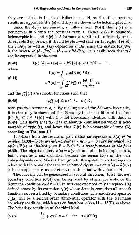
§ 6. Eigenvalue problems in the generalized form 425
they are defined in the fixed Hilbert space H, so that the precedingresults are applicable if T (x) and A (x) are shown to be holomorphic in M.
Since the k (x) are smooth, it follows from (6.41) that J (x) is apolynomial in x with the constant term 1. Hence A (x) is bounded-holomorphic in x and A (x) z S for some S > 0 if IxI is sufficiently small.As regards T (x) or t (x), it should be observed that on the right of (6.39),the axf/ayk as well as J(x) depend on x. But since the matrix (ax;/ay,)is the inverse of (ay;/axle) = (61k + x it is easily seen that t(x)can be expressed in the form
(6.43) t(x) [u]=t[u]+xt(')[i]+x2t(2)[12]+where
(6.44)
t [u] = f grad ii (x) 11 dx ,E
t(r) [u] =J PPi('2(x) dx
d i ax{ axgE
and the p, (x) are smooth functions such that
(6.45) IP,k(x)I <bc'-1, xEE,with positive constants b, c. By making use of the Schwarz inequality,it is then easy to show that the t(r) satisfy the inequalities of the formIt(T) [u]1 S b cr-1 t [u] with b, c not necessarily identical with those in(6.45). This shows that t (x) has an analytic continuation which is holo-morphic of type (a), and hence that T (x) is holomorphic of type (B),according to Theorem 4.8.
It follows from the results of par. 2 that the eigenvalues A(x) of theproblem (6.33) - (6.34) are holomorphic in x near x = 0 when the underlyingregion E (x) is obtained from E = E (0) by a transformation of the form(6.35). The eigenfunctions u (x) = u (y, x) are also holomorphic in x,but it requires a new definition because the region E (x) of the vari-able y depends on x. We shall not go into this question, contenting our-selves with the remark that the transformed eigenfunction u (x) = u (x, x)is holomorphic in x as a vector-valued function with values in H.
These results can be generalized in several directions. First, the zeroboundary condition (6.34) can be replaced by others, for instance theNeumann condition au/a'n = 0. In this case one need only to replace t (x)defined above by its extension t1 (x) whose domain comprises all smoothfunctions not restricted by boundary conditions. The associated operatorTl (x) will be a second order differential operator with the Neumannboundary condition, which acts on functions is (x) E H = L2 (E) as above.The boundary condition of the third kind
(6.46) an + v(x) u = 0 for x E aE (x)
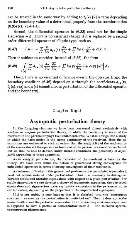
426 VIII. Asymptotic perturbation theory
can be treated in the same way by adding to tl (e) [it] a term dependingon the boundary value of u determined properly from the transformation(6.35) (cf. VI-§ 4.4).
Second, the differential operator in (6.33) need not be the simpleLaplacian -d. There is no essential change if it is replaced by a secondorder differential operator of elliptic type, such as
(6.47) Lu= - a ail. (x) au + bj(x) au + c(x) U.j.5 axj ax_ j axj
Then it suffices to consider, instead of (6.36), the form
(6.48) f L aj k (y) aau auk ayj + P bi (y) ayj u + c (y) hula, dy.
E(x)
Third, there is no essential difference even if the operator L and theboundary condition (6.46) depend on x through the coefficients ajk (x),b5 (x), c (x) and 6 (x) (simultaneous perturbation of the differential operatorand the boundary).
Chapter Eight
Asymptotic perturbation theoryIn the foregoing chapters we have been concerned almost exclusively with
analytic or uniform perturbation theory, in which the continuity in norm of theresolvent in the parameter plays the fundamental role. We shall now go into a studyin which the basic notion is the strong continuity of the resolvent. Here the as-sumptions are weakened to such an extent that the analyticity of the resolvent orof the eigenvalues of the operator as functions of the parameter cannot be concluded,but we shall be able to deduce, under suitable conditions, the possibility of asym-ptotic expansions of these quantities.
As in analytic perturbation, the behavior of the resolvent is basic for thetheory. We shall even define the notion of generalized strong convergence forunbounded operators in terms of strong convergence of their resolvents.
An inherent difficulty in this generalized problem is that an isolated eigenvalue Aneed not remain isolated under perturbation. Thus it is necessary to distinguishbetween stable and unstable eigenvalues, with respect to a given perturbation. Forstable eigenvalues we can develop a theory of asymptotic expansion; the perturbedeigenvalues and eigenvectors have asymptotic expansions in the parameter up tocertain orders, depending on the properties of the unperturbed eigenspace.
If A is not stable, it may happen that it is absorbed into the "continuousspectrum" as soon as the perturbation is "switched on". Then it does not makesense to talk about the perturbed eigenvalue. But the resulting continuous spectrumis supposed to have a particular concentration near A - the so-called spectralconcentration phenomenon.
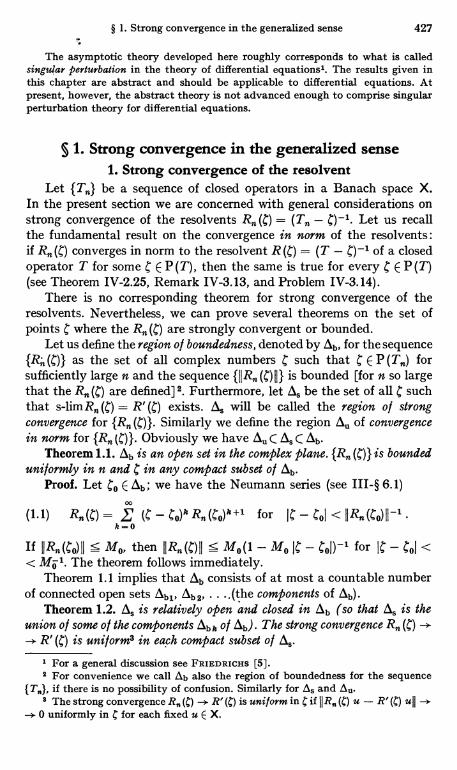
§ 1. Strong convergence in the generalized sense 427
The asymptotic theory developed here roughly corresponds to what is calledsingular perturbation in the theory of differential equations'. The results given inthis chapter are abstract and should be applicable to differential equations. Atpresent, however, the abstract theory is not advanced enough to comprise singularperturbation theory for differential equations.
§ 1. Strong convergence in the generalized sense1. Strong convergence of the resolvent
Let be a sequence of closed operators in a Banach space X.In the present section we are concerned with general considerations onstrong convergence of the resolvents R (C) = (T - C)-1. Let us recallthe fundamental result on the convergence in norm of the resolvents:if R (C) converges in norm to the resolvent R (C) = (T - C)-1 of a closedoperator T for some C E P (T), then the same is true for every C E P (T)(see Theorem IV-2.25, Remark IV-3.13, and Problem IV-3.14).
There is no corresponding theorem for strong convergence of theresolvents. Nevertheless, we can prove several theorems on the set ofpoints C where the R,,, (C) are strongly convergent or bounded.
Let us define the region of boundedness, denoted by Lb, for the sequence{R;, (C)} as the set of all complex numbers C such that C E P forsufficiently large n and the sequence is bounded [for n so largethat the R (C) are defined] 2. Furthermore, let Og be the set of all C suchthat s-lim R (C) = R' (C) exists. Og will be called the region of strongconvergence for {R. (C)}. Similarly we define the region Au of convergencein norm for {R (C)}. Obviously we have Au C 4 C Ob.
Theorem 1.1. Ob is an open set in the complex plane. {R. (C)} is boundeduniformly in n and C in any compact subset of Ob.
Proof. Let Co E Ob; we have the Neumann series (see III-§ 6.1)00
(1.1) R.(C) = Z' (C - Co)k Rn(C0)k+1 for IC - Col < IIRn(C0)II-1k=0
If IIR.(Co)II 5 M0, then IIR.(C)II S Mo(1 - Mo IC - Col)-1 for IC - Col << Mo 1. The theorem follows immediately.
Theorem 1.1 implies that Ob consists of at most a countable numberof connected open sets Ab1, Ab2, ...,(the components of Ab).
Theorem 1.2. A. is relatively open and closed in Ab (so that A. is theunion of some of the components Ob k of Ab). The strong convergence R. (C) -- R' (C) is uni f orm2 in each compact subset of A,
1 For a general discussion see FRIEDRICHS [5].S For convenience we call Ab also the region of boundedness for the sequence
if there is no possibility of confusion. Similarly for AS and 0,,.The strong convergence R. (C) - R' (C) is uniform in C if 11R (4) u - R' (C) u11 -
- 0 uniformly in 4 for each fixed u E X.
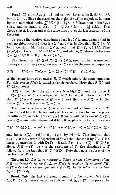
428 VIII. Asymptotic perturbation theory
Proof. If s-lira R,,, (Co) = A exists, we have s-lim R,,, (Co)k = Ak,k = 1, 2, .... Since the series on the right of (1.1) is majorized in normby the numerical series ' Mok+1 IC - Colk, it follows that s-limR (C)exists and is equal to A (1 - (4 - Co) A)-1 for IC - oI < Mo 1. Thisshows that As is open and at the same time proves the last assertion of thetheorem.
To prove the relative closedness of As, let 4 E Ab and assume that ineach neighborhood of C there is a Co E As C E Ab implies that IIR. (C) 11 5 Mfor a constant M. Take a Co E As such that IC - CoI < 1/2M. ThenIIR. (C0)II < (1 - 2-1)-'M = 2M = M, and s-limR (C) also exists becauseIC - Col < 1/2M = Mi 1. Hence C E As.
The strong limit R' of R,, (C) for C E As need not be the resolventof an operator. In any case, however, R' satisfies the resolvent equation
(1.2) R' (CI) - R' (C2) = (Cl - C2) R' (C,,) R' (S2), C11 C2 E As ,
as the strong limit of operators R,, (C) which satisfy the same equation.For this reason R' is called a Pseudo-resolvent. Note that R' (C1) andR' (C2) commute.
(1.2) implies that the null space N = N (R' (C)) and the range R= R(R' (a)) of R' (C) are independent of C. In fact, it follows from (1.2)that R' (C, 2) u = 0 implies R' (C1) u = 0 and that u = R' (C2) v impliesu = R' (C,) w with w = v - % - S2) u.
The pseudo-resolvent R' (C) is a resolvent (of a closed operator T)if and only if N = 0. The necessity of this condition is obvious. To proveits sufficiency, we note that every u E R can be written as u = R' (C) v (C);here v (C) is uniquely determined if N = 0. Application of (1.2) to u gives
R' (Ci) R'%) (v (b2) - v (Ci)) = R' (CI) u - R' (C2) u = (Cl - S2)R' (Ci) R' (C2) u
and hence v (C,2) - v (CI) = (Cl - b2) u by N = 0. This implies thatv (C) + C u is a vector independent of C ; we shall denote it by T u, T is alinear operator in X with D (T) = R and T u - C u = v (C) = R' (C)-1 u.Hence R'(C) = (T - b)-1 is the resolvent of T; the closedness of Tfollows from the fact that R' M E Note that As is a subset of theresolvent set P (T).
Theorem 1.3. Let A. be nonempty. There are the alternatives: eitherR' (C) is invertible for no C E As or R' (C) is equal to the resolvent R (C)= (T - a)-1 of a unique operator T E '(X). In the latter case we haveAs = P (T) n Ab.
Proof. Only the last statement remains to be proved. We haveAs C P (T) n Ab since we proved above that As C P (T). To prove the
§ 1. Strong convergence in the generalized sense 429
opposite inclusion, we note the identity
(1.3) R. (C) - R (C) _ (1 + (C - Co) R. (C)) (R (Co) - R (Co)) (1 + (C - Co) R (C))
for C, Co E P(T) n Ab; this is a simple consequence of the resolventequations for R (C) and R (C). If Co E As, we have s-lim R (CO) = R'(C0)= R (CO) so that (1.3) gives s-lim R,, (C) = R (C) by the uniform bounded-ness of {R (C)}. This shows that C E AS and completes the proof.
Corollary 1.4. Let T and T be selfadjoint operators in a Hilbert space,with the resolvents R (C) and R (C). If s-lim R,, (C) = R (C) for some complexnumber C, then the same is true for every nonreal C.
Proof. Since 11Rn(C)Jj 5 1/lImCl, all nonreal numbers C are includedin Ab as well as in P (T). Thus P (T) n Ab also includes all nonreal C,and the assertion follows from Theorem 1.3.
When the second alternative of Theorem 1.3 is realized, we shall saythat R (C) converges strongly to R (C) on A, and that T converges stronglyto T (T,, - T, in symbol) in the generalized sense'.
s
A criterion for generalized strong convergence is given byTheorem 1.5. Let T, T E ' (X) and let there be a core D of T such that
each u E D belongs to D for sufficiently large n and T u T u. IfP (T) n Ab is not empty, T converges strongly to T in the generalized senseand A5 = P (T) n Ab.
Proof. For any C E P (T) n Ab, we have R (C) u - R (C) u = R (C)(T - T) R (C) u -> 0 if R (C) u E D (note that the IIR (C) 11 are bounded).
But such u form a dense set in X because D is a core of T (see Problem111-6.3). Since the IjR (C) II are bounded, it follows that R (C) . R (C)
(see Lemma 111-3.5). Thus A. ) P (T) n Ab and the second alternative ofTheorem 1.3 must be realized.
Corollary 1.6. Let T, T be selfadjoint operators in a Hilbert space,and let there be a core D of T such that T u -* T u for u E D. ThenR (C) 5 R (C) for every nonreal C, and T converges to T strongly in the
generalized sense.Remark 1.7. In general there is no simple relationship between the
strong convergence of in the generalized sense and that of(assuming that the T are densely defined so that the T, exist). This istrue even when T E -4 (X) and s-lim T = T exists in the propersense. But the following theorem should be noted.
Theorem 1.8. Let {T} and {Tn*} converge strongly to T and T*, re-spectively, in the generalized sense, T and T being densely defined. Let Asand A$ be the regions of strong convergence of the resolvents of T andrespectively. Then A: is identical with the mirror image Os of A. withrespect to the real axis.
1 For a related notion cf. MASLOV [2].
430 VIII. Asymptotic perturbation theory
Proof. This is a direct consequence of the formula 4 = Ab n P (T)and a similar one for A,*, for we have Ob = b and P (T*) = I (seeTheorem 111-6.22).
Remark 1.9. We have been considering the strong convergence of asequence {R,, (C)} of resolvents, but we can deal in quite the same. waywith a family of resolvents R (C, x) = (T (x) - a)-' depending on acontinuous parameter x. In what follows we shall do this without anyexplicit comments.
Example 1.10. Let H be a selfadjoint operator in a Hilbert space H, and letT. = n-I H. Then T. u -+ 0 for every u E D (H). Since D (H) is dense in H, it is acore of the bounded operator T = 0. Hence Corollary 1.6 is applicable, with theresult that R. (4) --> R (4) = -1/C strongly for any nonreal C. This implies that(1 - n-1 a H)-I 1 strongly for any nonreal a. This result is not quite trivial. Ifthe spectrum E (H) of H is the whole real axis, Eb is the union of the upper andlower half-planes (ImC C 0), and Ab = As = P (T) n Ab [P (T) is the whole planewith the exception of the origin].
Example 1.11. Let X = L2(0, oo) and
(1.4) T. = -d2/dx2 + qn(x) , T = -d2/dx2 + q(x)
with the boundary condition u (0) = 0, say, where q (x) and the q (x) are real-valued functions. Under certain conditions (see V-§ 3.6) T. and T are selfadjointand Co (0, oo) is a core of T. Suppose now that
b
(1.5) f Jgn(x) -q(x)I2dx-+0a
for any a, b such that 0 < a < b < oo. Then we have T. u --> T u for u E COT. Itfollows from Corollary 1.6 that R. (4) s R (4) for every nonreal C. This means thatthe solution of the boundary value problem
(1.6) =l(x), u(0) = 0, uEL2(0,cc),
converges in L2 (0, oo) to the solution of the same problem with q replaced by q.See also the examples of par. 4.
Example 1.12. Consider the operator T (x) = T + x A in which T and A are theshift operators in P (- oo, oo) discussed in Example IV-3.8. The spectrum E (T (x))for x 4 0 is the unit circle J41 = 1. Let R (g, x) = (T (x) - C)-I. Since JJR (C, x) 11 5S (ICI - 1)-I for ICI > I and Jul S 1 (see Problem IV-3.10), the exterior of the unitcircle belongs to the region of boundedness Ab for R (4, x) for x -* 0. But the interiorof this circle does not belong to Ab (see be. cit.). Here we have the relations P (T)= Ab = As = the exterior of the unit circle.
Example 1.13. Let T be a closed, maximal symmetric operator in a Hilbert spaceH and suppose T is not selfadjoint. We may assume that the upper half-planeI m C > 0 is the resolvent set P (T), whereas the lower half-plane has no point inP (T). Let be a sequence of orthogonal projections with the following properties.i) The P. are nondecreasing (P15 P2 5 ) with s-lim P = 1; ii) P. X C D (1);
00
iii) P. T P. u -+ T u if u belongs to the linear manifold D = U P. X; iv) D isn=1
§ 1. Strong convergence in the generalized sense 431
a core of T. Such a sequence can be constructed in the following way'. Let u,, E D (T)be a sequence dense in H. Let be the orthonormal family obtained by applyingthe Schmidt orthogonalization process to the sequence {u,,, (T - i)-1 un}. If P. isthe projection on the n-dimensional subspace spanned by v1, ..., v,,, hasthe required properties.
Set T. = P. T P.. The T. are obviously bounded and symmetric, hence self-adjoint. Thus the region of boundedness Ab for {Tn} comprises all nonreal numbers.Furthermore, it follows from iii), iv) and Theorem 1.5 that As = P(T) r) Ob isexactly the upper half-plane. This is an example in which As is a proper subset of Ab.
2. Generalized strong convergence and spectra
We have seen before that the spectrum E (T) is upper-semicontinuouswith respect to the generalized convergence (convergence in gap) of theoperator, that is, Y. (T) does not expand suddenly when T is changedslightly in the sense of generalized convergence (in gap). The situationis quite different if generalized convergence (in gap) is replaced bygeneralized strong convergence defined above or even by strong con-vergence. This is one of the reasons why we had to introduce the regionof strong convergence Os in the theorems proved above.
A very simple counter-example is furnished by a sequence oforthogonal projections in a Hilbert space such that E -- 0. The limit
s
operator 0 has the single point C = 0 in its spectrum, but E in generalcontains two points C = 0, 1. Since, on the other hand, E (T) is in generalnot lower-semicontinuous even in the sense of convergence in norm,we conclude that it is neither upper- nor lower-semicontinuous in thesense of strong convergence.
However, the lower-semicontinuity of the spectrum can be provedunder certain restrictions.
Theorem 1.14. Let H, H be sel/adjoint operators in a Hilbert space Hand let H converge to H strongly in the generalized sense. Then every openset containing a point of Y. (H) contains, at least a point of Y. for sul-fieiently large n.
Proof. LetA E(H) and set C = A+ i e, e>. 0. We have 11 R (C) 11 = 1/8since H is selfadjoint, so that there is a u E H such that 11R (C) ull z 1/2 s,11 u11 = 1. But we have R (C) u -* R (C) u by hypothesis (see also Corollary1.4). Hence JJR,, (C) ull z 1/3 s for sufficiently large n. Since H. is self-adjoint, this implies that there is a 4 E E such that IA,, - Cl 5 3 s orI2 - Al S 4 e. Since s > 0 is arbitrary, this proves the theorem.
Theorem 1.14 can be strengthened in a certain sense to the followingone:
1 See STONE (1), p. 166.
432 VIII. Asymptotic perturbation theory
Theorem 1.15. In Theorem 1.14 let H = f H = f dE(A)be the spectral representations o l the operators involved. Then 1, a
(1.7) s-lim E,1(A) = E (A) if E (A - 0) = E (A) .n_00
Proof. We may assume without loss of generality that A = 0. Werecall that E. (0) + E,1 (- 0) is given by Lemma VI-5.6 with A = 0 and Hreplaced by H. Or we may write
(1.8) (1 - E.(0) - H. (H.2 + 1) -100
f H. (Hn + r1a)-1 H. (Hn + 1) -1 dr1;0
ein this form we need not write lim f on the right, for the integral is
e-*0 ee Mabsolutely convergent by
(1.9) II Hn(HH + rl2)-1 HH(Hn + 1)-11I 5 min(1, 77-2)
Furthermore, we note that (E (0) - E. (- 0)) H. (Hn + 1)-1 = 0, forE. (0) - E. (- 0) is the projection on the null space of H. Hence theE,,(-0) on the left of (1.8) can be replaced by E (0) . We have also aformula similar to (1.8) with H, E replaced by H, E respectively.
The integrand in (1.8) tends to H(Ha + 172) -1 H(Ha + 1) -1 stronglyas is -+ oo since R (C) -3. R (C) for any nonreal C. In view of (1.9), it
s
follows by the principle of dominated convergence that
(1.10) (1 - 2E,, (0)) H,, (H.2 + 1) -1g (1 - 2E(0)) H(Ha + I)-I.
On the other hand, 1)-1-H(H2+ 1)-1 byR.(fi) g R(+i).Hence(1.11) (1 - 2En(0)) [H.(HH+ 1) -1 - H(H2+ 1)-1]g0.
(1.10) and (1.11) together give
(1.12) (E (0) - E (0)) H (Ha + 1) -1 . 0.S
1 (1.7) can be generalized to s-limE (An) = E (A) for 4 -+ A. For the proof itsuffices to note that E E;, (A) where E is the spectral family for H = H. --(A. - A) and thatHagH since A.- 2 -+ 0. We remark also that s-limEn (An - O)= E (A) is true. For the proof note that E. (A - n-1) has the samestrong limit E (A), so that E. (A - n-1) g 0; then 0 S E. (A -
E. E. E. E. (An - 0) g 0.S We could also raise the question whether 0 --b (H) is true for a given
sfunction 0. We shall not consider this problem in the general form. For a relatedproblem for spectral operators see FOGUEL [1].
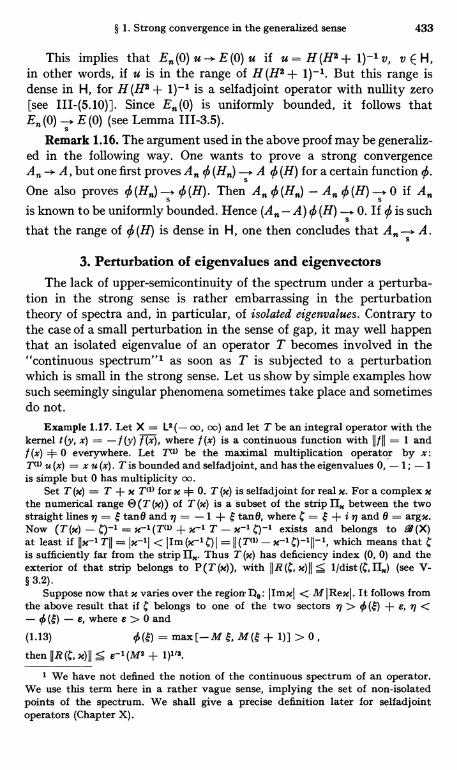
§ 1. Strong convergence in the generalized sense 433
This implies that E (0) u --. E (0) u if u = H (Ha + 1) -1 v, v E H,in other words, if u is in the range of H (Ha + 1)-1. But this range isdense in H, for H(H2+ 1)-1 is a selfadjoint operator with nullity zero[see III-(5.10)]. Since E71(0) is uniformly bounded, it follows thatE,,, (0) -. E (0) (see Lemma 111-3.5).
S
Remark 1.16. The argument used in the above proof may be generaliz-ed in the following way. One wants to prove a strong convergenceA,,, -> A, but one first proves A 0 A q (H) for a certain function c.
S
One also proves 0 (H.) (H). Then A,, (H..) - A7, 0 (H) --. 0 if AS S
is known to be uniformly bounded. Hence (A,,, - A) 0 (H) -. 0. If 0 is suchS
that the range of 0 (H) is dense in H, one then concludes that A. -.. A.S
3. Perturbation of eigenvalues and eigenvectorsThe lack of upper-semicontinuity of the spectrum under a perturba-
tion in the strong sense is rather embarrassing in the perturbationtheory of spectra and, in particular, of isolated eigenvalues. Contrary tothe case of a small perturbation in the sense of gap, it may well happenthat an isolated eigenvalue of an operator T becomes involved in the"continuous spectrum"' as soon as T is subjected to a perturbationwhich is small in the strong sense. Let us show by simple examples howsuch seemingly singular phenomena sometimes take place and sometimesdo not.
Example 1.17. Let X = L2 (- no, oo) and let T be an integral operator with thekernel t (y, x) = - f (y) f (x), where f (x) is a continuous function with 11th = 1 andf (x) + 0 everywhere. Let PI) be the maximal multiplication operator by x:211) u (x) = x u (x). T is bounded and selfadjoint, and has the eigenvalues 0, - 1; -1is simple but 0 has multiplicity no.
Set T (x) = T + x PI) for x + 0. T (x) is selfadjoint for real x. For a complex xthe numerical range O (T (x)) of T (x) is a subset of the strip 1Ix between the twostraight lines i _ tang and i = -1 + $ tanO, where C = $ + i ri and 0 = argx.Now (T (x) - C)-1 = x-1(T"u + x-1 T - x-1 C)-1 exists and belongs to V (X)at least if jr'ITIC = Ix-1I < IIm (x-1 C) I = II (Tu) which means that Cis sufficiently far from the strip IIX. Thus T (x) has deficiency index (0, 0) and theexterior of that strip belongs to P (T (u)), with II R (g, x) I S 1(dist (g, (see V-§ 3.2).
Suppose now that x varies over the region D.: IImxI < M IRexl. It follows fromthe above result that if C belongs to one of the two sectors > ¢ (g) + e, 11 <
where e >0 and(1.13)
then IIR(C, x)11;5 ---I (MI + 1)112.
1 We have not defined the notion of the continuous spectrum of an operator.We use this term here in a rather vague sense, implying the set of non-isolatedpoints of the spectrum. We shall give a precise definition later for selfadjointoperators (Chapter X).
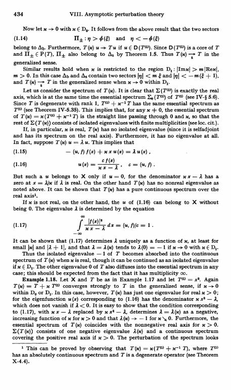
434 VIII. Asymptotic perturbation theory
Now let x -+ 0 with x E Do. It follows from the above result that the two sectors
(1.14) and
belong to Ob. Furthermore, T (x) u -* T u if u E D (T1)). Since D (T'>) is a core of Tand II± E P (T), II± also belong to As by Theorem 1.5. Thus T (m) ---' T in the
sgeneralized sense.
Similar results hold when x is restricted to the region D,: JImxI > m lRexl,m > 0. In this case Ab and As contain two sectors InI < m and 1271 < - m ( + 1),and T (x) - T in the generalized sense when x 0 within D,
sLet us consider the spectrum of T (x). It is clear that E (TM) is exactly the real
axis, which is at the same time the essential spectrum Me W'>) of TW (see IV-§ 5.6).Since T is degenerate with rank 1, 2'W + x'1 T has the same essential spectrum as211> (see Theorem IV-5.35). This implies that, for any x 4 0, the essential spectrumof T (x) = x (T<') + x-1 T) is the straight line passing through 0 and x, so that therest of E (T (x)) consists of isolated eigenvalues with finite multiplicities (see loc. cit.).
If, in particular, x is real, T (x) has no isolated eigenvalue (since it is selfadjointand has its spectrum on the real axis). Furthermore, it has no eigenvalue at all.In fact, suppose T (x) u = A u. This implies that
(1.15) - (u, f) / (x) + x x u (x) = A u (x) ,
(1.16) U W =c l (x)
xx -A,
c = (u, f) .
But such a u belongs to X only if u = 0, for the denominator x x - A has azero at x = A/x if A is real. On the other hand T (m) has no nonreal eigenvalue asnoted above. It can be shown that T (m) has a pure continuous spectrum over thereal axis'.
If x is not real, on the other hand, the u of (1.16) can belong to X withoutbeing 0. The eigenvalue A is determined by the equation
0(1.17) f i/(x)I2 dx = (u, f)lc = Ixx - A
-00
It can be shown that (1.17) determines A uniquely as a function of x, at least forsmall IxI and IA + 11, and that A = A (x) tends to A (0) = -1 if x -+ 0 with x E Dl.
Thus the isolated eigenvalue -1 of T becomes absorbed into the continuousspectrum of T (x) when x is real, though it can be continued as an isolated eigenvalueif x E Dl. The other eigenvalue 0 of T also diffuses into the essential spectrum in anycase; this should be expected from the fact that it has multiplicity co.
Example 1.18. Let X and T be as in Example 1.17 and let 711> = x2. AgainT (x) = T + x TO) converges strongly to T in the generalized sense, if x -+ 0within De or D,. In this case, however, T (x) has just one eigenvalue for real x > 0;for the eigenfunction u (x) corresponding to (1.16) has the denominator x x2 - A,which does not vanish if A < 0. It is easy to show that the condition correspondingto (1.17), with x x - A replaced by x x9 - A, determines A = A (x) as a negative,increasing function of x for x > 0 and that A (x) -* -1 for x y 0. Furthermore, theessential spectrum of T (m) coincides with the nonnegative real axis for x > 0.E (T (x)) consists of one negative eigenvalue A (x) and a continuous spectrumcovering the positive real axis if x > 0. The perturbation of the spectrum looks
1 This can be proved by observing that T (x) = x (T11) + x'' T), where PI)has an absolutely continuous spectrum and T is a degenerate operator (see TheoremX-4.4).
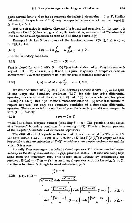
§ 1. Strong convergence in the generalized sense 435
quite normal for x > 0 so far as concerns the isolated eigenvalue -1 of T. Similarbehavior of the spectrum of T (x) may be expected when x is not real but 1argx1 SsX-e,e>0.
But the situation is entirely different if x is real and negative. In this case it iseasily seen that T (x) has no eigenvalue; the isolated eigenvalue -1 of T is absorbedinto the continuous spectrum as soon as T is changed into T (m).
Example 1.19. Let X be any one of the function spaces L9(0, 1), 1 S p < oo,or C [0, 1]. Let
d d$(1.18) T(x)=2adx-xdxa' a+0,with the boundary condition
(1.19) u(0) = u(1) = 0.
T (x) is closed for x + 0 with D = D (T (n)) independent of x. T (x) is even self-adjoint if X = L', x is real, x + 0 and at is pure imaginary. A simple calculationshows that if x + 0 the spectrum of T (x) consists of isolated eigenvalues
(1.20) (x) = n$ n$ x + n = 1, 2, 3, ... .
What is the "limit" of T (x) as x 0 ? Formally one would have T (0) = 2 at d/dx.If one keeps the boundary condition (1.19) for this first-order differentialoperator, the spectrum of the closure T (O)- of T (O) is the whole complex plane(Example 111-6.8). But T (0)" is not a reasonable limit of T (x) since it is natural torequire not two, but only one boundary condition of a first-order differentialoperator. There are an infinite number of possible boundary conditions compatiblewith (1.19), namely(1.21) u(0)=0u(1)
where 0 is a fixed complex number (including 0 = oo). The question is the choiceof a "correct" boundary condition from among (1.21). This is a typical problemof the singular perturbation of differential operators.
The difficulty of this problem lies in that it is not covered by Theorem 1.5.We have indeed T (x) u -+ T (0)" u, x 0, for u E D, but P (T (0)') is empty and it isimpossible to find an extension of T (0)" which has a nonempty resolvent set and forwhich D is a core.
Actually T (x) converges to a definite closed operator T in the generalized sense,not only in the strong sense but even in gap, provided that x 0 with x/a being keptaway from the imaginary axis. This is seen most directly by constructing theresolvent R (C, x) = (T (x) - 0-1 as an integral operator with the kernel g (y, x; C),the Green function. A straightforward calculation gives
(1.22) g. (y, x.; C) =
(Y-x)
U«' - xa' - x C sinh -x
8 - 8 -sinh
ax
xy) sinh
ax
x C (1 - x) , Y;5 x,
C (1 - y)) sinh a x x x), y z X.sinh V a x
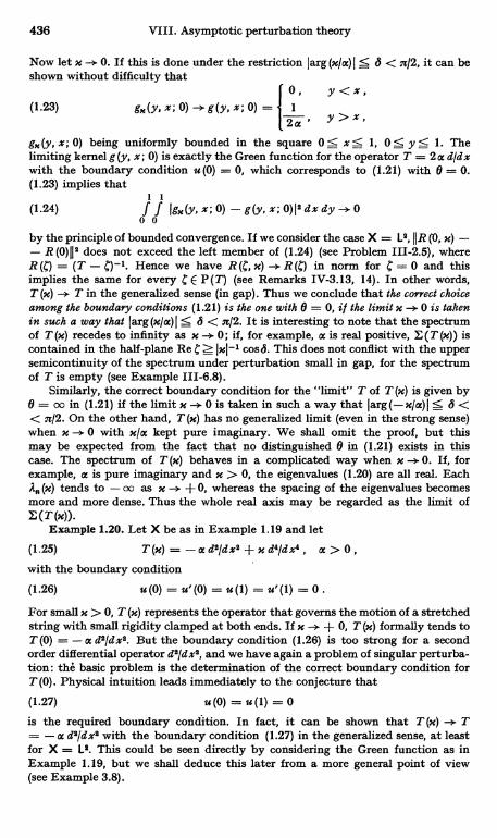
436 VIII. Asymptotic perturbation theory
Now let x -+ 0. If this is done under the restriction larg (x/a) I S 6 < ac/2, it can beshown without difficulty that
0, y <x,(1.23) gx (y, x; 0) - g (y, x; 0) = 1 y>x,gm (y, x; 0) being uniformly bounded in the square 0 < x < 1, 0:&- y S 1. Thelimiting kernel g (y, x; 0) is exactly the Green function for the operator T = 2 a d/dxwith the boundary condition u (0) = 0, which corresponds to (1.21) with 0 = 0.(1.23) implies that
1 1
(1.24) f f Igx(y,x;0) -g(y,x;0)12dxdy-* 00 0
by the principle of bounded convergence. If we consider the case X = L2, IDR (0, x) -- R(0)I12 does not exceed the left member of (1.24) (see Problem 111-2.5), whereR (C) = (T - C)-1. Hence we have R (C, x) R (C) in norm for C = 0 and thisimplies the same for every C E P (T) (see Remarks IV-3.13, 14). In other words,T (x) T in the generalized sense (in gap). Thus we conclude that the correct choiceamong the boundary conditions (1.21) is the one with 0 = 0, it the limit x -+ 0 is takenin such a way that Iarg(x/a) I S & < x/2. It is interesting to note that the spectrumof T (x) recedes to infinity as x 0; if, for example, a is real positive, E (T (x)) iscontained in the half-plane Re 4 Ixl-1 cos8. This does not conflict with the uppersemicontinuity of the spectrum under perturbation small in gap, for the spectrumof T is empty (see Example 111-6.8).
Similarly, the correct boundary condition for the "limit" T of T (x) is given by0 = oo in (1.21) if the limit x 0 is taken in such a way that larg(-x/a)I < & << n/2. On the other hand, T (x) has no generalized limit (even in the strong sense)when x ->- 0 with x/a kept pure imaginary. We shall omit the proof, but thismay be expected from the fact that no distinguished 0 in (1.21) exists in thiscase. The spectrum of T (x) behaves in a complicated way when x 0. If, forexample, a is pure imaginary and x > 0, the eigenvalues (1.20) are all real. EachA, (x) tends to - on as x + 0, whereas the spacing of the eigenvalues becomesmore and more dense. Thus the whole real axis may be regarded as the limit ofE (T (x)).
Example 1.20. Let X be as in Example 1.19 and let
(1.25) T (x) _ - a d2/d x2 + x d6/d 0 ° , a > 0 ,with the boundary condition
(1.26) u(0) = u'(0) = u(1) = u'(1) = 0.
For small x > 0, T (x) represents the operator that governs the motion of a stretchedstring with small rigidity clamped at both ends. If x + 0, T (x) formally tends toT (0) = -a da/dx$. But the boundary condition (1.26) is too strong for a secondorder differential operator d2/dx2, and we have again a problem of singular perturba-tion: the basic problem is the determination of the correct boundary condition forT (0). Physical intuition leads immediately to the conjecture that
(1.27) u(0) = u(1) = 0is the required boundary condition. In fact, it can be shown that T (m) T= - a d2/dx8 with the boundary condition (1.27) in the generalized sense, at leastfor X = L2. This could be seen directly by considering the Green function as inExample 1.19, but we shall deduce this later from a more general point of view(see Example 3.8).
§ 1. Strong convergence in the generalized sense 437
The generalized convergence T (m) -* T (in gap) implies that each isolatedeigenvalue A. of T is continued continuously to the corresponding eigenvalueA. (x) of T (x). It is known that'
r x1 112
(x) = n2 n2 aL1
+ 4 -/ +0(.)] , x > 0 .
Thus the eigenvalues are continuous at x = 0 but not differentiable.
These examples will suffice to show that the spectrum of an operatorcan behave in quite a complicated way under a "singular" perturbation.In particular, it should be noticed that the behavior may be essentiallydifferent for different directions from which the parameter x tends to zero.Thus the perturbation is not very singular in Examples 1.19 and 1.20if a > 0 and x 0, for here we have a generalized convergence in gapof T (m) to T.
Under such a singular perturbation an isolated eigenvalue does notin general remain isolated; it may be absorbed into the continuousspectrum. If one wants to develop a singular perturbation theory ofisolated eigenvalues, therefore, it is necessary to assume explicitly thatsuch an absorption does not take place. But the question of decidingwhen this assumption is satisfied is complicated, and a satisfactoryanswer does not seem to exist in general. We shall consider these ques-tions in due course.
If the eigenvalue A is absorbed by the continuous spectrum, we canno longer speak of the perturbation of the eigenvalue A. Sometimes,however, the perturbed continuous spectrum has a certain kind ofconcentration near A. This phenomenon of spectral concentration will bediscussed in § 5.
4. Stable eigenvaluesAccording to the remark given in the preceding paragraph, we
consider the perturbation of an isolated eigenvalue under the assumptionthat it remains isolated in spite of the perturbation. To make thisassumption more precise, we introduce the following definition.
Let T.n -. T, n ->- oo, in the generalized sense. An isolated eigenvalue As
of T with finite multiplicity is said to be stable under this perturbation ifthe following conditions i), ii) are satisfied.
i) The region of convergence A, for R,,(C) contains a neighborhoodof A with the exception of A. In other words, there is a 6 > 0 such thatevery C with 0 < IC - Al < 6 belongs to P (T,,) for sufficiently large n(depending on C) and R. 5 R (C), n oo.
This condition implies that the circle P : - Al = r, 0 < r <is a subset of A., and that the convergence R,, (C) --i R (C) is uniform on r
8
' See RAYLEIGH (1), p. 300.
438 VIII. Asymptotic perturbation theory
(see Theorem 1.2). Therefore, the projection
(1.29) P11 = - 2 % JR. (C) d C
ris defined and
(1.30) P,S
P=-2n% f R(C)dC,r
where P is the eigenprojection for the eigenvalue A of T.ii) dim P. s dim P for sufficiently large n.In view of (1.30), ii) actually implies that
(1.31 a) dim P = dim P for sufficiently large n ,
(1.31b) JJ(P,,-P)PII-.0, 0, 1J(P,,-P)2F1-0,
(1.31c) PX) -> 0 , n -- oo,
where 8 is the gap function introduced in IV, § 2.1. These relations followfrom Lemma 1.23 proved below. [We shall express (1.31 c) by sayingthat P -> P in gap.]
dim P = dim P = m < oo implies that the spectrum of T. inside thecircle r consists of isolated eigenvalues with total multiplicity m. Sincethis is true for any choice of the radius r of r provided n is sufficientlylarge, it follows that these isolated eigenvalues of T. converge to A.At the same time, (1.31 c) implies that the total projection associated withthese eigenvalues (that is, the projection to the m-dimensional spacewhich is the direct sum of the algebraic eigenspaces for these eigenvalues)tends in gap to the eigenprojection P for A of T. Thus the stability of 2implies already the convergence of the eigenvalues and the eigenspacesinvolved. It should be remarked, however, that the eigenspace for eachindividual eigenvalue of T 'need not be convergent ; such an eigenspaceneed not even have constant dimension.
Example 1.22. The eigenvalue -1 of T of Example 1.17 is not stable for theperturbation considered if x is real and x -. 0. But it is stable if x -. 0 along astraight line different from the real axis. In Example 1.18, the eigenvalue -1 of Tis stable if x -. 0 along a ray different from the negative real axis. In Example 1.19,T has no eigenvalue at all so that there is no question of stability. In Example 1.20,all the eigenvalues of T are stable if x ->- 0 along the positive real axis.
Lemma 1.23. Let n = 1,2, . . . , be a sequence of projections in aBanach space X such that P, P E 9(X). Then P is also a projection.Suppose further that dim P.;5 dim P < oo for all n. Then (1.31 a), (1.31 b),and (1.31 c) are true.
§ 1. Strong convergence in generalized sence 439
Proof. Pn = P and P. - P together imply P2 = P, so that P is aprojection. Let {x1, . . ., x.) be a basis of P X, where m = dim P. Then
M
(1.33) P= E ( ,ek)xk, ejEP*X*k=1
by III-(4.6); the fact that e; E P* X* can be seen by noting III-(4.9). Thecondition P2 = P leads, as is easily seen, to
(1.35) (xk,eI)=8;k, k,j=1,...,m.Hence {e1, . . . , e,,} is exactly the basis of P* X* adjoint to the basis{x1,...,x,,} of PX.
Set
(1.36) ask = (Pnxk, ej) , j, k = 1, ... , m ; n = 1,2, ... .
Since Pnxk -> Pxk = xk as n -*oo, we have
(1.37) cck-+ bjk, n->oo
In particular det(a7k) 1, which implies that Pnx1, ... , P,, x,n are line-arly independent if n is sufficiently large. Since dim P m by hypo-thesis, they form a basis of P. X with dim P,, = m. This proves (1.31 a).
Also we can writem
(1.38) Pn= , ' (,/) Pnxk,k=1
where {fl, ... , fm} is the basis of P* X* adjoint to the basis {Pnx1.... Pnxm} of P X (see the argument for P given above). Thus
711
P*= Fi (,Pnxk)!.k=1
(again by III-(4.9)) and, in particular,
by (1.36). Hence
m mnnP* et = E (ei, Pnxk) !k = E ayklk
k=1 k=1
M
(1.39) / = E fk1 P* e, ,i=1
where (S7k) is the inverse matrix to (4h), so that
(1.40) P7k-+ f, , n-* oo.
440 VIII. Asymptotic perturbation theory
Since P,, P implies P* w P*, we have P* e1 w P* e i = ej. Hence(1.39) and (1.40) give
(1.41) fk w ek, n-*oo
Now we can complete the proof of the lemma. The first convergencein (1.31 b) follows from Pn s P and dim P < oo by virtue of Lemma III-3.7. Indeed, II (Pn - P) PII = sup II (Pn - P) Pull sup II (Pn - P) vil
II-11S1 IIvIE IIIPIIP
0. To prove the second one, we note that (1.38) implies
(Pn-P)Pn=Fi (,fk)(P.-P)Pnxk,k=1
hence
IIPn- P)Pnil s X IIfkII IIPn- P)Pnxkllk=1
Since Ilfkll 5 const. by (1.41) (see Problem 111-1.30) and sinceII (Pn - P) Pnxkll - 0 by Pn P, we have II (P,, - P) Pnll -> 0 as required.
Obviously the last convergence in (1.31 b) follows from the precedingtwo.
To prove (1.31c), it suffices to notice that
8 (P X, P. X) = sup dirt (u, P. X) ` sup II (P - P) PulluEPX,llullsl uEPx,llulls1
II(P.-P)PII-Oby (1.31b) and similarly 6(P,, X, P X);5 ll (P,, - P) P,II --).. 0. Then wehave 6(P X, PX) = max{6(P, X, PX), 6(PX, P,, X) 0 as required.This completes the proof of Lemma 1.23.
For later use we add
Lemma 1.24. In addition to the assumptions of Lemma 1.21 a, assumethat P* P*. Then IIPn - PII - 0.
Proof. In this case we have P* e, -> P* e, = e; . Hence (1.39) and(1.40) give
(1.42) 1"-sek,
SinceM
P. - P = E [( , fk) (Pn xk - xk) + (, fk - ek) xklk=1
by (1.33) and (1.38), we obtain
m
IIPn - PII: E [IIfk1IIIPnxk-xkif+ll/, -ekUllxkll] -,0k=1
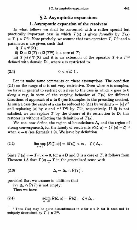
§ 2. Asymptotic expansions 441
§ 2. Asymptotic expansions1. Asymptotic expansion of the resolvent
In what follows we shall be concerned with a rather special butpractically important case in which T (m) is given formally by T (m)= T + x T(1). More precisely, we assume that two operators T, T(1) and aparameter x are given, such that
i) T E W (X)ii) D = D (T) n D (T(1)) is a core of T ;
iii) T (x) E' (X) and it is an extension of the operator T + x T(l)defined with domain D 1, where x is restricted to
(2.1) 0 < x < 1.
Let us make some comments on these assumptions. The condition(2.1) on the range of x is not very restrictive. Even when x is complex,we have in general to restrict ourselves to the case in which x goes to 0along a ray, in view of the varying behavior of T (m) for differentdirections of approach of x to 0 (see Examples in the preceding section).In such a case the range of x can be reduced to (2.1) by writing x = Iki eieand replacing (xI by x and ei0 T(') by TM, respectively. If ii) is notsatisfied, we can replace T by the closure of its restriction to D ; thisrestores ii) without affecting the definition of T (m).
We can now define the region of boundedness A b and the region ofstrong convergence A, for the family of resolvents R (C, x) = (T (x) - C,)-11when x -+ 0 (see Remark 1.9). We have by definition
(2.2) Jim yuPIIR(C, x)II = M(C) < oo , C E Ob
Since T (x) u -+ T u, x -+ 0, for u E D and D is a core of T, it follows fromTheorem 1.5 that T (x) T in the generalized sense with
(2.3) As = Ob n P (T) ,
provided that we assume in addition thativ) Ab n P (T) is not empty.Thus we have
(2.4) s-Jim R (C, x) = R (C) , C E / .
1 Thus T (m) may be quite discontinuous in x for x > 0, for it need not beuniquely determined by T + x Tu).
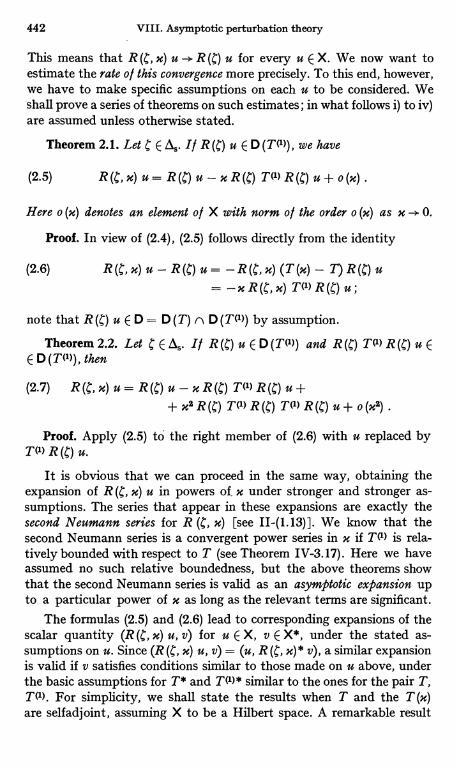
442 VIII. Asymptotic perturbation theory
This means that R (C, x) u -+ R (C) u for every u E X. We now want toestimate the rate of this convergence more precisely. To this end, however,we have to make specific assumptions on each u to be considered. Weshall prove a series of theorems on such estimates ; in what follows i) to iv)are assumed unless otherwise stated.
Theorem 2.1. Let C E A, If R (C) u E D (T(1)), we have
(2.5) R (C, x) u = R (C) u - x R (C) TM R (C) u + o (x) .
Here o (x) denotes an element of X with norm of the order o (x) as x -> 0.
Proof. In view of (2.4), (2.5) follows directly from the identity
(2.6) R (C, x) u - R (C) u = - R (C, x) (T (x) - T) R (C) ux R (C, x) TM R (C) u ;
note that R (C) u E D = D (T) n D (TM) by assumption.
Theorem 2.2. Let C E As. I/ R (C) u E D (TM) and R (C) Tel) R (C) u EE D(T(1)), then
(2.7) R (C, x) u = R (g) u - x R (C) TM R (C) u ++ xs R (C) TM R (g) TM R (C) u + o (x$) .
Proof. Apply (2.5) to the right member of (2.6) with u replaced byTM R (C) u.
It is obvious that we can proceed in the same way, obtaining theexpansion of R (C, x) u in powers of. x under stronger and stronger as-sumptions. The series that appear in these expansions are exactly thesecond Neumann series for R (C, x) [see II-(1.13)]. We know that thesecond Neumann series is a convergent power series in x if Tel) is rela-tively bounded with respect to T (see Theorem IV-3.17). Here we haveassumed no such relative boundedness, but the above theorems showthat the second Neumann series is valid as an asymptotic expansion upto a particular power of x as long as the relevant terms are significant.
The formulas (2.5) and (2.6) lead to corresponding expansions of thescalar quantity (R (C, x) u, v) for u E X, v E X*, under the stated as-sumptions on u. Since (R (C, x) u, v) = (u, R (C, x) * v), a similar expansionis valid if v satisfies conditions similar to those made on u above, underthe basic assumptions for T* and T(')* similar to the ones for the pair T,Tel). For simplicity, we shall state the results when T and the T (x)are selfadjoint, assuming X to be a Hilbert space. A remarkable result
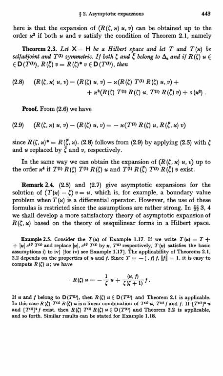
§ 2. Asymptotic expansions 443
here is that the expansion of (R (C, x) u, v) can be obtained up to theorder x2 if both u and v satisfy the condition of Theorem 2.1, namely
Theorem 2.3. Let X = H be a Hilbert space and let T and T (x) besel f adjoint and Till symmetric. I/ both C and belong to i and i f R (C) u EE D(T(')), v= R(C)* v E D(T(')), then
(2.8) (R (C, x) u, v) = (R (C) u, v) - x (R (C) T(1) R (C) u, , v) +
+ M2 (R (C) T(1) R (C) u, T(') R v) + o (x2)
Proof. From (2.6) we have
(2.9) (R (C, x) u, v) - (R (C) u, v) x (T(1) R (C) u, R (C, x) v)
since R (C, x) * = R x). (2.8) follows from (2.9) by applying (2.5) withand u replaced by and v, respectively.
In the same way we can obtain the expansion of (R x) u, v) up tothe order x4 if TM R (C) TM R (C) u and Till R (C) T(') R ( ) v exist.
Remark 2.4. (2.5) and (2.7) give asymptotic expansions for thesolution of (T (x) - C) v = u, which is, for example, a boundary valueproblem when T (x) is a differential operator. However, the use of theseformulas is restricted since the assumptions are rather strong. In §§ 3, 4we shall develop a more satisfactory theory of asymptotic expansion ofR (C, x) based on the theory of sesquilinear forms in a Hilbert space.
Example 2.5. Consider the T (x) of Example 1.17. If we write T (x) = T ++ Ixl ete T(l) and replace Ixl, et0 T(l) by x, T'1> respectively, T (m) satisfies the basicassumptions i) to iv) [for iv) see Example 1:17]. The applicability of Theorems 2.1,2.2 depends on the properties of u and /. Since T 1, it is easy tocompute R (C) u; we have
If u and t belong to D (T<1>), then R (C) u E D (T<1)) and Theorem 2.1 is applicable.In this case R (C) T(l) R (C) u is a linear combination of Tu> u, TO) f and f. If [T<1>]2 uand [T(1)]2 f exist, then R (C) T11> R (C) u E D (Tu)) and Theorem 2.2 is applicable,and so forth. Similar results can be stated for Example 1.18.
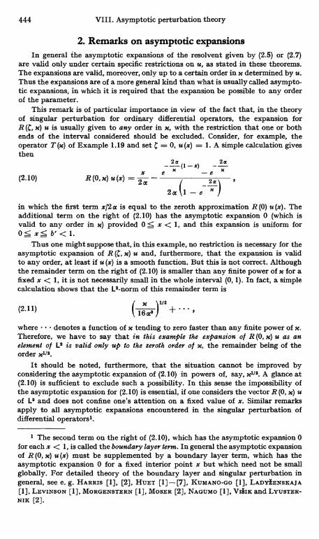
444 VIII. Asymptotic perturbation theory
2. Remarks on asymptotic expansionsIn general the asymptotic expansions of the resolvent given by (2.5) or (2.7)
are valid only under certain specific restrictions on u, as stated in these theorems.The expansions are valid, moreover, only up to a certain order in x determined by u.Thus the expansions are of a more general kind than what is usually called asympto-tic expansions, in which it is required that the expansion be possible to any orderof the parameter.
This remark is of particular importance in view of the fact that, in the theoryof singular perturbation for ordinary differential operators, the expansion forR (C, x) u is usually given to any order in x, with the restriction that one or bothends of the interval considered should be excluded. Consider, for example, theoperator T (x) of Example 1.19 and set = 0, u (x) = 1. A simple calculation givesthen
2a
x x x(2.10) R (0, x) u (x) =
2- 2
2a (1 - e x )
in which the first term x/2 a is equal to the zeroth approximation R (0) u (x). Theadditional term on the right of (2.10) has the asymptotic expansion 0 (which isvalid to any order in x) provided OS x < 1, and this expansion is uniform for05xSb'<1.
Thus one might suppose that, in this example, no restriction is necessary for theasymptotic expansion of R (C, x) u and, furthermore, that the expansion is validto any order, at least if u (x) is a smooth function. But this is not correct. Althoughthe remainder term on the right of (2.10) is smaller than any finite power of x for afixed x < 1, it is not necessarily small in the whole interval (0, 1). In fact, a simplecalculation shows that the L2-norm of this remainder term is
'/2(2.11) 6ae) +'where denotes a function of x tending to zero faster than any finite power of X.Therefore, we have to say that in this example the expansion of R (0, x) u as anelement of L2 is valid only up to the zeroth order of x, the remainder being of theorder xl1s.
It should be noted, furthermore, that the situation cannot be improved byconsidering the asymptotic expansion of (2.10) in powers of, say, MIN. A glance at(2.10) is sufficient to exclude such a possibility. In this sense the impossibility ofthe asymptotic expansion for (2.10) is essential, if one considers the vector R (0, x) uof L2 and does not confine one's attention on a fixed value of x. Similar remarksapply to all asymptotic expansions encountered in the singular perturbation ofdifferential operators'.
' The second term on the right of (2.10), which has the asymptotic expansion 0for each x < 1, is called the boundary layer term. In general the asymptotic expansionof R (0, x) u (x) must be supplemented by a boundary layer term, which has theasymptotic expansion 0 for a fixed interior point x but which need not be smallglobally. For detailed theory of the boundary layer and singular perturbation ingeneral, see e. g. HARRIS [1], [2], HURT [1]-[7], KUMANO-GO [1], LADYIENSKAJA[1], LEVINSON [1], MORGENSTERN [1], MOSER [2], NAGUMO [1], VAIK and LYUSTER-NIK [2].
§ 2. Asymptotic expansions 445
3. Asymptotic expansions of isolated eigenvalues andeigenvectors
We now consider the rate of convergence of the eigenvalues andeigenvectors of T (m) arising from an eigenvalue A of T (see § 1.4), underthe basic assumptions of par. I and the additional assumption that A isstable: We assume that A has multiplicity m < oo. We take over thenotations Ob, Os, 6, r, r, etc. of § 1.4. In particular we note that theregion of strong convergence Os contains the set of C such that 0 <<IC-AI<6.
We recall also that E (T (x)) inside the circle P : IC - Al = r consists ofisolated eigenvalues with total multiplicity m and that these eigenvaluesconverge to A as x 0. Let us denote these repeated eigenvalues byIt, (x), ..., ,u, (x):
(2.12) ,u5(x)-.A, x--> 0, j=1,...,m.The total projection
(2.13) P (M) _- 2 n i f R (C, x) d Cr
tends in gap to P, the eigenprojection for A [see (1.31 a, b, c)] :
(2.14 a)II(P(x)-P)PII-0,
II (P (x) - P) P (x) II - 0, dim P (x) = dim P = m .
If m = 1, P(x) is itself the eigenproj ection on the one-dimensionaleigenspace of T (x) for the eigenvalue A (x) _ p, (m), which converges to A.(2.14) implies that an eigenvector 92 (x) of T (x) for the eigenvalue A (x)can be chosen in such a way that
(2.15) T (x) -+ c , x -- 0 ,
where 92 is an eigenvector of T for the eigenvalue A:
(2.16) T qp = A p, T (x) qp (x) = A (x) qp (x) .
To see this, it suffices to set 99 (x) = P (x) 99.In general it is impossible to deduce more precise results on the rate
of convergence in (2.12) or (2.14) or (2.15). Such a refinement is possible,however, if one makes further assumptions on the eigenspace P X of T.We have namely'
Theorem 2.6. Let A be an isolated, semisimple eigenvalue o l T with theeigenprojection P, dimP = m < oo. Let A be stable and let PX C D (T(1)).
1 The results of this and the following paragraphs were proved in T. KATO [1],[3] for selfadjoint operators by making use of the spectral representations. Thegeneralization to operators in Banach spaces given here needs an entirely differentproof.
446 VIII. Asymptotic perturbation theory
Then the eigenvalues, u1 (x) admit asymptotic expansions'
(2.17) ,u3 (x)=A+x,u(1) +o(x), j=1,...,m,where the 1u,(1) are the repeated eigenvalues of the operator P TM P consideredin the m-dimensional space P X. The total projection P (x) for these eigen-values has the property that
(2.18) P (m) P= P- x S TM P+ o (x) ,
where S is the reduced resolvent for A of T (see III-§ 6.5) and o (x) denotesan operator such that x-1 11 o 0 as x 0. If in particular m = 1, aneigenvector 99 (x) for the eigenvalue A (x) = ,u1(x) of T (x) can be chosen insuch a way that(2.19) q9(x)=99 -xST(11g9+o(x),where 99 is an eigenvector of T for A.
Proof. I. We start with the remark that R Pv = (A - 0-1 Pv EE D (T(11) for every v E X so that (2.6) gives
R (C, x) Pv = (A - Pv - x (A - c)-1 R (C, x) TM Pv= (A-l;)-1Pv-x(A-lc)-1R(C) T(11 Pv+o(x)
where o (x) is uniform in C for C E P. Since dim P X = m < oo, thisimplies 2
(2.20) R (C, x) P = (I - a)-1 P - x (R - l;)-1 R (C, x) T(1) P_ (I-c)-1P-x(I-l;)-1R(C) T(11 P+o(x)u,
where o (x) is uniform in C E r. Substitution of (2.20) into (2.13) multi-plied by P from the right leads immediately to (2.18) ; recall the expansionR (C) = (A - a)-1 P + S + (C - 2) S2 + [see III-(6.32) where D = 0by assumption] and note that
(2.21) T(11 P E 9 (X)
by the assumption that PX C D(T(1)). (2.19) follows from (2.18) onsetting 99(x) = P (m) 99 = P (m) P qq for a 92 EM= P X
II. To deduce the asymptotic expansion for ,u1 (x), we introducethe operator [see (2.18) just proved]
(2.22) V (x) = 1- P+ P (x) P= 1- x S TM P+ o (x),, .
Since V (x) P = P (x) P and V (x) (1 - P) = 1 - P, V (x) maps the eigen-space M = P X onto M (x) = P (x) X and leaves every element of thecomplementary subspace (1 - P) X unchanged. The map M - V (x) M
1 If T and T (x) are selfadjoint (in a Hilbert space), we have expansions of theµJ (x) up to the order x2, see Theorem 2.9 and the attached footnote.
2 Note that A B s 0 implies 11A B11 -+ 0 if B has finite rank.
§ 2. Asymptotic expansions 447
= M (x) is onto since 11 (P (x) - P)211 -+ 0 by (2.14 a) (see Problem 1-4.12).It follows that the inverse
(2.23) V (x)-' = 1 + x ST(') P+ o (x)u
maps M (x) onto M, keeping every element of (1 - P) X invariant.We now consider the operator R1 (C, x) = V (x)-1 R (C, x) V (x) P.
V (x) P has range M (x) by the above remark, R (C, x) sends M (x) intoitself because P (x) commutes with R (C, x), and V (x)-1 maps M (x) ontoM; hence R1 (C, x) has range in M. Thus
Rl x) = PR, (g, x) = P V (x)-l R (C, x) V (x) P
(P + o (x)u) R (C, x) (P - x S TM P + o (x)u)
(note that PS = 0). Substituting for R (C, x) P from (2.20) and notingthat R (C, x) S TM P -> R (C) S TM Pin norm, PR (A - C)-' P, andPS = 0, we obtain
(2.24) V (x)-' R (C, x) V (x) P
= (A-c)-1P-x(A-C)-2PT('> P+o(x)u,where o (x)u is uniform for C E P.
Since
(2.25) T (x) P (x) 2 n i f C R (C, x) d Cr
[see III-(6.24)], integration of (2.24) along P after multiplication by- g/2 a i gives'
(2.26) V (x)-' T (x) P (x) V (x) P= 2 P+ x P T (1) P+ o (x)u .
Now the p, (x) are the repeated eigenvalues of T (x) considered in them-dimensional subspace M (x), hence equal to the eigenvalues of T (x) P (x)in M (x) and therefore also to those of V (x)-' T (x) P (x) V (x) = To (x),which is similar to T (x) P (x). Since V (x)-' M (x) = M as remarked above,these are in turn equal to the eigenvalues of To (x) P, that is, of theoperator (2.26), considered in M. In view of (2.26), this remark leadsimmediately to the result (2.17) by Theorem 11-5.4 concerning thedifferentiability of eigenvalues in a finite-dimensional space. Thiscompletes the proof of Theorem 2.6.
Remark 2.7. (2.18) shows that P (x) P admits an asymptotic expan-sion up to the first order in x. P (x) itself does not seem to have such anexpansion, for the formal expansion of P (x) is P (x) = P - x (S TM P ++ P TM S) + [see II-(2.14) ], in which the term P TM S need not
1 In view of the unboundedness of T (m), it would be difficult to deduce (2.26)by simply expanding the left member into a formal power series in x.
448 VIII. Asymptotic perturbation theory
make sense under the present assumptions. (This is one reason why theproof of Theorem 2.6 is rather complicated.) Thus the expansion (2.19)of the eigenvector (but not of the eigenprojection) is the best one canobtain even for m = 1.
In Theorem 2.6 it is in general impossible to give any statement onthe behavior of the eigenvectors or eigenspaces of T(x) except in thecase m = 1. If we assume that the p(l) are distinct, however, we have
Theorem 2.8. In Theorem 2.6 assume that the m eigenvalues i(1) ofPTM1> P are distinct, and let P(1) be the associated eigenprojections. Thenthe, a1 (x) are also distinct for sufficiently small Ix 1. Let P(1) (x) be the one-dimensional eigenprojections o l T (x) for the eigenvalues ,ui (x). Then
(2.27) P1 ')(x) -> P(') in gap as x -+ 0 .
Proof. (x) is the eigenprojection of the operator T (') (x) = x-1(T (x) -- A) P (x) for the eigenvalue x-1(,uf (x) - A) = /z(1) + o (1). But we have,in virtue of (2.26),
(2.28) V (x)-1 TM (x) V (x) P = PTM1> P + o (1)
since V (x)-1 P (m) V (x) P= V (x)-1 V (x) P = P. Since PT(') P has mdistinct eigenvalues jz,(1), the operator (2.28) has the same property.Thus we can choose its m eigenvectors v. (x) E M in such a way thatvi (x) - 99f, 991 E M being the eigenvectors of P TM P (continuity ofeigenvalues and eigenprojections, see II-§ 5.1). Now 9,s (x) = V (x) tp, (x)is an eigenvector of TM (x) and qq, (x) - qq; since V (x) - 1.
The 99j (x) form a basis of M (x), so that for any w E X we have
P W w = $1(x) 991 (x) + ....+ $m (x) 99m (x)
Since 91j (x) -> 991 and the 99j form a basis of M and since P (x) w - Pw,it is easily seen that lim s (x) = 1:s exists and Pw = S1 921 + - - - + 92..
On the other hand we have $j (x) 99; (x) = P(1) (x) w and $j q21= P(1) W.Hence we conclude that P,(1) (x) w -* P11> w, that is, P(1) (x) -> P(1) strong-ly. Since dim Pj(') (x) = dim Pj(') = 1, the convergence is actually in gapby Lemma 1.23. This completes the proof of Theorem 2.8.
4. Further asymptotic expansionsWe shall now show that a higher approximation to the eigenvalues
can be obtained if we assume that P TM is bounded, in addition to theassumptions of Theorem 2.6. Since P TM has range in the finite-dimen-sional subspace M = P X, it can then be extended to an operator of-V(X) with range in M. Such an extension is not unique unless TM isdensely defined, but we take any such extension and denote it by [P TM];
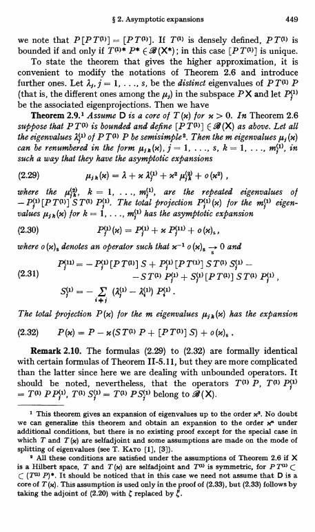
§ 2. Asymptotic expansions 449
we note that P [P TM] _ [P T(1)]. If TM is densely defined, P TM isbounded if and only if T(')* P* E .4 (X*) ; in this case [P TM] is unique.
To state the theorem that gives the higher approximation, it isconvenient to modify the notations of Theorem 2.6 and introducefurther ones. Let d j, j = 1, . . ., s, be the distinct eigenvalues of P T(11) P(that is, the different ones among the ,u;) in the subspace PX and let PJl)be the associated eigenprojections. Then we have
Theorem 2.9.1 Assume D is a core o l T (m) for x > 0. In Theorem 2.6suppose that P TM is bounded and define [P TM] E .4 (X) as above. Let allthe eigenvalues A,(1) o l P TM P be semisimple2. Then the m eigenvalues ,a; (x)can be renumbered in the form yj1,(u), j = 1, . . ., s, k = 1, ..., m}1), insuch a way that they have the asymptotic expansions
(2.29) lei k (x) x A(1) X2 k + o (x2) ,
where the ,u k , k = 1, ... , m(1), are the repeated eigenvalues o l
- p(1) [P TM ] S TM P(1). The total projection P}1) (x) for the m(l) eigen-values ,uf k (x) for k = 1, . . ., m,(1) has the asymptotic expansion
(2.30) P(1) (x) = p(l) + X p(ll) + o (X)s ,
where o (u)s denotes an operator such that x-1 o (x)s --> 0 and5
p(lu) _ - p(l) [PT(')] S + Pi(t) [P T(1)] STMT) S}1) -(2.31) -STMT) P(1) + S(1) [PTMJ STM1) P(1) ,
S?l) _ - (A(1) - )(1)) pil)
The total projection P (x) for the m eigenvalues µj t (x) has the expansion
(2.32) P (m) = P - x (S T (1) P + [P T (l) ] S) + o (m), .
Remark 2.10. The formulas (2.29) to (2.32) are formally identicalwith certain formulas of Theorem II-5.11, but they are more complicatedthan the latter since here we are dealing with unbounded operators. Itshould be noted, nevertheless, that the operators Tel) P, TM P11)= TM PP11), TM S(1) = TM belong to 9 (X).
1 This theorem gives an expansion of eigenvalues up to the order x2. No doubtwe can generalize this theorem and obtain an expansion to the order X" underadditional conditions, but there is no existing proof except for the special case inwhich T and T (m) are selfadjoint and some assumptions are made on the mode ofsplitting of eigenvalues (see T. KATO [1], [3]).
2 All these conditions are satisfied under the assumptions of Theorem 2.6 if Xis a Hilbert space, T and T (x) are selfadjoint and Ti" is symmetric, for P Ti"C (Ti') P)*. It should be noticed that in this case we need not assume that D is acore of T (x). This assumption is used only in the proof of (2.33), but (2.33) follows bytaking the adjoint of (2.20) with C replaced by C.
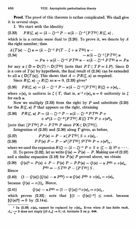
450 VIII. Asymptotic perturbation theory
Proof. The proof of this theorem is rather complicated. We shall giveit in several steps.
1. We start with the identity
(2.33) PR (C, x) = (A - c)-1 P - x (A - C)-1 [P T(1)] R (C, x) ,
which is in a certain sense dual to (2.20). To prove it, we denote by Athe right member; then
(2.34) - x (A - C)-1 [P T(1)] u=Pu+x(A-C)-1PTO1)u-x(A-C)-1PT(1)u=Pu
for any u E D = D (T) n D (T(1)) (note that P T C T P = A P). Since Dis a core of T (x) by hypothesis, the final result of (2.34) can be extendedto all u E D (T (x)). This shows that A = PR (C, x) as required.
Since R (C, x) -> R (C) as x -+ 0, (2.33) gives"
(2.35) P - x(d - )-" o(x)s
where o (x)s is uniform in C E r, that is, x-1 o (x)5 u --> 0 uniformly in Cfor each u.
Now we multiply (2.33) from the right by P and substitute (2.20)for the R (C, x) P that appears on the right, obtaining
(2.36) PR(C,x)P=(A-C)-1P-x(A-C)-2PT(1)P++x2(A-C)-2[PT(1)]R(g) T(1)P+o(x2)
[note that [PT(1)] P = PT(1) P since PXC D(T(1))].Integration of (2.35) and (2.36) along r gives, as before,
(2.37) PP(m) = P - x[ P T (1)] S + o(x)S .
(2.38) P P (x) P = P - x2 [P DO] S2 TO) P + o (x2)u ,
where we used the expansion R (C) = (A - C) -1 P + S + (C - A) S2 +II. To prove (2.32), let us write Q (x) = P (x) - P. Making use of (2.37)
and a similar expansion (2.18) for P (m) P proved above, we obtain
(2.39) Q(x)2 = P (x) + P - P (x) P - P P (x) = Q (x) - x ' P(1) + o (x)s ,
HenceP(1) = - S T(1) P - [P T(1)] S .
(2.40) (1 - Q (x)) (Q (x) - x P(1)) = x Q (x) P(1) + o (x)s = o (x)5
because Q(x) = o(1)8. Hence,
(2.41) Q (x) - XP(1) = (1 - Q (x))-1 o (x)8 = o (x)8which proves (2.32); note that II(1 - Q(x))-1II s const. becauseIIQ(x)200 - 0 by (2.14 a).
1 In (2.35) o (x)s cannot be replaced by o (x)u. Even when B has finite rank,A. -- 0 does not imply JIBA 11 -+ 0; cf. footnote 2 on p. 444.
S
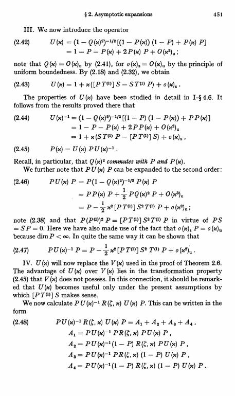
§ 2. Asymptotic expansions 451
III. We now introduce the operator
(2.42) U(x) = (1 - Q(x)2)-1/2[(1 - P(x)) (1 - P) + P(x) P]= 1 - P - P(x) + 2P(x) P + O(x2)u ;
note that Q (x) = 0 (x)u by (2.41), for o (m) r, = 0 (x)u by the principle ofuniform boundedness. By (2.18) and (2.32), we obtain
(2.43) U(x) = I + x([PT(')] S - ST(1> P) + o(x)5.
The properties of U (m) have been studied in detail in I-§ 4.6. Itfollows from the results proved there that
(2.44) U(x)-1= (1 - Q(X)I)-112[(l - P) (1 - P(x)) + PP(x)]= 1 - P - P(x) + 2PP(x) + O(x2)u= I + x(STcl) P - [PTT] S) + o(x)5,
(2.45) P (M) = U (M) P U (x)-1 .
Recall, in particular, that Q (x)2 commutes with P and P (x).We further note that P U (x) P can be expanded to the second order:
(2.46) P U (x) P = P(1 - Q (x)2)-1/2 P (x) P
= PP(M) P + P Q (x) 2 P + 0 (x3)u
= P- x2[PT(1)]S2TM P+o(x2)u;
note (2.38) and that P(P('))2 P = [P T(1)] S2 TM P in virtue of PS= S P = 0. Here we have also made use of the fact that o (x)s P = o (x)ubecause dim P < cc. In quite the same way it can be shown that
(2.47) PU(x)-1P=P- x2[PT(l)]S2TM P+o(x2)u.
IV. U (x) will now replace the V (x) used in the proof of Theorem 2.6.The advantage of U (x) over V (x) lies in the transformation property(2.45) that V (x) does not possess. In this connection, it should be remark-ed that U (x) becomes useful only under the present assumptions bywhich [PT(') ] S makes sense.
We now calculate P U (x)-1 R (C, x) U (x) P. This can be written in theform
(2.48) P U (x)-1 R (C, x) U (m) P = Al + As + A 3 + A4,
Al = PU(x)-1 PR(C, x) PU(x) P,As = P U (x)-1(1 - P) R (C, x) P U (x) P,
As = P U (x)-1 PR (C, x) (1 - P) U (x) P ,
A4 = PU(x)-1(1 - P) R(C, x) (1 - P) U(x) P .
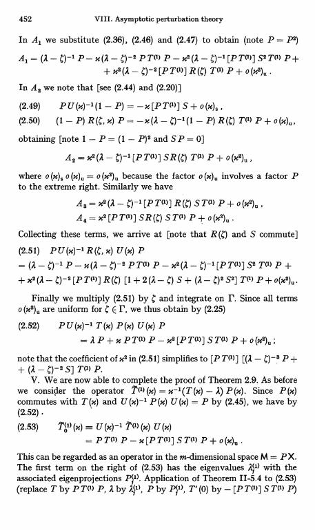
452 VIII. Asymptotic perturbation theory
In Al we substitute (2.36), (2.46) and (2.47) to obtain (note P = P2)
A1= (A - c)-1 P- x(A - C)-2 PT(1) P - x2(A - C)-'[PT('] S2T() P++ x2 (A - C)-2 [P Tel)] R (C) T(1) P + o (x2)u
In A2 we note that [see (2.44) and (2.20)]
(2.49) PU(x)-1(1 - P) = -m [PTO)] S+o(x)s,(2.50) (1 - P) R(C, x) P = -x(A- C)-1(1 - P) R(C) TO) P+ o(x),,,
obtaining [note 1 - P = (1 - P)2 and SP = 0]
A2 = x2 (A - C)-1 [PT(1)] SR (g) T(1) P + o(x2),
where o (x)5 o (x)0 = o (x2)0 because the factor o (x)0 involves a factor Pto the extreme right. Similarly we have
A3 = x2 (A - C)-1 [P T(1)] R (C) S TO) P + 0 (X2)u,
A4 = x2 [P TM] SR (C) S T(1) P + o (x2)u
Collecting these terms, we arrive at [note that R (C) and S commute]
(2.51) PU(x)-1 R(g, x) U(x) P=(A - C)-1 P - x(A - ')-2 PT(1) P - X2 (A - C)-1 [PT(')] S2 T(1) P +
+ x2 (A - C)-2 [P T(1)] R (C) [1 + 2 (A - C) S + (A - C)2 S2] T(1) P + o(x2)0.
Finally we multiply (2.51) by C and integrate on P. Since all termso (x2)0 are uniform for C E r, we thus obtain by (2.25)
(2.52) P U (x)-1 T (m) P (m) U (m) P
=AP+xPT(')P-x2[PT(')]ST(')P+0(x2)0;
note that the coefficient of x2 in (2.51) simplifies to [P T(1)] [(A - C) -.3 P ++ (A - C)-2 S] T(1) P.
V. We are now able to complete the proof of Theorem 2.9. As beforewe consider the operator 7(') (x) = x-1(T (x) - A) P (x). Since P (m)commutes with T (x) and U (x)-1 P (x) U (x) = P by (2.45), we have by(2.52).
(2.53) 7(')(x) = U(x)-1 T(1)(x) U(x)= PT(1) P-x[PT(')]ST(') P+0(x)0.
This can be regarded as an operator in the m-dimensional space M = P X.The first term on the right of (2.53) has the eigenvalues A,(1) with theassociated eigenprojections P(1). Application of Theorem 11-5.4 to (2.53)(replace T by PT(1) P, A by A,(1), P by P(1), T'(0) by - [P TM] ST(1) P)
§ 3. Generalized strong convergence of sectorial operators 453
shows immediately that the 2)-group eigenvalues of Toll (x) have the form
(2.54) A w -1- x It(2)(k
+ o (x) , k = 1, ..., mil)
with the ,u, k as given in the theorem. TVI) (x) has exactly the same eigen-values, and the eigenvalues of T (x) are given by (2.29). Also the totalprojection for the 24')-group eigenvalues of Tal) (x) is given by II-(5.9)with P replaced by P(1), T'(0) by - [P TM] ST(1) P and S by Sail.This gives
(2.55) Pk1) + x{P(1) [PT(')] S T(1) S}') + S,(') [PT(')] S T(1) p(1)} + 0M.-
The corresponding projection P(1)(x) for T(l)(u), which is the totalprojection for the d + x )41)-group eigenvalues of T (x), is obtained from(2.55) by multiplication from the left by U (m) and from the right byU(m)-l. Noting that (2.55) is unchanged by multiplication by P eitherfrom the left or from the right and that
(256)U(x) P = P-xST1) P+o(x),,,
PU(x)-1= 1 -x[PT(1)]S+o(x)s,
we obtain the required result (2.30). This completes the proof of Theorem2.9.
Example 2.11. The assumptions of Theorems 2.6 and 2.9 are simple and easyto verify'. Here we consider the T (m) of Example 1.17. Rewriting it as T (M) = T ++ x TM as in Example 2.5, with x > 0 and T'> = 00 x, the eigenvalue d = -1of T is stable if ete is not real (see Example 1.22), which will be assumed in the fol-lowing. Since the eigenvector of T for the simple eigenvalue -1 is f and since T'>differs from a selfadjoint operator x only by a numerical factor et0, Theorem 2.9is applicable if f E D (T(')), that is, if z f (z) E L2. [Of course this can be verifieddirectly from (1.17).] Similar results can be stated for the T(x) of Example 1.18;Theorem 2.9 is applicable to the eigenvalue -1 of T if f E D (T1)).
§ 3. Generalized strong convergence of sectorialoperators
1. Convergence of a sequence of bounded formsLet be a sequence of bounded sesquilinear forms defined on a
Hilbert space H. We say that t converges to a form t, in symbol t,,-+ t, if tis also bounded and defined on H and if t [u, v] - t [u, v] for all u, v E H.By virtue of the polarization principle VI-(1.1), it suffices to assume thatt [u] -+ t [u]. Let T., T E (H) be the operators associated with these
1 They are satisfied in many problems related to differential operators, exceptwhen T'> is of higher order than T and involves boundary conditions which arenot satisfied by elements of P H. Some of the examples considered later (§ 4) inconnection with the theory of forms can also be regarded as examples of Theorems2.6, 2.8, and 2.9.
454 VIII. Asymptotic perturbation theory
forms. Then t -> t is equivalent to (T,, u, v) (T u, v) for all u, v,that is, T,, - T. In general, however, it is difficult to draw from the weak
convergence T -. T any interesting conclusion regarding the spectralw
properties of T and T. Thus we have to assume something more on themode of convergence of the sequence in order to attain results ofinterest from the point of view of perturbation theory.
A fundamental theorem on the convergence of bounded forms in isgiven by
Theorem 3.1. Let be a sequence of bounded sesquilinear formsdefined everywhere on H. Let be uniformly sectorial in the sense that
(3.1) Ilmt [u] I s M Ret [u] , u E H,
where M > 0 is independent of n. I/ t 0, the operator T E -4 (H) as-sociated with t tends to zero strongly. The same is true of T.*.
Proof. (3.1) implies that h = Ret 0. It follows by VI-(1.15) that
(3.2) I (T. U, v) I =It. [u, v] I s (1 + M) h,, [u]1/2 hn [V]1/2.
Set v = T,, u in (3.2). Since T is weakly convergent and thus uniformlybounded (II Tnji S N), hn [v] = hn [T u] = Re (T u, T u) is boundedby N3 11 U II 2. Since h,, [u] = Re t [u] 0 by hypothesis, it follows from(3.2) that II T. oil -+ 0. Since the adjoint forms to satisfy the same condi-tions as t,,, we have also Tn* --. 0.
s
Corollary 3.2. If a sequence of bounded, nonnegative selfadjoint operatorsconverges weakly to 0, it converges strongly to 0.
A related theorem isTheorem 3.3. Let {fjn} be a nonincreasing sequence of bounded sym-
metric forms on H bounded from below:
(3.3) 01?4$?...z-c.
Then there is a bounded symmetric form 4 such that 4,, z 0 and 0,,-* 0.The associated bounded selfadjoint operators H. and H have the propertythat H. -+ H strongly.
Proof. (3.3) implies that, for each u E H, hn [u] is a nonincreasingsequence bounded below by - c II u II 2. Hence lim 4n [u] exists, so thatlim hn [u, v] = h [u, v] exists for each u, v by polarization. h is bounded bythe principle of uniform boundedness. We have h,, z h and 0, andthe assertion on H. follows from Corollary 3.2.
Remark 3.4. In Corollary 3.2 the sequence need not be monotonicbut the existence of the limit is assumed. The situation is in a sensereversed in Theorem 3.3. Obviously there are similar theorems in whichthe inequalities Z are replaced by :!9.
§ 3. Generalized strong convergence of sectorial operators 455
These results will be generalized to unbounded sectorial forms in thefollowing paragraphs. Here we add another theorem.
Theorem 35. In Theorem 3.3 let H,, - H be compact for all n. ThenIIHn-HIHH0.
Proof. Set H,, - H = K,,; we have K. z 0 and K,,-> 0 stronglyby Theorem 3.3. Since KI is compact, we can find, for any e > 0, adecomposition H = M ® N of H into the direct sum of orthogonal sub-spaces M, N, both invariant under KI, in such a way that dim M < oo andIIKI uDI S EIIuII for u E N (see V-§ 2.3). For any u E H, let u = u' + u",u' E M, u" E N. Since K z 0, we have by the triangle inequality
(3.4) 0 5 (K,, u, u) s 2 (K u', u') + 2 (K u", u") .
Since M is finite-dimensional, the convergence K -* 0 is locally uniformon M, so that there exists an N such that
(3.5) 0 S (K u', u') s SIIu'II2 for n > N .
On the other hand, the definition of N gives
(3.6) 0 s (K u", u") S (KI u", u") e I) u" II 2 for all n.It follows from (3.4)-(3.6) that
(3.7) 0s (K,, u, u) s 2s(IIu'II2+IIu"II2)=2EIIulI2 for n > N.
Hence IIK,II S 2s for n > N so that IIK,II - 0, n- oo.
2. Convergence of sectorial forms "from above"Let us now consider the convergence of a sequence of unbounded
sesquilinear forms t in H. The following is a fundamental theorem, whichgeneralizes Theorem 3.1.
Theorem 3.6. 1 Let t,,, n = 1, 2, ..., and t be densely defined, closedsectorial forms in H with the following properties:
i) D (Q C D (t), n = 1, 2, ... .
ii) t = t - t is uniformly sectorial in the sense that
(3.8) n = 1, 2,..., M > 0.iii) There is a core D o l t such that D C lim inf D (that is, each
u E D belongs to D for sufficiently large n) and
(3.9) lim t [u]=t[u] if uED.IS- 00
I The results of this and the following paragraphs were proved in T. KATO [3],[7], [8], for symmetric forms and the associated selfadjoint operators. For theirapplications see KILLEEN [1]. See also BIRMAN [3], [4], GOL'DBERG [1]. Similarresults for nonsymmetric forms were first given by HuET [1], [2]; these and sub-sequent papers [3] - [7] by HUET contain applications to partial differential equations.
456 VIII. Asymptotic perturbation theory
Let T and T be the m-sectorial operators associated with t and t, respecti-vely, according to the first representation theorem (Theorem VI-2. 1). ThenT and T and T*, respectively, strongly in ,the generalizedsense. More precisely, let Os, A* be the regions of strong convergence for
respectively. Then A* is the mirror image of A, with respect tothe real axis and both i and A* contain the half-plane Re C < y, where yis a vertex of t, and we have as n -+ 00
(3.10) R. (C) - R (c) , t [R (C) u - R (C) u] -+ 0 , to [R,a (C) u] -. 0 ,
R. (C) s R (C) t [R,, (C) * u - R (C) * u] -+ 0, to [R. (C) * u] -+ 0 ,
for C E A, and u E H, where R. (C), R(C) are the resolvents of T,,, T, re-spectively. The convergences in (3.10) are uniform in each compact subsetof 4.
Proof. I. Set hn = Re t,,, Re t, h» = Re t;,. By adding a suitablescalar to t and to t if necessary, we may assume that t has a vertexy = 0, so that
(3.11) t [u] > h [u] > 0, u E D C D (t) ,
where is a consequence of (3.8). Thus the half-plane ReC < 0belongs to P(T) with [see V-(3.38)]
(3.12) S 1/Re(-C) , IIR(C)II s 1/Re(-C) , Ret; < 0.
Recalling the definition of T and T, we see that, for any u E H
(3.13) (4 - ) [R,a (C) u] < (4n - $) [R,a (C) u] = Re (t - C) [R,, (C) u]= Re ((T. - C) R. (l;) u, R. (C) u) = Re(u, R. (C) u) 5
Hull llR.(C) u)) S ((h - s) [R,,(C) u])1/1
It follows from (3.13) first that (h - ) [R,, (C) u] S (- )-1 1IuIl2 and then,considering the second and the last member, that
(3.14)[R. (C) u]
} S (hn - ) [R. (C) U] S (- )-1 )IujJa .[R. (C) u]
II. Let'v E D and u E H. By hypothesis we have v E D (t), R. (C) u EE D
(t - C) [R. (C) u - R (C) u, v] _ (t,2 - C) [R. (C) u, v] -- t [R. (C) u, v] - (t - [R (C) u, v] _ - [R. (C) u, v]
since the first and the third terms in the middle member cancel eachother, both being equal to (u, v). It follows by (3.8) and VI-(1.15) that
(3.16) 1 (t - C) [Rn (C) u - R (C) u, v] I s (1 F M) h;, [Rn (C) u]1/2 hn [v]lta -> 0,
§ 3. Generalized strong convergence of sectorial operators 457
since the h [R,,, (C) u] are bounded by (3.14) and l [v] = Re t [v] -+ 0by iii).
Let Ho be the Hilbert space into which D (t) is converted on introduc-ing the inner product (u, v)q = h [u, v] + (u, v) and the associated normIIuII, (see VI-§ 1.3). That D is a core of t means that D is dense in H,(Theorem VI-1.21). On the other hand, (3.14) shows that the sequenceR (C) u is bounded in H4. Therefore, the relation (3.16) is extended to allv E Ho = D (t) since t is a bounded form on H4. In particular we have
oo .(3.17) (t - C) [R (C) u - R (C) u, R (C) u], 0, n,
III. We have now
(3.18) (t - C) [R. (C) u - R (C) u] + t;, [R. (C) u]_ (tn - C) [R. (C) u] + (t - C) [R (C) u] -
- (t - C) [R. (C) u, R (C) u] - (t - C) [R (C) u, R. (C) u]_ (t - C) [R (C) u - R. (C) u, R (C) u] -> 0 ,
since the first and the last terms in the middle member cancel each other,both being equal to (u, R (C) u). Taking the real part of (3.18) and notingthat t , - and fj;, are all nonnegative, we see that R (C) u -* R (C) u,h [R (C) u - R (C) u] - 0 and 0,, [R (C) u] -> 0 for n -+ oo. In virtue ofthe sectorial property of the forms t and t;,, this gives the first threeconvergences in (3.10) for Re C < 0.
IV. So far we have been assuming that Re C < 0. We shall noweliminate this restriction. The first formula of (3.10) is true for all C E A,by the very definition of Os. To prove the second, it suffices to show thath [R (C) u - R (C) u] --> 0. Substituting from (1.3), we have
(3.19) h [R. (C) u - R (C) u] = 4 [(1 + (C - Co) R. (C)) v.] S 2 h [v.] +
+2IC-Coll0[R.(pb)v,],
where v = (R (Co) - R (Co)) (1 + (C - Co) R (c)) u and Co is any fixednumber with ReCo < 0. Now 0 by what was proved above.Furthermore, h [R. (pp S) v,,] S i
,[R,, (S) v.] = Re (t - C) [R,, (C) v,,] +
+ ReC IIR.(C) v,IIQ = Re(v,,, R.(b) v.) + ReCIIRn(pb) vnlla-. 0 since 0and R (C) is uniformly bounded as n -->. oo by C E Os. Thus the rightmember of (3.19) goes to zero as n -+ oo as we wished to show. (3.19)also shows that the convergences in question are uniform in C on anycompact subset of ; note that R (C) u varies over a compact subsetof Ho and apply Lemma 111-3.7.
Once the first two formulas of (3.10) have been extended to everyC E i , the same is true of the third by (3.18).
Finally we remark that the assumptions of the theorem are alsosatisfied for the adjoint forms t*. Therefore, the above results hold
458 VIII. Asymptotic perturbation theory
true when T, T are replaced by T,*,, T* respectively. This proves (3.10),and Os = OS follows from Theorem 1.8.
Theorem 3.6 is very useful as a criterion for the generalized strongconvergence T. - T. In many cases it is more powerful than Theorem 1.5
swhen X = H.
Example 3.7. Let H = L2(0, oo) and
(3.20)
t[u] = f (Iu1 (x)I2 + q(x)lu(x)12) dx,000
to [u] = f (I u' (x)12 + qn (x) j u (x) 12) dx,000
where q and q are real-valued functions with the properties stated in VI-§ 4.1,so that t and t are closed symmetric forms bounded from below (with an appropriatedefinition of their domains). Furthermore, let q (x) Z q (x) and
b
(3.21)a
for any a, b such that 0 < a < b < oo. It is easily verified that the assumptionsof Theorem 3.6 are satisfied [with D = D(t)]. The operators associated with theseforms are T = -d2/dxs + q(x) and T. = -d2/dx2 + q. (x) (see Theorem VI-4.2)with appropriate domains. It follows from Theorem 3.6 that T. - Tin the generaliz-
eed sense. Note that the condition (3.21) is weaker than the corresponding one (1.5)in Example 1.11. It will also be remarked that q and q need not be real-valued;the main condition is that the q - q are uniformly sectorial.
Example 3.8. Consider the operator T (m) of Example 1.20. It is obvious thatTheorem 3.6 is applicable to this case with T. replaced by T (M). If Re a > 0 andRex > 0, T (x) is the operator associated with the form
(3.22) t (x) [u, v] = f (a u' (x) v' (x -{- x u" (x) v" (x)) dx0
with the boundary condition (1.26). It is easy to show that t(x) is sectorial andclosed. We have t (x) t, x -+ 0, in the sense required in Theorem 3.6, wheret [u, v] is given by the first term of (3.22) with the boundary condition u(0) = u (1)= 0. In fact, we have t (x) [u] -+ t [u] if u E D = D (t (x)) (which is independent of x),and D is a core of t as is easily seen.
The operator associated with this t is exactly the T of Example 1.20. Since,moreover, t (x) - t is uniformly sectorial in the sense of (3.8) if x is restricted to asector jargxj < 6 < x/2, Theorem 3.6 shows that T (x) -+ T in the generalizedsense. If we further assume that a and x are real positive, T (x) and T are self-adjoint and have compact resolvents (as is always the case with a regular differentialoperator on a bounded domain), and the monotonicity of t (x) [u] in x implies thatT (x)-1 is monotone nondecreasing as x -+ 0 (see Theorem VI-2.21). It followsfrom Theorem 3.5 that T (x)'1-+ T-1 in norm, so that we have also R (C, x) -> R (C)in norm and T (x) --a T in the generalized sense (in gap). This gives a complete proofof the statements given in Example 1.20.
Note that Theorem 1.5 is not applicable to this example, for D (T (n)) is not acore of T. In this connection it should be remarked that even Theorem 3.6 is not
tapplicable to Example 1.19, for the limiting form t [u, v] = 2 a f u' (x) j _(x) d x that
0would correspond to the limiting operator T is not sectorial.
§ 3. Generalized strong convergence of sectorial operators 459
Remark 3.9. Another remark to Theorem 3.6 is that the convergence(3.9) is required only for u E D, D being some core of t such that D CC lim inf D (t ). It is not necessary that (3.9) hold for all u E lim inf D (t.).A pertinent example is given by
Example 3.10. Let H = L2 (0, 1) and define t by1
(3.23) t,,[u] = n-1 PJ Ju'(x)12 dx + (u(0)12 + Ju(1)120
with no boundary condition. D Do is the set of u E L2 such that u' E L2;Do is independent of n. Theorem 3.6 is applicable if we set t = 0 [with D (t) = H].The only condition to be considered is iii).,the other two conditions being triviallysatisfied. iii) is satisfied if D is chosen as the set of u E Do such that u(0) = u(1) = 0.Even with these restrictions D is a core of t, for t is bounded and D is dense in H.It follows from Theorem 3.6 that 0 in the generalized sense. This result is by
sno means trivial. T. is the differential operator -n-1 d2/dx2 with the boundarycondition u'(0) = n u(0), u'(1) = -n u(1).
It should be noted that limt [u] exists for all u E Do, but it is not necessarilyequal to t [u] = 0.
3. Nonincreasing sequences of symmetric formsIn Theorem 3.6 it is assumed that the limiting form t is given.
It would be desirable to have a theorem in which only the sequenceis given and the limiting form t, or at least the limiting operator T, isto be constructed. The circumstance stated in Remark 3.9 and Example3.10, however, suggests that this is not easy, for in Theorem 3.6 limt [u]need not be equal to t [u] for all u for which this limit exists. Thus theattempt to construct t by t [u] = lim t [u] must fail.
At present there seem to exist no theorems of the desired kind for asequence of nonsymmetric sectorial forms. But we can give at least atheorem on monotonic sequences o l symmetric forms.
Let us recall that, when 41 and 4$ are symmetric forms boundedfrom below, 01 z 4z means that D (fjl) C D (02) and 01 [u] z t 2 [u] foru E D(t)1) (the larger form has the smaller domain!) (see VI-§ 2.5).A sequence of symmetric forms bounded from below is nonincreasing(nondecreasing) if 0,, z 0,,+, (0"-;5 0,.+,) for all n.
Theorem 3.11. Let be a nonincreasing sequence o l densely defined,closed symmetric forms uniformly bounded from below : h z y, y being aconstant. I l H is the sel f adjoint operator associated with fj,,, H convergesto a selfadjoint operator H Z y strongly in the generalized sense. We haveas n-> oo (writing R(C) = (H - C)-1)
(3.24) R5()-+R(), Re C < y ,
(3.25) (H - S)1/2 u W (H - )1/2 u for u E U D(`/n) and < y .
460 VIII. Asymptotic perturbation theory
It, in Particular, the symmetric form h defined by 1 [u] = lim hn [u] withD (tj) = U D (tx) is closable, then H is the self adjoint operator associated
with 6, the closure o l 1, and the convergence in (3.25) is strong convergence.
Proof. We may assume without loss of generality that y = 0, sothat 0n and Hn are nonnegative. As we know (see Theorem VI-2.21),the nonincreasing property of {0,,} implies that the sequence of boundedselfadjoint operators Rn with e < 0 is nondecreasing. Since the Rnare uniformly bounded from above by (-it follows from Theorem3.3(with the order relation reversed) that s-lim Rn R exists. R isinvertible, for, since 0 s Rn S R (i), R u = 0 implies Rn u = 0and so u = 0. It follows from Theorem 1.3 that R (l:) is the resolvent of aclosed linear operator H. H is selfadjoint since R is. It follows alsothat Rn (C) S R (C) _ (H - c)-1 for any C with Re C < 0, for suchbelong to Ab, the region of boundedness.
0 5 Rn S R for e < 0 implies Hn - H - by TheoremVI-2.21, which implies that D(fjn) = D((H,, - e)11/2) c D((H - x)1/2).
Similarly we have D (1)m) C D (fjn) for m < n. For any u E D (hm), v E Hand n > m, < 0, we have therefore
(3.26) ((H. - S)1/2 u - (H - )1/2 u, (H1 - S)-1/2 v)
=(u-(Hn - ) 1/2 (H1 - 1:)-1/2 E M(H) because D ((HH - x)1/2)
= D (hn)) D %); note that Rn (l:) S R implies R. g R
(see Problem V-3.52) and that 11 B,,11 5 1 because 0. 5 0, Since 11 (H, -- )1/2 uil < II (Hm - )1/2 uil is bounded for n-+ oo and (H1 - )-1/2 vvaries over D %), which is dense in H, when v varies over H, itfollows that (Hn - l:)1/2 u -, (H - $)1/2 U if u ED (tam). Since m is
w
arbitrary, we have proved (3.25).
Suppose now that the limiting form h as defined in the theorem isclosable. Then we have a situation of Theorem 3.6, with tl, t replacedrespectively by tin, 6. Let Ho be the selfadjoint operator associated with 6.We must have H. = H, for both (H - tc)-1 and (Ho - a)-1 are the stronglimit of Rn (la). It only remains to show that (3.25) is a strong convergence.Since the weak convergence has been proved, it suffices (see LemmaV-1.2) to show that 11 (H,, - )1/2 u112 _. 11 (H - )1/2 0112 for u E U D (0.).
But this is another expression of the assumption that tin [u] - h [u]=6[u]
Remark 3.12. In general the weak convergence in (3.25) cannot bereplaced by strong convergence. This is seen from Example 3.10, inwhich tin [u] 0 [u] is not true for all u E Do.
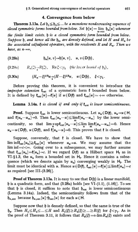
§ 3. Generalized strong convergence of sectorial operators 461
4. Convergence from belowTheorem 3.13a. Let 015 02S ... be a monotone nondecreasing sequence o l
closed symmetric forms bounded from below. Set 0[u] = lim On[u] whenevern- 00
the finite limit exists. 0 is a closed symmetric form bounded from below.Suppose 0, and hence all the On, are densely defined, and let H and Hn bethe associated self adjoint operators, with the resolvents R and R. Then wehave, as n-,
(3.28a) On [u, v]-O [u, v] , u, v E D(O) ,
(3.29x) R,(,)s.R(,) , Re l<y, (the lower boil 'dolt),),
(3.30a) s u E D(O) , <y,
Before proving this theorem, it is convenient to introduce theimproper extension text of a symmetric form f bounded from below.It is defined by text [u] =f [u] if u E D(f) and feRt[u] _ +00 otherwise.
Lemma 3.14a. t is closed i f and only i f text is lower semicontinuous.
Proof. Suppose teYt is lower semicontinuous. Let un E D(t), un-*u E H,and t[un-um]-+0. Then text [un-u] 5 limt[un-um] by the lower semi-
m
continuity, so that lim suptext [un-u] <lim linmt[un-um] =0. Henceun-u E D(t), u E D(t), and t [un-u]->0. This proves that t is closed.
Suppose, conversely, that f is closed. We have to show thatlim inffext [un] Z text [u] whenever un->u. We may assume that thelim inf=c<oo. Going over to a subsequence, we may further assumethat text [un] =f[un]-+c. If we regard D(f) as a Hilbert space He as inVI-§ 1.3, the un form a bounded set in He. Hence it contains a subse-quence (which we denote again by un) converging weakly in He. Thelimit must be identical with u. Hence u E D(f), feXt [u] =t[u] s limt[un] =cas required [see III-(3.26)].
Proof of Theorem 3.13a. It is easy to see that D(0) is a linear manifold,is a quadratic form, and that (3.28a) holds [see VI-(1.1), (1.16)]. To see
that 0 is closed, it suffices to note that Oext is lower semicontinuous(Lemma 3.14a). Indeed, the semicontinuity follows from that of theOn,ext because On,ext [u] tOext [u] for each u E H.
Suppose now that 0 is densely defined, so that the same is true of theOn. Then H,SH25,,,<H and R,( )zR2( for <yl. As inthe proof of Theorem 3.11, it follows that Ro(1:)'=s-limRn($) exists and
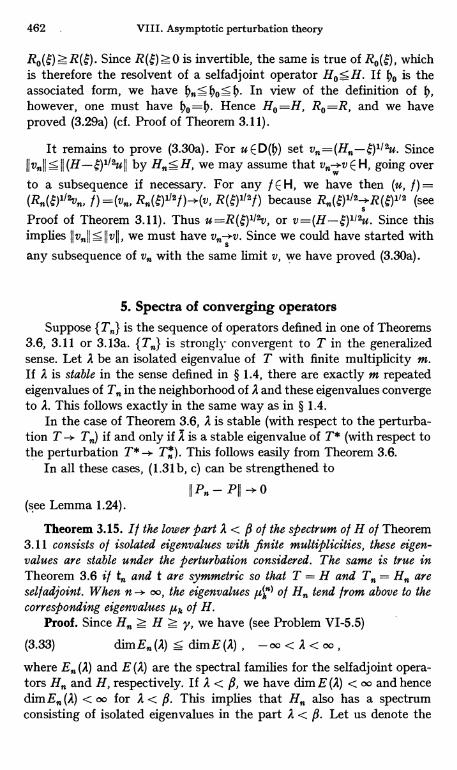
462 , VIII. Asymptotic perturbation theory
Re(d)>R(e). Since is invertible, the same is true of Ro(d), whichis therefore the resolvent of a selfadjoint operator H0 H. If tjo is theassociated form, we have In view of the definition of 1j,however, one must have fjo =fj. Hence Ho =H, R, =R, and we haveproved (3.29a) (cf. Proof of Theorem 3.11).
It remains to prove (3.30a). For uED(O) set SinceIIvnII < II (H-e)1/2uII by H,,s H, we may assume that v W v E H, going over
to agg subsequence if necessary. For any f E H, we have then (u, f) _(Rn(b)1/2vn, f) =(v., f)_+( R(e)112f) because
S (see
Proof of Theorem 3.11). Thus or v=(H-e)1/2u. Since thisimplies IIvn.II<IIvii, we must have Since we could have started with
s
any subsequence of v, with the same limit v, we have proved (3.30a).
5. Spectra of converging operatorsSuppose {T,n} is the sequence of operators defined in one of Theorems
3.6, 3.11 or 3.13a. is strongly convergent to T in the generalizedsense. Let A be an isolated eigenvalue of T with finite multiplicity m.If A is stable in the sense defined in § 1.4, there are exactly m repeatedeigenvalues of T,, in the neighborhood of A and these eigenvalues convergeto A. This follows exactly in the same way as in § 1.4.
In the case of Theorem 3.6, A is stable (with respect to the perturba-tion T ->- if and only if is a stable eigenvalue of T* (with respect tothe perturbation T*-. T,*,). This follows easily from Theorem 3.6.
In all these cases, (1.31b, c) can be strengthened to
IIP - PII - o(see Lemma 1.24).
Theorem 3.15. I l the lower part A < ,B o l the spectrum o l H o l Theorem3.11 consists o l isolated eigenvalues with finite multiplicities, these eigen-values are stable under the perturbation considered. The same is true inTheorem 3.6 i f t,, and t are symmetric so that T = H and T,, = H,, aresel f adjoint. When n oo the eigenvalues 1uk"> o f H,, tend from above to thecorresponding eigenvalues ,uk of H.
Proof. Since R. z H y, we have (see Problem VI-5.5)
(3.33) dim R. (A) dim E (A) , - oo < A < co ,
where E (A) and E (A) are the spectral families for the selfadjoint opera-tors H,, and H, respectively. If A < P, we have dim E (A) < oo and hencedim E,, (A) < oo for A < j$. This implies that H,, also has a spectrumconsisting of isolated eigenvalues in the part A < P. Let us denote the
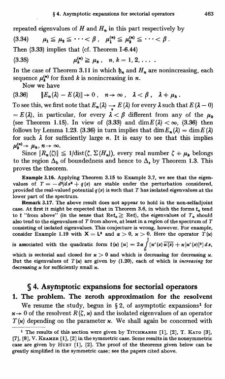
§ 4. Asymptotic expansions for sectorial operators 463
repeated eigenvalues of H and H in this part respectively by
(3.34) 5 fps 5 ... < P , i4' - lu2ri) - ... < PThen (3.33) implies that (cf. Theorem 1-6.44)
(3.35) AA")Zftk, n,k=1,2,... .In the case of Theorem 3.11 in which 0 and H are nonincreasing, eachsequence ,z") for fixed k is nonincreasing in n.
Now we have(3.36) IIEn(A)-E(A)II->0, n oo, A<j9, A+/z,.To see this, we first note that E. (A) - E (A) for every A such that E (A - 0)
= E (A), in particular, for every A < f different from any of the ,uk(see Theorem 1.15). In view of (3.33) and dimE (A) < oo, (3.36) thenfollows by Lemma 1.23. (3.36) in turn implies that dim E. (A) = dim E (A)for such A for sufficiently large n. It is easy to see that this impliesykn) -* p,, n-* oo.
Since II R. (C) II 5 E (Hn)), every real number C + 1u, belongsto the region A b of boundedness and hence to A, by Theorem 1.3. Thisproves the theorem.
Example 3.16. Applying Theorem 3.15 to Example 3.7, we see that the eigen-values of T = - d2/dx$ + q (x) are stable under the perturbation considered,provided the real-valued potential q (x) is such that T has isolated eigenvalues at thelower part of the spectrum.
Remark 3.17. The above result does not appear to hold in the non-selfadjointcase. At first it might be expected that in Theorem 3.6, in which the forms t tendto t "from above" (in the sense that Ret), the eigenvalues of T. shouldalso tend to the eigenvalues of T from above, at least in a region of the spectrum of Tconsisting of isolated eigenvalues. This conjecture is wrong, however. For example,consider Example 1.19 with X = L2 and a > 0, x > 0. Here the operator T (x)
iis associated with the quadratic form t (x) [u] = 2 at f [u' (x) u7 + x Iu' (x) 12] d x,
0which is sectorial and closed for x > 0 and which is decreasing for decreasing X.But the eigenvalues of T(x) are given by (1.20), each of which is increasing fordecreasing x for sufficiently small x.
§ 4. Asymptotic expansions for sectorial operators1. The problem. The zeroth approximation for the resolvent
We resume the study, begun in § 2, of asymptotic expansions' forx->- 0 of the resolvent R (g, x) and the isolated eigenvalues of an operatorT (x) depending on the parameter x. We shall again be concerned with
' The results of this section were given by TITCHMARSH [1], [2], T. KATO [3],[7], [8], V. KRAMER [1], [2] in the symmetric case. Some results in the nonsymmetriccase are given by HURT [1], [2]. The proof of the theorems given below can begreatly simplified in the symmetric case; see the papers cited above.
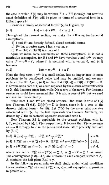
464 VIII. Asymptotic perturbation theory
the case in which T (m) may be written T + x T(') formally, but now theexact definition of T (m) will be given in terms of a sectorial form in aHilbert space H.
Consider a family of sectorial forms t (x) in H given by
(4.1) t(x) =t+xt('), 0<x s 1 .Throughout the present section, we make the following fundamentalassumptions.
i) t and t(') are densely defined, closed sectorial forms.ii) t(') has a vertex zero; t has a vertex
iii) D = D (t) n D (t(')) is a core of t.Again we make some comments on these assumptions. ii) is not a
restrictive assumption, for if t and t(l) have vertices y and y(l), we maywrite t(') = y(') + t', where t' is sectorial with a vertex 0, and (4.1)becomes
(4.2) t(x)=xy(l) +t+xt'.Here the first term x y(') is a small scalar, has no importance in mostproblems to be considered below and may be omitted, and we mayreplace t' by 0). Again, (4.1) implies that D (t (x)) = D (t) n D (t(')) = D.If D were not a core of t, we could replace t by the closure of its restrictionto D; this does not affect t (x), while D is a core of the new t. For the samereason we could have assumed that D is also a core of t(1>, but we neednot assume this explicitly.
Since both t and t(') are closed sectorial, the same is true of t (x)(see Theorem VI-6. 1). D(t(x)) = D is dense, since it is a core of thedensely defined form t by iii). Let T (x) be the m-sectorial operatorassociated with t (m) by the first representation theorem. Similarly, wedenote by T the m-sectorial operator associated with t.
Now Theorem 3.6 is applicable to the present problem, with t,t, T replaced by t (x), t, T (x), respectively. It follows that T (x) convergesas x -> 0 strongly to T in the generalized sense. More precisely, we haveby (3.10)
(4.3) R (C, x) s R R (, x) * 5 R x ->- 0,
(4.4) t [R (C, x) u - R ( )_ u] -. 0, t [R x) * u - R (C) * u] - 0 C E A5,
(4.5) x tC') [R (C, x) u] -. 0 , x t(l) [R x) * u] 0 u E H,
where we write R (g, x) = (T (x) - ()-1, R (g) = (T - -1 as usual.The convergences (4.3)-(4.5) are uniform in each compact subset of A5.AS contains the half-plane ReC < y.
In the following paragraphs we shall study under what conditionsthe expressions R (C, x) u and (R (C, x) u, v) admit asymptotic expansionsin powers of x.
§ 4. Asymptotic expansions for sectorial operators 465
We write(4.6) h = Ret, h(') = Ret(l), fj(x) = Ret(x) = h + x fjnl , = ReC,
and denote by Tt1>, H, H(1>, H (x) the operators associated with tnl,t, , ('), h (u), respectively. Also we have
(4.7) IImt [u] I S M(1 - y) [u] . IImt(1) [u] I < M' t') [u] .
Where M = tan 0, M' = tan 0' if 0, 0' are the semi-angles for the sectorialforms t, t (1). Finally we note that there need not be any simple relationshipbetween D (T) and D (T(')), so that T (u) need not be equal to T + u TO).
Remark 4.1. Since D (t*) = D (t), etc., the assumptions i) - iii) implythe same for their adjoint forms.
2. The 1/2-order approximation for the resolventTheorem 4.2. Let C E AS, u E H and R (C) u E D (t(1)). Then we have
as x-* 0(4.8) II R (C, x) u - R (C) ull = o (xl/2)
(4.9) t [R (C, x) - R (C) u] = o (x) , t(1) [R (C, x) u - R (C) u] = o (1) .
I/ R (C) u E D (0)) and R (C) * v E D (t (1)), then
(4.10) (R (C, x) u, v) _ (R (C) u, v) - x t(l)[R (C) u, R (C)* v] + o (u) .
Proof. I. Set(4.11) w=w(x)=R(C,x)u-R(C)u;note that w E D since R (C) u E D (T) C D (t) and R (C) u E D (t M) byassumption and since R (g, x) u E D (T (u)) C D (t (x)) = D. Then we have
(4.12) (t (x) - C) [w] = (t (x) - C) [R (C, x) u - R (C) u, w]= (u, w) - (u, w) - x t(') [R (C) u, w] = - x t(1> [R (C) u, w] .
Suppose, for the moment, that = Reg < 0, assuming y = 0 for sim-plicity (which does not affect the generality). Then Re (t (x) - C) = 4 -- + x ha) z x lM >_ 0, and (4.12) implies
(4.13) x 00) [w] s x it() [R (g) is, w] I S (1 + M') is fj(l) [R (g) u]1/2 0(1) [w ]1/2
[see VI-(1.15)] and hence
(4.14) h(1) [w] < (1 + M')2 h(1) [R (C) U]
This shows that w = w (x) is bounded as is -> 0 with respect to the normIIwJJ (I) = (4(1) [w] + IIw1I2)1/2 by which D (t(1)) becomes a Hilbert space Ht(1).But we have, for any v E H, (h(1) + 1) [w, (H(') + 1)-1 v] = (w, v) ->. 0because w-. 0 by (4.3). Since (H(1) + 1)-1 H = D(H(1>) is a core of h(l)and hence dense in Ht(x), it follows that w-. 0 weakly in Ht(1). Since t(1)
466 VIII. Asymptotic perturbation theory
is a bounded form on Ht(i), this implies that t(l> [R (C) u, w] -+ 0. Thusthe right member of (4.12) is o (x).
Again taking the real part of (4.12) and noting that Re (t (x) - C) [w]h [w] + (- ) IIwII2 + x I)(l) [w],- in which all three terms are non-
negative, we see that h [w], IIwII2 and x 1(') [w] are all o (x). This proves(4.8) and (4.9).
II. Now (4.8), (4.9) can be extended to the general case in whichC E A. and R (C) u E D (t(')). To show this we use a version of (1.3) :
(4.15) R x) - R(1 + (C - Co) R (C, x)) (R (Co, x) - R (Co)) (1 + (C - Co) R (C)) ,
in which we choose Co as a fixed number with ReCo < 0. Set x = (1 ++ (C - Co) R (C)) u. Then we have R (Co) x = R (C) u E D (t(')) by the resol-vent equation. Hence y (x) = (R (Co, x) - R (Co)) x = o (xl/2) by what wasproved above. Since R(C, x) is bounded when x -* 0, (4.8) follows from(R (C, x) - R(C)) u = (1 + (C - Co) R(C, x))y(x)
To prove (4.9), we note that
(4.16) t (x) [(R (C, x) - R (C)) u] (x) [y (x) + (C - Co) R (C, x) y (x)] S
5 2l (x) [y (x) ] + 2 I C - Co I2 4 (x) [R (C, x) y (X)]
We shall show that the last member of (4.16) is o (x). This is true for thefirst term by what has already been proved. In the second term, we mayreplace 4 (x) by 4 (x) - since IIR (C, x) y (X)112 = o (x) as shown above. But
(fj (x) - ) [R (C, x) y (m)] = Re (t (x) - C) [R (C, x) y (m)]
= Re (y (x), R (C, x) y (x)) s 11R (C, x) II IIy (x)II2 = 0 (x)
Thus (4.16) is o (x) and hence (4.9) follows immediately.III. To prove (4.10), we use the identity
(4.17) (w, v) _ (t - C) [w, R(C)* v]_ (t - C) [R (C, x) u, R (C) * v] - (t - C) [R (C) u, R (C) * v]
_ (u, R (C) * v) - x 0) [R (C, x) u, R (C)* v] - (u, R (C) * v)
_ -x t(') [R (C) u, R(C)* v] - x t(') [w, R(C)* v] .
This is true since R (C) * v E D, which follows from the assumption thatR())* v E D(t(')) as before. (4.10) follows from (4.17) in virtue of (4.9),which implies that w -* 0 in Hj(i).
3. The first and higher order approximations for the resolventOnce Theorem 4.2 for the 1/2-order approximation has been establish-
ed, the further approximations are rather straightforward. For example,we have
§ 4. Asymptotic expansions for sectorial operators 467
Theorem 4.3. Let E A5 and u E H. If R (C) u E D (T(1)), we have asx-> 0(4.18) R(C,x)uR(C)u-xR(C)T(1)R(C)u+o(x).If R(C) u E D(T(1)) and R(C)* v E D(T(1)*), then
(4.19) (R (C, x) u, v) = (R (C) u, v) - x (R (C) TM R (C) u, v) +
+ x2(R(C) T(1) R(C) u, T(1)* R(C)* v) + o(x2)
Proof. Using the same notations as in the preceding paragraph, wehave for any v E H(4.20) (w, v) _ (t (x) - C) [w, R (C, x) * v]
_ (t (x) - C) [R (C, x) u, R (C, x) * v] - (t (x) - C) [R (C) u,R (C, x) * v]
_ (u, R (C, x) * v) - (u, R (C, x) * v) - x 0) [R (C) u, R (C, x) * v]
_ - x (T(1) R (C) u, R (C, x) * v) _ - x (R (C, x) TM R (C) u, v)
since R (C) u E D (T(1)). Hence
(4.21) R(C,x)u-R(C)u=wxR(C,x)T(1)R(C)u.(4.18) follows from (4.21) in virtue of (4.3).
Suppose now that R(C)* v E D(T(1)*). Since T*, T(x)* and T(1)*are the operators associated with the adjoint forms t*, t(x)* and t(1)*,respectively, application of (4.21) to these adjoint forms with C replacedby leads to(4.22) R(C,x)*v-R(C)*v=-xR(C,x)*T(1)*R(C)*v.
Taking the inner product of (4.22) with u and using (4.21), we obtain
(4.23) (R(C, x) u, v) - (R(C) u, v) = -x(R(C, x) u, T(1)* R(C)* v)
= -x(R(C) u, T(1)* R(C)* v) + x2(R(C, x) T(1) R(C) u, T(1)* R(C)* v) ,
from which (4.19) follows in virtue of (4.3).Theorem 4.4. 1/ R (C) T(1) R (C) u exists and belongs to D (t(1)),
(4.24) R (C, x) u = R (C) u - x R (C) TM R (C) u + o (x3/2) .
If, in addition, R())* T(1)* R(C)* v exists and belongs to D(t(1)),
(4.25) (R (C, x) u, v) = (R (C) u, v) - x (R (C) TM R (C) u, v) +
+ x2(R(C) T(') R(C) u, T(1)* R(C)* v) -.- x3 t(1) [R (C) TM R (C) u, R (C) * T(')* R (C) * v] + o(x3)
Proof. (4.24) follows by applying (4.8) to the right member of (4.21).To prove (4.25), it suffices to apply (4.10) to the last term of (4.23)[with u, v replaced by T(1) R(C) u, T(1)* R(C)* v, respectively].
It is now easy to see how further approximations should proceed.It will not be necessary to write them down explicitly.
468 VIII. Asymptotic perturbation theory
Problem 4.5. If R (C) 211) R (C) u exists and belongs to D (tu)) and if R (C) * v EE D (tu)), then(4.26) (R (C, x) u, v) = (R (C) u, v) - x (R (C) T(l) R (C) u. v) +
+ x8 ill) [R (C) Ta> R (C) u, R (C) * v] + o (x8)
Remark 4.6. All the above formulas are, in spite of their different forms, essen-tially the second Neumann series for the resolvent, which may be written formally
(4.27) R x) = R x R (C) T<1> R (C) + x$ R (C) T(l) R (C) Ta> R (C) + .. .
For example, the coefficient of ms in (4.25) is formally equal to
(4.28) - t(l) [R (C) r') R (C) u, R (5) * T('>* R v](Ta) R T(l) R (C) is, R ()) * T(')* R (C) * v)
(R (C) Tl) R (C) T'> R (C) To) R (C) u, v) ,
corresponding to the coefficient of x' in (4.27). Actually (4.28) is correct only whenT(l) R (C) Tl) R (C) T(l) R (C) is makes sense. The left member of (4.28) exists,however, without assuming so much on is if we impose on v the assumptions stated.The formula (4.25) is particularly useful when t and t(') are symmetric and C is real;then T(')* = Ta>, R (C) * = R (C) so that it is valid for v = is if we assume only thatR (C) To) R (C) u E D (t(')). A similar remark applies to all the other formulas.
Example 4.7. Consider the differential operator
(4.29) T (x) = - d2/d x2 + q (x) + x qu> (x) , 0 x < oo ,
with the boundary condition is (0) = 0. T (x) is associated with the quadratic form
(4.30) t (x) [u] _ f [Iu'(x) 12 + q (x) j u (z) 11 + x q(1) (x) Iu (z)12] dx .000
This example is a version of Example 3.7 with a continuous parameter x rather thana discrete one n. If q (x) satisfies the assumptions of Theorem VI-4.2 and if qu> (x)is nonnegative and locally integrable, T (x) is selfadjoint and the above results areapplicable. The zeroth approximation (4.3) for the resolvent is valid for everyu E H = L2 (0, oo), the 1/2-order approximation (4.8) is true if R() u E D (t 1),that is, if
00
(4.31) f q(1) (x) I R (C) U (X) 12 d x < oo ,0
and the first order approximations (4.18) and (4.19) with v = u are valid if R (C) is EE D (Tu>), that is if
(4.32)00
'f qu> (X)2 IR (C) u (x) I' d x < oo ,
0and so on.
Suppose, in particular, that q (x) -> 0 as x -> oo, as is often the case in theSchr6dinger operators. w = R (C) is is the solution of (T - C) w = u or
(4.33) - w" + q (x) w - C w = u (x) , w(0)=0.If C is real and negative, it can be shown that the solution w (z) of (4.33) belong-ing to L2 must decrease in magnitude very rapidly as x -> oo, provided this is thecase with is (x). In such cases (4.31) and (4.32) are satisfied even when I qu) (x) I is largeasx ->oo.
q(l) (x) may also have a rather strong singularity at x = 0. If q (x) is o (x- 2) asx -> 0, w (z) = R (C) is (z) is 0 (x). In order that (4.31) be satisfied, therefore, q(l) (x)need only be of the order 0 (x- 8 } 8) with s > 0. Similarly, a singularity of 0 (X-1.6+8)is allowed to qu> (x) for (4.32) to be satisfied. Thus the above results are quite
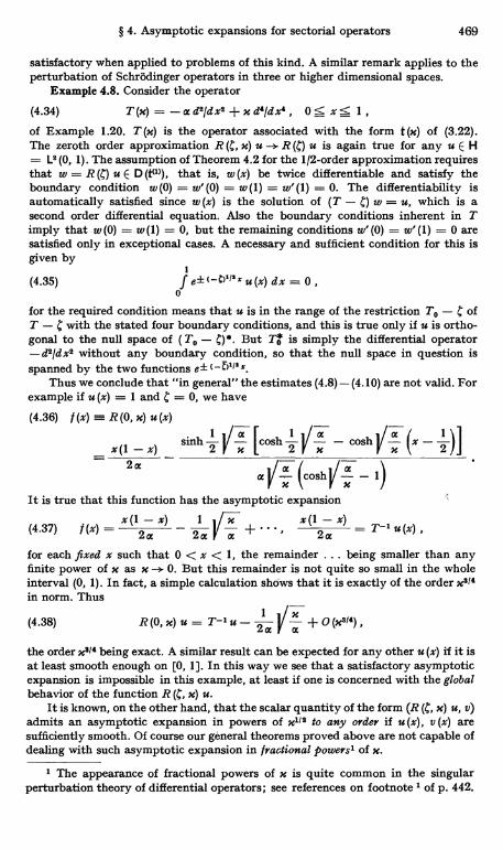
§ 4. Asymptotic expansions for sectorial operators 469
satisfactory when applied to problems of this kind. A similar remark applies to theperturbation of Schrodinger operators in three or higher dimensional spaces.
Example 4.8. Consider the operator
(4.34) T (m) _ -a d2/dx9 + x d4/dx4 , 0 < x 5 1,of Example 1.20. T (m) is the operator associated with the form t (M) of (3.22).The zeroth order approximation R (C, x) u R (C) u is again true for any u E H= L2 (0, 1). The assumption of Theorem 4.2 for the 1/2-order approximation requiresthat w = R u E D (t(1)), that is, w (x) be twice differentiable and satisfy theboundary condition w(0) = w'(0) = w(1) = w'(1) = 0. The differentiability isautomatically satisfied since w (x) is the solution of (T - C) w = u, which is asecond order differential equation. Also the boundary conditions inherent in Timply that w (0) = w (1) = 0, but the remaining conditions w' (0) = w' (1) = 0 aresatisfied only in exceptional cases. A necessary and sufficient condition for this isgiven by
(4.35)
If e±(-;>'"'xu(x)dx=0,
0
for the required condition means that u is in the range of the restriction To - ofT - C with the stated four boundary conditions, and this is true only if u is ortho-gonal to the null space of (To - But To is simply the differential operator-d2/dx2 without any boundary condition, so that the null space in question isspanned by the two functions of (- CS'I' x.
Thus we conclude that "in general" the estimates (4.8) - (4.10) are not valid. Forexample if u (x) = 1 and C = 0, we have
(4.36) f (x) = R (0, x) u (x)
x(1 - x) sinh 2V
,c I cosh 2V
-cosh2 at
[cosh
i
x
cosh V X- 111
It is true that this function has the asymptotic expansion
(4.37) f(x) = x(12ax)
2a V a I... X(12
x) = T-1 u(x)
for each fixed x such that 0 < x < 1, the remainder ... being smaller than anyfinite power of x as x -. 0. But this remainder is not quite so small in the wholeinterval (0, 1). In fact, a simple calculation shows that it is exactly of the order xa14in norm. Thus
,/(4.38) R (0, x) u = T-1 u - tara + 0
the order x°14 being exact. A similar result can be expected for any other u (x) if it isat least smooth enough on [0, 1]. In this way we see that a satisfactory asymptoticexpansion is impossible in this example, at least if one is concerned with the globalbehavior of the function R x) u.
It is known, on the other hand, that the scalar quantity of the form (R (C, x) u, v)admits an asymptotic expansion in powers of x1/2 to any order if u (x), v (x) aresufficiently smooth. Of course our general theorems proved above are not capable ofdealing with such asymptotic expansion in fractional powers' of x.
1 The appearance of fractional powers of x is quite common in the singularperturbation theory of differential operators; see references on footnote 1 of p. 442.
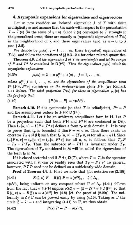
470 VIII. Asymptotic perturbation theory
4. Asymptotic expansions for eigenvalues and eigenvectorsLet us now consider an isolated eigenvalue A of T with finite
multiplicity m and assume that A is stable with respect to the perturbationT T (m) (in the sense of § 1.4). Since T (m) converges to T strongly inthe generalized sense, there are exactly m (repeated) eigenvalues of T (x)in the neighborhood of A and these eigenvalues tend as x -* 0 to A(see § 3.5).
We denote by ,uf (x), j = 1, ..., m, these (repeated) eigenvalues ofT (u), and follow the notations of §§ 2.3-2.4 for other related quantities.
Theorem 4.9. Let the eigenvalue A of T be semisimple and let the rangeso l P and P* be contained in D (t(1)). Then the eigenvalues ,u; (x) admit theasymptotic expansions
(4.39) AUf(x)=A+xIt()+o(x), j= 1,...,m,where = 1, ..., m, are the eigenvalues o l the sesquilinear formt(1) [Pu, P* v] considered in the m-dimensional space PH (see Remark4.11 below). The total projection P (m) for these m eigenvalues u5 (x) hasthe property that(4.40) 11P(M) - P11 = o (x1/2)
Remark 4.10. If t is symmetric (so that T is selfadjoint), P* = Pand the assumptions reduce to P H C D (t(')).
Remark 4.11. Let t be an arbitrary sesquilinear form in H. Let Pbe a projection such that both PH and P* H are contained in D (t).Then tP [u, v] = t [Pu, P*v] defines a form tp with domain H. It is easyto prove that tP is bounded if dim P = m < oo. Thus there exists anoperator TP E.4 (H) such that tp [u, v] _ (Tp u, v) for all u, v E H. SincetP [Pu, v] = tp [u, v] = tp [u, P*v] for all u, v, it follows that TPP= TP = P Tp. Thus the subspace M = P H is invariant under T.The eigenvalues of TP considered in M will be called the eigenvalues ofthe form tp in M.
If t is closed sectorial and if P H C D (T), where T = Tt is the operatorassociated with t, it can be readily seen that Tp = P T P. In general,however, P T P need not be defined on a sufficiently wide domain.
Proof of Theorem 4.9. I. First we note that [for notation see (2.18)]
(4.41) R (C, x) P - R (l;) P =0 (x1/2) , t; E AS ,
o(x1/2) being uniform on any compact subset r of AS. (4.41) followsfrom the fact that u E PH implies R (l;) u = (A - C)-1 U E D (t(1)) so thatR (C, x) u - R (C) u = o (x1/2) by (4.8) [cf. the proof of (2.20)]. The uni-formity in C E r can be proved easily by using (4.15). Taking as r thecircle - Al = r and integrating (4.41) on r, we thus obtain
(4.42) P (x) P - P = 0 (x1/2) .
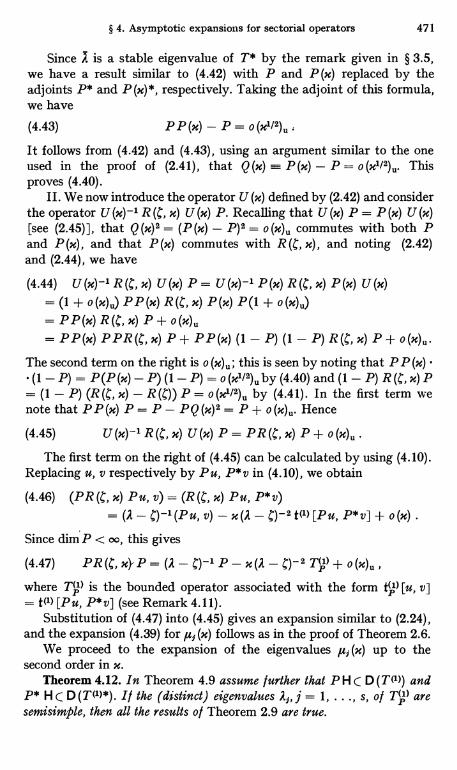
§ 4. Asymptotic expansions for sectorial operators 471
Since A is a stable eigenvalue of T* by the remark given in § 3.5,we have a result similar to (4.42) with P and P (x) replaced by theadjoints P* and P(x)*, respectively. Taking the adjoint of this formula,we have
(4.43) P P (x) - P = o (x1/2) 0,
It follows from (4.42) and (4.43), using an argument similar to the oneused in the proof of (2.41), that Q (x) = P (x) - P = o (x1/2) 0. Thisproves (4.40).
II. We now introduce the operator U (x) defined by (2.42) and considerthe operator U (x) R (C, x) U (x) P. Recalling that U (x) P = P (x) U (x)[see (2.45)], that Q (x)2 = (P (x) - P)2 = o (x)0 commutes with both Pand P (x), and that P (x) commutes with R (C, x), and noting (2.42)and (2.44), we have
(4.44) U(m)-l' R (C, x) U (m) P = U(m)-l' P (m) R (C, x) P (m) U (m)
_ (1 + o (x)0) PP (x) R (C, x) P (x) P(1 + o (x)0)= PP(x) R (C, x) P + o(x) 0
= PP(x) PPR(C, x) P + PP(x) (1 - P) (1 - P) R(C, x) P + o(x)0.
The second term on the right is o (x)0 ; this is seen by noting that P P (x)(1 - P) = P(P(x) - P) (1- P) = o (x1/2)0 by (4.40) and (1 - P) R (C, x) P
= (1 - P) (R (C, x) - R (C)) P = o (x1/2)0 by (4.41). In the first term wenote that PP (x) P = P - PQ (x)2 = P + o (m), Hence
(4.45) U(m)-1 R (C, x) U (m) P = PR (C, x) P + o(x)0 .
The first term on the right of (4.45) can be calculated by using (4.10).Replacing u, v respectively by Pu, P*v in (4.10), we obtain
(4.46) (PR(, x) Pu, v) = (R (C, x) Pu, P* v)= (2 - C)-1(Pu, v) -X (2 - C)-2 t(1) [Pu, P*v] + o (x) .
Since dim P < oo, this gives
(4.47) PR(, x)- P = (2 - c)-1 P - x (2 - C)- 2 TP' + o (x)0
where T' is the bounded operator associated with the form tP> [u, v]= t(1> [Pu, P*v] (see Remark 4.11).
Substitution of (4.47) into (4.45) gives an expansion similar to (2.24),and the expansion (4.39) for p1 (x) follows as in the proof of Theorem 2.6.
We proceed to the expansion of the eigenvalues ,u, (x) up to thesecond order in x.
Theorem 4.12. In Theorem 4.9 assume further that P H C D (T(1)) andP* H C D (T(l)*). I/ the (distinct) eigenvalues A1, j = 1, . . ., s, ol T(') aresemisimple, then all the results o l Theorem 2.9 are true.

472 VIII. Asymptotic perturbation theory
Remark 4.13. The operator [P T01)] of Theorem 2.9 is here equal to(T (')* P*) * ; note that T (')* P* E a (H) by the assumption P* H C D(T (')*).
Proof of Theorem 4.12. If u E P H we have R (C) u = (I - 0`u E D (T(')),so that we have the expansion (4.18) for R (C, x) u. The o (x) on the rightof (4.18) is uniform in C on any compact subset of Os, as is seen from(4.21) and Lemma 111-3.7. Considering that dimP < oo, we again obtainthe formula (2.20) for R (C, x) P.
Considering the adjoints R(C)* etc., we arrive at the same formula(2.20) with P, R (c), ... replaced by P*, R (C)*, .... Taking the adjointof this result, we obtain the formula (2.35) for PR(C, x), with o(x)5replaced by o (x),,.
Once we have these two expressions, the proof of Theorem 2.9 canbe applied without change to deduce the required results.
Remark 4.14. In the same way we could proceed to the expansion ofthe eigenvalues and eigenvectors to higher orders of x. We shall not givethe details', for the second approximation for the eigenvalues is suf-ficient for most problems in application. It will only be noted that, inview of the formal expansion of A (x) in which the third coefficient A(3)contains the term trT(') ST(') ST(') P = t(') [ST(') 92, S* T(')* 99] (assum-ing m = 1), we have to assume that(4.48) ST(') P X (:D (t(')) , S* T (')* P* X C D (t(')) ,
in order to obtain the expansion of the eigenvalues up to the order x8.Similarly, the expansion of the eigenvalues up to the order x4 wouldrequire the existence of(4.49) T(') ST(') F , T(')* S* T(')* p* E V(H) .
Example 4.15. Consider the differential operator T (m) given by (4.29) with theboundary condition u (0) = 0 (see Example 4.7). To be definite, assume that thereal-valued unperturbed potential q (x) tends to zero as x oo. Then it is wellknown that the unperturbed operator T has only negative eigenvalues, which areall isolated. Let A be one of them and let T be the associated eigenfunction (A issimple). Since the associated eigenprojection P is the orthogonal projection on theone-dimensional subspace spanned by p, Theorem 4.9 is applicable to A if
00
(4.50) f qa> (x) IT(X)12 d x < oo .
0
Similarly, Theorem 4.12 is applicable if (note that P and Ti'> are selfadjoint here)M
(4.51) f q(1) (x)' 19, (x) I' d z < co .
0
In other words, we have the expansion of A (x) up to the order x if (4.50) is satisfied,and up to the order x' if (4.51) is satisfied.
It is well known, however, that 9' (z) behaves like x as x -s 0 and likeexp [- (- A)1I$ x] as x -a co [more precise behavior depends on q (x)]. Therefore,
1 See V. KRAMER [1], [2], where a detailed result is given in the special case whenH (x) is a selfadjoint Friedrichs family [that is, t (x) is defined by t (x) [u] = (K (x) u, u)from a given family K (x) of symmetric operators].
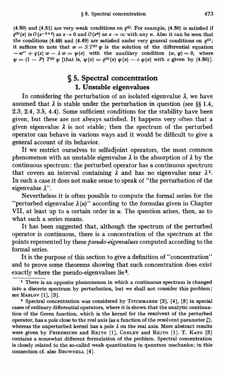
§ 5. Spectral concentration 473
(4.50) and (4.51) are very weak conditions on q(1). For example, (4.50) is satisfied ifqa> (x) is O (x- 8 } e) as x -> 0 and O (x") as x oo with any n. Also it can be seen thatthe conditions (4.48) and (4.49) are satisfied under very general conditions on q(1);it suffices to note that w = S 711> q> is the solution of the differential equation- w" + q (x) w - A w = y> (z) with the auxiliary condition (w, q>) = 0, whereV = (1 - P) T11> q> [that is, v> (x) = q(1) (x) 92 (x) - c q> (x) with c given by (4.50)].
§ 5. Spectral concentration1. Unstable eigenvalues
In considering the perturbation of an isolated eigenvalue A, we haveassumed that I is stable under the perturbation in question (see §§ 1.4,2.3, 2.4, 3.5, 4.4). Some sufficient conditions for the stability have beengiven, but these are not always satisfied. It happens very often that agiven eigenvalue A is not stable; then the spectrum of the perturbedoperator can behave in various ways and it would be difficult to give ageneral account of its behavior.
If we restrict ourselves to selfadjoint operators, the most commonphenomenon with an unstable eigenvalue 2 is the absorption of 2 by thecontinuous spectrum: the perturbed operator has a continuous spectrumthat covers an interval containing I and has no eigenvalue near 21.In such a case it does not make sense to speak of "the perturbation of theeigenvalue A".
Nevertheless it is often possible to compute the formal series for the"perturbed eigenvalue A (x) " according to the formulas given in ChapterVII, at least up to a certain order in x. The question arises, then, as towhat such a series means.
It has been suggested that, although the spectrum of the perturbedoperator is continuous, there is a concentration of the spectrum at thepoints represented by these pseudo-eigenvalues computed according to theformal series.
It is the purpose of this section to give a definition of "concentration"and to prove some theorems showing that such concentration does existexactly where the pseudo-eigenvalues lie $.
1 There is an opposite phenomenon in which a continuous spectrum is changedinto a discrete spectrum by perturbation, but we shall not consider this problem;see MASLOV [1], [3].
Spectral concentration was considered by TITCHMARSH [3], [4], [5] in specialcases of ordinary differential operators, where it is shown that the analytic continua-tion of the Green function, which is the kernel for the resolvent of the perturbedoperator, has a pole close to the real axis (as a function of the resolvent parameter ]),whereas the unperturbed kernel has a pole A on the real axis. More abstract resultswere given by FRIEDRICHS and REJTO [1], CONLEY and REJTO [1]. T. KATO [3]contains a somewhat different formulation of the problem. Spectral concentrationis closely related to the so-called weak quantization in quantum mechanics; in thisconnection cf. also BROWNELL [4].
474 VIII. Asymptotic perturbation theory
2. Spectral concentrationLet H be a Hilbert space and {H,,} a sequence of selfadjoint operators
in H, with the associated spectral families {En (A)}. We denote by En (S)the spectral measure 1 constructed from En (2), where S varies oversubsets of the real line R. (In what follows all subsets of R considered areassumed to be Borel sets.)
Let Sn C R, n = 1, 2, .... We say that the spectrum of Hn is (asym-ptotically) concentrated on Sn if
(5.1) E'n(Sn) s 1 , n-* oo,or, equivalently,
(5.2) En (R - Sn) s 0,
where R - Sn is the complementary set of Sn with respect to R. HereSn = S may be independent of n; then we say that the spectrum of Hnis concentrated on S. It is obvious that if the spectrum of Hn is con-centrated on Sn, it is concentrated on any S such that Sn C S.
Thus spectral concentration is an asymptotic notion related to a givensequence (or a family) {Hn} of operators; it does not make sense to speakof spectral concentration for a single operator H (except in the trivialspecial case of a sequence {Hn} in which all Hn are equal to H).
More generally, we shall say that the part of the spectrum of Hn in asubset T of R is (asymptotically) concentrated on Sn if
(5.3) En (T - Sn) s 0,
where T - Sn = T n (R - Sn) (the S. need not be subsets of T). Itis obvious that (5.2) implies (5.3) for any T because En (T - Sn) SS En (R - Sn). If, conversely, the parts of the spectrum of Hn in T andin R - T are concentrated on Sn, then the spectrum is concentrated onSn, for E. (R - Sn) = E. (T - Sn) + E. (R - T - Sn). For this reason itsuffices, for most purposes, to consider concentration with respect tosome given set T.
A basic result for spectral concentration is given byTheorem 5.1. Let Hn H in the generalized sense, where H is sell-
s
adjoint. Let S ( R be an open set containing E (H). Then the spectrum of Hnis asymptotically concentrated on S. Furthermore, we have En (S n I) -/ E (I)
s
for any interval I if the end points of I are not eigenvalues of H (E denotesthe spectral measure for H).
1 See VI-§ 5.1 and X-§ 1.2. Here we need only elementary properties of thespectral measure; in most cases it suffices to consider sets S which are unions ofintervals.
§ 5. Spectral concentration 475
Proof. The open set S is the union of at most a countable number ofdisjoint open intervals I, all of which are finite except possibly one ortwo. E (H) C S implies that ' E (Ik) = E (S) = 1, in which the series
k
converges in the strong sense. Hence the span of the subspaces E (Ik) His dense in H. In order to prove (5.1), therefore, it suffices to show thatE (S) u -* u whenever u E E (Ik) H for some k.
First assume that It = (ak, bk) is finite. Then a, b, belong to P (H),for they cannot belong to E (H). Thus there are ak, bk such that at << ak < bk < bk and the two intervals [ak, ak], [bk, bk] are subsets ofP (H). On setting Ik = (ak, bk), we have E (Ik) = E (Ik) and so En (Ik) u=En(bk-0)u-En(ak)u-> E(bk)u-E(ak)u=E(Ik)u=E(Ik)u=u(see Theorem 1.15 and the attached footnote). Since Ik C S, we haveE. (It) S E. (S) and so E,, (S) u -+ u, as we wished to show.
When Ik is not a finite interval, we need a slight modification in theabove proof. If, for example, bk = oo, we set bk = oo ; then E,, (oo) u= u = E (oo) u and the above proof goes through.
The last assertion of the theorem follows from E,, (S n I) = E,, (S) E,,(I)by noting that E (I) - E (I) in virtue of Theorem 1.15.
S
3. Pseudo-eigenvectors and spectral concentration
Theorem 5.1 shows that if H H in the generalized sense, thes
spectrum of H is asymptotically concentrated on any neighborhood ofE (H). In particular let A be an isolated eigenvalue of H with isolationdistance d, and let I = (A - d/2, A + d/2). Then the part of the spectrumof H. in I is asymptotically concentrated on an arbitrarily small neigh-borhood of A [see (5.3)].
We shall now sharpen this result by localizing the concentration to asmaller interval (or intervals) depending on n, under some additionalassumptions.
Theorem 5.2. Let H -. H in the generalized sense, and let A and Is
be as above. Let P be the eigenprojection of H for A and let dim P = m < oo.Suppose there exist m sequences of "pseudo-eigenvalues" {A1n} and "pseudo-eigenvectors" {99;n} of Hn, j = 1, . . ., m, such that
(5.4) II (Hn - A!n) 9,j.JJ = e,n -+ 0 , 99in -*99i , n "oo ,
where 4p, . . , 99. form a basis of PH with II 9'3II = 1. Then the part of thespectrum of Hn in I is asymptotically concentrated on the union of mintervals IJn = (Afn - an Efn, A3n + an Efn), where {an} is any sequence ofpositive numbers such that an -> oo.
476 VIII. Asymptotic perturbation theory
Proof. (5.4) implies that00
Ean = f Cu - 2. )2 d(En(u) (Pin, 9'9n) z_00
tCn Ean f d(E.(p) 9P1n, 9,,n)µfflio
= an Ean 11(1 - E. (I,.)) 991n112 .
Hence 11 (1 - En(I1n)) (P;nll s 1/a -> 0, n -*. oo. Since X1(1- En(Iin))(9Pin -';)p s 1199j. - qq;jj - 0, it follows that
(5.5) (1 - E. (Iin)) 991 + 0 , n -> oo .
If we denote by In the union of Iln, ..., Imn, then 1 - En (In) S 1 -- En (Iin) and so (5.5) implies (1 - En (In)) 99j -+ 0. Since the 99a span P H,it follows that
(5.6) (1 - En (In)) P + 0 in norm .
On the other hand we have
(5.7) En (I) (1 - P) s 0,
since En (I) s E (I) = P by Theorem 1.15. Multiplying (5.6) by En (I),(5.7) by 1 - E. (In) and adding the results, we obtain En (I - In)= E. (I) (1 - E. (In)) . 0, as we wished to prove.
s
Remark 5.3. We can arrange that II,, f = 2an efn ->- 0 by choosingan -> oo appropriately. Hence the part of the spectrum of H. in I isasymptotically concentrated on a set In with measure II, 1 -> 0, andTheorem 5.2 strengthens Theorem 5.1. It should be noted that for anyneighborhood I' C I of A, In C I' is true for sufficiently large n. In fact,let I" be a proper subinterval of I' containing d; then En (I") q'; ->- P Q,;= 99f so that En (Ifn n I") q'; = E. (Iin) En (I") q'3 -> Tf by (5.5). SinceI I;,, I --- 0, this implies I1,. C I', and hence In C I', for sufficiently large n.In particular we must have A -. A for every j.
4. Asymptotic expansions
We now consider a family H(x) of selfadjoint operators formallygiven by H + x H('), where H is selfadjoint and H(') is symmetric. Moreprecisely, we assume the conditions ii), iii) of § 2.1, namely that D= D (H) n D (H(')) is a core of H and that H + x H(') (with domain D)has a selfadjoint extension H (x) for 0 < x 5 1. Then iv) of § 2.1 isautomatically satisfied, for Ob n P (H) contains all nonreal complexnumbers.
§ 5. Spectral concentration 477
Under these conditions it has been shown that H (x) x -+ 0H,s
, ,
in the generalized sense (see loc. cit.)". It follows from Theorem 5.1 thatthe spectrum of H (x) is asymptotically concentrated on any neighborhoodof E (H). If d is an isolated eigenvalue of H with the isolation distance dand the eigenprojection P, then the part of the spectrum of H(x) inI = (A - d/2, A + d/2) is asymptotically concentrated on any smallneighborhood of d, with
(5.8) E (I, x) S P, x ->O.
We shall now sharpen this result by making specific assumptions on theunperturbed eigenspace P H.
Theorem 5.4. Let dim P = m < oo and P H D (H(1)). Let 0.), j = 1,m, be the repeated eigenvalues of the symmetric operator PH(') P in the
m-dimensional subspace PH. Then the Part of the spectrum of H (x) in Iis asymptotically concentrated on the union of m intervals with the centersA + x y() and with the width o (x).
Remark 5.5. The result of Theorem 5.4 may be interpreted to meanthat H (x) has m pseudo-eigenvalues A + x ,u(l) + o (x) (cf. the correspond-ing Theorem 2.6 when A is assumed to be stable). Of course such a state-ment is not fully justified unless the corresponding pseudo-eigenvectorsare constructed, which will be done in the course of the proof.
Proof. Let {qqj} be an orthonormal basis of PH consisting of eigen-vectors of PH(I) P:
(5.9) PH(1) P 921 = y(1) q,j j = 1, . . ., m.
We shall construct pseudo-eigenvectors of H (x) in the form
(5.10) 991 (x) = 993 + x 9914) (x) , II q,;l) (x) II s M
so that as x -- 0
(5.11) x-1 II (H (x) - A - x ,1)) cPJ(x) II < S M - 0
Then an application of Theorem 5.2 will lead to the desired result (withthe discrete, parameter n replaced by the continuous one x); it suffices totake the interval Ijx with center 2 + x u(i) and width 2 x a (x) 6 (x),where a (x) -+ oo and a (x) a (x) - 0.
Let S be the reduced resolvent of H for A (see III-§ 6.5). S has theproperties S E 9(H), (H - 2) S = 1 - P [see III-(6.34)]. Let s > 0.Since - SH(1) q, E D (H) and D is a core of H, there is a q' E D such thatII99;II s IISH(1) ggjII + 1 s M and II(H - A) (mi + SH(1) 99j)II < E12. Since(H - 2) SH(1) q'1 = (1 - P) H(1) q'f = H(1) qq, - 1u(1) 993, we have [note
1 The same result holds if we replace the above assumptions by those of § 4.1,with the additional assumption that t = 4 and P) = 000 are symmetric [so thatT = H and T(x) = H(x) are selfadjoint].
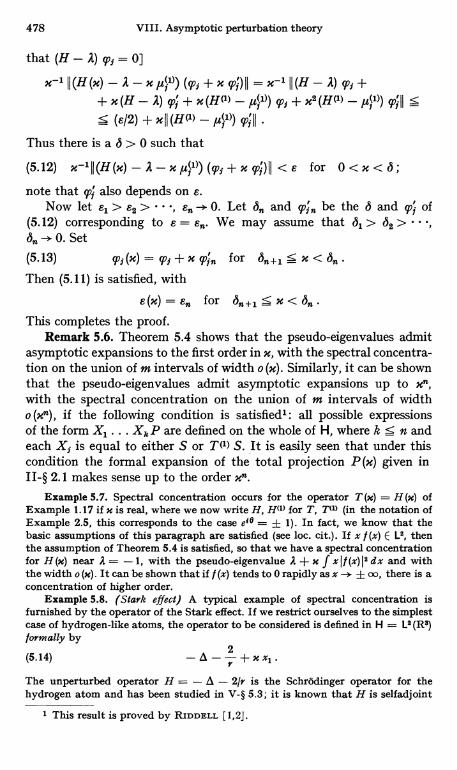
478 VIII. Asymptotic perturbation theory
that (H - R) q, = 0]
M-1 II (H (x) - A - x j4'1) (99j + x 99i) II = x-1 II (H - d) qq, ++ x (H - R) 99i + x (HO) - ju;1)) 993 + x2 (Ha) - p(')) 99i II S
s (e/2) + x II (HM - ,u(1)) 99i II
Thus there is a 6 > 0 such that
(5.12) x-1II(H (x) - A - e (1)) (991 + x 99j') 11 < s for 0 < x < 8 ;
note that 99i also depends on s.Now let e1 > e2 > , en -* 0. Let 8n and 99, be the 6 and q of
(5.12) corresponding to e = e,,. We may assume that 81 > 82 > ,An -> 0. Set
(5.13) 99j (x) = q't + x cpi for 6n+1 x < 8n .
Then (5.11) is satisfied, with
s (m) = e for Sn+1 S x < 1 .
This completes the proof.Remark 5.6. Theorem 5.4 shows that the pseudo-eigenvalues admit
asymptotic expansions to the first order in x, with the spectral concentra-tion on the union of m intervals of width o (x). Similarly, it can be shownthat the pseudo-eigenvalues admit asymptotic expansions up to xn,with the spectral concentration on the union of m intervals of widtho (xn), if the following condition is satisfied' : all possible expressionsof the form X1 ... Xk P are defined on the whole of H, where k s n andeach X; is equal to either S or TM S. It is easily seen that under thiscondition the formal expansion of the total projection P(x) given inII-§ 2.1 makes sense up to the order xn.
Example 5.7. Spectral concentration occurs for the operator T (x) = H (x) ofExample 1.17 if x is real, where we now write H, H(1) for T, 711) (in the notation ofExample 2.5, this corresponds to the case eie = ± 1). In fact, we know that thebasic assumptions of this paragraph are satisfied (see loc. cit.). If x f (x) E L2, thenthe assumption of Theorem 5.4 is satisfied, so that we have a spectral concentrationfor H (m) near A = -1, with the pseudo-eigenvalue A + x f x 1f (x)12 dx and withthe width o (x). It can be shown that if f (x) tends to 0 rapidly as x -+ f oo, there is aconcentration of higher order.
Example 5.8. (Stark effect) A typical example of spectral concentration isfurnished by the operator of the Stark effect. If we restrict ourselves to the simplestcase of hydrogen-like atoms, the operator to be considered is defined in H = L2 (R8)formally by
(5.14) -A-2+xx1.The unperturbed operator H = - A - 2/r is the Schr6dinger operator for thehydrogen atom and has been studied in V-§ 5.3; it is known that H is selfadjoint
1 This result is proved by RIDDELL [1,2J.
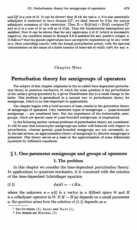
IX. Perturbation theory for semigroups of operators 479
and Co is a core of H. It can be shown' that (5.14) for real x r 0 is also essentiallyselfadjoint if restricted to have domain Co ; we shall denote by H (x) the uniqueselfadjoint extension of this restriction. Then D = D (H (x)) n D (H) contains Coand so it is a core of H as well as of H(x). Thus the fundamental assumptions aresatisfied. Now it can be shown that for any eigenvalue A of H (which is necessarilynegative), the condition stated in Remark 5.6 is satisfied for any positive integer n.It follows 2 that the pseudo-eigenvalues have asymptotic expansions up to any orderin x (thus coinciding exactly with the formal perturbation series), with the spectralconcentration on the union of a finite number of intervals of width o (x") for any n.
Chapter Nine
Perturbation theory for semigroups of operatorsThe subject of this chapter originates in the so-called time-dependent perturba-
tion theory in quantum mechanics, in which the main question is the perturbationof the unitary group generated by a given Hamiltonian due to a small change in thelatter. This problem is generalized in a natural way to perturbation theory forsemigroups, which is no less important in applications.
The chapter begins with a brief account of basic results in the generation theoryof semigroups of operators. Only restricted types of semigroups - quasi-boundedsemigroups - are considered here. But the importance of the holomorphic semi-groups, which are special cases of quasi-bounded semigroups, is emphasized.
In the following section various problems of perturbation theory are considered.It will be seen that holomorphic semigroups are rather well-behaved with respect toperturbation, whereas general quasi-bounded semigroups are not necessarily so.In the last section, an approximation theory of semigroups by discrete semigroups ispresented.. This theory serves as a basis in the approximation of some differentialequations by difference equations.
§ 1. One-parameter semigroups and groups of operators1. The problem
In this chapter we consider the time-dependent perturbation theory.In applications to quantum mechanics, it is concerned with the solutionof the time-dependent Schrodinger equation
(1.1) du/dt = -i Hu,
where the unknown u = u (t) is a vector in a Hilbert space H and His a selfadjoint operator in H. If H = H (x) depends on a small parameterx, the question arises how the solution of (1.1) depends on x.
' See STUMMEL [1], IKEBE and KATO [1].$ For details see RIDDELL [1].
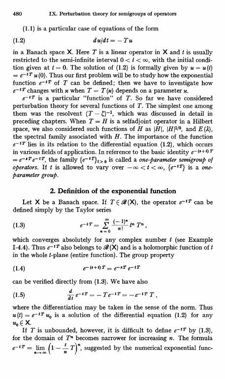
480 IX. Perturbation theory for semigroups of operators
(1.1) is a particular case of equations of the form
(1.2) du/dt= - Tuin a Banach space X. Here T is a linear operator in X and t is usuallyrestricted to the semi-infinite interval 0 < t < oo, with the initial condi-tion given at t = 0. The solution of (1.2) is formally given by u = u (t)= e-tT u (0). Thus our first problem will be to study how the exponentialfunction e-tT of T can be defined; then we have to investigate howe- t T changes with x when T = T (x) depends on a parameter x.
e-tT is a particular "function" of T. So far we have consideredperturbation theory for several functions of T. The simplest one amongthem was the resolvent (T - c)-', which was discussed in detail inpreceding chapters. When T = H is a selfadjoint operator in a Hilbertspace, we also considered such functions of H as JHI, IHIl/a, and E (A),the spectral family associated with H. The importance of the functione-tT lies in its relation to the differential equation (1.2), which occursin various fields of application. In reference to the basic identity e-(8+t)T= e-8T a-t T, the family {e-tT}t, o is called a one parameter semigroup o/operators. If t is allowed to vary over -oo < t < oo, {e-tT} is a one-parameter group.
2. Definition of the exponential function
Let X be a Banach space. If T E 9 (X), the operator e- *I can bedefined simply by the Taylor series
(1.3) a-tT = fn I
to Tn00
n=0
which converges absolutely for any complex number t (see Example1-4.4). Thus a-tT also belongs to R(X) and is a holomorphic function of tin the whole t-plane (entire function). The group property
(1.4) e-(a+t)T = e-8T a-tT
can be verified directly from (1.3). We have also
(1.5) e-tT = -Te-tT_ -e-tT T,
where the differentiation may be taken in the sense of the norm. Thusu (t) = e- tT uo is a solution of the differential equation (1.2) for anyuo E X.
If T is unbounded, however, it is difficult to define a-tT by (1.3),for the domain of Tn becomes narrower for increasing n. The formulae-tT = Jim (1 - T)n, suggested by the numerical exponential func-
n-aoo ` 9t

§ 1. One-parameter semigroups and groups of operators 481
tion, is not useful for the same reason. But a slight modification of thisformula, namely,
(1.6) a-tT = lim (1 + t T
is found to be useful. In fact (1 + t T)-1is the resolvent of - T, apart
from a constant factor, and it can be iterated even when T is unbounded.The following is a sufficient condition in order that the limit (1.6)
exist in an appropriate sense.i) T E '(X) with domain D(T) dense in X.
ii) The negative real axis belongs to the resolvent set of T, and theresolvent (T + )-1 satisfies the inequality
(1.7) 11 (T + e)-111 s 1/ , E > 0 .
To see this, we note first that (1.7) implies
(1.8) 11(1 +a T)-1J1 s 1, a? 0.Set
(1.9) VV(t) _ I+ t T)-n
, t z 0, n = 1, 2,... .
It follows from (1.8) that jjV,,(t)Ii s 1, so that the V, (t) are uniformlybounded. Furthermore, Vn (t) is holomorphic in t for t > 0, for(T + )-1 is holomorphic in 1: > 0; in particular
(1.10) dt V. (t) T 1 -} n T)-n-1E R(X), t> 0.
Vn (t) is not necessarily holomorphic at t = 0, but it is strongly continuous :
(1.11) V. (t) g V n (0) = 1 as t' 0 ;this follows from
(1.12) (1+aT)-1 S 1, a\0,which can be proved in the same way as in Problem V-3.33.
To prove the existence of lim Vn (t), we estimate V. (t) u - Vm (t) u.For this we note that, in virtue of (1.11),
t-8
(1.13) Vn (t) U - V. (t) u = lim f a [Vm (t - s) V. (s) u] dse
9-8
=lim
f [- V;n (t - s) Vn (s) u + Vm (t - s) V (s) u] d s .8
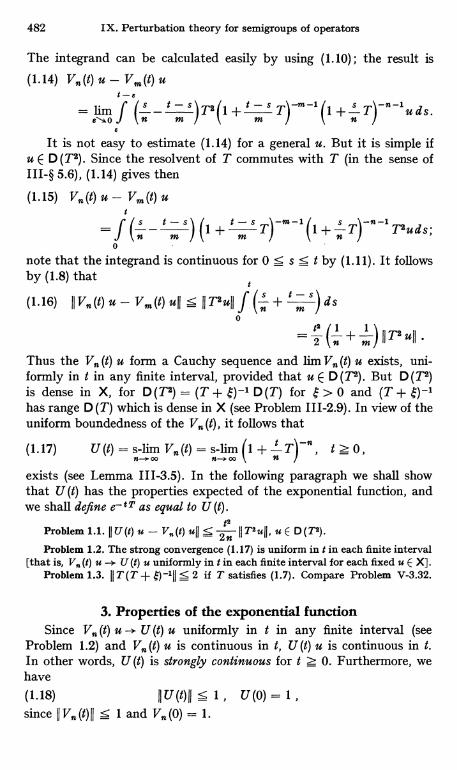
482 IX. Perturbation theory for semigroups of operators
The integrand can be calculated easily by using (1.10) ; the result is(1.14) V,, (t) u - Vm(t) u
t-e
lim f In t m s)Ta(1 + t m ST)-"`6-1 (1 n T)-"-suds.
e tIt is not easy to estimate (1.14) for a general u. But it is simple if
u E D (T2). Since the resolvent of T commutes with T (in the sense ofIII-§ 5.6), (1.14) gives then
(1.15) V. (t) u - V. (t) ut
- f (n tm S) (1 + t m T)-m-1(1
F n T)-n-1T2uds;o
/
note that the integrand is continuous for 0 s s s t by (1.11). It followsby (1.8) that
t
(1.16) II Vv(t) u - Vm(t) u11 s IIT2uJI f (n + t m)
ds0
= 2 (n + m) IIT2u11
Thus the V (t) u form a Cauchy sequence and Jim V,, (t) u exists, uni-formly in t in any finite interval, provided that u E D (T2). But D (T2)is dense in X, for D (T2) = (T + )-1 D (T) for $ > 0 and (T + $)-1
has range D (T) which is dense in X (see Problem 111-2.9). In view of theuniform boundedness of the V,, (t), it follows that
(1.17) U (t) = s-lim Vn (t) = s-lim (1 + T)-n' t z 0 ,n-s ao n-- oo n
exists (see Lemma 111-3.5). In the following paragraph we shall showthat U (t) has the properties expected of the exponential function, andwe shall define e- IT as equal to U(t).
Problem 1.1. 11 U(t) u - V. (t) ull S 2n 11 T2 U11, u E D(T$).
Problem 1.2. The strong convergence (1.17) is uniform in tin each finite interval[that is, V. (t) u U (t) u uniformly in tin each finite interval for each fixed It E X].
Problem 1.3. 11 T(T + ) -111 S 2 if T satisfies (1.7). Compare Problem V-3.32.
3. Properties of the exponential functionSince V. (t) u -> U (t) u uniformly in t in any finite interval (see
Problem 1.2) and V. (t) u is continuous in t, U (t) u is continuous in t.In other words, U (t) is strongly continuous for t Z 0. Furthermore, wehave(1.18) 11U(t)II S 1, U(0)=1,since 11 V,, (t) 11 s 1 and V,, (0) = 1.
§ 1. One-parameter semigroups and groups of operators 483
Now it follows from (1.10) that
(1.19) (1+n T)-1
TVn(t)(1+ t T)-1But
(1.20) T(1+T)-lu=(1+nT)-1Tu->Tu for uED(T)by (1.11). Hence the third member of (1.19), when applied to u, tendsto' - U (t) T u. Since the factor after T of the fourth member, whenapplied to u, tends to U (t) u for a similar reason, it follows from theclosedness of T that T U (t) u exists and equals U (t) T u. In other words Tcommutes with U (t) :(1.21) T U (t) ) U (t) T.
It follows also from (1.10) and (1.11) thate
(1.22) Vn(t) u - u = - f (1 + n T)-n-1 Tu ds, u E D(T) .0
Since I+ T(1 + t T)-1Vn(t) S U(t) uniformly in t in
each finite interval, we can go to the limit n -* oo under the integralsign in (1.22), obtaining
t
(1.23) U(t)u-u=- f U(s)Tuds, uED(T).0
Since U (s) T u is continuous in s, (1.23) shows that U (t) u is differentiablein t if u E D (T), with
(1.24) tU(t)u=-U(t)Tu=-Tu(t)u, tz0, uED(T),the second equality being a consequence of (1.21). Thus u(t) = U(t) u0is a solution of the differential equation (1.2) with the initial valueu (0) = u0, provided the initial value u0 belongs to D (T).
This solution is unique. In fact, let u (t) be any solution of (1.2) ;by this we mean that u (t) is continuous for t z 0, the strong derivativedu (t)/d t exists for 2 t > 0, u (t) E D (T) for t > 0 and (1.2) holds true.Then (see Lemma 111-3.11)
(1.25)d
U (t - s) u (s) U' (t - s) u (s) + U (t - s) u' (s)
= U(t - s) Tu(s) - U(t - s) Tu(s) = 0, 0<s-<-t,1 Here and in what follows we frequently use, without further comments, the
lemma that A. --* A and B. -- B imply An B - A B (Lemma 111-3.8).S
s s
8 In the initial value problem it is customary not to require the differentiabilityat t = 0 of the solution.
484 IX. Perturbation theory for semigroups of operators
by (1.24). Thus U(t - s) u(s) is constant for 0 5 s S t (see Lemma111-1.36). On setting s = t and s = 0, we have
(1.26) U (t) = U (t - s) U (s) = U (t) U (O) , 0 s s s t.Applying (1.26) to the solution u (t) = U (t) u0, we obtain U (t) u0
= U (t - s) u (s) = U (t - s) U (s) u0. Since this is true for all u0 E D (T),we have U (t) = U (t - s) U (s). This may be written
(1.27) U (t + s) = U (t) U (s) , s, t Z 0.
Thus {U(t)}too forms a one-parameter semigroup. Since JjU(t)jj S 1,{U (t)} is called a contraction semigroup. - T is called the infinitesimalgenerator (or simply the generator) of this semigroup. We write U (t)= e-tT.
Finally we shall show that different generators generate differentsemigroups. For this it suffices to give a formula expressing T in termsof U (t). Such a formula is
00
(1.28) (T+l;)-1 f e-ctU(t)dt, Ret>0,0
which shows that the resolvent (T + c)-1 of T is the Laplace transformof the semigroup U(t). Note that the integral on the right of (1.28) is animproper Riemann integral, defined as the limit as z - oo (which exists
in the sense of the norm) of the strong Riemann integral f [which is0
defined as an operator A (z) such that A (r) u = f e-tt U(t) u dt for0
every u E X, the last integral being defined because the integrand is acontinuous function of t] ; see III-§ 3.1.
To prove (1.28), let u E D (T). Then d U (t) u/dt = - U (t) Tu and(d/d t) e- t t U (t) u = - e- t t U (t) (T + l;) u. Integration of this equality
00
gives u = f e-tt U(t) (T + l;) u dt. With v = (T + C) u, this becomes0
00
(T + l;)-1 v = f e-C' U(t) v dt. If l; is real and C > 0, then C E P(- T)0
and so v varies over X when u varies over D (T). Hence we obtain (1.28)if C > 0. But the right member of (1.28) is holomorphic in C for ReC > 0,as is easily seen by noting that 11 U (t) ( S 1. Thus (1.28) must be true forReC > 0 (see Theorem 111-6.7).
In particular the half-plane Re C > 0 belongs to P (- T) and00
(1.29) JI(T + l;)-1IF 5 f le-tt1 dt = 1/Relt, ReC > 0,0
although we started from the assumption ii) which means that (1.29)is true for real l; > 0. Of course (1.29) can be deduced directly from ii).
§ 1. One-parameter semigroups and groups of operators 485
Remark 1.4. We have constructed a strongly continuous, contractionsemigroup U (t) starting from a given generator - T. If, conversely,a strongly continuous, contraction semigroup U (t) is given, we candefine the generator - T of U (t) by (1.28) and show that T satisfies theconditions i), ii) and that the semigroup generated by - T coincides withU (t). We shall not give a proof of this part of semigroup theory, thoughit is not difficult'. We shall be content with the following remark.
Suppose T satisfies i), ii) and suppose there is an operator-valued00
function V (t) such that 11 V (t) JI is bounded and f e- E t V (t) d t = (T + )-'0
for all 1 > 0. Then V (t) = U(t) = e-tT00
To prove this, set W (t) = V (t) - U (t). Then f e-E t W (t) dt = 00
for all > 0. Writing a-t = s, we see that f sE -' (W (log s-') u, /) d s = 00
for all 1 > 0 and for all u E X, l E X*. Thus the continuous functions(W(logs-') u, /) is orthogonal to all s"', n = 0, 1, 2, ..., and so mustvanish identically. This proves that W (t) = 0.
Remark 1.5. We have seen above that e-tT u is strongly differentiablein t if u E D (T). The converse is true in the following strengthened form:if e-tT u is weakly differentiable at t = 0 with the weak derivative v, thenu E D (T) and - T u = v. To prove this, we note that h-' (U (t + h) u -- U (t) u) = U (t) h-' (U (h) u - u) has a weak limit U (t) v as h ' 0.Hence e-t(U(t) u, /) has the right derivative e-Et(U(t) (v - u), /) forevery / E X*. Since this derivative is continuous in t, we have on integra-
tion (u, f) f e-Et(U(t) (v - 1+ u), /) dt and so u= - f e-EtU(t)0 0
(v - u) d t = -(T+ )-' (v - u). This shows that u E D (T) and thatTu + $ u = -v + u, that is, Tu = -v.
Example 1.6. If X = H is a Hilbert space and T = iH with H a selfadjointoperator, both T and - T satisfy the conditions i) and ii). Hence U (t) = e-'T isdefined for - oo < t < + oo and satisfies (1.24). It follows as above that (1.27)is satisfied for all real s, t, positive, negative or zero. In particular U (t) U (- t)= U (0) = 1, so that 11 U (t) u11 = Hull and U (t) is isometric. Since U (t)-' = U (- t) E
E 9(H), U(t) is even unitary: U(t) = e-61H forms a unitary group.Example 1.7. Let X = U, (0, oo), 1 Sp <oo, and T = d/dx with the boundary
condition u (0) = 0. For > 0, (T + )-' i9 the integral operator given by (seeProblem 111-6.9)
(1.30)Y
(T + e)-1 u(y) = f e-Ecv-xI u(z) dz.0
M X
Since f e-$(Y) dy = 1/e and f e-VY-14 dz5 1/e, we'have 1](T + g)-' S 1/e0
(see Example III-2.11). Thus the conditions i), ii) are satisfied and - T generates a
' For this result and for more details on semigroup theory, see HILLE andPHILLIPS Q11, YOSIDA Q11.
486 IX. Perturbation theory for semigroups of operators
semigroup U (t) = e-' T. This semigroup is given by U (t) u (x) = u (x - t) for x > tand U (t) u (x) = 0 for x < t. This may be seen from the remark above, for
00 zf e-6' U(t) u(x) dt = f u(x - t) dt0 0
f u(s) ds = (T + $)-1 u(x)0
Example 1.8. In the preceding example replace T by another operator Tdefined by T = -d/dx without any boundary condition. Then (see Problem111-6.9)
(1.31) (T + i)-' u(Y) = f u(x) dxY
and it can be shown as above that T satisfies i), ii). The semigroup U(t) = e- 12' isgiven by U(t) u(x) = u(x + t).
Problem 1.9. Let X = L9 (- oo, + oo) and T = d/dx. Both T and - T satisfy i),ii) so that T generates a group U (t) = e- which is given by U (t) u (z) = u (x - t)(see Problem 111-6.10).
Problem 1.10. In the examples and problems given above, construct e-12'directly according to the formula (1.17).
Problem 1.11. If Tu = A u, then a-'T u = e-2' u, t Z 0.Problem 1.12. In Example 1.6 we have
00
(1.32) e-(tH= f e-ttxdE(A).
where {E (A)} is the spectral family for H.
4. Bounded and quasi-bounded semigroups
In order that an operator - T generate a semigroup U (t) of boundedlinear operators, it is not necessary that T satisfy the conditions i),ii) stated in par. 2. For example, the inequality (1.7) can be replaced by aweaker condition
(1.33) jj(T+ )-kjjs 0 , k= 1, 2, 3, ... ,
where M is a constant independent of and k.In fact, (1.33) implies
(1.34) jI(1+aT)-kjC5M, a2;0,so that the operators V (t) defined by (1.9) are uniformly bounded by11 V (t) 11 5 M. Thus the construction of U (t) = s-lim V,, (t) can be carriedout exactly as before; the only modification needed is to put the factor M2into the right member of (1.16). The operator e-tT = U (t) is againstrongly continuous for t Z 0 and satisfies
(1.35) 11 U (t) HH 5 M , U (O) = 1 .
§ 1. One-parameter semigroups and groups of operators 487
The semigroup property of U (t) and all the other results of the precedingparagraphs can be proved quite in the same way. We shall call U (t) abounded semigroup.
The condition ii) on T can further be relaxed as follows.ii') Let the semi-infinite interval > f belong to the resolvent
set of - T and let
(1.36) SM($-f)-k, >f, k=1,2,3,... .
Then T1= T + P satisfies the assumptions sated above, so that thebounded semigroup U1(t) = e-tT1 is defined. If we set U(t) = ept U1(t),it is easily verified that U (t) has all the properties stated above, with thefollowing modification of (1.35) :
(1.37) IIU(t)II s Melt, U (0) = 1 .
We define by e- IT = (t)-thTTUMjgrbup generated by - T. Here II U (t) IIneed not be bounded as t - -. We shall call U (t) a quasi-boundedsemigroup. The set of all operators T satisfying the conditions i) and ii')will be denoted by', 2 (M, P). - T is the infinitesimal generator of acontraction semigroup if and only if T E T(1, 0).
Problem 1.13. M z I if 9 (M, P) is not empty3.Problem 1.14. T E 9(M, P) implies T - at E 9(M, at + P) and e-t(T-00
= eat a-t'Problem 1.15. If T E 9F (M, fl), we have
00
(1.38) f the-tte-tTdt=hi(T+Ret>)4.0
It follows from (1.38) that the half-plane Rel > P belongs to the resolvent setP (- T) and the following generalizations of (1.36) hold [cf. (1.29)]:
(1.39) II(T+C)-kIISM(ReC-P)-A, ReC>P, h=1,2,... .Problem 1.16. If T E 9 (M, 0), then
(1.40) II(l+at T)-"(1+a'T)-"IISM, a,a'Z0, h,h=1,2,....Also generalize this to the case of more than two factors. [hint: (1.38).]
Problem 1.17. Let T E 9F (M, 0). Use the preceding problem to show that weneed only to put the factor M (instead of M2 as stated above) into the right memberof (1.16). Furthermore
e
(1.41) IIU(t)26-V (t)ubs 2n IIT'uII,
Problem 1.18. Let X be a Hilbert space. Then T E 9F (1, 0) if and only if T ism-accretive, and T E 9F (1, )4) for some )4 if and only if T is quasi-m-accretive.
1 There are more general kinds of semigroups (see HILLS-PHILLIPS (1)), butwe shall be concerned only with quasi-bounded semigroups.
2 The infimum of the set of )4 for which T E OF (M, fi) is called the type of thesemigroup {e-t)}.
3 Assuming dim X > 0.
488 IX. Perturbation theory for semigroups of operators
5. Solution of the inhomogeneous differential equationLet T E (M, f). U (t) = e-tT gives the solution of the differential
equation du/dt = - T u in the form u = u (t) = U (t) u(0); see (1.26).U (t) can also be used to express the solution of the inhomogeneousdifferential equation(1.42) d u/d t = - T u + f (t) , t > 0 ,
where f (t) is a given function with values in X and is assumed to bestrongly continuous for t Z 0.
If u = u (t) is a solution of (1.42), a calculation similar to (1.25) gives(d/d s) U (t - s) u (s) = U (t - s) / (s). Integrating this on (0, t), we obtain[note that U (t - s) f (s) is strongly continuous in s]
(1.43) U (t) = U (t) u0 + f U (t - s) 1(s) d s , u0 = u(0).0
In particular this implies that the solution of (1.42) is uniquely determin-ed by u (0).
Conversely, we haveTheorem 1.19.1 Let T E 9 (M, P) and let f (t) be continuously differen-
tiable for t Z 0. For any u0 E D (T), the u (t) given by (1.43) is continuouslydifferentiable for t > 0 and is a solution o l (1.42) with the initial valueu(0)=u0.
Proof. Since we know that the first term U(t) u0 on the right of (1.43)satisfies the homogeneous differential equation and the initial condition,it suffices to show that the second term satisfies (1.42) and has initialvalue 0. Denoting this term by v (t), we have
1(1.44) v(t) = f U(t - s) 1(s) ds = f U(t - s) 1f (0) + f f'(r) dr1 ds
But
=I f U(t-s)dssf(0)+ f If U(t-s)dsJf'(r)dr.
t(1.45) T f U(s)ds=U(r)-U(t), 0<rst.
r
To see this we note that if u E D (T), T U (s) u = - d U (s) u/d s and hencet
f T U (s) u d s = U (r) u - U (t) u. Recalling the definition of the integral
and the closedness of T, we may write this as T f U(s) u ds = (U(r) -
- U (t)) u. This can be extended to an arbitrary u E X by choosinga sequence u E D (T) such that u ->. u and going to the limit, for
1 See PHILLIPS [1].
§ 1. One-parameter semigroups and groups of operators 489
t tf U(s) u.d s -> f U (s) u d s and (U (r) - U (t)) u (U (r) - U (t)) ur r(here again the closedness of T is essential). In this way we obtain (1.45).
(1.45) implies thatt
(1.46) T f U(t-s)ds=1-U(t-r), 05r<t.r
It follows from (1.44) and (1.46) that v (t) E D (T) and
(1.47) T v (t) = (1 - U (t)) f (0) + f (1 - U (t - r)) /'(r) d r0
t= 1(t) - UM /(0) - f U (t - r) 1'(r) dr.
0
On the other hand, v (t) = f U (s) f (t - s) d s and so0
(1.48) d v (t) /d t = U (t) f (0) + f U (s) 1'(t - s) d s .
0
Comparison of (1.47) and (1.48) shows that d v (t)/d t = - T v (t) + f (t),as we wished to prove. Also it is easy to show that (t) -> 0, t -> 0. Thecontinuity of dv(t)/dt can be concluded easily fro9fn (1.48) using thecontinuity of 1'(t).
For later use we shall estimate 1l u' (t) II and II T u (t)11. We see from (1.43)and (1.48) that
(1.49) IIu'(t)11 s IIU(t) Tuoll + Iiv'(t)it st
s Me"(11 Tuoll + 111(0)11) + M f e1811 f'(t - s)11 ds0
IITu(t)II = Ilu'(t) -f(t)II s Ilu'(t)II + Ill(t)11
6. Holomorphic semigroupsThe construction of the semigroup U(t) = e-tT described in the
preceding paragraphs is rather complicated. One may raise the questionwhether a Dunford-Taylor integral of the form
(1.50) U(t)=2nz ett(T+C)-'dcrJ
cannot be used. Obviously (1.50) is valid if T E 9 (X) and r is a positively-oriented, closed curve enclosing the spectrum of - T in its interior. In themore general case of T E 9 (M, 9), one may try to justify (1.50) by takingas r the straight line running from c - i oo to c + i oo with c > P, byanalogy with the ordinary inverse Laplace transformation. But it is noteasy to prove the convergence of this integral.
490 IX. Perturbation theory for semigroups of operators
(1.50) is useful, however, if we assume slightly more on T. Supposethat T is densely defined and closed, P (- T) contains not only the half-
plane ReC > 0 but a sector 2 + w, co > 0, and that for anye>0,(1.51) (T + C)-1II S M8/ICI for IargCI s 2 + CO - s
with Me independent of C1. Then the integral in (1.50) is absolutelyconvergent for t > 0 if r is chosen as a curve in P (- T) running, within
the sector mentioned, from infinity with argC = - (2 + CO - e) to infin-
ity with arg C = 2 + co - s, where e < co.The semigroup property of U (t) thus defined can be easily proved by a
standard manipulation of Dunford integrals. Suppose U (s) is given by aformula like (1.50) with r replaced by another path P similar to rbut shifted to the right by a small amount. Then
(1.52) U(s)U(t)i)2f.1 ec's+tt(T+(T+C)-1dCdCr' r
_ ( 1 )2r f et'-(T + c')-1 dC' r ett(C - c')-1 dC -L r- f e;t(T + C)-1 dC f e;',' (C - a')-1 dc']
r r, J1 f et (t+s) (T + a)-1 dC = U (t + s) ,2ai r
where we have used the resolvent equation (T + C1)-1 (T + C)-1
_ (C - c')-1 [(T + a')-1- (T + C)-1] and the relations f e" (C - c')-1 dC=0, f e;8(C-a')-'dC'=-2n iec8. r
r'(1.50) is defined even for complex t if Jarg tJ < w, for then we can
deform r to ensure that Iarg t CI > z for C E P and J CJ -> oo. Since (1.50)
can be differentiated in t under the integral sign, it follows that U (t) isholomorphic in tin the open sector Iarg tI < w. In fact we have
(1.53) U(t) Tc: TU(t) = -dU(t)/dtE .4 (X) , Iargtl <w,
fordU(t)/dt= 2ni f ectC(T+C)-1dC= 2-- f ett(1-T(T+C)-1)dCr r
= 2 scZ T f et t (T -I- C) -1 d C = T U (t) ; here the closedness of T isr
used to justify taking the factor T out of the integral sign.
1 The main difference of (1.51) from (1.39) for T E OF (M, P) is the appearanceof ICI instead of ReC.
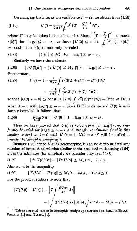
§ 1. One-parameter semigroups and groups of operators 491
On changing the integration variable to C' = Ct, we obtain from (1.50)
(1.54) U (t) = 2,c i t ,f ec ( T+ t)-I dC',rwhere r, may be taken independent of t. Since II(T+ t)-I s const.
It/C'I for largtl s co - e, we have IIU(t)II s const. f ICSI-I IdC'l
= const. Thus U (t) is uniformly bounded : r(1.55) IIU(t)II s M' for largtl s co - e .
Similarly we have the estimate
(1.56) IIdU(t)/dtil =IITU(t)II S M' Itl-I, largtl s w - e.Furthermore,
(1.57) U(t) - 1 = zn i ,f e; ((tT + )-I - c'-I) dC'r= 2 i f V
T (t T d C,,
so that II U (t) u - uII S const. Itl II T ull f let I ICI I-2 IdC' I -> O for u E D (T)r,
when Itl -+ 0 with largtl S co - s. Since D (T) is dense and U(t) is uni-formly bounded, it follows that
(1.58) s-limU(t) = U(0) = 1 (largtl s co - s) .
Thus we have proved that U(t) is holomorphic for largtl < co, uni-formly bounded for largtl 5 co - e and strongly continuous (within thissmaller sector) at t = 0 with U (0) = 1. U (t) = e- tT will be called abounded holomorphic semigroup'.
Remark 1.20. Since U (t) is holomorphic, it can be differentiated anynumber of times. A calculation similar to the one used in deducing (1.56)gives the estimates (for simplicity we consider only real t > 0)
(1.59) II do U(t)ldt"II = II TO U(t)II S M,, t-' , t> 0.Also we note the inequality
(1.60) II T(U(t) - U(s))II 5 M2(t - s)/t s , 0 < s s t .For the proof, it suffices to note that
II T (U(t) - U(s))II =7f rd r drdr
t t= II f T2 U(r) drII s M2 f r-2 dr = M,(t - s)/st.
S s
I This is a special case of holomorphic semigroups discussed in detail in HILLE-PHILLIPS (1) and YOSIDA Q11.
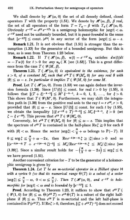
492 IX. Perturbation theory for semigroups of operators
We shall denote by .*' (co, 0) the set of all densely defined, closedoperators T with the property (1.51). We denote by .*'(w, 9), P real,the set of all operators of the form T = T° - P with T° E .*'(co, 0).Obviously e-4T = est e-IT, is a semigroup holomorphic for jargtj < Co.e-tT need not be uniformly bounded, but it is quasi-bounded in the sensethat Ile-tTll S const. left) in any sector of the form Jargtj < co - e.
Remark 1.21. It is not obvious that (1.51) is stronger than the as-sumption (1.33) for the generator of a bounded semigroup. But this istrue, as is seen from Theorem 1.23 below.
Remark 1.22. If T E .*'(w, A), u(t) = e-tT u° satisfies du(t)/dt_ - T u (t) for t > 0 for any u° E X [see (1.53)]. This is a great differ-ence from the case T E 9 (M, fi).
Theorem 1.23. T E J r (co, 0) is equivalent to the existence, for eache > 0, of a constant M' such that et ° T E 9 (Me, 0) for any real 0 with101 S co - s. In Particular it implies T E T (M, 0) for some M.
Proof. Let T E .*'(co, 0). From (1.53) we can again deduce the inver-sion formula (1.38). Since 11U(t)11 s const. for real t> 0 by (1.55), itfollows that JI(T + l:)-k-1lj s M' $-71-1, It = 0, 1, 2, ..., for 1: > 0.This shows that T E 9 (M', 0). Furthermore, we may shift the integra-tion path in (1.38) from the positive real axis to the ray t = r ei0, r > 0,provided that 101 s co - e. Since I U (t) 11 < const. for such t by (1.55),we obtain the inequality l (l a-d0 + T)-k-111 S M;> 0 (set
_ e- d°). This proves that ed0 T E 9 (Me, 0).Conversely, let 00 T E 9 (Me, 0) for 101 s co - e. This implies that
the spectrum of 08T is contained in the half-plane ReC Z 0 for each 0
with 101 < co. Hence the sector IargCI < z + co belongs to P(- T). If
0 5 argC 5 n+ co -2e, then Ree-d(w-e) t; z JCJ sine > 0 and soe-d(°'-e) T e-d(°'-e) C)-111 s MB Ree-'(-1) s M;IICI sine [see
(1.39)]. Since a similar result holds for - (2 + co - 2e) s argC S 0,we have proved (1.51).
Another convenient criterion for - T to be the generator of a holomor-phic semigroup is given by
Theorem 1,24. Let T be an m-sectorial operator in a Hilbert space Hwith a vertex 0 (so that its numerical range 0(T) is a subset of a sector
jargCj 2 - co, 0 < co s 2 ). Then T E.* (w, 0), and e-tT is holo-morphic for jargtl < co and is bounded by jje-tTjj S 1.
Proof. According to Theorem 1.23, it suffices to show that e{° T EE 9 (1, 0) for 101 s co. 0 (ed8 T) = eiB 0 (T) is a subset of the right half-plane if 101 s co. Thus edB T is m-sectorial and the left half-plane iscontained in P (et0 T). If ReC > 0, therefore, 11(C+ ed° T)-1lI does not exceed
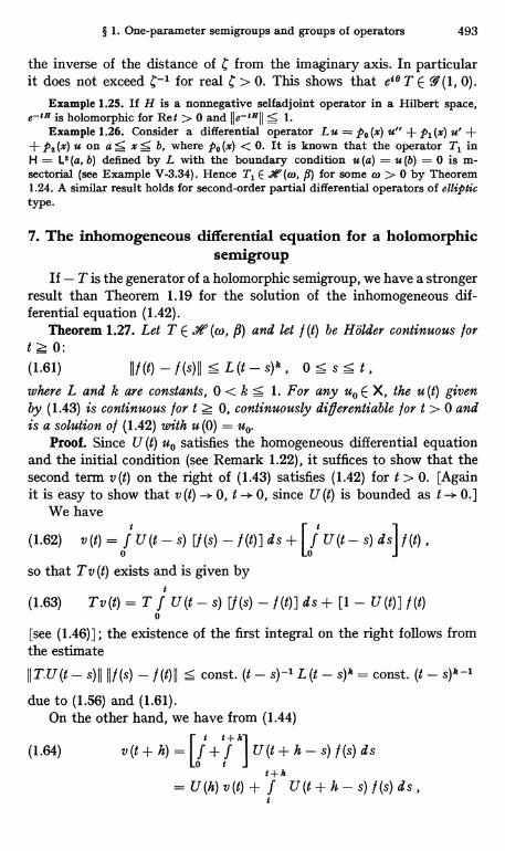
§ 1. One-parameter semigroups and groups of operators 493
the inverse of the distance of C from the imaginary axis. In particularit does not exceed l;-1 for real C > 0. This shows that et0T E 9(1, 0).
Example 1.25. If H is a nonnegative selfadjoint operator in a Hilbert space,e-'$ is holomorphic for Ret > 0 and Ile-'9 S 1.
Example 1.26. Consider a differential operator L u = po (x) u" + pl (x) u' ++ p2 (x) u on a S x s b, where p0 (x) < 0. It is known that the operator T1 inH = L2 (a, b) defined by L with the boundary condition u (a) = u (b) = 0 is m-sectorial (see Example V-3.34). Hence T1 E X (0), P) for some uw > 0 by Theorem1.24. A similar result holds for second-order partial differential operators of elliptictype.
7. The inhomogeneous differential equation for a holomorphicsemigroup
If - T is the generator of a holomorphic semigroup, we have a strongerresult than Theorem 1.19 for the solution of the inhomogeneous dif-ferential equation (1.42).
Theorem 1.27. Let T E .*' (co, f) and let f (t) be Holder continuous fortz0:(1.61) II/(t) - f(s)II 5 L(t-s)k, 0 s s 5 t,where L and k are constants, 0 < k s 1. For any u0 E X, the u (t) givenby (1.43) is continuous for t Z 0, continuously dillerentiable for t > 0 andis a solution o l (1.42) with u (0) = u0.
Proof. Since U (t) uo satisfies the homogeneous differential equationand the initial condition (see Remark 1.22), it suffices to show that thesecond term v (t) on the right of (1.43) satisfies (1.42) for t > 0. [Againit is easy to show that v (t) -). 0, t -)- 0, since U (t) is bounded as t - 0. ]
We have
(1.62) v (t) = f U (t - s) [f (s) - 1(t)] d s + [ f U (t - s) ds] f (t) ,
so that T v (t) exists and is given by
(1.63) Tv(t) = T f U(t - s) [f (s) - 1(t)] ds + [1 - U(t)] 1(t)0
[see (1.46)]; the existence of the first integral on the right follows fromthe estimate
II T. U (t - s) II 11t (s) - f (t) II 5 const. (t - s)-1 L (t - s) k = const. (t - s) J1 -1
due to (1.56) and (1.61).On the other hand, we have from (1.44)
(1.64) V (t + h) = [f +t f kIU (t + h - s) 1(s) ds
o tt+h
= U (h) v (t) + f U (t + h - s) 1(s) d s ,t
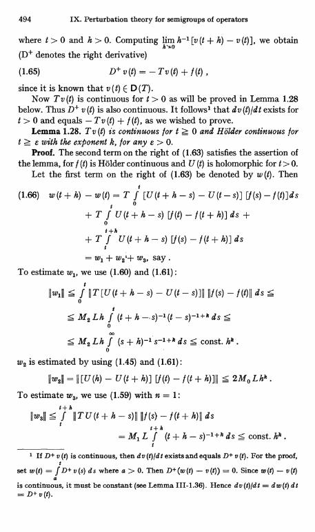
494 IX. Perturbation theory for semigroups of operators
where t > 0 and h > 0. Computing lim h-1 [v (t + h) - v (t)], we obtainh1+0
(D+ denotes the right derivative)
(1.65) D+v(t) = - Tv(t) + f(t)
since it is known that v (t) E D (T).Now T v (t) is continuous for t > 0 as will be proved in Lemma 1.28
below. Thus D+ v (t) is also continuous. It follows' that dv (t)/dt exists fort > 0 and equals - T v (t) + f (t), as we wished to prove.
Lemma 1.28. T v (t) is continuous for t Z 0 and Holder continuous fort ? e with the exponent k, for any e > 0.
Proof. The second term on the right of (1.63) satisfies the assertion ofthe lemma, for f (t) is Holder continuous and U (t) is holomorphic for t > 0.
Let the first term on the right of (1.63) be denoted by w (t). Then
(1.66) w (t + h) - w (t) = T f [U(t+h-s)-U(t-s)][f(s)-f(t)]dst 0
+ T f U (t +0 h - s) Y (t)(t) - 1(t + h) ] d s +0t+h
+ T f U(t+h-s) [f(s)- f(t+h)]dst
= wl + w2,+ w3, say.
To estimate w1, we use (1.60) and (1.61) :t
IIw,II s f IIT[U(t+h-s)- U(t-s)]II Ill(s)- f(t)II dss0
ts M2 Lh f (t + h s)-' (t - s)-l+k ds S
000
S M2 Lh f (s + h) -1 s-1+11 ds S const. hk .0
w2 is estimated by using (1.45) and (1.61) :
IIW2ll = II [U(h) - U(t + h)] [f (t) - 1(t + h)]II s 2M0 Lhk .
To estimate w3, we use (1.59) with n = 1:t+h
IIw3I1 s f IITU(t+h-s)IIIIt(s)-/(t+h)II dst t+h
=M,L f (t+h-s)-'+kds s const.hk.t
1 If D+ v (t) is continuous, then dv (t)ldt exists and equals D+ v (t). For the proof,t
set w (t) = f D+ v (s) d s where a > 0. Then D+ (w (t) - v (t)) = 0. Since w(t) - v (t)a
is continuous, it must be constant (see Lemma 111-1.36). Hence dv (t)/dt = dw(t) dt= D+ v (t).
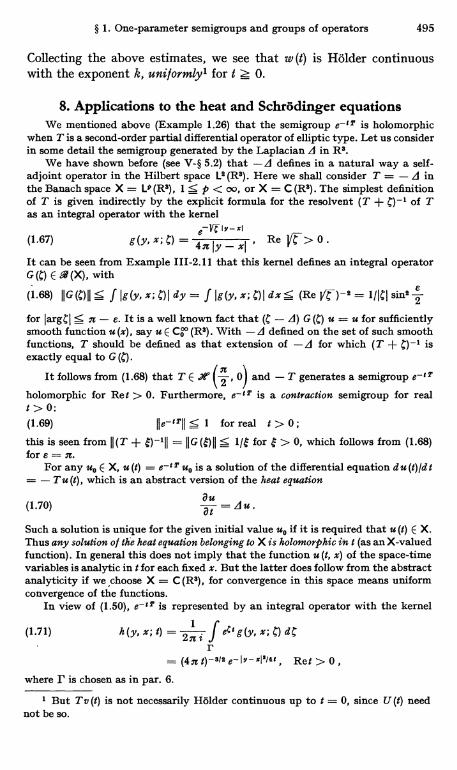
§ 1. One-parameter semigroups and groups of operators 495
Collecting the above estimates, we see that w (t) is Holder continuouswith the exponent k, uni f ormly1 for t z 0.
8. Applications to the heat and Schrodinger equationsWe mentioned above (Example 1.26) that the semigroup e-12' is holomorphic
when T is a second-order partial differential operator of elliptic type. Let us considerin some detail the semigroup generated by the Laplacian A in R3.
We have shown before (see V-§ 5.2) that -d defines in a natural way a self-adjoint operator in the Hilbert space L2 (R8). Here we shall consider T = - A inthe Banach space X = L9 (R3), 1 S p < oo, or X = C (R8). The simplest definitionof T is given indirectly by the explicit formula for the resolvent (T + c)-1 of Tas an integral operator with the kernel
e Iv-xl _(1.67) 4nly_xI ,
It can be seen from Example 111-2.11 that this kernel defines an integral operatorG (C) E -4 (X), with
(1.68) IIG(C)II S f Ig(Y, x; C)I dY = f Ig(Y, x; C)I dx< (Re j)-2 = 1/ICI sine2
for IargCI 5 n - e. It is a well known fact that (C - d) G (C) u = u for sufficientlysmooth function u (x), say u E Co (R3). With - d defined on the set of such smoothfunctions, T should be defined as that extension of -d for which (T + isexactly equal to G (c).
It follows from (1.68) that T E ,aG° 12 , 01 and - T generates a semigroup e-'T
holomorphic for Ret > 0. Furthermore, a-'-' is a contraction semigroup for realt > 0:(1.69) IIe-891 < I for real t > 0;this is seen from II(T + )-'II = JIG(e)II S leg for > 0, which follows from (1.68)fore=x.
For any uo E X, u (t) = e-'T uo is a solution of the differential equation d u (t) Id tT u (t), which is an abstract version of the heat equation
(1.70) at =du.Such a solution is unique for the given initial value uo if it is required that u (t) E X.Thus any solution of the heat equation belonging to X is holomorphic in t (as an X-valuedfunction). In general this does not imply that the function u (t, x) of the space-timevariables is analytic in t for each fixed x. But the latter does follow from the abstractanalyticity if we choose X = C (R8), for convergence in this space means uniformconvergence of the functions.
In view of (1.50), e-'T is represented by an integral operator with the kernel
(1.71) h(y, x; t) = 2ni ,f et`g(Y, x; C) dt'r
_ (4n t)-812 a-I r-xl'la' Ret > 0 ,where r is chosen as in par. 6.
1 But T v (t) is not necessarily Holder continuous up to t = 0, since U (t) neednot be so.
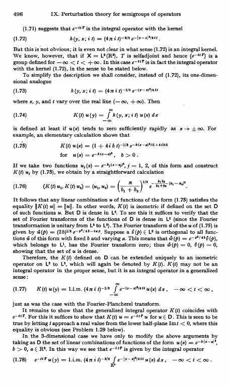
496 IX. Perturbation theory for semigroups of operators
(1.71) suggests that e- rtT is the integral operator with the kernel
(1.72) h(y, x; i t) _ (4a i t)-312 e-ly-x('l41t
But this is not obvious; it is even not clear in what sense (1.72) is an integral kernel.We know, however, that if X = L3(R3), T is selfadjoint and hence {e-4t T} is agroup defined for - oo < t < + oo. In this case a-rtT is in fact the integral operatorwith the kernel (1.72), in the sense to be stated below.
To simplify the description we shall consider, instead of (1.72), its one-dimen-sional analogue
(1.73) h (y, x; i t) _ (4n i t)-1/3 e-(y-x)'/art
where x, y, and t vary over the real line (- oo, + oo). Then
(1.74) K(t) u(y) = f k(y, x; i t) u(x) dx
is defined at least if u (x) tends to zero sufficiently rapidly as x -+ f oo. Forexample, an elementary calculation shows that
(1.75) K(t) u(x) _ (1 + 4i b t)-1/3 e-b(x-°)'/a+4rbt>
for u(x) = e b(x-°)', b > 0.
If we take two functions ut (x) = e-b9(z-°t)', j = 1, 2, of this form and constructK(t) of by (1.75), we obtain by a straightforward calculation
1/3 - bb b(1.76) (K (t) u1, K (t) u2) _ (u1, us) _ I e iosb1 + b$
It follows that any linear combination u of functions of the form (1.75) satisfies theequality JJK(t) ull = 1lull. In other words, K(t) is isometric if defined on the set Dof such functions u. But D is dense in L3. To see this it suffices to verify that theset of Fourier transforms of the functions of D is dense in L2 (since the Fouriertransformation is unitary from L2 to L3). The Fourier transform 4 of the u of (1.75) isgiven by 4(p) = (2b)'/3 e-p'/4b-r°p. Suppose a v(() E L$ is orthogonal to all func-tions 4 of this form with fixed b and varying a. This means that W' (P) = e-P'/4bv" (p),which belongs to L', has the Fourier transform zero; thus zew (p) = 0, v" (p) = 0,showing that the set of u is dense.
Therefore, the K (t) defined on D can be extended uniquely to an isometricoperator on L2 to La, which will again be denoted by K (t). K (t) may not be anintegral operator in the proper sense, but it is an integral operator in a generalizedsense:
w(1.77) K(t) u(y) = 1.i.m. (4x it)-113 f e-(Y-x)'14 itu(x) dx, -oo <t < co,
_00
just as was the case with the Fourier-Plancherel transform.It remains to show that the generalized integral operator K (t) coincides with
e-ttT. For this it suffices to show that K(t) u = e-rtT u for u E D. This is seen to betrue by letting t approach a real value from the lower half-plane Imt < 0, where thisequality is obvious (see Problem 1.29 below).
In the 3-dimensional case we have only to modify the above arguments bytaking as D the set of linear combinations of functions of the form u (x) = e-b ix-ol',b > 0, a E R8. In this way we see that a-t tT is given by the integral operator
(1.78) e-"2'u (y) = l.i.m. (4n i t)-313 f e-ly-xl'/" u(z) dx, - oo < t < oo .R'
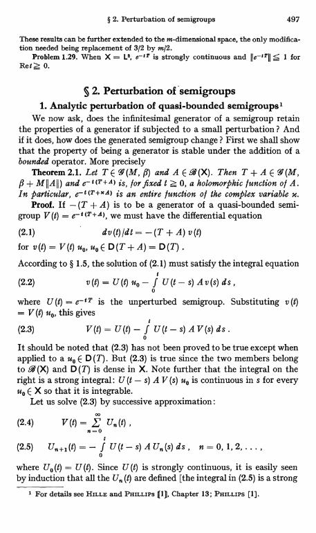
§ 2. Perturbation of semigroups 497
These results can be further extended to the m-dimensional space, the only modifica-tion needed being replacement of 3/2 by m/2.
Problem 1.29. When X = L2, e-'T is strongly continuous and ile-`TII < 1 forRe t Z 0.
§ 2. Perturbation of semigroups1. Analytic perturbation of quasi-bounded semigroups I
We now ask, does the infinitesimal generator of a semigroup retainthe properties of a generator if subjected to a small perturbation ? Andif it does, how does the generated semigroup change? First we shall showthat the property of being a generator is stable under the addition of abounded operator. More precisely
Theorem 2.1. Let T E 9 (M, fl) and A E a (X). Then T + A E 9r (M,+ MIIAII) and e-d(T+A) is, for fixed t > 0, a holomorphic function of A.
In particular, a-d (T+XA) is an entire function o l the complex variable x.Proof. If - (T + A) is to be a generator of a quasi-bounded semi-
group V (t) = e-t (T+ A), we must have the differential equation
(2.1) dv (t) /d t = - (T + A) v (t)
for v (t) = V (t) u0, u0 E D (T + A) = D (T) ,
According to § 1.5, the solution of (2.1) must satisfy the integral equation
(2.2) v (t) = U (t) u0 - f U (t - s) A v (s) d s ,0
where U (t) = e- 17' is the unperturbed semigroup. Substituting v (t)= V (t) u0, this gives
d
(2.3) V (t) = U (t) - f U (t - s) A V (s) d s .0
It should be noted that (2.3) has not been proved to be true except whenapplied to a u0E D (T). But (2.3) is true since the two members belongto 9 (X) and D (T) is dense in X. Note further that the integral on theright is a strong integral : U (t - s) A V (s) u0 is continuous in s for everyu0 E X so that it is integrable.
Let us solve (2.3) by successive approximation :00
(2.4) V (t) U. (t)n=0
(2.5) UU+I(t)=- f n=0,1,2,...,0
where UO (t) = U (t). Since U (t) is strongly continuous, it is easily seenby induction that all the U (t) are defined [the integral in (2.5) is a strong
1 For details see HILLE and PHILLIPS (1), Chapter 13; PHILLIPS [1].
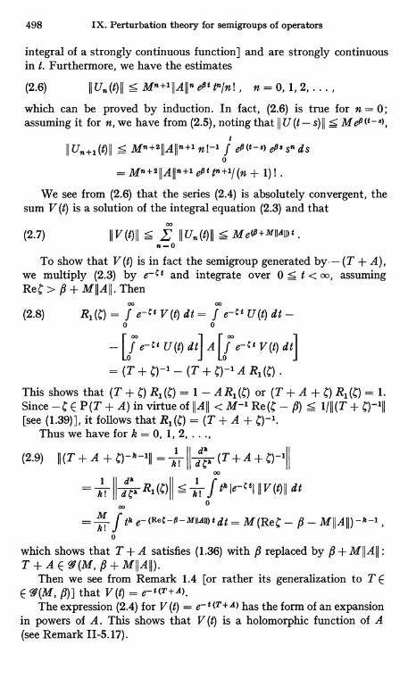
498 IX. Perturbation theory for semigroups of operators
integral of a strongly continuous function] and are strongly continuousin t. Furthermore, we have the estimates
(2.6) II Un (t) II s Mn+l II All n ePt to/n ! , n=0, 1,2, ... ,which can be proved by induction. In fact, (2.6) is true for n = 0;assuming it for n, we have from (2.5), noting that II U (t - s) II s MOO-),
t
II U-+1(t)II s Mn}2IIAIIn+1 n!-' f 00-8) eft8 sn ds0
= Mn+2IIAIIn+l est to+l/(n + 1) ! .
We see from (2.6) that the series (2.4) is absolutely convergent, thesum V (t) is a solution of the integral equation (2.3) and that
00
(2.7) IIV(t)II s E IIUn(t)II s Me(a+MIIAII)t.
n=0
To show that V (t) is in fact the semigroup generated (T + A),we multiply (2.3) by e-Ct and integrate over 0 5 t < oo, assumingRel;>
(2.8) R1(C) = f e-11 V (t) dt = f U(t) dt -0 0
-[7e_t U(t) dt] ALf e-;tV(t)dt]0
_ (T + a)-1 - (T + C)-1 A R1 (C)
This shows that (T + l;) R1 (l;) = 1 - A R1 (l;) or (T + A + l;) R1 (g) = 1.Since -l; E P(T + A) in virtue of IIAII < M-1 Re (C - fl) S 1/11 (T + C)-111[see (1.39)], it follows that R1(C) _ (T + A + c)-1.
Thus we have for k = 0, 1, 2, ...,
(2.9)II (T +A + C)-71-1II = k,
1
ck R1M00
(T + A + c)-1
s k) f tkle-ttl IIV(t)II dt0
M dt = M(ReC - - MIIAII) -11-1,klrtk e-(Re;-p-MIIAII)t
which shows that T + A satisfies (1.36) with 9 replaced by 9 + M II A II :
T + A E 9(M, P + MIIAII)Then we see from Remark 1.4 [or rather its generalization to T E
E `.Pi(M, 9)] that V(t) = e-t(T+A).The expression (2.4) for V (t) = e-t (T+A) has the form of an expansion
in powers of A. This shows that V (t) is a holomorphic function of A(see Remark 11-5.17).
§ 2. Perturbation of semigroups 499
Remark 2.2. The above proof is indirect in so far as it concerns theproperty of - (T + A) being a generator. It is possible to verify directlythe final inequalities of (2.9). This proof is in general not very simple; it isnecessary to make some combinatorial computations'. But the proof istrivial if M = 1. In this case we need only to verify (2.9) for k = 1, butthis is obvious from the second Neumann series for the resolvent
00
(T + A + c)-1= E (T + 4)-1 [-A (T + 4)_1]n and II (T + C)-11I s=
(Red' - fl)-I.n 0
Problem 2.3. Prove by successive approximation that v (t) = U. (t) uo satisfiesthe differential equation d t = - T v. - A v _1 (set v_1 = 0) and v = E vsatisfies dv/dt = -(T + A) v, provided that uo E D(T). [hint: Theorem 1.19.]
2. Analytic perturbation of holomorphic semigroupsIn the preceding paragraph we considered a bounded perturbation of
the generator - T of a quasi-bounded semigroup. In general it is dif-ficult to add an unbounded operator A to T without destroying theproperty of - T being a generator. For example, - (T + A) need not be agenerator of a quasi-bounded semigroup even if A is relatively boundedwith respect to T.
If - T is assumed to be the generator of a holomorphic semigroup,however, perturbations of a wider class are permitted.
Theorem 2.4.2 For any T E and s > 0, there exist Positiveconstants y, S with the following properties. I/ A is relatively bounded withrespect to T so that
(2.10) IIAull s alluII+bilTull , uED(T)CD(A),with a < 6, b < 6, then T + A E .*'(co - e, y). 1/, in Particular, fi = 0 anda=0, then T+AE. ((O - e,0).
Proof. As is easily seen, we may assume = 0 without loss of genera-lity 2. (2.10) implies that
(2.11) IIA(T+C)-III s all(T+C)-III+bilT(T+
If Iargt;I 5 2 + co - e, we have II(T + C)-III < MEflCI by (1.51) andIIT(T+C)-III=II1-C(T+C)-III s 1+M..Hence
(2.12) IIA (T + C)-III saM.ICI-I + b(1 +
1 See HILLS and PHILLIPS [11, p. 389.2 See HILLS and PHILLIPS [11, p. 418.S If #<O, T E -Y(w, fl) C JY(w, 0). If #>O, set To= T+ fl; then To E
E .7r (w, 0) and IIA ull S (a + b P) IIull + bui To uII If yo, do denote the y, d of thetheorem for fi = 0, then To + A E .7£° (w - s, Yo) for a + b fi < do, b < do. HenceT + A E -W (w - e, yo + f4) if a < do/2, b < min (do, do/2 fl), so that it suffices totake y = Yo + Ii. d = min (do/2, do/2 fl).
500 IX. Perturbation theory for semigroups of operators
and the second Neumann series for (T + t + A) -I converges if the rightmember of (2.12) is smaller than 1, with
(2.13)M-ICI-1' A -IT
Me[1 - b(1 + Me)]-1
+ + )II( II - 1 -aM.I-I-1-b(1 +M8) -aM8[1 -b(1 +M.)]-1
If b < (1 + M,)-', (2.13) shows that II (T + A + C)-III s M'fi4 - yIfor Iarg (C - y) 15 2 + co - e, where M' and y are some positiveconstants depending on a, b and M,. If a = 0, we can take y = 0.
Corollary 2.5. 1/ - T is the generator of a quasi-bounded holomorphicsemigroup and A is T-bounded with relative bound 0, then - (T + A) isalso the generator of a quasi-bounded holomorphic semigroup.
Proof. It suffices to observe that b can be chosen arbitrarily small inthe proof of Theorem 2.4.
Theorem 2.6. Let T (x) E ' (X) be a holomorphic family of type (A)defined near x = 0. 1/ T (0) is the generator of a quasi-bounded holomorphicsemigroup, the same is true for T (x) with sufficiently small In 1. In this caseU (t, x) = e-IT (x) is holomorphic in x and t when t is in some open sectorcontaining t > 0. Moreover, all a" U (t, x) lam" are strongly continuous in tup to t = 01. 11, in particular, T (x) = T + x A where T and A satisfy theconditions of Corollary 2.5, then e- t (T +uA) is an entire function of x fortin such a sector.
Proof. Since T (x) - T (0) is relatively bounded with respect to T (0)(see VII-§ 2.1), T (x) belongs to some .° (co, fi) for sufficiently small IxI.Replacing T (m) ,by T (x) + fi if necessary, we may assume T (x) E .%°(w, 0).
It follows from (1.50) for U (t,lx) that
(2.14) 2x^ U(t' x) = 2n i f ect ' (T (x) + C)-I dC.r
But we have
(2.15) 2x (T (x) + C)-I = 2ni f (T (x') + a)-I (x' - x)-"-1 du' ,c
where C is a small circle in the x-plane and x is inside C. Since (1.51) istrue for T = T (x) uniformly in x near x = 0, we have
(2.16)II a (T (x) + )-III 5
M, NA n!, IargCI S 2 + w - e,
ICI
I As is seen from the proof, the conclusions of this theorem are true for anyholomorphic family T (m) provided that T W E Jr (w, f4) for small IxI. The "type(A)" assumption is used to show that T (O) E Jr (wo, flo) implies TM E Jr (w, M.It is easy to show that "type (A)" can be replaced by "type (B)" (see VII-§ 4);in this case t(x) - t(0) is relatively bounded with respect to t(0) [t(x) denotingthe form associated with T (x) ], so that T (x) E r (co, fl) is true with some constantsw, fi for all x in any compact subset of the domain in which x varies.
§ 2. Perturbation of semigroups 501
with some constant N if Ixl is sufficiently small. Thus the same argumentas given in § 1.6 shows that an U (t, x)/a x" is holomorphic in t in someopen sector and strongly continuous up to t = 0. In particular, thisimplies that U (t, x) is holomorphic in x with its Taylor coefficientsholomorphic in t.
The last statement of the theorem is true since T (m) satisfies theabove condition for all x in virtue of Corollary 2.5.
These results show that holomorphic semigroups are rather stableunder perturbation.
3. Perturbation of contraction semigroupsWe have remarked in the preceding paragraph that when - T is the
generator of a bounded semigroup, - (T + A) need not be such agenerator even when A is relatively bounded with respect to T. Anexception to this statement occurs when both - T and - A are generatorsof contraction semigroups. We have namely
Theorem 2.7.' Let T and A belong to T (1, 0) and let A be relativelybounded with respect to T with T-bound < 1/2. Then T + A E T (1, 0) too.
Proof. P(T) covers the half-plane Red' < 0 and 11 (T + )-III S -Ifor > 0. A satisfies an inequality of the form (2.10), with b < 1/2, so that
s 5 ifis sufficiently large. It follows from the second Neumann series that theresolvent (T + A + )-I exists for such .
Let us estimate (T + A + $)-I. To this end we consider the vectorv(t) = e-ta e-t(T+E) u where u E D(T) C D(A). We have
(2.17) u - v(t) = (u - e-to u) + e- to (u - e-t(T+f) u) .
Since a-ta u and e-t(T+f) u are differentiable in t, we have
(2.18) limt-,(ut`-A 0
by (1.24). On the other hand, we have Il v (t) II 5 e- t1 jI uII since e- t & ande-tT are contraction semigroups. Hence
(2.19) t-Illu - v(t)II z t-I (IIuII - e-tf lull) -* $IIull , t -+ 0 .
It follows from (2.18) and (2.19) that
(2.20)
II (T + A + $)-III < -I, at least for $ sufficientlylarge that (T + A + i)-' exists. Then one sees by means of the first
I This theorem and Theorem 2.11 are essentially contained in TROTTER [2],in which the semigroup e-t(T+&) is constructed as the limit of (e-UUt">T e-""n)e)' asn -+ oo. An interesting application of this method is given by NELSON [1]. Cf. alsoBABBITT [1].
502 IX. Perturbation theory for semigroups of operators
Neumann series that (T + A + a)-1 exists with the same inequalityfor every > 0. This shows that T + A E 9(1, 0), as we wished to show.
Problem 2.8. If T E 9 (1, fl), A E T (1, fi') and A is T-bounded with T-bound<1/2, then T+AE9(1,fi+fi').
Problem 2.9. The bound 1/2 for the T-bound of A in Theorem 2.7 and Problem2.8 can be replaced by 1, if X is a Hilbert space.
Remark 2.10. Theorem 2.7 does not imply that e- t (T+. 4A) is holo-morphic in x. In fact x < 0 is in general not permissible if xA is to belongto 9 (1, fl). But it can be shown that e- t (T+xA) is strongly continuous in ;efor x z 0. More generally, e- t e-7' if A,, tends to zero in the
s
sense that A,, is T-bounded and II A,,u II S a,,II u II + b,,I) T u lI with an, b -*0.This is a consequence of Theorem 2.16 proved below.
The T-boundedness of A in Theorem 2.7 is used essentially onlyin showing that - E P (T + A) for sufficiently large . The proof of(2.20) is valid without any such assumption if u E D (T+ A) = D (T) n D (A).If the range of T + A + is dense in X and if T + A is closable, itfollows that - E P (S) with 11 (S + )-1I1 S -1, where S is the closureof T + A. If S is densely defined, it follows as above that S E 9r (1, 0).Thus we have the following theorem, which is symmetric with respectto T and A.
Theorem 2.11. Let T and A belong to 9 (1, 0), let D (T) n D (A) bedense in X and let T + A + have a dense range for sufficiently large real $.If T + A is closable, its closure S belongs to 9(1, 0).
4. Convergence of quasi-bounded semigroups in a restrictedsense
Let us return to the generators of quasi-bounded semigroups ingeneral. When - T is such a generator, it is in general difficult to provethe same for - S = - (T + A) for an unbounded perturbation A. If weassume that -S is also a generator, however, we can show that a-ts -- e-tT is small relative to T provided A is small relative to T, evenif A is unbounded. More precisely, we have
Theorem 2.12. Let T, S E (M, A), f z 0, and let S = T + A where Ais T-bounded so that (2.10) is true. Then we have for > 8
(2.21) II(e- ts - e-tT) (T + )-11I s
sM2 tes4 [b(M+1)+(a+bP)M(
Proof. Let u E D (T) = D (S). Then we have, as in (2.2),t
(2.22) (e-ts-e-tT)u=- f e-(t-8)s Ae-8Tuds;0
§ 2. Perturbation of semigroups 503
here Ae-8T u = A (T + $) -1 e-8T (T + ) u is continuous in s becauseA (T + a)-1 is bounded. Since (T + a)-1 v E D (T) for any v E X, (2.22)applied to u = (T + )-1 v gives
t(2.23) (e-IS - e- IT) (T + )-1 = - f e-(t-8)s A (T + )-1 a-8T ds .
0
Since IIe-(t-0811 < MOO-8), IIe-8TII < Me'B, and
(2.24) IIA(T+ )-III < all (T+ )-III + bjIT(T+ )-III < fl)-1
(2.21) follows from (2.23).Remark 2.13. Theorem 2.12 shows that (e-18 - e-tT) u tends to zero
when a, b -+ 0, not uniformly for IIulI 1 but uniformly for all u E D (T)with II (T + ) ull < 1.
In this direction we can go further and obtain a certain kin(t ofestimate for e-t8 - e- IT without assuming anything on S - T.
Theorem 2.14. Let T, S E 07 (M, fl). Then
(2.25) II(S + C)-1 (e-ts - e- IT) (T + S)-III < M2 t efttlI(S + b)-I --(T+C)-III, Red'>
Proof. e-tT (T + l;)-1 is strongly differentiable in t: (d/d t) e-tT (T ++ C)-I u = -e-tT T (T + C)-I u = _ e-tT [1 - C (T + C)-I], and simi-larly for e- t s (S + C) -1. Hence
(2.26)ds
e-(t-8)s(S +C)-I e-8T (T + C)-I = e-0-8)s8)s a-8T (Tpp+ C)-I -- e- (t-8) S (S + C)-I a-BT = e- (t-8) S [(T + C)-1 - (S + b)-il a-8T.
Integrating with respect to s on (0, t), we obtain J
(2.27) (S + C)-1(e-tT - e-ts) (7' + C)-It
= f e-(1-8) s [(T + C)-I - (S + C)-'] a-8T ds0
from which (2.25) follows by IIe-0 -8)s9I 5 Me(t-8)0 and IIe-8TII s Me"8.
Example 2.15. Let T = iH where H is a selfadjoint operator in a Hilbert spaceH. If K is a symmetric operator relatively bounded with respect to H with H-bound< 1, H + K is selfadjoint (see Theorem V-4.3). The unitary operator e-Wa+a)tends.to a-"$ in the sense of Remark 2.13 when K tends to zero in the sense stated.
5. Strong convergence of quasi-bounded semigroupsIf we content ourselves with strong convergence of the semigroups
generated by a given sequence of generators, we can weaken the assump-tions on the perturbation considerably. The following theorem is funda-mental in the approximation theory of semigroups.
504 IX. Perturbation theory for semigroups of operators
Theorem 2.16. Let T and Tn, n = 1, 2, ..., belong to 9(M, f). If
(2.28) (Tn + (T +for some l; with Re l; > f, then
(2.29) a-tT a-tTS
uniformly in any finite interval of t > 01. Conversely, if (2.29) holds for all tsuch that 0 S t S b, b > 0, then (2.28) holds for every 4 with Re4 > j9.
Proof. We may assume = 0 without loss of generality. We startfrom the identity (2.27) in which S is replaced by T. Since IIe- (t-s) Tall 5s M, we have for any u E X
(2.30) II (Tn + YY S)-1 (e- IT- - e- tT) (T + S) -1 uiJ St
s M f II [(T. + C)-1- (T + ) -1] e- IT uJI ds .0
If (T,, + I,)-1--. (T + t;)-1, the integrand on the right of (2.30) tends asS
n -> cc to zero for each fixed s. Furthermore, the integrand is majorizedby 2M -1 MIIuiI, which is independent of n, where = Ret; > 0. There-fore, the right member of (2.30) tends to zero by the principle of boundedconvergence. Obviously the convergence is uniform in t in any finiteinterval.
On writing v = (T + C)-1 u, we have thus shown that
(2.31) (Tn + C)-1 (e-tT - e-tT) v -+ O , n-+ oo ,
uniformly in t. This is true for all v E D (T), since v varies over D (T) whenu varies over X. But the operator on the left of (2.31) is uniformlybounded with bound not exceeding 2M2 r-1. Hence (2.31) is true for allvEX.
On the other hand we have
(2.32) (Tn + C)-1 a-tT v - e-tTn(T + c)-1 v
= e-tT L(T. + p b)-1 v - (T + ppb)-1 v] -' 0,
since IIe-IT"II S M and (Tn + C)-1 v - (T + la)-1 v - 0. Similarly,
(2.33) . (Tn + C)-l a-tT v - e-tT(T + C)-l v
= [(T. + C)-1 _ (T + C)-1] a-tT v -* 0.
It follows from (2.31)-(2.33) that
(2.34) (e-tTn - e-tT) (T + C)-1 v -, 0.
Recall that (2.28) means that T.I
T in the generalized sense (see VIII-§ 1)
Sufficient conditions for (2.28) are extensively studied in VIII-§§ 1 and 3.
§ 2. Perturbation of semigroups 505
This means that (e-tT- - e- tT) w -* 0 for all w E D (T). It follows asabove that e-tTn - e-IT -. 0.
s
That this convergence is uniform in t follows from the uniformity ofconvergence in (2.31)-(2.33). For (2.31) this was remarked above. For(2.32) it is obvious. For (2.33) it follows from the continuity of 6- IT v in t,which implies that the set of e- 9T v for all t of a finite interval is compact,so that Lemma 111-3.7 is applicable.
Conversely, suppose that (2.29) is true for 0 S t < b. By e-mtT_ (e-tT)m etc., it follows that (2.29) is true for any t > 0. Then
00
f e-tt(e-tTn - e-II) dt--. 0, Red' > 0,0 s
by dominated convergence. In view of the inversion formula (1.28),this gives (2.28) for every 4 with ReZ > 0.
In Theorem 2.16 the limit - T of the generators - T is assumedto be a generator. The question naturally arises whether this is a conse-quence of the other assumptions. It turns out that the answer is yes ifone assumes a certain uniformity on the behavior of the resolvents ofthe T. We have namely
Theorem 2.17.1 Let T.E 9 (M, A n = 1, 2,..., and let s-lim (1 + aa *0
= 1 uniformly in n. Let s-lim (T + t;)-1 exist for some t; with Re C > B.
Then there is a T E 9 (M, j9) such that the results of Theorem 2.16 hold.Proof. Again we may assume P = 0. T E 9 (M, 0) implies that the
(T + C,)-1 are uniformly bounded inn for each fixed complex number Cwith ReC > 0. In other words, the right half-plane Red' > 0 belongs tothe region of boundedness Ab for the sequence of the resolvents of - T(see VII 1-§ 1.1). But it follows from the assumptions that at least one Cwith Red' > 0 belongs to the region of strong convergence A8. Since A,is relatively open and closed in Ab by Theorem VIII-1.2, A. must containthe half-plane Re t; > 0.
Thus s-lim (T + C) -1 = -R' (C) exists for all t; of this half-plane, andR' (C) is a pseudo-resolvent (see loc. cit.). We shall now show that R' (C)is the resolvent of a densely defined closed operator - T.
For any u E X wehave u =alim
0(1 + a T)-1 u = limes
Since this convergence is uniform in n by hypothesis, it follows that
(2.35) U=- lim R' u , u E X .
Now the R' (C) have a common null space N and a common range D(see loc. cit.). If u E N, we have R' u = 0 so that u = 0 by (2.35).
1 Cf. TROTTER [1].S s-lim (1 + a T.) -1 = 1 follows from T. E 9(M, fl); see (1.12). The uniformity
in n of this convergence is the essential assumption.
506 IX. Perturbation theory for semigroups of operators
Thus N = 0. Also (2.35) implies that D is dense in X, for any u E X is thelimit of - R'($) u E D. It follows (see loc. cit.) that R' (C) is the resolventof a densely defined operator - T: R' (C) = - (T + C)-1.
The inequalities 11 (Ti, + )-kll S go over for n --> oo to the sameinequalities for 11 (T + )-kll This shows that T E 9r (M, 0), completingthe proof.
6. Asymptotic perturbation of semigroupsWe have been able to develop a satisfactory analytic perturbation
theory for quasi-bounded semigroups only for bounded perturbations(see par. 1). In the more restricted class of holomorphic semigroups,it was possible to admit relatively bounded perturbations (see par. 2).In applications, however, we have often to deal with non-holomorphicsemigroups, the most important case being the unitary groups in aHilbert space. Therefore, it is desirable to develop the perturbationtheory for non-holomorphic semigroups further by admitting unboundedperturbations. Naturally, then, we have to content ourselves withobtaining weaker results than the analytic dependence of the semigroupon the parameter x. In this way we are led to consider asymptotic seriesin x which are valid for x -+ 0. A simple example of asymptotic behaviorof semigroups is obtained if we set A = x TM and let x -+ 0 in Theorem2.12 [assuming that T + x T (') E 9 (M, 9) for all x]. What we are goingto do in the sequel is to extend the result to higher orders of the para-meter 1 x.
For simplicity we shall consider a family of operators
(2.36) T (m) = T + x TM,
though we could as well consider a formal infinite series in M. We assumethat T E 9(M, j9) and Tel) is T-bounded:
(2.37) II TC') ull 5 a llull + b lI T ull , u E D (T) C D (TM) .
As remarked before, this does not guarantee that - T (x) is the generatorof a semigroup, though T (x) is a closed operator with domain D = D (T)for Ixl < 1/b by Theorem IV-1.1. Therefore we add the assumption thatT (x) E 9 (M, 0) for x E Do, where Do is a subset of the disk I,I < 1/b.Do may be an open set, a subset of the real axis or a subset of the positivereal axis. In what follows x is always assumed to belong to Do. Also weassume = 0, for this does not affect the generality [otherwise considerT (x) + 8 instead of T (x)].
Under these assumptions, - T (x) generates a semigroup U (t, x)= e- 17(11) for each x. We write U (t, 0) = U (t). The U (t, x) are uniformly
1 The following theorems were given by T. KATO [3] in the case in which theT(x) are selfadjoint.
§ 2. Perturbation of semigroups 507
bounded by(2.38) IIU(t, x)II S M, t z 0.
Theorem 2.18. U (t, x) - U (t), x --> 0, uniformly in t in any finiteS
interval.Proof. This is a direct consequence of Theorem 2.12.Theorem 2.19. Let u E D. Then
(2.39) U (t, x) u = U (t) u + x u(') (t) + o (x) , x -> 0 ,
with
(2.40) UMW f U(t - s) TM U(s) uds ,
0
where o (x) denotes a vector with norm o (x) uniformly in each finite intervalof t. The integrand on the right of (2.40) is continuous in s so that theintegral is well defined.
Proof. The second term on the right of (2.39) is formally identicalwith the v1 (t) = U1 (t) u of par. 1 if we set A = x TM and u0 = u. AlthoughTM is not bounded, the integrand of (2.40) is continuous in s because
(2.41) TM U(s) u = B (C) U(s) {T + l;) u ,
where [cf. (2.24)]
(2.42) B(C) = T 1)(T + C)-1 E '(X) , ReC > 0 ,
(2.43) II B (C) II 5 a M r-1 + b (l + M) , 1:' = Re.
Similarly TM U (s, x) u is continuous in s. To see this we write
(2.44) TM U (s, x) u = B (C, x) U (s, x) (T (x) + l;) u,
where
(2.45) B (C, x) = T (1) (T (x) + ))-1 E -4 (X)
because TM is T (x)-bounded too (see Problem IV-1.2). B x) is evenholomorphic in C and x, for we have from the second Neumann seriesfor (T (x) + C)-1 = (T + C + x TM) -1
(2.46)00
B(S, x) = Lr (-x)k-1 B(C)I.
Since u E D implies that U (t, x) u E D and d U (t, x) u/ d t=- T (x) U (t, x) u = - T U(t, x) u - x TM U (t, x) u, it follows from (1.43)that(2.47) U (t' x) u = U (t) u - x f U (t - s) TM U (s, x) u d s.
0
(2.39) follows from (2.47) if it is proved that the integral on the righttends as x -+ 0 to -un> (t) uniformly in t. For this it suffices to show

508 IX. Perturbation theory for semigroups of operators
that 11 TM U (t, x) u - TM U (t) u VV -+ 0 boundedly in t (principle ofbounded convergence). But this is obvious from (2.44) and (2.41) sinceB (C, x), U (t, x), (T (x) + C) u = (T + l4) u + x TM u are all uniformlybounded, B (C, x) u B and U (t, x) S U (t) by Theorem 2.18 (weneed only a fixed 0.
Theorem 2.20. Let u E D (T2). Then
(2.48) U (t, x) u = U (t) u + x u(l> (t) + x2 u(2) (t) + o (x2)
uniformly in each finite interval o l t, where u(') (t) is given by (2.40) and
(2.49) u(2) (t) f U(t - s) TAM u(') (s) ds .
0
TM 0) (t) exists and is continuous in t, so that the integrand in (2.49) iscontinuous in s.
Proof. First we show that TM U (t) u, which exists because U (t) u EE D, is continuously differentiable in t, with
T Ml> UM u=- TM U (t) Tu.(2.50)'-Wt-
fact, we have TM U (t) u = B (C) U (t) (T + t;) u by (2.41) and soIn(d/d t) TM U (t) u = - B (C) U (t) T (T + C) u = - B (C) U (t) (T + C) T u_ - TM U (t) T u because T (T + t;) u exists by hypothesis.
According to Theorem 1.19, it follows that the u(1) (t) given by (2.40)is continuously differentiable and Tun) (t) is continuous. Then TM u('> (t)= B (C) (T'+ C) u(') (t) is also continuous. This proves the last statementof the theorem.
In view of (2.47), (2.41) and (2.49), (2.48) will be proved if it isshown that
(2.51) f U(t-s)TM{x [U(s,x)u-U(s)u]-UM (s)}ds-+00
uniformly in each finite interval of t. Since 11 U (t - s) 11 5 M and TMis T-bounded, (2.51) is true if
(2.52) (T + t;) { [U(t, x) u - U(t) u] - un> (t)}.+ 0
boundedly for a fixed But we have
(2.53) (T + C) [U (t, x) u - U(t) u]
(1 + x B(C))-1 U (t, x) (T + C + x TM) u - U (t) (T + C) u=-xB(4)(1+xB(C))-1U(t,x)(T+C +xTMM>)u+
+ [U(t, x) - U(t)] (T + C) u + x U(t, x) TM u.
§ 3. Approximation by discrete semigroups 509
Hence
(2.54) (T + C) [U (t, x) u - U (t) u] -+
--B(C) U (t) (T + C) u + v(1) (t) + U (1) Ti') u ,
where v(') (t) is the coefficient of x in the asymptotic expansion ofU(t, x) (T + C) u, which exists by Theorem 2.19 because (T + C) u EE D(T); in other words,
(2.55) V M (t) f U (t - s) TM U (s) (T + C) u d s .
0
Since B (l4) U (t) (T + l4) u = TM U (t) u, the right member of (2.54)is equal to
(2.56) - DO U (t) u + U (t) TM u - f U (t - s) T (l) U (s) (T + C) u d st 0
(T + C) f U(t - s) TO) U(s) u ds,0
where we have used (1.47) with 1(t) = TO-) U (t) u, noting (2.50). Thisproves (2.52) and completes the proof of Theorem 2.20.
Remark 2.21. The proof of Theorem 2.20 is somewhat complicatedsince the assumption u E D (T2) does not imply u E D (T (x)3). It is noteasy to go on in the same way to higher approximations of U (t, x) uwithout introducing severe restrictions on u. For example, it is notpossible to expand U (t, x) u up to the third order in x under the assump-tion u E D (T3) alone; it would be necessary to assume that T(l) u E D (T)in addition. We shall not pursue this problem any further.
Example 2.22. Let T = iH where H is a selfadjoint operator in a Hilbertspace H, and T11) = iK where K is symmetric and H-bounded. Then H + x K isselfadjoint for sufficiently small real x and T (x) = T + x VI) generates a unitarygroup, as does T. Thus the fundamental assumptions are satisfied if we take as Doa neighborhood of x = 0 on the real axis, and Theorems 2.18 to 2.20 are applicableto U (t, x) = e-MH+MA).
§ 3. Approximation by discrete semigroups1. Discrete semigroups
The perturbation theory of semigroups discussed in the precedingsection may be regarded as a theory of approximation of a semigroupU (t) by a family of semigroups, which may depend on a discrete para-meter n (Theorems 2.16, 2.17) or on a continuous parameter x (Theorems2.18-2.20). In this section we consider approximation of a semigroup U (t)by a sequence of discrete semigroups ; the result will have applications tothe approximation theory of differential equations by difference equations'.
1 The following presentation leans heavily on TROTTER [1].
510 IX. Perturbation theory for semigroups of operators
A discrete semigroup is simply a family {Uk}k = 0, 1, 2,... consistingof powers of an operator U E °.,A N; it has the semigroup propertyU' Uk = U1 +k. In approximation theory, however, it is necessary tocorrelate the exponent k with the "time" variable t. To this end weassociate a "time unit" r > 0 with each discrete semigroup {U71} andwrite Uk = U(k r), k = 0, 1, 2, ..., the function U(t) being thus definedonly for a discrete set of values t = k T. {U (k r)} will be called a discretesemigroup with time unit r. To distinguish them from discrete semigroups,the semigroups {U (t)} considered in preceding sections will be calledcontinuous semigroups.
A discrete semigroup {U (k r)} is said to be bounded if II U (k r) ( sM, k = 0, 1, 2, ..., with a constant M, where M z 1 since U(0) = 1.For a discrete semigroup {U (k r)} with time unit r, set
(3.1) T=r-1(1-U(r)).- T is called the generator of {U (k r)}. Thus
(3.2) U(k r) _ (1 - r T)k .
Since T Ed N, - T also generates a continuous semigroup {e-tT},which will be called the continuous semigroup associated with {U (k r)}.{e- I'} is an approximation to {U (k r)} in a certain sense, as is seen from
Lemma 3.1. I l {U (k r)} is bounded by II U (k r) II 5 M, the semigroup{e- tT} is also bounded by 11 e- t TII < M and
(3.3) I U (k z) u - e-kTlull 5 Mk r2 11 T2 ulI .
Proof. a-tT can be defined simply by the Taylor series. Since -tT_ - (t/r) + (t/r) U (r), we have
00(3.4) U (k r) e-41= e- t/r U (k r) 0' nil U (n T)n0
00= e-t/T E (n1 )a U((n + k) r) ,n=0
hence
(3.5) II U(k r) e-tTII S Me-tIT ltn!}n = M.n-0
In particular IIe-tIII 5 M.Since the U (k r) and T commute, we have
(3.6) U(kr)-e-krT=IlU((k-j-1)r)e-5TT](U(r)-e-TT).r o
§ 3. Approximation by discrete semigroups 511
But
U(r)-e-=T= 1-rT-e-=T=-f (r - s) e-8T T2ds0
so that
II U((k -j - 1) r) a-5rT(U (r) - e-tT) uII 5
f (r- s)MIIT2UIIds= 2 MIIT2UII
by (3.5). Thus (3.3) follows from (3.6).Remark 3.2. To avoid the inconvenience that a discrete semigroup
U (t) is defined only for t = k r, we set
(3.7) U (t) = U ([ 2, r)
for any t z 0, where [t/r] is the greatest integer not exceeding (Jr. Ofcourse {U(t)} is then not a continuous semigroup, but we have
(3.8) IIU(t) u - a-°T UII s 2 MrtIIT2UII +MrIITup .
In fact, let k r 5 t < (k + 1) r ; then U (t) = U (k r) and 116-IT u -
- e_ T uII 5 I f e-ST T u d sl 5 M rII T u II , so that (3.8) follows fromkr
2. Approximation of a continuous semigroup by discrete semi-groups
Consider a sequence {Uj of discrete semigroups with time units T.,n = 1, 2, . . ., where r,, -+ 0, n --> oo. {Uj is said to approximate a conti-nuous semigroup U = {U (t)} at t = to if
(3.9) Un (kn rn) -, U (to) , n -+ oo ,
for any sequence {k."} of nonnegative integers such that k.T,, -> to.{U."} is said to approximate U on an interval I of t if (3.9) is true for eachto E I.
Lemma 3.3. Il {Uj approximates U on an interval 0 s t < b, {UJapproximates U on the whole interval 0 5 t < oo. (In this case we simplysay that {Uj approximates U, and write U,, -+ U.)
Proof. Let to z 0 and k. r,, -+ to. Let m be an integer such thatto < m b, and let k,, = m q,, + r,,, 0 s r < m (qn, r,, are integers). Thenr,, r,, -+ 0 and q r,, -+ to/m < b. Hence U,, (r,, r,,) U (0) = 1 and
g
U. (qn r,,) - U (t0/m), so that U. (kn r,,) = U. (qn r.")"" U. (rn 'r.) s U (to/m) m
= U (to).
512 IX. Perturbation theory for semigroups of operators
Lemma 3.4. 1/ U -* U, the U,, are uniformly quasi-bounded in thesense that
(3.10) II U. (t) II 5 Me' t , t z 0 ,
where M and fi are independent o l n and t, and where U,, (t) is defined forall t z 0 according to (3.7).
Proof. For each fixed u E X, the values II U (k u11 are boundedfor all integers n and k such that k r 1; otherwise there would exist asequence {k,,} such that II U. (k r -* to 5 1, when n -> 00along a subsequence, contrary to the assumption. It follows from theprinciple of uniform boundedness that II U. (k r S
Mk r k = q m + r, 0 5 r < m = [1/r,,]
(q, r are integers). Then
IIUm(krm)II = IIUm(mnrn)11 Un(rrn)II <
< II U. (mn rn) II a 11 U. (r rn) II < M4+1
But since m + 1 > 1/r,,, we have q < k/m < rr < 1/2. Hence II U (k 11 5 M exp (2 k r log M), which is also truefor k -r,,;5 1. Since U (t) = U (k where k = [t/r,,] 5 t/r,,, we obtainII U.(t)II M exp (2t log M). Since there are only finitely many n forwhich r > 1/2, this proves the lemma with fi = 2 logM, with some laterchange in M and fi if necessary.
Lemma 3.5. For U -+ U, it is necessary that U (t) -, U (t) uniformlyS
in each finite interval o l t, and it is sufficient that this be true for someinterval [0, b].
Proof. Let U -+ U and suppose that for some u E X and some finiteclosed interval I, it is not true that U (t) u -+ U (t) u uniformly for t E I.Then there is a sequence t E I such that
(3.11) II U.(t,.)u-U(t,,)ujI Ze>0
(replacing by a subsequence if necessary). Choosing a furthersubsequence, we may assume that t --- to E I, n --- oo. Set k,, = [t /r ].Then k r -+ to because r -- 0. Since U U (k by (3.7) andsince U u -+ U (to) u by the strong continuity of U (t), (3.11) giveslim sup II U. (k u - U (to) u II z e, a contradiction to (3.9).
Suppose, conversely, that U (t) u -+ U (t) u uniformly for t E [0, b]for each u E X. Then U (k r,,) u - U (k r,,) u -+ 0 for k r E [0, b].In particular it is true if k r -+ to < b. Since U (k r,,) u -+ U (to) u by thestrong continuity of U (t), (3.9) follows for to < b. Hence U -+ U byLemma 3.3.
§ 3. Approximation by discrete semigroups 513
3. Approximation theoremsIn this paragraph we consider a sequence {Un} of discrete semigroups
with time units -r,, and generators - T, where zn -+ 0. For {U,,} to approx-imate a continuous semigroup, it is necessary that {Un} be uniformlyquasi-bounded (see Lemma 3.4). Therefore we consider only such asequence {U,,}.
Theorem 3.6. Let {U,.} be uniformly quasi-bounded as in (3.10), andlet U be a continuous semigroup with the generator - T. For Un -+ U, it isnecessary and sufficient that T,, -. T in the generalized sense ; in other
s
words, it is necessary that
(3.12) (T. + s (T +
for every l; with Re 4 > f, and it is sufficient that (3.12) hold for some Cwith Ret > j9.
Proof. It is not difficult to see that the general case can be reducedto the case P = 0 by the transformations U,, (t) -+ e-t U,, (t), U (t) -+-+ a-P t U (t). Thus we assume that {U,,} is uniformly bounded : 11 U,, (t) IJ
s M, t z 0, where U, (t) is defined for all t z 0 according to (3.7).Suppose now that U -+ U. Then U (t) U (t) uniformly in each
finite interval of t by Lemma 3.5. Hence for Re4 > 0
(T. + 0-1 = [ + Zn 1h1 - U. (r.))]-100
0-0+ U (k TO - /' U (t) d i= ZukG (1 J (1 +to0117n]+1
0
It follows by the dominated convergence theorem that00
(T. + )-1 $ f e-tt U (t) dt = ( T + ) ' ;0
here it should be noted that (1 + r ) - It/T-] -1-+ e- t t dominatedly, for
I(1 + Zn C)-[t/T-]-1I s (1 + Z,, Ret;)-[t/TR]-1 S
(1 + Z,, Re C) (1 + t Red' -} 2 t2(Ret;)2
the last member being integrable on 0 S t < oo.Suppose, conversely, that (3.12) is satisfied by some C with Ret > 0.
Since T,, E 9 (M, 0) by Lemma 3.1, it follows from Theorem 2.16 that(3.12) is true for any C with Red' > 0 and that e-tT uniformly
s
in each finite interval of t. Thus it remains to show that
(3.13) U,, (t) - e- t Ta 0S
uniformly in each finite interval.
514 IX. Perturbation theory for semigroups of operators
To this end we apply (3.8) with U replaced by U,,. Replacing u by(T + 1)-2 u, we see that
II (Un (t) - e-1Tn) (T + 1)-211
Ma l2 t1ITn(T.+ 1)-211 + IIT.(T.+ 1)-2p) 0
since II T.1 (T. + 1)-211 S (1 + M)2, II T. (T + 1)-211 S M(1 + M). Since(T + 1)-2 5 (T + 1)-2 and U (t), e-17'- are uniformly bounded, itfollows that
(UU(t) - e-tT°) (T + 1)-2 0.Since R ((T + 1) - 2) is dense in X, (3.13) follows again by using the uniformboundedness of and e-II,.
Remark 3.7. (3.12) is satisfied if there is a core D of T such thatT,, u-+ T u for u E D (see Theorem VIII-1.5).
Example 3.8. Let T E 9 (M, fi) and U (t) = e-12. Let U (kin) = (1 + n-1 T)- k.U. is a discrete semigroup with time unit T. = l/n. The generator - T. ofU. is given by T. = n [1 - (1 + n-1 T)-1] = T (1 + n-1 T)-1. Hence T. u= (1 + n-1 T)-1 Tu - Tu if u E D (T) [see (1.12)]. Thus U. -- U by Remark 3.7;this is another formulation of the result of § 1.4, where U (t) was defined exactlyin this way.
The following theorem, which does not assume explicitly that thelimit in (3.12) is the resolvent of a generator, can be proved exactly asTheorem 2.17.
Theorem 3.9. Let be uniformly quasi-bounded and let(1 + at 1, a \ 0, uniformly in n. Let s-lim(T + C,)-1 exist for
s n - 00some C with Red' > P. Then there is a continuous semigroup U(t) = e-tTsuch that U. -+ U and T. T in the generalized sense.
S ,
4. Variation of the spaceThe approximation theorems proved in the preceding paragraph
are not directly applicable to the approximation of a differential equationby difference equations', since the difference operators act in spacesdifferent from the one in which the differential operator acts. To dealwith such a problem, it is necessary to consider the approximation of acontinuous semigroup U of operators in a Banach space X by a sequence
of discrete semigroups acting in other Banach spaces X,,.Let X and X. be Banach spaces. Suppose there exists, for each n,
a P E .1 (X, such that
i) II PnII s N (N independent of n) ;ii) 1IP uIl - IIull, n -+ oo, for each u E X;
1 Except when only the time variable t is discretized.
§ 3. Approximation by discrete semigroups 515
iii) there is a constant N' (independent of n) such that each v E Xcan be expressed as v = Pn u with dull 5 N' jjv jj.
Then a sequence {un}, u,, E X,,, is said to converge to u E X, in symbolun -* u, if,
(3.14) Ilun-Pnull--0, n-.oo.A sequence An E 4 (X,,) is said to converge strongly to A E 9 (X), insymbol An . -> A, if
S
(3.15) An Pn u -+ A u , that is, jjAn Pn u - Pn A u Il -+ 0 .
With this definition of the strong convergence An , A, it is easy toS
show that An -+ A implies that the An are uniformly bounded, An -+ As S
and Bn - B imply A Bn --> A B, etc.S S
Once the notion of strong convergence is defined with these properties,it is easy to define the approximation Un -* U of a continuous semigroupU in X by a sequence { Un} of discrete semigroups, where Un acts in Xn,exactly as before. Then it is easy to verify that Lemmas and Theorems3.3-3.9 are valid. Details may be left to the reader2.
Example 3.10. Let X be the subspace of C[0,1] consisting of all func-tions vanishing at 0 and 1, X. = CN [the set of m,, dimensional numericalvectors v = s',,,,,) with the norm IIvII = max l'4] . For each u E X set P. u= v = (gf) E X. with 4a = u (j h.), h = 1/(m + 1). P. u is the approximation of acontinuous function u (x) by the set of its values at the m mesh points for the meshwidth h,,. If m -* oo, the conditions i) to iii) are satisfied with N = N' = 1. Thenotion of convergence u -+ u defined as above is well adapted to such an ap-proximation.
Now consider the operators T and T. defined as follows. T is an operator in Xgiven by Tu = -d2 uldx2 with D (T) consisting of all u E X with u" E X. T. isan operator in X. such that for v = ($j), T. v = w = (ref) is given by
i]f = - ($f+1- 2srf + f-1)/h2 (set eo = 0)
Then it is easily seen that T. P u -+ T u for u E D (T), in the sense of (3.15). Thusthe condition corresponding to Remark 3.7 is satisfied. It follows that the discretesemigroups U. generated by the - T. approximate U (t) = e-IT provided thatthe U. are uniformly quasi-bounded8. Whether or not this condition is satisfieddepends on the rate of convergence Sr,, -+ 0. It is known * that it is satisfied ifr*1h2,, S c < 1/2. If, on the other hand, we set TA = T. (1 + T. T.)-1 and define thediscrete semigroup Un generated by - T' with time unit T,,, the condition of Theorem3.6 is satisfied and U' i U is true if only Sr,, - 0 (without any restriction on theratios {U,) and {U.) correspond respectively to the choice of the forward andbackward difference coefficients in time, in the approximation of the heat equationaulai = a2u/ax2 by difference equations.
1 In what follows we denote by IIII
the norms in different spaces X and X,,,but there should be no possibility of confusion.
2 Cf. TROTTER [1].8 This is called the stability condition.4 See e. g. RicETMYER Q1D.
516 X. Perturbation of continuous spectra and unitary equivalence
Chapter Ten
Perturbation of continuous spectraand unitary equivalence
This chapter is concerned with the perturbation theory for continuous spectra.The operators considered are mostly selfadjoint. The stability of the continuousspectrum under a small perturbation has been studied rather extensively, thoughthe results are by no means satisfactory. It is known that the continuous spectrum israther unstable, even under degenerate perturbations. In this respect it is muchworse-behaved than the essential spectrum (which is in general larger than thecontinuous spectrum). On the other hand, the absolutely continuous spectrum(which is in general smaller than the continuous spectrum) is stable under certainrestricted perturbations; furthermore, the absolutely continuous parts of theperturbed and the unperturbed operators are seen to be unitarily equivalent.
These results are closely related to scattering theory in: quantum mechanics.They are even proved here by the so-called time-dependent method in scatteringtheory, for it seems to be the most elementary way to deduce general results. Thereare other useful methods (stationary methods) in scattering theory. It is impossibleto include these methods in full here, partly because they are currently under rapiddevelopment. But an account of a special one of them is given in the last section,which has results not covered by the time-dependent method.
§ 1. The continuous spectrum of a selfadjoint operator1. The point and continuous spectra
Let H be a selfadjoint operator in a Hilbert space H. We have thespectral representation (see VI-§ 5)
00
(1.1) H= f AdE(A),-00
where {E (A)} is the right-continuous spectral family associated with H.We set
(1.2) P (A) = E (A) - E (A - 0) .
P (A) = 0 if and only if A is an eigenvalue of H; in this case P (A) is theorthogonal projection on the associated eigenspace. The P (A) for dif-ferent A are mutually orthogonal: P (A) P (p) = 0 for A + 4u.
The set of all eigenvalues of H is called the point spectrum of H,Ep (H) in symbol. It is at most a countable set if H is separable.
§ 1. The continuous spectrum of a selfadjoint operator 517
Let Hp be the closed linear manifold spanned by all the P (A) H.If Hp = H, H is said to have a Pure Point spectrum', or to be spectrallydiscontinuous. In general Hp reduces H since each P (A) does. Let Hpbe the part of H in Hp. Hp is spectrally discontinuous; in fact P(A) His, if not 0, exactly the eigenspace of Hp for the eigenvalue A.
If Hp = 0, H is said to have a Pure continuous spectrum or to bespectrally continuous; in this case E(A) is strongly continuous in A. Ingeneral, the part He of H in H, = HP is spectrally continuous. E (He) iscalled the continuous spectrum2 of H and is denoted by Z, (H).
Hp and H, will be called the (spectrally) discontinuous and continuousparts, respectively, of H. The subspaces Hp and Ht are called the sub-spaces of discontinuity and of continuity, respectively, with respect to H.
Remark 1.1. An eigenvalue of H need not be an isolated point ofE (H), even when H has a pure point spectrum. A point spectrum can bea countable set everywhere dense on the real axis.
Problem 1.2. u E He if and only if (E (A) u, u) is continuous in A.
A convenient means for separating the point spectrum from thecontinuous spectrum is furnished by the mean ergodic theorem. Thistheorem gives a formula that expresses P (A) in terms of the group {ei tH}generated by iH. (For eiaH see Example IX-1.6.)
Theorem 1.3. For any real A we have
(1.3) P(A) =a,
S-lirn (t2 - t1)-1 f ei"H a-ixa dt.ti
Proof. We may assume that A = 0; this amounts simply to consideringH - A instead of H. If u E P(0) H, then Hu = 0 and so eitH u = u; hence
a,
(1.4) (t2-t1)-1 t2-t1 -*oo.a,
If u is in the range of H so that u = H v, v E D (H), then ei aH u = e{ 4H H v= -i(d/dt) ecaH v by IX-(1.24). Hence the left member of (1.4) is equalto - i (t2 - tl)-1(ei a,H - ei a=H) v -* 0 = P (0) u, for P (0) u = H P (0) v = 0.Thus (1.3) is true when applied to any u belonging to the span of theranges of P (O) and of H. But this span is dense in H, for any u E Horthogonal to the range of H belongs to P (0) H, the null space of H* = H
1 This does not imply E (H) = Ep (H), for E (H) is a closed set but Ep (H)need not be closed. But it implies that E (H) is the closure of Ep (H).
2 Here we follow Rixsz and Sz.-NAGY [11. There is a different definition ofcontinuous spectrum, which can be applied to any operator T E 'B (X) in a Banachspace X. By this definition a complex number A belongs to the continuous spectrumof T if and only if T - A is invertible with dense range but (T - A)-1 is not bounded.It must be admitted that there is a disparity between the definitions of point andcontinuous spectra.
518 X. Perturbation of continuous spectra and unitary equivalence
[see III-(5.10)]. Since the operator on the right of (1.3) is uniformlybounded, it follows that (1.3) is true (see Lemma 111-3.5).
Remark 1.4. If A is an isolated point of the spectrum of H, P (A) can beexpressed as a contour integral of the resolvent of H [see VI-(5.34)].In general this is impossible and (1.3) is a convenient substitute for it.
2. The absolutely continuous and singular spectraIt is convenient to divide the spectrally continuous part H', of a
selfadjoint operator H into two parts.The spectral family {E (A)} determines a spectral measure E (S).
If S is the interval (a, b], E ((a, b]) = E (b) - E (a). For other types ofintervals, we define E ([a, b]) = E (b) - E (a - 0), E ([a, b)) = E (b - 0) -- E (a - 0), E ((a, b)) = E (b - 0) - E (a). It is seen that this determinesa projection-valued function E (S) defined for all Borel sets S of the realline with the properties'
(1.5) E (S n S') = E (S) E (S') ,
(1.6) E (S u S') = E (S) + E (S') if S and S' are disjoint ,
(1.7) E (nU E E if S,,, S.m are disjoint for m + n .
For any fixed u E H, mu (S) = (E (S) u, u) = JJE (S) uIl2 is a nonnegative,countably additive measure 2 defined for Borel sets S. If this measure isabsolutely continuous (with respect to the Lebesgue measure ISI), weshall say that u is absolutely continuous with respect to H. In other words,u is absolutely continuous with respect to H if and only if ISO = 0 impliesE (S) u = 0. If, on the other hand, mu (S) is singular, we shall say thatu is singular with respect to H. Thus u is singular if and only if there is aBorel set So with JSOJ = 0 such that mu (S) = m (S n So). It is equi-valent to (1 - E (So)) u = 0.
The set of all u E H which are absolutely continuous (singular) with, (H5) and is called the subspace of absoluterespect to H is denoted by Ha,
continuity (of singularity) with respect to H (see the following theorem).Theorem 1.5. 3 Hac and H5 are closed linear manifolds o l H, are ortho-
gonal complements to each other and reduce H.Proof. First we show that Hac L H. Let u E Hac and V E Ha. There
is a Borel set So with ISO1 = 0 such that (1 - E(So)) v = 0. Hence (u, v)_ (u, E (So) v) = (E (Se) u, v) = 0 since E (So) u = 0.
1 For the exact definition of the spectral measure see standard books on Hilbertspace theory, e. g. HALMOS (1), STONE (1).
t For elementary results of measure theory used here and below, see e. g.ROYDEN [1D.
8 This is a special case of a theorem of HALMOS [11, p. 104.
§ 1. The continuous spectrum of a selfadjoint operator 519
Next we show that Hac + H5 = H, that is, any w E H can be writtenas a sum u + v with u E Hac and v E H5. To this end we decompose thenonnegative measure me (S) into the sum of an absolutely continuousmeasure m' (S) and a singular measure m" (S) (the Lebesgue decomposi-tion). With m" is associated a Borel set So with ISOI = 0 such that m" (S)= m" (S n So). Let v = E (So) w and u = w - v; we assert that u E Hacand v E H5. In fact, me(S) = IIE (S) vII2 =IIE (S) E (S0) wII2 = IIE (S nn So) W112 = mu, (S n So) = m" (S) since m' (S n So) = 0 and m" (S n So)= m" (S), and m,,(S) = IIE (S) u1I2 = IIE (S) (1 - E (S,)) wII2 = IIE (S) wII2 -- IIE (S n So) wII2 = mw (S) - m" (S) = m' (S). Thus mu is absolutelycontinuous and me is singular: u E Ha, and v E H5.
As is easily seen, Hac 1 H5 and Hac + H5 = H proved above implythat Hay and H5 are closed linear manifolds of H and are orthogonalcomplements to each other.
If u is absolutely continuous, the same is true of all E (A) u, forE (S) E (A) u = E (A) E (S) u = 0 for ISI = 0. Thus Hac reduces H, and sodoes H. = H -L. This completes the proof of Theorem 1.5.
Theorem 1.6. Let M be a subspace of H that reduces H. Then the ortho-gonal projections E on M and P on Hac commute. In other words, u E Mimplies Pu E M and u E Hac implies Eu E Hac.
Proof. Q = 1 - P is the projection on H5. For any w E H, we haveQw = v = E(SO) w with an So such that ISoI = 0, where So may dependon w (see the proof of Theorem 1.5). Since M reduces H, we have EE (SO)= E (So) E so that (1 - E (So)) E Q w = 0 and E Q w is singular. ThusPE Q w = 0 for all w E H and so PE Q = 0, E Q = QEQ. Taking theadjoint gives QE = QEQ and so QE = EQ, PE = EP.
(see Problem 1.2). Hence H5) H. WeIt is obvious that Hao H,write H. 8 Hao = H50. Thus
(1.8) H = HacG H5C® HP= Hac® H5= H09 H.
If Hao = H (so that H. = 0), H is said to be (spectrally) absolutelycontinuous. If H. = H, H is (spectrally) singular; if H50 = H, H is(spectrally) singularly continuous. In general, the part H., (H., H. of Hin the reducing subspace Ha, (H5, H5C) is called the spectrally absolutelycontinuous (singular, singularly continuous) part of H. E (Hac) (E (H5),E (H5C)) is the absolutely continuous (singular, singularly continuous)spectrum of H and is denoted by Ea,,(H) (E5(H), E50(H)).
Theorem 1.7. It u E Hao and / E H, then (E (R) u, f) is. absolutelycontinuous in A and
(1.9) aR (E (A) u, fl2
d a,/ 0 ,
almost everywhere, where fo is the projection of / on Hao.
520 X. Perturbation of continuous spectra and unitary equivalence
Proof. Note that the right member of (1.9) is nonnegative and finitealmost everywhere, for (E (A) u, u) and (E (A) fo, f o) are absolutelycontinuous and nondecreasing in A.
Now (E (A) u, f) _ (E (A) u, fo) since E (A) u E Hac by Theorem 1.6.But (E (A) u, fo) is absolutely continuous as is easily seen by the polariza-tion principle I-(6.26). (1.9) follows immediately from the estimate
l (E (I) u, fo)I2 S IIE (I) uII2 IIE (I) /oil2 = (E (I) u, u) (E (I) fo, fo)
where E (I) = E (A") - E (A') , A' S AllRemark 1.8. For most selfadjoint operators that appear in applica-
tions, the (spectrally) continuous part is absolutely continuous so thatthere is no singularly cgntinuous part. But there are second orderordinary differential operators which are (spectrally) singularly conti-nuous'.
Example 1.9. Consider the selfadjoint multiplication operator H defined byHu (x) = I (x) u (x) in H = L2 (E), where I (x) is a real-valued measurable functionon a region E of R", say. Then the range of E (A) is the set of u E H such that u (x) = 0if / (x) > A. Hence 11E (S) u112 = f l u (x) 12 dz. If f (x) is continuously differen-
/-'(S)tiable and grad f (x) + 0 almost everywhere in E, then it follows that H is spectrallyabsolutely continuous.
Example 1.10. Let H be the selfadjoint operator defined from -j in H = L2(RI)(see V-§ 5.2). H is unitarily equivalent to the multiplication operator by 1x12, hence His spectrally absolutely continuous.
Remark 1.11. There is a third way of decomposing the spectrum of aselfadjoint operator H into two parts. Remove from the spectrum allisolated points which are eigenvalues with finite multiplicities; theremaining set Ee (H) is the essential spectrum of H (see IV-§ 5.6) 2.
A point A of Z. (H) is characterized by
(1.10) dim [E (A + e) - E (A - e) ] = oo for any 6>0.
Another characterization is that nul' (H - A) = def' (H - A) = co [seeIV-(5.33)]. The equivalence of the latter condition with (1.10) is easilyverified if one recalls the definition of nul' and def' (see Theorem IV-5.9).Set M, = [E (A + e) - E (A - e) ] H. If (1.10) is true, 11 (H - A) ull S s IIull
for all u E M, where dim M, = oo. Since e > 0 is arbitrary, it follows thatnul' (H - A) = oo; note that def' (H - A) = nul' (H - A) since H isselfadjoint. If, on the other hand, dim M, = m < oo for some e > 0,then nul' (H - A) < oo. To see this, let N, be a subspace such thatII (H - A) uIl 5 e1IuOI/2 for u E N,. If dim N, > m, there would exist a
1 See ARONSZAJN [3].2 It was remarked (see loc. cit.) that there are many different definitions of
Z. (T). But all these definitions coincide when T is selfadjoint.
§ 1. The continuous spectrum of a selfadjoint operator 521
u E N,, u +- 0, such that u 1 M,. Then II (H - A) u11 z E 11 u 11, contradictingthe above inequality. Thus dim N. < m so that nul' (H - 1) < m < oo.
Problem 1.12. Ee (H) ) Ec (H) .
3. The trace classIn what follows we are concerned with certain classes of compact
operators in separable Hilbert spaces. We have already considered theSchmidt class M2(H, H') in some detail (V-§ 2.4). We now consider theso-called trace class, denoted by 91(H, H') (or by 91(H) if H' = H).
Let T E 9o (H, H') (the class of compact operators on H to H') andlet oc be the singular values of T (see V-§ 2.3). We define the trace normof T by
00
(1.11) 11 T111 = ' ock
k=1
We set 11 Till = oo if the series on the right diverges. The set of all Twith 11 Till < oo is the trace class 91 (H, H'). That 11111 has the propertiesof a norm can be proved easily except for the triangle inequality, whichwill be proved later.
Since the nonzero singular values of T, T* and ITI are identical,we have [see V-(2.34)]
(1.12) 11 Till = 11T*II1=111TI III =111TI1/2112
It is obvious that
(1.13) 11T112 S 11Till, 91(H, H') C 9 2(H, H') .
Furthermore, we have
(1.14) IIS TI!1 IIS11211 T112;
this should be read in the following sense: if T E -42 (H, H') and S E 92 (H',H"), then ST E.41(H, H") and (1.14) is true. To prove it, let
(1.15) ST=ENk( , 'k)Vk, Nk> 0,be the canonical expansion of S T E .4do (H, H ") [see V-(2.23) ]. We haveby definition
(1.16) IISTill =E#k=E(ST4Vk,Vk)=E(T+Vk,S' Vh") S
s Ell T Vkll IIS* Vk11 (EIIT v1, 112)1"2 (E 11 S* pk112)"2 s
S 11T112IIS*II2= 11TII2IIS112
Conversely, any operator T E 21(H, H') can be written as the productof two operators of the Schmidt class, and the latter may be taken from.92 (H) if T E.41 (H). For example, we may write T = U I TI = U I T1112 I TI112
522 X. Perturbation of continuous spectra and unitary equivalence
by VI-(2.26), where Til/2 belongs to -42 (H) by (1.12) and U I TII12 belongsto -42 (H, H') since U E -4 (H, H').
We have the further inequalities
(1.17) IISTIII s IISII 11T111, IITSIII s 11 Till IISII
which should be read in a sense similar to (1.14). To prove (1.17), letT = U I TI as above. We have S T = S U I TI = S U I TIl/21 TI1/2, so that
(1.18) IISTIII s IISUITI'121121IITI1/2112 s IISUII IIITII/2112 s IISII IITIII
by (1.14), V-(2.30) and (1.12). The second inequality of (1.17) can beproved in the same way, or may be deduced from the first by 11 TSIII= IIS* T*IIl
Finally we shall prove the triangle inequality
(1.19) I1T+Sill s IITIII+IISIII -
Let T = UITI, S = V ISI, T + S = WIT + SI be the polar decomposi-tions of T, S, T + S, respectively. Denoting by xk the eigenvectors ofI T + SI and setting xk = W xk, we have, as in (1.16),
(1.20) 11 T + Sill = u ((T + S) xk, xk) =f [(T xk, xk) + (S xk, xk)k k
_ [(UITI xk, xk) + (VISI xk, xk))k
=f [(I T1112 xk, I Till' U* xk) + (ISII12 xk, ISII/2 V* xk)]k
IITII/2112 111 T1112 U*112 + 111 S 1'/2112 IIISI112 V*II2 s
I I TIl/2112 + II ISII/2112 = 11 Till + IIS111
.41(H, H') is a normed vector space with the norm II IIl It is a completenormed space, but the proof will be omitted'.
Problem 1.13. If T E 9I (H, H'), the canonical expansion V-(2.23) of T convergesin the norm II III.
Problem 1.14. If T E 9I (H) is symmetric, 11 TIII is equal to the sum of the absolutevalues of the repeated eigenvalues of T.
Remark 1.15. There are other classes of compact operators than theSchmidt and trace classes with more or less analogous properties. Eachof these classes can be defined in terms of a certain: norm. An exampleof such a norm is the p-norm
(1.21) 11TIIfl=(Eak)l/fl, 15co,k
The set of all compact T with II Tllp < oo forms a normed vector spacewith the norm II II.. Again this space is complete and is a two-sided idealof .4 (H) if H' = H.
I See SCHATTEN M.

§ 1. The continuous spectrum of a selfadjoint operator 523
More generally, a similar norm IIITIII can be defined as a certainfunction of the singular values ak of T, which is symmetric in the uk andnondecreasing in each ak. We shall not state an exact condition for thisfunction to define a true norm. In any case IIITIII is unitarily invariantin the sense that
(1.22) III U T VIII = IIITIII
for any unitary operators U, V ; this is a simple consequence of ProblemV-2.13. The set of all T with IIITIII < oo forms a Banach space. Thenorm III III is usually normalized in such a way that III TIII = 1 if I TI is aone-dimensional orthogonal projection. These norms are called crossnorms'.
The p-norm for p = oo is identical with the ordinary norm :II II = II II
as is seen from the fact that a' = III TI 11 = II TII. The ordinary norm andthe trace norm are the smallest and the largest ones among the crossnorms; we have namely
(1.23) II TII 5 III Till s II TIII
for any T E-4o(H, H').
Problem 1.16. If T E 9(H, H') is of finite rank m, IITIJbS m"1PIITII.Problem 1.17. If II T" - T II -* 0 and II T" II s S M, then II T II n S M. [hint :
II T. - TII -+ 0 implies 11 1 T"I8 -I TI2II - . 0 so that orb. -; orb for each k, where theap,,, k = 1, 2, ..., are the singular values of T<"> (continuity of the spectrum for
m mselfadjoint operators). Thus E ax S lim sup E aR" S M9 for any m.]
k=1 k=1
4. The trace and determinant
We, have considered the trace tr T of operators in earlier chapters(III-§ 4.3, IV-§ 6), but it was restricted to degenerate operators T. Weshall now show that tr T can be defined for operators T of the traceclass .°,d, (H). As we have seen above, T E 41 (H) can be written as theproduct T = A B of two operators A, B of the Schmidt class 9, (H).We define
(1.24) trT = (A, B*) = (B, A*)
in the notations of V-(2.31) [see also V-(2.35)]. (1.24) is independent ofthe particular decomposition T = A B, for
(1.25) trT = (B, A*) (B 9k, A* pk) (AB yak, p h)k k
(T pk, 9pk)k
I For details see SCHATTEN QlJ.
524 X. Perturbation of continuous spectra and unitary equivalence
Thus tr T is the diagonal sum of the matrix of T in any matrix re-presentation of T in terms of a complete orthonormal family. (1.25)implies that the diagonal sum is always absolutely convergent.
It follows from (1.24) that
(1.26) trAB = trBA
for A, B E 92 (H). It is true more generally for A E `42 (H, H') andB E °92 (H', H) ; in this case we have A B E °.,A, (H') and B A E 9, (H), andthe proof follows from V-(2.35). (1.26) is true also for A E 9, (H, H')and B E -4 (H', H) ; then we have again A B E -41(H'), BA E 91(H).For the proof let A = CD with C E 92 (H, H') and D E A2 (H). ThentrAB = trCDB = trDBC = trBCD = trBA, where we have applied(1.26) first to the pair C, D B (both of the Schmidt class) and then to thepair D, B C.
The determinant has been defined so far only for operators of theform 1 + T with a degenerate T. Now we can extend it to the case whenT E .4, (H). We set
(1.27) det (1 + T) = etr log (1 + T).
This definition is not complete inasmuch as log (1 + T) is not definedunambiguously for all T E -4, (H). If II TII < 1 (or, more generally, ifspr T < 1), however, log (1 + T) can be defined by the Taylor serieslog (1 + T) = T(1 - T/2 + T2/3 - ) and belongs to .41(H) with T.Hence (1.27) defines det (1 + T) for II TII < 1. Even in the general case,(1.27) is useful if the operator log (1 + T) is defined more carefully.Another way to define det (1 + T) is by the analytic continuation of thefunction det(1 + z T), which is defined as above by the Taylor series atleast for Izi < II T11 -1. We shall not go into details since we shall nothave occasion to use det (1 + T) for general T E .41(H)1.
Example 1.18. Let H = L2 (a, b) and T E M1 (H). T can be written as T = R Swith R, S E M2(H). R, S can be regarded as integral operators with kernels r(y, x),s (y, x) of Schmidt type (Example V-2.19). Thus T is an integral operator with thekernel
b
(1.28) t (y, x) = f r (y, z) s (z, x) d z .a
Then tr T = (R, S*) = f f r (x, z) s* (x, z) dx dz = f f r (x, z) s (z, x) dz dx orb
(1.29) tr T= f f (x, x) d x.a
It should be remarked, however, that (1.29) is correct only if one uses theparticular kernel given by (1.28). Note that t(x, x) as given by (1.28) is defined foralmost all x. If, on the other hand, one is given simply a kernel t (y, x) of T asan integral operator in some sense or other, the right member of (1.29) need not
1 For details on the trace and determinant, see e. g. DuNFORD and SCHWARTZQl).
§ 2. Perturbation of continuous spectra 525
make sense, for one could change the values of t (x, x) arbitrarily without changingthe operator T.
It can be shown that if T E 691 (H) is represented by a kernel t (y, x) continuousin x, y, then the trace formula (1.29) is correct. But it must be noticed that not allintegral operators with a continuous kernel belong to the trace class. In such acase one could define tr T by (1.29), but it might not have the properties of the tracededuced above,
§ 2. Perturbation of continuous spectra1. A theorem of WEYL-VON NEUMANN
One of the important results on the perturbation of continuousspectra was given by H. WEYL and later generalized by VON NEU-MANN. This theorem asserts that any selfadjoint operator H in aseparable Hilbert space H can be changed into a selfadjoint operatorH + A with a pure point spectrum by the addition of a suitable "small"operator' A. The smallness of A can be expressed by the condition that Acan be chosen from the Schmidt class 92(H) with arbitrarily smallSchmidt norm IIAII2 More precisely, we have
Theorem 2.1.2 Let H be a sel f adjoint operator in a separable Hilbertspace H. For any e > 0, there exists a sel f adjoint operator A E M2 (H) withIIAII2 < e such that H + A has a pure point spectrum.
To prove this theorem, we need a lemma.Lemma 2.2. For any / E H and , > 0, there is a finite-dimensional
orthogonal projection P and a selfadjoint operator Y E92(H) such that11(1 - P) /II < 71, 11 Y112 < i? and H + Y is reduced by P H.
00
Proof. Let H = f A dE (A) be the spectral representation of H.
Let a > 0 be chosen in such a way that-00
(2.1) II[1-(E(a)-E(-a))]/II <
which is possible because the left member tends to 0 as a -+ oo. Let nbe a positive integer and set
(2.2) Ek=E(2kn na)-E(2k-n -2 a), k=1,2,...,n..The El, form an orthogonal family of orthogonal projections: E3 Ek= Bf4Ek. Set(2.3) fk=Ekf, gkllfkll-1fk, k= 1,2.... ,nwith the agreement that gk = 0 whenever fk = 0. Since 4, gk E Ek H,the gk form a normalized orthogonal family (if those gk equal to 0 are
1 This is a rather negative result as regards the perturbation of continuousspectra.
2 The proof given below is due to VON NEUMANN [1]. This theorem will begeneralized in the following paragraph; see Theorem 2.3.
526 X. Perturbation of continuous spectra and unitary equivalence
omitted). We haven n
(2.4) II/7,1Ig7, = /,=((E(a)-E(-a))/.k=1 k=1
The gk are approximate eigenvectors of H in the sense that
(2.5) I I (H - 2 )gkll aln, A =2k
n- 1 a,
as is seen from VI-(5.21). Let P be the orthogonal projection on thesubspace spanned by g1i ..., gn, so that dim P S n. Since (1 - P) gk = 0,we have
(2.6) II (1 - P) HgkII = II (1 - P) (H _ Ak) gk II s II (H - Ak) gkll S a/n.
Furthermore, we have
(2.7) ((1-P)Hg,,(1-P)Hgk)=0, j+k.To see this it suffices to show that (1 - P) Hgk E Ek H. But Hg, E Ek Hsince gk E Ek H and Ek H reduces H. Hence Hg, 1 g,, j + k, and there-fore PHgk = ' (Hgk, g;) g; = (Hgk, gk) gk E Ek H and so (1 - P) Hgk E
E Ek H.For any u E H, we now have by (2.7), (2.6) and the Bessel inequality
(2.8) 11(l - P) HPu1I2 = III (u, gk) (1 - P) Hg1,112
_' I(u,gk)I2II(1- P) HgkII2 a2n-2IIuII2k
that is,
(2.9) II (1 - P) HPII s a/n .
The operator (1 - P) HP is degenerate with ranks n. Hence(see Problem 1.16)
(2.10) II (1 - P) HPII2 s n1/2II (1 - P) HPII s a/n112.
Now we have
(2.11) H=PHP+(1-P)H(1-P)+(1-P)HP+[(1-P)HP]*.The first two terms on the right are reduced by PH. Each of the lasttwo terms has Schmidt norm not exceeding a/n1/2 by (2.10), which canbe made smaller than 27/2 by choosing n large enough. On the other hand,(2.4) implies that (1 - P) ((E (a) - E (-a)) / = 0 so that
(2.12) II(1-P)/II=II(1-P) [}-((E(a)-E(-a))/]II <ij
by (2.1). Thus the lemma is proved by setting - Y = (1 - P) H P ++ [(1 - P) HP]*.
§ 2. Perturbation of continuous spectra 527
Proof of Theorem 2.1. Let {uk}, k = 1, 2, . . ., be a dense subset of H.We apply Lemma 2.2 for H, / = u1 and q = 8/2; let the resulting P and Ybe denoted by P1 and Y1, respectively. Then we apply the same lemmato the part of H + Y1 in the subspace (1 - Pl) H with / = (1 - Pl) u2and ,q = e/22; let the resulting P and Y be denoted by P2 and Y2. Weextend P2 and Y2 to the whole space H by simply setting P2v = 0,Y2v = 0 for v E P1 H ; then H + Y1 + Y2 is reduced by P1 H and P2 H.We then apply the lemma to the part of H + Y1 + Y2 in (1 - P1- P2) Hwith / = (1 - P1- P2) u3 and rl = e/23, denoting the resulting P and Yby P3 and Y. and extending these operators to the whole H by settingthem equal to zero in (P1 + P2) H. Proceeding in the same way, we getseries of projections Pl, P2, ... and selfadjoint operators Y1, Y,,. . . suchthat II (1 - P1 - ... - Pk) ukll s e/2k and II YJ 2 S 8/21
Set A = Y1 + Y2 + ; this series converges by II YkI! 2 S e/211 in theSchmidt norm and so defines a selfadjoint operator A E °.,A2(H) withIIAII2 5 e. We shall show that A has the other properties required byTheorem 2.1.
The Pk form an orthogonal family of projections by construction.
This family is complete: Pk = 1. To see this, let any u E H andk=1
rl > 0 be given. Then there is an n such that 11u,, - uHI < 77 and 8/20 < 77.Since e/2'n<77 we have 11(1-P1-.. -- P,4) uII 5 2rj. This shows that Z Pk u = u as required (note LemmaV-2.3).
Next we show that each Pk H reduces H + A. By construction P His a subspace of (1 - P1 - - P,1) 1) H and reduces H + Y1 + ++ Y,,. Hence P commutes with H + Y1 + + Y,,. Since P,, Yk= Yk P,, = 0 fork > n, P,, commutes with H + A, that is, P,, H reducesH + A.
The fact that P H reduces H implies that there are a finite numberof eigenvectors of H + A that constitute an orthonormal basis of P,, H,which is finite-dimensional by construction. By the completeness ofthe totality of these eigenvectors for all n forms a complete orthonormalfamily of H. This shows that H + A has a pure point spectrum, com-pleting the proof of Theorem 2.1.
2. A generalization
The appearance of the Schmidt norm IIAII2 in Theorem 2.1 is notessential. We have the following generalization due to S. T. KURODA [1].
Theorem 2.3. In Theorem 2.1, A can be chosen in such a way that111A III < e. Here III III is any (unitarily invariant) cross norm, with the singleexception of the trace norm or its equivalent.
528 X. Perturbation of continuous spectra and unitary equivalence
Proof. It suffices to show that II YII2 in Lemma 2.2 can be replaced byIIIYIII; then the proof of Theorem 2.1 works by simply replacing II 112 by111 111. If one recalls the inequality (2.10) used in the proof of the lemma,in which the essential point is that the right member tends to zero asn -- oo, we need only to prove that
(2.13) IIIXnIII S n CnII Xnll
for any degenerate operator X of rank n, where c,, is a constant tendingto zero as n -* oo.
Since both III III and I II are unitarily invariant, we may assume that X,ais nonnegative symmetric. Let oc z a2 z z an be the positiverepeated eigenvalues of X, , so that IIX,,II = al. Since IIIXnIII is non-decreasing in each al, (see Remark 1.15) it suffices to prove the state-ment for al = = an = 1, that is, that
(2.14) n-1 IIIEnIII = cn -+ 0
for any orthogonal projection En with dimEn = n. Note that IIIEnIIIdepends only on n by the unitary invariance.
En can be written as the sum P1 + + Pn where the Pk form anorthogonal family of one-dimensional orthogonal projections. Hence
(2.15)
s+IIIP2+...+Pn+IIII
1) IIIEnIII
since IIIP1 + + PnIII = IIIP2 + + Pn+IIII etc. by the unitary in-variance of III III (2.15) implies that cn is a nonincreasing function of n.
Suppose that (2.14) is not true, that is, cn z c > 0. Then IIIEnIII n cand, for al, z 0,
(2.16) n c (al + + o6) s (al + + an) IIIEnIII
(Pl+...+PP)IIIIIIaIP1+ +anP-III+IIIa2P1 P-III+ +
+IIIanPI+...+an-IPnIII=nIIIa1P1+ +anPnlli,
again by the unitary invariance of 111 111. With al P1 + + an Pn = X,,(2.16) gives
(2.17) cIIXXI11 5 IIIXnIII ,
which is valid for any degenerate operator Xn of arbitrary rank. Now(2.17) can be extended to all X with IIIXIII < oo by approximating X
§ 3. Wave operators and the stability of absolutely continuous spectra 529
by a sequence of degenerate operators X,, and going to the limit n -+ oo.The resulting inequality IIIXIII c II X IIl means, however, that III III isequivalent to the trace norm II IIi, for the opposite inequality is alwaystrue [see (1.23)]. This proves the required generalization of Lemma 2.2and completes the proof of Theorem 2.3.
Remark 2.4. The question remains whether or not Theorem 2.1 istrue with IIAII2 replaced by IIAIJ,. The answer is no; we shall see later that aselfadjoint operator H with a nonvanishing Hae (absolutely continuouspart) can never be changed into an operator with a pure point spectrumby the addition of an operator of the trace class (Theorem 4.3)1.
Remark 2.5. Theorems 2.1 and 2.3 state that a pure continuousspectrum can be converted into a pure point spectrum by perturbingthe operator by a "small" amount. It should not be imagined that thispoint spectrum consists of isolated eigenvalues. On the contrary, thedistribution of the eigenvalues will be everywhere dense in an interval I,if the continuous spectrum of the unperturbed operator covers I. Thisis a consequence of the stability of the essential spectrum under theaddition of a compact operator (see Theorem IV 5.35), for E,. (H) is asubset of Ee (H) so that I C Ee (H) = Ee (H + A). (This implies that theset of the eigenvalues of H + A must be dense in I, if H + A has a purepoint spectrum.)
§ 3. Wave operators and the stability of absolutelycontinuous spectra
1. IntroductionIn what follows we are exclusively concerned with a separable Hilbert
space H. Let Hl, H2 be two selfadjoint operators in H. Consider the one-parameter groups e - t tH=, e - t tH9 generated by - i Hl, - i H2, respectively,and the one-parameter family of unitary operators
(3.1) W(t)=eitH,a-teH,, -00<t<0o
In general W (t) does not form a group. We are interested in theasymptotic behavior of W (t) as t -* ± oo, which is important in physicalapplications because W (t) is used to describe the motion of a quantum-mechanical system in the so-called interaction representation. In particu-lar, the limits Wt of W (t) as t -> ± oo, if they exist, are called the waveoperators and S = W+ W_ the scattering operator; these are basic quanti-
i For the perturbation of the continuous spectra of ordinary differential opera-tors (Sturm-Liouville problems), see ARONSZAJN [3], PUTNAM [1], [2], BUTLER[2], [3], MosER [1].
530 X. Perturbation of continuous spectra and unitary equivalence
ties in scattering theory'. On the other hand, the question has an indepen-dent mathematical interest, for it is closely related to the problem of theunitary equivalence of Hl and H2, as will be seen from the theoremsproved below.
In these studies, the existence of the wave operators is one of themain problems. Naturally, the wave operators exist only under ratherstrong restrictions. It would be necessary that H2 differ from Hl onlyslightly in some sense or other; thus the problem essentially belongs toperturbation theory. Another important question is the unitarity of S.As the limits of W (t), W} may be expected to be unitary. But thisis not necessarily the case. If we assume Wt to be the strong limitsof W (t), they are isometric but need not be unitary. S = W+ W_ isunitary if and only if the ranges of W± are the same 2. In physical applica-tions it is essential that S be unitary3. Thus the second of the mainmathematical problems will be to see under what conditions the rangesof W± coincide.
The theory centering around the wave operators is peculiar to aninfinite-dimensional Hilbert space, without having any analogue infinite-dimensional spaces. In fact, the wave operators can reasonablybe expected to exist only when Hl has a pure continuous spectrum.Suppose that Hl has an eigenvalue R : Hl u = A u, u + 0. Then W (t) u= e' t (H. _) u. If W+ = s-lim W (t) should exist, we must have 11 W (t +a) u -
t'00- W (t) u ei a (H, -A) u - ujj -- 0, t -* oo, for any real a. This impliesthat ef a(H4-A) u = u and so H2 u = A u. Thus any eigenvector of Hlmust also be an eigenvector of H2 with the same eigenvalue. Except forsuch special cases, the wave operators exist only when Hl has a purecontinuous spectrum.
Example 3.1. Let H = L2 (- oo, + oo) and Hi = - i d/dz, H$ i d/dz ++ q (z), where q (z) is a real-valued function. Hl is selfadjoint. H. is also selfadjointat least if q (x) is a bounded function (so that it defines a bounded operator). Weknow that -iH, = - d/dx generates a group a-itHi given by e_itHi u (x) = u (x - t)
i For the mathematical formulation of scattering theory see FRIEDRICHS [4],JAUCH [1], [2], KURODA [2]. What we consider in this chapter corresponds to a veryspecial case of scattering phenomena (simple scattering system according to JAUCH).There are few mathematical results for more general, multi-channel scattering,except JAUCH [2], HACK [2], FADDEEV [1], [2].
2 Sometimes the W± are themselves unitary so that S is automatically unitary.In such a case the W± have their own spectral representations. Here we are notinterested in the spectral properties of W±. For these and related problems seePUTNAM [4], [6], [8], [9], [10].
8 As is easily seen, S commutes with Hi. Therefore, S can be expressed as adirect integral of unitary operators S (2), - oo < A < oo, where S (d) acts in aHilbert space Hl (d) and Hl is the direct integral of the scalar operator R in Hi (d)(for direct integrals see DIXMIER (1)). S (A) is called the S-matrix.
§ 3. Wave operators and the stability of absolutely continuous spectra 531
(see Problem IX-1.9). Let us find what the group e-"$e is. As is easily verified,H2 may be written as H2 = Wo 1 H1Wo, where Wo is a unitary operator given by
/W. u (x) = e'n(x) u (x) with p (x) = f q (y) dy. Thus (H2 - C)-1 = Wo' (H1 - C)-1W.
0for any nonreal C, and it follows from the construction of the groups that e tH1= Wo i e11H, Wo. Hence eiiH, u(x) = e-trcx> eftH, Wo u(x) = e-'9(x) eiP(+0 u(x + t)It follows that W(t) is simply the multiplication operator by e'(D(x+°>-P(x)). Goingto the limit t -* oo, we obtain
(3.2) W+ = exp (ifq(y)dyJ
provided the improper integral f q (y) d y exists. It is easy to verify that the limit0
(3.2) exists as a(strong limit. Obviously W+ is unitary. Similarly W_ exists and is
given by exp I - i f q (y) d y 1 provided the relevant improper integral exists.-oo
If both these integrals exist, we have S = W.* W_ = exp (_ifq(y) d y) , which
is simply a multiplication by a scalar with absolute value 1. -00
2. Generalized wave operatorsWe denote by Hk,aC, k = 1, 2, the spectrally absolutely continuous
part of Hk, that is, the part of Hk in the space Hk,ac of absolute continuityfor Hk. The orthogonal projection on Hk,ac will be denoted by Pk,k=1,2.
We have remarked above that the wave operators will in general notexist unless H, has a pure continuous spectrum. As we shall see, ithappens frequently that
(3.3) W± = W± (H21 Hl) = s-lim W (t) Plt_* ± 00
exist even when the proper wave operators do not exist'. For this andother reasons, we prefer to consider the limits (3.3) rather than theproper wave operators. Wt will be called the generalized wave operator(s)associated with the pair Hl, H2 whenever one or both of them exist.If in particular H, is spectrally absolutely continuous so that Pl = 1,Wt coincide with the proper wave operators.
The basic properties of the generalized wave operators are given bythe following theorems 2.
Theorem 3.2. It W+ = W+ (H2, H,) exists, it is partially isometricwith initial set Hj,ac and final set M+ contained in H2,ao. M+ reduces H2-
I The choice of strong limit is essential for W± to be partially isometric. Some-times, however, one defines Wt as the weak limits or in some weaker sense. Cf.Coox [2]. The limits as t -+ ± no of operators of the form W (t) A W (t)-' areconsidered by Y. KATO and MUGIBAYASHI [1].
2 See T. KATO [10], [11], [17], KURODA [2].
532 X. Perturbation of continuous spectra and unitary equivalence
Thus
(3.4) W+ W+ = P" W+ W+ _ E,;5 P2
(3.5) W+=W+P1=E+W+= P2W+, W+*=P1W+=W+E+=W+P2,
where E+ is the orthogonal projection on M+ and commutes with H2. Further-more, we have
(3.6) H2 W+ = H2 P2 W+ = W+ H1 P1) W+ H1 , H1 W+) W+* H2 .
In particular (3.6) implies that H1,ac is unitarily equivalent to the part ofH2,ac in M+ and Eac(H1) C Eac(H2). Similar results hold for W+ replacedby W_ whenever the latter exists.
Proof. W+ = s-lim W (t) P1 implies II W+ u II = lim II W (t) P1 u II = II Pi u IIfor every u E H, which is equivalent to W+ W+ = P1. Hence W+ ispartially isometric with initial set P1 H = H1,ac (see V-§ 2.2). E+= W+W+is the projection on the final set of W+, which we denote by M+. Theseremarks prove (3.4) and (3.5) so far as P. is not concerned (see loc. cit.).
On the other hand 1, we have for any real s
(3.7) es8H. W+ = s-lim W (s + t) e'8Hz = W+ e18Hi .
Multiply both members by e- i 8, Im C < 0, and integrate on 0 < s < 00(Laplace transformation) ; then [see IX-(1.28)]
(3.8) (H2 - 0-1 W+ = W+(H1 -
The same is true for Im C > 0 too; we need only to integrate on - 00 << s < 0. (3.8) is equivalent to 2
(3.9) H2 W+ 7 W+ H1 .
As is easily seen, (3.9) implies the adj oint relation H1 W+) W,,* H2.
It follows that
(3.10) E+ H2 = W+W+H2CW+H1W+C H2 W+W.*F= H2 E+.
This shows that E+ commutes with H2 and so M+ reduces H2. Also wehave E+ H2 E+ C H2 E+ E+ = H2 E. Here, however, we must haveequality instead of inclusion, for E+ H2 E+ and H2 E+ have the samedomain. Hence H2 E+ = E+ H2 E+ and so (3.10) must give all equalities
1 (3.7), (3.8), (3.9) and (3.12) are true even if W+ is a weak limit of W (t) insteadof a strong limit. But then W+ need not be partially isometric and might even bezero; then these results will be void.
2 The proof of the equivalence of (3.8) and (3.9) is similar to the proof thata bounded operator W commutes with H if and only if W commutes with theresolvent (H - 0-1; see Theorem 111-6.5.
§ 3. Wave operators and the stability of absolutely continuous spectra 533
when multiplied by E+ from the right. In particular E+ H2 E+= W+ H1 W+ E+ = W+ H1 W+ and hence
(3.11) H2W+=H2E+W+=E+H2E+W+=W+H1W+W+=W+H1P1.
Let E, (2), k = 1, 2, be the spectral family for Hk. For every 2 atwhich Ek (R) is continuous, Ek (A) can be expressed as an integral of(Hk - )-1 along a certain curve (see Lemma VI-5.6). Since there are atmost a countable number of discontinuities of Ek(2), it follows from(3.8) that
(3.12) E2 (2) W+ = W+ El (1) , - ao < 2 < oo ,
at first except for the discontinuities of either of Ek (A) and then for all Iby the right continuity of Ek ().). Hence I!E2(1) W+ u1I2 = II W+ El (A) U112
= II P1 E1(1) u1I2 = IIE1 (A) P1 u1I2 is absolutely continuous in I by P1 u EE Hl,ac. Thus W+ u E H2,ac= P2 H for any u E H. Since the range of W+is M+= E+ H, this proves that M+C H2,ac or E+ 5 P2. In particularW+ = P2 W+ and W* = W** P2, and this completes, together with (3.11),the proof of (3.6) and the remaining equalities in (3.4) and (3.5).
In Theorem 3.2, M+ is a subset of H2,ac and in general a propersubset. If M+ = H2,ac or, equivalently, E+ = P2, the wave operator W+will be said to be complete'. A similar definition applies to W_. It eitherW+ or W_ exists and is complete, then H1,ac is unitarily equivalent to H2,ac
Theorem 3.3. If W+ = W+ (H2, H1) exists, we have the following strongconvergence as t --> oo.
(3.13) eitH, a-it'. P1-1. W+, eitH, a-itI, E+_, W*S S +
(3.14) e - i t H, W + - e - t t H, P1 _., 0, e i * H, e - t t H, yy+ _, P1S S
(3.15) (W+- 1) a-itH, Pl ..0, (W+- 1) a-itH, p1 5 0
(3.16) eitH, W+ a-sex, s pi eitH, W+*, a- itH, pl S Pl
(3.17) (1 - E+) a-itH, Pl 5 0 , (1 - P2) a-ttH, P1g 0.
Similar relations hold as t -* - oo with W+ replaced by W_ if the latterexists.
Proof. The first of (3.13) is the definition of W+, from which the firstof (3.14) follows by multiplication from the left 2 by e- i tH, and the second
1 For an example of non-complete W+, see T. KATO and Kuxonn [1].s Note that any relation of the form A, - 0 may be multiplied from the left
by a uniformly bounded operator B,, while multiplication of B, from the right is ingeneral not permitted unless B, is independent of t.
534 X. Perturbation of continuous spectra and unitary equivalence
by a further multiplication by ei tH-. The second of (3.13) follows fromthe second of (3.14) by multiplication from the right by W. The first of(3.15) is the same thing as the first of (3.14) in virtue of (3.7) and W+= W+ P1, and the second of (3.15) follows from it by multiplicationfrom the left' by - W+ (note that W+ W+ = P1 commutes with e1 tH=).The two relations of (3.16) follow from the corresponding ones of (3.15)by multiplication from the left by et tH=. Finally, the first of (3.17)follows from 11(1 - E+) a-itHi P1 ull = Il ettHs(1 - E+) e-itH P1 ull == 11(1 - E+) e:tHE e-itHi P1 u11 -+ X1(1 - E+) W+uDl = 0, and the secondfollows from it because 1 - P2 < 1 - E+.
Theorem 3.4. (The chain rule) I/ W+ (H2, H1) and W+ (H3, H2) exist,then W+ (H3, Hi) also exists and
(3.18) W+ (H31 Hi) = W+ (H3 H2) W+ (H21 Hi)
A similar result holds for W+ replaced by W_.Proof. We have W+(H2, H1) = s-limeitHz a-itH. P1 and W+(H3, H2)
= s-limeitH, a-itH. P2. Hence
(3.19) W+ (H3, H2) W+ (H21 H1) = s-lim ei tH. P2 e-i tH1 Pi
since P2 and ei tH, commute. The proof of the theorem is complete if weshow that s-limeitH, (1 - P2) e-11H, P1= 0. But this is obvious fromthe second relation of (3.17).
Theorem 3.5. Let both W+ (H21 H1) and W+ (H1, H2) exist. Then
(3.20) W+ (H1, H2) = W+ (H21 H1) * ;
W+ (H2, H1) is Partially isometric with initial set Hl,ao and final set H2,ac,while W+(HI, H2) is partially isometric with initial set H2 ao and finalset Hi,ao. Both of these two generalized wave operators are complete, andH1,ac and H2,ac are unitarily equivalent. Similar results hold with W+replaced by W_.
Proof. We can set H3 = H1 in Theorem 3.4; we obtain W+ (H1,H2) W+ (H2, H1) = P1 since it is obvious that W+ (H1, H1) = P1. WritingW21 = W+ (H2, H1) etc. for simplicity, we have thus W12 W21 = P1 and soW21 W12 = P2 by symmetry. In virtue of (3.5) and (3.6), it follows thatW12 = P1 W12 = (W 1 W21) W12 = Wi(W21 W12) = W& P2 = W. Thisproves (3.20), and the other assertions follow automatically.
Remark 3.6. In the theorems proved above it is not at all essentialthat the P1 appearing in the definition (3.3) of Wt is the projection onHl,ac. We could as well have chosen P1 to be the projection on H1thespace of continuity for H1. The importance of the choice of H1,ao will berecognized when we consider the conditions for the existence of W.
§ 3. Wave operators and the stability of absolutely continuous spectra 535
3. A sufficient condition for the existence of the wave operator
The following theorem gives a sufficient condition for the existenceof the generalized wave operator, which is not very strong but is con-venient for application.
Theorem 3.7.1 Let there exist a fundamental subset D of H1,ac with thefollowing properties: it u E D, there exists a real s such that e-" H, u EE D (Hl) n D (H2) toy s < t < oo, (H2 - H,) e- i tH, u is continuous in t,and II (H2 - Hi) e-i tHI ull is integrable on (s, oo). Then W+ (H2, H,) exists.(A similar theorem holds for the existence of W_ (H2, H,), with an obviousmodification.)
Proof. If u E D we have (d/d t) W (t) u = (d/d t) ei tH, e-i t H, u= i ei tH, (H2 - Hl) e- i tH, u (see IX-§ 1.3), and this derivative is conti-nuous by hypothesis. Hence we have by integration
(3.21) W(t") u- W(t') u=if eitH,(H2-H1)e-itH,udt.
Since IleitH'II = 1, we have
t'
(3.22) 11 W(t") U - W(t') u11 < f II(H2 - Hl) a-itH, u11 dt .
E'
Since the integrand on the right is integrable on (s, oo), the right membertends to zero when t', t" -> oo and s-limW (t) u exists.
t-> 00
Since this is true for all u of D, which is fundamental in Hi,ac, andsince W (t) is uniformly bounded, it follows (see Lemma 111-3.5) thatthe same limit exists for every u E Hl,ac = P, H. This is equivalent to theexistence of W+ (H2, HI).
In connection with the identity (3.21), we note the following lemmafor future use
Lemma 3.8. Let H2 = H1 + A where A E .4 (H). I/ W+ = W+ (H2, H1)exists, then we have for any u E H1,ac
00
(3.23) IIW+u - W(t) u1I2= -2Im f (e'BH,W*Ae-i8H,u, u) ds.t
Proof. If u E D(H1), we have the identity (3.21). This identity is eventrue for every u E H if we replace H2 - H1 by A, for the two members of(3.21) are then elements of -4 (H). If in particular u E H1,a,, lim W (t") ut y
= W+ u exists, so thatCo
(3.24) W+u-W(t)u=i f ei8H2Ae-18H,uds, uEHl,ac.I
1 See Coox [1], JAUCH [1], KURODA [2].
536 X. Perturbation of continuous spectra and unitary equivalence
Since II W+ uII = lull because u E Hi,ac and since W (t) is unitary, II W+ u -- W (t) u1I2 = 2IIu112 - 2 Re (W (t) u, W + u) = 2 Re (W + u - W (t) u, W+u).Thus substitution from (3.24) gives (3.23) if we note that W+ ei8Hs= eii" W+ [a relation adjoint to (3.7)].
4. An application to potential scatteringLet H= L2 (R3) and set
(3.25) H1= -A, H2= -J + q (x) ,
where d is the Laplacian and q (x) is a real-valued function. We knowthat H1 is selfadjoint if d is taken in a generalized sense and that H2 isalso selfadjoint with D (H2) = D (H1) at least if q (x) is the sum of afunction of L2(R3) and a bounded function (see Theorem V-5.4). Wefurther note that H1 is spectrally absolutely continuous (see Example1.10) so that P1= 1.
We shall show that Theorem 3.7 is applicable to the pair H1, H2 undersome additional restrictions on q (x). Set
(3.26) u (x) = e - Ix- al'/2 a E R3
Then we have
(3.27) e-4'H, u(x) = (1 + 21 t)-3/2 e-1x-al'/2(1+2it)
as is seen from the results of IX-§ 1.8 [the corresponding one-dimen-sional formula is IX-(1.75)]. The function (3.27) is bounded in x withbound (1 + 412)-3/4. Consequently,
(3.28) 11(H2 - H1) a-11H. uII S (1+4 t2) - 81411qll
provided q E L2 (R3), where II4I1 denotes the L2-norm of q. Obviously(3.28) is integrable on - oo < t < oo. Since the set of functions of theform (3.26) with different a is fundamental in H (see loc. cit.), it followsfrom Theorem 3.7 that Wt (H2, H1) exist, and they are proper waveoperators since P1= 1. In particular, H1 is unitarily equivalent to a partof H2. This implies, in particular, that E (H2) includes the whole positivereal axis. This is not a trivial result and is not easy to deduce by an in-dependent consideration.
The assumption made above that q E L2 can be weakened slightlyif one notes that the rate of decrease as t-+ ± oo of the right member of(3.28) is Iti-3/2, which is stronger than necessary for the integrability.To obtain a better estimate, we note that
(3.29) v(x) _ (H2 - H1) e_ 11H' U (X)(%) x-aa-80
' e-fix-al /2 (1+2{t)_ (1 + 2 i t)-1-12 Ix -4 al(-s)/2 (1 + 2 i 9)(1-4/2
§ 4. Existence and completeness of wave operators 537
for any s with 0 < s < 1. The product of the last two factors in thelast member is bounded in x with bound independent of t [note thatlexp (- Ix - al2/2(1 + 2 i t))I = exp(- Ix - all/2(l + 4t2)]. The secondfactor is majorized by a constant times lq(x)l/(1 + IxU(1-8)/2 in theregion Ix - al z 1. Hence the integral of Ivt (x) 12 in this region does notexceed a constant times (1 + 4t')-l-2 if
(3.30) f (1 + Ixi)-1+8 jq(x) 12 dx < oo for some s > 0.R'
On the other hand, the integral of Ivt (x) I2 taken in Ix - al S 1 is majoriz-ed by (1 + 4t2) - 3/2 times the integral of I q (x) I2 in this bounded region
[for the same reason as in (3.28)]. Hence Ilv,II S const. (1 + 4t2)-
and IIvtj) is integrable on (- co, oo).Thus we have provedTheorem 3.9.1 Let H1, H2 be as above, where q (x) is the sum of a func-
tion of L2 (R2) and a bounded function. If q (x) satisfies the additionalcondition (3.30), then Wt (H2, H1) exist and are proper wave operators.In Particular, H1 is unitarily equivalent to a part of H2, and Eac(H2)includes the positive real axis.
Remark 3.10. (3.30) is satisfied if q(x) = 0(Ixl-1-e) as IxI - oo.Remark 3.11. According to Theorem V-5.7, H2 has only isolated
eigenvalues on the negative real axis under a condition similar to thatof Theorem 3.9; but it showed only that the positive real axis is Y'. (H,).Thus Theorem 3.9 and Theorem V-5.7 complement each other.
§ 4. Existence and completeness of wave operators1. Perturbations of rank one (special case)
We are now going to prove several theorems on the existence andcompleteness of the generalized wave operators W± (H,, H1). The proofneeds several steps. We begin by considering a very special case.
Let H = L2 (- oo, oo) and let H1 be the maximal multiplicationoperator defined by H1 u (x) = x u (x). H1 is selfadjoint and spectrallyabsolutely continuous, with D (H1) consisting of all u E H with x u (x) E H.Let A be an operator of rank one given by
(4.1) Au= c(u, f) /,
where c is a real constant and f is a given element of H with I f II = 1.We further assume that f = f (x) is a smooth function and rapidlydecreasing as x-+ ±oo.
1 See KURODA [2]. Cf. also COOK [1], HACK [1], JAUCH and ZINNES [1], BROW-NELL [3]. For the wave operators of many-particle systems, see HACK [2].
538 X. Perturbation of continuous spectra and unitary equivalence
Set H2 = H1 + A ; H2 is selfadjoint with D (H2) = D (H1). We shallshow that W± (H2, H1) exist. For this it suffices to show that the as-sumptions of Theorem 3.7 are satisfied. For any u E H, we have
(4.2)
and
A e- b tH, u= c (e- t H, u, f) 1
(4.3) 1IA e-atH, ull = lcl J (e-"H, u, /)I = J CJ
00
f e-{t" u(x) [J dx
If u (x) is a smooth, rapidly decreasing function, the Fourier transform ofu f is again smooth and rapidly decreasing, so that (4.3) is integrable in ton (- oo, oo). Thus the assumptions of Theorem 3.7 are satisfied, for theset of such functions u is dense in H = Hl,ac
Let us estimate the rate of convergence W (t) -+ W+, t-* oo. Sub-stitution of (4.2) into (3.23) gives
00
(4.4) lI W+ u - W (t) u112 = -2c Im f (e-f8H, u,/) (et8H1 W+ 1, u) ds sI
S21cl 1(e-iSH,u.f)12ds]lIt
I(el8H,W+1,u)I2ds[f00t J : 1
The integrals on the right of (4.4) are convergent. In fact (e-t8H1 u, f)is the Fourier transform of u f as noted above, so that (Parseval'sequality)
CO
(4.5) f I(e-18H. u,f)I2ds=2n11u1111 2r1I111211ulI2 =2n11u11010-00
and the same inequality holds for the other integral in (4.4). 11 U11 denotesthe maximum norm of u (x), which is smooth by assumption. Note that
W,* /11 s 11111= 1 since W* is partially isometric.Since we do not know what kind of a function W+* f (x) is, we shall
replace the second integral on the right of (4.4) by its majorant 2,n11u112.,obtaining
ll2(4.6) IIW+u- W(t) u112 _<2Ic1(27v)1/211u1100 [11e_iaHi u , f)12ds]
This estimates the rate of convergence W (t) u-> W+ u. Taking thesquare root of (4.6) and subtracting two inequalities for different valuesof t, we obtain
(4.7) II W u - W (t') ull (8,x)1/4lel1/2IIuII1//2 .
11 11{{Jie_isui1)12ds]+ [tf I(e-isH,u,/)12ds]1
It should be remarked that (4.7) does not contain W. or W*. More-over, the fact that f (x) is smooth does not appear explicitly in this
§ 4. Existence and completeness of wave operators 539
inequality [the integrals involved are finite if only f E H, see (4.5)].This suggests that (4.7) is true for any / E H and any u E H n L°°. We shallprove this by going to the limit' from smooth / and u.
First let f (x) be smooth and rapidly decreasing and assume u E H n L°°.There exists a sequence {u,,} of smooth, rapidly decreasing functions suchthat llun - ull - . 0 and I1unll00-> llull0. Since (4.7) is true for u replacedby u, we obtain (4.7) for u itself by going to the limit n-- oo, makinguse of the inequality
(4.8)
00
Itun,/)I2ds]1/2-t
1/2
V I (e-idH. u, f)I2 ds]
< It-u),f)I2ds]1,2< (2r)'/2llun-ullllflloo-- 0.t
The first inequality in (4.8) is the triangle inequality in L2 (t, oo) andthe second is the same as (4.5) with the roles of u and f exchanged.
Consider now the general case f E H, 1If11 = 1, and u E H n L°°. Let fnbe a sequence of smooth and rapidly decreasing functions such thatIlfnll = 1 and llfn - f 1l - 0. If we define Hen = H1 + c (4.7) is truewhen f is replaced by f n and W (t) by Wn (t) = e2 t H,,, e- i tH, Then (4.7)follows on letting n -+ co ; here we make use of the following facts. SinceIIHzn - Hill < 2lcl Ilfn - fll -+ 0, II W. (t)-W(t)ll =lleitH, -eitHall-*0byTheorem IX-2. 1. Again, the integrals on the right of (4.7) with f replacedby fn converge to the ones with f as n -+ oo; the proof is similar to (4.8),with the roles of u and f exchanged.
Since the integrals on the right of (4.7) exist, (4.7) implies thatlim W (t) u exists for any u E H n L°°. From this we conclude as above
t-. 00that s-lim W (t) = W+ (H2, H1) exists. Since the situation for t -> - 00
is the same, we have provedTheorem 4.1. Let H = L2 (- oo, oo) and let H1 be the multiplication
operator H1 u (x) = x u (x). Then H1 is spectrally absolutely continuous,and the wave operators Wt (H2, H1) exist for any self adjoint operator H2obtained from H1 by a perturbation of rank one : H2 = H1 + c ( , f) f, f E H.
Remark 4.2. For future use we shall give here a formal generalizationof Theorem 4.1. Suppose that H1 is a selfadjoint operator in an abstractHilbert space H, and that Hl ac is unitarily equivalent to the H1 ofTheorem 4.1. Then we maintain that W± (H2, H1) exist for any H.=Hi+c( ,f)f, /E H.
This can be proved by the same arguments as in the proof of Theorem4.1. First we note that H1,a° may be identified with L2(-oo, oo) andHl ac with the H1 of Theorem 4.1. Then we set f = g + h, g = P1 /,
I It is rather embarrassing that no direct proof of (4.7) has been found.
540 X. Perturbation of continuous spectra and unitary equivalence
h = (1 - P1) /. g belongs to Hi,ac = L2 so that it is represented by afunction g (x). We first consider the case in which g (x) is a smooth andrapidly decreasing function. Then the existence of W± can be proved inthe same way as above. The only change required is to restrict u toelements of Hl, ac [so that u = u (x) E L2]; then u = P1 u and (e- i tx1 u, f)_ (e-ith i u, P1 /) = (e-ttH. U, g) can be expressed by the integral in(4.3) with / replaced by g. Also the estimate (4.4) is true with / replacedby g (W+ *1 should not be changed, but it belongs to H1,a° and so isrepresented by a function of L2). Hence (4.6) and (4.7) remain true with freplaced by g.
Then the extension of (4.7) from smooth u (x) to any u (x) E L2 n L°°can be done in the same way as above (always with / replaced by g).The further extension to an arbitrary / can also be achieved in the sameway; here we define fn = gn + h where gn = gn (x) E Hl ac are smoothfunctions such that IIgnll = 1Jgil and 11g,, - g1l - 0 (so that fnll = 1,JIfn - /11 -> 0), and the proof proceeds without modification.
It follows that lim W (t) u exists for any u E L2 n L°°. Since such uform a dense set in L2 = Hl,a°, the existence of s-lim W(t) has been proved.
2. Perturbations of rank one (general case)In Theorem 4.1 proved above, the unperturbed operator H1 was a
very special one: multiplication by x in H = L2 (- 00, oo). We shall nowremove this restriction.
First we take the case in which H = L2 (S), where S is an arbitraryBorel set on the real line (- on, oo), and H1 is the maximal multiplicationoperator H1 u (x) = x u (x) with D (H1) consisting of all u (x) E H such thatx u (x) E H ; H1 is spectrally absolutely continuous as before. We shallshow that the wave operators Wt (H2, H1) exist for any H2 = H1 + c (, f) fobtained from H1 by a perturbation of rank one.
H can be regarded as a subspace of a larger Hilbert space H' == L2 (- oo, oo), consisting of all u E H' such that u (x) = 0 for x ff S.Let Hi be the maximal multiplication operator by x in H'. Then thesubspace H of H' reduces Hi, and the part of Hi in H is identical with H1.Let H2= Hi + c ( , f) f, where / is regarded as an element of H' by settingI (x) = 0 for x ( S. Then H2 is also reduced by H and its part in H is H2.Thus e-ttH1' and e-tta,' are also reduced by H and their parts in H aree-ttH1 and a-11H., respectively.
But we know from Theorem 4.1 that W' (t) = eitH,' a-ttal" has stronglimits as t -> ± no. Since W' (t) is also reduced by H and its part in H isW M = et t H, e- i tH1, it follows that Wt = s-lim W (t) exist.
Again we can extend the result obtained to the more general case inwhich H1 need not be absolutely continuous, in the manner described
§ 4. Existence and completeness of wave operators 541
in Remark 4.2. Suppose that Hl,ac is unitarily equivalent to the H1considered above: multiplication by x in L2 (S). We assert that, for anyH2 = H1 + c ( , f) f, / E H, the generalized wave operators Wt (H2, H1)exist. For the proof it suffices to proceed in the same way as in Remark4.2. We may identify Hi,ae with L2 (S) and Hl,ac with the multiplicationoperator by x, and regard Hl, ac = L2 (S) as a subspace of a larger Hilbertspace Ho = L2 (- 00, co) and, accordingly, H as a subspace of H' = Ho® H1,,. (H1,s is the subspace of singularity for H1.) Then H1 may beregarded as the part in H of the operator H'1 = Hi, ac ® H1, s where Hi, acis multiplication by x in Ho = L2 (- oo, co). We set H2 = H'1 + c ( , /) /,where / is regarded as an element of H' by setting f = g + h, g E Ho,h E H1,,, where g (x) = 0 for x J S [originally g (x) was defined for x E S].In this way the same argument as given above applies, using Remark 4.2in place of Theorem 4.1.
Now we shall consider the perturbation of rank one without anyassumption on H1. Let H1 be an arbitrary selfadjoint operator in aHilbert space H and set H2 = H 1 + c ( , f) f, where / E H with 1 1/ 1 1 = 1and c is real. Let Ho be the smallest subspace containing / which reducesH1, and let PO he the projection on Ho. Ho may be characterized as theclosed span of the set of vectors {E1 (A) t) for all real A. H2 is also reducedby Ho, for Po u E D (H1) = D (H2) if u E D (H2) = D (H1) and H2 PI U
H1Pou+c(Pou,f)/EHO.Let Ho be the orthogonal complement of Ho. in H. Ho reduces
i tH, .both H1 and H2 and H1 u = H2 u for u E HO L. Hence W (t) u = ee-i tg= u = u for ucE Ho . Since u E Ho implies P1 u E Ho by Theorem 1.6,
W (t) P1 U = P1 u and so s-lim W (t) PI u = P1 u for u E Ho . In order toprove the existence of Wt (H2, H1) = s-lim W (t) P1, it is thereforesufficient to prove the existence of s-limW (t) P1 u for u E Ho. Since Pl,H1 and H2 are all reduced by Ho and since Hk,ao n Ho, k = 1, 2, isexactly the subspace of absolute continuity for the part of Hk in Hoby Theorem 1.6, we may assume from the outset that Ho = H (thisamounts simply to changing the notation).
Thus we assume that the smallest subspace containing f whichreduces H1 is the whole space' H. Let
(4.9) f=g+h, g=Plf, h=(1-P1)f.Since the subspace spanned by the set {E (A)/} is Ho = H, the twosubspaces spanned by the sets {E (A) g} and {E (A) h} together span thewhole space H. But these two subspaces consist respectively of absolutelycontinuous vectors and singular vectors with respect to H1. Hence theymust coincide with the subspaces of absolute continuity and of singularity
1 In other words, H1 has a simple spectrum and / is a generating vector.
542 X. Perturbation of continuous spectra and unitary equivalence
for HI. In other words, Hi,ae is spanned by the set {E (A) g} and H,,5 isspanned by {E (A) h}. Thus Hj,ac is the closure of the set of all vectors
00
of the form 0 (HI) g = f 0 (A) dE (A) g, where 0 (A) is any bounded (Borel-00
measurable) function [or one may restrict 0 (A) to smoother functions].Now we have
00
(4.10) (q1 (Hi) g, 02 (Hi) b') = f o, (A) Y'2 (A) d (E, (A) g, b') = f iV1(A) 7V2 (A) d A-00 s
where
(4.11) k=1,2, P(A)=d(E,(A)g,g)ldA,and S is the set of all A such that d(El (A) g, g)ldA exists and is positive;note that this derivative exists almost everywhere because g E H1.acS is a Borel set.
If 0 (A) varies over all bounded functions, tp (A) _ c (A) P (A)1/2
varies over a dense subset of L2(S). Hence we may identify H1,ac withL2 (S) by the correspondence q (HI) g-* tp. In this realization of H,,ac,the operator H1 is represented by multiplication by A I. Therefore, theabsolutely continuous part H,,ac of H, is of the type considered above,and the existence of the generalized wave operators follows. This provesthe following theorem (note Theorem 3.5).
Theorem 4.3.2 Let H1, H2 be selfadjoint operators in a Hilbert space Hsuch that H2 = H, + c ( , f) f, f E H, c real. Then the generalized waveoperators W± (H2, HI) and W± (HI, H2) exist and are complete. In particu-lar, the absolutely continuous parts HI ac, H2, a c of these two operators areunitarily equivalent.
3. Perturbations of the trace classTheorem 4.3 can further be generalized toTheorem 4.4.3 Let HI, H2 be selfadjoint operators in a Hilbert space H
such that H2 = HI + A where A belongs to the trace class .°,d1 (H). Then thegeneralized wave operators W± (H2, HI) and W± (HI, H2) exist and arecomplete4. The absolutely continuous parts of HI, H2 are unitarily equi-valent.
1 This is essentially the theorem that any spectrally absolutely continuous,selfadjoint operator with a simple spectrum is unitarily equivalent to the multiplica-tion operator by A in some space L2 (S) ; see e. g. STONE Ill.
2 Cf. T. KATO [10], in which the theorem is proved by a "stationary method".8 This theorem was proved by ROSENBLUM [1] when both H1, H9 are spectrally
absolutely continuous, and by T. KATO [1l] in the general case.4 The scattering operator S = W+ W_ is unitary on P1 H to itself and commutes
with H1. The corresponding S-matrix S (A) (see footnote 3 on p. 528) has been studiedby BIRMAN and KREIN [1] using the trace formula due to LIFlIC [4] and KREIN[3], [6].
§ 4. Existence and completeness of wave operators 543
Proof. Let the expansion of A [see V-(2.20)] be given by00
(4.12) A ck (, fk) fk ,k=1
where the fk form an orthonormal family of eigenvectors and the ck(real) are the associated (repeated) eigenvalues. A E .41(H) implies that
00
(4.13) E IckI = IIAIII < cok=1
(see Problem 1.14).Let A,, be the partial sum of the first n terms of the series in (4.12),
and set H(n) = H1 + An with the convention that H(°) = H1. Then eachH(n) - HO-1) is of rank one and W f (H(n), HO-1)) exist by Theorem4.3. By successive application of the chain rule (Theorem 3.4), it thenfollows that Wn f = W± (H(n), H1) exist for n = 1, 2, ... .
We see from Lemma 3.8 that for each u E Hl,ac, with W,,(t)= eitH<n1 a-itH,,
00
(4.14) II Wn+u - W. (t) u112= - 2 Im f (eisH, W.* A,, 6-i8H, u, u) ds .t
Let us estimate the right member of (4.14). Sincen+
(4.15) (ei"H, Wn* An e-i8H, u, u) = c,, (e-£aH, u &) (eiaH, u7n+fk, u)k=1
we have by the Schwarz inequality00 00 11/2,
f J (e-181, u, fk) I2 ds(4.16) II Wn+ u - Wn (t) ujI2 s 2 [ I ck 1
+k=1 t
1[L Iekl f I(ei8H,gkn,u)I2ds]1I200
k=1 t
where gkn = W. fk, Ilgknll s 1.The right member of (4.16) is finite, not necessarily for all u E P1 H
but for some restricted u. This is due to the following lemma, the proofof which will be given later.
00
Lemma 4.5. Let H = f A dE (A) be a sel f adjoint operator in H. Let
u E H be absolutely continuous with respect to H and let
(4.17) IIIuIII2 = ess-sup d (E (A) u, u)/d A .
Then we have' for any / E H00
(4.18) f I (e-itH u, f)I2 dt s 2n IIIu1112 IIfI12.-00
I This is a generalization of (4.5).
544 X. Perturbation of continuous spectra and unitary equivalence
It follows from this lemma that the first factor (except 2) on theright of (4.16) does not exceed y2n IIIuIII (E ckl)111= IIIuIII (2orIIAIII)h"asince IIfkjj = 1. The same is true of the second factor. We use this estimateonly for the second factor, obtaining
(4.19)
whereII Wn+ u - W. (t) ull 5 IIIu!I1111(8nVIAII1)1!471 (t; U)114'
00 00
(4.20) it (t; u) I ckI f I(e_tBH,
u, fk)I2 ds S 2n IIIulII2 IIAIIIk=1 t
From (4.19) we further obtain
(4.21) II Wn (t") u - W. (t') uII IIIuCIII/a (82IIA III)1!4 [77 (t'; u)1/4 + n(t"; U)1/41,
which is valid for any u E Hl,acWe can now go to the limit n-+ oo in (4.21). Since Ha = H(n)'+
+ A - An and II A - A,n!I -+ 0, we have e1 t H" -- et t H, in norm (seeTheorem IX-2.1) and so Wn (t) -; W (t) in norm, for any fixed t. Thus(4.21) gives
(4.22) II W(t")
u - W (t') u!i s IIIu!II1/2(8y!IAIII)1/4 [,q(t'; u)1/4 +,q(t"; u)1/4J,
which shows clearly that tlim W (t) u exists if IIIuIII < co, for then 77 (t; u) --0 000
as is seen from (4.20).The set of all u E Hl,ac such that IIIuIII < oo is dense in Hi,ao. In fact,
let v E H,,ac; we have to show that there are u E Hl,ac such that IIIun!II <ooand un -+ v. (E, (A) v, v) is absolutely continuous and o (d) = d (El (A) v,v)/d A exists almost everywhere and is nonnegative. Let S be the setof values A for which o (A) > n; then {Sn} is a nonincreasing sequence withIlimSnl = 0. Set un = (1 - E, (Sn)) v. Then (E1 (A) un , un) _ ((1 - E, (Sn))
'El (A) v, v) = f (1 - X. (A')) d (E1(A') v, v) = f (1 - xn (A')) o (A') dA',-00 -00
where xn (A') = 1 for A' E Sn and = 0 for A' I S, . Hence d (El (A) un, un)/d A= (1 - X. (A)) o (A) s n almost everywhere and IIIunIII2 s n. SinceE, (Sn) v -+ 0 by the absolute continuity of v, it follows that un -+ v.
Since W (t) is uniformly bounded, it follows that lim W (t) u existsfor every u E Hj,ac = P, H. In other words,
is-limW(t) P, = W+ exists.
Since the same is true of s-lim W (t) P, and since H, = H2 - A witht-. -00- A E 91 (H), the proof of Theorem 4.4 is complete.
Incidentally we note that, on letting t" -+ co in (4.22) and writingt for t', we get
(4.23) IIW+u-W(t)UII S IIIu!III!a(8n1IAIII)1"4, (t; u)1/4 S IIIuIII (4n1IAI6)1112.
Proof of Lemma 4.5. Denote by P the projection on the space Ha,, ofabsolute continuity with respect to H. Since u = P u, (E (A) u, f) is
§ 4. Existence and completeness of wave operators 545
absolutely continuous and its derivative is majorized by [ dA
(E (A) u, u)
dA (E (A) fo, f0)]1/2
Illullld AA (E (A) fm f0)] 1/2 where fo = PI (see Theo-
rem 1.7). Hence dA (E (A) u, f) belongs to L2 (- 00, co) with L2-norm not
exceeding Illulll [f d (E (A) /0' fo)]1/2 = IIJUJII DD f o1I plulll 11/11. But (e-c tH u, f )00
f d(E (A) u, f) is just the Fourier transform of d(E (A) u,- f).
-00Hence Lemma 4.5 follows from the Parseval theorem.
4. Wave operators for functions of operatorsWe shall now show that not only the (generalized) wave operators
Wt = W± (H2, H1) but also the wave operators W± (0 (H2), 0 (H1)) existfor certain functions 0 (A) provided H2 - H1 belongs to the trace class-41(H). This will extend the applicability of Theorem 4.4 to a great ex-tent. Moreover, we have the remarkable result that W± (0 (H2), 0 (H1)) donot depend on 0 for a wide class of functions 0. This result will be calledthe invariance of the wave operators.
First we proveLemma 4.6. Let 0 (A) be a real-valued function on (- oo, co) with the
following properties : the whole interval (- oo, oo) can be divided into afinite number of subintervals in such a way that in each open subinterval,0 (A) is dillerentiable with 0'(A) continuous, locally of bounded variation,and positive. Then, for every w (A) E L2 (- oo, oo) we have
00
(4.24) 2;rflwii2 f dt0
l.i.m. f e-ttA-t8d(x) w(A) dA00
-00
2
-+ 0
as s-* -I- oo .
Proof. Let H be the selfadjoint operator Hw(A) = A w (A) acting inH = L2 (- oo, oo), and let U be the unitary operator given by the Fouriertransformation. Then the inner integral of (4.24) represents the function(2yr)1/2(Ue-t80(r) w) (t), and the middle member of (4.24) is equal to27rflEUe-'80('7) w112 s 2n IIw112 where E is the projection of H onto thesubspace consisting of all f (t) such that f (t) = 0 for t < 0. Hence (4.24)is equivalent to s-lim EUe-'80(27) = 0. Since EUe-i80(H) is uniformly
s--3.+ 00
bounded with norm < 1, it suffices to prove (4.24) for all w belonging to afundamental subset of H. Thus we may restrict ourselves to consideringonly characteristic functions w (A) of finite intervals [a, b] : w (A) = I forA E [a, b] and = 0 otherwise. Furthermore, we may assume that [a, b] iscontained in an open interval in which q (A) is continuously differentiablewith the properties stated in the lemma.
546 X. Perturbation of continuous spectra and unitary equivalence
We have then00 b
(4.25) v(t, s) = f w(t) d22 = f e-iex-s86(A) d ta
b
= if (t + s 0' (A))-I ade-.tx-i8¢(x) dd.A
If t, s > 0, v (A) _ (t + s is positive and of bounded variation.An elementary computation shows that the total variation of v(A) on[a, b] satisfies
b
f idV(2) 15 Ms/(t+ c s)2 s M/c (t + c s) ,a
where c > 0 is the minimum of 0'(A) and M is the total variation of0'(A), both on [a, b]. Integrating (4.25) by parts, we thus obtain
dtp(.,)v(t, s) = I['(,I) e-i:x-'80(1)]ba - if e-itx-'80(4
b
i v (t, s) j 5 7' (a) + 7' (b) + f I d y, (A) I < (2c + M)/c (t + c s) .a
Hence the middle member of (4.24) is00
f Iv (t, S)I2 dt < (2c + M) 2/C3 S-+ 0 , s-). +oo .0
We can now prove the invariance of the wave operators in thefollowing form.
Theorem 4.7. 1 Let H1, H2 be sel f adjoint operators such that H2 = H, + Awhere A E 91(H). I l 0 (A,) is a function with the properties described inLemma 4.6, the generalized wave operators W±(q (H2), 0 (H1)) exist, arecomplete, and are independent of 0; in particular they are respectivelyequal to Wt (H2, H1).
Proof. We start from the estimate (4.23) in which u is replaced byv = e-E 80 (H') u. Since (E1 (A) v, v) = (EI (A) u, u), we have IlIvIjI = IjjuIII by(4.17). On setting t = 0, we obtain
(4.26) II(W+ - 1) e-180(") uIl 5 IIIuIVV1/2 (8 vjIAIII)1/4, (0; e-c80(H1) u)1/4,
where00 00
(4.27) i(0; e-i80(H1) u) _ f Ickl f i(e -t(Hx-s8¢(Hi) u, fk)I2dtk=1 0
by (4.20).
I This theorem can further be generalized by permitting 0 to be increasing insome subintervals and decreasing in others. Then W ± , ,, = W (cb (He), 0 (H1)) stillexist, though they are no longer equal to W±. Instead we have W±, 0 u = Wt u orW±, d u = W:F u for u E El (I) H, where I is one of the subintervals in which 0 isincreasing or decreasing. The proof is essentially the same as that of Theorem 4.17.See T. KATO [17], BIRMAN [9], [10], [11].
§ 4. Existence and completeness of wave operators 547
The integrals on the right of (4.27) have the form (4.24), where w (A)is to be replaced by d (El (A) u, f,0)/d2, which belongs to L2 (- 00, oo) withL2-norm S IIIuIII as noted at the end of par. 3. According to Lemma 4.6each term on the right of (4.27) tends to 0 as s + oo. Since the series isuniformly (in s) majorized by the convergent series EI ckI 2n IIIuIII2= 2n IIIuIII2 IIAII1, (4.27) itself tends to 0 as s-> +oo. Thus the left memberof (4.26) tends to 0 as s-> +oo. Since the set of u with IIIuIII < co is densein P1 H as remarked in par. 3, it follows that
(4.28) (W+ - 1) e-is11 (H1) P , 0 , s-> +oo .S
But W+ e-28O (Hl) = e-4d# (H') W+ by (3.12) [note that e-'WHO00
= f e-48 (x) dE, (2) ]. On multiplying (4.28) from the left by ei80 (Ha)
we thus obtain
(4.29) s-lim es89S (H,) a-"# (g1) P1= W+ P, = W+S->+00
This proves the existence of W+(0 (H2), 0 (H,)) and its identity withW+= W+ (H2, Hl), provided we can show that P1 is also the projectionon the subspace of absolute continuity for O (H1), that is, the lattersubspace is identical with H1,ac.
To see this, let {Fl (2)} be the spectral family associated with(H1). Then'
(4.30) F1(S) = E,(0-1(S))
for any Borel subset S of the real line, where -1(S) denotes the inverseimage of S under the map 0. If ISI = 0, we have I0-1(S)I = 0 by theproperties of 0, so that F, (S) u = 0 if u E Hl,ac. On the other hand,Fl(O (S))= E,(0-1[0(S)]) z E,(S).If ISI = 0, we have 10 (S) 0 so thatIIE,(S) uII IIF,(q(S)) uII = 0 if u is absolutely continuous with respectto 0 (H1). This proves the required result.
By specializing 0 we get many useful results2 from Theorem 4.7.For example,
Theorem 4.8.2' Let H,, H2 be selfadjoint operators with positive lowerbounds (so that their inverses belong to 9 (H)). If Hi Hl a belongs to thetrace class for some at > 0, then Wt (H2, H,) exist, are equal to W:F (Hi-Hi-) and are complete.
1 See STONE (11.9 If we take 0 (A) = 2 arc cot 2, then the unitary operator e-10(Hk) = (HA -i)
(HR + i)-1 = Up is the so-called Cayley transform of Hg. Since 0 satisfies thecondition of Theorem 4.7, it follows that lim Ut " U1 P1 = Wt (0 (H2), 0 (H1))
"- ±00= W± (H8, H1). This limit is a discrete analogue of (3.3). Cf. BIRMnx and KREIN [1].
a See BIRMAN [8]. The idea to consider Hi 1, Ha 1 in proving the unitary equi-valence of H1, H8 is found in PUTNAM [2]. See also BIRMAN and KREIN [1].
548 X. Perturbation of continuous spectra and unitary equivalence
Proof. The function q (),) defined by 0 (A) = for A z y and(A) = A for A < y satisfies the conditions of Lemma 4.6 (where y > 0
is the smaller one of the lower bounds of H1 and H2). Theorem 4.8 followsfrom Theorem 4.7 applied to H1, H, replaced by Hi a, Hi -a respectively,with the above 0 (A) ; here the values of 0 (A) for A < y are immaterial.Note that T± (H2, H,) = WT (- H2, - HI).
Theorem 4.9.1 Let H1 be selfadjoint and bounded from below. Let Vbe symmetric and relatively bounded with respect to H1 with H1-bound lessthan 1. Furthermore, let V = V" V' where V' (Hl - y)-1 and V" * (HI - y)-I
belong to the Schmidt class for some y smaller than the lower bound o l H1.Then H, = H1 + V is selfadjoint and bounded from below, and Wt (H2, HI),W± (HI, H2) exist and are complete.
Proof. H, is selfadjoint and bounded from below by Theorem V-4.11.Since W± (H2 - y, HI - y) = Wt (H21 H1), we may assume that bothHI, H, have positive lower bounds and the assumptions of thetheorem are satisfied with y = 0. [Note that if V' (HI - l;)-1 E °.4z (H)for C = y, then the same is true for any t; E P (HI) because V' (HI - C)-I
= V' (H1 - y)-' (Hi - y) (HI - C)-1 where (Hi - y) (H1 - O' E °M (H).]Thus the theorem follows from Theorem 4.8 with a= 1 if we can
show that Hi -1 - Hi-' E .4I (H). Now Hi -1 - Hi -1 = - Hi -1 V Hl 1 == - (V" * H21)* (V' Hi 1) belongs to °9I (H) since V" * H21 and V'Hi 1belong to . , (H). For V' Hl1 this is the assumption. For V" * H2 I= (V" * Hi 1) (HI Hi'), it follows from the assumption and the factthat H1 HQ' E 9(H).
Example 4.10.' Let us again consider the operators H, H8 = - d ++ q (x) in H = L' (R'), see § 3.4. We have shown (Theorem 3.9) that Wf (Ha, HI)exist under certain general conditions on q (x), but we have not ascertained whetheror not they are complete.
We shall show that Wt (H$, H1) are complete if'
(4.31) q E L1 (R') r L'(R') .
Since we know that q E L' implies that V = q (x) is Hl-bounded with HI-bound 0,it suffices to show that JV 111 (HI + c')-1, c > 0, belongs to the Schmidt class,
1 See KURODA [2], [3]. There is an analogous theorem in which H1, H. arerespectively associated with symmetric forms hI, h, bounded from below, such thatha = 01 + a where a is "of relative trace class with respect to h1". We shall not statethe exact theorem but refer to KURODA [2], [4]. See also Problem 4.14.
' As other examples in which the above theorems have been applied, we mention:the absolute continuity of the Toeplitz's matrices by PUTNAM [3], [5], RosEN-BLUM [2]; the invariance of the absolutely continuous spectrum of partial dif-ferential operators under variation of the boundary and boundary condition byBIRMAN [6], [7]; some problems in neutron scattering by SHIZUTA [2].
Similar results hold in the one-dimensional problem: H, = -d'/dx', H$d'/dx' + q (x) in H = L' (0, oo) [with boundary condition u (0) = 0], if
q E L1(\ L'. An improved theory (see footnote 1 above) shows that q E L1 is enough(in this case H8 must be defined as in Theorem VI-4.2).
§ 4. Existence and completeness of wave operators 549
where I VI1/2 is the multiplication operator by I q (x) I1/2. (Apply Theorem 4.9 withV = V11 V
V,
= I V I1r2 V = U I V1112, where 'U is the multiplication operator bysign q (x) and is bounded.)
(H1 + c2)-1 is an integral operator with kernel e-0 I '- x1 /4 n l y - xI [see IX-(1.67) ].Hence I V I1/2 (H1 + c2) -1 is an integral operator with kernel Iq (y) I1/2 a-0 lv - XI /4 n I y - xI.This kernel is of Schmidt type since
J J
Iq(y)I a-211Y X1 r e-2e' if I'Vr dx CoJ Iq(Y)I dyIY - xIadxdyS R R
R'xR'
if q E L'. The same is true for UI V11/2 (HI + c2)-'.
It follows, in particular, that H2, ac is unitarily equivalent to H1 (H1 is itselfabsolutely continuous). In general H2 will have a singular part H2,5, includinga discontinuous part. It is not known whether or not H2 can have a continuoussingular part'.
5. Strengthening of the existence theorems
The assumption that H2 - Hl be in the trace class, made in Theorems4.4 and 4.7, will now be weakened. First we prove
Lemma 4.11. Let Rk (Hk - l;)-1 be the resolvent o l HA, k = 1, 2.If R2 (l;) - RI M E °1(H) for some nonreal 4, then it is true for everynonreal 4.
Proof. Suppose R2 (CO) - RI (Co) E .i (H). From the Neumann seriesfor the R, (t;) given by I-(5.6), we have
00
R2 M - R1(S) = E (S - So)n [R2 (So)n+1 - Rl (So)n+1In=0
for IC - Col < IImCol [note that IIRk(Co)II 5 IImC0I-1]. But
IIRZ(Co)n+ l -
R1(Co)n+lII1 f RZ (n-k(RZ (Co) - Rl (Co)) Rl (Co)k= o)
k=0
s E IIR2(Co)IIn-k
IIR2(Co) - Rl(Co)II1 IIR1(Co)IIk <k=0
s (n + 1) IImCoL-nIIR2(Co)-R1(40)II1
' It is known that H. has no continuous singular part under somewhat differentassumptions on q (x). This was proved by IKEBE [1] by a stationary method, wherethe Wt are constructed explicitly as singular integral operators, whose kernels areimproper eigenfunctions (not in L2) of H2. For these eigenfunctions see also BUSLAEV[1], HUNZIKER [1], IKEBE [2]. For a similar result regarding the operator -din a domain exterior to a bounded set in R3, see SHIZUTA [1], IKEBE [3]. Forthe phase shift formula see GREEN and LANFORI. [1], KURODA [6]. There arescattering problems related to the wave equation (even nonlinear) instead of theSchrOdinger equation; see BROWDER and STRAUSS [1], LAx and PHILLIPS [1],NIt:NIK [1], STRAUSS [1], [2].
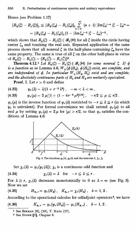
550 X. Perturbation of continuous spectra and unitary equivalence
Hence (see Problem 1.17)00
IIR2(0 - R,(C)II15 IIR2(CO) - R1(CO)Ill -' (n + 1) IIm4ul-n IC - Coin=n=0
= IJR2(Co) - Ri(Co)II1(1 - ImCoJ-1 IC -Col)-2
which shows that R2 P - R, (4) E -41(H) for all 4 inside the circle havingcenter o and touching the real axis. Repeated application of the sameprocess shows that all nonreal 4 in the half-plane containing o have thesame property. The same is true of all C on the other half-plane in virtueof R2 (4) - R, (C) = (R2 (c) -
Theorem 4.12.1 Let R2 (4) - R, M E 9, (H) for some nonreal C. If 0is a function as in Lemma 4.6, W± (0 (H2), 0 (H1)) exist, are complete, andare independent of 0. In particular W± (H2, H1) exist and are complete,and the absolutely continuous parts of H, and H2 are unitarily equivalent.
Proof. I. Let r > 0 and define
(4.32) 7Vr(A)=A/(1+r-2A2), -oo<A<oo,(4.33) ryr(u) = 2,u/[1 + (1 - 4r-2 y2)1/2] , -r/2:5--,u5 r/2.97r (,u) is the inverse function of tpr (A) restricted to - r 5 A 5 r (in which4pr is univalent). For formal convenience we shall extend T, ('u) to allreal ,u by setting (p,. (,u) = 2,u for I,uI > r/2, so that 97r satisfies the con-ditions of Lemma 4.6.
/ 11. x$611i%
11
------------
r sue -Fig. 3. The functions X, (A), X. (1) and the intervals I, J,, Ja
Set Zr (A) = 9 . (°r (A)) ; Zr is a continuous odd function and
(4.34) xr (A) = A for - r 5 A:5 Y.
For A z r, X, (A) decreases monotonically to 0 as A-* oo (see Fig. 3).Now we set(4.35) Hk, r = r (Hk) , K7,,. = Xr (Hk) , k = 1, 2.
According to the operational calculus for selfadjoint operators2, we have
(4.36) Kk,r = 99r(tVr(Hk))= 99r(Hk,r) , k= 1, 2.1 See BiRMnx [9], [10], T. KATO [17].2 See STONE (1), Chapter 6.
§ 4. Existence and completeness of wave operators 551
In virtue of (4.34), however, K,,,, and Hk coincide on the subspaceH,,, - (El (r) - El, (- r)) H, which reduces Hk and K,,,. Hence
(4.37) a-it9S(K .d u = e- itd(Hs) u for u E Hk,, .
II. Since Hk, , = Hk (1 + r- 2 H2)-1= (r2/2) [(H,, + i r)-1 + (Hk -- i r)-1], it follows from Lemma 4.11 that H2,1 - H1,, E -41(H). Hence
(4.38) W+(0 (cp, (H2, T), 0 (w, A, r)) = W f (w, (H2, r), A, r)) =
exist by Theorem 4.7 for any 0 satisfying the conditions of Lemma 4.6,for the composite function 0 (99, (A)) also satisfies the same conditions.In view of (4.36), this implies that
s-lim e i tO (K, ,) e- i t 6 (K,..) p1= W+, , ;t-,+ o0
here P1 is the projection on Hl,ao but the subspace of absolute continuity, (the proof is the same as in the proof offor 0 (K1,,) coincides with H1,a,
Theorem 4.7). Using (4.37) for k = 1, we have therefore
(4.39) eitO(K,..) e-tt¢(H,) P1 u-+ W+,, u for uE H1,, .
III. Let I = (a, b] where 0 < a < b < r. The inverse image of Iunder the map x, is the union of I itself and another finite interval J,lying to the right of r (see Fig. 3). If we denote by Fk,, the spectralmeasure for Kk, , = x, (Hk), k = 1, 2, we have [see (4.30) ]
(4.40) Fk, r (I) = Ek (X;71 (I)) = E,,(I) + Ek (Jr) z Ek (I)
Let u E El (I) H. Then u E Hl,, and (4.39) holds. Since W+, , = W+ (K2, ,,K1,,) by (4.38) and u E Fl, (I) H by (4.40), we have
(4.41) W+,, u E F2,, (I) H .
From (4.39) and (4.41), we obtain for u E El (I) H
II (1-F2,,(I)) e-it#(H,)piuII= II(1-F2,,(I)) eitd(Ks,r) e-it0(H,)PiuI -*
II(1-F2,,(I)) W+,,Ull =0, t-*+0
note that F2,,(I) and eitl(K,.,) commute. Hence
(1), e-it"(H') Plu ,r F2,,(I) e-itm(H,) Plu
where - means that the difference of the two members tends to zero ast -+ + oo. The same is true if r is replaced by any s > r, which result willbe called (1)S. Ifs is sufficiently large, we have F2,,(I)F2,S(I) = E2(I) asis easily verified. Multiplying (1), from the left by F2,,(I) and using
552 X. Perturbation of continuous spectra and unitary equivalence
(1), we thus obtaine-it¢(H1) P,u ^' E2(I) e-it0(.%)plu
and hence by (4.37) and (4.39)eifO(H") e-itt(x,)Plu - eito(Ha)E2(I) a tt-A(H,) plu
= E2(I) eit o (K2. r) e-"O (Hi) pl u -* E2 (I) W+ , u .
Thus lime it"'(H,) e`0 (H,) Plu exists and is independent of .IV. We have proved that
(4.43) W, (t) P , u -W+, , u , t + + O ,provided u E El (I) H where I = (a, b] and 0 < a < b < Y. The sameresult holds when I is replaced by (- b, -a]. The allowable u and theirlinear combinations form a dense set in H1,, = (E1(r) - El (- r)) H,except for the possible eigenspaces of H1 for the eigenvalues 0 and r.But these eigenspaces are unimportant, being annihilated by P1.
Since W, (t) is unitary and uniformly bounded, it follows that (4.43)holds for all u E H1,,..
Since s-lim W, (t) P1 u exists for all u E Hl,, and since the unionof all H1, , for r > 0 is dense in H, it follows finally that s-lim Wo (t) P,= W+(0 (H2), 0 (H,)) exists. This limit is independent of 0 as is seenfrom (4.43). Obviously the same is true for W_. Since the assumptionof the theorem is symmetric in H, and H2, the same is true when H1, H2are exchanged, so that these wave operators are complete.
Remark 4.13. The assumption R2 (4) - R, (0 E 91(H) in Theorem 4.12is not essential. The point is that for any r > 0, there is a function iv,. (R)with the following properties :
1) tp, (R) is piecewise monotonic like 0 (d) but may be increasing insome subinterval and decreasing in others;
2) ip, (d) is univalent for - r < 2 < r;3) lVr (H2) = V,. (Hj) + A, where A, E 2, (H).The proof of Theorem 4.12 can be adapted to this general case with a
slight modification'.According to this generalization, the results of Theorem 4.12 are true
if R2 Mm - R, (0 m E .41(H) for every pure imaginary C (or at least for asequence c',, = ±i r,, with rb -+ oo). In this case we need only to takeV, (A) = i [(r + i 2) - (r - i A)-m] with r = r,,, V, (A) is univalent on aneighborhood of 2 = 0, the size of which is proportional to Y.
Problem 4.14. In Theorem 4.9 remove the assumptions that H, is bounded belowand y is real. The conclusions are still true, except the one that H. is bounded frombelow.
I This gives very general sufficient conditions for the existence and completenessof the generalized wave operators. There are some conditions not included in thiscategory; see BIRMAN [11], BIRMAN and ENTINA [1], STANKEVI6 [1].
§ 5. A stationary method 553
6. Dependence of W.. (H2, H1) on H1 and H2Theorem 4.15. Let H1, H2 be self adjoint operators such that W+ (H2, H1)
exists. Then W+ (H2 + A, H1) and W., (H2, H1 + A) exist for any A E °.,A1(H)and
(4.44) W + (H2 +A,
H1) S W+ (H2, H1)
W+ (H2, H1 + A) -. W+ (H21 Hi)W
as II A 111-+ 0. Similar results hold with W+ replaced by W_.Proof. W+ (H2 + A, H2) exists by Theorem 4.4 and, therefore,
W+ (H2 + A, H1) exists and equals W+ (H2 + A, H2) W+ (H2, H1) byTheorem 3.4. Similarly, W+ (H21 H1 + A) = W+ (H21 H1) W+ (H1, H1 + A)exists. Thus it suffices to prove (4.44) for the special case H2 = H1.
We see from (4.23), on setting t = 0, that 11 W+ (H1 + A, H1) u - ull 55 IIIujfl (4avIIAjj1)112_ 0 as IIAII1-* 0. Since the set of u with IIIuIII < cc isdense in P1 H, it follows that W+ (H1 + A, H1) = W+ (H1 + A, H1) P1-i. P1
5
= W+ (H1, H1) as 11 A 111- 0. Since W+ (H1, H1 + A) = W+ (H1 + A, H1) *by Theorem 3.5, it then follows that W+ (H1, H1 + A) W Pl = P1= W+(H1, H1).
Remark 4.17. The above results on the continuity of W± (H2, H1) asfunctions of H1, H2 are very weak inasmuch as a very strong topology isemployed for H1, H2. A stronger result is obtained by using Theorem 4.12instead of Theorem 4.4. Thus, for example, W+ (H2 + A, H1) - W+ (H2, H1)
if A tends to zero in the sense that 11 (H2 + A - c)-1 - (H2 - C)_1111-+ 0for some nonreal C; here A need not even be bounded'. In generalWt (H2, H1) are not continuous in H1, H2 jointly2.
Problem 4.18. Discuss the continuity of Wf (H2, H1) in Example 4.10 when q (x)is changed.
§ 5. A stationary method1. Introduction
There are other ways to construct the generalized wave operatorsWt (H2, H1). In contrast with the "time-dependent" method developedin preceding sections, these schemes do not make explicit use of the"time variable" t, and in consequence are known as the stationary
1 It is difficult to deduce a stronger continuity of W± (H2, H1) by the methodused above. But there is a different topology for H1, H2 under which W± (H2, H1)aquires stronger continuity, for example, continuity in norm. A special case will beconsidered in the following section. The discontinuity of Wf in norm was discussedby PUTNAM [7].
2 See T. KATO [11].
554 X. Perturbation of continuous spectra and unitary equivalence
methods. There are several varieties among them'. In this section weshall give an account of one of them, which seems to complement thetime-dependent theory most effectively.
In this method the Wt are constructed as solutions of certain opera-tional equations. To deduce these equations, it is convenient to startfrom the time-dependent formulas (inasmuch as we have defined W±in the time-dependent scheme). For simplicity let us assume that H2= Hl + A where A E 9 (H). Then we have the formula (3.21), from whichwe obtain the identity
(5.1) WV11) - W (t') = if eitH, Ae-itHi dtt'
(see the proof of Lemma 3.8). Similarly, we have by exchanging Hl, H2,r.
(5.2) W(t")-'-W(t')-'=,-i f eitH,Ae-lH,dt.11
Suppose now that W+ = s-li(t) PI exists. Then W (t)-' W. Pl5as t -+ co. Thus (5.2) gives, when multiplied by - W+ from the right,with t' = 0 and t" co
Co
(5.3) W + - PI = i f ei tHl A W+ e- i 1H' d t (strong),0
where we have also used the relationship e_ i tH= W+ = W+ e-i tH,C
[see (3.7)]. The integral on the right of (5.3) exists as the strong limit of f0
as t"-+ oo, which is indicated by the symbol (strong).At this point it is convenient to introduce the notations
(5.4) f1 T= f;,T=i f eitH,Te- ItH- dt,0
whenever one or both of the integrals on the right exists as the strongt"
limit 2 off as t" -+ ± oo. Then (5.3) can be written0
(5.5)+ W+ = PI + f'j (A W+) .
Similarly, if W_ = W_ (H2, HI) exists, it must satisfy
(5.5)_ W_ = PI + f i (A W_) .
Let us now forget all about the assumption on the existence ofWt (H2, HI). Instead we start from the "integral equations" (5.5) f
i For stationary methods see BIRMAN and ENTINA [1], DE BRANGES [1],T. KATO [10], KURODA [7], [8] and the papers related to the Friedrichs equationreferred to in footnote I on page 553.
2 Sometimes it is convenient to define weak 1'i, in which weak convergence isused instead of strong convergence. We do not consider this definition, however.
§ 5. A stationary method 555
and try to construct W+ as their solutions. These equations are "statio-nary", for the time t does not appear in them explicitly.
The operations 1'1 and the equations (5.5)± were introduced byFRIEDRICHS, though the original definition is formally different from theabove'. It should be noted that they are linear operators acting in thespace _I(H) of bounded linear operators in H ; their domains are notthe whole space 9(H) since (5.4) need not exist for all T E .4(H).
In the following paragraphs we shall study basic properties of I'1and, using the results obtained, show that the solutions of (5.5) ± areindeed the generalized wave operators W± (H2, H,). Then we shallproceed to the problem of solving (5.5) f.
2. The I' operationsThe T1 = I'H1 as defined by (5.4) depend on the selfadjoint operator
Hl. In this paragraph we write H for Hl and I't for T1; H may be anyselfadjoint operator. The domains and ranges of T+ are denoted by-9 (f) , . ? (TI), respectively ; these are linear manifolds of a (H).
Lemma 5.1.2 Let B E .4(H) commute with H. Then T E -q (I'+) impliesthat B T and T B are in 3 (T+) and I'+ (B T) = B (T+ T), T+ (T B)
(T+ T) B. Similarly for F-.Proof. Obvious since B commutes with e+ i tH.Lemma 5.2. Let T E -9 (T+) and S = T+ T. Then S D (H) C D (H),
Tu = SHu - HSu for every u E D (H) and Se-itH- 0 as t--> +oo.s
Similarly for T-, with + oo replaced by - oo in the last proposition.Proof. We have
+00(5.6) eitH Se-"H = i f e'BH Te-18H ds (strong)
i
as is seen by multiplying (5.4) by 01H from the left and by e-i4H from theright. Denoting by S (t) the right member of (5.6), we have ei tH S= S (t) 04H. Since d S (t)/d t = - i ei tH T e- i tH in the strong sense, we have
d ei4HSu= d S(t)eitHu=-ieiOHTu+iS(t)e' Huat atfor u E D (H). Thus ei 1H Su is strongly differentiable in t, which impliesSuE D(H) (see Remark IX-1.5) so that (d/dt) eitHSu= ieitHHSu.
1 Friedrichs defines T, T for integral operators T of special types; see FrIED-RICHS [2], [3], [7]. (5.5)± are called the Friedrichs equations. For these equationssee also FADDEEV [3], LADYIENSKAJA and FADDEEV [1], REJTO [1], [2], SCHWARTZ[2], [3], [4]. A discrete analogue of the Friedrichs equation was consideredrecently by FREEMAN [1], in which T is defined in terms of a discrete semigroupinstead of a group e- «$.
9 The properties of P± given in the following lemmas are proved in FRIEDRICHS[2], [3]. Here we need different proofs since we employ a formally different definitionof r±.
556 X. Perturbation of continuous spectra and unitary equivalence
On setting t = 0, we thus obtain HSu = - Tu + SHu, which provesthe first part of the lemma.
The last part follows from (5.6), which implies that ettHSe-t1H_,0
Sas t -- +oo; multiplication from the left by the unitary operator e-{tHgives Se-ttH-, 0.
s
Lemma 5.3. A necessary and sufficient condition for an S E 9(H)to belong to R (T+) is that S D (H) C D (H), S H - H S [defined on D (H) ]be bounded, and Se-ttH-, 0 as t-+ +oo. In this case S = T+ T if T is the
s
closure of S H - HS. Similarly for T-, with + co replaced by - oo.Proof. The necessity part was proved in Lemma 5.2. To prove the
sufficiency part, we note that
(5.7) ds ei8H Se-88H u = i eisH(HS - SH) a-t8H u
if u E D (H), for then e-"H u E D (H) and so Se-{8H u E D (H) by hypo-thesis. Since HS - SH can be replaced by its closure - T, we obtainby integrating (5.7) on 0 S s S t
(5.8)
t
0
Here the restriction u E D (H) can be removed, since the operatorsinvolved are bounded and D (H) is dense in H. Then, going to the limitI--> + oo and using the assumption S e-t t H -+ 0, we see that the right
s
member of (5.8) has the limit - Su. This means that I'+ T exists andequals S.
Lemma 5.4.1 Let T', T" E .9 (I'+). Then (I'+ T') T" + T' (I'+ T")belongs to .9 (1'+) and
(5.9) I'+ [(f+ T') T" + T' (1'+ T") ] = (I'+ T') (I'+ T") .
Similarly for I'-.Proof. Set r+ T' = S', r+ T" = S". We claim that S' S" E 9P (I+)
Since both S' and S" map D (H) into itself by Lemma 5.2, S' S" has thesame property. If u E D (H), we have
(5.10) S'S"Hu-HS'S"u=S'(S"Hu-HS"u)+ (S'H-HS')S"u=S'T"u+T'S"u
by Lemma 5.2. Thus S' S" H - HS' S" has a bounded extension
(5.11) T=S'T"+T'S"Ef(H).Finally(5.12) 5'S" e-ttH= S'(S"e-t.tH) 0 as t-).+oo
s
(eitH Se-itH - S) u = - (i f eisH Te-t8H ds) u.
1 Similarly one can deduce rf [T' (I'-. T") + (r+ T') T"] = (r+ T') (I' T"),assuming T', T" E .9 (I'+) n 9 (I'-), and many other formulas of a similar kind.
§ 5. A stationary method 557
by Lemma 5.2. It follows from Lemma 5.3 that T E -9 (P+) and F+ T= S' S", which is exactly (5.9).
Remark 5.5. Lemma 5.3 shows that the operator I'+ is in a certainsense inverse to the commutator operator S-* [S, H] = SH - HS.(5.9) is a relation inverse to the formula
(5.13) [S'S", H] = S' [S", H] + [S', H] S".
Lemma 5.6. 1/ both T and T* belong to-9 (I'+), then (I'+T)* _ F+ (T*)Similarly for T-.
Proof. Obvious from the definition (5.4). Note, however, that TE9 (I'+)need not imply T* E .9 (I'+).
Remark 5.7. We have considered above the operations I'+ T only forT E a (H). This restriction is neither necessary nor natural, and can beweakened to some extent. Set
(5.14) (I's T)u= feitHTe-atHudt.0
(5.14) has a meaning for u E D (H) at least if T is relatively boundedwith respect to H. If (I's T) u has a limit v as s -. + co, we may writev = S' u. If S' is bounded, its closure determines an operator S E -4 (H),which we define as T+ T. Most of the results stated above remain validfor this generalized definition of I'+, but we shall not consider it in detail.
3. Equivalence with the time-dependent theoryWe can now proveTheorem 5.8. Let H1 and A be selfadjoint and let A E 9 (H). Suppose
that there exists a W+ E . (H) satisfying (5.5)+. Then the generalized waveoperator W. (H8, H1) exists and coincides with W+, where Hz = H1 + A.Similarly for (5.5)_.
Proof. Since W+ - P1= fj (A W+), it follows from Lemma 5.2that (W+ - PI) H1 u - H1(W+ - P1) u = A W+ u for u E D (H1). SinceP1 H1 u = H1 P1 u, this implies H$ W+ u = W+ H1 u or
(5.15) H2 W+) W+ H1 .
This further implies (H2 - C)-1 W+ = W+ (H1 - c)-1 for every nonrealC and hence (recall the construction of e'1H*, IX-§ 1.2)
(5.16) ei t H, W+ = W+ et t H, _00<t<+00.
It follows also from Lemma 5.2 that (W+ - Pl) e-1tHi -, 0 asg
t-* --oo. In view of (5.16), this implies a-stHa W+ - e-ttH' P1- 0. Onmultiplying from the left by ettH., we obtain W+ - ettH, a-ttH, P1 0.
This shows that W+ (H2, H1) exists and coincides with W+.
558 X. Perturbation of continuous spectra and unitary equivalence
Remark 5.9. The equations (5.5) _ make sense, and can have solutions,even if A is not symmetric. The above proof is valid in this general caseexcept for the multiplication by eitH. used in the final part; note thati H2 = i (H1 + A) is still the generator of a quasi-bounded group (seeTheorem IX-2.1) but the group may not be bounded. In particular wenote that (5.15), (5.16) are valid for a non-symmetric A.
4. The I' operations on degenerate operatorsIn this paragraph we consider a selfadjoint operator H with the
spectral family {E (A.)} and the operators I' = I. We first ask underwhat conditions an operator
(5.17) T= ( g) f
of rank one belongs to 9 (f+), where f, g are assumed to be absolutelycontinuous with respect to H.
For any u E H we have [for the notation r see (5.14)]a
(5.18) (I'a T) u = i (2;r)1/2 f 0., g (t) ei t H / d t0
where00
(5.19) 0u,g(t)= (2n)-1/2 (e-itH u, g) = (27v)-1/2 f e-itAeu,g(A)dA-00
with
(5.20) a, (E (1) u, g) E L1(- co, co)
note that (E (A) u, g) is absolutely continuous if g is (see Theorem 1.7).Using the spectral formula eitH = f eitA dE (d), we have from (5.18)
(5.21) (I', T) u = i (27v)1/2 f (f ou, g (t) eitx dl) dE (2) f = i o'a-00
wherea
(5.22) Qau,g(A)= (2 v)1/2 f cu,g(t)eitxdt.
0
(2r)-1 tsau,g may be regarded as the inverse Fourier transform ofXa (t) 0., g (t), Xa (t) being the characteristic function of the interval (0, a).
Suppose now that (we write Cog for eg, g)
(5.23) IIIglI12= IIPgll00= supd(E(A)g,g)/d)<ool.
Then cu, g E L2(-00,00) with 110u, gll 5 1VIgIUU Iull (see Lemma 4.5). Thusxa 0u, g -' X+ 0u, g in L2 as a-* + oo, where x+ is the characteristic function
1 Here and in what follows we write simply sup where we should write ess sup.
§ 5. A stationary method 559
of (0, oo). Going over to the Fourier transforms, we see that as ..,gi ou,gin L2, where a,+,,/2 n is the inverse Fourier transform of x+ 0u, g :
00
(5.24) (2n)'/2l.i.m. f 0.,, (t) ell' dt,0
so that(5.25) Il au g1l S 2nII ).,ell S 2n lull 111 llI
Now it follows from (5.21) that (F,,+ T) u tends as a- - + oo to
(5.26) (r+ T) u = i au g (H) /
provided III/III < oo too. In fact lla++u,g(H) f - au g(H) /112 = fa,, ,g (A) l2 (d/d 1) (E (2) f, f) d2 < Il oa u,g - au,gII2111/1112 -; 0. This shows
that r+ T exists and justifies the notation (r+ T) u used in (5.26). At thesame time we have II (F+ T) ull S ll a,+ti,gll 1l1/1I1 s 2n lull III/III IIIglII Hence
(5.27) I I r + T I I S 2a 111/111 I I IgI l l
As was seen above, the Fourier transform of a+, 9/2n is x+ times theFourier transform of o., g. If we set
(5.28) oru, g = 2 n G+ Pu, g ,
G+ is an orthogonal projection in L2, being the Fourier transform of themultiplication operator by X+(t). G+ is associated with the so-calledHilbert transform.
A convenient expression for G+ is given by
(5.29) G+ = s-lim G8 , G8 P (2) _ey0
00
1
2n i , fL - R- .du.-00
To prove this, we note that the multiplication operator by X+ (t) is thestrong limit as e \ 0 of the multiplication operator by e-e t x+ (t). Goingover to the Fourier transform, the latter operator becomes
00 00
G6 Lo(A) = (2;r)-If esta e-8t dt f e-ctr. P (,u) d,u0 -00
which is equal to (5.29).r- T can be dealt with quite in the same way. In the final result,
it is only necessary to replace G+ by G- defined by replacing a by - ein (5.29). In this way we have proved
Lemma 5.10. Let T = ( , g) / be an operator of rank one, where /, gare absolutely continuous with respect to the sel f adjoint operator H. 1/ 111/111and IIIgIII are finite, PI: T exist and (I'1 T) u = i au g (H) f for any u E H.Here au g = 2n G1 e.,g and Qu, g (R) = d (E (.I) u, g)I d 2 E Ll n L2. Wehave 111" Tll s 2n 111/111 IIlgill.
560 X. Perturbation of continuous spectra and unitary equivalence
We now consider an operator of finite rank
(5.30) T gk) fkk=1
where all the f k, g, are absolutely continuous with respect to H. Since Tis the sum of operators of rank one, application of Lemma 5.10 showsthat l'tA exist if the IIIfkIII, IIIgkIII are finite and IIP All S 2n' IIIfkIII IIIgkIIIBut we shall deduce a somewhat sharper estimate.
Lemma 5.11. Let T be as above. Then I'} T exist and II 1':L- T IIm m
5 2 n IX f where IX2 = sup fk (A) and f2 = sup f Pg, (A). Herek=1 k=1
Pf(A) = Pf,f(2) = d(E(A) f, f)/dA.Proof. By Lemma 5.10 we have (I't T) u = i f vug, (H) /,. Hence
k=1m
II (l't T) ull 2 = f ((1g, (H) I, , Qug, (H) fk) _i,k=1
_ I f 1u g, (A.) o d (E (A) fs, fk) 5i,k
f E laug, (2) I lau g, (A) I ef, (A)112 ef, (A)1/2 d A S [by (1.9)]9, k
f [,f Iorug,(A)I Pf,(A)1/2]2d2k
5 f (E ICug,(A)I2)(.' Pf,(A))dA
X2, IIQu g,112 S (2n IX)2, Ileu,g,ll2 -k k
_ (2n IX) 2f f I d(E (A) u, gk)I2dA
5 (2 n IX) 2 f ess (A) (' 0,, (A)) d d 5
5 (2nIXf)2f ou(d)dA= (2nat ,)2Ilull2.
[by (1.9)]
5. Solution of the integral equation for rank A = 1We shall now solve the "integral equations" (5.5). For simplicity we
assume in the remainder of this section that H1 is spectrally absolutelycontinuous so that P1= 1, and we shall write H for H1. Introducing forconvenience a numerical parameter x, we thus consider the equation
(5.31) W= 1+xF(AW);here T and W stand for either of 1'1 and Wt, respectively.
A natural idea for solving (5.31) is to use a successive approximation:M
(5.32) W = W (M) = E Mn W (n) , W (o) = 1 ,n=o
W(n+1) = I'(A W(n)) , n = 0, 1, 2, ... .
§ 5. A stationary method 561
But it is not at all clear whether all the W(n) can be constructed, for I'is not defined everywhere on M(H).
We shall show, however, that this method works if A is of rank one :
(5.33) A= (,g) land if /, g are restricted properly. We shall later extend the results tomore general cases. We do not assume A to be symmetric; it is an interestingfact that (5.31) can be solved for a non-symmetric A.
Suppose 111/111, IIIgIII are finite [see (5.23)]. Then Lemma 5.10 showsthat W M = FA exists and II W (1)lI s 2n III/III IIIgIll To construct W(2)= I'(A W(1)), we want to apply Lemma 5.10 with T = A W(1) g(1)) f,where(5.34) 9(1)= W(1)*g= (I'A)*g= -(I'A*)g= -iae,1(H)g
by Lemmas 5.6 and 5.10 [note that A* _ (, f) g also satisfies the as-sumptions of Lemma 5.10]. Hence (d/d A) (E (A) g('), g(1)) = I ae,1(A)12
(d/d2.) (E(2) g, g), so that 1119(1)111 5 MIIIg1II < oo if we assume that'
(5.35) II ag,1II 00 = sup l ag, f (2) I = M<-.
It turns out that we can construct the W(n) for n = 3, 4, ... withoutintroducing any further assumptions. In fact we can apply Lemma 5.10to construct W(n+1) from W(n), where A W(n) g(n)) / is of rank onewith(5.36) g(n) = W(n)* g = (- i)n ag,, (H)n g'
which implies as above
(5.37) IIIg(n)III s Mn IIlgfII <
(5.36) can be proved by induction; we have g(n+1) = W(n+1) * g_ (T A W (n)) * g = - [I' (A W (n)) *] g = - i ag,1(H) g(n) since (A W())*
, /) 9(" ).It follows also that
(5.38) II W(n+1)11= III'(A W(n))II s 2n Ilig(n)III III/III s 21c Mn 111/1111119111
Thus the series (5.32) converges in norm if I ml < 1/M. It is easy to seethat the sum W satisfies the equation (5.31) : it suffices to show thatP(A W) can be calculated term by term by substituting for W theseries (5.32). This can be done by noting that II I'a (A W) 11 s 2 n Mn I l lfl l l
III9lII and that I'a (A W (n)) g I' (A W(')) as a -+ oo for each n.
1 C,,1 is bounded since leg,,(A)12 S pg(A) ef(A), but it does not imply thatag,1 = 2n G Qg.1(G = G±) is bounded. It is known that ag, j(A) is bounded (andHolder continuous) if eg,/ (%) is Holder continuous and goes to zero as I A I -+ oo nottoo slowly. In the problem under consideration, it is convenient to assume (5.35).
562 X. Perturbation of continuous spectra and unitary equivalence
Thus we have provedLemma 5.12. I/ A = (,g) / where 1111111, 111gI11 are finite and ore s'' 0 = M<oo,
(5.31) has a solution W = W (m) which is holomorphic in x for ImI < 1/M.For further study of W (m), it is convenient to consider an associated
equation(5.39) Z= 1 - x r(ZA) ,which is dual to (5.31) in a certain sense. (5.39) can be solved quite in thesame way as above under the same conditions. We have namely
00
(5.40) Z = Z (x) _ f xn Z(n) , Z(°) = 1 Z(n+1) f (Z(n) A)n=0
Z(n) A = ( , g) 1(n) , /(n) = Z(n) / _ (- i)n or, g (H)n 1
Since a,., s are, f ii ), we obtainLemma 5.13. Under the same assumptions as in Lemma 5.12, (5.39)
has a solution Z = Z(x) holomorphic for Ixj < 1/M.There is a simple relationship between the solutions of (5.31) and
(5.39). We have namelyLemma 5.14. For each fixed x with 1xj < 1/M, the solutions of (5.31) and
(5.39) are unique. These solutions are related to each other by Z(x)= W(x)-1, W(x) = Z(x) -1.
Proof. Let W and Z be any solutions of these equations. Multiplyingthe two equations, we have
ZW = 1 -)- x T(AW) - x F(ZA) - x2 F(ZA) .P(AW) .
Using (5.9) and the equations (5.31), (5.39) once more, we obtain
(5.41) ZW= 1+x.F[AW -ZA - xF(ZA) A W -xZA F(AW)]= 1 + x.F [ZA W - ZA W] = 1.
This implies that Z has range H ; in other words Z is semi-Fredholmwith def Z = 0 (see IV-§ 5.1). In particular it is true of the Z(x) ofLemma 5.13 for all x. But since Z (x) is holomorphic in x, it follows fromthe stability theorem for the index (see Theorem IV-5.17) that nul Z (x)is constant. Since Z (0) = 1, this constant must be 0. Thus Z (x) maps Honto itself one to one, and Z(x)-1 has the same property.
Now (5.41) gives Z(x) W = 1, hence W = Z(x)-1. Since this is trueof any solution W of (5.31), the solution of (5.31) is unique. Similarly,using this W = Z (x)-' in (5.41), we have ZZ (x)-1 = 1 or Z = Z (x). Sincethis is true of any solution Z of (5.39), the solution of (5.39) is unique'.
1 One can argue without using the index theorem. We have Z (x) W (x) = 1 by(5.41). Since W (x) and Z (x) are holomorphic in x with W (0) = Z (0) = 1, W (x) -1exists for sufficiently small 1x1 and Z (x) = W (m)-1, hence W (x)Z (x) = 1. But sinceW(x)Z(x) is holomorphic for (x1 <1/M, we have W(x)Z(x) = 1 for 1x1 < 1/M.Thus Z(x) = W(x)-1 for 1x1 < 1/M. The uniqueness then follows from (5.41). Forexample, any W must satisfy Z (x) W = 1, hence W = Z (x)-1 = W (x).
§ 5. A stationary method 563
Summing up the above lemmas, we haveTheorem 5.15. Let H be self adjoint and spectrally absolutely continuous,
let A = ( , g) / where III/III < co, IIIgIII < oo and IIori gII. = M < oo. Then(5.31) and (5.39) have unique solutions W+ (x) and Z+ (m), respectively,for r= I'H and l or I ml < 1/M. These solutions are holomorphic in x and areinverse to each other. Similar results hold with F = F . H (x) = H + x Ais similar to H : H (x) = W+ (x) H W+ (x) -1. If f = g and x is real, thenH (x) is self adjoint, the Wt (x) are unitary and coincide with the waveoperators Wt (H (x), H), and H (x) is unitarily equivalent to H. The spectralfamily E,(A, x) for H (x) is holomorphic in x (for real x) for each fixed A 1.
The similarity of H (x) to H follows from Remark 5.9 and the identityof the W± (x) with the wave operators follows from Theorem 5.8. Notethat II o ,II = II Qj,t II so that both W± (x) exist if g = f . The assertionon E (A, x) follows from E (2, x) = W+ (x) E (A) W+ (x) -1.
6. Solution of the integral equation for a degenerate AThe results of the preceding paragraph can be generalized to the case
in which A is degenerate (of finite rank m)
(5.42) A gk)fk, f,,gkEHk=1
in a straightforward fashion. (We keep the assumption that H is spectrallyabsolutely continuous.) We can use the successive approximation (5.32)to solve (5.31). In fact, it is easy to see as before that, at least formally,
m
(5.43) A W (n) = v (, g$ )) /Ak=1
M(5.44) g")= WOO gk= -i ak,s(H)g}n-1)
i=1where we have written ik, j = ig,,, f, for brevity. It is easy to see as beforethat these results are valid if the IIIfaIIj, IIIgkIII and IIO'k,,II. are all finite.
To estimate II W (n)II , we first observe that Op (/,%)1/2 = [d (E (A) f , f) fd A]1/2
satisfies the triangle inequality in / for each fixed d; Nr+ g (d)1/2 5 Pf (x)1/2 ++ Qg(A)1/2, as is easily seen from (1.9). We apply this inequality to thesum (5.44) ; on writing &) (A) for Pe (A) with g = & for brevity, we obtain
m
(5.45) Pk") (x)1/2 S IQk, 7 (A) In -1) (A)1/2
i=1
[note that f = a (H) g implies e, (d) = Io' (A) I2 Pg (A) ]
1 In the time-dependent theory we did not prove any theorem which assertsthe continuity in norm of W} (H + x A, H) in x (to say nothing of analyticity).Thus Theorem 5.15 supplements earlier results.
564 X. Perturbation of continuous spectra and unitary equivalence
Let M (A) be the norm of the linear operator defined by the matrix(A) 1) acting in the m-dimensional unitary space Cm. Then (5.45)
gives
(2))1/2 C M (A) (E Pk" -1)
Successive application of this formula gives
(5.46) (E ek) (A))1,2 5 M (A)n (E e7' (A))1/2
Set M = supM (A) ; M is finite since we assumed that all the IIa;, 7,1I
are finite. Applying Lemma 5.11 to T = A W (n) [see (5.43) ], we thusobtain(5.47) II W (n+1)II = II P(A W(n)) II s 2n (sup E ek") (2))112 (Sup L ef. (A))111:<
2nMnllLeg.11121IL'ef.Illm"
It follows, as in the preceding paragraph, that the series for W(x)converges for Ixl < 1/M and gives a solution of (5.31). All further resultsof Theorem 5.15 can now be deduced exactly as before. Thus we haveproved
Theorem 5.16. In Theorem 5.15 replace A by A gk) fk wherek=1
IIIfk1II < oc, IIIgkIII < oo and < oo, j, k = 1, ..., m. Then the asser-tions remain valid if M = sup M (A), where M (A) is the norm of the
- <A<COm x m matrix (I e., f (A)) as an operator in the m-dimensional unitaryspace. (In the last statement o l Theorem 5.15 replace f = g by fk = ± gk,where ± can be chosen at random for each k.)
Remark 5.17. Let M' be the norm of the m x m matrixthen M _< M'. This is due to the simple fact that the norm of a matrixwith nonnegative elements is not decreased when some of the elements areincreased.
Remark 5.18. These results can be further generalized to the case inwhich A is no longer degenerate and the series in (5.42) is infinite.Looking at (5.47), we can expect the successive approximation toconverge if
(5.48) ll' ef.ll. < oo , lIE eejlo, < oo and IxI < 1/M ,
k k
where M = sup M (A) and M (A) is now the norm of the operator, actingin C' = 12, defined by the infinite matrix (log,, f; (A) I). It should beremarked, however, that some supplementary assumption such as
(5.49) EIlfkll llgkll < 00
would be required in order that A E 9(H), for we have defined 1'Xonly for bounded X. But (5.49) is not essential and can be replaced by a
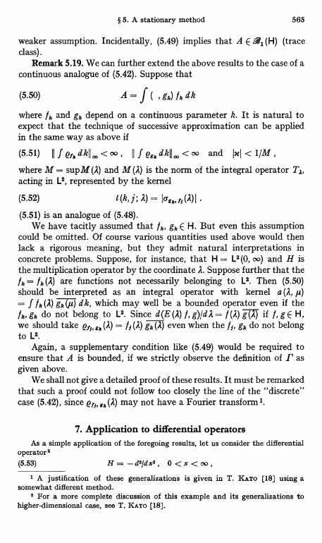
§ 5. A stationary method 565
weaker assumption. Incidentally, (5.49) implies that A E 9, (H) (traceclass).
Remark 5.19. We can further extend the above results to the case of acontinuous analogue of (5.42). Suppose that
(5.50) A= f ( ,gk) fkdk
where f k and gk depend on a continuous parameter k. It is natural toexpect that the technique of successive approximation can be appliedin the same way as above if
(5.51) III et', dkll. < co , II f eeR dkll QQ< oo and Iki < 1/M ,
where M = supM (A) and M (A) is the norm of the integral operator TA,acting in L2, represented by the kernel
(5.52) t (k, j ; A) (A)
(5.51) is an analogue of (5.48).We have tacitly assumed that fk, gk E H. But even this assumption
could be omitted. Of course various quantities used above would thenlack a rigorous meaning, but they admit natural interpretations inconcrete problems. Suppose, for instance, that H = L2 (0, oo) and H isthe multiplication operator by the coordinate A. Suppose further that thefk = fk (A) are functions not necessarily belonging to L2. Then (5.50)should be interpreted as an integral operator with kernel a (A, ,u)= f f k (A) gk Fiz) d k, which may well be a bounded operator even if thefk, gk do not belong to L2. Since d (E (A) /, #d A = I (A) gg if t, g E H,we should take et,, ,,(A) = /,(A) gk7( even when the /1, gk do not belongto L2.
Again, a supplementary condition like (5.49) would be required toensure that A is bounded, if we strictly observe the definition of I' asgiven above.
We shall not give a detailed proof of these results. It must be remarkedthat such a proof could not follow too closely the line of the "discrete"case (5.42), since et,, gR (A) may not have a Fourier transform 1.
7. Application to differential operatorsAs a simple application of the foregoing results, let us consider the differential
operators(5.53) H = - d21d x2 , 0 < x < oo,
1 A justification of these generalizations is given in T. KATO [18] using asomewhat different method.
2 For a more complete discussion of this example and its generalizations tohigher-dimensional case, see T. KATO [18].
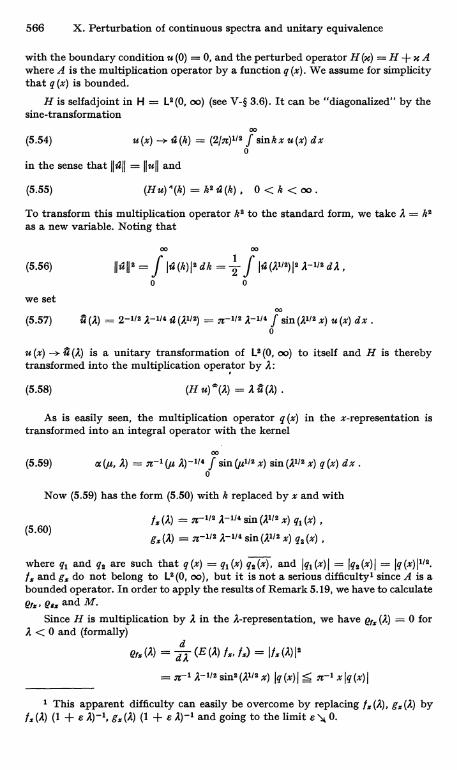
566 X. Perturbation of continuous spectra and unitary equivalence
with the boundary condition u (0) = 0, and the perturbed operator H (x) = H + x Awhere A is the multiplication operator by a function q (x). We assume for simplicitythat q (x) is bounded.
H is selfadjoint in H = L2(0, oo) (see V-§ 3.6). It can be "diagonalized" by thesine-transformation
(5.54) u(x) -*-R(k) = (2/n)1/2 f sinkx u(x) dx0
in the sense that IIiII = IIuDI and
(5.55) (Hu)'(h) = k2 a (k) , 0 < h < oo .
To transform this multiplication operator k2 to the standard form, we take A = k$as a new variable. Noting that
(5.56)
we set
0 f00
IIaII2 = f Id.(k)I2 dk = 2 J Ia(A1/2)12 A-1/2 dA ,
0 0
00
(5.57) 24 (A) = 2-1/2 A-1/4 1 (A1/2) = n-1/2 A-1/4 f sin (A1/2 x) u (x) dx .0
u (x) -a i (A) is a unitary transformation of L2 (0, oo) to itself and H is therebytransformed into the multiplication operator by A:
(5.58) (H u) *(2) = A U (A) .
As is easily seen, the multiplication operator q (x) in the x-representation istransformed into an integral operator with the kernel
(5.59) aC(, A) = n-1 (p A)-1/4 f sin (,u1/2 x) sin (A1/2 x) q (x) dx.0
Now (5.59) has the form (5.50) with k replaced by x and with
(5.60)!a (A) = n-1/2 A-1/4 sin (A1/2 x) q, (x)
g: (A) = n-1/2 A-1/4 sin (A1/2 x) q2 (x)
where q, and q2 are such that q (x) = q1 (x) q2 (x), and 1q, (x) I = Iq2 (x) I = Iq (x)11/2.
fx and gx do not belong to L2 (0, oo), but it is not a serious difficulty' since A is abounded operator. In order to apply the results of Remark 5.19, we have to calculateex, a and M.
Since H is multiplication by A in the A-representation, we have ex (A) = 0 forA < 0 and (formally)
21x (A) = d (E (A) fx, fx) = I fm (A) 12
=7g-IA-112Sin2(AI12X)lq(x)I=Sn-lxlq(x)I
I This apparent difficulty can easily be overcome by replacing & (A), g., (A) byfx (A) (1 + a A)-', g. (A) (1 + e A)-' and going to the limit e 14 0.
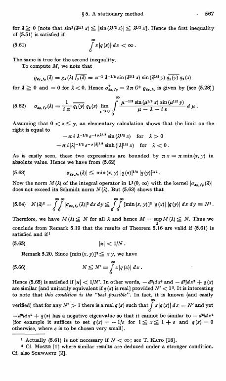
§ 5. A stationary method . 567
for A Z 0 [note that sins (A112 X) S Isin (Al/2 x) I S A1/2 x]. Hence the first inequalityof (5.51) is satisfied if
00
(5.61) f xjq(x)I dx < oo.0
The same is true for the second inequality.To compute M, we note that
Pex.fY (A) = g. (A) /Y (A) = n-1 A-1/2 sin (Al/2 x) sin (A1/2 y) q1 (y) q2 (x)
for A 0 and = 0 for A < 0. Hence a s, f,, = 2 n G+ C e:.fy is given by [see (5.28) ]
(5.62) oes.f,,(A) _
00
-1/2 sin /M..1/2 x) sin (,2112 y)1
q1 (Y) 42 (x) "M1-1 1f ei A- i d
uOT 810J0
-Assuming that 0 < x S y, an elementary calculation shows that the limit on theright is equal to
- z i A-1/2 a-'YAI" sin (A1/2 x) for A> O- n i IAI-I/2 e Y ICI"' sinh (IAI1/2 x) for A < 0 .
As is easily seen, these two expressions are bounded by n x = n min (x, y) inabsolute value. Hence we have from (5.62)
(5.63) I0rea.fy (A) I S minx, y) Iq (x) I1/2 I q (Y)11/2 ,
Now the norm M (A) of the integral operator in L2 (0, oo) with the kernel I0'e:. fY (A) Idoes not exceed its Schmidt norm N(A). But (5.63) shows that
00 00
00 00
(5.64) N(A)2= f f Ios:.fY(A)I2dxdy5 f f [min (x,y)]2Iq(x)IIq(Y)I dxdy-N2.00 00
Therefore, we have M(A) 5 N for all A and hence M = supM(A) S N. Thus wex
conclude from Remark 5.19 that the results of Theorem 5.16 are valid if (5.61) issatisfied and if'
(5.65) IxI < 11N.
Remark 5.20. Since [min (x, y)]2;5 x y, we have
(5.66) NS N'm f xIq(x)I dx.00
0
Hence (5.65) is satisfied if IxI < 1IN'. In other words, - d2/dx2 and - d2/dx2 + q (x)are similar [and unitarily equivalent if q (x) is real] provided N' < 12. It is interestingto note that this condition is the "best possible". In fact, it is known (and easily
00
verified) that for any N' > 1 there is a real q (x) such that f x I q (x) I d x = N' and yet0
- d2/d x2 + q (x) has a negative eigenvalue so that it cannot be similar to - d2/d x2[for example it suffices to set q (x) = - 1 /s for 1 5 x S 1 + a and q (x) = 0otherwise, where a is to be chosen very small].
I Actually (5.61) is not necessary if N < oo; see T. KATO [18].2 Cf. MOSER [1] where similar results are deduced under a stronger condition.
Cf. also SCHWARTZ [2].
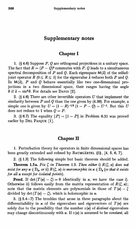
568 Supplementary notes
Supplementary notes
Chapter I
1. (§ 4.6) Suppose P, Q are orthogonal projections in a unitary space.The fact that R = (P - Q)2 commutes with P, Q leads to a simultaneousspectral decomposition of P and Q. Each eigenspace M (2) of the selfad-joint operator R (0 _< R:_5 1) for the eigenvalue A reduces both P and Q.In M (2), P and Q behave essentially like two one-dimensional pro-jections in a two dimensional space, their ranges having the angle0 if 2 = sin20. For details see DAVIS [2].
2. (§ 4.6) There are other invertible operators U that implement thesimilarity between P and Q than the one given by (4.38). For example, asimple one is given by U = (1 - R)-1/2 (1 - P - Q) = U-1. But this Udoes not reduce to 1 when Q = P.
3. (§ 6.7) The equality IIPII = III - PII in Problem 6.31 was provedearlier by DEL PASQUE [1].
Chapter II
1. Perturbation theory for operators in finite dimensional spaces hasbeen greatly extended and refined by BntMGARTEL (1), [4, 5, 6, 7].
2. (§ 1.3) The following simple but basic theorem should be added.Theorem 1.5 a. Fix C in Theorem 1.5. Then either i) R (C, x) does not
exist for any x E Do, or ii) R (C, x) is meromorphic in x E Do (so that it existsfor all x except for isolated points).
Proof. If det (T (x) - C) = 0 identically in x, we have the case i).Otherwise ii) follows easily from the matrix representation of R (c, X);note that the matrix elements are polynomials in those of T (X) - Cdivided by det (T (x) - C), which is holomorphic in x.
3. (§ 5.4-7) The troubles that arose in these paragraphs about thedifferentiability in x of the eigenvalues and eigenvectors of T (x) aresolely due to the possibility that the number s (x) of distinct eigenvaluesmay change discontinuously with x. If s (x) is assumed to be constant, all
Supplementary notes 569
the difficulties disappear and eigenvalues and eigenprojections behave assmoothly as the operator T (m) itself. For example, suppose that T (m)depends continuously on x = (xl, ..., E Do C R' and that s (x) = sis constant. Then the results of par. 1-2 show that the eigenvalues ofT (x) can be numbered as 2 (x), ..., 2 (x), so that each Ah (x) is continuousin x, at least in a neighborhood of any given point in Do, which we mayassume to be x = 0. Then the eigenprojection Ph (x) associated with2h(x) is given by the integral (1.16), in which r = Ph may be chosen asa small fixed circle about 2h (0) as long as INI is sufficiently small. Supposenow that T (m) is Ch (k-times continuously differentiable). Then it is easyto see that R (C, x) is also Ch in x uniformly for C E Ph. It follows from theintegral representation that Ph (x) is also Ch. Then the formula (2.5) withm = mh = dim Ph (x) = const shows that 2h (x) is also Ch. That the eigen-vectors (or generalized eigenvectors) can also be chosen as Ch functionsis seen by the argument given in § 4.1. Similar results hold when T (x) isanalytic in x where x is a set of several real or complex variablesxl, ..., For another proof of differentiability of a more "real variable"type, see NoMizu [1].
4. (§ 6.5) Add DAVIS [3], DAVIS and KAHN [1] to footnote on p. 125.
Chapter III
1. The following may be added to the general reference : DIEUDONN>121, DUNFORD and SCHWARTZ (2), GOFFMAN and PEDRICK (1), REEDand SIMON (1).
2. (§ 2.1) For integral operators see JoRGENS 11).
3. (§ 4.2) The proof of Theorem 4.10 given in text is too long. Asimple proof is given, for example, in YOSIDA (1), p. 282.
4. (§ 4.3) We have the following theorem on det (1 + T).
Theorem. Let T be a degenerate operator in X. Then (1 + T) E 9 ( X)exists i f and only i f det (1 + T) + 0.
Proof. Necessity. Let TR be defined as in text. If det (1 + T) = 0,then det (1 R + TO = 0 and there is a nonzero u E R such that u + T u = 0.Hence 1 + T is not invertible. Sufficiency. First we show that 1 + T isinvertible if det (1 + T) + 0. Suppose u + T u = 0. Then u = - T u E Rso that (1R + TO u = 0. Since det (1R + TR) + 0, it follows that u = 0.Next we show that 1 + T is onto X. Let / E X. Then T1 E R. Sincedet(1R + TR) + 0 implies that 1R + TR is onto R and has a boundedinverse, there is v E R such that v + T v=- T j with IIvhI 5 c 11 T111 with c
570 Supplementary notes
independent of /. If we write u = / + v, we have u + T u = / withIIuII < (1 + c II TII) IIf1I. Hence 1 + T is onto X with (1 + 7)-1 E -4 A.
Chapter IV1. (§ 1.2) Inequality (1.15) is not very sharp. The factor 2V-2 can
be replaced by 2; this follows from a general theorem for the generatorof a contraction semigroup due to KALLMAN and ROTA (1). If p = 2, itcan even be replaced by v2 (see HARDY, LITTLEWOOD, and POLYA 111,p. 187; for an abstract result applicable to this case, see KATO [24]),
2. (§ 2.4) For further results for the gap between subspaces in aHilbert space, see LABROUSSE [1].
3. (§ 3). For explicit estimates for the eigenvalues of differential oper-ators, see e. g. BAZLEY [1], BAZLEY and Fox [1], GOULD (1), STENGER [1],WEINSTEIN [1-5].
4. (§ 4.1) The minimum gap between two subspaces in a Banachspace was studied in detail by DEL PASQUE [1, 2].
5. (§ 5.1) For more results related to nullity, deficiency, and othernotions (ascent, descent, etc.) for linear operators, see TAYLOR [1],KAASHOEK [2, 3, 4, 5], KAASHOEK and LAY [1], CARDUS [1], NEU-BAUER [3].
6. (§ 5.1) There is an addition theorem for the index : ind (S T) _= ind S + ind T. Here S E ' (Y, Z) and T E W (X,Y) are assumed to beFredholm and densely defined. Then S T E ' (X, Z) and S T is also Fred-holm. Moreover, S T depends continuously on S and T in the gaptopology. For the proof see NEUBAUER [3].
7. (§ 5.5) A theorem stronger than Theorem 5.31 is found in MAR-xus [1]. For more recent results in this direction, see KAASHOEK [1, 2, 3],OLIVER [1], RIBARI6 and VIDAV [1], BART [1], BART, KAASHOEK andLAY [1], BART and LAY [1], FORSTER [1], GRAMSCH [1,2].
8. (§6.2) For a further generalization of Theorem 6.2, see How-LAND [6], which also contains application of the W - A formulas toembedded eigenvalues of a selfadjoint operator.
9. (§ 6) Analytic functions with values in the set of degenerateoperators have been studied in detail by HOWLAND [7] and some of theauthors cited in note 7 above.
Chapter V1. The following may be added to the general reference: HALMOS (3),
HELSON (1), PUTNAM (1), REED and SIMON (2), SZ.-NAGY and FOIAq (1).
Supplementary notes 571
2. (§ 3.2) The proof of Theorem 3.1 (convexity of the numericalrange) is quite simple if one notes that the problem is essentially two-dimensional. Indeed, one wants to show that for each pair z1, z2 E 0 (T),the segment (z1, z2) is contained in 0 (T). Choose u; such that z7 _ (T u,, uj),11uiDD = 1, j = 1,2. It suffices to show that if u varies over the unit spherein the two-dimensional subspace spanned by u1, u2, then (T u, u) coversthe segment (z1, z2). Thus it suffices to prove the theorem for a two-dimensional space H. In this case, however, it is a direct consequence ofProblem 3.5. (The answer to this problem is that the numerical range isan ellipse with the two eigenvalues as foci. For the proof of the theorem,the exact shape of the numerical range of a two-dimensional operator isnot necessary, but such a knowledge is useful anyway.)
3. (§ 3.11) Regarding the fractional powers of linear operators in aBanach space [see (3.53)], we refer to a comprehensive study by KOMATSU[1-6] and YOSHIKAWA [1].
4. (§ 4.1) Regarding Theorems 4.3-4, we want to note that it is ingeneral impossible to improve the limit 1 of the T-bound of A, even whenboth T and A are bounded from below. This is seen from the followingexample. Let T = - d2/dx2 + (3/2) x-2 in H = L2 (0, oo). If we chooseD (T) = Co (0, oo), it is known that T is essentially selfadjoint (see VII-Example 4.15). Let A = - d2/dx2 with the same domain as T. Then asimple calculation shows that IlA ull s ll Tull. But T + ;CA == (1 + x) [- d2/dx2 + (3/2) (1 + x)-1x-2] is not essentially selfadjoint ifx > I because (3/2) (1 + x)-1 < 3/4 (see loc. cit). Note that T and A arenonnegative.
5. (§ 4.1) The problem considered in Theorems 4.3-4 can be general-ized to the following. Suppose T E ' (X, Y) is densely defined, where X, Yare Banach spaces. Let A be a densely defined operator from X to Y suchthat A is T-bounded and A* is T*-bounded, with the relative boundssmaller than 1. Then (T + A)* = T* + A*. For this and related pro-blems see HESS and KATO [1].
6. (§ 4.1) Theorem 4.6 was strengthened by WvsT [1] to the case inwhich the weaker inequality (4.1) [rather than (4.2)] is assumed withb = 1. It has further been generalized by OKAZAWA [2] and CHERNOFF [2]to the case in which T and A are accretive (or dissipative) operators in aBanach space, under certain mild restrictions. (T is accretive ifIlu + a T ull z Ilull for all u E D (T) and a > 0; T is dissipative if - T isaccretive.) The generalized form of Theorem 4.6 also generalizes TheoremIX-2.7, with the limit 1/2 replaced by 1. This was first proved by GUSTAF-SON [1, 2]. For further related results see OKAZAWA [1, 3, 4], YOSHIKAWA [3].It was found that Theorem 4.6 is often useful for the proof of essential
572 Supplementary notes
selfadjointness in various delicate problems; see KONRADY [1], SIMON [6],GRCTTER [1].
7. (§ 4.4) Theorem 4.12 implies that if T, S are nonnegative selfad-joint operators such that D (T) c D (S), then D (T1/2) c D (S1/2). Indeed,the assumption implies that IISull < c 11 (T + 1) ull for u E D(T) (see IV-Remark 1.5). Hence 11S1/2u11 < c1/211(T+ 1)1/2u1 by (4.15). Since D(T) isa core of (T + 1)1/2 by Theorem 3.35, it follows that D (S1/2) ) D (P/2)with the last inequality extended to all u E D (T1/2). These results areimplicitly contained in VII-§ 4.5. They are special cases of the inter-polation theorems for the fractional powers of linear operators (seeHEINZ [1], KATO [5, 14], KOMATSU [1-6]).
8. (§ 5.2) Inequality (5.13) is true even for y = 1/2. It is a specialcase of the Sobolev imbedding theorem (see e. g. NIRENBERG [1]). Notethat D (Ho) is exactly the Sobolev space H2 (R3) or W2,2 (R3) in the usualnotation.
9. (§ 5.3-4) The essential selfadjointness of the Schrodinger and Diracoperators continue to be the object of extensive study. The following is apartial list that may be added to the footnote to Theorem 5.4: FARIS [I),JORGENS and WEIDMANN (1), SCHECHTER 111, CARLEMAN [1], CHER-NOFF [3], CORDES [2], EVANS [1], FARIS [3], FARIS and LAVINE [1],GROTTER [1], HELLWIG [2, 3], JORGENS [2, 3], KALF and WALTER [1],KATO [21, 25, 26, 28], REJTO [8], ROHDE [2], SCHMINCKE [1, 2], SIMADER[1], SIMON [6], STETKAER-HANSEN [1], WALTER [1, 2, 3], WEIDMANN [3],WIENHOLTZ [2], J. WOLF [1]. Here we mention a typical result forL = -,J + q (z) on Rm. For the minimal operator S to be essentiallyselfadjoint, the following is a sufficient condition for q: q = q1 + q2, whereq1, q2 are real-valued and locally square-integrable on Rm; q, (x) Z - q* (I xJ)where q* (r) z 0 is monotone increasing for 0 < r < oo and q* (r) = 0 (y2)as r -> oo; the integral of 1g212 on the ball I xJ < r is at most of the order0 (r2s) with some real number s as r -> oo; and
flvl <,Jg2(x -y)I lylm-2dy-> 0 as r--> 0 uniformly in x E Rm
(lyJm-2 should be replaced by - log lyl if m = 2 and by 1 if m = 1). (InKATO [25] it was assumed that q* (r) = 0 (r2), but it can be replaced byq* (r) = 0 (r2) with a slight modification of the proof, cf. KATO [28]).
10. (§ 5.3-4) For further results on the spectral properties of theSchrodinger and Dirac operators, see ARAI [1, 2], BALSLEV [2-4],HUNZIKER [2], JORGENS [2, 3], KATO [21], KONNO and KURODA [1],SCHECHTER [1), [4], SIMON [2], UCHIYAMA [1-3], USHIJIMA [1, 2],WEIDMANN [1, 2], ZISLIN [2, 3].
Supplementary notes 573
Chapter VI
1. Symmetric forms that are not semibounded, and their relationshipto selfadjoint operators, are considered by Mc INTOSH [1, 2]. An extensivestudy of Hamiltonian operators in quantum mechanics defined in termsof quadratic forms is given by SIMON 111, [3].
2. (§ 1.4) Another convenient criterion for closability is given by thefollowing theorem, which is a generalization of Theoren 1.27 but whichdoes not involve an operator in its statement.
Theorem. A sectorial form t is closable if and only if ut E D (t),It 1 5 M, n = 1,2, ..., and u -* 0 together imply that t [v, -3- 0 foreach v E D (t).
Proof. The sufficiency of the condition can be proved as inTheorem 1.27, with obvious modifications. To prove the necessity, wemay assume without loss of generality that D (t) is dense in H. Suppose tis closable and let T be the m-sectorial operator associated with t, theclosure oft (see Theorem 2.1). Then t [v, (T v, 0 for v = D (T).If we introduce the Hilbert space H4 with = Re t as in par. 3, t is abounded form on H4 and {u,,} is a bounded sequence in H4. Since D (T)is dense in H4 by Theorems 1.21 and 2.1, it follows that t [v, t [v,
0 for each v E D (t).
3. (§ 2.3) For the Friedrichs extension of differential operators witha singular potential see KALF [1].
4. (§ 2.6) The question raised in Remark 2.29 was solved by McIN-TOSH [3], who gave an example of an m-sectorial operator T for whichD (Tl/$) + D (T*1/s). In this connection it should be noted thatD (T") = D (T* ") is true for any a with 0 S a < 1/2 and any m-accretive(not necessarily sectorial) operator T (see KATO [16], SZ.-NAGY andFoIAq (1J).
5. (§ 4.3) This paragraph has been completely revised. The newTheorem 4.6a is simpler but stronger than the old Theorem 4.6. Theimprovement was made possible by the use of a lemma on differentialequations given in KATO [25], also cited in note 9, Chapter V. The useof the theory of forms is effective in constructing a selfadjoint restrictionH of L, but the characterization of D (H) would require some other means.Construction of a selfadjoint restriction of L under very general assump-tions is given by SCHECHTER [5].
574 Supplementary notes
Chapter VII1. (§ 1.2) Sometimes R x) may be extended to some x as a pseudo-
resolvent (see VIII-§ 1.1), even when T (x) no longer makes sense. For arelated theory and its application to Dirac operators see VESELI6 [2].
2. (§ 1.3) An interesting application of analytic perturbation theoryto the study of Schrodinger operators, in particular for many-particlesystems, is contained in the theory of dilatation analytic potentials due toCOMBES and BALSLEV. See AGUILAR and COMBES [1], BALSLEV andCOMBES [1], SIMON [5].
3. (§ 1.3) Theorem 1.9 can be strengthened by adding the follow-ing assertion: in the second alternative case, the resolvent R(1, x)_ (T (x) - 1)-i is meromorphic in x E Do. Similarly for Theorem 1.10,with R(0, x) = T(x)-1 instead of R(1, x). These results are directconsequences of the following theorem.
Theorem. Let T (x) be a holomorphic family for x E Do. Let 2 be anisolated eigenvalue of T (xo) with finite multiplicity m (this means2 E P(T (xo)) if m = 0). Then either i) R(2, x) does not exist for any x in aneighborhood of n , or else ii) R (A, x) is meromorphic in x in a neighborhoodof xo (so that xo is at most a pole of the meromorphic function R (2, x)).
Proof. We may assume xo = 0. In the proof of Theorem 1.7, choose Fas a small circle about 2. Let T' (x), T" (x)be the parts of T (x) in M' (x),M" (x), respectively. Then 2 E P (T" (x)) so that (T" (x) - 2) -1 E .4 (X)exists and is holomorphic in x near x = 0. On the other hand,
T' (x) - 2 = U (m) (T' (x) - A) U(m)-1,
where T' (x) is the part in M' (0) of T (x). Since dim M' (0) = m < oo, itfollows from Theorem 1.5a in note 2 for Chapter II that (T'(x) - A)-1
either does not exist for any small x or else is meromorphic. This leads tothe required results. (For related results see STEINBERG [1].)
4. (§ 1.4) A detailed function-theoretic study of the behavior of theeigenvalues of the operator H = - d2/dx2 + x2 + xx4 in H = L2 (- oo, oo)is given by SIMON [1]. It is analogous to the situation in Example 1.11but much more complicated, since we have a singular perturbation here.
5. (§ 4.2) In (4.7) we have to assume that 4 (x) >--_ 1 for all x considered,not only for x = 0. (But this is not an essential restriction as long as x isconfined to a compact subset of Do.)
Chapter VIII1. The problem of determining the eigenvalues from divergent per-
turbation series is studied in SIMON [4].
Supplementary notes 575
2. (§ 1.1) We add the following theorem.
Theorem. Let T,, 8 T in the generalized sense and A,, -- A in theproper sense [so that A E . (X) ]. Then T,, + %A,, g T + xA in thegeneralized sense for sufficiently small jxj. x is arbitrary if, for example, T.and T are selfadjoint operators in a Hilbert space.
The proof is easy, depending on the Neumann series expansion for(T,, + xA,, - a)-1, etc.
3. (§ 2.5) For approximation of semigoups, see STRANG [1].
4. (§ 3.2) Add HUET [8-16] to footnote to Theorem 3.6.
5. (§3.4) Theorem 3.13a for a monotone nondecreasing sequence ofsymmetric forms is a strengthening of Theorem 3.13 of the first andsecond editions. Its proof depends on Lemma 3.14a for the equivalenceof closedness and lower semicontinuity of forms. Similar results havebeen given by B. Simon, Lower semicontinuity of positive quadraticforms, Proc. Roy. Soc. Edinburgh 79, 267-273 (1977); A canonicaldecomposition for quadratic forms with applications to monotoneconvergence theorems, J. Functional Anal. 28, 377-385 (1978).
6. (§ 4.4) When T (x) is selfadjoint, the rate of convergence for theresolvent, eigenvatues and eigenprojections was studied in greater detailby GREENLEE [2, 3], based on the theory of forms and interpolationspaces, where the rate is given in the fractional powers of x. (This doesnot mean that the expansion in powers of a fractional power of x isgiven.) See also YOSHIKAWA [2]:
7. (§ 5.1) Add CONLEY and REJTO [2], GREENLEE [1], VESELI6 [1]to the footnote. Spectral concentration naturally occurs when an eigen-value embedded in the continuous spectrum undergoes a perturbation.Such a problem was already considered by FRIEDRICHS [3]. For a generaltreatment of this problem and related problems, see HOWLAND [2, 4, 5,8, 9], SIMON [7], THOMAS [1].
Chapter IX
1. (§ 2.3) It was shown by YOSIDA [1] that if D (A) D D (T") for somea with 0 < a < 1, then A is T-bounded with an arbitrarily small T-bound,so that the result of Theorem 2.7 holds. Theorem 2.7 itself was improvedby GUSTAFSON [1, 2] by replacing 1/2 by 1. For further generalizations ofthis theorem, see note 6 to Chapter V. For the Trotter product formula,see FARIS [1, 2], CHERNOFF [1, 4], KATO [29].
576 Supplementary notes
2. (§ 2.6) Regarding Remark 2.21, a sufficient condition for U (t, x) uto have an asymptotic expansion up to x" was obtained by Kai-NanChueh.
3. (§ 3.4) The convergence of operators acting in different Banachspaces is studied in greater detail by STUMMEL [2-5].
Chapter X
1. (§ 1) For some interesting problems iri perturbation theory seeKREIN [7], BAUMGARTEL [8].
2. (§ 1.1) Theorem 1.6 can be slightly strengthened by asserting thatP commutes with every operator A E,V(H) that commutes with H. Theproof is the same, since A commutes with E (S0).
3. (§ 2.1) A problem opposite to Theorem 2.1 in some sense was con-sidered by BAUMGARTEL [2], in which the following theorem is proved.Given any selfadjoint operator H with a pure point spectrum, witheigenvalues all simple and dense in an interval [a, b], there exists aselfadjoint operator V of rank one such that H + xV has pure con-tinuous spectrum on [a, b] for all real x with sufficiently small 1xI.
4. (§ 3.2) Regarding Remark 3.6, we note that a theory with Prreplaced by a formally different projection is proposed by WILCOX [3].
5. (§ 3.4) For further sufficient conditions for the existence of thewave operators in potential scattering, see LUNDQVIST [1], JoRGENS andWEIDMANN [1]. Very general (not necessarily differential) operators areconsidered by VESELI6 and WEIDMANN [1, 2]. KUPSCH and SANDHAS [1]consider scattering by highly singular potentials and show that only theirbehavior at infinity matters for the existence of the wave operators. Thesituation is different, however, for the completeness of the wave operators ;see PEARSON [2].
6. (§ 3.4) For the decay rate of wave packets satisfying the Schrodin-ger equation, see WILCOX [1], HUNZIKER [3].
7. (§ 4.3) For a generalization of the trace formula (see footnote 4 toTheorem 4.3) to non-selfadjoint (or non-unitary) operators, see LANGER[2].
8. The last three sections of Chapter X is concerned with scatteringtheory, which is currently under rapid progress. Most of the generaltheory given in the text is still useful, but there has been much improve-ment in detail. Moreover, many new ideas, methods, and problems have
Supplementary notes 577
appeared since the publication of the first edition of the book. In whatfollows we shall give a brief review of the development. For a generalsurvey, see also NEWTON 111, DOLLARD [3], DOLPH [3], KATO [23, 27].
(a) Abstract theory of stationary methods. The text is inclinedtowards the time-dependent theory of scattering, only a special kind ofstationary method being presented in § 5 (a variant of the Friedrichsmethod). Recently, however, more emphasis has been laid on stationaryrather than time-dependent methods, resulting in greater generality,refinement, and ramification. Basic contributions to the abstract theoryof stationary methods are due to REJTO [1, 2, 4-7] (gentle and partlygentle perturbations), BIRMAN [9-13], BIRMAN and ENTINA [1, 2],KURODA [7-12], HOWLAND [1, 3], KATO and KURODA [2, 3], SCHECHTER[7]. In a certain sense stationary methods are the Laplace transform oftime-dependent methods. The resolvents R H.) are the basic tools inthe former in place of the unitary groups a °6Hi in the latter, and thereare many technical advantages (as well as some disadvantages) in theuse of the resolvents. In the stationary theory one constructs the waveoperators W} independently of the time-limit formulas (3.3). Then W}are used for the proof of the existence of the time limits limei , e s H, Pland their identity with W.
The expression for W} in the stationary methods usually takes theform of "spectral integrals", such as W. = f A } (A) dEl (A) Pl withcertain operator-valued functions A ± (A), but the interpretation of suchintegrals require considerable work. Roughly speaking, the differenceamong various stationary methods lies in the different assumptions anddifferent ways to interpret such integrals. Very often the integrals areinterpreted by introducing a topology, in the space of the operatorsinvolved, which is different from the usual ones, and this is done by usingcertain auxiliary subspaces X of H with a topology different from thatof H. Sometimes one can dispense with an explicit use of X by employingthe so-called factorization method (see e. g. KURODA [10], KATO [18], KATOand KURODA [2, 3]). Other attempts have been made to interpret thespectral integrals directly (see BAUMGARTEL [3], AMREIN, GEORGESCUand JAUCH [1]). But it seems to the author that the freedom of the choiceof X is a great advantage in the stationary theory (see, for example, theapplication of the general stationary theory to the three-body problemby HOWLAND [11]).
(b) Trace conditions versus smooth perturbations. In most cases thetime-dependent methods were explicitly or implicitly tied to a tracecondition (which says that a certain operator is in the trace class), at leastwhen the completeness of the wave operators is concerned. A typicalexample is the result on potential scattering given in Example 4.10. More
578 Supplementary notes
general second-order elliptic differential operator in R3 are considered byIKEBE and TAYOSHI [1], also by using a trace condition. Some of thestationary methods also use the trace conditions (e.g. BIRMAN, BIRMANand ENTINA cited in (a)). On the other hand, some stationary methodsare adapted to "smooth perturbations", in which the resolvents are con-tinuous up to the real axis in a certain topology (e.g. HOWLAND). It ispossible, however, to construct a general theory that comprises the twotypes of perturbation and possibly others (e.g. KATO and KURODA).
(c) Potential scattering. The development of the stationary theoryhas made it possible to improve greatly the results on potential scatteringgiven in Theorem 3.9 and Example 4.10. For example, it has been shownthat W f (H2, Hl) for Hi = -A and H2 = Hl + q (x) in H = L2 (R-) existand are complete if q is real and
(1) Iq(x)I < c(1 + IxJ)-P, 9 > 1 ,
(see KATO [22]). Strictly speaking, (1) is not comparable with (4.31) butpractically it is weaker than the latter. More general conditions are givenby KURODA [14], REJTO [9, 10], SCHECHTER [6], and others. For relatedproblems see DOLLARD [2, 3], FADDEEV [4], KURODA [15].
Scattering by highly singular potentials was studied by KUPSCH andSANDHAS [1], HUNZIKER [4], AMREIN and GEORGESCU [2], PEARSON [1, 2].PEARSON shows, among others, that there are spherically symmetricpotentials with compact support' for which the wave operators exist butare not complete.
Following the pioneering work of FADDEEV [1, 2], scattering theoryfor many-particle systems has been developed by many authors: VANWINTER [1, 2], YAKUBOVSKI [1], HEPP [1], COMBES [1, 2], IORIO andO'CARROL [1], SIGAL [1], DOLLARD [4], THOMAS [4], GINIBRE and MOULIN[1], HOWLAND [11].
For scattering theory for the Dirac equation, see THOMPSON [1],YAMADA [1], ECKARDT [1, 2]. For scattering for crystals, see KURODA[13], THOMAS [2].
(d) Nonexistence of the singular continuous spectrum. The stationarymethods are not only able to prove the existence and completeness ofthe wave operators, but they provide means to answer the question ofwhether or not the singular continuous spectrum of H2 exists, a questionthat appears to be out of reach of the time-dependent theory. Thus it canbe shown that under condition (1), H2 has no singular continuous part.This was first proved by AGMON [1, 2] for a more general elliptic differ-ential operator in R-, independently of the theory of wave operators.The same result was obtained by KURODA [16, 17] in the framework of
Supplementary notes 579
abstract scattering theory. For a similar result for uniformly propagativesystems [which are related to subjects (g), (h) below], see SUZUKI [1].
Potentials that (roughly) satisfy (1) are called short range Potentials.For certain long range Potentials q [which do not satisfy (1)], the nonex-istence of the singular continuous part of HQ was proved by LAVINE [1,3-5], ARAI [2], IKEBE and SAITO [1]. In such cases, the wave operatorsare not likely to exist [see (i) below]. But they may exist if q is rapidlyoscillating; see BUSLAEV [2], MATVEEV and SKRIGANOV [1].
(e) The invariance principle. The invariance principle, proved in§ 4.4 under a trace condition, has been shown to be valid under moregeneral conditions. It was an empirical fact that whenever the existenceand completeness of both W,, were proved, the invariance principlewas found to hold (see KATO and KURODA [2, 3] ; for earlier resultssee also SHENK [2]). On the other hand, it was shown by WOLLEN-BERG [1] that the existence and completeness of W+ (H2, H1) do notnecessarily imply the existence of W+(0 (HQ), 0 (H1)). He shows, however,that if W+ (HQ, H1) exists and is complete and if W+ (0 (H2), 0 (H1))exists, then the invariance principle holds.
In this connection, it is interesting to note that the principle wasproved in some cases in which only the existence of W+ is known; seeDONALDSON, GIBSON, and HERSH [1]. The principle was proved also forsome non-selfadjoint problems (see GOLDSTEIN [4]) and for the generalizedwave operators to be discussed in (i) (see MATVEEV [1], SAHNOVIC [5]).
(f) Eigenfunction expansions. By the stationary methods one canhandle the eigenfunction expansions for the continuous spectrum in anabstract setting. Here the eigenfunctions do not belong to the basicHilbert space, and it is necessary to interpret them as elements of someabstract space [for example the dual space of the auxiliary space Xmentioned in (a)]. For these results, see KURODA [11, 12], HOWLAND [3],KATO and KURODA [2, 3].
A variant of the stationary method starts with a concrete construc-tion of eigenfunctions and use them to construct the wave operators. Thismethod is less abstract but gives more detailed results for differentialoperators. It was first used by POVZNER [1, 2] and IKEBE [1] (cf. alsoTITCHMARSH (10) and has been applied to a great variety of problems byALSHOLM and SCHMIDT [1], ECKARDT [2], GOLDSTEIN [1, 2], IKEBE [4-8],MOCHIZUKI [1, 3, 4], SCHULENBERGER and WILCOX [2], SHENK [1],SHENK and THOE [1, 2], THOMPSON [1], and others. The most completeresults are contained in a recent paper by AGMON [2]. Another variantof this approach is to regard the second-order differential operator suchas -A + q (x) in Rm as an ordinary differential operator acting onfunctions on (0, oo) with values in X = L2 (Sm-1), where Sm-1 is the unit
580 Supplementary notes
sphere in R. This enables one to use techniques in ordinary differentialequations and leads to eigenfunction expansions for X-valued functions.It was successfully applied to potential scattering; see JAGER [1],SAITO [1].
(g) Two-Hilbert space theory. In some problems in scattering theory,in particular those related to classical physics (wave equations, Maxwellequations, etc.), it is necessary to consider selfadjoint operators H1, H2acting in different Hilbert spaces H1, H2, respectively. In such a case thewave operators are defined by
(2) W± = Wt (H21 H1; J) = s-lim e'ex, Je-'ex, PIJ- ±M
where J E 9 (H1, H2), the identification operator, is to be determined fromphysical considerations. Since j is not necessarily isometric, Wt neednot be either. In many cases, however, they turn out to be isometric.Such wave operators were implicitly considered by WILCOX [2], SCHMIDT[1] and THOE [1]. A general theory and applications of two-space waveoperators were given by KATO [19]. See also HUNZIKER [4], BELOPOL'SKIIand BIRMAN [1], BIRMAN [13-15], SCHECHTER [7].
Scattering for wave equations and symmetric systems of partial dif-ferential equations has been studied by abstract method as well as byeigenfunction expansions; see IKEBE [6, 7], KAKO [1], SCHULENBERGERand WILCOX [1, 2], SUZUKI [1], YAJIMA [1], SCHECHTER [7].
(h) Non-selfadjoint operators. Scattering theory for non-selfadjointoperators (or non-unitary operators) has also been developed. Actuallythe stationary method in § 5 of the text is of this kind, since A need notbe a symmetric operator. But it is a "small perturbation" theory sincethe parameter x is assumed to be sufficiently small. The original theoryof FRIEDRICHS was even valid in Banach spaces (FRIEDRICHS [2, 3]). Arather general theory of small and smooth perturbations in a Hilbertspace was given by KATO [18]. It was partially extended to semigroups(rather than groups) in Banach spaces by LIN [1, 2]. Non-selfadjointperturbations that are not necessarily small were studied by MOCHIZUKI[2], GOLDSTEIN [3, 4], LJANCE [1-4], and others, under various assump-tions, which may or may not be verified easily in applications. For relatedproblems see also SAHANOVIC [1, 2], STANKEVIC [2]. A general (stationary)theory of perturbation of spectral operators was given by HUIGE [1].
It should be noted that the scattering theory for non-selfadjointoperators is closely related to the two-Hilbert space theory discussed in(g). Indeed, (2) can be written
(3) J-1W± (H1, HZ; J) = s-lim e'eii, a- sex, p1*--,.± 00
Supplementary notes 581
if we assume that J-1 E, (H2, H1) exists and write n2 = J-'H2J. If J isnot unitary, fl2 is not necessarily selfadjoint though it is similar to aselfadjoint operator (and hence spectral). In this sense the two-spacetheory is essentially a non-selfadjoint theory, although it is a ratherspecial case of the latter. In this connection, it is useful to note thatdifferent choices of J often lead to the same W± and that among thepossible J's there may be a unitary operator. Since f72 with a unitary Jis selfadjoint, we have here a means to convert a non-selfadjoint probleminto a selfadjoint one (see KATO [19]).
(i) Generalized wave operators of Dollard type. As noted in (c), therenow exists a satisfactory theory for potential scattering with a shortrange potential. It was shown by DOLLARD [1], on the other hand, thatthe wave operators do not exists if q(x) is a Coulomb potential c Jxl-1 in
R3. Nevertheless, he was able to show that the generalized wave operators
(4) WD, ± = WD, ± (H21 H1) = s-lim eitx, e isH, - ix,t--*±co
exist, have properties of the proper wave operators (isometry, intertwin-ing property, etc.) and lead to a satisfactory scattering operator. HereXt = cHi'12 log Itl in the Coulomb case. This result suggests that the waveoperators in the usual sense could not exist for long range potentials thatdecay like JxJ-1 or more slowly (though this has not been provedrigorously to the author's knowledge). Dollard's proof also suggests thatin a more general case Xt should be chosen as
(5)t
Xt = f q(sp) ds , P = (P,' P21 P3) I P = i-ia/axt0
This conjecture has been verified to be correct if the decay of q is not tooslow (roughly like ixJ-f with 1/2 < # s 1) ; see AMREIN, MARTIN, andMISRA [1], BUSLAEV and MATVEEV [1], ALSHOLM [1], ALSHOLM andKATO [1]. [For a more slowly decaying potential q, (5) must be replacedby another, more complicated expression.] It appears that so far thecompleteness of the generalized wave operators of Dollard type has notbeen proved except in the special cases of spherically symmetric poten-tials. (For related results see SAHANOVIC [3, 4].)
Recently a spectral representation for Schrodinger operatorsH2 = - d + q (x) with certain long range potentials was constructed byIKEBE [9]. His result implies that there exist complete wave operatorsof a generalized type in the sense of the stationary theory (so that H2.ac
582 Supplementary notes
is unitarily equivalent to H1 = -A). But the relationship of these waveoperators to the time-dependent theory is as yet unclear.
Other kinds of generalized wave operators than those of Dollard typemay exist for a given pair H1, H2. The operators (2) mentioned above inthe two-space theory are examples. Indeed (2) may be useful even whenH2 = H1, and some J + 1 may lead to a pair Wt (H2, H1; J) with niceproperties even when J = I fails to do so. Although the physical meaningof (2) is vague for an arbitrary choice of J, the resulting W., will giveuseful information on the structure of H2 if they do exist. MATVEEV andSKRIGANOV [2] prove the existence and completeness of such generalizedwave operators for the radial Schrodinger operator with certain longrange potentials.
(j) Other formulations of scattering theory. There are different waysto formulate scattering theory in quantum mechanics. The wave operatorsare mathematically convenient but not indispensable for physical pur-poses. What is essential is the existence of the limits
(6) w (A) = lim ei`H Ae ie1, p2t ±-
for operators A in a certain subset a of -4 (H) (here P2 should be looselyinterpreted as the projection onto H2,11or H2,a(,). In the case of potentialscattering in R3, one may choose sad as the set of all A = 0 (pi, p2, p3) withp; = i-18/8xj. It can be shown that (6) exist and equal WD, I A WD, ± ifWD, I = WD, I (H2, H1) exist and are complete (with a choice of Xt thatcommutes with the p;). But (6) could exist without WD, t existing. A"weak scattering theory" in this sense was developed by LAVINE [2] andapplied to potential scattering with a long range potential. On the otherhand, it was shown by AMREIN, MARTIN, and MISRA [1] that the existenceof (6) for sufficiently large class a implies the existence of isometricoperators S2± such that cf (A) = S2f A Q. for all A E a and, moreover,that Q} can be expressed by time-limits of the form (4). (On the otherhand, one cannot require that a = , (H) unless H2 is a trivial operator;see HOWLAND [10]). For other formulations of scattering theory, seeJAUCH, MISRA, and GIBSON [1], RUELLE [1], WILCOX [3], THOMAS [3],AMREIN and GEORGESCU [1].
(k) Lax-Phillips theory. There is a comprehensive theory of scatteringdue to Lax and Phillips, which has been developed independently of thetheory presented in this book. Naturally there is a close relationshipbetween the two-theories, but so far it has not been clarified completely.For the Lax-Phillips theory we refer to LAX and PHILLIPS 111, [1-3],among others.
Bibliography 583
BibliographyArticles
ARONSZAJN, N.: [1] The Rayleigh-Ritz and the Weinstein methods for approxima-tion of eigenvalues. I. Operators in a Hilbert space. II. Differential operators.Proc. Nat. Acad. Sci. U.S.A. 34, 474-480, 594-601 (1948). [2] Approximationmethods for eigenvalues of completely continuous symmetric operators. Pro-ceedings of the Symposium on Spectral Theory and Differential Problems,Oklahoma A. M. College, 1955, 179-202. [3] On a problem of Weyl in the theoryof singular Sturm Liouville equations. Am. J. Math. 79, 597-610 (1957).[4] Quadratic forms on vector spaces. Proceedings of International Symposiumon Linear Spaces, Hebrew Univ. Jerusalem, 1960, 29-87.
ARONSZAJN, N., and A. WEINSTEIN: [1] Existence, convergence and equivalence inthe unified theory of plates and membranes. Proc. Nat. Acad. Sci. 64, 181-191(1941). [2] On a unified theory of eigenvalues of plates and membranes. Am. J.Math. 64, 623-645 (1942).
ATKINSON, F. V.: [1] The normal solvability of linear equations in normed spaces.Mat. Sbornik 28, (70), 3-14 (1951) (Russian). [2] A spectral problem for com-pletely continuous operators. Acta Math. Acad. Sci. Hungar. 3, 53-60 (1952).[3] On relatively regular operators. Acta Sci. Math. Szeged. 15, 38-56 (1953).
BABBITT, D.: [1] The Wiener integral and perturbation theory of the Schrodingeroperator. Bull. Am. Math. Soc. 70, 254-259 (1964).
BALSLEV, E.: [1] Perturbation of ordinary differential operators. Math. Scand. 11,131-148 (1962).
BALSLEV, E., and T. W. GAMELIN: [1] The essential spectrum of a class of ordinarydifferential operators. Pacific. J. Math. 14, 755-776 (1964).
BARY, N.: [1] Sur les syst6mes complets de fonctions orthogonales. Mat. Sbornik 14(56), 51-108,(1944).
BAUMGARTEL, H.: [1] Zur StSrungstheorie beschr5.nkter linearer Operatoren einesBanachschen Raumes. Math. Nachr. 26, 361-379 (1964).
BAZLEY, N. W.: [1] Lower bounds for eigenvalues. J. Math. Mech. 10, 289-308(1961).
BAZLEY, N. W., and D. W. Fox: [1] Lower bounds to eigenvalues using operatordecompositions of the form B*B. Arch. Rational Mech. Anal. 10, 352-360(1962).
BERKSON, E,: [1 ] Some metrics on the subspaces of a Banach space. Pacific J. Math.13, 7-22 (1963).
BIRKHOFF, G.: [1] Three observations on linear algebra. Univ. Nac. Tucum'n Rev.Ser. A. 5, 147-151 (1946).
BIRMAN, M. SH.: [1] On the theory of selfadjoint extension of positive definiteoperators. Mat. Sbornik 38 (80), 431-450 (1956) (Russian). [2] On the methodof Friedrichs for extending a positive-definite operator to a selfadjoint operator.Leningrad. Gorn. Inst. Zap. 33, 132-136 (1956) (Russian). [3] Method ofquadratic forms in the problems of small parameter for the highest derivatives.Vestnik Leningrad. Univ. No. 13, 9-12 (1957) (Russian). [4] On many-dimen-sional boundary problems with small parameter in the highest derivatives.
584 Bibliography
Uspehi Mat. Nauk 12, 6 (78), 212-213 (1957) (Russian). [5] Perturbations of qua-dratic forms and the spectrum of singular boundary value problems. Dokl. Akad.Nauk SSSR 125, 471-474 (1959) (Russian). [6] Perturbation of the spectrum ofa singular elliptic operator for variation of boundary and boundary conditions.Dokl. Akad. Nauk SSSR 137, 761-763 (1961) (Russian). [7] Perturbations of thecontinuous spectrum of a singular elliptic operator for changing boundary andboundary conditions. Vestnik Leningrad. Univ. No. 1, 22-55 (1962) (Russian).[8] Conditions for the existence of wave operators. Dokl. Akad. Nauk SSSR143, 506-509 (1962) (Russian). [9] A test for the existence of wave operators.Dokl. Akad. Nauk SSSR 147, 1008-1009 (1962) (Russian). [10] On the con-ditions for the existence of wave operators. Izv. Akad. Nauk SSSR Ser. Mat.27, 883-906 (1963) (Russian). [11] A local symptom of the existence of waveoperators. Dokl. Akad. Nauk SSSR 159, 485-488 (1964) (Russian).
BIRMAN, M. SH., and S. B. ENTINA: [1] Stationary approach in the abstract theoryof scattering. Dokl. Akad. Nauk SSSR 155, 506-508 (1964) (Russian).
BIRMAN, M. SH., and M. G. KREIN: [1] On the theory of wave operators andscattering operators. Dokl. Akad. Nauk SSSR 144, 475-478 (1962) (Russian).
BLOCH, C.: [1] Sur la th6orie des perturbations des 6tats li6s. Nuclear Phys. 6,329-347 (1958).
BOUWKAMP, C. J.: [1] A note on Mathieu functions. Indag. Math. 10, 319-321(1948).
BRANGES, L. DE: [1] Perturbations of self-adjoint transformations. Am. J. Math.84, 543-560 (1962).
BRODSKII, M. S., and M. S. LIv61c: [1] Spectral analysis of non-selfadjoint operatorsand intermediate systems. Uspehi Mat. Nauk 13, 1 (79), 3-85 (1958) (Russian).
BROWDER, F. E.: [1] Functional analysis and partial differential equations. I. Math.Ann. 138, 55-79 (1959). [2] On the spectral theory of elliptic differentialoperators. I. Math. Ann. 142, 22-130 (1961). [3] Functional analysis andpartial differential equations. II. Math. Ann. 145, 81-226 (1962).
BROWDER, F. E., and W. A. STRAUSS: [1] Scattering for non-linear wave equations.Pacific J. Math. 13, 23-43 (1963).
BROWN, A.: [1] On the adjoint of a closed transformation. Proc. Am. Math. Soc. 15,239-240 (1964).
BROWNELL, F. H.: [1] A note on Kato's uniqueness criterion for Schrodingeroperator self-adjoint extensions. Pacific J. Math. 9, 953-973 (1959). [2] Finitedimensionality of the Schrodinger operator bottom. Arch. Rational Mech. Anal.8, 59-67 (1961). [3] A note on Cook's wave-matrix theorem. Pacific J. Math.12, 47-52 (1962). [4] Perturbation theory and an atomic transition model.Arch. Rational Mech. Anal. 10, 149-170 (1962).
BUSLAEV, V. S.: [1] Trace formulas for Schrodinger's operators in three-dimensionalspace. Dokl. Akad. Nauk SSSR 143, 1067-1070 (1962) (Russian).
BUTLER, J. B. JR.: [1] Perturbation series for eigenvalues of analytic non-symmetricoperators. Arch. Math. 10, 21-27 (1959). [2] Perturbation of the continuousspectrum of even order differential operators. Canad. J. Math. 12, 309-323(1960). [3] Perturbation of the continuous spectrum of systems of ordinarydifferential operators. Canad. J. Math. 14, 359-379 (1962).
CLOIZEAUX, J. DES: [1] Extension d'une formule de Lagrange 6, des problemes devaleurs propres. Nuclear Phys. 20, 321-346 (1960).
COESTER, F.: [1] Scattering theory for relativistic particles. Helv. Phys. Acta 38,7-23 (1965).
CONLEY, C. C., and P. A. REJTO: [1] On spectral concentration. Technical ReportIMM-NYU 293, New York Univ., 1962.
Bibliography 585
Coox, J. M.: [I] Convergence to the Moller wave-matrix. J. Math. Phys. 36, 82-87(1957). [2] Asymptotic properties of a boson field with given source. J. Mathe-matical Phys. 2, 33-45 (1961).
CORDES, H. 0.: [1] A matrix inequality. Proc. Am. Math. Soc. 11, 206-210 (1960).CORDES, H. 0., and J. P. LABROUSSE: [1] The invariance of the index in the metric
space of closed operators. J. Math. Mech. 12, 693-720 (1963).DAVIS, C.: [I] The rotation of eigenvectors by a perturbation. J. Math. Anal. Appl.
6, 159-173 (1963).DIEUDONNL, J.: [I] Sur les homomorphismes d'espaces norm6s. Bull. Sci. Math. 67,
72-84 (1943).DOLPH, C. L.: [1] Recent developments in some non-self-adjoint problems of mathe-
matical physics. Bull. Am. Math. Soc. 67, 1-69 (1961). [2] Positive real resol-vents and linear passive Hilbert systems. Ann. Acad. Sci. Fenn. Ser. A. I. No.336/9, (1963).
DOLPH, C. L., and F. PENZLIN: [I] On the theory of a class of non-self-adjointoperators and its applications to quantum scattering theory. Ann. Acad. Sci.Fenn. Ser. A. I. No. 263 (1959).
DUNFORD, N.: [I] A survey of the theory of spectral operators. Bull. Am. Math.Soc. 64, 217-274 (1958).
FADDEEV, L. D.: [I] The structure of the resolvent of Schrodinger's operator for asystem of three particles and the scattering problem. Dokl. Akad. Nauk SSSR145, 301-304 (1962) (Russian). [2] Mathematical problems of quantum scatter-ing theory for three-particle systems. Trud. Math. Inst. Steklov. 69, 1-122(1963) (Russian). [3] On the Friedrichs model in the perturbation theory ofcontinuous spectrum. Trud. Math. Inst. Steklov. 73, 292-313 (1964) (Russian).
FOGUEL, S. R.: [1] A perturbation theorem for scalar operators. Comm. Pure Appl.Math. 11, 293-295 (1958). [2] Finite dimensional perturbations in Banachspaces. Am. J. Math. 82, 260-270 (1960).
FREEMAN, J. M.: [1] Perturbations of the shift operator. Trans. Am. Math. Soc.114, 251-260 (1965).
FREUDENTHAL, H.: [1] tlber die Friedrichssche Fortsetzung halbbeschrankterHermitescher Operatoren. Proc. Acad. Amsterdam 39, 832-833 (1936).
FRIEDMAN, B.: [1] Operators with a closed range. Comm. Pure Appl. Math. 8,539-550 (1955).
FRIEDRICHS, K. 0.: [1] Spektraltheorie halbbeschrankter Operatoren and Anwen-dung auf die Spektralzerlegung von Differentialoperatoren. I. Math. Ann. 109,465-487 (1934). [2] t7ber die Spektralzerlegung eines Integraloperators. Math.Ann. 115, 249-272 (1938). [3] On the perturbation of continuous spectra.Comm. Pure Appl. Math. 1, 361-406 (1948). [4] Zur asymptotischen Beschrei-bung von Streuprozessen. Nachr. Akad. Wiss. Gottingen Math.-Phys. Kl. IIb,43-50, 1952. [5] Asymptotic phenomena in mathematical physics. Bull. Am.Math. Soc. 61, 485-504 (1955). [6] Symmetric positive linear differentialequations. Comm. Pure Appl. Math. 11, 333-418 (1958).
FRIEDRICHS, K. 0., and P. A. REJTO: [1] On a perturbation through which adiscrete spectrum becomes continuous. Comm. Pure Appl. Math. 15, 219-235(1962).
GAMELIN, T. W.: [1] Decomposition theorems for Fredholm operators. Pacific J.Math. 15, 97-106 (1965).
GARRIDO, L. M.: [1] Generalized adiabatic invariance. J. Mathematical Phys. 5,355-362 (1964).
GARRIDO, L. M., and F. J. SANCHO: [1] Degree of approximate validity of theadiabatic invariance in quantum mechanics. Physica 28, 553-560 (1962).
586 Bibliography
GINDLER, H. A., and A. E. TAYLOR: [1] The minimum modulus of a linear operatorand its use in spectral theory. Studia Math. 22, 15-41 (1962).
GOHBERG, I. C., and M. G. KREIN: [1] The basic propositions on defect numbers,root numbers, and indices of linear operators. Uspehi Mat. Nauk 12, 2 (74),43-118 (1957) (Russian).
GOHBERG, I. C., and A. S. MARKUS: [1] Two theorems on the opening of subspacesof Banach space. Uspehi Mat. Nauk 14, 5 (89) 135-140 (1959 ) (Russian).
GOHBERG, I. C., A. S. MARKUS, and I. A. FEL'DMAN: [1] On normally solvableoperators and related ideals. Izv. Moldav. Filial Akad. Nauk SSSR 10 (76)51-69 (1960) (Russian).
GOL'DBERG, V. N.: [1] Perturbation of linear operators with a purely discretespectrum. Dokl. Akad. Nauk SSSR 115, 643-645 (1957) (Russian).
GREEN, T. A., and O. E. LANFORD, III: [1] Rigorous derivation of the phase shiftformula for the Hilbert space scattering operator of a single particle. J. Mathe-matical Phys. 1, 139-148 (1960).
GREINER, P. C.: [1] Eigenfunction expansions and scattering theory for perturbedelliptic partial differential operators. Bull. Am. Math. Soc. 70, 517-521 (1964).
HACK, M. N.: [1] On convergence to the Moller wave operators. Nuovo Cimento 9,731-733 (1958). [2] Wave operators in multichannel scattering. Nuovo Cimento13, 231-236 (1959).
HARRIS, W. A. JR.: [1] Singular perturbations of two-point boundary problems forsystems of ordinary differential equations. Arch. Rational Mech. Anal, 5,212-225 (1960). [2] Singular perturbations of eigenvalue problems. Arch.Rational Mech. Anal. 7, 224-241 (1961).
HARTMAN, P.: [1] On the essential spectra of symmetric operators in Hilbert space.Am. J. Math. 75, 229-240 (1953).
HEINZ, E.: [1] Beitrage zur Storungstheorie der Spektralzerlegung. Math. Ann.123, 415-438 (1951).
HELLWIG, B.: [1] Ein Kriterium fur die Selbstadjungiertheit elliptischer Differen-tialoperatoren im R. Math. Z. 86, 255-262 (1964).
HILDING, S. H.: [1] On the closure of disturbed complete orthonormal sets inHilbert space. Ark. Mat. Astr. Fys. 32 B, No. 7 (1946).
HOFFMAN, A. J., and H. W. WIELANDT: [1] The variation of the spectrum of anormal matrix. Duke Math. J. 20, 37-39 (1953).
HOLDER, F.: [1] Vber die Vielfachheiten gestorter Eigenwerte. Math. Ann. 113,620-628 (1937).
HUET, D.: [1] Phenomenes de perturbation singuliere. C. R. Acad. Sci. Paris 244,1438-1440 (1957) ; 246, 2096-2098 (1958) ; 247, 2273 - 2276 (1958) ; 248,58-60 (1959). [2] Phdnomenes de perturbation singuliPre dans les problPmesaux limites. Ann. Inst. Fourier Grenoble 10; 1-96 (1960). [3] Perturbationssinguliceres. C. R. Acad. Sci. Paris 257, 3264-3266 (1963). [4] PerturbationssinguliPres. C. R. Acad. Sci. Paris 258, 6320-6322 (1964). [5] Perturbations sin-guliPres relatives an proble me de Dirichlet dans un demi-espace. Ann. ScuolaNorm. Sup. Pisa 18, 425 -448 (1964). [6] Sur quelques problemes de perturbationsinguliere dans les espaces Lp, Rev. Fac. Ci Lisboa, Ser. A, Vol. XI, 1965, 137-164. [7] Perturbations singulieres. C. R. Acad. Sci. Paris. 259, 4213-4215 (1964).
HUKUHARA, M.: [1] Theorie des endomorphismes de l'espace vectoriel. J. Fac. Sci.Univ. Tokyo, Sect. I, 7, 129-192; 305-332 (1954).
HUNZIKER, W.: [1] Regularitatseigenschaften der Streuamplitude im Fall derPotentialstreuung. Helv. Phys. Acta 34, 593-620 (1961).
IKEBE, T.: [1] Eigenfunction expansions associated with the Schroedinger operatorsand their applications to scattering theory. Arch. Rational Mech. Anal. 5, 1-34

Bibliography 587
(1960). [2] On the phase-shift formula for the scattering operator. Pacific J.Math. 15, 511-523 (1965). [3] Orthogonality of the eigenfunctions for the exteriorproblem connected with - A. Arch. Rational Mech. Anal. 19, 71-73 (1965).
IKEBE, T., and T. KATO: [1] Uniqueness of the self-adjoint extension of singularelliptic differential operators. Arch. Rational Mech. Anal. 9, 77-92 (1962).
IsEKI, K.: [1] On complete orthonormal sets in Hilbert space. Proc. Japan Acad.33, 450-452 (1957).
JAUCH, J. M.: [1] Theory of the scattering operator. Helv. Phys. Acta 31, 127-158(1958). [2] Theory of the scattering operator. II. Multichannel scattering. Helv.Phys. Acta 31, 661-684 (1958).
JAUCH, J. M., and I. I. ZINNES: [1] The asymptotic condition for simple scatteringsystems. Nuovo Cimento 11, 553-567 (1959).
JOICHI, J. T.: [1] On operators with closed range. Proc. Am. Math. Soc. 11, 80-83(1960).
JaRGENS, K.: [1] Wesentliche Selbstadjungiertheit singularer elliptischer Differen-tialoperatoren zweiter Ordnung in Co (G). Math. Scand. 15, 5-17, (1964).
KAASHOEK, M. A.: [1] Closed linear operators on Banach spaces. Thesis, Universityof Leiden, 1964.
KANIEL, S., and M. SCHECHTER: [1] Spectral theory for Fredholm operators. Comm.Pure Appl. Math. 16, 423-448 (1963).
KATO, T.: [1] On the convergence of the perturbation method, I, II. Progr. Theor.Phys. 4, 514-523 (1949); 5, 95-101; 207-212 (1950). [2] On the adiabatictheorem of quantum mechanics. J. Phys. Soc. Japan 5, 435-439 (1950). [3] Onthe convergence of the perturbation method. J. Fac. Sci. Univ. Tokyo Sect. I,6, 145-226 (1951). [4] Fundamental properties of Hamiltonian operators ofSchrodinger type. Trans. Am. Math. Soc. 70, 195-211 (1951). [4a] On theexistence of solutions of the helium wave equation. Trans. Am. Math. Soc. 70,212-218 (1951). [5] Notes on some inequalities for linear operators. Math. Ann.125, 208-212 (1952). [6] On the perturbation theory of closed linear operators.J. Math. Soc. Japan 4, 323-337 (1952). [7] Perturbation theory of semi-boundedoperators. Math. Ann. 125, 435-447 (1953). [8] Quadratic forms in Hilbertspaces and asymptotic perturbation series. Technical Report No. 7, Univ. Calif.,1955. [9] Notes on projections and perturbation theory. Technical Report No. 9,Univ. Calif., 1955. [10] On finite-dimensional perturbation of selfadjoint opera-tors. J. Math. Soc. Japan 9, 239-249 (1957). [11] Perturbation of continuousspectra by trace class operators. Proc. Japan Acad. 33, 260-264 (1957).[12] Perturbation theory for nullity, deficiency and other quantities of linearoperators. J. Analyse Math. 6, 261-322 (1958). [13] Estimation of iteratedmatrices, with application to the von Neumann condition. Numer. Math. 2,22-29 (1960). [14] A generalization of the Heinz Inequality. 'Proc. Japan Acad.37, 305-308 (1961). [15] Fractional powers of dissipative operators. J. Math.Soc. Japan 13, 246-274 (1961). [16] Fractional powers of dissipative operators,II. J. Math. Soc. Japan 14, 242-248 (1962). [17] Wave operators and unitaryequivalence. Pacific J. Math. 15, 171-180 (1965). [18] Wave operators andsimilarity for some non-selfadjoint operators. Math. Ann. 162, 258-279 (1966).
KATO, T., and S. T. KURODA: [1] A remark on the unitarity property of the scatter-ing operator. Nuovo Cimento 14, 1102-1107 (1959).
KATO, Y.: [1] Some converging examples of the perturbation series in the quantumfield theory. Progr. Theoret. Phys. 26, 99-122 (1961).
KATO, Y., and N. MUGIBAYASHI: [1] Regular perturbation and asymptotic limitsof operators in quantum field theory. Progr. Theoret. Phys. 30, 103-133 (1963).
588 Bibliography
KILLEEN, J.: [I ]Asymptotic perturbation of differential equations. Technical ReportUCRL-3056, Radiation Lab., Univ. Calif., 1955.
KLEINECKE, D. C.: [1] Degenerate perturbations. Technical Report No. 1, Univ.Calif., 1953. [2] Finite perturbations and the essential spectrum. TechnicalReport No. 4, Univ. Calif., 1954.
KRAMER, H. P.: [1] Perturbation of differential operators. Pacific J. Math. 7,1405-1435 (1957).
KRAMER, V. A.: [1] Asymptotic inverse series. Proc. Am. Math. Soc. 7, 429-437(1956). [2] Asymptotic perturbation series. Trans. Am. Math. Soc. 85, 88-105(1957).
KREIN, M. G.: [1] On self-adjoint extension of bounded and semibounded Hermitiantransformations. Dokl. Akad. Nauk SSSR 48, 303-306 (1945). [2] The theoryof self-adjoint extensions of semi-bounded Hermitian transformations and itsapplications. I. Mat. Sbornik 20 (62) 431-495 (1947) (Russian). [3] On the traceformula in the theory of perturbation. Mat. Sbornik 33, (75) 597-626 (1953)(Russian). [4] On the Bary basis of Hilbert space. Uspehi Mat. Nauk 12, 3 (75),333-341 (1957). [5] A contribution to the theory of linear non-selfadjointoperators. Dokl. Akad. Nauk SSSR 130, 254-256 (1960) (Russian). [6] Pertur-bation determinants and trace formula for unitary and selfadjoint operators.Dokl. Akad. Nauk SSSR 144, 268-271 (1962).
KREIN, M. G., and M. A. KRASNOSEL'SKII: [1] Stability of the index of an un-bounded operator. Mat. Sbornik 30 (72), 219-224 (1952) (Russian).
KREIN, M. G., M. A. KRASNOSEL'SKII, and D. C. MIL'MAN: [1] On the defectnumbers of linear operators in Banach space and on some geometric problems.Sbornik Trud. Inst. Mat. Akad. Nauk Ukr. SSR 11, 97-112 (1948) (Russian).
KREITH, K., and F. WOLF: [1] On the effect on the essential spectrum of the changeof the basic region. Indag. Math. 22, 312-315 (1960).
KUMANO-GO, H.: [1 ] On singular perturbation of linear partial differential equationswith constant coefficients, II. Proc. Japan Acad. 35, 541-546 (1959).
KURODA, S. T.: [1] On a theorem of Weyl-von Neumann. Proc. Japan Acad. 34,11-15 (1958). [2] On the existence and the unitary property of the scatteringoperator. Nuovo Cimento 12, 431-454 (1959). [3] Perturbation of continuousspectra by unbounded operators, I. J. Math. Soc. Japan 11, 247-262 (1959).[4] Perturbation of continuous spectra by unbounded operators, II. J. Math.Soc. Japan 12, 243-257 (1960). [5] On a generalization of the Weinstein-Aronszajn formula and the infinite determinant. Sci. Papers Coll. Gen. Ed. Univ.Tokyo 11, 1-12 (1961). [6] On a paper of Green and Lanford. J. MathematicalPhys. 3, 933-935 (1962). [7] Finite-dimensional perturbation and a represen-tation of scattering operator. Pacific J. Math. 13, 1305-1318 (1963). [8] On astationary approach to scattering problem. Bull. Am. Math. Soc. 70, 556-560(1964).
LADY'a<ENSKAJA, O. A.: [1] On partial differential equations with a small parameterin the highest derivatives. Vestnik Leningrad Univ. No. 7, 104-120 (1957)(Russian).
LADYIENSKAJA, O.A., and L. D. FADDEEV : [1] On continuous spectrum perturbationtheory. Dokl. Akad. Nauk SSSR 120, 1187-1190 (1958).
LANGER, H.: [1] trber die Wurzeln eines maximalen dissipativen Operators. ActaMath. Acad. Sci. Hungar. 13, 415-424 (1962).
LAX, P. D., and A. N. MILGRAM: [1] Parabolic equations. Contributions to the theoryof partial differential equations, Annals of Mathematics Studies, No. 33,167-190, Princeton, 1954.
Bibliography 589
LAX, P. D., and R. S. PHILLIPS: [1] Scattering theory. Bull. Am. Math. Soc. 70,130-142 (1964).
LEVINSON, N.: [I] The first boundary value problem for ed u + Aux+ Bu,,+ Cu= D for small e. Ann. Math. 51, 428-445 (1950).
LIDSKII, V. B.: [I ] The proper values of the sum and product of symmetric matrices.Dokl. Akad. Nauk SSSR 75, 769-772 (1950) (Russian).
LIFAIC, I. M.: [1] On the theory of regular perturbations. Dokl. Akad. Nauk SSSR48, 79-81 (1945). [2] On degenerate regular perturbations I. Discrete spectrum.2. Eksper. Teoret. Fiz. 17, 1017-1025 (1947) (Russian). [3] On degenerateregular perturbations. II. Quasicontinuous and continuous spectrum. 2. Eksper.Teoret. Fiz. 17, 1076-1089 (1947) (Russian). [4] On a problem of perturbationtheoryrelated to quantum statistics. Uspehi Mat. Nauk 7, 1 (47) 171-180 (1952)(Russian).
LIONS, J. L.: [1] Espaces d'interpolation et domaines de puissances fractionnairesd'ope rateurs. J. Math. Soc. Japan 14, 233-241 (1962).
LIV§IC, B. L.: [1] Perturbation theory for a simple structure operator. Dokl. Akad.Nauk SSSR 133, 800-803 (1960) (Russian).
LIv IC, M. S.: [1] On the spectral resolution of linear non-selfadjoint operators.Mat. Sbornik 34, (76) 145-179 (1954) (Russian).
LdWNER, K.: [1] Vber monotone Matrixfunctionen. Math. Z. 38, 177-216 (1934).LUMER, G., and R. S. PHILLIPS: [1] Dissipative operators in a Banach space.
Pacific J. Math. 11, 679-698 (1961).MASLOV, V. P.: [1] Perturbation theory for the transition from discrete spectrum to
continuous spectrum. Dokl. Akad. Nauk SSSR 109, 267-270 (1956) (Russian).[2] The theory of perturbations of linear operator equations and the problem ofthe small parameter in differential equations. Dokl. Akad. Nauk SSSR 111,531-534 (1956) (Russian). [3] The use of the perturbation theory for finding thespectrum of ordinary differential operators involving a small parameter in theterm with the highest derivative. Doki. Akad. Nauk SSSR 111, 977-980 (1956)(Russian).
MORGENSTERN, D.: [1] Singulare Stdrungstheorie partieller Differentialgleichungen.J. Rational Mech. Anal. 5, 204-216 (1956).
MOSER, J.: [1] Stdrungstheorie des kontinuierlichen Spektrums fair gewdhnlicheDifferentialgleichungen zweiter Ordnung. Math. Ann. 125, 366-393 (1953). [2]Singular perturbation of eigenvalue problems for linear differential equations ofeven order. Comm. Pure Appl. Math. 8, 251-278 (1955).
MOTZKIN, T. S., and O. TAUSSKY: [1] Pairs of matrices with property L. Trans. Am.Math. Soc. 73, 108-114 (1952). [2] Pairs of matrices with property L. II. Trans.Am. Math. Soc. 80, 387-401 (1955).
NAGUMO, M.: [1] On singular perturbation of linear partial differential equationswith constant coefficients, I. Proc. Japan Acad. 35, 449-454 (1959).
NAGY, B. Sz. - (See under SZ.-NAGY).NELSON, E.: [1] Feynman inetgrals and the Schrddinger equation. J. Mathematical
Phys. 5, 332-343 (1964).NEUBAUER, G.: [1] ttber den Index abgeschlossener Operatoren in Banachraumen.
Math. Ann. 160, 93-130 (1965). [2] t rber den Index abgeschlossener Operatorenin Banachraumen II. Math. Ann. 162, 92-119 (1965).
NEUMANN, J. VON: [1] Charakterisierung des Spektrums eines Integraloperators.Actualites Sci. Ind. No. 229, 38-55 (1935).
NEWBURGH, J. D.: [1] The variation of spectra. Duke Math. J. 18, 165-176 (1951).[2] A topology for closed operators. Ann. Math. 53, 250-255 (1951).
590 Bibliography
NILNIK, L. P.: [1] Scattering problem for non-stationary perturbation. Dokl. Akad.Nauk SSSR 132, 40-43 (1960) (Russian).
PHILLIPS, R. S.: [1] Perturbation theory for semi-groups of linear operators. Trans.Am. Math. Soc. 74, 199-221 (1954). [2] Dissipative hyperbolic systems. Trans.Am. Math. Soc. 86, 109-173 (1957). [3] Dissipative operators and hyperbolicsystems of partial differential equations. Trans. Am. Math. Soc. 90, 193-254(1959). [4] Dissipative operators and parabolic partial differential equations.Comm. Pure Appl. Math. 12, 249-276 (1959).
PORATH, G.: [1 ] Storungstheorie der isolierten Eigenwerte fur abgeschlossene lineareTransformationen im Banachschen Raum. Math. Nachr. 20, 175-230 (1959).[2] Storungstheorie fur lineare Transformationen im Banachschen Raum. Wiss.Z. Tech. Hochsch. Dresden 9, 1121-1125 (1959/60).
POVZNER, A. YA.: [1] On the expansions of arbitrary functions in terms of theeigenfunctions of the operator -Au + cu. Mat. Sbornik 32 (74), 109-156(1953) (Russian).
PROSSER, R. T.: [1] Relativistic potential scattering. J. Mathematical Phys. 4,1048-1054 (1963). [2] Convergent perturbation expansions for certain waveoperators. J. Mathematical Phys. 5, 708-713 (1964).
PUTNAM, C. R.: [1] On the continuous spectra of singular boundary value problems.Canad. J. Math. 6, 420-426 (1954). [2] Continuous spectra and unitary equi-valence, Pacific J. Math. 7, 993-995 (1957). [3] Commutators and absolutelycontinuous operators. Trans. Am. Math. Soc. 87, 513-525 (1958). [4] Ondifferences of unitarily equivalent self-adjoint operators. Proc. Glasgow Math.Assoc. 4, 103-107 (1960). [5] A note on Toeplits matrices and unitary equi-valence. Boll. Un. Mat. Ital. 15, 6-9 (1960). [6] Commutators, perturbationsand unitary spectra. Acta Math. 106, 215-232 (1961). [7] On the spectra ofunitary half-scattering operators. Quart. Appl. Math. 20, 85-88 (1962/63).[8] Absolute continuity of certain unitary and half-scattering operators. Proc.Am. Math. Soc. 13, 844-846 (1962). [9] Absolutely continuous Hamiltonianoperators. J. Math. Anal. Appl. 7, 163-165 (1963). [10] Commutators, absolu-tely continuous spectra, and singular integral operators. Am. J. Math. 86,310-316 (1964).
REJTO, P. A.: [1] On gentle perturbations. I. Comm. Pure Appl. Math. 16, 279-303(1963). [2] On gentle perturbations, II. Comm. Pure Appl. Math. 17, 257-292(1964).
RELLICH, F.: [1] Storungstheorie der Spektralzerlegung, I. Math. Ann. 113,600-619(1937). [2] Storungstheorie der Spektralzerlegung, II. Math. Ann. 113, 677-685(1937). [3] Storungstheorie der Spektralzerlegung, III. Math. Ann. 116, 555-570(1939). [4] Storungstheorie der Spektralzerlegung, IV. Math. Ann. 117, 356-382(1940). [5] Storungstheorie der Spektralzerlegung, V. Math. Ann. 118, 462-484(1942). [6] Storungstheorie der Spektralzerlegung. Proceedings of the Inter-
national Congress of Mathematicians, 1950, Vol. 1, 606-613. [7] New resultsin the perturbation theory of eigenvalue problems. Nat. Bur. Standards Appl.Math. Ser. 29, 95-99 (1953). [8] Perturbation theory of eigenvalue problems.Lecture Notes, New York Univ. 1953.
RIDDELL, R. C.: [1] Spectral concentration for self adjoint operators. Thesis, Univ.Calif. 1965.
ROHDE, H.-W.: [1] tYber die Symmetrie elliptischer Differentialoperatoren. Math.Z. 86, 21-33 (1964).
ROSENBLOOM, P.: [1] Perturbation of linear operators in Banach spaces. Arch.Math. 6, 89-101 (1955).
Bibliography 591
ROSENBLUM, M.: [1]Terturbation of the continuous spectrum and unitary equiv-alence. Pacific J. Math. 7, 997-1010 (1957). [2] The absolute continuity ofToeplitz's matrices. Pacific J. Math. 10, 987-996 (1960).
ROTA, G. C.: [1] Extension theory of differential operators, I. Comm. Pure Appl.Math. 11, 23-65 (1958).
RUSTON, A. F.: [1] On the Fredholm theory of integral equations for operatorsbelonging to the trace class of a general Banach space. Proc. London Math. Soc.53, 109-124 (1951).
SAITO, T.: [1] The perturbation method due to the small change in the shape of theboundary. J. Phys. Soc. Japan 15, 2069,-2080 (1960).
SCHAFKE, F. W.: [1] Zur Parameterabhangigkeit beim Anfangswertproblem furgewohnliche lineare Differentialgleichungen. Math. Nachr. 3, 20-39 (1949).[2] Zur Parameterabhangigkeit bei gewohnlichen linearen Differentialgleichun-gen mit singularen Stellen der Bestimmtheit. Math. Nachr. 4, 45-50 (1951).[3] tYber Eigenwertprobleme mit zwei Parametern. Math. Nachr. 6, 109-124(1951). [4] Verbesserte Konvergenz- and Fehlerabschatzungen fur die Storungs-rechnung. Z. angew. Math. Mech. 33, 255-259 (1953). [5] Zur Storungstheorieder Spektralzerlegung. Math. Ann. 133, 219-234 (1957).
SCHECHTER, M.: [1] Invariance of the essential spectrum. Bull. Am. Math. Soc. 71,365-367 (1965). [2] On the essential spectrum of an arbitrary operator. I. J.Math. Anal. Appl. 13, 205-215 (1966). [3] On the invariance of the essentialspectrum of an arbitary operator, II. Ricerche Mat. 16, 3-26 (1967).
SCHRODER, J.: [1] Fehlerabschatzungen zur Storungsrechnung bei linearen Eigen-wertproblemen mit Operatoren eines Hilbertschen Raumes. Math. Nachr. 10,113-128 (1953). [2] Fehlerabschatzungen zur Storungsrechnung fur lineareEigenwertprobleme bei gewohnlichen Differentialgleichungen. Z. angew. Math.Mech. 34, 140-149 (1954). [3] Storungsrechnung bei Eigenwert- and Ver-zweigungsaufgaben. Arch. Rational Mech. Anal. 1, 436-468 (1958).
SCHRODINGER, E.: [1] Quantisierung als Eigenwertproblem. (Dritte Mitteilung:Storungstheorie, mit Anwendung auf den Starkeffekt der Balmerlinien.) Ann.Physik 80, 437 - 490 (1926).
SCHWARTZ, J.: [1] Perturbations of spectral operators, and applications, I. Boundedperturbations. Pacific J. Math. 4, 415-458 (1954). [2] Some non-selfadjointoperators. Comm. Pure Appl. Math. 13, 609-639 (1960). [3] Some non-self-adjoint operators II. A family of operators yielding to Friedrichs' method.Comm. Pure Appl. Math. 14, 619-626 (1961). [4] Some results on the spectraand spectral resolutions of a class of singular integral operators. Comm. PureAppl. Math. 15, 75-90 (1962).
SEGEL, L. A.: [1] Application of conformal mapping to boundary perturbation pro-blems for the membrane equation. Arch. Rational Mech. Anal. 8, 228-262(1961).
SHIZUTA, Y.: [1] Eigenfunction expansion associated with the operator -d in theexterior domain. Proc. Japan Acad. 39, 656-660 (1963). [2] On fundamentalequations of spatially independent problems in neutron thermalization theory.
XX
Progr. Theoret. Phys. 32, 489-511 (1964).3MUL'YAN, Yu. L.: [1] Completely continuous perturbation of operators. Dokl.
Akad. Nauk SSSR 101, 35-38 (1955) (Russian).STANKEVI6, I. V.: [1] On the theory of perturbation of continuous spectra. Dokl.
Akad. Nauk SSSR 144, 279-282 (1962) (Russian).STRAUSS, W. A.: [1] Scattering for hyperbolic equations. Trans. Am. Math. Soc.
108, 13-37 (1963). [2] Les operateurs d'onde pour des equations d'onde nonlineaires independants du temps. C. R. Acad. Sci. Paris. 256, 5045-5046 (1963).
592 Bibliography
STUMMEL, F.: [1] Singulare elliptische Differentialoperatoren in Hilbertschen Min-men. Math. Ann. 132, 150-176 (1956).
SZ.-NAGY, B.: [1] Perturbations des transformations autoadjointes dans l'espace deHilbert. Comment. Math. Helv. 19, 347-366 (1946/47). [2] Perturbations destransformations Iin6aires ferm6es. Acta Sci. Math. Szeged. 14, 125-137 (1951).[3] On the stability of the index of unbounded linear transformations. ActaMath. Acad. Sci. Hungar. 3, 49-51 (1952). [4] On a spectral problem of Atkin-son. Acta Math. Acad. Sci. Hungar. 3, 61-66 (1952).
TITCHMARSH, E. C.: [1] Some theorems on perturbation theory. Proc. Roy. Soc.London Ser. A, 200, 34-46 (1949). [2] Some theorems on perturbation theory. II.Proc. Roy. Soc. London Ser. A, 201, 473-479 (1950). [3] Some theorems onperturbation theory. III. Proc. Roy. Soc. London Ser. A, 207, 321-328 (1951).[4] Some theorems on perturbation theory. IV. Proc. Roy. Soc. London Ser. A.210, 30-47 (1951). [5] Some theorems on perturbation theory. V. J. AnalyseMath. 4, 187-208 (1954/56).
TROTTER, H. F.: [1] Approximation of semi-groups of operators. Pacific J. Math.8, 887-919 (1958). [2] On the product of semi-groups of operators. Proc. Am.Math. Soc. 10, 545-551 (1959).
VINE, M. I.: [1] On general boundary problems for elliptic differential equations.Trud. Moskov. Mat. Obei. 1, 187-246 (1952) (Russian).
VIaIK, M. I., and L. A. LYUSTERNIK: [1] Perturbation of eigenvalues and eigen-elements for some non-selfadjoint operators. Dokl. Akad. Nauk SSSR 130,251-253 (1960) (Russian). [2] Regular degeneration and boundary layer forlinear differential equations with small parameter. Uspehi Mat. Nauk 12, 5 (77)3-122 (1957).
WATSON, G. N.: [1] The convergence of the series in Mathieu's functions. Proc.Edinburgh Math. Soc. 33, 25-30 (1915).
WEINSTEIN, A.: [1] Etude des spectres des equations aux d6riv6es partielles de latheorie des plaques elastique. Memor. Sci. Math. 88, 1937. [2] The intermediateproblems and the maximum-minimum theory of eigenvalues. J. Math. Mech.12, 235-246 (1963). [3] Bounds for eigenvalues and the method of intermediateproblems. Proceedings of International Conference on Partial DifferentialEquations and Continuum Mechanics, 39-53. Univ. of Wisconsin Press 1961.
WEYL, H.: [1] Uber beschrankte quadratische Formen, deren Differenz vollstetigist. Rend. Circ. Mat. Palermo 27, 373-392 (1909).
WIENHOLTZ, E.: [1] Halbbeschrankte partielle Differentialoperatoren zweiter Ord-nung vom elliptischen Typus. Math. Ann. 135, 50-80 (1958).
WILSON, A. H.: [1] Perturbation theory in quantum mechanics, I. Proc. Roy. Soc.London Ser. A, 122, 589-598 (1929).
WOLF, F.: [1] Analytic perturbation of operators in Banach spaces. Math. Ann. 124,'317-333 (1952). [2] Perturbation by changes one-dimensional boundary con-ditions. Indag. Math. 18, 360-366 (1956). [3] On the invariance of the essentialspectrum under a change of boundary conditions of partial differential boundaryoperators. Indag. Math. 21, 142-147 (1959). [4] On the essential spectrum ofpartial differential boundary problems. Comm. Pure Appl. Math. 12, 211-228(1959).
Yoon, B.: [1] Properties of linear transformations preserved under addition of acompletely continuous transformation. Duke Math. J. 18, 599-612 (1951).
2ISLIN, G. M.: [I] Discussion of the Schradinger operator spectrum. Trud. Moskov.Mat. ObI6. 9, 82 -120 (1960).
Bibliography 593
Books and monographsAKHIEZER, N. I., and I. M. GLAZMAN: (1) Theory of linear operators in Hilbert space
(English translation), Vol. I and II. New York: Frederick Ungar 1961 and 1963.ALEXANDROFF. P., and H. HOPF: (1) Topologie, I. Berlin: Springer 1935.BANACH, S.: (11 Th6orie des operations lin6aires. Warsaw 1932.BAUMGARTEL, H.: Ill Endlichdimensionale analytische Stdrungstheorie. Berlin:
Akademie-Verlag 1972.CODDINGTON, E. A., and N. LEVINSON: [II Theory of ordinary differential equations.
New York-Toronto-London: McGraw-Hill 1955.COURANT, R., and D. HILBERT: (1) Methods of mathematical physics, I. New York:
Interscience 1953.DIEUDONNA, J.: QID Foundations of modem analysis. New York-London: Academic
Press 1960. (2) Treatise on analysis, Vol. II. New York-London: AcademicPress 1970.
DIXMIER, J.: (1) Les algebres d'op6rateurs dazes 1'espace hilbertien. Paris: Gauthiers-Villars 1957.
DUNFORD, N., and J. T. SCHWARTZ: (11 Linear operators, Part I: General theory;Part II: Spectral theory. New York: Interscience 1958, 1963. (21 Linear opera-tors, Part III: Spectral operators. New York-London-Sydney-Toronto: Wiley1971.
EGGLESTON, H. G.: (1) Convexity. Cambridge: University Press 1963.FARIS, W. G.: (1) Self-adjoint operators, Lecture Notes in Math. 433, Springer 1975.FRIEDRICHS, K. 0.: Ill Perturbation of spectra in Hilbert space. Providence:
Am. Math. Soc. 1965.GEL'FAND, I. M.: (11 Lectures on linear algebra. (English translation). New York:
Interscience 1961.GOFFMAN, G., and G. PEDRICK: Ill First course in functional analysis. Englewood
Cliffs: Prentice Hall 1965.GOLDBERG, S.: Ill Unbounded linear operators with applications. New York:
McGraw-Hill 1966.GOULD, S. H.: (11 Variational methods for eigenvalue problems. Toronto : University
of Toronto Press 1957.GROTHENDIECK, A.: QID Produits tensoriels topologiques et espaces nucl6aires.
Mem. Am. Math. Soc. No. 16, 1955.HALMOS, P. R.: (1) Introduction to Hilbert space and the theory of spectral multi-
plicity. New York: Chelsea 1951. (2) Finite-dimensional vector spaces. 2nd Ed.Princeton: D. van Nostrand 1958. 131 A Hilbert space problem book. Princeton-Toronto-London: D. van Nostrand 1967.
HARDY, G. H., J. E. LITTLEWOOD, and G. P6LYA: Ill Inequalities. 2nd Ed.Cambridge: University Press 1952.
HAUSDORFF, F.: (11 Mengenlehre. 3. Aufl. Berlin-Leipzig: W. de Gruyter 1935.HELLWIG, G.: QID Differentialoperatoren der mathematischen Physik. Berlin-
Gdttingen-Heidelberg: Springer 1964.HELSON, H.: [11 Lectures on invariant subspaces. New York-London: Academic
Press 1964.HILLE, E., and R. S. PHILLIPS: QID Functional analysis and semigroups. Revised
Ed. Providence: Am. Math. Soc. Colloq. Publ. Vol. 31, 1957.HOFFMAN, K., and R. KuxzE: f1D Linear algebra. Englewood Cliffs: Prentice-Hall
1961.JdRGENS, K.: [11 Lineare Integraloperatoren. Stuttgart: B. G. Teubner 1970.
JdRGENS, K., and J. WEIDMANN: QID Spectral properties of Hamiltonian operators.Lecture Notes in Mathematics 313. Berlin-Heidelberg-New York: Springer 1973.
594 Bibliography
KEMBLE, E. C.: Q11 The fundamental principles of quantum mechanics. New York:Dover 1958.
KNOPP, K.: QID, 121 Theory of functions. (English translation) Parts I and II.New York: Dover 1945 and 1947.
LAX, P. D., and R. S. PHILLIPS: QID Scattering theory. New York-London: AcademicPress 1967.
LIONS, J. L.: Q11 Equations differentielles operationnelles et problemes aux limites.Berlin-Gottingen-Heidelberg: Springer 1961.
LORCH, E. R.: III Spectral theory. New York: Oxford University Press 1962.LYUSTERNIK, L. A., and V. I. SOBOLEV: Q1D Elements of functional analysis,
(English translation). New York: Frederick Ungar 1955.MASLOV, V. P.: Q1D Perturbation theory and asymptotic methods, Moscow Univ.
Press 1965.MORSE, P. M., and H. FESHBACH: Ill Methods of theoretical physics. 2 vols. New
York-Toronto-London: McGraw-Hill 1953.NAIMARK, M. A.: Ill Linear differential operators. Moskow 1954 (Russian).NEWTON, R. G.: Ill Scattering theory of waves and particles. McGraw-Hill,
New York 1966.P6LYA, G., and G. SZEGO: Ill Aufgaben and Lehrsatze aus der Analysis, I. 3. Aufl.
Berlin-G6ttingen-Heidelberg: Springer 1964.PUTNAM, C. R.: Q1D Commutation properties of Hilbert space operators and related
topics. Berlin-Heidelberg-New York: Springer 1967.RAYLEIGH, LORD: QID The theory of Sound. Vol. I. London: 1927.REED, M., and B. SIMON: Ill Methods of modern mathematical physics. Vol. I., II.
New York-London: Academic Press 1972, 1975.RICHTMYER, R. D.: Q1D Difference methods for initial value problems. New York:
Interscience 1957.RICKART, C. E.: 11D General theory of Banach algebras. Princeton: D. van Nostrand
1960.RIESZ, F., and B. SZ.-NAGY: Q1D Functional analysis (English translation). New York:
Frederick Unger 1955.ROYDEN, H. L.: Q11 Real analysis. New York: Macmillan 1963.SCHATTEN, R.: 11D Norm ideals of completely continuous operators. Ergebnisse der
Mathematik and ihrer Grenzgebiete. Berlin-GOttingen-Heidelberg: Springer1960.
SCHECHTER, M.: QID Spectra of partial differential operators. North Holland 1971.SCHIFF, L. I.: Ill Quantum mechanics. New York-Toronto-London: McGraw-Hill
1955.SCHRODINGER, E.: Ill Collected papers on wave mechanics. London and Glasgow:
1928.SIMON, B.: Q11 Quantum mechanics for Hamiltonians defined as quadratic forms.
Princeton: Princeton University Press 1971.SOBOLEV, S. L.: Ill Applications of functional analysis in mathematical physics.
Translations of Mathematical Monographs, Vol. 7. Providence: Am. Math. Soc.1963.
STONE, M. H.: QID Linear transformations in Hilbert space and their applications toanalysis. Providence: Am. Math. Soc. Colloq. Publ. Vol. 15, 1932.
SZ.-NAGY, B.: Ill Spektraldarstellung linearer Transformationen des HilbertschenRaumes. Ergebnisse der Mathematik and ihrer Grenzgebiete. Berlin: Springer1942.
SZ.-NAGY, B., and C. FoIA$: Ill Analyse harmonique des de 1'espace deHilbert. Budapest: Akaddmiai Kiad6. 1967.
Bibliography 595
TAYLOR, A. E.: III Introduction to functional analysis. New York: Wiley 1961.TITCHMARSH, E. C.: III Eigenfunction expansions associated with second-order
differential equations, Part I. (Second Edition.) Part II. Oxford: ClarendonPress, 1962, 1958.
WILCOX, C. H.: 111 Perturbation theory and its applications in quantum mechanics.New York-London-Sydney: Wiley 1966.
YOSIDA, K.: III Functional analysis. Berlin-Gottingen-Heidelberg: Springer 1965.ZAANEN, A. C.: III Linear analysis. New York: Interscience 1953.
596 Supplementary Bibliography
Supplementary Bibliography
Articles
AGMON, S.: [I] Spectral properties of Schrodinger operators. Actes, Congri s intern.math., 1970, Tome 2, pp. 679-683. [2] Spectral properties of Schrodingeroerators and scattering theory. Ann. Scuola Norm. Sup. Pisa, Ser. 4, 2, 151-218(1975).
AGUILAR, J., and J. M. CoMBEs: [1] A class of analytic perturbations for one-bodySchrodinger Hamiltonians. Comm. Math. Phys. 22, 269-279 (1971).
ALSHOLM, P.: [1] Wave operators for long-range scattering. Thesis, Univ. California,1972.
ALSHOLM, P., and T. KATO: [1] Scattering with long range potentials. Proc. Symp,in Pure Math., Vol. 23, Amer. Math. Soc., Providence 1973, pp. 393-399.
ALSHOLM, P., and G. SCHMIDT: [1] Spectral and scattering theory for Schrodingeroperators. Arch. Rational Mech. Anal. 40, 281-311 (1971).
AMREIN, W. 0., and V. GEORGESCU: [1] On the characterization of bound states andscattering states in quantum mechanics, Helv. Phys. Acta 46, 635-657 (1973).[2] Strong asymptotic completeness of wave operators for highly singular poten-tials,. Helv. Phys. Acts, 47, 517-533 (1974).
AMREIN, W. 0., V. GEORGESCU, and J. M. JAUCH: [1] Stationary state scatteringtheory. Helv. Phys. Acts, 44, 407-434 (1971).
AMREIN, W. 0., PH. A. MARTIN, and B. MISRA: [1] On the asymptotic condition ofscattering theory. Helv. Phys. Acts, 43, 313-344 (1970).
ARAI, M.: [1] On the essential spectrum of the many-particle Schrodinger operatorwith combined Zeeman and Stark effect. Publ. Res. Inst. Math. Sci. 3, 271-287(1968). [2] Absolute continuity of Hamiltonian operators with repulsive poten-tials. Publ. Res. Inst. Math. Sci. 7, 621-635 (1972).
BALSLEV, E.: [2] The essential spectrum of elliptic differential operators in LP (R.).Trans. Amer. Math. Soc. 116, 193-217 (1965). [3] The singular spectrum ofelliptic differential operators in LP (R.). Math. Scand. 19, 193-210 (1966).[4] Spectral theory of Schrodinger operators of many-body systems with permut-ation and rotation symmetries. Ann. Phys. 73, 49-107 (1972).
BALSLEV, E., and J. M. COMBES: [1] Spectral properties of many-body Schrodingeroperators with dilatation-analytic interactions. Comm. Math. Phys. 22, 280-294(1971).
BART, H.: [1] Holomorphic relative inverses of operator valued functions, Math.Ann. 208, 179-194 (1974).
BART, H., M. A. KAASHOEK, and D. C. LAY: [1] Stability properties of finite mero-morphic operator functions, Indag. Math. 36, 217-259 (1974).
BART, H., and D. C. LAY: [1] Poles of a generalised resolvent operator, Proc. RoyalIrish Acad. 74 A, 147-168 (1974).
BAUMGARTEL, H.: [2] Eindimensionale Storung eines selbstadjungierten Operatorsmit reinem Punktspektrum. Monatsb. Deutsch. Akad. Wiss. Berlin 7, 245-251(1965). [3] Integraldarstellung der Wellenoperatoren von Streusystemen. Mo-
Supplementary Bibliography 597
natsb. Deutsch. Akad. Wiss. Berlin 9, 170-174 (1967). [4] Analytische Storungisolierter Eigenwerte endlicher algebraischer Vielfachheit von nichtselbstadjun-gierten Operatoren. Monatsb. Deutsch. Akad. Wiss. Berlin 10, 250-257 (1968).[5] Jordansche Normalform holomorpher Matrizen. Monatsb. Deutsch. Akad.Wiss. Berlin 11, 23-24 (1969). [6] Ein ReduktionsprozeB fur analytische StSrun-gen nichthalbeinfacher Eigenwerte. Monatsb. Deutsch. Akad. Wiss. Berlin 11,81-89(1969). [7] Zur Abschatzung der Konvergenzradien von St6rungsreihen.Monatsb. Deutsch. Akad. Wiss. Berlin 11, 556-572 (1969). [8] Zu einemProblem von M. G. KREIN. Math. Nachr. 58, 279-294 (1973).
BELOPOL'sxII, A. L., and M. SH. BIRMAN: [1] Existence of wave operators in scatter-ing theory for a pair of spaces. Izv. Akad. Nauk SSSR 32, 1162-1175 (1968).
BIRKHOFF, G., and G.-C. ROTA: [1] On the completeness of Sturm-Liouville ex-pansions. Amer. Math. Monthly 67, 835-841 (1960).
BIRMAN, M. SH.: [12] A local test for the existence of wave operators, Izv. Akad.Nauk SSSR 32, 914-942 (1968). [13] Some applications of a local criterion forthe existence of wave operators. Dokl. Akad. Nauk SSSR 185, 735-738 (1969).[14] Scattering problems for differential operators with constant coefficients.Funkcional. Anal. i Prilolen. 3, 1-16 (1969). [15] Scattering problems for differ-ential operators under a perturbation of the space. Izv. Akad. Nauk SSSR 35,440-455 (1971).
BIRMAN, M. SH., and S. B. ENTINA: [2] Stationary approach in abstract scatteringtheory. Izv. Akad. Nauk SSSR 31, 401-430 (1967).
BUSLAEV, V. S.: [2] Generalized wave operators. Vestnik Leningrad. Univ. 25(No. 13), 153-154 (1970).
BUSLAEV, V. S., and V. B. MATVEEV: [1] Wave operators for the Schroedingerequation with a slowly decreasing potential. Teoret. Mat. Fiz. 1, 367-376 (1970).
CARADUS, S. R.: [1] Operators of Riesz type. Pacific J. Math. 18, 61-71 (1966).CARLEMAN, T.: [1] Sur la mathematique de de Schroedinger. Ark.
Mat. Astr. Fys. 24 B, No. 11, 1-7 (1934).CHERNOFF, P.: [1 ] Note on product formulas for operator semi-groups. J. Functional
Anal. 2, 238-242 (1968). [2] Perturbations of dissipative operators with relativebound one. Proc. Amer. Math. Soc. 33, 72-74 (1972). [3] Essential self-ad-jointness of powers of generators of hyperbolic equations. J. Functional Anal.12, 401-414 (1973). [4] Product formulas, nonlinear semigroups, and additionof unbounded operators. Mem. Amer. Math. Soc. No. 140 (1974),
CLARK, C.: [1] On relatively bounded perturbations of ordinary differential oper-ators. Pacific J. Math. 25, 59-70 (1968).
COMBES, J. M.: [1] Time-dependent approach to nonrelativistic multichannelscattering. Nuovo Cimento 64 A, 111-144 (1969). [2] Relatively compact inter-actions in many particle systems. Comm. Math. Phys. 12, 283-295 (1969).
CONLEY, C. C., and P. A. REJTO: [2] Spectral concentration II (see WILCOX [1),pp. 129-143).
CORDES, H. 0.: [2] Self-adjointness of powers of elliptic operators on non-compactmanifolds. Math. Ann. 195, 257-272 (1972).
DAVIS, C.: [2] Separation of two linear subspaces. Acta Sci. Math. Szeged. 19,172-189 (1958). [3] The rotation of eigenvectors by a perturbation, II. J. Math.Anal. Appl. 11, 20-27 (1965).
DAVIS, C., and W. M. KAHAN: [11 The rotation of eigenvectors by a perturbation,III. SIAM J. Numer. Anal. 7, 1-46 (1970).
DEL PASQUE, D.: [1] Su una nozioni di variety, lineari disgiunte di uno spazio diBanach. Rendi. di Mat. 13, 1-17 (1955). [2] Sulle coppie di variety, linearisupplementari di uno spazio di Banach. Rendi, di Mat. 15, 1-11 (1956).
598 Supplementary Bibliography
DOLLARD, J. D.: [1] Asymptotic convergence and the Coulomb interaction. J.Mathematical Phys. 5, 729-738 (1964). [2] Scattering into cones, I: potentialscattering. Comm. Math. Phys. 12, 193-203 (1969). [3] Quantum-mechanicalscattering theory for short-range and Coulomb interactions. Rocky MountainJ. Math. 1, 5-88 (1971); 2, 317 (1972). [4] Scattering into cones, II: n bodyproblems. J. Mathematical Phys. 14, 708-718 (1973).
DOLPH, C. L.: [3] The integral equation method in scattering theory. Problems inAnalysis. Princeton University Press, Princeton 1970, pp. 201-227.
DONALDSON, J. A., A. G. GIBSON, and R. HERSH: [1] On the invariance principle ofscattering theory. J. Functional Anal. 14, 131-145 (1973).
ECKARDT, K-J.: [1] On the existence of wave operators for Dirac operators. Manus-cripta Math. 11, 359-371 (1974). [2] Scattering theory for Dirac operators.Math. Z. 139, 105-131 (1974).
EVANS, W. D.: [1] On the unique self-adjoint extension of the Dirac operator andthe existence of the Green matrix. Proc. London Math. Soc. 20, 537-557 (1970).
FADDEEV, L. D.: [4] Factorization of the S-matrix for the multidimensional SchrS-dinger operator. Dokl. Akad. Nauk SSSR 167, 69-72 (1966).
FARIS, W. G.: [1] The product formula for semigroups defined by Friedrichs exten-sions. Pacific J. Math. 22, 47-70 (1967). [2] Product formulas for perturbationsof linear propagators. J. Functional Anal. 1, 93-108 (1967). [3] Essential self-adjointness of operators in ordered Hilbert space. Technical Report, Battelle,1972.
FARIS, W. G., and R. B. LAVINE: [1] Commutators and self-adjointness of Hamil-tonian operators. Comm. Math. Phys. 35, 39-48 (1974).
FORSTER, K-H.: [1] Ober lineare, abgeschlossene Operatoren, die analytisch voneinem Parameter abhangen. Math. Z. 95, 251-258 (1967).
GINIBRE, J., and M. MOULIN: [1] Hilbert space approach to the quantum mechanicalthree-body problem. Ann. Inst. Henri Poincare. Sec. A, 21, 97-145 (1974).
GOLDSTEIN, C. I.: [1] Eigenfunction expansions associated with the Lanlacian forcertain domains with infinite boundaries, I. Trans. Amer. Math. Soc. 135, 1-31(1969). [2] -, II. Applications to scattering theory. Trans. Amer. Math Soc. 135,33-50 (1969). [3] Perturbation of non-selfadjoint operators, I. Arch. RationalMech. Anal. 37, 268-296 (1970). [4] -, II. Arch. Rational Mech. Anal. 42,380-402 (1971).
GRAMscH, B.: [1] Meromorphie in der Theorie der Fredholmoperatoren mit Anwen-dungen auf elliptische Differentialoperatoren. Math. Ann. 188, 97-112 (1970).[2] Inversion von Fredholmfunkionen bei stetiger and holomorpher Abhangig-keit von Parametern. Math. Ann. 214, 95-147 (1975).
GREENLEE, W. M.: [1] On spectral concentration for semi-bounded operators. J.Functional Anal. 5, 66-70 (1969). [2] Rate of convergence in singular per-turbations. Ann. Inst. Fourier (Grenoble) 18, 135-191 (1968). [3] Singularperturbation of eigenvalues. Arch. Rational Mech. Anal. 34, 143-164 (1969).
GRUTTER, A.: [1] Wesentliche Selbstadjungiertheit eines Schrddinger-Operators.Math. Z. 135, 289-291 (1974).
GUSTAFSON, K.: [1] A perturbation lemma. Bull. Amer. Math. Soc. 72, 334-338(1966). [2] Doubling perturbation sizes and preservation of operator indices innormed spaces. Proc. Camb. Phil. Soc. 66, 281-294 (1969).
HELLWIG, B.: [2] Ein Kriterium fur die Selbstadjungiertheit singularer elliptischerDifferentialoperatoren im Gebiet G. Math. Z. 89, 333-344 (1965). [3] A criterionfor self-adjointness of singular elliptic differential operators. J. Math. Anal.Appl. 26, 279-291 (1969).
Supplementary Bibliography 599
HEPP, K.: [1] On the quantum mechanical N-body problem. Helv. Phys. Acta 42,425-458 (1969).
HESS, P., and T. KATO: [1] Perturbation of closed operators and their adjoints.Comment. Math. Helv. 45, 524-529 (1970).
HOWLAND, J. S.: [1] Banach space techniques in the perturbation theory of self-adjoint operators with continuous spectra. J. Math. Anal. Appl. 20, 22-47(1967). [2] Perturbation of embedded eigenvalues by operators of finite rank.J. Math. Anal. Appl. 23, 575-584 (1968). [3] A perturbation-theoretic approachto eigenfunction expansions. J. Functional Anal. 2, 1-23 (1968). [4] Spectralconcentration and virtual poles. Amer. J. Math. 91, 1106-1126 (1969). [5]Embedded eigenvalues and virtual poles. Pacific J. Math. 29, 565-582 (1969).[6] On the Weinstein-Aronszajn formula. Arch. Rational Mech. Anal. 39,323-339 (1970). [7] Analyticity of determinants of operators on a Banachspace. Proc. Amer. Math. Soc. 28, 177-180 (1971). [8] Spectral concentrationand virtual poles, II., Trans. Amer. Math. Soc. 162, 141-156 (1971). [9] Per-turbation of embedded eigenvalues. Bull. Amer. Math. Soc. 78, 280-283 (1972).[10] Nonexistence of asymptotic observables. Proc. Amer. Math. Soc. 35,175-176 (1972). [11] Abstract stationary theory of multichannel scattering.J. Functional Anal., to appear.
HUET, D.: [8, 9, 10] Perturbations singulieres. C. R. Acad. Sci. Paris 260, 6800-6801(1965); 272, 430-432, 789-791 (1971). [11, 12, 13] Perturbations singulieres etr6gularite. C. R. Acad. Sci. Paris 265,316-318 (1967); 266,924-926,1237-1239(1968). [14] Perturbations singulieres variationnelles. C. R. Acad.Sci. Paris 267, 932-934 (1968). [15] Remarque sur un thdoreme d'Agmon etapplications a quelques probli mes de perturbation singulii re. Boll. Un. Mat.Ital. 21, 219-227 (1966). [16] Singular perturbations of elliptic problems. Ann.Mat. Pura Appl. 95, 77-114 (1973).
HUIGE, G. E.: [1] Perturbation theory of some spectral operators. Comm. PureAppl. Math. 24, 741-757 (1971).
HUNZIKER, W.: [2] On the spectra of SchrSdinger multiparticle Hamiltonians.Helv. Phys. Acta 39, 451-462 (1966). [3] On the space-time behaviour ofSchroedinger wave functions. J. Mathematical Phys. 7, 300-304 (1966).[4] Time-dependent scattering theory for singular potentials. Helv. Phys. Acta40, 1052-1062 (1967).
IKEBE, T.: [4] On the eigenfunction expansion connected with the exterior problemfor the Schrodinger equation. Japan. J. Math. 36, 33-55 (1967). [5] Scatteringfor the SchrSdinger operator in an exterior domain. J. Math. Kyoto Univ. 7,93-112 (1967). [6] Wave operators for -d in a domain with non-finite bounda-ry. Publ. Res. Inst. Math. Sci. 4, 413-418 (1968). [7] Scattering for uniformlypropagative systems. Proc. Intern. Conference on Functional Anal. and RelatedTopics, Tokyo 1969, pp. 225-230. [8] Remarks on the orthogonality of eigen-functions for the SchrSdinger operator in R". J. Fac. Sci. Univ. Tokyo. Sec. I,Vol. 17, 1970, pp. 355-361. [9] Spectral representation for SchrSdinger oper-ators with long-range potentials. J. Functional Anal. 20, 158-177 (1975).
IKEBE, T., and Y. SAITO: [1] Limiting absorption method and absolute continuityfor the SchrSdinger operator. J. Math. Kyoto Univ. 12, 513-542 (1972).
IKEBE, T., and T. TAYOSHI: [1] Wave and scattering operators for second-orderelliptic operators in R8. Publ. Res. Inst. Math. Sci. 4, 483-496 (1968).
IoRIo, R. J., and M. O'CARROL: [1] Asymptotic completeness for multi-particleSchroedinger Hamiltonians with weak potentials. Comm. Math. Phys. 27,137-145 (1972).
600 Supplementary Bibliography
JAGER, W.: [1] Ein gewohnlicher Differentialoperator zweiter Ordnung fur Funk-tionen mit Werten in einem Hilbertraum. Math. Z. 113, 68-98 (1970).
JAUCH, J. M., B. MISRA, and A. G. GiBSON: [1] On the asymptotic condition ofscattering theory. Helv. Phys. Acta 41, 513-527 (1968).
JORGENS, K.: [2] Zur Spektraltheorie der Schr6dinger-Operatoren. Math. Z. 96,355-372 (1967). [3] Perturbation of the Dirac operator. Conference on thetheory of ordinary and partial differential equations, Dundee 1972. LectureNotes in Math. 280, Springer, pp. 87-102.
J6RGENS, K., and J. WEIDMANN: [1] Zur Existenz der Wellenoperatoren. Math. Z.131, 141-151 (1973).
KAASHOEK, M. A.: [2] Closed linear operators on Banach spaces. Indag. Math. 27,405-414 (1965). [3] Stability theorems for closed linear operators. Indag. Math.27, 452-466 (1965). [4] On the Riesz set of a linear operator. Indag. Math. 30,46-53 (1968). [5] Ascent, descent, nullity and defect, a note on a paper by A. E.TAYLOR. Math. Ann. 172, 105-115 (1967).
KAASHOEK, M. A., and D. C. LAY: [1] On operators whose Fredholm set is thecomplex plane. Pacific J. Math. 21, 275-278 (1967).
KAKO, T.: [1] Scattering theory for abstract differential equations of second order.J. Fac. Sci. Univ. Tokyo Sec. IA, Vol. 19, 1972, pp. 377-392.
KALE, H.: [1] On the characterization of the Friedrichs extension of ordinary orelliptic differential operators with a strongly singular potential. J. FunctionalAnal. 10, 230-250 (1972).
KALF, H., and J. WALTER: [1] Strongly singular potentials and essential self-adjointness of singular elliptic operators in Co (R"\{0}). J. Functional Anal. 10,114-130 (1972).
KALLMAN, R. R., and G-C. ROTA: [1] On the inequality 11 f'1J2 S 411/I111 f" 11. Inequali-ties, Vol. 2, Academic Press, New York and London 1970, pp. 187-192.
KATO, T.: [19] Scattering theory with two Hilbert spaces. J. Functional Anal. 1,342-369 (1967). [20] Similarity for sequences of projections. Bull. Amer. Math.Soc. 73, 904-905 (1967). [21] Some mathematical problems in quantum me-chanics. Progr. Theoret. Phys. Suppl. 40, 3-19 (1967). [22] Some results onpotential scattering. Proc. Intern. Conference on Functional Anal. and RelatedTopics, Tokyo 1969, pp. 206-215. [23] Scattering theory and perturbation ofcontinuous spectra. Actes, Congres intern. math. 1970, Tome 1, pp. 135-140.[24] On an inequality of Hardy, Littlewood, and Pblya. Advances in Math. 7,217-218 (1971). [25] Schrodinger operators with singular potentials. Israel J.Math. 13, 135-148 (1972). [26] A remark to the preceding paper by CHERNOFF.J. Functional Anal. 12, 415-417 (1973). [27] Scattering theory, Studies inMathematics. Math. Assoc. Amer., Vol. 7, 1971, pp. 90-115. [28] A second lookat the essential selfadjointness of the Schrddinger operators, Physical Realityand Mathematical Description. D. Reidel Publ. Co., Dordrecht 1974, pp. 193-201.[29] On the Trotter-Lie product formula. Proc. Japan Acad. 50, 694-698 (1974).
KATO, T., and S. T. KURODA: [2] Theory of simple scattering and eigenfunctionexpansions. Functional Anal. and Related Fields. Springer 1970, pp. 99-131.[3] The abstract theory of scattering. Rocky Mountain J. Math. 1, 127-171(1971).
KOMATSU, H.: [1] Fractional powers of operators. Pacific J. Math. 19, 285-346(1966). [2] II. Interpolation spaces. Pacific J. Math. 21, 89-111 (1967). [3] III.Negative powers. J. Math. Soc. Japan 21, 205-220 (1969). [4] IV. Potential ope-rators. J. Math. Soc. Japan 21, 221-228 (1969). [5] V. Dual operators. J. Fac. Sci.
Supplementary Bibliography 601
Univ. Tokyo, Sec. I, Vol. 17, 1970, pp. 373-396. [6] VI. Interpolation of non-negative operators and imbedding theorems. J. Fac. Sci. Univ. Tokyo, Sec. I,Vol. 19, 1972, pp. 1-63.
KONNO, R., and S. T. KURODA: [1] On the finiteness of perturbed eigenvalues. J.Fac. Sci. Univ. Tokyo, Sec. I, Vol. 13, 1966, pp. 55-63.
KONRADY, J.: [1] Almost positive perturbations of positive selfadjoint operators.Comm. Math. Phys. 22, 295-300 (1971).
KREIN, M. G.: [7] Analytic problems and results of the theory of linear operators inHilbert space. Proc. Intern. Congr. Math., Moscow, 1966, pp. 189-216.
KUPSCH, J., and W. SANDHAS: [1] Moller operators for scattering on singular poten-tials. Comm. Math. Phys. 2, 147-154 (1966).
KURODA, S. T.: [9] Stationary methods in the theory of scattering, (see WILCOX 111,pp. 185-214). [10] An abstract stationary approach to perturbation of con-tinuous spectra and scattering theory. J. d'Analyse Math. 20, 57-117 (1967).[11] Perturbation of eigenfunction expansions. Proc. Nat. Acad. Sci. 57, 1213-1217 (1967). [12] Construction of eigenfunction expansions by the perturbationmethod and its application to n-dimensional Schrbdinger operators. MRCTechnical Report No. 744, Univ. Wisconsin, 1967. [13] A stationary method ofscattering and some applications. Proc. Intern. Conference on Functional Anal.and Related Topics, Tokyo 1969, pp. 231-239. [14] Some remarks on scatteringfor Schrbdinger operators. J. Fac. Sci. Univ. Tokyo, Sec. I, Vol. 17, 1970,pp. 315-329. [15] Spectral representations and the scattering theory forSchrodinger operators. Actes, Congres intern. Math. 1970, Tome 2, pp. 441-445.[16] Scattering theory for differential operators, I. Operator theory. J. Math. Soc.Japan 25, 75-104 (1973). [17] II. Self-adjoint elliptic operators. J. Math. Soc.Japan 25, 222-234 (1973).
LABROUSSE, J. P. [1] On a metric of closed operators on a Hilbert space. Rev. Mat.Fis. Teor. (Tucuman) 16, 45-77 (1966).
LANGER, H.: [2] Eine Erweiterung der Spurformel der St6rungstheorie. Math.Nachr. 30, 123-135 (1965).
LAVINE, R. B.: [1] Absolute continuity of Hamiltonian operators with repulsivepotential. Proc. Amer. Math. Soc. 22, 55-60 (1969). [2] Scattering theory forlong range potentials. J. Functional Anal. 5, 368-382 (1970). [3] Commutatorsand scattering theory: I. repulsive interactions. Comm. Math. Phys. 20, 301-323(1971). [4] II. A class of one body problems. Indiana Univ. Math. J. 21,643-656 (1972). [5] Absolute continuity of positive spectrum for Schrodingeroperators with long-range potentials. J. Functional Anal. 12, 30-54 (1973).
LAX, P. D., and R. S. PHILLIPS: [2] Scattering theory. Rocky Mountain J. Math. 1,173-223 (1971). [3] Scattering theory for dissipative hyperbolic systems. J.Functional Anal. 14, 172-235 (1973).
LIN, S-C.: [1] Wave operators and similarity for generators of semigroups in Banachspaces. Trans. Amer. Math. Soc. 139, 469-494 (1969). [2] On smoothness of.gentle perturbations. Bull. Amer. Math. Soc. 75, 445-449 (1969).
LJANCE, V. E.: [1] Nonselfadjoint one-dimensional perturbation of the operator ofmultiplication by the independent variable. Dokl. Akad. Nauk SSSR 182,1010-1013 (1968). [2] On the perturbation of a continuous spectrum. Dokl.Akad. Nauk SSSR 187, 514-517 (1969). [3] Completely regular perturbation ofa continuous spectrum. Mat. Sb. 82 (124), 126-156 (1970). [4] II. Mat. Sb.84 (126), 141-158 (1971).
LUNDQVIST, E.: [1] On the existence of the scattering operator. Ark. Mat. 7,145-157 (1967).
602 Supplementary Bibliography
MARKUS, A. S.: [1] On holomorphic operator-functions. Dokl. Akad. Nauk SSSR119, 1099-1102 (1958).
MATVEEV, V. B.: [1] Invariance principle for generalized wave operators. Teoret.Mat. Fiz. 8, 49-54 (1971).
MATVEEV, V. B., and M. M. SKRIGANOV: [1] Wave operators for the Schrodingerequation with rapidly oscillating potential. Dokl. Akad. Nauk SSSR 202,755-758 (1972). [2] Scattering problem for the radial Schrodinger equationwith slowly decreasing potential. Teoret. Mat. Fiz. 10, 238-248 (1972).
MCINTOSH, A.: [1] Representation of bilinear forms in Hilbert space by linearoperators. Trans. Amer. Math. Soc. 131, 365-377 (1968). [2] Bilinear forms inHilbert space. J. Math. Mech. 19, 1027-1045 (1970). [3] On the comparabilityof A112 and A#112. Proc. Amer. Math. Soc. 32, 430-434 (1972).
MOCHIZUKI, K.: [1] Eigenfunction expansions associated with the Schrodingeroperator with a complex potential and the scattering inverse problem. Proc.Japan Acad. 43, 638-643 (1967). [2] On the large perturbation by a class ofnon-selfadjoint operators. J. Math. Soc. Japan 19, 123-158 (1967). [3] Eigen-function expansions associated with the Schrodinger operator with a complexpotential and the scattering theory. Publ. Res. Inst. Math. Sci. 4, 419-466(1968). [4] Spectral and scattering theory for symmetric hyperbolic systems inan exterior domain. Publ. Res. Inst. Math. Sci. 5, 219-258 (1969).
NEUBAUER, G.: [3] Homotopy properties of semi-Fredholm operators in Banachspaces. Math. Ann. 176, 273-301 (1968).
NIRENBERG, L.: [1] On elliptic partial differential equations. Ann. Scuola Norm.Sup. Pisa 13, 115-162 (1959).
NOMIzu, K.: [1] Characteristic roots and vectors of a differentiable family of sym-metric matrices. Linear and Multilinear Algebra 1, 159-162 (1973).
OKAZAWA, N.: [1] Two perturbation theorems for contraction semigroups in aHilbert space. Proc. Japan Acad. 45, 850-853 (1969.) [2] A perturbation theoremfor linear contraction semigroups on reflexive Banach spaces. Proc. Japan Acad.47, 947-949 (1971). [3] Perturbation of linear m-accretive operators. Proc.Amer. Math. Soc. 37, 169-174 (1973). [4] Remarks on linear m-accretiveoperators in a Hilbert space. J. Math. Soc. Japan 27, 160-165 (1975).
OLIVER, R. K.: [1] Note on a duality relation of Kaashoek. Indag. Math. 28,364-368 (1966).
PEARSON, D. B.: [1] Time-dependent scattering theory for highly singular potentials,Helv. Phys. Acta 47, 249-264 (1974). [2] An example in potential scatteringillustrating the breakdown of asymptotic completeness. Comm. Math. Phys. 40,125-146 (1975).
POVZNER, A. YA.: [2] On expansions in functions which are solutions of a scatteringproblem. Dokl. Akad. Nauk SSSR 104, 360-363 (1955).
REJTO, P. A.: [3] On the essential spectrum of the hydrogen energy and relatedoperators. Pacific J. Math. 19, 109-140 (1966). [4] On gentle perturbations.(See WILCOX III, pp. 57-95). [5] On partly gentle perturbations, I. J. Math.Anal. Appl. 17, 453-462 (1967). [6] II. J. Math. Anal. Appl. 20, 145-187(1967). [7] III. J. Math. Anal. Appl. 27, 21-67 (1969). [8] Some essentially self-adjoint one-electron Dirac operators. Israel J. Math. 9, 144-171 (1971).[9] Some potential perturbations of the Laplacian. Helv. Phys. Acta 44, 708-736(1971). [10] On a limiting case of a theorem of Kato and Kuroda. J. Math. Anal.Appl. 39, 541-557 (1972).
RIBARI6, M., and I. VIDAV: [1] Analytic properties of the inverse A-' (z) of ananalytic linear operator valued function A (z). Arch. Rational Mech. Anal. 32,298-310 (1969).
Supplementary Bibliopraphy 603
RIDDELL, R. C.: [2] Spectral concentration for self-adjoint operators. Pacific J.Math. 23, 377-401 (1967).
ROHDE, H-W.: [2] Ein Kriterium fur das Fehlen von Eigenwerten elliptischerDifferentialoperatoren. Math. Z. 112, 375-388 (1969).
RUELLE, D.: [1] A remark on bound states in potential-scattering theory. NuovoCimento A 61, 655-662 (1969).
SAHNOVIC, L. A.: [1] Nonunitary operators with absolutely continuous spectrumon the unit circle. Dokl. Akad. Nauk SSSR 181, 558-561 (1968). [2] Dissipativeoperators with absolutely continuous spectrum. Trudy Moscow. Mat. Obl6. 19,211-270 (1968). [3] Generalized wave operators and regularization of the seriesof perturbation theory. Teoret. Mat. Fiz. 2, 80--86 (1970). [4] Generalized waveoperators. Mat. Sb. 81, 209-227 (1970). [5] The invariance principle for generaliz-ed wave operators. Funkcional. Anal. i Prilolen. 5, 61-68 (1971).
SAITO, Y.: [1] Spectral and scattering theory for second-order differential operatorswith operator-valued coefficients. Osaka J. Math. 9, 463-498 (1972).
SCHECHTER, M.: [4] Essential spectra of elliptic partial differential equations. Bull.Amer. Math. Soc. 73, 567-572 (1967). [5] Hamiltonians for singular potentials.Indiana Univ. Math. J. 22, 483-503 (1972). [6] Scattering theory for ellipticoperators of arbitrary order. Comment. Math. Helv. 49, 84-113 (1974). [7] Aunified approach to scattering. J. Math. Pures Appl. 53, 373-396 (1974).
SCHMIDT, G.: [1] Scattering theory for Maxwell's equations in an exterior domain.Arch. Rational Mech. Anal. 28, 284-322 (1967/1968).
SCHMINCKE, U-W.: [1] Essential selfadjointness of a Schrodinger operator with strong-ly singular potential. Math. Z. 124, 47-50 (1972). [2] Essential selfadjointness ofDirac operators with a strongly singular potential. Math. Z. 216, 71-81 (1972).
SCHULENBERGER, J. R., and C. H. WILCOX: [1] Completeness of the wave operators forperturbations of uniformly propagative systems. J. Functional Anal. 7, 447-474(1971). [2] Eigenfunction expansions and scattering theory for wave propagationproblems of classical physics. Arch. Rational Mech. Anal. 46, 280-320 (1972).
SHENK, N.: [1] Eigenfunction expansions and scattering theory for the waveequation in an exterior region. Arch. Rational Mech. Anal. 21, 120-150 (1966).[2] The invariance of wave operators associated with perturbations of -d. J.Math. Mech. 17, 1005-1022 (1968).
SHENK, N., and D. THOE: [1] Eigenfunction expansions and scattering theory forperturbations of-d. Rocky Mountain J. Math. 1, 89-125 (1971). [2] Eigen-function expansions and scattering theory for perturbations of -d. J. Math.Anal. Appl. 36, 313-351 (1971).
SIGAL, I. M.: [1] Reduction to diagonal form of the Schrodinger operator in Fokspace. Teor. Mat. Fiz. 10, 249-258 (1972).
SIMADER, C. G.: [1 ] Bemerkungen caber Schrodinger-Operatoren mit stark singularenPotentialen. Math. Z. 138, 53-70 (1974).
SIMON, B.: [1] Coupling constant analyticity for the anharmonic oscillator. Ann.Phys. 58, 76-136 (1970). [2] On the infinitude or finiteness of the number ofbound states of an N-body quantum system, I. Helv. Phys. Acta 43, 607-630(1970). [3] Hamiltonians defined as quadratic forms. Comm. Math. Phys. 21,192-210 (1971). [4] Determination of eigenvalues by divergent perturbationseries. Advances in Math. 7, 240-253 (1971). [5] Quadratic form techniques andthe Balslev-Combes theorem. Comm. Math. Phys. 27, 1-9 (1972). [6] Essentialself-adjointness of Schrodinger operators with positive potentials. Math. Ann.201, 211-220 (1973). [7] Resonances in n-body quantum systems with dilatationanalytic potentials and the foundations of time-dependent perturbation theory.Ann. Math. 97, 247-274 (1973).
604 Supplementary Bibliography
STANKEVIC, I. V.: [2] Asymptotic behavior for t oo of the solution of Schro-dinger's nonstationary equation with a nonselfadjoint Hamiltonian. Dokl. Akad.Nauk SSSR 160, 1271-1274 (1965).
STEINBERG, S.: [1] Meromorphic families of compact operators. Arch. RationalMech. Anal. 31, 372-379 (1968/1969).
STENGER, W.: [1] On perturbations of finite rank. J. Math. Anal. Appl. 28, 625-635(1969).
STETKAER-HANSEN, H.: [1] A generalization of a theorem of Wienholtz concerningessential selfadjointness of singular elliptic operators. Math. Scand. 19, 108-112(1966).
STRANG, G.: [1] Approximating semigroups and consistency of difference schemes.Proc. Amer. Math. Soc. 20, 1-7 (1969).
STUMMEL, F.: [2] Diskrete Konvergenz linearer Operatoren. I. Math. Ann. 190,45-92 (1970/1971). [3] II. Math. Z. 120, 231-264 (1971). [4] III. Proc. Ober-wolfach Conference on Linear Operators and Approx. 1971, Vol. 20, pp. 196-216.[5] Singular perturbations of elliptic sesquilinear forms. Conference on theTheory of Ordinary and Partial Differential Equztions. Lecture Notes in Math.280. Springer 1972, pp. 155-180.
SUZUKI, T.: [1] The limiting absorption principle and spectral theory for a certainnon-selfadjoint operator and its application. J. Fac. Sci. Univ. Tokyo, Sec. IA,20, 401-412 (1973).
TAYLOR, A.: [1] Theorems on ascent, descent, nullity and defect of linear operators.Math. Ann. 163, 18-49 (1966).
THOE, D.: [1] Spectral theory for the wave equation with a potential term. Arch.Rational Mech. Anal. 22, 364-406 (1966).
THOMAS, L. E.: [1] On the spectral properties of some one-particle SchrodingerHamiltonians. Helv. Phys. Acta 45, 1057-1065 (1972). [2] Time dependentapproach to scattering from impurities in a crystal. Comm. Math. Phys. 33,335-343 (1973). [3] On the algebraic theory of scattering. J. Functional Anal.15, 364-377 (1974). [4] Asymptotic completeness in two- and three-particlequantum mechanical scattering. Ann. Phys. 90, 127-165 (1975).
THOMPSON, M.: [1] Eigenfunction expansions and the associated scattering theoryfor potential perturbations of the Dirac equation. Quart. J. Math. Oxford,Ser. 11 23, 17-55 (1972).
TURNER, R. E. L.: [1] Perturbation of compact spectral operators. Comm. PureAppl. Math. 18, 519-541 (1965). [2] Perturbation of ordinary differentialoperators. J. Math. Anal. Appl. 13, 447-457 (1966). [3] Eigenfunction expan-sions in Banach spaces. Quart. J. Math. Oxford 19, 193-211 (1968).
UCHIYAMA, J.: [1] On the discrete eigenvalues of the many-particle system. Publ.Res. Inst. Math. Sci. 2, 117-132 (1966). [2] On the spectra of integral operatorsconnected with Boltzmann and Schrodinger operators. Publ. Res. Inst. Math.Sci. 3, 101-107 (1967). [3] Finiteness of the number of discrete eigenvalues ofthe Schrodinger operator for a three particle system. Publ. Res. Inst. Math. Sci.5, 51-63 (1969).
USHIJIMA, T.: [1] Spectral theory of the perturbed homogeneous elliptic operatorwith real constant coefficients. Sci. Papers College Gen. Ed. Univ. Tokyo 16,27-42 (1966). [2] Note on the spectrum of some Schrodinger operators. Publ.Res. Inst. Math. Sci. 4, 497-509 (1968).
VESELI5, K.: [1] On spectral concentration for some classes of selfadjoint operators.Glasnik Mat. 4 (24), 213-229 (1969). [2] Perturbation of pseudoresolvents andanalyticity in 1/c in relativistic quantum mechanics. Comm. Math. Phys. 22,27-43 (1971).
Supplementary Bibliography 605
VESELId, K., and J. WEIDMANN: [1] Existenz der Wellenoperatoren fur eine all-gemeine Klasse von Operatoren. Math. Z. 134, 255-274 (1973). [2] Asymptoticestimates of wave functions and the existence of wave operators. J. FunctionalAnal. 17, 61-77 (1974).
WALTER, J.: [1] Symmetrie elliptischer Differentialoperatoren. Math. Z. 98,401-406 (1967). [2] II. Math. Z. 106, 149-152 (1968). [3] Note on a paperby Stetkaer-Hansen concerning essential selfadjointness of Schrodinger oper-ators. Math. Skand. 25, 94-96 (1969).
WEIDMANN, J.: [1] On the continuous spectrum of Schrodinger operators. Comm.Pure Appl. Math. 19, 107-110 (1966). [2] The virial theorem and its applicationto the spectral theory of Schrodinger operators. Bull. Amer. Math. Soc. 73,452-456 (1967). [3] Spectral theory of partial differential operators. LectureNotes in Math. 448. Springer 1975, pp. 71-111.
WEINSTEIN, A.: [4] La teoria di massimo-minimo degli: autovalori ed it metodo deiproblemi intermidi. Seminari Ist. Naz. di Alta Mat. 1962/1963, pp. 596-609.[5] Some applications of the new maximum-minimum theory of eigenvalues. J.Math. Anal. Appl. 12, 58-64 (1965).
WIENHOLTZ, E.: [2] Bemerkungen fiber elliptische Differentialoperatoren. Arch.Math. 10, 126-133 (1959).
WILCOX, C. H.: [1] Uniform asymptotic estimates for wave packets in the quantumtheory of scattering. J. Mathematical Phys. 6, 611-620 (1965). [2] Waveoperators and asymptotic solutions of wave propagation problems of classicalphysics. Arch. Rational Mech. Anal. 22, 37-78 (1966). [3] Scattering states andwave operators in the abstract theory of scattering. J. Functional Anal. 12,257-274 (1973).
WINTER, C. VAN: [1] Theory of finite systems of particles, I. The Green function.Mat. Fys. Skr. Dan. Vid. Selsk. 2, No. 8, 1-60 (1964). [2] II. Scattering theory.Mat. Fys. Skr. Dan. Vid. Selsk. 2, No. 10, 1-94 (1965).
WOLF, J. A.: [1] Essential self-adjointness for the Dirac operator and its square.Indiana Univ. Math. J. 22, 611-640 (1973).
WOLLENBERG, M.: [1] The invariance principle for wave operators, Pacific J.Math. 59, 303-315 (1975).
WusT, R.: [1] Generalizations of Rellich's theorem on perturbation of (essentially)selfadjoint operators. Math. Z. 119, 276-280 (1971).
YAJIMA, K.: [1] The limiting absorption principle for uniformly propagativesystems. J. Fac. Sci. Univ. Tokyo, Sec. IA, 21, 119-131 (1974).
YAKUBOVSKI, O. A.: [1] On the integral equations in the theory of N particlescattering. Sov. J. Nucl. Phys. 5, 937-942 (1967).
YAMADA, 0.: [1] On the principle of limiting absorption for the Dirac operator. Pub.Res. Inst. Math. Sci. 8, 557-577 (1972/1973).
YOSHIKAWA, A.: [1] Fractional powers of operators, interpolation theory andimbedding theorems. J. Fac. Sci. Univ. Tokyo, Sec. IA, 18, 335-362 (1971).[2] Note on singular perturbation of linear operators. Proc. Japan Acad. 48,595-598 (1972). [3] On perturbation of closed operators in a Banach space. J.Fac. Sci. Hokkaido Univ. Ser. I, 22, 50-61 (1972).
YOSIDA, K.: [1] A perturbation theorem for semi-groups of linear operators. Proc.Japan Acad. 41, 645-647 (1965).
ZISLIN, G. M.: [2] An investigation of the spectrum of differential operators of manyparticle quantum mechanical systems in function spaces of given symmetry.Izv. Akad. Nauk SSSR 33, 590-649 (1969). [3] On the finiteness of discretespectrum of energy operator of the negative atomic and molecular ions. Theoret.Mat. Fiz. 7, 332-341 (1971).
Notation index
(A), type 375(a), type 395
Hac, Hs 518Hc, Hp 517Hsc 519
(B), type 395 Ht, HO 314(B0), type 401 ..l° (w, fl) 492R (X, Y), 2 (X) 18, 19, 149 41 Z 2, 2 '1 330. 0 (X, Y), . 0 (X) 158
91(H, H'), .41(H) 521 Imt 3109,(H, H'), .2 (H) 263 ind(M, N) 219
BV [a, b] 135 ind T 230
(C), type 413 1, lP, 1OD 127, 128c, ca 130 L9 (a, b), LO (E), LP (E, d y), Lc° (E) 128CN 2 lim 4, 25C [a b], C (E) 128,
C' [a, b] 128Co (a, b), Co (E)' (X, Y), W (X)
codim M 4
Dh (x) 68
m 127
130 M (E) 128
164 M®N 4M e N 50
N (T) 17, 142
d (M, N), d (M, N) 198Ad (T, S) 202D(f) 132D(T) 142D (t) 3091(r±) 555def (M, N) 218def T 16, 230def'(M, N) 225def'T 233det (,ply,) 3det T 18dimX 1
dimP 21dist(u, S) 7
f[u] 10
(f, u) 12
f 1 u 16
G (T), G' (T) 165W (M, fi) 487Hac, Hs, Hse 519Hc, Hp 517
nul(M, N) 218nulT 17, 230nul'(M, N) 225nul'T 233
O (x), o (x) 111, 442O MS, o (x)s 449O(x)u, o(x)u 446, 451
P (x), Ph (x) 67, 68
R- 2R (C) 36R (C, x) 66R (T) 16, 142, (r±) 555Re T 337Ret 310rank T 16
6 108Sl 16S + S' 3s-lim 137, 150spr T 27
Notation index 607
T* 23 S (M, N), S (M, N) 197
T** 24 S (T, S), S (T, S) 201
TlIS 281DTI 262, 334 O (T) 267Tt 323 0(t) 310T (x) 63, 375T°) 63, 375T(-) 77T(1) (x) 81T Z S, S :!g T 21, 53, 257, 330T -j- S 329t [u, v] 49, 309t (m) 394, 398t(*) 394, 398tr T 18[T/S] 142
Ah(x) 54A(x) 75AW 78A-group 66, 108A + x Ails-group 82, 116A + x A(,') + x2 ?-group 82
P(2) 36, 173P(T) 177
u-lim 150(u, f) 16(u, v) 47u l f 16u 1v 48
w-lim 137, 150w*-lim 140
X x Y 164X* 11, 134X** 15, 136
r±, rr 554r 557y(M, N), P N) 219y(T) 231
AN As, Au 427AF 242
E (T) 35, 1741(T) 177F+ac(H), Es(H), Esc(H)Ec (H) 517Ee(T) 243, 520Ep(H) 516
() 12, 16, 47
5, 13, 26127, 128, 521127, 128, 262127, 128, 522
519
-+ 4, 25, 202- , -, -* 137, 150, 429
s U w140
wT 164
t 313
Author indexAgmon 578, 579Aguilar 574Akhieser 33, 56, 251Alexandroff 200Alsholm 579, 581Amrein 577, 578, 581, 582Arai 572, 579Aronszajn 244, 248, 308, 423, 520, 529Atkinson 229, 235, 238, 370
Babbitt 303, 501Balslev 194, 244, 572, 574Banach 127, 234Bart 570Bary 265Baumgartel 63, 64, 73, 370, 568, 576,
577
Bazley 570Belopol'skii 580Berkson 198Birkhoff 126, 266Birman 244, 304, 326, 423, 455, 542,
546, 547, 548, 550, 552, 554, 577,
578, 580Bloch 97Bouwkamp 390Branges, de 554Brodskii 279Browder 229, 234, 235, 243, 549Brown 235Brownell 303, 304, 473, 537Buslaev 549, 579, 581Butler 70, 529
Caradus 570Carleman 572Chernoff 571, 572, 575Chueh 576Clark 294Cloizeaux 117Coddington 146, 147, 403Combes 574, 578Conley 473, 575Cook 287, 531, 535, 537
Cordes 197, 201, 229, 235, 292, 572Courant 300, 423
Davis 63, 125, 568, 569Del Pasque 568, 570Dieudonne 127, 229, 235, 569Dixmier 411, 530Dollard 577, 578, 581Dolph 279, 577Donaldson 579Dunford 19, 63, 127, 131, 156, 177, 186,
240, 251, 294, 524. 569
Eckardt 578, 579
Eggleston 14Entina 552, 554, 577, 578Evans 572
Faddeev 530, 555, 578Faris 572, 575Fel'dman 238Feshbach 423Foguel 244, 432Foiaq 570, 573FSrster 570Fox 570Freeman 555Freudenthal 326Friedman 238Friedrichs XX, 279, 308, 322, 326,
427, 473, 530, 555, 575, 580
Gamelin 242, 244Garrido 106Gel'fand IGeorgescu 577, 578, 582Gibson 579, 582Gindler 231Ginibre 578Glazman 33, 56, 251Goffman 569Gohberg XXI, 197, 198, 199, 229, 235,
238, 242Goldberg, S. 127, 146, 191, 231, 235Gol'dberg, V. N. 455
Author index 609
Goldstein 579, 580Gould 248, 570Gramsch 570Green 549Greenlee 575Grothendieck 161, 230Griitter 572Gustafson 571, 575
Hack 530, 537Halmos 1, 12, 251, 518, 570Hardy 29, 127, 570Harris 444Hartman 244Hausdorff 198Heinz 292, 362, 375, 415, 416, 572Hellwig, B. 303, 572Hellwig, G. 303Helson 570Hepp 578Hersh 579Hess 571Hilbert 300, 423Hilding 266Hille XXI, 28, 127, 485, 487, 491, 497,
499Hoffman, A. J. 126Hoffman, K. 1, 2Holder 375Hopf 200Howland 570, 575, 577, 578, 579, 582Huet 444, 455, 463, 575Huige 580Hukuhara 240Hunziker 549, 572, 576, 578, 580
Ikebe 303, 304, 479, 549, 578, 579, 580,581
Iorio 578Iseki 266
Jager 580
Jauch 530, 535, 537, 577, 582Joichi 234JSrgens 303, 569, 572, 576
Kaashoek 229, 570Kahan 569Kako 580Kalf 572, 573Kaniel 229, 240
Kato, T. XXI, 28, 33, 34, 56, 63, 67,88, 95, 99, 106, 197, 199, 229, 234,235, 238, 242, 287, 292, 294, 303,
304, 305, 308, 318, 319, 332, 338,
350, 370, 375, 395, 406, 410, 445,
449, 455, 463, 473, 479, 506, 531,
533, 542, 550, 554, 565, 567, 570,
571, 572, 573, 575, 577, 578, 579,
580, 581Kato, Y. 287, 531Kemble 74, 81, 410, 411Killeen 455Kleinecke 244Knopp 9, 10, 37, 38, 39, 40, 44, 64, 65,
85, 88, 90, 129, 248, 368Komatsu 571, 572Konno 572Konrady 572Kramer, H. P. 294Kramer, V. A. 406, 463, 472Krasnosel'skii 199, 229, 235Krein XXI, 197, 199, 229, 235, 238, 242,
248, 265, 326, 542, 547, 576Kreith 244, 423Kumano-Go 444Kunze 1, 2Kupsch 576, 578Kuroda 247, 248, 527, 530, 531, 533,
535, 537, 548, 549, 554, 572, 577,
578, 579
Labrousse 197, 201, 229, 235, 570Ladyienskaja 444, 555Lanford 549Langer 281, 576Lavine 572, 579, 582Lax 323, 549, 582Lay 570Levinson 146, 147, 403, 444
Lidskii 126Liffic 244, 542Lin 580Lions 308, 322, 332, 353Littlewood 29, 127, 570LivAic, B. L. 63Liv4ic, M. S. 279Ljance 580Lorch 12, 127,LSwner 292Lumer 279Lundqvist 576Lyusternik 63, 127, 157, 444
610 Author index
Markus 198, 238, 570 Riddell 478, 479Martin 581, 582 Riesz 12, 63, 127, 218, 251, 283, 517Maslov 429, 473 Rohde 303, 572Matveev 579, 581, 582 Rosenbloom 63, 375, 382McIntosh 572 Rosenblum 542, 548Milgram 323 Rota 234, 244, 266, 570Mil'man 199 Royden 6, 29, 127, 128, 129, 130, 131,Misra 581, 582 132, 133, 134, 144, 157, 518Mochizuki 579, 580 Ruelle 582Morgenstern 444 Ruston 161Morse 423Moser 444, 529, 567 Sahnovic 579, 580, 581Motzkin 85 Saito, T. 423Moulin 578 Saito, Y. 579, 580Mugibayashi 287, 531 Sancho 106
Nagumo 444Sandhas 576, 578Schafke 63, 88, 95, 370, 380, 390
Naimark 146 Schatten 522, 523Nelson 303, 501 Schechter 229, 240, 243, 318, 572, 573,Neubauer 229, 235, 570 577, 578, 580Neumann, von 525 Schiff 74, 81, 305Newburgh 198, 201, 208 Schmidt 579, 580Newton 577 Schmincke 572Nirenberg 351, 572 SchrSder 63, 89, 97, 375, 380Niinik 549 Schrodinger XIX, 74Nomizu 569 Schulenberger 579, 580
Schwartz 63, 127, 131, 156, 177, 186,O'Carrol 578Okazawa 571Oliver 570
Pearson 576, 578Pedrick 569Penzlin 279Phillips XXI, 28, 127, 279, 485, 487,
488, 491, 497, 499, 549, 582P61ya 28, 29, 127, 570Porath 63, 375, 380Povzner 304, 579Prosser 305, 306Putnam 529, 530, 547, 548, 553, 570
Rayleigh, Lord XIX, 437Reed 569, 570Rejto 473, 555, 572, 575, 577, 578Rellich XIX, 63, 67, 89, 97, 106, 111,
113, 116, 122, 123, 207, 287, 292,366, 367, 371, 375, 377, 392, 393,401, 408, 423
Ribari6 570Richtmyer 515Rickart 210, 216
240, 251, 294, 524, 555, 567, 569Segel 423Shenk 579Shizuta 548, 549Sigal 578Simader 572Simon 569, 570, 572, 573, 574, 575Skriganov 579, 582Amul'yan 63, 375Sobolev, S. L. 127, 131, 191, 302Sobolev, V. I. 127, 157Stankevi6 552, 580Steinberg 574
Stenger 570
Stetkaer-Hansen 572Stone 36, 146, 251, 255, 259, 267, 270,
274, 356, 431, 518, 542, 547, 550Strang 575Strauss 549Stummel 303, 479, 576Suzuki 579, 580Szegd 28Sz.-Nagy XIX, XXI, 12, 33, 34, 63, 67,
88, 102, 127, 218, 229, 235, 238, 251,283,370,375,517
Author index 611
Taussky 85 Wielandt 126Taylor 127, 133, 134, 231, 570 Wienholtz 393, 572Tayoshi 578 Wilcox 576, 579, 580, 582Thoe 579, 580 Wilson XIXThomas 575, 578, 582 Winter, van 578Thompson 578, 579 Wolf, F. XXI, 33, 34, 63, 233, 243, 244,Titchmarsh XXI, 463, 473, 579 370, 375, 423Trotter 501, 505, 509, 515 Wolf, J. 572Turner 294
Uchiyama 572
Wollenberg 579Wiist 571
Ushijima 572 Yajima 580Yakubovski 578
Veselie 574, 575, 576 Yamada 578Vidav 570 Yood 229, 238Vilik 63, 326, 444 Yoshikawa 571, 575
Yosida 127, 129, 133, 134, 251, 301, 349,Walter 572Watson 390
485, 491, 569
Weidmann 572, 576 Zaanen 127, 251Weinstein 244, 570 Zinnes 537
Weyl 244, 525 2islin 304, 572, 575
Subject index
absolute convergence 8, 29- value (of an operator) 334absolutely continuous (function) 145- - (vector) 518accretive operator 279, 571adapted (basis) 21adjoint (to each other) 167- basis 12- eigenvalue problem 43, 184- equation 148- (sesquilinear) form 309- matrix 24- operator 23, 51, 154, 167- space 11, 13, 48, 134algebra 19, 153, 216algebraic eigenspace 41, 181- multiplicity 41, 181analytic family 365- function 9, 32- perturbation 63, 120, 364, 497annihilator 16, 136, 252anti-linear form 11aperture 197
approximation (of vectors) 130- (of semigroups) 502, 511approximate deficiency 225, 233- nullity 225, 233Ascoli's theorem 157asymptotic expansion (of eigenvalues
etc.) 115, 445, 470, 575- (of pseudo-eigenvalues etc.) 475- (of the resolvent) 441, 463- (of semigroups) 506, 576
Bair's category theorem 132ball 7Banach algebra 153, 216- space 6, 129basis 2, 265Bessel's inequality 50binomial series 33, 420biorthogonal family 51Bolzano-Weierstrass theorem 7bound 132, 145boundary 7- condition 144
boundary layer term 444- perturbation 423bounded linear form 132- operator 145, 149, 256- semigroup 487- sesquilinear form 253- spectral family 354- from above 278, 310, 354
below 278, 310, 354the left 310
bounded-holomorphic family 366, 393bounded variation, function of 133
canonical basis 3, 28, 131- expansion 261, 335- form (of an operator) 40category theorem 132Cauchy condition 6, 129- sequence 6, 129Cauchy's integral theorem 10Cayley transform 547center (of a ball) 7- (of a cycle) 65characteristic equation 43, 63- value 35- vector 35
closable operator 165
- sectorial form 315closed ball 7- graph theorem 166- linear manifold 7, 130- operator 164- range theorem 234
- sectorial form 313- set 7
- span 130closure (of an operator) 166- (of a sectorial form) 315- (of a set) 7codimension 4, 141coefficient 2, 254column vector 2commutative algebra 19, 217commutator 100, 557commute 19, 171compact operator 157, 185
Subject index 613
compact resolvent 187- set 7- support 130
complementary linear manifold 20, 155complete family of eigenvectors (eigen-
projections) 260, 293, 392, 408- family of projections 257- normed space 129- orthonormal family 49, 255- wave operator 533completely continuous operator 157completion 129, 251component 2conjugate space 11conjugate-linear form 11continuation of eigenvalues 387, 408continuity of eigenvalues etc. 106, 110,
122, 213, 438- of a linear form 132- of the norm 6- of an operator 25, 145- of the scalar product 14- of the total projection 107- of a vector- (operator-) valued func-
tion 8, 31- of the vector operations 5, 26- of T-1 in T 31continuous semigroup 510- spectrum 517contraction operator 290- semigroup 484convergence 4, 7, 25, 29, 127- circle 37- in the generalized sense 202, 206,
429, 453- in norm 150- radius 32, 88, 381, 405convex function 29- set 14
convolution 217coordinate 2
- transformation 3, 11, 17core 166, 317coset 4
cross norm 523crossing 124cycle 65
decomposition 23, 172deficiency 4, 16, 141, 218, 230- index 268, 271
defining sequence (of a shift operator)
154
degenerate eigenvalue 41- operator 160- perturbation 244, 373, 537, 563dense subset 130densely defined 142, 309derivative 9, 31, 152determinant 18, 161, 524, 569diagonable (diagonalizable) 41diagonalization of a matrix function 106differentiability of the eigenvalues etc.
111, 113, 122, 124, 568, 569differential operator 144, 146, 157, 169,
174, 175, 182, 183, 185, 187, 193, 215,270, 272, 274, 277, 280, 293, 297, 327,328, 343, 367, 380, 382, 384, 387, 388,389, 390, 400, 402, 407, 408, 423, 430,435, 436, 438, 442, 456, 461, 466, 467,470, 491, 493, 513, 518, 528, 534, 546,563
dimension 1Dirac operator (equation) 305, 390 572,
574direct extension 142- integral 530- restriction 142- sum 4, 23Dirichlet form 346- problem 299discrete semigroup 507- spectrum 187dissipative operator 279distance 7, 198, 202distinguished closed linear manifold 224distribution 301domain 132, 142, 309- space 16, 142dual space 12Dunford-Taylor integral 44
eigennilpotent 41, 181eigenprojection 41, 181eigenspace 35, 173eigenvalue 35, 172- problem 35, 58, 172eigenvector 35, 98, 172enumerative method 97equibounded 157equicontinuous 157equivalence class 128, 129equivalent functions 128
614 Subject index
equivalent norms 6, 26error estimate 30, 88, 381essential spectrum 243, 520- singularity 10essentially selfadjoint operator 269everywhere dense-(subset) 130exceptional point 64expansion 2, 50, 255exponential function 30, 32, 480extended resolvent set 177- spectrum 177extension 132, 142, 309- principle 133, 145exterior point 7
family 2field of values 267final set 258finite extension 142- restriction 142- system of eigenvalues 181, 213, 368,
437, 445first Neumann series 37- representation theorem 322
- stability theorem 238
- W-A formula 247formal differential operator 146formally selfadjoint 274Fourier coefficients 259- transform(ation) 259Fredholm domain 242- operator 230- pair of subspaces 219Friedrichs equation 555- extension 325, 401, 573function of an operator 44- space 128fundamental solutions 2- subset 131
gap 197, 201, 273, 438general stability theorem 232generalized convergence 202, 206, 429,
453- eigenvector 41, 98- function 301- resolvent 417
- spectrum 417- wave operator 531generating vector 541generator 484, 510geometric eigenspace 35, 173
geometric multiplicity 35, 173graph 164Green function 147, 175, 183group (of operators) 480growth rate of eigenvalues 390, 407
Hahn-Banach theorem 134Hausdorff distance 198heat equation 495, 515Hermitian conjugate 24Hilbert space 251- transform 559Holder inequality 129holomorphic family 365, 366- family of type (A) 375, 421- family of type (a) 395- family of type (B) 395, 422- family of type (Bo) 401- family of type (C) 413- function 9, 32, 119- semigroup 491hydrogen atom 411
ideal 158idempotent 21identity operator 19image 16, 142imaginary part (of a quadratic form) 310improper eigenfunction 549index 219, 230, 570induce (an operator) 22infinite series 7, 29infinitesimal generator 484inhomogeneous linear manifold 4- differential equation 488, 493initial set 258inner product 47integral 9, 32- operator 143, 144, 146, 149, 153, 154,
155, 157, 257, 264, 433, 434, 438, 443,453, 469, 478, 524, 569
- operator of Schmidt type 264- operator of trace class 524- operator of Volterra type 147interior point 7invariance of the wave operators 545,
579invariant linear manifold 22, 171inverse 17, 143, 216inverse graph 165- Fourier transform 259- image 16, 142
Subject index 615
inverse Laplace transform 489invertible 143, 216irreducible eigenspace 82, 121isolated eigenvalue 180, 213, 239, 273,
368, 437, 445- singularity 10isolation distance 273isometric operator 54, 257isomorphism 2, 34iteration method 30
Jordan canonical form 42
kernel 16, 144
Laplace operator 299, 346- transform(ation) 484Laurent series 10- series for the resolvent 38left inverse 20- shift operator 154Lidskii's theorem 124limit 4, 25, 127- circle (point) case 403linear combination I
dependence lform 10, 132functional 10manifold 2operator 16, 51, 142span 2sum 3transformation 16variety 4
Liouville's theorem 10, 37locally compact space 7, 131logarithmic function 46, 524lower bound 53, 54, 278, 310, 354
m-accretive operator 279m-sectorial operator 280, 323majorizing function (series) 89Mathieu equation 389, 407matrix 17- operator 143, 146, 149, 154, 155, 207,
210, 237, 238, 244, 250, 259, 269, 327,430
- representation 17, 52maximal accretive operator 279- differential operator 144, 146, 299- integral operator 144
maximal interval for an eigenvalue 387- matrix operator 143- multiplication operator 143- symmetric operator 271mean ergodic theorem 517meromorphic function 39metric space 7minimal differential operator 145, 298minimax principle 60minimum gap 219- modulus 231Minkowski inequality 127monotonic sequence of symmetric forms
454, 459, 461monotonicity principle 61Motzkin-Taussky theorem 85multi-channel scattering 530, 578multiplication operator 143, 146, 272,
327, 333, 520multiplicity 35, 41, 173, 181- function 246, 247
n-linear form 119nearest point 200neighborhood 7Neumann problem 299- series 30, 32, 37von Neumann's theorem 275nilpotent (operator) 22nonlinear eigenvalue problem 35, 117,
370nonnegative operator 53, 257, 269- symmetric form 53, 257, 310nonsingular operator 17, 153norm 5, 13, 26, 27normal operator 54, 59, 94, 257, 276, 383normalization 5normally solvable operator 234nonmed algebra (ring) 27, 153- vector space 6, 127null space 16, 142nullity 17, 218, 230, 570numbering of the eigenvalues 108numerical range 267, 310, 571- vector 2
open ball 7- set 7operator 16, 142- algebra 19, 27, 153
assocoated with a sectorial form 323with compact resolvent 187

616 Subject index
operator-valued function 31order (of extension-restriction) 142- relation 53, 275, 330ordered basis 2orthogonal 48- complement 50, 252- family 49- projection 49, 55, 61, 123, 252orthonormal basis 49- family 49, 121, 254
p-norm 28, 128, 522pair of projections 32, 56, 568Parseval's equality 50, 255part (of an operator) 22, 172partial fraction 40partial differentiability of the eigen-
values 116, 118, 124partially differentiable function 118- isometric operator 258period (of a cycle) 65periodic boundary condition 389permanently degenerate eigenvalue 64perpendicular 48perturbation of the eigenvalues and
eigenprojections 63, 213, 244, 293,368, 404, 419, 437, 445, 470
- of m-sectorial operators 338- of orthonormal families 264- of the resolvent 66, 210, 427, 441, 463,
568- of selfadjoint operators 120, 287- of semibounded operators 291- of semigroups 497, 575- of sesquilinear forms 336, 395, 453,
575- of the spectral family 361, 414- of the spectrum 208, 290, 431, 462,
525- of symmetric operators 120- series 74, 372, 379, 404phase shift 549point of constancy 355- spectrum 516, 576polar decomposition 334- form 49, 309polarization principle 49, 52pole 10positive operator 53, 257- symmetric form 53, 257potential scattering 536, 548, 565, 578
power series 10, 119pre-Hilbert space 251, 314principal subspace 41- vector 41principle of uniform boundedness 136product space 164projection (operator) 20, 55, 155-- theorem 252proper value 35- vector 35property (A), (B) 109, 113pseudo-eigenvalue 473, 475pseudo-eigenvector 475pseudo-Friedrichs extension 341pseudo-resolvent 428Puiseux series 65pure continuous spectrum 517- point spectrum 517Pythagorean theorem 49
quadratic form 49, 309quadratic forms associated with dif-
ferential operators 312, 313, 318,321, 327, 328, 343, 348, 400, 402, 407,408, 424, 458, 573
quasi-accretive operator 279quasi-bounded semigroup 487quasi-m-accretive operator 279quasi-nilpotent (operator) 153quotient space 4, 140
radius 7Radon-Stieltjes integral 356range 16, 142- space 16, 142rank 16, 86real part (of a quadratic form) 310- part (of an operator) 337- vector space 14real-holomorphic family 365, 366real-linear form 15reduce 23, 278reduced minimum modulus 231- resolvent 40, 76, 180reduction process 81, 104, 121reflexive space 136region 2- of boundedness 427- of convergence in norm 427- of strong convergence 427regular (analytic) function 9, 32- differential operator 149
Subject index
regular pair of subspaces 223relative bound 190relatively bounded form 319- bounded operator 190- bounded perturbation 189, 214, 236,
287, 338, 376, 396, 501, 506, 571, 575- compact operator 194- degenerate operator 195- semibounded form 320repeated eigenvalues 42, 108representation theorem 322, 331resolution of the identity 354resolvent 36, 173, 183, 217
equation 36, 173- set 36, 173, 216
restriction 132, 142, 309Riesz theorem 253Riesz-Schauder theorem 186right inverse 20- shift operator 154row vector 2
S-matrix 530scalar I- operator 19
- product 12
scattering operator 529
- .theory 530, 576Schmidt class 262, 519
norm 262orthogonalization process 50
Schrodinger equation (time dependent)479, 495
- operator (equation) 297, 302, 348,380, 388, 390, 409, 410,478, 520, 536,548, 572, 573, 574, 578
Schwarz inequality 13, 47, 53second adjoint space 15, 136- Neumann series 67- representation theorem 331
- stability theorem 238- W-A formula 248sectorial form 310, 573- operator 280, 318sectorially bounded form 310sectorially-valued operator 280selfadjoint basis 51
family 120, 385, 397operator 53, 269, 287
semi-angle 280, 311sernibounded form 310- operator 278
617
semicontinuity (of the spectrum) 208,212, 431
semi-discontinuity (of the spectrum) 209semi-Fredholm domain 242- operator 230
- pair of subspaces 219semigroup 480semilinear form 11, 134semisimple eigenvalue 41- operator 41separable space 131separation of the spectrum 178sesquilinear form 47, 49, 51, 308several parameters 116shift operator 154, 210, 231, 232, 237,
238, 239, 244, 250similar (operators) 34, 46similarity transformation 46, 98simple eigenvalue 41- operator 41
- scattering system 530- spectrum 541- subdomain 65singular differential operator 149- element (vector) 518- operator 17
- value 261singularities of the eigennilpotents 69- of the eigenprojections 69- of the eigenvalues 65- of the resolvent 38Sobolev inequalities 191, 302, 572span 2, 130spectral concentration 437, 473, 575- family 354- mapping theorem 45, 177- measure 355, 472, 516- operator 19, 294, 580- radius 27, 153- representation 41, 181
- theorem 360
spectrally absolutely continuous opera-
tor (part) 519- continuous operator (part) 517--- discontinuous operator (part) 517
singular operator (part) 519singularly continuous operator(part) 519
spectrum 35, 174, 184, 185, 217splitting 66
618 Subject index
square root (of an operator) 281,572,573square-well potential 388stability condition (in numerical ana-
lysis) 515- of bounded invertibility 196, 205- of closedness 189- of the index 101, 229, 235, 236, 238,
562- of the nullity and deficiency 227,
235, 236, 241- of selfadjointness 287- of the spectral family 361stable eigenvalue 437Stark effect 478stationary method 553, 577Stieltjes integral 356strictly accretive operator 281- convex space 200- singular operator 238strong continuity 152- convergence 129, 137, 150, 427, 453,
575- derivative 152- integral 152subadditive sequence 27subprojection 21subspace 2, 130- of absolute continuity 518, 576- of continuity 517- of discontinuity 517- of singularity 518- of singular continuity 519sum (linear) 3- of forms 309- of operators 18, 149, 163- of operators in a generalized sense
329
support (of a spectral measure) 356- hyperplane 15, 135symmetric family 120- form 52, 257, 309, 573- function 119- n-linear form 119
operator 53, 257, 269perturbation 120
T-bound(ed) 190T-compact 194T-degenerate 195t-bound(ed) 319t-semibounded 320
Taylor series 10- series for the resolvent 37tensor product 411time unit (of a discrete semigroup) 510topological notions 6total eigenspace 68- differential 118- projection 68, 74- system of eigenvalues 215, 392, 407- variation 133totally differentiable 116, 118, 124trace 18, 162, 523- class 521- norm 521transformation 46- function 99, 122, 369triangle inequality 5, 53two-electron problem 410type (of a semigroup) 487
unbounded form 133, 308- operator 163, 267uniform boundedness principle 136- convergence 150- strong convergence 427unit ball 7- element 19, 216- form 309unitary equivalence 258, 533, 542, 550,
563- group 121, 485- norm 47- operator 54, 258- space 47unordered N-tuple 108unperturbed operator 63unstable eigenvalue 473upper bound 53, 54, 278, 310, 354
vector 1
- space 1vector-valued function 8
vertex 280, 311Volterra type (integral operator) 147
W-A determinant 245- formula 246wave operator 529weak continuity 138, 152
Subject index 619
weak convergence 137, 150- derivative 138, 152- limit 137, 150- quantization 473- topology 137weak* complete 140- convergence 140- topology 140weakly complete 137Weierstrass theorem 131
weighted mean of the eigenvalues 75, 77Weinstein-Aronszajn determinant 245,
570
Weyl-von Neumann theorem 525Wiener's theorem 218Wronskian 147
zero form 308- operator 18- vector I
000IM C L A S S I C S I N M A T H E M A T I C S
Springer-Verlag began publishing books in highermathematics in 1920, when the series Grundlehrender mathematischen Wissenschaften, initiallyconceived as a series of advanced textbooks, wasfounded by Richard Courant. A few years later,a new series Ergebnisse der Mathemntik and ihrerGrenzgebiete, survey reports of recent mathema-tical research, was added.
Of over 400 books published in these series, manyhave become recognized classics and remainstandard references for their subject. Springer isreissuing a selected few of these highly successfulbooks in a new, inexpensive softcover edition tomake them easily accessible to younger genera-tions of students and researchers.
ISBN 3-540-58661-x 9


