PERT 03 Manajemen Persediaan (1) - DINUSdinus.ac.id/repository/docs/ajar/agp-1-03.pdfPERT 03...
32
PERT 03 Manajemen Persediaan (1) Fungsi Inventory Inventory Management Inventory Model dengan Independent Demand. EOQ Model
Transcript of PERT 03 Manajemen Persediaan (1) - DINUSdinus.ac.id/repository/docs/ajar/agp-1-03.pdfPERT 03...

PERT 03 Manajemen Persediaan (1)
� Fungsi Inventory
� Inventory Management
� Inventory Model dengan Independent
Demand.
� EOQ Model
What Is Inventory?
� Stock of items kept to meet future demand
� Purpose of inventory management
– how many units to order
– when to order
��1313--22

Types of Inventory
� Raw material
� Work-in-progress
� Maintenance/repair/operating supply
� Finished goods
The Functions of Inventory
� To ”decouple” or separate various parts of the
production process
� To provide a stock of goods that will provide a
“selection” for customers
� To take advantage of quantity discounts
� To hedge against inflation and upward price
changes
The Functions of Inventory (Lanj)
� Bullwhip effect
– demand information is distorted as it moves away
from the end-use customer
– higher safety stock inventories to are stored to
compensate
� Seasonal or cyclical demand
� Inventory provides independence from vendors
� Take advantage of price discounts
� Inventory provides independence between stages
and avoids work stoppages

Two Forms of Demand�� DependentDependent
�� Demand for items used to Demand for items used to produce final products produce final products
� Tires stored at a Goodyear plant are an example of a dependent demand item
�� IndependentIndependent
�� Demand for items used by Demand for items used by external customersexternal customers
� Cars, appliances, computers, and houses are examples of independent demand inventory
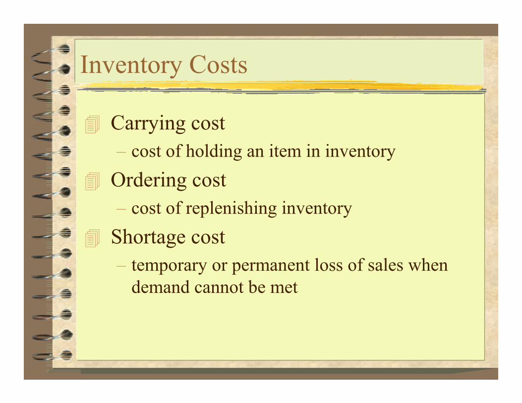
Inventory Costs
� Carrying cost
– cost of holding an item in inventory
� Ordering cost
– cost of replenishing inventory
� Shortage cost
– temporary or permanent loss of sales when
demand cannot be met
Holding Costs
� Obsolescence
� Insurance
� Extra staffing
� Interest
� Pilferage
� Damage
� Warehousing
� Etc.
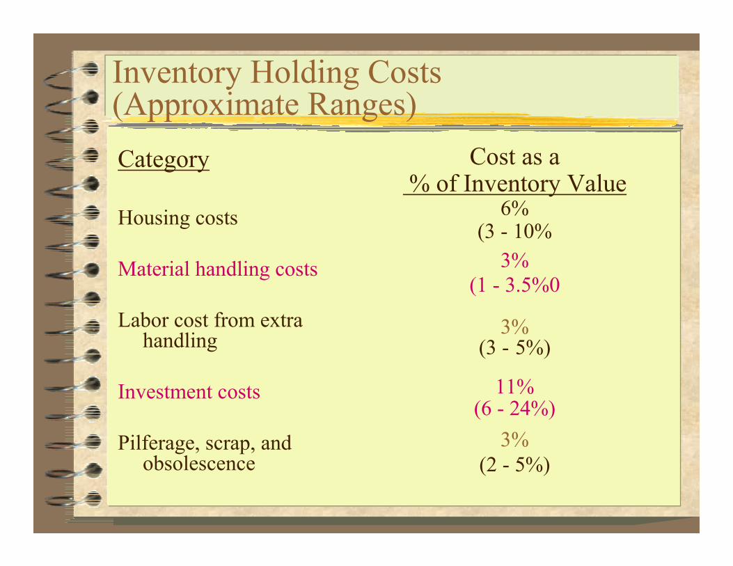
Inventory Holding Costs(Approximate Ranges)
Category
Housing costs
Material handling costs
Labor cost from extra handling
Investment costs
Pilferage, scrap, and obsolescence
Cost as a% of Inventory Value
6%(3 - 10%
3%(1 - 3.5%0
3%(3 - 5%)
11%(6 - 24%)
3%
(2 - 5%)

Ordering Costs
� Supplies
� Forms
� Order processing
� Clerical support
� Etc.
Setup Costs
� Clean-up costs
� Re-tooling costs
� Adjustment costs
� Etc.
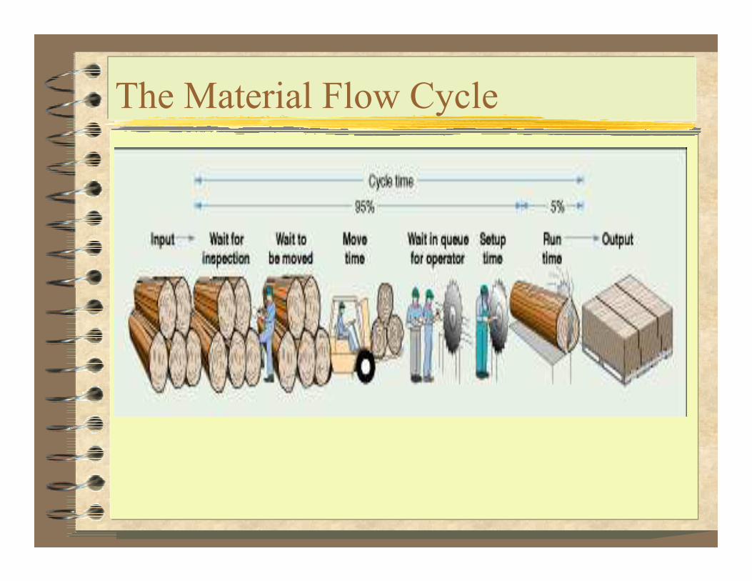
The Material Flow Cycle
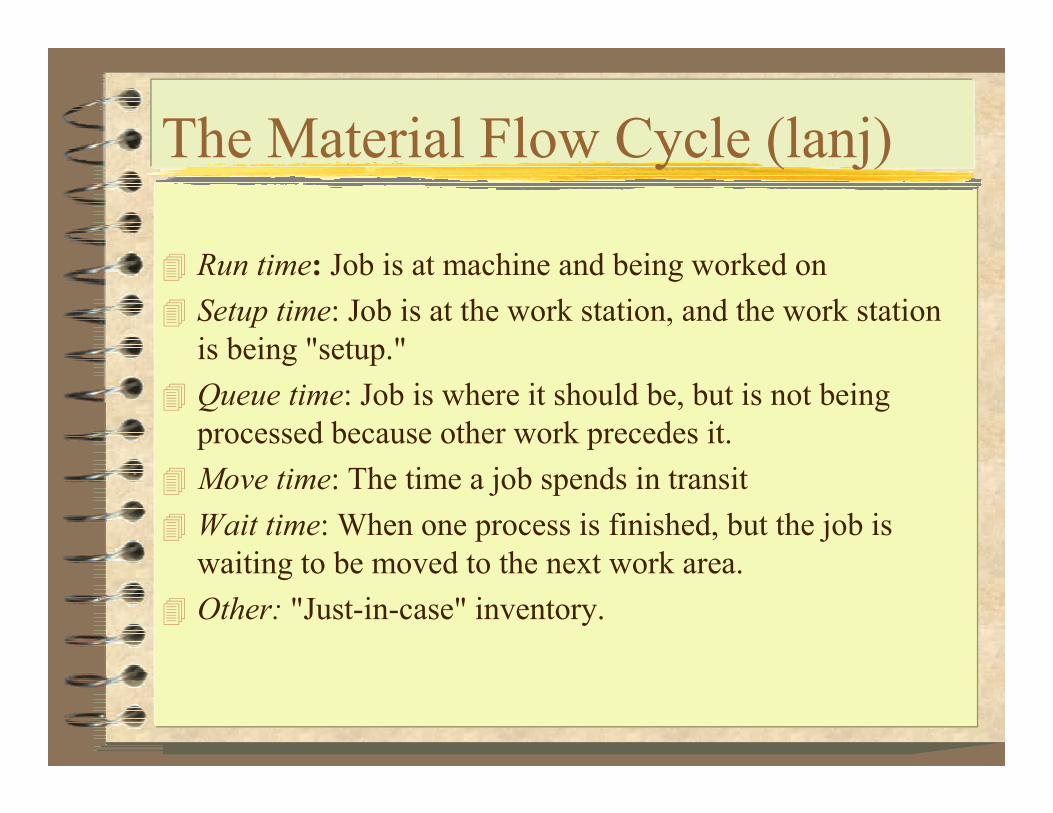
The Material Flow Cycle (lanj)
� Run time: Job is at machine and being worked on
� Setup time: Job is at the work station, and the work station
is being "setup."
� Queue time: Job is where it should be, but is not being
processed because other work precedes it.
� Move time: The time a job spends in transit
� Wait time: When one process is finished, but the job is
waiting to be moved to the next work area.
� Other: "Just-in-case" inventory.
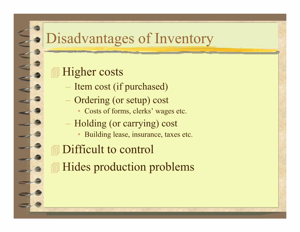
�Higher costs– Item cost (if purchased)
– Ordering (or setup) cost• Costs of forms, clerks’ wages etc.
– Holding (or carrying) cost• Building lease, insurance, taxes etc.
�Difficult to control
�Hides production problems
Disadvantages of Inventory
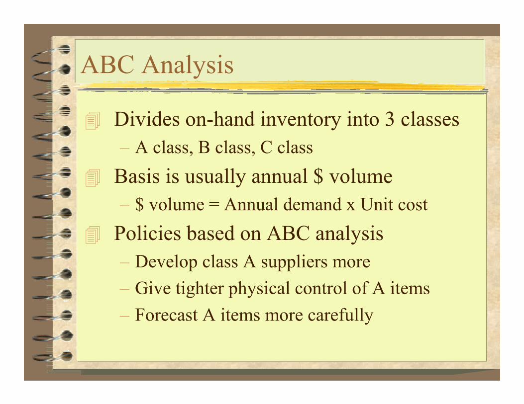
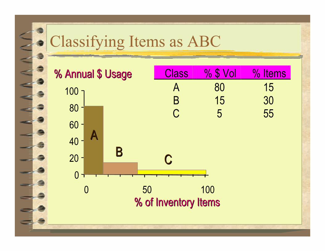
� Divides on-hand inventory into 3 classes
– A class, B class, C class
� Basis is usually annual $ volume
– $ volume = Annual demand x Unit cost
� Policies based on ABC analysis
– Develop class A suppliers more
– Give tighter physical control of A items
– Forecast A items more carefully
ABC Analysis
0
20
40
60
80
100
0 50 100
% of Inventory Items% of Inventory Items
% Annual $ Usage% Annual $ Usage
AA
BBCC
Class % $ Vol % ItemsA 80 15B 15 30C 5 55
Classifying Items as ABC

ABC Classification: Example
��1313--1717
11 $ 60$ 60 9090
22 350350 4040
33 3030 130130
44 8080 6060
55 3030 100100
66 2020 180180
77 1010 170170
88 320320 5050
99 510510 6060
1010 2020 120120
PARTPART UNIT COSTUNIT COST ANNUAL USAGEANNUAL USAGE

ABC Classification: Example (cont.)
��1313--1818
Example 10.1Example 10.1
11 $ 60$ 60 9090
22 350350 4040
33 3030 130130
44 8080 6060
55 3030 100100
66 2020 180180
77 1010 170170
88 320320 5050
99 510510 6060
1010 2020 120120
PARTPART UNIT COSTUNIT COST ANNUAL USAGEANNUAL USAGETOTAL % OF TOTAL % OF TOTALPART VALUE VALUE QUANTITY % CUMMULATIVE
9 $30,600 35.9 6.0 6.08 16,000 18.7 5.0 11.02 14,000 16.4 4.0 15.01 5,400 6.3 9.0 24.04 4,800 5.6 6.0 30.03 3,900 4.6 10.0 40.06 3,600 4.2 18.0 58.05 3,000 3.5 13.0 71.0
10 2,400 2.8 12.0 83.07 1,700 2.0 17.0 100.0
$85,400
AA
BB
CC
% OF TOTAL % OF TOTALCLASS ITEMS VALUE QUANTITY
A 9, 8, 2 71.0 15.0B 1, 4, 3 16.5 25.0C 6, 5, 10, 7 12.5 60.0
Techniques for Controlling Service Inventory Include:
�Good personnel selection, training, and
discipline
�Tight control of incoming shipments
�Effective control of all goods leaving the
facility

� Fixed order-quantity
models
– Economic order quantity
– Production order quantity
– Quantity discount
� Probabilistic models
� Fixed order-period models
Help answer the
inventory planning
questions!
Help answer the
inventory planning
questions!
© 1984-1994 T/Maker Co.
Inventory Models
� Known and constant demand
� Known and constant lead time
� Instantaneous receipt of material
� No quantity discounts
� Only order (setup) cost and holding cost
� No stockouts
EOQ Assumptions

Order QuantityOrder Quantity
Annual CostAnnual Cost
Holding
Cost C
urve
Holding
Cost C
urve
Total Co
st Curve
Total Co
st Curve
Order (Setup) Cost CurveOrder (Setup) Cost Curve
Optimal Optimal
Order Quantity (Q*)Order Quantity (Q*)
EOQ Model, How Much to Order?

�More units must be stored if more are ordered
Purchase Order
Description Qty.
Microwave 1
Order quantityOrder quantity
Purchase Order
Description Qty.
Microwave 1000
Order quantityOrder quantity
Why Holding Costs Increase
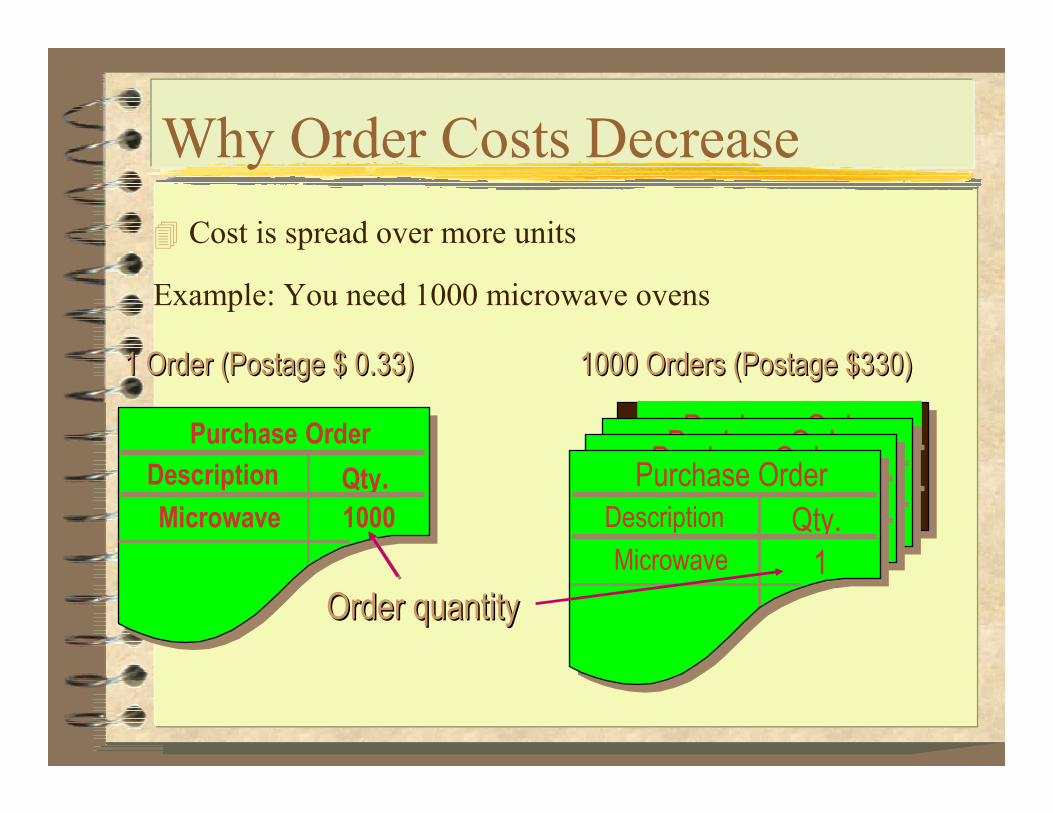
� Cost is spread over more units
Example: You need 1000 microwave ovens
Purchase Order
Description Qty.
Microwave 1
Purchase Order
Description Qty.
Microwave 1
Purchase Order
Description Qty.
Microwave 1
Purchase OrderDescription Qty.Microwave 1
1 Order (Postage $ 0.33)1 Order (Postage $ 0.33) 1000 Orders (Postage $330)1000 Orders (Postage $330)
Order quantityOrder quantity
Purchase Order
Description Qty.Microwave 1000
Why Order Costs Decrease

Deriving an EOQ
� Develop an expression for setup or
ordering costs
� Develop an expression for holding cost
� Set setup cost equal to holding cost
� Solve the resulting equation for the best
order quantity
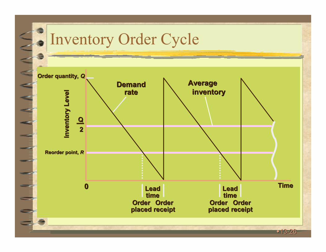
Inventory Order Cycle
��1313--2626
Demand Demand raterate
TimeTimeLead Lead timetime
Lead Lead timetime
Order Order placedplaced
Order Order placedplaced
Order Order receiptreceipt
Order Order receiptreceipt
Inven
tory
Le
vel
Inven
tory
Le
vel
Reorder point, Reorder point, RR
Order quantity, Order quantity, QQ
00
Average Average
inventoryinventory
22
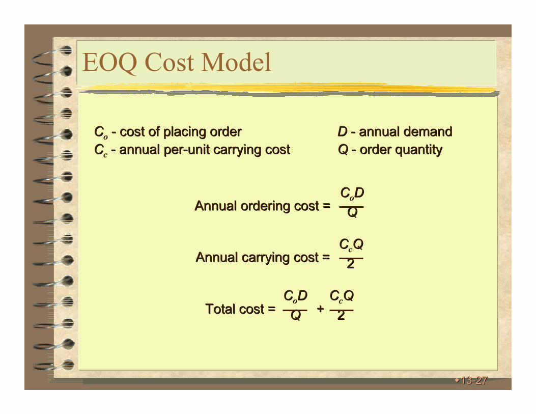
EOQ Cost Model
��1313--2727
CCoo -- cost of placing ordercost of placing order DD -- annual demandannual demand
CCcc -- annual perannual per--unit carrying costunit carrying cost QQ -- order quantityorder quantity
Annual ordering cost =Annual ordering cost =CCooDD
Annual carrying cost =Annual carrying cost =CCccQQ
22
Total cost = +Total cost = +CCooDD
CCccQQ
22
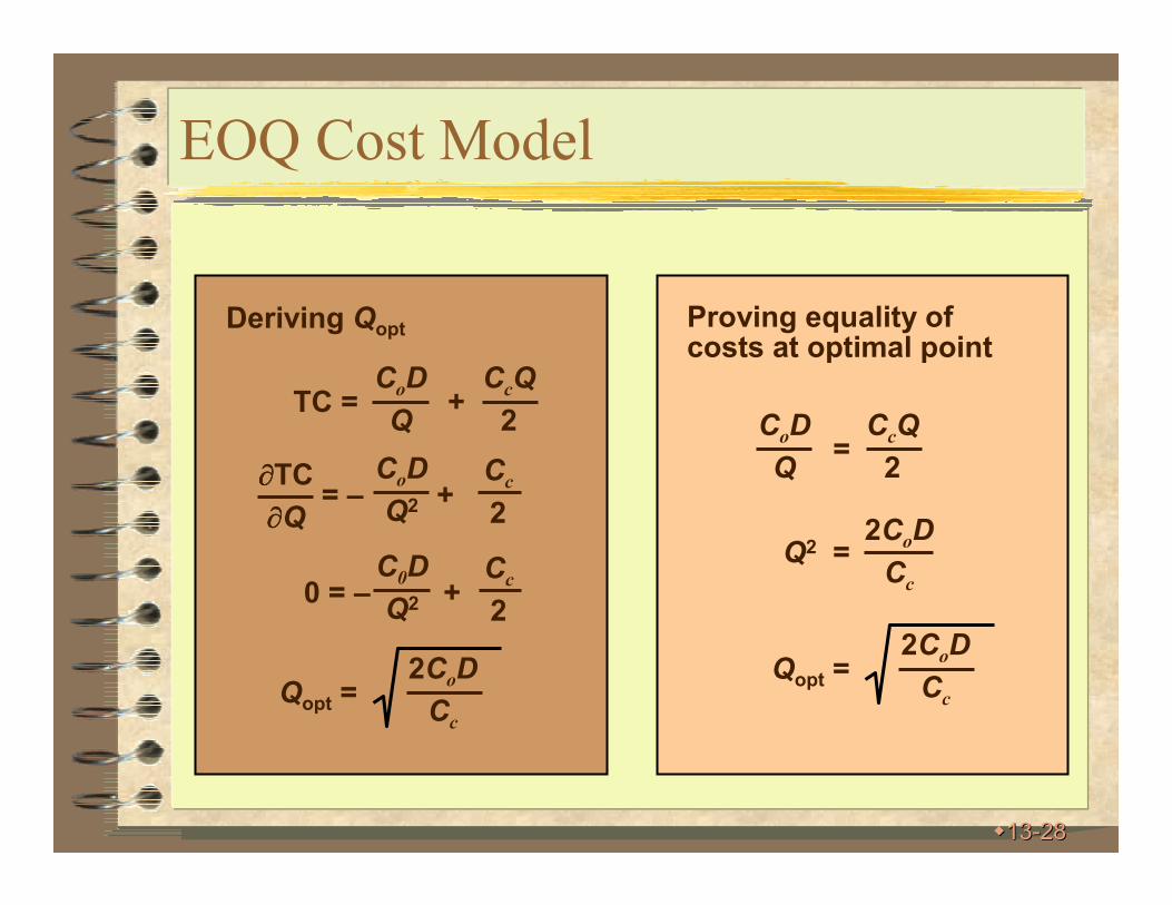
EOQ Cost Model
��1313--2828
TC = +CoD
Q
CcQ
2
= – +CoD
Q2
Cc
2
∂∂∂∂TC
∂∂∂∂Q
0 = – +C0D
Q2
Cc
2
Qopt =2C
oD
Cc
Deriving Qopt Proving equality of costs at optimal point
=CoD
Q
CcQ
2
Q2 =2C
oD
Cc
Qopt =2C
oD
Cc
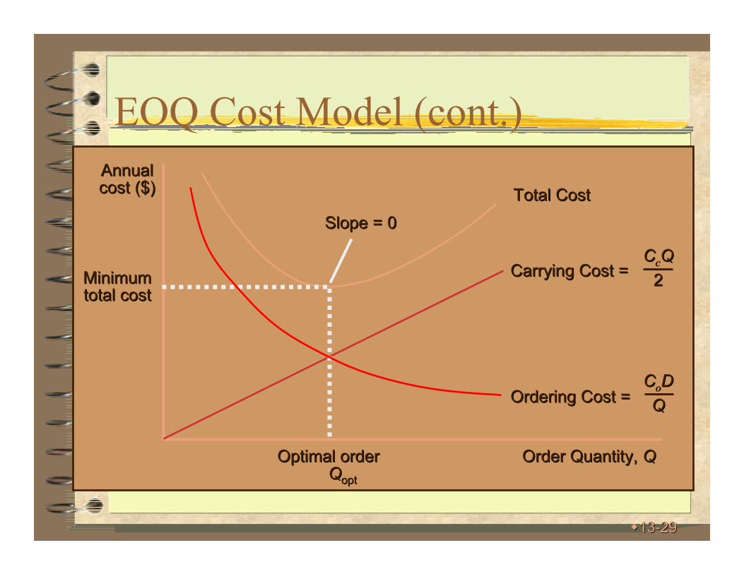
EOQ Cost Model (cont.)
��1313--2929
Order Quantity, Order Quantity, QQ
Annual Annual cost ($)cost ($) Total CostTotal Cost
Carrying Cost =Carrying Cost =CCccQQ
22
Slope = 0Slope = 0
Minimum Minimum total costtotal cost
Optimal orderOptimal orderQQoptopt
Ordering Cost =Ordering Cost =CCooDD

EOQ Example
��1313--3030
CCcc = $0.75 per gallon= $0.75 per gallon CCoo = $150= $150 DD = 10,000 gallons= 10,000 gallons
QQoptopt ==22CCooDD
CCcc
QQoptopt ==2(150)(10,000)2(150)(10,000)
(0.75)(0.75)
QQoptopt = 2,000 gallons= 2,000 gallons
TCTCminmin = += +CCooDD
CCccQQ
22
TCTCminmin = += +(150)(10,000)(150)(10,000)
2,0002,000
(0.75)(2,000)(0.75)(2,000)
22
TCTCminmin = $750 + $750 = $1,500= $750 + $750 = $1,500
Orders per year =Orders per year = DD//QQoptopt
== 10,000/2,00010,000/2,000
== 5 orders/year5 orders/year
Order cycle time =Order cycle time = 311 days/(311 days/(DD//QQoptopt))
== 311/5311/5
== 62.2 store days62.2 store days

EOQ Model, When To Order
Reorder Reorder
Point (ROP)Point (ROP)
TimeTime
Inventory LevelInventory Level
AverageAverage
Inventory Inventory
(Q*/2)(Q*/2)
Lead TimeLead Time
Optimal Optimal
Order Order
QuantityQuantity
(Q*)(Q*)
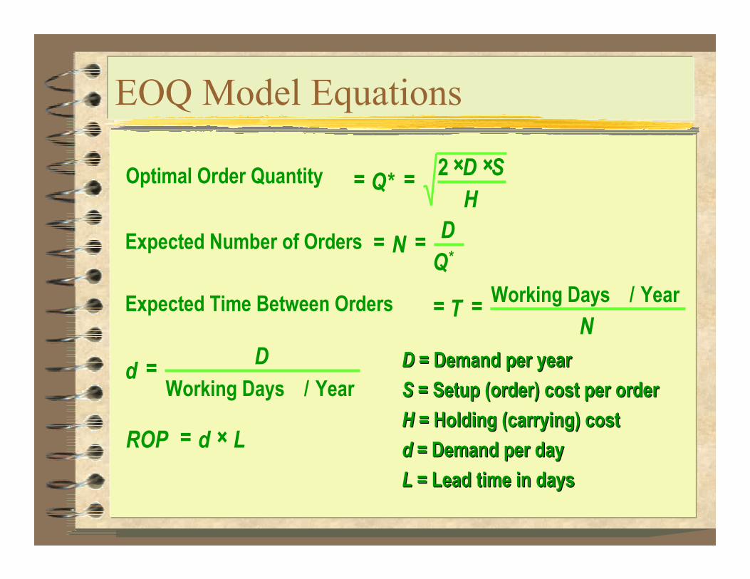
Optimal Order Quantity
Expected Number of Orders
Expected Time Between Orders Working Days / Year
Working Days / Year
= =× ×
= =
= =
=
= ×
Q*D S
H
ND
Q*
TN
dD
ROP d L
2
DD = Demand per year= Demand per year
SS = Setup (order) cost per order= Setup (order) cost per order
HH = Holding (carrying) cost = Holding (carrying) cost
dd = Demand per day= Demand per day
LL = Lead time in days= Lead time in days
EOQ Model Equations