Motivation - Keys To Unlock Your Personal Mojo For Business Success
Upload
wynter-grahamCategory
view
26download
1description
Examination of Analysis Methods for Positive Continuous Dependent Variables: Model Fit and Cost Saving Implications
Brian P Smith Maria De Yoreo
Biostatistics Director Department of Applied Mathematics UC Santa Cruz
May 22, 2013
Midwest Biostatistics Workshop; Muncie, IN

2
Personal Motivation• Compositional Data Analysis Using Liouville Distributions … -
Forgettable Ph.D. Dissertation by BP Smith
• Compositional Data – Multivariate Data That Sum to 1
• Clay – 0.2, Silt - 0.53, Sand - 0.27
• John Aitchison – The Statistical Analysis of Compositional Data
• ln odds – ln (x1/x3), ln(x2/x3) – Bivariate Normal

3
Basic principle
• Underlying distribution should match the sample space of the data
• If using multivariate normal, then must transform compositional data from
Simplex Multivariate Reals
• Could use Dirichlet or Liouville
4
How to follow principle with positive valued data?• log transformation – Positive reals to reals
• Yet, colleagues were using natural scale or percent change from baseline
• Why?
– That was what had always been done
– Central limit theorem protection for type 1 error
• Easy to show with simulation if true distribution is log-normal and use normal distribution to analyze then there is a power loss

5
What do the critics think?
• Real data is not log-normal or normal
• So what factor
• Arguing a theoretical argument for a real world problem

6
Personal Motivation Part 2• It is generally accepted among statisticians that in a clinical trials
the simple use of baseline as a covariate provides more power
• More than once with scientist – “What is this analysis of covariance, we should just do percent change from baseline.”
• “That is the analysis Jennings did in their paper...” Or “this is what Goodguy Pharmaceuticals did in their NDA”
• Me – “But you will lose power” but I have already lost this argument
• There appears to me to be a higher appreciation that good design can affect power than good analysis.

7
What Do I (and Maybe Some of You, if you are like minded) need?• Research that not only suggests that log-transformation is better for
positive data
• But also quantifies how much better
• Research that not only suggests analysis of covariance is better
• But also quantifies how much better
• This should exist, right?
• Not that I can find

8
What Did We Do?
• 70 Continuous Endpoints Analyzed
• 10 Analyses Endpoints Each– 4 Phase 1 Studies
– 1 Phase 2 Study
– 1 Phase 3 Study
• 10 Endpoints Chosen from 3 Preclinical Studies
9
What Did We Do? (cont)
• Chose primary or secondary endpoints if continuous 1-3 per study
• Remaining 7-9 randomly selected from– ECGs
– Vitals
– Laboratory Measurements
• Variety of endpoints from range of studies chosen in non-subjective manner

10
The Analyses• All endpoints had repeated observations over time
• Used Mixed Effect Model– Random subject effect
– Fixed Effects• Treatment
• Time
• Treatment by Time Interaction
– If Cross-over study, additional random effects added
• 8 models examined for each endpoint

11
Eight Models
Identifier Response Covariate for BL?
UN Y no
LN Ln(y) no
UR y-BL no
LR Ln(y/BL) no
PR 100∙(y-BL)/BL no
UC y Yes; BL
LC Ln(y) Yes; ln(BL)
PC 100∙(y-BL)/BL Yes; BL

12
Three Means of Comparison
• For ANCOVA Only– P-value of Covariate
• For Log Scale – Compare Likelihoods
• For All Analyses– Compare Costs

13
How to Compare Costs?• Compare Standard Errors of Estimates for Treatment Effect
• Determine change in sample size that would be needed under one model to obtain a standard error equivalent to that of another model
• Scaling Issue due to log-transformation
• If no scaling issue and two models
• (se1/se2)2 is how many fold more subjects that analysis 1 would need to have the same standard error as analysis 2

14
Dealing with the Scaling Issue
• Natural Scale
• Log Scale – Consider
• If start with log scale and work towards natural scale
)()( ptnptn xxsexxse
)()( ptpntn xxxsexse
))exp()(exp()exp()exp( ptplt yyysey
)1))(exp(exp( lt sey
)1)(exp( lt sex

15
Which to use?
• If data is skewed right then
Geometric Mean < Mean
• Use of the mean favors the natural scale (most conservative)
• Use of geometric mean more consistent with data
• We do both but
• Prefer Geometric Mean
)1))(exp(exp( lt sey )1)(exp( lt sex
16
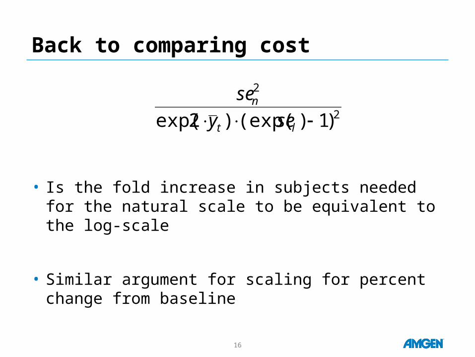
Back to comparing cost
• Is the fold increase in subjects needed for the natural scale to be equivalent to the log-scale
• Similar argument for scaling for percent change from baseline
2
2
)1)(exp()2exp( lt
n
sey
se
17
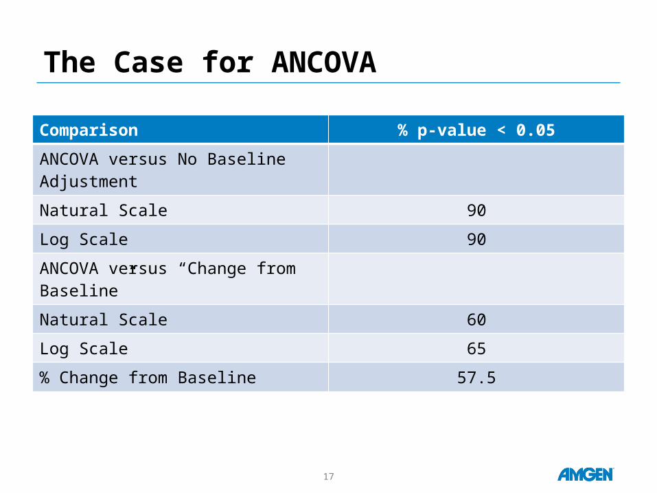
The Case for ANCOVA
Comparison % p-value < 0.05
ANCOVA versus No Baseline Adjustment
Natural Scale 90
Log Scale 90
ANCOVA versus “Change from Baseline”
Natural Scale 60
Log Scale 65
% Change from Baseline 57.5

18
The Case for ANCOVA Cont.
Comparison Average Fold-Increase In Sample Size
ANCOVA versus No Baseline Adjustment
Natural Scale 3.32
Log Scale 3.72
ANCOVA versus “Change from Baseline”
Natural Scale 1.25
Log Scale 1.48
% Change from Baseline 1.29

19
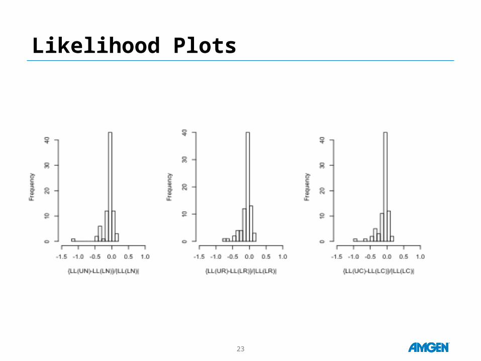
The Case for Log Ratio over Percent Change from Baseline
Comparison % Likelihood Log Ratio > Likelihood Percent Change from
Baseline
No Covariate 80
Covariate 80

20
Likelihood Plots

21
The Case for Log Ratio over Percent Change from Baseline (Cont)
Comparison Average Fold-Increase In Sample Size
With Mean With Geometric Mean
No Covariate 1.14 1.30
Covariate 1.24 1.62

22
The Case for Log over Natural Scale
Comparison % Likelihood Log Ratio > Likelihood Percent Change from
Baseline
No Baseline Adjustiment 80
“Change from Baseline” 79
ANCOVA 82
23
Likelihood Plots

24
The Case for Log Ratio over Natural Scale (Cont)
Comparison Average Fold-Increase In Sample Size
With Mean With Geometric Mean
No Baseline Adjustiment 1.13 1.49
“Change from Baseline” 1.28 1.24
ANCOVA 1.18 1.52
25
Conclusions• Don’t just trust us, do it yourself
• If these results continue to replicate can conclude– If a baseline is available, use of baseline as a covariate should always be
undertaken
– Although we recommend exploration of data from previous studies, percent change from baseline analyses should not be undertaken unless there is strong empirical evidence that for that endpoint it is preferred
– Again with the caveat that nothing replaces exploration of data from previous studies, log-transformation ought to be the default analysis of positive data unless exploration of previous data provides convincing evidence that the natural scale is preferred.