PERIODICAL FOR MINING, METALLURGY AND GEOLOGY … · 2008-04-02 · PERIODICAL FOR MINING,...
152
RMZ-M&G, Vol. 55, No. 1 pp. 1-146 (2008) Ljubljana, February 2008 ISSN 1408-7073 PERIODICAL FOR MINING, METALLURGY AND GEOLOGY RMZ – MATERIALI IN GEOOKOLJE REVIJA ZA RUDARSTVO, METALURGIJO IN GEOLOGIJO
Transcript of PERIODICAL FOR MINING, METALLURGY AND GEOLOGY … · 2008-04-02 · PERIODICAL FOR MINING,...
RMZ-M&G, Vol. 55, No. 1 pp. 1-146 (2008)Ljubljana, February 2008
ISSN 1408-7073
PERIODICAL FOR MINING, METALLURGY AND GEOLOGY
RMZ – MATERIALI IN GEOOKOLJEREVIJA ZA RUDARSTVO, METALURGIJO IN GEOLOGIJO
II Historical Review
RMZ-M&G 2008, 55
Historical Review
More than 80 years have passed since in 1919 the University Ljubljana in Slovenia was founded. Technical fields were joint in the School of Engineering that included the Geologic and Mining Division while the Metallurgy Division was established in 1939 only. Today the Departments of Geology, Mining and Geotechnology, Materials and Metallurgy are part of the Faculty of Natural Sciences and Engineering, University of Ljubljana.
Before War II the members of the Mining Section together with the Association of Yugoslav Mining and Metallurgy Engineers began to publish the summaries of their research and studies in their technical periodical Rudarski zbornik (Mining Proceed-ings). Three volumes of Rudarski zbornik (1937, 1938 and 1939) were published. The War interrupted the publication and not until 1952 the first number of the new journal Rudarsko-metalurški zbornik - RMZ (Mining and Metallurgy Quarterly) has been pub-lished by the Division of Mining and Metallurgy, University of Ljubljana. Later the journal has been regularly published quarterly by the Departments of Geology, Mining and Geotechnology, Materials and Metallurgy, and the Institute for Mining, Geotech-nology and Environment.
On the meeting of the Advisory and the Editorial Board on May 22nd 1998 Rudarsko-metalurški zbornik has been renamed into “RMZ - Materials and Geoenvironment (RMZ -Materiali in Geookolje)” or shortly RMZ - M&G.
RMZ - M&G is managed by an international advisory and editorial board and is ex-changed with other world-known periodicals. All the papers are reviewed by the cor-responding professionals and experts.
RMZ - M&G is the only scientific and professional periodical in Slovenia, which is pub-lished in the same form nearly 50 years. It incorporates the scientific and professional topics in geology, mining, and geotechnology, in materials and in metallurgy.
The wide range of topics inside the geosciences are welcome to be published in the RMZ -Materials and Geoenvironment. Research results in geology, hydrogeology, mining, geotechnology, materials, metallurgy, natural and antropogenic pollution of environ-ment, biogeochemistry are proposed fields of work which the journal will handle. RMZ - M&G is co-issued and co-financed by the Faculty of Natural Sciences and Engineering Ljubljana, and the Institute for Mining, Geotechnology and Environment Ljubljana. In addition it is financially supported also by the Ministry of Higher Education, Science and Technology of Republic of Slovenia.
Editor in chief
IIITable of Contents – Kazalo
RMZ-M&G 2008, 55
Table of Contents – Kazalo
Internal oxidation of Cu-C and Ag-C compositesNotranja oksidacija Cu-C in Ag-C kompozitov
Čevnik, G., kosec, G., kosec, L., RudoLf, R., kosec, B., AnžeL, i. .............................. 1
Composition and morphology of diborides in Al-Ti-B alloysafter annealing at 1873 K
Sestava in morfologija diboridov v zlitinah Al-Ti-B po žarjenju na 1873 K
ZupAniČ, f. ...................................................................................................................... 7
Tool for programmed open-die forging – case studyOrodje za programsko vodeno prosto kovanje – študija primera
BomBAČ, d., fAZARinc, m., kuGLeR, G., TuRk, R. ........................................................ 19
A laboratory test for simulation of solidification on Gleeble 1500Dthermo-mechanical simulatorLaboratorijski test simulacije strjevanja na termo-mehanskemsimulatorju Gleeble 1500DBRAdAskjA, B., koRuZA, j., fAZARinc, m., knAp, m., TuRk, R. ..................................... 31
Comparative test of active and passive multichannel analysis of surface waves (MASW) methods and microtremor HVSR methodPrimerjalni test aktivne in pasivne večkanalne analize površinskih valov (MASW) ter metode mikrotremorjev (HVSR)GosAR, A., sTopAR, R., RošeR, j. .................................................................................... 41
Application of seismic tomography in investigations of themotorway alignment in the Šentvid tunnel areaUporaba seizmične tomografije pri raziskavah AC trase na območjupredora ŠentvidRošeR, j., sTopAR, R., GosAR, A. .................................................................................... 67
Surveying for geophysical exploration, using a single-frequency global navigation satellite system receiver capable of 30 cm horizontal kinematical positioning uncertaintyUporaba enofrekvenčnega sprejemnika GNSS s 30 cm negotovostjo v kinematičnem načinu dela za terenske geofizikalne preiskavedimc, f., mušiČ, B., osRedkAR, R. ................................................................................. 85
IV Table of Contents – Kazalo
RMZ-M&G 2008, 55
The possibility of using homogeneous (projective) coordinates in 2D measurement exercisesMožnost uporabe homogenih (projektivnih) koordinat v dvodimenzionalnih merskih nalogahGAnić, A., vuLić, m., Runovc, f., HABe, T. ................................................................... 111
How we calculate volume with the use of “NTF” methodKako izračunamo volumen z uporabo metode “NTF”
duRGuTović, A., vuLić, m. ............................................................................................. 127
Strokovna literaturaProfessional literature
kos, m. ........................................................................................................................... 135
Author`s Index, Vol. 55, No. 1 ................................................................................ 136
Instructions to Authors ............................................................................................ 137
Template ...................................................................................................................... 140

1RMZ – Materials and Geoenvironment, Vol. 55, No. 1, pp. 1-6, 2008
Preliminary note
Internal oxidation of Cu-C and Ag-C composites
Notranja oksidacija Cu-C in Ag-C kompozitov
GABRijeLA Čevnik1,3, GoRAZd kosec2,3, LAdisLAv kosec3, ReBekA RudoLf4, BoRuT kosec3, ivAn AnžeL4
1METAL Ravne d.o.o., Koroška cesta 14, SI-2390 Ravne na Koroškem, Slovenia; E-mail: [email protected]
2ACRONI d.o.o., Cesta Borisa Kidriča 44, SI-4270 Jesenice, Slovenia; E-mail: [email protected]
3University of Ljubljana, Faculty of Natural Sciences and Engineering, Aškerčeva cesta 12, SI-1000 Ljubljana, Slovenia; E-mail: [email protected], [email protected]
4University of Maribor, Faculty of Mechanical Engineering, Smetanova ulica 17, SI-2000 Maribor, Slovenia; E-mail: [email protected], [email protected]
Received: December 3, 2007 Accepted: January 11, 2008
Abstract: The internal oxidation in copper-carbon and silver-carbon composites occurs when they are exposed to air or oxygen at high temperature. Solu-bility of carbon in copper or in silver is very low. The kinetics of oxidation at high temperature and activation energy were determined and the mecha-nism of internal oxidation was analysed. The kinetics of internal oxidation was determined for both cases and it is depended from the diffusion of oxygen following parabolic time dependence according to Wagner's theory. The activation energy for Cu-C composite is 70.5 kJ/mol, and for Ag-C composite is 50.1 kJ/mol, what is in both cases close to the activation ener-gy for the volume diffusion of oxygen in copper or in silver. In both cases gas products are formed during the internal oxidation of composites. In the internal oxidation zone pores, bubbles occur. The carbon oxidates directly with the oxygen from solid solution as long there is a contact, which breaks down with the presence of gas products. Then the oxidation occurs over the gas mixture of CO and CO2.
Izvleček: Pri visokih temperaturah kompoziti bakra in srebra z ogljikom na zraku ali v kisiku reagirajo po mehanizmu notranje oksidacije. Topnost ogljika v trdnem bakru in trdnem srebru je zelo majhna. Analizirali smo kinetiko oksidacije kompozitov, določili aktivacijsko energijo in mehanizem notra-nje oksidacije. Kinetika oksidacije je pri obeh skupinah materialov odvisna od difuzije kisika in sledi parabolični odvisnosti od časa v skladu z Wa-gnerjevo teorijo. Aktivacijska energija procesa je za kompozit Cu-C enaka 70,5 kJ/mol, za kompozit Ag-C pa 50,1 kJ/mol, kar je blizu aktivacijski energiji za volumsko difuzijo kisika v trdnem bakru oziroma srebru. Pri
2 Čevnik, G., kosec, G., kosec, L., RudoLf, R., kosec, B., AnžeL, i.
RMZ-M&G 2008, 55
oksidaciji kompozita nastajajo plinski produkti. Oksidacija ogljika poteka neposredno s kisikom iz trdne raztopine, ko pa se zaradi nastanka plinske faze stik prekine, pa preko plinske zmesi CO in CO2.
Key words: internal oxidation, internal oxidation zone (IOZ), composite, copper, silver, diffussion, kinetics
Ključne besede: notranja oksidacija, cona notranje oksidacije (CNO), kompozit, baker, srebro, difuzija, kinetika
IntroductIon
Internal oxidation is a general term for the process taking place under the surface of alloys and including the selective reaction of a less noble composite constituent with oxygen[1,2]. The phenomenon of internal oxidation was first noticed in copper allo-ys with silicon, nickel, tin, manganese and zinc, but it is also seen in silver alloys with additions of less noble alloy constituents[3]. The oxidation of these alloys results in the zone with a typical heterogeneous compo-sition, the so called internal oxidation zone (IOZ)[4,5].
The internal oxidation is a phenomenon that includes several elementary processes with oxygen transmission as the most im-portant factor of growth and morphologi-cal characteristics of the oxidized zone.
Conditions for the process of internal oxi-dation are[4,6]:
larger electronegativity of alloy con-•stituent from the basic metal, larger oxygen solubility in basic metal, •and higher diffusion rate of oxygen in ba-•sic metal in comparison with the diffu-sion rate of alloy constituent.
Special examples require additional condi-
tions like the maximal concentration of al-loy constituent, oxidation temperature and partial oxygen pressure in atmosphere. All these influence the transmission process from the internal to external oxidation or passivation.
theoretIcal prIncIples
The first theoretic analysis being the principle of further research was made by Wagner[4] who used his own principle mathematic pattern for the caluclation of process kinetics to explore typical exam-ples of internal oxidation in different allo-ys.
The discussed examples of oxidation of Cu-C and Ag-C composites belong to the examples of internal oxidation of two-phase alloys. Copper and silver dissolve a small portion of carbon in both liquid and solid state, and do not create compouds with carbon. Therefore their composites are two-phase composites and consist of a matrix and carbon particles.
Copper and silver meet the conditions that are necessary for internal oxidation:
both metals are more noble than carbon, •oxygen solubility in both metals is relati-•vely high, and
3Internal oxidation of Cu-C and Ag-C composites
RMZ-M&G 2008, 55
diffusion rate of oxygen exceeds the •diffusion rate of carbon.
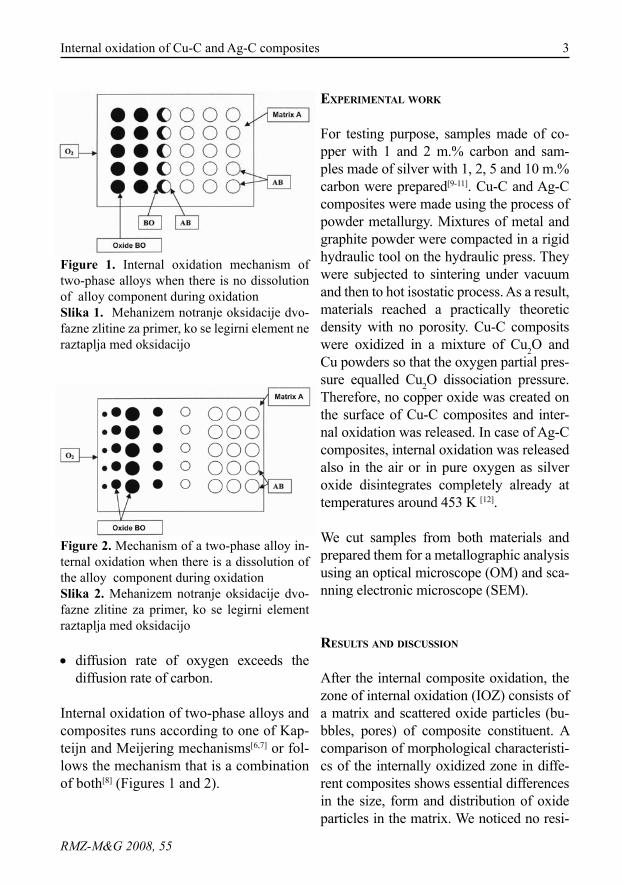
Internal oxidation of two-phase alloys and composites runs according to one of Kap-teijn and Meijering mechanisms[6,7] or fol-lows the mechanism that is a combination of both[8] (Figures 1 and 2).
Figure 1. Internal oxidation mechanism of two-phase alloys when there is no dissolution of alloy component during oxidationSlika 1. Mehanizem notranje oksidacije dvo-fazne zlitine za primer, ko se legirni element ne raztaplja med oksidacijo
Figure 2. Mechanism of a two-phase alloy in-ternal oxidation when there is a dissolution of the alloy component during oxidationSlika 2. Mehanizem notranje oksidacije dvo-fazne zlitine za primer, ko se legirni element raztaplja med oksidacijo
experImental work
For testing purpose, samples made of co-pper with 1 and 2 m.% carbon and sam-ples made of silver with 1, 2, 5 and 10 m.% carbon were prepared[9-11]. Cu-C and Ag-C composites were made using the process of powder metallurgy. Mixtures of metal and graphite powder were compacted in a rigid hydraulic tool on the hydraulic press. They were subjected to sintering under vacuum and then to hot isostatic process. As a result, materials reached a practically theoretic density with no porosity. Cu-C composits were oxidized in a mixture of Cu2O and Cu powders so that the oxygen partial pres-sure equalled Cu2O dissociation pressure. Therefore, no copper oxide was created on the surface of Cu-C composites and inter-nal oxidation was released. In case of Ag-C composites, internal oxidation was released also in the air or in pure oxygen as silver oxide disintegrates completely already at temperatures around 453 K [12].
We cut samples from both materials and prepared them for a metallographic analysis using an optical microscope (OM) and sca-nning electronic microscope (SEM).
results and dIscussIon
After the internal composite oxidation, the zone of internal oxidation (IOZ) consists of a matrix and scattered oxide particles (bu-bbles, pores) of composite constituent. A comparison of morphological characteristi-cs of the internally oxidized zone in diffe-rent composites shows essential differences in the size, form and distribution of oxide particles in the matrix. We noticed no resi-
4 Čevnik, G., kosec, G., kosec, L., RudoLf, R., kosec, B., AnžeL, i.
RMZ-M&G 2008, 55
dues of porosity at the microscopic level. We found that the thermodynamic condition for the internal oxidation is met in the Cu-C and Ag-C composites.
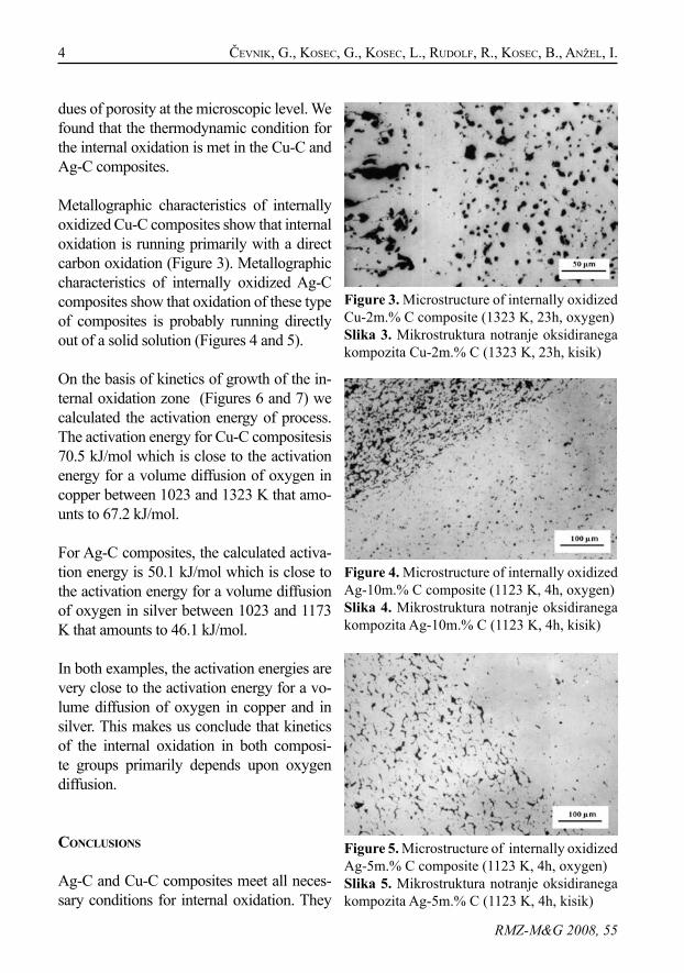
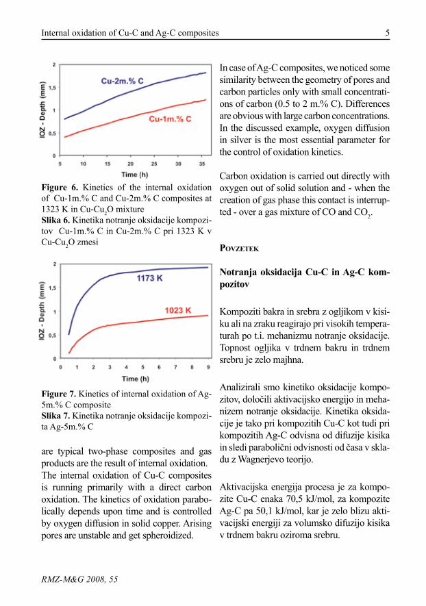
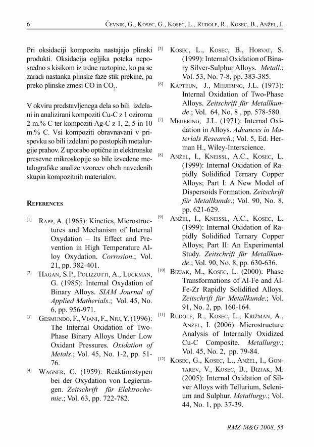
Metallographic characteristics of internally oxidized Cu-C composites show that internal oxidation is running primarily with a direct carbon oxidation (Figure 3). Metallographic characteristics of internally oxidized Ag-C composites show that oxidation of these type of composites is probably running directly out of a solid solution (Figures 4 and 5).
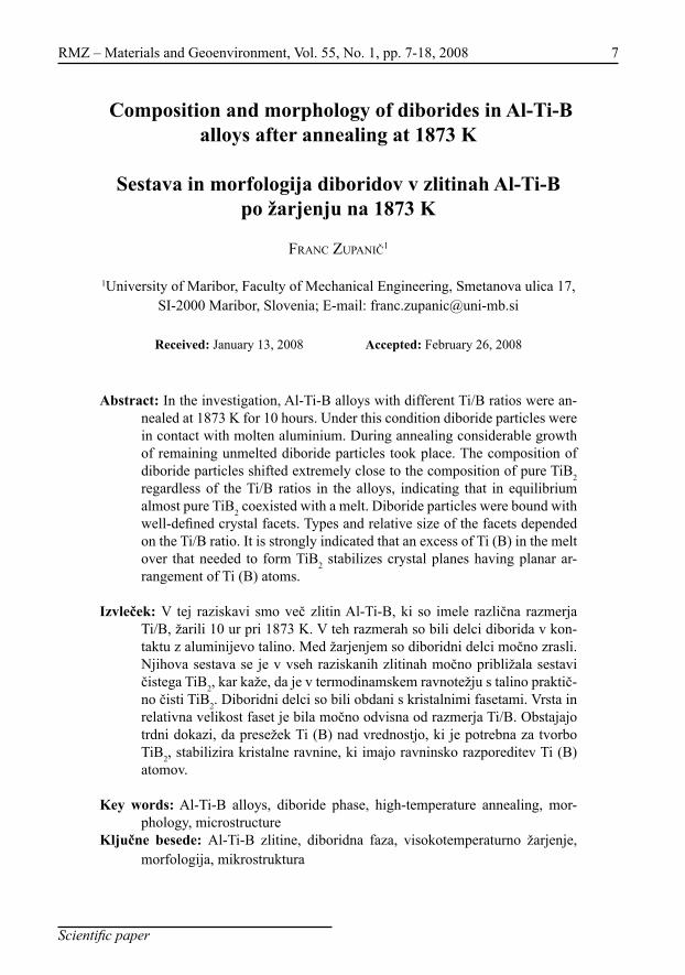
On the basis of kinetics of growth of the in-ternal oxidation zone (Figures 6 and 7) we calculated the activation energy of process. The activation energy for Cu-C compositesis 70.5 kJ/mol which is close to the activation energy for a volume diffusion of oxygen in copper between 1023 and 1323 K that amo-unts to 67.2 kJ/mol.
For Ag-C composites, the calculated activa-tion energy is 50.1 kJ/mol which is close to the activation energy for a volume diffusion of oxygen in silver between 1023 and 1173 K that amounts to 46.1 kJ/mol.
In both examples, the activation energies are very close to the activation energy for a vo-lume diffusion of oxygen in copper and in silver. This makes us conclude that kinetics of the internal oxidation in both composi-te groups primarily depends upon oxygen diffusion.
conclusIons
Ag-C and Cu-C composites meet all neces-sary conditions for internal oxidation. They
Figure 3. Microstructure of internally oxidized Cu-2m.% C composite (1323 K, 23h, oxygen)Slika 3. Mikrostruktura notranje oksidiranega kompozita Cu-2m.% C (1323 K, 23h, kisik)
Figure 4. Microstructure of internally oxidized Ag-10m.% C composite (1123 K, 4h, oxygen)Slika 4. Mikrostruktura notranje oksidiranega kompozita Ag-10m.% C (1123 K, 4h, kisik)
Figure 5. Microstructure of internally oxidized Ag-5m.% C composite (1123 K, 4h, oxygen)Slika 5. Mikrostruktura notranje oksidiranega kompozita Ag-5m.% C (1123 K, 4h, kisik)
5Internal oxidation of Cu-C and Ag-C composites
RMZ-M&G 2008, 55
Figure 6. Kinetics of the internal oxidation of Cu-1m.% C and Cu-2m.% C composites at 1323 K in Cu-Cu2O mixtureSlika 6. Kinetika notranje oksidacije kompozi-tov Cu-1m.% C in Cu-2m.% C pri 1323 K v Cu-Cu2O zmesi
Figure 7. Kinetics of internal oxidation of Ag-5m.% C compositeSlika 7. Kinetika notranje oksidacije kompozi-ta Ag-5m.% C
are typical two-phase composites and gas products are the result of internal oxidation. The internal oxidation of Cu-C composites is running primarily with a direct carbon oxidation. The kinetics of oxidation parabo-lically depends upon time and is controlled by oxygen diffusion in solid copper. Arising pores are unstable and get spheroidized.
In case of Ag-C composites, we noticed some similarity between the geometry of pores and carbon particles only with small concentrati-ons of carbon (0.5 to 2 m.% C). Differences are obvious with large carbon concentrations. In the discussed example, oxygen diffusion in silver is the most essential parameter for the control of oxidation kinetics.
Carbon oxidation is carried out directly with oxygen out of solid solution and - when the creation of gas phase this contact is interrup-ted - over a gas mixture of CO and CO2.
povzetek
Notranja oksidacija Cu-C in Ag-C kom-pozitov
Kompoziti bakra in srebra z ogljikom v kisi-ku ali na zraku reagirajo pri visokih tempera-turah po t.i. mehanizmu notranje oksidacije. Topnost ogljika v trdnem bakru in trdnem srebru je zelo majhna.
Analizirali smo kinetiko oksidacije kompo-zitov, določili aktivacijsko energijo in meha-nizem notranje oksidacije. Kinetika oksida-cije je tako pri kompozitih Cu-C kot tudi pri kompozitih Ag-C odvisna od difuzije kisika in sledi parabolični odvisnosti od časa v skla-du z Wagnerjevo teorijo.
Aktivacijska energija procesa je za kompo-zite Cu-C enaka 70,5 kJ/mol, za kompozite Ag-C pa 50,1 kJ/mol, kar je zelo blizu akti-vacijski energiji za volumsko difuzijo kisika v trdnem bakru oziroma srebru.
6 Čevnik, G., kosec, G., kosec, L., RudoLf, R., kosec, B., AnžeL, i.
RMZ-M&G 2008, 55
Pri oksidaciji kompozita nastajajo plinski produkti. Oksidacija ogljika poteka nepo-sredno s kisikom iz trdne raztopine, ko pa se zaradi nastanka plinske faze stik prekine, pa preko plinske zmesi CO in CO2.
V okviru predstavljenega dela so bili izdela-ni in analizirani kompoziti Cu-C z 1 oziroma 2 m.% C ter kompoziti Ag-C z 1, 2, 5 in 10 m.% C. Vsi kompoziti obravnavani v pri-spevku so bili izdelani po postopkih metalur-gije prahov. Z uporabo optične in elektronske presevne mikroskopije so bile izvedene me-talografske analize vzorcev obeh navedenih skupin kompozitnih materialov.
references
[1] RApp, A. (1965): Kinetics, Microstruc-tures and Mechanism of Internal Oxydation – Its Effect and Pre-vention in High Temperature Al-loy Oxydation. Corrosion.; Vol. 21, pp. 382-401.
[2] HAGAn, s.p., poLiZZoTTi, A., LuckmAn, G. (1985): Internal Oxydation of Binary Alloys. SIAM Journal of Applied Matherials.; Vol. 45, No. 6, pp. 956-971.
[3] Gesmundo, f., viAni, f., niu, Y. (1996): The Internal Oxidation of Two-Phase Binary Alloys Under Low Oxidant Pressures. Oxidation of Metals.; Vol. 45, No. 1-2, pp. 51-76.
[4] WAGneR, c. (1959): Reaktionstypen bei der Oxydation von Legierun-gen. Zeitschrift für Elektroche-mie.; Vol. 63, pp. 722-782.
[5] kosec, L., kosec, B., HoRvAT, s. (1999): Internal Oxidation of Bina-ry Silver-Sulphur Alloys. Metall.; Vol. 53, No. 7-8, pp. 383-385.
[6] kApTeijn, j., meijeRinG, j.L. (1973): Internal Oxidation of Two-Phase Alloys. Zeitschrift für Metallkun-de.; Vol. 64, No. 8 , pp. 578-580.
[7] meijeRinG, j.L. (1971): Internal Oxi-dation in Alloys. Advances in Ma-terials Research.; Vol. 5, Ed. Her-man H., Wiley-Interscience.
[8] AnžeL, i., kneissL, A.c., kosec, L. (1999): Internal Oxidation of Ra-pidly Solidified Ternary Copper Alloys; Part I: A New Model of Dispersoids Formation. Zeitschrift für Metallkunde.; Vol. 90, No. 8, pp. 621-629.
[9] AnžeL, i., kneissL, A.c., kosec, L. (1999): Internal Oxidation of Ra-pidly Solidified Ternary Copper Alloys; Part II: An Experimental Study. Zeitschrift für Metallkun-de.; Vol. 90, No. 8, pp. 630-636.
[10] BiZjAk, m., kosec, L. (2000): Phase Transformations of Al-Fe and Al-Fe-Zr Rapidly Solidified Alloys. Zeitschrift für Metallkunde.; Vol. 91, No. 2, pp. 160-164.
[11] RudoLf, R., kosec, L., kRižmAn, A., AnžeL, I. (2006): Microstructure Analysis of Internally Oxidized Cu-C Composite. Metallurgy.; Vol. 45, No. 2, pp. 79-84.
[12] kosec, G., kosec, L., AnžeL, i., Gon-TARev, v., kosec, B., BiZjAk, m. (2005): Internal Oxidation of Sil-ver Alloys with Tellurium, Seleni-um and Sulphur. Metallurgy.; Vol. 44, No. 1, pp. 37-39.
7RMZ – Materials and Geoenvironment, Vol. 55, No. 1, pp. 7-18, 2008
Scientific paper
Composition and morphology of diborides in Al-Ti-B alloys after annealing at 1873 K
Sestava in morfologija diboridov v zlitinah Al-Ti-B po žarjenju na 1873 K
fRAnc ZupAniČ1
1University of Maribor, Faculty of Mechanical Engineering, Smetanova ulica 17, SI-2000 Maribor, Slovenia; E-mail: [email protected]
Received: January 13, 2008 Accepted: February 26, 2008
Abstract: In the investigation, Al-Ti-B alloys with different Ti/B ratios were an-nealed at 1873 K for 10 hours. Under this condition diboride particles were in contact with molten aluminium. During annealing considerable growth of remaining unmelted diboride particles took place. The composition of diboride particles shifted extremely close to the composition of pure TiB2 regardless of the Ti/B ratios in the alloys, indicating that in equilibrium almost pure TiB2 coexisted with a melt. Diboride particles were bound with well-defined crystal facets. Types and relative size of the facets depended on the Ti/B ratio. It is strongly indicated that an excess of Ti (B) in the melt over that needed to form TiB2 stabilizes crystal planes having planar ar-rangement of Ti (B) atoms.
Izvleček: V tej raziskavi smo več zlitin Al-Ti-B, ki so imele različna razmerja Ti/B, žarili 10 ur pri 1873 K. V teh razmerah so bili delci diborida v kon-taktu z aluminijevo talino. Med žarjenjem so diboridni delci močno zrasli. Njihova sestava se je v vseh raziskanih zlitinah močno približala sestavi čistega TiB2, kar kaže, da je v termodinamskem ravnotežju s talino praktič-no čisti TiB2. Diboridni delci so bili obdani s kristalnimi fasetami. Vrsta in relativna velikost faset je bila močno odvisna od razmerja Ti/B. Obstajajo trdni dokazi, da presežek Ti (B) nad vrednostjo, ki je potrebna za tvorbo TiB2, stabilizira kristalne ravnine, ki imajo ravninsko razporeditev Ti (B) atomov.
Key words: Al-Ti-B alloys, diboride phase, high-temperature annealing, mor-phology, microstructure
Ključne besede: Al-Ti-B zlitine, diboridna faza, visokotemperaturno žarjenje, morfologija, mikrostruktura
8 ZupAniČ, f.
RMZ-M&G 2008, 55
IntroductIon
It is believed that particles of the diboride phase (Al,Ti)B2 present in Al-Ti-B alloys play the most important role in the grain-refining process in aluminium alloys[1,2]. Therefore, they were the subject of several investigations[1-5]. The results show that during manufacturing of Al-Ti-B alloys by an aluminothermic synthesis the diboride phase is formed with compositions rang-ing from that of the stoichiometric AlB2 to that of the stoichiometric TiB2
[1-3]. All di-borides, pure AlB2 and TiB2, as well as the mixed diboride (AlxTi1-x)B2 (0 < x < 1) pos-ses the same crystal structure (space group P6/mmm, Ref. 6) and very similar lattice parameters (see Figure 1). On this ground it was suggested that the mixed diboride phase (AlxTi1-x)B2 represents a thermody-namically stable phase in the aluminium-
rich corner of the Al-Ti-B ternary system[7]. However, some experimental results do not support this assumption[2,8]. joHnsson and jAnsson[2] found out that the composition of the mixed diboride moved toward the compositions of pure TiB2 and AlB2 during holding in liquid aluminium. In addition, it was discovered that during synthesis of Al-Ti-B alloys by arc melting almost pure AlB2 and TiB2 formed. Furthermore, the formation of the mixed diboride (AlxTi1-x)B2 from pure diborides AlB2 and TiB2 did not take place even after exposure for 1000 h at 1073 K[8].
However, 1073 K is relatively low temper-ature since it amounts only 0.3 Tm of TiB2, where Tm indicates melting temperature of pure TiB2: 3498 K[9]. This could mean that even if the mixed boride would be a ther-modynamically stable phase, the transfor-
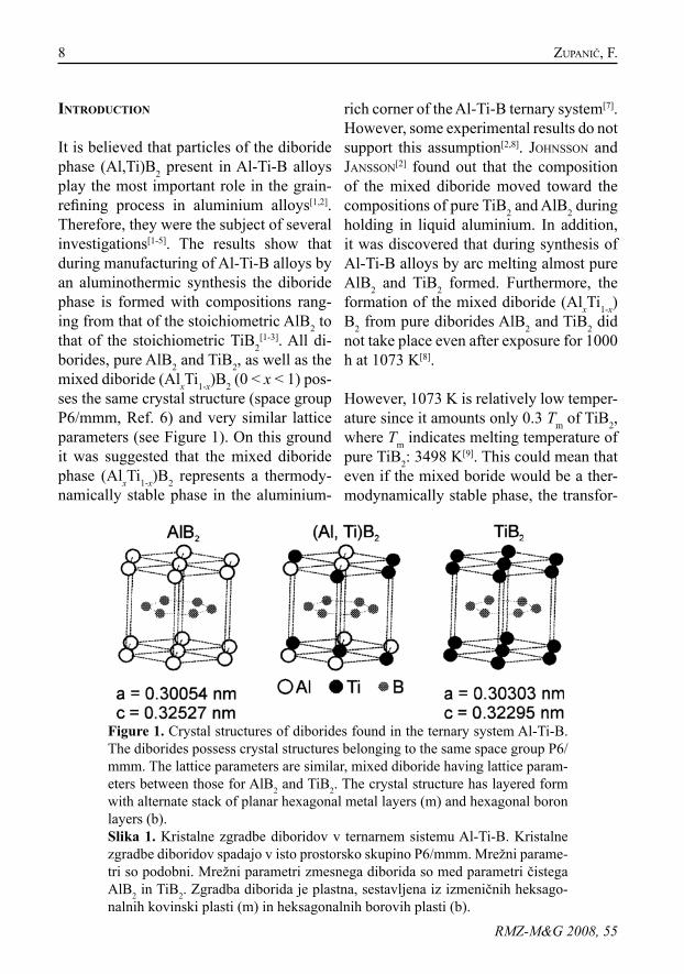
Figure 1. Crystal structures of diborides found in the ternary system Al-Ti-B. The diborides possess crystal structures belonging to the same space group P6/mmm. The lattice parameters are similar, mixed diboride having lattice param-eters between those for AlB2 and TiB2. The crystal structure has layered form with alternate stack of planar hexagonal metal layers (m) and hexagonal boron layers (b).Slika 1. Kristalne zgradbe diboridov v ternarnem sistemu Al-Ti-B. Kristalne zgradbe diboridov spadajo v isto prostorsko skupino P6/mmm. Mrežni parame-tri so podobni. Mrežni parametri zmesnega diborida so med parametri čistega AlB2 in TiB2. Zgradba diborida je plastna, sestavljena iz izmeničnih heksago-nalnih kovinski plasti (m) in heksagonalnih borovih plasti (b).
9Composition and morphology of diborides in Al-Ti-B alloys...
RMZ-M&G 2008, 55
mation of pure AlB2 and TiB2 to the mixed diboride (AlxTi1-x)B2 might be suppressed by kinetic reasons. Annealing of Al-Ti-B alloys containing both pure AlB2 and TiB2 is not possible at much higher tempera-tures that should allow completion of the transformation in shorter times, because AlB2 would transform via a peritectic reac-tion to the liquid phase and α-AlB12 above 1253 K[10]. As a consequence, the diboride phase can be studied at higher temperatures only in equilibrium with other phases.
In this work some Al-Ti-B alloys with dif-ferent Ti/B ratios were heated to 1873 k. This temperature exceeded 0.5 Tm of TiB2, therefore in these conditions kinetic ob-stacles for achieving heterogeneous equi-librium between diboride phase and alu-minium melt should be eliminated. The main purpose of the work was to determine the composition of the diboride phase co-existing with the liquid phase in order to contribute new information for the con-stitution of the ternary system Al-Ti-B. In addition, special attention was paid to the influence of Ti/B ratio on the morphology of diboride particles.
experImental
Annealing of alloysIn this investigation samples of Al-Ti-B alloys were manufactured by an alumino-thermic reduction of Ti and B from K2TiF6 and KBF4 salts, respectively. The chemi-cal compositions of the alloys are given in Table 1. Details of alloy preparation can be found elsewhere[12]. Before annealing at 1873 K the samples were put into small alumina crucibles situated inside a covered
alumina vessel. The annealing took place in a high temperature furnace ASTRO in an argon atmosphere. Heating and cooling rates were 60 K/min, whereas the holding time at 1873 K was 10 hours.
Metallographic preparationSamples for the light (LM) and scan-ning electron microscopy (SEM) were prepared using standard metallographic techniques[13]. The samples were polished directly before analyses with energy dis-persive spectroscopy (EDS) to remove possible etching products and oxide layers on the investigated surface.
For investigation of the morphology of di-boride particles deep etching was applied using two different etchants: (1) a solution consisting of 50 % HCl and water, and (2) a methanol-iodine solution (30 ml metha-nol, 3 g tartaric acid and 1 g iodine). Sat-isfying results were obtained after 10-15 min etching in the HCl solution and 1-2 hours etching in the methanol-iodine solu-tion. It is important to stress that the mor-
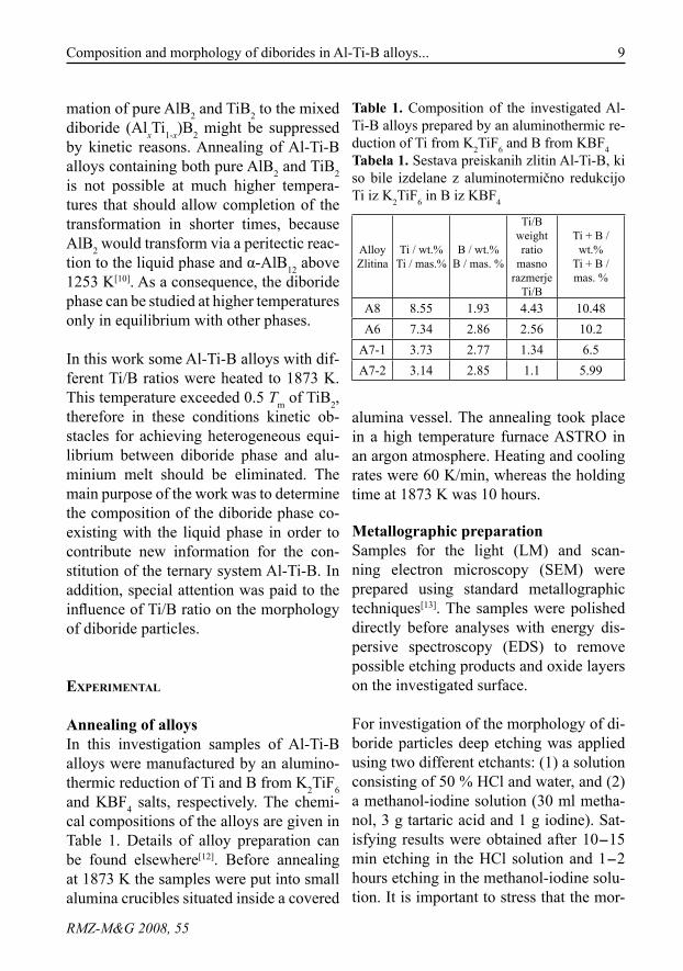
Table 1. Composition of the investigated Al-Ti-B alloys prepared by an aluminothermic re-duction of Ti from K2TiF6 and B from KBF4Tabela 1. Sestava preiskanih zlitin Al-Ti-B, ki so bile izdelane z aluminotermično redukcijo Ti iz K2TiF6 in B iz KBF4
AlloyZlitina
Ti / wt.%Ti / mas.%
B / wt.%B / mas. %
Ti/B weight ratio
masno razmerje
Ti/B
Ti + B / wt.%
Ti + B / mas. %
A8 8.55 1.93 4.43 10.48A6 7.34 2.86 2.56 10.2
A7-1 3.73 2.77 1.34 6.5A7-2 3.14 2.85 1.1 5.99
10 ZupAniČ, f.
RMZ-M&G 2008, 55
phology of diboride particles in each alloy was the same regardless of the applied etchant. This strongly indicates that both etchants dissolved only aluminium matrix and, what is of utmost importance, did not attack diboride particles.
Energy dispersive spectroscopyEDS was performed in a scanning electron microscope SIRION 400 NC (FEI Com-pany), equipped with an energy dispersive analyser INCA 350 (Oxford Analytical). Boron was mainly determined qualitative-ly, whereas titanium and aluminium were determined quantitatively in all observed phases. We used titanium and aluminium standard spectra obtained from pure tita-nium and aluminium, as well as from pure diborides AlB2 (large AlB2 particles in bi-nary Al-B alloy) and TiB2 (from pure arc-melted TiB2).
X-ray diffractionThe phase composition of alloys was de-termined using an X-ray diffractometer Philipps PW 1710. The general diffrac-tion curves were recorded at a scanning rate of 0.025 °/s (Bragg angle) scan range from 5° to 70° and the detailed diffraction curves with 0.025 °/10 s with a scan range between 33.5° and 35° (around the (100) diboride peak).
The results of X-ray diffraction were pri-marily used for the determination of the di-boride lattice parameters. It was found out that lattice parameters a and c of the dibo-ride phase can be calculated reliably if po-sitions of at least five diffraction peaks can be determined. In some cases only (100) peak was well defined. In this case only the value of a-axis could be calculated.
The composition of the diboride phase – the atomic fraction of aluminium on the metallic sublattice of diboride phase CAl – was estimated on the basis of two criteria:
the deviation of the lattice parameter - a from that of pure TiB2
[3]:
(1)
the deviation of the axis ratio - c/a from that of pure TiB2
[4]:
2
2 2
TiBAl
AlB TiB
/ ( / )100 %
( / ) ( / )c a c a
Cc a c a
−=
−
(2)
results and dIscussIon
The compositions of Al-Ti-B alloys were chosen so that the diboride phase should exists in the equilibrium with the liquid phase at the annealing temperature (1873 K). During heating of Al-Ti-B alloys all other phases present initially (e.g. Al3Ti, α-AlB12, AlB2) were melted completely, only the titanium-rich diboride remained partly unmelted. To estimate the quantity of unmelted TiB2 the solubility product proposed by siGWoRTH[14] was used:
2Ti Blog ( )( ) 8.526 16,043/w w T= − (3)
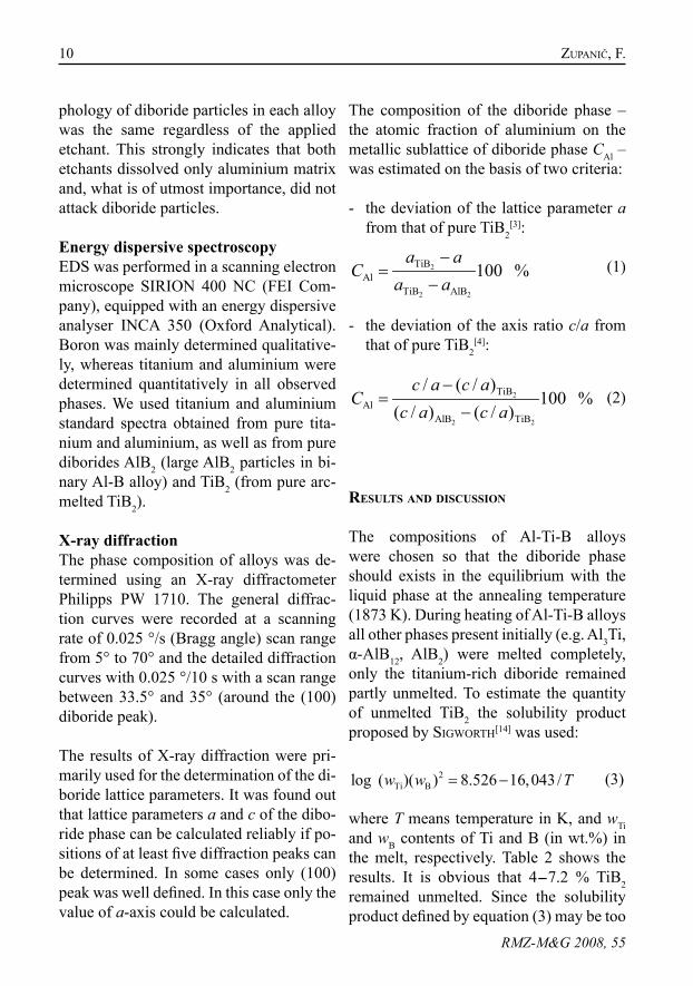
where T means temperature in K, and wTi and wB contents of Ti and B (in wt.%) in the melt, respectively. Table 2 shows the results. It is obvious that 4-7.2 % TiB2 remained unmelted. Since the solubility product defined by equation (3) may be too
2
2 2
TiBAl
TiB AlB
100 %a a
Ca a
−=
−
11Composition and morphology of diborides in Al-Ti-B alloys...
RMZ-M&G 2008, 55
high, the amount of unmelted TiB2 is to be slightly higher.
Morphology of diboride particlesThe size of the diboride particles in the ini-tial state (after aluminothermic reduction) rarely exceeded 1 µm (Figure 2). In alloys with hypostoichiometric and stoichiomet-ric composition (Ti/B ≤ 2.21) agglomer-ates of diboride particles in Al-rich solid solution could be observed. In alloys with hiperstoichiometric composition, in addi-tion to boride agglomerates also Al3Ti par-ticles were present.
However, during annealing at 1873 K very large hexagonal plates of the titanium-rich diboride formed. The height of the plates often exceeded 5 µm and their edge 10 µm (Figures 3 and 4).
All diboride particles were bound with very well defined crystal faces; however their morphology was not the same in all investigated alloys. In the alloy A7-1 hav-ing an excess of B over that needed for
Table 2. Concentration of titanium and boron in the liquid phase and the quantity of unmelted TiB2 at 1873 K using equation (3)Tabela 2. Koncentracija titana in bora v talini in količina nestaljenega TiB2 pri 1873 K, izra-čunana z uporabo enačbe (3)
AlloyTi dissolved in the melt /
wt.%
B dissolved in the melt /
wt.%
estimated initial
quantity of TiB2 /
wt.%
unmelted TiB2 at
1873 K / wt.%
A8 5.22 0.42 6.2 4.8A6 2.40 0.62 9.2 7.2
A7-1 0.53 1.32 5.4 4.7A7-2 0.36 1.59 4.6 4
formation of TiB2 (Ti/B) = 1.34, the ba-sal {0001} facets dominate (Figure 4a). Note also traces of the prismatic {1010} and pyramidal facets. It is not possible to determine the Miller-Bravais indices of these pyramidal planes by inspection of deep-etched specimens only. However, it seems possible that their indices could be {hk 01}, h > l, h = –k.
In the near-stoichiometric alloy A6 (Ti/B = 2.56) two additional types of facets were observed (Figure 4b): prismatic {1120} and pyramidal {1121} facets. In the alloy A8 having an excess of Ti over that to form TiB2 (Ti/B = 4.43), the diboride particles were bound by basal {0001} and prismatic {1010}facets (Figure 4c).
To explain the influence of Ti/B ratio on the observed morphology of the diboride particles we must take a closer look to the atomic arrangements in the following crystallographic planes: {0001}, {1010}, {1120}, {1121} and {2201}. In the {0001} planes, boron and titanium atoms form al-ternate planar layers (Figure 1). Thus, the outer layer in the contact with the liquid phase could be occupied only by boron or only by titanium atoms. In the family of {1010}planes only titanium atoms can be arranged in a planar array, whereas the arrangement of boron atoms cannot be planar (Figure 5a). In both {1120} and {1121} families of planes it is not possible to get the planar outer layer occupied by only one kind of atoms, but in each case with both boron and titanium atoms (Fig-ure 5a). On the other hand, boron atoms can be arranged in a planar manner, there-fore the facets of this plane dominate in al-loy A7-1.
12 ZupAniČ, f.
RMZ-M&G 2008, 55
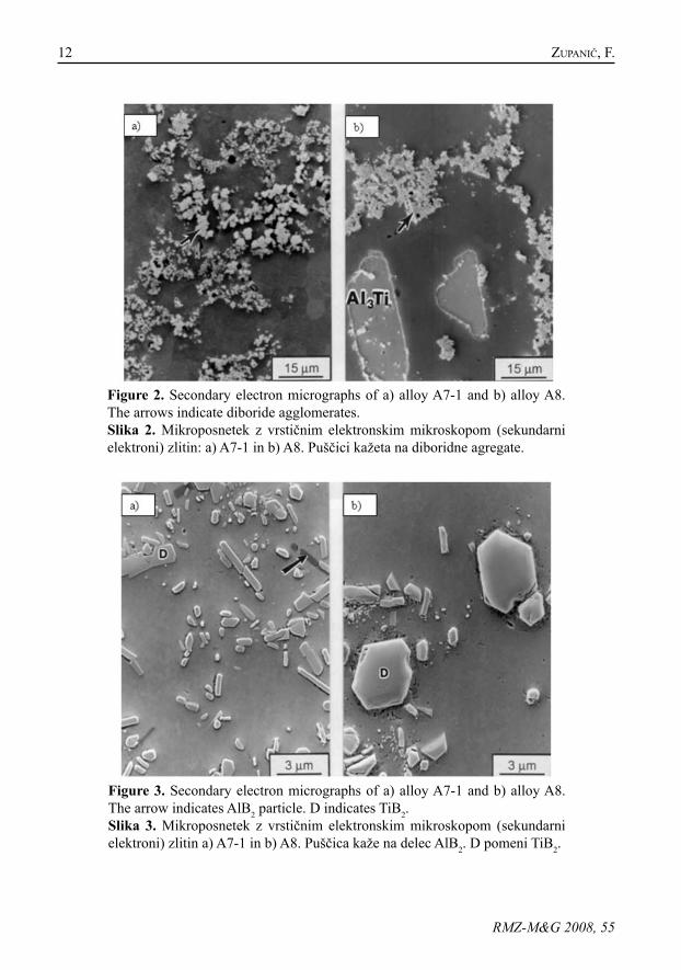
Figure 2. Secondary electron micrographs of a) alloy A7-1 and b) alloy A8. The arrows indicate diboride agglomerates. Slika 2. Mikroposnetek z vrstičnim elektronskim mikroskopom (sekundarni elektroni) zlitin: a) A7-1 in b) A8. Puščici kažeta na diboridne agregate.
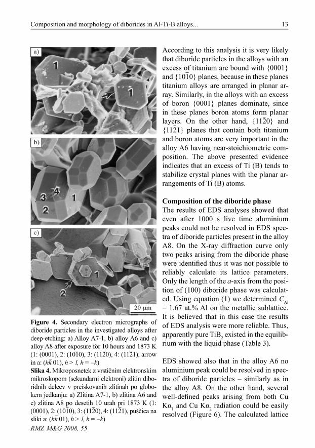
Figure 3. Secondary electron micrographs of a) alloy A7-1 and b) alloy A8. The arrow indicates AlB2 particle. D indicates TiB2. Slika 3. Mikroposnetek z vrstičnim elektronskim mikroskopom (sekundarni elektroni) zlitin a) A7-1 in b) A8. Puščica kaže na delec AlB2. D pomeni TiB2.
13Composition and morphology of diborides in Al-Ti-B alloys...
RMZ-M&G 2008, 55
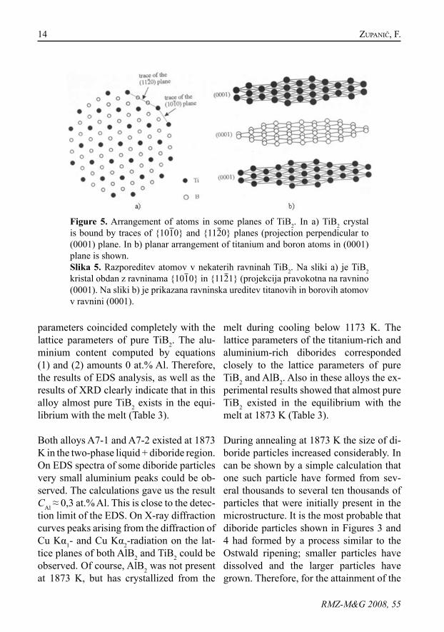
Figure 4. Secondary electron micrographs of diboride particles in the investigated alloys after deep-etching: a) Alloy A7-1, b) alloy A6 and c) alloy A8 after exposure for 10 hours and 1873 K (1: (0001), 2: (1010), 3: (1120), 4: (1121), arrow in a: (hk 01), h > l, h = –k)Slika 4. Mikroposnetek z vrstičnim elektronskim mikroskopom (sekundarni elektroni) zlitin dibo-ridnih delcev v preiskovanih zlitinah po globo-kem jedkanju: a) Zlitina A7-1, b) zlitina A6 and c) zlitina A8 po desetih 10 urah pri 1873 K (1: (0001), 2: (1010), 3: (1120), 4: (1121), puščica na sliki a: (hk 01), h > l, h = –k)
According to this analysis it is very likely that diboride particles in the alloys with an excess of titanium are bound with {0001} and {1010} planes, because in these planes titanium alloys are arranged in planar ar-ray. Similarly, in the alloys with an excess of boron {0001} planes dominate, since in these planes boron atoms form planar layers. On the other hand, {1120} and {1121} planes that contain both titanium and boron atoms are very important in the alloy A6 having near-stoichiometric com-position. The above presented evidence indicates that an excess of Ti (B) tends to stabilize crystal planes with the planar ar-rangements of Ti (B) atoms.
Composition of the diboride phaseThe results of EDS analyses showed that even after 1000 s live time aluminium peaks could not be resolved in EDS spec-tra of diboride particles present in the alloy A8. On the X-ray diffraction curve only two peaks arising from the diboride phase were identified thus it was not possible to reliably calculate its lattice parameters. Only the length of the a-axis from the posi-tion of (100) diboride phase was calculat-ed. Using equation (1) we determined CAl = 1.67 at.% Al on the metallic sublattice. It is believed that in this case the results of EDS analysis were more reliable. Thus, apparently pure TiB2 existed in the equilib-rium with the liquid phase (Table 3).
EDS showed also that in the alloy A6 no aluminium peak could be resolved in spec-tra of diboride particles – similarly as in the alloy A8. On the other hand, several well-defined peaks arising from both Cu Kα1 and Cu Kα2 radiation could be easily resolved (Figure 6). The calculated lattice
14 ZupAniČ, f.
RMZ-M&G 2008, 55
Figure 5. Arrangement of atoms in some planes of TiB2. In a) TiB2 crystal is bound by traces of {1010} and {1120} planes (projection perpendicular to (0001) plane. In b) planar arrangement of titanium and boron atoms in (0001) plane is shown.Slika 5. Razporeditev atomov v nekaterih ravninah TiB2. Na sliki a) je TiB2 kristal obdan z ravninama {1010} in {1121} (projekcija pravokotna na ravnino (0001). Na sliki b) je prikazana ravninska ureditev titanovih in borovih atomov v ravnini (0001).
parameters coincided completely with the lattice parameters of pure TiB2. The alu-minium content computed by equations (1) and (2) amounts 0 at.% Al. Therefore, the results of EDS analysis, as well as the results of XRD clearly indicate that in this alloy almost pure TiB2 exists in the equi-librium with the melt (Table 3).
Both alloys A7-1 and A7-2 existed at 1873 K in the two-phase liquid + diboride region. On EDS spectra of some diboride particles very small aluminium peaks could be ob-served. The calculations gave us the result CAl ≈ 0,3 at.% Al. This is close to the detec-tion limit of the EDS. On X-ray diffraction curves peaks arising from the diffraction of Cu Kα1- and Cu Kα2-radiation on the lat-tice planes of both AlB2 and TiB2 could be observed. Of course, AlB2 was not present at 1873 K, but has crystallized from the
melt during cooling below 1173 K. The lattice parameters of the titanium-rich and aluminium-rich diborides corresponded closely to the lattice parameters of pure TiB2 and AlB2. Also in these alloys the ex-perimental results showed that almost pure TiB2 existed in the equilibrium with the melt at 1873 K (Table 3).
During annealing at 1873 K the size of di-boride particles increased considerably. In can be shown by a simple calculation that one such particle have formed from sev-eral thousands to several ten thousands of particles that were initially present in the microstructure. It is the most probable that diboride particles shown in Figures 3 and 4 had formed by a process similar to the Ostwald ripening; smaller particles have dissolved and the larger particles have grown. Therefore, for the attainment of the
15Composition and morphology of diborides in Al-Ti-B alloys...
RMZ-M&G 2008, 55
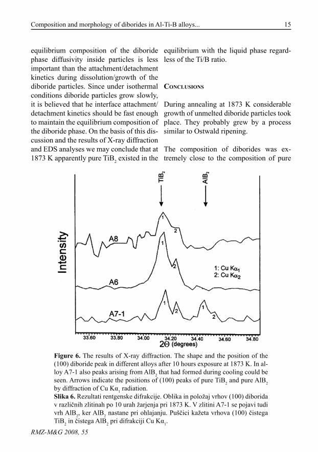
Figure 6. The results of X-ray diffraction. The shape and the position of the (100) diboride peak in different alloys after 10 hours exposure at 1873 K. In al-loy A7-1 also peaks arising from AlB2 that had formed during cooling could be seen. Arrows indicate the positions of (100) peaks of pure TiB2 and pure AlB2 by diffraction of Cu Kα1 radiation.Slika 6. Rezultati rentgenske difrakcije. Oblika in položaj vrhov (100) diborida v različnih zlitinah po 10 urah žarjenja pri 1873 K. V zlitini A7-1 se pojavi tudi vrh AlB2, ker AlB2 nastane pri ohlajanju. Puščici kažeta vrhova (100) čistega TiB2 in čistega AlB2 pri difrakciji Cu Kα1.
equilibrium composition of the diboride phase diffusivity inside particles is less important than the attachment/detachment kinetics during dissolution/growth of the diboride particles. Since under isothermal conditions diboride particles grow slowly, it is believed that he interface attachment/detachment kinetics should be fast enough to maintain the equilibrium composition of the diboride phase. On the basis of this dis-cussion and the results of X-ray diffraction and EDS analyses we may conclude that at 1873 K apparently pure TiB2 existed in the
equilibrium with the liquid phase regard-less of the Ti/B ratio.
conclusIons
During annealing at 1873 K considerable growth of unmelted diboride particles took place. They probably grew by a process similar to Ostwald ripening.
The composition of diborides was ex-tremely close to the composition of pure
16 ZupAniČ, f.
RMZ-M&G 2008, 55
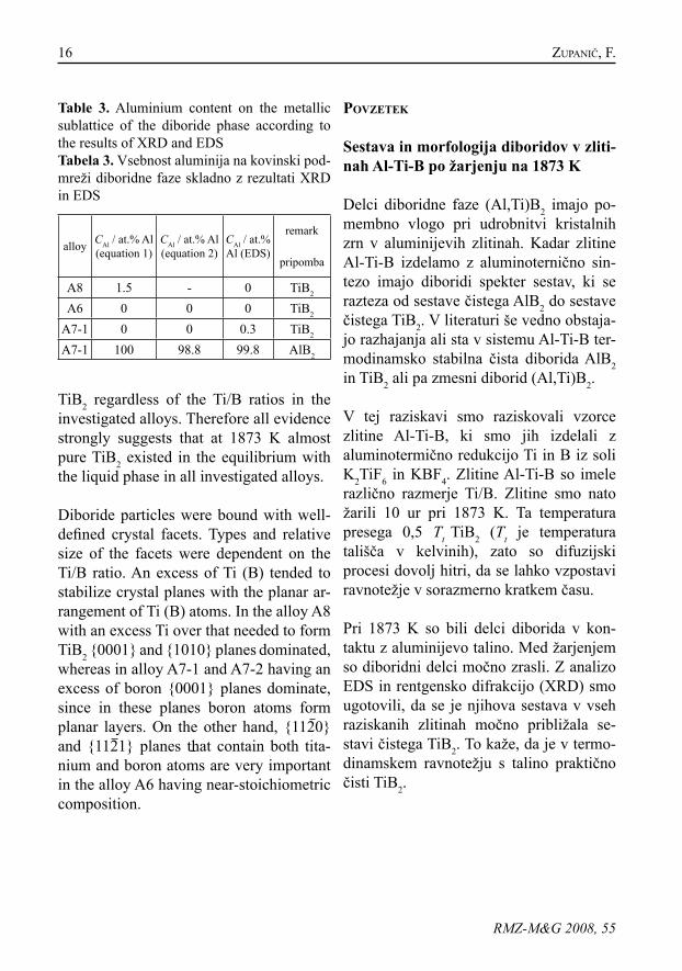
Table 3. Aluminium content on the metallic sublattice of the diboride phase according to the results of XRD and EDSTabela 3. Vsebnost aluminija na kovinski pod-mreži diboridne faze skladno z rezultati XRD in EDS
alloy CAl / at.% Al (equation 1)
CAl / at.% Al (equation 2)
CAl / at.% Al (EDS)
remark
pripomba
A8 1.5 - 0 TiB2
A6 0 0 0 TiB2
A7-1 0 0 0.3 TiB2
A7-1 100 98.8 99.8 AlB2
TiB2 regardless of the Ti/B ratios in the investigated alloys. Therefore all evidence strongly suggests that at 1873 K almost pure TiB2 existed in the equilibrium with the liquid phase in all investigated alloys.
Diboride particles were bound with well-defined crystal facets. Types and relative size of the facets were dependent on the Ti/B ratio. An excess of Ti (B) tended to stabilize crystal planes with the planar ar-rangement of Ti (B) atoms. In the alloy A8 with an excess Ti over that needed to form TiB2 {0001} and {1010} planes dominated, whereas in alloy A7-1 and A7-2 having an excess of boron {0001} planes dominate, since in these planes boron atoms form planar layers. On the other hand, {1120} and {1121} planes that contain both tita-nium and boron atoms are very important in the alloy A6 having near-stoichiometric composition.
povzetek
Sestava in morfologija diboridov v zliti-nah Al-Ti-B po žarjenju na 1873 K
Delci diboridne faze (Al,Ti)B2 imajo po-membno vlogo pri udrobnitvi kristalnih zrn v aluminijevih zlitinah. Kadar zlitine Al-Ti-B izdelamo z aluminoternično sin-tezo imajo diboridi spekter sestav, ki se razteza od sestave čistega AlB2 do sestave čistega TiB2. V literaturi še vedno obstaja-jo razhajanja ali sta v sistemu Al-Ti-B ter-modinamsko stabilna čista diborida AlB2 in TiB2 ali pa zmesni diborid (Al,Ti)B2.
V tej raziskavi smo raziskovali vzorce zlitine Al-Ti-B, ki smo jih izdelali z aluminotermično redukcijo Ti in B iz soli K2TiF6 in KBF4. Zlitine Al-Ti-B so imele različno razmerje Ti/B. Zlitine smo nato žarili 10 ur pri 1873 K. Ta temperatura presega 0,5 Tt TiB2 (Tt je temperatura tališča v kelvinih), zato so difuzijski procesi dovolj hitri, da se lahko vzpostavi ravnotežje v sorazmerno kratkem času.
Pri 1873 K so bili delci diborida v kon-taktu z aluminijevo talino. Med žarjenjem so diboridni delci močno zrasli. Z analizo EDS in rentgensko difrakcijo (XRD) smo ugotovili, da se je njihova sestava v vseh raziskanih zlitinah močno približala se-stavi čistega TiB2. To kaže, da je v termo-dinamskem ravnotežju s talino praktično čisti TiB2.
17Composition and morphology of diborides in Al-Ti-B alloys...
RMZ-M&G 2008, 55
Ugotovili smo tudi, da so bili diboridni delci obdani s kristalnimi fasetami. Vrsta in relativna velikost faset je bila močno odvisna od razmerja Ti/B. V zlitini A8, v kateri je bil presežek titana glede na ideal-no stehiometrično razmerje (2,21:1) so bili diboridni delci obdani s fasetami osnovne ploskve {0001} in prizmatičnimi ravni-nami {1010}. V zlitini s skoraj stehiome-trično sestavo (Ti/B = 2,56) sta se pojavile še fasete dveh dodatnih ravnin: prizmatič-ne {1120} in piramidne {1121}. V zlitini A7-1, ki je imela presežek B (Ti/B = 1,34) je prevladovala faseta osnovne ravnine {0001}.
Z analizo rezultatov in primerjavo faset z razporeditvijo atomov v diboridu smo ugotovili, da presežek Ti nad vrednostjo, ki je potrebna za tvorbo TiB2, stabilizira kristalne ravnine, ki imajo ravninsko raz-poreditev Ti atomov. Podoben učinek ima B, ki stabilizira ravnine, v katerih so atomi B razporejeni v ravnini.
references
[1] WAnG, c., WAnG, m., Yu, B., cHen, d., Qin, p., fenG, m. and dAi, Q. (2007): The grain refinement be-havior of TiB2 particles prepared with in situ technology. Materials Science and Engineering A.; Vol. 459, Issues 1-2, pp. 238-243.
[2] joHnsson, m., jAnsson, k. (1989): Study of Al1-xTixB2 particles ex-tracted from Al-Ti-B alloys. Z. Metallkd.; Vol. 89, pp. 394-398.
[3] kiussALAAs, R. (1986): Relation be-tween phases present in master al-loys of the Al-Ti-B type. Chemical Communications. Stockholm Uni-versity.
[4] sToLZ, u.k., sommeR, f., pRedeL, B. (1995): Phase equilibria of alumi-nium-rich Al-Ti-B alloys – solu-bility of TiB2 in aluminium melts. Aluminium.; Vol. 71, pp. 350-355.
[5] fenG, c. f., fRoYen, L. (1997): Incor-poration of Al into TiB2 in Al ma-trix composites and Al-Ti-B master alloys. Materials Letters.; Vol. 32, pp. 275-279.
[6] poHL, A., kiZLeR, p., TeLLe, R., ALdin-GeR, f. (1994): EXAFS studies of (Ti,W)B2 compounds. Z. Metallk-de.; Vol. 85, pp. 658-663.
[7] HAYes, f. H., LukAs, H. L., effenBeRG, G., peTZoW, G. (1989): Themody-namic calculation of the Al-rich corner of the Al-Ti-B system. Z. Metallkde.; Vol. 80, pp. 361-365.
18 ZupAniČ, f.
RMZ-M&G 2008, 55
[8] ZupAniČ, f., spAić, s., kRižmAn, A. (1998): Contribution to the ternary system Al-Ti-B. Part 1: The study of diborides present in the alumin-ium corner. Materials Science and Technology.; Vol. 14, pp. 601-607.
[9] mAssALski, T. B. (1990): Binary alloys phase diagrams. ASM Internation-al.; pp. 544-548.
[10] mAssALski, T. B. (1990): Binary alloys phase diagram. ASM International.; pp. 123-125.
[11] ZupAniČ, f., spAić, s., kRižmAn, A. (1998): Contribution to the ternary system Al-Ti-B. Part 1: The study of alloys in the triangle Al-AlB2-TiB2. Materials Science and Tech-nology.; Vol. 14, pp. 1203-1212.
[12] ZupAniČ, f., spAić, s. (1999): Metall (Berl. West). Vol. 53, No. 3, pp. 125-130.
[13] peTZoW, G. (1994): Atzen. 6. Aufla-ge. Gebrüder Borntraeger, Berlin Stuttgart.
[14] siGWoRTH, G. k. (1984): The grain-re-fining of aluminium and phase re-lationships in the Al-Ti-B system. Metall. Trans. A.; Vol. 15A, pp. 272-282.
19RMZ – Materials and Geoenvironment, Vol. 55, No. 1, pp. 19-29, 2008
Scientific paper
Tool for programmed open-die forging – case study
Orodje za programsko vodeno prosto kovanje – študija primera
dAvid BomBAČ1, mATevž fAZARinc1, GoRAn kuGLeR1, RAdomiR TuRk1
1University of Ljubljana, Faculty of Natural Sciences and Engineering, Department of Materials and Metallurgy, Aškerčeva cesta 12, SI-1000 Ljubljana, Slovenia;
E-mail: [email protected], [email protected], [email protected], [email protected]
Received: November 26, 2007 Accepted: January 13, 2008
Abstract: An open-die forging process as referred to in the following assumptions is a process where plastic material is compressed in one main axis only and the spread into the two other main axes is not limited. In view of present competitive markets modern open-die forging plants are highly dynamic production plants and vastly explore possibilities of programmed forging. Computer aided technology tools for programmed forging is the basis for innovative and cost effective technology planning which consider the per-formance limits of forging equipment and material in order to achieve the optimum productivity.
Izvleček: Proces prostega kovanja, ki je obravnavan v tej študiji, je postopek, kjer je material tlačno deformiran v eni smeri, v ostalih dveh pa se prosto širi. Na današnjem izredno konkurenčnem trgu so obrati prostih kovačnic izredno dinamični obrati in široko izkoriščajo možnost programiranega ko-vanja. Računalniško podprta tehnološka orodja za programirano kovanje so osnova za inovativno in cenovno učinkovito planiranje proizvodnje. Ta preuči meje zmožnosti stiskalnice in mejne vrednosti materiala, ter na pod-lagi teh določi optimalne pogoje preoblikovanja.
Key words: hot forming, open-die forging, programmed forging, pass schedule, forging simulation
Ključne besede: vroče preoblikovanje, prosto kovanje, programirano kovanje, plan vtikov, simulacija kovanja
20 BomBAČ, d., fAZARinc, m., kuGLeR, G., TuRk, R.
RMZ-M&G 2008, 55
IntroductIon
In metal forming, open-die forging is a metal forming process in which a work-piece is usually pressed between flat dies with a series of compressive deformation steps and manipulated and/or rotated. The open-die forging process as referred to in the following assumptions is a process where plastic material is compressed in one main axis only and the spread into the two other main axes is not limited. It has not lost its importance in recent times and is for steel manufacturing carried out un-der hot working conditions when the metal is deformed plastically above its recrystal-lization temperature. The open-die forging plants consist of a forging press and one or two rail-bound manipulators. The dies or tools are small compared with the overall sizes of the forgings. The process is carried out incrementally, where only a part of the workpiece is being deformed at each stage. The principle of such an incremental forg-ing process is simply the compressing or upsetting of the material step-by-step until it reaches the final target shape. In the fur-ther development of this type of forming operation, the requirements are for accu-racy of load prediction and metal flow[1-3].
In view of present competitive markets modern open-die forging plants are highly dynamic production plants and vastly ex-plore possibilities of programmed forging. Apart from the pure production speed, the main focus today is on the achievement of minimum forging tolerances and a con-sistent level of quality. In the past proce-dures in open-die forging were based on the individual forgemaster’s experience and observation of each forging stroke to
determine both elongation and sideways spreading. An experienced forge master can develop a geometrical pass schedule quite easily, however; the optimization of a pass schedule to minimize forging time is quite difficult as it involves the consid-eration of numerous factors which influ-ence the production rate. Computer aided technology tools for programmed forging is the basis for innovative and cost effec-tive technology planning which consider the performance limits of forging equip-ment and material in order to achieve the optimum productivity. It must consider all of the important factors including spread behaviour, die geometry and the speeds of the press and manipulators. The required pressing force relative to the material re-sistance is calculated as a function of the instantaneous temperature and compared to the maximum available press force.
Optimization of the pass schedules in the open-die forging technology and activities for successful implementation of the com-puter aided forging technology demand close cooperation between forging plants and science. Technology developed in co-operation must be constantly maintained and adapted to the latest technological breakthroughs.
theoretIcal framework for pro-grammed forgIng
The open-die forging as mentioned be-fore is incremental process where after one forging pass on a square bar the side faces take on an irregular shape, com-monly termed barrelling, which is due to frictional constraint at the tool faces and to
21Tool for programmed open-die forging - case study
RMZ-M&G 2008, 55
the influence of the adjacent undeformed portion of the bar. The influence of the machine operator experience on the moni-toring of the process must be decreased in order to ensure reproducible process that increases productivity and improve qual-ity of the forgings hence reducing machine operator experience related fluctuations. Moreover computer aided forging technol-ogy enables judgment of the characteristic forging capabilities of the plant and their influence on the productivity[4]. However the machine operator has ability to initi-ate corrections to the programmed forging schedule any time if it is necessary.
Pass schedule calculation is determination of relevant process data for processing a defined end piece from initial ingot. Such calculation is very demanding due to com-plexity of open-die forging process. For instance to enable a mutual harmonisation between forging press and manipulator a proper description of the material being pressed between two flat dies is required. Moreover material does not only deform in the forging direction but also towards the manipulator. In order to fully exploit capa-bilities of forging equipment manipulator feeding rate or manipulator bite has to be determined. This can be achieved by em-ploying the empirical formula proposed by Tomlinson and Stringer[3] which is based on assumption of constant volume dur-ing plastic deformation and describes the relationship between manipulator feeding rate, material shape and reduction for steel. The change of length and width of a forg-ing can be described by a spread factor and the reduction ratio. From practical experi-ence with programmed forging it is known
that the influence of reduction ratio on the spread is negligible[4].
To compute the forging pass schedules for bars and predict the changes of shape as well as other important parameters dur-ing the forging process empirical formulae have been proposed. The pass procedure for the forging of final shape depends on initial and final cross section shape of bar and are: 1) from square stock to a square bar, 2) from square to round, 3) from round to square and round to round, where same forging principle is used. Breakdown pro-cedure is as follows 1) square to square process goes through next shapes: square – rectangular – square where the reduction ratio can be varied every second pass. A square forged down to a rectangular sec-tion with a certain reduction ratio, turned 90° and forged down again with the same reduction ratio and the same bite ratio, turns automatically into a new square with smaller size. To obtain sharp corners of bar decrease of the reduction ratio is required. 2) The process square to round follows the same breakdown routine square – rectan-gular – square, ending in four passes with an octagon, which have about 7 % more area than the final round. Finish to the round is made in a swaging die. 3) Forg-ing pass schedule of round to square and round to round follows the same forging principle. Forging of rectangular cross sections requires a different technology, where shape factor of h/w (height/width) plays important role leading to a variation of the spread factor. For example rectangu-lar bars where a shape factor exceeds 1/6 results in the normal forging range practi-cally no spread but only elongation[4].
22 BomBAČ, d., fAZARinc, m., kuGLeR, G., TuRk, R.
RMZ-M&G 2008, 55
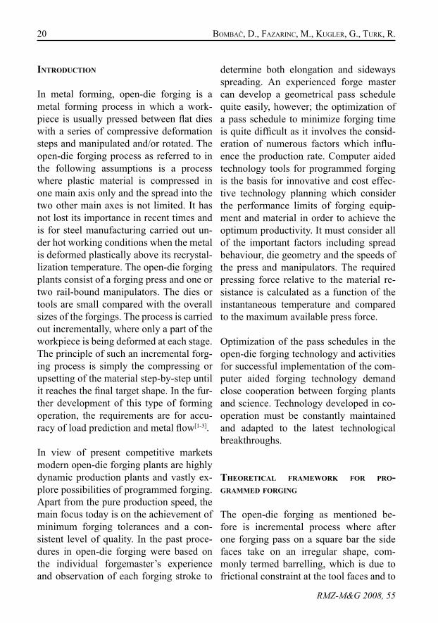
Ingots are extensively used as forging stock in the open-die forging of large com-ponents. In Figure 1 typical steelmaking material flow from electric arc furnace to forging press is shown. Whenever ingots are used it is often mandatory to adopt a forging procedure that will remove the cast structure in the finished forging.
Another important aspect of calculation and optimisation of apt pass schedule is to be aware of limits of ingots, products, ma-terials and technology. When all properties are collected and stored to databases we can start calculating efficient pass sched-ule.
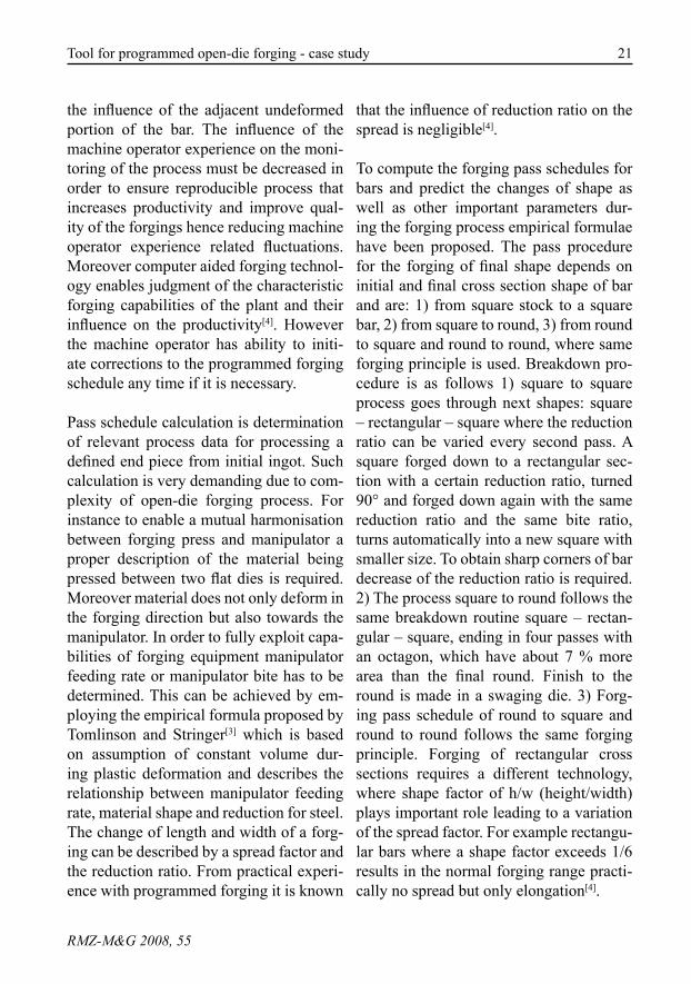
Use of computer aided technology, as de-picted in Figure 2 for development and optimization of pass schedules in open-
Figure 1. Material flow for open-die forged productsSlika 1. Tok materiala pri prostem kovanju
die forging requires some input of forg-ing know-how. This applies particularly to the reduction factor which has to take care of the shape of the ingot, surface condi-tions, and brittleness of the material and in most cases must be varied with the drop-ping forging temperature. Also important is the bite ratio which defines the depth of deformation and grain change in the forg-ing. Grater bite ratio is better but leads to increase of forging force, which is limited with equipment.
results and dIscussIon
HFS software fundamentals for calcula-tion of pass schedules are models where some of them are physically based e.g. temperature. Other models are deductions
23Tool for programmed open-die forging - case study
RMZ-M&G 2008, 55
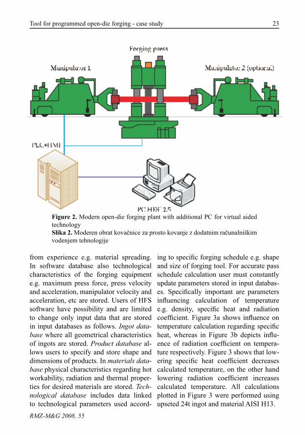
Figure 2. Modern open-die forging plant with additional PC for virtual aided technologySlika 2. Moderen obrat kovačnice za prosto kovanje z dodatnim računalniškim vodenjem tehnologije
from experience e.g. material spreading. In software database also technological characteristics of the forging equipment e.g. maximum press force, press velocity and acceleration, manipulator velocity and acceleration, etc are stored. Users of HFS software have possibility and are limited to change only input data that are stored in input databases as follows. Ingot data-base where all geometrical characteristics of ingots are stored. Product database al-lows users to specify and store shape and dimensions of products. In materials data-base physical characteristics regarding hot workability, radiation and thermal proper-ties for desired materials are stored. Tech-nological database includes data linked to technological parameters used accord-
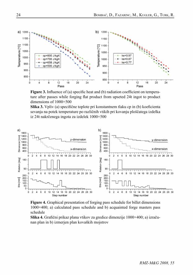
ing to specific forging schedule e.g. shape and size of forging tool. For accurate pass schedule calculation user must constantly update parameters stored in input databas-es. Specifically important are parameters influencing calculation of temperature e.g. density, specific heat and radiation coefficient. Figure 3a shows influence on temperature calculation regarding specific heat, whereas in Figure 3b depicts influ-ence of radiation coefficient on tempera-ture respectively. Figure 3 shows that low-ering specific heat coefficient decreases calculated temperature, on the other hand lowering radiation coefficient increases calculated temperature. All calculations plotted in Figure 3 were performed using upseted 24t ingot and material AISI H13.
24 BomBAČ, d., fAZARinc, m., kuGLeR, G., TuRk, R.
RMZ-M&G 2008, 55
Figure 3. Influence of (a) specific heat and (b) radiation coefficient on tempera-ture after passes while forging flat product from upseted 24t ingot to product dimensions of 1000×500Slika 3. Vpliv (a) specifične toplote pri konstantnem tlaku cp in (b) koeficienta sevanja na potek temperature po različnih vtikih pri kovanju ploščatega izdelka iz 24t nakrčenega ingota za izdelek 1000×500
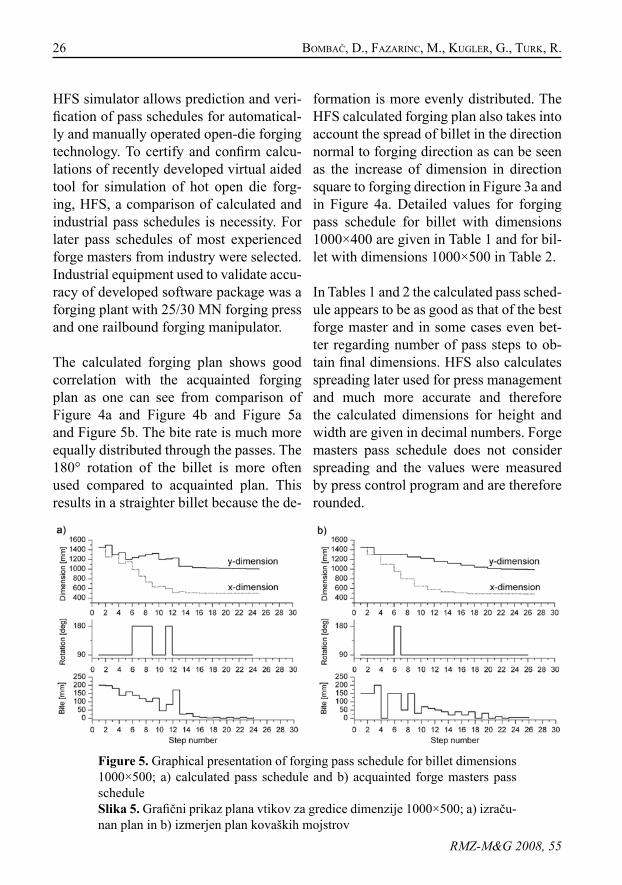
Figure 4. Graphical presentation of forging pass schedule for billet dimensions 1000×400; a) calculated pass schedule and b) acquainted forge masters pass scheduleSlika 4. Grafični prikaz plana vtikov za gredice dimenzije 1000×400; a) izraču-nan plan in b) izmerjen plan kovaških mojstrov

25Tool for programmed open-die forging - case study
RMZ-M&G 2008, 55
Table 1. Detailed characteristics of pass schedules for billet dimensions 1000×400Tabela 1. Natančen prikaz planov vtika za gredico z dimenzijami 1000×400
Calculated pass schedule Acquainted pass scheduleStep Height Width Bite Rotation Step Height Width Bite Rotation
1 1450 1450 189.43 90 1 1450 1450 150 902 1260 1464.07 164.61 90 2 1300 1450 150 903 1299.46 1299.46 169.76 90 3 1300 1300 100 904 1129.69 1339.02 139.02 90 4 1200 1300 150 1805 1200 1164.22 152.1 90 5 1050 1300 150 1806 1012.13 1236.74 132.23 180 6 900 1300 50 907 879.9 1268.24 114.95 180 7 1250 900 150 908 764.95 1295.32 99.93 180 8 750 1250 50 909 665.01 1317.36 117.36 90 9 1200 750 150 9010 1200 700 91.53 90 10 600 1200 50 9011 609.09 1220.84 79.57 180 11 1150 600 60 9012 529.51 1238.28 38.28 90 12 540 1150 30 9013 1200 533.68 34.7 90 13 1120 540 40 9014 498.99 1207.66 65.19 180 14 500 1120 20 9015 433.8 1221.09 159.53 90 15 1100 500 40 9016 1061.57 451.5 42.74 90 16 460 1100 20 9017 408.76 1070.83 42.05 90 17 1080 460 40 9018 1028.78 413.58 10 90 18 420 1080 60 9019 403.58 1028.78 6 90 19 1020 420 10 9020 1022.78 403.58 2 90 20 410 1020 10 9021 401.58 1022.78 6 90 21 1010 410 5 9022 1016.78 401.58 1.58 90 22 405 1010 5 9023 400 1016.78 6 90 23 1005 405 3 9024 1010.78 400 0 90 24 402 1005 3 9025 400 1010.78 6 90 25 1002 402 2 9026 1004.78 400 0 90 26 400 1002 2 9027 400 1004.78 4.78 90 27 1000 400 0 9028 1000 400 28 400 1000
26 BomBAČ, d., fAZARinc, m., kuGLeR, G., TuRk, R.
RMZ-M&G 2008, 55
HFS simulator allows prediction and veri-fication of pass schedules for automatical-ly and manually operated open-die forging technology. To certify and confirm calcu-lations of recently developed virtual aided tool for simulation of hot open die forg-ing, HFS, a comparison of calculated and industrial pass schedules is necessity. For later pass schedules of most experienced forge masters from industry were selected. Industrial equipment used to validate accu-racy of developed software package was a forging plant with 25/30 MN forging press and one railbound forging manipulator.
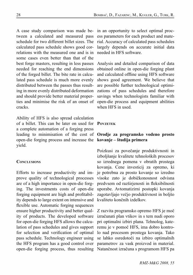
The calculated forging plan shows good correlation with the acquainted forging plan as one can see from comparison of Figure 4a and Figure 4b and Figure 5a and Figure 5b. The bite rate is much more equally distributed through the passes. The 180° rotation of the billet is more often used compared to acquainted plan. This results in a straighter billet because the de-
formation is more evenly distributed. The HFS calculated forging plan also takes into account the spread of billet in the direction normal to forging direction as can be seen as the increase of dimension in direction square to forging direction in Figure 3a and in Figure 4a. Detailed values for forging pass schedule for billet with dimensions 1000×400 are given in Table 1 and for bil-let with dimensions 1000×500 in Table 2.
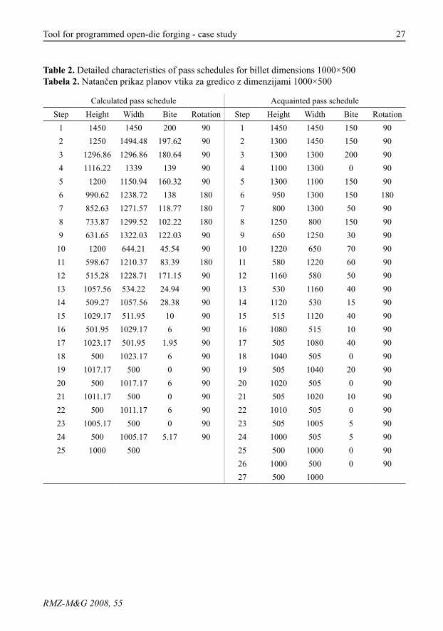
In Tables 1 and 2 the calculated pass sched-ule appears to be as good as that of the best forge master and in some cases even bet-ter regarding number of pass steps to ob-tain final dimensions. HFS also calculates spreading later used for press management and much more accurate and therefore the calculated dimensions for height and width are given in decimal numbers. Forge masters pass schedule does not consider spreading and the values were measured by press control program and are therefore rounded.
Figure 5. Graphical presentation of forging pass schedule for billet dimensions 1000×500; a) calculated pass schedule and b) acquainted forge masters pass scheduleSlika 5. Grafični prikaz plana vtikov za gredice dimenzije 1000×500; a) izraču-nan plan in b) izmerjen plan kovaških mojstrov
27Tool for programmed open-die forging - case study
RMZ-M&G 2008, 55
Table 2. Detailed characteristics of pass schedules for billet dimensions 1000×500Tabela 2. Natančen prikaz planov vtika za gredico z dimenzijami 1000×500
Calculated pass schedule Acquainted pass scheduleStep Height Width Bite Rotation Step Height Width Bite Rotation
1 1450 1450 200 90 1 1450 1450 150 902 1250 1494.48 197.62 90 2 1300 1450 150 903 1296.86 1296.86 180.64 90 3 1300 1300 200 904 1116.22 1339 139 90 4 1100 1300 0 905 1200 1150.94 160.32 90 5 1300 1100 150 906 990.62 1238.72 138 180 6 950 1300 150 1807 852.63 1271.57 118.77 180 7 800 1300 50 908 733.87 1299.52 102.22 180 8 1250 800 150 909 631.65 1322.03 122.03 90 9 650 1250 30 9010 1200 644.21 45.54 90 10 1220 650 70 9011 598.67 1210.37 83.39 180 11 580 1220 60 9012 515.28 1228.71 171.15 90 12 1160 580 50 9013 1057.56 534.22 24.94 90 13 530 1160 40 9014 509.27 1057.56 28.38 90 14 1120 530 15 9015 1029.17 511.95 10 90 15 515 1120 40 9016 501.95 1029.17 6 90 16 1080 515 10 9017 1023.17 501.95 1.95 90 17 505 1080 40 9018 500 1023.17 6 90 18 1040 505 0 9019 1017.17 500 0 90 19 505 1040 20 9020 500 1017.17 6 90 20 1020 505 0 9021 1011.17 500 0 90 21 505 1020 10 9022 500 1011.17 6 90 22 1010 505 0 9023 1005.17 500 0 90 23 505 1005 5 9024 500 1005.17 5.17 90 24 1000 505 5 9025 1000 500 25 500 1000 0 90
26 1000 500 0 9027 500 1000
28 BomBAČ, d., fAZARinc, m., kuGLeR, G., TuRk, R.
RMZ-M&G 2008, 55
A case study comparison was made be-tween a calculated and measured pass schedule for two different billet sizes. The calculated pass schedule shows good cor-relations with the measured one and is in some cases even better than that of the best forge masters, resulting in less passes needed for reaching the end dimensions of the forged billet. The bite rate in calcu-lated pass schedule is much more evenly distributed between the passes thus result-ing in more evenly distributed deformation and should provide better material proper-ties and minimise the risk of an onset of cracks.
Ability of HFS is also spread calculation of a billet. This can be later on used for a complete automation of a forging press leading to minimisation of the cost of open-die forging process and increase the yield.
conclusIons
Efforts to increase productivity and im-prove quality of technological processes are of a high importance in open-die forg-ing. The investments costs of open-die forging equipment are high and profitabil-ity depends to large extent on intensive and flexible use. Automatic forging sequences ensure higher productivity and better qual-ity of products. The developed software for open-die forging HFS allows the calcu-lation of pass schedules and gives support for selection and verification of optimal pass schedule. Technology engineer using the HFS program has a good control over open-die forging process, thus resulting
in an opportunity to select optimal proc-ess parameters for each product and mate-rial. Accuracy of calculated pass schedules largely depends on accurate initial data needed in HFS software.
Analysis and detailed comparison of data obtained online in open-die forging plant and calculated offline using HFS software shows good agreement. We believe that are possible further technological optimi-zations of pass schedules and therefore savings when technologists familiar with open-die process and equipment abilities when HFS in used.
povzetek
Orodje za programsko vodeno prosto kovanje – študija primera
Poizkusi za povečanje produktivnosti in izboljšanje kvalitete tehnoloških procesov so izrednega pomena v obratih prostega kovanja. Cene investicij za opremo, ki je potrebna za prosto kovanje so izredno visoke zato je dobičkonosnost odvisna predvsem od razširjenosti in fleksibilnosti uporabe. Avtomatizirni postopki kovanja zagotavljajo večjo produktivnost in boljšo kvaliteto končnih izdelkov.
Z razvita programsko opremo HFS je moč izračunati plan vtikov in s tem nudi oporo pri optimalni izbiri plana. Tehnolog, kate-remu je v pomoč HFS, ima dobro kontro-lo nad procesom prostega kovanja. Tako se lahko osredotoči na izbiro optimalnih parametrov za vask proizvod in material. Natančnost izračuna s programom HFS pa
29Tool for programmed open-die forging - case study
RMZ-M&G 2008, 55
je v veliki meri odvisna od natančnsti zače-tnih podatkov v programu.
Narejena je bila študija primera med izra-čunanim in izmerjenim planom vtika za dve različni dimenziji gredic. Izračunan plan kaže dobro ujemanje s planom, ki je bil izmerjen pri ekipi najboljših kovaških mojstrov. V nekaterih primerih je ta celo boljši, saj je bilo potrebnih manj vtikov za dosego končnih dimezij.
Stopnja odvzema je pri izračunanem planu bolj enakomerno razporejena med prevle-ki. S tem je dosežena tudi bolj enakomer-na razporeditev deformacije med prevleki, kar ima za posledico boljše materialne lastnosti in preprečuje vrjetnost nastanka razpok.
Program HFS izračunava in upošteva tudi širjenje gredice. Vse te lastnosti je moč uporabiti kasneje za avtomatizacijo preše za prosto kovanje. To bi zmanjšalo stro-ške prostega kovanja in povečalo končni izplen.
references
[1] AksAkAL, B., osmAn, f.H., BRAmLeY, A.n. (1997): Upper-bound analy-sis for the automation of open-die forging. Journal of Materials Processing Technology.; Vol. 71, pp. 215-223.
[2] cHoi, s.k., cHun, m.s., vAn TYne, c.j., moon, Y.H. (2006): Optimi-zation of open die forging of round shapes using FEM analysis. Jour-nal of Materials Processing Tech-nology.; Vol. 172, pp. 88-95.
[3] TomLinson, A., sTRinGeR, j.d. (1959): Spread and elongation in flat tool forging. Journal of Iron Steel In-stitute.; Vol. 193-2, pp. 157-162.
[4] pHAnke, H.j. (1983): Grundlagen des programmierten Schmidens. Stahl und Eisen.; Vol. 103, pp. 547-552.

31RMZ – Materials and Geoenvironment, Vol. 55, No. 1, pp. 31-40, 2008
Scientific paper
A laboratory test for simulation of solidification on Gleeble 1500D thermo-mechanical simulator
Laboratorijski test simulacije strjevanja na termo-mehanskem simulatorju Gleeble 1500D
BošTjAn BRAdAskjA1, juRij koRuZA2, mATevž fAZARinc2, mATjAž knAp2, RAdomiR TuRk2
1ACRONI d.o.o., Cesta Borisa Kidriča 44, SI-4270 Jesenice, Slovenia; E-mail: [email protected]
2University of Ljubljana , Faculty of Natural Sciences and Engineering, Departmant of Materials and Metallurgy, Aškerčeva cesta 12, SI-1000 Ljubljana, Slovenia;
E-mail: [email protected], [email protected], [email protected], [email protected]
Received: November 18, 2007 Accepted: January 7, 2008
Abstract: A highly repeatable solidification test was developed. It was designed to study the effect of process parameters on solidified micro and macrostruc-tures. Different cooling rates were used for solidification and cooling of S 355 J2 construction steel. It was observed that cooling rate has a substantial influence on final grain size and on columnar-to-equiaxed transition zone (CET). Within the interval of constant thermal gradient, different macro- and micro-structural features have been provided, which consequently en-ables the study of dynamics of precipitation dependence on solidification processing parameters.
Izvleček: Razvit je bil visoko ponovljiv test strjevanja. Razvit je bil kot orodje, za preučevanje vpliva procesnih parametrov na lito mikro in makrostrukturo. Za strjevanje konstrukcijskega jekla S 355 J2 so bile uporabljene različne ohlajevalne hitrosti. Opažen je bil močan vpliv ohlajevalne hitrosti tako na končno velikost zrn, kot tudi na mejno plast med stebričastimi in ekviaksi-alnimi zrni. Znotraj intervala, kjer je bil temperaturni gradient konstanten, so bile s pomočjo različnih ohlajevalnih hitrosti, v vzorcih dobljene raz-lične mikro in makrostrukturne značilnosti, kar omogoča študij dinamike izločanja v odvisnosti od parametrov strjevanja.
Key words: solidification test, macrostructure, cooling rate, GleebleKljučne besede: test strjevanja, makrostruktura, ohlajevalna hitrost, Gleeble
32 BRAdAskjA, B., koRuZA, j., fAZARinc, m., knAp, m., TuRk, R.
RMZ-M&G 2008, 55
IntroductIon
The solidification of molten steel is one of the most important processes in the pro-cessing path of steel manufacturing. The microstructure that derives from the solidi-fied ingot or slab has a large influence on the characteristic of the produced material and process path that follows.
The micro and macrostructures in ingots usually show spatial variations of features and properties. This can be simulated with combination of computer simulation of in-got/slab cooling and high temperature test-ing with controlled solidification and cool-ing of the specimens.
The high temperature experiments on the Gleeble testing machine that were found in literature are mainly focused on charac-teristics of metal in the mushy zone or the mechanical properties of solidified speci-mens for continuous casting application and do not deal with the development of microstructure. The investigations have not been focused on influence of process parameters on development of micro and macrostructure. In these tests, the solidi-fication process was only the first stage followed by tensile mechanical loading and no observations of solidified structure were made.
seoL et al.[1,2] were studying the behavior of material under tensile loading of in-situ melted and solidified cylindrical speci-mens. The tensile strength and ductility of carbon steels was measured in the tem-perature range of mushy zone. Also the stress – strain relations in austenite and
δ-ferrite phase regions at various tempera-tures and strain rates were analyzed. nA et al.[3] used the Gleeble system to investigate cracking occurrence during continuous casting of steels by tensile testing. In this work effects of carbon content, strain rate and sampling orientation on hot ductility were investigated. GLoWAcki et al.[4] used tensile test to study the deformation behav-ior of steel within the mushy zone. suZuki et al.[5-7] employed different methods of laboratory simulation of continuous cast-ing and direct rolling of steels with special emphasis on embrittlement in dependence to chemical composition, thermal history, strain rate and fracture mode.
Nevertheless some investigations were made on development of solidified mi-crostructure of aluminum alloys, using the Gleebe system, by kosTRivAs and LippoLd[8]. Although the testing procedure was similar, the difference between the physical properties of aluminum and steel brings up new problems and requires some different approaches.
Because of the above mentioned reasons it was decided that a highly repeatable solidification test should be developed with accurate knowledge and control of the temperature field in the specimen. The test was developed using a Gleeble 1500D thermo-mechanical simulator. This machine enables simultaneous, computer guided, thermal and mechanical loading of the specimen, within a very precise range. The main goal was to track the develop-ment of micro and macrostructure in de-pendence to testing parameters.

33A laboratory test for simulation of solidification on Gleeble 1500D...
RMZ-M&G 2008, 55
experImental procedure and materIal
The laboratory test for controlled solidifi-cation has been developed using Gleeble 1500D thermo-mechanical simulator, which has been equipped with specially developed additional parts for solidifica-tion simulation.
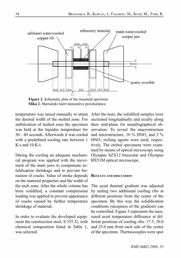
Cylindrical specimens, 110 mm long with a diameter of 10 mm, as shown in Figure 1 were used for the experiments. A 10 mm screw-thread was engraved on each side of the specimen which enabled the fixation of the specimen into the jaws with aim to per-form tensile and compression loadings. To support the melt zone a 30 mm quartz cru-cible with a 1 mm wall thickness has been placed around the center part of the speci-men. Quartz material was used because of its high temperatures endurance, small linear coefficient of thermal expansion and negligible diffusion with the specimen ma-terial. Crucibles have been furnished with axially running 2 mm slot for insertion of the thermo couples and also to provide an opening for exiting gasses. To decrease the radial thermal gradient, refractory material was placed over the crucible. Addition-ally two special water-cooling ribs made from copper were placed on each side of
the specimen, to attain sufficient thermal gradient in axial direction. Varying the po-sition of the ribs enabled the control of the axial thermal gradient and consequently the width of the melting zone. Schematic plan of placing of the specimen is shown on Figure 2.
Temperature was controlled by 0.35 mm thick S-type (Pt10wt%Rh-Pt) thermo-couple, spot-welded in the middle of the specimen and isolated with alumina tubes. An additional thermocouple stand was ap-plied to prevent the motion of the leading thermocouple and to assure the correct temperature measurements during the up-set of liquid phase. In order to minimize the surface oxidation and consequently the detachment of the welded thermocouple, all experiments were conducted in protec-tive Ar atmosphere.
Before setting up the temperature program for the test, Thermo-Calc software was used to define the liquidus and solidus tempera-ture of the material studied. The specimen was heated with the heating rate of 15 K/s up to 100 K below liquidus temperature. The heating rate was then decreased to 1 K/s for better control of temperature near the melting temperature. If necessary, the
Figure1. Cross section of the specimenSlika 1. Shematski načrt preizkušanca
34 BRAdAskjA, B., koRuZA, j., fAZARinc, m., knAp, m., TuRk, R.
RMZ-M&G 2008, 55
Figure 2. Schematic plan of the mounted specimenSlika 2. Shematski načrt namestitve preizkušanca
temperature was raised manually to attain the desired width of the melted zone. For stabilization of melted zone the specimen was held at the liquidus temperature for 30 - 40 seconds. Afterwards it was cooled with a predefined cooling rate between 1 K/s and 10 K/s.
During the cooling an adequate mechani-cal program was applied with the move-ment of the main jaws to compensate so-lidification shrinkage and to prevent for-mation of cracks. Value of stroke depends on the material properties and the width of the melt zone. After the whole volume has been solidified, a constant compression loading was applied to prevent appearance of cracks caused by further temperature shrinkage of material.
In order to evaluate the developed equip-ment the construction steel, S 355 J2, with chemical composition listed in Table 1, was selected.
After the tests, the solidified samples were sectioned longitudinally and axially along their mid-plane for metallographical ob-servation. To reveal the macrostructure and microstructure, 10 % HNO3 and 2 % HNO3 etching agents were used, respec-tively. The etched specimens were exam-ined by means of optical microscopy using Olympus SZX12 binocular and Olympus BX51M optical microscope.
results and dIscussIon
The axial thermal gradient was adjusted by setting two additional cooling ribs at different positions from the center of the specimen. By this way the solidification conditions (steepness of the gradient) can be controlled. Figure 3 represents the mea-sured axial temperature difference at dif-ferent positions of cooling ribs: 17.5, 20.0 and 25.0 mm from each side of the center of the specimen. Thermocouples were spot
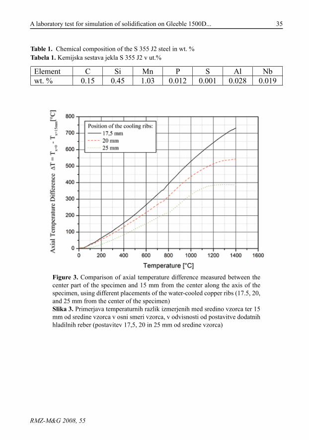
35A laboratory test for simulation of solidification on Gleeble 1500D...
RMZ-M&G 2008, 55
Table 1. Chemical composition of the S 355 J2 steel in wt. %Tabela 1. Kemijska sestava jekla S 355 J2 v ut.%
Element C Si Mn P S Al Nbwt. % 0.15 0.45 1.03 0.012 0.001 0.028 0.019
Figure 3. Comparison of axial temperature difference measured between the center part of the specimen and 15 mm from the center along the axis of the specimen, using different placements of the water-cooled copper ribs (17.5, 20, and 25 mm from the center of the specimen)Slika 3. Primerjava temperaturnih razlik izmerjenih med sredino vzorca ter 15 mm od sredine vzorca v osni smeri vzorca, v odvisnosti od postavitve dodatnih hladilnih reber (postavitev 17,5, 20 in 25 mm od sredine vzorca)
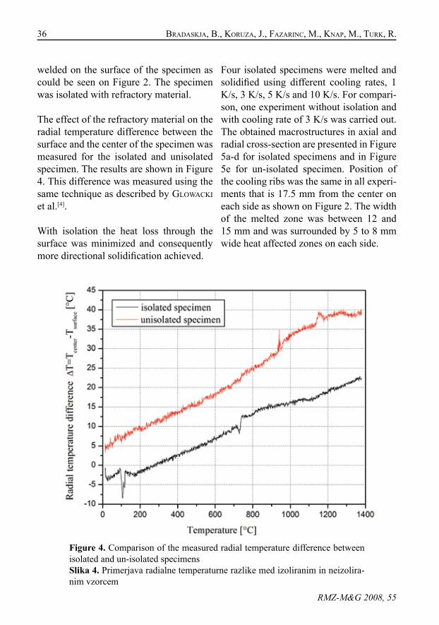
36 BRAdAskjA, B., koRuZA, j., fAZARinc, m., knAp, m., TuRk, R.
RMZ-M&G 2008, 55
welded on the surface of the specimen as could be seen on Figure 2. The specimen was isolated with refractory material.
The effect of the refractory material on the radial temperature difference between the surface and the center of the specimen was measured for the isolated and unisolated specimen. The results are shown in Figure 4. This difference was measured using the same technique as described by GLoWAcki et al.[4].
With isolation the heat loss through the surface was minimized and consequently more directional solidification achieved.
Figure 4. Comparison of the measured radial temperature difference between isolated and un-isolated specimensSlika 4. Primerjava radialne temperaturne razlike med izoliranim in neizolira-nim vzorcem
Four isolated specimens were melted and solidified using different cooling rates, 1 K/s, 3 K/s, 5 K/s and 10 K/s. For compari-son, one experiment without isolation and with cooling rate of 3 K/s was carried out. The obtained macrostructures in axial and radial cross-section are presented in Figure 5a-d for isolated specimens and in Figure 5e for un-isolated specimen. Position of the cooling ribs was the same in all experi-ments that is 17.5 mm from the center on each side as shown on Figure 2. The width of the melted zone was between 12 and 15 mm and was surrounded by 5 to 8 mm wide heat affected zones on each side.
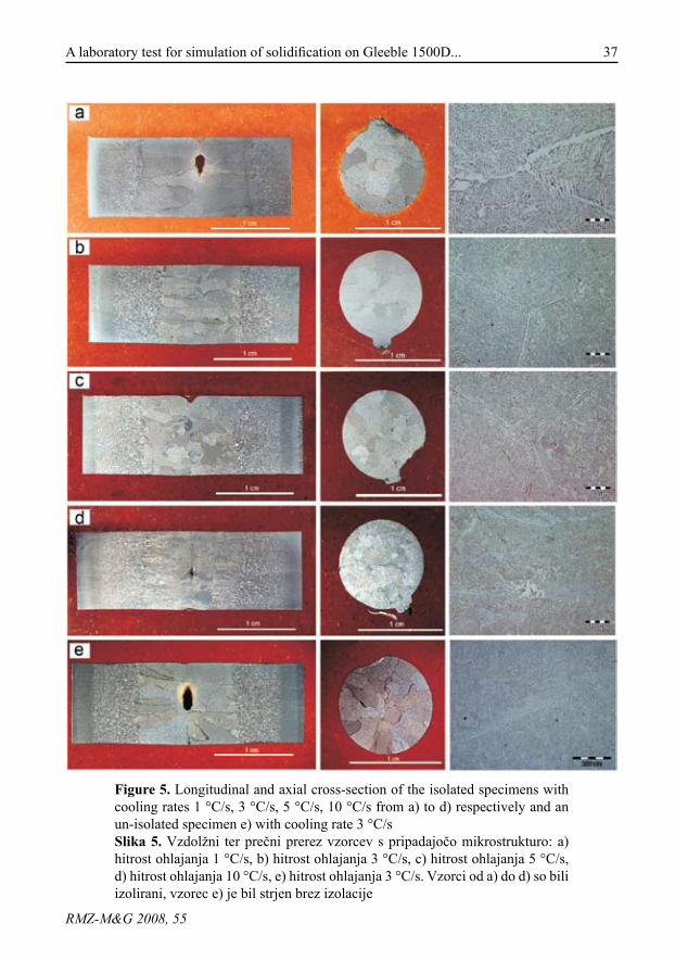
37A laboratory test for simulation of solidification on Gleeble 1500D...
RMZ-M&G 2008, 55
Figure 5. Longitudinal and axial cross-section of the isolated specimens with cooling rates 1 °C/s, 3 °C/s, 5 °C/s, 10 °C/s from a) to d) respectively and an un-isolated specimen e) with cooling rate 3 °C/sSlika 5. Vzdolžni ter prečni prerez vzorcev s pripadajočo mikrostrukturo: a) hitrost ohlajanja 1 °C/s, b) hitrost ohlajanja 3 °C/s, c) hitrost ohlajanja 5 °C/s, d) hitrost ohlajanja 10 °C/s, e) hitrost ohlajanja 3 °C/s. Vzorci od a) do d) so bili izolirani, vzorec e) je bil strjen brez izolacije
38 BRAdAskjA, B., koRuZA, j., fAZARinc, m., knAp, m., TuRk, R.
RMZ-M&G 2008, 55
Lower cooling rates caused the formation of columnar grains which can be observed in the macrostructures presented in the Figure 5a-d. These grains start to form on the solid material on the edge of the melted zone and grow into the center of the melt, in the opposite direction of the heat flow.
With increase of the cooling rate the so-lidification time shortens which resulted in increased number of smaller sized grains (Figure 5a-d). Above a certain thresh-old of cooling rate, as seen in Figure 5d, a relatively large amount of latent heat is momentarily set free. The heat flow is not sufficient thus the cooling rate of the remained liquid in the center of the speci-men is reduced. Therefore the center of the specimen is solidified with a slower cool-ing rate. Consequently the observed solidi-fied structure consists of two different grain structures where the CET zone is clearly seen. The first grains are columnar and are more numerous than those obtained from the specimens solidified with slower cool-ing rate. The second type of grains is more globular type and is solidified last. These grains did not solidify directionally.
In order to investigate the effect of the iso-lation on macro- and microstructure, one specimen was solidified without isolation. The cooling rate was 3 °C/s and the mac-rostructure is shown on Figure 5e. Because of the large radial heat loses due to radia-tion the solidification was not directional and there was also a large shrinkage cav-ity. The surface was solidified prior to the center of the specimen and the lack of the material appears because it could not be compensated by compression loading.
The grain size does not differ from that obtained from the specimen which was so-lidified with isolation.
conclusIons
A solidification test was developed, us-ing thermo-mechanical simulator Gleeble 1500D which enables simultaneous com-puter guided mechanical and thermal load-ing.
Additional cooling ribs were used to con-trol the axial thermal gradient. With vary-ing the position of these ribs different temperature fields were obtained. The ra-dial temperature difference was minimized by means of refractory material, placed around the quartz crucible. With an ad-ditional test without refractory material it was proven that solidification was not unidirectional and a large shrinkage cavity was observed.
A comparison between four samples so-lidified and cooled with different cooling rates was made. It was observed that cool-ing rate has a substantial influence on final grain size. With increasing the cooling rate the grains are found to be smaller. CET zone was also observed in the sample that was cooled with the highest cooling rate.
povzetek
Laboratorijski test simulacije strjevan-ja na termo-mehanskem simulatorju Gleeble 1500D
39A laboratory test for simulation of solidification on Gleeble 1500D...
RMZ-M&G 2008, 55
Razvit je bil test za strjevanje kovinskih materialov. Test je bil razvit kot dodatek termo-mehanskemu simulatorju metalur-ških stanj, Gleeble 1500D, ki omogoča simultano računalniško vodenje tempera-turnega in mehanskega programa obreme-njevanja vzorca.
Z dodatnimi, vodno hlajenimi, bakrenimi, hladilnimi rebri je bil kontroliran aksialni temperaturni gradient. S premikanjem le-teh je moč doseči različna temperaturna polja. Radialni temperaturni gradient je bil zmanjšan z uporabo ognjevzdržnega mate-riala, ki je obdajal kvarčno cevko. Z doda-tnim testom, ki je bil izveden brez ognje-vzdržnega materiala, je bilo pokazano, da strjevanje ni potekalo usmerjeno, oziroma ni bilo enoosno.
Narejena je bila primerjava med štirimi vzorci, strjenimi in ohlajenimi z različnimi ohlajevalnimi hitrostmi. Opaženo je bilo, da ima ohlajevalna hitrost močan vpliv na končno velikost zrn. Z povečevanjem ohla-jevalne hitrosti so zrna postajala manjša, v vzorcu, ki je bil ohlajen z najvišjo hitro-stjo, pa je moč opaziti prehodno cono med stebričastimi in ekviaksialnimi kristali.
references
[1] seoL, d.j., Won, Y.m., oH, k. H., sHin, Y.c. and Yim, c.H. (2000): Mechanical Behaviour of Carbon Steels in the Temperature Range of Mushy Zone. ISIJ Internatio-nal.; Vol. 40, No. 4, pp. 356-363.
[2] seoL, d. j., Won, Y.m., Yeo, T., oH, k.H., pARk, j.k. and Yim, c. H. (1999): High Temperature Defor-mation Behavior of Carbon Steel in the Austenite and δ-Ferrite Re-gions. ISIJ International.; Vol. 39, No. 1, pp. 91-98.
[3] nA, W., Zijiu d., WeicHAnG, c., YAn, Z. (1989): Hot Ducility of Con-tinuous Casting Carbon Steel. SPT3.; vol. 10-12, Vienna.
[4] GLpWAcki, m., mALinoWski, Z., HojnY, m., jedRZejcZYk, d. (2004): The phisical and mathematical mo-delling of plastic deformation of samples with mushy zone. Inverse Problems, Design and Optimiza-tion Symposium. Rio de Janeiro, Brazil.
[5] suZuki, H.G., nisHimuRA, s. and YA-mAGucHi, s. (1988): Physical Si-mulation of the Continuous Ca-sting of Steel. The International Symposium on Physical Simulati-on of Welding, Hot Forming and Continuous Casting held in Otta-wa. Canada.
[6] suZuki, H.G., nisHimuRA, s. and YAmAGuTcHi, s. (1984): Improve-ment of Hot Ductility of Continu-ously Cast Carbon Steels. Trans-actions ISIJ.; Vol. 24, pp. 54-59.
[7] suZuki, H.G., nisHimuRA, s. and YAmAGuTcHi, s. (1982): Charac-

40 BRAdAskjA, B., koRuZA, j., fAZARinc, m., knAp, m., TuRk, R.
RMZ-M&G 2008, 55
teristics of Hot Ductility in Steels. Transactions ISIJ.; Vol. 22, pp. 48-56.
[8] kosTRivAs, A. and LippoLd, j.c. (2000): A Method for Studying Weld Fu-sion Boundary Microstructure Evolution in Aluminum Alloys. Welding Research Supplement. pp. 1-8.
41RMZ – Materials and Geoenvironment, Vol. 55, No. 1, pp. 41-66, 2008
Scientific paper
Comparative test of active and passive multichannel analysis of surface waves (MASW) methods
and microtremor HVSR method
Primerjalni test aktivne in pasivne večkanalne analize površinskih valov (MASW) ter metode
mikrotremorjev (HVSR)
AndRej GosAR1,2, RoBeRT sTopAR3, jAneZ RošeR2
1Environmental Agency of the Republic of Slovenia, Seismology and Geology Office, Dunajska cesta 47, SI-1000 Ljubljana, Slovenia, E-mail: [email protected]
2University of Ljubljana, Faculty of Natural Sciences and Engineering, Aškerčeva cesta 12,SI-1000 Ljubljana, Slovenia; E-mail: [email protected]
3Geoinženiring d.o.o., Dimičeva ulica 14, SI-1000 Ljubljana, Slovenia; E-mail: [email protected]
Received: December 5, 2007 Accepted: January 15, 2008
Abstract: Shallow shear-wave velocity structure is important for seismological ground motion studies and for geotechnical engineering, but it is quite difficult and expensive to derive by using conventional geophysical tech-niques. Multichannel analysis of surface waves (MASW) and microtremor methods are therefore a valuable alternative developed in the last decade. A test of active and passive MASW and microtremor HVSR method was con-ducted in the southern part of Ljubljana which is characterised by soft sedi-ments and strong seismological site effects. Land streamer which allows fast movement of geophones array in the field was successfully applied for the first time. Shear-wave velocities in the range 50-200 m/s were obtained in the 25 m thick layer of Quaternary sediments overlying Palaeozoic bed-rock. The correspondence of velocity profiles obtained with different meth-ods was satisfactory. Active MASW proved most useful in a case of target depth which does not exceed 30 m and passive MASW for greater depths. The advantage of microtremor HVSR is that it yields direct estimate of the fundamental resonance frequency of the sediments.
Izvleček: Hitrost strižnih seizmičnih valov v površinskih plasteh je pomembna za seizmološke analize nihanja tal ob potresu in v geotehniki, vendar pa jo je dokaj težko in drago določiti z uveljavljenimi geofizikalnimi metodami. V zadnjem desetletju pa so razvili nove metode večkanalne analize povr-šinskih valov (MASW) in spektralnih razmerij mikrotremorjev (HVSR). V južnem delu Ljubljane, za katerega so značilni mehki sedimenti in izra-
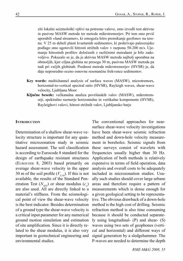
42 GosAR, A., sTopAR, R., RošeR, j.
RMZ-M&G 2008, 55
ziti lokalni seizmološki vplivi na potresne valove, smo izvedli test aktivne in pasivne MASW metode ter metode mikrotremorjev. Pri tem smo prvič uporabili »land streamer«, ki omogoča hitro premikanje geofonov na tere-nu. V 25 m debeli plasti kvartarnih sedimentov, ki prekrivajo paleozojsko podlago smo ugotovili hitrosti strižnih valov v razponu 50-200 m/s. Uje-manje hitrostnih profilov določenih z različnimi metodami je bilo zado-voljivo. Pokazalo se je, da je aktivna MASW metoda najbolj uporabna na območjih, kjer ciljna globina ne presega 30 m, pasivna MASW metoda pa tudi pri večjih globinah. Prednost metode mikrotremorjev (HVSR) je, da daje neposredno oceno osnovne resonančne frekvence sedimentov.
Key words: multichannel analysis of surface waves (MASW), microtremors, horizontal-to-vertical spectral ratio (HVSR), Rayleigh waves, shear-wave velocity, Ljubljana Moor
Ključne besede: večkanalna analiza površinskih valov (MASW), mikrotrem-orji, spektralno razmerje horizontalne in vertikalne komponente (HVSR), Rayleighovi valovi, hitrost strižnih valov, Ljubljansko barje
IntroductIon
Determination of a shallow shear-wave ve-locity structure is important for any quan-titative microzonation study in seismic hazard assessment. The soil classification is according to Eurocode 8 standard for the design of earthquake resistant structures (euRocode 8, 2003) based primarily on average shear-wave velocity in the upper 30 m of the soil profile (VS,30). If this is not available, the results of the Standard Pen-etration Test (NSPT) or shear modulus (cu) are also used. All are directly linked to a material’s stiffness. From the seismologi-cal point of view the shear-wave velocity is the best indicator. Besides determination of a ground type the shear-wave velocity is a critical input parameter for any numerical ground motion simulation and estimation of site amplification. Since it is directly re-lated to the shear modulus, it is also very important in geotechnical engineering and environmental studies.
The conventional approaches for near-surface shear-wave velocity investigations have been shear-wave seismic refraction method and down-hole velocity measure-ment in boreholes. Seismic signals from these surveys consist of wavelets with frequencies usually higher than 30 Hz. Application of both methods is relatively expensive in terms of field operation, data analysis and overall costs to be adequately included in microzonation studies. Usu-ally such studies should cover large urbane areas and therefore require a pattern of measurements which is dense enough for a given geological setting to be representa-tive. The obvious drawback of a down-hole method is the high cost of drilling. Seismic refraction method is also time consuming because it should be conducted separate-ly using longitudinal- (P) and shear- (S) waves using two sets of geophones (verti-cal and horizontal) and different ways of signal generation by a sledgehammer. The P-waves are needed to determine the depth
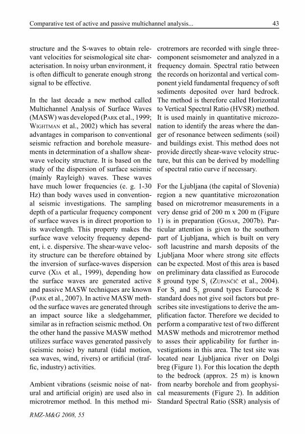
43Comparative test of active and passive multichannel analysis...
RMZ-M&G 2008, 55
structure and the S-waves to obtain rele-vant velocities for seismological site char-acterisation. In noisy urban environment, it is often difficult to generate enough strong signal to be effective.
In the last decade a new method called Multichannel Analysis of Surface Waves (MASW) was developed (pARk et al., 1999; WiGHTmAn et al., 2002) which has several advantages in comparison to conventional seismic refraction and borehole measure-ments in determination of a shallow shear-wave velocity structure. It is based on the study of the dispersion of surface seismic (mainly Rayleigh) waves. These waves have much lower frequencies (e. g. 1-30 Hz) than body waves used in convention-al seismic investigations. The sampling depth of a particular frequency component of surface waves is in direct proportion to its wavelength. This property makes the surface wave velocity frequency depend-ent, i. e. dispersive. The shear-wave veloc-ity structure can be therefore obtained by the inversion of surface-waves dispersion curve (XiA et al., 1999), depending how the surface waves are generated active and passive MASW techniques are known (pARk et al., 2007). In active MASW meth-od the surface waves are generated through an impact source like a sledgehammer, similar as in refraction seismic method. On the other hand the passive MASW method utilizes surface waves generated passively (seismic noise) by natural (tidal motion, sea waves, wind, rivers) or artificial (traf-fic, industry) activities.
Ambient vibrations (seismic noise of nat-ural and artificial origin) are used also in microtremor method. In this method mi-
crotremors are recorded with single three-component seismometer and analyzed in a frequency domain. Spectral ratio between the records on horizontal and vertical com-ponent yield fundamental frequency of soft sediments deposited over hard bedrock. The method is therefore called Horizontal to Vertical Spectral Ratio (HVSR) method. It is used mainly in quantitative microzo-nation to identify the areas where the dan-ger of resonance between sediments (soil) and buildings exist. This method does not provide directly shear-wave velocity struc-ture, but this can be derived by modelling of spectral ratio curve if necessary.
For the Ljubljana (the capital of Slovenia) region a new quantitative microzonation based on microtremor measurements in a very dense grid of 200 m x 200 m (Figure 1) is in preparation (GosAR, 2007b). Par-ticular attention is given to the southern part of Ljubljana, which is built on very soft lacustrine and marsh deposits of the Ljubljana Moor where strong site effects can be expected. Most of this area is based on preliminary data classified as Eurocode 8 ground type S1 (ZupAnČiČ et al., 2004). For S1 and S2 ground types Eurocode 8 standard does not give soil factors but pre-scribes site investigations to derive the am-plification factor. Therefore we decided to perform a comparative test of two different MASW methods and microtremor method to asses their applicability for further in-vestigations in this area. The test site was located near Ljubljanica river on Dolgi breg (Figure 1). For this location the depth to the bedrock (approx. 25 m) is known from nearby borehole and from geophysi-cal measurements (Figure 2). In addition Standard Spectral Ratio (SSR) analysis of
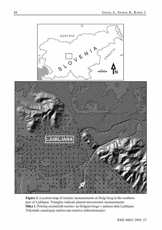
44 GosAR, A., sTopAR, R., RošeR, j.
RMZ-M&G 2008, 55
Figure 1. Location map of seismic measurements at Dolgi breg in the southern part of Ljubljana. Triangles indicate planed microtremor measurements.Slika 1. Položaj seizmičnih meritev na Dolgem bregu v južnem delu Ljubljane. Trikotniki označujejo načrtovane meritve mikrotremorjev.
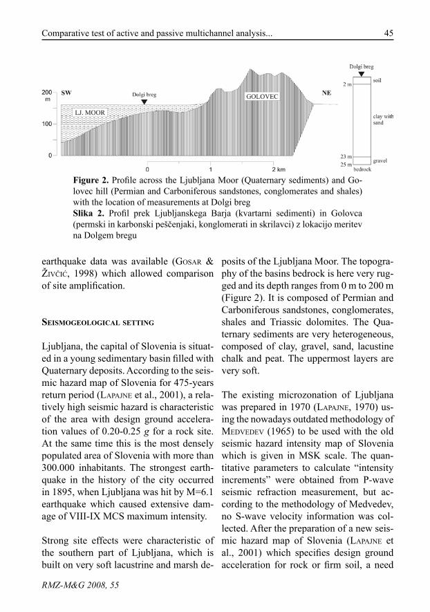
45Comparative test of active and passive multichannel analysis...
RMZ-M&G 2008, 55
earthquake data was available (GosAR & živČić, 1998) which allowed comparison of site amplification.
seIsmogeologIcal settIng
Ljubljana, the capital of Slovenia is situat-ed in a young sedimentary basin filled with Quaternary deposits. According to the seis-mic hazard map of Slovenia for 475-years return period (LApAjne et al., 2001), a rela-tively high seismic hazard is characteristic of the area with design ground accelera-tion values of 0.20-0.25 g for a rock site. At the same time this is the most densely populated area of Slovenia with more than 300.000 inhabitants. The strongest earth-quake in the history of the city occurred in 1895, when Ljubljana was hit by M=6.1 earthquake which caused extensive dam-age of VIII-IX MCS maximum intensity.
Strong site effects were characteristic of the southern part of Ljubljana, which is built on very soft lacustrine and marsh de-
posits of the Ljubljana Moor. The topogra-phy of the basins bedrock is here very rug-ged and its depth ranges from 0 m to 200 m (Figure 2). It is composed of Permian and Carboniferous sandstones, conglomerates, shales and Triassic dolomites. The Qua-ternary sediments are very heterogeneous, composed of clay, gravel, sand, lacustine chalk and peat. The uppermost layers are very soft.
The existing microzonation of Ljubljana was prepared in 1970 (LApAjne, 1970) us-ing the nowadays outdated methodology of medvedev (1965) to be used with the old seismic hazard intensity map of Slovenia which is given in MSK scale. The quan-titative parameters to calculate “intensity increments” were obtained from P-wave seismic refraction measurement, but ac-cording to the methodology of Medvedev, no S-wave velocity information was col-lected. After the preparation of a new seis-mic hazard map of Slovenia (LApAjne et al., 2001) which specifies design ground acceleration for rock or firm soil, a need
Figure 2. Profile across the Ljubljana Moor (Quaternary sediments) and Go-lovec hill (Permian and Carboniferous sandstones, conglomerates and shales) with the location of measurements at Dolgi bregSlika 2. Profil prek Ljubljanskega Barja (kvartarni sedimenti) in Golovca (permski in karbonski peščenjaki, konglomerati in skrilavci) z lokacijo meritev na Dolgem bregu
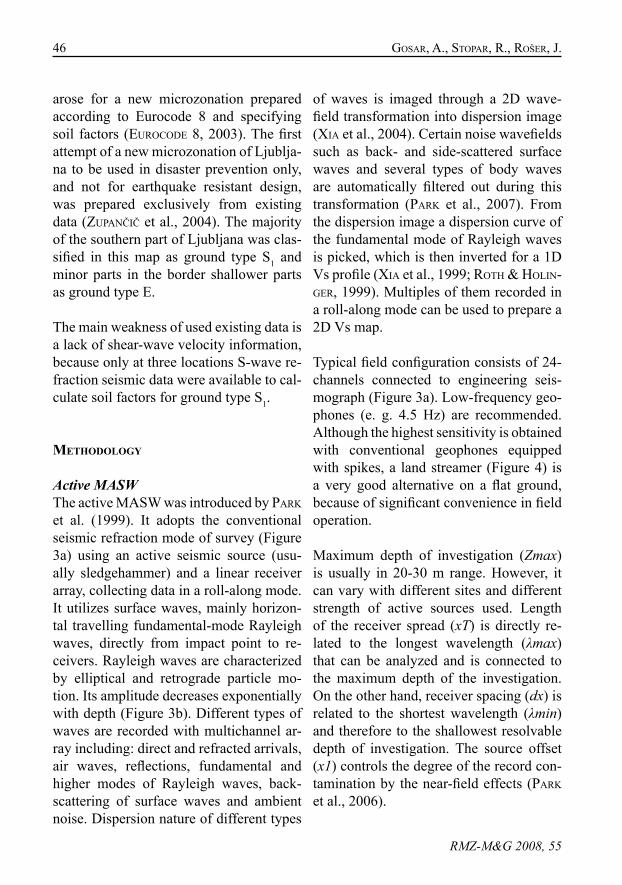
46 GosAR, A., sTopAR, R., RošeR, j.
RMZ-M&G 2008, 55
arose for a new microzonation prepared according to Eurocode 8 and specifying soil factors (euRocode 8, 2003). The first attempt of a new microzonation of Ljublja-na to be used in disaster prevention only, and not for earthquake resistant design, was prepared exclusively from existing data (ZupAnČiČ et al., 2004). The majority of the southern part of Ljubljana was clas-sified in this map as ground type S1 and minor parts in the border shallower parts as ground type E.
The main weakness of used existing data is a lack of shear-wave velocity information, because only at three locations S-wave re-fraction seismic data were available to cal-culate soil factors for ground type S1.
methodology
Active MASWThe active MASW was introduced by pARk et al. (1999). It adopts the conventional seismic refraction mode of survey (Figure 3a) using an active seismic source (usu-ally sledgehammer) and a linear receiver array, collecting data in a roll-along mode. It utilizes surface waves, mainly horizon-tal travelling fundamental-mode Rayleigh waves, directly from impact point to re-ceivers. Rayleigh waves are characterized by elliptical and retrograde particle mo-tion. Its amplitude decreases exponentially with depth (Figure 3b). Different types of waves are recorded with multichannel ar-ray including: direct and refracted arrivals, air waves, reflections, fundamental and higher modes of Rayleigh waves, back-scattering of surface waves and ambient noise. Dispersion nature of different types
of waves is imaged through a 2D wave-field transformation into dispersion image (XiA et al., 2004). Certain noise wavefields such as back- and side-scattered surface waves and several types of body waves are automatically filtered out during this transformation (pARk et al., 2007). From the dispersion image a dispersion curve of the fundamental mode of Rayleigh waves is picked, which is then inverted for a 1D Vs profile (XiA et al., 1999; RoTH & HoLin-GeR, 1999). Multiples of them recorded in a roll-along mode can be used to prepare a 2D Vs map.
Typical field configuration consists of 24-channels connected to engineering seis-mograph (Figure 3a). Low-frequency geo-phones (e. g. 4.5 Hz) are recommended. Although the highest sensitivity is obtained with conventional geophones equipped with spikes, a land streamer (Figure 4) is a very good alternative on a flat ground, because of significant convenience in field operation.
Maximum depth of investigation (Zmax) is usually in 20-30 m range. However, it can vary with different sites and different strength of active sources used. Length of the receiver spread (xT) is directly re-lated to the longest wavelength (λmax) that can be analyzed and is connected to the maximum depth of the investigation. On the other hand, receiver spacing (dx) is related to the shortest wavelength (λmin) and therefore to the shallowest resolvable depth of investigation. The source offset (x1) controls the degree of the record con-tamination by the near-field effects (pARk et al., 2006).
47Comparative test of active and passive multichannel analysis...
RMZ-M&G 2008, 55
Figure 3. a) Schematic representation of active MASW measurements. b) Par-ticle motion for Rayleigh waves showing amplitude decrease with depth (after sHeRiff & GeLdART, 1995).Slika 3. a) Shematski prikaz aktivnih MASW meritev. b) Gibanje delcev pri Rayleighjevem valovanju, ki kaže upadanje amplitude z globino (po sHeRiff & GeLdART, 1995).
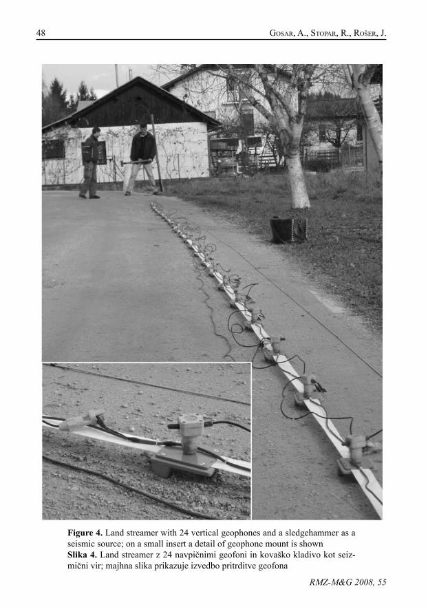
48 GosAR, A., sTopAR, R., RošeR, j.
RMZ-M&G 2008, 55
Figure 4. Land streamer with 24 vertical geophones and a sledgehammer as a seismic source; on a small insert a detail of geophone mount is shown Slika 4. Land streamer z 24 navpičnimi geofoni in kovaško kladivo kot seiz-mični vir; majhna slika prikazuje izvedbo pritrditve geofona
49Comparative test of active and passive multichannel analysis...
RMZ-M&G 2008, 55
When using sledgehammer or weight drop as a source a vertical stacking of multiple impacts can suppress ambient noise sig-nificantly.
Passive MASWThe main disadvantage of active MASW is the maximum depth of investigation which is usually 20-30 m. The amount of active-source energy needed to gain a few more Hz at the low-frequency end of the disper-sion image, and thereby to increase inves-tigation depth by several tens of meters, often rises several orders of magnitude, rendering efforts with an active source im-practical and uneconomical (pARk et al., 2007). On the other hand, passive surface waves generated by natural (tidal motion, sea waves, wind, rivers) or artificial (traf-fic, industry) activities are usually of a low frequency (1-30 Hz) with wavelengths ranging from few km (natural sources) to a few tens or hundreds of meters (artificial sources), providing a wide range of pen-etration depths.
This method was originally developed in Japan and called microtremor survey method (okAdA, 2003) and adopted a smaller number (usually less than ten) of receivers. It is sometimes called also Mi-crotremor Array Measurements or MAM (HAYAsHi et al., 2006). Louie (2001) first in-troduced linear refraction microtremor ar-rays (ReMi method). These methods were later developed as passive MASW method, which uses 24 or more geophones to fully exploit the advantages of multichannel re-cording and processing (pARk et al., 2007). It therefore has an increased resolution in the analysis of both the modal nature and azimuthal properties of surface waves.
The passive MASW method employs a 2D geophone array such as a cross (Figure 8) or circular layout to record passive surface waves. Other array types as triangular or square are also common, but it is recom-mended that they have a symmetric shape. Any asymmetry can bias a result toward a specific direction of incoming surface waves that do not necessarily coincide with the actual direction of major surface-wave energy.
Array dimension is directly related to the longest wavelength (λmax) that can be analyzed and is connected to the maxi-mum depth of the investigation. On the other hand, minimum receiver spacing is related to the shortest wavelength (λmin) and therefore to the shallowest resolvable depth of investigation. The typical depth of investigation for passive MASW is up to 100 m.
Data processing and analysis is similar as in active MASW and includes three steps: 1) generation of the dispersion image (phase velocity-frequency chart), 2) extraction of the dispersion curve from the image and 3) inversion of 1D shear-wave velocity profile from the dispersion curve (pARk et al., 2006). Some techniques like ReMi use slowness instead of phase velocity.
It is often useful to combine dispersion im-ages from active and passive sets for two reasons: to enlarge the usable bandwidth of dispersion (and therefore the depth range) and to better identify the modal nature of dispersion trends (pARk et al., 2005).
Microtremor HVSRThe microtremor HVSR method is in the
50 GosAR, A., sTopAR, R., RošeR, j.
RMZ-M&G 2008, 55
last decade widely used for microzona-tion and site effects studies (e. g. GosAR, 2007a, 2007b). However, the theoretical basis of HVSR method is still debated and different explanations have been given. “Body waves” explanation is based on S-wave resonance in soft sediments layer with minor or neglecting influence of sur-face waves. More widely accepted is the “surface waves” explanation that HVSR is related to the ellipticity of Rayleigh waves which is frequency dependent (BARd, 1999). HVSR exhibits therefore a sharp peak at the fundamental frequency of the sediments, if there is a high impedance contrast between the sediments and the un-derlying bedrock. Criticism of the HVSR method was often related to the fact that there is no common practice for data acqui-sition and processing. Attempts to provide standards were only recently been made (SESAME, 2004). It is widely accepted today that the frequency of the HVSR peak reflects the fundamental frequency of the sediments. Its amplitude depends mainly on the impedance contrast with the bedrock and cannot be used as a site am-plification. However, a comparison with results of standard spectral ratio method has shown that the HVSR peak amplitude underestimates the actual site amplifica-tion (BARd, 1999; SESAME, 2004). HVSR also does not provide any estimate of the actual bandwidth over which the ground motion is amplified. The main advantages of HVSR method are therefore simple and low-cost measurements and direct esti-mates of the resonance frequency of sedi-ments without knowing the geological and S-velocity structure of the underground. Any knowledge about the thickness or/and velocity of sediments and the comparison
of HVSR results with other methods and with the observed earthquake damage can significantly improve the reliability of the results.
Microtremor HVSR method does not pro-vide directly shear-wave velocity struc-ture, but this can be derived by modelling of spectral ratio curve if necessary. It is usually based on the search for the model whose theoretical HVSR response best matches the observed HVSR by random perturbation of model parameters within preselected limits (HeRAk, 2007).
data acquIsItIon and analysIs
A comparative test of three different meth-ods was performed at Dolgi breg near Ljubljanica river on the Ljubljana Moor (Figures 1 and 2). This site was selected for several reasons: a) the depth to the bed-rock (approx. 25 m) is known from nearby borehole and geophysical measurements, b) the thickness of soft sediments is inside the depth penetration of active MASW method (less than 30 m), c) strong acous-tic impedance contrast between sediments and bedrock is known from previous mi-crotremor measurements (GosAR, 2007b) and d) at a nearby location earthquake data were recorded which allows Standard Spectral Ratio (SSR) analysis (GosAR & živČić, 1998) for comparison.
Data acquisition parameters for all three methods are summarized in Table 1. Ac-tive and passive MASW measurements were performed using 24 channel ABEM Terraloc Mk6 seismograph with 24 bit digitiser. Because active MASW and mi-
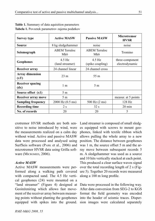
51Comparative test of active and passive multichannel analysis...
RMZ-M&G 2008, 55
crotremor HVSR methods are both sen-sitive to noise introduced by wind, were the measurements realized on a calm day without wind. Active and passive MASW data were processed and analysed using SurfSeis software (pARk et al., 2006) and microtremor HVSR data using Grilla soft-ware (micRomed, 2006).
Active MASWActive MASW measurements were per-formed along a walking path covered with compacted sand. The 4.5 Hz verti-cal geophones (24) were mounted on a “land streamer” (Figure 4) designed at Geoinženiring which allows fast move-ment of the receiver array between measur-ing points without planting the geophones equipped with spikes into the ground.
Table 1. Summary of data aquisition parametersTabela 1. Povzetek parametrov zajema podatkov
Survey type Active MASW Passive MASW Microtremor HVSR
Source 8 kg sledgehammer noise noise
Seismograph ABEM Terraloc Mk6
ABEM Terraloc Mk6 Tromino
Geophones 4.5 Hz (land streamer)
4.5 Hz(spike coupling)
three-componentelectrodynamic
Receiver array 24 channel linear 24 channel crossArray dimension (xT) 23 m 55 m
Receiver spacing (dx) 1 m 5 m
Source offset (x1) 5 mReceiver array move 5 m measur. at 5 pointsSampling frequency 2000 Hz (0.5 ms) 500 Hz (2 ms) 128 HzRecording time 2 s 32 s 20 minNo. of records 20 20 5
Land streamer is composed of small sledg-es equipped with screws to mount geo-phones, linked with textile ribbon which allows pulling the whole array to a new position. The distance between geophones was 1 m, the source offset 5 m and the ar-ray move between subsequent records 5 m. A sledgehammer was used as a source and 10 hits vertically stacked at each point. This produced a clear surface waves signal over the total recording length of 2 s (Fig-ure 5). Together 20 records were measured along a 100 m long profile.
Data were processed in the following way. After data conversion from SEG-2 to KGS format the field geometry was encoded into the header of seismic traces. Disper-sion images were calculated separately
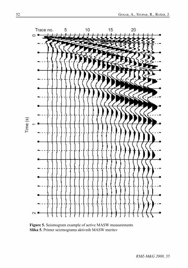
52 GosAR, A., sTopAR, R., RošeR, j.
RMZ-M&G 2008, 55
Figure 5. Seismogram example of active MASW measurementsSlika 5. Primer seizmograma aktivnih MASW meritev
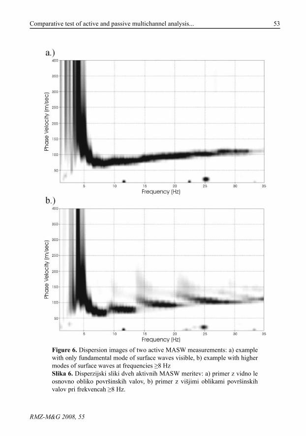
53Comparative test of active and passive multichannel analysis...
RMZ-M&G 2008, 55
Figure 6. Dispersion images of two active MASW measurements: a) example with only fundamental mode of surface waves visible, b) example with higher modes of surface waves at frequencies ≥8 HzSlika 6. Disperzijski sliki dveh aktivnih MASW meritev: a) primer z vidno le osnovno obliko površinskih valov, b) primer z višjimi oblikami površinskih valov pri frekvencah ≥8 Hz.
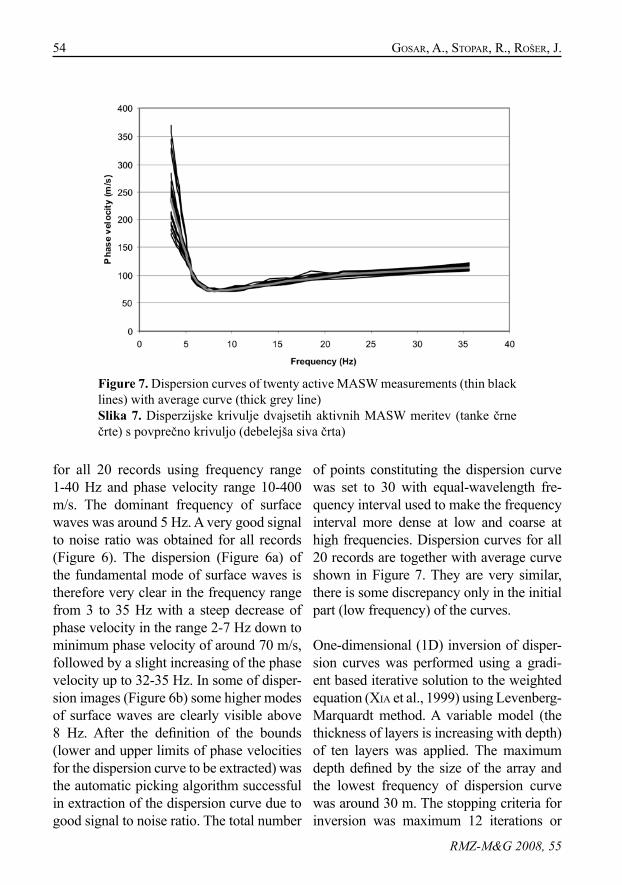
54 GosAR, A., sTopAR, R., RošeR, j.
RMZ-M&G 2008, 55
for all 20 records using frequency range 1-40 Hz and phase velocity range 10-400 m/s. The dominant frequency of surface waves was around 5 Hz. A very good signal to noise ratio was obtained for all records (Figure 6). The dispersion (Figure 6a) of the fundamental mode of surface waves is therefore very clear in the frequency range from 3 to 35 Hz with a steep decrease of phase velocity in the range 2-7 Hz down to minimum phase velocity of around 70 m/s, followed by a slight increasing of the phase velocity up to 32-35 Hz. In some of disper-sion images (Figure 6b) some higher modes of surface waves are clearly visible above 8 Hz. After the definition of the bounds (lower and upper limits of phase velocities for the dispersion curve to be extracted) was the automatic picking algorithm successful in extraction of the dispersion curve due to good signal to noise ratio. The total number
of points constituting the dispersion curve was set to 30 with equal-wavelength fre-quency interval used to make the frequency interval more dense at low and coarse at high frequencies. Dispersion curves for all 20 records are together with average curve shown in Figure 7. They are very similar, there is some discrepancy only in the initial part (low frequency) of the curves.
One-dimensional (1D) inversion of disper-sion curves was performed using a gradi-ent based iterative solution to the weighted equation (XiA et al., 1999) using Levenberg-Marquardt method. A variable model (the thickness of layers is increasing with depth) of ten layers was applied. The maximum depth defined by the size of the array and the lowest frequency of dispersion curve was around 30 m. The stopping criteria for inversion was maximum 12 iterations or
Figure 7. Dispersion curves of twenty active MASW measurements (thin black lines) with average curve (thick grey line)Slika 7. Disperzijske krivulje dvajsetih aktivnih MASW meritev (tanke črne črte) s povprečno krivuljo (debelejša siva črta)
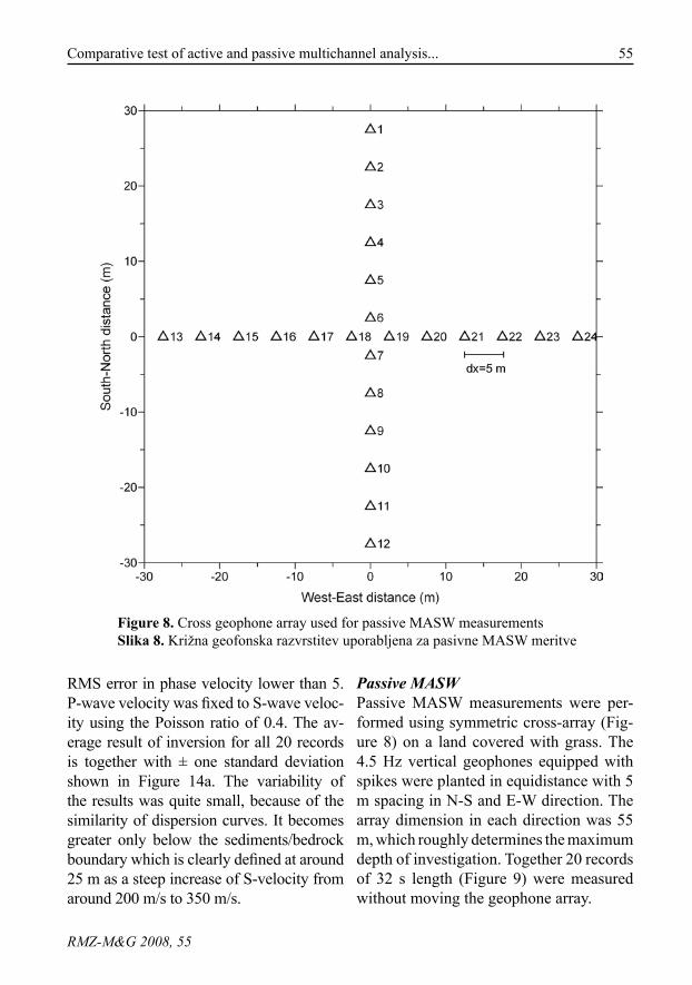
55Comparative test of active and passive multichannel analysis...
RMZ-M&G 2008, 55
RMS error in phase velocity lower than 5. P-wave velocity was fixed to S-wave veloc-ity using the Poisson ratio of 0.4. The av-erage result of inversion for all 20 records is together with ± one standard deviation shown in Figure 14a. The variability of the results was quite small, because of the similarity of dispersion curves. It becomes greater only below the sediments/bedrock boundary which is clearly defined at around 25 m as a steep increase of S-velocity from around 200 m/s to 350 m/s.
Figure 8. Cross geophone array used for passive MASW measurementsSlika 8. Križna geofonska razvrstitev uporabljena za pasivne MASW meritve
Passive MASWPassive MASW measurements were per-formed using symmetric cross-array (Fig-ure 8) on a land covered with grass. The 4.5 Hz vertical geophones equipped with spikes were planted in equidistance with 5 m spacing in N-S and E-W direction. The array dimension in each direction was 55 m, which roughly determines the maximum depth of investigation. Together 20 records of 32 s length (Figure 9) were measured without moving the geophone array.
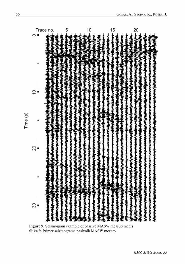
56 GosAR, A., sTopAR, R., RošeR, j.
RMZ-M&G 2008, 55
Figure 9. Seismogram example of passive MASW measurementsSlika 9. Primer seizmograma pasivnih MASW meritev
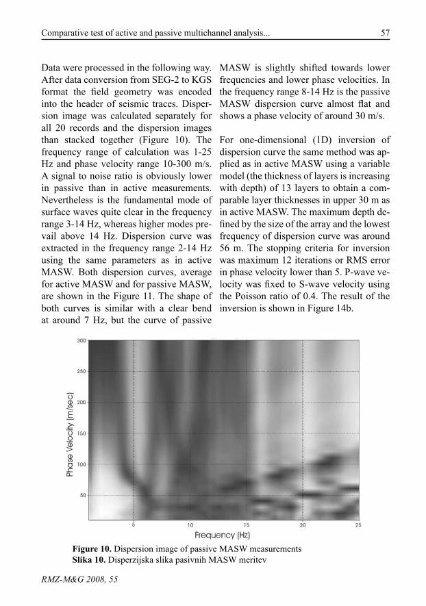
57Comparative test of active and passive multichannel analysis...
RMZ-M&G 2008, 55
Data were processed in the following way. After data conversion from SEG-2 to KGS format the field geometry was encoded into the header of seismic traces. Disper-sion image was calculated separately for all 20 records and the dispersion images than stacked together (Figure 10). The frequency range of calculation was 1-25 Hz and phase velocity range 10-300 m/s. A signal to noise ratio is obviously lower in passive than in active measurements. Nevertheless is the fundamental mode of surface waves quite clear in the frequency range 3-14 Hz, whereas higher modes pre-vail above 14 Hz. Dispersion curve was extracted in the frequency range 2-14 Hz using the same parameters as in active MASW. Both dispersion curves, average for active MASW and for passive MASW, are shown in the Figure 11. The shape of both curves is similar with a clear bend at around 7 Hz, but the curve of passive
MASW is slightly shifted towards lower frequencies and lower phase velocities. In the frequency range 8-14 Hz is the passive MASW dispersion curve almost flat and shows a phase velocity of around 30 m/s.
For one-dimensional (1D) inversion of dispersion curve the same method was ap-plied as in active MASW using a variable model (the thickness of layers is increasing with depth) of 13 layers to obtain a com-parable layer thicknesses in upper 30 m as in active MASW. The maximum depth de-fined by the size of the array and the lowest frequency of dispersion curve was around 56 m. The stopping criteria for inversion was maximum 12 iterations or RMS error in phase velocity lower than 5. P-wave ve-locity was fixed to S-wave velocity using the Poisson ratio of 0.4. The result of the inversion is shown in Figure 14b.
Figure 10. Dispersion image of passive MASW measurementsSlika 10. Disperzijska slika pasivnih MASW meritev
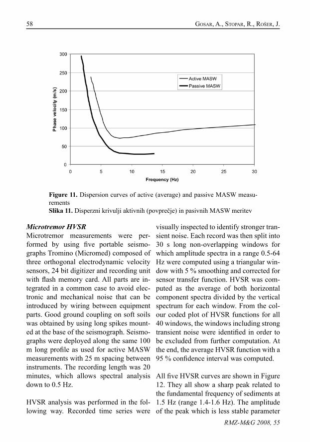
58 GosAR, A., sTopAR, R., RošeR, j.
RMZ-M&G 2008, 55
Figure 11. Dispersion curves of active (average) and passive MASW measu-rementsSlika 11. Disperzni krivulji aktivnih (povprečje) in pasivnih MASW meritev
Microtremor HVSRMicrotremor measurements were per-formed by using five portable seismo-graphs Tromino (Micromed) composed of three orthogonal electrodynamic velocity sensors, 24 bit digitizer and recording unit with flash memory card. All parts are in-tegrated in a common case to avoid elec-tronic and mechanical noise that can be introduced by wiring between equipment parts. Good ground coupling on soft soils was obtained by using long spikes mount-ed at the base of the seismograph. Seismo-graphs were deployed along the same 100 m long profile as used for active MASW measurements with 25 m spacing between instruments. The recording length was 20 minutes, which allows spectral analysis down to 0.5 Hz.
HVSR analysis was performed in the fol-lowing way. Recorded time series were
visually inspected to identify stronger tran-sient noise. Each record was then split into 30 s long non-overlapping windows for which amplitude spectra in a range 0.5-64 Hz were computed using a triangular win-dow with 5 % smoothing and corrected for sensor transfer function. HVSR was com-puted as the average of both horizontal component spectra divided by the vertical spectrum for each window. From the col-our coded plot of HVSR functions for all 40 windows, the windows including strong transient noise were identified in order to be excluded from further computation. At the end, the average HVSR function with a 95 % confidence interval was computed.
All five HVSR curves are shown in Figure 12. They all show a sharp peak related to the fundamental frequency of sediments at 1.5 Hz (range 1.4-1.6 Hz). The amplitude of the peak which is less stable parameter
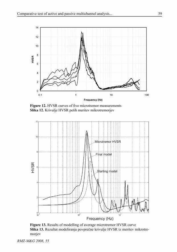
59Comparative test of active and passive multichannel analysis...
RMZ-M&G 2008, 55
Figure 12. HVSR curves of five microtremor measurementsSlika 12. Krivulje HVSR petih meritev mikrotremorjev
Figure 13. Results of modelling of average microtremor HVSR curveSlika 13. Rezultat modeliranja povprečne krivulje HVSR iz meritev mikrotre-morjev
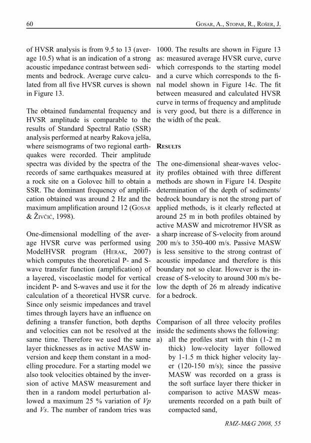
60 GosAR, A., sTopAR, R., RošeR, j.
RMZ-M&G 2008, 55
of HVSR analysis is from 9.5 to 13 (aver-age 10.5) what is an indication of a strong acoustic impedance contrast between sedi-ments and bedrock. Average curve calcu-lated from all five HVSR curves is shown in Figure 13.
The obtained fundamental frequency and HVSR amplitude is comparable to the results of Standard Spectral Ratio (SSR) analysis performed at nearby Rakova jelša, where seismograms of two regional earth-quakes were recorded. Their amplitude spectra was divided by the spectra of the records of same earthquakes measured at a rock site on a Golovec hill to obtain a SSR. The dominant frequency of amplifi-cation obtained was around 2 Hz and the maximum amplification around 12 (GosAR & živČić, 1998).
One-dimensional modelling of the aver-age HVSR curve was performed using ModelHVSR program (HeRAk, 2007) which computes the theoretical P- and S-wave transfer function (amplification) of a layered, viscoelastic model for vertical incident P- and S-waves and use it for the calculation of a theoretical HVSR curve. Since only seismic impedances and travel times through layers have an influence on defining a transfer function, both depths and velocities can not be resolved at the same time. Therefore we used the same layer thicknesses as in active MASW in-version and keep them constant in a mod-elling procedure. For a starting model we also took velocities obtained by the inver-sion of active MASW measurement and then in a random model perturbation al-lowed a maximum 25 % variation of Vp and Vs. The number of random tries was
1000. The results are shown in Figure 13 as: measured average HVSR curve, curve which corresponds to the starting model and a curve which corresponds to the fi-nal model shown in Figure 14c. The fit between measured and calculated HVSR curve in terms of frequency and amplitude is very good, but there is a difference in the width of the peak.
results
The one-dimensional shear-waves veloc-ity profiles obtained with three different methods are shown in Figure 14. Despite determination of the depth of sediments/bedrock boundary is not the strong part of applied methods, is it clearly reflected at around 25 m in both profiles obtained by active MASW and microtremor HVSR as a sharp increase of S-velocity from around 200 m/s to 350-400 m/s. Passive MASW is less sensitive to the strong contrast of acoustic impedance and therefore is this boundary not so clear. However is the in-crease of S-velocity to around 300 m/s be-low the depth of 26 m already indicative for a bedrock.
Comparison of all three velocity profiles inside the sediments shows the following:
all the profiles start with thin (1-2 m a) thick) low-velocity layer followed by 1-1.5 m thick higher velocity lay-er (120-150 m/s); since the passive MASW was recorded on a grass is the soft surface layer there thicker in comparison to active MASW meas-urements recorded on a path built of compacted sand,
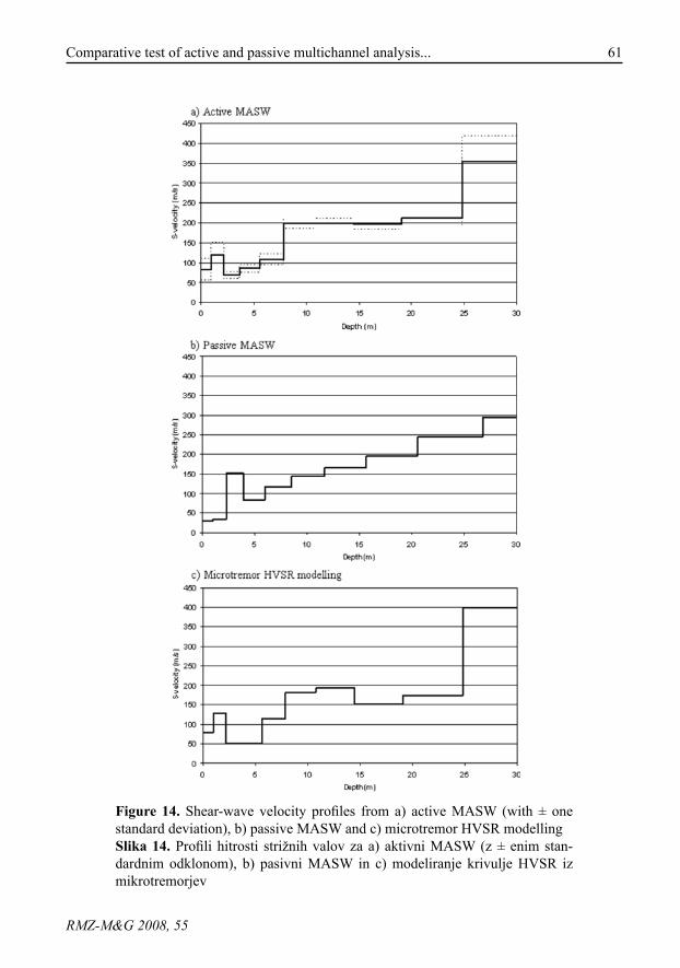
61Comparative test of active and passive multichannel analysis...
RMZ-M&G 2008, 55
Figure 14. Shear-wave velocity profiles from a) active MASW (with ± one standard deviation), b) passive MASW and c) microtremor HVSR modellingSlika 14. Profili hitrosti strižnih valov za a) aktivni MASW (z ± enim stan-dardnim odklonom), b) pasivni MASW in c) modeliranje krivulje HVSR iz mikrotremorjev
62 GosAR, A., sTopAR, R., RošeR, j.
RMZ-M&G 2008, 55
in the depth range 2-7.5 m there is a b) low velocity layer (50-120 m/s),in the depth range 7.5-25 m is the ve-c) locity according to active MASW and microtremor HVSR quite stable (150-210 m/s), while according to passive MASW there is a gradual increase of velocity from 150 to 250 m/s.
The S-velocities from dispersion of sur-face waves for the upper five meters are comparable to the velocities from shal-low seismic refraction measurements per-formed at geologically similar location at Park Svoboda, also in the southern part of Ljubljana, where the velocities between 95 and 180 m/s were measured in the first five meters (živAnović & sTopAR, 1995).
The parameter widely applied in seismic microzonation, also the main parameter for ground type classification in Eurocode 8 standard (euRocode 8, 2003), is average shear-wave velocity in upper 30 m (VS,30). It is computed according to the following expression
where hi and Vi denote the thickness (in m) and shear-wave velocity (in m/s) in the i-th formation of layer, in a total of N, existing in the top 30 metres.
Since the shear-wave velocity in the bed-rock can not be well defined with applied methods we computed equivalent average velocity for the total thickness of sediments (around 25 m) and obtained the following values:
active MASW – 145 m/s,•
passive MASW – 120 m/s,•microtremor HVSR – 120 m/s.•
Considering only this parameter to define the ground type in Eurocode 8, can be the investigated site classified as ground type D (Vs<180 m/s). But if we consider also a description of the stratigraphic profile, it is more likely ground type S1 (Vs<100 m/s) described as: deposits consisting - or con-taining a layer at least 10 m thick – of soft clay/silts with high plasticity index and high water content.
conclusIons
Performed investigations with three differ-ent methods have shown that they are all effective in the determination of a shallow shear-waves velocity profile, but there are also some important differences between them. Obtained one-dimensional velocity profiles are similar to acceptable extent. The average shear-wave velocity in the 25 m thick layer of sediments is between 120 m/s and 145 m/s. The value obtained by ac-tive MASW (145 m/s) is 20 % greater than the values obtained by passive MASW and microtremor HVSR modelling (120 m/s). We found no explanation for this, but the difference is not too big to have a consider-able influence on the determination of the ground type in seismic microzonation. The ground at investigated site can be therefore according to Eurocode 8 classified as type D or more likely S1, if we consider also a description of the stratigraphic profile.
Comparison of active and passive MASW has shown that if the depth of investigation does not exceed 30 m much more clear dis-
63Comparative test of active and passive multichannel analysis...
RMZ-M&G 2008, 55
persion image of surface waves is obtained with active method and is therefore prefer-able. A possible solution to increase the us-able frequency range of dispersion would be to combine dispersion images obtained from active and passive measurements at the same location with different geophone arrays (pARk et al., 2005) or using even the same linear array along a road where the traffic represents strong enough source of surface waves (pARk et al., 2006). In the later case a long record is used triggered by a single hit of a sledgehammer. Initial part of the record is then processed as active and the remaining part as passive MASW.
Land streamer array of geophones was tested for the first time and proved very efficient for active MASW measurements along a two-dimensional profile. The only condition is that the surface of the ground is flat enough to assure near-vertical position of geophones. In a case of expected lateral variations of velocity, two-dimensional measurements have additional advantages with respect to passive measurements.
Microtremor HVSR method yield directly the fundamental frequency of the sedi-ments overlying the bedrock which itself is a very valuable parameter of any microzo-nation, because it provides an estimate of the danger of soil-structure resonance. S-velocity profile can be derived by model-ling of HVSR curve only if a reliable con-straint on the thickness of the sediments can be done. If this is a case, as shown in our test, also microtremor data can pro-vide a good estimate of one-dimensional S-velocity profile. Moreover, applicabil-ity of microtremor HVSR method highly depends on a strength of the impedance
contrast between sediments and bedrock. On the contrary, MASW methods provide velocity profiles also for sites with gradual increase of velocity with depth.
povzetek
Primerjalni test aktivne in pasivne večkanalne analize površinskih valov (MASW) ter metode mikrotremorjev (HVSR)
Hitrost strižnih seizmičnih valov v povr-šinskih plasteh je pomembna za seizmo-loške analize nihanja tal ob potresu in v geotehniki, vendar pa jo je z uveljavljeni-mi geofizikalnimi metodami dokaj težko in drago določiti. V zadnjem desetletju pa so razvili nove metode večkanalne analize površinskih valov (MASW) in spektralnih razmerij mikrotremorjev (HVSR). MASW metoda temelji na disperziji površinskih (predvsem Rayleighjevih) valov, ki ima-jo precej nižje frekvence (1-30 Hz) kot prostorski seizmični valovi. Pri aktivnem MASW generiramo seizmične valove z udarci kladiva, pri pasivnem MASW in pri metodi mikrotremorjev pa uporabljamo seizmični nemir naravnega in umetnega izvora, ki je stalno prisoten v okolju.
V južnem delu Ljubljane, za katerega so značilni mehki sedimenti in izraziti lokal-ni seizmološki vplivi na potresne valove, smo izvedli test aktivne in pasivne MASW metode ter metode mikrotremorjev. Te-stno območje se nahaja na Dolgem bregu ob Ljubljanici, kjer je debelina kvartar-nih sedimentov okoli 25 m. Pri aktivnem MASW smo prvič uporabili geofone pri-trjene na posebnih nosilcih povezanih s
64 GosAR, A., sTopAR, R., RošeR, j.
RMZ-M&G 2008, 55
trakom (»land streamer«), ki omogoča hitro premikanje linearne razvrstitve 24-ih geofonov v medsebojni razdalji 1 m. Pri pasivnem MASW smo uporabili križno razvrstitev 2 x 12 geofonov v medsebojni razdalji 5 m. Meritve mikrotremorjev pa smo izvedli s posebnimi trikomponentni-mi seizmografi. Pokazalo se je, da je ak-tivna MASW metoda najbolj uporabna na območjih, kjer ciljna globina ne presega 30 m, pasivna MASW metoda pa tudi pri večjih globinah. Prednost metode mikro-tremorjev (HVSR) je, da daje neposredno oceno osnovne resonančne frekvence sedi-mentov. Pri slednji smo hitrostni profil do-ločili z eno-dimenzionalnim modeliranjem spektralnega razmerja obeh vodoravnih glede na navpično komponento zapisa.
V 25 m debeli plasti kvartarnih sedimentov v katerih prevladujeta glina in pesek smo ugotovili hitrosti strižnih valov v razponu 50-200 m/s, v podlagi iz paleozojskega peščenjaka, konglomerata in skrilavca pa 350-400 m/s. Pod 1-2 m debelo površinsko nizkohitrostno plastjo je 1-1,5 m debela višjehitrostna plast (120-150 m/s). V glo-bini 2-7,5 m sledi nižjehitrostna plast (50-120 m/s). Med 7,5 m in 25 m je hitrost po aktivnem MASW in mikrotremorjih dokaj stalna (150-210 m/s), po podatkih pasivne-ga MASW pa postopoma narašča od 150 do 250 m/s. Ujemanje hitrostnih profilov določenih z različnimi metodami je bilo zadovoljivo. Povprečna hitrost sedimentov v vrhnjih 30 m (VS,30), ki se po standardu Eurocode 8 uporablja za klasifikacijo tal v potresni mikrorajonizaciji, je med 120 in 145 m/s. To bi uvrstilo obravnavana tla v vrsto D (Vs<180 m/s). Če pa upoštevamo še dodaten opis stratigrafskega profila, pa je bolj ustrezna uvrstitev v S1 (Vs<100 m/s)
saj profil vsebuje debelejšo plast zelo meh-kih glinenih sedimentov z visoko vsebno-stjo vode.
Acknowledgments
The authors are indebted to Ivan Majhen for the construction of a land streamer and to Sandi Kmetič for his help in field meas-urements.
65Comparative test of active and passive multichannel analysis...
RMZ-M&G 2008, 55
references
BARd, p.Y. (1999): Microtremor measure-ments: a tool for site effect estima-tion? The effects of surface geol-ogy on seismic motion. Editors: (Irikura, K., Kudo, K., Okada, H. and Sasatami, T.), Balkema, pp. 1251-1279.
HAYAsHi, k., inAZAki, T., suZuki, H. (2006): Buried incised-channels delineati-on using microtremor array me-asurements at Soka and Misato Cities in Saitama Prefecture. Bull. Geol. Surv. Japan.; Vol. 57/9-10, pp. 309-325.
GosAR, A., živČić, m. (1998): Ojačanje ni-hanja tal zaradi lokalne geološke zgradbe na južnem obrobju Lju-bljane (Rakova jelša). Potresi v letu 1997.; pp. 59-66.
GosAR, A. (2007a): Microtremor HVSR study for assessing site effects in the Bovec basin (NW Slovenia) related to 1998 Mw5.6 and 2004 Mw5.2 earthquakes. Engineering geology.; Vol. 91, pp. 178-193.
GosAR, A. (2007b): Raziskave vpliva lokalne geološke zgradbe na potresno nihanje tal in ranljivosti objektov z mikrotremorji. Geolog-ija.; Vol. 50/1, pp. 65-76.
HeRAk, m. (2007): ModelHVSR 3.3 user manual. University of Zagreb, 6 pp. <http://nato.gfz.hr/Software.html>.
euRocode 8 (2003): Design of structures for earthquake resistance. Part 1: General rules, seismic actions and rules for buildings. European Committe for Standardization.
LApAjne, j. (1970): Seizmična mikrora-jonizacija Ljubljane. Geofizikalne raziskave 1969-1970. Geološki zavod Ljubljana, 16 pp. (unpub-lished report).
LApAjne, j., škeT moTnikAR, B., ZupAnČiČ, p. (2001): Karta potresne nevarnosti Slovenije – projektni pospešek tal. Agencija RS za okolje.
Louie, L.n. (2001): Faster, Better: Shear-wave velocity to 100 meters depth from refraction microtremor ar-rays. Bul. Seism. Soc. Am.; Vol. 91, pp. 347-364.
medvedev, s. v. (1965): Inženjerska se-izmologija. Gradjevinska knjiga, 270 pp.
micRomed (2006): Grilla 2.2, spectral and HVSR analysis - user manual. Mi-cromed, 48 pp.
okAdA, H. (2003): The microtremor survey method. Society of Exploration Geophysicists, 135 pp.
pARk, c.B., miLLeR, R.d., XiA, j. (1999): Multichannel analysis of surface waves (MASW). Geophysics.; Vol. 64, pp. 800-808.
pARk, c.B., miLLeR, R.d., RYden, n., XiA, j., ivAnov, j. (2005): Combined use of active and passive surface waves. Journal of Engineering and Environmental Geophysics.; Vol. 10/3, pp. 323-334.
pARk, c.B., ivAnov, j., BRoHAmmeR, m. (2006): SurfSeis 2.0 user manual. Kansas Geological Survey, 38 pp.
pARk, c.B., miLLeR, R.d., RYden, n., XiA, j., ivAnov, j. (2007): Multichan-nel analysis of surface waves (MASW)-active and passive meth-ods. The Leading Edge.; Vol. 26/1, pp. 60-64.
66 GosAR, A., sTopAR, R., RošeR, j.
RMZ-M&G 2008, 55
RoTH, m., HoLLiGeR, k. (1999): Inversion of source-generated noise in high-resolution seismic data. The Lead-ing Edge.; Vol. 18/12, pp. 1402-1406.
SESAME (2004): Guidelines for the im-plementation of the H/V spectral ratio technique on ambient vibra-tions: measurements, processing and interpretation.; 62 pp. <http://sesame-fp5.obs.ujf-grenoble.fr/Delivrables/Del-D23 HV_User_Guidelines.pdf>.
sHeRiff, R.e., GeLdART, L.p. (1995): Ex-ploration seismology. Cambridge University Press, 592 pp.
WiGHTmAn, W.e., jALinoos, f., siRLes, p., HAnnA, k. (2002): Multichannel Analysis of Surface Waves Meth-od. http://www.cflhd.gov/agm/engApplications/Pavements/414 MultichannelAnalysisSurfWaves-Method.htm
XiA, j., miLLeR, R.d., pARk, c.B. (1999): Estimation of near-surface shear-wave velocity by inversion of Rayleigh waves. Geophysics.; Vol. 64, pp. 691-700.
XiA, j., miLLeR, R.d., pARk, c.B., ivAnov, j., TiAn, G., cHen, c. (2004): Utili-zation of high-frequency Rayleigh waves in near-surface geophysics. The Leading Edge.; Vol. 23/8, pp. 753-759.
ZupAnČiČ, p., škeT-moTnikAR, B., Gos-AR, A., pRosen, T. (2004): Karta potresne mikrorajonizacije mestne občine Ljubljana. Potresi v letu 2002.; pp. 32-54.
živAnoviČ, m., sTopAR, R. (1995): Ge-ofizikalne raziskave lokacij monitoringa močnih potresov na območju mesta Ljubljane. Geoinženiring, 14 pp. (unpub-lished report).
67RMZ – Materials and Geoenvironment, Vol. 55, No. 1, pp. 67-83, 2008
Review paper
Application of seismic tomography in investigations of the motorway alignment in the Šentvid tunnel area
Uporaba seizmične tomografije pri raziskavah AC trase na območju predora Šentvid
jAneZ RošeR1, RoBeRT sTopAR2, AndRej GosAR1,3
1University of Ljubljana, Faculty of Natural Sciences and Engineering, Aškerčeva cesta 12, SI-1000 Ljubljana, Slovenia; E-mail: [email protected]
2Geoinženiring d.o.o., Dimičeva ulica 14, SI-1000 Ljubljana, Slovenia;E-mail: [email protected]
3Environmental Agency of the Republic of Slovenia, Dunajska cesta 47, SI-1000 Ljubljana, Slovenia; E-mail: [email protected]
Received: December 19, 2007 Accepted: January 12, 2008
Abstract: The motorway tunnel Šentvid construction area has a very demanding geotechnical structure. On the basis of previous investigations, it was not possible to exactly define the best locations of merging caverns with ramp tunnels. That is why initially an exploration gallery has been constructed, in which different geological, geomechanical and geophysical investigations have been carried out. The goal of geophysical investigations was to obtain seismic parameters to define geomechanical rock mass characteristics in the region of planned merging caverns. Final solution is the velocity field of longitudinal and transversal seismic waves in the investigated region. Dynamic elastic moduli distribution of rock mass was also computed from seismic parameters. Seismic velocity fields and the distribution of dynamic elastic moduli well define areas of more compact rock mass.
Izvleček: Območje AC predora Šentvid je v geotehničnem smislu zelo zahtevno. Ker na podlagi predhodno izvršenih preiskav ni bilo mogoče natančno določiti lokacij kavern dveh priključnih predorov, je bil najprej izdelan raziskovalni rov, v katerem so bile izvedene različne geološke, geome-hanske in geofizikalne raziskave. Cilj geofizikalnih raziskav je bil s pomočjo seizmičnih parametrov določiti geomehanske lastnosti posameznih kamnin v območjih načrtovanih priključnih kavern. Končni rezultat je hitrostno polje longitudinalnega in transverzalnega seizmičnega valovanja preisko-vanega območja ter iz njiju izračunani dinamični elastični moduli hribine. Seizmična tomografija je dobro opredelila območja kompaktnejše kamnine, kar odražajo tako hitrosti longitudinalnega in transverzalnega valovanja kot tudi dinamični elastični moduli.
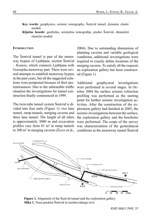
68 RošeR, j., sTopAR, R., GosAR, A.
RMZ-M&G 2008, 55
Key words: geophysics, seismic tomography, Šentvid tunnel, dynamic elastic moduli
Ključne besede: geofizika, seizmična tomografija, predor Šentvid, dinamični elastični moduli
IntroductIon
The Šentvid tunnel is part of the motor-way bypass of Ljubljana, section Šentvid – Koseze, which connects Ljubljana with Gorenjska motorway part. There were sev-eral attempts to establish motorway bypass in the past years, but all the suggested solu-tions were postponed because of their pre-tentiousness. Due to the unbearable traffic situation the investigations for tunnel con-struction finally commenced in 1999.
The twin-tube tunnel system Šentvid is di-vided into four units (Figure 1): two lane tunnel, ramp tunnels, merging caverns and three lane tunnel. The length of all tubes is approximately 3000 m and excavation profiles vary from 81 m2 in ramp tunnels to 300 m2 in merging caverns (žiGon et al.,
Figure 1. Alignment of the Šentvid tunnel and the exploration gallerySlika 1. Trasa predora Šentvid in raziskovalnega rova
2004). Due to outstanding dimensions of planning caverns and variable geological conditions, additional investigations were required to exactly define locations of the merging caverns. To satisfy all the requests an exploration gallery has been construct-ed (Figure 1).
Additional geophysical investigations were performed in several stages. In Oc-tober 2004 the surface seismic refraction profiling was performed as the starting point for further seismic investigation ac-tivities. After the construction of the ex-ploration gallery had finished in 2005, the seismic investigations between the surface, the exploration gallery and the boreholes were performed. The scope of the survey was characterization of the geotechnical conditions in the motorway tunnel Šentvid
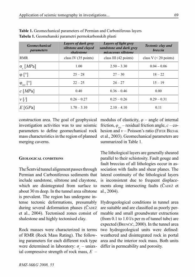
69Application of seismic tomography in investigations...
RMZ-M&G 2008, 55
construction area. The goal of geophysical investigation activities was to use seismic parameters to define geomechanical rock mass characteristics in the region of planned merging caverns.
geologIcal condItIons
The Šentvid tunnel alignment passes through Permian and Carboniferous sediments that include sandstone, siltstone and claystone, which are disintegrated from surface to about 30 m deep. In the tunnel area siltstone is prevalent. The region has undergone in-tense tectonic deformations, presumably during several deformation phases (ČAdež et al., 2004). Tectonised zones consist of shalestone and highly tectonised clay.
Rock masses were characterized in terms of RMR (Rock Mass Rating). The follow-ing parameters for each different rock type were determined in laboratory: σc – uniax-ial compressive strength of rock mass, E –
modulus of elasticity, φ – angle of internal friction, φrez – residual friction angle, c – co-hesion and v – Poisson’s ratio (fifeR BiZjAk et al., 2003). Geomechanical parameters are summarized in Table 1.
The lithological layers are generally sheared parallel to their schistosity. Fault gouge and fault breccias of all lithologies occur in as-sociation with faults and shear planes. The lateral continuity of the lithological layers is inconsistent due to frequent displace-ments along intersecting faults (ČAdež et al., 2004).
Hydrogeological conditions in tunnel area are suitable and are classified as poorly per-meable and small groundwater extractions (from 0.1 to 1.0 l/s per m of tunnel tube) are expected (BRenČiČ, 2000). In the tunnel area two hydrogeological units were defined: weathered and disintegrated rock in portal area and the interior rock mass. Both units differ in permeability and porosity.
Table 1. Geomechanical parameters of Permian and Carboniferous layersTabela 1. Geomehanski parametri permokarbonskih plasti
Geomechanical parameters
Layers of dark grey siltstone and clayed
shalestone
Layers of light grey sandstone and dark grey
micaceous siltstone
Tectonic clay and breccia
RMR class IV (35 points) class III (42 points) class V (< 20 points)
σc [MPa] 1.00 2.50 – 3.30 0.04 – 0.06
φ [°] 25 – 28 27 – 30 18 – 22
φrez [°] 22 – 25 24 – 27 15 – 19
c [MPa] 0.40 0.36 – 0.46 0.00
v [/] 0.26 – 0.27 0.25 – 0.26 0.29 – 0.31
E [GPa] 1.70 – 3.10 2.10 – 4.10 0.11
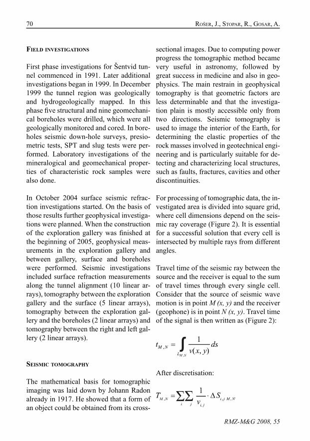
70 RošeR, j., sTopAR, R., GosAR, A.
RMZ-M&G 2008, 55
fIeld InvestIgatIons
First phase investigations for Šentvid tun-nel commenced in 1991. Later additional investigations began in 1999. In December 1999 the tunnel region was geologically and hydrogeologically mapped. In this phase five structural and nine geomechani-cal boreholes were drilled, which were all geologically monitored and cored. In bore-holes seismic down-hole surveys, presio-metric tests, SPT and slug tests were per-formed. Laboratory investigations of the mineralogical and geomechanical proper-ties of characteristic rock samples were also done.
In October 2004 surface seismic refrac-tion investigations started. On the basis of those results further geophysical investiga-tions were planned. When the construction of the exploration gallery was finished at the beginning of 2005, geophysical meas-urements in the exploration gallery and between gallery, surface and boreholes were performed. Seismic investigations included surface refraction measurements along the tunnel alignment (10 linear ar-rays), tomography between the exploration gallery and the surface (5 linear arrays), tomography between the exploration gal-lery and the boreholes (2 linear arrays) and tomography between the right and left gal-lery (2 linear arrays).
seIsmIc tomography
The mathematical basis for tomographic imaging was laid down by Johann Radon already in 1917. He showed that a form of an object could be obtained from its cross-
sectional images. Due to computing power progress the tomographic method became very useful in astronomy, followed by great success in medicine and also in geo-physics. The main restrain in geophysical tomography is that geometric factors are less determinable and that the investiga-tion plain is mostly accessible only from two directions. Seismic tomography is used to image the interior of the Earth, for determining the elastic properties of the rock masses involved in geotechnical engi-neering and is particularly suitable for de-tecting and characterizing local structures, such as faults, fractures, cavities and other discontinuities.
For processing of tomographic data, the in-vestigated area is divided into square grid, where cell dimensions depend on the seis-mic ray coverage (Figure 2). It is essential for a successful solution that every cell is intersected by multiple rays from different angles.
Travel time of the seismic ray between the source and the receiver is equal to the sum of travel times through every single cell. Consider that the source of seismic wave motion is in point M (x, y) and the receiver (geophone) is in point N (x, y). Travel time of the signal is then written as (Figure 2):
After discretisation:
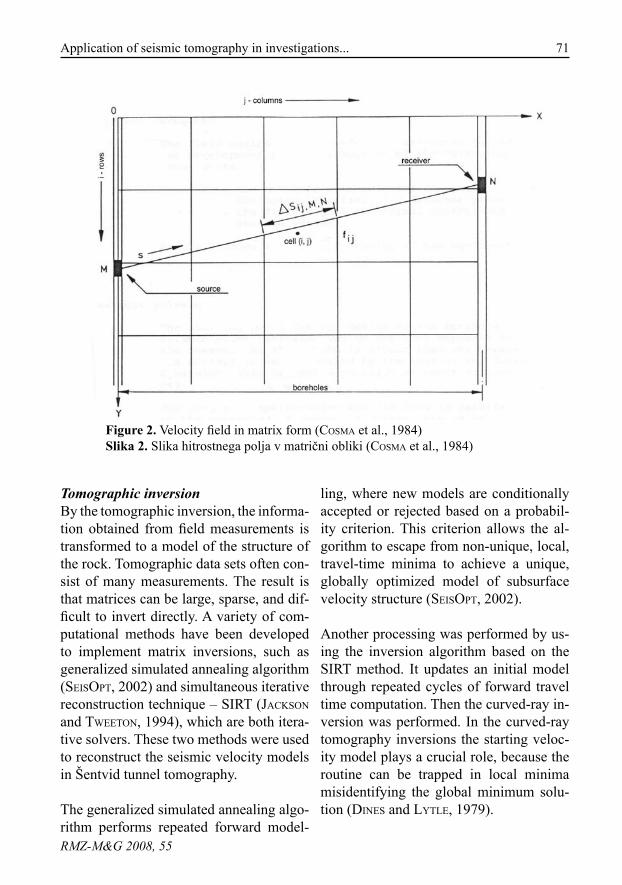
71Application of seismic tomography in investigations...
RMZ-M&G 2008, 55
Tomographic inversionBy the tomographic inversion, the informa-tion obtained from field measurements is transformed to a model of the structure of the rock. Tomographic data sets often con-sist of many measurements. The result is that matrices can be large, sparse, and dif-ficult to invert directly. A variety of com-putational methods have been developed to implement matrix inversions, such as generalized simulated annealing algorithm (seisopT, 2002) and simultaneous iterative reconstruction technique – SIRT (jAckson and TWeeTon, 1994), which are both itera-tive solvers. These two methods were used to reconstruct the seismic velocity models in Šentvid tunnel tomography.
The generalized simulated annealing algo-rithm performs repeated forward model-
Figure 2. Velocity field in matrix form (cosmA et al., 1984)Slika 2. Slika hitrostnega polja v matrični obliki (cosmA et al., 1984)
ling, where new models are conditionally accepted or rejected based on a probabil-ity criterion. This criterion allows the al-gorithm to escape from non-unique, local, travel-time minima to achieve a unique, globally optimized model of subsurface velocity structure (seisopT, 2002).
Another processing was performed by us-ing the inversion algorithm based on the SIRT method. It updates an initial model through repeated cycles of forward travel time computation. Then the curved-ray in-version was performed. In the curved-ray tomography inversions the starting veloc-ity model plays a crucial role, because the routine can be trapped in local minima misidentifying the global minimum solu-tion (dines and LYTLe, 1979).
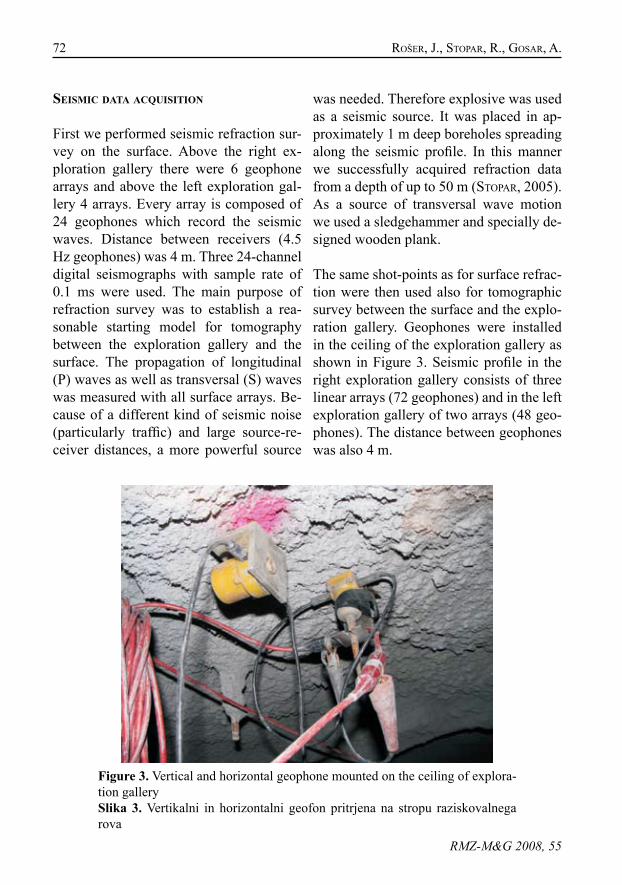
72 RošeR, j., sTopAR, R., GosAR, A.
RMZ-M&G 2008, 55
seIsmIc data acquIsItIon
First we performed seismic refraction sur-vey on the surface. Above the right ex-ploration gallery there were 6 geophone arrays and above the left exploration gal-lery 4 arrays. Every array is composed of 24 geophones which record the seismic waves. Distance between receivers (4.5 Hz geophones) was 4 m. Three 24-channel digital seismographs with sample rate of 0.1 ms were used. The main purpose of refraction survey was to establish a rea-sonable starting model for tomography between the exploration gallery and the surface. The propagation of longitudinal (P) waves as well as transversal (S) waves was measured with all surface arrays. Be-cause of a different kind of seismic noise (particularly traffic) and large source-re-ceiver distances, a more powerful source
was needed. Therefore explosive was used as a seismic source. It was placed in ap-proximately 1 m deep boreholes spreading along the seismic profile. In this manner we successfully acquired refraction data from a depth of up to 50 m (sTopAR, 2005). As a source of transversal wave motion we used a sledgehammer and specially de-signed wooden plank.
The same shot-points as for surface refrac-tion were then used also for tomographic survey between the surface and the explo-ration gallery. Geophones were installed in the ceiling of the exploration gallery as shown in Figure 3. Seismic profile in the right exploration gallery consists of three linear arrays (72 geophones) and in the left exploration gallery of two arrays (48 geo-phones). The distance between geophones was also 4 m.
Figure 3. Vertical and horizontal geophone mounted on the ceiling of explora-tion gallerySlika 3. Vertikalni in horizontalni geofon pritrjena na stropu raziskovalnega rova
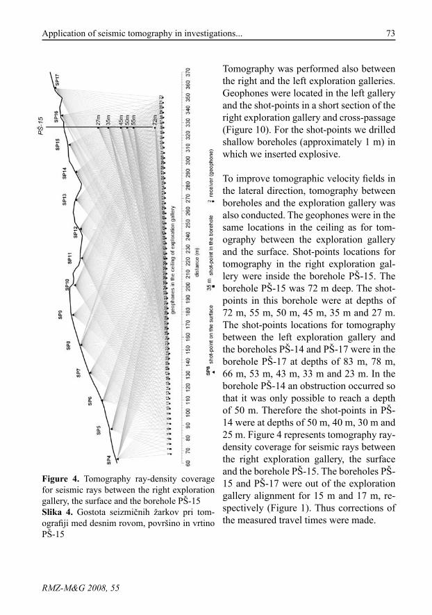
73Application of seismic tomography in investigations...
RMZ-M&G 2008, 55
Tomography was performed also between the right and the left exploration galleries. Geophones were located in the left gallery and the shot-points in a short section of the right exploration gallery and cross-passage (Figure 10). For the shot-points we drilled shallow boreholes (approximately 1 m) in which we inserted explosive.
To improve tomographic velocity fields in the lateral direction, tomography between boreholes and the exploration gallery was also conducted. The geophones were in the same locations in the ceiling as for tom-ography between the exploration gallery and the surface. Shot-points locations for tomography in the right exploration gal-lery were inside the borehole PŠ-15. The borehole PŠ-15 was 72 m deep. The shot-points in this borehole were at depths of 72 m, 55 m, 50 m, 45 m, 35 m and 27 m. The shot-points locations for tomography between the left exploration gallery and the boreholes PŠ-14 and PŠ-17 were in the borehole PŠ-17 at depths of 83 m, 78 m, 66 m, 53 m, 43 m, 33 m and 23 m. In the borehole PŠ-14 an obstruction occurred so that it was only possible to reach a depth of 50 m. Therefore the shot-points in PŠ-14 were at depths of 50 m, 40 m, 30 m and 25 m. Figure 4 represents tomography ray-density coverage for seismic rays between the right exploration gallery, the surface and the borehole PŠ-15. The boreholes PŠ-15 and PŠ-17 were out of the exploration gallery alignment for 15 m and 17 m, re-spectively (Figure 1). Thus corrections of the measured travel times were made.
Figure 4. Tomography ray-density coverage for seismic rays between the right exploration gallery, the surface and the borehole PŠ-15Slika 4. Gostota seizmičnih žarkov pri tom-ografiji med desnim rovom, površino in vrtino PŠ-15
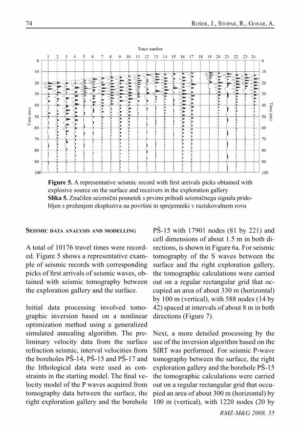
74 RošeR, j., sTopAR, R., GosAR, A.
RMZ-M&G 2008, 55
seIsmIc data analysIs and modellIng
A total of 10176 travel times were record-ed. Figure 5 shows a representative exam-ple of seismic records with corresponding picks of first arrivals of seismic waves, ob-tained with seismic tomography between the exploration gallery and the surface.
Initial data processing involved tomo-graphic inversion based on a nonlinear optimization method using a generalized simulated annealing algorithm. The pre-liminary velocity data from the surface refraction seismic, interval velocities from the boreholes PŠ-14, PŠ-15 and PŠ-17 and the lithological data were used as con-straints in the starting model. The final ve-locity model of the P waves acquired from tomography data between the surface, the right exploration gallery and the borehole
Figure 5. A representative seismic record with first arrivals picks obtained with explosive source on the surface and receivers in the exploration gallerySlika 5. Značilen seizmični posnetek s prvimi prihodi seizmičnega signala prido-bljen s proženjem eksploziva na površini in sprejemniki v raziskovalnem rovu
PŠ-15 with 17901 nodes (81 by 221) and cell dimensions of about 1.5 m in both di-rections, is shown in Figure 6a. For seismic tomography of the S waves between the surface and the right exploration gallery, the tomographic calculations were carried out on a regular rectangular grid that oc-cupied an area of about 330 m (horizontal) by 100 m (vertical), with 588 nodes (14 by 42) spaced at intervals of about 8 m in both directions (Figure 7).
Next, a more detailed processing by the use of the inversion algorithm based on the SIRT was performed. For seismic P-wave tomography between the surface, the right exploration gallery and the borehole PŠ-15 the tomographic calculations were carried out on a regular rectangular grid that occu-pied an area of about 300 m (horizontal) by 100 m (vertical), with 1220 nodes (20 by
75Application of seismic tomography in investigations...
RMZ-M&G 2008, 55
61) spaced at intervals of about 5 m in both directions (Figure 6b). Figure 8 represents the final velocity model of the P waves ac-quired from tomography data between the surface, the left exploration gallery and the boreholes PŠ-14 and PŠ-17. The model consists of 700 nodes (25 by 28) spaced at intervals of about 7 m and 6 m in the x and y directions, respectively. In order to build a reasonable initial model for the curved-ray inversion, we started by invert-ing the travel time data with a straight-ray approximation using an initial velocity model obtained from the surface refraction data. A smoothed version of the updated model, obtained after 16 straight-ray itera-tions, was then used as a starting model for the successive curved-ray iterations. Be-fore running new iterations, however, sev-eral explicit global and node constraints were incorporated into the model. Global constraints were imposed specifying the maximum and minimum allowable veloci-ties, which equal to 6000 and 340 m/s (the P-wave velocity in the air), respectively. Node constraints, which force the solution to match known boundary values, were ap-plied with a fuzzy logic approach (jAckson and TWeeTon, 1994) using measured speci-men velocities and other supplemental site information. Constraining the grid node is mainly where low ray-coverage imposed by source-to-receiver geometry, improved mathematical resolution by reducing the ill-conditioning of the inversion. For seis-mic tomography of the S waves between the surface and the left exploration gal-lery the tomographic calculations based on the SIRT technique was also performed. Due to a bad signal-to-noise ratio in the S wave data we had to use a smaller amount of data. That is why the model consists of
121 nodes and the cell dimensions are ap-proximately 28 by 10 m (Figure 9). The tomographic calculations of the P waves data between the right and the left explora-tion gallery were carried out on a regular rectangular grid with 450 nodes (45 by 10) spaced at intervals of about 6.7 m and 5.5 m in x and y directions, respectively (Fig-ure 10).
From the relation between the longitudinal and the transversal wave velocity, the dy-namic elastic moduli were calculated. For the calculations we also needed the rock density data. The data were obtained from observations, laboratory and in situ meas-urements and are shown in Table 2 (LikAR and ČAdež, 2006). Calculations were based on a regular rectangular grid that occupied an area of about 340 m (horizontal) by 110 m (vertical), with 588 nodes (42 by 14) spaced at intervals of about 8 m in both di-rections. Rock density distribution inside the grid was determined with linear inter-polation based on the range of wave ve-locity inside individual cells. We consider that higher seismic velocity corresponds to higher rock density and vice versa.
results and dIscussIon
Tomography between the right explora-tion gallery, the surface and the borehole PŠ-15With the tomography between the right exploration gallery, the surface and the borehole PŠ-15 we acquired the exact data above the right tube of the Šentvid tunnel (Figure 6). From the result of modelling based on a nonlinear optimization method a low P velocity zone (velocities under 3000
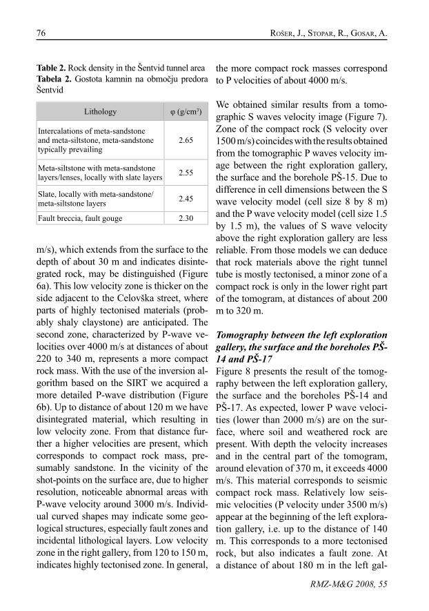
76 RošeR, j., sTopAR, R., GosAR, A.
RMZ-M&G 2008, 55
Table 2. Rock density in the Šentvid tunnel areaTabela 2. Gostota kamnin na območju predora Šentvid
Lithology φ (g/cm3)
Intercalations of meta-sandstone and meta-siltstone, meta-sandstone typically prevailing
2.65
Meta-siltstone with meta-sandstone layers/lenses, locally with slate layers 2.55
Slate, locally with meta-sandstone/meta-siltstone layers 2.45
Fault breccia, fault gouge 2.30
m/s), which extends from the surface to the depth of about 30 m and indicates disinte-grated rock, may be distinguished (Figure 6a). This low velocity zone is thicker on the side adjacent to the Celovška street, where parts of highly tectonised materials (prob-ably shaly claystone) are anticipated. The second zone, characterized by P-wave ve-locities over 4000 m/s at distances of about 220 to 340 m, represents a more compact rock mass. With the use of the inversion al-gorithm based on the SIRT we acquired a more detailed P-wave distribution (Figure 6b). Up to distance of about 120 m we have disintegrated material, which resulting in low velocity zone. From that distance fur-ther a higher velocities are present, which corresponds to compact rock mass, pre-sumably sandstone. In the vicinity of the shot-points on the surface are, due to higher resolution, noticeable abnormal areas with P-wave velocity around 3000 m/s. Individ-ual curved shapes may indicate some geo-logical structures, especially fault zones and incidental lithological layers. Low velocity zone in the right gallery, from 120 to 150 m, indicates highly tectonised zone. In general,
the more compact rock masses correspond to P velocities of about 4000 m/s.
We obtained similar results from a tomo-graphic S waves velocity image (Figure 7). Zone of the compact rock (S velocity over 1500 m/s) coincides with the results obtained from the tomographic P waves velocity im-age between the right exploration gallery, the surface and the borehole PŠ-15. Due to difference in cell dimensions between the S wave velocity model (cell size 8 by 8 m) and the P wave velocity model (cell size 1.5 by 1.5 m), the values of S wave velocity above the right exploration gallery are less reliable. From those models we can deduce that rock materials above the right tunnel tube is mostly tectonised, a minor zone of a compact rock is only in the lower right part of the tomogram, at distances of about 200 m to 320 m.
Tomography between the left exploration gallery, the surface and the boreholes PŠ-14 and PŠ-17Figure 8 presents the result of the tomog-raphy between the left exploration gallery, the surface and the boreholes PŠ-14 and PŠ-17. As expected, lower P wave veloci-ties (lower than 2000 m/s) are on the sur-face, where soil and weathered rock are present. With depth the velocity increases and in the central part of the tomogram, around elevation of 370 m, it exceeds 4000 m/s. This material corresponds to seismic compact rock mass. Relatively low seis-mic velocities (P velocity under 3500 m/s) appear at the beginning of the left explora-tion gallery, i.e. up to the distance of 140 m. This corresponds to a more tectonised rock, but also indicates a fault zone. At a distance of about 180 m in the left gal-
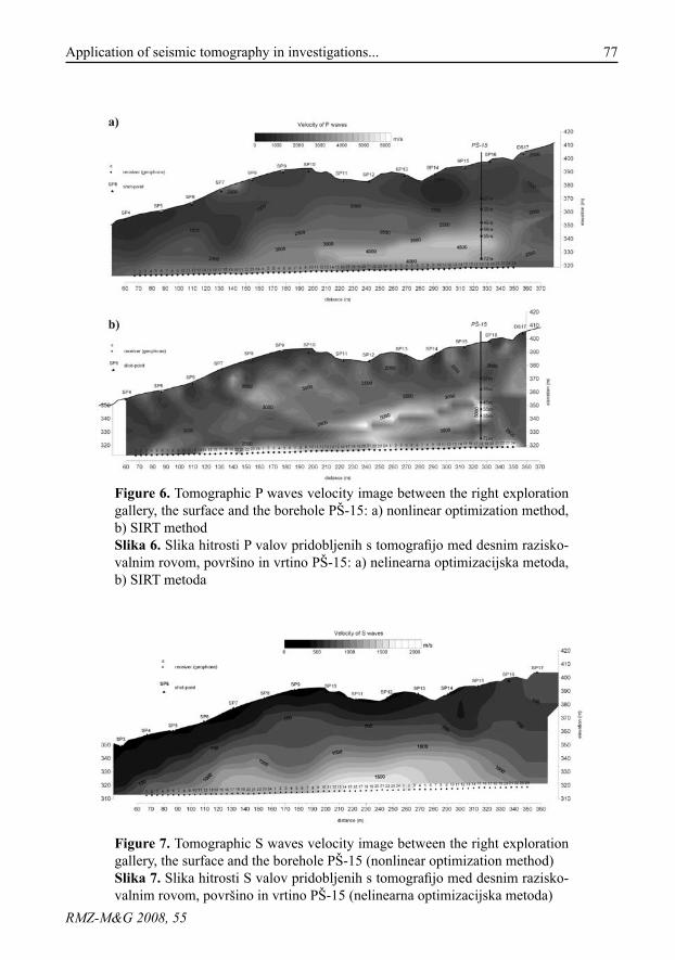
77Application of seismic tomography in investigations...
RMZ-M&G 2008, 55
Figure 6. Tomographic P waves velocity image between the right exploration gallery, the surface and the borehole PŠ-15: a) nonlinear optimization method, b) SIRT methodSlika 6. Slika hitrosti P valov pridobljenih s tomografijo med desnim razisko-valnim rovom, površino in vrtino PŠ-15: a) nelinearna optimizacijska metoda, b) SIRT metoda
Figure 7. Tomographic S waves velocity image between the right exploration gallery, the surface and the borehole PŠ-15 (nonlinear optimization method)Slika 7. Slika hitrosti S valov pridobljenih s tomografijo med desnim razisko-valnim rovom, površino in vrtino PŠ-15 (nelinearna optimizacijska metoda)
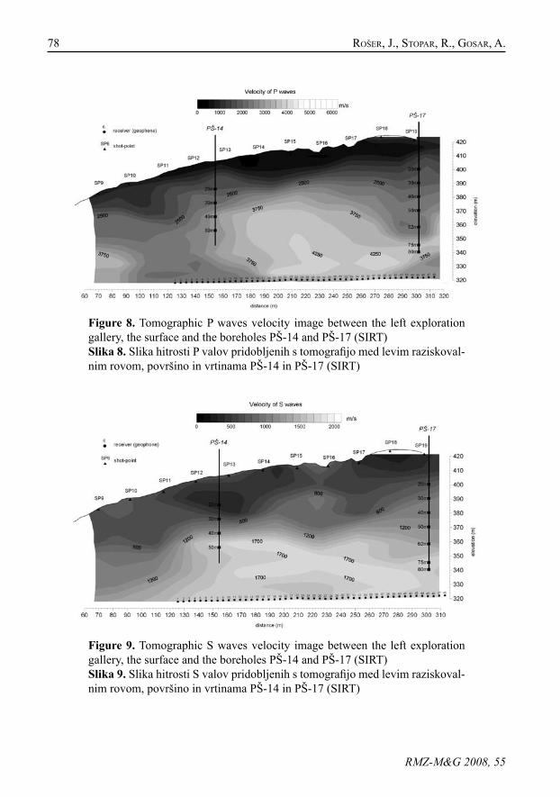
78 RošeR, j., sTopAR, R., GosAR, A.
RMZ-M&G 2008, 55
Figure 8. Tomographic P waves velocity image between the left exploration gallery, the surface and the boreholes PŠ-14 and PŠ-17 (SIRT)Slika 8. Slika hitrosti P valov pridobljenih s tomografijo med levim raziskoval-nim rovom, površino in vrtinama PŠ-14 in PŠ-17 (SIRT)
Figure 9. Tomographic S waves velocity image between the left exploration gallery, the surface and the boreholes PŠ-14 and PŠ-17 (SIRT)Slika 9. Slika hitrosti S valov pridobljenih s tomografijo med levim raziskoval-nim rovom, površino in vrtinama PŠ-14 in PŠ-17 (SIRT)
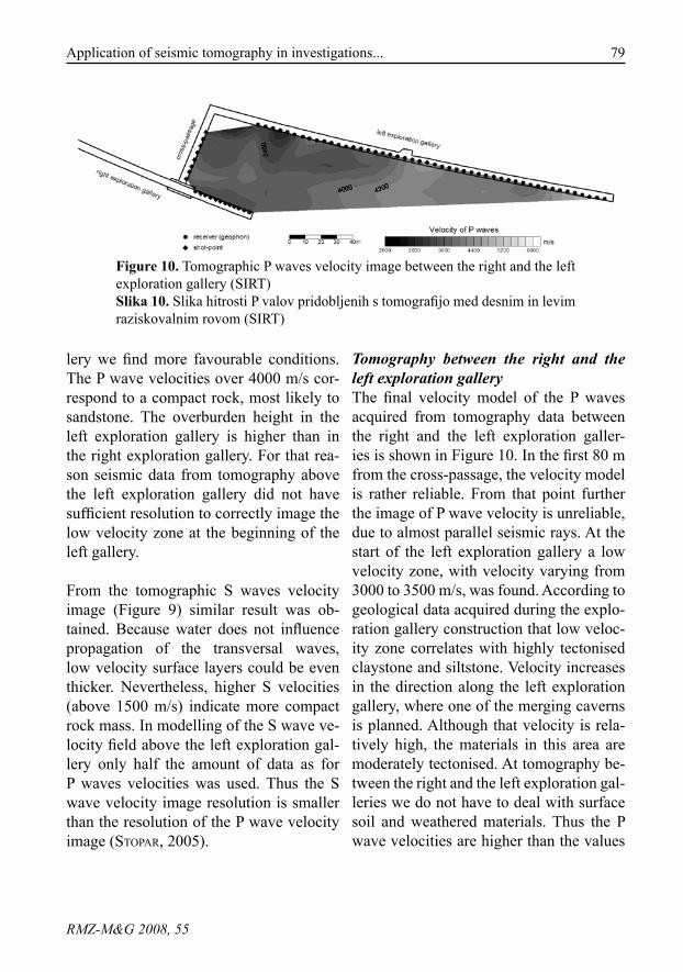
79Application of seismic tomography in investigations...
RMZ-M&G 2008, 55
lery we find more favourable conditions. The P wave velocities over 4000 m/s cor-respond to a compact rock, most likely to sandstone. The overburden height in the left exploration gallery is higher than in the right exploration gallery. For that rea-son seismic data from tomography above the left exploration gallery did not have sufficient resolution to correctly image the low velocity zone at the beginning of the left gallery.
From the tomographic S waves velocity image (Figure 9) similar result was ob-tained. Because water does not influence propagation of the transversal waves, low velocity surface layers could be even thicker. Nevertheless, higher S velocities (above 1500 m/s) indicate more compact rock mass. In modelling of the S wave ve-locity field above the left exploration gal-lery only half the amount of data as for P waves velocities was used. Thus the S wave velocity image resolution is smaller than the resolution of the P wave velocity image (sTopAR, 2005).
Tomography between the right and the left exploration galleryThe final velocity model of the P waves acquired from tomography data between the right and the left exploration galler-ies is shown in Figure 10. In the first 80 m from the cross-passage, the velocity model is rather reliable. From that point further the image of P wave velocity is unreliable, due to almost parallel seismic rays. At the start of the left exploration gallery a low velocity zone, with velocity varying from 3000 to 3500 m/s, was found. According to geological data acquired during the explo-ration gallery construction that low veloc-ity zone correlates with highly tectonised claystone and siltstone. Velocity increases in the direction along the left exploration gallery, where one of the merging caverns is planned. Although that velocity is rela-tively high, the materials in this area are moderately tectonised. At tomography be-tween the right and the left exploration gal-leries we do not have to deal with surface soil and weathered materials. Thus the P wave velocities are higher than the values
Figure 10. Tomographic P waves velocity image between the right and the left exploration gallery (SIRT)Slika 10. Slika hitrosti P valov pridobljenih s tomografijo med desnim in levim raziskovalnim rovom (SIRT)
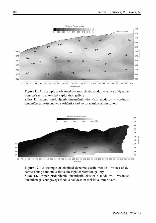
80 RošeR, j., sTopAR, R., GosAR, A.
RMZ-M&G 2008, 55
Figure 11. An example of obtained dynamic elastic moduli – values of dynamic Poisson’s ratio above left exploration gallerySlika 11. Primer pridobljenih dinamičnih elastičnih modulov – vrednosti dinamičnega Poissonovega količnika nad levim raziskovalnim rovom
Figure 12. An example of obtained dynamic elastic moduli – values of dy-namic Young’s modulus above the right exploration gallerySlika 12. Primer pridobljenih dinamičnih elastičnih modulov – vrednosti dinamičnega Youngovega modula nad desnim raziskovalnim rovom
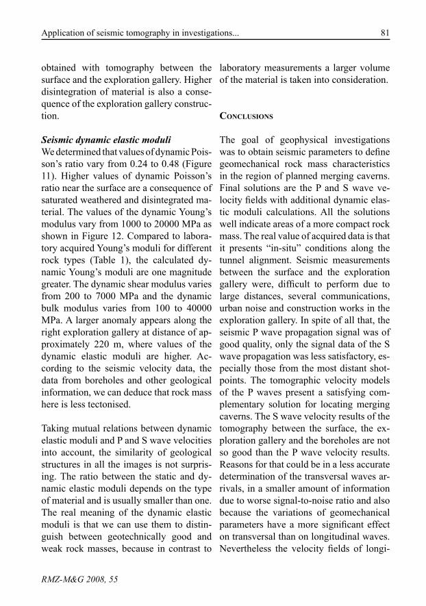
81Application of seismic tomography in investigations...
RMZ-M&G 2008, 55
obtained with tomography between the surface and the exploration gallery. Higher disintegration of material is also a conse-quence of the exploration gallery construc-tion.
Seismic dynamic elastic moduliWe determined that values of dynamic Pois-son’s ratio vary from 0.24 to 0.48 (Figure 11). Higher values of dynamic Poisson’s ratio near the surface are a consequence of saturated weathered and disintegrated ma-terial. The values of the dynamic Young’s modulus vary from 1000 to 20000 MPa as shown in Figure 12. Compared to labora-tory acquired Young’s moduli for different rock types (Table 1), the calculated dy-namic Young’s moduli are one magnitude greater. The dynamic shear modulus varies from 200 to 7000 MPa and the dynamic bulk modulus varies from 100 to 40000 MPa. A larger anomaly appears along the right exploration gallery at distance of ap-proximately 220 m, where values of the dynamic elastic moduli are higher. Ac-cording to the seismic velocity data, the data from boreholes and other geological information, we can deduce that rock mass here is less tectonised.
Taking mutual relations between dynamic elastic moduli and P and S wave velocities into account, the similarity of geological structures in all the images is not surpris-ing. The ratio between the static and dy-namic elastic moduli depends on the type of material and is usually smaller than one. The real meaning of the dynamic elastic moduli is that we can use them to distin-guish between geotechnically good and weak rock masses, because in contrast to
laboratory measurements a larger volume of the material is taken into consideration.
conclusIons
The goal of geophysical investigations was to obtain seismic parameters to define geomechanical rock mass characteristics in the region of planned merging caverns. Final solutions are the P and S wave ve-locity fields with additional dynamic elas-tic moduli calculations. All the solutions well indicate areas of a more compact rock mass. The real value of acquired data is that it presents “in-situ” conditions along the tunnel alignment. Seismic measurements between the surface and the exploration gallery were, difficult to perform due to large distances, several communications, urban noise and construction works in the exploration gallery. In spite of all that, the seismic P wave propagation signal was of good quality, only the signal data of the S wave propagation was less satisfactory, es-pecially those from the most distant shot-points. The tomographic velocity models of the P waves present a satisfying com-plementary solution for locating merging caverns. The S wave velocity results of the tomography between the surface, the ex-ploration gallery and the boreholes are not so good than the P wave velocity results. Reasons for that could be in a less accurate determination of the transversal waves ar-rivals, in a smaller amount of information due to worse signal-to-noise ratio and also because the variations of geomechanical parameters have a more significant effect on transversal than on longitudinal waves. Nevertheless the velocity fields of longi-
82 RošeR, j., sTopAR, R., GosAR, A.
RMZ-M&G 2008, 55
tudinal and transversal waves and the dy-namic elastic moduli distribution well in-dicate areas of a more compact rock mass.
povzetek
Uporaba seizmične tomografije pri raziskavah AC trase na območju pre-dora Šentvid
Predmet geofizikalnih raziskav je bilo območje izgradnje predora Šentvid. Šent-viški hrib bo avtocesta prečkala v obliki dveh ločenih predorskih cevi s priključ-nima cevema, poseg pa je zaradi neugo-dne geološke zgradbe zelo zahteven. Ker na podlagi predhodno izvršenih preiskav ni bilo mogoče natančno določiti lokacij priključnih kavern, je bil najprej izdelan raziskovalni rov, v katerem so bile izve-dene različne geološke, geomehanske in geofizikalne raziskave. Cilj geofizikalnih raziskav je bil, s pomočjo seizmičnih pa-rametrov, določiti geomehanske karakteri-stike posameznih kamnin v območjih na-črtovanih priključnih kavern. Geofizikalne raziskave so vključevale površinsko seiz-
mično refrakcijsko profiliranje in seizmič-no tomografijo med površino, vrtinami in raziskovalnim rovom.
Rezultati seizmičnih preiskav v in nad raziskovalnim rovom predora Šentvid od-ražajo predvsem mehanske lastnosti pre-iskovane kamnine v nadkritju predora. Vrednost pridobljenih podatkov je v tem, da predstavljajo “in-situ” podatek vzdolž zveznih profilov. Glede na to, da velik del vrednosti hitrosti longitudinalnega valova-nja izvedenih raziskav seizmične tomogra-fije dosega 3000 m/s in več, lahko govori-mo o hribini. Izjema so površinske plasti, ki zlasti v smeri proti severnemu portalu dosegajo tudi debelino več deset metrov. Posamezne nižje hitrostne anomalije so posledica pretrte kamnine ali prelomnih con. Seizmične raziskave so dobro podale območja kompaktnejše kamnine, kar od-ražajo tako slike hitrosti longitudinalnega in transverzalnega valovanja kot tudi slike dinamičnih elastičnih modulov. Predvideni lokaciji priključnih kavern sta bili na osno-vi dodatnih raziskav, med katere sodijo tudi geofizikalne, potrjeni.
83Application of seismic tomography in investigations...
RMZ-M&G 2008, 55
references
BRenČiČ, m. (2000): Hidrogeološko poročilo za predor Šentvid. Geološki zavod Slovenije, Ljubljana, unpublished report, 45 p.
cosmA, c., iHALAinen, m., koRHonen, R. (1984): The Crosshole Seismic Method. Report of phase II. of de-velopment programme. Helsinki, 36 pp.
ČAdež, f., kLeBeRGeR, j., GenseR, W., pöscHL, i. (2004): Sentvid Mo-torway Tunnel – Interim Results from Slovenia’s Most Recent Ex-ploration Gallery. 7. mednarodno posvetovanje o gradnji predorov in podzemnih prostorov, zbornik referatov. Uredila: Kostiov, L. in Likar, J., Ljubljana: Društvo za podzemne in geotehnične kon-strukcije in Univerza v Ljubljani, pp. 50-56.
dines, k. A. and LYTLe, j.R. (1979): Com-puterized Geophysical Tomog-raphy. Proceedings of the IEEE.; Vol. 67, No. 7, pp. 1065-1073.
fifeR BiZjAk, k., peTkovšek, B., peT-RicA, R. (2003): Geološke in ge-omehanske raziskave za predor Šentvid. Gradbeni vestnik.; Vol. 52, pp. 15-21.
jAckson, m.j., TWeeTon, d.R. (1994): MI-GRATOM – Geophysical tomog-raphy using wavefront migration and fuzzy constraints. USBM Re-port of Investigation 9497. United states department of the interior, Bureau of mines, 35 p.
LikAR, j., ČAdež, j. (2006): Verification analysis of the stability of large underground caverns in the three-lane road tunnel Šentvid. FLAC and Numerical Modeling in Geo-mechanics – 2006, proceedings of the 4th international FLAC sympo-sium, Spain, pp 71 – 77.
seisopT@2d (2002): Ver. 3.0, Seismic Refraction Tomography software copyright Optim, Inc., University of Nevada, Reno, Nevada.
sTopAR, R. (2005): Poročilo o geofizikalnih preiskavah na območju predora Šentvid (levi in desni razisko-valni rov). Geoinženiring d.o.o., Ljubljana, unpublished report, 16 p.
žiGon, A., žiBeRT, m. in jemec, p. (2004): Projektiranje predorskega sistema Šentvid. 7. mednarodno posveto-vanje o gradnji predorov in pod-zemnih prostorov, zbornik refera-tov. Uredila: Kostiov, L. in Likar, J., Ljubljana: Društvo za podzem-ne in geotehnične konstrukcije in Univerza v Ljubljani, pp. 125-147.

85RMZ – Materials and Geoenvironment, Vol. 55, No. 1, pp. 85-109, 2008
Scientific paper
Surveying for geophysical exploration, using a single-frequency global navigation satellite system receiver capable of 30 cm
horizontal kinematical positioning uncertainty
Uporaba enofrekvenčnega sprejemnika GNSS s 30 cm negotovostjo v kinematičnem načinu dela za terenske
geofizikalne preiskave
fRAnc dimc1, BRAnko mušiČ2, RAdko osRedkAR3
1University of Ljubljana, Faculty of Maritime Studies and Transportation, Pot pomorščakov 4, SI-6320 Portorož, Slovenia; E-mail: [email protected]
2University of Ljubljana, Faculty of Arts, Department of Archaeology, Zavetiška 5, SI-1000 Ljubljana, Slovenia; E-mail: [email protected]
3University of Ljubljana, Faculty of Computer and Information Science, Tržaška cesta 25, SI-1001 Ljubljana, Slovenia; E-mail: [email protected]
Received: January 7, 2008 Accepted: February 25, 2008
Abstract: Some preliminary tests of various types of inexpensive Global position-ing system (GPS) receivers were performed in order to assess the utility of the technique to geophysical surveying conditions. A 30 cm basic kinemati-cal accuracy of the fixes was sought. Different sources of positioning errors are analyzed under different, realistic conditions in the field (multipath, sat-ellite obscuration, etc) and the influence of the sampling rate and phase data processing on the relative accuracy for static and kinematical positioning analyzed. It is demonstrated that under favorable conditions a 30 cm rela-tive uncertainty of the kinematical positioning is achievable and that under conditions where a degradation of the GPS fixes occurs during the scans, it is possible to a certain extent, by post-processing of the measurement data, to compensate for the errors and to refine the positioning results.
Izvleček: V članku so predstavljeni začetni preizkusi različnih vrst cenejših sprejemnikov GPS, opravljenih z namenom ugotoviti uporabnost radio-navigacijske satelitske tehnike za geofizikalne preiskave. Preizkuse smo začeli z namenom ugotavljanja, če je natančnost določitve položaja 30 cm dosegljiva. Na terenih smo analizirali različne vzroke napak (večpotje, zas-trtost satelitov) in vpliv pogostnosti odčitavanja in obdelave faze na rela-tivno natančnost statičnih in kinematičnih preizkusov. Pokazali smo, da je v dobrih pogojih relativna natančnost 30 cm dosegljiva in da je v določenih pogojih možno z naknadno obdelavo odčitkov (kompenzacijo napak) re-zultate popraviti.
86 dimc, f., mušiČ, B., osRedkAR, R.
RMZ-M&G 2008, 55
Key words: GPS tracking, kinematic measurements, geophysical exploration Ključne besede: sledenje z GPS, kinematične meritve, geofizikalne raziskave
IntroductIon
The idea behind the construction of an in-expensive single frequency GPS system that is simple to use arises from the need for flexibility and effectiveness of geo-physical surveys. A sufficient degree of flexibility can only be assured by the com-plete autonomy of the team in the planning and executing of fieldwork through the positioning of identified anomalous areas. This is the data layer in integral bases, which in archaeo-geophysical prospection represents the basis for the planning of further systematic and detailed geophysi-cal research on identified sites through the application of the multi-method approach (see: mušiČ & HoRvAT, 2007; mušiČ et al., 2008).
GPS equipment (receivers) is relatively cheap, is easily portable, offers real-time fixes and thus makes kinematical posi-tioning possible (WAnG et al., 2002). Nei-ther does its application require specialist skills. It makes GPS positioning technolo-gy well suited for autonomous geophysical prospection (GAffneY, 2003), in particular in large-scale evaluation projects, where total detailed survey is not as important as establishing background levels and acquir-ing a good understanding of the effects of the geology and pedology. Its efficient ap-plication is of crucial importance for sur-veys in the regions where geodetic fixed points for terestrial position meaurements are not accessible. The nominal accuracy
of the GPS positioning can be greatly im-proved by advanced signal processing and post processing, which means that a 30 cm accuracy of kinematical relative position-ing (vAn sickLe, 2001), deemed sufficient for the autonomous use of the GPS for geophysical prospection, is attainable.
It is characteristic of GPS positioning meth-ods that the accuracy of relative positions fixes is usually considerably better than the accuracy of absolute position fixes. After a comprehensive post-processing efforts a very accurate static positioning by single frequency GPS receiver it is also possible (BeRAn, 2007). We have thus attempted to improve the performance of relatively in-expensive GPS receivers by use of refer-ence points of known position in the field. We were concerned solely with horizontal positioning, which is of primary impor-tance, leaving the more difficult problem of vertical positioning to a future project. In the autonomous mode with a single fre-quency receiver, the position of a reference point is first measured as accurately as pos-sible. A roving receiver then continuously corrects its position outputs by calculating its pseudo range by using single pseudo range differences (DGPS) obtained from a nearby monitoring static GNSS station on a known location, from a network of such stations, or from geostationary satellites known also as SBAS (vAn sickLe, 2001).
Kinematical sub-meter accuracy as deter-mined by a single receiver was also stud-
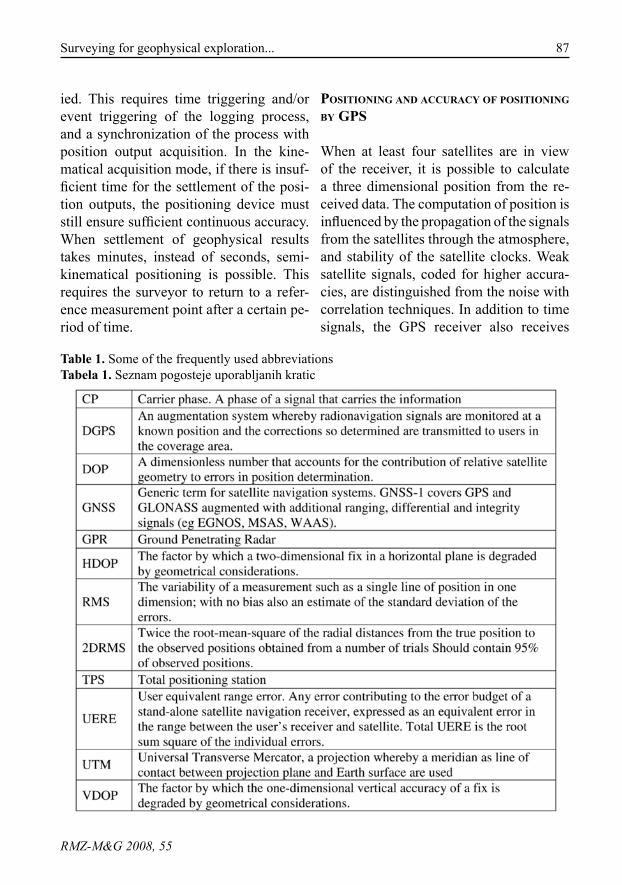
87Surveying for geophysical exploration...
RMZ-M&G 2008, 55
ied. This requires time triggering and/or event triggering of the logging process, and a synchronization of the process with position output acquisition. In the kine-matical acquisition mode, if there is insuf-ficient time for the settlement of the posi-tion outputs, the positioning device must still ensure sufficient continuous accuracy. When settlement of geophysical results takes minutes, instead of seconds, semi-kinematical positioning is possible. This requires the surveyor to return to a refer-ence measurement point after a certain pe-riod of time.
Table 1. Some of the frequently used abbreviationsTabela 1. Seznam pogosteje uporabljanih kratic
posItIonIng and accuracy of posItIonIng by gps
When at least four satellites are in view of the receiver, it is possible to calculate a three dimensional position from the re-ceived data. The computation of position is influenced by the propagation of the signals from the satellites through the atmosphere, and stability of the satellite clocks. Weak satellite signals, coded for higher accura-cies, are distinguished from the noise with correlation techniques. In addition to time signals, the GPS receiver also receives
88 dimc, f., mušiČ, B., osRedkAR, R.
RMZ-M&G 2008, 55
navigation signals comprising positions of satellites and their operational status. Receivers can operate in an autonomous mode or as rovers. Higher accuracies can normally be achieved by also taking into account the corrections transmitted by a primary positioning receiver station, locat-ed at a known position. Single, double and triple difference methods diminish some of the errors generated either by the primary station and/or the rover and the satellites (vAn sickLe, 2001).
Equipment manufacturers normally state the accuracy of positioning of their prod-ucts with respect to certain conditions (sig-nal to noise ratio) of reception, and this is considered as the greatest possible abso-lute accuracy that can be achieved by a de-vice. However, nominal accuracy does not depend solely on the stated conditions, but to a much larger extent on processing and post processing of the satellite data avail-able to the receiver. In satellite positioning it is impossible to completely exclude all the environmental factors that may influ-ence the results. They result in an accuracy interval, which is related to the experimen-tal standard deviation (estimated position error, also known as (d)RMS error) (USM, 1999). Since more variables (dimensions) are observed, the accuracy is noted in each dimension separately. Two dimensional (2DdRMS) is calculated for two variables. The compound error of positioning is the result of all the contributing factors: inac-curate satellite ephemeris data and inac-curate clock corrections sent, changes of propagation delays due to ionosphere den-sity fluctuations with solar or geomagnetic activity and signals reflected from highly conductive surfaces resulting in multipath
signals at the receiver position, disturbing the processing of the directly received sig-nals and receiver thermal noise. Process-ing methods (phase averaging, estimation filter scenarios) of the raw signals also in-fluence the accuracy of the results.
Reducing the influence of the limited re-ceiver view of satellite constellation (dilu-tion of precision, DOP: HDOP – horizontal DOP, VDOP – vertical DOP) during signal processing yields the final positioning er-ror, the so called “user equivalent range error” (UERE) (de jonG et al., 2001). The precision of a position measurement output (known as the fix) depends both upon the measurement geometry, as represented by the DOP values, and range errors caused by signal strength, ionospheric effects, and multipath errors. The latter depend upon physical surroundings of the measuring point, i.e. to terrain relief, near-by buildings or other highly reflective surfaces (water bodies), or foliage plants (LAcHApeLLe at al., 1994). Multipath errors cause system-atic variations of GPS fixes, while other sources of errors cause random, chaotic or bias type of variations. Overall uncertainty of positioning of a point is thus calculated as a product of the accuracy (experimental deviation of the measurements) and DOP (vAn sickLe, 2001).
The positioning accuracy of a moving re-ceiver (rover) is in general not equal to the uncertainty of a stationary fix and should at a certain areas be determined separate-ly. For this purpose a reference trajectory (charted path, on-site measured distances) is established and marked on the measure-ment site. Deviations of fixes from the ref-erence trajectory are measured while tak-
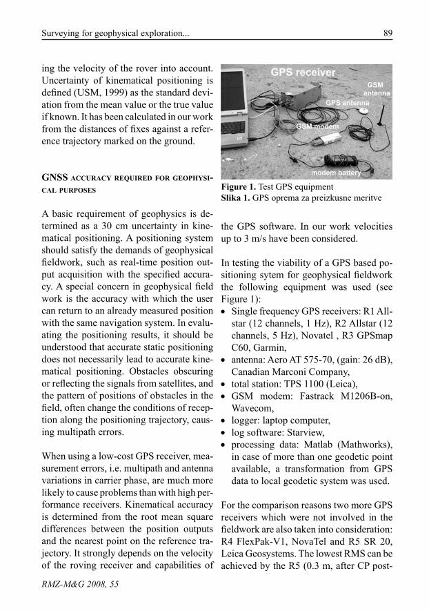
89Surveying for geophysical exploration...
RMZ-M&G 2008, 55
ing the velocity of the rover into account. Uncertainty of kinematical positioning is defined (USM, 1999) as the standard devi-ation from the mean value or the true value if known. It has been calculated in our work from the distances of fixes against a refer-ence trajectory marked on the ground.
gnss accuracy requIred for geophysI-cal purposes
A basic requirement of geophysics is de-termined as a 30 cm uncertainty in kine-matical positioning. A positioning system should satisfy the demands of geophysical fieldwork, such as real-time position out-put acquisition with the specified accura-cy. A special concern in geophysical field work is the accuracy with which the user can return to an already measured position with the same navigation system. In evalu-ating the positioning results, it should be understood that accurate static positioning does not necessarily lead to accurate kine-matical positioning. Obstacles obscuring or reflecting the signals from satellites, and the pattern of positions of obstacles in the field, often change the conditions of recep-tion along the positioning trajectory, caus-ing multipath errors.
When using a low-cost GPS receiver, mea-surement errors, i.e. multipath and antenna variations in carrier phase, are much more likely to cause problems than with high per-formance receivers. Kinematical accuracy is determined from the root mean square differences between the position outputs and the nearest point on the reference tra-jectory. It strongly depends on the velocity of the roving receiver and capabilities of
the GPS software. In our work velocities up to 3 m/s have been considered.
In testing the viability of a GPS based po-sitioning sytem for geophysical fieldwork the following equipment was used (see Figure 1):
Single frequency GPS receivers: R1 All-•star (12 channels, 1 Hz), R2 Allstar (12 channels, 5 Hz), Novatel , R3 GPSmap C60, Garmin,antenna: Aero AT 575-70, (gain: 26 dB), •Canadian Marconi Company,total station: TPS 1100 (Leica),•GSM modem: Fastrack M1206B-on, •Wavecom,logger: laptop computer,•log software: Starview,•processing data: Matlab (Mathworks), •in case of more than one geodetic point available, a transformation from GPS data to local geodetic system was used.
For the comparison reasons two more GPS receivers which were not involved in the fieldwork are also taken into consideration: R4 FlexPak-V1, NovaTel and R5 SR 20, Leica Geosystems. The lowest RMS can be achieved by the R5 (0.3 m, after CP post-
Figure 1. Test GPS equipmentSlika 1. GPS oprema za preizkusne meritve
90 dimc, f., mušiČ, B., osRedkAR, R.
RMZ-M&G 2008, 55
processing) whereas the highest 2DRMS is get by the commercial R3 (static 2.5 m). Under good receiving conditions the ex-perimentally observed RMS values might become very similar, however in atmo-sphere changing conditions for example a benefits of R5 would result in lower RMS as of R3. Comparison of the prices to the price of R3 as the etalon price (1 EP) gives the following sequence: R2 as already ob-solete device (1.9 EP), R4 (5 EP) and R5 (from 10 EP up to 13 EP).
results and dIscussIon
Test sites and equipment types In order to test the positioning capabili-ties and accuracy of a GPS system, several types of equipment were tested at 5 dif-ferent and well defined testing areas: the Adria sports field at Ankaran (site S1), an archaeological site at Veselov Cvinger, near Stična (site S2), a car park in front of a building in Ankaran (site S3), the sur-roundings of the geodetic point at Malija (site S4), and an archaeological site of Nauportus at Dolge njive, near Vrhnika (site S5) (see: mušiČ & HoRvAT, 2007; mušiČ et al. 2008). The third archaeologi-cal site is Tanagra (Greece) (site S6) (see: BinTLiff et al., 2000, 2002; BiLc, 2003;
Table 2. Test sites with brief descriptionsTabela 2. Oznake preizkusnih terenov s kratkimi opisi
mušiČ et al., 2004). The different locations have considerably different topological and signal propagation characteristics: Site S1 (a sports field) has simple geometry and is topologically well defined, site S2 is an exposed location on a ridge, signals at site S3 are especially prone to multipath errors and signal losses due to obscuration, site S4 (geodetic reference point of the 1st de-gree) has a well defined position and low multipath variations, however it is exposed to interference and other errors, and site S5 is an archaeological site close to a river.
A summary of the static positioning mea-surement results on the sites is given in Table 3. It can be seen that uncertainty of fixes is decreased by the absence of multi-path errors as well as open sky, and by the use of DGPS. Uncertainty was calculated for three locations: Site S2 where moder-ate multipath error was observed (point No. 1, was used further as a reference point at this site, as it is also a geodetic point), a location at site S3 with obvious multi-path errors, and a location at site S4, again with moderate multipath errors and addi-tional sources of error, whose effects can only partially be resolved by data analysis. Variations of HDOP strongly influence the uncertainty. Average HDOP of experiment No. 2 was 1.24 while for experiment No. 3
91Surveying for geophysical exploration...
RMZ-M&G 2008, 55
it was 1.12. In the absence of loss of data due to cycle slips, the numbers of fixes is simply the product of measurement time (in seconds), and the data acquisition rate (number of fixes per second, 1 for R3 and 5 for R2).
Static positioning measurementsThe measurements of static positioning at sites S2 and S3 are presented in Figure 2. Measurements were performed continu-ously for 5 consecutive days at S3 (Figure 2.a). Accuracy was determined as dRMS and was 2.96 m. The details of transformed angle/length ratio resolution are shown around a geodetic point, chosen as (0,0) position. The repeatability of observa-tions at S2 with receiver R2 (DGPS) are shown in Figure 2.b. Measurements were performed over two days, separated by 42 days. Repeatability of positioning at points No. 2, No. 3 and No. 4 from the reference point (No. 1, with relative position 0 m) is shown. The relative experimental stan-dard deviation of distances for points No. 2, No. 3, and No. 4 are 23 cm, 30 cm and 29 cm respectively, with a standard devia-tion of the reference point from its true po-sition of 32 cm. It should be pointed out, that the large excursions of data in Fig-ure 2.b do not represent settling times of
Table 3. Statistical parameters of static measurementsTabela 3. Statistične značilnosti statičnega določanja položaja
the measurements, but real excursions of the instrument fixes from the points under consideration, caused by the movement of the experimenter from one point to anoth-er. The largest source of the uncertainties in this case are not the multipath errors, but the unfavourable position of the sites chosen (S2, S3), which have a reduced view of the satellites, not insuring optimal number of satellites in view. Data in Figure 2.b demonstrate that fixes, relative to a ref-erence point, under unfavourable measur-ing conditions (obscuration of satellites) do not satisfy the accuracy requirements. However, even under such conditions the average accuracy of fixes is 8 cm from the requirement. These results cannot be di-rectly compared to uncertainties presented in Table 3, as the relation between accu-racy and uncertainty involves the variable HDOP.
Assesment of kinematic uncertaintyThe results of assessment of kinematical uncertainty, relative to reference lines of 30.00 m and 41.30 m lengths, marked on the ground, are presented in Figure 3 and Figure 4 respectively. Measurements were performed by two receivers R1 and R2 on three different sites S1, S4 and S6. It can be observed from Figure 3 that in all cases

92 dimc, f., mušiČ, B., osRedkAR, R.
RMZ-M&G 2008, 55
Figure 2. Results of static positioning at S3, centered with geodetic procedure (2.a) and repeatability of a distance from the reference point during fieldwork at S2 (2.b)Slika 2. Rezultati določanja položaja točke na terenu S3, osredinjeni z geo-detsko izmero (2.a) in ponovljivosti določanja razdalje do referenčne točke na terenu S2 (2.b)
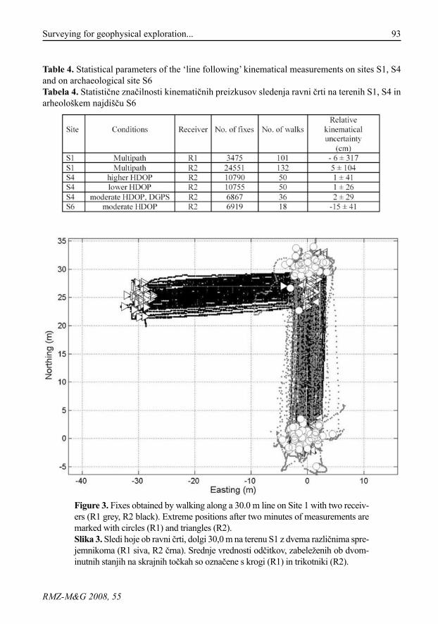
93Surveying for geophysical exploration...
RMZ-M&G 2008, 55
Table 4. Statistical parameters of the ‘line following’ kinematical measurements on sites S1, S4 and on archaeological site S6Tabela 4. Statistične značilnosti kinematičnih preizkusov sledenja ravni črti na terenih S1, S4 in arheološkem najdišču S6
Figure 3. Fixes obtained by walking along a 30.0 m line on Site 1 with two receiv-ers (R1 grey, R2 black). Extreme positions after two minutes of measurements are marked with circles (R1) and triangles (R2). Slika 3. Sledi hoje ob ravni črti, dolgi 30,0 m na terenu S1 z dvema različnima spre-jemnikoma (R1 siva, R2 črna). Srednje vrednosti odčitkov, zabeleženih ob dvom-inutnih stanjih na skrajnih točkah so označene s krogi (R1) in trikotniki (R2).
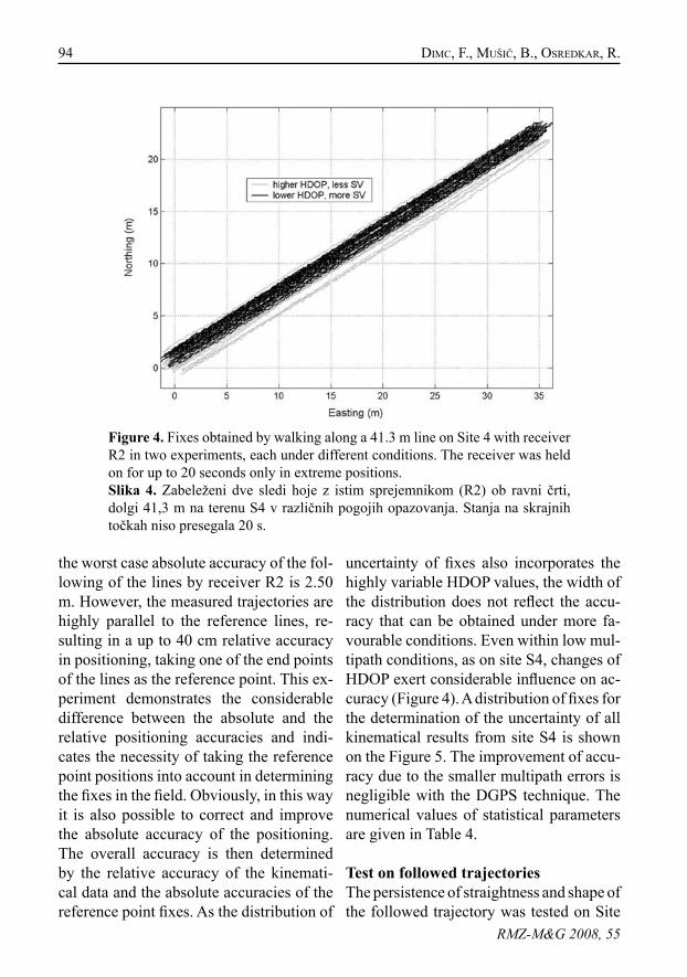
94 dimc, f., mušiČ, B., osRedkAR, R.
RMZ-M&G 2008, 55
the worst case absolute accuracy of the fol-lowing of the lines by receiver R2 is 2.50 m. However, the measured trajectories are highly parallel to the reference lines, re-sulting in a up to 40 cm relative accuracy in positioning, taking one of the end points of the lines as the reference point. This ex-periment demonstrates the considerable difference between the absolute and the relative positioning accuracies and indi-cates the necessity of taking the reference point positions into account in determining the fixes in the field. Obviously, in this way it is also possible to correct and improve the absolute accuracy of the positioning. The overall accuracy is then determined by the relative accuracy of the kinemati-cal data and the absolute accuracies of the reference point fixes. As the distribution of
uncertainty of fixes also incorporates the highly variable HDOP values, the width of the distribution does not reflect the accu-racy that can be obtained under more fa-vourable conditions. Even within low mul-tipath conditions, as on site S4, changes of HDOP exert considerable influence on ac-curacy (Figure 4). A distribution of fixes for the determination of the uncertainty of all kinematical results from site S4 is shown on the Figure 5. The improvement of accu-racy due to the smaller multipath errors is negligible with the DGPS technique. The numerical values of statistical parameters are given in Table 4.
Test on followed trajectoriesThe persistence of straightness and shape of the followed trajectory was tested on Site
Figure 4. Fixes obtained by walking along a 41.3 m line on Site 4 with receiver R2 in two experiments, each under different conditions. The receiver was held on for up to 20 seconds only in extreme positions. Slika 4. Zabeleženi dve sledi hoje z istim sprejemnikom (R2) ob ravni črti, dolgi 41,3 m na terenu S4 v različnih pogojih opazovanja. Stanja na skrajnih točkah niso presegala 20 s.
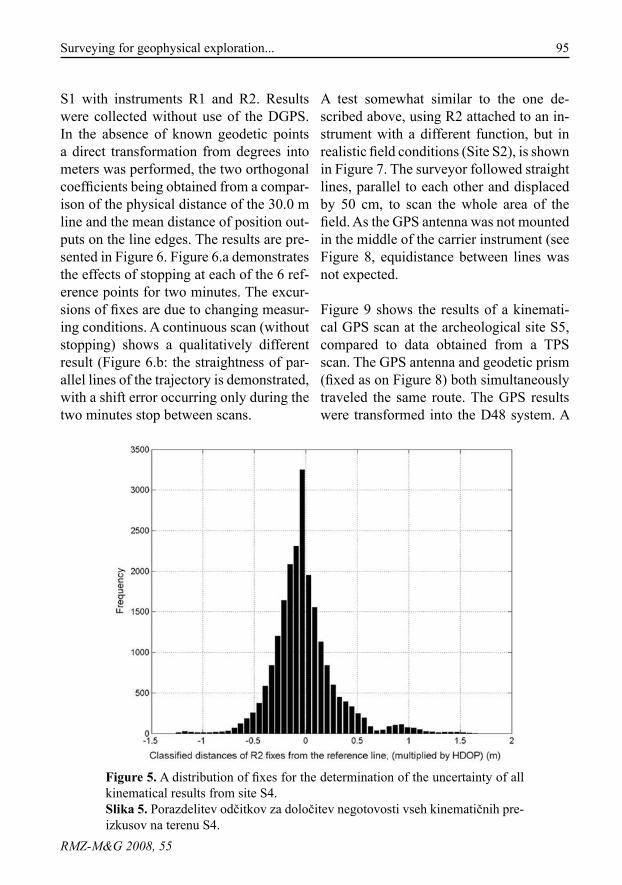
95Surveying for geophysical exploration...
RMZ-M&G 2008, 55
Figure 5. A distribution of fixes for the determination of the uncertainty of all kinematical results from site S4.Slika 5. Porazdelitev odčitkov za določitev negotovosti vseh kinematičnih pre-izkusov na terenu S4.
S1 with instruments R1 and R2. Results were collected without use of the DGPS. In the absence of known geodetic points a direct transformation from degrees into meters was performed, the two orthogonal coefficients being obtained from a compar-ison of the physical distance of the 30.0 m line and the mean distance of position out-puts on the line edges. The results are pre-sented in Figure 6. Figure 6.a demonstrates the effects of stopping at each of the 6 ref-erence points for two minutes. The excur-sions of fixes are due to changing measur-ing conditions. A continuous scan (without stopping) shows a qualitatively different result (Figure 6.b: the straightness of par-allel lines of the trajectory is demonstrated, with a shift error occurring only during the two minutes stop between scans.
A test somewhat similar to the one de-scribed above, using R2 attached to an in-strument with a different function, but in realistic field conditions (Site S2), is shown in Figure 7. The surveyor followed straight lines, parallel to each other and displaced by 50 cm, to scan the whole area of the field. As the GPS antenna was not mounted in the middle of the carrier instrument (see Figure 8, equidistance between lines was not expected.
Figure 9 shows the results of a kinemati-cal GPS scan at the archeological site S5, compared to data obtained from a TPS scan. The GPS antenna and geodetic prism (fixed as on Figure 8) both simultaneously traveled the same route. The GPS results were transformed into the D48 system. A
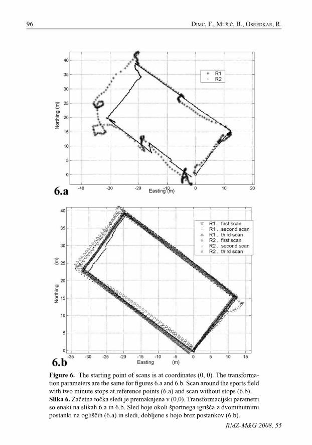
96 dimc, f., mušiČ, B., osRedkAR, R.
RMZ-M&G 2008, 55
Figure 6. The starting point of scans is at coordinates (0, 0). The transforma-tion parameters are the same for figures 6.a and 6.b. Scan around the sports field with two minute stops at reference points (6.a) and scan without stops (6.b).Slika 6. Začetna točka sledi je premaknjena v (0,0). Transformacijski parametri so enaki na slikah 6.a in 6.b. Sled hoje okoli športnega igrišča z dvominutnimi postanki na ogliščih (6.a) in sledi, dobljene s hojo brez postankov (6.b).
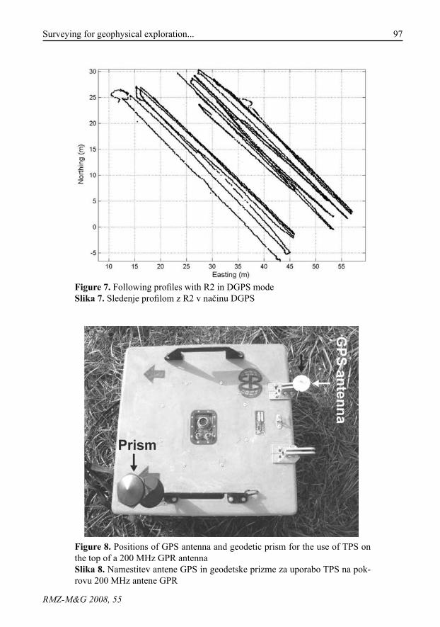
97Surveying for geophysical exploration...
RMZ-M&G 2008, 55
Figure 7. Following profiles with R2 in DGPS modeSlika 7. Sledenje profilom z R2 v načinu DGPS
Figure 8. Positions of GPS antenna and geodetic prism for the use of TPS on the top of a 200 MHz GPR antennaSlika 8. Namestitev antene GPS in geodetske prizme za uporabo TPS na pok-rovu 200 MHz antene GPR
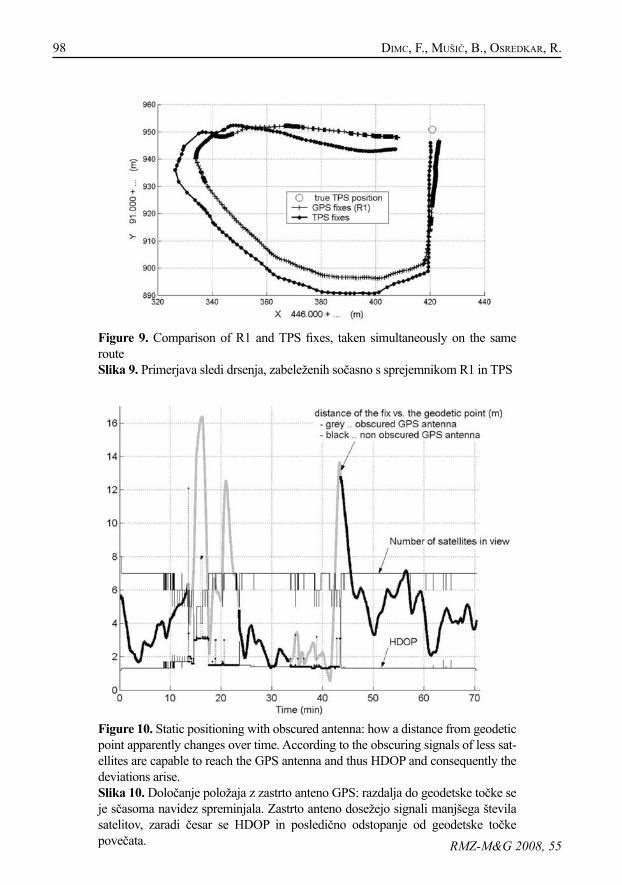
98 dimc, f., mušiČ, B., osRedkAR, R.
RMZ-M&G 2008, 55
Figure 9. Comparison of R1 and TPS fixes, taken simultaneously on the same routeSlika 9. Primerjava sledi drsenja, zabeleženih sočasno s sprejemnikom R1 in TPS
Figure 10. Static positioning with obscured antenna: how a distance from geodetic point apparently changes over time. According to the obscuring signals of less sat-ellites are capable to reach the GPS antenna and thus HDOP and consequently the deviations arise.Slika 10. Določanje položaja z zastrto anteno GPS: razdalja do geodetske točke se je sčasoma navidez spreminjala. Zastrto anteno dosežejo signali manjšega števila satelitov, zaradi česar se HDOP in posledično odstopanje od geodetske točke povečata.
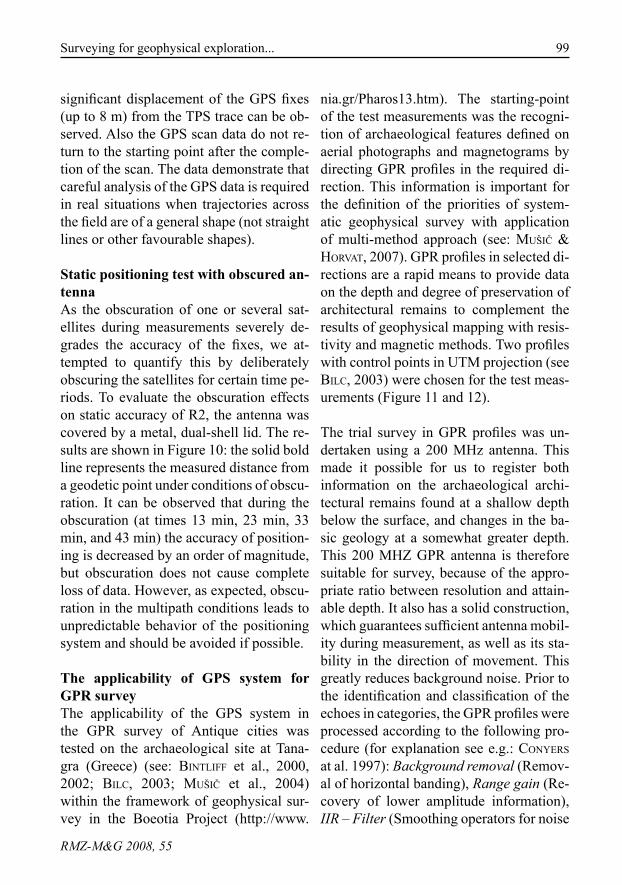
99Surveying for geophysical exploration...
RMZ-M&G 2008, 55
significant displacement of the GPS fixes (up to 8 m) from the TPS trace can be ob-served. Also the GPS scan data do not re-turn to the starting point after the comple-tion of the scan. The data demonstrate that careful analysis of the GPS data is required in real situations when trajectories across the field are of a general shape (not straight lines or other favourable shapes).
Static positioning test with obscured an-tennaAs the obscuration of one or several sat-ellites during measurements severely de-grades the accuracy of the fixes, we at-tempted to quantify this by deliberately obscuring the satellites for certain time pe-riods. To evaluate the obscuration effects on static accuracy of R2, the antenna was covered by a metal, dual-shell lid. The re-sults are shown in Figure 10: the solid bold line represents the measured distance from a geodetic point under conditions of obscu-ration. It can be observed that during the obscuration (at times 13 min, 23 min, 33 min, and 43 min) the accuracy of position-ing is decreased by an order of magnitude, but obscuration does not cause complete loss of data. However, as expected, obscu-ration in the multipath conditions leads to unpredictable behavior of the positioning system and should be avoided if possible.
The applicability of GPS system for GPR surveyThe applicability of the GPS system in the GPR survey of Antique cities was tested on the archaeological site at Tana-gra (Greece) (see: BinTLiff et al., 2000, 2002; BiLc, 2003; mušiČ et al., 2004) within the framework of geophysical sur-vey in the Boeotia Project (http://www.
nia.gr/Pharos13.htm). The starting-point of the test measurements was the recogni-tion of archaeological features defined on aerial photographs and magnetograms by directing GPR profiles in the required di-rection. This information is important for the definition of the priorities of system-atic geophysical survey with application of multi-method approach (see: mušiČ & HoRvAT, 2007). GPR profiles in selected di-rections are a rapid means to provide data on the depth and degree of preservation of architectural remains to complement the results of geophysical mapping with resis-tivity and magnetic methods. Two profiles with control points in UTM projection (see BiLc, 2003) were chosen for the test meas-urements (Figure 11 and 12).
The trial survey in GPR profiles was un-dertaken using a 200 MHz antenna. This made it possible for us to register both information on the archaeological archi-tectural remains found at a shallow depth below the surface, and changes in the ba-sic geology at a somewhat greater depth. This 200 MHZ GPR antenna is therefore suitable for survey, because of the appro-priate ratio between resolution and attain-able depth. It also has a solid construction, which guarantees sufficient antenna mobil-ity during measurement, as well as its sta-bility in the direction of movement. This greatly reduces background noise. Prior to the identification and classification of the echoes in categories, the GPR profiles were processed according to the following pro-cedure (for explanation see e.g.: conYeRs at al. 1997): Background removal (Remov-al of horizontal banding), Range gain (Re-covery of lower amplitude information), IIR – Filter (Smoothing operators for noise
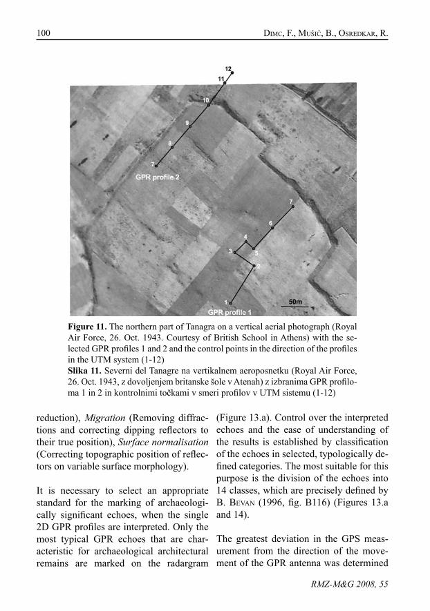
100 dimc, f., mušiČ, B., osRedkAR, R.
RMZ-M&G 2008, 55
Figure 11. The northern part of Tanagra on a vertical aerial photograph (Royal Air Force, 26. Oct. 1943. Courtesy of British School in Athens) with the se-lected GPR profiles 1 and 2 and the control points in the direction of the profiles in the UTM system (1-12)Slika 11. Severni del Tanagre na vertikalnem aeroposnetku (Royal Air Force, 26. Oct. 1943, z dovoljenjem britanske šole v Atenah) z izbranima GPR profilo-ma 1 in 2 in kontrolnimi točkami v smeri profilov v UTM sistemu (1-12)
reduction), Migration (Removing diffrac-tions and correcting dipping reflectors to their true position), Surface normalisation (Correcting topographic position of reflec-tors on variable surface morphology).
It is necessary to select an appropriate standard for the marking of archaeologi-cally significant echoes, when the single 2D GPR profiles are interpreted. Only the most typical GPR echoes that are char-acteristic for archaeological architectural remains are marked on the radargram
(Figure 13.a). Control over the interpreted echoes and the ease of understanding of the results is established by classification of the echoes in selected, typologically de-fined categories. The most suitable for this purpose is the division of the echoes into 14 classes, which are precisely defined by B. BevAn (1996, fig. B116) (Figures 13.a and 14).
The greatest deviation in the GPS meas-urement from the direction of the move-ment of the GPR antenna was determined
101Surveying for geophysical exploration...
RMZ-M&G 2008, 55
Figure 12. The GPS readings at a distance of 2 m are indicated by the white points in the direction of GPR profile 1 Slika 12. Z belimi točkami v smeri GPR profila 1 so prikazani GPS v razdalji 2 m
at points 3, 4 and 5 (Figure 14), which was a result of a a sharp change in the direc-tion of movement of the antenna at an angle to an approximate right angle. The deviations are in accordance with the es-tablished aims of the research on the level areas and correspond to the deviations, which were determined in GPR profile 2, where there was no greater change in the direction of movement. Figures 11, 14 and 15 indicate that at each change in direction the GPS measurements »returned to the right« place, but some time nevertheless passes before this happens. If the direction of movement changes too frequently and time is not taken for the GPS readings to
settle down, then these errors accumulate. The deviation in the direction of movement in fourth loop in trial GPR profile 1 already amounted to almost 2 m (Figures 14.b and 15). The GPS fixes »settled down« accord-ing to the reference lines after circa 35 me-ters of linear movement (see the segment from point No. 3 to No. 2).
GPR profile 2 runs in a straight line, cross-es the town wall and descends via a steep slope on the exterior of the wall at a height of 113 metres above sea level (from 122 m down to 109 m). A deviation (in the horizontal plane: average of fixes includ-ing HDOP according to the reference lines between reference points is 44 cm while 95 % of fixes lie closer than or equal to 55 cm to the reference lines) from the actual direction of movement in the particular case of linear movement due to the rapid change in height (z) was determined in this profile.
On the basis of these results it is possible to conclude that the precision of this GPS system only meets our requirements com-pletely in the specific case of linear move-ment. Effective use requires the selection of a direction of movement with the least possible number of changes in direction at a greater angle. This problem can be solved by planning the prospection in long, rela-tively straight traverses.
The estimation of the accuracy of the loca-tion of the GPR echoes by the GPS system was also correlated in relation to the loca-tion of the magnetic anomalies, mapped by the Geometrics G-858 magnetometer (see mušiČ et al., 2004), which had been geo-referenced by TS measurements, using a
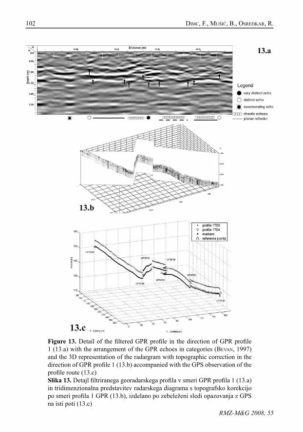
102 dimc, f., mušiČ, B., osRedkAR, R.
RMZ-M&G 2008, 55
Figure 13. Detail of the filtered GPR profile in the direction of GPR profile 1 (13.a) with the arrangement of the GPR echoes in categories (BevAn, 1997) and the 3D representation of the radargram with topographic correction in the direction of GPR profile 1 (13.b) accompanied with the GPS observation of the profile route (13.c)Slika 13. Detajl filtriranega georadarskega profila v smeri GPR profila 1 (13.a) in tridimenzionalna predstavitev radarskega diagrama s topografsko korekcijo po smeri profila 1 GPR (13.b), izdelano po zebeleženi sledi opazovanja z GPS na isti poti (13.c)
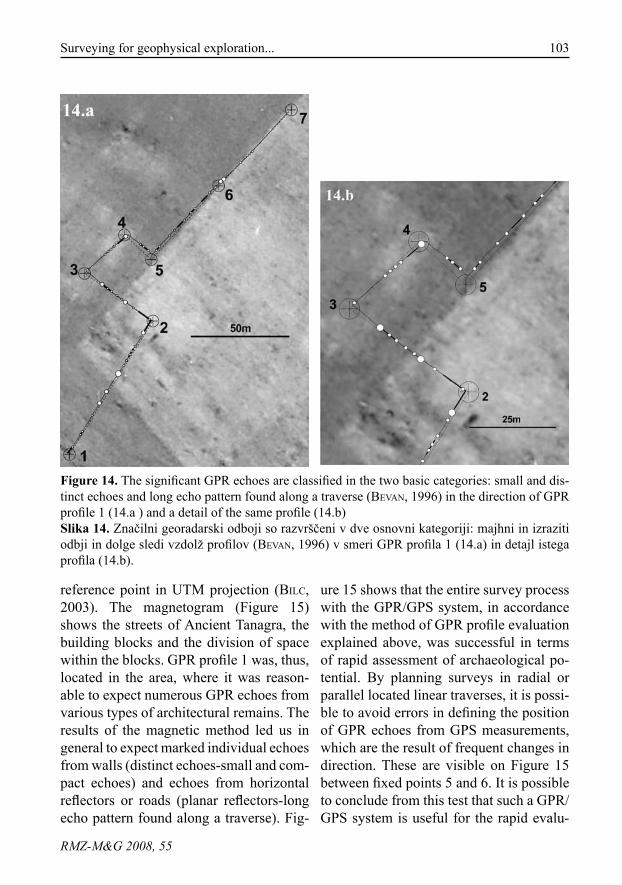
103Surveying for geophysical exploration...
RMZ-M&G 2008, 55
Figure 14. The significant GPR echoes are classified in the two basic categories: small and dis-tinct echoes and long echo pattern found along a traverse (BevAn, 1996) in the direction of GPR profile 1 (14.a ) and a detail of the same profile (14.b)Slika 14. Značilni georadarski odboji so razvrščeni v dve osnovni kategoriji: majhni in izraziti odbji in dolge sledi vzdolž profilov (BevAn, 1996) v smeri GPR profila 1 (14.a) in detajl istega profila (14.b).
reference point in UTM projection (BiLc, 2003). The magnetogram (Figure 15) shows the streets of Ancient Tanagra, the building blocks and the division of space within the blocks. GPR profile 1 was, thus, located in the area, where it was reason-able to expect numerous GPR echoes from various types of architectural remains. The results of the magnetic method led us in general to expect marked individual echoes from walls (distinct echoes-small and com-pact echoes) and echoes from horizontal reflectors or roads (planar reflectors-long echo pattern found along a traverse). Fig-
ure 15 shows that the entire survey process with the GPR/GPS system, in accordance with the method of GPR profile evaluation explained above, was successful in terms of rapid assessment of archaeological po-tential. By planning surveys in radial or parallel located linear traverses, it is possi-ble to avoid errors in defining the position of GPR echoes from GPS measurements, which are the result of frequent changes in direction. These are visible on Figure 15 between fixed points 5 and 6. It is possible to conclude from this test that such a GPR/GPS system is useful for the rapid evalu-
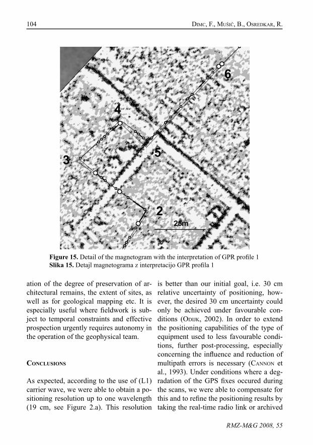
104 dimc, f., mušiČ, B., osRedkAR, R.
RMZ-M&G 2008, 55
Figure 15. Detail of the magnetogram with the interpretation of GPR profile 1Slika 15. Detajl magnetograma z interpretacijo GPR profila 1
ation of the degree of preservation of ar-chitectural remains, the extent of sites, as well as for geological mapping etc. It is especially useful where fieldwork is sub-ject to temporal constraints and effective prospection urgently requires autonomy in the operation of the geophysical team.
conclusIons
As expected, according to the use of (L1) carrier wave, we were able to obtain a po-sitioning resolution up to one wavelength (19 cm, see Figure 2.a). This resolution
is better than our initial goal, i.e. 30 cm relative uncertainty of positioning, how-ever, the desired 30 cm uncertainty could only be achieved under favourable con-ditions (odijk, 2002). In order to extend the positioning capabilities of the type of equipment used to less favourable condi-tions, further post-processing, especially concerning the influence and reduction of multipath errors is necessary (cAnnon et al., 1993). Under conditions where a deg-radation of the GPS fixes occured during the scans, we were able to compensate for this and to refine the positioning results by taking the real-time radio link or archived
105Surveying for geophysical exploration...
RMZ-M&G 2008, 55
fixes from the nearest reference station into account. As described in the literature (vAn sickLe, 2001; sAkA et al., 2004), a dual frequency receiver enables faster real time kinematical positioning than single frequency receiver, eliminating some of the multipath and receiver noise errors. In order to describe positioning conditions the processing of the carrier phase (CP), based on smoothing the pseudo ranges, should also be considered (foRd, 2003). The techniques described are not adequate for archaeological work in extreme con-ditions, e.g. underground caves or urban environments, where navigation satellite signals are obscured from the receiver. A hybrid positioning technology, involving relative positioning by wideband carrier waves or by some other types of sensors (meZenTsev et al., 2004) would be recom-mended in such circumstances. It is now well known that many of the positioning problems investigated in our work will be solved by better basic accuracy in new sat-ellite positioning technologies, based on a new satellite network that is now under the new satellite networks that are now under construction (Galileo, GLONASS, CNSS, GAGAN). As the new system still seems to be several years from becoming opera-tional, the necessary experience in the geo-physical fieldwork using satellite position-ing can be obtained by utilizing the exist-ing, though barely adequate GPS system. Nevertheless, the vulnerability of the satel-lite navigation systems due to intentioned jamming and the rate of errors due to the observation conditions, lead to the imple-mentation of a complementary sensor.
Acknowledgments
The authors express their gratitude to Messrs. Andrej Bilban (Geoservis, Lju-bljana), Guido Lenz (FSL Deutschland, Germany), Duško Vranac (Harphasea, Ko-per) for the discussions and help with the equipment selection and use.
povzetek
Uporaba enofrekvenčnega sprejem-nika GNSS s 30 cm negotovostjo v kinematičnem načinu dela za terenske geofizikalne preiskave
Zamisel o izdelavi cenenega, enofrekvenč-nega GPS sistema, ki je preprost za upra-vljanje izhaja iz potrebe po večji fleksibil-nosti in učinkovitosti terenskega dela pri geofizikalnih raziskavah. Zadostno fleksi-bilnost zagotavlja le popolna avtonomija ekipe pri načrtovanju in izvajanju teren-skih postopkov pri natančnem prostor-skem umeščanju ugotovljenih anomalnih območij.
Uveljavljeni geodetski terenski postopki, tudi s pomočjo satelitske navigacijske teh-nike, so pogosto dolgotrajni, cenovno pre-dragi in za našo rabo pogosto tudi preveč natančni. Z žrtvovanjem visoke natančno-sti bi skrajšali čas pridobivanja dovolj za-nesljivih podatkov o položaju merilnih in-strumentov z uporabo enofrekvenčnih (L1) sprejemnikov GPS srednjega razreda.
106 dimc, f., mušiČ, B., osRedkAR, R.
RMZ-M&G 2008, 55
Preizkusni tereni obravnavani v članku so enaki realnim situacijam in imajo napake določanja položaja s satelitskim sistemom enake vzroke: zastrtost, večpotje, spremen-ljivost ionosfere. Vplivov spremenljivosti ionosfere na rezultate v predstavljenih pri-merih še nismo opazovali.
V pogojih večpotja je raztros rezultatov (Slika 2a), izmerjen s preprosto GPS ante-no (glej sliki 1 in 8), pričakovano prevelik. Pri geofizikalnih raziskavah je pomembna tudi zanesljiva ponovljivost določanja po-ložaja, kadar je potrebno meritve ponoviti pri drugačnih nastavitvah geofizikalnega instrumenta ipd. Z določanjem razdalje do referenčne točke s statičnimi preizku-si (Slika 2b) smo dokazali, da je v dobrih pogojih oz. pri majhni zastrtosti satelitov, ponovljivost rezultatov položaja ustrezna. V tabeli 3 vidimo, da imajo na negotovost meritev pričakovano večji vpliv okoliščine in izbira sprejemnika kot način opazovanja (samostojni GPS, diferencialni - DGPS). Vpliv izbire naprave na rezultate kinema-tičnih preizkusov je razviden iz tabele 4: v enakih pogojih je negotovost precej manj-ša, v pogojih z malo večpotja je negotovost ustrezna. Sliki 3 in 4 prikazujeta rezultate z dveh terenov: v pogojih nezanemarljivega večpotja smo preizkušali različna spreje-mnika (Slika 3), ob različnih razporeditvah satelitov nad obzorjem (HDOP) smo na terenu z malo večpotja in zastrtosti preiz-kušali isti sprejemnik. Ponovljivost oblike sledi smo v različnih režimih hoje opazo-vali v enakih pogojih večpotja (Slika 6a in 6b). Sledenje ravnim profilom ob znatnem večpotju je razvidno s slike 7. Sočasno do-ločanje položaja s sprejemnikom GPS in te-odolitom (TPS) na sliki 9 kaže odstopanja, pričakovana v slabših pogojih sprejema.
Namerno zastiranje mirujoče antene GPS (Slika 10) povzroča velika nihanja rezulta-tov položaja oziroma navidezne premike. Na arheološkem terenu (Slika 11) smo za-znali odstopanja od referenčne črte, ki so naključno (glej Slika 5) naraščala z odda-ljevanjem od oglišča, v katerem smo začeli hojo. Z določitvijo parametrov odstopanja ob upoštevanju vpliva HDOP in kvantita-tivne ocene večpotja na določenem terenu, je odstopanja možno kompenzirati.
Testno rekognosciranje v georadarskih profilih smo izvajali z 200 MHz anteno, s katero poleg informacij o arheoloških ar-hitekturnih ostalinah, ki se nahajajo plitvo pod površjem, registriramo tudi spremem-be v geološki podlagi na nekoliko večjih globinah. Ta GPR antena je ustrezna za re-kognosciranje zaradi ustreznega razmerja med ločljivostjo in globino dosega ter ma-sivne konstrukcije, ki ob zadostni mobil-nosti antene med meritvami zagotavljajo tudi njeno stabilnost v smeri gibanja, kar bistveno zmanjšuje šum.
Največja odstopanja GPS meritev od sme-ri gibanja GPR antene so bila ugotovljena v točkah 3, 4 in 5 (glej sliki 14b in 15), kjer smo naglo spreminjali smer gibanja antene, dejanske spremembe smeri so pri-bližno ustrezale pravemu kotu. Na ravnih odsekih so odstopanja v skladu z zastavlje-nimi cilji raziskave in ustrezajo odstopa-njem, ki so bila ugotovljena v GPR profilu 2, kjer večjih sprememb v smeri gibanja ni bilo. Na istih slikah vidimo, da se pri vsaki spremembi smeri odčitki GPS »vrnejo na pravo« mesto vendar vmes vselej preteče nekaj časa. Če smer gibanja spreminja-mo pogosto in ne počakamo, da se odčitki GPS ustalijo, se te napake akumulirajo. Na
107Surveying for geophysical exploration...
RMZ-M&G 2008, 55
osnovi te ugotovitve lahko zaključimo, da natančnost tega GPS sistema popolnoma odgovarja našim zahtevam samo v poseb-nem primeru premočrtnega gibanja. Za učinkovito rabo moramo izbirati smeri gi-banja z najmanjšim možnim številom spre-memb smeri pod večjimi koti. Ta problem rešimo tako, da prospekcijo načrtujemo v dolgih, približno ravnih prečnicah.
Oceno natančnosti pozicioniranja geora-darskih odbojev z GPS smo preverjali tudi v odnosu do položaja magnetnih anomalij, kartiranih z magnetometrom Geometrics G-858 (mušiČ et al., 2004), ki so bile ge-oreferencirane z zemeljskimi meritvami z uporabo referenčnih točk v UTM projek-ciji (BiLc, 2003). Na magnetogramu (slika 15a) vidimo ulice antične Tanagre, stavbne bloke in razdelitve prostorov znotraj blo-kov. GPR profil 1 je bil torej izbran na ob-močju, kjer smo lahko pričakovali številne radarske odboje od različnih tipov arhitek-turnih ostalin. Glede na rezultate magnetne metode smo v splošnem pričakovali izra-zite posamične odboje od zidov in odboje od horizontalnih reflektorjev oziroma cest. Iz slike 15 je razvidno, da je celoten posto-pek rekognosciranja z GPR/GPS sistemom v skladu z obrazloženim načinom vredno-tenja radarskih profilov učinkovit v smislu hitre ocene arheološkega potenciala. Z na-črtovanjem pregledov v radialno oziroma vzporedno zastavljenih ravnih prečnicah se izognemo napakam v določanju položa-ja radarskih odbojev iz opazovanj z GPS, ki so posledica pogostega spreminjanja smeri in so vidne na sliki 15 med točkama 5 in 6.
Iz rezultatov statičnih in kinematičnih pri-merjalnih preizkusov različnih vrst prepro-stejših sprejemnikov GPS vidimo, da ima-jo preprostejše naprave pričakovano širši interval zaupanja. Kakovost obdelave sa-telitskih signalov namreč v večji meri za-gotavljajo zmogljivejša elektronska vezja.
Možnost kompenziranja napak z nakna-dno obdelavo izmerjenih odčitkov spre-jemnikov GPS obstaja, če zadosti dobro poznamo vzroke napak oziroma pogoje, v katerih izvajamo terenske raziskave. Pri-čakovanja od novih sistemov satelitske navigacije (Galileo - Evropa, GLONASS - Rusija, CNSS - Kitajska, GAGAN - In-dija) in posodobitve obstoječega (GPS - ZDA) so zaradi raznih nedorečenosti še v domeni prihodnosti. Dva splošna poja-va zmanjšujeta zanesljivost določanja po-ložaja satelitskih navigacijskih sistemov: že omenjene napake zaradi okoliščin na terenu in neodpornost na namerno radio-frekvenčno motenje (jamming). Eden od ustreznih odgovorov za zagotovitev zahte-vane zanesljivosti GPS meritev z enofre-kvenčnim sprejemnikom je vključevanje dodatnih komplementarnih senzorjev (npr. pospeškometer pri kinematičnih meritvah) v odvisnosti od narave motenj.
108 dimc, f., mušiČ, B., osRedkAR, R.
RMZ-M&G 2008, 55
references
BeRAn, T., LAnGLeY, R. B., BisnATH, s. B. & seRRAno, L. (2007): High-Accuracy Point Positioning With Low-Cost Receivers. Navigation, Journal of The Institute of Naviga-tion.; Vol. 54, No. 1, pp. 53-63.
BevAn, B. (1996): Geophysical explora-tion for Archaeology. Volume B: Introduction to geophysical explo-ration. Geosight Technical Report Number 4.
BiLc, A. (2003): Tanagra 2003, Report on groundwork for use of GPS mea-surements.
BinTLiff, j. L., eveLpidou, n., fARineTTi, e., mušiČ, B. & sLApšAk, B. (2002): The Tanagra survey. Report on the 2001 season. Pharos.; Vol. 9, pp. 33-74.
BinTLiff, j. L., fARineTTi, e., sBoniAs, k., siGALos, L., sLApšAk, B. & mušiČ, B. (2000): The Tanagra survey. Re-port on the 2000 season. Pharos.; Vol. 8, pp. 93-128.
cAnnon, m. e., LAcHApeLLe, G. & Lu, G. (1993): Kinematic Ambigu-ity Resolution With a High Preci-sion C/A Code Receiver. Journal of Surveying Engineering, Amer. Soc. Civil Eng.; Vol. 119, No. 4, pp 147- 155.
conYeRs, L. B. & GoodmAn, d. (1997): Ground-Penetrating Radar. An introduction for archaeologists. Altamira Press. A division of Sage Publications, Ins.
de jonG, c.d. & LAcHApeLLe, G. (2001): Hydrography, 2nd edition. Series on mathematical geodesy and po-sitioning. Delft University Press: Blue Print, Delft.
foRd, T. (2003): A New Positioning Filter: Phase Smoothing in the Position Domain, Navigation. Journal of The Institute of Navigation.; Vol. 50, No. 2, pp. 65-78.
GAffneY, c. & GATTeR, j. (2003): Reveal-ing The Buried Past: Geophysics for Archaeologists. Tempus Pub-lishing Ltd.
GPS Position Accuracy Measures, Appli-cation note, APN-029 Rev 1, No-vatel. (www.novatel.com).
International Vocabulary of Basic and General Terms in Metrology. USM, Ljubljana, 1999.
LAcHApeLLe, G., HenRiksen, j. & meL-GAeRd, T. (1994): Seasonal Effect of Tree Foliage on GPS Signal Availability and Multipath for Vehicular Navigation. Proceed-ings of GPS-94 (Salt Lake City, September 21-23). The Institute of Navigation, Alexandria, VA, pp. 527-532.
meZenTsev, o., coLLin, j., kuusniemi, H. & LAcHApeLLe, G. (2004): Accuracy Assessment of a High Sensitivity GPS Based Pedestrian Navigation System Aided by Low-Cost Sen-sors. 11th Saint Petersburg Inter-national Conference on Integrated Navigation Systems. May 24-26, Saint Petersburg, Russia, pp. 156-164.
109Surveying for geophysical exploration...
RMZ-M&G 2008, 55
mušiČ, B., sLApšAk, B. & fARineTTi, e. (2004): Ancient Tanagra (Grimad-ha): Geophysical prospection and modelling for understanding of ur-ban plan and on-site activity are-as. In: Fischer Auesserer K. (ed.). [Enter the past] : the e-way into the four dimensions of cultural herita-ge : proceedings of the 30th con-ference, 2003, (BAR international series). Oxford: Archaeopress, pp. 317-320.
mušiČ, B. & HoRvAT, j. (2007): Nauportus – an early Roman trading post at Dolge njive in Vrhnika. The re-sults of geophysical prospection using a variety of independent methods. Arheol. Vest.; Vol. 58, pp. 219-283.
mušiČ, B., HoRvAT, j. & dimc, f. (2008): Comparison of different geophysi-cal techniques in relation to ar-chaeological data for settlement reconstruction – the case study of Nauportus, Slovenia. Cultural Heritage and New Technologies. Workshop 12 – Archäeologie und Computer. November 5. – 7. 2007, Vienna City Hall. – in print.
odijk, d. (2002): Fast precise GPS posi-tioning in the presence of iono-spheric delays: PhD thesis. Delft University.
sAkA, m. H., kAvZoGLu, T., oZsAmLi, c. & ALkAn, R. m. (2004): Sub-Metre Accuracy for Stand Alone GPS Positioning in Hydrographic Sur-veying. The Journal of Naviga-tion.; Vol. 57, No. 1, pp. 135-144.
vAn sickLe, j. (2001): GPS for Land Sur-veyors. Taylor and Francis, New York.
WAnG, c. & LAcHApeLLe, G. (2002): GPS Attitude Determination Reliability Performance Improvement Using Low Cost Receivers. Journal of Global Positioning Systems.; Vol. 1, No. 2, pp. 85-95.

111RMZ – Materials and Geoenvironment, Vol. 55, No. 1, pp. 111-126, 2008
Scientific paper
The possibility of using homogeneous (projective) coordinatesin 2D measurement exercises
Možnost uporabe homogenih (projektivnih) koordinatv dvodimenzionalnih merskih nalogah
ALeksAndAR GAnić1, miLivoj vuLić2, fRAnc Runovc2, TinA HABe3
1University of Belgrade, Faculty of Mining and Geology, Đušina 7, 11000 Belgrade, Serbia: E-mail: [email protected]
2University of Ljubljana, Faculty of Natural Sciences and Engineering, Aškerčeva cesta 12, SI-1000 Ljubljana, Slovenia;
E-mail: [email protected], [email protected] d.o.o., Dimičeva ulica 16, SI-1000 Ljubljana, Slovenia;
E-mail: [email protected]
Received: November 29, 2007 Accepted: January 12, 2008
Abstract: This work’s intention is to present the basic characteristics of projec-tive geometry and the use of homogeneous (projective) coordinates in two-dimensional (further denoted as 2D) measurement exercises. The concept of a projective plane originates from the Euclidean plane, assuming all our given points are ideal and lie upon an ideal line verging towards infinity. The term “ideal point” is taken to mean an intersection of all lines that are parallel in the finite space. By introducing these so-called ideal points and ideal lines, the calculations in 2D measurement exercises – ones that are usually carried out under the rules of Euclidean trigonometry – have been simplified, as the calculations of directional angles and lengths are no longer necessary. As a practical example of the use of projective coor-dinates, an intersection is presented, such that it can also be used for the Collins Method of Resection, seeing as it is based upon using said intersec-tion twice.
Izvleček: Predstavljene so osnovne značilnosti projektivne geometrije in s tem uporaba homogenih (projektivnih) koordinat v dvodimenzionalnih merskih nalogah. Projektivno ravnino dobimo iz evklidske ravnine, če privzamemo točke in premico v neskončnosti na kateri ležijo vse točke v neskončnosti. Neskončna točka predstavlja presečišče vseh premic, ki so v končnosti med seboj vzporedne. Z uvedbo neskončnih točk in neskončne premice se izračuni v dvodimenzionalnih merskih nalogah, ki se navadno vršijo po pravilih evklidske trigonometrije, poenostavijo saj računanje smernih ko-tov in dolžin ni potrebno. Kot praktični primer uporabe projektivnih koor-
112 GAnić, A., vuLić, m, Runovc, f., HABe, T.
RMZ-M&G 2008, 55
dinat je prikazan zunanji urez, ki ga je možno uporabiti tudi pri Collinsovi metodi notranjega ureza, saj temelji na dvakratni uporabi zunanjega ureza.
Key words: homogeneous coordinates of a point, homogeneous coordinates of a line, incidence relation, principle of duality, ideal point, ideal line, intersec-tion, resection
Ključne besede: homogene koordinate točke, homogene koordinate premice, rel-acija incidence, princip dualnosti, neskončna točka, premica v neskončnosti, zunanji urez, notranji urez
IntroductIon
In 2D measurement exercises, all calculations are usually carried out under the rule of Euclidean geometry - where the points, lines and their relationships are defined dif-ferently than in a projective plane - in which the coordinates of an unknown point are established through the aid the calculation of so-called lengths and angles of our site. As a reaction to the latter, the article at hand is meant to present the basic relations between points and lines of the projective plane and depict their use in 2D measurement exer-cises. A practical example of using said projective coordinates would be an intersection, in which the coordinates of a new point are calculated from the measured angles of given points of an existing triangulation network. In what follows, the coordinates of a point and the formulas of lines on a Euclidean plane shall be marked using upper case, whereas the coordinates of points and formulas of lines on the projective plane will be denoted using lower case letters.
poInt and lIne
In projective geometry, a point is defined as a set of three coordinates that equal the set (y x ω) and therefore obviously also as an ordered set of three numbers (y x ω) - which do not all equal zero at the same time, since then (λy λx λω) would be the same point for any given λ ≠ 0.
For example, (2 3 6) is our exemplary point, and (⅓ ½ 1) is another of the numerous ways to mark that exact same point, bearing in mind the principle that an unlimited number of sets of three numbers (y x ω) may correspond to each point, but only one point may correspond to each ordered set. Furthermore, from non-homogeneous coor-dinates of any given point, we beget an infinite number of sets of homogeneous coordi-nates of that same point:
(1)
113The possibility of using homogeneous (projective) coordinates...
RMZ-M&G 2008, 55
And from homogeneous coordinates of that certain point, we can get one single ordered pair of numbers:
(2)
A line is defined in almost the same way as a point, the one difference being that the line is treated as a set of all points that equal the set of three (v u w). For example, if (3 2 -2) defines a line, then (-3/2 -1 1) is the notation for that same line. In other words, a line is an ordered set of three numbers, denoted as (v u w), which do not equal zero all at the same time, in which case (μv μu μw) would be the same line for any given μ ≠ 0 [1].
IncIdence relatIon
Given point P and line l - where P and l are short for (y x ω) and (v u w), respectively - we say that the two are incident to one another (incidence relation being descriptive of the relation simply summed up as the point lying on the line i.e. the line going “through” the point) in the case, the following is true: {P ∙ l} = {l ∙ P} = yv + xu + ωw = vy + ux + wω = 0 [2].
the prIncIple of dualIty
The axiom of geometry says that there is exactly one line that is in incidence with two different points P1 and P2, i.e. exactly one line goes through both different points. If we exchange the term “line” with the term “point” in the above axiom, we get a geometrical theorem that states there is exactly one point that is in incidence with two different lines l1 and l2 - in other words, two different lines intersect at exactly one point in space. The afore-mentioned axiom and theorem are said to be mutually dual, i.e. points and lines are mutually dual spatial elements, while the “running” and intersecting of lines are mutually dual operations[3].
For different points P1(y1 x1 ω1) and P2(y2 x2 ω2); y1 ≠ λ ∙ y2, x1 ≠ λ ∙ x2 , ω1 ≠ λ ∙ ω2 there is always an ordered set of three elements, (v u w), for which the following need most definitely apply:
y1v + x1u + ω1w = 0 y2v + x2u + ω2w = 0 (3)

114 GAnić, A., vuLić, m, Runovc, f., HABe, T.
RMZ-M&G 2008, 55
And for two different lines, in our particular example l1 (v1 u1 w1) and l2 (v2 u2 w2); v1 ≠ μ∙ v2, u1 ≠ μ ∙ u2 , w1 ≠ μ ∙ w2; there is always an ordered set of three elements, (y x ω), for which the following need apply:
v1y + u1x + w1 ω = 0 v2y + u2x + w2 ω = 0 (4)
Thus, homogeneous systems of equations are combined with the following expression:
(5)
Then we are able to beget the formula of the point or line:
(6)
Each set of three
wux
vy ω therefore represents a solution to the system under
question.
The coordinates of the point or line follow:
(7)
A point or a line pertaining to a projective plane can be multiplied by any number λ or μ , as long as the value is not equal to zero, which then gives us the actual coordinates of this same point or line:
(8)

115The possibility of using homogeneous (projective) coordinates...
RMZ-M&G 2008, 55
For a point, this would be:
(9)
And for a line:
(10)
the Ideal poInt and lIne
The parallels (coefficient of site k = k1 = k2) l1 and l2 with formulas Y = k1X + n1 and Y = k2X + n2 are given. For X, we enter values X = , and for Y values Y = , then multiplying the equations with ω, which in turn gives us the formulas of lines using homogeneous coordinates:
y = kx + n1ω and y = kx + n2ω (11)
Considering that the lines are parallel, we are interested in the set of three, (v u w), such that it must correspond to both formulas.
By subtracting the equations we get: ω(n1 - n2) = 0.
As n1 ≠ n2, then ω = 0 and the equations y = kx + n1ω and y = kx + n2ω are reduced into y = xk.
Since we are dealing with homogeneous coordinates, we can say that x = 1. From this, we come to the conclusion that y = k. Thus, we obtain a set of three, (k 1 0), which does indeed correspond to both equations.
If the lines l1 and l2 are parallel to the y-axis, then the formulas of the lines in homogene-ous coordinates have the form x = ωx1 and x = ωx2. In this case, the set of three (0 1 0) corresponds to both formulas.
To summarize, the set of three, (k 1 0), corresponds to a formula of the forms y = kx + n1ω and y = kx + n2ω only when k = k1 = k2, or when the lines are parallel and the coef-ficient of site equals k. The set of three (0 1 0) corresponds to all formulas of the form x = ωx1 that describe the parallels of the y-axis.
A bouquet of parallel lines (all parallel lines are of the same class and form organised heaps of parallel lines denoted as “bouquets”) defines a point P∞ in projective plane that has been defined as an ideal point. The bouquet P∞ consists of all lines that are parallel to
xω
yω
116 GAnić, A., vuLić, m, Runovc, f., HABe, T.
RMZ-M&G 2008, 55
a certain line l. The equation pertaining to line l is Y = kX + n, or X = XP if it is parallel to the y rather than the x-axis.
The line l belongs to bouquet P∞ exactly when the set of three (k 1 0) corresponds to the equation of line l in its homogeneous coordinates, and to pencil P∞ exactly when what corresponds to this equation is this set of three: (0 1 0). Consequentially, we can have the set of three (k 1 0) in the former case, and the set of three (0 1 0) in the latter case for homogeneous coordinates of the ideal point P∞.
Since we may multiply homogeneous coordinates with any number that is different than zero, we may say that the set of three (y x 0) represents the homogeneous coordinates of one ideal point, where y and x are any given elements different from zero. In this way, we have adjusted our homogeneous coordinates (y x ω) so that they befit each and every point of our projective plane. The point with such coordinates also lies in the Euclidean plane if ω ≠ 0, and is an ideal point when ω = 0 [4].
Two ideal points define the ideal line l ∞:
(12)
The solution of the system are the very coordinates of our ideal line l ∞:
(13)
or, if:
(14)
The set of three (0 0 1) represents the coordinates of an ideal line such that all ideal points lie on it.
the Ideal lIne and angle of sIte
An ideal point represents the intersection of a group of all lines that are parallel to one another in finite space. A specific ideal point upon an ideal line belongs to each group of parallel lines that in finite space represent a so-called »angle of site« between the lines of a certain class and the positive end of the x-axis.

117The possibility of using homogeneous (projective) coordinates...
RMZ-M&G 2008, 55
The coordinates of the line that goes through the points P1(y1 x1 ω1) and P2(y1 + d cos φ x1 + d sin φ ω2), where φ is the so-called angle of site are enclosed within the line P1P2 and the positive side of x-axis, and d represents the distance between the points P1 and P2, which would be:
(v u w) = μ (x1(ω2 - ω1) - d cos φω1 y(ω1 - ω2) + d sin φω2 d(y1 cos φ - x1 sin φ)) (15)
If :
ω2 = ω1 = 1 => (v u w) = μ (-d cos φ d sin φ d(y1 cos φ - x1 sin φ)) (16)
or, when:
(ω2= ω1= 1 ^ d ≠ 0 ^ d ≠ ∞ ^ μ = ) => (v u w) = (- cosφ sinφ (y1 cosφ - x1 sinφ)) (17)
The set (v u w) = (- cos φ sin φ (y1 cos φ - x1 sin φ)) represents the coordinates of the line that is notated using polar coordinates.
The intersection of the line given with polar coordinates and the ideal line (0 0 1) is the ideal line, now denoted using polar coordinates:
(18)
or, if:
λ = 1 => (y∞ x∞ ω∞) = (sin φ cos φ 0) (19)
The notation (y∞ x∞ ω∞) = (sin φ cos φ 0) at the same time alos represents standardised coordinates of said ideal line, for which the following is valid:
(20)
where:
(21)
1d
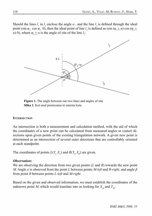
118 GAnić, A., vuLić, m, Runovc, f., HABe, T.
RMZ-M&G 2008, 55
Should the lines l1 in l2 enclose the angle α , and the line l1 is defined through the ideal point (sin φ1 cos φ1 0), then the ideal point of line l2 is defined as (sin (φ1 + α) cos (φ1 + α) 0), where φ1 + α is the angle of site of the line l2:
Figure 1. The angle between our two lines and angles of siteSlika 1. Kot med premicama in smerna kota
IntersectIon
An intersection is both a measurement and calculation method, with the aid of which the coordinates of a new point can be calculated from measured angles or (outer) di-rections upon given points of the existing triangulation network. A given new point is determined as an intersection of several outer directions that are controllably oriented at each standpoint.
The coordinates of points L(YL XL) and R(YR XR) are given.
Observation:We are observing the direction from two given points (L and R) towards the new point M. Angle α is observed from the point L between points M-left and R-right, and angle β from point R between points L-left and M-right.
Based on the given and observed information, we must establish the coordinates of the unknown point M, which would translate into us looking for XM and YM:
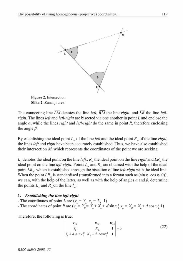
119The possibility of using homogeneous (projective) coordinates...
RMZ-M&G 2008, 55
Figure 2. IntersectionSlika 2. Zunanji urez
The connecting line LM denotes the line left, RM the line right, and LR the line left-right. The lines left and left-right are bisected via one another in point L and enclose the angle α, while the lines right and left-right do the same in point R, therefore enclosing the angle β.
By establishing the ideal point L∞ of the line left and the ideal point R∞ of the line right, the lines left and right have been accurately established. Thus, we have also established their intersection M, which represents the coordinates of the point we are seeking.
L∞ denotes the ideal point on the line left,, R∞ the ideal point on the line right and LR∞ the ideal point on the line left-right. Points L∞ and R∞ are obtained with the help of the ideal point LR∞, which is established through the bisection of line left-right with the ideal line. When the point LR∞ is standardised (transformed into a format such as (sin φ cos φ 0)), we can, with the help of the latter, as well as with the help of angles α and β, determine the points L∞ and R∞ on the line l∞.
Establishing the line left-right1. - The coordinates of point L are (yL = YL xL = XL 1) - The coordinates of point R are (yL = YR = YL + XL + d sin υ L xL = XR = XL + d cos υ L 1)
Therefore, the following is true:
(22)
R R

120 GAnić, A., vuLić, m, Runovc, f., HABe, T.
RMZ-M&G 2008, 55
The formula of the line left-right is:
(23)
or, its coordinates:
(24)
(25)
(26)
Establishing the ideal point on the line left-right2. The line left-right is bisected with the ideal point (0 0 1):
(27)
The coordinates of the ideal point are denoted as follows:
(28)
(29)
(30)

121The possibility of using homogeneous (projective) coordinates...
RMZ-M&G 2008, 55
The point LR∞ = λ( - d sin υL - d cos υL 0) is standardised, which means that it is multi-plied by factor:
Consequentially, we transform the notation LR∞ = λ( - d sin υL - d cos υL 0) into LR∞ = λ( + sin υL + cos υL 0).
(31)
(32)
(33)
(34)
(35)
So, finally, the standardised ideal point is:
(36)or: (37)
Establishing the ideal points on the lines left and right3. Ideal point (a) L∞ of the line left
The line left-right encloses, along with the positive side of x-axis, the angle υL, and with the line left, the angle α. The angle of site of the line left is υL = υL – α and the ideal line is of the form:
L∞ = ( sin (υL – α) cos (υL – α) 0) (38)
Ideal point (b) R∞ of the line right
The coefficient of site of the line right is υL = υL + β and the ideal line is of the form:
R∞ = ( sin (υL + β) cos (υL + β) 0) (39)
R R
R R
R
M R
R R
M R
R R
R R

122 GAnić, A., vuLić, m, Runovc, f., HABe, T.
RMZ-M&G 2008, 55
Establishing the lines left and right4. Establishing the line (a) left:
The line left goes through the points L∞ and L:
(40)
(41)
(42)
(43)
Coordinates of the line left:
(44)
Establishing the line (b) right
The line right is defined by the points R and R∞:
(45)
(46)
(47)
(48)
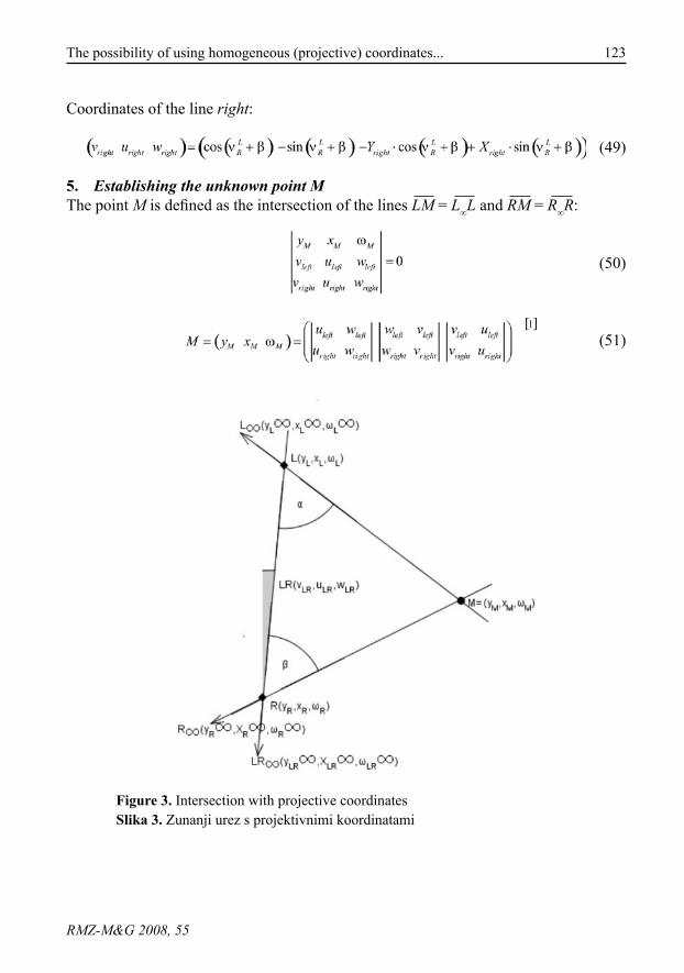
123The possibility of using homogeneous (projective) coordinates...
RMZ-M&G 2008, 55
Coordinates of the line right:
(49)
Establishing the unknown point M5. The point M is defined as the intersection of the lines LM = L∞L and RM = R∞R:
(50)
(51)
Figure 3. Intersection with projective coordinatesSlika 3. Zunanji urez s projektivnimi koordinatami
[ ]1
124 GAnić, A., vuLić, m, Runovc, f., HABe, T.
RMZ-M&G 2008, 55
conclusIons
In projective geometry, the lines have their own coordinates inasmuch as points do. A point is defined as an ordered set of three numbers (y x ω), which are not allowed to simultaneously take on the value of zero, seeing as the latter would make (λy λx λω) the same point for any given λ ≠ 0. We can obtain an infinite number of ordered sets of coordinates of a given point from the non-homogeneous coordinates of that same point, just as well as we can obtain only one ordered pair of numbers from homogeneous co-ordinates.
A line, much like a point, is an ordered set of three numbers, (v u w), which must not all equal zero at the same time, seeing as that would again make (μv μu μw) the same line for any given μ ≠ 0. The set (v u w) = (x1-x2 y1-y2 y1x2-y2x1) represents the coordinates of the line that are denoted using rectangular coordinates, whilst the set (v u w) = (- cos φ sin φ y1 cos φ - x1 sin φ) represents the coordinates of the line that is denoted using polar coordinates.
By using projective coordinates, the establishment of the intersection R(Y X) of two lines – the line l1, defined by the points A1(Y1 X1) and A2(Y2 X2), and the line l2, on which the points B1(Y1 X1) and B2(Y2 X2) lie – is very simple, and is defined using the help of nine second order determinants:
First, the coordinates of lines l1 and l2 are established, for which six of secondary-order determinants need to be calculated:
(52)
(53)
The intersection R, as the intersection of lines l1 and l2, is established with the calcula-tion of another three secondary-order determinants:
(54)
(55)
The projective plane, as has already been mentioned, originates from the Euclidean plane when we assume ideal points and an ideal line. Thus, the point with coordinates (y
125The possibility of using homogeneous (projective) coordinates...
RMZ-M&G 2008, 55
x ω) lies in the Euclidean plane if ω ≠ 0, and ω = 0 to render our point ideal.
Two different ideal points define the ideal line (0 0 1), on which all ideal points lie. The notation (sin φ cos φ 0) represents these coordinates of our ideal point, from which we can find the angle which a given line encloses in partnership with the positive side of the x-axis.
If the line l1 and the positive side of the first axis enclose the angle φ1, and both l1 and l2 enclose the angle α, then the ideal point of the line l2 can be determined as (sin(φ1+α) cos(φ1+α) 0), where φ2 = φ1+α is the angle of site of the line l2.
Via the introduction of ideal points and an ideal line, we are able to avoid the process of calculation of lengths and angles of site in 2D measurement exercises (the practical ex-ample here being the one depicted using intersections). The coordinates of an unknown point may always be established as the intersection of two lines, defined by the given and ideal points.
povzetek
Možnost uporabe homogenih (projektivnih) koordinat v dvodimenzionalnih mer-skih nalogah
V projektivni geometriji imajo poleg točk tudi premice koordinate.
Točka je definirana kot urejena trojka števil (y x ω), ki niso vse hkrati enake nič, s tem da je (λy λx λω) ista točka za katerikoli λ ≠ 0. Iz nehomogenih koordinat neke točke do-bimo neskončno urejenih trojk homogenih koordinat iste točke, iz homogenih koordinat neke točke pa lahko dobimo eno samo urejeno dvojico števil.
Premica je urejena trojka števil (v u w), ki niso vse hkrati enake nič, s tem da je (μv μu μw) ista premica za katerikoli μ ≠ 0. Trojka (v u w) = (x1-x2 y1-y2 y1 x2- y2 x1) predstavlja koordinate premice zapisane s pravokotnimi koordinatami, trojka (v u w) = (- cos φ sin φ y1 cos φ - x1 sin φ) pa koordinate premice zapisane s polarnimi koordinatami.
Z uporabo projektivnih koordinat je določitev presečišča R(Y X) dveh premic, premice l1, ki ju določata točki A1(Y1 X1) in A2(Y2 X2) ter premice l2 na kateri ležita točki B1(Y1 X1) in B2(Y2 X2) zelo enostavna, saj se presečišče določi s pomočjo devetih determinant drugega reda:
Najprej se določijo koordinate premic l1 in l2 za kar je potrebno rešiti šest determinant drugega reda:
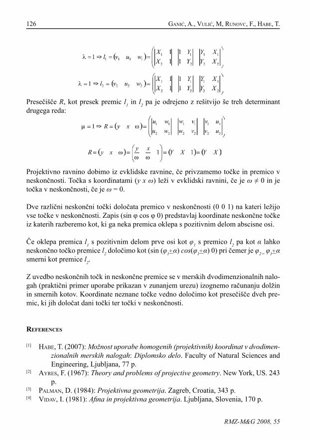
126 GAnić, A., vuLić, m, Runovc, f., HABe, T.
RMZ-M&G 2008, 55
Presečišče R, kot presek premic l1 in l2 pa je odrejeno z rešitvijo še treh determinant drugega reda:
Projektivno ravnino dobimo iz evklidske ravnine, če privzamemo točke in premico v neskončnosti. Točka s koordinatami (y x ω) leži v evklidski ravnini, če je ω ≠ 0 in je točka v neskončnosti, če je ω = 0.
Dve različni neskončni točki določata premico v neskončnosti (0 0 1) na kateri ležijo vse točke v neskončnosti. Zapis (sin φ cos φ 0) predstavlaj koordinate neskončne točke iz katerih razberemo kot, ki ga neka premica oklepa s pozitivnim delom abscisne osi.
Če oklepa premica l1 s pozitivnim delom prve osi kot φ1 s premico l2 pa kot α lahko neskončno točko premice l2 določimo kot (sin (φ1+α) cos(φ1+α) 0) pri čemer je φ2 = φ1+α smerni kot premice l2.
Z uvedbo neskončnih točk in neskončne premice se v merskih dvodimenzionalnih nalo-gah (praktični primer uporabe prikazan v zunanjem urezu) izognemo računanju dolžin in smernih kotov. Koordinate neznane točke vedno določimo kot presečišče dveh pre-mic, ki jih določat dani točki ter točki v neskončnosti.
references
[1] HABe, T. (2007): Možnost uporabe homogenih (projektivnih) koordinat v dvodimen-zionalnih merskih nalogah: Diplomsko delo. Faculty of Natural Sciences and Engineering, Ljubljana, 77 p.
[2] AYRes, f. (1967): Theory and problems of projective geometry. New York, US. 243 p.
[3] pALmAn, d. (1984): Projektivna geometrija. Zagreb, Croatia, 343 p.[4] vidAv, i. (1981): Afina in projektivna geometrija. Ljubljana, Slovenia, 170 p.
127RMZ – Materials and Geoenvironment, Vol. 55, No. 1, pp. 127-134, 2008
Scientific paper
How we calculate volume with the use of “NTF” method
Kako izračunamo volumen z uporabo metode “NTF”
Anes duRGuTović1, miLivoj vuLić2
1Oikos d.o.o., Jarška cesta 30, SI-1230 Ljubljana, Slovenia;E-mail: [email protected]
2University of Ljubljana, Faculty of Natural sciences and Engineering, Department of Geotechnology and Mining Engineering, Aškerčeva cesta 12,
SI-1000 Ljubljana, Slovenia; E-mail: [email protected]
Received: November 23, 2007 Accepted: January 4, 2008
Abstract: In the article titled Volume calculation with the use of “NTF” method and the “UDF” for calculation of volumes with the use of ”NTF” meth-od, mathematic plan of the mentioned principal method is presented and instructions for the use of “UDF” are also given. When it comes to the introduction into work with new computer programs the most effective ex-planation of the method of use is on the basis of a practical example. The purpose of this article is to represent the calculation of volumes with the use of “NTF” method with the use of “UDF” in the simple way on a practi-cal example.
Izvleček: V prispevkih z naslovoma Izračun volumnov z uporabo metode “NTF” ter “UDF”-ji za izračun volumnov po metodi “NTF”, je predstavljena ma-tematična zasnova osnove omenjene metode ter so podana navodila za uporabo “UDF”-jev. Pri uvajanju v delo z novimi računalniškimi programi se najbolje obnese razlaga načina uporabe na praktičnem primeru. Z na-menom, da vam izračun volumnov z metodo “NTF” čim bolj enostavno prikažemo, vam bomo v tem prispevku, na praktičnem primeru, prikazali postopek izračuna prostornine po metodi “NTF”, z uporabo “UDF”-jev.
Key words: volume calculation, Delauney triangulation, MS Excel, “UDF”Ključne besede: izračun volumnov, Delaunayeva triangulacija, MS Excel ,
“UDF”

128 duRGuTović, A., vuLić, m.
RMZ-M&G 2008, 55
IntroductIon
In order to carry out, calculation of the volume with the use “NTF” method, in the simple way. We have on the basis of the result which is shown in the above mentioned paragraph, prepared our own written functions of “UDF” which enable realization of the calculation of volume with the use of program MS Excel. When it comes to the introduction into work with new computer programs the most effective explanation of the method of use is on the basis of a practical example. The purpose of this article is to represent the calculation of volumes with the use of “NTF” method with the use of “UDF” in the simple way on a practical example.
For the representation of the calculation of volume with the use of “NTF” method we have, in the program »Rhinoceros 3D«, made 3D model of an imaginary geometri-cal shape which is formed by the selection of thirty points. Graphic representation of the model is represented in the picture be-low.
After we have carried out Delaney triangu-lation and got data about the edges of the triangles we can, therefore, calculate the volume of the shape which is formed, in our case, by the selected points.
The process of calculation can be divided into three points:
The calculation of the volume between •upper surface of the shape and the sur-face on the reference high (volume of the upper part of the shape),
Determination of the outline points •(only in the case if we do not have data about the points of the down surface) and the calculation of the volume be-tween down surface of the shape and the surface on the reference high (volume of the down part of the shape),The calculation of the final volume.•
how we carry out delaney trIangula-tIon
In order to carry out Delaney triangulation of the upper or rather down surface we use the computer program »Triangel Net«, which is available for free on the internet[6]. For the use of the mentioned program we need collective data of coordinate points in the text file with ending “.nod”.
When we have prepared the data in al-ready mentioned file “.nod” we can use the already mentioned computer program »Triangel Net«. With a simple series of commands the program automatically car-ries out the Delaunay triangulation. On the place where we have saved the file with ending “.nod” we get new file with ending “.tri”. In that file edge of Delaunay triangle are written.
With it we have carried out Delaunay trian-gulation of our collected points and got file with edge of Delaunay triangles. We trans-mit data from the mentioned file with end-ing “.tri” on the work sheet program tools Microsoft Excel where we have saved data of collective coordinated points.
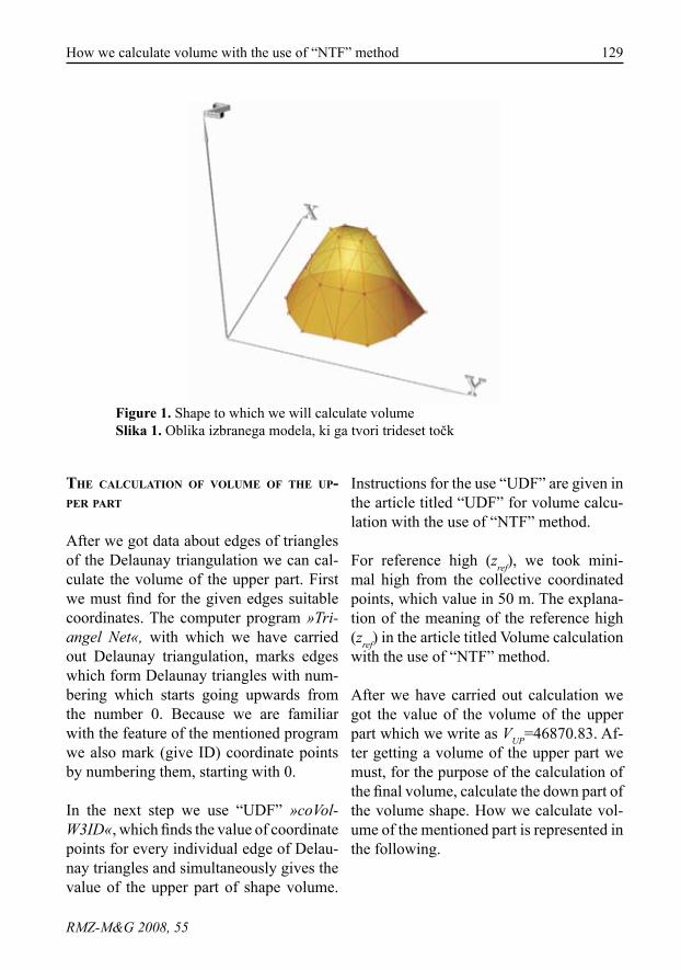
129How we calculate volume with the use of “NTF” method
RMZ-M&G 2008, 55
Figure 1. Shape to which we will calculate volumeSlika 1. Oblika izbranega modela, ki ga tvori trideset točk
the calculatIon of volume of the up-per part
After we got data about edges of triangles of the Delaunay triangulation we can cal-culate the volume of the upper part. First we must find for the given edges suitable coordinates. The computer program »Tri-angel Net«, with which we have carried out Delaunay triangulation, marks edges which form Delaunay triangles with num-bering which starts going upwards from the number 0. Because we are familiar with the feature of the mentioned program we also mark (give ID) coordinate points by numbering them, starting with 0.
In the next step we use “UDF” »coVol-W3ID«, which finds the value of coordinate points for every individual edge of Delau-nay triangles and simultaneously gives the value of the upper part of shape volume.
Instructions for the use “UDF” are given in the article titled “UDF” for volume calcu-lation with the use of “NTF” method.
For reference high (zref), we took mini-mal high from the collective coordinated points, which value in 50 m. The explana-tion of the meaning of the reference high (zref) in the article titled Volume calculation with the use of “NTF” method.
After we have carried out calculation we got the value of the volume of the upper part which we write as VUP=46870.83. Af-ter getting a volume of the upper part we must, for the purpose of the calculation of the final volume, calculate the down part of the volume shape. How we calculate vol-ume of the mentioned part is represented in the following.
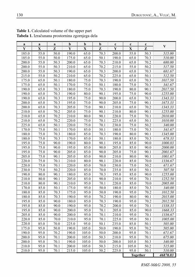
130 duRGuTović, A., vuLić, m.
RMZ-M&G 2008, 55
Table 1. Calculated volume of the upper partTabela 1. Izračunana prostornina zgornjega dela
a a a b b b c c c VY X Z Y X Z Y X Z185.0 55.0 50.0 190.0 65.0 70.3 200.0 55.0 50.3 515.00185.0 55.0 50.0 175.0 65.0 50.1 190.0 65.0 70.3 510.00200.0 55.0 50.3 200.0 65.0 70.3 210.0 65.0 70.2 680.00200.0 55.0 50.3 210.0 65.0 70.2 215.0 55.0 50.2 517.50200.0 55.0 50.3 190.0 65.0 70.3 200.0 65.0 70.3 681.67215.0 55.0 50.2 210.0 65.0 70.2 225.0 65.0 50.1 512.50175.0 65.0 50.1 180.0 75.0 70.3 190.0 65.0 70.3 1017.50175.0 65.0 50.1 170.0 75.0 50.1 180.0 75.0 70.3 341.67190.0 65.0 70.3 180.0 75.0 70.3 190.0 80.0 90.1 2017.50190.0 65.0 70.3 190.0 80.0 90.1 195.0 75.0 90.0 1255.00190.0 65.0 70.3 195.0 75.0 90.0 200.0 65.0 70.3 1343.33200.0 65.0 70.3 195.0 75.0 90.0 205.0 75.0 90.1 1673.33200.0 65.0 70.3 205.0 75.0 90.1 210.0 65.0 70.2 1343.33210.0 65.0 70.2 205.0 75.0 90.1 210.0 80.0 90.1 1255.00210.0 65.0 70.2 210.0 80.0 90.1 220.0 75.0 70.1 2010.00210.0 65.0 70.2 220.0 75.0 70.1 225.0 65.0 50.1 1010.00225.0 65.0 50.1 220.0 75.0 70.1 230.0 75.0 50.2 340.00170.0 75.0 50.1 170.0 85.0 50.1 180.0 75.0 70.3 341.67180.0 75.0 70.3 180.0 85.0 70.3 190.0 80.0 90.1 1345.00180.0 75.0 70.3 170.0 85.0 50.1 180.0 85.0 70.3 678.33195.0 75.0 90.0 190.0 80.0 90.1 195.0 85.0 90.0 1000.83195.0 75.0 90.0 195.0 85.0 90.0 205.0 85.0 90.0 2000.00195.0 75.0 90.0 205.0 85.0 90.0 205.0 75.0 90.1 2001.67205.0 75.0 90.1 205.0 85.0 90.0 210.0 80.0 90.1 1001.67220.0 75.0 70.1 210.0 80.0 90.1 220.0 85.0 70.0 1336.67220.0 75.0 70.1 220.0 85.0 70.0 230.0 75.0 50.2 671.67230.0 75.0 50.2 220.0 85.0 70.0 235.0 85.0 50.1 507.50190.0 80.0 90.1 180.0 85.0 70.3 195.0 85.0 90.0 1255.00210.0 80.0 90.1 205.0 85.0 90.0 210.0 95.0 70.1 1252.50210.0 80.0 90.1 210.0 95.0 70.1 220.0 85.0 70.0 2005.00170.0 85.0 50.1 175.0 95.0 50.0 180.0 85.0 70.3 340.00180.0 85.0 70.3 175.0 95.0 50.0 190.0 95.0 70.2 1012.50180.0 85.0 70.3 190.0 95.0 70.2 190.0 80.0 90.1 2015.00195.0 85.0 90.0 180.0 85.0 70.3 190.0 95.0 70.2 2012.50195.0 85.0 90.0 190.0 95.0 70.2 200.0 95.0 70.1 1338.33195.0 85.0 90.0 200.0 95.0 70.1 205.0 85.0 90.0 1668.33205.0 85.0 90.0 200.0 95.0 70.1 210.0 95.0 70.1 1336.67220.0 85.0 70.0 210.0 95.0 70.1 225.0 95.0 50.1 1005.00220.0 85.0 70.0 225.0 95.0 50.1 235.0 85.0 50.1 505.00175.0 95.0 50.0 190.0 105.0 50.0 190.0 95.0 70.2 505.00190.0 95.0 70.2 190.0 105.0 50.0 200.0 95.0 70.1 671.67200.0 95.0 70.1 200.0 105.0 50.3 210.0 95.0 70.1 675.00200.0 95.0 70.1 190.0 105.0 50.0 200.0 105.0 50.3 340.00210.0 95.0 70.1 200.0 105.0 50.3 215.0 105.0 50.2 515.00210.0 95.0 70.1 215.0 105.0 50.2 225.0 95.0 50.1 510.00
Together 46870.83
131How we calculate volume with the use of “NTF” method
RMZ-M&G 2008, 55
defInItIon of the outlIne poInts
When we do not have the definition of the down surface, we can only from the out-line points determine the surface which we use as down surface. As the first step of defining of the outline points of the down surface of the mentioned shape we have, among the given edges which form Delau-nay triangles, connected straight lines.
During that we eliminated straight lines which have appeared among the same edg-es twice. For the calculation of that men-tioned process we use “UDF” »linesSort-edW3«. The functions offers us, from the individual edges of triangle net, classifica-tion of lines between two edges and also mark the ones which occur only once. (See the article titled “UDF” for volume calcu-lation with the use of “NTF” method).
In the next step we use udf »outLineW«, which, from contour lines between two edges in triangle net, gives us only con-tour lines. (See the article titled “UDF” for volume calculation with the use of “NTF” method).
By doing this we must pay attention to the given selection of outpoints and checks the given selection by drawing them in some program for designing. In this way we will check whether we got the actual shape of the outline surface. Because of that the ex-ample, where it is necessary to eliminate the last three given outlines, is presented. The reason for that, is that represented way of determining of outpoints, can cause mistakes. In the already presented example there are 14 outpoints which we will use for the further calculation.
For the selection of outpoints of the down surface we use “UDF” »outPoints« which, from sorted contour lines between two edges in triangle net, gives us only con-tour point. (See the article titled UDF for volume calculation with the use of “NTF” method).
the calculatIon of volume of the down part
After we have determined the points of the down surface, we can start with calcula-tion of the volume between down surface of the shape and the surface on the refer-ence high (volume of the down part of the shape). Firstly, we must determine suitable coordinate values to the outline points of the down surface. For the selection of the suitable coordinate values we use “UDF” »coEntW« see the article titled “UDF” for volume calculation with the use of “NTF” method). Therefore, we get written coor-dinate values of the outpoints of the down surface.
After getting written coordinate values of the outpoints of the down surface, we again carry out the same steps which we have made at volume calculation of the up-per surface. At first, we prepared the data (coordinate values of the outpoints of the down surface) in the text file with ending ‘’.nod. Therefore, with the use of program (»Triangel Net«), carry out the Delaunay triangulation of down surface.
We carry out the calculation of the down surface volume in the same way as we cal-culated the upper surface volume. After we have carried out calculation which is pre-
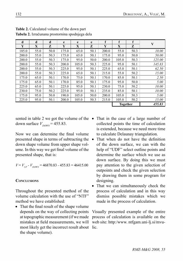
132 duRGuTović, A., vuLić, m.
RMZ-M&G 2008, 55
sented in table 2 we got the volume of the down surface VDOWN = 455.83.
Now we can determine the final volume presented shape in terms of subtracting the down shape volume from upper shape vol-ume. In this way we get final volume of the presented shape, that is:
V = VUP - VDOWN = 46870.83 - 455.83 = 46415.00
conclusIons
Throughout the presented method of the volume calculation with the use of “NTF” method we have established:
That the final result of the shape volume •depends on the way of collecting points at topographic measurement (if we made mistakes at field measurements, we will most likely get the incorrect result about the shape volume).
Table 2. Calculated volume of the down partTabela 2. Izračunana prostornina spodnjega dela
d d d e e e f f f VY X Z Y X Z Y X Z185.0 55.0 50.0 175.0 65.0 50.1 200.0 55.0 50.3 10.00200.0 55.0 50.3 175.0 65.0 50.1 175.0 95.0 50.0 50.00200.0 55.0 50.3 175.0 95.0 50.0 200.0 105.0 50.3 125.00200.0 55.0 50.3 200.0 105.0 50.3 225.0 95.0 50.1 145.83200.0 55.0 50.3 225.0 95.0 50.1 225.0 65.0 50.1 62.50200.0 55.0 50.3 225.0 65.0 50.1 215.0 55.0 50.2 15.00175.0 65.0 50.1 170.0 75.0 50.1 170.0 85.0 50.1 2.50175.0 65.0 50.1 170.0 85.0 50.1 175.0 95.0 50.0 5.00225.0 65.0 50.1 225.0 95.0 50.1 230.0 75.0 50.2 10.00230.0 75.0 50.2 225.0 95.0 50.1 235.0 85.0 50.1 10.00175.0 95.0 50.0 190.0 105.0 50.0 200.0 105.0 50.3 5.00225.0 95.0 50.1 200.0 105.0 50.3 215.0 105.0 50.2 15.00
Together 455.83
That in the case of a large number of •collected points the time of calculation is extended, because we need more time to calculate Delaunay triangulation.That when do not have the definition •of the down surface, we can with the help of “UDF” select outline points and determine the surface which we use as down surface. By doing this we must pay attention to the given selection of outpoints and check the given selection by drawing them in some program for designing.That we can simultaneously check the •process of calculation and in this way dismiss possible mistakes which we made in the process of calculation.
Visually presented example of the entire process of calculation is available on the web site: http:/www. ntfgam.uni-lj.si/mvu-lic.
133How we calculate volume with the use of “NTF” method
RMZ-M&G 2008, 55
povzetek
Kako izračunamo volumen z uporabo metode “NTF”
V prispevku je na praktičnem primeru prikazan postopek izračuna prostornine po metodi “NTF”, z uporabo “UDF”-jev. Prispevek je nadaljevanje člankov Calcu-lation of volume with the use of “NTF” method[9] and ''UDF” for volume calcu-lation with the use of “NTF” method[8]. Za prikaz postopka izračuna na praktič-nem primeru je bil predhodno oblikovan model telesa, ki ga tvori trideset izbranih točk. Model telesa smo oblikovali z upora-bo računalniškega programa »Rhinoceros 3D«. Delaunayevo triangulacijo iz točk iz-branega telesa izvedemo v računalniškem programu ''Triangel Net''. Na podlagi izve-dene triangulacije dobimo podatke o ogli-ščih, ki tvorijo Delaunayeve trikotnike. To nam je tudi osnova za izvedbo izračuna. Ko smo izvedli Delaunayevo triangulaci-jo ter dobili podatke o ogliščih trikotnikov izvedene triangulacije, lahko izračunamo prostornino telesa, ki ga tvorijo, v našem primeru izbrane točke. Sam postopek izra-čuna lahko razdelimo na tri dele:
določitev prostornine med plaščem in •referenčno ravnino,izbor konturnih točk ter določanje pro-•stornine med konturo in referenčno rav-nino,določitev končne prostornine.•
Postopek izračuna volumna po izvedeni Delaunayevi triangulaciji izvedemo z upo-rabo lastno zapisanih funkcij (MS Excel) “UDF”.
Vizualna predstavitev praktičnega primera izračuna oz. prikaz celotnega procesa je dostopen na: http:/www.ntfgam.uni-lj.si/mvulic.
references
[1] BRonšTejn, j.n., semendjAjev, k.A. (1978): Matematični priročnik. Tehniška založba Slovenije, Lju-bljana, 683 p.
[2] o`RouRke, j. (1997): Computational geometry in C. Cabbridge univer-ity press, 350 p.
[3] vuLić, m. (2005): User Defined Function. Naravoslovnotehniška fakulteta, Ljubljana.
[4] vuLić, m. (2005): Matematične osnove določanja prostornin tristranih prizem (interna predavanja). Naravoslovnotehniška fakulteta, Ljubljana.
[5] vuLić, m. (2005): Osnove Delaunay-eve triangulacije in Voronoi dia-gramov (interna predavanja). Naravoslovnotehniška fakulteta, Ljubljana.
[6] http://www.codeproject.com/cpp/ka-zumi.asp.
[7] duRGuTović, A. (2005): Izmera in določanje prostornin ne-pravilnih teles z uporabo metode “RTK-GPS”: diplomsko delo. Naravoslovnotehniška fakulteta, Ljubljana.
[8] vuLić, m., duRGuTović, A. (2007): “UDF” for volume calculation with the use of “NTF” method. RMZ - Materials and Geoenviron-ment; Vol. 54, No. 3, pp. 419-425.

134 duRGuTović, A., vuLić, m.
RMZ-M&G 2008, 55
[9] vuLić, m., duRGuTović, A. (2006): Calculation of volume with the use of “NTF” method. RMZ - Ma-terials and Geoenvironment; Vol. 53, No. 2, pp. 221-227.
[10] vuLić, m. (2005): Osnove to-pologije (interna predavanja). Naravoslovnotehniška fakulteta, Ljubljana.
[11] vuLić, m. (2005): Transformacije koordinatnih sistemov (interna pre-davanja). Naravoslovnotehniška fakulteta, Ljubljana.
135RMZ – Materials and Geoenvironment, Vol. 55, No. 1, pp. 135, 2008
Book Review
Strokovna literatura - Professional literature
Marko ZlokarnikPrenos merila
Izdajatelj: Ljubljana: Zavod za tehnično izobraževanje, 2007.
Obseg: 106 strani, format 24 x 17 cm, cena: 20 EUR.
ISBN: 978-961-6135-60-3.
V slovenščini je izšla knjiga Prenos merila svetovno znanega strokovnjaka za procesno tehnologijo prof. dr. Marka Zlokarnika, ki je deloval kot raziskovalec 35 let v kemijski multinacionalki Bayer A. G. v Leverkusnu z obširno bibliografijo in nato kot profe-sor na tehniški univerzi Köln. Njegovo strokovno delo je zadevalo laboratorijske meritve najrazličnejših postopkov, katerih rezultate je bilo treba nato prenesti v indus-trijsko, tehnično merilo. Tako si je pridobil neštevilne izkušnje, katerih pravilnost je bila vselej preizkušena in potrjena v indus-trijskem merilu. Knjiga je skrajšana izdaja originalnega dela, ki je izšlo pri renomirani založbi J. Wiley – VCH v ZDA v letih 2000 oz. 2002 v angleščini pod naslovom Scale-up in Chemical Engineering in v nemščini pod naslovom Scale-up – Modellübertra-gung in der Verfahrenstechnik. Knjigi sta bili po samo štirih letih razprodani in izšla je 2., za sto strani razširjena izdaja. Kdor se bo želel razgledati po tem področju podrob-neje, mu bosta ti knjigi v veliko oporo, kajti slovenska izdaja ima samo tretjino original-nega obsega. Leta 2007 so odkupili Kitajci licenco za knjigo in izšla je v veliki nakladi v kitajščini, kar priča o njeni veliki uporab-nosti v tehničnem svetu.
Pri prenosu merila iz majhnega v veliko (ali pa tudi obratno!) je zahtevana popol-na podobnost med modelom in tehnično izvedbo, in to v geometričnem, snovnem in procesno-tehničnem pogledu. Osnova metode je dimenzijska analiza, s katero se prenese relevantne veličine, s katerimi je proces popolnoma opisan, v brezdimenzi-jska števila. Teh je po eni strani manj, kot je dimenzijskih (t.i. pi-teorem), po drugi strani pa je predstava meritev v brezdimen-zijskem prostoru “invariantna” z ozirom na sleherno merilo, tako tudi z ozirom na dolžinsko merilo. Zato predstavlja ta meto-da edin zanesljiv prenos postopka iz malega v veliko.
Prva polovica knjige prinaša osnove di-menzijske analize in prenosa merila, druga polovica knjige pa prinaša praktične prim-ere. Knjiga izpolnjuje veliko vrzel: področje prenosa izdelkov in rezultatov meritev iz malih dimenzij na realne velike, s čemer se pečajo projektanti tovarniških naprav, ni bilo dovolj jasno obdelano na nobeni ravni od strokovnih do visokih šol, najbrž zato, ker predstavlja proizvodni tehnološki vidik, za katerega teoretiki nimajo posluha, so pa osnovne naloge procesnega inženiringa. Problem prenosljivosti eksperimentalnih rezultatov na realne velikosti zavzema os-rednje mesto v procesnem projektiranju. Težavnost problema je nazornejša, ker se tekom procesa dogajajo pomembne spre-membe lastnosti snovi. Ker je procesno področje zelo blizu tudi našim metalurgom, jim bo ta knjiga dobro služila.
Dr. Marko Kos
136 Author’s Index
RMZ-M&G 2008, 55
Author`s Index, Vol. 55, No. 1
Anžel Ivan [email protected] 1
Bombač David [email protected] 19
Bradaskja Boštjan [email protected] 31
Čevnik Gabrijela [email protected] 1
Dimc Franc [email protected] 85
Durgutović Anes [email protected] 127
Fazarinc Matevž [email protected] 19, 31
Ganić Aleksandar [email protected] 111
Gosar Andrej [email protected] 41, 67
Habe Tina [email protected] 111
Knap Matjaž [email protected] 31
Koruza Jurij [email protected] 31
Kosec Gorazd [email protected] 1
Kosec Borut [email protected] 1
Kosec Ladislav [email protected] 1
Kugler Goran [email protected] 19
Mušič Branko [email protected] 85
Osredkar Radko [email protected] 85
Rošer Janez [email protected] 41, 67
Rudolf Rebeka [email protected] 1
Runovc Franc [email protected] 111
Stopar Robert [email protected] 41, 67
Turk Radomir [email protected] 19, 31
Vulić Milivoj [email protected] 111, 127
Zupanič Franc [email protected] 7
137Instructions to authors
RMZ-M&G 2008, 55
INSTRUCTIONS TO AUTHORS
RMZ-MATERIALS & GEOENVIRONMENT (RMZ- Materiali in geookolje) is a periodical publication with four issues per year (established 1952 and renamed to RMZ-M&G in 1998). The main topics of contents are Mining and Geotechnology, Metallurgy and Materials, Geology and Geoenvironment.RMZ-M&G publishes original Scientific articles, Review papers, Technical and Expert contributions (also as short papers or letters) in English. In addition, evaluations of other publications (books, monographs,...), short letters and comments are welcome. A short summary of the contents in Slovene will be included at the end of each paper. It can be included by the author(s) or will be provided by the referee or the Editorial Office. * Additional information and remarks for Slovenian authors:English version with extended »Povzetek«, and additional roles (in Template for Slovenian authors) can be written. Only exceptionally the articles in the Slovenian language with summary in English will be published. The contribu tions in English will be considered with priority over those in the Slovenian language in the review process.
Authorship and originality of the contributions. Authors are responsible for originality of presented data, ideas and conclusions as well as for correct citation of data adopted from other sources. The publication in RMZ-M&G obligate authors that the article will not be published anywhere else in the same form.
Specification of Contributions
Optimal number of pages of full papers is 7 to 15, longer articles should be discussed with Editor, but 20 pages is limit.Scientific papers represent unpublished results of original research.Review papers summarize previously published scientific, research and/or expertise articles on the new scientific level and can contain also other cited sources, which are not mainly result of author(s).Technical and Expert papers are the result of technological research achievements, application research results and information about achievements in practice and industry.Short papers (Letters) are the contributions that contain mostly very new short reports of advanced investigation. They should be approximately 2 pages long but should not exceed 4 pages.Evaluations or critics contain author's opinion on new published books, monographs,
138 Instructions to authors
RMZ-M&G 2008, 55
textbooks, exhibitions...(up to 2 pages, figure of cover page is expected).In memoriam (up to 2 pages, a photo is expected).Professional remarks (Comments) cannot exceed 1 page, and only professional disagreements can be discussed. Normally the source author(s) reply the remarks in the same issue.
Supervision and review of manuscripts. All manuscripts will be supervised. The referees evaluate manuscripts and can ask authors to change particular segments, and propose to the Editor the acceptability of submitted articles. Authors can suggest the referee but Editor has a right to choose another. The name of the referee remains anonymous. The technical corrections will be done too and authors can be asked to correct missing items. The final decision whether the manuscript will be published is made by the Editor in Chief.
The Form of the Manuscript
The manuscript should be submitted as a complete hard copy including figures and tables. The figures should also be enclosed separately, both charts and photos in the original version. In addition, all material should also be provided in electronic form on a diskette or a CD. The necessary information can conveniently also be delivered by E-mail.
Composition of manuscript is defined in the attached Template
The original file of Template is temporarily available on E-mail addresses:[email protected], [email protected]
References - can be arranged in two ways:- first possibility: alphabetic arrangement of first authors - in text: (Borgne, 1955),or- second possibility: [1] numerated in the same order as cited in the text: example[1]
Format of papers in journals:Le Borgne, E. (1955): Susceptibilite magnetic anomale du sol superficiel. Annales de Geophysique, 11, pp. 399-419.
Format of books:Roberts, J. L. (1989): Geological structures, MacMillan, London, 250 p.

139Instructions to authors
RMZ-M&G 2008, 55
Text on the hard print copy can be prepared with any text-processor. The electronic version on the diskette, CD or E-mail transfer should be in MS Word or ASCII format.Captions of figures and tables should be enclosed separately. Figures (graphs and photos) and tables should be original and sent separately in addition to text. They can be prepared on paper or computer designed (MSExcel, Corel, Acad).Format. Electronic figures are recommended to be in CDR, Al, EPS, TIF or JPG formats. Resolution of bitmap graphics (TIF, JPG) should be at least 300 dpi. Text in vector graphics (CDR, Al, EPS) must be in MSWord Times typography or converted in curves.Color prints. Authors will be charged for color prints of figures and photos.Labeling of the additionally provided material for the manuscript should be very clear and must contain at least the lead author's name, address, the beginning of the title and the date of delivery of the manuscript. In case of an E-mail transfer the exact message with above asked data must accompany the attachment with the file containing the manuscript.Information about RMZ-M&G:Editor in Chief prof. dr. Peter Fajfar (tel. ++386 1 4250-316) orSecretary Barbara Bohar Bobnar, un. dipl. ing. geol. (++386 1 4704-630),Aškerčeva 12, Ljubljana, Slovenia
or at E-mail addresses:[email protected], [email protected]
Sending of manuscripts. Manuscripts can be sent by mail to the Editorial Office address:
RMZ-Materials & Geoenvironment• Aškerčeva 12, 1000 Ljubljana, Slovenia or delivered to:
Reception• of the Faculty of Natural Science and Engineering (for RMZ-M&G) Aškerčeva 12, 1000 Ljubljana, Slovenia
E-mail - addresses of Editor and Secretary•You can also contact them on their phone numbers.•
140 Template
RMZ-M&G 2008, 55
TEMPLATE
The title of the manuscript should be written in bold letters(Times New Roman, 14, Center)
nAme suRnAme1, …. , & nAme suRnAmeX (Times neW RomAn, 12, cenTeR)
xFaculty of ... , University of ... , Address…, Country, e-mail: ... (Times New Roman, 11, Center)
THE LENGTH OF FULL PAPER SHOULD NOT EXCEED TWENTY (20, INCLUDING FIGURES AND TABLES) PAGES (OPTIMAL 7 TO 15), SHORT PAPER FOUR (4) AND OTHER TWO (2) WITHOUT TEXT FLOWING BY GRAPHICS AND TABLES.
Abstract (Times New Roman, Normal, 11): The text of the abstract is placed here. The abstract should be concise and should present the aim of the work, essential results and conclusion. It should be typed in font size 11, single-spaced. Except for the first line, the text should be indented from the left margin by 10 mm. The length should not exceed fifteen (15) lines (10 are recommended).
Key words: a list of up to 5 key words (3 to 5) that will be useful for indexing or searching. Use the same styling as for abstract.
IntroductIon (tImes new roman, bold, 12)
Two lines below the keywords begin the introduction. Use Times New Roman, font size 12, Justify alignment. There are two (2) admissible methods of citing references in text:
by stating the first author and the year of publication of the reference 1. in the parenthesis at the appropriate place in the text and arranging the reference list in the alphabetic order of first authors; e.g.:
“Detailed information about geohistorical development of this zone can be found in: Antonijević (1957), Grubić (1962), ...”“… the method was described previously (Hoefs, 1996)”

141Template
RMZ-M&G 2008, 55
by consecutive Arabic numerals in square brackets, superscripted at the 2. appropriate place in the text and arranging the reference list at the end of the text in the like manner; e.g.:
“... while the portal was made in Zope[3] environment.”
materIals and methods (tImes new roman, bold, 12)
This section describes the available data and procedure of work and therefore provides enough information to allow the interpretation of the results, obtained by the used methods.
results and dIscussIon (tImes new roman, bold, 12)
Tables, figures, pictures, and schemes should be incorporated in the text at the appropriate place and should fit on one page. Break larger schemes and tables into smaller parts to prevent extending over more than one page.
conclusIons (tImes new roman, bold, 12)
This paragraph summarizes the results and draws conclusions.
Acknowledgements (Times New Roman, Bold, 12, Center - optional)
This work was supported by the ****.
references (tImes new roman, bold, 12)
In regard to the method used in the text, the styling, punctuation and capitalization should conform to the following:
FIRST OPTION - in alphabetical orderCasati, P., Jadoul, F., Nicora, A., Marinelli, M., Fantini-Sestini, N. & Fois, E.
(1981): Geologia della Valle del’Anisici e dei gruppi M. Popera - Tre

142 Template
RMZ-M&G 2008, 55
Cime di Lavaredo (Dolomiti Orientali). Riv. Ital. Paleont.; Vol. 87, No. 3, pp. 391-400, Milano.
Folk, R. L. (1959): Practical petrographic classification of limestones. Amer. Ass. Petrol. Geol. Bull.; Vol. 43, No. 1, pp. 1-38, Tulsa.
SECOND OPTION - in numerical order[1] Trček, B. (2001): Solute transport monitoring in the unsaturated zone of the
karst aquifer by natural tracers. Ph.D. Thesis. Ljubljana: University of Ljubljana 2001; 125 p.
[2] Higashitani, K., Iseri, H., Okuhara, K., Hatade, s. (1995): Magnetic Effects on Zeta Potential and Diffusivity of Nonmagnetic Particles. Journal of Colloid and Interface Science 172, pp. 383-388.
Citing the Internet site:CASREACT-Chemical reactions database [online]. Chemical Abstracts Service, 2000, updated 2.2.2000 [cited 3.2.2000]. Accessible on Internet: http://www.cas.org/CASFILES/casreact.html.
povzetek (tImes new roman, 12)A short summary of the contents in Slovene (up to 400 characters) can be written by the author(s) or will be provided by the referee or by the Editorial Board.
143Template
RMZ-M&G 2008, 55
TEMPLATE for Slovenian Authors
The title of the manuscript should be written in bold letters(Times New Roman, 14, Center)
Naslov članka (Times New Roman, 14, Center)
nAme suRnAme1,…. , & nAme suRnAmeX (Times neW RomAn, 12, cenTeR)ime pRiimek1, …, ime pRiimekX (Times neW RomAn, 12, cenTeR)
xFaculty of ... , University of ... , Address…, Country; e-mail: ... (Times New Roman, 11, Center)
XFakulteta…, Univerza…, Naslov…, Država; e-mail: … (Times New Roman, 11, Center)
THE LENGTH OF ORIGINAL SCIENTIFIC PAPER SHOULD NOT EXCEED TWENTY (20, INCLUDING FIGURES AND TABLES) PAGES (OPTIMAL 7 TO 15), SHORT PAPER FOUR (4) AND OTHER TWO (2) WITHOUT TEXT FLOWING BY GRAPHICS AND TABLES.DOLŽINA IZVIRNEGA ZNANSTVENEGA ČLANKA NE SME PRESEGATI DVAJSET (20, VKLJUČNO S SLIKAMI IN TABELAMI), KRATKEGA ČLANKA ŠTIRI (4) IN OSTALIH PRISPEVKOV DVE (2) STRANI.
Abstract (Times New Roman, Normal, 11): The text of the abstract is placed here. The abstract should be concise and should present the aim of the work, essential results and conclusion. It should be typed in font size 11, single-spaced. Except for the first line, the text should be indented from the left margin by 10 mm. The length should not exceed fifteen (15) lines (10 are recommended).
Izvleček (TNR, N, 11): Kratek izvleček namena članka ter ključnih rezultatov in ugotovitev. Razen prve vrstice naj bo tekst zamaknjen z levega roba za 10 mm. Dolžina naj ne presega petnajst (15) vrstic (10 je priporočeno).
Key words: a list of up to 5 key words (3 to 5) that will be useful for indexing or searching. Use the same styling as for abstract.
Ključne besede: seznam največ 5 ključnih besed (3-5) za pomoč pri indeksiranju ali iskanju. Uporabite enako obliko kot za izvleček.

144 Template
RMZ-M&G 2008, 55
IntroductIon – uvod (tImes new roman, bold, 12)
Two lines below the keywords begin the introduction. Use Times New Roman, font size 12, Justify alignment. All captions of text and tables as well as the text in graphics must be prepared in English and Slovenian language.Dve vrstici pod ključnimi besedami se začne Uvod. Uporabite pisavo TNR, velikost črk 12, z obojestransko poravnavo. Naslovi slik in tabel (vključno z besedilom v slikah) morajo biti pripravljeni v slovenskem in angleškem jeziku.
Figure (Table) X. Text belonging to figure (table)Slika (Tabela) X. Pripadajoče besedilo k sliki (tabeli)
There are two (2) admissible methods of citing references – obstajata dve sprejemljivi metodi navajanja referenc:
by stating the first author and the year of publication of the reference 1. in the parenthesis at the appropriate place in the text and arranging the reference list in the alphabetic order of first authors; e.g.:
1. z navedbo prvega avtorja in letnice objave reference v oklepaju na ustreznem mestu v tekstu in z ureditvijo seznama referenc po abecednem zaporedju prvih avtorjev; npr.:
“Detailed information about geohistorical development of this zone can be found in: Antonijević (1957), Grubić (1962), ...”
“… the method was described previously (Hoefs, 1996)”
or/ali
by consecutive Arabic numerals in square brackets, superscripted at the 2. appropriate place in the text and arranging the reference list at the end of the text in the like manner; e.g.:
2. z zaporednimi arabskimi številkami v oglatih oklepajih na ustreznem mestu v tekstu in z ureditvijo seznama referenc v številčnem zaporedju navajanja; npr.;“... while the portal was made in Zope[3] environment.”
145Template
RMZ-M&G 2008, 55
materIals and methods (tImes new roman, bold, 12)
This section describes the available data and procedure of work and therefore provides enough information to allow the interpretation of the results, obtained by the used methods.Ta del opisuje razpoložljive podatke, metode in način dela ter omogoča zadostno količino informacij, da lahko z opisanimi metodami delo ponovimo.
results and dIscussIon – rezultatI In razprava (tImes new roman, bold, 12)
Tables, figures, pictures, and schemes should be incorporated (inserted, not pasted) in the text at the appropriate place and should fit on one page. Break larger schemes and tables into smaller parts to prevent extending over more than one page. Tabele, sheme in slike je potrebno vnesti (z ukazom Insert, ne Paste) v tekst na ustreznem mestu. Večje sheme in tabele je potrebno ločiti na manjše dele, da ne presegajo ene strani.
conclusIons – sklepI (tImes new roman, bold, 12)
This paragraph summarizes the results and draws conclusions.Povzetek rezultatov in zaključki.
Acknowledgements – Zahvale (Times New Roman, Bold, 12, Center - optional)
This work was supported by the ………..Izvedbo tega dela je omogočilo ………
references - vIrI (tImes new roman, bold, 12)
With regard to the method used in the text, the styling, punctuation and capitalization should conform to the following:

146 Template
RMZ-M&G 2008, 55
Glede na uporabljeno metodo citiranja referenc v tekstu upoštevajte eno od naslednjih oblik:
FIRST OPTION (recommended) – PRVA MOŽNOST (priporočena) – in alphabetical order (v abecednem zaporedju)Casati, P., Jadoul, F., Nicora, A., Marinelli, M., Fantini-Sestini, N. & Fois, E.
(1981): Geologia della Valle del’Anisici e dei gruppi M. Popera – Tre Cime di Lavaredo (Dolomiti Orientali). Riv. Ital. Paleont.; Vol. 87, No. 3, pp. 391-400, Milano.
Folk, R. L. (1959): Practical petrographic classification of limestones. Amer. Ass. Petrol. Geol. Bull.; Vol. 43, No. 1, pp. 1-38, Tulsa.
SECOND OPTION – DRUGA MOŽNOST - in numerical order (v numeričnem zaporedju)[1] Trček, B. (2001): Solute transport monitoring in the unsaturated zone of the
karst aquifer by natural tracers. Ph.D. Thesis. Ljubljana: University of Ljubljana 2001; 125 p.
[2] Higashitani, K., Iseri, H., Okuhara, K., Hatade, s. (1995): Magnetic Effects on Zeta Potential and Diffusivity of Nonmagnetic Particles. Journal of Colloid and Interface Science 172, pp. 383-388.
Citing the Internet site:CASREACT-Chemical reactions database [online]. Chemical Abstracts Service, 2000, updated 2.2.2000 [cited 3.2.2000]. Accessible on Internet: http://www.cas.org/CASFILES/casreact.html.
Citiranje Internetne strani:CASREACT-Chemical reactions database [online]. Chemical Abstracts Service, 2000, obnovljeno 2.2.2000 [citirano 3.2.2000]. Dostopno na svetovnem spletu: http://www.cas.org/CASFILES/casreact.html.
povzetek – summary (tImes new roman, 12)
An extended summary of the contents in Slovene (from one page to approximately1 3 of the original article length).Razširjeni povzetek vsebine prispevka v Angleščini (od ene strani do približno 1 3 dolžine izvirnega članka).