Performance Optimization and Measurement - Essbase… · Performance Optimization and Measurement:...
89
Performance Optimization and Measurement: New Thoughts and Test Results for BSO and ASO Dan Pressman [email protected] Jun 25, 2013 New Orleans, LA
Transcript of Performance Optimization and Measurement - Essbase… · Performance Optimization and Measurement:...

Performance Optimization and Measurement:
New Thoughts and Test Results for BSO and ASO
Dan Pressman [email protected]
Jun 25, 2013
New Orleans, LA

Warning – Danger!
The Information and Techniques in this
Presentation will Soon Be
So sayeth Gabby Rubin
so sayeth Kumar Ramaiyer
Warning – Danger!
But they won’t sayeth WHEN †
We all look forward to that day!
But in the meantime …
† As governed by Oracle NDA and advance disclosure requirements and other legally necessary equivocations

This Presentation Is Based on:
Data from over 1,300 test runs
● Over 1,900 hrs of testing
● Tests run on three machines:
● 12 CPU 128gB RAM,1.5 tB SSD (John Booth “Zeus”)
● 40/80 CPU 1 tB RAM Exalytics (Rittman-Mead “Asgard”)
● 4 CPU 32gB Ram (My Laptop “The Beast”)
Major Thank You’s To:
● Robin Moffatt and Mark Rittman
● John Booth

This Presentation Includes:
Conclusions drawn from the tests
Discussion of underlying causes
Actionable recommendations
A few surprising (?) results
At least one modification to a long-standing
Standard Practice
What’s Not Included, or Is Assumed
How to build, load or calculate cubes
“Standard” performance best practices:
● Hour Glass
● BSO Dense/Sparse or Stored/Dynamic calc criteria
● ASO Stored or Dynamic hierarchies
● (You’ve heard these before)
Basic hardware knowledge
● You know enough to ask the Infrastructure team
for what you need

A description of the tests
A word about disk speed
More words about memory management
Data load tests Data calculation tests
and
A few ASO-specific performance issues
Agenda
ASO and BSO with varying:
● Cache Sizes: BSO – five; ASO – four
● Data Input
● File Count: One-part-serial or five-in-parallel
● Prepare Threads: Nine for each file count
● Calc Parallel: Four (1, 4, 8, 12) + three (30, 40, 125)
● Three file formats
● DLSTHREADPREPARE & DLSTHREADWRITE
● 1, 2, 3, 4, 5, 6, 7, 10, 15, 20, 25, 30, 35
● Sort Order: One primarily, 11 others for BSO tests
● Disk Drive Types: SSD and Physical
The Tests
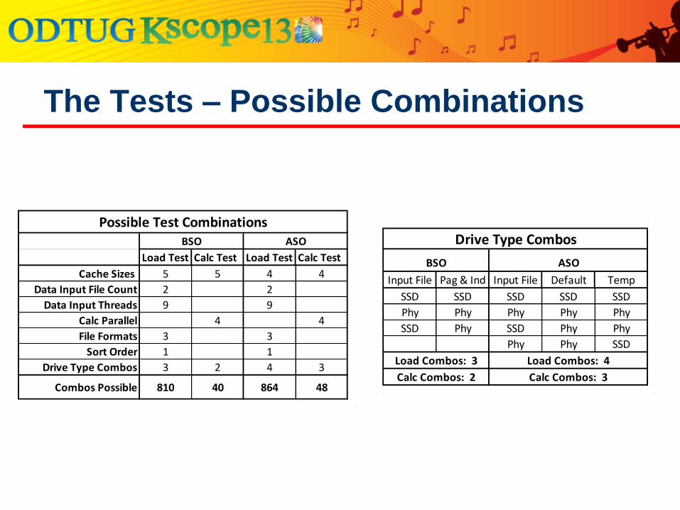
The Tests – Possible Combinations
Load Test Calc Test Load Test Calc Test
Cache Sizes 5 5 4 4
Data Input File Count 2 2
Data Input Threads 9 9
Calc Parallel 4 4
File Formats 3 3
Sort Order 1 1
Drive Type Combos 3 2 4 3
Combos Possible 810 40 864 48
Possible Test CombinationsBSO ASO
Input File Pag & Ind Input File Default Temp
SSD SSD SSD SSD SSD
Phy Phy Phy Phy Phy
SSD Phy SSD Phy Phy
Phy Phy SSD
Load Combos: 3 Load Combos: 4
Calc Combos: 2 Calc Combos: 3
Drive Type Combos
BSO ASO
All test results will be available online soon
● Spreadsheet
● Graphs
Contact me if you’d like to run comparable
benchmarks
The Tests
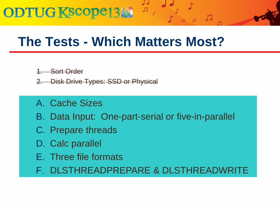
1. Sort Order
2. Disk Drive Types: SSD or Physical
The Tests - Which Matters Most?
A. Cache Sizes
B. Data Input: One-part-serial or five-in-parallel
C. Prepare threads
D. Calc parallel
E. Three file formats
F. DLSTHREADPREPARE & DLSTHREADWRITE

Cube size before Calc All: 9 gB
Cube size after Calc All: 175 gB
Data input file:
● 12 gB in standard format
● 76 million rows
The Tests - Cube and Data Size - BSO
Loaded
Data Only
After
Calculation
Outline File 14 mB na
Ind File 25 mB 393 mB
Pag Files 9.11 gB 175.10 gB
Blocks 500,000 7,832,000
Cells 907 mm 14,776 mm
Density 5.0% 5.2%
Cube Size

The Tests - Cube and Data Size - ASO
Cube Size:
● 4 billion cells
● 54 gB (before aggregations)
Data input file:
● 274 gB
● 1.3 billion rows
● (standard format)
Loaded
Data OnlyAgg Cells
Outline File 681 Mb na
Dat File 54 Gb 121 Mb
Cells 4 bn 12mm
"Blocks" 1.3 bn
Size on Disk 54.0 Gb
Cube Size
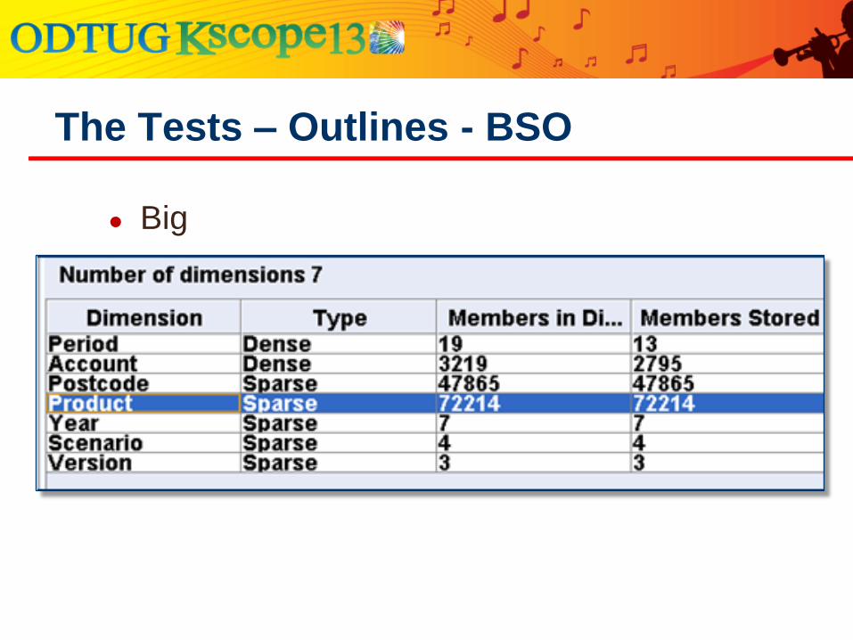
The Tests – Outlines - BSO
● Big
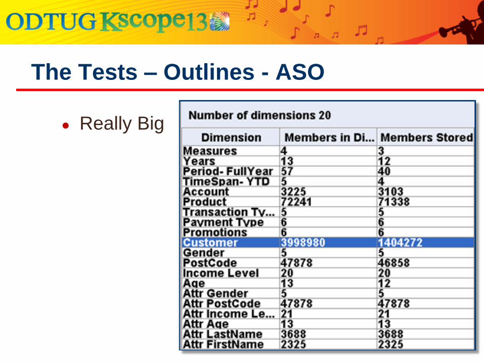
The Tests – Outlines - ASO
● Really Big
“You can never be too rich or too thin.”
Wallis Simpson
Disk Speed, CPU Speed and Ram
Both Unix and Windows cache files in memory
Separate (and somewhat redundant) vs.
familiar Data and Index caches
During data load, both input file and output pag,
ind or dat files are cached
Called memory mapped IO
Seen in Windows Resource Manager or on
UNIX in top or nmon:
Memory Management
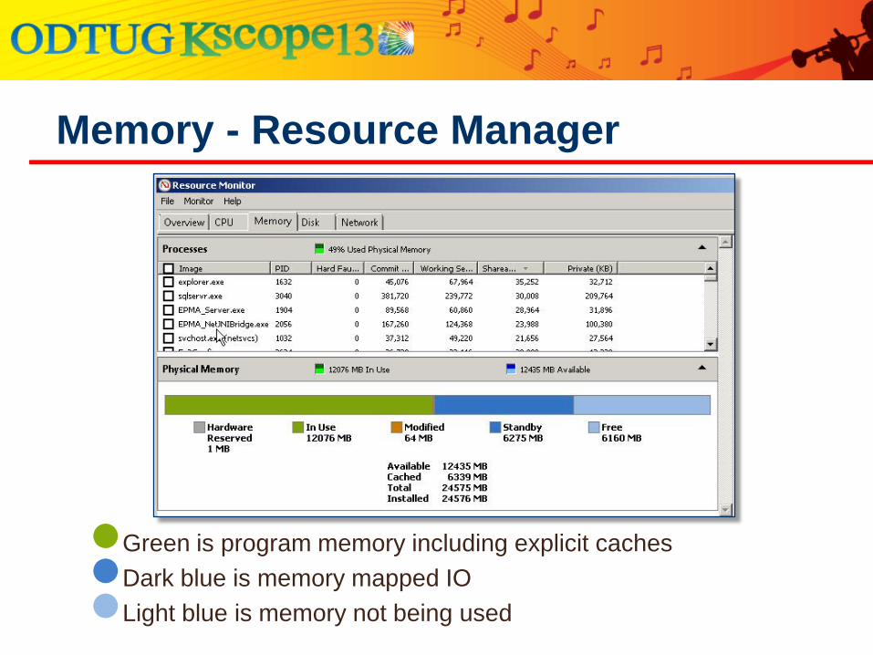
Memory - Resource Manager
Green is program memory including explicit caches
Dark blue is memory mapped IO
Light blue is memory not being used
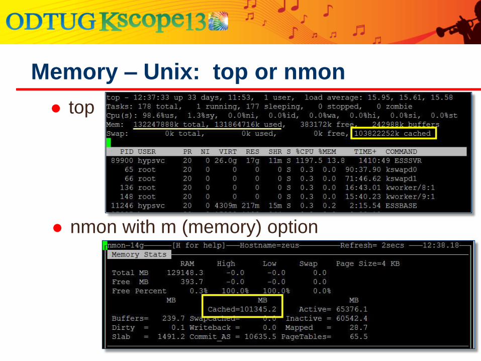
top
Memory – Unix: top or nmon
nmon with m (memory) option
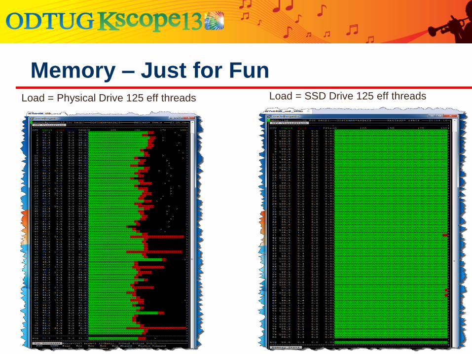
Memory – Just for Fun Load = Physical Drive 125 eff threads
Load = SSD Drive 125 eff threads
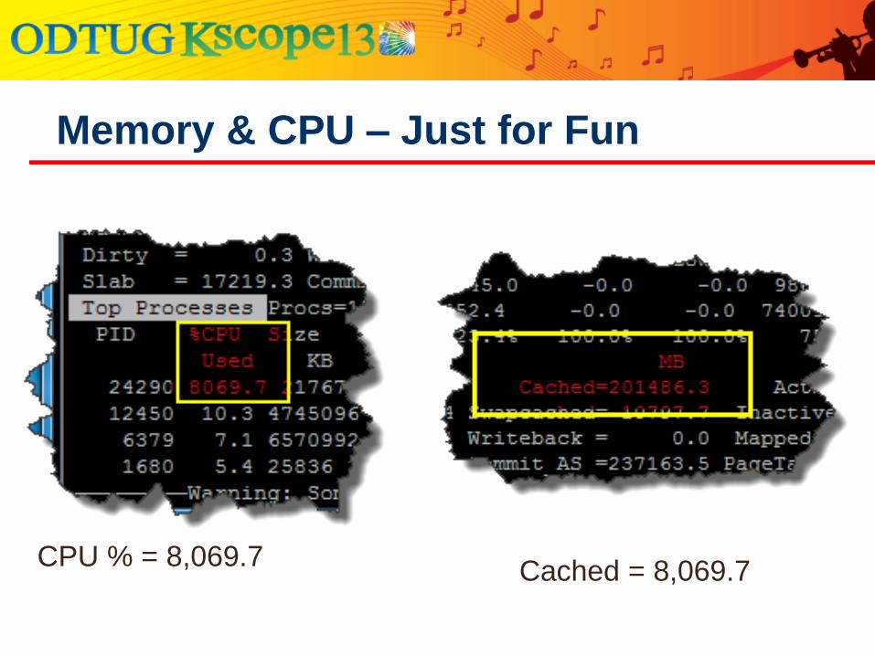
Memory & CPU – Just for Fun
CPU % = 8,069.7 Cached = 8,069.7
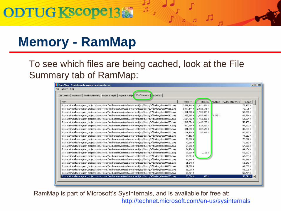
To see which files are being cached, look at the File
Summary tab of RamMap:
Memory - RamMap
RamMap is part of Microsoft’s SysInternals, and is available for free at:
http://technet.microsoft.com/en-us/sysinternals
… take longer to run sometimes?
Very often, it’s memory-mapped IO
● A copied input file may still be in RAM
● After a calc/query, the dat/pag file is still in RAM
Can be seen in Resource Manager and RamMap
when a file is unzipped and loaded into a cube:
Why Does My Query/Load/Calc…

After Unzip and before load:
Memory – BSO – Unzip and Load
Both zipped and unzipped files remain in
memory
● Unzipped not needed, but remains in memory
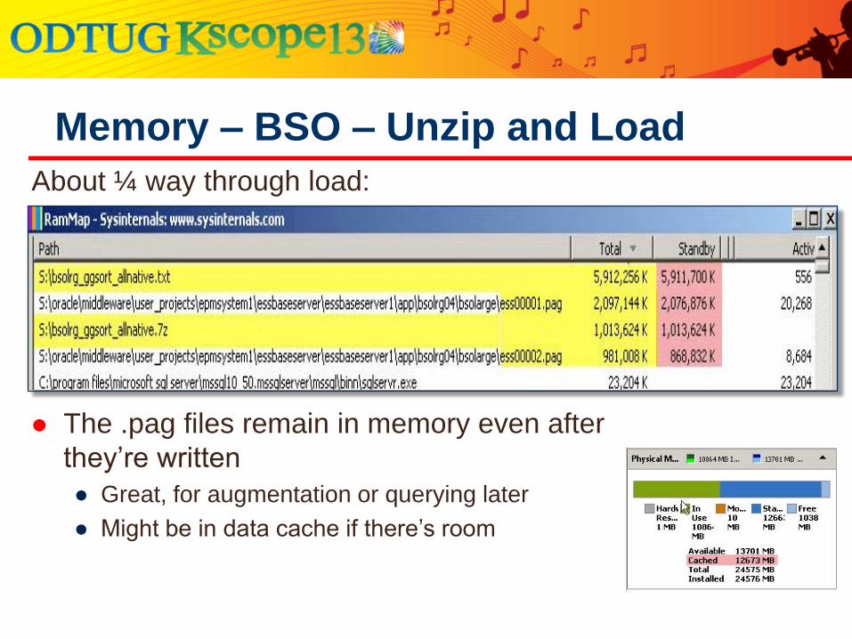
About ¼ way through load:
Memory – BSO – Unzip and Load
The .pag files remain in memory even after
they’re written
● Great, for augmentation or querying later
● Might be in data cache if there’s room
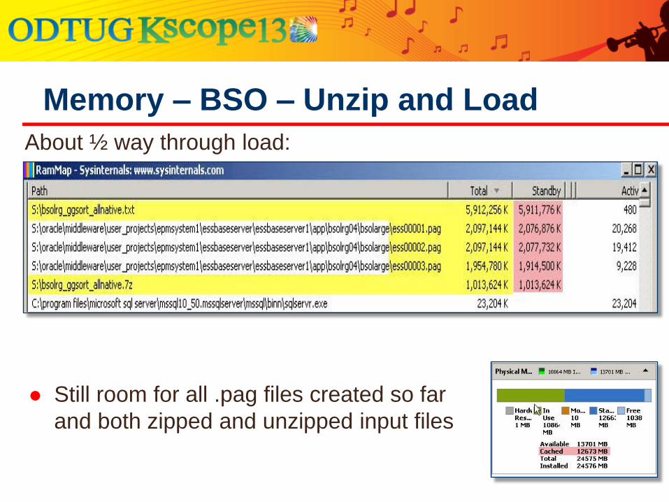
About ½ way through load:
Memory – BSO – Unzip and Load
Still room for all .pag files created so far
and both zipped and unzipped input files
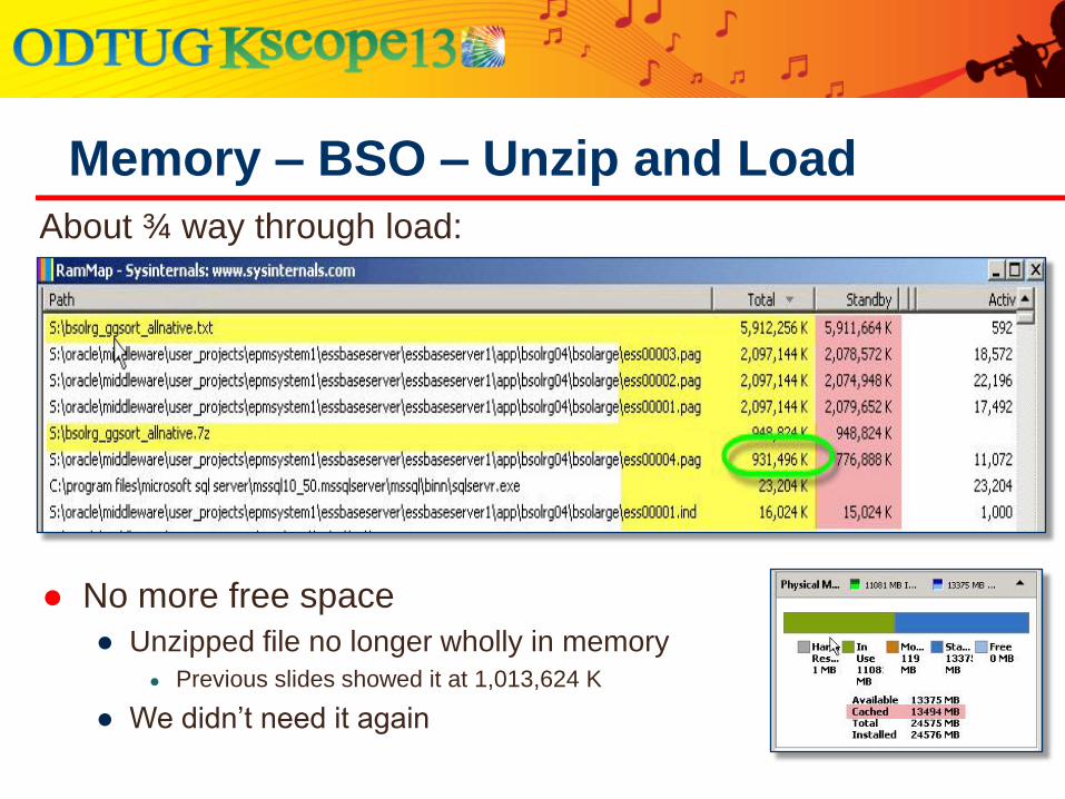
About ¾ way through load:
Memory – BSO – Unzip and Load
No more free space
● Unzipped file no longer wholly in memory
● Previous slides showed it at 1,013,624 K
● We didn’t need it again
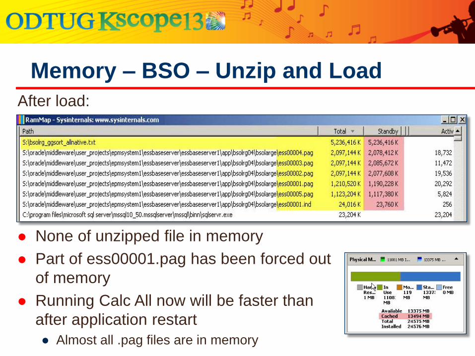
After load:
Memory – BSO – Unzip and Load
None of unzipped file in memory
Part of ess00001.pag has been forced out
of memory
Running Calc All now will be faster than
after application restart
● Almost all .pag files are in memory
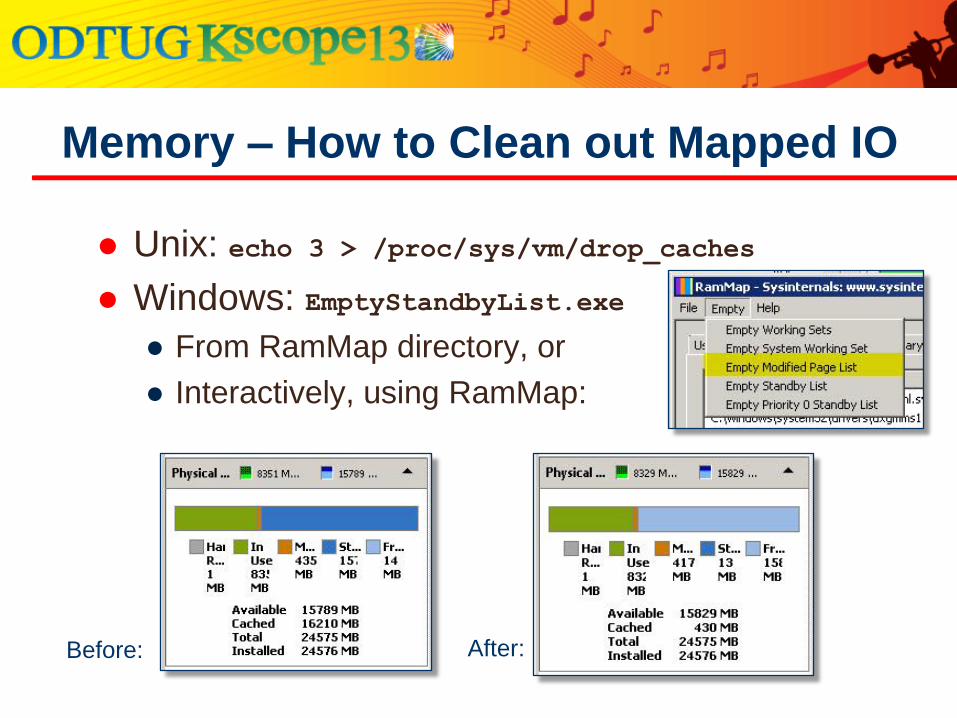
Unix: echo 3 > /proc/sys/vm/drop_caches
Windows: EmptyStandbyList.exe
● From RamMap directory, or
● Interactively, using RamMap:
Memory – How to Clean out Mapped IO
Before: After:
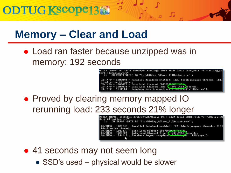
Load ran faster because unzipped was in
memory: 192 seconds
Memory – Clear and Load
Proved by clearing memory mapped IO
rerunning load: 233 seconds 21% longer
41 seconds may not seem long
● SSD’s used – physical would be slower
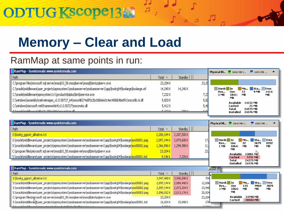
RamMap at same points in run:
Memory – Clear and Load
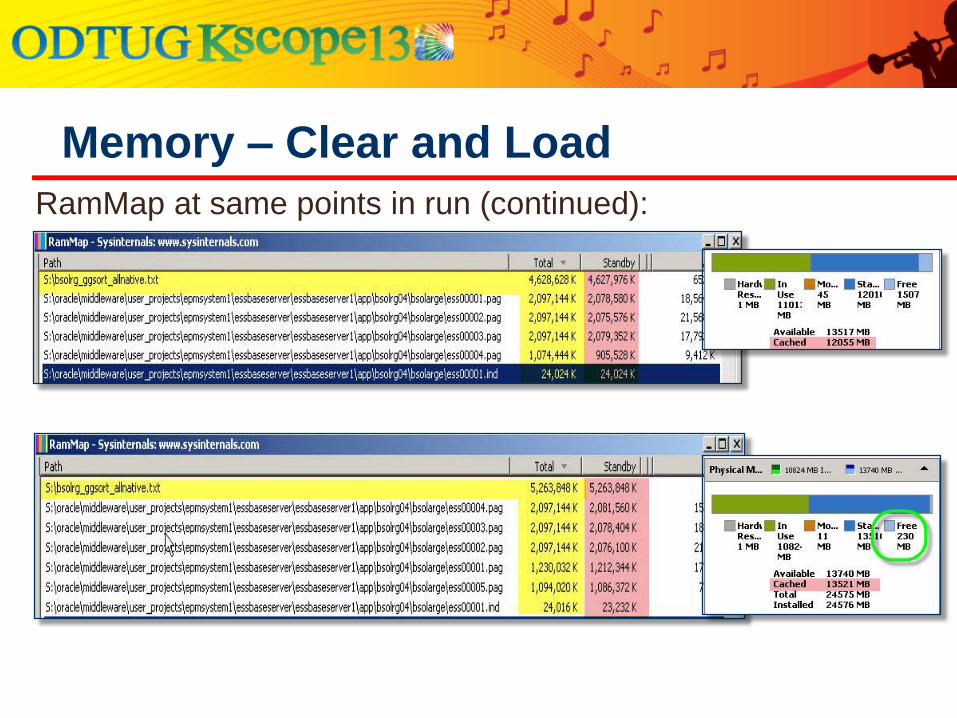
RamMap at same points in run (continued):
Memory – Clear and Load
“Best Practice” for BSO
● Index Cache should be at least as large as .ind file
● Alternatives not even considered
BSO Cache on following pages refers only to
data cache
Memory mapped IO works almost like cache
Data Load - Caches
Both BSO and ASO sparse dimensions should
be sorted
● ASO - only compression dimension is dense
● All other Dimensions considered sparse
Key “Best Practice” - followed in most tests
“Best Practice” has been to sort Sparse in
outline order
Data Load – Sort Order
“Bad” sorts highly sensitive to memory:
● But only when input .pag or .dat files exhaust
memory mapped IO space
Data Load – Sort Order and Cache
Cache used in BSO and ASO to combine data
arriving on different data rows
“Bad” sorts and small caches show little impact
on performance when memory is available
● Blocks in cache are uncompressed, but moving and
uncompressing is fast when block is in memory
Small BSO caches increase calc fragmentation
● Large calcs only - incremental effect is small
Small caches don’t affect load fragmentation
● If “Good” sort is used
No frag change if commit blocks not changed
Data Load – Why Cache?
Recommendation: Increase commit blocks, minimize
caches, particularly with multiple cubes running
● Cache “hogs” memory
● Let cubes fight for memory mapped IO space on
equal basis
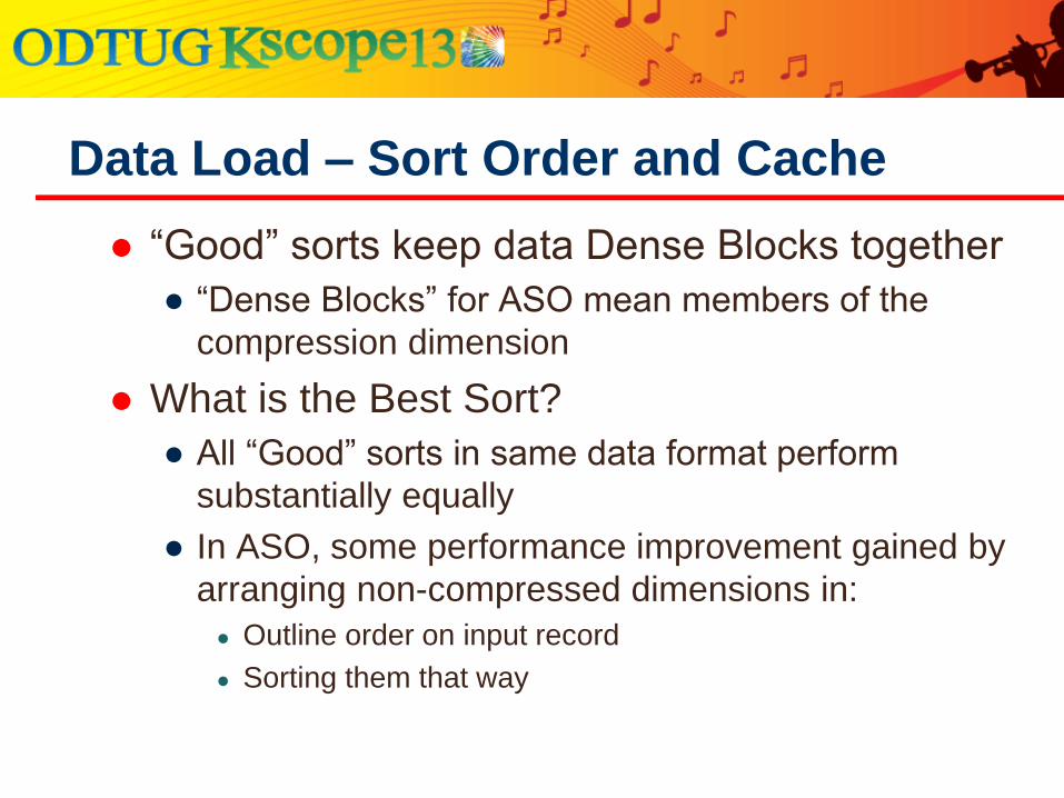
“Good” sorts keep data Dense Blocks together
● “Dense Blocks” for ASO mean members of the
compression dimension
What is the Best Sort?
● All “Good” sorts in same data format perform
substantially equally
● In ASO, some performance improvement gained by
arranging non-compressed dimensions in:
● Outline order on input record
● Sorting them that way
Data Load – Sort Order and Cache
Maybe not – let’s discuss data format first
Then, let’s re-consider Sort order
Is That the Last Word on Sort Order?

Data Load – Data Format
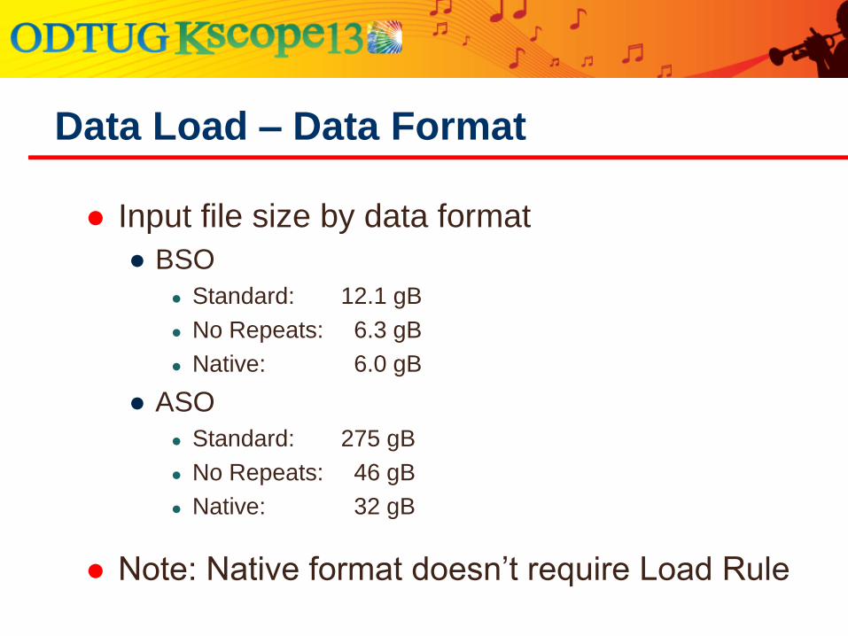
Input file size by data format
● BSO
● Standard: 12.1 gB
● No Repeats: 6.3 gB
● Native: 6.0 gB
● ASO
● Standard: 275 gB
● No Repeats: 46 gB
● Native: 32 gB
Note: Native format doesn’t require Load Rule
Data Load – Data Format
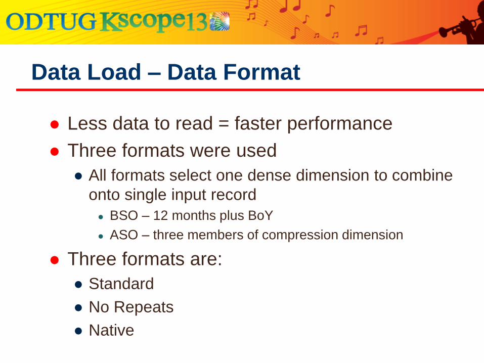
Less data to read = faster performance
Three formats were used
● All formats select one dense dimension to combine
onto single input record
● BSO – 12 months plus BoY
● ASO – three members of compression dimension
Three formats are:
● Standard
● No Repeats
● Native
Data Load – Data Format
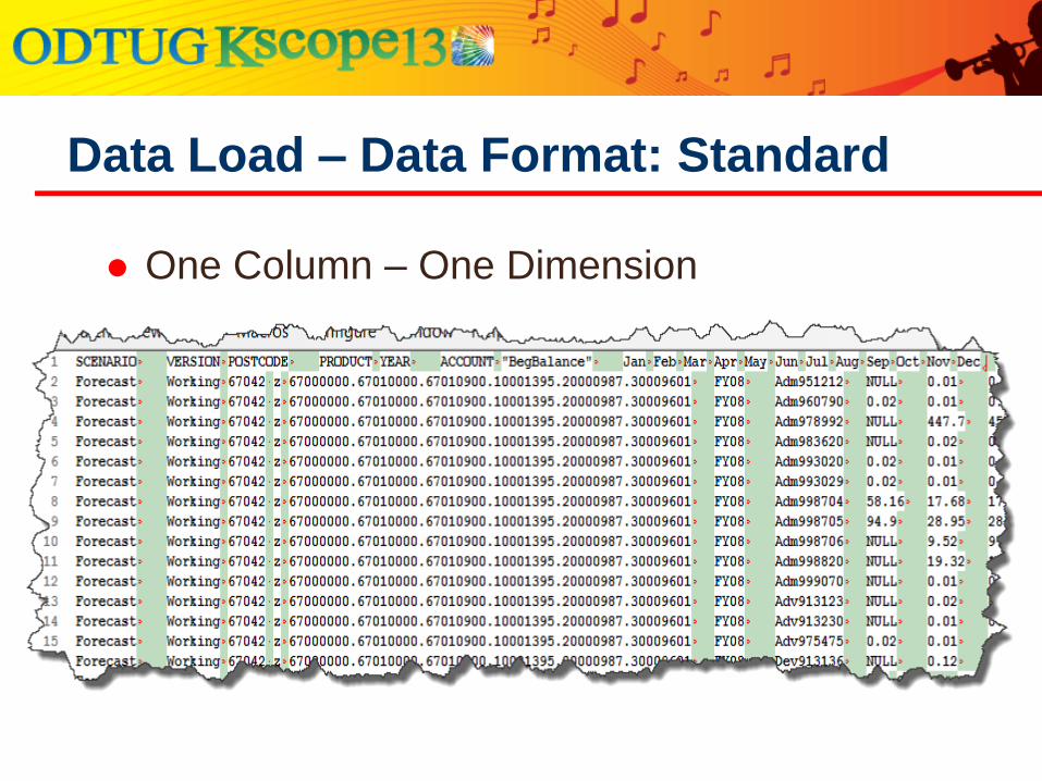
One Column – One Dimension
Data Load – Data Format: Standard
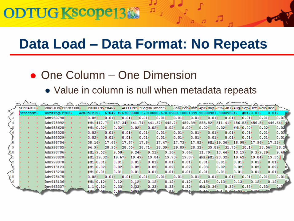
One Column – One Dimension
● Value in column is null when metadata repeats
Data Load – Data Format: No Repeats
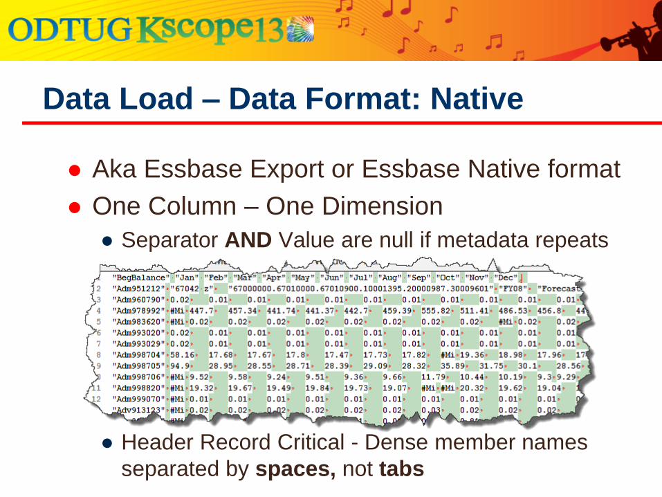
Aka Essbase Export or Essbase Native format
One Column – One Dimension
● Separator AND Value are null if metadata repeats
● Header Record Critical - Dense member names
separated by spaces, not tabs
Data Load – Data Format: Native

With Standard format, you would:
Sort in Cardinality order
● Sparse: Largest to smallest dimensions
● Dense: Largest to smallest
● Combine dense dimension members on input row (optional)
● i.e., Jan, Feb, Mar…
● Your choice of dense dim (densest of dense is best)
Physical order of dimensions on input record
doesn’t matter
Change Standard Practice - OLD
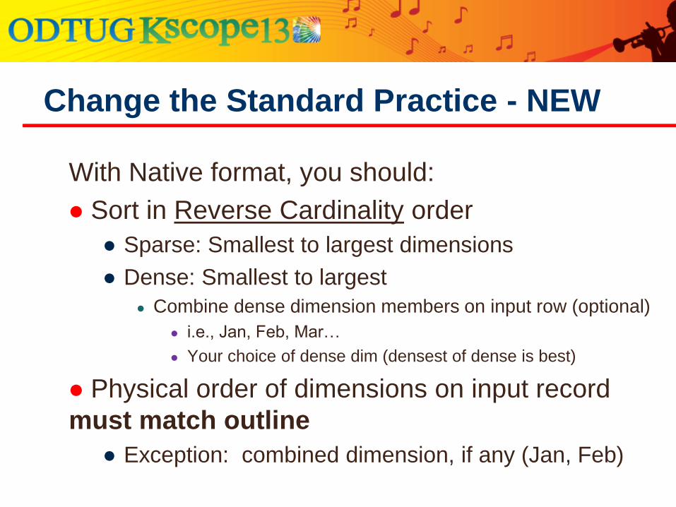
With Native format, you should:
Sort in Reverse Cardinality order
● Sparse: Smallest to largest dimensions
● Dense: Smallest to largest
● Combine dense dimension members on input row (optional)
● i.e., Jan, Feb, Mar…
● Your choice of dense dim (densest of dense is best)
Physical order of dimensions on input record
must match outline
● Exception: combined dimension, if any (Jan, Feb)
Change the Standard Practice - NEW
Why Reverse Cardinality?
Indexes use Forward Cardinality because they
want to get as close as possible to one single
record in the first “jump”
● To find Dan Pressman in a list I will get closer if I can
jump to the Pressman’s rather than the Dan’s
Here we are not trying find one record but
reading them all – and we hate repeating
ourselves
Change the Standard Practice - New
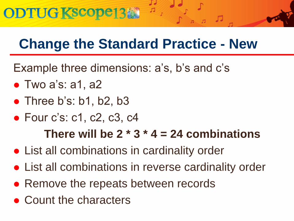
Example three dimensions: a’s, b’s and c’s
Two a’s: a1, a2
Three b’s: b1, b2, b3
Four c’s: c1, c2, c3, c4
There will be 2 * 3 * 4 = 24 combinations
List all combinations in cardinality order
List all combinations in reverse cardinality order
Remove the repeats between records
Count the characters
Change the Standard Practice - New
Change the Standard Practice - New
c1 b1 a1 a1 b1 c1 c1 b1 a1 a1 b1 c1
c1 b1 a2 a1 b1 c2 a2 c2
c1 b2 a1 a1 b1 c3 b2 a1 c3
c1 b2 a2 a1 b1 c4 a2 c4
c1 b3 a1 a1 b2 c1 b3 a1 b2 c1
c1 b3 a2 a1 b2 c2 a2 c2
c2 b1 a1 a1 b2 c3 c2 b1 a1 c3
c2 b1 a2 a1 b2 c4 a2 c4c2 b2 a1 a1 b3 c1 b2 a1 b3 c1c2 b2 a2 a1 b3 c2 a2 c2c2 b3 a1 a1 b3 c3 b3 a1 c3c2 b3 a2 a1 b3 c4 a2 c4c3 b1 a1 a2 b1 c1 c3 b1 a1 a2 b1 c1c3 b1 a2 a2 b1 c2 a2 c2c3 b2 a1 a2 b1 c3 b2 a1 c3c3 b2 a2 a2 b1 c4 a2 c4c3 b3 a1 a2 b2 c1 b3 a1 b2 c1c3 b3 a2 a2 b2 c2 a2 c2c4 b1 a1 a2 b2 c3 c4 b1 a1 c3c4 b1 a2 a2 b2 c4 a2 c4c4 b2 a1 a2 b3 c1 b2 a1 b3 c1c4 b2 a2 a2 b3 c2 a2 c2
c4 b3 a1 a2 b3 c3 b3 a1 c3
c4 b3 a2 a2 b3 c4 a2 c4
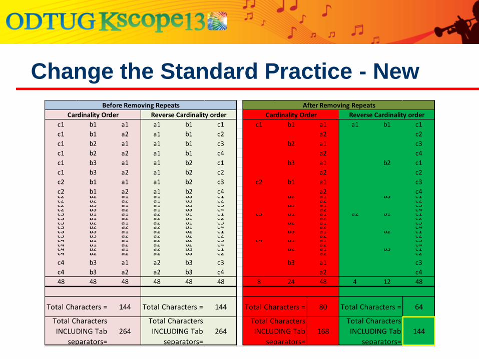
48 48 48 48 48 48 8 24 48 4 12 48
144 144 80 64
264 264 168 144
Cardinality Order Reverse Cardinality order Cardinality Order Reverse Cardinality order
After Removing RepeatsBefore Removing Repeats
Total Characters =
Total Characters
INCLUDING Tab
separators=
Total Characters =
Total Characters
INCLUDING Tab
separators=
Total Characters =
Total Characters
INCLUDING Tab
separators=
Total Characters =
Total Characters
INCLUDING Tab
separators=
No need to change outline order in BSO
ASO - Consider change to outline order
● Some advantage to having ASO data sorted in outline
order
● Native format dictates sort order, so it follows that
outline order should be changed to match
Test to see if it’s worth it
Change the Standard Practice - NEW

Your IT department is going to protest!
Reverse Cardinality sort is slower (correct)
● SQL is designed for sorting
● Perfect time for them to try Columnar Indexing
● You may convince them when you say:
● The SQL hardware likely has more horsepower
Native format SQL is difficult
● How do we do that?
● Just wrap your current SQL
Change the Standard Practice - NEW
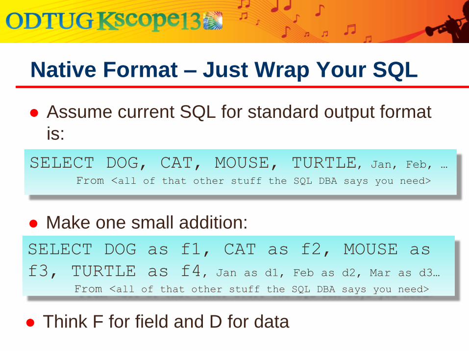
Assume current SQL for standard output format
is:
Native Format – Just Wrap Your SQL
SELECT DOG, CAT, MOUSE, TURTLE, Jan, Feb, … From <all of that other stuff the SQL DBA says you need>
Make one small addition:
SELECT DOG as f1, CAT as f2, MOUSE as
f3, TURTLE as f4, Jan as d1, Feb as d2, Mar as d3… From <all of that other stuff the SQL DBA says you need>
Think F for field and D for data
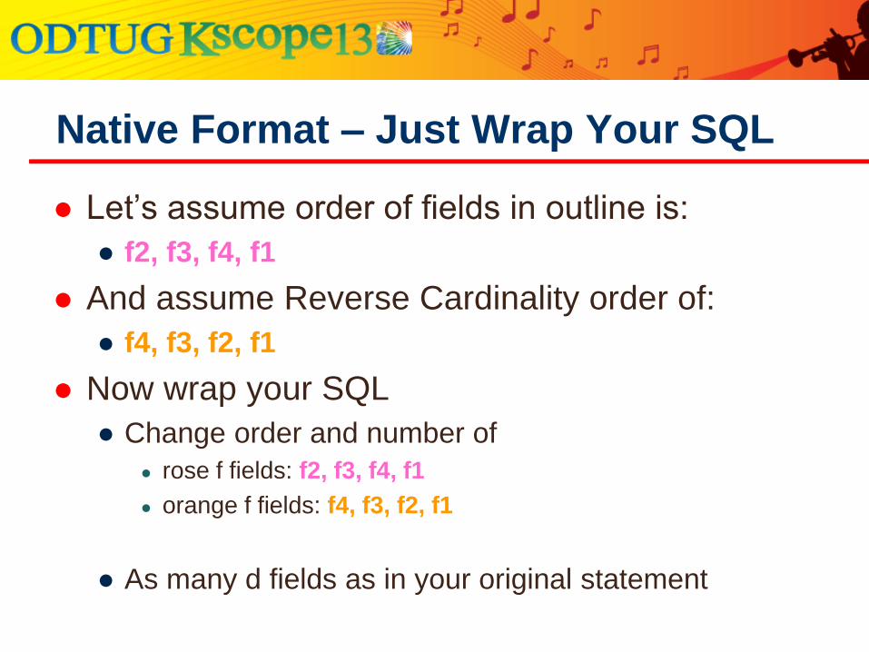
Let’s assume order of fields in outline is:
● f2, f3, f4, f1
And assume Reverse Cardinality order of:
● f4, f3, f2, f1
Now wrap your SQL
● Change order and number of
● rose f fields: f2, f3, f4, f1
● orange f fields: f4, f3, f2, f1
● As many d fields as in your original statement
Native Format – Just Wrap Your SQL
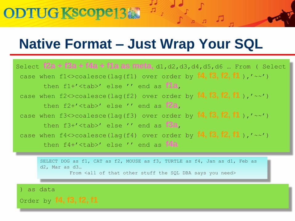
Native Format – Just Wrap Your SQL
SELECT DOG as f1, CAT as f2, MOUSE as f3, TURTLE as f4, Jan as d1, Feb as
d2, Mar as d3…
From <all of that other stuff the SQL DBA says you need>
Select f2a + f3a + f4a + f1a as meta, d1,d2,d3,d4,d5,d6 … From ( Select
case when f1<>coalesce(lag(f1) over order by f4, f3, f2, f1 ),’~~’)
then f1+’<tab>’ else ’’ end as f1a,
case when f2<>coalesce(lag(f2) over order by f4, f3, f2, f1 ),’~~’)
then f2+’<tab>’ else ’’ end as f2a,
case when f3<>coalesce(lag(f3) over order by f4, f3, f2, f1 ),’~~’)
then f3+’<tab>’ else ’’ end as f3a,
case when f4<>coalesce(lag(f4) over order by f4, f3, f2, f1 ),’~~’) then f4+’<tab>’ else ’’ end as f4a
) as data
Order by f4, f3, f2, f1
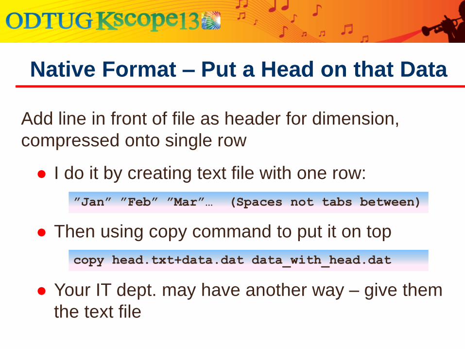
Add line in front of file as header for dimension,
compressed onto single row
Native Format – Put a Head on that Data
I do it by creating text file with one row:
Then using copy command to put it on top
Your IT dept. may have another way – give them
the text file
”Jan” ”Feb” ”Mar”… (Spaces not tabs between)
copy head.txt+data.dat data_with_head.dat
One large file or five small files?
One prepare thread or five threads?
Tested with runs using:
● One file with 5, 10, 15, 20, 25, 30, 35 threads
● Five files with 1, 2, 3, 4, 5, 6, 7 threads each
● Effective thread counts were equal
● 5*1=5, 5*2=10, 5*3=15 … 5*7=35
Data Load – Serial or Parallel?
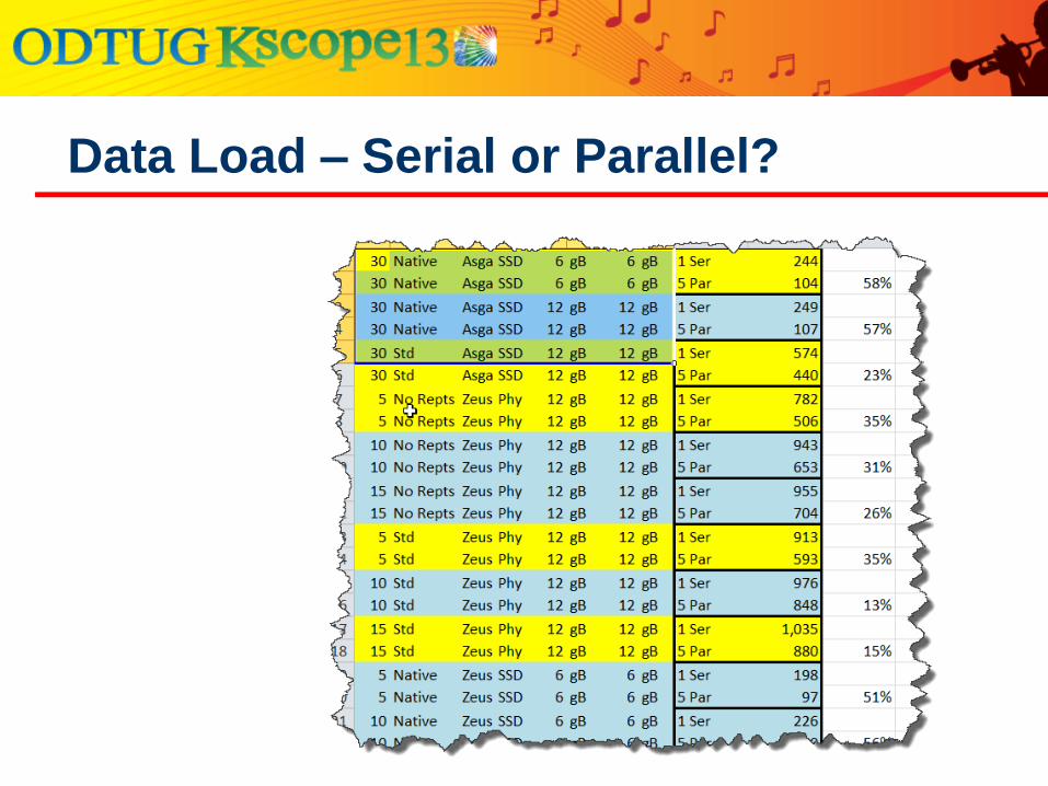
Data Load – Serial or Parallel?
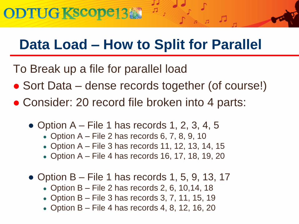
To Break up a file for parallel load
Sort Data – dense records together (of course!)
Consider: 20 record file broken into 4 parts:
● Option A – File 1 has records 1, 2, 3, 4, 5 ● Option A – File 2 has records 6, 7, 8, 9, 10
● Option A – File 3 has records 11, 12, 13, 14, 15
● Option A – File 4 has records 16, 17, 18, 19, 20
● Option B – File 1 has records 1, 5, 9, 13, 17 ● Option B – File 2 has records 2, 6, 10,14, 18
● Option B – File 3 has records 3, 7, 11, 15, 19
● Option B – File 4 has records 4, 8, 12, 16, 20
Data Load – How to Split for Parallel
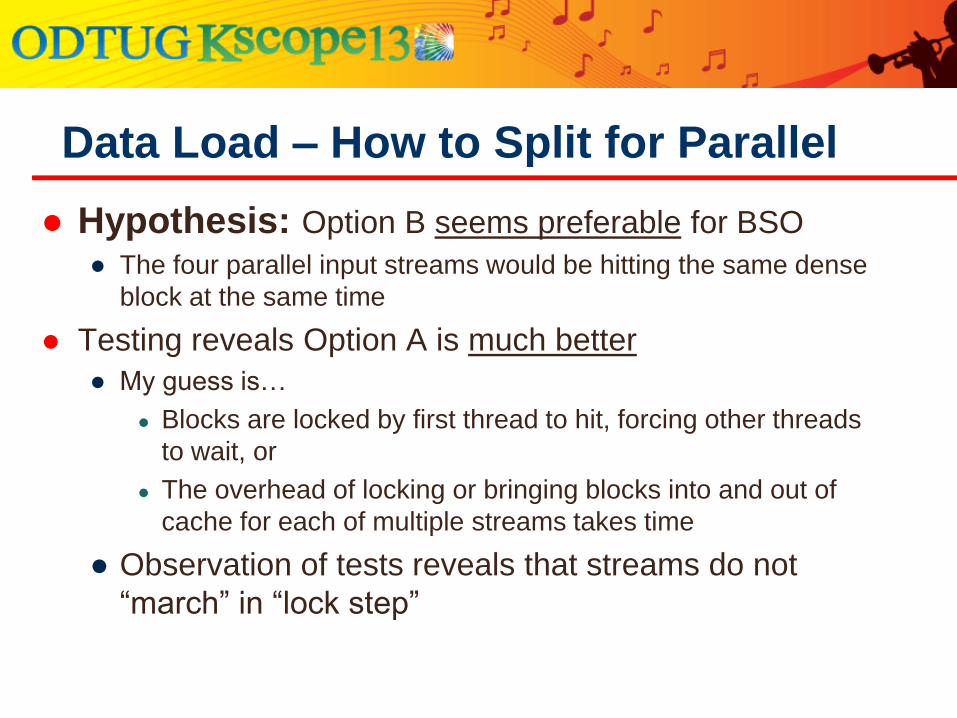
Hypothesis: Option B seems preferable for BSO
● The four parallel input streams would be hitting the same dense
block at the same time
Testing reveals Option A is much better
● My guess is…
● Blocks are locked by first thread to hit, forcing other threads
to wait, or
● The overhead of locking or bringing blocks into and out of
cache for each of multiple streams takes time
● Observation of tests reveals that streams do not
“march” in “lock step”
Data Load – How to Split for Parallel
The following slides detail the outline
hierarchies created for this project and the
generation of the data and queries
Check Back on the ODTUG site in a couple of
weeks if you want to see more data
Appendix
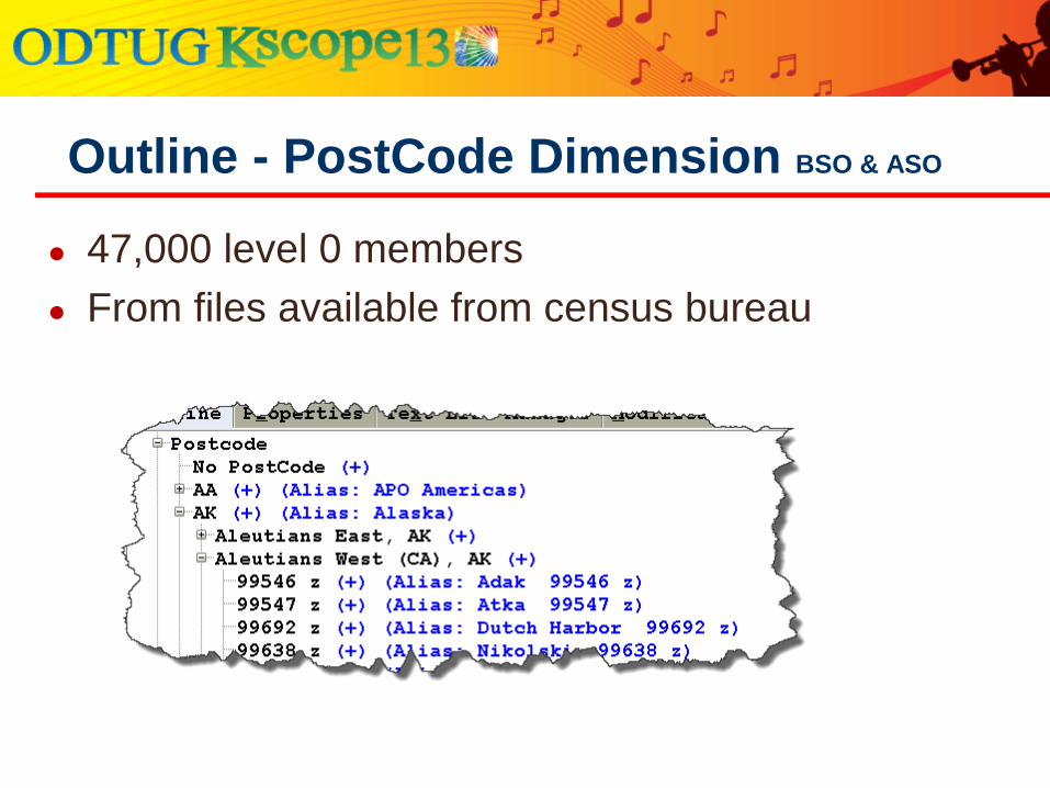
Outline - PostCode Dimension BSO & ASO
● 47,000 level 0 members
● From files available from census bureau
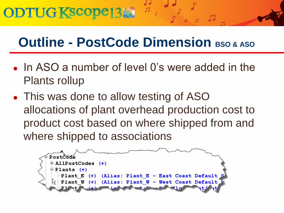
Outline - PostCode Dimension BSO & ASO
● In ASO a number of level 0’s were added in the
Plants rollup
● This was done to allow testing of ASO
allocations of plant overhead production cost to
product cost based on where shipped from and
where shipped to associations

Outline – Accounts Dimension BSO
● 3,200 level 0 members
● A very large, 19 level deep P&L was created
from a combination of real client ERP/Hyperion
Hierarchies
Outline – Year Dimension BSO & ASO
● Six level 0 members in BSO
● Data Generated 100% dense for BSO
● Twelve level 0 members in ASO
● Data Generated 100% dense for 1st 11 years in ASO
● Only Slice data generated for 12th year (FY18)
● Only BoY and Jan in FY18 slices
● Nothing special
● No rollups or alternate hierarchies
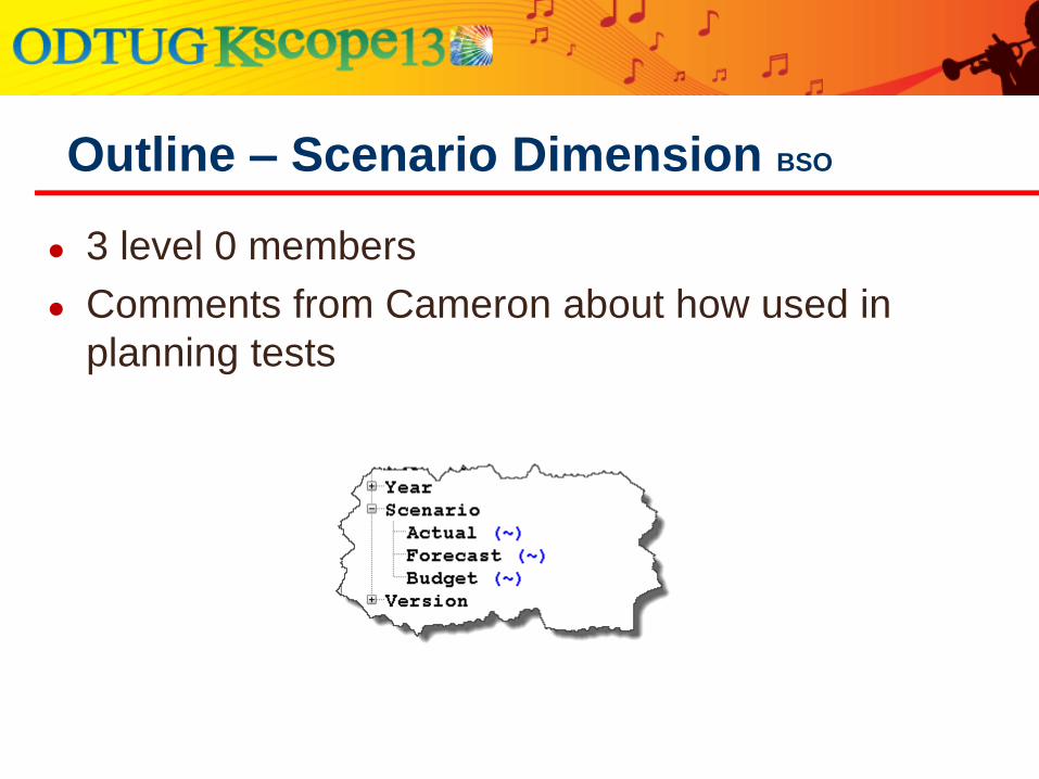
Outline – Scenario Dimension BSO
● 3 level 0 members
● Comments from Cameron about how used in
planning tests
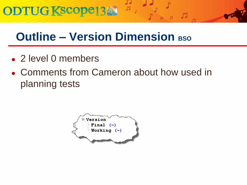
Outline – Version Dimension BSO
● 2 level 0 members
● Comments from Cameron about how used in
planning tests
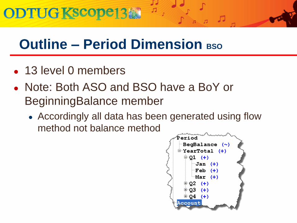
Outline – Period Dimension BSO
● 13 level 0 members
● Note: Both ASO and BSO have a BoY or
BeginningBalance member
● Accordingly all data has been generated using flow
method not balance method
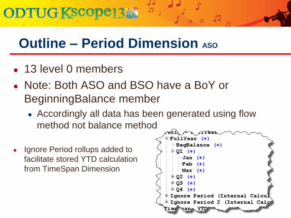
Outline – Period Dimension ASO
● 13 level 0 members
● Note: Both ASO and BSO have a BoY or
BeginningBalance member
● Accordingly all data has been generated using flow
method not balance method
● Ignore Period rollups added to
facilitate stored YTD calculation
from TimeSpan Dimension
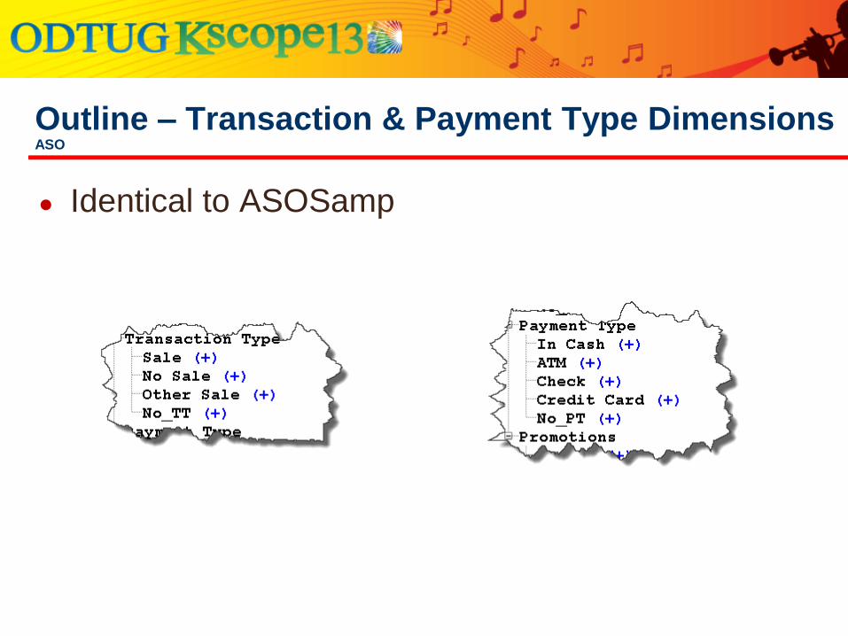
Outline – Transaction & Payment Type Dimensions ASO
● Identical to ASOSamp
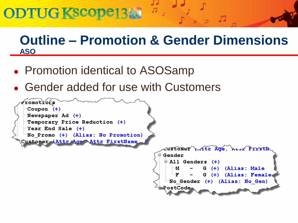
Outline – Promotion & Gender Dimensions ASO
● Promotion identical to ASOSamp
● Gender added for use with Customers
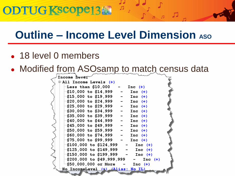
Outline – Income Level Dimension ASO
● 18 level 0 members
● Modified from ASOsamp to match census data
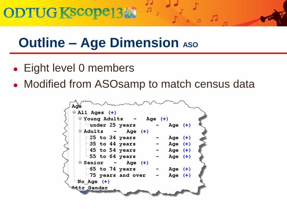
Outline – Age Dimension ASO
● Eight level 0 members
● Modified from ASOsamp to match census data
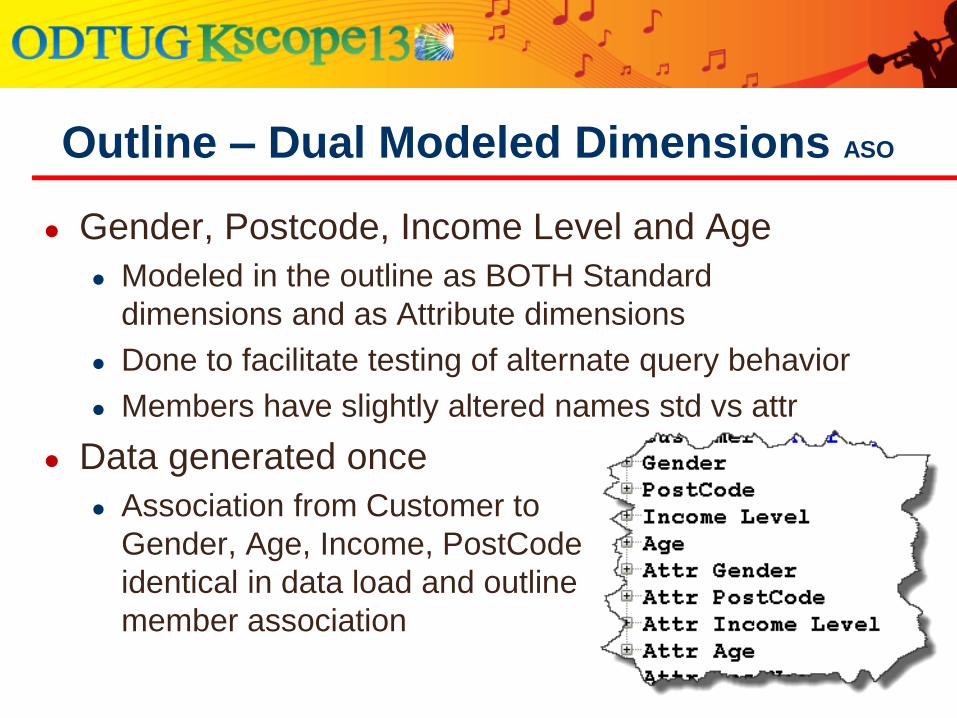
Outline – Dual Modeled Dimensions ASO
● Gender, Postcode, Income Level and Age
● Modeled in the outline as BOTH Standard
dimensions and as Attribute dimensions
● Done to facilitate testing of alternate query behavior
● Members have slightly altered names std vs attr
● Data generated once
● Association from Customer to
Gender, Age, Income, PostCode
identical in data load and outline
member association
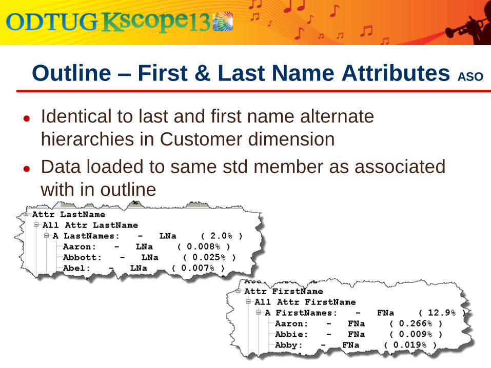
Outline – First & Last Name Attributes ASO
● Identical to last and first name alternate
hierarchies in Customer dimension
● Data loaded to same std member as associated
with in outline
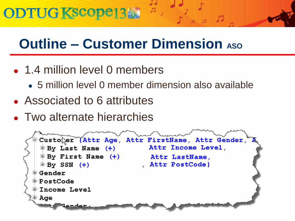
Outline – Customer Dimension ASO
● 1.4 million level 0 members
● 5 million level 0 member dimension also available
● Associated to 6 attributes
● Two alternate hierarchies

Outline – Customer Dimension ASO
● Numbers in Parentheses show the percentage of the real US population and generated data for that category ● Example: 2% have last names starting with A
● Example: .008% have last name of Aaron
● Note: All SSNs are generated NOT REAL
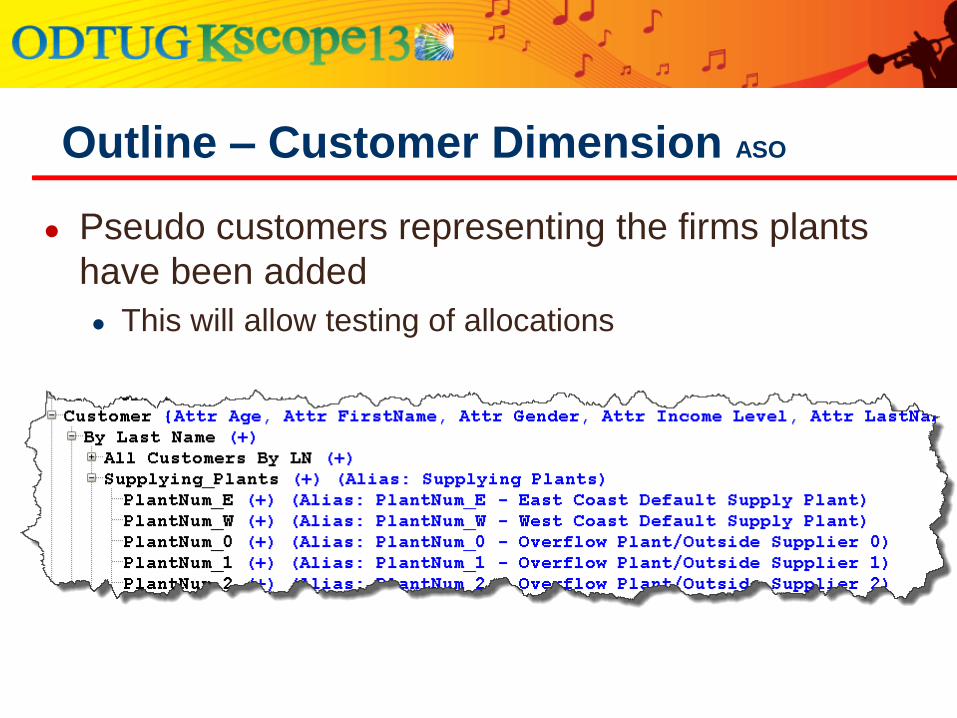
Outline – Customer Dimension ASO
● Pseudo customers representing the firms plants
have been added
● This will allow testing of allocations
Outline – Customer Dimension ASO
● Customers with the same name
● A few were generated during the random process
● SSN’s were generated to be unique so no problem
● There are a few names that were unusually popular
Outline – Customer Dimension ASO
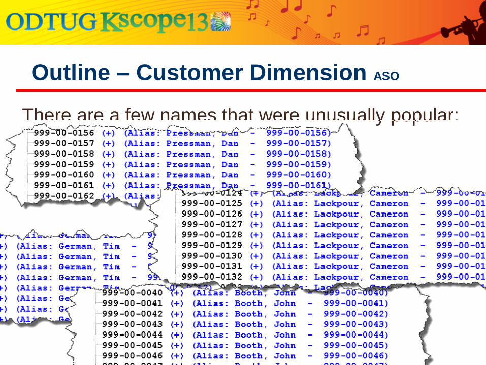
There are a few names that were unusually popular:
Outline – Customer Dimension ASO
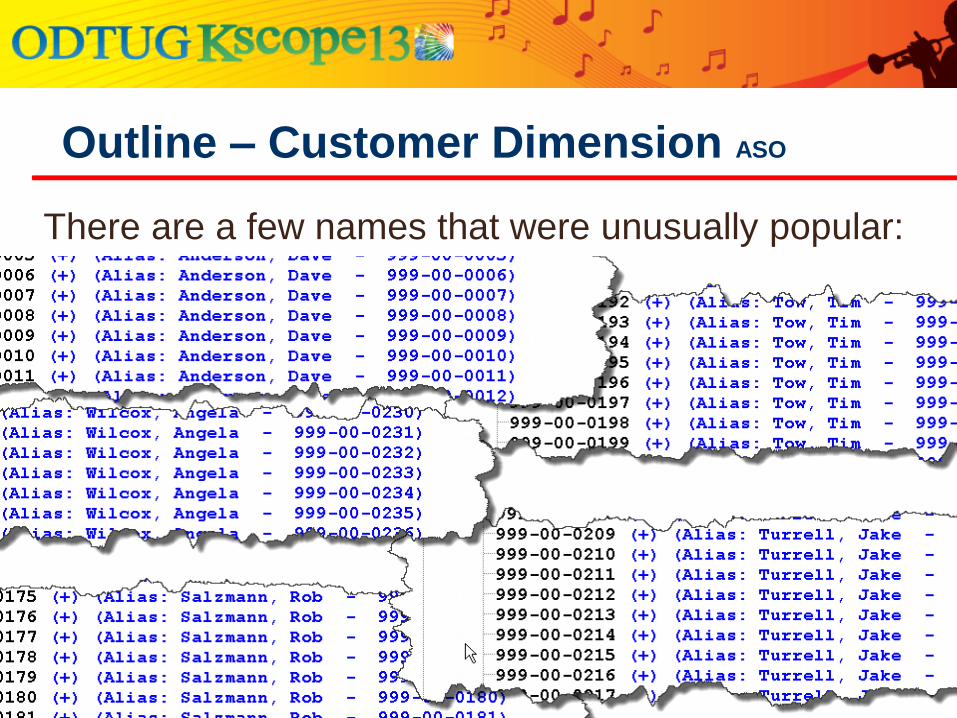
There are a few names that were unusually popular:

Outline – Customer Dimension ASO
There are a few names that were unusually popular:

Outline – Customer Dimension ASO
How it Was Generated
● US census Bureau files combined:
● 1,600 most popular US last names
● 1,200 most popular US male first names
● 1,200 most popular US female names
● 1.4mm (and 5.2mm) Statistically accurate
names
● More Smith’s than Pressman’s
● More Daniel’s than Cameron’s
● Not Stat Accurate: equal male & female
Outline – Customer Dimension ASO
How it Was Generated
● Randomly assigned (unique) SSN assigned to
each name (non-unique)
● US Census files were used to assign
statistically accurate zip codes to each SSN
● Census data on income and age distribution by
zip was then used to assign an age and income
to each SSN
● 14 names were added with ?? Unique zip codes and
every possible income/age

Outline – Customer Dimension ASO
How it Was Generated
● The resulting list was used to create attribute
associations
● The 1.4 mm name/attribute combinations were
then assigned a random frequency (normal
distribution)
● They were now ready for data generation
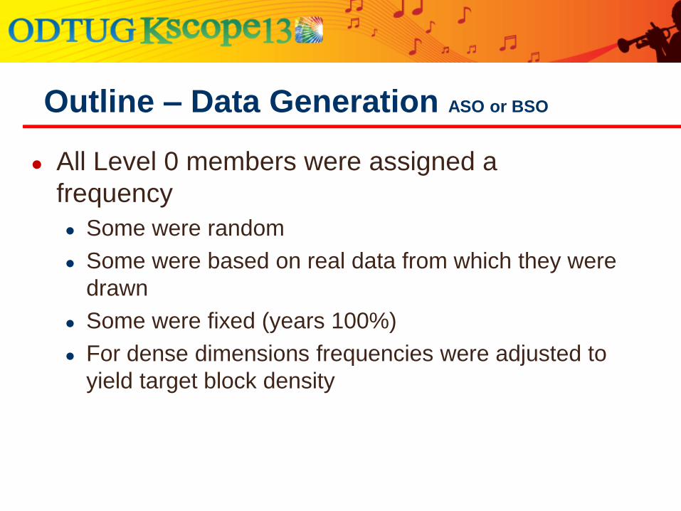
Outline – Data Generation ASO or BSO
● All Level 0 members were assigned a
frequency
● Some were random
● Some were based on real data from which they were
drawn
● Some were fixed (years 100%)
● For dense dimensions frequencies were adjusted to
yield target block density
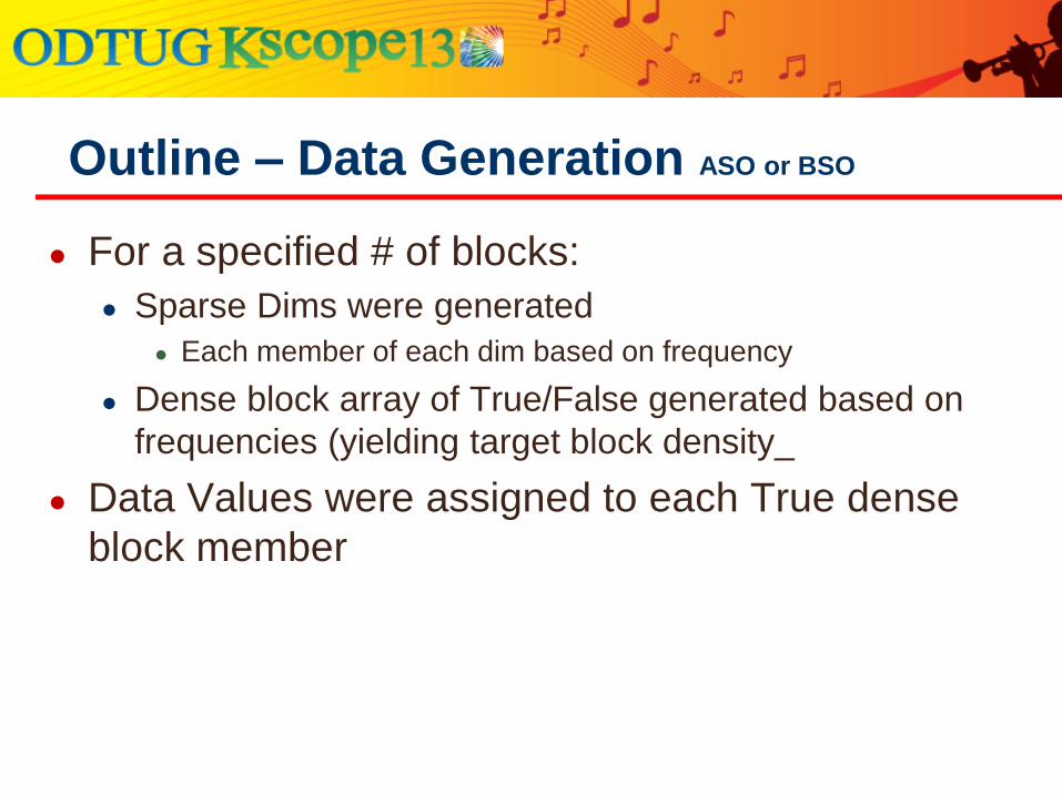
Outline – Data Generation ASO or BSO
● For a specified # of blocks:
● Sparse Dims were generated
● Each member of each dim based on frequency
● Dense block array of True/False generated based on
frequencies (yielding target block density_
● Data Values were assigned to each True dense
block member

Outline – Data Generation ASO or BSO
● Data Values were assigned to members
● Either randomly or based on real data in two parts
● Multiplier: (product A = 5; B = 1.3 ) ( dept X = 2; Y = 12)
● Value: product ( A =2; B = 23 ) ( dept X = 1; Y = 1.2 )
● Randomization ranges were set for each part
● ( product .8 to 1.1 )
● ( dept .2 to 12 )
● Value for each generated cell equals:
● Sum{ randomized value for each dimension }
● Value-AX = ( 2 + 1 ) Note: randomization of 5 & 1 not shown
● Value-BY = ( 23 + 1.2 ) …
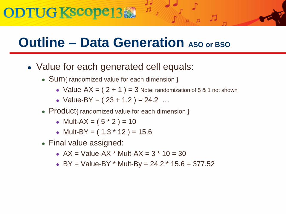
Outline – Data Generation ASO or BSO
● Value for each generated cell equals:
● Sum{ randomized value for each dimension }
● Value-AX = ( 2 + 1 ) = 3 Note: randomization of 5 & 1 not shown
● Value-BY = ( 23 + 1.2 ) = 24.2 …
● Product{ randomized value for each dimension }
● Mult-AX = ( 5 * 2 ) = 10
● Mult-BY = ( 1.3 * 12 ) = 15.6
● Final value assigned:
● AX = Value-AX * Mult-AX = 3 * 10 = 30
● BY = Value-BY * Mult-By = 24.2 * 15.6 = 377.52

Outline – Data Generation ASO or BSO
● Final Output
● One dense dimension tagged as “Densest”
● Remaining dense dimensions “Dense-Minus”
● For each sparse block one row for each True dense-
Minus intersection
● Each row contained all Densest members
● Some of which could be #Missing