Eindhoven, September 2013

Performance of machine learning algorithms to predict

anastomotic failure in bariatric surgery.

Master Thesis

Business Information Systems

Luis Jorge De Luna Orozco

Supervisor: Prof. dr.ir. Uzay Kaymak

Information Systems Group Eindhoven University of Technology

2

Acknowledgements Several people were involved and helped me to make this happen. I would like to thank specially prof. Kaymak for providing me with the guidance and feedback necessary to undertake this thesis project. Also to the doctors of the Catharina Hospital: Dr. Korsten, Dr. Nienhuijs and Dr. Buise who provided me with their help with everything related to patient information and the medical research.

3

Abstract The main purpose of this report is to perform a machine learning study to find out to which degree these algorithms can predict occurrence of anastomotic failure in bariatric surgery. The information used in this study was obtained from two databases provided by the Catharina Hospital in Eindhoven which contain preoperative information about patients (Sleeves) and perioperative blood pressure (4KP) recorded for 1116 surgeries since 2006. First part of this study covers an analysis to find out which features or variables can be obtained from this set of data and to which degree they have predictive power to identify complications after bariatric surgery, more specifically intestinal leakage when using them in classification predictive models. Second, investigation and performance analysis of three different machine learning classification algorithms is carried using techniques to compensate imbalanced sets of data due to the fact that only 3% of the patients present anastomotic failure after surgery. Finally relation between hypotension episodes an anastomotic failure is studied and explained. Main results of this study show that Random Forest classifying technique can offer predictive accuracy up to 90% when taking into consideration perioperative and preoperative bariatric surgery information like smoking assessment, surgery duration, medication assessment, surgery technique and occurrence of hypotension episodes under sedation. At the end all these results are discussed and a Random Forest model in WEKA is provided, moreover possible future work is suggested to continue with the creation of a full clinical decision support system.

4

Table of Contents

Acknowledgements ....................................................................................................................... 2

Abstract ......................................................................................................................................... 3

List of tables and figures ............................................................................................................... 6

1. Introduction .............................................................................................................................. 8

1.2 Research questions ............................................................................................................. 9

1.3 Methodology ...................................................................................................................... 10

1.4 Scope ................................................................................................................................. 11

1.5 Thesis outline ..................................................................................................................... 11

2. Bariatric Surgery ...................................................................................................................... 12

2.1 Sleeve gastrectomy ............................................................................................................ 14

2.2 Complications..................................................................................................................... 14

2.3 Anastomotic failure ............................................................................................................ 15

3. Predicting Modeling ................................................................................................................ 16

3.1 Data mining overview ......................................................................................................... 16

3.2 Data Mining Applied to Healthcare ..................................................................................... 18

3.3 Predictive models for surgery complications....................................................................... 19

3.3.1 Logistic regression ....................................................................................................... 20

3.3.2 Decision trees .............................................................................................................. 22

3.3.3 Random Forest ............................................................................................................ 22

3.4 Evaluating the performance of predictive models ............................................................... 23

4. Experiment Design .................................................................................................................. 27

4.1 Data collection ................................................................................................................... 27

4.1.1 Description of the Sleeves database............................................................................. 27

4.1.2 Description of the 4KP database .................................................................................. 30

4.2 Data preprocessing ............................................................................................................. 32

4.3 Feature Selection ............................................................................................................... 37

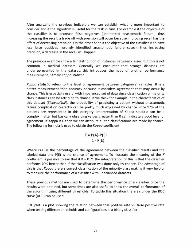
4.3.1 Fisher’s exact test on categorical variables................................................................... 41

4.3.2 Wilcoxon-Mann-Whitney on continuous variables ....................................................... 42

4.4 statistical analysis results.................................................................................................... 43

5

4.5 WEKA (Waikato Environment for Knowledge Analysis) ....................................................... 48

4.5.1 Dealing with imbalanced set of data for classification in WEKA .................................... 50

5. Experiment Results: Interpreting Classification Outcome. ...................................................... 54

5.1 Logistic regression results SMOTE....................................................................................... 55

5.2 Logistic regression results Cost-Sensitive Learning .............................................................. 56

5.3 Decision Tree results SMOTE .............................................................................................. 57

5.4 Decision Tree Cost-Sensitive Learning ................................................................................. 58

5.5 Random Forest results SMOTE............................................................................................ 59

5.6 Random Forest results Cost-Sensitive learning ................................................................... 60

5.7 Discussion .......................................................................................................................... 61

6. Conclusions ............................................................................................................................. 62

6.1 Reflection on the research questions .................................................................................. 62

6.2 Thesis Conclusions.............................................................................................................. 63

6.3 Future work........................................................................................................................ 64

References .................................................................................................................................. 65

Appendices .................................................................................................................................. 67

6

List of tables and figures

Figure 1: Number tendency of the number of overweight children around the world. Source:

Government Office for Science UK. .............................................................................................. 12

Figure 2: Number of procedures for bariatric surgery during the last ten years. Sources:

MedMarket Diligence, LLC ........................................................................................................... 13

Figure 3: Sleeve gastrectomy ....................................................................................................... 14

Figure 4: General approach to create a data mining solution. Source: computation.llnl.gov ......... 17

Figure 5: Example of a ROC curve in WEKA ................................................................................... 26

Figure 6: ID and patient information fields ................................................................................... 28

Figure 7: Weight and obesity fields .............................................................................................. 28

Figure 8: Fields related to the assessment of lifestyle and diseases related to obesity .................. 29

Figure 9: Surgery general information. ......................................................................................... 29

Figure 10: Example of a record contain in the 4KP databases for different surgeries. ................... 30

Figure 11: Example of invasive blood pressure records. ................................................................ 31

Figure 12: 4kp loaded and restored in a new SQL Server instance. ............................................... 32

Figure 13: Bulk insertion of Sleeves database into SQL Server ...................................................... 33

Figure 14: General overview of the 4 steps on the ETL (SSIS) ........................................................ 34

Figure 15: Example of hypotension episode ................................................................................. 35

Figure 16: Groups created for each episode of a continuous drop of the blood pressure below the

threshold ..................................................................................................................................... 36

Figure 17: Final table showing hypotension episodes ................................................................... 37

Figure 18: Analysis of smoking as an influence for leakage ........................................................... 41

Figure 19: Fisher’s exact test formula ........................................................................................... 42

Figure 20: Wilcoxon-Mann test web application ........................................................................... 43

Figure 21: WEKA main screen....................................................................................................... 48

Figure 22: Example CVS file containing relevant features for predicting anastomotic failure. ....... 49

Figure 23: WEKA classification groups .......................................................................................... 49

Figure 24: Imbalanced classes in WEKA ........................................................................................ 50

Figure 25: SMOTE filter selected in WEKA .................................................................................... 51

Figure 26: Over-sampling the minority class ................................................................................. 52

Figure 27: Randomize filter .......................................................................................................... 52

Figure 28: Filling the cost matrix in WEKA .................................................................................... 53

Figure 30: Roc curve for logistic regression with SMOTE over sampling ........................................ 55

Figure 31: Roc curve for logistic regression with Cost-Sensitive learning ....................................... 56

Figure 32: Roc curve for Decision Trees with SMOTE over-sampling ............................................. 57

Figure 33: Roc curve for decision tree with Cost-Sensitive learning .............................................. 58

Figure 34: Roc curve for Random Forest with SMOTE over-sampling ............................................ 59

Figure 35: Roc curve for Random Forest with Cost-Sensitive learning ........................................... 60

7

Table 1: Classification of Sleeve gastrectomy complications ......................................................... 15

Table 2: Example of Confusion Matrix .......................................................................................... 23

Table 3: Fisher’s 2x2 contingency table ........................................................................................ 41

Table 4: Patient Characteristics .................................................................................................... 44

Table 5: Assessment of comorbidities and medication taken by the patient before surgery. ........ 44

Table 6: Bariatric surgery characteristics ...................................................................................... 45

Table 7: Hypotension episodes mean blood pressure. .................................................................. 46

Table 8: Hypotension episodes mean blood pressure ................................................................... 47

8

1. Introduction

Nowadays hospitals are dealing with an increasing amount of patients demanding complex surgical procedures. As is the case with any other business, health care institutions need to improve and develop their procedures in order to archive better revenue and shorten the throughput times while dealing with an increasing patient population. Analyzing data in order to predict events before they happen provides the possibility to take actions early in their processes and provide better solutions and ways of dealing with complications. Clinical decision systems were created to tackle these situations; they provide the doctors with software tools to improve health care services by helping to determine the diagnosis of a patient based on previously discovered knowledge. The idea behind these systems is to gather and study patients’ items in order to provide the physician with advice on which is the best way to proceed according to patients’ particular symptoms and characteristics. Clinical decision systems are supported by predictive models. This notion is quite important for this report since the main goal is to find on which degree a predictive model can be used to predict the appearance of anastomotic failure in bariatric surgery. Predictive models have been used before in a lot of facets among businesses to predict trends and even measure performance (KPIs). Nevertheless this approach for data analysis has been considered only recently within hospitals due to the appearance of large sources of digital information in health care domain. Hospitals have started implementing digital records and storing real time surgery information all around the world. The fact that this huge quantity of data is now available creates the need to find proper algorithms to derive knowledge and create guidelines for decision making. Measuring the performance of these algorithms is crucial since there is not a huge margin of error when diagnosing life threatening diseases or complications in a medical field. Better and customized prediction models are needed to each clinical situation since is really difficult to generalize a model to be applied to most complications, this is the reason why a performance analysis of specific predictive models for bariatric surgery is needed. Data mining becomes a very important notion when dealing with this newly available information in health care due to the fact that this data needs to be processed, cleaned and understood. The patterns hidden behind the huge amount of unorganized information are not easily found and the rate on which data arrives makes it difficult to handle. Because of this difficulties data mining tools are needed to derive knowledge and to deal with this overload of information. The type of information stored in health care records includes preoperative data like comorbidities and lifestyle assessment of patients combined with perioperative information recorded on real time during the surgery, provides with enough information to test predictive models and draw conclusions on their performance.

9

A particular important case is bariatric surgery because obesity is becoming an epidemic problem in the world. Just a few days ago it was found out that Mexico is now the country with the fattest population (surpassing the US) with almost 33% of the adults considered as obese (U.N. Food and Agriculture Organization, 2013). This kind of situation is not an isolated event. Most of the developed countries are experiencing a rise in their measurements about obesity. Sedentary lifestyles and a fast food culture had helped to make this problem worst every year. The bad news is that more than aesthetical problem obesity can lead to physical and psychological problems like depression, heart disease, diabetes, cancer and osteoarthritis (Dixon, 2010). The motivation behind this study is that there is a gap in the research in the analysis of anastomotic failure after bariatric surgery. There are quite a few studies trying to predict anastomotic leakage after colorectal cancer surgery by finding the risk factors as intraoperative blood pressure etc. (I. L. Post, 2012). Nevertheless, these kinds of studies don’t focus on measuring the performance of possible predictive models and second and more important, they haven’t been done for anastomotic failure after bariatric surgery. It’s also important to mention that a previous Master’s thesis by TU/e student Pablo Perdiguer (Perdiguer, 2012) analyzing operative times a consequence prediction was presented on 2012. This thesis project implements some of his future work suggestions, namely merging Sleeves databases with the 4KP database to create groups of hypotension episodes which might help to predict specific complications like anastomotic failure.

Finally is important to mention that this thesis is a contribution to the health care cluster in the Information Systems group of the TU/e in cooperation with the Catharina Hospital in Eindhoven.

1.2 Research questions Main research question: To which degree can machine learning algorithms be used to predict anastomotic failure in bariatric surgery? This questions aims to answer if machine learning algorithms can be applied to the data contained at the hospital information systems in order to predict anastomotic failure. Also to find which is the optimal algorithm for this specific situation (in the case an algorithm is suitable). In order to answer the main research question of this thesis a set of sub-questions need to be answered. Important sub-questions RSQ1. - Which information from the available hospital databases can be obtained to train a predictive model?

10

An analysis of the data contained in the databases needs to be done in order to answer this question and determine which of these variables have predictive power to be use on as features for a classifying problem to predict if a patient will present anastomotic failure. Doctors will provide their medical expertise which is essential when trying to understand which patient items are leading to anastomotic failure complication. RSQ2. – What is the performance of different machine learning methods when predicting anastomotic failure? This question needs to be answered in order to know if a machine learning technique is robust enough to be used as a predicting tool for anastomotic failure. It is important to test the algorithms with different setting to overcome the problem of imbalanced classes in the data. A comparison using different metrics like accuracy, precision, recall, kappa statistic and area under the ROC curve will be presented to measure the performance of the predictive models. RSQ3. - Are hypotension episodes useful for predicting anastomotic failure? Intraoperative hypotension episodes may play an important role when predicting anastomotic failure. Information contained on the 4KP database gives the opportunity to identify hypotension episodes and relate them to patient traits in order to answer how strong their influence on the appearance of anastomotic failure is. This is a valuable question from the medical point of view since provide insight on how this episodes may be a crucial characteristic in patients when predicting complications.

1.3 Methodology In order to answer the purposed research questions a methodology needs to be define to provide guidance during this research. The following structure was followed all through the process of this research. The first step involves acquiring the necessary knowledge about bariatric surgery and how information related to this procedure is stored. To complete this process several meetings were held with the doctors in charge of the databases at the Catharina Hospital in order to understand how their databases are composed and to discuss with them about possible relevant variables to look into. Both databases provided by the hospital were merged (4KP and Sleeves) to have a new dataset for analysis containing all patient’s items, later on hypotension episodes were detected and stored in new tables for each patient according to medical hypotension thresholds(determined with the help of Dr. Marc Buise). Second step involves carrying a statistical analysis of the variables to identify the strongest predictors of anastomotic failure according to their statistical significance (p-value). This second step provided the basis for feature selection for the tested machine learning algorithms (classifiers) and gives the opportunity to answer if hypotension episodes are statistically significant to predict anastomotic failure.

11

Finally logistic regression, decision trees and random forest algorithms were tested in WEKA to find out which predictive model is more suitable to classify patients according to the presence of anastomotic failure (or not) after bariatric surgery.

1.4 Scope The amount of Information contained in the databases is significant; therefore a scope needs to be defined in this section. Basically this project has a scope of 1116 patients who underwent bariatric surgery between 2006 and 2012 and whose information is contained in the Sleeves database. The content of the Sleeve database describes information about patient traits, surgery characteristics, patient assessment and follow ups. For this report the follow up information for the patients was not considered. Regarding the 4KP database information about intraoperative blood pressure is used in the project but only for the 1116 patients who underwent bariatric surgery. It is important to mention that 4KP database contains information for patients undergoing any kind of surgery which requires sedation, so a filter for this was applied in order to reduce the amount of information used the analysis. From the 1116 patients who underwent bariatric surgery 36 of them presented anastomotic failure, so that is the scope for positive cases. 4KP and Sleeves databases were merged to carry a statistical analysis to find variables with strong influence on anastomotic failure occurrences after bariatric surgery. Afterwards (using only the statistically significant variables) a machine learning solution comparison in WEKA will be provided to select the best algorithm for classification and prediction.

1.5 Thesis outline This thesis consists of 6 chapters. The first one covers the introduction, motivation behind this project and explains the necessity of predictive models in health care. Moreover it presents the research questions that will be answered in this report and gives an overview of the methodology and scope of the project. Chapter 2 presents a literature study with the intention to familiarize the reader with the bariatric surgery procedure and the anastomotic failure complication. Third chapter presents the current state of data mining in the health care domain and introduces a description about the predictive methods that were used in this thesis. Also an explanation is presented about of why these methods are selected and the advantages that they present when they are applied in the medical field. Chapter 4 presents the experiment settings: design and description, data collection and preprocessing and the introduction to the WEKA data mining tool application. Chapter 5 presents the results of the experiments and a discussion about how to interpret these results. Finally chapter 6 presents the conclusions, answers to the research questions and a proposal for future work in the field.

12

2. Bariatric Surgery

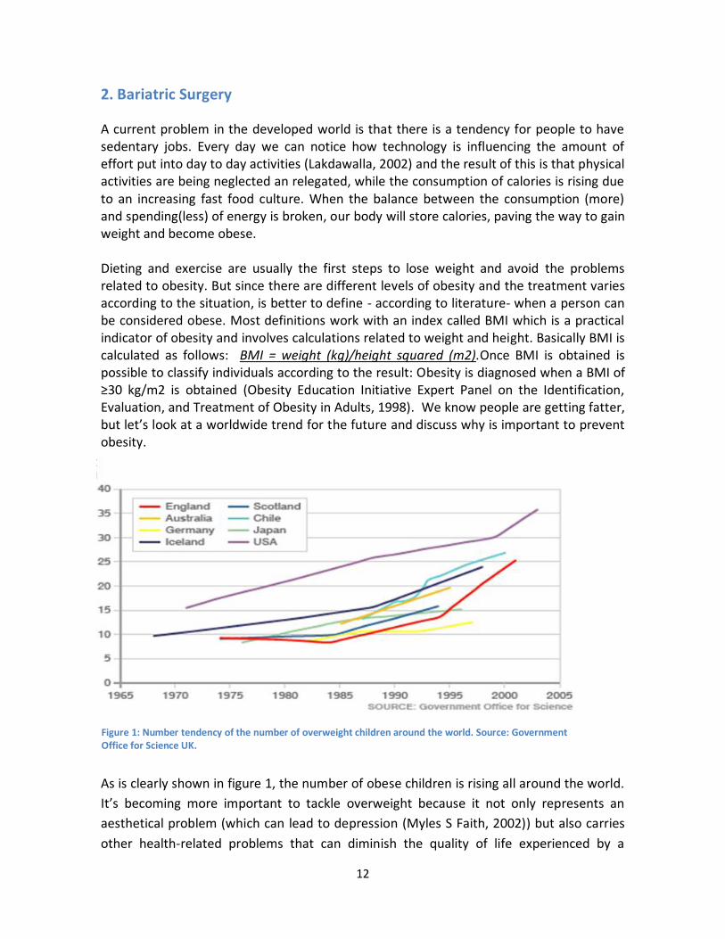
A current problem in the developed world is that there is a tendency for people to have sedentary jobs. Every day we can notice how technology is influencing the amount of effort put into day to day activities (Lakdawalla, 2002) and the result of this is that physical activities are being neglected an relegated, while the consumption of calories is rising due to an increasing fast food culture. When the balance between the consumption (more) and spending(less) of energy is broken, our body will store calories, paving the way to gain weight and become obese. Dieting and exercise are usually the first steps to lose weight and avoid the problems related to obesity. But since there are different levels of obesity and the treatment varies according to the situation, is better to define - according to literature- when a person can be considered obese. Most definitions work with an index called BMI which is a practical indicator of obesity and involves calculations related to weight and height. Basically BMI is calculated as follows: BMI = weight (kg)/height squared (m2).Once BMI is obtained is possible to classify individuals according to the result: Obesity is diagnosed when a BMI of ≥30 kg/m2 is obtained (Obesity Education Initiative Expert Panel on the Identification, Evaluation, and Treatment of Obesity in Adults, 1998). We know people are getting fatter, but let’s look at a worldwide trend for the future and discuss why is important to prevent obesity.

As is clearly shown in figure 1, the number of obese children is rising all around the world.

It’s becoming more important to tackle overweight because it not only represents an

aesthetical problem (which can lead to depression (Myles S Faith, 2002)) but also carries

other health-related problems that can diminish the quality of life experienced by a

Figure 1: Number tendency of the number of overweight children around the world. Source: Government Office for Science UK.

13

person, also represent an economic burden for society since this people are prone to

chronic diseases. The most common conditions associated with obesity are heart disease,

hypertension, diabetes, stroke, liver and gallbladder disease and sleep apnea (Clinical

Guidelines on the Identification, Evaluation, and Treatment of Overweight and Obesity in

Adults, 1998). Doctors are aware of the consequence that being obese brings to a person

that is why surgical procedures have been developed in order to provide patients with an

option to lose weight. One of these procedures is the bariatric surgery. The popularity of

bariatric surgery is increasing at the same pace as obesity problems are becoming more

common in the world. Figure 2 can show the global trend in 2013 for bariatric surgery and

also which are the most common approaches taken to operate a patient.

Bariatric surgery refers to a variety of procedures performed to help people to lose weight. These procedures can be grouped into three main categories (Abell TL, 2006): Predominantly malabsorptive procedures, predominantly restrictive procedures and mixed procedures. For the specific case of this project, an analysis of the sleeve gastrectomy (a subgroup of the predominantly malabsorptive procedures) is made.

Figure 2: Number of procedures for bariatric surgery during the last ten years. Sources: MedMarket Diligence, LLC

14

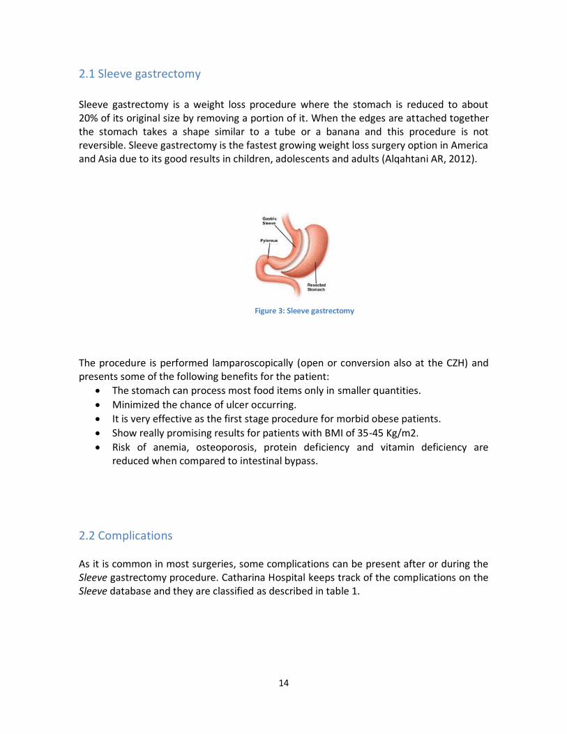
2.1 Sleeve gastrectomy Sleeve gastrectomy is a weight loss procedure where the stomach is reduced to about 20% of its original size by removing a portion of it. When the edges are attached together the stomach takes a shape similar to a tube or a banana and this procedure is not reversible. Sleeve gastrectomy is the fastest growing weight loss surgery option in America and Asia due to its good results in children, adolescents and adults (Alqahtani AR, 2012).

The procedure is performed lamparoscopically (open or conversion also at the CZH) and presents some of the following benefits for the patient:

The stomach can process most food items only in smaller quantities.

Minimized the chance of ulcer occurring.

It is very effective as the first stage procedure for morbid obese patients.

Show really promising results for patients with BMI of 35-45 Kg/m2.

Risk of anemia, osteoporosis, protein deficiency and vitamin deficiency are reduced when compared to intestinal bypass.

2.2 Complications As it is common in most surgeries, some complications can be present after or during the Sleeve gastrectomy procedure. Catharina Hospital keeps track of the complications on the Sleeve database and they are classified as described in table 1.

Figure 3: Sleeve gastrectomy

15

Leakage (Anastomotic Failure)

Abscess Bleeding Other complications

-Leakage -Leakage+ Abscess -Leakage + Pulmonary. -Leakage + Urinary track. -Leakage + Abscess + Sepsis. -Leakage + Abscess + Wound Infection + Pulmonary

-Abscess. -Sepsis. -Bleeding + Sepsis. -Abscess + Dysphagia. -Abscess + Urinary Track.

-Bleeding. -Bleeding + Dysphagia. -Bleeding + Pulmonary. -Bleeding + Cardiac.

-Wound infection. -Dysphagia. -Pulmonary. -Urinary track. -Cardiac

Table 1: Classification of Sleeve gastrectomy complications

As for the scope of this project patients in the leakage and abscess groups are taken into consideration for the analysis, also the information contained in the Sleeve database refers to patients who underwent bariatric surgery using the sleeve gastrectomy approach explained in this chapter.

2.3 Anastomotic failure Even though bariatric surgeries are being commonly performed and Sleeve gastrectomy is generally considered an effective and safe procedure, anastomotic failure is considered to be the most life threatening complications that a patient can present. (Xabier de Aretxabala, 2011). The incidence of Anastomotic failure on a bariatric surgery is about 3%. This statistic is congruent with the information contained at the hospital’s database on which 36 patients out of 1116 presented a leak. But let’s define what Anastomotic failure is. According to the UK surgical infection study group leakage is define as “the leak of luminal contents from a surgical join between two hollow viscera”. This is a serious threat to the patient’s health and recovery, which is why it was selected for the scope of this report. Predicting the occurrence of Anastomotic leak according to hypotension and patient’s traits using predictive models is relevant because the leakage can only be detected after the patient underwent surgery. It is generally diagnosed when the patient already was discharged and so far there are not clear indications on what can increase the chances of having leakage after a bariatric surgery (Hyman N, 2007).

16

3. Predicting Modeling

Recently due to the improvements on storage capacity and the availability of systems which record surgery information on real time, a lot of data is being generated and saved at the hospitals regarding patient’s information. Making conclusions from this data is a big challenge and it has been tackle applying data mining techniques and predictive models. Knowledge discovery, finding best practices and predicting results are some of the main advantages of applying data mining to any domain and in this chapter a general overview of this process will be presented. Moreover a detailed explanation about the predictive models used in this research and the performance measurements will be also included.

3.1 Data mining overview It is important to present then a brief introduction to data mining and define how it is applied to the health care domain. Data mining can be seen as the meeting point for several disciplines like of database technologies, statistics, machine learning algorithms, high performance computing, visualization and pattern recognition. It aims at finding patterns and understanding the underlying behavior of a repository of data. The goal of applying data mining is to discover knowledge that might be hidden inside data and that is not obvious at first sight. The starting points to apply data mining is gathering the information and obtaining access to the sources of the data. Once this step is completed a selection of the data has to be made in order to decide which information is relevant for analysis. It is usually unrealistic to work with all the data that is available and therefore a procedure to limit the quantity of information is required. After relevant information is defined a process to certify the quality of information shall take place. This is commonly known as the pre-processing of the data. This process involves cleansing the data and combining the sources of information into data marts which contained information that ready to use. The third step involves transforming the data into something which will fit the requirements of the data mining software or algorithm. This third step is usually known as feature selection which means that certain variables are selected as the most important or relevant for the data mining process. When the previous steps are completed information is ready to undergo the data mining process to discover possible patterns. The most common approaches to discover patterns and making predictions with data are: unsupervised learning (clustering) and supervised learning (classification) techniques. Cluster analysis is based on the notion that objects contained on the database can be put on a certain group (cluster) according to their characteristics, but these clusters are not define beforehand. When an object has a certain set of attributes which are similar to the attributes of the other objects contained on a given cluster, this object is labeled inside the same category. Cluster analysis is used when the data doesn’t have an explicit label or group defined previously for the objects. On the other hand, classification involves identifying (according to previously labeled groups) to which category a new observation belongs. This is especially important for this project

17

since it aims to predict if a patient has a risk of anastomotic leak or not. Figure 4 shows an overall framework on how a data mining solution can be constructed for any domain and it was used as a basis for this research.

Figure 4: General approach to create a data mining solution. Source: computation.llnl.gov

Several algorithms are available to perform and construct data mining solutions; the most

popular are (Xindong Wu, 2008):

K-means algorithms

Support Vector Machines

Apriori Algorithm

EM Algorithm

Page Rank

Ada boost

K-nearest neighbor

Naive Bayes

Decision Trees (Random Forest)

18

3.2 Data Mining Applied to Healthcare Electronic health records are becoming the norm around the world because they make life easier for doctors and patients. Also they provide the possibility to share information among hospitals and, hopefully in the near future, even between countries. The main challenges about this digitalization of a patient’s medical records are how privacy will be enforced and how can they lead to improving the performance of the health care procedures. The second challenge is addressed in this report by applying data mining to a relative small set of patient’s records in order to discover how suitable these algorithms to predict complications after bariatric surgery are. As it is expected, previous efforts related to mining health records have been done and a set of ideas are being push on the scientific communities about possible applications for clinical decision support systems using prediction models. It is relevant to enumerate some directions that are being researched or purposed for the future (Peter B. Jensen1, 2012): Administrative data: Being completely straightforward it is important to mention that running a hospital is pretty much the same as running any other business. Improvements to gain in efficiency, reduce costs, increase customer satisfaction and maximize the revenue are needed and valued. Knowing your customers and predicting their behavior can really impact your processes and the way they are carried. Socio economic information and insurance usage analysis can be performed with this kind of data which is available at the hospital’s main systems. Classification of raw clinical text: Most of the data in a hospital is still recorded on paper. This is a fact that most be considered since all explanations given by doctors and the diagnosis that they make about diseases are expressed in text. Complications during surgeries and the events that caused them are recorded on the systems by human beings and not automatically identified and recorded by computers. Text mining is far from perfect at this point, but hospitals can benefit from it on the future when patterns can be discovered automatically and easily classified without reading through a bunch of documents. A big challenge is the fact that legacy information should be digitalized to take full advantage of text mining. Comorbidities, patient’s traits and adverse events to predict complications: This particular field of opportunity is relevant to the scope of this thesis because analysis of how these 3 things correlate to complications during surgeries is being carried with promising results. Applying algorithms like associating rule mining, decision trees and logistic regression makes possible to identify a set of features on a patient that might lead to complications or undesirable medical scenarios. At the end the objective of this approach can be defined as predicting the likelihood that an event may occur if a patient presents certain traits. This patient’s predisposition can then be tackled helping hospitals to save lives and money.

19

Predictions at molecular level: Looking at the most visible signs and patient characteristics (weight, age, comorbidities, etc.) was the first step taken when applying data mining in health care. Of course this approach was used because limitations for obtaining and saving other kind of information were present in previous years. Developments in genetics are now present in medicine and they can benefit a lot from data mining algorithms. Just imagine being able to detect sets of genes that are causing diseases like cancer, lupus and Alzheimer and taking actions before they manifest in patients. All this will be possible in the near future improving chances of recovery providing better quality of life for people all around the world. This brief explanation of how data mining can be applied to health care wants to create on the reader a sense of curiosity and present possible fields on which research can be developed and applied. Technology will continue to move towards better decision support systems and knowledge management applications, healthcare will follow this trend since it already started to see some benefits out of it. Insurance companies will also jump on the wagon because saving costs and preventing fraud is another advantage of information analysis. At the end collaborations among entities will provide information about the whole health care network extending the benefits to GPs, nursing houses, hospitals and insurance companies. Benefits in the financial front, patient care, quality, performance and marketing will become tangible when defining proper KPI for measuring the success of the whole network. Analysis of information is here to stay and healthcare is not an exception for this situation.

3.3 Predictive models for surgery complications Trying to predict complications after surgery is not a new idea; several studies have been performed in order to find a relationship between perioperative characteristics, adverse events and patient traits to help predicting complications. It is of course impossible to mention all the studies made in this specific area, but to provide with a general idea of the variety of surgeries that have been analyzed we can mention a few like pulmonary complications after non-thoracic surgery (Fisher BW, 2002), postoperative respiratory failure in men after major non-cardiac surgery (Ahsan M. Arozullah, 2000) and even bariatric surgery complications in a general sense (Finks JF, 2011). The studies related to bariatric surgery are really limited and what makes this research different from previous publications is that it is concentrated on the appearance of anastomotic failure in bariatric surgery using sleeves gastrectomy approach. Most of the research carried to find suitable predictive models to predict surgery complications follow the same methodology: Discovering which information is available at the hospital sources, carrying a statistical analysis to find the most relevant variables and applying those variables to a predictive model. The most commonly used predictive models aim to find a correlation between the statistically significant variables and the

20

outcome of the surgery. The kind of predictions basically fit in two categories, either the outcome (dependent variable) is categorical (i.e. anastomotic failure or not) or continuous (i.e. the weight of a patient after surgery). The same situation applies to independent variables (explanatory variables selected as features to feed the predictive model) they are either categorical (smoker, diabetic, high blood pressure, gender, etc.) or continuous (age, weight, BMI, etc.). According to the type of available variables, different predictive models are more (or less) suitable to predict complications like anastomotic failure, hence a selection of the best algorithm is needed. Since the scope of this research is to find to which degree a classification solution can predict anastomotic failure, the dependent variable is of course categorical. On the other hand the set of explanatory variables contains categorical and continuous variables, a detailed description of these variables can be found on chapter 4. The most commonly used method for predicting categorical dependent variables in medicine is logistic regression (Tu, 2006). It provides a robust predictive model when trying to find a relationship between the binary outcome and the independent variables. These independent variables are assumed to be continuous or categorical, but regularly continuous variables are used with the logistic regression approach. The main disadvantage of logistic regression is that it demands quite good statistical training to be interpreted and that it fails when complex non-linear relationships between the dependent and independent variables exist. Another disadvantage with logistic regression is that coding the correct dummy variables for categorical independent variables may introduce noise to the data diminishing the performance of this algorithm. To overcome this kind of problems other non-linear statistical models (machine learning algorithms) can be used. In this research decision trees and random forest algorithms will be tested but it is important to be aware that they also present some disadvantages like their “black box” nature, the need of more computational resources to execute them and proneness to overfitting. A description of these three algorithms (logistic regression, decision trees and random forest) will be now presented to gain deeper insight on how they work in the context of surgery complications.

3.3.1 Logistic regression In statistics linear regression is a common approach to find a relationship between a dependent continuous variable (i.e. weight, price of a house) and some independent explanatory variables. This approach is of course useful when trying to explain the occurrence of anastomotic failure and how it is related to other variables related to the patient, surgery or hypotension episodes. The tricky situation is that in the medical field dependent variable is not necessarily a continuous variable. Most of the times we want to predict the appearance of a certain disease (i.e. diabetes, cancer) hence in order to

21

perform a regression analysis with a categorical dependent variable; logistic regression must be used instead of the linear regression. It is not in the scope of this project to explain all statistical particularities related to logistic regression but it is important to interpret the results that most data mining solutions provide. In order to do this some basic understanding behind the logistic regression calculations needs to be done. The common output of logistic regression is a list of coefficients and odds ratios. Coefficients denote the influence that an independent variable has in the occurrence of one of the classes of the categorical dependent variable, when a variable has a positive coefficient it is contributing to predict one class as a result; when it is negative it has a negative influence on predicting the dependent variable and decreases the chance of getting it as a result. Odds ratios obviously explain the odds of getting a class as a result. To exemplify this we can think about a patient who is a smoker. Let’s say that we are trying to find what are the odds of a patient having a successful surgery after obtaining an odds ratio of 0.7913 in logistic regression for smoker assessment independent variable. We need to apply some math and get the result of the operation (0.7913*100-100) which equals 20.8% less odds of having a successful surgery for every additional unit in the variable smoker. Since smoker assessment is a categorical variable this gives us odds between categories (smokers and non-smokers). Conclusion is that smokers have a 20% lower odd of having a surgery without occurrence of anastomotic failure. Those results are very interesting and similar to carrying a univariate statistical analysis with Fisher’s Test, but they are still explaining only one variable and its relationship to predicting anastomotic failure. Logistic regression comes handy here because it can provide a model to predict the class that can be assigned to a new patient, this means classifying the patient. In order to do this all the coefficients are used to create a mathematical expression and obtain the probability of the patient belonging to one of the classes. Let’s say a patient has 3 variables in his features vector for no anastomotic failure (var1, var2, var3). Var1= -0.2013, Var2= 0.3089, Var3= -0.018 for coefficients and the interception is equal to 1.1906 for this model. With this data a logistic regression model can be constructed as:

f(x) = 1.1906-0.2013*var1+0.3089*var2-0.018*var3

With the result of this formula we can obtain the probability as follows:

P= exp (f(x))/ [exp (f(x)) + 1]

Once the probability is obtained, if it is greater than 0.5 we can classify the patient in the No-leakage class.

22

3.3.2 Decision trees Decision trees are a very common data mining algorithm. They present several advantages compared other machine learning approaches. Let’s describe briefly the motivation behind selecting decision tress for this study. First, since models for decision making are supposed to be easy to interpret by people with different backgrounds, a graphical representation of the model can be incredible convenient. Instead of interpreting the data about coefficients and odds presented on logistic regression we can only follow a depicted tree in order to make a decision and get the overall feeling about which variables have influence on the classification result. Second decision trees are able to deal with categorical and continuous variables with small intervention from the user. Data preparation is not always required and the results are satisfactory most of the times. Again as it was done with logistic regression a brief explanation on how decision trees are created will be presented. The most common approach to construct a decision tree is the C4.5 algorithm. The steps to create a decision tree as explained in a really high level as follows (Kotsiantis, 2007):

Review instances in the feature vector and select base cases.

For each of the variables in the vector find the information gain that is obtained from splitting from the current variable.

Select the variable with highest information gain as the best.

Create a node with the previously selected variable.

Go back recursively on the features vector to split again according to the information gain according to the new created node.

Decision trees can be easily overfitted when dealing with data that is imbalanced, cost-sensitive learning or oversampling methods (see chapter 4) provides a benefit in this sense since helps to implement pruning on a more generalized model.

3.3.3 Random Forest The Random Forest algorithm is a method of classification which is part of the ensemble learning techniques. Ensemble learning benefits from using multiple models to increase predictive performance of the data mining algorithms. In the specific case of Random Forest, several decision trees are created, each of them “vote” or grade each instance of the dataset and in the end the mean value of this voting scheme is returned in order to classify the instance in turn. The way Random Forest is constructed makes it less sensitive to noise than single decision trees. Now let’s take a look on how Random Forest is constructed.

23

Each of the decision trees constructed for Random Forest is created based on random sets of instances from the dataset to be analyzed. This can be a problem since the minority class in an imbalanced set of data can be underrepresented if no instances from it are selected in the process. To avoid this situation oversampling can be applied to compensate the imbalance in the data. Decision trees in Random Forest are not usually prune so they are built to their maximum size. Features from the feature vector are also selected randomly when deciding how to make partitions in the decision trees. There is of course the flexibility of selecting how many trees will be created and how many instances of the dataset are going to be used for creating the trees. This randomness introduced in to the trees makes them less sensitive to noise and overfitting. To conclude this brief description we can enumerate some advantages of Random Forest algorithm (Williams, 2010):

Very little pre-processing of data needs to be done.

Data doesn’t need to be normalized.

Random forest can deal with many input variables without the necessity to implement an extensive feature selection procedure.

Since every tree is an independent model, the tendency to overfit the whole model is decreased.

3.4 Evaluating the performance of predictive models There are some metrics that can be obtained when performing a classification problem in order to evaluate its performance. In this section an explanation of the notions of recall, precision, accuracy, Kappa statistic and AUC (Area under the ROC curve) will be introduced. Also a brief overview of a new performance measurement call AUK (Area under Kappa) will be presented in this section to complement the idea on how ROC interpretation can be improved. We can start with introducing the concept of confusion matrix. This is a specific table used in machine learning to get a general overview of the performance of a classification algorithm. It represents the classes and how the instances were classified according to these classes; a simple example is shown on the following table.

Leak

No Leak Leak No Leak 1000(TN) 80(FP)

Leak 98(FN) 298(TP)

Table 2: Example of Confusion Matrix

24

When trying to predict anastomotic failure (Leak) an instance is contained in one of four possible groups.

TP/True Positives: Patients who were predicted to have anastomotic failure that actually presented the complication.

FP/False Positives: Patients predicted with anastomotic failure that didn’t have it.

TN/True Negatives: Patients with no prediction of anastomotic failure that didn’t present the complication.

FN/False Negatives: Patients with no prediction of anastomotic failure which presented the complication.

With the number of patients in each of these groups is now possible to calculate the accuracy, precision, recall and Kappa statistic of the algorithm. Accuracy: This notion refers to the percentage of the instances that were classified correctly. To calculate the accuracy a very simple operation is needed:

Accuracy = (TP+TN)/Total number of instances

(1000+298)/1476 = 0.87 With our running example (table 2) we get that 87% of the cases were correctly classified. This interpretation can be misleading when classifying an imbalanced set of data, for example is possible to have a highly unrepresented class with only 36 instances and a majority class with 2000 instances, in this cases even classifying by chance will provide a high accuracy which doesn’t mean that the classifier is performing in a good way. Precision: Refers to what percent of all anastomotic failure predictions were correct. Again a simple formula can be used to obtain the precision:

Precision = TP/(FP+TP) 298/ (298+80) = 0.78

It is show that with the running example a precision of 78% was obtained. This gives a better overview since we can calculate precision for each of the classes, in this example the presence of anastomotic failure was taken into account. Recall: Identify the percent of anastomotic failure cases that were detected by the classifier, recall is also known as sensitivity. The following formula can be used to obtain the recall:

Recall = TP/ (FN+TP) 298/ (98+298) = 0.75

The result shows that 75% of the anastomotic failure cases were detected by the classifier.

25

After analyzing the previous indicators we can establish what is more important to consider and if the algorithm is useful for the task in turn. For example if the objective of the classifier is to decrease false negatives (undetected anastomotic failure), thus increasing the recall, a trade off with precision will occur because improving recall has the effect of decreasing precision. On the other hand if the objective of the classifier is to have less false positives (wrongly identified anastomotic failure cases), thus increasing precision, a decrease in the recall will happen. The previous example show a fair distribution of instances between classes, but this is not common in medical datasets. Generally we encounter that strange diseases are underrepresented in the dataset, this introduces the need of another performance measurement, namely Kappa statistic. Kappa statistic refers to the level of agreement between categorical variables. It is a better measurement than accuracy because it considers agreement that may occur by chance. This is especially useful with imbalanced set of data since classification of majority class instances can be attribute to chance. If we think for example in the characteristics of this dataset (Sleeves/4KP), the probability of predicting a patient without anastomotic failure complication correctly can be pretty much explained by chance since 97% of the patients are represented in this category. Interpretation of Kappa statistic can be a complex matter but basically observing values greater than 0 can indicate a good level of agreement. If Kappa is 0 then we can attribute all the classifications are made by chance. The following formula is used to obtain the Kappa coefficient:

K = P(A)-P(E) 1 - P(E)

Where P(A) is the percentage of the agreement between the classifier results and the labeled data and P(E) is the chance of agreement. To illustrate the meaning of the K coefficient is possible to say that if K = 0.71 the interpretation of this is that the classifier performs 70% better than if the classification was done only by chance. The advantage of this is that Kappa prefers correct classification of the minority class making it very helpful to measure the performance of a classifier with unbalanced datasets. These previous metrics are used to determine the performance of a classifier once the results were obtained, but sometimes are also useful to know the overall performance of the algorithm using different thresholds. To tackle this situation the area under the ROC curve (AUC) can be used. ROC plot is a plot showing the relation between true positive rate vs. false positive rate when testing different thresholds and configurations in a binary classifier.

26

Figure 5 shows an example of a ROC plot with an AUC value of 0.723 created in WEKA (See Chapter 4 for a complete explanation of WEKA).On the X axis false positive rate is represented and on the Y axis the true positive rate is shown for cases of anastomotic failure.

All points above the diagonal that divides the ROC space are considered as good classification

results since they perform better than random. The best point on the plot is the one nearest to the upper left corner since on that threshold true positives rate is maximized and false positive rate is minimized. In general if the area under the curve (AUC) is greater than 0.5 we can say that the classifier can discriminate between classes. AUC doesn’t have an explicit relationship with Kappa but a new notion (although not included in this research) is the Area under the Kappa curve (AUK). Basically this new concept introduces the idea of calculating the Kappa statistic for each point of the ROC curve. The advantage that AUK presents is that it takes into consideration class skewness which makes it a possible better option to measure the performance of a model. For the interested reader there is more information available about AUK in here (Uzay Kaymak, 2010).

Figure 5: Example of a ROC curve in WEKA

27

4. Experiment Design This chapter will provide an overview of the process followed to find how suitable a predictive model is to predict anastomotic failure. The first part consist of an explanation of the data that is contained in the hospital’s system and how it can be combined to create a relevant dataset to be used in a classification problem. Second a statistical analysis will be carried to select the most relevant features when predicting anastomotic failure. Moreover two statistical procedures will be explained briefly to justify why they were selected for this research. Finally WEKA software will be introduced along with the experiment settings that were set to carry the classification task, also concepts about unbalanced sets of data and how overcome this issue will be discussed.

4.1 Data collection One of the research questions of this thesis asks about what kind of information is available at the hospital which may be used to feed a predictive model for anastomotic failure. In order to answer this question one of the technical challenges of this project was to combine the information contained on two databases which are owned by the hospital. One of them is known as the Sleeve database and contains information about patients undergoing bariatric surgery. This data was gathered by a surgeon at the hospital and keeps information about the patient’s profile, his health status and the outcome of the bariatric procedure. The second database being used for this research is known as 4KP database, it stores the behavior of a patient while he is under anesthesia. Once this two databases are combined it should be possible to find variables which help to predict possible complications during the bariatric surgery.

4.1.1 Description of the Sleeves database. The Sleeves database contains a set of data about the patient’s general health information and also about the outcome (complications) of the bariatric procedure. It was provided on a SPSS file which has been recorded by a surgeon on the hospital for 1116 cases. The structure of the database is very simple and can be describe as follows:

ID and patient information Each patient is assigned with an ID number. This serves the purpose of being the main key of Sleeve’s database. It’s an important field because it provides a way to connect the Sleeves DB with the 4KP DB. Also it helps to anonymize the data because the name, date of birth of the patient and other personal information can be removed from the database without affecting the analysis of the data or the relation between both databases.

28

Weight and obesity measures

As a bariatric procedure helps a patient to lose weight, it is obvious to assume that the database contains information about the patient’s current situation regarding obesity problems. A set of fields are used for this purposed (i.e. BMI, ideal weight, current weight, excess of weight, height, waist measure, age and BMI_group classification.) giving an overall idea of the profile of the person undergoing the procedure.

Assessment of lifestyle and current diseases related to obesity Having an obesity problem carries a set of health problems which are related to this condition and that can be improved once the surgery is performed. The surgeon assesses the current patient lifestyle and habits (i.e. smoker/non-smoker, psychological assessment) health problems he might have (i.e. glucose, insulin-resistance, hypertension, lipids, reflux etc.) and medicines that he is taking (i.e. antacids, painkillers, insulin). These fields are especially important to find correlations between complications and patient’s traits during classification. Moreover this variables help to find if some medication could predispose a patient to present anastomotic failure.

Figure 6: ID and patient information fields

Figure 7: Weight and obesity fields

29

Information about the surgery Information about the duration of the surgery, the age of the patient at the time that the surgery was performed, approach of the surgery (laparoscopic, conversion, open), number of staplers, extra or previous interventions (if they were needed), the length of the hospital stay (days) and the complications are all recorded in these set of fields in the Sleeves database.

Follow up The database has an extensive set of information about the follow up of the surgery. The kind of data recorded about the follow up includes: BMI, weight and excess weight. All of this data is recorded periodically after 3, 6 and 12 months of the surgery. Some diseases associated to obesity can also improve after bariatric surgery and this information is stored in the database also. The scope of this project doesn’t take into account this fields

Figure 8: Fields related to the assessment of lifestyle and diseases related to obesity

Figure 9: Surgery general information.

30

for analysis, nevertheless is worth mentioning them because further explorations of the data can benefit from this fields.

4.1.2 Description of the 4KP database 4KP database is maintained by an anesthesiologist to keep track of the behavior a patient has while under sedation and having surgery. The information is recorded automatically through the measurement equipment. Records include data about the heart rate, saturation complications, oxygen and breathing among others. This database is quite big because it contains information of all patients who underwent surgery and needed sedation. The scope of the project defined that only information related to the 1116 patients in the Sleeves database is needed; hence the 4KP version of the database used in this project has to be understood as a small part of the whole database provided by the hospital. Certainly 4KP contains a lot of useful information for the doctors and it is helpful to infer and study data from all the major surgeries performed in the hospital. But it is important to mention that only a few tables were used in this project. These tables are related to blood pressure behavior during bariatric surgeries. The reason behind this selection is that is of the interest of this project is to know if the appearance of and interoperation hypotension episode is related to occurrence of anastomotic failure (leakage).

4KP is contained on a Microsoft SQL Server at the Catharina Hospital with Dr. Dick Koning as main expert of the content of this database. Basically every time that a new patient comes to hospital for surgery an ID is created to identify him. All personal information from the patient is recorded with this ID number as the key for its record (i.e. Name, Address, Insurance, Age, etc.). So this patient_id field is the main identifier for patients who had surgery. Of course there is a possibility that the same patient needs a second or third surgery so, to handle this scenario each surgery is assigned with a case_id to identify the specific procedure. Figure 10 shows an example of a patient undergoing two surgeries with a different case_id.

There are some relevant tables for this study contained in the 4KP database, let’s now take a look on them to understand why they are important for this research.

Figure 10: Example of a record contain in the 4KP databases for different surgeries.

31

Tb_case_descriptor table The table tb_case_descriptor contains general information about the patient and the sedation team who worked at the procedure, moreover data about the date of the procedure is also recorded in here. This table is the principal reference to relate all the other tables by case_id. An example of the records contain in this table can be seen in figure 10. For the sake of patients anonymity only five fields were included.

Blood pressure Tb_nibp and Tb_abp tables There are two ways of measuring blood pressure during surgery at the Catharina Hospital; therefore two tables keeping record of these measurements are used in the 4KP database. Tb_nibp stores the blood pressure using a non-invasive technique. This means that external equipment is use on the arms or legs to measure the blood pressure of the patient during surgery. Noninvasive blood pressure is recorded every five minutes on average during a bariatric surgery: systolic, mean and diastolic blood pressures are recorded in every of these measurements. On the other hand invasive methods to measure blood pressure are more accurate but also more expensive and uncomfortable for the patient since a needle needs to be inside the body. Catharina hospital stopped doing invasive blood pressure measurements around 2009 when they changed to a fast track(see feature selection section for further explanation) approach of treating patients. As is presented on figure 11 every case_id has several measurements depending on the length of surgery.

Is worth mentioning that the tables in the 4KP database are all related by the case_id field, which is use as a key to connect tables. Heart rates, respiratory records, medication administrated during surgery among other measurements are recorded in similar tables as the blood pressure example. After presenting what relevant information is contained in

Figure 11: Example of invasive blood pressure records.

32

the databases at the hospital a procedure on how they can be merged is presented in the next section of this chapter.

4.2 Data preprocessing After understanding the contents of both databases the next step is create a version of the 4KP which contains only information related only to the 1116 cases contained in the Sleeves database. In order to start the analysis of information, a small ETL needs to be created on SQL Server Integration Services (SSIS) to automate the process of loading both databases into a new database instance. SSIS is part of the SQL Server database implementation and is helpful when data transformations are needed. Its functionality allows the user to create packages containing sub-tasks related to database connections, SQL scripts execution, insertion of information, data transformation, lookups etc. In this particular case version 2008 of SSIS was used to implement the ETL solution. The first challenge encountered when trying to merge the databases was that they are in different formats. The Sleeves database has been captured by surgeons on a SPSS file which format is not currently supported by SSIS. This means that a direct connection to the file was not possible which is why a transformation was needed. Fortunately after obtaining the SPSS software the Sleeves database can be transformed to an Excel file which is supported by SISS. The transformation of the SPSS file is as easy as saving the file on an Excel version directly from SPSS just selecting to keep the variable names as the column titles. Once this step was completed the 4KP database needs to be imported to a new instance of SQL server. Catharina hospital provided a .bak file containing a backup of the 4KP database with information up to March 2013 which is enough to cover the needs and scope of this project. In order to load this backup a new instance of SQL server was installed. Afterwards the wizard menu of SQL to restore a database was used to import the .bak file containing 4KP. As it is shown on figure 12 the database is now imported in SQL server.

Figure 12: 4kp loaded and restored in a new SQL Server instance.

33

An empty database called Thesis_4KP was created to contain the Sleeves database with the records of the patients that underwent bariatric surgery. Finally both databases are available and ready to be marge on SSIS. To archive this task a new package was created containing the following tasks: Drop and create Sleeves table: The first step on the ETL is to drop the Sleeves table, (in case that it exist inside the database), once this step is completed Sleeves table is created inside the Thesis_4KP database and a new table is available with all the structure needed for the information to be loaded. Load Sleeves file into database: A connection to the Sleeves excel file is created in order to make bulk insertion of data into the newly created table. Moreover a connection to the table is also created. The content of this task is shown on figure 13.

Fill the zeros for patient ID: Since the identifier for the patient in the Sleeves database doesn’t have the same format that the identifier used in the 4KP database a small transformation is needed. The ID field in the 4KP contains a number of 11 digits, when this field contains an identifier with less than 11 numbers the rest of the spaces are filled with zeros. The identifier for the patient on the Sleeves database doesn’t have this peculiarity hence the need to fill the remaining space with zeros with the following SQL statement: UPDATE Sleeves SET IPnr = (select right('0' + IPnr,11))

Merge and recreate the tables: Now the Sleeves table is loaded and prepared to be merged with the records of the 4KP. Let’s remember that the final goal is to recreate all the tables in the 4KP but containing only the data related to the 1116 patients recorded on the Sleeves database. To tackle this task a SQL script is created. The basic idea behind it is to look into the tb_descritor_table for the patient_id number matching the IPnr number contained in the Sleeves database. This join is not enough since a patient can have several surgeries at the hospital while keeping the same patient_id. To overcome this problem we also need to look at the date of the procedure. On the Sleeves database the surgery’s date is contained on the field DOS (Date of surgery) and on tb_case_descritor the field begintijd gives the date of the beginning of the surgery. Yet another problem appeared, the format of the date on tb_case_descritor is different than the format than the date on Sleeves DB in the sense that field begintijd also contains hours, minutes and seconds. Of course the solution is simple: just take the date part of the field and compare the two dates. The

Figure 13: Bulk insertion of Sleeves database into SQL Server

34

following extract of the SQL script provides a general idea on how each table was populated.

The previous script only shows how 4 tables were merged but of course the process was replicated for every table on the 4KP. It is important to remind that the case_id field relates a specific surgery to the tables containing the measurements recorded by the hospital equipment while patient is under sedation. The resulting ETL looks as depicted on figure 14.

Figure 14: General overview of the 4 steps on the ETL (SSIS)

35

Creating the hypotension tables One of the research questions purposed in this project asks if is possible to prove that intraoperative hypotension combined with patient’s traits have influence on the occurrence of anastomotic failure after bariatric surgery. In order to make this analysis we need to create tables containing the duration of intraoperative hypotension episodes and also the number of times that they are happening during surgery. Defining what can be considered as a hypotension episode was discussed with Dr. Marc Buise at the hospital. After reviewing medical literature some thresholds where set based on a previous study carried at the University Medical Center Utrecht (Bijker JB, 2009). The outcome of this literature review is that for measurements of Mean Blood Pressure a hypotension episode is defined as pressure dropping below 70, 60, 50 or 40 mmHg for a duration time larger than 10 minutes. On a similar way, hypotension episodes for Systolic Blood Pressure dropping below 100, 90, 80, 70 mmHg for 10 minutes were defined. The challenge was to get continuous hypotension episodes out of the blood pressure records; it is a particularly difficult task because blood pressure measurements are recorded on arbitrary intervals of time (although the average is every 5 minutes) and they are not grouped together. To exemplify this situation let’s say a patient has a measurements of 68 mmHg, 78 mmHg, 60 mmHg, 62 mmHg Mean Blood Pressure on that particular order. The measurements were taken every 5 minutes so we can see that the last two measurements form a hypotension episode of less than 70 mmHg for ten minutes. This is the kind of groups that are interesting for studying intraoperative hypotension. On figure 15 an example of the records contained on tb_nibp table is presented.

Figure 15: Example of hypotension episode

36

The approach that was taken to give a solution to this issue was to create an SQL cursor that goes through the blood pressure tables creating groups of consecutive measurements under a certain threshold value. The idea behind these groups are that for every case_id when a measurement is found with a value below the threshold a group number is assigned to the record starting from one. If the next measurement is also a value below the threshold the same group number is assigned to the record also (records on the cursor are sorted by timestamp). When the cursor finds a measurement with a value higher than the threshold it is assigned to group zero. Figure 16 presents the outcome of the cursor in a table containing groups of hypotension episodes.

As it was mentioned before measurements are taken on arbitrary intervals of time so

obtaining the duration of a hypotension episode is not as simple as saying “if we have 4

measurements in group 1 then the episode lasted 20 minutes”. Also since some patients

had invasive blood pressure measurements the calculation of the duration becomes less

obvious and more difficult to get. In order to get the duration an aggregation per group

was made and a date difference between the maximum and minimum timestamp on each

group was calculated. The SQL queries to do this are the following:

The first part of the query creates a temporal table to store the beginning of the episode

and also the ending. After this the temporal table is used to calculate the difference

between the starting moment of the hypotension episode and the last occurrence in the

group. That final aggregation is done with the following query:

Figure 16: Groups created for each episode of a continuous drop of the blood pressure below the threshold

37

Finally the episodes of hypotension are recorded in the database. Figure 17 presents the

final version of the table for Mean Blood Pressure of less than 70 mmHg used as a

threshold. Statistical analysis is now possible and will be discussed in the next section of

this chapter.

Figure 17: Final table showing hypotension episodes

4.3 Feature Selection Next step is carrying a statistical analysis to discover risk factors which influence the appearance of anastomotic failure. This section will explain which variables are selected as possible features for a classifier and the statistical methods used to select these predictors of leakage. All these variables are analyzed independently and the analysis carried in this section is a univariate test.

Description of the variables Basically this study performs an analysis on two types of variables. The first type explains categorical variables; under this kind of variables you can find gender of the patient or assessments like smoking, diabetes etc. Second types of variables are known as continuous variables. In this group variables related to hypotension, duration of surgery or ages of patients are described. A brief description of the variables and their type is going to be presented in this chapter to give the reader a better understanding on the selected features.

38

Patient traits

Age (continuous): This variable represents the age of the patient at the time he/she underwent surgery. Most patients undergo bariatric surgery in their mid-40s.

BMI (continuous): Shows the body mass index at the time patient is scheduled for surgery. Patients are generally really obese with a mean of 45 BMI at the time they have the procedure.

Gender (categorical): 70 % of the patients having a bariatric surgery are women.

Waist (continuous): Not every patient in the sleeves database had its waist measurement recorded, but on average the waistline of a patient is 145 cm.

Weight (continuous): Patients with weight problems are candidates to bariatric surgery. In the specific case of the Catharina Hospital the mean weight for the patients is 133.2 Kg.

Excess weight (continuous): The amount of kilograms on which the patient exceed its ideal weight. In this case the mean is 50 Kg.

Assessment of patient

Smoking (categorical): Doctors record if a patient is smoking regularly before having surgery. From the 1116 patients, 16% of them are regular smokers.

Diabetes (categorical): Assessment about insulin requirements and diabetes as a comorbidity is recorded in this variable. Surprisingly, only 22% of the patients have diabetes at the time the get surgery.

Osteoarticular (categorical): Assessment about problems with bones and joints and if a medicine is being taken to take care of that problem. 45% of the patients present this kind of problems.

Reflux (categorical): Assessment about the presence of gastric reflux disease. Some patients present scenarios of acid coming up from their stomach. The 13.5% of patients have reflux episodes.

Cardiovascular (categorical): Assessment about possible problems with the heart, blood vessels or both. Prevalence of cardiovascular problems 10% of the population who underwent bariatric surgery.

Antihypertension(categorical): The assessment about the existence of hypotension disease. The rate of hypertension in the sample of patients is 31%.

Anticoagulance (categorical): Assessment about the intake of anticoagulance medicine on a patient. 11% of the patients take them.

Lipids lower(categorical): Assessment on cholesterol level and the use of lipid-lowering drugs. The 18.5 % of the populations are taking medication to lower their level LDL (low density lipoprotein) also known as bad cholesterol.

Puffs(categorical): Refers To inhalation medication for lung problems which 13% of the patients on sample population is taking.

39

Antacids (categorical): Some patients take antacids to combat their stomach acidity problems. This assessment shows that 17% of the sample population is taking them.

Pain killers(categorical): Patients may be under medication because of different kinds of pain in their body. The 12% of the sample population is taking some kind of pain killer.

Surgery characteristics

Fast-track approach (categorical): Since January 2011 the hospital changed to the fast track perioperative care program. This approach is also known as Enhanced recovery after surgery and involves optimization techniques of several aspects of patient management such as pre-operative counseling, pre-operative nutrition, and avoidance of perioperative fasting and finally standardized anesthetic and analgesic regimens. The 54% of the patients have benefited from the fast-track approach.

Normal-track approach (categorical): This approach was used before January 2011 and doesn’t have the benefits of the fast track approach. This is known as the conventional track at the hospital.

Laparoscopic approach (categorical): Laparoscopic surgery is a modern technique to operate the stomach by doing really small incisions. These incisions are about 0.5-1.5 cm therefore this method is also called minimally invasive method or keyhole method. Bariatric surgery is carried using the Laparoscopic procedure in 98% of the cases.

Conversion approach (categorical): Conversion refers to patients having a second procedure or a revision of their bariatric surgery. Less than 10 patients of the sample population had a conversion procedure.

Open approach (categorical): In this situation a large surgical cut is done in the stomach to open it. Only 1% of the patients had this kind of procedure.

Endo GIATM stapler (categorical): Before December 2009 the stapler technique was to use green and blue cartridges on Endo GIATM stapler. Around 21% Sleeves were performed under this scheme.

DUET TRSTM stapler (categorical): From December 2009 to May 2010 another stapler was used on surgery, 10% of the patients had a procedure using DUET TRSTM stapler.

TRI-stapleTM stapler (categorical): From May 2010 onwards this stapler was used and is the current model operating at the hospital.

40

Hypotension episodes mean blood pressure

MBP < 70 mmHg for 15 or more minutes (categorical): Determines how many patients had an episode under this threshold value. In this particular case 15 or more minutes with a mean blood pressure fewer than 70 mmHg.

MBP < 70 mmHg for 20 or more minutes (categorical): Determines how many patients had an episode under this threshold value. In this particular case 20 or more minutes with a mean blood pressure fewer than 70 mmHg.

MBP < 60 mmHg for 15 or more minutes (categorical): Determines how many patients had an episode under this threshold value. In this particular case 15 or more minutes with a mean blood pressure fewer than 60 mmHg.

MBP < 60 mmHg for 20 or more minutes (categorical): Determines how many patients had an episode under this threshold value. In this particular case 20 or more minutes with a mean blood pressure fewer than 60 mmHg

Mean duration of an hypotension episode MBP(continuous): This variable shows the mean duration of mean blood pressure episodes.

Hypotension episodes systolic blood pressure

SBP < 100 mmHg for 15 or more minutes (categorical): Determines how many patients had an episode under this threshold value. In this particular case 15 or more minutes with a mean blood pressure fewer than 70 mmHg.

SBP < 100 mmHg for 20 or more minutes (categorical): Determines how many patients had an episode under this threshold value. In this particular case 20 or more minutes with a mean blood pressure fewer than 70 mmHg.

SBP < 90 mmHg for 15 or more minutes (categorical): Determines how many patients had an episode under this threshold value. In this particular case 15 or more minutes with a mean blood pressure fewer than 60 mmHg.

SBP < 90 mmHg for 15 or more minutes (categorical): Determines how many patients had an episode under this threshold value. In this particular case 15 or more minutes with a mean blood pressure fewer than 60 mmHg

Mean duration of an hypotension episode SBP (continuous): This variable shows the mean duration of mean blood pressure episodes.

Methods for statistical analysis

Once all information was gathered and the variables were analyzed, defined and explained. A method to find statistically significant variables needs to be applied to data. Let’s start with explaining Fisher’s exact test which was performed on categorical variables. Afterwards, an explanation of Wilcoxon-Mann-Whitney applied to continuous variables will be introduced.

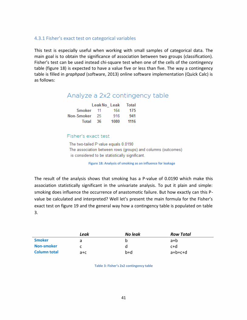
41

4.3.1 Fisher’s exact test on categorical variables This test is especially useful when working with small samples of categorical data. The main goal is to obtain the significance of association between two groups (classification). Fisher’s test can be used instead chi-square test when one of the cells of the contingency table (figure 18) is expected to have a value five or less than five. The way a contingency table is filled in graphpad (software, 2013) online software implementation (Quick Calc) is as follows:

The result of the analysis shows that smoking has a P-value of 0.0190 which make this

association statistically significant in the univariate analysis. To put it plain and simple:

smoking does influence the occurrence of anastomotic failure. But how exactly can this P-

value be calculated and interpreted? Well let’s present the main formula for the Fisher’s

exact test on figure 19 and the general way how a contingency table is populated on table

3.

Leak No leak Row Total Smoker a b a+b Non-smoker c d c+d Column total a+c b+d a+b+c+d

Table 3: Fisher’s 2x2 contingency table

Figure 18: Analysis of smoking as an influence for leakage

42

Now that a general idea of how a contingency table works it’s time to introduce the formula to obtain the P-value:

Resulting p-value can be interpreted as “the probability of obtaining a test statistic at least as extreme as the one that was actually observed, assuming the null hypothesis is true [3.2]”. P values under 0.05 are generally considered to be statistically significant to determine that a variable has a strong influence on the outcome that is being measured.

4.3.2 Wilcoxon-Mann-Whitney on continuous variables The Wilcoxon-Mann-Whitney test is used to compare statistical significance between independent groups when the variables are continuous. Let’s exemplify a scenario where this approach is useful: Comparing the duration of surgery between patients presenting anastomotic failure and patients who doesn’t present this complication. Here we encounter that there are two independent random variables with duration in minutes, one from patients with anastomotic leakage and one from the rest of the patients. At the end the P-value will again show the significance of the variable to predict anastomotic failure. In general we can consider 2 assumptions to justify applying this test to a variable in this report:

The first assumption is that the dependent variable should be ordinal or an interval, this means that for example we are analyzing the weight of a patient in Kg. We clearly see that the interval is probably contained between 0 and 300 Kg.

Second assumption is that independent variable consists on groups of observations that are not related between each other. This means that there are different participants in the groups, for the analysis of patient information this is really obvious since we have two clearly defined groups (leak and no leak) with different patients on each of them.

When these two assumptions are completed we can proceed to apply the algorithm to calculate the P-value for Wilcoxon-Mann-Whitney. The standard algorithm consists on the following steps:

Figure 19: Fisher’s exact test formula

43

First step consist on sorting the values of both samples. Let’s say that group A has the values 3, 4, 22, 25 and group B has 1, 2, and 26. The sorted values will be 1, 2, 3, 4, 22, 25, and 26.

Second step consists on obtaining the product of size of Sample A and Sample B. In this particular example 3*4 =12

Third step is calculate N*(N+1)/2 Sample A has four instances hence 4*5/2 = 10

Fourth step is obtaining the sum the order of the group used on the last step. In this case we used Sample A so we obtain the sum 1+2+3+4= 10

Finally we sum the result from step two to the result of step 3 and we subtract the result of step 4. In this example 12 + 10 -10 = 12. These results give us the U variable which can be checked on a tabulation table.

Obviously the algorithm can be applied manually for small samples, for this report a python script already implemented on a web application was used (Sciences, 2013). Figure 20 shows an example of how this application works.

4.4 statistical analysis results Now is time to present the results of the univariate analysis. Let’s determine which variables are statistically relevant to this study and select them as features for the classifiers.

Figure 20: Wilcoxon-Mann test web application

44

Variable Total sample N= 1116

Anastomotic Failure N= 36

Anastomotic failure not

present N=1080

P value

Gender Male Female

321(28.76%) 795(71.23%)

11(30.5%) 25(69.4%)

310(28.7%) 770(71.29%)

0.8519 0.8519

BMI 45.66 ± 7.23 45.28 ± 7.71 45.68 ± 7.22 0.5417

Weight 133.12 ± 25.43 133.72 ± 24.88 133.10 ± 25.46 0.7513

Age 44 ± 11.54 44 ± 10.65 44 ± 11.58 0.4607

Excess Weight 49.33 ± 35.110 55.51 ± 28.86 49.12 ± 35.29 0.4607

Table 4: Patient Characteristics

The results of analyzing patient characteristics and their influence on anastomotic failure are presented on table 4. This part of the analysis shows that there are no variables with a P-value less than 0.05 which is the threshold that is generally used to determine the significance of a variable in a univariate test. We can conclude then, that there is not a direct influence on the occurrence of leakage with this set of variables.

Variable Total sample N= 1116

Anastomotic Failure N= 36

Anastomotic failure not

present N=1080

P value

Smoking 175 (15.6%) 11 (30.55%) 164 (15.1%) 0.0190

Diabetes 254(22.7%) 6(16.6%) 248(22.9%) 0.5436

Osteaoarticular 502(45%) 15(41.6%) 488(45.1%) 0.7355

Reflux 151(13.5%) 6(16%) 145(13.4%) 0.6177

Cardiovascular 107(9.5%) 4(11.1%) 103(9.53%) 0.7708

Antihypertension 346(31%) 9(25%) 337(31.2%) 0.4706

Anticoagulance 121(10.8%) 5(13.88%) 116(10.7%) 0.5815

Lipids lower 207(18.5%) 6(16.6)% 201(18.6%) 0.9999

Puff 155(13.8%) 10(27.7%) 145(12.9%) 0.0240

Antacids 190(17%) 12(33%) 178(16.4%) 0.0129

Pain killers 136(12.1%) 6(16.6%) 130(12.3%) 0.4326

Table 5: Assessment of comorbidities and medication taken by the patient before surgery.

45

Table 5 starts to show that there are actually variables with a strong influence on leakage. It is widely known and expected that smoking is related to a lot of health problems so it comes as no surprise that 30% of patients presenting anastomotic failure are smokers compared to only 15% of the patients not presenting this complication. The surprising result is that 2 medications have also a statistically significant value when predicting anastomotic failure and these are: antacids and inhalation medication. Doctors should pay special attention to patients in these three groups (smokers, antacids, inhalation medication).

Variable Total sample N= 1116

Anastomotic Failure N= 36

Anastomotic failure not present N=1080

P value

Fast-track approach

601(53.85%) 11(30.5%) 590(54.62%) 0.0059

Normal track approach

515(46.1%) 25(69%) 490(45.3%) 0.0058

Laparoscopic approach

1097(98.2%) 31(86%) 1066(98.7%) 0.0002

Conversion approach

7(0.006%) 2(5.55%) 5(0.4%) 0.0197

Open approach

12(1%) 3(8.33%) 9(0.8%) 0.0056

Endo GIATM stapler

242 (21.6%) 15(41.6%) 227(21%) 0.0063

DUET TRSTM stapler

117(10.4%) 4(11%) 113(10.4%) 0.7850

TRI-strapleTM stapler

757(67.8%) 17(47.2%) 740(68.5%) 0.0100

Duration

54.38± 25.72 76.55± 41.26 53.64± 24.73 0.0003

Table 6: Bariatric surgery characteristics

The characteristics of the surgery have the strongest influence on the occurrence of anastomotic failure (especially considering older procedures at the hospital), nevertheless in very important to mention that the hospital went from practices that were leading to anastomotic failure, to reducing the percentage of patients presenting the complication. To elaborate further in this explanation we can mention that for example the use of Normal track approach has an influence on the appearance of anastomotic failure after surgery, but the change to a Fast track approach completely reversed the tendency and now it even has a positive statistical significance. It is possible to say now that Fast track approach is actually helping to prevent anastomotic failure. Moreover we can see that the stapling technique also improved over time. If we take the first stapler surgeons were using called Endo GIATM a P value of 0.0063 is obtained showing that it has a bad

46

performance and was causing more cases of anastomotic failure. This situation changes completely when the latest stapler technique is taken into account, the TRI-strapleTM stapler has a positive influence with a P-value of 0.0100 showing that the change on the stapler machine helped to reduced occurrences of anastomotic failure.

Another important situation to consider is that even if 98% of the bariatric surgeries are performed using a laparoscopic procedure (with good results) things change a drastically when surgery is performed as a conversion or using an open approach. These two approaches present a high risk of anastomotic failure after surgery, to exemplify this is possible to see on table 6 that only 1.7% (19 cases) of the patients are having surgery with one of these two approaches, but looking at the incidence of anastomotic failure 5 cases are related to a surgery performed with either open or conversion approach which account of 14% of the total cases of anastomotic failure. Finally the duration of the surgery comes as a very strong predictor for leakage. How can the duration be interpreted or related to the occurrence of complications as anastomotic failure can be seen as follows: The longer the surgery the more complex it was. When a patient undergo a complicated surgery there is a higher probability that some complications may appear after the procedure. This is reflected on the P value obtained when analyzing surgery duration (P = 0.0003). After analyzing these results, is possible to conclude that the hospital is moving in a good direction by improving their equipment (Staplers) and processes (Fast track) in order to lower occurrences of anastomotic failure.

Variable Total sample N= 1116

Anastomotic Failure N= 36

Anastomotic failure not

present N=1080

P value

MBP < 70 mmHg for 15 or more minutes

414(37%)

19(52.7%)

395(36.5%)

0.0542

MBP < 70 mmHg for 20 or more minutes

315(28.22%)

17(47.22%)

298(27.5%)

0.0139

MBP < 60 mmHg for 15 or more minutes

133(11.9%)

6(16.6%)

127(11.7%)

0.4274

MBP < 60 mmHg for 20 or more minutes

64(5%)

1(2%)

63(5.8%)

0.7174

Mean duration of hypotension episode MBP

15.21± 16.17

20.19± 29.11

14.99± 15.35

0.3015

Table 7: Hypotension episodes mean blood pressure.

47

One of the research questions purposed on this project mentions the interest of knowing how hypotension episodes and their duration influence the appearance of anastomotic failure after surgery. As it is shown on table 7 almost 48% of the patients presenting leakage had a hypotension episode of mean blood pressure below 70 mmHg for 20 or more minutes. Patients without the anastomotic failure complication only presented this episode on 28% of the cases therefore we see a statistically significant P value of 0.0139 showing that special attention needs to be put on patients that present long mean blood pressure hypotension episodes. On average the mean duration of a mean blood pressure hypotension episode is longer on patients who presented complications, but because the standard deviation is quite big this variable doesn’t have a statistically significant P value according to Wilcoxon-Mann-Whitney test.

Variable Total sample N= 1116

Anastomotic Failure N= 36

Anastomotic failure not

present N=1080

P value

SBP < 100 mmHg for 15 or more minutes

506(45.3%) 23(62.88%) 483(44.7%) 0.0267

SBP < 100 mmHg for 20 or more minutes

405(36.2%) 21(58.33%) 384(35.5%) 0.0075

SBP < 90 mmHg for 15 or more minutes

293(26.2%) 13(36.11) 280(25.9%) 0.1798

SBP < 90 mmHg for 20 or more minutes

200(17.2%) 9(25%) 191(17.6%) 0.1794

Mean duration of an hypotension episode SBP

17.34± 17.71

22.99± 27.67

17.1± 17.1

0.03258

Table 8: Hypotension episodes mean blood pressure

Thresholds were also set for systolic blood pressure hypotension episodes (100 and 90 mmHg for 15 or more minutes). According to the statistical analysis presented on table 7 conclusions can be drawn from the information contained on the hypotension tables created for systolic blood. In a similar interpretation as the one given to mean blood pressure analysis, it can be determined that the occurrence of hypotension episodes do influence the appearance of anastomotic failure in patients.

48

In this particular case, episodes below 100 mmHg with duration larger than 15 minutes show a P value of 0.0267 and episodes with duration larger than 20 minutes show a P value of 0.0075 which shows a really strong statistical significance to predict leakage. Comparing the mean duration of the episodes it was found that in the case of systolic blood pressure it does have an influence on anastomotic failure (P= 0.03258).

4.5 WEKA (Waikato Environment for Knowledge Analysis) In order to compare machine learning algorithms and their performance in the 4KP/Sleeves databases to find to which degree they are suitable to predict anastomotic failure, WEKA software will be used. WEKA is suite of machine learning algorithms for data mining written in Java. It has the advantage of providing Java code to use on your own application given the case the user wants to build a prediction application from scratch while using already implemented machine learning algorithms. WEKA also provides a graphical front-end to carry analysis of data when the user provides raw files in the form of CVS or Excel files. WEKA software is open source and therefore highly adaptable to specific needs that developers might have. It is also supported by a really active community and extensive documentation which makes it easy to use and learn.

The final goal of this project is determined which machine learning algorithms are more suitable to predict anastomotic failure. In order to archive this goal a series of CVS files were created from the features obtained in the previous section and the graphical front end of WEKA was used to analyze the results. Figure 21 presents the main screen that users get when opening WEKA.

Figure 21: WEKA main screen

49

From this screen the user can choose to load one file containing features to perform clustering or classification tasks. Specifically for this analysis a CVS file was created containing the statistically significant features obtained from statistical analysis described on previous section of this chapter (See feature selection). The file contains the following fields: Smoke assessment, antacids assessment, inhalation medication assessment, surgery duration, systolic blood pressure hypotension episodes under 100 mmHg for 20 minutes or more, mean blood pressure hypotension episodes under 80 mmHg, average systolic blood pressure, stapler technique, surgery approach, track (fast or normal) and outcome (leak or no leak).

WEKA provides users with several machine learning algorithms, they are grouped according to their characteristics and are really easy to select and play around with. To perform data mining tasks, algorithms are conveniently grouped as follows (main groups):

Bayes: This group contains obviously all the variables of Naïve Bayes algorithms including Bayesian logistic regression.

Functions: Multiple regression algorithms.

Lazy: Contains lazy learning algorithms based on entropy distance, generalization beyond training data, nearest neighbors etc.

Trees: A set of decision trees algorithms like random forest, CART, and J48.

Figure 22: Example CVS file containing relevant features for predicting anastomotic failure.

Figure 23: WEKA classification groups

50

4.5.1 Dealing with imbalanced set of data for classification in WEKA

4KP/Sleeves database has the particularity of being really imbalanced on the class distribution (leak or not leak). Only 3% of the patients present anastomotic failure which makes this class heavily unrepresented in comparison with the rest of patients who don’t present this complication (Figure 24).

Of course this characteristic is very important because it can lead classification algorithms to misclassify instances. There are common approaches to overcome this kind of situations, one research that really describes and offer solutions to the overall problem is The class imbalance problem in pattern classification and learning published by Universitat Jaume 1 in Spain (V.García, 2007). They describe four possible approaches to increase the accuracy of machine learning algorithms when dealing with imbalanced sets of data, for the scope of this project two of them are specially relevant and applicable in WEKA:

Resample to balance the data set: This approach involves over-sampling or under-sampling the classes in order to have a balance between the classes so that they are represented equally. In the particular case of patients presenting anastomotic failure an over-sampling of this class can be performed, because there are only 36 cases to analyze. One of the main drawbacks of over-sampling is that for big amounts of data this can damage the performance of data mining algorithms due to the increased load of computational work that this can signify. Of course this is not a huge problem in this case since the size of the database is only 1116 records.

Figure 24: Imbalanced classes in WEKA

51

Nevertheless the distribution of the class might change introducing some noise to the analysis.

Modify data at algorithm level: Adding some weight to the classification outcome can help balancing the dataset. To illustrate this we can talk about cost-sensitive classifiers implemented in WEKA. The idea behind this is to give weight to the examples. Let’s say is possible to assign a higher weight to false negatives. In the case of this data set 10 false negatives are equivalent to 3 false positives. So the idea is to give false negatives a higher weight in order to balance the representation of the data and penalized them more.

The way to implement these two approaches in WEKA involves some pre-processing of information and tuning the classification algorithms a little bit. Let’s start by explaining what is SMOTE (synthetic minority over-sampling technique) and how to implement over-sampling in WEKA. This approach has been use in health care field because it is fairly common that rare diseases can create highly imbalanced data sets (Rok Blagus, 2013). Different approaches for over-sampling the under-represented class can be applied depending on the data mining algorithm used to analyze the data. For example decision trees are especially sensitive to over-sampling because they tend to overfit when several exact copies of the class instances are created. One way to overcome this problem is using SMOTE approach for over-sampling. The idea behind SMOTE is not to replicate exactly the instances of the minority class several times in order to balance the number of appearances of the under-represented class, instead it will generate synthetic class instances interpolated between instances contained in the dataset that are similar to them. This can be understood basically as nearest neighbor approach to generate new instances and this is the way WEKA actually creates the new instances for the minority class. After this brief explanation of SMOTE, now it is time to proceed to WEKA and implement that for Sleeves/4KP dataset. WEKA has several filters to pre-process the data. These filters are basically divided in two groups: Supervised (classification) and unsupervised (clustering) filters. In this particular case is obvious that a supervised approach to add instances is needed. Figure 25 shows how SMOTE can be selected from the set of filters.

Figure 25: SMOTE filter selected in WEKA

52

Arbitrary number if new instances can be added using this filter in order to do over-sampling. After applying the filter the minority class is now properly represented with around 30% of the instances representing patients with anastomotic failure. Figure 26 shows the change in size of the minority class.

Over sampling is now done for the vector space. Unfortunately the way WEKA creates

these instances is not optimal for doing cross-validation since all the created instances are

written at the end of the CVS file. This means that when the folds for cross-classification

are selected there is a very high possibility that one of the folds will contain a huge

amount of patients with anastomotic failure. Of course this problem will decrease the

accuracy of the classifier. WEKA offers another filter to deal with this particularity and it is

called randomize. This filter will take all instances and just create a file with them

combined in random order.

Figure 26: Over-sampling the minority class

Figure 27: Randomize filter

53

The second approach to overcome imbalanced class distribution in sets of data is use cost-sensitive classifiers wrappers. Like it was already explained the idea behind this is to assign weights to the false negatives in order to balance the classifier. The application of this technique is very straightforward in WEKA and can be done in four simple steps.

Load the features vector into WEKA using the pre-process tab.

Select the Cost-Sensitive-Classifier in WEKA’s classification tab and access the properties tab.

Fill the 2x2 cost matrix to assign values to the false negatives and true positives according to the classification needs (Figure 28).

Finally select the classifier on which Cost-sensitive learning will be applied and perform the classification task.

Most classification algorithms can benefit from applying a cost-sensitive learning. J48

Decision trees, Random Forest and Support Vector Machines can benefit a lot from this

approach since they have intrinsic procedures of optimization in their algorithms.

Now that the problem of imbalanced data is solved the classification task for anastomotic failure can be performed using different algorithms. It was explained on chapter 3 that logistic regression, decision trees and random forest are going to be tested and compared in order to find a suitable predictive model for anastomotic failure using the data provided at the Catharina Hospital. In the next chapter the results of applying these algorithms with WEKA will be presented and conclusions will be introduced.

Figure 28: Filling the cost matrix in WEKA

54

5. Experiment Results: Interpreting Classification Outcome. We can now recapitulate on the main goals of this research. First goal was to discover which data was available at the hospital that was helpful to determine which kind of predictions could be made about bariatric surgery complications. The second was to find if hypotension episodes are related to the occurrence of anastomotic failure. Finally is time to compare the performance of the different predictive models for anastomotic failure. Each machine learning algorithm will be tested with the cost-sensitive learning approach and afterwards with the SMOTE over-sampling approach. Each algorithm will used cross- validation with ten folds of the data. The way of comparing the performance will be according to the WEKA output namely: Kappa statistic, ROC Area under the curve (AUC), accuracy, precision and recall. In this chapter the outcome of each algorithm will be presented and interpreted in order to find the most suitable predictive model for this classification problem.

55

5.1 Logistic regression results SMOTE

Prediction quality measures

Accuracy 78.11% Precision(leak) 66%

Recall(leak) 36% Kappa statistic 0.3507

ROC area 0.788

Predicted as

No Leak Leak

No Leak 1007 73 Leak 250 146

Roc Curve

Results description: An overall accuracy of 78% reflects a good performance of the classifier under these settings, nevertheless taking a closer look at the metrics is possible to notice that only 36% cases of leakage were detected. Moreover even if AUC shows that the classifier can discriminate fairly well under different thresholds, the Kappa statistic for the optimal threshold is only 0.35 which indicates that there are a good amount of instances selected by chance. Overall this predictive model doesn’t perform well detecting anastomotic failure.

Figure 29: Roc curve for logistic regression with SMOTE over sampling

56

5.2 Logistic regression results Cost-Sensitive Learning

Prediction quality measures

Accuracy 95.69% Precision(leak) 20%

Recall(leak) 11% Kappa statistic 0.1226

ROC area 0.573

Predicted as

No Leak Leak

No Leak 1064 16 Leak 32 4

Roc Curve

Results description: Accuracy is really high on this settings but this metric is misleading. Only 11% of the cases of anastomotic failure were detected and the ROC curve shows that the classifier’s performance under different thresholds doesn’t discriminate between classes better than chance. The high accuracy can be explained by the over-representation of the majority class.

Figure 30: Roc curve for logistic regression with Cost-Sensitive learning

57

5.3 Decision Tree results SMOTE

Prediction quality measures

Accuracy 87.94% Precision(leak) 78%

Recall(leak) 75% Kappa statistic 0.6884

ROC area 0.896

Predicted as

No Leak Leak

No Leak 1000 80 Leak 98 298

Roc Curve

Results description: These settings offer satisfactory results. Accuracy is high predicting 87% of the cases correctly. Anastomotic failure prediction is also good because 75% of the cases were detected by the classifier. Kappa shows that with the optimal settings the classifier behaves 68% better than if the results were by chance. AUC indicates that the classifier discriminates very well under different thresholds also.

Figure 31: Roc curve for Decision Trees with SMOTE over-sampling

58

5.4 Decision Tree Cost-Sensitive Learning

Prediction quality measures

Accuracy 94.7% Precision(leak) 15%

Recall(leak) 13% Kappa statistic 0.1177

ROC area 0.442

Predicted as

No Leak Leak

No Leak 1052 28 Leak 31 5

Roc Curve

Results description: Decision tree with Cost-Sensitive learning presents bad results. Only 13% of the cases of anastomotic were detected which makes this a very flawed predictive model to be applied to classify this complication.

Figure 32: Roc curve for decision tree with Cost-Sensitive learning

59

5.5 Random Forest results SMOTE

Prediction quality measures

Accuracy 90.44% Precision(leak) 84%

Recall(leak) 78% Kappa statistic 0.7513

ROC area 0.948

Predicted as

No Leak Leak

No Leak 1023 57 Leak 84 312

Roc Curve

Results description: These are the best results of the experiment. They present a really high accuracy and precision, also 78% of the cases of anastomotic failure were detected by the classifier which provides certainty. The AUC shows that the classifier discriminates instances almost perfectly under several different thresholds. Kappa for the optimal threshold shows that results are not selected by chance.

Figure 33: Roc curve for Random Forest with SMOTE over-sampling

60

5.6 Random Forest results Cost-Sensitive learning

Prediction quality measures

Accuracy 95.44% Precision(leak) 11%

Recall(leak) 5% Kappa statistic 0.0595

ROC area 0.606

Predicted as

No Leak Leak

No Leak 1065 15 Leak 34 2

Roc Curve

Results description: Again some bad results were obtained with cost-sensitive classification. All results are classified by chance according to Kappa and the algorithm doesn’t make a discrimination of the classes. Minority class doesn’t have the characteristics to draw conclusive results even when penalizing false negatives since only 5% of the cases of anastomotic failure were detected.

Figure 34: Roc curve for Random Forest with Cost-Sensitive learning

61

5.7 Discussion

There are several studies related to the prediction of surgical outcomes. However finding to which degree a predictive model is suitable for predicting anastomotic failure on bariatric surgery is a new contribution and was the main goal behind this study. Gathering data at the hospital supported by the opinion of experts was a fundamental step to perform a data mining study. Statistical analysis was used to justify the selection of features to be used on a classifying task and it provided medical insight on the causes of anastomotic failure. It was found that duration of the surgery (complexity), having en open surgery, following the conventional track, using ENDO GIATM stapling technique, taking antacids, having systolic blood pressure episodes, smoking, inhalation medicine, mean blood pressure episodes and the duration of the hypotension episodes play a significant role on the appearance of anastomotic failure after surgery (See chapter 4 for the statistical analysis details). Fortunately for the Catharina Hospital some of the practices that are leading to anastomotic failure have been updated or are not very common. For example doing surgery with the conventional track or the use of ENDO GIATM staplers are not applicable anymore, also open and conversion surgeries account only for 3% of the procedures. This situation indicates that new procedures at the hospital are making bariatric surgery safer. Nevertheless this studied took into consideration all the variables contained in the hospital’s databases across time so these particularities of the procedures were used in the classification task. Three predictive models (logistic regression, decision trees, and random forest) were tested to find if their performance is good enough to predict anastomotic failure and use them as possible guide for decision making. SMOTE over-sampling and Cost-sensitive classification wrapper were used to overcome the problem of having an imbalanced set of data. The models were tested against different metrics like accuracy, precision, recall, kappa statistic and AUC. In general the models had a good performance when using SMOTE over-sampling, but a careful interpretation of these results is needed. The synthetic instances introduced by WEKA, even though similar to the instances contained on the data, present small difference which may alter the distribution of the minority class. Of course the models benefit from the fact that more instances are present in the dataset and therefore a better generalization can be made; this is the main reason of the good performance of the algorithms. On the other hand Cost-Sensitive learning probably was affected due the fact that the 10 fold settings of the classifier in WEKA prevent instances from the minority class to be represented in these folds in a proper way so diminishes the opportunity to obtain a general model. Random Forest and decision trees using SMOTE over sampling are suitable algorithms to predict anastomotic failure, both of them detected more than 75%of the cases for this complication. Moreover a decision tree can provide a graphical representation for decision making and the relationship between variables. The underperformance of logistic regression can be explained because of the complex non-linear relations that might exists in the data, also is arguable if logistic regression is the more suitable model when using categorical variables mostly.

62

6. Conclusions This chapter will provide a reflection on the research questions purposed on for this investigation also a conclusion and future work will be suggested in order to provide direction for people who wants to continue this research.

6.1 Reflection on the research questions Main research question: To which degree can machine learning algorithms be used to predict anastomotic failure in bariatric surgery? This research demonstrates that machine learning algorithms can present a good solution to predict the appearance of anastomotic failure after surgery. An accuracy of 90% on the prediction was archived when taking into account both classes (leak and no_leak) when applying a Random Forest solution, moreover 78% of the cases of anastomotic failure were detected successfully under these settings. It is also possible to provide a graphical representation of a predictive model when a decision tree is implemented. J48 decision tree algorithm provides 88% accuracy with 75% of the cases of anastomotic failure detected by the predictive model. To conclude we can say that it is possible to use predictive models as a guide to determine if a patient will present anastomotic failure. Important sub-questions RSQ1. - Which information from the available hospital databases can be obtained to train a predictive model? The doctors provided two datasets containing extensive information about the patient’s characteristics and their behavior while they are under sedation. This information helped to create a new database containing complete information to draw conclusions and find relationships on this data. The expertise of the doctors also helped in the process of variable selection. Their insight provided the guide to find out which variables could be relevant when using a classification approach. It was found that data about the patient’s lifestyle, surgery characteristics, blood pressure during surgery and medication assessment was available at the hospital’s information systems. This data was enough to test different predictive models with satisfactory results. RSQ2. – What is the performance of different machine learning methods when predicting anastomotic failure? Overall decision trees and random forest presented satisfactory results when using SMOTE over-sampling (please refer to chapter 5 for a complete overview of the

63

performance results). The optimal performance was found when using random forest with SMOTE over-sampling with performance of an accuracy of 90% and a detection of 78% of the cases of anastomotic failure. Cost-sensitive learning didn’t provide good results because of the 10 fold cross validation set up for this experiment. RSQ3. - Are hypotension episodes useful for predicting anastomotic failure? It was demonstrated that hypotension episodes are statistically significant variables when trying to predict anastomotic failure (See chapter 4). Systolic blood pressure hypotension episode of 20 or more minutes below 100 mmHg is statistically significant to predict anastomotic failure. In a similar way mean blood pressure hypotension episodes of 15 or more minutes with less than 70 mmHg also help to predict the complication. To give an example patients presenting a systolic hypotension episode of 100 mmHg with duration of 20 minutes or more combined with conventional track, TRI-stapler technique, average blood pressure of more than 85 mmHg, smokers, and a surgery with duration of more than 58 minutes have a really high probability to present leakage (6 out of 7 patients with this characteristics presented leakage). In order to find more of this type of relations a look at the decision tree presented by WEKA can be helpful.

6.2 Thesis Conclusions

After getting the results of the classification task is possible to provide some conclusions about the outcome of the study. The first conclusion deals with the fact that Cost-Sensitive learning was not a successful approach to deal with imbalanced data. The reason for this is that explanatory variables in the features vector are probably not enough to find an underlying model for prediction while having only 36 cases of anastomotic failure. Cost-Sensitive learning doesn’t create more instances and therefore cross-validation folding can prevent the machine learning algorithm of noticing some patients with anastomotic failure.

Logistic regression is not a good approach for classifying anastomotic failure because inserting new instances with SMOTE over-sampling means introducing noise and outliers to the data in a random way. Decision trees and Random Forest are really good dealing with this situation (noise in the data) but Logistic regression doesn’t offer this benefits. It is possible to argue that since most of the selected features are constructed from categorical variables, Logistic regression is not the best approach to begin with. Decision trees can predict anastomotic failure with an accuracy of 75%, which is acceptable. The advantage of this model is that it provides a graphical outcome which can be interpreted easily by the doctors without implementing software to get the prediction.

64

Random Forest presented the best solution for this classification problem, with 90% accuracy to predict leakage. The disadvantage of this result is that its “black box” nature doesn’t give insight about the relation about the variables relationships.

6.3 Future work This research is a starting point to predict complications on bariatric surgery. The scope of this project was to set the foundation of data analysis with the 4KP and Sleeves databases. Similar approaches can be followed in the future for every kind of complication and not only for anastomotic failure. A nice project would be to develop a general application in Java to use the WEKA models in order to predict complications just after the surgery. This could provide the doctors with an advanced clinical decision system that can help them to save lives and costs related to complications in surgeries. Another important improvement would be to find a way of create the Sleeves database automatically. So far it is filled by hand by the surgeons in a SPSS file, which makes the update process quite slow. I consider that the priority is to develop architecture to implement an application for clinical decision making with WEKA as a front-end with an underlying ETL to update Sleeves database automatically and merged it with the 4KP on a daily basis.

65

References Abell TL, M. A. (2006). Gastrointestinal complications of bariatric surgery: diagnosis and therapy.

Mississippi: Am. J. Med. Sci.

Ahsan M. Arozullah, J. D. (2000). Multifactorial Risk Index for Predicting Postoperative Respiratory

Failure in Men After Major Noncardiac Surgery. Ann Surg, 242-253.

Alqahtani AR, A. B. (2012). Laparoscopic sleeve gastrectomy in 108 obese children and adolescents

aged 5 to 21 years. Department of Biostatistics, Obesity Research Chair, College of

Medicine, King Saud University, Riyadh, Saudi Arabia, 266-273.

Bijker JB, v. K. (2009). Intraoperative hypotension and 1-year mortality after noncardiac surgery.

Anesthesiology, 1217-1226.

Dixon, J. B. (2010). The effect of obesity on health outcomes. Molecular and Cellular

Endocrinology, 104–108.

Finks JF, K. K. (2011). Predicting risk for serious complications with bariatric surgery: results from

the Michigan Bariatric Surgery Collaborative. Ann Surg, 633-640.

Fisher BW, M. S. (2002). Predicting pulmonary complications after nonthoracic surgery: a

systematic review of blinded studies. Am J Med, 219-225.

Hyman N, M. T. (2007). Anastomotic leaks after intestinal anastomosis: it's later than you think.

Dept. of Surgery, Fletcher 464, University of Vermont College of Medicine, 254-258.

I. L. Post, P. M. (2012). Intraoperative blood pressure changes as a risk factor for anastomotic

leakage in colorectal surgery. International Journal of Colorectal Disease , 765-772.

Kotsiantis, S. B. (2007). Supervised Machine Learning: A Review of Classification Techniques.

Informatica, 249–268.

Lakdawalla, D. &. (2002). The Growth of Obesity and Technological Change: A Theoretical and

Empirical Examination. Economics and Human Biology, 283-293.

Myles S Faith, P. E. (2002). Obesity–depression associations in the population. Journal of

Psychosomatic Research, 935-942.

Obesity Education Initiative Expert Panel on the Identification, Evaluation, and Treatment of

Obesity in Adults. (1998). Clinical Guidelines on the Identification, Evaluation, and

Treatment of Overweight and Obesity in Adults. Maryland: National Heart, Lung, and Blood

Institute.

66

Perdiguer, P. (2012). Analysis of operative times in bariatric surgery and modeling for

intraoperative complications’ consequence prediction in anesthetic procedures. Eindhoven:

Eindhoven University of Technology.

Peter B. Jensen1, L. J. (2012). Mining electronic health records: towards better research

applications and clinical care. Nat Rev Genet, :395-405.

Rok Blagus, L. L. (2013). SMOTE for high-dimensional class-imbalanced data. Ljubljana: BMC

Bioinformatics .

Sciences, P. (May de 2013). Phonetic Sciences, Amsterdam. Recuperado el May de 2013, de

http://www.fon.hum.uva.nl/Service/Statistics/Wilcoxon_Test.html

software, G. p. (2013, May). QuickCalcs. Retrieved May 2013, from

http://graphpad.com/quickcalcs/contingency2/

Tu, J. V. (2006). Advantages and disadvantages of using artificial neural networks versus logistic

regression for predicting medical outcomes. Journal of Clinical Epidemiology, 1225-1231.

Tu, J. V. (2006). Advantages and disadvantages of using artificial neural networks versus logistic

regression for predicting medical outcomes. Journal of Clinical Epidemiology, 1225-1231.

U.N. Food and Agriculture Organization. (2013). The State of Food and Agriculture. Rome: U.N.

Food and Agriculture Organization.

Uzay Kaymak, A. B.-D. (2010). AUK: a simple alternative to the AUC. Rotterdam: Academic

Repository at Erasmus University.

V.García, J. R. (2007). The class imbalanced problem in patter classification and learning. Castelló:

Universitat Jaume.

Williams, G. (2010). Data Mining Desktop Survival Guide . togaware.com.

Xabier de Aretxabala, J. L. (2011). Gastric Leak After Sleeve Gastrectomy: Analysis of Its

Management. Obesity Surgery, 1232-1237.

Xindong Wu, V. K.-H. (2008). Top 10 algorithms in data mining. Knowledge and Information

Systems, 1-37.

67

Appendices Not much was left out of the main document, but in the appendices some SQL scripts and an overview of the decision tree created by WEKA using SMOTE over-sampling are included.

Appendix A SQL Hypotension cursor DECLARE @case_id INT

DECLARE @last_case_id INT

DECLARE @timestamp datetime

DECLARE @sysnibp smallint

DECLARE @meannibp smallint

DECLARE @dianibp smallint

DECLARE @group smallint

DECLARE @flag smallint

SET @group = 0

DECLARE db_cursor CURSOR FOR

SELECT *

FROM [Thesis].[dbo].s_tb_nibp

order by case_id, timestmp

OPEN db_cursor

FETCH NEXT FROM db_cursor INTO @case_id, @timestamp, @sysnibp, @meannibp,

@dianibp

Set @last_case_id = @case_id

WHILE @@FETCH_STATUS = 0

BEGIN

IF @meannibp > 80

BEGIN

INSERT INTO dbo.s_tb_nibp_groups (case_id, timestmp, sysnibp,

meannibp,dianibp, n_group)

Values(@case_id, @timestamp, @sysnibp, @meannibp,@dianibp, 0)

SET @flag = 0

FETCH NEXT FROM db_cursor INTO @case_id, @timestamp, @sysnibp,

@meannibp, @dianibp

IF @last_case_id != @case_id

BEGIN

SET @group = 0

SET @last_case_id = @case_id

END

END

ELSE

BEGIN

68

IF @flag = 0

BEGIN

SET @group= @group+1

END

INSERT INTO dbo.s_tb_nibp_groups (case_id, timestmp, sysnibp,

meannibp,dianibp, n_group)

Values(@case_id, @timestamp, @sysnibp, @meannibp,@dianibp, @group)

FETCH NEXT FROM db_cursor INTO @case_id, @timestamp, @sysnibp,

@meannibp, @dianibp

SET @flag = 1

IF @last_case_id != @case_id

BEGIN

SET @group = 0

SET @last_case_id = @case_id

END

END

END

CLOSE db_cursor

DEALLOCATE db_cursor

Vector for logistic regression insert into dbo.Sleeves_Vector

(IPnr,Gender,DOB,PBS,W,EW,BMI,Waist,DM_ass,Osteoart_ass,Reflux_ass,

Psych_ass,Smoke_ass,Cardio_ass,Med_anticoag_ass,Med_stomach_ass,Med_pain_

ass,Med_antiHT_ass,Med_lipid_ass,

Med_puffs_ass,DOS,YOS,[AS],Approach,DS,C)

Select IPnr,Gender,DOB,PBS,W,EW,BMI,Waist,DM_ass,Osteoart_ass,Reflux_ass,

Psych_ass,Smoke_ass,Cardio_ass,Med_anticoag_ass,Med_stomach_ass,Med_pain_

ass,Med_antiHT_ass,Med_lipid_ass,

Med_puffs_ass,DOS,YOS,[AS],Approach,DS,C

from Sleeves2006

go

UPDATE dbo.Sleeves_Vector

SET Class_Outcome = 'No_Leak'

WHERE C not in ('2', '23','26','27', '239','2346','3','9','19', '35',

'37' )

go

UPDATE dbo.Sleeves_Vector

SET Approach_tech = 'Laparoscopic'

WHERE Approach in ('1')

go

UPDATE dbo.Sleeves_Vector

SET Approach_tech = 'Conversion'

WHERE Approach in ('2')

go

69

UPDATE dbo.Sleeves_Vector

SET Approach_tech = 'Open'

WHERE Approach in ('3')

go

UPDATE dbo.Sleeves_Vector

SET Track = 'Conventional'

where DOS < '01-01-2011'

go

UPDATE dbo.Sleeves_Vector

SET Stapler_tech = 'ENDO'

where DOS < '2009-12-01'

go

UPDATE dbo.Sleeves_Vector

SET Stapler_tech = 'DUET'

where DOS >= '2009-12-01' and DOS < '2010-05-01'

go

UPDATE dbo.Sleeves_Vector

SET Stapler_tech = 'TRI'

where DOS >= '2010-05-01'

go

UPDATE dbo.Sleeves_Vector

SET Hypo_MBP_less70_20min = 'No'

where IPnr COLLATE DATABASE_DEFAULT not in (Select distinct z.patient_id

COLLATE DATABASE_DEFAULT from

[Hypotension].[dbo].[Duration_Ep_Hypo_MBP_Less70] p join

s_tb_case_descriptor z on

z.case_id = p.case_id where p.duration >=20)

go

UPDATE dbo.Sleeves_Vector

SET Hypo_SBP_less100_15min = 'Yes'

where IPnr COLLATE DATABASE_DEFAULT in (Select distinct z.patient_id

COLLATE DATABASE_DEFAULT from

[Hypotension].[dbo].[Duration_Ep_Hypo_SBP_Less100] p join

s_tb_case_descriptor z on

z.case_id = p.case_id where p.duration >=15)

go

UPDATE dbo.Sleeves_Vector

SET Hypo_SBP_less100_20min = 'No'

where IPnr COLLATE DATABASE_DEFAULT not in (Select distinct z.patient_id

COLLATE DATABASE_DEFAULT from

[Hypotension].[dbo].[Duration_Ep_Hypo_SBP_Less100] p join

s_tb_case_descriptor z on

z.case_id = p.case_id where p.duration >=20)

70

Getting the number of hypotension episodes --Number of episodes

Select d.patient_id, count(*) as episodes into temp_ep_mbp

from [Hypotension].[dbo].Duration_Ep_Hypo_MBP_Less70 b join (Select

case_id, patient_id from [Thesis].[dbo].s_tb_case_descriptor ) d

on b.case_id = d.case_id

group by patient_id

order by patient_id

go

Select d.patient_id, count(*) as episodes into temp_ep_sbp

from [Hypotension].[dbo].Duration_Ep_Hypo_SBP_Less100 b join (Select

case_id, patient_id from [Thesis].[dbo].s_tb_case_descriptor ) d

on b.case_id = d.case_id

group by patient_id

order by patient_id

go

UPDATE dbo.Sleeves_Vector

SET number_ep_hypo_MBP = episodes

from dbo.Sleeves_Vector join temp_ep_mbp on Ipnr COLLATE DATABASE_DEFAULT

= patient_id COLLATE DATABASE_DEFAULT

go

UPDATE dbo.Sleeves_Vector

SET number_ep_hypo_SBP = episodes

from dbo.Sleeves_Vector join temp_ep_sbp on Ipnr COLLATE DATABASE_DEFAULT

= patient_id COLLATE DATABASE_DEFAULT

go

drop table temp_ep_sbp

go

drop table temp_ep_mbp

go Script to merge Sleeve and 4KP databases. Select p.* into s_tb_case_descriptor

from [4kp].[dbo].tb_case_descriptor p, Sleeves2006 s

where (patient_id COLLATE DATABASE_DEFAULT = CAST(IPnr as varchar)

COLLATE DATABASE_DEFAULT)

and CAST (p.begintijd as date)= CAST (s.DOS as date)

order by patient_id

--Query to extract the patients from the tb_case_descriptor

Select * into mytable_from_descriptor

from tb_case_descriptor

where patient_id in (--Ids from my table (remember to use strings)

71

--Joins with other tables (tb_nibp)

Select p.* into s_tb_nibp

from [4kp].[dbo].tb_nibp p, s_tb_case_descriptor s

where p.case_id = s.case_id

--Joins with other tables (tb_abp)

Select p.* into s_tb_abp

from [4kp].[dbo].tb_abp p, s_tb_case_descriptor s

where p.case_id = s.case_id

--Joins with other tables (tb_aps_patdata)

Select p.* into s_tb_aps_patdata

from [4kp].[dbo].tb_aps_patdata p, s_tb_case_descriptor s

where p.case_id = s.case_id

--Joins with other tables (tb_bis)

Select p.* into s_tb_bis

from [4kp].[dbo].tb_bis p, s_tb_case_descriptor s

where p.case_id = s.case_id

--Joins with other tables (dbo.tb_compli_pending)

Select p.* into s_tb_compli_pending

from [4kp].[dbo].tb_compli_pending p, s_tb_case_descriptor s

where p.case_id = s.case_id

--Joins with other tables (dbo.tb_complicatie_nva)

Select p.* into s_tb_complicatie_nva

from [4kp].[dbo].tb_complicatie_nva p, s_tb_case_descriptor s

where p.case_id = s.case_id

--Joins with other tables (dbo.tb_complications)

Select p.* into s_tb_complications

from [4kp].[dbo].tb_complications p, s_tb_case_descriptor s

where p.case_id = s.case_id

--Joins with other tables (dbo.tb_csok_time_messages)

Select p.* into s_tb_csok_time_messages

from [4kp].[dbo].tb_csok_time_messages p, s_tb_case_descriptor s

where p.case_id = s.case_id

--Joins with other tables (dbo.tb_cvp_mean)

Select p.* into s_tb_cvp_mean

from [4kp].[dbo].tb_cvp_mean p, s_tb_case_descriptor s

where p.case_id = s.case_id

--Joins with other tables (dbo.tb_events)

Select p.* into s_tb_events

from [4kp].[dbo].tb_events p, s_tb_case_descriptor s

where p.case_id = s.case_id

--Joins with other tables (dbo.tb_fluidsheet)

Select p.* into s_tb_fluidsheet

72

from [4kp].[dbo].tb_fluidsheet p, s_tb_case_descriptor s

where p.case_id = s.case_id

--Joins with other tables (dbo.tb_given_infuus)

Select p.* into s_tb_given_infuus

from [4kp].[dbo].tb_given_infuus p, s_tb_case_descriptor s

where p.case_id = s.case_id

--Joins with other tables (dbo.tb_given_pumps)

Select p.* into s_tb_given_pumps

from [4kp].[dbo].tb_given_pumps p, s_tb_case_descriptor s

where p.case_id = s.case_id

--Joins with other tables (dbo.tb_given_pumps)

Select p.* into s_tb_given_pumps

from [4kp].[dbo].tb_given_pumps p, s_tb_case_descriptor s

where p.case_id = s.case_id

--Joins with other tables (dbo.tb_heart_sat)

Select p.* into s_tb_heart_sat

from [4kp].[dbo].tb_heart_sat p, s_tb_case_descriptor s

where p.case_id = s.case_id

--Joins with other tables (dbo.tb_icp_mean)

Select p.* into s_tb_icp_mean

from [4kp].[dbo].tb_icp_mean p, s_tb_case_descriptor s

where p.case_id = s.case_id

--Joins with other tables (dbo.tb_impactprinted)

Select p.* into s_tb_impactprinted

from [4kp].[dbo].tb_impactprinted p, s_tb_case_descriptor s

where p.case_id = s.case_id

--Joins with other tables (dbo.tb_masimo)

Select p.* into s_tb_masimo

from [4kp].[dbo].tb_masimo p, s_tb_case_descriptor s

where p.case_id = s.case_id

--Joins with other tables (dbo.tb_masimo_output)

Select p.* into s_tb_masimo_output

from [4kp].[dbo].tb_masimo_output p, s_tb_case_descriptor s

where p.case_id = s.case_id

--Joins with other tables (dbo.tb_nirs)

Select p.* into s_tb_nirs

from [4kp].[dbo].tb_nirs p, s_tb_case_descriptor s

where p.case_id = s.case_id

--Joins with other tables (dbo.tb_nmt)

Select p.* into s_tb_nmt

from [4kp].[dbo].tb_nmt p, s_tb_case_descriptor s

where p.case_id = s.case_id

--Joins with other tables (dbo.tb_oknr_history)

73

Select p.* into s_tb_oknr_history

from [4kp].[dbo].tb_oknr_history p, s_tb_case_descriptor s

where p.case_id = s.case_id

--Joins with other tables (dbo.tb_pap)

Select p.* into s_tb_pap

from [4kp].[dbo].tb_pap p, s_tb_case_descriptor s

where p.case_id = s.case_id

--Joins with other tables (dbo.tb_perfusie)

Select p.* into s_tb_perfusie

from [4kp].[dbo].tb_perfusie p, s_tb_case_descriptor s

where p.case_id = s.case_id

--Joins with other tables (dbo.tb_postop_sheet_simple)

Select p.* into s_tb_postop_sheet_simple

from [4kp].[dbo].tb_postop_sheet_simple p, s_tb_case_descriptor s

where p.case_id = s.case_id

--Joins with other tables (dbo.tb_preop_quality_survey)

Select p.* into s_tb_preop_quality_survey

from [4kp].[dbo].tb_preop_quality_survey p, s_tb_case_descriptor s

where p.case_id = s.case_id

--Joins with other tables (dbo.tb_printimage)

Select p.* into s_tb_printimage

from [4kp].[dbo].tb_printimage p, s_tb_case_descriptor s

where p.case_id = s.case_id

--Joins with other tables (dbo.tb_pulse_plethysmo_variation)

Select p.* into s_tb_pulse_plethysmo_variation

from [4kp].[dbo].tb_pulse_plethysmo_variation p, s_tb_case_descriptor s

where p.case_id = s.case_id

--Joins with other tables (dbo.tb_pulse_pressure_variation)

Select p.* into s_tb_pulse_pressure_variation

from [4kp].[dbo].tb_pulse_pressure_variation p, s_tb_case_descriptor s

where p.case_id = s.case_id

--Joins with other tables (dbo.tb_registration_form)

Select p.* into s_tb_registration_form

from [4kp].[dbo].tb_registration_form p, s_tb_case_descriptor s

where p.case_id = s.case_id

--Joins with other tables (dbo.tb_respiratie)

Select p.* into s_tb_respiratie

from [4kp].[dbo].tb_respiratie p, s_tb_case_descriptor s

where p.case_id = s.case_id

--Joins with other tables (dbo.tb_tee)

Select p.* into s_tb_tee

from [4kp].[dbo].tb_tee p, s_tb_case_descriptor s

where p.case_id = s.case_id

--Joins with other tables (dbo.tb_viewers_log)

Select p.* into s_tb_viewers_log

74

from [4kp].[dbo].tb_viewers_log p, s_tb_case_descriptor s

where p.case_id = s.case_id

--Joins with other tables (dbo.tb_vigileo)

Select p.* into s_tb_vigileo

from [4kp].[dbo].tb_vigileo p, s_tb_case_descriptor s

where p.case_id = s.case_id

--Joins with other tables (dbo.tb_waveforms)

Select p.* into s_tb_waveforms

from [4kp].[dbo].tb_waveforms p, s_tb_case_descriptor s

where p.case_id = s.case_id

75

Appendix B WEKA

The decision tree should be open in WEKA for a better appreciation.