Performance of Financial Ratios and Hedging

towards Firm Value of LQ45 companies in

Indonesia

By

Irdian

014201400063

A Skripsi presented to the

Faculty of Business President University

in partial fulfillment of the requirements for

Bachelor Degree in Management

January 2018

i

PANEL EXAMINERS

APPROVAL SHEET

The Panel of Examiners declares that the skripsi entitled

“PERFORMANCE OF FINANCIAL RATIOS AND

HEDGING TOWARDS FIRM VALUE OF LQ45

COMPANIES IN INDONESIA” that was submitted by Irdian

majoring in Management from the Faculty of Business was

assessed and approved to have passed the Oral Examinations on

26th February 2018.

Panel of Examiners

Name and Signature of

Chair – Panel of Examiner

Name and Signature of

Examiner 2

Name and Signature of

Examiner 3

ii

SKRIPSI ADVISER

RECOMMENDATION LETTER

This skripsi entitled “PERFORMANCE OF FINANCIAL

RATIOS AND HEDGING TOWARDS FIRM VALUE OF

LQ45 COMPANIES IN INDONESIA” prepared and

submitted by Irdian in partial fulfilment of the requirements for

the degree of Bachelor in Management. The skripsi has been

reviewed and has been satisfied to accord with the requirement

for further examination. Therefore, I recommend this skripsi to

proceed for the Oral Defence

Cikarang, Indonesia, 24th January 2018

Acknowledged by, Recommended by,

Dr. Dra. Genoveva, M.M. Dr. Drs. Chandra Setiawan, M.M., Ph.D

Head of Management Study Program Advisor

iii

DECLARATION OF ORIGINALITY

I declare that this skripsi, entitled “PERFORMANCE

OF FINANCIAL RATIOS AND HEDGING

TOWARDS FIRM VALUE OF LQ45 COMPANIES

IN INDONESIA” is, to the best of my knowledge and

belief, an original piece of work that has not been

submitted, either in whole or in part, to another

university to obtain a degree.

Cikarang, January 26th, 2018

Irdian

iv

Abstract

This research aims to determine the factors that affect firm value proxy by

Tobin Q ratio. The determinants factors used are financial ratios such as

current ratio, debt to asset ratio and return on equity along with other

factors: tax rate, firm size and hedging dummy. Quantitative method is used

and 16 companies with specific criteria under LQ45 that listed in Indonesia

Stock Exchange are chosen as sample. The results revealed that current ratio

and return on equity have a positive significant affect toward firm value,

meanwhile debt to asset and firm size have a negative significant affect

toward firm value. Hedging and tax rate have no significant affect toward

the firm value. The most significant affect toward firm value from this

research is Return on Equity.

Keywords: firm value, financial ratios, tax rate, firm size, hedging

v

ACKNOWLEDGEMENT

In the name of God, the Most Gracious and the Most Merciful.

First of all, the researcher would like to deliver my highest gratitude to the

One and Only God, for His guidance and reinforcement in all time

especially during the completion of this study.

Researcher would like to convey immeasurable appreciation and deepest

thankfulness to these distinctive people who have given their full support in

making this study possible.

1. Researcher‟s best adviser, Dr. Drs. Chandra Setiawan, M.M., Ph.D., for

his indulgent guidance and constant support. The success of this research is

built within his constructive feedbacks during the research process.

2. Researcher‟s beloved parents, Syaiful Bunardi and Bong Siu Lan

together with the most outstanding brothers, Irwan Saputra, Hengki Setiadi,

Irvin for their support to encourage me until finished.

3. Tommy Saputra, Bayu Surya Dani, Ni Putu Kanilla Wati, Frengki

Wijaya, Aloysius Haryo Nugroho, Yasika Ayudaning Puspita, Laila

Sundari, Riska Ayu Saraswati, Jimmy Tan, Tubagus Achmad Rachmad

Saleh, Kaori Diana Putri, Marlinda and Sir Chandra’s fellow guidance and

all the Zombie squads, thanks for the moral support, sincere friendship and

unforgettable memories.

vi

To those who indirectly contribute in this research, your kindness matters a

lot for the researcher. Thank you very much.

Cikarang, January 26th, 2018

Irdian

vii

Table of Contents

PANEL EXAMINERS .............................................................................. i

SKRIPSI ADVISER ................................................................................. ii

RECOMMENDATION LETTER ............................................................ ii

DECLARATION OF ORIGINALITY .................................................... iii

Abstract .................................................................................................... iv

ACKNOWLEDGEMENT ........................................................................ v

List of Acronym ........................................................................................ x

Chapter I .................................................................................................... 1

INTRODUCTION .................................................................................... 1

1.1 Background of Study ....................................................................... 1

1.1.1 Need for study ............................................................................... 4

1.2 Problem Statement ........................................................................... 5

1.3 Research Questions .......................................................................... 6

1.4 Research Objectives ......................................................................... 6

1.5 Significant of Study ......................................................................... 7

1.6 Limitation ......................................................................................... 7

1.7 Thesis organization .......................................................................... 8

Chapter II .................................................................................................. 9

LITERATURE REVIEW ......................................................................... 9

2.1 Theoretical Review .......................................................................... 9

2.1.1 Firm Value ............................................................................. 9

2.1.2 Theory of Capital Asset Pricing Model ................................. 9

2.1.3 Corporate Risk Management ............................................... 10

2.1.5 Tobin Q Ratio as Measured ................................................. 11

2.2 Previous Research .......................................................................... 15

2.3 Research Gap ................................................................................. 18

viii

2.4 Theoretical Framework .................................................................. 19

2.5 Hypotheses ..................................................................................... 20

Chapter III ............................................................................................... 21

METHODOLOGY .................................................................................. 21

3.1 Research Method ........................................................................... 21

3.2 Research Framework ..................................................................... 22

3.3 Research Instrument ...................................................................... 23

3.4 Sampling Design ............................................................................ 23

3.4.1 Size of Population .................................................................... 23

3.4.2 Size of Sample ......................................................................... 24

3.5 Data Analysis ................................................................................. 26

3.5.1 Descriptive Statistic Analysis .............................................. 26

3.5.2 Panel Data Regression ......................................................... 27

3.5.3 Classical Assumption Test ................................................... 30

3.5.4 Multiple Regression Analysis .............................................. 34

3.6 Testing Hypotheses .................................................................... 36

3.6.1 Significant Level .................................................................. 36

3.6.2 T-test .................................................................................... 36

3.6.3 F-Test ................................................................................... 38

3.6.4 Coefficient of Determination ............................................... 40

Chapter IV ............................................................................................... 41

ANALYSIS OF DATA ........................................................................... 41

4.1 Company Profile ............................................................................ 41

4.2 Descriptive Analysis ...................................................................... 44

4.3 Data Analysis ................................................................................. 46

4.3.1 Classical Assumption Test ................................................... 46

4.3.2 Multiple Regression Analysis .............................................. 50

ix

4.4 T-Test, F-Test, and Coefficient of Determination ......................... 52

Chapter V ................................................................................................ 60

Conclusions and Recommendation ......................................................... 60

5.1 Conclusions .................................................................................... 60

5.2 Recommendations .......................................................................... 61

References ............................................................................................... 62

Journal .................................................................................................. 62

Book ..................................................................................................... 63

Thesis / Dissertation ............................................................................. 64

Website ................................................................................................ 65

Conference ........................................................................................... 65

Lists of Figures ........................................................................................ 66

x

List of Acronym

IFRS: International Financial Reporting Standards

CR: Current Ratio

TR: Tax Rate

DAR: Debt to Asset Ratio

ROE: Return on Equity

FS: Firm Size

Hg: Hedging

FV: Firm Value

LQ45: Top 45 Indonesia Companies

IDX: Indonesia Stock Exchange

BLUE: Best Linear Unbiased Estimator

1

CHAPTER I

INTRODUCTION

The scope of chapter I consist of Background of study, problem statement,

research questions, research objectives, limitations and thesis organization.

Background of study gives brief explanation about reason why the

researcher conducted this research. In the problem statement shows the

findings related to the hedging impact to the firm value. Research questions

contain the question about significant influence independent variables to

dependent variable. Research objectives contain the purpose of this

research. Significant of study explain about the research’s benefit.

Limitations explain several limitations that implemented in this research.

Thesis organization gives brief explanation for each chapter.

1.1 Background of Study

In financial world, growth of company has become consideration to the

people, stakeholder and shareholders. The growth and development of stock

companies overtime led an emergence the increased of stratum capital

owners which is they don’t directly involve to the company management

(Nabavand & Rezaei, 2015). Management is a representative of owner and

monitoring the activities of operations in the company. Company has

become larger overtime and makes people want to invest to the company to

get involved in the ownership. The one who invest in the company called

investor. Company performance is key indicator for the investor to do

investment. Investor judge the company based on their performance. Good

performance indicates that the company has generate more earnings by

utilize the asset that the company has. To determine whether the company

2

has a good or a bad performance, investor uses financial ratios to measure

the capability of the company.

Firm value is the easiest way for the investor to do valuation of the

company. Combination of the firm value and another financial ratio can

assess the financial areas. Based on Murtaqi (2017) firm value cover the

firm’s unique factors and affect the income. Financial ratios represent the

information that the investor need regarding to assess the company value.

Beside shareholder, creditor also has role to assess the firm’s asset because

creditor give loan to the firm. Debt is also a tool to maintain their capital

structure, besides using equity to gain their capital. Fail to pay the debt also

one of the reasons why many companies default. The larger debt of the

company the larger also risk to default. To minimize company become

default, hedging is a tool to reduce it.

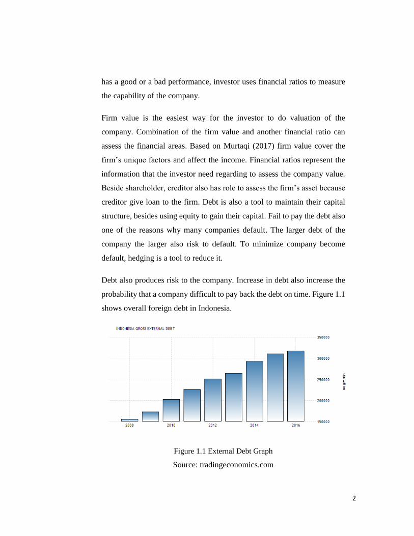
Debt also produces risk to the company. Increase in debt also increase the

probability that a company difficult to pay back the debt on time. Figure 1.1

shows overall foreign debt in Indonesia.

Figure 1.1 External Debt Graph

Source: tradingeconomics.com

3

To mitigate business that dealing with potential high risk, the enterprise risk

management is needed. To face uncertainty and reduce the risk while doing

businesses, using financial derivatives may be useful for the company. Most

likely, non-financial firms already using financial derivatives in their daily

business. Risk arise in many ways through global economy and financial

markets, risk become systematic with other units and interact with many

external parties (Sheng, 2010). On the other hand, George S. Oldfield

(1997) started wondering about which is better off transferring the risk to

the other parties or absorb the risk of the financial product and how they

manage the risk. Because of that many companies still used to transferring

their risk to the others rather than take the risk and managed it by

themselves.

Hedging has become a tool for the company to mitigate the risk but there

are still many companies are avoiding hedging itself. The factor that affects

a company hedging is a debt foreign currency. The companies think that

hedging is the same as insurance, when the accident doesn’t occur and they

still need to pay. Hedging is used to prevent any uncertainty in the financial

world and also prevent the financial crisis may occur in any time. There are

many components to prevent financial crisis may bring the companies to

bankruptcy. Another factor that company does hedge is fluctuated currency.

Because company cannot predict the fluctuated currency in financial world,

hedging is tool to anticipate the loss of income from trying to do business

using different currency. Hence, hedging might be a factor that impact to

the firm value. In figure 1.2 shows the fluctuation currency with the lowest

and the highest exchange rate of IDR 12,451 and IDR 14,739 to USD in

2015.

4

Figure 1.2 Fluctuation Currency History 2015

Source: usd.fx-exchange.com

Hedging is important to the firms when they do business using other

currency to fixing their currency rate in a length of time. Hedging is needed

for a business that related to export and import, also it needed for aviation

sector. Based on the IFRS accounting hedging rules, companies must

recognize the changes of fair value to the asset or liability or unrecognized

firm commitment or other components that could affect the profit or loss to

the firms.

1.1.1 Need for study

This researched has purpose to determine the relationship between firm

value and the control variables such as ROE, DAR, current ratio, firm size,

tax rate, and hedging dummy. This researched will focusing on the hedging;

therefore, the researcher aims to know “Performance of Financial Ratios

and Hedging towards Firm Value of LQ45 Companies in Indonesia”.

5

1.2 Problem Statement

According to F. Modigliani and Miller (1958) theory shows that risk

management using capital structure will not affect to the firm value;

therefore, hedging won’t affect the firm value. There are some research

theories and still argued that hedging has no impact to the firm value of the

company in Swedish firm (Nguyen, 2015). Meanwhile, Ayturk, et al.

(2016) found the result of the derivative uses doesn’t impact to the firm

value in Turkish market. The similarity on their research is they didn’t

diversify the industry that they chose. The opposite result can be found on

the research made by Dan, et al. (2005) stated hedging on gas with leverage,

profitability and reserves has significant impact to the firm value evidence

oil & gas Canadian companies but the result can be questionable also

because there is a research using oil & gas companies in U.S. Jin & Jorion

(2004) analyze that hedging doesn’t give impact to the market value of the

industry evidence U.S. oil & gas producers. The researches have different

result to other researches. Dan, et al. (2005) used oil & gas Canadian

companies as their sample different from the another researches. Jin and

Jorion (2004) found hedging doesn’t affect to the market value of the

industry although that they used same industry. Another research of Nguyen

(2015) and Ayturk, et al. (2016), they took sample based on derivative uses

of company based on their market. The differences of their results are

questionable whether the hedging does or doesn’t give impact to the firm

value. Investors might be still wondering if the hedging does or doesn’t give

them higher firm value. Firm that used hedging as their tool to mitigate the

risk can be speculated. Speculate the hedging might impact to their profit

loss. Those different results become matrix or references to me to do this

study.

6

1.3 Research Questions

The purpose of this study to know whether hedging does impact to the firm

value based on the Indonesia market or not. Because of the different results

to the previous researches, the study aims if hedging affect to the market

value positively.

1. Is there any significant influence on Current Ratio (CR) to Firm

Value?

2. Is there any significant influence on Tax Rate to Firm Value?

3. Is there any significant influence on Debt to Asset Ratio (DAR) to

Firm Value?

4. Is there any significant influence on Return on Equity (ROE) to Firm

Value?

5. Is there any significant influence on Firm Size to Firm Value?

6. Is there any significant influence on Hedging to Firm Value?

7. Is there a simultaneous significant influence on Current Ratio, Tax

Rate, Debt to Asset Ratio, Return on Equity, Firm Size and Hedging

to Firm Value?

1.4 Research Objectives

Based on the questions above, the purpose of this research are:

1. To determine the significant influence on Current Ratio (CR) to

Firm Value

2. To determine the significant influence on Tax Rate to Firm Value

3. To determine the significant influence on Debt to Asset Ratio

(DAR) to Firm Value

4. To determine the significant influence on Return on Equity (ROE)

to Firm Value

5. To determine the significant influence on Firm Size to Firm Value

7

6. To determine the significant influence on Hedging to Firm Value

7. To determine the simultaneous significant influence on Current

Ratio, Tax Rate, Debt to Asset Ratio, Return on Equity, Firm Size

and Hedging to Firm Value

1.5 Significant of Study

This study is given benefit to:

1. The investors

To give information for the investors about determinants to the

company firm value based on the key indicators to know whether

the company overvalue or undervalue and choose the best company

to invest in.

2. The researcher

This study can be as a foundation to create a new research using firm

value with the key indicators and enrich the knowledge deeper for

the researcher.

3. The students and university

To enrich the knowledge regarding firm value of company and apply

key indicators to measuring the performance of the company.

1.6 Limitation

1. This research is only focusing in the company that categorized as

LQ45 and listed in the Indonesia Stock Exchange (IDX).

2. In this research, researcher took seven year’s period of study started

from 2010 to 2016 that observed firms hedging activities. Therefore,

the researcher doesn’t know the requirement how long the hedging

firm’s activities affect firm value.

3. In this research, regression model can only be done using common

effect because of the variable hedging dummy value is 1 and 0.

8

1.7 Thesis organization

Thesis organization conducted as follows.

1. Chapter I – Introduction / Background

This chapter represent the research background of study, problem

statement, research questions, research objectives, significant of

study, limitations and organization paper. This chapter provide key

comprehension of this research.

2. Chapter II – Literature review

This chapter represent the theories of previous research. This

chapter consist of theoretical review, previous research, research

gap and hypothesis.

3. Chapter III – Research Methodology

This chapter represent the research data consist of research method,

research framework, research sample and data analysis method.

4. Chapter IV – Analysis and Interpretation

This chapter represent the finding analysis and interpretation of

result and consist of company profile, descriptive analysis, classical

assumption test, regression model analysis and interpretation of

results.

5. Chapter V – Conclusion and Recommendations

This chapter represent the conclusions and recommendations from

result of this paper.

9

CHAPTER II

LITERATURE REVIEW

2.1 Theoretical Review

2.1.1 Firm Value

Firm value is measure the asset of the company. It represents the future

business of the company. Fundamental of organization describe the value

of firm which is the manager who are being the representative to optimal

maximization of a firm (Ilaboya, Izevbekhai, & Ohiokha, 2016). The

prosperity of company and shareholder’s wealth can be seen when the firm

has high firm value. Firm value has become one of the indicator to investor

whether the firm has good prosperity in the future.

According to F. Modigliani and Miller (1963) stated that financing method

will not affect the firm value of a company since calculated by earning

power and risk of underlying assets. Therefore, financing method with debt

or equity will not affect the firm value because firm value increment based

on the earning power of the company.

According to Ilaboya, et al. (2016) stated that firm value has two

perspective measurement using profitability ratio such as return on asset

(ROA), return on equity (ROE) also profit margin and stock market

perspective using share price in the stock exchange market.

2.1.2 Theory of Capital Asset Pricing Model

Capital Asset Pricing model has become a famous model in financial

history. This model describes the relationship between expected return and

systematic risk that occurs in the financial world. Basic idea from this model

10

is the investor would like to choose efficient portfolio when the investor are

price takers and expect to have maximum return with the minimum variance

of risk (Nguyen, 2015). The formula to expected return as follows.

(Eq.1)

Where:

rf = risk free rate

βi = beta from industry

rm = expected market return

Researcher include CAPM in the literature review to give understanding

contradictive theories regarding risk management could affect the firm

value. From shareholder’s perspective risk management should contribute

to the firm value. However, it is no entirely obvious why risk management

can increase firm value (Nguyen, 2015).

2.1.3 Corporate Risk Management

Risk is interwoven with the corporate business’s strategy and impact

considerably to the competitive position (Aleš S. Berk, 2009). The risk is a

combination of the likelihood of an occurrence of a hazardous event or

exposures to danger and the damaged might be caused by action or event.

There are several risks according to the type and impact of organization and

its environment. There are written as follows.

1. Strategic risk is risk occurs and affect the strategy of the firm.

11

2. Operation risk is affect the firm capability of producing the goods.

3. Supply risk is affect the flow of resources to enable the operations.

4. Fiscal risk is arising through the taxation.

5. Reputation risk is loss in confidence of the firm.

6. Asset impairment risk is risk due to reduce in capability to increase

net profit.

7. Regulatory risk is risk caused the change of regulatory and affect the

business.

One of the tools to minimize the corporate risk by doing hedging. Hedging

is an investment tool to reduce the risk adverse movement in an asset.

Hedging often used for the company which is the business operations using

foreign currency as their main currency to purchase goods. Shareholder

maximization state that firm do hedging to reduce the cost that involved

with highly volatile cash flows (Jin & Jorion, 2004). There are three type

explanation about hedging with literature. Mayer et al. (1982) stated that

hedging reduces the financial distress and hedging is a way to get tax

incentives. When firm hedging, it will help to reduce the taxes. Leland and

Hayne (1997) stated debt from firm capacity will also increase, therefore

realizing the great leverage with greater taxes advantages. In addition,

hedging might be a signal for the investor to observed the managerial ability

of the firm.

2.1.5 Tobin Q Ratio as Measured

Tobin q ratio popularized by James Tobin of Yale University. The q ratio

defined as the market value of firm divided by replacement cost of firm total

asset (Ilaboya et al. 2016). Most of study used Tobin q ratio as measurement

for firm market value. Tobin q ratio defined market value by number of

share multiple by share price in stock exchange market and divided to book

12

value total asset of firm. Tobin q ratio is one of the tool to assess

performance of company. Tobin q ratio formula can be determined below.

(Eq.2)

Where:

Total market value of firm = share price x number of shares

If the Tobin q ratio is 1 means that the market value has same value with

the replacement cost of the firm. Tobin q ratio with less than 1 means that

the company has lower market value compared to the book value total asset

of firm and categorized as “Undervalued”. Tobin q ratio with greater than 1

means that the company has higher market value compared to the book

value of total asset of firm and categorized as “Overvalued”. Hence, Tobin

q ratio give an information to the investor whether the company has

undervalued or overvalued and the performance of future growth for the

firm.

2.1.5.1 Current Ratio

Current ratio is liquidity ratio to measure the ability of the firm pay its debt

whether its short-term or long-term debt (Murtaqi, 2017). Murtaqi, (2017)

stated that current ratio has positive significant influence to the firm value

using Tobin q ratio even thought, current ratio doesn’t give the highest

significant to the firm value.

If the current ratio value is less than 1 means that the firm has more debt to

pay indicates that obligation of firm to pay would be unable to paid their

13

debt on time. It tells the investor that the firm has liquidity problem and

indicated the firm has financial health issues.

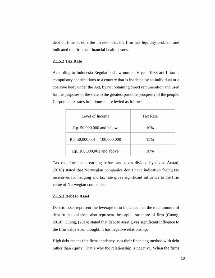
2.1.5.2 Tax Rate

According to Indonesia Regulation Law number 6 year 1983 act 1, tax is

compulsory contributions to a country that is indebted by an individual or a

coercive body under the Act, by not obtaining direct remuneration and used

for the purposes of the state to the greatest possible prosperity of the people.

Corporate tax rates in Indonesia are levied as follows:

Level of Income Tax Rate

Rp. 50,000,000 and below 10%

Rp. 50,000,001 – 100,000,000 15%

Rp. 100,000,001 and above 30%

Tax rate formula is earning before and taxes divided by taxes. Årstad,

(2010) stated that Norwegian companies don’t have indication facing tax

incentives for hedging and tax rate gives significant influence to the firm

value of Norwegian companies.

2.1.5.3 Debt to Asset

Debt to asset represent the leverage ratio indicates that the total amount of

debt from total asset also represent the capital structure of firm (Cuong,

2014). Cuong, (2014) stated that debt to asset gives significant influence to

the firm value even thought, it has negative relationship.

High debt means that firms tendency uses their financing method with debt

rather than equity. That’s why the relationship is negative. When the firms

14

have high debt means the firms have less equity. High debt also give high

probability of firm cannot pay their debt and become default.

2.1.5.4 Return on Equity

Return on equity represent the profitability ratio indicates that how much

the firm generate profit from their shares. Nabavand and Rezaei (2015)

stated that return on equity gives positive significant influence to the firm

value. Return on equity formula is net profit divided by total equity of firm.

High growth company expected to give higher return on equity means that

the company has good profitability. Therefore, investor can measure the

profitability of company using return on equity. Higher the ROE, higher

also the net profit that the company generate.

2.1.5.5 Firm Size

Firm size represent the size of the company indicates that bigger size of

company also has bigger value of asset. (Nguyen, 2015) stated that firm size

gives significant influence to the firm value even thought, it gives negative

relationship.

Based on the Grossman and Hart, (1983) theorem of principal and agency

problem stated that big firm has tendency to hired agent and pay the

incentives to them although the incentive might be expensive. It leads the

company become less efficiency. Big firm size also has tendency using debt

as their financing method. That’s why, it has negative relationship.

2.1.5.6 Hedging Dummy

Hedging dummy represent the company does or doesn’t hedging based on

the annual report and using dummy variable is appropriate for this

15

regression analysis due to it is hard to measure the size of hedging cost for

each company. Hedging doesn’t give significant influence to the firm value

based on the (Nguyen, 2015). It has contradictive result with Dan et al.

(2005) found that hedging has significant influence to the firm value. The

result might be bias because their research environment is different.

In this research, hedging dummy value is 1 if the company does hedge and

0 if the company doesn’t hedge. Hedging also related to the debt and tax.

When company does hedge means that the company has foreign debt. That

explains the tax shield of company. When company does hedge explain that

the company must pay higher interest rate and will impact to lower taxes.

2.2 Previous Research

Previous Research

No. Author, Title Variable Method Result

1. Nadya Marsha and

Isrochmani

Murtaqi (2017);

The Effect of

Financial Ratios

on Firm Value in

The Food and

Beverage Sector of

The IDX

DV: Firm

Value (Tobin

Q Ratio)

IV: ROA,

Current

Ratio, Acid

Test Ratio

Linear

Regress

ion

ROA, Current

Ratio has positive

significant

influence and

Acid Test Ratio

has negative

significant

influence and

simultaneous

significant

influence to the

Firm Value

(Tobin Q Ratio)

2. Yusuf Ayturk, Ali

Osman Gurbuz

and Serhat Yanik

(2016); Corporate

derivatives use and

firm value:

Evidence from

Turkey

DV: Firm

Value (Tobin

Q Ratio)

IV: Ln Total

Asset, ROA,

Dividend

Dummy,

Leverage,

Diversificati

Linear

Regress

ion

Ln Total Asset

has negative

significant

influence and

Dividend Dummy

have positive

significant

influence to the

Firm Value

16

on, Cap.

Ex/Sales,

Foreign

Sales,

Liquidity

and

Derivative

uses

(Tobin Q Ratio);

ROA, Leverage,

Diversification,

Cap. Ex/ Sales,

Foreign Sales,

Liquidity and

Derivatives uses

have no

significant

influence to the

Firm Value

(Tobin Q Ratio)

3. Eirik Haavaldsen

and Hans Fredrik

Ø. Årstad (2010);

Determinants and

Effects of

Corporate

Currency Hedging

DV: Firm

Value (Tobin

Q Ratio)

IV:

Derivatives,

Current

Ratio, Net

Debt, YoY

Revenue

Growth,

ROE% Mean

Tax Rate,

Hedging

Linear

Regress

ion

YoY Growth

Revenue, Tax

Rate, Hedging

have negative

significant

influence and

Current Ratio has

positive

significant

influence to the

Firm Value

(Tobin Q Ratio);

Derivatives, Net

Debt and ROE%

Mean has no

significant

influence to the

Firm Value

(Tobin Q Ratio)

4. Yanbo Jin and

Philippe Jorion

(2004); Firm

Value and

Hedging: Evidence

from U.S. Oil and

Gas Procedurs

DV: Firm

Value (Tobin

Q Ratio)

IV: Firm

Size,

Profitability,

Investment

Growth,

Leverage,

Dividend

Dummy,

Hedging

Linear

Regress

ion

Investment

Growth and

Dividend Dummy

have positive

significant

influence to the

Firm Value

(Tobin Q Ratio);

Firm Size,

Profitability,

Leverage,

Hedging Dummy

17

Dummy and

Production

Cost

and Production

Cost have no

significant

influence to the

Firm Value

(Tobin Q Ratio)

5. Behrooz Nabavand

and Javad Rezaei

(2015); Review

between Tobin's Q

with performance

Evaluation Scale

Based Accounting

and Marketing

Information in

Accepted

Companies in

Tehran Stock

Exchange

DV: Firm

Value (Tobin

Q Ratio)

IV: P/E

Ratio, EPS

Ratio, P/B

Ratio, ROE,

and ROA

Linear

Regress

ion

EPS Ratio, P/B

Ratio and ROE

have significant

influence to the

Firm Value

(Tobin Q Ratio);

P/E Ratio and

ROA have no

significant

influence to the

Firm Value

(Tobin Q Ratio)

6. Ngan Nguyen

(2015); Does

Hedging Increase

Firm Value?

DV: Firm

Value (Tobin

Q Ratio)

IV: Capex,

Diversified

Dummy,

Dividend

Dummy,

Hedging

Dummy,

Leverage,

Profitability,

Firm Size

Linear

Regress

ion

Dividend,

Profitability and

Firm Size have

positive

significant

influence and

Leverage has

negative

significant

influence to the

Firm Value

(Tobin Q Ratio);

Capex,

Diversified and

Hedging have no

significant

influence to the

Firm Value

(Tobin Q Ratio)

7. Chang Dan, Hong

Gu and Kuan Xu;

The Impact of

Hedging on Stock

Return and Firm

DV: Firm

Value (Tobin

Q Ratio)

IV: ROA,

Investment

Linear

Regress

ion

ROA and

Hedging Dgr

have positive

significant

influence to the

18

Value: New

Evidence from

Canadian Oil and

Gas Companies

Growth,

Access to

Financial

Market,

Leverage,

Hedging Dgr

(Delta Gas

Reserves)

and Hedging

Dgp (Delta

Gas

Production)

Firm Value and

Hedging Dgp and

Leverage have

negative

significant

influence to the

Firm Value

(Tobin Q Ratio);

Investment

Growth, Access

to Financial

Market have no

significant

influence to the

Firm Value

(Tobin Q Ratio

2.3 Research Gap

In the previous research, there are still many arguments that hedging doesn’t

affect firm value. However, there was a research showed that hedging

impact to the firm value (Dan et al. 2005). Those researches have many

different type of ways to see whether hedging affects the firm value and

those researches done in their country. Some countries may have different

economic condition. Hedging may impact to those countries that have

fluctuated economic or otherwise. The country may already become a

develop country and less volatility or fluctuated currency. That’s why,

hedging still be argued to many researchers that does hedging impact to firm

value. Uncertainty financial world has become a problem to the developing

country like Indonesia. When crisis impact to the develop country,

economic condition might also impact to the developing country. That’s

why, hedging has role to maintain their risk financial distress and future

cash flow so the investor will calmly invest their money to the company.

19

2.4 Theoretical Framework

Based on the theoretical review from previous research, the researcher had

developed model for theoretical framework of this research as in figure 2

According from this research, the researcher wants to know the relationship

between Current Ratio, Tax Rate, DAR, ROE, Firm Size and Hedging

towards the Firm Value of the company LQ45 and listed in Indonesia Stock

Exchange. In this research, researcher put current ratio as liquidity

measurement; tax rate taken from previous research, debt to asset ratio as

leverage measurement, ROE as profitability measurement, firm size taken

from previous research and hedging taken from previous research.

Figure 2 Research Theoretical Framework Firm Value

Source: Adjusted by Researcher 2017

FV

CR Hg FS ROE DAR TR

H1 H6 H5 H4 H3 H2

H7

20

2.5 Hypotheses

Based on the theoretical framework of this research, research conducted the

hypothesis as follows.

H1: There is a significance influence on Current Ratio towards Firm Value

in LQ45 Companies.

H2: There is a significance influence on Tax Rate towards Firm Value in

LQ45 Companies.

H3: There is a significance influence on Debt to Asset towards Firm Value

in LQ45 Companies.

H4: There is a significance influence on Return on Equity towards Firm

Value in LQ45 Companies.

H5: There is a significance influence on Firm Size towards Firm Value in

LQ45 Companies.

H6: There is a significance influence on Hedging towards Firm Value in

LQ45 Companies.

H7: There is significant simultaneous influence on Current Ratio, Tax Rate,

Debt to Asset, Return on Equity, Firm Size and Hedging towards Firm

Value in LQ45 Companies.

21

CHAPTER III

METHODOLOGY

3.1 Research Method

Quantitative Method

Quantitative research has purpose to explaining and determining the

predicted variable through numerical observation and presentation that

reflect from the independent variable. Quantitative method has two methods

to determine the data. In this research, researcher uses secondary data as

method to gathering the information that related to the research.

In this research, researcher collected the secondary data from audited annual

report of LQ45 companies from period of 2010 - 2016. The secondary data

are current ratio (X1), tax rate (X2), debt to asset ratio (X3), return on equity

(X4), firm size (X5), hedging dummy (X6) as the independent variable and

firm value (Y) as the dependent variable. Using quantitative method,

researcher can determine the result of this study using Eviews (Econometric

Views) 10 to generate the data analysis.

Researcher uses Eviews to produce the result of this study by processing the

raw data. By using Eviews 10, researcher can determine the mean,

minimum, maximum and standard deviation through descriptive statistic. In

order to fulfill the BLUE parameter, researcher uses Eviews to generate

normality test, heteroscedasticity, autocorrelation and multicollienarity.

After this research fulfill the BLUE parameter, researcher continues to

generate regression model using Eviews 10. Hypothesis can be determined

by using F-test and T-test also interpretation of each independent variable

that influenced the dependent variable.

22

3.2 Research Framework

Research framework is framework that has logical argument with the

previous research that has successful created (Suryana, 2010). In figure 3.1

shows the research framework of this research.

Figure 3.1 Research Framework of “Performance of Financial Ratios and

Hedging towards Firm Value of LQ45 Companies in Indonesia"

Figure 3.1 Research Framework

Source: Created by researcher for research purpose, based on Suryana (2010).

Observation

Problem Identification

Findings

Formulate Problem

Formulate Hypothesis

Collecting Data from Annual Report

Data Analysis

Processing Data

Interpretation of Results

Summary and Conclusion

23

3.3 Research Instrument

Research instrument is a tool that chosen by researcher in their research or

study to collect the data into a systematic (Arikunto, 2000). By using

random sampling of LQ45 companies, researcher took randomly 16

companies. These companies are Adaro, Indofood CBP, Indofood, Astra

International, Astra Agro Lestari, Indocement, Lippo Karawaci, Pakuwon

Jati, AKR Corporindo, Bumi Serpong Damai, Kalbe Farma, Adhi Karya,

Telkom, Wijaya Karya, Perusahaan Gas Negara, Gudang Garam.

Researcher collected the data through audited annual report from Indonesia

Stock Exchange period of 2010 until 2016.

To optimize the results of this study, researcher uses Eviews 10 as a tool to

produce the analysis and regression model of this study. Beside using

Eviews 10 as tool to produce the analysis, researcher uses Microsoft Excel

2016 to maintain the raw information from annual report. To make it easier

to calculated, researcher categorize the data annually using table.

3.4 Sampling Design

Sampling is process selecting part of object that taken by researcher to

become an object of observation (Nasution, 2003). If a sampling is correctly

observed, the statistical analysis can conclude the whole population.

3.4.1 Size of Population

Population is a whole of object to be observed (Nasution, 2003).

Population has very large of number to be observed which is not

really proper to be observed. Therefore, a proportion of population

is selected to be observed in this research. In this research,

population is focused on the companies under LQ45 and listed in

Indonesia Stock Exchange.

24

3.4.2 Size of Sample

Sample is a part of population that can be representative to estimate

the whole population (Nasution, 2003). There are two technic of

sampling design. First, probability sample or random sample.

Probability sample has purpose to minimalize the bias of the object

taken by researcher. Second, non-probability sample or non-random

sample. Non-probability sample has characteristic that deviations of

sample value towards population cannot be measure. In this

research, researcher uses non-probability sample using purposive

sample. Purposive sample is sample that taken by researcher with

purpose for this research.

Therefore, probability sample using purposive sampling is chosen

in this research. There are several criteria to choose specific sample

in this research which are:

1. Company that listed in Indonesia Stock Exchange.

2. Company must have positive asset, liabilities and equity.

3. Financial institution and non-financial institution are

excluded due to different nature of business.

4. Company that listed under LQ45 at least 3 years in row or

more.

5. Company that should not be suspended under LQ45 from

2010 – 2016.

Therefore, there are 16 companies chosen as sample in this research

using the several criteria that determined by researcher.

As of 2017, this research takes sixteen companies and categorizes

as LQ45 listed in Stock Exchange Indonesia

25

1. PT. Adaro

2. PT. Adhi Karya

3. PT. Astra International Indonesia

4. PT. Astra Agro Lestari Indonesia

5. PT. AKR Corporindo

6. PT. Bumi Serpong Damai

7. PT. Gudang Garam

8. PT. Indocement

9. PT. Indofood

10. PT. Indofood CBP

11. PT. Kalbe Farma

12. PT. Lippo Karawaci

13. PT. Pakuwon Jati

14. PT. Perusahaan Gas Negara

15. PT. Telkom Indonesia

16. PT. Wijaya Karya

Therefore, there are sixteen companies chosen as sample with

population of LQ45 listed in Indonesia Stock Exchange is 45

companies.

In this research, researcher implement panel data which is consist of

cross-section and time series data. The cross-section data is sixteen

companies listed in Indonesia Stock Exchange as LQ45 and the time

series is seven years of period from 2010 to 2016. This research

decides to choose seven years as availability. Therefore, the number

of observation using panel data by sixteen companies with seven

years of period which are 112 data.

26

3.5 Data Analysis

3.5.1 Descriptive Statistic Analysis

Descriptive Statistic Analysis is analysis of activity that conduct an

assessment towards value, score or sizes of variables and as indicator of

independent variable that being reviewed (Agung, 2000). The information

generate in descriptive statistics are mean, minimum, maximum and

standard deviation.

Mean is average value of data by add up all the number and divide by how

many the numbers are (Nicholas, 2006). Min and Max are the smallest and

highest value of the observation. Mean can be measure as follows (Schwert,

2010).

(Eq.3)

Where:

N = Number of observations

Standard deviation is average of deviation from the mean (Nicholas, 2006).

The smaller standard deviation indicates that the narrower range between

highest and lowest value closely to average value. The formulation can be

measure as follows (Schwert, 2010).

27

(Eq.4)

Where:

N = Number of sample

y = Mean

3.5.2 Panel Data Regression

Panel data is formed between the time series and cross-section data (Endri,

2011). In time series model usually, the model just use many time periods

with one object of observation and cross-section model is the model with

more than one as object but with one-time period. Regression using data

panel usually called pooled data (Endri, 2011). There are two advantages

using pooled data (Endri, 2011). First, pooled data is combination of time

series and cross-section data able to create many degree of freedom with

high value. Second, combination of time series and cross-section able to

solve the issues when there is omitted-variable.

According to Endri (2011) there are three method of estimation parameter

model, which is:

1. Common Effect: Ordinary Least Square

This method is regression model by combination of the time series

and cross-section using OLS method or called common effect. In

common effect, the regression ignored the differences of individual

and time period. This model assumes that there are no differences

between object that observed such as a company has a same

behavior in various period time.

28

2. Fixed Effect.

Different with the common effect that has assumption there are no

differences between company and the period. Fixed effect has

assumption that there are variables that cannot fill the regression

model and allowing intercept inconsistent. This model has

advantages for the research with more time series than cross-section.

3. Random Effect.

In fixed effect, differences of individual and period through

intercept. Random effect shows the differences through the errors.

This model has advantages for the research that using more cross-

section than time series.

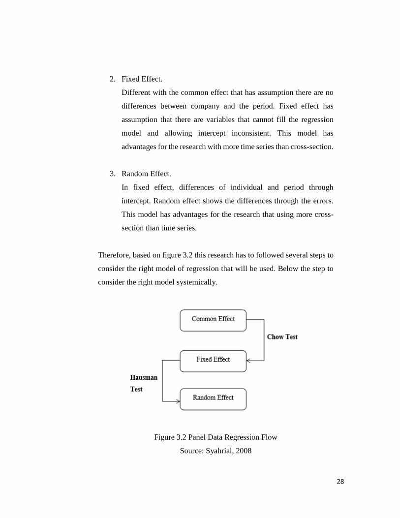
Therefore, based on figure 3.2 this research has to followed several steps to

consider the right model of regression that will be used. Below the step to

consider the right model systemically.

Figure 3.2 Panel Data Regression Flow

Source: Syahrial, 2008

29

1. Chow Test

Chow test is a test to determine the right model between fixed effect

and common effect. This model uses F-statistic to test by adding

dummy variable to know the differences intercept between fixed

effect and common effect (Endri, 2011). The formulate stated

below.

(Eq.5)

Where:

RSS = Residual sum of square

The null hypothesis is dummy variable is not significant towards

dependent variable so the research will choose common effect. The

alternate hypothesis is dummy variable is significant towards

dependent variable so the research will choose fixed effect. The

results of chow test can be determined as follows.

1. Ho is accepted and Ha is rejected if Probability value > 0.05,

which means common effect model is accepted.

2. Ho is rejected and Ha is accepted if Probability value < 0.05,

which means fixed effect model is accepted.

2. Hausman test

Hausman test is a test to determine the right model between random

effect and fixed effect. This test formed by hausman has asymptotic

χ2 distribution. The formula stated as follows.

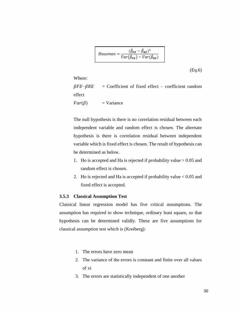
30

(Eq.6)

Where:

𝛽𝐹𝐸−𝛽𝑅𝐸 = Coefficient of fixed effect – coefficient random

effect

𝑉𝑎𝑟(𝛽) = Variance

The null hypothesis is there is no correlation residual between each

independent variable and random effect is chosen. The alternate

hypothesis is there is correlation residual between independent

variable which is fixed effect is chosen. The result of hypothesis can

be determined as below.

1. Ho is accepted and Ha is rejected if probability value > 0.05 and

random effect is chosen.

2. Ho is rejected and Ha is accepted if probability value < 0.05 and

fixed effect is accepted.

3.5.3 Classical Assumption Test

Classical linear regression model has five critical assumptions. The

assumption has required to show technique, ordinary least square, so that

hypothesis can be determined validly. These are five assumptions for

classical assumption test which is (Kreiberg):

1. The errors have zero mean

2. The variance of the errors is constant and finite over all values

of xi

3. The errors are statistically independent of one another

31

4. There is no relationship between the error and the

corresponding x

5. εi is normally distributed

Therefore, the research can be called fulfilled the classical assumption test

if five assumptions above are implemented. To test whether the classical

assumption test fulfilled or not. Researcher uses these steps as follows.

1. Normality Test

Normality test is test to measure whether the data for the research is

normally distributed or not in parametric statistics (Widhiarso).

Normality test can be done through statistical analysis or histogram.

The statistical analysis will show the estimated of distribution for

the regression. Histogram can describe the normality of distribution

data. If the curve of histogram focused on the middle and going

down for the both side or called the bell-shape, histogram can

conclude that the regression model is normally distributed.

However, just looking at the histogram with the bell-shaped. It

doesn’t rule out the possibility of the data is normally distributed.

The best way to check it whether it has normally distributed using

statistical analysis. Jacque-Bera is a method to test whether it is

normal distributed (Dian Christiani Kabasaranga, 2013).

(Eq.7)

Where:

S = Skewness

N = Number of Observation

K = Kurtosis

32

Dian (2013) stated that Jacque-Bera has distribution of chi-square

with X2. Compared to table with two degree of freedom with

significant value of 0.05 (α=5%).

1) Jacque-Bera value > X2, the residual is not normally

distributed.

2) Jacque-Bera value < X2, the residual is normally distributed.

Winarno (2011) stated that distribution of data can be tested by

Jacque-Bera probability. If the probability of Jacque-Bera is greater

than significant value of 0.05 then the data is normally distributed

and vice versa.

1) Jacque-Bera Probability > 0.05, the data is normally

distributed.

2) Jacque-Bera Probability < 0.05, the data is not normally

distributed.

2. Heteroscedasticity

Heteroscedasticity is distribution of same probability in the same

observation of x, and variance each residual is same (BASUKI,

2017). Heteroscedasticity can be detected by the scatterplot. If the

scatterplot created a same form or spread, then it can be concluded

there is a heteroscedasticity in the research. The regression model

called a good regression if there is no heteroscedasticity which

means that there is a singular metric of dependent variable that has

related to the two or more singulars metric of independent variable.

For testing the heteroscedasticity using white test based on the

BASUKI (2017), if the probability of Chi-Square value is greater

than 0.05 then the regression has fulfilled homoscedasticity or there

is no heteroscedasticity in the research vice versa.

33

1) If Prob. Chi-Square > 0.05, there is no heteroscedasticity.

2) If Prob. Chi-Square < 0.05, there is heteroscedasticity.

3. Autocorrelation

Autocorrelation is the correlation between each variances are same

or the variables are related to each other (BASUKI, 2017). If the

autocorrelation occurs the estimation of regression model will bias

or inefficiency. Classical assumption can be fulfilled if there is no

autocorrelation occurs in the research. To determine there is a

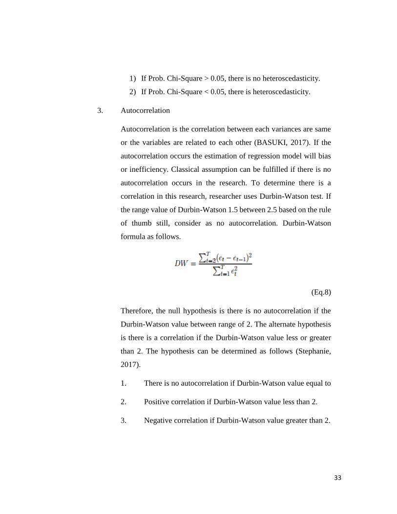
correlation in this research, researcher uses Durbin-Watson test. If

the range value of Durbin-Watson 1.5 between 2.5 based on the rule

of thumb still, consider as no autocorrelation. Durbin-Watson

formula as follows.

(Eq.8)

Therefore, the null hypothesis is there is no autocorrelation if the

Durbin-Watson value between range of 2. The alternate hypothesis

is there is a correlation if the Durbin-Watson value less or greater

than 2. The hypothesis can be determined as follows (Stephanie,

2017).

1. There is no autocorrelation if Durbin-Watson value equal to

2. Positive correlation if Durbin-Watson value less than 2.

3. Negative correlation if Durbin-Watson value greater than 2.

34

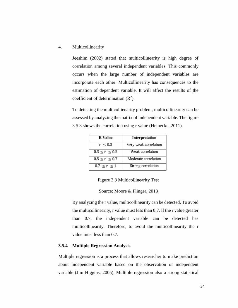
4. Multicollinearity

Jeeshim (2002) stated that multicollinearity is high degree of

correlation among several independent variables. This commonly

occurs when the large number of independent variables are

incorporate each other. Multicollinearity has consequences to the

estimation of dependent variable. It will affect the results of the

coefficient of determination (R2).

To detecting the multicollienarity problem, multicollinearity can be

assessed by analyzing the matrix of independent variable. The figure

3.5.3 shows the correlation using r value (Heinecke, 2011).

Figure 3.3 Multicollinearity Test

Source: Moore & Flinger, 2013

By analyzing the r value, multicollinearity can be detected. To avoid

the multicollinearity, r value must less than 0.7. If the r value greater

than 0.7, the independent variable can be detected has

multicollinearity. Therefore, to avoid the multicollinearity the r

value must less than 0.7.

3.5.4 Multiple Regression Analysis

Multiple regression is a process that allows researcher to make prediction

about independent variable based on the observation of independent

variable (Jim Higgins, 2005). Multiple regression also a strong statistical

35

and extremely powerful when the researcher develops “model” of the wide

various observation. Multiple regression provides the analysis of

relationship between two variables.

Researcher choose multiple regression to predict or estimate the

relationship between dependent variable based on the independent variable.

Firm value is a dependent variable that chosen by the research and the

independent variables are current ratio, tax rate, debt to asset ratio, return

on equity, firm size and hedging dummy. The multiple regression can be

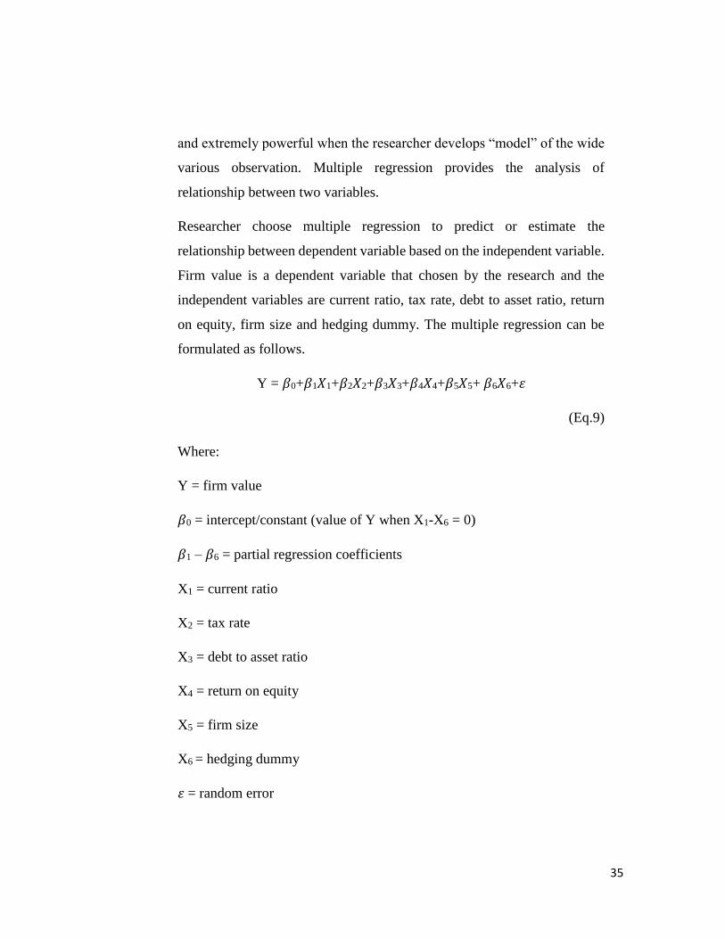
formulated as follows.

Y = 𝛽0+𝛽1𝑋1+𝛽2𝑋2+𝛽3𝑋3+𝛽4𝑋4+𝛽5𝑋5+ 𝛽6𝑋6+𝜀

(Eq.9)

Where:

Y = firm value

𝛽0 = intercept/constant (value of Y when X1-X6 = 0)

𝛽1 – 𝛽6 = partial regression coefficients

X1 = current ratio

X2 = tax rate

X3 = debt to asset ratio

X4 = return on equity

X5 = firm size

X6 = hedging dummy

𝜀 = random error

36

The partial regression coefficient is really important to predict the

contribution of independent variable to dependent variable. If the partial

regression coefficient has positive value means that the behavior of

dependent variable will follow the independent. An increment of

independent variable value also raising the value of dependent variable, vice

versa. If the partial regression coefficient has negative value means that

dependent and independent has opposite behavior. An increment of

independent variable will impact to the decreasing value of dependent

variable.

3.6 Testing Hypotheses

Testing hypothesis is test that conducted to know whether there is an

influence between independent variable to dependent variable in the

research. There are two type of hypothesis testing. First, null hypothesis (βn

= 0) that represent as H0. Second, alternative hypothesis (βn ≠ 0) that

represent as Ha. Null hypothesis means there is no significant influence

between independent variable to dependent variable meanwhile alternative

hypothesis mean there is significant influence between independent variable

to dependent variable.

3.6.1 Significant Level

This research apply test at significant value of 0.05 or α=5%. If probability

value or P-value greater than significant value, null hypothesis will be

applied which is mean that there is no significant influence.

3.6.2 T-test

T-test in multiple regression is to test whether the parameter estimation of

multiple regression is already right parameter or not. Right parameter means

that the parameter able to explain the dependent variable through

independent variable (Iqbal, 2015).

37

(Eq.10)

Where:

𝛽𝑖 = parameters of the model; the intercept and slope coefficients

𝛽 ̂ = estimator of 𝛽𝑖

se = standard error

The result of hypothesis can conclude to accept or reject hypothesis using

probability value of t-statistic each independent variable with significant

value of 0.05. The hypothesis of t-test conclude as follows.

1) Probability of t-statistics > 0.05 means that there is no significant

influence of independent variable to dependent variable and H0 is

accepted and Ha is rejected.

2) Probability of t-statistics < 0.05 means that there is a significant

influence of independent variable to dependent variable and H0 is

rejected and Ha is accepted.

To help the researcher determine the hypothesis for each independent

variable whether there is significant influence or not. Below is the t-test

hypothesis of this research.

1. 𝐻01: 𝛽1 = 0 or if probability t-statistics > α then there is no significant

partial influence of current ratio towards firm value in LQ45.

𝐻a1: 𝛽1 ≠ 0 or if probability t-statistics < α then there is significant

partial influence of current ratio towards firm value in LQ45.

38

2. 𝐻02: 𝛽2 = 0 or if probability t-statistics > α then there is no significant

partial influence of tax rate towards firm value in LQ45.

𝐻a2: 𝛽2 ≠ 0 or if probability t-statistics > α then there is significant

partial influence of tax rate towards firm value in LQ45.

3. 𝐻03: 𝛽3 = 0 or if probability t-statistics > α then there is no significant

partial influence of debt to asset towards price to firm value in LQ45.

𝐻a3: 𝛽3 ≠ 0 or if probability t-statistics > α then there is significant

partial influence of debt to asset towards price to firm value in LQ45.

4. 𝐻04: 𝛽4 = 0 or if probability t-statistics > α then there is no significant

partial influence of return on equity towards firm value in LQ45.

𝐻a4: 𝛽4 ≠ 0 or if probability t-statistics > α then there is significant

partial influence of return on equity towards firm value in LQ45.

5. 𝐻05: 𝛽5 = 0 or if probability t-statistics > α then there is no significant

partial influence of firm size towards firm value in LQ45.

𝐻a5: 𝛽5 ≠ 0 or if probability t-statistics > α then there is significant

partial influence of firm size towards firm value in LQ45.

6. 𝐻06: 𝛽6 = 0 or if probability t-statistics > α then there is no significant

partial influence of hedging dummy towards firm value in LQ45.

𝐻a6: 𝛽6 ≠ 0 or if probability t-statistics > α then there is significant

partial influence of hedging dummy towards firm value in LQ45.

3.6.3 F-Test

F-test or called test simultaneous model is step to identify the regression

model is feasible to use. Feasible means that the model estimation can

39

explain the dependent variable through independent variable (Iqbal, 2015).

The formula for t-test as follows.

(Eq.11)

Where:

𝑅2 = coefficient of determination

N = samples

k = number of independent variables

The result of hypothesis can conclude to accept or reject hypothesis using

probability value of f-statistic each independent variable with significant

value of 0.05. The hypothesis of t-test conclude as follows.

a) Probability of f-statistics > 0.05 means that there is no significant

influence of independent variable to dependent variable and H0 is

accepted and Ha is rejected.

b) Probability of f-statistics < 0.05 means that there is a significant

influence of independent variable to dependent variable and H0 is

rejected and Ha is accepted.

In this research, f-test will help the researcher to determine the simultaneous

influence of independent variable to dependent variable. The hypothesis for

f-test as follows.

1. H07: β1 = β2 = β3 = β4 = β5 = β6 0 or if probability f-statistics > α then

there is no significant simultaneous influence of current ratio, tax

rate, debt to asset, return on equity, firm size and hedging dummy

towards price to firm value in LQ45.

40

Ha7: at least there is one βi ≠ 0 or if probability f-statistics < α then

there is significant simultaneous influence of current ratio, tax rate,

debt to asset, return on equity, firm size and hedging dummy

towards price to firm value in LQ45.

3.6.4 Coefficient of Determination

Coefficient of Determination explained about variance of independent

variable to dependent variable (Iqbal, 2015). Coefficient determination

value can be measure as R-Square (R2) or Adjusted R-Square. R-Square

normally used when the independent variable just one and Adjuster R-

Square used when the independent more than 1. Normally all the researcher

use R-Square rather than Adjusted R-Square.

Value of R-Square can range from 0 to 1

a) Independent variables have weak capability to explain dependent

variable when R-Square is close to 0.

b) Independent variables have strong capability to explain dependent

variable when R-Square is close to 1.

Value of R-Square also can explain the multicollinearity. When value of R-

Square close to 0, the research might also expose to multicollinearity

Therefore, the research must have strong capability to explain the dependent

variable through independent variable.

41

CHAPTER IV

ANALYSIS OF DATA

4.1 Company Profile

1. Adaro

Adaro was established in 1982. PT. Adaro Energy Tbk. is an energy group

from Indonesia with coal mining through subsidiaries as main business.

Headquarters of Adaro Energy in Tabalong, South Kalimantan and the CEO

is Garibaldi Thohir.

2. Adhi Karya

PT. Adhi Karya (Persero) Tbk. is a company that has construction as main

business and located in Jakarta, Indonesia. PT. Adhi Karya Tbk has founded

on 1960 and the President director is Kiswodarmawan and the main

commissioner is Fadjroel Rachman.

3. Astra International

Astra International is a multinational company that has automotive as main

business. The founders of Astra International are Tjia Kien Tie, William

Soerjadjaja and Liem Peng Hong. Astra International was founded on 1957

and located in Jakarta.

4. Astra Agro Lestari Indonesia

Astra Agro Lestari is a company that located in Jakarta and has main

business on plantation. Astra Agro Lestari was founded on 1997 and

subsidiaries from Astra International. Crude Palm Oil and Kernels is a main

product of Astra Agro Lestari.

42

5. AKR Corporindo

PT. AKR Corporindo is a multinational company that located in Jakarta and

has main business on fuels and natural gas. AKR Corporindo was founded

on 28 November 1977 and the founder is Soegiarto Adikoesoemo

6. Bumi Serpong Damai

PT. Bumi Serpong Damai is an Indonesia real-estate developer company

located in Tangerang. Its business segments are land, industrial building,

house, shop house, hotel, industrial building, office space and educational

centre. The company was founded on 1984 and the founder is Muktar

Widjaja.

7. Gudang Garam

PT. Gudang Garam Tbk. is an Indonesia company that has main business

on cigarettes located in Kediri, East Java. The founder is Surya

Wonowidjojo and founded on 1958.

8. Indocement

PT. Indocement Tunggal Prakarsa Tbk. is an Indonesia company that has

main business on cement. Indocement was founded on 1985 and the

president director is Christian Kartawijaya.

9. Indofood Sukses Makmur

PT. Indofood Sukses Makmur Tbk. is producer of food and beverages and

located in Jakarta. Indofood was founded on 14 August 1990 and the

founder is Sudono Salim.

43

10. Indofood CBP

PT. Indofood CBP Sukses Makmur Tbk. is a subsidiaries company from

Indofood and the company involved in the food industry. The headquarters

located in Jakarta.

11. Kalbe Farma

PT. Kable Farma Tbk. is an international company that produces pharmacy,

supplement, nutrition and health services that located in Jakarta. Kalbe

Farma was founded on 10 September 1966 and the founder are Khouw Lip

Tjoen,Khouw Lip Hiang, Khouw Lip Swan, Boenjamin Setiawan, Maria

Karmila, F. Bing Aryanto.

12.Lippo Karawaci

PT. Lippo Karawaci is a real-estate and developer company in Indonesia

and subsidiaries from Lippo Group. Lippo Karawaci was founded on

October 1990 and the CEO is Gouw Vi Ven.

13. Pakuwon Jati

PT. Pakuwon Jati Tbk. is a real-estate company and located in Surabaya.

PT. Pakuwon Jati Tbk. was founded on 1982. The founder is Alexander

Tedja.

14. Perusahaan Gas Negara

PT. Perusahaan Gas Negara (Persero) Tbk. is state-owned enterprises from

Indonesia and has main business on transmission and distributor of natural

gas. The company was founded on 1859 as I.J.N Eindhoven & Co. On 13

May 1965 change into PGN. The president director is Jobi Triananda

Hasjim.

44

15. Telkom Indonesia

PT. Telekomunikasi Indonesia Tbk. is a state-owned enterprises company

that provide information and communication. Telkom was founded on 23

October 1856 and the founder is Cacuk Sudarijanto.

16. Wijaya Karya

PT. Wijaya Karya Tbk. is an Indonesia company that operates in

construction. The company was founded on 11 Maret 1960. The main

commissioner is Dr. Ir. M. Basuki Hadimuljono, M.Sc and president

director is Bintang Perbowo, SE, MM.

4.2 Descriptive Analysis

Descriptive analysis describes the information for each variable that are

being observed. Using EViews 10, descriptive analysis mostly explained

about mean, median, maximum, minimum, standard deviation, skewness,

kurtosis, Jacque-Bera, probability and sum of observations. In this study,

there are 112 observations using cross-section data with seven years (2010-

2016) and sixteen companies. Summary of descriptive statistic will be

shown on table 4.1 interpret using EViews 10.

Table 4.1 Descriptive Statistic Result

FV_Y CR_X1 TR_X2 DAR_X3 ROE_X4 FS_X5 HD_X6

Mean 1.795 2.326 0.248 0.451 0.187 13.443 0.437

Maximum 5.126 6.985 0.530 0.850 0.475 14.418 1.000

Minimum 0.152 0.450 0.043 0.133 0.045 12.693 0.000

STD 1.224 1.528 0.100 0.176 0.087 0.412 0.498

∑Observ. 112 112 112 112 112 112 112

Source: Eviews10

According to the descriptive statistic result, we can conclude the

explanations as below:

45

1. Firm Value (FV) explained the dependent variable. It shows mean value

of 1.795 along with standard deviation of 1.224 indicates that the data

mostly spread around 1.795 ± 1.224. Standard deviation value has small

gap to the mean due to volatility between firm value of each company.

The maximum value of 5.126 happens to Kalbe Farma in 2012 and

minimum value of 0.152 happens to Adhi Karya in 2011.

2. Current Ratio (CR) explained the independent variable. It shows mean

value of 2.326 along with standard deviation of 1.528 indicates that the

data mostly spread around 2.326 ± 1.528. Standard deviation value still

under to the mean because of value of each company has different

fluctuatuion. The maximum value of 6.985 occurs to Indocement in

2011 and the minimum value of 0.450 occurs to Astra Agro Lestari in

2013.

3. Tax Rate (TR) explained the independent variable. It shows mean value

of 0.248 along with the standard deviation of 0.100 indicates that the

data mostly spread around 0.248 ± 0.100. Smaller standard deviation

indicates that the data has narrow between the lowest value to the

highest value. The maximum value of 0.530 occurs to Adaro in 2010

and the minimum value of 0.043 occurs to Astra Agro Lestari in 2016.

4. Debt to Asset Ratio (DAR) explained the independent variable. It shows

mean value of 0.451 along with the standard deviation of 0.176

explained that the data mostly spread around 0.451 ± 0.176. Standard

deviation has smaller value and narrower spread between the lowest

value to the highest value. The maximum value of 0.850 occurs to Adhi

Karya in 2012 and the minimum value of 0.133 occurs to Indocement

in 2016.

5. Return on Equity (ROE) explained the independent variable. It shows

mean value of 0.187 along with standard deviation of 0.087 explained

that the data mostly spread around 0.187 ± 0.087. Standard deviation

46

still smaller to the mean due to each company has small volatility. The

maximum value of 0.475 occurs to Telkom in 2016 and the minimum

value of 0.045 occurs to Adaro in 2015.

6. Firm Size (FS) explained the independent variable. It shows mean value

of 13.443 along with the standard deviation of 0.412 explained that the

data mostly spread around the 13.433 ± 0.412. Standard deviation has

small value indicates that the steady value of firm size for each

company. The maximum value of 14.418 occurs to Astra in 2016 and

the minimum value of 12.693 occurs to Pakuwon Jati in 2010.

7. Hedging Dummy explained the independent variable. It shows the mean

value of 0.437 along with the standard deviation of 0.498 indicates that

the data mostly spread around 0.437 ± 0.498. Standard deviation has

greater value to the mean value due to the data of hedging just 0 and 1.

When 0 is the company doesn’t do hedging and when 1 is the company

does hedging that explained the minimum and maximum of the value.

4.3 Data Analysis

4.3.1 Classical Assumption Test

Classical assumption test needed to test whether the model has passed the

requirement. The model has to fulfilled the normality test,

heteroscedasticity, multicollinearity, and autocorrelation in order to reach

the valid result using multiple regression.

1. Normality Test

One of the statistical test used to know whether the data normally distributed

or not using normality test (Fallo, Setiawa, & Susanto, 2013). Normality

test generate the statistical and graphic information about distribution each

variable. By looking at the histogram, researcher knows the data normally

distributed or not. This research will show the analysis of the normality test

47

that conducted by the researcher using Jarque-Bera and probability that

shown by table.

Table 4.2 Normality Test Result

0

2

4

6

8

10

12

14

-1.0 -0.5 0.0 0.5 1.0 1.5

Series: Standardized Residuals

Sample 2010 2016

Observations 112

Mean -1.05e-16

Median -0.102699

Maximum 1.553917

Minimum -1.236007

Std. Dev. 0.603921

Skewness 0.354543

Kurtosis 2.715587

Jarque-Bera 2.723907

Probability 0.256160

Source: Eviews 10

To know whether this research normally distributed or not using Jarque-

Bera by comparing the table X2 with two degrees of freedom and significant

value α = 0.05 that is 5.991 (Dian Christiani Kabasaranga, 2013). If the

Jarque-Bera value less than X2 with significant value of 0.05, the data is

normally distributed (Dian Christiani Kabasaranga, 2013). Based on table

4.2 Jarque-Bera value of this research is 2.723907 < 5.991 explained that

the data for each variable are normally distributed. Jarque-Bera probability

also another way to know whether the data is normally distributed or not. If

probability greater than significant value of 0.05 then it proves that the data

is normally distributed. Based on table 4.2 probability of this research is

0.256160 > 0.05 explained the data is normally distributed.

2. Heteroscedasticity.

Heteroscedasticity occurs when there is a constant distribution of proportion

probability in all X observation (BASUKI, Uji Heteroskedastisitas dan

Perbaikan Heteroskedastisitas, 2017). If there is no heteroscedasticity in the

regression model, therefore the regression model of this research accepted.

Using white cross-sectiom coefficient covariance method help the

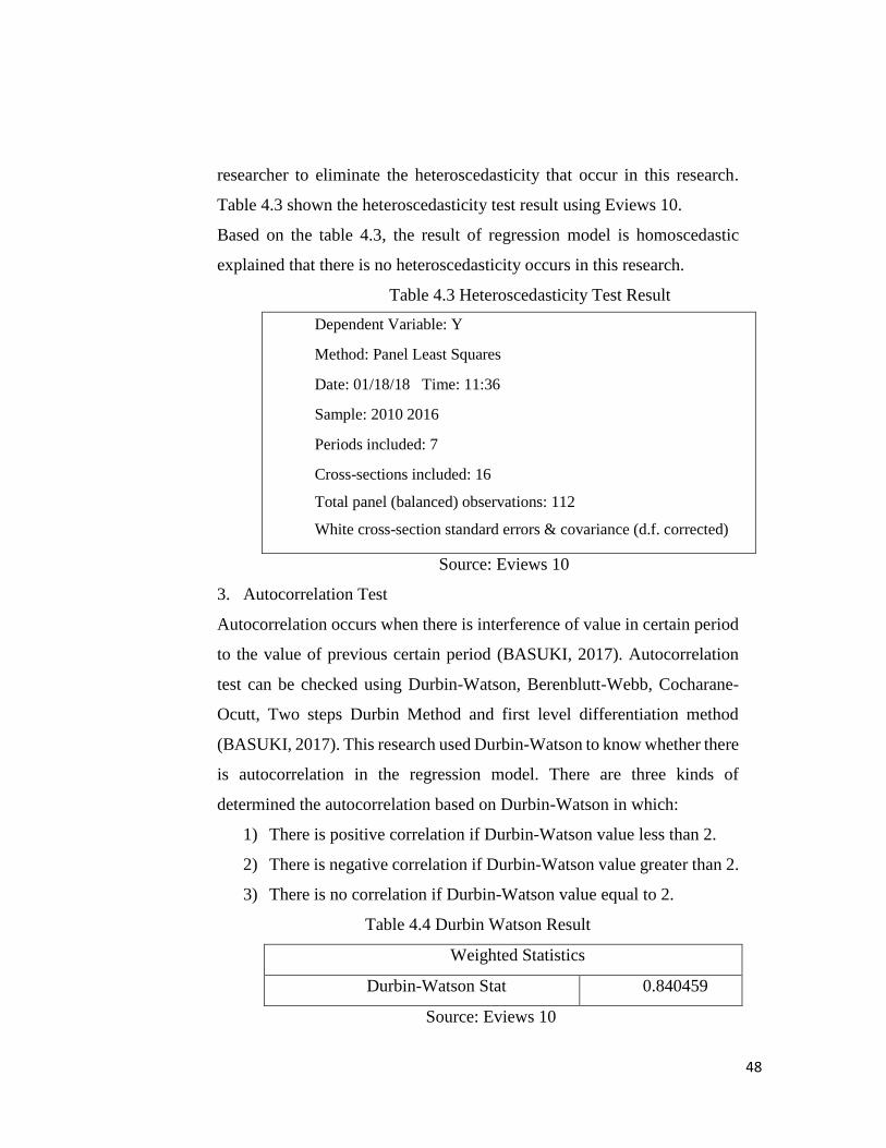
48

researcher to eliminate the heteroscedasticity that occur in this research.

Table 4.3 shown the heteroscedasticity test result using Eviews 10.

Based on the table 4.3, the result of regression model is homoscedastic

explained that there is no heteroscedasticity occurs in this research.

Table 4.3 Heteroscedasticity Test Result

Source: Eviews 10

3. Autocorrelation Test

Autocorrelation occurs when there is interference of value in certain period

to the value of previous certain period (BASUKI, 2017). Autocorrelation

test can be checked using Durbin-Watson, Berenblutt-Webb, Cocharane-

Ocutt, Two steps Durbin Method and first level differentiation method

(BASUKI, 2017). This research used Durbin-Watson to know whether there

is autocorrelation in the regression model. There are three kinds of

determined the autocorrelation based on Durbin-Watson in which:

1) There is positive correlation if Durbin-Watson value less than 2.

2) There is negative correlation if Durbin-Watson value greater than 2.

3) There is no correlation if Durbin-Watson value equal to 2.

Table 4.4 Durbin Watson Result

Weighted Statistics

Durbin-Watson Stat 0.840459

Source: Eviews 10

Dependent Variable: Y

Method: Panel Least Squares

Date: 01/18/18 Time: 11:36

Sample: 2010 2016

Periods included: 7

Cross-sections included: 16

Total panel (balanced) observations: 112

White cross-section standard errors & covariance (d.f. corrected)

49

Based on the table 4.4 Durbin-Watson result on autocorrelation value of

0.840459 indicates that there is autocorrelation occurs in this research

because of the Durbin-Watson value less than 2. Autocorrelation occurs in

this research because of the independent variable formula using stock price.

Stock price value related to the historical of stock price several days which

is mean that previous stock price will also affect the next stock price.

Autocorrelation of daily stock returns influenced by both the spread and the

information of gradual incorporation (CERQUEIRA, 2006).

4. Multicollinearity Test

Multicollinearity test conducted to test whether there is a correlation

between variable to the another variable that observed in this research.

There are 6 independent variables that used in this research which are

current ratio, tax rate, debt to asset ratio, return on equity, firm size and

hedging dummy. Multicollinearity occurs when the variable value equal or

greater than 0.7 to each other variable. Thus, the value of the variable should

less than 0.7 to reach the valid test of multicollinearity. The result of

multicollinearity will be shown in table 4.5.

Table 4.5 Multicollinearity Test Result

Source: Eviews 10

Based on the table 4.5, the highest value of correlation between tax rate to

the debt to asset ratio that is 0.356 and it still consider as no correlation

CR TR DAR ROE FS HD

CR 1 -0.249 -0.411 -0.051 -0.058 0.361

TR -0.249 1 0.356 -0.090 -0.105 -0.154

DAR -0.411 0.356 1 -0.287 -0.153 -0.018

ROE -0.051 -0.090 -0.287 1 0.039 -0.207

FS -0.058 -0.105 -0.153 0.039 1 0.462

HD 0.361 -0.154 -0.018 -0.207 0.462 1

50

between the variable because the value doesn’t exceed 0.7. Thus, there is

no multicollinearity in this research and the data valid to be continued.

4.3.2 Multiple Regression Analysis

Multiple regression analysis is a statistic analysis used to determine the

value of dependent variable that influenced by independent variable. This

research will show the estimated or predicted value of dependent variable.

Table 4.6 show the result of multiple regression using common effect.

“Coefficient” in the table 4.6 explained the value change in dependent

variable along with the change of independent variable while the coefficient

remains constant (Hoaglin, 2013). Multiple regression formula conducted

based on the coefficient of each variable.

The multiple regression formula shown in the table 4.6 as follows:

Y = 9.115765 + 0.084995 X1 + 1.0875512 X2 – 4.382373 X3 + 5.461090

X4 – 0.496884 X5 – 0.342122 X6

(Eq.12)

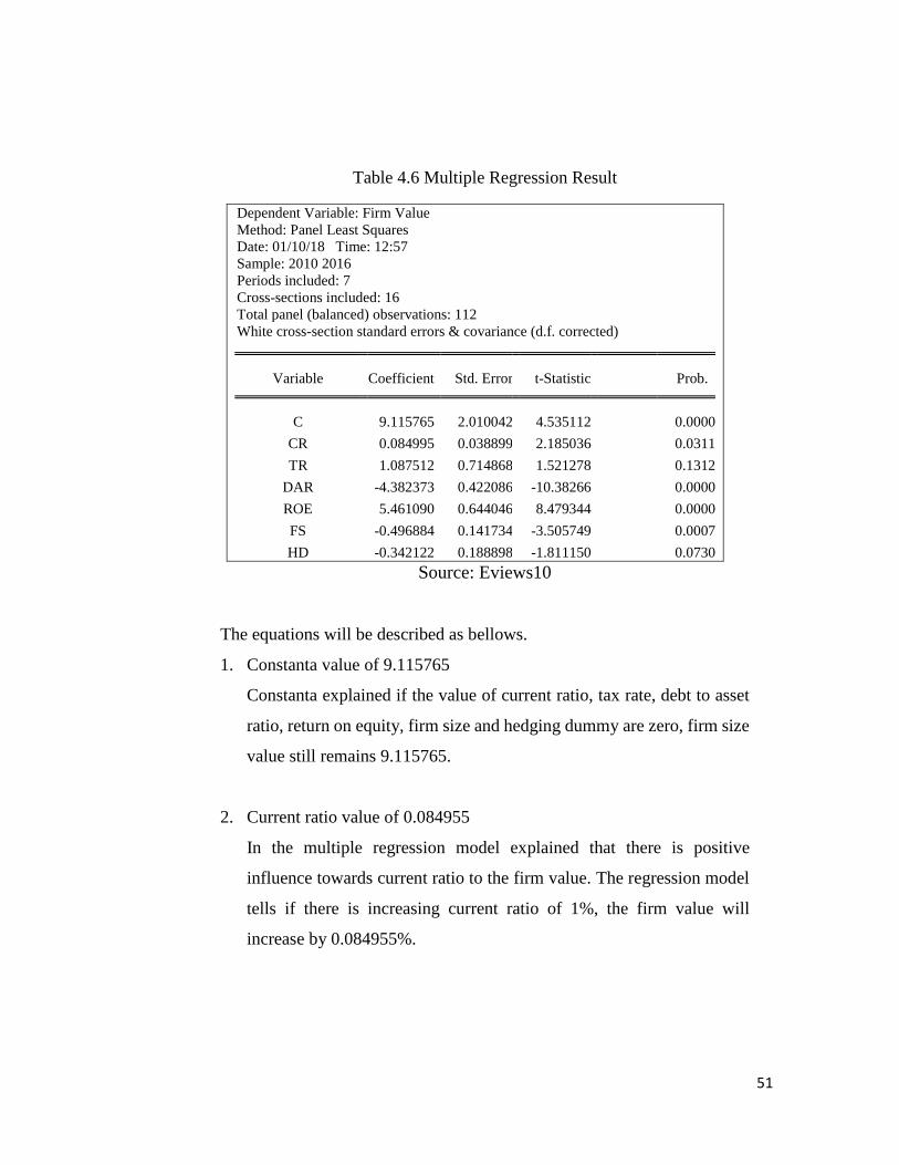
51

Table 4.6 Multiple Regression Result

Source: Eviews10

The equations will be described as bellows.

1. Constanta value of 9.115765

Constanta explained if the value of current ratio, tax rate, debt to asset

ratio, return on equity, firm size and hedging dummy are zero, firm size

value still remains 9.115765.

2. Current ratio value of 0.084955

In the multiple regression model explained that there is positive

influence towards current ratio to the firm value. The regression model

tells if there is increasing current ratio of 1%, the firm value will

increase by 0.084955%.

Dependent Variable: Firm Value

Method: Panel Least Squares

Date: 01/10/18 Time: 12:57

Sample: 2010 2016

Periods included: 7

Cross-sections included: 16

Total panel (balanced) observations: 112

White cross-section standard errors & covariance (d.f. corrected)

Variable Coefficient Std. Error t-Statistic Prob.

C 9.115765 2.010042 4.535112 0.0000

CR 0.084995 0.038899 2.185036 0.0311

TR 1.087512 0.714868 1.521278 0.1312

DAR -4.382373 0.422086 -10.38266 0.0000

ROE 5.461090 0.644046 8.479344 0.0000

FS -0.496884 0.141734 -3.505749 0.0007

HD -0.342122 0.188898 -1.811150 0.0730

52

3. Tax rate value of 1.0875512

Multiple regression model explained that there is positive influence

towards tax rate to the firm value. If the tax rate value increase of 1%,

firm value also increased by 1.0875512%.

4. Debt to asset ratio value of -4.382373

This multiple regression model explained there is negative influence of

debt to asset value towards firm value. If debt to asset ratio value

increasing of 1%, firm value will decrease by -4.382373%.

5. Return on equity value of 5.461090

Multiple regression model explained that there is positive influence of

return on equity towards firm value. If return on equity value increase

by 1%, firm value will also increase by 5.461090%.

6. Firm size value of -0.496884

Multiple regression model explained that there is negative influence of

firm size towards firm value. If firm size increased by 1%, firm value

will decrease by -0.496884%.

7. Hedging dummy value of -0.342122

Multiple regression model explained that there is negative influence of

hedging to the firm value. Value of company hedging is 1 and value of

company non-hedging is 0. If the company hedging, the firm value will

decrease by -0.342122.

4.4 T-Test, F-Test, and Coefficient of Determination

T-Test

T-test is a parameter that capable to determine or explained for each

independent variable’s behavior in influencing the dependent variable

(Iqbal, 2015). By looking at the table 4.6 result from t-test can be determine.

T-test will determine the result by comparing the t probability to the

53

significant value of 0.05 (α=5%). If the t probability less than significant

value of 0.05 therefore there is significant influence of independent variable

to the dependent variable and if the t probability greater than significant

value of 0.05 therefore there is no significant influence of independent to

the dependent variable. Based on the table 4.3.2 result of t-test can be

determined as bellows.

1. Current ratio has probability value of 0.0311 less than the significant

value of 0.05. Therefore, H01 is rejected and Ha1 is accepted which

means that current ratio has significant influence towards firm value in

LQ45 companies.

2. Tax rate has probability value of 0.1312 greater than the significant

value of 0.05. Therefore, H02 is accepted and Ha2 is rejected which

means that tax rate has no significant influence towards firm value in

LQ45 companies.

3. Debt to asset ratio has probability of 0.0000 less than significant value

of 0.05. Therefore, H03 is rejected and Ha3 is accepted which means that

debt to asset ratio has significant influence towards firm value in LQ45

companies.

4. Return on equity ratio has probability of 0.0000 less than significant

value of 0.05. Therefore, H04 is rejected and Ha4 is accepted which

means that return on equity ratio has significant influence towards firm

value in LQ45 companies.

5. Firm size has probability of 0.0007 less than significant value of 0.05.

Therefore, H05 is rejected and Ha5 is accepted which means that firm

size has significant influence towards firm value in LQ45 companies.

6. Hedging dummy has probability of 0.0730 greater than significant value

of 0.05. Therefore, H06 is accepted and Ha6 is rejected which means that

hedging dummy has no significant influence towards firm value in

LQ45 companies.

54

Based on the result of t-test, there are two independent variables that has no

significant influence to the dependent variable. Due to there are two

independent variables that has no significant influence which are tax rate

and hedging dummy, regression model has to eliminated two independent

variables. New regression model formula written as bellows.

Y = 9.115765 + 0.084995 CR - 4.382373 DAR + 5.461090 ROE –

0.496884 FS

F-Test

F-test used to indicate the regression model whether the estimation or

prediction of the model valid or not (Iqbal, 2015). The regression model can

be determined valid if the independent variable can explain the influence

towards the dependent variable. if the result of F-statistic probability less

than significant value of 0.05 (α=5%), the regression model can be

determined as valid and vice versa.

Table 4.7 F-Test Result

Weighted Statistics

F-Statistic 54.37384

Prob (F-Statistic) 0.000000

Source: Eviews 10

Based on the table 4.7, Probability F-Statistic has value of 0.000000 less

than the significant value of 0.05. Therefore, Ha is accepted and H0 is

rejected which means there is significant influence of current ratio, tax

rate, debt to asset ratio, return on equity, firm size and hedging dummy

towards firm value in LQ45 companies.

55

Coefficient of Determination

Coefficient of Determination explained the influence of independent

variable towards dependent variable or the influence proportion for all

independent variables towards dependent variable (Iqbal, 2015).

Coefficient of determination value can be measured by R2 value.

Table 4.8 Coefficient of Determination Result

Weighted Statistic

R-squared 0.756533

Adjusted R-squared 0.742621

Source: Eviews 10

Based on the table 4.8, coefficient of determination value is 0.756533 means

that current ratio, tax rate, debt to asset ratio, return on equity ratio, firm

size and hedging explained 75.6533% influence towards firm value and the

rest of 24.3467% explained by the other factor. Coefficient of determination

categorized as good when the value closer to the 1.

Interpretation of Result

1. Interpretation influence current ratio towards firm value.

Based on the table 4.3.2 shows that the significant value of 0.0311 and

Ha1 is accepted. Thus, the first hypothesis is “there is significant

influence of current ratio towards firm value”. Coefficient regression

value of 0.084995 indicates that current ratio has positive influence

towards firm value.

This result supported with the theory Murtaqi (2017) that current ratio

has positive correlation to the firm value. Their research about “The

Effect of Financial Ratios on Firm Value in the Food and Beverage

Sector of the IDX” using 14 firms in Indonesia with period from 2010

56

– 2014. Current ratio and firm value has positive correlation when the

current ratio increase means that lower the debt higher the equity

meanwhile firm value calculation based on the stock multiple with the

number of shares and divided with total asset. Higher the equity higher

also the number of share or stock that investor holds.

2. Interpretation influence tax rate towards firm value.

Based on the table 4.3.2 shows that the significant value of 0.1312 and

H02 is accepted. Thus, the second hypothesis is “there is no significant

influence of current ratio towards firm value”. Coefficient regression

value of 1.087512 indicates that tax rate has positive influence towards

firm value.

This result has contradictive with the theory Årstad (2010) stated the tax

rate has significant influence towards firm value and Norwegian

companies has tendency in hedging due to that the tax rate has influence

the financial performance in their research. Meanwhile, the researcher

found that tax rate has no significant influence toward firm value in

Indonesia and low tendency of hedging might cause insignificant result.

Contradictive result might be found the research done using Indonesia’s

company.

3. Interpretation influence debt to asset ratio towards firm value.

Based on the table 4.3.2 shows that the significant value of 0.0000 and

Ha3 is accepted. Thus, the third hypothesis is “there is significant

influence of debt to asset towards firm value”. Coefficient regression

value of -4.382373 indicates that debt to asset has negative influence

towards firm value.

57

This result supported by Cuong, (2014) stated that TA/TD ratio has

significant influence to the firm value with negative coefficient.

Negative coefficient indicates that if the debt to asset ratio higher and

firm value will decrease. Nguyen (2015) also stated that previous

studies had shown that leverage increase the level of distress of

company. Based on the company’s annual report that debt mostly comes

from public and private bank to financing the infrastructure of

Indonesia.

4. Interpretation influence return on equity towards firm value.

Based on the table 4.3.2 shows that the significant value of 0.0000 and

Ha4 is accepted. Thus, the fourth hypothesis is “there is significant

influence of return on equity towards firm value”. Coefficient regression

value of 5.461090 indicates that return on equity has positive and the

most significant influence towards firm value.

This results also supported by Nabavand and Rezaei (2015) stated that

return on equity has significant influence towards firm value. Return on

equity can be used to measuring profitability of company. Profitability

is one of the reason increasing in firm value related to the pecking theory

order suggests that company with less debt avoiding financing with debt

because external fund might costly for the company (Myers, 1984).

Based on the company’s annual report that big companies have

tendency to do financing using their equity.

5. Interpretation influence firm size towards firm value.

Based on the table 4.3.2 shows that the significant value of 0.0007 and

Ha5 is accepted. Thus, the fifth hypothesis is “there is significant

influence of firm size towards firm value”. Coefficient regression value

58

of -0.496884 indicates that firm size has negative influence towards firm

value.

This results also supported by Nguyen (2015) found that firm size has

significant influence towards the firm value with positive relationship.

Meanwhile, this research has negative influence to the firm value.

Ayturk et al. (2016) also found that firm size has negative influence to

the firm value. According to the theory principal and agency problem

when bigger company hired an agent and pay incentives cause

inefficiency and less effectiveness of company (Grossman & Hart,

1983). This theory will lead less firm value for the bigger firm size.

6. Interpretation influence hedging towards firm value.

Based on the table 4.3.2 shows that the significant value of 0.0730 and

H06 is accepted. Thus, the sixth hypothesis is “there is no significant

influence of hedging towards firm value”. Coefficient regression value

of -0.342122 indicates that hedging has negative influence towards firm

value.

This result line with theory Nguyen (2015) stated there is no significant

influence of hedging towards firm value and contradictive with Dan et

al. (2005) and Årstad (2010) stated hedging has significant influence

towards firm value. This result might be different from the researcher

result. Dan et al. (2005) researched= about the oil & gas in Canadian

meanwhile researcher done the result using random sampling based on

LQ45 in Indonesia.

59

7. Simultaneous influence of current ratio, tax rate, debt to asset, return on

equity, firm size and hedging towards firm value.

Based on the hypothesis states that “there is significant simultaneous

influence current ratio, tax rate, debt to asset, return on equity, firm size

and hedging towards firm value” is accepted. F-statistic has proved the

hypothesis which is f-statistic value 0.000000 < 0.05. Current ratio, tax

rate, debt to asset, return on equity, firm size, and hedging has explained

the variance towards firm value which is 75.633% meanwhile

24.3467% explained by the other variables or factor which are the

variable doesn’t state in this research.

60

CHAPTER V

CONCLUSIONS AND RECOMMENDATION

5.1 Conclusions

After the researcher passed the classical assumption test and interpret the

regression model, the conclusion can be summarizing as follows.

1. There is positive significant influence of current ratio and return on

equity towards firm value. Positive significant influence explains that

when increment of current ratio and return on equity will impact to the

increment of firm value.

2. There is negative significant influence of debt to asset and firm size

towards firm value. Negative significant influence explains that

increment of debt to asset and firm size of company impact to the lower

firm value.

3. There is no significant influence of tax rate and hedging towards firm

value. Tax rate doesn’t really impact to the firm value whether the tax

rate increase or decrease. Hedging has p-value of 0.0730 and will

significant in this research if the researcher uses significant value of

10%. So, hedging and tax rate has weak impact to the firm value of

company.

4. ROE gives the most significant or impact to the firm value.

5. There is a simultaneous significant influence of current ratio, tax rate,

debt to asset, return on equity, firm size and hedging towards firm value.

Overall within 7 years in this research, researcher found that debt to asset

and ROE give most significant impact to the firm value. Enhancement of

infrastructure in Indonesia impact to the increment of debt in Infrastructure

companies. Source of debt of infrastructure companies mostly come from

private and public banks in Indonesia. Meanwhile, ROE gives significant

impact to the other company beside infrastructure company that using their

equity to financing their company. Hedging gives weak impact to the firm

61

value because public and private bank Indonesia directly give the loan to

the company so the company with high debt will not hedge.

5.2 Recommendations Based on the results from regression model and conclusion of this research,

researcher could conduct the recommendations based on the research. The

recommendations are:

1. For investors

Debt and ROE give signal for the investor to choose the right company

to invest in. Investor should be careful to the company with high debt

because of the company might be default but the firm value of the

company will be undervalued and investor could buy the stock with

affordable price. Otherwise, ROE give signal to the investor that high

ROE means high firm value and the company will be overvalued with

the high price of stock. So to consider which the best company to invest

in, investor should evaluate the company by using their management

and their financial ratios.

2. For future research.

In order to get more relevance result, the researcher encourage to uses

longer time series for the future research. The usage of another financial

ratio might give different impact to the firm value.

3. For students and university.

Enrich their knowledge of how financial performance and hedging

impact to the firm value.

62

References

Journal Agung, I. G. (2000). Analisis Statistik Sederhana Untuk Pengambilan

Keputusan. Journal Populasi, 11(2).

Cuong, N. T. (2014). Threshold Effect of Capital Structure on Firm

Value: Evidence from Seafood Processing Enterprises in the

South Central Region of Vietnam. International Journal of

Finance & Banking Studies, Vol.3 No.3.

George S. Oldfield, A. M. (1997). Risk Management in Financial

Intitution. Sloan Management Review, 39(1),33.

Ilaboya, O. .., Izevbekhai, M. .., & Ohiokha, F. .. (2016). Tax Planning

and Firm Value: A Review of Literature. Business and

Management Research, Vol. 5, No. 2.

Jin, Y., & Jorion, P. (2004). Firm Value and Hedging: Evidence from

U.S. Oil & Gas Producers. The Journal of Finance, 61(2), 893-

919.

Leland, & Hayne. (1997). Agency Cost, Risk Management and Capital

Structure. Journal of Finance, 53, 1213-43.

Mayer, David, & Smith. (1982). On the Corporate Demand for Insurance.

Journal of Business, 55,281-296.

Murtaqi, N. M. (2017). The Effect of Financial Ratios on Firm Value in

The Food and Beverage Sector of The IDX. Journal of Business

and Management, Vol. 6, No.2, 2017: 214-226.

Myers, S. C. (1984). The Capital Structure Puzzle. Journal of Finance,

Vol. 39, pp. 575- 592.

63

Nabavand, B., & Rezaei, J. (2015). Review between Tobin's Q with

performance Evaluation Scale Based Accounting and Marketing

Information in Accepted Companies in Tehran Stock Exchange.

Journal of Applied Environmental and Biological Sciences.

W., E. (2013). Risks Management: New Literature Review. Polish

Journal of Management Studies, Vol. 8.

Book Arikunto, S. (2000). Manajemen Penelitian. Jakarta: Rineka Cipta.

BASUKI, A. T. (2017). Uji Autokorelasi dan Perbaikan Autokorelasi.

Yogyakarta: Universitas Muhammadiyah Yogyakarta.

BASUKI, A. T. (2017). Uji Heteroskedastisitas dan Perbaikan

Heteroskedastisitas. Yogyakarta: Universitas Muhammadiyah

Yogyakarta.

Endri. (2011). Model Regresi Panel Data dan Aplikasi Eviews. Jakarta:

Universitas Persada Indonesia.

Modigliani, F., & Miller, M. H. (1963). Corporate income taxes and the

cost of capital: A correction. The American Economic Review,

53(3), 433-444.

Modigliani, F., & Miller, M. H. (1958). The cost of capital: corporation

finance and the theory of investment. America Economic Review,

261-297.

Grossman, S. J., & Hart, O. D. (1983). An Analysis of the Principal-Agent

Problem. Econometrica, Vol. 51, No. 1, pp. 7-45.

Heinecke, P. (2011). Success Factors of Regional Strategies for

Multinational Corporations. London: Physica-Verlag: Appropriate

Degrees of Management Autonomy and Product Adaptation.

64

Schwert. (2010). EViews 7 User’s Guide I. Quantitative Micro Software,

LLC.

Winarno, W. W. (2011). Analisis Ekonometrika dan Statistika dengan

EViews. Yogyakarta: Unit Penerbit dan Percetakan STIM YKPN

Yogyakarta.

Thesis / Dissertation Årstad, E. H. (2010). Determinants and Effects of Corporate Currency

Hedging. Bergen: Norges Handelshøyskole.

Ayturk, Y., Gurbuz, A. O., & Yanik, S. (2016). Corporate derivatives use

and firm value: Evidence from Turkey. Borsa Istanbul Review,

108-120.

Dan, C., Du, H., & Xu, K. (2005). The Impact of Hedging on Stock Return

and Firm Value: New Evidence of Canadian Oil and Gas

Companies. Canada: Dalhousie University.

Dian Christiani Kabasaranga, A. S. (2013). Uji Normalitas Menggunakan

Statistik Jarque-BeraBerdasarkan Metode Bootstrap. Salatiga:

Universitas Kristen Satya Wacana.

Fallo, J. O., Setiawa, A., & Susanto, B. (2013). Uji Normalitas

Berdasarkan Metode Anderson-Darling, Cramer-Von Mises dan

Liliefors Menggunakan Metode Bootsap. Prosiding Seminar

Nasional Matematika dan Pendidikan Matematika, (Vol. 9, pp.

151-158).

Hoaglin, D. C. (2013). Making sense of coefficients in multiple regression.

United States: University of Massachusetts Medical School.

Nguyen, N. (2015). Does Hedging Increase Firm Value? Does Hedging

Increase Firm Value?, 1-44.

65

Website Iqbal, M. (2015). Pengolahan Data dengan Regresi Linier Berganda

(dengan Eviews 8). Jakarta: Diktat STIE Perbanas. Retrieved from

http://dosen. perbanas. id/wpcontent/uploads/2015/08/Regresi-

Linier-Berganda-Eviews. pdf.

Stephanie. (2017, October 15). Statistics How To. Retrieved from Durbin

Watson Test & Test Statistic.

Conference CERQUEIRA, A. (2006). Autocorrelation in Daily Stock Returns. 4th

International Conference of the PFN. Portugal: Portuguese

Finance Network.

Sheng, A. L. (2000). The Importance of Risk Management. In CONFERENCE

SERIES-FEDERAL RESERVE BANK OF BOSTON (pp. (Vol. 44, pp.

237-242)). Boston: Federal Reserve Bank of Boston.

66

Lists of Figures

Figure 1.1 External Debt Graph

Source: tradingeconomics.com

Figure 1.2 Fluctuation Currency History 2015

Source: usd.fx-exchange.com

67

Company Year X1 X2 X3 X4 X5 X6 Y

ICBP 2010 2.59804346 0.2647 0.299306812 0.195243929 13.1258491 0 2.04019694

ICBP 2011 2.87107116 0.2472 0.296467608 0.192941998 13.1824962 0 1.99180488

ICBP 2012 2.76252994 0.2461 0.32481981 0.190407063 13.2492835 0 2.66036447

ICBP 2013 2.41062811 0.2473 0.376243107 0.168482234 13.3277158 0 2.79655882

ICBP 2014 2.1832023 0.2529 0.396233657 0.168330447 13.3963774 0 3.06643317

ICBP 2015 2.32600797 0.271 0.383037424 0.178383101 13.4242383 0 2.95821759

ICBP 2016 2.40678199 0.2722 0.359876262 0.196277809 13.4609271 0 3.46000419

KLBF 2010 4.3886548 0.2508 0.179219628 0.232816751 12.8471095 0 4.33257644

KLBF 2011 3.65274448 0.2459 0.212533392 0.233728054 12.9177446 0 3.85218135

KLBF 2012 3.40539741 0.2309 0.217277858 0.240800958 12.9739567 0 5.12652318

KLBF 2013 2.83925917 0.234 0.248792582 0.231819082 13.0536569 0 4.26700082

KLBF 2014 3.40363666 0.2326 0.209863171 0.216052543 13.0942975 0 4.71579477

KLBF 2015 3.69649506 0.2438 0.20137612 0.18811853 13.136607 0 4.5176165

KLBF 2016 4.13114433 0.2394 0.181410771 0.188616316 13.1825861 0 4.66411185

GGRM 2010 2.700834 0.2515 0.306470021 0.197689233 13.4877276 0 2.50355617

GGRM 2011 2.2447937 0.2505 0.371917591 0.201951714 13.5920513 0 3.05432632

GGRM 2012 2.17021686 0.2643 0.359042504 0.152926216 13.6181457 0 2.59577644

GGRM 2013 1.72207934 0.2615 0.420600245 0.149030854 13.7056093 0 1.59171354

GGRM 2014 1.62016495 0.2513 0.429261808 0.162368367 13.7650767 0 2.00602779

GGRM 2015 1.77035886 0.2527 0.40150127 0.169776085 13.8028107 0 1.66639086

GGRM 2016 1.93789066 0.2529 0.371513883 0.168654422 13.799007 0 1.95307437

AALI 2010 1.93169764 0.2903 0.151793962 0.282094609 12.9440778 0 4.47143232

AALI 2011 1.30967174 0.2503 0.174269966 0.296524822 13.0087915 0 3.19069465

AALI 2012 0.68462512 0.285 0.209386287 0.26910362 13.0941153 0 2.30750399

AALI 2013 0.45000658 0.2695 0.313792113 0.185344189 13.1750242 0 2.51695002

AALI 2014 0.58468531 0.2896 0.362146991 0.221438488 13.2685389 0 1.96063223

AALI 2015 0.79898261 0.4082 0.456183282 0.059466336 13.3326883 0 1.10549409

AALI 2016 1.02753688 0.043 0.273780508 0.120175131 13.3842839 0 1.22348101

BSDE 2010 2.17247127 0.159 0.365931702 0.070085654 13.0679909 0 1.34652727

BSDE 2011 2.11857326 0.135 0.354267505 0.122563433 13.1067815 0 1.3409362

BSDE 2012 2.90204087 0.1285 0.371493607 0.140419701 13.224189 0 1.14859582

BSDE 2013 2.66712184 0.1137 0.405670588 0.216592165 13.3535731 0 0.9999542

BSDE 2014 2.18107792 0.072 0.343393982 0.21633578 13.4492427 0 1.17865671

BSDE 2015 2.73160732 0.1341 0.724055306 0.106413223 13.2840377 0 1.80132032

BSDE 2016 2.93583865 0.1596 0.635026087 0.083667124 13.3414494 0 1.53880626

ADHI 2010 1.19282333 0.4049 0.823902502 0.219178879 12.6926439 0 0.29553266

ADHI 2011 1.10299929 0.4385 0.837988662 0.184469572 12.7862511 0 0.1518389

ADHI 2012 1.24442635 0.4748 0.84998629 0.180636892 12.8960891 0 0.35971145

68

ADHI 2013 1.39100332 0.4282 0.84070889 0.263769924 12.9877092 0 0.27980701

ADHI 2014 1.30185917 0.4506 0.843120843 0.199086076 13.0194853 0 0.59935601

ADHI 2015 1.56048773 0.3767 0.692016453 0.090084013 13.2243016 0 0.45463808

ADHI 2016 1.29062643 0.4856 0.729153427 0.057894639 13.3030974 0 0.3685696

TLKM 2010 0.91481463 0.259 0.438662302 0.281308163 14.0021704 0 1.59473034

TLKM 2011 0.95804227 0.2583 0.408261688 0.253685574 14.0130649 0 1.37916039

TLKM 2012 1.0416443 0.245 0.303336141 0.358528016 13.798768 0 2.86777808

TLKM 2013 1.01164021 0.2552 0.352664322 0.362422698 13.8688794 0 2.93102505

TLKM 2014 1.06201349 0.2565 0.351282891 0.376692503 13.8995579 0 3.63937884

TLKM 2015 1.28171828 0.256 0.387508027 0.434313231 13.9247237 0 3.72218905

TLKM 2016 1.31643141 0.2361 0.338724229 0.47490315 13.9531844 0 4.46847313

PAKU 2010 1.14952714 0.1792 0.588805478 0.156187977 12.6927157 0 1.76597863

PAKU 2011 1.38242511 0.1944 0.586900811 0.159506885 12.7592682 0 1.57186765

PAKU 2012 1.34236051 0.1494 0.585697838 0.244532529 12.878856 0 1.36856476

PAKU 2013 1.30192592 0.1462 0.558430056 0.276813392 12.968401 0 1.39844584

PAKU 2014 1.40730483 0.091 0.506486905 0.313998256 13.2245523 0 1.47889667

PAKU 2015 1.22263914 0.1957 0.496485552 0.148127533 13.2736522 0 1.27207408

PAKU 2016 1.32665766 0.1344 0.466981799 0.161552128 13.3154275 0 1.31614535

WIKA 2010 1.36031046 0.3424 0.695088295 0.162378159 12.7983954 0 0.60120375

WIKA 2011 1.13879731 0.379 0.733343587 0.176151548 12.9202788 0 0.40915709

WIKA 2012 1.13703587 0.3716 0.734745656 0.235544708 12.9229888 0 1.08633753

WIKA 2013 1.09057614 0.3859 0.750725842 0.198869899 13.1001969 0 0.70931168

WIKA 2014 1.11858918 0.3471 0.693463613 0.152513125 13.2016489 0 1.31525645

WIKA 2015 1.18520826 0.3598 0.722579904 0.129273989 13.2923094 0 0.76693696

WIKA 2016 1.47557571 0.3644 0.598067325 0.091781027 13.4927121 0 0.68075373

PGAS 2010 3.43395554 0.1984 0.529381007 0.428012664 13.5063349 1 3.34275709

PGAS 2011 5.49921556 0.2007 0.445232933 0.356026314 13.4910316 1 2.48449791

PGAS 2012 4.19634152 0.203 0.397468225 0.388678176 13.5765899 1 2.87560761

PGAS 2013 2.01008134 0.2053 0.374944501 0.32776321 13.7250932 1 2.04280222

PGAS 2014 2.59282311 0.236 0.433269944 0.260017134 13.9054767 1 1.80801108

PGAS 2015 2.58126591 0.08 0.534596814 0.133240163 13.9520662 1 0.74302371

PGAS 2016 2.60577322 0.1985 0.536124908 0.097339147 13.9641329 1 0.74772

LPKR 2010 4.49145187 0.1738 0.493703347 0.072684996 13.2083173 1 0.91033603

LPKR 2011 6.42370612 0.1736 0.484696322 0.086522773 13.2614811 1 0.83417121

LPKR 2012 5.59881841 0.1611 0.538784431 0.115329969 13.3956635 1 0.92795911

LPKR 2013 4.9597876 0.1725 0.547047631 0.112324668 13.4955494 1 0.67094103

LPKR 2014 5.23329922 0.1515 0.5326833 0.177668374 13.577046 1 0.62337083

LPKR 2015 6.91326723 0.2029 0.542261323 0.054138277 13.6162292 1 0.57796753

LPKR 2016 5.45466407 0.2121 0.515935171 0.055599831 13.6589999 1 0.38206685

69

ASII 2010 1.28400307 0.1915 0.479970228 0.289730614 14.0525285 1 1.95679295

ASII 2011 1.36399909 0.1822 0.50600895 0.277921359 14.1861678 1 1.95138315

ASII 2012 1.39907342 0.1848 0.353096179 0.253212194 14.2607247 1 1.16725221

ASII 2013 1.24196292 0.1899 0.411701132 0.209976645 14.3304016 1 1.0513

ASII 2014 1.32259293 0.1911 0.441866682 0.183878528 14.3729654 1 1.14792684

ASII 2015 1.37930537 0.2046 0.454075729 0.123390736 14.3899365 1 0.92761765

ASII 2016 1.23938302 0.1776 0.46571194 0.130816405 14.4180609 1 1.27933934

INDF 2010 2.03648988 0.2757 0.474302782 0.158324293 13.6746403 1 0.90541966

INDF 2011 1.90952798 0.23 0.410102181 0.154749705 13.7290508 1 0.75374188

INDF 2012 2.04885437 0.2424 0.425146 0.139994517 13.773709 1 0.86489324

INDF 2013 1.66729915 0.2683 0.508621353 0.089037175 13.8926109 1 0.74207639

INDF 2014 1.81007219 0.1662 0.532115657 0.129847129 13.9348884 1 0.68854289

INDF 2015 1.70533427 0.1478 0.530427132 0.086024211 13.9629918 1 0.4948051

INDF 2016 1.50813143 0.0854 0.465267023 0.119861981 13.9147371 1 0.84679392

INDC 2010 5.55373872 0.241 0.146326511 0.246147619 13.1859993 1 3.82608413

INDC 2011 6.98536771 0.235 0.133179214 0.228900929 13.2589085 1 3.45787317

INDC 2012 6.02762901 0.2366 0.146622656 0.245298536 13.3570799 1 3.66421937

INDC 2013 6.14806599 0.24 0.136412265 0.218137448 13.4249998 1 2.76709013

INDC 2014 4.93374694 0.2232 0.141948272 0.212792066 13.460672 1 3.18611316

INDC 2015 4.8865736 0.2282 0.136491818 0.182547144 13.4415123 1 2.97353018

INDC 2016 4.52502806 0.0664 0.133061354 0.148068517 13.4792957 1 1.88026128

AKRC 2010 1.20885123 0.1737 0.627056358 0.083876592 12.8845456 1 0.85600443

AKRC 2011 1.35734308 0.197 0.569740138 0.166204872 12.9195092 1 1.39157059

AKRC 2012 0.69354852 0.2357 0.642864807 0.147000371 13.0714226 1 1.32329273

AKRC 2013 1.17131728 0.1602 0.633492168 0.114788031 13.1653376 1 1.1602555

AKRC 2014 1.0866769 0.2041 0.597070492 0.132618506 13.1699712 1 1.09020108

AKRC 2015 1.4955856 0.214 0.520745034 0.145308199 13.181933 1 1.86371443

AKRC 2016 1.27093375 0.1646 0.489959411 0.129652038 13.1995012 1 1.5129227

Adaro 2010 1.72192578 0.53 0.54537877 0.121471639 13.6050439 1 2.02514312

Adaro 2011 1.66519935 0.45 0.568432615 0.226065761 13.7102003 1 1.10339844

Adaro 2012 1.57232967 0.463 0.566859294 0.127979996 13.7990152 1 0.81295064

Adaro 2013 1.77189635 0.4532 0.539960017 0.073088498 13.8996885 1 0.4392355

Adaro 2014 1.64167339 0.4303 0.483804916 0.056332616 13.9072939 1 0.41181185

Adaro 2015 2.40392499 0.4606 0.399491464 0.045034615 13.9538834 1 0.18318218

Adaro 2016 2.4710304 0.3766 0.419544185 0.089988542 13.9438461 1 0.61699695