University of Passau

Department of Informatics and Mathematics

Master’s Thesis

Performance Measurement of CSoftware Product Lines

Author:

Florian Garbe

March 15, 2017

Advisors:

Prof. Dr.-Ing. Sven Apel

Chair of Software Engineering

Prof. Christian Lengauer, Ph.D.

Chair of Programming

Garbe, Florian:Performance Measurement of C Software Product LinesMaster’s Thesis, University of Passau, 2017.

Abstract

Software Product Line (SPL) are the answer to the rising demand for configurableand cross-platform systems. For such a system with just 33 configurable features,there are already more possible derivable variants than humans on our planet. Main-taining and analyzing these highly configurable software systems can be a difficulttask. It is not uncommon that performance-related issues, especially in the main-tenance phase, are a major risk to the longevity of a project. Variability encodingis the transformation of compile-time variability into load-time variability and is atechnique that can be applied to SPL for further analysis. This work introduces thecombination of performance measuring functions and variability encoding in orderto gain performance related information for individual features and compositionsof features. We also propose a method to make performance predictions programconfigurations by utilizing the previously mentioned feature data that was obtainedthrough analyzing other configurations.

v

AST Abstract Syntax Tree

CNF Conjunctive Normal Form

CPP C Preprocessor

FID Feature-Interaction Degree

FM Feature Model

FTH Feature-Time Hashmap

PE Percent Error

SPL Software Product Line

vi

Contents

List of Figures iv

List of Tables v

List of Code Listings vii

1 Introduction 11.1 Objective of this Thesis . . . . . . . . . . . . . . . . . . . . . . . . . 21.2 Structure of the Thesis . . . . . . . . . . . . . . . . . . . . . . . . . . 3

2 Background 52.1 Software Product Lines . . . . . . . . . . . . . . . . . . . . . . . . . . 52.2 Introduction of our Example SPL: Calculator . . . . . . . . . . . . . 52.3 Features and Feature Models . . . . . . . . . . . . . . . . . . . . . . . 62.4 Variability in C Software Product Lines . . . . . . . . . . . . . . . . . 82.5 Variability Encoding . . . . . . . . . . . . . . . . . . . . . . . . . . . 9

2.5.1 Introduction . . . . . . . . . . . . . . . . . . . . . . . . . . . . 92.5.2 Approach . . . . . . . . . . . . . . . . . . . . . . . . . . . . . 92.5.3 Example . . . . . . . . . . . . . . . . . . . . . . . . . . . . . . 102.5.4 Goal . . . . . . . . . . . . . . . . . . . . . . . . . . . . . . . . 112.5.5 Behavior Preservation . . . . . . . . . . . . . . . . . . . . . . 112.5.6 Shortcomings . . . . . . . . . . . . . . . . . . . . . . . . . . . 11

3 Approach 133.1 Overview . . . . . . . . . . . . . . . . . . . . . . . . . . . . . . . . . 133.2 Combining Variability Encoding with Performance Measuring . . . . 143.3 Example Software Product Line . . . . . . . . . . . . . . . . . . . . . 163.4 Dealing with Control Flow Irregularities . . . . . . . . . . . . . . . . 183.5 Feature Interactions . . . . . . . . . . . . . . . . . . . . . . . . . . . . 203.6 Post Processing of Measurements . . . . . . . . . . . . . . . . . . . . 213.7 Collection of Prediction Information . . . . . . . . . . . . . . . . . . . 213.8 Limitations and Problematic Aspects . . . . . . . . . . . . . . . . . . 22

4 Evaluation 254.1 Test System Specifications . . . . . . . . . . . . . . . . . . . . . . . . 254.2 Elevator Case Study . . . . . . . . . . . . . . . . . . . . . . . . . . . 25

4.2.1 Performance Measuring . . . . . . . . . . . . . . . . . . . . . . 274.2.2 Overhead calculation flaws . . . . . . . . . . . . . . . . . . . . 28

ii Contents

4.2.3 Performance Prediction . . . . . . . . . . . . . . . . . . . . . . 284.3 SQLite Case Study . . . . . . . . . . . . . . . . . . . . . . . . . . . . 29

4.3.1 SQLite TH3 Test Suite Setup . . . . . . . . . . . . . . . . . . 304.3.2 Test Setup Modifications and Restrictions . . . . . . . . . . . 314.3.3 Statistics for the Measuring Process . . . . . . . . . . . . . . . 324.3.4 Performance Results . . . . . . . . . . . . . . . . . . . . . . . 334.3.5 Prediction Results . . . . . . . . . . . . . . . . . . . . . . . . 364.3.6 Comparing Execution Times . . . . . . . . . . . . . . . . . . . 37

5 Conclusion 39

6 Future Work 41

7 Related Work 43

A Appendix 45A.1 Percent Error calculation example . . . . . . . . . . . . . . . . . . . . 45A.2 Prediction results continued . . . . . . . . . . . . . . . . . . . . . . . 45A.3 Prediction result table excerpt . . . . . . . . . . . . . . . . . . . . . . 45

Bibliography 49

List of Figures

2.1 Feature model for the Calculator SPL . . . . . . . . . . . . . . . . . . 7

2.2 Expressing variability in the AST . . . . . . . . . . . . . . . . . . . . 8

2.3 Code before and after variability encoding . . . . . . . . . . . . . . . 10

3.1 Overview for our Performance Measuring Process . . . . . . . . . . . 13

3.2 Context stack progression . . . . . . . . . . . . . . . . . . . . . . . . 17

3.3 Generating prediction data . . . . . . . . . . . . . . . . . . . . . . . . 22

4.1 Elevator FM visualized . . . . . . . . . . . . . . . . . . . . . . . . . . 26

4.2 Elevator FM as propositional formula . . . . . . . . . . . . . . . . . . 26

4.3 Performance Measuring results in Elevator’s allyes configuration . . 27

4.4 SPLConqueror results using all configurations . . . . . . . . . . . 27

4.5 SQLite TH3 test setup . . . . . . . . . . . . . . . . . . . . . . . . . 30

4.6 Amount of function calls to our measuring functions in SQLite . . . 32

4.7 Runtime distribution for performance measuring in SQLite . . . . . 33

4.8 Percentage of overhead compared to the previous execution time inSQLite . . . . . . . . . . . . . . . . . . . . . . . . . . . . . . . . . . 33

4.9 Example feature interaction degree of 6 in SQLite . . . . . . . . . . 34

4.10 Execution time distributed among different degrees of feature inter-actions . . . . . . . . . . . . . . . . . . . . . . . . . . . . . . . . . . . 34

4.11 Execution time distributed among degrees of feature interactions,grouped by configuration mode . . . . . . . . . . . . . . . . . . . . . 35

4.12 Pair-wise distribution after removing 4 TH3 configurations . . . . . . 35

4.13 Percent error in cross predictions for the different configuration modes 37

4.14 Percent error in cross predictions for the different configuration modesincluding deviation . . . . . . . . . . . . . . . . . . . . . . . . . . . . 37

4.15 Taking deviation into consideration for calculation of PE . . . . . . . 38

iv List of Figures

4.16 Comparing execution times: meta product vs variant . . . . . . . . . 38

A.1 Example calculations for PE with deviation . . . . . . . . . . . . . . 45

A.2 Percent error in cross predictions for the different configuration modes 47

A.3 Percent error in cross predictions for the different configuration modesincluding deviation . . . . . . . . . . . . . . . . . . . . . . . . . . . . 47

List of Tables

3.1 Feature time hashmap . . . . . . . . . . . . . . . . . . . . . . . . . . 17

3.2 FTH from Table 3.1 after Post Processing . . . . . . . . . . . . . . . 21

3.3 Combining information of multiple FTHs . . . . . . . . . . . . . . . . 22

4.1 Comparing all variants to our prediction . . . . . . . . . . . . . . . . 29

A.1 Excerpt from the prediction data . . . . . . . . . . . . . . . . . . . . 48

vi List of Tables

List of Code Listings

2.1 Exponential explosion of variability in SQLite . . . . . . . . . . . . . 11

3.1 Injection of performance measuring functions . . . . . . . . . . . . . . 17

3.2 Handling control flow irregularities in SQLite: break . . . . . . . . . 18

3.3 Handling control flow irregularities in SQLite: return . . . . . . . . . 19

3.4 Feature interaction example . . . . . . . . . . . . . . . . . . . . . . . 20

4.1 Implementation for feature Weight in Elevator . . . . . . . . . . . 26

4.2 Deallocation in perf after affects preceding measurements . . . . . . . 28

viii List of Code Listings

1. Introduction

Performance is often Importanceofperformance

a very important factor for software systems, especially for em-bedded systems [Hen08]. A well optimized software system has less restrictions to-wards the required hardware components and saves (battery) power. Often, the cus-tomer uses these design parameters to rank the different service or software providersaccording to their results. “93 percent of the performance-related project-affectingissues were concentrated in the 30 percent of systems that were deemed to be mostproblematic” [WV00]. Furthermore pinpointing the parts of a software system, thatare most suitable for conducting performance related improvements, can be difficult.

These concerns increase SPLintroduction

in complexity for the Software Product Line (SPL) domain.SPL are highly configurable systems that can be customized in different aspects, e.g.,to deploy a product for different platforms. However in the domain of C SPL thevariability is implemented in the form of preprocessor directives which are obliviousto the underlying programming language. In order to use the code or reuse existingverification tools these preprocessor annotations have to be resolved. The amount ofderivable variants for a SPL scales exponentially with the amount of configurationoptions and, as a consequence traditional analysis methods applied to each derivablevariant is not feasible [SRK+11].

In order to tackle Family-basedapproach

these issues new analysis methods have been explored, so calledfamily-based analysis [TAK+12, LvRK+13, KvRE+12]. Their research demonstratesthat family-based or variability-aware analysis are able to produce results in thefraction of time compared to sequential analysis of each variant. Furthermore, thevariability-aware results are complete, in contrast to other analysis methods thatonly look at a small subset of the whole configuration space.

Post et al. introduce the idea of Variabilityencoding

variability encoding as a method to reuse Mi-crosoft’s Static Driver Verifier for device drivers that are implemented asSPLs [PS08]. They lay out rules to transform the compile-time variability intorun-time variability, e.g., configuration-dependent execution of a statement is trans-formed into a standard C IF statement. The preprocessor configuration options areencoded as global variables and used as conditions in the previously mentioned IF

2 1. Introduction

statements. The output of variability encoding is a so called meta product or simu-lator and these simulators are able to find bugs in existing systems [vR16, PS08].

Looking back at the initialPerformancemeasuring

problem, we now want to manipulate the variability en-coding process to automatically conduct performance measurements for the differ-ent configuration options. Since variability encoding already transforms conditionalpreprocessor directives into standard IF statements it seems reasonable to add per-formance measuring functionality at that point. The results can then be analyzedto judge the impact that the selection of a configuration option has on the productas a whole, which can be very useful during development or maintenance or even forthe users.

The results of thesePerformanceprediction

performance measurements are gained by executing the simu-lator in a certain configuration, or in multiple configurations. This data can also beused to make performance predictions for one of the remaining configurations. Theaccuracy of these predictions depend on the compatibility of the configurations orthe code-coverage of the initial data set. A perfect example scenario is a SPL thatconsists of optional and independent configuration options that all add functionality.Conduct performance measurements for the configuration with all options turnedon and use these results to make accurate predictions for all the other combinationsof selectable options. This saves a lot of effort for medium and large scale SPLcompared to individually analyzing each derivable variant.

1.1 Objective of this Thesis

The main objective of this thesis is to introduce the concept of combining variabilityencoding with performance measuring. Since this is a novelty approach in the C

SPL domain, we highlight the potential shortcomings of our methods to discusspossible improvements. Next, we explain how to utilize the measured performancedata for one or multiple SPL configurations to predict the performance of anotherconfiguration.

We implemented this approach in the Hercules project, which is an extension tothe variability-aware parsing framework TypeChef (see Chapter 2). We decidedto use two different case studies to apply our performance analysis and to conductdifferent performance predictions. One of our test systems is a small basic modelof an elevator and the other one is the real-world SPL SQLite. These two vastlydiverse target systems will help us answer the following research questions:

RQ1 What is the ideal scenario for our approach towards performance measure-ments for SPLs?

RQ2 How is the execution time distributed? Does the annotation-free code baseuse up most of it?

RQ3 What efforts have to be made in order to make accurate performance predic-tions?

RQ4 How do different groups of configurations perform in predicting other config-urations?

1.2. Structure of the Thesis 3

1.2 Structure of the Thesis

Chapter 2 first introduces different concepts in the preprocessor-based SPL domainin order to properly explain variability encoding. Chapter 3 then highlights how weuse the variability encoding process to weave in performance measuring functions.These functions are easily exchangeable so it is important to explain their currentimplementation in detail to nurture ideas for improvements. Chapter 4 focuses onthe results of applying our approach to different case studies. Finally Chapter 5,Chapter 6 and Chapter 7 complete our thesis with a conclusion, as well as futurework and related work.

4 1. Introduction

2. Background

In this section we will briefly introduce different concepts and terminology. First weexplain Software Product Lines (SPLs) and other concepts that are related to them.Last we establish the core asset that the thesis is based on, variability encoding.

2.1 Software Product Lines

Clements et al. [CN+99]: ”A software product line is a set of software-intensive systems that share a common, managed set of features satisfy-ing the specific needs of a particular market segment or mission and thatare developed from a common set of core assets in a prescribed way.”

The above definition from Clements et al. describes the important aspects of SPLs.Their goal is to reduce development and maintenance efforts by applying strategicreuse of core aspects of a product and to offer customization in order to be able tomarket variants of the product to different customer groups or different hardwaresystems.

We will now specify this general explanation of SPL for our context of preprocessor-based C SPLs. On the one hand the common set of core assets equates to the sharedcode base of the product line which is basically the preprocessor-free code. On theother hand the code segments that are part of conditional preprocessor directivesresemble the code parts that belong to these optional program features. A programfeature is a unit that encapsulates program functionality, more in Section 2.3. Com-piler arguments or build tools can then be utilized to decide the selection status ofeach individual feature and derive a variant of the software product line.

2.2 Introduction of our Example SPL: Calculator

Throughout this thesis, we will explain different topics and provide specific exampleson the basis of a hypothetical Calculator SPL. The general concept and goals ofthis product line are to implement a basic calculator. The most basic variant of the

6 2. Background

Calculator is only able to display numbers and operations like addition and divisionare implemented as features. This Calculator product line will be constantly usedfor demonstrations in this thesis. However, these examples and snippets from theCalculator system are not supposed to be complete or represent functional code.Instead they are used as basic examples and reduced to the parts that are necessaryfor the explanations.

2.3 Features and Feature Models

In the previous section we already mentioned features in the context of softwareproduct lines and will now introduce them. First we will look at different definitionsfor features that can be found in publications:

Zave [Zav99, Bat05]: A feature is an increment in program function-ality.

Kang et al. [KCH+90]: A prominent or distinctive user-visible aspect,quality, or characteristic of a software system or systems.

Kastner et al. [KA13]: A feature is a unit of functionality of a softwaresystem that satisfies a requirement, represents a design decision, andprovides a potential configuration option.

These are three different ways to characterize features in the software domain. Thefirst two definitions focus on features as general concepts in the software domainwhereas the third definition is much more specific and applicable to our use of theterm feature.

Since we are mostly working on the source code level the term feature in the contextof this thesis will be used when we talk about the conditions inside the conditionalpreprocessor directives. These conditions can either be just basic feature names asin #ifdef OS_UNIX or feature expressions which utilize boolean operators, e.g. #ifdefined (OS_WIN) || defined (OS_OTHER). We will refer to these conditions aseither feature (expression), context or presence condition. Selecting a feature inthe compilation process will then include all the different preprocessor directivesscrambled across the whole code base that this feature selection satisfies.

Most product lines have limitations and restrictions for the feature selection process,the so called Feature Model (FM). A FM is a structure that defines valid featurecombinations. Visual representations of FMs are tree-like structures [Bat05]wherethe nodes can have different relationships to each other. Example relations:

• Mandatory and optional relation between parent and child nodes.

• Requires and exclude relation between any two nodes.

• Alternative or select at least 1 group relation between parent and its childnodes.

2.3. Features and Feature Models 7

MultDivide requires PlusMinusHistory requires Memory

mandatory

optional

at least 1

alternative

Figure 2.1: Feature model for the Calculator SPL

These are just a few example relations and the visualizations and relations can differgreatly between different publications. In Figure 2.1 we briefly illustrated the FM ofthe Calculator SPL. In order to generate a valid Calculator variant we have to fulfillthe requirements of the FM, for example, we have to select all mandatory features,we can only choose one of the features Memory or File or the selection of the featureMultDivide also requires PlusMinus to be selected.

The previously explained visualization of the FM can also either be developed asa propositional formula instead or turned into one. Each feature corresponds to aboolean variable where true indicates that the feature has been selected or enabledand false otherwise. This propositional formula can be used for automated checksand tasks related to the feature model [MWC09, MWCC08, TBK09]. Checking if

c 1 Historyc 2 F i l ec 3 Memory. . .c 12 ShowErrorsp cn f 12 5−2 −1−2 −32 3. . .

DIMACS excerpt

a chosen configuration A is valid for a FM M for example requiresa satisfiability check isSat(M && A). This propositional for-mula can be saved in various different formats. The variability-aware parsing framework TypeChef1 we are using is able toparse FM descriptions in the dimacs2 format which is basi-cally a list of terms followed by clauses & expressions in theConjunctive Normal Form (CNF) format. The dimacs excerptshows how the formulas for the optional feature History looklike when taking into account that History requires Memory

and Memory is part of an alternative group together with thefeature File.

1https://github.com/ckaestne/TypeChef2http://www.domagoj-babic.com/uploads/ResearchProjects/Spear/dimacs-cnf.pdf

8 2. Background

2.4 Variability in C SPL

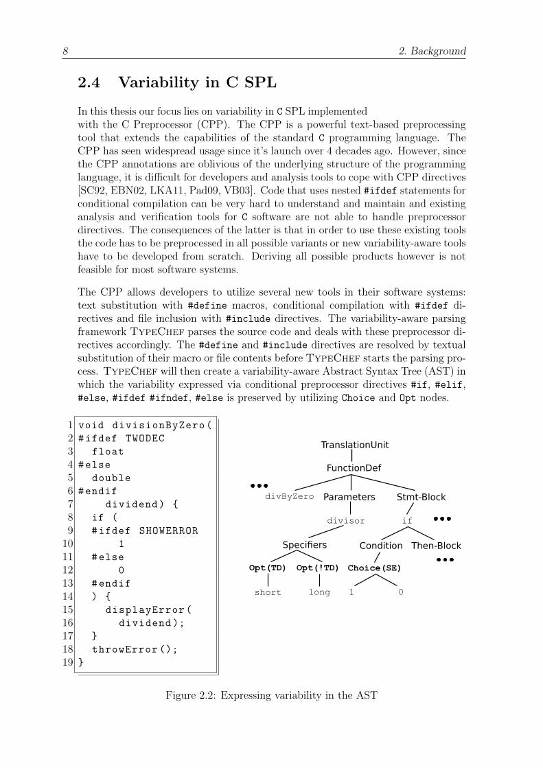
In this thesis our focus lies on variability in C SPL implementedwith the C Preprocessor (CPP). The CPP is a powerful text-based preprocessingtool that extends the capabilities of the standard C programming language. TheCPP has seen widespread usage since it’s launch over 4 decades ago. However, sincethe CPP annotations are oblivious of the underlying structure of the programminglanguage, it is difficult for developers and analysis tools to cope with CPP directives[SC92, EBN02, LKA11, Pad09, VB03]. Code that uses nested #ifdef statements forconditional compilation can be very hard to understand and maintain and existinganalysis and verification tools for C software are not able to handle preprocessordirectives. The consequences of the latter is that in order to use these existing toolsthe code has to be preprocessed in all possible variants or new variability-aware toolshave to be developed from scratch. Deriving all possible products however is notfeasible for most software systems.

The CPP allows developers to utilize several new tools in their software systems:text substitution with #define macros, conditional compilation with #ifdef di-rectives and file inclusion with #include directives. The variability-aware parsingframework TypeChef parses the source code and deals with these preprocessor di-rectives accordingly. The #define and #include directives are resolved by textualsubstitution of their macro or file contents before TypeChef starts the parsing pro-cess. TypeChef will then create a variability-aware Abstract Syntax Tree (AST) inwhich the variability expressed via conditional preprocessor directives #if, #elif,#else, #ifdef #ifndef, #else is preserved by utilizing Choice and Opt nodes.

1 void divisionByZero(

2 #ifdef TWODEC

3 float

4 #else

5 double

6 #endif

7 dividend) {

8 if (

9 #ifdef SHOWERROR

10 1

11 #else

12 0

13 #endif

14 ) {

15 displayError(

16 dividend );

17 }

18 throwError ();

19 }

FunctionDef

Stmt-Block

if

Condition Then-Block

1 0

Choice(SE)

TranslationUnit

divByZero Parameters

divisor

Specifiers

Opt(TD) Opt(!TD)

short long

Figure 2.2: Expressing variability in the AST

2.5. Variability Encoding 9

Developers can now implement new variability-aware analyses which utilize this ASTdata structure. Kenner et al. developed TypeChef as a framework for variability-aware type checking [KKHL10] however their framework has been used for othervariability-aware tasks, as well. Liebig et al. have developed Morpheus, a refactor-ing tool for preprocessor based SPL [LJG+15] and presented results of type checkingand liveness analysis [LvRK+13].

Going back to our Calculator SPL, Figure 2.2 depicts a code snippet on the leftside and the complying variability-aware AST representation on the right side. Thisexample shows how variability is preserved by TypeChef AST generation process.The function parameter dividend in line 7 has two different specifiers float anddouble, which depend on the selection of the feature TWODEC. In the AST the twopossible specifiers are represented by Opt nodes. Opt nodes are basically tuples with2 entries: a feature expression and an AST element, e.g. Opt<!TD, LongSpecifier>

Besides Opt nodes TypeChef also uses Choice nodes to express variability. Thegeneral concept of the choice calculus was presented by Erwig et al. in his publi-cation “The Choice Calculus: A Representation for Software Variation” [EW11]. InTypeChef these Choice nodes are implemented as a tree-like data structure thathas 3 data fields: a feature expression and two child nodes. If the feature of thefeature expression is selected then the first child node will be evaluated, otherwisethe second child node will be chosen. The two child nodes can either be Choice

nodes or One nodes, where the One node is a terminal node that only holds a leafAST element. This makes it possible to have nested Choice nodes.

2.5 Variability Encoding

The following section introduces the most important core aspect for our performancemeasuring process: variability encoding. We will talk about the general concept ofvariability encoding and go into details specifically when applied to the C program-ming language by providing examples. At last we will highlight shortcomings andproblematic aspects we encountered as we applied variability encoding on real-worldproduct lines.

2.5.1 Introduction

As we have seen in the previous sections, C SPL heavily utilize external languagetools like the CPP to express variability. These CPP annotations however have tobe resolved before compilation since they are not a part of the standard C language.The objective of variability encoding is to transform these annotations, that theprogramming language itself is oblivious to, into standard programming constructswithout changing the behavior of the software system. These transformations createa new meta product which encapsulates the behavior of all different variants of thesoftware product line. This meta product is also called product simulator.

2.5.2 Approach

Our general approach towards variability encoding in the domain of C software sys-tems is to first rename or rename & duplicate top level declarations inside #ifdef

10 2. Background

directives and second transform the remaining #ifdef statements in functions toC-conform IF statements. The first practical advances have been made by Post etal. [PS08] in their paper Configuration Lifting: Verification meets software config-uration where they manually execute the transformation process on a small Linuxsound driver. Based on their idea we have developed the tool Hercules3 underguidance and in heavy collaboration with (but not limited to) Jorg Liebig, Alexan-der von Rhein and Christian Kastner. Hercules is implemented as an extensionto the variability-aware parsing framework TypeChef and automates the trans-formation from compile-time variability expressed via CPP directives to run-timevariability by utilizing renamings, duplications and IF statements. The FM is usedin order to avoid unnecessary code duplications by checking satisfiability of everycomputed variant that has to be created by the duplication process. The feature se-lection state is encoded in the form of global variables, one for each distinct #ifdefname.

1 #ifdef TWODEC

2 float

3 #else

4 double

5 #endif

6 result;

7 // ...

8 #ifdef SHOWERROR

9 displayError(result );

10 #endif

a) Original source code

1 float _TD_result;

2 double _NTD_result;

3 // ...

4 if (opt.SHOWERROR) {

5 if (opt.TWODEC) {

6 displayError(_TD_result );

7 } else {

8 displayError(_NTD_result );

9 }

10 }

b) Meta product code

Figure 2.3: Code before and after variability encoding

2.5.3 Example

Taking a look at Figure 2.3 we can see how the transformation of this example lookslike. The original source code is on the left side and the result of our variabilityencoding can be found on the right side. The variable result in a) lines 1-6 hastwo derivable variants, one with the specifier float and the other one with specifierdouble. As we previously mentioned dealing with variable declarations requires usto duplicate code and the example shows that there are now two new definitionsfloat _TD_result and double _NTD_result in b) lines 1-2. On the other handthe optional function call of displayError is embedded into an IF statement whichuses our feature selection variable opt.SHOWERROR. As a consequence of replacingthe original declaration of result with two new declarations we also have to createnew IF statements every time result has been used in the original source code, seelines 5 and 7 b).

3https://github.com/joliebig/Hercules

2.5. Variability Encoding 11

2.5.4 Goal

The newly created meta product can be used with traditional verification tools,which are not variability aware, and the current configuration can be switched onthe fly by changing the global feature variables. To give an example, model checkingtools can potentially analyze the result of variability encoding and explore the wholeconfiguration space at once [vR16].

2.5.5 Behavior Preservation

The crucial property of the variability encoding transformation has to be behaviorpreservation. In order to draw meaningful conclusions about the properties of theoriginal SPL by analyzing its meta product the behavior must not change. Alexandervon Rhein [vR16] has developed a formal correctness proof for the behavior preserv-ing properties of variability encoding for the language Featherweight Java, afunctional subset of the Java programming language. Since the C programminglanguage includes complex language mechanics such as switch-case statements,goto statements, enums and structs a formal correctness proof is not feasible.However, we were still able to utilize Hercules and apply transformations to real-world product lines such as BusyBox, SQLite and a few Linux drivers.

2.5.6 Shortcomings

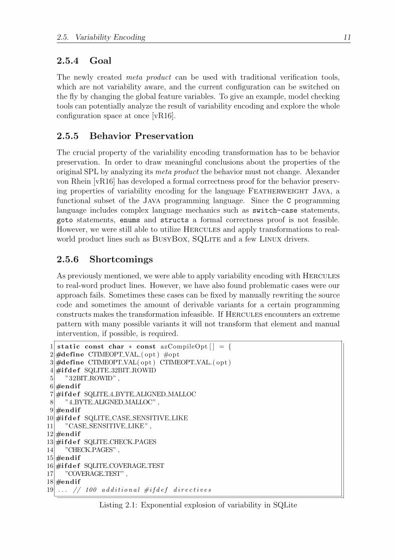
As previously mentioned, we were able to apply variability encoding with Herculesto real-word product lines. However, we have also found problematic cases were ourapproach fails. Sometimes these cases can be fixed by manually rewriting the sourcecode and sometimes the amount of derivable variants for a certain programmingconstructs makes the transformation infeasible. If Hercules encounters an extremepattern with many possible variants it will not transform that element and manualintervention, if possible, is required.

1 stat ic const char ∗ const azCompileOpt [ ] = {2 #define CTIMEOPT VAL ( opt ) #opt3 #define CTIMEOPT VAL( opt ) CTIMEOPT VAL ( opt )4 #ifde f SQLITE 32BIT ROWID5 ”32BIT ROWID” ,6 #endif7 #ifde f SQLITE 4 BYTE ALIGNED MALLOC8 ”4 BYTE ALIGNED MALLOC” ,9 #endif

10 #ifde f SQLITE CASE SENSITIVE LIKE11 ”CASE SENSITIVE LIKE” ,12 #endif13 #ifde f SQLITE CHECK PAGES14 ”CHECK PAGES” ,15 #endif16 #ifde f SQLITE COVERAGE TEST17 ”COVERAGE TEST” ,18 #endif19 . . . // 100 add i t i o n a l #i f d e f d i r e c t i v e s

Listing 2.1: Exponential explosion of variability in SQLite

12 2. Background

We encountered these patterns in product lines like BusyBox and SQLite [LvRK+13].Listing 2.1 depicts an example for this pattern that was taken from SQLite: a vari-able declaration thatVariant

explosioncontains a total of 105 different #ifdef directives. This leads

to an exceptional large number of variants of azCompileOpt[] even when takinginto account that some variants are not valid according to the FM of SQLite. Tomake things worse all usages of azCompileOpt[] have to be duplicated as well.But in this case we were able to create a function that assigns the correct content toazCompileOpt[] by using 105 IF statements that append the content of the comply-ing #ifdef statement to the current contents, similar to a StringBuilder. However,this solution cannot be applied to enums and structs which can theoretically beimplemented in similar fashion with an explosion of variants.

TypeChef and Hercules are stillSetupproblems

work in progress and there are still signifi-cant limitations that prevent applying them to real-world systems [KKHL10, vR16].Hercules can only start the transformation process if TypeChef is able to parsethe source code and there are no type errors. Any type error found by TypeChefwould immediately propagate into the meta product created by the variability en-coding process and as a consequence the meta product cannot be compiled. Mostreal-world systems do not provide a thorough FM and if features are not compatibletogether TypeChef will immediately find these type errors. In this case the FMhas to be forged and tweaked manually.

3. Approach

In this section we talk about our approach towards performance measuring for C

Software Product Lines (SPLs) by utilizing variability encoding.

3.1 Overview

#ifdef A#define X 4#else#define X 5#endif2*3+X

2 · ∗ · 3 · + · 4A · 5¬ A

variability-aware

parser

+

♦A

54

*

32

variability-aware

type systemvariability-aware

lexer

include directories partial configuration

variability-awareTypeChef

variabilityencoding

variability-aware

further analysis

parser framework

Hercules

injection of performance

measuring functionsgcc compile & execute

different configurations

collect measured data &

predict performancefor other configurations

¬A

Figure 3.1: Overview for our Performance Measuring Process

Figure 3.1 depicts our general idea behind our performance measuring and predictionprocess. The top part breaks down the different steps that TypeChef has to executein order to generate the variability-aware Abstract Syntax Tree (AST) [KKHL10].Next, the bottom half shows how Hercules utilizes the AST to generate the socalled meta product or product simulator through variability encoding and the nextsteps that are needed for generating performance measurements. For the remainder

14 3. Approach

of this thesis we will refer to the result of variability encoding as product simulatorand to the result of the injection of measuring functions as performance simulator.The following sections provide a detailed explanation of these individual procedures.

3.2 Combining Variability Encoding with Perfor-

mance Measuring

Section 2.5 shows how code can be manipulated to transform compile-time variabilityto run-time variability. One of the code transformation techniques is to transformoptional or variable statements to IF statements. This is where the performancemeasuring process starts. Every time one of these statements is turned into a new IF

statement we add two function calls, one at the beginning of IF and one at the end.We can now measure the difference in the timestamps between these two functioncalls, which resembles the execution time for this IF statement. The injection ofthese functions is pretty straight forward for most of the affected transformations.In Section 3.4 we will briefly talk about our approach towards dealing with morecomplex programming structures.

It is important to highlight that our current implementation for these performancemeasuring functions is easily interchangeable and can be manipulated to add furtherimprovements because their definition is part of a separate file that is loaded via#include. We will now explain their implementation:

Algorithm 1: Implementation of the performance measuring function perf before

1 Stack<String> context stack;2 Stack<Integer> time stack;3 Stack<Boolean> is new context;4 Hashmap<String, Integer> context times;

5 function perf before (context);Input : String representation of associated context

6 Integer before outer = getTime;7 time stack.push(before outer);8 if context /∈ context stack then9 context stack.push(context);

10 is new context.push(TRUE);

11 else12 is new context.push(FALSE);13 end14 Integer before inner = getTime;15 time stack.push(before inner);

The first function, inserted at the start of each IF statement that was created byvariability encoding, is called perf before and is responsible for multiple things. Thisfunction requires a char* argument that resembles the representation of the contextthat is also part of the IF condition. The general overview can be seen in algorithm 1.

3.2. Combining Variability Encoding with Performance Measuring 15

Calling perf_before first generates an immediate time stamp before_outer, thatis used to measure the measurement overhead itself later on. Next, it puts thelabel of the previous #ifdef statement on top of the context stack of #ifdef labelsbut only if the context is not already present in the current context stack, see lines8-13. This is to avoid recursive function calls or loops to unnecessarily affect thecontext stack. An example for this is optional code in context X64 calls a functionthat also has optional code parts under context X64. In the same lines we also keeptrack of the information whether the context is a new addition to context_stack,or not by adding it to is new context for later use. In a scenario of nested #ifdefs

we are able to produce the absolute context of the current statement by combiningall #ifdef labels from the context stack with the boolean & operator. The last stepis to generate a second time stamp before inner and throw both before time stampsonto the time stack so we can use this information for our second function perf after.

Algorithm 2: Implementation of the performance measuring function perf after

Stack<String> context stack;Stack<Integer> time stack;Stack<Boolean> is new context;Hashmap<String, Integer> context times;// ...

16 function perf after;

17 Integer after inner = getTime;18 Integer context time = after inner - time stack.pop;19 Integer new context time = context time;20 String assembled context = getContext(context stack);21 if is new context.pop then22 context stack.pop;23 end24 if assembledContext ∈ context times then25 new context time += context times.get(assembled context);26 end27 context times.put(assembled context, new context time);28 Integer before outer = time stack.pop;29 Integer after outer = getTime;30 Integer measurement overhead = (after outer - before outer) - context time;

algorithm 2 shows the general idea behind the perf after implementation. The firstobligation of the perf_after function in line 16 is to also generate a time stampcalled after inner. This time stamp is used with before inner to compute the elapsedtime between the end of perf before and the beginning of perf after in the very nextline. context time then resembles the execution time of the statements between ourinjected function calls. This information is put into a Hashmap[String,Double],where we add the current time for the combination of features in our time stackto previously measured execution time for this feature combination. The last stepis once again to take a time stamp after outer. These outer time stamps are used

16 3. Approach

during post processing to account for the execution time of our injected performancemeasuring functions.

We also injected similar functions at the start and end of the MAIN function whichmeasure the time for the context BASE. This way the program itself generates ahashmap, which contains the sum of all execution times for each context and com-bination of nested features of statements that have been executed in the given con-figuration. Each different configuration generates a different hashmap, unless twoconfigurations have exactly the same executable code. However, in that case theexecution times should still be different because they fluctuate. This hashmap hasto be post processed to account for multiple nested measurements as explained inSection 3.6. We will refer to this hashmap as the Feature-Time Hashmap (FTH).

3.3 Example Software Product Line

Before we go into details about how we utilize the information in the resulting FTHlet us take a look at what actually happens to the code in our calculator productline.

Listing 3.1 shows how the code for multiplication looks after variability encodingand injection of our performance measuring functions perf before and perf after.The #ifdef and #else directives from Listing 3.1 (a) Line 5 and 11 have beentransformed to IF statements, Listing 3.1 (b) Line 5 and 11 respectively. Addition-ally the performance functions have been inserted at the start and end at each ofthe generated IF statements.

Execution of the calculator product line with features TWODEC and HISTORY selectedwill now automatically measure the time the code of each of these features needsto be executed when calling function multiply. Figure 3.2 shows how the contextstack progresses during the execution of the program. # is used as a separatorbetween features or feature expressions in nested #ifdef directives and M# is anabbreviation for MultDivide#. The following line numbers are in reference toListing 3.1 b). Since the function multiply itself is defined in an #ifdef directivewith identifier MULTDIVIDE the function call also has to be inside a similar #ifdef

directive. This is why the initial state of the context stack already contains theinformation for the feature MULTDIVIDE. Each execution of our perf before functionthen adds a new feature or logical combination of features to the context stack.The first execution in line 7 pushes TWODEC on the stack. On the other hand callingperf after removes the last feature of the context stack. In line 11 the feature TWODECis discarded and in line 14 the new feature HISTORY is added.

3.3. Example Software Product Line 17

1 #ifdef MULTDIVIDE

2 double multiply(double a,

3 double b) {

4 double res = a*b;

5 double rf;

6 #ifdef TWODEC

7 // 2 decimal places

8 rf = 100.0;

9 res = round(res*rf)

10 / rf;

1112 #endif

13 #ifdef HISTORY

1415 saveResult(res);

1617 #endif

18 return res;

19 }

20 #endif

a) Original source code

12 double multiply(double a,

3 double b) {

4 double res = a*b;

5 double rf;

6 if (opt.twodec) {

7 perf_before(twodec );

8 rf = 100.0;

9 res = round(res*rf)

10 / rf;

11 perf_after ();

12 }

13 if (opt.history) {

14 perf_before(history );

15 saveResult(res);

16 perf_after ();

17 }

18 return res;

19 }

20

b) Performance measuring code

Listing 3.1: Injection of performance measuring functions

One of the requirements of successfully generating performance measurements isthat each call of perf_before is followed by the corresponding call of perf_afterbecause otherwise the information inside the context stack would be corrupted. Thiswill be discussed in further detail in Section 3.4.

The end result of executing our program is a hashmap, FTH, which accumulatesthe execution time of statements tied to their context in the form of features orcombinations of features. Table 3.1 shows what the hashmap looks like after onemultiplication with the calculator product line and features MultDivide, twodecand history enabled. It is important to note that the time measured for MultDi-

vide includes the execution time of the other two features, which are nested insidethe #ifdef directive from the function call of multiply.

After line 1

MULTDIVIDE

After line 13M#SAVEHISTMULTDIVIDE

After line 7M#TWODECMULTDIVIDE

After line 16

MULTDIVIDE

Figure 3.2: Context stack progression

feature time (seconds)

MULTDIVIDE 10M#TWODEC 2M#HISTORY 4

Table 3.1: Feature time hashmap

18 3. Approach

3.4 Dealing with Control Flow Irregularities

When applying our approach to real world product lines we quickly noticed that it’snot as simple as inserting a function to start the measurement and a correspondingfunction to end that measurement. In Section 3.3 we mentioned that it’s necessarythat each performance measuring starting function is at some point followed by itscorresponding measuring ending function in order to avoid corrupting the contextstack. However, the C programming language contains multiple programming con-structs that make it possible to skip the corresponding measurement ending functioncall: break, continue, goto, return statements. These statements cause con-trol flow irregularities meaning that they have the ability to prevent the execution ofa time measurement ending function after its corresponding measurement startingfunction has already been called.

In order to tackle this issue we add additional measurement ending calls as neces-sary before these statements. This is done in a top down traversal of the AST ofthe program after applying variability encoding where we have to keep track of thenumber of currently active time measurements when encountering certain program-ming elements. A measurement is considered as active after calling the functionperf_before and before its corresponding perf_after function is called. Multipleactive measurements happen when the original source code contained nested #ifdef

directives.

1 // Case statements and breaks

2 case 29:

3 if (! omit_pragma && !omit_pager_pragmas) {

4 1 perf_before("!omit_pragma && !omit_pager_pragmas");

5 if ((! zRight )) {

6 returnSingleInt(pParse , "synchronous", (pDb ->safety_level - 1));

7 } else {

8 if ((! db->autoCommit )) {

9 sqlite3ErrorMsg(pParse , "Safety level may not be changed

10 inside a transaction");

11 } else {

12 (pDb ->safety_level = (getSafetyLevel(zRight , 0, 1) + 1));

13 setAllPagerFlags(db);

14 }

15 }

16 x perf_after ();

17 break;

18 1 perf_after ();

19 } else {

20 // more code

21 }

22 break;

23 case 30:

24 // more code

Listing 3.2: Handling control flow irregularities in SQLite: break

For return statements we calculate the difference between active time measurementsbefore executing the return call and active time measurements when entering thebody of the function that the return belongs to. Afterwards an additional amount

3.4. Dealing with Control Flow Irregularities 19

of perf_after function calls is added in front of the return statement. The ex-act amount depends on the previously mentioned difference. goto statements arehandled in a similar way and for continue and break statements we keep trackof the difference in active measurements to the associated loop (or case statementfor break). This way we ensure that previously started measurements are properlyfinalized before jumping to a different part of the program code.

Listing 3.2 and Listing 3.3 depict examples from our SQLite case study. Codeparts which were not relevant to the following explanation were left out. The injectedperformance measuring functions from Section 3.2 are annotated with numbers, e.g.,Listing 3.2 line 4 and 18 are annotated with the same number which indicates thatthese are corresponding performance starting and ending functions. The additionalperformance ending function calls from Section 3.4 are annotated with the lettersxyz.

First, we take a look at Listing 3.2 where parts of a switch statement can be seen.The IF statement in line 3 is generated from an #ifdef directive in the originalsource code. The next line then starts the performance measuring process and it isconsidered active from line 5 to line 18 where the if statement ends. However, sincethere is a break statement in line 17 the corresponding perf_after function willnever be executed. This is why according to our previous explanation we are addingone additional perf_after call to properly terminate the performance measuring forthe feature !omit pragma && !omit pager pragmas because there is one additionalactive measurement when executing the break statement compared to the start ofthe case statement in line 2.

1 // Functions and return

2 static int btreeCreateTable(Btree *p , int *piTable , int createTabFlags ) {

3 int rc;

4 // more code

5 if (! omit_autovacuum) {

6 2 perf_before("OMIT_AUTOVACUUM");

7 rc = allocateBtreePage(pBt , (& pPageMove), (& pgnoMove), pgnoRoot , 1);

8 // more code

9 if (rc == 0) {

10 y perf_after ();

11 return rc;

12 }

13 if ((( id2i_sqlite_coverage_test ) )) {

14 3 id2iperf_time_before_counter("SQLITE_COVERAGE_TEST", 628);

15 if (rc != 0) {

16 releasePage(pRoot);

17 z perf_after (); perf_after ();

18 return rc;

19 }

20 3 perf_after ();

21 }

22 2 perf_after ();

23 }

24 }

Listing 3.3: Handling control flow irregularities in SQLite: return

20 3. Approach

In our other example Listing 3.3 the focus is on return statements. There are twoplaces in which variability encoding generated if statements, lines 30 and 38. Beforeexecuting the return in line 36 there is 1 active time measurement from line 31 andso we have to add one perf_after call annotated with y . The return statementin line 42 the situation is different. Both measurements from lines 30 and 38 areconsidered active and this is why we have to add two perf_after function calls inline 42 z before executing the return statement.

3.5 Feature InteractionsWe have already mentioned examples where we feature interactions occur but did notexplain them yet. Feature interactions in the context of this thesis describes eithera direct nesting of conditional preprocessor directives in the code itself or a nestingvia function calls. We use a delimiter symbol # to differentiate between nestingof #ifdefs and the preprocessor expressions themselves. The so called Feature-Interaction Degree (FID) for a given feature combination in the context stack equalsthe amount of # that occur in the combination.

Listing 3.4 presents different cases of feature interaction. First of all, lines 12-13 arenested #ifdefs and therefore the performance measurement in line 14 has a FID of 1.Second, line 4 is a preprocessor directive and executes a function call in line 6. Hencethe performance measurement for line 22 also has a FID of 1: PLUSMINUS#HISTORY.In contrast, the feature expression inside the random function in line 27 et seqq.has FID of 0 since it is not a feature interaction by itself. These interactions aregenerated automatically during execution of the performance simulator by checkingthe context stack.

1 int first , second , result;

2 switch (op) {

3 #ifdef PLUSMINUS

4 case ‘+’:

5 result = add(first ,

6 second );

7 break;

8 #endif

9 // ...

10 }

11 #ifdef SHOWERRORS

12 #ifdef TWODEC

13 errors = round(errors );

14 #endif

15 showErrors(errors );

16 #endif

17 }

a) Calling add

19int add(int a, int b) {

20int result = a + b;

21#ifdef HISTORY

22archiveInHistory(result );

23#endif

24return result;

25}

2627int random () {

28#ifdef TWODEC && HISTORY

29seed = getNewSeed ();

30#endif

31// ...

32}

b) add function implementation

Listing 3.4: Feature interaction example

3.6. Post Processing of Measurements 21

3.6 Post Processing of Measurements

The previously generated FTH has to be processed to yield useful information.The C implementation of our performance measuring functions is intended to bevery basic to not affect the overall program run time too much by introducing

feature time (seconds)

MULTDIVIDE 4M#TWODEC 2M#HISTORY 4

Table 3.2: FTH from Table 3.1 afterPost Processing

complex time measuring and collecting al-gorithms. Since we are working with timestamps and nested performance measure-ments we need to subtract the time of aninner measuring from its direct predeces-sor. Therefore, we use a delimiter sym-bol that allows us to differentiate betweena nesting of feature #ifdef A in feature#ifdef B from their composition #if de-

fined A && defined B. Looking back at Table 3.1 generated from the code in List-ing 3.1 the final numbers for MultDivide changes and the resulting FTH after postprocessing can be seen in Table 3.2.

This information by itself can already provide some useful insight into how the pro-gram execution time is divided between the different features that were executed inthe run under the given program configuration. In order to generate performancepredictions for the other possible program configurations we can use the previouslygenerated FTH and filter out all the features that are incompatible with the newconfiguration. Feature A and feature B are considered incompatible when their com-position A && B is not satisfiable in the context of the feature model for that productline. The FTH only provides valuable information after post processing its informa-tion. For that reason in the remainder of this thesis the usage of FTH implies it hasalready been post processed.

3.7 Collection of Prediction Information

Since it is very unlikely that one configuration can cover the whole code basis becauseof restrictions in the Feature Model (FM) or mutually exclusive code parts from#ifdef and #else preprocessor directives, we implemented a way to collect theinformation from multiple FTHs generated over several program runs, each witha different program configuration. If configuration one includes the performancemeasurements for feature x64 and configuration two includes the mutually exclusivemeasurements for x86 we can combine the data from both runs to gain information.

However, these FTHs can contain the same feature entries with different executiontimes across different configurations. This can happen when there are data-flowdependencies across the different features. It is important to note that this datadependence between two features occur when one feature manipulates data insideits preprocessor directive and another feature accesses that data in its own directivewithout being nested in the previous one. If the same feature entries have differentmeasured times across multiple FTHs, we compute the average of these executiontimes, the standard deviation, and populate a new summarized FTH with thesevalues. If a feature entry is unique to a configuration it is added to the summarizedFTH without further changes. We anticipate that users with insightful knowledge

22 3. Approach

about the configuration options of their product line can come up with a small subsetof configurations which can be used to create a solid basis for multiple predictionscenarios.

Table 3.3: Combining information of multiple FTHs

feature time (seconds)config 1 config 2 config 3 avg. std dev.

MULTDIVIDE 4 - 5 4.5 0.5TWODEC - 2.2 2.4 2.3 0.08HISTORY 1 1.1 4.2 2.1 1.29

Table 3.3 shows how we combine performance measurement information from mul-tiple FTH. In this example there are 3 different configurations that were used andthey all have different times for features in their FTH. Most of the feature timesare similar however HISTORY in config 3 needs a lot more execution time comparedto the two previous configurations. This is the case because there is a dataflowdependency between HISTORY if TWODEC and MULTDIVIDE are both selected. Thiscauses HISTORY to have a very high standard deviation of 1.29 seconds, which isabout 61% of its average time 2.1 seconds. Using this data set as a basis to computeperformance predictions for other configurations can lead to a high variance becauseof the uncertainty in the feature HISTORY.

p =∑e∈F

{e, if e ∈ SAT (e&c&fm)

0, otherwise

where:

p = predicted datae = entry in FTHF = FTHSAT = function to check satisfiability of a boolean expressionc = configuration to generate prediction forfm = FM

Figure 3.3: Generating prediction data

In order to make predictions we utilize the data from the combination of multipleFTHs, as seen in Figure 3.3. Although the predicted data consists of two differentnumbers, the average and the deviation. In the end both are just the sum of allentries in FTH that are still considered satisfiable when combined with the FM andthe new configuration that is to be predicted.

3.8 Limitations and Problematic Aspects

Now that we have explained our general approach towards performance measuring& prediction for software product lines it is time to look at potential shortcomings:

3.8. Limitations and Problematic Aspects 23

First of all the meta product meta productperformancedifference

of a product line encapsulates the properties of allderivable variants. A widespread usage of the C Preprocessor (CPP) is implementingcode for different hardware architectures, e.g. to choose between different types forvariables like int and long. In order to utilize these variable types in the metaproduct we have to resort to code duplications. But these code duplications cancause an increase in memory consumption and negatively affect the performance ofthe meta product compared to the original product line, see Section 4.3.6.

The time measurements are injected nogranularitycontrol

in every former #ifdef directive even when thenumber of statements inside the #ifdef directive is low or the execution time of thecode is completely negligible. These measurements cause additional measurementoverhead which can negatively affect the accuracy of our predictions. Even whenaccounting for the measurement time by using inner and outer timestamps there willalways be a call to free for variables after the last outer time stamp is generated.The execution time of these performance concluding statements like free is not partof the calculated measurement overhead. Instead they are included in the time of aprevious outer measurement.

The next potential problem is that our mutuallyexclusivecode

approach can only measure the executiontime of actually executed code in one configuration at a time. The consequenceis that mutually exclusive code from #ifdef and #else directives can never bemeasured in a single program run. In these cases it is important to come up with asound list of configurations and combine their results as mentioned in Section 3.7

When dealing with multiple configurations variancebecause ofdatadependency

the time measured for equal featurescan differ greatly. The consequence is a high standard deviation for that particularfeature in the FTH and as a consequence an increased variance for the performanceprediction. The reason for the difference in observed execution time of the samefeatures across different configurations can be data dependency: if feature A affectsthe upper limit of a computational loop that is used by feature B in an unrelatedpreprocessor directive, then the time of feature B is increased in configurations wherefeature A is also selected.

The last two paragraphs show that the selection of configurations which are measuredand used as basis for the prediction is crucial. In the next section we will take athorough look at a few different prediction scenarios we selected and how they affectthe result of our prediction.

24 3. Approach

4. Evaluation

As previously mentioned, the data we get from measuring the performance in aconfiguration can be used in many different ways. The results display the measuredexecution times for each feature and combinations of features, that are nested inconditional preprocessor directives. We can also collect the information of one orseveral different configurations and use that data to predict the performance forother configurations. In the following section we take a look at two different casestudies and present possible answers to the research questions that were posed inthe introduction.

4.1 Test System Specifications

Our experiments were conducted by one of the following computer setups:

DS The desktop system is a personal desktop machine that is powered by an Inteli7-4790K@4.0GHz with 4 cores & 8 threads, 16Gb DDR3 RAM that runs onUbuntu 14.04.

CS The cluster system consists of 17 nodes, each with an Intel Xeon E-5 2690v2@3.0GHz with 10 cores, 20 hyper-threads, 64 GB RAM that run on Ubuntu 16.04.

4.2 Elevator Case Study

The Elevator or Lift system has been designed by Plath and Ryan[PR01] as a ba-sic model of an elevator that can be extended by different features, e.g. TWOTHIRDS-FULL will not accept new elevator calls after reaching over 2

3of its capacity since it is

unlikely to be able to accept more passengers. This software system has been usedin research to reason about feature properties, interactions, analysis strategies andmore[AvRW+13, SvRA14].

The Elevator system has 6 features and the feature model can be seen in Fig-ure 4.1. The feature Base is mandatory, all other features are optional except for

26 4. Evaluation

Figure 4.1: Elevator FM visualized

((Overloaded => Weight) && (Tworthirdsfull => Weight)) && Base

Figure 4.2: Elevator FM as propositional formula

two implications for the features Overloaded and TwoThirdsFull. The proposi-tional formula for this Feature Model (FM) can be seen in Figure 4.2. According tothis FM there are 20 valid configurations for the Elevator system. All times weremeasured on our system DS.

This case study is very close to the ideal scenario for our approach and will helpus answer RQ1. Elevator does not contain any feature interactions in the formof nested #ifdefs in the code or via function calls. All regular features are imple-mented in isolated conditional #ifdefs without any mutually exclusive code partsand it is possible to select all features together, which covers the whole code base.These are the perfect terms for our approach. The only downside of the Elevatorcase study is the code that belongs to the features has a very low execution time.

1 void enterElevator(int p) {

2 enterElevator__before__weight(p);

3 #ifdef WEIGHT

4 usleep (100);

5 weight = weight + getWeight(p);

6 #endif

7 }

8 // ... other Code

9 void leaveElevator__before__empty(int p) {

10 leaveElevator__before__weight(p);

11 #ifdef WEIGHT

12 weight = weight - getWeight(p);

13 #endif

14 }

Listing 4.1: Implementation for feature Weight in Elevator

4.2. Elevator Case Study 27

feature time (ms) NoMExecutiveFloor 80.038330 2500Weight 30.349609 400Empty 20.287354 200Overloaded 0.209473 1302TwoThirdsFull 0.070557 1202Base 6.579589 1

Figure 4.3: Performance Measuringresults in Elevator’s allyes

configuration

feature time (ms)ExecutiveFloor 79.332507Weight 30.962723Empty 20.771696Overloaded 1.498675TwoThirdsFull -0.245845Overloaded&ExecutiveFloor -1.822054TwoThirdsFull&Overloaded 0.420249Base 0.473498

Figure 4.4: SPLConqueror resultsusing all configurations

Listing 4.1 shows the implementation for the Weight feature. We have artificiallyincreased the execution time for this feature by adding a sleep call in line 4. If notfor the sleep call the feature only performs a simple addition or subtraction and thiscauses increased fluctuations in measured execution times. This also reduces theeffect that the measurement overhead has on the overall observed execution times.

4.2.1 Performance Measuring

We have applied our performance measuring approach and created a variant simu-lator that is able to produce different Feature-Time Hashmap (FTH). The configu-ration for the variant simulator can be exchanged by editing the values of the globalfeature variables in the external configuration file. For this case study the allyesconfiguration, where all 6 features are selected, covers all parts of the source code.

There are data dependencies across the features, e.g. Weight changes the valuefor the elevator and Overloaded uses this information to judge if the elevator istoo crowded. However, these dependencies occur in all valid configurations whereOverloaded is selected since according to the FM it requires feature Weight. Addi-tionally, the fact that Weight changes an int value that is used in a comparison byOverloaded does not affect the execution time of that comparison.

The results after post processing Section 3.6 can be seen in Figure 4.3. Althoughonly the BASE feature has undergone changes since all the other features do nothave any nested features inside them. A total of 5605 measurements (see columnNoM ). Looking at the Base feature we immediately notice that the execution timeis significantly higher compared to the other features Overloaded and TwoThirds-

Full although none execute any sleep statements. This is one of the downsides ofour approach, since all measurements outside of the Base feature are nested insidethe measurement for Base the last free call that is executed at the end of everymeasurement is included in the overlying BASE feature.

We have measured each configuration of Elevator 10 times and computed theiraverage execution times. Using these numbers in SPL Conqueror1, a machine-learning library for measuring and predicting performance, we can generate a de-tailed breakdown of how features and feature combinations affect the performance

1http://www.infosun.fim.uni-passau.de/se/projects/splconqueror/

28 4. Evaluation

of the Elevator system, seen in Figure 4.4. Comparing these results, which weregenerated by executing 20 variants, to our performance measuring results in Fig-ure 4.3, which was generated in a single execution of the allyes configuration, wecan see that the times for the first three features are very close. The other timeshowever are not comparable, possibly because of data dependencies or inaccuracyfor measurements below 2 ms.

4.2.2 Overhead calculation flaws

As the results for the BASE feature in Section 4.2.1 show, there is a flaw in ourapproach that affects the performance measurements. Looking back at algorithm 2in Section 3.2 this flaw is not included. As our performance measuring functionsare implemented in C, we have to deallocate a variable after conducting the finalmeasurement that computes the internally calculated overhead.

1 void perf_after () {

2 double after_inner = getTime ();

3 time_struct* t = (time_struct *) pop(& time_stack );

4 // Omitted code

5 double measurement_overhead = getTime ()

6 - before_outer - context_time;

7 // store overhead

8 free(t);

9 }

Listing 4.2: Deallocation in perf after affects preceding measurements

The code in Figure 4.2 is a more accurate representation of our implementation.Line 5 executes the final measurement for that feature and calculates the internaloverhead. But the time_struct* t has to be deallocated and the time needed forthis deallocation (+ storing overhead) is attributed to the preceding measurement.Starting the measurement for BASE is the first statement inside the main function.All of the other performance measurements are nested inside BASE or other features.Consequently all measurements, except for BASE, are attributed additional execu-tion time from their nested successor measurements. We will talk about potentialsolutions for this flaw in Chapter 6.

4.2.3 Performance Prediction

We can now utilize the numbers generated from a single execution of the allyesconfiguration from the previous section to make predictions about the performanceof other configurations. We already computed the variant times for all 20 con-figurations of Elevator in the previous section in order to generate results forSPLConqueror.

Table 4.1 shows the 20 different configurations using abbreviations for the featuresand their execution times compared to the predicted time using our performanceprediction approach. To account for incorrectly assigning a free call to our time

4.3. SQLite Case Study 29

configuration variant time predicted time percent errorB 0.460100 0.460100* -B&EM 20.7212925 20.747454 0.13%B&W 31.0513020 30.809709 0.78%B&W&T 31.131196 30.880266 0.81%B&W&T&O 32.6761007 31.089739 4.86%B&W&O 32.7689886 31.019182 5.34%B&W&EM&T 52.3653030 51.167620 2.29%B&W&EM 52.7860880 51.097063 3.20%B&W&EM&O 53.693986 51.306536 4.45%B&W&EM&T&O 54.4927120 51.377093 5.72%B&EX 80.3105116 80.498430 0.23%B&EM&EX 100.610495 100.785784 0.17%B&W&T&EX 110.584903 110.918596 0.30%B&W&EX 110.721207 110.848039 0.11%B&W&T&EX&O 110.799599 111.128069 0.30%B&W&EX&O 110.803103 111.057512 0.23%B&W&EM&T&EX 130.88851 131.20595 0.24%B&W&EM&T&EX&O 131.033087 131.415423 0.29%B&W&EM&EX&O 131.037807 131.344866 0.23%B&W&EM&EX 131.394696 131.135393 0.20%

Table 4.1: Comparing all variants to our prediction

for the Base feature we will instead use the time that was observed for the BASE

configuration as is stated in the first data row and noted with a ‘*’. There are 6outliers with a Percent Error (PE)2 of over 1% but overall the numbers are prettysimilar. Reasoning about the distribution of execution times between features andthe shared code base according to RQ2 does not make sense for this case study,since we artificially tinkered with these execution times. The majority of the timeis spent inside optional features.

The effort that is required for this approach is applying variability encoding to thesource code and then executing a configuration or multiple configurations in orderto generate data used for the prediction of other configurations. For Elevator theefforts according to RQ3 are as follows: ∼600 ms for variability encoding and 133ms for executing the performance simulator in the allyes configuration. If we addup the execution times of the 20 variants that alone amouints to over 1500 ms. Casestudies with more features and many more derivable variants will further increasethis gap. However, with more features and possible feature interactions it is possiblethat measuring one allyes configuration will not produce good predictions for allconfigurations.

4.3 SQLite Case Study

Our next case study is the real-world software system SQLite3. It is a highly-configurable database product line and is considered the most widespread database

2

percent error =|predicted value− expected value|

expected value

3https://www.sqlite.org/

30 4. Evaluation

system worldwide [LJG+15]. SQLite has 93 different configuration options in itsamalgamation version 3.8.1 and can be tested by its extensive TH3 test suite4.

Our variability approach has been examined for SQLite towards behavior preser-vation and the amount of overhead in the form of additional Abstract SyntaxTree (AST) nodes in the meta product vs the original source code [vR16]. The gen-eral conclusion is that SQLite is highly compatible for variability encoding with afew restrictions.

The SQLite case study combined with the TH3 test suite are considered black boxsystems. Without any further insider knowledge and because of the sheer complexitywe argue that this software system is not an ideal scenario according to RQ1.

4.3.1 SQLite TH3 Test Suite Setup

We will now explain the setup we used for testing our approach with the SQLitecase study. The execution times were generated on our cluster system CS as averagetimes from 10 runs.

TH3

bugscov1

session

dev

...

TH3/cfgCFG 64k.cfgCFG c1.cfgCFG c2.cfg

CFG wal1.cfg

...

6 testdirectories

25 TH3configurations

X X

SQLite/cfg

85 SQLiteconfigurations

23 feature-wise

11 pair-wise

50 random

1 allyes

6 * 25 * 85 = 12.750 test scenarios

Figure 4.5: SQLite TH3 test setup

First, we need to explain how the TH3 test suite operates. At its core is a scriptthat converts one .test file or multiple files in a given directory into a C file thatexecutes all given tests if linked with SQLite. The SQLite amalgamation version5

is a concatenation of all the source files required to embed SQLite. After our mod-ifications to the test suite setup (see Section 4.3.2) we are left with 6 test directories,and each consists of 1 to 355 .test files.

Second, the TH3 test suite itself is configurable. In order to avoid confusion ofSQLite and TH3 configurations we will refer to the latter as TH3 configs. Thereare 25 different TH3 configs in our modified setup and each defines a set of different

4https://www.sqlite.org/th3/5https://www.sqlite.org/amalgamation.html

4.3. SQLite Case Study 31

properties (P). The previously mentioned .test files declare a set of REQUIRED (R)and DISALLOWED (D) properties and during execution these tests are skipped for aproperty φ if φ ∈ P ∧ φ ∈ D or if φ /∈ P ∧ φ ∈ R and executed otherwise.

Last, are the configurations of SQLite itself. Since it is infeasible to analyze allpossible configurations and because we had no thorough FM, we decided to focuson a subset of 23 features, the focus features. We then created four different groupsof configurations for these features:

Feature-wise Each configuration consists of one enabled focus feature and as littleas possible other features, which can be required according to the FM. Thisleaves us with 23 different feature-wise configurations.

Pair-wise These configurations have been generated with the SPLCA tool6. Thebasic idea is to generate all possible pairs for the focus features and generateconfigurations, which cover multiple pairs at the same time. SPLCA hasgenerated 11 pair-wise configurations.

Random We generated 50 different configurations by mapping randomly generatedbinary numbers between 0 and 223 to a configuration. Duplicate and invalidconfigurations according to the FM have already been discarded during thegeneration process.

Allyes We have already mentioned the allyes configuration in previous sections.For this configuration we simply enabled all 23 focus features.

4.3.2 Test Setup Modifications and Restrictions

After establishing the general concept of the TH3 test suite we now talk about thedetails for the modifications and restrictions that were applied. It is very importantto note that the numbers in the following section are comparisons in execution timesbetween our meta product from variability encoding and our meta product afterintegrating the performance measuring functions. We decided to compare these twobecause the meta product itself has already a very different performance comparedto the software variant that is tested. We will talk about this further in Section 4.3.6.

During our testing approach we noticed that one of the 26 TH3 configs never ex-ecutes any test cases. This configuration is responsible for testing a DOS relatedfilename scheme and is not compatible with our UNIX setup, so we excluded it.We also excluded two .test files because one contains an array declaration that isloaded with over 100 #ifdefs across nearly 3000 lines of code and the second testfile performs time and date tests for which we cannot verify the behavior preserva-tion between variant and meta product. For us to verify behavior preservation, werequire a binary test result success or failure. Some tests however deviate from thisscheme by utilizing information that is not constant for different test executions,e.g. current system time or memory consumption.

6http://martinfjohansen.com/splcatool/

32 4. Evaluation

Next, the TH3 test suite originally consists of 10 folders that contain .test files.We have excluded the stress folder since it contains tests with a very high run time.These stress tests can verify robustness by loading a corrupted database, simulatea power-failure in the middle of a transaction and more. After excluding the stressfolder we ran into SQLite out of memory errors during execution of our metaproduct in two directories. We decided to create partitions for these two folders andthus reduce the amount of .test files per folder. One directory was partitioned onceand the other one had to be partitioned twice. We further excluded 3 more folderswhich only consist of 1-2 .test files each because their execution time is too low(<2 ms) to be useful. In summary we excluded four folders and created three newfolders to balance out the test load.

Last, to generate compatible test scenarios across the different SQLite configura-tions we excluded all .test files that are not executed in all our SQLite config-urations for a given combination of TH3 config & test directory and added themto a list of shared tests. With 12 test directories and 25 TH3 configs this equals300 different shared test lists. We reason that comparing execution times from test-ing different SQLite configurations does not make sense when both configurationsperform different test cases.

We revalidated the results after applying these restrictions and filtered one morefolder where the execution time was very low (<2 ms), this is mostly because notest cases or just a few quick test cases remained. We also had to remove twofolders which produced a lot of TH3 test suite errors. In summary we are left with6 test directories, 25 TH3 configs and 85 SQLite configurations, as presented inFigure 4.5. All of these three can be combined in any arbitrary way and thus thereare 12750 different test scenarios.

4.3.3 Statistics for the Measuring Process

First, we start by presenting various statistics about our approach before the nextsections illustrate our results from analyzing the performance of SQLite.

● ●●● ●●●● ●●●●● ● ●● ●● ●●●●●●●● ●●●● ●● ●● ●● ●●●● ●● ●●● ●●●● ●●●● ●●●●● ●●●●● ●●●●●●● ●●● ●●● ●●● ●●●● ●● ●●●●● ●●● ●● ● ●●●●●●● ●● ● ●●●● ●●●●●● ●● ●● ● ●● ●●●● ●●●● ●●●● ●●●● ●●●●● ●●●●●●● ● ●●●● ● ●●●●●● ●●●●● ● ●● ● ●●●●●●●●●● ●● ●● ●●● ●●●●●●●●●● ●●●● ●●● ● ●●● ●●●●●● ●● ● ●● ●●●●●● ●●● ● ●●● ●●

0 50000000 100000000 150000000Total number ofmeasurements

Figure 4.6: Amount of function calls to our measuring functions in SQLite

The injected function perf_before tracks the amounts of measurements that havebeen started for each context. We will now take a look at the total amount of mea-surements that have been performed across all of the 12750 different test scenarios.Figure 4.6 shows that these numbers vary greatly and take on anywhere between180 to 180712831 measurements. The red dot resembles the mean amount of mea-surements at 23005422. This is something that has to be kept in mind, we already

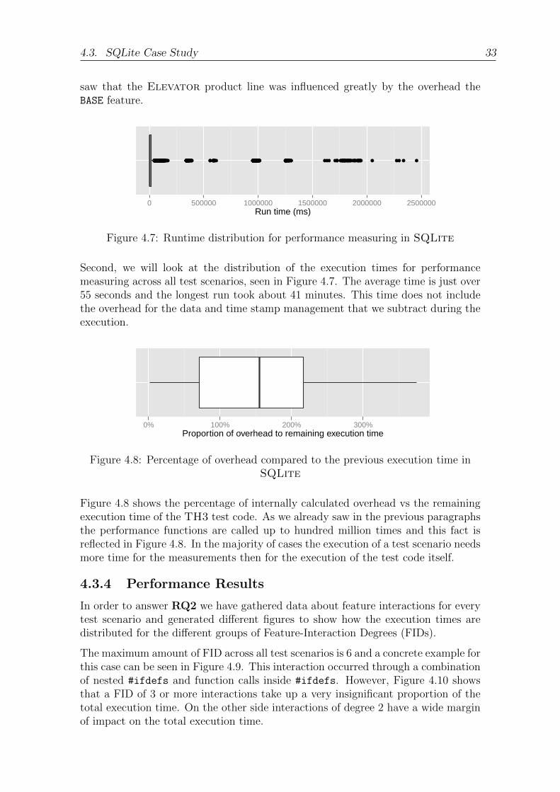
4.3. SQLite Case Study 33

saw that the Elevator product line was influenced greatly by the overhead theBASE feature.

●●●●●●●●●●●●●●●●●●●●●●●●●●●●●●●●●●●●●●●●● ●●●●●●●● ●●●●●●●●●●●●●●●●●●●●●●●●●●●●●●●●●●●●●●●●●●●●●●● ●●●●●●●● ●●●●●●●●●●●●●●●●●●●●●●●●●●●● ●●●●●●●●●●●●●●●●●●●●●●●●●● ●●●●●●●●●●●●●●●●●● ●●●●●●●●●●●●●●●●●●●●●●●●●●●●●●●● ●●●●●●●●●●●●●●●●●●●●●●●●●●●●●●●●●●●●●●●●●●●●●●●●●●●●●● ●●●●●●●●●●●●●●●●●●●●●●●●●●●●●●●●●●●●●●●●●●●●●●●●●●●●●● ●●●●●●●●●●●●●●●●●●●●●●●●●●●●●●●●●●●●●●●●●●●●●●●●●●●●●● ●●●●●●●●●●●●●●●●●●●●●●●●●●●●●●●●●●●●●●●●●●●●●●●●●●●●●● ●●●●●●●●●●●●●●●●●●●●●●●●●●●●●●●●●●●●● ●●●●●●●●●●●●●●●●●●●●●●●●●●●●●● ●●●●●●●●●●●●●●●●●●●●●●●●● ●●●●●●●●●●●●●●●●●●●●●● ●● ●●●●●●●●●●●●●●●●●● ●●●●●●●●●●●●●● ●●●●●●●●●●●●●●●●●●●●●● ● ●●●●●●●●●●●●●●●●●● ●●●●●●●●●●●●● ●●●●●●●●●●●●●●●●●● ●●●● ● ●●● ●●●●●●● ●● ●●●●●● ●●● ●●●● ●●●●● ●●●●●●●●●●●●●●●●●●●●●●● ●●● ●●●●●●●●●●●●●●●●●● ●●●●●●●●●●●●●●●●●●●●●●●●●●●●●●●●●●● ●●● ●●●●●●●●●●●●●●●●●● ●●●●●●●●●●●●●●●●●●●●●●●●●●●●●●●●●●● ●● ●●●●●●●●●●●●●●●●●● ●●●●●●●●●●●●●●●●●●●●●●●●●●●●●●●●●●● ●●●●●●●●●●●●●●●●●●● ●●●●●●●●●●●●●●●●●●●●●●●●●●●●●●●●●●● ●●●●●●●●●●●●●●●●●●● ●●●●●●●●●●●●●●●●●●●●●●●●●●●●●● ●●●●● ●●● ●●●●●● ●●● ●●● ●●●●●● ●●●● ●●● ●●●●●●●●●●●●●●●●●●●●● ●●●●● ●● ●● ●●●●●● ●●● ●●● ●●●●●● ●●●● ●●● ●●●●

0 500000 1000000 1500000 2000000 2500000Run time (ms)

Figure 4.7: Runtime distribution for performance measuring in SQLite

Second, we will look at the distribution of the execution times for performancemeasuring across all test scenarios, seen in Figure 4.7. The average time is just over55 seconds and the longest run took about 41 minutes. This time does not includethe overhead for the data and time stamp management that we subtract during theexecution.

0% 100% 200% 300%Proportion of overhead to remaining execution time

Figure 4.8: Percentage of overhead compared to the previous execution time inSQLite

Figure 4.8 shows the percentage of internally calculated overhead vs the remainingexecution time of the TH3 test code. As we already saw in the previous paragraphsthe performance functions are called up to hundred million times and this fact isreflected in Figure 4.8. In the majority of cases the execution of a test scenario needsmore time for the measurements then for the execution of the test code itself.

4.3.4 Performance Results

In order to answer RQ2 we have gathered data about feature interactions for everytest scenario and generated different figures to show how the execution times aredistributed for the different groups of Feature-Interaction Degrees (FIDs).

The maximum amount of FID across all test scenarios is 6 and a concrete example forthis case can be seen in Figure 4.9. This interaction occurred through a combinationof nested #ifdefs and function calls inside #ifdefs. However, Figure 4.10 showsthat a FID of 3 or more interactions take up a very insignificant proportion of thetotal execution time. On the other side interactions of degree 2 have a wide marginof impact on the total execution time.

34 4. Evaluation

feature interaction stack

VDBE PROFILE!SQLITE OMIT SUBQUERY

!SQLITE OMIT OR OPTIMIZATIONSQLITE OMIT FOREIGN KEY

!SQLITE COVERAGE TEST!SQLITE OMIT EXPLAIN

SQLITE ENABLE FTS4 || SQLITE ENABLE FTS3

Figure 4.9: Example feature interaction degree of 6 in SQLite

●●

●

●

●

●●●●●●●

●

●●●●●●●●●●●●

●●●●●●●

●

●●

●

●

●

●●

●●

●●●

●

●●●

●

●●●●●●●●●●●●●●●●●●●●●●●●●●●●●●●●●●●●●●●●●●●●●●●●●●

●●●●●●●●●●●●●●●●●●●●●●●●●●●●●●●●●●●●●●

●●●●●●●●●●●●●●●●●●●●●●●●

●

●●●

●●

●●●

●

●●●

●●●●●●

●

●

●●

●●●

●●●

●

●●●●●●●●

●●

●●●●●●●●●●●●●●●●●●●●●●●●●●●●●●●●●●●

●●

●●●●●●●

●●●●●●●●●●●●●●●●●●●●●●●●●●●●●●

●●●●●●●

●●●●●●●●

●●●●●●●●●

●●●●●●●●●●●●●●●●●●●●●●●●

●●●●

●●

●●●

●

●●●

●●●●●●

●

●

●●

●●●

●●●●

●●●●●●●●

●●●●●●●●●●●●●●●●●●●●●●●●●●●●●●●●●●●●●●●●●●●●●

●

●●●●●●●●●●

●●●●●●●●●●●●●●

●

●●●●●

●●●

●

●●●

●●●●●●

●

●

●●

●●●

●●●●

●●●●●●●●

●●●●●●●●●●●●●●●●

●●●●●●

●●●

●

●●●

●●●●●●

●

●

●●

●●●

●●●

●

●●●●●●●●●●●●●●●●●●●●●

●●

●●●●●●●●●●●●●●●●●●●●●●●●●●●●●●●

●●●

●●●●

●

●●●●●●

●●●●●●●

●●

●●●●●●

●●●●●●●●●●

●●●●●●●●●●●

●●●

●●

●●●

●●●●

●

●

●●●●●●●●●●●●

●●●

●●●●●●●●●●

●●●●●●●●●●●●●●●●●

●●●●●●●●●●●●●●●●●●

●●●●●●●●●●●●

●●●●

●

●●●●●●●●●●●●●●●●

●●●

●●●

●

●

●

●●●●●●●●●●●●●●●●●●●●●●●●●●●●●●●●●●●●●●●●

●●●●●●

●●●

●●●●

●●●●●●

●

●

●●●●●●●●●●●●●●●●●

●●

●●●●●●●●●●●●●●

●●●●●●

●●●

●

●●●

●●

●●●●

●

●

●●●●●●●●●●●●●●●●●

●●

●●●●●●●●●●●●●●

●●●●●●

●●●●●●●

●●●●●●●●

●●●●●●●●●●●●●●●●●●●●●●●●●●●●●●●●●

●●●●●●

●●●

●

●●●

●●●●●●

●

●

●●●●●●●●●●●●●●●●●

●●

●●●●●●●●●●●●●●

●●●●●●

●●●●●●●

●●●●●●●●

●●●●●●●●●●●●●●●●●

●●

●●●●●●●●●●●●●●

●●●●●●

●●●●●●●

●●●●●●●●

●●●●●●●●●●●●●●●●●

●●●●●●●●●●●●●●●●

●●●●●●

●●●

●

●●●

●●●●●●

●

●

●●●●●●●●●●●●●●●●●

●●

●●●●●●●●●●●●●●

●●●●●●

●●●

●

●●●

●●●●●●

●

●

●●●●●●●●●●●●●●●●●

●●

●●●●●●●●●●●

●●●●●●●●●●●●●●

●●●●●●●●●

●●●●●●●●●●●●●●●●●●●●●●●●●●●●●●●●●●●●●●●●●●●●●●●●●●●●●●●

●●●●●●●●●●●●●●●●●●●●●●●●●●●●●●●●●●●

●●●●●●●●●●●●●●●●●●●●●●●●●●●●●●●●●●●●●●●●●●●●●●●●●●●●●●●●●●●●●●●●●●●●●●●●●●●●●●●●●●●●●●●●●●●●●●●●●●●●●●●●●●●●●●●●●●●●●●●●●●●●●●●●●●●●●●●●●●●●●●●●●●●●●●●●●●●●●●●

●●●●●●●●●●●●●●●●●●●●●●

●●●●●●●●●●

●

●●●●

●

●●●●●●●●●●●●

●●●●

●●●

●

●●●●

●●

●

●●

●●

●●●●

●

●

●

●●●●●

●●

●●●

●

●

●●●●

●●●

●●●●●●●

●●

●●●

●●

●

●

●

●

●●●●●

●

●

●

●●●●●●●

●●●●

●

●●●●●●●

●●●●●●

●

●●

●●●

●●

●

●

●

●

●

●●●●●●●●

●

●●●

●

●●

●

●

●

●

●

●●●

●

●●

●

●

●●

●

●●●●

●

●

●

●

●

●

●

●

●●

●

●

●

●

●●●

●

●●

●●

●

●

●

●●●

●

●●

●

●

●●

●

●●●●

●

●

●

●

●

●

●

●

●●

●

●

●

●●●●●●●●●

●●●●

●

●●

●

●●

●●

●●●

●

●●

●●

●●

●

●●●●

●

●

●

●●

●●

●

●

●

●

●

●●●●●

●

●●

●

●●

●●

●●●

●

●●

●●

●●

●

●●●●

●

●

●

●●

●●●

●●

●

●

●

●●●●●●

●●●●

●●●

●

●●●●

●●

●

●●

●●●●

●

●

●

●●

●

●●

●●

●●●

●

●

●●

●●

●●

●

●●●●

●

●

●

●●

●●

●

●●

●

●

●

●

●●●●●

●

●

●

●●

●

●●

●●

●●●

●

●

●●

●●

●●

●

●●●●

●

●

●

●●

●●

●

●●

●

●

●

●

●

●●

●

●

●●

●●●

●

●

●

●●

●

●●●

●

●

●●

●●

●

●

●

●●●

●●

●●

●

●●●●

●●

●

●

●

●

●

●●

●

●

●

●

●

●

●

●●●

●

●

●●

●

●

●

●

●

●

●

●

●

●

●

●

●●●●●●●●

●

●●

●●

●●●●●

●●

●●

●

●●●●

●

●

●

●

●●●●●●●●

●

●

●

●●

●

●●

●

●●

●

●

●

●

●●●

●

●●●

●

●●●●●●

●

●

●●

●

●

●

●

●●●

●

●

●●●

●

●

●

●●

●

●

●

●●

●

●

●

●●

●●

●

●

●

●

●

●●●

●

●

●●

●

●

●●

●

●●●●

●

●

●

●

●

●●●●●

●●

●

●

●

●

●●

●

●●

●

●

●

●●

●

●

●

●

●

●

●

●●●

●

●

●●

●

●

●●

●

●●●●●

●

●

●

●

●●

●●

●

●●

●

●

●

●

●

●

●●●●●●●●●●●●●

●●●●

●●

●●

●●●

●●●●●

●

●●●●●●●

●●●●

●●

●●●●●

●●

●●●●●

●●●●●

●●●●●●●

●

●●●●

●●●

●●●●●●●●●●●●●●●●●●●●●●●●●●●●●●●●●●●●●●●●●●●●●●●●●●●●●●●●●●●●●●●●●●●●●●●●●●●●●●●●●●●●●●●●●●●●●●●●●●●●●●●●●●●●●●●●●●●●●●●●●●●●●●●●●●●●●●●●●●●●●●●●●●●●●●●●●●●●●●●●●●●●●●●●●●●●●●●●●●●●●●●●●●●●●●●●●●●●●●●●●●●●●●●●●●●●●●●●●●●●●●●●●●●●●●●●●●●●●●●●●●●●●●●●●●●●●●●●●●●●●●●●●●●●●●●●●●●●●●●●●●●●●●●●●●●●●●●●●●●●●●●●●●●●●●●●●●●●●●●●●●●●●●●●●●●●●●●●●●●●●●●●●●●●●●●●●●●●●●●●●●●●●●●●●●●●●●●●●●●●●●●●●●●●●●●●●●●●●●●●●●●●●●●●●●●●●●●●●●●●●●●●●●●●●●●●●●●●●●●●●●●●●●●●●●●●●●●●●●●●●●●●●●●●●●●●●●●●●●●●●●●●●●●●●●●●●●●●●●●●●●●●●●●●●●●●●●●●●●●●●●●●●●●●●●●●●●●●●●●●●●●●●●●●●●●●●●●●●●●●●●●●●●●●●●●●●●●●●●●●●●●●●●●●●●●●

●

●

●●

●●●●

●●

●●●●●●●●

●●●●●●

●●

●●●

●●

●●

●

●●●●

●●●

●

●

●

●●●●●●●●●●●●●●●●●●●●●●●●●●●●●●●●●●●●●●●●●●●●●●●●●●●●●●●●●●●●●●●●●●●●●●●●●●●●●●●●●●●●●●●●●●●●●●●●●●●●●●●●●●●●●●●●●●●●●●●●●●●●●●●●●●●●●●●●●●●●●●●●●●●●●●●●●●●●●●●●●●●●●●●●●●●●●●●●●●●●●●●●●●●●●●●●●●●●●●●●●●●●●●●●●●●●●●●●●●●●●●●●●●●●●●●●●●●●●●●●●●●●●●●●●●●●●●●●●●●●●●●●●●●●●●●●●●●●●●●●●●●●●●●●●●●●●●●●●●●●●●●●●●●●●●●●●●●●●●●●●●●●●●

●

●●●●●

●

●●●●●●●●●●

●●●●●●●●

●●●●●●●●●●●●

●

●

●

●●●●●●●●●●●●●●●●●●●●●●●●●●●●●●●●●●●●●●●●●●●●●●●●●●●●●●●●●●●●●●●●●●●●●●●●●●●●●●●●●●●●●●●●●●●●●●●●●●●●●●●●●●●●●●●●●●●●●●●●●●●●●●●●●●●●●●●●●●●●●●●●●●●●●●●●●●●●●●●●●●●●●●●●●●●●●●●●●●●●●●●●●●●●●●●●●●●●●●●●●●●●●●●●●●●●●●●●●●●●●●●●●● ●●●●●●●●●●●●●●●●●●●●●●●●●●●●●●●●●●●●●●●●●●●●●●●●●●●●●●●●●●●●●●●●●●●●●●●●●●●●●●●●●●●●●●●●●●●●●●●●●●●●●●●●●●●●●●●●●●●●●●●●●●●●●●●●●●●●●●●●●●●●●●●●●●●●●●●●●●●●●●●●●●●●●●●●●●●●●●●●●●●●●●●●●●●●●●●●●●●●●●●●●●●●●●●●●●●●●●●●●●●●●●●●●●●●●●●●●●●●●●●●●●●●●●●●●●●●●●●●●●●●●●● ●●●●●●●●●●●●●●●●●●●●●●●●●●●●●●●●●●●●●●●●●●●●●●●●●●●●●●●●●●●●●●●●●●●●●●●●●●●●●●●●●●● ●●●●●●●●●●●●●●●●●●●●●●●●●●●●●●●●●●●●●●●●0%

25%

50%

75%

100%

base 0 1 2 3 4 5 6

Interaction degree

Per

cent

age

of to

tal e

xecu

tion

time

Figure 4.10: Execution time distributed among different degrees of featureinteractions

Grouping up the previous data by our four different configuration groups in Fig-ure 4.11 shows that the configurations have a great effect on the distribution. Theallyes configuration group consists of one configuration and is very stable across allTH3 configurations and test directories. Most of the run time is spent in contextwithout any interactions (FID of 0), followed by one interaction (FID of 1) and theBASE code. The BASE code is not part of any FID and is categorized separately.

This changes drastically for the feature-wise configurations, which are very incon-sistent across all FIDs. There are quite a few cases where the vast majority of theexecution time is used up by a FID of 2 and this also occurs in the pair-wise and ran-dom configurations. The latter two also have a very identical distribution. Removing4 specific TH3 configs from the data set removes most outliers for interaction de-gree 2. Figure 4.12 depicts how this removal affects the pair-wise configurations. Itseems that the tests related to these configurations focus on testing computationallyintensive code in feature interactions of second degree.

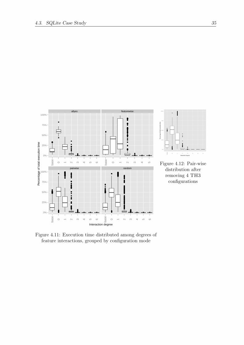
4.3. SQLite Case Study 35

●●●●●●●●●●●●

●

●

●●

●

●

●●

●

●●

●●●●●●●●●●●●●●●●●●●●●●●●●● ●●●●●● ●● ●●

●●

●

●

●●●●●●●●●●●●●●●●●●●●●●●●●●●●●●●●●●●●●●●●●●

●●●●●

●

●●●●●●●●●●●●●

●●●●●●●

●

●●●●●●●●●●●●●

●●

●

●●●●●●●●●●●●●●●●●●

●

●●●●●●●●●●●●●●●●●●●●

●

●●

●

●●●●●●●●●●●●●●●●●●●●●●●●●●●●●●●●●●●●●●●●●●

●●

●

●●●●●●●●●●●●●●●●●●●●

●

●

●●●●●●●●●●●●●●●●●●●●

●●●●●●●●●●●●●●●●●●●●●

●●●●●●●●●●●●●●●●●●●●●●●●●●●●●●●●●●●●●●●●

●●●●●●●●●●●●●●●●●●●●●●●●●●●●●●●●●●●●●●●●●●●●●●●●●●●●●●●●●●●●●●●●●●●●●●●●●●●●●●●●●●●●●●●●●●●●●●●●●●●●●●●●●●●●●●●●●●●●●●●●●●●●●●●●●●●●●●●●●●●●●●●●●●●●●●●●●●●●●●●●●●●●●●●●●●●●●●●●●●●●●●●●●●●●●●●●●●●●●●●●●●●●●●●●●●●●●●●●●●●●●●●●●●●●●●●●●●●●●●●●●

●●

●●●●●●●●●●●●●●●●●●●●●●●●●●●●●●●●●●●●●●●●●●●●●●●●●●●●●●●●●●●●●●●●●●●●●●●●●●●●●●●●●●●●●●●●●●●●●●●●●●●●●●●●●●●●●●●●●●●●●● ●●●●●●●●●●●●●●●●●●●●●●●●●●●●●●●●●●● ●●●●●●●●●●●●●●

●●●●

●●●●●

●●

●●

●

●●●●●●●●●●●●●●●●●●●●●●●●●●●●●●●●●●●●●●●●●●●●●●●●●●●●●●●●●●●●●

●●●●●●●●●●●●●●●●●●●●●●●●●●●●●●●●●●●●●●●●●●●●●●●●●●●●●●●●●●●●●●●●●●●●●●●●●●●●●●●●●●●●●●●●●●●●●●●●●●●●●●●●●●●●●●●●●●●●●●●●●●●●●●●●●●●●●●●●●●●●●●●●●●●●●●●●●●●●●●●●●●●●●●●●●●●●●●●

●●

●●●●●●●●●●●●●●●●●●●●●●●●●●●●●●●●●●●●●●●

●●●●●

●●●●●●●●●●●●●●●●●●●●●●●●●●

●●●●●●●●●●●●●●●●●●●●●●●●●●●●●●●●●●●●●●●●●●●●●●●●●●●

●

●●●●●●●●●●●●●●●●●

●

●●●●●

●

●●●●●●●●●●●●

●●●●●●●●●●●●

●●●●

●

●●●

●●

●●●●●●●●●●●●

●

●●●●●

●

●●●●●

●

●●●●●

●

●●●●●

●

●●●

●●●●●●●●●●●●●●●●●●●●●●●●●●●●●●●●●●●●●●●●●●●●●●●●●●●●●●●●●●●●●●●●●●●●●●●●●●●●●●●●●●●●●●●●●●●●●●●●●●●●●●●●●●●●●●●●●●●●●●●●●●●●

●●●●●●

●●

●●●●●

●●

●

●●●●●●●●●●

●

●

●

●

●

●●

●

●

●

●

●●

●●●

●

●●●●

●

●

●●

●●

●●●●

●●●●●●

●

●●

●

●

●

●

●●

●●●

●

●

●

●

●●

●●

●●●●●●●●●●

●●●●●●●●●●●●●●●●●●●●

●●●●●●

●●●●●●●●●●●●●●●●●●●●●●●●●●●●●●●●●●●●●●●●●●●●●●●●●●●●●●●●●●●

●

●●●●

●

●●●●●●●●●●●●●●●●●●●●●●●●●●●●●●●●●●●●●●●●●●●●●●●●●●●●●●●●●●●●●●●●●●● ●●●●●●●●●●●●●●●●●●●●●●●●●●●●●●●●●●●●● ●●●●●●●●●●●●●●● ●●●●●●●

●

●●●●

●

●

●●●●●●●●●●●●●●

●

●

●●●●

●●●●●

●●

●

●●●●

●

●●●

●●●●●●●●●●●●●●●●●●●●●●●●●●●●●●●●●●●●●●●●●●●●●●●●●●●●●●●●●●●●●●●●●●●●●●●●●●●●●●●●●●●●●●●●●●●●●●●●●●●●●●●●●●●●●●●●●●●●●●●●●●●●●●●●●●●●●●●●●●●●●●●●●●●●●●●●●●●●●●●●●●●●●●●●●●●●●●●●●●●●●●●●●●●●●●●●●●●●●●●●●●●●●●●●●●●●●●●●●●●●●●●●●●

●●●●●●●●●●●●●●●●●●●●●●●●●●●●●●●●●●●●●●●●●●●●●●●●●●●●●●●●●●●●●●●●●●●●●●●●●●●●●●●●●●●●●●●●●●●●●●●●●●●●●●●●●●●●●●●●●●●●●●●●●●●●●●●●●●●●●●●●●●●●●●●●●●●●●●●●●●●●●●●●●●●●●●●●●●●●●●●●●●●●●●●●●●●●●●●●●●●●●●●●●●●●●●●●●●●●●●●●●●●●●●●●●●●●●●●●●

●●●●

●●●●●●●●●●●●●●●●●●●●●●●●●●●●●●●●●●●●●●●●●●●●●●●●●●●●●●●●●●●●●●●●●●●●●●●●●●●●●●●●●●●●●●●●●●●●●●●●●●●●●●●●●●●●●●●●●●●●●●●●●●●●●●●●●●●●●●●●●●●●●●●●●●●●●●●●●●●●●●●●●●●●●●●●●●●●●

●●●●●●●●●●●●●●●●●●●●●●●●●●●●●●●●●●●●●●●●●●●●●●●●●●●●●●●●●●●●●●●●●●●●●●●●●●●●●●●●●●●●●●●●●●●●●●●●●●●●●●●●●●●●●●●●●●●●●●●●●●●●●●●●●●●●●●●●●●●●●●●●●●●●●●●●●●●●●●●●●●●●●●●●●●●●●●●●●●●●●●●●●●●●●●●●●●●●●●●●●●●●●●●●●●●●●●●●●●●●●●●●●●●●●●●●

●●●●●●●●●

●●●●●●●●●●●●●●●●●●●●●●●●●●●●●●●●●●●●●●●●●●●●●●●●●●●●●●●●●●●●●●●●●●●●●●●●●●●●●●●●●●●●●●●●●●●●●●●●●●●●●●●●●●●●●●●●●●●●●●●●●●●●●●●●●●●●●●●●●●●●●●●●●●●●●●●●●●●●●●●●●●●●●●●●●●●●●●●●●●●●●●●●●●●●●●●●●●●●●●●●●●●●●●●●●●●●●●●●●●●●●●●●●●●●●●●●●●●●●●●●●●●●●●●●●●●●●●●●●●●●●●●●●●

●●●●●●●●●

●●●●●●●●●●●●●●●●●●●●●●●●●●

●●●●●●●●●●●●●●●●●●●●●●●●●●●●●●●●●●●●●●●●●●●●●●●●●●●●

●●●●●●●●●●●●●●●●●●●●●●●●●●●●●●●●●●●●●●●●●●●●●●●●●●●●●●●●●●●●●●●●●●●●●●●●●●●●●●

●●●●●●●●●●●●●●●●●●●●●●●●●●

●●●●●●●●●●●●●●●●●●●●●●●●●●●●●●●●●●●●●●●●●●●●●●●●●●●●●●●●●●●●●●●●●●●●●●●●●●●●●●●●●●●●●●●●●●●●●●●●●●●●●●●●●●●●●●●●●●●●●●●●●●●●●●●●●●●●●●●●●●●

●●●●●●●●●●●●

●

●●●●

●

●●●●●●●●●●●●●●●

●●●

●●

●

●●●●

●

●

●●

●●

●

●●

●●●●●

●

●●●●●●●

●●

●●

●●

●●●●●

●

●●●●●●●

●●

●

●●●●●●

●●●

●

●●

●

●●●●●●●

●●●

●

●●

●

●●●●●●●

●●●

●●

●

●●●

●●

●

●

●

●●●●●●●

●

●

●

●●

●

●

●●●●●●●

●

●●

●

●●●

●●●

●●

●

●●●●●

●●

●

●●

●●●●●

●

●●●●●●●

●●

●●

●●

●●

●●●

●

●●●●●●●

●●

●

●●

●

●

●

●●

●

●

●

●●

●

●●

●

●●

●●

●

●●●

●

●●●●●

●●

●

●

●

●

●

●●

●

●

●

●

●

●

●●

●

●

●●

●

●

●●

●

●

●

●

●●●

●

●●

●●●●●●●●●●●

●●●●●

●

●●

●

●●

●●

●

●●●●●●

●

●

●

●

●

●●●

●●

●

●●●●●

●●

●

●

●

●

●●

●

●●●

●

●●●●

●

●

●●●

●

●

●

●●

●●

●●

●

●●●

●

●

●●●

●

●

●●●

●

●

●

●

●●●●●●●●●●●●●●●●●●●●●●●●●●●●●●●●●●●●●●●●●●●●●●●●●●●●●●●●●●

●

●●

●●●●●●

●●

●●●●●

●●●●●●●●●●●●●●●●●●●●●●●●●●●●●●●●●●●●●●●●●●●●●●●●●●●●●●●●●●●●●●●●●●●●●●●●●●●●●●●●●●●●●●●●●●●●●●●●●●●●●●●●●●●●●●●●●●●●●●●●●●●●●●●●●●●●●●●●●●●●●●●●●●●●●●●●●●●●●●●●●●●●●●●●●●●●●●●●●●●●●●●●●●●●●●●●●●●●●●●●●●●●●●●●●●●●●●●●●●●●●●●●●●●●●●●●●●●●●●●●●●●●●●●●●●●●●●●●●●●●●●●●●●●●●●●●●●●●●●●●●●●●●●●●●●●●●●●●●

●●

●

●●●●●●●●●●●●●●●●●●●●●●●●●●●●

●

●

●

●●●●●●●●●●●●●●●●●●●●●●●●●●●●●●●●●●●●●●●●●●●●●●●●●●●●●●●●●●●●●●●●●●●●●●●●●●●●●●●●●●●●●●●●●●●●●●●●●●●●●●●●●●●●●●●●●●●●●●●●●●●●●●●●●●●●●●●●●●●●●●●●●●●●●●●●●●●●●●●●●●●●●●●●●●●●●●●●●●●●●●●●●●●●●●●●●●●●●●●●●●●●●●●●●●●●●●●●●●●●●●●●●●●●●●●●●●●●●●●●●●●●●●●●●●●●●●●●●●●●●●●●●●●●●●●●●●●●●●●●●●●●●●●●●●●●●●●●●●●●●●●●●●●●●●●●●●●●●●●●●●●●●●●●●●●●●●●●●●●●●●●●●●●●●●●●●●●●●●●●●●●●●●●●●●●●●●●●●●●●● ●●●●●●●●●●●●●●●●●●●●●●●●●●●●●●●●●●●●●●●●●●●●●●●●●●●●●●●●●●●●●●●●●●●●●●●●●●●●●●●●●●●●●●●●●●●●●●●●●●●●●●●●●●●●●●●●●●●●●●●●●●●●●●●●●●●●●●●●●●●●●●●●●●●●●●●●●●●●●●●●●●●●●●●●●●●●●●●●●●●●●●●● ●●●●●●●●●●●●●●●●●●●●●●●●●●●●●●●●●●●●●●●●●●●●●●●●●●●●●●●●●●●●● ●●●●●●●●●●●●●●●●●●●●●●●●●●●●●●●●●

allyes featurewise

pairwise random

0%

25%

50%

75%

100%

0%

25%

50%

75%

100%

base 0 1 2 3 4 5 6

base 0 1 2 3 4 5

base 0 1 2 3 4 5 6

base 0 1 2 3 4 5 6

Interaction degree

Per

cent

age

of to

tal e

xecu

tion

time

Figure 4.11: Execution time distributed among degrees offeature interactions, grouped by configuration mode

●●●●

●●●

●

●●

●

●●●●●●

●●●●●●●●●●●●

●●●●●●●●●●●●●●

●●●●●●●●●●●●●●●●●●

●●●●●●●●●●●●●●●●●●●●●●●●●●●●●●●●●●●●●●●●●●●●●●●●●

●

●●

●

●

●●●●●●●

●●●●●●

●

●●

●

●●

●

●●●

●●

●

●●

●

●●

●

●●

●

●●

●

●●

●

●

●●●

●

●●

●

●

●

●●

●●●●●●●●●●●●●●●●●●●●●●●●

●●●●●●●●●●●●●●●●●●●●●●●●●●●●●●●●●●●●●●●●●●●●●●●●●●●●●●●●●●●●

●●

●●●●●●●●●●●●●●●●●●●●●●●●●●●●●●●●●●●●

●●●●●●●●●●●●●●●●●●●●●●●●

●●●●●●●●●●●●●●●●●●●●●●●●●●●●●●●●●●●●●●●●●●●●●●●●

●

●

●●

●

●

●●●●●●●

●

●●●●●

●

●●●

●●

●

●●●

●●

●

●●

●

●●

●

●●

●

●●

●

●●

●

●

●

●●●●

●

●

●●

●

●

●

●

●●

●●●●●●●●

●●●●●●●●●●●●●●●●●●●

●●●●●●●●●●●

●●●●●●●●●●●●●●●●●●●●●●●●●●●●●●●●●●●●●●●●●●●●●●●●●●●●●●●●●●●●●●●●●●●●●●●●●●●●●●●●●●●●●

●●●●●●●●●●●●●●●●●●●●●●●●

●

●

●●●●●●

●

●●

●●●●

●●

●●

●●

●●

●

●

●

●

●

●

●

●

●

●

●

●●

●

●

●●●●●●●●●●●●●●●●●●●●●●●●●●●●●●●

●●●●●●●●●●●●●●●●●●●●●●●●●●●●●●●●●●●●●●●●●●●●●●●●●

●

●●

●

●

●

●●●●●●●●●●●●●●●●●●●●●●●●●●●●●●●●●●●●●●●●●●●●●●●●●● ●●●●●●●●●●●●●●●●●●●●●●●●●●●●●●● ●●●●●●●●●●● ●●●●0%

25%

50%

75%

100%

base 0 1 2 3 4 5 6

Interaction degree

Per

cent

age

of to

tal e

xecu

tion

time

Figure 4.12: Pair-wisedistribution afterremoving 4 TH3

configurations

36 4. Evaluation

In the end the data can be grouped in various ways but without in-depth knowledgeabout SQLite, TH3 and their configurations these data remain observations. Toanswer RQ2, it is interesting that the annotation-free code is on average in thirdplace ranked by proportion of total time consumed. Context without interactionsand context with one interaction consume more time for SQLite.

4.3.5 Prediction Results

For this section the data generated during our performance analysis is used to gener-ate performance predictions. Since we already generated detailed numbers for eachof our 85 SQLite configurations the next step is to make cross predictions for thedifferent configuration modes. These results will show which configuration group issuited for prediction other configurations, see RQ4 and also which groups are notcompatible and produce predictions that are off the mark.

In order to get more accurate numbers we compared the time of a prediction forconfiguration φ to the time that the performance simulator actually takes whenexecuted in configuration φ. In practice the goal has to be to compare the predictionto the actual execution time of that variant, but since our measurement processassigns deallocation calls to the preceding time measurement, this is a compromise.See Chapter 6 for possible improvements.

Figure 4.13 displays the different cross predictions7. The PE2 is computed by takingthe average prediction time and comparing it to the actual time that the performancemeasuring of that configuration needs. The result of a prediction for a configura-tion group with multiple configurations is then again the average for all individualpredictions of that group. A PE of 0 indicates a perfect prediction. The differentmodes show diverse compatibility to each other. The allyes configuration makes theworst predictions, especially allyes predicts feature-wise. A reason for this is thatthe allyes configuration enables the feature SQLITE_NO_SYNC, which is only enabledin one of the 23 feature-wise configurations. Further these 22 configurations thathave disabled SQLITE_NO_SYNC all have an execution time of over 3100 ms, whereasthe remaining feature-wise configuration has a run time of ∼ 90 ms. The allyesconfiguration with about ∼170 ms execution time does not have any measurementinformation for the SQLITE_NO_SYNC feature and thus all of its predictions for con-figurations that include this feature are off the mark.

Figure 4.14 now displays the same information from the previous paragraph but itincludes the deviation that is computed for the predictions. Since we have accessto the actual results the performance error including deviation is computed as seenin Figure 4.15. Examples for this calculation can be seen in Figure A.1. Especially,example b) highlights how a high variance instantly produces a perfect result whichis not applicable if you do not know the expected values. The results for randompredicts have improved substantially by including the deviation because they havethe highest deviation when compared to the average time. As a result they can-not be considered good candidates for predictions. Their high deviation leads toan inaccurate prediction result. See Section A.2 for predictions grouped by testdirectory.

7We excluded one combination of TH3 config and test directory since it can produce a percent-age error of ∼6 and messes up the y scale of the boxplots

4.3. SQLite Case Study 37

●

●

●

●

●●●●●●

●

●

●●

●

●

●●●●●

●

●

●

●●●●●

●

●●

●

●●

●

●●

●●

●

●●

●●

allyes predicts featurewise allyes predicts pairwise allyes predicts random

featurewise predicts allyes featurewise predicts pairwise featurewise predicts random

pairwise predicts allyes pairwise predicts featurewise pairwise predicts random

random predicts allyes random predicts featurewise random predicts pairwise

0%

50%

100%

150%

0%

50%

100%

150%

0%

50%

100%

150%

0%

50%

100%

150%

Per

cent

Err

or

Figure 4.13: Percent error in crosspredictions for the different

configuration modes

●

●

●●●●●●●●●●●●●

●●●●●●●●●●

●

●●

●

●●●●●●●●●●●●●●●●●●●● ●

●●●●●●

allyes predicts featurewise allyes predicts pairwise allyes predicts random

featurewise predicts allyes featurewise predicts pairwise featurewise predicts random

pairwise predicts allyes pairwise predicts featurewise pairwise predicts random

random predicts allyes random predicts featurewise random predicts pairwise

0%

50%

100%

150%

0%

50%

100%

150%

0%

50%

100%

150%

0%

50%

100%

150%

Per

cent

Err

or in

clud

ing

Var

ianc

e

Figure 4.14: Percent error in crosspredictions for the different

configuration modes includingdeviation

4.3.6 Comparing Execution Times

Section 3.8 already mentioned that the performance can vary between the meta prod-uct (without performance measurements) and the derivable variants. Figure 4.16shows the PE when comparing the execution times. Overall the times are relativelyclose but there are some outliers which deviate by nearly 90%. We reason that thesedifferences vary between different case studies and depend on the way that the con-ditional preprocessor directives are utilized. The closer this overall number is thebetter the prediction results. As a consequence, we suggest avoiding case studies,where the meta product performance deviates a lot from the software variants.

38 4. Evaluation

PEV (a, v, r) =

PE(a+ v), if a+ v < r

PE(a− v), if a− v > r

0, otherwise, since r ∈ ]a− v, a+ v[

where:

PE = function to compute PEa = predicted averaged = predicted deviationr = actual result

Figure 4.15: Taking deviation into consideration for calculation of PE

●● ●●●● ●● ●●● ● ●● ● ●●●● ●●●● ● ● ●●● ●●● ●● ● ●●● ●●● ●● ● ●●●● ●●● ●● ●● ●● ●● ●● ● ●● ●● ●●● ● ●●● ●● ●●● ● ●●●●● ●●● ● ●● ● ●●● ●● ●● ●● ●● ● ●● ●● ●●●●●● ● ●●● ●● ●●● ●● ●●● ●●● ●●● ● ●●●● ● ●● ●●● ●● ● ● ●● ●●● ● ●●●● ●●● ●● ● ●●● ●● ● ●● ● ●●●●● ●●● ●●●● ●●●●● ●●● ●●●● ●●●●●●●●● ●● ●●●● ●● ●● ●●●●●● ● ●● ● ●● ●

0% 25% 50% 75%Percent errorin run times

Figure 4.16: Comparing execution times: meta product vs variant

5. Conclusion

The amounf of derivable variants for a configurable systems scales exponentiallywith its number of configuration options. Thus they pose to be a tough problem tosolve for analysis and verification tools. In this thesis we present the combination ofperformance measuring and variability encoding in order to analyze the performanceof Software Product Lines (SPLs).

Our case studies show that the results vary. For the Elevator case study weare able to provide very accurate results by analyzing just one configuration in oursimulator. Elevator helps us to characterize the properties that represent a goodtarget SPL for our approach:

• No mutually-exclusive conditional preprocessor directives.

• Feature Model (FM) with very few restrictions, which allows us to select allfeatures and gather a lot of information from a single execution.

• The different features do not have any grave performance-altering data depen-dencies.

The second case study, SQLite, shows that our approach is applicable even tocomplex systems. SQLite in its amalgamation version has 93 configurable featuresspread over 180.000 lines of code [sql]. RQ2 posed the question of time distributionand SQLite has shown, that in contrast to our expectations, the most executiontime is used by features with a Feature-Interaction Degree (FID) of zero or one andthe shared code BASE only comes in third place. On the other hand it has shownthat the code inside preprocessor directives with a FID of 2 or more does not havea significant impact on the performance.

As far as performance prediction in SQLite is concerned we received varying results.The allyes configuration is the worst configuration for predicting the performanceof other configurations. We found out that a certain group of features in the formof SQLITE_OMIT_SOMETHING contain a lot of executable routines whenever they are

40 5. Conclusion

turned off. Using the randomly generated configuration set yields the best predictiondata when taking the deviation into account. However, the random configuration setconsists of 50 different configurations which is more than all the other configurationgroups combined. Consequently the random configuration predictions require themost effort and also have a high variance. Overall the predictions for SQLite vary,but to make final verdict about its compatibility with our performance measuringapproach, further knowledge about its configurations and test suite is required.

6. Future Work

The possibilities for future work are manifold. First Granularitycontrol

of all we measure the perfor-mance of every preprocessor directive, even if it only contains one negligible calcula-tion. The effort to perform the measurement for such a statement is multiple ordersof magnitudes higher than the statement execution itself. This further increases therun time of the performance simulator and as SQLite has shown with an average of23 million performance measurements the internally calculated overhead is alreadysurpassing the execution time of the remaining code. Adding different metrics forgranularity control to avoid unnecessary performance measurements can potentiallyreduce the overhead without affecting the accuracy of the measurements.

Second Measure-ments inseparatethread

, in order to lessen the effect that these performance measurements have onthe remaining execution we advise revisiting their implementation and conduct thesemeasurements in a separate processor thread. Our internal overhead calculations donot take the very last memory deallocation from a free call into account, instead it’sexecution time is assigned to the execution time of the preceding measurement. Forfeatures without any Feature-Interaction Degree (FID) this preceding measurementis the measurement for BASE. The Elevator case study has already shown thatthe numbers for the features are very accurate but the numbers for BASE are offby about ∼6 ms because it includes 5604 free calls from its nested performancemeasurements.

Third Deviations infeature times

, making accurate predictions requires the execution times for a feature φ tobe constant across all configurations that include φ. We already mentioned datadependencies as a possible example, where the time measured for a feature φ isaffected by a different feature χ, e.g. χ increases the upper limit of a loop. Ifthis manipulation in χ is part of an unrelated (not nested) preprocessor directivethe measurements for φ is affected. If a Software Product Line (SPL) utilizes theconditional preprocessor directives in this way, our approach is not able to generateaccurate predictions.

Fourth Codecoverageconf. set

, in order to measure the whole code base in regards to mutually exclusivepreprocessor directives we advise finding a small set of configurations that covers all

42 6. Future Work

parts of the source code. The so called code coverage set of configurations shouldbe the best candidate to generate performance data for predictions. The closer thisheuristic is to generating the minimal set of configurations the less effort has to bemade for performance predictions.

LastMore casestudies

, in order to properly judge our approach it needs to be applied to more casestudies. Liebig et al. showed that SQLite is one of the very few exceptions, in ananalysis of 40 SPL, where the code inside the preprocessor directives exceeds 50% ofthe code base. SQLite is a complex software system and with that degree of vari-ability, we categorize it as a suboptimal target for our performance measuring andprediction approach. However, new case studies have to fulfill certain requirementsbefore they can be utilized. The parsing framework TypeChef has to be able tonot only successfully parse these new SPLs, but also to type check them withoutany errors. Though, providing a detailed Feature Model (FM) is able to solve mostof these issues. The next step is for Hercules to generate compilable C code, thatdoes not have any active, un-terminated performance measurements at the end ofthe program execution.

7. Related Work

Our thesis is influenced by prior work from Post et al. about configuration lifting[PS08] and the paper of Siegmund et al. “Family-Based Performance Measure-ment” [SvRA14]. While configuration lifting is the motivation behind variability en-coding, the collaboration with Siegmund et al. has started the idea of performancemeasuring in the context of C Software Product Lines (SPLs). The backgroundfor the work of Siegmund et al. are Java SPL and their tool chain is based Fea-tureHouse1, a software-artifact composition framework [AKL09]. In contrast toour approach, the variability occurs only on a function level, whereas C Preproces-sor (CPP) directives can be used in any arbitrary way. Siegmund et al. apply theirapproach to 5 different test systems and obtain a prediction accuracy of 98%, onaverage. They also verify, that their approach requires only fraction of the effort,that a brute-force approach requires. One of the crucial results is that the time savedby using of family-based performance measurements increases with the number offeatures in a SPL, but also decreases with the amount of configurations, that arerequired to gain 100% code coverage.

Regarding family-based analysis methods, in general they are an exciting devel-opment that displays promising results [TAK+12, SvRA14, LvRK+13, KvRE+12,NKN14]. The exact implementation for these approaches differs from the softwaredomain and analysis context that they are applied to. However, the core conceptremains the same: employ the similarities between the different products in order tosave analysis efforts, since the shared code base (ideally) takes up the vast majorityof the source code.

An empirical study by Ernst et al. analyzes 26 packages with 1.4 million linesof C code [EBN02] and shows that conditional preprocessor directives, on average,account for 4% of the total code. Liebig et al. analyzed the preprocessor usage in40 different SPLs [LAL+10]. They come to the conclusion that variability correlateswith the size of the project and the #ifdef nesting is used sparsely.

1http://www.infosun.fim.uni-passau.de/spl/apel/fh/

44 7. Related Work

Finally, performance related publications can be split up into different categories.First, the machine-learning or data-set training approach[GSKA16, SK01], whichbenefits immensely from domain knowledge as Grebhan et al. show [GSKA16].Using this knowledge reduces the training efforts, however, they stress that thisknowledge needs to be precise or the results lose accuracy. Second, the measurement-based approach, that is used by Siegmund et al. [SRK+11, SKK+12]. They gatherperformance data per feature by measuring the influence of each feature and allrelated deltas. Deltas are a way to express the influence that a feature A has onanother feature B. The feature-specific data and appropriate deltas can then beused to calculate the performance for different configurations. Weyuker et al. dis-cuss their experience with performance testing [WV00]. They stress the importanceof performance-related testing and argue, that performance is a very importantand project-affecting property. Further, they mention that the test case genera-tion or generation strategies for measuring performance is a crucial criteria for allmeasurement-based approaches.

A. Appendix

A.1 Percent Error calculation example

This is just a brief example that did not fit into Section 4.3.5 for a calculation ofthe Percent Error (PE) with deviation.

Example a)

p = 65.3ms+ 7.7ms

r = 75.0ms

PEV (65.3, 7.7, 75.0) = PE(73.0, 75)

=|73.0− 75|

75= 2.66%

Example b)

p = 29.3ms+ 19.0ms

r = 47.4ms

PEV (29.3, 19.0, 47.4) = 0%

Figure A.1: Example calculations for PE with deviation

A.2 Prediction results continued

The following Figure A.2 and Figure A.3 present the results from Section 4.3.5 forthe cross predictions grouped by TH3 test directory.

A.3 Prediction result table excerpt

Table A.1 is an excerpt of data gained from the prediction process. The IDs rangefrom 0 to 299 because the initial numbering included all 12 TH3 test directories andtogether with its 25 configs we generated 300 different test scenarios. The unusableresults were omitted afterwards.

Since we did not only predict the performance, but also measure the performanceof all configurations, we are able to generate a lot more data about the differencesbetween our prediction and the result. E.g., MPSFD displays the impact of the

46 A. Appendix

difference in measured times for the shared features between the prediction Feature-Time Hashmap (FTH) and the result FTH as a proportion of the total differencebetween the predicted time and the actual time. The figures in previous sectionsabout performance predictions for SQLite have been generated from this table.

A.3. Prediction result table excerpt 47

●●● ● ●

●

●● ●●● ●●

●

● ●●

● ●● ●

●

● ●●

● ●

● ●

●●●

●

●●●

●● ●

●●

ally

es p

redi

cts

feat

urew

ise

ally

es p

redi

cts

pairw

ise

ally

es p

redi

cts

rand

om

feat

urew

ise

pred

icts

ally

esfe

atur

ewis

e pr

edic

ts p

airw

ise

feat

urew

ise

pred

icts

ran

dom

pairw

ise

pred

icts

ally

espa

irwis

e pr

edic

ts fe

atur

ewis

epa

irwis

e pr

edic

ts r

ando

m

rand

om p

redi

cts

ally

esra

ndom

pre

dict

s fe

atur

ewis

era

ndom

pre

dict

s pa

irwis

e

0%50%

100%

150% 0%50

%

100%

150% 0%50

%

100%

150% 0%50

%

100%

150%

bugs

cov1

_p2

dev

dev_

p1ex

tra1

req1

bugs

cov1

_p2

dev

dev_

p1ex

tra1

req1

bugs

cov1

_p2

dev

dev_

p1ex

tra1

req1

bugs

cov1

_p2

dev

dev_

p1ex

tra1

req1

bugs

cov1

_p2

dev

dev_

p1ex

tra1

req1

bugs

cov1

_p2

dev

dev_

p1ex

tra1

req1

bugs

cov1

_p2

dev

dev_

p1ex

tra1

req1

bugs

cov1

_p2

dev

dev_

p1ex

tra1

req1

bugs

cov1

_p2

dev

dev_

p1ex

tra1

req1

bugs

cov1

_p2

dev

dev_

p1ex

tra1

req1

bugs

cov1

_p2

dev

dev_

p1ex

tra1

req1

bugs

cov1

_p2

dev

dev_

p1ex

tra1

req1

Test

Fol

der

Nam

e

Percent Error

Fig

ure

A.2

:P

erce

nt

erro

rin

cros

spre

dic

tion

sfo

rth

ediff

eren

tco

nfigu

rati

onm

odes

●●● ● ●

●

● ● ●● ●

●

● ●●

● ●●●

●● ● ●●●

● ●● ●●● ● ●● ●

●●

●●●

●

ally

es p

redi

cts

feat

urew

ise

ally

es p

redi

cts

pairw

ise

ally

es p

redi

cts

rand

om

feat

urew

ise

pred

icts

ally

esfe

atur

ewis

e pr

edic

ts p

airw

ise

feat

urew

ise

pred

icts

ran

dom

pairw

ise

pred

icts

ally

espa

irwis

e pr

edic

ts fe

atur

ewis

epa

irwis

e pr

edic

ts r

ando

m

rand

om p

redi

cts

ally

esra

ndom

pre

dict

s fe

atur

ewis

era

ndom

pre

dict

s pa

irwis

e

0%50%

100%

150% 0%50

%

100%

150% 0%50

%

100%

150% 0%50

%

100%

150%

bugs

cov1

_p2

dev

dev_

p1ex

tra1

req1

bugs

cov1

_p2

dev

dev_

p1ex

tra1

req1

bugs

cov1

_p2

dev

dev_

p1ex

tra1

req1

bugs

cov1

_p2

dev

dev_

p1ex

tra1

req1

bugs

cov1

_p2

dev

dev_

p1ex

tra1

req1

bugs

cov1

_p2

dev

dev_

p1ex

tra1

req1

bugs

cov1

_p2

dev

dev_

p1ex

tra1

req1

bugs

cov1

_p2

dev

dev_

p1ex

tra1

req1

bugs

cov1

_p2

dev

dev_

p1ex

tra1

req1

bugs

cov1

_p2

dev

dev_

p1ex

tra1

req1

bugs

cov1

_p2

dev

dev_

p1ex

tra1

req1

bugs

cov1

_p2

dev

dev_

p1ex

tra1

req1

Test

Fol

der

Nam

e

Percent Error including Variance

Fig

ure

A.3

:P

erce

nt

erro

rin

cros

spre

dic

tion

sfo

rth

ediff

eren

tco

nfigu

rati

onm

odes

incl

udin

gdev

iati

on

48 A. Appendix

IDIM

PM

PE

PE

DD

PM

PT

PM

PT

RM

PSF

DM

PSF

DD

10pai

rwis

eal

lyes

0.20

7184

0.16

8329

0.04

901

0.01

4898

0.00

1458

-0.1

93745

-0.1

76822

11pai

rwis

eal

lyes

0.17

7823

0.13

293

0.05

4603

0.01

4655

0.00

1605

-0.1

64773

-0.1

45056

12pai

rwis

eal

lyes

0.08

9712

00.

1148

930.

0142

30.

0008

44-0

.076326

-0.0

83381

235

feat

ure

wis

era

ndom

0.17

6358

0.15

9393

0.01

9849

0.17

3136

0.00

6296

0.039298

0.0

34812

236

feat

ure

wis

era

ndom

0.19

8365

0.18

6149

0.01

6944

0.17

4804

0.00

6151

0.038666

0.0

33707

237

feat

ure

wis

era

ndom

0.47

3009

0.43

0184

0.03

5791

0.02

8087

0.00

0009

0.500204

0.4

60544

24ra

ndom

feat

ure

wis

e0.

4447

280.

0003

20.

4210

640.

0000

80.

0186

240.

463425

0.0

09282

75ra

ndom

feat

ure

wis

e0.

0905

810.

0089

330.

2261

340.

0000

940.

0016

860.

089256

0.0

14736

76ra

ndom

feat

ure

wis

e0.

0378

340.

0058

070.

0499

370

00.

037833

0.0

10379

ID:

test

scen

ario

IDfr

om0-

299;

IM:

inpu

tm

od

e;PM

:p

red

ict

mod

e;PE

:p

erce

nt

erro

r;PED

:p

erce

nt

erro

rin

cl.

dev

iati

on;

DP

:d

evia

tion

per

centa

ge;

MPTP

:m

ean

per

centa

ge

of

tim

eon

lyin

pre

dic

tion

;M

PTR

:m

ean

per

centa

ge

of

tim

eon

lyin

resu

lt;

MPSFD

:m

ean

per

centa

geof

shar

edfe

atu

red

iffer

ence

;M

PSFDD

:m

ean

per

centa

ge

of

share

dfe

atu

red

iffer

ence

incl

.d

evia

tion;

Tab

leA

.1:

Exce

rpt

from

the

pre

dic

tion

dat

a

Bibliography

[AKL09] Sven Apel, Christian Kastner, and Christian Lengauer. Featurehouse:Language-independent, automated software composition. In Proceed-ings of the 31st International Conference on Software Engineering,pages 221–231. IEEE Computer Society, 2009. (cited on Page 43)

[AvRW+13] Sven Apel, Alexander von Rhein, Philipp Wendler, Armin Großlinger,and Dirk Beyer. Strategies for product-line verification: Case studiesand experiments. Proc. of ICSE. IEEE, 2013. (cited on Page 25)

[Bat05] Don Batory. Feature Models, Grammars, and Propositional Formulas,pages 7–20. Springer Berlin Heidelberg, Berlin, Heidelberg, 2005. (cited

on Page 6)

[CN+99] Paul Clements, Linda Northrop, et al. A framework for software prod-uct line practice. SEI Interactive, 2(3), 1999. (cited on Page 5)

[EBN02] Michael D. Ernst, Greg J. Badros, and David Notkin. An empiricalanalysis of c preprocessor use. Software Engineering, IEEE Transac-tions on, 28(12):1146–1170, 2002. (cited on Page 8 and 43)

[EW11] Martin Erwig and Eric Walkingshaw. The choice calculus: A repre-sentation for software variation. ACM Transactions on Software En-gineering and Methodology (TOSEM), 21(1):6, 2011. (cited on Page 9)

[GSKA16] Alexander Grebhahn, Norbert Siegmund, Harald Kostler, and SvenApel. Performance prediction of multigrid-solver configurations. InSoftware for Exascale Computing-SPPEXA 2013-2015, pages 69–88.Springer, 2016. (cited on Page 44)

[Hen08] Thomas A Henzinger. Two challenges in embedded systems design:predictability and robustness. Philosophical Transactions of the RoyalSociety of London A: Mathematical, Physical and Engineering Sciences,366(1881):3727–3736, 2008. (cited on Page 1)

[KA13] Christian Kastner and Sven Apel. Feature-oriented software develop-ment. In Generative and Transformational Techniques in Software En-gineering IV, pages 346–382. Springer Berlin Heidelberg, 2013. (cited

on Page 6)

50 Bibliography

[KCH+90] Kyo C Kang, Sholom G Cohen, James A Hess, William E Novak, andA Spencer Peterson. Feature-oriented domain analysis (foda) feasibilitystudy. Technical report, DTIC Document, 1990. (cited on Page 6)

[KKHL10] Andy Kenner, Christian Kastner, Steffen Haase, and Thomas Leich.Typechef: toward type checking# ifdef variability in c. In Proceed-ings of the 2nd International Workshop on Feature-Oriented SoftwareDevelopment, pages 25–32. ACM, 2010. (cited on Page 9, 12, and 13)

[KvRE+12] Christian Kastner, Alexander von Rhein, Sebastian Erdweg, JonasPusch, Sven Apel, Tillmann Rendel, and Klaus Ostermann. Towardvariability-aware testing. 2012. (cited on Page 1 and 43)

[LAL+10] Jorg Liebig, Sven Apel, Christian Lengauer, C Kastner, and MichaelSchulze. An analysis of the variability in forty preprocessor-based soft-ware product lines. In Software Engineering, 2010 ACM/IEEE 32ndInternational Conference on, volume 1, pages 105–114. IEEE, 2010.(cited on Page 43)

[LJG+15] Jorg Liebig, Andreas Janker, Florian Garbe, Sven Apel, and ChristianLengauer. Morpheus: Variability-aware refactoring in the wild. In Pro-ceedings of the 37th International Conference on Software Engineering-Volume 1, pages 380–391. IEEE Press, 2015. (cited on Page 9 and 30)

[LKA11] Jorg Liebig, Christian Kastner, and Sven Apel. Analyzing the disciplineof preprocessor annotations in 30 million lines of c code. In Proceed-ings of the tenth international conference on Aspect-oriented softwaredevelopment, pages 191–202. ACM, 2011. (cited on Page 8)

[LvRK+13] Jorg Liebig, Alexander von Rhein, Christian Kastner, Sven Apel, JensDorre, and Christian Lengauer. Scalable analysis of variable software.In Proceedings of the 2013 9th Joint Meeting on Foundations of Soft-ware Engineering, pages 81–91. ACM, 2013. (cited on Page 1, 9, 12,

and 43)

[MWC09] Marcilio Mendonca, Andrzej W ↪asowski, and Krzysztof Czarnecki. Sat-based analysis of feature models is easy. In Proceedings of the 13th In-ternational Software Product Line Conference, pages 231–240. CarnegieMellon University, 2009. (cited on Page 7)

[MWCC08] Marcilio Mendonca, Andrzej Wasowski, Krzysztof Czarnecki, and Don-ald Cowan. Efficient compilation techniques for large scale featuremodels. In Proceedings of the 7th international conference on Gen-erative programming and component engineering, pages 13–22. ACM,2008. (cited on Page 7)

[NKN14] Hung Viet Nguyen, Christian Kastner, and Tien N Nguyen. Exploringvariability-aware execution for testing plugin-based web applications.In Proceedings of the 36th International Conference on Software Engi-neering, pages 907–918. ACM, 2014. (cited on Page 43)

Bibliography 51

[Pad09] Yoann Padioleau. Parsing c/c++ code without pre-processing. In Com-piler Construction, pages 109–125. Springer, 2009. (cited on Page 8)

[PR01] Malte Plath and Mark Ryan. Feature integration using a feature con-struct. Science of Computer Programming, 41(1):53–84, 2001. (cited

on Page 25)

[PS08] Hendrik Post and Carsten Sinz. Configuration lifting: Verificationmeets software configuration. In Automated Software Engineering,2008. ASE 2008. 23rd IEEE/ACM International Conference on, pages347–350. IEEE, 2008. (cited on Page 1, 2, 10, and 43)

[SC92] Henry Spencer and Geoff Collyer. # ifdef considered harmful, or porta-bility experience with c news. 1992. (cited on Page 8)

[SK01] Martin Shepperd and Gada Kadoda. Using simulation to evaluate pre-diction techniques [for software]. In Software Metrics Symposium, 2001.METRICS 2001. Proceedings. Seventh International, pages 349–359.IEEE, 2001. (cited on Page 44)

[SKK+12] Norbert Siegmund, Sergiy S Kolesnikov, Christian Kastner, Sven Apel,Don Batory, Marko Rosenmuller, and Gunter Saake. Predicting perfor-mance via automated feature-interaction detection. In Software Engi-neering (ICSE), 2012 34th International Conference on, pages 167–177.IEEE, 2012. (cited on Page 44)

[sql] The SQLite amalgamation. https://www.sqlite.org/amalgamation.html. Accessed: 2017-03-14. (cited on Page 39)

[SRK+11] Norbert Siegmund, Marko Rosenmuller, Christian Kastner, Paolo GGiarrusso, Sven Apel, and Sergiy S Kolesnikov. Scalable prediction ofnon-functional properties in software product lines. In Software Prod-uct Line Conference (SPLC), 2011 15th International, pages 160–169.IEEE, 2011. (cited on Page 1 and 44)

[SvRA14] Norbert Siegmund, Alexander von Rhein, and Sven Apel. Family-basedperformance measurement. ACM SIGPLAN Notices, 49(3):95–104,2014. (cited on Page 25 and 43)

[TAK+12] Thomas Thum, Sven Apel, Christian Kastner, Martin Kuhlemann, InaSchaefer, and Gunter Saake. Analysis strategies for software productlines. School of Computer Science, University of Magdeburg, Germany,Tech. Rep. FIN-004-2012, 2012. (cited on Page 1 and 43)

[TBK09] Thomas Thum, Don Batory, and Christian Kastner. Reasoning aboutedits to feature models. In Proceedings of the 31st International Confer-ence on Software Engineering, pages 254–264. IEEE Computer Society,2009. (cited on Page 7)

[VB03] Laszlo Vidacs and Arpad Beszedes. Opening up the c/c++ preprocessorblack box. In Proceedings of the Eight Symposium on ProgrammingLanguages and Software Tools (SPLST), 2003. (cited on Page 8)

52 Bibliography

[vR16] Alexander von Rhein. Analysis Strategies for Configurable Systems.PhD thesis, Universitat Passau, 2016. (cited on Page 2, 11, 12, and 30)

[WV00] Elaine J Weyuker and Filippos I Vokolos. Experience with performancetesting of software systems: issues, an approach, and case study. IEEEtransactions on software engineering, 26(12):1147–1156, 2000. (cited

on Page 1 and 44)

[Zav99] Pamela Zave. Faq sheet on feature interaction. Link: http://www.research.att.com/˜pamela/faq.html, 1999. (cited on Page 6)

Eidesstattliche Erklarung:

Hiermit versichere ich an Eides statt, dass ich diese Masterarbeit selbstandig undohne Benutzung anderer als der angegebenen Quellen und Hilfsmittel angefertigthabe und dass alle Ausfuhrungen, die wortlich oder sinngemaß ubernommen wur-den, als solche gekennzeichnet sind, sowie dass ich die Masterarbeit in gleicher oderahnlicher Form noch keiner anderen Prufungsbehorde vorgelegt habe.

Name

Passau, den 15. Marz 2017