Performance Measurement, Forecasting and Optimization ... · Performance Measurement, Forecasting...
279
Performance Measurement, Forecasting and Optimization Models for Construction Projects Seyedeh-Sara Fanaei A Thesis In the Department of Building, Civil and Environmental Engineering Presented in Partial Fulfillment of the Requirements for the Degree of Doctor of Philosophy (Building Engineering) at Concordia University Montreal, Quebec, Canada April 2019 © Seyedeh-Sara Fanaei, 2019
Transcript of Performance Measurement, Forecasting and Optimization ... · Performance Measurement, Forecasting...

Performance Measurement, Forecasting and Optimization Models for Construction Projects
Seyedeh-Sara Fanaei
A Thesis
In the Department of
Building, Civil and Environmental Engineering
Presented in Partial Fulfillment of the Requirements
for the Degree of Doctor of Philosophy (Building Engineering) at
Concordia University Montreal, Quebec, Canada
April 2019
© Seyedeh-Sara Fanaei, 2019

CONCORDIA UNIVERSITY
SCHOOL OF GRADUATE STUDIES
This is to certify that the thesis prepared
By: Seyedeh-Sara Fanaei
Entitled: Performance Measurement, Forecasting and Optimization Models for Construc-
tion Projects
and submitted in partial fulfillment of the requirements for the degree of
Doctor of Philosophy (Building Engineering)
complies with the regulations of the University and meets the accepted standards with respect to
originality and quality.
Signed by the final examining committee:
____________________________________ Dr. A. R. Sebak
Chair
____________________________________ Dr. A. Bouferguene
External Examiner
____________________________________ Dr. G. Gopakumar
External to Program
____________________________________ Dr. S. H. Han
Examiner
____________________________________ Dr. A. Bagchi
Examiner
____________________________________ Dr. O. Moselhi
Thesis Co-Supervisor
____________________________________ Dr. S. T. Alkass
Thesis Co-Supervisor
Approved by ______________________________________________________________________
Dr. A. Bagchi, Chair, Department of Building, Civil & Environmental Engineering June 11, 2019 _________________________________________________________________
Dr. A. Asif, Dean, Gina Cody School of Engineering and Computer Science
iii
ABSTRACT
Performance Measurement, Forecasting and Optimization Models for Construction Pro-jects
Seyedeh-Sara Fanaei, Ph.D. Concordia University, 2019
Performance evaluation facilitates tracking and controlling project progress. Project control
consists of two main steps: measurement and decision-making. In the measurement step, key
performance indicators (KPIs) are designed to evaluate a project’s different aspects and are used
as a thermometer to determine the health status of the project. In the decision-making step project
performance is forecasted and analyzed to support needed management actions. While considera-
ble work is available on the quantitative performance of projects, less attention is directed to qual-
itative performance. This research presents a framework for qualitative measurement, prediction,
and optimization of construction project performance to enhance the progress reporting process
and to support management in taking corrective actions, if needed. The framework has three newly
developed models; KPI prediction model, performance indicator (PI) prediction model and perfor-
mance optimization model (POM). The framework is developed for performance measurement,
prediction, and optimization of construction projects based on six selected KPIs (cost, time, qual-
ity, safety, client satisfaction, and project team satisfaction). The selection is based on the results
of a questionnaire and the literature review. Qualitative data of KPIs was collected from 119 con-
struction projects and were then utilized in the development of the three models.
The first model maps the KPIs of three critical project stages to the whole project KPIs, based on
soft computing methods. Three different soft computing techniques are studied for this purpose
and their results are compared: the neuro-fuzzy technique, using Fuzzy C-means algorithm (FCM),
and subtractive clustering, and artificial neural networks (ANN). The neuro-fuzzy model is
developed for predicting the KPIs of the next stages of a project. The second model used the fore-
casted results of the first model to generate a single composite PI expressing the health status of
the project. The relative weight of each KPI used in calculating the project PI is determined using
the Analytic Hierarchy Process (AHP) and Genetic Algorithm (GA).
iv
Performance Optimization Model (POM) is the third model. It is used for selecting suitable cor-
rective actions considering the project status expressed by the six KPIs stated above. The devel-
oped model can be applied in the initial and middle stage of the project to assist owners in the
improvement of the overall project PI and in the improvement of individual KPIs. Different possible
modes are considered for project activities based on different ways, referee to here as modes, for
resource allocation, execution methods, and/or choice of different materials. GA is applied to
choose among different activity modes and optimize project performance using POM. The number
of activities and their modes are flexible and do not have any limitations. MATLAB software is
used for developing the models in this research. The developed framework and its three models
are expected to assist owners and their agents in managing their project effectively.
Validation was conducted by using the data from 16 real projects to confirm the model’s effec-
tiveness and to compare the results of the soft computing techniques. These results indicate that a
neuro-fuzzy technique using subtractive clustering performs better than both the neuro-fuzzy tech-
nique with FCM and ANN in predicting project KPIs. The automated framework employs a set
of performance indicators to evaluate, predict, and optimize the construction project’s perfor-
mance, qualitatively. It applies different soft computing techniques and compares their results to
choose the best technique. The developed framework can be used in construction projects to help
decision-makers evaluate and improve the performance of their projects.

v
ACKNOWLEDGEMENTS
My deepest acknowledgement is to God. I would like to express my sincere gratitude to my super-
visors Professor Osama Moselhi and Professor Sabah T. Alkass for their continuous and invaluable
support of my Ph.D. study and related research, for their patience, motivation, and immense
knowledge. Their guidance helped me in all the time of research and writing of this thesis. I believe
that without their guidance this research would have been much more challenging to complete.
Besides my supervisors, I would like to thank Dr. Govind Gopakumar, Dr. S. H. Han, Dr. A.
Bagchi, not only for their insightful comments and constructive feedback, but for their difficult
questions, which inspired me to widen my research to cover more perspectives.
My sincere thanks also go to my fellow lab mates, Dr. Zahra Zangenehmadar, Dr. Vale Moayeri,
Dr. Laya Parvizsedghy, Mr. Sasan Golnaraghi all my friends who provided me with their helpful
comments and stimulating discussions as colleagues in the Construction Automation Lab. I appre-
ciate having the opportunity to work in a professional and welcoming atmosphere that was ethni-
cally and intellectually diverse. Many thanks also go to my friend Ali Ashgar Nazem Boushehri for
his support and encouragements.
Sincere appreciation goes to my parents (Mrs. Mahdis Mahmoodi Gilani and Dr. Gholamreza
Fanaei) and my siblings (Sina and Saba) and my daughter (Zahra) for their infinite love and cares
throughout my work on this thesis and in my life in general.
Last but not the least, I would like to thank the person who has always stood by my side, who has
provided me with his continuous love and understanding, the love of my life, my wonderful hus-
band.

vi
To My Beloved Mother, Dear Father
and
My Husband
vii
TABLE OF CONTENTS
LIST OF FIGURES ................................................................................................................................... X
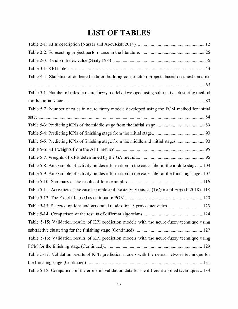
LIST OF TABLES ................................................................................................................................. XIV
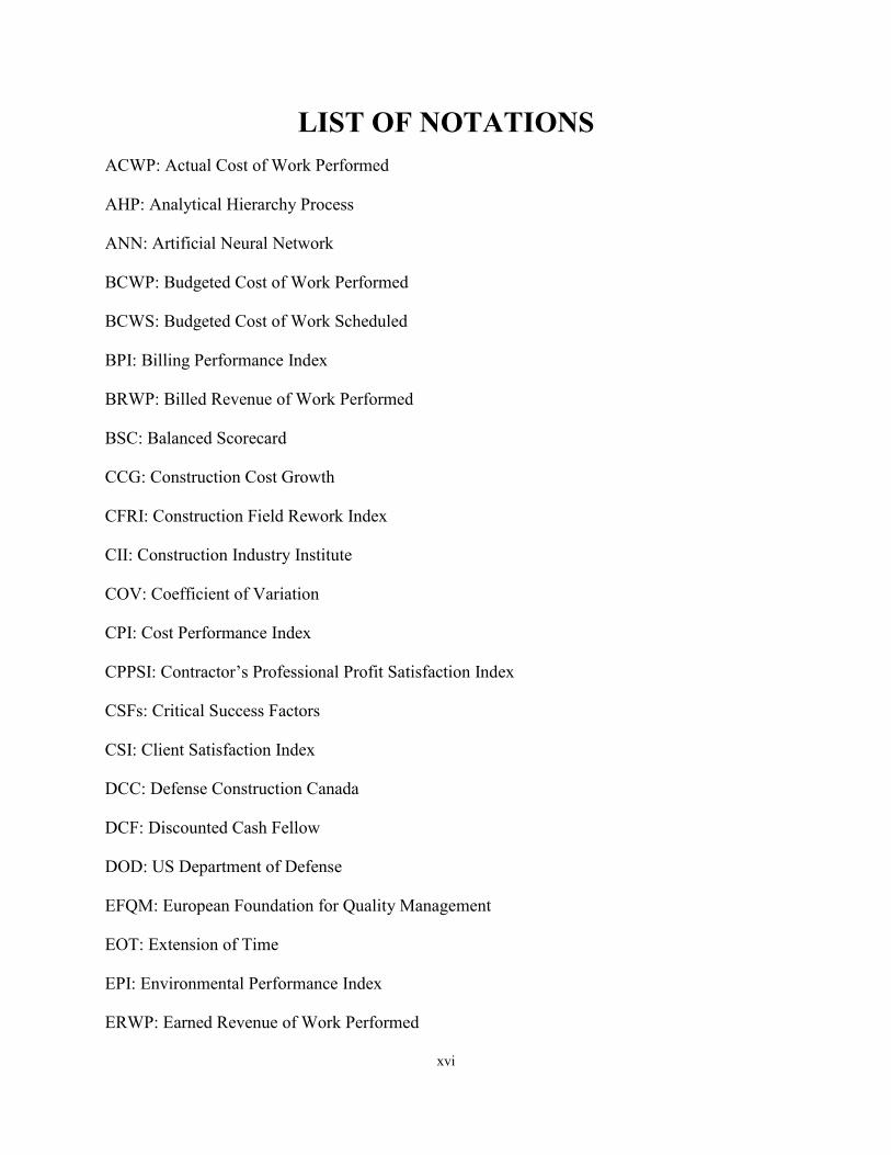
LIST OF NOTATIONS ......................................................................................................................... XVI
CHAPTER 1: INTRODUCTION .............................................................................................................. 1
1.1 Problem Statement and Research Motivation ..................................................................................... 1
1.2 Objectives ........................................................................................................................................... 2
1.3 Research Methodology ....................................................................................................................... 2
1.4 Organization of the Thesis .................................................................................................................. 3
CHAPTER 2: LITERATURE REVIEW .................................................................................................. 5
2.1 Chapter overview ................................................................................................................................ 5
2.2 Project Performance ........................................................................................................................... 5
2.2.1 Definition .................................................................................................................................... 5
2.2.2 Project Performance Measurement ............................................................................................. 6
2.2.3 Key Performance Indicators (KPIs) .......................................................................................... 18
2.2.4 KPIs Definitions ........................................................................................................................ 20
2.3 Project Performance Forecasting ...................................................................................................... 24
2.4 Related Research Tools .................................................................................................................... 28
2.4.1 Fuzzy Inference System (FIS) ................................................................................................... 28
2.4.2 Neuro-Fuzzy Technique ............................................................................................................ 31
2.4.3 Artificial Neural Network (ANN) ............................................................................................. 33
2.4.4 Analytical Hierarchy Process (AHP) ........................................................................................ 35
2.4.5 Genetic Algorithm (GA) ........................................................................................................... 37
2.5 Findings, Limitations, and Research Gaps ....................................................................................... 38
CHAPTER 3: RESEARCH METHODOLOGY ................................................................................... 40
3.1 Overall Research Methodology ........................................................................................................ 40
3.2 KPIs Identification ............................................................................................................................ 43
viii
3.3 KPI Prediction Model ....................................................................................................................... 45
3.3.1 Neuro-fuzzy Technique ............................................................................................................. 46
3.3.2 Artificial Neural Network Technique ........................................................................................ 54
3.4 KPIs Trend Forecasting Model ......................................................................................................... 56
3.5 PI Prediction Model .......................................................................................................................... 59
3.6 Performance Optimization Model (POM) for selecting Corrective Action in Construction Projects
................................................................................................................................................................ 61
CHAPTER 4: DATA COLLECTION AND ANALYSIS...................................................................... 66
4.1 Chapter Overview ............................................................................................................................. 66
4.2 Questionnaires .................................................................................................................................. 66
4.2.1 Questionnaire 1 ......................................................................................................................... 66
4.2.2 Questionnaire 2 ......................................................................................................................... 69
CHAPTER 5: MODEL DEVELOPMENT AND IMPLEMENTATION ............................................ 72
5.1 Chapter Overview ............................................................................................................................. 72
5.2 KPIs Prediction Models .................................................................................................................... 72
5.2.1 Neuro-Fuzzy Technique ............................................................................................................ 73
5.2.2 ANN Technique ........................................................................................................................ 84
5.3 KPIs Trend Forecasting Model ......................................................................................................... 89
5.3.1 Next Stage KPIs Forecasting ..................................................................................................... 89
5.3.2 KPIs Trend Visualization .......................................................................................................... 90
5.4 PI Prediction Model .......................................................................................................................... 93
5.4.1 AHP Method ............................................................................................................................. 94
5.4.2 GA Method ................................................................................................................................ 95
5.4.3 Comparing the PI of the Model and the PI of the Questionnaire .............................................. 97
5.5 Performance Optimization Model (POM) for selecting Corrective Action in Construction Projects
.............................................................................................................................................................. 100
5.5.1 PI Optimization Model ............................................................................................................ 100
5.5.2 Trade-off between Indicators .................................................................................................. 116
5.6 Validation ....................................................................................................................................... 125
ix
5.6.1 Validation of KPI Prediction models ...................................................................................... 125
5.6.2 PI Prediction Model Validation ............................................................................................... 134
CHAPTER 6: CONCLUSION AND RECOMMENDATIONS ......................................................... 138
6.1 Summary and Conclusion ............................................................................................................... 138
6.2 Research Contributions ................................................................................................................... 140
6.2.1 Academic Contributions .......................................................................................................... 140
6.2.2 Practical Contributions ............................................................................................................ 141
6.3 Research Limitations ...................................................................................................................... 141
6.4 Future Work and Recommendations .............................................................................................. 142
REFERENCES ........................................................................................................................................ 144
APPENDICES ......................................................................................................................................... 150
Appendix A: Questionnaires ................................................................................................................ 150
Appendix A1: Questionnaire 1- KPIs amount questionnaire ........................................................... 150
Appendix A2: Questionnaire 2- KPIs’ selection questionnaire ....................................................... 154
Appendix A3: Respondent's information ......................................................................................... 156
Appendix B: Information About Collected Data .................................................................................. 161
Appendix C: Neural Network Training Errors ..................................................................................... 170
Appendix D: Coding ............................................................................................................................. 171
Appendix D1: Neuro-Fuzzy coding ................................................................................................. 171
Appendix D2: Genetic Algorithm codes .......................................................................................... 197
Appendix D3: Predicting KPIs of Next Stage .................................................................................. 199
Appendix D4: Performance Optimization Model (POM) for selecting Corrective Action in
Construction Projects ....................................................................................................................... 212
x
LIST OF FIGURES Figure 2-1: KPI zone interface ..................................................................................................... 14
Figure 2-2: The balanced scorecard (Norton, 1992) ..................................................................... 17
Figure 2-3: The EFQM Excellence Model (Wongrassamee et al., 2003) .................................... 18
Figure 2-4: The use of performance measurement frameworks in leading construction firms
(Bassioni et al., 2004) ................................................................................................................... 18
Figure 2-5: Fuzzy inference system (Jang 1993) .......................................................................... 29
Figure 2-6: Main components of a FIS (Jang and Gulley 2015) .................................................. 30
Figure 2-7: The ANFIS architecture (Jang 1993) ......................................................................... 31
Figure 2-8: An example of an ANN network with three layers .................................................... 34
Figure 3-1: Overall research methodology framework ................................................................. 42
Figure 3-2: Histogram of KPIs frequency .................................................................................... 44
Figure 3-3: Sum of Scores of selected KPIs from the questionnaire ............................................ 45
Figure 3-4: Developing KPI prediction models ............................................................................ 46
Figure 3-5: Developing 18 neuro-fuzzy models for predicting six KPIs for three critical stages 47
Figure 3-6: Neuro-fuzzy model structure ..................................................................................... 48
Figure 3-7: Flowchart of modeling the initial FIS using subtractive clustering ........................... 51
Figure 3-8: Flowchart of modeling initial FIS using FCM ........................................................... 53
Figure 3-9: ANN model development steps ................................................................................. 56
Figure 3-10: Steps for predicting KPIs of next stages and KPIs Trends ...................................... 57
Figure 3-11: The prediction models for predicting the KPIs of the next stages ........................... 58
Figure 3-12: Interpolation for predicting KPIs trends .................................................................. 59
Figure 3-13: Model for predicting the KPIs of the next stages and KPI trends............................ 59
Figure 3-14: Steps for using the developed model ....................................................................... 60
Figure 3-15: Performance Optimization Steps ............................................................................. 62
Figure 3-16: Performance Optimization Model (POM) ............................................................... 64
Figure 4-1: Sample questions from KPIs amount questionnaire .................................................. 68
Figure 4-2: Sample questions from KPIs selection questionnaire ................................................ 70
Figure 4-3: KPI scores from Questionnaire 2 ............................................................................... 71
Figure 5-1: Inputs and outputs of KPIs prediction models ........................................................... 73
xi
Figure 5-2: Trained and forecasted model .................................................................................... 74
Figure 5-3: General structure of the Neuro-Fuzzy model ............................................................. 75
Figure 5-4: Fuzzy logic designer in the model developed using subtractive clustering ............... 75
Figure 5-5: Membership Function Editor in the model developed using subtractive clustering .. 76
Figure 5-6: Surface Viewer in the model developed using subtractive clustering ....................... 76
Figure 5-7: Rule viewer in the model developed using subtractive clustering ............................. 77
Figure 5-8: Example of input and output of the forecasting model .............................................. 78
Figure 5-9: Neuro-fuzzy model using subtractive clustering in the initial stage .......................... 79
Figure 5-10: Fuzzy logic designer in the model developed using FCM ....................................... 81
Figure 5-11: Membership Function Editor in the model developed using FCM .......................... 81
Figure 5-12: Surface Viewer in the model developed using FCM ............................................... 81
Figure 5-13: Rule viewer in the model developed using FCM ..................................................... 82
Figure 5-14: Neuro-fuzzy model using FCM in the initial stage .................................................. 83
Figure 5-15: Sample structure of the neural network in MATLAB ............................................. 85
Figure 5-16: The structure of the neural network ......................................................................... 86
Figure 5-17: MAE values of ANN models ................................................................................... 87
Figure 5-18: R2 values of ANN models ........................................................................................ 87
Figure 5-19: Coefficient of determination (R2) values for the final model .................................. 88
Figure 5-20: Example of input and output for predicting the KPIs of the next stages ................. 91
Figure 5-21: Sample diagram for the safety indicator trend ......................................................... 92
Figure 5-22: Example of input and output for predicting the KPIs for a specific project progress
percentage ..................................................................................................................................... 92
Figure 5-23: Example of the input and output for the PI prediction model .................................. 94
Figure 5-24: Flowchart of the GA method ................................................................................... 96
Figure 5-25: Comparison between PI of the model and PI of questionnaires in three stages ...... 99
Figure 5-26: Project network activities of Case Study adapted from Ghoddousi et al. (2013) .. 101
Figure 5-27: An example of the user interface for the initial stage and good situation .............. 101
Figure 5-28: An example of forecasted PI in the initial stage and in a good situation ............... 102
Figure 5-29: An example of the user interface showing the optimization results of the model when
the project is in the initial stage and good situation .................................................................... 104
xii
Figure 5-30: Iteration diagram of PI optimization using GA for the initial stage and good situation
..................................................................................................................................................... 105
Figure 5-31: An example of the user interface for the middle stage and good situation ............ 106
Figure 5-32: An example of forecasted PI in the middle stage and good situation .................... 107
Figure 5-33: An example of user interface showing the optimization results of the model when the
project is in the middle stage and good situation ........................................................................ 109
Figure 5-34: Iteration diagram of PI optimization using GA for the middle stage and good situation
..................................................................................................................................................... 109
Figure 5-35: An example of the user interface for the initial stage and bad situation ................ 110
Figure 5-36: An example of forecasted PI in the initial stage and bad situation ........................ 110
Figure 5-37: An example of user interface showing the optimization results of the model when the
project is in the initial stage and bad situation ............................................................................ 111
Figure 5-38: Iteration diagram of PI optimization using GA for the initial stage and bad situation
..................................................................................................................................................... 112
Figure 5-39: An example of the user interface for the middle stage and bad situation .............. 113
Figure 5-40: An example of forecasted PI in the middle stage and bad situation ...................... 114
Figure 5-41: An example of user interface showing the optimization results of the model when the
project is in the middle stage and bad situation .......................................................................... 114
Figure 5-42: Iteration diagram of PI optimization using GA for the middle stage and bad situation
..................................................................................................................................................... 115
Figure 5-43: comparison if the result of four examples .............................................................. 116
Figure 5-44: Project network activities of Case Study adapted from Toğan and Eirgash (2018)
..................................................................................................................................................... 117
Figure 5-45: The user interface for optimizing project time and cost ........................................ 119
Figure 5-46: Sample output of the POM..................................................................................... 122
Figure 5-47: A sample iteration diagram .................................................................................... 123
Figure 5-48: Comparison of Pareto Front results of different algorithms for 18 Activity ......... 125
Figure 5-49: Comparing the predicted output of the model and questionnaire in the initial stage
..................................................................................................................................................... 135
Figure 5-50: Comparing the predicted output of the model and questionnaire in the middle stage
..................................................................................................................................................... 136

xiii
Figure 5-51: Comparing the predicted output of the model and questionnaire in the finishing stage
..................................................................................................................................................... 137
xiv
LIST OF TABLES Table 2-1: KPIs description (Nassar and AbouRizk 2014). ......................................................... 12
Table 2-2: Forecasting project performance in the literature........................................................ 26
Table 2-3: Random Index value (Saaty 1988) .............................................................................. 36
Table 3-1: KPI table ...................................................................................................................... 43
Table 4-1: Statistics of collected data on building construction projects based on questionnaires
....................................................................................................................................................... 69
Table 5-1: Number of rules in neuro-fuzzy models developed using subtractive clustering method
for the initial stage ........................................................................................................................ 80
Table 5-2: Number of rules in neuro-fuzzy models developed using the FCM method for initial
stage .............................................................................................................................................. 84
Table 5-3: Predicting KPIs of the middle stage from the initial stage .......................................... 89
Table 5-4: Predicting KPIs of finishing stage from the initial stage............................................. 90
Table 5-5: Predicting KPIs of finishing stage from the middle and initial stages ........................ 90
Table 5-6: KPI weights from the AHP method ............................................................................ 95
Table 5-7: Weights of KPIs determined by the GA method ......................................................... 96
Table 5-8: An example of activity modes information in the excel file for the middle stage .... 103
Table 5-9: An example of activity modes information in the excel file for the finishing stage . 107
Table 5-10: Summary of the results of four examples ................................................................ 116
Table 5-11: Activities of the case example and the activity modes (Toğan and Eirgash 2018) . 118
Table 5-12: The Excel file used as an input to POM .................................................................. 120
Table 5-13: Selected options and generated modes for 18 project activities .............................. 123
Table 5-14: Comparison of the results of different algorithms................................................... 124
Table 5-15: Validation results of KPI prediction models with the neuro-fuzzy technique using
subtractive clustering for the finishing stage (Continued) .......................................................... 127
Table 5-16: Validation results of KPI prediction models with the neuro-fuzzy technique using
FCM for the finishing stage (Continued) .................................................................................... 129
Table 5-17: Validation results of KPIs prediction models with the neural network technique for
the finishing stage (Continued) ................................................................................................... 131
Table 5-18: Comparison of the errors on validation data for the different applied techniques .. 133

xv
Table 5-19: Comparison of the output of the model and questionnaire in the initial stage ........ 135
Table 5-20: Comparison of the predicted output of the model and questionnaire in the middle stage
..................................................................................................................................................... 136
Table 5-21: Comparison of the output of the model and questionnaire in the finishing stage ... 137
xvi
LIST OF NOTATIONS ACWP: Actual Cost of Work Performed
AHP: Analytical Hierarchy Process
ANN: Artificial Neural Network
BCWP: Budgeted Cost of Work Performed
BCWS: Budgeted Cost of Work Scheduled
BPI: Billing Performance Index
BRWP: Billed Revenue of Work Performed
BSC: Balanced Scorecard
CCG: Construction Cost Growth
CFRI: Construction Field Rework Index
CII: Construction Industry Institute
COV: Coefficient of Variation
CPI: Cost Performance Index
CPPSI: Contractor’s Professional Profit Satisfaction Index
CSFs: Critical Success Factors
CSI: Client Satisfaction Index
DCC: Defense Construction Canada
DCF: Discounted Cash Fellow
DOD: US Department of Defense
EFQM: European Foundation for Quality Management
EOT: Extension of Time
EPI: Environmental Performance Index
ERWP: Earned Revenue of Work Performed
xvii
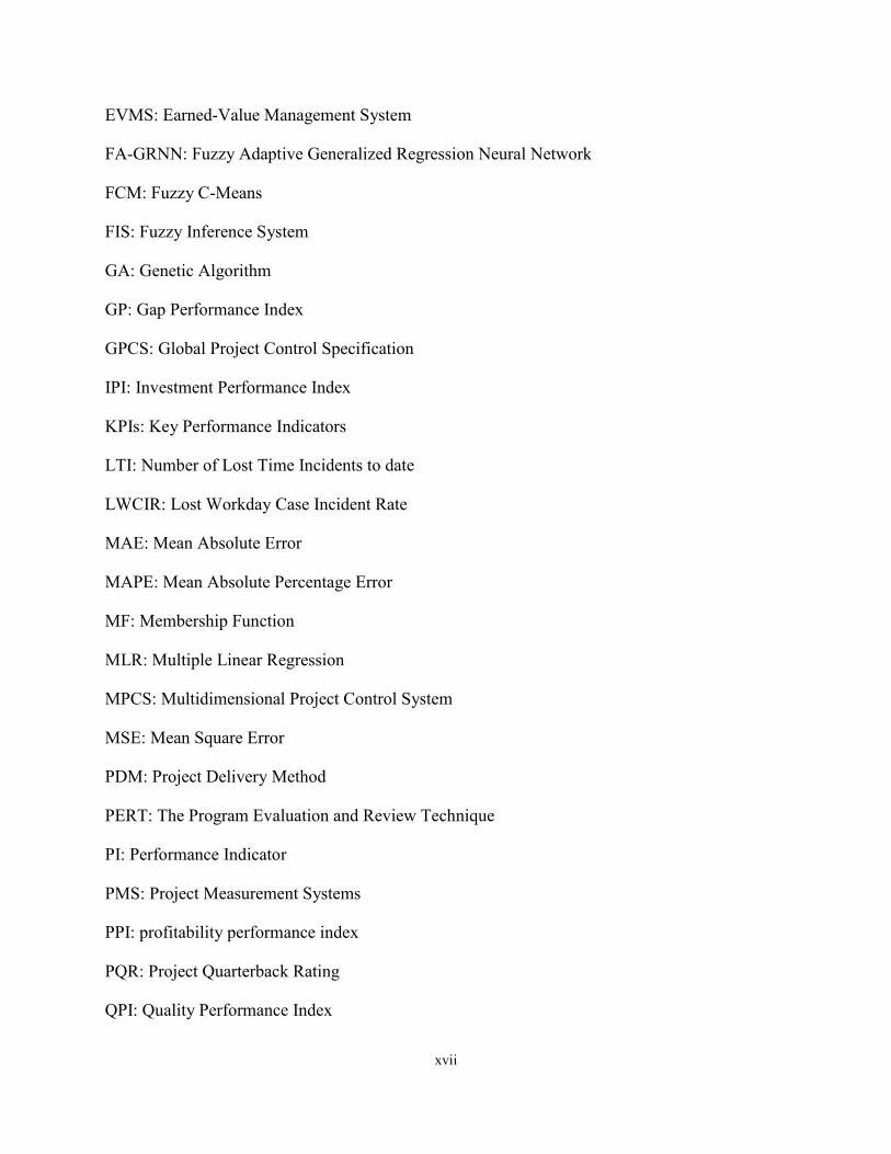
EVMS: Earned-Value Management System
FA-GRNN: Fuzzy Adaptive Generalized Regression Neural Network
FCM: Fuzzy C-Means
FIS: Fuzzy Inference System
GA: Genetic Algorithm
GP: Gap Performance Index
GPCS: Global Project Control Specification
IPI: Investment Performance Index
KPIs: Key Performance Indicators
LTI: Number of Lost Time Incidents to date
LWCIR: Lost Workday Case Incident Rate
MAE: Mean Absolute Error
MAPE: Mean Absolute Percentage Error
MF: Membership Function
MLR: Multiple Linear Regression
MPCS: Multidimensional Project Control System
MSE: Mean Square Error
PDM: Project Delivery Method
PERT: The Program Evaluation and Review Technique
PI: Performance Indicator
PMS: Project Measurement Systems
PPI: profitability performance index
PQR: Project Quarterback Rating
QPI: Quality Performance Index
xviii
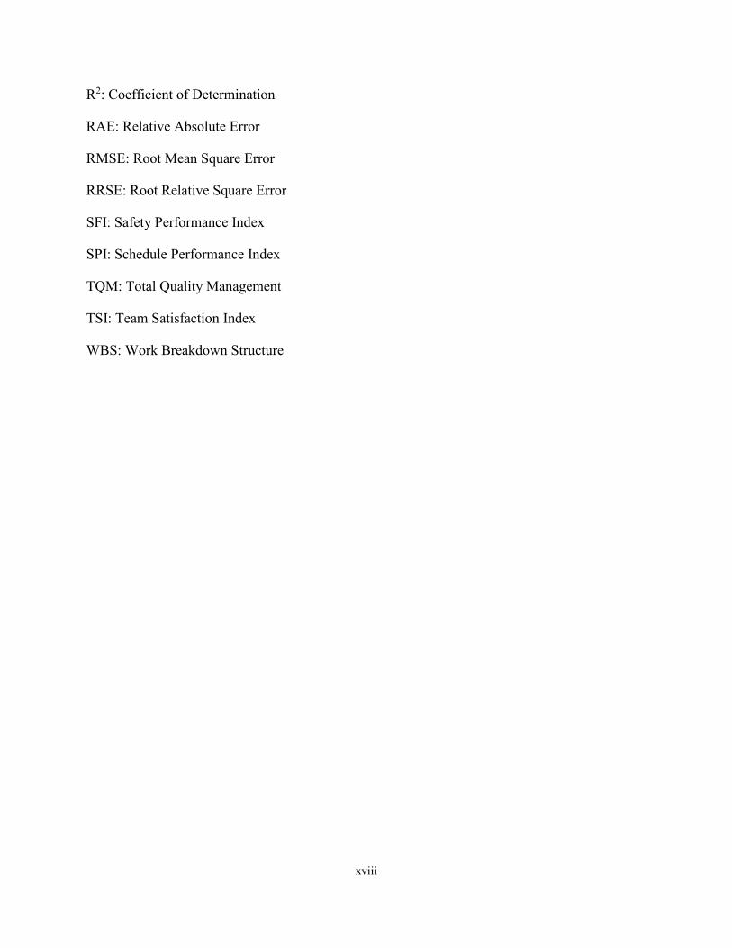
R2: Coefficient of Determination
RAE: Relative Absolute Error
RMSE: Root Mean Square Error
RRSE: Root Relative Square Error
SFI: Safety Performance Index
SPI: Schedule Performance Index
TQM: Total Quality Management
TSI: Team Satisfaction Index
WBS: Work Breakdown Structure
1
CHAPTER 1: INTRODUCTION
1.1 Problem Statement and Research Motivation Project management uses project monitoring and control to evaluate how successful a project is,
and if necessary, to determine which preventive or corrective action should be undertaken. Evalu-
ating the performance facilitates monitoring a project’s progress. It is accepted that one of the major
causes of project failure is the lack of monitoring and control of construction operations.
In project monitoring and control, any deviation of a project from its baseline should be identified.
Corrective actions can then be suggested to minimize the variance. The performance of the project
should also be assessed by offering a comprehensive performance measurement system.
For the effective monitoring of a construction project’s progress, different aspects of performance
should be quantified and integrated. The motivation of this research is to develop a framework to
manage various project performance attributes by using different Key Performance Indicators
(KPIs). This framework helps to monitor and control construction operations by forecasting the
project performance to deliver a successful project.
By dynamic project performance prediction, dynamic information (new information that becomes
available during the project) can be used to enhance project performance prediction. Although this
subject has been studied in the literature, the following limitations have been identified. First, in
existing methods, project control systems generally use cost and time indicators and neglect other
main aspects of performance such as quality, safety, client satisfaction, etc. Second, only limited
work has been done on forecasting project performance using KPIs at the project level.
Third, most of the previous work has focused on the quantitative performance forecasting of pro-
jects, and less attention has been directed to qualitative methods. However, many construction
KPIs, such as client satisfaction, quality and safety have a qualitative nature and cannot be meas-
ured quantitatively. Also, for other KPIs such as time and cost, issues of confidentiality and a lack
of data are the norm in construction projects. Therefore, it is more feasible to develop a qualitative
rather than a quantitative framework to measure and forecast project KPIs. Fourth, most of the
previous works measure project performance only after completion, and not during the construc-
tion phase (Haponava and Al-Jibouri 2012). The benefits of measuring the performance during the
2
project are that stakeholders can use the measurements to suggest corrective action and to forecast
the rest of the project’s performance.
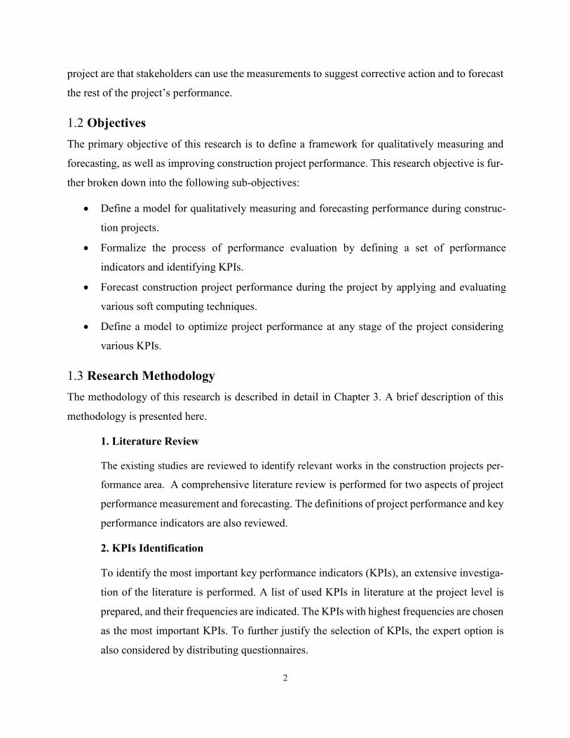
1.2 Objectives The primary objective of this research is to define a framework for qualitatively measuring and
forecasting, as well as improving construction project performance. This research objective is fur-
ther broken down into the following sub-objectives:
Define a model for qualitatively measuring and forecasting performance during construc-
tion projects.
Formalize the process of performance evaluation by defining a set of performance
indicators and identifying KPIs.
Forecast construction project performance during the project by applying and evaluating
various soft computing techniques.
Define a model to optimize project performance at any stage of the project considering
various KPIs.
1.3 Research Methodology The methodology of this research is described in detail in Chapter 3. A brief description of this
methodology is presented here.
1. Literature Review
The existing studies are reviewed to identify relevant works in the construction projects per-
formance area. A comprehensive literature review is performed for two aspects of project
performance measurement and forecasting. The definitions of project performance and key
performance indicators are also reviewed.
2. KPIs Identification
To identify the most important key performance indicators (KPIs), an extensive investiga-
tion of the literature is performed. A list of used KPIs in literature at the project level is
prepared, and their frequencies are indicated. The KPIs with highest frequencies are chosen
as the most important KPIs. To further justify the selection of KPIs, the expert option is
also considered by distributing questionnaires.
3
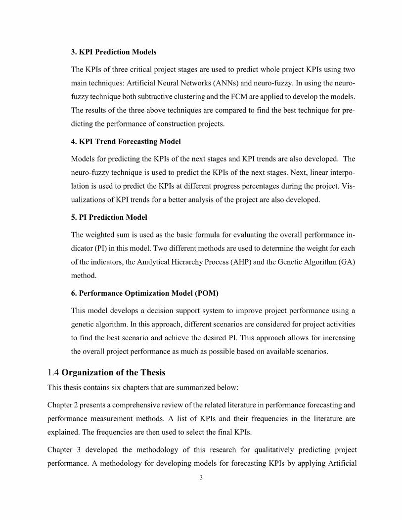
3. KPI Prediction Models
The KPIs of three critical project stages are used to predict whole project KPIs using two
main techniques: Artificial Neural Networks (ANNs) and neuro-fuzzy. In using the neuro-
fuzzy technique both subtractive clustering and the FCM are applied to develop the models.
The results of the three above techniques are compared to find the best technique for pre-
dicting the performance of construction projects.
4. KPI Trend Forecasting Model
Models for predicting the KPIs of the next stages and KPI trends are also developed. The
neuro-fuzzy technique is used to predict the KPIs of the next stages. Next, linear interpo-
lation is used to predict the KPIs at different progress percentages during the project. Vis-
ualizations of KPI trends for a better analysis of the project are also developed.
5. PI Prediction Model
The weighted sum is used as the basic formula for evaluating the overall performance in-
dicator (PI) in this model. Two different methods are used to determine the weight for each
of the indicators, the Analytical Hierarchy Process (AHP) and the Genetic Algorithm (GA)
method.
6. Performance Optimization Model (POM)
This model develops a decision support system to improve project performance using a
genetic algorithm. In this approach, different scenarios are considered for project activities
to find the best scenario and achieve the desired PI. This approach allows for increasing
the overall project performance as much as possible based on available scenarios.
1.4 Organization of the Thesis This thesis contains six chapters that are summarized below:
Chapter 2 presents a comprehensive review of the related literature in performance forecasting and
performance measurement methods. A list of KPIs and their frequencies in the literature are
explained. The frequencies are then used to select the final KPIs.
Chapter 3 developed the methodology of this research for qualitatively predicting project
performance. A methodology for developing models for forecasting KPIs by applying Artificial
4
Neural Network (ANN) and neuro-fuzzy technique is developed. This chapter also discusses a
model for predicting the KPIs of the next stages and KPIs trends. Also, chapter 3 offers an integra-
tion method to determine the overall project performance indicator (PI) using AHP (Analytical
Hierarchy Process) and GA (Genetic Algorithm) methods. Lastly, a performance optimization
model based on KPIs is developed to assist the decision making process and to improve project
performance.
Chapter 4 contains the data collection and analysis. It explains how data was collected using
questionnaires and how the data was analyzed. Chapter 5 explains the model development and
implementation based on the methodology described in Chapter 3. The results from KPI
forecasting models developed with different computing methods are compared in this chapter. A
comparison between the predicted performance indicators of the model and the performance
indicators derived from the questionnaires is also developed. Also, the validation process is
performed in this chapter.
Chapter 6 contains the conclusions and highlights the contributions of this research. It also includes
research limitations and offers recommendations for future work.
5
CHAPTER 2: LITERATURE REVIEW
2.1 Chapter overview By offering a comprehensive performance measurement system, a better project control tool im-
plemented for managing construction operations. Project management is becoming more
integrated, creating the need for a project performance measurement system capable of evaluating
all project’s attributes. Our purpose is to identify and measure the project performance indicators
for evaluating project performance.
Project control consists of two steps, measurement, and decision-making. The measurement phase
consists of, defining a project baseline and collecting data, evaluating the performance of the
project. Forecasting performance and decision-making consist of analyzing the variance, listing the
corrective actions and carrying out the corrective action for improving performance (Nassar 2005).
This chapter developed a comprehensive review of the literature. The next section reviews the
existing literature on project performance, including the definition and use of project performance
measurement approaches in section 2.2. Section 2.3 presents a review of the existing approaches
for forecasting project performance. The last section, Section 2.4, explain an overview of the re-
lated research tools. Section 2.5 elaborates findings, limitations, and research gaps in this area.
2.2 Project Performance
2.2.1 Definition
Performance is defined as the amount of efficiency and effectiveness in all of a project’s objectives
(Nassar and AbouRizk 2014). Efficiency means doing things right, in other words, getting the most
output for the least input, and effectiveness means “doing the right things” that means attaining
organizational goals.
“Project performance assessment is the process of comparing actual project performance against
planned performance and identifying variances from planned performance” (Hollmann 2012). Each
stakeholder does performance evaluation to ensure profit achievement due to the different benefits
for different stakeholders. The first step in defining a project’s success is identifying from whose
point of view the success will be measured. The performance measurement by different stakehold-
ers such as owners, project managers, or contractors can vary.
6
Project success was based on three objectives in 1980: 1) completed on time;2) completed within
budget, and 3) completed with desirable quality. All of these focus on the internal performance of
the project and do not include other important factors such as customer satisfaction and safety
(Khosravi and Afshari 2011). The logical way of improving performance by measuring and
comparing your performance against others is referred to as benchmarking (Swan and Kyng 2004).
Nyariki (2014) mentions that the definition of project success may change due to the project type,
size, and stakeholders. He also identifies success as the achievement of goals and objectives plus
good results in a project that will have a positive impact on people’s lives. Next section illustrates
an overview of construction project performance measurement methods in the literature.
2.2.2 Project Performance Measurement
Most performance measurement methods are related to the work on project control. It helps to
carry out accurate and timely corrective actions. Measuring performance is vital for all project
stakeholders. However, different project stakeholders want different forms of project control and
performance measurement. Previous researchers have worked on performance measurement sys-
tems (PMS) and developed key performance indicators (KPIs) to quantify the concept of project
performance.
Earned Value is a classic project control method that uses time and cost. This method is based on
the work breakdown structure (WBS) tool to define work packages. “In 1967, the US Department
of Defense (DOD) issued their Cost/Schedule Control Systems Criteria, known as C/SCSC. Cur-
rently, these criteria are known as the Earned-Value Management System (EVMS) criteria ”(Nas-
sar 2005). This method is an integrated control of projects’ time and cost. It uses three S-curves
for controlling project time and cost, the Budgeted Cost of Work Performed (BCWP), the
Budgeted Cost of Work Scheduled (BCWS), and the Actual Cost of Work Performed (ACWP).
Project performance is measured using the EV method by using the Cost Performance Index (CPI)
and the Schedule Performance Index (SPI).
The Program Evaluation and Review Technique (PERT) method was introduced by the US Navy
in 1957. The S-curve and PERT methods use cost and schedule indicators independently to eval-
uate performance, while the earned value method integrates cost and schedule indicators. They did
not mention other performance aspects such as quality and safety. Other models are therefore
needed to comprehensively measure the performance of a construction project.
7
Freeman and Beale (1992) used seven criteria as project success criteria. Their study uses a meas-
uring system that consists of a discounted cash flow (DCF) principle. One of the shortcomings of
this method is that it requires information that can be calculated only after a project’s completion.
Ashley et al. (1987) used ten criteria to evaluate project success. The criteria’s are budget
performance, schedule performance, client satisfaction, functionality, contractor satisfaction,
project management team satisfaction, follow-on work, capabilities build up, end-user satisfaction,
and specification (quality). The main problem of this method is that the four latter criteria are not
well defined. Also, the defined criteria are not inclusive to cover all project aspects.
Alarcón and Ashley (1996) developed a model based on knowledge of project experts, the
experience of a project’s team and decision analysis techniques. Their model uses four perfor-
mance indicators: cost, schedule, value to the owner, and effectiveness. A general performance
model is developed using experience captured from experts and assessments from the project team.
Chua et al. (1999) evaluated project success through three objectives, cost, schedule, and quality.
Sixty-seven critical success factors (CSFs) that influence the performance of these three objectives
and affect overall project success are defined by a survey using experts’ opinions. This approach
uses the analytical hierarchical process (AHP) to determine these success factors and assess the
importance of the three objectives of construction project success. This paper does not consider
other criteria that affect the success of a project, such as safety and client satisfaction.
Griffith et al. (1999) measured industrial project performance by calculating a success index that
combines four variables, budget achievement (B), schedule achievement (S), design capacity (C),
and plant utilization (U), and then multiplied the variables in their weight based on Equation 2-1.
Success Index = 0.35B + 0.25S + 0.28C + 0.12U 2-1
Where design capacity is “measured in percent of units of product produced as compared with the
planned amount”. And plant utilization is “the percentage of days in a year the plant actually
produces product”. The weight of variables is derived from the interview process. Each variable
amount must then be classified into three separate values (1-3-5) based on how well its
performance measured against the project’s original plan. The shortcomings are that these indexes
do not consider all aspects of project success such as safety and quality. And due, to the variable’s
8
definition, the success index can only assess performance after six months of operation. Also, this
equation mixes construction performance indicators with design and operations success variables.
Cheng et al. (2000) built a model that determined the degree of success of partnering by subjective
measures (individual perceptual scales) and objective measures (cost variation). Only a couple of
the measures used in partnering construction projects are defined, and this model did not mention
how to evaluate and assign weight to each measure. The measures here are cost variation, rejection
of work, client satisfaction, quality of work, schedule variation, change in scope, profit variation,
safety measure, rework, litigation, and tender efficiency.
Gao et al. (2002) identified 16 factors for project success factors (CSFs) listed in the literature;
four of these are cost, schedule, technical performance, and client satisfaction. They identified
criteria required for the success of a project based on interviews with experts and literature
analysis, but they did not suggest ways for measuring them and also do not consider other aspects
of success such as safety and profitability.
Rad (2003) measured the success or failure of a project based on a subjective approach. He
proposed a model to evaluate the success of the project from two different aspects, the client, and
the project team. He also defined a series of success indicators for client success and success
factors for project team success using a WBS structure. However, he did not mention how to
calculate and quantify their proposed indicators and their weights.
Tucker et al. (2003) built a model to quantify construction phase success (CPS) from the
viewpoints of both clients and contractors. The study reviewed 209 industrial projects in North
America. The indicators used are cost performance (cost growth: CGS), schedule performance
(schedule growth: SGS), quality performance (rework factor: RFS) and safety performance (lost
workday case incident rate: LWCIRS), as shown in Equation 2-2:
CPS = [C1/C𝑇] CGS + [C2/C𝑇] SGS + [C3/C𝑇] RFS + [C4/C𝑇] LWCIRS 2-2
where C1 is the cost of the average construction phase cost growth, C2 is the cost of the average
construction phase schedule growth, C3 is the average rework factor cost, C4 is the cost of the
average number of lost workday case incidents, and CT is the total cost. The weight of each indi-
cator is defined using a cost ratio according to Equation 2-3.
CPS = 0.4CGS + 0.25SGS + 0.3RFS + 0.05LWCIRS 2-3
9
The main shortcomings of this model are that it is not applicable to an ongoing project and thus
can only be used when a project is finished when it is too late to carry out any corrective action.
Also, the weights for variables are based on cost ratios, which may not always be true.
Rozenes et al. (2004) proposed a multidimensional Project Control System (MPCS) that quantita-
tively evaluated project performance by measuring the performance of eight criteria defined in two
categories that are functional and operational category. The MPCS uses a quantitative approach to
define a deviation from the planned phase. This model evaluates project performance by measuring
the Gap Performance Index (GPI), which is the gap existing between the planned and actual per-
formance. It is obvious that the ideal amount of GP is zero. The primary shortcoming of this model
is that there is no clear distinction between the success factor and the project success criteria.
Bassioni et al. (2004) reviewed methods in the performance measurement framework and identi-
fied gaps in this area. Their emphasis is on the application of these frameworks in construction
firms in the United Kingdom from the view of internal management.
Nassar (2005) proposed a model for defining project performance from a contractor’s view. The
Earned Value Management Indicators are used plus six more indicators. Then proposed mathe-
matical relation for calculating the project performance indexes. After normalizing some of the
indicators, he incorporated them in a comprehensive model for calculating the success of a project
from the contractor’s perspective. The main shortcoming of this model is that it does not consider
the difference between the success factor and project success criteria in the definitions of some of
its indicators.
Menches and Hanna (2006) proposed a process for converting a project manager’s qualitative as-
sessment of “successful performance” to a quantitative amount. Six indicators were used that are
actual percent profit, percent schedule overrun, amount of time given, communication between
team members, budget achievement, and change in work hours. Twenty-seven random electrical
contractors throughout the United States were selected to collect planning and performance data.
Companies were asked to give information about two projects, one successful and one less
successful project, by completing a questionnaire and being interviewed about the planning and
performance of their submitted projects. Validation was used which indicated that the model was
useful for quantitatively measuring successful performance based on the project managers’ point
of view.
10
Khosravi and Afshari (2011) developed a successful measurement model by providing a project
success index for every finished project in the Mapna Special Projects Construction & Develop-
ment Co (MD-3). The model is from the view of the performing organization. Their model was
designed to compare finished projects and create a benchmark for improving project success.
Cha and Kim (2011) defined a quantitative performance measurement system by using eighteen
key performance indicators for residential building projects. They defined the performance
indicators based on a literature review and interviews with experts and assigned weight to
each project performance indicator. These weighted indicators were used to develop a
mathematical model to quantifiably assess project performance.
Deng et al. (2012) assessed the literature on PMS (Project Measurement Systems), especially at
the company level and identified gaps. They found that traditional performance measurement is
inappropriate because it does not consider non-financial measures such as productivity. They iden-
tified the need to focus more on the design and implementation issues of PMS in construction and
showed the essential need for future research in performance measurement (PM) in construction
projects and firms.
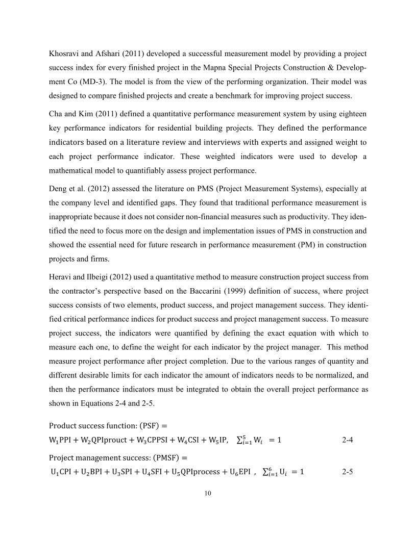
Heravi and Ilbeigi (2012) used a quantitative method to measure construction project success from
the contractor’s perspective based on the Baccarini (1999) definition of success, where project
success consists of two elements, product success, and project management success. They identi-
fied critical performance indices for product success and project management success. To measure
project success, the indicators were quantified by defining the exact equation with which to
measure each one, to define the weight for each indicator by the project manager. This method
measure project performance after project completion. Due to the various ranges of quantity and
different desirable limits for each indicator the amount of indicators needs to be normalized, and
then the performance indicators must be integrated to obtain the overall project performance as
shown in Equations 2-4 and 2-5.
Product success function: (PSF) =
W1PPI + W2QPIprouct + W3CPPSI + W4CSI + W5IP, ∑ W𝑖5𝑖=1 = 1 2-4
Project management success: (PMSF) =
U1CPI + U2BPI + U3SPI + U4SFI + U5QPIprocess + U6EPI , ∑ U𝑖6𝑖=1 = 1 2-5
11
profitability performance index (PPI), product quality performance index (QPI Product), client satisfaction index (CSI),
contractor’s professional profit satisfaction index (CPPSI), and the investment performance index (IPI)., cost
performance index (CPI), billing performance index (BPI), schedule performance index (SPI), safety performance
index (SFI), process quality performance index (QPI Process), and the environmental performance index (EPI)
Haponava and Al-Jibouri (2012) measured project performance in three phases dynamically, using
some process-based performance indicators. Their system relied on questions related to both pro-
cess completeness and process quality. The project is divided into three stages, the pre-project
stage, design stage, and construction stage. To develop a generic system for measuring process
performance. KPIs are measured in two aspects; the first is for process completeness, defining the
question of “how much sub-processor is complete? “, and the second is process quality, which
answers the query of “how the completed part is done?”
Ali et al. (2013) defined a set of important KPIs that can be used to measure the performance of
construction companies. They identified 47 KPIs from the literature and designed a questionnaire
to define the main KPIs as well as to rank the importance of each KPI (1= very low importance, 2
= low importance, 3= medium importance, 4= high importance, and 5 = very high importance).
Twenty-four surveys were analyzed, resulting in ten indicators for measuring company
performance. They used a statistical method to analyze the questionnaires’ data about the im-
portance of each KPI.
Wester (2013) recognized key performance indicators in the design stage for advanced high-tech-
nological construction projects using a qualitative approach. Although this research only focused
on identifying KPIs during the design stage of projects and did not consider other stages, also it
did not predict performance indicators.
Kam et al. (2013) proposed using KPIs to help construction project teams in Virtual Design and
Construction (VDC) /Building Information Modeling (BIM) decision-making. They suggested us-
ing statistical methods to identify relations between KPIs. In their proposal, they recommended
providing models for benchmarking, decision-prioritization, and performance prediction. How-
ever, this is a proposal, and the implemented work is not presented and not yet implemented.
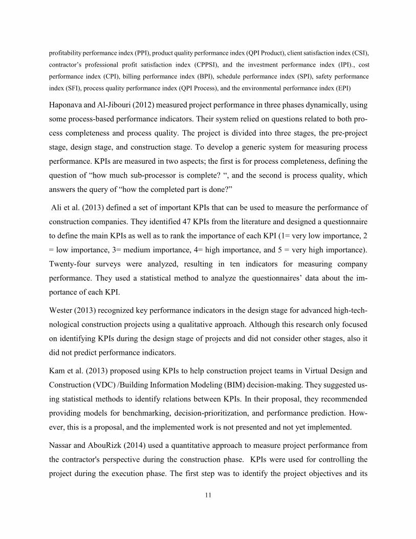
Nassar and AbouRizk (2014) used a quantitative approach to measure project performance from
the contractor's perspective during the construction phase. KPIs were used for controlling the
project during the execution phase. The first step was to identify the project objectives and its
12
performance indexes and sub-indexes. The project manager defined the project objectives. The
indexes were determined from discussions with fifteen contractors and in accordance with the
authors’ experience. A hierarchy for project performance is proposed in which each indicator is
divided into sub-indicators, but its applicability was checked for each project, as each project is
unique. The second step is to quantify the project indexes as shown in Table 2-1.
Table 2-1: KPIs description (Nassar and AbouRizk 2014).
Index Description Calculation
Cost Performance Index (CPI) Cost efficiency of the project CPI = BCWP/ACWP
Schedule Performance Index
(SPI) Schedule efficiency of the project SPI = BCWP/BCWS
Billing Performance Index (BPI) The efficiency of invoicing the client for
earned work; determines cash flow BPI = BRWP/ERWP
Profitability Performance Index
(PPI) Profitability of the project to date PPI = ERWP/ACWP
Safety Performance Index (SFI) Safety of project to date SFI = LTI × C/M
Quality Performance Index (QPI) Consistency in application of project
standards and procedures QPI = CFRI
Team Satisfaction Index (TSI) Satisfaction of the project team TSI = ∑ WiRi
12
𝑖=1
Client Satisfaction Index (CSI) Satisfaction of the client CSI = ∑ WiRi
12
𝑖=1
BCWP = Budgeted cost of work performed: the cumulative budgeted cost for work completed to date, or the cost allowed (based on budget) to spend on the actual work done. ACWP = Actual cost of work performed: the cumulative cost incurred to complete the accomplished work to date. BCWS = Budgeted cost of work scheduled: the budgeted cost for work scheduled (as per budget) to date. BRWP = Billed revenue of work performed, or the cumulative amount of invoices. ERWP = Earned revenue of work performed or the cumulative revenue earned for the actual work accomplished to date. LTI = Number of lost time incidents to date. C = a constant (200,000), which represents 100 employees working for a full year (100 × 2; 000). M = Total work hours expended to date. CFRI = Construction field rework index: the total direct and indirect cost of rework performed in the field/total field construction phase cost. Wi = Relative weights (determined by the AHP method) for various areas of concern to the client or project team.
13
Ri = Satisfaction ratings from 1-10 for various areas of concern to the client or project team.
Each sub-index is calculated by the above formula and then summed to get the value of the index.
The weight shows how important each factor is for defining the total project performance. The
AHP (Analytical Hierarchy process) was used to define the weight (w) of each factor. The third
step was to normalize the indexes. The fourth step was to calculate the total project performance
by integrating the indexes according to Equation 2-6. By using the assumption that every two in-
dexes are mutually independent, they can calculate the project performance by summing up eight
performance indices with their weights.
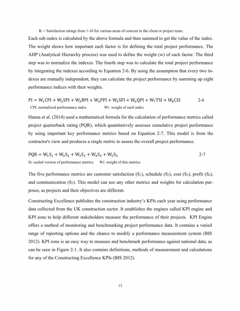
PI = W1CPI + W2SPI + W3BPI + W4PPI + W5SFI + W6QPI + W7TSI + W8CSI 2-6 CPI: normalized performance index Wi: weight of each index
Hanna et al. (2014) used a mathematical formula for the calculation of performance metrics called
project quarterback rating (PQR), which quantitatively assesses cumulative project performance
by using important key performance metrics based on Equation 2-7. This model is from the
contractor's view and produces a single metric to assess the overall project performance.
PQR = W1S1 + W2S2 + W3S3 + W4S4 + W5S5 2-7 Si: scaled version of performance metrics Wi: weight of this metrics
The five performance metrics are customer satisfaction (S1), schedule (S2), cost (S3), profit (S4),
and communication (S5). This model can use any other metrics and weights for calculation pur-
poses, as projects and their objectives are different.
Constructing Excellence publishes the construction industry’s KPIs each year using performance
data collected from the UK construction sector. It establishes the engines called KPI engine and
KPI zone to help different stakeholders measure the performance of their projects. KPI Engine
offers a method of monitoring and benchmarking project performance data. It contains a varied
range of reporting options and the chance to modify a performance measurement system (BIS
2012). KPI zone is an easy way to measure and benchmark performance against national data, as
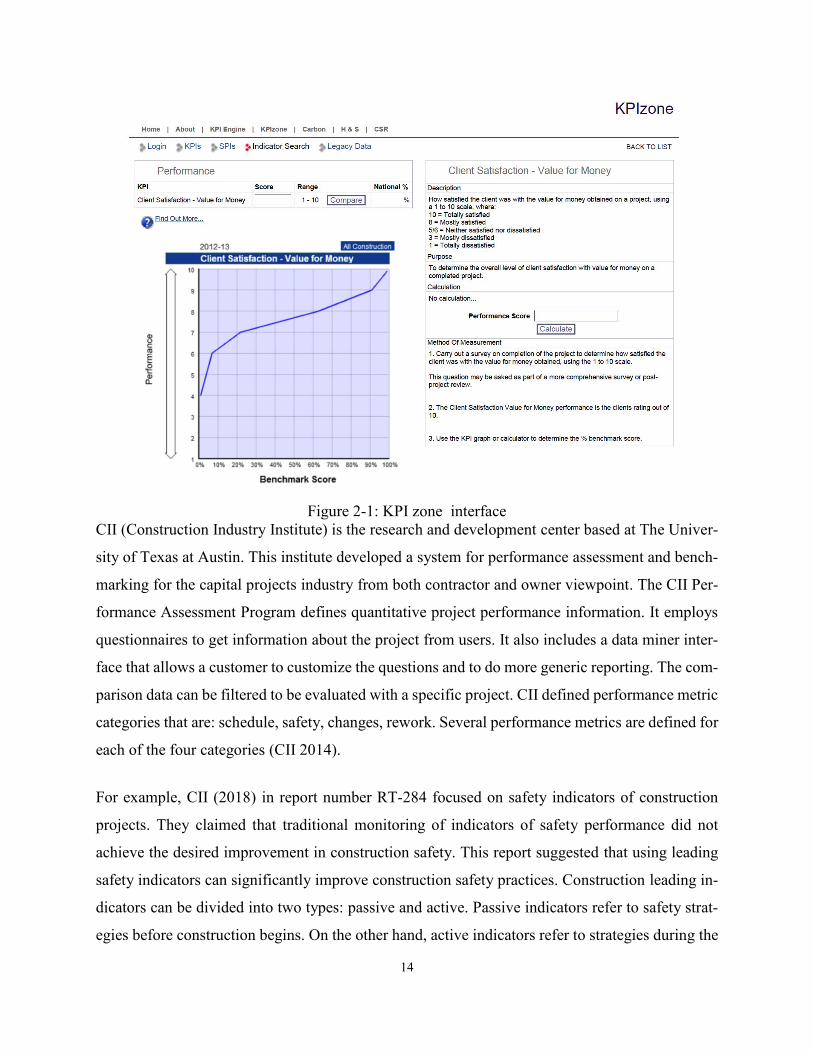
can be seen in Figure 2-1. It also contains definitions, methods of measurement and calculations
for any of the Constructing Excellence KPIs (BIS 2012).
14
Figure 2-1: KPI zone interface
CII (Construction Industry Institute) is the research and development center based at The Univer-
sity of Texas at Austin. This institute developed a system for performance assessment and bench-
marking for the capital projects industry from both contractor and owner viewpoint. The CII Per-
formance Assessment Program defines quantitative project performance information. It employs
questionnaires to get information about the project from users. It also includes a data miner inter-
face that allows a customer to customize the questions and to do more generic reporting. The com-
parison data can be filtered to be evaluated with a specific project. CII defined performance metric
categories that are: schedule, safety, changes, rework. Several performance metrics are defined for
each of the four categories (CII 2014).
For example, CII (2018) in report number RT-284 focused on safety indicators of construction
projects. They claimed that traditional monitoring of indicators of safety performance did not
achieve the desired improvement in construction safety. This report suggested that using leading
safety indicators can significantly improve construction safety practices. Construction leading in-
dicators can be divided into two types: passive and active. Passive indicators refer to safety strat-
egies before construction begins. On the other hand, active indicators refer to strategies during the
15
construction phase. It identified ten key passive safety leading indicators and 14 active safety in-
dicators (CII 2018).
CII’s newest approach for benchmarking of capital projects is introduced in the 10-10 program
(CII 2018). This program illustrates an important linkage with the CII Performance Assessment
System: CII Performance Assessment System defines performance measurement of project exe-
cution, while 10-10 program defines a system for ongoing project diagnostic. Therefore, 10-10
program allows practitioners to identify problems and to take corrective action for improving on-
going projects. CII’s 10-10 program is based on surveying members of a project’s management
team about the performance, team dynamics, and organizational relationships of their project.
The 10-10 Program is based on questionnaires for five project phases: (1) front end planning, (2)
engineering and design, (3) procurement, (4) Construction, and 5) commissioning and Startup. At
the end of each phase, customers will have an assessment of that part. Ten leading indicators or
input measures are obtained using questionnaires: Planning, Organizing, Leading, Controlling,
Design, Human resources, Quality, Sustainability, Supply, and Safety. These measures can warn
management team of future problems. Ten outcome measures or lagging indicators are suggested
by the system to inform the management team about how the project is proceeding (CII 2018).
Ngacho and Das (2015) developed a performance assessment framework of construction projects
based on six KPIs: time, cost, quality, safety, site disputes and environmental impact. These KPIs
were recognized through interviews and a literature review. They used several characteristic fea-
tures, called critical success factors (CSFs), to assess the performance of these KPIs.
Nilashi et al. (2015) focused on finding the importance of factors and calculating the weight as
well as the interdependencies among their selected criteria. This paper does not define an approach
for predicting KPIs based on the status of the project.
Stillman and Norwood (2015) proposed a method of performance assessment using KPI within
programs and organizations. They developed three concepts that are identifying the root causes of
critical issues, employing visual graphs to clarify trends and opportunities, and adjusting KPIs to
impact change at all levels. They claimed that by applying these concepts to programs and organ-
izations, positive change during the execution of the work can be derived.
16
Defense Construction Canada (DCC) used two sets of performance indicators to measure the
success of Canadian projects from contractor viewpoint: key performance indicators (KPIs) and
business performance indicators (BPIs). Key performance indicators (KPIs) measure DCC’s suc-
cess in achieving strategic objectives, such as leadership and governance. The KPIs’ outcomes are
published in the Annual Report and in the Corporate Plan Summary. Business performance indi-
cators (BPIs) measure DCC’s achievement in tactical points, such as business management and
service delivery objectives (DCC 2016).
Ingle and Mahesh (2016) developed a project quarter back rating (PQR) system that is for project
benchmarking. PQR identified seven project performance metrics, responsible for the successful
completion of a project. It then combined these performance metrics to evaluate the overall per-
formances of projects.
Wan (2017) used KPIs to forecast performance of E-Commerce companies to indicate their pro-
gress and to confirm attaining business goals. The main objective was to enhance the forecasting
of KPIs using past data applying Linear and non-linear models. Though, this study was focused
on E-Commerce companies’ performance and did not mention construction projects. Shaikh and
Darade (2017) focused on quality of activities by considering KPIs in the planning stage. This
study tried to find KPIs of activities and prepared a Project Quality Plan for activities and their
importance. However, this research did not predict performance and only focused on quality indi-
cators without considering other KPIs
Project performance management framework consists of performance measurement, and forecast-
ing combined with defining and optimizing the corrective actions for improving the performance
of the remaining work. Project Performance Management frameworks are described below.
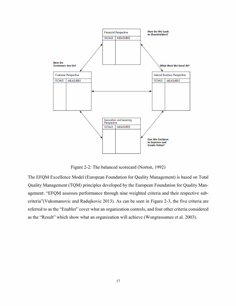
Balanced Scorecard (BSC) is a concept created in 1992 (Kaplan and Norton 1992). It has four
main perspectives, financial perspective, customer perspective, internal process perspective and
innovation perspective as shown in Figure 2-2. The main purpose of BSC is to use the objectives
of an organization. Indicators should be defined for each perspective to be able to measure them
correctly. The limitations of this framework are that the four perspectives have the same weight,
and that it does not cover all aspects of performance.
17
Figure 2-2: The balanced scorecard (Norton, 1992)
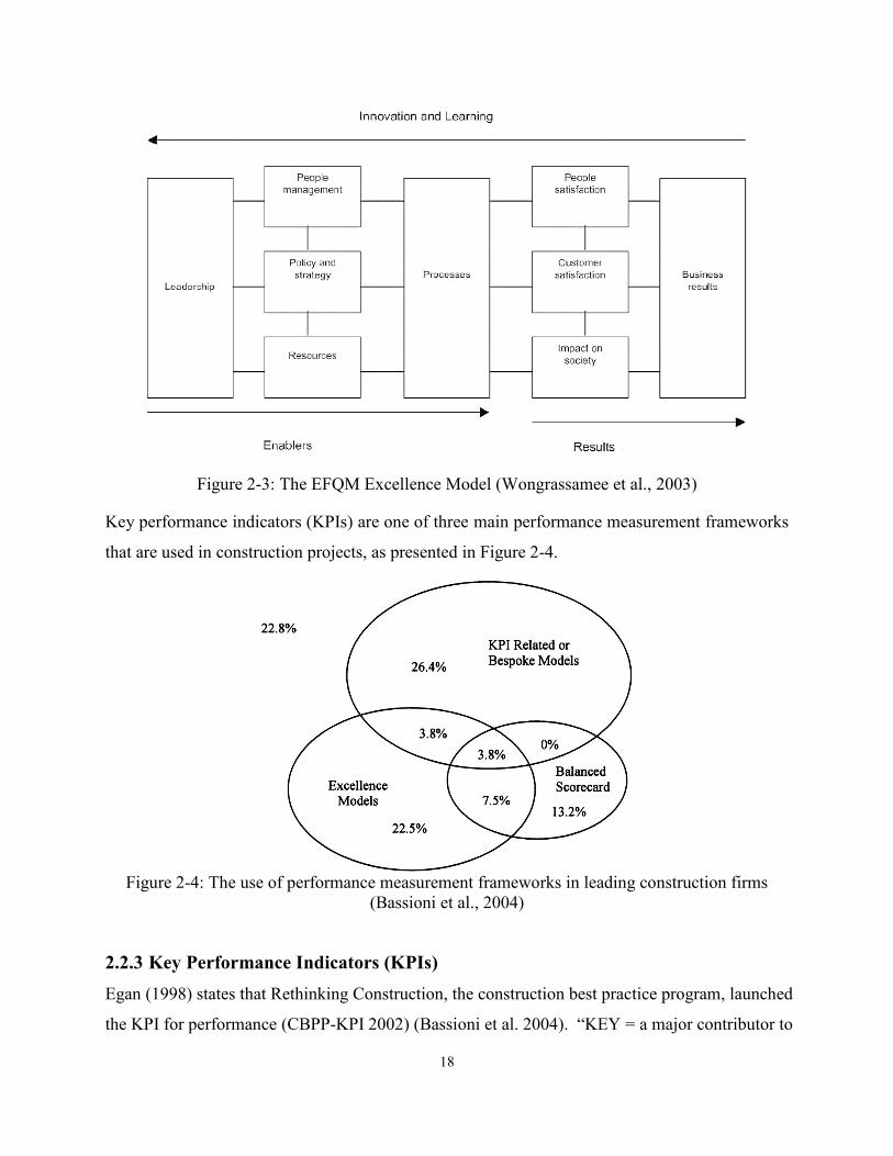
The EFQM Excellence Model (European Foundation for Quality Management) is based on Total
Quality Management (TQM) principles developed by the European Foundation for Quality Man-
agement. “EFQM assesses performance through nine weighted criteria and their respective sub-
criteria”(Vukomanovic and Radujkovic 2013). As can be seen in Figure 2-3, the five criteria are
referred to as the “Enabler” cover what an organization controls, and four other criteria considered
as the “Result” which show what an organization will achieve (Wongrassamee et al. 2003).
18
Figure 2-3: The EFQM Excellence Model (Wongrassamee et al., 2003)
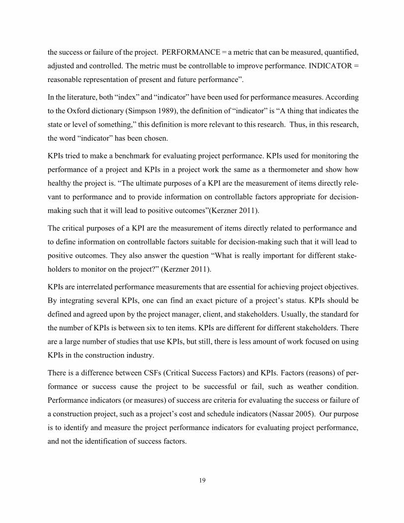
Key performance indicators (KPIs) are one of three main performance measurement frameworks
that are used in construction projects, as presented in Figure 2-4.
Figure 2-4: The use of performance measurement frameworks in leading construction firms
(Bassioni et al., 2004)
2.2.3 Key Performance Indicators (KPIs)
Egan (1998) states that Rethinking Construction, the construction best practice program, launched
the KPI for performance (CBPP-KPI 2002) (Bassioni et al. 2004). “KEY = a major contributor to
19
the success or failure of the project. PERFORMANCE = a metric that can be measured, quantified,
adjusted and controlled. The metric must be controllable to improve performance. INDICATOR =
reasonable representation of present and future performance”.
In the literature, both “index” and “indicator” have been used for performance measures. According
to the Oxford dictionary (Simpson 1989), the definition of “indicator” is “A thing that indicates the
state or level of something,” this definition is more relevant to this research. Thus, in this research,
the word “indicator” has been chosen.
KPIs tried to make a benchmark for evaluating project performance. KPIs used for monitoring the
performance of a project and KPIs in a project work the same as a thermometer and show how
healthy the project is. “The ultimate purposes of a KPI are the measurement of items directly rele-
vant to performance and to provide information on controllable factors appropriate for decision-
making such that it will lead to positive outcomes”(Kerzner 2011).
The critical purposes of a KPI are the measurement of items directly related to performance and
to define information on controllable factors suitable for decision-making such that it will lead to
positive outcomes. They also answer the question “What is really important for different stake-
holders to monitor on the project?” (Kerzner 2011).
KPIs are interrelated performance measurements that are essential for achieving project objectives.
By integrating several KPIs, one can find an exact picture of a project’s status. KPIs should be
defined and agreed upon by the project manager, client, and stakeholders. Usually, the standard for
the number of KPIs is between six to ten items. KPIs are different for different stakeholders. There
are a large number of studies that use KPIs, but still, there is less amount of work focused on using
KPIs in the construction industry.
There is a difference between CSFs (Critical Success Factors) and KPIs. Factors (reasons) of per-
formance or success cause the project to be successful or fail, such as weather condition.
Performance indicators (or measures) of success are criteria for evaluating the success or failure of
a construction project, such as a project’s cost and schedule indicators (Nassar 2005). Our purpose
is to identify and measure the project performance indicators for evaluating project performance,
and not the identification of success factors.
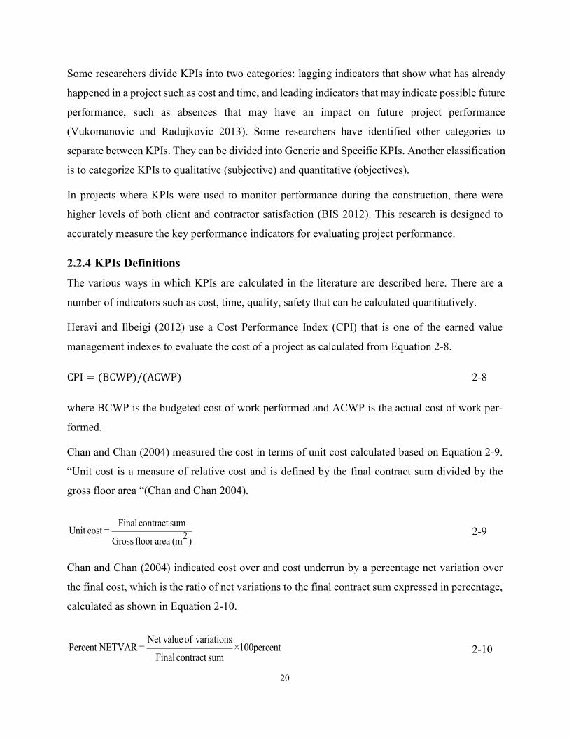
20
Some researchers divide KPIs into two categories: lagging indicators that show what has already
happened in a project such as cost and time, and leading indicators that may indicate possible future
performance, such as absences that may have an impact on future project performance
(Vukomanovic and Radujkovic 2013). Some researchers have identified other categories to
separate between KPIs. They can be divided into Generic and Specific KPIs. Another classification
is to categorize KPIs to qualitative (subjective) and quantitative (objectives).
In projects where KPIs were used to monitor performance during the construction, there were
higher levels of both client and contractor satisfaction (BIS 2012). This research is designed to
accurately measure the key performance indicators for evaluating project performance.
2.2.4 KPIs Definitions
The various ways in which KPIs are calculated in the literature are described here. There are a
number of indicators such as cost, time, quality, safety that can be calculated quantitatively.
Heravi and Ilbeigi (2012) use a Cost Performance Index (CPI) that is one of the earned value
management indexes to evaluate the cost of a project as calculated from Equation 2-8.
CPI = (BCWP)/(ACWP) 2-8
where BCWP is the budgeted cost of work performed and ACWP is the actual cost of work per-
formed.
Chan and Chan (2004) measured the cost in terms of unit cost calculated based on Equation 2-9.
“Unit cost is a measure of relative cost and is defined by the final contract sum divided by the
gross floor area “(Chan and Chan 2004).
Final contract sumUnit cost = 2Gross floor area (m )
2-9
Chan and Chan (2004) indicated cost over and cost underrun by a percentage net variation over
the final cost, which is the ratio of net variations to the final contract sum expressed in percentage,
calculated as shown in Equation 2-10.
Net value of variationsPercent NETVAR = ×100percent
Final contract sum 2-10

21
where Net value of variations = Final contract sum – Base and
Base = Original contract sum + Final rise and fall - Contingency allowance
Tucker et al. (2003) used construction cost growth (CCG) indexes to represent the cost component
computed from Equation 2-11.
CCG = Actual Construction Phase Cost - Initial Predicted Construction Phase CostInitial Predicted Construction PhaseCost
2-11
Heravi and Ilbeigi (2012) used the Schedule performance index (SPI) to measure the scheduling
efficiency of a project (Heravi and Ilbeigi 2012). The SPI is defined by the standard of the EVM,
as shown in Equation 2-12.
SPI=(BCWP)/(BCWS) 2-12
where BCWP is the budgeted cost of work performed and BCWS the budgeted cost of work
scheduled.
“If the project’s delay leads to the postponing of the end of the project, after passing the primary
deadline, the quantity of the BCWS will remain constant, and in continuation of the project, the
result of Equation 2-12 will not show the scheduling efficiency of the project. Consequently, an
improvement is needed to apply to Equation 2-12. Therefore, they have suggested another equation
for the calculation of SPI presented in Equation 2-13.
SPI=[(BCWP)/(BCWS)] × [(DUR)/(DUR+DLY)] 2-13
where DUR is the primary duration of the project and DLY is the amount of delay after the primary
date of the project’s finish date.
Chan and Chan (2004) used three formulae to evaluate the time category: construction time, the
speed of construction and time variation. They define construction time as the absolute time,
calculated as the number of days/weeks from the start on site to practical completion of the project,
as shown in Equation 2-14.
Construction time = Practical completion date- Project commencement date 2-14
Chan and Chan (2004) evaluated the speed of construction in relative time, which is defined by
the gross floor area divided by the construction time:
22
2Gross floor area (m )Speed of construction=
Construction time (days/weeks) 2-15
They measured time variation by using the percentage of increase or decrease in the estimated
project time in days/weeks, discounting the effect of the extension of time (EOT) granted by the
client, as presented in Equation 2-16.
Construction time - Revised contract periodTime variation= 100 per centRevised contract period
2-16
Revised contract period = Original contract period + EOT
Tucker et al. (2003) used construction schedule growth to represent the schedule component, as
calculated in Equation 2-17. If the construction schedule growth is positive, it means the owner
probably loses revenue because the project will be completed late, and if the scheduled growth is
negative, the owner has the chance to use the constructed facility early to produce revenue (Tucker
et al. 2003).
Construction schedule growth =
Actual Construction Phase Duration - Initial Predicted Construction Phase DurationInitial Predicted Construction Phase Duration
2-17
Heravi and Ilbeigi (2012) used two different indexes for evaluating quality: a Product Quality
Performance Index (QPI Product) and a Process Quality Performance Index (QPI Process). The
QPI Product reflects the quality of the final project product calculated from Equation 2-18.
QPIProduct = (SELQPrd)/(TECP) 2-18
where SELQPrd is the sum of direct and indirect expenses due to a lack of quality of the final project
product and TECP is the total expenses of the project’s construct phases.
The Process Quality Performance Index (QPI Process) is the index for evaluating the quality of
the process of a project and focuses only on the execution process of the project, calculated as in
Equation 2-19.
QPI=(SELQPrs)/(TECP) 2-19
23
Where SELQPrs is the sum of the direct and indirect expenses due to a lack of quality in the project
process, and TECP is the total expenses of a project’s construction phases. The TECP consists of
all the direct costs of construction phases such as materials, machinery, sub-contractors, etc.
Tucker et al. (2003) represented quality by the rework factor, which is calculated based on Equa-
tion 2-20.
Rework Factor = Total Direct Cost of Field ReworkActual Construction PhaseCost
2-20
Heravi and Ilbeigi (2012) used a Safety Performance Index (SFI), the sum of two sub-indices as
calculated from Equation 2-21.
1 2SFI= ×SFI + ×SFI=1
c s
i
x xx
2-21
Where SFIc is the safety performance index of the project outcome in terms of expenses and SFIs
the safety performance index of the project outcome in terms of scheduling. The SFI of the project
outcome in terms of expenses (SFIc) is computed from Equation 2-22.
SFI𝑐 = (ELSO)/(TECP) 2-22
Where ELSO is the expense arising from damages due to the lack of safety observance and TECP
is the total expenses of the project’s construction phases. The SFI of a project’s outcome in terms
of scheduling (SFIs) is calculated based on Equation 2-23.
SFI𝑠 = (IDWH)/(TIHW) 2-23
Where IDWH is the number of the individual or missed working hours due to a lack of safety
observance, and TIWH is the total number of individuals or working hours in the construction
phase. Used the accident rate to represent project safety as shown in Equation 2-24.
Accident rate = (Total no. of reportable construction site accidents) / (Total no. of workers em-ployed, or man-hours worked on a specific project) × 1,000 2-24
Tucker et al. (2003) used the Lost Workday Case Incident Rate (LWCIR) to define project safety.
LWCIR is calculated based on Equation 2-25.
24
LWCIR = Number of Lost Workday Cases 200,000 Site Craft Workhours
2-25
2.3 Project Performance Forecasting The accurate forecasting of project performance in the construction industry is vital for controlling
a construction project. The prediction of construction performance has been carried out by differ-
ent methods.
Ling et al. (2004) used multiple linear regression (MLR) modeling and SPSS software to predict
project performance. The limitation of this paper is that they predicted 11 performance criteria
(measures) but did not define an overall project performance metric. Wong (2004) used the logistic
regression approach to predict the performance of construction contractors for the United King-
dom. They proposed using clients’ tender evaluation preferences to forecast contractor perfor-
mance. The proposed performance prediction model is only for tender stage and not during the
construction stage. Nassar (2005) performed a probabilistic forecast using a Markov Chain and
then used a genetic algorithm for corrective action optimization. His model predicts performance
at the completion of the project and any other future point. Nassar (2005) only chose Markov Chain
technique and did not compare other techniques for predicting project performance. The choice of
Markov Chain technique has the limitation of not considering the performance of previous project
stages on the overall project performance. This is because the Markov process is based on the
“memoryless” assumption meaning that the probability of upcoming project performance depends
only on the present project performance and not any past conditions of performance. He also did
not consider the difference between the success factor and project success criteria in the definitions
of some of its indicators.
Cheung et al. (2006) predicted the performance of the successful tenderers through neural net-
works. However, their developed model was for the tender stage. Also, some important aspects of
project performance such as safety have not been considered. Li et al. (2006) used a forecasting
method for predicting the potential cost overrun and schedule delay on construction projects based
on a set of performance indicators identified by employing a fuzzy inference process. The model
forecasted time and cost overrun of the project and did not consider other important aspects such
as quality and safety.
25
Dissanayake and Fayek (2008) developed a model for monitoring performance and identifying the
causes of performance failures for Canadian projects using fuzzy, Artificial Neural Network
(ANN) and Genetic Algorithm (GA) methods. They have performed a qualitative diagnosis and
prediction of the causes of construction performance deviations at the activity level of construction
projects on a daily basis. Their model did not consider overall project performance and only focus
on activity.
Hedberg and Skjutar (2010) used ANNs for predicting team performance based on past individual
achievements. Their developed model did not consider overall project performance and only focus
on team performance. Jha and Chockalingam (2011) used the ANNs to predict the schedule per-
formance of Indian construction projects. They employed a comprehensive list of factors impact-
ing schedule performance but did not consider other performance metrics. Wang et al. (2012) used
ANNs and support vector machines classification models for predicting construction cost and
schedule success. But, they did not consider other performance aspects such as quality and safety.
Tang et al. (2012) used system dynamics for forecasting the capability of a construction organiza-
tion. The developed model only predicts the financial performance of construction organizations
and is not capable of forecasting project performance.
Mohamad et al. (2014) used the neural network and Genetic algorithm for modeling the financial
performance of construction companies. However, the focus of this research is not performance
during the construction phase and only financial aspects of performance are considered.
Salari and Khamooshi (2016) presented a framework that estimates project performance based on
past performance data. Their model used a fuzzy time series forecasting model in the estimation
process. They only consider project performance from a cost and schedule perspective. Reenu et
al. (2017) showed how the success of construction projects depends mostly on the success of a
project’s performance. ANN technique was employed to predict project performance based on
four performance metrics of cost, schedule, quality, and satisfaction performance. Their model
only focused on predicting performance metrics individually and did not predict the overall project
performance. Also, other projects aspects such as safety were not considered.
Leon et al. (2017) developed a system dynamics (SD) model using eight construction project per-
formance indicators (cost, schedule, quality, profitability, safety, environment, team satisfaction,
and client satisfaction) to predict construction project performance. Overall project performance
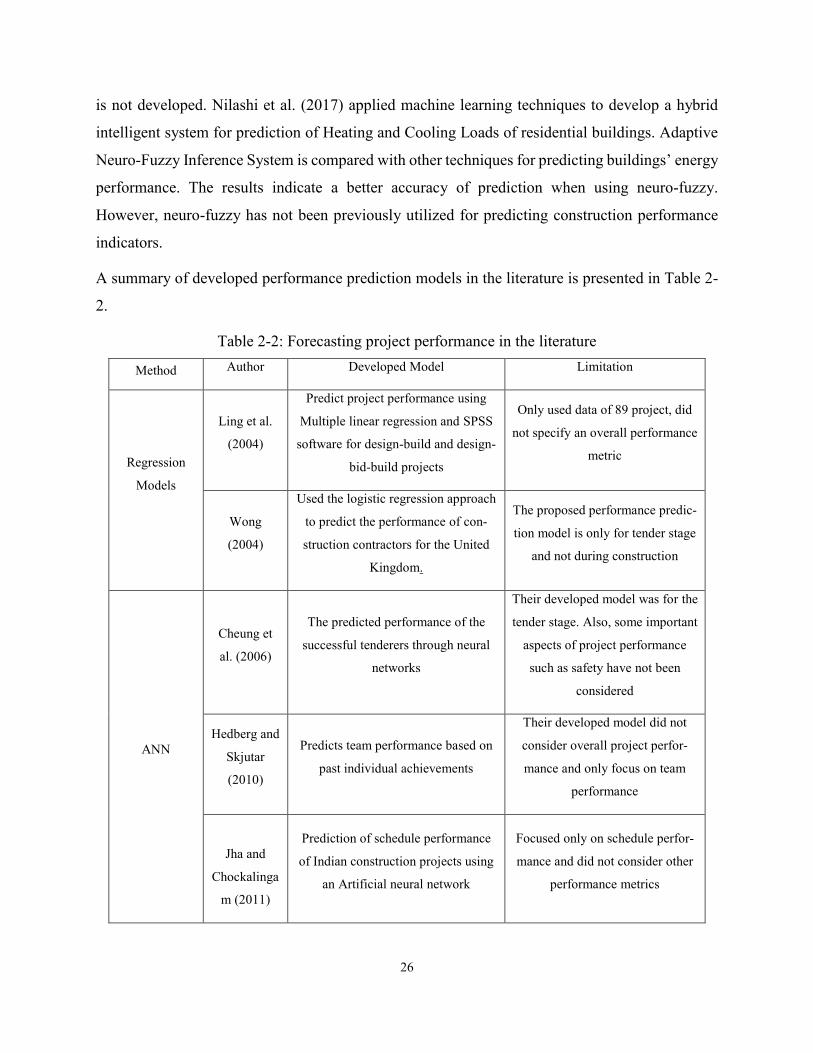
26
is not developed. Nilashi et al. (2017) applied machine learning techniques to develop a hybrid
intelligent system for prediction of Heating and Cooling Loads of residential buildings. Adaptive
Neuro-Fuzzy Inference System is compared with other techniques for predicting buildings’ energy
performance. The results indicate a better accuracy of prediction when using neuro-fuzzy.
However, neuro-fuzzy has not been previously utilized for predicting construction performance
indicators.
A summary of developed performance prediction models in the literature is presented in Table 2-
2.
Table 2-2: Forecasting project performance in the literature
Method Author Developed Model Limitation
Regression
Models
Ling et al.
(2004)
Predict project performance using
Multiple linear regression and SPSS
software for design-build and design-
bid-build projects
Only used data of 89 project, did
not specify an overall performance
metric
Wong
(2004)
Used the logistic regression approach
to predict the performance of con-
struction contractors for the United
Kingdom.
The proposed performance predic-
tion model is only for tender stage
and not during construction
ANN
Cheung et
al. (2006)
The predicted performance of the
successful tenderers through neural
networks
Their developed model was for the
tender stage. Also, some important
aspects of project performance
such as safety have not been
considered
Hedberg and
Skjutar
(2010)
Predicts team performance based on
past individual achievements
Their developed model did not
consider overall project perfor-
mance and only focus on team
performance
Jha and
Chockalinga
m (2011)
Prediction of schedule performance
of Indian construction projects using
an Artificial neural network
Focused only on schedule perfor-
mance and did not consider other
performance metrics
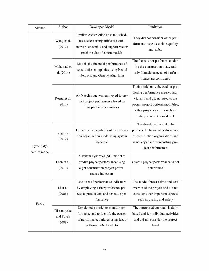
27
Method Author Developed Model Limitation
Wang et al.
(2012)
Predicts construction cost and sched-
ule success using artificial neural
network ensemble and support vector
machine classification models
They did not consider other per-
formance aspects such as quality
and safety
Mohamad et
al. (2014)
Models the financial performance of
construction companies using Neural
Network and Genetic Algorithm
The focus is not performance dur-
ing the construction phase and
only financial aspects of perfor-
mance are considered
Reenu et al.
(2017)
ANN technique was employed to pre-
dict project performance based on
four performance metrics
Their model only focused on pre-
dicting performance metrics indi-
vidually and did not predict the
overall project performance. Also,
other projects aspects such as
safety were not considered
System dy-
namics model
Tang et al.
(2012)
Forecasts the capability of a construc-
tion organization mode using system
dynamic
The developed model only
predicts the financial performance
of construction organizations and
is not capable of forecasting pro-
ject performance
Leon et al.
(2017)
A system dynamics (SD) model to
predict project performance using
eight construction project perfor-
mance indicators
Overall project performance is not
determined
Fuzzy
Li et al.
(2006)
Use a set of performance indicators
by employing a fuzzy inference pro-
cess to predict cost and schedule per-
formance
The model forecast time and cost
overrun of the project and did not
consider other important aspects
such as quality and safety
Dissanayake
and Fayek
(2008)
Developed a model to monitor per-
formance and to identify the causes
of performance failures using fuzzy
set theory, ANN and GA.
Their proposed approach is daily
based and for individual activities
and did not consider the project
level
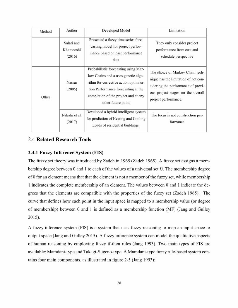
28
Method Author Developed Model Limitation
Salari and
Khamooshi
(2016)
Presented a fuzzy time series fore-
casting model for project perfor-
mance based on past performance
data
They only consider project
performance from cost and
schedule perspective
Other
Nassar
(2005)
Probabilistic forecasting using Mar-
kov Chains and a uses genetic algo-
rithm for corrective action optimiza-
tion Performance forecasting at the
completion of the project and at any
other future point
The choice of Markov Chain tech-
nique has the limitation of not con-
sidering the performance of previ-
ous project stages on the overall
project performance.
Nilashi et al.
(2017)
Developed a hybrid intelligent system
for prediction of Heating and Cooling
Loads of residential buildings.
The focus is not construction per-
formance
2.4 Related Research Tools
2.4.1 Fuzzy Inference System (FIS)
The fuzzy set theory was introduced by Zadeh in 1965 (Zadeh 1965). A fuzzy set assigns a mem-
bership degree between 0 and 1 to each of the values of a universal set U. The membership degree
of 0 for an element means that that the element is not a member of the fuzzy set, while membership
1 indicates the complete membership of an element. The values between 0 and 1 indicate the de-
grees that the elements are compatible with the properties of the fuzzy set (Zadeh 1965). The
curve that defines how each point in the input space is mapped to a membership value (or degree
of membership) between 0 and 1 is defined as a membership function (MF) (Jang and Gulley
2015).
A fuzzy inference system (FIS) is a system that uses fuzzy reasoning to map an input space to
output space (Jang and Gulley 2015). A fuzzy inference system can model the qualitative aspects
of human reasoning by employing fuzzy if-then rules (Jang 1993). Two main types of FIS are
available: Mamdani-type and Takagi-Sugeno-type. A Mamdani-type fuzzy rule-based system con-
tains four main components, as illustrated in figure 2-5 (Jang 1993):
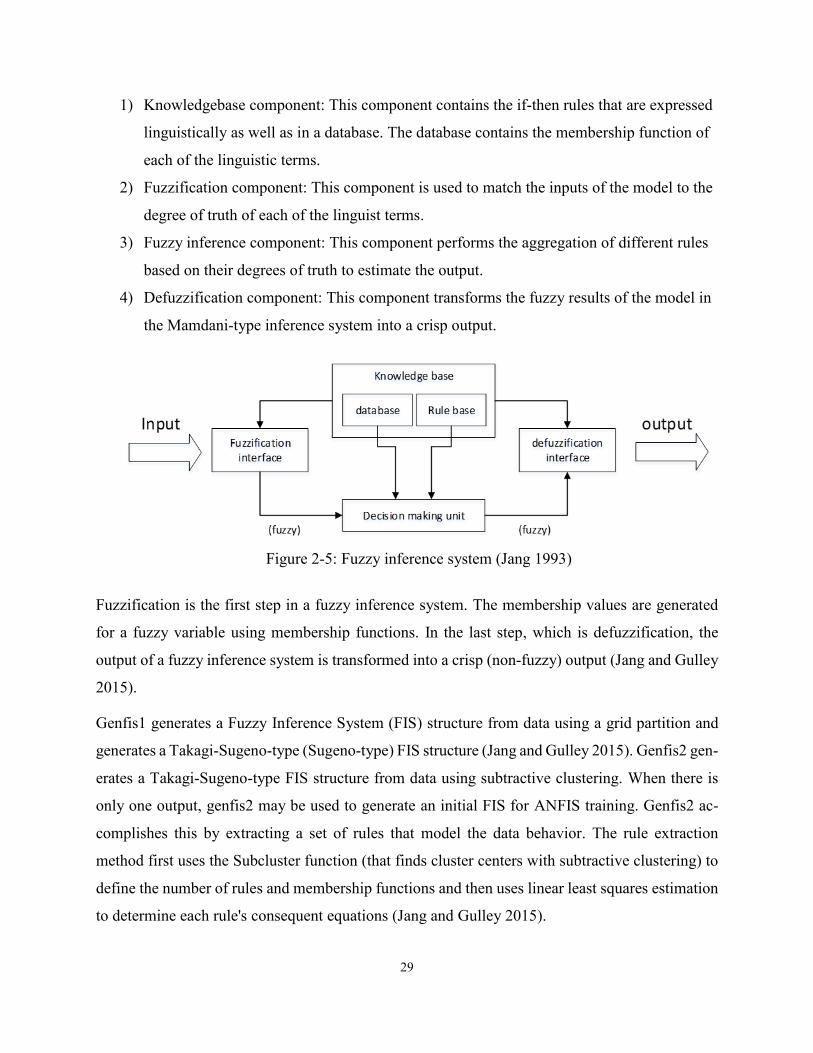
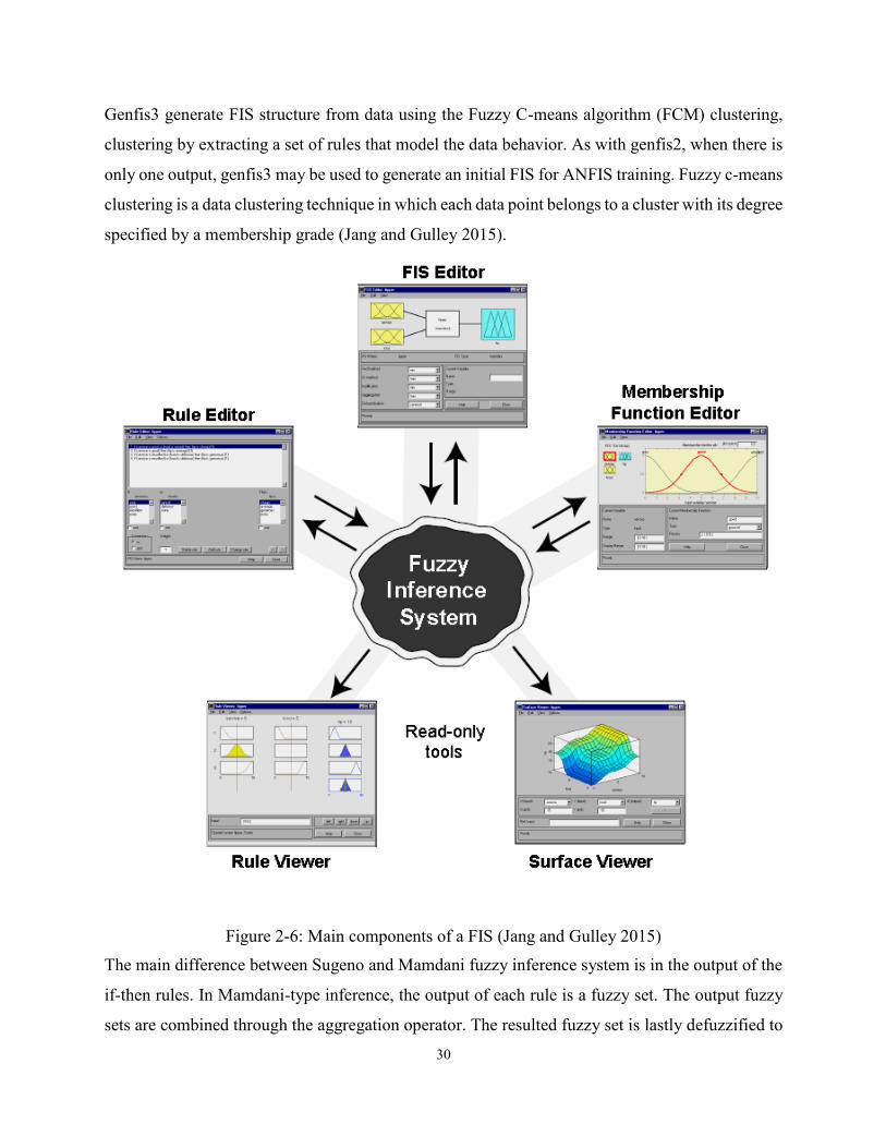
30
Genfis3 generate FIS structure from data using the Fuzzy C-means algorithm (FCM) clustering,
clustering by extracting a set of rules that model the data behavior. As with genfis2, when there is
only one output, genfis3 may be used to generate an initial FIS for ANFIS training. Fuzzy c-means
clustering is a data clustering technique in which each data point belongs to a cluster with its degree
specified by a membership grade (Jang and Gulley 2015).
Figure 2-6: Main components of a FIS (Jang and Gulley 2015)
The main difference between Sugeno and Mamdani fuzzy inference system is in the output of the
if-then rules. In Mamdani-type inference, the output of each rule is a fuzzy set. The output fuzzy
sets are combined through the aggregation operator. The resulted fuzzy set is lastly defuzzified to
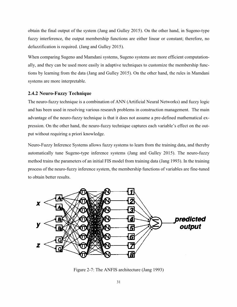
31
obtain the final output of the system (Jang and Gulley 2015). On the other hand, in Sugeno-type
fuzzy interference, the output membership functions are either linear or constant; therefore, no
defuzzification is required. (Jang and Gulley 2015).
When comparing Sugeno and Mamdani systems, Sugeno systems are more efficient computation-
ally, and they can be used more easily in adaptive techniques to customize the membership func-
tions by learning from the data (Jang and Gulley 2015). On the other hand, the rules in Mamdani
systems are more interpretable.
2.4.2 Neuro-Fuzzy Technique The neuro-fuzzy technique is a combination of ANN (Artificial Neural Networks) and fuzzy logic
and has been used in resolving various research problems in construction management. The main
advantage of the neuro-fuzzy technique is that it does not assume a pre-defined mathematical ex-
pression. On the other hand, the neuro-fuzzy technique captures each variable’s effect on the out-
put without requiring a priori knowledge.
Neuro-Fuzzy Inference Systems allows fuzzy systems to learn from the training data, and thereby
automatically tune Sugeno-type inference systems (Jang and Gulley 2015). The neuro-fuzzy
method trains the parameters of an initial FIS model from training data (Jang 1993). In the training
process of the neuro-fuzzy inference system, the membership functions of variables are fine-tuned
to obtain better results.
Figure 2-7: The ANFIS architecture (Jang 1993)

32
The Adaptive Network-Based Fuzzy Inference System (ANFIS) is a version of neuro-fuzzy first
introduced by Jang in 1993 as illustrated in Figure 2-7. ANFIS is the neuro-fuzzy inference system
toolbox in MATLAB. It develops a model to transform human knowledge or experience into a set
of fuzzy rules and simultaneously fine-tunes the membership functions of fuzzy sets. ANFIS ap-
plies the Takagi-Sugeno method in the fuzzy modeling step due to the advantages of this system.
It uses the backpropagation algorithm alone or in combination with the least squares method to
identify parameters. It is trained to imitate any given training data. ANFIS is utilized in this re-
search to improve and adjust FIS models; it optimizes membership function parameters and
controls overfitting with test data.
Clustering can be employed to identify natural groupings in data. The identified cluster centers can
represent a system's behavior (Jang and Gulley 2015). Clustering can be used to automatically
generate fuzzy inference systems from data. Each of the clusters represents a rule in the fuzzy rule-
based system. The fuzzy membership functions for the rules are formed based on the projection of
the developed clusters on the input space (Delgado et al. 1997, Nauck and Kruse 1999). The main
clustering methods found in the literature for generating fuzzy inference systems are subtractive
clustering and Fuzzy C-means (FCM) (Jang and Gulley 2015).
Subtractive clustering was proposed by Chiu in 1994 (Chiu 1994). In Subtractive clustering, each
data point is a candidate for being a cluster center, and a density measure for each data point is
defined. The density measure of a data point is considered to be high if it has many neighboring
data points. Two data points are neighbors to each other if their distance is less than the radius
value r. This radius value is the input parameter of the subtractive clustering algorithm that should
be defined. A very small value for this radius will neglect the effect of neighboring data points,
while a very large value for r will give the assumption that all the data points are in the
neighborhood of each point results in canceling the effect of the cluster (Hammouda and Karray
2000).
The first cluster center is defined as the point with the highest density value. The density measure
of each data point is then revised to reduce the density measure of the data point neighboring to
the first cluster center. The next data point with the greatest density value is then selected as the
next cluster center. This process continues until all data have been clustered.
33
“The subclust function finds the clusters by using the subtractive clustering method. The genfis2
function builds upon the subclust function to provide a fast, one-pass method to take input-output
training data and generate a Sugeno-type fuzzy inference system that models the data
behavior”(Jang and Gulley 2015).
In Fuzzy C-Means clustering method, each data point in non-fuzzy clustering is either a member
or not a member of a cluster. In fuzzy clustering, however, a degree of membership is assigned to
each data point for each cluster. Dunn (1973) developed the Fuzzy C-Means (FCM) algorithm,
which is a type fuzzy clustering algorithm. Bezdek (1981) later enhanced the FCM technique. In
the FCM algorithm, data points farther to the cluster center have a lesser membership degree com-
pared with points closer to the cluster center. The initial input of the FCM algorithm is the number
of clusters. The FCM algorithm works based on the following procedure:
1) Randomly assume initial cluster centers
2) Estimate the membership degree of each data point in each of the clusters based on
their distance from those cluster centers
3) Re-Calculate the cluster centers based on the membership degrees of each of the data
points
4) Continue to step 2 if the termination condition is not reached
The termination condition can be a specific threshold for the difference between the newly calcu-
lated cluster centers and previous cluster centers. Or, the termination condition may also be a
threshold for the number of the algorithm’s iterations.
2.4.3 Artificial Neural Network (ANN) Artificial Neural Network (ANN) can model comprehensive and complex real systems by learning
from examples (Gurney 2014). Learning can be either supervised or unsupervised. In supervised
learning the output is available in the training phase, otherwise it is unsupervised. ANN technique
is based on the learning mechanism of the human brain. The neural network tries to find a rela-
tionship between the input and output data.
ANN includes neurons and layers. Each layer contains a number of neurons that are working to-
gether. Generally, a neural network has an input layer, hidden layer(s) and an output layer. The
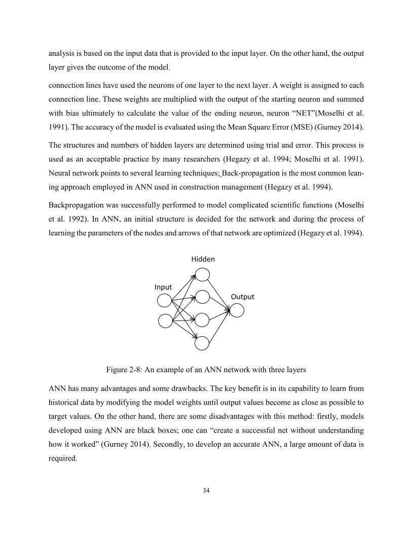
34
analysis is based on the input data that is provided to the input layer. On the other hand, the output
layer gives the outcome of the model.
connection lines have used the neurons of one layer to the next layer. A weight is assigned to each
connection line. These weights are multiplied with the output of the starting neuron and summed
with bias ultimately to calculate the value of the ending neuron, neuron “NET”(Moselhi et al.
1991). The accuracy of the model is evaluated using the Mean Square Error (MSE) (Gurney 2014).
The structures and numbers of hidden layers are determined using trial and error. This process is
used as an acceptable practice by many researchers (Hegazy et al. 1994; Moselhi et al. 1991).
Neural network points to several learning techniques; Back-propagation is the most common lean-
ing approach employed in ANN used in construction management (Hegazy et al. 1994).
Backpropagation was successfully performed to model complicated scientific functions (Moselhi
et al. 1992). In ANN, an initial structure is decided for the network and during the process of
learning the parameters of the nodes and arrows of that network are optimized (Hegazy et al. 1994).
Figure 2-8: An example of an ANN network with three layers
ANN has many advantages and some drawbacks. The key benefit is in its capability to learn from
historical data by modifying the model weights until output values become as close as possible to
target values. On the other hand, there are some disadvantages with this method: firstly, models
developed using ANN are black boxes; one can “create a successful net without understanding
how it worked” (Gurney 2014). Secondly, to develop an accurate ANN, a large amount of data is
required.
Input
Hidden
Output
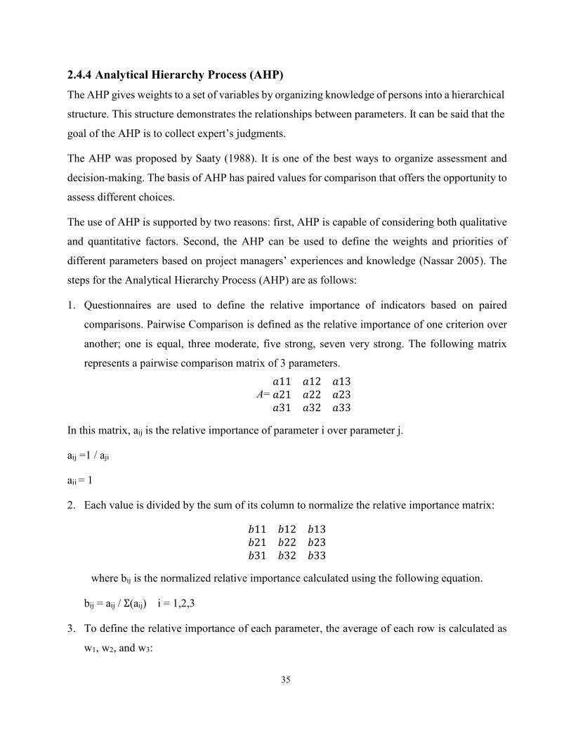
35
2.4.4 Analytical Hierarchy Process (AHP) The AHP gives weights to a set of variables by organizing knowledge of persons into a hierarchical
structure. This structure demonstrates the relationships between parameters. It can be said that the
goal of the AHP is to collect expert’s judgments.
The AHP was proposed by Saaty (1988). It is one of the best ways to organize assessment and
decision-making. The basis of AHP has paired values for comparison that offers the opportunity to
assess different choices.
The use of AHP is supported by two reasons: first, AHP is capable of considering both qualitative
and quantitative factors. Second, the AHP can be used to define the weights and priorities of
different parameters based on project managers’ experiences and knowledge (Nassar 2005). The
steps for the Analytical Hierarchy Process (AHP) are as follows:
1. Questionnaires are used to define the relative importance of indicators based on paired
comparisons. Pairwise Comparison is defined as the relative importance of one criterion over
another; one is equal, three moderate, five strong, seven very strong. The following matrix
represents a pairwise comparison matrix of 3 parameters.
A= 𝑎11 𝑎12 𝑎13𝑎21 𝑎22 𝑎23𝑎31 𝑎32 𝑎33
In this matrix, aij is the relative importance of parameter i over parameter j.
aij =1 / aji
aii = 1
2. Each value is divided by the sum of its column to normalize the relative importance matrix:
𝑏11 𝑏12 𝑏13𝑏21 𝑏22 𝑏23𝑏31 𝑏32 𝑏33
where bij is the normalized relative importance calculated using the following equation.
bij = aij / Σ(aij) i = 1,2,3
3. To define the relative importance of each parameter, the average of each row is calculated as
w1, w2, and w3:
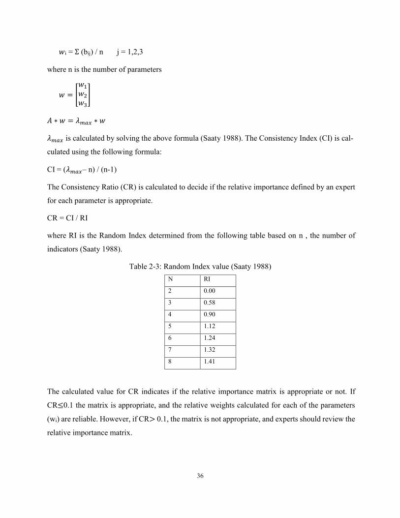
36
𝑤i = Σ (bij) / n j = 1,2,3
where n is the number of parameters
𝑤 = [
𝑤1
𝑤2
𝑤3
]
𝐴 ∗ 𝑤 = 𝜆𝑚𝑎𝑥 ∗ 𝑤
𝜆𝑚𝑎𝑥 is calculated by solving the above formula (Saaty 1988). The Consistency Index (CI) is cal-
culated using the following formula:
CI = (𝜆𝑚𝑎𝑥– n) / (n-1)
The Consistency Ratio (CR) is calculated to decide if the relative importance defined by an expert
for each parameter is appropriate.
CR = CI / RI
where RI is the Random Index determined from the following table based on n , the number of
indicators (Saaty 1988).
Table 2-3: Random Index value (Saaty 1988) N RI
2 0.00
3 0.58
4 0.90
5 1.12
6 1.24
7 1.32
8 1.41
The calculated value for CR indicates if the relative importance matrix is appropriate or not. If
CR≤0.1 the matrix is appropriate, and the relative weights calculated for each of the parameters
(wi) are reliable. However, if CR> 0.1, the matrix is not appropriate, and experts should review the
relative importance matrix.
37
2.4.5 Genetic Algorithm (GA)
John Holland (1975) introduced Genetic Algorithms for the first time. The Genetic Algorithm (GA)
is an optimization algorithm inspired by the process of natural selection (Adeli and Hung 1994).
In a GA, any possible solution to a problem is presented as a chromosome. A fitness function is
defined for the problem to be optimized. The input argument of the fitness function is a chromo-
some representing a solution to the problem. The output of a fitness function is the degree of opti-
mality, adaptation, or quality of that solution. GA is based on generations, where each generation
includes a population of chromosomes.
For the first generation, a random population of chromosomes is generated representing possible
solutions to the problem. The parents of the next generations are selected based on their fitness
values from the chromosomes of each generation. For this selection, a chromosome with a higher
fitness value has a higher probability to be selected. Crossover and mutation operations are applied
to parent chromosomes to generate new child chromosomes for the next generation. Crossover
combines sections of parent chromosomes based on one-point, two points or more points in the
parent chromosomes. Mutation randomly substitutes one or more values in a chromosome with
another value. The process of producing new generations is repeated in GA until the termination
condition is reached. Termination conditions are usually defined as reaching a satisfactory fitness
level or a maximum number of generations. The result of a GA is the chromosome with the best
fitness value among all of the generated chromosomes.
Haupt et al. (1998) summarized the GA implementation as follows:
1. Initialize the first population: The first population of parents is randomly generated. This
population size should be selected so that a favourite solution can be accomplished. How-
ever, a very big size could increase the running time of the algorithm.
2. Determine the fitness function: The objective function for the problem is presented as the
fitness function. Then, find the fitness value for each solution.
3. If the results are satisfactory, then present the best solution and terminate the optimization
process.
38
4. Otherwise, choose new parents based on their fitness values.
5. Crossover: mix chromosomes of parents to generate a new solution.
6. Mutation: change a few genes randomly by replacing them with new and undiscovered
genes in the population.
7. Go to step 2 to find the optimum solution.
The major advantages of GA in comparison to other methods is that it can consider both discrete
and continuous variables. Also, it is capable of providing a list of solutions and not only one solu-
tion.
2.5 Findings, Limitations, and Research Gaps There has been extensive effort to evaluate and predict project performance in previous research. How-
ever, according to the literature review most existing research have not developed a comprehensive
model that predicts project KPIs as well as overall project performance.
In many common project performance measurement and forecasting models, only a few aspects of
project performance (such as cost and time) are considered, and other important aspects are
overlooked. For the effective monitoring of a construction project’s progress, different aspects of
performance should be quantified and integrated.
Most of the previous work has focused on the quantitative performance forecasting of projects, and
less attention has been directed to qualitative methods. However, many construction KPIs, such as
client satisfaction, quality and safety have a qualitative nature and cannot be measured quantita-
tively. Also, for other KPIs such as time and cost, issues of confidentiality and a lack of data are
the norm in construction projects. Therefore, it is more feasible to develop a framework that can
qualitatively measure and forecast all project KPIs
Also, in most previous research, the performance of the project is measured at its end. However,
it also very important to measure the performance while a project is in progress, and not only after
its completion. Forecasting the performance for the rest of the project is only possible when the
performance measurement is measured during the project. The benefit of measuring the perfor-
mance during the project is that stakeholders can forecast the rest of the project’s performance and
suggest corrective action(s). The effect of project performance during project progress on the rest
of the project has not been examined in previous research.

39
In the literature review, several powerful techniques were found such as neural network, fuzzy logic
and system dynamics. However, a limited study comparing different methods in predicting KPIs and
project performance was conducted in the literature. Also, limited work has been done on forecasting
project using KPIs at the project level. Instead many previous researches focused on productivity
at the activity level or organization level.
Limited studies focused on the effect of Project Delivery Method (PDM) on the project perfor-
mance evaluation framework. Less attention has been paid for defining the role (impact) of each
stakeholder on the performance of a construction project (success or failure of the project).
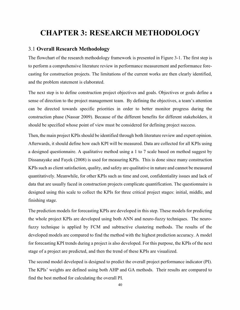
40
CHAPTER 3: RESEARCH METHODOLOGY
3.1 Overall Research Methodology The flowchart of the research methodology framework is presented in Figure 3-1. The first step is
to perform a comprehensive literature review in performance measurement and performance fore-
casting for construction projects. The limitations of the current works are then clearly identified,
and the problem statement is elaborated.
The next step is to define construction project objectives and goals. Objectives or goals define a
sense of direction to the project management team. By defining the objectives, a team’s attention
can be directed towards specific priorities in order to better monitor progress during the
construction phase (Nassar 2009). Because of the different benefits for different stakeholders, it
should be specified whose point of view must be considered for defining project success.
Then, the main project KPIs should be identified through both literature review and expert opinion.
Afterwards, it should define how each KPI will be measured. Data are collected for all KPIs using
a designed questionnaire. A qualitative method using a 1 to 7 scale based on method suggest by
Dissanayake and Fayek (2008) is used for measuring KPIs. This is done since many construction
KPIs such as client satisfaction, quality, and safety are qualitative in nature and cannot be measured
quantitatively. Meanwhile, for other KPIs such as time and cost, confidentiality issues and lack of
data that are usually faced in construction projects complicate quantification. The questionnaire is
designed using this scale to collect the KPIs for three critical project stages: initial, middle, and
finishing stage.
The prediction models for forecasting KPIs are developed in this step. These models for predicting
the whole project KPIs are developed using both ANN and neuro-fuzzy techniques. The neuro-
fuzzy technique is applied by FCM and subtractive clustering methods. The results of the
developed models are compared to find the method with the highest prediction accuracy. A model
for forecasting KPI trends during a project is also developed. For this purpose, the KPIs of the next
stage of a project are predicted, and then the trend of these KPIs are visualized.
The second model developed is designed to predict the overall project performance indicator (PI).
The KPIs’ weights are defined using both AHP and GA methods. Their results are compared to
find the best method for calculating the overall PI.

41
An automated system is developed allowing to decide between different activity modes to achieve
the highest possible PI value. This model performs PI optimization based on KPIs using a genetic
algorithm for choosing corrective action. Validation is done to see if the model works correctly or
not. The last step is to develop a decision support system for users.
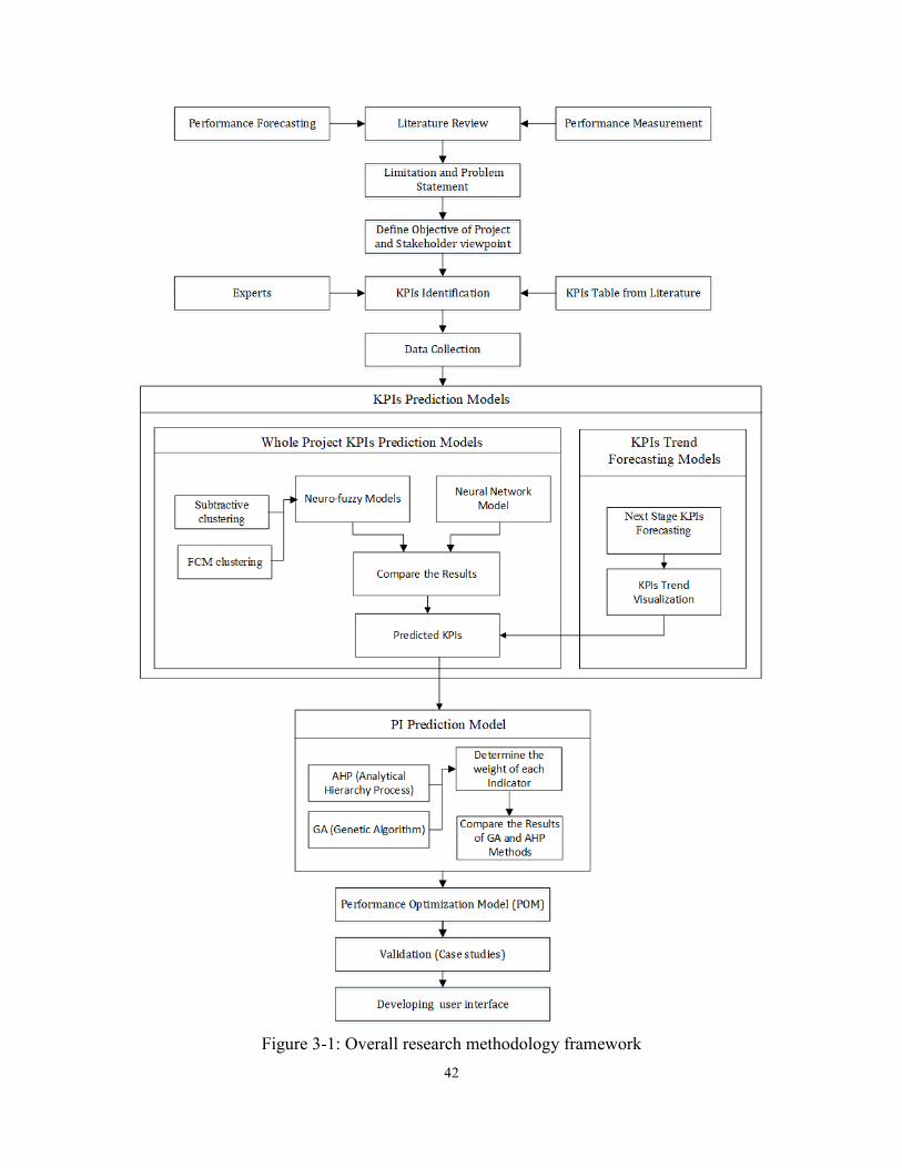
42
Figure 3-1: Overall research methodology framework
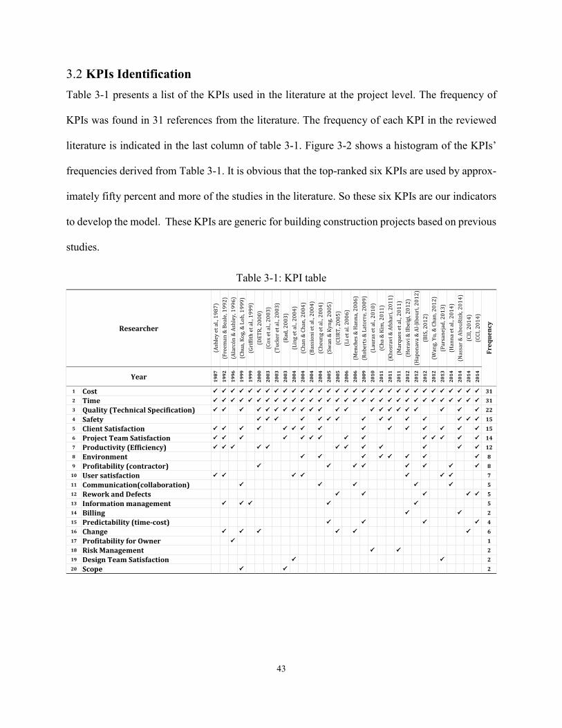
43
3.2 KPIs Identification Table 3-1 presents a list of the KPIs used in the literature at the project level. The frequency of
KPIs was found in 31 references from the literature. The frequency of each KPI in the reviewed
literature is indicated in the last column of table 3-1. Figure 3-2 shows a histogram of the KPIs’
frequencies derived from Table 3-1. It is obvious that the top-ranked six KPIs are used by approx-
imately fifty percent and more of the studies in the literature. So these six KPIs are our indicators
to develop the model. These KPIs are generic for building construction projects based on previous
studies.
Table 3-1: KPI table
(Ash
ley
et
al.,
19
87
)
(Fre
eman
& B
eale
, 19
92
)
(Ala
rcó
n &
Ash
ley
, 19
96
)
(Ch
ua,
Ko
g, &
Lo
h, 1
99
9)
(Gri
ffit
h e
t al
., 1
99
9)
(DE
TR
, 20
00
)
(Co
x et
al.,
20
03
)
(Tu
cker
et
al.,
20
03
)
(Rad
, 20
03
)
(Lin
g et
al.,
20
04
)
(Ch
an &
Ch
an, 2
00
4)
(Bas
sio
ni e
t al
., 2
00
4)
(Ch
eun
g et
al.,
20
04
)
(Sw
an &
Ky
ng,
20
05
)
(CU
RT
, 20
05
)
(Li e
t al
. 20
06
)
(Men
ches
& H
ann
a, 2
00
6)
(Ro
ber
ts &
Lat
orr
e, 2
00
9)
(Lau
ras
et a
l., 2
01
0)
(Ch
a &
Kim
, 20
11
)
(Kh
osr
avi &
Afs
har
i, 2
01
1)
(Mar
qu
es e
t al
., 2
01
1)
(Her
avi &
Ilb
eigi
, 20
12
)
(Hap
on
ava
& A
l-Ji
bo
uri
, 20
12
)
(BIS
, 20
12
)
(Wan
g, Y
u, &
Ch
an, 2
01
2)
(Par
san
ejad
, 20
13
)
(Han
na
et a
l., 2
01
4)
(Nas
sar
& A
bo
uR
izk
, 20
14
)
(CII
, 20
14
)
(CC
I, 2
01
4)
19
87
19
92
19
96
19
99
19
99
20
00
20
03
20
03
20
03
20
04
20
04
20
04
20
04
20
05
20
05
20
06
20
06
20
09
20
10
20
11
20
11
20
11
20
12
20
12
20
12
20
12
20
13
20
14
20
14
20
14
20
14
1 Cost P P P P P P P P P P P P P P P P P P P P P P P P P P P P P P P 31
2 Time P P P P P P P P P P P P P P P P P P P P P P P P P P P P P P P 31
3 Quality (Technical Specification) P P P P P P P P P P P P P P P P P P P P P P 22
4 Safety P P P P P P P P P P P P P P P 15
5 Client Satisfaction P P P P P P P P P P P P P P P 15
6 Project Team Satisfaction P P P P P P P P P P P P P P 14
7 Productivity (Efficiency) P P P P P P P P P P P P 12
8 Environment P P P P P P P P 8
9 Profitability (contractor) P P P P P P P P 8
10 User satisfaction P P P P P P P 7
11 Communication(collaboration) P P P P P 5
12 Rework and Defects P P P P P 5
13 Information management P P P P P 5
14 Billing P P 2
15 Predictability (time-cost) P P P P 4
16 Change P P P P P P 6
17 Profitability for Owner P 1
18 Risk Management P P 2
19 Design Team Satisfaction P P 2
20 Scope P P 2
Fre
qu
en
cyResearcher
Year
44
Figure 3-2: Histogram of KPIs frequency
Figure 3-3 further demonstrates the justification for the use of the first six KPIs. This figure
prepared based on the questionnaires distributed to experts. The questionnaires were distributed to
34 owners of building construction projects who are asked to define a score between 1 to 7 for
each of the KPIs (Fanaei et al. 2016). Fig 3-3 demonstrates sum of the scores of each of the KPIs
from the questionnaire. The scores represent the importance level of each of the KPIs defined by
experts. This is used to justify using six selected KPIs for model development. Based on the
questionnaire outcomes, the top six KPIs got 40 to 90 percent of the score, with the seventh KPI
receiving a score of 27, and the remaining KPIs receiving a score of 20 to 27 percent. Given the
tangibly larger score ratio between KPI number six and seven in the questionnaire, it is fair to
conclude that the experts found the first six KPIs more important than the others. Based on the
literature review and the questionnaire, this study decided to select the first six KPIs, cost, time,
quality, safety, client satisfaction, and project team satisfaction to develop the model. The selected
KPIs comply with previous Canadian studies (DCC 2016; Dissanayake and Fayek 2008; Nassar
and AbouRizk 2014). The study in this area should be concise in order to cover different aspects
0 5 10 15 20 25 30 35
Scope
Design Team Satisfaction
Risk Management
Profitability for Owner
Change
Predictability (time-cost)
Billing
Information management
Rework and Defects
Communication(collaboration)
User satisfaction
Profitability (contractor)
Environment
Productivity (Efficiency)
Project Team Satisfaction
Client Satisfaction
Safety
Quality (Technical Specification)
Time
Cost
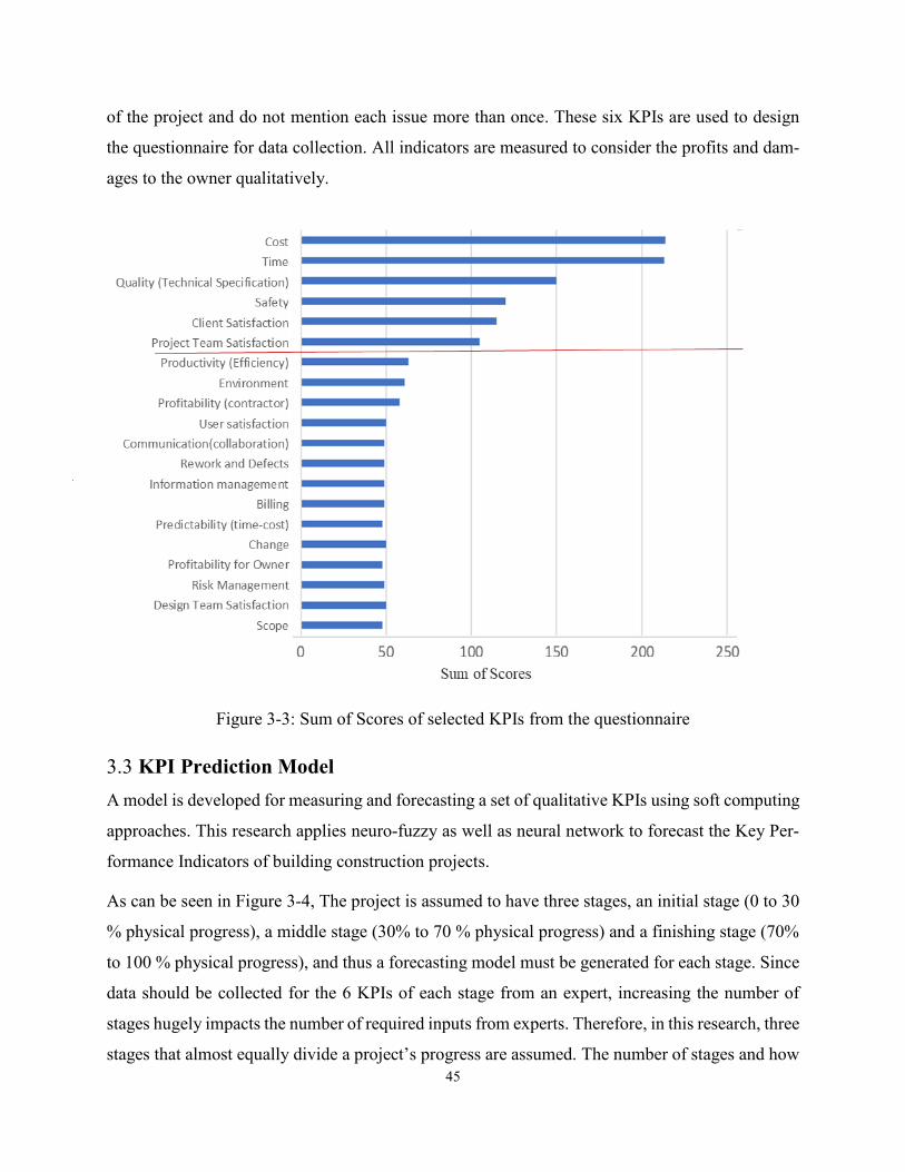
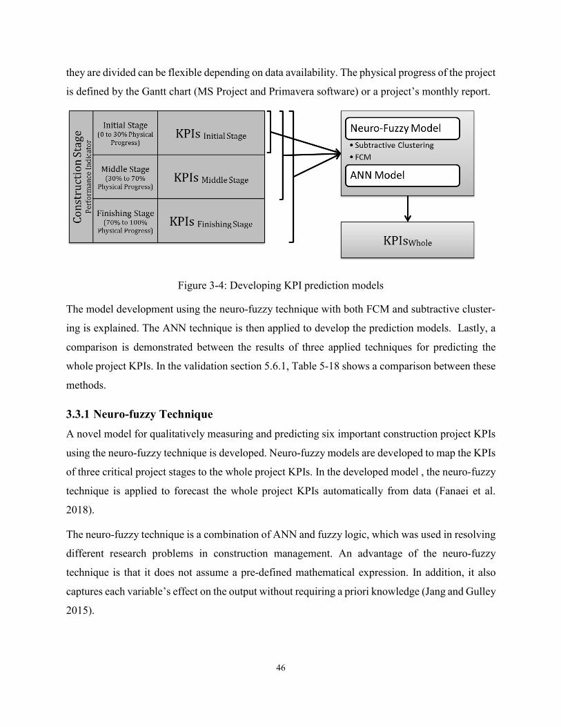
3.3.1 Neuro-fuzzy Technique
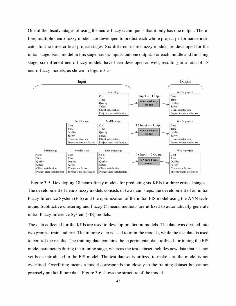
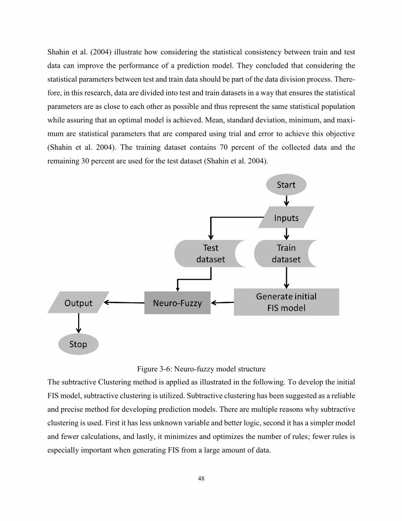
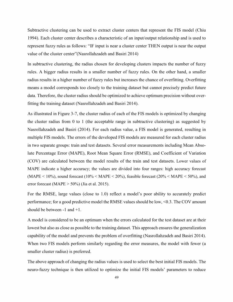
49
Subtractive clustering can be used to extract cluster centers that represent the FIS model (Chiu
1994). Each cluster center describes a characteristic of an input/output relationship and is used to
represent fuzzy rules as follows: “IF input is near a cluster center THEN output is near the output
value of the cluster center”(Nasrollahzadeh and Basiri 2014)
In subtractive clustering, the radius chosen for developing clusters impacts the number of fuzzy
rules. A bigger radius results in a smaller number of fuzzy rules. On the other hand, a smaller
radius results in a higher number of fuzzy rules but increases the chance of overfitting. Overfitting
means a model corresponds too closely to the training dataset but cannot precisely predict future
data. Therefore, the cluster radius should be optimized to achieve optimum precision without over-
fitting the training dataset (Nasrollahzadeh and Basiri 2014).
As illustrated in Figure 3-7, the cluster radius of each of the FIS models is optimized by changing
the cluster radius from 0 to 1 (the acceptable range in subtractive clustering) as suggested by
Nasrollahzadeh and Basiri (2014). For each radius value, a FIS model is generated, resulting in
multiple FIS models. The errors of the developed FIS models are measured for each cluster radius
in two separate groups: train and test datasets. Several error measurements including Mean Abso-
lute Percentage Error (MAPE), Root Mean Square Error (RMSE), and Coefficient of Variation
(COV) are calculated between the model results of the train and test datasets. Lower values of
MAPE indicate a higher accuracy; the values are divided into four ranges: high accuracy forecast
(MAPE < 10%), sound forecast (10% < MAPE < 20%), feasible forecast (20% < MAPE < 50%), and
error forecast (MAPE > 50%) (Jia et al. 2015).
For the RMSE, large values (close to 1.0) reflect a model’s poor ability to accurately predict
performance; for a good predictive model the RMSE values should be low, <0.3. The COV amount
should be between -1 and +1.
A model is considered to be an optimum when the errors calculated for the test dataset are at their
lowest but also as close as possible to the training dataset. This approach ensures the generalization
capability of the model and prevents the problem of overfitting (Nasrollahzadeh and Basiri 2014).
When two FIS models perform similarly regarding the error measures, the model with fewer (a
smaller cluster radius) is preferred.
The above approach of changing the radius values is used to select the best initial FIS models. The
neuro-fuzzy technique is then utilized to optimize the initial FIS models’ parameters to reduce

50
model error as much as possible. The neuro-fuzzy inference system develops a FIS whose mem-
bership function parameters are tuned using a backpropagation algorithm in combination with the
least squares method. This tuning allows the FIS model to learn from the data it is modeling (Jang
and Gulley 2015).
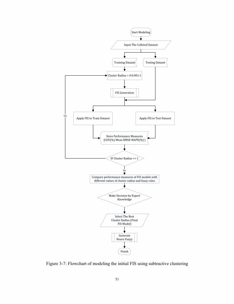
No
Yes

52
Fuzzy C-means (FCM) Clustering method is applied as illustrated in the following. To develop
the initial FIS model, the Fuzzy C-means (FCM) clustering approach is applied to be compared to
the subtractive clustering approach in the previous section. FCM is a very common and popular
approach for fuzzy clustering. It defines a methodology for grouping data points to populate some
multidimensional space into a specific number of different clusters. FCM assigns a membership
degree for each cluster and iteratively updates the cluster centers and the membership degrees to
minimize the objective function. The objective function is the distance from any given data point
to a cluster center weighted by that data point's membership degree (Bezdek 1981).
In FCM, instead of changing the cluster radius as described in subtractive clustering, the number
of rules (clusters) is changed to find the optimum number of clusters. Thus, in this research, the
number of rules is changed within the range of 1 to 50 to find the optimum number of cluster
centers that is equal to the number of fuzzy rules in the initial FIS model, as shown in Figure 3-8.
The errors of the developed FIS models are measured for each number of clusters in two separate
groups: train and test datasets. Several error measures including MAPE, RMSE, and COV are
calculated between the model results of the train and test datasets. The optimum model is chosen
when the errors calculated for the test dataset are at their lowest but also as close as possible to
train dataset. This approach ensures the generalization capability of the model and prevents the
problem of overfitting (Nasrollahzadeh and Basiri 2014).
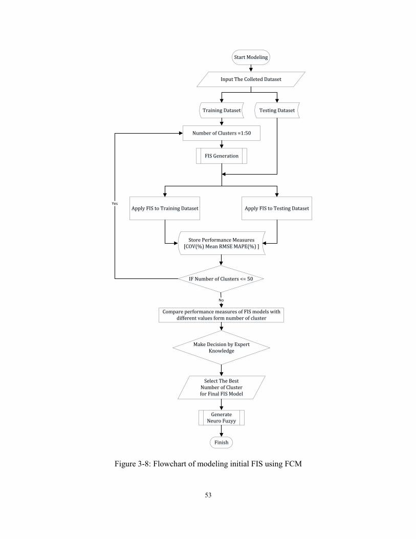
No
Yes
54
The above approach of changing the number of clusters is used to select the best initial FIS models.
The neuro-fuzzy technique is then utilized to optimize the initial FIS models’ parameters to reduce
model error as much as possible. The neuro-fuzzy inference system develops a FIS whose mem-
bership function parameters are tuned using a backpropagation algorithm in combination with the
least squares method, similar to the approach applied for subtractive clustering. After developing
the models for predicting KPIs using both subtractive clustering and FCM, the results of the mod-
els are compared using validation data to decide which method performs better. For this purpose,
different error measures are compared based on the output of the developed models and the actual
values of the validation data.
3.3.2 Artificial Neural Network Technique
In Artificial Neural Network technique is applied to estimate the KPIs of construction projects. The
neural network can predict the non-linear and complex of unknown functions. As described in the
literature review, the main advantage of ANN is its learning ability. ANN models can find relationships
between inputs and outputs using training examples. The trained model can then be used to predict the
outputs of new inputs.
In this research, the ANN model is used to predict the KPIs of the project. Six KPIs: Cost, Time,
Quality, Safety, Client satisfaction, Project team Satisfaction are used. The input of the prediction
models is 18 KPIs, 6 KPIs for each of the three stages. The outputs are 6 KPIs of the whole project.
ANN models were developed, trained and tested in MATLAB 2016a.
Figure 3-9 represents the overall flowchart for developing and selecting the final model. The
models were developed using three training algorithms available for neural networks: the
Levenberg–Marquardt (LM), Bayesian Regularization (BR) and the Scaled Conjugate Gradient
(SCG). Additionally, different models are developed using different neuron numbers. The neurons
number is changed between 5 to 50 neurons with a spacing of 5. which leads to 10 models for each
training algorithm. Considering the different training algorithms and neuron numbers, 30 different
models are developed and the results compared.
The performance of the models is assessed based on the Coefficient of determination (R2), the
mean absolute error (MAE), the relative absolute error (RAE), the root relative square error
(RRSE) and the mean absolute percentage error (MAPE) and the amounts of each error index.
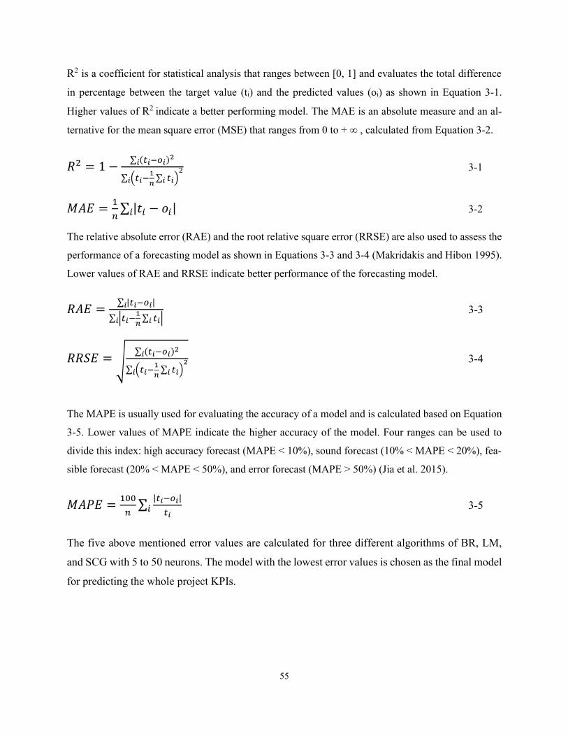
55
R2 is a coefficient for statistical analysis that ranges between [0, 1] and evaluates the total difference
in percentage between the target value (ti) and the predicted values (oi) as shown in Equation 3-1.
Higher values of R2 indicate a better performing model. The MAE is an absolute measure and an al-
ternative for the mean square error (MSE) that ranges from 0 to + ∞ , calculated from Equation 3-2.
𝑅2 = 1 −∑ (𝑡𝑖−𝑜𝑖)2
𝑖
∑ (𝑡𝑖−1
𝑛∑ 𝑡𝑖𝑖 )
2
𝑖
3-1
𝑀𝐴𝐸 =1
𝑛∑ |𝑡𝑖 − 𝑜𝑖|𝑖 3-2
The relative absolute error (RAE) and the root relative square error (RRSE) are also used to assess the
performance of a forecasting model as shown in Equations 3-3 and 3-4 (Makridakis and Hibon 1995).
Lower values of RAE and RRSE indicate better performance of the forecasting model.
𝑅𝐴𝐸 =∑ |𝑡𝑖−𝑜𝑖|𝑖
∑ |𝑡𝑖−1
𝑛∑ 𝑡𝑖𝑖 |𝑖
3-3
𝑅𝑅𝑆𝐸 = √∑ (𝑡𝑖−𝑜𝑖)2
𝑖
∑ (𝑡𝑖−1
𝑛∑ 𝑡𝑖𝑖 )
2
𝑖
3-4
The MAPE is usually used for evaluating the accuracy of a model and is calculated based on Equation
3-5. Lower values of MAPE indicate the higher accuracy of the model. Four ranges can be used to
divide this index: high accuracy forecast (MAPE < 10%), sound forecast (10% < MAPE < 20%), fea-
sible forecast (20% < MAPE < 50%), and error forecast (MAPE > 50%) (Jia et al. 2015).
𝑀𝐴𝑃𝐸 =100
𝑛∑
|𝑡𝑖−𝑜𝑖|
𝑡𝑖𝑖 3-5
The five above mentioned error values are calculated for three different algorithms of BR, LM,
and SCG with 5 to 50 neurons. The model with the lowest error values is chosen as the final model
for predicting the whole project KPIs.
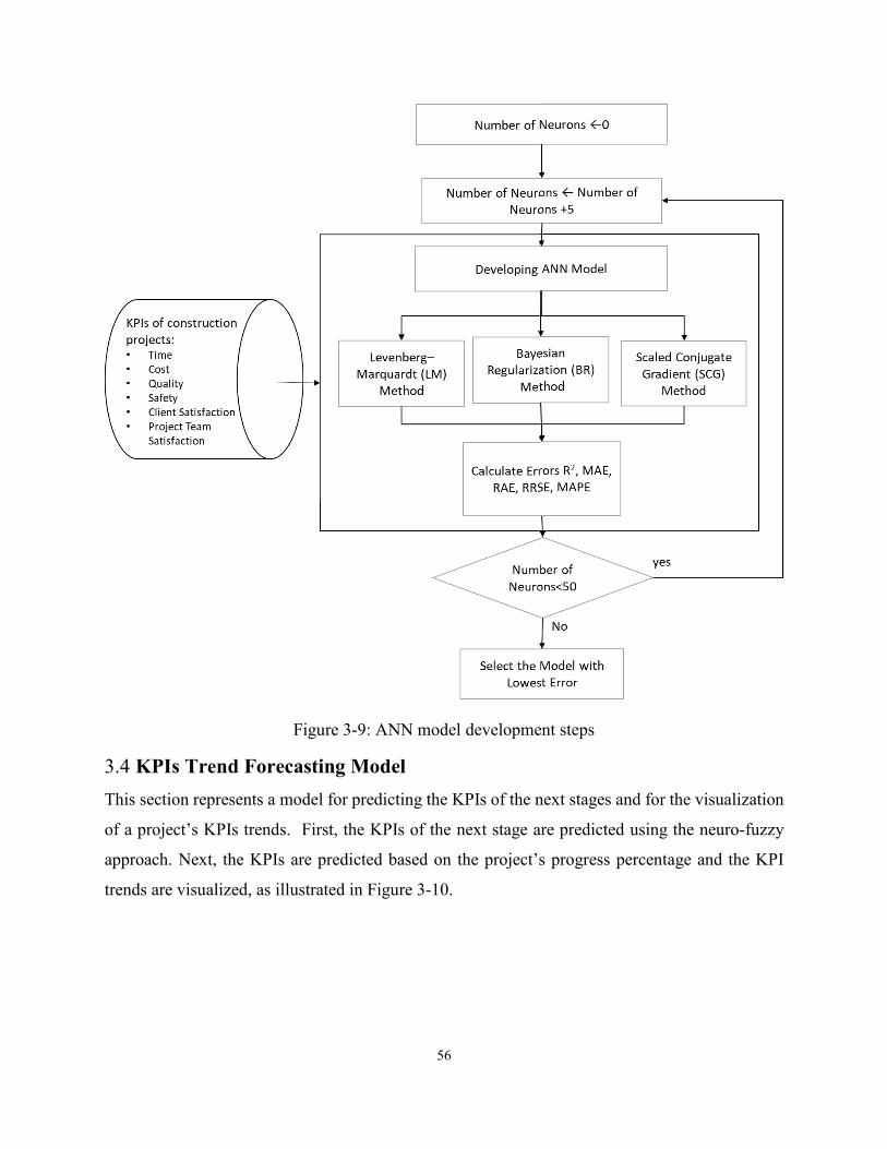
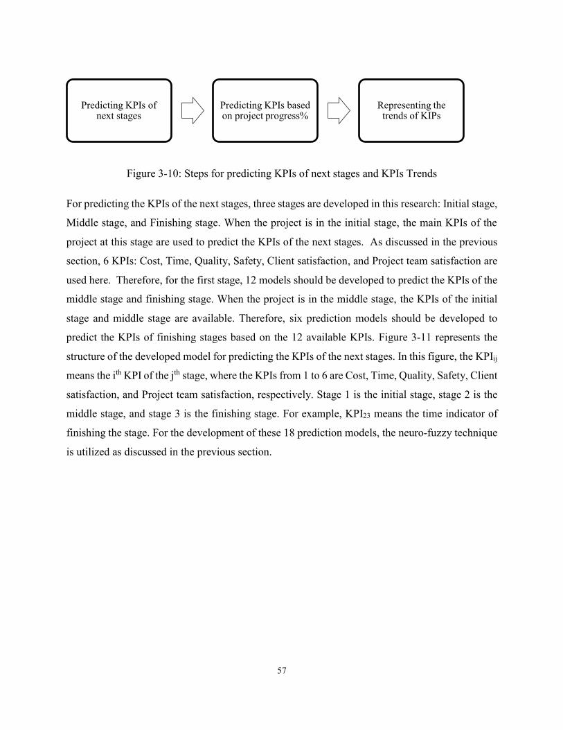
57
Figure 3-10: Steps for predicting KPIs of next stages and KPIs Trends
For predicting the KPIs of the next stages, three stages are developed in this research: Initial stage,
Middle stage, and Finishing stage. When the project is in the initial stage, the main KPIs of the
project at this stage are used to predict the KPIs of the next stages. As discussed in the previous
section, 6 KPIs: Cost, Time, Quality, Safety, Client satisfaction, and Project team satisfaction are
used here. Therefore, for the first stage, 12 models should be developed to predict the KPIs of the
middle stage and finishing stage. When the project is in the middle stage, the KPIs of the initial
stage and middle stage are available. Therefore, six prediction models should be developed to
predict the KPIs of finishing stages based on the 12 available KPIs. Figure 3-11 represents the
structure of the developed model for predicting the KPIs of the next stages. In this figure, the KPIij
means the ith KPI of the jth stage, where the KPIs from 1 to 6 are Cost, Time, Quality, Safety, Client
satisfaction, and Project team satisfaction, respectively. Stage 1 is the initial stage, stage 2 is the
middle stage, and stage 3 is the finishing stage. For example, KPI23 means the time indicator of
finishing the stage. For the development of these 18 prediction models, the neuro-fuzzy technique
is utilized as discussed in the previous section.
Predicting KPIs of next stages
Predicting KPIs based on project progress%
Representing the trends of KIPs
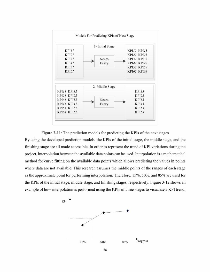
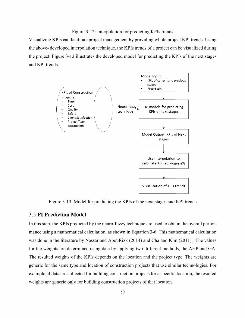
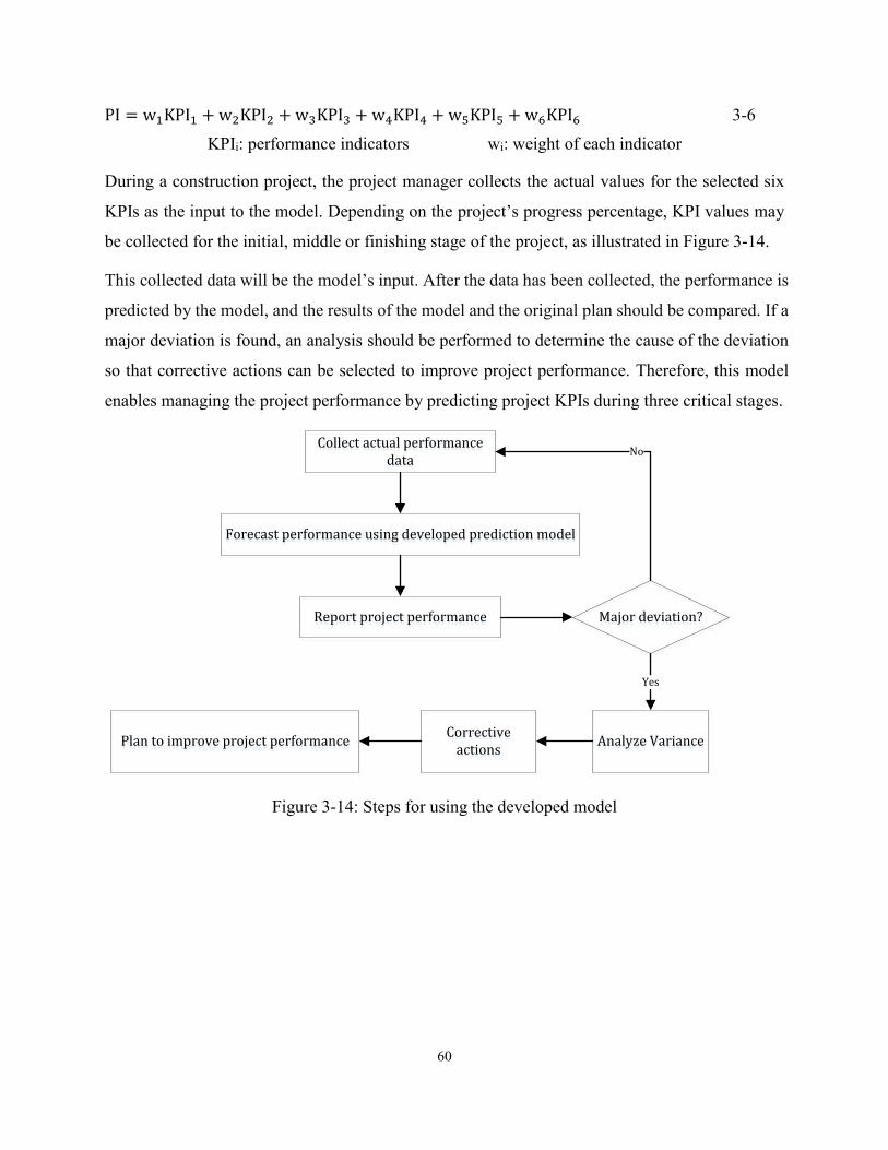
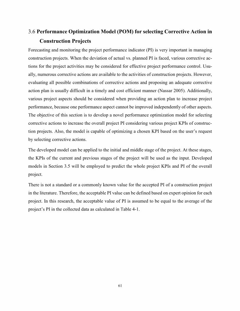
61
3.6 Performance Optimization Model (POM) for selecting Corrective Action in
Construction Projects Forecasting and monitoring the project performance indicator (PI) is very important in managing
construction projects. When the deviation of actual vs. planned PI is faced, various corrective ac-
tions for the project activities may be considered for effective project performance control. Usu-
ally, numerous corrective actions are available to the activities of construction projects. However,
evaluating all possible combinations of corrective actions and proposing an adequate corrective
action plan is usually difficult in a timely and cost efficient manner (Nassar 2005). Additionally,
various project aspects should be considered when providing an action plan to increase project
performance, because one performance aspect cannot be improved independently of other aspects.
The objective of this section is to develop a novel performance optimization model for selecting
corrective actions to increase the overall project PI considering various project KPIs of construc-
tion projects. Also, the model is capable of optimizing a chosen KPI based on the user’s request
by selecting corrective actions.
The developed model can be applied to the initial and middle stage of the project. At these stages,
the KPIs of the current and previous stages of the project will be used as the input. Developed
models in Section 3.5 will be employed to predict the whole project KPIs and PI of the overall
project.
There is not a standard or a commonly known value for the accepted PI of a construction project
in the literature. Therefore, the acceptable PI value can be defined based on expert opinion for each
project. In this research, the acceptable value of PI is assumed to be equal to the average of the
project’s PI in the collected data as calculated in Table 4-1.
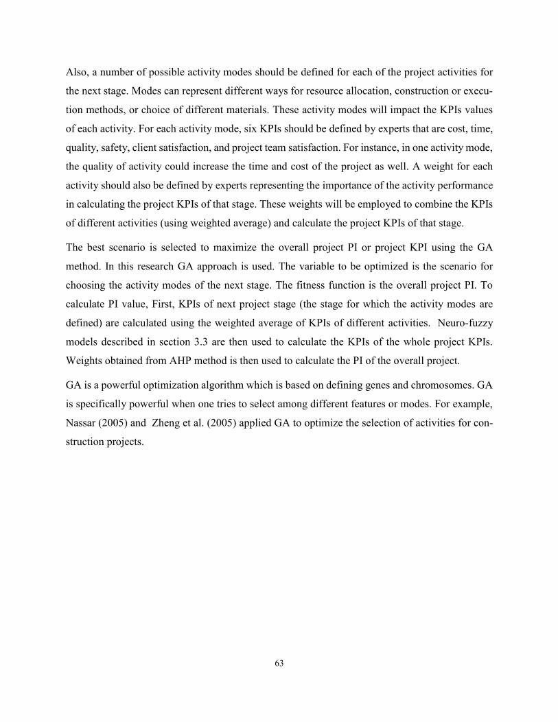
63
Also, a number of possible activity modes should be defined for each of the project activities for
the next stage. Modes can represent different ways for resource allocation, construction or execu-
tion methods, or choice of different materials. These activity modes will impact the KPIs values
of each activity. For each activity mode, six KPIs should be defined by experts that are cost, time,
quality, safety, client satisfaction, and project team satisfaction. For instance, in one activity mode,
the quality of activity could increase the time and cost of the project as well. A weight for each
activity should also be defined by experts representing the importance of the activity performance
in calculating the project KPIs of that stage. These weights will be employed to combine the KPIs
of different activities (using weighted average) and calculate the project KPIs of that stage.
The best scenario is selected to maximize the overall project PI or project KPI using the GA
method. In this research GA approach is used. The variable to be optimized is the scenario for
choosing the activity modes of the next stage. The fitness function is the overall project PI. To
calculate PI value, First, KPIs of next project stage (the stage for which the activity modes are
defined) are calculated using the weighted average of KPIs of different activities. Neuro-fuzzy
models described in section 3.3 are then used to calculate the KPIs of the whole project KPIs.
Weights obtained from AHP method is then used to calculate the PI of the overall project.
GA is a powerful optimization algorithm which is based on defining genes and chromosomes. GA
is specifically powerful when one tries to select among different features or modes. For example,
Nassar (2005) and Zheng et al. (2005) applied GA to optimize the selection of activities for con-
struction projects.
65
In the GA method, first, an initial population is generated by randomly generating some scenarios
for the next stage. The fitness function is then applied to each of the scenarios. If the maximum
number of iterations is not reached, crossover and mutation will be employed to generate a new
population of scenarios. Otherwise, the best scenario is selected as the output of the POM.
It should be noted that the number of activities, activity modes, as well as the acceptable project
PI value is flexible in the developed model. Therefore, these values are project dependent.
66
CHAPTER 4: DATA COLLECTION AND ANALY-
SIS
4.1 Chapter Overview This Chapter describes the process of data collection as the first step for developing the models for
predicting project performance. The data in this study were collected from experts . Two sets of
questionnaires were designed. The first questionnaire was used to collect data from different pro-
jects. The second questionnaire was used to justify why six KPIs used in this research. Another 16
questionnaires are used in the next chapter to validate the model and to verify that the developed
models work properly.
4.2 Questionnaires In this research, two sets of questionnaires were sent to two different groups of experts. The first
set was used to obtain the qualitative KPIs’ amounts from different projects as well as whole pro-
ject KPIs. The values of the 6 KPIs in three different stages of projects are used to develop and
train the models. The second questionnaire was designed to select the six most important KPIs.
4.2.1 Questionnaire 1
To collect data on building construction projects, a questionnaire was designed and distributed to
the owners of building construction projects in Tehran, Iran. Two-hundred questionnaires were
distributed in 2017 to experts, of which 119 with consistent results were selected for analysis. All
the responses were collected in two months. The questionnaire was designed in an online format
on a Qualtrics website, a data collection platform. The questionnaire was designed based on the
most important KPIs found in the literature. The experts were asked to qualitatively rank the per-
formance of 6 KPIs in three stages in different construction projects. The questionnaire divided
each project into three stages: an initial stage (0 to 30% physical progress), a middle stage (30%
to 70% physical progress) and a finishing stage (70% to 100% physical progress). The first part of
this questionnaire requests some general information from the respondents. The next part asks for
information about the specific project that the questionnaire is being completed for, such as
information about the project delivery method. The experts are then asked to rank the 6 KPIs’
performance in each of the three stages of the project, as well as to rank the whole project’s

67
performance. In the end, there are some questions about any possible problems that the project has
encountered. The data is collected using a 1 to 7 scale, where 1=Very Low, 2=Low, 3=Medium-
Low, 4=Medium, 5=Medium-High, 6=High, 7=Very High (Dissanayake and Fayek 2008). The
interpretation and the method for answering the questions are defined to the experts. For example,
experts are asked to rank the time KPI based on its deviations from the original schedule. When
Time (initial stage) is 1 or very low, it means that there is a time overrun in the initial stage of the
project. Using quantitative scales allows soft computing methods to be applied to the qualitative
data. The information is summarized in an excel table. Sample questions of the first questionnaire
are shown in Figure 4-1. Complete questionnaire is available in Appendix A1.
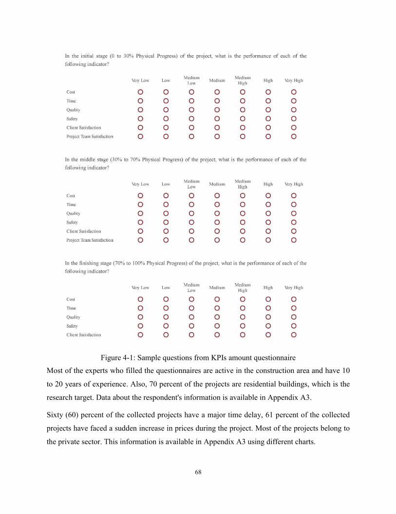
68
Figure 4-1: Sample questions from KPIs amount questionnaire Most of the experts who filled the questionnaires are active in the construction area and have 10
to 20 years of experience. Also, 70 percent of the projects are residential buildings, which is the
research target. Data about the respondent's information is available in Appendix A3.
Sixty (60) percent of the collected projects have a major time delay, 61 percent of the collected
projects have faced a sudden increase in prices during the project. Most of the projects belong to
the private sector. This information is available in Appendix A3 using different charts.
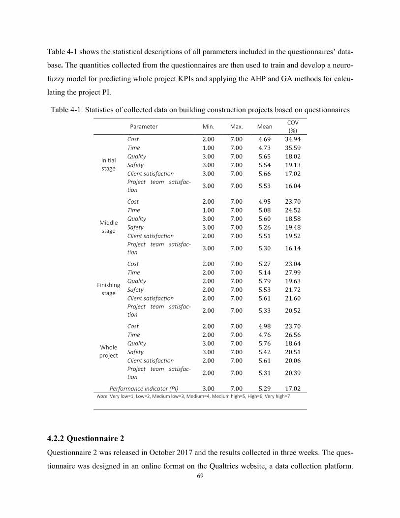
69
Table 4-1 shows the statistical descriptions of all parameters included in the questionnaires’ data-
base. The quantities collected from the questionnaires are then used to train and develop a neuro-
fuzzy model for predicting whole project KPIs and applying the AHP and GA methods for calcu-
lating the project PI.
Table 4-1: Statistics of collected data on building construction projects based on questionnaires
Parameter Min. Max. Mean COV (%)
Initial stage
Cost 2.00 7.00 4.69 34.94
Time 1.00 7.00 4.73 35.59
Quality 3.00 7.00 5.65 18.02
Safety 3.00 7.00 5.54 19.13
Client satisfaction 3.00 7.00 5.66 17.02 Project team satisfac-tion
3.00 7.00 5.53 16.04
Middle stage
Cost 2.00 7.00 4.95 23.70
Time 1.00 7.00 5.08 24.52
Quality 3.00 7.00 5.60 18.58
Safety 3.00 7.00 5.26 19.48
Client satisfaction 2.00 7.00 5.51 19.52 Project team satisfac-tion
3.00 7.00 5.30 16.14
Finishing stage
Cost 2.00 7.00 5.27 23.04
Time 2.00 7.00 5.14 27.99
Quality 2.00 7.00 5.79 19.63
Safety 2.00 7.00 5.53 21.72
Client satisfaction 2.00 7.00 5.61 21.60
Project team satisfac-tion
2.00 7.00 5.33 20.52
Whole project
Cost 2.00 7.00 4.98 23.70
Time 2.00 7.00 4.76 26.56
Quality 3.00 7.00 5.76 18.64
Safety 3.00 7.00 5.42 20.51
Client satisfaction 2.00 7.00 5.61 20.06
Project team satisfac-tion
2.00 7.00 5.31 20.39 Performance indicator (PI) 3.00 7.00 5.29 17.02
Note: Very low=1, Low=2, Medium low=3, Medium=4, Medium high=5, High=6, Very high=7
4.2.2 Questionnaire 2
Questionnaire 2 was released in October 2017 and the results collected in three weeks. The ques-
tionnaire was designed in an online format on the Qualtrics website, a data collection platform.
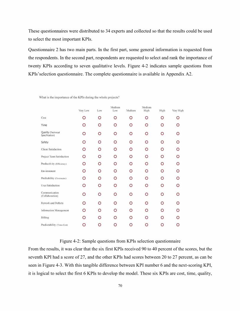
70
These questionnaires were distributed to 34 experts and collected so that the results could be used
to select the most important KPIs.
Questionnaire 2 has two main parts. In the first part, some general information is requested from
the respondents. In the second part, respondents are requested to select and rank the importance of
twenty KPIs according to seven qualitative levels. Figure 4-2 indicates sample questions from
KPIs’selection questionnaire. The complete questionnaire is available in Appendix A2.
Figure 4-2: Sample questions from KPIs selection questionnaire From the results, it was clear that the six first KPIs received 90 to 40 percent of the scores, but the
seventh KPI had a score of 27, and the other KPIs had scores between 20 to 27 percent, as can be
seen in Figure 4-3. With this tangible difference between KPI number 6 and the next-scoring KPI,
it is logical to select the first 6 KPIs to develop the model. These six KPIs are cost, time, quality,
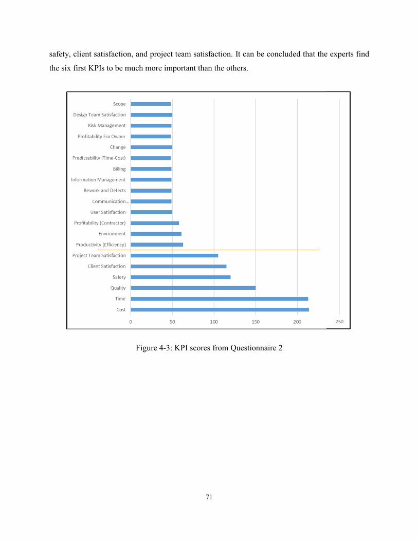
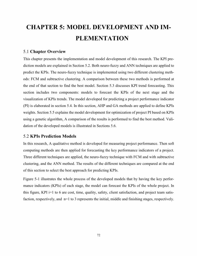
72
CHAPTER 5: MODEL DEVELOPMENT AND IM-
PLEMENTATION
5.1 Chapter Overview This chapter presents the implementation and model development of this research. The KPI pre-
diction models are explained in Section 5.2. Both neuro-fuzzy and ANN techniques are applied to
predict the KPIs. The neuro-fuzzy technique is implemented using two different clustering meth-
ods: FCM and subtractive clustering. A comparison between these two methods is performed at
the end of that section to find the best model. Section 5.3 discusses KPI trend forecasting. This
section includes two components: models to forecast the KPIs of the next stage and the
visualization of KPIs trends. The model developed for predicting a project performance indicator
(PI) is elaborated in section 5.4. In this section, AHP and GA methods are applied to define KPIs
weights. Section 5.5 explains the model development for optimization of project PI based on KPIs
using a genetic algorithm. A comparison of the results is performed to find the best method. Vali-
dation of the developed models is illustrated in Sections 5.6.
5.2 KPIs Prediction Models In this research, A qualitative method is developed for measuring project performance. Then soft
computing methods are then applied for forecasting the key performance indicators of a project.
Three different techniques are applied, the neuro-fuzzy technique with FCM and with subtractive
clustering, and the ANN method. The results of the different techniques are compared at the end
of this section to select the best approach for predicting KPIs.
Figure 5-1 illustrates the whole process of the developed models that by having the key perfor-
mance indicators (KPIs) of each stage, the model can forecast the KPIs of the whole project. In
this figure, KPI i=1 to 6 are cost, time, quality, safety, client satisfaction, and project team satis-
faction, respectively, and n=1 to 3 represents the initial, middle and finishing stages, respectively.
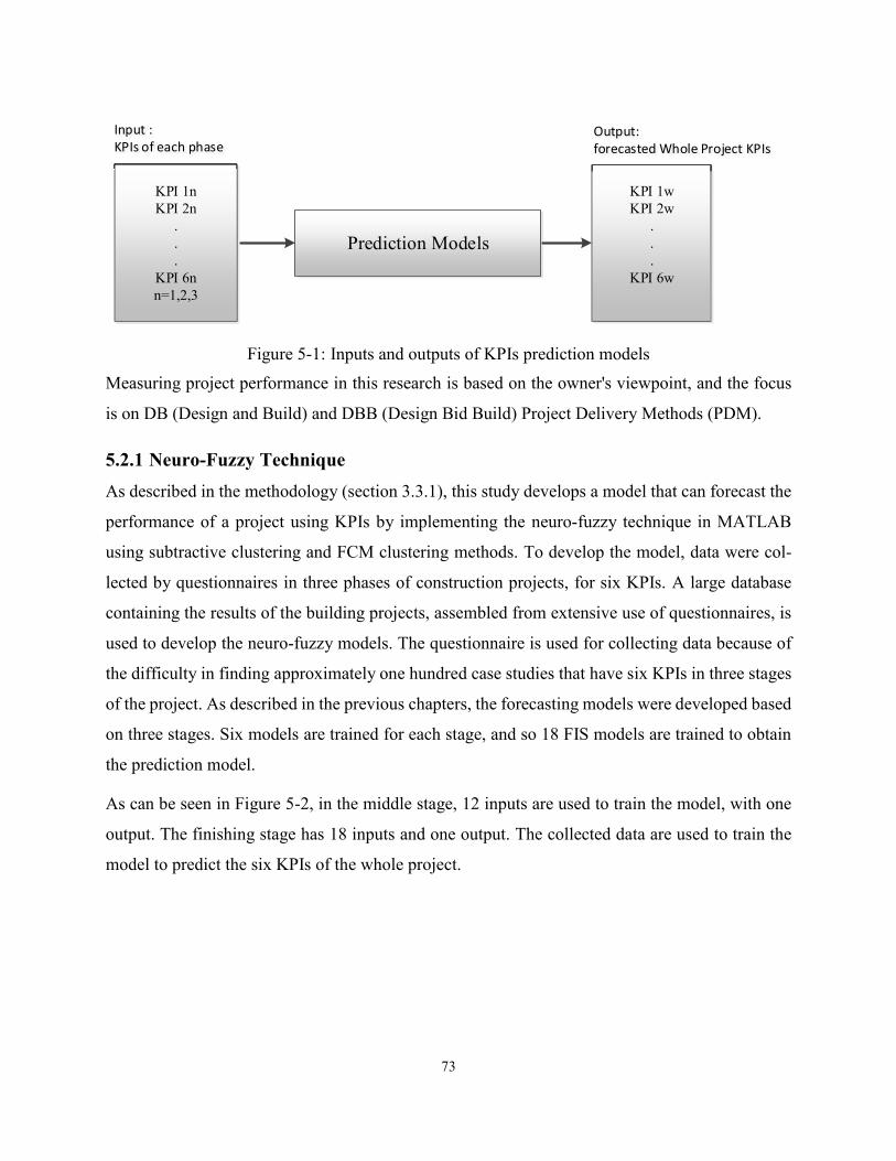
Input : KPIs of each phase
Output: forecasted Whole Project KPIs
5.2.1 Neuro-Fuzzy Technique
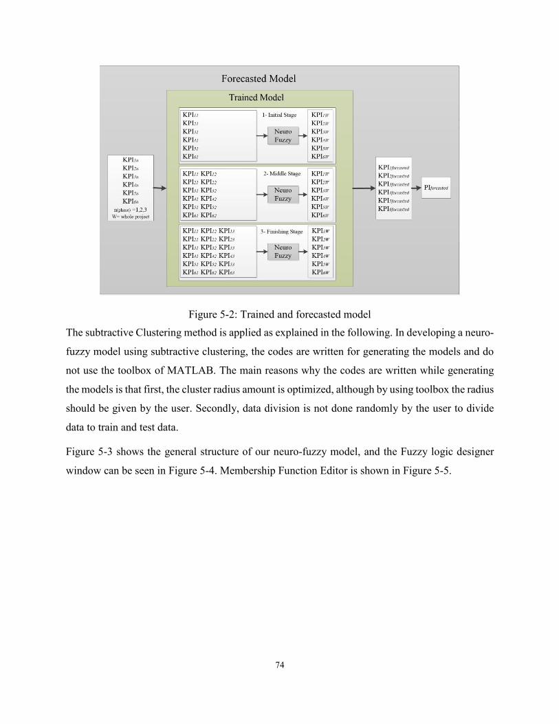
74
Figure 5-2: Trained and forecasted model The subtractive Clustering method is applied as explained in the following. In developing a neuro-
fuzzy model using subtractive clustering, the codes are written for generating the models and do
not use the toolbox of MATLAB. The main reasons why the codes are written while generating
the models is that first, the cluster radius amount is optimized, although by using toolbox the radius
should be given by the user. Secondly, data division is not done randomly by the user to divide
data to train and test data.
Figure 5-3 shows the general structure of our neuro-fuzzy model, and the Fuzzy logic designer
window can be seen in Figure 5-4. Membership Function Editor is shown in Figure 5-5.
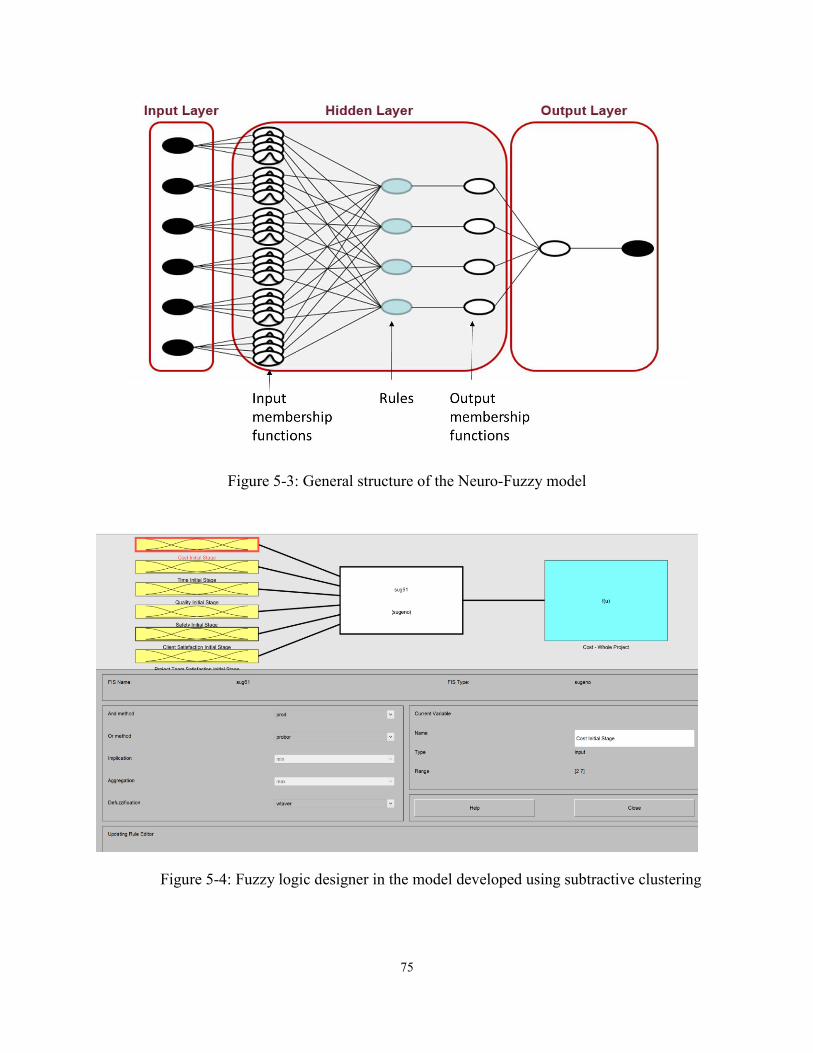
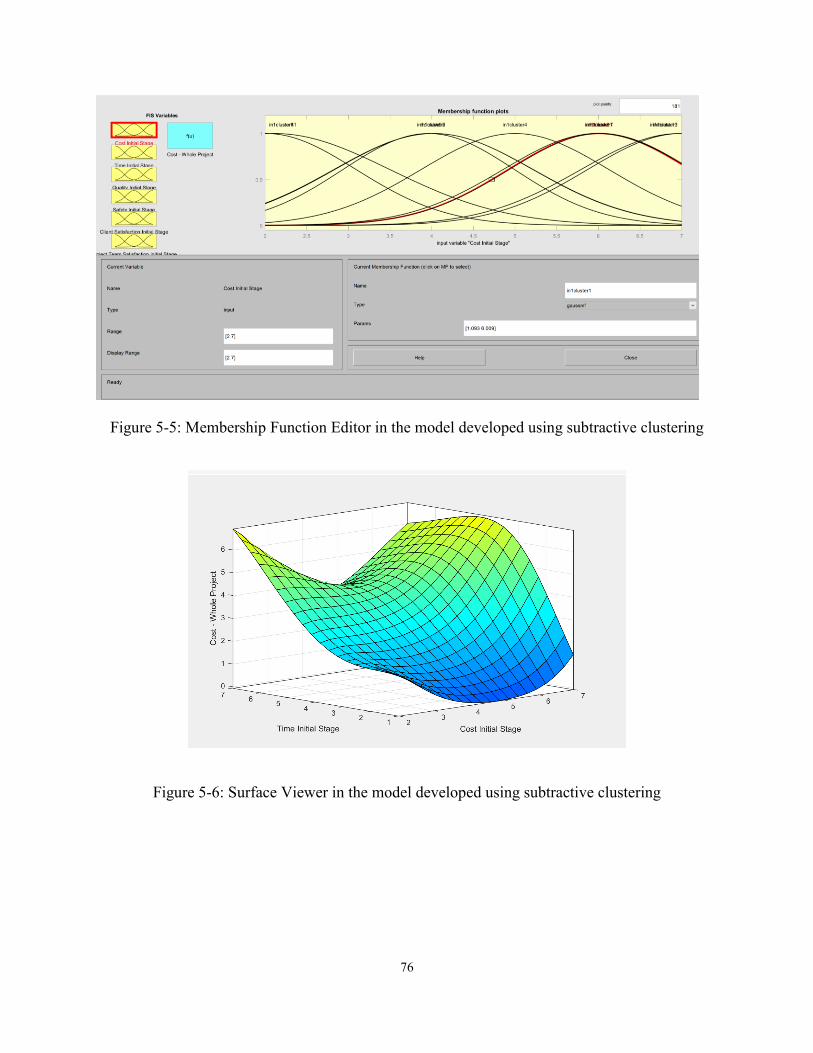
76
Figure 5-5: Membership Function Editor in the model developed using subtractive clustering
Figure 5-6: Surface Viewer in the model developed using subtractive clustering
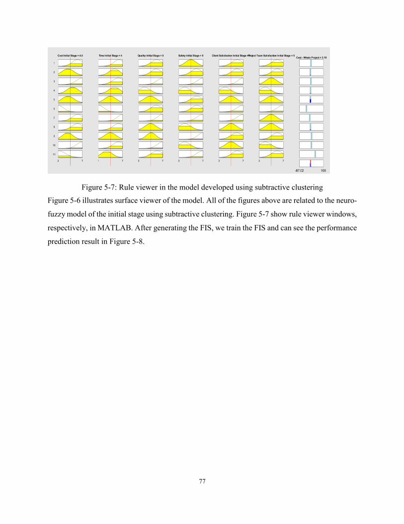
77
Figure 5-7: Rule viewer in the model developed using subtractive clustering Figure 5-6 illustrates surface viewer of the model. All of the figures above are related to the neuro-
fuzzy model of the initial stage using subtractive clustering. Figure 5-7 show rule viewer windows,
respectively, in MATLAB. After generating the FIS, we train the FIS and can see the performance
prediction result in Figure 5-8.
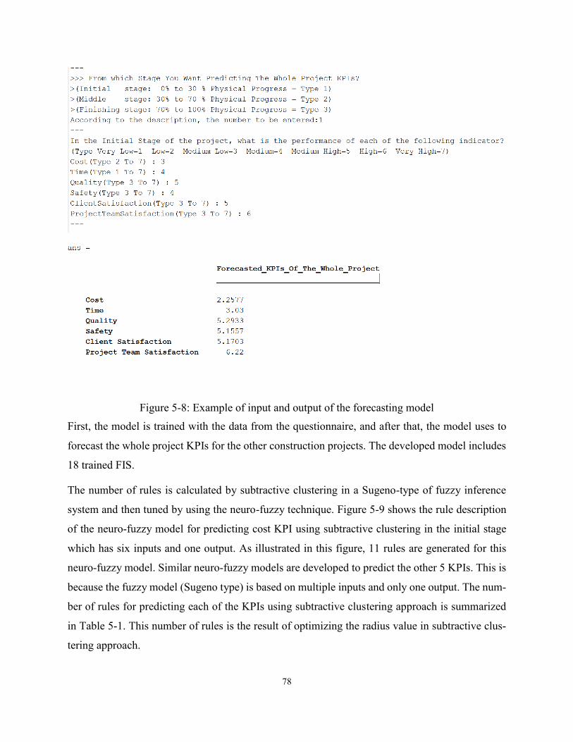
78
Figure 5-8: Example of input and output of the forecasting model First, the model is trained with the data from the questionnaire, and after that, the model uses to
forecast the whole project KPIs for the other construction projects. The developed model includes
18 trained FIS.
The number of rules is calculated by subtractive clustering in a Sugeno-type of fuzzy inference
system and then tuned by using the neuro-fuzzy technique. Figure 5-9 shows the rule description
of the neuro-fuzzy model for predicting cost KPI using subtractive clustering in the initial stage
which has six inputs and one output. As illustrated in this figure, 11 rules are generated for this
neuro-fuzzy model. Similar neuro-fuzzy models are developed to predict the other 5 KPIs. This is
because the fuzzy model (Sugeno type) is based on multiple inputs and only one output. The num-
ber of rules for predicting each of the KPIs using subtractive clustering approach is summarized
in Table 5-1. This number of rules is the result of optimizing the radius value in subtractive clus-
tering approach.
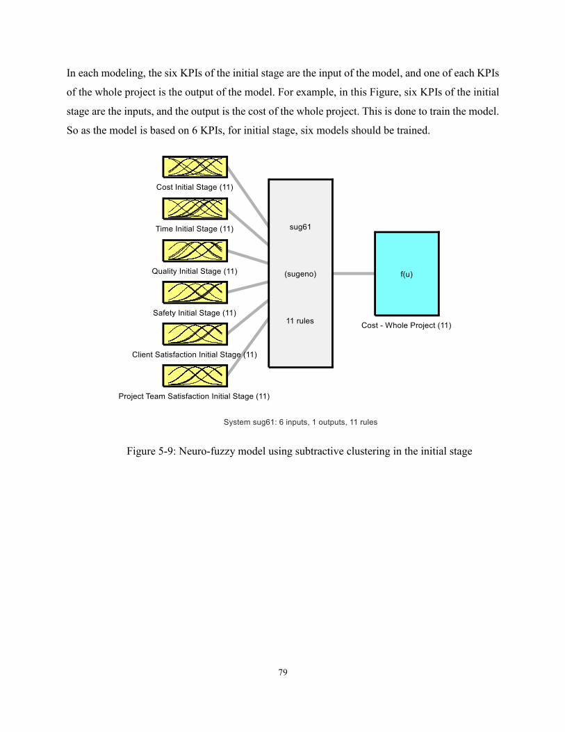
79
In each modeling, the six KPIs of the initial stage are the input of the model, and one of each KPIs
of the whole project is the output of the model. For example, in this Figure, six KPIs of the initial
stage are the inputs, and the output is the cost of the whole project. This is done to train the model.
So as the model is based on 6 KPIs, for initial stage, six models should be trained.
Figure 5-9: Neuro-fuzzy model using subtractive clustering in the initial stage
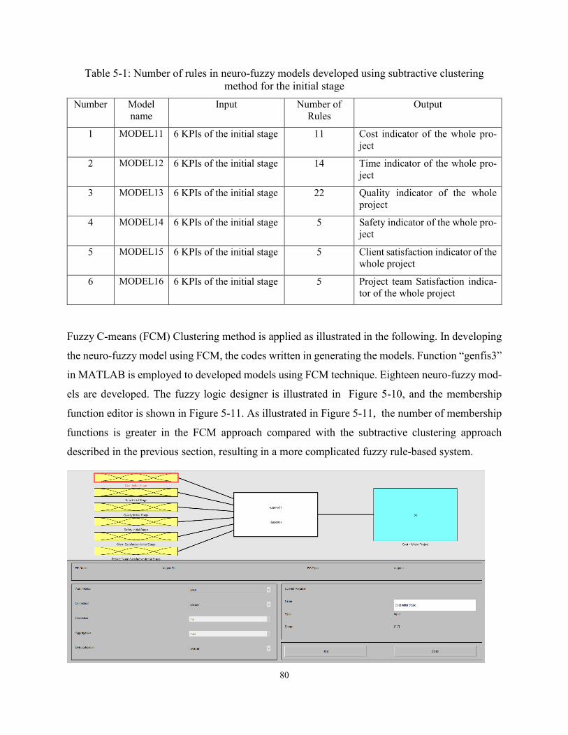
80
Table 5-1: Number of rules in neuro-fuzzy models developed using subtractive clustering method for the initial stage
Number Model name
Input Number of Rules
Output
1 MODEL11 6 KPIs of the initial stage 11 Cost indicator of the whole pro-ject
2 MODEL12 6 KPIs of the initial stage 14 Time indicator of the whole pro-ject
3 MODEL13 6 KPIs of the initial stage 22 Quality indicator of the whole project
4 MODEL14 6 KPIs of the initial stage 5 Safety indicator of the whole pro-ject
5 MODEL15 6 KPIs of the initial stage 5 Client satisfaction indicator of the whole project
6 MODEL16 6 KPIs of the initial stage 5 Project team Satisfaction indica-tor of the whole project
Fuzzy C-means (FCM) Clustering method is applied as illustrated in the following. In developing
the neuro-fuzzy model using FCM, the codes written in generating the models. Function “genfis3”
in MATLAB is employed to developed models using FCM technique. Eighteen neuro-fuzzy mod-
els are developed. The fuzzy logic designer is illustrated in Figure 5-10, and the membership
function editor is shown in Figure 5-11. As illustrated in Figure 5-11, the number of membership
functions is greater in the FCM approach compared with the subtractive clustering approach
described in the previous section, resulting in a more complicated fuzzy rule-based system.
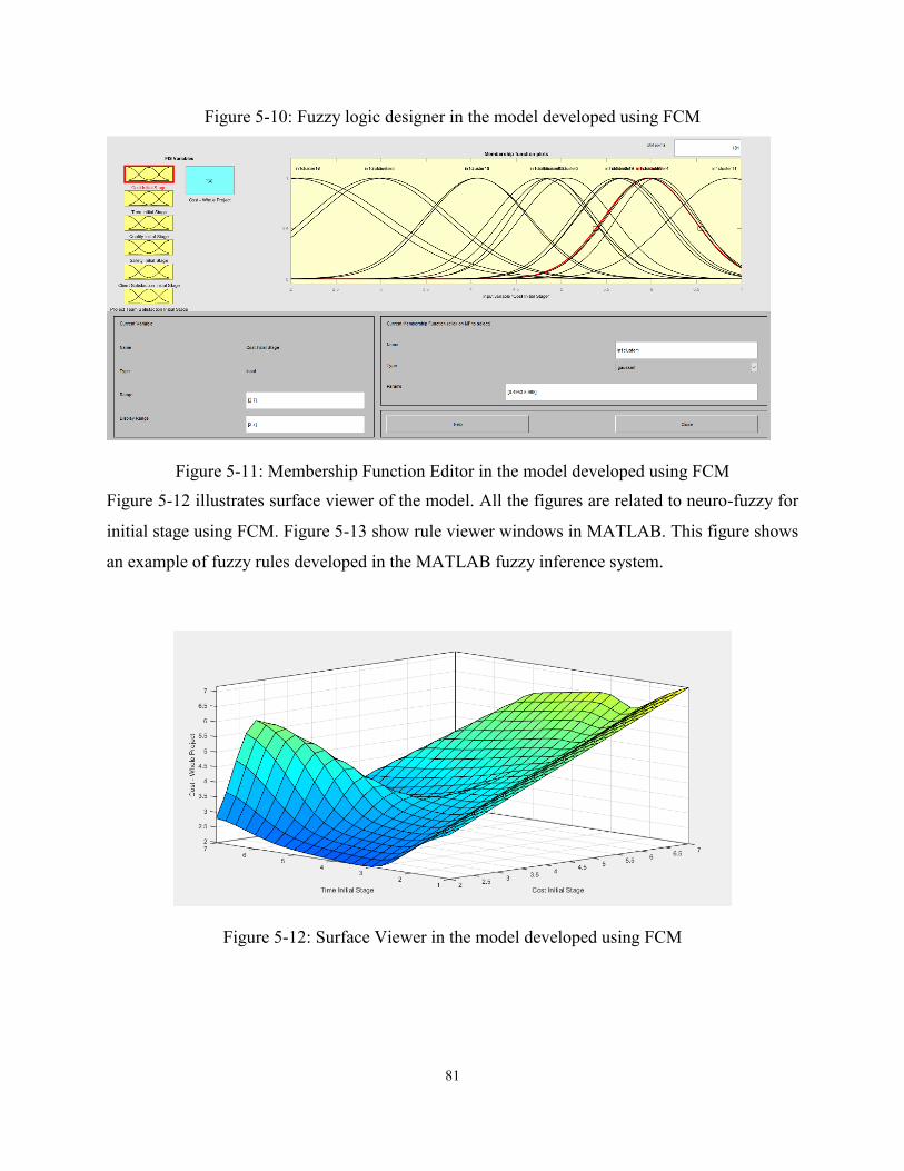
81
Figure 5-10: Fuzzy logic designer in the model developed using FCM
Figure 5-11: Membership Function Editor in the model developed using FCM Figure 5-12 illustrates surface viewer of the model. All the figures are related to neuro-fuzzy for
initial stage using FCM. Figure 5-13 show rule viewer windows in MATLAB. This figure shows
an example of fuzzy rules developed in the MATLAB fuzzy inference system.
Figure 5-12: Surface Viewer in the model developed using FCM
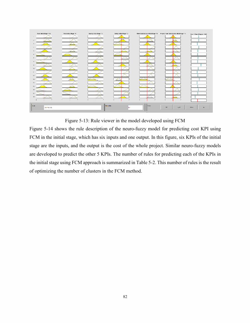
82
Figure 5-13: Rule viewer in the model developed using FCM Figure 5-14 shows the rule description of the neuro-fuzzy model for predicting cost KPI using
FCM in the initial stage, which has six inputs and one output. In this figure, six KPIs of the initial
stage are the inputs, and the output is the cost of the whole project. Similar neuro-fuzzy models
are developed to predict the other 5 KPIs. The number of rules for predicting each of the KPIs in
the initial stage using FCM approach is summarized in Table 5-2. This number of rules is the result
of optimizing the number of clusters in the FCM method.
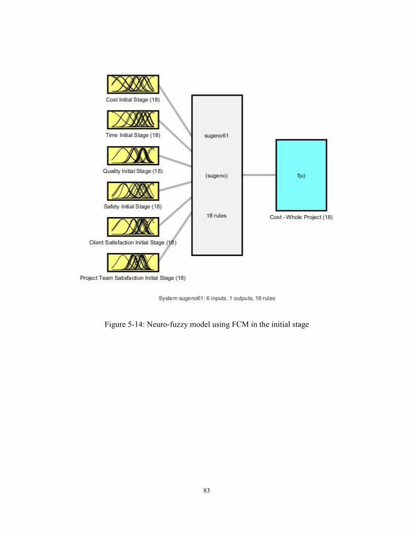
83
Figure 5-14: Neuro-fuzzy model using FCM in the initial stage
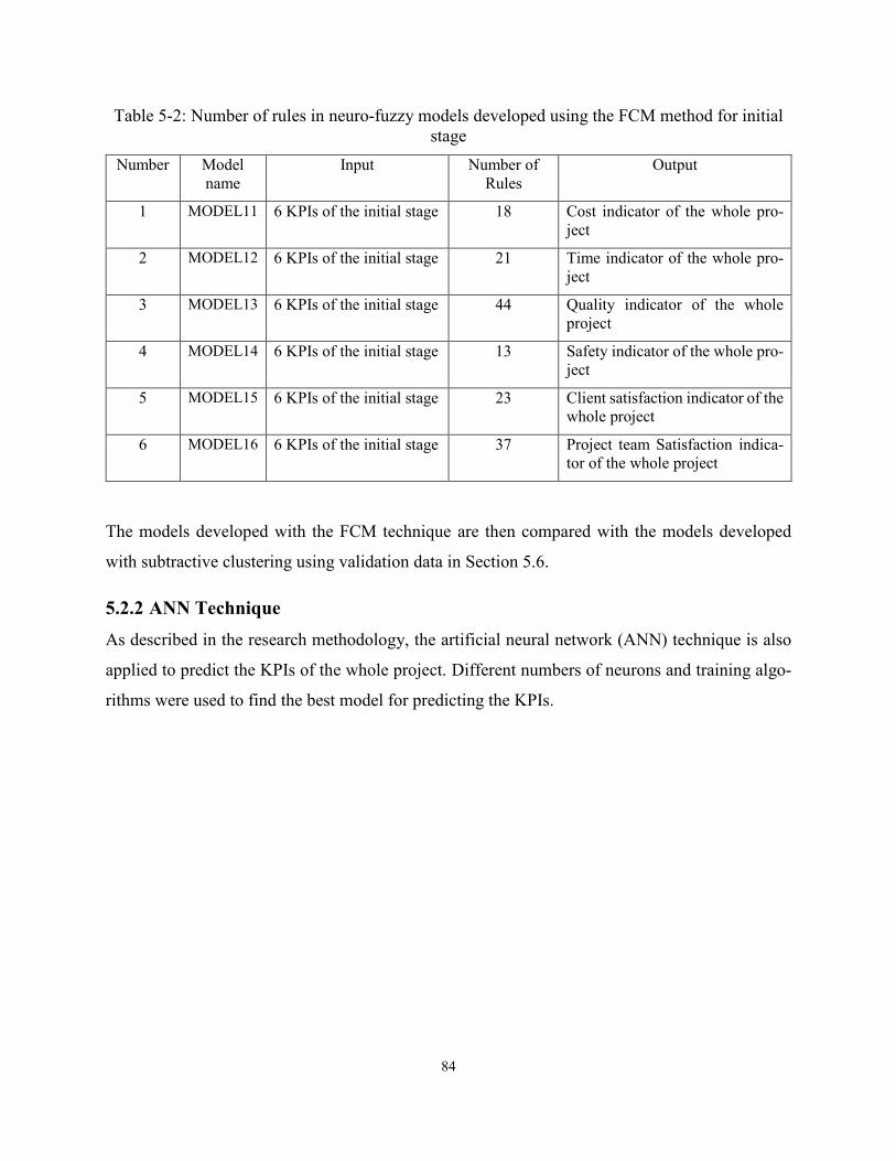
84
Table 5-2: Number of rules in neuro-fuzzy models developed using the FCM method for initial stage
Number Model name
Input Number of Rules
Output
1 MODEL11 6 KPIs of the initial stage 18 Cost indicator of the whole pro-ject
2 MODEL12 6 KPIs of the initial stage 21 Time indicator of the whole pro-ject
3 MODEL13 6 KPIs of the initial stage 44 Quality indicator of the whole project
4 MODEL14 6 KPIs of the initial stage 13 Safety indicator of the whole pro-ject
5 MODEL15 6 KPIs of the initial stage 23 Client satisfaction indicator of the whole project
6 MODEL16 6 KPIs of the initial stage 37 Project team Satisfaction indica-tor of the whole project
The models developed with the FCM technique are then compared with the models developed
with subtractive clustering using validation data in Section 5.6.
5.2.2 ANN Technique
As described in the research methodology, the artificial neural network (ANN) technique is also
applied to predict the KPIs of the whole project. Different numbers of neurons and training algo-
rithms were used to find the best model for predicting the KPIs.
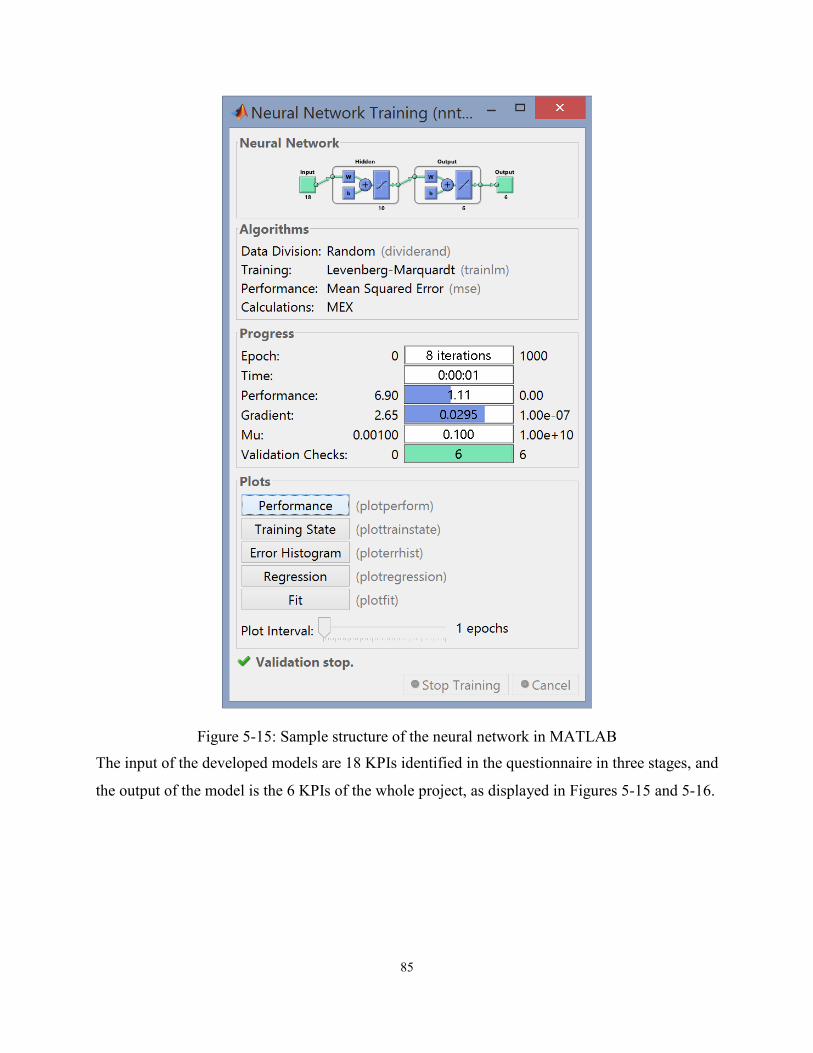
85
Figure 5-15: Sample structure of the neural network in MATLAB The input of the developed models are 18 KPIs identified in the questionnaire in three stages, and
the output of the model is the 6 KPIs of the whole project, as displayed in Figures 5-15 and 5-16.
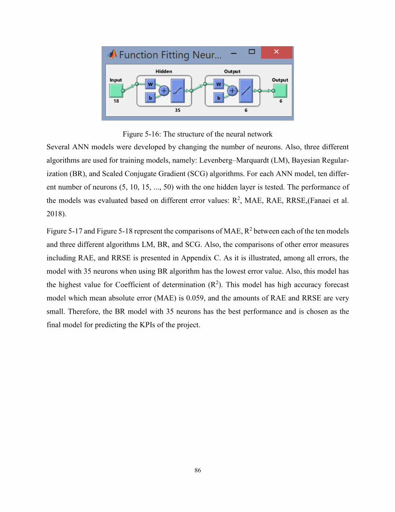
86
Figure 5-16: The structure of the neural network Several ANN models were developed by changing the number of neurons. Also, three different
algorithms are used for training models, namely: Levenberg–Marquardt (LM), Bayesian Regular-
ization (BR), and Scaled Conjugate Gradient (SCG) algorithms. For each ANN model, ten differ-
ent number of neurons (5, 10, 15, ..., 50) with the one hidden layer is tested. The performance of
the models was evaluated based on different error values: R2, MAE, RAE, RRSE,(Fanaei et al.
2018).
Figure 5-17 and Figure 5-18 represent the comparisons of MAE, R2 between each of the ten models
and three different algorithms LM, BR, and SCG. Also, the comparisons of other error measures
including RAE, and RRSE is presented in Appendix C. As it is illustrated, among all errors, the
model with 35 neurons when using BR algorithm has the lowest error value. Also, this model has
the highest value for Coefficient of determination (R2). This model has high accuracy forecast
model which mean absolute error (MAE) is 0.059, and the amounts of RAE and RRSE are very
small. Therefore, the BR model with 35 neurons has the best performance and is chosen as the
final model for predicting the KPIs of the project.
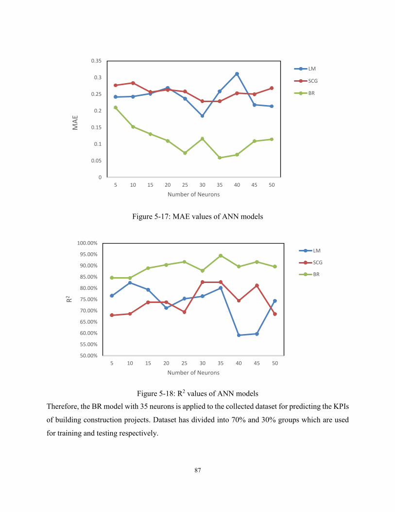
0
0.05
0.1
0.15
0.2
0.25
0.3
0.35
5 10 15 20 25 30 35 40 45 50
MAE
Number of Neurons
LM
SCG
BR
50.00%
55.00%
60.00%
65.00%
70.00%
75.00%
80.00%
85.00%
90.00%
95.00%
100.00%
5 10 15 20 25 30 35 40 45 50
R2
Number of Neurons
LM
SCG
BR
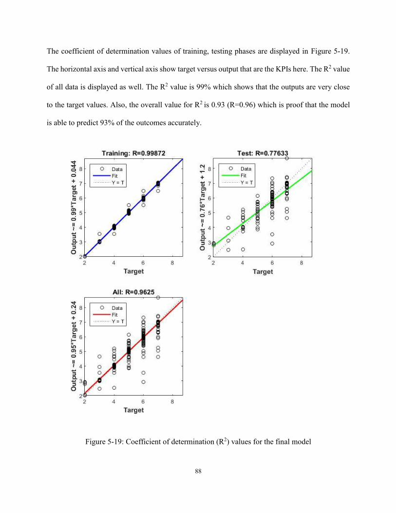
88
The coefficient of determination values of training, testing phases are displayed in Figure 5-19.
The horizontal axis and vertical axis show target versus output that are the KPIs here. The R2 value
of all data is displayed as well. The R2 value is 99% which shows that the outputs are very close
to the target values. Also, the overall value for R2 is 0.93 (R=0.96) which is proof that the model
is able to predict 93% of the outcomes accurately.
Figure 5-19: Coefficient of determination (R2) values for the final model
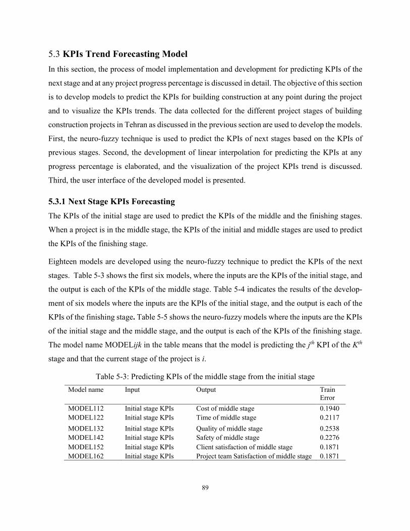
89
5.3 KPIs Trend Forecasting Model In this section, the process of model implementation and development for predicting KPIs of the
next stage and at any project progress percentage is discussed in detail. The objective of this section
is to develop models to predict the KPIs for building construction at any point during the project
and to visualize the KPIs trends. The data collected for the different project stages of building
construction projects in Tehran as discussed in the previous section are used to develop the models.
First, the neuro-fuzzy technique is used to predict the KPIs of next stages based on the KPIs of
previous stages. Second, the development of linear interpolation for predicting the KPIs at any
progress percentage is elaborated, and the visualization of the project KPIs trend is discussed.
Third, the user interface of the developed model is presented.
5.3.1 Next Stage KPIs Forecasting
The KPIs of the initial stage are used to predict the KPIs of the middle and the finishing stages.
When a project is in the middle stage, the KPIs of the initial and middle stages are used to predict
the KPIs of the finishing stage.
Eighteen models are developed using the neuro-fuzzy technique to predict the KPIs of the next
stages. Table 5-3 shows the first six models, where the inputs are the KPIs of the initial stage, and
the output is each of the KPIs of the middle stage. Table 5-4 indicates the results of the develop-
ment of six models where the inputs are the KPIs of the initial stage, and the output is each of the
KPIs of the finishing stage. Table 5-5 shows the neuro-fuzzy models where the inputs are the KPIs
of the initial stage and the middle stage, and the output is each of the KPIs of the finishing stage.
The model name MODELijk in the table means that the model is predicting the jth KPI of the Kth
stage and that the current stage of the project is i.
Table 5-3: Predicting KPIs of the middle stage from the initial stage
Model name Input Output Train Error
MODEL112 Initial stage KPIs Cost of middle stage 0.1940 MODEL122 Initial stage KPIs Time of middle stage 0.2117 MODEL132 Initial stage KPIs Quality of middle stage 0.2538 MODEL142 Initial stage KPIs Safety of middle stage 0.2276 MODEL152 Initial stage KPIs Client satisfaction of middle stage 0.1871 MODEL162 Initial stage KPIs Project team Satisfaction of middle stage 0.1871
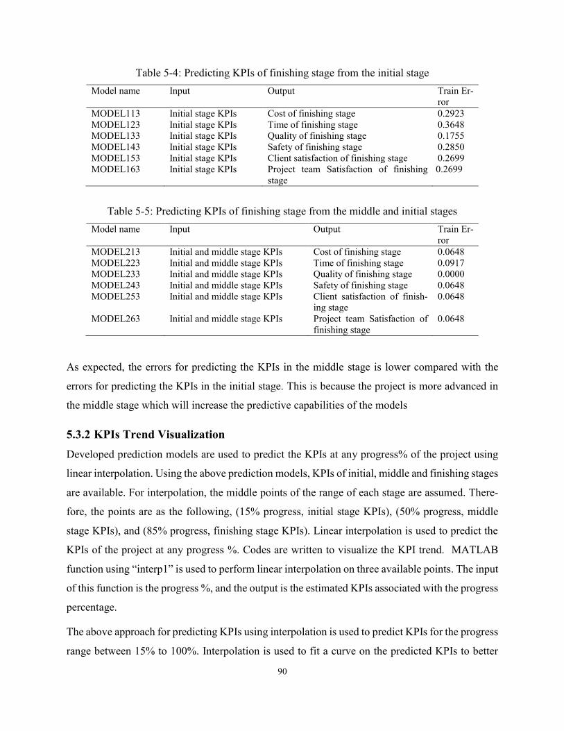
90
Table 5-4: Predicting KPIs of finishing stage from the initial stage Model name Input Output Train Er-
ror MODEL113 Initial stage KPIs Cost of finishing stage 0.2923 MODEL123 Initial stage KPIs Time of finishing stage 0.3648 MODEL133 Initial stage KPIs Quality of finishing stage 0.1755 MODEL143 Initial stage KPIs Safety of finishing stage 0.2850 MODEL153 Initial stage KPIs Client satisfaction of finishing stage 0.2699 MODEL163 Initial stage KPIs Project team Satisfaction of finishing
stage 0.2699
Table 5-5: Predicting KPIs of finishing stage from the middle and initial stages
Model name Input Output Train Er-ror
MODEL213 Initial and middle stage KPIs Cost of finishing stage 0.0648 MODEL223 Initial and middle stage KPIs Time of finishing stage 0.0917 MODEL233 Initial and middle stage KPIs Quality of finishing stage 0.0000 MODEL243 Initial and middle stage KPIs Safety of finishing stage 0.0648 MODEL253 Initial and middle stage KPIs Client satisfaction of finish-
ing stage 0.0648
MODEL263 Initial and middle stage KPIs Project team Satisfaction of finishing stage
0.0648
As expected, the errors for predicting the KPIs in the middle stage is lower compared with the
errors for predicting the KPIs in the initial stage. This is because the project is more advanced in
the middle stage which will increase the predictive capabilities of the models
5.3.2 KPIs Trend Visualization
Developed prediction models are used to predict the KPIs at any progress% of the project using
linear interpolation. Using the above prediction models, KPIs of initial, middle and finishing stages
are available. For interpolation, the middle points of the range of each stage are assumed. There-
fore, the points are as the following, (15% progress, initial stage KPIs), (50% progress, middle
stage KPIs), and (85% progress, finishing stage KPIs). Linear interpolation is used to predict the
KPIs of the project at any progress %. Codes are written to visualize the KPI trend. MATLAB
function using “interp1” is used to perform linear interpolation on three available points. The input
of this function is the progress %, and the output is the estimated KPIs associated with the progress
percentage.
The above approach for predicting KPIs using interpolation is used to predict KPIs for the progress
range between 15% to 100%. Interpolation is used to fit a curve on the predicted KPIs to better
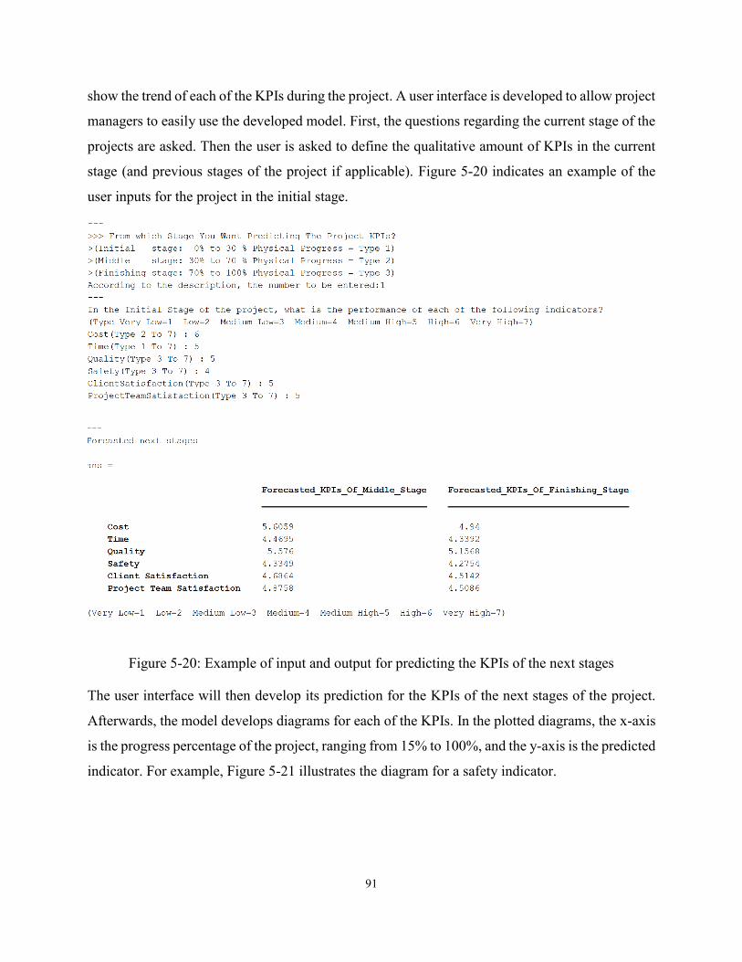
91
show the trend of each of the KPIs during the project. A user interface is developed to allow project
managers to easily use the developed model. First, the questions regarding the current stage of the
projects are asked. Then the user is asked to define the qualitative amount of KPIs in the current
stage (and previous stages of the project if applicable). Figure 5-20 indicates an example of the
user inputs for the project in the initial stage.
Figure 5-20: Example of input and output for predicting the KPIs of the next stages
The user interface will then develop its prediction for the KPIs of the next stages of the project.
Afterwards, the model develops diagrams for each of the KPIs. In the plotted diagrams, the x-axis
is the progress percentage of the project, ranging from 15% to 100%, and the y-axis is the predicted
indicator. For example, Figure 5-21 illustrates the diagram for a safety indicator.
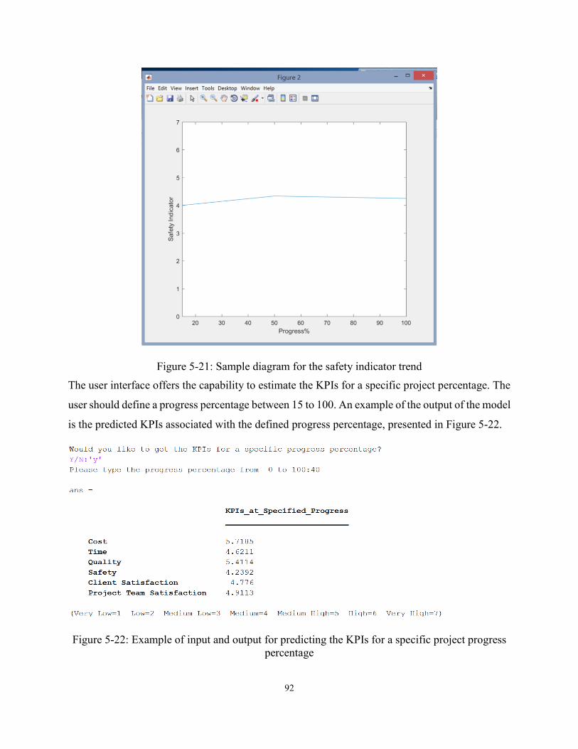
92
Figure 5-21: Sample diagram for the safety indicator trend The user interface offers the capability to estimate the KPIs for a specific project percentage. The
user should define a progress percentage between 15 to 100. An example of the output of the model
is the predicted KPIs associated with the defined progress percentage, presented in Figure 5-22.
Figure 5-22: Example of input and output for predicting the KPIs for a specific project progress percentage
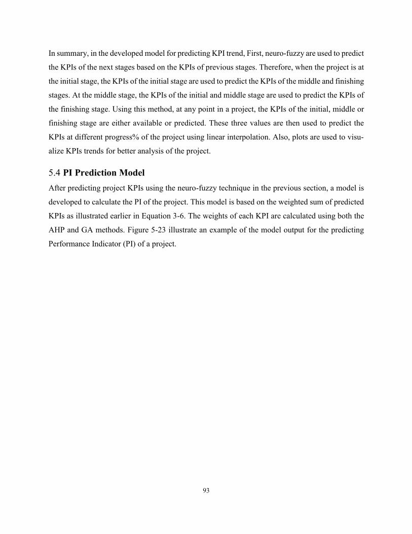
93
In summary, in the developed model for predicting KPI trend, First, neuro-fuzzy are used to predict
the KPIs of the next stages based on the KPIs of previous stages. Therefore, when the project is at
the initial stage, the KPIs of the initial stage are used to predict the KPIs of the middle and finishing
stages. At the middle stage, the KPIs of the initial and middle stage are used to predict the KPIs of
the finishing stage. Using this method, at any point in a project, the KPIs of the initial, middle or
finishing stage are either available or predicted. These three values are then used to predict the
KPIs at different progress% of the project using linear interpolation. Also, plots are used to visu-
alize KPIs trends for better analysis of the project.
5.4 PI Prediction Model After predicting project KPIs using the neuro-fuzzy technique in the previous section, a model is
developed to calculate the PI of the project. This model is based on the weighted sum of predicted
KPIs as illustrated earlier in Equation 3-6. The weights of each KPI are calculated using both the
AHP and GA methods. Figure 5-23 illustrate an example of the model output for the predicting
Performance Indicator (PI) of a project.
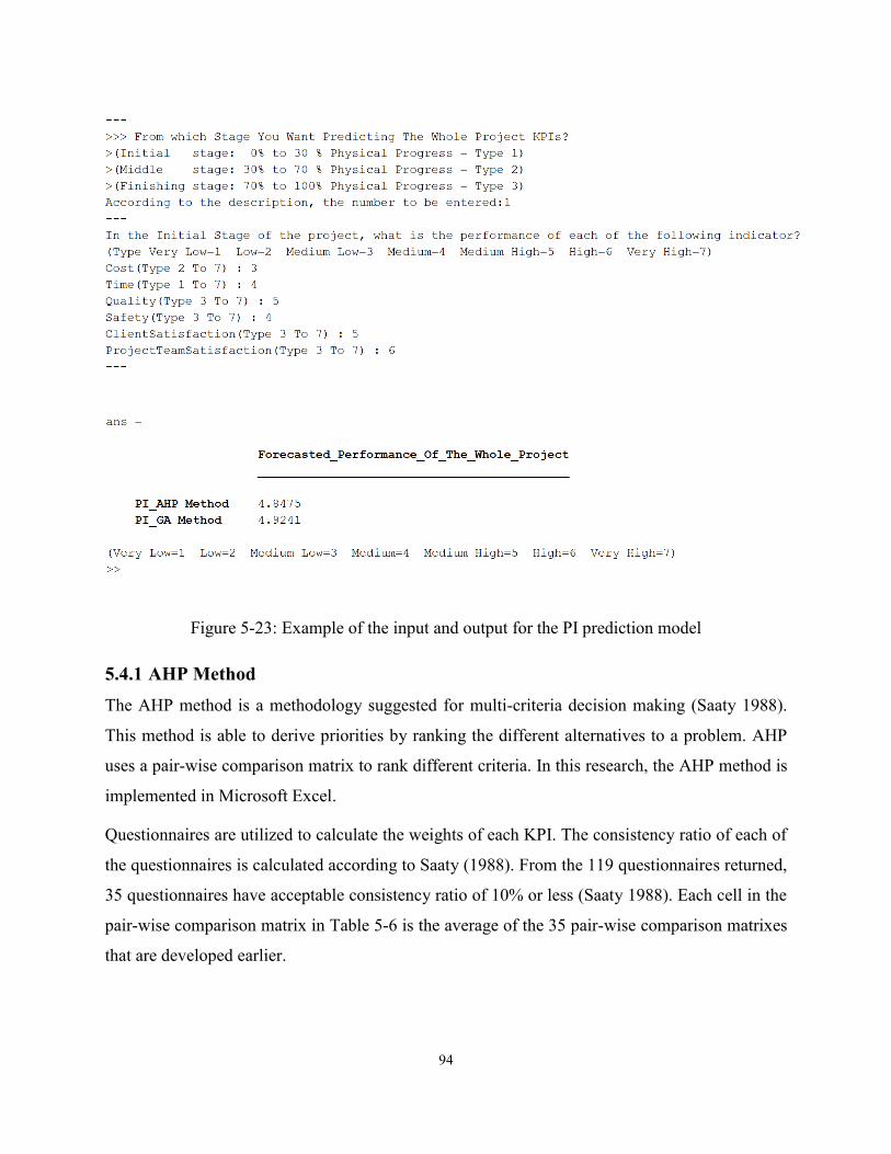
94
Figure 5-23: Example of the input and output for the PI prediction model
5.4.1 AHP Method
The AHP method is a methodology suggested for multi-criteria decision making (Saaty 1988).
This method is able to derive priorities by ranking the different alternatives to a problem. AHP
uses a pair-wise comparison matrix to rank different criteria. In this research, the AHP method is
implemented in Microsoft Excel.
Questionnaires are utilized to calculate the weights of each KPI. The consistency ratio of each of
the questionnaires is calculated according to Saaty (1988). From the 119 questionnaires returned,
35 questionnaires have acceptable consistency ratio of 10% or less (Saaty 1988). Each cell in the
pair-wise comparison matrix in Table 5-6 is the average of the 35 pair-wise comparison matrixes
that are developed earlier.
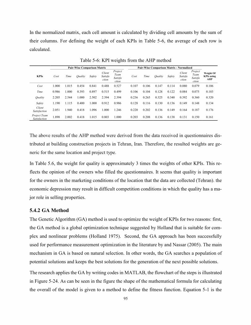
95
In the normalized matrix, each cell amount is calculated by dividing cell amounts by the sum of
their columns. For defining the weight of each KPIs in Table 5-6, the average of each row is
calculated.
Table 5-6: KPI weights from the AHP method
The above results of the AHP method were derived from the data received in questionnaires dis-
tributed at building construction projects in Tehran, Iran. Therefore, the resulted weights are ge-
neric for the same location and project type.
In Table 5.6, the weight for quality is approximately 3 times the weights of other KPIs. This re-
flects the opinion of the owners who filled the questionnaires. It seems that quality is important
for the owners in the marketing conditions of the location that the data are collected (Tehran). the
economic depression may result in difficult competition conditions in which the quality has a ma-
jor role in selling properties.
5.4.2 GA Method
The Genetic Algorithm (GA) method is used to optimize the weight of KPIs for two reasons: first,
the GA method is a global optimization technique suggested by Holland that is suitable for com-
plex and nonlinear problems (Holland 1975). Second, the GA approach has been successfully
used for performance measurement optimization in the literature by and Nassar (2005). The main
mechanism in GA is based on natural selection. In other words, the GA searches a population of
potential solutions and keeps the best solutions for the generation of the next possible solutions.
The research applies the GA by writing codes in MATLAB, the flowchart of the steps is illustrated
in Figure 5-24. As can be seen in the figure the shape of the mathematical formula for calculating
the overall of the model is given to a method to define the fitness function. Equation 5-1 is the
Pair-Wise Comparison Matrix Pair-Wise Comparison Matrix - Normalized
KPIs Cost Time Quality Safety Client Satisfaction
Project Team
Satisfaction
Cost Time Quality Safety Client Satisfaction
Project Team
Satisfaction
Weight Of KPIs using
AHP
Cost 1.000 1.015 0.454 0.841 0.488 0.527 0.107 0.106 0.147 0.114 0.080 0.079 0.106
Time 0.986 1.000 0.393 0.897 0.515 0.499 0.106 0.104 0.128 0.122 0.084 0.075 0.103
Quality 2.205 2.544 1.000 2.502 2.394 2.394 0.236 0.265 0.325 0.340 0.392 0.360 0.320
Safety 1.190 1.115 0.400 1.000 0.912 0.986 0.128 0.116 0.130 0.136 0.149 0.148 0.134 Client
Satisfaction
2.051 1.940 0.418 1.096 1.000 1.246 0.220 0.202 0.136 0.149 0.164 0.187 0.176
Project Team Satisfaction 1.898 2.002 0.418 1.015 0.803 1.000 0.203 0.208 0.136 0.138 0.131 0.150 0.161
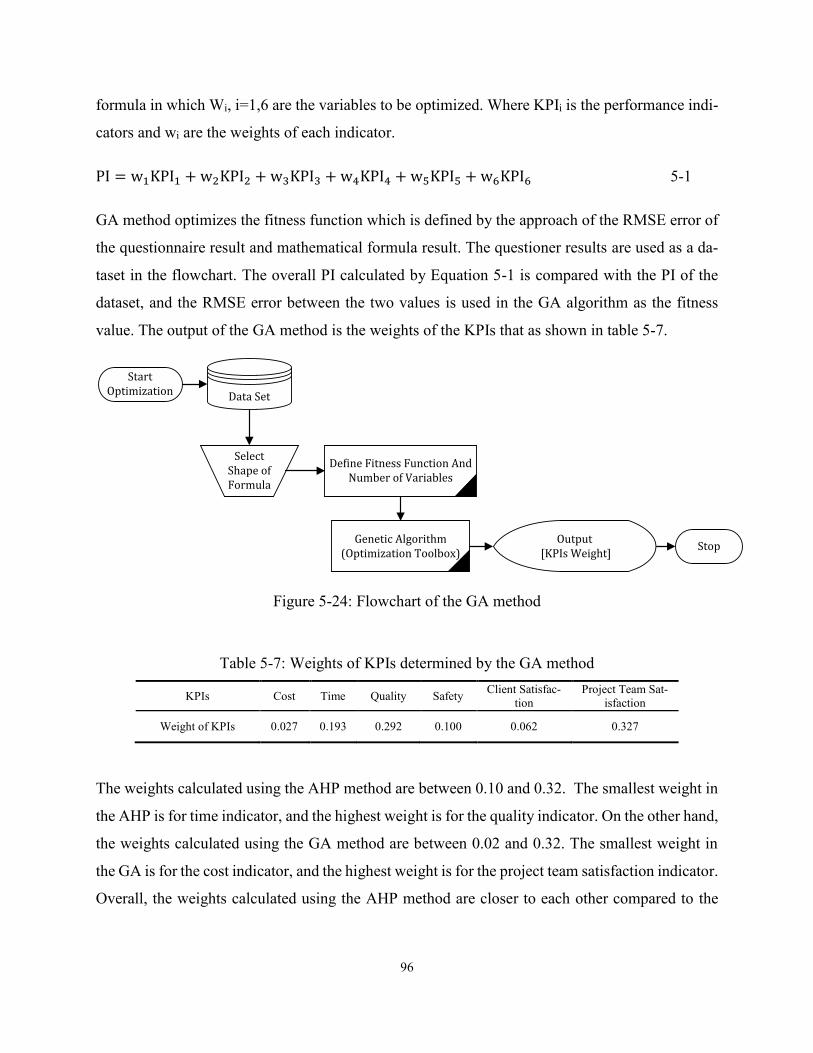
96
formula in which Wi, i=1,6 are the variables to be optimized. Where KPIi is the performance indi-
cators and wi are the weights of each indicator.
PI = w1KPI1 + w2KPI2 + w3KPI3 + w4KPI4 + w5KPI5 + w6KPI6 5-1
GA method optimizes the fitness function which is defined by the approach of the RMSE error of
the questionnaire result and mathematical formula result. The questioner results are used as a da-
taset in the flowchart. The overall PI calculated by Equation 5-1 is compared with the PI of the
dataset, and the RMSE error between the two values is used in the GA algorithm as the fitness
value. The output of the GA method is the weights of the KPIs that as shown in table 5-7.
Start Optimization
Output [KPIs Weight]
Data Set
Define Fitness Function And Number of Variables
Select Shape of Formula
Genetic Algorithm (Optimization Toolbox)
Stop
Figure 5-24: Flowchart of the GA method
Table 5-7: Weights of KPIs determined by the GA method
KPIs Cost Time Quality Safety Client Satisfac-tion
Project Team Sat-isfaction
Weight of KPIs 0.027 0.193 0.292 0.100 0.062 0.327
The weights calculated using the AHP method are between 0.10 and 0.32. The smallest weight in
the AHP is for time indicator, and the highest weight is for the quality indicator. On the other hand,
the weights calculated using the GA method are between 0.02 and 0.32. The smallest weight in
the GA is for the cost indicator, and the highest weight is for the project team satisfaction indicator.
Overall, the weights calculated using the AHP method are closer to each other compared to the
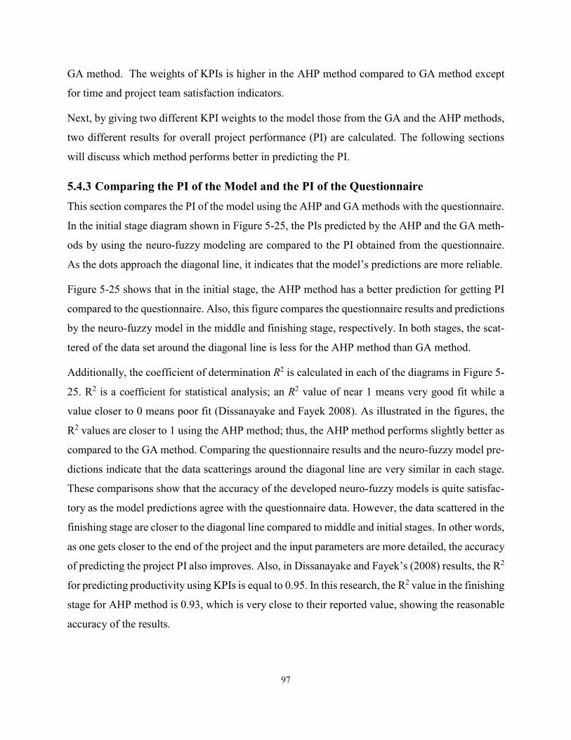
97
GA method. The weights of KPIs is higher in the AHP method compared to GA method except
for time and project team satisfaction indicators.
Next, by giving two different KPI weights to the model those from the GA and the AHP methods,
two different results for overall project performance (PI) are calculated. The following sections
will discuss which method performs better in predicting the PI.
5.4.3 Comparing the PI of the Model and the PI of the Questionnaire
This section compares the PI of the model using the AHP and GA methods with the questionnaire.
In the initial stage diagram shown in Figure 5-25, the PIs predicted by the AHP and the GA meth-
ods by using the neuro-fuzzy modeling are compared to the PI obtained from the questionnaire.
As the dots approach the diagonal line, it indicates that the model’s predictions are more reliable.
Figure 5-25 shows that in the initial stage, the AHP method has a better prediction for getting PI
compared to the questionnaire. Also, this figure compares the questionnaire results and predictions
by the neuro-fuzzy model in the middle and finishing stage, respectively. In both stages, the scat-
tered of the data set around the diagonal line is less for the AHP method than GA method.
Additionally, the coefficient of determination R2 is calculated in each of the diagrams in Figure 5-
25. R2 is a coefficient for statistical analysis; an R2 value of near 1 means very good fit while a
value closer to 0 means poor fit (Dissanayake and Fayek 2008). As illustrated in the figures, the
R2 values are closer to 1 using the AHP method; thus, the AHP method performs slightly better as
compared to the GA method. Comparing the questionnaire results and the neuro-fuzzy model pre-
dictions indicate that the data scatterings around the diagonal line are very similar in each stage.
These comparisons show that the accuracy of the developed neuro-fuzzy models is quite satisfac-
tory as the model predictions agree with the questionnaire data. However, the data scattered in the
finishing stage are closer to the diagonal line compared to middle and initial stages. In other words,
as one gets closer to the end of the project and the input parameters are more detailed, the accuracy
of predicting the project PI also improves. Also, in Dissanayake and Fayek’s (2008) results, the R2
for predicting productivity using KPIs is equal to 0.95. In this research, the R2 value in the finishing
stage for AHP method is 0.93, which is very close to their reported value, showing the reasonable
accuracy of the results.

98
Comparing the questionnaire results and predictions made by the neuro-fuzzy model indicates that
the scattering of the data set around the diagonal line is very similar, which shows the good gen-
eralization of the model.
99
Figure 5-25: Comparison between PI of the model and PI of questionnaires in three stages
100
5.5 Performance Optimization Model (POM) for selecting Corrective Action in
Construction Projects Codes are written in MATLAB software to implement the developed model in section 3.6. The
developed model offers a user interface to interact with the experts. After providing the overall
project PI and whole project KPIs using the developed models in the previous section, the interface
asks the experts if they would like to increase overall project PI or a selected KPI by providing
different activity modes for the remaining of the project. When the user chooses to increase the
overall project PI, the interface asks the user to fill the values in the excel file. The number of
activities and their modes does not have any limitations. The number of activities as well as a
number of activity modes are flexible and can be changed depending on the project. Different
activity modes, as well as, KPIs of each activity mode should be entered by the user in an excel
file. The activity modes represent the possible corrective actions to be applied to the project for
improving performance. Modes can represent different ways for resource allocation, construction
or execution methods, or choice of different materials. The codes for this optimization is presented
in Appendix D4. After GA optimization, the user-interface defines a list for the proper activity
modes of the project to increase the overall project PI as much as possible. It should be mentioned
that the model is capable of optimizing each of KPIs separately if requested by the user. Also, the
interface developed the forecasted KPIs and PI that will be achieved using the suggested activity
modes. The option to change certain activity and certain modes (not all activities) for optimization
are considered in the model because the number of modes for each activity is flexible. When the
user does not want to change the modes of certain activities, only one mode should be defined for
that activity. The PI and KPIs are optimized in two different examples of construction project. In
the first examples, the impact of different project situations on PI optimization is discussed. In the
second example, the developed model is applied on an example taken from the literature and the
capability of the developed model on optimizing time and cost performance indicators is evaluated
by comparing with the results in the literature.
5.5.1 PI Optimization Model
A model for PI optimization is developed for a real project adapted from Ghoddousi et al. (2013)
to better illustrate the capabilities of the developed model. Figure 5-26 illustrates the CPM of this
project. The CPM is divided into three stages: the initial stage, middle stage, and finishing stage
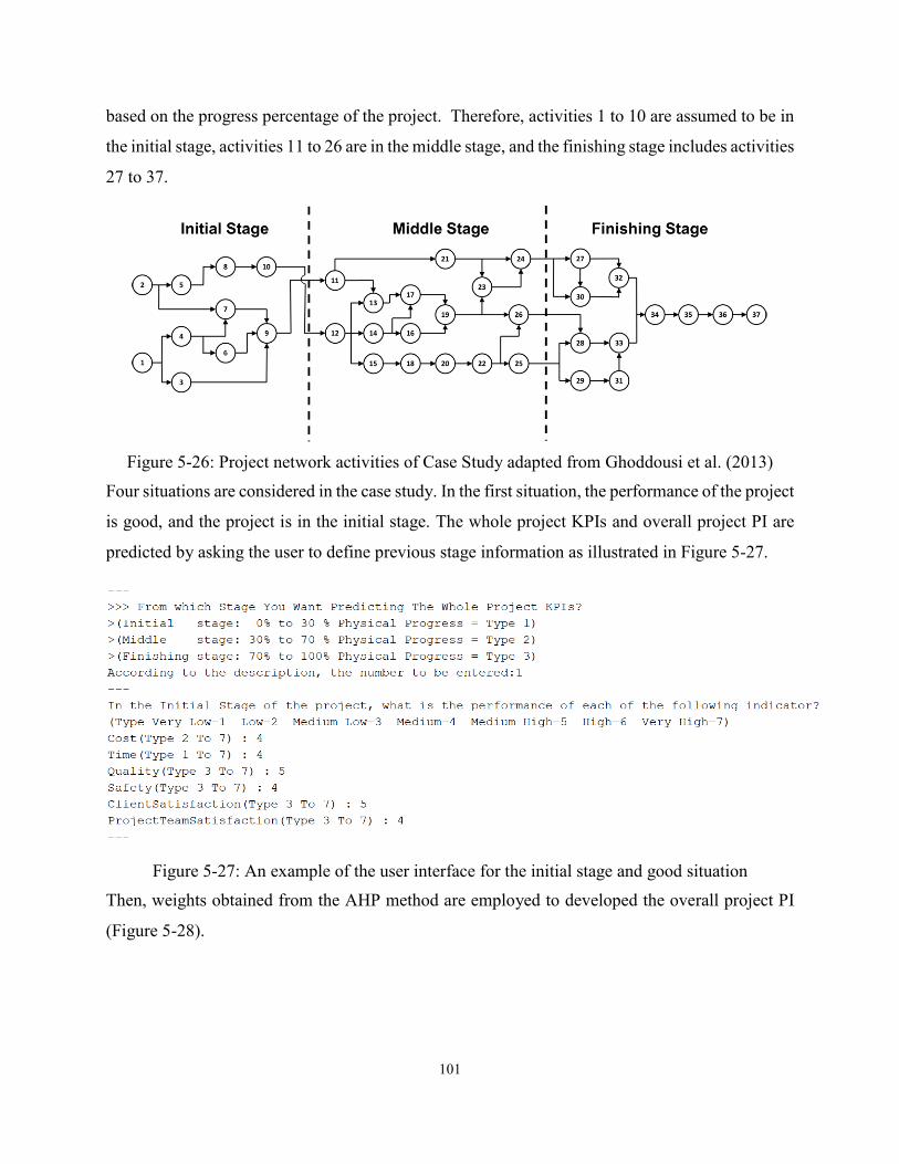
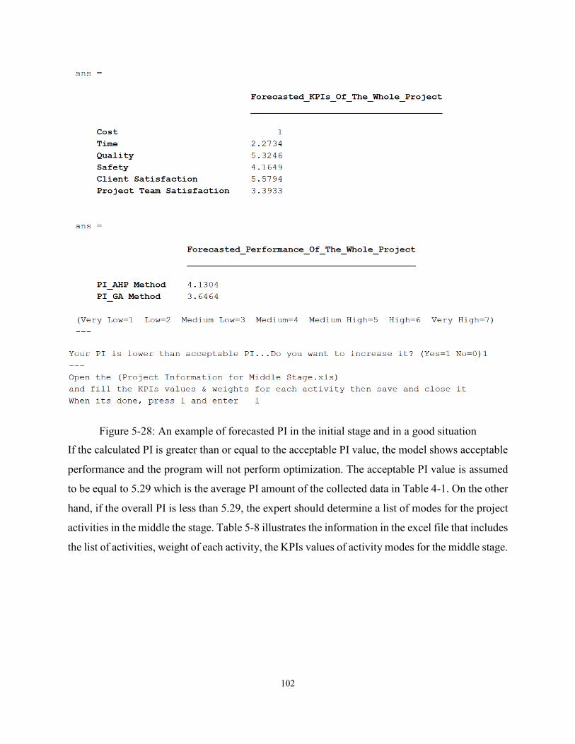
102
Figure 5-28: An example of forecasted PI in the initial stage and in a good situation If the calculated PI is greater than or equal to the acceptable PI value, the model shows acceptable
performance and the program will not perform optimization. The acceptable PI value is assumed
to be equal to 5.29 which is the average PI amount of the collected data in Table 4-1. On the other
hand, if the overall PI is less than 5.29, the expert should determine a list of modes for the project
activities in the middle the stage. Table 5-8 illustrates the information in the excel file that includes
the list of activities, weight of each activity, the KPIs values of activity modes for the middle stage.
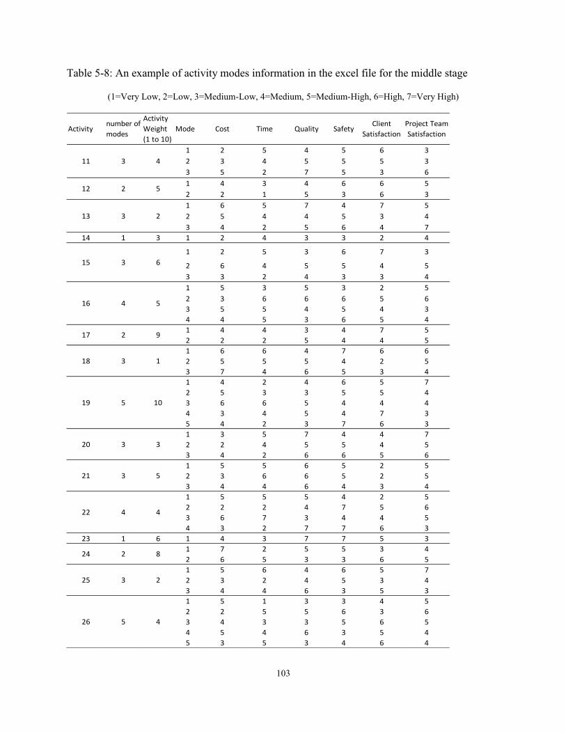
103
Table 5-8: An example of activity modes information in the excel file for the middle stage
(1=Very Low, 2=Low, 3=Medium-Low, 4=Medium, 5=Medium-High, 6=High, 7=Very High)
Activitynumber of
modes
Activity
Weight
(1 to 10)
Mode Cost Time Quality SafetyClient
Satisfaction
Project Team
Satisfaction
1 2 5 4 5 6 3
2 3 4 5 5 5 3
3 5 2 7 5 3 6
1 4 3 4 6 6 5
2 2 1 5 3 6 3
1 6 5 7 4 7 5
2 5 4 4 5 3 4
3 4 2 5 6 4 7
14 1 3 1 2 4 3 3 2 4
1 2 5 3 6 7 3
2 6 4 5 5 4 5
3 3 2 4 3 3 4
1 5 3 5 3 2 5
2 3 6 6 6 5 6
3 5 5 4 5 4 3
4 4 5 3 6 5 4
1 4 4 3 4 7 5
2 2 2 5 4 4 5
1 6 6 4 7 6 6
2 5 5 5 4 2 5
3 7 4 6 5 3 4
1 4 2 4 6 5 7
2 5 3 3 5 5 4
3 6 6 5 4 4 4
4 3 4 5 4 7 3
5 4 2 3 7 6 3
1 3 5 7 4 4 7
2 2 4 5 5 4 5
3 4 2 6 6 5 6
1 5 5 6 5 2 5
2 3 6 6 5 2 5
3 4 4 6 4 3 4
1 5 5 5 4 2 5
2 2 2 4 7 5 6
3 6 7 3 4 4 5
4 3 2 7 7 6 3
23 1 6 1 4 3 7 7 5 3
1 7 2 5 5 3 4
2 6 5 3 3 6 5
1 5 6 4 6 5 7
2 3 2 4 5 3 4
3 4 4 6 3 5 3
1 5 1 3 3 4 5
2 2 5 5 6 3 6
3 4 3 3 5 6 5
4 5 4 6 3 5 4
5 3 5 3 4 6 4
20
3
3
1
13
15
11 4
2
6
3
4 516
4526
5212
3
3
25 23
21
224
217 9
19 5 10
53
422 4
8
3
18
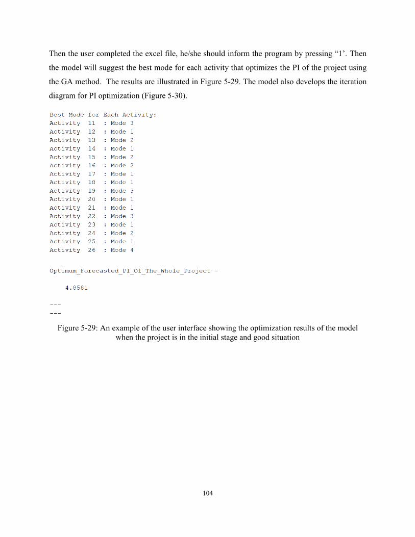
104
Then the user completed the excel file, he/she should inform the program by pressing “1’. Then
the model will suggest the best mode for each activity that optimizes the PI of the project using
the GA method. The results are illustrated in Figure 5-29. The model also develops the iteration
diagram for PI optimization (Figure 5-30).
Figure 5-29: An example of the user interface showing the optimization results of the model when the project is in the initial stage and good situation
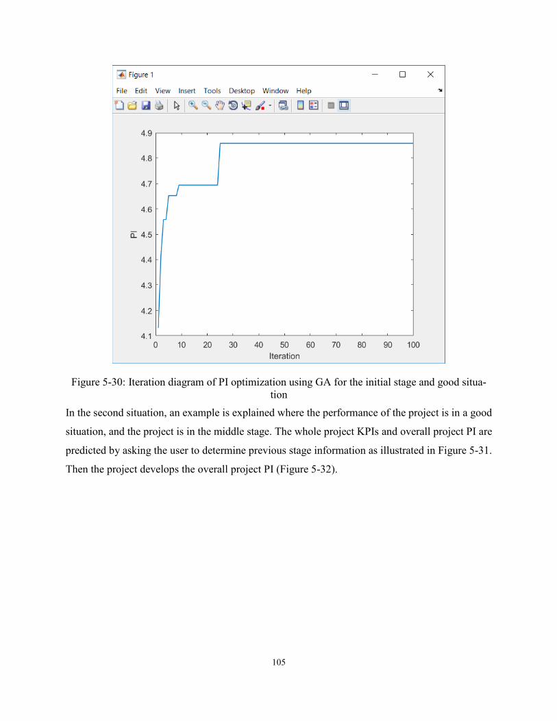
105
Figure 5-30: Iteration diagram of PI optimization using GA for the initial stage and good situa-tion
In the second situation, an example is explained where the performance of the project is in a good
situation, and the project is in the middle stage. The whole project KPIs and overall project PI are
predicted by asking the user to determine previous stage information as illustrated in Figure 5-31.
Then the project develops the overall project PI (Figure 5-32).
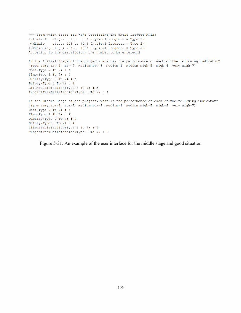
106
Figure 5-31: An example of the user interface for the middle stage and good situation
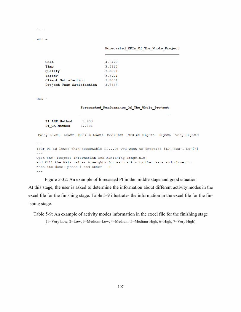
107
Figure 5-32: An example of forecasted PI in the middle stage and good situation At this stage, the user is asked to determine the information about different activity modes in the
excel file for the finishing stage. Table 5-9 illustrates the information in the excel file for the fin-
ishing stage.
Table 5-9: An example of activity modes information in the excel file for the finishing stage (1=Very Low, 2=Low, 3=Medium-Low, 4=Medium, 5=Medium-High, 6=High, 7=Very High)
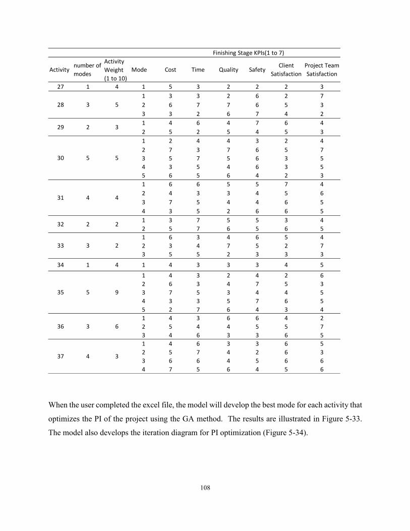
108
When the user completed the excel file, the model will develop the best mode for each activity that
optimizes the PI of the project using the GA method. The results are illustrated in Figure 5-33.
The model also develops the iteration diagram for PI optimization (Figure 5-34).
Activitynumber of
modes
Activity
Weight
(1 to 10)
Mode Cost Time Quality SafetyClient
Satisfaction
Project Team
Satisfaction
27 1 4 1 5 3 2 2 2 3
1 3 3 2 6 2 7
2 6 7 7 6 5 3
3 3 2 6 7 4 2
1 4 6 4 7 6 4
2 5 2 5 4 5 3
1 2 4 4 3 2 4
2 7 3 7 6 5 7
3 5 7 5 6 3 5
4 3 5 4 6 3 5
5 6 5 6 4 2 3
1 6 6 5 5 7 4
2 4 3 3 4 5 6
3 7 5 4 4 6 5
4 3 5 2 6 6 5
1 3 7 5 5 3 4
2 5 7 6 5 6 5
1 6 3 4 6 5 4
2 3 4 7 5 2 7
3 5 5 2 3 3 3
34 1 4 1 4 3 3 3 4 5
1 4 3 2 4 2 6
2 6 3 4 7 5 3
3 7 5 3 4 4 5
4 3 3 5 7 6 5
5 2 7 6 4 3 4
1 4 3 6 6 4 2
2 5 4 4 5 5 7
3 4 6 3 3 6 5
1 4 6 3 3 6 5
2 5 7 4 2 6 3
3 6 6 4 5 6 6
4 7 5 6 4 5 6
28 53
29
5530
4431
Finishing Stage KPIs(1 to 7)
23
4
32
22
95
37 3
32
33
3 636
35
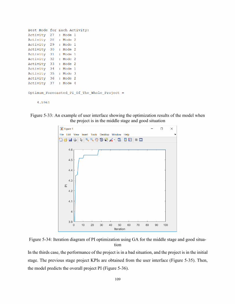
109
Figure 5-33: An example of user interface showing the optimization results of the model when the project is in the middle stage and good situation
Figure 5-34: Iteration diagram of PI optimization using GA for the middle stage and good situa-tion
In the thirds case, the performance of the project is in a bad situation, and the project is in the initial
stage. The previous stage project KPIs are obtained from the user interface (Figure 5-35). Then,
the model predicts the overall project PI (Figure 5-36).
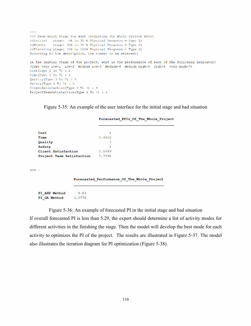
110
Figure 5-35: An example of the user interface for the initial stage and bad situation
Figure 5-36: An example of forecasted PI in the initial stage and bad situation If overall forecasted PI is less than 5.29, the expert should determine a list of activity modes for
different activities in the finishing the stage. Then the model will develop the best mode for each
activity to optimizes the PI of the project. The results are illustrated in Figure 5-37. The model
also illustrates the iteration diagram for PI optimization (Figure 5-38).

111
Figure 5-37: An example of user interface showing the optimization results of the model when the project is in the initial stage and bad situation
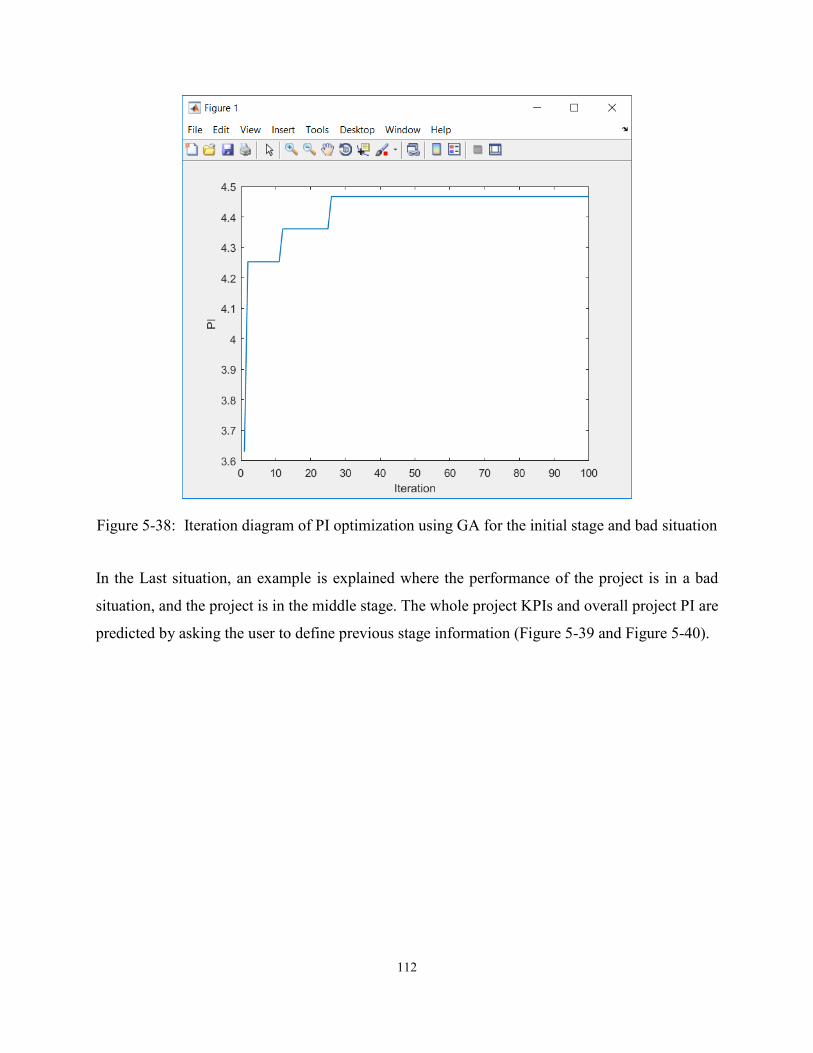
112
Figure 5-38: Iteration diagram of PI optimization using GA for the initial stage and bad situation
In the Last situation, an example is explained where the performance of the project is in a bad
situation, and the project is in the middle stage. The whole project KPIs and overall project PI are
predicted by asking the user to define previous stage information (Figure 5-39 and Figure 5-40).
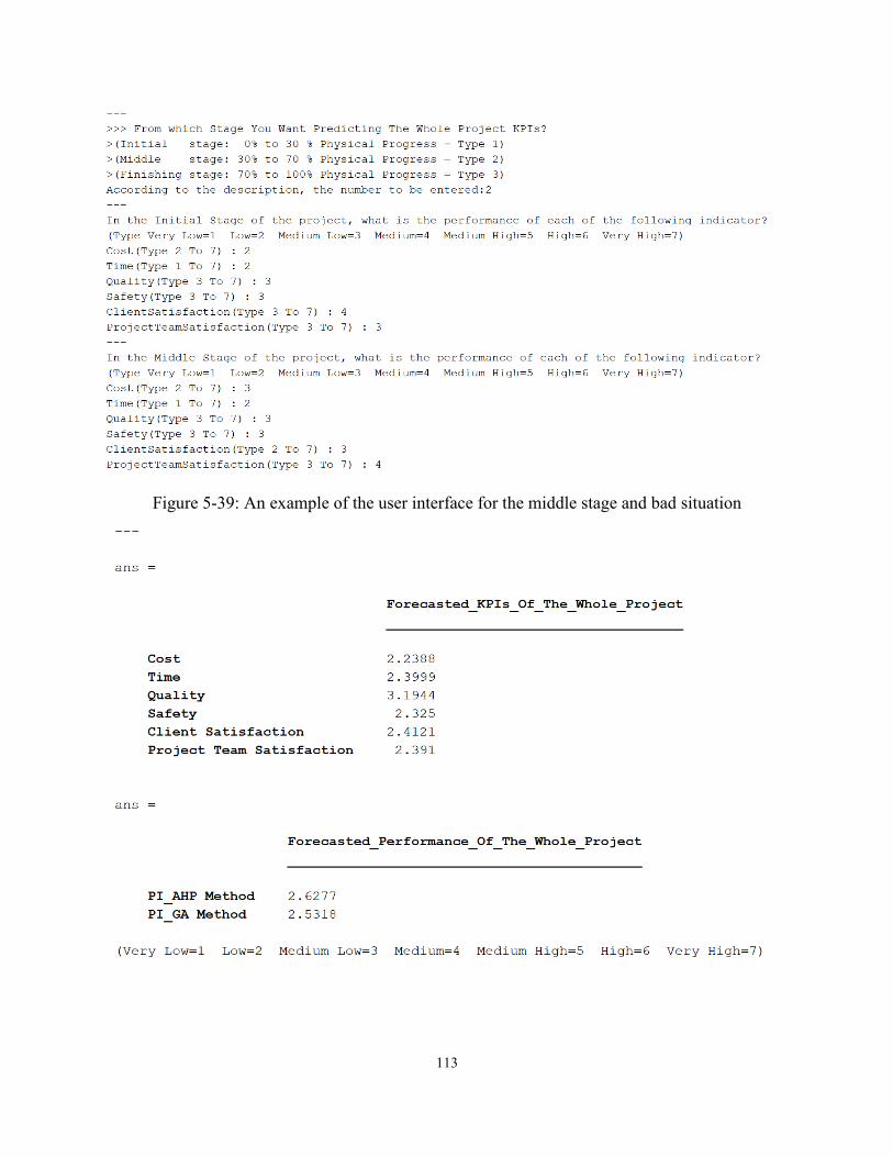
113
Figure 5-39: An example of the user interface for the middle stage and bad situation

114
Figure 5-40: An example of forecasted PI in the middle stage and bad situation At this stage, the user defines the information about different activity modes in the excel file. When
the user completed the excel file, the model will develop the best mode for each activity that opti-
mizes the PI of the project using the GA method. The results are illustrated in Figure 5-41. The
model also illustrates the iteration diagram for PI optimization (Figure 5-42).
Figure 5-41: An example of user interface showing the optimization results of the model when the project is in the middle stage and bad situation
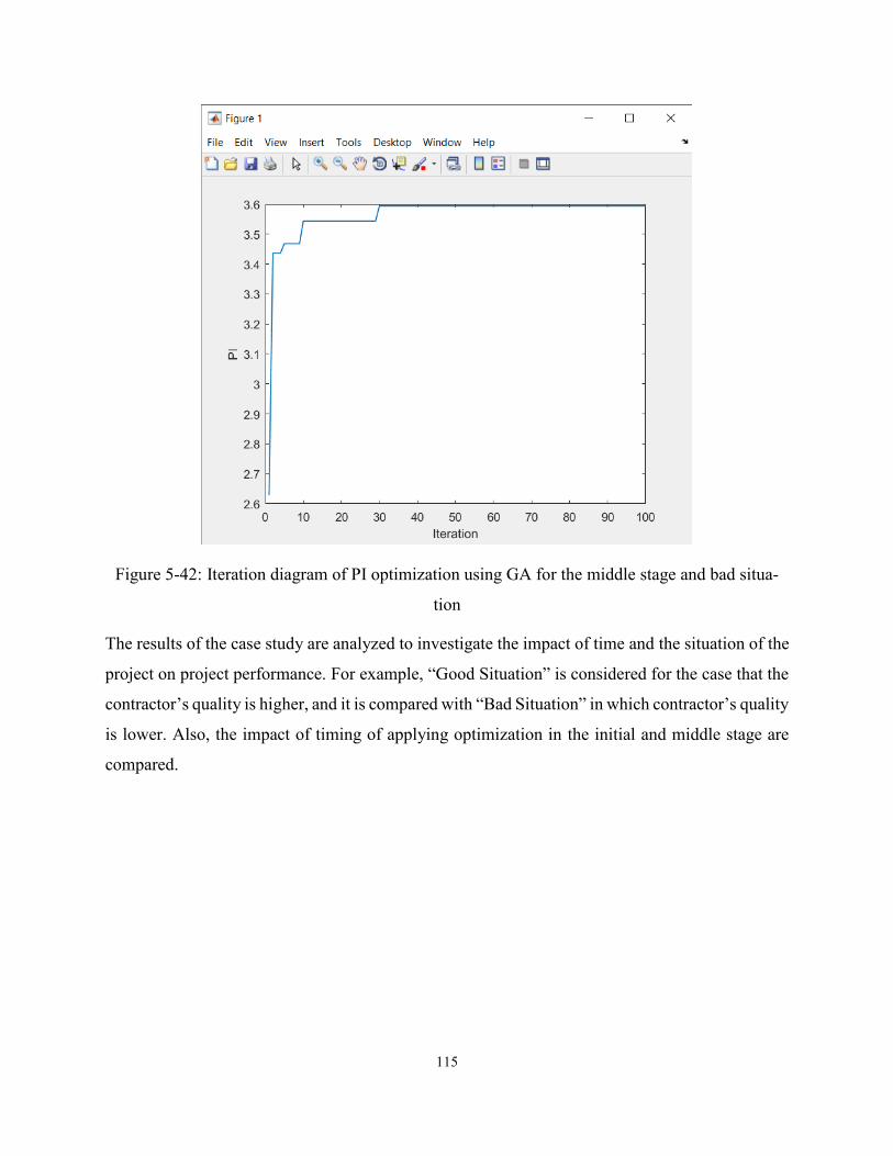
115
Figure 5-42: Iteration diagram of PI optimization using GA for the middle stage and bad situa-
tion
The results of the case study are analyzed to investigate the impact of time and the situation of the
project on project performance. For example, “Good Situation” is considered for the case that the
contractor’s quality is higher, and it is compared with “Bad Situation” in which contractor’s quality
is lower. Also, the impact of timing of applying optimization in the initial and middle stage are
compared.
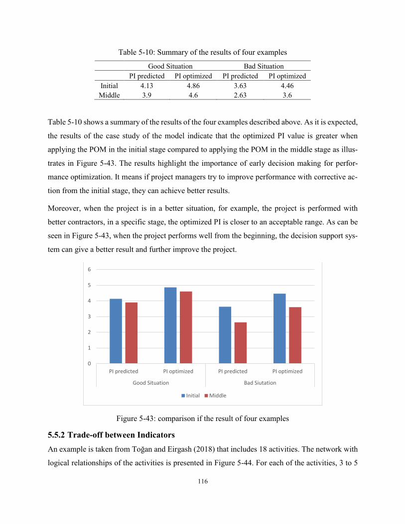
116
Table 5-10: Summary of the results of four examples
Good Situation Bad Situation PI predicted PI optimized PI predicted PI optimized
Initial 4.13 4.86 3.63 4.46 Middle 3.9 4.6 2.63 3.6
Table 5-10 shows a summary of the results of the four examples described above. As it is expected,
the results of the case study of the model indicate that the optimized PI value is greater when
applying the POM in the initial stage compared to applying the POM in the middle stage as illus-
trates in Figure 5-43. The results highlight the importance of early decision making for perfor-
mance optimization. It means if project managers try to improve performance with corrective ac-
tion from the initial stage, they can achieve better results.
Moreover, when the project is in a better situation, for example, the project is performed with
better contractors, in a specific stage, the optimized PI is closer to an acceptable range. As can be
seen in Figure 5-43, when the project performs well from the beginning, the decision support sys-
tem can give a better result and further improve the project.
Figure 5-43: comparison if the result of four examples
5.5.2 Trade-off between Indicators
An example is taken from Toğan and Eirgash (2018) that includes 18 activities. The network with
logical relationships of the activities is presented in Figure 5-44. For each of the activities, 3 to 5
0
1
2
3
4
5
6
PI predicted PI optimized PI predicted PI optimized
Good Situation Bad Siutation
Initial Middle
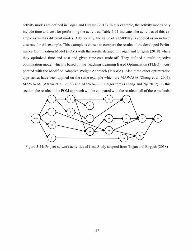
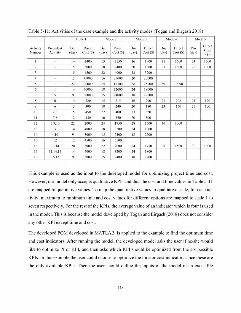
118
Table 5-11: Activities of the case example and the activity modes (Toğan and Eirgash 2018) Mode 1 Mode 2 Mode 3 Mode 4 Mode 5
Activity Number
Precedent Activity
Dur (day)
Direct Cost ($)
Dur (day)
Direct Cost ($)
Dur (day)
Direct Cost ($)
Dur (day)
Direct Cost ($)
Dur (day)
Direct Cost ($)
1 - 14 2400 15 2150 16 1900 21 1500 24 1200 2 - 15 3000 18 2400 20 1800 23 1500 25 1000 3 - 15 4500 22 4000 33 3200 4 - 12 45000 16 35000 20 30000 5 1 22 20000 24 17500 28 15000 30 10000 6 1 14 40000 18 32000 24 18000 7 5 9 30000 15 24000 18 22000 8 6 14 220 15 215 16 200 21 208 24 120 9 6 15 300 18 240 20 180 23 150 25 100 10 2,6 15 450 22 400 33 320 11 7,8 12 450 16 350 20 300 12 5,9,10 22 2000 24 1750 28 1500 30 1000 13 3 14 4000 18 3200 24 1800 14 4,10 9 3000 15 2400 18 2200 15 12 12 4500 16 3500 16 13,14 20 3000 22 2000 24 1750 28 1500 30 1000 17 11,14,15 14 4000 18 3200 24 1800 18 16,17 9 3000 15 2400 18 2200
This example is used as the input to the developed model for optimizing project time and cost.
However, our model only accepts qualitative KPIs and thus the cost and time values in Table 5-11
are mapped to qualitative values. To map the quantitative values to qualitative scale, for each ac-
tivity, maximum to minimum time and cost values for different options are mapped to scale 1 to
seven respectively. For the rest of the KPIs, the average value of an indicator which is four is used
in the model. This is because the model developed by Toğan and Eirgash (2018) does not consider
any other KPI except time and cost.
The developed POM developed in MATLAB is applied to the example to find the optimum time
and cost indicators. After running the model, the developed model asks the user if he/she would
like to optimize PI or KPI, and then asks which KPI should be optimized from the six possible
KPIs. In this example the user could choose to optimize the time or cost indicators since these are
the only available KPIs. Then the user should define the inputs of the model in an excel file
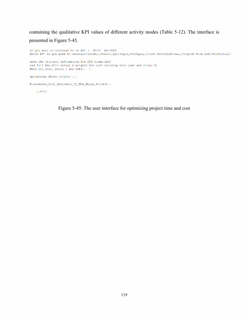
119
containing the qualitative KPI values of different activity modes (Table 5-12). The interface is
presented in Figure 5-45.
Figure 5-45: The user interface for optimizing project time and cost
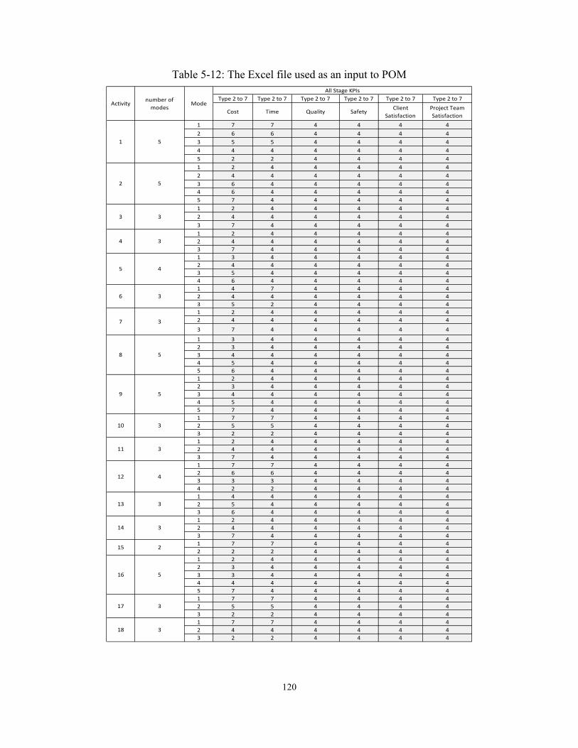
120
Table 5-12: The Excel file used as an input to POM
Type 2 to 7 Type 2 to 7 Type 2 to 7 Type 2 to 7 Type 2 to 7 Type 2 to 7
Cost Time Quality SafetyClient
Satisfaction
Project Team
Satisfaction
1 7 7 4 4 4 4
2 6 6 4 4 4 4
3 5 5 4 4 4 4
4 4 4 4 4 4 4
5 2 2 4 4 4 4
1 2 4 4 4 4 4
2 4 4 4 4 4 4
3 6 4 4 4 4 4
4 6 4 4 4 4 4
5 7 4 4 4 4 4
1 2 4 4 4 4 4
2 4 4 4 4 4 4
3 7 4 4 4 4 4
1 2 4 4 4 4 4
2 4 4 4 4 4 4
3 7 4 4 4 4 4
1 3 4 4 4 4 4
2 4 4 4 4 4 4
3 5 4 4 4 4 4
4 6 4 4 4 4 4
1 4 7 4 4 4 4
2 4 4 4 4 4 4
3 5 2 4 4 4 4
1 2 4 4 4 4 4
2 4 4 4 4 4 4
3 7 4 4 4 4 4
1 3 4 4 4 4 4
2 3 4 4 4 4 4
3 4 4 4 4 4 4
4 5 4 4 4 4 4
5 6 4 4 4 4 4
1 2 4 4 4 4 4
2 3 4 4 4 4 4
3 4 4 4 4 4 4
4 5 4 4 4 4 4
5 7 4 4 4 4 4
1 7 7 4 4 4 4
2 5 5 4 4 4 4
3 2 2 4 4 4 4
1 2 4 4 4 4 4
2 4 4 4 4 4 4
3 7 4 4 4 4 4
1 7 7 4 4 4 4
2 6 6 4 4 4 4
3 3 3 4 4 4 4
4 2 2 4 4 4 4
1 4 4 4 4 4 4
2 5 4 4 4 4 4
3 6 4 4 4 4 4
1 2 4 4 4 4 4
2 4 4 4 4 4 4
3 7 4 4 4 4 4
1 7 7 4 4 4 4
2 2 2 4 4 4 4
1 2 4 4 4 4 4
2 3 4 4 4 4 4
3 3 4 4 4 4 4
4 4 4 4 4 4 4
5 7 4 4 4 4 4
1 7 7 4 4 4 4
2 5 5 4 4 4 4
3 2 2 4 4 4 4
1 7 7 4 4 4 4
2 4 4 4 4 4 4
3 2 2 4 4 4 4
Activity Mode
13 3
12 4
3
1 5
2 5
3 3
4
17
318
All Stage KPIs
3
5
number of
modes
215
16
14
3
5 4
6 3
37
58
59
310
11 3

121
The model will develop optimized KPIs value and the activity modes chosen based on the
optimization. A sample output of the model is presented in Figure 5-46. The quantitative values of
cost and duration of the project are calculated based on the chosen activity modes. For calculating
the duration, the duration of the activities which are on the critical path are summed. For calculat-
ing the cost, the direct cost of each of the activities based on the chosen mode is summed and
added to the indirect cost of the project. Also, the iteration diagram of the optimization process is
illustrated in the developed program. A sample of this diagram is presented in Figure 5-47. Se-
lected options and generated modes for 18 activities are given in Table 5-13.
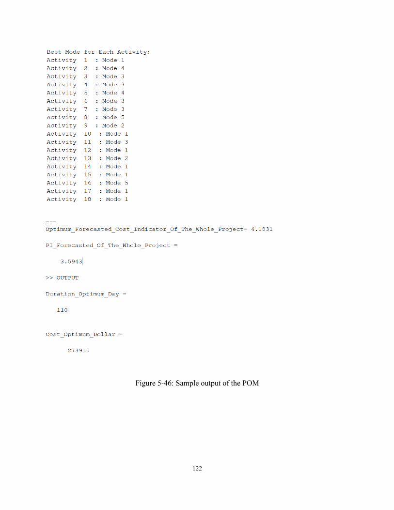
122
Figure 5-46: Sample output of the POM
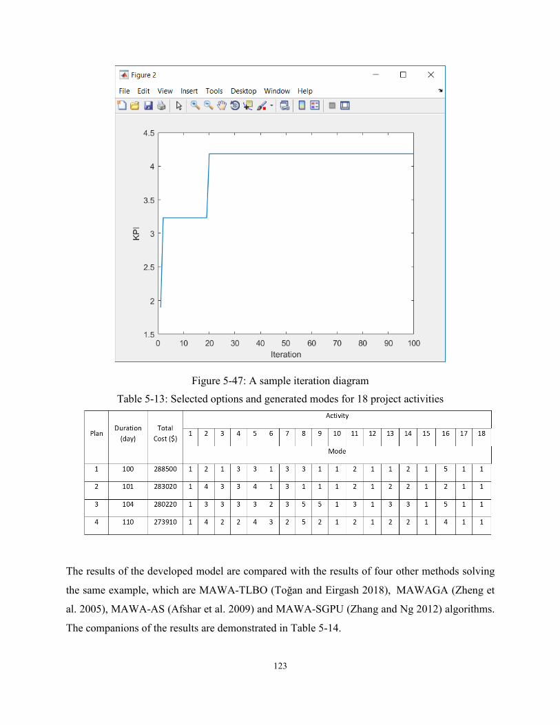
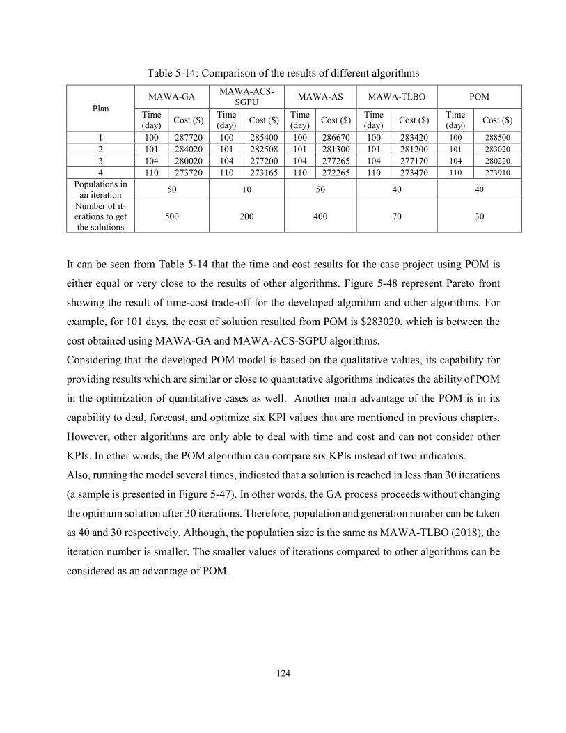
124
Table 5-14: Comparison of the results of different algorithms
Plan MAWA-GA MAWA-ACS-
SGPU MAWA-AS MAWA-TLBO POM
Time (day) Cost ($) Time
(day) Cost ($) Time (day) Cost ($) Time
(day) Cost ($) Time (day) Cost ($)
1 100 287720 100 285400 100 286670 100 283420 100 288500 2 101 284020 101 282508 101 281300 101 281200 101 283020 3 104 280020 104 277200 104 277265 104 277170 104 280220 4 110 273720 110 273165 110 272265 110 273470 110 273910
Populations in an iteration 50 10 50 40 40
Number of it-erations to get the solutions
500 200 400 70 30
It can be seen from Table 5-14 that the time and cost results for the case project using POM is
either equal or very close to the results of other algorithms. Figure 5-48 represent Pareto front
showing the result of time-cost trade-off for the developed algorithm and other algorithms. For
example, for 101 days, the cost of solution resulted from POM is $283020, which is between the
cost obtained using MAWA-GA and MAWA-ACS-SGPU algorithms.
Considering that the developed POM model is based on the qualitative values, its capability for
providing results which are similar or close to quantitative algorithms indicates the ability of POM
in the optimization of quantitative cases as well. Another main advantage of the POM is in its
capability to deal, forecast, and optimize six KPI values that are mentioned in previous chapters.
However, other algorithms are only able to deal with time and cost and can not consider other
KPIs. In other words, the POM algorithm can compare six KPIs instead of two indicators.
Also, running the model several times, indicated that a solution is reached in less than 30 iterations
(a sample is presented in Figure 5-47). In other words, the GA process proceeds without changing
the optimum solution after 30 iterations. Therefore, population and generation number can be taken
as 40 and 30 respectively. Although, the population size is the same as MAWA-TLBO (2018), the
iteration number is smaller. The smaller values of iterations compared to other algorithms can be
considered as an advantage of POM.
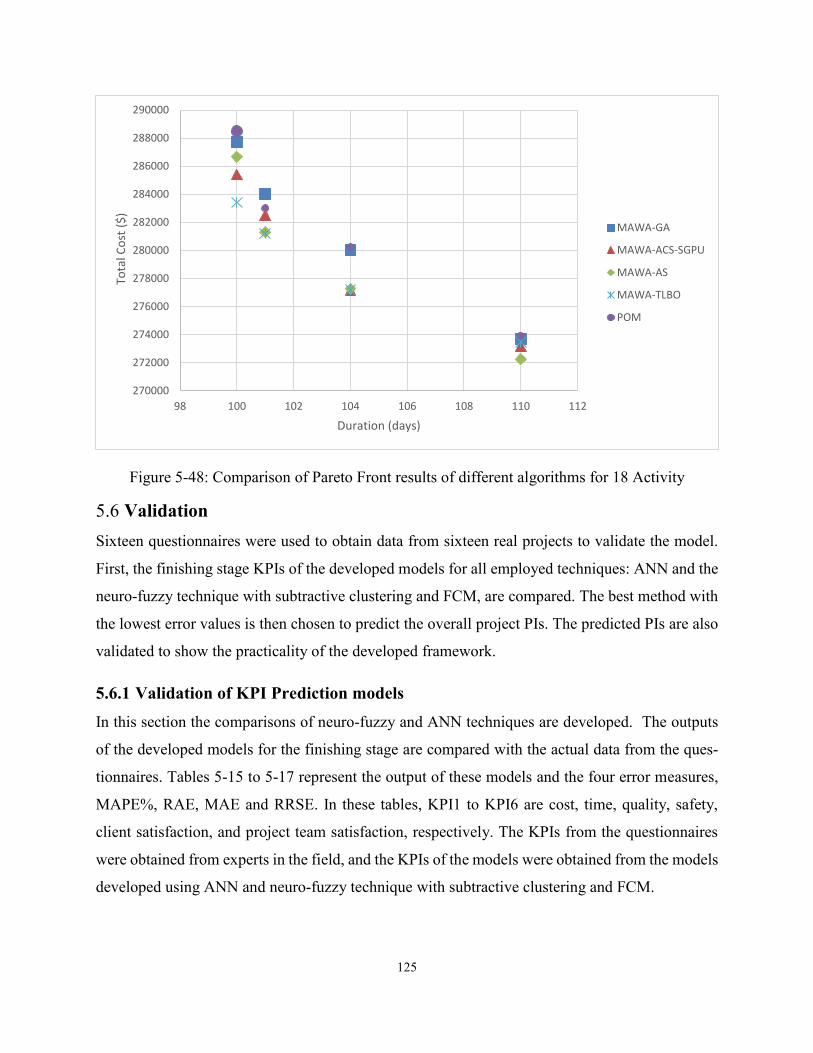
125
Figure 5-48: Comparison of Pareto Front results of different algorithms for 18 Activity
5.6 Validation Sixteen questionnaires were used to obtain data from sixteen real projects to validate the model.
First, the finishing stage KPIs of the developed models for all employed techniques: ANN and the
neuro-fuzzy technique with subtractive clustering and FCM, are compared. The best method with
the lowest error values is then chosen to predict the overall project PIs. The predicted PIs are also
validated to show the practicality of the developed framework.
5.6.1 Validation of KPI Prediction models
In this section the comparisons of neuro-fuzzy and ANN techniques are developed. The outputs
of the developed models for the finishing stage are compared with the actual data from the ques-
tionnaires. Tables 5-15 to 5-17 represent the output of these models and the four error measures,
MAPE%, RAE, MAE and RRSE. In these tables, KPI1 to KPI6 are cost, time, quality, safety,
client satisfaction, and project team satisfaction, respectively. The KPIs from the questionnaires
were obtained from experts in the field, and the KPIs of the models were obtained from the models
developed using ANN and neuro-fuzzy technique with subtractive clustering and FCM.
270000
272000
274000
276000
278000
280000
282000
284000
286000
288000
290000
98 100 102 104 106 108 110 112
Tota
l Co
st (
$)
Duration (days)
MAWA-GA
MAWA-ACS-SGPU
MAWA-AS
MAWA-TLBO
POM

126
Table 5-15 shows validation results of KPI prediction models with the neuro-fuzzy technique using
subtractive clustering for the finishing stage. The MAPE error for KPI3 is less than 20% showing
a sound forecast. KPI1, KPI2, KPI5, and KPI6 have MAPE amount between 20% to 50%
indicating a feasible forecast. Although, KPI4 has a MAPE around 50%. Table 5-16 illustrate the
validation results of KPI prediction models with the neuro-fuzzy technique using FCM for the
finishing stage. The results show that the MAPE for KPI1 and KPI3 and KPI4 is greater than 50%
indicating an error forecast. On the other hand, KPI2, KPI5, and KPI6 have MAPE lower than
50% showing a feasible forecast. Table 5-17 represent validation results of KPIs prediction models
with the neural network technique for the finishing stage. As shown in the table, the amount of
MAPE for all KPI1, KPI2, KPI3, KPI5, and KPI6 is between 20% to 50% showing a feasible
forecast. Although, MAPE of KPI4 is above 50%.
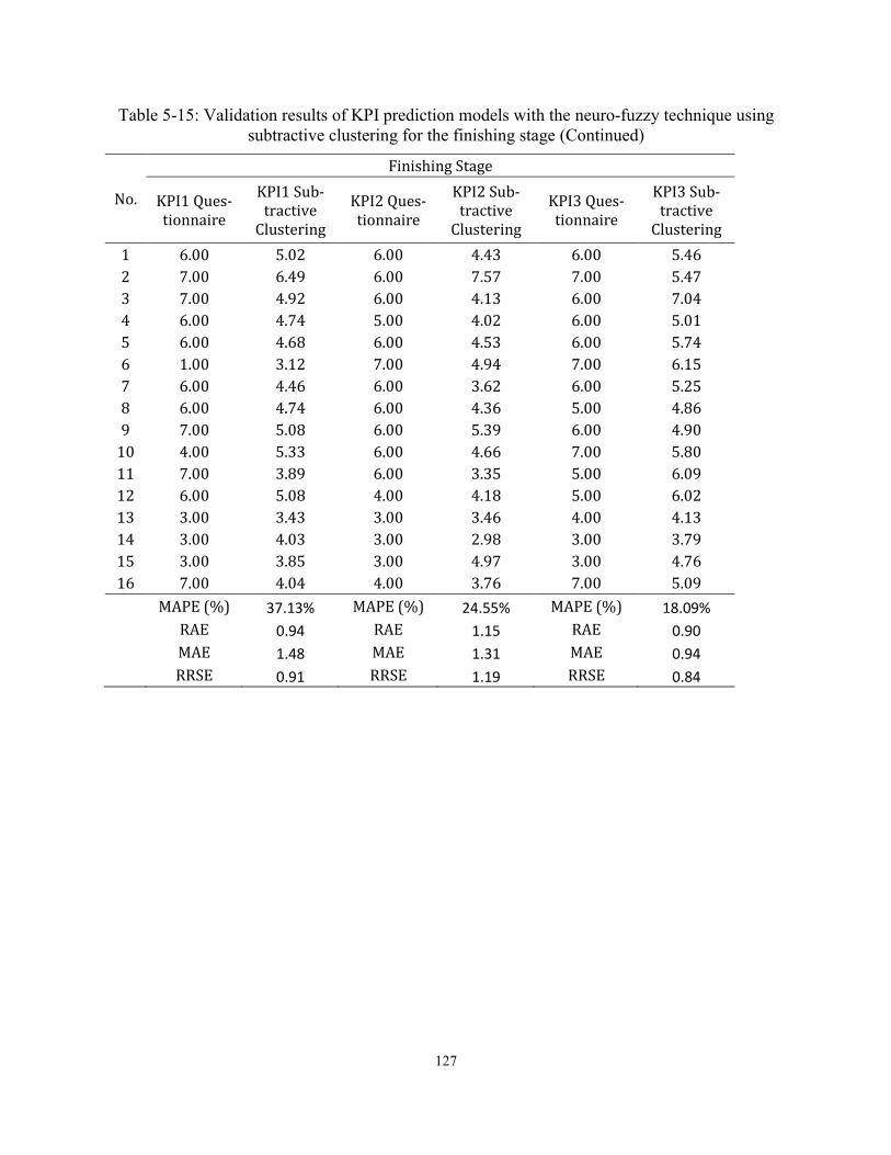
127
Table 5-15: Validation results of KPI prediction models with the neuro-fuzzy technique using subtractive clustering for the finishing stage (Continued)
No.
Finishing Stage
KPI1 Ques-tionnaire
KPI1 Sub-tractive
Clustering
KPI2 Ques-tionnaire
KPI2 Sub-tractive
Clustering
KPI3 Ques-tionnaire
KPI3 Sub-tractive
Clustering
1 6.00 5.02 6.00 4.43 6.00 5.46
2 7.00 6.49 6.00 7.57 7.00 5.47
3 7.00 4.92 6.00 4.13 6.00 7.04
4 6.00 4.74 5.00 4.02 6.00 5.01
5 6.00 4.68 6.00 4.53 6.00 5.74
6 1.00 3.12 7.00 4.94 7.00 6.15
7 6.00 4.46 6.00 3.62 6.00 5.25
8 6.00 4.74 6.00 4.36 5.00 4.86
9 7.00 5.08 6.00 5.39 6.00 4.90
10 4.00 5.33 6.00 4.66 7.00 5.80
11 7.00 3.89 6.00 3.35 5.00 6.09
12 6.00 5.08 4.00 4.18 5.00 6.02
13 3.00 3.43 3.00 3.46 4.00 4.13
14 3.00 4.03 3.00 2.98 3.00 3.79
15 3.00 3.85 3.00 4.97 3.00 4.76
16 7.00 4.04 4.00 3.76 7.00 5.09 MAPE (%) 37.13% MAPE (%) 24.55% MAPE (%) 18.09% RAE 0.94 RAE 1.15 RAE 0.90 MAE 1.48 MAE 1.31 MAE 0.94
RRSE 0.91 RRSE 1.19 RRSE 0.84
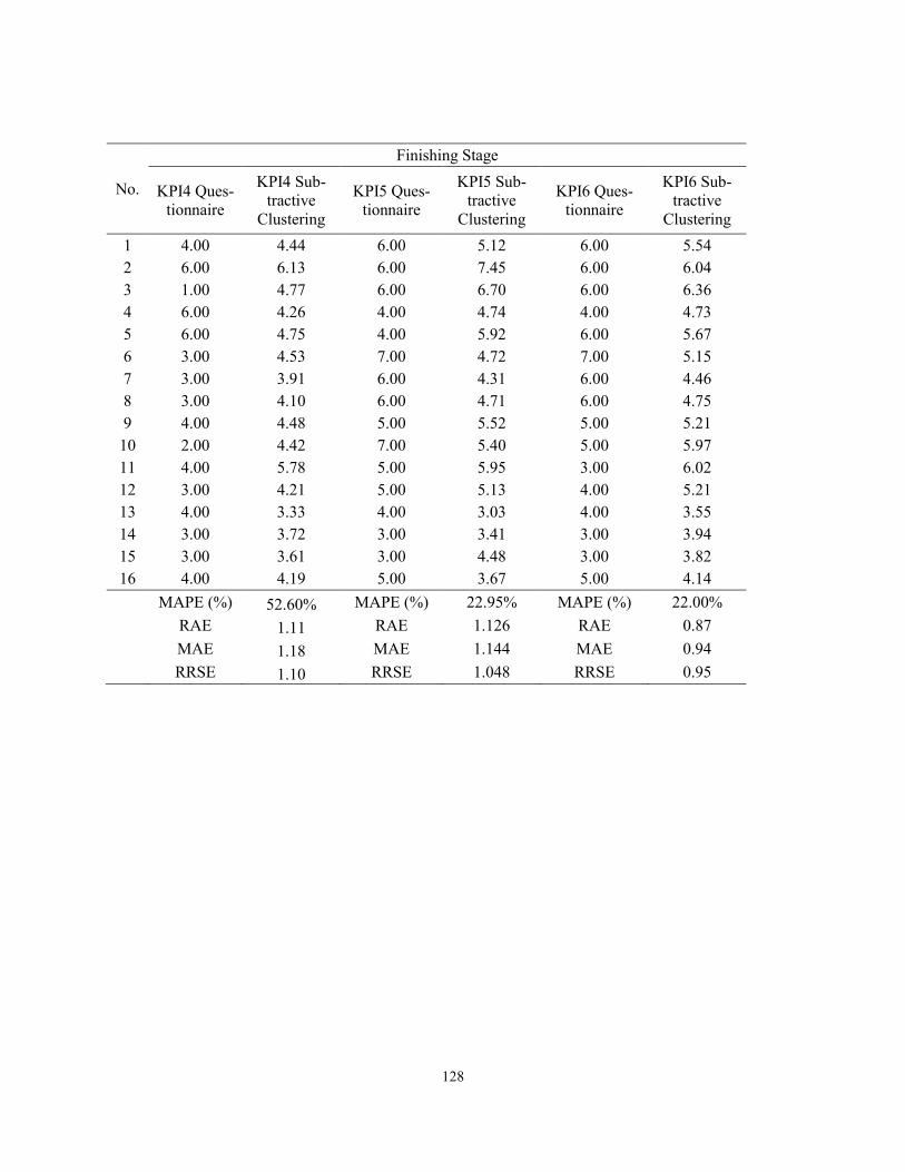
128
No.
Finishing Stage
KPI4 Ques-tionnaire
KPI4 Sub-tractive
Clustering
KPI5 Ques-tionnaire
KPI5 Sub-tractive
Clustering
KPI6 Ques-tionnaire
KPI6 Sub-tractive
Clustering 1 4.00 4.44 6.00 5.12 6.00 5.54 2 6.00 6.13 6.00 7.45 6.00 6.04 3 1.00 4.77 6.00 6.70 6.00 6.36 4 6.00 4.26 4.00 4.74 4.00 4.73 5 6.00 4.75 4.00 5.92 6.00 5.67 6 3.00 4.53 7.00 4.72 7.00 5.15 7 3.00 3.91 6.00 4.31 6.00 4.46 8 3.00 4.10 6.00 4.71 6.00 4.75 9 4.00 4.48 5.00 5.52 5.00 5.21
10 2.00 4.42 7.00 5.40 5.00 5.97 11 4.00 5.78 5.00 5.95 3.00 6.02 12 3.00 4.21 5.00 5.13 4.00 5.21 13 4.00 3.33 4.00 3.03 4.00 3.55 14 3.00 3.72 3.00 3.41 3.00 3.94 15 3.00 3.61 3.00 4.48 3.00 3.82 16 4.00 4.19 5.00 3.67 5.00 4.14 MAPE (%) 52.60% MAPE (%) 22.95% MAPE (%) 22.00% RAE 1.11 RAE 1.126 RAE 0.87 MAE 1.18 MAE 1.144 MAE 0.94 RRSE 1.10 RRSE 1.048 RRSE 0.95
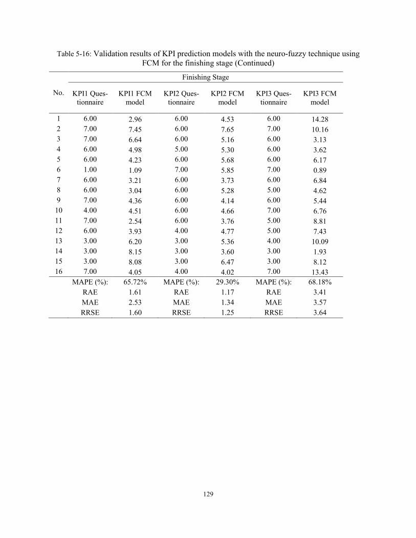
129
Table 5-16: Validation results of KPI prediction models with the neuro-fuzzy technique using FCM for the finishing stage (Continued)
No.
Finishing Stage
KPI1 Ques-tionnaire
KPI1 FCM model
KPI2 Ques-tionnaire
KPI2 FCM model
KPI3 Ques-tionnaire
KPI3 FCM model
1 6.00 2.96 6.00 4.53 6.00 14.28 2 7.00 7.45 6.00 7.65 7.00 10.16 3 7.00 6.64 6.00 5.16 6.00 3.13 4 6.00 4.98 5.00 5.30 6.00 3.62 5 6.00 4.23 6.00 5.68 6.00 6.17 6 1.00 1.09 7.00 5.85 7.00 0.89 7 6.00 3.21 6.00 3.73 6.00 6.84 8 6.00 3.04 6.00 5.28 5.00 4.62 9 7.00 4.36 6.00 4.14 6.00 5.44
10 4.00 4.51 6.00 4.66 7.00 6.76 11 7.00 2.54 6.00 3.76 5.00 8.81 12 6.00 3.93 4.00 4.77 5.00 7.43 13 3.00 6.20 3.00 5.36 4.00 10.09 14 3.00 8.15 3.00 3.60 3.00 1.93 15 3.00 8.08 3.00 6.47 3.00 8.12 16 7.00 4.05 4.00 4.02 7.00 13.43 MAPE (%): 65.72% MAPE (%): 29.30% MAPE (%): 68.18% RAE 1.61 RAE 1.17 RAE 3.41 MAE 2.53 MAE 1.34 MAE 3.57 RRSE 1.60 RRSE 1.25 RRSE 3.64
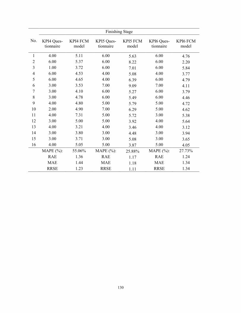
130
No.
Finishing Stage
KPI4 Ques-tionnaire
KPI4 FCM model
KPI5 Ques-tionnaire
KPI5 FCM model
KPI6 Ques-tionnaire
KPI6 FCM model
1 4.00 5.11 6.00 5.63 6.00 4.76 2 6.00 5.37 6.00 8.22 6.00 2.20 3 1.00 3.72 6.00 7.01 6.00 5.84 4 6.00 4.53 4.00 5.08 4.00 3.77 5 6.00 4.65 4.00 6.39 6.00 4.79 6 3.00 3.53 7.00 9.09 7.00 4.11 7 3.00 4.10 6.00 5.27 6.00 3.79 8 3.00 4.78 6.00 5.49 6.00 4.46 9 4.00 4.80 5.00 5.79 5.00 4.72
10 2.00 4.90 7.00 6.29 5.00 4.62 11 4.00 7.31 5.00 5.72 3.00 5.38 12 3.00 5.00 5.00 3.92 4.00 5.64 13 4.00 3.21 4.00 3.46 4.00 3.12 14 3.00 3.80 3.00 4.48 3.00 3.94 15 3.00 3.71 3.00 5.08 3.00 3.65 16 4.00 5.05 5.00 3.87 5.00 4.05 MAPE (%): 55.06% MAPE (%): 25.88% MAPE (%): 27.73% RAE 1.36 RAE 1.17 RAE 1.24 MAE 1.44 MAE 1.18 MAE 1.34 RRSE 1.23 RRSE 1.11 RRSE 1.34
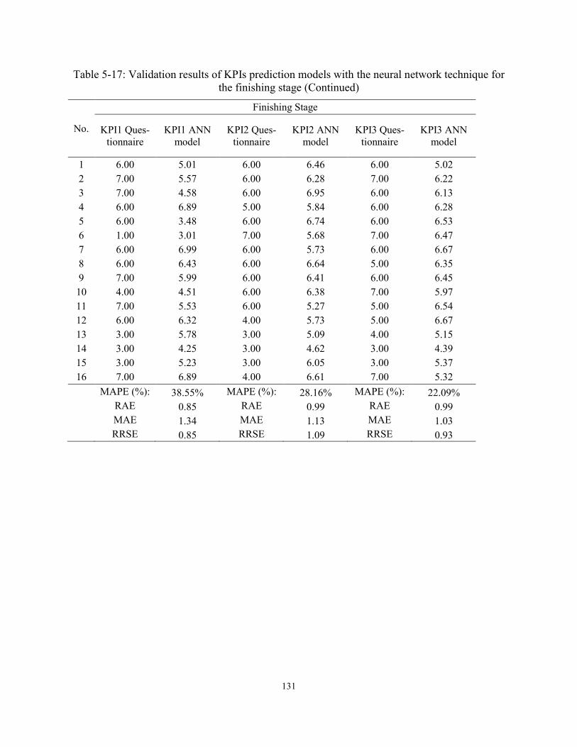
131
Table 5-17: Validation results of KPIs prediction models with the neural network technique for the finishing stage (Continued)
No.
Finishing Stage
KPI1 Ques-tionnaire
KPI1 ANN model
KPI2 Ques-tionnaire
KPI2 ANN model
KPI3 Ques-tionnaire
KPI3 ANN model
1 6.00 5.01 6.00 6.46 6.00 5.02 2 7.00 5.57 6.00 6.28 7.00 6.22 3 7.00 4.58 6.00 6.95 6.00 6.13 4 6.00 6.89 5.00 5.84 6.00 6.28 5 6.00 3.48 6.00 6.74 6.00 6.53 6 1.00 3.01 7.00 5.68 7.00 6.47 7 6.00 6.99 6.00 5.73 6.00 6.67 8 6.00 6.43 6.00 6.64 5.00 6.35 9 7.00 5.99 6.00 6.41 6.00 6.45
10 4.00 4.51 6.00 6.38 7.00 5.97 11 7.00 5.53 6.00 5.27 5.00 6.54 12 6.00 6.32 4.00 5.73 5.00 6.67 13 3.00 5.78 3.00 5.09 4.00 5.15 14 3.00 4.25 3.00 4.62 3.00 4.39 15 3.00 5.23 3.00 6.05 3.00 5.37 16 7.00 6.89 4.00 6.61 7.00 5.32 MAPE (%): 38.55% MAPE (%): 28.16% MAPE (%): 22.09% RAE 0.85 RAE 0.99 RAE 0.99 MAE 1.34 MAE 1.13 MAE 1.03 RRSE 0.85 RRSE 1.09 RRSE 0.93
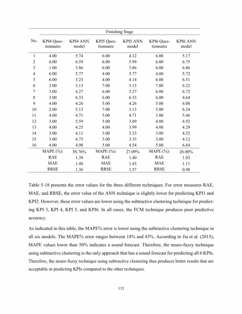
132
No.
Finishing Stage
KPI4 Ques-tionnaire
KPI4 ANN model
KPI5 Ques-tionnaire
KPI5 ANN model
KPI6 Ques-tionnaire
KPI6 ANN model
1 4.00 5.74 6.00 4.12 6.00 5.17 2 6.00 6.59 6.00 5.99 6.00 6.75 3 1.00 3.86 6.00 3.86 6.00 6.86 4 6.00 5.77 4.00 5.77 4.00 5.72 5 6.00 3.23 4.00 4.14 6.00 6.51 6 3.00 3.13 7.00 3.13 7.00 6.32 7 3.00 4.27 6.00 3.27 6.00 6.72 8 3.00 6.33 6.00 6.33 6.00 4.64 9 4.00 4.26 5.00 4.26 5.00 6.08
10 2.00 5.13 7.00 3.13 5.00 6.24 11 4.00 4.71 5.00 4.71 3.00 5.46 12 3.00 5.59 5.00 3.09 4.00 4.92 13 4.00 4.25 4.00 3.99 4.00 4.29 14 3.00 4.11 3.00 5.33 3.00 4.52 15 3.00 4.75 3.00 3.33 3.00 4.12 16 4.00 4.98 5.00 4.54 5.00 6.64 MAPE (%): 58.76% MAPE (%): 27.09% MAPE (%): 26.00% RAE 1.39 RAE 1.40 RAE 1.03 MAE 1.48 MAE 1.43 MAE 1.11 RRSE 1.36 RRSE 1.57 RRSE 0.98
Table 5-18 presents the error values for the three different techniques. For error measures RAE,
MAE, and RRSE, the error value of the ANN technique is slightly lower for predicting KPI1 and
KPI2. However, these error values are lower using the subtractive clustering technique for predict-
ing KPI 3, KPI 4, KPI 5, and KPI6. In all cases, the FCM technique produces poor predictive
accuracy.
As indicated in this table, the MAPE% error is lower using the subtractive clustering technique in
all six models. The MAPE% error ranges between 18% and 43%. According to Jia et al. (2015),
MAPE values lower than 50% indicates a sound forecast. Therefore, the neuro-fuzzy technique
using subtractive clustering is the only approach that has a sound forecast for predicting all 6 KPIs.
Therefore, the neuro-fuzzy technique using subtractive clustering thus produces better results that are
acceptable in predicting KPIs compared to the other techniques.
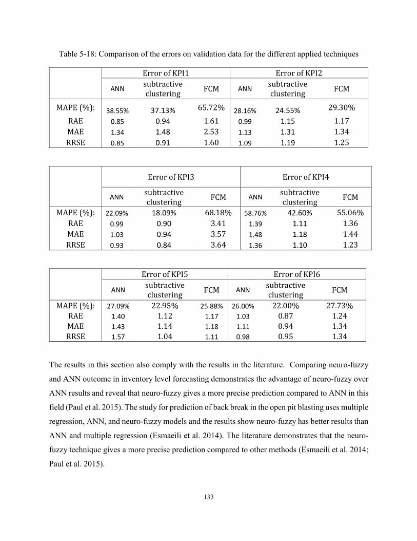
133
Table 5-18: Comparison of the errors on validation data for the different applied techniques
Error of KPI1 Error of KPI2
ANN subtractive clustering
FCM ANN subtractive clustering
FCM
MAPE (%): 38.55% 37.13% 65.72% 28.16% 24.55% 29.30%
RAE 0.85 0.94 1.61 0.99 1.15 1.17
MAE 1.34 1.48 2.53 1.13 1.31 1.34
RRSE 0.85 0.91 1.60 1.09 1.19 1.25
Error of KPI3 Error of KPI4
ANN subtractive clustering
FCM ANN subtractive clustering
FCM
MAPE (%): 22.09% 18.09% 68.18% 58.76% 42.60% 55.06%
RAE 0.99 0.90 3.41 1.39 1.11 1.36
MAE 1.03 0.94 3.57 1.48 1.18 1.44
RRSE 0.93 0.84 3.64 1.36 1.10 1.23
Error of KPI5 Error of KPI6
ANN subtractive clustering
FCM ANN subtractive clustering
FCM
MAPE (%): 27.09% 22.95% 25.88% 26.00% 22.00% 27.73% RAE 1.40 1.12 1.17 1.03 0.87 1.24 MAE 1.43 1.14 1.18 1.11 0.94 1.34 RRSE 1.57 1.04 1.11 0.98 0.95 1.34
The results in this section also comply with the results in the literature. Comparing neuro-fuzzy
and ANN outcome in inventory level forecasting demonstrates the advantage of neuro-fuzzy over
ANN results and reveal that neuro-fuzzy gives a more precise prediction compared to ANN in this
field (Paul et al. 2015). The study for prediction of back break in the open pit blasting uses multiple
regression, ANN, and neuro-fuzzy models and the results show neuro-fuzzy has better results than
ANN and multiple regression (Esmaeili et al. 2014). The literature demonstrates that the neuro-
fuzzy technique gives a more precise prediction compared to other methods (Esmaeili et al. 2014;
Paul et al. 2015).
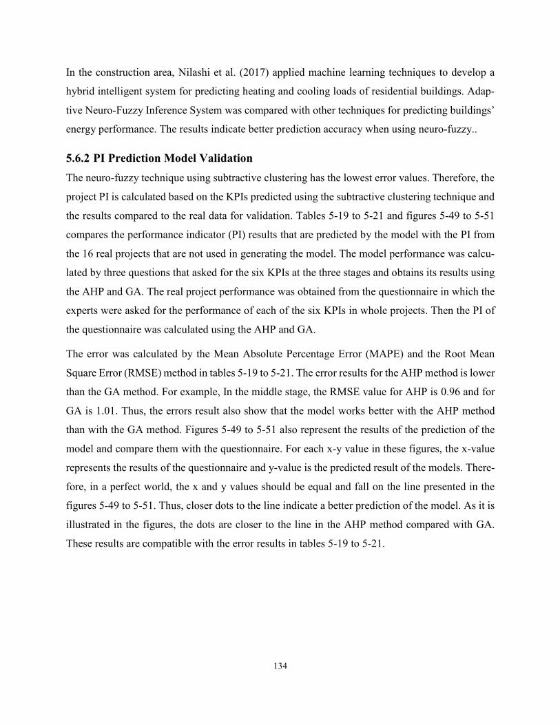
134
In the construction area, Nilashi et al. (2017) applied machine learning techniques to develop a
hybrid intelligent system for predicting heating and cooling loads of residential buildings. Adap-
tive Neuro-Fuzzy Inference System was compared with other techniques for predicting buildings’
energy performance. The results indicate better prediction accuracy when using neuro-fuzzy..
5.6.2 PI Prediction Model Validation
The neuro-fuzzy technique using subtractive clustering has the lowest error values. Therefore, the
project PI is calculated based on the KPIs predicted using the subtractive clustering technique and
the results compared to the real data for validation. Tables 5-19 to 5-21 and figures 5-49 to 5-51
compares the performance indicator (PI) results that are predicted by the model with the PI from
the 16 real projects that are not used in generating the model. The model performance was calcu-
lated by three questions that asked for the six KPIs at the three stages and obtains its results using
the AHP and GA. The real project performance was obtained from the questionnaire in which the
experts were asked for the performance of each of the six KPIs in whole projects. Then the PI of
the questionnaire was calculated using the AHP and GA.
The error was calculated by the Mean Absolute Percentage Error (MAPE) and the Root Mean
Square Error (RMSE) method in tables 5-19 to 5-21. The error results for the AHP method is lower
than the GA method. For example, In the middle stage, the RMSE value for AHP is 0.96 and for
GA is 1.01. Thus, the errors result also show that the model works better with the AHP method
than with the GA method. Figures 5-49 to 5-51 also represent the results of the prediction of the
model and compare them with the questionnaire. For each x-y value in these figures, the x-value
represents the results of the questionnaire and y-value is the predicted result of the models. There-
fore, in a perfect world, the x and y values should be equal and fall on the line presented in the
figures 5-49 to 5-51. Thus, closer dots to the line indicate a better prediction of the model. As it is
illustrated in the figures, the dots are closer to the line in the AHP method compared with GA.
These results are compatible with the error results in tables 5-19 to 5-21.
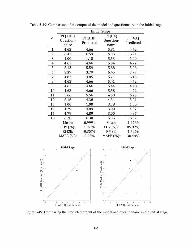
135
Table 5-19: Comparison of the output of the model and questionnaire in the initial stage
o.
Initial Stage
PI (AHP) Question-
naire
PI (AHP) Predicted
PI (GA) Question-
naire
PI (GA) Predicted
1 4.63 4.66 5.81 4.72 2 6.42 6.59 6.33 6.21 3 1.00 1.18 5.53 1.00 4 4.63 4.66 5.04 4.72 5 5.13 5.59 5.88 5.08 6 3.37 3.79 6.45 3.77 7 4.82 3.85 5.71 6.15 8 4.63 4.66 5.41 4.72 9 4.62 4.66 5.44 4.48
10 4.63 4.66 5.58 4.72 11 5.66 5.56 4.50 6.23 12 5.16 4.38 4.31 5.01 13 1.00 1.00 3.78 1.00 14 4.79 4.89 3.00 4.87 15 4.79 4.89 3.00 4.87 16 6.20 6.30 5.35 6.32
Mean: 0.9991 Mean: 1.4769 COV (%): 9.36% COV (%): 85.92% RMSE: 0.3574 RMSE: 1.7869 MAPE (%): 5.52% MAPE (%): 30.49%
Figure 5-49: Comparing the predicted output of the model and questionnaire in the initial stage
136
Table 5-20: Comparison of the predicted output of the model and questionnaire in the middle stage
No.
Middle Stage PI (AHP) Question-
naire
PI (AHP) Predicted
PI (GA) Question-
naire
PI (GA) Predicted
1 5.73 4.35 5.81 4.37 2 6.43 6.26 6.33 5.99 3 5.44 5.65 5.53 5.63 4 5.22 4.94 5.04 4.69 5 6.00 5.00 6.01 5.00 6 5.83 5.34 6.45 5.55 7 5.60 3.94 5.71 3.90 8 5.28 4.54 5.41 4.36 9 5.50 4.79 5.44 4.69
10 5.24 5.08 5.46 5.10 11 4.51 4.19 4.37 4.12 12 4.40 5.10 4.25 5.10 13 3.79 4.25 3.78 4.25 14 3.00 4.92 3.00 4.90 15 3.00 4.30 3.00 4.20 16 5.62 4.41 5.35 4.27
Mean: 1.0520 Mean: 1.0691 COV (%): 19.79% COV (%): 20.23% RMSE: 0.9609 RMSE: 1.0111 MAPE (%): 17.79% MAPE (%): 18.85%
Figure 5-50: Comparing the predicted output of the model and questionnaire in the middle stage
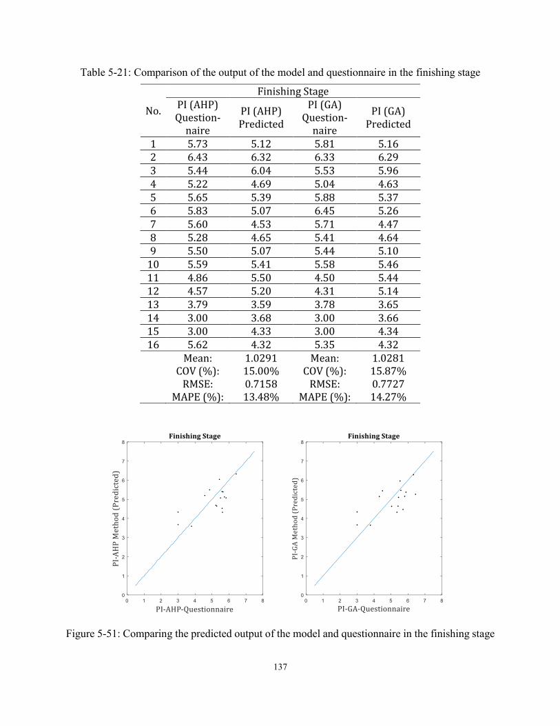
137
Table 5-21: Comparison of the output of the model and questionnaire in the finishing stage
No.
Finishing Stage PI (AHP) Question-
naire
PI (AHP) Predicted
PI (GA) Question-
naire
PI (GA) Predicted
1 5.73 5.12 5.81 5.16 2 6.43 6.32 6.33 6.29 3 5.44 6.04 5.53 5.96 4 5.22 4.69 5.04 4.63 5 5.65 5.39 5.88 5.37 6 5.83 5.07 6.45 5.26 7 5.60 4.53 5.71 4.47 8 5.28 4.65 5.41 4.64 9 5.50 5.07 5.44 5.10
10 5.59 5.41 5.58 5.46 11 4.86 5.50 4.50 5.44 12 4.57 5.20 4.31 5.14 13 3.79 3.59 3.78 3.65 14 3.00 3.68 3.00 3.66 15 3.00 4.33 3.00 4.34 16 5.62 4.32 5.35 4.32
Mean: 1.0291 Mean: 1.0281 COV (%): 15.00% COV (%): 15.87% RMSE: 0.7158 RMSE: 0.7727 MAPE (%): 13.48% MAPE (%): 14.27%
Figure 5-51: Comparing the predicted output of the model and questionnaire in the finishing stage
138
CHAPTER 6: CONCLUSION AND RECOMMEN-
DATIONS
6.1 Summary and Conclusion Key Performance Indicators (KPIs) evaluate different projects aspects and are used to determine
the health status of building projects. Therefore, by evaluating and predicting KPIs, monitoring
and controlling project progress can be facilitated. A comprehensive literature review of the exist-
ing research is performed, highlighting the limitations of the previously developed models for
forecasting project KPIs and overall project performance. First, limited work has been done on
forecasting project performance using KPIs at the project level. Second, there has been little focus
on dynamic performance measurement and forecasting during projects.
Based on the limitations mentioned above, this research is motivated to develop a framework for
measuring and forecasting project KPIs and overall project performance indicator (PI). Because
of different stakeholder investments and benefits, the first thing that needs to be defined is from
whose viewpoint the performance is to be measured. A list of KPIs used in the literature at the
project level was prepared, and their frequencies indicated. The first six KPIs were chosen due to
the frequency of their use in the literature; they were used by approximately 50 percent of the
studies. To further justify the selection of these six KPIs, a questionnaire was distributed among
experts in the field. Based on the questionnaire responses, the first six KPIs got 40 to 90 percent
of the score, with the seventh KPI receiving a score of only 27. Given the tangibly larger score
ratio between KPI number six and seven in the questionnaire, the first six KPIs were chosen for
model development. The selected KPIs are cost, time, quality, safety, client satisfaction, and pro-
ject team satisfaction.
The KPIs of three critical project stages (initial, middle, and finishing) are used to predict the whole
project KPIs using two main techniques: Artificial Neural Networks (ANN) and neuro-fuzzy mod-
els. In the ANN, the best model is selected by changing the number of neurons of the hidden layer.
Neuro-fuzzy models are developed in two steps; first, initial Fuzzy Inference System (FIS) models
are developed using both subtractive clustering and Fuzzy C-means (FCM). In subtractive cluster-
ing, the cluster radius is optimized to achieve optimum precision without overfitting. Next, the
139
optimization of the initial FIS model is performed using ANN. In the neuro-fuzzy technique, 18
different models are developed, six models for each of the three critical project stages.
Also, this research develops a model for predicting the KPIs of the next stages and KPIs trends.
First, neuro-fuzzy models are used to predict the KPIs of the next stages based on the KPIs of
previous stages. Linear interpolation is then used to predict the KPIs at different progress% of the
project. Graphic plots are also used to visualize KPIs trends for better analysis of a project.
The weighted sum of the project KPIs is then used to calculate the overall project Performance
Indicator (PI). Two different methods were used to determine the weight for each of the indicators,
the Analytical Hierarchy Process (AHP) and the Genetic Algorithm (GA) method. In the AHP, the
relative importance of each indicator is determined based on paired comparisons in a matrix.
A Performance Optimization Model (POM) is also developed to optimize the overall project PI
considering various project KPIs using GA. The developed model can be applied at the initial and
middle stage of the project for selecting corrective action. If the overall PI of the project is less
than the acceptable value, the best scenario for the next stage could be found using POM. Codes
are written in MATLAB to implement performance optimization model for corrective action se-
lection. The developed model allows a user interface to interact with the experts. Examples are
employed to analyze the performance of the developed model showing improvement in the project
PI. Also, the results highlight the importance of early decision making for performance optimiza-
tion.
All KPIs were measured qualitatively by designing a questionnaire. The KPIs are measured qual-
itatively using a 1 to 7 scale for three critical project stages. The data in this study was collected
from experts in construction companies in Tehran, Iran. Two sets of questionnaires were designed.
The first questionnaire was used to collect data from different projects to run the model, and then
the second questionnaire was used to justify the selected six KPIs used in this research. This re-
search measures project performance from the owner's point of view.
Models are developed using the steps described above to forecast project performance using
MATLAB software. ANN and neuro-fuzzy using both FCM and subtractive clustering, are used
to develop models for predicting whole project KPIs. Models are also developed for predicting
KPIs of the next stage.
140
To validate the model, questionnaires were designed to obtain information about 16 real projects.
The errors of the three methods used for predicting KPIs, namely: ANN, neuro-fuzzy with FCM
and neuro-fuzzy with subtractive clustering, were compared using different error calculation meth-
ods. The results indicate that the neuro-fuzzy technique using subtractive clustering performs
better and has lower error values than the other two methods. The PIs obtained from the neuro-
fuzzy technique with subtractive clustering (using the AHP and the GA approaches) and the PIs
obtained from the questionnaire responses were compared. The results indicate that the AHP
method performs better than the GA method. Also, the PIs resulted from the questionnaire and
those calculated by the model are very similar.
This research develops a comprehensive framework to predict the KPIs of the next stages and for
whole projects KPIs and PI. The key benefit of the developed framework is that it allows project
managers to suggest timely corrective actions during a project to improve project performance.
The developed framework is designed to be flexible and to be adaptable for other countries and
other types of projects.
6.2 Research Contributions
6.2.1 Academic Contributions
The contributions of this research are as follows:
Identification of the most important KPIs based on an extensive review of the literature
and the responses to a designed questionnaire sent to professionals in the field.
Development of a model to qualitatively measure and predict construction project KPIs by
applying a neuro-fuzzy technique using two clustering methods: FCM and subtractive clus-
tering. A methodology to optimize the cluster radius in developing a neuro-fuzzy model
with subtractive clustering.
Development of a model to predict the KPIs of next stages based on the current stage of a
project and to estimate KPIs during a project based on the project progress percentage.
Visualization of KPI trends during a project is also developed.
Development of a KPI prediction model using an artificial neural network (ANN).
Comparison of the results of the neuro-fuzzy and ANN to identify which of the following
models can better predict the whole project KPIs.
141
Development of a model for predicting the project performance indicator (PI) applying
AHP and GA methods for defining KPI weights. A comparison of the results is performed
to find the best method.
Development of a novel project performance optimization model to suggest corrective
actions based on project KPIs using GA.
6.2.2 Practical Contributions
Development of a model to map six selected KPIs of three critical project stages to the
whole project KPIs using a qualitative approach. Project stakeholders can predict the KPIs
of the whole project, so they can forecast the status of future work and perform necessary
corrective actions. This can help to improve the performance of the project.
Facilitate and enhance progress reporting of construction projects by predicting project
KPIs of next stages. Developed models can predict the KPIs of the next stages and KPIs at
different progress% of the project. The research allows representing KPI trends for report-
ing purposes, as well.
Providing the overall project performance (PI) as a thermometer representing the health
status of the project. The weighted average of the whole project KPIs used to identify PI
value.
Developing a decision support system to optimize project performance by automatically
selecting the best scenario among different available project activity modes.
6.3 Research Limitations This research has some limitations that can be summarized as follows:
Qualitative questioners have been used for collecting data for the KPIs even when these
values are quantifiable (e.g., time and cost) due to the lack of access to the actual project
data.
The developed models divide projects into three stages, an initial stage (0 to 30 % physical
progress), a middle stage (30% to 70 % physical progress) and a finishing stage (70% to
100 % physical progress).
The user needs to manually enter the data for the six KPIs in a qualitative manner.
142
The data for this model was collected for residential buildings in Tehran, Iran, so the model
is only usable in this country and for this type of project. Also, the relative weights obtained
through asking from participants are local which is one of this research limitations. The
generalizability of the models can increase by increasing the number of data collected from
construction projects.
The developed model is based on the owners’ point of view in DB and DBB delivery meth-
ods; the viewpoints of other stakeholders are not considered. The applicability of the neuro-
fuzzy models is limited to the numerical range of the input parameters in the collected data.
The developed neuro-fuzzy models are not capable of accepting input values that are out
of this range.
The performance optimization model developed an optimized scenario based on the infor-
mation developed by experts. Therefore, the developed scenario is not necessarily the best
scenario in all situations.
6.4 Future Work and Recommendations The developed framework and its implementation achieved the suggested objectives of the research.
However, some enhancements and extensions could improve the existing study:
The developed framework for developing the performance prediction model could be
applied to data collection in other locations or for other types of projects, that should be
addressed in future research.
The framework could be modified to encompass to the viewpoint of other stakeholders
(this model only considers the owner's viewpoint).
Another delivery method could be applied to this model, as this research only considers
the DB and DBB delivery methods.
Other methods for defining the weights in the calculation of overall project performance
could be applied; this model only uses the AHP and GA for defining the weights.
Using actual project data rather than using questionnaires for collecting some of the quan-
tifiable KPIs (for example time and cost) would improve the accuracy of the developed
model in future research.
The model could be improved to automatically derive KPIs values as input to the model in
any stage of a project based on project information instead of providing the KPIs values by
143
the project manager, making it more user-friendly. For example, the performance optimi-
zation model can be linked to the database of big companies that include the performance
of each situation for different project activities. By linking the model to such a database,
there is no need to define information to the model manually.
The model could be extended to accept the whole input range for each KPI.
The developed prediction model could be further validated by sending more questionnaires
to additional experts.
144
REFERENCES Adeli, H., and Hung, S.-L. (1994). Machine learning: neural networks, genetic algorithms, and
fuzzy systems, John Wiley & Sons, Inc., Hoboken, New Jersey. Afshar, A., Ziaraty, A. K., Kaveh, A., and Sharifi, F. (2009). "Nondominated archiving
multicolony ant algorithm in time–cost trade-off optimization." Journal of Construction Engineering and Management, 135(7), 668-674.
Alarcón, L. F., and Ashley, D. B. (1996). "Modeling project performance for decision making." Journal of Construction Engineering and Management, 122(3), 265-273.
Ali, H. A. E. M., Al-Sulaihi, I. A., and Al-Gahtani, K. S. (2013). "Indicators for measuring performance of building construction companies in Kingdom of Saudi Arabia." Journal of King Saud University - Engineering Sciences, 25(2), 125-134.
Ashley, D. B., Lurie, C. S., and Jaselskis, E. J. (1987). "Determinants of construction project success." Project Management Journal, 18(2), 69-77.
Bassioni, H., Price, A., and Hassan, T. (2004). "Performance Measurement in Construction." Journal of Management in Engineering, 20(2), 42-50.
Bezdek, J. C. (1981). "Objective Function Clustering." In Pattern recognition with fuzzy objective function algorithms, Springer, Boston, MA, 43-93.
BIS (2012). "UK Industry Performance Report Based on the UK Construction Industry Key Performance Indicators." Report 2012, Department for Buisness Innovation and Skills (BIS).
CCI (2014). "KPI Zone." Centre for Construction Innovation (CCI), http://www.kpiengine.com/KPIzoneHome/index.php (Jan. 22, 2017), University of Salford, UK.
Cha, H. S., and Kim, C. K. (2011). "Quantitative approach for project performance measurement on building construction in South Korea." KSCE Journal of Civil Engineering, 15(8), 1319-1328.
Chan, A. P., and Chan, A. P. (2004). "Key performance indicators for measuring construction success." Benchmarking: An International Journal, 11(2), 203-221.
Cheng, E. W., Li, H., and Love, P. (2000). "Establishment of critical success factors for construction partnering." Journal of management in engineering, 16(2), 84-92.
Cheung, S. O., Suen, H. C., and Cheung, K. K. (2004). "PPMS: a web-based construction project performance monitoring system." Automation in construction, 13(3), 361-376.
Cheung, S. O., Wong, P. S. P., Fung, A. S., and Coffey, W. (2006). "Predicting project performance through neural networks." International Journal of Project Management, 24(3), 207-215.
Chiu, S. L. (1994). "Fuzzy model identification based on cluster estimation." Journal of intelligent and Fuzzy systems, 2(3), 267-278.
Chua, D. K. H., Kog, Y.-C., and Loh, P. K. (1999). "Critical success factors for different project objectives." Journal of construction engineering and management, 125(3), 142-150.
CII (2014). "Performance Metric Formulas and Definitions." Construction Industry Institute (CII), Austin, TX, USA.
CII (2018). "Driving to Zero with Safety Leading Indicators (Best Practice)." Report No. RT-284, Construction Industry Institute (CII), Austin, TX, USA.
145
CII (2018). "Performance Assessment." Construction Industry Institute (CII), https://www.construction-institute.org/resources/performance-assessment (Nov. 20, 2017), Austin, TX, USA.
Cox, R. F., Issa, R. R., and Ahrens, D. (2003). "Management's perception of key performance indicators for construction." Journal of construction engineering and management, 129(2), 142-151.
CURT (2005). "Construction Measures: Key Performance Indicators.", Report No. UP-101, The Construction Users Roundtable (CURT).
DCC (2016). "Corporate Plan Summary 2016–2017 to 2020–2021." Report Corp Plan 2017-18, Defense Construction Canada (DCC), Canada, 1-58.
Deng, F., Smyth, H. J., and Anvuur, A. M. (2012). "A critical review of PMS in construction: Towards a research agenda." 28th Annual ARCOM Conference, Association of Researchers in Construction Management, Edinburgh, UK, 807-816.
DETR (2000). "KPI Report for the Minister for Construction." Report 2000, Department of the Environment, Transport and the Regions (DETR), London, 1-34.
Dissanayake, M., and Fayek, A. R. (2008). "Soft computing approach to construction performance prediction and diagnosis." Canadian Journal of Civil Engineering, 35(8), 764-776.
Dunn, J. C. (1973). "A fuzzy relative of the ISODATA process and its use in detecting compact well-separated clusters." Journal of Cybernetics 3(3), 32-57.
Egan, J. (1998). "The Egan report-rethinking construction." Report of the construction industry task force to the deputy prime minister,London.
Esmaeili, M., Osanloo, M., Rashidinejad, F., Bazzazi, A. A., and Taji, M. (2014). "Multiple regression, ANN and ANFIS models for prediction of backbreak in the open pit blasting." Engineering with computers, 30(4), 549-558.
Fanaei, S. S., Moselhi, O., and Alkass, S. (2016). "Dynamic performance forecasting model and measurement system in construction project " CSCE Annual Conference, London, Ontario, Canada, GEN-20.
Fanaei, S. S., Moselhi, O., and Alkass, S. (2018). "Performance Prediction of Construction Projects using Soft Computing Methods." Canadian Journal of Civil Engineering, Published on the web 19 December 2018(Just-IN Article).
Fanaei, S. S., Moselhi, O., Alkass, S. T., and Zangenehmadar, Z. (2018). "Application of Machine Learning in Predicting Key Performance Indicators for Construction Projects." International Research Journal of Engineering and Technology (IRJET), 5(09), 1-8.
Freeman, M., and Beale, P. (1992). "Measuring project success." Project Management Journal, 23(1), 8-17.
Gao, Z., Smith, G. R., and Minchin Jr, R. E. (2002). "Budget and schedule success for small capital-facility projects." Journal of Management in Engineering, 18(4), 186-193.
Ghoddousi, P., Eshtehardian, E., Jooybanpour, S., and Javanmardi, A. (2013). "Multi-mode resource-constrained discrete time–cost-resource optimization in project scheduling using non-dominated sorting genetic algorithm." Automation in construction, 30, 216-227.
Griffith, A. F., Gibson, G. E., Hamilton, M. R., Tortora, A. L., and Wilson, C. T. (1999). "Project success index for capital facility construction projects." Journal of Performance of Constructed Facilities, 13(1), 39-45.
Gurney, K. (2014). An introduction to neural networks, CRC press (Taylor & Francis Group), London.
146
Hammouda, K., and Karray, F. (2000). "A comparative study of data clustering techniques." Tools of intelligent systems design, Course project, University of Waterloo, Ontario, Canada, 1-17.
Hanna, A. S., Lotfallah, W., Aoun, D. G., and Asmar, M. E. (2014). "Mathematical Formulation of the Project Quarterback Rating: New Framework to Assess Construction Project Performance." Journal of Construction Engineering and Management, 140(8), 04014033.
Haponava, T., and Al-Jibouri, S. (2012). "Proposed System for Measuring Project Performance Using Process-Based Key Performance Indicators." Journal of Management in Engineering, 28(2), 140-149.
Haupt, R. L., Haupt, S. E., and Haupt, S. E. (1998). Practical genetic algorithms, John Wiley & Sons, Inc. , Hoboken, New Jersey.
Hedberg, F., and Skjutar, K. (2010). "Predicting Team Performance Based on Past Individual Achievements Using Artificial Neural Networks." PMI Research Conference: Defining the Future of Project Management,Washington, DC. Newtown Square, 1-21.
Hegazy, T., Fazio, P., and Moselhi, O. (1994). "Developing practical neural network applications using back‐propagation." Computer‐Aided Civil and Infrastructure Engineering, 9(2), 145-159.
Heravi, G., and Ilbeigi, M. (2012). "Development of a comprehensive model for construction project success evaluation by contractors." Engineering, Construction and Architectural Management, 19(5), 526-542.
Holland, J. (1975). Adaption in natural and artificial systems, The University of Michigan Press, Michigan, USA.
Hollmann, J. K. (2012). Total Cost Management Framework: An Integrated Approach to Portfolio, Program, and Project Management, AACE International, Morgantown, West Virginia, USA.
Ingle, P., and Mahesh, G. (2016). "Project Performance Appraisal using PQR: A Review." Journal of Construction Engineering, Technology and Management, 6(2), 25-33.
Jang, J. R. (1993). "ANFIS: adaptive-network-based fuzzy inference system." Systems, Man and Cybernetics, IEEE Transactions on, 23(3), 665-685.
Jang, J. R., and Gulley, N. (2015). "Fuzzy logic toolbox user’s guide." The Mathworks Inc. Jha, K. N., and Chockalingam, C. (2011). "Prediction of schedule performance of Indian
construction projects using an artificial neural network." Construction Management and Economics, 29(9), 901-911.
Jia, C., Wei, L., Wang, H., and Yang, J. (2015). "A hybrid model based on wavelet decomposition-reconstruction in track irregularity state forecasting." Mathematical Problems in Engineering, 1, 1-13.
Kam, C. K., Khalessi, S., Fischer, M., and Senaratna, D. (2013). "Statistical Analysis of KPIs: the Missing Links in the VDC Decision-making Process." CIFE Proposal, Center for Integrated Facility Engineering (CIFE), Stanford University, Stanford, California, USA.
Kaplan, R. S., and Norton, D. P. (1992). "The balanced scorecard-measures that drive performance." Harvard Business Review, 70(1), 71-79.
Kerzner, H. R. (2011). Project management metrics, KPIs, and dashboards: a guide to measuring and monitoring project performance, John Wiley & Sons, Hoboken, New Jersey.
Khosravi, S., and Afshari, H. (2011). "A success measurement model for construction projects." International Conference on Financial Management and Economics,Singapore, 186-190.
147
Lauras, M., Marques, G., and Gourc, D. (2010). "Towards a multi-dimensional project performance measurement system." Decision Support Systems, 48(2), 342-353.
Leon, H., Osman, H., Georgy, M., and Elsaid, M. (2017). "System Dynamics Approach for Forecasting Performance of Construction Projects." Journal of Management in Engineering, 34(1), 04017049.
Li, J., Moselhi, O., and Alkass, S. (2006). "Forecasting project status by using fuzzy logic." Journal of construction engineering and management, 132(11), 1193-1202.
Ling, F. Y. Y., Chan, S. L., Chong, E., and Ee, L. P. (2004). "Predicting performance of design-build and design-bid-build projects." Journal of Construction Engineering and Management, 130(1), 75-83.
Makridakis, S., and Hibon, M. (1995). Evaluating accuracy(or error) measures, INSEAD working paper.
Marques, G., Gourc, D., and Lauras, M. (2011). "Multi-criteria performance analysis for decision making in project management." International Journal of Project Management, 29(8), 1057-1069.
Menches, C. L., and Hanna, A. S. (2006). "Quantitative measurement of successful performance from the project manager’s perspective." Journal of construction engineering and management, 132(12), 1284-1293.
Mohamad, H., Ibrahim, A. H., and Massoud, H. H. (2014). "Modelling the financial performance of construction companies using neural network via genetic algorithm." Canadian Journal of Civil Engineering, 41(11), 945-954.
Moselhi, O., Hegazy, T., and Fazio, P. (1991). "Neural networks as tools in construction." Journal of Construction Engineering and Management, 117(4), 606-625.
Moselhi, O., Hegazy, T., and Fazio, P. (1992). "Potential applications of neural networks in construction." Canadian Journal of Civil Engineering, 19(3), 521-529.
Nasrollahzadeh, K., and Basiri, M. M. (2014). "Prediction of shear strength of FRP reinforced concrete beams using fuzzy inference system." Expert Systems with Applications, 41(4), 1006-1020.
Nassar, N., and AbouRizk, S. (2014). "Practical Application for Integrated Performance Measurement of Construction Projects." Journal of Management in Engineering, 30(6), 04014027.
Nassar, N. K. (2005). "An integrated framework for evaluation, forecasting and optimization of performance of construction projects."Ph.D. Thesis, University of Alberta, Edmonton, AB, Canada.
Nassar, N. K. (2009). "An integrated framework for evaluation of performance of construction projects " PMI Global Congress 2009-North America. Proceedings, Project Management Institute (PMI),, Orlando, Florida, 1-13.
Ngacho, C., and Das, D. (2015). "A performance evaluation framework of construction projects: insights from literature." International Journal of Project Organisation and Management, 7(2), 151-173.
Nilashi, M., Dalvi-Esfahani, M., Ibrahim, O., Bagherifard, K., Mardani, A., and Zakuan, N. (2017). "A soft computing method for the prediction of energy performance of residential buildings." Measurement, 109, 268-280.
Nilashi, M., Zakaria, R., Ibrahim, O., Majid, M. Z. A., Zin, R. M., and Farahmand, M. (2015). "MCPCM: a DEMATEL-ANP-based multi-criteria decision-making approach to evaluate
148
the critical success factors in construction projects." Arabian Journal for Science and Engineering, 40(2), 343-361.
Nyariki, W. M. (2014). "Evaluation of success indicators of building construction projects in Kenya." Master Thesis, University of Nairobi, Kenya.
Parsanejad, M. (2013). "Applying Association Rules to Explore Relationships among Project Success Criteria." Journal of Industrial and Intelligent Information, 1(2), 77-80.
Paul, S. K., Azeem, A., and Ghosh, A. K. (2015). "Application of adaptive neuro-fuzzy inference system and artificial neural network in inventory level forecasting." International Journal of Business Information Systems, 18(3), 268-284.
Rad, P. F. (2003). "Project success attributes." Cost Engineering-Morgantown, 45(4), 23-29. Reenu, M., Kumar, R., and Babu, S. (2017). "Construction Project Performance Model Using
Artificial Neural Network." International Journal of Recent Trends in Engineering & Research (IJRTER), 3(5), 77-86.
Roberts, M., and Latorre, V. (2009). "KPIs in the UK's Construction Industry: Using System Dynamics to Understand Underachievement." Revista de la Construcción, 8(1), 69-82.
Rozenes, S., Vitner, G., and Spraggett, S. (2004). "MPCS: Multidimensional Project Control System." International Journal of Project Management, 22(2), 109-118.
Saaty, T. L. (1988). "What is the analytic hierarchy process?" Mathematical models for decision support, Springer, Berlin, Heidelberg, 109-121.
Salari, M., and Khamooshi, H. (2016). "A better project performance prediction model using fuzzy time series and data envelopment analysis." Journal of the Operational Research Society, 67(10), 1274-1287.
Shahin, M. A., Maier, H. R., and Jaksa, M. B. (2004). "Data division for developing neural networks applied to geotechnical engineering." Journal of Computing in Civil Engineering, 18(2), 105-114.
Shaikh, S. S., and Darade, M. M. (2017). "Key Performance Indicator for Measuring and Improving Quality of Construction Projects." International Research Journal of Engineering and Technology (IRJET), 4(5), 2133-2139.
Simpson, J., and E. S. Weiner. (1989). "Oxford english dictionary ", Oxford: Clarendon Press. Stillman, M., and Norwood, J. (2015). "Re-Assessing KPIs and Trend Charts for Staff, PMs and
Stakeholders." AACE InternationalLas Vegas, Nevada, USA., 1-20. Swan, W., and Kyng, E. (2004). "An introduction to key performance indicators." Report 2004,
Centre for Construction Innovation (CCI), Manchester. Tang, Y., Lim, P., and Gan, S. (2012). "Forecasting capability of a construction organisation
model: 10 years later." 28th Annual ARCOM (Association of Researchers in Construction Management) Conference,Edinburgh, UK, 347-356.
Toğan, V., and Eirgash, M. A. (2018). "Time-Cost Trade-off Optimization of Construction Projects using Teaching Learning Based Optimization." KSCE Journal of Civil Engineering, 23(1), 10-20.
Tucker, R. L., Shields, D. R., and Thomas, S. R. (2003). "Measurement of Construction Phase Success of Projects." Construction Research Congress American Society of Civil Engineers (ASCE), Honolulu, Hawaii, US, 1-8.
Vukomanovic, M., and Radujkovic, M. (2013). "The balanced scorecard and EFQM working together in a performance management framework in construction industry." Journal of Civil Engineering and Management, 19(5), 683-695.
149
Wan, C. C. (2017). "Forecasting E-commerce Key Performance Indicators." Master Project Business Analytics, Vrije Universiteit Amsterdam, Netherlands.
Wang, Y.-R., Yu, C.-Y., and Chan, H.-H. (2012). "Predicting construction cost and schedule success using artificial neural networks ensemble and support vector machines classification models." International Journal of Project Management, 30(4), 470-478.
Wester, S. (2013). "Identify and Develop Key Performance Indicators for High-Technological Engineering and Construction Projects-A Case Study of Kockums AB." Master Thesis, Lunds University, Lund, Sweden.
Wong, C. H. (2004). "Contractor performance prediction model for the United Kingdom construction contractor: study of logistic regression approach." Journal of construction engineering and management, 130(5), 691-698.
Wongrassamee, S., Simmons, J., and Gardiner, P. (2003). "Performance measurement tools: the Balanced Scorecard and the EFQM Excellence Model." Measuring Business Excellence, 7(1), 14-29.
Zadeh, L. A. (1965). "Fuzzy sets." Information and control, 8(3), 338-353. Zhang, Y., and Ng, T. S. (2012). "An ant colony system based decision support system for
construction time-cost optimization." Journal of Civil Engineering and Management, 18(4), 580-589.
Zheng, D. X., Ng, S. T., and Kumaraswamy, M. M. (2005). "Applying Pareto ranking and niche formation to genetic algorithm-based multiobjective time–cost optimization." Journal of Construction Engineering and Management, 131(1), 81-91.
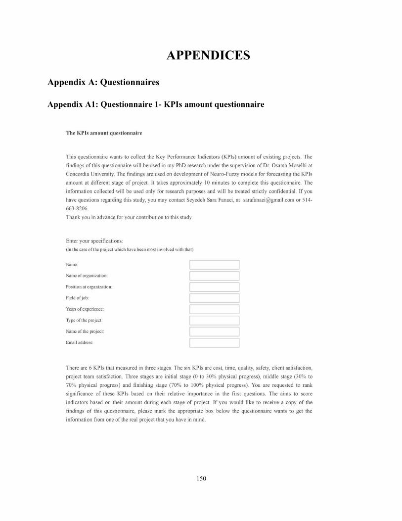
150
APPENDICES
Appendix A: Questionnaires
Appendix A1: Questionnaire 1- KPIs amount questionnaire
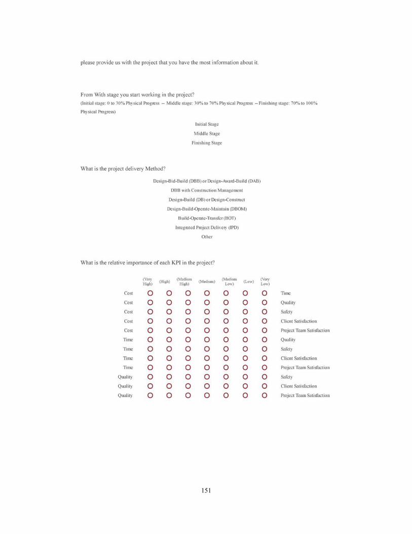
151
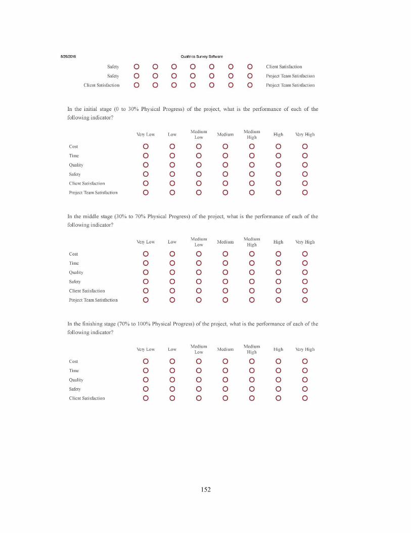
152
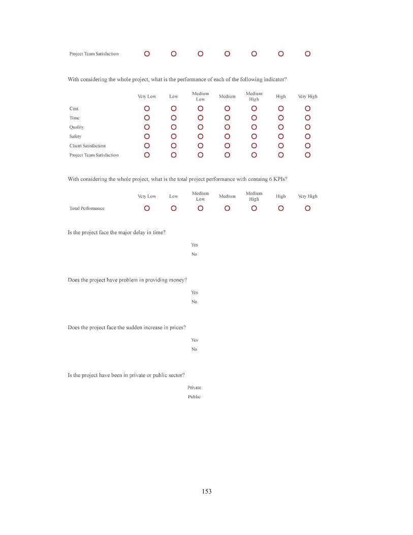
153
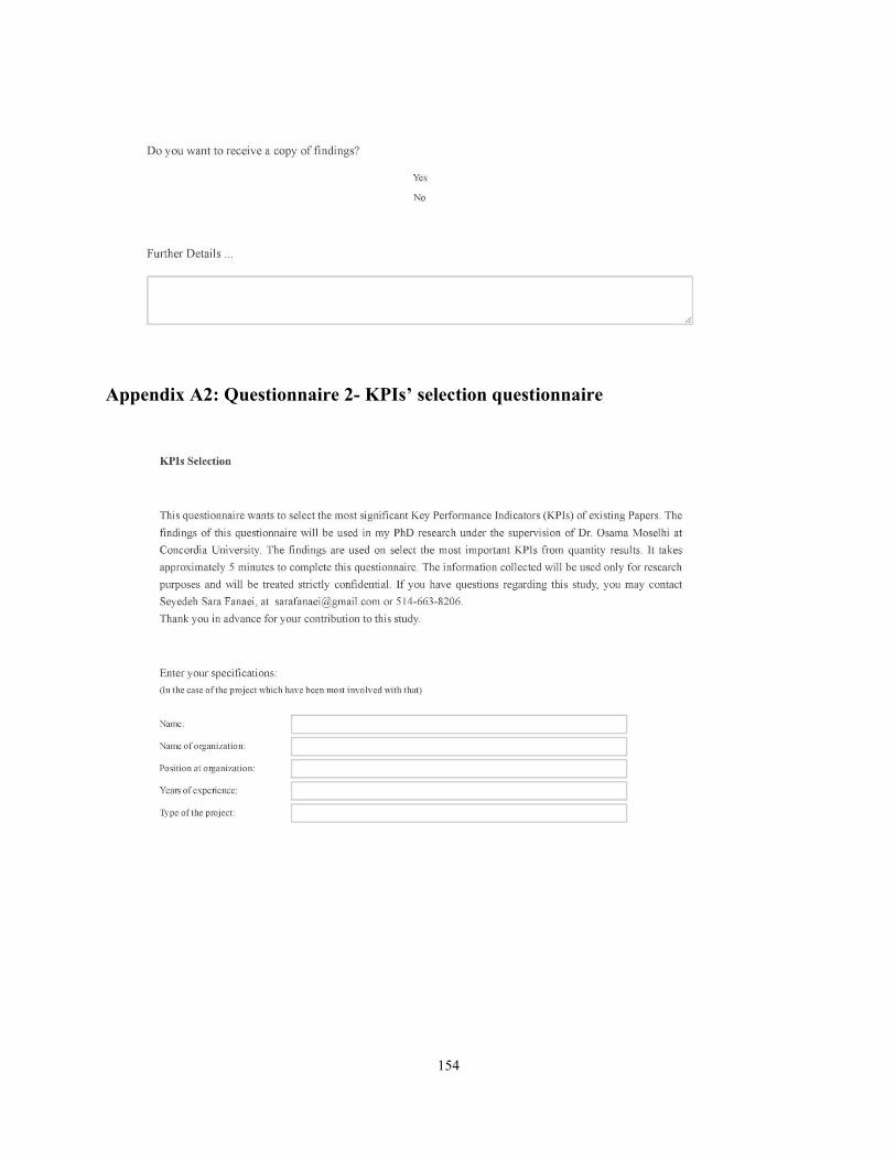
154
Appendix A2: Questionnaire 2- KPIs’ selection questionnaire
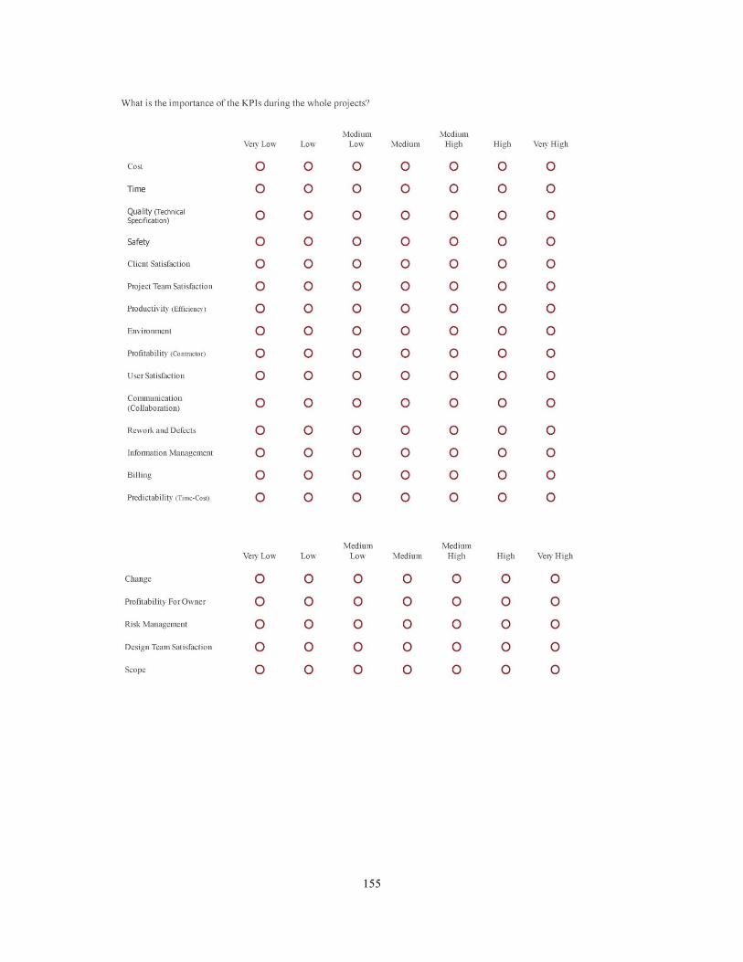
155
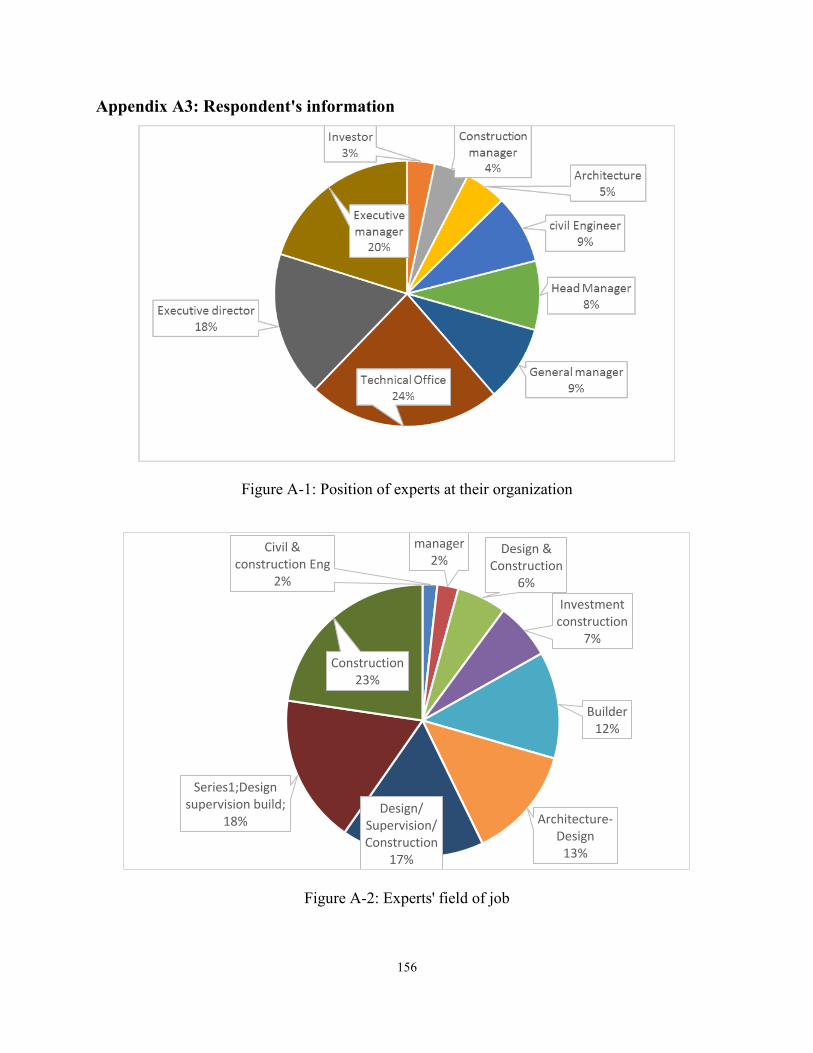
Appendix A3: Respondent's information
Civil & construction Eng
2%
manager2%
Design & Construction
6%Investment
construction7%
Builder12%
Architecture-Design
13%
Design/ Supervision/ Construction
17%
Series1;Design supervision build;
18%
Construction23%
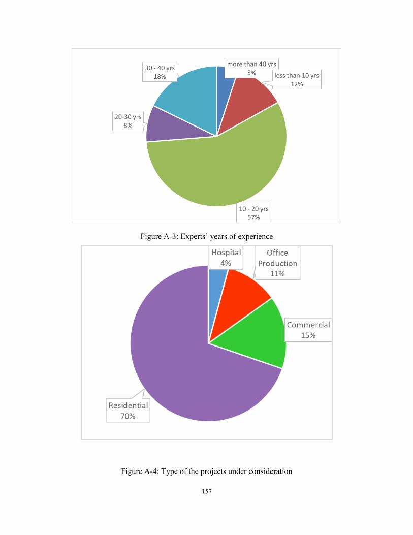
more than 40 yrs5% less than 10 yrs
12%
10 - 20 yrs57%
20-30 yrs8%
30 - 40 yrs18%
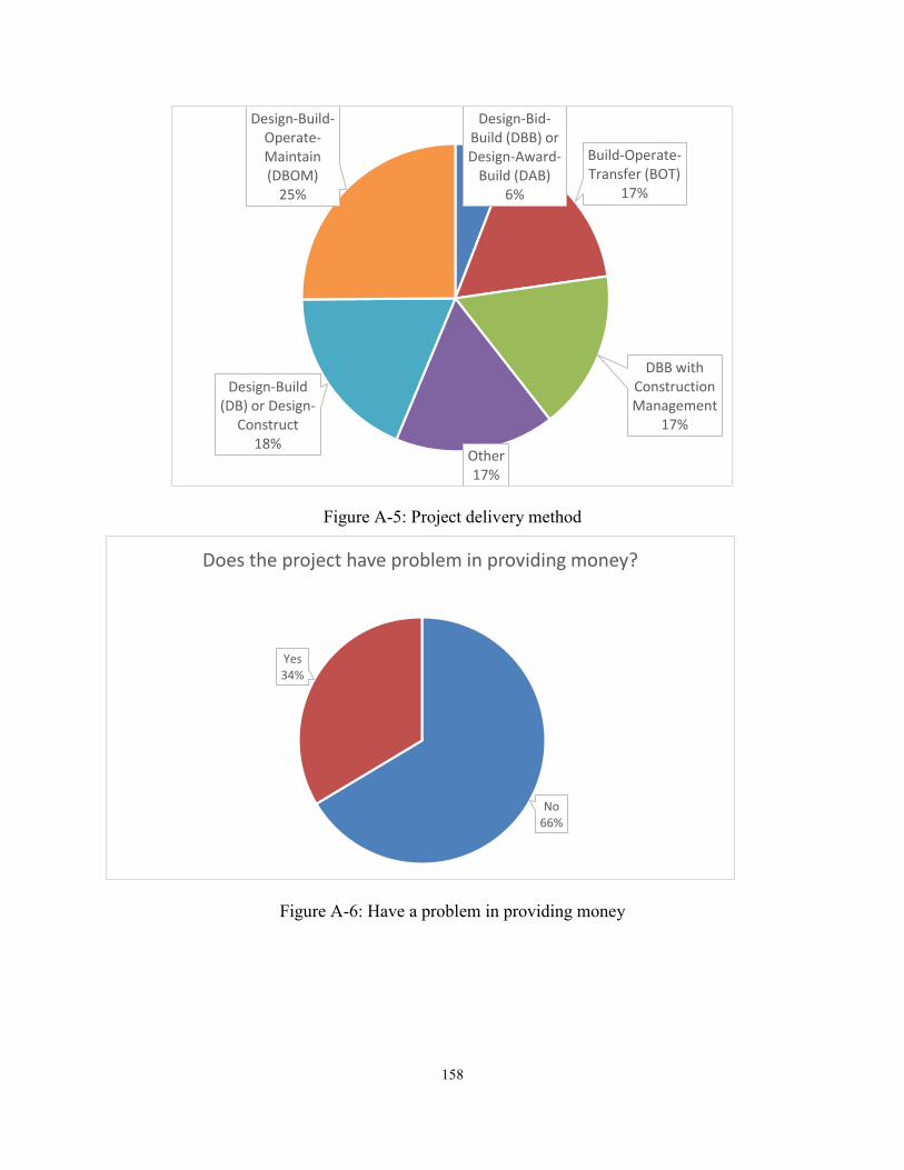
158
Figure A-5: Project delivery method
Figure A-6: Have a problem in providing money
Design-Bid-Build (DBB) or Design-Award-
Build (DAB)6%
Build-Operate-Transfer (BOT)
17%
DBB with Construction Management
17%
Other17%
Design-Build (DB) or Design-
Construct18%
Design-Build-Operate-Maintain (DBOM)
25%
No66%
Yes34%
Does the project have problem in providing money?
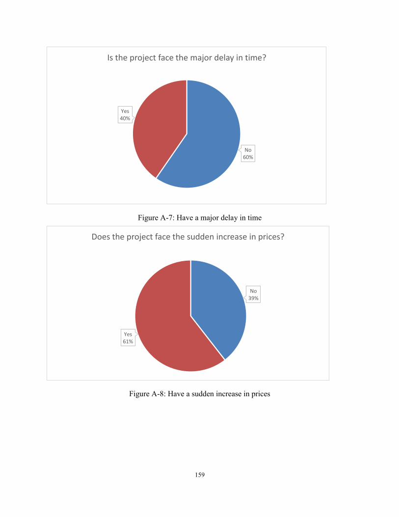
159
Figure A-7: Have a major delay in time
Figure A-8: Have a sudden increase in prices
No60%
Yes40%
Is the project face the major delay in time?
No39%
Yes61%
Does the project face the sudden increase in prices?

160
Figure A-9: Project belong to the private or public sector
public7%
private93%
Is the project have been in private or public sector?
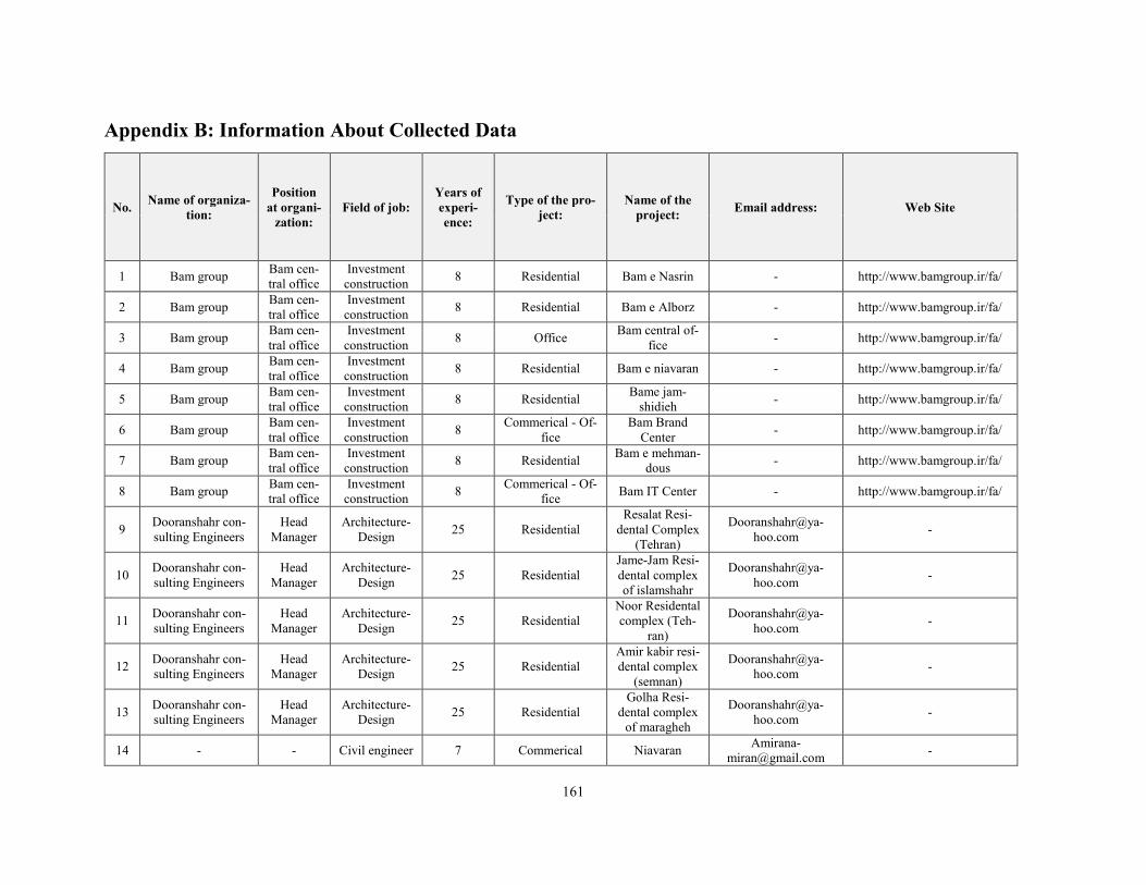
161
Appendix B: Information About Collected Data
No. Name of organiza-tion:
Position at organi-
zation: Field of job:
Years of experi-ence:
Type of the pro-ject:
Name of the project: Email address: Web Site
1 Bam group Bam cen-tral office
Investment construction 8 Residential Bam e Nasrin - http://www.bamgroup.ir/fa/
2 Bam group Bam cen-tral office
Investment construction 8 Residential Bam e Alborz - http://www.bamgroup.ir/fa/
3 Bam group Bam cen-tral office
Investment construction 8 Office Bam central of-
fice - http://www.bamgroup.ir/fa/
4 Bam group Bam cen-tral office
Investment construction 8 Residential Bam e niavaran - http://www.bamgroup.ir/fa/
5 Bam group Bam cen-tral office
Investment construction 8 Residential Bame jam-
shidieh - http://www.bamgroup.ir/fa/
6 Bam group Bam cen-tral office
Investment construction 8 Commerical - Of-
fice Bam Brand
Center - http://www.bamgroup.ir/fa/
7 Bam group Bam cen-tral office
Investment construction 8 Residential Bam e mehman-
dous - http://www.bamgroup.ir/fa/
8 Bam group Bam cen-tral office
Investment construction 8 Commerical - Of-
fice Bam IT Center - http://www.bamgroup.ir/fa/
9 Dooranshahr con-sulting Engineers
Head Manager
Architecture-Design 25 Residential
Resalat Resi-dental Complex
(Tehran)
-
10 Dooranshahr con-sulting Engineers
Head Manager
Architecture-Design 25 Residential
Jame-Jam Resi-dental complex of islamshahr
-
11 Dooranshahr con-sulting Engineers
Head Manager
Architecture-Design 25 Residential
Noor Residental complex (Teh-
ran)
-
12 Dooranshahr con-sulting Engineers
Head Manager
Architecture-Design 25 Residential
Amir kabir resi-dental complex
(semnan)
-
13 Dooranshahr con-sulting Engineers
Head Manager
Architecture-Design 25 Residential
Golha Resi-dental complex
of maragheh
-
14 - - Civil engineer 7 Commerical Niavaran [email protected]
-
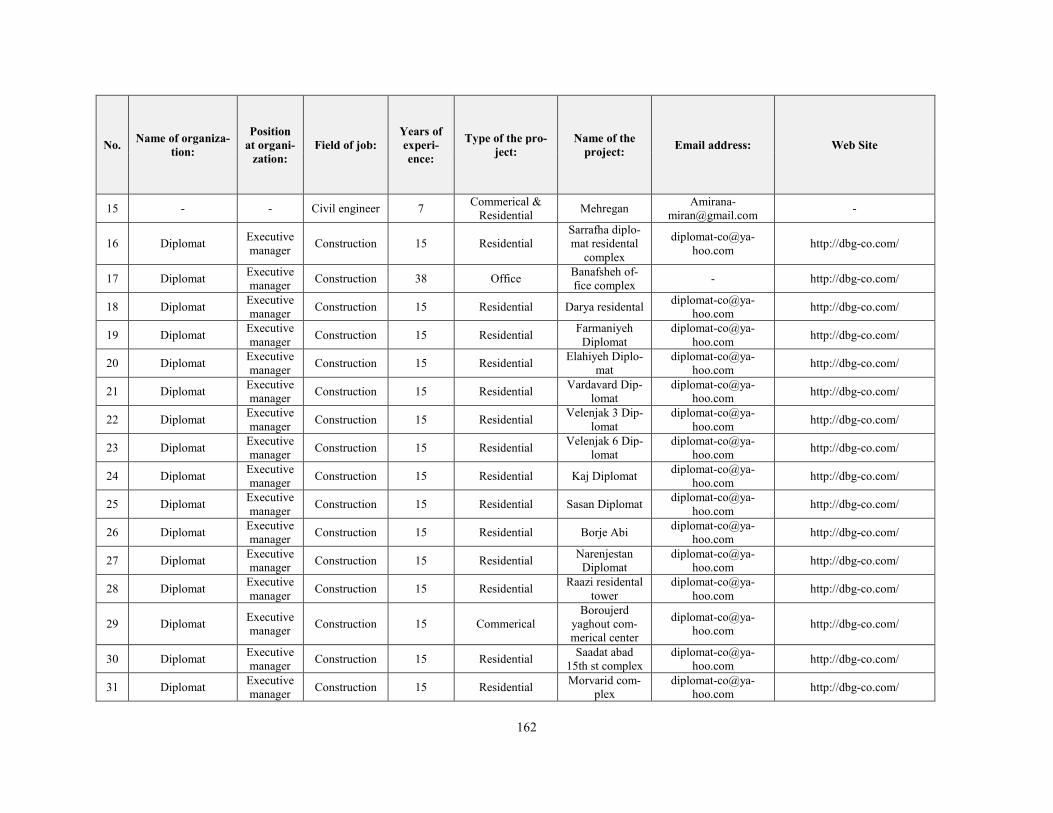
162
No. Name of organiza-tion:
Position at organi-
zation: Field of job:
Years of experi-ence:
Type of the pro-ject:
Name of the project: Email address: Web Site
15 - - Civil engineer 7 Commerical & Residential Mehregan Amirana-
-
16 Diplomat Executive manager Construction 15 Residential
Sarrafha diplo-mat residental
complex
http://dbg-co.com/
17 Diplomat Executive manager Construction 38 Office Banafsheh of-
fice complex - http://dbg-co.com/
18 Diplomat Executive manager Construction 15 Residential Darya residental diplomat-co@ya-
hoo.com
http://dbg-co.com/
19 Diplomat Executive manager Construction 15 Residential Farmaniyeh
Diplomat diplomat-co@ya-
hoo.com
http://dbg-co.com/
20 Diplomat Executive manager Construction 15 Residential Elahiyeh Diplo-
mat diplomat-co@ya-
hoo.com
http://dbg-co.com/
21 Diplomat Executive manager Construction 15 Residential Vardavard Dip-
lomat diplomat-co@ya-
hoo.com
http://dbg-co.com/
22 Diplomat Executive manager Construction 15 Residential Velenjak 3 Dip-
lomat diplomat-co@ya-
hoo.com
http://dbg-co.com/
23 Diplomat Executive manager Construction 15 Residential Velenjak 6 Dip-
lomat diplomat-co@ya-
hoo.com
http://dbg-co.com/
24 Diplomat Executive manager Construction 15 Residential Kaj Diplomat diplomat-co@ya-
hoo.com
http://dbg-co.com/
25 Diplomat Executive manager Construction 15 Residential Sasan Diplomat diplomat-co@ya-
hoo.com
http://dbg-co.com/
26 Diplomat Executive manager Construction 15 Residential Borje Abi diplomat-co@ya-
hoo.com
http://dbg-co.com/
27 Diplomat Executive manager Construction 15 Residential Narenjestan
Diplomat diplomat-co@ya-
hoo.com
http://dbg-co.com/
28 Diplomat Executive manager Construction 15 Residential Raazi residental
tower diplomat-co@ya-
hoo.com
http://dbg-co.com/
29 Diplomat Executive manager Construction 15 Commerical
Boroujerd yaghout com-merical center
http://dbg-co.com/
30 Diplomat Executive manager Construction 15 Residential Saadat abad
15th st complex diplomat-co@ya-
hoo.com
http://dbg-co.com/
31 Diplomat Executive manager Construction 15 Residential Morvarid com-
plex diplomat-co@ya-
hoo.com
http://dbg-co.com/
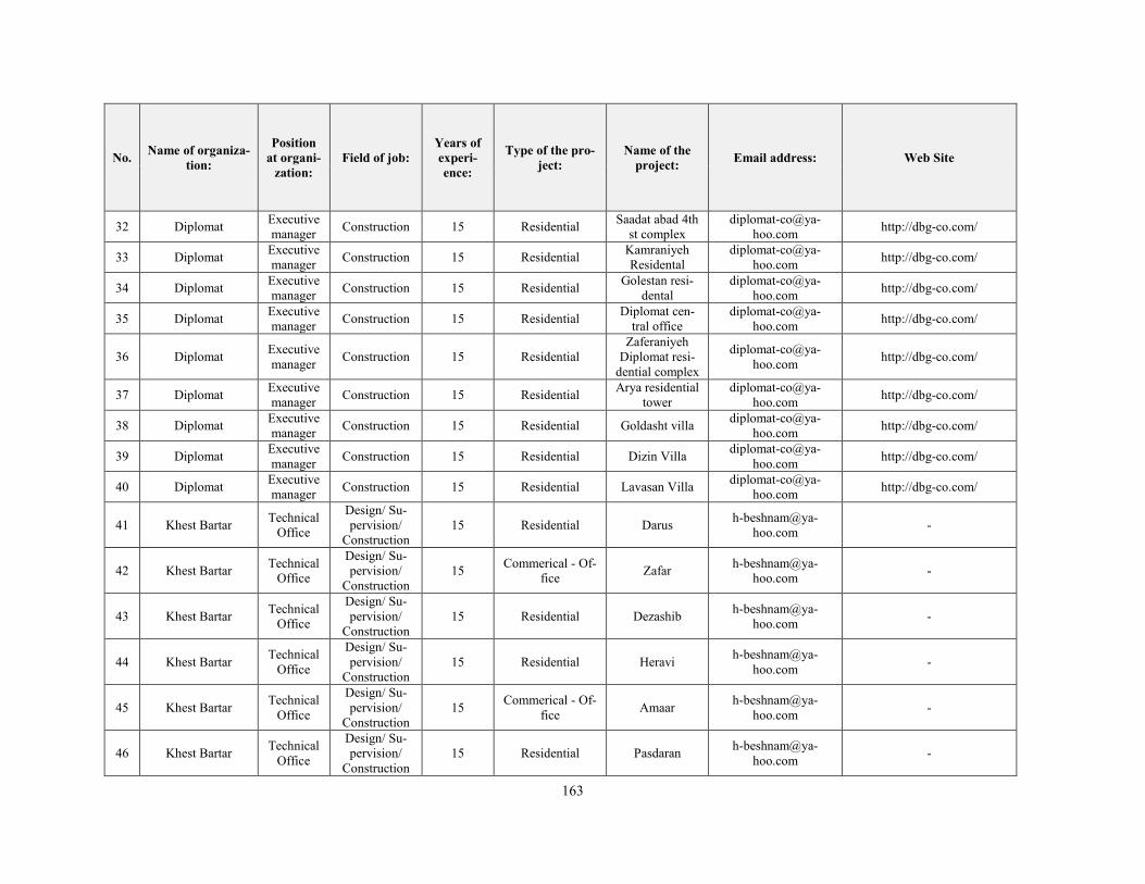
163
No. Name of organiza-tion:
Position at organi-
zation: Field of job:
Years of experi-ence:
Type of the pro-ject:
Name of the project: Email address: Web Site
32 Diplomat Executive manager Construction 15 Residential Saadat abad 4th
st complex diplomat-co@ya-
hoo.com
http://dbg-co.com/
33 Diplomat Executive manager Construction 15 Residential Kamraniyeh
Residental diplomat-co@ya-
hoo.com
http://dbg-co.com/
34 Diplomat Executive manager Construction 15 Residential Golestan resi-
dental diplomat-co@ya-
hoo.com
http://dbg-co.com/
35 Diplomat Executive manager Construction 15 Residential Diplomat cen-
tral office diplomat-co@ya-
hoo.com
http://dbg-co.com/
36 Diplomat Executive manager Construction 15 Residential
Zaferaniyeh Diplomat resi-
dential complex
http://dbg-co.com/
37 Diplomat Executive manager Construction 15 Residential Arya residential
tower diplomat-co@ya-
hoo.com
http://dbg-co.com/
38 Diplomat Executive manager Construction 15 Residential Goldasht villa diplomat-co@ya-
hoo.com
http://dbg-co.com/
39 Diplomat Executive manager Construction 15 Residential Dizin Villa diplomat-co@ya-
hoo.com
http://dbg-co.com/
40 Diplomat Executive manager Construction 15 Residential Lavasan Villa diplomat-co@ya-
hoo.com
http://dbg-co.com/
41 Khest Bartar Technical Office
Design/ Su-pervision/
Construction 15 Residential Darus h-beshnam@ya-
hoo.com
-
42 Khest Bartar Technical Office
Design/ Su-pervision/
Construction 15 Commerical - Of-
fice Zafar [email protected]
-
43 Khest Bartar Technical Office
Design/ Su-pervision/
Construction 15 Residential Dezashib h-beshnam@ya-
hoo.com
-
44 Khest Bartar Technical Office
Design/ Su-pervision/
Construction 15 Residential Heravi h-beshnam@ya-
hoo.com
-
45 Khest Bartar Technical Office
Design/ Su-pervision/
Construction 15 Commerical - Of-
fice Amaar [email protected]
-
46 Khest Bartar Technical Office
Design/ Su-pervision/
Construction 15 Residential Pasdaran h-beshnam@ya-
hoo.com
-
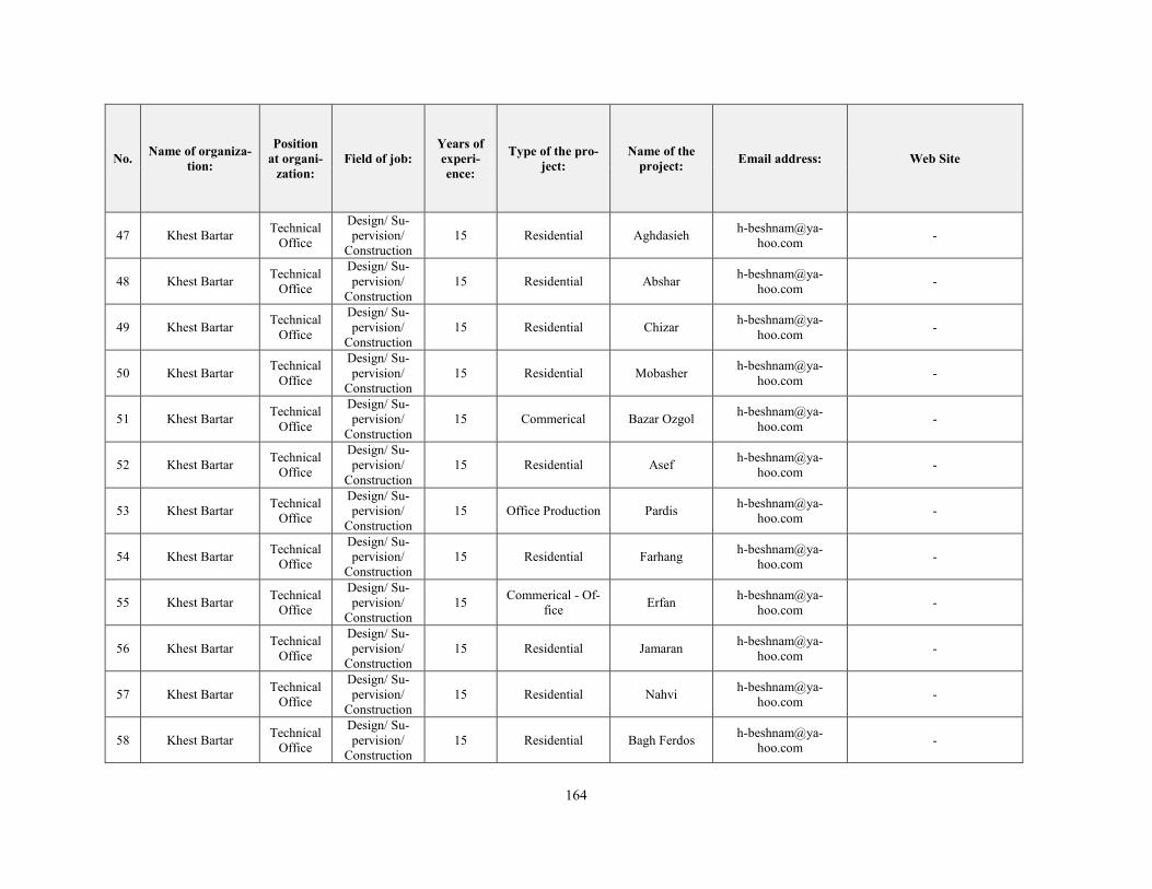
164
No. Name of organiza-tion:
Position at organi-
zation: Field of job:
Years of experi-ence:
Type of the pro-ject:
Name of the project: Email address: Web Site
47 Khest Bartar Technical Office
Design/ Su-pervision/
Construction 15 Residential Aghdasieh h-beshnam@ya-
hoo.com
-
48 Khest Bartar Technical Office
Design/ Su-pervision/
Construction 15 Residential Abshar h-beshnam@ya-
hoo.com
-
49 Khest Bartar Technical Office
Design/ Su-pervision/
Construction 15 Residential Chizar h-beshnam@ya-
hoo.com
-
50 Khest Bartar Technical Office
Design/ Su-pervision/
Construction 15 Residential Mobasher h-beshnam@ya-
hoo.com
-
51 Khest Bartar Technical Office
Design/ Su-pervision/
Construction 15 Commerical Bazar Ozgol h-beshnam@ya-
hoo.com
-
52 Khest Bartar Technical Office
Design/ Su-pervision/
Construction 15 Residential Asef h-beshnam@ya-
hoo.com
-
53 Khest Bartar Technical Office
Design/ Su-pervision/
Construction 15 Office Production Pardis h-beshnam@ya-
hoo.com
-
54 Khest Bartar Technical Office
Design/ Su-pervision/
Construction 15 Residential Farhang h-beshnam@ya-
hoo.com
-
55 Khest Bartar Technical Office
Design/ Su-pervision/
Construction 15 Commerical - Of-
fice Erfan [email protected]
-
56 Khest Bartar Technical Office
Design/ Su-pervision/
Construction 15 Residential Jamaran h-beshnam@ya-
hoo.com
-
57 Khest Bartar Technical Office
Design/ Su-pervision/
Construction 15 Residential Nahvi h-beshnam@ya-
hoo.com
-
58 Khest Bartar Technical Office
Design/ Su-pervision/
Construction 15 Residential Bagh Ferdos h-beshnam@ya-
hoo.com
-
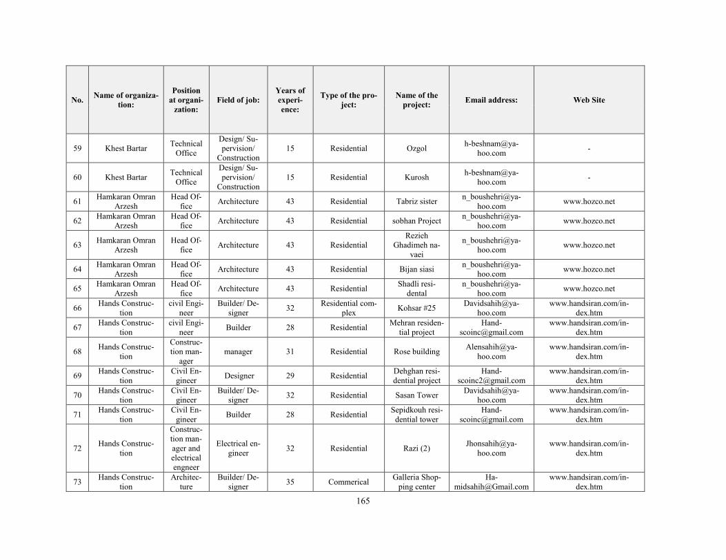
165
No. Name of organiza-tion:
Position at organi-
zation: Field of job:
Years of experi-ence:
Type of the pro-ject:
Name of the project: Email address: Web Site
59 Khest Bartar Technical Office
Design/ Su-pervision/
Construction 15 Residential Ozgol h-beshnam@ya-
hoo.com
-
60 Khest Bartar Technical Office
Design/ Su-pervision/
Construction 15 Residential Kurosh h-beshnam@ya-
hoo.com
-
61 Hamkaran Omran Arzesh
Head Of-fice Architecture 43 Residential Tabriz sister n_boushehri@ya-
hoo.com
www.hozco.net
62 Hamkaran Omran Arzesh
Head Of-fice Architecture 43 Residential sobhan Project n_boushehri@ya-
hoo.com
www.hozco.net
63 Hamkaran Omran Arzesh
Head Of-fice Architecture 43 Residential
Rezieh Ghadimeh na-
vaei
www.hozco.net
64 Hamkaran Omran Arzesh
Head Of-fice Architecture 43 Residential Bijan siasi n_boushehri@ya-
hoo.com
www.hozco.net
65 Hamkaran Omran Arzesh
Head Of-fice Architecture 43 Residential Shadli resi-
dental n_boushehri@ya-
hoo.com
www.hozco.net
66 Hands Construc-tion
civil Engi-neer
Builder/ De-signer 32 Residential com-
plex Kohsar #25 [email protected]
www.handsiran.com/in-dex.htm
67 Hands Construc-tion
civil Engi-neer Builder 28 Residential Mehran residen-
tial project Hand-
www.handsiran.com/in-dex.htm
68 Hands Construc-tion
Construc-tion man-
ager manager 31 Residential Rose building Alensahih@ya-
hoo.com
www.handsiran.com/in-dex.htm
69 Hands Construc-tion
Civil En-gineer Designer 29 Residential Dehghan resi-
dential project Hand-
www.handsiran.com/in-dex.htm
70 Hands Construc-tion
Civil En-gineer
Builder/ De-signer 32 Residential Sasan Tower Davidsahih@ya-
hoo.com
www.handsiran.com/in-dex.htm
71 Hands Construc-tion
Civil En-gineer Builder 28 Residential Sepidkouh resi-
dential tower Hand-
www.handsiran.com/in-dex.htm
72 Hands Construc-tion
Construc-tion man-ager and electrical engneer
Electrical en-gineer 32 Residential Razi (2) Jhonsahih@ya-
hoo.com
www.handsiran.com/in-dex.htm
73 Hands Construc-tion
Architec-ture
Builder/ De-signer 35 Commerical Galleria Shop-
ping center Ha-
www.handsiran.com/in-dex.htm
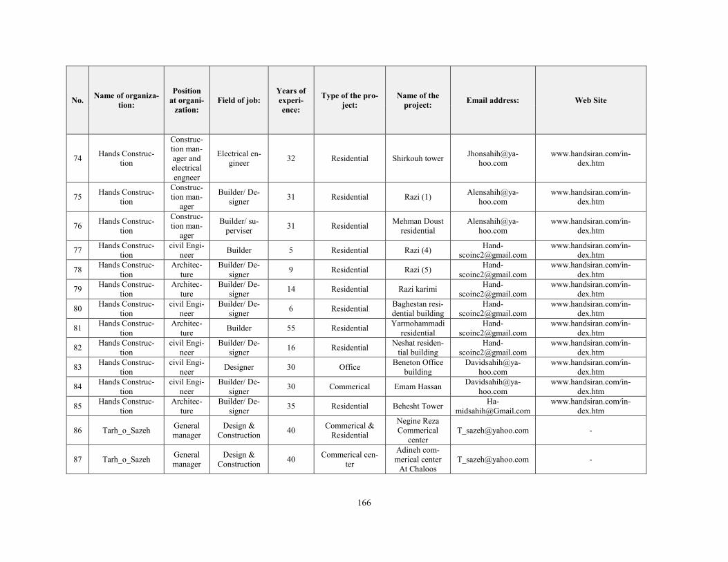
166
No. Name of organiza-tion:
Position at organi-
zation: Field of job:
Years of experi-ence:
Type of the pro-ject:
Name of the project: Email address: Web Site
74 Hands Construc-tion
Construc-tion man-ager and electrical engneer
Electrical en-gineer 32 Residential Shirkouh tower Jhonsahih@ya-
hoo.com
www.handsiran.com/in-dex.htm
75 Hands Construc-tion
Construc-tion man-
ager
Builder/ De-signer 31 Residential Razi (1) Alensahih@ya-
hoo.com
www.handsiran.com/in-dex.htm
76 Hands Construc-tion
Construc-tion man-
ager
Builder/ su-perviser 31 Residential Mehman Doust
residential Alensahih@ya-
hoo.com
www.handsiran.com/in-dex.htm
77 Hands Construc-tion
civil Engi-neer Builder 5 Residential Razi (4) Hand-
www.handsiran.com/in-dex.htm
78 Hands Construc-tion
Architec-ture
Builder/ De-signer 9 Residential Razi (5) Hand-
www.handsiran.com/in-dex.htm
79 Hands Construc-tion
Architec-ture
Builder/ De-signer 14 Residential Razi karimi Hand-
www.handsiran.com/in-dex.htm
80 Hands Construc-tion
civil Engi-neer
Builder/ De-signer 6 Residential Baghestan resi-
dential building Hand-
www.handsiran.com/in-dex.htm
81 Hands Construc-tion
Architec-ture Builder 55 Residential Yarmohammadi
residential Hand-
www.handsiran.com/in-dex.htm
82 Hands Construc-tion
civil Engi-neer
Builder/ De-signer 16 Residential Neshat residen-
tial building Hand-
www.handsiran.com/in-dex.htm
83 Hands Construc-tion
civil Engi-neer Designer 30 Office Beneton Office
building Davidsahih@ya-
hoo.com
www.handsiran.com/in-dex.htm
84 Hands Construc-tion
civil Engi-neer
Builder/ De-signer 30 Commerical Emam Hassan Davidsahih@ya-
hoo.com
www.handsiran.com/in-dex.htm
85 Hands Construc-tion
Architec-ture
Builder/ De-signer 35 Residential Behesht Tower Ha-
www.handsiran.com/in-dex.htm
86 Tarh_o_Sazeh General manager
Design & Construction 40 Commerical &
Residential
Negine Reza Commerical
center [email protected] -
87 Tarh_o_Sazeh General manager
Design & Construction 40 Commerical cen-
ter
Adineh com-merical center
At Chaloos [email protected] -
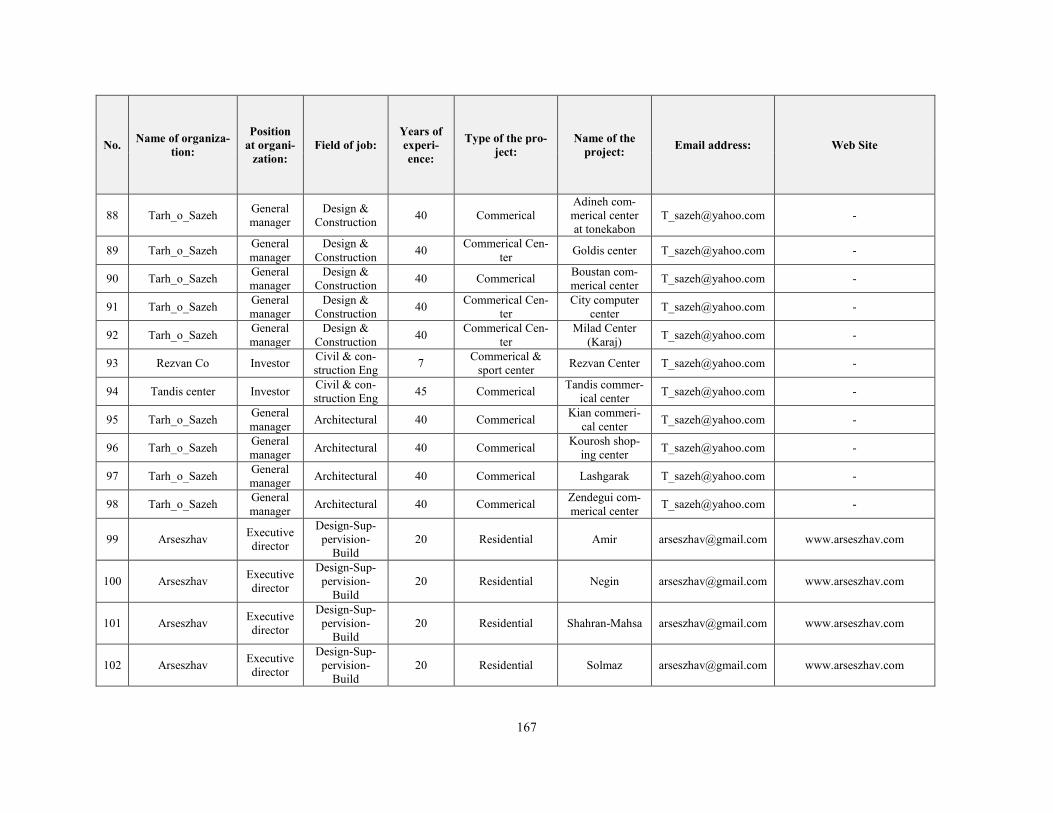
167
No. Name of organiza-tion:
Position at organi-
zation: Field of job:
Years of experi-ence:
Type of the pro-ject:
Name of the project: Email address: Web Site
88 Tarh_o_Sazeh General manager
Design & Construction 40 Commerical
Adineh com-merical center at tonekabon
89 Tarh_o_Sazeh General manager
Design & Construction 40 Commerical Cen-
ter Goldis center [email protected] -
90 Tarh_o_Sazeh General manager
Design & Construction 40 Commerical Boustan com-
merical center [email protected] -
91 Tarh_o_Sazeh General manager
Design & Construction 40 Commerical Cen-
ter City computer
center [email protected] -
92 Tarh_o_Sazeh General manager
Design & Construction 40 Commerical Cen-
ter Milad Center
(Karaj) [email protected] -
93 Rezvan Co Investor Civil & con-struction Eng 7 Commerical &
sport center Rezvan Center [email protected] -
94 Tandis center Investor Civil & con-struction Eng 45 Commerical Tandis commer-
ical center [email protected] -
95 Tarh_o_Sazeh General manager Architectural 40 Commerical Kian commeri-
cal center [email protected] -
96 Tarh_o_Sazeh General manager Architectural 40 Commerical Kourosh shop-
ing center [email protected] -
97 Tarh_o_Sazeh General manager Architectural 40 Commerical Lashgarak [email protected] -
98 Tarh_o_Sazeh General manager Architectural 40 Commerical Zendegui com-
merical center [email protected] -
99 Arseszhav Executive director
Design-Sup-pervision-
Build 20 Residential Amir [email protected] www.arseszhav.com
100 Arseszhav Executive director
Design-Sup-pervision-
Build 20 Residential Negin [email protected] www.arseszhav.com
101 Arseszhav Executive director
Design-Sup-pervision-
Build 20 Residential Shahran-Mahsa [email protected] www.arseszhav.com
102 Arseszhav Executive director
Design-Sup-pervision-
Build 20 Residential Solmaz [email protected] www.arseszhav.com
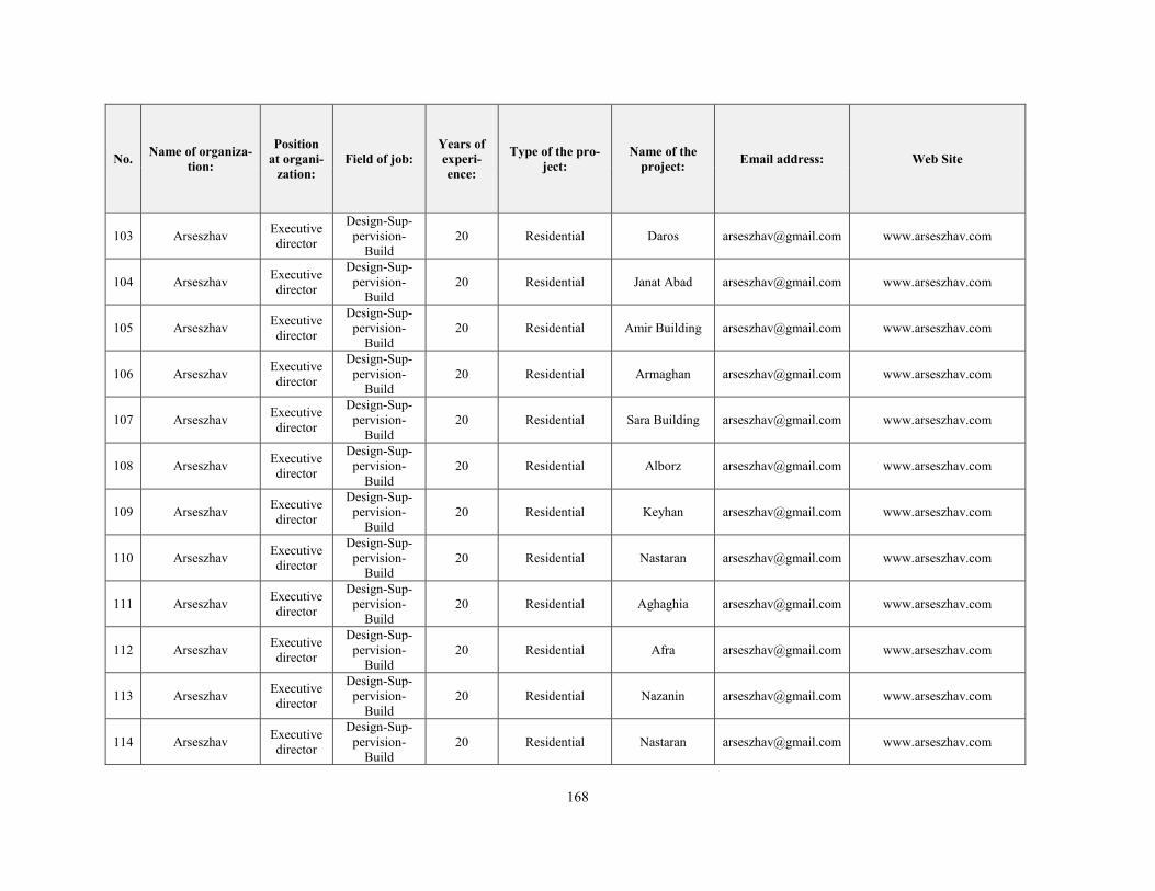
168
No. Name of organiza-tion:
Position at organi-
zation: Field of job:
Years of experi-ence:
Type of the pro-ject:
Name of the project: Email address: Web Site
103 Arseszhav Executive director
Design-Sup-pervision-
Build 20 Residential Daros [email protected] www.arseszhav.com
104 Arseszhav Executive director
Design-Sup-pervision-
Build 20 Residential Janat Abad [email protected] www.arseszhav.com
105 Arseszhav Executive director
Design-Sup-pervision-
Build 20 Residential Amir Building [email protected] www.arseszhav.com
106 Arseszhav Executive director
Design-Sup-pervision-
Build 20 Residential Armaghan [email protected] www.arseszhav.com
107 Arseszhav Executive director
Design-Sup-pervision-
Build 20 Residential Sara Building [email protected] www.arseszhav.com
108 Arseszhav Executive director
Design-Sup-pervision-
Build 20 Residential Alborz [email protected] www.arseszhav.com
109 Arseszhav Executive director
Design-Sup-pervision-
Build 20 Residential Keyhan [email protected] www.arseszhav.com
110 Arseszhav Executive director
Design-Sup-pervision-
Build 20 Residential Nastaran [email protected] www.arseszhav.com
111 Arseszhav Executive director
Design-Sup-pervision-
Build 20 Residential Aghaghia [email protected] www.arseszhav.com
112 Arseszhav Executive director
Design-Sup-pervision-
Build 20 Residential Afra [email protected] www.arseszhav.com
113 Arseszhav Executive director
Design-Sup-pervision-
Build 20 Residential Nazanin [email protected] www.arseszhav.com
114 Arseszhav Executive director
Design-Sup-pervision-
Build 20 Residential Nastaran [email protected] www.arseszhav.com
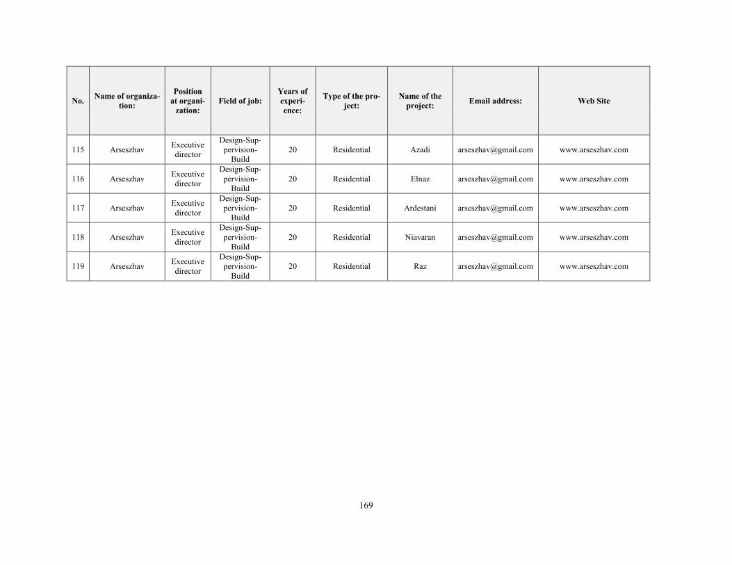
169
No. Name of organiza-tion:
Position at organi-
zation: Field of job:
Years of experi-ence:
Type of the pro-ject:
Name of the project: Email address: Web Site
115 Arseszhav Executive director
Design-Sup-pervision-
Build 20 Residential Azadi [email protected] www.arseszhav.com
116 Arseszhav Executive director
Design-Sup-pervision-
Build 20 Residential Elnaz [email protected] www.arseszhav.com
117 Arseszhav Executive director
Design-Sup-pervision-
Build 20 Residential Ardestani [email protected] www.arseszhav.com
118 Arseszhav Executive director
Design-Sup-pervision-
Build 20 Residential Niavaran [email protected] www.arseszhav.com
119 Arseszhav Executive director
Design-Sup-pervision-
Build 20 Residential Raz [email protected] www.arseszhav.com
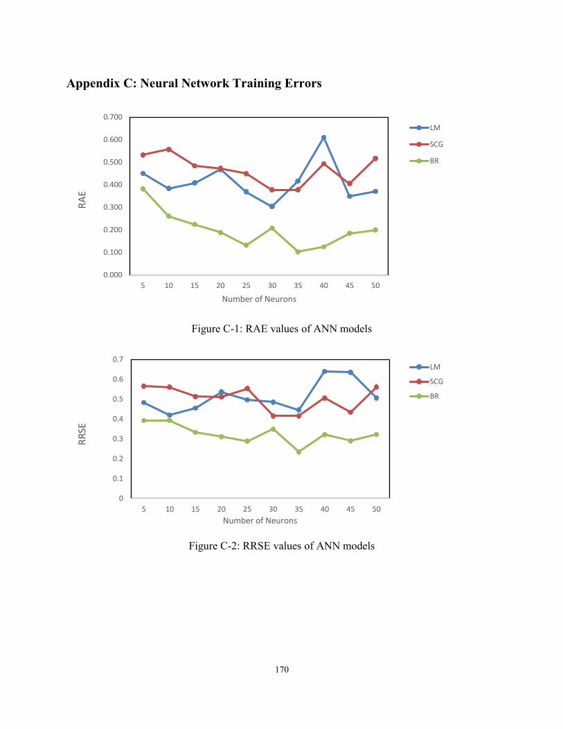
0.000
0.100
0.200
0.300
0.400
0.500
0.600
0.700
5 10 15 20 25 30 35 40 45 50
RAE
Number of Neurons
LM
SCG
BR
0
0.1
0.2
0.3
0.4
0.5
0.6
0.7
5 10 15 20 25 30 35 40 45 50
RRSE
Number of Neurons
LM
SCG
BR
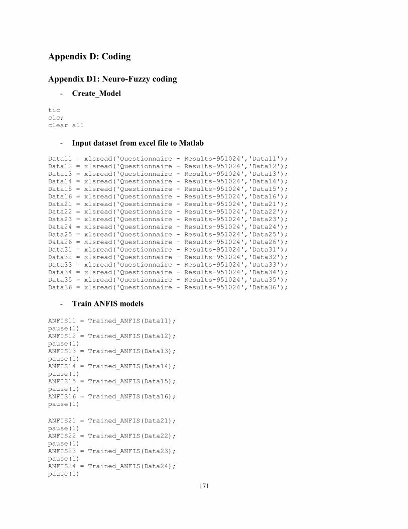
171
Appendix D: Coding
Appendix D1: Neuro-Fuzzy coding
- Create_Model
tic clc; clear all
- Input dataset from excel file to Matlab
Data11 = xlsread('Questionnaire - Results-951024','Data11'); Data12 = xlsread('Questionnaire - Results-951024','Data12'); Data13 = xlsread('Questionnaire - Results-951024','Data13'); Data14 = xlsread('Questionnaire - Results-951024','Data14'); Data15 = xlsread('Questionnaire - Results-951024','Data15'); Data16 = xlsread('Questionnaire - Results-951024','Data16'); Data21 = xlsread('Questionnaire - Results-951024','Data21'); Data22 = xlsread('Questionnaire - Results-951024','Data22'); Data23 = xlsread('Questionnaire - Results-951024','Data23'); Data24 = xlsread('Questionnaire - Results-951024','Data24'); Data25 = xlsread('Questionnaire - Results-951024','Data25'); Data26 = xlsread('Questionnaire - Results-951024','Data26'); Data31 = xlsread('Questionnaire - Results-951024','Data31'); Data32 = xlsread('Questionnaire - Results-951024','Data32'); Data33 = xlsread('Questionnaire - Results-951024','Data33'); Data34 = xlsread('Questionnaire - Results-951024','Data34'); Data35 = xlsread('Questionnaire - Results-951024','Data35'); Data36 = xlsread('Questionnaire - Results-951024','Data36');
- Train ANFIS models
ANFIS11 = Trained_ANFIS(Data11); pause(1) ANFIS12 = Trained_ANFIS(Data12); pause(1) ANFIS13 = Trained_ANFIS(Data13); pause(1) ANFIS14 = Trained_ANFIS(Data14); pause(1) ANFIS15 = Trained_ANFIS(Data15); pause(1) ANFIS16 = Trained_ANFIS(Data16); pause(1)
ANFIS21 = Trained_ANFIS(Data21); pause(1) ANFIS22 = Trained_ANFIS(Data22); pause(1) ANFIS23 = Trained_ANFIS(Data23); pause(1) ANFIS24 = Trained_ANFIS(Data24); pause(1)
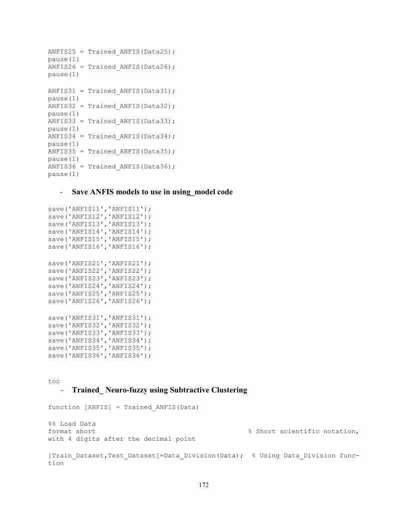
172
ANFIS25 = Trained_ANFIS(Data25); pause(1) ANFIS26 = Trained_ANFIS(Data26); pause(1)
ANFIS31 = Trained_ANFIS(Data31); pause(1) ANFIS32 = Trained_ANFIS(Data32); pause(1) ANFIS33 = Trained_ANFIS(Data33); pause(1) ANFIS34 = Trained_ANFIS(Data34); pause(1) ANFIS35 = Trained_ANFIS(Data35); pause(1) ANFIS36 = Trained_ANFIS(Data36); pause(1)
- Save ANFIS models to use in using_model code
save('ANFIS11','ANFIS11'); save('ANFIS12','ANFIS12'); save('ANFIS13','ANFIS13'); save('ANFIS14','ANFIS14'); save('ANFIS15','ANFIS15'); save('ANFIS16','ANFIS16');
save('ANFIS21','ANFIS21'); save('ANFIS22','ANFIS22'); save('ANFIS23','ANFIS23'); save('ANFIS24','ANFIS24'); save('ANFIS25','ANFIS25'); save('ANFIS26','ANFIS26');
save('ANFIS31','ANFIS31'); save('ANFIS32','ANFIS32'); save('ANFIS33','ANFIS33'); save('ANFIS34','ANFIS34'); save('ANFIS35','ANFIS35'); save('ANFIS36','ANFIS36');
toc
- Trained_ Neuro-fuzzy using Subtractive Clustering function [ANFIS] = Trained_ANFIS(Data)
%% Load Data format short % Short scientific notation,
with 4 digits after the decimal point
[Train_Dataset,Test_Dataset]=Data_Division(Data); % Using Data_Division func-
tion
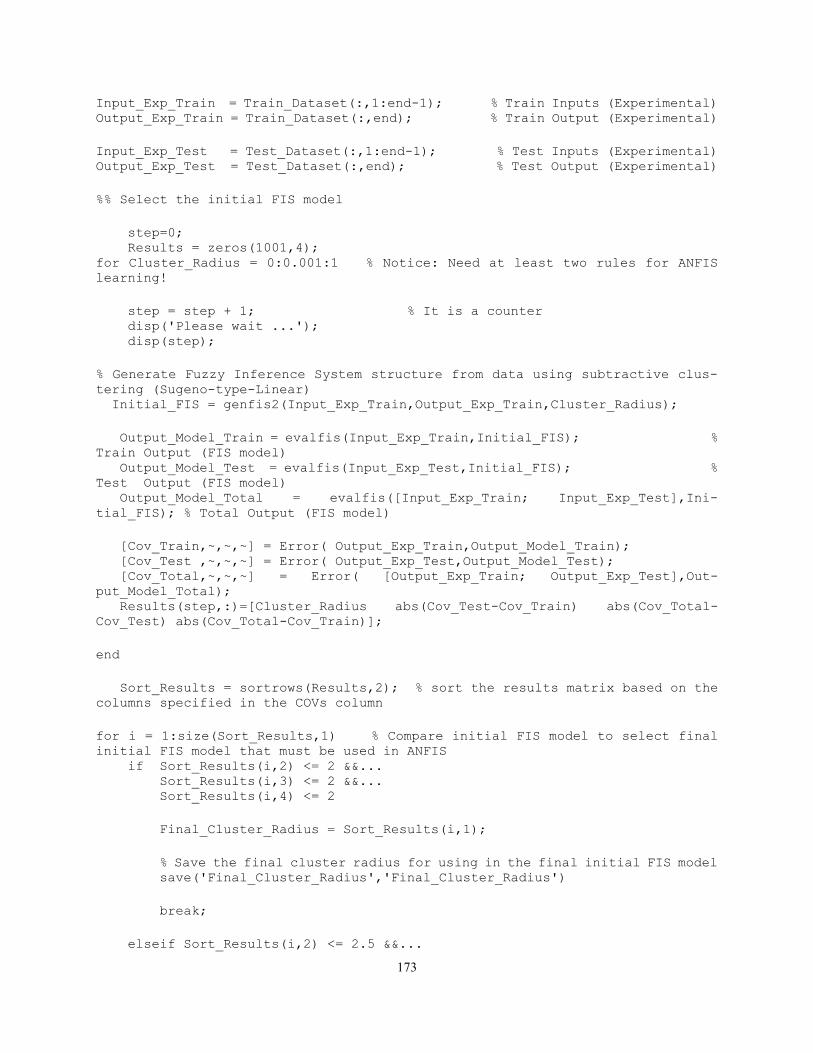
173
Input_Exp_Train = Train_Dataset(:,1:end-1); % Train Inputs (Experimental) Output_Exp_Train = Train_Dataset(:,end); % Train Output (Experimental)
Input_Exp_Test = Test_Dataset(:,1:end-1); % Test Inputs (Experimental) Output_Exp_Test = Test_Dataset(:,end); % Test Output (Experimental)
%% Select the initial FIS model
step=0; Results = zeros(1001,4); for Cluster_Radius = 0:0.001:1 % Notice: Need at least two rules for ANFIS
learning!
step = step + 1; % It is a counter disp('Please wait ...'); disp(step);
% Generate Fuzzy Inference System structure from data using subtractive clus-
tering (Sugeno-type-Linear) Initial_FIS = genfis2(Input_Exp_Train,Output_Exp_Train,Cluster_Radius);
Output_Model_Train = evalfis(Input_Exp_Train,Initial_FIS); %
Train Output (FIS model) Output_Model_Test = evalfis(Input_Exp_Test,Initial_FIS); %
Test Output (FIS model) Output_Model_Total = evalfis([Input_Exp_Train; Input_Exp_Test],Ini-
tial_FIS); % Total Output (FIS model)
[Cov_Train,~,~,~] = Error( Output_Exp_Train,Output_Model_Train); [Cov_Test ,~,~,~] = Error( Output_Exp_Test,Output_Model_Test); [Cov_Total,~,~,~] = Error( [Output_Exp_Train; Output_Exp_Test],Out-
put_Model_Total); Results(step,:)=[Cluster_Radius abs(Cov_Test-Cov_Train) abs(Cov_Total-
Cov_Test) abs(Cov_Total-Cov_Train)];
end
Sort_Results = sortrows(Results,2); % sort the results matrix based on the
columns specified in the COVs column
for i = 1:size(Sort_Results,1) % Compare initial FIS model to select final
initial FIS model that must be used in ANFIS if Sort_Results(i,2) <= 2 &&... Sort_Results(i,3) <= 2 &&... Sort_Results(i,4) <= 2
Final_Cluster_Radius = Sort_Results(i,1);
% Save the final cluster radius for using in the final initial FIS model save('Final_Cluster_Radius','Final_Cluster_Radius')
break;
elseif Sort_Results(i,2) <= 2.5 &&...
174
Sort_Results(i,3) <= 2.5 &&... Sort_Results(i,4) <= 2.5 Final_Cluster_Radius = Sort_Results(i,1);
% Save the final cluster radius for using in the final initial FIS
model save('Final_Cluster_Radius','Final_Cluster_Radius')
break; elseif Sort_Results(i,2) <= 3 &&... Sort_Results(i,3) <= 3 &&... Sort_Results(i,4) <= 3 Final_Cluster_Radius = Sort_Results(i,1);
% Save the final cluster radius for using in the final initial FIS
model save('Final_Cluster_Radius','Final_Cluster_Radius')
break; elseif Sort_Results(i,2) <= 3.5 &&... Sort_Results(i,3) <= 3.5 &&... Sort_Results(i,4) <= 3.5 Final_Cluster_Radius = Sort_Results(i,1);
% Save the final cluster radius for using in the final initial FIS
model save('Final_Cluster_Radius','Final_Cluster_Radius')
break; elseif Sort_Results(i,2) <= 4 &&... Sort_Results(i,3) <= 4 &&... Sort_Results(i,4) <= 4 Final_Cluster_Radius = Sort_Results(i,1);
% Save the final cluster radius for using in the final initial FIS
model save('Final_Cluster_Radius','Final_Cluster_Radius')
break; elseif Sort_Results(i,2) <= 4.5 &&... Sort_Results(i,3) <= 4.5 &&... Sort_Results(i,4) <= 4.5 Final_Cluster_Radius = Sort_Results(i,1);
% Save the final cluster radius for using in the final initial FIS
model save('Final_Cluster_Radius','Final_Cluster_Radius')
break; elseif Sort_Results(i,2) <= 5 &&... Sort_Results(i,3) <= 5 &&... Sort_Results(i,4) <= 5 Final_Cluster_Radius = Sort_Results(i,1);
175
% Save the final cluster radius for using in the final initial FIS
model save('Final_Cluster_Radius','Final_Cluster_Radius')
break; elseif Sort_Results(i,2) <= 5.5 &&... Sort_Results(i,3) <= 5.5 &&... Sort_Results(i,4) <= 5.5 Final_Cluster_Radius = Sort_Results(i,1);
% Save the final cluster radius for using in the final initial FIS
model save('Final_Cluster_Radius','Final_Cluster_Radius')
break; elseif Sort_Results(i,2) <= 6 &&... Sort_Results(i,3) <= 6 &&... Sort_Results(i,4) <= 6 Final_Cluster_Radius = Sort_Results(i,1);
% Save the final cluster radius for using in the final initial FIS
model save('Final_Cluster_Radius','Final_Cluster_Radius')
break; elseif Sort_Results(i,2) <= 6.5 &&... Sort_Results(i,3) <= 6.5 &&... Sort_Results(i,4) <= 6.5 Final_Cluster_Radius = Sort_Results(i,1);
% Save the final cluster radius for using in the final initial FIS
model save('Final_Cluster_Radius','Final_Cluster_Radius')
break; elseif Sort_Results(i,2) <= 7 &&... Sort_Results(i,3) <= 7 &&... Sort_Results(i,4) <= 7 Final_Cluster_Radius = Sort_Results(i,1);
% Save the final cluster radius for using in the final initial FIS
model save('Final_Cluster_Radius','Final_Cluster_Radius')
break; elseif Sort_Results(i,2) <= 7.5 &&... Sort_Results(i,3) <= 7.5 &&... Sort_Results(i,4) <= 7.5 Final_Cluster_Radius = Sort_Results(i,1);
% Save the final cluster radius for using in the final initial FIS
model save('Final_Cluster_Radius','Final_Cluster_Radius')
break;
176
elseif Sort_Results(i,2) <= 8 &&... Sort_Results(i,3) <= 8 &&... Sort_Results(i,4) <= 8 Final_Cluster_Radius = Sort_Results(i,1);
% Save the final cluster radius for using in the final initial FIS
model save('Final_Cluster_Radius','Final_Cluster_Radius')
break; elseif Sort_Results(i,2) <= 8.5 &&... Sort_Results(i,3) <= 8.5 &&... Sort_Results(i,4) <= 8.5 Final_Cluster_Radius = Sort_Results(i,1);
% Save the final cluster radius for using in the final initial FIS
model save('Final_Cluster_Radius','Final_Cluster_Radius')
break; elseif Sort_Results(i,2) <= 9 &&... Sort_Results(i,3) <= 9 &&... Sort_Results(i,4) <= 9 Final_Cluster_Radius = Sort_Results(i,1);
% Save the final cluster radius for using in the final initial FIS
model save('Final_Cluster_Radius','Final_Cluster_Radius')
break; elseif Sort_Results(i,2) <= 9.5 &&... Sort_Results(i,3) <= 9.5 &&... Sort_Results(i,4) <= 9.5 Final_Cluster_Radius = Sort_Results(i,1);
% Save the final cluster radius for using in the final initial FIS
model save('Final_Cluster_Radius','Final_Cluster_Radius')
break; elseif Sort_Results(i,2) <= 10 &&... Sort_Results(i,3) <= 10 &&... Sort_Results(i,4) <= 10 Final_Cluster_Radius = Sort_Results(i,1);
% Save the final cluster radius for using in the final initial FIS
model save('Final_Cluster_Radius','Final_Cluster_Radius')
break; end
end
177
%% Create ANFIS Structure
% The final cluster Radius from compare algorithm load('Final_Cluster_Radius.mat')
% Create initial FIS with final cluster radius (sugeno-Linear with Subtractive
Clustering) Initial_FIS = genfis2(Input_Exp_Train,Output_Exp_Train,Final_Cluster_Ra-
dius);
% ANFIS Options % Training Options MaxEpoch=100; ErrorGoal=0; InitialStepSize=0.01; StepSizeDecRate=0.9; StepSizeIncRate=1.1; TrainOptions=[MaxEpoch ErrorGoal InitialStepSize StepSiz-
eDecRate StepSizeIncRate];
% Display Options ShowAnfisInformation=true; ShowError=true; ShowStepSize=true; ShowFinalResult=true; DisplayOptions=[ShowAnfisInformation ShowError ShowStepSize
ShowFinalResult];
% Training Algorithm - Select Training Algorithm %TrainAlgorithm=0; % BP TrainAlgorithm=1; % Hybrid LS-BP % ANIFS works [~,~,~,ANFIS,~] = anfis(Train_Dataset,Initial_FIS,TrainOptions,DisplayOp-
tions, Test_Dataset,TrainAlgorithm);
End
- Trained_ Neuro-fuzzy using FCM
function [ANFIS] = Trained_ANFIS(Data)
%% Load Data
format short % Short scientific notation,
with 4 digits after the decimal point
[Train_Dataset,Test_Dataset]=Data_Division(Data); % Using Data_Division func-
tion
Input_Exp_Train = Train_Dataset(:,1:end-1); % Train Inputs (Experimental)
Output_Exp_Train = Train_Dataset(:,end); % Train Output (Experimental)
Input_Exp_Test = Test_Dataset(:,1:end-1); % Test Inputs (Experimental)
Output_Exp_Test = Test_Dataset(:,end); % Test Output (Experimental)
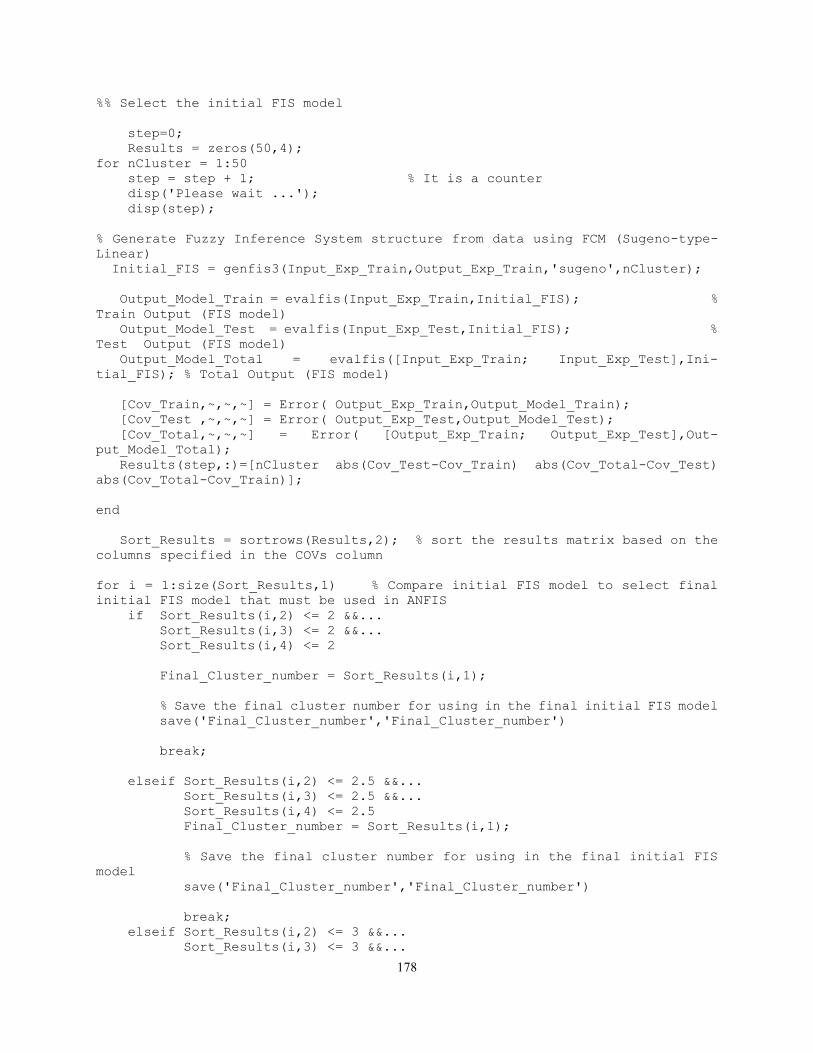
178
%% Select the initial FIS model
step=0;
Results = zeros(50,4);
for nCluster = 1:50
step = step + 1; % It is a counter
disp('Please wait ...');
disp(step);
% Generate Fuzzy Inference System structure from data using FCM (Sugeno-type-
Linear)
Initial_FIS = genfis3(Input_Exp_Train,Output_Exp_Train,'sugeno',nCluster);
Output_Model_Train = evalfis(Input_Exp_Train,Initial_FIS); %
Train Output (FIS model)
Output_Model_Test = evalfis(Input_Exp_Test,Initial_FIS); %
Test Output (FIS model)
Output_Model_Total = evalfis([Input_Exp_Train; Input_Exp_Test],Ini-
tial_FIS); % Total Output (FIS model)
[Cov_Train,~,~,~] = Error( Output_Exp_Train,Output_Model_Train);
[Cov_Test ,~,~,~] = Error( Output_Exp_Test,Output_Model_Test);
[Cov_Total,~,~,~] = Error( [Output_Exp_Train; Output_Exp_Test],Out-
put_Model_Total);
Results(step,:)=[nCluster abs(Cov_Test-Cov_Train) abs(Cov_Total-Cov_Test)
abs(Cov_Total-Cov_Train)];
end
Sort_Results = sortrows(Results,2); % sort the results matrix based on the
columns specified in the COVs column
for i = 1:size(Sort_Results,1) % Compare initial FIS model to select final
initial FIS model that must be used in ANFIS
if Sort_Results(i,2) <= 2 &&...
Sort_Results(i,3) <= 2 &&...
Sort_Results(i,4) <= 2
Final_Cluster_number = Sort_Results(i,1);
% Save the final cluster number for using in the final initial FIS model
save('Final_Cluster_number','Final_Cluster_number')
break;
elseif Sort_Results(i,2) <= 2.5 &&...
Sort_Results(i,3) <= 2.5 &&...
Sort_Results(i,4) <= 2.5
Final_Cluster_number = Sort_Results(i,1);
% Save the final cluster number for using in the final initial FIS
model
save('Final_Cluster_number','Final_Cluster_number')
break;
elseif Sort_Results(i,2) <= 3 &&...
Sort_Results(i,3) <= 3 &&...
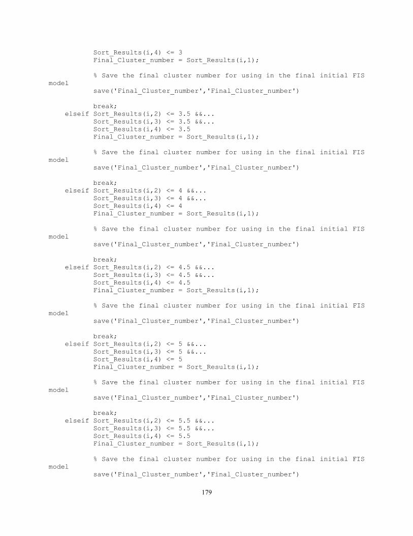
179
Sort_Results(i,4) <= 3
Final_Cluster_number = Sort_Results(i,1);
% Save the final cluster number for using in the final initial FIS
model
save('Final_Cluster_number','Final_Cluster_number')
break;
elseif Sort_Results(i,2) <= 3.5 &&...
Sort_Results(i,3) <= 3.5 &&...
Sort_Results(i,4) <= 3.5
Final_Cluster_number = Sort_Results(i,1);
% Save the final cluster number for using in the final initial FIS
model
save('Final_Cluster_number','Final_Cluster_number')
break;
elseif Sort_Results(i,2) <= 4 &&...
Sort_Results(i,3) <= 4 &&...
Sort_Results(i,4) <= 4
Final_Cluster_number = Sort_Results(i,1);
% Save the final cluster number for using in the final initial FIS
model
save('Final_Cluster_number','Final_Cluster_number')
break;
elseif Sort_Results(i,2) <= 4.5 &&...
Sort_Results(i,3) <= 4.5 &&...
Sort_Results(i,4) <= 4.5
Final_Cluster_number = Sort_Results(i,1);
% Save the final cluster number for using in the final initial FIS
model
save('Final_Cluster_number','Final_Cluster_number')
break;
elseif Sort_Results(i,2) <= 5 &&...
Sort_Results(i,3) <= 5 &&...
Sort_Results(i,4) <= 5
Final_Cluster_number = Sort_Results(i,1);
% Save the final cluster number for using in the final initial FIS
model
save('Final_Cluster_number','Final_Cluster_number')
break;
elseif Sort_Results(i,2) <= 5.5 &&...
Sort_Results(i,3) <= 5.5 &&...
Sort_Results(i,4) <= 5.5
Final_Cluster_number = Sort_Results(i,1);
% Save the final cluster number for using in the final initial FIS
model
save('Final_Cluster_number','Final_Cluster_number')

180
break;
elseif Sort_Results(i,2) <= 6 &&...
Sort_Results(i,3) <= 6 &&...
Sort_Results(i,4) <= 6
Final_Cluster_number = Sort_Results(i,1);
% Save the final cluster number for using in the final initial FIS
model
save('Final_Cluster_number','Final_Cluster_number')
break;
elseif Sort_Results(i,2) <= 6.5 &&...
Sort_Results(i,3) <= 6.5 &&...
Sort_Results(i,4) <= 6.5
Final_Cluster_number = Sort_Results(i,1);
% Save the final cluster number for using in the final initial FIS
model
save('Final_Cluster_number','Final_Cluster_number')
break;
elseif Sort_Results(i,2) <= 7 &&...
Sort_Results(i,3) <= 7 &&...
Sort_Results(i,4) <= 7
Final_Cluster_number = Sort_Results(i,1);
% Save the final cluster number for using in the final initial FIS
model
save('Final_Cluster_number','Final_Cluster_number')
break;
elseif Sort_Results(i,2) <= 7.5 &&...
Sort_Results(i,3) <= 7.5 &&...
Sort_Results(i,4) <= 7.5
Final_Cluster_number = Sort_Results(i,1);
% Save the final cluster number for using in the final initial FIS
model
save('Final_Cluster_number','Final_Cluster_number')
break;
elseif Sort_Results(i,2) <= 8 &&...
Sort_Results(i,3) <= 8 &&...
Sort_Results(i,4) <= 8
Final_Cluster_number = Sort_Results(i,1);
% Save the final cluster number for using in the final initial FIS
model
save('Final_Cluster_number','Final_Cluster_number')
break;
elseif Sort_Results(i,2) <= 8.5 &&...
Sort_Results(i,3) <= 8.5 &&...
Sort_Results(i,4) <= 8.5
Final_Cluster_number = Sort_Results(i,1);
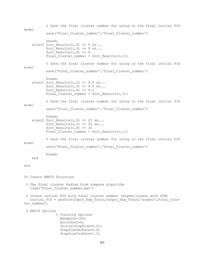
181
% Save the final cluster number for using in the final initial FIS
model
save('Final_Cluster_number','Final_Cluster_number')
break;
elseif Sort_Results(i,2) <= 9 &&...
Sort_Results(i,3) <= 9 &&...
Sort_Results(i,4) <= 9
Final_Cluster_number = Sort_Results(i,1);
% Save the final cluster number for using in the final initial FIS
model
save('Final_Cluster_number','Final_Cluster_number')
break;
elseif Sort_Results(i,2) <= 9.5 &&...
Sort_Results(i,3) <= 9.5 &&...
Sort_Results(i,4) <= 9.5
Final_Cluster_number = Sort_Results(i,1);
% Save the final cluster number for using in the final initial FIS
model
save('Final_Cluster_number','Final_Cluster_number')
break;
elseif Sort_Results(i,2) <= 25 &&...
Sort_Results(i,3) <= 25 &&...
Sort_Results(i,4) <= 25
Final_Cluster_number = Sort_Results(i,1);
% Save the final cluster number for using in the final initial FIS
model
save('Final_Cluster_number','Final_Cluster_number')
break;
end
end
%% Create ANFIS Structure
% The final cluster Radius from compare algorithm
load('Final_Cluster_number.mat')
% Create initial FIS with final cluster number (sugeno-Linear with FCM)
Initial_FIS = genfis3(Input_Exp_Train,Output_Exp_Train,'sugeno',Final_Clus-
ter_number);
% ANFIS Options
% Training Options
MaxEpoch=100;
ErrorGoal=0;
InitialStepSize=0.01;
StepSizeDecRate=0.9;
StepSizeIncRate=1.1;
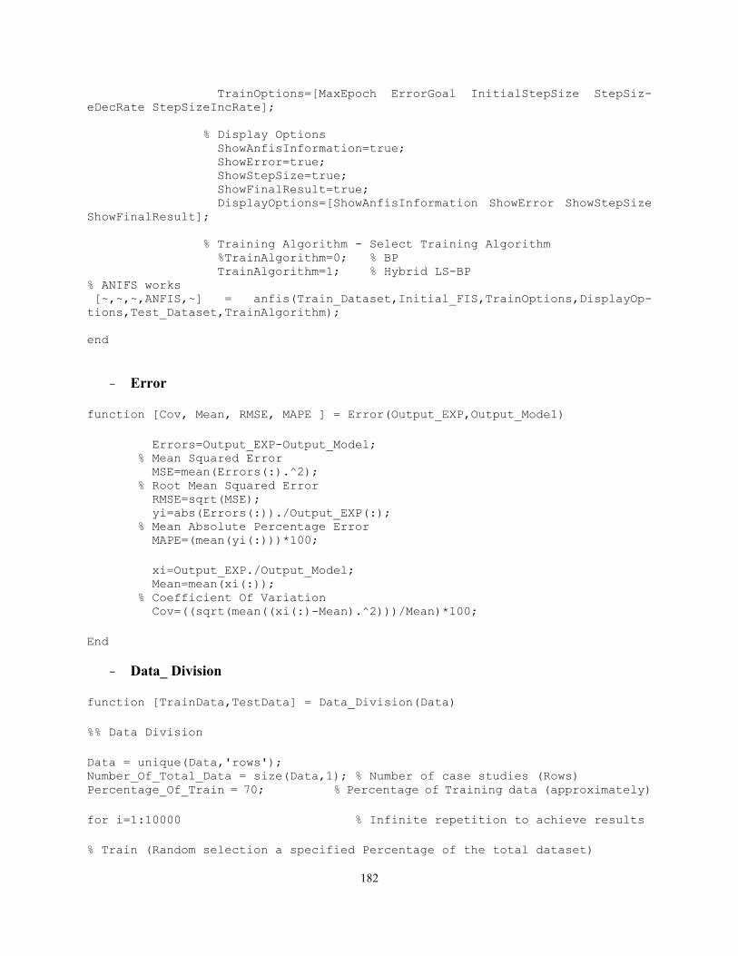
182
TrainOptions=[MaxEpoch ErrorGoal InitialStepSize StepSiz-
eDecRate StepSizeIncRate];
% Display Options
ShowAnfisInformation=true;
ShowError=true;
ShowStepSize=true;
ShowFinalResult=true;
DisplayOptions=[ShowAnfisInformation ShowError ShowStepSize
ShowFinalResult];
% Training Algorithm - Select Training Algorithm
%TrainAlgorithm=0; % BP
TrainAlgorithm=1; % Hybrid LS-BP
% ANIFS works
[~,~,~,ANFIS,~] = anfis(Train_Dataset,Initial_FIS,TrainOptions,DisplayOp-
tions,Test_Dataset,TrainAlgorithm);
end
- Error
function [Cov, Mean, RMSE, MAPE ] = Error(Output_EXP,Output_Model)
Errors=Output_EXP-Output_Model; % Mean Squared Error MSE=mean(Errors(:).^2); % Root Mean Squared Error RMSE=sqrt(MSE); yi=abs(Errors(:))./Output_EXP(:); % Mean Absolute Percentage Error MAPE=(mean(yi(:)))*100;
xi=Output_EXP./Output_Model; Mean=mean(xi(:)); % Coefficient Of Variation Cov=((sqrt(mean((xi(:)-Mean).^2)))/Mean)*100;
End
- Data_ Division function [TrainData,TestData] = Data_Division(Data)
%% Data Division
Data = unique(Data,'rows'); Number_Of_Total_Data = size(Data,1); % Number of case studies (Rows) Percentage_Of_Train = 70; % Percentage of Training data (approximately)
for i=1:10000 % Infinite repetition to achieve results
% Train (Random selection a specified Percentage of the total dataset)
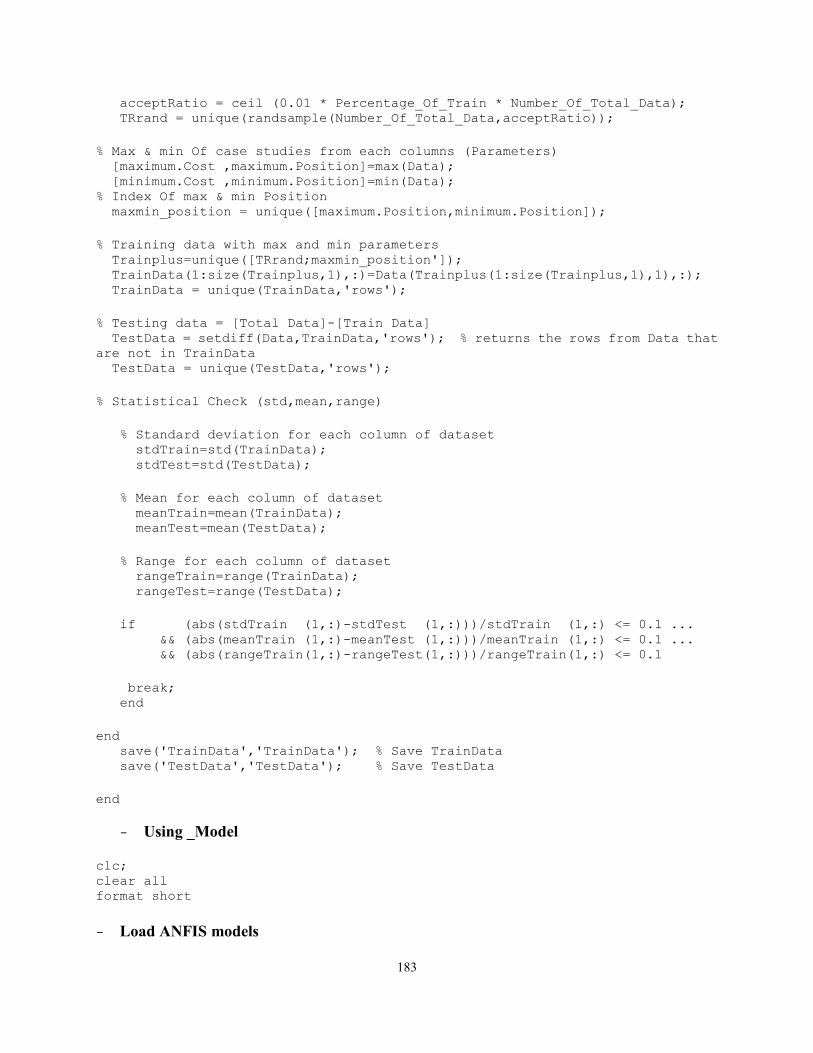
183
acceptRatio = ceil (0.01 * Percentage_Of_Train * Number_Of_Total_Data); TRrand = unique(randsample(Number_Of_Total_Data,acceptRatio));
% Max & min Of case studies from each columns (Parameters) [maximum.Cost ,maximum.Position]=max(Data); [minimum.Cost ,minimum.Position]=min(Data); % Index Of max & min Position maxmin_position = unique([maximum.Position,minimum.Position]);
% Training data with max and min parameters Trainplus=unique([TRrand;maxmin_position']); TrainData(1:size(Trainplus,1),:)=Data(Trainplus(1:size(Trainplus,1),1),:); TrainData = unique(TrainData,'rows');
% Testing data = [Total Data]-[Train Data] TestData = setdiff(Data,TrainData,'rows'); % returns the rows from Data that
are not in TrainData TestData = unique(TestData,'rows');
% Statistical Check (std,mean,range)
% Standard deviation for each column of dataset stdTrain=std(TrainData); stdTest=std(TestData);
% Mean for each column of dataset meanTrain=mean(TrainData); meanTest=mean(TestData);
% Range for each column of dataset rangeTrain=range(TrainData); rangeTest=range(TestData);
if (abs(stdTrain (1,:)-stdTest (1,:)))/stdTrain (1,:) <= 0.1 ... && (abs(meanTrain (1,:)-meanTest (1,:)))/meanTrain (1,:) <= 0.1 ... && (abs(rangeTrain(1,:)-rangeTest(1,:)))/rangeTrain(1,:) <= 0.1
break; end
end save('TrainData','TrainData'); % Save TrainData save('TestData','TestData'); % Save TestData
end
- Using _Model clc; clear all format short
- Load ANFIS models
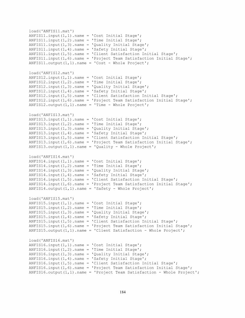
184
load('ANFIS11.mat') ANFIS11.input(1,1).name = 'Cost Initial Stage'; ANFIS11.input(1,2).name = 'Time Initial Stage'; ANFIS11.input(1,3).name = 'Quality Initial Stage'; ANFIS11.input(1,4).name = 'Safety Initial Stage'; ANFIS11.input(1,5).name = 'Client Satisfaction Initial Stage'; ANFIS11.input(1,6).name = 'Project Team Satisfaction Initial Stage'; ANFIS11.output(1,1).name = 'Cost - Whole Project';
load('ANFIS12.mat') ANFIS12.input(1,1).name = 'Cost Initial Stage'; ANFIS12.input(1,2).name = 'Time Initial Stage'; ANFIS12.input(1,3).name = 'Quality Initial Stage'; ANFIS12.input(1,4).name = 'Safety Initial Stage'; ANFIS12.input(1,5).name = 'Client Satisfaction Initial Stage'; ANFIS12.input(1,6).name = 'Project Team Satisfaction Initial Stage'; ANFIS12.output(1,1).name = 'Time - Whole Project';
load('ANFIS13.mat') ANFIS13.input(1,1).name = 'Cost Initial Stage'; ANFIS13.input(1,2).name = 'Time Initial Stage'; ANFIS13.input(1,3).name = 'Quality Initial Stage'; ANFIS13.input(1,4).name = 'Safety Initial Stage'; ANFIS13.input(1,5).name = 'Client Satisfaction Initial Stage'; ANFIS13.input(1,6).name = 'Project Team Satisfaction Initial Stage'; ANFIS13.output(1,1).name = 'Quality - Whole Project';
load('ANFIS14.mat') ANFIS14.input(1,1).name = 'Cost Initial Stage'; ANFIS14.input(1,2).name = 'Time Initial Stage'; ANFIS14.input(1,3).name = 'Quality Initial Stage'; ANFIS14.input(1,4).name = 'Safety Initial Stage'; ANFIS14.input(1,5).name = 'Client Satisfaction Initial Stage'; ANFIS14.input(1,6).name = 'Project Team Satisfaction Initial Stage'; ANFIS14.output(1,1).name = 'Safety - Whole Project';
load('ANFIS15.mat') ANFIS15.input(1,1).name = 'Cost Initial Stage'; ANFIS15.input(1,2).name = 'Time Initial Stage'; ANFIS15.input(1,3).name = 'Quality Initial Stage'; ANFIS15.input(1,4).name = 'Safety Initial Stage'; ANFIS15.input(1,5).name = 'Client Satisfaction Initial Stage'; ANFIS15.input(1,6).name = 'Project Team Satisfaction Initial Stage'; ANFIS15.output(1,1).name = 'Client Satisfaction - Whole Project';
load('ANFIS16.mat') ANFIS16.input(1,1).name = 'Cost Initial Stage'; ANFIS16.input(1,2).name = 'Time Initial Stage'; ANFIS16.input(1,3).name = 'Quality Initial Stage'; ANFIS16.input(1,4).name = 'Safety Initial Stage'; ANFIS16.input(1,5).name = 'Client Satisfaction Initial Stage'; ANFIS16.input(1,6).name = 'Project Team Satisfaction Initial Stage'; ANFIS16.output(1,1).name = 'Project Team Satisfaction - Whole Project';
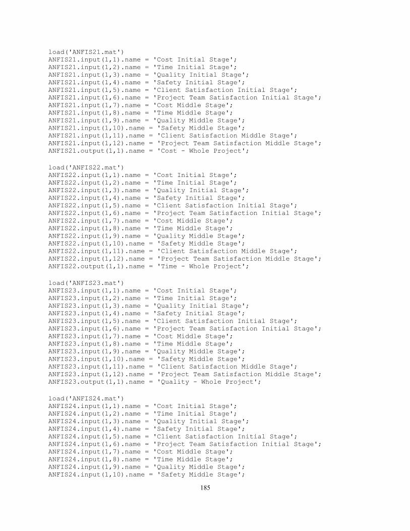
185
load('ANFIS21.mat') ANFIS21.input(1,1).name = 'Cost Initial Stage'; ANFIS21.input(1,2).name = 'Time Initial Stage'; ANFIS21.input(1,3).name = 'Quality Initial Stage'; ANFIS21.input(1,4).name = 'Safety Initial Stage'; ANFIS21.input(1,5).name = 'Client Satisfaction Initial Stage'; ANFIS21.input(1,6).name = 'Project Team Satisfaction Initial Stage'; ANFIS21.input(1,7).name = 'Cost Middle Stage'; ANFIS21.input(1,8).name = 'Time Middle Stage'; ANFIS21.input(1,9).name = 'Quality Middle Stage'; ANFIS21.input(1,10).name = 'Safety Middle Stage'; ANFIS21.input(1,11).name = 'Client Satisfaction Middle Stage'; ANFIS21.input(1,12).name = 'Project Team Satisfaction Middle Stage'; ANFIS21.output(1,1).name = 'Cost - Whole Project';
load('ANFIS22.mat') ANFIS22.input(1,1).name = 'Cost Initial Stage'; ANFIS22.input(1,2).name = 'Time Initial Stage'; ANFIS22.input(1,3).name = 'Quality Initial Stage'; ANFIS22.input(1,4).name = 'Safety Initial Stage'; ANFIS22.input(1,5).name = 'Client Satisfaction Initial Stage'; ANFIS22.input(1,6).name = 'Project Team Satisfaction Initial Stage'; ANFIS22.input(1,7).name = 'Cost Middle Stage'; ANFIS22.input(1,8).name = 'Time Middle Stage'; ANFIS22.input(1,9).name = 'Quality Middle Stage'; ANFIS22.input(1,10).name = 'Safety Middle Stage'; ANFIS22.input(1,11).name = 'Client Satisfaction Middle Stage'; ANFIS22.input(1,12).name = 'Project Team Satisfaction Middle Stage'; ANFIS22.output(1,1).name = 'Time - Whole Project';
load('ANFIS23.mat') ANFIS23.input(1,1).name = 'Cost Initial Stage'; ANFIS23.input(1,2).name = 'Time Initial Stage'; ANFIS23.input(1,3).name = 'Quality Initial Stage'; ANFIS23.input(1,4).name = 'Safety Initial Stage'; ANFIS23.input(1,5).name = 'Client Satisfaction Initial Stage'; ANFIS23.input(1,6).name = 'Project Team Satisfaction Initial Stage'; ANFIS23.input(1,7).name = 'Cost Middle Stage'; ANFIS23.input(1,8).name = 'Time Middle Stage'; ANFIS23.input(1,9).name = 'Quality Middle Stage'; ANFIS23.input(1,10).name = 'Safety Middle Stage'; ANFIS23.input(1,11).name = 'Client Satisfaction Middle Stage'; ANFIS23.input(1,12).name = 'Project Team Satisfaction Middle Stage'; ANFIS23.output(1,1).name = 'Quality - Whole Project';
load('ANFIS24.mat') ANFIS24.input(1,1).name = 'Cost Initial Stage'; ANFIS24.input(1,2).name = 'Time Initial Stage'; ANFIS24.input(1,3).name = 'Quality Initial Stage'; ANFIS24.input(1,4).name = 'Safety Initial Stage'; ANFIS24.input(1,5).name = 'Client Satisfaction Initial Stage'; ANFIS24.input(1,6).name = 'Project Team Satisfaction Initial Stage'; ANFIS24.input(1,7).name = 'Cost Middle Stage'; ANFIS24.input(1,8).name = 'Time Middle Stage'; ANFIS24.input(1,9).name = 'Quality Middle Stage'; ANFIS24.input(1,10).name = 'Safety Middle Stage';
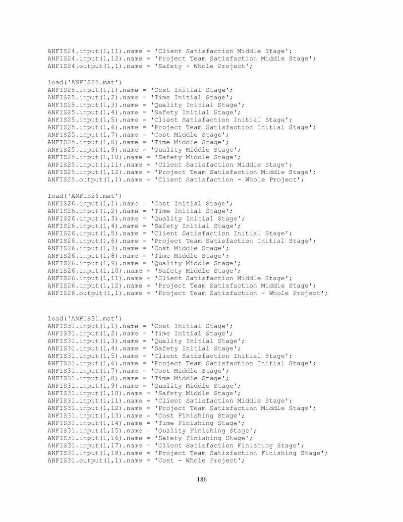
186
ANFIS24.input(1,11).name = 'Client Satisfaction Middle Stage'; ANFIS24.input(1,12).name = 'Project Team Satisfaction Middle Stage'; ANFIS24.output(1,1).name = 'Safety - Whole Project';
load('ANFIS25.mat') ANFIS25.input(1,1).name = 'Cost Initial Stage'; ANFIS25.input(1,2).name = 'Time Initial Stage'; ANFIS25.input(1,3).name = 'Quality Initial Stage'; ANFIS25.input(1,4).name = 'Safety Initial Stage'; ANFIS25.input(1,5).name = 'Client Satisfaction Initial Stage'; ANFIS25.input(1,6).name = 'Project Team Satisfaction Initial Stage'; ANFIS25.input(1,7).name = 'Cost Middle Stage'; ANFIS25.input(1,8).name = 'Time Middle Stage'; ANFIS25.input(1,9).name = 'Quality Middle Stage'; ANFIS25.input(1,10).name = 'Safety Middle Stage'; ANFIS25.input(1,11).name = 'Client Satisfaction Middle Stage'; ANFIS25.input(1,12).name = 'Project Team Satisfaction Middle Stage'; ANFIS25.output(1,1).name = 'Client Satisfaction - Whole Project';
load('ANFIS26.mat') ANFIS26.input(1,1).name = 'Cost Initial Stage'; ANFIS26.input(1,2).name = 'Time Initial Stage'; ANFIS26.input(1,3).name = 'Quality Initial Stage'; ANFIS26.input(1,4).name = 'Safety Initial Stage'; ANFIS26.input(1,5).name = 'Client Satisfaction Initial Stage'; ANFIS26.input(1,6).name = 'Project Team Satisfaction Initial Stage'; ANFIS26.input(1,7).name = 'Cost Middle Stage'; ANFIS26.input(1,8).name = 'Time Middle Stage'; ANFIS26.input(1,9).name = 'Quality Middle Stage'; ANFIS26.input(1,10).name = 'Safety Middle Stage'; ANFIS26.input(1,11).name = 'Client Satisfaction Middle Stage'; ANFIS26.input(1,12).name = 'Project Team Satisfaction Middle Stage'; ANFIS26.output(1,1).name = 'Project Team Satisfaction - Whole Project';
load('ANFIS31.mat') ANFIS31.input(1,1).name = 'Cost Initial Stage'; ANFIS31.input(1,2).name = 'Time Initial Stage'; ANFIS31.input(1,3).name = 'Quality Initial Stage'; ANFIS31.input(1,4).name = 'Safety Initial Stage'; ANFIS31.input(1,5).name = 'Client Satisfaction Initial Stage'; ANFIS31.input(1,6).name = 'Project Team Satisfaction Initial Stage'; ANFIS31.input(1,7).name = 'Cost Middle Stage'; ANFIS31.input(1,8).name = 'Time Middle Stage'; ANFIS31.input(1,9).name = 'Quality Middle Stage'; ANFIS31.input(1,10).name = 'Safety Middle Stage'; ANFIS31.input(1,11).name = 'Client Satisfaction Middle Stage'; ANFIS31.input(1,12).name = 'Project Team Satisfaction Middle Stage'; ANFIS31.input(1,13).name = 'Cost Finishing Stage'; ANFIS31.input(1,14).name = 'Time Finishing Stage'; ANFIS31.input(1,15).name = 'Quality Finishing Stage'; ANFIS31.input(1,16).name = 'Safety Finishing Stage'; ANFIS31.input(1,17).name = 'Client Satisfaction Finishing Stage'; ANFIS31.input(1,18).name = 'Project Team Satisfaction Finishing Stage'; ANFIS31.output(1,1).name = 'Cost - Whole Project';
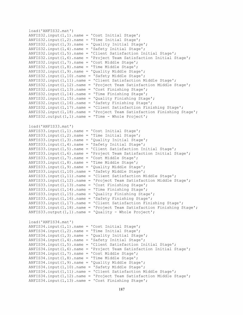
187
load('ANFIS32.mat') ANFIS32.input(1,1).name = 'Cost Initial Stage'; ANFIS32.input(1,2).name = 'Time Initial Stage'; ANFIS32.input(1,3).name = 'Quality Initial Stage'; ANFIS32.input(1,4).name = 'Safety Initial Stage'; ANFIS32.input(1,5).name = 'Client Satisfaction Initial Stage'; ANFIS32.input(1,6).name = 'Project Team Satisfaction Initial Stage'; ANFIS32.input(1,7).name = 'Cost Middle Stage'; ANFIS32.input(1,8).name = 'Time Middle Stage'; ANFIS32.input(1,9).name = 'Quality Middle Stage'; ANFIS32.input(1,10).name = 'Safety Middle Stage'; ANFIS32.input(1,11).name = 'Client Satisfaction Middle Stage'; ANFIS32.input(1,12).name = 'Project Team Satisfaction Middle Stage'; ANFIS32.input(1,13).name = 'Cost Finishing Stage'; ANFIS32.input(1,14).name = 'Time Finishing Stage'; ANFIS32.input(1,15).name = 'Quality Finishing Stage'; ANFIS32.input(1,16).name = 'Safety Finishing Stage'; ANFIS32.input(1,17).name = 'Client Satisfaction Finishing Stage'; ANFIS32.input(1,18).name = 'Project Team Satisfaction Finishing Stage'; ANFIS32.output(1,1).name = 'Time - Whole Project';
load('ANFIS33.mat') ANFIS33.input(1,1).name = 'Cost Initial Stage'; ANFIS33.input(1,2).name = 'Time Initial Stage'; ANFIS33.input(1,3).name = 'Quality Initial Stage'; ANFIS33.input(1,4).name = 'Safety Initial Stage'; ANFIS33.input(1,5).name = 'Client Satisfaction Initial Stage'; ANFIS33.input(1,6).name = 'Project Team Satisfaction Initial Stage'; ANFIS33.input(1,7).name = 'Cost Middle Stage'; ANFIS33.input(1,8).name = 'Time Middle Stage'; ANFIS33.input(1,9).name = 'Quality Middle Stage'; ANFIS33.input(1,10).name = 'Safety Middle Stage'; ANFIS33.input(1,11).name = 'Client Satisfaction Middle Stage'; ANFIS33.input(1,12).name = 'Project Team Satisfaction Middle Stage'; ANFIS33.input(1,13).name = 'Cost Finishing Stage'; ANFIS33.input(1,14).name = 'Time Finishing Stage'; ANFIS33.input(1,15).name = 'Quality Finishing Stage'; ANFIS33.input(1,16).name = 'Safety Finishing Stage'; ANFIS33.input(1,17).name = 'Client Satisfaction Finishing Stage'; ANFIS33.input(1,18).name = 'Project Team Satisfaction Finishing Stage'; ANFIS33.output(1,1).name = 'Quality - Whole Project';
load('ANFIS34.mat') ANFIS34.input(1,1).name = 'Cost Initial Stage'; ANFIS34.input(1,2).name = 'Time Initial Stage'; ANFIS34.input(1,3).name = 'Quality Initial Stage'; ANFIS34.input(1,4).name = 'Safety Initial Stage'; ANFIS34.input(1,5).name = 'Client Satisfaction Initial Stage'; ANFIS34.input(1,6).name = 'Project Team Satisfaction Initial Stage'; ANFIS34.input(1,7).name = 'Cost Middle Stage'; ANFIS34.input(1,8).name = 'Time Middle Stage'; ANFIS34.input(1,9).name = 'Quality Middle Stage'; ANFIS34.input(1,10).name = 'Safety Middle Stage'; ANFIS34.input(1,11).name = 'Client Satisfaction Middle Stage'; ANFIS34.input(1,12).name = 'Project Team Satisfaction Middle Stage'; ANFIS34.input(1,13).name = 'Cost Finishing Stage';
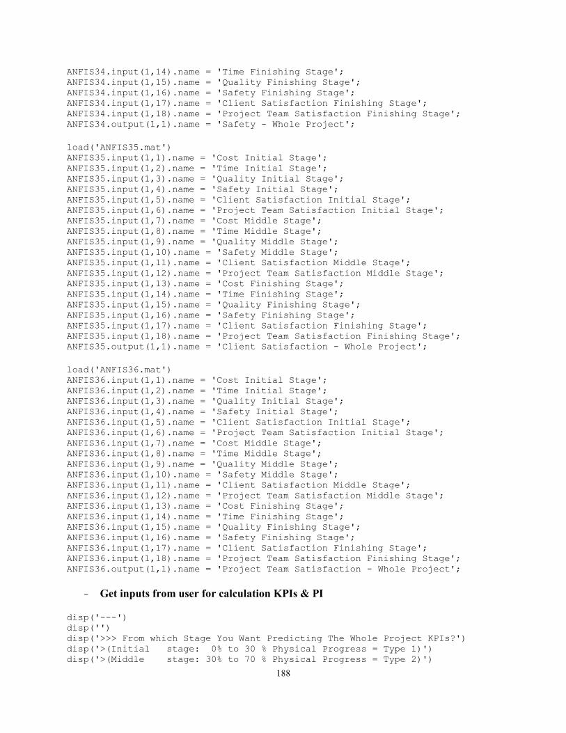
188
ANFIS34.input(1,14).name = 'Time Finishing Stage'; ANFIS34.input(1,15).name = 'Quality Finishing Stage'; ANFIS34.input(1,16).name = 'Safety Finishing Stage'; ANFIS34.input(1,17).name = 'Client Satisfaction Finishing Stage'; ANFIS34.input(1,18).name = 'Project Team Satisfaction Finishing Stage'; ANFIS34.output(1,1).name = 'Safety - Whole Project';
load('ANFIS35.mat') ANFIS35.input(1,1).name = 'Cost Initial Stage'; ANFIS35.input(1,2).name = 'Time Initial Stage'; ANFIS35.input(1,3).name = 'Quality Initial Stage'; ANFIS35.input(1,4).name = 'Safety Initial Stage'; ANFIS35.input(1,5).name = 'Client Satisfaction Initial Stage'; ANFIS35.input(1,6).name = 'Project Team Satisfaction Initial Stage'; ANFIS35.input(1,7).name = 'Cost Middle Stage'; ANFIS35.input(1,8).name = 'Time Middle Stage'; ANFIS35.input(1,9).name = 'Quality Middle Stage'; ANFIS35.input(1,10).name = 'Safety Middle Stage'; ANFIS35.input(1,11).name = 'Client Satisfaction Middle Stage'; ANFIS35.input(1,12).name = 'Project Team Satisfaction Middle Stage'; ANFIS35.input(1,13).name = 'Cost Finishing Stage'; ANFIS35.input(1,14).name = 'Time Finishing Stage'; ANFIS35.input(1,15).name = 'Quality Finishing Stage'; ANFIS35.input(1,16).name = 'Safety Finishing Stage'; ANFIS35.input(1,17).name = 'Client Satisfaction Finishing Stage'; ANFIS35.input(1,18).name = 'Project Team Satisfaction Finishing Stage'; ANFIS35.output(1,1).name = 'Client Satisfaction - Whole Project';
load('ANFIS36.mat') ANFIS36.input(1,1).name = 'Cost Initial Stage'; ANFIS36.input(1,2).name = 'Time Initial Stage'; ANFIS36.input(1,3).name = 'Quality Initial Stage'; ANFIS36.input(1,4).name = 'Safety Initial Stage'; ANFIS36.input(1,5).name = 'Client Satisfaction Initial Stage'; ANFIS36.input(1,6).name = 'Project Team Satisfaction Initial Stage'; ANFIS36.input(1,7).name = 'Cost Middle Stage'; ANFIS36.input(1,8).name = 'Time Middle Stage'; ANFIS36.input(1,9).name = 'Quality Middle Stage'; ANFIS36.input(1,10).name = 'Safety Middle Stage'; ANFIS36.input(1,11).name = 'Client Satisfaction Middle Stage'; ANFIS36.input(1,12).name = 'Project Team Satisfaction Middle Stage'; ANFIS36.input(1,13).name = 'Cost Finishing Stage'; ANFIS36.input(1,14).name = 'Time Finishing Stage'; ANFIS36.input(1,15).name = 'Quality Finishing Stage'; ANFIS36.input(1,16).name = 'Safety Finishing Stage'; ANFIS36.input(1,17).name = 'Client Satisfaction Finishing Stage'; ANFIS36.input(1,18).name = 'Project Team Satisfaction Finishing Stage'; ANFIS36.output(1,1).name = 'Project Team Satisfaction - Whole Project';
- Get inputs from user for calculation KPIs & PI disp('---') disp('') disp('>>> From which Stage You Want Predicting The Whole Project KPIs?') disp('>(Initial stage: 0% to 30 % Physical Progress = Type 1)') disp('>(Middle stage: 30% to 70 % Physical Progress = Type 2)')
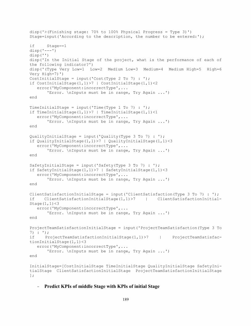
189
disp('>(Finishing stage: 70% to 100% Physical Progress = Type 3)') Stage=input('According to the description, the number to be entered:');
if Stage==1 disp('---') disp('') disp('In the Initial Stage of the project, what is the performance of each of
the following indicator?') disp('(Type Very Low=1 Low=2 Medium Low=3 Medium=4 Medium High=5 High=6
Very High=7)') CostInitialStage = input('Cost(Type 2 To 7) : '); if CostInitialStage(1,1)>7 | CostInitialStage(1,1)<2 error('MyComponent:incorrectType',... 'Error. \nInputs must be in range, Try Again ...') end
TimeInitialStage = input('Time(Type 1 To 7) : '); if TimeInitialStage(1,1)>7 | TimeInitialStage(1,1)<1 error('MyComponent:incorrectType',... 'Error. \nInputs must be in range, Try Again ...') end
QualityInitialStage = input('Quality(Type 3 To 7) : '); if QualityInitialStage(1,1)>7 | QualityInitialStage(1,1)<3 error('MyComponent:incorrectType',... 'Error. \nInputs must be in range, Try Again ...') end
SafetyInitialStage = input('Safety(Type 3 To 7) : '); if SafetyInitialStage(1,1)>7 | SafetyInitialStage(1,1)<3 error('MyComponent:incorrectType',... 'Error. \nInputs must be in range, Try Again ...') end
ClientSatisfactionInitialStage = input('ClientSatisfaction(Type 3 To 7) : '); if ClientSatisfactionInitialStage(1,1)>7 | ClientSatisfactionInitial-
Stage(1,1)<3 error('MyComponent:incorrectType',... 'Error. \nInputs must be in range, Try Again ...') end
ProjectTeamSatisfactionInitialStage = input('ProjectTeamSatisfaction(Type 3 To
7) : '); if ProjectTeamSatisfactionInitialStage(1,1)>7 | ProjectTeamSatisfac-
tionInitialStage(1,1)<3 error('MyComponent:incorrectType',... 'Error. \nInputs must be in range, Try Again ...') end
InitialStage=[CostInitialStage TimeInitialStage QualityInitialStage SafetyIni-
tialStage ClientSatisfactionInitialStage ProjectTeamSatisfactionInitialStage
];
- Predict KPIs of middle Stage with KPIs of initial Stage
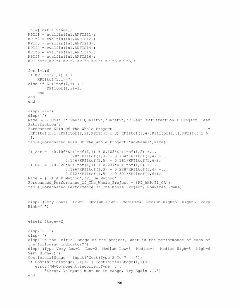
190
In1=[InitialStage]; KPIf1 = evalfis(In1,ANFIS11); KPIf2 = evalfis(In1,ANFIS12); KPIf3 = evalfis(In1,ANFIS13); KPIf4 = evalfis(In1,ANFIS14); KPIf5 = evalfis(In1,ANFIS15); KPIf6 = evalfis(In1,ANFIS16); KPI1tof=[KPIf1 KPIf2 KPIf3 KPIf4 KPIf5 KPIf6];
for i=1:6 if KPI1tof(1,i) > 7 KPI1tof(1,i)=7; else if KPI1tof(1,i) < 1 KPI1tof(1,i)=1; end end end
disp('---') disp('') Name = {'Cost';'Time';'Quality';'Safety';'Client Satisfaction';'Project Team
Satisfaction'; Forecasted_KPIs_Of_The_Whole_Project =
[KPI1tof(1,1);KPI1tof(1,2);KPI1tof(1,3);KPI1tof(1,4);KPI1tof(1,5);KPI1tof(1,6
)]; table(Forecasted_KPIs_Of_The_Whole_Project,'RowNames',Name)
PI_AHP = (0.106*KPI1tof(1,1) + 0.103*KPI1tof(1,2) +... 0.320*KPI1tof(1,3) + 0.134*KPI1tof(1,4) +... 0.176*KPI1tof(1,5) + 0.161*KPI1tof(1,6)); PI_GA = (0.026*KPI1tof(1,1) + 0.237*KPI1tof(1,2) +... 0.196*KPI1tof(1,3) + 0.228*KPI1tof(1,4) +... 0.012*KPI1tof(1,5) + 0.301*KPI1tof(1,6)); Name = {'PI_AHP Method';'PI_GA Method'}; Forecasted_Performance_Of_The_Whole_Project = [PI_AHP;PI_GA]; table(Forecasted_Performance_Of_The_Whole_Project,'RowNames',Name)
disp('(Very Low=1 Low=2 Medium Low=3 Medium=4 Medium High=5 High=6 Very
High=7)')
elseif Stage==2
disp('---') disp('') disp('In the Initial Stage of the project, what is the performance of each of
the following indicator?') disp('(Type Very Low=1 Low=2 Medium Low=3 Medium=4 Medium High=5 High=6
Very High=7)') CostInitialStage = input('Cost(Type 2 To 7) : '); if CostInitialStage(1,1)>7 | CostInitialStage(1,1)<2 error('MyComponent:incorrectType',... 'Error. \nInputs must be in range, Try Again ...') end
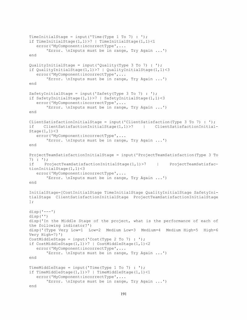
191
TimeInitialStage = input('Time(Type 1 To 7) : '); if TimeInitialStage(1,1)>7 | TimeInitialStage(1,1)<1 error('MyComponent:incorrectType',... 'Error. \nInputs must be in range, Try Again ...') end
QualityInitialStage = input('Quality(Type 3 To 7) : '); if QualityInitialStage(1,1)>7 | QualityInitialStage(1,1)<3 error('MyComponent:incorrectType',... 'Error. \nInputs must be in range, Try Again ...') end
SafetyInitialStage = input('Safety(Type 3 To 7) : '); if SafetyInitialStage(1,1)>7 | SafetyInitialStage(1,1)<3 error('MyComponent:incorrectType',... 'Error. \nInputs must be in range, Try Again ...') end
ClientSatisfactionInitialStage = input('ClientSatisfaction(Type 3 To 7) : '); if ClientSatisfactionInitialStage(1,1)>7 | ClientSatisfactionInitial-
Stage(1,1)<3 error('MyComponent:incorrectType',... 'Error. \nInputs must be in range, Try Again ...') end
ProjectTeamSatisfactionInitialStage = input('ProjectTeamSatisfaction(Type 3 To
7) : '); if ProjectTeamSatisfactionInitialStage(1,1)>7 | ProjectTeamSatisfac-
tionInitialStage(1,1)<3 error('MyComponent:incorrectType',... 'Error. \nInputs must be in range, Try Again ...') end
InitialStage=[CostInitialStage TimeInitialStage QualityInitialStage SafetyIni-
tialStage ClientSatisfactionInitialStage ProjectTeamSatisfactionInitialStage
];
disp('---') disp('') disp('In the Middle Stage of the project, what is the performance of each of
the following indicator?') disp('(Type Very Low=1 Low=2 Medium Low=3 Medium=4 Medium High=5 High=6
Very High=7)') CostMiddleStage = input('Cost(Type 2 To 7) : '); if CostMiddleStage(1,1)>7 | CostMiddleStage(1,1)<2 error('MyComponent:incorrectType',... 'Error. \nInputs must be in range, Try Again ...') end
TimeMiddleStage = input('Time(Type 1 To 7) : '); if TimeMiddleStage(1,1)>7 | TimeMiddleStage(1,1)<1 error('MyComponent:incorrectType',... 'Error. \nInputs must be in range, Try Again ...') end
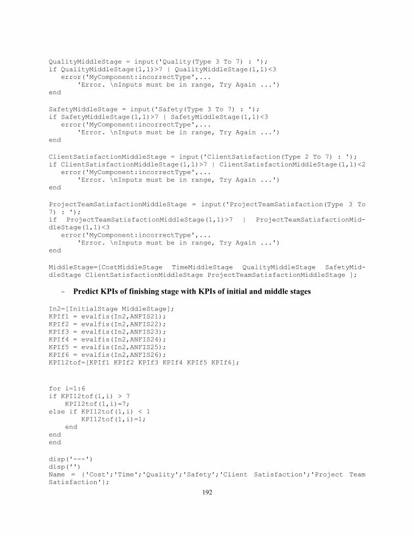
192
QualityMiddleStage = input('Quality(Type 3 To 7) : '); if QualityMiddleStage(1,1)>7 | QualityMiddleStage(1,1)<3 error('MyComponent:incorrectType',... 'Error. \nInputs must be in range, Try Again ...') end
SafetyMiddleStage = input('Safety(Type 3 To 7) : '); if SafetyMiddleStage(1,1)>7 | SafetyMiddleStage(1,1)<3 error('MyComponent:incorrectType',... 'Error. \nInputs must be in range, Try Again ...') end
ClientSatisfactionMiddleStage = input('ClientSatisfaction(Type 2 To 7) : '); if ClientSatisfactionMiddleStage(1,1)>7 | ClientSatisfactionMiddleStage(1,1)<2 error('MyComponent:incorrectType',... 'Error. \nInputs must be in range, Try Again ...') end
ProjectTeamSatisfactionMiddleStage = input('ProjectTeamSatisfaction(Type 3 To
7) : '); if ProjectTeamSatisfactionMiddleStage(1,1)>7 | ProjectTeamSatisfactionMid-
dleStage(1,1)<3 error('MyComponent:incorrectType',... 'Error. \nInputs must be in range, Try Again ...') end
MiddleStage=[CostMiddleStage TimeMiddleStage QualityMiddleStage SafetyMid-
dleStage ClientSatisfactionMiddleStage ProjectTeamSatisfactionMiddleStage ];
- Predict KPIs of finishing stage with KPIs of initial and middle stages In2=[InitialStage MiddleStage]; KPIf1 = evalfis(In2,ANFIS21); KPIf2 = evalfis(In2,ANFIS22); KPIf3 = evalfis(In2,ANFIS23); KPIf4 = evalfis(In2,ANFIS24); KPIf5 = evalfis(In2,ANFIS25); KPIf6 = evalfis(In2,ANFIS26); KPI12tof=[KPIf1 KPIf2 KPIf3 KPIf4 KPIf5 KPIf6];
for i=1:6 if KPI12tof(1,i) > 7 KPI12tof(1,i)=7; else if KPI12tof(1,i) < 1 KPI12tof(1,i)=1; end end end
disp('---') disp('') Name = {'Cost';'Time';'Quality';'Safety';'Client Satisfaction';'Project Team
Satisfaction'};
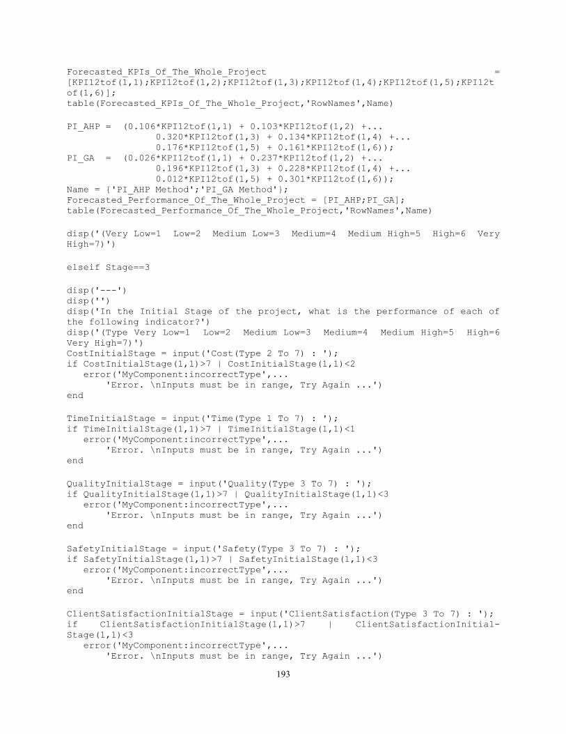
193
Forecasted_KPIs_Of_The_Whole_Project =
[KPI12tof(1,1);KPI12tof(1,2);KPI12tof(1,3);KPI12tof(1,4);KPI12tof(1,5);KPI12t
of(1,6)]; table(Forecasted_KPIs_Of_The_Whole_Project,'RowNames',Name)
PI_AHP = (0.106*KPI12tof(1,1) + 0.103*KPI12tof(1,2) +... 0.320*KPI12tof(1,3) + 0.134*KPI12tof(1,4) +... 0.176*KPI12tof(1,5) + 0.161*KPI12tof(1,6)); PI_GA = (0.026*KPI12tof(1,1) + 0.237*KPI12tof(1,2) +... 0.196*KPI12tof(1,3) + 0.228*KPI12tof(1,4) +... 0.012*KPI12tof(1,5) + 0.301*KPI12tof(1,6)); Name = {'PI_AHP Method';'PI_GA Method'}; Forecasted_Performance_Of_The_Whole_Project = [PI_AHP;PI_GA]; table(Forecasted_Performance_Of_The_Whole_Project,'RowNames',Name)
disp('(Very Low=1 Low=2 Medium Low=3 Medium=4 Medium High=5 High=6 Very
High=7)')
elseif Stage==3
disp('---') disp('') disp('In the Initial Stage of the project, what is the performance of each of
the following indicator?') disp('(Type Very Low=1 Low=2 Medium Low=3 Medium=4 Medium High=5 High=6
Very High=7)') CostInitialStage = input('Cost(Type 2 To 7) : '); if CostInitialStage(1,1)>7 | CostInitialStage(1,1)<2 error('MyComponent:incorrectType',... 'Error. \nInputs must be in range, Try Again ...') end
TimeInitialStage = input('Time(Type 1 To 7) : '); if TimeInitialStage(1,1)>7 | TimeInitialStage(1,1)<1 error('MyComponent:incorrectType',... 'Error. \nInputs must be in range, Try Again ...') end
QualityInitialStage = input('Quality(Type 3 To 7) : '); if QualityInitialStage(1,1)>7 | QualityInitialStage(1,1)<3 error('MyComponent:incorrectType',... 'Error. \nInputs must be in range, Try Again ...') end
SafetyInitialStage = input('Safety(Type 3 To 7) : '); if SafetyInitialStage(1,1)>7 | SafetyInitialStage(1,1)<3 error('MyComponent:incorrectType',... 'Error. \nInputs must be in range, Try Again ...') end
ClientSatisfactionInitialStage = input('ClientSatisfaction(Type 3 To 7) : '); if ClientSatisfactionInitialStage(1,1)>7 | ClientSatisfactionInitial-
Stage(1,1)<3 error('MyComponent:incorrectType',... 'Error. \nInputs must be in range, Try Again ...')
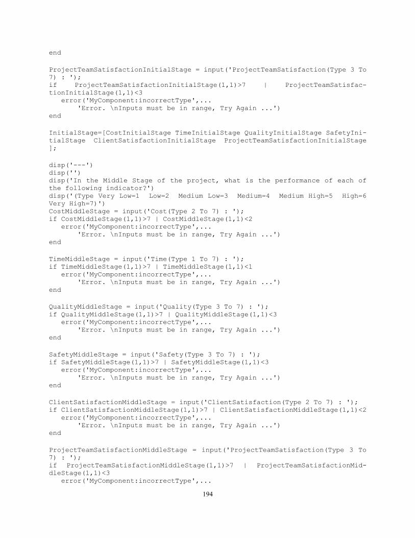
194
end
ProjectTeamSatisfactionInitialStage = input('ProjectTeamSatisfaction(Type 3 To
7) : '); if ProjectTeamSatisfactionInitialStage(1,1)>7 | ProjectTeamSatisfac-
tionInitialStage(1,1)<3 error('MyComponent:incorrectType',... 'Error. \nInputs must be in range, Try Again ...') end
InitialStage=[CostInitialStage TimeInitialStage QualityInitialStage SafetyIni-
tialStage ClientSatisfactionInitialStage ProjectTeamSatisfactionInitialStage
];
disp('---') disp('') disp('In the Middle Stage of the project, what is the performance of each of
the following indicator?') disp('(Type Very Low=1 Low=2 Medium Low=3 Medium=4 Medium High=5 High=6
Very High=7)') CostMiddleStage = input('Cost(Type 2 To 7) : '); if CostMiddleStage(1,1)>7 | CostMiddleStage(1,1)<2 error('MyComponent:incorrectType',... 'Error. \nInputs must be in range, Try Again ...') end
TimeMiddleStage = input('Time(Type 1 To 7) : '); if TimeMiddleStage(1,1)>7 | TimeMiddleStage(1,1)<1 error('MyComponent:incorrectType',... 'Error. \nInputs must be in range, Try Again ...') end
QualityMiddleStage = input('Quality(Type 3 To 7) : '); if QualityMiddleStage(1,1)>7 | QualityMiddleStage(1,1)<3 error('MyComponent:incorrectType',... 'Error. \nInputs must be in range, Try Again ...') end
SafetyMiddleStage = input('Safety(Type 3 To 7) : '); if SafetyMiddleStage(1,1)>7 | SafetyMiddleStage(1,1)<3 error('MyComponent:incorrectType',... 'Error. \nInputs must be in range, Try Again ...') end
ClientSatisfactionMiddleStage = input('ClientSatisfaction(Type 2 To 7) : '); if ClientSatisfactionMiddleStage(1,1)>7 | ClientSatisfactionMiddleStage(1,1)<2 error('MyComponent:incorrectType',... 'Error. \nInputs must be in range, Try Again ...') end
ProjectTeamSatisfactionMiddleStage = input('ProjectTeamSatisfaction(Type 3 To
7) : '); if ProjectTeamSatisfactionMiddleStage(1,1)>7 | ProjectTeamSatisfactionMid-
dleStage(1,1)<3 error('MyComponent:incorrectType',...
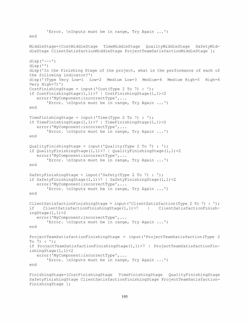
195
'Error. \nInputs must be in range, Try Again ...') end
MiddleStage=[CostMiddleStage TimeMiddleStage QualityMiddleStage SafetyMid-
dleStage ClientSatisfactionMiddleStage ProjectTeamSatisfactionMiddleStage ];
disp('---') disp('') disp('In the Finishing Stage of the project, what is the performance of each of
the following indicator?') disp('(Type Very Low=1 Low=2 Medium Low=3 Medium=4 Medium High=5 High=6
Very High=7)') CostFinishingStage = input('Cost(Type 2 To 7) : '); if CostFinishingStage(1,1)>7 | CostFinishingStage(1,1)<2 error('MyComponent:incorrectType',... 'Error. \nInputs must be in range, Try Again ...') end
TimeFinishingStage = input('Time(Type 2 To 7) : '); if TimeFinishingStage(1,1)>7 | TimeFinishingStage(1,1)<2 error('MyComponent:incorrectType',... 'Error. \nInputs must be in range, Try Again ...') end
QualityFinishingStage = input('Quality(Type 2 To 7) : '); if QualityFinishingStage(1,1)>7 | QualityFinishingStage(1,1)<2 error('MyComponent:incorrectType',... 'Error. \nInputs must be in range, Try Again ...') end
SafetyFinishingStage = input('Safety(Type 2 To 7) : '); if SafetyFinishingStage(1,1)>7 | SafetyFinishingStage(1,1)<2 error('MyComponent:incorrectType',... 'Error. \nInputs must be in range, Try Again ...') end
ClientSatisfactionFinishingStage = input('ClientSatisfaction(Type 2 To 7) : '); if ClientSatisfactionFinishingStage(1,1)>7 | ClientSatisfactionFinish-
ingStage(1,1)<2 error('MyComponent:incorrectType',... 'Error. \nInputs must be in range, Try Again ...') end
ProjectTeamSatisfactionFinishingStage = input('ProjectTeamSatisfaction(Type 2
To 7) : '); if ProjectTeamSatisfactionFinishingStage(1,1)>7 | ProjectTeamSatisfactionFin-
ishingStage(1,1)<2 error('MyComponent:incorrectType',... 'Error. \nInputs must be in range, Try Again ...') end
FinishingStage=[CostFinishingStage TimeFinishingStage QualityFinishingStage
SafetyFinishingStage ClientSatisfactionFinishingStage ProjectTeamSatisfaction-
FinishingStage ];
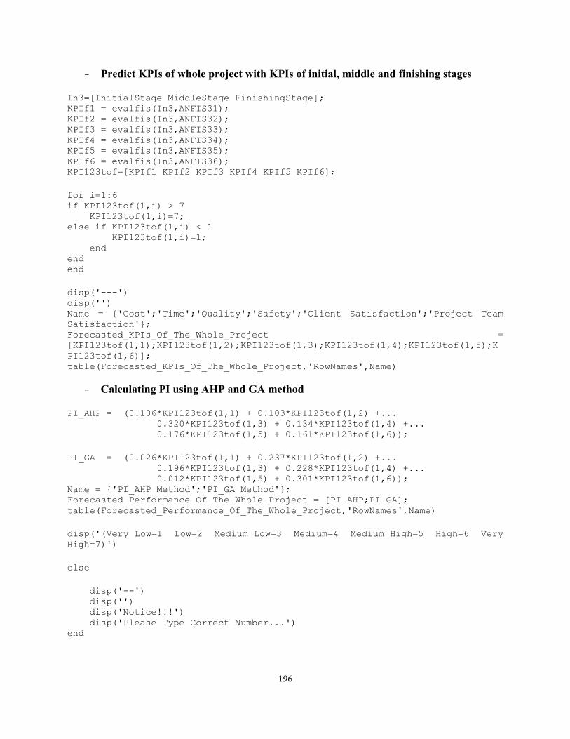
196
- Predict KPIs of whole project with KPIs of initial, middle and finishing stages In3=[InitialStage MiddleStage FinishingStage]; KPIf1 = evalfis(In3,ANFIS31); KPIf2 = evalfis(In3,ANFIS32); KPIf3 = evalfis(In3,ANFIS33); KPIf4 = evalfis(In3,ANFIS34); KPIf5 = evalfis(In3,ANFIS35); KPIf6 = evalfis(In3,ANFIS36); KPI123tof=[KPIf1 KPIf2 KPIf3 KPIf4 KPIf5 KPIf6];
for i=1:6 if KPI123tof(1,i) > 7 KPI123tof(1,i)=7; else if KPI123tof(1,i) < 1 KPI123tof(1,i)=1; end end end
disp('---') disp('') Name = {'Cost';'Time';'Quality';'Safety';'Client Satisfaction';'Project Team
Satisfaction'}; Forecasted_KPIs_Of_The_Whole_Project =
[KPI123tof(1,1);KPI123tof(1,2);KPI123tof(1,3);KPI123tof(1,4);KPI123tof(1,5);K
PI123tof(1,6)]; table(Forecasted_KPIs_Of_The_Whole_Project,'RowNames',Name)
- Calculating PI using AHP and GA method PI_AHP = (0.106*KPI123tof(1,1) + 0.103*KPI123tof(1,2) +... 0.320*KPI123tof(1,3) + 0.134*KPI123tof(1,4) +... 0.176*KPI123tof(1,5) + 0.161*KPI123tof(1,6));
PI_GA = (0.026*KPI123tof(1,1) + 0.237*KPI123tof(1,2) +... 0.196*KPI123tof(1,3) + 0.228*KPI123tof(1,4) +... 0.012*KPI123tof(1,5) + 0.301*KPI123tof(1,6)); Name = {'PI_AHP Method';'PI_GA Method'}; Forecasted_Performance_Of_The_Whole_Project = [PI_AHP;PI_GA]; table(Forecasted_Performance_Of_The_Whole_Project,'RowNames',Name)
disp('(Very Low=1 Low=2 Medium Low=3 Medium=4 Medium High=5 High=6 Very
High=7)')
else
disp('--') disp('') disp('Notice!!!') disp('Please Type Correct Number...') end
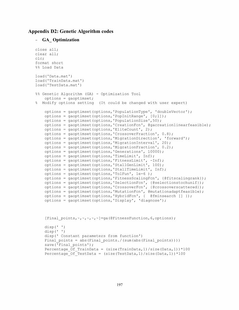
197
Appendix D2: Genetic Algorithm codes
- GA_ Optimization
close all;
clear all;
clc;
format short
%% Load Data
load('Data.mat')
load('TrainData.mat')
load('TestData.mat')
%% Genetic Algorithm (GA) - Optimization Tool
options = gaoptimset;
% Modify options setting (It could be changed with user expert)
options = gaoptimset(options,'PopulationType', 'doubleVector');
options = gaoptimset(options,'PopInitRange', [0;1]);
options = gaoptimset(options,'PopulationSize',50);
options = gaoptimset(options,'CreationFcn', @gacreationlinearfeasible);
options = gaoptimset(options,'EliteCount', 2);
options = gaoptimset(options,'CrossoverFraction', 0.8);
options = gaoptimset(options,'MigrationDirection', 'forward');
options = gaoptimset(options,'MigrationInterval', 20);
options = gaoptimset(options,'MigrationFraction', 0.2);
options = gaoptimset(options,'Generations', 10000);
options = gaoptimset(options,'TimeLimit', Inf);
options = gaoptimset(options,'FitnessLimit', -Inf);
options = gaoptimset(options,'StallGenLimit', 100);
options = gaoptimset(options,'StallTimeLimit', Inf);
options = gaoptimset(options,'TolFun', 1e-6 );
options = gaoptimset(options,'FitnessScalingFcn', {@fitscalingrank});
options = gaoptimset(options,'SelectionFcn', {@selectionstochunif});
options = gaoptimset(options,'CrossoverFcn', {@crossoverscattered});
options = gaoptimset(options,'MutationFcn', @mutationadaptfeasible);
options = gaoptimset(options,'HybridFcn', { @fminsearch [] });
options = gaoptimset(options,'Display', 'diagnose');
[Final_points,~,~,~,~,~]=ga(@FitnessFunction,6,options);
disp(' ')
disp(' ')
disp(' Constant parameters from function')
Final_points = abs(Final_points./(sum(abs(Final_points))))
save('Final_points');
Percentage_Of_TrainData = (size(TrainData,1)/size(Data,1))*100
Percentage_Of_TestData = (size(TestData,1)/size(Data,1))*100

198
- Fitness Function Function [ RMSE ] = FitnessFunction(X)
load('TrainData.mat') % Load Train dataset
load('TestData.mat') % Load Test dataset
TotalData = [TrainData;TestData]; % Total dataset
DataInUse = TrainData; % The Data is used in optimization
for i=1:size(DataInUse,1)
% Output from experimental
Output_Exp(i,1) = DataInUse(i,end);
% Output from function
Output_Model(i,1)= X(1)*DataInUse(i,1)+...
X(2)*DataInUse(i,2)+...
X(3)*DataInUse(i,3)+...
X(4)*DataInUse(i,4)+...
X(5)*DataInUse(i,5)+...
X(6)*DataInUse(i,6);
Errors(i,1) = abs(Output_Exp(i,1)-Output_Model(i,1));
end
MSE = mean(Errors(:,1).^2); % Calculate MSE
RMSE = sqrt(MSE); % Calculate RMSE,RMSE must be optimized
End
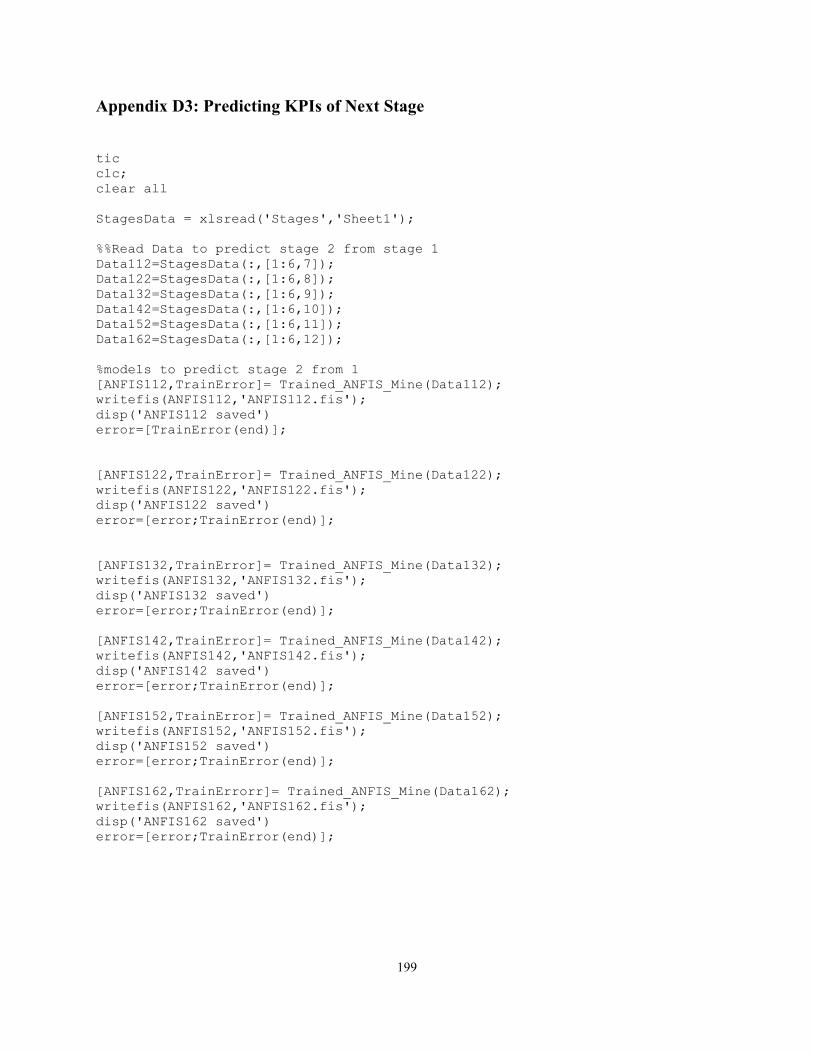
199
Appendix D3: Predicting KPIs of Next Stage
tic
clc;
clear all
StagesData = xlsread('Stages','Sheet1');
%%Read Data to predict stage 2 from stage 1
Data112=StagesData(:,[1:6,7]);
Data122=StagesData(:,[1:6,8]);
Data132=StagesData(:,[1:6,9]);
Data142=StagesData(:,[1:6,10]);
Data152=StagesData(:,[1:6,11]);
Data162=StagesData(:,[1:6,12]);
%models to predict stage 2 from 1
[ANFIS112,TrainError]= Trained_ANFIS_Mine(Data112);
writefis(ANFIS112,'ANFIS112.fis');
disp('ANFIS112 saved')
error=[TrainError(end)];
[ANFIS122,TrainError]= Trained_ANFIS_Mine(Data122);
writefis(ANFIS122,'ANFIS122.fis');
disp('ANFIS122 saved')
error=[error;TrainError(end)];
[ANFIS132,TrainError]= Trained_ANFIS_Mine(Data132);
writefis(ANFIS132,'ANFIS132.fis');
disp('ANFIS132 saved')
error=[error;TrainError(end)];
[ANFIS142,TrainError]= Trained_ANFIS_Mine(Data142);
writefis(ANFIS142,'ANFIS142.fis');
disp('ANFIS142 saved')
error=[error;TrainError(end)];
[ANFIS152,TrainError]= Trained_ANFIS_Mine(Data152);
writefis(ANFIS152,'ANFIS152.fis');
disp('ANFIS152 saved')
error=[error;TrainError(end)];
[ANFIS162,TrainErrorr]= Trained_ANFIS_Mine(Data162);
writefis(ANFIS162,'ANFIS162.fis');
disp('ANFIS162 saved')
error=[error;TrainError(end)];
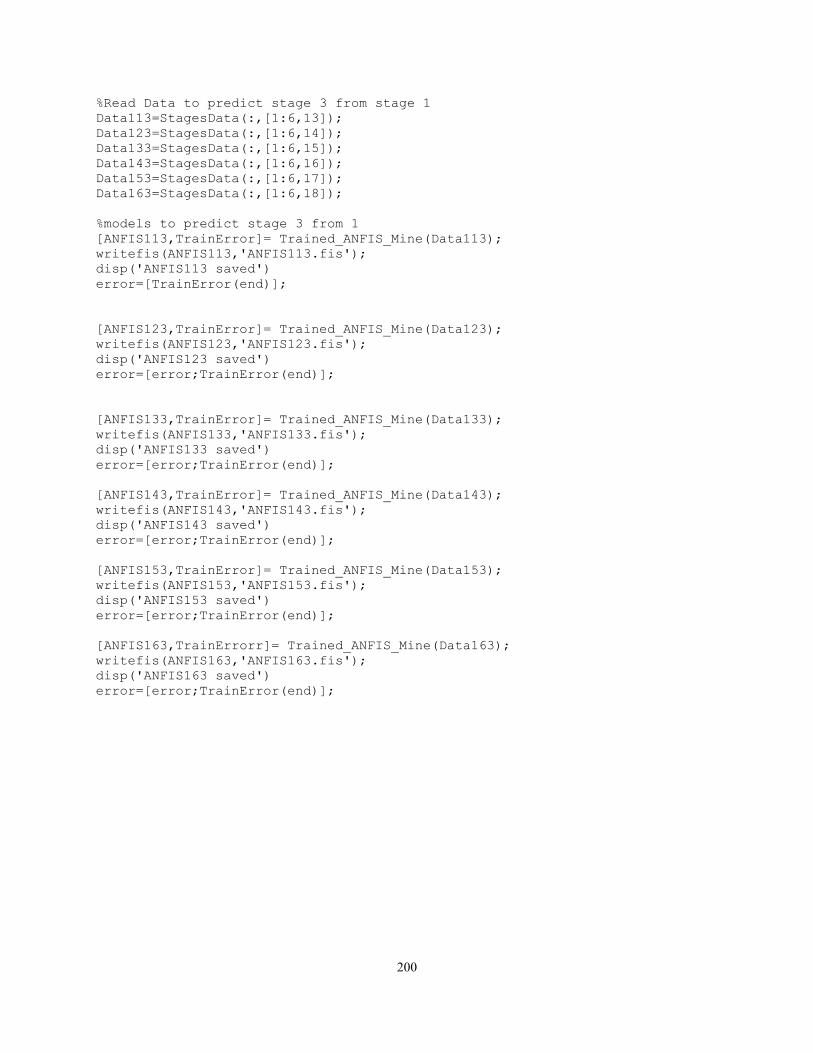
200
%Read Data to predict stage 3 from stage 1
Data113=StagesData(:,[1:6,13]);
Data123=StagesData(:,[1:6,14]);
Data133=StagesData(:,[1:6,15]);
Data143=StagesData(:,[1:6,16]);
Data153=StagesData(:,[1:6,17]);
Data163=StagesData(:,[1:6,18]);
%models to predict stage 3 from 1
[ANFIS113,TrainError]= Trained_ANFIS_Mine(Data113);
writefis(ANFIS113,'ANFIS113.fis');
disp('ANFIS113 saved')
error=[TrainError(end)];
[ANFIS123,TrainError]= Trained_ANFIS_Mine(Data123);
writefis(ANFIS123,'ANFIS123.fis');
disp('ANFIS123 saved')
error=[error;TrainError(end)];
[ANFIS133,TrainError]= Trained_ANFIS_Mine(Data133);
writefis(ANFIS133,'ANFIS133.fis');
disp('ANFIS133 saved')
error=[error;TrainError(end)];
[ANFIS143,TrainError]= Trained_ANFIS_Mine(Data143);
writefis(ANFIS143,'ANFIS143.fis');
disp('ANFIS143 saved')
error=[error;TrainError(end)];
[ANFIS153,TrainError]= Trained_ANFIS_Mine(Data153);
writefis(ANFIS153,'ANFIS153.fis');
disp('ANFIS153 saved')
error=[error;TrainError(end)];
[ANFIS163,TrainErrorr]= Trained_ANFIS_Mine(Data163);
writefis(ANFIS163,'ANFIS163.fis');
disp('ANFIS163 saved')
error=[error;TrainError(end)];
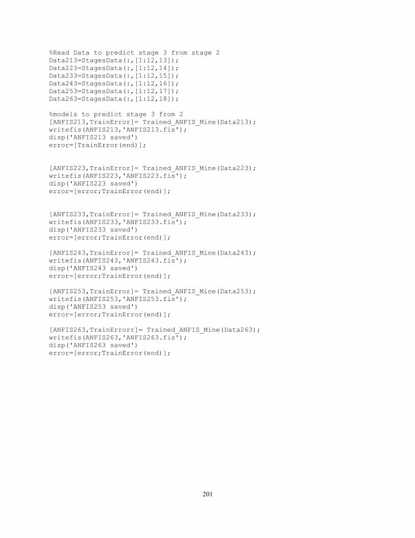
201
%Read Data to predict stage 3 from stage 2
Data213=StagesData(:,[1:12,13]);
Data223=StagesData(:,[1:12,14]);
Data233=StagesData(:,[1:12,15]);
Data243=StagesData(:,[1:12,16]);
Data253=StagesData(:,[1:12,17]);
Data263=StagesData(:,[1:12,18]);
%models to predict stage 3 from 2
[ANFIS213,TrainError]= Trained_ANFIS_Mine(Data213);
writefis(ANFIS213,'ANFIS213.fis');
disp('ANFIS213 saved')
error=[TrainError(end)];
[ANFIS223,TrainError]= Trained_ANFIS_Mine(Data223);
writefis(ANFIS223,'ANFIS223.fis');
disp('ANFIS223 saved')
error=[error;TrainError(end)];
[ANFIS233,TrainError]= Trained_ANFIS_Mine(Data233);
writefis(ANFIS233,'ANFIS233.fis');
disp('ANFIS233 saved')
error=[error;TrainError(end)];
[ANFIS243,TrainError]= Trained_ANFIS_Mine(Data243);
writefis(ANFIS243,'ANFIS243.fis');
disp('ANFIS243 saved')
error=[error;TrainError(end)];
[ANFIS253,TrainError]= Trained_ANFIS_Mine(Data253);
writefis(ANFIS253,'ANFIS253.fis');
disp('ANFIS253 saved')
error=[error;TrainError(end)];
[ANFIS263,TrainErrorr]= Trained_ANFIS_Mine(Data263);
writefis(ANFIS263,'ANFIS263.fis');
disp('ANFIS263 saved')
error=[error;TrainError(end)];
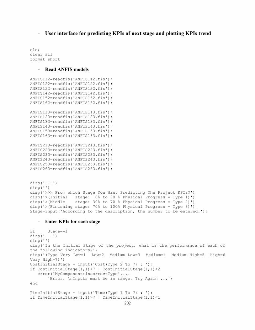
202
- User interface for predicting KPIs of next stage and plotting KPIs trend
clc;
clear all
format short
- Read ANFIS models
ANFIS112=readfis('ANFIS112.fis');
ANFIS122=readfis('ANFIS122.fis');
ANFIS132=readfis('ANFIS132.fis');
ANFIS142=readfis('ANFIS142.fis');
ANFIS152=readfis('ANFIS152.fis');
ANFIS162=readfis('ANFIS162.fis');
ANFIS113=readfis('ANFIS113.fis');
ANFIS123=readfis('ANFIS123.fis');
ANFIS133=readfis('ANFIS133.fis');
ANFIS143=readfis('ANFIS143.fis');
ANFIS153=readfis('ANFIS153.fis');
ANFIS163=readfis('ANFIS163.fis');
ANFIS213=readfis('ANFIS213.fis');
ANFIS223=readfis('ANFIS223.fis');
ANFIS233=readfis('ANFIS233.fis');
ANFIS243=readfis('ANFIS243.fis');
ANFIS253=readfis('ANFIS253.fis');
ANFIS263=readfis('ANFIS263.fis');
disp('---')
disp('')
disp('>>> From which Stage You Want Predicting The Project KPIs?')
disp('>(Initial stage: 0% to 30 % Physical Progress = Type 1)')
disp('>(Middle stage: 30% to 70 % Physical Progress = Type 2)')
disp('>(Finishing stage: 70% to 100% Physical Progress = Type 3)')
Stage=input('According to the description, the number to be entered:');
- Enter KPIs for each stage
if Stage==1
disp('---')
disp('')
disp('In the Initial Stage of the project, what is the performance of each of
the following indicators?')
disp('(Type Very Low=1 Low=2 Medium Low=3 Medium=4 Medium High=5 High=6
Very High=7)')
CostInitialStage = input('Cost(Type 2 To 7) : ');
if CostInitialStage(1,1)>7 | CostInitialStage(1,1)<2
error('MyComponent:incorrectType',...
'Error. \nInputs must be in range, Try Again ...')
end
TimeInitialStage = input('Time(Type 1 To 7) : ');
if TimeInitialStage(1,1)>7 | TimeInitialStage(1,1)<1
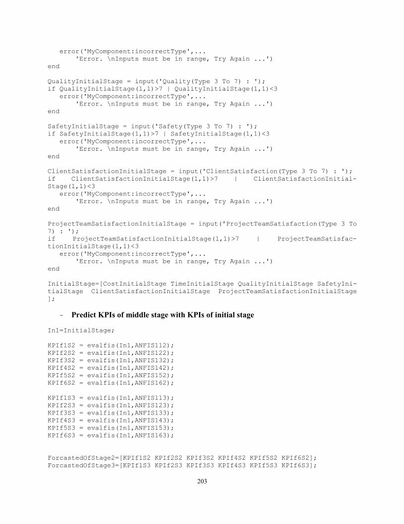
203
error('MyComponent:incorrectType',...
'Error. \nInputs must be in range, Try Again ...')
end
QualityInitialStage = input('Quality(Type 3 To 7) : ');
if QualityInitialStage(1,1)>7 | QualityInitialStage(1,1)<3
error('MyComponent:incorrectType',...
'Error. \nInputs must be in range, Try Again ...')
end
SafetyInitialStage = input('Safety(Type 3 To 7) : ');
if SafetyInitialStage(1,1)>7 | SafetyInitialStage(1,1)<3
error('MyComponent:incorrectType',...
'Error. \nInputs must be in range, Try Again ...')
end
ClientSatisfactionInitialStage = input('ClientSatisfaction(Type 3 To 7) : ');
if ClientSatisfactionInitialStage(1,1)>7 | ClientSatisfactionInitial-
Stage(1,1)<3
error('MyComponent:incorrectType',...
'Error. \nInputs must be in range, Try Again ...')
end
ProjectTeamSatisfactionInitialStage = input('ProjectTeamSatisfaction(Type 3 To
7) : ');
if ProjectTeamSatisfactionInitialStage(1,1)>7 | ProjectTeamSatisfac-
tionInitialStage(1,1)<3
error('MyComponent:incorrectType',...
'Error. \nInputs must be in range, Try Again ...')
end
InitialStage=[CostInitialStage TimeInitialStage QualityInitialStage SafetyIni-
tialStage ClientSatisfactionInitialStage ProjectTeamSatisfactionInitialStage
];
- Predict KPIs of middle stage with KPIs of initial stage
In1=InitialStage;
KPIf1S2 = evalfis(In1,ANFIS112);
KPIf2S2 = evalfis(In1,ANFIS122);
KPIf3S2 = evalfis(In1,ANFIS132);
KPIf4S2 = evalfis(In1,ANFIS142);
KPIf5S2 = evalfis(In1,ANFIS152);
KPIf6S2 = evalfis(In1,ANFIS162);
KPIf1S3 = evalfis(In1,ANFIS113);
KPIf2S3 = evalfis(In1,ANFIS123);
KPIf3S3 = evalfis(In1,ANFIS133);
KPIf4S3 = evalfis(In1,ANFIS143);
KPIf5S3 = evalfis(In1,ANFIS153);
KPIf6S3 = evalfis(In1,ANFIS163);
ForcastedOfStage2=[KPIf1S2 KPIf2S2 KPIf3S2 KPIf4S2 KPIf5S2 KPIf6S2];
ForcastedOfStage3=[KPIf1S3 KPIf2S3 KPIf3S3 KPIf4S3 KPIf5S3 KPIf6S3];
204
for i=1:6
if ForcastedOfStage2(1,i) > 7
ForcastedOfStage2(1,i)=7;
else if ForcastedOfStage2(1,i) < 1
ForcastedOfStage2(1,i)=1;
end
end
end
for i=1:6
if ForcastedOfStage3(1,i) > 7
ForcastedOfStage3(1,i)=7;
else if ForcastedOfStage3(1,i) < 1
ForcastedOfStage3(1,i)=1;
end
end
end
disp('---')
disp('')
disp('Forcasted next stages')
Name = {'Cost';'Time';'Quality';'Safety';'Client Satisfaction';'Project Team
Satisfaction'};
Forecasted_KPIs_Of_Middle_Stage=ForcastedOfStage2';
Forecasted_KPIs_Of_Finishing_Stage=ForcastedOfStage3';
table(Forecasted_KPIs_Of_Middle_Stage,Forecasted_KPIs_Of_Finish-
ing_Stage,'RowNames',Name)
disp('(Very Low=1 Low=2 Medium Low=3 Medium=4 Medium High=5 High=6 Very
High=7)')
Stage1= InitialStage;
Stage2=ForcastedOfStage2;
Stage3=ForcastedOfStage3;
elseif Stage==2
disp('---')
disp('')
disp('In the Initial Stage of the project, what is the performance of each of
the following indicator?')
disp('(Type Very Low=1 Low=2 Medium Low=3 Medium=4 Medium High=5 High=6
Very High=7)')
CostInitialStage = input('Cost(Type 2 To 7) : ');
if CostInitialStage(1,1)>7 | CostInitialStage(1,1)<2
error('MyComponent:incorrectType',...
'Error. \nInputs must be in range, Try Again ...')
end
TimeInitialStage = input('Time(Type 1 To 7) : ');
if TimeInitialStage(1,1)>7 | TimeInitialStage(1,1)<1
error('MyComponent:incorrectType',...
'Error. \nInputs must be in range, Try Again ...')
end
QualityInitialStage = input('Quality(Type 3 To 7) : ');
205
if QualityInitialStage(1,1)>7 | QualityInitialStage(1,1)<3
error('MyComponent:incorrectType',...
'Error. \nInputs must be in range, Try Again ...')
end
SafetyInitialStage = input('Safety(Type 3 To 7) : ');
if SafetyInitialStage(1,1)>7 | SafetyInitialStage(1,1)<3
error('MyComponent:incorrectType',...
'Error. \nInputs must be in range, Try Again ...')
end
ClientSatisfactionInitialStage = input('ClientSatisfaction(Type 3 To 7) : ');
if ClientSatisfactionInitialStage(1,1)>7 | ClientSatisfactionInitial-
Stage(1,1)<3
error('MyComponent:incorrectType',...
'Error. \nInputs must be in range, Try Again ...')
end
ProjectTeamSatisfactionInitialStage = input('ProjectTeamSatisfaction(Type 3 To
7) : ');
if ProjectTeamSatisfactionInitialStage(1,1)>7 | ProjectTeamSatisfac-
tionInitialStage(1,1)<3
error('MyComponent:incorrectType',...
'Error. \nInputs must be in range, Try Again ...')
end
InitialStage=[CostInitialStage TimeInitialStage QualityInitialStage SafetyIni-
tialStage ClientSatisfactionInitialStage ProjectTeamSatisfactionInitialStage
];
disp('---')
disp('')
disp('In the Middle Stage of the project, what is the performance of each of
the following indicator?')
disp('(Type Very Low=1 Low=2 Medium Low=3 Medium=4 Medium High=5 High=6
Very High=7)')
CostMiddleStage = input('Cost(Type 2 To 7) : ');
if CostMiddleStage(1,1)>7 | CostMiddleStage(1,1)<2
error('MyComponent:incorrectType',...
'Error. \nInputs must be in range, Try Again ...')
end
TimeMiddleStage = input('Time(Type 1 To 7) : ');
if TimeMiddleStage(1,1)>7 | TimeMiddleStage(1,1)<1
error('MyComponent:incorrectType',...
'Error. \nInputs must be in range, Try Again ...')
end
QualityMiddleStage = input('Quality(Type 3 To 7) : ');
if QualityMiddleStage(1,1)>7 | QualityMiddleStage(1,1)<3
error('MyComponent:incorrectType',...
'Error. \nInputs must be in range, Try Again ...')
end
SafetyMiddleStage = input('Safety(Type 3 To 7) : ');
if SafetyMiddleStage(1,1)>7 | SafetyMiddleStage(1,1)<3
error('MyComponent:incorrectType',...
206
'Error. \nInputs must be in range, Try Again ...')
end
ClientSatisfactionMiddleStage = input('ClientSatisfaction(Type 2 To 7) : ');
if ClientSatisfactionMiddleStage(1,1)>7 | ClientSatisfactionMiddleStage(1,1)<2
error('MyComponent:incorrectType',...
'Error. \nInputs must be in range, Try Again ...')
end
ProjectTeamSatisfactionMiddleStage = input('ProjectTeamSatisfaction(Type 3 To
7) : ');
if ProjectTeamSatisfactionMiddleStage(1,1)>7 | ProjectTeamSatisfactionMid-
dleStage(1,1)<3
error('MyComponent:incorrectType',...
'Error. \nInputs must be in range, Try Again ...')
end
MiddleStage=[CostMiddleStage TimeMiddleStage QualityMiddleStage SafetyMid-
dleStage ClientSatisfactionMiddleStage ProjectTeamSatisfactionMiddleStage ];
- Predict KPIs of finishing stage with KPIs of initial and middle stages
In2=[InitialStage MiddleStage];
KPIf1S3=evalfis(In2,ANFIS213);
KPIf2S3=evalfis(In2,ANFIS223);
KPIf3S3=evalfis(In2,ANFIS233);
KPIf4S3=evalfis(In2,ANFIS243);
KPIf5S3=evalfis(In2,ANFIS253);
KPIf6S3=evalfis(In2,ANFIS263);
KPIS3=[KPIf1S3 KPIf2S3 KPIf3S3 KPIf4S3 KPIf5S3 KPIf6S3];
for i=1:6
if KPIS3(1,i) > 7
KPIS3(1,i)=7;
else if KPIS3(1,i) < 1
KPIS3(1,i)=1;
end
end
end
Stage1=InitialStage;
Stage2=MiddleStage;
Stage3=KPIS3;
disp('---');
Name = {'Cost';'Time';'Quality';'Safety';'Client Satisfaction';'Project Team
Satisfaction'};
Forecasted_KPIs_Of_Stage3=KPIS3';
table(Forecasted_KPIs_Of_Stage3,'RowNames',Name)
disp('(Very Low=1 Low=2 Medium Low=3 Medium=4 Medium High=5 High=6 Very
High=7)')
elseif Stage==3
207
disp('---')
disp('')
disp('In the Initial Stage of the project, what is the performance of each of
the following indicator?')
disp('(Type Very Low=1 Low=2 Medium Low=3 Medium=4 Medium High=5 High=6
Very High=7)')
CostInitialStage = input('Cost(Type 2 To 7) : ');
if CostInitialStage(1,1)>7 | CostInitialStage(1,1)<2
error('MyComponent:incorrectType',...
'Error. \nInputs must be in range, Try Again ...')
end
TimeInitialStage = input('Time(Type 1 To 7) : ');
if TimeInitialStage(1,1)>7 | TimeInitialStage(1,1)<1
error('MyComponent:incorrectType',...
'Error. \nInputs must be in range, Try Again ...')
end
QualityInitialStage = input('Quality(Type 3 To 7) : ');
if QualityInitialStage(1,1)>7 | QualityInitialStage(1,1)<3
error('MyComponent:incorrectType',...
'Error. \nInputs must be in range, Try Again ...')
end
SafetyInitialStage = input('Safety(Type 3 To 7) : ');
if SafetyInitialStage(1,1)>7 | SafetyInitialStage(1,1)<3
error('MyComponent:incorrectType',...
'Error. \nInputs must be in range, Try Again ...')
end
ClientSatisfactionInitialStage = input('ClientSatisfaction(Type 3 To 7) : ');
if ClientSatisfactionInitialStage(1,1)>7 | ClientSatisfactionInitial-
Stage(1,1)<3
error('MyComponent:incorrectType',...
'Error. \nInputs must be in range, Try Again ...')
end
ProjectTeamSatisfactionInitialStage = input('ProjectTeamSatisfaction(Type 3 To
7) : ');
if ProjectTeamSatisfactionInitialStage(1,1)>7 | ProjectTeamSatisfac-
tionInitialStage(1,1)<3
error('MyComponent:incorrectType',...
'Error. \nInputs must be in range, Try Again ...')
end
InitialStage=[CostInitialStage TimeInitialStage QualityInitialStage SafetyIni-
tialStage ClientSatisfactionInitialStage ProjectTeamSatisfactionInitialStage
];
disp('---')
disp('')
disp('In the Middle Stage of the project, what is the performance of each of
the following indicator?')
disp('(Type Very Low=1 Low=2 Medium Low=3 Medium=4 Medium High=5 High=6
Very High=7)')
CostMiddleStage = input('Cost(Type 2 To 7) : ');
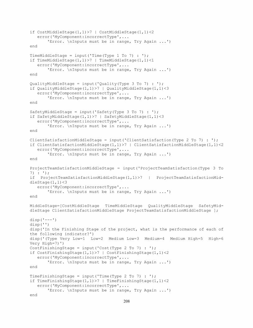
208
if CostMiddleStage(1,1)>7 | CostMiddleStage(1,1)<2
error('MyComponent:incorrectType',...
'Error. \nInputs must be in range, Try Again ...')
end
TimeMiddleStage = input('Time(Type 1 To 7) : ');
if TimeMiddleStage(1,1)>7 | TimeMiddleStage(1,1)<1
error('MyComponent:incorrectType',...
'Error. \nInputs must be in range, Try Again ...')
end
QualityMiddleStage = input('Quality(Type 3 To 7) : ');
if QualityMiddleStage(1,1)>7 | QualityMiddleStage(1,1)<3
error('MyComponent:incorrectType',...
'Error. \nInputs must be in range, Try Again ...')
end
SafetyMiddleStage = input('Safety(Type 3 To 7) : ');
if SafetyMiddleStage(1,1)>7 | SafetyMiddleStage(1,1)<3
error('MyComponent:incorrectType',...
'Error. \nInputs must be in range, Try Again ...')
end
ClientSatisfactionMiddleStage = input('ClientSatisfaction(Type 2 To 7) : ');
if ClientSatisfactionMiddleStage(1,1)>7 | ClientSatisfactionMiddleStage(1,1)<2
error('MyComponent:incorrectType',...
'Error. \nInputs must be in range, Try Again ...')
end
ProjectTeamSatisfactionMiddleStage = input('ProjectTeamSatisfaction(Type 3 To
7) : ');
if ProjectTeamSatisfactionMiddleStage(1,1)>7 | ProjectTeamSatisfactionMid-
dleStage(1,1)<3
error('MyComponent:incorrectType',...
'Error. \nInputs must be in range, Try Again ...')
end
MiddleStage=[CostMiddleStage TimeMiddleStage QualityMiddleStage SafetyMid-
dleStage ClientSatisfactionMiddleStage ProjectTeamSatisfactionMiddleStage ];
disp('---')
disp('')
disp('In the Finishing Stage of the project, what is the performance of each of
the following indicator?')
disp('(Type Very Low=1 Low=2 Medium Low=3 Medium=4 Medium High=5 High=6
Very High=7)')
CostFinishingStage = input('Cost(Type 2 To 7) : ');
if CostFinishingStage(1,1)>7 | CostFinishingStage(1,1)<2
error('MyComponent:incorrectType',...
'Error. \nInputs must be in range, Try Again ...')
end
TimeFinishingStage = input('Time(Type 2 To 7) : ');
if TimeFinishingStage(1,1)>7 | TimeFinishingStage(1,1)<2
error('MyComponent:incorrectType',...
'Error. \nInputs must be in range, Try Again ...')
end
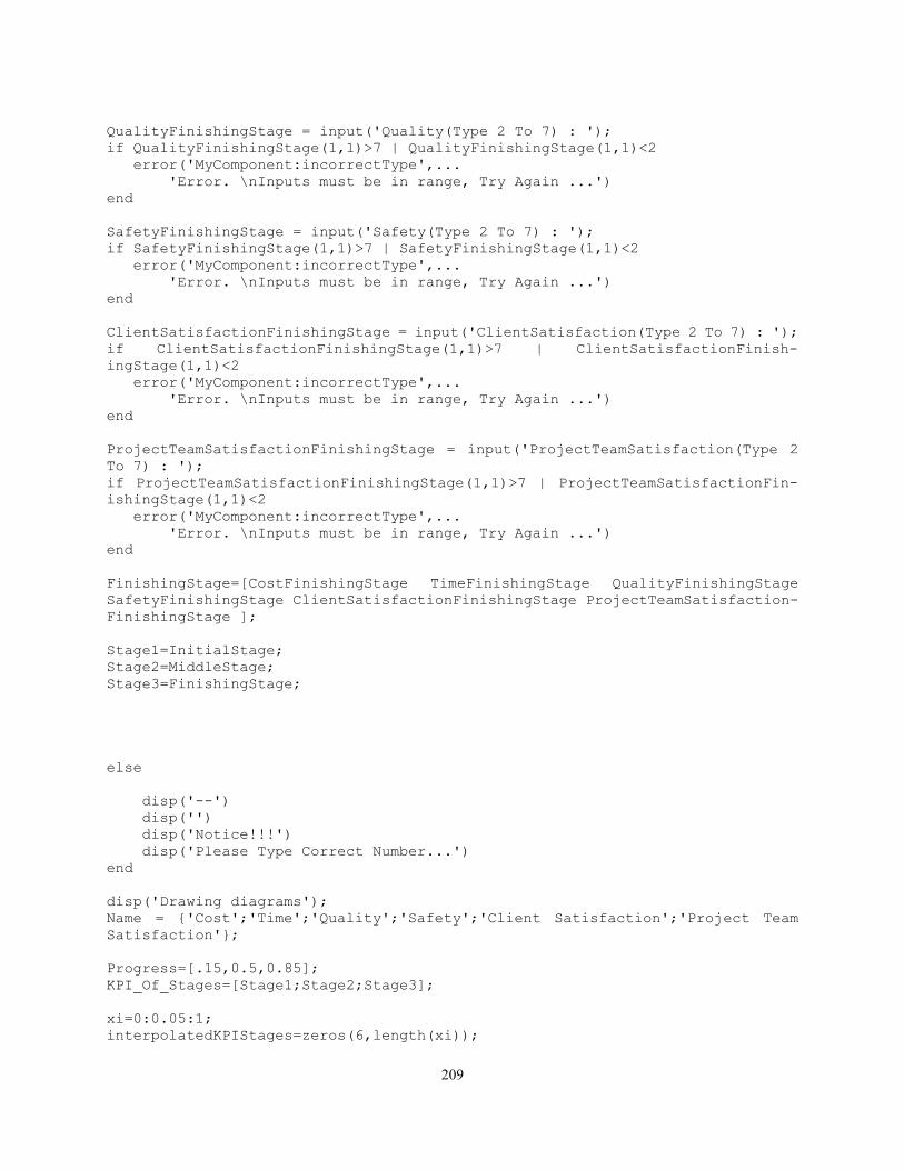
209
QualityFinishingStage = input('Quality(Type 2 To 7) : ');
if QualityFinishingStage(1,1)>7 | QualityFinishingStage(1,1)<2
error('MyComponent:incorrectType',...
'Error. \nInputs must be in range, Try Again ...')
end
SafetyFinishingStage = input('Safety(Type 2 To 7) : ');
if SafetyFinishingStage(1,1)>7 | SafetyFinishingStage(1,1)<2
error('MyComponent:incorrectType',...
'Error. \nInputs must be in range, Try Again ...')
end
ClientSatisfactionFinishingStage = input('ClientSatisfaction(Type 2 To 7) : ');
if ClientSatisfactionFinishingStage(1,1)>7 | ClientSatisfactionFinish-
ingStage(1,1)<2
error('MyComponent:incorrectType',...
'Error. \nInputs must be in range, Try Again ...')
end
ProjectTeamSatisfactionFinishingStage = input('ProjectTeamSatisfaction(Type 2
To 7) : ');
if ProjectTeamSatisfactionFinishingStage(1,1)>7 | ProjectTeamSatisfactionFin-
ishingStage(1,1)<2
error('MyComponent:incorrectType',...
'Error. \nInputs must be in range, Try Again ...')
end
FinishingStage=[CostFinishingStage TimeFinishingStage QualityFinishingStage
SafetyFinishingStage ClientSatisfactionFinishingStage ProjectTeamSatisfaction-
FinishingStage ];
Stage1=InitialStage;
Stage2=MiddleStage;
Stage3=FinishingStage;
else
disp('--')
disp('')
disp('Notice!!!')
disp('Please Type Correct Number...')
end
disp('Drawing diagrams');
Name = {'Cost';'Time';'Quality';'Safety';'Client Satisfaction';'Project Team
Satisfaction'};
Progress=[.15,0.5,0.85];
KPI_Of_Stages=[Stage1;Stage2;Stage3];
xi=0:0.05:1;
interpolatedKPIStages=zeros(6,length(xi));
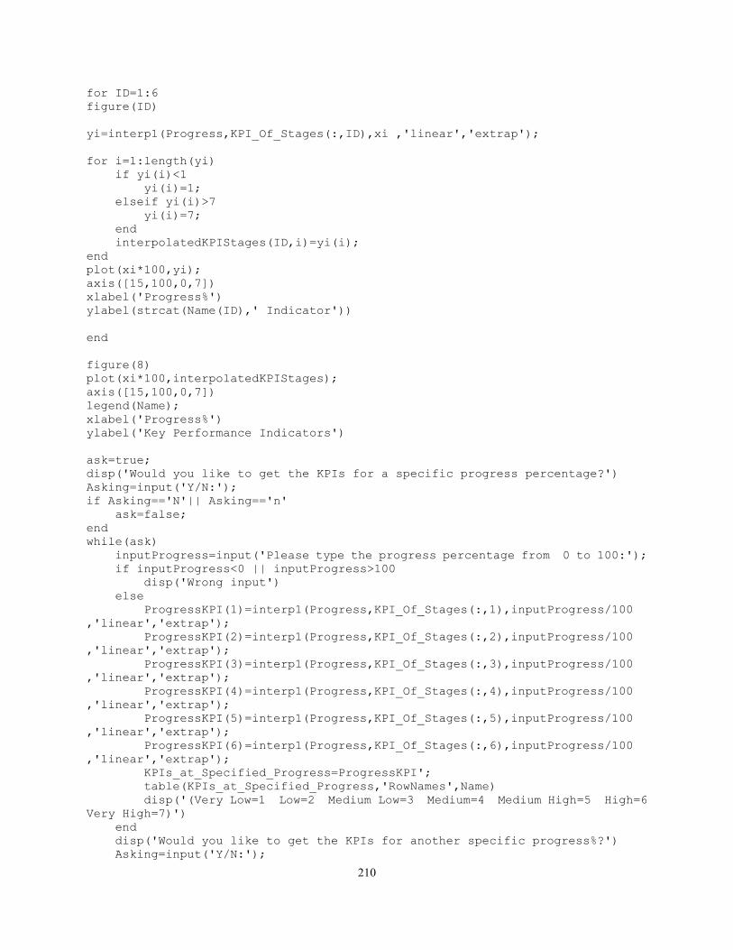
210
for ID=1:6
figure(ID)
yi=interp1(Progress,KPI_Of_Stages(:,ID),xi ,'linear','extrap');
for i=1:length(yi)
if yi(i)<1
yi(i)=1;
elseif yi(i)>7
yi(i)=7;
end
interpolatedKPIStages(ID,i)=yi(i);
end
plot(xi*100,yi);
axis([15,100,0,7])
xlabel('Progress%')
ylabel(strcat(Name(ID),' Indicator'))
end
figure(8)
plot(xi*100,interpolatedKPIStages);
axis([15,100,0,7])
legend(Name);
xlabel('Progress%')
ylabel('Key Performance Indicators')
ask=true;
disp('Would you like to get the KPIs for a specific progress percentage?')
Asking=input('Y/N:');
if Asking=='N'|| Asking=='n'
ask=false;
end
while(ask)
inputProgress=input('Please type the progress percentage from 0 to 100:');
if inputProgress<0 || inputProgress>100
disp('Wrong input')
else
ProgressKPI(1)=interp1(Progress,KPI_Of_Stages(:,1),inputProgress/100
,'linear','extrap');
ProgressKPI(2)=interp1(Progress,KPI_Of_Stages(:,2),inputProgress/100
,'linear','extrap');
ProgressKPI(3)=interp1(Progress,KPI_Of_Stages(:,3),inputProgress/100
,'linear','extrap');
ProgressKPI(4)=interp1(Progress,KPI_Of_Stages(:,4),inputProgress/100
,'linear','extrap');
ProgressKPI(5)=interp1(Progress,KPI_Of_Stages(:,5),inputProgress/100
,'linear','extrap');
ProgressKPI(6)=interp1(Progress,KPI_Of_Stages(:,6),inputProgress/100
,'linear','extrap');
KPIs_at_Specified_Progress=ProgressKPI';
table(KPIs_at_Specified_Progress,'RowNames',Name)
disp('(Very Low=1 Low=2 Medium Low=3 Medium=4 Medium High=5 High=6
Very High=7)')
end
disp('Would you like to get the KPIs for another specific progress%?')
Asking=input('Y/N:');

211
if Asking~='Y' && Asking~='y'
ask=false;
end
end
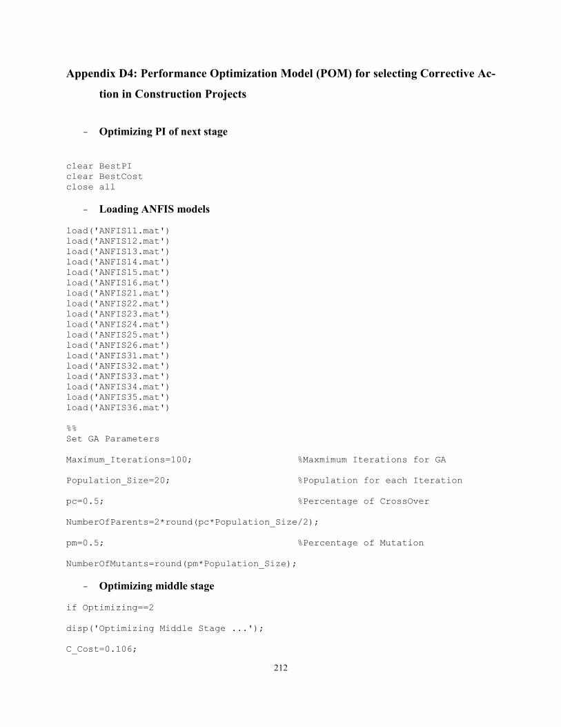
212
Appendix D4: Performance Optimization Model (POM) for selecting Corrective Ac-
tion in Construction Projects
- Optimizing PI of next stage
clear BestPI
clear BestCost
close all
- Loading ANFIS models
load('ANFIS11.mat')
load('ANFIS12.mat')
load('ANFIS13.mat')
load('ANFIS14.mat')
load('ANFIS15.mat')
load('ANFIS16.mat')
load('ANFIS21.mat')
load('ANFIS22.mat')
load('ANFIS23.mat')
load('ANFIS24.mat')
load('ANFIS25.mat')
load('ANFIS26.mat')
load('ANFIS31.mat')
load('ANFIS32.mat')
load('ANFIS33.mat')
load('ANFIS34.mat')
load('ANFIS35.mat')
load('ANFIS36.mat')
%%
Set GA Parameters
Maximum_Iterations=100; %Maxmimum Iterations for GA
Population_Size=20; %Population for each Iteration
pc=0.5; %Percentage of CrossOver
NumberOfParents=2*round(pc*Population_Size/2);
pm=0.5; %Percentage of Mutation
NumberOfMutants=round(pm*Population_Size);
- Optimizing middle stage
if Optimizing==2
disp('Optimizing Middle Stage ...');
C_Cost=0.106;
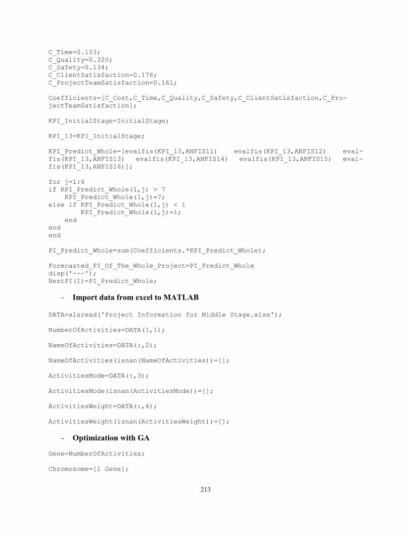
213
C_Time=0.103;
C_Quality=0.320;
C_Safety=0.134;
C_ClientSatisfaction=0.176;
C_ProjectTeamSatisfaction=0.161;
Coefficients=[C_Cost,C_Time,C_Quality,C_Safety,C_ClientSatisfaction,C_Pro-
jectTeamSatisfaction];
KPI_InitialStage=InitialStage;
KPI_13=KPI_InitialStage;
KPI_Predict_Whole=[evalfis(KPI_13,ANFIS11) evalfis(KPI_13,ANFIS12) eval-
fis(KPI_13,ANFIS13) evalfis(KPI_13,ANFIS14) evalfis(KPI_13,ANFIS15) eval-
fis(KPI_13,ANFIS16)];
for j=1:6
if KPI_Predict_Whole(1,j) > 7
KPI_Predict_Whole(1,j)=7;
else if KPI_Predict_Whole(1,j) < 1
KPI_Predict_Whole(1,j)=1;
end
end
end
PI_Predict_Whole=sum(Coefficients.*KPI_Predict_Whole);
Forecasted_PI_Of_The_Whole_Project=PI_Predict_Whole
disp('---');
BestPI(1)=PI_Predict_Whole;
- Import data from excel to MATLAB DATA=xlsread('Project Information for Middle Stage.xlsx');
NumberOfActivities=DATA(1,1);
NameOfActivities=DATA(:,2);
NameOfActivities(isnan(NameOfActivities))=[];
ActivitiesMode=DATA(:,3);
ActivitiesMode(isnan(ActivitiesMode))=[];
ActivitiesWeight=DATA(:,4);
ActivitiesWeight(isnan(ActivitiesWeight))=[];
- Optimization with GA
Gene=NumberOfActivities;
Chromosome=[1 Gene];
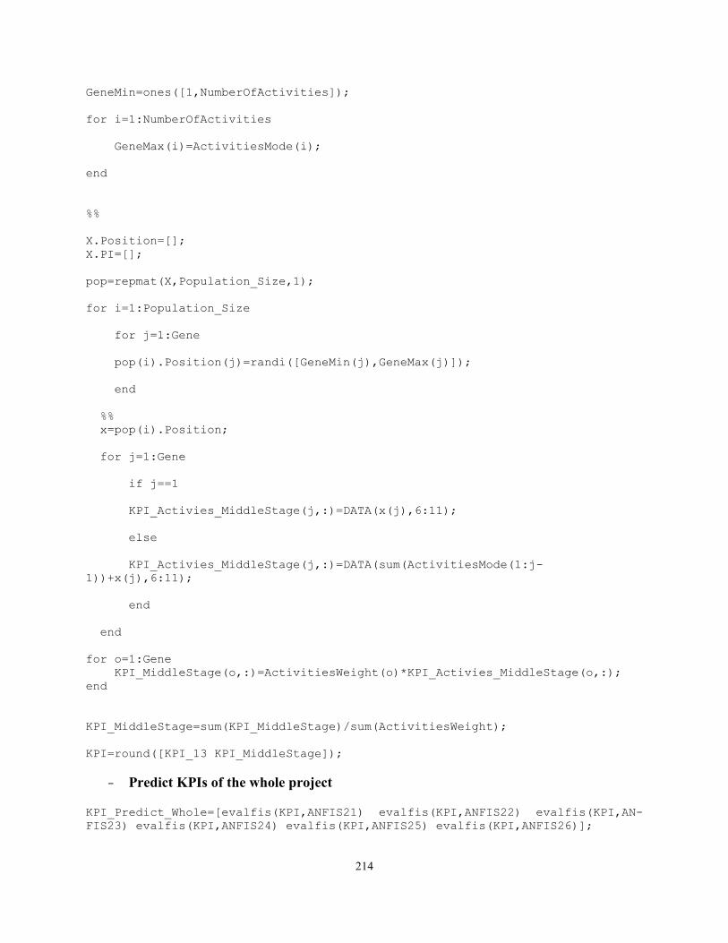
214
GeneMin=ones([1,NumberOfActivities]);
for i=1:NumberOfActivities
GeneMax(i)=ActivitiesMode(i);
end
%%
X.Position=[];
X.PI=[];
pop=repmat(X,Population_Size,1);
for i=1:Population_Size
for j=1:Gene
pop(i).Position(j)=randi([GeneMin(j),GeneMax(j)]);
end
%%
x=pop(i).Position;
for j=1:Gene
if j==1
KPI_Activies_MiddleStage(j,:)=DATA(x(j),6:11);
else
KPI_Activies_MiddleStage(j,:)=DATA(sum(ActivitiesMode(1:j-
1))+x(j),6:11);
end
end
for o=1:Gene
KPI_MiddleStage(o,:)=ActivitiesWeight(o)*KPI_Activies_MiddleStage(o,:);
end
KPI_MiddleStage=sum(KPI_MiddleStage)/sum(ActivitiesWeight);
KPI=round([KPI_13 KPI_MiddleStage]);
- Predict KPIs of the whole project KPI_Predict_Whole=[evalfis(KPI,ANFIS21) evalfis(KPI,ANFIS22) evalfis(KPI,AN-
FIS23) evalfis(KPI,ANFIS24) evalfis(KPI,ANFIS25) evalfis(KPI,ANFIS26)];
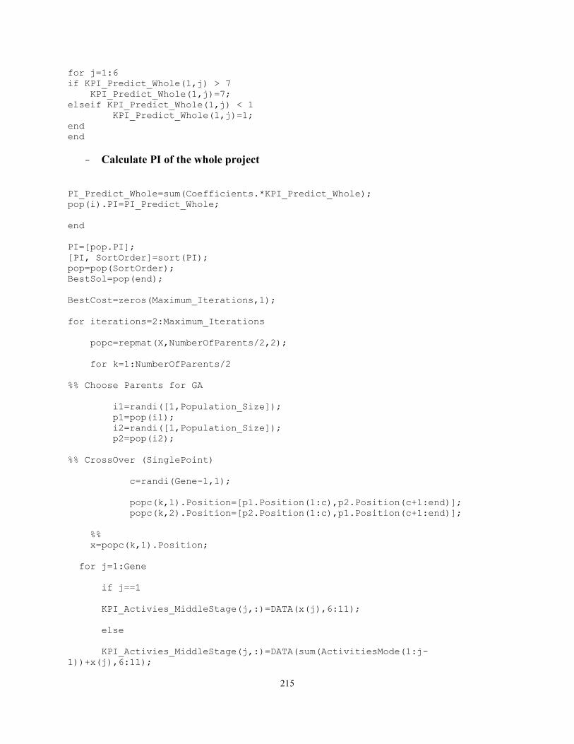
215
for j=1:6
if KPI_Predict_Whole(1,j) > 7
KPI_Predict_Whole(1,j)=7;
elseif KPI_Predict_Whole(1,j) < 1
KPI_Predict_Whole(1,j)=1;
end
end
- Calculate PI of the whole project
PI_Predict_Whole=sum(Coefficients.*KPI_Predict_Whole);
pop(i).PI=PI_Predict_Whole;
end
PI=[pop.PI];
[PI, SortOrder]=sort(PI);
pop=pop(SortOrder);
BestSol=pop(end);
BestCost=zeros(Maximum_Iterations,1);
for iterations=2:Maximum_Iterations
popc=repmat(X,NumberOfParents/2,2);
for k=1:NumberOfParents/2
%% Choose Parents for GA
i1=randi([1,Population_Size]);
p1=pop(i1);
i2=randi([1,Population_Size]);
p2=pop(i2);
%% CrossOver (SinglePoint)
c=randi(Gene-1,1);
popc(k,1).Position=[p1.Position(1:c),p2.Position(c+1:end)];
popc(k,2).Position=[p2.Position(1:c),p1.Position(c+1:end)];
%%
x=popc(k,1).Position;
for j=1:Gene
if j==1
KPI_Activies_MiddleStage(j,:)=DATA(x(j),6:11);
else
KPI_Activies_MiddleStage(j,:)=DATA(sum(ActivitiesMode(1:j-
1))+x(j),6:11);
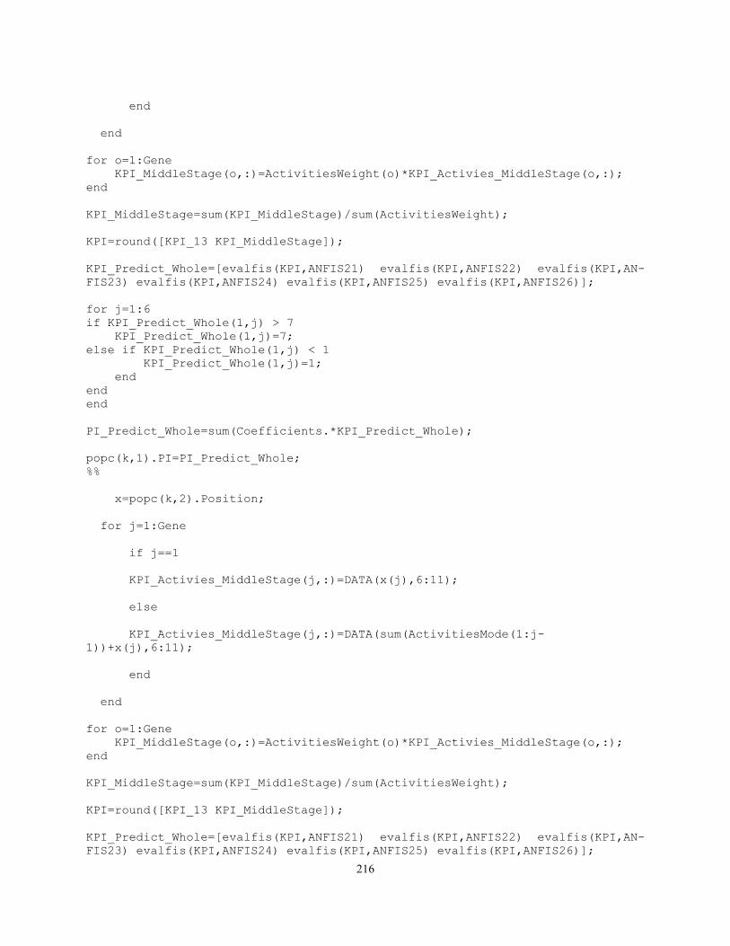
216
end
end
for o=1:Gene
KPI_MiddleStage(o,:)=ActivitiesWeight(o)*KPI_Activies_MiddleStage(o,:);
end
KPI_MiddleStage=sum(KPI_MiddleStage)/sum(ActivitiesWeight);
KPI=round([KPI_13 KPI_MiddleStage]);
KPI_Predict_Whole=[evalfis(KPI,ANFIS21) evalfis(KPI,ANFIS22) evalfis(KPI,AN-
FIS23) evalfis(KPI,ANFIS24) evalfis(KPI,ANFIS25) evalfis(KPI,ANFIS26)];
for j=1:6
if KPI_Predict_Whole(1,j) > 7
KPI_Predict_Whole(1,j)=7;
else if KPI_Predict_Whole(1,j) < 1
KPI_Predict_Whole(1,j)=1;
end
end
end
PI_Predict_Whole=sum(Coefficients.*KPI_Predict_Whole);
popc(k,1).PI=PI_Predict_Whole;
%%
x=popc(k,2).Position;
for j=1:Gene
if j==1
KPI_Activies_MiddleStage(j,:)=DATA(x(j),6:11);
else
KPI_Activies_MiddleStage(j,:)=DATA(sum(ActivitiesMode(1:j-
1))+x(j),6:11);
end
end
for o=1:Gene
KPI_MiddleStage(o,:)=ActivitiesWeight(o)*KPI_Activies_MiddleStage(o,:);
end
KPI_MiddleStage=sum(KPI_MiddleStage)/sum(ActivitiesWeight);
KPI=round([KPI_13 KPI_MiddleStage]);
KPI_Predict_Whole=[evalfis(KPI,ANFIS21) evalfis(KPI,ANFIS22) evalfis(KPI,AN-
FIS23) evalfis(KPI,ANFIS24) evalfis(KPI,ANFIS25) evalfis(KPI,ANFIS26)];
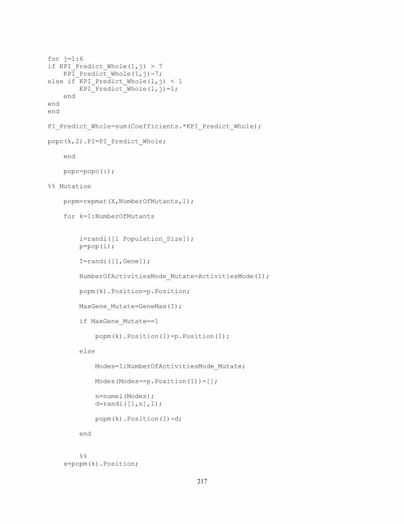
217
for j=1:6
if KPI_Predict_Whole(1,j) > 7
KPI_Predict_Whole(1,j)=7;
else if KPI_Predict_Whole(1,j) < 1
KPI_Predict_Whole(1,j)=1;
end
end
end
PI_Predict_Whole=sum(Coefficients.*KPI_Predict_Whole);
popc(k,2).PI=PI_Predict_Whole;
end
popc=popc(:);
%% Mutation
popm=repmat(X,NumberOfMutants,1);
for k=1:NumberOfMutants
i=randi([1 Population_Size]);
p=pop(i);
I=randi([1,Gene]);
NumberOfActivitiesMode_Mutate=ActivitiesMode(I);
popm(k).Position=p.Position;
MaxGene_Mutate=GeneMax(I);
if MaxGene_Mutate==1
popm(k).Position(I)=p.Position(I);
else
Modes=1:NumberOfActivitiesMode_Mutate;
Modes(Modes==p.Position(I))=[];
n=numel(Modes);
d=randi([1,n],1);
popm(k).Position(I)=d;
end
%%
x=popm(k).Position;
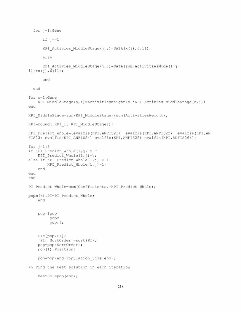
218
for j=1:Gene
if j==1
KPI_Activies_MiddleStage(j,:)=DATA(x(j),6:11);
else
KPI_Activies_MiddleStage(j,:)=DATA(sum(ActivitiesMode(1:j-
1))+x(j),6:11);
end
end
for o=1:Gene
KPI_MiddleStage(o,:)=ActivitiesWeight(o)*KPI_Activies_MiddleStage(o,:);
end
KPI_MiddleStage=sum(KPI_MiddleStage)/sum(ActivitiesWeight);
KPI=round([KPI_13 KPI_MiddleStage]);
KPI_Predict_Whole=[evalfis(KPI,ANFIS21) evalfis(KPI,ANFIS22) evalfis(KPI,AN-
FIS23) evalfis(KPI,ANFIS24) evalfis(KPI,ANFIS25) evalfis(KPI,ANFIS26)];
for j=1:6
if KPI_Predict_Whole(1,j) > 7
KPI_Predict_Whole(1,j)=7;
else if KPI_Predict_Whole(1,j) < 1
KPI_Predict_Whole(1,j)=1;
end
end
end
PI_Predict_Whole=sum(Coefficients.*KPI_Predict_Whole);
popm(k).PI=PI_Predict_Whole;
end
pop=[pop
popc
popm];
PI=[pop.PI];
[PI, SortOrder]=sort(PI);
pop=pop(SortOrder);
pop(1).Position;
pop=pop(end-Population_Size:end);
%% Find the best solution in each iteration
BestSol=pop(end);
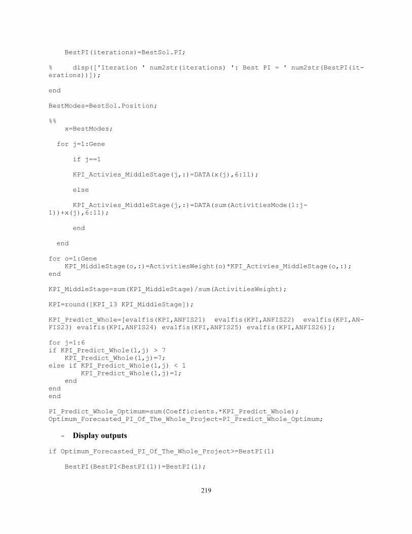
219
BestPI(iterations)=BestSol.PI;
% disp(['Iteration ' num2str(iterations) ': Best PI = ' num2str(BestPI(it-
erations))]);
end
BestModes=BestSol.Position;
%%
x=BestModes;
for j=1:Gene
if j==1
KPI_Activies_MiddleStage(j,:)=DATA(x(j),6:11);
else
KPI_Activies_MiddleStage(j,:)=DATA(sum(ActivitiesMode(1:j-
1))+x(j),6:11);
end
end
for o=1:Gene
KPI_MiddleStage(o,:)=ActivitiesWeight(o)*KPI_Activies_MiddleStage(o,:);
end
KPI_MiddleStage=sum(KPI_MiddleStage)/sum(ActivitiesWeight);
KPI=round([KPI_13 KPI_MiddleStage]);
KPI_Predict_Whole=[evalfis(KPI,ANFIS21) evalfis(KPI,ANFIS22) evalfis(KPI,AN-
FIS23) evalfis(KPI,ANFIS24) evalfis(KPI,ANFIS25) evalfis(KPI,ANFIS26)];
for j=1:6
if KPI_Predict_Whole(1,j) > 7
KPI_Predict_Whole(1,j)=7;
else if KPI_Predict_Whole(1,j) < 1
KPI_Predict_Whole(1,j)=1;
end
end
end
PI_Predict_Whole_Optimum=sum(Coefficients.*KPI_Predict_Whole);
Optimum_Forecasted_PI_Of_The_Whole_Project=PI_Predict_Whole_Optimum;
- Display outputs
if Optimum_Forecasted_PI_Of_The_Whole_Project>=BestPI(1)
BestPI(BestPI<BestPI(1))=BestPI(1);
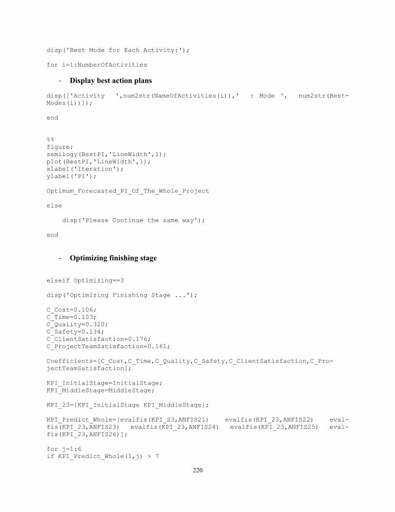
220
disp('Best Mode for Each Activity:');
for i=1:NumberOfActivities
- Display best action plans
disp(['Activity ',num2str(NameOfActivities(i)),' : Mode ', num2str(Best-
Modes(i))]);
end
%%
figure;
semilogy(BestPI,'LineWidth',1);
plot(BestPI,'LineWidth',1);
xlabel('Iteration');
ylabel('PI');
Optimum_Forecasted_PI_Of_The_Whole_Project
else
disp('Please Continue the same way');
end
- Optimizing finishing stage
elseif Optimizing==3
disp('Optimizing Finishing Stage ...');
C_Cost=0.106;
C_Time=0.103;
C_Quality=0.320;
C_Safety=0.134;
C_ClientSatisfaction=0.176;
C_ProjectTeamSatisfaction=0.161;
Coefficients=[C_Cost,C_Time,C_Quality,C_Safety,C_ClientSatisfaction,C_Pro-
jectTeamSatisfaction];
KPI_InitialStage=InitialStage;
KPI_MiddleStage=MiddleStage;
KPI_23=[KPI_InitialStage KPI_MiddleStage];
KPI_Predict_Whole=[evalfis(KPI_23,ANFIS21) evalfis(KPI_23,ANFIS22) eval-
fis(KPI_23,ANFIS23) evalfis(KPI_23,ANFIS24) evalfis(KPI_23,ANFIS25) eval-
fis(KPI_23,ANFIS26)];
for j=1:6
if KPI_Predict_Whole(1,j) > 7
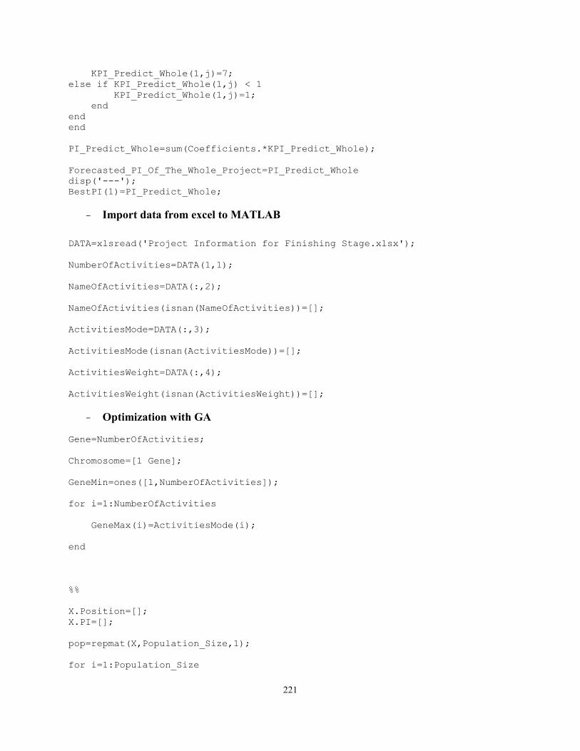
221
KPI_Predict_Whole(1,j)=7;
else if KPI_Predict_Whole(1,j) < 1
KPI_Predict_Whole(1,j)=1;
end
end
end
PI_Predict_Whole=sum(Coefficients.*KPI_Predict_Whole);
Forecasted_PI_Of_The_Whole_Project=PI_Predict_Whole
disp('---');
BestPI(1)=PI_Predict_Whole;
- Import data from excel to MATLAB DATA=xlsread('Project Information for Finishing Stage.xlsx');
NumberOfActivities=DATA(1,1);
NameOfActivities=DATA(:,2);
NameOfActivities(isnan(NameOfActivities))=[];
ActivitiesMode=DATA(:,3);
ActivitiesMode(isnan(ActivitiesMode))=[];
ActivitiesWeight=DATA(:,4);
ActivitiesWeight(isnan(ActivitiesWeight))=[];
- Optimization with GA
Gene=NumberOfActivities;
Chromosome=[1 Gene];
GeneMin=ones([1,NumberOfActivities]);
for i=1:NumberOfActivities
GeneMax(i)=ActivitiesMode(i);
end
%%
X.Position=[];
X.PI=[];
pop=repmat(X,Population_Size,1);
for i=1:Population_Size
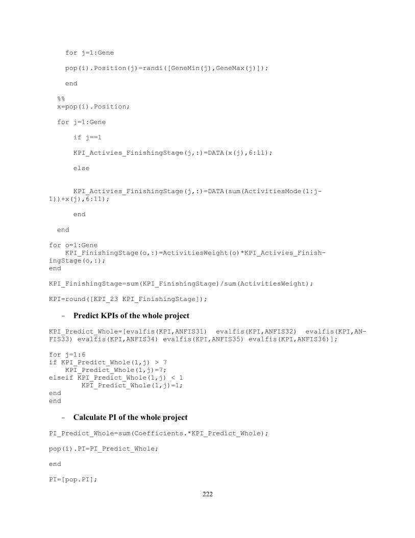
222
for j=1:Gene
pop(i).Position(j)=randi([GeneMin(j),GeneMax(j)]);
end
%%
x=pop(i).Position;
for j=1:Gene
if j==1
KPI_Activies_FinishingStage(j,:)=DATA(x(j),6:11);
else
KPI_Activies_FinishingStage(j,:)=DATA(sum(ActivitiesMode(1:j-
1))+x(j),6:11);
end
end
for o=1:Gene
KPI_FinishingStage(o,:)=ActivitiesWeight(o)*KPI_Activies_Finish-
ingStage(o,:);
end
KPI_FinishingStage=sum(KPI_FinishingStage)/sum(ActivitiesWeight);
KPI=round([KPI_23 KPI_FinishingStage]);
- Predict KPIs of the whole project
KPI_Predict_Whole=[evalfis(KPI,ANFIS31) evalfis(KPI,ANFIS32) evalfis(KPI,AN-
FIS33) evalfis(KPI,ANFIS34) evalfis(KPI,ANFIS35) evalfis(KPI,ANFIS36)];
for j=1:6
if KPI_Predict_Whole(1,j) > 7
KPI_Predict_Whole(1,j)=7;
elseif KPI_Predict_Whole(1,j) < 1
KPI_Predict_Whole(1,j)=1;
end
end
- Calculate PI of the whole project
PI_Predict_Whole=sum(Coefficients.*KPI_Predict_Whole);
pop(i).PI=PI_Predict_Whole;
end
PI=[pop.PI];
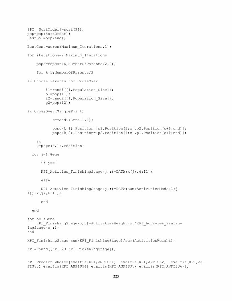
223
[PI, SortOrder]=sort(PI);
pop=pop(SortOrder);
BestSol=pop(end);
BestCost=zeros(Maximum_Iterations,1);
for iterations=2:Maximum_Iterations
popc=repmat(X,NumberOfParents/2,2);
for k=1:NumberOfParents/2
%% Choose Parents for CrossOver
i1=randi([1,Population_Size]);
p1=pop(i1);
i2=randi([1,Population_Size]);
p2=pop(i2);
%% CrossOver(SinglePoint)
c=randi(Gene-1,1);
popc(k,1).Position=[p1.Position(1:c),p2.Position(c+1:end)];
popc(k,2).Position=[p2.Position(1:c),p1.Position(c+1:end)];
%%
x=popc(k,1).Position;
for j=1:Gene
if j==1
KPI_Activies_FinishingStage(j,:)=DATA(x(j),6:11);
else
KPI_Activies_FinishingStage(j,:)=DATA(sum(ActivitiesMode(1:j-
1))+x(j),6:11);
end
end
for o=1:Gene
KPI_FinishingStage(o,:)=ActivitiesWeight(o)*KPI_Activies_Finish-
ingStage(o,:);
end
KPI_FinishingStage=sum(KPI_FinishingStage)/sum(ActivitiesWeight);
KPI=round([KPI_23 KPI_FinishingStage]);
KPI_Predict_Whole=[evalfis(KPI,ANFIS31) evalfis(KPI,ANFIS32) evalfis(KPI,AN-
FIS33) evalfis(KPI,ANFIS34) evalfis(KPI,ANFIS35) evalfis(KPI,ANFIS36)];
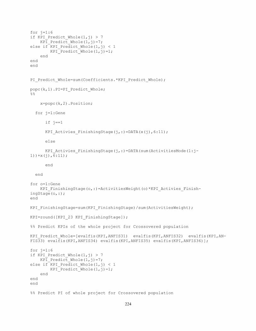
224
for j=1:6
if KPI_Predict_Whole(1,j) > 7
KPI_Predict_Whole(1,j)=7;
else if KPI_Predict_Whole(1,j) < 1
KPI_Predict_Whole(1,j)=1;
end
end
end
PI_Predict_Whole=sum(Coefficients.*KPI_Predict_Whole);
popc(k,1).PI=PI_Predict_Whole;
%%
x=popc(k,2).Position;
for j=1:Gene
if j==1
KPI_Activies_FinishingStage(j,:)=DATA(x(j),6:11);
else
KPI_Activies_FinishingStage(j,:)=DATA(sum(ActivitiesMode(1:j-
1))+x(j),6:11);
end
end
for o=1:Gene
KPI_FinishingStage(o,:)=ActivitiesWeight(o)*KPI_Activies_Finish-
ingStage(o,:);
end
KPI_FinishingStage=sum(KPI_FinishingStage)/sum(ActivitiesWeight);
KPI=round([KPI_23 KPI_FinishingStage]);
%% Predict KPIs of the whole project for Crossovered population
KPI_Predict_Whole=[evalfis(KPI,ANFIS31) evalfis(KPI,ANFIS32) evalfis(KPI,AN-
FIS33) evalfis(KPI,ANFIS34) evalfis(KPI,ANFIS35) evalfis(KPI,ANFIS36)];
for j=1:6
if KPI_Predict_Whole(1,j) > 7
KPI_Predict_Whole(1,j)=7;
else if KPI_Predict_Whole(1,j) < 1
KPI_Predict_Whole(1,j)=1;
end
end
end
%% Predict PI of whole project for Crossovered population
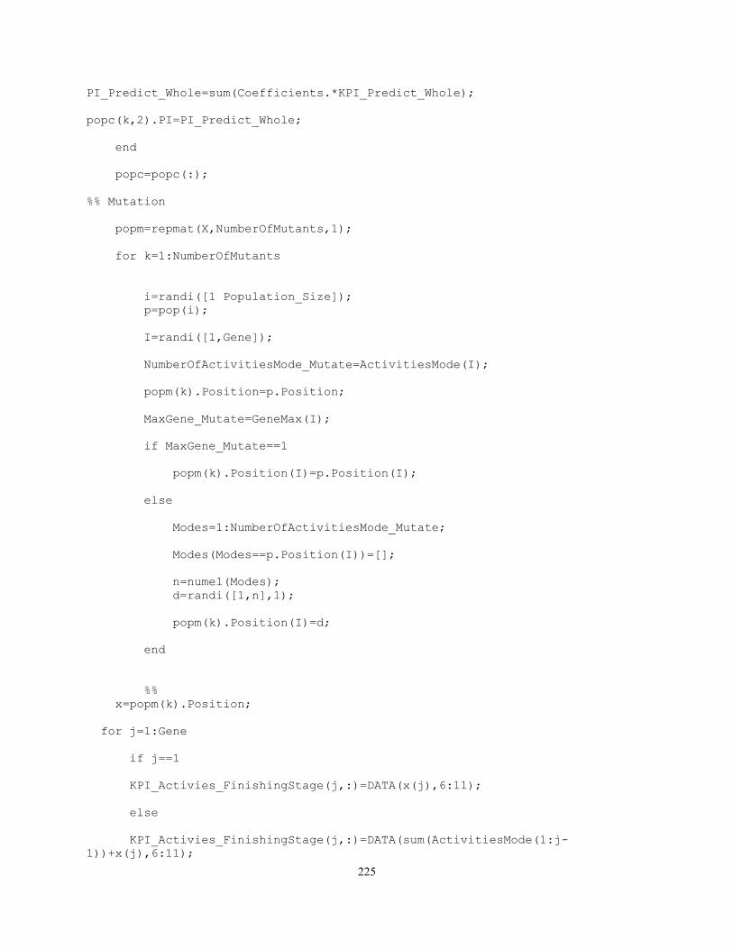
225
PI_Predict_Whole=sum(Coefficients.*KPI_Predict_Whole);
popc(k,2).PI=PI_Predict_Whole;
end
popc=popc(:);
%% Mutation
popm=repmat(X,NumberOfMutants,1);
for k=1:NumberOfMutants
i=randi([1 Population_Size]);
p=pop(i);
I=randi([1,Gene]);
NumberOfActivitiesMode_Mutate=ActivitiesMode(I);
popm(k).Position=p.Position;
MaxGene_Mutate=GeneMax(I);
if MaxGene_Mutate==1
popm(k).Position(I)=p.Position(I);
else
Modes=1:NumberOfActivitiesMode_Mutate;
Modes(Modes==p.Position(I))=[];
n=numel(Modes);
d=randi([1,n],1);
popm(k).Position(I)=d;
end
%%
x=popm(k).Position;
for j=1:Gene
if j==1
KPI_Activies_FinishingStage(j,:)=DATA(x(j),6:11);
else
KPI_Activies_FinishingStage(j,:)=DATA(sum(ActivitiesMode(1:j-
1))+x(j),6:11);
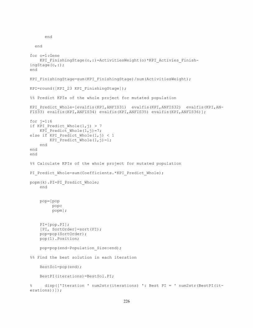
226
end
end
for o=1:Gene
KPI_FinishingStage(o,:)=ActivitiesWeight(o)*KPI_Activies_Finish-
ingStage(o,:);
end
KPI_FinishingStage=sum(KPI_FinishingStage)/sum(ActivitiesWeight);
KPI=round([KPI_23 KPI_FinishingStage]);
%% Predict KPIs of the whole project for mutated population
KPI_Predict_Whole=[evalfis(KPI,ANFIS31) evalfis(KPI,ANFIS32) evalfis(KPI,AN-
FIS33) evalfis(KPI,ANFIS34) evalfis(KPI,ANFIS35) evalfis(KPI,ANFIS36)];
for j=1:6
if KPI_Predict_Whole(1,j) > 7
KPI_Predict_Whole(1,j)=7;
else if KPI_Predict_Whole(1,j) < 1
KPI_Predict_Whole(1,j)=1;
end
end
end
%% Calculate KPIs of the whole project for mutated population
PI_Predict_Whole=sum(Coefficients.*KPI_Predict_Whole);
popm(k).PI=PI_Predict_Whole;
end
pop=[pop
popc
popm];
PI=[pop.PI];
[PI, SortOrder]=sort(PI);
pop=pop(SortOrder);
pop(1).Position;
pop=pop(end-Population_Size:end);
%% Find the best solution in each iteration
BestSol=pop(end);
BestPI(iterations)=BestSol.PI;
% disp(['Iteration ' num2str(iterations) ': Best PI = ' num2str(BestPI(it-
erations))]);
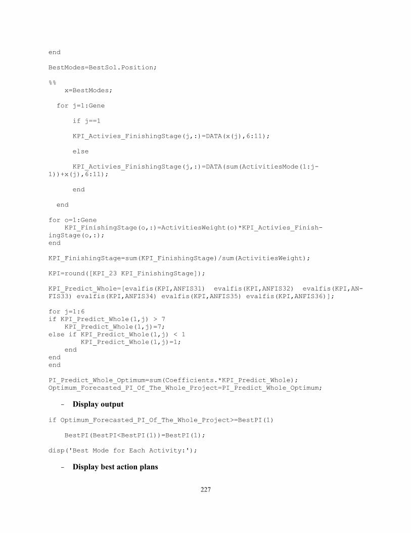
227
end
BestModes=BestSol.Position;
%%
x=BestModes;
for j=1:Gene
if j==1
KPI_Activies_FinishingStage(j,:)=DATA(x(j),6:11);
else
KPI_Activies_FinishingStage(j,:)=DATA(sum(ActivitiesMode(1:j-
1))+x(j),6:11);
end
end
for o=1:Gene
KPI_FinishingStage(o,:)=ActivitiesWeight(o)*KPI_Activies_Finish-
ingStage(o,:);
end
KPI_FinishingStage=sum(KPI_FinishingStage)/sum(ActivitiesWeight);
KPI=round([KPI_23 KPI_FinishingStage]);
KPI_Predict_Whole=[evalfis(KPI,ANFIS31) evalfis(KPI,ANFIS32) evalfis(KPI,AN-
FIS33) evalfis(KPI,ANFIS34) evalfis(KPI,ANFIS35) evalfis(KPI,ANFIS36)];
for j=1:6
if KPI_Predict_Whole(1,j) > 7
KPI_Predict_Whole(1,j)=7;
else if KPI_Predict_Whole(1,j) < 1
KPI_Predict_Whole(1,j)=1;
end
end
end
PI_Predict_Whole_Optimum=sum(Coefficients.*KPI_Predict_Whole);
Optimum_Forecasted_PI_Of_The_Whole_Project=PI_Predict_Whole_Optimum;
- Display output
if Optimum_Forecasted_PI_Of_The_Whole_Project>=BestPI(1)
BestPI(BestPI<BestPI(1))=BestPI(1);
disp('Best Mode for Each Activity:');
- Display best action plans
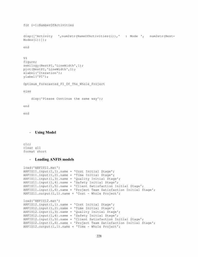
228
for i=1:NumberOfActivities
disp(['Activity ',num2str(NameOfActivities(i)),' : Mode ', num2str(Best-
Modes(i))]);
end
%%
figure;
semilogy(BestPI,'LineWidth',1);
plot(BestPI,'LineWidth',1);
xlabel('Iteration');
ylabel('PI');
Optimum_Forecasted_PI_Of_The_Whole_Project
else
disp('Please Continue the same way');
end
end
- Using Model
clc;
clear all
format short
- Loading ANFIS models load('ANFIS11.mat')
ANFIS11.input(1,1).name = 'Cost Initial Stage';
ANFIS11.input(1,2).name = 'Time Initial Stage';
ANFIS11.input(1,3).name = 'Quality Initial Stage';
ANFIS11.input(1,4).name = 'Safety Initial Stage';
ANFIS11.input(1,5).name = 'Client Satisfaction Initial Stage';
ANFIS11.input(1,6).name = 'Project Team Satisfaction Initial Stage';
ANFIS11.output(1,1).name = 'Cost - Whole Project';
load('ANFIS12.mat')
ANFIS12.input(1,1).name = 'Cost Initial Stage';
ANFIS12.input(1,2).name = 'Time Initial Stage';
ANFIS12.input(1,3).name = 'Quality Initial Stage';
ANFIS12.input(1,4).name = 'Safety Initial Stage';
ANFIS12.input(1,5).name = 'Client Satisfaction Initial Stage';
ANFIS12.input(1,6).name = 'Project Team Satisfaction Initial Stage';
ANFIS12.output(1,1).name = 'Time - Whole Project';
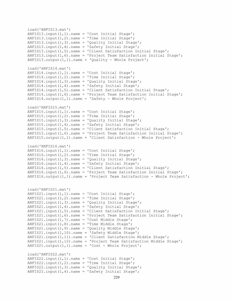
229
load('ANFIS13.mat')
ANFIS13.input(1,1).name = 'Cost Initial Stage';
ANFIS13.input(1,2).name = 'Time Initial Stage';
ANFIS13.input(1,3).name = 'Quality Initial Stage';
ANFIS13.input(1,4).name = 'Safety Initial Stage';
ANFIS13.input(1,5).name = 'Client Satisfaction Initial Stage';
ANFIS13.input(1,6).name = 'Project Team Satisfaction Initial Stage';
ANFIS13.output(1,1).name = 'Quality - Whole Project';
load('ANFIS14.mat')
ANFIS14.input(1,1).name = 'Cost Initial Stage';
ANFIS14.input(1,2).name = 'Time Initial Stage';
ANFIS14.input(1,3).name = 'Quality Initial Stage';
ANFIS14.input(1,4).name = 'Safety Initial Stage';
ANFIS14.input(1,5).name = 'Client Satisfaction Initial Stage';
ANFIS14.input(1,6).name = 'Project Team Satisfaction Initial Stage';
ANFIS14.output(1,1).name = 'Safety - Whole Project';
load('ANFIS15.mat')
ANFIS15.input(1,1).name = 'Cost Initial Stage';
ANFIS15.input(1,2).name = 'Time Initial Stage';
ANFIS15.input(1,3).name = 'Quality Initial Stage';
ANFIS15.input(1,4).name = 'Safety Initial Stage';
ANFIS15.input(1,5).name = 'Client Satisfaction Initial Stage';
ANFIS15.input(1,6).name = 'Project Team Satisfaction Initial Stage';
ANFIS15.output(1,1).name = 'Client Satisfaction - Whole Project';
load('ANFIS16.mat')
ANFIS16.input(1,1).name = 'Cost Initial Stage';
ANFIS16.input(1,2).name = 'Time Initial Stage';
ANFIS16.input(1,3).name = 'Quality Initial Stage';
ANFIS16.input(1,4).name = 'Safety Initial Stage';
ANFIS16.input(1,5).name = 'Client Satisfaction Initial Stage';
ANFIS16.input(1,6).name = 'Project Team Satisfaction Initial Stage';
ANFIS16.output(1,1).name = 'Project Team Satisfaction - Whole Project';
load('ANFIS21.mat')
ANFIS21.input(1,1).name = 'Cost Initial Stage';
ANFIS21.input(1,2).name = 'Time Initial Stage';
ANFIS21.input(1,3).name = 'Quality Initial Stage';
ANFIS21.input(1,4).name = 'Safety Initial Stage';
ANFIS21.input(1,5).name = 'Client Satisfaction Initial Stage';
ANFIS21.input(1,6).name = 'Project Team Satisfaction Initial Stage';
ANFIS21.input(1,7).name = 'Cost Middle Stage';
ANFIS21.input(1,8).name = 'Time Middle Stage';
ANFIS21.input(1,9).name = 'Quality Middle Stage';
ANFIS21.input(1,10).name = 'Safety Middle Stage';
ANFIS21.input(1,11).name = 'Client Satisfaction Middle Stage';
ANFIS21.input(1,12).name = 'Project Team Satisfaction Middle Stage';
ANFIS21.output(1,1).name = 'Cost - Whole Project';
load('ANFIS22.mat')
ANFIS22.input(1,1).name = 'Cost Initial Stage';
ANFIS22.input(1,2).name = 'Time Initial Stage';
ANFIS22.input(1,3).name = 'Quality Initial Stage';
ANFIS22.input(1,4).name = 'Safety Initial Stage';
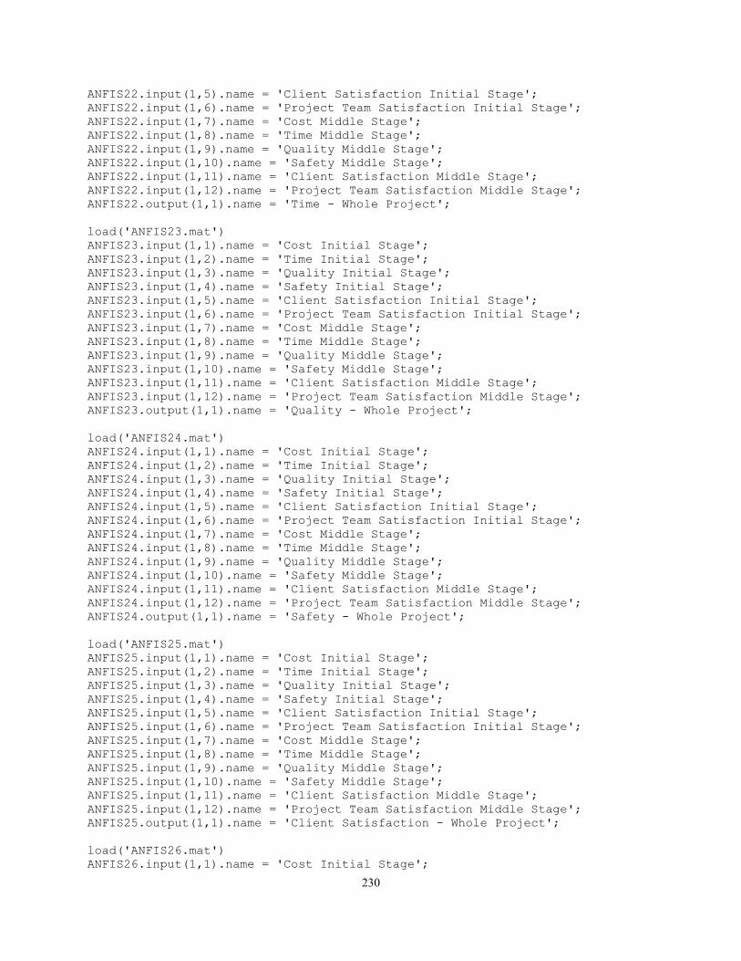
230
ANFIS22.input(1,5).name = 'Client Satisfaction Initial Stage';
ANFIS22.input(1,6).name = 'Project Team Satisfaction Initial Stage';
ANFIS22.input(1,7).name = 'Cost Middle Stage';
ANFIS22.input(1,8).name = 'Time Middle Stage';
ANFIS22.input(1,9).name = 'Quality Middle Stage';
ANFIS22.input(1,10).name = 'Safety Middle Stage';
ANFIS22.input(1,11).name = 'Client Satisfaction Middle Stage';
ANFIS22.input(1,12).name = 'Project Team Satisfaction Middle Stage';
ANFIS22.output(1,1).name = 'Time - Whole Project';
load('ANFIS23.mat')
ANFIS23.input(1,1).name = 'Cost Initial Stage';
ANFIS23.input(1,2).name = 'Time Initial Stage';
ANFIS23.input(1,3).name = 'Quality Initial Stage';
ANFIS23.input(1,4).name = 'Safety Initial Stage';
ANFIS23.input(1,5).name = 'Client Satisfaction Initial Stage';
ANFIS23.input(1,6).name = 'Project Team Satisfaction Initial Stage';
ANFIS23.input(1,7).name = 'Cost Middle Stage';
ANFIS23.input(1,8).name = 'Time Middle Stage';
ANFIS23.input(1,9).name = 'Quality Middle Stage';
ANFIS23.input(1,10).name = 'Safety Middle Stage';
ANFIS23.input(1,11).name = 'Client Satisfaction Middle Stage';
ANFIS23.input(1,12).name = 'Project Team Satisfaction Middle Stage';
ANFIS23.output(1,1).name = 'Quality - Whole Project';
load('ANFIS24.mat')
ANFIS24.input(1,1).name = 'Cost Initial Stage';
ANFIS24.input(1,2).name = 'Time Initial Stage';
ANFIS24.input(1,3).name = 'Quality Initial Stage';
ANFIS24.input(1,4).name = 'Safety Initial Stage';
ANFIS24.input(1,5).name = 'Client Satisfaction Initial Stage';
ANFIS24.input(1,6).name = 'Project Team Satisfaction Initial Stage';
ANFIS24.input(1,7).name = 'Cost Middle Stage';
ANFIS24.input(1,8).name = 'Time Middle Stage';
ANFIS24.input(1,9).name = 'Quality Middle Stage';
ANFIS24.input(1,10).name = 'Safety Middle Stage';
ANFIS24.input(1,11).name = 'Client Satisfaction Middle Stage';
ANFIS24.input(1,12).name = 'Project Team Satisfaction Middle Stage';
ANFIS24.output(1,1).name = 'Safety - Whole Project';
load('ANFIS25.mat')
ANFIS25.input(1,1).name = 'Cost Initial Stage';
ANFIS25.input(1,2).name = 'Time Initial Stage';
ANFIS25.input(1,3).name = 'Quality Initial Stage';
ANFIS25.input(1,4).name = 'Safety Initial Stage';
ANFIS25.input(1,5).name = 'Client Satisfaction Initial Stage';
ANFIS25.input(1,6).name = 'Project Team Satisfaction Initial Stage';
ANFIS25.input(1,7).name = 'Cost Middle Stage';
ANFIS25.input(1,8).name = 'Time Middle Stage';
ANFIS25.input(1,9).name = 'Quality Middle Stage';
ANFIS25.input(1,10).name = 'Safety Middle Stage';
ANFIS25.input(1,11).name = 'Client Satisfaction Middle Stage';
ANFIS25.input(1,12).name = 'Project Team Satisfaction Middle Stage';
ANFIS25.output(1,1).name = 'Client Satisfaction - Whole Project';
load('ANFIS26.mat')
ANFIS26.input(1,1).name = 'Cost Initial Stage';
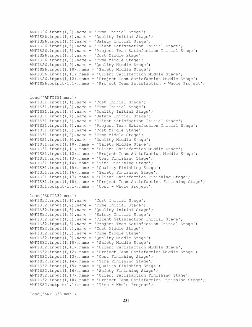
231
ANFIS26.input(1,2).name = 'Time Initial Stage';
ANFIS26.input(1,3).name = 'Quality Initial Stage';
ANFIS26.input(1,4).name = 'Safety Initial Stage';
ANFIS26.input(1,5).name = 'Client Satisfaction Initial Stage';
ANFIS26.input(1,6).name = 'Project Team Satisfaction Initial Stage';
ANFIS26.input(1,7).name = 'Cost Middle Stage';
ANFIS26.input(1,8).name = 'Time Middle Stage';
ANFIS26.input(1,9).name = 'Quality Middle Stage';
ANFIS26.input(1,10).name = 'Safety Middle Stage';
ANFIS26.input(1,11).name = 'Client Satisfaction Middle Stage';
ANFIS26.input(1,12).name = 'Project Team Satisfaction Middle Stage';
ANFIS26.output(1,1).name = 'Project Team Satisfaction - Whole Project';
load('ANFIS31.mat')
ANFIS31.input(1,1).name = 'Cost Initial Stage';
ANFIS31.input(1,2).name = 'Time Initial Stage';
ANFIS31.input(1,3).name = 'Quality Initial Stage';
ANFIS31.input(1,4).name = 'Safety Initial Stage';
ANFIS31.input(1,5).name = 'Client Satisfaction Initial Stage';
ANFIS31.input(1,6).name = 'Project Team Satisfaction Initial Stage';
ANFIS31.input(1,7).name = 'Cost Middle Stage';
ANFIS31.input(1,8).name = 'Time Middle Stage';
ANFIS31.input(1,9).name = 'Quality Middle Stage';
ANFIS31.input(1,10).name = 'Safety Middle Stage';
ANFIS31.input(1,11).name = 'Client Satisfaction Middle Stage';
ANFIS31.input(1,12).name = 'Project Team Satisfaction Middle Stage';
ANFIS31.input(1,13).name = 'Cost Finishing Stage';
ANFIS31.input(1,14).name = 'Time Finishing Stage';
ANFIS31.input(1,15).name = 'Quality Finishing Stage';
ANFIS31.input(1,16).name = 'Safety Finishing Stage';
ANFIS31.input(1,17).name = 'Client Satisfaction Finishing Stage';
ANFIS31.input(1,18).name = 'Project Team Satisfaction Finishing Stage';
ANFIS31.output(1,1).name = 'Cost - Whole Project';
load('ANFIS32.mat')
ANFIS32.input(1,1).name = 'Cost Initial Stage';
ANFIS32.input(1,2).name = 'Time Initial Stage';
ANFIS32.input(1,3).name = 'Quality Initial Stage';
ANFIS32.input(1,4).name = 'Safety Initial Stage';
ANFIS32.input(1,5).name = 'Client Satisfaction Initial Stage';
ANFIS32.input(1,6).name = 'Project Team Satisfaction Initial Stage';
ANFIS32.input(1,7).name = 'Cost Middle Stage';
ANFIS32.input(1,8).name = 'Time Middle Stage';
ANFIS32.input(1,9).name = 'Quality Middle Stage';
ANFIS32.input(1,10).name = 'Safety Middle Stage';
ANFIS32.input(1,11).name = 'Client Satisfaction Middle Stage';
ANFIS32.input(1,12).name = 'Project Team Satisfaction Middle Stage';
ANFIS32.input(1,13).name = 'Cost Finishing Stage';
ANFIS32.input(1,14).name = 'Time Finishing Stage';
ANFIS32.input(1,15).name = 'Quality Finishing Stage';
ANFIS32.input(1,16).name = 'Safety Finishing Stage';
ANFIS32.input(1,17).name = 'Client Satisfaction Finishing Stage';
ANFIS32.input(1,18).name = 'Project Team Satisfaction Finishing Stage';
ANFIS32.output(1,1).name = 'Time - Whole Project';
load('ANFIS33.mat')

232
ANFIS33.input(1,1).name = 'Cost Initial Stage';
ANFIS33.input(1,2).name = 'Time Initial Stage';
ANFIS33.input(1,3).name = 'Quality Initial Stage';
ANFIS33.input(1,4).name = 'Safety Initial Stage';
ANFIS33.input(1,5).name = 'Client Satisfaction Initial Stage';
ANFIS33.input(1,6).name = 'Project Team Satisfaction Initial Stage';
ANFIS33.input(1,7).name = 'Cost Middle Stage';
ANFIS33.input(1,8).name = 'Time Middle Stage';
ANFIS33.input(1,9).name = 'Quality Middle Stage';
ANFIS33.input(1,10).name = 'Safety Middle Stage';
ANFIS33.input(1,11).name = 'Client Satisfaction Middle Stage';
ANFIS33.input(1,12).name = 'Project Team Satisfaction Middle Stage';
ANFIS33.input(1,13).name = 'Cost Finishing Stage';
ANFIS33.input(1,14).name = 'Time Finishing Stage';
ANFIS33.input(1,15).name = 'Quality Finishing Stage';
ANFIS33.input(1,16).name = 'Safety Finishing Stage';
ANFIS33.input(1,17).name = 'Client Satisfaction Finishing Stage';
ANFIS33.input(1,18).name = 'Project Team Satisfaction Finishing Stage';
ANFIS33.output(1,1).name = 'Quality - Whole Project';
load('ANFIS34.mat')
ANFIS34.input(1,1).name = 'Cost Initial Stage';
ANFIS34.input(1,2).name = 'Time Initial Stage';
ANFIS34.input(1,3).name = 'Quality Initial Stage';
ANFIS34.input(1,4).name = 'Safety Initial Stage';
ANFIS34.input(1,5).name = 'Client Satisfaction Initial Stage';
ANFIS34.input(1,6).name = 'Project Team Satisfaction Initial Stage';
ANFIS34.input(1,7).name = 'Cost Middle Stage';
ANFIS34.input(1,8).name = 'Time Middle Stage';
ANFIS34.input(1,9).name = 'Quality Middle Stage';
ANFIS34.input(1,10).name = 'Safety Middle Stage';
ANFIS34.input(1,11).name = 'Client Satisfaction Middle Stage';
ANFIS34.input(1,12).name = 'Project Team Satisfaction Middle Stage';
ANFIS34.input(1,13).name = 'Cost Finishing Stage';
ANFIS34.input(1,14).name = 'Time Finishing Stage';
ANFIS34.input(1,15).name = 'Quality Finishing Stage';
ANFIS34.input(1,16).name = 'Safety Finishing Stage';
ANFIS34.input(1,17).name = 'Client Satisfaction Finishing Stage';
ANFIS34.input(1,18).name = 'Project Team Satisfaction Finishing Stage';
ANFIS34.output(1,1).name = 'Safety - Whole Project';
load('ANFIS35.mat')
ANFIS35.input(1,1).name = 'Cost Initial Stage';
ANFIS35.input(1,2).name = 'Time Initial Stage';
ANFIS35.input(1,3).name = 'Quality Initial Stage';
ANFIS35.input(1,4).name = 'Safety Initial Stage';
ANFIS35.input(1,5).name = 'Client Satisfaction Initial Stage';
ANFIS35.input(1,6).name = 'Project Team Satisfaction Initial Stage';
ANFIS35.input(1,7).name = 'Cost Middle Stage';
ANFIS35.input(1,8).name = 'Time Middle Stage';
ANFIS35.input(1,9).name = 'Quality Middle Stage';
ANFIS35.input(1,10).name = 'Safety Middle Stage';
ANFIS35.input(1,11).name = 'Client Satisfaction Middle Stage';
ANFIS35.input(1,12).name = 'Project Team Satisfaction Middle Stage';
ANFIS35.input(1,13).name = 'Cost Finishing Stage';
ANFIS35.input(1,14).name = 'Time Finishing Stage';
ANFIS35.input(1,15).name = 'Quality Finishing Stage';
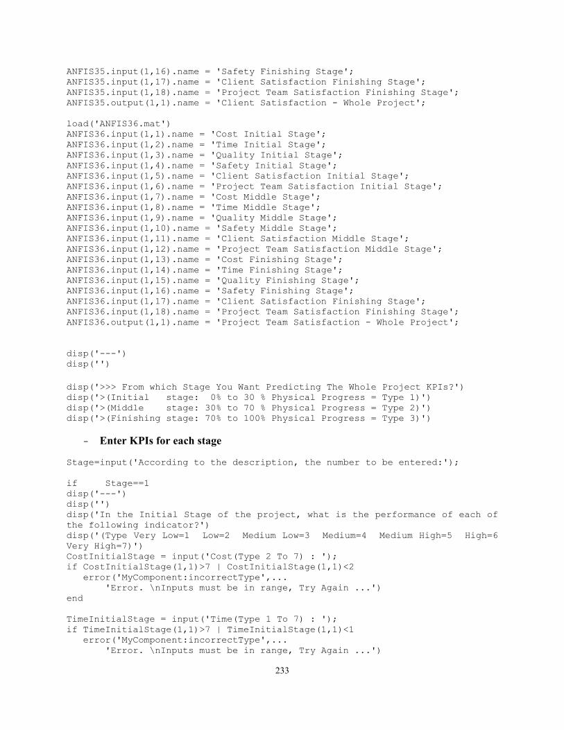
233
ANFIS35.input(1,16).name = 'Safety Finishing Stage';
ANFIS35.input(1,17).name = 'Client Satisfaction Finishing Stage';
ANFIS35.input(1,18).name = 'Project Team Satisfaction Finishing Stage';
ANFIS35.output(1,1).name = 'Client Satisfaction - Whole Project';
load('ANFIS36.mat')
ANFIS36.input(1,1).name = 'Cost Initial Stage';
ANFIS36.input(1,2).name = 'Time Initial Stage';
ANFIS36.input(1,3).name = 'Quality Initial Stage';
ANFIS36.input(1,4).name = 'Safety Initial Stage';
ANFIS36.input(1,5).name = 'Client Satisfaction Initial Stage';
ANFIS36.input(1,6).name = 'Project Team Satisfaction Initial Stage';
ANFIS36.input(1,7).name = 'Cost Middle Stage';
ANFIS36.input(1,8).name = 'Time Middle Stage';
ANFIS36.input(1,9).name = 'Quality Middle Stage';
ANFIS36.input(1,10).name = 'Safety Middle Stage';
ANFIS36.input(1,11).name = 'Client Satisfaction Middle Stage';
ANFIS36.input(1,12).name = 'Project Team Satisfaction Middle Stage';
ANFIS36.input(1,13).name = 'Cost Finishing Stage';
ANFIS36.input(1,14).name = 'Time Finishing Stage';
ANFIS36.input(1,15).name = 'Quality Finishing Stage';
ANFIS36.input(1,16).name = 'Safety Finishing Stage';
ANFIS36.input(1,17).name = 'Client Satisfaction Finishing Stage';
ANFIS36.input(1,18).name = 'Project Team Satisfaction Finishing Stage';
ANFIS36.output(1,1).name = 'Project Team Satisfaction - Whole Project';
disp('---')
disp('')
disp('>>> From which Stage You Want Predicting The Whole Project KPIs?')
disp('>(Initial stage: 0% to 30 % Physical Progress = Type 1)')
disp('>(Middle stage: 30% to 70 % Physical Progress = Type 2)')
disp('>(Finishing stage: 70% to 100% Physical Progress = Type 3)')
- Enter KPIs for each stage
Stage=input('According to the description, the number to be entered:');
if Stage==1
disp('---')
disp('')
disp('In the Initial Stage of the project, what is the performance of each of
the following indicator?')
disp('(Type Very Low=1 Low=2 Medium Low=3 Medium=4 Medium High=5 High=6
Very High=7)')
CostInitialStage = input('Cost(Type 2 To 7) : ');
if CostInitialStage(1,1)>7 | CostInitialStage(1,1)<2
error('MyComponent:incorrectType',...
'Error. \nInputs must be in range, Try Again ...')
end
TimeInitialStage = input('Time(Type 1 To 7) : ');
if TimeInitialStage(1,1)>7 | TimeInitialStage(1,1)<1
error('MyComponent:incorrectType',...
'Error. \nInputs must be in range, Try Again ...')
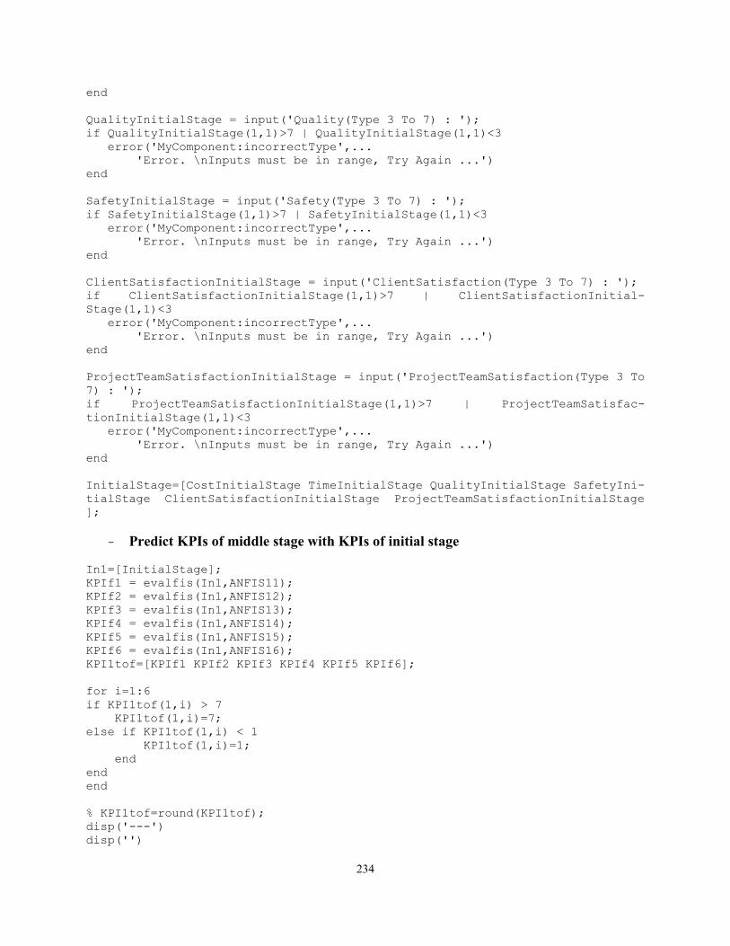
234
end
QualityInitialStage = input('Quality(Type 3 To 7) : ');
if QualityInitialStage(1,1)>7 | QualityInitialStage(1,1)<3
error('MyComponent:incorrectType',...
'Error. \nInputs must be in range, Try Again ...')
end
SafetyInitialStage = input('Safety(Type 3 To 7) : ');
if SafetyInitialStage(1,1)>7 | SafetyInitialStage(1,1)<3
error('MyComponent:incorrectType',...
'Error. \nInputs must be in range, Try Again ...')
end
ClientSatisfactionInitialStage = input('ClientSatisfaction(Type 3 To 7) : ');
if ClientSatisfactionInitialStage(1,1)>7 | ClientSatisfactionInitial-
Stage(1,1)<3
error('MyComponent:incorrectType',...
'Error. \nInputs must be in range, Try Again ...')
end
ProjectTeamSatisfactionInitialStage = input('ProjectTeamSatisfaction(Type 3 To
7) : ');
if ProjectTeamSatisfactionInitialStage(1,1)>7 | ProjectTeamSatisfac-
tionInitialStage(1,1)<3
error('MyComponent:incorrectType',...
'Error. \nInputs must be in range, Try Again ...')
end
InitialStage=[CostInitialStage TimeInitialStage QualityInitialStage SafetyIni-
tialStage ClientSatisfactionInitialStage ProjectTeamSatisfactionInitialStage
];
- Predict KPIs of middle stage with KPIs of initial stage
In1=[InitialStage];
KPIf1 = evalfis(In1,ANFIS11);
KPIf2 = evalfis(In1,ANFIS12);
KPIf3 = evalfis(In1,ANFIS13);
KPIf4 = evalfis(In1,ANFIS14);
KPIf5 = evalfis(In1,ANFIS15);
KPIf6 = evalfis(In1,ANFIS16);
KPI1tof=[KPIf1 KPIf2 KPIf3 KPIf4 KPIf5 KPIf6];
for i=1:6
if KPI1tof(1,i) > 7
KPI1tof(1,i)=7;
else if KPI1tof(1,i) < 1
KPI1tof(1,i)=1;
end
end
end
% KPI1tof=round(KPI1tof);
disp('---')
disp('')
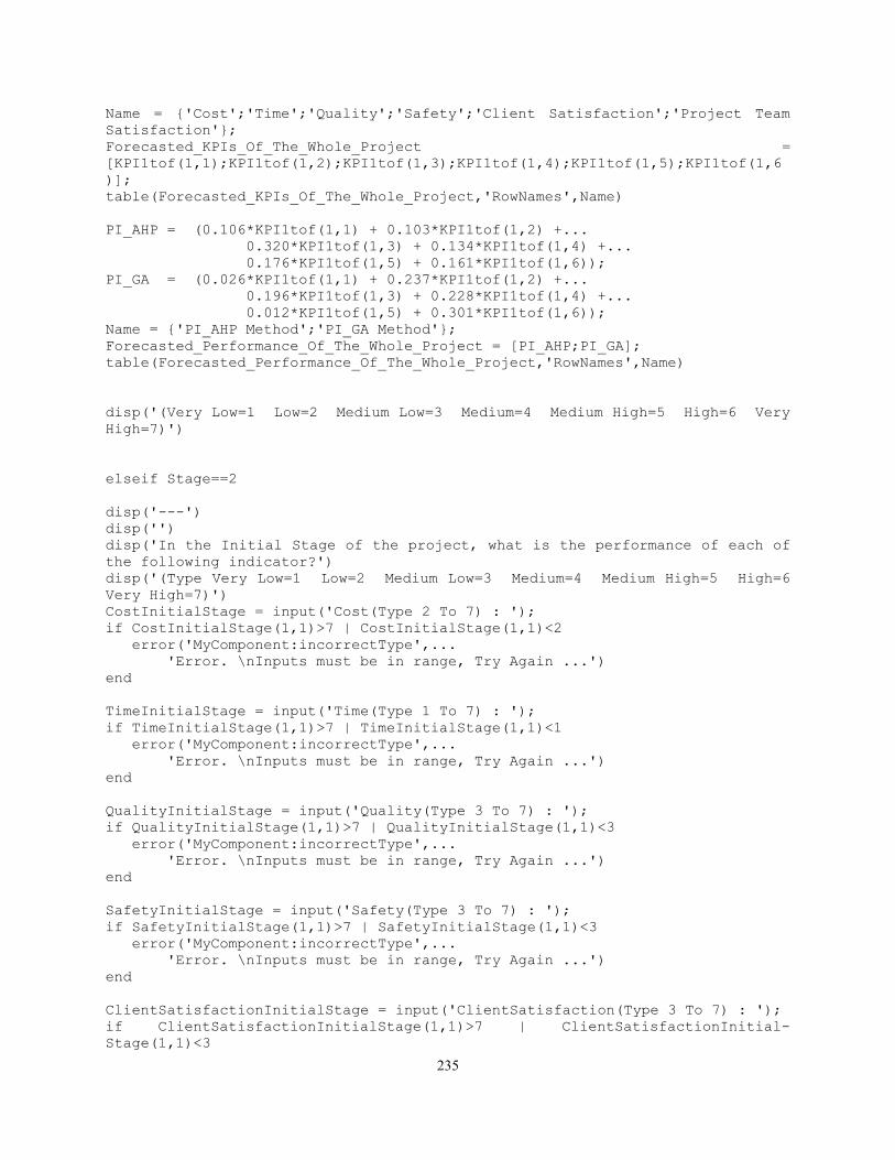
235
Name = {'Cost';'Time';'Quality';'Safety';'Client Satisfaction';'Project Team
Satisfaction'};
Forecasted_KPIs_Of_The_Whole_Project =
[KPI1tof(1,1);KPI1tof(1,2);KPI1tof(1,3);KPI1tof(1,4);KPI1tof(1,5);KPI1tof(1,6
)];
table(Forecasted_KPIs_Of_The_Whole_Project,'RowNames',Name)
PI_AHP = (0.106*KPI1tof(1,1) + 0.103*KPI1tof(1,2) +...
0.320*KPI1tof(1,3) + 0.134*KPI1tof(1,4) +...
0.176*KPI1tof(1,5) + 0.161*KPI1tof(1,6));
PI_GA = (0.026*KPI1tof(1,1) + 0.237*KPI1tof(1,2) +...
0.196*KPI1tof(1,3) + 0.228*KPI1tof(1,4) +...
0.012*KPI1tof(1,5) + 0.301*KPI1tof(1,6));
Name = {'PI_AHP Method';'PI_GA Method'};
Forecasted_Performance_Of_The_Whole_Project = [PI_AHP;PI_GA];
table(Forecasted_Performance_Of_The_Whole_Project,'RowNames',Name)
disp('(Very Low=1 Low=2 Medium Low=3 Medium=4 Medium High=5 High=6 Very
High=7)')
elseif Stage==2
disp('---')
disp('')
disp('In the Initial Stage of the project, what is the performance of each of
the following indicator?')
disp('(Type Very Low=1 Low=2 Medium Low=3 Medium=4 Medium High=5 High=6
Very High=7)')
CostInitialStage = input('Cost(Type 2 To 7) : ');
if CostInitialStage(1,1)>7 | CostInitialStage(1,1)<2
error('MyComponent:incorrectType',...
'Error. \nInputs must be in range, Try Again ...')
end
TimeInitialStage = input('Time(Type 1 To 7) : ');
if TimeInitialStage(1,1)>7 | TimeInitialStage(1,1)<1
error('MyComponent:incorrectType',...
'Error. \nInputs must be in range, Try Again ...')
end
QualityInitialStage = input('Quality(Type 3 To 7) : ');
if QualityInitialStage(1,1)>7 | QualityInitialStage(1,1)<3
error('MyComponent:incorrectType',...
'Error. \nInputs must be in range, Try Again ...')
end
SafetyInitialStage = input('Safety(Type 3 To 7) : ');
if SafetyInitialStage(1,1)>7 | SafetyInitialStage(1,1)<3
error('MyComponent:incorrectType',...
'Error. \nInputs must be in range, Try Again ...')
end
ClientSatisfactionInitialStage = input('ClientSatisfaction(Type 3 To 7) : ');
if ClientSatisfactionInitialStage(1,1)>7 | ClientSatisfactionInitial-
Stage(1,1)<3
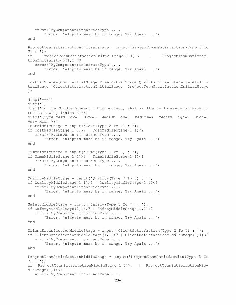
236
error('MyComponent:incorrectType',...
'Error. \nInputs must be in range, Try Again ...')
end
ProjectTeamSatisfactionInitialStage = input('ProjectTeamSatisfaction(Type 3 To
7) : ');
if ProjectTeamSatisfactionInitialStage(1,1)>7 | ProjectTeamSatisfac-
tionInitialStage(1,1)<3
error('MyComponent:incorrectType',...
'Error. \nInputs must be in range, Try Again ...')
end
InitialStage=[CostInitialStage TimeInitialStage QualityInitialStage SafetyIni-
tialStage ClientSatisfactionInitialStage ProjectTeamSatisfactionInitialStage
];
disp('---')
disp('')
disp('In the Middle Stage of the project, what is the performance of each of
the following indicator?')
disp('(Type Very Low=1 Low=2 Medium Low=3 Medium=4 Medium High=5 High=6
Very High=7)')
CostMiddleStage = input('Cost(Type 2 To 7) : ');
if CostMiddleStage(1,1)>7 | CostMiddleStage(1,1)<2
error('MyComponent:incorrectType',...
'Error. \nInputs must be in range, Try Again ...')
end
TimeMiddleStage = input('Time(Type 1 To 7) : ');
if TimeMiddleStage(1,1)>7 | TimeMiddleStage(1,1)<1
error('MyComponent:incorrectType',...
'Error. \nInputs must be in range, Try Again ...')
end
QualityMiddleStage = input('Quality(Type 3 To 7) : ');
if QualityMiddleStage(1,1)>7 | QualityMiddleStage(1,1)<3
error('MyComponent:incorrectType',...
'Error. \nInputs must be in range, Try Again ...')
end
SafetyMiddleStage = input('Safety(Type 3 To 7) : ');
if SafetyMiddleStage(1,1)>7 | SafetyMiddleStage(1,1)<3
error('MyComponent:incorrectType',...
'Error. \nInputs must be in range, Try Again ...')
end
ClientSatisfactionMiddleStage = input('ClientSatisfaction(Type 2 To 7) : ');
if ClientSatisfactionMiddleStage(1,1)>7 | ClientSatisfactionMiddleStage(1,1)<2
error('MyComponent:incorrectType',...
'Error. \nInputs must be in range, Try Again ...')
end
ProjectTeamSatisfactionMiddleStage = input('ProjectTeamSatisfaction(Type 3 To
7) : ');
if ProjectTeamSatisfactionMiddleStage(1,1)>7 | ProjectTeamSatisfactionMid-
dleStage(1,1)<3
error('MyComponent:incorrectType',...
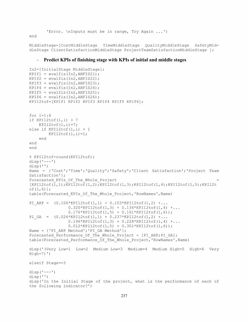
237
'Error. \nInputs must be in range, Try Again ...')
end
MiddleStage=[CostMiddleStage TimeMiddleStage QualityMiddleStage SafetyMid-
dleStage ClientSatisfactionMiddleStage ProjectTeamSatisfactionMiddleStage ];
- Predict KPIs of finishing stage with KPIs of initial and middle stages
In2=[InitialStage MiddleStage];
KPIf1 = evalfis(In2,ANFIS21);
KPIf2 = evalfis(In2,ANFIS22);
KPIf3 = evalfis(In2,ANFIS23);
KPIf4 = evalfis(In2,ANFIS24);
KPIf5 = evalfis(In2,ANFIS25);
KPIf6 = evalfis(In2,ANFIS26);
KPI12tof=[KPIf1 KPIf2 KPIf3 KPIf4 KPIf5 KPIf6];
for i=1:6
if KPI12tof(1,i) > 7
KPI12tof(1,i)=7;
else if KPI12tof(1,i) < 1
KPI12tof(1,i)=1;
end
end
end
% KPI12tof=round(KPI12tof);
disp('---')
disp('')
Name = {'Cost';'Time';'Quality';'Safety';'Client Satisfaction';'Project Team
Satisfaction'};
Forecasted_KPIs_Of_The_Whole_Project =
[KPI12tof(1,1);KPI12tof(1,2);KPI12tof(1,3);KPI12tof(1,4);KPI12tof(1,5);KPI12t
of(1,6)];
table(Forecasted_KPIs_Of_The_Whole_Project,'RowNames',Name)
PI_AHP = (0.106*KPI12tof(1,1) + 0.103*KPI12tof(1,2) +...
0.320*KPI12tof(1,3) + 0.134*KPI12tof(1,4) +...
0.176*KPI12tof(1,5) + 0.161*KPI12tof(1,6));
PI_GA = (0.026*KPI12tof(1,1) + 0.237*KPI12tof(1,2) +...
0.196*KPI12tof(1,3) + 0.228*KPI12tof(1,4) +...
0.012*KPI12tof(1,5) + 0.301*KPI12tof(1,6));
Name = {'PI_AHP Method';'PI_GA Method'};
Forecasted_Performance_Of_The_Whole_Project = [PI_AHP;PI_GA];
table(Forecasted_Performance_Of_The_Whole_Project,'RowNames',Name)
disp('(Very Low=1 Low=2 Medium Low=3 Medium=4 Medium High=5 High=6 Very
High=7)')
elseif Stage==3
disp('---')
disp('')
disp('In the Initial Stage of the project, what is the performance of each of
the following indicator?')
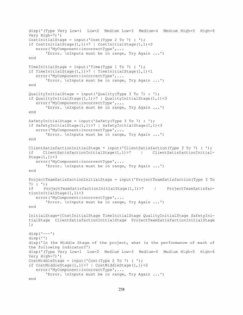
238
disp('(Type Very Low=1 Low=2 Medium Low=3 Medium=4 Medium High=5 High=6
Very High=7)')
CostInitialStage = input('Cost(Type 2 To 7) : ');
if CostInitialStage(1,1)>7 | CostInitialStage(1,1)<2
error('MyComponent:incorrectType',...
'Error. \nInputs must be in range, Try Again ...')
end
TimeInitialStage = input('Time(Type 1 To 7) : ');
if TimeInitialStage(1,1)>7 | TimeInitialStage(1,1)<1
error('MyComponent:incorrectType',...
'Error. \nInputs must be in range, Try Again ...')
end
QualityInitialStage = input('Quality(Type 3 To 7) : ');
if QualityInitialStage(1,1)>7 | QualityInitialStage(1,1)<3
error('MyComponent:incorrectType',...
'Error. \nInputs must be in range, Try Again ...')
end
SafetyInitialStage = input('Safety(Type 3 To 7) : ');
if SafetyInitialStage(1,1)>7 | SafetyInitialStage(1,1)<3
error('MyComponent:incorrectType',...
'Error. \nInputs must be in range, Try Again ...')
end
ClientSatisfactionInitialStage = input('ClientSatisfaction(Type 3 To 7) : ');
if ClientSatisfactionInitialStage(1,1)>7 | ClientSatisfactionInitial-
Stage(1,1)<3
error('MyComponent:incorrectType',...
'Error. \nInputs must be in range, Try Again ...')
end
ProjectTeamSatisfactionInitialStage = input('ProjectTeamSatisfaction(Type 3 To
7) : ');
if ProjectTeamSatisfactionInitialStage(1,1)>7 | ProjectTeamSatisfac-
tionInitialStage(1,1)<3
error('MyComponent:incorrectType',...
'Error. \nInputs must be in range, Try Again ...')
end
InitialStage=[CostInitialStage TimeInitialStage QualityInitialStage SafetyIni-
tialStage ClientSatisfactionInitialStage ProjectTeamSatisfactionInitialStage
];
disp('---')
disp('')
disp('In the Middle Stage of the project, what is the performance of each of
the following indicator?')
disp('(Type Very Low=1 Low=2 Medium Low=3 Medium=4 Medium High=5 High=6
Very High=7)')
CostMiddleStage = input('Cost(Type 2 To 7) : ');
if CostMiddleStage(1,1)>7 | CostMiddleStage(1,1)<2
error('MyComponent:incorrectType',...
'Error. \nInputs must be in range, Try Again ...')
end
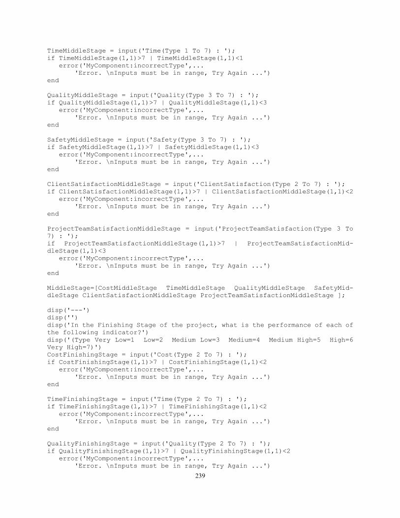
239
TimeMiddleStage = input('Time(Type 1 To 7) : ');
if TimeMiddleStage(1,1)>7 | TimeMiddleStage(1,1)<1
error('MyComponent:incorrectType',...
'Error. \nInputs must be in range, Try Again ...')
end
QualityMiddleStage = input('Quality(Type 3 To 7) : ');
if QualityMiddleStage(1,1)>7 | QualityMiddleStage(1,1)<3
error('MyComponent:incorrectType',...
'Error. \nInputs must be in range, Try Again ...')
end
SafetyMiddleStage = input('Safety(Type 3 To 7) : ');
if SafetyMiddleStage(1,1)>7 | SafetyMiddleStage(1,1)<3
error('MyComponent:incorrectType',...
'Error. \nInputs must be in range, Try Again ...')
end
ClientSatisfactionMiddleStage = input('ClientSatisfaction(Type 2 To 7) : ');
if ClientSatisfactionMiddleStage(1,1)>7 | ClientSatisfactionMiddleStage(1,1)<2
error('MyComponent:incorrectType',...
'Error. \nInputs must be in range, Try Again ...')
end
ProjectTeamSatisfactionMiddleStage = input('ProjectTeamSatisfaction(Type 3 To
7) : ');
if ProjectTeamSatisfactionMiddleStage(1,1)>7 | ProjectTeamSatisfactionMid-
dleStage(1,1)<3
error('MyComponent:incorrectType',...
'Error. \nInputs must be in range, Try Again ...')
end
MiddleStage=[CostMiddleStage TimeMiddleStage QualityMiddleStage SafetyMid-
dleStage ClientSatisfactionMiddleStage ProjectTeamSatisfactionMiddleStage ];
disp('---')
disp('')
disp('In the Finishing Stage of the project, what is the performance of each of
the following indicator?')
disp('(Type Very Low=1 Low=2 Medium Low=3 Medium=4 Medium High=5 High=6
Very High=7)')
CostFinishingStage = input('Cost(Type 2 To 7) : ');
if CostFinishingStage(1,1)>7 | CostFinishingStage(1,1)<2
error('MyComponent:incorrectType',...
'Error. \nInputs must be in range, Try Again ...')
end
TimeFinishingStage = input('Time(Type 2 To 7) : ');
if TimeFinishingStage(1,1)>7 | TimeFinishingStage(1,1)<2
error('MyComponent:incorrectType',...
'Error. \nInputs must be in range, Try Again ...')
end
QualityFinishingStage = input('Quality(Type 2 To 7) : ');
if QualityFinishingStage(1,1)>7 | QualityFinishingStage(1,1)<2
error('MyComponent:incorrectType',...
'Error. \nInputs must be in range, Try Again ...')
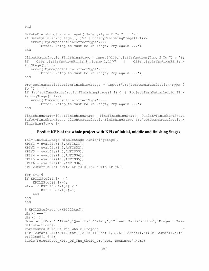
240
end
SafetyFinishingStage = input('Safety(Type 2 To 7) : ');
if SafetyFinishingStage(1,1)>7 | SafetyFinishingStage(1,1)<2
error('MyComponent:incorrectType',...
'Error. \nInputs must be in range, Try Again ...')
end
ClientSatisfactionFinishingStage = input('ClientSatisfaction(Type 2 To 7) : ');
if ClientSatisfactionFinishingStage(1,1)>7 | ClientSatisfactionFinish-
ingStage(1,1)<2
error('MyComponent:incorrectType',...
'Error. \nInputs must be in range, Try Again ...')
end
ProjectTeamSatisfactionFinishingStage = input('ProjectTeamSatisfaction(Type 2
To 7) : ');
if ProjectTeamSatisfactionFinishingStage(1,1)>7 | ProjectTeamSatisfactionFin-
ishingStage(1,1)<2
error('MyComponent:incorrectType',...
'Error. \nInputs must be in range, Try Again ...')
end
FinishingStage=[CostFinishingStage TimeFinishingStage QualityFinishingStage
SafetyFinishingStage ClientSatisfactionFinishingStage ProjectTeamSatisfaction-
FinishingStage ];
- Predict KPIs of the whole project with KPIs of initial, middle and finishing Stages
In3=[InitialStage MiddleStage FinishingStage];
KPIf1 = evalfis(In3,ANFIS31);
KPIf2 = evalfis(In3,ANFIS32);
KPIf3 = evalfis(In3,ANFIS33);
KPIf4 = evalfis(In3,ANFIS34);
KPIf5 = evalfis(In3,ANFIS35);
KPIf6 = evalfis(In3,ANFIS36);
KPI123tof=[KPIf1 KPIf2 KPIf3 KPIf4 KPIf5 KPIf6];
for i=1:6
if KPI123tof(1,i) > 7
KPI123tof(1,i)=7;
else if KPI123tof(1,i) < 1
KPI123tof(1,i)=1;
end
end
end
% KPI123tof=round(KPI123tof);
disp('---')
disp('')
Name = {'Cost';'Time';'Quality';'Safety';'Client Satisfaction';'Project Team
Satisfaction'};
Forecasted_KPIs_Of_The_Whole_Project =
[KPI123tof(1,1);KPI123tof(1,2);KPI123tof(1,3);KPI123tof(1,4);KPI123tof(1,5);K
PI123tof(1,6)];
table(Forecasted_KPIs_Of_The_Whole_Project,'RowNames',Name)
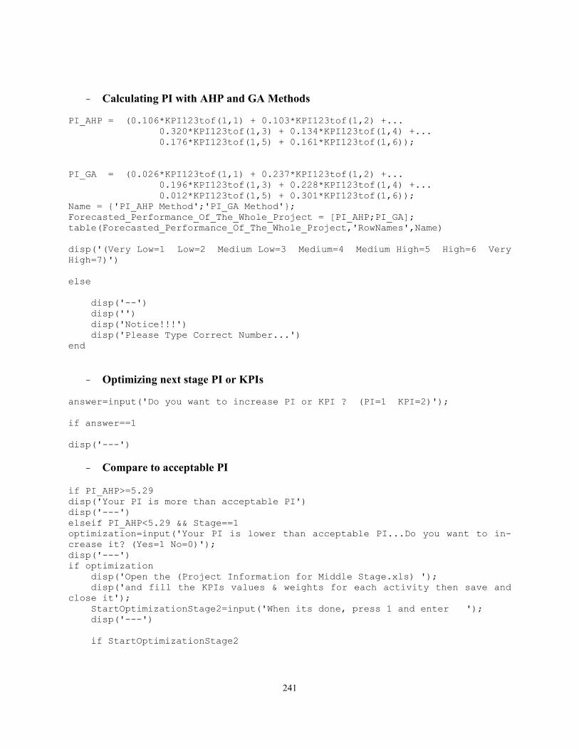
241
- Calculating PI with AHP and GA Methods
PI_AHP = (0.106*KPI123tof(1,1) + 0.103*KPI123tof(1,2) +...
0.320*KPI123tof(1,3) + 0.134*KPI123tof(1,4) +...
0.176*KPI123tof(1,5) + 0.161*KPI123tof(1,6));
PI_GA = (0.026*KPI123tof(1,1) + 0.237*KPI123tof(1,2) +...
0.196*KPI123tof(1,3) + 0.228*KPI123tof(1,4) +...
0.012*KPI123tof(1,5) + 0.301*KPI123tof(1,6));
Name = {'PI_AHP Method';'PI_GA Method'};
Forecasted_Performance_Of_The_Whole_Project = [PI_AHP;PI_GA];
table(Forecasted_Performance_Of_The_Whole_Project,'RowNames',Name)
disp('(Very Low=1 Low=2 Medium Low=3 Medium=4 Medium High=5 High=6 Very
High=7)')
else
disp('--')
disp('')
disp('Notice!!!')
disp('Please Type Correct Number...')
end
- Optimizing next stage PI or KPIs
answer=input('Do you want to increase PI or KPI ? (PI=1 KPI=2)');
if answer==1
disp('---')
- Compare to acceptable PI
if PI_AHP>=5.29
disp('Your PI is more than acceptable PI')
disp('---')
elseif PI_AHP<5.29 && Stage==1
optimization=input('Your PI is lower than acceptable PI...Do you want to in-
crease it? (Yes=1 No=0)');
disp('---')
if optimization
disp('Open the (Project Information for Middle Stage.xls) ');
disp('and fill the KPIs values & weights for each activity then save and
close it');
StartOptimizationStage2=input('When its done, press 1 and enter ');
disp('---')
if StartOptimizationStage2
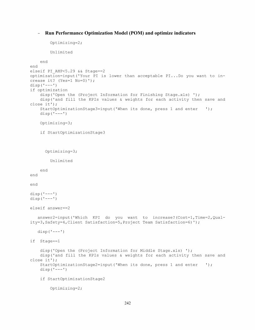
242
- Run Performance Optimization Model (POM) and optimize indicators
Optimizing=2;
Unlimited
end
end
elseif PI_AHP<5.29 && Stage==2
optimization=input('Your PI is lower than acceptable PI...Do you want to in-
crease it? (Yes=1 No=0)');
disp('---')
if optimization
disp('Open the (Project Information for Finishing Stage.xls) ');
disp('and fill the KPIs values & weights for each activity then save and
close it');
StartOptimizationStage3=input('When its done, press 1 and enter ');
disp('---')
Optimizing=3;
if StartOptimizationStage3
Optimizing=3;
Unlimited
end
end
end
disp('---')
disp('---')
elseif answer==2
answer2=input('Which KPI do you want to increase?(Cost=1,Time=2,Qual-
ity=3,Safety=4,Client Satisfaction=5,Project Team Satisfaction=6)');
disp('---')
if Stage==1
disp('Open the (Project Information for Middle Stage.xls) ');
disp('and fill the KPIs values & weights for each activity then save and
close it');
StartOptimizationStage2=input('When its done, press 1 and enter ');
disp('---')
if StartOptimizationStage2
Optimizing=2;

243
Optimize_KPI
end
elseif Stage==2
disp('Open the (Project Information for Finishing Stage.xls) ');
disp('and fill the KPIs values & weights for each activity then save and
close it');
StartOptimizationStage3=input('When its done, press 1 and enter ');
disp('---')
Optimizing=3;
if StartOptimizationStage3
Optimizing=3;
Optimize_KPI
end
end
disp('---')
disp('---')
end
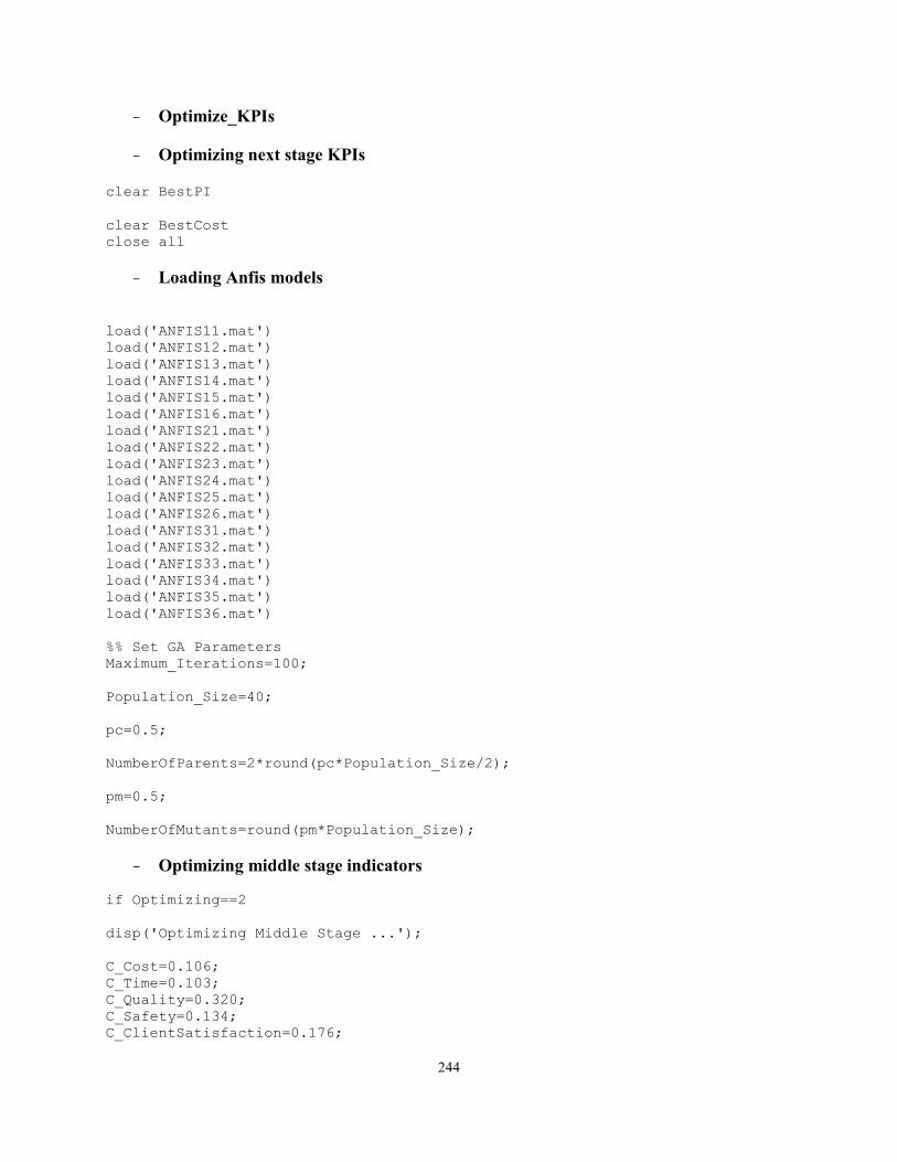
244
- Optimize_KPIs
- Optimizing next stage KPIs
clear BestPI
clear BestCost
close all
- Loading Anfis models
load('ANFIS11.mat')
load('ANFIS12.mat')
load('ANFIS13.mat')
load('ANFIS14.mat')
load('ANFIS15.mat')
load('ANFIS16.mat')
load('ANFIS21.mat')
load('ANFIS22.mat')
load('ANFIS23.mat')
load('ANFIS24.mat')
load('ANFIS25.mat')
load('ANFIS26.mat')
load('ANFIS31.mat')
load('ANFIS32.mat')
load('ANFIS33.mat')
load('ANFIS34.mat')
load('ANFIS35.mat')
load('ANFIS36.mat')
%% Set GA Parameters
Maximum_Iterations=100;
Population_Size=40;
pc=0.5;
NumberOfParents=2*round(pc*Population_Size/2);
pm=0.5;
NumberOfMutants=round(pm*Population_Size);
- Optimizing middle stage indicators
if Optimizing==2
disp('Optimizing Middle Stage ...');
C_Cost=0.106;
C_Time=0.103;
C_Quality=0.320;
C_Safety=0.134;
C_ClientSatisfaction=0.176;
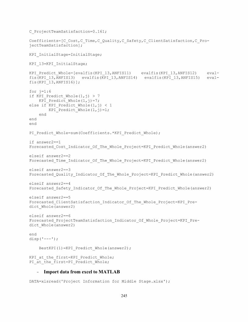
245
C_ProjectTeamSatisfaction=0.161;
Coefficients=[C_Cost,C_Time,C_Quality,C_Safety,C_ClientSatisfaction,C_Pro-
jectTeamSatisfaction];
KPI_InitialStage=InitialStage;
KPI_13=KPI_InitialStage;
KPI_Predict_Whole=[evalfis(KPI_13,ANFIS11) evalfis(KPI_13,ANFIS12) eval-
fis(KPI_13,ANFIS13) evalfis(KPI_13,ANFIS14) evalfis(KPI_13,ANFIS15) eval-
fis(KPI_13,ANFIS16)];
for j=1:6
if KPI_Predict_Whole(1,j) > 7
KPI_Predict_Whole(1,j)=7;
else if KPI_Predict_Whole(1,j) < 1
KPI_Predict_Whole(1,j)=1;
end
end
end
PI_Predict_Whole=sum(Coefficients.*KPI_Predict_Whole);
if answer2==1
Forecasted_Cost_Indicator_Of_The_Whole_Project=KPI_Predict_Whole(answer2)
elseif answer2==2
Forecasted_Time_Indicator_Of_The_Whole_Project=KPI_Predict_Whole(answer2)
elseif answer2==3
Forecasted_Quality_Indicator_Of_The_Whole_Project=KPI_Predict_Whole(answer2)
elseif answer2==4
Forecasted_Safety_Indicator_Of_The_Whole_Project=KPI_Predict_Whole(answer2)
elseif answer2==5
Forecasted_ClientSatisfaction_Indicator_Of_The_Whole_Project=KPI_Pre-
dict_Whole(answer2)
elseif answer2==6
Forecasted_ProjectTeamSatisfaction_Indicator_Of_Whole_Project=KPI_Pre-
dict_Whole(answer2)
end
disp('---');
BestKPI(1)=KPI_Predict_Whole(answer2);
KPI_at_the_first=KPI_Predict_Whole;
PI_at_the_first=PI_Predict_Whole;
- Import data from excel to MATLAB
DATA=xlsread('Project Information for Middle Stage.xlsx');
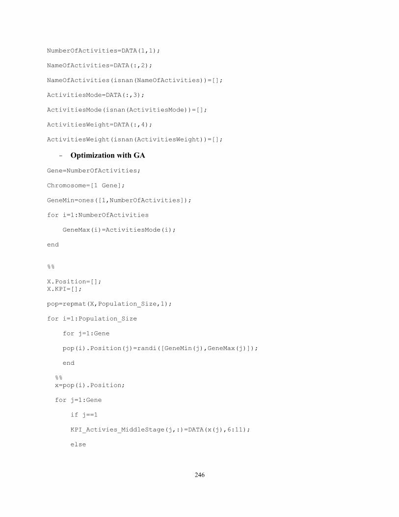
246
NumberOfActivities=DATA(1,1);
NameOfActivities=DATA(:,2);
NameOfActivities(isnan(NameOfActivities))=[];
ActivitiesMode=DATA(:,3);
ActivitiesMode(isnan(ActivitiesMode))=[];
ActivitiesWeight=DATA(:,4);
ActivitiesWeight(isnan(ActivitiesWeight))=[];
- Optimization with GA
Gene=NumberOfActivities;
Chromosome=[1 Gene];
GeneMin=ones([1,NumberOfActivities]);
for i=1:NumberOfActivities
GeneMax(i)=ActivitiesMode(i);
end
%%
X.Position=[];
X.KPI=[];
pop=repmat(X,Population_Size,1);
for i=1:Population_Size
for j=1:Gene
pop(i).Position(j)=randi([GeneMin(j),GeneMax(j)]);
end
%%
x=pop(i).Position;
for j=1:Gene
if j==1
KPI_Activies_MiddleStage(j,:)=DATA(x(j),6:11);
else
247
KPI_Activies_MiddleStage(j,:)=DATA(sum(ActivitiesMode(1:j-
1))+x(j),6:11);
end
end
for o=1:Gene
KPI_MiddleStage(o,:)=ActivitiesWeight(o)*KPI_Activies_MiddleStage(o,:);
end
KPI_MiddleStage=sum(KPI_MiddleStage)/sum(ActivitiesWeight);
KPI=round([KPI_13 KPI_MiddleStage]);
KPI_Predict_Whole=[evalfis(KPI,ANFIS21) evalfis(KPI,ANFIS22) evalfis(KPI,AN-
FIS23) evalfis(KPI,ANFIS24) evalfis(KPI,ANFIS25) evalfis(KPI,ANFIS26)];
for j=1:6
if KPI_Predict_Whole(1,j) > 7
KPI_Predict_Whole(1,j)=7;
elseif KPI_Predict_Whole(1,j) < 1
KPI_Predict_Whole(1,j)=1;
end
end
PI_Predict_Whole=sum(Coefficients.*KPI_Predict_Whole);
pop(i).KPI=KPI_Predict_Whole(answer2);
end
KPII=[pop.KPI];
[KPII, SortOrder]=sort(KPII);
pop=pop(SortOrder);
BestSol=pop(end);
BestCost=zeros(Maximum_Iterations,1);
for iterations=2:Maximum_Iterations
popc=repmat(X,NumberOfParents/2,2);
for k=1:NumberOfParents/2
%% Choose Parents for GA
i1=randi([1,Population_Size]);
p1=pop(i1);
i2=randi([1,Population_Size]);
p2=pop(i2);
%% CrossOver (SinglePoint)
c=randi(Gene-1,1);
248
popc(k,1).Position=[p1.Position(1:c),p2.Position(c+1:end)];
popc(k,2).Position=[p2.Position(1:c),p1.Position(c+1:end)];
%%
x=popc(k,1).Position;
for j=1:Gene
if j==1
KPI_Activies_MiddleStage(j,:)=DATA(x(j),6:11);
else
KPI_Activies_MiddleStage(j,:)=DATA(sum(ActivitiesMode(1:j-
1))+x(j),6:11);
end
end
for o=1:Gene
KPI_MiddleStage(o,:)=ActivitiesWeight(o)*KPI_Activies_MiddleStage(o,:);
end
KPI_MiddleStage=sum(KPI_MiddleStage)/sum(ActivitiesWeight);
KPI=round([KPI_13 KPI_MiddleStage]);
KPI_Predict_Whole=[evalfis(KPI,ANFIS21) evalfis(KPI,ANFIS22) evalfis(KPI,AN-
FIS23) evalfis(KPI,ANFIS24) evalfis(KPI,ANFIS25) evalfis(KPI,ANFIS26)];
for j=1:6
if KPI_Predict_Whole(1,j) > 7
KPI_Predict_Whole(1,j)=7;
else if KPI_Predict_Whole(1,j) < 1
KPI_Predict_Whole(1,j)=1;
end
end
end
PI_Predict_Whole=sum(Coefficients.*KPI_Predict_Whole);
popc(k,1).KPI=KPI_Predict_Whole(answer2);
%%
x=popc(k,2).Position;
for j=1:Gene
if j==1
KPI_Activies_MiddleStage(j,:)=DATA(x(j),6:11);
else
249
KPI_Activies_MiddleStage(j,:)=DATA(sum(ActivitiesMode(1:j-
1))+x(j),6:11);
end
end
for o=1:Gene
KPI_MiddleStage(o,:)=ActivitiesWeight(o)*KPI_Activies_MiddleStage(o,:);
end
KPI_MiddleStage=sum(KPI_MiddleStage)/sum(ActivitiesWeight);
KPI=round([KPI_13 KPI_MiddleStage]);
KPI_Predict_Whole=[evalfis(KPI,ANFIS21) evalfis(KPI,ANFIS22) evalfis(KPI,AN-
FIS23) evalfis(KPI,ANFIS24) evalfis(KPI,ANFIS25) evalfis(KPI,ANFIS26)];
for j=1:6
if KPI_Predict_Whole(1,j) > 7
KPI_Predict_Whole(1,j)=7;
else if KPI_Predict_Whole(1,j) < 1
KPI_Predict_Whole(1,j)=1;
end
end
end
PI_Predict_Whole=sum(Coefficients.*KPI_Predict_Whole);
popc(k,2).KPI=KPI_Predict_Whole(answer2);
end
popc=popc(:);
%% Mutation
popm=repmat(X,NumberOfMutants,1);
for k=1:NumberOfMutants
i=randi([1 Population_Size]);
p=pop(i);
I=randi([1,Gene]);
NumberOfActivitiesMode_Mutate=ActivitiesMode(I);
popm(k).Position=p.Position;
MaxGene_Mutate=GeneMax(I);
if MaxGene_Mutate==1
popm(k).Position(I)=p.Position(I);
250
else
Modes=1:NumberOfActivitiesMode_Mutate;
Modes(Modes==p.Position(I))=[];
n=numel(Modes);
d=randi([1,n],1);
popm(k).Position(I)=d;
end
%%
x=popm(k).Position;
for j=1:Gene
if j==1
KPI_Activies_MiddleStage(j,:)=DATA(x(j),6:11);
else
KPI_Activies_MiddleStage(j,:)=DATA(sum(ActivitiesMode(1:j-
1))+x(j),6:11);
end
end
for o=1:Gene
KPI_MiddleStage(o,:)=ActivitiesWeight(o)*KPI_Activies_MiddleStage(o,:);
end
KPI_MiddleStage=sum(KPI_MiddleStage)/sum(ActivitiesWeight);
KPI=round([KPI_13 KPI_MiddleStage]);
KPI_Predict_Whole=[evalfis(KPI,ANFIS21) evalfis(KPI,ANFIS22) evalfis(KPI,AN-
FIS23) evalfis(KPI,ANFIS24) evalfis(KPI,ANFIS25) evalfis(KPI,ANFIS26)];
for j=1:6
if KPI_Predict_Whole(1,j) > 7
KPI_Predict_Whole(1,j)=7;
else if KPI_Predict_Whole(1,j) < 1
KPI_Predict_Whole(1,j)=1;
end
end
end
PI_Predict_Whole=sum(Coefficients.*KPI_Predict_Whole);
popm(k).KPI=KPI_Predict_Whole(answer2);
end
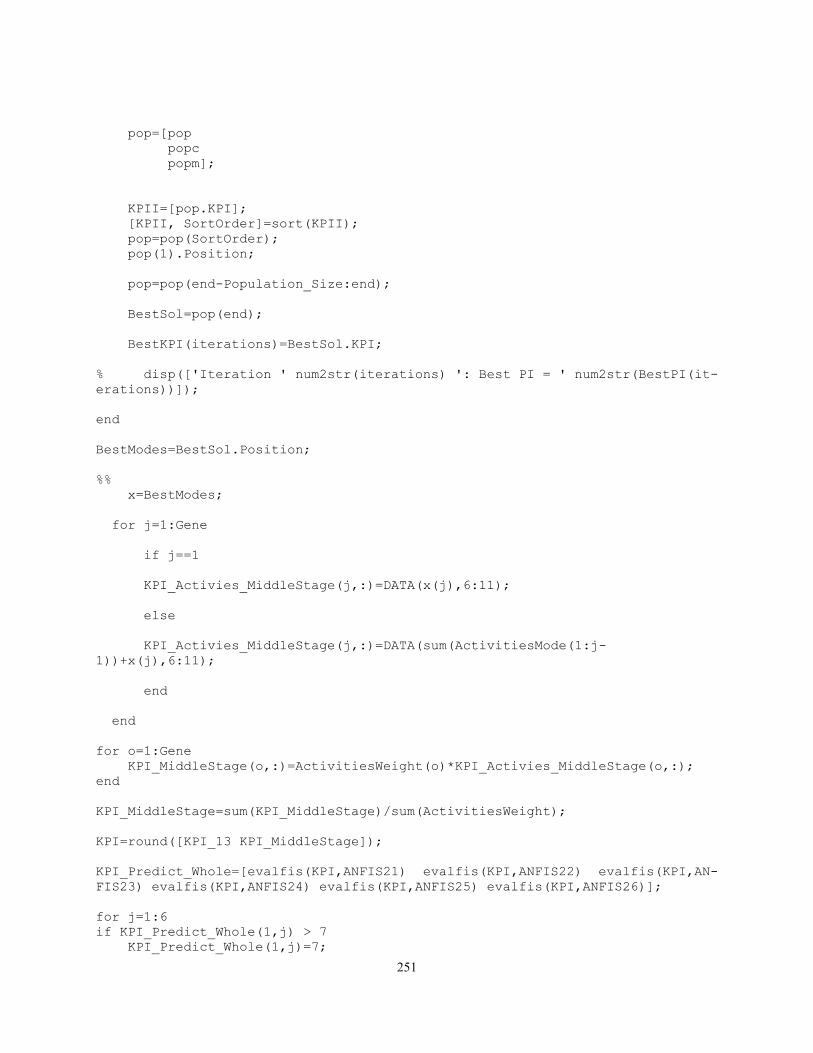
251
pop=[pop
popc
popm];
KPII=[pop.KPI];
[KPII, SortOrder]=sort(KPII);
pop=pop(SortOrder);
pop(1).Position;
pop=pop(end-Population_Size:end);
BestSol=pop(end);
BestKPI(iterations)=BestSol.KPI;
% disp(['Iteration ' num2str(iterations) ': Best PI = ' num2str(BestPI(it-
erations))]);
end
BestModes=BestSol.Position;
%%
x=BestModes;
for j=1:Gene
if j==1
KPI_Activies_MiddleStage(j,:)=DATA(x(j),6:11);
else
KPI_Activies_MiddleStage(j,:)=DATA(sum(ActivitiesMode(1:j-
1))+x(j),6:11);
end
end
for o=1:Gene
KPI_MiddleStage(o,:)=ActivitiesWeight(o)*KPI_Activies_MiddleStage(o,:);
end
KPI_MiddleStage=sum(KPI_MiddleStage)/sum(ActivitiesWeight);
KPI=round([KPI_13 KPI_MiddleStage]);
KPI_Predict_Whole=[evalfis(KPI,ANFIS21) evalfis(KPI,ANFIS22) evalfis(KPI,AN-
FIS23) evalfis(KPI,ANFIS24) evalfis(KPI,ANFIS25) evalfis(KPI,ANFIS26)];
for j=1:6
if KPI_Predict_Whole(1,j) > 7
KPI_Predict_Whole(1,j)=7;
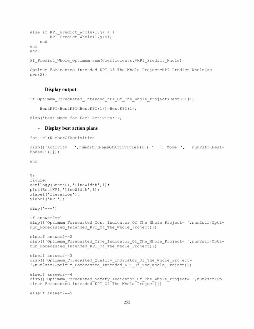
252
else if KPI_Predict_Whole(1,j) < 1
KPI_Predict_Whole(1,j)=1;
end
end
end
PI_Predict_Whole_Optimum=sum(Coefficients.*KPI_Predict_Whole);
Optimum_Forecasted_Intended_KPI_Of_The_Whole_Project=KPI_Predict_Whole(an-
swer2);
- Display output
if Optimum_Forecasted_Intended_KPI_Of_The_Whole_Project>BestKPI(1)
BestKPI(BestKPI<BestKPI(1))=BestKPI(1);
disp('Best Mode for Each Activity:');
- Display best action plans
for i=1:NumberOfActivities
disp(['Activity ',num2str(NameOfActivities(i)),' : Mode ', num2str(Best-
Modes(i))]);
end
%%
figure;
semilogy(BestKPI,'LineWidth',1);
plot(BestKPI,'LineWidth',1);
xlabel('Iteration');
ylabel('KPI');
disp('---')
if answer2==1
disp(['Optimum_Forecasted_Cost_Indicator_Of_The_Whole_Project= ',num2str(Opti-
mum_Forecasted_Intended_KPI_Of_The_Whole_Project)])
elseif answer2==2
disp(['Optimum_Forecasted_Time_Indicator_Of_The_Whole_Project= ',num2str(Opti-
mum_Forecasted_Intended_KPI_Of_The_Whole_Project)])
elseif answer2==3
disp(['Optimum_Forecasted_Quality_Indicator_Of_The_Whole_Project=
',num2str(Optimum_Forecasted_Intended_KPI_Of_The_Whole_Project)])
elseif answer2==4
disp(['Optimum_Forecasted_Safety_Indicator_Of_The_Whole_Project= ',num2str(Op-
timum_Forecasted_Intended_KPI_Of_The_Whole_Project)])
elseif answer2==5
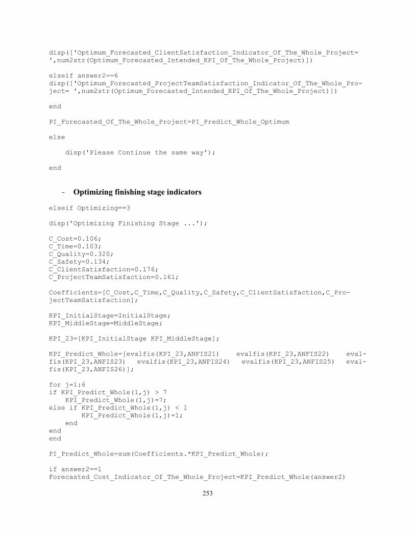
253
disp(['Optimum_Forecasted_ClientSatisfaction_Indicator_Of_The_Whole_Project=
',num2str(Optimum_Forecasted_Intended_KPI_Of_The_Whole_Project)])
elseif answer2==6
disp(['Optimum_Forecasted_ProjectTeamSatisfaction_Indicator_Of_The_Whole_Pro-
ject= ',num2str(Optimum_Forecasted_Intended_KPI_Of_The_Whole_Project)])
end
PI_Forecasted_Of_The_Whole_Project=PI_Predict_Whole_Optimum
else
disp('Please Continue the same way');
end
- Optimizing finishing stage indicators
elseif Optimizing==3
disp('Optimizing Finishing Stage ...');
C_Cost=0.106;
C_Time=0.103;
C_Quality=0.320;
C_Safety=0.134;
C_ClientSatisfaction=0.176;
C_ProjectTeamSatisfaction=0.161;
Coefficients=[C_Cost,C_Time,C_Quality,C_Safety,C_ClientSatisfaction,C_Pro-
jectTeamSatisfaction];
KPI_InitialStage=InitialStage;
KPI_MiddleStage=MiddleStage;
KPI_23=[KPI_InitialStage KPI_MiddleStage];
KPI_Predict_Whole=[evalfis(KPI_23,ANFIS21) evalfis(KPI_23,ANFIS22) eval-
fis(KPI_23,ANFIS23) evalfis(KPI_23,ANFIS24) evalfis(KPI_23,ANFIS25) eval-
fis(KPI_23,ANFIS26)];
for j=1:6
if KPI_Predict_Whole(1,j) > 7
KPI_Predict_Whole(1,j)=7;
else if KPI_Predict_Whole(1,j) < 1
KPI_Predict_Whole(1,j)=1;
end
end
end
PI_Predict_Whole=sum(Coefficients.*KPI_Predict_Whole);
if answer2==1
Forecasted_Cost_Indicator_Of_The_Whole_Project=KPI_Predict_Whole(answer2)
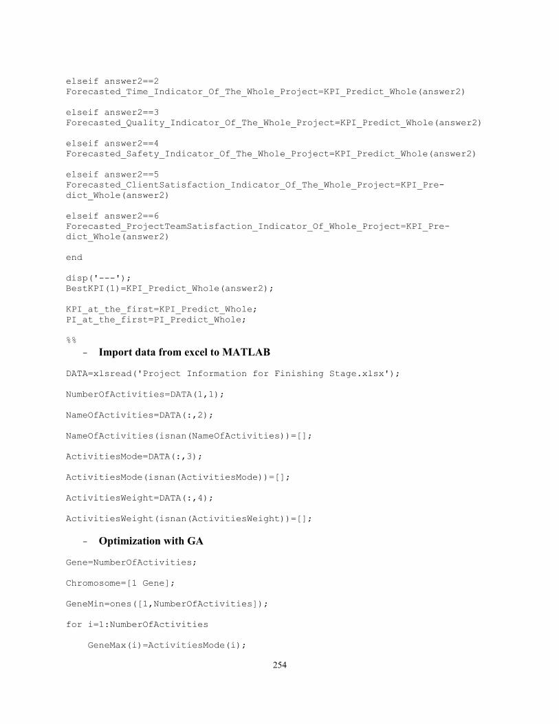
254
elseif answer2==2
Forecasted_Time_Indicator_Of_The_Whole_Project=KPI_Predict_Whole(answer2)
elseif answer2==3
Forecasted_Quality_Indicator_Of_The_Whole_Project=KPI_Predict_Whole(answer2)
elseif answer2==4
Forecasted_Safety_Indicator_Of_The_Whole_Project=KPI_Predict_Whole(answer2)
elseif answer2==5
Forecasted_ClientSatisfaction_Indicator_Of_The_Whole_Project=KPI_Pre-
dict_Whole(answer2)
elseif answer2==6
Forecasted_ProjectTeamSatisfaction_Indicator_Of_Whole_Project=KPI_Pre-
dict_Whole(answer2)
end
disp('---');
BestKPI(1)=KPI_Predict_Whole(answer2);
KPI_at_the_first=KPI_Predict_Whole;
PI_at_the_first=PI_Predict_Whole;
%%
- Import data from excel to MATLAB
DATA=xlsread('Project Information for Finishing Stage.xlsx');
NumberOfActivities=DATA(1,1);
NameOfActivities=DATA(:,2);
NameOfActivities(isnan(NameOfActivities))=[];
ActivitiesMode=DATA(:,3);
ActivitiesMode(isnan(ActivitiesMode))=[];
ActivitiesWeight=DATA(:,4);
ActivitiesWeight(isnan(ActivitiesWeight))=[];
- Optimization with GA
Gene=NumberOfActivities;
Chromosome=[1 Gene];
GeneMin=ones([1,NumberOfActivities]);
for i=1:NumberOfActivities
GeneMax(i)=ActivitiesMode(i);
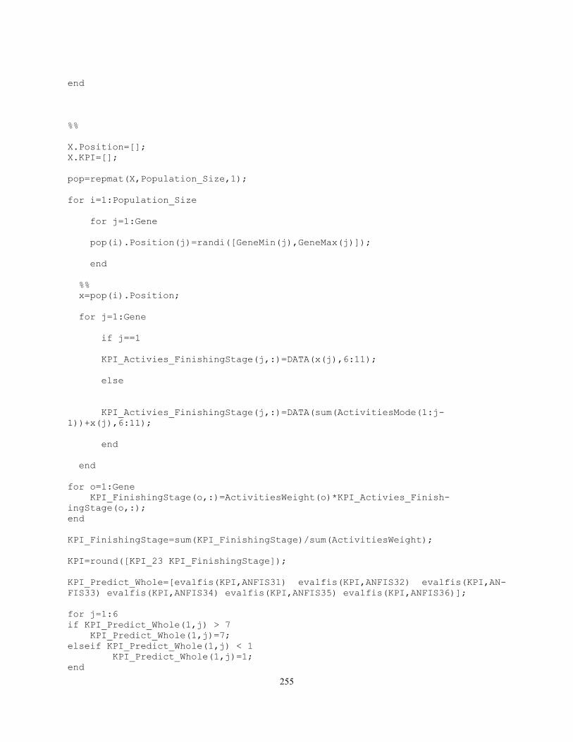
255
end
%%
X.Position=[];
X.KPI=[];
pop=repmat(X,Population_Size,1);
for i=1:Population_Size
for j=1:Gene
pop(i).Position(j)=randi([GeneMin(j),GeneMax(j)]);
end
%%
x=pop(i).Position;
for j=1:Gene
if j==1
KPI_Activies_FinishingStage(j,:)=DATA(x(j),6:11);
else
KPI_Activies_FinishingStage(j,:)=DATA(sum(ActivitiesMode(1:j-
1))+x(j),6:11);
end
end
for o=1:Gene
KPI_FinishingStage(o,:)=ActivitiesWeight(o)*KPI_Activies_Finish-
ingStage(o,:);
end
KPI_FinishingStage=sum(KPI_FinishingStage)/sum(ActivitiesWeight);
KPI=round([KPI_23 KPI_FinishingStage]);
KPI_Predict_Whole=[evalfis(KPI,ANFIS31) evalfis(KPI,ANFIS32) evalfis(KPI,AN-
FIS33) evalfis(KPI,ANFIS34) evalfis(KPI,ANFIS35) evalfis(KPI,ANFIS36)];
for j=1:6
if KPI_Predict_Whole(1,j) > 7
KPI_Predict_Whole(1,j)=7;
elseif KPI_Predict_Whole(1,j) < 1
KPI_Predict_Whole(1,j)=1;
end
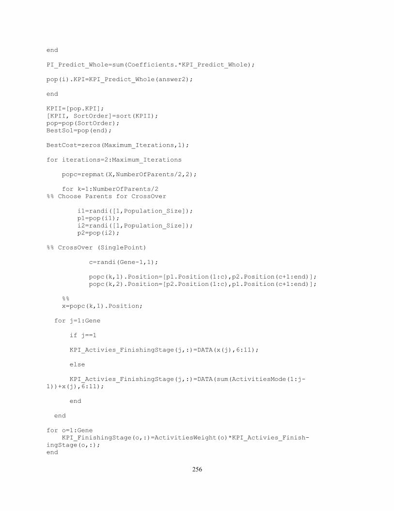
256
end
PI_Predict_Whole=sum(Coefficients.*KPI_Predict_Whole);
pop(i).KPI=KPI_Predict_Whole(answer2);
end
KPII=[pop.KPI];
[KPII, SortOrder]=sort(KPII);
pop=pop(SortOrder);
BestSol=pop(end);
BestCost=zeros(Maximum_Iterations,1);
for iterations=2:Maximum_Iterations
popc=repmat(X,NumberOfParents/2,2);
for k=1:NumberOfParents/2
%% Choose Parents for CrossOver
i1=randi([1,Population_Size]);
p1=pop(i1);
i2=randi([1,Population_Size]);
p2=pop(i2);
%% CrossOver (SinglePoint)
c=randi(Gene-1,1);
popc(k,1).Position=[p1.Position(1:c),p2.Position(c+1:end)];
popc(k,2).Position=[p2.Position(1:c),p1.Position(c+1:end)];
%%
x=popc(k,1).Position;
for j=1:Gene
if j==1
KPI_Activies_FinishingStage(j,:)=DATA(x(j),6:11);
else
KPI_Activies_FinishingStage(j,:)=DATA(sum(ActivitiesMode(1:j-
1))+x(j),6:11);
end
end
for o=1:Gene
KPI_FinishingStage(o,:)=ActivitiesWeight(o)*KPI_Activies_Finish-
ingStage(o,:);
end
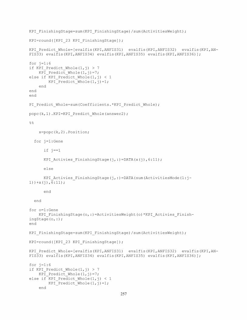
257
KPI_FinishingStage=sum(KPI_FinishingStage)/sum(ActivitiesWeight);
KPI=round([KPI_23 KPI_FinishingStage]);
KPI_Predict_Whole=[evalfis(KPI,ANFIS31) evalfis(KPI,ANFIS32) evalfis(KPI,AN-
FIS33) evalfis(KPI,ANFIS34) evalfis(KPI,ANFIS35) evalfis(KPI,ANFIS36)];
for j=1:6
if KPI_Predict_Whole(1,j) > 7
KPI_Predict_Whole(1,j)=7;
else if KPI_Predict_Whole(1,j) < 1
KPI_Predict_Whole(1,j)=1;
end
end
end
PI_Predict_Whole=sum(Coefficients.*KPI_Predict_Whole);
popc(k,1).KPI=KPI_Predict_Whole(answer2);
%%
x=popc(k,2).Position;
for j=1:Gene
if j==1
KPI_Activies_FinishingStage(j,:)=DATA(x(j),6:11);
else
KPI_Activies_FinishingStage(j,:)=DATA(sum(ActivitiesMode(1:j-
1))+x(j),6:11);
end
end
for o=1:Gene
KPI_FinishingStage(o,:)=ActivitiesWeight(o)*KPI_Activies_Finish-
ingStage(o,:);
end
KPI_FinishingStage=sum(KPI_FinishingStage)/sum(ActivitiesWeight);
KPI=round([KPI_23 KPI_FinishingStage]);
KPI_Predict_Whole=[evalfis(KPI,ANFIS31) evalfis(KPI,ANFIS32) evalfis(KPI,AN-
FIS33) evalfis(KPI,ANFIS34) evalfis(KPI,ANFIS35) evalfis(KPI,ANFIS36)];
for j=1:6
if KPI_Predict_Whole(1,j) > 7
KPI_Predict_Whole(1,j)=7;
else if KPI_Predict_Whole(1,j) < 1
KPI_Predict_Whole(1,j)=1;
end
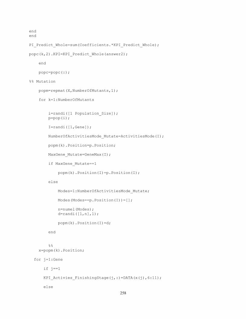
258
end
end
PI_Predict_Whole=sum(Coefficients.*KPI_Predict_Whole);
popc(k,2).KPI=KPI_Predict_Whole(answer2);
end
popc=popc(:);
%% Mutation
popm=repmat(X,NumberOfMutants,1);
for k=1:NumberOfMutants
i=randi([1 Population_Size]);
p=pop(i);
I=randi([1,Gene]);
NumberOfActivitiesMode_Mutate=ActivitiesMode(I);
popm(k).Position=p.Position;
MaxGene_Mutate=GeneMax(I);
if MaxGene_Mutate==1
popm(k).Position(I)=p.Position(I);
else
Modes=1:NumberOfActivitiesMode_Mutate;
Modes(Modes==p.Position(I))=[];
n=numel(Modes);
d=randi([1,n],1);
popm(k).Position(I)=d;
end
%%
x=popm(k).Position;
for j=1:Gene
if j==1
KPI_Activies_FinishingStage(j,:)=DATA(x(j),6:11);
else
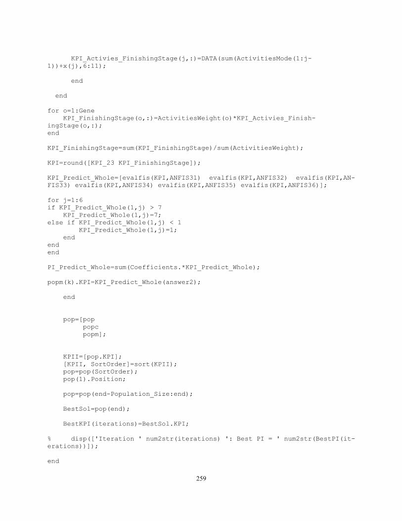
259
KPI_Activies_FinishingStage(j,:)=DATA(sum(ActivitiesMode(1:j-
1))+x(j),6:11);
end
end
for o=1:Gene
KPI_FinishingStage(o,:)=ActivitiesWeight(o)*KPI_Activies_Finish-
ingStage(o,:);
end
KPI_FinishingStage=sum(KPI_FinishingStage)/sum(ActivitiesWeight);
KPI=round([KPI_23 KPI_FinishingStage]);
KPI_Predict_Whole=[evalfis(KPI,ANFIS31) evalfis(KPI,ANFIS32) evalfis(KPI,AN-
FIS33) evalfis(KPI,ANFIS34) evalfis(KPI,ANFIS35) evalfis(KPI,ANFIS36)];
for j=1:6
if KPI_Predict_Whole(1,j) > 7
KPI_Predict_Whole(1,j)=7;
else if KPI_Predict_Whole(1,j) < 1
KPI_Predict_Whole(1,j)=1;
end
end
end
PI_Predict_Whole=sum(Coefficients.*KPI_Predict_Whole);
popm(k).KPI=KPI_Predict_Whole(answer2);
end
pop=[pop
popc
popm];
KPII=[pop.KPI];
[KPII, SortOrder]=sort(KPII);
pop=pop(SortOrder);
pop(1).Position;
pop=pop(end-Population_Size:end);
BestSol=pop(end);
BestKPI(iterations)=BestSol.KPI;
% disp(['Iteration ' num2str(iterations) ': Best PI = ' num2str(BestPI(it-
erations))]);
end
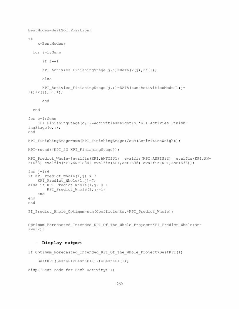
260
BestModes=BestSol.Position;
%%
x=BestModes;
for j=1:Gene
if j==1
KPI_Activies_FinishingStage(j,:)=DATA(x(j),6:11);
else
KPI_Activies_FinishingStage(j,:)=DATA(sum(ActivitiesMode(1:j-
1))+x(j),6:11);
end
end
for o=1:Gene
KPI_FinishingStage(o,:)=ActivitiesWeight(o)*KPI_Activies_Finish-
ingStage(o,:);
end
KPI_FinishingStage=sum(KPI_FinishingStage)/sum(ActivitiesWeight);
KPI=round([KPI_23 KPI_FinishingStage]);
KPI_Predict_Whole=[evalfis(KPI,ANFIS31) evalfis(KPI,ANFIS32) evalfis(KPI,AN-
FIS33) evalfis(KPI,ANFIS34) evalfis(KPI,ANFIS35) evalfis(KPI,ANFIS36)];
for j=1:6
if KPI_Predict_Whole(1,j) > 7
KPI_Predict_Whole(1,j)=7;
else if KPI_Predict_Whole(1,j) < 1
KPI_Predict_Whole(1,j)=1;
end
end
end
PI_Predict_Whole_Optimum=sum(Coefficients.*KPI_Predict_Whole);
Optimum_Forecasted_Intended_KPI_Of_The_Whole_Project=KPI_Predict_Whole(an-
swer2);
- Display output
if Optimum_Forecasted_Intended_KPI_Of_The_Whole_Project>BestKPI(1)
BestKPI(BestKPI<BestKPI(1))=BestKPI(1);
disp('Best Mode for Each Activity:');
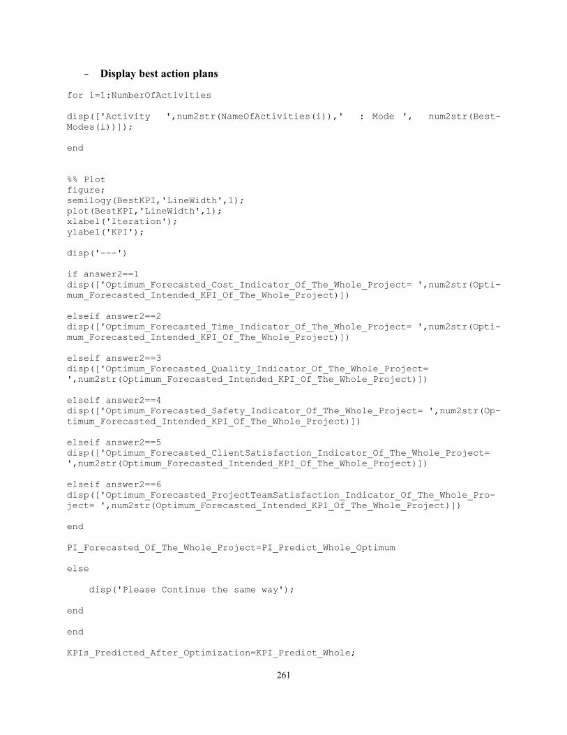
261
- Display best action plans
for i=1:NumberOfActivities
disp(['Activity ',num2str(NameOfActivities(i)),' : Mode ', num2str(Best-
Modes(i))]);
end
%% Plot
figure;
semilogy(BestKPI,'LineWidth',1);
plot(BestKPI,'LineWidth',1);
xlabel('Iteration');
ylabel('KPI');
disp('---')
if answer2==1
disp(['Optimum_Forecasted_Cost_Indicator_Of_The_Whole_Project= ',num2str(Opti-
mum_Forecasted_Intended_KPI_Of_The_Whole_Project)])
elseif answer2==2
disp(['Optimum_Forecasted_Time_Indicator_Of_The_Whole_Project= ',num2str(Opti-
mum_Forecasted_Intended_KPI_Of_The_Whole_Project)])
elseif answer2==3
disp(['Optimum_Forecasted_Quality_Indicator_Of_The_Whole_Project=
',num2str(Optimum_Forecasted_Intended_KPI_Of_The_Whole_Project)])
elseif answer2==4
disp(['Optimum_Forecasted_Safety_Indicator_Of_The_Whole_Project= ',num2str(Op-
timum_Forecasted_Intended_KPI_Of_The_Whole_Project)])
elseif answer2==5
disp(['Optimum_Forecasted_ClientSatisfaction_Indicator_Of_The_Whole_Project=
',num2str(Optimum_Forecasted_Intended_KPI_Of_The_Whole_Project)])
elseif answer2==6
disp(['Optimum_Forecasted_ProjectTeamSatisfaction_Indicator_Of_The_Whole_Pro-
ject= ',num2str(Optimum_Forecasted_Intended_KPI_Of_The_Whole_Project)])
end
PI_Forecasted_Of_The_Whole_Project=PI_Predict_Whole_Optimum
else
disp('Please Continue the same way');
end
end
KPIs_Predicted_After_Optimization=KPI_Predict_Whole;