Performance Analysis of Distributed MAC Protocols for ...
162
Performance Analysis of Distributed MAC Protocols for Wireless Networks by Xinhua Ling A thesis presented to the University of Waterloo in fulfillment of the thesis requirement for the degree of Doctor of Philosophy in Electrical and Computer Engineering Waterloo, Ontario, Canada, 2007 c Xinhua Ling 2007
Transcript of Performance Analysis of Distributed MAC Protocols for ...
Performance Analysis of Distributed MAC
Protocols for Wireless Networks
by
Xinhua Ling
A thesis
presented to the University of Waterloo
in fulfillment of the
thesis requirement for the degree of
Doctor of Philosophy
in
Electrical and Computer Engineering
Waterloo, Ontario, Canada, 2007
c©Xinhua Ling 2007

I hereby declare that I am the sole author of this thesis. This is a true copy of the
thesis, including any required final revisions, as accepted by my examiners.
I understand that my thesis may be made electronically available to the public.
ii

Abstract
How to improve the radio resource utilization and provide better quality-of-service
(QoS) is an everlasting challenge to the designers of wireless networks. As an indis-
pensable element of the solution to the above task, medium access control (MAC)
protocols coordinate the stations and resolve the channel access contentions so that
the scarce radio resources are shared fairly and efficiently among the participating
users. With a given physical layer, a properly designed MAC protocol is the key to
desired system performance, and directly affects the perceived QoS of end users.
Distributed random access protocols are widely used MAC protocols in both
infrastructure-based and infrastructureless wireless networks. To understand the
characteristics of these protocols, there have been enormous efforts on their perfor-
mance study by means of analytical modeling in the literature. However, the existing
approaches are inflexible to adapt to different protocol variants and traffic situations,
due to either many unrealistic assumptions or high complexity.
In this thesis, we propose a simple and scalable generic performance analysis
framework for a family of carrier sense multiple access with collision avoidance (CSMA/
CA) based distributed MAC protocols, regardless of the detailed backoff and channel
access policies, with more realistic and fewer assumptions. It provides a systematic ap-
proach to the performance study and comparison of diverse MAC protocols in various
situations. Developed from the viewpoint of a tagged station, the proposed frame-
work focuses on modeling the backoff and channel access behavior of an individual
station. A set of fixed point equations is obtained based on a novel three-level renewal
process concept, which leads to the fundamental MAC performance metric, average
frame service time. With this result, the important network saturation throughput is
then obtained straightforwardly. The above distinctive approach makes the proposed
analytical framework unified for both saturated and unsaturated stations.
iii

The proposed framework is successfully applied to study and compare the per-
formance of three representative distributed MAC protocols: the legacy p-persistent
CSMA/CA protocol, the IEEE 802.15.4 contention access period MAC protocol, and
the IEEE 802.11 distributed coordination function, in a network with homogeneous
service. It is also extended naturally to study the effects of three prevalent mech-
anisms for prioritized channel access in a network with service differentiation. In
particular, the novel concepts of “virtual backoff event” and “pre-backoff waiting pe-
riods” greatly simplify the analysis of the arbitration interframe space mechanism,
which is the most challenging one among the three, as shown in the previous works
reported in the literature. The comparison with comprehensive simulations shows
that the proposed analytical framework provides accurate performance predictions in
a broad range of stations. The results obtained provide many helpful insights into
how to improve the performance of current protocols and design better new ones.
iv

Acknowledgements
I am extremely grateful to my supervisors, Professor Xuemin (Sherman) Shen and
Professor Jon W. Mark for their continuous guidance, encouragement, support and
patience during my Ph.D. study at the University of Waterloo. I have benefitted
tremendously from their invaluable advice on how to select research topics, define the
problems, work on them, and present the results. Most importantly, I have learned
from them the highly positive mental attitude when facing difficulties, which will help
me greatly in my future career.
I am very grateful to my thesis examining committee members: Professor Jelina
Misic, Professor Fakhri Karray, Professor Sagar Naik and Professor Pin-Han Ho.
They contributed their precious time in reviewing my thesis and providing insightful
comments and suggestions that helped to improve the quality of this thesis.
I would also like to thank Professor Weihua Zhuang. The knowledge of stochastic
processes I learned from her excellent course E&CE 604 is the foundation of the
research work in this thesis.
My deep appreciation goes to Dr. Yu Cheng, Dr. Mehrdad Dianati, Mr. Kuang-
Hao (Stanley) Liu and Ms. Lin X. Cai for their timely encouragement, warm friend-
ship and professional collaborations.
The financial support from Research In Motion and NSERC under strategic
project #STPGP257682, the scholarships and fellowships from the Electrical & Com-
puter Engineering Department and Ontario Ministry of Training, Colleges and Uni-
versities are gratefully acknowledged. Many thanks to the administrative staff: Ms.
Wendy Boles, Ms. Lisa Hendel and Ms. Karen Schooley.
I am greatly indebted to my parents, parents-in-law, siblings and their families for
their love and support. My deepest gratitude goes to my wife, Runhong Deng, who
takes care of our daughter Angela, supports my study, and successfully completes
v

her MMSc program at the University of Waterloo. I thank Angela, who uniquely
contributes to my study and life with her amazing growth and joyful laughter. With-
out their unconditional love, support and understanding, it is impossible for me to
complete my Ph.D. program.
vi

To Runhong and Angela
vii
Contents
1 Introduction 1
1.1 Wireless Communication Networks . . . . . . . . . . . . . . . . . . . 1
1.2 Wireless Medium Access Control Protocols . . . . . . . . . . . . . . . 3
1.3 Performance Modeling Approaches for Distributed MAC Protocols . . 5
1.3.1 The S-G Analysis . . . . . . . . . . . . . . . . . . . . . . . . . 5
1.3.2 The Equilibrium Point Analysis . . . . . . . . . . . . . . . . . 6
1.3.3 The Markov Analysis . . . . . . . . . . . . . . . . . . . . . . . 6
1.4 Motivations and Objectives . . . . . . . . . . . . . . . . . . . . . . . 8
1.5 Main Contributions . . . . . . . . . . . . . . . . . . . . . . . . . . . . 9
1.6 Outline of the Thesis . . . . . . . . . . . . . . . . . . . . . . . . . . . 10
2 System Model 11
2.1 Network Model . . . . . . . . . . . . . . . . . . . . . . . . . . . . . . 11
2.2 Four Representative Distributed MAC Protocols . . . . . . . . . . . . 14
2.2.1 The p-persistent CSMA/CA Protocol . . . . . . . . . . . . . . 14
2.2.2 The IEEE 802.15.4 MAC . . . . . . . . . . . . . . . . . . . . . 15
2.2.3 The IEEE 802.11 Distributed Coordination Function . . . . . 18
2.2.4 The IEEE 802.11e Enhanced Distributed Channel Access Mech-
anisms . . . . . . . . . . . . . . . . . . . . . . . . . . . . . . . 21
viii

3 A Generic Performance Analysis Framework for Distributed MAC
Protocols 24
3.1 Introduction . . . . . . . . . . . . . . . . . . . . . . . . . . . . . . . . 24
3.2 Renewal Process Based Framework . . . . . . . . . . . . . . . . . . . 25
3.2.1 Three-Level Renewal Process . . . . . . . . . . . . . . . . . . 25
3.2.2 MAC Performance Analysis . . . . . . . . . . . . . . . . . . . 27
3.3 Discussion . . . . . . . . . . . . . . . . . . . . . . . . . . . . . . . . . 29
3.3.1 Modeling Unsaturated Stations . . . . . . . . . . . . . . . . . 29
3.3.2 Modeling Networks with Service Differentiation . . . . . . . . 31
3.4 Summary . . . . . . . . . . . . . . . . . . . . . . . . . . . . . . . . . 31
4 Networks with Homogeneous Service 33
4.1 The p-persistent CSMA/CA Protocol . . . . . . . . . . . . . . . . . . 34
4.1.1 Analysis of Saturated Stations . . . . . . . . . . . . . . . . . . 34
4.1.2 Analysis of Unsaturated Stations . . . . . . . . . . . . . . . . 36
4.1.3 Numerical Results . . . . . . . . . . . . . . . . . . . . . . . . 37
4.2 The CAP-MAC in IEEE 802.15.4 . . . . . . . . . . . . . . . . . . . . 43
4.2.1 The Basic Analysis . . . . . . . . . . . . . . . . . . . . . . . . 43
4.2.2 The Single-Sensing Case (One CCA) . . . . . . . . . . . . . . 45
4.2.3 The Double-Sensing Case (Two CCAs) . . . . . . . . . . . . . 49
4.2.4 Analysis of Unsaturated Stations . . . . . . . . . . . . . . . . 52
4.2.5 Numerical Results . . . . . . . . . . . . . . . . . . . . . . . . 53
4.3 The IEEE 802.11 DCF . . . . . . . . . . . . . . . . . . . . . . . . . . 61
4.3.1 Analysis of Saturated Stations . . . . . . . . . . . . . . . . . . 61
4.3.2 Analysis of Unsaturated Stations . . . . . . . . . . . . . . . . 64
4.3.3 With Default Parameters in DCF . . . . . . . . . . . . . . . . 65
ix

4.3.4 Numerical Results . . . . . . . . . . . . . . . . . . . . . . . . 69
4.4 Discussion on the Proper Selection of Fixed Point . . . . . . . . . . . 72
4.5 Maximum Saturation Throughput of the Three Protocols . . . . . . . 73
4.5.1 p-Persistent CSMA/CA . . . . . . . . . . . . . . . . . . . . . 74
4.5.2 CAP-MAC . . . . . . . . . . . . . . . . . . . . . . . . . . . . 75
4.5.3 DCF . . . . . . . . . . . . . . . . . . . . . . . . . . . . . . . . 79
4.5.4 Numerical Results . . . . . . . . . . . . . . . . . . . . . . . . 80
4.5.5 Discussion on the Optimization for Unsaturated Stations . . . 83
4.6 Related Work . . . . . . . . . . . . . . . . . . . . . . . . . . . . . . . 85
4.7 Summary . . . . . . . . . . . . . . . . . . . . . . . . . . . . . . . . . 89
5 Networks with Service Differentiation 91
5.1 Service Differentiation with CWs . . . . . . . . . . . . . . . . . . . . 92
5.1.1 Analysis of Saturated Stations . . . . . . . . . . . . . . . . . . 92
5.1.2 Analysis of Unsaturated Stations . . . . . . . . . . . . . . . . 94
5.1.3 Numerical Results . . . . . . . . . . . . . . . . . . . . . . . . 95
5.2 Service Differentiation with TXOP . . . . . . . . . . . . . . . . . . . 100
5.2.1 Analysis of Saturated Stations . . . . . . . . . . . . . . . . . . 101
5.2.2 Analysis of Unsaturated Stations . . . . . . . . . . . . . . . . 102
5.2.3 Numerical Results . . . . . . . . . . . . . . . . . . . . . . . . 103
5.3 Service Differentiation with AIFS . . . . . . . . . . . . . . . . . . . . 106
5.3.1 Analysis of Saturated Stations . . . . . . . . . . . . . . . . . . 106
5.3.2 Analysis of Unsaturated Stations . . . . . . . . . . . . . . . . 113
5.3.3 Numerical Results . . . . . . . . . . . . . . . . . . . . . . . . 113
5.4 Related Work . . . . . . . . . . . . . . . . . . . . . . . . . . . . . . . 115
5.5 Summary . . . . . . . . . . . . . . . . . . . . . . . . . . . . . . . . . 120
x
6 Conclusions and Future Work 122
6.1 Major Research Contributions . . . . . . . . . . . . . . . . . . . . . . 122
6.2 Future Work . . . . . . . . . . . . . . . . . . . . . . . . . . . . . . . . 125
Abbreviations and Symbols 128
xi

List of Tables
4.1 Some DCF Parameters Used in the Analysis and Simulations . . . . . 69
5.1 Parameters for the 64kbps ITU-T G.711 Voice Codec . . . . . . . . . 105
xii

List of Figures
2.1 IEEE 802.15.4 superframe structure in the beacon-enabled mode . . . 16
2.2 The IEEE 802.11 DCF channel access mechanisms . . . . . . . . . . . 20
2.3 An illustration of prioritized channel access for different station classes 22
3.1 Illustration of the concept of 3-level renewal process . . . . . . . . . . 26
3.2 The level-3 cycle for unsaturated stations . . . . . . . . . . . . . . . . 30
4.1 Saturation throughput of p-persistent CSMA/CA protocol . . . . . . 40
4.2 Average frame service time for saturated stations with p-persistent
CSMA/CA protocol . . . . . . . . . . . . . . . . . . . . . . . . . . . 41
4.3 Average frame service time in unsaturated case of p-persistent CSMA/CA
protocol . . . . . . . . . . . . . . . . . . . . . . . . . . . . . . . . . . 42
4.4 The level-1 renewal cycle for IEEE 802.15.4 MAC . . . . . . . . . . . 44
4.5 Performance of CAP-MAC with saturated stations . . . . . . . . . . 55
4.6 Comparison between the SS and DS cases . . . . . . . . . . . . . . . 57
4.7 Saturation throughput comparison between SS and DS modes . . . . 58
4.8 Average frame service time in the SS case . . . . . . . . . . . . . . . 59
4.9 Average frame service time in unsaturated case . . . . . . . . . . . . 60
4.10 Saturation throughput and average frame service time of DCF in basic
and RTS/CTS modes . . . . . . . . . . . . . . . . . . . . . . . . . . . 71
xiii

4.11 Capacity of DCF in the basic mode . . . . . . . . . . . . . . . . . . . 72
4.12 Saturation throughput comparison between p-persistent CSMA/CA
and CAP-MAC . . . . . . . . . . . . . . . . . . . . . . . . . . . . . . 76
4.13 Maximum network throughput and optimal p of p-persistent CSMA/CA
protocol with saturated stations . . . . . . . . . . . . . . . . . . . . . 81
4.14 Optimal initial backoff window and maximum network throughput of
CAP-MAC SS protocol with saturated stations . . . . . . . . . . . . 82
4.15 Minimum average frame service time and optimal p for p-persistent
CSMA/CA protocol with unsaturated stations . . . . . . . . . . . . . 84
5.1 Effect of CWmin,1 on the average frame service times for saturated
stations . . . . . . . . . . . . . . . . . . . . . . . . . . . . . . . . . . 96
5.2 ζ2/ζ1 vs. CWmin,2/CWmin,1 . . . . . . . . . . . . . . . . . . . . . . . 97
5.3 Effect of CWmax,1 on the average frame service times for saturated
stations . . . . . . . . . . . . . . . . . . . . . . . . . . . . . . . . . . 98
5.4 Average frame service times with changing traffic load . . . . . . . . . 99
5.5 Effect of class 1 payload size for saturated stations . . . . . . . . . . . 104
5.6 Voice capacity with background data traffic . . . . . . . . . . . . . . 105
5.7 Illustration of the backoff segments and pre-backoff waiting periods for
a class 2 station . . . . . . . . . . . . . . . . . . . . . . . . . . . . . 110
5.8 Effects of AIFS for saturated stations . . . . . . . . . . . . . . . . . . 116
5.9 Effects of N for saturated stations . . . . . . . . . . . . . . . . . . . . 117
5.10 Average frame service time with changing traffic load . . . . . . . . . 118
xiv
Chapter 1
Introduction
1.1 Wireless Communication Networks
Driven by the vision of communications from anywhere, anytime, various wireless
networks such as nation- or continent-wide cellular networks, wireless metropolitan
area networks (WMANs) and wireless local area networks (WLANs) have been de-
ployed almost ubiquitously in recent years. Meanwhile, as the Internet has evolved
to a worldwide information transport platform, many wireless networks serve as ac-
cess networks to the Internet. The combination of these two types of networks have
greatly promoted the rapid growth of wireless communications and mobile computing
around the world.
As the most popular wireless network, cellular networks can provide wide area
coverage and seamless roaming. Evolved from the analog technology based first gen-
eration (1G), digital technology based second generation (2G) to the current wideband
code division multiple access (CDMA) technology based third generation (3G), cellu-
lar networks can now provide 144kbps-2Mbps data rate to users in different environ-
ments. The next generation (4G) cellular networks may be based on the orthogonal
1

Introduction 2
frequency division multiplex (OFDM) technology [64], and are expected to provide
high transmission rate of 100 Mbps [35].
The representative WMAN is the emerging worldwide interoperability for mi-
crowave access (WiMAX) network [34]. Based on the IEEE 802.16 series stan-
dards [47], WiMax networks use the orthogonal frequency division multiple access
(OFDMA) and multiple input multiple output (MIMO) technologies [108] and can
support data rates up to 75 Mbps in a 20 MHz channel.
Compared with the above two types of networks, WLANs are much easier and
cheaper1 to set up, and usually cover small hotspot areas such as airports, malls,
offices, hotels and residential homes. Due to its great success in the past years, the
IEEE 802.11 series standards [45] are the de facto standards for present WLANs. The
current main stream IEEE 802.11g standard uses OFDM technology to provide up
to 54 Mbps data rate at the 2.4 GHz band. The next generation WLAN standard,
IEEE 802.11n, is expected to provide data rate as high as 200 Mbps using OFDM
and MIMO [107]. High data rate WLANs are expected to have higher market share
in the next a few years [114].
The above networks with increasingly higher data rates have or will contribute
to meeting the rapid growth of demand for wireless access to the Internet. In the
development of these networks, the common challenge of how to further improve
the resource utilization efficiency and provide better quality-of-service (QoS) attracts
great efforts from both industry and academia. Medium access control (MAC) pro-
tocols play a critical role in determining the performance of these wireless networks,
which directly affects the perceived QoS of end users. In the next section, we give an
overview of the prominent wireless MAC protocols.
1WLANs operate in the unlicensed Industrial, Scientific and Medical (ISM) bands.

Introduction 3
1.2 Wireless Medium Access Control Protocols
A medium access control (MAC) protocol coordinates the nodes in a network and
resolves the contention among their accessing the shared medium (the wireless chan-
nel in wireless networks) so that the scarce system resources are shared fairly and
efficiently [75]. With a given physical layer, a properly designed MAC protocol is the
key to desired system performance such as high throughput and short delay.
Wireless MAC protocols can be classified into three categories [16]: random ac-
cess, guaranteed access and hybrid access protocols. Random access protocols are
distributed contention-based protocols that are quite suitable for networks with sta-
tions carrying bursty traffic. Classic random access protocols include ALOHA [2],
slotted ALOHA [80], and non/p/1-persistent CSMA [55]. To avoid the possible con-
tinuous collisions, random backoff policies (e.g., uniform backoff, geometric backoff,
binary exponential backoff) have been added to the classic protocols2. One resulting
protocol family is the various CSMA/CA protocols widely used in WLANs, WPANs
and WSNs, etc. The main advantage of the random access protocol are that it does
not require a central controller and its relatively simple implementation; while the
main disadvantage is that channel idle periods and frame collisions are inevitable,
which wastes the valuable channel bandwidth. Guaranteed access are contention-free
protocols with which stations access the channel in an orderly manner (via polling
or scheduling), and thus a certain level of QoS can be provided. The main overhead
2Stations in wireless systems are usually operating in half-duplex mode. Due to the fact that
a large fraction of transmitting energy leaks into the receiving path, it is very difficult for a node
to receive data reliably when its transmitter is transmitting unless the transmission and reception
use different frequency bands. As a result, collision detection is almost impossible and carrier sense
multiple access with collision avoidance (CSMA/CA) instead of with collision detection (CSMA/CD)
is usually deployed in wireless systems.

Introduction 4
of guaranteed access protocols incurs when the polled or scheduled station has no
need to use the medium at the moment, which usually occurs to stations with bursty
traffic. A hybrid access protocol normally combines the advantages of the random
access and guaranteed access protocols to achieve flexibility, efficiency and QoS provi-
sioning [16]. With the hybrid protocols, each station sends a request, using a random
access protocol, to the central controller (e.g., the base station in a cellular system or
the access point in a WLAN) indicating the time or bandwidth required for its future
transmissions. After a request is received, usually the admission control scheme (if
exists) decides whether to grant it or not. For the former, the controller allocates
time slots and notifies the requesting stations the start time and duration assigned.
Later transmissions from these stations are then collision-free. Hybrid MAC proto-
cols are normally deployed in infrastructure-based networks to support a variety of
delay-sensitive multimedia applications with satisfactory QoS provisioning.
Due to its flexibility, random access protocols may be used alone in infrastructure-
less wireless networks (e.g., mobile ad hoc networks or ad hoc mode WLANs) or be
used as part of the hybrid protocols in infrastructure-based wireless networks (e.g.,
uplinks of cellular or WiMAX systems). In addition, random access protocols can
easily incorporate some mechanisms to provide prioritized channel access to differ-
ent stations [1], which is indispensable for networks providing service differentiation.
Since the MAC protocol adopted is critical to not only the system performance but
also the perceived QoS of end users in a wireless network, it is important to fully
understand the characteristics of the widely used random access protocols. In this
thesis, we focus mainly on studying the performance of CSMA/CA based distributed
MAC protocols in various wireless networks.

Introduction 5
1.3 Performance Modeling Approaches for Distri-
buted MAC Protocols
Performance evaluation of MAC protocols is usually carried out by simulations/field
measurements or theoretical modeling approach. While simulation/field measure-
ment studies, usually time consuming, may only address particular scenarios under
specific conditions, analytical modeling enables one to gain deeper insight into the
characteristics of the protocol.
The performance of MAC protocols is traditionally analyzed by developing stochas-
tic models, often with various assumptions and approximations. In the literature,
there are mainly three techniques commonly used in this area, as briefly discussed
below. More details of the related work will be given in Chapters 4 and 5.
1.3.1 The S-G Analysis
The so-called “S-G” approach [87], where S is the carried load and G is the offered
load, was widely used in the 1970’s-90’s to analyze the throughput-delay perfor-
mance of both slotted and non-slotted multiple access protocols such as ALOHA and
CSMA [55, 96, 97, 91, 4, 88, 83]. It assumes an infinite number of nodes collectively
generate traffic equivalent to an independent Poisson source with an aggregate mean
packet generating rate of S packets per slot, and the aggregated new transmissions
and retransmissions are approximated as a Poisson process with rate of G packets
per slot. The scenario considered is mainly of theoretical interest in the sense that a
practical system has just a finite number of users, each of which usually has a buffer
size larger than one as assumed in the S-G analysis. In addition, this technique is
usually used only for a homogeneous network.
Introduction 6
1.3.2 The Equilibrium Point Analysis
Equilibrium point analysis (EPA) is a fluid-type approximation analysis usually ap-
plied to systems in steady state [32, 91]. It assumes that the system always works
at its equilibrium point so that the number of users in any working mode is always
fixed, i.e., the expected increase in the number of stations in each mode is zero at
this point. For its analysis, it requires a set of nonlinear equations, the number of
which equals the number of the working modes (e.g., different backoff stages [79, 106]
or the frame queue length in the buffer [90, 17]) in the system. When the number
of working modes increases, e.g., considering both the backoff stages and the queue
lengths, the computing complexity of the EPA approach increases quickly even just
for a homogeneous network, which is similar to that of the Markov analysis discussed
next.
1.3.3 The Markov Analysis
Compared with the previous two techniques, the Markov analysis is the most widely
used one in the performance modeling of MAC protocols. It has been used mainly
from two different perspectives:
• Modeling the system state — The early works in this category (e.g., [54, 95])
usually consider a simple MAC protocol for a homogeneous system in which
the stations have only two states: 1) backlogged, in which a frame is waiting in
the buffer for transmission; and 2) thinking, in which the buffer is empty and a
frame will be generated according to a Bernoulli experiment. Therefore, those
works usually take the number of backlogged stations as the system state to form
a one-dimensional Markov chain, and thus the size of the state space equals the
number of stations. When the MAC protocols become more complicated, multi-
Introduction 7
dimensional Markov chains are introduced. For instance, when some multi-stage
backoff policies are included in the protocol, a multi-dimensional Markov chain
with each dimension representing the number of stations in a corresponding
backoff stage can be developed as in [79]. On the other hand, if the protocol
defines different behavior for different classes of stations, each dimension of
the Markov chain may represent the number of stations in an individual class
(e.g., [109] for integrated voice and data system with packet reservation multiple
access (PRMA) [37]. Furthermore, Markov analysis may also be extended to
consider the buffer status of each station, but only limited to a homogeneous
network with a very small number of stations and small buffer sizes [87].
• Modeling the state of an individual station — This type of usage of the Markov
analysis becomes popular after it appears in the saturation throughput analysis
of the IEEE 802.11 DCF in [5, 6]. In this model, the backoff stage and the
backoff counter value are combined together to form the state space of the two-
dimensional discrete time Markov chain that models the backoff procedure of
an individual station in the WLAN. Numerous variants of this model have been
proposed for the performance study of DCF (e.g., [110, 15, 104, 19, 31]) and
many other protocols such as the IEEE 802.11e EDCA [48, 115, 82, 56], IEEE
802.15.4 [46, 68, 76, 89] and HomePlug [60, 51].
For the Markov analysis, the state transition probabilities of the Markov chain
must be found to solve the model. To determine the state transition probabilities,
usually the traffic is assumed to be Poisson or Bernoulli so that the memoryless
characteristic of the Markov chain is maintained, or the stations are assumed to
be saturated as always having at least one frame waiting for transmission. Even
with such simplifying assumptions, a common issue in all the above models is the
Introduction 8
complexity involved in deciding the transition probability matrix for the single- or
multi-dimensional Markov chain, especially when the number of states is large. The
state space of the Markovian model increases with both the complexity of the protocol
studied and the number of stations in the system, which hinders its usage in systems
with large station population.
1.4 Motivations and Objectives
Performance study of MAC protocols by means of analytical modeling is helpful for
researchers to understand the complex relationships among protocol parameters, find
the bottleneck and improve the protocol performance. All these also shed light to
future protocol design. It is desirable to have a systematic approach of analyzing the
diverse MAC protocols so that their performance can be studied and compared in an
efficient manner. However, the existing performance modeling approaches discussed in
the previous section are inflexible to adapt to different protocol variants, due to either
the many unrealistic assumptions or the high complexity. The main objective of this
thesis is to propose a simple and scalable generic performance analysis framework
for various CSMA/CA based distributed MAC protocols regardless of the detailed
backoff and channel access policies, with more realistic and fewer assumptions, and
provide accurate performance predictions. In particular, the objectives of this thesis
are to
• extract the common essence of various CSMA/CA based distributed MAC pro-
tocols;
• propose a general framework to reflect the common essence of these protocols;

Introduction 9
• provide an analytical approach for performance modeling of both saturated and
unsaturated stations, with general arrival traffic distributions;
• apply the proposed framework to study the performance of representative distri-
buted MAC protocols in networks with homogeneous service or service differen-
tiation, in terms of average frame service time and network saturation through-
put;
1.5 Main Contributions
The main contributions of this thesis are listed as follows:
• Proposal of a three-level renewal process method to model the backoff and chan-
nel access behavior of a tagged station in a wireless network with CSMA/CA
based MAC protocols;
• Development of a generic analysis framework based on the above method for
the performance study of such MAC protocols; the computational complexity
of this framework does not scale up with the complexity of the backoff and
channel access policies as in other models (e.g., Markov analysis based models
in Section 1.3);
• Proposal of a performance modeling approach for unsaturated stations oper-
ating in practical networks; the approach also naturally covers the saturated
stations as a special case. In addition, it is applicable to station traffic with
general frame arrival process. On the contrary, other existing approaches mainly
focus on saturated stations that rarely work in reality, and the few reported ex-
tensions to those approaches can only handle limited traffic models.
Introduction 10
• Performance analysis and comparison of three representative distributed MAC
protocols; possible improvements are suggested; the intrinsic relationship among
the protocols is also revealed;
• Insights of the different effects of popular service differentiation mechanisms in
networks supporting multi-service or with multiple classes of stations; especially,
within one framework, different effects of the same mechanism in different traffic
situations are revealed for the first time in the open literature. The insights
provided by this work will help wireless network designers and operators to select
proper service differentiation mechanism(s) for their specific requirements.
1.6 Outline of the Thesis
The remainder of this thesis is organized as follows. Chapter 2 describes the sys-
tem model, including the wireless networks under consideration and the distributed
MAC protocols to be studied. The generic analytical framework for CSMA/CA based
distributed MAC protocols is presented in Chapter 3. In Chapter 4, we analyze the
performance of three representative distributed MAC protocols in networks with ho-
mogeneous service, demonstrating the applications of the proposed framework. Three
commonly used service differentiation mechanisms in wireless LANs are analyzed in
Chapter 5. Finally, concluding remarks and discussion on future work are given in
Chapter 6. The content of this thesis is disseminated in papers [131]–[137].

Chapter 2
System Model
In this chapter, we first present the basic network model that will be used in Chap-
ters 3 and 4, followed by the extended network model that will be studied in Chapter 5.
Four representative distributed MAC protocols (three for homogeneous service and
one for heterogeneous service) are introduced in the Section 2.2.
2.1 Network Model
A basic network is considered in Chapter 3 for the development of the generic perfor-
mance model and in Chapter 4 for the analysis of networks with homogeneous service.
It is a single-hop wireless network consisting of N functionally identical stations and
an optional receiving-only central receiver1. Specifically, all the stations are within
the transmission range of one another so there are no hidden terminals in the network.
The time axis is slotted, and all the stations are synchronized so that all stations start
their transmissions only at the beginning of a slot. In addition, all the stations can
1This optional central receiver can be the base station in a cellular network (note only uplink is
considered), or a data sink in a sensor network, etc.
11

System Model 12
correctly sense the channel status. Ideal wireless channel without transmission error
is assumed so that all transmitted frames may be lost only due to collisions caused
by simultaneous transmissions from multiple stations. All MAC frames are assumed
to have the same fixed length, which is a widely adopted assumption in MAC proto-
col analysis [4], and can be easily achieved in practice by commonly used link layer
functions, such as fragmentation or concatenation of the upper layer packets. A short
acknowledgment (ACK) frame is transmitted by the receiver immediately after every
successful MAC frame transmissions, and a negative ACK (NACK) frame is trans-
mitted in respond to a collision. Alternatively, the sending stations will determine
that there is a collision if the ACK frame is not received within a timeout period,
in which no station other than the receiver is allowed to transmit. In this case, the
timeout period can be deemed as if it is occupied by a virtual negative ACK (NACK)
frame transmitted by the central receiver. The aggregate transmission time of the
MAC frame and the associated ACK or NACK is L slots, and no new transmission
from any station will start during this period.
The basic network model described above is extended to a multi-service network
in Chapter 5 when service differentiation mechanisms are studied. The multi-service
network consists of S classes of stations, with Ns stations in each class. MAC frame
lengths or the physical layer data rates used by each class may be different. For
stations in the same class, the incoming traffic is the same and they receive the
same type of service from the network. The optional central receiver in the basic
network model can be naturally included in the extended network model, say, as a
station of its own class. Thus, the extended network model can represent either an
infrastructure-based or an infrastructureless wireless network, and can be used to
study networks with a broad range of traffic situations: peer-to-peer traffic only as
in an ad hoc network, all uplink traffic over a wireless access channel in a cellular

System Model 13
or WiMax network, or either symmetric or asymmetric to-and-from AP traffic in a
WLAN [11].
In this thesis, two important performance metrics of MAC protocols are of our
primary interest: the average frame service time of an individual station and the
network throughput. The former is the most important metric in evaluating the
perceived QoS of each station, since it directly determines the service rate for the
MAC frames of the station. The latter is obtained as the aggregation of the per station
throughput, which can be derived easily if the average frame service time is given. In
particular, for the network throughput, we concentrate mainly on the saturation case
in which every station always has at least one frame in the MAC buffer waiting for
transmission. The throughput in this case, saturation throughput, is a fundamental
performance figure defined as the limit reached by the system throughput as the
offered load increases, and represents the maximum load that the system can carry
in stable conditions [6]. On the contrary, the network throughput is trivially given by
the total incoming traffic load in the unsaturation case where none of the stations in
the network is saturated. The average frame service time is always studied in both
saturation and unsaturation cases.
All the MAC protocols studied in this article belong to the CSMA/CA family. In
the sequel, for ease of presentation, a successful channel sensing refers to the event
that a station senses the channel and the channel is idle. In contrast, a failed channel
sensing or channel sensing failure refers to the event that a station senses the channel
which is busy due to transmission(s) from other station(s).

System Model 14
2.2 Four Representative Distributed MAC Proto-
cols
In this thesis, four representative distributed MAC protocols that are widely used in
current wireless networks will be studied, and they are briefly reviewed one by one in
this section.
2.2.1 The p-persistent CSMA/CA Protocol
As a simple but highly efficient multiple access protocol, the slotted p-persistent
CSMA/CA protocol was first proposed in [55]. Since then it has been widely used
and its application can still be found nowadays in various networks such as mobile
ad hoc network (MANET) [50], vehicular networks [98, 120] and factory control net-
works [69].
In the slotted p-persistent CSMA/CA protocol, a station will sense the channel
when it has a frame for transmission. If the channel is idle, the station transmits the
frame with probability p. With probability 1− p, the station will defer its decision of
frame transmission by one slot. If the channel is still idle in the next slot, the station
will repeat the above procedure. When the channel is sensed busy, the station waits
until the channel becomes idle again and then operates as above. This probabilistic
channel access rule can be deemed as that the station follows a geometric backoff pol-
icy, and the backoff procedure stops when there is a transmission from other stations
and restarts itself after the transmissions ends. From this perspective, this protocol
is an exact fit for the proposed analytical model (presented in Chapter 3), and it will
be used as a basic example to illustrate the details of the model in Section 4.1.
System Model 15
2.2.2 The IEEE 802.15.4 MAC
The fast growth of public interest in wireless sensor networks and wireless personal
area networks (WPAN) in recent years has led to the standardization of the IEEE
802.15.4-2003 [46], which contains a protocol stack targeting at low-power low-rate
wireless networks. The standard has been quickly accepted by industry, and many
products have appeared in the market since its ratification. In this subsection, we
briefly review the MAC protocol specified in the IEEE 802.15.4-2003 standard. More
details of the protocol, such as specific parameter settings or physical layer related
information, can be found in [46, 127].
The MAC layer in the IEEE 802.15.4 standard specifies two operating modes: an
ad hoc non-beacon-enabled mode and a beacon-enabled mode. In the ad hoc mode,
nodes in the network use a non-slotted CSMA with collision avoidance (CSMA/CA)
mechanism to contend for channel access. If the channel is sensed to be idle, the trans-
mission of a frame will begin immediately; otherwise the node will backoff and try to
access the channel in a future slot. This mechanism has been extensively studied in
the literature and its performance is well understood [55, 4]. In the beacon-enabled
mode, a personal area network (PAN) coordinator transmits a beacon periodically to
form the so-called “superframe” time structure, as shown in Figure 2.1. A superframe
consists of a beacon that enables the beacon-enabled mode, contention access period
(CAP), contention free period (CFP), and an optional inactive portion in which all
the nodes may enter a sleep mode to reduce power consumption. The CAP and CFP
together form the active portion of the superframe, during which all communication
among the nodes should take place. In the CFP, the network coordinator alone con-
trols entirely the contention-free channel access by assigning guaranteed time slots
(GTS) to those nodes with their GTS requests granted. The assignment of the GTS
to those nodes is determined by the scheduling scheme adopted by the network coordi-

System Model 16
Beacon Beacon
inactive portion
Superframe Durataion
Beacon Interval
Contention Access Period Contention Free Period
...... GTS GTS
Figure 2.1: IEEE 802.15.4 superframe structure in the beacon-enabled mode
nator, which is open in the standard. Therefore, depending on the specific scheduling
scheme used, the performance analysis of CFP is actually the same as that of the
well-studied centralized scheduling schemes in cellular systems (e.g., [52, 119]).
In the CAP, a non-persistent slotted CSMA/CA with binary exponential backoff
multiple access protocol is defined in the standard. Three variables need to be main-
tained for each frame before it is successfully transmitted. They are respectively the
number of random backoff stages experienced (NB), the current backoff exponent
(BE), and the contention window (CW )2. According to this protocol, a node with
a frame waiting for transmission at the MAC buffer is required to backoff a random
number of slots first, with CW set at a value of two. At the end of this backoff stage,
the node will do the first channel clear assessment (CCA). If the channel is sensed
idle, CW is decremented by one and the node will do the second CCA in the next
slot. Only when both CCAs indicate an idle channel (thus CW reaches zero), will the
node start the transmission in the next slot; otherwise, it will enter the next backoff
2The term contention window is the number of slots that the channel has to be sensed idle by a
node before its transmission of a frame, which is completely different from the contention window
defined in the IEEE 802.11 DCF.
System Model 17
stage and reset CW to two.
The number of backoff slots in stage NB, 0 ≤ NB ≤ NBmax, is drawn from a
uniform distribution over [0, 2BENB − 1], where BE0 = macMinBE is the initial and
minimum backoff exponent for each frame. BENB+1 = BENB + 1 is upper-bounded
by aMaxBE which is the default maximum value of backoff exponent, and NBmax is
the maximum number of backoff stages allowed for a frame. If all the NBmax backoff
stages end up with a busy channel indicated by the associated CCAs, a Channel
Access Failure event will be reported to the upper layer; the node may then start
the above procedure again for the next frame. The standard specifies the following
default parameter values: macMinBE = 3, aMaxBE = 5 and NBmax = 5. Their
impact on the protocol performance will be discussed in Section 4.2.5. During the
backoff procedure, if the node succeeds in accessing the channel, it will reset the three
parameters NB,BE and CW to the default values for initial transmission of the next
frame.
In this study, we focus on the contention access period only to illustrate the
protocol performance by the proposed analytical model, i.e., the inactive portion
and the contention free period in the active portion will not be considered in the
superframe time structure. With this protocol, termed CAP-MAC in the sequel,
a node will always contend for channel access according to the protocol for CAP,
whenever it has a frame to transmit. Therefore, the superframe contains equal-
size time slots with fixed length, which is normalized to unit time in the sequel for
presentation simplicity. In fact, since the contention access related activities such
as backoff counter decrement occurs only in the CAPs and freeze in the CFPs and
inactive portion of the superframes, the impact of these two periods on the MAC
performance can be taken into our proposed model as having a constant time cost
(equal to the aggregate length of the CFP and the inactive portion of a superframe)

System Model 18
associated to every A slots, where A is the length of each CAP in units of slots. A
similar approach is used in [76], but for generating low duty cycle constant rate traffic
as a special case of unsaturated nodes.
2.2.3 The IEEE 802.11 Distributed Coordination Function
The recent popularity of WLAN is mainly due to the simple and robust MAC proto-
col specified in the IEEE 802.11 standard, which defines two modes: the mandatory
distributed coordination function (DCF) and the optional point coordination func-
tion (PCF). Although the PCF is designed for real-time traffic [23, 101], it is not
widely deployed due to its inefficient polling schemes, limited QoS provisioning, and
implementation complexity [11]. In practice, most of the WLANs deploy DCF as the
MAC protocol. Therefore, we will focus on the DCF only in the following.
In the standard, DCF specifies the channel access method as follows. Every station
adopts the CSMA/CA principle. When a station has a frame at the MAC sublayer
buffer, it will first sense the channel. If the channel is busy, it will backoff with a
randomly chosen number BOslot of time slots, where BOslot is uniformly distributed
over [0, CWr), and CWr is the contention window for retransmission stage r. After
the channel becomes idle for a duration of DCF-interframe-space (DIFS), the backoff
counter counts down for each time slot when the channel is idle. Different from the
CAP-MAC described previously, in DCF the backoff counter (BC) freezes when the
channel is busy due to a successful transmission or collisions from other stations,
and it resumes after the channel turns idle again. When the BC reaches zero, the
station will transmit immediately. A station resets its CW to the minimum value
CWmin = 32 after each successful transmission. If two or more stations transmit at
the same time slot, a collision occurs and all involved stations will double their CWs,
which is upper-bounded by CWmax = 1024 in the standard, and backoff again. The

System Model 19
frame will be discarded if retransmission fails after a pre-defined retry limit, which
depends on the frame length.
Usually a sender transmits data frames directly when its backoff counter reaches
zero, and the receiver will reply with an explicit acknowledgment (ACK) after a
duration of short interframe space (SIFS) if the data frame is successfully decoded
(see Figure 2.2(a)). This is called the basic access mode. To improve the efficiency of
transmitting long frames, the standard also defines an optional request-to-send/clear-
to-send (RTS/CTS) access mode. When the frame length is larger than a threshold,
the source station will send out an RTS frame to its intended destination station,
which will reply with a CTS frame if the RTS is correctly decoded. After that, the
source will transmit the data frame and wait for the corresponding ACK frame from
the destination. There are periods of short-interframe-space (SIFS) in between the
RTS, CTS, data and ACK frames (see Figure 2.2(b)). As DIFS is longer than SIFS,
an ongoing transmission sequence as described above will not be interrupted by a new
transmission. In case of a collision, the source stations in the basic mode will wait
for duration of (ACK timeout + DIFS) before resuming their backoff procedure;
in the RTS/CTS mode, the source stations wait a duration with the same length
because the CTS frame has the same length as the ACK frame. In both the basic
and the RTS/CTS access modes, neighboring stations that detect a collision will
defer a duration of extended-interframe-space (EIFS) before resuming their backoff
procedure. The EIFS equals the summation of SIFS, DIFS and the transmission time
of the CTS or ACK frame with the lowest mandatory transmission rate so that all
the stations will resume their backoff procedure at the same time. The CTS/ACK
timeout and EIFS mechanism serves as an implicit NACK in DCF. The above timing
relationship is illustrated in Figure 2.2(c).
In addition to the above physical carrier sense (PCS) mechanism, a virtual carrier

System Model 20
destination
source
neighbor
DIFS
DIFSDIFS
NAV
DIFS
SIFS
Data
ACK
DIFS DIFS
...
...
...
(a)
destination
source
neighbor
3 slots
DIFS
NAV
DIFS DIFS
DIFS
SIFS
RTS
CTS
DIFS
Data
ACK
...
...
...
DIFS
(b)
DIFS
DIFS
DIFS
source 1
source 2
neighbor
Data
Data
EIFS
...
...
...
collisiondetected
ACK_timeout
+ DIFS
ACK_timeout
+ DIFS
(c)
Figure 2.2: The IEEE 802.11 DCF channel access mechanisms

System Model 21
sense (VCS) mechanism is also introduced in the DCF. It is implemented by means of
the so-called network allocation vector (NAV), which is maintained by every station
that is not currently involved in any transmission or reception of frames. Each such
station may set the NAV according to the information in the Duration/ID field of the
RTS or Data frame. In the RTS/CTS mode, stations may reset its NAV (to zero) if a
transmission does not start during a period with a duration of (2 SIFS+CTS+2 Slot)
after the NAV is set according to the duration value of the RTS frame3. Before the
NAV expires, the station may stop the physical carrier sensing activity to save energy.
2.2.4 The IEEE 802.11e Enhanced Distributed Channel Ac-
cess Mechanisms
In the widely deployed IEEE 802.11 based WLANs, DCF is the dominant MAC proto-
col, which guarantees an equal long term channel access probability to all stations [41].
When heterogeneous applications coexist in a WLAN, the DCF MAC is inefficient in
protecting Quality-of-Service (QoS)-critical applications (e.g., real-time voice sessions
or teleconferences) from the QoS-resilient applications (e.g., emails). Aiming to en-
hance the QoS provisioning demanded by multimedia services in WLANs, the IEEE
802.11e amendment [48] to the legacy IEEE 802.11 standard was released recently. In
this standard, the newly defined enhanced distributed channel access (EDCA) sup-
ports service differentiation mainly by distributed prioritized channel access among
different access categories (ACs) with three AC-dependent parameters: contention
window (CW), transmission opportunity (TXOP) and arbitration interframe space
(AIFS). The details of their usage are given below and their service differentiation
3This does not occur in the single-hop network studied in this work because all the neighboring
stations either correctly set the NAV and the source station will surely transmit within the specified
duration, or the NAV is not set due to a collision.

System Model 22
���������������
���������������
Z3Z2
SIFS
Z1
AIFS1
AIFS2Z4
...time
AIFS3AIFS4
channel busy periodAIFSN1*slot
��������������������
��������������������
Figure 2.3: An illustration of prioritized channel access for different station classes
effects are analyzed in Chapter 5.
In the EDCA, user traffic is first classified into multiple ACs, such as voice, video,
best-effort and background. Each station regulates its frame transmission using the
contention parameters associated with each AC. When a station has a frame at the
MAC sublayer buffer, it will first sense the channel. If the channel is busy, it performs
the backoff procedure by first setting the backoff counter to an integer sampled from
the minimum CW size. Therefore the first differentiation mechanism is to assign
higher priority ACs with a smaller value of minimum CW size such that higher priority
ACs statistically spend less time on backoff. After the channel becomes idle for the
AC-dependent AIFS, the station can count down the backoff counter at the beginning
of each idle slot and also the first slot of a channel busy period. Since the higher
priority ACs are assigned with smaller value AIFS, they obtain higher chances to
access the channel than low priority ACs. Fig. 2.3 shows an example of four ACs,
where AC1 has the highest priority. To illustrate the effect of different AIFS lengths,
the time between two busy periods, except AIFS1, is divided into four contention
zones, Zi, i = 1, 2, 3, 4. In Z1, only AC1 stations are allowed to contend for channel
access, while in Z2 the contentions are between AC1 and AC2, i.e., contentions in
Zi involve ACj, j ≤ i. Consequently, each AC encounters different contentions in

System Model 23
its allowable contention zones. After one station succeeds in contending for channel
access, it can transmit for a duration up to the TXOP. Different TXOP durations can
be assigned to different ACs to further differentiate the service. The three mechanisms
may be used individually or be combined together.

Chapter 3
A Generic Performance Analysis
Framework for Distributed MAC
Protocols
3.1 Introduction
A simple yet accurate analytical model is proposed in this chapter to analyze the
performance of a family of carrier sense multiple access with collision avoidance
(CSMA/CA) based MAC protocols commonly used in wireless networks. We model
the behavior of an individual station instead of modeling the channel. The proposed
model is based on a novel concept of three-level renewal process, the key parameter
of which can be solved by the fixed point technique. The new modeling approach
significantly simplifies the mathematical analysis, where the important performance
metrics of MAC throughput (of individual station or the whole network) and the
average frame service time can be directly obtained. The proposed model is a gen-
24

A Generic Analytical Framework 25
eral framework which is applicable to CSMA/CA based MAC protocols with various
backoff procedures and channel access policies.
In the remainder of this chapter, we first present the three-level renewal process
which is the core of the analytical framework. Following that, the MAC performance
analysis based on it is given. Finally, we present two extensions of the basic frame-
work.
3.2 Renewal Process Based Framework
In a steady state network with a CSMA/CA based MAC protocol as described in
Chapter 2, a randomly tagged station contends for the channel access following the
same rule for each frame, i.e., it uses the same initial parameters pertaining to the
backoff, transmitting and possible retransmitting processes for each frame. Therefore,
the channel access process of an individual station is regenerative with respect to
the time instants of the completion of its each successful frame transmission. The
period between two consecutive successful frame transmissions from the same station
thus forms a renewal cycle in a renewal process [70], which directly relates to some
important MAC performance metrics such as MAC throughput and average frame
service time. This key observation inspires the derivation of the basic analytical model
presented below.
3.2.1 Three-Level Renewal Process
For many CSMA/CA based MAC protocols, a hierarchical three-level renewal process,
as illustrated in Fig. 3.1, can model precisely the behavior of a tagged station. A
common characteristic of these protocols is that a certain form of backoff procedure
is required before a station can access the channel, and the backoff procedure may be

A Generic Analytical Framework 26
����������������
����������������
����������������
������������
������������
����������������
����
����
����������������
����������������
����������������
����������������
. . .. . . . . . . . .. . .. . . time. . .level-3 Z ZZY1 Y2Y1 ollision
time. . .of the tagged stationsu essful transmission. . .Z . . .Y2
the tagged stationtransmission ofother stationstransmission oflevel-2 Y1 X1 X2X2 X1X1 . . .. . .. . . timelevel-1Figure 3.1: Illustration of the concept of 3-level renewal process
interrupted usually by transmissions from other stations and resume after the channel
becomes idle again. The time instants that the backoff procedure resumes (or restarts
itself) can naturally be viewed as basic renewal points. Over a larger time scale, the
end of each transmission from the tagged station is a higher level of renewal point
of the frame service process. If the time scale is even larger, the renewal points can
also be set at the end of each successful transmission from the tagged station, which
delimit the important highest level renewal cycle as identified earlier.
In Figure 3.1, a level-1 renewal cycle X is defined as the period between the end
of a channel busy event to the end of the next one. There may be a number of idle
slots in which no station transmits between two consecutive channel busy events.

A Generic Analytical Framework 27
From the viewpoint of the tagged station, a level-1 cycle is of type X1 if the busy
channel is caused by transmission from other stations, and it will be of type X2 if
its own transmission causes the channel busy. Notice that the transmission in an X2
level-1 cycle may be a successful transmission or a collision due to the simultaneous
transmissions from other stations.
A level-2 renewal cycle Y is from the end of an X2 cycle to the end of the next X2
cycle. As shown in Fig. 3.1, there can be U (U ≥ 0) X1-cycles before the X2-cycle.
Depending on the result of transmission in the X2-cycle included, a level-2 cycle can
be either of type Y1, in which the transmission results in a collision, or of type Y2, in
which the transmission succeeds.
Finally, a level-3 renewal cycle Z is from the end of a Y2 level-2 cycle to the end
of the next Y2 cycle. Similarly, there can be V, V ≥ 0, Y1 cycles before the Y2 cycle.
Therefore, the successful transmission of a frame in the Z cycle can be viewed as the
reward for the level-3 renewal cycle. The throughput of the tagged station can thus
be obtained as the average reward in a Z cycle.
3.2.2 MAC Performance Analysis
As an important MAC performance metric, the average frame service time (or access
delay) ζ, is defined as the average duration from the instant that a frame becomes
the head-of-line at the MAC buffer to the end of its successful transmission. As can
be seen, ζ is exactly the average length of the level-3 renewal cycle in the proposed
analytical model. The normalized throughput obtained by an individual station, per
station MAC throughput, is the ratio of the transmission time of the MAC frame
over ζ, and the saturation throughput of the network is thus simply the aggregation
of the per station throughput.
To obtain the average length of the level-3 cycle, we need to find out the character-

A Generic Analytical Framework 28
istics of the random variables that determine the structure of the whole hierarchical
renewal process. Depending on the specific channel access policies, the basic fixed
point equations extracted from the analysis of level-1 cycles may be slightly different
for different MAC protocols. After the average length of a level-1 cycle E[X] has
been obtained, however, the analysis of the other two levels is shared by different
protocols, which is one of the advantages of the proposed framework.
As shown in Figure 3.1, a level-2 cycle contains a number U of type X1 cycles
and an ending X2 cycle, where U follows a geometric distribution with parameter
Ptx, which is the probability that a level-1 cycle is of type X2. Therefore, the average
length of a level-2 cycle is
E[Y ] =E[X]
Ptx
. (3.1)
Similar to the case in a Y cycle, the number of level-2 cycles contained in a level-3 cycle
also follows a geometric distribution, but with parameter Psuc, which is the probability
that a transmission from the tagged station is successful. Thus, the average length
of a level-3 cycle is
E[Z] =E[Y ]
Psuc
. (3.2)
Notice that E[Z] equals the average frame service time ζ. Therefore, in the
remainder of this dissertation, E[Z] and ζ will be used interchangeably. Since there is
only one successful MAC frame transmission from the tagged station during a level-3
cycle, the normalized per station throughput is directly given by
ηs =L
E[Z], (3.3)
and the aggregated throughput in a homogeneous network is thus
η = Nηs. (3.4)
In the above analysis, the detailed expressions of Ptx and Psuc depend on the
specific backoff procedure and channel access policy defined in the protocol being

A Generic Analytical Framework 29
studied. Since there is no assumption on the backoff procedure, the proposed analyt-
ical framework is applicable to protocols with various backoff procedures as long as
the procedure restarts itself for each MAC frame.
3.3 Discussion
To simplify the presentation of the development of the above framework, we have
implicitly assumed that the network is composed of saturated stations with only one
type of service. In what follows, we discuss two extensions of the framework with this
assumption relaxed.
3.3.1 Modeling Unsaturated Stations
The above analysis is directly applicable for a network with saturated stations. The
throughput in this case, saturation throughput, is a fundamental performance figure
defined as the limit reached by the system throughput as the offered load increases,
and represents the maximum load that the system can carry in stable conditions [6].
It is of theoretical importance to obtain this MAC performance metric. In practice, a
network with saturated stations corresponds to the case when some delay-insensitive
data applications (such as bulk file transfer through FTP) running on the stations.
With multimedia applications that usually generate bursty traffic, a station may
work in the unsaturated situation in which the MAC buffer may be empty from time
to time. The proposed analytical framework can also be applied to the analysis of
unsaturated stations. In this case, a station will contend to access the channel only
when it has a frame in the buffer waiting for transmission, which occurs with the
probability of having a non-empty buffer. For a station usually having a MAC buffer
that can accommodate tens of frames (which is in effect almost a lossless queueing

A Generic Analytical Framework 30level-3 time. . .. . . . . . . . .Z PSIZPSI 1/� PSIZ 1/�PSI: possible station idle period of the tagged stationsu essful transmissionframe arrivalFigure 3.2: The level-3 cycle for unsaturated stations
system in practice), this probability can be satisfactorily approximated by the ratio
of the average frame service time ζ ′ over a given average frame inter-arrival time 1/λ.
Since the proposed framework is developed from the viewpoint of a busy station,
i.e., it does have a frame in service, ζ ′ can be obtained from the above analysis for
saturated stations with just slight changes reflecting the effects of the aforementioned
probability to the contention behavior of other stations. The details of this extension
can be found in the application instances in Chapter 4.
More specifically, the level-3 cycle for an unsaturated station is slightly different
from the one for a saturated station. As shown in Figure 3.2, the level-3 cycle Z is
changed to the period between the instant of a frame arrival to the one when it is
successfully transmitted. Between two Z cycles, there exists a possible station idle
period (PSI) if the MAC buffer becomes empty after the current frame is transmitted.
The PSI can be of length zero, e.g., when at least one more frame is waiting in the
buffer. Since the tagged station is always busy in a Z cycle, the same structure of
the lower two level renewal cycles still applies to the Z cycles as in the basic model
in Figure 3.1.

A Generic Analytical Framework 31
3.3.2 Modeling Networks with Service Differentiation
The analysis and discussion up to this point are for networks with homogeneous
services in which all the stations carry the same type of traffic and follow the same
backoff and channel access policy with same relevant parameters. In practice, wireless
networks are usually designed and operated to provide heterogeneous services to users.
In addition, service differentiation is either a required or desired feature. In such
networks, stations may carry different types of traffic, with backoff and channel access
policies using different parameters determined by their service requirements.
The proposed analytical framework can be readily extended to the analysis of
networks with service differentiation. We may select one tagged station from each
service class and analyze them respectively according to the proposed framework.
This is because the framework is developed from the viewpoint of any tagged station,
and the effect of all the other stations are effectively reflected by the success or
failure of the frames transmitted and the channel status seen by the tagged station.
As explained earlier, usually a set of fixed point equations can be obtained for one
tagged station. For K classes of stations, we may obtain K sets of equations which
are interconnected among one another. These equations can be solved numerically
to obtain the key parameters for further derivation of the desired MAC performance
metrics. Several types of service differential mechanisms commonly used in current
wireless networks are studied in Chapter 5.
3.4 Summary
We have proposed a simple yet accurate (as will be shown in later chapters) analytical
framework for CSMA/CA based MAC protocols. By proposing a novel hierarchical
three-level renewal process mechanism, we can describe and analyze the protocols in a

A Generic Analytical Framework 32
straightforward manner. Two important MAC protocol performance metrics, the per
station throughput and the average frame service time, are obtained immediately, due
to the direct relationship between the level-3 renewal cycle and the frame service time.
We have also discussed the extension of this framework to the analysis of networks
with unsaturated stations and/or with service differentiation. The only assumption
made in developing the proposed analytical framework is that a station restarts its
backoff procedure upon serving a new MAC frame, regardless of the detailed param-
eter changing mechanisms of the backoff procedures. Therefore, the framework has
a wide applicability to a family of CSMA/CA based MAC protocols. In the next
chapter, application instances are given for networks with homogeneous service to
show the usage details of the framework.

Chapter 4
Networks with Homogeneous
Service
For CSMA/CA based protocols, the hierarchical three-level renewal process based
analytical framework proposed in Chapter 3 makes the performance analysis easy to
follow. The representative protocol is the legacy slotted p-persistent CSMA/CA [55].
Other good examples include the MAC protocol for the contention access periods
of the IEEE 802.15.4 standard [46], and the de facto standard MAC protocol for
WLANs, IEEE 802.11 distributed coordination function (DCF).
In the remainder of this chapter, we first study the legacy slotted p-persistent
CSMA/CA protocol, followed by the analysis of the IEEE 802.15.4 MAC and the
IEEE 802.11 DCF, respectively. We then compare the performance of the three
protocols with same input traffic in Section 4.5. In each of the first three sections,
the basic analysis for saturated stations is given first, followed by the analysis for
unsaturated stations and some numerical results for performance evaluation.
For presentation simplicity, we will use the same notations for the key variables
such as E[X], E[Y ], E[Z], Ptx, and Psuc in the analysis of the different protocols when
33

Networks with Homogeneous Service 34
there is no confusion from the context. Self-explanatory subscripts are applied to the
variables in Section 4.5 to avoid ambiguity.
4.1 The p-persistent CSMA/CA Protocol
According to the protocol description in Section 2.2.2, the probabilistic channel access
rule of the p-persistent CSMA/CA protocol can be deemed as that the station adopts
a geometric backoff policy. This backoff procedure stops when there is a transmission
from other stations and restarts itself after the transmissions ends. A level-1 cycle is
thus the period between the two instants when the backoff procedure restarts. From
this perspective, this protocol is an exact fit for the proposed three-level renewal
process model. With the given parameter p, the mean length of a level-1 cycle can be
obtained straightforwardly, and so do the average lengths of level-2 and level-3 cycles
by following the approach outlined in Section 3.2.2.
4.1.1 Analysis of Saturated Stations
As explained above, starting from the first idle slot after a channel busy period either
caused by a successful frame transmission or a collision, the stations will backoff
according to the geometric backoff procedure with the parameter p. The channel is
sensed idle in a slot only when none of the stations transmits, which occurs with
probability
q = (1 − p)N , (4.1)
otherwise the channel becomes busy. Therefore, the number of consecutive idle slots
preceding the channel busy period follows a geometric distribution with parameter

Networks with Homogeneous Service 35
1 − q. The average number E[I] of idle slots preceding a busy slot is thus given by
E[I] =q
1 − q. (4.2)
Notice that the ending part of a level-1 cycle is a busy channel period with length of
L slots. The average length of a level-1 cycle is thus given by
E[X] = E[I] + L
=L − (L − 1)(1 − p)N
1 − (1 − p)N.
(4.3)
As explained in Section 3.2.1, a level-1 cycle is of type X2 if the ending transmission
block involves a transmission from the tagged station. Given that there is at least
one station transmits, the conditional probability that the tagged station transmits
in a level-1 cycle is
Ptx = Pr{the tagged station transmits | at least one station transmits}
=Pr{the tagged station transmits, at least one station transmits}
Pr{at least one station transmits}=
p
1 − (1 − p)N.
(4.4)
Among the level-2 cycles, the transmission from the tagged station will be suc-
cessful only when none of the other N − 1 stations transmits in the same slot. This
occurs with probability
Psuc = (1 − p)N−1. (4.5)
Substituting (4.3) – (4.5) into (3.1) – (3.4), we obtain the average length of the
level-3 cycle
E[Z] =L − (L − 1)(1 − p)N
p(1 − p)N−1, (4.6)
the per station throughput
ηs =Lp(1 − p)N−1
L − (L − 1)(1 − p)N, (4.7)

Networks with Homogeneous Service 36
and the network throughput
η =NLp(1 − p)N−1
L − (L − 1)(1 − p)N. (4.8)
4.1.2 Analysis of Unsaturated Stations
For unsaturated stations, the following analysis is carried out as outlined in Sec-
tion 3.3.1. In the sequel, the superscript ′ will be added to relevant variables to
indicate the unsaturated analysis.
Consider a generally distributed traffic with average frame inter-arrival time 1/λ
slots at the MAC layer buffer of a station. Denote E[Z ′] the average frame service
time in slots. The key is that an unsaturated station will contend for channel access
only with probability
ρ = ⌈λ · ζ ′⌉1 = ⌈λ · E[Z ′]⌉1, (4.9)
where ⌈x⌉1 is the smaller of x or one, which is necessary because ρ can reach its upper
bound of one if the frame service time is longer than the average frame inter-arrival
time, which corresponds to the saturated case analyzed previously.
Notice that the three-level renewal process model is developed from the tagged
station’s viewpoint, with the condition that the station is serving a frame, i.e., it is
contending for channel access with other busy stations. With this condition taken
into consideration, the channel is idle in a slot with probability
q′ = (1 − p)(1 − pρ)N−1. (4.10)
Accordingly, the average length of a level-1 cycle is changed to
E[X ′] =L − (L − 1)(1 − p)(1 − pρ)N−1
1 − p(1 − pρ)N−1. (4.11)

Networks with Homogeneous Service 37
Given that the tagged station is contending for channel access, the conditional prob-
ability that it transmits in a level-1 cycle is given by
P ′tx =
p
1 − (1 − p)(1 − pρ)N−1, (4.12)
and the probability of successful transmission is
P ′suc = (1 − pρ)N−1. (4.13)
With the above results, we can obtain the average length of the level-3 cycle as
E[Z ′] =L − (L − 1)(1 − p)(1 − pρ)N−1
p(1 − pρ)N−1, (4.14)
and the per station throughput
η′s =
Lp(1 − pρ)N−1
L − (L − 1)(1 − p)(1 − pρ)N−1. (4.15)
Since the stations are unsaturated, the network throughput is not the summation of
per station throughput as for the saturated stations, but equals the total incoming
traffic, i.e.,
η′ = NLλ. (4.16)
Given N , L, λ and p, equations (4.9) and (4.14) can be solved numerically. If λ
is too large such that the average frame service time ζ ′ = E[Z ′] becomes larger than
the average frame inter-arrival time 1/λ, the station enters the saturated situation,
i.e., ρ will be set to one and equations (4.10) – (4.15) reduce to their corresponding
versions for saturated stations (4.1) – (4.7).
4.1.3 Numerical Results
In order to verify the accuracy of the analytical results given by the proposed frame-
work, computer simulations1 have been conducted and simulation results are com-
pared to analytical ones. The network simulated is basically the same as described in
1The simulator is written in C language.

Networks with Homogeneous Service 38
Chapter 2. We have simulated an ideal channel without transmission errors, mainly
because the effect of such errors to the performance is not studied in our work2. The
assumption of an unbreakable channel busy period of L slots caused by the frame
and ACK/NACK transmissions is slightly relaxed in the sense that L can be a non-
integer in the simulation. The stations are synchronized again at the end of each L
slots, so the time slot boundaries are not always fixed-length apart as in the analysis.
For unsaturated stations, we have tested Poisson and constant bit rate (CBR) arrival
traffic with the same average inter-arrival time in each case simulated. In particular,
the initiating times for the CBR traffic are uniformly distributed over the average
inter-arrival time period in different simulation rounds. For all the simulation results
presented in this thesis, each data point shown in the figures is the mean result of
at least 20 rounds of simulations with different random number generator seeds, and
each round of simulation lasts for successful transmission of at least 100, 000 frames.
We have run two groups of simulations to verify the accuracy of the analysis for
the p-persistent CSMA/CA protocol with saturated stations. One group is for L = 10
and the other group is for L = 100. The number of stations in the network varies
from N = 5 to 60, with three different values of p : 0.005, 0.01 and 0.05, respectively.
The normalized network throughput η is shown in Figure 4.1. With the same
pair of p and N , the network throughputs of L = 10 and L = 100 are remarkably
different. For instance, with p = 0.005, the throughput for the former increases with
N when N < 60 while that for the latter increases only when N < 35 and then starts
to decrease. In addition, the maximum network throughput that can be achieved by
different L differs as well. From the figure, the maximum η for L = 10 is about 0.63
while that for L = 100 can reach about 0.9. We will study the maximum network
throughput of p-persistent CSMA/CA protocol in detail in Section 4.5.1.
2It can be easily included in our framework following the approach in [24, 128]
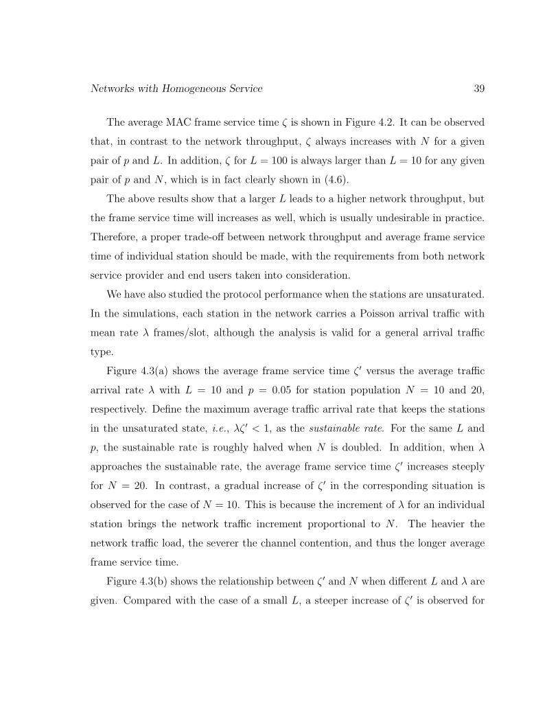
Networks with Homogeneous Service 39
The average MAC frame service time ζ is shown in Figure 4.2. It can be observed
that, in contrast to the network throughput, ζ always increases with N for a given
pair of p and L. In addition, ζ for L = 100 is always larger than L = 10 for any given
pair of p and N , which is in fact clearly shown in (4.6).
The above results show that a larger L leads to a higher network throughput, but
the frame service time will increases as well, which is usually undesirable in practice.
Therefore, a proper trade-off between network throughput and average frame service
time of individual station should be made, with the requirements from both network
service provider and end users taken into consideration.
We have also studied the protocol performance when the stations are unsaturated.
In the simulations, each station in the network carries a Poisson arrival traffic with
mean rate λ frames/slot, although the analysis is valid for a general arrival traffic
type.
Figure 4.3(a) shows the average frame service time ζ ′ versus the average traffic
arrival rate λ with L = 10 and p = 0.05 for station population N = 10 and 20,
respectively. Define the maximum average traffic arrival rate that keeps the stations
in the unsaturated state, i.e., λζ ′ < 1, as the sustainable rate. For the same L and
p, the sustainable rate is roughly halved when N is doubled. In addition, when λ
approaches the sustainable rate, the average frame service time ζ ′ increases steeply
for N = 20. In contrast, a gradual increase of ζ ′ in the corresponding situation is
observed for the case of N = 10. This is because the increment of λ for an individual
station brings the network traffic increment proportional to N . The heavier the
network traffic load, the severer the channel contention, and thus the longer average
frame service time.
Figure 4.3(b) shows the relationship between ζ ′ and N when different L and λ are
given. Compared with the case of a small L, a steeper increase of ζ ′ is observed for

Networks with Homogeneous Service 40
0 10 20 30 40 50 600
0.1
0.2
0.3
0.4
0.5
0.6
N
Nor
mal
ized
net
wor
k th
roug
hput
η
L=10 (slots)
p=0.005, ana.p=0.005, sim.p=0.01, ana.p=0.01, sim.p=0.05, ana.p=0.05, sim.
(a)
0 10 20 30 40 50 600
0.1
0.2
0.3
0.4
0.5
0.6
0.7
0.8
0.9
1
N
Nor
mal
ized
net
wor
k th
roug
hput
η
L=100 (slots)
p=0.005, ana.p=0.005, sim.p=0.01, ana.p=0.01, sim.p=0.05, ana.p=0.05, sim.
(b)
Figure 4.1: Saturation throughput of p-persistent CSMA/CA protocol
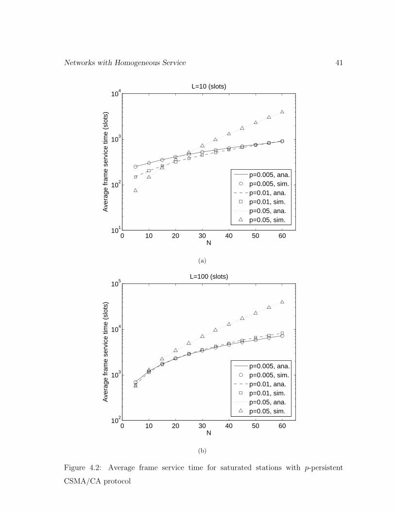
Networks with Homogeneous Service 41
0 10 20 30 40 50 6010
1
102
103
104
N
Ave
rage
fram
e se
rvic
e tim
e (s
lots
)
L=10 (slots)
p=0.005, ana.p=0.005, sim.p=0.01, ana.p=0.01, sim.p=0.05, ana.p=0.05, sim.
(a)
0 10 20 30 40 50 6010
2
103
104
105
N
Ave
rage
fram
e se
rvic
e tim
e (s
lots
)
L=100 (slots)
p=0.005, ana.p=0.005, sim.p=0.01, ana.p=0.01, sim.p=0.05, ana.p=0.05, sim.
(b)
Figure 4.2: Average frame service time for saturated stations with p-persistent
CSMA/CA protocol

Networks with Homogeneous Service 42
1 2 3 4 5 6 7
x 10−3
0
50
100
150
200
250
300
350
400
λ (frames/slot)
ζ(u) (
slot
s)
L=10, p=0.05
saturated
N=10, anaN=10, simN=20, anaN=20, sim
(a)
0 10 20 30 40 50 60 700
500
1000
1500
2000
2500
3000
3500
4000
4500
N
ζ(u) (
slot
s)
p=0.01
saturated
saturated
L=10, λ=1e−3, anaL=10, λ=1e−3, simL=100, λ=2.5e−4, anaL=100, λ=2.5e−4, sim
(b)
Figure 4.3: Average frame service time in unsaturated case of p-persistent CSMA/CA
protocol

Networks with Homogeneous Service 43
a large L, even with reduced λ and smaller N .
In fact, two applications of the proposed analytical model for unsaturated stations
have been demonstrated in Figure 4.3. For a network with given number of stations,
we can obtain the sustainable rate for each station, as shown in Figure 4.3(a). On the
other hand, with a given per station average traffic arrival rate, we can also determine
the maximum number of stations that can be admitted into a network (usually called
admission region), as shown in Figure 4.3(b). Such results are very useful to the design
of the call admission control scheme, which is usually an indispensable element in a
network with QoS provisioning capability.
Inspection of Figures 4.1-4.3 shows that the analytical results approximate the
simulation results very well in all cases, even though the analytical and simulation
models are not identical, as mentioned earlier in this subsection. The reason for
this can be attributed to the fact that the performances shown are average values.
Therefore, for the p-persistent CSMA/CA protocol, analytical results will be given
without further comparison to simulation results in the remainder of the this chapter.
4.2 The CAP-MAC in IEEE 802.15.4
4.2.1 The Basic Analysis
According to the channel access policy of this protocol (see Section 2.2.2), the renewal
point of the level-1 renewal cycle can be set when a station resets its contention
window to the minimum value after each transmission trial (regardless of the result)
or when it senses a busy channel at the end of the Mth backoff stage. Correspondingly,
in Figure 4.4, a level-1 renewal cycle is defined as the period between the two adjacent
time instants that the tagged station starts a stage 0 backoff. Although the renewal
points are different from those in the model for the slotted p-persistent CSMA/CA

Networks with Homogeneous Service 44. . . b1b0b0 b1 b2 b3 b4level-1X2 X1X1 X2. . .X1 hannel sensing failure timesu essful hannel sensingtransmission of the tagged nodeFigure 4.4: The level-1 renewal cycle for IEEE 802.15.4 MAC
protocol, level-1 renewal cycles in this case can still be classified into two types, as
illustrated in Figure 4.4. The X1 type is a cycle that includes no transmission from
the tagged station, resulting from M channel sensing failures. In contrast, the X2
type is a cycle that contains a period L of transmission from the tagged station, after
experiencing m backoff stages, 0 ≤ m ≤ M . Again, the ending points of the X2 cycles
delimit the level-2 cycles as in the basic model. Also, the transmission in an X2 cycle
may be a successful transmission or a collision due to the simultaneous transmissions
from other stations. Thus, the level-2 and level-3 renewal cycles remain the same as
in the basic model (Figure 3.1). Note that the difference in the level-1 cycle modeling
from the one for p-persistent CSMA/CA results from the fact that the backoff period
of the tagged station overlaps with the transmission time from other stations in the
CAP-MAC, which means that there is no explicit L in its X1 cycles.
To analyze this variant of the model, the number of channel sensing attempts
R conducted by the tagged station is viewed as a reward associated to a level-1
renewal cycle. For a homogeneous service network, the sensing failure probability α,
defined as the probability of finding a busy channel when the tagged station senses
the channel in a slot, is the same for all the channel sensing activities from all the
stations. With a given α, the number of sensing attempts for one station in a level-1

Networks with Homogeneous Service 45
renewal cycle follows a truncated3 geometric distribution with parameters α and M .
More specifically, with probability 1−α the station succeeds in sensing an idle channel
and transmits the frame by only one sensing attempt; with probability α(1 − α) the
station succeeds in transmitting the frame by two sensing attempts, and so forth. The
number of backoff stages contained in a level-1 cycle follows the same distribution.
Therefore, the average length of a level-1 cycle can be obtained accordingly. By the
renewal reward theorem [70], the channel sensing probability τ for the tagged station
is given by the ratio of the average sensing attempts over the average length of the
level-1 cycle, which is a function of α. On the other hand, the channel sensing failure
probability α can be obtained as a function of τ by carefully studying the transition
probabilities among the channel states (idle and busy). These two equations can
be solved by the fixed point technique to obtain α and τ , which can then be used
to derive the average lengths of the three-level cycles and, finally, the desired MAC
performance metrics.
In what follows, we first consider a slightly simpler protocol to illustrate the essence
of the above model, then extend to the double channel sensing (DS) case specified in
the standard.
4.2.2 The Single-Sensing Case (One CCA)
In the single-sensing (SS) case, a station senses the channel once at the end of a backoff
stage. If the channel is idle, the station transmits at the beginning of the next slot;
otherwise, it enters the next backoff stage. This is the only difference between the SS
and the DS.
According to the discussion in the previous subsection, with a given channel sens-
ing failure probability α, the average number of sensing attempts for one station in a
3It is truncated because the maximum number of sensing attempts allowed in an X cycle is M .

Networks with Homogeneous Service 46
level-1 renewal cycle is
E[R] = (1 − α) + 2α(1 − α) + 3α2(1 − α) + · · ·
+ (M − 1)αM−2(1 − α) + MαM−1
=M−1∑
m=0
αm, (4.17)
and the average length of a level-1 renewal cycle is
E[X] = (1 − α)(b0 + 1 + L) + α(1 − α)(b0 + b1 + 2 + L) + · · ·
+ αM−1(1 − α)(M−1∑
m=0
(bm + 1) + L) + αM
M−1∑
m=0
(bm + 1)
=M−1∑
m=0
αm(bm + 1) + (1 − αM)L, (4.18)
where L is the duration of a frame transmission in units of slots, and bm, 0 ≤ m ≤ M ,
is the average number of slots in backoff stage m. Note that at the end of each
backoff stage, there is always one slot used for sensing the channel. In addition, with
the probability of αM , the tagged station encounters M contiguous sensing failures
and thus ends up the current renewal cycle without a transmission period incurred.
Therefore, a period of L is included in the level-1 renewal cycle only with probability
(1 − αM), which is reflected by the last term in (4.18).
According to the renewal reward theorem [70], the sensing attempt rate for the
tagged station is given by E[R]/E[X], i.e., τ can be obtained as
τ =E[R]
E[X]=
∑M−1m=0 αm
∑M−1m=0 αm(bm + 1) + (1 − αM)L
. (4.19)
Next we derive the sensing failure probability α. In a randomly chosen slot, the
channel state is either idle with probability Pi or busy with probability Pb = 1 − Pi,

Networks with Homogeneous Service 47
depending on the behavior of the stations. To obtain Pi, consider the channel status
for two consecutive slots. Using conditional probabilities, we have
Pi = P(i,i)Pi + P(b,i)(1 − Pi), (4.20)
which yields
Pi =P(b,i)
1 + P(b,i) − P(i,i)
, (4.21)
where P(b,i)
(P(i,i)
)is the conditional probability that the next channel state is idle
given that the current channel state is busy (idle). Since a transmission lasts for L
slots, a randomly chosen busy slot will end with probability 1/L in the next slot,
which comes from
P(b,i) = Pr{next slot is idle | current slot is the last busy slot}×
Pr{current slot is the last busy slot}
+ Pr{next slot is idle | current slot is not the last busy slot}×
Pr{current slot is not the last busy slot}
= 1 × 1
L+ 0 × L − 1
L
=1
L.
(4.22)
On the other hand, considering the sensing probability independence assumption, the
channel will remain in the idle state in slot k + 1 when it is idle in slot k only if none
of the stations starts to sense in slot k, where k is an arbitrary slot index. Thus, we
have
P(i,i) = (1 − τ)N . (4.23)
Substituting P(b,i) and P(i,i) into (4.21), we obtain
Pi =1
1 + L(1 − (1 − τ)N). (4.24)

Networks with Homogeneous Service 48
Thus, the sensing failure probability α is given by
α = 1 − Pi
=L(1 − (1 − τ)N)
1 + L(1 − (1 − τ)N).
(4.25)
With given L, N and bm, the set of fixed-point equations (4.19) and (4.25) can be
solved numerically to obtain α, τ and E[X].
To complete the analysis, we need to obtain the parameters Ptx and Psuc. As
shown in Figure 4.4, for every level-1 renewal cycle X, it contains a transmission of
L slots (i.e., it is a type X2 cycle) with probability
Ptx = 1 − αM . (4.26)
Furthermore, the conditional probability that a transmission from the tagged station
is successful is
Psuc = (1 − τ)N−1, (4.27)
because none of the other N − 1 stations should sense the channel in the same slot
as the tagged station does.
Combining (4.18), (4.26), (4.27) and (3.1) – (3.4), we obtain the average length
of level-3 cycles E[Z] as:
E[Z] =1
τ(1 − τ)N−1(1 − α), (4.28)
which is also the average frame service time, ζ. Following the basic model, the
throughput of an individual station is
ηs =L
E[Z]= Lτ(1 − τ)N−1(1 − α). (4.29)
For the homogeneous network, the throughput is
η = Nηs = NLτ(1 − τ)N−1(1 − α). (4.30)

Networks with Homogeneous Service 49
4.2.3 The Double-Sensing Case (Two CCAs)
In this subsection, we study the double-sensing channel access mechanism specified
in the standard. Similar to the single sensing case, the analysis can be done with
appropriate changes in the equations regarding α and τ . In the following, the super-
script (d) is added to all the relevant variables for the double-sensing case.
Let p1 denote the probability of sensing a busy channel in the first CCA, and p2
the probability of sensing a busy channel in the second CCA given that the channel
is idle in the first CCA. Let α(d) denote the probability of sensing failure, which is
defined as sensing a busy channel in either of the two CCA events. At the end of
each backoff stage, the tagged station will either enter the next backoff stage with
probability α(d) or start a transmission with probability 1 − α(d). Therefore,
α(d) = p1 + (1 − p1)p2. (4.31)
In addition, for each backoff stage, a station must spend one slot for the first
CCA, and spend another slot for the second CCA with probability 1 − p1. Hence,
the average number of slots spent for channel sensing in each backoff stage ending up
without a transmission is
c = 1 + (1 − p1) = 2 − p1. (4.32)
In the situation that the station succeeds in starting a transmission at the end of a
backoff stage, the two successful CCA events will occupy two slots. In summary, the
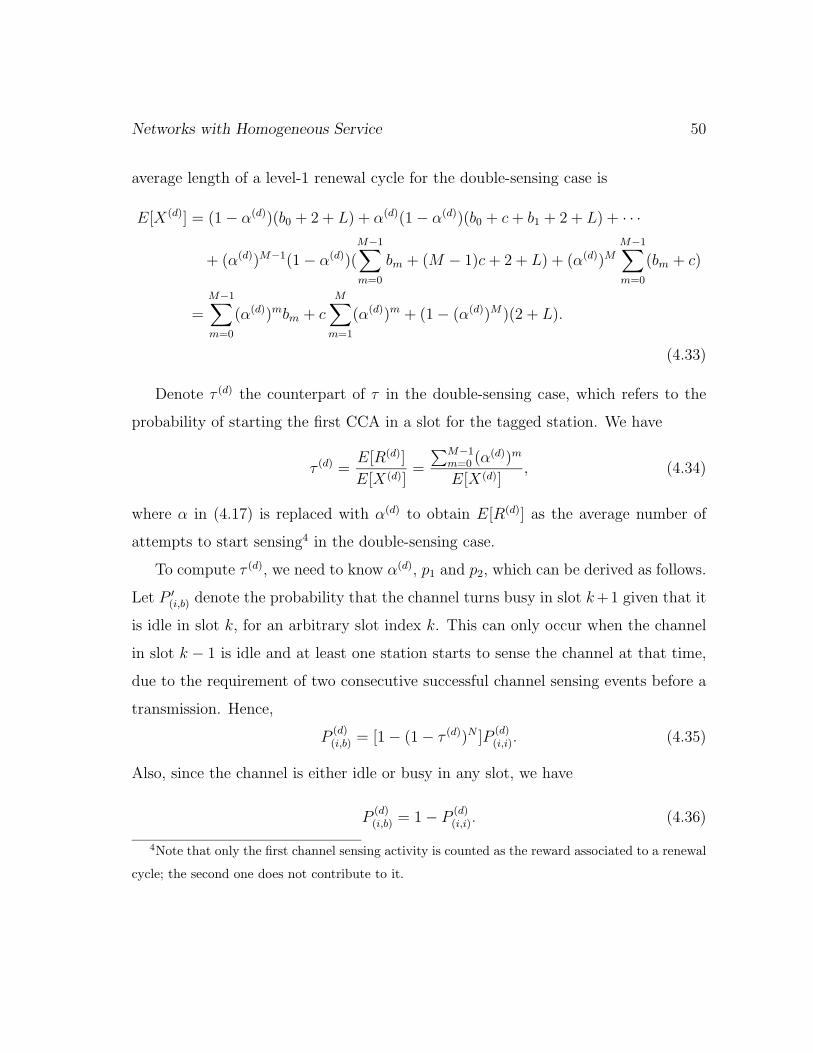
Networks with Homogeneous Service 50
average length of a level-1 renewal cycle for the double-sensing case is
E[X(d)] = (1 − α(d))(b0 + 2 + L) + α(d)(1 − α(d))(b0 + c + b1 + 2 + L) + · · ·
+ (α(d))M−1(1 − α(d))(M−1∑
m=0
bm + (M − 1)c + 2 + L) + (α(d))M
M−1∑
m=0
(bm + c)
=M−1∑
m=0
(α(d))mbm + c
M∑
m=1
(α(d))m + (1 − (α(d))M)(2 + L).
(4.33)
Denote τ (d) the counterpart of τ in the double-sensing case, which refers to the
probability of starting the first CCA in a slot for the tagged station. We have
τ (d) =E[R(d)]
E[X(d)]=
∑M−1m=0 (α(d))m
E[X(d)], (4.34)
where α in (4.17) is replaced with α(d) to obtain E[R(d)] as the average number of
attempts to start sensing4 in the double-sensing case.
To compute τ (d), we need to know α(d), p1 and p2, which can be derived as follows.
Let P ′(i,b) denote the probability that the channel turns busy in slot k+1 given that it
is idle in slot k, for an arbitrary slot index k. This can only occur when the channel
in slot k − 1 is idle and at least one station starts to sense the channel at that time,
due to the requirement of two consecutive successful channel sensing events before a
transmission. Hence,
P(d)(i,b) = [1 − (1 − τ (d))N ]P
(d)(i,i). (4.35)
Also, since the channel is either idle or busy in any slot, we have
P(d)(i,b) = 1 − P
(d)(i,i). (4.36)
4Note that only the first channel sensing activity is counted as the reward associated to a renewal
cycle; the second one does not contribute to it.

Networks with Homogeneous Service 51
Combining (4.35) and (4.36) and letting t = 1 − (1 − τ (d))N , we obtain
P(d)(i,i) =
1
1 + t. (4.37)
Note that the derivation of (4.21) does not rely on any specific assumption of the
channel sensing mechanism, so the relationship among the relevant probabilities is
also valid for the DS case. Substituting (4.37) into (the DS version of) (4.21), and
noting that P(d)(b,i) = 1/L, we have
P(d)i =
1 + t
1 + (L + 1)t. (4.38)
Then, the channel sensing failure probabilities for the two sensing attempts can be
obtained as:
p1 = 1 − P(d)i =
Lt
1 + (L + 1)t, (4.39)
p2 = P(d)(i,b) =
t
1 + t. (4.40)
Substituting the above two equations into (4.31), we obtain
α(d) =L(1 − (1 − τ (d))N)
1 + L(1 − (1 − τ (d))N). (4.41)
Note that the channel sensing failure probability α(d) for the DS case has a rela-
tionship to the channel sensing probability τ (d) exactly same as that of α to τ in the
SS case. However, τ (d) as a function of α(d) is different from τ as a function of α, due
to the time cost of the second CCA slot in the DS case. This difference causes the
lower throughput of the DS mechanism compared to the SS with the same protocol
parameters, as will be shown in Sec. 4.2.5.
Similarly to the SS case, with α(d) and τ (d) we can obtain straightforwardly the
performance metrics for the DS case. The average frame service time is
E[Z(d)] =1
τ (d)(1 − τ (d))N−1(1 − α(d)), (4.42)

Networks with Homogeneous Service 52
the MAC throughput of an individual station is
η(d)s = Lτ (d)(1 − τ (d))N−1(1 − α(d)), (4.43)
and the network throughput is
η(d) = Nη(d)s = NLτ (d)(1 − τ (d))N−1(1 − α(d)), (4.44)
where τ (d) and α(d) are given in (4.34) and (4.41), respectively. Note that the network
throughput η(d) is consistent with (29) in [76], which is obtained with a much more
complicated Markov chain based approach.
4.2.4 Analysis of Unsaturated Stations
For presentation succinctness, we only give the analysis for unsaturated stations in
the single-sensing case. The analysis is based on the key idea that a station will
not attempt to sense5 the channel when its MAC buffer is empty, i.e., the station
will contend to access the channel only when it has a frame in the buffer waiting for
transmission, which occurs with probability ρ = ⌈λE[Z ′]⌉1. The sensing probability
τ ′ for a busy station remains in the same format as in (4.19) except α is now α′.
Thus, τ ′ is given by
τ ′ =
∑M−1m=0 (α′)m
∑M−1m=0 (α′)m(bm + 1) + (1 − (α′)M)L
. (4.45)
Consider the conditional probability that the channel will remain in the idle state
in slot k +1 given that it is idle in slot k. Such an event will occur only when neither
the tagged station nor any of the n, 0 ≤ n ≤ N − 1, other busy stations starts to
sense in slot k. Hence, we have
P ′(i,i) = (1 − τ ′)(1 − ρτ ′)N−1 (4.46)
5In fact, the station will not transmit in this case either.
Networks with Homogeneous Service 53
Following the approach in Sec. 4.2.2, α′ can be obtained as
α′ =L(1 − P ′
(i,i))
1 + L(1 − P ′(i,i))
, (4.47)
and
E[Z ′] =1
τ ′P ′(i,i)(1 − α′)
, (4.48)
ρ = ⌈λE[Z ′]⌉1, (4.49)
With given λ,N and L, τ ′, α′, E[Z ′] and ρ can be obtained from equations (4.45)–
(4.63). Following the method given earlier, the throughput and average frame service
time in the unsaturated case can be readily obtained from E[Z ′].
4.2.5 Numerical Results
In this subsection, we present simulation results and compare them with the analytical
ones to demonstrate the accuracy of the proposed analytical model. The simulator is
written in the C language. In the following, the normalized throughput and average
frame service time in units of slots are given, but they can be easily converted to
actual throughput in units of bit per second and time in units of seconds with the
parameter values given in the standard.
Performance of Default Parameters and Potential Improvements
First, we study the performance of the MAC protocol with default parameter values
given in the standard, i.e., the minimum backoff exponent BEmin = 3, the maximum
backoff exponent BEmax = 5, and the maximum allowed backoff stage for a frame
NBmax = 5. The saturation throughput and average frame service time versus the
number of stations N in the networks with the above default settings are shown in

Networks with Homogeneous Service 54
Figure 4.5(a) and Figure 4.5(b), respectively, marked as “def” in the figures. The
frame length is L = 8. It can be seen that the throughput decreases sharply with the
number of stations while the average frame service time shows an opposite trend. This
is because with small values of BEmin = 3 (corresponding to b0 = 3.5) and BEmax = 5,
the backoff slots are uniformly distributed over a relatively small range of [0, 31], which
causes the probability of simultaneous channel sensing conducted by multiple stations
increases quickly with N . In contrast, the probability of finding the channel idle in
the sensing slots decreases quickly when N increases. Therefore, a large portion
of time is spent in backoff and thus the network throughput downgrades with the
significantly increased frame service time. To overcome this issue, a straightforward
solution is to remove the upper limit of maximum backoff exponent (or set it to a
large number, e.g., 10 as in IEEE 802.11). That is, every time a station enters a
new backoff stage, it simply increments the backoff exponent by one. In this way,
the selection range of backoff slots is enlarged so that the probability of simultaneous
channel sensing increases slower with N than it does in the default settings. The
performance of this slightly different variant of the standard protocol is shown in the
figures as “BEmin=3”. We can see that the performance is about the same when
N is small (N < 10). However, the performance gain becomes obvious when N is
large. The network throughput is almost doubled for N = 30 and it is ten-folded for
N = 60. Meanwhile, the average frame service time is always shorter than that in
the default setting, and the gap between them increases with N , e.g., ζ for N = 60
decreases to just 1/3 of that with the default settings.
For larger BEmin’s (4 and 5), the performance is also shown in Figure 4.5 as
“BEmin=4” and “BEmin=5”, respectively. It is interesting to observe that the sat-
uration network throughput first increases with N when N is small (less than 15 for
“BEmin=4” and 25 for “BEmin=5”), then start to decrease with N , but much slower

Networks with Homogeneous Service 55
0 10 20 30 40 50 600
0.1
0.2
0.3
0.4
0.5
0.6
N
Thr
ough
put
Double−sensing, L=8
def, anadef, simBEmin=3, anaBEmin=3, simBEmin=4, anaBEmin=4, simBEmin=5, anaBEmin=5, sim
(a)
0 10 20 30 40 50 6010
1
102
103
104
105
N
MA
C s
ervi
ce ti
me
(slo
ts)
Double−sensing, L=8
def, anadef, simBEmin=3, anaBEmin=3, simBEmin=4, anaBEmin=4, simBEmin=5, anaBEmin=5, sim
(b)
Figure 4.5: Performance of CAP-MAC with saturated stations

Networks with Homogeneous Service 56
than in the “BEmin=3” and the default settings cases. This is because when N is
small, stations can access the channel to transmit frames relatively easily with rela-
tively small collision probability. For a small N , a larger BEmin means the stations
spend more time in backoff for each frame transmission, resulting in a larger portion
of channel idle time and lower network throughput. As N increases, more stations
contribute to the increase of network throughput by more successful frame transmis-
sions and more overlapped backoff time until this is offset by the increasing collision
probability, upon which the maximum network throughput is reached. After that
optimal point, further increasing N will cause a busier channel with less opportunity
for stations to transmit and, even worse, higher collision probability for transmissions,
leading to decreased network throughput. A larger BEmin gives a larger range for the
selection of the number of backoff slots, which mitigates the above two adverse effects
and makes the degradation of network throughput slower. For the same reason, ζ
for larger BEmin cases is slightly longer when N is small, but becomes much shorter
with large N , as shown in Figure. 4.5(b).
Single Sensing vs. Double Sensing
In developing the analytical model in this section, we have considered both the single
sensing and double sensing mechanisms. Two expressions with the same form, (4.25)
and (4.41), have been obtained for the channel sensing failure probabilities α and
α(d) as a function of the sensing probability τ and τ (d), respectively. However, the
difference in channel sensing requirements leads to the two different expressions for
the relationship between the two probabilities, as shown in (4.19) and (4.34). In
the following, we study the effect of this difference on the performance of the two
mechanisms.
The probabilities of success for a frame transmission (Psuc) in the SS and DS cases

Networks with Homogeneous Service 57
0 10 20 30 40 50 600
0.1
0.2
0.3
0.4
0.5
0.6
0.7
0.8
0.9
1
N
Tra
nsm
issi
on s
ucce
ssfu
l pro
babi
lity
BEmin=5, L=8
SSDS
(a) Transmission successful probabilities
0 10 20 30 40 50 600
0.1
0.2
0.3
0.4
0.5
0.6
0.7
0.8
0.9
1
N
Cha
nnel
bus
y pr
obab
ility
BEmin=5, L=8
αp1p2α′
(b) Channel busy probabilities
Figure 4.6: Comparison between the SS and DS cases

Networks with Homogeneous Service 58
0 10 20 30 40 50 600
0.1
0.2
0.3
0.4
0.5
0.6
N
Thr
ough
put
L=8
BEmin=3, SSBEmin=3, DSBEmin=4, SSBEmin=4, DSBEmin=5, SSBEmin=5, DS
Figure 4.7: Saturation throughput comparison between SS and DS modes
are compared in Figure 4.6(a). With the same parameter (e.g., N,L and BEmin)
values, Psuc of the DS is higher than that of the SS, which may suggest that the
DS mechanism is preferable over the SS. However, as shown in Figure 4.6(b), the
probability p1 of sensing a busy channel in the first CCA slot in the DS case alone is
always larger than that in the SS, which means a station gets less chance to transmit
in the DS than in the SS during the same given period of time. Therefore, the DS
mechanism is in an obvious disadvantage position, considering further the potential
adverse effect of the probability p2 of sensing a busy channel in the second CCA slot.
The net effect of the above two contradicting factors is a lower network throughput of
DS, which is clearly shown in Figure 4.7. It can be seen that with the same parameters
(L=8), network throughput of the SS mode is always about 10% higher than that of

Networks with Homogeneous Service 59
0 10 20 30 40 50 6010
1
102
103
104
N
MA
C s
ervi
ce ti
me
(slo
ts)
Single−sensing, L=8
BEmin=3, anaBEmin=3, simBEmin=4, anaBEmin=4, simBEmin=5, anaBEmin=5, sim
Figure 4.8: Average frame service time in the SS case
the DS mode, which conforms with the simulation results presented in [78, 89]. In
addition, the performance gain of larger BEmin still exists in the SS case due to the
similar reasons given in Section 4.2.5.
Figure 4.8 shows the average frame service time for the SS case. The relationships
among the results for different parameter settings are similar to those in Figure 4.5(b).
It should be mentioned that according to the general relationship between network
throughput and average frame service time of the SS case is always shorter than that
of the DS case with the same protocol parameters.

Networks with Homogeneous Service 60
Unsaturated Stations
To demonstrate the effectiveness of the model for the unsaturated case, Figure 4.9
shows the average frame service time versus the frame arrival rate for N = 20. Poisson
traffic is used in the simulation to compare with the analytical results. Ts increases
quite slowly with low to medium load, and it soars when the load becomes high until
it reaches a saturation level which depends only on N when the other parameters are
given. It can be seen that the analytical results approximate the simulation ones very
well.
1 1.5 2 2.5 3 3.5 4
x 10−3
0
50
100
150
200
250
300
λ (frame/slot)
MA
C s
ervi
ce ti
me
(slo
ts)
Single−sensing, L=8, BEmin=4
N=20, anaN=20, sim saturation service time
Figure 4.9: Average frame service time in unsaturated case

Networks with Homogeneous Service 61
4.3 The IEEE 802.11 DCF
4.3.1 Analysis of Saturated Stations
According to the protocol described in Section 2.2.3, there are two salient attributes
of the DCF as listed below:
• The backoff procedure freezes when the channel is busy, which is similar to the
p-persistent CSMA/CA protocol but different from the CAP-MAC;
• The backoff parameter changes after each collision involving the tagged station,
which is different from the p-persistent CSMA/CA protocol but similar to the
behavior of the CAP-MAC when it encounters channel sensing failure.
Therefore, although a level-1 cycle for DCF is still the period between two consecutive
transmissions from the tagged station as in the basic model, the level-2 cycles are
actually semi-renewal due to the changing backoff parameters caused by the binary
exponential backoff activity at this level. However, the renewal points for level-3
cycles remain to be the time instants when a new frame starts to be served. Note
that they are equivalent to the instants when the CW is reset to CW0, which are the
same as the renewal points for level-1 cycles in the model for the CAP-MAC. This
resemblance inspires us to analyze DCF directly at level-3, using an approach similar
to the one used for analyzing the level-1 cycles in CAP-MAC, as outlined below.
The assumption that each transmission results in a collision with a constant in-
dependent probability β regardless of the backoff and transmission history of the
frame [6] is adopted in this analysis. With a given collision probability, the number
of transmission trials H is thus a random variable with geometric distribution. For
each new frame, H can also be deemed as a reward associated to the level-3 renewal
cycle. Therefore, by the renewal reward theorem, the probability of a station to

Networks with Homogeneous Service 62
transmit (or equivalently, access the channel) at the beginning of a randomly chosen
generic slot, γ, is given by the ratio of the average number of transmission trials to
the total number of generic slots in the level-3 cycle. On the other hand, the collision
probability β can also be obtained as a simple function of the transmitting probabil-
ity γ, due to the fact that a collision occurs only when any other station transmits
simultaneously with the tagged station. These two equations can be jointly solved to
obtain the above two probabilities.
More specifically, a collision occurs if at least one of the other N − 1 stations
transmit in the same slot. Thus, we have
β = 1 − (1 − γ)N−1. (4.50)
Denote M the retry limit specified in the protocol, and E[ω] the average number of
total backoff slots the tagged station has to wait during the level-3 cycle. It is clear
that there are E[H] transmissions during E[ω] +E[H] slots. Hence, the transmitting
probability is given by
γ =E[H]
E[ω] + E[H]. (4.51)
In fact, the probability of successfully delivering a frame with one transmission is
(1 − β), with two transmissions is β(1 − β), and so on. Moreover, the frame will be
removed from the MAC sublayer buffer after the Mth trial regardless of the transmis-
sion result. Therefore, similar to the E[R] in (4.17), H follows a truncated geometric
distribution with parameters β and M , and the average number of transmissions for
a frame is given by
E[H] =M−1∑
i=1
iβi−1(1 − β) + MβM−1
=M−1∑
i=0
βi.
(4.52)

Networks with Homogeneous Service 63
Let br denote the average number of backoff slots in backoff stage r, r = 0, 1, . . . ,M ,
where r = 0 refers to the initial backoff stage with the minimum contention window
W = CW0. It is clear that the average number of backoff slots for a frame is the
weighted summation of the br’s as given by
E[ω] =M−1∑
i=0
(βi(1 − β)
i∑
r=0
br
)+ βM
M−1∑
i=0
bi
=M−1∑
i=0
(βibi).
(4.53)
Finally, we have
γ =
∑M−1i=0 βi
∑M−1i=0 βi(bi + 1)
. (4.54)
Given a specific backoff policy, i.e., the backoff parameters such as W and M , the
equation set (4.50) and (4.54) can be solved numerically to obtain a pair of β and γ.
Note that different from the fixed length slot used in the previous two protocols,
a generic slot in the above analysis may refer to an idle time slot, a successful trans-
mission or a collision with corresponding probabilities, as in [6]. According to the
above argument, a level-3 cycle can be deemed as a sequence of generic slots in which
the tagged station either does not transmit or it transmits but encounters a collision,
followed by an ending generic slot containing the successful transmission from the
tagged station. In other words, in each generic slot, the tagged station conducts a
Bernoulli experiment with its successful transmission defined as the event success.
Consequently, the average length of the level-3 cycle in units of generic slots has a
geometric distribution with parameter γ(1 − β). Thus, E[Z] can be obtained as
E[Z] =1
γ(1 − β)E[GS], (4.55)
Networks with Homogeneous Service 64
where E[GS] is the average length of a generic slot, as given by
E[GS] = Pr{channel is idle} · 1 + Pr{channel is busy} · L
= (1 − γ)N · 1 + (1 − (1 − γ)N) · L
= (1 − γ)N + L − L(1 − γ)N .
(4.56)
The network throughput can be obtained following the approach given in the basic
model, i.e.,
η =NL
E[Z]. (4.57)
Alternatively, it can be obtained as the portion of the average time used for successful
transmissions in a generic slot [6]. The former item is given by Nγ(1−γ)N−1L, while
the latter is given in (4.56). Combining the two expressions, we have
η =Nγ(1 − γ)N−1L
(1 − γ)N + L − L(1 − γ)N. (4.58)
Noticing from (4.50) that 1 − β = (1 − γ)N−1, it is easy to verify that the two
expressions for the network throughput (4.57) and (4.58) are equivalent.
4.3.2 Analysis of Unsaturated Stations
We have successfully applied the proposed model to analyze the network with unsat-
urated stations for the previous two protocols. Similar analysis for the DCF can be
carried out straightforwardly. Following the same key idea that a station will compete
for channel access only when it has a frame for service, we can obtain the following
Networks with Homogeneous Service 65
equation set for DCF:
β′ = 1 − (1 − ργ′)N−1 (4.59)
γ′ =
∑M−1i=0 (β′)i
∑M−1i=0 (β′)i(bi + 1)
(4.60)
E[GS ′] = (1 − γ′)(1 − γ′ρ)N−1 + L(1 − (1 − γ′)(1 − γ′ρ)N−1
)(4.61)
E[Z ′] =E[GS ′]
γ′(1 − β′)(4.62)
ρ = ⌈λE[Z ′]⌉1, (4.63)
where λ is the average frame arrival rate on an individual station. The above equation
set can be solved numerically when N , L and λ are given to obtain E[Z ′], which is
the main desired MAC performance metric for unsaturated stations.
4.3.3 With Default Parameters in DCF
Contention Window
In the DCF specification, the initial value of the backoff counter in backoff stage r is
uniformly chosen over [0, CWr), where CWr = 2r · W = 2r · 32 is the corresponding
contention window. Therefore, the average backoff time in stage r is br = CWr
2
slots. The maximum number of allowed retransmission is M = 7. In addition, the
contention window is bounded by 1024, so m′ = log2(1024/32) = 5 is the number of
backoff stages that have different contention window size. That is, when the backoff
stage r ≥ m′, the contention window will be the same (1024). Substituting these
parameters into (4.53), we obtain the average number of backoff time slots of a station

Networks with Homogeneous Service 66
as
E[ω] =W − 1
2(1 − β) + · · · +
∑m′
i=0(2iW − 1)
2βm′
(1 − β)
+ · · · +∑m′
i=0(2iW − 1) + (M − m′)2m′
W
2βM
=A − B
2(1 − β)(1 − 2β),
A = W (1 − β)(1 − (2β)m′+1) + Wβ(1 − 2β)(2β)m′
(1 − βM−m′
),
B = (1 − 2β)(1 − βM+1).
(4.64)
The final expression for E[ω] in (4.64) is valid only when β 6= 0.5, but E[ω] can be
evaluated directly at the first step of (4.64) for β = 0.5.
Combining (4.54) and (4.64), the transmission probability of the station is thus
obtained as
τ =2(1 − βm)(1 − 2β)
A + B, (4.65)
where A and B are given in (4.64). This result is consistent with that derived in [110]
using the much more complicated two-dimension Markov chain approach.
Successful Frame Transmission Time and Collision Time Calculation
Denote Ts the time duration spent by the tagged station on a successful transmission,
and Tc the time duration for a collision. In the basic access mode,
Ts = T(data) + SIFS + T(ACK) + DIFS, (4.66)
Tc = T(data) + ACK Timeout + DIFS. (4.67)
In the above, T(x) represents the transmission time of the corresponding frame
type x. In fact, Ts ≈ Tc because ACK Timeout ≈ SIFS + T(ACK) as specified in
the standard. Note that Ts also represents the time duration that the channel is

Networks with Homogeneous Service 67
sensed busy by the tagged station due to a successful transmission of another station.
For the time period of busy channel due to a collision among other stations, it is
Tdata + EIFS for the basic access mode, which can be safely approximated by Tc
in (4.67) according to the standard. Once a transmission starts, the channel will be
deemed busy for the whole period of either Ts or Tc due to two reasons:
1. In the case of a successful transmission, the duration of SIFS is shorter than
a slot time given by the standard, which assures that no new transmission will
start before the transmission of the ACK frame from the receiver;
2. In the case of a collision, the EIFS period helps to prevent new transmissions
to start before the end of Tc.
Therefore, we can use Ts (or Tc) normalized by the slot time as L in the analysis for
the basic mode of DCF.
In the RTS/CTS mode, for the tagged station we have
T (RTS)s = T(RTS) + T(CTS) + T(data) + T(ACK) + 3SIFS + DIFS, (4.68)
T (RTS)c = T(RTS) + CTS Timeout + DIFS. (4.69)
Similar to the basic mode, T(RTS)s is for the channel busy period caused by a successful
transmission from either the tagged station or others. Thus, we may still set L equal
to the normalized T(RTS)s . On the other hand, the channel busy period caused by
collisions from other stations is T(RTS) + EIFS, which can also be approximated by
T(RTS)c in (4.69). However, since T
(RTS)s 6= T
(RTS)c in this mode, the calculation of

Networks with Homogeneous Service 68
E[GS] need to be changed to
E[GS](RTS) = Pr{channel is idle} · 1 +
Pr{channel is busy due to a successful transmission} · T (RTS)s +
Pr{channel is busy due to a collsion} · T (RTS)c
= (1 − γ)N + Nγ(1 − γ)N−1T (RTS)s +
(1 − (1 − γ)N − Nγ(1 − γ)N−1)T (RTS)c .
(4.70)
The remaining part of the analytical model can be applied to the RTS/CTS mode
without further modification.
We have used L to represent the time for successful frame transmission in the
analysis and directly used it in the calculation of network throughput. If a more
accurate expression for throughput is desired, the L in the numerator of (4.58) should
be replaced by the normalized Tdata. Similar replacement is also applicable to the
other two protocols when necessary.
Usually T(RTS)c << Tc (or Ts) < T
(RTS)s , so E[GS](RTS) is usually much smaller
than E[GS] in the basic mode and thus a higher network throughput can be achieved
in the RTS/CTS mode compared with the basic mode, when all the other parameters
(e.g., W and M) are the same. Therefore, the RTS/CTS mode is “recommended
for the majority of the practical cases” in [6]. With the advance of physical layer
technologies, the data rate of WLAN has increased dramatically, e.g., the emerging
standard IEEE 802.11n [114] can provide raw data rate of 216Mbps.

Networks with Homogeneous Service 69
The high data rate makes T(data) much smaller, and it is possible that the extra
cost of (T(RTS) + T(CTS) + 2SIFS) in T(RTS)s occupies so large a portion that the
benefit from the reduction of T(RTS)c is offset6. Therefore, the RTS/CTS mode is not
always recommended for networks with high data rate.
4.3.4 Numerical Results
As for the previous two protocols, simulations have also been run to verify the analysis
accuracy for the DCF. As an illustration of converting the normalized units to the
practical ones, the throughput is in units of Mbps and the average frame service time
is in units of mili-second.
Table 4.1: Some DCF Parameters Used in the Analysis and Simulations
minimum CW (W ) 32 retransmit limit (M) 7
m′ 5 MAC frame data rate 11 Mbps
slot time 20 µs SIFS 10 µs
DIFS 50 µs DSSS PHY header 192 µs
RTS frame size 28 Bytes CTS frame size 14 Bytes
ACK frame size 14 Bytes control frame data rate 1Mbps
We have tested the performance of DCF in both the basic mode and the RTS/CTS
mode for a given range of N , with two different MAC frame payload values, 1000 Bytes
(Payload-1) and 3000 Bytes (Payload-2), respectively. The parameters used in the
6Every frame is associated with the same amount of physical layer overhead, regardless of the
payload (the whole frame from the MAC layer). It is such fixed and relatively large physical layer
overhead that makes the effect described here possible to occur in high data rate systems.

Networks with Homogeneous Service 70
analysis and simulations are for the IEEE 802.11b as given in Table 4.1. With this
setting, the time for the RTS/CTS exchange sequence is 2 ∗ 192 + 10 + 28 ∗ 8 +
14 ∗ 8 = 730µs, which is quite large, especially compared with the transmission time
of Payload-1 (2 ∗ 192 + 10 + 1000 ∗ 8/11 + 14 ∗ 8 ≈ 1233µs). The disadvantage of
using RTS/CTS mode when the channel data rate is just relatively high (still much
lower than the 216Mbps in IEEE 802.11n) is clearly shown in Figure 4.10. It is
observed that with Payload-1, the RTS/CTS mode always gives a lower throughput
(Figure 4.10(a)) and longer average frame service time (Figure 4.10(b)) than those
given by the basic mode, due to the large overhead of the RTS/CTS control frame
exchange. With Payload-2, the RTS/CTS mode outperforms the basic mode only
after N > 30, where the collision probability becomes relatively high. This is because
only in this case does the time saved by short collision time of the RTS frames (in
comparison with the longer collision time of the date frame) become larger than
the extra time cost of the RTS and CTS frames in the final successful transmission.
Therefore, the RTS/CTS mode should be used with caution when the overhead of
the control frames is large.
To illustrate the application of the analysis model for the unsaturated stations,
we show in Figure 4.11 the maximum supportable N for a given range of traffic
arrive rates with two different payload values. The maximum supportable N refers
to the maximum number of stations that can remain in the unsaturated situation
with the given payload size and average traffic arrival rate. Due to the fixed overhead
of physical layer headers and the associated ACK frame, double valued payload size
does not decrease the maximum supportable N by half. From the figure we can also
observe that the maximum supportable N decreases non-linearly with the increasing
λ, because there are more overlapped backoff and collisions slots shared by the stations
when the traffic load is high.

Networks with Homogeneous Service 71
0 10 20 30 40 50 603
4
5
6
7
8
9
10
11
N
Net
wor
k th
roug
hput
(M
bps)
M1: basic mode, M2: RTS/CTS mode
1000Bytes, M1, ana1000Bytes, M2, ana3000Bytes, M1, ana3000Bytes, M2, ana1000Bytes, M1, sim1000Bytes, M2, sim3000Bytes, M1, sim3000Bytes, M2, sim
(a)
0 10 20 30 40 50 600
50
100
150
200
250
300
N
Ave
rage
fram
e se
rvic
e tim
e (m
s)
M1: basic mode, M2: RTS/CTS mode
1000Bytes, M1, ana1000Bytes, M2, ana3000Bytes, M1, ana3000Bytes, M2, ana1000Bytes, M1, sim1000Bytes, M2, sim3000Bytes, M1, sim3000Bytes, M2, sim
(b)
Figure 4.10: Saturation throughput and average frame service time of DCF in basic
and RTS/CTS modes

Networks with Homogeneous Service 72
10 15 20 25 3010
15
20
25
30
35
40
45
50
55
60
λ (frames/second)
max
imum
sup
port
able
N1000Bytes, ana1000Bytes, sim2000Bytes, ana2000Bytes, sim
Figure 4.11: Capacity of DCF in the basic mode
4.4 Discussion on the Proper Selection of Fixed
Point
From the above application instances, we can see that it is important to properly de-
termine the fixed point, which is the key to the quantitative analysis in the proposed
analytical framework. To model the MAC protocol, the criterion for selecting the
fixed point is that the MAC behavior of each node can be independently modeled
around the parameter associated with the fixed point; the equations describing differ-
ent nodes are coupled by the fixed point. For the p-persistent CSMA/CA protocol,
it is obvious that the transmitting probability p is the fixed point because this is
the only parameter that determines the channel access behavior of the stations. In

Networks with Homogeneous Service 73
analyzing the CAP-MAC, the probability to start sensing the channel is selected as
the fixed point; in contrast, the channel access probability serves as the fixed point
in the analysis of IEEE 802.11 DCF. It is difficult, if not impossible, to present a
theoretical proof that these two probabilities strictly meet the fixed point selection
criterion in their respective context, but it can be intuitively justified. In the CAP-
MAC protocol, each node observes the shared common channel, and independently
determines its backoff behavior according to the protocol specification. The channel
sensing probability associated with a certain node is exclusively determined by the
node’s backoff procedure; therefore, the channel sensing probabilities associated with
different nodes are independent from each other due to the independent backoff pro-
cedures. In the homogeneous network, all the nodes are configured with the same
backoff parameters, and therefore they have the same channel sensing probability.
Similar arguments hold for the channel access probability for the DCF case. It is
noteworthy that if an improper fixed point without the independency property is
selected, the analytical model will lead to inaccurate performance results.
4.5 Maximum Saturation Throughput of the Three
Protocols
In this section, we compare the maximum network throughput that can be achieved
with the three protocols studied in this chapter. Meanwhile, we will derive the optimal
key parameter(s) that lead to the maximum network throughput for each protocol.
In the following, for a fair comparison, the network under study has N stations; the
channel busy period due to a frame transmission and the associated overhead (e.g.,
ACK/NACK, inter-frame spaces) is L slots; and the slot length is normalized to unit
for all the three protocols.

Networks with Homogeneous Service 74
4.5.1 p-Persistent CSMA/CA
In the p-persistent CSMA/CA protocol, the only parameter that can be adjusted is
the backoff probability p. The expression for network throughput in (4.8) is complex
and it is difficult to do an exact optimization. However, when p << 1 and it is
acceptable to approximate (1−p)N by (1−Np), we can get a much simpler expression
for the network throughput as
ηpp =NLp(1 − p)N−1
L − (L − 1)(1 − p)N
≈ NLp[1 − (N − 1)p]
L − (L − 1)(1 − Np)
=NLp[1 − (N − 1)p]
1 + N(L − 1)p.
(4.71)
Taking the derivative of the above ηpp with respect to p and letting it equal to zero,
we have the second degree equation
N(N − 1)(L − 1) · p2 + 2(N − 1) · p − 1 = 0. (4.72)
The optimal p∗ rendering the maximum network throughput is the solution of the
above equation, as given by
p∗ =−2(N − 1) +
√(2(N − 1))2 − 4N(N − 1)(L − 1) · (−1)
2N(N − 1)(L − 1)
=
√N
N−1(L − 1) + 1 − 1
N(L − 1).
(4.73)
Substituting p∗ back into (4.71), we can obtain a complex expression for the maximum
network throughput η∗pp.
When L and N are large so that 1 can be neglected as compared with L,√
L and
N , we can further simplify (4.73) as
p∗ ≈ 1
N√
L. (4.74)

Networks with Homogeneous Service 75
Substituting the above p∗ into (4.71), the maximum achievable network throughput
is approximated by a simple expression as
η∗pp ≈
√L − 1√L + 1
. (4.75)
It is noteworthy that η∗pp → 1 when L → ∞.
4.5.2 CAP-MAC
To obtain the maximum network throughput of the CAP-MAC, we re-write (4.30) as
ηCAP = NLτ(1 − τ)N−1(1 − α)
=NLτ(1 − τ)N−1
1 + L(1 − (1 − τ)N).
(4.76)
When τ is very small, we may again use the approximation (1 − Nτ) to replace
(1 − τ)N so that
ηCAP ≈ NLτ [1 − (N − 1)τ ]
L + 1 − L(1 − Nτ)
=NLτ [1 − (N − 1)τ ]
1 + NLτ.
(4.77)
Comparing the above expression for ηCAP to (4.71), we notice that, if τ is replaced
by p, they are in fact very similar except for a slight difference in the denominator:
an item of NLτ in (4.77) corresponds to an item of N(L − 1)p in (4.71). Hence,
intuitively, for the same value of p and τ , ηCAP will be smaller than ηpp. We compare
them with the same value of p and τ in Figure 4.12. It can be seen that when L is
small (L = 10 in the figure), the throughput gap is obvious; when L is large (L = 100
in the figure) so that L − 1 ≈ L, the throughput gap is almost negligible. In both
cases, N does not affect the gap.

Networks with Homogeneous Service 76
0 0.01 0.02 0.03 0.04 0.05 0.060
0.1
0.2
0.3
0.4
0.5
0.6
0.7
0.8
0.9
p or τ
Net
wor
k th
roug
hput
p−persistenCAP−MAC
N=10, L=10
N=10, L=100
N=100, L=100
N=100, L=10
Figure 4.12: Saturation throughput comparison between p-persistent CSMA/CA and
CAP-MAC
A procedure similar to the previous one can be used to find the optimal τ ∗ as
given by
τ ∗ =
√N
N−1L + 1 − 1
NL, (4.78)
and another complex expression for the maximum network throughput for CAP-
MAC. The τ ∗ in (4.78) is very close to p∗ in (4.73), especially when N and/or L
are large compared to 1. The key parameter p can be directly adjusted in the p-
persistent CSMA/CA protocol. However, it is not straightforward to adjust the τ to
its optimal value. In the CAP-MAC protocol, τ is not directly adjustable; instead, the
corresponding parameters are: the minimum backoff exponent BE0, the maximum
backoff exponent BEmax, and the maximum allowed retry limit M . The optimal τ
Networks with Homogeneous Service 77
can only be approached by adjusting these three parameters. Next we discuss a viable
way of achieving this target.
As discussed in Section 4.2.5, we may select a large BEmax such that BEmax ≥BE0 + M , which effectively removes the upper limit of the backoff window so that
the protocol can work well in a network with large station population. Then, we can
select a parameter pair of (BE0,M) for the CAP-MAC to achieve the τ ∗. Given the
optimal τ ∗, the corresponding α∗ can be obtained from (4.25).
With Binary Exponential Backoff
Noticing that for the binary exponential backoff procedure adopted in the CAP-MAC,
we have
bm = 2BEm−1 = 2m · 2BE0−1,m = 0, 1, . . . ,M,
in (4.18) and (4.19). Given τ and α, equation (4.19) determines the relationship
between BE0 and M . SinceM−1∑
m=0
αm =1 − αM
1 − α,
we may rewrite (4.19) as
τ =
∑M−1m=0 αm
∑M−1m=0 αm(2m2BE0−1 + 1) + (1 − αM)L
=(1 − αM)/(1 − α)
2BE0−1(1 − (2α)M)/(1 − 2α) + (1 − αM)/(1 − α) + (1 − αM)L
=
[2BE0−1 (1 − (2α)M)(1 − α)
(1 − 2α)(1 − αM)+ 1 + L(1 − α)
]−1
.
(4.79)
Thus, we have
2BE0−1 =(1 − 2α)(1 − αM)
(1 − (2α)M)(1 − α)
[1
τ− 1 − L(1 − α)
]
⇒BE0 = 1 + log2
[(1 − 2α)(1 − αM)
(1 − (2α)M)(1 − α)
(1
τ− 1 − L(1 − α)
)] (4.80)
Networks with Homogeneous Service 78
Given a BE0 we may get the corresponding M , and vice versa.
However, there are other constraints: BE0 > 1, M > 0, and both have to be
integers in the CAP-MAC. Therefore, with the optimal τ ∗ and α∗ given previously,
we may not always be able to choose an appropriate pair of integer BE∗0 and M∗ with
the current version of CAP-MAC. This problem can be solved if we let W = 2b0 and
remove the constraint that log2 W has to be an integer. Instead of adjusting BE0, we
change W according to a given M . In this way, we may achieve a network throughput
closer to the maximum one than by adjusting BE0.
With Fixed Backoff Window
If a fixed backoff window W is adopted, we have
bm =W
2,m = 0, 1, . . . ,M. (4.81)
Equation (4.19) can thus be re-written as
τ =(1 − αM)/(1 − α)
(1 + W/2)(1 − αM)/(1 − α) + L(1 − αM)
=1
(1 + W/2) + L(1 − α),
(4.82)
which yields
W = 2
(1
τ− L(1 − α) − 1
). (4.83)
The optimal fixed backoff window size W ∗ is obtained by the above expression with
the given optimal values τ ∗ and α∗. Note that M , the maximum number of allowed re-
transmissions for a frame, does not appear in the above expression, which is expected
because the backoff window is fixed.

Networks with Homogeneous Service 79
SS versus DS
Some numerical results given in Section 4.2.5 show that for the same network con-
figuration (i.e., N , L, BEmin, BEmax and M), the throughput of the DS mode is
always less than that of the SS mode. However, the resemblance between (4.30) and
(4.44) implies that the DS mode can give the same maximum network throughput as
the SS mode if τ (d) can be set to the optimal τ ∗. Indeed, by adjusting the backoff
related parameters, we may also achieve the target τ ∗ in the DS mode. Taking the
fixed backoff window as an example, similar to the SS mode, we just need to set
W (d) = 2
(1
τ ∗− L(1 − α(d)∗) − 1 − c∗
), (4.84)
where α(d)∗ and c∗ can be obtained from (the corresponding version of) (4.41) and
(4.32), respectively, with the given τ ∗.
4.5.3 DCF
A careful examination of the expression (4.58) will reveal that they are in fact the same
expressions if γ is replaced by p. Then, we obtain immediately the same expression
for the optimal γ∗ as
γ∗ =
√N
N−1(L − 1) + 1 − 1
N(L − 1). (4.85)
In addition, since the binary exponential backoff policy is also adopted in DCF as in
CAP-MAC, we can follow a procedure similar to the one in Section 4.5.2 to approach
the optimal γ∗ by adjusting the minimum contention window W and the maximum
allowed retransmissions M .
Networks with Homogeneous Service 80
4.5.4 Numerical Results
Figure 4.13 shows the maximum network throughput ηmax and the corresponding
optimal transmission probability p∗ for the p-persistent CSMA/CA protocol with
saturated stations, for three cases L = 10, 100 and 1000, respectively. It can be seen
that with the optimal p∗ selected according to the number of saturated stations N
in the network, the maximum network throughput is basically determined by the
parameter L and independent of N , as indicated in (4.75).
As pointed out in the previous section, the theoretical maximum network through-
put of the IEEE 802.11 DCF is the same as that of the p-persistent CSMA/CA pro-
tocol when all the protocol overheads are the same. However, the specific binary
exponential backoff policy adopted by the IEEE 802.11 standards brings difficulty
in approaching the theoretical maximum network throughput as discussed earlier.
Similar difficulty exists for the CAP-MAC to achieve its theoretical maximum net-
work throughput. In Figure 4.14(a), the symbol η∗ refers to the theoretical maximum
network throughput, and η∗ refers to the one achieved by the BEB backoff policy
adopted by the CAP-MAC (without the BEmax limit). It is observed that due to the
limited ability of adjusting the τ to approach the optimal value in the BEB policy,
η∗ is always lower than η∗. The corresponding initial contention window (by symbol
2BE0) is given in Figure 4.14(b). In contrast, if the fixed contention window policy
is adopted and the limitation of W ∗ = 2n (n integer) is removed, the protocol does
achieve the theoretical maximum network throughput with the corresponding optimal
backoff window W ∗ shown in Figure 4.14(b).

Networks with Homogeneous Service 81
10 20 30 40 50 600
0.1
0.2
0.3
0.4
0.5
0.6
0.7
0.8
0.9
1
N
η max
Maximum network throughput with saturated stations
L=10L=100L=1000
(a)
10 20 30 40 50 6010
−4
10−3
10−2
10−1
N
p*
Optimal p for saturated stations
L=10L=100L=1000
(b)
Figure 4.13: Maximum network throughput and optimal p of p-persistent CSMA/CA
protocol with saturated stations
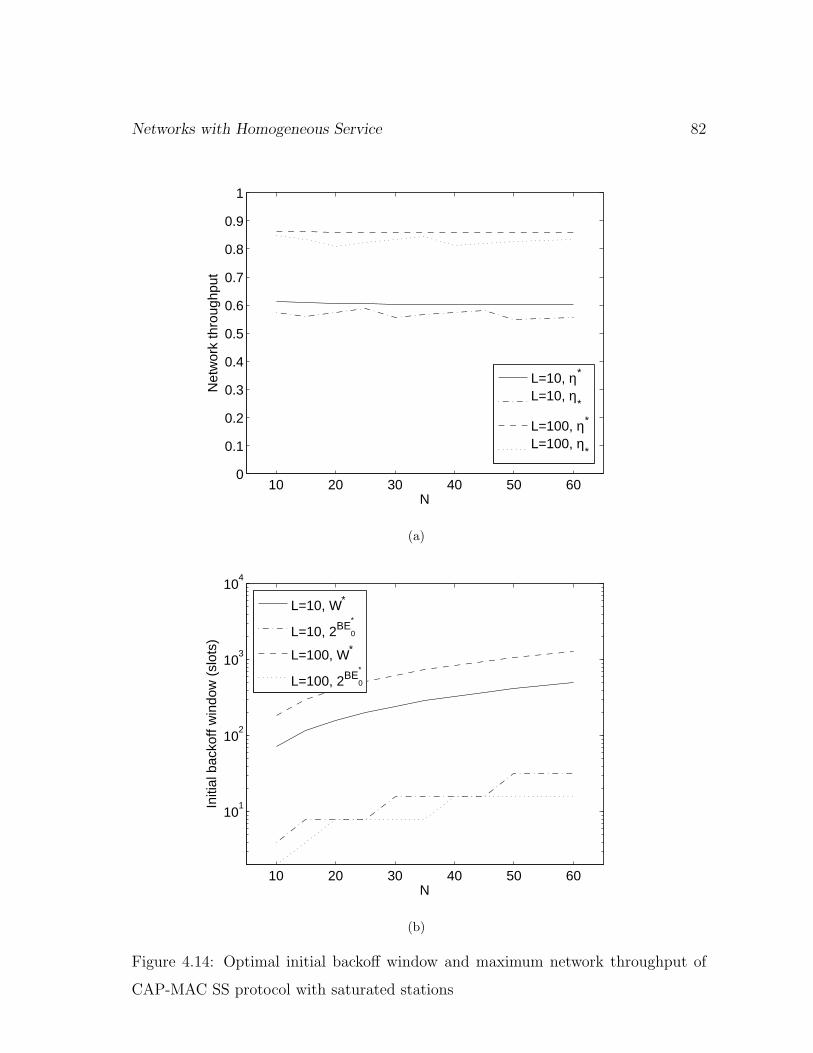
Networks with Homogeneous Service 82
10 20 30 40 50 600
0.1
0.2
0.3
0.4
0.5
0.6
0.7
0.8
0.9
1
N
Net
wor
k th
roug
hput
L=10, η*
L=10, η*
L=100, η*
L=100, η*
(a)
10 20 30 40 50 60
101
102
103
104
N
Initi
al b
acko
ff w
indo
w (
slot
s)
L=10, W*
L=10, 2BE0
*
L=100, W*
L=100, 2BE0
*
(b)
Figure 4.14: Optimal initial backoff window and maximum network throughput of
CAP-MAC SS protocol with saturated stations

Networks with Homogeneous Service 83
4.5.5 Discussion on the Optimization for Unsaturated Sta-
tions
The objective of the optimization in the previous subsection is to maximize the net-
work throughput for saturated stations. For a network with unsaturated stations,
the network throughput is always the given aggregate incoming traffic. Therefore,
the objective of optimization for such a case is naturally switched to minimize the
average frame service time ζ ′, or equivalently, E[Z ′].
Without loss of generality, we take the p-persistent CSMA/CA protocol as an
example to discuss the possible parameter optimization with a given per station traffic
load λ. In this protocol, the adjustable parameter is p and the relationship between
E[Z ′] and p are given by equations (4.9) and (4.14). Nevertheless, it is very difficult, if
not impossible, to give a closed-form solution to these two non-linear equations, which
makes the task of finding the expression for the optimal p that minimizes E[Z ′] even
more challenging. Notice that p is limited over (0, 1), however, we propose to use the
global search algorithm to find the optimal p. For a given λ, the p increases from a
small value close to zero (e.g., 0.001) to a value close to and strictly less than one (e.g.,
0.999) with a small incremental step ∆p = 0.001. In each step, the corresponding
E[Z ′] is calculated by solving numerically the aforementioned two equations and
compared with the recorded E[Z ′]min, which is updated when necessary. With this
global search algorithm, the final E[Z ′]min and its corresponding p∗ can be found
for a given λ. It is possible that some values of p may make the stations saturate.
However, this renders no adverse effect to the algorithm because in such cases the
resulting E[Z] is larger than the final E[Z ′]min.
As an example, Figure 4.15 shows the E[Z ′]min and the corresponding p∗ versus
λ for the case of L = 10 with two different N values (10 and 20). The results show

Networks with Homogeneous Service 84
1 2 3 4 5 6
x 10−3
0
20
40
60
80
100
120
140
λ (frames/slot)
E[Z
(u) ] m
in
L=10
N=10N=20
(a)
1 2 3 4 5 6
x 10−3
0
0.1
0.2
0.3
0.4
0.5
0.6
0.7
0.8
0.9
1
λ (frames/slot)
p*
L=10
N=10N=20
(b)
Figure 4.15: Minimum average frame service time and optimal p for p-persistent
CSMA/CA protocol with unsaturated stations

Networks with Homogeneous Service 85
that when the traffic load is light, the optimal transmission probability should be
set relatively high; with the increase of the traffic load, p∗ decreases almost linearly.
When the traffic load increases close to the sustainable rate, the service time increases
very fast as in Figure 4.3(a) even though the optimal p∗ is used.
Note that the above approach is effectively applicable to both the CAP-MAC
and the DCF protocols with appropriate mapping between the optimal p and the
adjustable parameters such as BEmin and W following the discussion in Section 4.5.2.
Also, the weakness of unable to give a transmission probability equal to the theoretical
optimal still exists in the BEB policies; thus the minimum E[Z ′] achieved by BEB is
slightly larger than the theoretical one.
4.6 Related Work
Being a simple and elegant random access protocol, the p-persistent CSMA/CA pro-
tocol is first analyzed by Kleinrock and Tobagi with the “S-G” technique to obtain
the throughput-delay characteristics for infinite stations in [55]. Its performance in a
network with finite number of stations is studied by the same authors in [97], using
the technique of embedded Markov chain, the computational complexity of which
becomes inhibitive for systems with large station population. After these two classic
papers, there is a long time in which the analysis of this protocol is of very limited
interest to researchers, until it is studied again much later by Cali et al. when they
use p-persistent CSMA/CA as an alternative version of the IEEE 802.11 DCF MAC
protocol in [12] and [13].
In contrast, the wide deployment of IEEE 802.11 DCF based wireless LANs (Wi-Fi
networks) has attracted great interests from researchers. There are numerous work on
the performance study of DCF in terms of throughput and average frame service time,

Networks with Homogeneous Service 86
especially for the saturation case. A well-known one on this topic is first reported
in [5] and further detailed in [6] by Bianchi. The BEB procedure is modeled as a
discrete time two-dimensional Markov chain. The assumption of constant conditional
collision probability of frames regardless of the transmission history is first adopted in
these papers and later justified theoretically by Sharma et al. in [86] by relating it to
the mean-field models in statistical physics. A direct extension of the Markov model
in [6] is proposed by Wu et al. in [110] and Chatzimisios et al. in [18] to take into
consideration the retransmission limit for each frame as specified in the standard.
Along this line, many papers modify the basic Markov model proposed in [6] to
consider some other details of the DCF [15, 104, 19, 31, 7], or adapt the Markov model
to other backoff variants [74, 102, 111]. Cali et al. analyze the p-persistent version of
IEEE 802.11 DCF in [12] and [13], using the concept of virtual transmission time of a
frame. Based on simulation results, they conclude that the maximum throughput is
achieved when the average channel idle time is equal to the average time for collisions,
which is further justified analytically in [10]. Tay and Chua analyze the protocol
behavior from the long term average point of view in [92]. By computing the average
rates of transmission, collision and successful transmission, and utilizing the condition
that all these rates sum up to one, the saturation throughput is obtained. Based on
the analysis, some insights on how to achieve the optimal performance by adjusting
the protocol parameters according to the number of stations are also given in the
paper. Following this direction, Kumar et al. represent the average transmission
attempt rate as the ratio of average transmission times over the average backoff slots,
and calculate it using the fixed point technique [57]. It is also pointed out in this
paper that by using the fixed point equations, the analysis of the Markov chain in
[6] is in fact not necessary. Medepalli and Tobagi extend further this approach to
compute the average cycle time of a frame and the saturation throughput in [66].

Networks with Homogeneous Service 87
The only paper adopts the equilibrium point analysis is [106] by Wang et al., which
requires a computational effort comparable to that of the Markov chain based models.
Another thread of work is to obtain higher moments of the frame service time.
Carvalho and Garcia-Luna-Aceves compute the first two moments of the service time
in [15]. In [123], Zanella and Pellegrini study the statistical characteristics of the
frame service time by means of probability generating function (PGF), considering
directly the distributions of the time of successful transmission, collisions and backoff
slots. In another paper [125], Zhai et al. give the PGF of frame service time using
generalized state transition diagram [81] based on the Markov chain developed in [6].
Vu and Sakurai present a more accurate service time PGF compared with that in
[125] by taking into consideration of the dependence between the number of backoff
slots and the number of transmissions and collisions of the stations [103]. Using a
two-dimensional absorbing discrete time Markov chain, Issariyakul et al. model the
channel access time in DCF as a phase-type distribution in [49], which is numerically
solved by the matrix geometric technique [71].
Recently there are also some papers on the performance of DCF with unsaturated
stations. Among them, Zhai et al. combine the results in [125] with M/G/1 analysis
to calculate the throughput, delay, jitter and packet loss rate for Poisson arrival
traffic [124]. Zaki and EI-Hadidi[122] modified the basic Markov model proposed
in [6] to have a constant state transition time equal to the slot time. Cantieni et
al. [14] proposed another modified Markov model by adding some extra states for
the so-called “post-backoff” procedure. In both papers, M/G/1 queueing analysis
is used to obtain the channel throughput, which may not be directly applicable to
some practical applications such as VoIP over WLAN. The post-backoff states are
also incorporated in the Markov chain developed by Duffy et al. in [25], where the
stations are assumed to buffer one frame only. Similar Markov chain based analytical
Networks with Homogeneous Service 88
models for finite load situation (e.g., [85] ,[130]) have also been proposed, all assuming
specific traffic sources such as Poisson or Bernoulli arrivals. Tikoo and Sikdar [93, 94]
extended the work in [92] to the unsaturation case by considering the MAC sublayer
queue status. It also models each station as a discrete time G/G/1 queue to obtain
the frame delays. Along this thread, Ling et al. propose a more accurate model
in calculating the average frame service time in [135] and use it to obtain the voice
capacity of a DCF based ad hoc mode WLAN.
For the IEEE 802.15.4 MAC protocol considered in this paper, there are several
recent analytical works appeared in the literature. A Markov chain based analyti-
cal model is proposed in [68, 67] to analyze the access delay of uplink transmissions
in an IEEE 802.15.4 beacon enabled PAN of nodes with finite size buffer. Many
details of the protocol are taken into consideration in the model. With the assump-
tion of Poisson arrivals to each node and the use of M/G/1/K queueing model, the
probability generating functions (PGF) of the access delay and packet queue size at
the nodes are derived. In addition, up to date these are the only papers that analyze
comprehensively the performance of 802.15.4 MAC protocol with the complete super-
frame structure. With the assumption that each station’s probability to start sensing
the channel is independent, the Markov model proposed in [76] gives satisfactory
throughput accuracy in the saturated case, where all the nodes always have frames in
their MAC buffers waiting for transmission. A more complicated three-dimensional
Markov chain is proposed in [89], also for the saturated case only. Another Markov
chain based model is presented in [78], and both throughput and power efficiency
are studied. It replaces the uniform distribution with a geometric distribution in the
selection of a random number of slots in each backoff stage, primarily for analytical
tractability. Also, the model limits itself only to a Bernoulli frame arrival process for
the unsaturated case. Both [89] and [78] advocate changing the initialization of CW
Networks with Homogeneous Service 89
to one, i.e., using single sensing instead of double sensing for the collision avoidance
purpose.
Simulation-based studies of the IEEE 802.15.4 protocol have also been reported in
the literature for the studies of delay performance [127], energy efficiency in a dense
wireless mircosensor network [9], a small size star-topology network [65], scalability
issues and the impact of interference from co-existing WLANs in medical environment
(e.g, hospitals) [36]. The only performance evaluation that is based on real hardware
experiments is reported in [58].
4.7 Summary
We have applied the analytical framework proposed in Chapter 3 to analyze three rep-
resentative CSMA/CA based MAC protocols: p-persistent CSMA/CA, IEEE 802.15.4
CAP-MAC and IEEE 802.11 DCF. In each application instance of the framework,
a pair of fixed point equations is obtained by properly deriving the parameters to
capture the features of the specific backoff procedure and channel access policy in the
protocol studied. After the fixed point equations are solved, the MAC throughput
and the average frame service time for an individual station are obtained. The ap-
plications have demonstrated that the proposed framework is a versatile one. It can
be used for networks with saturated or unsaturated stations, and for diverse back-
off policies. The accuracy of the analysis has been verified by extensive simulation
results.
In addition to the analysis of protocols with default parameters given in the stan-
dards, we have also analyzed the the theoretical and practical maximum throughput
for networks with saturated stations. We found that the theoretical maximum net-
work throughputs of the three protocols are very close especially with large L, despite

Networks with Homogeneous Service 90
that the backoff policies are completely different. Besides, in the course of deriving
the optimal values of the adjustable parameters in the three protocols, the limita-
tion of binary exponential backoff is discussed in detail. A backoff scheme with fixed
backoff window for all the backoff stages is found to be more flexible than the BEB,
and is able to approach the theoretical maximum network throughput.
For performance optimization in networks with unsaturated stations, we have
studied the minimum average frame service time and the corresponding optimal trans-
mission probability, taking p-persistent CSMA/CA as an example. The approach
used is easily extensible to the other two protocols, considering the direct mapping
relationship between p and the backoff parameters.

Chapter 5
Networks with Service
Differentiation
In the previous chapter, we have studied the performance of several representative
distributed MAC protocols in networks with homogeneous service. With the increas-
ing popularity of multimedia applications, wireless networks nowadays are more likely
to provide multi-service to users. Accordingly, QoS-aware MAC protocols that can
provision differentiated service to different stations have emerged. For instance, in
order to enhance the QoS provisioning demanded by multimedia services in WLANs,
the recently released IEEE 802.11e [48] defines three service differentiation mech-
anism: contention window (CW), transmission opportunity (TXOP) and arbitrary
interframe space (AIFS). Similar approaches have also been adopted by the Multi-
band OFDM Alliance (MBOA) in its contention based medium access protocol called
prioritized channel access (PCA) [26] for emerging ultra-wideband wireless personal
area networks (WPANs).
Performance evaluation of these mechanisms by means of simulations and theoret-
ical modeling approaches have shown that they are effective in service differentiation
91

Networks with Service Differentiation 92
provisioning. However, the scenarios studied are quite limited, mostly for networks
with saturated stations. To better understand and quantify the effects of these mech-
anisms in a broader range of network situations, in this chapter, we extend the an-
alytical framework for DCF in Chapter 4 to evaluate their performance in networks
with both saturated and unsaturated stations.
The remainder of this chapter is organized as follows. The three mechanisms are
analyzed using the proposed framework one by one in the following three sections. Re-
lated work on the performance study of these mechanisms is discussed in Section 5.4.
The salient features discussed in this chapter are summerized in Section 5.5.
5.1 Service Differentiation with CWs
In this section, the channel busy time caused by frame transmissions from all the
stations are assumed to have the same fixed length of L physical slots, regardless of
the transmission result as a success or collision. The case of different frame lengths
are analyzed in the next section. We derive two key probabilities first, then proceed
to the MAC performance metrics.
5.1.1 Analysis of Saturated Stations
Let γk and βk denote the transmitting probability and the frame collision probability
of a station of class k, respectively1. A frame transmitted by a class k station will
experience a collision only when one or more stations of any class transmit in the
1In this chapter, the terms “class” and “AC” are used interchangeably.

Networks with Service Differentiation 93
same slot. Therefore, we have the frame collision probability for a class k station as
βk = 1 − (1 − γk)Nk−1
K∏
i=1,i6=k
(1 − γi)Ni
= 1 −∏K
i=1(1 − γi)Ni
1 − γk
, k = 1, . . . , K.
(5.1)
Since each station performs its backoff procedure only depending on the transmission
result of its frame, it enters the next backoff stage only when its frame experiences a
collision, which occurs with probability βk. Therefore, similar to the derivation of γ
in (4.54) in Chapter 4, we have the transmitting probability of a class k station given
by
γk =
∑Mk−1i=0 (βk)
i
∑Mk−1i=0 (βk)i(bi,k + 1)
, k = 1, . . . , K, (5.2)
where bi,k = CWi,k/2 is the average number of backoff slots in backoff stage i, i =
0, . . . ,Mk, and Mk is the retry limit of class k stations. Note that the class-dependent
CW parameters have been included in the analysis.
Equations (5.1) and (5.2) can be solved numerically to obtain the transmitting
probability γk and frame collision probability βk for all the classes.
In the network with K classes of stations, the channel is idle when none of the
stations transmit, which occurs with probability
Pidle =K∏
k=1
(1 − γk)Nk . (5.3)
Therefore, the average length of generic slots in this network is
E[GS] = Pidle · 1 + (1 − Pidle) · L
= L − (L − 1)K∏
k=1
(1 − γk)Nk .
(5.4)
Following the reasoning in Section 4.3.1, from the viewpoint of a tagged class k
station, it conducts a Bernoulli experiment in each generic slot with its successful
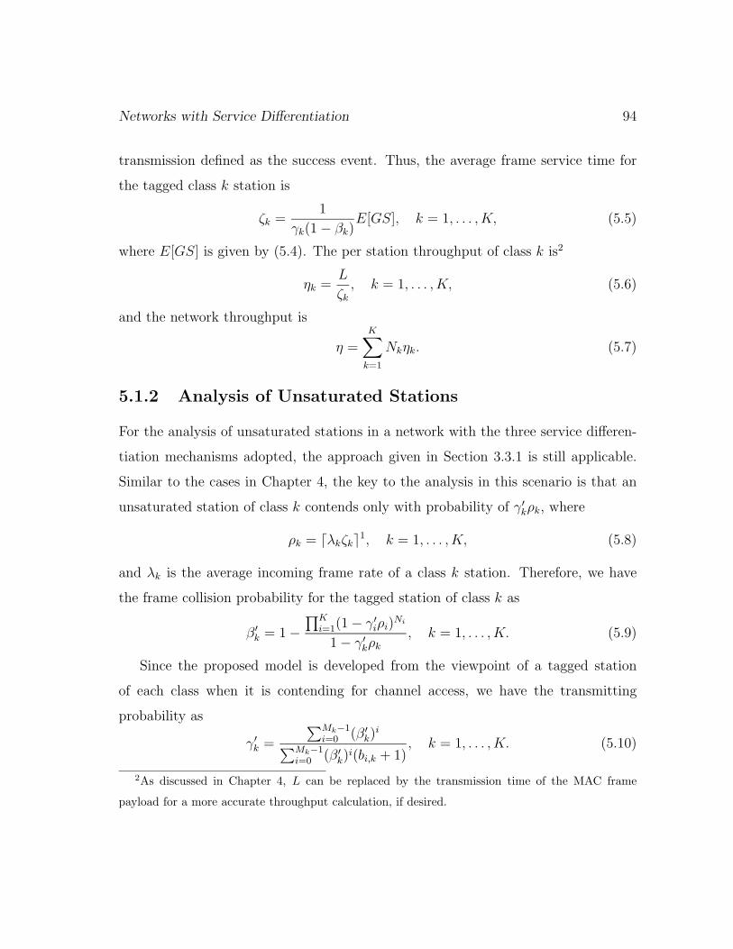
Networks with Service Differentiation 94
transmission defined as the success event. Thus, the average frame service time for
the tagged class k station is
ζk =1
γk(1 − βk)E[GS], k = 1, . . . , K, (5.5)
where E[GS] is given by (5.4). The per station throughput of class k is2
ηk =L
ζk
, k = 1, . . . , K, (5.6)
and the network throughput is
η =K∑
k=1
Nkηk. (5.7)
5.1.2 Analysis of Unsaturated Stations
For the analysis of unsaturated stations in a network with the three service differen-
tiation mechanisms adopted, the approach given in Section 3.3.1 is still applicable.
Similar to the cases in Chapter 4, the key to the analysis in this scenario is that an
unsaturated station of class k contends only with probability of γ′kρk, where
ρk = ⌈λkζk⌉1, k = 1, . . . , K, (5.8)
and λk is the average incoming frame rate of a class k station. Therefore, we have
the frame collision probability for the tagged station of class k as
β′k = 1 −
∏K
i=1(1 − γ′iρi)
Ni
1 − γ′kρk
, k = 1, . . . , K. (5.9)
Since the proposed model is developed from the viewpoint of a tagged station
of each class when it is contending for channel access, we have the transmitting
probability as
γ′k =
∑Mk−1i=0 (β′
k)i
∑Mk−1i=0 (β′
k)i(bi,k + 1)
, k = 1, . . . , K. (5.10)
2As discussed in Chapter 4, L can be replaced by the transmission time of the MAC frame
payload for a more accurate throughput calculation, if desired.

Networks with Service Differentiation 95
In addition, the tagged station of class k contends only with the busy stations from
both its own class and the other classes. Therefore, the channel seen by a class k busy
station is different from that seen by a busy station of another class. Consequently,
the channel idle probability is class-dependent as
P ′idle,s = (1 − γ′
k)(1 − γ′kρk)
Nk−1
K∏
i=1,i6=s
(1 − γ′iρi)
Ni , k = 1, . . . , K. (5.11)
We further have the class-dependent average length of generic slots as
E[GS ′k] = P ′
idle,s · 1 + (1 − P ′idle,k) · L, k = 1, . . . , K, (5.12)
and the average frame service time for the tagged class k station as
ζ ′k =
1
γ′k(1 − β′
k)E[GS ′
k], k = 1, . . . , K. (5.13)
5.1.3 Numerical Results
The differentiation effects of class-dependent CW parameters have been examined by
both analysis and simulations. We take the basic access mode of the IEEE 802.11e as
the example protocol and consider two classes of stations with different CW param-
eters. In the following numerical examples, the frame payload is set to 1,000 bytes.
Other parameters are set as given in Table 4.1 unless explicitly stated.
For saturated stations of both classes, Figure 5.1 shows the average frame service
times for both classes versus the minimum CW (CWmin,1) of class 1 stations while
keeping CWmin,2 = 32 and the maximum CW for both classes as 1024. It can be seen
from Figure 5.1(a) that the average frame service time of class 1 stations (ζ1) does
not change much with CWmin,1, especially when the number of stations in each class
N is small. In contrast, as shown in Figure 5.1(b), the average frame service time
of class 2 stations (ζ2) is obviously affected by CWmin,1, even for a small N . When

Networks with Service Differentiation 96
4 8 16 240
10
20
30
40
50
60
70
CWmin,1
Ave
rage
fram
e se
rvic
e tim
e of
AC
1 (m
s)
CWmin,2
= 32, CWmax
=1024, N1=N2=N
N=5, anaN=5, simN=10, anaN=10, simN=15, anaN=15, sim
(a)
4 8 16 240
50
100
150
200
250
CWmin,1
Ave
rage
fram
e se
rvic
e tim
e of
AC
2 (m
s)
CWmin,2
= 32, CWmax
=1024, N1=N2=N
N=5, anaN=5, simN=10, anaN=10, simN=15, anaN=15, sim
(b)
Figure 5.1: Effect of CWmin,1 on the average frame service times for saturated stations
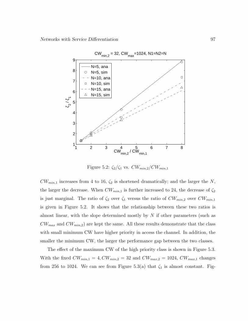
Networks with Service Differentiation 97
1 2 3 4 5 6 7 81
2
3
4
5
6
7
8
9
CWmin,2
/ CWmin,1
ζ 2 / ζ 1
CWmin,2
= 32, CWmax
=1024, N1=N2=N
N=5, anaN=5, simN=10, anaN=10, simN=15, anaN=15, sim
Figure 5.2: ζ2/ζ1 vs. CWmin,2/CWmin,1
CWmin,1 increases from 4 to 16, ζ2 is shortened dramatically; and the larger the N ,
the larger the decrease. When CWmin,1 is further increased to 24, the decrease of ζ2
is just marginal. The ratio of ζ2 over ζ1 versus the ratio of CWmin,2 over CWmin,1
is given in Figure 5.2. It shows that the relationship between these two ratios is
almost linear, with the slope determined mostly by N if other parameters (such as
CWmax and CWmin,2) are kept the same. All these results demonstrate that the class
with small minimum CW have higher priority in access the channel. In addition, the
smaller the minimum CW, the larger the performance gap between the two classes.
The effect of the maximum CW of the high priority class is shown in Figure 5.3.
With the fixed CWmin,1 = 4, CWmin,2 = 32 and CWmax,2 = 1024, CWmax,1 changes
from 256 to 1024. We can see from Figure 5.3(a) that ζ1 is almost constant. Fig-

Networks with Service Differentiation 98
256 512 10245
10
15
20
25
30
35
40
CWmax,1
Ave
rage
fram
e se
rvic
e tim
e of
AC
1 (m
s)
CWmin,1
= 4, CWmax,2
=1024, N1=N2=N
N=5, anaN=5, simN=10, anaN=10, simN=15, anaN=15, sim
(a)
256 512 102480
100
120
140
160
180
200
220
240
260
CWmax,1
Ave
rage
fram
e se
rvic
e tim
e of
AC
2 (m
s)
CWmin,1
= 4, CWmax,2
=1024, N1=N2=N
N=5, anaN=5, simN=10, anaN=10, simN=15, anaN=15, sim
(b)
Figure 5.3: Effect of CWmax,1 on the average frame service times for saturated stations
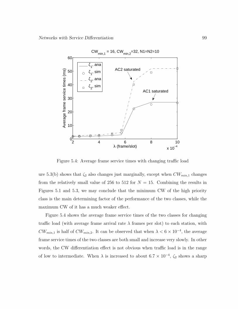
Networks with Service Differentiation 99
2 4 6 8 10
x 10−4
0
10
20
30
40
50
60
λ (frame/slot)
Ave
rage
fram
e se
rvic
e tim
es (
ms)
CWmin,1
= 16, CWmin,2
=32, N1=N2=10
ζ1, ana
ζ1, sim
ζ2, ana
ζ2, sim
AC2 saturated
AC1 saturated
Figure 5.4: Average frame service times with changing traffic load
ure 5.3(b) shows that ζ2 also changes just marginally, except when CWmin,1 changes
from the relatively small value of 256 to 512 for N = 15. Combining the results in
Figures 5.1 and 5.3, we may conclude that the minimum CW of the high priority
class is the main determining factor of the performance of the two classes, while the
maximum CW of it has a much weaker effect.
Figure 5.4 shows the average frame service times of the two classes for changing
traffic load (with average frame arrival rate λ frames per slot) to each station, with
CWmin,1 is half of CWmin,2. It can be observed that when λ < 6 × 10⁻⁴, the average
frame service times of the two classes are both small and increase very slowly. In other
words, the CW differentiation effect is not obvious when traffic load is in the range
of low to intermediate. When λ is increased to about 6.7 × 10⁻⁴, ζ2 shows a sharp

Networks with Service Differentiation 100
increase because class 2 stations become saturated with this load. This phenomenon
is similar to those in Figures 4.3 and 4.9, and the reason is also similar. Interestingly,
ζ1 also experience a remarkable increase, which is due to the severer contention from
class 2 stations resulting from the largely increased ζ2. More interestingly, despite
that class 2 stations have already been saturated, ζ2 further increases with λ until
class 1 stations also become saturated when λ reaches about 8 × 10⁻⁴. The reason
of this further increase is that ζ1 keeps increasing before class 1 stations become
saturated finally, which corresponds to deteriorating contention and longer ζ2; and it
stops only after class 1 stations also become saturated.
From the above, we can see that the service differentiation effect of class-dependent
CW is only obvious when the stations are about to enter the saturation situation,
and it is enforced when the number of high priority class stations becomes larger.
5.2 Service Differentiation with TXOP
With the TXOP service differentiation mechanism, the stations of different classes
may be allowed to transmit different number of frames after one successful chan-
nel access. In effect, this mechanism also includes the cases of allowing stations to
transmit frames of different lengths with the same data rate, or to transmit the same
length of frames with different data rates, or both. The effect of allowing different
TXOPs on the analysis lies in the calculation of the duration of channel busy peri-
ods, which depends on the stations involved in the transmission. Therefore, equations
(5.1) and (5.2) are applicable to the analysis of saturated stations and equations (5.9)
and (5.10) are applicable to the analysis of unsaturated stations.

Networks with Service Differentiation 101
5.2.1 Analysis of Saturated Stations
For notation simplicity, let Lk denote the TXOP assigned to class k stations and also
the duration of channel busy time caused by a transmission from a class k station.
Without loss of generality, assume that L1 ≥ L2 ≥ · · · ≥ LK . Since the stations
start to transmit at the beginning of a generic slot independently, it is not difficult to
obtain the probability of having at least one class k station transmitting in a slot as
φk = 1 − (1 − γk)Nk , k = 1, . . . , K. (5.14)
In the basic access mode, the duration of a channel busy period is determined
by the longest Lk, no matter whether the busy period is caused by a successful
transmission or a collision. Then, the average duration of a randomly chosen channel
busy period can be calculated as
E[L] =K∑
k=1
(Lk · φk
k−1∏
i=1
(1 − φi)). (5.15)
Accordingly, the average length of a generic slot is3
E[GS] = Pidle · 1 + E[L], (5.16)
where Pidle is given in (5.3).
In the RTS/CTS access mode, the duration of channel busy time caused by a
collision is constant (denoted as Lcol) while that caused by a successful transmission
will depend on the transmitting station. In addition, the transmission time of the
RTS/CTS exchange has to be included in the channel busy time L(RTS)k for each
successful transmission from class k stations. Hence, to calculate the average length
of a generic slot, we need the probabilities of having a collision (Pcol) or a successful
3Note that all the probabilities in (5.15) sum up to (1-Pidle).

Networks with Service Differentiation 102
transmission from a class k station (Psuc,k) in a slot, which can be obtained as
Psuc,k = Nkγk(1 − γk)Nk−1
K∏
i=1,i6=s
(1 − γi)Ni , k = 1, . . . , K, (5.17)
Pcol = 1 − Pidle −K∑
k=1
Psuc,k. (5.18)
With the above results, the average length of generic slots in the RTS/CTS mode is
calculated as
E[GS(RTS)] = Pidle · 1 + Pcol · Lcol +K∑
k=1
Psuc,kL(RTS)k . (5.19)
Equations (5.16) and (5.19) can be substituted into (5.6) to obtain the per station
throughput of class k in the basic and the RTS/CTS access mode, respectively. After
that, (5.7) can be used to obtain the corresponding network throughput.
5.2.2 Analysis of Unsaturated Stations
We consider the basic access mode in this subsection to explain the main point of the
analysis. As explained in Section 5.1.2, the channel seen by the tagged busy stations
is class-dependent in a network with unsaturated stations. Thus, from the viewpoint
of a tagged busy station of class k, it sees a slot containing transmission from at least
one class i station with probability
φ′i,k =
1 − (1 − γ′iρi)
Ni−1(1 − γ′i), k = i
1 − (1 − γ′iρi)
Ni , k 6= ik = 1, . . . , K, i = 1, . . . , K. (5.20)

Networks with Service Differentiation 103
Accordingly, we have the class-dependent E[L′k] and the E[GS ′
k] for a tagged busy
station of class k as follows
E[L′k] =
K∑
i=1
(Li · φ′
i,k
i−1∏
j=1
(1 − φ′j,k)
), (5.21)
E[GS ′k] = P ′
idle, k · 1 + E[L′k], (5.22)
where P ′idle, k is given in (5.11). Then, the average frame service time for the tagged
class k station can be obtained according to (5.13).
5.2.3 Numerical Results
To show the net effect of TXOP to saturated stations, the CW parameters for the
two classes of stations are set to the same. In the following numerical results, the
payload size of class 2 stations is 500 bytes, and that of class 1 stations ranges from
1000 to 3000 bytes.
As shown in Figure 5.5(a), the average frame service times (ζ) are almost the same
for the two classes. This is because for saturated stations, the contention behavior is
completely determined by the CW parameters. With the same CW parameters, all
the stations get the same chance in accessing the channel to transmit their frames in
the long run [41]. On the contrary, the per station throughputs (η) of the two classes
are different due to the different payloads they carry. When ζ increases with the
class 1 payload size, η1 increases proportionally while η2 decreases slightly. Note that
with the given payload parameters, the average frame service time in the RTS/CTS
mode is always longer than that in the basic mode, due to the large overhead of
RTS/CTS exchange, especially for the class 2 stations with small payload size (see
Section 4.3.4). Correspondingly, the throughput in the RTS/CTS mode is lower than
that in the basic mode.

Networks with Service Differentiation 104
1000 1500 2000 2500 300025
30
35
40
45
50
55
60
Class 1 payload size (bytes)
Ave
rage
fram
e se
rvic
e tim
e (m
s)
CWmin
= 32, CWmax
=1024, N1=N2=10
basic mode
RTS/CTS mode
(a)
1000 1500 2000 2500 300050
100
150
200
250
300
350
400
450
Class 1 payload size (bytes)
Thr
ough
put (
kbps
) pe
r st
atio
n
CWmin
= 32, CWmax
=1024, N1=N2=10
η1, M1, ana
η1, M1, sim
η2, M1, ana
η2, M1, sim
η1, M2, ana
η1, M2, sim
η2, M2, ana
η2, M2, sim
M1: basic modeM2: RTS/CTS mode
(b)
Figure 5.5: Effect of class 1 payload size for saturated stations

Networks with Service Differentiation 105
2 4 6 8 100
5
10
15
20
25
30
N1
N2 m
ax
CWmin
= 32, CWmax
=1024
G.711−20ms, anaG.711−20ms, simG.711−30ms, anaG.711−30ms, sim
Figure 5.6: Voice capacity with background data traffic
To demonstrate the efficacy of the analytical model for the TXOP, we show the
maximum number of supportable voice sessions N2max (also called voice capacity [11])
in a network with background data traffic from saturated class 1 stations with frame
payload of 1000 bytes. Each class 2 station carries a 64kbps voice session using the
ITU-T G.711 codec [8], the parameters of which is given in Table 5.1. Figure 5.6
shows that the model predicts the voice capacity of the network accurately as verified
Table 5.1: Parameters for the 64kbps ITU-T G.711 Voice Codec
Sample Period (ms) Arrival Rate (frames/sec) Payload (bytes)
20 50 160
30 33.33 240

Networks with Service Differentiation 106
by simulations.
5.3 Service Differentiation with AIFS
With the AIFS mechanism, stations are classified according to their assigned AIFS.
In order to focus on the analysis of this mechanism, the following assumptions are
adopted in this section: 1) stations belonging to the same class have the same CW;
2) all the stations have the same TXOP; and 3) the basic access mode is used by all
the stations, and L denotes the time duration of a channel busy period.
5.3.1 Analysis of Saturated Stations
Due to the different AIFS values assigned, stations of different classes are eligible to
contend for channel access in different zones, as shown in Figure 2.3. More specifi-
cally, a station of class k is eligible to decrease its backoff counter and transmit, if its
backoff counter has been decremented to zero, in zones Zk to ZK , for k = 1, . . . , K.
As a result, stations face different contention situations and experience different frame
collision probabilities in different zones. On the other hand, each station performs
its backoff procedure only depending on the transmission results of its frames trans-
mitted in the eligible zones, i.e., it enters the next backoff stage only when its frame
experiences a collision, which occurs with probability of βk, the mean collision prob-
ability of frames transmitted in any of the eligible zones. Therefore, (5.2) still holds
for stations following the AIFS mechanism, with the above new interpretation of βk.
Then, with the assumption that a station of class k transmits independently with
probability γk in any slot in its eligible zones, we have the following analysis for the
collision probabilities.

Networks with Service Differentiation 107
Frame Collision Probabilities
For a class k station, the collision probability of its transmitted frames in Zone z is
given by
βz,k = 1 −∏z
i=1(1 − γi)Ni
1 − γk
, k = 1, . . . , K, z = k, . . . ,K, (5.23)
where the eligibility for transmission in the zones of the station classes has been taken
into consideration. The probability βz,k’s where z = 1, . . . , k−1 are undefined because
there is no frame transmission from any class k stations in these zones .
In Zone z, a slot is idle when none of the eligible stations transmit. Hence, the
probability that a Zone z slot is idle is
az =z∏
i=1
(1 − γi)Ni , z = 1, . . . , K. (5.24)
For a randomly chosen transmission in the network, it starts in Zone z with probability
πz = (1 − (az)∆z)
z−1∏
i=1
(ai)∆i , z = 1, . . . , K − 1,
πK =K−1∏
i=1
(ai)∆i .
(5.25)
Since a class k station transmits with independent constant probability in its eligible
zones, the average collision probability of its transmitted frames can be obtained as
βk =K∑
z=k
( πz∑K
z=k πz
βz,k
), k = 1, . . . , K, z = k, . . . ,K. (5.26)
Equations (5.2) and (5.23)–(5.26) can be solved numerically to obtain γk and βk
for k = 1, . . . , K. With these probabilities given, we can proceed to obtain the average
frame service time for each station class using either of the two methods introduced
below.
Networks with Service Differentiation 108
Average Frame Service Time (Method 1)
The contention zones caused by the AIFS mechanism raise new challenges to the
analysis of average frame service time for each station class. In this subsection,
we derive the average frame service time based on the analysis of a randomly chosen
transmission in the network and its effects on the backoff counter decrement procedure
and the associated delay of different stations, as Method 1. The other method that
follows the approach in Section 4.3.1 is presented in the next subsection.
Define ∆z = AIFSNz+1 − AIFSNz, z = 1, . . . , K − 1 as the length of Zone z in
units of slots in Figure 2.3, which is also the number of idle slots for which a class z+1
station has to wait more than a class z station does before it is eligible to decrement
the backoff counter or transmit. Given a transmission starts in any of the ∆z slots of
Zone z, z = 1, . . . , K − 1, the transmission may start at the first slot with probability
1 − az, at the second slot with probability az(1 − az), and so on. Therefore, for such
a transmission, the average number of generic slots spent in Zone z is
E[Oz] =(1 − az) · 1 + az(1 − az) · 2 + · · · + a∆z−1
z (1 − az) · ∆z
1 − (az)∆z
=
∑∆z−1i=0 (az)
i − ∆z(az)∆z
1 − (az)∆z
, z = 1, . . . , K − 1.
(5.27)
Thus, the corresponding time spent in Zone z can be obtained as
E[Dz] =(1 − az) · (0 + L) + az(1 − az) · (1 + L)
1 − (az)∆z
+ · · ·
+(az)∆z−1(1 − az) ·
((∆z − 1) + L
)
1 − (az)∆z
=(1 − az)
∑∆z−1i=1 i(az)
i + (1 − (az)∆z)L
1 − (az)∆z
, z = 1, . . . , K − 1.
(5.28)
For Zone K (i.e., the last zone), the number of slots spent in it is simply given by
E[OK ] =1
1 − aK
, (5.29)
Networks with Service Differentiation 109
because it follows the geometric distribution with parameter aK and the transmission
must occur in Zone K if the previous zones have been passed idly. Accordingly, the
time spent in Zone K is
E[DK ] = (1
1 − aK
− 1) + L. (5.30)
Note that if a transmission occurs in Zone z, the (possibly existing) preceding
zones are all idle4. Hence, a station of class k can deduct the average value of
E[Oz,k] =
∑z−1i=k ∆i + E[Oz], z = 1, . . . , K, k = 1, . . . , z
0, z = 1, . . . , K, k > z. (5.31)
from its backoff counter for a transmission occurring in Zone z. In contrast, the
corresponding average time cost associated to this transmission is the same for stations
of all the classes, as given by
E[Dz,k] = E[Dz] =z−1∑
i=1
∆i · 1 + E[Dz], z = 1, . . . , K, k = 1, . . . , K. (5.32)
Therefore, for a randomly chosen transmission in the network, a class k station may
deduct its backoff counter by the average value of
E[Ok] =K∑
z=1
πz · E[Oz,k], k = 1, . . . , K, (5.33)
and spends a time period with average duration of
E[Dk] =K∑
z=1
πz · E[Dz], k = 1, . . . , K. (5.34)
Define such a randomly chosen transmission in the network as a virtual backoff event
for all the stations. A class k station spends an average of E[Zk] =∑Mk−1
i=0 βik(bi,k +1)
4This is not applicable to z = 1 because the channel idle time in AIFS1 is included in the
calculation of L for each channel busy period.

Networks with Service Differentiation 110
����������������
������������
������������
������������
������������
������������
������������
segmentbackoff
Z2
...PBOW
PBOW: pre−backoff waitingAIFS1 channel busy period
...PBOW...
...
PBOW
...
time
AIFS2
Z1
AIFS2
Z1
������������
������������
������������
������������
AIFS2
Z1
Figure 5.7: Illustration of the backoff segments and pre-backoff waiting periods for a
class 2 station
backoff slots for one frame5, as given in (5.2). According to the above, for a class k
station, it takes (E[Zk]/E[Ok]) virtual backoff events for it to finish the the E[Z]
backoff slots, on average. In each such virtual backoff event, the station spends a
time period with duration of E[Dk]. Therefore, the average frame service time of a
class k station is given by
ζk =
∑Mk−1i=0 (βk)
i(bi,k + 1)
E[Ok]E[Dk], k = 1, . . . , K. (5.35)
The above ζk can be substituted into (5.6) to obtain the per station throughput of
class k, and further into (5.7) for the corresponding network throughput.
Average Frame Service Time (Method 2)
In this method, the average frame service time of a class k station is decomposed
into two parts: the pre-backoff waiting time and the backoff time. Define one backoff
segment of a class k station as the period from it begins to decrement the backoff
counter in the first eligible zone to the end of this decrement procedure caused by a
transmission from any station, as illustrated in Figure 5.7. For each backoff segment,
there may be zero or more pre-backoff waiting periods preceding it, the number of
5Note that the generic slots used for transmitting the frame are included in E[Zk].
Networks with Service Differentiation 111
which is a random variable. Based on the above main understanding, we take a
network with two classes of stations as an example to present the essence of this
method as below.
As the high priority class station, the tagged class 1 station involves the contention
in both Zone 1 and Zone 2. Therefore, it experiences no pre-backoff waiting periods.
Among the average E[Z1] generic slots it spends for one frame, approximately E[Z1]π1
are in Zone 1 and E[Z1]π2 are in Zone 2. The average length of a generic slot in Zone z
can be computed as
E[GSz] = az · 1 + (1 − az) · L, z = 1, 2, (5.36)
where az is the probabilities of the channel being idle in Zone z, as given by (5.24).
Then, the average frame service time for AC1 is given by
ζ1 = E[Z1](π1E[GS1] + π2E[GS2]
)(5.37)
The frame service time of the tagged class 2 station contains two parts, as ex-
plained earlier. The backoff time that it spends in Zone 2 is given by
ξ = E[Z2]E[GS2]. (5.38)
The pre-backoff waiting time can derived as follows. As shown in Fig. 5.7, when the
tagged class 2 station is backing off in Zone 2, the backoff procedure is interrupted
when any station transmits, which occurs with probability 1 − a2. Therefore, the
backoff procedure of total E[Z2] slots is divided into E[Z2](1− a2) segments. In each
segment, only when there are M consecutive idle slots (i.e., an idle Zone 1) after
the end of a channel busy period can the class 2 stations start their backoff counter
decrementing procedure. This occurs with probability equal to π2. With probability
π1, one or more class 1 stations may transmit in any of the slot in Zone 1 and the
Networks with Service Differentiation 112
current uncompleted Zone 1 is ended immediately by this transmission. Therefore, for
the tagged class 2 station, there are 1/π2 such pre-backoff waiting periods preceding
each of its backoff segment, on average. The mean length of the pre-backoff waiting
periods is E[D1] given by (5.28). Thus, the total time spent in such pre-backoff
waiting periods by the tagged class 2 station is given by
ω = E[Z2](1 − a2)E[D1]
π2
. (5.39)
Summing up the two parts given in (5.38) and (5.39), we obtain the average frame
service time for the tagged class 2 station as
ζ2 = ξ + ω. (5.40)
In the above example, only two contention zones are involved so the time of backoff
segments for class 1 stations and that of pre-backoff waiting periods for class 2 are
relatively simple to calculate. In a network with more than two classes, for a station
of class k with k > 2, the pre-backoff waiting periods are of k−1 types, each of which
covers different number of contention zones. In addition, for a station of class k with
k > 1, each backoff segment may cover more than one contention zones. These factors
make the analysis with Method 2 much more complicated as compared to Method 1.
Therefore, Method 1 is recommended in obtaining the average frame service time for
the stations.

Networks with Service Differentiation 113
5.3.2 Analysis of Unsaturated Stations
Following the approach used for the analysis of the previous two mechanisms, we have
the following equations for unsaturated stations
β′z,k = 1 −
∏z
i=1(1 − γ′iρi)
Ni
1 − γ′kρk
, k = 1, . . . , K, z = k, . . . ,K, (5.41)
β′k =
K∑
z=k
( π′z,k∑K
z=k π′z,k
β′z,k
), k = 1, . . . , K, z = k, . . . ,K, (5.42)
γ′k =
∑Mk−1i=0 (β′
k)i
∑M−1i=0 (β′
k)i(bi,k + 1)
, k = 1, . . . , K (5.43)
a′z,k =
(1 − γ′k)(1 − γ′
kρk)Nk−1
∏z
i=1,i6=s(1 − γ′iρi)
Ni , z = 1, . . . , K, k = 1, . . . , z,
∏z
i=1(1 − γ′iρi)
Ni , z = 1, . . . , K, k = min(z + 1, K − 1), . . . , K − 1,
(5.44)
π′z,k = (1 − (a′
z,k)∆z)
z−1∏
i=1
(a′i,k)
∆i , z = 1, . . . , K − 1, k = 1, . . . , K, (5.45)
π′K,k =
K−1∏
i=1
(a′i,k)
∆i , k = 1, . . . , K. (5.46)
With the above results of a′z,k and πz,k, each tagged busy station of class k can obtain
a set of class-dependent equations as the counterparts of (5.33)–(5.35) in Method 1.
All these equations can then be solved jointly to obtain the average frame service
time for each station class.
5.3.3 Numerical Results
The net effect of class-dependent AIFS on service differentiation is examined in this
subsection. For all the station classes, CWmin = 32, CWmax = 1024 and the MAC
frame payload size is 1000 bytes.

Networks with Service Differentiation 114
First, a network with three station classes and 5 saturated stations in each class is
considered. The difference between the AIFS of the first two classes is fixed as ∆1 = 1.
Figure 5.8 shows the average frame service time (ζ’s) and the throughput (η’s) versus
∆2, the difference between the AIFS of class 2 and class 3. When ∆2 increases
from 1 to 6, ζ3 increases almost exponentially while ζ1 almost keeps constant and ζ2
decreases slightly6. Correspondingly, η3 decreases exponentially while ζ1 almost keeps
constant and ζ2 have a slight increase. This shows that ∆2 affects mainly the class 3
stations, because it determines the length of Zone 2 which delays the backoff counter
decrement procedure and the channel access of class 3 stations only. A large ∆2
gives class 3 stations little chance to start the backoff counter decrement procedure.
On the contrary, a longer Zone 2 gives class 1 and class 2 stations more chance to
contend just between these two classes, which renders a better successful transmission
probability than that in Zone 3 where class 3 stations join the contention. Compared
with class 2 stations, however, class 1 stations can further backoff and access the
channel in Zone 1, which is even less crowded than Zone 2. Hence, the length of
Zone 2 (∆2) has much smaller effect on the class 1 stations than on the class 2 ones.
With ∆1 = ∆2 = 2, Figure 5.9 shows the effect of N , the number of saturated
stations in each class, on the perceived performance of each class. As N increases,
the performance of all the stations degrades (i.e., longer average frame service time
and lower throughput), due to the severer contention in channel access. Moreover,
the performance gaps among the classes increases with N . This is because a larger N
means more higher priority stations contend and succeed in accessing the channel in
the zone(s) where the lower priority stations are ineligible to contend, which causes
longer pre-backoff waiting time to lower priority stations. In addition, class 3 stations,
having the lowest priority in channel access, are more sensitive to N than stations in
6Note the log-scale of the y-axis in the figure.

Networks with Service Differentiation 115
the other two classes.
The effect of AIFS for unsaturated stations is also studied. Two classes with the
difference between their AIFS as ∆ = 1 are considered, and there are 10 stations in
each class. Figure 5.10 shows the average frame service time (ζ) of the two classes
changing with the incoming traffic on each station (λ frames per slot). When λ is
smaller than about 6.2 × 10⁻⁴, both classes are unsaturated; and the smaller the λ,
the smaller the performance gap between the two classes. After the class 2 stations
become saturated at λ = 6.3 × 10⁻⁴, ζ1 has a slow but steady increase with λ until
class 1 stations also become saturated when λ reaches around 7.6× 10⁻⁴. Therefore,
ζ2 still increases accordingly because the service time for low priority stations is
still affected by the increasing ζ1 in this area. Comparing Figures 5.4 and 5.10, we
observe that the service differentiation effect of ∆ = 1 is roughly the same as having
the CWmin halved. As ∆ = 1 is the minimum possible difference between AIFS while
the ratios of CWmin among the classes can be fine-tuned, one may conclude that
the service differentiation effect of AIFS mechanism is coarser than that of the CW
mechanism.
5.4 Related Work
The three main service differentiation mechanisms discussed above were proposed and
evaluated by means of simulation in [1]. Performance studies of one or more of the
three mechanisms by simulations have also been reported in [38, 39, 63, 22, 116, 73].
Test-bed based experimental evaluation of the IEEE 802.11e protocol is reported
in [72]. All these studies demonstrate the diverse effectiveness of service differentiation
provided by the three mechanisms.
In the literature, two main techniques have been used to analyze the performance

Networks with Service Differentiation 116
1 2 3 4 5 610
1
102
103
∆2
Ave
rage
fram
e se
rvic
e tim
e (m
s)
∆1=1
AC1, ana
AC1, sim
AC2, ana
AC2, sim
AC3, ana
AC3, sim
(a)
1 2 3 4 5 610
1
102
103
∆2
Ave
rage
per
sta
tion
thro
ughp
ut (
kbps
)
∆1=1
AC1, ana
AC1, sim
AC2, ana
AC2, sim
AC3, ana
AC3, sim
(b)
Figure 5.8: Effects of AIFS for saturated stations

Networks with Service Differentiation 117
2 4 6 8 10 12 140
100
200
300
400
500
600
700
800
900
1000
Number of stations in each class
Ave
rage
fram
e se
rvic
e tim
e (m
s)
∆1=2, ∆
2=2
AC1, ana
AC1, sim
AC2, ana
AC2, sim
AC3, ana
AC3, sim
(a)
2 4 6 8 10 12 140
200
400
600
800
1000
1200
1400
Number of stations in each class
Ave
rage
per
sta
tion
thro
ughp
ut (
kbps
)
∆1=2, ∆
2=2
AC1, ana
AC1, sim
AC2, ana
AC2, sim
AC3, ana
AC3, sim
(b)
Figure 5.9: Effects of N for saturated stations

Networks with Service Differentiation 118
5 5.5 6 6.5 7 7.5 8
x 10−4
0
5
10
15
20
25
30
35
40
45
50
λ (frame/slot)
Mea
n fr
ame
serv
ice
time
(ms)
∆=1
AC1, ana
AC1, sim
AC2, ana
AC2, sim
AC2
saturatedAC
1saturated
Figure 5.10: Average frame service time with changing traffic load
of these service differentiation mechanisms. The discrete time Markov chain widely
used in modeling the DCF has been extended to study the performance of EDCA and
PCA. Setting up a two-dimension (2-D) Markov chain for stations of each class, the
differentiation effect of CW is studied in [77]. Similar 2-D Markov models also appear
in [40, 43] for the same topic. A three-dimensional Markov chain is used in [113, 112,
117, 115], where the third dimension represents the station classes. Effects of three
backoff related parameters (initial window size, retry limit and the backoff increasing
factor) on saturation throughput and delay are studied. The same 3-D Markov model
is used in [129] to study the effects of TXOP. The effects of AIFS, however, are not
investigated in all the above papers. The contention in different zones delimitated
by AIFS is analyzed and the network throughput is given in [82], again with a 2-

Networks with Service Differentiation 119
D Markov chain for each station class. A three-dimensional Markov chain different
from the one in [113] is developed in [126] to obtain the saturation throughput, where
the third dimension represents the remaining idle slots before the backoff counter
decrements as required by the AIFS of a station. A similar model is used in [61] to
analyze a network with only two classes of stations. In [56], another three-dimension
Markov chain is developed to describe the protocol behavior and a recursive method
is proposed to compute the mean access delay. In [118], a multi-dimensional Markov
chain model is proposed for throughput and delay analysis. As the dimension equals
the number of stations in the network and each dimension represents the backoff
counter value of a station, the state space of the multi-dimensional Markov chain is
huge even for a moderate number of stations, and the computational complexity to
solve the model is prohibitively high.
Another technique is to approximate the system dynamics by mean value analysis,
which is applied in [62] to derive the network saturation throughput. Due to the
specific approach of handling the extra delay to low priority stations caused by longer
AIFS, the model in [62] is applicable only to the case of small difference in AIFS’ of
the station classes. In [44], the station transmission probabilities are obtained from
both mean value analysis and multiple two-dimension Markov chain analysis; then the
network throughput and frame service time are derived. In [42], the PCA is analyzed
using the similar approach introduced in [44], and only throughput is given.
All of the above papers study the saturated situation case only. The common
procedure in these models is that the network saturation throughput is obtained
first, usually from the analysis of a typical transmission in the network. Then the
per station saturation throughput is derived according to the proportional sharing of
network throughput among the stations. Finally, the average frame service time is
given as the reciprocal of the per station throughput. However, the last step cannot be

Networks with Service Differentiation 120
applied to unsaturated stations, as have been explained in Section 4.1.2. Therefore,
even if the per station throughput were known (same as the given incoming traffic
load), the frame service time would be very difficult, if not impossible, to obtain
with those models. This is the main obstacle in extending those previously reported
models to the unsaturated station case.
Recently, the analysis of EDCA with unsaturated stations has been reported in
[27] and its follow-up series [28, 29], which extend the three-dimensional Markov
model [117] for saturated stations by adding a set of states with no frame to trans-
mit. The frame service time for low priority stations is underestimated due to the
overly simplified calculation of blocking delay in the AIFS periods caused by higher
priority stations. Moreover, only “extreme non-saturation condition” is considered in
the service time analysis for unsaturated stations, which leads to a seriously flawed
estimation of the key parameter (queue utilization factor) of the model and further
undermines its accuracy.
5.5 Summary
In this chapter, we have proposed a novel analytical model for EDCA-like service
differentiation MAC protocols unified for both saturated and unsaturated stations.
We model the backoff and channel access behavior of a tagged station in each class,
and obtain their respective average frame service time. Based on this result, satura-
tion throughput of individual station is derived. The wide applicability of the model
enables us to understand the different effects of the same prioritizing mechanisms in
saturated and unsaturated conditions. In addition, the analysis of all the three main
service differentiation mechanisms are naturally integrated into this model.
The numerical results show that the service differentiation effects of the three

Networks with Service Differentiation 121
mechanisms are effective especially in a network with saturated stations. Their effects
are not so obvious when the traffic load in the network is light and most of the stations
are far from saturated. Basically, in the CW mechanism, the minimum CW of each
class has a larger effect than the maximum CW when the latter is sufficiently large.
Also, the CW mechanism may achieve fine-tuning in service differentiation due to the
small granularity of the CW parameter. The TXOP mechanism, if used alone, does
not provide differentiation in the chance of channel access, but it does yields different
throughput for different classes. The AIFS parameters in the AIFS mechanism has
a very strong effect of service differentiation, especially for the lower priority classes.
Due to the nature of the AIFS parameter, the smallest possible change of it is one
slot. However, an increase of just one slot in the AIFS of a low priority class will cause
significant performance degradation to this class and the lower priority ones, but has
much smaller effect on the higher priority classes. Compared to the CW mechanism,
the AIFS mechanism usually has a much larger granularity in service differentiation
among the classes. In general, the three mechanisms may be combined together to
achieve the desired level of service differentiation effectively and efficiently.
Chapter 6
Conclusions and Future Work
In this chapter, we summarize the major research contributions of this thesis, and
propose future work.
6.1 Major Research Contributions
In this thesis, we have proposed a simple but accurate generic performance analysis
framework for a family of CSMA/CA based distributed MAC protocols and applied
it to analyze the performance of several popular MAC protocols in wireless networks
with homogeneous service and with service differentiation. Any CSMA/CA based
distributed MAC protocols can be analyzed with the proposed framework, as long
as the backoff and channel access policies are the same for each MAC frame. More
specifically, the main contributions of this thesis are
• A generic performance analysis framework for CSMA/CA based distributed
MAC protocols : Developed from the perspective of a tagged station (of each
class), the generic performance framework focuses on modeling the backoff pro-
cedure and the channel access behavior and setting up a set of fixed point
122

Conclusions and Future Work 123
equations for the key element in the analysis of CSMA/CA based protocols, the
probability of channel accessing of an individual station. Based on this key vari-
able, two important MAC performance metrics, average frame service time and
the per station throughput are derived from a novel three-level renewal process.
The proposed generic framework is applicable to a family of CSMA/CA based
distributed MAC protocols regardless of the details of the backoff procedure,
the channel access policy and the arrival traffic. First, the backoff procedure
may be memoryless (as the geometric backoff in the p-persistent CSMA/CA
protocol), and the counting down of the backoff counter may depend on the
channel status (as in the IEEE 802.11 DCF), or not (as in the IEEE 802.15.4
CAP-MAC). Secondly, the station may access the channel immediately or one
time slot after one successful channel sensing, or after two successful channel
sensing events, or even more. Finally, for unsaturated stations, traffic arrival
distribution can be general, instead of being limited to Bernoulli or Poisson
arrivals as assumed in most previous works.
• A unified performance modeling approach for both saturated and unsaturated sta-
tions : Most previously reported performance analysis models follow the path of
setting up a model to derive the system throughput, obtaining the per station
throughput based on the proportional sharing of resource among the stations,
and then the average frame service time for each station. Such a path is vi-
able for networks with saturated stations. However, it is not applicable to
networks with unsaturated stations or with mixed saturated and unsaturated
stations because it is impossible to derive the average frame service time from
the throughput of an unsaturated station. The modeling approach in this thesis
takes the opposite way by focusing on obtaining the average frame service time,
which is the key performance metric for networks with both unsaturated and

Conclusions and Future Work 124
saturated stations. With this result, the per station throughput and system
throughput for networks with saturated stations are straightforwardly derived.
Therefore, the modeling approach is unified for networks with saturated and/or
unsaturated stations. This unification of modeling helps in studying, within
one framework, the protocol performance under a broad range of traffic load,
especially in the transition stage where stations change from unsaturation to
saturation. Using this unified approach, the capacity region of a network with
regard to given applications can be obtained, which is the most important in-
formation needed by the call admission control scheme to guarantee satisfactory
QoS provisioning to end users.
• Insights into three representative distributed MAC protocols : The performance
of three popular distributed MAC protocols — p-persistent CSMA/CA, the
IEEE 802.15.4 CAP-MAC and the IEEE 802.11 DCF — in a network with ho-
mogeneous service have been analyzed and compared with the proposed frame-
work. By studying the saturation throughput, we show the mutual-convertible
relationship between the p-persistent CSMA/CA protocol and the IEEE 802.11
DCF. We found that the saturation throughput of the three protocols are very
close to each other when N and L are large. In addition, we pointed out that, for
the CAP-MAC, the double-sensing mechanism can achieve the same maximum
saturation throughput as the single-sensing mechanism does, although the for-
mer gives a lower saturation throughput with a variety of protocol parameters,
especially the default parameters given in the standard. The limitation of the
widely used binary exponential backoff has also been discussed in detail.
• Simple and elegant performance analysis of prevalent service differentiation
mechanisms : Assigning class dependent minimum contention window (CW)

Conclusions and Future Work 125
size, transmission opportunity (TXOP) and arbitration inter-frame space (AIFS)
to stations of different classes are the three main service differentiation mech-
anisms used in current WLANs and WPANs. The proposed analytical frame-
work is naturally extended to study the effects of CW and TXOP, because of
the station-centric modeling approach used. Two novel concepts, virtual back-
off events and pre-backoff waiting periods, have been introduced in the more
challenging analysis of the effects of AIFS. These two concepts directly reflect
the essential service differentiation effect of AIFS (delay the channel access of
lower priority class stations) from two different aspects, which make the analysis
much simpler and easier to follow than those in other models. The analysis of
the three mechanisms show that although all of them can provide service dif-
ferentiation to stations of different classes, the AIFS mechanism gives a coarser
differentiation effect than the CW mechanism, and the TXOP alone just gives
throughput differentiation. It is favorable to jointly use the three mechanisms
to achieve an effective and efficient service differentiation effect in a network.
An immediate application of the above extended framework is to analyze
a network with heterogeneous traffic among the stations even though a non-
differentiation MAC protocol is used, e.g., a WLAN with an access point (AP)
serving as a gateway to the outside networks and many mobile nodes (MNs)
carrying different applications within the WLAN.
6.2 Future Work
The research work in this thesis focuses on the performance analysis of distributed
MAC protocols in single-hop wireless networks. The following relevant research topics
are of importance and deserve further investigation:

Conclusions and Future Work 126
• Closed-form solution to the proposed analytical model : In the current work, the
two important MAC performance metrics — average frame service time and
per station throughput — are obtained from the proposed analytical model by
numerical methods. It is desirable to find a closed-form solution to a (proba-
bly) simplified analytical model, so that optimization of the parameters can be
performed with methods other than the exhaustive search used in this work.
In addition, a sensitivity analysis of each parameter may be conducted. Such
results will be helpful in the design of a relatively simple, implementable, dy-
namic/adaptive tuning scheme of the MAC parameters according to the required
QoS level of various services coming from upper layers.
• Cross-layer design for QoS Provisioning : Most modern wireless networks, in-
cluding WLANs and WPANs, are required to support multimedia applications
with diverse QoS requirements. One typical QoS requirements is the effective
bandwidth [53] of a bursty traffic with variable data rate [84]. The QoS anal-
ysis and flow (or call) level capacity planning in wireless networks is in fact a
cross-layer problem, in which the effective bandwidth required by the network
layer of QoS guarantee needs to be provisioned by the MAC layer with the help
of call admission control (CAC) [21, 100]. Our proposed analytical model uni-
fied for both saturated and unsaturated stations is an indispensable element in
the cross-layer analytical framework. The MAC service time statistics obtained
from the proposed model can be used by the queueing analysis at the network
layer to predict the performance of both the existing and the newly arrived
flows, and the proper admission control decision can be made to guarantee the
QoS requirements of all the admitted flows. Such a cross-layer design framework
is an interesting and challenging topic.
Conclusions and Future Work 127
• Performance model for multi-hop wireless networks: The wireless networks con-
sidered in this thesis are single-hop networks in which all the stations are within
the transmission ranges of one another and the carrier sensing result is the
same for all the stations at a given time. The situation is different in multi-
hop wireless networks such as the emerging wireless mesh networks [30, 59]
and vehicular networks [99, 121], where the carrier sensing results are location
dependent. The resulting hidden-terminal problem [96] degrades significantly
the performance of CSMA/CA based MAC protocols in multi-hop wireless net-
works. Since the DCF and EDCA have been naturally used in multi-hop wireless
networks [105, 3, 20] due to their success in WLANs, it is important to ana-
lyze their performance taking into consideration the hidden-terminal problem
and other issues such as the effects of routing schemes on the traffic load on
stations along a path [33]. How to extend the proposed model to analyze the
performance of such protocols in multi-hop networks needs more investigation.

Abbreviations and Symbols
Abbreviations
AC access category
ACK acknowledgement
AIFS arbitration interframe space
AP access point
BO backoff
BE backoff exponent
CAC call admission control
CAP contention access period
CCA channel clear assessment
CDMA code division multiple access
CFP contention free period
CSMA carrier sense multiple access
CSMA/CA carrier sense multiple access with collision avoidance
CTS clear to send
CW contention window
128

ABBREVIATIONS AND SYMBOLS 129
DCF distributed coordination function
DIFS DCF interframe space
DS double sensing
EPA equilibrium point analysis
EDCA enhanced distributed channel access
GS generic slot
GTS guaranteed time slot
MAC medium access control
MIMO multiple in put multiple output
NACK negative acknowledgement
NAV network allocation vector
OFDM orthogonal frequency division multiplex
OFDMA orthogonal frequency division multiple access
PCF point coordination function
PCS physical carrier sense
PSI possible station idle period
QoS quality of service
RTS request to send
SIFS short interframe space
SS single sensing
TXOP transmission opportunity
VCS virtual carrier sense
WiMAX worldwide interoperability for microwave access
WLAN wireless local area network

ABBREVIATIONS AND SYMBOLS 130
WMAN wireless metropolitan area network
WPAN wireless personal area network
Main Symbols
Dz the time spent in zone z of a randomly chosen transmission
H the number of transmission trials for a frame
K the number of station classes in a network with service differentiation
L the channel busy period in units of slots caused by a frame, the
associated ACK/NACK transmission and the interframe spaces
M the frame transmission retry limit in CAP-MAC and DCF
Mk the frame transmission retry limit for class k stations
N the number of stations in a network with homogeneous service
Nk the number of stations in class k in a network with K station classes
Oz the number of generic slots spent in zone z of a randomly chosen
transmission
p transmitting probability in the p-persistent CSMA/CA protocol
Pb the probability that the channel is busy
Pcol the probability of a collision in the channel
Pi the probability that a channel is idle
Pidle the probability that a generic slot is idle
Psuc the probability of a Y cycle is of type Y2
Psuc,k the probability of a successful transmission from a class k station
Ptx the probability of a X cycle is of type X2

ABBREVIATIONS AND SYMBOLS 131
R the random number of transmission trials for a frame
W (CW0) the minimum contention window
W the fixed contention window size
X level-one renewal cycle
X1 level-one cycle with transmission from other stations
X2 level-two cycle with transmission from the tagged station
Y level-two renewal cycle
Y1 level-two cycle with a collision involving the tagged station
Y2 level-two cycle with a successful transmission from the tagged station
Z level-three renewal cycle
bm the average number of backoff slots in backoff stage m
∆z the length of zone z in units of slots
α the channel sensing failure probability in CAP-MAC
β the conditional frame collision probability in DCF
ηs the throughput of an individual station
η the network throughput
γ the transmission probability of a tagged station in DCF
λ the frame arrival rate in units of frame per slot
ω the number of total backoff slots for a frame in DCF
πz the probability of a randomly chosen transmission starting in zone z
φk the probability that a class k station transmits
ρ the probability of having an empty MAC buffer of a station
τ the transmitting probability of a frame in CAP-MAC
ζ average frame service time

ABBREVIATIONS AND SYMBOLS 132
(d) the superscript indicating variables for the DS case in CAP-MAC
∗ the superscript indicating the optimal value of a variable
′ the superscript indicating variables for unsaturated stations

Bibliography
[1] I. Aad and C. Castelluccia. Differentiation mechanisms for IEEE 802.11. In
Proc. IEEE INFOCOM’01, pages 209–218, 2001.
[2] N. Abramson. The ALOHA System–Another Alternative for Computer Com-
munications. In Proc. 1970 Fall Joint Comput. Conf. AFIPS Conf., pages
281–285, 1970.
[3] Y. Barowski, S. Biaz, and P. Agrawal. Towards the performance analysis of
IEEE 802.11 in multi-hop ad-hoc networks. In Proc. IEEE WCNC’05, pages
100–106, 2005.
[4] D. Bertsekas and R. Gallager. Data Networks. Prentice Hall, 2nd edition, 1992.
[5] G. Bianchi. IEEE 802.11: saturation throughput analysis. IEEE Commun.
Lett., 2(12):318–320, 1998.
[6] G. Bianchi. Performance analysis of the IEEE 802.11 distributed coordination
function. IEEE J. Select. Areas Commun., 18(3):535–547, Mar. 2000.
[7] G. Bianchi and I. Tinnirello. Remarks on IEEE 802.11 DCF performance anal-
ysis. IEEE Commun. Lett., 9(8):765–767, Aug. 2005.
[8] U. Black. Voice Over IP. Prentice Hall, 2nd edition, 2001.
133

Biblography 134
[9] B. Bougard et al. Energy efficiency of the IEEE 802.15.4 standard in dense
wireless microsensor networks: modeling and imporovement perspectives. In
Proc. Design Automation and Test in Europe Conference and Exhibition, pages
196 – 201, Mar. 2005.
[10] R. Bruno, M. Conti, and E. Gregori. Optimal capacity of p-persistent CSMA
protocols. IEEE Commun. Lett., 7(3):139–141, 2003.
[11] L. X. Cai, X. Shen, J. W. Mark, L. Cai, and Y. Xiao. Voice capacity analysis
of WLAN with unbalanced traffic. IEEE Trans. Veh. Technol., 55(3):752–761,
May 2006.
[12] F. Calı, M. Conti, and E. Gregori. Dynamic tuning of the IEEE 802.11 pro-
tocol to achieve a theoretical throughput limit. IEEE/ACM Trans. Network.,
8(6):785C–799, Dec. 2000.
[13] F. Calı, M. Conti, and E. Gregori. IEEE 802.11 Protocol: Design and Perfor-
mance Evaluation of an Adaptive Backoff Mechanism. IEEE J. Select. Areas
Commun., 18(9):1774–1786, 2000.
[14] G. R. Cantieni, Q. Ni, C. Barakat, and T. Turletti. Performance analysis under
finite load and improvements for multirate 802.11. Elsevier Science, 28:1095–
1109, 2005.
[15] M. M. Carvalho and J. J. Garcia-Luna-Aceves. Delay analysis of IEEE 802.11
in single-hop networks. In Proc. IEEE ICNP’03, pages 146–155, Nov. 2003.
[16] A. Chandra, V. Gummalla, and J. O. Limb. Wireless medium access control
protocols. IEEE Commun. Surv., 3(2):2–15, 2000.

Biblography 135
[17] C. J. Chang and C. H. Wu. Slot allocation for an integrated voice/data TDMA
mobile radiosystem with a finite population of buffered users. IEEE Trans. Veh.
Technol., 43(1):21–26, 1994.
[18] P. Chatzimisios, A. C. Boucouvalas, and V. Vitsas. IEEE 802.11 packet delay
— a finite retry limit analysis. In Proc. IEEE Globecom’03, pages 950–954, Dec.
2003.
[19] P. Chatzimisios, A. C. Boucouvalas, and V. Vitsas. IEEE 802.11 wireless LANs:
performance analysis and protocol refinement. EURASIP J. Appl. Sig. Process.,
1(1):67–78, Mar. 2005.
[20] C. Chaudet, D. Dhoutaut, I. G. Lassous, and F. ENST. Performance issues
with IEEE 802.11 in ad hoc networking. IEEE Commun. Mag., 43(7):110–116,
2005.
[21] Y. Cheng, X. Ling, W. Song, L. X. Cai, W. Zhuang, and X. Shen. A cross-layer
approach for WLAN voice capacity planning. IEEE J. Select. Areas Commun.,
May 2007.
[22] S. Choi, J. del Prado, S. S. N, and S. Mangold. IEEE 802.11e contention-based
channel access (EDCF) performance evaluation. In Proc. IEEE ICC’03, pages
1151–1156, 2003.
[23] B. P. Crow, I. Widjaja, J. G. Kim, and P. T. Sakai. Investigation of the
IEEE 802.11 medium access control (MAC) sublayer functions. In Proc. IEEE
INFOCOM’97, volume 13, pages 126–133, Apr. 1997.

Biblography 136
[24] X. J. Dong and P. Varaiya. Saturation throughput analysis of IEEE 802.11
wireless LANs for a lossy channel. IEEE Commun. Lett., 9(2):100–102, Feb.
2005.
[25] K. Duffy, D. Malone, and D. J. Leith. Modeling the 802.11 distributed coordina-
tion function in non-saturated conditions. IEEE Commun. Lett., 9(8):715–717,
2005.
[26] ECMA International. High rate ultra wideband PHY and MAC
standard ECMA-368, Dec. 2005. available at http://www.ecma-
international.org/publications/standards/Ecma-368.htm.
[27] P. E. Engelstad and O. N. Østerbø. Non-saturation and saturation analysis of
IEEE 802.11e EDCA with starvation prediction. In Proc. ACM MSWiM’05,
pages 224–233, 2005.
[28] P. E. Engelstad and O. N. Østerbø. Analysis of the total delay of IEEE 802.11e
EDCA and 802.11 DCF. In Proc. IEEE ICC’06, pages 552–559, 2006.
[29] P. E. Engelstad and O. N. Østerbø. The delay distribution of IEEE 802.11e
EDCA and 802.11 DCF. In Proc. IEEE IPCCC’06, pages 87–96, 2006.
[30] SM Faccin, C. Wijting, J. Kenckt, and A. Damle. Mesh WLAN networks:
concept and system design. IEEE Wirel. Commun., 13(2):10–17, 2006.
[31] C. H. Foh and J. W. Tantra. Comments on IEEE 802.11 saturation throughput
analysis with freezing of backoff counters. IEEE Commun. Lett., 9(2):130–132,
2005.
[32] A. Fukuda and S. Tasaka. The equilibrium point analysis-a unified analytic tool
for packet broadcast networks. In Proc. IEEE Globecom’83, pages 1–33, 1983.

Biblography 137
[33] Y. Gao, D.-M. Chiu, and J. C. S. Lui. Determining the end-to-end throughput
capacity in multi-hop networks: methodology and applications. In Proc. ACM
SIGMETRICS’06, pages 39–50, 2006.
[34] A. Ghosh, D. R. Wolter, J. G. Andrews, and R. Chen. Broadband wireless access
with WiMax/802. 16: current performance benchmarks and future potential.
IEEE Commun. Mag., 43(2):129–136, 2005.
[35] S.G. Glisic. Advanced Wireless Communications: 4G technologies. John Wiley
and Sons, 2004.
[36] N. Golmie, D. Cyhper, and O. Rebala. Performance analysis of low rate wireless
technologies for mdeical applications. (Elsevier) Comput. Commun., 28:1266–
1275, June 2005.
[37] D. J. Goodman, R. A. Valenzuela, K. T. Gayliard, and B. Ramamurthi. Packet
reservation multiple access for local wirelesscommunications. IEEE Trans. Com-
mun., 37(8):885–890, 1989.
[38] A. Grilo and M. Nunes. Performance evaluation of IEEE 802.11e. In Proc.
IEEE PIMRC’02, pages 511–517, 2002.
[39] D. He and C. Q. Shen. Simulation study of IEEE 802.11e EDCF. In IEEE
VTC’03-Spring, pages 685–689, 2003.
[40] J. He, L. Zheng, Z. Yang, and C. T. Chou. Performance analysis and service
differentiation in IEEE 802.11 WLAN. In Proc. IEEE LCN’03, pages 691–697,
2003.
[41] M. Heusse, F. Rousseau, G. Berger-Sabbatel, and A. Duda. Performance
anomaly of 802.11 b. In Proc. IEEE INFOCOM’03, pages 836–843, 2003.

Biblography 138
[42] C. Hu, H. Kim, J. Hou, D. Chi, and S. S. N. Provisioning quality controlled
medium access in ultrawideband-operated WPANs. In Proc. IEEE INFO-
COM’06, Apr. 2006.
[43] J. Hui and M. Devetsikiotis. Designing improved MAC packet schedulers for
802.11e WLAN. In Proc. IEEE Globecom’03, pages 184–189, 2003.
[44] J. Hui and M. Devetsikiotis. A unified model for the performance analysis of
IEEE 802.11e EDCA. IEEE Trans. Commun., 53(9):1498–1510, Sept. 2005.
[45] IEEE. Wireless Medium Access Control (MAC) and Physical Layer (PHY)
Specifications (IEEE 802.11), 1999.
[46] IEEE. Wireless Medium Access Control (MAC) and Physical Layer (PHY)
specifications for low-rate wireless personal area networks (LR-WPANs) (IEEE
802.15.4), 2003.
[47] IEEE. IEEE Standard for Local and Metropolitan Area Networks part 16: Air
Interface for Fixed Broadband Wireless Access Systems (IEEE 802.16), 2004.
[48] IEEE. IEEE Std. 802.11e-2005 (Amendment to IEEE Std. 802.11 1999 Edition),
2005.
[49] T. Issariyakul, D. Niyato, E. Hossain, and A. S. Alfa. Exact distribution of
access delay in IEEE 802.11 DCF MAC. In Proc. IEEE GLOBECOM’05, pages
2534–2538, Nov.-Dec. 2005.
[50] S. Jiang, J. Rao, D. He, X. Ling, and C. C. Ko. A simple distributed PRMA
for MANETs. IEEE Trans. Veh. Technol., 51(2):293–305, 2002.
[51] M. H. Jung, M. Y. Chung, and T. J. Lee. MAC throughput analysis of Home-
Plug 1.0. IEEE Commun. Lett., 9(2):184–186, 2005.

Biblography 139
[52] AC Kam, T. Minn, and K.Y. Siu. Supporting rate guarantee and fair access for
bursty data trafficin W-CDMA. IEEE J. Select. Areas Commun., 19(11):2121–
2130, 2001.
[53] F. P. Kelly. Notes on effective bandwidth. In F. P. Kelly, S. Zachary, and
I. Ziedins, editors, Stochastic Networks: Theory and Applications, pages 141–
168. Oxford Univ. Press, 1996.
[54] L. Kleinrock and S. S. Lam. Packet switching in a multiaccess broadcast chan-
nel: performance evaluation. IEEE Trans. Commun., 23(4):410–423, 1975.
[55] L. Kleinrock and F. A. Tobagi. Packet switching in radio channels: Part I–
Carrier sense multiple-access modes and their throughput-delay characteristics.
IEEE Trans. Commun., 23(12):1400–1416, Dec. 1975.
[56] Z.-N. Kong, D. H. K. Tsang, B. Bensaou, and D. Gao. Performance analysis of
IEEE 802.11e contention-based channel access. IEEE J. Select. Areas Commun.,
22(10):2095–2106, Dec. 2004.
[57] A. Kumar, E. Altman, D. Miorandi, and M. Goyal. New insights from a fixed
point analysis of single cell IEEE 802.11 WLANs. In Proc. IEEE INFOCOM’05,
pages 1550–1561, Mar. 2005.
[58] J.-S. Lee. Performance evaluation of IEEE 802.15.4 for low-rate wireless per-
sonal area networks. IEEE Trans. Consum. Electron., 52(3):742–749, Aug.
2006.
[59] M. J. Lee, J. Zheng, Y. B. Ko, and D. M. Shrestha. Emerging standards for
wireless mesh technology. IEEE Wirel. Commun., 13(2):56–63, 2006.

Biblography 140
[60] M. K. Lee, R. E. Newman, H. A. Latchman, S. Katar, and L. Yonge. Home-
Plug 1. 0 powerline communication LANsprotocol description and performance
results. Intern. J. Commun. Syst., 16(5):447–473, 2003.
[61] B. Li and R. Battiti. Supporting service differentiation with enhancements
of the IEEE 802.11 MAC protocol: models and analysis. Technical report,
University of Trento, Italy, May 2003.
[62] Y. Lin and V. W.S. Wong. Saturation throughput of IEEE 802.11e EDCA
based on mean value analysis. In Proc. IEEE WCNC’06, Apr. 23-29 2006.
[63] A. Lindgren, A. Almquist, and O. Schelen. Quality of service schemes for
IEEE 802.11 wireless LANs–an evaluation. Mobile Networks and Applications,
8(3):223–235, 2003.
[64] H. Liu and G. Li. OFDM-Based Broadband Wireless Networks: Design and
Optimization. Wiley-Interscience, 2005.
[65] G. Lu, B. Krishnamachari, and C. Raghavendra. Performance evaluation of the
IEEE 802.15.4 MAC for low-rate low-power networks. In Proc. IEEE ICPCC’04,
Apr. 2004.
[66] K. Medepalli and F. A. Tobagi. Throughput Analysis of IEEE 802.11 Wireless
LANs using an Average Cycle Time Approach. In Proc. IEEE Globecom’05,
pages 3007–3011, Nov.-Dec. 2005.
[67] J. Misic and V. B. Misic. Access delay for nodes with finite buffers in IEEE
802.15.4 beacon enabled PAN with uplink transmissions. Comp. Commun.,
28(10):1152–1166, June 2005.

Biblography 141
[68] J. Misic, V. B. Misic, and S. Shafi. Performance of IEEE 802.15.4 beacon
enabled PAN with uplink transmissions in non-saturation mode – access delay
for finite buffers. In Proc. BROADNETS’04, pages 416 – 425, Oct. 2004.
[69] M. Miskowicz, M. Sapor, M. Zych, and W. Latawiec. Performance analysis
of predictive p-persistent CSMA protocol for control networks. In Proc. IEEE
WFCS’02, pages 249–256, 2002.
[70] R. Nelson. Probability, Stochastic Processes, and Queueing Theory. Spinger-
Verlag, 1995.
[71] M. F. Neuts. Matrix-Geometric Solutions in Stochastic Models. Johns Hopkins
University Press, 1981.
[72] A. C. H. Ng, D. Malone, and D. J. Leith. Experimental evaluation of TCP
performance and fairness in an 802.11e test-bed. In Proc. ACM SIGCOMM’05,
pages 17–22, 2005.
[73] Q. Ni. Performance analysis and enhancements for IEEE 802.11e wireless net-
works. IEEE Network, 19(4):21–27, 2005.
[74] Q. Ni, I. Aad, C. Barakat, and T. Turletti. Modeling and analysis of slow
CW decrease IEEE 802.11 WLAN. In Proc. IEEE PIMRC’03, volume 2, pages
1717–1721, Sept. 2003.
[75] Tero Ojanpera and Ramjee Prasad. Wideband CDMA for third generation
mobile communications. Artech House Publishers, 1998.
[76] S. Pollin et al. Performance analysis of slotted IEEE 802.15.4 medium ac-
cess layer. Technical report, Interuniversity Micro-Electronics Center, Belgium,
Sept. 2005.

Biblography 142
[77] D. Qiao and K. G. Shin. Achieving efficient channel utilization and weighted
fairness for data communications in IEEE 802.11 WLAN under the DCF. In
IEEE IWQoS, pages 227–236, 2002.
[78] I. Ramachandran, A. K. Das, and S. Roy. Analysis of the contention access
period of IEEE 802.15.4 MAC. Technical Report UWEETR-2006-0003, Univ.
Washington, Feb. 2006.
[79] D. Raychaudhuri and K. Joseph. Performance evaluation of slotted ALOHA
with generalizedretransmission backoff. IEEE Trans. Commun., 38(1):117–122,
1990.
[80] L. G. Roberts. ALOHA packet system with and without slots and capture. (ASS
Note 8), Stanford Research Institute, Advanced Research Projects Agency, Net-
work Information Center, 1972. Reprinted in ACM Comput. Commun. Rev.,
vol. 5, pp. 28–42, Apr. 1975.
[81] L. P. A. Robichaud, M. Boisvert, and J. Robert. Signal Flow Graphs and
Applications. Prentice-Hall Inc., 1962.
[82] J. W. Robinson and T. S. Randhawa. Saturation throughput analysis of IEEE
802.11e enhanced distributed coordination function. IEEE J. Select. Areas
Commun., 22(5):917–928, June 2004.
[83] S. Roy and H.Y. Wang. Performance of CDMA slotted ALOHA multiple access
with multiuserdetection. In Proc. IEEE WCNC’99, pages 839–843, 1999.
[84] M. Schwartz. Broadband Integrated Networks. Prentice Hall, 1996.
[85] F. A. Shabdiz and S. Subramaniam. A finite load analytical model for the IEEE
802.11 distributed coordination function MAC. In Proc. WiOpt’03, Mar. 2003.

Biblography 143
[86] G. Sharma, A. Ganesh, and P. Key. Performance Analysis of Contention Based
Medium Access Control Protocols. In Proc. IEEE INFOCOM’06, 2006.
[87] A. Sheikh, T. Wan, and Z. Alakhdhar. A unified approach to analyze multiple
access protocols for buffered finite users. (Elsevier) J. Net. Comput. Applic.,
27:49–76, 2004.
[88] H. H. Tan and K. Tsai. Packet output processes of CSMA and CSMA/CD
protocols. IEEE Trans. Commun., 44(4):464–474, 1996.
[89] Z. Tao, S. Panwar, D. Gu, and J. Zhang. Performance analysis and a pro-
posed improvement for the IEEE 802.15.4 contention access period. In Proc.
WCNC’06, pages 1811 – 1818, Apr. 2006.
[90] S. Tasaka. Dynamic behavior of a CSMA-CD system with a finite population
of buffered users. IEEE Trans. Commun., 34(6):576–586, 1986.
[91] S. B. Tasaka. Performance Analysis of Multiple Access Protocols. MIT Press,
1986.
[92] Y.C. Tay and K.C. Chua. A capacity analysis for the IEEE 802.11 MAC pro-
tocol. Wirel. Net. (Kluwer), 7:159–171, 2001.
[93] O. Tickoo and B. Sikdar. Queueing analysis and delay mitigation in IEEE 802.11
random access MAC based wireless networks. In Proc. IEEE INFOCOM’04,
volume 2, pages 1404–1413, Mar. 2004.
[94] O. Tickoo and B. Sikdar. A queueing model for finite load IEEE 802.11 random
access MAC. In Proc. IEEE ICC’04, pages 175–179, June 2004.
[95] F. A. Tobagi. Distributions of packet delay and interdeparture time in slotted
ALOHA and carrier sense multiple access. J. ACM, 29(4):907–927, 1982.

Biblography 144
[96] F. A. Tobagi and L. Kleinrock. Packet switching in radio channels: Part II–
the hidden terminal problem in carrier sense multiple-access and the busy-tone
solution. IEEE Trans. Commun., 23(12):1417–1433, 1975.
[97] F. A. Tobagi and L. Kleinrock. Packet Switching in Radio Channels: Part
IV–Stability Considerations and Dynamic Control in Carrier Sense Multiple
Access. IEEE Transactions on Communications, 25(10):1103–1119, 1977.
[98] K. Tokuda, M. Akiyama, and H. Fujii. DOLPHIN for inter-vehicle communi-
cations system. In Proc. IEEE IV’00, pages 504–509, 2000.
[99] M. Torrent-Moreno, D. Jiang, and H. Hartenstein. Broadcast reception rates
and effects of priority access in 802.11-based vehicular ad-hoc networks. In
Proc. ACM VANET’04, pages 10–18, 2004.
[100] M. Van Der Schaar and S. S. N. Cross-layer wireless multimedia transmission:
challenges, principles, and new paradigms. IEEE Wirel. Commun., 12(4):50–58,
2005.
[101] M. Veeraraphavan, N. Cocker, and T. Moors. Support of voice services in IEEE
802.11 wireless LANs. In Proc. IEEE INFOCOM’01, pages 448–497, Apr. 2001.
[102] V. Vitsas and A. C. Boucouvalas. Performance Analysis of the Advanced In-
frared (AIr) CSMA/CA MAC Protocol for Wireless LANs. Wireless Networks,
9(5):495–507, 2003.
[103] H. L. Vu and T. Sakurai. Accurate delay distribution for IEEE 802.11 DCF.
IEEE Commun. Lett., 10(4):317–319, 2006.
[104] G. Wang, Y. Shu, L. Zhang, and O. W. W. Yang. Delay Analysis of the IEEE
802.11 DCF. In Proc. IEEE PIMRC’03, pages 1737–1741, Sept. 2003.

Biblography 145
[105] K. Wang, F. Yang, Q. Zhang, and Y. Xu. Modeling path capacity in multi-
hop IEEE 802.11 networks for QoS services. IEEE Trans. Wirel. Commun.,
6(2):738–749, Feb. 2007.
[106] X. Wang, G. Min, and J. E. Mellor. Performance modeling of IEEE 802.11
DCF using equilibrium point analysis. In Proc. IEEE AINA’06, Apr. 2006.
[107] J. M. Wilson. The next generation of wireless LAN emerges with 802.11n.
Technology Intel Mag., 12, 2004.
[108] WiMAX Forum. Mobile WiMAX - part I: a technical overview and performance
evaluation. White paper, WiMAX ForumTM, Aug. 2006.
[109] G. Wu, K. Mukumoto, and A. Fukuda. Analysis of an integrated voice and
data transmission system usingpacket reservation multiple access. IEEE Trans.
Veh. Technol., 43(2):289–297, 1994.
[110] H. Wu, Y. Peng, K.g Long, S. Cheng, and J. Ma. Performance of reliable
transport protocol over IEEE 802.11 wireless LAN: analysis and enhancement.
In Proc. IEEE INFOCOM’02, pages 599–607, 2002.
[111] Y. Xiao. A Simple and Effective Priority Scheme for IEEE 802.11. IEEE
Commun. Lett., 7(2):70–72, 2003.
[112] Y. Xiao. Backoff-based priority schemes for IEEE 802.11. In Proc. IEEE
ICC’03, pages 1568–1572, 2003.
[113] Y. Xiao. Enhanced DCF of IEEE 802.11e to support QoS. In Proc. IEEE
WCNC’03, pages 1291–1296, 2003.
[114] Y. Xiao. IEEE 802.11n: enhancements for higher throughput in wireless LANs.
IEEE Wirel. Commun., 12(6), Dec. 2005.
Biblography 146
[115] Y. Xiao. Performance analysis of priority schemes for IEEE 802.11 and IEEE
802.11e wireless LANs. IEEE Trans. Wirel. Commun., 4(4):1506–1515, July
2005.
[116] Y. Xiao, H. Li, and S. Choi. Protection and guarantee for voice and video
traffic in IEEE 802.11e wireless LANs. In Proc. IEEE INFOCOM’04, pages
2152–2162, 2004.
[117] Yang Xiao. Performance analysis of IEEE 802.11e EDCF under saturation
conditions. In Proc. IEEE ICC’04, pages 170–174, 2004.
[118] K. Xu, Q. Wang, and H. Hassanein. Performance analysis of differentiated
QoS supported by IEEE 802.11e enhanced distributed coordination function
(EDCF) in WLAN. In Proc. IEEE Globecom’03, pages 1048–1053, 2002.
[119] L. Xu, X. Shen, and J. W. Mark. Dynamic fair scheduling with QoS con-
straints in multimedia wideband CDMA cellular networks. IEEE Trans. Wirel.
Commun., 3(1):60–73, 2004.
[120] Q. Xu, T. Mak, J. Ko, and R. Sengupta. Vehicle-to-vehicle safety messaging in
DSRC. In Proc. ACM VANET ’04, pages 19–28, 2004.
[121] R. M. Yadumurthy, C. H. Adithya, M. Sadashivaiah, and R. Makanaboyina.
Reliable MAC broadcast protocol in directional and omni-directional transmis-
sions for vehicular ad hoc networks. In Proc. ACM VANET’05, pages 10–19,
2005.
[122] A. N. Zaki and M. T. EI-Hadidi. Throughput analysis of IEEE 802.11 DCF
under finite load traffic. In Proc. IEEE-EURASIP ISCCSP, pages 535–538,
Hammamet, Tunisia, Mar. 2004.
Biblography 147
[123] A. Zanella and F. De Pellegrini. Statistical characterization of the service time
in saturated IEEE 802.11 networks. IEEE Commun. Lett., 9(3):225–227, 2005.
[124] H. Zhai, X. Chen, and Y. Fang. How well can the IEEE 802.11 wireless LAN
support quality of service? IEEE Trans. Wirel. Commun., 4(6):3084 – 3094,
Nov. 2005.
[125] H. Zhai, Y. Kwon, and Y. Fang. Performance analysis of IEEE 802.11 MAC
protocols in wireless LANs. Wirel. Commun. Mobile Comput., 4:917–931, Dec.
2004.
[126] J. Zhao, Z. Guo, Q. Zhang, and W. Zhu. Performance study of MAC for service
differentiation in IEEE 802.11. In Proc. IEEE Globecom’02, pages 778–782,
2002.
[127] J. Zheng and M. J. Lee. Will IEEE 802.15.4 make ubiquitous networking a
reality? - A discussion on a potential low power, low bit rate standard. IEEE
Commun. Mag., 42(6):140 – 146, June 2004.
[128] Y. Zheng, K. Lu, D. Wu, and Y. Fang. Performance analysis of IEEE 802.11
DCF in imperfect channels. IEEE Trans. Veh. Technol., 55(5):1648–1656, Sept.
2006.
[129] J. Zhu and A. O. Fapojuwo. A new call admission control method for providing
desired throughput and delay performance in IEEE802.11e wireless LANs. IEEE
Trans. Wirel. Commun., 6(2):701–709, Feb. 2007.
[130] E. Ziouva and T. Antonakopoulos. The IEEE 802.11 distributed coordination
function in small-scale ad-hoc-wireless LANs. International J. Wirel. Infor.
Net., 10:1–15, January 2003.

Biblography 148
(The following is a list of the author’s publications pertaining to this thesis.)
[131] X. Ling, Y. Cheng, J. W. Mark, and X. Shen. A renewal theory based analytical
model for the contention access period of IEEE 802.15.4 MAC. IEEE Trans.
Wirel. Commun., accepted with minor revision in Apr. 2007.
[132] X. Ling, Y. Cheng, J. W. Mark, and X. Shen. A generic framework for mod-
eling MAC protocols in wireless broadband access networks IEEE Networks,
submitted in Jan. 2007.
[133] X. Ling, L. X. Cai, J. W. Mark, and X. Shen. Performance analysis of MAC
protocols for WLAN with heterogeneous traffic. to appear in Medium Access
Control in Wireless Networks Volume II: Practice and Stardards, H. Wu and
Y. Pan, editors, Nova Science Publishers, 2007.
[134] X. Ling, K.-H. Liu, Y. Cheng, X. Shen, and J. W. Mark. A unified performance
model for distributed prioritized MAC protocols. IEEE Trans. Wirel. Commun.,
to be submitted.
[135] X. Ling, L. X. Cai, J. W. Mark, and X. Shen. Performance analysis of IEEE
802.11 DCF with heterogeneous traffic. In Proc. IEEE CCNC’07, Jan. 2007.
[136] X. Ling, Y. Cheng, J. W. Mark, and X. Shen. A general analytical model for
the IEEE 802.15.4 contention access period. In Proc. IEEE WCNC’07, Mar.
2007.
[137] X. Ling, K.-H. Liu, Y. Cheng, X. Shen, and J. W. Mark. A novel performance
model for distributed prioritized MAC protocols. IEEE Globecom’07, submitted
in Mar. 2007.


