Perceptual Evaluation of Vibrato Models

Vincent Verfaille, SPCL, Faculty of Music, McGill University, Montréal, Qc, Canadavincent@music.mcgill.ca http://www.music.mcgill.ca/musictech/

Catherine Guastavino, Department of Psychology, McGill University, Montréal, Qc, CanadaCatherine.Guastavino@mail.mcgill.ca http://www.psych.mcgill.ca/

Philippe Depalle, SPCL, Faculty of Music, McGill University, Montréal, Qc, Canadadepalle@music.mcgill.ca http://www.music.mcgill.ca/musictech/

Proceedings of the Conference on Interdisciplinary Musicology (CIM05)Actes du Colloque interdisciplinaire de musicologie (CIM05)

Montréal (Québec) Canada, 10-12/03/2005

Abstract

We promote a clearer definition of vibrato (Seashore, 1932), based on a review of variousvibrato features. We also propose a generalised vibrato effect generator that includes spectralenvelope modulation, and a frequency-dependent hysteresis behaviour. We then investigatethe influence of spectral envelope modulation on perceived quality with a double-blind ran-domized AB comparison task. Eight participants listened to 12 pairs of sounds with vibratomatched for loudness. Each pair included one sound with constant average spectral envelope(identical amplitude modulation over all frequencies) and one with modulated spectral enve-lope (frequency dependent amplitude modulation). Participants were asked to choose whichversion sounded the most natural. The statistical analysis revealed a significant preferencefor sounds with modulated spectral envelope (p < 0.001). Our results highlight the need toconsider spectral envelope modulation for vibrato modelling.

IntroductionVibrato was developed in the 17th century's Western music as an ornament to emphasize a particularnote. It was originally used on the viola de gamba, the flute, and the singing voice, to enhance presencein musical ensembles and convey musical expression (Toff, 1996). It was imitated in the organ using atremulant1. The regularity of this pulsation was then proposed as reference for the voice vibrato. In the19th century, vibrato emerged in a more continuous form, thus becoming an attribute of musical timbre.This timbre effect, which is controlled/generated by performers, is now used on most musical instrumentsin Western music, including brass and wind instruments, intending to imitate the voice vibrato.

The present research aims to develop a generalised model that can account for the diversity of vibratobehaviour among different instruments (voice, string, brass and wind instruments). This model can beused to transform the vibrato of traditional instruments in the analysis/synthesis paradigm, and furtherto generate synthesis vibrato sounds on digital instruments.

We first present the state of the art about vibrato, from history, perception, acoustic and signal processingpoints of view. We then focus on a model of amplitude, frequency and spectral envelope modulation,simulating the complex behaviour of the frequencies and amplitudes of harmonics during vibrato. Wefinally present the perceptual evaluation of this model that was carried out to determine whether spectralenvelope modulations were perceptible on saxophonees sounds with vibrato, and to investigate therelevance of traditional models for adding vibrato to sounds. The implications of this study on musicalpractice and musicological interdisciplinarity are indicated, and we then conclude and indicate the futurdirections of this research.

Vibrato State of the ArtVibrato in PerceptionVibrato is generally defined as a vibrating quality related to pseudo-harmonic modulations of pitch,intensity or spectrum which alone or in combination serve to enrich the timbre of musical sounds.Indeed, a voice with vibrato is often denoted as bright or ``timbrée'' (Garnier et al. , 2004). Vibrato can

1This air flow modulation system induces amplitude and frequency modulation, and then provides a good vibrato.

1

thus be considered as a timbre related perceptual attribute, since it may results from complex spectrumand spectral envelope modulations. This vibrating of pulsating aspect of vibrato can be attributed to atleast one of these three components:

• fundamental frequency pulsations which are perceived as pitch pulsations, and then integrated asa vibrating quality (Frequency Modulation or pitch vibrato),

• intensity pulsations which are perceived as loudness pulsations, and then integrated as a vibratingquality (Amplitude Modulation or intensity vibrato),

• spectral enrichment cycles which correspond to spectral envelope pulsations, and are perceivedas brightness modulation: the spectral centroid also varies periodicly and synchronously with AMand/or FM pulsations if any (Spectral Envelope Modulation).

Previous research investigated perceptual aspects of vibrato features that sound synthesis can benefitfrom, including pitch perception, vibrato rate (number of vibrato cycles per second), vibrato extent(difference between the mean and the extreme frequencies, sometimes denoted as vibrato deviation),and vibrato shape (shape of the waveform).

The pitch which is perceived for sounds with vibrato has been shown to depend on the duration of thenotes. For sustained vibrato notes the perceived pitch can be estimated by the geometric mean betweenthe two extreme frequencies (See (Shonle & Horan, 1980) for synthetic sounds and (Brown & Vaughn,1996) for a replication with violin sounds). It has further been shown that the perception of pitch isaccurate and independent from vibrato deviation (Järveläinen, 2002). However, for short notes withless than two vibrato cycles, the final part of the vibrato plays an important role, and the perceivedpitch corresponds to a weighted time average where the note ending is weighted (see (d'Alessandro &Castellengo, 1994) for synthesized vocal vibrato).

The vibrato rate is generally around 6 Hz with with a variation of about ±8% (Prame, 1997), but it canrange from 4 to 12 Hz (Desain et al. , 1999), and it increases towards note endings. This increase ofvibrato rate towards note endings was estimated at around +15% by (Prame, 1997) for violin sounds andas an exponential increase for soprano singers (Bretos & Sundberg, 2003), who further showed that thevibrato rate differed significantly across notes.

The vibrato extent ranges between 0.6 − 2 semitones for singers and between 0.2 − 0.35 semitones forstring players (see (Timmers & Desain, 2000) for a review). (Bretos & Sundberg, 2003) showed thatthe vibrato extent and the mean fundamental frequency were correlated with sound level. Results fromsimilarity ratings indicate that the vibrato rate is perceptually more relevant than the vibrato extent(Järveläinen, 2002).

The use of vibrato by performers to convey musical expression was investigated in (Timmers & Desain,2000). A strong effect of musical structure, particularly metrical stress, was observed on both vibratorate and extent, yielding a consistent use of vibrato over repetitions.

The temporal evolution of vibrato has been investigated aspects during sustained notes and transitionbetween notes. Results indicate that performers anticipate transition and that transitions occur in phasewith vibrato, i.e. a note ascending towards the following note finishes with an ascending movement inthe vibrato, and a note descending towards the following note finishes with a descending movement inthe vibrato (d'Alessandro & Castellengo, 1994, Desain & Honing, 1996).

The perceptual prominence of amplitude modulation (AM) over frequency modulation (FM) for violinvibrato was investigated in (Mellody & Wakefield, 2000) using a same-different discrimination procedureand a multidimensional scaling task. The absence of frequency modulation had little effect on eithertask, while the absence of amplitude modulation affected both discrimination and sound quality scalingresults.

The shape of the vibrato has received little attention. (Horii, 1989) quoted by (Timmers & Desain,2000) proposed a classification of singer-vibrato-shapes into sinusoidal, triangular, trapezoidal, andunidentifiable. But the impact of vibrato shape of perceived sound quality remains to be studied.

2

Vibrato in Acoustics

Vibrato Sound Production We now explain vibrato production from an acoustical point of view, forvarious class of instruments.

For the singing voice, the vibrato is due to air flow modulations by the glottal source, coupled withresonances' modulations (Sundberg, 1987): variations in fundamental frequency (FM) are generated inthe glottal source, and modify timbre (SEM) and amplitude (AM). The resonances' modulations are alsoresponsible for SEM and AM, and are coupled to glottal source modulation, due to mechanical aspects ofthe voice production system.

For string instruments, the vibrato is obtained by moving the finger around a central position. Thelength of the string slightly varies, and the fundamental frequency varies accordingly (small FM). Thefinger motion adds a small amount of energy when moving, so the note can be sustained with no otherexcitation (e.g. the guitar), and this implies an AM. The body of the instrument does not move, so thespectral envelope is supposed constant (no SEM).

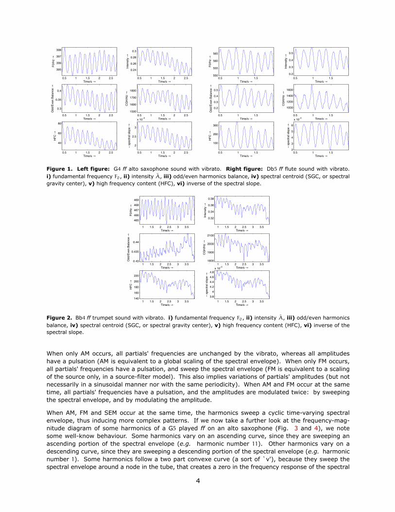
For wind and wood instruments (cf. Fig. 1), the vibrato is obtained by modulating the air flow: thisvaries amplitude (AM) and fundamental frequency (FM). Due to non-linearities inside the tube, a spectralenrichment appears when blowing louder, and disappears when blowing softer. This is the reason forthe cycles of spectral enrichments (and then SEM). Depending on the instrument, modulations of the airflow can be obtained by different means. In the case of the saxophone for example, the instrumentistcan apply the vibrato in two ways: by modulating the pressure on the reed on the mouth piece (softvibrato, for soft notes) or the air pressure in the mouth.

Several observations can be made from Fig. 1, where six sound features are depicted2. The amplitudemodulation (AM) is revealed by the modulation on the intensity, and is due to the production of the soundwith vibrato. The frequency modulation (FM) is revealed by the modulation of the fundamental frequencyF0. The modulations of spectral centroid (SGC), high frequency content (HFC) and the inverse of thespectral slope (ISS) reveal the spectral envelope modulation (SEM). The odd/even balance modulation isalso due to the spectral envelope modulation, but one can wonder if it is not also due to other effects inthe tube, when the intensity is modulated. Indeed, the odd harmonics could be modulated in a slightlydifferent way than the even harmonics, depending on the pressure node and non-linearities.

We note that some differences appear between instruments in that class. For example, the flute andthe alto saxophone do not behave similarly during vibrato. Both have AM, FM and SEM, but the FM is inphase opposition for the saxophone, whereas it is not for the flute. For both sounds, the intensity, theSGC, the HFC and the ISS are phase synchronous. Also, modulations on SGC are more regular for thealto saxophone than for the flute. Concerning the odd/even balance modulation, it seems to always bein phase with FM for the alto saxophone, and sometimes in phase opposition for the flute. However, afurther enquiry is necessary to generalise this to the whole frequency range.

For brass instruments, the vibrato is also obtained by modulating the air flow (cf. wind instruments).With the example given in Fig. 2, we notice how the FM is more regular than all the other modulations(AM, SGC, HFC, spectral slope). From our experience, the odd/even balance is less significative, and issometimes in phase opposition, sometimes not (as for the flute).

To resume, a vibrato is made of at least one of these three kind of modulations:

• amplitude modulation (predominent in wind and brass instruments),• frequency modulation (predominent in voice and string instruments),• spectral envelope modulation and hysteresis (existing in wind, brass, voice).

Behaviour of Harmonics' Frequencies and Amplitudes With the information given below, we candepict how the amplitude and the frequency of each harmonic3 is behaving, depending on which kind ofmodulation (AM, FM and SEM) is included in the vibrato.

2The features are defined in Appendix 1.3We consider instrumental sounds, so the partials can be perfectly harmonic or nearly-harmonic for string instru-

ments. We however confound the two cases by naming them `harmonics'.

3

0.5 1 1.5 2 2.5

395

396

397

398

Time/s !

F0/H

z !

0.5 1 1.5 2 2.5

0.24

0.26

0.28

0.3

Time/s !

Inte

nsity

!

0.5 1 1.5 2 2.5

0.3

0.35

0.4

Time/s !

Odd

/Eve

n Ba

lanc

e !

0.5 1 1.5 2 2.51500

1600

1700

1800

Time/s !

CGH/

Hz !

0.5 1 1.5 2 2.5

40

60

80

Time/s !

HFC !

0.5 1 1.5 2 2.5

2

2.5

3

x 10!6

Time/s !

! sp

ectra

l slo

pe !

0.5 1 1.5550

555

560

565

Time/s !

F0/H

z !

0.5 1 1.50.2

0.3

0.4

0.5

Time/s !

Inte

nsity

!

0.5 1 1.5

0.2

0.3

0.4

0.5

Time/s !

Odd

/Eve

n Ba

lanc

e !

0.5 1 1.5

1000

1200

1400

1600

Time/s !

CGH/

Hz !

0.5 1 1.5

100

200

300

Time/s !

HFC !

0.5 1 1.52

3

4

5

6

x 10!6

Time/s !

! sp

ectra

l slo

pe !

Figure 1. Left figure: G4 ff alto saxophone sound with vibrato. Right figure: Db5 ff flute sound with vibrato.i) fundamental frequency F0, ii) intensity A, iii) odd/even harmonics balance, iv) spectral centroid (SGC, or spectralgravity center), v) high frequency content (HFC), vi) inverse of the spectral slope.

1 1.5 2 2.5 3 3.5

465466467468469

Time/s !

F0/H

z !

1 1.5 2 2.5 3 3.5

0.32

0.34

0.36

0.38

Time/s !

Inte

nsity

!

1 1.5 2 2.5 3 3.50.43

0.435

0.44

Time/s !

Odd

/Eve

n Ba

lanc

e !

1 1.5 2 2.5 3 3.51800

1900

2000

2100

Time/s !

CGH/

Hz !

1 1.5 2 2.5 3 3.5140

160

180

200

220

Time/s !

HFC !

1 1.5 2 2.5 3 3.53.8

44.24.44.64.8

x 10!6

Time/s !

! sp

ectra

l slo

pe !

Figure 2. Bb4 ff trumpet sound with vibrato. i) fundamental frequency F0, ii) intensity A, iii) odd/even harmonicsbalance, iv) spectral centroid (SGC, or spectral gravity center), v) high frequency content (HFC), vi) inverse of thespectral slope.

When only AM occurs, all partials' frequencies are unchanged by the vibrato, whereas all amplitudeshave a pulsation (AM is equivalent to a global scaling of the spectral envelope). When only FM occurs,all partials' frequencies have a pulsation, and sweep the spectral envelope (FM is equivalent to a scalingof the source only, in a source-filter model). This also implies variations of partials' amplitudes (but notnecessarily in a sinusoidal manner nor with the same periodicity). When AM and FM occur at the sametime, all partials' frequencies have a pulsation, and the amplitudes are modulated twice: by sweepingthe spectral envelope, and by modulating the amplitude.

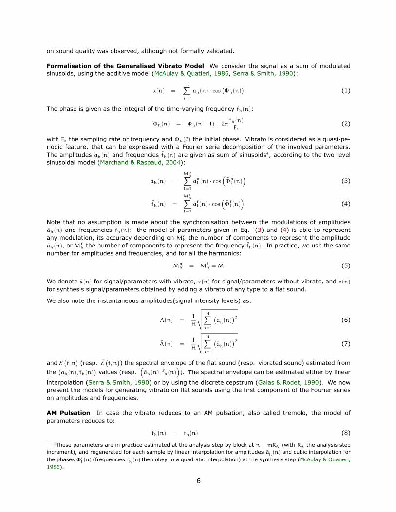
When AM, FM and SEM occur at the same time, the harmonics sweep a cyclic time-varying spectralenvelope, thus inducing more complex patterns. If we now take a further look at the frequency-mag-nitude diagram of some harmonics of a G5 played ff on an alto saxophone (Fig. 3 and 4), we notesome well-know behaviour. Some harmonics vary on an ascending curve, since they are sweeping anascending portion of the spectral envelope (e.g. harmonic number 11). Other harmonics vary on adescending curve, since they are sweeping a descending portion of the spectral envelope (e.g. harmonicnumber 1). Some harmonics follow a two part convexe curve (a sort of `v'), because they sweep thespectral envelope around a node in the tube, that creates a zero in the frequency response of the spectral

4

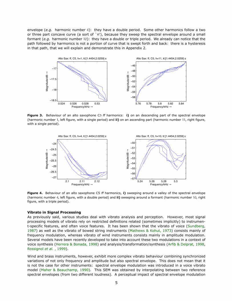
envelope (e.g. harmonic number 4): they have a double period. Some other harmonics follow a twoor three part concave curve (a sort of `n'), because they sweep the spectral envelope around a smallformant (e.g. harmonic number 10): they have a double or triple period. We already can notice that thepath followed by harmonics is not a portion of curve that is swept forth and back: there is a hysteresisin that path, that we will explain and demonstrate this in Appendix 2.

0.524 0.526 0.528 0.53!18.5

!18

!17.5

!17

Frequency/kHz !

Mag

nitu

de/d

B !

Alto Sax: ff, C5, h=1, t"[1.4454,2.0259] s

5.76 5.78 5.8 5.82 5.84

!58

!56

!54

!52

!50

!48

!46

Frequency/kHz !

Mag

nitu

de/d

B !

Alto Sax: ff, C5, h=11, t"[1.4454,2.0259] s

Figure 3. Behaviour of an alto saxophone C5 ff harmonics: i) on an descending part of the spectral envelope(harmonic number 1, left figure, with a single period) and ii) on an ascending part (harmonic number 11, right figure,with a single period).

2.1 2.11 2.12!27

!26.5

!26

!25.5

!25

!24.5

!24

Frequency/kHz !

Mag

nitu

de/d

B !

Alto Sax: ff, C5, h=4, t"[1.4454,2.0259] s

5.24 5.26 5.28 5.3!57

!56

!55

!54

!53

!52

!51

!50

Frequency/kHz !

Mag

nitu

de/d

B !

Alto Sax: ff, C5, h=10, t"[1.4454,2.0259] s

Figure 4. Behaviour of an alto saxophone C5 ff harmonics, i) sweeping around a valley of the spectral envelope(harmonic number 4, left figure, with a double period) and ii) sweeping around a formant (harmonic number 10, rightfigure, with a triple period).

Vibrato in Signal ProcessingAs previously said, various studies deal with vibrato analysis and perception. However, most signalprocessing models of vibrato rely on restricted definitions related (sometimes implicitly) to instrumen-t-specific features, and often voice features. It has been shown that the vibrato of voice (Sundberg,1987) as well as the vibrato of bowed string instruments (Mathews & Kohut, 1973) consists mainly offrequency modulation, whereas vibrato of wind instruments consists mainly in amplitude modulation.Several models have been recently developed to take into account these two modulations in a context ofvoice synthesis (Herrera & Bonada, 1998) and analysis/transformation/synthesis (Arfib & Delprat, 1998,Rossignol et al. , 1999).

Wind and brass instruments, however, exhibit more complex vibrato behaviour combining synchronizedvariations of not only frequency and amplitude but also spectral envelope. This does not mean that itis not the case for other instruments: spectral envelope modulation was introduced in a voice vibratomodel (Maher & Beauchamp, 1990). This SEM was obtained by interpolating between two referencespectral envelopes (from two different loudness). A perceptual impact of spectral envelope modulation

5

on sound quality was observed, although not formally validated.

Formalisation of the Generalised Vibrato Model We consider the signal as a sum of modulatedsinusoids, using the additive model (McAulay & Quatieri, 1986, Serra & Smith, 1990):

x(n) =H!

h=1

ah(n) · cos `Φh(n)

´(1)

The phase is given as the integral of the time-varying frequency fh(n):

Φh(n) = Φh(n − 1) + 2πfh(n)

Fs(2)

with Fs the sampling rate or frequency and Φh(0) the initial phase. Vibrato is considered as a quasi-pe-riodic feature, that can be expressed with a Fourier serie decomposition of the involved parameters.The amplitudes ah(n) and frequencies fh(n) are given as sum of sinusoids4, according to the two-levelsinusoidal model (Marchand & Raspaud, 2004):

ah(n) =

Mah!

l=1

aal (n) · cos

“Φa

l (n)”

(3)

fh(n) =

Mfh!

l=1

afl (n) · cos

“Φf

l (n)”

(4)

Note that no assumption is made about the synchronisation between the modulations of amplitudesah(n) and frequencies fh(n): the model of parameters given in Eq. (3) and (4) is able to representany modulation, its accuracy depending on Ma

h the number of components to represent the amplitudeah(n), or Mf

h the number of components to represent the frequency fh(n). In practice, we use the samenumber for amplitudes and frequencies, and for all the harmonics:

Mah = Mf

h = M (5)

We denote x(n) for signal/parameters with vibrato, x(n) for signal/parameters without vibrato, and x(n)

for synthesis signal/parameters obtained by adding a vibrato of any type to a flat sound.

We also note the instantaneous amplitudes(signal intensity levels) as:

A(n) =1

H

vuut H!h=1

`ah(n)

´2 (6)

A(n) =1

H

vuut H!h=1

`ah(n)

´2 (7)

and E `f, n

´(resp. E `

f, n´) the spectral envelope of the flat sound (resp. vibrated sound) estimated from

the`ah(n), fh(n)

´values (resp.

“ah(n), fh(n)

”). The spectral envelope can be estimated either by linear

interpolation (Serra & Smith, 1990) or by using the discrete cepstrum (Galas & Rodet, 1990). We nowpresent the models for generating vibrato on flat sounds using the first component of the Fourier serieson amplitudes and frequencies.

AM Pulsation In case the vibrato reduces to an AM pulsation, also called tremolo, the model ofparameters reduces to:

fh(n) = fh(n) (8)

4These parameters are in practice estimated at the analysis step by block at n = mRA (with RA the analysis stepincrement), and regenerated for each sample by linear interpolation for amplitudes ah(n) and cubic interpolation forthe phases Φf

l(n) (frequencies fh(n) then obey to a quadratic interpolation) at the synthesis step (McAulay & Quatieri,1986).

6

ah(n) = γa(n) · ah(n) (9)

γa(n) = 1 + aa0 (n) · cos

“Φa

0 (n)”

(10)

where Φa0 (n) the phase of the AM is given as a function of fa

0 (n) the frequency (or rate) of the AM andaa

0 (n) the amplitude (or extent) of the AM, as:

Φa0 (n) = Φa

0 (n − 1) + 2πfa0 (n)

Fs(11)

Notice that the AM is globally applied to the signal, by giving the same ratio to all harmonics' amplitudes.

FM Pulsation In case the vibrato reduces to a FM pulsation with constant spectral envelope, as for theviolin model (Mathews & Kohut, 1973) or the voice model (Sundberg, 1987, Arfib & Delprat, 1998), themodel of parameters reduces to:

fh(n) = γf(n) · fh(n) (12)

γf(n) = 1 + af0(n) · cos

“Φf

0(n)”

(13)

Φf0(n) = Φf

0(n − 1) + 2πff0(n)

Fs(14)

ah(n) = E `fh(n), n

´(15)

with ff0(n) the frequency (or rate) of the FM and af

0(n) the amplitude (or extent) of the FM. The amplitudemodulation is a result of the spectral envelope scanning by the harmonics.

AM/FM Pulsation In case the vibrato reduces to an AM/FM pulsation (Herrera & Bonada, 1998,Rossignol et al. , 1999), the model of parameters reduces to:

fh(n) = γf(n) · fh(n) (16)

ah(n) = γa(n) · E `fh(n), n

´(17)

with the assumption that the AM and FM pulsations are synchronous:

Φf0(n) = Φa

0 (n) = Φ0(n) (18)

The amplitude modulation of each harmonic is a result of both the spectral envelope scanning by theharmonics and the global AM by γa(n).

AM, FM and SEM Pulsation In order to apply a combined AM/FM/SEM, let us first express thetime-varying modelling of the spectral envelope (SE). The time-varying SE can be obtained by scalingthe original SE with a linear function of the frequency (thus changing its slope):

E `fh(n), n

´= γe(n) · fh(n) · E `

fh(n), n´

(19)

where γe(n) renders the spectral modulation:

γe(n) = c(n) + ae0(n) · cos

“Φe

0(n)”

(20)

where c(n) and ae0(n) must be estimated. To our knowledge, this SEM model is well suited for the singing

voice, wind instruments such as flute, and brass instruments.

The time-varying SE can also be obtained by interpolating between two extrema spectral envelopes(Maher & Beauchamp, 1990), when the previous solution does not suit to the instrument:

E `fh(n), n

´= βe(n) · E+

`fh(n), n

´+ (1 − βe(n)) · E−

`fh(n), n

´(21)

βe(n) =1 + cos

“Φe

0(n)”

2(22)

7

Using this time-varying spectral envelope, the frequencies and amplitudes are determined accordinglyusing:

fh(n) = γf(n) · fh(n) (23)

ah(n) = γa(n) · E `fh(n), n

´(24)

with the assumption that AM, FM and SEM pulsations are synchronous, so they have the same phase:

Φe0(n) = Φa

0 (n) = Φf0(n) = Φ0(n) (25)

Notice that it does not mean that the resulting amplitude modulation of harmonics occur at the samefrequency. The scanning of a formant region might double the frequency of modulation.

Comparison of Vibrato Models The limit of the AM, FM and AM/FM models is that they considervibrato modulation as made of only one modulated sinusoidal component. This exclude more realisticmodulation curves: the two-level sinusoidal model provides a solution to this. Moreover, the AM/FMmodel consider phase synchronous modulations, whereas they can be in opposite phase (e.g. thesaxophone, as explained in the acoustic part). None of these three models take into account the SEM,which is important, as we will show with the perceptual test.

Let us consider the example of the time-scaling of a voice sound with vibrato by using a model: if thereis no SEM in the signal, then the approach proposed in (Arfib & Delprat, 1998), that consists in removingthe FM vibrato by pich-shifting, time-scaling the flat sound, and then applying back the FM vibrato bypitch-shifting, is valid and similar to a real longer vibrated sound. However, if there is SEM in the signal,then the FM and SEM components are not processed in a coherent manner: SEM is time-scaled whereasthe FM is not, thus resulting in a processed sound with artifacts that could be audible.

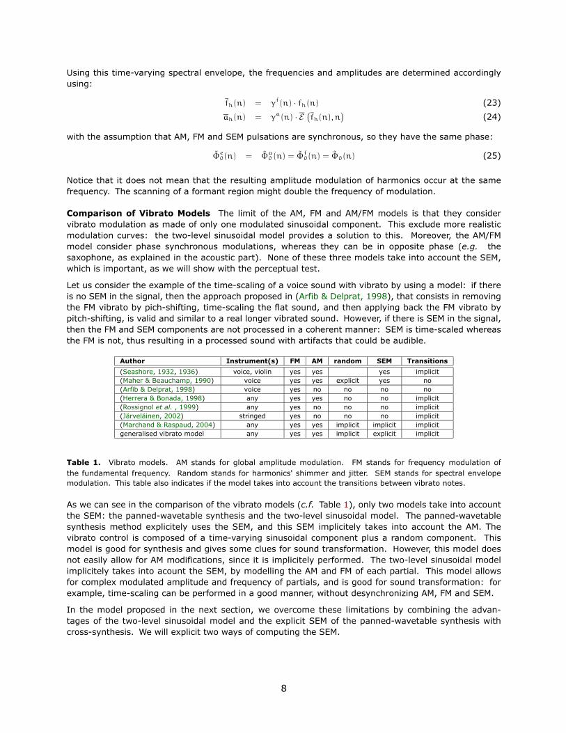
Author Instrument(s) FM AM random SEM Transitions

(Seashore, 1932, 1936) voice, violin yes yes yes implicit(Maher & Beauchamp, 1990) voice yes yes explicit yes no(Arfib & Delprat, 1998) voice yes no no no no(Herrera & Bonada, 1998) any yes yes no no implicit(Rossignol et al. , 1999) any yes no no no implicit(Järveläinen, 2002) stringed yes no no no implicit(Marchand & Raspaud, 2004) any yes yes implicit implicit implicitgeneralised vibrato model any yes yes implicit explicit implicit

Table 1. Vibrato models. AM stands for global amplitude modulation. FM stands for frequency modulation ofthe fundamental frequency. Random stands for harmonics' shimmer and jitter. SEM stands for spectral envelopemodulation. This table also indicates if the model takes into account the transitions between vibrato notes.

As we can see in the comparison of the vibrato models (c.f. Table 1), only two models take into accountthe SEM: the panned-wavetable synthesis and the two-level sinusoidal model. The panned-wavetablesynthesis method explicitely uses the SEM, and this SEM implicitely takes into account the AM. Thevibrato control is composed of a time-varying sinusoidal component plus a random component. Thismodel is good for synthesis and gives some clues for sound transformation. However, this model doesnot easily allow for AM modifications, since it is implicitely performed. The two-level sinusoidal modelimplicitely takes into acount the SEM, by modelling the AM and FM of each partial. This model allowsfor complex modulated amplitude and frequency of partials, and is good for sound transformation: forexample, time-scaling can be performed in a good manner, without desynchronizing AM, FM and SEM.

In the model proposed in the next section, we overcome these limitations by combining the advan-tages of the two-level sinusoidal model and the explicit SEM of the panned-wavetable synthesis withcross-synthesis. We will explicit two ways of computing the SEM.

8

A Generalised Vibrato Model, with Explicit AM/FM/SEMAfter proposing a definition of vibrato, we explain the signal processing model we developed and basedon the panned-wavetable synthesis and the two-level sinusoidal model.

Vibrato DefinitionOften in signal processing, only AM and FM vibrato are considered, and timbre modulation only concernsthe complex behaviour of FM vibrato scanning the AM spectral envelope, but not the SEM. A clearerdefinition of vibrato is presented on the basis of a review of vibrato features (Seashore, 1932, Toff, 1996):we define the vibrato as a vibrating quality of musical sounds, corresponding to simultaneousmodulations of amplitude (AM), frequency (FM) and/or spectral envelope (SEM). Note that inorder to take into account the specific behaviour of harmonics' amplitudes, we consider the modulationsas simultaneous and not synchronous. However, we can already better define these modulations sayingthat the SEM, the FM and the global AM (not the AM of each frequency) are nearly sinusoidal and aresynchronous or in phase opposition. We have established that the spectral envelope modulation impliesa frequency-dependent hysteresis behaviour (see Appendix 2 for the demonstration).

Generalised Vibrato ModelDue to the limitations of the AM, FM and AM/FM vibrato models, it is clear that a generalised AM/FM/SEMmodel is needed: moreover, it is more adapted for transforming various instrument sounds with vibrato.

We developed a generalised vibrato model based on the definition given previously, for use in an ana-lysis/transformation/synthesis context. We use the analysis by synthesis paradigm (Risset & Wessel,1999): the quality of the model will be perceptually evaluated. Our model uses the two-level sinusoidalmodel5 that represents the amplitudes and frequencies of harmonics as sums of sinusoids, thus implicitlyintegrating the spectral envelope modulation. It also uses the panned-wavetable synthesis technique6

in order to explicitely represent the SEM. By doing so, we provide controls on the three components ofvibrato (AM, FM and SEM) as follows:

1. we compute the two-level sinusoidal model data:“ah(n), fh(n), φh

”;

2. the explicit control over the FM is given by the modulated frequencies of harmonics: fh(n) =

Tf(fh(n)), with Tf a transformation of the frequencies (for example changing the frequency, thedepth, the frequency composition of the vibrato controls);

3. the interpolation between two spectral envelopes (or the spectral envelope slope changes) allowsfor an explicit control over the SEM: E = Te

“E

”with Te a transformation of the spectral envelope;

4. the new amplitudes ah(n) are computed by interpolation in the spectral envelope E `fh(n), n

´;

5. the instantaneous amplitude A(n) is computed from the new amplitudes ah(n).6. when modelled as a sum of sinusoids, the instantaneous amplitude allows for an explicit control

on the AM: A(n) = Ta(A(n)), with Ta a transformation of the instantaneous amplitude, applied bymultiplying all the ah(n) by the same ratio r(n).

7. the final amplitudes are then given as: A(n) = r(n)A(n).

Note that the two-level sinusoidal model also considers more than one component for the periodicvibrato, which is more realistic. It has however been shown in (Maher & Beauchamp, 1990) that therandom component (jitter and shimmer) added to the vibrato control curve is not perceived by listeners.In the context of pure synthesis, this question may have importance for the realism of the syntheticsound. In our context of analysis/transformation/synthesis, the original instrument sound already haveits harmonics' frequencies and amplitudes made of a general trend (due to the control) and randomcomponents (jitter and shimmer). It does not make any sense to add jitter/shimmer when adding avibrato to a flat sound; it may however make sens to wonder what to do with that jitter/shimmer whentime-scaling the vibrated sound. It does not seem that this question has been addressed yet.

5The two-level sinusoidal model was design in the analysis/transformation/synthesis context.6The panned-wavetable synthesis technique was developed in order to produce a realistic vibrato for synthesis

sounds.

9

In a context of vibrato sound synthesis, this model has to be combined with cross-synthesis, in order totake into account realistic vibrato control curves and spectral envelope modulations. Therefore, whensynthesizing the test sounds, we combined this AM/FM/SEM model with cross-synthesis, since we neededto synthesize AM/FM sounds with and without SEM: a mean spectral envelope was needed, and extractedfrom a second sound.

Some More Insights in the Vibrato ModelWe now develop some specific aspects of the generalised vibrato model, dealing with the hysteresis ofharmonics' path in the frequency/amplitude domain, the difference of behaviour of SGC and HFC featuresdepending on the exsitence of SEM, the way to implicitely take into account the AM in the SEM, the nonlinear coupling between the source and the filter, and finally the questions that may arise concerning thedefinition and perception of formants and valleys of the spectral envelope during vibrato.

Is There Hysteresis on the Harmonics' Path? This question deals with the symmetrical profile ofthe vibrato. We here question wether the vibrato has the same behaviour during the rise and during thefall. To answer this question, we consider the ideal case where all the vibrato parameters are constantwith time. The demonstration is given in Appendix 2. The conditions on the spectral envelope for nohysteresis imply either oscillating spectral envelopes around each harmonics (SEM by changing the slope)or a flat spectral envelope (SEM by interpolation). In any other condition, the AM/FM/SEM pulsationimplies hysteresis on the harmonics' path. In the general case where the pulsation rate and amplitudesare not constant with time, the AM/FM/SEM pulsation always have hysteresis.

Harmonics' amplitudes behaviour, with/without SEM To better understand the consequences ofSEM harmonics' behaviour, let us plot the magnitudes and frequencies of harmonics, without SEM and withSEM (Fig. 5). As depicted, the `no-SEM' harmonics have identical (and translated) amplitude patterns,

0 0.5 1 1.5 2 2.5 3!60

!55

!50

!45

!40

!35

!30

!25

!20

!15

!10

Time/s !

Mag

nitu

de/d

B !

0 0.5 1 1.5 2 2.5 3!60

!55

!50

!45

!40

!35

!30

!25

!20

!15

!10

Time/s !

Mag

nitu

de/d

B !

0 0.5 1 1.5 2 2.5 30

1000

2000

3000

4000

5000

6000

7000

8000

9000

10000

11000

Time/s !

Freq

uenc

y/Hz

!

Figure 5. Comparison of harmonics' amplitudes when only preserving AM/FM (left figure) and when preservingAM/FM and SEM (middle figure). Frequencies are identical for both sounds (right figure).

whereas `SEM' harmonics have partials with simple, double and triple period patterns, sometimes inopposite phase. This is due to the fact that the spectral envelope (without SEM) we used is constant, andnot well enough discretized. Indeed, the spectral envelope estimation is smoother that the real spectralenvelope: most of the zeros are not present, thus implying the absence of SEM specific behaviour, suchas big range of magnitude variation around zeros when a harmonic sweeps around it.

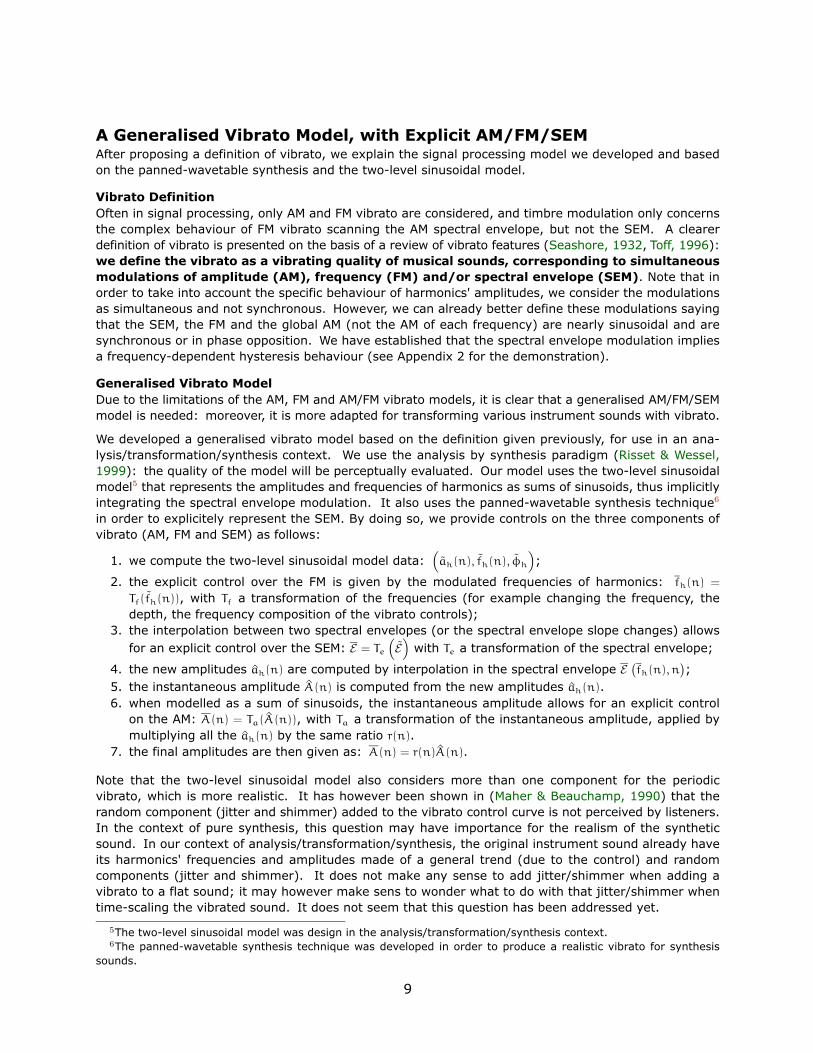
This has some implications on the sound features. As depicted in Fig. 6, SGC and HFC have differentbehaviours depending if SEM is in the model or not. The extend of SGC is greater when there is aSEM, and the two SGC modulations are not in phase. These two effects are due to the way the SGC iscomputed as well as to the fact the spectral envelope is not modulated without SEM. The extend of HFCis greater when there is a SEM, and the two HFC modulations are in phase.

Setting the Parameters of the Two SEM Models We proposed two ways to modify the spectralenvelope (SEM), we now explain how to set their parameters. When interpolating between two extremaspectral envelope (SE), these extrema correspond to the SE of notes at different loudness, and can be

10

0.5 1 1.5 2 2.51500

1600

1700

1800

1900

Time/s !

Freq

uenc

y/Hz

!SGC with SEMSGC without SEM

0 0.5 1 1.5 2 2.5 3

1020304050607080

Time/s !

HFC !

HFC with SEMHFC without SEM

Figure 6. Comparison between spectral gravity centers (SGC, left figure) and high frequency contents (HFC, rightfigure) with and without SEM. The extend of SGC and HFC is greater when there is a SEM. The two SGC modulationsare in opposite phase, and the two HFC modulations are in phase.

obtained precisely from estimated SE from flat sounds. For some instruments (e.g. brass and flute),these extrema can also be computed as the maximum SE with a slope change. Interpolating betweentwo spectral envelopes is the most general case.

Concerning the slope changing, the c(n) and ae0(n) values have to be estimated. Considering that we

know the extrema spectral envelopes E−

`fh(n), n

´and E+

`fh(n), n

´, they are approximated by:

E+

`fh(n), n

´= (c(n) + ae

0(n)) · fh(n) · E `fh(n), n

´(26)

E−

`fh(n), n

´= (c(n) − ae

0(n)) · fh(n) · E `fh(n), n

´(27)

so c(n) and ae0(n) minimise the two following quantities:

εc(n) = c(n) · fh(n) · E `fh(n), n

´−

E+

`fh(n), n

´+ E−

`fh(n), n

´2

(28)

εa(n) = ae0(n) · fh(n) · E `

fh(n), n´

−E+

`fh(n), n

´− E−

`fh(n), n

´2

(29)

In the optimal case where the extrema SE exactly corresponds to a SE with a given slope change, then:

E+

`fh(n), n

´= d+(n) · fh(n) · E `

fh(n), n´

(30)

E−

`fh(n), n

´= d−(n) · fh(n) · E `

fh(n), n´

(31)

and c(n) and ae0(n) are explicitely given as:

c(n) =d+(n) + d−(n)

2(32)

ae0(n) =

d+(n) − d−(n)

2(33)

SEM Models with Implicit AM Both methods can implicitely combine AM and SEM in the SEM. Wegive the corresponding mathematical developments, in order to highlight the way the usual two-levelsinusoidal model does this. When changing the slope of the SE:

E `fh(n), n

´= γa(n) · E `

fh(n), n´

(34)

= γa(n) · γe(n) · fh(n) · E `fh(n), n

´(35)

= γe(n) · fh(n) · Eγa

`fh(n), n

´(36)

with the notation:

Eγa

`fh(n), n

´= γa(n) · E `

fh(n), n´

(37)

When interpolating between two extrema SE:

E `fh(n), n

´= γa(n) · E `

fh(n), n´

(38)

= γa(n) · βe(n) · E+

`fh(n), n

´+ γa(n) · (1 − βe(n)) · E−

`fh(n), n

´(39)

= βe(n) · Eγa,+

`fh(n), n

´+ (1 − βe(n)) · Eγa,−

`fh(n), n

´(40)

11

with the new extrema spectral envelopes:

Eγa,+

`fh(n), n

´= γa(n) · E+

`fh(n), n

´(41)

Eγa,−

`fh(n), n

´= γa(n) · E−

`fh(n), n

´(42)

Non Linear Coupling Between the Source and the Filter The spectral enrichment (and so forth theSEM) when the loudness increases is due to a non linear effect, such as for trumpet and more generallyfor brass sounds (Risset, 1965). In the usual source-filter model, the filter being a linear system, thereis no such non linear coupling between the source and the filter. The source/filter model is not idealfrom that point of view, and physical modelling may give more accurate values of the parameters of themodel. However, the generalised signal processing model of vibrato intends to take into account thisnon linear coupling between the source and the filter, using an additive/substractive representation ofsound and the SEM to explicit the effect of non linear coupling.

Figure 7. Sonagram of the spectral envelope filtered by linear interpolation on magnitudes.

Questions That Arise From the spectral envelope filtered sonagram (Fig. 7), we notice that formantsand valleys' frequencies are preserved (but of course not magnitudes). It is well-known that a constantspectral envelope (SE) is better perceived thanks to jitter on harmonics, which then sweep the SE. Inthat case, the following open questions arise: How about the fact that SEM preserves formants andvalleys' frequencies? Cannot this be of any help to perceive the formants? These questions are beyondthe scope of this paper and will be adressed in future works.

12

Validation of this Vibrato ModelIn the context of analysis/transformation/synthesis, flat sounds are added a vibrato by AM/FM. The modelwe propose combines AM/FM with SEM, as in (Maher & Beauchamp, 1990). We now must evaluate if thedifference is perceptually relevant.

The influence of spectral envelope modulation on perceived quality was then investigated using a dou-ble-blind randomized AB comparison task. Eight participants listened to 12 pairs of sounds with vibrato.Each pair included one sound with constant average spectral envelope (identical amplitude modulationover all frequencies) and one with modulated spectral envelope (frequency dependent amplitude mod-ulation). Both sounds in each pair were matched subjectively for loudness by 5 experts listeners ina preliminary experiment. In the main experiment, participants were asked to choose which versionsounded the most natural and justify their choices in an open questionnaire. The statistical analysis (bi-nomial test) revealed a significant preference for sounds with modulated spectral envelope (p < 0.001).

Methods

Synthesis of the Experimental Sounds Cross-synthesis techniques were used to create hybrid soundsfrom two saxophonee sounds with and without vibrato. Using the knowledge and notations about AM,FM, SEM sounds described with the two-level sinusoidal model, we can explicit how we synthesized theexperimental sounds.

We had the following constraints on material (sounds):

• sounds are created by cross-synthesis between a sound with vibrato and a sound without vibrato,so we need pairs of sound having the same nuance, pitch and duration. We selected sound pairsfrom the IOWA database (IOWA, 2005);

• in order to provide a good analysis and synthesis, the original sounds must be exempt of reverber-ation. This is the case for the sounds from the IOWA database, as they are recorded in an anechoicroom;

• the frequency range must be representative of the instrument. We studied alto saxophonee sounds,ranging in pitch from F3 to C5.

and on the synthesis:

• in order to use the two-level sinusoidal model, we first need to use an additive analysis/transfor-mation/synthesis, the transformation being applied at the second level;

• the residual of analyzed sound was removed as we focus on the modification of the deterministicparts.

The hypothesis that we wanted to test is wether the spectral envelope modulation (SEM) can be heard ornot. This implies to synthesize sounds for the experiment with and without this SEM. Another constraintis that any existing amplitude modulation and/or frequency modulation must be preserved.

The sound with SEM is directly synthesized from the analysis data, as:

x(n) =N!

h=1

ah(n) · cos“Φh(n)

”(43)

Φh(n) = Φh(n − 1) + 2πfh(n)

Fs(44)

with ah(n), fh(n) and φh(n) provided by the analysis.

The sound without SEM are synthesized by cross synthesis between the sound with vibrato and the soundwithout vibrato, as follows:

1. we compute the two-level sinusoidal model data:`ah(n), fh(n), φh(n)

´and

“ah(n), fh(n), φh(n)

”;

13

2. the synthesized harmonics' frequencies are the modulated frequencies of the sound with vibrato:fh(n) = fh(n);

3. the amplitudes are given by interpolation in the mean spectral envelope (constant SE) and thenmultiplication by the ratio of global instantaneous amplitudes, so that both sounds have the sameamplitude modulation:

ah(n) = E“fh(n), n

”· A(n)

A(n)(45)

The first level of sinusoidal analysis was performed using CLAM (Amatriain et al. , 2002a) and exportedas SDIF data to Matlab. The second level of sinusoidal analysis was performed using Matlab, and thematlab SMS version (Amatriain et al. , 2002b). The synthesis data were then stored as SDIF, and thesounds were synthesized using CLAM.

Experimental Design Considerations One possibility for such a listening test would be to use one ofa number of standard psychophysical tests to determine discriminability, that is, the ability of listenersto detect a difference between the two signals. These include AB-X, AAA XYZ, AX, etc. A potentialdrawback of such tests is that if differences are detectable between the two sets of sound samples, nodata will exist as to which samples are preferred by listeners. After initial pilot testing, we determinedthat differences were readily apparent and easily detectable, even by unskilled listeners. Consequently,an A-B Preference Test was conducted. In an A-B Preference Test, listeners hear two samples (A and B)and are asked to indicate which they prefer. If they have no preference, they are instructed to pick ananswer at random. Stimuli are presented in random, counterbalanced order, so that over the course ofmany trials and many subjects, systematic effects of presentation order (`order effects' or `sequenceeffects') are nullified. As well, over the course of many trials, listeners who can discriminate one soundsound sample from another will choose each one an equal number of times (the samples were presentedrandomly and the listeners are choosing randomly) and hence inability to discriminate will be revealedas `no preference' in the final results.

Apparatus Soundfiles were played through a MOTU 828mkII 24-bit 96KHz D/A convertor, attached toa MacIntosh Apple computer via Firewire. Listeners used AKG 240 Gold Professional Closed Ear 600Ω

headphones. The test samples were presented with a graphical interface, programmed in Max/MSP(Cycling'74, 2003, Puckette, 1991).

Procedure

Loudness Matching Test Because the two synthesized sounds for each note contained unequal spec-tral distributions, automated methods for equating overall power in the soundfiles may not have yieldedsamples that would sound matched for loudness: the sample with the highest spectral centroid wouldalways tend to sound louder. We thus employed a subjective evaluation experiment prior to the pref-erence test to match for loudness. 5 listeners (4 males, 1 female, mean age 28; s.d.3.4) served withoutpay in the experiment. They were experts listeners, with a minimum of 7 years of musical training andfamiliar with loudness matching tasks. Participants were presented with pairs of sound samples in adouble-blind, randomized listening test. Participants were instructed to set the level of one of them sothat both sounds appeared equally loud. Each pair was presented twice in counterbalanced order. Thegraphical interface enabled participants to adjust the level on a slider in real time, and to switch backand forth between the two versions as many times as desired. Loudness judgments were consistentwithin and across subjects (s.d. < 1 dB for all samples). The volume settings were averaged over allparticipants, and the amplitude of sound samples were subsequently adjusted for each pair (averagegain of 2.3 dB).

Preference Test A new set of 8 subjects (5 males, 3 females; mean age 29; s.d.10.5) participated withoutpay in the preference test. 5 participants were expert listeners with a minimum of 11 years of musicaltraining, 3 were participants were non-musically trained. Participants were given instructions to choosewhich of two sounds they preferred, and to choose at random if they had no preference. Preferenceswere indicated by clicking the computer mouse inside a box underneath the icon for Sound A or Sound B.An additional on-screen button allowed participants to play the sound pairs as many times as they liked.

14

The sound pairs were always played in their entirety, and pressing the `play again' button on the screendid not cause the currently playing sound to terminate. At the beginning of each trial, the two soundswere played sequentially. An icon on the computer monitor indicated which of the two sounds, A or Bwas playing and after participants indicated their preference by clicking the mouse in the appropriatebox, the next trial started. Each sound pair was presented to each subject twice in counter-balancedorder. Following the experiment, participants were asked to freely describe the difference between the2 versions presented in each trial, and to justify their choices in an open questionnaire.

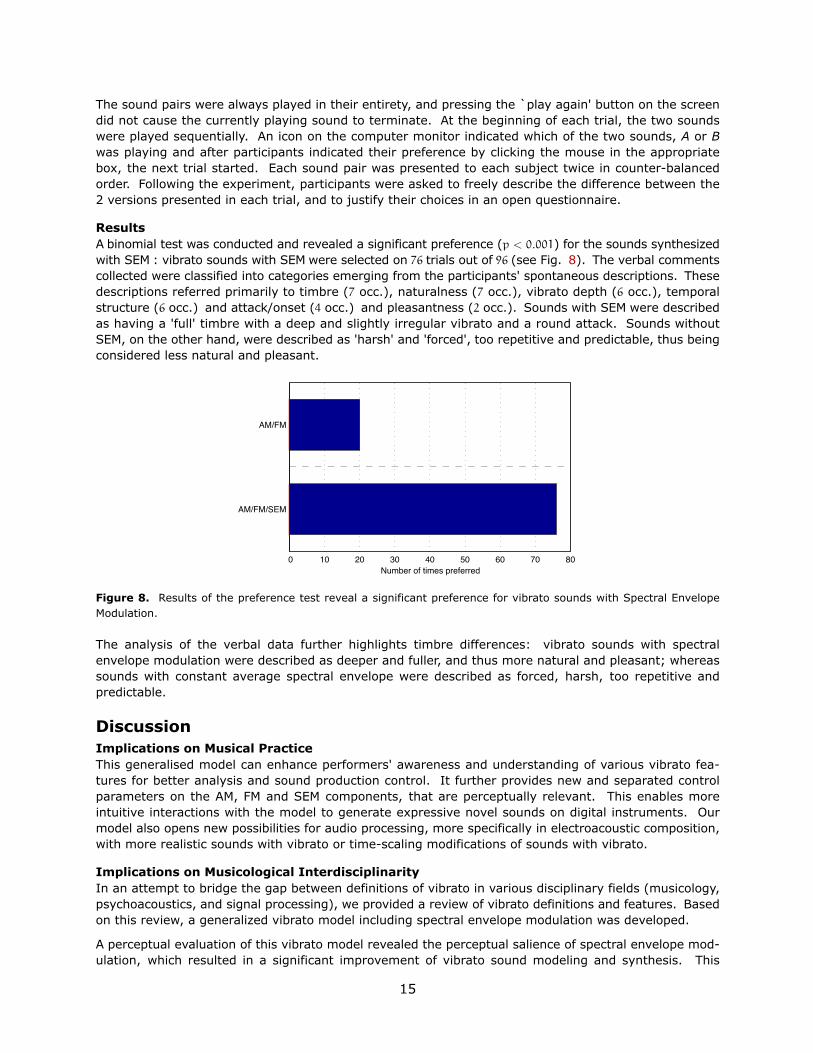
ResultsA binomial test was conducted and revealed a significant preference (p < 0.001) for the sounds synthesizedwith SEM : vibrato sounds with SEM were selected on 76 trials out of 96 (see Fig. 8). The verbal commentscollected were classified into categories emerging from the participants' spontaneous descriptions. Thesedescriptions referred primarily to timbre (7 occ.), naturalness (7 occ.), vibrato depth (6 occ.), temporalstructure (6 occ.) and attack/onset (4 occ.) and pleasantness (2 occ.). Sounds with SEM were describedas having a 'full' timbre with a deep and slightly irregular vibrato and a round attack. Sounds withoutSEM, on the other hand, were described as 'harsh' and 'forced', too repetitive and predictable, thus beingconsidered less natural and pleasant.

0 10 20 30 40 50 60 70 80

AM/FM

AM/FM/SEM

Number of times preferred

Figure 8. Results of the preference test reveal a significant preference for vibrato sounds with Spectral EnvelopeModulation.

The analysis of the verbal data further highlights timbre differences: vibrato sounds with spectralenvelope modulation were described as deeper and fuller, and thus more natural and pleasant; whereassounds with constant average spectral envelope were described as forced, harsh, too repetitive andpredictable.

DiscussionImplications on Musical PracticeThis generalised model can enhance performers' awareness and understanding of various vibrato fea-tures for better analysis and sound production control. It further provides new and separated controlparameters on the AM, FM and SEM components, that are perceptually relevant. This enables moreintuitive interactions with the model to generate expressive novel sounds on digital instruments. Ourmodel also opens new possibilities for audio processing, more specifically in electroacoustic composition,with more realistic sounds with vibrato or time-scaling modifications of sounds with vibrato.

Implications on Musicological InterdisciplinarityIn an attempt to bridge the gap between definitions of vibrato in various disciplinary fields (musicology,psychoacoustics, and signal processing), we provided a review of vibrato definitions and features. Basedon this review, a generalized vibrato model including spectral envelope modulation was developed.

A perceptual evaluation of this vibrato model revealed the perceptual salience of spectral envelope mod-ulation, which resulted in a significant improvement of vibrato sound modeling and synthesis. This

15

research also provides new insights for vibrato analysis and automatic recognition, since brightnessmodulation can be inferred from the spectral centroid and the high frequency content variations. Thisinterdisciplinary approach could be beneficial for modeling other stylistic effects (trill, glissando, flat-terzung).

Future WorksWe propose here some future directions of research:

• analysis of the residual and its modulations during vibrato, as well as its effect on vibrato perception.• analysis of other sounds: strings (violin), brass (trumpet).• comparison of preference between AM, FM, AM/FM, AM/SEM, FM/SEM, AM/FM/SEM models.• perceptual effect of the vibrato shape (perfectly sinusoidal versus natural), and of phase decay

between harmonics.• perceptual effect of time-scaling sounds with vibrato using the two-level sinusoidal model, when

taking into account or not the scaling of the jitter/shimmer.

AcknowledgmentsDaniel Levitin, Jean-Claude Risset and Gary Scavone for discussions about perception and acoustics.

Appendices

Appendix 1: Definition of Sound Features We define the six features of sounds with vibrato thatare depicted on Fig. 1. The fundamental frequency F0(n) is given as the analysis frequency of the firstharmonic f1(n). The intensity level is given by the instantaneous amplitude, as

A(n) =1

H

vuut H!h=1

`ah(n)

´2 (46)

The odd/even balance is the square root of the ratio between the sum of the odd harmonics' power andthe sum of all harmonics' energy:

bo/e(n) =

vuut 1H2

"H/2h=1

`a2h(n)

´2`A(n)

´2(47)

The spectral centroid (SGC or spectral gravity center) is correlated to the timbre attribute named bright-ness, and is computed as the gravity center of the harmonic spectrum, as:

cgs(n) =

s"Hh=1 ah(n)fh(n)"H

h=1 ah(n)(48)

The high-frequency content is usually used for attack detection ans is computed as:

hfc(n) =1

H

H!h=1

`ah(n)

´2fh(n) (49)

The spectral slope is the slope of the linear regression of the harmonic spectrum, i.e. the slope of theline that minimizes the distance between itself and the harmonic spectrum.

Appendix 2: Is There Hysteresis the Harmonics' Path? This question, deals with the symmetricalprofile of its vibrato. We here wonder if the vibrato have the same behaviour during the rise and duringthe fall. To answer this question, we consider the ideal case where all the vibrato parameters are constantover time and where the vibrato period is an integer number of time indexes. The assumptions are:

• AM, FM and SEM vibrato parameters are constant: aa0 (n) = aa

0 and fa0 (n) = fa

0 = f0; af0(n) = af

0 andff0(n) = ff

0 = f0; ae0(n) = ae

0 and fe0(n) = fe

0 = f0,• partials have constant amplitude and frequency before applying vibrato: ah(n) = ah and fh(n) = fh,

16

• the flat sound spectral envelope is constant with time: E `f(n), n

´= E `

f(n)´.

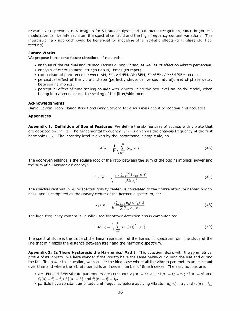
Let us note φ0 the red initial phase; the phase is then given for current time index n as:

Φ0(n) = 2πf0n

Fe+ φ0 (50)

0 1000 2000 3000 4000 5000 6000!1

!0.5

0

0.5

1

Time index n !

cos

(2"

f 0 n /

F s ! "

/2) !

n0n 2 n0 ! n

Figure 9. Symmetrical values of the sinusoidal control curve γ(n) = cos`10πn/Fe −π/2

´at time indexes n = 1040

and 2n0 −n (around the maximum at n0 = 2205).

Let us note n0 the location of the next maximum in the period, in the ideal case where the maximumhappens exactly at the time n/Fe. Then, n and 2n0 − n are symmetrical around n0 (see Fig. 9), with n0

defined as:

cos

„2πf0

n0

Fe+ φ0

«= 1 (51)

n0 =Fe

2πf0

“2πM − φ0

”(52)

with M suitably chosen so that n and n0 belong to the same period. This is equivalent to:

cos

„2πf0

2n0 − n

Fe+ φ0

«= cos

„2πf0

n

Fe+ φ0

«(53)

and then implies that:

γa(n) = γa(2n0 − n) (54)

γf(n) = γf(2n0 − n) (55)

γe(n) = γe(2n0 − n) (56)

βe(n) = βe(2n0 − n) (57)

fh(n) = fh(2n0 − n) (58)

When applying the SEM by changing the slope, the new SE is:

E `fh(n), n

´= γe(n) · fh(n) · E `

fh(n)´

(59)

= γe(n) · fh · E `fh(n)

´(60)

We compute it for 2n0 − n:

E `fh(2n0 − n), 2n0 − n

´= γe(2n0 − n) · fh · E `

fh(2n0 − n)´

(61)

= γe(n) · fh · E `fh(2n0 − n)

´(62)

The condition for no hysteresis is:

E `fh(2n0 − n), 2n0 − n

´= E `

fh(n), n´

(63)

17

and is equivalent to:

E `fh(2n0 − n)

´= E `

fh(n)´

(64)

This means that the only condition for no hysteresis is to have a flat spectral envelope E `fh(n)

´on the

frequency range fh(n) ∈ ˆfh · `

1 − af0

´, fh · `

1 + af0

´˜of each partial. In any other condition, the AM/FM/SEM

pulsation implies hysteresis on the harmonics' path. In the general case where the pulsation rates andextents are not constant with time, the AM/FM/SEM pulsation always have hysteresis.

When applying the SEM by interpolating between two spectral envelopes, the new SE is:

E `fh(n), n

´= βe(n) · E+

`fh(n)

´+ (1 − βe(n)) · E−

`fh(n)

´(65)

We compute it for 2n0 − n:

E `fh(2n0 − n), 2n0 − n

´= βe(2n0 − n) · E+

`fh(2n0 − n)

´+ (1 − βe(2n0 − n)) · E−

`fh(2n0 − n)

´(66)

= βe(n) · E+

`fh(2n0 − n)

´+ (1 − βe(n)) · E−

`fh(2n0 − n)

´(67)

The condition for no hysteresis given Eq. (63) is equivalent to:

E+

`fh(2n0 − n)

´= E+

`fh(n)

´(68)

E−

`fh(2n0 − n)

´= E−

`fh(n)

´(69)

This means that the only condition for no hysteresis is to have two flat spectral envelopes E+

`fh(n)

´and E−

`fh(n)

´on the frequency range fh(n) ∈ ˆ

fh · `1 − af

0

´, fh · `

1 + af0

´˜of each partial. In any other

condition, the AM/FM/SEM pulsation implies hysteresis on the harmonics' path. In the general casewhere the pulsation rates and extents are not constant with time, the AM/FM/SEM pulsation always havehysteresis.

References

Amatriain, X., de Boer, M., Robledo, E., & Garcia, D. 2002a. CLAM: an OO framework for devel-oping audio and music applications. In: Companion of the 17th annual ACM SIGPLAN Conf. onObject-oriented Prog., Systems, Languages, and Applications. 14

Amatriain, X., Bonada, J., Loscos, A., & Serra, X. 2002b. DAFX - Digital Audio Effects. U. Zoelzer ed.,J. Wiley & Sons. Chap. Spectral Processing, pages 373–438. 14

Arfib, D., & Delprat, N. 1998. Selective transformations of Sound using Time-frequency representa-tions: An Application to the Vibrato Modification. In: 104th Conv. of the Audio Eng. Soc., Amsterdam.5, 7, 8

Bretos, J., & Sundberg, J. 2003. Measurements of Vibrato Parameters in Long Sustained CrescendoNotes as Sung by Ten Sopranos. Jour. of Voice, 17(3), 343–52. 2

Brown, J. C., & Vaughn, K. V. 1996. Pitch center of stringed instrument vibrato tones. Jour. of the Ac.Soc. of America, 100(1), 1728–34. 2

Cycling'74. 2003. Max/MSP, http://www.cycling74.com/. 14

d'Alessandro, C., & Castellengo, M. 1994. The pitch if Sort-Duration Vibrato Tones. Jour. of the Ac.Soc. of America, 95(3), 1617–30. 2

Desain, P., & Honing, H. 1996. Modeling continuous aspects of music performance: Vibrato andportamento. In: Proc. Int. Conf. on Music Perception and Cognition. 2

Desain, P., Honing, H., Aarts, R., & Timmers, R. 1999. Rhythm Perception and Production. P. Desainand W. L. Windsor (eds.), Lisse: Swets & Zeitlinger. Chap. Rhythmic aspects of vibrato, pages 203–16.2

18

Galas, T., & Rodet, X. 1990. An improved cepstral method for deconvolution of source-filter systemswith discrete spectra: Application to musical sounds. Pages 82–8 of: Proc. of the Int. ComputerMusic Conf. (ICMC'90), Glasgow. 6

Garnier, M., Henrich, N., Castellengo, M., Dubois, D., & Poitevineau, J. 2004. Perception et descriptionacoustique de la qualité vocale dans le chant lyrique: une approche cognitive. In: Journées d'Étudesur la Parole. 1

Herrera, P., & Bonada, J. 1998. Vibrato extraction and parameterization in the Spectral ModelingSynthesis framework. In: Proc. of the COST-G6 Workshop on Digital Audio Effects (DAFx-98),Barcelona, Spain. 5, 7, 8

Horii, Y. 1989. Frequency modulation characteristics of sustained /a/ sung in vocal vibrato. Jour.Speech and Hearing Research, 32, 829–36. 2

IOWA. 2005. http://theremin.music.uiowa.edu/MIS.html. 13

Järveläinen, H. 2002. Perception-based control of vibrato parameters in string instrument synthesis.Pages 287–294 of: Proc. Int. Computer Music Conf. 2, 8

Maher, R. C., & Beauchamp, J. 1990. An Investigation of Vocal Vibrato for Synthesis. Applied Acoustics,30, 219–45. 5, 7, 8, 9, 13

Marchand, S., & Raspaud, M. 2004. Enhanced Time-Stretching Using Order-2 Sinusoidal Modeling.Proc. of the Int. Conf. on Digital Audio Effects (DAFx-04), Naples, Italy, 76–82. 6, 8

Mathews, M., & Kohut, J. 1973. Electronic Simulation of Violin Resonances. Jour. of the Ac. Soc. ofAmerica, 53(6), 1620–6. 5, 7

McAulay, R. J., & Quatieri, T. F. 1986. Speech Analysis/Synthesis Based on a Sinusoidal Representation.IEEE Trans. on Acoustics, Speech, and Signal Processing, 34(4), 744–54. 6

Mellody, M., & Wakefield, G. 2000. The Time-Frequency characteristic of violon vibrato: modaldistribution analysis and synthesis. Jour. of the Ac. Soc. of America, 107, 598–611. 2

Prame, E. 1997. Vibrato Extent and Intonation in Professional Western Lyric Singing. Jour. of the Ac.Soc. of America, 102(1), 616–21. 2

Puckette, M. 1991. Combining Event and Signal Processing in the MAX Graphical ProgrammingEnvironment. Computer Music Jour., 15(3), 68–77. 14

Risset, J.-C. 1965. Computer Study of Trumpet Tones. Jour. of the Ac. Soc. of America, 33, 912. 12

Risset, J.-C., & Wessel, D. L. 1999. Exploration of timbre by analysis and synthesis. D. Deutsch,Academic Press, New York. Pages 113–69. 9

Rossignol, S., Depalle, P., Soumagne, J., Rodet, X., & Collette, J.-L. 1999. Vibrato: Detection,Estimation, Extraction, Modification. In: Proc. of the COST-G6 Workshop on Digital Audio Effects(DAFx-99), Trondheim, Norway. 5, 7, 8

Seashore, C. E. 1932. The Vibrato. University of Iowa studies, New series, 225. 1, 8, 9

Seashore, C. E. 1936. Psychology of the Vibrato in Voice and Speech. Studies in the Psychology ofMusic, 3, 212–9. 8

Serra, X., & Smith, J. O. 1990. A Sound Decomposition System Based on a Deterministic plus ResidualModel. Jour. of the Ac. Soc. of America, sup. 1, 89(1), 425–34. 6

Shonle, J. I., & Horan, K. E. 1980. The Pitch of Vibrato Tones. Jour. of the Ac. Soc. of America, 67,246–52. 2

Sundberg, J. 1987. The Science of the Singing Voice. Dekalb, IL: Northern Illinois University Press.3, 5, 7

Timmers, R., & Desain, P. 2000. Vibrato: Questions and Answers From Musicians and Science. In:Proc. Int. Conf. on Music Perception and Cognition. 2

Toff, N. 1996. The Flute Book, A complete Guide for Students and Performers. Oxford UniversityPress, New York. Chap. Vibrato, pages 106–15. 1, 9

19