Per Capita Income and the Demand for Skills

Justin Caron, Thibault Fally and James Markusen∗

March 2017

Abstract

Almost all of the literature about the growth of income inequality and the relationship be-tween skilled and unskilled wages approaches the issue solely from the production side of generalequilibrium (skill-biased technical change, international trade). Here we add a role for income-dependent demand interacted with factor intensities in production. We explore how income growthand trade liberalization influence the demand for skilled labor when preferences are non-homotheticand income-elastic goods are more intensive in skilled labor. First, we estimate key model param-eters and confirm, as in Caron, Fally and Markusen (2014), that income-elastic goods tend to beskilled-labor intensive. In one experiment, counterfactual simulations show that sector-neutral pro-ductivity growth, which generates large shifts in consumption towards skill-intensive goods, leadsto large increases in the skill premium, especially in developing countries. In a second experiment,we show that trade cost reductions generate quantitatively very different outcomes once we accountfor non-homothetic preferences. For a majority of developing countries, trade cost reductions undernon-homotheticity lower the predicted net factor content of trade and shift consumption patternsdue to trade-induced income growth. Both mitigate the predicted negative effect of trade costreductions on the skill premium under homothetic preferences for developing countries.Keywords: Non-homothetic preferences, skill premium, per capita income, international trade.JEL Classification: F10, O10, F16, J31.

∗Justin Caron: Department of Applied Economics, HEC Montreal, and Joint Program on the Science and Policyof Global Change, Massachusetts Institute of Technology. Thibault Fally: Department of Agricultural and ResourceEconomics, University of California Berkeley; James Markusen: University of Colorado-Boulder. This paper was part ofthe working paper Caron, Fally and Markusen (2012) which was divided in two. The work presented here correspondsto the second part and has not been published elsewhere. We thank Donald Davis, Peter Egger, Ana-Cecilia Fieler,Lionel Fontanie, Juan Carlos Hallak, Gordon Hanson, Jerry Hausman, Larry Karp, Wolfgang Keller, Ethan Ligon, KeithMaskus, Tobias Seidel, Ina Simonovska, David Weinstein, conference and seminar participants for helpful comments.

1

1 Introduction

Over the past three decades, the large increase in income inequality, especially between skilled and

unskilled workers, has led to a vast body of research aiming to explain these changes, often focusing

on the roles of trade and (or versus) skilled-biased technological change.1 Other recent work has

highlighted the role of several alternative channels in explaining these changes, such as trade and off-

shoring through Heckscher-Ohlin-type mechanisms,2 heterogeneous technology adoption across firms,3

changes in matching patterns between heterogeneous workers and firms,4 and quality upgrading en-

couraged by trade liberalization.5 While this significant body of work concentrates on the production

side of general equilibrium, there is a smaller literature that considers shifting patterns of demand

across sectors which require different types of skills.6 The source of these demand shifts are in some

cases modeled explicitly and in others are simply taken as exogenous and the consequences of the

shifts for the skill premium are explored. Our paper fits with some of this demand-driven literature,

though we link characteristics of goods in consumption to characteristics of goods in production in

a very explicit way. We will first describe our approach, and then provide explanations as to how it

relates to other literature later in the section.

In this paper, we illustrate how income growth and reductions in trade costs affect the skill premium

when preferences are non-homothetic. Our results rely on the correlation between income elasticity

in consumption and skill intensity in production across goods, shown to be very large in Caron et al

(2014). This correlation implies that homogeneous productivity growth across sectors and countries is

no longer neutral for the skill premium in general equilibrium. It implies that as countries get richer,

their consumers increase their relative consumption of goods which are more skill-intensive in their

production, thereby increasing the returns to skilled labor relative to those of unskilled labor. The

effect of trade cost reductions on the skill premium also differ when preferences are non-homothetic

and when income-elastic goods are more skill intensive, as they affect the factor content of trade and

interact with trade-driven income growth.

To quantify these mechanisms, our analysis proceeds in three steps. In step 1, we describe a model

of production, trade and consumption in general equilibrium. In step 2, we estimate the preference,

trade cost and technology parameters of the model. We take a cross-sectional approach which allows

us to identify the role of income in explaining shifts in consumption. In step 3, we simulate various

counterfactual equilibria to quantify and illustrate the impact of productivity growth and trade costs

reduction on the skill premium.

Before proceeding, it might be appropriate to emphasize that our methodology does not permit

a “horse race” between alternative theories of the skill premium mentioned above, and we make

no attempt to evaluate the relative contributions or lack thereof of alternative mechanisms. Our

1Katz and Murphy (1992), Goldberg and Pavnick (2007), Autor et al. (2015)2Krugman (2000), Feenstra and Hanson (1997)3Bustos (2011), Burstein and Vogel (2017).4Card et al. (2013), Helpman et al. (2017)5Hallak (2010), Feenstra and Romalis (2014), Fieler, Eslava and Xu (2016)6Buera and Kaboski (2012), Johnson and Keane (2013)

1

conclusions are limited to the argument that the overlooked correlation between income elasticities

and skill intensities is likely an important contributor to understanding the skill premium, especially

for developing countries where standard trade theory offers quite different predictions.

The first step of our analysis is to develop a model combining non-homothetic preferences with a

standard multi-sector and multi-factor model on the supply side. Consumption patterns are derived

from “constant relative income elasticity” (CRIE) preferences as in Caron et al (2014) and Fieler

(2011). The supply-side structure is an extension of Costinot et al. (2012) and Eaton and Kortum

(2002) with multiple factors of production and an input-output structure as in Caliendo and Parro

(2012). The model can be used to derive first-order approximations of the response of the skill

premium to small changes in productivity and trade costs, with and without taking the demand for

intermediate goods into account. These approximations help develop intuition behind the mechanisms

and emphasize the role played by the correlation between income elasticity and skill intensity.

In a second step, we estimate preferences, trade costs and technology parameters. Our estimations

rely on the Global Trade Analysis Project (GTAP) version 8 dataset (Narayanan et al., 2012) for

2007, which comprises 109 countries with a wide range of income levels, 56 broad sectors including

manufacturing and services, and 5 factors of production including the disaggregation of skilled and less

skilled labor. This dataset is uniquely suited to our purposes, as it contains a consistent and reconciled

cross-section of production, input-output, consumption and trade data. However, the broad categories

of goods and services make it unsuitable for the discussion of issues related to product quality and

within-industry heterogeneity. We follow the same estimation method as Caron et al (2014). We first

estimate gravity equations within each sector, which allows us to identify patterns of comparative

advantage and construct price indexes across importers and sectors. We then estimate consumer

preferences, adjusting for these price differences. To account for endogeneity, we instrument prices

with indices which do not depend on domestic demand. This strategy allows us to estimate and

identify price and income elasticity parameters for a large range of sectors. Doing so is usually

complicated by the lack of consistent price and expenditure data as well as endogenous prices. We

find that per capita income plays a crucial role in determining demand patterns across countries and

sectors. Income-elasticity in consumption varies largely across goods and is highly correlated with

skill intensity in production, as documented also in Caron et al (2014), with an estimated correlation

close to 50 percent across all goods, and even higher if we exclude services.

In a third step, we use our estimates of preferences and gravity equations to quantitatively il-

lustrate the role of non-homothetic preferences, by comparing them to homothetic preferences, with

two sets of counterfactual simulations in general equilibrium. The first set of counterfactual exer-

cises aims to quantify the potential for growth in income to affect the skill premium through shifts

in consumption patterns. We simulate a homogeneous one percent increase in factor productivity

across all sectors. If this increase is uniform in all countries, homothetic preferences imply that the

counterfactual equilibrium should be identical to the baseline equilibrium in terms of skill premium,

consumption shares, trade and production patterns. However, with our non-homothetic preference

estimates, homogeneous productivity growth leads to an increase in the skill premium in all countries

2

in our dataset. Our results are very close to the first-order approximation provided in our theory

section. They are driven by the high correlation between skill intensity and income elasticity, which

induces a quantitatively large increase in the demand for skill intensive goods as per capita income

increases. The main mechanism in this counterfactual does not rely on trade and we obtain no sizable

difference between closed and open economy simulations, except for a few small open countries. The

results are also only slightly mitigated when we account for input-output linkages, since the industries

that are upstream of skill-intensive final demand industries tend to be skill intensive themselves.

We also simulate country-specific productivity growth based on historic rates. The magnitude of

the skill premium estimates coming out of the model suggests that this demand-driven mechanism

may have played a quantitatively important role in driving observed changes in relative wages7. The

predicted increase in the skill premium is especially large in the developing world. For example, the

growth in income which occurred between 1990 and 2014 would have led to a 10% predicted increase

in the skill premium in China. This compares to the 40% increase believed to have occurred in China

between 1992 and 2006 (Ge and Tao Yang, 2009). The predicted increase is larger in many of the

least developed countries. In rich countries the effect is smaller, but not negligible: the mechanism

generates an increase in the skill premium which is about 20% of the increase of what was observed

in the US over that period (Parro, 2012). These findings are overall consistent with the fact that the

observed skill premium increases have generally been more important in developing countries.

Our second set of counterfactuals examines how preferences affect the relationship between trade

liberalization and the skill premium. We simulate a one percent trade cost reduction, both uniformly

across all countries or to and from a given country. The impact of trade costs reductions depends on

export and import patterns across industries. The standard Stolper-Samulelson argument suggests

that in skill-abundant rich countries, the direct effect of trade costs reductions is to lead to an increase

in the relative demand for skilled workers. The reverse would occur in developing countries. Our results

suggest that the introduction of non-homothetic preferences into the model substantially moderates

this prediction: the benefits of trade for the unskilled workers of the developing world are smaller. We

highlight and quantify four channels through which non-homothetic preferences affect results.

The first channel reflects how non-homothetic preference affect predicted trade patterns and the

strength of the Stolper-Samulelson effect. With non-homothetic preferences, consumption and pro-

duction patterns are more correlated, as rich and skill abundant countries are predicted to consume

more of the income-elastic and skill-intensive goods which they have a comparative advantage in pro-

ducing. As documented in Caron et al (2014), this leads to less trade overall and relatively more trade

between countries which have similar levels of income per capita. The net factor content of trade is

thus smaller, which leads to a weakening of the Stolper-Samuelson effect and a weaker relationship

between trade cost reductions and the relative demand for skilled labor. Our results indicate this to

7We emphasize that our discussion of the skill premium is strictly a counterfactual: we do not estimate the effectof actual productivity changes on the skill premium nor do we assert that neutral technical change is a characteristicof recent history. Previous research has emphasized the role of skill-biased technological change (Autor et al., 1998), aswell as outsourcing and competition from low-wage countries (Feenstra and Hanson, 1999). Our counterfactual does notdispute the findings of this research, we just use it to help quantify the significance of our results.

3

be especially important for developing countries which are predicted to export less unskilled-intensive

goods and for which trade liberalization has a smaller depressing effect on the skill premium. The

opposite occurs to rich countries, but to a lesser extent.

A second channel highlights the income effect of trade. As trade costs decline, gains from trade

make countries richer. Similar to the effect productivity growth, consumption thus shifts towards

income-elastic and skill intensive goods. Simulations show that the trade-induced income effect is

quantitatively large in many developing countries and neutralizes a significant share of the remaining

Stolper-Samuelson effect on the skill premium. We also illustrate the role of input-output linkages

(which magnify our results) and general-equilibrium feedbacks (which mitigate our results), but we find

that these two channels only moderately affect the first two. Combined, these effects suggest that non-

homothetic preferences generate a higher skill premium for the same amount of trade liberalization.

The difference is most striking for developing countries, many of which see trade’s depressing effect

on the skill premium disappear altogether.

As noted earlier, there is a great deal of literature on the skill premium. Since we are not attempting

to run a horse race among approaches as also noted earlier, we will not review the large literatures

focusing on skill-biased technical change and standard Heckscher-Ohlin type trade mechanisms. These

models and results are clearly empirically important, but in order be manageable, we will instead focus

on work more related to our own.

In the international trade literature, Markusen (2013) theoretically identified the potential con-

sumption - driven impacts on the skill premium which we quantify. In a stylized model, he postulates

that non-homothetic preferences and a possible correlation between income elasticity in consumption

and skill intensity in production would make neutral productivity growth increase the relative wage

of skilled workers. Caron, Fally and Markusen (2014) show that the correlation is empirically strong

and illustrate the consequences for trade patterns, trade-to-GDP ratios, and the missing trade puzzle.

Here, we examine and quantify the implications of this correlation for the skill premium.8

More generally, this paper is part of a renewed interest in non-homothetic preferences in open-

economy settings in the trade literature. Fieler (2011), Simonovska (2015), Fajgelbaum and Khandel-

wal (2016) also incorporate non-homotheticities in consumption, adding to a literature initiated by

Markusen (1986), Flam and Helpman (1987), Matsuyama (2000) among others. While related to our

work in terms of non-homotheticity, these papers concentrate on issues other than the skill premium,

such as explaining trade volumes and patterns, and markups in relation to per-capita incomes. Mat-

suyama (2017) pushes this literature further by endogenizing the relationship between non-homothetic

preferences and differential productivity growth rates across sectors and patterns of specialization in

production.

Conversely, the work on trade and the skill premium has mostly focused on supply-side effects.

Few papers have confirmed Stolper-Samuelson effects for developing countries (e.g. Robertson 2004

8A working paper version, Caron et al. (2012), included some of our results on the skill premium. The working paperhad to be split in two and these results are not part of the published version, Caron et al. (2014).

4

for Mexico, Gonzaga et al. 2006 for Brazil) which are often at odds with increasing wage inequality

that we observe in most countries (Goldberg and Pavcnik 2007). Most of the recent literature on trade

and the skill premium aims at explaining how trade can have a larger increase on the skill premium

than the standard Heckscher-Ohlin model. Bustos (2011) proposes a mechanism whereby access to

foreign markets triggers the adoption of skill-biased technologies and provides supportive evidence

from Argentinian firm-level data. Burstein and Vogel (2016) also examine how the heterogeneous

effect of trade across firms influences the relative demand for skilled labor, and show that this within-

sector reallocation channel can be potentially much larger than standard Heckscher-Ohlin channels.

Costinot and Vogel (2010) indicate that poor countries facing large demand from rich countries in skill

intensive goods might well have opposite effect of trade on skill premium, but they do not examine

this claim empirically. Cravino and Sotelo (2016) show that a reduction in trade costs leads to a

relative expansion of the service sector relative to the manufacturing sector when those are strong

complements. Since service activities are more intensive in skilled labor, this leads to a larger increase

in the skill premium.

Non-homotheticity in consumption also plays an important role in the literature on trade and

quality (e.g. Hallak, 2010, Feenstra and Romalis, 2014). If the production of higher-quality goods

requires relatively more skilled labor, the idea developed here can be applied to link the skill premium

to the demand for quality. Opening to trade with richer countries, as well as increasing income per

capita should both lead to increasing demand for higher-quality goods and an increase in the skill

premium. The link between quality and skill labor is present in the work of Fieler et al. (2016) who

examine the effect of trade liberalization in Columbia. They argue that opening to trade led to a

quantitatively important increase in the demand for skilled workers due to the increase in the quality

of goods being produced.

Our model and approach relies on shifts in the composition of demand across sectors, and so a least

two papers that give strong evidence on this should be noted. In the literature examining the source

and consequences of structural change, Buera and Kaboski (2012) discuss how productivity growth

leads to an increase in the skill premium. They develop and calibrate a two-sector model, where

growth leads to higher share of services that are more skill intensive. They do not however estimate

or quantify the role of non-homothetic preferences, nor do they discuss the correlation between skill

intensity and income elasticity beyond the two-sector approach. Our estimated income elasticities

tend to be larger for services sectors, but the correlation between skill intensity and income elasticity

holds even when we exclude services. This correlation among traded goods also has implications for

the composition of trade, and can help us explain why trade has a smaller effect on the skill premium

in developing countries relative to standard models. A second paper is Johnson and Keane (2013)

who examine how sectoral demand shifts influence the demand for many different types of labor. In

particular, they document the importance of demand shifts across occupations, such as a demand shift

toward (heavily female) service occupations.9 However, Johnson and Keane (2013) do not model or

9Parenthetically, they document a number of other facts as well that cast doubt on the proposition that skill-biasedtechnical change is the main culprit behind the skill premium.

5

explain these sectoral demand shifts, a primary purpose of our paper.

Finally, a growing literature examine the differential effect of trade on the cost of living across

workers and households within a country. This channel has been examined, among others, by Fajgel-

baum and Kandelwahl (2015), Nigai (2016), He and Zhang (2017).10 For most countries, Fajgelbaum

and Kandelwahl (2015) estimate that poor households gain relatively more from trade through cost-of-

living effects, while Nigai (2016) tends to find the opposite. He and Zhang (2017) extend Fajgelbaum

and Kandelwahl (2015) to allow for worker sorting across multiple sectors, and show that the effect

of trade on the cost of living can be quantitatively larger than the effects on nominal income. While

we acknowledge that cost-of-living effects matter for welfare, we focus here on the channels through

which trade (and growth) affects the skill premium in nominal terms.11 Our approach is closer to the

Heckscher-Ohlin tradition of multiple factors of production, so we can easily analyze skilled versus

unskilled wages and distinguish sectors by factor intensities, which is exactly what we have in our

data.

The rest of the paper is organized in three sections. We describe our theoretical framework in

Section 2, our empirical strategy and estimation results in Section 3, and the implications for trade

patterns and trade puzzles in Section 4.

2 Theoretical framework

2.1 Benchmark Model set-up

The model follows Caron et al (2014). As in Caron et al (2014), we allow for non-homothetic prefer-

ences

Demand

The economy is constituted of heterogeneous industries. In turn, each industry k is composed of a

continuum of product varieties indexed by jk ∈ [0, 1]. Preferences take the form:

U =∑k

α1,kQ

σk−1

σkk

where α1,k is a constant (for each industry k) and Qk is a CES aggregate:

Qk =

(∫ 1

jk=0q(jk)

ξk−1

ξk djk

) ξkξk−1

10See also Porto (2006) for Argentina, Faber (2014), Cravino and Levchenko (2016) for Mexico, Faber and Fally (2017)for the US.

11Our approach allows us to generate predictions on the change in the relative wage of skilled vs. unskilled workerseven if there is no available data on initial wages by skill category in most of the developing countries in our sample.Adjusting for cost-of-living effects would instead require data on initial wages differences between types of workers andthe distribution within each type.

6

Preferences are identical across countries, but non-homothetic if σk varies across industries. If σk = σ,

we are back to traditional homothetic CES preferences.12

The CES price index of goods from industry k in country n is Pnk =(∫ 1

0 pnk(jk)1−ξkdjk

) 11−ξk Given

this price index, individual expenditures (PnkQnk) in country n for goods in industry k equal:

xnk = λ−σkn α2,k(Pnk)1−σk (1)

where λn is the Lagrange multiplier associated with the budget constraint of individuals in country

n, and α2,k = (α1,kσk−1σk

)σk . The income elasticity of demand ηnk for goods in industry k and country

n equals:

ηnk = σk .

∑k′ xnk′∑

k′ σk′xnk′(2)

which implies that the ratio of the income elasticities of any pair of goods k and k′ equals the ratio of

their σ parameters: ηnkηnk′

= σkσk′

and is constant across countries.13

Production

We assume a constant-returns-to-scale production function that depends on several factors and bundles

of intermediate goods from each industry. We assume that factors of production are perfectly mobile

across sectors but immobile across countries. We denote by γhk the share of the input bundles from

industry h in total costs of industry k (direct input-output coefficient), and each input bundle is a

CES aggregate of all varieties available in this industry (for the sake of exposition we assume that

the elasticity of substitution between varieties is the same as for final goods). Labor inputs such as

skilled and unskilled labor are combined into a CES aggregate with elasticity of substitution ρ. We

denote by wfn the price of factor f in country n. Total factor productivity Zik(jk) varies by country,

industry and variety.

As common in the trade literature, we assume iceberg transport costs dnik ≥ 1 from country i to

country n in sector k. The unit cost of supplying variety jk to country n from country i equals:

pnik(jk) =dnik

Zik(jk)(cikLab)

γkL∏f 6=L

(wif )γkf∏h

(Phi)γhk (3)

where the cost of labor cikLab is a CES aggregate of the wage of high-skilled and low-skilled workers:

cikLab =[µikLw

1−ρiL + µikH w

1−ρiH

] 11−ρ (4)

12These preferences are used in Fieler (2011), with early analyses and applications found in Hanoch (1975) and Chaoand Manne (1982). To the best of our knowledge, there is no common name attached to these preferences, so we willrefer to them as constant relative income elasticity (CRIE) tastes.

13Note that CRIE preferences (and separable preferences in general) preclude any inferior good: the income elasticityof demand is always positive for any good. Another notable feature of income elasticities is that they decrease as incomeincreases (holding prices fixed). This property is actually quite general: average income elasticities decrease with incomefor any Walrasian demand.

7

where Pih is the price index of goods h in country i and∑f γkf +

∑h γhk = 1 to ensure constant

returns to scale in each industry k. Parameters µikH and µikL captures the high and low-skilled-labor

intensity of sector k in country i, and ρ the elasticity of substitution between types of labor.

There is perfect competition for the supply of each variety jk. Hence, the price of variety jk in

country n in industry k equals:

pnk(jk) = mini{pnik(jk)}

We follow Eaton and Kortum (2002) and assume that productivity Zik(jk) is a random variable

with a Frechet distribution. This setting generates gravity within each sector. Productivity is inde-

pendently drawn in each country i and industry k, with a cumulative distribution:

Fik(z) = exp[−(z/zik)

−θk]

where zik is a productivity shifter reflecting average TFP of country i in sector k. As in Eaton and

Kortum (2002), θk is related to the inverse of productivity dispersion across varieties within each

sector.14 As in Costinot, Donaldson and Komunjer (2010), we also allow the shift parameter zik to

vary across exporters and industries, keeping a flexible structure on the supply side and controlling

for any pattern of Ricardian comparative advantage forces at the sector level.

Endowments

Each country i is populated by a number Li of individuals. The total supply of factor f is fixed in

each country and denoted by Vif . As a first approximation, each person is endowed by Vif/Li units

of factor Vfi implying no within-country income inequality. We relax this assumption in Appendix F

and examine how within-country income inequality affects our estimates.

2.2 Equilibrium

Equilibrium is defined by the following equations. On the demand side, total expenditures Dnk of

country n in final goods k simply equals population Ln times individual expenditures as shown in (1).

This gives:

Dnk = Ln(λn)−σkα2,k(Pnk)1−σk (5)

where λn is the Lagrange multiplier associated with the budget constraint:

Lnen =∑k

Dnk (6)

where en denotes per-capita income. Total demand Xnk for goods k in country n is the sum of the

14Note that we also assume θk > ξk − 1 for all k to insure a well-defined CES price index for each industry.

8

demand for final consumption Dnk and intermediate use:

Xnk = Dnk +∑h

γkhYnh (7)

where Ynh refers to total production in sector h.

On the supply side, each industry mimics an Eaton and Kortum (2002) economy. In particular,

given the Frechet distribution, we obtain a gravity equation for each industry. We follow Eaton and

Kortum (2002) notation with the addition of industry subscripts. By denoting πMnik import shares and

Xnik the value of trade from country i to country n, we obtain:

πMnik ≡Xnik

Xnk=Sik(dnik)

−θk

Φnk(8)

where Sik and Φnk are defined as follows. The “supplier effect”, Sik, is inversely related to the cost

of production in country i and industry k. It depends on the factor productivity parameter zik,

intermediate goods and factor prices:

Sik = zθkik (cikLab)−θkγkL

∏f /∈Lab

(wif )−θkγkf∏h

(Pih)−θkγhk (9)

with the cost of labor cikLab =[µikLw

1−ρiL + µikH w

1−ρiH

] 11−ρ as in equation (4).

In turn, we define Φnk as the sum of exporter fixed effects deflated by trade costs. Φnk plays the

same role as the “inward multilateral trade resistance index” as in Anderson and van Wincoop (2003):

Φnk =∑i

Sik(dnik)−θk (10)

This Φnk is actually closely related to the price index, as in Eaton and Kortum (2002):

Pnk = α3,k(Φnk)− 1θk (11)

with α3,k =[Γ(θk+1−ξk

θk

)] 1ξk−1 where Γ denotes the gamma function.15

Finally, two other market clearing conditions are required to determine factor prices and income in

general equilibrium. Income for each factor equals the sum of total production weighted respectively

by factor intensity. With factor supply Vfi and factor price wfi for factor f in country i, factor market

clearing other than for labor implies:

Vfiwfi =∑k

γkfYik =∑n,k

γkfXnik (12)

15Alternatively, we can generalize this model and assume that the elasticity of substitution for intermediate use differsfrom the elasticity of substitution for final use, and depends on the parent industry. This does not affect the elasticity ofthe price index w.r.t. Φk. Differences in elasticities of substitution would be captured by the industry fixed effect thatwe include in our estimation strategy and would not affect our estimates.

9

For each type of labor l ∈ {L,H}, factor intensity is given by:

βikl =µikl w

1−ρil

µikLw1−ρiL + µikH w

1−ρiH

= µkl w1−ρil cρ−1

ikLab (13)

and labor market clearing imposes:

Vliwli =∑k

βiklγkLYik =∑n,k

βiklγkLXnik. (14)

In turn, per-capita income is determined by average income across all factors:

ei =1

Li

∑f

Vfiwfi (15)

By Walras’ Law, trade is balanced at equilibrium.

2.3 Counterfactual equilibria

Following Dekle et al. (2007) and Caliendo and Parro (2014), the model lends itself naturally to

counterfactual simulations. Using a set of observed variables and only a few parameters to estimate,

the above equilibrium conditions can be reformulated to define a counterfactual equilibrium relative

to our baseline equilibrium.

We consider two sets of counterfactual simulations. In a first set of counterfactual equilibria, we

examine the impact of a growth in productivity zik =z′ikzik

across sectors k and countries i. We consider

first a homogeneous 1% productivity increase across all countries and sectors. We also examine a

growth in productivitiy corresponding to recent changes in real GDP per capita for each country in

our dataset, as well as the impact of factor-specific changes in productivity.

In a second set of counterfactual equilibria, we examine the impact of a 1% decrease in trade costs

dnik =d′nikdnik

across country pairs, as well as the impact of going back to autarky.

Using the hat notation, where Z = Z ′/Z denotes the relative change for variable Z, we obtain the

following set of equilibrium conditions:

Dnk = λn−σk

Pnk1−σk

(16)

en =

∑k DnkDnk∑kDnk

(17)

Xnk =1

Xnk

[DnkDnk +

∑h

γkhYnhYnh

](18)

Xnik = Sik dnik−θk

PnkθkXnk (19)

Yik =

∑nXnikXnik∑

nXnik(20)

10

Sik = zikθk ( cikLab)−θkγkL ∏

f 6=L(wif )−θkγkf

∏h

(Pih)−θkγhk (21)

Pnk =

[1

Xnk

∑i

XnikSik dnik−θk]− 1

θk

(22)

cikLab =[βikL wiL

1−ρ + βikH wiH1−ρ] 11−ρ (23)

wif =

[∑k

shikf cikLabρ−1Yik

] 1ρ

for f ∈ {L,H} (24)

wif =∑k

shikf Yik for f /∈ {L,H} (25)

ei =

∑f Vfiwfiwfi∑f Vfiwfi

(26)

where, in equation (26), shifk =βifkYik∑k′ βifk′Yik′

is the share of sector k in total revenues for factor f ,

and βifk is factor intensity described in equation (13).

Knowing the values of variables Dnk, en, Xnk, Xnik and Vfiwfi in the baseline equilibrium as well

as parameters σk, θk, γhk and βfk, we can solve for all changes Dnk, λn, en, Pnk, Snk and wfn for any

given change in productivity zik and trade costs dnik.

We solve this system in three iterative steps. In a first step, taking income and factor prices as

given, we use equations (21), (43) and (23) to solve for prices. Then, in a second step, given the

change in prices from step 1, we use equations (16) to (20) to solve for demand, trade and production.

In a third step, we adjust for changes in factor prices and income using (24) to (26). We iterate these

three steps until convergence is achieved.

2.4 Implications for the skill premium

In this section, we illustrate how productivity growth and trade can have an impact on the returns of

some factors production if demand is non-homothetic when there is a systematic relationship between

preference parameters and factor intensities. Such a relationship is supported by the results presented

in Caron et al (2014) which finds, in particular, a positive correlation across sectors between skilled-

labor intensity and income elasticity.

2.4.1 Productivity growth and the skill premium

When skill intensity and income elasticity are correlated across industries, productivity growth (TFP)

has a positive effect on the skill premium through the composition of consumption. The intuition is

simple. As productivity increases, people become richer and consume more goods from income-elastic

industries which are, as we show, more intensive in skilled labor.16 This increases the demand for

skilled labor relative to less skilled labor and thus increases the relative wage of skilled workers. On

16Assuming that the evolution of income is not driven by an accumulation of skills, which can of course mitigate theincrease in the skill premium.

11

the contrary, with homothetic preferences, uniform productivity growth across countries is neutral in

terms of skill premium. We show later on how this approximation compares with estimates of skill

premium increases from general equilibrium simulations.

Autarky without intermediate goods In autarky without intermediate goods, all changes in

production can be traced back to changes in domestic consumer demand. A homogeneous productivity

increase z leads to a homogeneous change in prices Pnk ≈ z−1 as a first approximation. Holding

nominal GDP constant and using equations (16) and (26), we obtain that the changes in demand and

production in country n in sector k are simply given by the income elasticity εnk: log ≈ (εnk−1) log z.

We can then obtain a simple expression for the elasticity of the skill premium wHnwLn

to a TFP increase

z:

log(wiHwiL

)=

1

ρilog z

∑k

(shHnk − shLnk) εnk (27)

where shHnk ≡βHkYnk∑k′ βHk′Ynk′

is the share of sector k in the total skill labor employment in country n

(and shLnk refers to to the share of unskilled workers in sector k), and εnk is the income elasticity in

sector k, country n. In this expression, the effect on the skill premium is deflated by an adjusted

elasticity of substitution ρi = ρ − (ρ − 1)∑k(shikH − shikL)βikH , which is very close to ρ for most

countries (and always smaller than ρ given the positive correlation between skill intensity and income

elasticity).

We can see that this term is positive if income elasticity εnk is correlated with the demand for high

vs. low-skilled labor (the term in shHnk − shLnk) across sectors. In that case, growth in TFP generates

an increase in the skill premium.

This first-order approximation neglects the feedback effect of the skill premium on relative prices

across products. When the skill premium increases, the relative price of skill-intensive goods increases,

the relative demand for skill intensive goods tends to decrease and thus the relative demand for skilled

workers tends to decrease. Our simulations indicate that that this feedback effect is small and can be

neglected in a first-order approximation. Note also that this equation provides a good approximation

of the skill premium increase even if labor is not the only factors of production – we will also consider

capital, land and other natural resources in our simulations and find that this is the case. Let us also

point out that this relationship holds with any other types of preferences as a first-order approximation.

The structure that we impose on the model only matters for large changes and for the estimation of

income elasticities. Input-output linkages and trade can also affect the relationship between income

elasticity and the demand for skills, and can be approximated as described just below.

With trade in final and intermediate goods: Under the assumption that the productivity increase

z augments all factors of production in all countries, the change in price Pnk still corresponds to z−1

when we neglect the feedback effect of wages on prices. Similarly, we obtain that Sik ≈ zθk for

each exporter i in industry k, which implies that trade shares XnikXnk

remain constant. Combining

equations 18, 19 and 20, we now account for trade and international production chains. The changes

12

in production and demand now satisfy:

YikYik =∑n

πnikDnkDnk +∑h

∑n

πnik γkhYnh Ynh (28)

Coefficients πnikγkh (direct requirement coefficients) reflect the value of inputs from industry k and

country i required for one unit of output in sector h and country n. The matrix with such coefficients

is a standard modeling tool for input-output linkages (Blair and Miller, 2009, Johnson 2014). If we

denote this matrix by Γ, the coefficients of the matrix (I−Γ)−1, also called Leontief total requirement

coefficients, can be then used to link changes in output to changes in final demand (see appendix for

additional details):

Yik =1

Yik

∑n,h

γtotnikhDnhDnh (29)

where γtotnikh is the value of inputs from i in sector k needed for each dollar of final good h consumed

in country n. Using this result and Yik =∑n,h γ

totnikhDnh, we can then express the difference in the

changes in wages between skilled and unskilled workers as function of the changes in final demand,

and therefore as a function of income elasticities in downstream sectors, following the same first-order

approximation as above:

log(wiHwiL

)=

1

ρi

∑k,h,n

(shHik − shLik)ϕdirnikh log Dnh︸ ︷︷ ︸+

1

ρi

∑k,h,n

(shHik − shLik)ϕindirnikh log Ynh︸ ︷︷ ︸Income effects in final demand IO linkage effects

=1

ρilog z

∑k,h,n

(shHik − shLik)ϕtotnikhεnh (30)

where ϕtotnikh = γtotnikhDnh/Yik denotes the share of production in country i sector k that is eventually

consumed as final good from sector h in country n. This generalizes equation (27) to account for

international trade and intermediate goods: a country’s skill premium will increase if a sector’s demand

for high vs. low-skilled labor (the term in shHnk−shLnk) is correlated with the average income elasticity

of all its downstream sectors, in all countries.

2.4.2 Trade costs and the skill premium with non-homothetic preferences

How does a reduction in trade costs affect the skill premium? Standard models of trade such as

Heckscher-Ohlin model have focused on the supply side and ignored any role for the demand side in

explaining the changes in the skill premium. Here we discuss how the structure of preferences may

affect these results relative to a similar structure where we impose homothetic preferences.

In a similar fashion as above for the productivity and the skill premium, we can provide a first-

order approximation of the effect of trade cost reductions d on the skill premium (additional details

are provided in Appendix) by neglecting second-order terms in (log d)2. The decomposition isolates

13

the direct effect of changes in trade costs and the direct effect of changing consumption patterns from

remaining general equilibrium effects. For the sake of exposition, we assume away intermediate goods.

Combining equations (25) for factor prices, (20) for production and (19) for bilateral trade, we

obtain:

log(wiHwiL

)≈ − 1

ρi

∑k

(shHik − shLik) θk

[(1− πXiik) −

∑n

πXnik (1− πMnnk)]

log d︸ ︷︷ ︸ (31)

Direct trade patterns effects

+1

ρi

∑k

(shHik − shLik)∑n

πXnik ϕnFk log(λn−σk

Pnk1−σk)

︸ ︷︷ ︸ (32)

Income effects in final demand

+1

ρi

∑k

(shHik − shLik)∑n,h

πXnik ϕnhk log Ynh︸ ︷︷ ︸(33)

IO linkage effects

+1

ρi

∑k

(shHik − shLik)∑n

πXnik∑j

πMnjk(log Sik − log Sjk)︸ ︷︷ ︸(34)

Cost feedback effects

where πXnik denotes the share of production from country i in sector k that is exported to country n

and ϕnhk = γhkYnhXnk

is the share of production in country n that is purchased as inputs by sector

h. πXnik and πMnik are constructed based on consumption patterns derived from both homothetic and

non-homothetic preferences.

This decomposition, (31) through (34), can be used to illustrate several mechanisms through which

consumption patterns and trade costs affect the demand for skills. The first term captures the direct

incidence of trade costs on production, ignoring changes in consumption patterns and changes in

factor costs, while the remaining terms capture indirect effects. The second term captures the effect

of changes in the composition of final demand caused by changes in income and prices. The third term

captures the effect of changes in intermediate demand through input-output linkages. The fourth term

captures changes in factor costs. As we will show, the quantification of all of these terms depends on

preferences being homothetic or non-homothetic.

The first term, which reflects the most direct effect of trade costs on production, depends crucially

on export shares πX across countries and sectors. In particular, it reveals that trade cost reductions

will lead to a larger increase in the skill premium in countries in which the sectors which employ

the largest shares of skilled workers (high shHik − shLik) have the highest export shares (1 − πXiik).∑n π

Xnik (1 − πMnnk) is a term capturing import competition, indicating that the skill premium will

be negatively affected by the decrease in trade costs if skill-intensive products are sold in markets

(including own market) which import a large share of their consumption.

As we will illustrate, fitted export shares depend not only on the supply side (comparative advan-

tage) but also differ largely across specifications on the demand side, whether we impose homothetic

14

preferences or allow for non-homotheticity in consumption. With non-homothetic preferences, poor

countries consume relatively less skill-intensive and income-elastic goods than other countries, hence

they face a higher export share for these goods. Conversely, they have relatively lower export shares

in income-inelastic and less skill-intensive goods. A consequence is that a reduction in trade leads to

proportionally larger increases in the production of skill-intensive goods relative to the homothetic

case in poor countries. In rich countries, the opposite should hold.

Another direct impact of trade cost reductions on the skill premium can stem from differences in

tradability across sectors. If skill-intensive sectors are systematically more easily traded (higher export

shares), they would expand relatively more with a reduction in trade costs, and the demand for skills

would increase with trade openness. This occurs if either trade shares πnik or θk are correlated with

skill intensity. In turn, whether this effect differs between homothetic and non-homothetic preferences

depends on whether income elasticities are correlated with both skill intensities and trade shares. In

section 3.4, we will test whether the specification of preferences tilts consumption towards more or

less tradable sectors and affects the skill premium.

The remaining channels in the decomposition relate to different ways in which the model’s en-

dogenous variables react to the reduction in trade costs. The second channel identifies the role of

trade-induced changes in consumption and captures the income effect described in (32). As a country

and its neighbors open to trade, their income increases, λn decreases, and consumption shifts towards

income-elastic and skill-intensive goods. This mechanism is the same as was highlighted in the first

set of counterfactuals in which we increase productivity. Obviously, this income effect is not present

if we assume homothetic preferences. The term (32) also captures a price effect, as trade affects the

relative price of final goods.

The third term in (33) captures the relationship between the skill premium and changes in the

demand for intermediate goods. Skill-intensive sectors tend to require skill-intensive inputs, so dif-

ferences in demand patterns caused by non-homothetic preferences can potentially magnify both the

direct effect and the final demand effect through input-output linkages.17

Finally, the fourth “Cost feedback” term (34) depends on the change in supplier terms Sjk and

captures general-equilibrium feedback on wages and other factor prices. This feedback mitigates the

effect of trade on the skill premium. For instance, a higher skill premium leads to relative higher

costs in skill-intensive industries, lower exports in these industries, which mitigates the skill premium

increase.

3 Estimation

We now discuss the data and the estimation of the key parameters in the model. The estimation here

follows Caron, Fally and Markusen (2014). In this section, we present a simplified estimation strategy

17One should note that we assume Cobb-Douglas production functions, which implies constant input-output require-ment coefficients. Additional effects on the skill premium can be obtained by assuming strong complementarity betweenmanufacturing goods and services, as described in Cravino and Sotelo (2016).

15

and we delegate a fully-structural estimation to the appendix.

3.1 Data

Our empirical analysis is mostly based on the Global Trade Analysis Project (GTAP) version 8 dataset

(Narayanan et al., 2012). This dataset contains consistent and harmonized production, consumption,

endowment, trade data and input-output tables for 57 sectors18 of the economy, 5 production factors,

and 109 countries in 2007. The set of sectors covers both manufacturing and services and the set of

countries covers a wide range of per-capita income levels. Demand systems are estimated over all avail-

able countries using final demand values based on the aggregation of private and public expenditures

in each sector.

Factor usage data by sector are directly available in GTAP and cover capital, high-skilled and

low-skilled labor, land and other natural resources. In our counterfactual simulations, we use country-

specific labor shares to characterize our benchmark equilibrium, but our results remain essentially

identical when we averages of labor shares instead, across all countries or relevant subset of countries.

These robustness checks are discussed in Section 4.3.19

Finally, bilateral variables on physical distance, common language, access to sea, colonial link

and contiguity, required to estimate gravity equations, are obtained from CEPII (www.cepii.fr).20

Dummies for regional trade agreement and common currency are from de Sousa (2012).

Among other parameters, all but one will be estimated. We will not estimate the elasticity of

substitution between skilled and unskilled labor, and instead we calibrate this elasticity ρ to 1.4 as

estimated by Katz and Murphy (1994). We examine alternative calibrations in Section 4.3 and show

that the effect of productivity growth and trade costs reductions are approximately proportional to 1ρ .

Since most estimates in the literature lie between 1 and 2, our main results are robust to alternative

calibrations.

3.2 Estimation strategy

Final demand in an industry (in value) is determined as in Equation (5) or equivalently Equation (1)

for individual expenditures xnk = DnkLn

. In log, the model provides:

log xnk = −σk. log λn + logα2,k + (1− σk). logPnk (35)

18Some sectors in GTAP are used primarily as intermediates and correspond to extremely low consumption shares offinal demand. 6 sectors for which less than 10% of output goes to final demand (coal, oil, gas, ferous metals, metalsn.e.c. and minerals n.e.c.) are assumed to be used exclusively as intermediates and are dropped from the final demandestimations. We also drop “dwellings” from our analysis, as it is associated with no trade and large measurement errorsin consumption and factor intensities.

19The results are also not sensitive to using either country-specific or average direct requirement coefficients to calibratethe cost parameters γkhi (equation 9).

20Distance between two countries is measured as the average distance between the 25 largest cities in each countryweighted by population. Similarly, internal distance within a country is measured as the weighted average of distanceacross each combination of city pairs. See Mayer and Zignago (2011).

16

where α2,k is a preference parameter which varies across industries only. In addition, final demand

should satisfy the budget constraint which determines λn: a higher income per capita is associated

with a smaller Lagrange multiplier λn.

If there were no trade costs, the price index Pnk would be the same across countries and could not

be distinguished from an industry fixed effect. If, in richer countries, consumption were larger in a

particular sector relative to other sectors, the estimated σk would be larger for this sector. Since trade

is not costless, estimated income elasticities would be biased if we did not control for the price index

Pnk (to capture supply-side characteristics). As richer countries have a comparative advantage in skill-

intensive industries, the price index is relatively lower in these industries. Conversely, poor countries

have a comparative advantage in unskilled-labor-intensive industries and thus have a lower price index

in these industries relative to other industries. When the elasticity of substitution between industries

is larger than one, these differences in price indexes in turn affect the patterns of consumption. If we

were not controlling for Pnk, we would overestimate the income elasticity in skill-intensive sectors.

We proceed in two steps. The main goal of the first step is to obtain a proxy for the price

index logPnk. According to the equilibrium condition (40), logPnk depends linearly on log Φnk which

itself can be identified using gravity equations. Gravity equations by sector derive from equation (8).

Specifying trade costs log dnik as a linear combinations of trade proxies, we obtain our first-step

estimation equation:

Xnik = exp

[FXik + FMnk −

∑var

βvar,kTCvar,ni + εGnik

](36)

where the set of variables TCvar,ni refers to trade costs proxies: log physical distance between countries

n and i, a border effect (dummy equal to one if n = i), dummies for common language, colonial links,

contiguity (equal to one if countries i and n share a common border), free-trade-agreements, common

currency and common legal origin (additional details are provided in Appendix). Following the model

structure and using our estimates, we can then construct :

Φnk =∑i

exp(FXik −

∑var

βvar,kTCvar,ni)

(37)

Notice that, if country n is close to an exporter that has a comparative advantage in industry k, i.e.

an exporter associated with a large exporter fixed effect FXik (large Sik), our constructed Φnk will be

relatively larger for this country reflecting a lower price index of goods from industry k in country n.

In a second step, we estimate the final demand equation (35) using Φnk, which can be rewritten

as:

log xnk = −σk. log λn + α3,k +(σk − 1)

θklog Φnk + εDnk (38)

where α3,k is an industry fixed effect and λn is the Lagrange multiplier associated with the budget

constraint which must be endogenously satisfied, such that∑k xnk = en (using observed per capita

income en). While the coefficient for log Φnk helps identify the ratio (σk−1)θk

, the level of each term

17

is not identified. We therefore also impose the average of θk across sectors to equal 4, a standard

calibration value in the trade literature (Simonovska and Waugh, 2014).21 We estimate equation (38)

by constrained non-linear least squares.

Using our σk estimates, income elasticities can be retrieved as:

ηnk = σk .

∑k′ xnk′∑

k′ σk′ xnk′(39)

given that the weighted average of income elasticities has to equal one (Engel aggregation).

We describe our procedure in the appendix in more details, along with alternative specifications to

examine the robustness of our estimates. Firstly, an alternative specification disregards the budget con-

straint in our estimation, i.e. estimates equation 38 without imposing the sum of fitted expenditures to

equal the sum of actual expenditures. Secondly, we instrument log Φnk by an alternative measure based

only on foreign markets, i.e. summing across i 6= n: ΦIVnk =

∑i 6=n exp

(FXik −

∑var βvar,kTCvar,ni

).

This leaves out own’s country exporter fixed effect FXnk which may be endogenously related to fi-

nal expenditures xnk. Thirdly, we examine an alternative specification approximating the log of the

Lagrange multiplier by a linear function of the log of income per capita: log λn ≈ −ν log en. This

approach allows us to identify σkν up to a constant term ν, but one can see that this constant term

drops out of equation (39): the implied income elasticities estimates are scale invariant. Finally, we

have also re-estimate 38 by calibrating θk = 4 across all sectors (Simonovska and Waugh 2012) thereby

imposing an additional constraint on the coefficient of log Φnk in equation (38).

3.3 Parameter estimates

Gravity Table 1 below presents the results of the gravity equation estimations (Equation 36). The

first column shows the average estimated coefficient across industries while the second column shows

the standard deviation of the coefficient estimate across industries. These standard deviations reflect

the variations of the coefficients across industries but do not reflect measurement errors: all coefficient

estimates are significantly different from zero for most industries. There is significant variation in

the distance and border effect coefficients across industries. As usually found in the gravity equation

literature, the coefficient for distance is on average close to minus one and the border effect coefficients

are large. Coefficients for political variables such as free trade agreements and currency unions are

also significant. These estimates imply an important role for geography in explaining relative prices.

Proximity to countries with a comparative advantage in certain industries leads to significantly lower

relative prices in these industries. These effects are captured in the Φnk terms, which vary greatly

across countries and sectors (the standard deviation of demeaned log Φnk is 1.22, taking the residual

of a regression of log Φnk on country and sector fixed effects).

21In our estimation, the coefficients for log Φnk equal 0.4 on average. This implies that σk lies around 2 for mostsectors. Note that the level of sigmas does not matter to compute income elasticities, as described in equation (39).In Section 4.3, we examine the robustness of our results by using Comin et al. (2015) preferences, with an estimatedelasticity of substitution of 0.76 across sectors.

18

Preferences: Table 2 describes our income elasticities estimates for the average-income country, as

well as differences in skill intensity across sectors. Estimates range from nearly zero for rice to 1.311

for financial services, with a clear dominance of agricultural sectors at the low end and service sectors

at the high end. Half of the estimates are significantly different than unity at 95 %, with standard

errors between 0.05 and 0.2 for most sectors.22

Comparing our estimation results with the same regression imposing homotheticity (i.e. impos-

ing σk = σ), we confirm the results from Caron, Fally and Markusen (2014): allowing for non-

homotheticity improves the R-squared (non-homotheticity reduces by 25.6% the variance left unex-

plained with a homothetic preference specification). The contribution of non-homotheticity to the fit of

demand patterns is statistically significant: the F-stats associated with imposing common σk’s across

industries show that homotheticity is clearly rejected (F-stat equal to 12.15, all P-values < 0.001).23

We also examine several alternative specifications as robustness checks. First, removing the budget

constraint as a constraint in our estimation leads to very similar results, with the new estimates of

Lagrange multipliers correlated at 99% with our baseline estimates. In other words, given the large

variations in per capita income, introducing error terms in the budget constraint constraint does not

affect our results. In all these regressions, Lagrange multipliers and per capita income are highly

correlated, hence once can obtain very similar results by approximating log λn by a linear function of

the log of per capita income. In an alternative specification, we instrument log Φnk by an alternative

measure based only on foreign markets, taking the sum of exporter fixed effects across all other

countries but excluding its own market, but the estimated income elasticity estimates remain very

close, as shown in Figure 13 in Appendix. Finally, imposing θk = 4 leads to estimates of income

elasticities that are highly correlated with our baseline estimates, as illustrated again in Figure 13 in

Appendix.

Aside from alternative estimations of preferences featuring Constant Relative Income Elastici-

ties (CRIE), we have also estimated preferences as in Comin, Lashkari and Mestieri (2016). These

preferences impose a common price elasticity σ across sectors while allowing for different income elas-

ticities of demand. Again, this specification leads to very similar results. We also refer to Caron et

al (2014) for a comparison between CRIE, LES (Stone Geary) and AIDS (Deaton and Muellbauer,

1980). While LES yields to much smaller differences in income elasticities across sectors, estimates

based on AIDS are fairly similar to CRIE (the rank correlation is higher than 85% between any two

of these specifications).

3.4 Empirical regularities

Correlation between income elasticity and skill intensity We now investigate the relationship

between income elasticities and factor intensities across sectors, as in Caron, Fally and Markusen

(2014). As we illustrated in the theory section, the correlation between skill intensity and income

22Two sectors have standard deviations between 0.2 and 0.3: gas and wheat23As in Caron et al (2014), the Akiake (AIC) and Bayesian (BIC) information criterions favor the specification allowing

for non-homotheticity.

19

elasticity plays a crucial role in determining the impact of productivity growth and trade on the

relative demand for skilled labor. Table 5 reports correlation coefficients between skill intensity and

income elasticity, or, in columns 2 and 4, the beta coefficients associated with each intensity parameter

in regressions of income elasticity on several factor intensities, as well as robust standard errors.24

Our measures of factor intensity correspond to the ratio of skilled labor, capital or natural resource

(including land) to total labor input. These factor intensities are computed including the factor usage

embedded in the intermediate sectors used in each sector’s production.

We find that skill intensity is positively and significantly correlated with income elasticity. This

correlation is particularly large and higher than 50%, while income elasticity is only weakly correlated

with natural resources intensity and capital intensity once we control for skill intensity. Part of this

large correlation is explained by the composition of consumption into services vs. manufacturing

industries, with services being generally associated with a larger income elasticity. However, the

correlation remains above 50% even after excluding service industries.

As described in appendix, we examine the robustness of our income elasticities estimates using

alternative specifications: imposing θk = 4, instrumenting log Φnk, using a reduced-form approxima-

tion, etc. In all these specifications, the correlation between the estimated income elasticity and skill

intensity remains very high, above 50%. Moreover, we find similar correlations if we estimate alterna-

tive (non-homothetic) preferences such as AIDS, LES or implicitly additive preferences as in Comin

et al (2016).

Correlation between income elasticity and other factor intensities It is interesting to note

that capital intensity is positively correlated with income elasticity, as found by Reimer and Hertel

(2010), but this correlation is not as large as for skill intensity (less than 10% in most specifications)

and not robust to controlling for skill intensity as shown in columns (2) and (4) of Table 5. In our

framework, this implies for instance that growth should not greatly affect the returns from capital

relative to wages. Income elasticity also tends to be negatively correlated with intensity in natural

resources, which supports Prebisch-Singer hypothesis and implies that a growth in income per capita

would lower the relative price of natural resources. However the correlation is small and not robust

to controlling for skill intensity (Table 5).

Correlation with trade shares Another potential determinant of the incidence of trade costs on

the skill premium is the correlation between trade shares and skill intensity across sectors. A decrease

in trade costs leads to a increase in the relative price of traded products, and therefore a change in the

relative employment share of sectors, depending on the elasticity of substitution among sectors. Here

we examine the cross-sectoral correlations between skill intensity and average export shares (1− πXiik)(averaged across countries).

24In Caron et al (2014), we find that robust standard errors are very close to bootstrap standard errors constructed byresampling importers and sectors in all steps of the estimation in order to account for generated variable biases (incomeelasticities are estimated rather than observed).

20

Burstein and Vogel (2016) document that skill intensive sectors tend to be more traded, but

do not consider service sectors. In our data, we find that the correlation depends crucially on the

inclusion of service sectors. If service sectors are ignored, the correlation is positive at +30%. Once

we include services, however, the correlation is considerably reduced, weakly negative (-6%) and no

longer significantly different from zero. These patterns are illustrated in Figure .

Similar patterns are observed for the correlation between export shares and income elasticities.

Looking across all sectors, income-elastic goods tend to be less traded (-27% correlation). Once we

exclude services, this correlation become significantly positive (+38%).

4 Quantitative implications for the skill premium

4.1 Productivity growth and the skill premium

As argued in Section 2.4, non-homothetic preferences may help explain why the skill premium has been

increasing for a large number of countries (see Goldberg and Pavcnik (2007), for empirical evidence

on the skill premium increase).

When preferences are homothetic, an homogeneous increase in productivity in all countries should

neither affect the patterns of trade nor the relative demand for skilled labor. However, when preferences

are non-homothetic and when the income elasticity of demand is positively correlated with the skill

intensity of production, an increase in productivity makes consumers richer which in turn induces a

relative increase in consumption in skill-intensive industries (high-income elastic industries) and thus

raises the relative demand for skilled labor. This demand-driven explanation contrasts with previous

studies that have focused on the supply side.

In this section, we use our general equilibrium model25 to quantitatively estimate the elasticity

of the skill premium to total factor productivity (TFP). Several approaches are used. In the results

below, the elasticity of substitution between skilled and unskilled labor, ρ, is calibrated to a value

of 1.4, in line with common estimates from the literature (Acemoglu, 2017). Section 4.3 tests the

sensitivity of results to this assumption.

We first simulate a 1% increase in TFP in all countries and examine how it affects the skill premium

in an open economy setting. This counterfactual pinpoints the role of non-homothetic preferences since

the same counterfactual would keep the skill premium unchanged if preferences are homothetic. We

also simulate productivity increases corresponding to growth rates of per capita income in each country

between 1990 and 2014. Finally, we use the approximations provided in Section 2.4.1 to decompose

the role of preferences, intermediate goods and trade.

Figure 3 displays the elasticity of the skill premium to technology when we simulate an exogenous

1% TFP increase in all countries26. Very similar elasticities are obtained by simulating a 10% increase.

Our simulations show that this elasticity is positive for all countries and often large, particularly for

25The model is formulated in GAMS and solved by the non-linear PATH solver.26The elasticity is simply the result of dividing the simulated change in the skill premium by the exogenous change in

TFP, 0.01.

21

developing countries. For instance, the elasticity of the skill premium to productivity is about 0.07

for China. The predicted elasticity is higher than 0.2 in a number of the least developed countries,

particularily in South Asia and Africa. The elasticity for South American countries and other middle

income countries is generally in the 0.05 to 0.10 range, while the elasticity for most rich countries is

around or below 0.05.

Role of trade and input-output linkages We now use the approximations derived in the theory

section to identify the relative roles of trade and intermediates in explaining the results above. As

discussed in section 2.4.1, the main argument on the role of non-homothetic preferences does not

involve trade. It also applies to closed economies. To identify the role of trade, we compute closed-

economy approximations of the elasticity of the skill premium to productivity. We use our estimates

for income elasticities (εnk) as well as labor shares (shHnk and shLnk) and input-output coefficients, in

the approximation of (30), accounting for input-output linkages.

These closed-economy elasticity approximations are plotted on figure 4 against the simulated open-

economy elasticity estimates. As can be seen, there is a very high correlation between the approximated

skill-premium elasticity in closed economy and the simulated elasticities in open economy. The coeffi-

cient of the fitted line yields a coefficient equal to 1.03 (s.e. 0.03) with an R-squared of 99%. Besides

production being mostly destined to local consumption, the difference between the closed-economy

and open-economy counterfactuals is small because countries tend to trade with countries of similar

per capita income, so that the change in the composition of consumption of their trading partners is

fairly similar to their own. We conclude that ignoring trade linkages when investigating the role of

income-driven shifts in consumption would not lead to substantial biases.

We next investigate the importance of input-output linkages in determining the skill premium

estimates. Figure 4 shows that the skill premium elasticity approximations implied by the formula

in equation (27), which only takes the final demand for goods into account, also provides a good

approximation of the open-economy simulated elasticity. In this case, though, approximated elasticities

are consistently above the simulated elasticities, suggesting that ignoring input-output linkages would

lead to over-estimating the increase in skill premium somewhat.

Decomposition Why is this effect on the skill premium larger for poor countries? As we have

shown in section 4, it depends on the income elasticity of demand and employment shares across

skills and sectors. CRIE preferences generate income elasticities of consumption which decrease with

income, which could explain why the effect on the skill premium may be smaller for richer countries:

income growth leads to less re-allocation of consumption across sectors.

A simple decomposition shows that while this mechanism is at play, differences in employment

shares across skills and countries play a more important role. In developing countries, a larger share

of the low-skilled labor force produce income-inelastic goods while skilled workers produce income-

elastic goods. In rich countries, there are smaller differences in income elasticity between the goods

that skilled and less-skilled workers produce. This is illustrated in Figure 5: the predicted elasticity

22

of the skill premium to productivity still decreases with income if we replace employment shares by

their average across countries within each sector, but the difference across countries is slightly more

pronounced if instead we replace income elasticity by its average across countries within each sector

(i.e. such that all the variations comes from differences in employment shares).

With actual growth in per capita GDP Finally, we examine the change in the skill premium

predicted by our mechanism if each country grew at historical rates. Figure 6 shows our estimates of

the change in the skill premium resulting from the simulation of growth rates from the Penn World

Table (version 9 “cgdpe”) between 1990 and 2014. Per capita GDP and simulated skill premium

increases are also reported in Table 4) in Appendix. The objective of the exercise is not to provide

predictions of future changes in the skill premium, nor quantify the share of observed changes which

the mechanism might have explained. Observed estimates of skill premium are likely caused by a

number of confounding and possibly interacting mechanisms. Rather, it allows to simply provide an

estimate of the potential magnitude of the effect and contrast estimates with observed values.

Results vary considerably between countries. The predicted increase can be very large (above 10%

for 18 countries) or negative (for only 3 countries). For China, our simulation leads to a 10.1% increase

in the skill premium. To contrast, Ge and Yang (2009) find that the skill premium increase was 40%

in China between 1992 and 2006. 27 Our simulation yield a 15.6% increase for India, to be contrasted

to an observed 11.9% increase over the 1987-2004 period (Azam, 2009). For Thailand, our simulations

lead to a 5% increase, to be contrasted to a 17.2% observed skill premium increase from 1990 to 2004

(DiGropello and Sakellariou, 2010). It is also very large in some fast growing developing economies

such as Nigeria (58.2%).

In Latin America, the mechanism explains smaller but still significant shares of observed increases:

our simulations lead to a 6.2 % increase in Peru, contrasted to an observed increase of 23.9% from 1994

to 2000 (Mazumdar and Quispe-Agnoli, 2004); a 1.8% increase in Mexico, contrasted to an observed

12.5% increase (Verhoogen, 2008) from 1990 to 2001; and a 3.5% increase in Columbia to be contrasted

to an observed 26.4% skill premium increase between 1990 and 2000 (Gutierrez, 2009).

Among developed countries, the predicted increase in skill premium driven by demand-side reallo-

cation is rather small but non-negligible: slightly less than 1% for instance for the US, contrasted to

an observed 3.1% skill premium increase (Parro, 2013); 1% in Great Britain, contrasted to an observed

2% increase for 1990-2005 (Parro, 2013). The low simulations results generally match lower observed

increases in the skill premium for the richest countries.

Another observation which we can make is that despite large differences in skill premium estimates,

we find that the implied elasticities of the skill premium to productivity are similar to what we obtain

in the neutral productivity growth simulations. Indeed, most of the variation in estimates stems from

the high variation in the growth rates which countries experienced during this time period, especially

among developing countries. This suggests again that trade linkages between countries are not major

27The Gini coefficient in China has also sharply increased from less than 30 in the early 1990s to 42 in 2005 (WorldBank data).

23

drivers of this demand-driven mechanism.

4.2 Trade liberalization and the skill premium

Our next set of counterfactual simulations examine the effect of a 1% reduction in trade costs, first

across all country pairs, then, in Section 4.3, country-by-country (to and from each country in turn).

In each case, we compare two specifications, one imposing homothetic preferences and one allowing

for non-homotheticity, using our baseline estimates.

Figure 7 displays the percentage change in the skill premium caused by the 1% reduction in trade

costs. With homothetic preferences, the effect of trade on the skill premium tends to be negative for

developing countries and positive among the richest countries. This is in line with standard Stolper-

Samuelson predictions: trade leads to a decrease in the relative demand for skilled labor in countries

that are abundant in unskilled labor, and an increase in the skill premium in more skilled-labor

abundant countries.

This effect is mitigated, and sometimes reversed, when we allow for non-homothetic preferences. As

can be seen in Figure 7, the significant correlation between the effect of trade on the skill premium and

a country’s per capita GDP largely disappears. To make things clearer, Figure 8 plots the difference in

the effect of trade on the skill premium between non-homothetic and homothetic preferences. While

the difference is largest for countries with low per capita income, it is positive for almost all countries:

trade cost reductions lead to a larger increase in the skill premium with non-homothetic preferences.

Decomposition: We use equations (31) through (34) to examine the channels that explain these

systematic differences between homothetic and non-homothetic preferences.

Figure 9(a) plots the “direct trade patterns effects” term of the decomposition, (31). This term

approximates the effect of a trade cost reduction on the skill premium, holding trade and demand

patterns constant and neglecting general-equilibrium feedback effects caused by changes in factor

costs. Figure 11(a) plots the difference between non-homothetic and homothetic preferences. These

differences are driven only by variations in trade shares caused differences in demand patterns, as the

supply-side parameters are held constant across both preference specifications. With non-homothetic

preferences, low income countries have a relatively smaller demand for skill-intensive goods, and thus

tend to export a larger share of these goods relative to the homothetic preferences benchmark. As

a result, a decrease in trade costs leads to a larger expansion of skill-intensive sectors and therefore

a larger increase in the relative demand for skilled labor and the skill premium. The converse holds

for rich countries, who end up facing a relatively smaller demand for skill-intensive goods when they

open up to trade. The difference between non-homothetic and homothetic preferences is quite large

and explains (on average) about half of the overall simultated difference in skill premium changes

for the poorest countries. While the effect on high-income countries is much weaker, it does reveal

that a homothetic model would over-estimate the impact of the skill premium on very open rich

countries. We conclude that models imposing homothetic preferences when describing trade shares

24

would substantially over-estimate the net factor content of trade, and therefore the effect of trade on

the skill premium.

As equation (31) suggests, the direct effect of trade costs may also be affected by a systematic

correlation between income elasticity, skill intensity and average tradability across sectors. In Section

3.4, however, we find that such a correlation is slightly negative but very weak once services are

included.28 In order to further test for the potential relevance of this correlation, we have re-evaluated

the direct effect using average export shares at the sector level. The difference between non-homothetic

and homothetic preferences in this case is very small. Most of the direct effect, thus, relies on variations

in country-specific export shares driven by differences in comparative advantage.

Figure 9(b) plots the second “income effects in final demand” term of the decomposition and Figure

11(b) plots the difference between the two preference specifications. This term captures changes in

consumption patterns driven by changes in prices and income. With homothetic preferences, trade

only generates small changes in consumption patterns.29 However with non-homothetic preferences,

trade liberalization generates an increase in real income which, similar to productivity growth,leads

to a reallocation of consumption towards income-elastic goods which are also more skill intensive,

and leads to an increase in the skill premium. Contrasted to the direct impact of trade on the skill

premium, this channel is quantitatively strong. The effect of trade on income changes consumption

patterns in a way that explains a large part of the differences in the effect of trade across preference

specifications. As in the first set of counterfactual simulations, it is strongest for developing countries.

Note that this term only reflects the direct impact of changes in final demand, the effect of intermediate

demand being captured in the following term.

Figure 10(a) illustrates the role of input-output linkages for each specification, while Figure 11(c)

plots the difference between the two specifications. Since trade leads to a larger expansion in skill-

intensive sectors with non-homothetic preferences, it also leads to a relatively larger demand for

skill-intensive intermediate goods. One can see in Figure 11(c) that the difference is not as large as

with the previous decomposition terms (about half the differential effect on final demand).

Finally, as illustrated in the fourth term of our decomposition, general equilibrium effects captured

by the differences in Sik mitigate the direct effect of trade costs. As shown in Figure 10(b) this feedback

effect can be large for some countries, especially those for which the direct effect was large. However,

the difference between homothetic and non-homothetic preferences is small (as also illustrated in

Figure 11(d) – notice the scale on the Y axis): while general equilibrium feedbacks mitigate the

differences described with the previous decomposition terms, they are far from offsetting them.

To summarize, a combination of the income-driven consumption composition effect (which drives

the second and third terms) and the substantially reduced Stolper-Samuelson effect (identified through

the first term) explains why, in our general equilibrium simulations, non-homothetic preferences imply

only a small depressing effect of trade on the skill premium in poor countries. For rich countries, non-

28Note that to be able to simulate general equilibrium effects on the skill premium, we must include all sectors in theeconomy.

29With lower price elasticities, as in Cravino and Sotelo (2016), we find higher effects on the skill premium, but theeffects remain larger with non-homothetic preferences, as documented in our robustness checks in Section 4.3.

25

homothetic preferences play a smaller role, in part because the two effects go in different directions.

In their case, though, the income effect generally dominates and the skill premium is slightly higher

than with homothetic preferences.

4.3 Robustness

Elasticity of substitution between skilled and unskilled workers As made evident in the

analytical approximations provided above, the effects of productivity and trade are sensitive to the

elasticity of substitution ρ between skilled and unskilled labor. Higher elasticity ρ leads to smaller

effects. While this elasticity is difficult to estimate in practice, most estimates lie between 1.4 and 1.7

(Acemoglu 2007).

Using the analytical approximations of Section 2.4, it is fairly straightforward to predict the role of

alternative elasticities on the effect of productivity and trade. Relative to the Cobb-Douglas specifica-

tion (ρ = 1), the change in the skill premium is scaled by a ratio of 1 over ρi = ρ− (ρ−1)∑k(shikH −

shikL)βikH (ρi. We find that this adjustment provides a very good approximation of actual simulations

results with higher elasticities as long as the changes are not too large and can be used to quickly

identify the sensitivity of results to ρ.

For instance, for the trade counterfactual (reducing trade costs by 1%), we compare results with

ρ = 1.4 (as in our benchmark calibration) and ρ = 1.7, after adjusting the skill premium increase by

ρi = ρ− (ρ− 1)∑k(shikH − shikL)βikH . Elasticities of substitutions between 1.4 and 1.7 imply values

of ρi between 1.3 and 1.6. As shown in Figure 12, there is virtually no difference between simulations

once we account for the ρi adjustment. The effect of growth and trade remains sizeable across this

range of elasticities.

Homogeneous trade elasticity θk = 4 Another parameter which may potentially affect our sim-

ulation results is θk. This parameter drives the response of trade flows to changes in trade costs. It

affects our price index estimates and thus the estimation of income elasticities, and may also affect

the results of the trade cost counterfactual. Our baseline simulations rely on sector-specific estimates

of θk which we recover from the estimation of preferences of equation (38). As documented in Caron

et al 2014, the income elasticity estimates are sensitive to this choice. Moreover, our estimated θk

are slightly correlated with income elasticity (11% correlation) but this correlation is not crucial for

our results. To check the robustness of results, a simple alternative is to assume that θk = 4 in all

sectors as in Simonovska and Waugh (2011), a calibrated value often borrowed by the international

trade literature, also in line with estimates by Costinot et al (2012), Donaldson (2012) among oth-

ers. In appendix, we show that this assumption leads to alternative estimates of income elasticities

that are highly correlated (at 86%) with our baseline estimates (and still highly correlated with skill

intensity). Using these estimates in our simulations leads to similar results. Figure 15 in appendix

replicates the productivity counterfactual and Figure 16 replicates the trade cost counterfactual with

these alternative preference estimates.

26

Price elasticity and Comin et al (2016) preferences The preferences assumed in our bench-

mark specification are separable. Separability is a natural and usual assumption but an important

downside is that it imposes a strong link between price elasticities and income elasticities in consump-

tion. Comin et al (2016) explore “implicitly-additive” preferences that have the advantage of breaking

the link between price and income elasticities. As a robustness check, we estimate Comin et al (2016)

preferences using our data and similar tools.

This specification is described in equation (50) in Appendix. We impose a value θk = 4 for this

specification, and estimate the elasticity of substitution between sectors. Our estimated elasticity

of substitution is equal to 0.76, which is within the range of Comin et al (2016) own estimates (0.8

and 0.6 with cross-section and panel data respectively). Using mean expenditure shares, implied

income elasticities are highly correlated with our benchmark income elasticities (CRIE) as described

in Figure 17 (89.9% correlation) and are again highly correlated with skill intensity in production

(71.2% correlation).

As argued by Cravino and Sotelo (2016), lower elasticity of substitution between sectors leads

to larger skill premium increases with both types of preferences, yet the difference between non-

homothetic and homothetic preferences remains large, if not larger with Comin et al (2016) implicitly-

additive specification. The results of our two main counterfactuals (1% productivity increase and

1% trade costs decrease) are plotted in Figure 5(a) and (b) and are qualitatively and quantitatively

similar to our benchmark specification.

Alternative measures of skill and unskilled labor intensity While the GTAP dataset provides

skilled and unskilled labor usage for all countries, part of this information is extrapolated from a subset

of European countries and 6 non-European countries (US, Canada, Australia, Japan, Taiwan and

South Korea).30 Also, skilled labor is defined on an occupational basis for a few of these countries (e.g.

the US). In our baseline analysis, we use country-specific shares of skilled labor (provided by GTAP)

βikL and βikH in equation 23 in order to solve for the counterfactual change in wages. Our results are

however not very sensitive to this choice. An alternative would be to use a cross-country average of

skilled labor and unskilled labor intensity (βkL and βkH) in equation 23. As shown in Figure 15 for the

productivity counterfactual and Figure 16 for the trade cost counterfactual, this specification leads to

similar results. The robustness of results is due to income elasticities being strongly correlated with

the country-specific measures of skill intensity of most countries, as documented in Caron et al (2014).

Reducing trade costs one country at a time An alternative set of counterfactual simulations is

to reduce trade costs for each country, one at a time (to and from a given country). The effect of trade

costs reductions on the skill premium slightly differ from the main counterfactuals, but the main point

remains: non-homothetic and homothetic preferences yield very different changes in the skill premium

for the country for which we consider a trade cost reduction. With this set of counterfactuals, we can

derive a similar decomposition as in Equation (31-34), highlighting a direct effect of trade costs on

30See: https://www.gtap.agecon.purdue.edu/resources/download/4183.pdf

27

production patterns (taking demand and factor prices as given) as well as an income effect and general-

equilibrium feedback effects. We provide the details in Appendix. Results are provided in Figure 19 in

Appendix. In this graph, each point is a different counterfactual (one counterfactual separately for each

country liberalizing trade) and we plot the effect on the skill premium for the corresponding country.

Simulated changes in the skill premium are similar to the baseline counterfactual for the country from

and to which trade costs are reduced. Importantly, the results strongly differ between homothetic and

non-homothetic specifications, especially for developing countries where the skill premium does not

decrease as much as in the homothetic case.

5 Summary and conclusions

Growing income inequality is a defining feature of our time, and many reasons for the increasing

premium awarded to skilled workers have been identified and studied by the literature. We provide a

quantitative assessment of a simple yet overlooked mechanism: growth in income increasingly shifts

consumption patterns towards goods and services that require relatively more skilled labor in their

production. We assess the potential scope for this mechanism through a general-equilibrium framework

which relates consumption choices to the demand for skills. Our approach relies on cross-country

variations in income and consumption to identify the income elasticity of demand.

Simulations suggest that factor-neutral productivity growth can indeed lead to substantial in-

creases in the skill premium, especially for developing countries which are rapidly transitioning out of

unskilled-labor intensive sectors such as agriculture and basic manufacturing. The predicted changes

in the skill premium caused by the changing composition of consumption represents a sizable share

of observed increases in many countries and is comparable in magnitude to other well-studied mech-

anisms such as skill-biased technological change in explaining why, despite accumulation of skills,

inequality has been increasing.

We then show that income-driven changes in the composition of consumption can also be quan-

titatively important during an episode of trade liberalization – another commonly studied cause of

changes in the skill premium. Like productivity, trade raises incomes and increases the return to skill

labor, with, once again, a strong effect in the developing world. The relationship between income

and consumption patterns has further implications: relative to a homothetic preference benchmark in

which consumption shares across sectors are independent of income, accounting for non-homothetic

preferences reduce trade’s impact on the skill premium. The sector-level correlation between income

elasticity and skill intensity implies a country-level correlation between relative specialization in con-

sumption and relative specialization in production. This leads to a lower predicted net factor content

of trade and therefore a weaker link between trade and relative wages. In many developing countries,

this weakening of Stolper-Samuelson forces, combined with the effect of shifting consumption patterns,

completely cancel the decrease on the skill premium predicted by a standard homothetic-preference

model. In rich countries, both of these effects are weaker. Overall, our simulations suggest much

smaller differences in the impact of trade liberalization on the skill premium between rich and poor

28

countries.

We do not claim this to be the main mechanism behind increasing wage disparities. It is likely

working alongside other forces, such as skill-biased technical change (Burstein and Vogel 2015) and

structural transformation (Cravino and Sotelo 2016), with which it is not incompatible. Future re-

search may want to integrate and contrast alternative mechanisms in a unified framework.

Our results are contingent on the cross-country approach which we have taken. While the broad

cross-section of countries allows us to predict the range of per capita incomes in which the effect is

likely to be strong, we cannot directly test whether preferences are indeed identical across countries nor

constant in time. Our approach also does not allow us to make out-of-sample predictions regarding

the continuing evolution of income-driven consumption shifts in the richest countries. Instead, we

rely on a robust empirical fact (the correlation between income elasticity and skill intensity) and a

structural approach to illustrate the impact of trade and growth on the skill premium.

References

Anderson, James E. and Eric van Wincoop, “Gravity with Gravitas: A Solution to the BorderPuzzle,” American Economic Review, 2003, 93(1), 170–192.

Autor, David H, David Dorn, and Gordon Hanson, “Untangling trade and technology: Evi-dence from local labour markets,” The Economic Journal, 2015, 125 (584), 621–646.

Autor, David H., Lawrence F. Katz, and Alan B. Krueger, “Computing Inequality: HaveComputers Changed The Labor Market?,” The Quarterly Journal of Economics, 1998, 113(4),1169–1213.

Azam, Mehtabul, “India’s Increasing Skill Premium: Role of Demand and Supply,” 2009. IZADiscussion Paper No. 3968.

Buera, Francisco J and Joseph Kaboski, “The rise of the service economy,” The AmericanEconomic Review, 2012, 102 (6), 2540–2569.

Burstein, Ariel and Jonathan Vogel, “International trade, technology, and the skill premium,”Journal of Political Economy, 2017. forthcoming.

Bustos, Paula, “Trade liberalization, exports, and technology upgrading: Evidence on the impactof MERCOSUR on Argentinian firms,” The American economic review, 2011, 101 (1), 304–340.

Caliendo, Lorenzo and Fernando Parro, “Estimates of the Trade and Welfare Effects of NAFTA,”November 2012. NBER Working Papers 18508.

and , “Estimates of the Trade and Welfare Effects of NAFTA,” The Review of Economic Studies,2014, 82(1), 1–44.

Card, David, Jorg Heining, and Patrick Kline, “Workplace Heterogeneity and the Rise of WestGerman Wage Inequality,” The Quarterly Journal of Economics, 2013, 128(3).

Caron, Justin, Thibault Fally, and James R Markusen, “Skill premium and trade puzzles:A solution linking production and preferences,” 2012. NBER working paper 18131, also issued asCEPR discussion paper 8999, May 2012.

29

, , and , “International trade puzzles: a solution linking production and preferences,” TheQuarterly Journal of Economics, 2014, 129 (3), 1501–1552.

Comin, Diego A, Danial Lashkari, and Martı Mestieri, “Structural change with long-runincome and price effects,” 2015. National Bureau of Economic Research w21595.

Costinot, Arnaud and Jonathan Vogel, “Matching and inequality in the world economy,” Journalof Political Economy, 2010, 118 (4), 747–786.

, Dave Donaldson, and Ivana Komunjer, “What Goods Do Countries Trade? A QuantitativeExploration of Ricardo’s Ideas,” Review of Economics Studies, 2012, 79 (2), 581–608.

Cravino, Javier and Andrei A Levchenko, “The distributional consequences of large devalua-tions,” 2016. Working Paper, University of Michigan.

and Sebastian Sotelo, “Trade Induced Structural Change and the Skill Premium,” 2016. WorkingPaper, University of Michigan.

de Sousa, Jose, “The currency union effect on trade is decreasing over time,” Economics Letters,2012, 117 (3), 917–920.

Dekle, Robert, Jonathan Eaton, and Samuel Kortum, “Unbalanced Trade,” American Eco-nomic Review, 2007, 97 (2), 351–355.

DiGropello, Emanuela and Chris Sakellariou, “Industry and skill wage premiums in east Asia,”2010. World Bank Policy Research Working Paper No. 5379.

Donaldson, Dave, “Railroads of the Raj: Estimating the Impact of Transportation Infrastructure,”American Economic Review, forthcoming, 2012.

Eaton, Jonathan and Samuel Kortum, “Technology, Geography, and Trade,” Econometrica,2002, 79(5), 1453–1498.

, , and Francis Kramarz, “An Anatomy of International Trade: Evidence From French Firms,”Econometrica, 2011, 79(5), 1453–1498.

Faber, Benjamin, “Trade liberalization, the price of quality, and inequality: Evidence from Mexicanstore prices,” Technical Report, UC Berkeley Working Paper 2014.

and Thibault Fally, “Firm heterogeneity in consumption baskets: Evidence from home and storescanner data,” Technical Report, National Bureau of Economic Research w23101, 2017.

Fajgelbaum, Pablo D and Amit K Khandelwal, “Measuring the unequal gains from trade,” TheQuarterly Journal of Economics, 2016, 113(3), 1113–1180.

Fally, Thibault, “Structural gravity and fixed effects,” Journal of International Economics, 2015,97 (1), 76–85.

Feenstra, Robert C. and Gordon H. Hanson, “The Impact Of Outsourcing And High-TechnologyCapital On Wages: Estimates For The United States, 1979-1990,” The Quarterly Journal of Eco-nomics, 1999, 114(3), 907–940.

Feenstra, Robert C and John Romalis, “International Prices and Endogenous Quality,” QuarterlyJournal of Economics, 2014, 129 (2), 477–527.

30

Fieler, Ana Cecilia, “Non-Homotheticity and Bilateral Trade: Evidence and a Quantitative Expla-nation,” Econometrica, 2011, 79(4), 1069–1101.

, Marcela Eslava, and Daniel Yi Xu, “Trade, Quality Upgrading, and Input Linkages: Theoryand Evidence from Colombia,” 2016.

Flam, Harry and Elhanan Helpman, “Vertical product differentiation and North-South trade,”The American Economic Review, 1987, pp. 810–822.

Ge, Suqin and Dennis T Yang, “Accounting for rising wages in China,” 2009. Manuscript, VirginiaTech and Chinese University of Hong Kong.

Goldberg, Pinelopi Koujianou and Nina Pavcnik, “Distributional Effects of Globalization inDeveloping Countries,,” Journal of Economic Literature, 2007, 45(1), 39–82.

Gonzaga, Gustavo, Naercio Menezes Filho, and Cristina Terra, “Trade liberalization and theevolution of skill earnings differentials in Brazil,” Journal of International Economics, 2006, 68 (2),345–367.

Gutierrez, Catalina, “Trade and Technology: Decomposing the Rise of the Skill Premium,” 2009.IZA manuscript.

Hallak, Juan Carlos, “A Product-Quality View of the Linder Hypothesis,” The Review of Economicsand Statistics, 2010, 92 (3), 453–466.

Hanoch, Giora, “Production and Demand Models with Direct or Indirect Implicit Additivity,”Econometrica, 1975, 43(3), 395–419.

He, Zheli and Feiran Zhang, “Trade and Real Wages of the Rich and Poor: Cross CountryEvidence,” 2017. Columbia University working paper.

Helpman, Elhanan, Oleg Itskhoki, Marc-Andreas Muendler, and Stephen J Redding,“Trade and inequality: From theory to estimation,” The Review of Economic Studies, 2017, 84(1),357–405.

Hung-po, Sehun Kim Chao and Alan S. Manne, “Computation of Equilibria for NonlinearEconomies: Two Experimental Model,” Journal of Policy Modeling, 1982, 4(1), 23–43.

Johnson, Matthew and Michael P Keane, “A dynamic equilibrium model of the US wage struc-ture, 1968–1996,” Journal of Labor Economics, 2013, 31 (1), 1–49.

Katz, Lawrence F and Kevin M Murphy, “Changes in relative wages, 1963–1987: supply anddemand factors,” The quarterly journal of economics, 1992, 107 (1), 35–78.

Krugman, Paul R, “Technology, trade and factor prices,” Journal of international Economics, 2000,50 (1), 51–71.

Markusen, James R., “Explaining the Volume of Trade: An Eclectic Approach,” American Eco-nomic Review, 1986, 76, 1002–1011.

, “Putting per-capita income back into trade theory,” Journal of International Economics, 2013, 90(2), 255–265.

31

Matsuyama, Kiminori, “A Ricardian Model with a Continuum of Goods under Non-HomotheticPreferences: Demand Complementarities, Income Distribution, and North-South Trade,” Journalof Political Economy, 2000, 108, 1093–2000.

, “Engel’s Law in the Global Economy: Demand-Induced Patterns of Structural Change and Tradeacross Countries,” 2017. Working paper, March 2017.

Mayer, Thierry and Soledad Zignago, “Notes on CEPII’s distances measures: The GeoDistdatabase,” Working Papers 2011-25, CEPII research center Dec 2011.

Mazumdar, Joy and Myriam Quispe-Agnoli, “Can capital-skill complementarity explain therising skill premium in developing countries? Evidence from Peru,” 2004. Federal Reserve Bank ofAtlanta working paper No 0411.

Narayanan, Badri, Angel Aguiar, and Robert McDougall, “Global Trade, Assistance, andProduction: The GTAP 8 Data Base,” 2012.

Nigai, Sergey, “On measuring the welfare gains from trade under consumer heterogeneity,” EconomicJournal, 2016, 216, 1193–1237.

Parro, Fernando, “Capital-skill complementarity and the skill premium in a quantitative model oftrade,” American Economic Journal: Macroeconomics, 2013, 5 (2), 72–117.

Porto, Guido G, “Using survey data to assess the distributional effects of trade policy,” Journal ofInternational Economics, 2006, 70 (1), 140–160.

Reimer, Jeffery J. and Thomas W. Hertel, “Nonhomothetic Preferences and InternationalTrade,” Review of International Economics, 2010, 18, 408–425.

Robertson, Raymond, “Relative prices and wage inequality: evidence from Mexico,” Journal ofInternational Economics, 2004, 64 (2), 387–409.

Silva, JMC Santos and Silvana Tenreyro, “The log of gravity,” The Review of Economics andstatistics, 2006, 88 (4), 641–658.

Simonovska, Ina, “Income differences and prices of tradables: Insights from an online retailer,” TheReview of Economic Studies, 2015, 82 (4), 1612–1656.

and Michael E Waugh, “The elasticity of trade: Estimates and evidence,” Journal of interna-tional Economics, 2014, 92 (1), 34–50.

Verhoogen, Eric A., “Trade, Quality Upgrading, and Wage Inequality in the Mexican Manufactur-ing Sector,” The Quarterly Journal of Economics, 05 2008, 123 (2), 489–530.

32

Tables and Figures

Table 1: Coefficients from the gravity equation estimations

Trade cost variable: Mean Standard Deviationacross sectors across sectors

Distance (log) -0.879 0.636Contiguity 0.328 0.460Common language 0.407 0.370Colonial link 0.320 0.534Both access to sea 0.574 0.610RTA 0.567 0.589Common currency 0.586 1.034Common legal origin 0.024 0.264Border effect 3.767 2.128Exporter FE YesImporter FE YesNb. of industries 55Pseudo-R2 (incl. domestic) 0.999Pseudo-R2 (excl. domestic) 0.833

Notes: Poisson regressions; dependent variable: trade flows. The coefficients aboveare estimated separately for each industry. Pseudo-R2 equal the square of the cor-relation coefficient between fitted and observed trade flows, including or excludingdomestic flows.

33

Table 2: Estimated income elasticity by sectors

GTAP code Sector name Skill intens. Income elast. Theta θk Export share

pdr Paddy rice 0.060 0.001 0.962 0.133wol Wool, silk-worm cocoons 0.088 1.042 1.354 0.423c b Sugar cane, sugar beet 0.090 0.633 2.226 0.020v f Vegetables, fruit, nuts 0.094 0.538 14.04 0.231ocr Crops nec 0.114 0.783 1.998 0.376wht Wheat 0.116 0.863 3.360 0.217frs Forestry 0.117 0.323 0.962 0.185osd Oil seeds 0.118 0.183 0.962 0.276fsh Fishing 0.123 0.270 0.962 0.145pcr Processed rice 0.129 0.137 0.962 0.151oap Animal products nec 0.131 0.310 4.397 0.114gro Cereal grains nec 0.134 0.212 1.555 0.146rmk Raw milk 0.151 0.466 0.962 0.004ctl Bovine cattle, sheep and goats, horses 0.163 0.186 1.988 0.085pfb Plant-based fibers 0.166 1.277 4.390 0.289lea Leather products 0.211 0.997 3.609 0.351vol Vegetable oils and fats 0.216 0.424 2.239 0.359sgr Sugar 0.220 0.587 3.709 0.250tex Textiles 0.230 0.769 3.517 0.384omt Meat products nec 0.232 1.075 3.837 0.116cmt Bovine meat products 0.237 0.970 4.587 0.107wap Wearing apparel 0.246 1.031 5.923 0.323mil Dairy products 0.247 0.884 3.356 0.106lum Wood products 0.247 0.626 4.299 0.318ofd Food products nec 0.267 0.706 2.077 0.225omf Manufactures nec 0.278 1.074 2.941 0.246nmm Mineral products nec 0.280 0.921 9.078 0.157cns Construction 0.293 0.972 3.820 0.012otp Transport nec 0.295 0.865 2.258 0.164b t Beverages and tobacco products 0.296 0.667 2.015 0.124fmp Metal products 0.296 0.908 4.787 0.203wtp Water transport 0.298 0.676 0.962 0.409trd Trade 0.307 1.052 2.347 0.063p c Petroleum, coal products 0.312 0.831 9.748 0.169atp Air transport 0.312 0.901 1.652 0.455ppp Paper products, publishing 0.339 0.879 1.913 0.159mvh Motor vehicles and parts 0.340 1.167 6.150 0.323otn Transport equipment nec 0.342 1.084 2.552 0.347crp Chemical, rubber, plastic products 0.355 0.992 11.82 0.393ele Electronic equipment 0.357 1.083 2.264 0.352ely Electricity 0.371 0.773 2.164 0.054ome Machinery and equipment nec 0.371 0.973 2.126 0.428wtr Water 0.377 0.829 0.962 0.029ros Recreational and other services 0.474 0.819 1.180 0.124cmn Communication 0.484 1.032 3.079 0.128osg Public Administration and services 0.502 1.060 2.905 0.037obs Business services nec 0.503 1.192 2.149 0.176isr Insurance 0.532 1.073 1.631 0.208ofi Financial services nec 0.545 1.311 3.159 0.094

Notes: Estimates of income elasticities and theta θk based on the benchmark specification; income elasticities evaluatedusing average country expenditure shares; skill intensity based on total requirements; export share is the sector averageof the export share (1 − πXiik) across countries.

34

Table 3: Correlation between income elasticity and skill intensity

Dependent variable: Income elasticity(1) (2) (3) (4)

All sectors All sectors Excl. services Excl. services

Skill intensity 0.583 0.546 0.613 0.660[0.108]∗∗ [0.114]∗∗ [0.126]∗∗ [0.154]∗∗

Capital intensity 0.177 -0.033[0.200] [0.274]

Natural resource Intensity -0.045∗ 0.138[0.021] [0.255]

Observations (sectors) 55 55 43 43

Notes: Dependent variable: income elasticity by sector evaluated using average expenditures; betacoefficients; robust standard errors in brackets; ∗ significant at 5%; ∗∗ significant at 1%.

35

Table 4: Skill premium increase – Based on actual per capita GDP growth1990 pcgdp 2014 pcgdp skill prem elasticity 90 pcgdp 14 pcgdp skill prem elasticity

ALB 3796 10581 0.0902 0.0880 KWT 20055 63486 0.0439 0.0381ARG 5931 20144 0.0514 0.0420 LAO 1297 5491 0.4368 0.3026ARM 5669 8576 0.0425 0.1025 LKA 2825 10262 0.1424 0.1104AUS 26759 42663 0.0109 0.0233 LTU 12066 28048 0.0319 0.0378AUT 25245 47285 0.0161 0.0257 LUX 44423 94224 0.0214 0.0285AZE 6967 15844 0.0490 0.0596 LVA 15274 23487 0.0169 0.0392BEL 25817 43203 0.0137 0.0267 MAR 4008 7063 0.0471 0.0831BGD 1379 2862 0.1519 0.2079 MDG 990 1227 0.0546 0.2544BGR 11068 17359 0.0188 0.0418 MEX 10208 15745 0.0147 0.0338BHR 15485 41325 0.0347 0.0354 MLT 13611 31432 0.0198 0.0236BLR 12591 20177 0.0446 0.0946 MNG 3141 11321 0.0927 0.0723BOL 2115 5988 0.0980 0.0942 MOZ 509 1118 0.1033 0.1315BRA 5678 14742 0.0390 0.0408 MUS 9140 17777 0.0451 0.0678BWA 6214 15891 0.0315 0.0335 MWI 947 949 0.0003 0.1350CAN 30293 41936 0.0079 0.0243 MYS 8266 22949 0.0274 0.0268CHE 38881 57855 0.0082 0.0206 NAM 4919 10783 0.0427 0.0545CHL 7638 21404 0.0403 0.0391 NGA 844 5485 0.5824 0.3112CHN 2363 12240 0.1013 0.0616 NLD 25657 46847 0.0165 0.0274CIV 2263 3336 0.0614 0.1581 NOR 26405 63479 0.0221 0.0252CMR 2348 2673 0.0185 0.1430 NPL 1000 2155 0.1639 0.2134COL 6860 12516 0.0351 0.0583 NZL 20642 34499 0.0163 0.0317CRI 7221 14099 0.0352 0.0525 OMN 10605 38075 0.0316 0.0247CYP 21036 28437 0.0096 0.0318 PAK 2443 4641 0.1006 0.1568CZE 21267 31567 0.0101 0.0255 PAN 6052 19437 0.0786 0.0674DEU 25465 45652 0.0145 0.0248 PER 3395 10915 0.0624 0.0535DNK 25970 44522 0.0151 0.0280 PHL 3452 6624 0.0562 0.0863ECU 4993 10871 0.0670 0.0861 POL 7771 25028 0.0379 0.0324EGY 2031 9893 0.1488 0.0939 PRT 14426 28306 0.0223 0.0332ESP 17693 33568 0.0170 0.0265 PRY 3686 8258 0.0706 0.0875EST 10860 28247 0.0347 0.0363 QAT 26221 142044 0.0405 0.0240ETH 848 1308 0.0984 0.2266 ROU 6479 20636 0.0684 0.0590FIN 24976 40027 0.0124 0.0262 RUS 18323 23918 0.0120 0.0450FRA 24742 39029 0.0139 0.0305 SAU 18588 47441 0.0325 0.0347GBR 24327 39960 0.0108 0.0218 SEN 1992 2228 0.0135 0.1203GEO 10201 9332 -0.0147 0.1657 SGP 20767 71568 0.0197 0.0159GHA 1886 3531 0.1532 0.2444 SLV 1022 7834 0.2010 0.0987GRC 16336 25888 0.0184 0.0399 SVK 16171 28421 0.0146 0.0260GTM 3610 6835 0.0551 0.0862 SVN 18940 30250 0.0108 0.0232HKG 24870 51400 0.0111 0.0152 SWE 27115 44175 0.0136 0.0278HND 2859 4397 0.0325 0.0754 THA 5015 13843 0.0500 0.0492HRV 13836 21519 0.0337 0.0764 TUN 5208 10286 0.0567 0.0833HUN 12149 25586 0.0202 0.0272 TUR 9887 19099 0.0418 0.0635IDN 3217 9576 0.0977 0.0896 TWN 18852 43999 0.0228 0.0269IND 1310 5168 0.1559 0.1135 TZA 1116 2189 0.1224 0.1815IRL 18087 48283 0.0262 0.0267 UGA 801 1824 0.1097 0.1333IRN 2976 15409 0.1219 0.0742 UKR 10218 10324 0.0006 0.0614ISR 20942 33024 0.0126 0.0278 URY 8936 20244 0.0325 0.0397ITA 25384 35531 0.0086 0.0256 USA 36620 51983 0.0078 0.0223JPN 26714 35107 0.0058 0.0214 VEN 8438 14007 0.0180 0.0355KAZ 10812 23340 0.0487 0.0633 VNM 1272 5310 0.1531 0.1071KEN 2032 2757 0.0632 0.2071 ZAF 8211 12044 0.0133 0.0346KGZ 6978 3350 -0.0922 0.1257 ZMB 1354 3672 0.1080 0.1082KHM 1051 2983 0.1391 0.1334 ZWE 4148 1867 -0.0551 0.0690KOR 12347 34701 0.0280 0.0271

36

atp

b_tc_b

cmncmt cns crp

ctl

ele

ely

frsfsh

gro

isrlea

lum

mil

mvh

nmm

oap

obs

ocrofd

ofi

oil

ome

omfomt

osd

osgotn

otpp_c

pcr

pdr

pfb

ppp

rmk

ros

sgr

tex

trd

v_f

vol

wap

wht

wol

wtp

wtr

0.5

11.

5In

com

e el

astic

ity o

f con

sum

ptio

n

.1 .2 .3 .4 .5Skill intensity

Figure 1: Income elasticity and skill intensity correlation.

37

atp

cmn

cns

ely

isrobs

ofi

osg

otp

ros

wtp

wtr

b_t

c_b

cmt

crp

ctl

ele

frs

fshgro

lealum

mil

mvh

nmm

oap

ocr

ofd

oilome

omf

omt

osd

otn

p_cpcr

pdr

pfb

ppp

rmk

sgr

tex

trd

v_f

vol

wap

wht

wol

0.1

.2.3

.4.5

Aver

age

expo

rt sh

ares

.1 .2 .3 .4 .5Skill intensity

All sectors Excluding services.Linear Fit Linear Fit

Figure 2: Correlation between average export shares and skill intensity across sectors.

38

AUSNZL

CHN

HKGJPN

KOR

MNG

TWN

KHM

IDN

LAO

MYS

PHL

SGP

THA

VNM

BGD

IND

NPL

PAK

LKA

CANUSAMEX

ARG

BOL

BRACHL

COL

ECUPRY

PER

URYVEN

CRI

GTMHND

NIC

PAN

SLV

AUTBELCYPCZE DNK

ESTFINFRA

DEU

GRC

HUN IRLITA

LVALTULUXMLT NLDPOL PRT

SVK SVNESPSWEGBRCHENOR

ALB

BGR

BLR

HRV

ROU

RUS

UKR KAZ

KGZ

ARM

AZE

GEO

BHR

IRN

KWT

QATSAU

TUR

ARE

EGYMARTUN

CMR

CIV

GHA

NGA

SEN

ETH

KEN

MDG

MWI

MUS

MOZ

TZA

UGA

ZMB

ZWE

BWA

NAM

ZAFISROMN

0.1

.2.3

Ela

sticity o

f skill

pre

miu

m to

pro

ductivity

6 8 10 12Log per capita expenditures

Figure 3: Simulated elasticity of the skill premium to TFP

39

0.1

.2.3

.4Ap

prox

imat

ions

0 .1 .2 .3 .4Skill premium increase: full counterfactual (open economy)

Skill premium increase: closed-economy approx.Skill premium increase: without IO linkages

Figure 4: Elasticity of the skill premium to TFP - Closed-economy approximations

40

0.1

.2.3

Skill

prem

ium

incr

ease

5 6 7 8 9 10 11 12Log per capita expenditures

Total effect Using mean income elasticity by sector

Figure 5: Elasticity of the skill premium to TFP - Decomposition of the closed-economy approximation,using average income elasticity

41

ALB

ARGARM

AUSAUT

AZE

BEL

BGD

BGRBHR

BLR

BOL

BRABWA

CANCHE

CHL

CHN

CIV

CMRCOLCRI

CYPCZE DEUDNK

ECU

EGY

ESPEST

ETH

FINFRAGBR

GEO

GHA

GRC

GTM

HKG

HND HRVHUN

IDN

IND

IRL

IRN

ISR ITAJPN

KAZKEN

KGZ

KHM

KORKWT

LKA

LTULUXLVA

MARMDG

MEX MLT

MNGMOZ

MUS

MWI

MYSNAM

NLD NOR

NPL

NZLOMN

PAK

PANPERPHL

POLPRT

PRY

QAT

ROU

RUS

SAU

SEN SGP

SLV

SVK SVN SWE

THATUNTUR

TWN

TZAUGA

UKR

URY

USAVEN

VNM

ZAF

ZMB

ZWE

-.10

.1.2

Skill

prem

ium

incr

ease

6 8 10 12Log per capita expenditures

Figure 6: Predicted increase in the skill premium caused by historical per capita GDP growth (1990to 2014)

42

ALB

ARE

ARG

ARM

AUSAUT

AZE

BEL

BGDBGR

BHR

BLR

BOL

BRA

BWA

CANCHE

CHLCHN

CIV

CMR

COLCRI

CYP

CZEDEU

DNK

ECU

EGY

ESPEST

ETH

FINFRA

GBR

GEO

GHA

GRC

GTM

HKG

HND

HRV

HUN

IDN

IND

IRL

IRNISR ITA

JPN

KAZKEN

KGZKHM

KOR

KWT

LAOLKA

LTU

LUX

LVA

MAR

MDG

MEX

MLT

MNG

MOZ

MUS

MWI

MYSNAM

NGA

NIC

NLD

NOR

NPL

NZL

OMN

PAK

PAN

PER

PHLPOL

PRT

PRY

QAT

ROU

RUS

SAU

SEN

SGP

SLVSVK

SVNSWETHA

TUN

TUR

TWN

TZA

UGA

UKR

URY

USAVEN

VNM

ZAF

ZMB

ZWE

ALB ARE

ARG

ARM

AUSAUT

AZE

BEL

BGD

BGR

BHR

BLR

BOL

BRA

BWA

CANCHE

CHLCHN

CIV

CMR

COLCRI

CYP

CZEDEU DNK

ECU

EGY

ESPESTETH FINFRA

GBRGEO

GHA

GRC

GTM

HKG

HND

HRV

HUN

IDN

IND

IRL

IRNISR ITA

JPN

KAZ

KEN

KGZKHM

KOR

KWTLAO

LKA

LTU

LUX

LVAMAR

MDG

MEX

MLTMNG

MOZ

MUS

MWI

MYS

NAM

NGA

NIC

NLD

NOR

NZL

OMN

PAK

PAN

PER

PHL

POL

PRT

PRY

QAT

ROU

RUS

SAU

SEN

SGP

SLV

SVK

SVNSWETHA

TUN

TUR

TWN

TZA

UGAUKR

URY

USAVEN

VNM

ZAF

ZMBZWE

-.3-.2

-.10

.1Sk

ill pr

emiu

m in

crea

se

5 6 7 8 9 10 11 12Per Capita Income

Homothetic preferences Non-homothetic pref.Linear Fit Linear Fit

Figure 7: Percent change in the skill premium caused by a 1% trade cost reduction

43

ALB

ARE

ARG

ARM

AUSAUT

AZE

BEL

BGD

BGRBHR

BLRBOL

BRABWACAN

CHECHL

CHN

CIVCMR

COLCRI

CYP

CZE DEUDNK

ECU

EGY

ESPEST

ETH

FINFRAGBR

GEO

GHA

GRC

GTM

HKG

HND

HRV

HUN

IDN

IND

IRL

IRN

ISR ITAJPN

KAZ

KEN

KGZ

KHM

KORKWT

LAO

LKA

LTU LUXLVA

MAR

MDG

MEX MLT

MNG

MOZ

MUS

MWI

MYS

NAM

NGA

NIC

NLDNOR

NPL

NZL

OMN

PAK

PANPER

PHL

POL PRT

PRY

QATROURUSSAU

SEN

SGP

SLV

SVK SVN SWE

THA

TUN

TURTWN

TZAUGA

UKR

URY USAVEN

VNM

ZAF

ZMB

ZWE

0.0

5.1

.15

Diff

eren

ce in

ski

ll pr

emiu

m in

crea

se

5 6 7 8 9 10 11 12Per Capita Income

Figure 8: Differential effect of a 1% trade cost reduction: Non-homothetic vs. homothetic preferences

44

Figure 9: Decomposition of the effect of trade cost reductions on the skill premium

ALB

ARE

ARG

ARMAUSAUT

AZE

BEL

BGDBGR

BHR

BLR

BOL

BRA

BWA

CANCHE

CHL

CHN

CIV

CMR

COL

CRI

CYP

CZE DEUDNK

ECU

EGYESPEST

ETH

FINFRAGBR

GEO

GHA

GRC

GTM

HKG

HND

HRVHUN

IDN

INDIRL

IRN

ISR

ITAJPN

KAZKEN

KGZ

KHM

KOR

KWT

LAO

LKALTU

LUX

LVA

MAR

MDG

MEX

MLT

MNG

MOZ

MUS

MWI

MYSNAM

NGA

NIC

NLD NOR

NPL

NZL

OMN

PAKPAN

PER

PHLPOL

PRT

PRY

QATROU

RUS

SAU

SEN

SGP

SLV

SVKSVN SWE

THATUN TUR

TWN

TZA

UGA

UKR

URY

USA

VEN

VNM

ZAFZMB

ZWE

ALBARE

ARG

ARM

AUSAUT

AZE

BEL

BGDBGR

BHR

BLR

BOL

BRABWA

CANCHE

CHL

CHN

CIV

CMRCOL

CRI

CYP

CZEDEU DNK

ECU

EGY ESPEST

ETH

FINFRAGBR

GEO

GHA

GRC

GTM

HKG

HND

HRVHUN

IDN

IND

IRL

IRN

ISR

ITAJPN

KAZ

KEN

KGZ

KHM

KOR

KWT

LAO

LKA LTU

LUX

LVA

MAR

MDG

MEX

MLT

MNG

MOZ

MUS

MWI

MYSNAM

NGA

NIC

NLD NOR

NPL

NZL

OMN

PAKPAN

PER

PHL POLPRT

PRY

QAT

ROU

RUS

SAU

SEN

SGP

SLV

SVKSVN SWE

THATUN TUR

TWN

TZA

UGA

UKR

URY

USA

VEN

VNM

ZAFZMBZWE

-.4-.2

0.2

.4Sk

ill pr

emiu

m in

crea

se --

dire

ct e

ffect

5 6 7 8 9 10 11 12Per Capita Income

Homothetic preferences Non-homothetic pref.Linear Fit Linear Fit

(a) First term: Direct trade patterns effect

ALB

AREARGARM

AUS

AUT

AZE

BEL

BGD

BGRBHR

BLR

BOL

BRA

BWA

CAN

CHE

CHL

CHNCIVCMR

COL

CRI

CYPCZEDEU DNK

ECUEGY ESP

EST

ETH

FIN

FRAGBR

GEO

GHA GRC

GTM

HKG

HND

HRVHUN

IDNIND

IRL

IRNISR

ITAJPNKAZ

KEN

KGZKHM

KOR

KWT

LAO LKA

LTU

LUX

LVAMAR

MDG

MEX

MLT

MNG

MOZ

MUS

MWI MYS

NAM

NICNLD

NORNPL

NZL

OMN

PAK

PAN

PER

PHLPOL PRT

PRYQAT

ROU

RUS

SAU

SEN

SGPSLV

SVK

SVNSWE

THATUN

TUR

TWN

TZAUGAUKR

URY

USA

VEN

VNM

ZAFZMB

ZWE

ALB

ARE

ARG

ARM

AUS

AUT

AZEBEL

BGDBGR

BHR

BLR

BOL

BRA

BWA

CAN

CHE

CHL

CHN

CIV

CMR

COL

CRI

CYPCZE DEU

DNKECUEGY

ESP

EST

ETH

FIN

FRAGBR

GEOGHA

GRC

GTM

HKG

HND

HRV

HUN

IDNIND

IRL

IRN

ISR

ITAJPN

KAZ

KEN

KGZKHM

KOR

KWT

LAO

LKA

LTU

LUX

LVA

MAR

MDG

MEX

MLT

MNG

MOZ

MUS

MWI

MYS

NAM

NGA

NIC

NLD

NOR

NPL

NZL

OMN

PAK

PAN

PER

PHL

POL PRT

PRYQAT

ROU

RUS

SAUSEN

SGP

SLV

SVK

SVN

SWETHA

TUN

TUR

TWN

TZA

UGA

UKR

URY

USA

VEN

VNM

ZAF

ZMB

ZWE

-.02

0.0

2.0

4.0

6.0

8Sk

ill pr

emiu

m in

crea

se --

Inco

me

effe

cts

5 6 7 8 9 10 11 12Per Capita Income

Homothetic preferences Non-homothetic pref.Linear Fit Linear Fit

(b) Second term: Income effects in final demand

45

Figure 10: Decomposition of the effect of trade costs on the skill premium

ALB

ARE

ARG

ARM

AUS

AUT

AZE

BELBGD

BGR

BHR

BLR

BOL

BRA

BWA

CANCHE

CHL

CHN

CIVCMR

COLCRI

CYP

CZE DEUDNKECU

EGY ESP

ESTETH

FIN

FRAGBRGEO

GHA

GRC

GTM

HKG

HND HRV

HUNIDNIND

IRL

IRN

ISR ITAJPNKAZ

KEN

KGZKHM

KOR

KWT

LAO

LKA

LTU

LUX

LVA

MAR

MDG

MEX

MLT

MNG

MOZ

MUS

MWI

MYS

NAM

NGANIC

NLD

NORNPL

NZL

OMN

PAK

PAN

PER

PHL

POL

PRT

PRY

QAT

ROU

RUS

SAU

SEN

SGP

SLV

SVKSVN SWE

THATUN

TUR TWN

TZA

UGA UKR

URY

USAVEN

VNM

ZAF

ZMB

ZWE

ALB

ARE

ARG

ARM

AUS

AUT

AZE

BEL

BGD

BGR

BHR

BLR

BOL

BRA

BWA

CANCHE

CHL

CHNCIV

CMR

COLCRI

CYP

CZE DEUDNK

ECU

EGY

ESP

ESTETH FIN

FRAGBR

GEO

GHA

GRCGTM

HKG

HND HRV

HUN

IDNIND

IRL

IRN

ISR ITAJPN

KAZKENKGZ

KHM

KOR

KWT

LAO

LKA

LTU

LUX

LVA

MAR

MDG MEX

MLT

MNGMOZ

MUS

MWI

MYS

NAM

NGA

NIC

NLD

NOR

NPL

NZL

OMN

PAK

PAN

PER

PHL

POL

PRT

PRY

QAT

ROU

RUS

SAU

SEN

SGP

SLV

SVK SVN SWE

THATUNTUR TWN

TZA

UGAUKR

URY

USAVEN

VNM

ZAF

ZMB

ZWE

-.1-.0

50

.05

Skill

prem

ium

incr

ease

-- IO

effe

cts

5 6 7 8 9 10 11 12Per Capita Income

Homothetic preferences Non-homothetic pref.Linear Fit Linear Fit

(a) Third term: input-output linkage effects

ALB ARE

ARG

ARM AUSAUT

AZE

BEL

BGD

BGR

BHR

BLR

BOL

BRA

BWA

CANCHE

CHL

CHN

CIV

CMR

COL

CYP

CZE DEUDNK

ECU

EGYESP

EST

ETH

FINFRAGBR

GEO

GHA

GRC

GTM

HKG

HND

HRVHUN

IDNIND

IRL

IRN

ISR

ITAJPN

KAZ

KEN

KHM KORLAO

LKA

LTULVA

MAR

MDG

MEX

MLT

MOZ

MUS

MWI

MYSNAM

NGA

NIC

NLD

NOR

NPL

NZL

OMN

PAKPANPER

PHL

POLPRT

PRYQAT

ROU

RUS

SAU

SEN

SGPSLV

SVKSVN SWE

THATUN TUR TWN

TZA

UGA

UKR

URY

USA

VEN

VNM

ZAFZMB

ZWE

ALBARE

ARG

ARMAUSAUT

AZE

BEL

BGD

BGRBHR

BLRBOL

BRA

BWA

CAN

CHE

CHL

CHN

CIV

CMR

COL

CYP

CZE DEUDNK

ECU

EGY ESP

EST

ETH

FINFRAGBRGEO

GHA

GRC

GTM

HKG

HND

HRVHUNIDN

INDIRL

IRN

ISR

ITAJPN

KAZKEN

KGZ

KHMKOR

LAOLKA

LTU

LUX

LVA

MAR

MDG

MEX

MLT

MOZMUS

MWI

MYSNAM

NGA

NICNLD

NOR

NPL

NZL

OMN

PAKPANPER

PHL

POLPRT

PRYQAT

ROU

RUS

SAU

SEN

SGPSLV

SVKSVN SWE

THA

TUN TUR TWNTZA

UGA

UKR

URY

USA

VEN

VNM

ZAFZMBZWE

-.10

.1.2

Skill

prem

ium

incr

ease

-- G

E ef

fect

s

5 6 7 8 9 10 11 12Per Capita Income

Homothetic preferences Non-homothetic pref.Linear Fit Linear Fit

(b) Fourth term: cost feedback effects

46

Figure 11: Difference in effects of trade cost reductions on the skill premium - Non-homothetic vs.homothetic preferences

ALB

ARE

ARGARMAUSAUT

AZE

BEL

BGD

BGR

BHR

BLR

BOL

BRABWA CAN

CHECHL

CHNCIV

CMR

COL

CRICYP

CZE DEUDNK

ECU

EGY

ESPEST

ETH

FINFRAGBR

GEO

GHA

GRC

GTM

HKGHND

HRVHUN

IDN

IND

IRLIRN

ISR

ITAJPN

KAZ

KEN

KHM

KOR

KWT

LAOLKA

LTU

LUX

LVA

MAR

MDG

MEX

MLTMNG

MOZ

MUS

MWI

MYSNAMNGA

NIC

NLDNOR

NPL

NZL

OMN

PAK

PAN

PER

PHL

POL PRTPRYQAT

ROURUS

SAU

SEN

SGPSLV SVK SVN SWETHA

TUN

TURTWN

TZA

UGA

UKRURY

USAVEN

VNM

ZAFZMB

ZWE

-.05

0.0

5.1

Diff

eren

ce in

ski

ll pr

emiu

m in

crea

se

5 6 7 8 9 10 11 12Per Capita Income

(a) First term: Difference in direct effect

ALB

ARE

ARG

ARM

AUS

AUT

AZE

BEL

BGD

BGRBHR

BLR

BOL

BRA

BWA

CANCHECHL

CHN

CIV

CMR

COL

CRI

CYP

CZE DEUDNK

ECU

EGY

ESP

EST

ETH

FINFRAGBR

GEO

GHA

GRC

GTM

HKG

HNDHRV

HUN

IDNIND

IRL

IRN

ISRITAJPN

KAZ

KEN

KGZ

KHM

KOR

KWT

LAO

LKA

LTU LUXLVA

MAR

MDG

MEX

MLT

MNGMOZ

MUS

MWI

MYS

NAM

NIC

NLD NOR

NPL

NZL

OMN

PAK

PAN

PER

PHL

POL PRT

PRY

QATROURUS

SAU

SEN

SGP

SLV

SVK SVN SWE

THA

TUN

TUR TWN

TZA

UGA

UKR

URY

USA

VEN

VNM

ZAF

ZMBZWE

0.0

2.0

4.0

6D

iffer

ence

in s

kill

prem

ium

incr

ease

5 6 7 8 9 10 11 12Per Capita Income

(b) Second term: Difference in income effect

ALB

ARE

ARG

ARM

AUSAUT

AZE

BEL

BGD

BGR BHR

BLR

BOL

BRABWA CANCHECHL

CHN

CIV

CMR

COL

CRI

CYPCZE DEUDNK

ECUEGY

ESPEST

ETH

FINFRAGBR

GEO

GHA

GRC

GTM

HKG

HND

HRVHUN

IDNIND

IRL

IRN

ISR ITAJPN

KAZ

KEN

KGZ

KHM

KOR

KWT

LAO

LKA

LTU

LUX

LVAMAR

MDG

MEX MLTMNG

MOZ

MUS

MWI

MYSNAM

NGA

NIC

NLD

NOR

NPL

NZL

OMN

PAK

PAN

PER

PHL

POL PRT

PRY

QAT

ROURUS

SAU

SEN

SGP

SLV

SVK SVN SWE

THA

TUNTUR

TWN

TZAUGA

UKR

URY

USAVEN

VNM

ZAF

ZMB

ZWE

0.0

1.0

2.0

3D

iffer

ence

in s

kill

prem

ium

incr

ease

5 6 7 8 9 10 11 12Per Capita Income

(c) Third term: Difference in input-output linkages effects

ALB

ARE

ARGARM

AUS

AUT

AZE

BEL

BGD BGR

BHR

BLR

BOL

BRABWA

CAN

CHECHL

CHN

CIV

COL

CRI

CYP

CZE DEUDNK

ECUEGY

ESPEST

ETH

FINFRAGBR

GEO

GRC

GTM

HKG

HND

HRVHUN

IDN

INDIRLIRN

ISR

ITAJPN

KAZ

KHM

KOR

KWT

LAO

LKA

LTU

LUX

LVA

MAR

MDG

MEXMLT

MNG

MOZ

MUS

MWI

MYSNAM

NGA

NIC

NLD

NOR

NPL

NZL

PAKPAN

PER

PHL

POL PRTPRY

QAT

ROURUS

SAU

SEN

SGP

SLVSVK SVN SWETHA

TUN

TURTWN

TZA

UGA

UKRURY USA

VEN

VNM

ZAFZMB

ZWE

-.03

-.02

-.01

0.0

1D

iffer

ence

in s

kill

prem

ium

incr

ease

5 6 7 8 9 10 11 12Per Capita Income

(d) Fourth term: Difference in cost feedback effects

47

-.3-.2

-.10

.1el

astic

ity o

f sub

stitu

tion

rho=

1.7

-.3 -.2 -.1 0 .1elasticity of substitution rho=1.4

Figure 12: Comparing skill premium increases times ρi, for ρ = 1.4 and 1.7

48

Appendix – For online publication

A) Baseline and counterfactual equilibria

From the demand equation (5):

Dnk = Ln(λn)−σkα2,k(Pnk)1−σk

It is easy to obtain the counterfactual change in demand as a function of the change in prices and

Lagrange multiplier, which yields equation (16) in the draft:

Dnk = λn−σk

Pnk1−σk

The change in the Lagrange multiplier at each period is such that total expenditures equal income

(equation 6). This yields equation (26); the change in total expenditures also equals the change in

income:

en =

∑k DnkDnk∑kDnk

Total demand Xnk for goods k in country n is the sum of the demand for final consumption Dnk and

intermediate use (equation 7). This also holds in the counterfactual equilibrium, which yields:

XnkXnk = DnkDnk +∑h

γkhYnhYnh

which can then be rewritten as in equation (18).

Next, using gravity equation (8) and (9), we directly obtain equation (19):

Xnik = Sik dnik−θk

PnkθkXnk

and equation (21):

Sik = zikθk ( cikLab)−θkγkL ∏

f 6=L(wif )−θkγkf

∏h

(Pih)−θkγhk

For the change in labor costs, we have:

c1−ρikLab cikLab1−ρ = µikL wiL

1−ρw1−ρiL + µikH wiH

1−ρw1−ρiH

Hence: cikLab1−ρ = βikL wiL1−ρ + βikH wiH

1−ρ

which gives equation (23).

1

In turn, for price indexes, we obtain from equation (10):

ΦnkΦnk =∑i

SikSik(dnik)−θk(dnik)

−θk

Hence:

Pnk−θk

= Φnk =

∑i SikSik(dnik)

−θk(dnik)−θk

Φnk=∑i

πMnikSik dnik−θk

(40)

which yields equation (43) in the text (πM are import shares).

Given the change in trade flows, equation (20) then follows from the equality between production

and total outward trade for country i sector k:

Yik =

∑nXnikXnik∑

nXnik=∑n

πXnikXnik

where πXnik refers to export shares.

We can now examine the changes in income and factor prices. From

Vfiwfi =∑k

γkfYik

and:

Vfiwfiwfi =∑k

γkfYikYik

we obtain for factors other than labor:

wfi =∑k

shifkYik

where shifk =γkfYik∑kγkfYik

is the share of factor f used in sector k.

Finally, for labor, we have (equation 13):

βikl = µkl w1−ρil cρ−1

ikLab

and thus:

βikl = wil1−ρ cikLabρ−1

For each type of labor f ∈ {L,H}, labor market clearing imposes:

Vifwif =∑k

βikfγkLYik

and thus:

wif =∑k

shikf βiklYik =∑k

shikf wif1−ρ cikLabρ−1Yik

2

where shikf =βikfγkLYikVifwif

is the share of labor type f employed in sector k. Solving for wikf as a

function of cikLab and Yik, we obtain equation (24):

wfi =

[∑k

shikf cikLabρ−1Yik

] 1ρ

This equation can also be combined with the change in labor costs cikLab, to yield:

wfiρ =

∑k

shikf Yik[βikL wiL

1−ρ + βikH wiH1−ρ]−1

B) Implications for the skill premium

First, we examine how the skill premium depends on changes in production patterns. A first-order

approx in log, for each f ∈ {L,H}, yields:

log cikLab = βikL log wiL + βikH log wiH

ρ log wif = (ρ− 1)∑k

shikf log cikLab +∑k

shikf log Yik

= (ρ− 1)∑k

shikf [βikL log wiL + βikH log wiH ] +∑k

shikf log Yik

Taking the difference between high- and low-skilled workers, we get the change in the skill premium:

ρ logwiHwiL

= (ρ−1)∑k

(shikH−shikL) [βikL log wiL + βikH log wiH ] +∑k

(shikH−shikL) log Yik

= (ρ−1)∑k

(shikH−shikL)

[log wiL + βikH log

wiHwiL

]+∑k

(shikH−shikL) log Yik

= (ρ−1)∑k

(shikH−shikL)βikH logwiHwiL

+∑k

(shikH−shikL) log Yik

Hence:

logwiHwiL

=1

ρi

∑k

(shikH−shikL) log Yik (41)

where ρi = ρ − (ρ − 1)∑k(shikH − shikL)βikH . This relationship between the skill premium and

production can then be used in each counterfactuals to link the changes in production patterns to

changes in the skill premium.

First counterfactuals: productivity growth First, without intermediate goods and trade, Pnk ≈z−1 as a first approximation. Holding nominal income constant and using equation (16), we get:

log Dnk = −σk log λn + (σk − 1) log z

3

Given the constraint on total expenditures provided by (26), we need:

0 = log en ≈∑k Dnk log Dnk∑

kDnk=

∑k Dnk (−σk log λn + (σk − 1) log z)∑

kDnk

Solving for log λn yields:

log λn =

∑k(σk − 1)Dnk∑

k σkDnklog z

Re-incorporating the solution for log λn into the change in demand, we obtain the first-order approx-

imation provided in the text:

log Dnk = (εnk − 1) log z

εnk =σk∑

k′ Dnk′∑k′ σk′Dnk′

is the income elasticity of demand in sector k, country n.

Using equation (41) above, we can then obtain a simple expression for the elasticity of the skill

premium wHnwLn

to a TFP increase z:

logwnSwnU

=1

ρilog z

∑k

(shHnk − shLnk) εnk (42)

Next, with trade in final and intermediate goods. Under the assumption that the productivity

increase z augments factors of production, the change in price Pnk is still corresponds to z−1 when we

neglect the feedback effect of wages on prices. One can check that Pik = z−1 and Sik = zθk are the

solutions to the following system of equations:

Sik = ( cikLab/z)−θkγkL ∏f 6=L

(wif/z)−θkγkf

∏h

(Pih)−θkγhk

Pnk =

[1

Xnk

∑i

XnikSik dnik−θk]− 1

θk

Hence relative prices and import shares remain constant (as a first-order approximation).

Equation 19 yields:

Xnik = Sik PnkθkXnk = Xnk

Combining with 20, we get:

Yik =∑n

πXnikXnik =∑n

πXnikXnk

Finally, using equation 18 we obtain that the changes in production and demand satisfy:

YikYik =∑n

πnikDnkDnk +∑h

∑n

πnik γkhYnh Ynh

If we denote by Γ the matrix with coefficients πnikγkh, by Π the matrix with coefficients πnik1k,h (and

where 1k,h is a dummy equal to one if h = k), by Y Y the vector of production and DD the vector

4

demand, we can write this equality as:

Y Y = Π . DD + Γ . Y Y

which yields:

Y Y = (I− Γ)−1 .Π . DD

Denoting by γtotinkh the coefficients of the matrix (I−Γ)−1Π, we can link changes in output to changes

in final demand:

Yik =1

Yik

∑n,h

γtotnikhDnhDnh

Given that we also have Yik =∑n,h γ

totnikhDnh, we also have:

Yik − 1 =1

Yik

∑n,h

γtotnikhDnh(Dnh − 1)

then, in log, a first-order approximation yields the two expressions in the text:

log wHi − log wLi =1

ρi

∑k,h,n

(shHik − shLik)ϕtotnikh log Dnh

=1

ρilog z

∑k,h,n

(shHik − shLik)ϕtotnikhεnh

Second counterfactuals: reduction in trade costs. Given equation (41), we need to examine

how a reduction in trade costs leads to a change in production patterns. Combining equations (20)

for production and (19) for bilateral trade, we have:

log Yik =∑n

πXnik log Xnik

=∑n

πXnik log[Sik dnik−θk

PnkθkXnk]

=∑n

πXnik log[Sik dnik−θk

Pnkθk

] +∑n

πXnikϕnkF log Dnk +∑n,h

πXnik ϕnkh log Ynh

where πXnik denotes the share of production from country i in sector k that is exported to country n

and ϕnhk = γnhkYnhXnk

is the share of production in country n that is purchased as inputs by sector h.

Then, using Pnk−θk

=∑i π

MnikSik dnik

−θk, we get:

log Pnk−θk ≈

∑j

πMnjk log(Sjk dnjk−θk

)

=∑j

πMnjk log Sjk − θk∑j

πMnjk log dnjk

5

=∑j

πMnjk log Sjk − θk(1− πMnnk) log d

for a change in trade costs log d between country i and all its foreign trading partners.

Using Dnk = λn−σk

Pnk1−σk

, plugging the change in prices back into the previous equation, we

get:

log Yik =∑n

πXnik log[Sik dnik−θk

Pnkθk

] +∑n

ϕnkF log(λn−σk

Pnk1−σk

) +∑n,h

ϕnkh log Ynh

=∑n

πXnik log[Sik dnik−θk

]−∑n,j

πXnik πMnjk log[Sjk dnjk

−θk]

+∑n

πXnik ϕnkF log(λn−σk

Pnk1−σk

) +∑n,h

πXnik ϕnkh log Ynh

=∑n

πXnik

log dnik−θk −

∑j

πMnjk log dnjk−θk

−∑n

πXnik∑j

πMnjk

(log Sjk − log Sik

)+∑n

πXnikϕnkF log λn−σk

Pnk1−σk

+∑n,h

πXnikϕnkh log Ynh (43)

These four terms reflect the decomposition provided in the text. The first term, capturing the direct

effect of the change in trade costs dnik, is also equal to:

Direct effect =∑n

πXnik

log dnik−θk −

∑j

πMnjk log dnjk−θk

= −θk

∑n

πXnik log dnik + θk∑n

πXnik∑j

πMnjk log dnjk

= −θk (1− πXiik) log d + θk∑n

πXnik (1− πMnnk) log d

= −θk log d

[(1− πXiik) −

∑n

πXnik (1− πMnnk)]

Combining this direct effect with the previous equality, we obtain:

log Yik ≈ −θk log d

[(1− πXiik) −

∑n

πXnik (1− πMnnk)]

−∑n

πXnik∑j

πMnjk(log Sjk − log Sik)

+∑n

πXnik ϕnFk log(λn−σk

Pnk1−σk)

+∑n,h

πXnik ϕnhk log Ynh

Combining these changes in production patterns with equation (41), we obtain a four-term decompo-

6

sition of the effect of a trade cost reduction on the skill premium:

logwiHwiL

≈ − 1

ρilog d

∑k

(shikH − shikL) θk

[(1− πXiik) −

∑n

πXnik (1− πMnnk)]

− 1

ρi

∑k

(shikH − shikL)∑n

πXnik∑j

πMnjk(log Sjk − log Sik)

+1

ρi

∑k

(shikH − shikL)∑n

πXnik ϕnFk log(λn−σk

Pnk1−σk)

+1

ρi

∑k

(shikH − shikL)∑n,h

πXnik ϕnhk log Ynh

C) Estimation strategy

Step 1: Gravity equation estimation and identification of Φnk

As described in the text, the model yields equation (36):

Xnik = exp

[FXik + FMnk −

∑var

βvar,kTCvar,ni + εGnik

](44)

In this equation, importer fixed effects correspond to log XnkΦnk

) and exporter fixed effects correspond to

logSik. These terms are identified up to an industry constant (e.g. αk in preferences). We normalize

the exporter fixed effect SUS,k to unity in each sector k.

TCvar,ni refers to the variables (indexed by var) included in the gravity equation to capture trade

costs between n and i. Following the literature on gravity, we include the log of physical distance

(including internal distance when i = n), a common language dummy, a colonial link dummy, a border

effect dummy (equal to one if i 6= n), a contiguity dummy (equal to one if countries i and n share

a common border), a free-trade-agreement dummy (equal to one if there is an agreement between

countries i and n), a common currency dummy and a common-legal-origin dummy (equal to one if i

and n have the same legal origin: British, French, German, Scandinavian or socialist). Parameters

δvar,k capture the elasticity of trade costs to each trade cost variable var, which may differ across

industries. Since all coefficients to be estimated are sector specific, we estimate this gravity equation

separately for each sector. Following Silva and Tenreyro (2006) and Fally (2015), we estimate gravity

using the Poisson pseudo-maximum likelihood estimator (Poisson PML).

We then use equation (10), Φnk =∑i Sik(dnik)

−θk , to construct Φnk. The exporter fixed effects

FXik) provide estimates for logSik while∑var βvar,kTCvar,ni yields an estimate of trade cost dnik

multiplied its elasticity for each sector and each country pair: θk log dnik.

Φnk =∑i

exp(FXik −

∑var

βvar,kTCvar,ni − βATC,ikBi 6=n)

(45)

7

This constructed Φnk varies across industries and countries in an intuitive way. It is the sum of all

potential exporters’ fixed effect (reflecting unit costs of production) deflated by distance and other

trade cost variables. If country n is close to an exporter that has a comparative advantage in industry

k, i.e. an exporter associated with a large exporter fixed effect FXik (large Sik), our constructed Φnk

will be relatively larger for this country reflecting a lower price index of goods from industry k in

country n. Note that Φnk also accounts for domestic supply in each industry k (when i = n).

Step 2: Demand system estimation and identification of σk

The first step estimation gives us an estimate of Φnk. From Equation (40), we know that the price

index Pnk is a log-linear function of Φnk which we can use as a proxy for Pnk on the right-hand side

of Equation (35) describing final demand.31

As described in the text, we estimate equation (38) for final demand:

log xnk = −σk. log λn + logα3,k +(σk − 1)

θklog Φnk + εDnk (46)

where εDnk denotes the error term. In each country n, we further impose the sum of fitted expendi-

tures across sectors to equal observed total per capita expenditures en, which leads to the following

constraint: ∑k

exp

[−σk. log λn + logα3,k +

(σk − 1)

θklog Φnk

]= en (47)

We jointly estimate these equations using constrained non-linear least squares (we minimize the sum

of squared errors (εDnk)2 while imposing both Equations 38 and 47 to hold). Observed variables

are: the price proxies Φnk, individual expenditures xnk per industry (net of intermediate goods) and

total expenditures en.Free parameters to be estimated are the σk, θk, λn and α3,k. This estimation

procedure can be seen as a non-linear least squares estimation of equation (38) in which λn is the

implicit solution of the budget constraint, equation (47), and thus a function of fitted coefficients and

observed per capita expenditures en.

At least one normalization is required. Given the inclusion of industry fixed effects, λn can be

identified only up to a constant.32 We normalize λUSA = 1 for the US.

Alternative specifications

We explore several alternative specifications to illustrate the robustness of our income elasticity esti-

mates:

• Specification without budget constraint

31In Caron et al (2014), we show that this approach yields better and more conservative outcomes than using actualprices from the International Comparison Program. Using actual prices leads to a lower R-squared and a strongercorrelation between income elasticity and skill intensity across sectors.

32To see this, we can multiply λn by a common multiplier λ′ and multiply the industry fixed effect αk by (λ′)σk . Usingλnλ

′ instead of λn and αk(λ′)σk instead of αk in the demand system generates the same expenditures by industry.

8

In our baseline estimation, we constraint our fitted per capita expenditures to sum up to observed

per capita total expenditures en for each country. In other words, we assume that en is observed

without measurement errors. However, we obtain similar estimates without this constraint, as

illustrated in Figure 13.

Given our good fit for final demand at the country-by-sector level, the fit of total expenditures

for each country is then also very good. The difference is negligible if we compare it to the very

large variations in per capita income across countries. Hence, imposing a perfect fit for en does

not generate substantial differences in our estimates.

• Reduced-form estimation

While our estimation procedure is consistent with general equilibrium conditions and our speci-

fication of preferences, we show that similar estimates are found when estimating Equation (38)

with a reduced-form approximation in which log λn is replaced by a linear function of log en.

Assuming that log λn ≈ ν log en, we obtain:

log xnk = −σkν log en + logα4,k +1− σkθk

. log Φnk + εnk (48)

where logα4,k and ν are constant terms. Even if ν is not separately identified from σk, we can

obtain an estimate of income elasticities in each sector:

εni =σkν

∑k′ xnk′∑

k′ σ′kνxnk′

(49)

We report our estimates in Figure 13.

• Specification with θk = 4

The benchmark specification described above identifies σk and income elasticities solely based

on the coefficient associated with the Lagrange multiplier λn. The σk parameter also appears

in the coefficient for Φnk in Equation (38) but the benchmark specification does not impose any

constraint on the coefficient for Φnk since θk is a free parameter. In an alternative estimation,

we jointly identify σk from the coefficients on λn and Φnk by constraining θk to equal 4 in all

sectors. This choice of θ is close to the Simonovska and Waugh (2014) estimates of 4.12 and

4.03. Donaldson (2012), Eaton et al. (2011), Costinot et al. (2012) provide alternative estimates

that range between 3.6 and 5.2. Alternative values for θ (e.g. θk = 8) yield very similar results

for income elasticities.

• Instrumenting or dropping log Φnk

Figure 14 illustrates an alternative estimation of income elasticities where log Φnk is instrumented

by an alternative measure constructed using foreign exporter fixed effects only. Instead of taking

the sum of fixed effects across all countries as in the text (including own market), we construct

9

as instrument ΦIVnk by taking the sum across foreign countries only:

ΦIVnk =

∑i 6=n

exp(FXik −

∑var

βvar,kTCvar,ni − βATC,ikBi 6=n)

Figure 14 indicates that the two approaches yield very similar estimates with the exception of a

few small sectors (“wtr”: water, “c b” cane and beet sugar, “ros”: recreational services).

To illustrate how controlling for trade costs matters, we also estimate final demand by dropping

log Φnk = 0 in the regression. This is equivalent to assuming that there is no trade costs and

that all countries face the same prices. In this specification, we find even larger differences in

estimated income elasticity, as illustrated in Figure 13. These estimates are correlated at 93%

with our baseline estimates.

• Comin, Lashkari and Mestieri (2016)

Following Comin, Lashkari and Mestieri (2016), we examine a specification where utility Un for

consumers in country n is implicitly defined by:

∑k

α1σk U

εk−σσ

n Qσ−1σ

nk = 1

This leads to final demand:33

xnk = αkeσnU

εk−σn P 1−σ

nk (50)

This implicit utility function does not impose any link between income elasticities (parameterized

by εk) and price elasticities (σ), unlike separable utility functions where income elasticities are

proportional to price elasticities across sectors for any country.

We estimate equation (50) by letting Un be a free parameter. An alternative (as in Comin

et al 2016) would be to construct a proxy for Un, which would be roughly equivalent to the

reduced-form approach discussed above (estimation equation 48).34

Using these estimates, the income elasticity can be retrieved as:

ηnk = 1 + (1− σ)εk − εnεn − σ

where εn is an average of εk weighted by consumption shares to ensure that the weighted average

of income elasticities equals one for each country n (Engel aggregation).

Figure 17 compares these estimates to our baseline specification, using average expenditures to

compute εn. The two sets of estimates are very close and correlated at 89.9%. Moreover, the

33In this sum, each term is equal to the share of good k in expenditures: xnken

= α1σk U

εk−σσ

n Qσ−1σ

i .34One can see from the definition of U above that we can rescale with any exponent U ′ = Ua, hence (εi−σ) is defined

only up to a constant term. However, the income elasticity in CLM can still be identified as it is invariant to re-scalingutility by an exponent a.

10

income elasticities estimated with Comin et al (2016) preferences remain highly correlated with

skill intensity in production (71.2% correlation).

D) Robustness of counterfactual simulation results

D1) Using Comin Lashkari Mestieri preferences

Here we describe the counterfactual equilibrium conditions for final demand when we use the prefer-

ences as in Comin et al (2016). Taking change ratios of final demand (equation 50), we obtain:

Dnk = enσUn

εk−σP 1−σnk

Like the Lagrange multiplier with CREI preferences, the change Un is constrained by consumers’

budget, which yields:

en =1

Lnen

∑k

DnkDnk =1

Lnen

∑k

DnkeσnUn

εk−σP 1−σnk

These two equations allow us to determine Dnk and Un depending on other outcome variables (changes

in income en and prices Pnk) and estimated parameters.

D2) Reducing trade costs, one country at a time

We now examine the effect of a trade cost reduction log dnik for all countries pairs that include a given

country i.

The decomposition is the same as before up to equation 43. The only term that differs from the

previous decomposition is the first “direct effect” term:

Direct effect = −∑n

θk πXnik log dnik +

∑n

θk πXnik

∑j

πMnjk log dnjk

With dnjk = d if n = i or j = i but n 6= j, and dnjk = 1 otherwise, we get:

Direct effect = − θk log d∑n 6=i

πXnik + θk log d πXiik∑j 6=i

πMijk + θk log d∑n6=i

πXnik πMnik

= − θk log d∑n 6=i

πXnik (1− πMnik) + θk log d πXiik (1− πMiik)

= θk log d

πXiik (1− πMiik) −∑n6=i

πXnik (1− πMnik)

Combining this direct effect with the previous equality we obtain:

log Yik ≈ θk log d

πXiik(1− πMiik)−∑n 6=i

πXnik(1− πMnik)

11

−∑n

πXnik∑j

πMnjk(log Sjk − log Sik)

+∑n

πXnik ϕnFk log(λn−σk

Pnk1−σk)

+∑n,h

πXnik ϕnhk log Ynh

Combining these changes in production patterns with equation (41), we obtain a four-term decompo-

sition of the effect of a trade cost reduction on the skill premium:

logwiHwiL

≈ 1

ρilog d

∑k

(shikH − shikL) θk

πXiik(1− πMiik)−∑n6=i

πXnik(1− πMnik)

− 1

ρi

∑k

(shikH − shikL)∑n

πXnik∑j

πMnjk(log Sjk − log Sik)

+1

ρi

∑k

(shikH − shikL)∑n

πXnik ϕnFk log(λn−σk

Pnk1−σk)

+1

ρi

∑k

(shikH − shikL)∑n,h

πXnik ϕnhk log Ynh

12

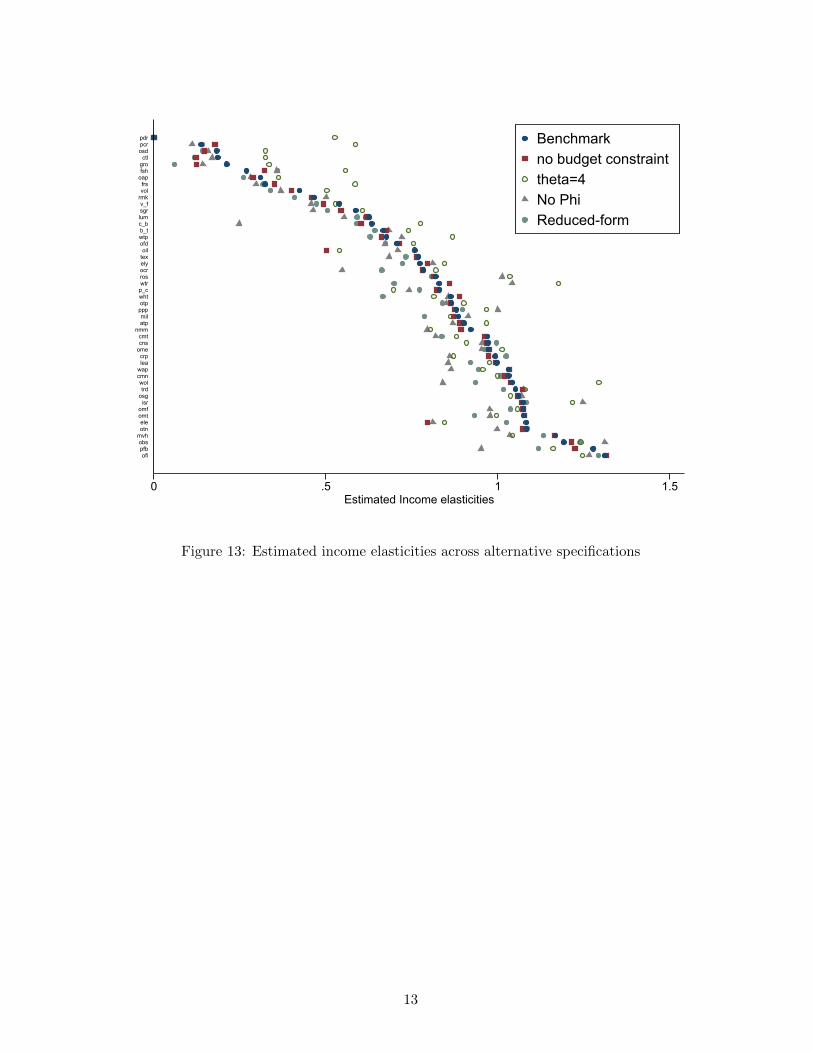
0 .5 1 1.5Estimated Income elasticities

ofipfbobs

mvhotnele

omtomf

isrosgtrd

wolcmnwapleacrp

omecnscmt

nmmatpmil

pppotpwhtp_cwtrrosocrelytexoil

ofdwtpb_tc_blumsgrv_f

rmkvolfrs

oapfshgroctl

osdpcrpdr Benchmark

no budget constrainttheta=4No PhiReduced-form

Figure 13: Estimated income elasticities across alternative specifications

13

atp

b_t

c_b

cmn

cmt

cnscrp

ctl

eleely

frs

fsh

gro

isr

lea

lum

mil

mvh

nmm

oap

obs

ocr

ofd

ofi

omeomf

omt

osd

osgotn

otp

p_c

pcr

pdr

pfbppp

rmk

ros

sgr

tex

trd

v_fvol

wap

wht

wol

wtp

wtr0

.51

1.5

Inco

me

elas

ticity

- in

stru

men

ted

Phi

0 .5 1 1.5Income elasticity - no IV

Figure 14: Estimated income elasticities – Instrumenting Φ

14

0.1

.2.3

Elas

ticity

of s

kill

prem

ium

to p

rodu

ctiv

ity

6 8 10 12Log per capita expenditures

Baseline Theta=4 Alternative skill intensity

Figure 15: Simulated elasticity of the skill premium increase to TFP across alternative specifications

15

0.0

5.1

.15

Diff

eren

tial s

kill

prem

ium

incr

ease

6 8 10 12Log per capita expenditures

Baseline Theta=4 Alternative skill intensity

Figure 16: Trade counterfactual: Differential skill premium increase across alternative specifications(non-homothetic preferences minus homothetic preferences)

16

atp

b_t

c_b

cmn

cmt

cnscrp

ctl

ele

ely

frsfshgro

isr

lea

lum

mil

mvh

nmm

oap

obs

ocr

ofd

ofi

oil

ome omfomt

osd

osgotn

otpp_c

pcr

pdr

pfbppp

rmk

ros

sgr

tex

trd

v_fvol

wapwht wol

wtp

wtr0

.51

1.5

Inco

me

elas

ticity

- C

LM

0 .5 1 1.5Income elasticity - Benchmark

Figure 17: Estimated income elasticities – based on Comin et al (2016) preferences

17

Figure 18: Robustness: counterfactuals based on Comin et al (2016) preferences

AUSNZLCHN

HKGJPNKOR

MNG

TWN

KHM

IDN

MYS

PHL

SGPTHA

VNM

BGD

IND

NPL

PAK

LKA

CANUSAMEXARG

BOL

BRACHLCOL

ECUPRY

PERURYVEN

CRI

GTMHNDNIC

PAN

SLV

AUTBELCYPCZE DNKESTFINFRADEU

GRCHUN IRLITALVALTU

LUXMLT NLDPOL PRTSVK SVNESPSWEGBRCHENOR

ALB

BGR

BLRHRVROU

RUSUKR

KAZ

KGZ

ARM

AZE

GEO

BHR

IRN

KWTQAT

SAUTUR

ARE

EGY MARTUN

CMR

CIV

SEN

ETH

KEN

MWI

MUS

MOZ

TZA

UGA ZMB

ZWE

BWANAM

ZAFISROMN

0.2

.4.6

Elas

ticity

of s

kill

prem

ium

to p

rodu

ctiv

ity

5 6 7 8 9 10 11 12Per capita income

(a) First counterfactual: homogeneous productivity increase

ALB

ARE

ARG

ARM

AUSAUT

AZE

BEL

BGD BGR

BHR

BLR

BOLBRABWA

CANCHE

CHLCHN

CIV

CMR

COL

CRI

CYP

CZE DEUDNK

ECU

EGY ESPEST

ETH

FIN

FRAGBRGEO

GHA

GRC

GTM

HKG

HND

HRV

HUN

IDN

IND IRL

IRNISR ITAJPN

KAZ

KENKGZKHM

KOR

KWT

LAO

LKALTU

LUX

LVA

MAR

MDG

MEX

MLT

MNGMOZ

MUS

MWI

MYSNAM

NGA

NIC

NLD

NOR

NPL

NZL

OMN

PAK

PAN

PER

PHL

POL

PRT

PRY

QAT

ROURUS

SAU

SEN

SGP

SLV SVKSVN SWE

THATUN

TUR

TWN

TZA

UGA

UKRURY

USAVEN

VNM

ZAF

ZMBZWE

ALB

ARE

ARG

ARM

AUSAUT

AZE

BEL

BGD

BGR

BHR

BLR

BOLBRABWA CANCHE

CHLCHN

CIV

CMRCOL

CRI

CYP

CZE DEUDNK

ECU

EGY

ESPEST

ETH

FIN

FRAGBR

GEO

GHA

GRCGTM

HKG

HND

HRV

HUNIDN

IND

IRL

IRN

ISR ITAJPN

KAZ

KEN

KGZKHM

KOR

KWT

LKALTU

LUX

LVA

MAR

MDG

MEX

MLTMNG

MOZ

MUS

MWI

MYSNAM

NGA

NIC NLDNOR

NPL

NZL

OMNPAK

PAN

PER

PHL

POL

PRT

PRY

QATROU

RUS

SAU

SEN

SGP

SLV

SVKSVN SWETHA

TUN

TURTWN

TZAUGA

UKR

URY

USAVEN

VNM

ZAF

ZMBZWE

-.2-.1

0.1

.2.3

Skill

prem

ium

incr

ease

5 6 7 8 9 10 11 12Per Capita Income

Homothetic preferences Comin et al. pref.Linear Fit Linear Fit

(b) Second counterfactual: trade cost reduction

18

AUS

NZL

CHNHKG

JPNKOR

MNG

TWN

KHM

IDN

LAO

MYSPHL

SGP

THA

VNM

BGD

IND

NPL

PAKLKA

CAN

USA

MEX

ARG

BOL

BRA

CHL

COL

ECU

PRY

PERURY

VEN

CRI

GTM

HNDNIC

PAN

SLV

AUT

BEL

CYP

CZEDNK

EST

FINFRA

DEU

GRC

HUN

IRL

ITALVALTU

LUX

MLT

NLD

POLPRT

SVKSVN ESP

SWE

GBR

CHE

NOR

ALB BGR

BLR

HRVROU

RUS

UKR

KAZ

KGZ

ARM

GEO

BHR

IRN

QATSAU

TUR

ARE

EGY

MAR

TUN

CMR

CIVGHANGA

SEN

ETH KENMDGMWI

MUSMOZ

TZA

UGA ZMB

ZWE

BWANAMZAF

ISR

OMN

AUS

NZL

CHN HKG

JPNKOR

MNG

TWN

KHM

IDN

LAO

MYS

PHL

SGP

THA

VNM

BGDIND

NPL

PAK LKACAN

USA

MEX

ARG

BOL

BRA

CHL

COL

ECU

PRY

PER URY

VEN

CRI

GTM

HND

NIC

PAN

SLV

AUT

BEL

CYP

CZEDNK

EST

FINFRA

DEU

GRC

HUN

IRL

ITALVALTU

LUX

MLT

NLD

POLPRT

SVKSVN

ESP

SWE

GBR

CHE

NORALB

BGR

BLR

HRVROU

RUS

UKR

KAZ

KGZ

ARM

GEO

BHR

IRN

QAT

SAU

TUR

ARE

EGY

MAR

TUN

CMR

CIVGHA

NGA

SEN

ETHKENMDG

MWIMUS

MOZ

TZA

UGA

ZMB

ZWE

BWANAM

ZAF

ISR

OMN

-.6-.4

-.20

.2Sk

ill pr

emiu

m in

crea

se

5 6 7 8 9 10 11 12Per Capita Income

Homothetic preferences Non-homothetic pref.Linear Fit Linear Fit

Figure 19: Change in the skill premium caused by a 1% trade cost reduction, one country at a time(each dot corresponds to a distinct counterfactual)

19