Penalized Regression Methods for Linear Models in SAS/STAT®

Funda Gunes, SAS Institute Inc.

Abstract

Regression problems with many potential candidate predictor variables occur in a wide variety of scientific fields andbusiness applications. These problems require you to perform statistical model selection to find an optimal model, onethat is as simple as possible while still providing good predictive performance. Traditional stepwise selection methods,such as forward and backward selection, suffer from high variability and low prediction accuracy, especially whenthere are many predictor variables or correlated predictor variables (or both). In the last decade, the higher predictionaccuracy and computational efficiency of penalized regression methods have made them an attractive alternative totraditional selection methods. This paper first provides a brief review of the LASSO, adaptive LASSO, and elastic netpenalized model selection methods. Then it explains how to perform model selection by applying these techniqueswith the GLMSELECT procedure, which includes extensive customization options and powerful graphs for steeringstatistical model selection.

Introduction

Advances in data collection technologies have greatly increased the numbers of candidate predictors in science andbusiness. Scientific applications with many candidate predictive variables include genomics, tumor classifications, andbiomedical imaging. Business problems with large numbers of predictors occur in scoring credit risk, predicting retailcustomer behavior, exploring health care alternatives, or tracking the effect of new pharmaceuticals in the population.For example, credit risk score modeling often requires many candidate predictor variables that reflect a customer’scredit history and loan application to predict their probability of making future credit payments on time.

Suppose you have a statistical modeling problem with many possible predictor effects and your goal is to find a simplemodel that also has good predictive performance. You want a simple model with fewer predictor variables becausethese models are easy to interpret, and they enable you to understand the underlying process that generates yourdata. For example, a lender who uses a statistical model to screen customers’ applications needs to explain why theapplication was denied. Fewer predictor variables also enhance the predictive accuracy of a statistical model.

Statistical model selection estimates the prediction performance of different models in order to choose the approximatebest model for your data (Hastie, Tibshirani, and Friedman 2001). Traditional model selection methods such asstepwise and forward selection methods achieve simplicity, but they have been shown to yield models that have lowprediction accuracy, especially when there are correlated predictors or when the number of predictors is large. Thehigh prediction accuracy and computational efficiency of penalized regression methods have brought them increasingattention over the last decade.

Similar to ordinary least squares (OLS) estimation, penalized regression methods estimate the regression coefficientsby minimizing the residual sum of squares (RSS). However although they minimize the RSS, penalized regressionmethods place a constraint on the size of the regression coefficients. This constraint or penalty on the size of theregression causes coefficient estimates to be biased, but it improves the overall prediction error of the model bydecreasing the variance of the coefficient estimates.

A penalized regression method yields a sequence of models, each associated with specific values for one or moretuning parameters. Thus you need to specify at least one tuning method to choose the optimum model (that is, themodel that has the minimum estimated prediction error). Popular tuning methods for penalized regression include fitcriteria (such as AIC, SBC, and the Cp statistic), average square error on the validation data, and cross validation.

This paper summarizes building linear models based on penalized regression. It then discusses three methods forpenalized regression: LASSO, adaptive LASSO, and elastic net. The first example uses LASSO with validation dataas a tuning method. The second example uses adaptive LASSO with information criteria as a tuning method. Afinal example uses elastic net with cross validation as a tuning method. The last section provides a summary andadditional information about the GLMSELECT procedure.

1

Methodology Overview

Linear Models

In a linear model, the response variable Y is modeled as a linear combination of the predictor variables, X1; : : : ; Xp ,plus random noise,

Yi D ˇ0 C ˇ1Xi1 C � � � C ˇpXip C �i

where ˇ0; ˇ1; : : : ; ˇp are regression parameters, � is the random noise term, and i is the observation number,i D 1; : : : ; N .

Linear models are often preferred to more complicated statistical models because you can fit them relatively easily.Moreover, linearity with respect to fixed functions of the predictors is often an adequate first approximation to morecomplex behavior. Other methods, such as nonlinear or nonparametric models, become computationally complicatedand fail as the number of variables increase. In many practical situations, linear models provide simpler models withgood predictive performance (Hastie, Tibshirani, and Friedman 2001).

Least squares estimation is the most common method used to estimate regression coefficients for a linear model, itfinds the coefficients (ˇ) that minimize the RSS:

RSS.ˇ/ DNXiD1

�Yi � ˇ0 � ˇ1Xi1 � � � � � ˇpXip

�2According to the Gauss-Markov theorem, the least squares estimate has the smallest variance among all linearunbiased estimates of ˇ under certain assumptions. However, when the number of predictor variables is large or ifthere are correlated predictor variables, some of these assumptions are violated. As a result least squares estimatesget highly variable (unstable) and the resulting model exhibit poor predictive performance. Another problem with leastsquares estimation is that it assigns nonzero values to all regression coefficients. Therefore, when there are manypredictors, least squares estimation does not necessarily lead to a simple model that identifies the variables that reallygenerated your data. Tackling these problems requires statistical model selection.

Model Selection

Statistical model selection involves estimating the predictive performance of different models and choosing a singleapproximate best model from among the alternatives, one that is simple and has good prediction accuracy. It isimportant to note that you can find only an approximate best model (that is, one that is pretty good), but not necessarilyone that represents the underlying truth, because no statistical method can be guaranteed to infallibly determine theunderlying truth. In addition, the selected model is not guaranteed to truly optimize the relevant performance criteriabecause global optimization problems are generally intractable. The best you can do is to use sophisticated methodsfor efficiently approximating their solution.

Traditional selection methods (such as forward, backward, and stepwise selection) are examples of such sophisticatedmethods. They first identify a subset of predictor variables by successively adding or removing variables (or both),and then they use least squares estimation to fit a model on the reduced set of variables. These traditional selectionalgorithms are greedy in the sense that they iteratively proceed by taking optimal individual steps. Not only can suchgreedy methods fail to find the global optimum, but the selected models can also be extremely variable, in the sensethat a small change in data can result in a very different set of variables and predictions. When you have correlatedpredictors or a large number of predictor variables (or both), the instability of traditional selection can be even moreproblematic (Harrell 2001). Penalized regression addresses this instability by decreasing the variance involved incoefficient estimation.

Penalized regression methods are examples of modern approaches to model selection. Because they produce morestable results for correlated data or data where the number of predictors is much larger than the sample size, theyare often preferred to traditional selection methods. Unlike subset selection methods, penalized regression methodsdo not explicitly select the variables; instead they minimize the RSS by using a penalty on the size of the regressioncoefficients. This penalty causes the regression coefficients to shrink toward zero. This is why penalized regressionmethods are also known as shrinkage or regularization methods. If the shrinkage is large enough, some regressioncoefficients are set to zero exactly. Thus, penalized regression methods perform variable selection and coefficientestimation simultaneously.

2

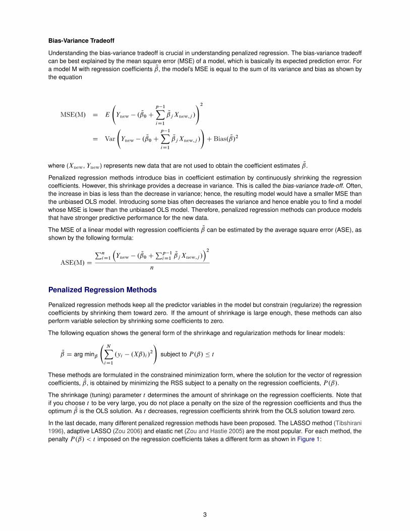
Bias-Variance Tradeoff

Understanding the bias-variance tradeoff is crucial in understanding penalized regression. The bias-variance tradeoffcan be best explained by the mean square error (MSE) of a model, which is basically its expected prediction error. Fora model M with regression coefficients Q, the model’s MSE is equal to the sum of its variance and bias as shown bythe equation

MSE.M/ D E

Ynew � . Q0 C

p�1XiD1

QjXnew;j /

!2

D Var

Ynew � . Q0 C

p�1XiD1

QjXnew;j /

!C Bias. Q/2

where (Xnew, Ynew) represents new data that are not used to obtain the coefficient estimates Q.

Penalized regression methods introduce bias in coefficient estimation by continuously shrinking the regressioncoefficients. However, this shrinkage provides a decrease in variance. This is called the bias-variance trade-off. Often,the increase in bias is less than the decrease in variance; hence, the resulting model would have a smaller MSE thanthe unbiased OLS model. Introducing some bias often decreases the variance and hence enable you to find a modelwhose MSE is lower than the unbiased OLS model. Therefore, penalized regression methods can produce modelsthat have stronger predictive performance for the new data.

The MSE of a linear model with regression coefficients Q can be estimated by the average square error (ASE), asshown by the following formula:

ASE.M/ D

PniD1

�Ynew � . Q0 C

Pp�1iD1QjXnew;j /

�2n

Penalized Regression Methods

Penalized regression methods keep all the predictor variables in the model but constrain (regularize) the regressioncoefficients by shrinking them toward zero. If the amount of shrinkage is large enough, these methods can alsoperform variable selection by shrinking some coefficients to zero.

The following equation shows the general form of the shrinkage and regularization methods for linear models:

Q D arg minˇ

NXiD1

.yi � .Xˇ/i /2

!subject to P.ˇ/ � t

These methods are formulated in the constrained minimization form, where the solution for the vector of regressioncoefficients, Q, is obtained by minimizing the RSS subject to a penalty on the regression coefficients, P.ˇ/.

The shrinkage (tuning) parameter t determines the amount of shrinkage on the regression coefficients. Note thatif you choose t to be very large, you do not place a penalty on the size of the regression coefficients and thus theoptimum Q is the OLS solution. As t decreases, regression coefficients shrink from the OLS solution toward zero.

In the last decade, many different penalized regression methods have been proposed. The LASSO method (Tibshirani1996), adaptive LASSO (Zou 2006) and elastic net (Zou and Hastie 2005) are the most popular. For each method, thepenalty P.ˇ/ < t imposed on the regression coefficients takes a different form as shown in Figure 1:

3

Table 1 Popular Penalized Regression Methods

Method Penalty

LASSOPpjD1 j ˇj j< t

Adaptive LASSOPpjD1

�j ˇj j=j Oj j

�< t

Elastic netPpjD1 j ˇj j< t1 and

PpjD1 ˇ

2j < t2

For LASSO selection, the penalty is placed on L1 norm of the regression coefficients; for adaptive LASSO, the penaltyis on weighted L1 norm of the regression coefficients; and for elastic net, the penalty is on the combination of L1 andL2 norms of the regression coefficients. Notice that elastic net includes two tuning parameters, t1 and t2, whereasLASSO and adaptive LASSO includes only one, t .

The penalized regression methods can also be formulated in Lagrangian form as shown in the following equation:

Q D arg minˇ

NXiD1

.yi � .Xˇ/i /2C �P.ˇ/

!

In Lagrangian form, the shrinkage parameter is a nonnegative number �. When �=0, the optimum Q is equal to theOLS solution. As � increases, you impose more shrinkage on the regression coefficients; hence, the regressioncoefficients shrink from OLS solution toward zero. Note that there is a one-to-one relationship between the tuningvalues of � and t .

A penalized regression method produces a series of models, M0;M1; : : : ;Mk , where each model is the solutionfor a unique tuning parameter value. In this series, M0 can be thought of as the least complex model, for whichthe maximum amount of penalty is imposed on the regression coefficients (typically, and not very usefully, settingall regression coefficients to zero), and Mk can be thought of as the most complex model, for which no penalty isimposed and the regression coefficients are estimated by OLS. This series of models can be generated by usingspecialized algorithms in a computationally efficient way. For example, the computational cost of LASSO for obtainingthe whole solution path can be less than one OLS fit when you use the efficient Least Angle Regression (LARS)algorithm (Efron et al. 2004), which constructs a piecewise linear path of solution starting from the null vector towardsthe OLS estimate.

After series of models are produced, you estimate the prediction error for each model and then you choose the modelthat yields the minimum prediction error. Prediction error of a model can be estimated directly or indirectly. Directtechniques estimate the prediction error by scoring validation data or by using cross validation. Indirect methodsestimate the prediction error by making mathematical adjustments to the RSS. Indirect estimation methods use criteriasuch as AIC, SBC, and the Cp statistic.

The following section describe the use of penalized regression methods by using the GLMSELECT procedure, whichperforms model selection for linear models.

LASSO Selection

For a specified tuning value t , LASSO selection finds the solution to the following constrained minimization problem,

arg minˇ

NXiD1

.yi � .Xˇ/i /2 subject to

pXjD1

j ˇj j� t

where the LASSO penalty is placed on the L1 norm of the regression coefficients, which is simply the sum of theirabsolute values. In order for the shrinkage to be applied equally on the regression coefficients, each predictor variable

4

needs to be standardized prior to performing the selection; this is done automatically by the GLMSELECT procedure.Using the coefficients on the same scale also helps produce plots to track the selection process.

The following example shows how to apply LASSO selection to a simulated data set. The DATA step code belowgenerates the data set, Simdata.

data Simdata;drop i j;array x{5} x1-x5;

do i=1 to 1000;do j=1 to 5;

x{j} = ranuni(1); /* Continuous predictors */end;c1 = int(1.5+ranuni(1)*7); /* Classification variables */c2 = 1 + mod(i,3);yTrue = 2 + 5*x2 - 17*x1*x2 + 6*(c1=2) + 5*(c1=5);y = yTrue + 2*rannor(1);output Simdata;

end;run;

The Simdata include 1,000 observations, five continuous variables (x1, . . . , x5), and two classification variables (c1and c2). As you can see, the response variable is generated from a linear function of only x1, x2, and c1.

The following statements request that the GLMSELECT procedure perform a LASSO fit for these data. The validationdata approach is used as a tuning method.

proc glmselect data=Simdata plots=all;partition fraction(validate=.3);class c1 c2;model y = c1|c2|x1|x2|x3|x4|x5 @2

/ selection=lasso(stop=none choose=validate);run;

The MODEL statement request that a linear model be built using all the effects (c1, c2, x1, x2, x3, x4 and x5) andtheir two-way interactions. The PARTITION statement randomly reserves 30% of the data as validation data anduses the remaining 70% as training data. The training set is used for fitting the models, and the validation set is usedfor estimating the prediction error for model selection. The SELECTION=LASSO option in the MODEL statementrequests LASSO selection. The CHOOSE=VALIDATE suboption in the MODEL statement requests that validationdata be used as the tuning method for the LASSO selection. If you have enough data, using a validation data set is thebest way to tune a penalized regression method. The observations in the training set are used to produce a LASSOsolution path (M0; : : : ;Mk), and the observations in the validation set are used to estimate the prediction error ofeach model (Mi ) on the solution path. The model that yields the smallest ASE on the validation data is then selected.

The “Dimensions” table in Figure 1 show that 106 variables are considered for selection. This is because c1 and c2are classification effects with several levels and the analysis includes all possible two-way interaction effects.

Figure 1 Class Level Information and Dimensions Tables

Class Level Information

Class Levels Values

c1 8 1 2 3 4 5 6 7 8

c2 3 1 2 3

Dimensions

Number of Effects 29

Number of Effects after Splits 106

Number of Parameters 106

5

Figure 2 shows that 292 observations are reserved for validation data and the rest (708) are reserved for trainingdata.

Figure 2 Number of Observations Table

Number of Observations Read 1000

Number of Observations Used 1000

Number of Observations Used for Training 708

Number of Observations Used for Validation 292

Figure 3 shows the ASE of the models on the LASSO solution path separately for the training and validation sets. TheLASSO solution path is created on a grid of the tuning parameter value (t ). The X axis shows the normalized tuningvalues, which are the L1 norm of the regression coefficients divided by the L1 norm of the ordinary least squaressolution.

Figure 3 Training versus Validation Set Errors

As you move from left to right on the X axis in Figure 3, the amount of shrinkage that is imposed on the regressioncoefficients decreases. Hence, the model complexity increases from the null model to the full OLS model, with all106 regression parameters. As the model complexity increases, the ASE on the training data consistently decreases,typically dropping to 0 if you increase the model complexity enough. However, a model that has a training error of 0 isoverfit to the training data and will typically generalize poorly on a new data set. Thus, training error is not a goodestimate of the prediction error. On the other hand, the prediction error on the validation data first decreases, but thenincreases; the point of minimum ASE is marked by the vertical line on the plot, at a tuning value of about 0.44. The

6

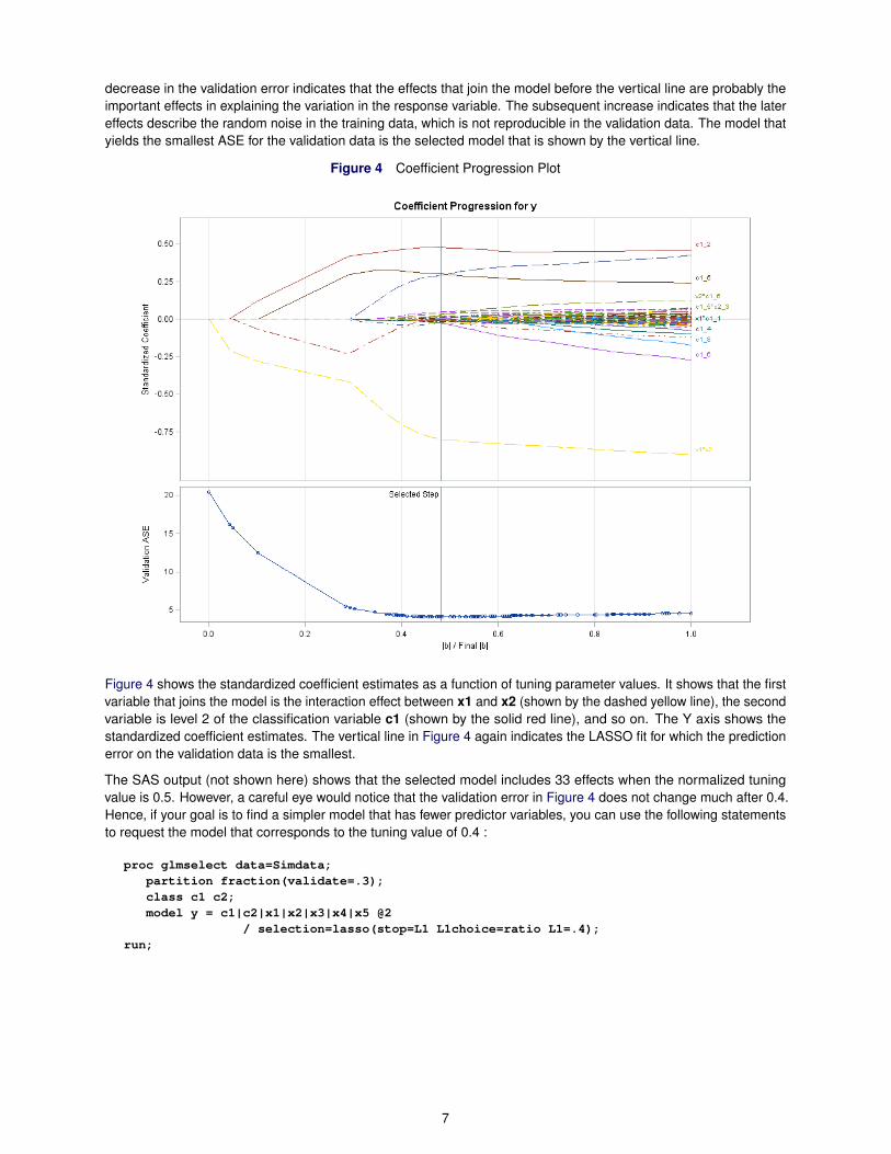
decrease in the validation error indicates that the effects that join the model before the vertical line are probably theimportant effects in explaining the variation in the response variable. The subsequent increase indicates that the latereffects describe the random noise in the training data, which is not reproducible in the validation data. The model thatyields the smallest ASE for the validation data is the selected model that is shown by the vertical line.

Figure 4 Coefficient Progression Plot

Figure 4 shows the standardized coefficient estimates as a function of tuning parameter values. It shows that the firstvariable that joins the model is the interaction effect between x1 and x2 (shown by the dashed yellow line), the secondvariable is level 2 of the classification variable c1 (shown by the solid red line), and so on. The Y axis shows thestandardized coefficient estimates. The vertical line in Figure 4 again indicates the LASSO fit for which the predictionerror on the validation data is the smallest.

The SAS output (not shown here) shows that the selected model includes 33 effects when the normalized tuningvalue is 0.5. However, a careful eye would notice that the validation error in Figure 4 does not change much after 0.4.Hence, if your goal is to find a simpler model that has fewer predictor variables, you can use the following statementsto request the model that corresponds to the tuning value of 0.4 :

proc glmselect data=Simdata;partition fraction(validate=.3);class c1 c2;model y = c1|c2|x1|x2|x3|x4|x5 @2

/ selection=lasso(stop=L1 L1choice=ratio L1=.4);run;

7

Figure 5 Selected Model

LASSO Selection Summary

StepEffectEntered

EffectRemoved

NumberEffects In ASE

ValidationASE

0 Intercept 1 18.9839 20.5025

1 x1*x2 2 15.3909 16.7325

2 x1 3 15.1343 16.4645

3 c1_2 4 10.8155 12.1724

4 c1_5 5 5.5538 6.3239*

* Optimal Value of Criterion

Notice that the model at t=0.4 correctly identifies all the true effects (x2, x1*x2, and levels 2 and 5 of c2) that generatethe response variable y.

Adaptive LASSO

In model selection, the Oracle property (Zou 2006) of statistical estimation method is desirable because it assurestwo important asymptotic properties: First, it assures that as the sample size approaches infinity, the selected set ofpredictor variables approaches the true set of predictor variables with probability 1 (selection consistency). Second, itassures that the estimators are asymptotically normal with the same means and covariance that they would haveby maximum likelihood estimation, when the zero coefficients were known in advance (estimation consistency).Asymptotically, LASSO has a non-ignorable bias when it estimates the nonzero coefficients; hence LASSO mightnot have the Oracle property (Fan and Li 2001). Adaptive LASSO, on the other hand, enjoys the Oracle property byallowing a relatively higher penalty for zero coefficients and a lower penalty for nonzero coefficients (Zou 2006).

Adaptive LASSO modifies the LASSO penalty by applying weights to each parameter that forms the LASSO constraint.These weights control shrinking the zero coefficients more than they control shrinking the nonzero coefficients:

Q D arg minˇ

NXiD1

.yi � .Xˇ/i /2 subject to

pXjD1

�wj j ˇj j

�� t

By default, the GLMSELECT procedure uses the OLS estimates of the regression coefficients in forming the adaptiveweights (wj D 1= j O j). However, the procedure also provides options so that you can supply your own weights. Forexample, when there are correlated variables or when the number of predictor variables exceeds the sample size, youmight prefer using more stable ridge regression coefficients as adaptive weights instead of using OLS coefficients.

Similar to LASSO, adaptive LASSO can be solved efficiently by using the LARS algorithm.

Analyzing Prostate Data by Using LASSO and Adaptive LASSO

An often-analyzed data, Prostate, contains observations from 97 prostate cancer patients (Stamey et al. 1989).Suppose you are interested in building a model that identifies the important predictors of the level of prostate-specificantigen and provides accurate predictions.

The following SAS statements create the Prostate data set:

data Prostate;input lpsa lcavol lweight age lbph svi lcp gleason pgg45;datalines;-0.43 -0.58 2.769 50 -1.39 0 -1.39 6 0-0.16 -0.99 3.32 58 -1.39 0 -1.39 6 0

... more lines ...

8

5.583 3.472 3.975 68 0.438 1 2.904 7 20;

This data set includes the response variable as the level of prostate-specific antigen (lspa) and the following clinicalpredictors: logarithm of the cancer volume (lcavol), logarithm of prostate weight (lweight), age (age), logarithm ofthe amount of benign prostatic hyperplasia (lbph), seminal vasicle invasion (svi), logarithm of capsular penetration(lcp), Gleason score (gleason), and percentage of Gleason scores of 4 or 5 (pgg45).

The following statements randomly reserve one third of the data as the test data (TestData) and the remaining twothirds as the training data (TrainData.) Unlike validation data, test data are not used to choose the final model for aparticular technique such as LASSO. Instead test data are used in assessing the generalization of the final chosenmodel.

data TrainData TestData;set prostate;if ranuni(1)<2/3 then output TrainData;

else output TestData;run;

The following calls to the GLMSELECT procedure request that a linear model be built for the Prostate data (by using alleight predictor variables) to predict the level of prostate-specific antigen. The first PROC GLMSELECT call requeststhe LASSO method, and the second PROC GLMSELECT call requests the adaptive LASSO method. In both calls, thetest data are specified by the TESTDATA= option in the PROC GLMSELECT statement, and the CHOOSE= suboptionin the MODEL statement specifies the SBC criterion for model selection.

proc glmselect data=TrainData testdata=TestData plots=all;model lpsa=lcavol lweight age lbph svi lcp gleason pgg45

/ selection=lasso( stop=none choose=sbc);run;

proc glmselect data=TrainData testdata=TestData plots=all;model lpsa=lcavol lweight age lbph svi lcp gleason pgg45

/ selection=lasso(adaptive stop=none choose=sbc);run;

Figure 6 shows that, although the solution paths are slightly different, LASSO and adaptive LASSO select the sameset of predictor variables (lcvol, svi, lweight) when they use SBC as a tuning method, and the estimated coefficientvalues are similar.

Figure 6 Coefficient Progression Plots

LASSO Adaptive LASSO

Figure 7 shows the fit statistics of the selected models by using LASSO and adaptive LASSO. Notice that the ASE ofthe test data for adaptive LASSO (0.58521) is slightly less than the one for LASSO (0.59053).

9

Figure 7 Fit Statistics Tables

LASSO Adaptive LASSOSelected ModelSelected Model

Root MSE 0.70137

Dependent Mean 2.58256

R-Square 0.6629

Adj R-Sq 0.6476

AIC 26.22033

AICC 27.15783

SBC -36.78569

ASE (Train) 0.46381

ASE (Test) 0.59053

Selected ModelSelected Model

Root MSE 0.68810

Dependent Mean 2.58256

R-Square 0.6755

Adj R-Sq 0.6608

AIC 23.54568

AICC 24.48318

SBC -39.46034

ASE (Train) 0.44642

ASE (Test) 0.58521

The main advantage of adaptive LASSO over LASSO is its asymptotic consistency, which can make a difference forvery large data sets. However, asymptotic consistency does not automatically result in optimal prediction performance,especially for finite samples. Hence, LASSO can still be advantageous in difficult prediction problems (Zou 2006).

Elastic Net

Although LASSO selection performs well for a wide range of variable selection problems, it has some limitations whenthe number of predictor variables (p) is much larger than the sample size (n), p >> n. Examples of a “large p, smalln” problem occur in text processing of Internet documents, microarray analysis, and combinatorial chemistry. Forexample, in a microarrays analysis p can be around 10,000s, whereas n is often less than 100.

One limitation of LASSO selection is that the number of predictor variables it selects cannot exceed the sample size.The other limitation of LASSO occurs when there are groups of correlated variables. LASSO fails to do a groupselection by selecting only one variable from a group and ignoring the others. For example, genes that share thesame biological pathway can be thought as forming a group, and you would want to identify these genes as a group.Elastic net removes the limitation on the number of selected variables and performs group selection by selecting allthe variables that form the group (Zou and Hastie 2005).

Elastic net solves the following optimization problem:

Q D arg minˇ

NXiD1

.yi � .Xˇ/i /2 subject to

pXjD1

j ˇj j� t1 andpXjD1

ˇ2j � t2

where the penalty is placed on both the L1 norm (PpjD1 j ˇj j) and the L2 norm (

PpjD1 ˇ

2j ) of the regression

coefficients. The L1 part of the penalty performs variable selection by setting some coefficients to exactly 0, and theL2 part of the penalty encourages the group selection by shrinking the coefficients of correlated variables towardeach other.

The same problem can be rewritten in the following Lagrangian form, where �1 and �2 are the tuning parameters:

Q D arg minˇ

0@ NXiD1

.yi � .Xˇ/i /2C �1

pXjD1

j ˇj j C�2

pXjD1

ˇ2j

1A

10

Simple Simulation Example

The following simple simulation example is taken from the original elastic net paper (Zou and Hastie 2005), whichshows how elastic net performs group selection as opposed to LASSO. Suppose there are two independent “hidden”factors (z1 and z2) that are generated from a uniform distribution for the range of 0 to 20:

z1; z2 � uniform.0; 20/

The response vector is generated by:

y D z1 C 0:1z2 CN.0; 1/

Suppose the observed predictors ( x1; x2; : : : ; x6) are generated from the “hidden” factors (z1, z2) in the followingway:

x1 D z1 C �1; x2 D �z1 C �2; x3 D z1 C �3

x4 D z2 C �4; x5 D �z2 C �5; x6 D z2 C �6

Based on the simulation setup, for a linear model where y is the response variable and x1; : : : ; x6 are the explanatoryvariables, a good selection procedure would identify x1, x2, and x3 (the z1 group) together as the most importantvariables. Figure 10 shows coefficient progression plots that are generated by LASSO and elastic net selection.

Figure 8 Coefficient Progression Plots

LASSO Elastic Net

Figure 10 shows that, in elastic net selection, x1, x2, and x3 variables join the model as a group long before the othergroup members x4, x5 and x6, whereas in LASSO selection the group selection is not clear. Also the elastic netsolution path is more stable and smoother than the LASSO path.

Cross Validation and External Cross Validation

When you have many predictor variables and data are scarce, setting aside validation or test data is often not possible.Cross validation uses part of the training data to fit the model and a different part to estimate the prediction error.For a k-fold cross validation, you split the data into k approximately equal-sized disjoint parts. You reserve one partof the data for validation, and you fit the model to the remaining k � 1 parts of the data. Then you use this fittedmodel to calculate the prediction error for the reserved part of the data. You do this for all k parts, and summationof k estimates of the prediction error divided by the total training sample size yields the k-fold cross validation error.Because calculation of cross validation error for k-fold requires fitting k models, using cross validation can becomecomputationally demanding as you increase the number of folds.

The regular cross validation method (CV) that is available in the GLMSELECT procedure uses the OLS estimation toobtain the prediction error for each of the k � 1 parts of the data, regardless of which estimation method is specified inthe MODEL statement. The external cross validation method (CVEX), on the other hand, uses the selection methodspecified in the MODEL statement to estimate the cross validation error. Therefore, for penalized regression problems,you should specify CVEX instead of CV in the CHOOSE= option. For more information about external cross validationsee the “Details” section of the PROC GLMSELECT documentation in the SAS/STAT Users’ Guide.

11

Choosing the Tuning Values for Elastic Net

Because elastic net handles “large p, small n” problems nicely, you do not want to decrease your sample size evenmore by setting aside validation or test data sets. Therefore, cross validation is the recommended method for choosingthe tuning parameters. In elastic net, the penalty is placed on both the L1 norm and the L2 norm of the regressioncoefficients; hence you must specify methods to choose both tuning parameters, �1 and �2. A typical approach forchoosing the tuning values is to first run the analysis on a grid of �2 values, such as (0, 0.01, 0.1, 1, 10, and 100).For each �2 value, the GLMSELECT procedure uses the efficient LARS-EN algorithm to produce the whole solutionpath that depend on �1 . Then for each �2 value, you can choose the �1 value that yields the smallest k-fold crossvalidation error. After this step, you can choose the �2 value that yields the minimum k-fold cross validation error.

Analyzing Prostate Data by Using Elastic Net

Figure 9 displays the correlation matrix for the eight predictors of the Prostate data. You can see that there is somesignificant correlation between the predictor variables, where the highest is 0.75 (between gleason and pgg45).Because of this correlation between the predictor variables, elastic net selection might be more suitable for analyzingthe prostate data.

Figure 9 Correlation Matrix for the Prostate Data

Pearson Correlation Coefficients, N = 97Prob > |r| under H0: Rho=0

lcavol lweight age lbph svi lcp gleason pgg45

lcavol 1.00000 0.280520.0054

0.225000.0267

0.027350.7903

0.53885<.0001

0.67531<.0001

0.43242<.0001

0.43365<.0001

lweight 0.280520.0054

1.00000 0.347970.0005

0.44226<.0001

0.155380.1286

0.164540.1073

0.056880.5800

0.107350.2953

age 0.225000.0267

0.347970.0005

1.00000 0.350190.0004

0.117660.2511

0.127670.2127

0.268890.0077

0.276110.0062

lbph 0.027350.7903

0.44226<.0001

0.350190.0004

1.00000 -0.085840.4031

-0.007000.9458

0.077820.4487

0.078460.4449

svi 0.53885<.0001

0.155380.1286

0.117660.2511

-0.085840.4031

1.00000 0.67311<.0001

0.320410.0014

0.45765<.0001

lcp 0.67531<.0001

0.164540.1073

0.127670.2127

-0.007000.9458

0.67311<.0001

1.00000 0.51483<.0001

0.63153<.0001

gleason 0.43242<.0001

0.056880.5800

0.268890.0077

0.077820.4487

0.320410.0014

0.51483<.0001

1.00000 0.75190<.0001

pgg45 0.43365<.0001

0.107350.2953

0.276110.0062

0.078460.4449

0.45765<.0001

0.63153<.0001

0.75190<.0001

1.00000

The following statements requests to build a model for Prostate using elastic net. The L2= suboption of theSELECTION= option in the MODEL statement specifies the tuning value of �2 as 0.1, and the CHOOSE= suboptionrequests that external cross validation be used for determining the tuning value �1. The CVMETHOD=requests thattenfold cross validation be used.

proc glmselect data=TrainData testdata=TestData plots(stepaxis=normb)=all;model lpsa = lcavol lweight age lbph svi lcp gleason pgg45

/selection=elasticnet(L2=0.1 stop=none choose=cvex) cvmethod=split(10);run;

Figure 10 shows the parameter estimates and the fit statistics of the model that is selected by elastic net. In additionto the three predictors (lcavol, lweight, and svi) selected by both LASSO and adaptive LASSO, elastic net choosestwo more variables (lcp and pgg45). However, notice that the coefficient estimates of these two parameters are veryclose to 0 (0.0303 and 0.0015). The ASE of the test data is 0.58317, which is slightly less than the ASE of the modelsthat are selected by LASSO (0.59053) and adaptive LASSO (0.58521).

12

Figure 10 Parameter Estimates and Fit Statistics Table

Selected ModelSelected Model

Parameter Estimates

Parameter DF Estimate

Intercept 1 -0.218325

lcavol 1 0.444499

lweight 1 0.551577

svi 1 0.579602

lcp 1 0.030312

pgg45 1 0.001500

Selected ModelSelected Model

Root MSE 0.70663

Dependent Mean 2.58256

R-Square 0.6682

Adj R-Sq 0.6423

AIC 29.11264

AICC 30.91909

SBC -29.39639

ASE (Train) 0.45653

ASE (Test) 0.58317

CVEX PRESS 0.52444

SUMMARY

This paper summarizes penalized regression methods and demonstrates how you can use the GLMSELECT procedureto perform model selection by using LASSO, adaptive LASSO and elastic net methods. Because of its stability,higher prediction accuracy, and computational efficiency, penalized regression has become an attractive alternative totraditional selection for correlated data or data that have large number of predictor variables. Several simulated dataexamples show the strengths of each method.

The GLMSELECT procedure is a powerful model selection procedure for linear models; it offers extensive customiza-tion options and effective graphs to control selection. It supports partitioning the data into training, validation, andtest sets;a variety of fit criteria, such as AIC and SBC; and k -fold cross validation to estimate prediction error. It alsoenables you to define spline effects for continuous variables, and it supports selecting individual levels of classificationeffects. In addition to providing penalized regression methods and traditional selection methods, the procedureoffers specialized methods for model selection, such as bootstrap based model averaging (Cohen 2009). For moreinformation about the GLMSELECT procedure, see the chapter “The GLMSELECT Procedure” in the SAS/STATUsers’ Guide.

REFERENCES

Cohen, R. (2009). “Applications of the GLMSELECT Procedure for Megamodel Selection.” In Proceedings of theSAS Global Forum 2009 Conference. Cary, NC: SAS Institute Inc. http://support.sas.com/resources/papers/proceedings09/259-2009.pdf.

Efron, B., Hastie, T. J., Johnstone, I. M., and Tibshirani, R. (2004). “Least Angle Regression (with Discussion).” Annalsof Statistics 32:407–499.

Harrell, F. E. (2001). Regression Modeling Strategies. New York: Springer-Verlag.

Hastie, T. J., Tibshirani, R. J., and Friedman, J. H. (2001). The Elements of Statistical Learning: Data Mining, Inference,and Prediction. New York: Springer-Verlag.

Tibshirani, R. (1996). “Regression Shrinkage and Selection via the Lasso.” Journal of the Royal Statistical Society,Series B 58:267–288.

13

Zou, H. (2006). “The Adaptive Lasso and Its Oracle Properties.” Journal of the American Statistical Association101:1418–1429.

Zou, H., and Hastie, T. (2005). “Regularization and Variable Selection via the Elastic Net.” Journal of the RoyalStatistical Society, Series B 67:301–320.

ACKNOWLEDGMENTS

The author is grateful to Maura Stokes and Randy Tobias of the Advanced Analytics Division. The author also thankAnne Baxter for editorial assistance.

CONTACT INFORMATION

Funda GunesSAS Institute Inc.SAS Campus DriveCary, NC, 27513funda.gunes@sas.com

SAS and all other SAS Institute Inc. product or service names are registered trademarks or trademarks of SASInstitute Inc. in the USA and other countries. ® indicates USA registration.

Other brand and product names are trademarks of their respective companies.

14