Peg-in-Hole Revisited: A Generic Force Model forHaptic Assembly∗

Morad BehandishComputational Design Laboratory

Department of Mechanical EngineeringUniversity of ConnecticutStorrs, Connecticut 06269

Email: m.behandish@engr.uconn.edu

Horea T. IliesComputational Design Laboratory

Department of Mechanical EngineeringUniversity of ConnecticutStorrs, Connecticut 06269

Email: ilies@engr.uconn.edu

ABSTRACTThe development of a generic and effective force model for semi-automatic or manual virtual assembly with

haptic support is not a trivial task, especially when the assembly constraints involve complex features of arbitraryshape. The primary challenge lies in a proper formulation of the guidance forces and torques that effectivelyassist the user in the exploration of the virtual environment, from repulsing collisions to attracting proper contact.The secondary difficulty is that of efficient implementation that maintains the standard 1 kHz haptic refresh rate.We propose a purely geometric model for an artificial energy field that favors spatial relations leading to properassembly, differentiated to obtain forces and torques for 6 DOF motion. The energy function is expressed in termsof a cross-correlation of shape-dependent affinity fields, precomputed offline separately for each object. We test theeffectiveness of the method using familiar peg-in-hole examples. We show that the proposed technique unifies thetwo phases of free motion and precise insertion into a single interaction mode, and provides a generic model toreplace the ad-hoc mating constraints or virtual fixtures, with no restrictive assumption on the types of the involvedassembly features.

1 IntroductionComputer Haptics is an emerging technology in the modern Virtual Reality (VR) systems, with applications in areas

as diverse as product design and prototyping, teleoperated and robot-assisted surgery, oral and dental implant operations,molecular simulation and training, rehabilitation systems, and gaming [2]. The growth in the availability and popularityof this fairly recent technology imposes increasing demands for geometric modeling and computing algorithms, to delivera realistic replication of the real-world experience in Virtual Environments (VE) as efficiently as possible. The efficiencyissue appears more challenging in the case of haptic feedback, when compared to graphic rendering, due to the well-knownphysiological requirement of 1 kHz refresh rate necessary for satisfactory tactile experience (especially, to acquire the neces-sary stiffness when manipulating rigid objects), while 30−60 Hz is typically perceived as adequate for appealing to humanvision [2].

One application domain that can tremendously benefit from an integration of multi-modal immersive user-interaction—i.e., an interaction through a multitude of human senses including vision, hearing, and more recently, touch—is Computer-Aided Design and Manufacturing (CAD/CAM). Today, most engineering design tasks are heavily assisted by powerfuland widely available computer simulation and visualization tools. Although a large subset of analysis and synthesis taskshave been partially (if not fully) automated, the designer’s decision-making remains central to certain aspects of the design

∗This article is based on earlier work presented in the ASME CIE’2014 Conference [1].

process. This in turn creates a demand for more effective human-computer interfaces to explore more efficient, creative, andcost-effective design solutions in semi-automatic setups. Haptic assistance has been found useful in several design activitiesthat can benefit from domain expertise and cognitive capabilities of human operators (which are hard to formalize for fullautomation), such as conceptual design, design review and function validation, ergonomics and human factors evaluation,etc. [3–5].

Recently, an early-stage examination of different product life-cycle aspects related to design, manufacturing, mainte-nance, service, and recycling has been made possible by integrating VR tools into the modern CAD environments, a practicereferred to as Virtual Prototyping (VP) [6–8]. Such an evaluation results in a significant reduction of time and cost associ-ated with physical prototyping, and allows for the elimination of a large subset of design issues in the earlier stages of theprocess. Although they cannot yet completely replace physical prototypes, virtual prototypes are less expensive, more re-peatable, and easily configurable for different variants, hence provide significant insight into the functionality of the productwhile eliminating redundant design trials and excessive tests [4]. Virtual Assembly (VA), defined as a simulated assembly ofthe virtual representations of mechanical parts in an immersive 3D user interface using natural human motions, characterizesan important subset of VP [6, 7], to which applying haptic feedback has been shown particularly beneficial in terms of taskefficiency and user satisfaction [9, 10].

Computer-Aided Assembly Planning (CAAP) typically deals with numerous part representations that are brought to-gether by a set of pairwise ‘mating constraints.’ In most commercially available digital environments such as the modernCAD software (e.g., CATIA, ProE, NX, etc.) these constraints are classified into simple spatial relationships between thecontact features, such as co-planarity of planar faces, co-axiallity of cylindrical features, distance and angle offsets, etc., andare manually specified by the designer. However, an automatic detection of these features on one hand, and identification ofthe correct one-to-one correspondence between them, on the other hand, for a given set of complex mechanical elements re-main challenging in geometric modeling and design. To the best of our knowledge, there is no universal model for automaticdetection and matching of assembly features for objects of arbitrary shape, purely based on part geometry and not reliant onadditional user input.

1.1 Related WorkIn the past two decades, there have been numerous studies focused on the development of immersive VEs for solving

assembly and disassembly problems. These systems have used a variety of visualization tools (e.g., stereoscopic displays andgoggles) and tracking devices (e.g., head tracking devices and data gloves) to assist the user in virtual object manipulationtasks. More recently, an increasing number of studies have leveraged haptic devices to provide a more realistic assemblyexperience with force feedback, a thorough account of which would require a separate full paper. We refer the reader to [11]for a more comprehensive survey of previous studies in VP/VA, and to [12–14] for recent insight on current knowledge andexpected future directions in haptic assembly. Here we provide a brief review of the most important techniques along withtheir advantages and limitations.

To realistically simulate the interactions in an assembly process, Physically-Based Modeling (PBM) is used in mosthaptic-enabled assembly systems, where dynamic ‘part behavior’ is simulated by integrating the (Newton+Euler’s or Lan-grange’s) equations of motion in real-time. The most challenging set of computations are due to solving the ‘physicalconstraints’ arising from contact between different objects in the scene, including rigid parts and sub-assemblies (typicallyimported from complex CAD models). There are two common approaches for computing the contact forces and torques inreal-time. The first method, referred to as the ‘penalty method,’ uses simple force models that make explicit use of collisionresponse—e.g., a linear spring/damper model for computing the normal contact forces proportional to a measure of penetra-tion between objects (or their offset shells) [15, 16] and a proper friction model using the normal pressure and the relativesliding/rolling kinematics to compute the tangential forces [17, 18]. This method is easy to implement and fast to integrate(given an efficient collision response and impact/friction modeling algorithm), but its robustness is heavily dependent onsmall integration time-steps to ensure minimal violations of constraints and rapid response to correct them. The secondmethod, referred to as ‘constraint-based,’ takes an implicit account of the unilateral contact constraints, and solves the morecomplex set of constrained equations of motion [19,20]. It is more difficult to implement and takes more computing time, butit produces more accurate and reliable results and provides straightforward means to model tangential friction forces. Bothmethods are dependent on Collision Detection (CD), although they might use different CD information such as minimumdistance, intersection volume, interpenetration depth, contact normal vector, etc.

There are several surveys of CD methods for rigid bodies [21–23] and flexible elements [24]. Here we restrict our-selves to review the most popular methods for real-time computations. The classical polyhedral CD methods were used inthe earliest systems for haptic assembly, such as Voronoi-clipping/marching methods (e.g., V-Clip [25], SWIFT [26], andSWIFT++ [27] used in HIDRA [28,29]), and Oriented Bounding Box (OBB) Tree-based methods (e.g, RAPID [30] used inMIVAS [31]). However, these combinatorial techniques could not handle high-polygon models in haptic-enabled scenes dueto the high frame rate requirement. For a long time, uniform volumetric enumeration methods such as the Voxmap PointShell(VPS) [32,33] and its various improvements [34,35] became very popular for VR applications [36–39] and haptic assembly

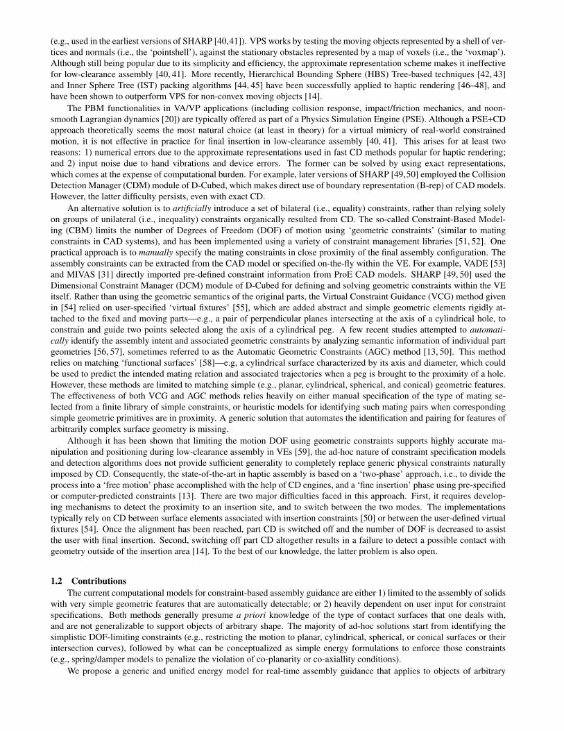
(e.g., used in the earliest versions of SHARP [40,41]). VPS works by testing the moving objects represented by a shell of ver-tices and normals (i.e., the ‘pointshell’), against the stationary obstacles represented by a map of voxels (i.e., the ‘voxmap’).Although still being popular due to its simplicity and efficiency, the approximate representation scheme makes it ineffectivefor low-clearance assembly [40, 41]. More recently, Hierarchical Bounding Sphere (HBS) Tree-based techniques [42, 43]and Inner Sphere Tree (IST) packing algorithms [44, 45] have been successfully applied to haptic rendering [46–48], andhave been shown to outperform VPS for non-convex moving objects [14].

The PBM functionalities in VA/VP applications (including collision response, impact/friction mechanics, and noon-smooth Lagrangian dynamics [20]) are typically offered as part of a Physics Simulation Engine (PSE). Although a PSE+CDapproach theoretically seems the most natural choice (at least in theory) for a virtual mimicry of real-world constrainedmotion, it is not effective in practice for final insertion in low-clearance assembly [40, 41]. This arises for at least tworeasons: 1) numerical errors due to the approximate representations used in fast CD methods popular for haptic rendering;and 2) input noise due to hand vibrations and device errors. The former can be solved by using exact representations,which comes at the expense of computational burden. For example, later versions of SHARP [49,50] employed the CollisionDetection Manager (CDM) module of D-Cubed, which makes direct use of boundary representation (B-rep) of CAD models.However, the latter difficulty persists, even with exact CD.

An alternative solution is to artificially introduce a set of bilateral (i.e., equality) constraints, rather than relying solelyon groups of unilateral (i.e., inequality) constraints organically resulted from CD. The so-called Constraint-Based Model-ing (CBM) limits the number of Degrees of Freedom (DOF) of motion using ‘geometric constraints’ (similar to matingconstraints in CAD systems), and has been implemented using a variety of constraint management libraries [51, 52]. Onepractical approach is to manually specify the mating constraints in close proximity of the final assembly configuration. Theassembly constraints can be extracted from the CAD model or specified on-the-fly within the VE. For example, VADE [53]and MIVAS [31] directly imported pre-defined constraint information from ProE CAD models. SHARP [49, 50] used theDimensional Constraint Manager (DCM) module of D-Cubed for defining and solving geometric constraints within the VEitself. Rather than using the geometric semantics of the original parts, the Virtual Constraint Guidance (VCG) method givenin [54] relied on user-specified ‘virtual fixtures’ [55], which are added abstract and simple geometric elements rigidly at-tached to the fixed and moving parts—e.g., a pair of perpendicular planes intersecting at the axis of a cylindrical hole, toconstrain and guide two points selected along the axis of a cylindrical peg. A few recent studies attempted to automati-cally identify the assembly intent and associated geometric constraints by analyzing semantic information of individual partgeometries [56, 57], sometimes referred to as the Automatic Geometric Constraints (AGC) method [13, 50]. This methodrelies on matching ‘functional surfaces’ [58]—e.g, a cylindrical surface characterized by its axis and diameter, which couldbe used to predict the intended mating relation and associated trajectories when a peg is brought to the proximity of a hole.However, these methods are limited to matching simple (e.g., planar, cylindrical, spherical, and conical) geometric features.The effectiveness of both VCG and AGC methods relies heavily on either manual specification of the type of mating se-lected from a finite library of simple constraints, or heuristic models for identifying such mating pairs when correspondingsimple geometric primitives are in proximity. A generic solution that automates the identification and pairing for features ofarbitrarily complex surface geometry is missing.

Although it has been shown that limiting the motion DOF using geometric constraints supports highly accurate ma-nipulation and positioning during low-clearance assembly in VEs [59], the ad-hoc nature of constraint specification modelsand detection algorithms does not provide sufficient generality to completely replace generic physical constraints naturallyimposed by CD. Consequently, the state-of-the-art in haptic assembly is based on a ‘two-phase’ approach, i.e., to divide theprocess into a ‘free motion’ phase accomplished with the help of CD engines, and a ‘fine insertion’ phase using pre-specifiedor computer-predicted constraints [13]. There are two major difficulties faced in this approach. First, it requires develop-ing mechanisms to detect the proximity to an insertion site, and to switch between the two modes. The implementationstypically rely on CD between surface elements associated with insertion constraints [50] or between the user-defined virtualfixtures [54]. Once the alignment has been reached, part CD is switched off and the number of DOF is decreased to assistthe user with final insertion. Second, switching off part CD altogether results in a failure to detect a possible contact withgeometry outside of the insertion area [14]. To the best of our knowledge, the latter problem is also open.

1.2 ContributionsThe current computational models for constraint-based assembly guidance are either 1) limited to the assembly of solids

with very simple geometric features that are automatically detectable; or 2) heavily dependent on user input for constraintspecifications. Both methods generally presume a priori knowledge of the type of contact surfaces that one deals with,and are not generalizable to support objects of arbitrary shape. The majority of ad-hoc solutions start from identifying thesimplistic DOF-limiting constraints (e.g., restricting the motion to planar, cylindrical, spherical, or conical surfaces or theirintersection curves), followed by what can be conceptualized as simple energy formulations to enforce those constraints(e.g., spring/damper models to penalize the violation of co-planarity or co-axiallity conditions).

We propose a generic and unified energy model for real-time assembly guidance that applies to objects of arbitrary

shape. Our formulation starts from the part geometries and directly computes the guidance forces and torques from shapedescriptors of interacting features. We do not make any simplifying assumption on the geometry of the mating features, andshow that implicit generalizations of the so-called ‘virtual fixtures’ automatically appear in the form of a density distributionin the 3D space, called the Skeletal Density Function (SDF). The spatial overlapping of individual part SDFs generates anartificial potential energy (called the ‘geometric energy’ field) which creates attraction forces and torques towards the properalignment of assembly features. We show that the same energy model also provides repulsion forces and torques as a naturalbi-product, in the case of collisions. Therefore, it unifies the two phases of free motion and precise insertion into a singleinteraction mode, thus avoids the duality and switch altogether.

2 FormulationGiven a set of mechanical components of a prospective assembly in a graphics- and haptics-enabled VE, the problem is

to formulate a computational model to perform the following tasks:

1. obtaining proper ‘shape descriptors’ that capture the geometric and topological characteristics of the different compo-nents which are relevant to assembly, and can be thought of as generic replacements for the ad-hoc virtual fixtures;

2. formulating a quantitative score function to measure the quality of the ‘geometric fit’ between the shapes for arbitraryspatial configurations, based on overlapping the previously extracted shape descriptors;

3. obtaining an artificial energy-field from the score model, whose gradient can be used as guidance and constraint forcesand torques during object manipulation in the VE (replacing the existing penalty methods based on linear spring/dampermodels).

The goal is to develop a potent framework that performs these tasks without making any simplifying assumption on theshape, the intended function, or the proper spatial relationships of the parts. The first step entails the most challenge froma theoretical point of view, since obtaining a quantitative description of assembly features requires an understanding of thethe qualitative notion of a ‘proper fit,’ and is not trivial for arbitrary geometry. The shape descriptors can be obtained in apreprocessing step for each rigid part. Therefore, the predominant computational challenges are pertaining to the real-timecomputations in the next two steps’, due to the 1 kHz haptic rendering rate requirement. We examine each of these tasks inparticular detail in the following sections, and introduce a novel paradigm that applies to arbitrarily complex shapes, withoutimposing any restricting assumption on the particular combination of contact features.

2.1 PreliminariesFollowing the good tradition of separating mathematical models from computational representations [60,61], we propose

our formulation for general ‘solid’ objects, defined as compact (i.e., bounded and closed), regular semi-analytic subsets ofthe Euclidean 3−space S ⊂ P (R3)1 (i.e., ‘r-sets’). The regularity condition ensures that the set’s ‘interior’ iS, ‘exterior’ cS,and ‘boundary’ ∂S are well-defined notions, and prevents undesirable artifacts (such as ‘dangling’ edges or isolated pointsthat do not correspond to physically realizable shapes) [60]. The semi-analytic requirement, on the other hand, guaranteestriangulability of the set and prevents undesirable pathological behavior at the boundary [60] and the skeleton [62]. Bothconditions are sufficiently specific to enable theoretical developments as well as algorithmic tractability, yet general enoughto encompass all practically significant shapes for most solid modeling applications. We make an additional assumption thatthe boundary ∂S is a piecewise C1−manifold, i.e., can be decomposed into a finite number of differentiable surface patchesthat are sewed together along sharp edges and corners. This enables formulating flux integrals over the boundary as a finitesummation of surface integrals over those patches, each with well-defined normal vectors throughout their interiors.

It is worthwhile noting that our formulation does not impose, in principle, any restriction on the representation scheme,as long as it satisfies the informational completeness and consistency requirements [61]—particularly, it suffices to supportEuclidean distance queries and Point Membership Classification (PMC) tests [63]. This applies to exact representations (e.g.,Constructive Solid Geometry (CSG) or NURBS-based boundary representations (B-reps) extracted directly from originalCAD models) as well as approximate representations (e.g., triangular mesh or volumetric enumerations of the exportedCAD models). It is important to note that, especially when using approximation schemes, the employed shape descriptorsmust be stable and robust with respect to small perturbations in the boundary; otherwise they cannot be used effectively fordesigning computational algorithms.

2.2 Shape DescriptorsThe assembly components need to be individually processed, each to be abstracted by certain shape descriptors that

capture the most relevant geometric and topological characteristics to the virtual assembly task. This is probably the mostchallenging part of the entire process, especially when dealing with an infinitely large number of possibilities for complex

1The collection P (A) = B | B⊂ A denotes the ‘power set’ of a set A, i.e., the set of all subsets of A.

(a)

S2

S1

MA overlap(b) (c)

M[ ]cS1

M[ ]iS1 M[ ]iS2

M[ ]cS2

(d) SDF of S1 (e) SDF of S2 (f) SDF overlap

T1 1S

T2 2S

Fig. 1: Assembly features captured by skeletal branches (a, b), which replace the virtual fixtures for assembly (c). Theimplicit skeletal density distribution (d, e) provides a robust substitute to facilitate measuring the overlap (f).

surface features, each of which may or may not be the key determinant of proper assembly. The existing approaches to thisand similar problems requiring feature recognition or characterization attempt to classify and match the potential contactfeatures with respect to the common combinations of simple building blocks [56–58]. These methods impose inevitablelimitations on the geometric semantics of the objects. We take a completely different approach to avoid these limitationsaltogether.

Skeletal Density. The basic premise of our approach is that automatic identification of a ‘proper fit’ in virtual assemblyrequires a quantification of the degree of effective geometric alignment, or shape complementarity, between pairs of ob-jects. To achieve this, we make use of the new concept of continuous shape skeletons that we introduced in [64] for shapecomplementarity analysis of objects of arbitrary shape.

Geometric skeletons such as the Medial Axis (MA) can be regarded as abstractions of certain combinatorial, topological,and geometrical information of the shape [65]. Figure 1 (a, b) shows the MAs of interiors M [iS1,2] and exteriors M [cS1,2]of the 2D r-sets S1,S2 ∈ S (in this case S ⊂ P (R2) for ease of illustration). The MA branches can be used as abstractions ofthe shape for assembly features—e.g., the two branches associated with the sharp corners and the one branch associated withthe fillet feature in Fig. 1 (a, b). Therefore, one could try to overlap the external MA branches of one object with the internalMA branches of its mating object (and vice versa) to guide the assembly process, as in Fig. 1 (c). This suggests using MAgeometry as a generic replacement for the virtual fixtures [55] mentioned earlier. This treatment is applicable to featuresof arbitrarily complex shape, and requires no user specification prior to or during the assembly, hence liberates automaticcomputation of guidance forces and torques regardless of model complexity.

Unfortunately, the traditional definition of the MA is very unstable with respect to small perturbations in the boundary,making it extremely difficult to compute and prune [66]. This motivated us to define a related concept in terms of a space-continuous, well-defined, and robust density function, called the Skeletal Density Functions (SDF), whose sublevel sets inthe limit are related to an implicit definition of the MA [64]. Figure 1 (d, e) shows the SDF field, that depends on a ‘thicknessparameter’ σ > 0. For σ 1, the SDF value of the points on the MA (particularly those with more extensive approximatenearest neighbors on ∂S) differentiates significantly from the points outside the MA. As σ→ 0+, the SDF is related to thedefining function of MA under certain restricting conditions [64]. We also showed that the SDF is a proper shape descriptorfor the purpose of automatic prediction of assembly relations by means of comparative overlapping. We briefly review theconcepts that lead to the formal definition of SDF, skipping rigorous elaborations in favor of clarifying the main ideas. Wedo not intend to repeat the propositions, but rather to provide some insight into the applications of SDF shape descriptors todefine an energy model for haptic-assisted virtual assembly. We refer the reader to [64] for further mathematical details.

Distance Mapping. Given a solid S∈ S of arbitrary shape, we define a Euclidean distance-based projection ζ :R3×∂S→Cof the boundary ∂S to the complex plane, with respect to an arbitrary query point p ∈R3 as

ζ(p,q;S) = ξ(p;S)+ iη(p,q), (1)

where the real-part ξ(p;S) = M(p;S)minq∈∂S ‖p− q‖2 is the signed Euclidean distance from the nearest neighbor on theboundary ∂S to the query point p ∈R3, whose sign is determined by the PMC function M :R3→−1,0,+1, i.e., ξ < 0 forinterior points (p ∈ iS), and ξ = 0 for boundary points (p ∈ ∂S), and ξ > 0 for exterior points (p ∈ cS). The imaginary-partη(p,q) = ‖p−q‖2 is simply the L2−distance between one particular boundary point q ∈ ∂S and the query point p ∈R3.

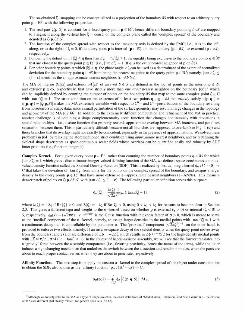
The so-obtained ζ−mapping can be conceptualized as a projection of the boundary ∂S with respect to an arbitrary querypoint p ∈R3, with the following properties:

1. The real-part ξ(p,S) is constant for a fixed query point p ∈ R3, hence different boundary points q ∈ ∂S are mappedto a segment along the vertical line ξ = const. on the complex plane called the ‘complex spread’ of the boundary anddenoted as ζ(p,∂S;S).

2. The location of the complex spread with respect to the imaginary axis is defined by the PMC; i.e., it is to the left,along, or to the right of ξ = 0, if the query point p is internal (p ∈ iS), on the boundary (p ∈ ∂S), or external (p ∈ cS),respectively.

3. Following the definition, if |ξ| ≤ η then | tan∠ζ|= η/|ξ| ≥ 1, the equality being exclusive to the boundary points q ∈ ∂Sthat are closest to the query point p ∈R3 (i.e., | tan∠ζ|= 1 iff q is the exact nearest neighbor of p on ∂S).

4. For other boundary points at which |ξ|< η, the phase angle ∠ζ can be used as a determinant of the extent of normalizeddeviation for the boundary point q ∈ ∂S from being the nearest neighbor to the query point p ∈R3; namely, | tan∠ζ| ≤(1+ ε) identifies the ε−approximate nearest neighbors (ε−ANNs).

The MA of interior M [iS] and exterior M [cS] of an r-set S ∈ S are defined as the loci of points in the interior p ∈ iS,and exterior p ∈ cS, respectively, that have strictly more than one exact nearest neighbor on the boundary [66],2 whichcan be implicitly defined by counting the number of points on the boundary ∂S that map to the same complex point ζ ∈ Cwith | tan∠ζ| = 1. The strict condition on the existence of at least two points q1,q2 ∈ ∂S that exactly satisfy η(p,q1) =η(p,q2) = |ξ(p,S)| makes the MA extremely unstable with respect to C0− and C1−perturbations of the boundary resultingfrom noise/errors in shape data, since a small perturbation of the surface geometry may result in large changes in the topologyand geometry of the MA [62, 66]. In addition to the extremely difficult computation and refinement of the MA in practice,another challenge is of obtaining a shape complementarity score function that changes continuously with deviations inspatial relationships—i.e., a score function that properly rewards approximate overlap between MA branches, and penalizesseparation between them. This is particularly difficult because not all branches are supposed to overlap (see Fig. 1 (c)) andthose branches that do overlap might not exactly be coincident, especially in the presence of approximations. We solved theseproblems in [64] by relaxing the aforementioned strict condition using approximate nearest neighbors, and by redefining theskeletal shape descriptors as space-continuous scalar fields whose overlaps can be quantified easily and robustly by SDFinner products (i.e., function integrals).

Complex Kernel. For a given query point p ∈ R3, rather than counting the number of boundary points q ∈ ∂S for which| tan∠ζ|= 1, which gives a discontinuous integer-valued defining function of the MA, we define a space-continuous complex-valued density function called the Skeletal Density Function (SDF). This is realized by first defining a kernel φσ :C−0→C that takes the deviation of | tan∠ζ| from unity for the points on the complex spread of the boundary, and assigns a largerdensity to the query points p ∈ R3 that have more extensive ε−approximate nearest neighbors (ε−ANNs). This means adenser patch of points on ζ(p,∂S;S) with | tan∠ζ| ≤ (1+ ε). The following particular definition serves this purpose:

φσ(ζ) =λ(ζ)√

2π

1ζ2 gσ (| tan∠ζ|−1) , (2)

where λ(ζ) = +λ1 if Reζ > 0, and λ(ζ) = −λ2 if Reζ < 0, using 0 < λ1 < λ2 for reasons to become clear in Section2.3. This gives a different sign and weight to the φ−kernel based on whether p is external (ξ > 0) or internal (ξ < 0) toS, respectively. gσ(x) = (

√2πσ)−1e−

12 (x/σ)2

is the Gauss function with thickness factor of σ > 0, which is meant to serveas the ‘medial’ component of the φ−kernel, namely, to assign larger densities to the medial points with | tan∠ζ| ≈ 1 witha continuous decay that is controllable by the parameter σ. The ‘proximal’ component (

√2πζ2)−1, on the other hand, is

provided to enforce two effects, namely, 1) an inverse-square decay of the skeletal density when the query point moves awayfrom the boundary; and 2) a phase difference of ∠φ =−2∠ζ which results in ∠φ≈∓π/2 for the high-density medial pointswith ∠ζ≈ π/2±π/4 (i.e., | tanζ| ≈ 1). In the context of haptic-assisted assembly, we will see that the former translates intoa ‘gravity’ force between the assembly components (i.e., favoring proximity, hence the name of the term), while the latterinduces a sign changing mechanism that underlies the switch between the attraction and repulsion modes, when the parts areabout to reach proper contact versus when they are about to penetrate, respectively.

Affinity Function. The next step is to apply the custom φ−kernel to the complex spread of the object under considerationto obtain the SDF, also known as the ‘affinity function’ ρσ : (R3−∂S)→ C:

ρσ(p;S) =∮

∂Sφσ

[ζ(p,q;S)

]dA⊥, (3)

2Although we loosely refer to the MA as a type of shape skeleton, the exact definitions of ‘Medial Axis,’ ‘Skeleton,’ and ‘Cut Locus’ (i.e., the closureof MA) are different (but closely related) for general open sets [62, 65].

(a) DomainS

p

ς-map

ξ

ηξ=ηξ η=(1+ε)

|ξ( ;p S)| (1+ ( ;ε)| )|ξ p S

η ξ

|ϕ |σ

ϕ-kernel

(b) Complex spread

| |ρσ( ; )p S

(c) SDF

ε-ANNs∫

Fig. 2: The affinity computation is decomposed into two steps: a ζ−projection in (1) that characterizes the distance distribu-tion as observed from the query point p ∈R3, followed by applying the φ−kernel in (2).

where dA⊥ is the area element normal to the line that connects p∈R3 to q∈ ∂S; that is, the infinitesimal area of the projectionof the surface element dA at the boundary point q on a sphere centered at the query point p with a radius of η(p,q). If welet v = (p−q)/η then dA⊥ = (v ·n)dA and (3) becomes a flux integral of the radial vector field φσ(ζ)v :C−0→C2 overthe oriented piecewise C1−manifold ∂S. Substituting for φ(ζ) from (2), and letting 1+ ε = | tan∠ζ| = η/|ξ|, the followingresults from (3):

|ρσ(p;S)|=∮

∂S

|λ|σ

e−12 (ε/σ)2

1+(1+ ε)−2dA⊥2πη2 , (4)

We showed in [64] that the exact SDF given in (3) can be approximated with a truncated SDF that is integrated over theregions of the boundary that form the ε−ANNs of p, i.e., the patches of the boundary that lie within a closed spherical shellof internal radius |ξ| and external radius (1+ ε)|ξ|, and proved truncation error bounds on the approximation. This can beexplained in simple terms by the fact that the Gaussian term in (2) decays exponentially for points outside the ε−approximatenearest neighborhood; in fact, for | tan∠ζ| > (1+ ε), the exponential term is at most e−

12 (ε/σ)2

, which is in turn less than10−4 if we choose ε > 3.4σ.

It is also interesting to note that dγ = dA⊥/(4πη2) is the infinitesimal solid angle by which the query point p ∈ R3

observes the surface element dA at q ∈ ∂S. Therefore, the surface integral in (4) aggregates the φ−kernel over the ε−ANNsto the query point on the boundary, assigning weights proportional to the spatial angles by which they are observed. Thisexplains the choice of the inverse-square law in the proximal term for the φ−kernel in (2) over any other possible decayfunction.

Figure 2 provides a schematic description of the SDF computation process, decomposed in principle into 1) computinga different representation of the object based on the Euclidean distance geometry, i.e., the ζ−projection of the boundary withrespect to different query points; and 2) the application of a custom φ−kernel to determine the distance distribution criteria,based on which the skeletal density is assigned in the 3−space. See [64] for examples of using different kernels and theirapplications.

Affinity Gradient. The gradient of the affinity function ∇ρσ = dρσ/dp :R3→ C3 (to be used in Section 2.3 to computethe guidance forces and torques) can be computed from (3) by applying the chain rule for differentiation:

∇ρσ(p;S) =∮

∂S

[∂φσ

∂ξ(ζ)∇ξ+

1η

∂φσ

∂η(ζ)(p−q)

]dA⊥, (5)

where ∇ξ = dξ/dp : R3→ R3 is the gradient of the signed Euclidean distance function,3 and the partial kernel derivatives∂φσ/∂ξ,∂φσ/∂η : C→ C can be obtained directly from (2).

2.3 Shape ComplementarityIn a complex virtual assembly scene with many components, the analysis of the proper contact between all parts can be

broken down in a bottom-up fashion into pairwise matching between the parts, and then between the resulted sub-assemblies,with an incremental growth of the number of constituents. This view is compatible with the actual process of semi-automatichaptic-enabled assembly, when the user drags and places the parts and resulting sub-assemblies one at a time.

3∇ξ = ±(p−q∗)/ξ where the sign depends on the PMC, and q∗ ∈ ∂S is the nearest neighbor to the query point p ∈R3 on the solid’s boundary. Thispoint is not unique when p belongs to the MA, resulting in undefined ∇ξ. One could use the extended gradient definition in [65] for the sake of theoreticalcompleteness. However, the resulted discontinuity does not create a problem when applied to guidance force and torque computations in (12) and (13)because the MA has zero volume, hence does not contribute to the volumetric integrals in (9) and (10) [64].

(a) Proper fit (b) Collision (c) Separation

Genericvirtualfixtures

StableEquilibrium

Attractiveforce

Repulsiveforce

PenaltyReward

Fig. 3: Possible spatial relations and the corresponding interactions. The generic virtual fixtures practically restrict the DOFif the stiffness properties (i.e., 2nd-order partial derivatives of EG at the energy well) are large enough.

Score Function. For a pair of solids S1,S2 ∈ S (each solid representing one part or sub-assembly as a single object), themotion of both objects at any instant of time can be described by the transformations T1,T2 ∈ SE(3) that relate the absolutecoordinate frame to an orthonormal triad attached to each object; SE(3) ∼= SO(3)nT(3) represents the Special Euclideangroup, i.e., combination of proper orthogonal rotations SO(3), and translations T(3), together representing all possible rigidbody motions. We proposed in [64] that the shape complementarity score for this configuration can be obtained as a cross-correlation of individual SDF fields over the 3−space:

fSC(T1,2;S1,2

)=

∫R3

ρσ

(p′;T1S1

)ρσ

(p′;T2S2

)dV, (6)

where ρσ(p′;S) is substituted from (3); the integration variable is p′ = (x1,x2,x3) ∈R3 and dV = dx1dx2dx3 is the volumeelement. The equation can be simplified using a kinematic inversion. Let p = T −1

1 p′ be the new coordinates of the querypoint measured with respect to a frame attached to S1, and T = T −1

1 T2 ∈ SE(3) be the motion of S2 observed from that sameframe. Noting that the SDF is solely formulated based on distance distributions, it is invariant under rigid body motion, i.e.,the affinity field moves rigidly with the object, hence ρσ(p;T S) = ρσ(T −1p;S) for all S ∈ S and T ∈ SE(3). Using thisproperty and rearranging the terms in (6) gives

fSC(T ;S1,S2

)=

∫R3

ρσ

(p;S1

)ρσ

(T −1p;S2

)dV. (7)

In practice, (7) is evaluated over a bounded cubic region of R3 that is large enough to cover the high density segments of theSDF branches, noting the inverse-square decay of ρσ(p;S) in (3).

The integral in (7) can be interpreted as an assessment of the degree of overlap between the continuous internal andexternal skeletons of one object, and the internal and external skeletons of the other object, hence four possible combinationscontributing differently to the overall score function. We describe the four scenarios in simple terms to convey an intuitiveunderstanding of (6) and (7). Consider a volume element at a point that belongs to a high skeletal density region of bothT1S1 and T2S2, hence contributing significantly to the integral. Assume that the distance distribution over the ε−ANNs onthe boundaries of the two objects as observed from the query point are similar, hence the medial and proximal componentsof the SDF are equally high with respect to both shapes, making the λ−function in (2) decide the separations between thefollowing cases:

• if the point is external to object-1 and internal to object-2, i.e., p′ ∈ c(T1S1)∩ i(T2S2) in (6), hence p ∈ cS1∩ i(T S2) in(7), then ρ1ρ2 ∝ (−iλ1)(+iλ2) = +λ1λ2 > 0;

• if the point is internal to object-1 and external to object-2, i.e., p′ ∈ i(T1S1)∩ c(T2S2) in (6), hence p ∈ iS1∩ c(T S2) in(7), then ρ1ρ2 ∝ (+iλ2)(−iλ1) = +λ2λ1 > 0;

• if the point is internal to object-1 and internal to object-2, i.e., p′ ∈ i(T1S1)∩ i(T2S2) in (6), hence p ∈ iS1 ∩ i(T S2) in(7), then ρ1ρ2 ∝ (+iλ2)(+iλ2) =−λ2

2 < 0;• if the point is external to object-1 and external to object-2, i.e., p′ ∈ c(T1S1)∩ c(T2S2) in (6), hence p ∈ cS1∩ c(T S2) in

(7), then ρ1ρ2 ∝ (−iλ1)(−iλ1) =−λ21 < 0;

The first two cases characterize the ‘proper fit’ alignment between the two objects, since the exterior of one object isaligned with the interior of another with similar distance geometries, carrying the hint of a proper complementary feature(Fig. 3 (a)). On the other hand, the third case implies ‘collision,’ since the interior points are being overlapped, and shouldbe strictly prohibited (Fig. 3 (b)). Lastly, the fourth case suggests a ‘separation’ at the observation point, which amountsless to a conclusion about the quality of fit (Fig. 3 (c)). Hence if we choose λ1 = O(1) and p := λ2/λ1 1, then the firsttwo cases contribute a positive-real reward of ∝ O(p) to the score function, the third term contributes a large negative-realpenalty of ∝ O(p2), and the last term contributes a smaller penalty of ∝ O(1). The ratio p is thus called the ‘penalty factor.’

These of course describe the distance geometry as observed from a single query point under consideration, which is why theoverlap is integrated over different observation points via (7) to obtain the cumulative effect.

Motion Decomposition. To simplify the subsequent development, let us decompose the motion into the translationalcomponent t ∈ T(3) described by a 3−tuple t = (t1, t2, t3) ∈R3, and the rotational component R ∈ SO(3) represented by a3× 3 proper orthogonal matrix [R ]3×3. As a result of the definition, the transformation sequence applies as T p = R p+ thence T −1p = R T(p− t).4 Substituting for the latter in (7) gives

fSC(R , t;S1,S2) =∫R3

ρ1(p)[ρ2 R T(p− t)

]dV. (8)

where the functions ρ1,2(p) = ρσ(p;S1,2) are independent of the motion parameters, and the inverse rotation operator istreated as a function R T :R3→R3.

Score Gradient. For a function fSC : SE(3)→ C whose domain is not a vector space, the generalized gradient function∇ fSC = (d fSC/dR ,d fSC/dt) : SE(3)→ C6 is composed of a 3D translational and a 3D rotational gradient vectors, charac-terizing the rate of change of the function with respect to infinitesimal translations and rotations, respectively.

The translational gradient function d fSC/dt : SE(3)→ C3 is computed using basic concepts from linear algebra, sincethe translation space T(3)∼=R3 is a vector space. Differentiating (8) and using the chain rule we obtain

〈d fSC

dt,e〉=−

∫R3

ρ1(p)[∇ρ2 R T(p− t)

]· (R Te)dV, (9)

where e∈R3 represents any direction in the vector space T(3)∼=R3, along which the differentiation occurs. The term (R Te)on the right-hand side can be factored out of the integral.

The rotational gradient function d fSC/dR : SE(3)→C3 is more difficult to formulate, since SO(3) is not a vector spaceand cannot be globally parameterized by a single continuous 3D grid. To obtain a local parametrization, the tangent directionat R ∈ SO(3) is obtained as R Ω where Ω∈ so(3) can be represented by a skew-symmetric matrix [Ω]3×3, and so(3) denotesthe Lie algebra, which is a vector space tangent to SO(3) at the identity rotation. Without getting into much detail, we presentthe rotational gradient as

〈d fSC

dR,e〉=−

∫R3

ρ1(p)[∇ρ2 R T(p− t)

]·Ω∗(p− t)dV, (10)

where e = R u and u ∈R3 is the dual vector of Ω ∈ so(3), and Ω∗ = R ΩR T is called the action of R T on Ω. The affinitygradient ∇ρ2 = ∇ρσ(p;S2) used in the integrands of both (9) and (10) is computed from (5).

The 3D translational and rotational gradient vectors can be computed in a componentwise fashion by substituting forthe base vectors e ∈ e1,e2,e3 one at a time in (9) and (10). The complete 6D gradient ∇ fSC : SE(3)→ C6 is defined as∇ fSC = (d fSC/dR ,d fSC/dt).

2.4 Geometric EnergiesThe described generic and continuous score distribution over the configuration space SE(3) rewards shape complemen-

tarity and penalizes collision and separation. This enables defining a potential pseudo-energy function EG ∝ ℜ fSC for usein real-time haptic assembly.

Energy Function. We define the ‘geometric energy’ function EG : SE(3)→R simply as:

EG(T ;S1,S2

)=−γSC ·ℜ

fSC(T ;S1,S2

), (11)

where ℜ· stands for the real-part, and the constant γSC > 0 is provided to scale the dimensionless score function fSCto proper energy units, before applying it to objects of certain mass and inertia properties in a scene, bearing in mind thepossibility of other forces being present.

4Note that R −1 = R T for all R ∈ SO(3), i.e., the inverse of a proper rotation with det(R ) = +1 is the same as its transpose.

One could appreciate an interesting analogy between this artificial, purely geometric energy field, and physical energyfields such as the electrostatic effect. It immediately follows that the product of affinity functions can be conceptualized asa complex ‘geometric potential,’ which applies on a complex ‘geometric charge’ density, the magnitude of which is dictatedby the λ−function in (2). Using this analogy, on one hand when charges on the two objects are imaginary numbers of thesame sign, there is a positive-real contribution to the energy, implying a repulsion force (Fig. 2 (b)). On the other hand, whenthe charges are imaginary numbers of opposite signs, they contribute a negative-real energy, which indicates an attractionforce (Fig. 2 (c)). Both attractive and repulsive effects decay with distance, due to the inverse-square law embedded in theφ−kernel defined in (2).

Force and Torque. The conservative ‘geometric force’ and ‘geometric torque’ are obtained as the gradient of the energyfunction with respect to the translational and rotational motion, respectively:

FG(R , t;S1,S2

)=−dEG

dt=+γSCℜ

d fSC

dt

, (12)

TG(R , t;S1,S2

)=−dEG

dR=+γSCℜ

d fSC

dR

. (13)

This can be consolidated into the 6D general force/torque vector (TG,FG) =−∇EG, where ∇EG : SE3→R6 is the complete6D energy gradient defined as ∇EG =−γSCℜ∇ fSC.

3 ImplementationIn this section we present an implementation of our method for a particularly simple representation (namely, triangular

mesh B-reps), along with the algorithms and data structures that support accurate computation of the SDF descriptors andthe cross-correlation integral. We briefly overview the computational complexity of the different techniques used in eachstep, and refer the reader to [64] for more elaborate treatments.

3.1 RepresentationAs described in Section 2, our method is independent of the representation scheme used to describe the solid objects

in the scene. Any representation scheme that satisfies the informational completeness and consistency requirements [61]can be used, provided that it supports the means to 1) compute unsigned Euclidean distance queries to the boundary points,and 2) a Point Membership Classification (PMC) test [63] to correct the sign of the distance function—both to an adequateaccuracy with respect to the smallest surface features. For the sake of simplicity, we present the implementation for B-repsin the form of triangular mesh surfaces with oriented boundary elements. In particular, we use a data structure that containsthe following:

• combinatorial structure: the adjacency and orientation information for the boundary faces, edges, and vertices (e.g.,using oriented half-edge or barycentric decomposition data structures); and

• metric information: the coordinates of the boundary vertices and (optionally) vertex normals, which can be used toobtain face normals defining a consistent orientation for the boundary manifold.5

Given a solid S ∈ S , we denote the underlying space6 of a triangulation that approximates its boundary ∂S with ∆n(S) =⋃nj=1 δ j, where the closed triangles are denoted by δ j (1≤ j≤ n), the number of triangles (i.e., faces) is n, and the number of

edges and vertices are both O(n) [60]. We use the NETGEN library [67] to triangulate the boundary of solid parts exportedin STEP format from any commercial CAD software. The boundary vertices need to be sampled with adequate density tocapture the local geometric features of the shape.

3.2 PreprocessingFor a single query point p∈R3, the sequence of computations is 1) unsigned distance queries from the n triangles; 2) the

PMC test to correct the distance sign for ζ−mapping in (1); and 3) applying the φ−kernel in (2) followed by the integrationin (3). The same sequence needs to be carried out over a 3D uniform grid Gm(S) of m nodes. Let q j ∈ ∆n(S) (1 ≤ j ≤ n)

5The orientation of the three edges, or equivalently, the traversal ordering of the three vertices stored in each face’s data structure together with vertexcoordinates are sufficient information to obtain unit normal vectors for the faces. The inward/outward normal orientation that is defined consistently withthe ordered edges/vertices (according to the right-hand rule) is also equivalent to and retrievable from the PMC.

6The ‘underlying space’ of a cell complex is the union of all cells in that complex. For a 2D meshed surface embedded in 3D, it means the 2D subspaceof the 3−space occupied by all faces, edges, and vertices of the triangulation [60].

denote a point (e.g., the mid-point) on a triangle δ j ⊂ ∆n(S), whose unit normal is n j ∈R3 and surface area is δA j > 0. Letpi ∈ Gm(S) (1≤ i≤ m) denote a arbitrary grid node. Then (3) can be approximated by the following discrete form:

ρσ(pi;S)≈n

∑j=1

φσ

[ξi + iηi, j

]cosθi, jδA j, (14)

where ξi = ξ(pi;S), ηi, j = η(pi,q j) = ‖pi−q j‖2 and cosθi, j = (pi−q j) ·n j/ηi, j. A similar discrete from can be obtainedfor the affinity gradient integral in (5). It is important to note that the approximation in (14) is reliable if the spatial angle bywhich the triangle δ j is observed from p is small (i.e., cosθi, jδA j η2

i, j) which is not necessarily true for grid nodes that areclose to the ∂S surface, constituting only a small fraction of all grid nodes. For those points, the triangle can be recursivelysubdivided into smaller faces, until an upperbound criterion on the spatial angle of observation is reached. Assuming that thenumber of recursions is O(1), computing (14) takes O(n) basic steps. Therefore, the computation of the SDF over the entiregrid Gm(S) takes O(mn) basic steps. The grid cell size should be small enough to capture the geometric features of the shapeby the SDF, which implies a lowerbound on m. As described in [64], this can be sped up to O(m′n) where m′ m by usingadaptively sampled query points, for instance over an octree Qm′(S) composed of m′ nodes but with the same minimum cellsize as that of Gm(S).

For unsigned distance field computation, we use Havoc3D [68], which cumulatively computes the unsigned distancefield |ξi| (1 ≤ i ≤ m) using interpolation-based polygon rasterization on the graphics hardware via OpenGL depth-buffer.For sign determination (i.e., PMC) we used the method in [69] which is based on winding numbers defined in terms ofsigned spatial angles. We implemented both PMC and SDF field computations in parallel on the CPU, assigning differentchunks of Gm(S) to different processors, using OpenMP. The SDF field needs to be precomputed offline, only once per eachrigid part or subassembly, hence can be done with high precision with little concern about the computation time.

3.3 Cross-CorrelationLet the two assembly partners S1 and S2 be represented with triangular meshes ∆n1(S1) and ∆n2(S2) composed of n1 and

n2 triangles, respectively. Assuming that the SDF fields for the individual objects are precomputed separately over Gm1(S1)and Gm2(S2) grids attached to each body, at every instance of the dynamic simulation with T1,T2 ∈ SE(3) the score integralin (6) can be discretized into

fSC(T1,2;S1,2)≈m

∑i=1

ρ(T −11 pi;S1)ρ(T −1

2 pi;S2)δV, (15)

where pi ∈ Gm(T1S1,T2S2) (1≤ i≤ m) is a node on a grid sampled uniformly over the intersection of the volumes coveredby T1Gm1(S1) and T1Gm2(S2), and δV = vol(Gm)/m is the cell volume of this grid. The SDFs are interpolated from theprecomputed values in (14). To save in interpolation time, the integration grid is picked as a subset of the smaller SDFgrid, hence m≤minm1,m2 and computing (15) takes O(m) basic steps. The score gradient in (9) and (10), needed for theguidance forces and torques in (12) and (13), can be discretized in a similar fashion. Alternatively, one could approximate thegradient using the Finite Difference Method (FDM) by multiple computations of (15) after applying small translational androtational variations, along each of the 3 coordinate axes one at a time, to the relative transformation T = T −1

1 T2 ∈ SE(3).We parallelize the force and torque computations on the CPU using OpenMP. Although the performance scales almost

linearly with the number of cores, the running times are not adequately small to keep up with the 1 kHz haptic renderingloop. The simplest solution is to precompute the geometric energy EG and/or forces and torques (TG,FG) over a samplingof relative transformations in SE(3), and interpolate the sample in real-time. This is not practical (both in terms of time andmemory) for a 6D configuration space, even with the powerful computers available today. Fortunately, for most assemblyscenarios the motion during the insertion phase is constrained to one or two DOF. For example, if the rotational space islimited to a finite number of permissible relative orientations, the field can be precomputed and stored over a 3D translationalsampling in T(3) for each orientation (i.e., a section through the configuration space). However, this approach goes againstthe philosophy of avoiding the multi-phase approach and manual specifications, from which we set off to pursue this method.We recently presented an alternative implementation in [70] that uses GPU-accelerated Fast Fourier Transforms (FFT) toenable real-time computations, the discussion of which is beyond the scope of this paper.

4 Results & DiscussionWe first demonstrate the effectiveness of the proposed approach for simple classical peg-in-hole examples. Figure 4 (a)

shows the three examples made of cylindrical pegs of circular, rectangular, and combined cross-sections, which were testedin assembly against their complementary holes. The geometric fit in all three cases is exact (i.e., zero clearance).

(a) Peg-in-hole examples

Exam

ple

1Ex

ampl

e 2

Exam

ple

3

(b) Hole SDF (front & left views)

x2

x3x1

x2

x2

x3x1

x2

x2

x3x1

x2

(c) Peg SDF (front & left views)

x2

x3x1

x2

x2

x3x1

x2

x2

x3x1

x2

(d) SDF overlap (front & left views)

x2

x3x1

x2

x2

x3x1

x2

x2

x3x1

x2

x1

x2

x3

x1

x2

x3

x1

x2

x3

Fig. 4: Three classical peg-in-hole assemblies (a), their SDF fields (imaginary-parts) (b, c), and their spatial overlap (real-part) (d).

AB

E

C

D

A

A

C

E

D

EA

(b) Example 2 (c) Example 3

AB

E

C

D

A

C

C

E

BB

A

D

EAx1

x2

x3x1

x2

x3

x2 x1

C BB

(a) Example 1x2x3 x1 x3

x2 x1

x2x3 x1 x3

SC S

core

SC S

core

SC S

core

SC S

core

SC S

core

SC S

core

A

B

E

C

D

A

A

C

E

D

EAx1

x2

x3

x2 x1

C BBx2x3 x1 x3

Fig. 5: The shape complementarity score variations versus bi-axial relative translation of the peg with respect to the hole.

4.1 Skeletal OverlapsIn Fig. 4 (b, c), the individual SDF maps of the parts are plotted only for their imaginary-parts. As expected, each part

has the highest positive-imaginary SDF values at the proximity of the high-prong internal MA branches (the red spots) andthe highest negative-imaginary SDF values at the proximity of the high-prong external MA branches (the blue spots). Thelatter are weaker in intensity due to the choice of p= λ2/λ1 = 3.0 in (2). It can be verified that the complementary featureshave similar SDF distributions on one part’s interior and the other part’s exterior, resulting in the ‘hot spots’ on the geometricenergy density map given in Fig. 4 (d), which dominate the ‘dark spots.’

Geometric Guidance. In the simplest case of Example 1, as the user brings the peg closer to the opening of the holeto perform the assembly task, the geometric force-field attracts the peg into the hole and tries to align the high-densitySDF regions, i.e., enforce co-axiallity of the two cylindrical faces. The circular symmetry of the cross-section results in acircular symmetry of the SDF, hence the force-field imposes no orientation preference around the axis of the hole, resultingin a partially constrained motion that resembles a cylindrical joint. However, in the case of Example 2, the cross-shapedskeletal form creates an additional orientation preference, hence the force-field tries to align the four corners of the twocomplementary objects. This results in a partially constrained motion that resembles a prismatic joint. In the case ofExample 3, the shape descriptors appear as a combination of the two cases, with part of the geometry being indifferent torotations around the hole, while another feature contributes energy terms to align the sharp corner.

It is clear from the above discussion that our SDF descriptors serve as generic replacements for the abstract virtualfixtures [55] (e.g., cylinder axes in Example 1 and diagonal planes in Example 2), variations of which were previouslyimplemented in [54] for haptic assembly guidance, and were limited to simple geometric constructs. The skeletal branchesformed automatically in our development serve as abstractions of the functional surfaces [58] for arbitrarily complex shapes,in contrast to the ad-hoc characterizations in [56]. As illustrated by Example 3, combinations of guiding mechanisms

(a)

(b)

(c)

(d)

(e)

(f)

Fig. 6: The geometric energy variations versus uni-axial relative translation and rotation of the peg with respect to the hole.

naturally appear with no theoretical limitation on the complexity of the assembly features. Furthermore, the force-fieldincorporates both collision response (as a repulsive force in the case of interpenetration) and assembly assistance (as anattractive force in the vicinity of the hole) in a single model that enforces geometric constraints. Hence the hybrid approachbased on two separate phases for free motion and precise insertion [13] is integrated into a single model, eliminating theneed to switch between the two using ‘blending’ algorithms.

Energy Variations. Figure 5 plots the shape complementarity score variations (only the real-parts) due to translationalmotion of the peg relative to the hole along the 3 Cartesian axes. To enable visual illustration, the motion in each plot isrestricted to a plane (i.e., changing only 2 out of 3 position coordinates at a time, of the peg with respect to the hole). It isclear that the score is maximal at configuration A (i.e., the zero translation, where the best fit occurs according to our visualjudgment), as expected from the definition. Other configurations are also sketched on the score profile, such as axis-alignedremoval of the peg at B (resulting in a decay of score from A to B along the x3−axis), collision at C and D, and contact (butlittle shape complementarity) at E.

Figure 6 (a) shows the corresponding geometric energy variations due to the same translational motion coordinates, thistime moving the peg along one Cartesian axis at a time. These correspond to sections through the 2D plots in Fig. 5, exceptwith a signed coefficient due to the definition in (11). Figure 6 (b) shows a similar set of geometric energy variation diagrams,plotted versus the rotational motions around one Cartesian axis at a time. For both translational and rotational motions, thereis an evident symmetry and equivalence between x1− and x2−axes in Examples 1 and 2, as expected from the symmetricalshapes, which is not the case for Example 3 due to its different geometry. One can also notice the indifference of the circularcross-section to rotations around the axis of the hole in Example 1, and four equivalent configurations for the cubic peg with90 phase difference in Example 2.

Constraint Stiffness. It is interesting to note that the size of the convex region of the geometric energy profile around thelocal minimum (characterizing the equilibrium point) can be conceptualized as the diameter of the geometric constraints,i.e., the degree of proximity necessary for the constraint to become activated for insertion. The second-order differentialproperties of the energy profile are directly related to the practical stiffness of the constraint enforcement in the VE. Forinstance, a Taylor series expansion of the energy function over the translational space T(3) (i.e., for fixed rotation) aroundthe stable equilibrium configuration t0 ∈ T(3) has the form EG = EG,min +(t− t0) ·H(t0)(t− t0)+O(‖t− t0‖3

2), noting thatdEG/dt(t0) = 0 where the Hessian matrix [H(t0)]3×3 carries the stiffness elements (i.e., tensile/compressive resistance indiagonal elements, and shear resistance in off-diagonal elements).7 A similar expansion is possible over the tangent spaceso(3) to SO(3) to obtain the rotational stiffness matrix. Both the diameter and stiffness can be adjusted by a proper settingof the thickness factor σ > 0 and coefficients λ1,2 in (2).

7Note than no constraint can be rigidly and strictly satisfied due to the electromechanical restrictions at the haptic device level. Even the DOF-limitingequality constraints are typically enforced by rendering resistance forces using a spring/damper model that penalizes the violation, whose stiffness isupperbounded due to the servo-loop rate of 1 kHz.

(a)

(b)

(c)

(d)

(e)

(f)

Fig. 7: Haptic force feedback versus time, for collision test (a–c) and snap test (d–f) for peg-in-hole examples in Fig. 4.

4.2 Haptic ExperimentsFinally, we conduct a few simple experiments to feel the applicability of the technique in real haptic-assisted assembly

applications. Two simple experiments are carried out on a SensAbler PHANTOMr Omnir device, namely:

1. Collision Test: The test is conducted by simply pushing the peg against the walls of the hole in random directions, in anattempt to disturb it from the proper fit configuration and penetrate into the walls of the object with the hole. The usertries to do this with complete control and steadiness, approximately once every two seconds.

2. Snap Test: The user carelessly moves the peg around the entrance of the hole, with random and uncontrolled (but gentle)impacts with the end-effector, positioning the peg in proximity of the proper fit configuration approximately once everysecond. The force field is expected to react immediately and snap the peg into the proper position.

The tests are carried out only in 3 translational DOF, and the experimentation with rotational motions requires to beaddressed in future studies with a 6 DOF haptic device. The force magnitude versus time is plotted in Fig. 7 (a) for thefirst experiment. The performance is satisfactory, with accurate geometric alignment up to observable precision, smooth andcontinuous repulsive force feedback resisting penetration in all directions, and a smaller attractive force resisting the pegleaving the hole along the axis. The results of the second experiment are plotted in Fig. 7 (b). In this case, the responsewas effective in snapping the object into position with very rare occasions of undesirable vibration or ‘buzzing.’ The hapticservo-loop rate was maintained within the acceptable range of 1.0±0.3 kHz at all times.

5 ConclusionLately, the dominant direction in haptic assembly has been aligned with a hybrid approach, separating the simulation

into a ‘free motion’ phase, using unilateral (i.e., inequality) ‘physical constraints’ originated from collision detection; and a‘fine insertion’ phase, using bilateral (i.e., equality) ‘geometric constraints’ introduced artificially to limit the DOF. Whilethe former fail to produce dynamically stable guidance for low-clearance insertion, the latter are either dependent on apriori manual specifications by the user, or are limited to simple algebraic subspaces (e.g., planar, cylindrical, spherical, orconical) that can be identified automatically from CAD semantics using heuristic algorithms. We proposed a novel paradigmthat unifies the two modes into a single interaction, by expanding the collision penalty function to a generic ‘geometricenergy’ field that not only penalizes the configurations which lead to interpenetration (hence produces the repulsive collisionresponse), but also rewards the configurations with high shape complementarity (hence produces the attractive guidanceforces). We accomplished this by formulating the energy function as a cross-correlation of new descriptors of shape, to whichwe referred as Skeletal Density Functions (SDF). The SDF interactions can be conceptualized as generic replacements forad-hoc virtual fixtures or simplistic mating constraints, and apply to objects of arbitrary shape. We showed that this approachautomatically ensures a continuous transition between collision response in free movement to insertion guidance in low-clearance or precise-fit assembly, avoiding the two-phase approach along with its several drawbacks—including the failureto prevent collision events outside the insertion site, and the need for blending the force feedback during the switch.

The unified paradigm provides a promising alternative direction for solving virtual assembly problems in general (and

for haptic rendering, in particular). It opens up new research opportunities to investigate faster implementations and verifyeffectiveness for 6 DOF manipulation in complex and crowded assembly scenes.

AcknowledgementsThis work was supported in part by the National Science Foundation grants CMMI-1200089, CMMI-0927105, and

CNS-0927105.

References[1] Behandish, M., and Ilies, H. T., 2014. “Peg-in-hole revisited: A generic force model for haptic assembly”. In Proceed-

ings of the 2014 ASME International Design Engineering Technical Conferences and Computers and Information inEngineering Conference (IDETC/CIE’2014).

[2] El Saddik, A., 2011. Haptics Technologies: Bringing Touch to Multimedia, 1st ed. Springer.[3] Moreau, G., Fuchs, P., and Stergiopoulos, P., 2004. “Applications of virtual reality in the manufacturing industry: From

design review to ergonomic studies”. Mecanique and Industries, 5, pp. 171–179.[4] Bordegoni, M., Colombo, G., and Formentini, 2006. “Haptic technologies for the conceptual and validation phases of

product design”. Computers and Graphics, 30(3), pp. 377–390.[5] Ferrise, F., Bordegoni, M., and Lizaranzu, J., 2010. “Product design review application based on a vision-sound-haptic

interface”. In Haptic and Audio Interaction Design, S. Nordahl, R.and Serafin, F. Fontana, and S. Brewster, eds.,Vol. 6306 of Lecture Notes in Computer Science. Springer Berlin Heidelberg, pp. 169–178.

[6] Bullinger, H. J., Breining, R., and Bauer, W., 1999. “Virtual prototyping–state of the art in product design”. In 26thInternational Conference on Computers and Industrial Engineering, pp. 103–107.

[7] Wang, G. G., 2002. “Definition and review of virtual prototyping”. Journal of Computing and Information Science inEngineering, 2(3), pp. 232–236.

[8] Deviprasad, T., and Kesavadas, 2003. “Virtual prototyping of assembly components using process modeling”. Journalof Manufacturing Systems, 22(1), pp. 16–27.

[9] Gomes de Sa, A., and Zachmann, G., 1999. “Virtual reality as a tool for verification of assembly and maintenanceprocesses”. Computers and Graphics, 23(3), pp. 389–403.

[10] Volkov, S., and Vance, J. M., 2001. “Effectiveness of haptic sensation for the evaluation of virtual prototypes”. Journalof Computing and Information Science in Engineering, 1(2), pp. 123–128.

[11] Seth, A., Vance, J. M., and Oliver, J. H., 2011. “Virtual reality for assembly methods prototyping: A review”. VirtualReality, 15(1), pp. 5–20.

[12] Lim, T., Ritchie, J. M., Sung, R., Kosmadoudi, Z., Liu, Y., and Thin, A. G., 2010. Haptic Virtual Reality Assembly -Moving Towards Real Engineering Applications. InTech, ch. Advances in Haptics, pp. 693–722.

[13] Vance, J. M., and Dumont, G., 2011. “A conceptual framework to support natural interaction for virtual assemblytasks”. In Proceedings of the 2011 ASME World Conference on Innovative Virtual Reality, pp. 273–278.

[14] Perret, J., Kneschke, C., Vance, J. M., and Dumont, G., 2013. “Interactive assembly simulation with haptic feedback”.Assembly Automation, 33(3), pp. 214–220.

[15] Hasegawa, S., and Fujii, N., 2003. “Real-time rigid body simulation based on volumetric penalty method”. In Proceed-ings of the 11th Symposium on Haptic Interfaces for Virtual Environment and Teleoperator Systems, pp. 326–332.

[16] Hasegawa, S., and Sato, M., 2004. “Real-time rigid body simulation for haptic interactions based on contact volume ofpolygonal objects”. Computer Graphics Forum, 23(3), pp. 529–538.

[17] Mirtich, B., and Canny, J., 1995. “Impulse-based simulation of rigid bodies”. In Proceedings of the 1995 Symposiumon Interactive 3D Graphics (I3D’1995), pp. 181–217.

[18] Hayward, V., and Armstrong, B., 2000. “A new computational model of friction applied to haptic rendering”. InExperimental Robotics VI. Springer-Verlag, pp. 403–412.

[19] Renouf, M., Acary, V., and Dumont, G., 2005. “3D frictional contact and impact multibody dynamics. a comparison ofalgorithms suitable for real-time applications”. In ECCOMAS Thematic Conference on Mutlibody Dynamics.

[20] Tching, L., and Dumont, G., 2008. “Haptic simulations based on non-smooth dynamics for rigid-bodies”. In Proceed-ings of the 15th ACM Symposium on Virtual Reality Software and Technology (VRST’2008), pp. 87–90.

[21] Lin, M., and Gottschalk, S., 1998. “Collision detection between geometric models: A survey”. In Proceedings of the1998 IMA Conference on Mathematics of Surfaces, Vol. 1, pp. 37–56.

[22] Jimenez, P., Thomas, F., and Torras, 2001. “3D collision detection: A survey”. Computers and Graphics, 25(2),pp. 269–285.

[23] Kockara, S., Halic, T., Iqbal, K., Bayrak, C., and Rowe, R., 2007. “Collision detection: A survey”. In Proceedings ofthe 2007 IEEE International Conference on Systems, Man and Cybernetics (ISIC’2007), pp. 4046–4051.

[24] Teschner, M., Kimmerle, S., Heidelberger, B., Zachmann, G., Raghupathi, L., Fuhrmann, A., Cani, M. P., Faure, F.,

Magnenat-Thalmann, N., Strasser, W., and Volino, P., 2005. “Collision detection for deformable objects”. ComputerGraphics Forum, 24(1), pp. 61–81.

[25] Mirtich, B., 1998. “V-Clip: Fast and robust polyhedral collision detection”. ACM Transactions on Graphics (TOG),17(3), pp. 177–208.

[26] Ehmann, S. A., and Lin, M. C., 2000. “Accelerated proximity queries between convex polyhedra by multi-levelVoronoi marching”. In Proceedings of the 2000 IEEE/RSJ International Conference on Intelligent Robots and Systems(IROS’2000), Vol. 3.

[27] Ehmann, S. A., and Lin, M. C., 2001. “Accurate and fast proximity queries between polyhedra using convex surfacedecomposition”. Computer Graphics Forum, 20(3), pp. 500–511.

[28] Coutee, A. S., McDermott, S. D., and Bras, B., 2001. “A haptic assembly and disassembly simulation environment andassociated computational load optimization techniques”. Journal of Computing and Information Science in Engineer-ing, 1(2), pp. 113–122.

[29] Coutee, A. S., and Bras, 2002. “Collision detection for virtual objects in a haptic assembly and disassembly simula-tion environment”. In Proceedings of the 2002 ASME International Design Engineering Technical Conferences andComputers and Information in Engineering Conference (IDETC/CIE’2002), pp. 11–20.

[30] Gottschalk, S., Lin, M. C., and Manocha, D., 1996. “OBBTree: A hierarchical structure for rapid interference detec-tion”. In Proceedings of the 23rd Annual Conference on Computer Graphics and Interactive Techniques, pp. 171–180.

[31] Wan, H., Gao, S., Peng, Q., Dai, G., and Zhang, F., 2004. “MIVAS: A multi-modal immersive virtual assemblysystem”. In Proceedings of the 2004 ASME International Design Engineering Technical Conferences and Computersand Information in Engineering Conference (IDETC/CIE’2004), pp. 113–122.

[32] McNeely, W. A., Puterbaugh, K. D., and Troy, J. J., 2005. “Six degree-of-freedom haptic rendering using voxelsampling”. In Proceedings of the ACM SIGGRAPH’2005 Courses.

[33] McNeely, W. A., Puterbaugh, K. D., and Troy, J. J., 2006. “Voxel-based 6-DOF haptic rendering improvements”.Haptics-e, 3(7).

[34] Barbic, J., and James, D., 2007. “Time-critical distributed contact for 6-DOF haptic rendering of adaptively sampledreduced deformable models”. In Proceedings of the ACM SIGGRAPH’2007/Eurographics Symposium on ComputerAnimation, pp. 171–180.

[35] Sagardia, M., Hulin, T., Preusche, C., and Hirzinger, 2008. “Improvements of the Voxmap-PointShell algorithm–fastgeneration of haptic data-structures”. In 53rd Internationales Wissenschaftliches Kolloquium Technische UniversittIlmenau.

[36] Renz, M., Preusche, C., Potke, M., Kriegel, H. P., and Hirzinger, G., 2001. “Stable haptic interaction with virtualenvironments using an adapted Voxmap-PointShell algorithm”. In Proceedings of the Eurohaptics 2001.

[37] Johnson, D. C., and Vance, J. M., 2001. “The use of the Voxmap PointShell method of collision detection in virtualassembly methods planning”. In Proceedings of the 2001 ASME International Design Engineering Technical Confer-ences and Computers and Information in Engineering Conference (IDETC/CIE’2001).

[38] Kim, C. E., and Vance, J. M., 2003. “Using VPS (Voxmap PointShell) as the basis for interaction in a virtual assem-bly environment”. In Proceedings of the 2003 ASME International Design Engineering Technical Conferences andComputers and Information in Engineering Conference (IDETC/CIE’2003), pp. 1153–1161.

[39] Kim, C. E., and Vance, J. M., 2004. “Collision detection and part interaction modeling to facilitate immersive virtualassembly methods”. Journal of Computing and Information Science in Engineering, 4(2), pp. 83–90.

[40] Seth, A., Su, H. J., and Vance, J. M., 2006. “SHARP: A system for haptic assembly and realistic prototyping”. In Pro-ceedings of the 2006 ASME International Design Engineering Technical Conferences and Computers and Informationin Engineering Conference (IDETC/CIE’2006), pp. 905–912.

[41] Seth, A., Su, H. J., and Vance, J. M., 2008. “Development of a dual-handed haptic assembly system: SHARP”. Journalof Computing and Information Science in Engineering, 8(4), pp. 1–8.

[42] Hubbard, P. M., 1996. “Approximating polyhedra with spheres for time-critical collision detection”. ACM Transac,15(3), pp. 179–210.

[43] Bradshaw, G., and O’Sullivan, C., 2004. “Adaptive medial-axis approximation for sphere-tree construction”. ACMTransactions on Graphics (TOG), 23(1), pp. 1–26.

[44] Weller, R., and Zachmann, G., 2009. “Inner sphere trees for proximity and penetration queries”. In Proceedings of the2009 Robotics: Science and Systems Conference (RSS’2009), Vol. 2.

[45] Weller, R., and Zachmann, G., 2011. “Inner sphere trees and their application to collision detection”. In VirtualRealities, G. Brunnett, S. Coquillart, and G. Welch, eds. Springer Vienna, pp. 181–201.

[46] Ruffaldi, E., Morris, D., Barbagli, F., Salisbury, K., and Bergamasco, M., 2008. “Voxel-based haptic rendering usingimplicit sphere trees”. In Proceedings of the 16th International Symposium on Haptic Interfaces for Virtual Environ-ment and Teleoperator Systems, pp. 319–325.

[47] Weller, R., and Zachmann, G., 2009. “A unified approach for physically-based simulations and haptic rendering”. InProceedings of the ACM SIGGRAPH’2009 Symposium on Video Games, pp. 151–159.

[48] Weller, R., and Zachmann, G., 2009. “Stable 6-DOF haptic rendering with inner sphere tees”. In Proceedings of the2009 ASME International Design Engineering Technical Conferences and Computers and Information in EngineeringConference (IDETC/CIE’2009).

[49] Seth, A., Vance, J. M., and Oliver, J. H., 2007. “Combining geometric constraints with physics modeling for virtualassembly using SHARP”. In Proceedings of the 2007 ASME International Design Engineering Technical Conferencesand Computers and Information in Engineering Conference (IDETC/CIE’2007).

[50] Seth, A., Vance, J. M., and Oliver, J. H., 2010. “Combining dynamic modeling with geometric constraint managementto support low clearance virtual manual assembly”. Journal of Mechanical Design, 132(8), pp. 081002–1–7.

[51] Marcelino, L., Murray, N., and Fernando, T., 2003. “A constraint manager to support virtual maintainability”. Com-puters and Graphics, 27(1), pp. 19–26.

[52] Murray, N., and Fernando, T., 2004. “An immersive assembly and maintenance simulation environment”. In Proceed-ings of the 2004 IEEE International Symposium on Distributed Simulation and Real-Time Applications (DS-RT’2004),pp. 159–166.

[53] Wang, Y., Jayaram, U., Jayaram, S., and Imtiyaz, S., 2003. “Methods and algorithms for constraint-based virtualassembly”. Virtual Reality, 6(4), pp. 229–243.

[54] Tching, L., Dumont, G., and Perret, J., 2010. “Interactive simulation of CAD models assemblies using virtual constraintguidance”. International Journal on Interactive Design and Manufacturing, 4(2), pp. 95–102.

[55] Rosenberg, L. B., 1993. “Virtual fixtures: Perceptual tools for telerobotic manipulation”. In Proceedings of the 1993IEEE Virtual Reality Annual International Symposium, pp. 76–82.

[56] Iacob, R., Mitrouchev, P., and Leon, J. C., 2008. “Contact identification for assembly-disassembly simulation with ahaptic device”. The Visual Computer, 24(11), pp. 973–979.

[57] Boussuge, F., Leon, J. C., Hahmann, S., and Fine, L., 2012. “An analysis of DMU transformation requirements forstructural assembly simulations”. In Proceedings of the 8th International Conference on Engineering ComputationalTechnology.

[58] Iacob, R., Mitrouchev, P., and Leon, J. C., 2011. “Assembly simulation incorporating component mobility modellingbased on functional surfaces”. International Journal on Interactive Design and Manufacturing, 5(2), pp. 119–132.

[59] Bowman, D., Johnson, D., and Hodges, L., 2001. “Testbed evaluation of virtual environment interaction techniques”.Presence, 10(1), pp. 75–95.

[60] Requicha, A. G., 1980. Mathematical models of rigid solid objects. Production Automation Project, Technical Memo.No. 28, University of Rochester.

[61] Requicha, A. G., 1980. Representations of rigid solid objects. Production Automation Project, Technical Memo. No.29, University of Rochester.

[62] Chazal, F., and Soufflet, R., 2004. “Stability and finiteness properties of medial axis and skeleton”. Journal of Dynam-ical and Control Systems, 10(2), pp. 149–170.

[63] Tilove, R. B., 1980. “Set membership classification: A unified approach to geometric intersection problems”. IEEETransactions on Computers, 100(10), pp. 874–883.

[64] Behandish, M., and Ilies, H. T., 2014. Shape complementarity analysis for objects of arbitrary shape. Tech. rep.,University of Connecticut.

[65] Lieutier, A., 2004. “Any open bounded subset of rn has the same homotopy type as its medial axis”. Computer-AidedDesign, 36(11), pp. 1029–1046.

[66] Attali, D., Boissonnat, J. D., and Edelsbrunner, H., 2009. “Stability and computation of medial axes: A state-of-the-artreport”. Mathematical Foundations of Scientific Visualization, Computer Graphics, and Massive Data Exploration,pp. 109–125.

[67] Schoberl, J., 1997. “NETGEN: An advancing front 2D/3D-mesh generator based on abstract rules”. Computing andVisualization in Science, 1(1), pp. 41–52.

[68] Hoff III, K. E., Culver, T., Keyser, J., Lin, M., and Manocha, D., 1999. “Fast computation of generalized Voronoi dia-grams using graphics hardware”. In Proceedings of the 26th Annual Conference on Computer Graphics and InteractiveTechniques, pp. 277–286.

[69] Klein, F., 2009. “A new approach to point membership classification in B-rep solids”. In Mathematics of Surfaces XIII.Springer Berlin Heidelberg, pp. 235–250.

[70] Behandish, M., and Ilies, H. T., 2015. “Haptic assembly using skeletal densities and Fourier transforms”. In Proceed-ings of the 2015 ASME International Design Engineering Technical Conferences and Computers and Information inEngineering Conference (IDETC/CIE’2015).