peeter joot peeterjoot protonmail com
183
peeter joot peeterjoot @protonmail . com ELECTROMAGNETIC THEORY
Transcript of peeter joot peeterjoot protonmail com

peeter joot peeterjoot@protonmail .com
E L E C T RO M AG N E T I C T H E O RY

E L E C T RO M AG N E T I C T H E O RY
peeter joot peeterjoot@protonmail .com
Notes and problems from UofT ECE1228H 2016
February 2017 – version v.4

Peeter Joot [email protected]: Electromagnetic Theory, Notes and problems fromUofT ECE1228H 2016, c© February 2017

C O P Y R I G H T
Copyright c©2017 Peeter Joot All Rights ReservedThis book may be reproduced and distributed in whole or in part, without fee, subject to the
following conditions:
• The copyright notice above and this permission notice must be preserved complete on allcomplete or partial copies.
• Any translation or derived work must be approved by the author in writing before distri-bution.
• If you distribute this work in part, instructions for obtaining the complete version of thisdocument must be included, and a means for obtaining a complete version provided.
• Small portions may be reproduced as illustrations for reviews or quotes in other workswithout this permission notice if proper citation is given.
Exceptions to these rules may be granted for academic purposes: Write to the author and ask.
Disclaimer: I confess to violating somebody’s copyright when I copied this copyright state-ment.
v


D O C U M E N T V E R S I O N
Version 0.25Sources for this notes compilation can be found in the github [email protected]:peeterjoot/latex-notes-compilations.gitThe last commit (Feb/2/2017), associated with this pdf was6677de80e6e6d80b3a6c942b26b6b13d8efabda9
vii


Dedicated to:Aurora and Lance, my awesome kids, and
Sofia, who not only tolerates and encourages my studies, but is also awesome enough to thinkthat math is sexy.

P R E FAC E
This document was produced while taking the Fall 2016, University of Toronto ElectromagneticTheory course (ECE1228H), taught by Prof. M. Mojahedi.
Course Syllabus This course covers the Fundamentals of electromagnetic theory, including(time permitting) topics such as
• Maxwell’s equations
• constitutive relations and boundary conditions
• wave polarization.
• Field representations: potentials
• Green’s functions and integral equations.
• Theorems and concepts: duality, uniqueness, images, equivalence, reciprocity and Babi-net’s principles.
• Plane cylindrical and spherical waves and waveguides.
• radiation and scattering.
THIS DOCUMENT IS REDACTED. THE PROBLEM SET SOLUTIONS ARE NOT VISIBLE.PLEASE EMAIL ME FOR THE FULL VERSION IF YOU ARE NOT TAKING ECE1228.
This document contains:
• Lecture notes (or transcriptions from the class slides when they went too fast).
• Personal notes exploring auxiliary details.
• Worked practice problems.
• Links to Mathematica notebooks associated with the course material and problems (butnot problem sets).
My thanks go to Professor Mojahedi for teaching this course.Peeter Joot [email protected]
xi

C O N T E N T S
Preface xi
i lecture notes 11 introduction 32 boundaries 5
2.1 Problems 103 electrostatics and dipoles . 19
3.1 Problems 264 magnetic moment, and boundary value conditions 29
4.1 Problems 355 poynting vector , and time harmonic (phasor) fields . 41
5.1 Problems 475.2 Problems 54
6 druid model 576.1 Problems 60
7 wave equation 617.1 Problems 63
8 wave equation solutions 658.1 Problems 65
9 wave equation solutions 699.1 Problems 71
10 quadrupole expansion 7510.1 Problems 81
11 fresnel relations 8311.1 Single interface TE mode. 8311.2 Single interface TM mode. 8611.3 Normal transmission and reflection through two interfaces. 8811.4 Total internal reflection 9111.5 Brewster’s angle 9311.6 Problems 95
12 gauge freedom . 10312.1 Problems 103
xiii
xiv contents
ii appendices 105a useful formulas and review 107b geometric algebra 111c jackson’s electrostatic self energy analysis 117d magnetostatic force and torque . 123e line charge field and potential 127f gradient, divergence , curl and laplacian in cylindrical coordinates . 133g gradient, divergence , curl and laplacian in spherical coordinates . 139h vector wave equation in spherical coordinates 147i transverse gauge 153j mathematica notebooks 157
iii index 159
iv bibliography 165
bibliography 167
L I S T O F F I G U R E S
Figure 2.1 Loop and pillbox configurations. 5Figure 2.2 Grating. 7Figure 2.3 Anisotropic field relations. 7Figure 2.4 Field lines 11Figure 2.5 Field lines. 12Figure 2.6 Conducting sheet with a hole. 13Figure 2.7 Line charge. 15Figure 3.1 Vector distance from charge to observation point. 20Figure 3.2 Dipole sign convention. 21Figure 3.3 Circuit with displacement current. 23Figure 3.4 Glass dielectric capacitor bound charge dipole configurations. 23Figure 3.5 A p-orbital dipole like electronic configuration. 24Figure 3.6 Electric dipole configuration. 26Figure 3.7 Circular disk geometry. 27Figure 4.1 Orientation of current loop. 29Figure 4.2 External magnetic field alignment of magnetic moments. 30Figure 4.3 Equal tangential fields. 32Figure 4.4 Boundary geometry. 33Figure 4.5 Boundary geometry. 37Figure 4.6 Current loop. 38Figure 5.1 LC circuit. 43Figure 5.2 Inductor. 43Figure 5.3 Capacitor. 44Figure 5.4 Non-sinusoidal time dependence. 45Figure 5.5 Field refraction. 47Figure 5.6 Undamped resonance. 53Figure 5.7 Damped resonance. 54Figure 6.1 Metal reflectivity. 59Figure 8.1 Superluminal tunneling. 65Figure 8.2 Linear wave front. 66Figure 9.1 Right handed triplet. 72Figure 11.1 Electric field TE mode Fresnel geometry. 83Figure 11.2 Two interface transmission. 89Figure 11.3 Transmission angle vs incident angle. 91
xv
xvi List of Figures
Figure 11.4 TM mode geometry. 96Figure 11.5 Slab geometry. 97Figure 11.6 1DPC photonic crystal. 99Figure 11.7 Finite photonic crystal. 100

Part I
L E C T U R E N OT E S

1I N T RO D U C T I O N
Maxwell’s equations
• Faraday’s Law
(1.1)∇ × E(r, t) = −∂B∂t
(r, t) −Mi
• Ampere-Maxwell equation
(1.2)∇ ×H(r, t) = Jc(r, t) +∂D∂t
(r, t)
• Gauss’s law
(1.3)∇ · D(r, t) = ρev(r, t)
• Gauss’s law for magnetism
(1.4)∇ · B(r, t) = ρmv(r, t)
After unpacking, we have a total of eight equations, with four vectoral field variables, and 8sources, all interrelated by partial derivatives in space and time coordinates.
It will be left to homework to show that without the displacement current ∂D/∂t, these equa-tions will not satisfy conservation relations.
The fields are and sources are
• E Electric field intensity V/m.
• B Magnetic flux density Vs/m2 (or Tesla).
• H Magnetic field intensity A/m.
• D Electric flux density C/m2.
• ρev Electric charge volume density
• ρmv Magnetic charge volume density
3
4 introduction
• Jc Impressed (source) electric current density A/m2. This is the charge passing througha plane in a unit time. Here c is for “conduction”.
• Mi Impressed (source) magnetic current density V/m2
In an undergrad context we’ll have seen the electric and magnetic fields in the Lorentz forcelaw
(1.5)F = qv × B + qE.
In SI there are 7 basic units. These include
• Length m.
• mass kg.
• Time s.
• Ampere A.
• Kelvin K (temperature)
• Candela (luminous intensity)
• Mole (amount of substance)
Note that the Coulomb is not a fundamental unit, but the Ampere is. This is because it iseasier to measure.
For homework: show that magnetic field lines must close on themselves when there are nomagnetic sources (zero divergence). This is opposed to electric fields that spread out from thecharge.
2B O U N DA R I E S
Integral forms Given Maxwell’s equations at a point
(2.1)
∇ × E = −∂B∂t
∇ ×H = J +∂D∂t
∇ · D = ρv
∇ · B = 0
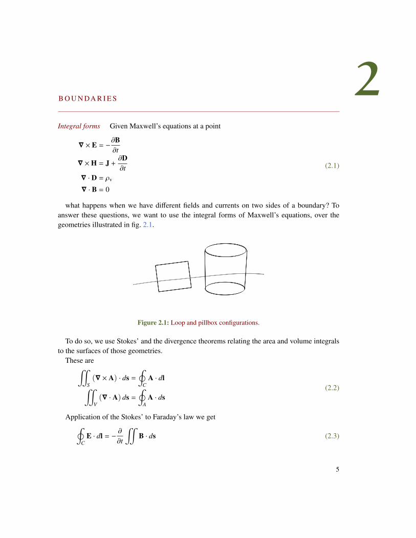
what happens when we have different fields and currents on two sides of a boundary? Toanswer these questions, we want to use the integral forms of Maxwell’s equations, over thegeometries illustrated in fig. 2.1.
Figure 2.1: Loop and pillbox configurations.
To do so, we use Stokes’ and the divergence theorems relating the area and volume integralsto the surfaces of those geometries.
These are
(2.2)
"S(∇ × A) · ds =
∮C
A · dl"V(∇ · A) ds =
∮A
A · ds
Application of the Stokes’ to Faraday’s law we get
(2.3)∮
CE · dl = −
∂
∂t
"B · ds
5
6 boundaries
UNITS: V/m ×mThe quantity
(2.4)"
B · ds,
is called the magnetic flux of B, and changing of this flux is responsible for the generation ofelectromotive force.
Similarly
(2.5)
∮H · dl =
"J · ds +
∂
∂t
"D · ds∮
D · ds =
$ρvdV = Qe∮
B · ds = 0.
Constitutive relations With 12 unknowns in E,B,D,H and 8 equations in Maxwell’s equa-tions (or 6 if the divergence equations are considered redundant), things don’t look too good forsolutions. In simple media, in the frequency domain, relations of the form
(2.6)D(r, ω) = εE(r, ω)
B(r, ω) = µH(r, ω).
The permeabilities ε and µ are macroscopic beasts, determined either experimentally, or the-oretically using an averaging process involving many (millions, or billions, or more) particles.However, the theoretical determinations that have been attempted do not work well in practiseand usually end up considerably different than the measured values. We are referred to [8] forone attempt to model the statistical microscopic effects non-quantum mechanically to justifythe traditional macroscopic form of Maxwell’s equations.
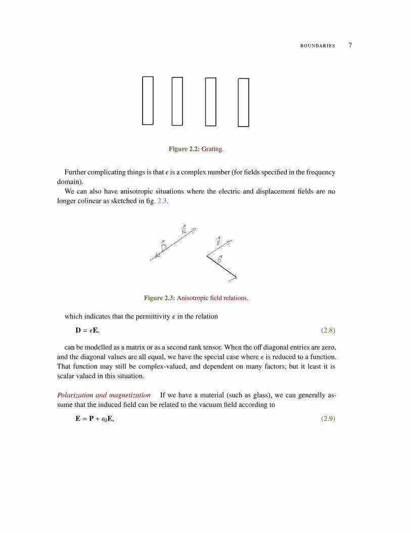
These can be position dependent, as in the grating sketched in fig. 2.2.The permeabilities can also depend on the strength of the fields. An example, application of
an electric field to gallium arsenide or glass can change the behaviour in the material. We canalso have non-linear effects, such as the effect on a capacitor when the voltage is increased. Theresponse near the breakdown point where the capacitor blows up demonstrates this spectacularly.We can also have materials for which the permeabilities depend on the direction of the field,or the temperature, or the pressure in the environment, the tensile or compression forces onthe material, or many other factors. There are many other possible complicating factors, forexample, the electric response ε can depend on the magnetic field strength |B|. We could thenwrite
(2.7)ε = ε(r, |E|,E/|E|,T, P,∣∣∣η∣∣∣, ω, k).
boundaries 7
Figure 2.2: Grating.
Further complicating things is that ε is a complex number (for fields specified in the frequencydomain).
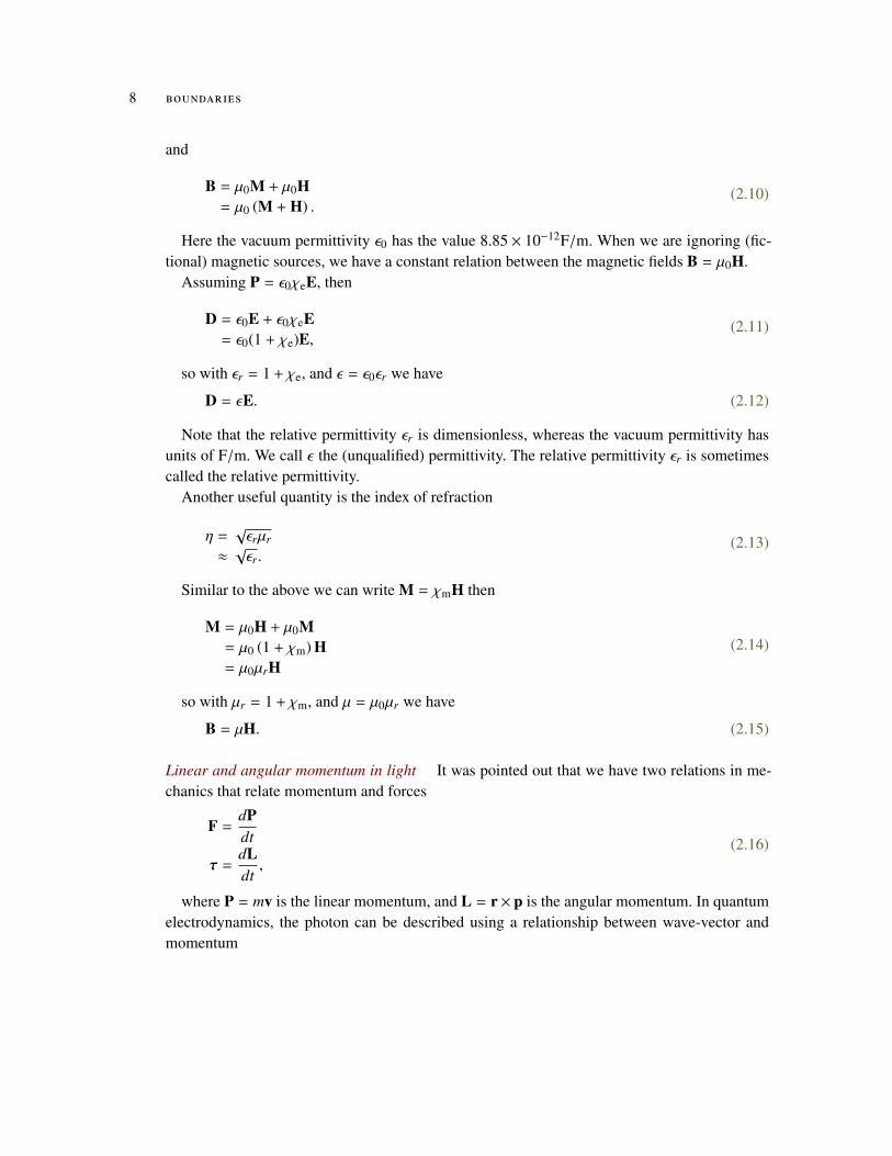
We can also have anisotropic situations where the electric and displacement fields are nolonger colinear as sketched in fig. 2.3.
Figure 2.3: Anisotropic field relations.
which indicates that the permittivity ε in the relation
(2.8)D = εE,
can be modelled as a matrix or as a second rank tensor. When the off diagonal entries are zero,and the diagonal values are all equal, we have the special case where ε is reduced to a function.That function may still be complex-valued, and dependent on many factors, but it least it isscalar valued in this situation.
Polarization and magnetization If we have a material (such as glass), we can generally as-sume that the induced field can be related to the vacuum field according to
(2.9)E = P + ε0E,
8 boundaries
and
(2.10)B = µ0M + µ0H= µ0 (M + H) .
Here the vacuum permittivity ε0 has the value 8.85 × 10⁻¹²F/m. When we are ignoring (fic-tional) magnetic sources, we have a constant relation between the magnetic fields B = µ0H.
Assuming P = ε0χeE, then
(2.11)D = ε0E + ε0χeE= ε0(1 + χe)E,
so with εr = 1 + χe, and ε = ε0εr we have
(2.12)D = εE.
Note that the relative permittivity εr is dimensionless, whereas the vacuum permittivity hasunits of F/m. We call ε the (unqualified) permittivity. The relative permittivity εr is sometimescalled the relative permittivity.
Another useful quantity is the index of refraction
(2.13)η =√εrµr
≈√εr.
Similar to the above we can write M = χmH then
(2.14)M = µ0H + µ0M
= µ0 (1 + χm) H= µ0µrH
so with µr = 1 + χm, and µ = µ0µr we have
(2.15)B = µH.
Linear and angular momentum in light It was pointed out that we have two relations in me-chanics that relate momentum and forces
(2.16)F =
dPdt
τ =dLdt,
where P = mv is the linear momentum, and L = r× p is the angular momentum. In quantumelectrodynamics, the photon can be described using a relationship between wave-vector andmomentum
boundaries 9
(2.17)
p = hk
= h2πλ
=h
2π2πλ
=hλ,
where h = 6.522 × 10⁻¹⁶ev s.Photons are also governed by
(2.18)E = hω= hν.
(De-Broglie’s relations).ASIDE: optical fibre at 1550 has the lowest amount of optical attenuation.Since photons have linear momentum, we can move things around using light. With photons
having both linear momentum and energy relationships, and there is a relation between betweentorque and linear momentum, it seems that there must be the possibility of light having angularmomentum.
Is it possible to utilize the angular momentum to impose patterns on beams (such as laserbeams). For example, what if a beam could have a geometrical pattern along its line of propaga-tion, being off in some regions, on in others. This is in fact possible, generating beams that are“self healing”.
The question was posed “Is it possible to solve electromagnetic problems utilizing the forceconcepts?”, using the Lorentz force equation
(2.19)F = qv × B + qE.
This was not thought to be a productive approach due to the complexity.FIXME: It appeared that this animated talk (probably not captured well) about momentum in
light was linked to the idea of the Helmholtz theorem. Exactly how was not clear to me.
Helmholtz’s theorem Suppose that we have a linear material where
(2.20)
∇ × E = −∂B∂t
∇ ×H = J +∂D∂t
∇ · E =ρv
ε0
∇ ·H = 0
10 boundaries
We have relations between the divergence and curl of E given the sources. Is that sufficientto determine E itself? The answer is yes, which is due to the Helmholtz theorem.
Extra homework question (bonus) : can knowledge of the tangential components of the fieldsalso be used to uniquely determine E?
2.1 problems
Exercise 2.1 Displacement current and Ampere’s law.
Show that without the displacement current ∂D/∂t, Maxwell’s equations will not satisfy conser-vation relations.Answer for Exercise 2.1
PROBLEM SET RELATED MATERIAL REDACTED IN THIS DOCUMENT.PLEASEFEEL FREE TO EMAIL ME FOR THE FULL VERSION IF YOU AREN’T TAKING ECE1228.
. .. .
.. . .
. .. . .
. .. .
. END-REDACTION
Exercise 2.2 Electric field due to spherical shell ([5] pr. 2.7)
Calculate the field due to a spherical shell. The field is
(2.21)E =σ
4πε0
∫(r − r′)|r − r′|3
da′,
where r′ is the position to the area element on the shell. For the test position, let r = ze3.Answer for Exercise 2.2
PROBLEM SET RELATED MATERIAL REDACTED IN THIS DOCUMENT.PLEASEFEEL FREE TO EMAIL ME FOR THE FULL VERSION IF YOU AREN’T TAKING ECE1228.
. .. .
.. . .
. .
2.1 problems 11
. . .. .
. .. END-REDACTION
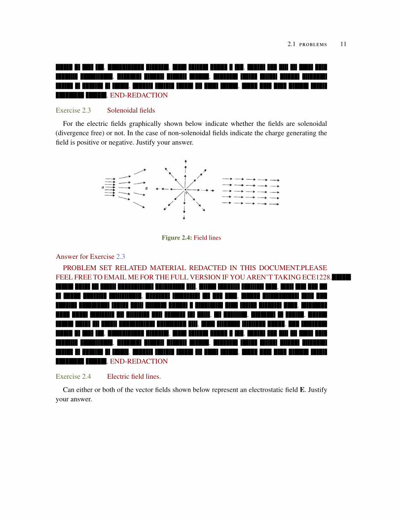
Exercise 2.3 Solenoidal fields
For the electric fields graphically shown below indicate whether the fields are solenoidal(divergence free) or not. In the case of non-solenoidal fields indicate the charge generating thefield is positive or negative. Justify your answer.
Figure 2.4: Field lines
Answer for Exercise 2.3
PROBLEM SET RELATED MATERIAL REDACTED IN THIS DOCUMENT.PLEASEFEEL FREE TO EMAIL ME FOR THE FULL VERSION IF YOU AREN’T TAKING ECE1228.
. .. .
.. . .
. .. . .
. .. .
. END-REDACTION
Exercise 2.4 Electric field lines.
Can either or both of the vector fields shown below represent an electrostatic field E. Justifyyour answer.

12 boundaries
(a) (b)
Figure 2.5: Field lines.
Answer for Exercise 2.4
PROBLEM SET RELATED MATERIAL REDACTED IN THIS DOCUMENT.PLEASEFEEL FREE TO EMAIL ME FOR THE FULL VERSION IF YOU AREN’T TAKING ECE1228.
. .. .
.. . .
. .. . .
. .. .
. END-REDACTION
Exercise 2.5 Solenoidal and irrotational fields.
In terms of E or H give an example for each of the following conditions:
a. Field is solenoidal and irrotational.
b. Field is solenoidal and rotational.
c. Field is non-solenoidal and irrotational.
d. Field is non-solenoidal and rotational.Answer for Exercise 2.5
PROBLEM SET RELATED MATERIAL REDACTED IN THIS DOCUMENT.PLEASEFEEL FREE TO EMAIL ME FOR THE FULL VERSION IF YOU AREN’T TAKING ECE1228.
. .. .
.. . .
. .
2.1 problems 13
. . .. .
. .. END-REDACTION
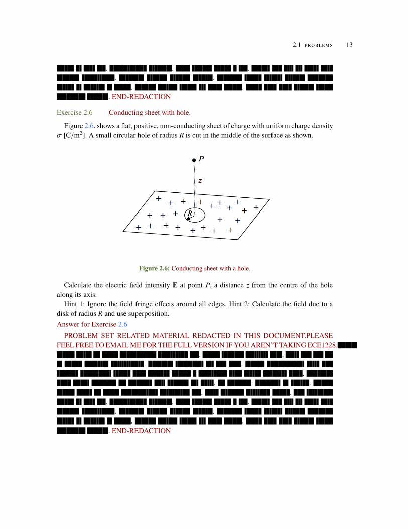
Exercise 2.6 Conducting sheet with hole.
Figure 2.6. shows a flat, positive, non-conducting sheet of charge with uniform charge densityσ [C/m2]. A small circular hole of radius R is cut in the middle of the surface as shown.
Figure 2.6: Conducting sheet with a hole.
Calculate the electric field intensity E at point P, a distance z from the centre of the holealong its axis.
Hint 1: Ignore the field fringe effects around all edges. Hint 2: Calculate the field due to adisk of radius R and use superposition.Answer for Exercise 2.6
PROBLEM SET RELATED MATERIAL REDACTED IN THIS DOCUMENT.PLEASEFEEL FREE TO EMAIL ME FOR THE FULL VERSION IF YOU AREN’T TAKING ECE1228.
. .. .
.. . .
. .. . .
. .. .
. END-REDACTION
14 boundaries
Exercise 2.7 Helmholtz theorem
Prove the first Helmholtz’s theorem, i.e. if vector M is defined by its divergence
(2.22)∇ ·M = s
and its curl
(2.23)∇ ×M = C
within a region and its normal component Mn over the boundary, then M is uniquely speci-fied.Answer for Exercise 2.7
PROBLEM SET RELATED MATERIAL REDACTED IN THIS DOCUMENT.PLEASEFEEL FREE TO EMAIL ME FOR THE FULL VERSION IF YOU AREN’T TAKING ECE1228.
. .. .
.. . .
. .. . .
. .. .
. END-REDACTION
Exercise 2.8 Waveguide field
The instantaneous electric field inside a conducting parallel plate waveguide is given by
(2.24)E(r, t) = e2E0 sin(π
ax)
cos (ωt − βzz)
where βz is the waveguide’s phase constant and a is the waveguide width (a constant). As-suming there are no sources within the free-space-filled pipe, determine
a. The corresponding instantaneous magnetic field components inside the conducting pipe.
b. The phase constant βz.
Answer for Exercise 2.8
PROBLEM SET RELATED MATERIAL REDACTED IN THIS DOCUMENT.PLEASEFEEL FREE TO EMAIL ME FOR THE FULL VERSION IF YOU AREN’T TAKING ECE1228.
. .. .
.
2.1 problems 15
. . .. .
. . .. .
. .. END-REDACTION
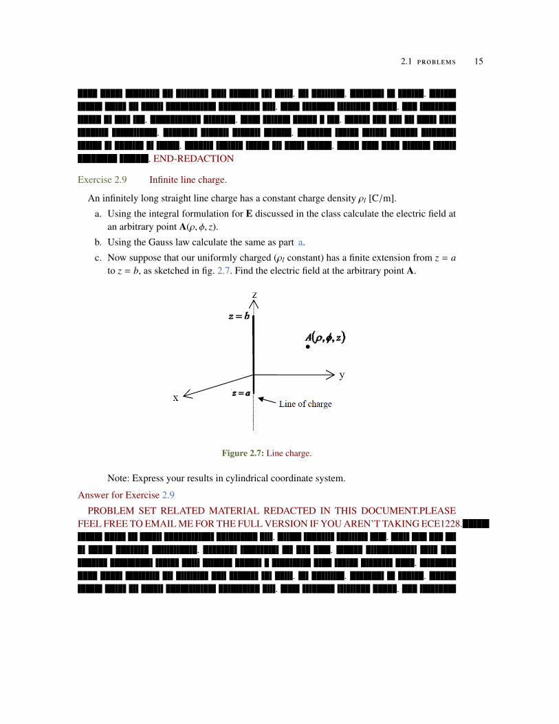
Exercise 2.9 Infinite line charge.
An infinitely long straight line charge has a constant charge density ρl [C/m].
a. Using the integral formulation for E discussed in the class calculate the electric field atan arbitrary point A(ρ, φ, z).
b. Using the Gauss law calculate the same as part a.
c. Now suppose that our uniformly charged (ρl constant) has a finite extension from z = ato z = b, as sketched in fig. 2.7. Find the electric field at the arbitrary point A.
Figure 2.7: Line charge.
Note: Express your results in cylindrical coordinate system.
Answer for Exercise 2.9
PROBLEM SET RELATED MATERIAL REDACTED IN THIS DOCUMENT.PLEASEFEEL FREE TO EMAIL ME FOR THE FULL VERSION IF YOU AREN’T TAKING ECE1228.
. .. .
.. . .
. .
16 boundaries
. . .. .
. .. END-REDACTION
Exercise 2.10 Gradient in cylindrical coordinates.
If gradient of a scalar function ψ rectangular coordinate system is given by
(2.25)∇ψ = x1∂ψ
∂x+ y2
∂ψ
∂y+ z
∂ψ
∂z,
using coordinate transformation and chain rule show that the gradient of ψ in cylindricalcoordinates is given by
(2.26)∇ψ = ρ∂ψ
∂ρ+ φ
1ρ
∂ψ
∂φ+ z
∂ψ
∂z.
Answer for Exercise 2.10
PROBLEM SET RELATED MATERIAL REDACTED IN THIS DOCUMENT.PLEASEFEEL FREE TO EMAIL ME FOR THE FULL VERSION IF YOU AREN’T TAKING ECE1228.
. .. .
.. . .
. .. . .
. .. .
. END-REDACTION
Exercise 2.11 Point charge.
a. Consider a point charge q. Using Maxwell equations, derive an expression for the elec-tric field E generated by q at the distance r from it. Clearly express your assumptionsand justify them.
b. Derive an expression for the force experience by the charge q′ located at distance r fromthe charge q. (This is called Coulomb force)
c. Derive an expression for the electrostatic potential V at the distance r from the chargeq with respect to the electrostatic potential at infinity. For convenience, set the value ofelectrostatic potential at infinity to zero.

2.1 problems 17
Answer for Exercise 2.11
PROBLEM SET RELATED MATERIAL REDACTED IN THIS DOCUMENT.PLEASEFEEL FREE TO EMAIL ME FOR THE FULL VERSION IF YOU AREN’T TAKING ECE1228.
. .. .
.. . .
. .. . .
. .. .
. END-REDACTION

3E L E C T RO S TAT I C S A N D D I P O L E S .
Polarization and Magnetization The importance of the polarization and magnetization givenby
(3.1)D = ε0E + PP = ε0χeE,
where
(3.2)
D = εEε = ε0εr
εr = 1 + χe.
Point charge.
(3.3)
E =q
4πε0
rr2
=q
4πε0
r|r|3
=q
4πε0
rr3 .
In more complex media the ε0 here can be replaced by ε. Here the vector r points from thecharge to the observation point.
Note that the class notes use aR instead of r.When the charge isn’t located at the origin, we must modify this accordingly
(3.4)E =
q4πε0
R|R|3
=q
4πε0
RR3 ,
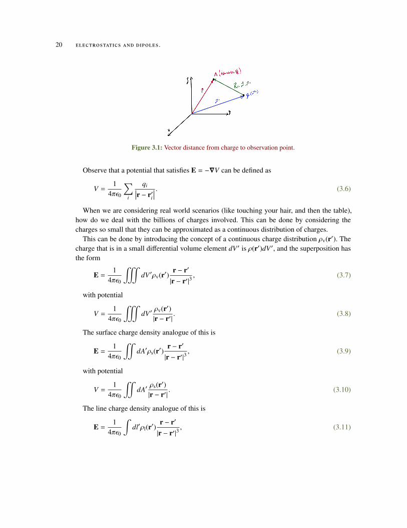
where R = r − r′ still points from the location of the charge to the point of observation, assketched in fig. 3.1.
This can be further generalized to collections of point charges by superposition
(3.5)E =1
4πε0
∑i
qir − r′i∣∣∣r − r′i
∣∣∣3 .
19
20 electrostatics and dipoles .
Figure 3.1: Vector distance from charge to observation point.
Observe that a potential that satisfies E = −∇V can be defined as
(3.6)V =1
4πε0
∑i
qi∣∣∣r − r′i∣∣∣ .
When we are considering real world scenarios (like touching your hair, and then the table),how do we deal with the billions of charges involved. This can be done by considering thecharges so small that they can be approximated as a continuous distribution of charges.
This can be done by introducing the concept of a continuous charge distribution ρv(r′). Thecharge that is in a small differential volume element dV ′ is ρ(r′)dV ′, and the superposition hasthe form
(3.7)E =1
4πε0
$dV ′ρv(r′)
r − r′
|r − r′|3,
with potential
(3.8)V =1
4πε0
$dV ′
ρv(r′)|r − r′|
.
The surface charge density analogue of this is
(3.9)E =1
4πε0
"dA′ρs(r′)
r − r′
|r − r′|3,
with potential
(3.10)V =1
4πε0
"dA′
ρs(r′)|r − r′|
.
The line charge density analogue of this is
(3.11)E =1
4πε0
∫dl′ρl(r′)
r − r′
|r − r′|3,
electrostatics and dipoles . 21
with potential
(3.12)V =1
4πε0
∫dl′
ρl(r′)|r − r′|
.
The difficulty with any of these approaches is the charge density is hardly ever known. Whenthe charge density is known, this sorts of integrals may not be analytically calculable, but theydo yield to numeric calculation.
We may often prefer the potential calculations of the field calculations because they are mucheasier, having just one component to deal with.
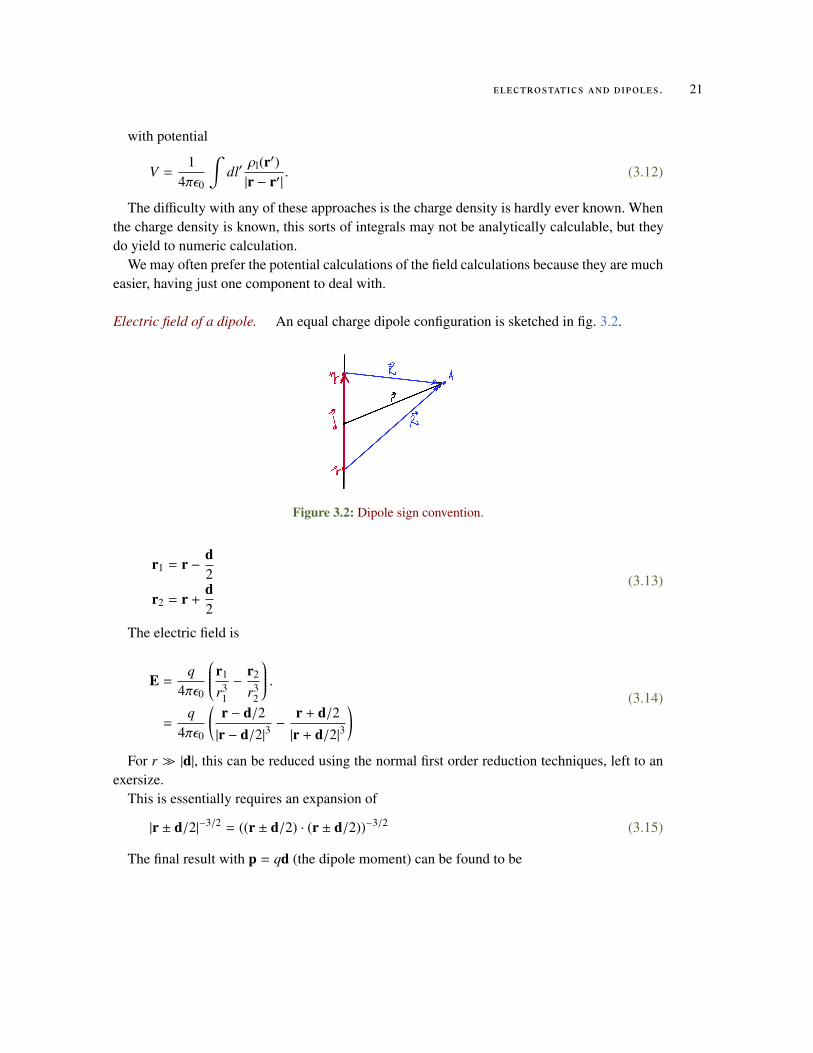
Electric field of a dipole. An equal charge dipole configuration is sketched in fig. 3.2.
Figure 3.2: Dipole sign convention.
(3.13)r1 = r −
d2
r2 = r +d2
The electric field is
(3.14)E =
q4πε0
r1
r31
−r2
r32
.=
q4πε0
(r − d/2|r − d/2|3
−r + d/2|r + d/2|3
)For r � |d|, this can be reduced using the normal first order reduction techniques, left to an
exersize.This is essentially requires an expansion of
(3.15)|r ± d/2|−3/2 = ((r ± d/2) · (r ± d/2))−3/2
The final result with p = qd (the dipole moment) can be found to be
22 electrostatics and dipoles .
(3.16)E =1
4πε0r3
(3
r · pr2 r − p
)With p = qz, we have spherical coordinates for the observation point, and Cartesian for the
dipole moment. To convert the moment to spherical we can use
(3.17)
Ar
AθAφ
=
sin θ cos φ sin θ sin φ cos θ
cos θ cos φ cos θ sin φ − sin θ
− sin φ cos φ 0
Ax
Ay
Az
.All such rotation matrices can be found in the appendix of [2] for example. For the dipole
vector this gives
(3.18)
pr
pθpφ
=
cos θp
− sin θp
0
.or
p = pz = p(cos θr − sin θθ
)(3.19)
Plugging in this eventually gives
(3.20)E =p
4πε0r3
(2 cos θr + sin θθ
),
where |r| = r.It will be left to a problem to show that the potential for an electric dipole is given by
(3.21)V =p · r
4πε0r2 .
Observe that the dipole field drops off faster than the field for a single electric charge. This istrue generally, with quadrupole and higher order moments dropping off faster as the degree isincreased.
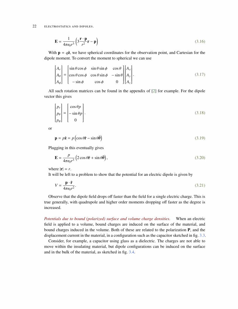
Potentials due to bound (polarized) surface and volume charge densities. When an electricfield is applied to a volume, bound charges are induced on the surface of the material, andbound charges induced in the volume. Both of these are related to the polarization P, and thedisplacement current in the material, in a configuration such as the capacitor sketched in fig. 3.3.
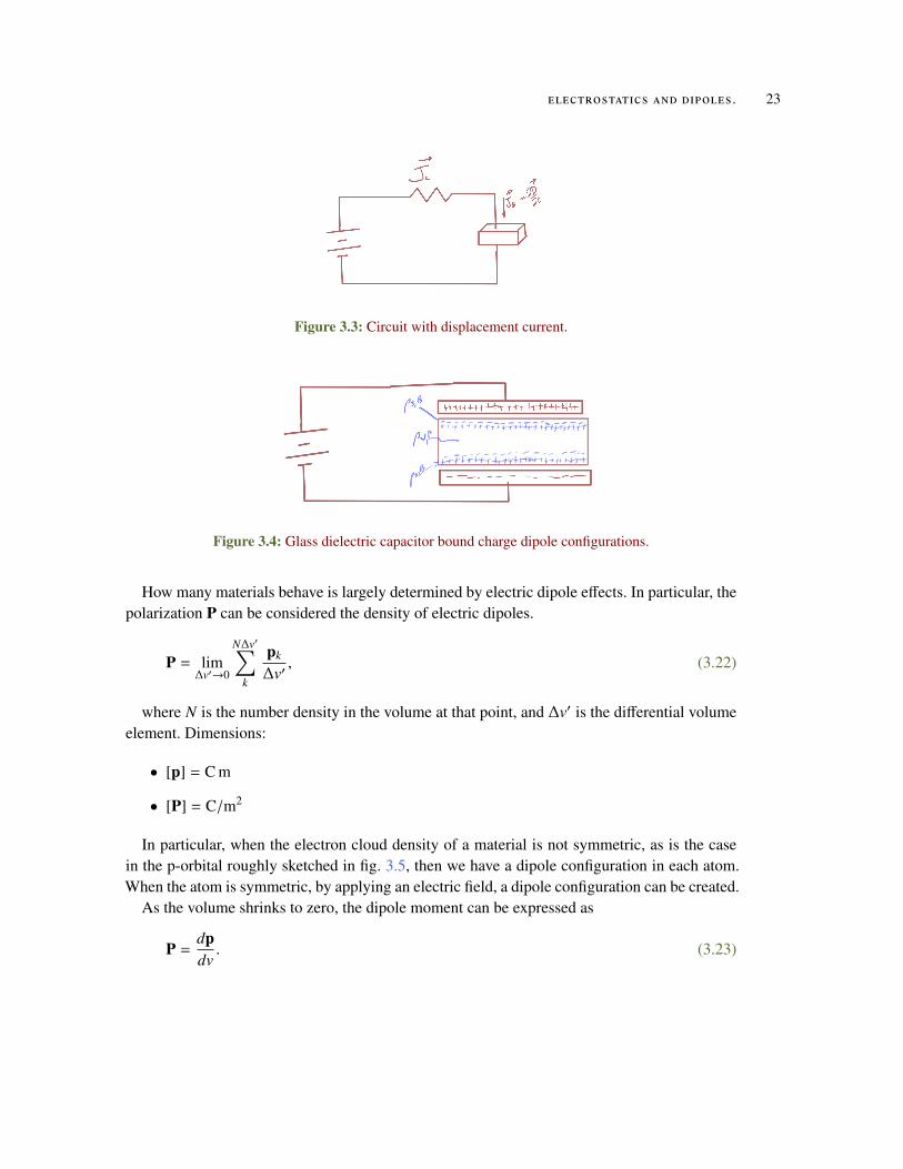
Consider, for example, a capacitor using glass as a dielectric. The charges are not able tomove within the insulating material, but dipole configurations can be induced on the surfaceand in the bulk of the material, as sketched in fig. 3.4.
electrostatics and dipoles . 23
Figure 3.3: Circuit with displacement current.
Figure 3.4: Glass dielectric capacitor bound charge dipole configurations.
How many materials behave is largely determined by electric dipole effects. In particular, thepolarization P can be considered the density of electric dipoles.
(3.22)P = lim∆v′→0
N∆v′∑k
pk
∆v′,
where N is the number density in the volume at that point, and ∆v′ is the differential volumeelement. Dimensions:
• [p] = C m
• [P] = C/m2
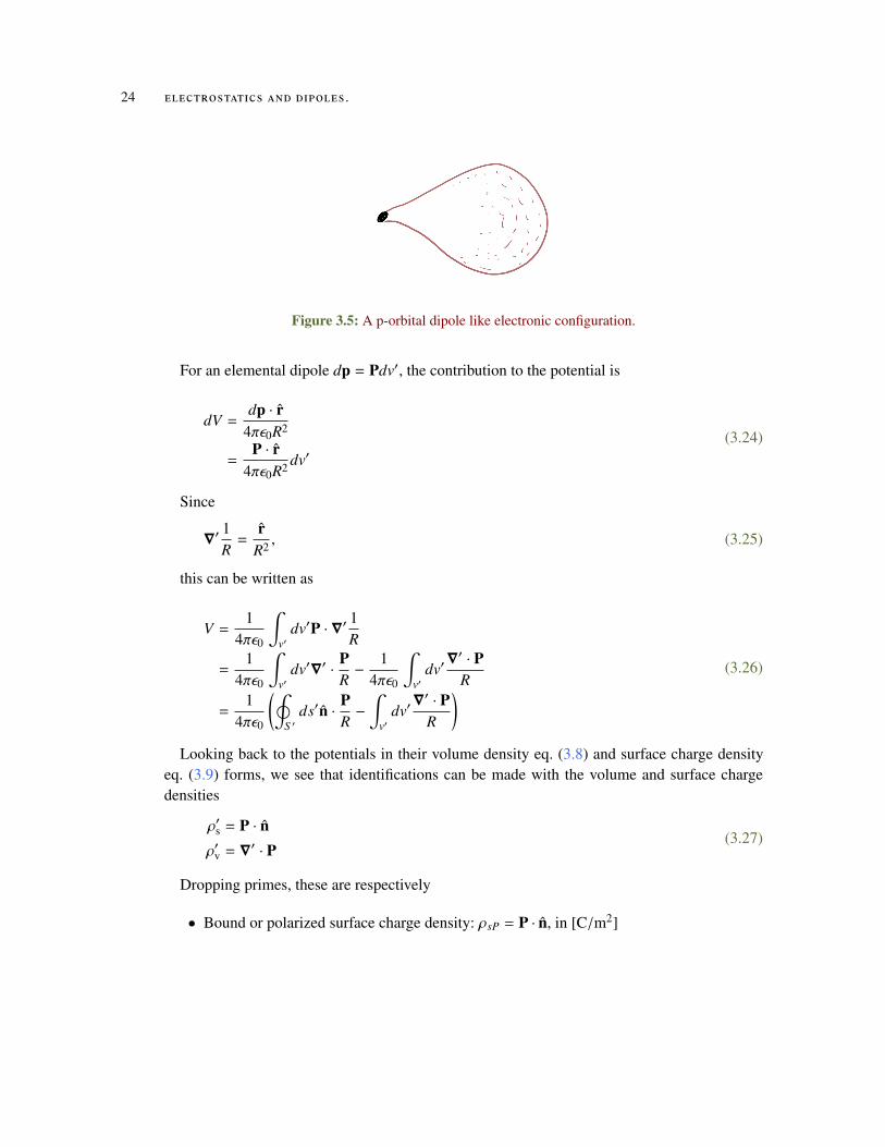
In particular, when the electron cloud density of a material is not symmetric, as is the casein the p-orbital roughly sketched in fig. 3.5, then we have a dipole configuration in each atom.When the atom is symmetric, by applying an electric field, a dipole configuration can be created.
As the volume shrinks to zero, the dipole moment can be expressed as
(3.23)P =dpdv.
24 electrostatics and dipoles .
Figure 3.5: A p-orbital dipole like electronic configuration.
For an elemental dipole dp = Pdv′, the contribution to the potential is
(3.24)dV =
dp · r4πε0R2
=P · r
4πε0R2 dv′
Since
(3.25)∇′ 1R
=r
R2 ,
this can be written as
(3.26)
V =1
4πε0
∫v′
dv′P · ∇′1R
=1
4πε0
∫v′
dv′∇′ ·PR−
14πε0
∫v′
dv′∇′ · P
R
=1
4πε0
(∮S ′
ds′n ·PR−
∫v′
dv′∇′ · P
R
)Looking back to the potentials in their volume density eq. (3.8) and surface charge density
eq. (3.9) forms, we see that identifications can be made with the volume and surface chargedensities
(3.27)ρ′s = P · nρ′v = ∇′ · P
Dropping primes, these are respectively
• Bound or polarized surface charge density: ρsP = P · n, in [C/m2]
electrostatics and dipoles . 25
• Bound or polarized volume charge density: ρvP = ∇ · P, in [C/m3]
Recall that in Maxwell’s equations for the vacuum we have
(3.28)∇ · E =ρv
ε0.
Here ρv represents “free” charge density. Adding in potential bound charges we have
(3.29)∇ · E =
ρv
ε0+ρvP
ε0
=ρv
ε0−∇ · Pε0
.
Rearranging we can write
(3.30)∇ · (ε0E + P) = ρv.
This finally justifies the Maxwell equation
(3.31)∇ · D = ρv,
where D = ε0E + P.Assuming a relationship between the polarization vector and the electric field of the form
(3.32)P = ε0χeE,
possibly a tensor relationship. The bound charges in the material are seen to related the dis-placement current and the electric field
(3.33)
D = ε0E + P= ε0E + ε0χeE,= ε0 (1 + χe) E,= ε0εrE,= εE.
Question: Think about why do we ignore the surface charges here? Answer: we are not con-sidering boundaries... they are at infinity.
26 electrostatics and dipoles .
3.1 problems
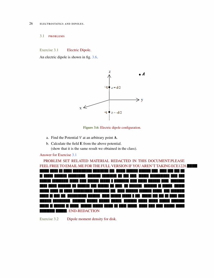
Exercise 3.1 Electric Dipole.
An electric dipole is shown in fig. 3.6.
Figure 3.6: Electric dipole configuration.
a. Find the Potential V at an arbitrary point A.
b. Calculate the field E from the above potential.(show that it is the same result we obtained in the class).
Answer for Exercise 3.1
PROBLEM SET RELATED MATERIAL REDACTED IN THIS DOCUMENT.PLEASEFEEL FREE TO EMAIL ME FOR THE FULL VERSION IF YOU AREN’T TAKING ECE1228.
. .. .
.. . .
. .. . .
. .. .
. END-REDACTION
Exercise 3.2 Dipole moment density for disk.
3.1 problems 27
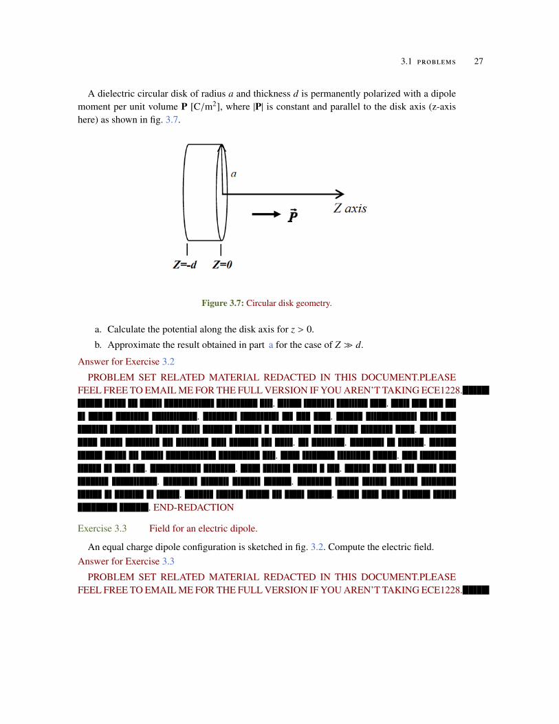
A dielectric circular disk of radius a and thickness d is permanently polarized with a dipolemoment per unit volume P [C/m2], where |P| is constant and parallel to the disk axis (z-axishere) as shown in fig. 3.7.
Figure 3.7: Circular disk geometry.
a. Calculate the potential along the disk axis for z > 0.
b. Approximate the result obtained in part a for the case of Z � d.
Answer for Exercise 3.2
PROBLEM SET RELATED MATERIAL REDACTED IN THIS DOCUMENT.PLEASEFEEL FREE TO EMAIL ME FOR THE FULL VERSION IF YOU AREN’T TAKING ECE1228.
. .. .
.. . .
. .. . .
. .. .
. END-REDACTION
Exercise 3.3 Field for an electric dipole.
An equal charge dipole configuration is sketched in fig. 3.2. Compute the electric field.Answer for Exercise 3.3
PROBLEM SET RELATED MATERIAL REDACTED IN THIS DOCUMENT.PLEASEFEEL FREE TO EMAIL ME FOR THE FULL VERSION IF YOU AREN’T TAKING ECE1228.
28 electrostatics and dipoles .
. .. .
.. . .
. .. . .
. .. .
. END-REDACTION
Exercise 3.4 Electric dipole potential
Having shown that
(3.34)E =1
4πε0r3 (3r (r · p) − p) ,
find the expression for the electric potential for this field.Answer for Exercise 3.4
PROBLEM SET RELATED MATERIAL REDACTED IN THIS DOCUMENT.PLEASEFEEL FREE TO EMAIL ME FOR THE FULL VERSION IF YOU AREN’T TAKING ECE1228.
. .. .
.. . .
. .. . .
. .. .
. END-REDACTION
4M AG N E T I C M O M E N T, A N D B O U N DA RY VA L U E C O N D I T I O N S
Magnetic moment. Using a semi-classical model of an electron, assuming that the electroncircles the nuclei. This is a completely wrong model, but useful. In reality, electrons are randomand probabilistic and do not follow defined paths. We do however have a magnetic momentassociated with the electron, and one associated with the spin of the electron, and a momentassociated with the spin of the nuclei. All of these concepts can be used to describe a moreaccurate model and such a model is discussed in [8] chapters 11,12,13.
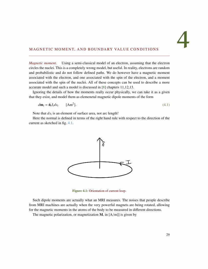
Ignoring the details of how the moments really occur physically, we can take it as a giventhat they exist, and model them as elemenetal magnetic dipole moments of the form
(4.1)dmi = niIidsi [Am2].
Note that dsi is an element of surface area, not arc length!Here the normal is defined in terms of the right hand rule with respect to the direction of the
current as sketched in fig. 4.1.
Figure 4.1: Orientation of current loop.
Such dipole moments are actually what an MRI measures. The noises that people describefrom MRI machines are actually when the very powerful magnets are being rotated, allowingfor the magnetic moments in the atoms of the body to be measured in different directions.
The magnetic polarization, or magnetization M, in [A/m]] is given by
29
30 magnetic moment, and boundary value conditions
(4.2)
M = lim∆v→0
(1
∆vmi
)= lim
∆v→0
1∆v
Nδv∑i=1
dmi
= lim
∆v→0
1∆v
Nδv∑i=1
niIidsi
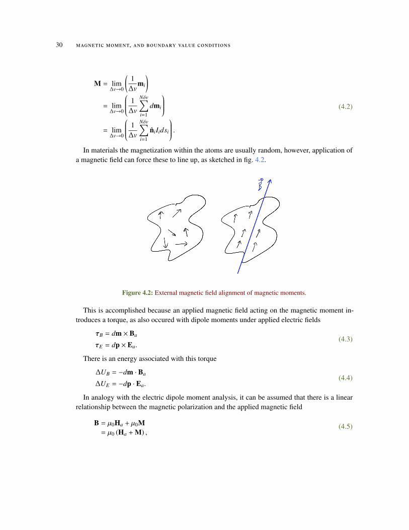
.In materials the magnetization within the atoms are usually random, however, application of
a magnetic field can force these to line up, as sketched in fig. 4.2.
Figure 4.2: External magnetic field alignment of magnetic moments.
This is accomplished because an applied magnetic field acting on the magnetic moment in-troduces a torque, as also occured with dipole moments under applied electric fields
(4.3)τB = dm × Ba
τE = dp × Ea.
There is an energy associated with this torque
(4.4)∆UB = −dm · Ba
∆UE = −dp · Ea.
In analogy with the electric dipole moment analysis, it can be assumed that there is a linearrelationship between the magnetic polarization and the applied magnetic field
(4.5)B = µ0Ha + µ0M= µ0 (Ha + M) ,
magnetic moment, and boundary value conditions 31
where
(4.6)M = χmHa,
so
B = µ0 (1 + χm)Ha ≡ µHa. (4.7)
Like electric dipoles, in a volume, we can have bound currents on the surface [A/m], as wellas bound volume currents [A/m2].
It can be shown, as with the electric dipoles related bound charge densities of eq. (3.27), thatmagnetic currents can be defined
(4.8)Jsm = M × nJvm = ∇ ×M,
Conductivity We have two constitutive relationships so far
(4.9)D = εEB = µH
but this needs to be augmented by
(4.10)Jc = εE.
There are a couple ways to discuss this. One is to model ε as a complex number. Such a modelis not entirely unconstrained. Like with the Cauchy-Riemann conditions that relate derivativesof the real and imaginary parts of a complex number, there is a relationship (Kramers-Kronig[10]), an integral relationship that relates the real and imaginary parts of the permittivity ε.
Boundary conditions. The boundary conditions are
• n × (E2 −E1) = −Ms This means that the tangential components of E is continuousaccross the boundary (those components of E1,E2 are equal on the boundary), when Ms
is zero.
Here Ms is the (fictitious) magnetic current density in [V/m].
• n × (H2 −H1) = Js
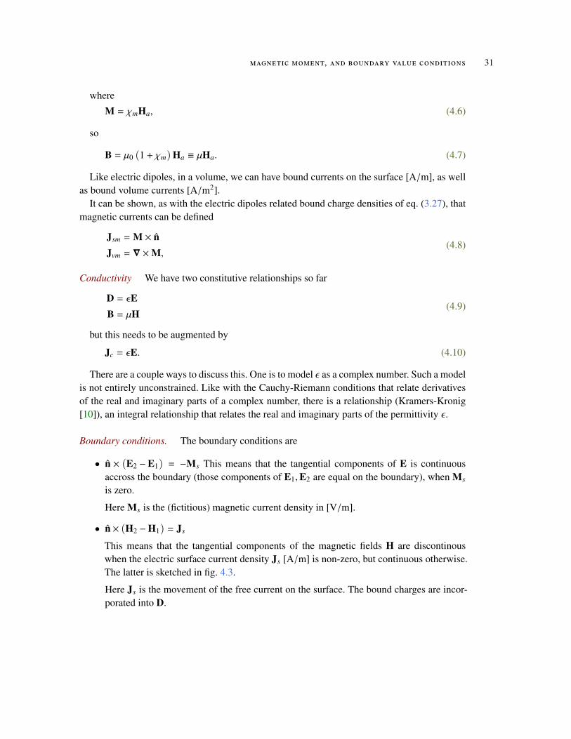
This means that the tangential components of the magnetic fields H are discontinouswhen the electric surface current density Js [A/m] is non-zero, but continuous otherwise.The latter is sketched in fig. 4.3.
Here Js is the movement of the free current on the surface. The bound charges are incor-porated into D.
32 magnetic moment, and boundary value conditions
Figure 4.3: Equal tangential fields.
• n · (D2 −D1) = ρes
Here ρes is the electric surface charge density [C/m2].
This means that the normal component of the electric displacement field D is discon-tinuous accross the boundary in the presence of electric surface charge densities, butcontinuous when that is zero.
• n · (B2 −B1) = ρms
Here ρms is the (fictional) magnetic surface charge density [Weber/m2].
This means that the magnetic fields B are continous in the abscense of (fictional) magneticsurface charge densities.
In the abscence of any free charges or currents, these relationships are considerably simplified
(4.11a)n × (E2 − E1) = 0
(4.11b)n × (H2 −H1) = 0
(4.11c)n · (D2 − D1) = 0
(4.11d)n · (B2 − B1) = 0
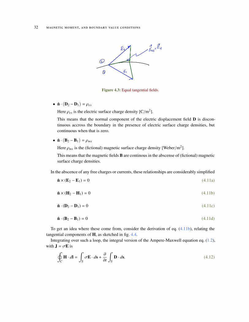
To get an idea where these come from, consider the derivation of eq. (4.11b), relating thetangential components of H, as sketched in fig. 4.4.
Integrating over such a loop, the integral version of the Ampere-Maxwell equation eq. (1.2),with J = σE is
(4.12)∮
CH · dl =
∫SσE · ds +
∂
∂t
∫S
D · ds.
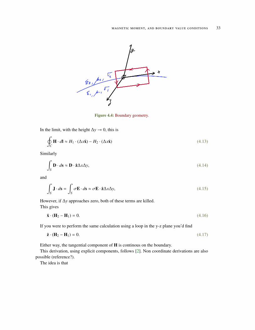
magnetic moment, and boundary value conditions 33
Figure 4.4: Boundary geometry.
In the limit, with the height ∆y→ 0, this is
(4.13)∮
CH · dl ≈ H1 · (∆xx) − H2 · (∆xx)
Similarly
(4.14)∫
SD · ds ≈ D · z∆x∆y,
and∫S
J · ds =
∫SσE · ds ≈ σE · z∆x∆y, (4.15)
However, if ∆y approaches zero, both of these terms are killed.This gives
(4.16)x · (H2 −H1) = 0.
If you were to perform the same calculation using a loop in the y-z plane you’d find
(4.17)z · (H2 −H1) = 0.
Either way, the tangential component of H is continous on the boundary.This derivation, using explicit components, follows [2]. Non coordinate derivations are also
possible (reference?).The idea is that
34 magnetic moment, and boundary value conditions
(4.18)n × ((H2 −H2n) − (H1 −H1n)) = n × (H2 −H1)= 0.
What if there is a surface current?
(4.19)lim∆y→0
Jic∆y = Js.
When this is the case the J = σE needs to be fixed up a bit, and showing how is left to aproblem.
In the notes the other boundary relations are derived. The normal ones follow by integratingover a pillbox volume.
Variations include the cases when one of the surfaces is made a perfect conductor. Such acase can be treated by noting that the E field must be zero.
Conducting media. It will be left to homework to show, using the continuity equation andGauss’s law that inside a conductor, that free charges distribute themselves exclusively on thesurface on the medium. Because of this there is no electric field inside the medium (Gauss’slaw). What does this imply about the magnetic field in the same medium. We must have
(4.20)∇ × E = −∂B∂t
so if E is zero in the medium the magnetic field must be either constant with respect to time,or zero. In a general electrodynamic configuration, both the magnetic and electric fields varywith time, which seems to imply that B must be zero if E is zero in that space.
However, this is not consistent with what we see with an iron core inductor. In such aninductor, the iron is used to concentrate the magnetic field. Clearly we have magnetic fields inthe iron bar, since that is the purpose of it being there. It turns out that if the frequencies arelow enough (and even some smaller GHz frequencies are), then we can consider the system tobe quasi-electrostatic, with zero electric fields inside a conductor, yet with finite approximatelytime independent magnetic fields. As the frequencies are increased, the magnetic fields areforced out of the conductor into the surrounding space.
The transition point that defines the boundary between electrostatic and quasi-electrostaticwill depend on the precision desired.
Boundary conditions with zero magnetic fields in a conductor For many calculations, we canproceed with the assumption that there are no appreciable electric nor magnetic fields inside ofa conductor. When that is the case, outside of a conducting medium, we have
(4.21)n × E2 = 0,
4.1 problems 35
so there is no tangential component to an electric field of a conductor. We also have
(4.22)n · D2 = ρes
Assuming there is also no magnetic field either in the conductor, we also have
(4.23)n ×H2 = Js,
and
(4.24)n · B2 = 0.
There is no normal component to the magnetic field at the surface of a conductor, and thetangential component is determined by the surface current density.
4.1 problems
Exercise 4.1 Magnetic moment for localized current.
Jackson [8] §5.6 derives an expression for the magnetic moment of a localized current distribu-tion, far from the source. Repeat this derivation, filling in the details.Answer for Exercise 4.1
PROBLEM SET RELATED MATERIAL REDACTED IN THIS DOCUMENT.PLEASEFEEL FREE TO EMAIL ME FOR THE FULL VERSION IF YOU AREN’T TAKING ECE1228.
. .. .
.. . .
. .. . .
. .. .
. END-REDACTION
Exercise 4.2 Vector Area. ([5] pr. 1.61)
The integral
(4.25)a =
∫S
da,
is sometimes called the vector area of the surface S .
a. Find the vector area of a hemispherical bowl of radius R.
36 magnetic moment, and boundary value conditions
b. Show that a = 0 for any closed surface.
c. Show that a is the same for all surfaces sharing the same boundary.
d. Show that
(4.26)a =12
�r × dl,
where the integral is around the boundary line.
e. Show that
(4.27)�
(c · r) dl = a × c.
Answer for Exercise 4.2
PROBLEM SET RELATED MATERIAL REDACTED IN THIS DOCUMENT.PLEASEFEEL FREE TO EMAIL ME FOR THE FULL VERSION IF YOU AREN’T TAKING ECE1228.
. .. .
.. . .
. .. . .
. .. .
. END-REDACTION
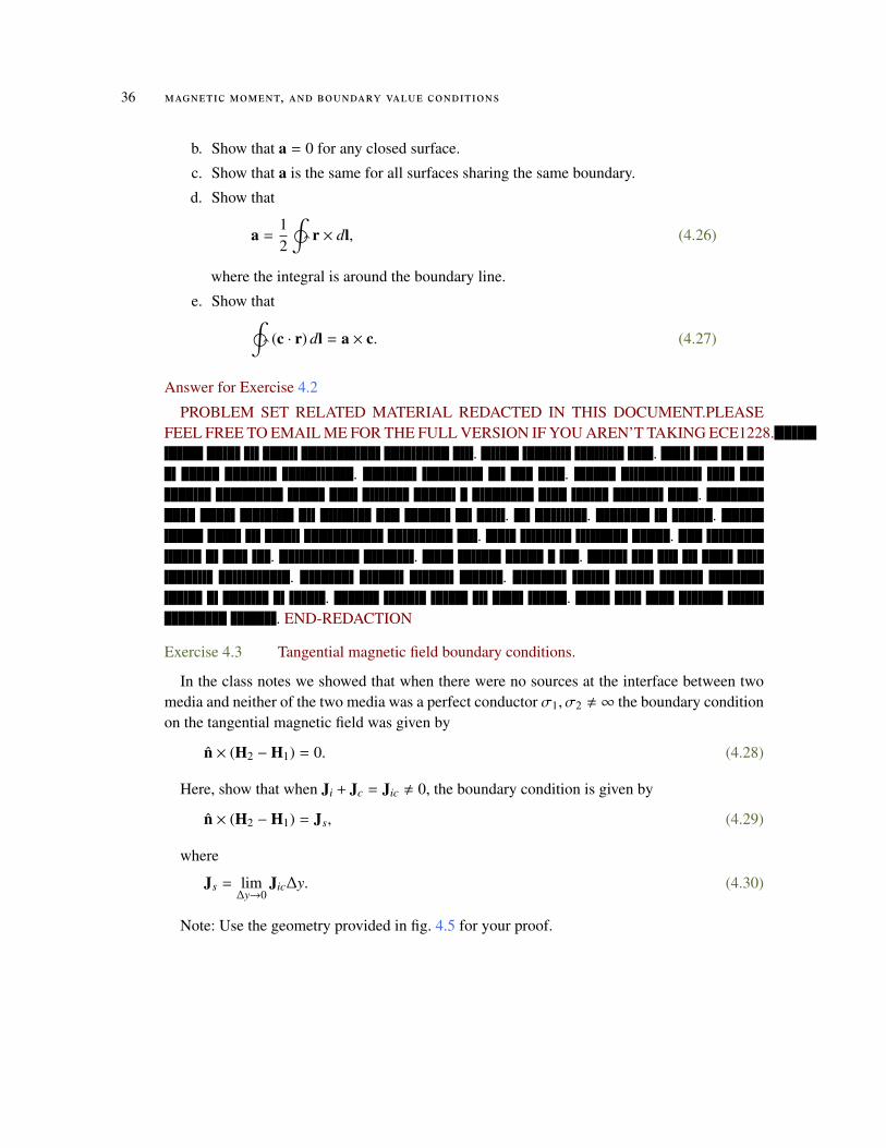
Exercise 4.3 Tangential magnetic field boundary conditions.
In the class notes we showed that when there were no sources at the interface between twomedia and neither of the two media was a perfect conductor σ1, σ2 , ∞ the boundary conditionon the tangential magnetic field was given by
(4.28)n × (H2 −H1) = 0.
Here, show that when Ji + Jc = Jic , 0, the boundary condition is given by
(4.29)n × (H2 −H1) = Js,
where
(4.30)Js = lim∆y→0
Jic∆y.
Note: Use the geometry provided in fig. 4.5 for your proof.
4.1 problems 37
Figure 4.5: Boundary geometry.
Answer for Exercise 4.3
PROBLEM SET RELATED MATERIAL REDACTED IN THIS DOCUMENT.PLEASEFEEL FREE TO EMAIL ME FOR THE FULL VERSION IF YOU AREN’T TAKING ECE1228.
. .. .
.. . .
. .. . .
. .. .
. END-REDACTION
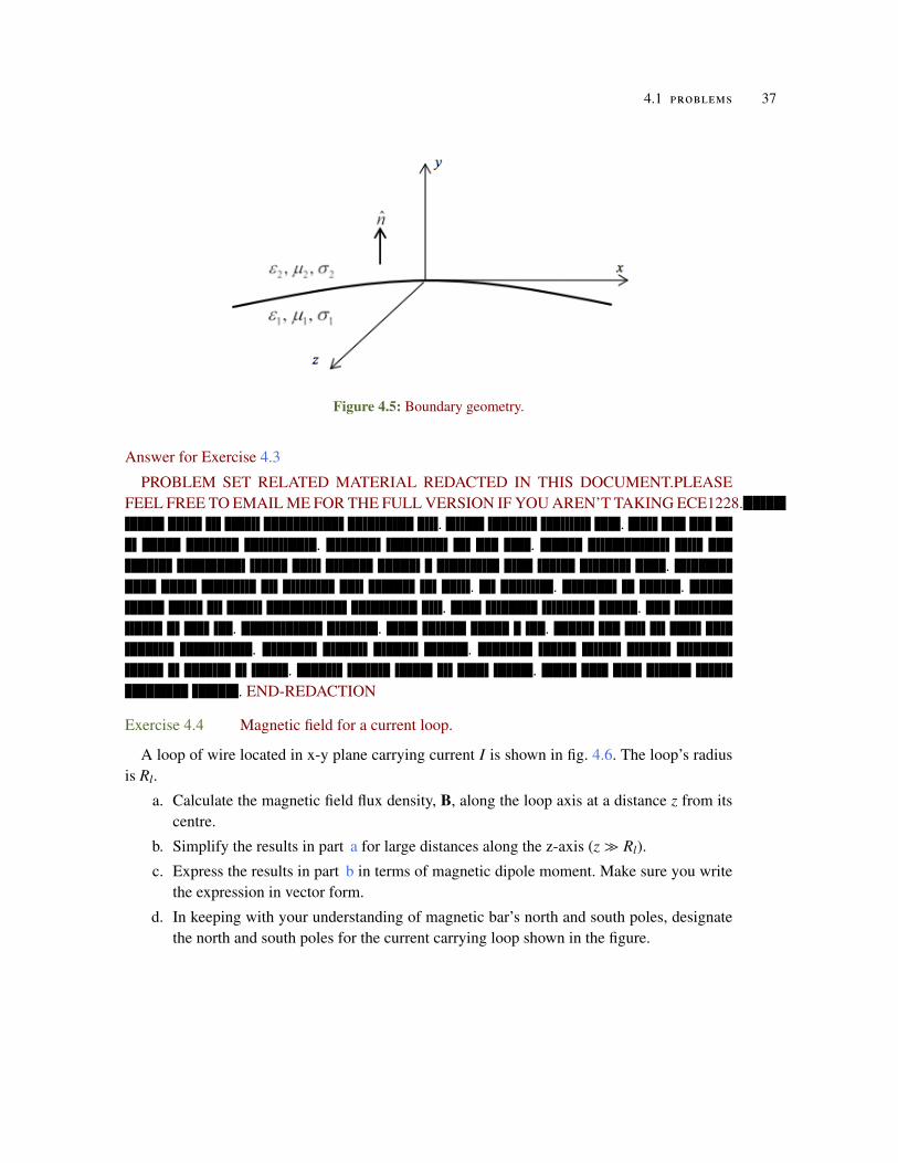
Exercise 4.4 Magnetic field for a current loop.
A loop of wire located in x-y plane carrying current I is shown in fig. 4.6. The loop’s radiusis Rl.
a. Calculate the magnetic field flux density, B, along the loop axis at a distance z from itscentre.
b. Simplify the results in part a for large distances along the z-axis (z � Rl).
c. Express the results in part b in terms of magnetic dipole moment. Make sure you writethe expression in vector form.
d. In keeping with your understanding of magnetic bar’s north and south poles, designatethe north and south poles for the current carrying loop shown in the figure.
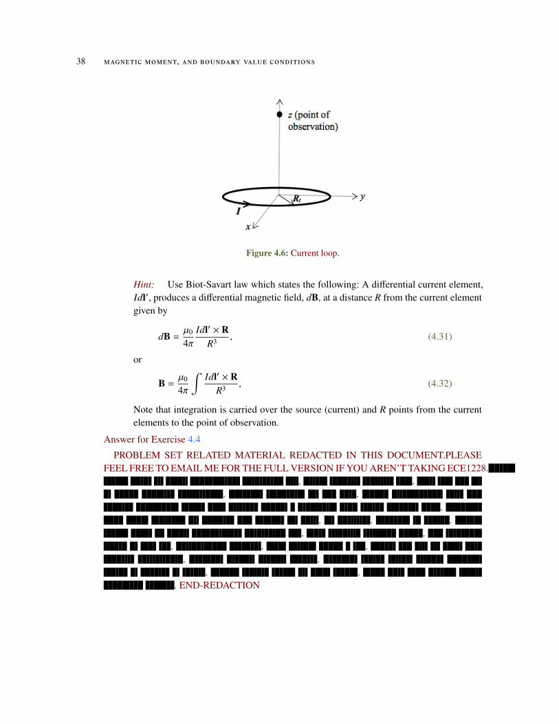
38 magnetic moment, and boundary value conditions
Figure 4.6: Current loop.
Hint: Use Biot-Savart law which states the following: A differential current element,Idl′, produces a differential magnetic field, dB, at a distance R from the current elementgiven by
(4.31)dB =µ0
4πIdl′ × R
R3 ,
or
(4.32)B =µ0
4π
∫Idl′ × R
R3 ,
Note that integration is carried over the source (current) and R points from the currentelements to the point of observation.
Answer for Exercise 4.4
PROBLEM SET RELATED MATERIAL REDACTED IN THIS DOCUMENT.PLEASEFEEL FREE TO EMAIL ME FOR THE FULL VERSION IF YOU AREN’T TAKING ECE1228.
. .. .
.. . .
. .. . .
. .. .
. END-REDACTION

4.1 problems 39
Exercise 4.5 Electric field across dielectric boundary.
The plane 3x + 2y + z = 12 [m] describes the interface between a dielectric and free space.The origin side of the interface has εr1 = 3 and E1 = 2x + 5z [V/m]. What is E2 (the field onthe other side of the interface)?Answer for Exercise 4.5
PROBLEM SET RELATED MATERIAL REDACTED IN THIS DOCUMENT.PLEASEFEEL FREE TO EMAIL ME FOR THE FULL VERSION IF YOU AREN’T TAKING ECE1228.
. .. .
.. . .
. .. . .
. .. .
. END-REDACTION
Exercise 4.6 Laplacian form of delta function.
Prove that
(4.33)−∇2 1r
= 4πδ3(r),
where r = |r| is the position vector.Answer for Exercise 4.6
PROBLEM SET RELATED MATERIAL REDACTED IN THIS DOCUMENT.PLEASEFEEL FREE TO EMAIL ME FOR THE FULL VERSION IF YOU AREN’T TAKING ECE1228.
. .. .
.. . .
. .. . .
. .. .
. END-REDACTION
Exercise 4.7 Conductor charge distribution on surface.
We have stated that the boundary condition for a perfect conductor is such that there is noelectric field or charge distribution inside of the conductor. Here we will study the dynamics

40 magnetic moment, and boundary value conditions
of this process. Start with continuity equation ∇ · J = −∂ρ/∂t, where J is the current density[A/m2] and ρ is the charge density [C/m3]. Show that a charge (charge density) placed inside aconductor will decay in an exponential manner.Answer for Exercise 4.7
PROBLEM SET RELATED MATERIAL REDACTED IN THIS DOCUMENT.PLEASEFEEL FREE TO EMAIL ME FOR THE FULL VERSION IF YOU AREN’T TAKING ECE1228.
. .. .
.. . .
. .. . .
. .. .
. END-REDACTION
Exercise 4.8 Magnetic field from moment.
The vector potential, to first order, for a magnetostatic localized current distribution wasfound to be
(4.34)A(x) =µ0
4πm × x|x|3
.
Use this to calculate the magnetic field.Answer for Exercise 4.8
PROBLEM SET RELATED MATERIAL REDACTED IN THIS DOCUMENT.PLEASEFEEL FREE TO EMAIL ME FOR THE FULL VERSION IF YOU AREN’T TAKING ECE1228.
. .. .
.. . .
. .. . .
. .. .
. END-REDACTION
5P OY N T I N G V E C T O R , A N D T I M E H A R M O N I C ( P H A S O R ) F I E L D S .
Poynting The cross product terms of Maxwell’s equation are
∇ ×E = −Mi −∂B∂t
= −Mi −Md, (5.1)
where Md is called the magnetic displacement current here. For the magnetic curl we have
∇ ×H = Ji + Jc +∂D∂t
= Ji + Jc + Jd. (5.2)
It is left as an exersize to show that
(5.3)∇ · (E ×H) + H · (Mi + Md) + E · (Ji + Jc + Jd) = 0,
or
(5.4)∮
da · (E ×H) +
∫dV (H · (Mi + Md) + E · (Ji + Jc + Jd)) = 0,
or
(5.5)∮
da · (E×H) +
∫dVH ·Mi +
∫dVE · Ji +
∫dVE · Jc +
∫dV
(H ·
∂B∂t
+ E ·∂D∂t
)= 0.
Define a supplied power density ρsupp
(5.6)−ρsupp =
∫dVH ·Mi +
∫dVE · Ji.
When the medium is not dispersive or lossy, we have
(5.7)
∫dVH ·
∂B∂t
= µ
∫dVH ·
∂H∂t
=∂
∂t
∫dVµ|H|2.
The units of [µ|H|2] are W, so one can defined a magnetic energy density µ|H|2, and
(5.8)Wm =
∫dVµ|H|2,
41
42 poynting vector , and time harmonic (phasor) fields .
for
(5.9)∫
dVH ·∂B∂t
=∂Wm
∂t.
This is the rate of change of stored magnetic energy [J/s = W].Similarly
(5.10)
∫dVE ·
∂D∂t
= ε
∫dVE ·
∂E∂t
=∂
∂t
∫dVε |E|2.
The electric energy density is ε|E|2. Let
(5.11)We =
∫dVε|E|2,
and
(5.12)∫
dVE ·∂D∂t
=∂We
∂t.
We also have a term
(5.13)
∫dVE · Jc =
∫dVE · (σE)
=
∫dVσ|E|2
This is the rate of change of stored electric energy.The remaining term is
(5.14)∮
da · (E ×H)
This is a density of the power that is leaving the volume. The vector E ×H is special, calledthe Poynting vector, and coincidentally points in the direction that the energy leaves the bound-ing surface per unit time. We write
(5.15)S = E ×H.
In vacuum the phase velocity vp, group velocity vg and packet(?) velocity vp all line up. Thisisn’t the case in the media.
It turns out that without dissipation
poynting vector , and time harmonic (phasor) fields . 43
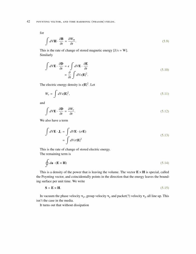
Figure 5.1: LC circuit.
(5.16)∫
H ·∂B∂t
=
∫E ·
∂D∂t.
For example in an LC circuit fig. 5.1 half the cycle the energy is stored in the inductor, andin the other half of the cycle the energy is stored in the capacitor.
Summarizing
(5.17)∮
(E ×H) · da = Pexit.
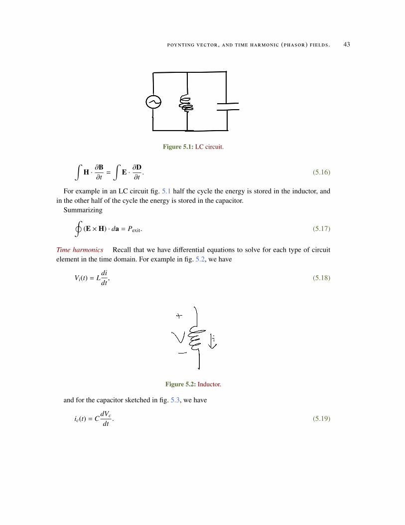
Time harmonics Recall that we have differential equations to solve for each type of circuitelement in the time domain. For example in fig. 5.2, we have
(5.18)Vi(t) = Ldidt,
Figure 5.2: Inductor.
and for the capacitor sketched in fig. 5.3, we have
(5.19)ic(t) = CdVc
dt.
44 poynting vector , and time harmonic (phasor) fields .
Figure 5.3: Capacitor.
When we use Laplace or Fourier techniques to solve circuits with such differential equationelements. The price that we paid for that was that we have to start dealing with complex-valued(phasor) quantities. We can do this for field equations as well. The goal is to remove the timedomain coupling in Maxwell equations like
(5.20)∇ × E(r, t) = −∂B∂t
(r, t)
(5.21)∇ ×H(r, t) = σE +∂D∂t
(r, t).
For a single frequency, assume that the time dependency can be written as
(5.22)E(r, t) = Re(E∗(r)e jωt
).
We may now have to require E(r) to be complex valued. We also have to be really carefulabout which convention of the time domain solution we are going to use, since we could just aseasily use
(5.23)E(r, t) = Re(E(r)e− jωt
).
For example
(5.24)Re(eikze−iωt) = cos(kz − ωt),
is identical with
(5.25)Re(e− jkze jωt) = cos(ωt − kz),
showing that a solution or its complex conjugate is equally valid.Engineering books use e jωt whereas most physicists use e−iωt.What if we have more complex time dependencies, such as that sketched in fig. 5.4?
poynting vector , and time harmonic (phasor) fields . 45
Figure 5.4: Non-sinusoidal time dependence.
We can do this using Fourier superposition, adding a finite or infinite set of single frequencysolutions. The first order of business is to solve the system for a single frequency.
Let’s write our Fourier transform pairs as
F(A(r, t)) = A(r, ω) =
∫ ∞
−∞
A(r, t)e− jωtdt (5.26a)
A(r, t) = F−1(A(r, ω)) =1
2π
∫ ∞
−∞
A(r, ω)e jωtdω. (5.26b)
In particular
F
(d f (t)
dt
)= jωF(ω), (5.27)
so the Fourier transform of the Maxwell equation
(5.28)F (∇ × E(r, t)) = F
(−∂B∂t
(r, t)),
is
(5.29)∇ × E(r, ω) = − jωB(r, ω).
The four Maxwell’s equations can be written as
• Faraday’s Law
(5.30)∇ × E(r, ω) = − jωB(r, ω) −Mi
• Ampere-Maxwell equation
(5.31)∇ ×H(r, ω) = Jc(r, ω) + D(r, ω)
46 poynting vector , and time harmonic (phasor) fields .
• Gauss’s law
(5.32)∇ · D(r, ω) = ρev(r, ω)
• Gauss’s law for magnetism
(5.33)∇ · B(r, ω) = ρmv(r, ω).
Now we can more easily model non-simple media with
(5.34)B(r, ω) = µ(ω)H(r, ω)
D(r, ω) = ε(ω)E(r, ω).
so Maxwell’s equations are
(5.35)∇ × E(r, ω) = − jωµ(ω)H(r, ω) −Mi
(5.36)∇ ×H(r, ω) = Jc(r, ω) + ε(ω)E(r, ω)
(5.37)ε(ω)∇ · E(r, ω) = ρev(r, ω)
(5.38)µ(ω)∇ ·H(r, ω) = ρmv(r, ω).
Frequency domain Poynting The frequency domain (time harmonic) equivalent of the instan-taneous Poynting theorem is
12
∮da ·
(E×H∗
)−
12
∫dV
(H∗ ·Mi + E · J∗i
)+
12
∫dVσ|E|2 + jω
12
∫dV
(µ|H|2 − ε|E|2
)= 0.
(5.39)
Showing this is left as an exersize. Since
(5.40)Re(A) × Re(B) , Re(A × B).
We want to find the instantaneous Poynting vector in terms of the phasor fields. Following[2], where script is used for the instantaneous quantities and non-script for the phasors, we find
(5.41)
S(r, t) = E(r, t) ×H(r, t)= Re(E(r, t)) × Re(H(r, t))
=Ee jωt + E∗e− jωt
2×
He jωt + H∗e− jωt
2
=14
(E ×H∗ + E∗ ×H + E ×He2 jωt + H × Ee−2 jωt
)=
12
Re(E ×H∗) +12
Re(E ×He2 jωt).
5.1 problems 47
Should we time average over a period 〈.〉 = (1/T )∫ T
0 (.) the second term is killed, so that
(5.42)〈S〉 =12
Re(E ×H∗) +12
Re(E ×He2 jωt).
The instantaneous Poynting vector is thus
(5.43)S(r, t) = 〈S〉 +12
Re(E ×He jωt
).
5.1 problems
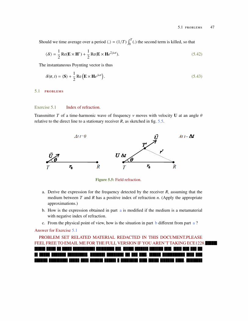
Exercise 5.1 Index of refraction.
Transmitter T of a time-harmonic wave of frequency ν moves with velocity U at an angle θrelative to the direct line to a stationary receiver R, as sketched in fig. 5.5.
Figure 5.5: Field refraction.
a. Derive the expression for the frequency detected by the receiver R, assuming that themedium between T and R has a positive index of refraction n. (Apply the appropriateapproximations.)
b. How is the expression obtained in part a is modified if the medium is a metamaterialwith negative index of refraction.
c. From the physical point of view, how is the situation in part b different from part a ?
Answer for Exercise 5.1
PROBLEM SET RELATED MATERIAL REDACTED IN THIS DOCUMENT.PLEASEFEEL FREE TO EMAIL ME FOR THE FULL VERSION IF YOU AREN’T TAKING ECE1228.
. .. .
.
48 poynting vector , and time harmonic (phasor) fields .
. . .. .
. . .. .
. .. END-REDACTION
Exercise 5.2 Phasor equality.
Prove that if
(5.44)Re(A(r)e jωt
)= Re
(B(r)e jωt
),
then A(r) = B(r). This means that the Re() operator can be removed on phasors of the samefrequency.Answer for Exercise 5.2
PROBLEM SET RELATED MATERIAL REDACTED IN THIS DOCUMENT.PLEASEFEEL FREE TO EMAIL ME FOR THE FULL VERSION IF YOU AREN’T TAKING ECE1228.
. .. .
.. . .
. .. . .
. .. .
. END-REDACTION
Exercise 5.3 Duality theorem.
Prove that if the time-harmonic fields E(r) and H(r) are solutions to Maxwell’s equations ina simple, source free medium ( Mi = Ji = Jc = 0, ρmv = ρev = 0 ), characterized by ε, µ ; thenE′(r) = ηH(r) and H′(r) = −
E(r)η are also solutions of the Maxwell equations. η is the intrinsic
impedance of the medium.
Remark : By showing the above you have proved the validity of the so called duality theorem.Answer for Exercise 5.3
PROBLEM SET RELATED MATERIAL REDACTED IN THIS DOCUMENT.PLEASEFEEL FREE TO EMAIL ME FOR THE FULL VERSION IF YOU AREN’T TAKING ECE1228.
. .. .
5.1 problems 49
.. . .
. .. . .
. .. .
. END-REDACTION
Exercise 5.4 Poynting theorem
Using Maxwell’s equations given in the class notes, derive the Poynting theorem in bothdifferential and integral form for instantaneous fields. Assume a linear, homogeneous mediumwith no temporal dispersion.Answer for Exercise 5.4
PROBLEM SET RELATED MATERIAL REDACTED IN THIS DOCUMENT.PLEASEFEEL FREE TO EMAIL ME FOR THE FULL VERSION IF YOU AREN’T TAKING ECE1228.
. .. .
.. . .
. .. . .
. .. .
. END-REDACTION
Exercise 5.5 Frequency domain time averaged Poynting theorem
The time domain Poynting relationship was found to be
(5.45)0 = ∇ · (E ×H) +ε
2E ·
∂E∂t
+µ
2H ·
∂H∂t
+ H ·Mi + E · Ji + σE · E.
Derive the equivalent relationship for the time averaged portion of the time-harmonic Poynt-ing vector.Answer for Exercise 5.5
PROBLEM SET RELATED MATERIAL REDACTED IN THIS DOCUMENT.PLEASEFEEL FREE TO EMAIL ME FOR THE FULL VERSION IF YOU AREN’T TAKING ECE1228.
. .. .
.. . .
50 poynting vector , and time harmonic (phasor) fields .
. .. . .
. .. .
. END-REDACTION
Lorentz-Lorenz Dispersion We will model the medium using a frequency representation ofthe permittivity
(5.46)ε(ω) = ε′(ω) − jε′′(ω)
µ(ω) = µ′(ω) − jµ′′(ω)
The real part is the phase, whereas the imaginary part is the loss.
(5.47)
n =cv
=
√εµ
√ε0µ0
=√εrµr
We can also write
(5.48)n(ω) = n′(ω) − jn′′(ω)
If we are considering an electric dipole
(5.49)Pi = Qixi
With
(5.50)P = ε0χeE,
and a time harmonic representation for the electric field
(5.51)E = E0e jωt.
The dipole moment is assumed to be
(5.52)
P = lim∆v→0
∑N∆vi=1 Pi
∆v
=N∆vp
∆v= Np= NQx.
5.1 problems 51
We model the oscillating electron and nucleus as a mass and spring. This electron oscillatormodel is often called the Lorentz model. It is not really a model for atoms as such, but the waythat an atom responds to pertubation. At the time when Lorentz formulated the model it was notknown that the nuclei havr massive mass as compared to the electrons. The Lorentz assumptionwas that in the absence of applied eletric fields the centroids of positive and neagivve chargescoincide, but when a field is applied, the electrons will experience a Lorentz force and will bedisplaced from their equilibrium position. The wrote “the displacement immediately gives riseto a new force by which the particle is pulled back towards its original position, and which wemay therefore appropriately distinguish by the name of elastic force.”
The forces of interest are
(5.53)
Ffriction = −Ddxdt
= −Dv
Felastic = −S x
Fexternal = QE = QE0e jωt
Adding all the forces, the electrical system, in one dimension, can be assumed to have theform
F = md2xdt2 = −D
dxdt− Dv − S x + QE0e jωt, (5.54)
or
(5.55)d2xdt2 +
Dm
dxdt
+Sm
x =QE0
me jωt
Let’s define
(5.56)γ =
Dm
ω20 =
Sm,
so that
(5.57)d2xdt2 + γ
dxdt
+ ω20x =
QE0
me jωt.
Calculating the permittivity and susceptibility With x = x0e jωt we have
(5.58)x0(−ω2 + jγω + ω2
0
)=
QE0
m,
or (with E = E0e jωt), just
x = x0e jωt =QE
m(−ω2 + jγω +ω2
0
) . (5.59)
52 poynting vector , and time harmonic (phasor) fields .
I Assume that dipoles are identical
II Assume no coupling between dipoles
III There are N dipoles per unit volume. In other words, N is the number of dipoles per unitvolume.
The polarization P(t) is given by(5.60)P(t) = NQx,
where Q is the charge associate with the unit dipole. This has dimensions of [ 1m3 ×C ×m], or
[C/m2]. This polarization is
(5.61)P(t) =Q2NE/m
ω20 − ω
2 + jγω.
In particular, the ratio of the polarization to the electric field magnitude is
(5.62)PE
=Q2N/m
ω20 − ω
2 + jγω.
With P = ε0χeE, we have
(5.63)χe =Q2N/mε0
ω20 − ω
2 + jγω.
Define
(5.64)ω2p =
Q2Nmε0
,
which has dimensions [1/s2]. Then
(5.65)χe =ω2
p
ω20 − ω
2 + jγω.
With εr = 1 + χe we have
εr =ε
ε0= 1 +
ω2p
ω20 −ω
2 + jγω. (5.66)
One can show that εr = ε′r − jε′′r are given bby
(5.67)ε′r =ω2
p
(ω2
0 − ω2)
(ω20 − ω
2)2 + (ωγ)2+ 1,
(5.68)ε′′r =ω2
pωγ
(ω20 − ω
2)2 + (ωγ)2.
FIXME: calculate this.
5.1 problems 53
No damping With D = 0, or γ = 0 then ε′′r = 0,
(5.69)x =QE0/mω2 − ω2 e jωt,
and
εr = ε′r =ε
ε0= 1 +
ω2p
ω20 −ω
2. (5.70)
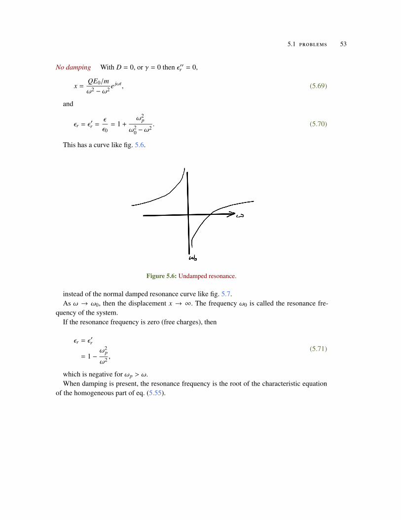
This has a curve like fig. 5.6.
Figure 5.6: Undamped resonance.
instead of the normal damped resonance curve like fig. 5.7.As ω → ω0, then the displacement x → ∞. The frequency ω0 is called the resonance fre-
quency of the system.If the resonance frequency is zero (free charges), then
(5.71)εr = ε′r
= 1 −ω2
p
ω2 ,
which is negative for ωp > ω.When damping is present, the resonance frequency is the root of the characteristic equation
of the homogeneous part of eq. (5.55).
54 poynting vector , and time harmonic (phasor) fields .
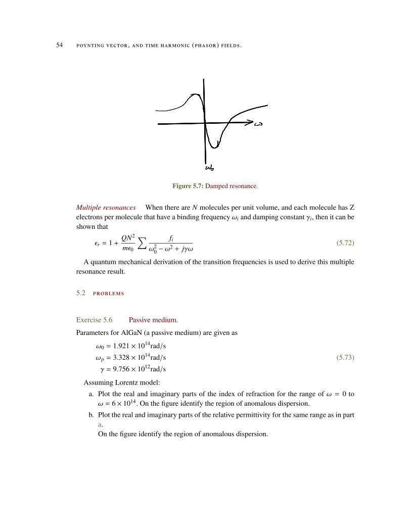
Figure 5.7: Damped resonance.
Multiple resonances When there are N molecules per unit volume, and each molecule has Zelectrons per molecule that have a binding frequency ωi and damping constant γi, then it can beshown that
(5.72)εr = 1 +QN2
mε0
∑ fiω2
0 − ω2 + jγω
A quantum mechanical derivation of the transition frequencies is used to derive this multipleresonance result.
5.2 problems
Exercise 5.6 Passive medium.
Parameters for AlGaN (a passive medium) are given as
(5.73)
ω0 = 1.921 × 10¹⁴rad/s
ωp = 3.328 × 10¹⁴rad/s
γ = 9.756 × 10¹²rad/s
Assuming Lorentz model:
a. Plot the real and imaginary parts of the index of refraction for the range of ω = 0 toω = 6 × 10¹⁴. On the figure identify the region of anomalous dispersion.
b. Plot the real and imaginary parts of the relative permittivity for the same range as in parta.On the figure identify the region of anomalous dispersion.
5.2 problems 55
Answer for Exercise 5.6
PROBLEM SET RELATED MATERIAL REDACTED IN THIS DOCUMENT.PLEASEFEEL FREE TO EMAIL ME FOR THE FULL VERSION IF YOU AREN’T TAKING ECE1228.
. .. .
.. . .
. .. . .
. .. .
. END-REDACTION
Exercise 5.7 Medium with multiple resonances.
Relative permittivity for a medium with multiple resonances is given by:
εr = 1 + χe = 1 +∑k=1
ωp,k
ω20,k −ω
2 + jγkω(5.74)
Moreover, the case of an active medium (i.e. medium with gain) can be modeled by allowingωp,k in above to become purely imaginary. Under these conditions, plot
(5.75)Re (n(ω)) − 1,
and
(5.76)Im (n(ω))
as a function of detuning frequency,
(5.77)ν =ω − ωc
2π,
for ammonia vapor (an active medium) where
(5.78)
ω0,1 = 2.4165825 × 10¹⁵rad/s
ω0,2 = 2.4166175 × 10¹⁵rad/s
ωp,k = ωp = 1010rad/s
γk = γ = 5 × 10⁹rad/s
(ω − ωc)/2π ∈ [−7, 7]GHz
ωc = 2.4166 × 10¹⁵rad/s
56 poynting vector , and time harmonic (phasor) fields .
Answer for Exercise 5.7PROBLEM SET RELATED MATERIAL REDACTED IN THIS DOCUMENT.PLEASE
FEEL FREE TO EMAIL ME FOR THE FULL VERSION IF YOU AREN’T TAKING ECE1228.. .
. ..
. . .. .
. . .. .
. .. END-REDACTION
Exercise 5.8 Susceptibility kernel.
a. Assuming that a medium is described by the time harmonic relationship D(x, ω) =
ε(ω)E(x,ω), show that the time domain relation between the electric flux density Dand the electric field E is given by,
(5.79)D(x, t) = ε0
(E(x, t) +
∫ ∞
−∞
G(τ)E(x, t − τ)dτ,)
where G(τ) is the susceptibility kernel given by
(5.80)G(τ) =1
2π
∫ ∞
−∞
(ε(ω)ε0− 1
)e− jωtdτ.
b. Show that(5.81)ε(−ω) = ε∗(ω)
c. Show that for ε(ω) = ε′(ω) + jε′′(ω), ε′(ω) is even and ε′′(ω) is odd.
Answer for Exercise 5.8PROBLEM SET RELATED MATERIAL REDACTED IN THIS DOCUMENT.PLEASE
FEEL FREE TO EMAIL ME FOR THE FULL VERSION IF YOU AREN’T TAKING ECE1228.. .
. ..
. . .. .
. . .. .
. .. END-REDACTION
6D RU I D M O D E L
Disclaimer. These notes are mostly a direct transcription of Prof. M. Mojahedi’s handwrittennotes on this topic, mostly skipped over in class. These become relevant because this is used inthe non-vacuum model of Maxwell’s equations.
A nice vector based derivation of these Druid model results can be found in [1]. The Meissnereffect is also discussed in that context.
Druid model In this section we will investigate the optical properties of free electrons, orwhat is commonly called free electron gas.
By free electron gas we mean electrons that do not experience the restoring force whichwe considered for bound charges in the case of Lorentz model. In particular, the resonancefrequency ω0 for free electrons is zero.
There are two typical cases of free electron systems
a Metals.
b Doped (n or p type) semiconductors.
For the moment we consider the case of metals.Free electrons are responsible for high reflectivity and good thermal conductivity of metals
up to optical frequencies. A model that can be used to describe the high reflectivity of metals isthe Drude model.
Plasma: A neutral gas of free electrons and heavy ions is called plasma. Examples of plasmaare metals and doped semiconductors, since these materials are a combination of free electronsand heavy ions which are, in sum, electrically neutral.
Drude-Lorentz model , (or Drude model for short): similar to the case of bound chargeswe already studied for free electron plasma, we can start with a harmonic oscillator model.However, in this case, since electrons are free, there is no restoring force (i.e. ω0 = 0. Recallthat in the spring mass model ω2
0 = S/m where S was the spring tension coefficient.With such a model the Lorentz model equation
(6.1)d2xdt2 + γ
dxdt
+ ω20x =
QE0
me jωt,
57
58 druid model
is reduced to
(6.2)d2xdt2 + γ
dxdt
=QE0
me jωt,
Again, assuming a solution of the form xp = x0e jωt for the particular solution and substitutingin eq. (6.2), we have
(6.3)x0(( jω)2 + γ( jω)
)=
QE0
m,
or
(6.4)x =QE/m−ω2 + jγω
,
Once more assuming identical particles that are not coupled and a linear isotropic mediumand using the fact that P = Np = NQx, and
(6.5)χe =|P|ε0|E|
,
we have
(6.6)χe =Q2N/mε0
−ω2 + jγω,
or with ω2p = Q2N/mε0,
(6.7)εr = 1 + χe
= 1 +ω2
p
−ω2 + jγω.
Plasma frequency, ωp, can be understood as the natural resonance frequency by which thefree electron gas (plasma) collectively (not individual electrons ) oscillates.
Note that if we neglect the last term, i.e., let γ = 0 then
(6.8)εr = 1 −ω2
p
ω2 .
From this it is clear that when ω < ωp, we have εr < 1 and n =√εr is purely imaginary, and
the wave attenuates inside the electron plasma.This means that for ω < ωp electromagnetic waves do not propagate a large distance inside
of metal. However, for ω > ωp the electron plasma (e.g. metal) is transparent. The latter iscalled ultraviolet transparency of metal, because for most metals ωp is in the ultraviolet part ofthe spectrum. For example,
druid model 59
• For Al
(6.9)ωp
2π= 3.82 × 10¹⁵Hz
=⇒ λp
= 79[nm],
• For Au
(6.10)ωp
2π= 5.9 × 10¹⁵Hz
=⇒ λp
= 138[nm],
Using eq. (6.8) one can calculate
(6.11)n =√εr,
and plot the reflectivity R at normal incidence
(6.12)R =
∣∣∣∣∣ n − 1n + 1
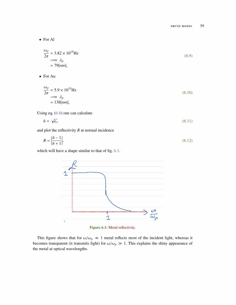
∣∣∣∣∣,which will have a shape similar to that of fig. 6.1.
Figure 6.1: Metal reflectivity.
This figure shows that for ω/ωp � 1 metal reflects most of the incident light, whereas itbecomes transparent (it transmits light) for ω/ωp � 1. This explains the shiny appearance ofthe metal at optical wavelengths.
60 druid model
The fact that plasma reflects EM waves below a ωp frequency can be used to transmit AMradio waves. The ionosphere can be viewed as a plasma gas due to free electrons generatedby cosmic radiation and ultraviolet light from the sun. The ωp for ionosphere plasma is ωp =
O(1MHz). Therefore AM signals modulated at frequencies below or in the range of a MHz willbe reflected from the ionosphere. But FM signals where the modulation frequency is greaterthan MHz will not be reflected, but will travel through the ionosphere and into space.
Conductivity
(6.13)
∇ ×H(r, ω) = σE(r, ω) + jωε0E(r, ω)
= jωε0
(1 +
σ
jωε0
)E(r, ω)
= jωε0
(1 −
jσωε0
)E(r, ω)
This complex factor is the relative permittivity
(6.14)εr = 1 −jσωε0
,
and is why we write
(6.15)ε(ω) = ε′(ω) − jε′′(ω)
6.1 problems
7WAV E E Q UAT I O N
Wave equation
(7.1)
∇ × E = −∂B
∂t−M
∇ ×H =∂D
∂t+ J
∇ ×B = ρmv
∇ ×D = ρev
Using an expansion of the triple cross product in terms of the Laplacian
(7.2)∇ × (∇ × f) = −∇ · (∇ ∧ f)= −∇2f + ∇ (∇ · f) ,
we can evaluate the cross products
(7.3)∇ × (∇ × E) = ∇ ×
(−∂B
∂t−M
)∇ × (∇ ×H) = ∇ ×
(∂D
∂t+ J
),
or
(7.4)−∇2E + ∇ (∇ · E) = −µ
∂
∂t∇ ×H − ∇ ×M
−∇2H + ∇ (∇ ·H) = ε∂
∂t(∇ × E) + ∇ × J,
or
(7.5)−∇2E +
1ε∇ρev = −µ
∂
∂t
(∂D
∂t+ J
)− ∇ ×M
−∇2H +1µ∇ρmv = ε
∂
∂t
(−∂B
∂t−M
)+ ∇ × J,
This decouples the equations for the electric and the magnetic fields
61
62 wave equation
(7.6)∇
2E = µε∂2E
∂t2 +1ε∇ρev + µ
∂J
∂t+ ∇ ×M
∇2H = εµ
∂2H
∂t2 +1µ∇ρmv + ε
∂M
∂t− ∇ × J,
Splitting the current between induced and bound (?) currents
J = Ji +Jc = Ji +σE, (7.7)
these become
(7.8)∇
2E = µε∂2E
∂t2 +1ε∇ρev + µσ
∂E
∂t+ ∇ ×M + µ
∂Ji
∂t
∇2H = εµ
∂2H
∂t2 +1µ∇ρmv + ε
∂M
∂t+ σµ
∂H
∂t+ σM − ∇ × Ji.
Time harmonic form Assuming time harmonic dependence X = Xe jωt, we find
(7.9)∇
2E =(−ω2µε + jωµσ
)E +
1ε∇ρev + ∇ ×M + jωµJi
∇2H =
(−ω2εµ + jωσµ
)H +
1µ∇ρmv + ( jωε + σ)M − ∇ × Ji.
For a lossy medium where ε = ε′ − jωε′′, the leading term factor is
(7.10)−ω2µε + jωµσ = −ω2µε′ + jωµ(σ + ωε′′
).
With the definition
γ2 = (α + jβ)2= −ω2µε′ + jωµ (σ +ωε′′) , (7.11)
the wave equations have the form
(7.12)∇
2E = γ2E +1ε∇ρev + ∇ ×M + jωµJi
∇2H = γ2H +
1µ∇ρmv + ( jωε + σ)M − ∇ × Ji.
Here
• α is the attenuation constant [Np/m]
• β is the phase velocity [rad/m]
• γ is the propagation constant [1/m]
We are usually interested in solutions in regions free of magnetic currents, induced electriccurrents, and free of any charge densities, in which case the wave equations are just
(7.13)∇
2E = γ2E∇
2H = γ2H.
7.1 problems 63
7.1 problems
Exercise 7.1 Meissner effect.
The constitutive relation for superconductors in weak magnetic fields can be macroscopicallycharacterized by the first London equation
(7.14)∂Jsup
∂t= αE,
and the second London equation
(7.15)∇ × Jsup = −α1B,
where Jsup stands for the superconducting current, α = nsq2/m and α1 ≈ α, with ns, m, andq denoting, respectively, the number density, the effective mass, and the charge of the Cooperpairs responsible for the superconductivity in a charged Boson fluid model.
a. From the first London equation, derive and equation for B = ∂B/∂t by using the staticMaxwell equation ∇ ×H = Jsup without the displacement current. Show that
(7.16)∇2B = µ0αB
b. From the second London equation and the Ampere’s law stated above derive an equationfor B.
c. What are the penetration depths in the part a and part b cases? Justify your answer.
Remark: from above analysis we see that both the current and magnetic field areconfined to a thin layer of the order of the penetration depth which is very small. Theexclusion of static magnetic field in a superconductor is known as the Meissner effectexperimentally discovered in 1933.
Answer for Exercise 7.1
PROBLEM SET RELATED MATERIAL REDACTED IN THIS DOCUMENT.PLEASEFEEL FREE TO EMAIL ME FOR THE FULL VERSION IF YOU AREN’T TAKING ECE1228.
. .. .
.. . .
. .. . .
. .. .
. END-REDACTION

8WAV E E Q UAT I O N S O L U T I O N S
In class, we walked through splitting up the wave equation into components, and separation ofvariables. I didn’t take notes on that.
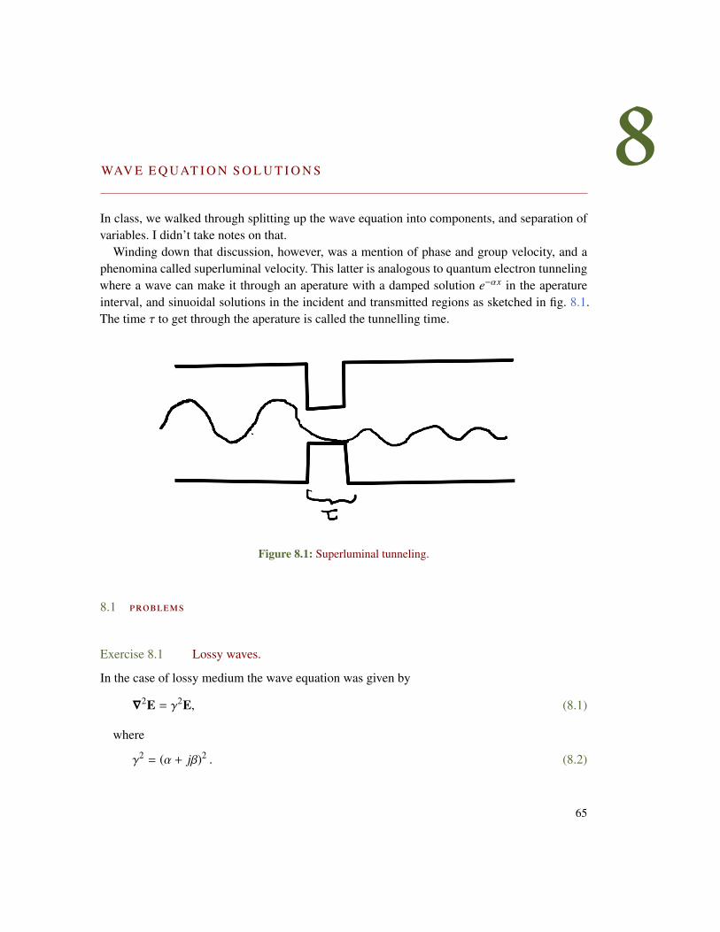
Winding down that discussion, however, was a mention of phase and group velocity, and aphenomina called superluminal velocity. This latter is analogous to quantum electron tunnelingwhere a wave can make it through an aperature with a damped solution e−αx in the aperatureinterval, and sinuoidal solutions in the incident and transmitted regions as sketched in fig. 8.1.The time τ to get through the aperature is called the tunnelling time.
Figure 8.1: Superluminal tunneling.
8.1 problems
Exercise 8.1 Lossy waves.
In the case of lossy medium the wave equation was given by
(8.1)∇2E = γ2E,
where
(8.2)γ2 = (α + jβ)2 .
65
66 wave equation solutions
Now consider a medium for which ε(ω) = ε′(ω) (i.e. ε′′(ω) = 0), σ = σ0 (i.e. ωτ ∼ 0 in theDrude model), and µ is a constant and real. For this case obtain the expression for α and β interms of ω, µ, ε′, σ0.Answer for Exercise 8.1
PROBLEM SET RELATED MATERIAL REDACTED IN THIS DOCUMENT.PLEASEFEEL FREE TO EMAIL ME FOR THE FULL VERSION IF YOU AREN’T TAKING ECE1228.
. .. .
.. . .
. .. . .
. .. .
. END-REDACTION
Exercise 8.2 Uniform plane wave.
Note: This seemed like a separate problem, and has been split out from the problem 2 asspecified in the original problem set handout.
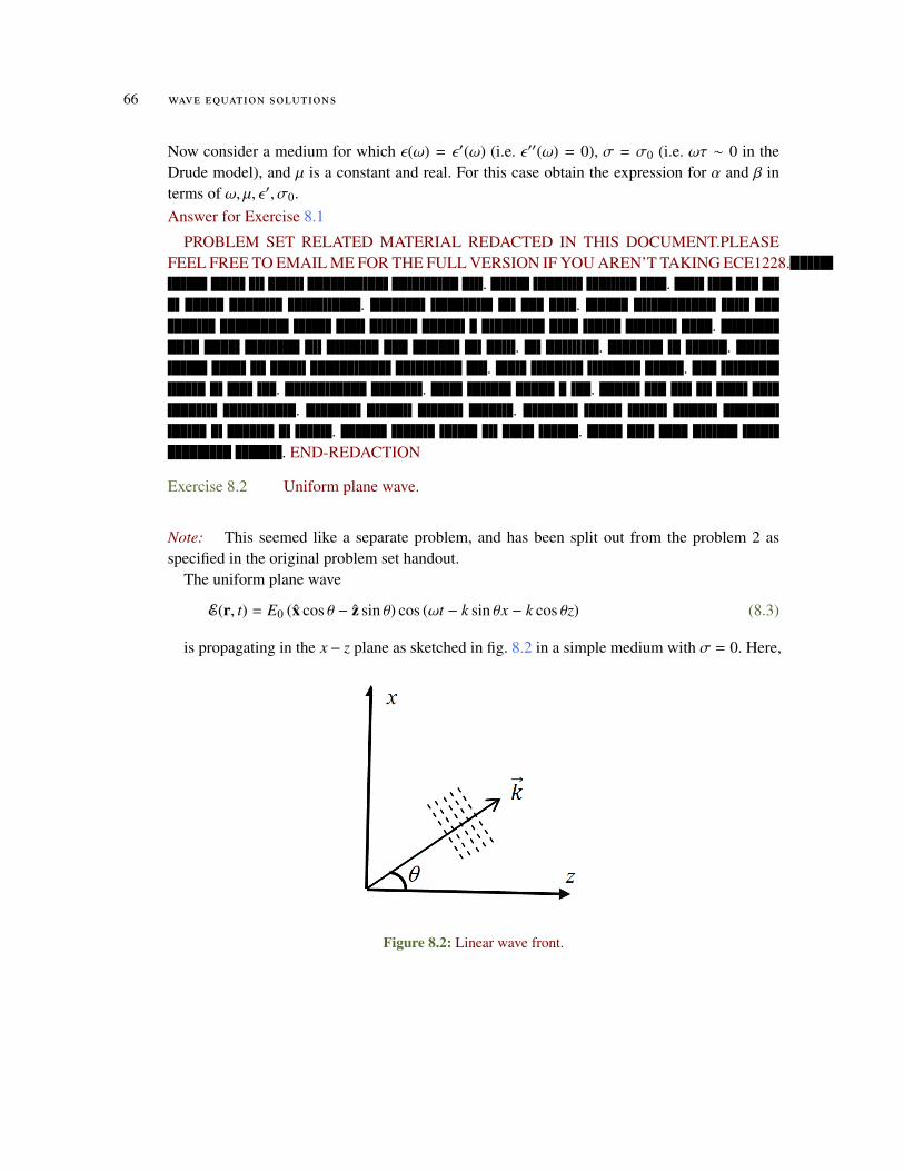
The uniform plane wave
(8.3)E(r, t) = E0 (x cos θ − z sin θ) cos (ωt − k sin θx − k cos θz)
is propagating in the x− z plane as sketched in fig. 8.2 in a simple medium with σ = 0. Here,
Figure 8.2: Linear wave front.

8.1 problems 67
E0 is a real constant and k is the propagation constant. Answer the following questions andshow all your work.
a. Determine the associated magnetic field H(r, t).b. Determine the time averaged Poynting vector, 〈S(r, t)〉.c. Determine the stored magnetic energy density, Wm(r, t).d. Determine the components of phase velocity vector vp along x and z.
Answer for Exercise 8.2
PROBLEM SET RELATED MATERIAL REDACTED IN THIS DOCUMENT.PLEASEFEEL FREE TO EMAIL ME FOR THE FULL VERSION IF YOU AREN’T TAKING ECE1228.
. .. .
.. . .
. .. . .
. .. .
. END-REDACTION

9WAV E E Q UAT I O N S O L U T I O N S
Cylindrical coordinates Seek a function
(9.1)E = Eρρ + Eφφ + Ezz
solving
(9.2)∇2E = −β2E.
One way to find the Laplacian in cylindrical coordinates is to use
(9.3)∇2E = ∇ (∇ · E) − ∇ × (∇ × E) ,
where
(9.4)∇ = ρ∂
∂ρ+φ
ρ
∂
∂φ+ z
∂
∂z.
It can be shown that:
(9.5)∇ · E =1ρ
∂
∂ρ
(ρEρ
)+
1ρ
∂Eφ
∂φ+∂Ez
∂z
and
(9.6)∇ × E = ρ
(1ρ∂φEz − ∂zEφ
)+ φ
(∂zEρ − ∂ρEz
)+ z
(1ρ∂ρ(ρEφ) −
1ρ∂φEρ
)This gives
(9.7)∇2ψ =
∂2ψ
∂ρ2 +1ρ
∂ψ
∂ρ+
1ρ2
∂2ψ
∂φ2 +∂2ψ
∂z2 .
and
(9.8)
∇2Eρ =
(−
Eρ
ρ2 −2ρ2
∂Eφ
∂φ
)∇
2Eφ =
(−
Eφ
ρ2 +2ρ2
∂Eρ
∂φ
)∇
2Ez = −β2Eφ.
This is explored in appendix F.
69
70 wave equation solutions
TEM: If we want to have a TEM mode it can be shown that we need an axial distributionmechanism, such as the core of a co-axial cable.
These are messy to solve in general, but we can solve the z-component without too muchpain
(9.9)∂2Ez
∂ρ2 +1ρ
∂Ez
∂ρ+
1ρ2
∂2Ez
∂φ2 +∂2Ez
∂z2 = −β2Ez
Solving this using separation of variables with
(9.10)Ez = R(ρ)P(φ)Z(z)
(9.11)1R
(R′′ +
1ρ
R′)
+1ρ2P
P′′ +Z′′
Z= −β2
Assuming for some constant βz that we have
(9.12)Z′′
Z= −β2
z ,
then
(9.13)1R
(ρ2R′′ + ρR′
)+
1P
P′′ + ρ2(β2 − β2
z
)= 0
Now assume that
(9.14)1P
P′′ = −m2,
and let β2 − β2z = β2
ρ, which leaves
(9.15)ρ2R′′ + ρR′ +(ρ2β2
ρ − m2)
R = 0.
This is the Bessel differential equation, with travelling wave solution
(9.16)R(ρ) = AH(1)m (βρρ) + BH(2)
m (βρρ),
and standing wave solutions
(9.17)R(ρ) = AJm(βρρ) + BYm(βρρ).
Here H(1)m ,H(2)
m are Hankel functions of the first and second kinds, and Jm,Ym are the Besselfunctions of the first and second kinds.
For P(φ)
(9.18)P′′ = −m2P
9.1 problems 71
Waves
• The field is a modification of space-time
• Mode is a particular field configuration for a given boundary value problem. Many fieldconfigurations can satisfy Maxwell equations (wave equation). These usually are referredto as modes. A mode is a self-consistent field distribution.
• In a TEM mode, E and H are every point in space are constrained in a local plane, inde-pendent of time. This plane is called the equiphase plane. In general equiphase planes arenot parallel at two different points along the trajectory of the wave.
9.1 problems
Exercise 9.1 Spherical wave solutions. (2016 ps7.)
Suppose under some circumstances (e.g. TEr or TMr modes), the partial differential equationsfor the wavefunction ψ can further be simplified to
(9.19)∇2ψ(r, θ, φ) = −β2ψ(r, θ, φ).
Using separation of variables
(9.20)ψ(r, θ, φ) = R(r)T (θ)P(φ),
find the differential equations governing the behaviour of R,T, P. Comment on the differentialequations found and their possible solutions.
Remarks : To have a more uniform answer, making it easier to mark the questions, use thefollowing conventions (notations) in your answer.
• Use −m2 as the constant of separation for the differential equation governing P(φ).
• Use −n(n + 1) as the constant of separation for the differential equation governing T (θ).
• Show that R(r) follows the differential equation associated with spherical Bessel or Han-kel functions.
Answer for Exercise 9.1
PROBLEM SET RELATED MATERIAL REDACTED IN THIS DOCUMENT.PLEASEFEEL FREE TO EMAIL ME FOR THE FULL VERSION IF YOU AREN’T TAKING ECE1228.
. .
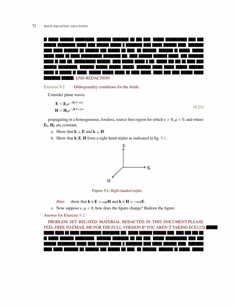
72 wave equation solutions
. ..
. . .. .
. . .. .
. .. END-REDACTION
Exercise 9.2 Orthogonality conditions for the fields.
Consider plane waves
(9.21)E = E0e− jk·r+ jωt
H = H0e− jk·r+ jωt
propagating in a homogeneous, lossless, source free region for which ε > 0, µ > 0, and whereE0,H0 are constant.
a. Show that k ⊥ E and k ⊥ H.
b. Show that k,E,H form a right hand triplet as indicated in fig. 9.1.
Figure 9.1: Right handed triplet.
Hint: show that k ×E = ωµH and k ×H = −ωεE.
c. Now suppose ε, µ < 0, how does the figure change? Redraw the figure.
Answer for Exercise 9.2
PROBLEM SET RELATED MATERIAL REDACTED IN THIS DOCUMENT.PLEASEFEEL FREE TO EMAIL ME FOR THE FULL VERSION IF YOU AREN’T TAKING ECE1228.
. .. .
.. . .

9.1 problems 73
. .. . .
. .. .
. END-REDACTION

10Q UA D RU P O L E E X PA N S I O N
Quadropole potential In Jackson [8] , is the following
(10.1)1
|x − x′|= 4π
∞∑l=0
l∑m=−l
12l + 1
(r′)l
rl+1 Y∗l,m(θ′, φ′)Yl,m(θ, φ),
where Yl,m are the spherical harmonics. It appears that this is actually just an orthogonalfunction expansion of the inverse distance (for a region outside of the charge density). Theproof of this in is scattered through chapter 3, dependent on a similar expansion in Legendrepolynomials, for an the azimuthally symmetric configuration.
It looks like quite a project to get comfortable enough with these special functions to fullyreproduce the proof of this identity. We are forced to play engineer, and assume the mathematicsworks out. If we do that and plug this inverse distance formula into the potential we have
(10.2)
φ(x) =1
4πε0
∫ρ(x′)d3x′
|x − x′|
=1
4πε0
∫ρ(x′)d3x′
4π ∞∑l=0
l∑m=−l
12l + 1
(r′)l
rl+1 Y∗l,m(θ′, φ′)Yl,m(θ, φ)
=
1ε0
∞∑l=0
l∑m=−l
12l + 1
∫ρ(x′)d3x′
((r′)l
rl+1 Y∗l,m(θ′, φ′)Yl,m(θ, φ))
=1ε0
∞∑l=0
l∑m=−l
12l + 1
(∫(r′)lρ(x′)Y∗l,m(θ′, φ′)d3x′
)Yl,m(θ, φ)
rl+1
The integral terms are called the coefficients of the multipole moments, denoted
(10.3)ql,m =
∫(r′)lρ(x′)Y∗l,m(θ′, φ′)d3x′,
The l = 0, 1, 2 terms are, respectively, called the monopole, dipole, and quadropole terms ofthe potential
(10.4)ρ(x) =1
4πε0
∞∑l=0
l∑m=−l
4π2l + 1
ql,mYl,m(θ, φ)
rl+1 .
Note the power of this expansion. Should we wish to compute the electric field, we have onlyto compute the qradient of the last (Yl,mr−l−1) portion (since ql,m is a constant).
75
76 quadrupole expansion
(10.5)
q1,1 = −
∫ √3
8πsin θ′e−iφ′r′ρ(x′)dV ′
= −
√3
8π
∫sin θ′
(cos φ′ − i sin φ′
)r′ρ(x′)dV ′
= −
√3
8π
(∫x′ρ(x′)dV ′ − i
∫y′ρ(x′)dV ′
)= −
√3
8π
(px − ipy
).
Here we’ve used
(10.6)
x′ = r′ sin θ′ cos φ′
y′ = r′ sin θ′ sin φ′
z′ = r′ cos θ′
and the Y11 representation
(10.7)
Y00 = −
√1
4π
Y11 = −
√3
8πsin θeiφ
Y10 =
√3
4πcos θ
Y22 = −14
√152π
sin2 θe2iφ
Y21 =12
√152π
sin θ cos θeiφ
Y20 =14
√5π
(3 cos2 θ − 1
)With the usual dipole moment expression
(10.8)p =
∫x′ρ(x′)d3x′,
and a quadropole moment defined as
(10.9)Qi, j =
∫ (3x′i x
′j − δi j(r′)2
)ρ(x′)d3x′,
the first order terms of the potential are now fully specified
(10.10)φ(x) =1
4πε0
q +p · xr3 +
12
∑i j
Qi jxix j
r5
.
quadrupole expansion 77
Explicit moment and quadrupole expansion We calculated the q1,1 coefficient of the elec-trostatic moment, as covered in [8] chapter 4. Let’s verify the rest, as well as the tensor sumformula for the quadrupole moment, and the spherical harmonic sum that yields the dipolemoment potential.
The quadrupole term of the potential was stated to be
(10.11)1
4πε0
4π5r3
2∑m =−2
∫(r′)2ρ(x′)Y∗lm(θ′, φ′)Ylm(θ, φ) =
12
∑i j
Qi jxix j
r5 ,
where
(10.12)Qi, j =
∫ (3x′i x
′j − δi j(r′)2
)ρ(x′)d3x′.
Let’s verify this. First note that
(10.13)Yl,m =
√2l + 1
4π(l − m)!(l + m)!
Pml (cos θ)eimφ,
and
(10.14)P−ml (x) = (−1)m (l − m)!
(l + m)!Pm
l (x),
so
(10.15)
Yl,−m =
√2l + 1
4π(l + m)!(l − m)!
P−ml (cos θ)e−imφ
= (−1)m
√2l + 1
4π(l − m)!(l + m)!
Pml (x)e−imφ
= (−1)mY∗l,m.
That means
(10.16)
ql,−m =
∫(r′)lρ(x′)Y∗l,−m(θ′, φ′)d3x′
= (−1)m∫
(r′)lρ(x′)Yl,m(θ′, φ′)d3x′
= (−1)mq∗lm.
In particular, for m , 0
78 quadrupole expansion
(10.17)(r′)lY∗l,m(θ′, φ′)rlYl,m(θ, φ) + (r′)lY∗l,−m(θ′, φ′)rlYl,−m(θ, φ)
= (r′)lY∗l,m(θ′, φ′)rlYl,m(θ, φ) + (r′)lYl,m(θ′, φ′)rlY∗l,m(θ, φ),
or
(r′)lY∗l,m(θ′, φ′)rlYl,m(θ, φ) + (r′)lY∗l,−m(θ′, φ′)rlYl,−m(θ, φ) = 2 Re((r′)lY∗l,m(θ′, φ′)rlYl,m(θ, φ)
).
(10.18)
To verify the quadrupole expansion formula in a compact way it is helpful to compute someintermediate results.
(10.19)rY1,1 = −r
√3
8πsin θeiφ
= −
√3
8π(x + iy),
(10.20)rY1,0 = r
√3
4πcos θ
=
√3
4πz,
(10.21)r2Y2,2 = −r2
√15
32πsin2 θe2iφ
= −
√15
32π(x + iy)2,
(10.22)r2Y2,1 = r2
√158π
sin θ cos θeiφ
=
√158π
z(x + iy),
(10.23)r2Y2,0 = r2
√5
16π
(3 cos2 θ − 1
)=
√5
16π
(3z2 − r2
).
quadrupole expansion 79
Given primed coordinates and integrating the conjugate of each of these with ρ(x′)dV ′, weobtain the qlm moment coefficients. Those are
(10.24)q11 = −
√3
8π
∫d3x′ρ(x′)(x − iy),
(10.25)q1,0 =
√3
4π
∫d3x′ρ(x′)z′,
(10.26)q2,2 = −
√15
32π
∫d3x′ρ(x′)(x′ − iy′)2,
(10.27)q2,1 =
√158π
∫d3x′ρ(x′)z′(x′ − iy′),
(10.28)q2,0 =
√5
16π
∫d3x′ρ(x′)
(3(z′)2 − (r′)2
).
For the potential we are interested in
(10.29)2 Re q11r2Y11(θ, φ) = 2
38π
∫d3x′ρ(x′) Re
((x′ − iy′)(x + iy)
)=
34π
∫d3x′ρ(x′)
(xx′ + yy′
),
(10.30)q1,0rY1,0(θ, φ) =3
4π
∫d3x′ρ(x′)z′z,
(10.31)
2 Re q22r2Y22(θ, φ) = 215
32π
∫d3x′ρ(x′) Re
((x′ − iy′)2(x + iy)2
)=
1516π
∫d3x′ρ(x′) Re
(((x′)2 − 2ix′y′ − (y′)2)(x2 + 2ixy − y2)
)=
1516π
∫d3x′ρ(x′)
(((x′)2 − (y′)2)(x2 − y2) + 4xx′yy′
),
(10.32)2 Re q21r2Y21(θ, φ) = 2
158π
∫d3x′ρ(x′)z Re
((x′ − iy′)(x + iy)
)=
154π
∫d3x′ρ(x′)z
(xx′ + yy′
),
80 quadrupole expansion
and
(10.33)q2,0r2Y20(θ, φ) =5
16π
∫d3x′ρ(x′)
(3(z′)2 − (r′)2
) (3z2 − r2
).
The dipole term of the potential is
(10.34)
14πε0
4π3r3
(3
4π
∫d3x′ρ(x′)
(xx′ + yy′
)+
34π
∫d3x′ρ(x′)z′z
)=
14πε0r3 x ·
∫d3x′ρ(x′)x′
=x · p
4πε0r3 ,
as obtained directly when a strict dipole approximation was used.Summing all the terms for the quadrupole gives
(10.35)
14πεr5
4π5(
1516π
∫d3x′ρ(x′)
(((x′)2 − (y′)2)(x2 − y2) + 4xx′yy′
)+
154π
∫d3x′ρ(x′)zz′ (xx′ + yy′)
+5
16π
∫d3x′ρ(x′)
(3(z′)2 − (r′)2
) (3z2 − r2
))
=1
4πεr5
∫d3x′ρ(x′)
14(3
(((x′)2 − (y′)2)(x2 − y2) + 4xx′yy′
)+ 12zz′ (xx′ + yy′)
+(3(z′)2 − (r′)2
) (3z2 − r2
)).
The portion in brackets is
(10.36)
3(((x′)2 − (y′)2)(x2 − y2) + 4xx′yy′
)+12zz′ (xx′ + yy′)
+(2(z′)2 − (x′)2 − (y′)2
) (2z2 − x2 − y2
)= x2
(3(x′)2 − 3(y′)2 −
(2(z′)2 − (x′)2 − (y′)2
))+y2
(−3(x′)2 + 3(y′)2 −
(2(z′)2 − (x′)2 − (y′)2
))+2z2
(2(z′)2 − (x′)2 − (y′)2
)+12xx′yy′ + xx′zz′ + yy′zz′
= 2x2(2(x′)2 − (y′)2 − (z′)2
)+2y2
(2(y′)2 − (x′)2 − (z′)2
)+2z2
(2(z′)2 − (x′)2 − (y′)2
)+12xx′yy′ + xx′zz′ + yy′zz′.
10.1 problems 81
The quadrupole sum can now be written as
(10.37)12
14πεr5
∫d3x′ρ(x′)(x2
(3(x′)2 − (r′)2
)+ y2
(3(y′)2 − (r′)2
)+ z2
(3(z′)2 − (r′)2
)+ 3
(xyx′y′ + yxy′x′ + xzx′z′ + zxz′x′ + yzy′z′ + zyz′y′
)),
which is precisely eq. (10.11), the quadrupole potential stated in the text and class notes.
10.1 problems
Exercise 10.1 Dipole multipole moment.
Following Jackson [8], derive the electric field contribution from the dipole terms of the multi-pole sum, but don’t skip the details.Answer for Exercise 10.1
PROBLEM SET RELATED MATERIAL REDACTED IN THIS DOCUMENT.PLEASEFEEL FREE TO EMAIL ME FOR THE FULL VERSION IF YOU AREN’T TAKING ECE1228.
. .. .
.. . .
. .. . .
. .. .
. END-REDACTION

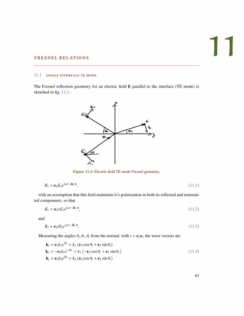
11F R E S N E L R E L AT I O N S
11.1 single interface te mode .
The Fresnel reflection geometry for an electric field E parallel to the interface (TE mode) issketched in fig. 11.1.
Figure 11.1: Electric field TE mode Fresnel geometry.
(11.1)Ei = e2Eie jωt− jki·x,
with an assumption that this field maintains it’s polarization in both its reflected and transmit-ted components, so that
(11.2)Er = e2rEie jωt− jkr ·x,
and
(11.3)Et = e2tEie jωt− jkt ·x,
Measuring the angles θi, θr, θt from the normal, with i = e3e1 the wave vectors are
(11.4)
ki = e3k1eiθi = k1 (e3 cos θi + e1 sin θi)
kr = −e3k1e−iθr = k1 (−e3 cos θr + e1 sin θr)
kt = e3k2eiθt = k2 (e3 cos θt + e1 sin θt)
83
84 fresnel relations
So the time harmonic electric fields are
(11.5)
Ei = e2Ei exp (− jk1 (z cos θi + x sin θi))
Er = e2rEi exp (− jk1 (−z cos θr + x sin θr))
Et = e2tEi exp (− jk2 (z cos θt + x sin θt)) .
The magnetic fields follow from Faraday’s law
(11.6)
H =1− jωµ
∇ × E
=1− jωµ
∇ × e2e− jk·x
=1
jωµe2 × ∇e− jk·x
= −1ωµ
e2 × ke− jk·x
=1ωµ
k × E
We have
(11.7)
ki × e2 = −e1 cos θi + e3 sin θi
kr × e2 = e1 cos θr + e3 sin θr
kt × e2 = −e1 cos θt + e3 sin θt,
Note that
(11.8)
kωµ
=k
kvµ
=
√µε
µ
=
√ε
µ
=1η.
so
(11.9)
Hi =Ei
η1(−e1 cos θi + e3 sin θi) exp (− jk1 (z cos θi + x sin θi))
Hr =rEi
η1(e1 cos θr + e3 sin θr) exp (− jk1 (−z cos θr + x sin θr))
Ht =tEi
η2(−e1 cos θt + e3 sin θt) exp (− jk2 (z cos θt + x sin θt)) .
11.1 single interface te mode . 85
The boundary conditions at z = 0 with n = e3 are
(11.10)
n ×H1 = n ×H2
n · B1 = n · B2
n × E1 = n × E2
n · D1 = n · D2,
At x = 0, this is
(11.11)
−1η1
cos θi +rη1
cos θr = −tη2
cos θt
k1 sin θi + k1r sin θr = k2t sin θt
1 + r = t
When t = 0 the latter two equations give Shell’s first law
sin θi = sin θr. (11.12)
Assuming this holds for all r, t we have
(11.13)k1 sin θi(1 + r) = k2t sin θt,
which is Snell’s second law in disguise
(11.14)k1 sin θi = k2 sin θt.
With
(11.15)
k =ω
v=ω
ccv
=ω
cn,
so eq. (11.14) takes the form
n1 sin θi = n2 sin θt. (11.16)
With
(11.17)k1z = k1 cos θi
k2z = k2 cos θt,
86 fresnel relations
we can solve for r, t by inverting
(11.18)
µ2k1z µ1k2z
−1 1
rt
=
µ2k1z
1
,which gives
(11.19)
rt =
1 −µ1k2z
1 µ2k1z
µ2k1z
1
,or
r =µ2k1z − µ1k2z
µ2k1z + µ1k2z
t =2µ2k1z
µ2k1z + µ1k2z
(11.20)
There are many ways that this can be written. Dividing both the numerator and denominatorby µ1µ2ω/c, and noting that k = ωn/c, we have
(11.21)
r =
n1µ1
cos θi −n2µ2
cos θtn1µ1
cos θi +n2µ2
cos θt
t =2 n1µ1
cos θin1µ1
cos θi +n2µ2
cos θt,
which checks against (4.32,4.33) in [6].
11.2 single interface tm mode .
For completeness, now consider the TM mode.Faraday’s law also can provide the electric field from the magnetic
(11.22)
k ×H = ηk ×(k × E
)= −ηk ·
(k ∧ E
)= −η
(E − k
(k · E
))= −ηE.
so
(11.23)E = ηH × k.
11.2 single interface tm mode . 87
So the magnetic and electric fields are
(11.24a)
Hi = e2Ei
η1exp (− jk1 (z cos θi + x sin θi))
Hr = e2rEi
η1exp (− jk1 (−z cos θr + x sin θr))
Ht = e2tEi
η2exp (− jk2 (z cos θt + x sin θt))
(11.24b)
Ei = −Ei (−e1 cos θi + e3 sin θi) exp (− jk1 (z cos θi + x sin θi))
Er = −rEi (e1 cos θr + e3 sin θr) exp (− jk1 (−z cos θr + x sin θr))
Et = −tEi (−e1 cos θt + e3 sin θt) exp (− jk2 (z cos θt + x sin θt)) .
Imposing the constraints eq. (11.10), at x = z = 0 we have
(11.25)
1η1
(1 + r) =tη2
cos θi − r cos θr = t cos θt
ε1 (sin θi + r sin θr) = tε2 sin θt
.
At t = 0, the first and third of these give θi = θr. Assuming this incident and reflection angleequality holds for all values of t, we have
(11.26)sin θi(1 + r) = t
ε2
ε1sin θt
sin θiη1
η2t =
or
(11.27)ε1η1 sin θi = ε2η2 sin θt.
This is also Snell’s second law eq. (11.16) in disguise, which can be seen by
(11.28)
ε1η1 = ε1
õ1
ε1
=√ε1µ1
=1v
=nc.
The remaining equations in matrix form are
88 fresnel relations
(11.29)
cos θi cos θt
−1 η1η2
rt
=
cos θi
1
,the inverse of which is
(11.30)
rt =
1η1η2
cos θi + cos θt
η1η2− cos θt
1 cos θi
cos θi
1
=
1η1η2
cos θi + cos θt
η1η2
cos θi − cos θt
2 cos θi
,or
r =η1 cos θi − η2 cos θt
η1 cos θi + η2 cos θt
t =2η2 cos θi
η1 cos θi + η2 cos θt.
(11.31)
Multiplication of the numerator and denominator by c/η1η2, noting that c/η = n/µ gives
(11.32)
r =
n2µ2
cos θi −n1µ1
cos θtn2µ2
cos θi +n1µ1
cos θt
t =2 n1µ1
cos θin2µ2
cos θi +n1µ1
cos θt
which checks against (4.38,4.39) in [6].
11.3 normal transmission and reflection through two interfaces .
The geometry of a two interface configuration is sketched in fig. 11.2.Given a normal incident ray with magnitude A, the respective forward and backwards rays in
each the mediums can be written as
I
(11.33)→ Ae− jk1zz
← Are jk1zz
II
(11.34)→ Ce− jk2zz
← De jk2zz
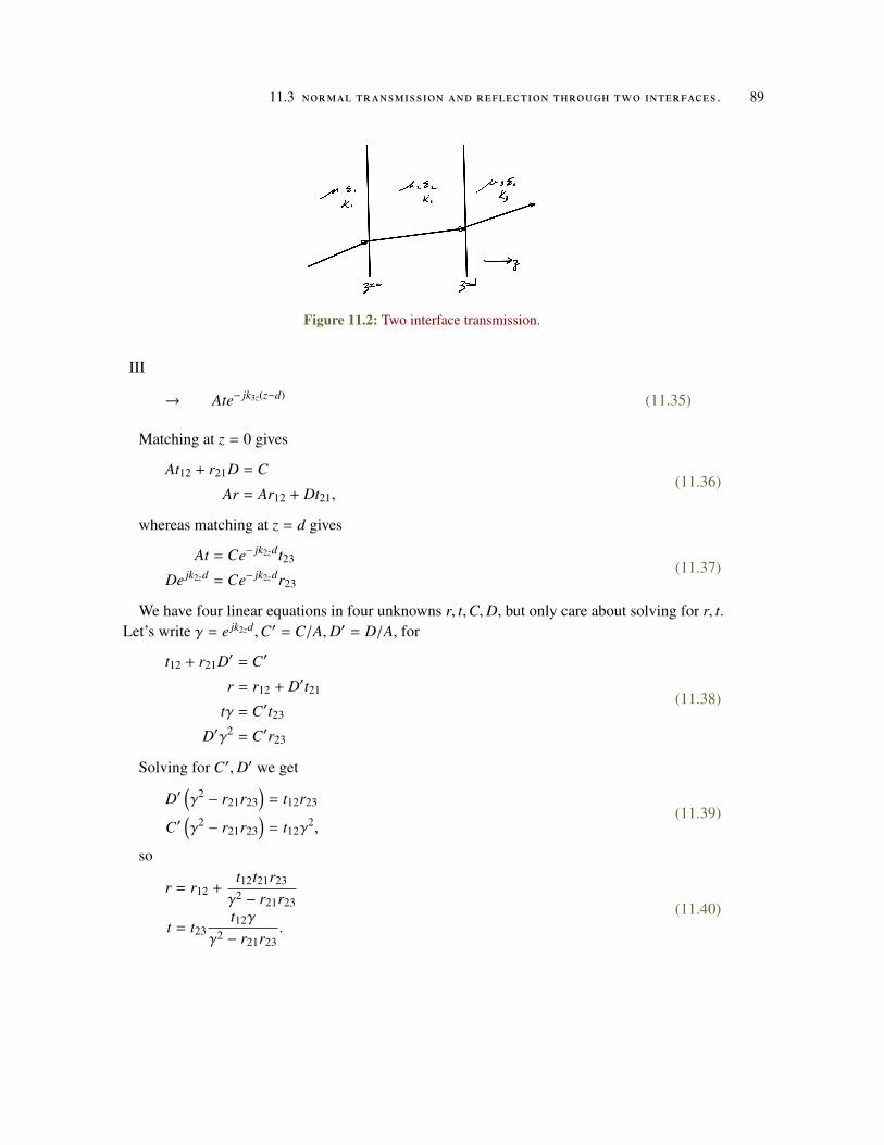
11.3 normal transmission and reflection through two interfaces . 89
Figure 11.2: Two interface transmission.
III
(11.35)→ Ate− jk3z(z−d)
Matching at z = 0 gives
(11.36)At12 + r21D = C
Ar = Ar12 + Dt21,
whereas matching at z = d gives
(11.37)At = Ce− jk2zdt23
De jk2zd = Ce− jk2zdr23
We have four linear equations in four unknowns r, t,C,D, but only care about solving for r, t.Let’s write γ = e jk2zd,C′ = C/A,D′ = D/A, for
(11.38)
t12 + r21D′ = C′
r = r12 + D′t21
tγ = C′t23
D′γ2 = C′r23
Solving for C′,D′ we get
(11.39)D′
(γ2 − r21r23
)= t12r23
C′(γ2 − r21r23
)= t12γ
2,
so
(11.40)r = r12 +
t12t21r23
γ2 − r21r23
t = t23t12γ
γ2 − r21r23.
90 fresnel relations
With φ = − jk2zd, or γ = e− jφ, we have
r = r12 +t12t21r23e2 jφ
1 − r21r23e2 jφ
t =t12t23e jφ
1 − r21r23e2 jφ .
(11.41)
A slab When the materials in region I, and III are equal, then r12 = r32. For a TE mode, wehave
r12 =µ2k1z − µ1k2z
µ2k1z + µ1k2z= −r21. (11.42)
so the reflection and transmission coefficients are
(11.43)
rTE = r12
1 − t12t21e2 jφ
1 − r221e2 jφ
tTE =
t12t21e jφ
1 − r221e2 jφ
.
It’s possible to produce a matched condition for which r12 = r21 = 0, by selecting
(11.44)
0 = µ2k1z − µ1k2z
= µ1µ2
(1µ1
k1z −1µ2
k2z
)= µ1µ2ω
(1
v1µ1θ1 −
1v2µ2
θ2
),
or
(11.45)1η1
cos θ1 =1η2
cos θ2,
so the matching condition for normal incidence is just
(11.46)η1 = η2.
Given this matched condition, the transmission coefficient for the 1,2 interface is
(11.47)
t12 =2µ2k1z
µ2k1z + µ1k2z
=2µ2k1z
2µ2k1z= 1,
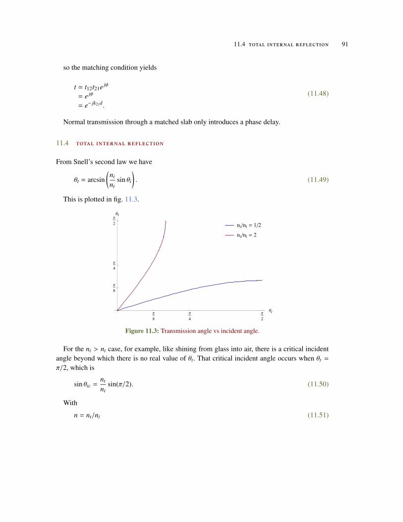
11.4 total internal reflection 91
so the matching condition yields
(11.48)t = t12t21e jφ
= e jφ
= e− jk2zd.
Normal transmission through a matched slab only introduces a phase delay.
11.4 total internal reflection
From Snell’s second law we have
(11.49)θt = arcsin(ni
ntsin θi
).
This is plotted in fig. 11.3.
Figure 11.3: Transmission angle vs incident angle.
For the ni > nt case, for example, like shining from glass into air, there is a critical incidentangle beyond which there is no real value of θt. That critical incident angle occurs when θt =
π/2, which is
(11.50)sin θic =nt
nisin(π/2).
With
(11.51)n = nt/ni
92 fresnel relations
the critical angle is
(11.52)θic = arcsin n.
Note that Snell’s law can also be expressed in terms of this critical angle, allowing for thesolution of the transmission angle in a convenient way
(11.53)sin θi =
nt
nisin θt
= n sin θt
= sin θic sin θt,
or
(11.54)sin θt =sin θi
sin θic.
Still for ni > nt, at angles past θic, the transmitted wave angle becomes complex as outlinedin [8] , namely
(11.55)
cos2 θt = 1 − sin2 θt
= 1 −sin2 θi
sin2 θic
= −
(sin2 θi
sin2 θic− 1
),
or
(11.56)cos θt = j
√sin2 θi
sin2 θic− 1.
Following the convention that puts the normal propagation direction along z, and the interfacealong x, the wave vector direction is
(11.57)kt = e3ee31θt
= e3 cos θt + e1 sin θt.
The phase factor for the transmitted field is
(11.58)
exp ( jωt ± jkt · x) = exp(
jωt ± jkkt · x)
= exp ( jωt ± jk (z cos θt + x sin θt))
= exp
jωt ± jk
z j
√sin2 θi
sin2 θic− 1 + x
sin θi
sin θic
= exp
jωt ± k
jxsin θi
sin θic− z
√sin2 θi
sin2 θic− 1
.

11.5 brewster’s angle 93
The propagation is channelled along the x axis, but the propagation into the second mediumdecays exponentially (or unphysically grows exponentially), only getting into the surface asmall amount.
What is the average power transmission into the medium? We are interested in the timeaverage of the normal component of the Poynting vector S · n.
(11.59)
S =12
E ×H∗
=12
E ×(1η
kt × E∗)
= −12η
E ·(kt ∧ E∗
)= −
12η
((E · kt)E∗ − ktE · E∗
)=
12η
kt|E|2.
(11.60)
kt · n = (e3 cos θt + e1 sin θt) · e3
= cos θt
= j
√sin2 θi
sin2 θic− 1.
Note that this is purely imaginary. The time average real power transmission is
(11.61)〈S · n〉 = Re
j
√sin2 θi
sin2 θic− 1
12η|E|2
= 0.
There is no power transmission into the second medium at or past the critical angle for totalinternal reflection.
11.5 brewster’s angle
Brewster’s angle is the angle for which there the amplitude of the reflected component of thefield is zero. Recall that when the electric field is parallel(perpendicular) to the plane of inci-dence, the reflection amplitude ([6] eq. 4.38)
(11.62)r ‖ =
ntµt
cos θi −niµi
cos θtntµt
cos θi +niµi
cos θt
94 fresnel relations
(11.63)r ⊥ =
niµi
cos θi −ntµt
cos θtniµi
cos θi +ntµt
cos θt
There are limited conditions for which r⊥ is zero, at least for µi = µt. Using Snell’s secondlaw ni sin θi = nt sin θt, that zero is found at
(11.64)
ni cos θi = nt cos θt
= nt
√1 − sin2 θt
= nt
√1 −
n2i
n2t
sin2 θi,
or
(11.65)n2
i
n2t
cos2 θi = 1 −n2
i
n2t
sin2 θi,
or
(11.66)n2
i
n2t
(cos2 θi + sin2 θi
)= 1.
This has solutions only when ni = ±nt. The ni = nt case is of no interest, since that isjust propagation, so naturally there is no reflection. The ni = −nt case is possible with thetransmission into a negative index of refraction material that is matched in absolute magnitudewith the index of refraction in the incident medium.
There are richer solutions for the r‖ zero. Again considering µ1 = µ2 those occur when
(11.67)
nt cos θi = ni cos θt
= ni
√1 −
n2i
n2t
sin2 θi
= ni
√1 −
n2i
n2t
sin2 θi
Let n = nt/ni, and square both sides. This gives
(11.68)n2 cos2 θi = 1 −
1n2 sin2 θi
= 1 −1n2 (1 − cos2 θi),
or
11.6 problems 95
(11.69)cos2 θi
(n2 +
1n2
)= 1 −
1n2 ,
or
(11.70)
cos2 θi =1 − 1
n2
n2 − 1n2
=n2 − 1n4 − 1
=n2 − 1
(n2 − 1)(n2 + 1)
=1
n2 + 1.
We also have
(11.71)sin2 θi = 1 −
1n2 + 1
=n2
n2 + 1,
so
(11.72)tan2 θi = n2,
and
(11.73)tan θiB = ±n,
For normal media where ni > 0, nt > 0, only the positive solution is physically relevant,which is
θiB = arctan(nt
ni
). (11.74)
11.6 problems
Exercise 11.1 Fresnel sum and difference formulas. ([6] pr. 4.39)
Given a µ1 = µ2 constraint, show that the Fresnel equations have the form
(11.75a)rTE =sin(θt − θi)sin(θt + θi)
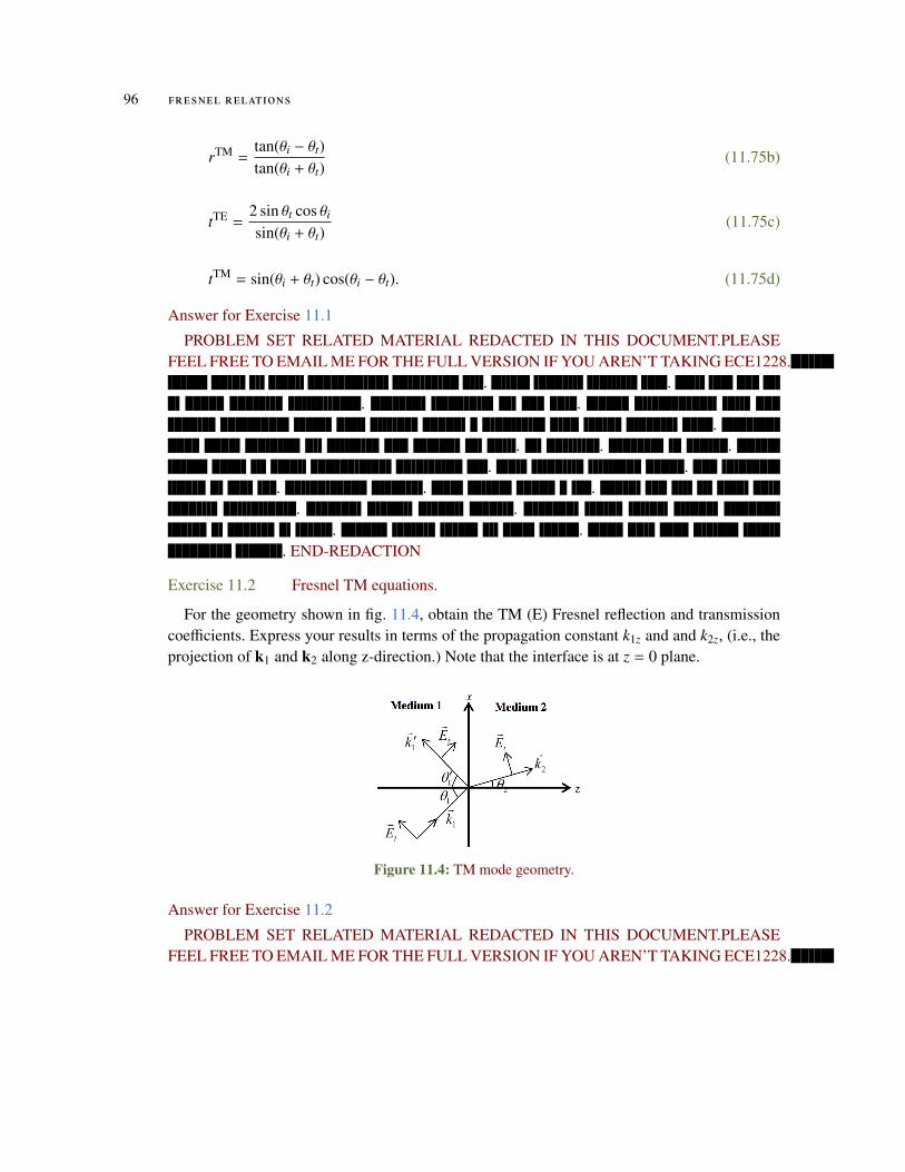
96 fresnel relations
(11.75b)rTM =tan(θi − θt)tan(θi + θt)
(11.75c)tTE =2 sin θt cos θi
sin(θi + θt)
(11.75d)tTM = sin(θi + θt) cos(θi − θt).
Answer for Exercise 11.1
PROBLEM SET RELATED MATERIAL REDACTED IN THIS DOCUMENT.PLEASEFEEL FREE TO EMAIL ME FOR THE FULL VERSION IF YOU AREN’T TAKING ECE1228.
. .. .
.. . .
. .. . .
. .. .
. END-REDACTION
Exercise 11.2 Fresnel TM equations.
For the geometry shown in fig. 11.4, obtain the TM (E) Fresnel reflection and transmissioncoefficients. Express your results in terms of the propagation constant k1z and and k2z, (i.e., theprojection of k1 and k2 along z-direction.) Note that the interface is at z = 0 plane.
Figure 11.4: TM mode geometry.
Answer for Exercise 11.2
PROBLEM SET RELATED MATERIAL REDACTED IN THIS DOCUMENT.PLEASEFEEL FREE TO EMAIL ME FOR THE FULL VERSION IF YOU AREN’T TAKING ECE1228.
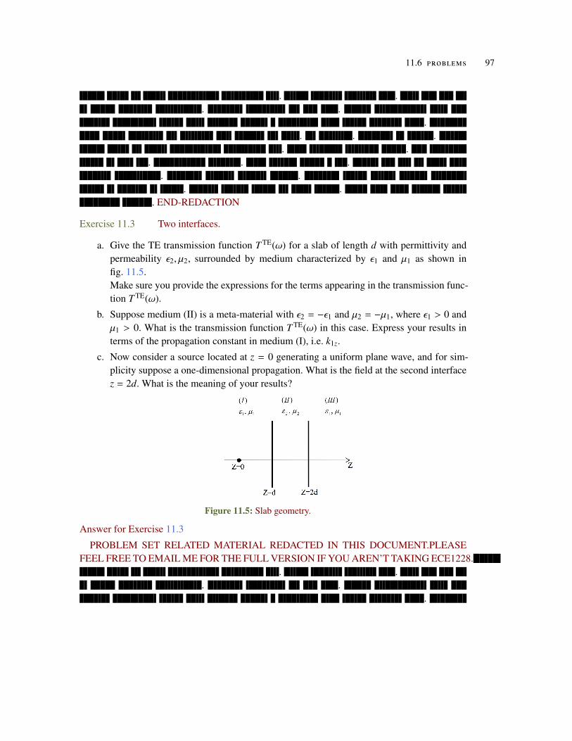
11.6 problems 97
. .. .
.. . .
. .. . .
. .. .
. END-REDACTION
Exercise 11.3 Two interfaces.
a. Give the TE transmission function T TE(ω) for a slab of length d with permittivity andpermeability ε2, µ2, surrounded by medium characterized by ε1 and µ1 as shown infig. 11.5.Make sure you provide the expressions for the terms appearing in the transmission func-tion T TE(ω).
b. Suppose medium (II) is a meta-material with ε2 = −ε1 and µ2 = −µ1, where ε1 > 0 andµ1 > 0. What is the transmission function T TE(ω) in this case. Express your results interms of the propagation constant in medium (I), i.e. k1z.
c. Now consider a source located at z = 0 generating a uniform plane wave, and for sim-plicity suppose a one-dimensional propagation. What is the field at the second interfacez = 2d. What is the meaning of your results?
Figure 11.5: Slab geometry.
Answer for Exercise 11.3
PROBLEM SET RELATED MATERIAL REDACTED IN THIS DOCUMENT.PLEASEFEEL FREE TO EMAIL ME FOR THE FULL VERSION IF YOU AREN’T TAKING ECE1228.
. .. .
.
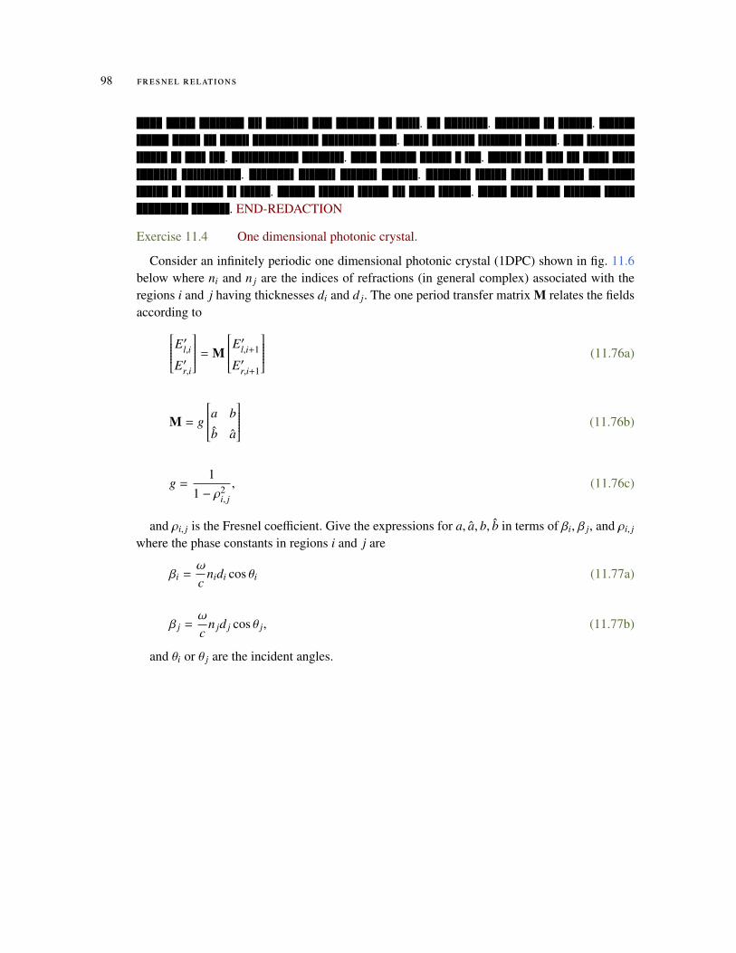
98 fresnel relations
. . .. .
. . .. .
. .. END-REDACTION
Exercise 11.4 One dimensional photonic crystal.
Consider an infinitely periodic one dimensional photonic crystal (1DPC) shown in fig. 11.6below where ni and n j are the indices of refractions (in general complex) associated with theregions i and j having thicknesses di and d j. The one period transfer matrix M relates the fieldsaccording to
(11.76a)
E′l,iE′r,i
= M
E′l,i+1
E′r,i+1
(11.76b)M = g
a b
b a
(11.76c)g =
11 − ρ2
i, j
,
and ρi, j is the Fresnel coefficient. Give the expressions for a, a, b, b in terms of βi, β j, and ρi, j
where the phase constants in regions i and j are
(11.77a)βi =ω
cnidi cos θi
(11.77b)β j =ω
cn jd j cos θ j,
and θi or θ j are the incident angles.
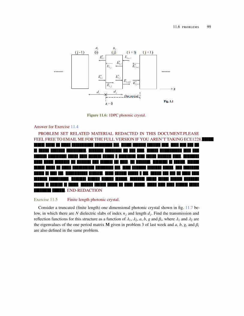
11.6 problems 99
Figure 11.6: 1DPC photonic crystal.
Answer for Exercise 11.4
PROBLEM SET RELATED MATERIAL REDACTED IN THIS DOCUMENT.PLEASEFEEL FREE TO EMAIL ME FOR THE FULL VERSION IF YOU AREN’T TAKING ECE1228.
. .. .
.. . .
. .. . .
. .. .
. END-REDACTION
Exercise 11.5 Finite length photonic crystal.
Consider a truncated (finite length) one dimensional photonic crystal shown in fig. 11.7 be-low, in which there are N dielectric slabs of index n j and length d j. Find the transmission andreflection functions for this structure as a function of λ1, λ2, a, b, g and βi, where λ1 and λ2 arethe eigenvalues of the one period matrix M given in problem 3 of last week and a, b, g, and βi
are also defined in the same problem.
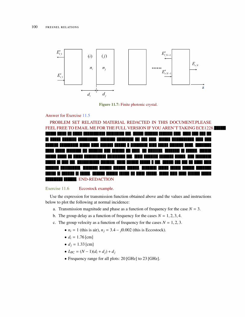
100 fresnel relations
Figure 11.7: Finite photonic crystal.
Answer for Exercise 11.5
PROBLEM SET RELATED MATERIAL REDACTED IN THIS DOCUMENT.PLEASEFEEL FREE TO EMAIL ME FOR THE FULL VERSION IF YOU AREN’T TAKING ECE1228.
. .. .
.. . .
. .. . .
. .. .
. END-REDACTION
Exercise 11.6 Eccostock example.
Use the expression for transmission function obtained above and the values and instructionsbelow to plot the following at normal incidence:
a. Transmission magnitude and phase as a function of frequency for the case N = 3.
b. The group delay as a function of frequency for the cases N = 1, 2, 3, 4.
c. The group velocity as a function of frequency for the cases N = 1, 2, 3.
• ni = 1 (this is air), n j = 3.4 − j0.002 (this is Eccostock).
• di = 1.76 [cm]
• d j = 1.33 [cm]
• LPC = (N − 1)(di + d j) + d j
• Frequency range for all plots: 20 [GHz] to 23 [GHz].
11.6 problems 101
• Use linear scale for transmission magnitude (not dB) and express the transmissionphase in Degrees.
• Plot the group delay in nanosecond.
• Plot the group velocity in units of Vg/c, where c is the speed of light in vacuum.
Answer for Exercise 11.6
PROBLEM SET RELATED MATERIAL REDACTED IN THIS DOCUMENT.PLEASEFEEL FREE TO EMAIL ME FOR THE FULL VERSION IF YOU AREN’T TAKING ECE1228.
. .. .
.. . .
. .. . .
. .. .
. END-REDACTION

12G AU G E F R E E D O M .
12.1 problems
Exercise 12.1 Potentials under different gauges.
Using the non-existence of magnetic monopole and Faraday’s law
a. Define the vector and scalar vector potentials A(r, t) and V(r, t).b. Let J = Ji + Jc be the current [A/m] and ρ be the charge [C/m] densities. Assum-
ing a simple medium and Lorentz gauge, derive the decoupled non-homogeneous waveequations for A(r, t) and V(r, t).
c. Replace the Lorentz gauge of part b with the Coulomb gauge, and obtain the non-homogeneous differential equations for A(r, t) and V(r, t).
d. What fundamental theorem allows us to use different gauges in part b and part b ?(Justify your answer.)
Note: From the problem’s statement, it should be clear that I want the results for theinstantaneous fields and not in the form of time harmonic fields.
Answer for Exercise 12.1
PROBLEM SET RELATED MATERIAL REDACTED IN THIS DOCUMENT.PLEASEFEEL FREE TO EMAIL ME FOR THE FULL VERSION IF YOU AREN’T TAKING ECE1228.
. .. .
.. . .
. .. . .
. .. .
. END-REDACTION
103


Part II
A P P E N D I C E S

AU S E F U L F O R M U L A S A N D R E V I E W
∇′ 1R
=r
R2 = −∇1R
(A.1)
∇R = r =RR
(A.2)
∇ f (R) = r∂ f∂R
(A.3)
−∇2 1R
= 4πδ(R) (A.4)
(A.5)∇ × f =
∣∣∣∣∣∣∣∣∣∣∣e1 e2 e3
∂/∂x ∂/∂y ∂/∂z
fx fy fz
∣∣∣∣∣∣∣∣∣∣∣ .
∇ × (∇ ×A) = ∇ (∇ ·A) −∇2A. (A.6)
Proofs. This result was used in ps1 problem 3,5, and 6.
(A.7)
∇ × (∇ × A) = εabcea∂b (εrster∂sAt)c= εabcea∂bεcst∂sAt
= δ[st]ab ea∂b∂sAt
= ea∂b (∂aAb − ∂bAa)= ∇ (∇ · A) − ∇2A.
107
108 useful formulas and review
Cylindrical coordinates
(A.8)
ρ = e1ee1e2φ
φ = e2ee1e2φ
z = e3
(A.9)∂φρ = φ
∂φφ = −ρ
(A.10)∇ = ρ∂ρ +φ
ρ∂φ + z∂z
(A.11)∇ · A =1ρ∂ρ(ρAρ) +
1ρ∂φAφ + ∂zAz
(A.12)∇ × A = ρ
(1ρ∂φAz − ∂zAφ
)+ φ
(∂zAρ − ∂ρAz
)+
1ρ
z(∂ρ(ρAφ) − ∂φAρ
)
(A.13)∇2 =
1ρ
∂
∂ρ
(ρ∂
∂ρ
)+
1ρ2
∂2
∂φ2 +∂2
∂z2
Spherical coordinates
(A.14)
r = e1eiφ sin θ + e3 cos θ
θ = cos θe1eiφ − sin θe3
φ = e2eiφ
(A.15)
∂θr = θ
∂φr = S θφ
∂θθ = −r∂φθ = Cθφ
∂θφ = 0
∂φφ = −rS θ − θCθ.
(A.16)∇ = r∂
∂r+θ
r∂
∂θ+
φ
r sin θ∂
∂φ.
useful formulas and review 109
(A.17)∇ · A =1r2 ∂r(r2Ar) +
1rS θ
∂θ(S θAθ) +1
rS θ∂φAφ.
(A.18)∇ ×A = r(
1rS θ
∂θ(S θAφ) −1
rS θ∂φAθ
)+ θ
(1
rS θ∂φAr −
1r∂r(rAφ)
)+ φ
(1r∂r(rAθ) −
1r∂θAr
)
(A.19)∇2ψ =
1r2
∂
∂r
(r2 ∂ψ
∂r
)+
1r2 sin θ
∂
∂θ
(sin θ
∂ψ
∂θ
)+
1r2 sin2 θ
∂2ψ
∂φ2
Vector calculus. Enumerate various vc theorems (divergence, curl, the cross product versionused in the BC problem, ...)
Normal and tangential decomposition. The decomposition of ?? can be derived easily usingGeometric Algebra
(A.20)A = n2A= n(n · A) + n(n ∧ A)
The last dot product can be expanded as a grade one (vector) selection
(A.21)
n(n ∧ A) = 〈n(n ∧ A)〉1= 〈nI(n × A)〉1= I2n × (n × A)= −n × (n × A),
so the decomposition of a vector A in terms of its normal and tangential projections is
(A.22)A = n(n · A) − n × (n × A).
I’m not sure how to naturally determine this relationship using traditional vector algebra.However, it can be verified by expanding the triple cross product in coordinates using tensorcontraction formalism
(A.23)
−n × (n × A) = −εxyzexny (n × A)z= −εxyzexnyεzrsnrAs
= −δ[rs]xy exnynrAs
= −exny(nxAy − nyAx
)= −n(n · A) + (n · n)A= A − n(n · A).
This last statement illustrates the geometry of this decomposition, showing that the tangentialprojection (or normal rejection) of a vector is really just the vector minus its normal projection.

BG E O M E T R I C A L G E B R A
Having used Geometric Algebra in a couple problems, it is justified to provide an overview.Further details can be found in [4], [3], [9], and [7].
Geometric Algebra defines a non-commutative, associative vector product
abc = (ab)c = a(bc), (B.1)
where the square of a vector equals the squared vector magnitude
(B.2)a2 = |a|2,
In Euclidean spaces such a squared vector is always positive, but that is not necessarily thecase in the mixed signature spaces used in special relativity.
There are a number of consequences of these two simple vector multiplication rules.
• Squared unit vectors have a unit magnitude (up to a sign). In a Euclidean space such aproduct is always positive
(B.3)(e1)2 = 1.
• Products of perpendicular vectors anticommute.
(B.4)2 = (e1 + e2)2
= (e1 + e2)(e1 + e2)= e2
1 + e2e1 + e1e2 + e22
= 2 + e2e1 + e1e2.
A product of two perpendicular vectors is called a bivector, and can be used to repre-sent an oriented plane. The last line above shows an example of a scalar and bivectorsum, called a multivector. In general Geometric Algebra allows sums of scalars, vectors,bivectors, and higher degree analogues (grades) be summed.
Comparison of the RHS and LHS of eq. (B.4) shows that we must have
(B.5)e2e1 = −e1e2.
111
112 geometric algebra
It is true in general that the product of two perpendicular vectors anticommutes. When,as above, such a product is a product of two orthonormal vectors, it behaves like a non-commutative imaginary quantity, as it has an imaginary square in Euclidean spaces
(B.6)
(e1e2)2 = (e1e2)(e1e2)= e1(e2e1)e2
= −e1(e1e2)e2
= −(e1e1)(e2e2)= −1.
Such “imaginary” (unit bivectors) have important applications describing rotations inEuclidean spaces, and boosts in Minkowski spaces.
• The product of three perpendicular vectors, such as
(B.7)I = e1e2e3,
is called a trivector. In R3, the product of three orthonormal vectors is called a pseu-doscalar for the space, and can represent an oriented volume element. The quantity Iabove is the typical orientation picked for the R3 unit pseudoscalar. This quantity alsohas characteristics of an imaginary number
(B.8)
I2 = (e1e2e3)(e1e2e3)= e1e2(e3e1)e2e3
= −e1e2e1e3e2e3
= −e1(e2e1)(e3e2)e3
= −e1(e1e2)(e2e3)e3
= −e21e2
2e23
= −1.
• The product of two vectors in R3 can be expressed as the sum of a symmetric scalarproduct and antisymmetric bivector product
(B.9)
ab =
n∑i, j=1
eie jaib j
=
n∑i=1
e2i aibi +
∑0<i, j≤n
eie jaib j
=
n∑i=1
aibi +∑
0<i< j≤n
eie j(aib j − a jbi).
geometric algebra 113
The first (symmetric) term is clearly the dot product. The antisymmetric term is desig-nated the wedge product. In general these are written
(B.10)ab = a · b + a ∧ b,
where
(B.11)a · b ≡
12(ab + ba)
a ∧ b ≡12(ab − ba) ,
The coordinate expansion of both can be seen above, but in R3 the wedge can also bewritten
a∧ b = e1e2e3(a × b) = I(a × b). (B.12)
This allows for an handy dot plus cross product expansion of the vector product
(B.13)ab = a · b + I(a × b).
This result should be familiar to the student of quantum spin states where one writes
(B.14)(σ · a)(σ · b) = (a · b) + i(a × b) · σ.
This correspondence is because the Pauli spin basis is a specific matrix representation ofa Geometric Algebra, satisfying the same commutator and anticommutator relationships.A number of other algebra structures, such as complex numbers, and quaterions can alsobe modelled as Geometric Algebra elements.
• It is often useful to utilize the grade selection operator 〈M〉n and scalar grade selectionoperator 〈M〉 = 〈M〉0 to select the scalar, vector, bivector, trivector, or higher grade alge-braic elements. For example, operating on vectors a,b, c, we have
(B.15)
〈ab〉 = a · b〈abc〉1 = a(b · c) + a · (b ∧ c)
= a(b · c) + (a · b)c − (a · c)b〈ab〉2 = a ∧ b〈abc〉3 = a ∧ b ∧ c.
114 geometric algebra
Note that the wedge product of any number of vectors such as a ∧ b ∧ c is associativeand can be expressed in terms of the complete antisymmetrization of the product of thosevectors. A consequence of that is the fact a wedge product that includes any colinearvectors in the product is zero.
Example B.1: Helmholz equations.
As an example of the power of eq. (B.13), consider the following Helmholtz equationderivation (wave equations for the electric and magnetic fields in the frequency domain.)
Application of eq. (B.13) to Maxwell equations in the frequency domain for source freesimple media gives
(B.16a)∇E = − jωIB
(B.16b)∇IB = − jωµεE.
These equations use the engineering (not physics) sign convention for the phasors wherethe time domain fields are of the form E(r, t) = Re(Ee jωt).
Operation with the gradient from the left produces the Helmholtz equation for each ofthe fields using nothing more than multiplication and simple substitution
(B.17a)∇2E = −µεω2E
(B.17b)∇2IB = −µεω2IB.
There was no reason to go through the headache of looking up or deriving the expansionof ∇ × (∇ × A) as is required with the traditional vector algebra demonstration of theseidentities.
Observe that the usual Helmholtz equation for B doesn’t have a pseudoscalar factor. Thatresult can be obtained by just cancelling the factors I since the R3 Euclidean pseudoscalarcommutes with all grades (this isn’t the case in R2 nor in Minkowski spaces.)
Example B.2: Factoring the Laplacian.
There are various ways to demonstrate the identity
(B.18)∇ × (∇ × A) = ∇ (∇ · A) − ∇2A,
geometric algebra 115
such as the use of (somewhat obscure) tensor contraction techniques. We can also dothis with Geometric Algebra (using a different set of obscure techniques) by factoring theLaplacian action on a vector
(B.19)
∇2A = ∇(∇A)
= ∇(∇ · A + ∇ ∧ A)= ∇(∇ · A) + ∇ · (∇ ∧ A) +(((((
∇ ∧ ∇ ∧ A= ∇(∇ · A) + ∇ · (∇ ∧ A).
Should we wish to express the last term using cross products, a grade one selectionoperation can be used
(B.20)
∇ · (∇ ∧ A) = 〈∇(∇ ∧ A)〉1= 〈∇I(∇ × A)〉1= 〈I∇ ∧ (∇ × A)〉1=
⟨I2∇ × (∇ × A)
⟩1
= −∇ × (∇ × A).
Here coordinate expansion was not required in any step.

CJAC K S O N ’ S E L E C T RO S TAT I C S E L F E N E R G Y A NA LY S I S
Motivation I was reading my Jackson [8], which characteristically had the statement “the [...]integral can easily be shown to have the value 4π”, in a discussion of electrostatic energy andself energy. After a few attempts and a couple of pages of calculations, I figured out how thiscan be easily shown.
Context Let me walk through the context that leads to the “easy” integral, and then the eval-uation of that integral. Unlike my older copy of Jackson, I’ll do this in SI units.
The starting point is a statement that the work done (potential energy) of one charge qi in aset of n charges, where that charge is brought to its position xi from infinity, is
(C.1)Wi = qiΦ(xi),
where the potential energy due to the rest of the charge configuration is
(C.2)Φ(xi) =1
4πε
∑i, j
q j∣∣∣xi − x j∣∣∣ .
This means that the total potential energy, making sure not to double count, to move all thecharges in from infinity is
(C.3)W =1
4πε
∑1≤i< j≤n
qiq j∣∣∣xi − x j∣∣∣ .
This sum over all unique pairs is somewhat unwieldy, so it can be adjusted by explicitlydouble counting with a corresponding divide by two
(C.4)W =12
14πε
∑1≤i, j≤n
qiq j∣∣∣xi − x j∣∣∣ .
The point that causes the trouble later is the continuum equivalent to this relationship, whichis
(C.5)W =1
8πε
∫ρ(x)ρ(x′)|x − x′|
d3xd3x′,
or
(C.6)W =12
∫ρ(x)Φ(x)d3x.
117
118 jackson’s electrostatic self energy analysis
There’s a subtlety here that is often passed over. When the charge densities represent pointcharges ρ(x) = qδ3(x − x′) are located at, notice that this integral equivalent is evaluated overall space, including the spaces that the charges that the charges are located at.
Ignoring that subtlety, this potential energy can be expressed in terms of the electric field, andthen integrated by parts
(C.7)
W =12
∫(∇ · (εE))Φ(x)d3x
=ε
2
∫(∇ · (EΦ) − (∇Φ) · E) d3x
=ε
2
∮dAn · (EΦ) +
ε
2
∫E · Ed3x.
The presumption is that EΦ falls off as the bounds of the integration volume tends to infinity.That leaves us with an energy density proportional to the square of the field
(C.8)w =ε
2E2.
Inconsistency It’s here that Jackson points out the inconsistency between eq. (C.8) and theoriginal discrete analogue eq. (C.4) that this was based on. The energy density is positive defi-nite, whereas the discrete potential energy can be negative if there is a difference in the sign ofthe charges.
Here Jackson uses a two particle charge distribution to help resolve this conundrum. For asuperposition E = E1 + E2, we have
(C.9)E =1
4πεq1(x − x1)
|x − x1|3 +
14πε
q2(x − x2)
|x − x2|3 ,
so the energy density is
(C.10)w =1
32π2ε
q21
|x − x1|4 +
132π2ε
q22
|x − x2|4 + 2
q1q2
32π2ε
(x − x1)
|x − x1|3 ·
(x − x2)
|x − x2|3 .
The discrete potential had only an interaction energy, whereas the potential from this squaredfield has an interaction energy plus two self energy terms. Those two strictly positive self energyterms are what forces this field energy positive, independent of the sign of the interaction energydensity. Jackson makes a change of variables of the form
(C.11)
ρ = (x − x1)/R
R = |x1 − x2|
n = (x1 − x2)/R,
jackson’s electrostatic self energy analysis 119
for which we find
(C.12)x = x1 + Rρ,
so
(C.13)x − x2 = x1 − x2 + RρR(n + ρ),
and
(C.14)d3x = R3d3ρ,
so the total interaction energy is
(C.15)
Wint =q1q2
16π2ε
∫d3x
(x − x1)
|x − x1|3 ·
(x − x2)
|x − x2|3
=q1q2
16π2ε
∫R3d3ρ
Rρ
R3|ρ|3·
R(n + ρ)R3|n + ρ|3
=q1q2
16π2εR
∫d3ρ
ρ
|ρ|3·
(n + ρ)
|n + ρ|3.
Evaluating this integral is what Jackson calls easy. The technique required is to express theintegrand in terms of gradients in the ρ coordinate system
(C.16)
∫d3ρ
ρ
|ρ|3·
(n + ρ)
|n + ρ|3=
∫d3ρ
(−∇ρ
1|ρ|
)·
(−∇ρ
1|n + ρ|
)=
∫d3ρ
(∇ρ
1|ρ|
)·
(∇ρ
1|n + ρ|
).
I found it somewhat non-trivial to find the exact form of the chain rule that is required tosimplify this integral, but after some trial and error, figured it out by working backwards from
(C.17)∇2ρ
1|ρ||n + ρ|
= ∇ρ ·
(1|ρ|∇ρ
1|n + ρ|
)+ ∇ρ ·
(1
|n + ρ|∇ρ
1|ρ|
).
120 jackson’s electrostatic self energy analysis
In integral form this is
(C.18)
∮dA′n′ · ∇ρ
1|ρ||n + ρ|
=
∫d3ρ′∇ρ′ ·
(1
|ρ′ − n|∇ρ′
1|ρ′|
)+
∫d3ρ∇ρ ·
(1
|n + ρ|∇ρ
1|ρ|
)=
∫d3ρ′
(∇ρ′
1|ρ′ − n|
· ∇ρ′1|ρ′|
)+
∫d3ρ′
1|ρ′ − n|
∇2ρ′
1|ρ′|
+
∫d3ρ
(∇ρ
1|n + ρ|
)· ∇ρ
1|ρ|
+
∫d3ρ
1|n + ρ|
∇2ρ
1|ρ|
= 2∫
d3ρ
(∇ρ
1|n + ρ|
)· ∇ρ
1|ρ|
− 4π∫
d3ρ′1
|ρ′ − n|δ3(ρ′) − 4π
∫d3ρ
1|ρ + n|
δ3(ρ)
= 2∫
d3ρ
(∇ρ
1|n + ρ|
)· ∇ρ
1|ρ|− 8π.
This used the Laplacian representation of the delta function δ3(x) = −(1/4π)∇2(1/|x|). Back-substitution gives
(C.19)∫
d3ρρ
|ρ|3·
(n + ρ)
|n + ρ|3= 4π +
∮dA′n′ · ∇ρ
1|ρ||n + ρ|
.
We can argue that this last integral tends to zero, since
(C.20)
∮dA′n′ · ∇ρ
1|ρ||n + ρ|
=
∮dA′n′ ·
((∇ρ
1|ρ|
)1
|n + ρ|+
1|ρ|
(∇ρ
1|n + ρ|
))
= −
∮dA′n′ ·
ρ
1|ρ|
3
1|n + ρ|
+1|ρ|
(ρ + n)
|n + ρ|3
= −
∮dA′
1|ρ||ρ + n|
(n′ · ρ|ρ|2
+n′ · (ρ + n)
|ρ + n|2
).
The integrand in this surface integral is of O(1/ρ3) so tends to zero on an infinite surface inthe ρ coordinate system. This completes the “easy” integral, leaving
(C.21)∫
d3ρρ
|ρ|3·
(n + ρ)
|n + ρ|3= 4π.
The total field energy can now be expressed as a sum of the self energies and the interactionenergy
(C.22)W =1
32π2ε
∫d3x
q21
|x − x1|4 +
132π2ε
∫d3x
q22
|x − x2|4 +
14πε
q1q2
|x1 − x2|.
jackson’s electrostatic self energy analysis 121
The interaction energy is exactly the potential energies for the two particles, the this totalenergy in the field is biased in the positive direction by the pair of self energies. It is interestingthat the energy obtained from integrating the field energy density contains such self energyterms, but I don’t know exactly what to make of them at this point in time.

DM AG N E T O S TAT I C F O R C E A N D T O R Q U E .
In Jackson [8], the following equations for the vector potential, magnetostatic force and torqueare derived
(D.1)m =12
∫x′ × J(x′)d3x′
(D.2)F = ∇(m · B),
(D.3)N = m × B,
where B is an applied external magnetic field and m is the magnetic dipole for the current inquestion. These results (and a similar one derived earlier for the vector potential A) all followfrom an analysis of localized current densities J, evaluated far enough away from the currentsources.
For the force and torque, the starting point for the force is one that had me puzzled a bit.Namely
(D.4)F =
∫J(x) × B(x)d3x
This is clearly the continuum generalization of the point particle Lorentz force equation,which for E = 0 is:
(D.5)F = qv × B
For the point particle, this is the force on the particle when it is in the external field BB. i.e.this is the force at the position of the particle. My question is what does it mean to sum all theforces on the charge distribution over all space. How can a force be applied over all, as opposedto a force applied at a single point, or against a surface?
In the special case of a localized current density, this makes some sense. Considering theother half of the force equation F = d
dt
∫ρmvdV , where ρm here is mass density of the charged
particles making up the continuous current distribution. The other half of this F = ma equationis also an average phenomena, so we have an average of sorts on both the field contribution tothe force equation and the mass contribution to the force equation. There is probably a centre-of-mass and centre-of-current density interpretation that would make a bit more sense of thiscontinuum force description.
It’s kind of funny how you can work through all the detailed mathematical steps in a booklike Jackson, but then go right back to the beginning and say “Hey, what does that even mean”?
123

124 magnetostatic force and torque .
Force Moving on from the pondering of the meaning of the equation being manipulated, let’sdo the easy part, the derivation of the results that Jackson comes up with.
Writing out eq. (D.4) in coordinates
(D.6)F = εi jkei
∫J jBkd3x.
To first order, a slowly varying (external) magnetic field can be expanded around a point ofinterest
(D.7)B(x) = B(x0) + (x − x0) · ∇B,
where the directional derivative is evaluated at the point x0 after the gradient operation. Set-ting the origin at this point x0 gives
(D.8)F = εi jkei
(∫J j(x′)Bk(0)d3x′ +
∫J j(x′)(x′ · ∇)Bk(0)d3x′
)= εi jkeik0
∫J j(x′)d3x′ + εi jkei
∫J j(x′)(x′ · ∇)Bk(0)d3x′.
We found in ?? that the first integral can be written as a divergence
(D.9)∫
J j(x′)d3x′ =
∫∇′ ·
(J(x′)x′j
)dV ′,
which is zero when the integration surface is outside of the current localization region. Wealso found in ?? that
∫(x · x′)J = −
12
x ×∫
x′ × J = m × x. (D.10)
so
(D.11)
∫(∇Bk(0) · x′)J j = −
12
(∇Bk(0) ×
∫x′ × J
)j
= (m × (∇Bk(0))) j .
This gives
(D.12)
F = εi jkei (m × (∇Bk(0))) j= εi jkei (m × ∇) j Bk(0)= (m × ∇) × B(0)
= −B(0) × (m ×←
∇)
= (B(0) ·m)←
∇ − (B ·←
∇)m= ∇(B(0) ·m) −m(∇ · B(0)).
The second term is killed by the magnetic Gauss’s law, leaving to first order(D.13)F = ∇ (m · B) .
magnetostatic force and torque . 125
Torque For the torque we have a similar quandary at the starting point. About what point is acontinuum torque integral of the following form
(D.14)N =
∫x′ × (J(x′) × B(x′))d3x′?
Ignoring that detail again, assuming the answer has something to do with the centre of massand parallel axis theorem, we can proceed with a constant approximation of the magnetic field
(D.15)
N =
∫x′ × (J(x′) × B(0))d3x′
= −
∫(x′ · J(x′))B(0)d3x′ +
∫(x′ · B(0))J(x′)d3x′
= −B(0)∫
(x′ · J(x′))d3x′ +∫
(x′ · B(0))J(x′)d3x′.
Jackson’s trick for killing the first integral is to transform it into a divergence by evaluating
(D.16)
∇ ·(J|x|2
)= (∇ · J)|x|2 + J · ∇|x|2
= J · ei∂ixmxm
= 2J · eiδimxm
= 2J · x,
so
(D.17)N = −
12
B(0)∫∇′ ·
(J(x′)
∣∣∣x′∣∣∣2) d3x′ +∫
(x′ · B(0))J(x′)d3x′
= −12
B(0)∮
n ·(J(x′)
∣∣∣x′∣∣∣2) d3x′ +∫
(x′ · B(0))J(x′)d3x′.
Again, the localized current density assumption kills the surface integral. The second integralcan be evaluated with eq. (D.10), so to first order we have
(D.18)N = m × B.

EL I N E C H A R G E F I E L D A N D P OT E N T I A L
When computing the most general solution of the electrostatic potential in a plane, Jackson [8]mentions that −2λ0 ln ρ is the well known potential for an infinite line charge (up to the unitspecific factor). Checking that statement, since I didn’t recall what that potential was offhand, Iencountered some inconsistencies and non-convergent integrals, and thought it was worthwhileto explore those a bit more carefully. This will be done here.
Using Gauss’s law. For an infinite length line charge, we can find the radial field contributionusing Gauss’s law, imagining a cylinder of length ∆l of radius ρ surrounding this charge withthe midpoint at the origin. Ignoring any non-radial field contribution, we have
(E.1)∫ ∆l/2
−∆l/2n · E(2πρ)dl =
λ0
ε0∆l,
or
(E.2)E =λ0
2πε0
ρ
ρ.
Since
(E.3)ρ
ρ= ∇ ln ρ,
this means that the potential is
(E.4)φ = −2λ0
4πε0ln ρ.
Finite line charge potential. Let’s try both these calculations for a finite charge distribution.Gauss’s law looses its usefulness, but we can evaluate the integrals directly. For the electric field
(E.5)E =λ0
4πε0
∫(x − x′)|x − x′|3
dl′.
Using cylindrical coordinates with the field point x = ρρ for convenience, the charge pointx′ = z′z, and a the charge distributed over [a, b] this is
(E.6)E =λ0
4πε0
∫ b
a
(ρρ − z′z)(ρ2 + (z′)2)3/2 dz′.
127
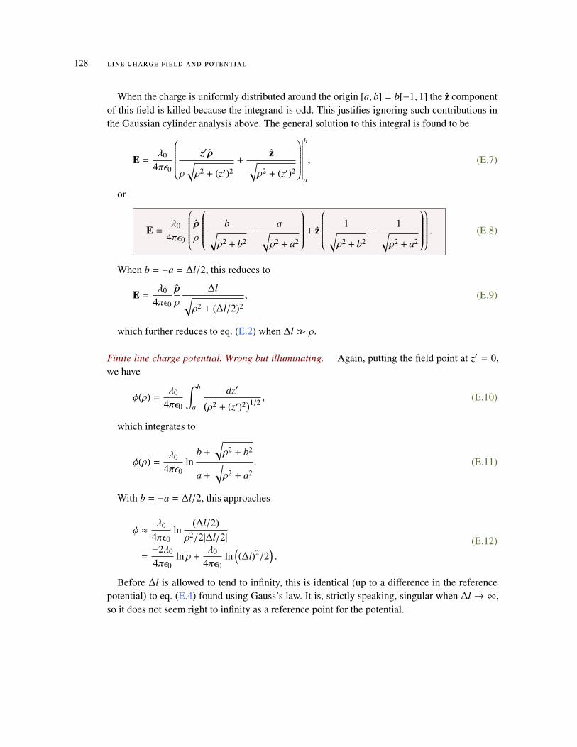
128 line charge field and potential
When the charge is uniformly distributed around the origin [a, b] = b[−1, 1] the z componentof this field is killed because the integrand is odd. This justifies ignoring such contributions inthe Gaussian cylinder analysis above. The general solution to this integral is found to be
(E.7)E =λ0
4πε0
z′ρ
ρ
√ρ2 + (z′)2
+z√
ρ2 + (z′)2
∣∣∣∣∣∣∣∣∣b
a
,
or
E =λ0
4πε0
ρρ b√
ρ2 + b2−
a√ρ2 + a2
+ z
1√ρ2 + b2
−1√
ρ2 + a2
. (E.8)
When b = −a = ∆l/2, this reduces to
(E.9)E =λ0
4πε0
ρ
ρ
∆l√ρ2 + (∆l/2)2
,
which further reduces to eq. (E.2) when ∆l � ρ.
Finite line charge potential. Wrong but illuminating. Again, putting the field point at z′ = 0,we have
(E.10)φ(ρ) =λ0
4πε0
∫ b
a
dz′(ρ2 + (z′)2)1/2 ,
which integrates to
(E.11)φ(ρ) =λ0
4πε0ln
b +
√ρ2 + b2
a +
√ρ2 + a2
.
With b = −a = ∆l/2, this approaches
(E.12)φ ≈
λ0
4πε0ln
(∆l/2)ρ2/2|∆l/2|
=−2λ0
4πε0ln ρ +
λ0
4πε0ln
((∆l)2/2
).
Before ∆l is allowed to tend to infinity, this is identical (up to a difference in the referencepotential) to eq. (E.4) found using Gauss’s law. It is, strictly speaking, singular when ∆l → ∞,so it does not seem right to infinity as a reference point for the potential.
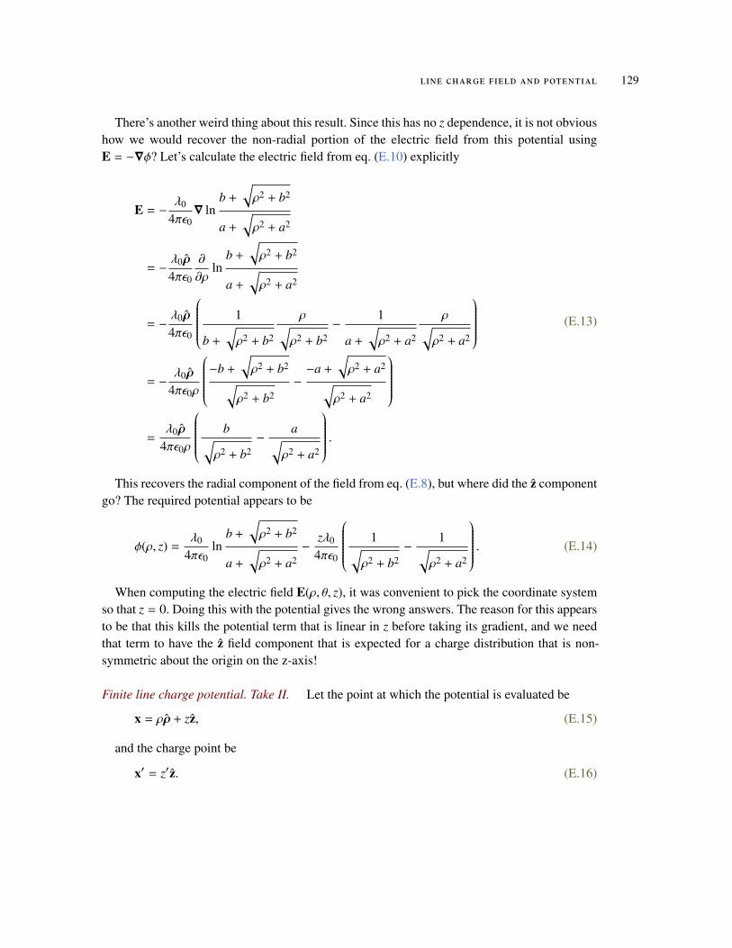
line charge field and potential 129
There’s another weird thing about this result. Since this has no z dependence, it is not obvioushow we would recover the non-radial portion of the electric field from this potential usingE = −∇φ? Let’s calculate the electric field from eq. (E.10) explicitly
(E.13)
E = −λ0
4πε0∇ ln
b +
√ρ2 + b2
a +
√ρ2 + a2
= −λ0ρ
4πε0
∂
∂ρln
b +
√ρ2 + b2
a +
√ρ2 + a2
= −λ0ρ
4πε0
1
b +
√ρ2 + b2
ρ√ρ2 + b2
−1
a +
√ρ2 + a2
ρ√ρ2 + a2
= −
λ0ρ
4πε0ρ
−b +
√ρ2 + b2√
ρ2 + b2−−a +
√ρ2 + a2√
ρ2 + a2
=
λ0ρ
4πε0ρ
b√ρ2 + b2
−a√
ρ2 + a2
.This recovers the radial component of the field from eq. (E.8), but where did the z component
go? The required potential appears to be
(E.14)φ(ρ, z) =λ0
4πε0ln
b +
√ρ2 + b2
a +
√ρ2 + a2
−zλ0
4πε0
1√ρ2 + b2
−1√
ρ2 + a2
.When computing the electric field E(ρ, θ, z), it was convenient to pick the coordinate system
so that z = 0. Doing this with the potential gives the wrong answers. The reason for this appearsto be that this kills the potential term that is linear in z before taking its gradient, and we needthat term to have the z field component that is expected for a charge distribution that is non-symmetric about the origin on the z-axis!
Finite line charge potential. Take II. Let the point at which the potential is evaluated be
(E.15)x = ρρ + zz,
and the charge point be
(E.16)x′ = z′z.
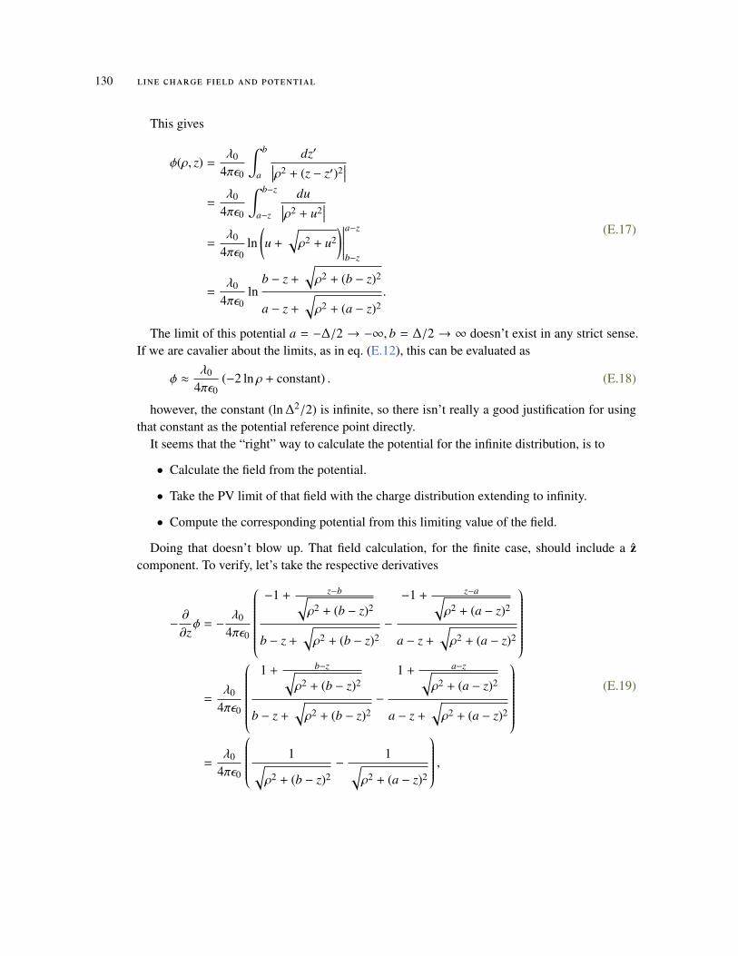
130 line charge field and potential
This gives
(E.17)
φ(ρ, z) =λ0
4πε0
∫ b
a
dz′∣∣∣ρ2 + (z − z′)2∣∣∣
=λ0
4πε0
∫ b−z
a−z
du∣∣∣ρ2 + u2∣∣∣
=λ0
4πε0ln
(u +
√ρ2 + u2
)∣∣∣∣∣∣a−z
b−z
=λ0
4πε0ln
b − z +
√ρ2 + (b − z)2
a − z +
√ρ2 + (a − z)2
.
The limit of this potential a = −∆/2 → −∞, b = ∆/2 → ∞ doesn’t exist in any strict sense.If we are cavalier about the limits, as in eq. (E.12), this can be evaluated as
(E.18)φ ≈λ0
4πε0(−2 ln ρ + constant) .
however, the constant (ln ∆2/2) is infinite, so there isn’t really a good justification for usingthat constant as the potential reference point directly.
It seems that the “right” way to calculate the potential for the infinite distribution, is to
• Calculate the field from the potential.
• Take the PV limit of that field with the charge distribution extending to infinity.
• Compute the corresponding potential from this limiting value of the field.
Doing that doesn’t blow up. That field calculation, for the finite case, should include a zcomponent. To verify, let’s take the respective derivatives
(E.19)
−∂
∂zφ = −
λ0
4πε0
−1 + z−b√
ρ2 + (b − z)2
b − z +
√ρ2 + (b − z)2
−
−1 + z−a√ρ2 + (a − z)2
a − z +
√ρ2 + (a − z)2
=
λ0
4πε0
1 + b−z√
ρ2 + (b − z)2
b − z +
√ρ2 + (b − z)2
−
1 + a−z√ρ2 + (a − z)2
a − z +
√ρ2 + (a − z)2
=
λ0
4πε0
1√ρ2 + (b − z)2
−1√
ρ2 + (a − z)2
,
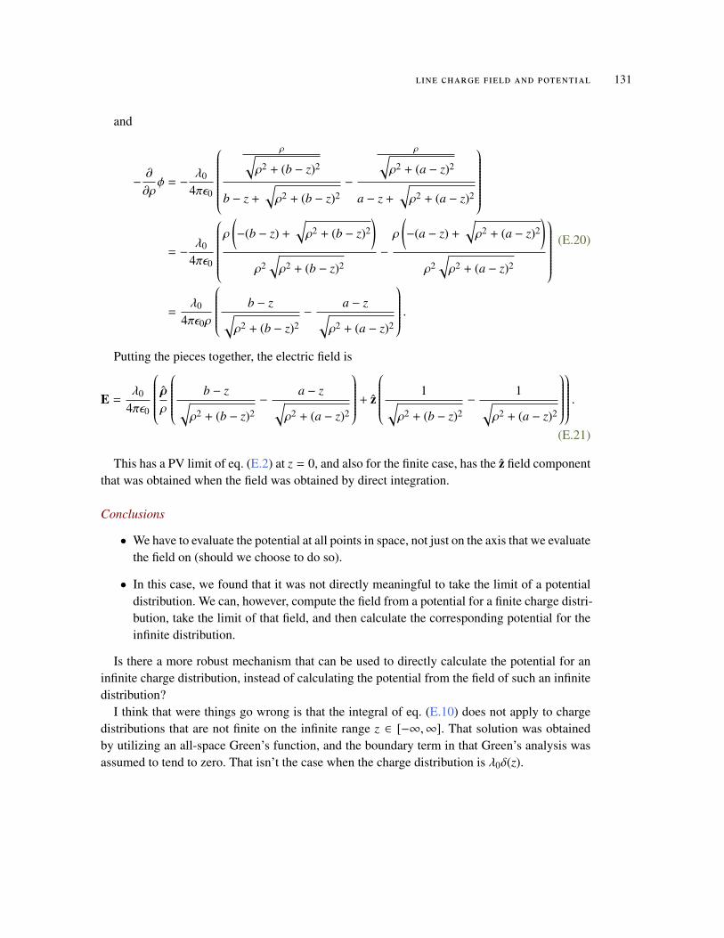
line charge field and potential 131
and
(E.20)
−∂
∂ρφ = −
λ0
4πε0
ρ√
ρ2 + (b − z)2
b − z +
√ρ2 + (b − z)2
−
ρ√ρ2 + (a − z)2
a − z +
√ρ2 + (a − z)2
= −
λ0
4πε0
ρ
(−(b − z) +
√ρ2 + (b − z)2
)ρ2
√ρ2 + (b − z)2
−
ρ
(−(a − z) +
√ρ2 + (a − z)2
)ρ2
√ρ2 + (a − z)2
=
λ0
4πε0ρ
b − z√ρ2 + (b − z)2
−a − z√
ρ2 + (a − z)2
.Putting the pieces together, the electric field is
E =λ0
4πε0
ρρ b − z√
ρ2 + (b − z)2−
a − z√ρ2 + (a − z)2
+ z
1√ρ2 + (b − z)2
−1√
ρ2 + (a − z)2
.
(E.21)
This has a PV limit of eq. (E.2) at z = 0, and also for the finite case, has the z field componentthat was obtained when the field was obtained by direct integration.
Conclusions
• We have to evaluate the potential at all points in space, not just on the axis that we evaluatethe field on (should we choose to do so).
• In this case, we found that it was not directly meaningful to take the limit of a potentialdistribution. We can, however, compute the field from a potential for a finite charge distri-bution, take the limit of that field, and then calculate the corresponding potential for theinfinite distribution.
Is there a more robust mechanism that can be used to directly calculate the potential for aninfinite charge distribution, instead of calculating the potential from the field of such an infinitedistribution?
I think that were things go wrong is that the integral of eq. (E.10) does not apply to chargedistributions that are not finite on the infinite range z ∈ [−∞,∞]. That solution was obtainedby utilizing an all-space Green’s function, and the boundary term in that Green’s analysis wasassumed to tend to zero. That isn’t the case when the charge distribution is λ0δ(z).

FG R A D I E N T, D I V E R G E N C E , C U R L A N D L A P L AC I A N I NC Y L I N D R I C A L C O O R D I NAT E S .
In class it was suggested that the identity
(F.1)∇2A = ∇ (∇ · A) − ∇ × (∇ × A) ,
can be used to compute the Laplacian in non-rectangular coordinates. Is that the easiest wayto do this?
How about just sequential applications of the gradient on the vector? Let’s start with thevector product of the gradient and the vector. First recall that the cylindrical representation ofthe gradient is
(F.2)∇ = ρ∂ρ +φ
ρ∂φ + z∂z,
where
(F.3)ρ = e1ee1e2φ
φ = e2ee1e2φ
Taking φ derivatives of eq. (F.3), we have
(F.4)∂φρ = e1e1e2ee1e2φ = e2ee1e2φ = φ
∂φφ = e2e1e2ee1e2φ = −e1ee1e2φ = −ρ.
The gradient of a vector A = ρAρ + φAφ + zAz is
133
134 gradient, divergence , curl and laplacian in cylindrical coordinates .
(F.5)
∇A =
(ρ∂ρ +
φ
ρ∂φ + z∂z
) (ρAρ + φAφ + zAz
)= ρ∂ρ
(ρAρ + φAφ + zAz
)+φ
ρ∂φ
(ρAρ + φAφ + zAz
)+ z∂z
(ρAρ + φAφ + zAz
)= ρ
(ρ∂ρAρ + φ∂ρAφ + z∂ρAz
)+φ
ρ
(∂φ(ρAρ) + ∂φ(φAφ) + z∂φAz
)+ z
(ρ∂zAρ + φ∂zAφ + z∂zAz
)= ∂ρAρ + ρφ∂ρAφ + ρz∂ρAz
+1ρ
(Aρ + φρ∂φAρ − φρAφ + ∂φAφ + φz∂φAz
)+ zρ∂zAρ + zφ∂zAφ + ∂zAz
= ∂ρAρ +1ρ(Aρ + ∂φAφ) + ∂zAz
+ zρ (∂zAρ − ∂ρAz)
+ φz(1ρ∂φAz − ∂zAφ
)+ ρφ
(∂ρAφ −
1ρ(∂φAρ − Aφ)
),
As expected, we see that the gradient splits nicely into a dot and curl
∇A = ∇ ·A +∇∧A = ∇ ·A + ρφz(∇ ×A), (F.6)
where the cylindrical representation of the divergence is seen to be
(F.7)∇ · A =1ρ∂ρ(ρAρ) +
1ρ∂φAφ + ∂zAz,
and the cylindrical representation of the curl is
(F.8)∇ × A = ρ
(1ρ∂φAz − ∂zAφ
)+ φ
(∂zAρ − ∂ρAz
)+
1ρ
z(∂ρ(ρAφ) − ∂φAρ
).
Should we want to, it is now possible to evaluate the Laplacian of A using eq. (F.1) , whichwill have the following components
gradient, divergence , curl and laplacian in cylindrical coordinates . 135
ρ ·(∇
2A)
= ∂ρ
(1ρ∂ρ(ρAρ) +
1ρ∂φAφ + ∂zAz
)−
(1ρ∂φ
(1ρ
(∂ρ(ρAφ) − ∂φAρ
))− ∂z
(∂zAρ − ∂ρAz
))= ∂ρ
(1ρ∂ρ(ρAρ)
)+ ∂ρ
(1ρ∂φAφ
)+ ∂ρzAz −
1ρ2 ∂φρ(ρAφ) +
1ρ2 ∂φφAρ + ∂zzAρ − ∂zρAz
= ∂ρ
(1ρ∂ρ(ρAρ)
)+
1ρ2 ∂φφAρ + ∂zzAρ −
1ρ2 ∂φAφ +
1ρ∂ρφAφ −
1ρ2 ∂φAφ −
1ρ∂φρAφ
= ∂ρ
(1ρ∂ρ(ρAρ)
)+
1ρ2 ∂φφAρ + ∂zzAρ −
2ρ2 ∂φAφ
=1ρ∂ρ
(ρ∂ρAρ
)+
1ρ2 ∂φφAρ + ∂zzAρ −
Aρρ2 −
2ρ2 ∂φAφ,
(F.9a)
φ ·(∇
2A)
=1ρ∂φ
(1ρ∂ρ(ρAρ) +
1ρ∂φAφ +∂zAz
)−
((∂z
(1ρ∂φAz−∂zAφ
)−∂ρ
(1ρ
(∂ρ(ρAφ)−∂φAρ
))))=
1ρ2 ∂φρ(ρAρ) +
1ρ2 ∂φφAφ +
1ρ∂φzAz −
1ρ∂zφAz + ∂zzAφ + ∂ρ
(1ρ∂ρ(ρAφ)
)− ∂ρ
(1ρ∂φAρ
)= ∂ρ
(1ρ∂ρ(ρAφ)
)+
1ρ2 ∂φφAφ + ∂zzAφ +
1ρ2 ∂φρ(ρAρ) +
1ρ∂φzAz −
1ρ∂zφAz − ∂ρ
(1ρ∂φAρ
)= ∂ρ
(1ρ∂ρ(ρAφ)
)+
1ρ2 ∂φφAφ + ∂zzAφ +
1ρ2 ∂φAρ +
1ρ∂φρAρ +
1ρ2 ∂φAρ −
1ρ∂ρφAρ
= ∂ρ
(1ρ∂ρ(ρAφ)
)+
1ρ2 ∂φφAφ + ∂zzAφ +
2ρ2 ∂φAρ
=1ρ∂ρ
(ρ∂ρAφ
)+
1ρ2 ∂φφAφ + ∂zzAφ +
2ρ2 ∂φAρ −
Aφρ2 ,
(F.9b)
z ·(∇
2A)
= ∂z
(1ρ∂ρ(ρAρ) +
1ρ∂φAφ + ∂zAz
)−
1ρ
(∂ρ
(ρ(∂zAρ − ∂ρAz
))− ∂φ
(1ρ∂φAz − ∂zAφ
))=
1ρ∂zρ(ρAρ) +
1ρ∂zφAφ + ∂zzAz −
1ρ∂ρ
(ρ∂zAρ
)+
1ρ∂ρ
(ρ∂ρAz
)+
1ρ2 ∂φφAz −
1ρ∂φzAφ
=1ρ∂ρ
(ρ∂ρAz
)+
1ρ2 ∂φφAz +∂zzAz +
1ρ∂zAρ+∂zρAρ+
1ρ∂zφAφ−
1ρ∂zAρ−∂ρzAρ−
1ρ∂φzAφ
=1ρ∂ρ
(ρ∂ρAz
)+
1ρ2 ∂φφAz + ∂zzAz
(F.9c)
Evaluating these was a fairly tedious and mechanical job, and would have been better suitedto a computer algebra system than by hand as done here.
136 gradient, divergence , curl and laplacian in cylindrical coordinates .
Explicit cylindrical Laplacian Let’s try this a different way. The most obvious potential strat-egy is to just apply the Laplacian to the vector itself, but we need to include the unit vectors insuch an operation
(F.10)∇2A = ∇2
(ρAρ + φAφ + zAz
).
First we need to know the explicit form of the cylindrical Laplacian. From the painful expan-sion, we can guess that it is
(F.11)∇2ψ =
1ρ∂ρ
(ρ∂ρψ
)+
1ρ2 ∂φφψ + ∂zzψ.
Let’s check that explicitly. Here I use the vector product where ρ2 = φ2
= z2 = 1, and thesevectors anticommute when different
∇2ψ =
(ρ∂ρ +
φ
ρ∂φ + z∂z
) (ρ∂ρψ +
φ
ρ∂φψ + z∂zψ
)= ρ∂ρ
(ρ∂ρψ +
φ
ρ∂φψ + z∂zψ
)+φ
ρ∂φ
(ρ∂ρψ +
φ
ρ∂φψ + z∂zψ
)+ z∂z
(ρ∂ρψ +
φ
ρ∂φψ + z∂zψ
)= ∂ρρψ + ρφ∂ρ
(1ρ∂φψ
)+ ρz∂ρzψ +
φ
ρ∂φ
(ρ∂ρψ
)+φ
ρ∂φ
(φ
ρ∂φψ
)+φzρ∂φzψ + zρ∂zρψ +
zφρ∂zφψ + ∂zzψ
= ∂ρρψ +1ρ∂ρψ +
1ρ2 ∂φφψ + ∂zzψ + ρφ
(−
1ρ2 ∂φψ +
1ρ∂ρφψ −
1ρ∂φρψ +
1ρ2 ∂φψ
)+ zρ
(−∂ρzψ + ∂zρψ
)+ φz
(1ρ∂φzψ −
1ρ∂zφψ
)= ∂ρρψ +
1ρ∂ρψ +
1ρ2 ∂φφψ + ∂zzψ,
(F.12)
so the Laplacian operator is
∇2 =
1ρ
∂
∂ρ
(ρ∂
∂ρ
)+
1ρ2
∂2
∂φ2 +∂2
∂z2 . (F.13)
All the bivector grades of the Laplacian operator are seen to explicitly cancel, regardless ofthe grade of ψ, just as if we had expanded the scalar Laplacian as a dot product ∇2ψ = ∇ · (∇ψ).Unlike such a scalar expansion, this derivation is seen to be valid for any grade ψ. We knownow that we can trust this result when ψ is a scalar, a vector, a bivector, a trivector, or even amultivector.
gradient, divergence , curl and laplacian in cylindrical coordinates . 137
Vector Laplacian Now that we trust that the typical scalar form of the Laplacian appliesequally well to multivectors as it does to scalars, that cylindrical coordinate operator can nowbe applied to a vector. Consider the projections onto each of the directions in turn
(F.14)∇2(ρAρ
)= ρ
1ρ∂ρ
(ρ∂ρAρ
)+
1ρ2 ∂φφ
(ρAρ
)+ ρ∂zzAρ
(F.15)∂φφ
(ρAρ
)= ∂φ
(φAρ + ρ∂φAρ
)= −ρAρ + φ∂φAρ + φ∂φAρ + ρ∂φφAρ= ρ
(∂φφAρ − Aρ
)+ 2φ∂φAρ
so this component of the vector Laplacian is
(F.16)∇
2(ρAρ
)= ρ
(1ρ∂ρ
(ρ∂ρAρ
)+
1ρ2 ∂φφAρ −
1ρ2 Aρ + ∂zzAρ
)+ φ
(2
1ρ2 ∂φAρ
)= ρ
(∇
2Aρ −1ρ2 Aρ
)+ φ
2ρ2 ∂φAρ.
The Laplacian for the projection of the vector onto the φ direction is
(F.17)∇2(φAφ
)= φ
1ρ∂ρ
(ρ∂ρAφ
)+
1ρ2 ∂φφ
(φAφ
)+ φ∂zzAφ,
Again, since the unit vectors are φ dependent, the φ derivatives have to be treated carefully
(F.18)∂φφ
(φAφ
)= ∂φ
(−ρAφ + φ∂φAφ
)= −φAφ − ρ∂φAφ − ρ∂φAφ + φ∂φφAφ= −2ρ∂φAφ + φ
(∂φφAφ − Aφ
),
so the Laplacian of this projection is
(F.19)∇
2(φAφ
)= φ
(1ρ∂ρ
(ρ∂ρAφ
)+ φ∂zzAφ,
1ρ2 ∂φφAφ −
Aφρ2
)− ρ
2ρ2 ∂φAφ
= φ
(∇
2Aφ −Aφρ2
)− ρ
2ρ2 ∂φAφ.
Since z is fixed we have(F.20)∇
2zAz = z∇2Az.
Putting all the pieces together we have
∇2A = ρ
(∇
2Aρ −1ρ2 Aρ −
2ρ2 ∂φAφ
)+ φ
(∇
2Aφ −Aφρ2 +
2ρ2 ∂φAρ
)+ z∇2Az. (F.21)
This matches the result eq. (F.9) from the painful expansion of ∇ (∇ ·A) −∇ × (∇ ×A).

GG R A D I E N T, D I V E R G E N C E , C U R L A N D L A P L AC I A N I NS P H E R I C A L C O O R D I NAT E S .
Unit vectors Two of the spherical unit vectors we can immediately write by inspection.
(G.1)r = e1 sin θ cos φ + e2 sin θ sin φ + e3 cos θ
φ = −e1 sin θ + e2 cos φ
We can compute θ by utilizing the right hand triplet property
(G.2)
θ = φ × r
=
∣∣∣∣∣∣∣∣∣∣∣e1 e2 e3
−S φ Cφ 0
S θCφ S θS φ Cθ
∣∣∣∣∣∣∣∣∣∣∣= e1
(CθCφ
)+ e2
(CθS φ
)+ e3
(−S θ
(S 2φ + C2
φ
))= e1 cos θ cos φ + e2 cos θ sin φ − e3 sin θ.
Here I’ve used Cθ = cos θ, S φ = sin φ, · · · as a convenient shorthand. Observe that withi = e1e2, these unit vectors admit a small factorization that makes further manipulation easier
r = e1eiφ sin θ + e3 cos θ
θ = cos θe1eiφ − sin θe3
φ = e2eiφ
(G.3)
It should also be the case that rθφ = I, where I = e1e2e3 = e123 is the R3 pseudoscalar,which is straightforward to check
(G.4)
rθφ =(e1eiφ sin θ + e3 cos θ
) (cos θe1eiφ − sin θe3
)e2eiφ
=(sin θ cos θ − cos θ sin θ + e31eiφ
(cos2 θ + sin2 θ
))e2eiφ
= e31e2e−iφeiφ
= e123.
This property could also have been used to compute θ.
139
140 gradient, divergence , curl and laplacian in spherical coordinates .
Gradient To compute the gradient, note that the coordinate vectors for the spherical parame-terization are
(G.5a)
xr =∂r∂r
=∂(rr)∂r
= r + r∂r∂r
= r,
(G.5b)
xθ =∂(rr)∂θ
= r∂
∂θ
(S θe1eiφ + Cθe3
)= r
∂
∂θ
(Cθe1eiφ − S θe3
)= rθ,
(G.5c)
xφ =∂(rr)∂φ
= r∂
∂φ
(S θe1eiφ + Cθe3
)= rS θe2eiφ
= r sin θφ.
Since these are all normal, the dual vectors defined by x j · xk = δjk, can be obtained by
inspection
xr = r
xθ =1rθ
xφ =1
r sin θφ.
(G.6)
The gradient follows immediately
(G.7)∇ = xr ∂
∂r+ xθ
∂
∂θ+ xφ
∂
∂φ,

gradient, divergence , curl and laplacian in spherical coordinates . 141
or
∇ = r∂
∂r+θ
r∂
∂θ+
φ
r sin θ∂
∂φ. (G.8)
More information on this general dual-vector technique of computing the gradient in curvi-linear coordinate systems can be found in [9].
Partials To compute the divergence, curl and Laplacian, we’ll need the partials of each of theunit vectors ∂r/∂θ, ∂r/∂φ, ∂θ/∂θ, ∂θ/∂φ, ∂φ/∂φ.
The θ partials are
(G.9)
∂θ
∂θ=
∂
∂θ
(Cθe1eiφ − S θe3
)= −S θe1eiφ −Cθe3
= −r,
(G.10)
∂θ
∂φ=
∂
∂φ
(Cθe1eiφ − S θe3
)= Cθe2eiφ
= Cθφ.
The φ partials are
(G.11)∂φ
∂θ=
∂
∂θe2eiφ
= 0.
(G.12)
∂φ
∂φ=
∂
∂φe2eiφ
= −e1eiφ
= −r⟨re1eiφ
⟩− θ
⟨θe1eiφ
⟩− φ
⟨φe1eiφ
⟩= −r
⟨(e1eiφS θ + e3Cθ
)e1eiφ
⟩− θ
⟨(Cθe1eiφ − S θe3
)e1eiφ
⟩= −r
⟨e−iφS θeiφ
⟩− θ
⟨Cθe−iφeiφ
⟩= −rS θ − θCθ.
The r partials are were computed as a side effect of evaluating xθ, and xφ, and are
142 gradient, divergence , curl and laplacian in spherical coordinates .
(G.13)∂r∂θ
= θ,
(G.14)∂r∂φ
= S θφ.
In summary
∂θr = θ
∂φr = S θφ
∂θθ = −r∂φθ = Cθφ
∂θφ = 0
∂φφ = −rS θ − θCθ.
(G.15)
Divergence and curl. The divergence and curl can be computed from the vector product ofthe spherical coordinate gradient and the spherical representation of a vector. That is
∇A = ∇ ·A +∇∧A = ∇ ·A + I∇ ×A. (G.16)
That gradient vector product is
(G.17)
∇A =
(r∂r +
θ
r∂θ +
φ
rS θ∂φ
) (rAr + θAθ + φAφ
)= r∂r
(rAr + θAθ + φAφ
)+θ
r∂θ
(rAr + θAθ + φAφ
)+
φ
rS θ∂φ
(rAr + θAθ + φAφ
)=
(∂rAr + rθ∂rAθ + rφ∂rAφ
)+
1r
(θ(∂θr)Ar + θ(∂θθ)Aθ + θ(∂θφ)Aφ + θr∂θAr + ∂θAθ + θφ∂θAφ
)+
1rS θ
(φ(∂φr)Ar + φ(∂φθ)Aθ + φ(∂φφ)Aφ + φr∂φAr + φθ∂φAθ + ∂φAφ
)=
(∂rAr + rθ∂rAθ + rφ∂rAφ
)+
1r
(θ(θ)Ar + θ(−r)Aθ + θ(0)Aφ + θr∂θAr + ∂θAθ + θφ∂θAφ
)+
1rS θ
(φ(S θφ)Ar + φ(Cθφ)Aθ − φ(rS θ + θCθ)Aφ + φr∂φAr + φθ∂φAθ + ∂φAφ
).
gradient, divergence , curl and laplacian in spherical coordinates . 143
The scalar component of this is the divergence
(G.18)
∇ · A = ∂rAr +Ar
r+
1r∂θAθ +
1rS θ
(S θAr + CθAθ + ∂φAφ
)= ∂rAr + 2
Ar
r+
1r∂θAθ +
1rS θ
CθAθ +1
rS θ∂φAφ
= ∂rAr + 2Ar
r+
1r∂θAθ +
1rS θ
CθAθ +1
rS θ∂φAφ,
which can be factored as
∇ ·A =1r2 ∂r(r2Ar) +
1rS θ
∂θ(S θAθ) +1
rS θ∂φAφ. (G.19)
The bivector grade of ∇A is the bivector curl
∇ ∧ A =(rθ∂rAθ + rφ∂rAφ
)+
1r
(θ(−r)Aθ + θr∂θAr + θφ∂θAφ
)+
1rS θ
(−φ(rS θ + θCθ)Aφ + φr∂φAr + φθ∂φAθ
)=
(rθ∂rAθ − φr∂rAφ
)+
1r
(rθAθ − rθ∂θAr + θφ∂θAφ
)+
1rS θ
(−φrS θAφ + θφCθAφ + φr∂φAr − θφ∂φAθ
)= θφ
(1
rS θCθAφ +
1r∂θAφ −
1rS θ
∂φAθ
)+ φr
(−∂rAφ +
1rS θ
(−S θAφ + ∂φAr
))+ rθ
(∂rAθ +
1r
Aθ −1r∂θAr
)= Ir
(1
rS θ∂θ(S θAφ) −
1rS θ
∂φAθ
)+ Iθ
(1
rS θ∂φAr −
1r∂r(rAφ)
)+ Iφ
(1r∂r(rAθ) −
1r∂θAr
)(G.20)
This gives
∇ ×A = r(
1rS θ
∂θ(S θAφ) −1
rS θ∂φAθ
)+ θ
(1
rS θ∂φAr −
1r∂r(rAφ)
)+ φ
(1r∂r(rAθ) −
1r∂θAr
).
(G.21)
This and the divergence result above both check against the back cover of [8].
144 gradient, divergence , curl and laplacian in spherical coordinates .
Laplacian Using the divergence and curl it’s possible to compute the Laplacian from those,but we saw in cylindrical coordinates that it was much harder to do it that way than to do itdirectly.
(G.22)
∇2ψ =
(r∂r +
θ
r∂θ +
φ
rS θ∂φ
) (r∂rψ +
θ
r∂θψ +
φ
rS θ∂φψ
)= ∂rrψ + rθ∂r
(1r∂θψ
)+ rφ
1S θ∂r
(1r∂φψ
)+θ
r∂θ (r∂rψ) +
θ
r2 ∂θ(θ∂θψ
)+θ
r2 ∂θ
(φ
S θ∂φψ
)+
φ
rS θ∂φ (r∂rψ) +
φ
r2S θ∂φ
(θ∂θψ
)+
φ
r2S 2θ
∂φ(φ∂φψ
)= ∂rrψ + rθ∂r
(1r∂θψ
)+ rφ
1S θ∂r
(1r∂φψ
)+θrr∂θ (∂rψ) +
1r2 ∂θθψ +
θφ
r2 ∂θ
(1
S θ∂φψ
)+φrrS θ
∂φrψ +φθ
r2S θ∂φθψ +
1r2S 2
θ
∂φφψ
+θ
r(∂θr)∂rψ +
θ
r2 (∂θθ)∂θψ +θ
r2 (∂θφ)φ
S θ∂φψ
+φ
rS θ(∂φr)∂rψ +
φ
r2S θ(∂φθ)∂θψ +
φ
r2S 2θ
(∂φφ)∂φψ
= ∂rrψ + rθ∂r
(1r∂θψ
)+ rφ
1S θ∂r
(1r∂φψ
)+θrr∂θ (∂rψ) +
1r2 ∂θθψ +
θφ
r2 ∂θ
(1
S θ∂φψ
)+φrrS θ
∂φrψ +φθ
r2S θ∂φθψ +
1r2S 2
θ
∂φφψ
+θ
r(θ)∂rψ +
θ
r2 (−r)∂θψ +θ
r2 (0)φ
S θ∂φψ
+φ
rS θ(S θφ)∂rψ +
φ
r2S θ(Cθφ)∂θψ +
φ
r2S 2θ
(−rS θ − θCθ)∂φψ
All the bivector factors are expected to cancel out, but this should be checked. Those with anrθ factor are
gradient, divergence , curl and laplacian in spherical coordinates . 145
(G.23)∂r
(1r∂θψ
)−
1r∂θrψ +
1r2 ∂θψ = −
1r2 ∂θψ +
1r∂rθψ −
1r∂θrψ +
1r2 ∂θψ
= 0,
and those with a θφ factor are
1r2 ∂θ
(1
S θ∂φψ
)−
1r2S θ
∂φθψ +1
r2S 2θ
Cθ∂φψ = −1r2
Cθ
S 2θ
∂φψ+1
r2S θ∂θφψ−
1r2S θ
∂φθψ+1
r2S 2θ
Cθ∂φψ
= 0,(G.24)
and those with a φr factor are
(G.25)−1
S θ∂r
(1r∂φψ
)+
1rS θ
∂φrψ −1
r2S 2θ
S θ∂φψ =1
S θ
1r2 ∂φψ −
1rS θ
∂rφψ +1
rS θ∂φrψ −
1r2S θ
∂φψ
= 0.
This leaves
(G.26)∇2ψ = ∂rrψ +
2r∂rψ +
1r2 ∂θθψ +
1r2S θ
Cθ∂θψ +1
r2S 2θ
∂φφψ.
This factors nicely as
∇2ψ =
1r2
∂
∂r
(r2 ∂ψ
∂r
)+
1r2 sin θ
∂
∂θ
(sin θ
∂ψ
∂θ
)+
1r2 sin2 θ
∂2ψ
∂φ2 , (G.27)
which checks against the back cover of Jackson. Here it has been demonstrated explicitly thatthis operator expression is valid for multivector fields ψ as well as scalar fields ψ.

HV E C T O R WAV E E Q UAT I O N I N S P H E R I C A L C O O R D I NAT E S
For a vector A in spherical coordinates, let’s compute the Laplacian
(H.1)∇2A,
to see the form of the wave equation. The spherical vector representation has a curvilinearbasis
(H.2)A = rAr + θAθ + φAφ,
and the spherical Laplacian has been found to have the representation
(H.3)∇2ψ =
1r2
∂
∂r
(r2 ∂ψ
∂r
)+
1r2 sin θ
∂
∂θ
(sin θ
∂ψ
∂θ
)+
1r2 sin2 θ
∂2ψ
∂φ2 .
Evaluating the Laplacian will require the following curvilinear basis derivatives
(H.4)
∂θr = θ
∂θθ = −r∂θφ = 0
∂φr = S θφ
∂φθ = Cθφ
∂φφ = −rS θ − θCθ.
We’ll need to evaluate a number of derivatives. Starting with the r components
(H.5a)∂r(r2∂r (rψ)
)= r∂r
(r2∂rψ
)
(H.5b)
∂θ (S θ∂θ (rψ)) = ∂θ(S θ(θψ + r∂θψ)
)= Cθ(θψ + r∂θψ) + S θ∂θ(θψ + r∂θψ)= Cθ(θψ + r∂θψ) + S θ∂θ((∂θθ)ψ + (∂θr)∂θψ) + S θ∂θ(θ∂θψ + r∂θθψ)= Cθ(θψ + r∂θψ) + S θ((−r)ψ + (θ)∂θψ) + S θ(θ∂θψ + r∂θθψ)= r (Cθ∂θψ − S θψ + S θ∂θθψ) + θ (Cθψ + 2S θ∂θψ)
147
148 vector wave equation in spherical coordinates
(H.5c)
∂φφ (rψ) = ∂φ((∂φr)ψ + r∂φψ
)= ∂φ
((S θφ)ψ + r∂φψ
)= S θ∂φ(φψ) + ∂φ
(r∂φψ
)= S θ(∂φφ)ψ + S θφ∂φψ + (∂φr)∂φψ + r∂φφψ= S θ(−S θr −Cθθ)ψ + S θφ∂φψ + (S θφ)∂φψ + r∂φφψ= r
(−S 2
θψ + ∂φφψ)
+ θ (−S θCθψ) + φ(2S θφ∂φψ
)This gives
∇2(rAr) = r
1r2 ∂r
(r2∂rAr
)+
1r2S θ
(Cθ∂θAr − S θAr + S θ∂θθAr) +1
r2S 2θ
(−S 2
θAr + ∂φφAr)
+ θ
(1
r2S θ(CθAr + 2S θ∂θAr) −
1r2S θ
S θCθAr
)+ φ
1r2S 2
θ
2S θ∂φAr
= r
(∇
2Ar −2r2 Ar
)+θ
r2
(Cθ
S θAr + 2∂θAr −CθAr
)+ φ
2r2S θ
∂φAr.
(H.6)
Next, let’s compute the derivatives of the θ projection.
(H.7a)∂r(r2∂r
(θψ
))= θ∂r
(r2∂rψ
)
(H.7b)
∂θ(S θ∂θ
(θψ
))= ∂θ
(S θ
((∂θθ)ψ + θ∂θψ
))= ∂θ
(S θ
((−r)ψ + θ∂θψ
))= Cθ
(−rψ + θ∂θψ
)+ S θ
(−(∂θr)ψ − r∂θψ + (∂θθ)∂θψ + θ∂θθψ
)= Cθ
(−rψ + θ∂θψ
)+ S θ
(−(θ)ψ − r∂θψ + (−r)∂θψ + θ∂θθψ
)= r (−Cθψ − 2S θ∂θψ) + θ (+Cθ∂θψ − S θψ + S θ∂θθψ)= r (−Cθψ − 2S θ∂θψ) + θ (+∂θ(S θ∂θψ) − S θψ)
(H.7c)
∂φφ(θψ
)= ∂φ
((∂φθ)ψ + θ∂φψ
)= ∂φ
((Cθφ)ψ + θ∂φψ
)= Cθ∂φ(φψ) + ∂φ(θ∂φψ)= Cθ(∂φφ)ψ + Cθφ∂φψ + (∂φθ)∂φψ + θ∂φφψ
= Cθ(−rS θ − θCθ)ψ + Cθφ∂φψ + (Cθφ)∂φψ + θ∂φφψ
= −rCθS θψ + θ(−CθCθψ + ∂φφψ
)+ 2φCθ∂φψ,
vector wave equation in spherical coordinates 149
which gives
∇2(θAθ) = r
1r2S θ
(−CθAθ − 2S θ∂θAθ) −1
r2S 2θ
CθS θAθ
+ θ
1r2 ∂r
(r2∂rAθ
)+
1r2S θ
(+∂θ(S θ∂θAθ) − S θAθ) +1
r2S 2θ
(−CθCθAθ + ∂φφAθ
)+ φ
1r2S 2
θ
2Cθ∂φAθ
= −2r
1r2S θ
∂θ(S θAθ) + θ
∇2Aθ −1r2 Aθ −
1r2S 2
θ
C2θAθ
+ 2φ 1
r2S 2θ
Cθ∂φAθ
.(H.8)
Finally, we can compute the derivatives of the φ projection.
(H.9a)∂r(r2∂r
(φψ
))= φ∂r
(r2∂rψ
)(H.9b)∂θ
(S θ∂θ
(φψ
))= φ∂θ (S θ∂θψ)
(H.9c)
∂φφ(φψ
)= ∂φ
((∂φφ)ψ + φ∂φψ
)= ∂φ
((−rS θ − θCθ)ψ + φ∂φψ
)= −((∂φr)S θ + (∂φθ)Cθ)ψ − (rS θ + θCθ)∂φψ + (∂φφ∂φψ + φ∂φφψ
= −((S θφ)S θ + (Cθφ)Cθ)ψ − (rS θ + θCθ)∂φψ + (−rS θ − θCθ)∂φψ + φ∂φφψ
= −2rS θ∂φψ − 2θCθ∂φψ + φ(∂φφψ − ψ
),
which gives
(H.10)
∇2(φAφ
)= −2r
1r2S θ
∂φAφ − 2θ1
r2S 2θ
Cθ∂φAφ
+ φ
1r2 ∂r
(r2∂rAφ
)+
1r2S θ
∂θ(S θ∂θAφ
)+
1r2S 2
θ
(∂φφAφ − Aφ
)= −2r
1r2S θ
∂φAφ − 2θ1
r2S 2θ
Cθ∂φAφ + φ
(∇
2Aφ −1r2 Aφ
).
The vector Laplacian resolves into three augmented scalar wave equations, all highly coupled
150 vector wave equation in spherical coordinates
r ·(∇
2A)
= ∇2Ar −2r2 Ar −
2r2S θ
∂θ(S θAθ) −2
r2S θ∂φAφ
θ ·(∇
2A)
=1r2
Cθ
S θAr +
2r2 ∂θAr −
1r2 CθAr +∇2Aθ −
1r2 Aθ −
1r2S 2
θ
C2θAθ − 2
1r2S 2
θ
Cθ∂φAφ
φ ·(∇
2A)
=2
r2S θ∂φAr +
2r2S 2
θ
Cθ∂φAθ +∇2Aφ −1r2 Aφ.
(H.11)
I’d guess one way to decouple these equations would be to impose a constraint that allows allthe non-wave equation terms in one of the component equations to be killed, and then substitutethat constraint into the remaining equations. Let’s try one such constraint
(H.12)Ar = −1
S θ∂θ(S θAθ) −
1S θ∂φAφ.
This gives
(H.13)
r ·(∇
2A)
= ∇2Ar
θ ·(∇
2A)
=
(1r2
Cθ
S θ+
2r2 ∂θ −
1r2 Cθ
) (−
1S θ∂θ(S θAθ) −
1S θ∂φAφ
)+ ∇2Aθ −
1r2 Aθ −
1r2S 2
θ
C2θAθ −
2r2S 2
θ
Cθ∂φAφ
φ ·(∇
2A)
= −2
r2S θ∂φ
(1
S θ∂θ(S θAθ) +
1S θ∂φAφ
)+
2r2S 2
θ
Cθ∂φAθ + ∇2Aφ −1r2 Aφ
= −2
r2S θ∂θAθ −
2r2S 2
θ
∂φφAθ + ∇2Aφ −1r2 Aφ
It looks like some additional cancellations may be had in the θ projection of this constrainedvector Laplacian. I’m not inclined to try to take this reduction any further without a thoroughcheck of all the algebra (using Mathematica to do so would make sense).
I also guessing that such a solution might be how the TEr and TMr modes were defined,but that doesn’t appear to be the case according to [2]. There the wave equation is formulatedin terms of the vector potentials (picking one to be zero and the other to be radial only). The

vector wave equation in spherical coordinates 151
solution obtained from such a potential wave equation then directly defines the TEr and TMr
modes. It would be interesting to see how the modes derived in that analysis transform withapplication of the vector Laplacian derived above.

IT R A N S V E R S E G AU G E
Jackson [8] has an interesting presentation of the transverse gauge. I’d like to walk through thedetails of this, but first want to translate the preliminaries to SI units (if I had the 3rd edition I’dnot have to do this translation step).
Gauge freedom The starting point is noting that∇ ·B = 0 the magnetic field can be expressedas a curl
(I.1)B = ∇ × A.
Faraday’s law now takes the form
(I.2)
0 = ∇ × E +∂B∂t
= ∇ × E +∂
∂t(∇ × A)
= ∇ ×
(E +
∂A∂t
).
Because this curl is zero, the interior sum can be expressed as a gradient
(I.3)E +∂A∂t≡ −∇Φ.
This can now be substituted into the remaining two Maxwell’s equations.
(I.4)∇ · D = ρv
∇ ×H = J +∂D∂t
For Gauss’s law, in simple media, we have
(I.5)ρv = ε∇ · E
= ε∇ ·
(−∇Φ −
∂A∂t
)For simple media again, the Ampere-Maxwell equation is
(I.6)1µ∇ × (∇ × A) = J + ε
∂
∂t
(−∇Φ −
∂A∂t
).
153
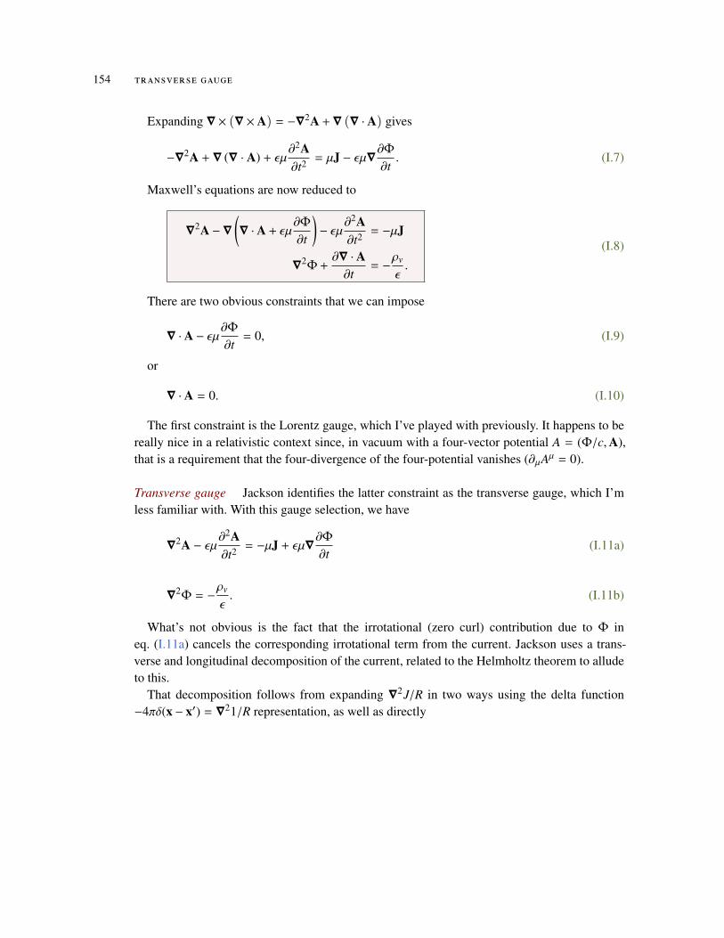
154 transverse gauge
Expanding ∇ × (∇ ×A) = −∇2A +∇ (∇ ·A) gives
(I.7)−∇2A + ∇ (∇ · A) + εµ∂2A∂t2 = µJ − εµ∇
∂Φ∂t.
Maxwell’s equations are now reduced to
∇2A −∇
(∇ ·A + εµ
∂Φ∂t
)− εµ
∂2A∂t2 = −µJ
∇2Φ +
∂∇ ·A∂t
= −ρv
ε.
(I.8)
There are two obvious constraints that we can impose
∇ ·A − εµ∂Φ∂t
= 0, (I.9)
or
∇ ·A = 0. (I.10)
The first constraint is the Lorentz gauge, which I’ve played with previously. It happens to bereally nice in a relativistic context since, in vacuum with a four-vector potential A = (Φ/c,A),that is a requirement that the four-divergence of the four-potential vanishes (∂µAµ = 0).
Transverse gauge Jackson identifies the latter constraint as the transverse gauge, which I’mless familiar with. With this gauge selection, we have
(I.11a)∇2A − εµ
∂2A∂t2 = −µJ + εµ∇
∂Φ∂t
(I.11b)∇2Φ = −
ρv
ε.
What’s not obvious is the fact that the irrotational (zero curl) contribution due to Φ ineq. (I.11a) cancels the corresponding irrotational term from the current. Jackson uses a trans-verse and longitudinal decomposition of the current, related to the Helmholtz theorem to alludeto this.
That decomposition follows from expanding ∇2J/R in two ways using the delta function−4πδ(x − x′) = ∇21/R representation, as well as directly
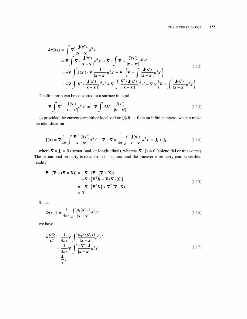
transverse gauge 155
(I.12)
−4πJ(x) =
∫∇
2 J(x′)|x − x′|
d3x′
= ∇
∫∇ ·
J(x′)|x − x′|
d3x′ + ∇ ·∫∇ ∧
J(x′)|x − x′|
d3x′
= −∇
∫J(x′) · ∇′
1|x − x′|
d3x′ + ∇ ·(∇ ∧
∫J(x′)|x − x′|
d3x′)
= −∇
∫∇′ ·
J(x′)|x − x′|
d3x′ + ∇∫∇′ · J(x′)|x − x′|
d3x′ − ∇ ×(∇ ×
∫J(x′)|x − x′|
d3x′)
The first term can be converted to a surface integral
(I.13)−∇
∫∇′ ·
J(x′)|x − x′|
d3x′ = −∇
∫dA′ ·
J(x′)|x − x′|
,
so provided the currents are either localized or |J|/R→ 0 on an infinite sphere, we can makethe identification
J(x) = ∇1
4π
∫∇′ · J(x′)|x − x′|
d3x′ −∇ ×∇ ×1
4π
∫J(x′)|x − x′|
d3x′ ≡ Jl + Jt, (I.14)
where ∇× Jl = 0 (irrotational, or longitudinal), whereas ∇ · Jt = 0 (solenoidal or transverse).The irrotational property is clear from inspection, and the transverse property can be verifiedreadily
(I.15)
∇ · (∇ × (∇ × X)) = −∇ · (∇ · (∇ ∧ X))= −∇ ·
(∇
2X − ∇ (∇ · X))
= −∇ ·(∇
2X)
+ ∇2 (∇ · X)= 0.
Since
(I.16)Φ(x, t) =1
4πε
∫ρv(x′, t)|x − x′|
d3x′,
we have
(I.17)
∇∂Φ∂t
=1
4πε∇
∫∂tρv(x′, t)|x − x′|
d3x′
=1
4πε∇
∫−∇′ · J|x − x′|
d3x′
=Jl
ε.
156 transverse gauge
This means that the Ampere-Maxwell equation takes the form
∇2A − εµ
∂2A∂t2 = −µJ + µJl = −µJt. (I.18)
This justifies the “transverse” in the label transverse gauge.

JM AT H E M AT I C A N OT E B O O K S
These Mathematica notebooks, some just trivial ones used to generate figures, others moreelaborate, and perhaps some even polished, can be found in
https://github.com/peeterjoot/mathematica/tree/master/.The free Wolfram CDF player, is capable of read-only viewing these notebooks to some
extent.
• Dec 31, 1969 ece1228-emt/BrewstersAngle.nb
Total internal reflection critical angle.
• Oct 21, 2016 ece1228-emt/ps5/ps5.nb
Plots of index of refraction and relative permittivity for passive and active media.
• Nov 4, 2016 ece1228-emt/ps6alphaPlusBetaSquareFactorization.nb
A verification of the hand calculated result.
• Nov 5, 2016 ece1228-emt/quadropoleVerificationJacksonChapter4.nb
Quadropole expansion comparison attempt.
• Dec 4, 2016 ece1228-emt/ps9/ps9p1Eigenvalues.nb
ps9, p1, Slab transfer matrix eigenvalues.
• Dec 4, 2016 ece1228-emt/ps9/ps9p2Plots.nb
Problem set 9, problem 2. Plots of transmission magnitude and phase for a one dimen-sional photonic crystal. Plots assume: µ1 = µ2 = 1, normal incidence, and use the Fresnelreflection coefficient ρi j for the TE mode polarization.
157


Part III
I N D E X

I N D E X
anisotropic, 7
Biot-Savart, 37bivector, 133bound charge, 22boundary, 5boundary conditions, 31
electric field, 39tangential magnetic field, 36
breakdown voltage, 6
capacitor, 6, 22conducting sheet, 13conductivity, 31conductor
charge dissipation, 39constitutive relations, 6constitutive relationships, 31continuity equation, 39curl, 107, 139
cylindrical coordinates, 133spherical coordinates, 139
curl of curl, 107current loop, 37
De-Broglie relation, 9delta function
Laplacian, 107, 120dielectric, 22
boundary conditions, 39dipole
electric, 21, 26, 27elemental, 24potential, 28
dipole moment density, 26
divergence, 139cylindrical coordinates, 133spherical coordinates, 139
divergence free, 11Divergence Theorem, 5doppler shift, 47duality theorem, 48
electric energy density, 42electric field
direction vector, 19spherical shell, 10
electrostatic energy, 117electrostatics, 19energy
torque, 30
Faraday’s law, 5field lines
electric, 11force, 123
Gauss’s lawmatter, 25
Geometric Algebra, 109, 133, 139grade one selection, 109gradient, 20, 139
cylindrical coordinates, 16, 133radial functions, 107spherical coordinates, 139
Green’s functionLaplacian representation, 39
Helmholtz’s theorem, 9, 14
161

162 Index
index of refraction, 8, 47irrotational, 12
Laplacian, 139cylindrical coordinates, 133decomposition, 107Green’s function, 39spherical coordinates, 139
LC circuit, 43line charge, 15Lorentz force, 123
macroscopic, 6magnetic energy density, 41magnetic flux, 6magnetic moment, 29magnetic polarization, 29magnetic surface charge density, 32magnetization, 7, 19, 29magnetostatics, 123Mathematica, 157Maxwell’s equations
point charge, 16time domain, 3
momentmagnetic, 29
non-solenoidal, 11normal component, 109normal field component, 32number density, 23
Ohm’s law, 31
permeability, 6permittivity
relative, 8vacuum, 8
phasor, 48photon
angular momentum, 8
momentum, 8point charge, 16, 19polarization, 7, 19, 22potential
electric, 20electric dipole, 26, 28
potential energy, 117Poynting theorem, 41Poynting vector, 41
frequency domain, 46projection, 109pseudoscalar, 139
rejection, 109
scalar, 133self energy, 117solenoidal, 11, 12spherical coordinates, 139
rotation matrix, 22Stokes’ Theorem, 5stored electric energy, 42stored magnetic energy, 42superposition, 19supplied power density, 41surface charge density, 20
tangential component, 109tangential field component, 31time harmonics, 43torque, 30, 123triple cross product, 109
unitampere, 4candela, 4Coulomb, 4Kelvin, 4mole, 4
units, 3

Index 163
waveguide, 14wedge product, 139


Part IV
B I B L I O G R A P H Y


B I B L I O G R A P H Y
[1] Neil W Ashcroft and N David Mermin. Solid State Physics. Holt, Rinehart and Winston,New York, 1976. (Cited on page 57.)
[2] Constantine A Balanis. Advanced engineering electromagnetics. Wiley New York, 1989.(Cited on pages 22, 33, 46, and 150.)
[3] C. Doran and A.N. Lasenby. Geometric algebra for physicists. Cambridge UniversityPress New York, Cambridge, UK, 1st edition, 2003. (Cited on page 111.)
[4] L. Dorst, D. Fontijne, and S. Mann. Geometric Algebra for Computer Science. MorganKaufmann, San Francisco, 2007. (Cited on page 111.)
[5] David Jeffrey Griffiths and Reed College. Introduction to electrodynamics. Prentice hallUpper Saddle River, NJ, 3rd edition, 1999. (Cited on pages 10 and 35.)
[6] E. Hecht. Optics. 1998. (Cited on pages 86, 88, 93, and 95.)
[7] D. Hestenes. New Foundations for Classical Mechanics. Kluwer Academic Publishers,1999. (Cited on page 111.)
[8] JD Jackson. Classical Electrodynamics. John Wiley and Sons, 2nd edition, 1975. (Citedon pages 6, 29, 35, 75, 77, 81, 92, 117, 123, 127, 143, and 153.)
[9] A. Macdonald. Vector and Geometric Calculus. CreateSpace Independent PublishingPlatform, 2012. (Cited on pages 111 and 141.)
[10] Wikipedia. Kramers-kronig relations — wikipedia, the free encyclopedia, 2016. URLhttps://en.wikipedia.org/w/index.php?title=Kramers%E2%80%93Kronig_
relations&oldid=740053860. [Online; accessed 6-October-2016]. (Cited on page 31.)
167