Peer Pressure and Job Market Signaling1

David Austen-Smith

Department of Political Science

Northwestern University

Evanston IL 60208

April 2001. This revision, January 2002.

1I am grateful to the John D. and Catherine T. MacArthur Foundation for Þnancial support

through the Social Interactions and Inequality Network. I am also grateful to members of the

Department of Economics at the University of Bristol for comments on an early attempt at the

project while I was a Benjamin Meaker Visiting Professor there in November 1999. All views and

any mistakes in the paper remain my own.

Abstract

Although the debilitating consequences of peer pressure are well-documented and carry a

strong intuition when applied to investment in education, it is not evident how such pressures

might arise or be sustained in any sort of rational choice setting. This paper develops a

multiperiod model of endogenous peer pressure and education in an effort to illuminate

these issues. The model involves an individual whose productive ability (type) is private

information. The key idea is that individuals face a tension between signaling their type to

the outside labour market and signaling their type to a peer group: signals that induce high

wages can be signals that induce peer rejection. The main results are that there exist no

equilibria in which all types of individual adopt distinct educational investment levels; that,

when individuals are not too patient, all equilibria satisfying a standard reÞnement involve

a binary partition of the type space in which all types accepted by the group pool on a

common low education and all types rejected by the group separate at distinctly higher levels

of education with correspondingly higher wages; and that when individuals are very patient,

there is an increase in the variation of education levels within the group and an increase

in the variance of types deemed acceptable by the group. Thus, the more those involved

discount the future, the more acute peer pressure becomes and the more homogenous groups

become.

�At the social level, peer groups discourage their members from putting forth

the time and effort required to do well in school and from adopting the attitudes

and standard practices that enhance academic success. ... Peer group pressures

against academic striving take many forms, including ... exclusion from peer

activities or ostracism, ... . Individuals �resist� striving to do well academically

partly out of fear of peer responses and partly to avoid affective dissonance�

(Fordham and Ogbu, 1986:183).

1 Introduction

The concept of peer pressure means many things in many contexts. It has, for example,

positive associations for encouraging voluntary contributions to collective action (e.g. Jones,

1984; Hollander, 1990; Kandel and Lazear, 1992), and it can be a source of concern, promot-

ing conformism on prima facie unproductive and debilitating behaviour (e.g. Fordham and

Ogbu, 1986; Ogbu 1991; Suskind, 1998; Akerlof and Kranton, 1999). This paper focuses on

the more negative aspects of peer pressure with respect to education.

A robust empirical regularity is that many minority groups do systematically worse in the

educational system, and are thereby systematically disadvantaged on the labour market, than

do other such groups or the majority group. Among explanations for this Þnding, particularly

in regard to the relative educational performance of African Americans, is that most clearly

articulated by Ogbu: �Because of the ambivalence, affective dissonance, and social pressures,

many black students who are academically able do not put forth the necessary effort and

perserverance in their schoolwork and, consequently, do poorly in school� (Fordham and

Ogbu, 1986:177). And, as suggested by the quotation beginning this paper, an important (if

not the only) means through which such behaviour is induced in otherwise able students is

1

peer pressure; the need or desire to be accepted by one�s peers leads individuals to behave

in ways they would otherwise avoid. Similar arguments motivate recent work by Akerlof

(1997) and Akerlof and Kranton (1999) on the economic implications of social conformism

and cultural �identity�. Inter alia, these authors survey a litany of works, both academic

and autobiographical, testifying to the tension many individuals of a minority culture feel

between doing what is expected to remain accepted by their peers or social group (be it

predicated on race, ethnicity or gender), and doing what is expected to succeed in a world

dominated by those in the majority culture.

Although the debilitating consequences of peer pressure are well-documented and carry a

strong intuition when applied to investment in education, it is not evident how such pressures

might arise or be sustained in any sort of rational choice setting. For instance, if an individual

demonstrates somehow that he or she is not �the right sort� of person for the group, why

would group members engage in costly efforts to keep them in line? And if such persons

are evidently not of the same sort as those in the group, what is it that leads them to

succumb to peer pressure encouraging prima facie suboptimal actions? Similarly, even with

answers to such questions, it remains unclear what the observable economic implications of

peer pressure might be in particular contexts. In what follows, I explore these issues in the

context of a stylized formal model of educational choice.

There are large literatures concerning group inßuences on individual decision-making in

sociology and social psychology, yet efforts to develop more formal models addressing how

such inßuences affect economic decisions in general, let alone with regard to education and

investment in human capital, are relatively new. And within the formal literature, most

of the work is devoted to understanding the economic implications of (more or less) given

social norms. Akerlof (1976, 1980) are early examples on how given norms of conformity

and fairness inßuence labour market behaviour and collective action. Recent contributions

2

beyond those cited earlier include Bernheim (1994), who provides an elegant signaling model

in which both conformism and �deviant� behaviours arise endogenously in equilibrium; Lind-

beck and Weibull (1999) look at a political economy model of redistributive taxation and

labour supply in which the tax-rate and the intensity to which �living off one�s work� is a

signiÞcant social norm are endogenous; Cole et al (1992) and contributions to a special is-

sue of the Journal of Public Economics (1998) devoted to norms and status explore various

models of social interaction and economic behaviour.1 While much of this literature bears in

some way on the issue here, none of it directly considers the role of peer pressure on human

capital formation.2

The model involves an individual whose productive ability (type) is private information.

The central underlying idea is that individuals face a tension between signaling their type

to the outside labour market and signaling their type to a peer group: signals that induce

high wages can be signals that induce peer rejection. It is important to emphasize at the

outset that, in the model, Þrms are assumed to have no interest in any employee�s group

membership, and groups are assumed not to have any basic preference over whether a po-

tential member is employed or wealthy. Consequently, there is no intrinsic conßict built into

the model between individuals being highly educated and employed, and being members

of a group. At the same time, other things equal, all types strictly prefer to be accepted

rather than rejected by their peer group; the group, however, is concerned only to accept

those individuals who will be reliable group members in that they can be depended upon

to support the group in difficult times. Examples of this sort of reliability are not hard to

Þnd; they range from gang members who can be trusted not to betray other members when1There is also a rapidly growing formal literature exploring the evolution of norms and conventions that

is tangential to the focus of this paper; see, for instance, Kandori (1992).2A partial exception to this assertion is Akerlof and Kranton (1999), who use the peer pressure and

education case to motivate one of their models.

3

subjected to police investigation, to residents of a community who can be relied upon to

make the time and effort to help their neighbours when the latter are in need. An important

characteristic of these and many other examples, one that in large part deÞnes what it is

to be a member of social group rather than a strictly economic market, is that the costs of

membership are in terms of personal time and effort, not money per se.3

Although the assumption that all individuals prefer to be accepted by their peers is

taken as primitive (and predicated on the sociological and psychological evidence that such

preferences exist and are widespread), the operationalization of which types constitute re-

liable group members is endogenous to the model, turns out to be far from a single type,

and gives rise naturally to a notion of peer pressure. The principal result is an existence

and characterization of a speciÞc class of equilibria, central to the canonic job signaling lit-

erature initiated by Spence (1974). Unlike in the canonic model where this class consists

exclusively of equilibria in which all types invest in distinct levels of education (i.e. sepa-

rate) and so attract distinct wages, in the present model there exist no separating equilibria.

Instead, equilibria in the class comprise a set of types all of whom choose the same, low,

education level (i.e. pool) while the remaining types separate, with the lowest separating

type making a signiÞcantly higher investment in education and earning a correspondingly

higher wage than those adopting the pooling investment. The resulting binary partition of

types corresponds to those accepted by their peers (the pooling types) and those rejected

(the separating types). And it is worth emphasizing that nothing is built into the model

that requires accepted types to adopt a common educational investment, it is an equilib-

rium outcome. On the other hand, the speciÞc class of equilibria is empty when individuals

value the future sufficiently highly. In this case, a natural extension of the original class of

equilibria leads to some variation in the education investment choices among those accepted3Less prosaically: �money can�t buy you love�.

4

by the peer group and a simultaneous increase in the variance of types deemed acceptable.

Inter alia, therefore, the model supports some comparative statics on group composition and

intra-group behaviour as functions of individuals� discount factors.

2 Model

There are an inÞnite number of discrete time periods, indexed t = 0, 1, 2, . . .. The initial

period, t = 0, is distinguished as the �school years�; periods t > 0 are collectively referred

to as the �post-school years�. In principle, three sorts of agent interact in each period:

individuals, Þrms and a (suitably anthropomorphized) peer group.

2.1 Individuals

An individual�s abilities (types) are private information to the individual and chosen by

Nature at the start of the school years according to a smooth common knowledge c.d.f. F

with density having support [0, θ), θ Þnite. Types, once chosen, are Þxed over time. With

some abuse of terminology, where there is no ambiguity I shall refer to an individual of

type θ simply as �individual θ�. In addition to a type, an individual is endowed with one

unit of effort in each period. In each period t, the individual chooses how to allocate his or

her endowment of effort; any effort level expended on any activity in a period is commonly

observable and effort is nonstorable.4

In the initial period t = 0, the �school years�, individual θ allocates effort between

leisure and a once-and-for-all investment in education. Since education and effort expended4It is perhaps more natural to think of an individual allocating time, rather than observable effort. The

use of the effort terminology, however, is to avoid the possibility of any notational confusion between time

periods and an individual�s allocation of time within any period.

5

on acquiring education are identiÞed without loss of generality here, let s ∈ [0, 1] denotethe level of education acquired, or input of individual effort to education expended, in the

school years. Although the output of education for any level of effort is independent of an

individual�s type, the cost of effort so expended is not. In addition to the direct opportunity

cost of effort used for education in the school years, assume there is a further cost of any

educational investment to individual θ, c(s, θ) ≥ 0. As in the canonical signaling literature,the cost function c is assumed to satisfy

cs > 0, cθ < 0; css > 0, csθ < 0 ∀s > 0; lims→0

cs(s, ·) = 0 and lims→1

cs(s, ·) =∞, (1)

where subscripts denote partial derivatives in the usual way. Thus effort is costly for all types

but higher types Þnd it less costly to acquire any given level of education. At the end of the

school years, an individual�s education level is Þxed and competitive bidding between Þrms

leads to post-school employment at an endogenously determined per period wage, w ≥ 0.At the start of any period t ≥ 1, individual θ may or may not be an accepted member of

her peer group. If θ is not such an accepted member then she consumes one unit of leisure

and her given wage; on the other hand, if is θ an accepted member of the group then θ may

face a period t effort allocation problem.5

Let individual θ be an accepted member of the peer group for period t ≥ 1. Membershipis valued because, other things equal, leisure time spent in the group is valued more highly

than leisure time spent outside the group. Group membership, however, involves some costs

on occasion. SpeciÞcally, while no direct contribution is required of any individual accepted

by the group in the school years, at the start of each subsequent period t = 1, 2, . . ., θ may

or may not be required to make a contribution to the group�s well-being. I assume that such5Adding a discrete effort cost for showing up to work in any period and assuming Þrms Þre an employee

who ever fails to show up, leaves the following analysis unaffected. However, it turns out that in equilibrium

no individual earning a strictly positive wage ever fails to show up for work.

6

contributions are observable and that their costs to an individual are measured in terms of

effort. Suppose that in any period t > 0, Nature chooses a required contribution κt ∈ {0, k}from the individual to the group, 0 < k < 1; for future reference, let π ∈ (0, 1) be the (dateinvariant) probability that κt = 0.6 The cost to an individual θ of making a contribution

k is assumed to depend on the individual�s type. The cost to θ of making a contribution

k, measured in terms of effort, is θk, so higher types Þnd it more onerous to comply than

lower types and any type θ > 1/k is unable to fulÞll a demand to contribute k (throughout,

assume θ > 1/k). The effort allocation problem in period t for an individual member of the

peer group, therefore, is on whether or not to contribute to the group if called upon do so

in that period.

For any t ≥ 0, let at ∈ {0, 1} denote whether the individual is rejected (at = 0) or

accepted (at = 1) by his or her peer group in t, and let v(lt|at) be the individual�s period tpayoff from leisure lt ∈ [0, 1]. Then given the individual�s type θ and school year educationdecision, s ∈ [0, 1], θ�s period t = 0 payoff is,

v(1− s|a0)− c(s, θ). (2)

Assume v(l|·) twice differentiable concave increasing in l on (0, 1). Further assume thathaving no leisure at all is worthless irrespective of group acceptance, and that both total

and marginal values from consuming any strictly positive amount leisure are greater as an

accepted group member than otherwise: formally, v(0|1) = v(0|0) = 0 and, for all l > 0,

v(l|1) > v(l|0) and v0(l|1) > v0(l|0). (3)6As suggested in the Introduction, an interpretation of such contributions here is in terms of helping

out in difficult times, where these fall upon the group or the average group member with frequency 1 − π.And while costs might then be more naturally modeled as continuous variables, doing so adds little further

insight.

7

In the case that θ is an accepted group member in some t > 0 and is asked to make a

contribution κt, let dt ∈ {0, 1} denote θ�s decision on whether or not to comply (respectively,dt = 1 or = 0). Then in any post-school year period, θ�s period t > 0 payoff from choosing

dt is,

w + v(1− atdtθκt|at). (4)

2.2 Firms

Assume there are at least two identical and noncollusive Þrms which, at the end of the

initial period t = 0, engage in Bertrand bidding for employees to produce a homogenous and

nonstorable product in each period t = 1, 2, . . .. The salient features of an employee for a

Þrm are education and type. So an employee is characterized by a pair (s, θ) and the net

value to a Þrm hiring employee (s, θ) at a wage-rate w ≥ 0 in any period t > 0 is

Yt(w, s, θ) = [y(s, θ)− w]. (5)

Assume (for convenience) that Þrms do not discount the future and that

ys > 0, yθ > 0; yss ≤ 0, ysθ > 0 and y(0, ·) ≡ 0. (6)

Firms have no interest in any individual save in his or her capacity as an employee,

deÞned by a pair (s, θ). In particular, the Þrm neither observes nor cares about what any

individual does while away from work. Nevertheless, it is evidently possible to imagine a

variety of employment contracts in this setting. Among other things, under the assumption

that per period output is observable, the Þrm learns any employee�s type for sure by the end

of the Þrst employment period. So in general we might expect to observe wage contracts

depending in part on future realized output. But dealing explicitly with such complications

8

here distracts greatly from the focus of the paper.7 Consequently I shall assume them away

by presuming Þrms sufficiently large, Þrst, that average realized output from individuals with

a given education level accurately reßects the Þrms� expectations at the time of recruitment

and, second, to render individual contract renegotiation unproÞtably expensive. So feasible

employment contracts are taken to specify a constant wage-rate over time.

2.3 Peer group

To avoid trivialities, assume throughout that the peer group is nonempty. Although, other

things equal, individuals prefer inclusion in the peer group they may not in fact be accepted

by the (suitably anthropomorphized) group. Just as group acceptance is important to indi-

viduals, individuals yield value to the group as a whole through consumption externalities,

contributions, collegiality and so forth.

Assume that if an individual is rejected by the group during that individual�s school

years, t = 0, then the individual cannot be accepted in any period t thereafter (it turns

out that this is without any loss of generality in the current model); however, an individual

accepted by the group at t = 0 may be rejected in any subsequent period. Normalize group

payoffs in any period t = 1, 2, . . . to be zero in the case that a given individual is rejected

at t = 0. Suppose the individual is accepted at t = 0 and remains accepted at the end of

period t − 1 > 0. At the beginning of the period t, the group decides whether to accept

(at = 1) or reject (at = 0) θ for that period, following which Nature randomly chooses the

group contribution κt ∈ {0, k} required of θ and the individual either does (dt = 1) or doesnot (dt = 0) make the contribution; both the realization κt and the individual�s decision are

observed by the group.7If individuals� types are fully revealed during the school years, then there is clearly no room for subsequent

contract renegotiation. But this is not true when equilibrium involves any pooling.

9

Let g(at, dt,κt) be the period t > 0 payoff to the group from action at, given the indi-

vidual makes decision dt when the required contribution is κt. Then, for all realizations κt,

g(0, dt,κt) = 0 for all dt and

g(1, 1,κt) = b > 0 ≥ g(1, 0,κt) = −Bκt.

The beneÞts B, b are (for simplicity) taken to be independent of t and κt.

Thus, irrespective of whether the individual chooses to contribute, the group receives

a zero payoff when it rejects the individual, but the group�s payoff when it accepts the

individual is contingent on the individual�s behaviour. The key feature of the group�s payoffs

for what follows is that the group is strictly worse off having accepted an individual who

chooses not to make her required contribution than it would be were such an individual

rejected; i.e. −Bk < 0. When κt = 0, the group strictly prefers to have accepted the

individual for period t.

The group�s payoffs above are conditional on t > 0. The group�s initial decision on

whether to accept an individual, however, is taken during the school years t = 0. Assume

that the net period t = 0 beneÞts to the group of accepting an individual are normalized

to zero (for example, there might be some cost to the group for initiating a new member,

offsetting any t = 0 expected beneÞt of adding the individual).

Recall that 1 − π is the probability that the individual is required to contribute k > 0to the group in any period t > 0 in which at = 1. The following assumption is maintained

throughout.

π < min

½Bk

Bk + b,v(1|0)v(1|1)

¾. (7)

Assuming π is strictly smaller than Bk/[Bk+ b] is a non-triviality condition; as will become

clear shortly, without the assumption all individuals are always accepted into the group.

Substantively, assuming π is smaller than v(1|0)/v(1|1) is equivalent to assuming that in-dividuals prefer surely consuming their leisure time on their own, to the expected value of

10

being an accepted group member when there is a chance that remaining in the group requires

having no leisure at all to consume; that is πv(1|1) + (1 − π)v(0|1) < v(1|0). Technically,the assumption precludes having to deal explicitly with some boundary cases in the later

analysis.

Finally, just as Þrms are presumed to observe only aggregate output from those of a given

education level, assume that if a group member is an employee in some Þrm (i.e. w > 0),

then the group cannot identify the speciÞc output of the Þrm attributable to that member.

This seems quite innocuous.

2.4 Strategies and payoffs

The basic solution concept used here is Perfect Bayesian equilibrium.

At t = 0, the school years, an individual learns his or her type θ ∈ [0, θ) and chooses anobservable effort level s ∈ [0, 1] according to an education investment strategy,

σ : [0, θ)→ [0, 1].

Having observed the individual�s choice of effort σ(θ) ∈ [0, 1], the peer group chooseswhether or not to accept the individual into the group. The group�s initial acceptance

strategy is a choice,

α0 : [0, 1]→ [0, 1]

where, for any s ∈ [0, 1], α0(s) is the probability the group accepts the individual in theschool years. While rejection in the school years involves rejection for all subsequent periods

(which turns out to be consistent with equilibrium behaviour), acceptance is contingent on

future decisions.

Firms observe an individual�s effort (equivalently, educational achievement), σ(θ) ∈ [0, 1],at the end of the period and engage in Bertrand wage bidding for his or her labour. Given

11

that wages cannot be renegotiated in subsequent periods, a wage strategy is a map,

w : [0, 1]→ [0,∞).

Given (5), it is routine that the equilibrium wage offered an individual with education level

s is simply

w(s, F |s) =Z θ

0

y(s, θ)dF (θ|s), (8)

where F |s ≡ F (θ|s) describes the Þrm�s (and group�s) conditional beliefs regarding theindividual�s type, and the Þrm makes zero expected proÞts at the time of recruitment. Once

the wage is set, the Þrm has no further decision to make. Hereafter, therefore, I take (8) as

given.

As will become clear later, there is no loss in generality by restricting attention to pure

strategies only during the post-school years. For t ≥ 1, a group history ht is a description

of all the actions taken in periods t0 = 0, 1, 2, . . . , t by Nature (κt ∈ {0, k}), the individual(σ(θ), dt ∈ {0, 1}), and the group (at ∈ {0, 1}). For t = 0 and realization a0 of the strategyα0(σ(θ)), set h0 = (σ(θ), w(σ(θ), F |σ(θ)), a0) and, for all t ≥ 1, set

ht = (ht−1, (κt; dt; at)).

Let Ht = {ht} denote the set of all possible group histories for t ≥ 0. Then we can deÞnethe peer group�s period t ≥ 1 (pure) strategy as a function,

αt : Ht−1 → {0, 1}

where αt(κt, ht−1) is the probability the group accepts the individual in period t.

Given individuals� preferences are separable in wages, period t ≥ 1 (pure) strategy for

the individual is a function,

ψt : {0, k} × [0, θ)×Ht−1 → {0, 1}.

12

Putting the pieces together, a strategy for an individual is a list, (σ, {ψt}∞t=1); a strategyfor the group is a list, (α0, {αt}∞t=1); and, under the assumptions on contracts, the (symmetric)wage strategy for any Þrm is Þxed to be the function w deÞned by (8).

Once an individual�s wage rate is determined at the end of the school years, it is Þxed

thereafter. Hence the discounted expected payoff for an individual of type θ given strategies

((σ, {ψt}∞t=1), (α0, {αt}∞t=1), w) is:

u[(σ, {ψt}∞t=1), (α0, {αt}∞t=1), w; θ] =

v(1− σ(θ)|α0(σ(θ)))− c(σ(θ), θ) +δ

1− δw(σ(θ), F |σ(θ)) +t=∞Xt=1

δtEv(lt(ψt(κt, θ, ht−1))|αt(ht−1)), (9)

where δ ∈ (0, 1) is the individual�s discount factor, E is the expectations operator over Na-ture�s choice of contribution κt and, by an abuse of notation, v(·|α0(σ(θ))) = α0(σ(θ))v(·|1)+[1− α0(σ(θ))]v(·|0).To deÞne payoffs for the group, Þrst suppose the group accepts the individual in the

school years, a0 = 1, and, for any t ≥ 1, recall g(at, dt,κt) ∈ {b,−Bκt, 0} is the stage-gamepayoff from decisions (at, dt) when the required contribution is κt. Now deÞne

z[(σ, {ψt}∞t=1), (α0, {αt}∞t=1), w] =0 if a0 = 0

Pt=∞t=1 γ

tR θ0[Eg(αt(ht−1),ψt(κt, θ, ht−1),κt)] dF (θ|ht−1) else

. (10)

3 Equilibrium

Fixing any Þrm�s strategy to be given by (8), an equilibrium is a strategy (σ∗, {ψ∗t}∞t=1) foran individual and a strategy (α∗0, {α∗t}∞t=1) for the group, constituting sequentially rational

13

mutual best responses at every subgame and supported by beliefs over an individual�s type,

F (θ|·), derived from Bayes rule wherever possible. To Þnd equilibria to the game, I begin

with behaviour in periods following the school years.

3.1 The post-school years

There are many equilibria to the model described above, but in what follows I focus only

on those in which the group adopts a simple, familiar and intuitive strategy in the subgame

beginning t = 1, viz. conditional on accepting an individual in the school years (t = 0),

the group continues to accept that individual so long as he or she has made the required

contribution to group maintenance in every preceeding period; should the individual ever

elect not to contribute as required in some period t ≥ 1, the group rejects the individual inevery period thereafter. Formally, the group�s strategy contingent on accepting an individual

during the school years, α0(σ(θ)) = 1, is taken to be:

[P1] : ∀t ≥ 1, α∗t (ht−1) = 1⇔ [ht−1 : dt−1 = 1].

Call the group strategy [P1] the peer pressure strategy.

Contingent on being accepted by the group in the school years, an individual�s best

response to the peer pressure strategy depends on his or her type. Formally, for any Þxed

type bθ ∈ [0, θ̄) deÞne the strategy ψ∗t [bθ] by:[P2] :

∀θ ≤ bθ, ψ∗t [bθ](κt, θ, ht−1) = 1 for all κt∀θ > bθ, [ψ∗t [bθ](0, θ, ht−1) = 1,ψ∗t [bθ](k, θ, ht−1) = 0]

.Under the strategy ψ∗t [bθ], any type lower than bθ always contributes and any type greaterthan bθ only contributes when the required cost is low.We are now in a position to describe the post-school year behaviour of interest. The

proof of Proposition 1, as with all subsequent formal results, is conÞned to an Appendix.

14

Proposition 1 Let σ(θ) be individual θ�s school year educational investment and suppose,

conditional on being accepted by the group in the school years, the individual�s post-school

year behaviour is described by [P2]. Then α0(σ(θ)) = 1 and [P1] jointly constitute a best

response to σ(θ) and [P2] if and only if

F (�θ|σ(θ)) ≥ [(1− π)Bk − πb](1− γ)[b+ (1− γ)Bk](1− π) .

Furthermore, there exists a unique type bθ(δ) < 1/k such that, conditional on being acceptedby the group in the school years, the strategy ψ∗t [bθ(δ)] deÞned by [P2] is a best response to[P1]. Moreover, bθ(δ) is strictly increasing in δ on [0, 1); and limδ↓0 bθ(δ) = 0.Assume hereon that the post-school years� behaviour is as described by Proposition 1 and call

any equilibrium to the full game in which Proposition 1 describes post-school year behaviour,

a peer pressure equilibrium.

Proposition 1 says that the peer pressure strategy induces a unique threshold strategy

ψ∗t [bθ(δ)] as a best response by individuals belonging to the group. The critical type bθ(δ) isdeÞned by precisely that type who, conditional on being accepted during the school years, is

indifferent between contributing and not contributing the high cost when so required (where,

given the group uses the peer pressure strategy, not contributing the high cost results in being

rejected). As usual, the more individuals� care about the future, the less they have to gain

from any short run free-riding and so this critical type increases in the discount factor.

It follows that, to accept an individual in the school years and support the peer pressure

strategy, the belief the group must hold regarding the individual�s type, F (�θ|σ(θ)), must beno smaller than the quantity

F0 ≡ [(1− π)Bk − πb](1− γ)[b+ (1− γ)Bk](1− π) . (11)

Assumption (7) insures the critical value F0 is strictly positive and it is easy to check that

F0 is decreasing in π, the group�s discount factor γ and the beneÞt b, but increasing in Bk.

15

Consequently, the critical type bθ(δ) (at least in part) vindicates the group never taking backa member who is rejected because of failing to contribute as required: in equilibrium, the

types rejected for not contributing are precisely those types who would never contribute a

high cost and who are thus unacceptable to the group.

Hereafter, to save notation I leave the dependency of the individual�s peer pressure equi-

librium strategy on the critical type bθ(δ) implicit and simply write ψ∗t (·) ≡ ψ∗t [bθ(δ)](·).3.2 The school years

Given any educational effort σ(θ) during the school years, t = 0, Þrms� best response decisions

are given by (8) with s = σ(θ). And as remarked earlier, ceteris paribus all individuals strictly

prefer to be accepted rather than rejected by the group during the school years. However,

Proposition 1 shows that the group is not happy to accept all types as members: the group

strictly prefers to accept θ if and only if F (�θ(δ)|σ(θ)) > F0 and is indifferent over acceptingand rejecting whenever F (�θ(δ)|σ(θ)) = F0.Given Proposition 1, the Þrms� wage schedules (8) and the group�s school year decision

criterion (11) depend essentially on the individual educational investment strategy, σ. As

in most signaling games, there are multiple equilibria possible, even within the class of peer

pressure equilibria. One sort of equilibrium, however, surely does not exist here and that is

any fully separating equilibria in which, for all types θ, θ0, θ 6= θ0 implies σ(θ) 6= σ(θ0).88Strictly speaking, the notion of a separating strategy here should be conÞned to the set of types for

which the utility-maximizing education under complete information is strictly positive. Nothing in the

analysis hinges on this and so, to avoid repeatedly having to make the appropriate qualiÞcations, assume

θ > 0 implies θ�s complete information maximizing choice of effort is not zero (whether or not θ is accepted

by the group). Given (1), this is assured if

lims→0[ys(s, 0)− v

0(1− s|·)] > 0.

16

Say that a peer pressure equilibrium is separating if the equilibrium educational invest-

ment strategy is separating over all types θ > 0.

Proposition 2 There exist no separating peer pressure equilibria.

Figure 1 illustrates the intuition behind Proposition 2. The Þgure describes the net

(peer pressure equilibrium) utility accruing to individual �θ(δ) as a function of the chosen

educational level under complete information, u∗(s, a0, w(s); �θ): at any given educational

investment level s, the individual�s net payoff is strictly greater being accepted than be-

ing rejected by the group and, further, in each case the net payoff is strictly concave in

educational effort with an interior maximum.

Figure 1 here

If there were a (fully) separating equilibrium, then there is no residual incomplete information

and only those types θ ≤ �θ(δ) would be accepted by the group. This implies that the

boundary type �θ(δ) has to be indifferent in equilibrium between being accepted with a wage

w and being rejected at a wage w0 > w, where the inequality follows from the marginal value

of leisure being lower for rejected than for accepted individuals at any positive educational

investment level. Therefore, as is clear from Figure 1, to support the equilibrium, the

educational level inducing the wage w must be strictly less than �θ(δ)�s most preferred level of

education conditional on group acceptance, s∗1. But this is inconsistent with separation under

which higher types must invest strictly more than they would under complete information

so as to deter lower types from mimicking them (Appendix, Lemma 4).

Proposition 2 asserts that whenever there is peer pressure of the sort deÞned here, then

necessarily the equilibrium involves some pooling of types. This still leaves a very large

17

number of possibilities for equilibria, depending in part on the parameters in effect. Before

considering any reÞnements, it is useful to establish some further general properties of any

peer pressure equilibrium. For any pair of strategies (σ,α0), denote the sets of types accepted

and rejected by the group as, respectively, A(σ,α0) = {θ : α0(σ(θ)) = 1} and R(σ,α0) ={θ : α0(σ(θ)) = 0}.

Proposition 3 Let (σ∗,α∗0) be components of some peer pressure equilibrium. Then,

(1) A(σ∗,α∗0) and R(σ∗,α∗0) are convex with supA(σ

∗,α∗0) = inf R(σ∗,α∗0);

(2) R(σ∗,α∗0) 6= [0, θ) implies there exists ² > 0 such that σ∗(θ) is constant on at least

one of the intervals (inf R(σ∗,α∗0)− ², inf R(σ∗,α∗0)) or (inf R(σ∗,α∗0), inf R(σ∗,α∗0) + ²); and(3) if σ∗ is separating on (inf R(σ∗,α∗0), inf R(σ

∗,α∗0) + ²), inf R(σ∗,α∗0) ≥ �θ(δ).

The Þrst claim of Proposition 3 is intuitive and follows easily from the monotonicity

of any equilibrium educational strategy in type (Appendix, Lemma 3); and the intuition

for the second claim is essentially identical to that supporting Proposition 2. The Þnal

claim of the result is suggestive: if types rejected by the group adopt a separating strategy,

then necessarily the group accepts some types in equilibrium which they would reject under

complete information. The implications of this for observed behaviour in the longer run are

discussed below.

Although the previous two results tell us a good deal about equilibria to the game, they

do not, as already remarked, pin down exactly what can occur. Consequently, I consider

further belief-based equilibrium reÞnements. As Banks (1990, p.16) observes, most of the

usual reÞnements used for costly signaling games support identical equilibria when payoffs

exhibit an appropriate monotonicity property, a property satisÞed here where, other things

being equal, higher wages are preferred to lower wages by all types (see also Cho and Sobel

1990). One such reÞnement much used in the literature is that of D1 equilibria (Banks and

Sobel,1987; Cho and Kreps, 1987; Cho and Sobel 1990).

18

Loosely speaking, the D1 reÞnement requires out-of-equilibrium actions to be interpreted

as being taken by those types having most to gain from the deviation relative to their pay-

offs from the candidate equilibrium, conditional on the uninformed agents best-responding

to these beliefs. Equilibria supported by such out-of-equilibrium beliefs are called D1 equi-

libria, and the only D1 equilibrium to the canonic Spence job signaling model is the Riley

(separating) equilibrium. The Riley equilibrium is the unique efficient separating equilib-

rium deÞned by the initial condition whereby the lowest separating type adopts its complete

information best educational investment level; all higher types choose the lowest educational

levels consistent with separation and these strictly exceed their respective complete infor-

mation decisions (Appendix, Lemma 4). Although it is not clearcut that the separating

equilibria to the Spence model constitute the �correct� predictions, they are certainly focal

from an analytical perspective and have considerable substantive intuition; insofar as high

type individuals can beneÞt from distinguishing themselves and are capable of so doing,

then we might expect any equilibrium behaviour to reßect this. Consequently, I look for

separation in equilibrium educational investment strategies in the current model; in particu-

lar, the intuition for why we might expect separation in the Spence model applies a fortiori

when considering the educational effort decisions of those rejected by the group during the

school years. Thus, for both this reason and to facilitate comparisons across models, it seems

reasonable to apply the D1 reÞnement to the current model.

Unfortunately, unlike for the Spence model, existence of D1 equilibria is not assured for

all admissible parameterizations. Before stating the existence result, it is useful to identify

some key properties of D1 equilibria conditional on their existence. For any type θ, let σc0(θ)

denote the individual�s utility maximizing choice of education assuming that θ is common

knowledge and that the group rejects θ in the school years, a0 = 0.

Proposition 4 Let (σ∗,α∗0) be components of a D1 peer pressure equilibrium. Then

19

(1) σ∗(θ) = σ∗(θ0) for all θ, θ0 ∈ A(σ∗,α∗0) = [0, θ∗], θ∗ ≥ �θ(δ); and(2) the restriction of σ∗ to the set of rejected types, R(σ∗,α∗0) = (θ∗, θ̄), is the unique

efficient separating equilibrium strategy on R(σ∗,α∗0) with initial condition, limη↓0 σ∗(θ∗+η) =

σc0(θ∗).

In words, in any D1 peer pressure equilibrium the type-space can be partitioned into two

intervals, [0, θ∗] and (θ∗,∞), such that all types in [0, θ∗] pool on a common educationalinvestment level and are accepted by the group, and all types greater than θ∗ separate and

are rejected by the group. Figure 2 illustrates Proposition 4.

Figure 2 here

There is no guarantee that D1 peer pressure equilibria, when they exist, are unique.

However, from the proposition and the monotonicity of payoffs in type at any given edu-

cation, wage and group decision, a strictly positive educational investment by individuals

accepted by the group, say s1 > 0, can be supported in a D1 equilibrium only if the lowest

accepted type is willing to choose s1 rather than invest in education at some s < s1. Such a

condition is necessary because, under D1, any out-of-equilibrium downward deviation from

s1 is interpreted by the Þrms as coming surely from the lowest type, θ = 0. The lower is

the discount factor, therefore, the more likely it is that peer pressure leads to pooling in the

group on minimal educational achievement.

Proposition 4 says that if a D1 equilibrium exists, the educational investment strategy σ∗

must be separating over the set of rejected types, R(σ∗,α∗0). By Proposition 3, therefore, we

must have the highest types accepted by the group using a pooling educational investment

strategy in equilibrium and the highest accepted type can be no lower than �θ(δ). But

since D1 also rules out any discontinuities in the educational strategy σ∗ on A(σ∗,α∗0), it is

possible for there not to exist an educational level s1 and an associated equilibrium wage

20

w(s1) consistent both with �θ(δ) and the lowest accepted type θ = 0 choosing s1 at w. Thus

there is no guarantee that D1 equilibria generally exist in the model. It turns out, however,

that so long as individuals are sufficiently impatient, there is no problem.

Proposition 5 There are discount factors δ1, δ2 with 0 < δ1 ≤ δ2 < 1, such that D1 peer

pressure equilibria exist if δ ≤ δ1 and only if δ ≤ δ2.

Proposition 5 says that D1 peer pressure equilibria surely exist for low discount factors

(δ ≤ δ1), might exist for some factors slightly higher (δ ∈ (δ1, δ2]), but surely do not exist forsufficiently high values of δ (δ > δ2). To get some intuition for the result, consider Figure 3.

Figure 3 here

The downward sloping curves labeled θ∗(δ; s) describe, as a function of δ, the type indifferent

between pooling on s ≥ 0 and being accepted by the group, and separating at his or her

complete information best educational choice, say s(θ∗), and being rejected. Individual

θ∗(δ; s), therefore, is the marginal equilibrium member of the group in an equilibrium in

which all individuals accepted by the group choose education level s.

Suppose Þrst that the discount factor is some δ0 < δ1 and assume that accepted types in an

equilibrium at δ0 pool on zero education; in this case, �θ(δ0) < θ∗(δ0; 0). Under the assumptions

on beliefs deÞning D1, any deviation to a strictly positive out-of-equilibrium education level

s ∈ (0, s(θ∗)) induces both Þrms and the group to infer the deviant�s type as θ∗(δ0; 0). Itfollows that by choosing to deviate to some education level ² > 0, the individual elicits an

appropriately higher wage (a beneÞt) but is rejected by the group (a cost); in equilibrium,

these responses deter θ∗(δ0; 0) from such a deviation and the equilibrium satisÞes D1.

Now consider some discount factor δ00 > δ2 and assume s00 > 0 is the highest educational

level that can be sustained in any equilibrium at δ00 in which all types [0, θ∗(δ00; s00)] are

21

willing to pool and be accepted by the group. Given s00 > 0 the common wage paid to

all accepted group members is strictly positive and so the indifferent marginal type here,

θ∗(δ; s00), is strictly greater than the type θ∗(δ; 0). In this case, however, �θ(δ00) > θ∗(δ00; s00).

Consequently, if this individual deviates to s00 + ² and reveals her type, she earns a higher

wage as before but is no longer rejected by the group; �θ(δ00) > θ∗(δ00; s00) implies the individual

is a reliable group member so the group�s best response conditional on learning her type is

to continue to accept her. Therefore, such a deviation makes θ∗(δ00; s00) strictly better off

implying the equilibrium at δ00 cannot satisfy D1.

The argument for the proposition shows that discount rates such as δ0 and δ00 surely

exist. In fact, the proof for the existence of D1 equilibria at rates δ ≤ δ1 is constructive andestablishes a stronger result:

Proposition 6 There is a discount factor δ1 > 0 such that a D1 peer pressure equilibrium

exists in which all accepted types pool on zero educational investment if and only if δ ≤ δ1.Moreover, at each δ ≤ δ1 there is a unique �zero education� D1 equilibrium.

Although the proposition involves no claim that the �zero education� D1 equilibrium is the

unique D1 equilibrium for δ ≤ δ1, the willingness of individuals to acquire any signiÞcant

education in the school years is much diminished when the future is heavily discounted.

That peer pressure incentives should drive equilibrium education to zero for group members

is therefore not implausible. And even if higher types would, absent peer pressure, select

signiÞcant education levels, the more costly it becomes for the lowest types to acquire ed-

ucation the more likely it becomes that the zero education D1 equilibrium is the only such

equilibrium.

When δ > δ2, insisting on the D1 reÞnement leads to equilibrium non-existence, as

discussed above, and may also do so for δ > δ1. However, there do exist many other (non-

D1) peer pressure equilibria for these discount rates. Since a particularly appealing property

22

of D1 equilibria when they exist is (I believe) that they demand separation over the set of

types rejected by the peer group, I propose to look only at equilibria for high factors that

preserve this property. And, to preserve some sort of continuity in the equilibrium selection,

I also restrict attention to those separating segments deÞned by the initial condition that

the least rejected type separates with its complete information best educational investment

level. In view of Proposition 3(3), this gives the following reÞned set of equilibria.

Proposition 7 Suppose δ > δ1 and no D1 equilibrium exists. Assume (σ∗,α∗0) are compo-

nents of a peer pressure equilibrium in which the restriction of σ∗ to the set of rejected types,

R(σ∗,α∗0) = (θ∗, θ̄), is the unique efficient separating equilibrium strategy on R(σ∗,α∗0) with

initial condition, limη↓0 σ∗(θ∗+η) = σc0(θ∗). Then θ∗ ≥ �θ(δ) and there exists a type θ1 < �θ(δ)

such that:

(1) θ1 > 0 and, for all θ, θ0 ∈ (θ1, θ∗), σ∗(θ) = σ∗(θ0) = s1 ∈ (0,σc0(θ∗));

(2) either the restriction of σ∗ to the interval [0, θ1) is separating, or there exists at least

one other pooling segment in this interval; in both cases limθ↑θ1 σ∗(θ) < s1.

Proposition 7 leaves open a variety of possibilities for equilibrium education decisions for

the lowest segment of types, [0, θ1). There are two polar cases worth making explicit here:

in the Þrst, all types θ ∈ [0, θ1) separate; and in the second, all types θ ∈ [0, θ1) pool on acommon educational investment. Figure 4 illustrates these alternatives.

Figure 4 here

The higher is the discount factor, the greater the long-run economic return to educational

investment in the school years. It seems intuitive that any negative impact of peer pressure on

individual effort in the school years is increasingly attenuated as people value the future more

highly and the equilibrium predictions of the last three propositions reßect this intuition.

23

When the discount factor is sufficiently low, peer pressure is effective and the desire to

signal that one is an appropriate type for the group induces considerable underinvestment

in education by many types, at least relative to the no-peer pressure separating equilibrium;

only the highest types break away. The consequence is that group members all share a

common minimal education level with the associated wage, while those rejected by the

group are discretely more educated and earn distinctly higher incomes. For higher discount

factors (δ > δ1), peer pressure is attenuated. At least for δ > δ2, there has to be variation

in the equilibrium distribution of educational efforts and economic returns among accepted

group members. And since the critical type is increasing in the discount factor (Proposition

1), the group, other things being equal, accepts a broader set of types; thus we expect to

Þnd not only increasing variation in education and wage levels within the group as δ goes

up, but also an increase in the type variation of accepted group members. Nevertheless peer

pressure remains manifest in that the high types accepted by the group in the school years

necessarily adopt the same educational effort strategy and continue to include types who will

almost surely renege on the group and be rejected at some post-school year date. Formally,

as illustrated in both Figures 2 and 4, Propositions 4 and 7 directly imply,

Corollary 1 Assume the restriction of the educational investment strategy in a peer pressure

equilibrium to the set of rejected types, R(σ∗,α∗0), is separating on that set. Then there

(almost always) exists a strictly positive measure of types who are accepted by the group in

the school years but who leave the group when Þrst asked to contribute the high cost, k > 0.

And since educational investment is sunk, these types see no change in their earned income.

Consequently, the model predicts that we should observe the (relatively) high types

leaving the group at some time, being rejected but continuing to work at their original,

low, wage. In other words, following the school years there are, eventually, three sorts of

24

individual in equilibrium: those accepted by the group who remain loyal and earn little;

those originally accepted who eventually renege on the group and are rejected but continue

to earn the low wage common to group members; and those rejected by the group in the

school years who are signiÞcantly more educated and earn distinctly higher incomes than

the other two sorts.

4 A benchmark: tolerant peer group

To provide a benchmark against which to juxtapose the results on peer pressure equilibria, I

consider a peer group that exerts no pressure at all. To do this, suppose Þrst that individual

θ is an accepted member of the group in any post-school year t ≥ 1 and assume Nature

has revealed the contribution κt. Before any individual compliance decision for the period is

taken, assume the individual makes a costless (i.e. cheap talk) statement about whether he or

she intends to make the contribution κt as required. Formally, for any type θ and realization

κt, let τ(κt, θ) describe the θ�s statement of intent, where τ (κt, θ) = 0 [respectively, 1] means

θ claims he or she does not [respectively, does] intend to contribute κt. It is not hard to

see that since making the statement involves no costs to the individual irrespective of any

realization (κt, θ), the preceding analysis of peer pressure equilibria is wholly unaffected;

given the peer pressure strategy [P1], the possibility of cheap talk adds nothing. However,

in groups devoid of peer pressure, the option to make cheap talk statements has bite.

A tolerant group is a peer group that adopts the following strategy:

[T1] : At t = 0, choose α∗0(s) = 1 all s ∈ [0, 1] and, for all t ≥ 1, choose

α∗t (ht−1) = 1⇔ [τ (κt, ·) = 1 and, ∀r = 1, . . . , t, ht−r : dt−r = τ (κt−r, ·)].

In words, all individuals are accepted during the school years and any individual is accepted

25

by the group in any period t ≥ 1 so long as that individual states that he or she intends

to make the period t required contribution and has always honoured previous statements of

intent. An individual is rejected in period t alone if she states an intention not to contribute

and has always done as she claimed she would in the past; and an individual is rejected for

all periods if she has ever claimed an intention to contribute but then reneged on that claim.

Tolerant groups are therefore more like trading partners than peer groups in which the op-

portunities for mutually proÞtable trade arrive stochastically and depend on an individual�s

type.

Given a tolerant group, deÞne the (low) type θT to be that type who is indifferent

between making every required contribution κt ∈ {0, k} in every period and making onlythe contribution κt = 0 in any period t. It is not hard to see that θ

T is independent of δ.

Consider the following strategy.

[T2] :

∀θ ≤ θT , τ (κt, θ) = 1 & ψ∗t (κt, θ, ht−1) = 1 for all κt∀θ > θT , τ(κt, θ) = 1 & ψ∗t (κt, θ, ht−1) = 1 iff κt = 0

.Thus any type greater than θT only claims an intention to contribute when the required

contribution is negligible; only the low types θ ≤ θT offer to make the high contribution.

Given [T1], all claims under [T2] are honoured.

Call any equilibrium in which post-school year behaviour is described by [T1] and [T2],

a tolerant equilibrium.

Proposition 8 There exists a tolerant equilibrium if and only if δ ≥ 1/[1+π]. Moreover, ifthere exists a tolerant equilibrium, then there exists a tolerant equilibrium in which all types

separate in the school years.

Tolerant groups can survive in equilibrium only when individuals are sufficiently patient

relative to the likelihood of having to contribute k > 0 to the group. To see why the Þrst

26

condition is required, recall that statements of intent are cheap talk and the payoff under for

an individual who reneges on his stated intent under [T1], is identical to that of an accepted

group member who defects under the peer pressure strategy [P1]. Similarly, the payoff to an

individual from making every contribution to the group is the same irrespective of whether

the group is tolerant or subject to peer pressure. Consequently, a necessary condition for the

existence of a tolerant group is that the value to an individual of always stating his or her

intent honestly and so remaining in the group at least for some periods, is at least as big as

the value of stating an intention to contribute k, reneging on this statement once accepted

by the group for that period, but being rejected thereafter. This condition is that θT ≤ �θ(δ)or, equivalently, that the joint restriction on δ and π holds.

When individuals are relatively impatient, tolerant groups do not exist and some form

of peer pressure is required to support the group. On the other hand, since tolerant groups

have evident prima facie efficiency advantages over groups with peer pressure when tolerant

equilibria exist, the obvious question is under what circumstances might peer effects be

observed when the tolerant strategy [T1] is available? Let σ(θ) denote the peer pressure

equilibrium educational strategy. Then we have

Proposition 9 Assume there exists a tolerant equilibrium. Then the group prefers peer

pressure to tolerance if and only if

F (�θ(δ)|σ(θ)) ≥ Bk + F (θT )b

Bk + b.

In interpreting this result, it should be emphasized that the assumption of an anthro-

pomorphized group makes the analysis here essentially one of the group�s decision on the

marginal prospective individual, the individual θ. Consequently, without explicitly allocat-

ing the group�s costs and beneÞts among existing members, virtually nothing can be said

about all individuals� relative payoffs across the equilibria. The exception is that all types

27

who separate and are rejected in the school years under peer pressure, are strictly better off

with a tolerant group than otherwise. On the other hand, the proposition does show that

peer pressure is more likely to be preferred when the beneÞts of from an individual (i.e. b)

are relatively high or when the distribution of types is distinctly skewed to the right and

there is a high proportion of low types in the population.

5 Conclusion

The model here formalizes a notion of peer pressure and explores its implications for individ-

uals� education decisions during their school years. Together, two of the main results from

the model yield the motivating stylized facts regarding peer pressure and underachievement

documented in the sociology literature: Þrst, there exist no equilibria in which all types of

individual adopt distinct educational investment levels and, second, when individuals are

not too patient, all equilibria satisfying a standard reÞnement involve a binary partition of

the type space in which all types accepted by the group pool on a common low education

and all types rejected by the group separate at distinctly higher levels of education with

correspondingly higher wages.

A third main result bears on the relative importance of peer pressure incentives. The

formal result is that when individuals are very patient, the reÞned equilibria do not exist

but a fairly natural (at least in spirit) extension of the reÞnement predicts an increase in

the variation of education levels within the group and an increase in the variance of types

deemed acceptable by the group. Substantively, this translates into stating that the more

those involved discount the future, the more acute peer pressure becomes and the more

homogenous groups become.9 And it is worth remarking that the nondegenerate pooling9Along these lines, the model also supports the intuitive comparative statics that peer pressure becomes

28

property of high accepted types when individuals are more patient, illustrated in Figure 3,

offers some justiÞcation for the Milgrom and Oster (1987) and Lundberg and Startz (1983)

assumption that the ability of minority workers is oftentimes perceived more noisily than

that of similarly qualiÞed majority workers. In their analyses, these authors point to some

empirical observations to support this assumption and exploit it to build theories of statistical

discrimination in the work place. Not surprisingly, since the assumption is theoretically

somewhat ad hoc and a key component of their models, it has been criticized (Altonji and

Blank, 1999). Suppose, however, that minority individuals are subject to a peer pressure at

school from which majority individuals are free. Then, in equilibrium, a minority individual

and a majority individual can both achieve the same intermediate educational level but,

whereas the latter can do so through separation, to avoid peer rejection the former can only

do so through pooling with other minority types. Thus the two signals are indeed distinct

in the way postulated by Milgrom et al.

One further result worth emphasizing is that there always exist some types of individual in

equilibrium who �succumb� to peer pressure and are accepted by the group in the school years,

but who subsequently defect from the group when expected to make a high contribution.

This last result predicts the existence of individuals who Þnd themselves eventually rejected

by their peers yet distinctly under-educated relative to what they would have been absent

peer pressure. Consequently, since education is accrued in the model only during the school

years, these individuals realize no change in their economic well-being once out of the group.

Along similar lines, it is not hard to check that if all Þrms experience a uniform upward

shift in productivity (say, for all strictly positive (s, θ), dy(s, θ) > 0) then (at least in a D1

equilibrium) the wages of those rejected by the group in the school years correspondingly

more acute as the expected contribution level increases, and as the costs to the group of any individual

defecting once admitted increase.

29

increase and do so strictly more than any increase in wages of those accepted by the peer

group; in particular, group members experience no economic improvement in a zero education

equilibrium. Against this, the change in wages for rejected group members induces the

marginal group member to break away in the school years and join those rejected by the

group.

The qualitative character of the results is robust to changes in some of the assumptions.

For instance, the assumption that required contributions from an individual to the group

are either low or high is a convenience. Assuming instead that such contributions could

take any one of a continuum of values induces a corresponding continuum of thresholds such

that different types defect from the group at different cost levels. The main consequence

of the change is that attrition from the group might occur during multiple periods, with

the highest admitted types defecting earliest. All else, including the basic structure of

equilibrium educational investment decisions, remains as described. On the other hand,

the restriction on admissible wage contracts that might be offered by Þrms is important.

Given the presumed technology, an employee whose type is not known surely at the time of

employment will necessarily reveal his or her type after one day of work since de facto output

and the employee�s education are observed; there are then incentives for renegotiating the

wage contract for future periods. Furthermore, since the group can observe any member�s

income, an individual�s status as a group member or not can be affected. Incorporating

wage renegotiation leads to considerable complications and the equilibrium consequences of

admitting a full slate of contracts is as yet obscure.

30

6 Appendix

For any r ∈ [0, 1] and a ∈ {0, 1}, deÞne

E(r)v(1− θ�κ|a) ≡ rv(1|a) + (1− r)v(1− θk|a).

Lemma 1 identiÞes a group member�s best response to the peer pressure strategy [P1] con-

ditional on being accepted by the group in the school years.

Lemma 1 Suppose σ and the peer pressure strategy [P1] are played in an equilibrium and

α0(σ(θ)) = 1. Then for all δ ∈ (0, 1), there exists a type bθ(δ) < 1/k such that bθ(δ) and thestrategy [P2], ψ∗t ≡ ψ∗t [bθ(δ)], is a best response to [P1], where(1) θ ≤ bθ(δ)⇒ ψ∗t (κt, θ, ht−1) = 1 for all κt;

(2) θ > bθ(δ)⇒ [ψ∗t (0, θ, ht−1) = 1, ψ∗t (k, θ, ht−1) = 0].

Moreover, ψ∗t (·) is the unique best response strategy to [P1] for all such t > 0, up to whetherbθ(δ) chooses 1 or 0 at κt = k; and bθ(δ) is strictly increasing in δ on [0, 1) with limδ↓0 �θ(δ) = 0.Proof. Let θ be accepted by the group for the current period t > 0 and assume the group

uses the peer pressure strategy. It is, without loss of generality, convenient for the argument

to follow to relabel time so the current (post-school years) period is indexed at zero. If κ = 0

then dt = 1 and dt = 0 are observationally identical and there is no decision to be taken. So

assume κ = k and Þrst note that, since lt(·, θ) ≥ 0 for all θ, choosing dt = 1 is not a feasibleaction for any type θ > 1/k, in which case ψt(k, θ, ht−1) = 0 is the unique best response

for such types. So assume θ ≤ 1/k. Given [P1], the expected discounted payoff to θ fromchoosing to contribute at every cost κt, dt = 1 all t, is:

U [1; k, θ] = w + v(1− θk|1) + δ

1− δ£w + E(π)v(1− θ�κ|1)

¤(12)

On the other hand, if κt = k and θ chooses not to contribute k > 0 today (t) then, under

the peer pressure strategy, θ receives the defect payoff for one period and is subsequently

31

rejected by the group thereafter. So the expected payoff from choosing dt = 0 when κt = k

is:

U [0; k, θ] = w + v(1|1) + δ

1− δ [w + v(1|0)] (13)

Hence, comparing (12) and (13), θ�s best response decision depends on the difference,

U [1; k, θ]− U [0; k, θ] = v(1− θk|1)− v(1|1) + δ

1− δ£E(π)v(1− θ�κ|1)− v(1|0)

¤.

Collecting terms we get

U [1; k, θ]

≥<

U [0; k, θ]⇔ E(πδ)v(1− θ�κ|1) ≥<

(1− δ)v(1|1) + δv(1|0). (14)

Since v(l(·, θ)|a) is strictly increasing in l,

limθ→0

E(πδ)v(1− θ�κ|1) = v(1|1).

Therefore, for θ sufficiently small,

E(πδ)v(1− θ�κ|1) > [(1− δ)v(1|1) + δv(1|0)].

On the other hand, l(·, θ) ≥ 0 implies

limθ→ j

k

E(πδ)v(1− θ�κ|1) = πδv(1|1)

and choosing dt = 1 is not a feasible action for θ > 1/k. However, by (7) and δ < 1,

πδv(1|1) ≤ δv(1|0) < [(1− δ)v(1|1) + δv(1|0)].

Therefore, by monotonicity of U [dt;κ, θ] in θ, there exists a unique type �θ ∈ (0, 1/k) suchthat U [1; k, �θ] = U [0; k, �θ]. By monotonicity, bθ(δ) = �θ is the required type. That is,

E(πδ)v(1− bθ(δ)�κ|1)− [(1− δ)v(1|1) + δv(1|0)] ≡ 0. (15)

32

Since bθ(δ) < 1/k, implicit differentiation through (15) with respect to δ yields �θ(δ) strictlyincreasing in δ on (0, 1). And Þnally, that limδ↓0 �θ(δ) = 0 follows directly from taking δ → 0

in (15); and the uniqueness claim is apparent from the existence argument. ¤

Hereafter, assume (as speciÞed in statement (1) of Lemma 3) that an individual of type bθ(δ)always chooses to contribute when indifferent.

Lemma 1 identiÞes an individual θ�s best response ψ∗t , to the peer pressure strategy,

contingent on being an accepted member of the group at the start of any period t ≥ 1.

Lemma 2 identiÞes the conditions under which the peer pressure strategy is a best response

to ψ∗t .

Lemma 2 Let σ(θ) be an individual θ�s educational investment decision at t = 0. Then in

any peer pressure equilibrium the group accepts the individual during the school years if

F (�θ(δ)|σ(θ)) > [(1− π)Bk − πb](1− γ)[b+ (1− γ)Bk](1− π)

and only if this inequality is weak.

Proof. By assumption, rejecting the individual during the school years, a0(σ(θ)) = 0,

implies a zero payoff to the group thereafter. On the other hand, by Lemma 1, accepting

the individual in t = 0 yields an expected payoff to the group of b > 0 in each period if the

individual is type θ ≤ �θ(δ) but not if θ > �θ(δ). Suppose the group accepts θ > �θ(δ). Thenwith probability 1−π the group receives −Bk < 0 in t = 1 following which the group rejectsθ and receives zero thereafter, and with probability π the group receives b and θ remains an

accepted group member, in which case the same lottery confronts the group for t = 2; and

so on. Discounting back to t = 0, the expected payoff to the group of accepting individual

θ > �θ(δ) in the school years sums to

[πb− (1− π)Bk]γ1− πγ .

33

Hence, in any peer pressure equilibrium the expected value to the group of accepting an

individual with observed educational effort σ(θ) in the school years is,

z[(σ(θ), {ψ∗t}∞t=1), (1, {α∗t}∞t=1), w]= F (�θ(δ)|σ(θ)) γb

1− γ + [1− F (�θ(δ)|σ(θ))]γ[πb− (1− π)Bk]

1− πγ .

Therefore, the group accepts an individual with educational investment σ(θ) in the school

years, i.e. α0(σ(θ)) = 1, only if z[(σ(θ), {ψ∗t}∞t=1), (1, {α∗t}∞t=1), w] ≥ 0. On collecting terms

and rearranging,

z[(σ(θ), {ψ∗t}∞t=1), (1, {α∗t}∞t=1), w] ≥ 0⇔F (�θ(δ)|σ(θ)) ≥ [(1− π)Bk − πb](1− γ)

[b+ (1− γ)Bk](1− π) .

as required for necessity. Furthermore, by (7), the RHS of the inequality lies strictly between

zero and one. That the group accepts surely whenever the preceding inequalities are strict

follows from sequential rationality. ¤

For future reference, recall

F0 ≡ [(1− π)Bk − πb](1− γ)[b+ (1− γ)Bk](1− π)

for the minimal belief necessary for the group to accept an individual into the group.

Proof of Proposition 1 The proposition follows directly from Lemmas 1 and 2. ¤

I now conÞrm some familiar properties of equilibrium strategies σ. By (6), no Þrm will

employ an individual without any education. Consequently, an individual θ�s expected payoff

(9) from choosing effort level σ(θ) > 0 in some peer pressure equilibrium is

u[(σ(θ), {ψ∗t}∞t=1), (α∗0, {α∗t}∞t=1), w; θ] =

v(1− σ(θ)|α∗0(σ(θ)))− c(σ(θ), θ) +δ

1− δw(σ(θ), F |σ(θ)) + V (α∗0(σ(θ)); θ) (16)

34

where V (α∗0(σ(θ)); θ, δ) ≡Pt=∞

t=1 δtE[v(lt(ψ

∗t (κt, θ, ht−1), θ)|α∗t (ht−1))] depends on σ(θ) only

insofar as θ�s effort choice inßuences whether θ is accepted by the group in the school years.

In particular, if α∗0(σ(θ)) = 0 then V (0; θ, δ) = δv(1|0)/(1− δ).

Lemma 3 Consider any pair of types θ0, θ00 and let σ be any equilibrium educational invest-

ment strategy. Suppose α0(σ(θ0)) = α0(σ(θ00)). Then θ0 < θ00 implies σ(θ0) ≤ σ(θ00).

Proof. Write s0 ≡ σ(θ0), w0 ≡ w(σ(θ0), F |σ(θ0)), and so forth. Then for the pair of types θ0,θ00, incentive compatibility requires

u[(s0, ·), (α0, ·), w0; θ0] ≥ u[(s00, ·), (α0, ·), w00; θ0],u[(s00, ·), (α0, ·), w00; θ00] ≥ u[(s0, ·), (α0, ·), w0; θ00].

Substituting from (16), the preceding inequalities can be written equivalently

[v(1− s0|α0)− c(s0, θ0)]− [v(1− s00|α0)− c(s00, θ0)] ≥ δ(w00 − w0)1− δ ,

[v(1− s0|α0)− c(s0, θ00)]− [v(1− s00|α0)− c(s00, θ00)] ≤ δ(w00 − w0)1− δ

which together yield,

c(s00, θ0)− c(s0, θ0) ≥ c(s00, θ00)− c(s0, θ00).

And since csθ(s, θ) < 0 by (1), θ0 < θ00 and the inequality jointly imply s0 ≤ s00, as claimed.

¤

Thus educational choice is monotonic in type, both among group members and among

those rejected by the group. The next result conÞrms the inefficiency inherent in separating

equilibria, should they exist. For any type θ, let σca0(θ) denote the individual�s utility maxi-

mizing choice of educational effort assuming θ is common knowledge and group membership

is Þxed at a0 ∈ {0, 1}.

35

Lemma 4 Let I ⊆ [0, θ) be any open interval, and assume σ is a separating equilibrium

strategy on I. Suppose α0(σ(θ)) = a0 ∈ {0, 1} is constant on I. Then for all θ ∈ I,

σ(θ) > σca0(θ).

Proof. By Lemma 3 and (e.g.) Royden (1968), since α0 ∈ {0, 1} is constant in σ(θ)on I, σ(·) is differentiable in θ almost everywhere on this interval. And α0 invariant alsogives V (α0(σ(θ)); θ, δ) = V (α0; θ, δ) all θ ∈ I. Moreover, since σ(θ) is separating and so(by deÞnition) fully reveals θ, (8) implies w(σ(θ), F |σ(θ)) = y(σ(θ), θ). Consequently, local

incentive compatibility and α0(·) = a0 invariant imply that for all θ ∈ I,d

dθ0[v(1− σ(θ0)|a0)− c(σ(θ0), θ) + δ

1− δy(σ(θ0), θ0)]

¯̄̄̄θ0=θ

= 0.

Doing the calculus, we obtain

dσ

dθ0

¯̄̄̄θ0=θ

=δyθ

[(1− δ)(v0(·|a0) + cs)− δys] , (17)

where the arguments of the functions are suppressed. By assumption, σ is a separating

equilibrium strategy on I and so Lemma 3 requires dσ(θ)/dθ > 0 almost everywhere on the

interval. Hence, (17) implies

[(1− δ)(v0(·|a0) + cs)− δys]|s=σ(θ) > 0. (18)

Now by deÞnition, σca0(θ) is a solution to the Þrst order condition

d

ds[v(1− s|a0)− c(s, θ) + δ

1− δy(s, θ)] = 0.

So, because the second order condition holds under the maintained assumptions, σca0(θ)

uniquely solves

[δys − (1− δ)(v0(·|a0) + cs)]|s=σca0(θ) = 0. (19)

The Lemma now follows by comparing (18) with (19). ¤

36

Remark 1 Given (3), inspection of (17) and (19) yields that under complete information -

either through use of a separating strategy or because types are common knowledge ex ante

- all θ > 0 individuals invest strictly more effort in education if they are rejected by the

group than if they are accepted.

To save on notation, for any education strategy σ, group action a0, and type θ let

U(σ(θ), a0; θ, δ) ≡ v(1− σ(θ)|a0)− c(σ(θ), θ) + δ

1− δw(σ(θ), F |σ(θ)).

Proof of Proposition 2 Suppose the contrary and let σ be an equilibrium separating

strategy, so w(σ(θ), F |σ(θ)) = y(σ(θ), θ) for all θ. By Lemma 2, there exists (in equilibrium)some type θ◦ ≤ �θ(δ) such that α0(σ(θ)) = 1 if and only if θ ≤ θ◦; write σ(θ) = σ0(θ) if θ > θ◦,and write σ(θ) = σ1(θ) if θ ≤ θ◦. By continuity of individual utility, θ◦ must be indifferentbetween being accepted and being rejected by the group in the school years. Using (16) and

σ separating, θ◦ is indifferent only if

U(σ0(θ◦), 0; θ◦, δ) + V (0; θ◦, δ) = U(σ1(θ◦), 1; θ◦, δ) + V (1; θ◦, δ). (20)

Because all θ > 0 are employed in a separating equilibrium, deÞnition of �θ(δ) in the proof to

Lemma 1 [see (14) and (15)] implies

V (1; θ, δ)− V (0; θ, δ) ≥ v(1|1)− v(1− θk|1) > 0

for all θ ≤ �θ(δ). Hence, (20) implies

U(σ0(θ◦), 0; θ◦, δ)− U(σ1(θ◦), 1; θ◦, δ) > 0. (21)

And under the maintained assumptions, (21) in turn requires σ0(θ◦) > σ1(θ◦). By Lemma 4

and Remark 2,

σ0(θ◦) > σc0(θ

◦) > σc1(θ◦) ≥ 0. (22)

37

But since U(s, a0; θ◦, δ) is strictly concave in s for each a0 and v(l|0) < v(l|1) all l > 0, (21)and (22) imply σc1(θ

◦) ≥ σ1(θ◦) which contradicts Lemma 4. ¤

Proof of Proposition 3 Since the prior cdf F is smooth with support [0, θ), claim (1) follows

directly from Lemmas 2 and 3. To establish the second claim, assume R(σ∗,α∗0) 6= [0, θ) andlet θm ≡ inf R(σ∗,α∗0). If there is no ² > 0 with σ∗(θ) constant on at least one of the intervals(θm−², θm) or (θm, θm+²), then Lemma 3 implies σ∗(θ)must be separating on (θm−²0, θm+²0)for some ²0 > 0. By deÞnition of θm, limη↓0 α∗0(σ

∗(θm−η)) = 1 and limη↓0 α∗0(σ∗(θm+η)) = 0.But since θm must be indifferent between being accepted and being rejected by the group,

the argument for Proposition 2 implies that either inf R(σ∗,α∗0) < θm− ²0 or inf R(σ∗,α∗0) >

θm + ²0, a contradiction in both cases. Finally, suppose σ∗ is separating on the interval

(θm, θm + ²) with ² > 0 and θm ≡ inf R(σ∗,α∗0) < �θ(δ). Then there exist η > 0 such that

θm+ η < �θ(δ); by Lemma 2, therefore, α∗0(σ∗(θm+ η)) = 1, contradicting θm+ η ∈ R(σ∗,α∗0)

and proving (3). ¤

Proof of Proposition 4 By Proposition 2, σ∗ cannot be separating on [0, θ) and, by (1),

σ∗(θ) < 1 for all θ ∈ [0, θ) in any equilibrium. By Proposition 3, R(σ∗,α∗0) is an interval(θ∗, θ); let limη↓0 σ∗(θ∗+η) = s∗. By Cho & Sobel (1990, Lemma 4.1(d)), if the equilibrium is

D1 then it is supported by beliefs under which, for any out-of-equilibrium signal s0 > s∗, the

group�s best response is likewise α0(s0) = 0. Consequently, since s∗ < 1, we can apply Cho &

Sobel (1990, Proposition 4.1) to yield pooling on R(σ∗,α∗0) inconsistent with D1. Therefore,

if σ∗ is part of a D1 peer pressure equilibrium, σ∗ must be separating on R(σ∗,α∗0), proving

the Þrst part of (2). Proposition 3 now implies there exists some θ0 < θ∗ such that σ∗(θ) = s̄

for all θ ∈ [θ0, θ∗] ⊆ A(σ∗,α∗0) and θ∗ ≥ �θ(δ). To complete the argument for (1), we have toshow θ0 = 0.

38

Suppose σ∗(θ) is not constant in θ on A(σ∗,α∗0) = [0, θ∗]. Then by Lemma 3 there exists

an equilibrium educational investment level s < s̄ such that σ∗(θ) = s for some θ ∈ A(σ∗,α∗0)and σ∗(θ) ∈ (s, s̄) for no θ ∈ [0, θ). Furthermore, Lemma 3 and (equilibrium) U continuousin educational investment for a Þxed group decision a0 imply there exists some type θ

◦ ≤ θ0

with U(s, 1; θ◦, δ) = U(s̄, 1; θ◦, δ). But then the argument for Cho & Sobel (1990, Proposition4.1) can again be applied, mutatis mutandis, to derive a contradiction with D1. Hence, if σ∗

is part of a D1 peer pressure equilibrium, θ0 = 0 and σ∗ must be pooling on A(σ∗,α∗0) with

σ∗(θ) = s̄ for all θ ∈ A(σ∗,α∗0).Let σ∗(θ) = s̄ for all θ ∈ A(σ∗,α∗0) = [0, θ∗], and let limη↓0 σ∗(θ∗ + η) = s∗. It remains to

check s∗ = σc0(θ∗). By continuity,

U(s∗, 0; θ∗, δ) + V (0; θ∗) = U(s̄, 1; θ∗, δ) + V (1; θ∗).

By Lemma 4 and concave preferences in s, s∗ ≥ σc0(θ∗) > s. Suppose s∗ > σc0(θ∗) and considerthe out-of-equilibrium deviation, σ(θ∗) = σc0(θ

∗). Since α∗0(σ∗(θ)) = 0 for all θ > θ∗ and θ∗ ≥

�θ(δ), Lemma 2 implies (generically) the group would reject θ∗ conditional on identifying θ∗

and σ(θ∗) ≥ s. Thus, Cho & Sobel (1990, Lemma 4.1(d)) yields that both Þrms and the groupput probability zero on the deviation being sent by any type θ < θ∗; and deÞnition of σc0(θ

∗)

implies all probability weight is placed on θ∗. But since U(s∗, 0; θ∗, δ) < U(σc0(θ∗), 0; θ∗, δ),continuity implies, limη↓0 U(σ∗(θ∗+ η), 0; θ∗+ η, δ) < limη↓0 U(σc0(θ∗), 0; θ∗+ η, δ). Hence, forsufficiently small η > 0, θ∗+ η strictly prefers to deviate to σc0(θ

∗), contradicting s∗ > σc0(θ∗)

in a D1 equilibrium. ¤

Proof of Proposition 5 Fix δ ∈ (0, 1) arbitrarily and write �θ(δ) ≡ �θ. By Proposition

4, it suffices to consider educational investment strategies of the following form: for any

θ0 ∈ [�θ, θ̄), deÞne the strategy σ(·|θ0) such that, for all θ ≤ θ0, σ(θ|θ0) = s and, for all

θ ∈ (θ0, θ̄), σ(·|θ0) ≡ σa(·|θ0) is the separating strategy deÞned by the unique solution to (17)

39

satisfying initial condition, limη↓0 σa(θ0 + η|θ0) = σca(θ0). Let

ω(s; θ0) ≡ 1

F (θ0)

Z θ0

0

y(s, θ)dF (θ)

and note that, for any θ > θ0, w(σa(θ|θ0), F |σa(·)) = y(σa(θ|θ0), θ) > 0; write wsep(θ; θ0) ≡y(σa(θ|θ0), θ). With these preliminaries, consider the sufficiency argument.

(Sufficiency) The proof is by construction: I Þrst show there exists a D1 equilibrium at

δ in which all accepted types pool on s = 0 if, and only if, �θ weakly prefers adopting the

pooling strategy σ(θ|�θ) = 0 to the separating strategy σ0(θ|�θ) = σc0(�θ); I then argue that

�θ(δ) weakly prefers this pooling strategy if and only if δ ≤ δ1. So set θ0 = �θ(δ) ≡ �θ and

choose s = 0; then by (6) and (8), ω(s; �θ) ≡ w(0, ·) = 0. By Lemma 2, α0(0) = 1 and,

by Lemma 2 and σa(·|�θ) continuous on (�θ, θ̄), α0(σca(�θ)) = a = 0. Writing σc0(�θ) = �s and

suppressing the arguments identifying post-school year strategies, the payoffs to �θ for using

the respective strategies, u[s, a0, w; �θ], are:

u[0, 1, 0; �θ] = v(1|1) + δ

1− δE(π)v(1−�θ�κ|1) (23)

and

u[�s, 0, wsep(�θ; �θ); �θ] = v(1− �s|0)− c(�s, �θ) + δ

1− δ [wsep(�θ; �θ) + v(1|0)]. (24)

If u[0, 1, 0; �θ] < u[�s, 0, wsep(�θ; �θ); �θ] then �θ strictly prefers to separate and, by Lemma 3 and

monotonicity of payoffs in type, u[0, 1, 0; θ] < u[σc0(θ), 0, wsep(θ; θ); θ] for all θ > �θ. By

Proposition 3, therefore, no D1 equilibrium with accepted types pooling on s = 0 exists in

this case. Suppose u[0, 1, 0; �θ] ≥ u[�s, 0, wsep(�θ; �θ); �θ]. If the weak inequality in fact holds withequality then, by monotonicity of payoffs in type, Propositions 1 and 4 imply (σ(·|�θ),α0)supports a D1 peer pressure equilibrium. Suppose the inequality holds strictly so, conditional

on other agents� strategies, �θ strictly prefers pooling on s = 0 and being accepted by the

group to separating on �s and being rejected by the group.

40

By Lemma 1(2), for any θ0 > �θ, the expected discounted payoff at t = 0 from pooling on

s = 0, earning zero wage, and being accepted by the group is

u[0, 1, 0; θ0] = v(1|1) + δ

1− πδ [v(1|1) + (1− π)δ

1− δv(1|0)]

> v(1|1) + δ

1− δE(π)v(1− θ0�κ|1),

with the inequality following from the deÞnition of �θ. Therefore, by continuity of E(π)v(1−θ�κ|1) and wsep(θ; �θ) in θ, if u[0, 1, 0; �θ] > u[�s, 0, wsep(�θ; �θ); �θ] then there exists an open

interval of types I = (�θ, �θ + ²) ⊆ R(σ(·|�θ),α0) such that, for all θ ∈ I, u[0, 1, 0; θ] >

u[σ0(θ|�θ), 0, wsep(θ; �θ); θ]. Holding s = 0 Þxed for the pooling set of types, consider an edu-cational investment strategy, σ(·|θ0) where �θ < θ0 < �θ + ². Since investing in no educationimplies a zero wage, conditional on α0(0) = 1 all types θ ∈ [0, �θ] are indifferent between play-ing σ(θ|θ0) or σ(θ|�θ). And by deÞnition of σ(·|θ0) and θ0 > �θ, limη↓0 σa(θ0 + η|θ0) = σc0(θ0);therefore, by Lemma 4, θ0 strictly prefers playing σc0(θ

0|θ0) to σ(θ0|�θ) = σ0(θ0|�θ). By deÞnitionof �θ, F (�θ|σ(θ|�θ) = 0) = 1; so by F smooth and Lemma 2, for θ0 = �θ + η with η > 0 suffi-

ciently small, σ(θ|θ0) = 0 implies α0(0) = 1. Consider an increasing sequence of educationalinvestment strategies {σ(·|θn)}θ∞=θ̄θ0=�θ

. By the preceding remarks, wages are constant at zero

on the pooling segment and wsep(θn; θn) is strictly increasing in θn along the sequence and,

for all n, α0(σ(θ|θn)) = 1 only if σ(θ|θn) = 0. DeÞne the difference

∆(θn) ≡ u[0, 1, 0; θn]− u[σc0(θn), 0, wsep(θn; θn); θn].

Doing the calculus and taking account of the deÞnition of σc0(θn) as the complete information

optimal decision for θn conditional on being excluded from the group, it is straightforward to

conÞrm that ∆(θn) is strictly decreasing in θn. There are two possibilities: either ∆(θn) = 0

for some θn ∈ (�θ, θ#], where θ# is deÞned by F (�θ|σ(θ|θ#) = 0) = F0 < 1; or ∆(θn) > 0

at θn = θ#. In the Þrst case Proposition 4 implies the strategies (σ(·|θn),α0) support a D1

41

peer pressure equilibrium. Consider the second case. By Lemma 2 and deÞnition of θ#, the

group is indifferent between accepting and rejecting any individual choosing σ(θ|θ#) = 0;

and by deÞnition of σc0(·),

u[0, 0, 0; θ#] < u[σc0(θ#|θ#), 0, wsep(θ#; θ#); θ#].

Hence there exists some probability α0(0) = α# ∈ (0, 1) such that α# is a best response tos = 0 and

α#u[0, 1, 0; θ#] + (1− α#)u[0, 0, 0; θ#] = u[σc0(θ#|θ#), 0, wsep(θ#; θ#); θ#].

By payoff monotonicity, given the mixed response to s = 0 all types θ > θ# strictly prefer to

separate on σ0(θ|θ#) > σc0(θ#|θ#) than to pool on s = 0. And since educational investmentcannot be negative, no type θ < θ# can deviate to a lower investment. By D1, any deviation

to some out-of-equilibrium level s0 ∈ (0, σc0(θ#|θ#)) is believed by the group to be sent byθ# > �θ and so induces sure rejection by the group. Therefore no type can make a proÞtable

deviation and the strategies again support a D1 equilibrium. This completes the Þrst step of

the argument; it remains to show there exists some δ1 ∈ (0, 1) such that �θ(δ) weakly preferspooling on s = 0 to separating with σc0(�θ(δ)|�θ(δ)) if and only if δ ≤ δ1.Assume the strategy σ(·|�θ(δ)) is to be played with pooling on s = 0. Then

u[0, 1, 0; �θ(δ)] = v(1|1) + δ

1− δE(π)v(1−�θ(δ)�κ|1)

anddu[0, 1, 0; �θ(δ)]

dδ=E(π)v(1− �θ(δ)�κ|1)

[1− δ]2 − δ

1− δ∂v(1− �θ(δ)k|1)

∂l(1− π)k�θ0(δ). (25)

Similarly let s(�θ(δ), δ) ≡ σc0(�θ(δ)) and [�v− �c](δ) ≡ [v(1− s(�θ(δ), δ)|0)− c(s(�θ(δ), δ), �θ(δ))], so

u[σc0(�θ(δ)), 0, wsep(�θ(δ); �θ(δ)); �θ(δ)] =

[�v − �c](δ) + δ

1− δ [y(s(�θ(δ), δ), �θ(δ)) + v(1|0)]

42

and, by the Envelope Theorem,

du[σc0(�θ(δ)), 0, wsep(�θ(δ); �θ(δ)); �θ(δ)]

dδ

=

"δ

1− δ∂y(·, �θ(δ))

∂θ− ∂c(·,

�θ(δ))

∂θ

#�θ0(δ) +

y(·, �θ(δ)) + v(1|0)[1− δ]2 . (26)

By (15), limδ↓0 �θ(δ) = 0. Hence

limδ↓0∆(�θ(δ)) = u[0, 1, 0; 0]− u[σc0(0), 0, wsep(0; 0); 0]

= v(1|1)− v(1|0) > 0. (27)

And since ∆(�θ(δ))

≥<

0 ash(1− δ)v(1|1) + δE(π)v(1− �θ(δ)�κ|1)

i ≥<

h(1− δ)[�v − �c] + δ[y(s(�θ(δ), δ), �θ(δ)) + v(1|0)]

i,

(15) and �θ(δ) < 1/k imply limδ↑1∆(�θ(δ)) < 0. Therefore, by continuity there exists at least

one δ < 1 at which ∆(�θ(δ)) = 0. Let δ1 denote any value in (0, 1) at which ∆(�θ(δ)) = 0.

Consider the difference

∆δ1 =du[σc0(

�θ(δ1)), 0, wsep(�θ(δ1); �θ(δ1)); �θ(δ1)]

dδ− du[0, 1, 0;

�θ(δ1)]

dδ.

Using (25) and (26), ∆δ1 > 0 if and only if"δ1

1− δ1

Ã∂y(·, �θ(δ1))

∂θ+∂v(1− �θ(δ1)k|1)

∂l(1− π)k

!− ∂c(·,

�θ(δ1))

∂θ

#�θ0(δ1)

>1

[1− δ1]2hE(π)v(1− �θ(δ1)�κ|1)− (y(·, �θ(δ1)) + v(1|0))

i.

By deÞnition, ∆(�θ(δ1)) = 0 so the RHS of the preceding inequality is strictly negative, and

the maintained assumptions imply the LHS of the inequality is strictly positive. Therefore,

43

(27) and continuity imply there can exist at most one value of δ ∈ (0, 1) at which∆(�θ(δ)) = 0.Setting this value equal to δ1 then proves the sufficiency part of the Proposition.

(Necessity) To establish the necessity claim, assume δ > δ1. By the argument for Suffi-

ciency, there is no D1 equilibrium in which σ(θ|θ0) = 0 for all θ ≤ θ0 ∈ [�θ(δ), θ̄). Therefore, ifthere is a D1 peer pressure equilibrium at δ, there must exist some educational investment

effort s0 such that: (i) for all θ ≤ �θ(δ), σ(θ|�θ(δ)) = s0 > 0; (ii) �θ(δ) weakly prefers choosings0 to the separating investment level σc0(�θ(δ)); and (iii) the lowest type, θ = 0, weakly prefers

choosing s0 to choosing any smaller educational effort. Noting that assumptions on F insure

ω(s0; θ0) is increasing in θ0, Properties (i) and (ii) follow from the same reasoning as for the

Þrst part of the Sufficiency argument, with pooling on s0 rather than on zero; to see why

(iii) must hold, suppose all types θ ∈ (0, �θ(δ)] pool on σ(θ|�θ(δ)) = s0 and θ = 0 deviates toany educational investment level s < s0. Such a deviation constitutes an out-of-equilibrium

message and, by monotonicity, D1 requires the Þrms� and the group�s beliefs about the type

sending the message to be concentrated on the lowest type. Hence, (6) and (8) imply the

wage induced by such a deviation is y(s, 0) < ω(s0; �θ(δ)), and Lemma 2 implies the group

surely accepts θ = 0 consequent on observing the deviation. So if θ = 0 strictly prefers to

separate at some s < s0, then pooling on s0 for the accepted set of types is untenable in

any D1 peer pressure equilibrium. Therefore, D1 equilibria exist at δ only if there is some

s0 such that (i) holds and, for all s ∈ [0, s0),

v(1− s0|1)− c(s0, 0) + δ

1− δ [ω(s0;�θ(δ)) + v(1|1)]

≥ v(1− s|1)− c(s, 0) + δ

1− δ [y(s; 0) + v(1|1)];

and

v(1− s0|1)− c(s0, �θ(δ)) + δ

1− δ [ω(s0;�θ(δ)) + E(π)v(1− �θ(δ)�κ|1)]

44

≥ v(1− σc0(�θ(δ))|0)− c(σc0(�θ(δ)), �θ(δ)) +δ

1− δ [wsep(�θ(δ); �θ(δ)) + v(1|0)].

Collecting terms, these two inequalities can be written equivalently for any δ ∈ [δ1, 1) as

ω(s0; �θ(δ)) ≥ 1− δδ[v(1− s|1)− c(s, 0)− v(1− s0|1) + c(s0, 0)] + y(s; 0); (28)

and

ω(s0; �θ(δ))− wsep(�θ(δ); �θ(δ)) ≥ v(1|0)−E(π)v(1− �θ(δ)�κ|1)+1− δδ[v(1− σc0(�θ(δ))|0)− c(σc0(�θ(δ)), �θ(δ))− v(1− s0|1) + c(s0, �θ(δ))]. (29)

Suppose there exists an investment level s0 > 0 at δ = δ1 such that both (28) and (29) obtain,

and let δ → 1 holding s0 Þxed. From Lemma 1, �θ(δ) is strictly increasing in δ on (0, 1) with

limδ↑1 �θ(δ) < ∞. Hence, ω(s0; �θ(δ)) is nondecreasing in δ, limδ↑1 ω(s0; �θ(δ)) ≥ ω(s0; �θ(δ1)),

and (28) continues to hold as we proceed to the limit. Consider (29). By Lemma 1, �θ(δ) < 1/k

for all δ < 1. Therefore, since every term in the square brackets on RHS(29) is Þnite under

the maintained assumptions, limδ↑1RHS(29) ≥ 0. But σc0(�θ(δ)) > s0 for all δ ∈ [δ1, 1), soω(s0; �θ(δ)) < w

sep(�θ(δ); �θ(δ)) all δ ∈ [δ1, 1) which implies

limδ→1[ω(s0; �θ(δ))− wsep(�θ(δ); �θ(δ))] < 0.

Hence, (29) cannot hold for δ sufficiently high. Therefore, if both (28) and (29) hold at

δ = δ1 for s0 > 0, there must exist some δ2 ∈ (δ1, 1) such that (29) fails at every δ > δ2.

This completes the proof. ¤

Proof of Proposition 6 This proposition is proved by the argument for the Sufficiency

claim of Proposition 5. ¤

Proof of Proposition 7 Given the separating assumption on the restriction of σ∗ to

R(σ∗,α∗0), Proposition 3(3) says inf R(σ∗,α∗0) ≡ θ∗ ≥ �θ(δ) and Proposition 3(2) implies there

45

must be a pooling segment (θ1, θ∗) on which σ∗ is constant. If θ1 ≥ �θ(δ) then Lemma 2 and

sequential rationality imply α∗0(σ∗(θ)) = 0, contradicting θ∗ = inf R(σ∗,α∗0); so θ1 < �θ(δ;10).

And if θ1 = 0 then the equilibrium would satisfy the D1 reÞnement, contradicting δ > δ1

by Proposition 4. Because Lemma 3 and θ1 > 0 give σ∗(θ) ∈ (0, σc0(θ∗)) for all θ ∈ (θ1, θ∗),these facts establish claim (1). Claim (2) simply exhausts the possibilities for any equilibrium

behaviours on the segment [0, θ1). ¤

Proof of Corollary 1 The claim follows directly from Proposition 3(2), Proposition 3(3)

and the deÞnition of �θ(δ) as the type just indifferent between remaining in the group and

contributing for all κt, and contributing to the group only if κt = 0. ¤

Proof of Proposition 8 The strategy [T1] is easily seen to be a best response to [T2]

for the post-school years. So Þx [T1] and consider an individual group member θ asked to

contribute k > 0 in period t ≥ 1 (trivially, if κt = 0, θ�s best response is τ(0, θ) = dt = 1). Thediscounted expected values to θ from contributing k and from stating she will contribute,

being accepted, and reneging on her statement, are given by expressions (12) and (13),

respectively, above. That is, θ is indifferent between always contributing k, and only claiming

an intention to contribute, but in fact reneging on her claim once accepted by the group in

the period, iff θ = �θ(δ) as deÞned earlier. On the other hand, θ�s expected discounted payoff

under [T1] from stating she will not contribute k in period t (but only contribute when

κt = 0), is

w + v(j|0) + δ

1− δ [w + πv(j|1) + (1− π)v(j|0)] .

Hence, under [T1], the difference between the payoff from stating an intention to contribute

and reneging, and that from stating an intention not to contribute, is independent of type

and given by·v(j|1) + δ

1− δv(j|0)¸−·v(j|0) + δ

1− δ [πv(j|1) + (1− π)v(j|0)]¸.

46

Collecting terms this difference is nonpositive if and only if δ ≥ 1/[1 + π]. Therefore, giventhis inequality, all types prefer to be honest about their intentions to contribute and so

be accepted by the group whenever they propose to contribute, to dissembling when the

required contribution is high and reaping the one period gain from the deception. Now by

deÞnition, θT is the type indifferent between always contributing and only contributing at

low cost, κt = 0. From (12), at any wage the expected payoff from always contributing is

strictly decreasing in θ. It follows that δ ≥ 1/[1 + π] implies θT ≤ �θ(δ) and [T2] describesthe best response to [T1].

If δ < 1/[1 + π] then θT > �θ(δ) and all types θ > �θ(δ) strictly prefer to lie about

their intent to contribute k in any period, in which case [T1] and [T2] cannot constitute

equilibrium strategies.

Since only types θ ≤ θT always contribute under [T1] and [T2], the tolerant group�s

expected payoff from accepting an individual in the school years with education σ(θ) is

F (θT |σ(θ)) b

1− γ + [1− F (θT |σ(θ))] πb

1− πγ .

Thus accepting all individuals is rational if and only F (θT |σ(θ)) ≥ 0, which is trivially thecase.

Assume there exists a tolerant equilibrium. Then because all types are accepted by

the group in the school years irrespective of their educational investment, and all types

strictly prefer to be honest regarding group contributions in the post-school years, there is

no incentive induced by [T1] for an individual to conceal his or her true type from the group.

Consequently, given all types are accepted, the separating result follows from the standard

existence argument for the Spence job-market signaling game. And since the tolerant group�s

expected payoff conditional on accepting θ is no smaller than πb/(1−πγ), accepting all typesin the school years is a best response here. ¤

47

Proof of Proposition 9 From the argument for Lemma 2, above, conditional on accepting

θ, the average payoff to the group in the peer pressure equilibrium is (discounted one period)

F (�θ(δ)|σ(θ)) b

1− γ + [1− F (�θ(δ)|σ(θ))] [πb− (1− π)Bk]

1− πγ .

And since only types θ ≤ θT always contribute under [T1] and [T2], the tolerant group�s

average expected (ex ante) payoff conditional on accepting θ is

F (θT )b

1− γ + [1− F (θT )]

πb

1− πγ .

Taking the difference between these two values gives the result. ¤

48

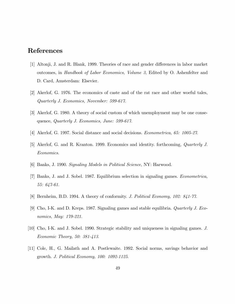
References

[1] Altonji, J. and R. Blank, 1999. Theories of race and gender differences in labor market

outcomes, in Handbook of Labor Economics, Volume 3, Edited by O. Ashenfelter and

D. Card, Amsterdam: Elsevier.

[2] Akerlof, G. 1976. The economics of caste and of the rat race and other woeful tales,

Quarterly J. Economics, November: 599-617.

[3] Akerlof, G. 1980. A theory of social custom of which unemployment may be one conse-

quence, Quarterly J. Economics, June: 599-617.

[4] Akerlof, G. 1997. Social distance and social decisions. Econometrica, 65: 1005-27.

[5] Akerlof, G. and R. Kranton. 1999. Economics and identity. forthcoming, Quarterly J.

Economics.

[6] Banks, J. 1990. Signaling Models in Political Science, NY: Harwood.

[7] Banks, J. and J. Sobel. 1987. Equilibrium selection in signaling games. Econometrica,

55: 647-61.

[8] Bernheim, B.D. 1994. A theory of conformity. J. Political Economy, 102: 841-77.

[9] Cho, I-K. and D. Kreps. 1987. Signaling games and stable equilibria. Quarterly J. Eco-

nomics, May: 179-221.

[10] Cho, I-K. and J. Sobel. 1990. Strategic stability and uniqueness in signaling games. J.

Economic Theory, 50: 381-413.

[11] Cole, H., G. Mailath and A. Postlewaite. 1992. Social norms, savings behavior and

growth. J. Political Economy, 100: 1092-1125.

49

[12] Fordham, S. and J. Ogbu. 1986. Black students� school success: coping with the �Burden

of Acting White�. The Urban Review, 18: 176-206.

[13] Hollander, H. 1990. A social exchange approach to voluntary cooperation. American

Economic Review, 80: 1157-67.

[14] Jones, S. 1984. The Economics of Conformism, Oxford: Blackwell.

[15] Kandel, E. and E. Lazear. 1992. Peer pressure and partnerships. J. Political Economy,

100: 801-17.

[16] Kandori, M. 1992. Social norms and community enforcement. Review of Economic Stud-

ies, 59: 63-80.

[17] Lindbeck, A. and J. Weibull. 1999. Social norms and economic incentives in the welfare

state. Quarterly J. Economics, February: 1-35.

[18] Lundberg, S. and R. Startz. 1983. Private discrimination and social intervention in

competitive labor markets. American Economic Review, 73: 340-47.

[19] Milgrom, P. and S. Oster. 1987. Job discrimination, market forces and the invisibility

hypothesis. Quarterly J. Economics, August: 453-76.

[20] Ogbu, J. 1991. Low performance as an adaptation: the case of Blacks in Stockton,

CA. in Minority Status and Schooling, Edited by M. Gibson and J. Ogbu, NY: Grand

Publishing.

[21] Spence, M. 1974. Market Signaling. Cambridge: Harvard University Press.

[22] Suskind, R. 1998. A Hope Unseen. NY: Broadway.

50

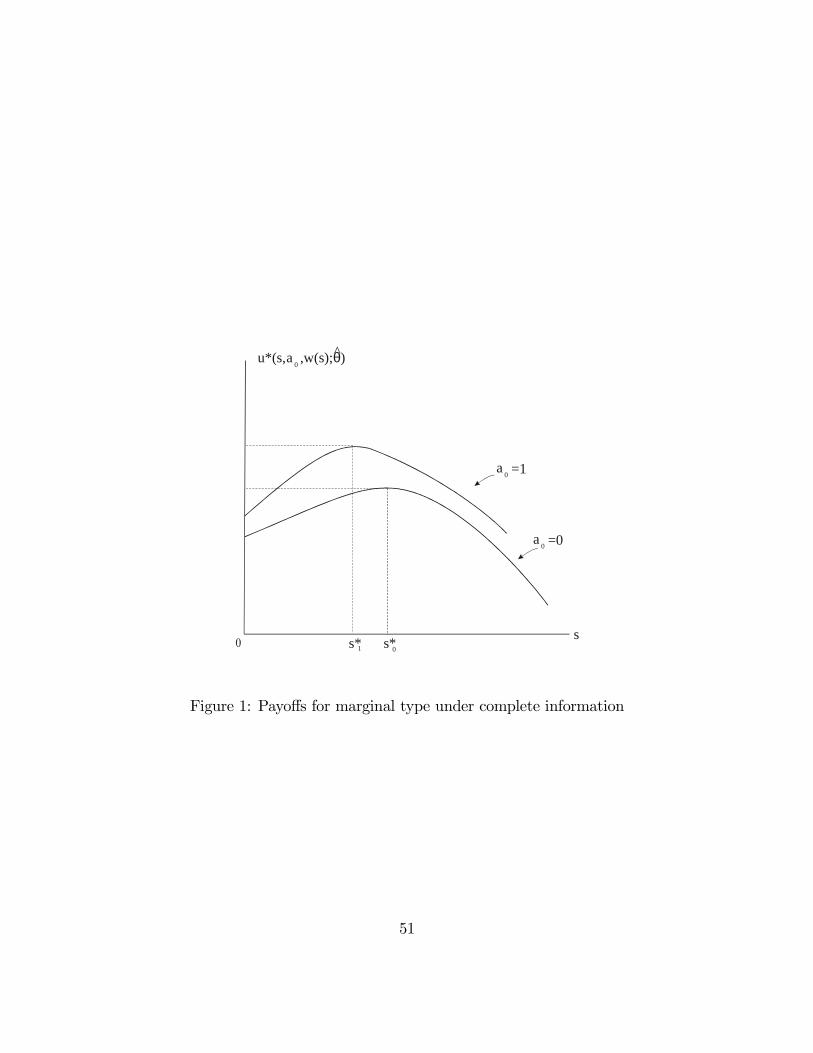
0a =0

0a =1

ss*1 s*0

u*(s, ,w(s); )θ0

a ^

Figure 1: Payoffs for marginal type under complete information

51

θ

σ*

θ*θ̂( )δAccepted types ][

Figure 2: Typical D1 peer pressure equilibrium strategies, (σ∗,α∗0)

52

δ�

θ δ*( ;s )�

θ δ*( ;0)

θ δ( )�^

θ δ( )^

θ δ*( ;s )� �θ δ*( ;0)�

θ δ( )�^

θ

δδ�

Figure 3: Existence of D1 peer pressure equilibria

53

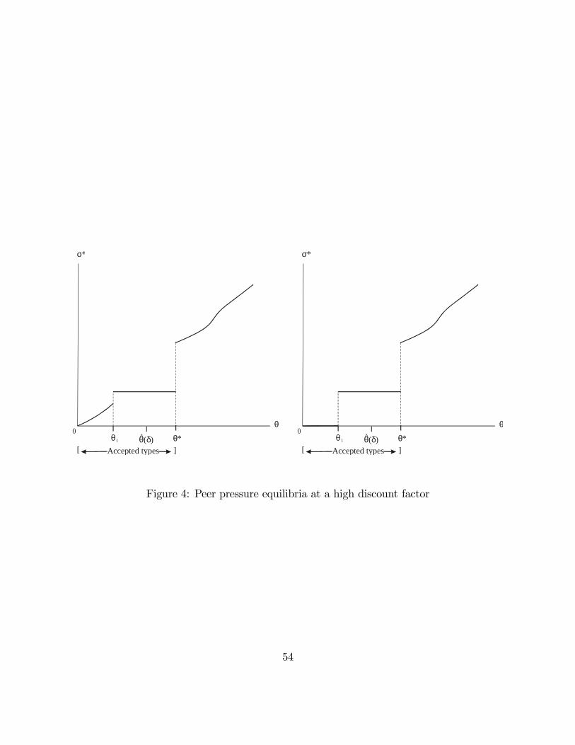
θ

σ*

θ*θ̂( )δθ1

Accepted types ][

θ

σ*

θ*θ̂( )δθ1

Accepted types ][

Figure 4: Peer pressure equilibria at a high discount factor

54