PEAT8002 - SEISMOLOGY Lecture 9: Anisotropy, …rses.anu.edu.au/~nick/teachdoc/lecture9.pdf ·...

PEAT8002 - SEISMOLOGYLecture 9: Anisotropy, attenuation and

anelasticity

Nick Rawlinson

Research School of Earth SciencesAustralian National University

AnisotropyIntroduction

Most of the theoretical development in the previouslectures has assumed that seismic waves propagatethrough an Earth that is made up of isotropic, linearlyelastic material.The assumption of isotropy means that the elastic modulicijkl reduces to two independent constants λ and µ, whichmeans that the elastic properties at a given point in themedium are the same in all directions.Although there can be up to 21 independent elasticconstants, any material with more than two is consideredanisotropic.In many cases, the assumption of isotropy is acceptable,but as we gradually refine our understanding of Earthstructure and composition, the need to consider the effectsof anisotropy becomes more important.

AnisotropyTransverse isotropy

Since only 21 of the 81 elastic constants cijkl areindependent, it is possible to reduce the 3× 3× 3× 3tensor to a 6× 6 symmetric matrix Cmn:

{cmn} =

c1111 c1122 c1133 c1123 c1113 c1112c2211 c2222 c2233 c2223 c2213 c2212c3311 c3322 c3333 c3323 c3313 c3312c2311 c2322 c2333 c2323 c2313 c2312c1311 c1322 c1333 c1323 c1313 c1312c1211 c1222 c1233 c1223 c1213 c1212


Which can also be written:

{Cmn} =

C11 C12 C13 C14 C15 C16C21 C22 C23 C24 C25 C26C31 C32 C33 C34 C35 C36C41 C42 C43 C44 C45 C46C51 C52 C53 C54 C55 C56C61 C62 C63 C64 C65 C66

For an isotropic material, cijkl = λδijδkl + µ(δikδjl + δilδjk ), so:

{Cmn} =

λ + 2µ λ λ 0 0 0λ λ + 2µ λ 0 0 0λ λ λ + 2µ 0 0 00 0 0 µ 0 00 0 0 0 µ 00 0 0 0 0 µ


Transverse isotropy occurs for a stack of layered material,and is otherwise known as radial anisotropy. Each layer isisotropic, but these properties differ between layers.An axis of symmetry can be defined, which isperpendicular to the layers. Displacement of the medium inany direction perpendicular to this axis is identical underrotation.For a wave propagating perpendicular to the axis ofsymmetry, the component of the shear wave oscillatingwithin the plane of the layers can travel at a different speedto the component oscillating across the layers.


Axi

s of

sym

met

ry

xz

y

Direction of wave propagation

z

y

xPSS


A transversely isotropic material can be characterised by 5independent elastic coefficients A,C,F, L and N. For an axisof symmetry in the z-direction (subscripts 1, 2 and 3correspond to x , y and z directions), the matrix coefficientbecomes:

{Cmn} =

A A− 2N F 0 0 0A− 2N A F 0 0 0

F F C 0 0 00 0 0 L 0 00 0 0 0 L 00 0 0 0 0 N

Compared to the isotropic case, the terms that differinvolve the z-direction, which has a different elasticresponse to stress applied parallel to the xy plane.


By analogy to the isotropic case, A corresponds to λ + 2µin the x-direction, N corresponds to µ in the y direction,and L corresponds to µ in the z direction. Thus, the bodywavespeeds that characterise horizontal wave propagationare:

Px =

√Aρ

, Sy =

√Nρ

, Sz =

√Lρ

If P- and S-waves propagate parallel to the axis ofsymmetry, then Sx = Sy , and C corresponds to λ + 2µ inthe z direction (i.e. Pz =

√C/ρ)

In many applications, the horizontally layered Earthexhibits transverse isotropy about a vertical axis. Both SHand Px waves tend to travel faster than SV and Pz wavesrespectively, because they preferentially sample the fastlayers, rather than evenly sampling all layers.

AnisotropyAzimuthal anisotropy

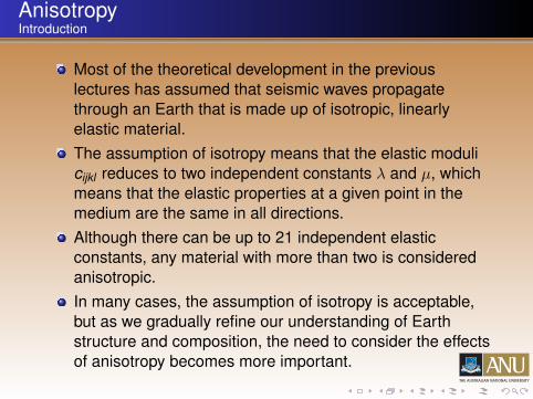
A medium that exhibits azimuthal anisotropy has elasticproperties varying with horizontal direction.In general, P-wave velocity varies with azimuth θ as:

P(θ) = A1 + A2 cos 2θ + A3 sin 2θ + A4 cos 4θ + A5 sin 4θ

where the constants Ai are a function of the 21 elasticconstants.A simple form of azimuthal anisotropy that is oftenassumed in applications is so-called elliptical anisotropy(which is equivalent to transverse isotropy with a horizontalaxis of symmetry). In terms of slowness U, this can bewritten:

U2 = Ux2 cos2 θ + Uy

2 sin2 θ


In the above equation, θ is the ray direction on thehorizontal plane relative to the principal axes in the x and ydirections. Ux and Uy are the corresponding orthogonalcomponents of slowness.

U y

U x

θ

yx

φ


In order to uniquely define the velocity at a point in anelliptically anisotropic medium, one needs to know thevalues of Ux and Uy (equivalent to the lengths of the majorand minor axes of the ellipse), and the angle φ these axesmake with a specified reference frame.There are many known sources of anisotropy within theEarth. These include anisotropy associated withsedimentary layers, flow processes in the asthenosphererelated to plate tectonics, and fluid filled cracks in theupper crust.Beneath Australia, seismic tomography has shown that thefast direction (Uy in the above diagram) of ellipticalazimuthal anisotropy is oriented approximately in thedirection of plate motion. This is probably caused by olivinecrystals in the asthenosphere being aligned in thisdirection.

AnisotropyShear wave splitting

A common technique for studying anisotropy within andbeneath continental lithosphere is called shear wavesplitting.When SKS waves convert from P-waves in the outer coreto S-waves in the lower mantle, the transversedisplacement is entirely polarised in the SV directionWhen these shear waves traverse the mantle and crust,they can be split when travelling through anisotropic media.Assuming elliptical azimuthal anisotropy (or transverseisotropy with a horizontal axis of symmetry), the twopolarised waves travel at different speeds and hence arriveat different times.


R

T

φRadial direction

Tra

nsve

rse

dire

ctio

n

Fast dire

ction

Slow direction

Sx

SyFast polarizationSlow polarization

Split shear waves

δt

From the above diagram, the fast (Sy ) and slow (Sx)components of the S-wave can be written in terms of theradial component (S) in an isotropic Earth as:

Sy (t) = S(t) cos φ, Sx(t) = −S(t − δt) sin φ

where δt is the time shift between the two pulses.


The radial (R) and transverse (T ) components of thesignal can now be written. For the radial component, thecontribution from the fast direction is Sy (t) cos φ, and thecontribution from the slow component is−Sx(t − δt) cos(90◦−φ). Putting these two terms together:

R(t) = S(t) cos2 φ + S(t − δT ) sin2 φ

For the transverse component, the contribution from thefast direction is Sy (t) cos(90◦ − φ), and the contributionfrom the slow component is Sx(t − δt) cos φ. Combiningboth terms yields:

T (t) =[S(t)− S(t − δt)] sin 2φ

2


In the above example, the uncorrected SKS appears onboth the radial and transverse components. Thesecomponents are then rotated to yield the fast and slowpolarisations. The time shift δt is then applied so that Syand Sx are in phases, and the signal is rotated again sothat all of it appears on a single component.

Sy

Sx

Sx Syand in phase


The component perpendicular to this new direction shouldnow be flat-line. In the above example, this is exactly whathappens, which demonstrates the applicability oftransverse isotropy in this case. The particle motion plotsalso reflect the success of the scheme.The polarisation angle φ and time shift δt are found byminimising the transverse signal (see above plot).Typical values for the magnitude of shear wave splitting, δt ,are between 0-2 seconds.Seismic anisotropy within continents is thought to reflectcrystal alignment created during a tectonic episode andthen “frozen in".

Attenuation and anelasticityAttenuation

Anelasticity refers to deviations from pure elasticity, acondition which our derivation of the wave equation carriedout in an earlier lecture assumed.Anelasticity is one reason why seismic waves attenuate, ordecrease in amplitude, as they propagate.In addition to anelasticity, three other processes reducewave amplitude: geometric spreading, scattering andreflection and transmission at a boundary.If the Earth was purely elastic, then seismic waves fromlarge earthquakes would still be reverberating.

Attenuation and anelasticityGeometric spreading

Geometric spreading is the most obvious cause for seismicwave amplitudes to vary with distance.For surface waves on a homogeneous flat Earth, thewavefront will spread out in a growing ring withcircumference 2πr , where r is the distance from thesource. Conservation of energy means that the energy perunit wave front decreases as 1/r , while amplitudedecreases as 1/r .On a global scale, surface waves behave differently due tothe ellipsoid shape of the Earth. In this case, surfacewaves spread out to an angular distance of 90◦, beforerefocusing to converge at an angular distance of 180◦. Theelliptical nature of the Earth, in addition to itsheterogeneity, means that the antipode does not act like asecondary source.


For body waves in a homogeneous medium, energy isconserved on an expanding spherical wavefront withsurface area 4πr2, where r is the radius of the wavefront.The energy therefore decays as 1/r2, and the amplitudedecreases as 1/r .For both surface and body waves, lateral and verticalheterogeneity in the Earth causes propagating wavefrontsto focus and defocus. These effects can result inamplitudes varying significantly along a wavefront.Particularly in the presence of strong lateral variations inwavespeed, multi-pathing can occur. Amplitudes can varyvery strongly when wavefronts self-intersect and formcaustics.

Attenuation and anelasticityScattering

When the seismic wavelength becomes significant incomparison to the scale length of the underlying seismicheterogeneity of the medium, scattering can occur.Strictly speaking, scattering is a finite frequency effect thatis not predicted by conventional asymptotic ray theory.However, whether the effects of velocity heterogeneity areregarded as scattering of energy or multi-pathing of energydepends on the ratio of the heterogeneity size to thewavelength and the distance the wave travels.When heterogeneities are much smaller than thewavelength, they simply change the overall properties ofthe medium.


As seen on the diagram onthe right, diffraction can beviewed as behaviourintermediate betweenscattering andmulti-pathing.Diffraction paths such ashead waves and corediffractions are not trulygeometric, as energy isrequired to follow pathsthat do not obey Snell’slaw.

a = scale length of heterogeneity = wavelengthλL = distance travelled


In some situations, it is possible to view scattering asdeterministic e.g. in reflection seismology, migrationattempts to reverse the effects of scattering and produce aclearer image.In other situations, the medium may contain manyscatterers, in which case their effects on the wavefield canbe considered statistically (e.g. core phases such as PKP).In general, scattering energy results in the arrival of agiven phase having an associated coda i.e. a tail ofincoherent energy that gradually decays over time.In a constant velocity medium, the locus of all possiblescatterers forms an ellipsoid with source and receiver asfoci.


The figure below shows the development of a P-wave codadue to scattering. The first-arrival follows the minimumarrival path according to Fermat’s principle.

Attenuation and anelasticityIntrinsic attenuation

Intrinsic attenuation refers to the gradual depletion ofkinetic energy carried by a seismic wave in the form of heatloss (internal friction) associated with the permanentdeformation of the medium.The small scale mechanisms that can be responsible forthis process include stress-induced migration of mineraldefects, frictional sliding on crystal grain boundaries,vibration of dislocations, and fluid flow across grainboundaries.Intrinsic attenuation is valuable for studying temperaturevariations within the Earth; it tends to vary exponentiallywith temperature, compared to only linearly for seismicvelocities.


In order to better understand the effects of intrinsicattenuation, consider a simple spring, which obeysNewton’s second law F = ma and has a restoring forcedefined by F = −ku, where k is the spring constant and uis displacement from an equilibrium position.Equating these two terms yields:

md2u(t)dt2 + ku(t) = 0

This second order ODE has a general solution of the form:

u(t) = A cos ω0t + B sin ω0t

where A and B are constants, and the mass has naturalfrequency ω0 =

√k/m


Once set in motion, the spring will continue a cycle ofharmonic oscillation forever, because no energy is lost.In a damped system, the damping force has a directionopposite to the instantaneous motion, and we assume thatit is proportional to the velocity du/dt of the body.The resultant force acting on the body is now:

md2u(t)

dt2 + γmdudt

+ ku(t) = 0

By defining the quality factor of the damping as Q = ω0/γ,the above equation can be written:

d2u(t)dt2 +

ω0

Qdudt

+ ω20u(t) = 0


It turns out that there are three possible classes of solutionto the above equation depending on whether the system isoverdamped, underdamped or critically damped.The anelasticity of the Earth is such that it will neverproduce critical or overdamping, so the relevant solution isproduced by the underdamped system:

u(t) = A0 exp(−ω0t/2Q) cos(ωt).

The above displacement corresponds to a harmonicoscillation provided by the cosine term, which graduallydecays according to the exponential term.Q is inversely proportional to the damping factor γ, so thesmaller the damping, the greater the Q.


In the case of the Earth, the attenuation of seismic wavesis often referred to in terms of the quality factor Q or itsinverse Q−1. In many instances, Q−1 is a more convenientterm, as it is directly proportional to the damping.The effects of intrinsic attenuation often differ betweencompressional and shear waves, so it is common to definea quality factor for both P- and S-waves. These are oftenwritten Qα and Qβ.Since the anelastic structure of the Earth is analogous tothe elastic velocity structure, it is often convenient toexpress Q as the imaginary part of c, the velocity. Thisformulation is useful in applications where both velocityand attenuation are treated together (e.g. surface waveinversion).

Attenuation and anelasticityPhysical dispersion

Seismic wave attenuation caused by anelasticity can giverise to physical dispersion, in which waves at differentfrequencies travel at different velocities.This differs from the geometrical dispersion encounteredearlier with surface waves, where waves of differentfrequencies have different apparent velocities at thesurface due to sampling different depths and hencematerials of different velocity.In general, physical dispersion will result in lower frequencywaves travelling more slowly. For example, the travel timeof an ScS phase with a period of T = 40 s may be up to 5seconds slower than the same phase with period T = 1 s.

Attenuation and anelasticityPhysical dispersion

This phenomenon causes a discrepancy between theseismic velocity structure found by inverting observationsof long period normal modes and short-period body waves.The velocities inferred from normal modes are consistentlyslower than those from body waves.Body wave attenuation is often characterised using theparameter t∗, defined as dt∗/dt = 1/Q, so that:

t∗ =

∫1Q

dt

Although the value of t∗ increases with distance, typicalvalues are around 1 s for a P-wave and 4 s for an S-wave.

PEAT8002 - SEISMOLOGY Lecture 9: Anisotropy, …rses.anu.edu.au/~nick/teachdoc/lecture9.pdf ·...

Documents

Transcript of PEAT8002 - SEISMOLOGY Lecture 9: Anisotropy, …rses.anu.edu.au/~nick/teachdoc/lecture9.pdf ·...