PEAR a massively parallel evolutionary computation...

Swarm and Evolutionary Computation 30 (2016) 78–92

Contents lists available at ScienceDirect

Swarm and Evolutionary Computation

http://d2210-65

n CorrStudiesIllinoisStates.

E-mwendyc

journal homepage: www.elsevier.com/locate/swevo

PEAR: a massively parallel evolutionary computation approach forpolitical redistricting optimization and analysis

Yan Y. Liu a,b,e,n, Wendy K. Tam Cho c,d,e, Shaowen Wang a,b,e

a CyberInfrastructure and Geospatial Information Laboratory and Department of Geography and Geographic Information Science, 605 East SpringfieldAvenue Champaign, IL 61820, United Statesb CyberGIS Center for Advanced Digital and Spatial Studies at the University of Illinois at Urbana-Champaign, 1205 West Clark Street, Urbana, IL 61801,United Statesc Department of Political Science at the University of Illinois at Urbana-Champaign, 1407 W. Gregory Street, Urbana, IL 61801, United Statesd Department of Statistics at the University of Illinois at Urbana-Champaign, 725 S. Wright Street, Champaign, IL 61801, United Statese National Center for Supercomputing Applications at the University of Illinois at Urbana-Champaign, 1205 West Clark Street, Urbana, IL 61801, United States

a r t i c l e i n f o

Article history:Received 7 January 2016Accepted 28 April 2016Available online 26 May 2016

Keywords:Combinatorial optimizationEvolutionary algorithmRedistrictingHigh-performance parallel computingHeuristicsSpatial optimization

x.doi.org/10.1016/j.swevo.2016.04.00402/& 2016 Elsevier Ltd. All rights reserved.

esponding author at: CyberGIS Center for Aand National Center for Supercomputing Appat Urbana-Champaign, 1205 West Clark Stre

ail addresses: [email protected] (Y.Y. Liu),[email protected] (W.K.T. Cho), shaowen@illinoi

a b s t r a c t

Political redistricting, a well-known problem in political science and geographic information science, canbe formulated as a combinatorial optimization problem, with objectives and constraints defined to meetlegal requirements. The formulated optimization problem is NP-hard. We develop a scalable evolutionarycomputational approach utilizing massively parallel high performance computing for political redis-tricting optimization and analysis at fine levels of granularity. Our computational approach is based instrong substantive knowledge and deep adherence to Supreme Court mandates. Since the spatial con-figuration plays a critical role in the effectiveness and numerical efficiency of redistricting algorithms, wehave designed spatial evolutionary algorithm (EA) operators that incorporate spatial characteristics andeffectively search the solution space. Our parallelization of the algorithm further harnesses massiveparallel computing power provided by supercomputers via the coupling of EA search processes and ahighly scalable message passing model that maximizes the overlapping of computing and communica-tion at runtime. Experimental results demonstrate desirable effectiveness and scalability of our approach(up to 131K processors) for solving large redistricting problems, which enables substantive research intothe relationship between democratic ideals and phenomena such as partisan gerrymandering.

& 2016 Elsevier Ltd. All rights reserved.

1. Redistricting

Political gerrymandering in U.S. dates back to at least 1812when the term was coined by the Boston Weekly Messenger in aneditorial cartoon depicting an eccentric election district that borean uncanny resemblance to a salamander, complete with a head,arms, and a tail. That year, the Massachusetts state senate districtswere redrawn under Governor Elbridge Gerry to favor the De-mocratic-Republican party by consolidating the Federalist vote. Byall accounts, the redistricting was successful; while the Federalistswon both the Massachusetts house and the governorship, thesenate remained firmly in the control of the Democratic-Repub-lican party. The practice of bolstering political power by carefully

dvanced Digital and Spatiallications at the University ofet, Urbana, IL 61801, United

s.edu (S. Wang).

orchestrating voters into meticulously crafted districts is as old asthe founding of the country. Even at its nascence, the irony wasglaring; in what is touted as the greatest democracy in the world,politicians are able to essentially hand-pick their voters. It is notalways, as we might presume in a democracy, the voters choosingtheir representative.

Gerrymanders are not looked upon favorably, and the practiceof gerrymandering is obviously controversial, but regulating thepractice has proven quite challenging. Despite general disdain forgerrymandering, its existence as part of American democracy islong-standing. While the Supreme Court has established guide-lines and mandates to protect our democratic system of elections,there are so many ways to draw gerrymanders within the legalconstraints that the phenomenon continues, scarcely impeded byregulation. The tools simply do not exist to conduct the types ofanalyses that are required by the Supreme Court to overturn ger-rymanders. Plainly, adherence to democratic ideals is simpler toarticulate than it is to ensure.

An under-explored vantage point stems from the realizationthat the Supreme Court's vision for regulation is closely aligned

www.sciencedirect.com/science/journal/22106502

www.elsevier.com/locate/swevo

http://dx.doi.org/10.1016/j.swevo.2016.04.004



http://crossmark.crossref.org/dialog/?doi=10.1016/j.swevo.2016.04.004&domain=pdf



mailto:[email protected]




Y.Y. Liu et al. / Swarm and Evolutionary Computation 30 (2016) 78–92 79

with a heavily computational analytic approach. The natural fit of acomputational approach and the legal mandates portends that asignificant gain to the science of redistricting will be realized viacomputational approaches. While others have sought to combinethe insights of operations research approaches with redistricting,the proposed methods have been either computationally in-tractable or exhibited limited computational capabilities, unable tofacilitate advanced quantitative study of the substantive problemat hand. We propose an effective evolutionary algorithm (EA) thatembeds spatial characteristics such as contiguity, compactness,and a hole-free property into the algorithm design. ConventionalEA operators, such as crossover and mutation, can disruptivelybreak spatial constraints such as contiguity and hole-free re-quirements in redistricting plans, making multi-objective optimi-zation even more difficult. We address this issue by efficientlyincorporating the spatial configurations of the underlying problemwithin each EA operator, while still effectively utilizing EA's sto-chastic manner for exploring the solution space. As a result, oursequential EA outperforms other selected heuristic algorithms(e.g., simulated annealing, tabu, and GRASP) in the literature foridentifying better solutions in less time in our case study of re-districting in North Carolina.

Our Parallel Evolutionary Algorithm for Redistricting, PEAR, isdesigned to tackle computational complexity and meet the chal-lenge of generating a large number of districting plans for analysis.The scalability of PEAR to both the problem size and the number ofprocessors is achieved by coupling the EA with a highly scalableparallel EA message passing framework. PEAR scales up to 131Kprocessors and efficiently leverages the massive computing powermade available from national cyberinfrastructures such as the BlueWaters supercomputer.1 This parallel computing solution collec-tively evolves independent EA instances through periodic migra-tions. A non-blocking asynchronous migration mechanism elim-inates the global communication barrier and the resulting sig-nificant communication cost in massively parallel computing en-vironments. The scalability of our algorithm brings two desirablebenefits for redistricting analysis. First, as the number of pro-cessors increases, our algorithm identifies solutions with higherquality. Second, larger numbers of processors provide a larger poolof good and feasible solutions, which in turn enables insightfulstatistical analysis of redistricting phenomena. To the best of ourknowledge, PEAR is the first redistricting algorithm that is scalableto over a hundred thousand processors.

This paper is organized as follows. In Section 2, we situate ourcontribution within the previous literature, which has broachedmany different aspects of the problem including heuristic ap-proaches, the consideration of spatial characteristics in redistrict-ing, as well as parallel evolutionary computation. In Section 3, weformally define the redistricting optimization problem and de-scribe how our problem formulation can be adapted to the man-dates of the Supreme Court. Section 4 presents the evolutionaryalgorithm and its associated EA operators. Section 5 presents theparallelization of the proposed evolutionary algorithm and dis-cusses the strategy for improving the efficiency of our algorithmcomputation in a massively parallel computing environment.Section 6 presents experiments and results to evaluate our se-quential algorithm by comparing it with previously proposedheuristic approaches in the literature. The results of scalabilityanalysis on the parallel EA are then presented. We also describethe application of our approach for studying the partisan gerry-mandering phenomenon. Finally, in Section 7, we discuss theimplications of our approach for the practice of redistricting.

1 http://bluewaters.ncsa.illinois.edu.

2. Literature review

Full enumeration approaches. The use of computers for redis-tricting was advocated many years ago [53,43,54]. The 1960s sawthe advent of early computer programs for this purpose[43,24,52,18]. The first explorations of this type focused on fullenumeration approaches where the objective was to examine allpossible redistricting maps in order to contextualize the currentplan as simply one plan among a large number of other possibi-lities [17,23,46,50,48]. Because the redistricting problem is socomputationally complex, the applications for this approach werefor only very small redistricting problems. Indeed, the im-plemented methods are infeasible and not generalizable for anyproblem of practical size. In the 1960s, though enthusiasm washigh, progress was essentially halted by computing technologythat was insufficiently advanced to permit nuanced and helpfulguidance for actual redistricting problems.

Simulation approaches. The goals and research design for thelatest round of redistricting research have followed the 1960sagenda closely. We are still enthralled by the full enumerationapproach but are mindful that the computing capacity to achievethis goal still eludes us. As a result, research has re-focused on anobtainable and more feasible objective in the current computingenvironment. Instead of a full enumeration, the literature hasshifted toward methods that are able to provide a large number ofpossible maps. The goal is to create a decision support system thatallows one to contextualize a particular redistricting map bycreating an ability to understand a range of possible redistrictingmaps for a particular geographic area.

Cirincione et al. [8] attempt to derive a sampling distribution ofmaps. They utilize four different algorithms for generating plans: acontiguity algorithm, a compactness algorithm, a county integrityalgorithm, and a county integrity and compactness algorithm.Their four algorithms all begin by randomly selecting a blockgroup to serve as the “base” of the first district. In the next step,depending on the algorithm, some criteria are used to select anunassigned contiguous unit to expand the district. This process isrepeated until the population of the district reaches a desired size.The next district begins with the random selection of a blockgroup from those adjacent to one of the completed districts. In all,they examine 10,000 of these generated plans (2500 from each ofthe four algorithms). Others have implemented a similar approachwhere districts are created by choosing an adjacent unassignedunit, considering the criteria of equal apportionment, contiguity,and compactness, though they produce a considerably smallernumber of simulated maps. Chen and Rodden [7] appraise only asmall and limited number of different plans (25, 250, and 200different plans) to investigate questions of partisan bias in differ-ent states.

Integer programming and heuristics. Another strand of the lit-erature capitalizes on the operations research literature on searchheuristics. The gain here is rather than simply simulating mapsthat satisfy a minimal legal standard, one can search the space oflegally viable maps and identify those that exhibit desirablecharacteristics. After all, the public, politicians, and the courts areinterested in maps that have a positive impact on democratic rule,not simply maps that unintelligently satisfy a minimum set of legalguidelines. In this vein, various integer programming approacheshave been implemented. Mehrotra et al. [40] developed a branch-and-price methodology. Macmillan and Pierce [38] implemented asimulated annealing algorithm for redistricting. Implementing agood search heuristic is non-trivial given the astronomically largenumber of feasible maps. Indeed, because of the computationalcomplexity, Mehrotra et al. [40] were only able to apply their al-gorithm successfully to county-level data from South Carolina.Likewise, while Macmillan and Pierce [38] restricted their

http://bluewaters.ncsa.illinois.edu

2 The numbers are taken from the 55 counties and 6 congressional districts inWest Virginia, USA.

Y.Y. Liu et al. / Swarm and Evolutionary Computation 30 (2016) 78–9280

algorithm to county data from Louisiana, Maine (16 counties and2 districts), and New Hampshire (10 counties and 2 districts), theyfound the run times to be “intolerably long.” Altman and McDonald[5] implement four metaheuristics: simulated annealing, greedysearch, tabu search, and greedy randomized adaptive search[12,21,19,11]. The authors state that their program “may yield auseful improvement over the starting map and may further enablethe public to generate constitutionally viable plans.” They alsostate that additional computational power may be needed andmay be achieved in a parallel computing environment by using thesnow package to run their R code. They do not present results froman actual redistricting application.

Spatial characteristics. Preserving contiguity, compactness, po-litical subdivisions and majority-minority groups requires properrepresentation of geographic information systems (GIS) data andmaintenance of the proper spatial and geometric properties. Indesigning a search heuristic, care must be taken to store the ne-cessary spatial and geometric attributes in appropriate datastructures (e.g., graphs) since maintaining these spatial char-acteristics has an impact on virtually all of the operations. Forinstance, the contiguity constraint influences the choice of newsolution generation and evaluation. Izakian and Pedrycz [29] use aspatial scanner to search a map for clusters in their particle swarmoptimization algorithm and had to check the contiguity of eachcluster when using centroid to include regions. In EA, traditionalbinary string genetic algorithm (GA) operators (e.g., crossover andmutation) tend to produce non-contiguous solutions [37]. Unlessusing a penalty function, non-contiguous solutions have to beavoided by using either contiguity-preserving operators or repairfunctions [41]. Xiao [55] summarized both approaches and appliedthem in a small redistricting case study. In [55,56], the mutationoperator is designed to maintain contiguity by changing either theshape or the location of a set of contiguous and moveable units.For crossover, since redistricting is similar to graph partitioning,crossover operators designed for graph partitioning, such as thosein Galinier and Hao [15], can be used in EAs for redistricting [55].The crossover and mutation repair strategies in Xiao [55], how-ever, are inefficient for large redistricting problems because theyinvolve costly and non-deterministic randomized trials and extraspatial and geometrical operations. Moreover, repairing contiguityis also likely to adversely affect gains in other objectives andconstraints such as population deviation and competitiveness.

Parallel evolutionary computation. The structure of EA/GA isfortuitously highly adaptable for exploiting high performance andparallel computing resources for the stochastic and iterative evo-lutionary computation. Basic EAs/GAs evolve an initial populationthrough a “survival of the fittest” rule via a set of standard sto-chastic operators, i.e., selection, crossover, mutation, and replace-ment [27,13,21]. In a parallel computing environment, a popula-tion may be naturally divided into a set of sub-populations (alsocalled demes or islands) that evolve and converge with a sig-nificant level of independence. In this vein, various parallel EAs(PEAs) have been developed and applied to a broad and rich set ofapplication domains [4,33,28,26,47,42]. Alba and Troya [2] showedthat PEA not only improves computational efficiency over se-quential EAs, but also facilitates more extensive exploration of thesolution space, resulting in a larger and better set of solutions.Ocenasek and Pelikan [44] analyzed the complexity and scalabilityof parallel estimation of distribution algorithms, a new paradigmof evolutionary algorithms. Though much efficiency can be gainedwith additional processors, one must also be wary of the sub-stantially increasing communication costs that arise with addi-tional processor cores [30,10]. Synchronized migration has beenlinked to serious performance degradation on PEAs. As a result,asynchronous inter-deme interactions have been recognized asdesirable for designing scalable PEAs [1,3,25,35].

In summary, computational complexity is formidable and amajor bottleneck for redistricting analysis. A full enumeration ofplans is still not possible, and investigations at fine levels of geo-graphic granularity have proven exceedingly difficult. How totraverse the space of possible redistricting maps is not straight-forward. The availability of massive computing power provided bysupercomputers provides an avenue for the development of scal-able heuristics that are able to efficiently exploit massively parallelhigh-end computing resources to find better solutions and create alarge number of unique feasible solutions for further statisticalstudy. This is the task that we tackle here. We develop a highlyscalable parallel evolutionary computation approach that in-telligently explores the space of possible maps and efficiently ex-tracts high quality feasible maps that satisfy flexible redistrictingcriteria.

3. Redistricting analysis: a new computational approach

Drawing electoral maps amounts to arranging a finite numberof indivisible geographic units of a study area (e.g., a U.S. state)into a small number of larger areas. For simplicity, call the formerunits, the latter districts or zones, and the study area region. Sinceevery unit must belong to exactly one district, a districting map isa partition of the set of all units into a pre-established number ofnon-empty districts. The redistricting problem is an application ofthe set-partitioning problem that is known to be NP-complete and,thus, computationally intractable [16]. The total number of possi-ble maps when drawing K districts using N units is a Stirlingnumber of the second kind, ( )S N K, , defined, combinatorially, as thenumber of partitions of an N-element set into K blocks [31]. Evenwith a modest number of units, the scale of the unconstrainedmap-making problem is awesome. If one wanted to divide N¼55units into K¼6 districts, the number of possibilities is ×8.7 1039, aformidable number.2 At the census block level, California has710,145 census blocks for 53 districts. Pointedly, the number ofpossibilities in actual redistricting problems is of staggering pro-portions, creating a prohibitively large computational problem.The large problem size and the computational complexity involvedwhenworking with fine-grained redistricting data has plagued theprogress of tool development for redistricting analysis.

3.1. Problem formulation

Solution space. The solution space in a redistricting problem isnot characteristic of a rugged solution space. While the spacelandscape is hilly in the sense that it has the usual peaks andvalleys, these peaks and valleys are not a rapid succession ofprecipices, but instead, a series of vast plateaus, and hence, notrugged in the traditional sense. These expansive plateaus manifestthemselves throughout the landscape because many possible re-districting plans are extremely similar—it is readily evident thatmoving a single census block from one district to another does notinduce much change, and there are a slew of such minor mod-ifications to any redistricting plan. This idiosyncratic surface typecoupled with the prohibitive size of the solution space behooves atailored search algorithm that is able to make large moves withinthe solution space and has some mechanism to guide the searchtoward distinct areas in the solution space.

Problem variables. The goal of the redistricting problem is toidentify a plan that optimizes one or more selected objectives (e.g.,competitiveness, safe districts, and incumbent protection) while

3 The user may decide how best to measure partisan bias (with registrationdata, turnout data, presidential vote data, etc.), a substantive debate on which wetake no position.


simultaneously satisfying legal constraints (e.g., contiguity andequipopulous districts). There are many ways to specify an ob-jective function. A linear programming formulation of the problemmight proceed as follows. We have a set of N geographic units,

…u u u, , , N1 2 , that we wish to partition into a set of K districts/zones, …d d d, , , K1 2 . We can create an ×N N adjacency matrix, C, toindicate the adjacency of the various units, where the entries aredefined as

⎧⎨⎩= =c

i j i j1 if unit and unit are adjacent or

0 otherwiseij

for ≤ ≤i N1 and ≤ ≤j N1 . The convention that =c 1ij for i¼ j isadopted to simplify the checking of connectedness of districts. Thepopulation of the N units is denoted by …p p p, , , N1 2 . So, if thedistricts are equipopulous, then the population in each districtwould be the average population, P , given by

∑==

PK

p1

.i

N

i1

Let X be an ×N K matrix with elements, xik, denoting our decisionvariables. To specify a map, these variables are chosen for ≤ ≤i N1and ≤ ≤k K1 so that

⎧⎨⎩=xu d1 if unit is assigned to district

0 otherwise.ik

i k

The population in district k is then

∑= = …=

P x p k Kfor 1, 2, , .ki

N

ik i1

Constraints. We have constraints of at least three types.

1. Each unit must be assigned to exactly one district,

∑ = = …=

x i N1 for 1, 2, , .k

K

ik1

2. The maximum population deviation across all K districts is nogreater than a specified value M. That is, for any two districts, diand dj,

∣ − ∣ ≤ = …P P M i j Kfor , 1, 2, , .d di j

To define the population deviation across all districts, we mayformulate population criteria as

=( ) − ( )

( )pP P

P

max min. 1

kk

kk

This measures the level of population deviation between the setof K districts. When the districts have identical population, p¼0.As their population increasingly deviates from one another, thevalue of p increases. In this formulation, it is possible for p toexceed 1. This occurs when the difference in population be-tween districts is sufficiently large. In these cases, we set p to itsmaximum value, 1, which already represents an extreme po-pulation difference.

3. The units in each district must form a connected set. That is,each unit is accessible from any other in the set via transitionsencoded in the adjacency matrix C.

Other constraints include the hole-free property and com-pactness. The hole-free property requires that no district is whollycontained in another district. Compactness is encouraged andvalued. However, since it is neither uniformly enforced by thecourts nor strictly defined, it has taken on various specifications. Apopular conceptualization, via an area–perimeter criterion, which

compares the perimeter of a shape to the area of the shape, wasfirst proposed by Ritter in 1882 [14]. With the area–perimetercompactness, a circle is the most compact shape and would havean area-to-perimeter ratio or compactness value of 1. The value ofa simple area-to-perimeter ratio would vary with the size of theshape, but we can create a scale invariance by dividing the area bythe square of the perimeter. We may also normalize the measureto have values in the ( ]0, 1 range by including π in the numerator.These changes result in one of the most widely used compactnessmeasures in the area–perimeter class of measures, CIPQ [45], whichis defined as

π= ( )CA

P4

. 2IPQ 2

In our minimization formulation, we use ( − )C1 IPQ as the com-pactness measure. There are many ways to constrain shape ordefine compactness. An area–perimeter approach is only one suchmethod. A shape may also be compared to a reference shape. Wemight use geometric pixel properties. Alternatively, other criteriamay be based on the dispersion of elements in the area [34].

Objectives. Subject to the constraints above, we seek to optimizea single or multiple objectives. In a multi-objective scenario, weimplement a weighted sum to incorporate multiple objectives inour solution fitness evaluation. The particular specification of theobjective function is flexible, simply depending on the particularsubstantive interest. If one were interested in optimizing compe-titiveness, for instance, one might proceed as follows. Let Dk be theDemocratic registration in district k and Rk be the Republican re-gistration in district k for = …k K1, 2, , .3 Assume that a district ismost competitive when Dk¼Rk. When all districts are considered,an overall measure of competitiveness in a map could be calcu-lated as

( )α β= + ( )f T T1 , 3p e

where

⎛⎝⎜⎜

⎞⎠⎟⎟∑

α β

=+

−

= − ≤ ≤ ≤ ≤ ≥

=T

KR

D R

TBK

T T

1 12

,

12

, for 0 0.5, 0 0.5, and , 0.

pk

Kk

k k

eR

p e

1

Here, Tp measures competitiveness as a deviation of the Repub-lican two-party registration from 0.50 in each district and Te is aweighting factor, which captures the differential in the number ofseats won by the two parties. In the formulation for Te, BR is thenumber of districts where Republican registration is larger thanthe Democratic registration; α defines the weight of Te in thecompetitiveness measure; and β is a normalizing constant so thatthe value of f spans the range [ ]0, 1 . For example, since ⎡⎣ ⎤⎦∈T 0, 0.5e

when α = 1, if we set β = 43, then ∈ [ ]f 0, 1 .

This formulation with both the Tp and Te components providestwo layers of differentiation. By making Te a weighting factor forTp, we can simultaneously encourage the average registrationdifferential, Tp, to be small while ensuring that this small differ-ential is spread equally between the parties. Under our formula-tion for competitiveness, when f¼0, Republican registration andDemocratic registration is the same and the number of districtswhere Republicans dominate and the number of districts wherethe Democrats dominate are identical.

Fig. 1. Chromosome encoding.


3.2. Formulation flexibility

The competitiveness, population, and compactness formula-tions are simply one of many ways to define constraints and ob-jectives. One nice feature of our particular measures, shown in Eqs.(1)–(3), is that the values are normalized so that they span thesame [ ]0, 1 interval with 0 being the desired or optimal value.When the criteria are normalized in the same range, it simplifiesthe weight specification in a multi-objective function that en-compasses measures reflecting competing interests that are ide-ally and simultaneously satisfied.

The criteria that are optimized are user-specified and may re-flect any aspect of a redistricting plan that the user finds helpful toconstrain or explore. In one specification, we could considercompetitiveness as the sole objective, and population deviationand compactness as constraints. We may also consider optimizing(as a minimization problem) competitiveness, population devia-tion, and compactness while simultaneously treating populationdeviation as a constraint, by specifying a maximum threshold.While these choices are far from the only way in which one mightguide such a computational model, they comprise reasonable ex-amples of a real-world redistricting scenario that features the in-terplay of political interests and traditional districting principles.Once measures of the individual criteria are specified, the usermay deploy any desired customized notion of how various criteriashould be weighted. These specifications are modular, flexible, andcustomizable across a wide set of preferences, interests, andconstraints.

4 Our algorithm is intended to be utilized at fine levels of granularity (e.g., unitsbeing census tracts or census blocks), however, because it is difficult to visualizethese small units, we illustrate our EA at the county level in this section.

4. Evolutionary algorithm

Once the objective function is specified, we proceed to searchfor solutions that exceed a user-defined threshold of goodness.There are two main criteria for the design of a search algorithm.First, a stochastic element helps the search avoid being trapped inlocal optima. Second, since the solution landscape for redistrictingmaps is characterized by a series of vast plateaus, the algorithmmust be able to make large jumps from one plateau in the solutionspace to another. Evolutionary searches are able to satisfy both ofthese criteria: (1) population-based heuristic search algorithmssuch as EA are always characterized by a strong random/stochasticelement, which helps the search process avoid being trapped inareas with local optima and (2) the crossover and mutation op-erator, in general, are intended to create large movements fromone solution to the next. We develop an EA as a general redis-tricting solver. We employ efficient data structures and designeffective EA operators to achieve these criteria for redistricting andhandle spatial and non-spatial objectives and constraints. Moreimportantly, the parallelization of our EA provides a scalablecomputational approach to employ a large number of processesthat can simultaneously work on many plateaus and jump fromone to another through inter-process communication.

4.1. Encoding and data structure

Similar to conventional binary string encoding, the basic datastructure of the EA, the chromosome, is encoded as an integerarray where each allele, indexed by the unit number, holds thezone (the terms zone and district are interchangeably used here-after) number that is assigned to each of the geographic units. Anexample is displayed in Fig. 1, where we can see, for instance, thatboth geographic units 1 and 2 are assigned to zone 8 while geo-graphic unit 3 is assigned to zone 5. Every geographic unit is as-signed to exactly one zone.

In addition to the binary string encoding of a solution/

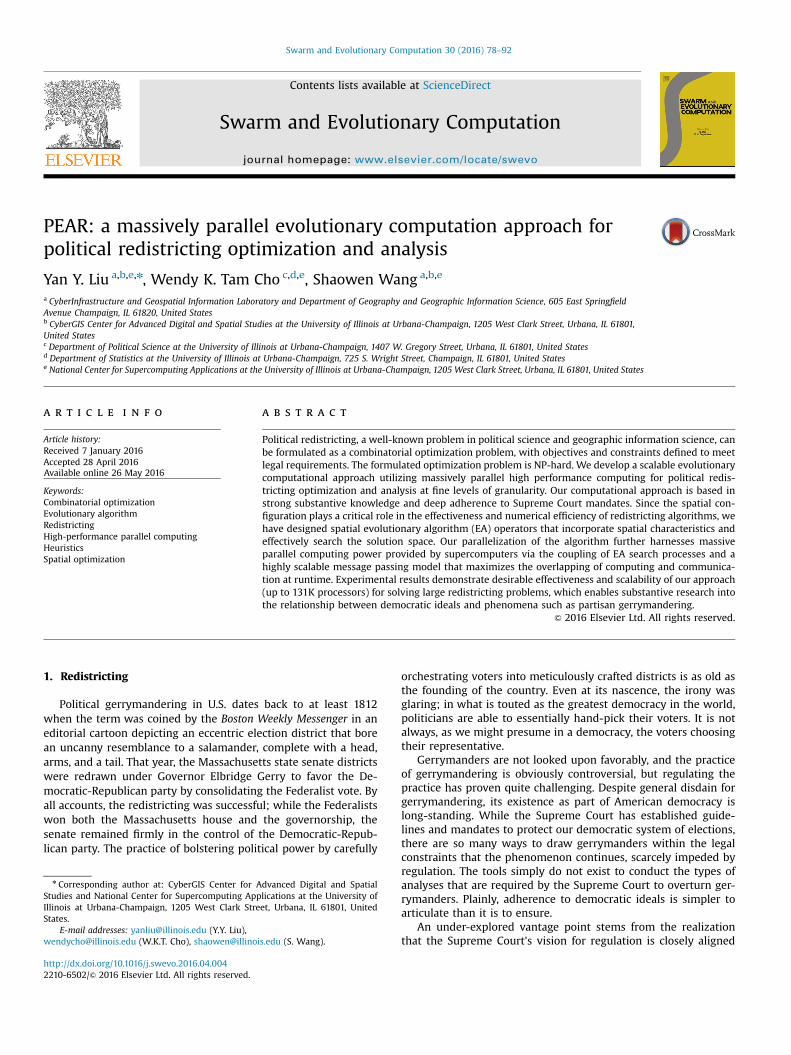
chromosome, we maintain several spatial data structures to enablespatial constraint checking and operations. We store two graphswith auxiliary indexing data: the unit graph and the zone graph.Consider an example redistricting problem derived from parti-tioning the 87 county geographic units in Minnesota into its8 congressional districts. The unit graph, which is also the countymap, is shown on the left in Fig. 2.4 We first convert the geo-graphic data/map into a network graph with vertices and edgeswhere the vertices are the counties and an edge exists whenevertwo geographic units are adjacent. We also define a virtual unit0 which is a polygon derived by subtracting the shape of the re-gion (state) from a rectangle that contains the region border. Unit0 is particularly useful in identifying units on the region border.The adjacency structure is shown on the right in Fig. 2 where theblue lines indicate rook adjacency and the red lines indicate queenadjacency (unit 0 is not shown). Since both rook and queen ad-jacency fall within the legal definition of contiguity, we encompassboth in our adjacency matrix. A zone graph, Gz, which is a ×K K 0–1 matrix, stores the adjacency of the districts. The zone graph isused to check if a district is contained in another district, thuscreating a “hole” in the redistricting map. Similar to the definitionof unit 0, zone 0 is a virtual district on the zone graph that has onlyone unit, which is unit 0. To handle large problems, the unit graphis stored as a linked list, instead of a 2-D array (the number ofedges of a planar graph is a linear factor of the number of vertices).Auxiliary data structures are also used to help accelerate sortingoperations on unit attributes loaded from GIS data.

Operations on the aforementioned data structures form thebasis for handling the spatial configurations of the redistrictingproblem in the EA operators. These operations include, for ex-ample, finding neighborhood units, identifying the border units ofa district, contiguity checking, hole checking at the district level,and compactness updating. We now describe how these opera-tions are designed efficiently to prevent excessively hampering theEA's numerical performance.

Contiguity checking. As we form districts, we must ensure thatall formed districts are contiguous and that all the units withineach district remain contiguous. At the district level, the small sizeof the zone graph makes this check simple and straightforward. Atthe unit level, the check is non-trivial since the associated com-putational cost increases dramatically as the number of unitsgrows. King et al. [32] described this cost and proposed a geo-graph approach to resolve the performance issue. Rather thanperforming the check after a new solution is generated, we adopt astrategy that integrates contiguity checking within the EA opera-tors. The correctness of our strategy is guaranteed by the followingtwo rules:

1. An initial solution satisfies the contiguity constraint; and2. Any changes to the solution created by unit movement (from

one district to another) does not lead to a non-contiguous so-lution.

While the second rule seemingly imposes a strong condition forthe design of EA operators (e.g., crossover and mutation) to satisfy,we find that maintaining contiguity within our EA operators

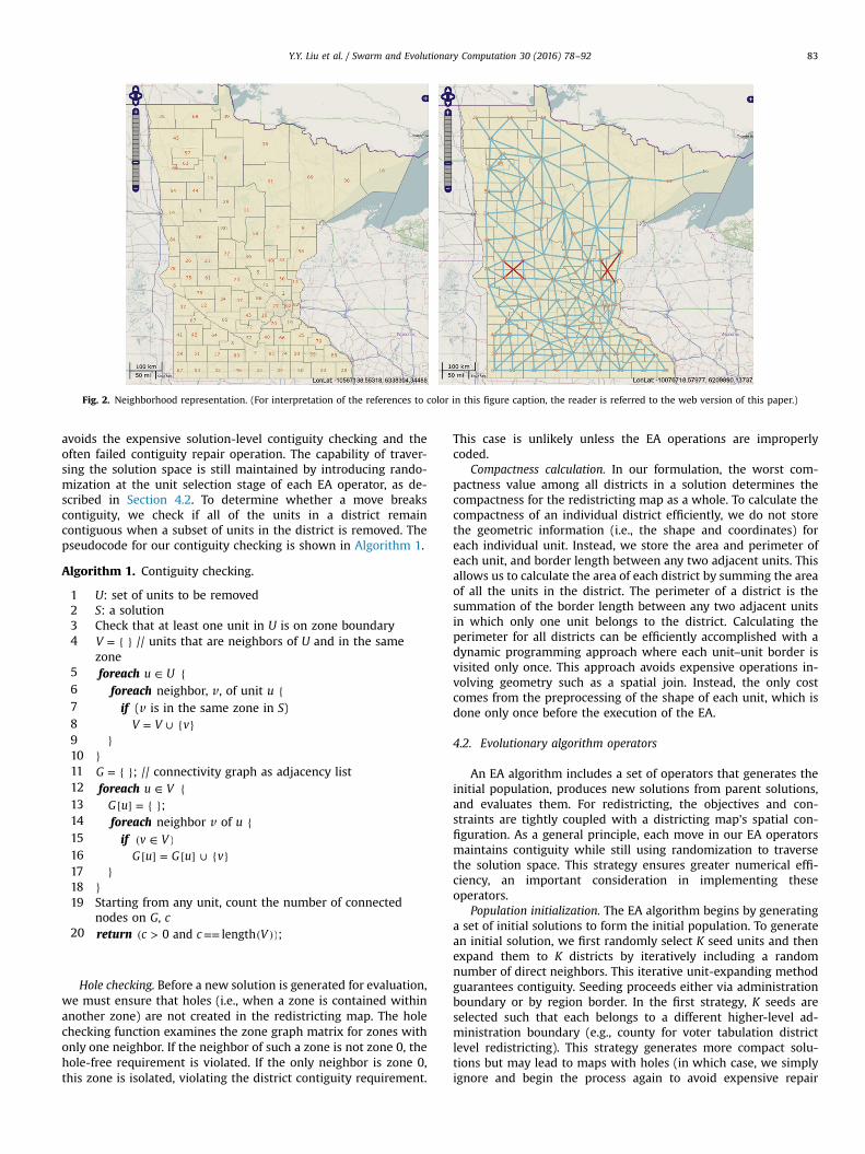
Fig. 2. Neighborhood representation. (For interpretation of the references to color in this figure caption, the reader is referred to the web version of this paper.)


avoids the expensive solution-level contiguity checking and theoften failed contiguity repair operation. The capability of traver-sing the solution space is still maintained by introducing rando-mization at the unit selection stage of each EA operator, as de-scribed in Section 4.2. To determine whether a move breakscontiguity, we check if all of the units in a district remaincontiguous when a subset of units in the district is removed. Thepseudocode for our contiguity checking is shown in Algorithm 1.

Algorithm 1. Contiguity checking.

1234

5678910111213141516171819

U: set of units to be removed
S: a solution Check that at least one unit in U is on zone boundary
= { }V // units that are neighbors of U and in the samezone

∈ {foreach u U
foreach neighbor, v, of unit u {
if (v is in the same zone in S)
= ∪ { }V V v
}
}
= { }G ; // connectivity graph as adjacency list
∈ {foreach u V
[ ] = { }G u ;
foreach neighbor v of u {
if ( ∈ )v V
[ ] = [ ] ∪ { }G u G u v
}
} Starting from any unit, count the number of connectednodes on G, c
( > == ( ))return c c V0 and length ;
20
Hole checking. Before a new solution is generated for evaluation,we must ensure that holes (i.e., when a zone is contained withinanother zone) are not created in the redistricting map. The holechecking function examines the zone graph matrix for zones withonly one neighbor. If the neighbor of such a zone is not zone 0, thehole-free requirement is violated. If the only neighbor is zone 0,this zone is isolated, violating the district contiguity requirement.

This case is unlikely unless the EA operations are improperlycoded.

Compactness calculation. In our formulation, the worst com-pactness value among all districts in a solution determines thecompactness for the redistricting map as a whole. To calculate thecompactness of an individual district efficiently, we do not storethe geometric information (i.e., the shape and coordinates) foreach individual unit. Instead, we store the area and perimeter ofeach unit, and border length between any two adjacent units. Thisallows us to calculate the area of each district by summing the areaof all the units in the district. The perimeter of a district is thesummation of the border length between any two adjacent unitsin which only one unit belongs to the district. Calculating theperimeter for all districts can be efficiently accomplished with adynamic programming approach where each unit–unit border isvisited only once. This approach avoids expensive operations in-volving geometry such as a spatial join. Instead, the only costcomes from the preprocessing of the shape of each unit, which isdone only once before the execution of the EA.

4.2. Evolutionary algorithm operators

An EA algorithm includes a set of operators that generates theinitial population, produces new solutions from parent solutions,and evaluates them. For redistricting, the objectives and con-straints are tightly coupled with a districting map's spatial con-figuration. As a general principle, each move in our EA operatorsmaintains contiguity while still using randomization to traversethe solution space. This strategy ensures greater numerical effi-ciency, an important consideration in implementing theseoperators.

Population initialization. The EA algorithm begins by generatinga set of initial solutions to form the initial population. To generatean initial solution, we first randomly select K seed units and thenexpand them to K districts by iteratively including a randomnumber of direct neighbors. This iterative unit-expanding methodguarantees contiguity. Seeding proceeds either via administrationboundary or by region border. In the first strategy, K seeds areselected such that each belongs to a different higher-level ad-ministration boundary (e.g., county for voter tabulation districtlevel redistricting). This strategy generates more compact solu-tions but may lead to maps with holes (in which case, we simplyignore and begin the process again to avoid expensive repair

Fig. 3. Solution initialization.


procedures). The second strategy randomly selects K seeds on theregion border, which guarantees the hole-free requirement sincedistricts touching the region border cannot be completely sur-rounded by any other district. In the algorithm, a probability valueis specified for each strategy to be applied in the populationinitialization.

The second strategy for initial solution generation is illustratedin the series of maps shown in Fig. 3. We begin by randomlychoosing 8 geographic edge units to be our seeds. An example isshown in the leftmost map of Fig. 3. We then expand these seedsby selecting contiguous units randomly (center map in Fig. 3) untilwe have all 8 connected districts composed of contiguous geo-graphic units in each (rightmost map in Fig. 3). The result is in-serted into the initial population as a feasible solution. This pro-cess is repeated until the initial population is fully populated. Thenumber of solutions in the initial population can be set to anyvalue. The default is 200. The corresponding pseudo-code appearsas Algorithm 2.

Algorithm 2. Generating a feasible contiguous solution.

1234567891011121314151617181920

/
/ choose K initial seeds S = ∅eeds G et the list of units neighboring unit 0, Nv
w
(| | < ) {hile Seeds K Randomly select a unit u from Nv if (u is not selected before)
= ∪ { }Seeds Seeds u
} / / generate a solution from seeds i nt soln [n] // initialized to zeros P ool¼Seeds w ( ≠ ∅) {hile Pool Pop a unit u from Pool
1
Get the neighbors of u, Nu
foreach unit v in Nu {
2 ( [ ] = ∉ )if v v Poolsoln 0 and 3 = ∪Pool Pool v
soln [v]¼soln [u]
4 } 5 } 6 r eturn soln
5 Reynolds v. Sims, 377 US 533 (1964), created the mandate of one man, onevote. Though strict equality is not demanded, there is no de minimus deviation thatis allowable (Karcher v. Daggett, 462 US 725 (1983)), and minimizing the populationinequality is a legal requirement.

21

Fitness evaluation. The fitness value of a solution is the same asthe objective function value, which is flexibility configured to besingle- or multi-objective via a weighted sum formula. Contiguity

and population equality must be satisfied by law.5 We incorporatethis legal requirement by considering a solution to be feasible if itspopulation deviation is below a specified threshold. We oper-ationalize this concept by calculating an unfitness value for each ofour solutions. The unfitness value is zero when the populationequality across the set of districts is within the threshold value andis otherwise the value of the population deviation measure. Sincecontiguity is required for all solutions, non-contiguous solutionsare discarded. In this way, our formulation incorporates con-straints that, unlike the objective, must be satisfied by any solu-tion. Each solution has a fitness and an unfitness value, whichfacilitates flexible replacement strategies (either through a penaltyfunction or other algorithmic logic).

Mutation. The spatial mutation operator is designed to maintaincontiguity while leveraging randomization to select units for dis-trict reassignment. It has two procedures:

1. Shift moves a number of units from one district to a neighboringdistrict. To ensure that a shift does not violate contiguity, theselected units include at least one unit on the boundary of thesending and receiving district.

2. Mutate makes a sequence of shifts to balance metrics such aspopulation deviation. This sequence may have one or morecyclic shifts.

In shift, we randomly select a boundary unit and then expand itrandomly to form a set of units to be moved. In mutate, we ran-domly choose a sequence of districts and randomly choose thenumber of cyclic shifts. The spatial mutation algorithm is outlinedin Algorithm 3. The parameter maxMutUnits is set at runtime.Larger redistricting problems should use a larger value in order toavoid small and ineffective moves.

Algorithm 3. Shifting mutation.

// Multi-unit mutation process that runs K times to make achain of shifts
mutate(solution) { Generate a random sequence s of size K using the Fisher-
Yates algorithm;
foreach zone ∈z s in solution {
if (z is a source zone of previous shifts) continue
if (population in z is below a threshold) continue

7891011

12131415

16171819202122232425


Randomly select a dstZone from neighboring zones of z
shift (z, dstZone)
}
} // Select a subset of units from the source zone to thedestination zone // srcZone: source zone to send the selected units // dstZone: destination zone to receive the selected units shift (srcZone, dstZone) {
1
2
Randomly select up to two adjacent units in srcZonebordering dstZone;

3
subZone¼selected units;
4
| | < {while subZone maxMutUnits
5
Find neighbor units U of subZone;
6
Generate a random number ∈ … | |q U1, 2, , ;
7
Randomly choose a subset ′ ⊂U U , where | ′| =U q; = ∪ ′subZone subZone U .
8
} 9 = ∪dstZone dstZone subZone;
= −srcZone srcZone subZone;
10 } 111213
14

15161718192021

222324

252627

26

Crossover. Just as the conventional mutation operator is notsuitable for spatial configuration, the binary string crossover op-erators must also be modified to take spatial considerations intoaccount. Our crossover operator, shown in Algorithm 4, overlapstwo redistricting maps (e.g., solution A, the first map in Fig. 4 andsolution B, the second map in Fig. 4), resulting in a set of inter-sected subzones/splits, shown in the third map, solution C, inFig. 4. Solution A has districts …A A A, , ,1 2 8. Solution B has districts

…B B B, , ,1 2 8. The third map will have between K and K2 split labels,Cij, where ∈ { … }i A A A, , ,1 2 8 and ∈ { … }j B B B, , ,1 2 8 . That is, eachsplit label is formed from exactly one district from solution A andone district from solution B. However, depending on the districtshapes, different splits may share a common label. We subse-quently relabel them as new splits.

The splits shown in the third map form a new split-level re-districting problem. The number of districts in the new problem isstill K. We form a new solution by treating splits as units via thesame population initialization strategies which will combine thesesplits into a feasible solution of K districts. Since each unit belongsto only one split, it is straightforward to convert this split-levelsolution to the unit level. The new solution is then returned as theoutput of the crossover operator. The last map in Fig. 4 showsSolution D, the map after the crossover. It is worth noting that,while the crossover is able to generate large movements to newsolutions, likely in different parts of the solution space, our em-pirical tests indicate that this process may be sufficiently

Fig. 4. Crossove

disruptive to the desirable attributes of the underlying maps thatthe resulting child map may not be of higher quality than theparent maps. Solution D seems to represent such a case. Accord-ingly, we apply the crossover operator with relatively low prob-ability. This permits larger moves in the solution space whilemaintaining reasonable numerical performance and EAconvergence.

Algorithm 4. Crossover.

r opera

crossover (solution1, solution2) {
// Identify splits by assigning unique index to each split foreach unit u { Calculate split label as z z1 2, where z1 is the zone index
of u
in solution1, and z2 is the zone index of u in solution2
}
Group units with the same split label into the same split,
form set Splits

// handle the case: two geographically separated splitsare assigned with same index

= ∅newSplits
foreach split ∈s Splits {
while ≠ ∅s {
Find a unit u in s, construct a spanning tree in s,
rooted at u
Form a new split ′s to include all of the units on the
spanning tree
= ∪ ′newSplits newSplits s
Remove all the units in ′s from s
}
}

// solve the split-level redistricting problem
Construct split graph (rook and queen neighborhood)
from newSplits
Check holes and repair Formulate a new redistricting problem Generate a solution using the 2nd seeding strategy in the
population initialization operator
Convert split-level solution to unit-level solution soln
return soln
} 28
After the mutation and crossover, a new solution, if its popu-lation deviation is above the defined threshold, goes through afine-tuning procedure that examines the population differencebetween any pair of connected districts by checking the zone

tor.


graph. If necessary, some units are exchanged between a pair ofdistricts to balance the population in a randomized way. The laststep in an EA iteration is to evaluate the resulting solution andapply a replacement strategy to update the population. Both thefitness and the unfitness are considered in the replacementstrategy. An existing solution with the worst fitness or unfitness isreplaced if a new solution is better. If a new solution is better thanthe current best, it becomes the elite solution. Therefore, our EA isa steady-state EA [21] in which each iteration selects two parentsto generate one child for replacement.

5. Parallelization

While the sequential EA algorithm efficiently incorporates thespatial characteristics of the redistricting problem in its formula-tion, the solution space for the redistricting problem is idiosyn-cratic, astronomically large, and characterized by sprawling pla-teaus. Traversal of this type of solution space requires significantcomputation that can be aided by employing parallel computingon a large number of processors. PEAR incorporates a migrationstrategy that exchanges solutions between any two directly con-nected islands (processes) at regular intervals. To ensure eachevolutionary process is independent, each island uses a uniquerandom number sequence generated by SPRNG [39]. The use ofSPRNG in the message passing (MPI) model ensures that no twoprocesses would repeat the same random number sequence(starting two processes with different seeds is not enough sincethey may use the same random number sequence) and, thus, ex-hibit similar search paths when running independently withoutexternal random noise. This is particularly important when a largenumber of processes run in parallel. Liu and Wang [36] develop ascalable PGA library with a suite of non-blocking migration op-erators (i.e., export, import, and inject) to eliminate the need for aglobal barrier in migration communication. PEAR extends this li-brary to enhance the parallelism control by handling application-level sending and receiving buffers for non-blocking messagepassing. The regular migration of elite or random solutions on allof the islands enables simultaneous exploration of a large numberof solution space plateaus as well as movement from one plateauto another through elite solution propagation and the collectivebut independent evolutionary searches surrounding these elitesolutions. The asynchronous migration strategy maximizes the

Table 1PEAR parameter settings.

Parameter Value

Population size per deme 200Initial population 80% by region border, 20% bSelection Binary tournamentSpatial mutation Probability: 0.95; maxMutUSpatial crossover Probability: 0.05Repair District population balancinReplacement Replacing the worst (fitnessElitism YesStopping rules No solution improvement, b

Process topology 2-D TorusNumber of islands per processor 1Process connectivity d 4 (number of direct neighboMigration rate r 2 (number of solutions sentExport interval Mexpt 50 (number of iterations beImport interval Mimpt 25 (number of iterations beSending parallelism 2 (number of exports to invSending buffer size Ksendbuf 2 solutions. Actual memoryReceiving buffer size Kimpt 8 solutions. Actual memoryMulti-objective fitness function Scalability test: ×0.8 compe

overlapping of computation and migration communication andremoves prohibitively costly global synchronization in a massivelyparallel computing environment. Table 1 lists the configuration ofour EA and PEA.

In Liu and Wang [36], the relationship between the config-uration of the PGA parameters (i.e., migration intervals, migrationrate, and topology attributes) and buffer sizes is established basedon the underlying message passing communication library andsupercomputer interconnect characteristics to avoid buffer over-flow issues at the system and application levels. It also providesexplicit programming control on the parallelism of the importoperator by configuring the import buffer size and the interval forinvoking the import operator in GA iterations. Further experi-ments, however, observed MPI communication layer failure whenscaling from 16K processors on the Stampede supercomputer tolarger numbers of faster processor cores on supercomputers suchas Blue Waters (with more than 700K integer cores). With moreprocessors, the outgoing message buffer, controlled by the MPI,experienced buffer overflow as message sending from the exportoperator become seriously skewed among PGA processes due tothe outpaced runtime delays from numerical operations and non-blocking sending and receiving. Consequently, we extended thePGA library to manage the sending buffer at the application leveland explicitly specified the degree of overlapping between EAiterations and message sending. Our enhanced PEA framework isshown in Fig. 5. The improved library has been tested and scaleswell on the Blue Waters supercomputer without failure and withmarginal communication cost. This extension has minimum im-pact on PEAR's numerical performance. The communication costremained consistently at around 0.015% with 16,384 processorcores on Blue Waters. Such scalability provides a dramatic increasein numerical capability, especially notable and consequential sinceexperiments using synchronous migration exhibited an increasedcommunication cost of 41.38%.

6. Evaluation

We evaluate our computational approach from three perspec-tives. First, we examine our base sequential algorithm by com-paring its solution quality to that obtained by other heuristics. Thiscomparison allows us to evaluate the effectiveness and numericalefficiency of our spatial EA operators. Second, we evaluate the

y administration boundary

nits: 15

g on infeasible solutions) or the unfittest

ounded solution quality reached, fixed number of iterations, execution walltime

rs of each process)to neighbors in each export)tween two consecutive exports)tween two consecutive imports)oke before waiting for their finish)requirement is ( × × + _ )n2 4 buffer overhead bytesrequirement is (8�n�4)

+ × _ + ×titiveness 0.2 population deviation 0.3 compactness

inject: random

export

Message Passing Library

Network

Message Passing Library

PEA Library

inject: random

PEA Library

inject: elite

export Redistricting EA

import

Fig. 5. Enhanced PEA framework.


parallel component by examining the scalability of the PEAR al-gorithm by quantifying the numerical work that is completed bydifferent numbers of processors. Third, we take note of the largenumber of feasible solutions that are generated in the scalabilitytest, consider a statistical analysis in the redistricting context, anddiscuss how the maps inform an investigation of partisangerrymandering.

6.1. Implementation and case study

Our EA is implemented in ANSI C. It can be compiled on Linux,OS X, and Windows as a standard makefile project. PEAR uses MPInon-blocking functions (i.e., MPI_Ibsend(), MPI_Iproble()), andregular MPI_Recv() for asynchronous migration. It uses the CSPRNG 2.0 library to provide a unique random number sequencefor each MPI process, which is necessary for running a largenumber of EA iterations. The evaluation of our sequential EA istested on the ROGER supercomputer. The scalability of our code istested against MVAPICH2 with up to 16,384 cores on the Stampedesupercomputer and the Cray MPI with up to 131,072 integer coreson the Blue Waters supercomputer. Each node on ROGER is con-figured with the Intel Xeon E5–2660 processor (2.6 GHz, 20 cores/node). Stampede employs the Intel Sandy bridge processor(2.7 GHz, 16 cores/node). Blue Waters utilizes the AMD Bulldozerprocessor (2.3 GHz, 32 integer cores and 16 floating point coresper node).

Without loss of generality, the data for the empirical evaluationof our algorithm come from North Carolina. Our evaluation is atthe voter tabulation district level (VTD). GIS census data areavailable online for all U.S. states while election results are avail-able at the VTD level for some states. These data include the shape,population, election, and party registration information for eachdistrict. North Carolina provides an especially interesting redis-tricting application because its long history of voting right issueshave helped shape the state of voting rights legislation in theUnited States. Our PEAR solver, however, is general and takes threetypes of inputs: the GIS data, the rook and queen neighborhoodmatrix, and information needed for compactness evaluation (i.e.,area and perimeter information as well as the unit–unit borderlength information). The latter two types of input can be obtainedusing open source GIS libraries such as PySAL (http://pysal.org)and GDAL (http://gdal.org).

6.2. Comparison with other redistricting tools

To evaluate the performance of our EA algorithm and the

effectiveness of the EA operators, we compare our sequential PEARalgorithm to the BARD redistricting software [5]. There are notmany software choices that perform functional automated redis-tricting for realistic redistricting applications [5]. We choose topresent a comparison with BARD v1.2.4 because it is a known Rpackage that provides a set of heuristic algorithms for redistrict-ing. BARD supports methods for generating initial redistrictingplans, including random generation [22], random but contiguousequipopulous districts [8], and simple and weighted k-meansbased generation. In addition, it provides several heuristics to re-fine initial plans, including simulated annealing, greedy search,tabu search, and Greedy Randomized Adaptive Search Procedure(GRASP). BARD formulates objectives and constraints as scorefunctions that can be defined by users. For computational effi-ciency, it employs efficient data structures and native C librariesfor routines which exhibit poor performance in R.

In the BARD implementation, the greedy algorithm is a hill-climbing local search method. The tabu search uses the greedyalgorithm to explore the solution space but maintains a tabu list toavoid duplicating search efforts in similar solution space regions.The GRASP algorithm is a multi-start greedy algorithm with mul-tiple randomly generated starting candidate solutions. Lastly, thesimulated annealing algorithm conducts a probabilistic search ofthe solution space and then conducts another hill-climbing searchafter the annealing process has completed. All of the heuristicscreate new solutions by examining exchangeable units near dis-trict borders through 1- or 2-exchange operations.

When we ran these heuristics, we used a seed solution to beginthe search process. Contiguity is, of course, legally required in theoutput plan. It is worth noting that if the seed solution was notcontiguous, BARD exhibited great difficulty in producing con-tiguous plans during the search. Likely, given the problem size(2690 units), the connectivity graph is too large to allow a fastmerge of any two disconnected subsets of a same district. To by-pass this issue, we generated only randomized contiguous plans toseed the BARD heuristics. In addition, because BARD's im-plementation of the area–perimeter compactness is sufficientlyinefficient to make the computation prohibitively slow, we did notinclude compactness in the specification of the objective function.Instead, the fitness function in this experiment is a weighted sumof the competitiveness and equal population measures. We alsoran two versions of GRASP. The default GRASP setting uses randomsampling, which generated numerous violations of the contiguityrequirement and hence was unable to produce comparable results.To fix this issue, we modified the R code for GRASP to constrain itto use random contiguous samples. This run is reported as “GRASP(contiguous).”

Table 2 displays the results from the five BARD runs and onesequential PEAR run. The best fitness value, the computation time,and the number of iterations required to achieve the best fitnessare measured. Each heuristic ran until either the search convergedor the stopping criteria were met. Both GRASP versions experi-enced long starving times (over 19 h) without improvement afterthe reported best fitness values were found. We had to terminateboth runs manually. Among the five BARD runs, GRASP (con-tiguous) produced the best fitness (0.0411), but it took more than5 h to reach this fitness and was not able to improve upon thisfitness even after an additional 19 h of subsequent searching effort.The simulated annealing algorithm produced the solution with theworst fitness (0.1237), though it took the fewest number of itera-tions. Its iterations were the slowest, taking about a second foreach iteration to complete. The greedy and GRASP (default)heuristics had almost identical performance: while their solutionquality was the second best, they ran more quickly (48.88 and47.72 iterations/second compared to 0.99 iterations/second forsimulated annealing). The solution found by the tabu search is

http://pysal.org

http://gdal.org

Table 2Performance of sequential heuristic algorithms.

Solution quality Cost Cost per improvement

Algorithms Best fitness Competitiveness Equal population Time (in seconds) Iterations Iterations per second Improvements Iterations Time

Simulated annealing 0.1237 0.0696 0.3402 1489.12 1472 0.99 130 11.32 11.45Greedy 0.0980 0.0659 0.2264 3817.91 186,619 48.88 858 217.50 4.45Tabu 0.0984 0.0658 0.2288 1968.94 92,659 47.06 794 116.70 2.48GRASP (default) 0.0980 0.0659 0.2264 3910.87 186,619 47.72 858 217.50 4.56GRASP (contiguous) 0.0411 0.0491 0.0093 19,140.91 320,386 16.74 2075 154.40 9.22PEAR snapshot 1 0.0403 0.0425 0.0316 1555.64 45,358 29.16 44 1030.86 35.36PEAR snapshot 2 0.0326 0.0303 0.0419 3511.02 99,300 28.28 65 1527.69 54.02PEAR snapshot 3 0.0219 0.0199 0.0300 5207.64 150,577 28.91 112 1344.44 46.50PEAR snapshot 4 0.0180 0.0176 0.0198 6746.70 200,653 29.74 121 1658.29 55.76PEAR snapshot 5 0.0167 0.0139 0.0279 8963.47 270,732 30.20 135 2005.42 66.40PEAR final 0.0145 0.0117 0.0256 10,784.55 329,572 30.56 142 2320.93 75.95


slightly worse than the greedy and the GRASP (default) solutions,and took much less time to compute, likely because of the use of atabu list. It, however, suffered from early convergence.

We ran the sequential PEAR algorithm for three hours. Thesequential PEAR run handily outperformed all five BARD runs,obtaining better solution fitness and doing so in much less time. InTable 2, we display snapshot results (every half hour) of PEAR'smetrics beginning after 1555.64 s into the run, at which time thesequential PEAR run identified a solution with fitness value0.0403, which is better than the best result found by any of theBARD runs. As we can see from the snapshots, PEAR continued tosteadily improve its solution quality without early termination or along starving period during which no better solution is identified.The best fitness obtained by the sequential PEAR run is 0.0145,which is significantly better than any of the solutions produced byany of the BARD heuristics.

Table 2 also presents metrics for assessing the numerical effi-ciency as measured by the cost to gain fitness improvement. Wepresent the overall computation cost as well as the computationcost per improvement. Since the iteration speed for the simulatedannealing algorithm was so much slower than the other algo-rithms, its metrics are accordingly affected. For the BARD heur-istics, the tabu search improved the most quickly, finding a bettersolution every 2.48 s. Neither the greedy nor the default GRASPalgorithms was able to identify significant improvements. Whilethey made a number of improvements (858), each improvementwas sufficiently small that they did not make a significant con-tribution to the solution fitness. More pointedly, the total numberof search iterations (186,619) eclipses this relatively small numberof modest improvements. The GRASP (contiguous) run benefitedfrom the multi-start strategy, but took almost 5 h more than PEARto obtain its best solution. In comparison, the sequential PEARalgorithm initially appears to be slow in identifying improve-ments. On average, it took 1030.86 iterations and 35.36 s to makeeach improvement in the first snapshot. However, these im-provements were substantial; the spatial EA operators were ableto make significant gains in solution quality with a relatively smallnumber of improvements. This performance can be attributed totwo specific aspects of the PEAR algorithm. First, unlike the BARDheuristics that concentrate on improving a single solution, theevolutionary process in the sequential PEAR heuristic attempts toimprove an entire population of solutions. The greater populationsize exacts a greater cost in iteration terms. Second, PEAR's moredramatic improvements clearly indicate that its numerical effi-ciency advantage has its roots in the utility of the evolutionaryalgorithm and the effectiveness of its spatial EA operators, notfrom the sheer quantity of iterations per second. Though it becameincreasingly difficult to find better solutions under tighter fitnessthresholds, as evidenced by the increased cost per improvement

shown in the subsequent snapshots, the sequential PEAR none-theless steadily progressed toward better solutions.

In summary, the EA in PEAR was able to find significantly bettersolutions overall, was more effective and efficient in its search, andsteadily improved even at increasingly tighter fitness levels inthese experiments. We attribute the performance differential toour consideration of the redistricting problem as an inherentlyspatial optimization problem, and thus to our design of EA op-erators that explicitly, effectively, and efficiently incorporate spa-tial configurations.

6.3. Scalability analysis

With an effective sequential EA as the base, we now evaluatethe capability of our parallel algorithm to scale its performancewith the number of processors employed. Strong scaling tests,which increase the number of processors while keeping the globalpopulation size intact, are problematic for measuring the perfor-mance of a PGA/PEA because the time taken to reach a solutionquality threshold depends on both the amount of numerical workdone by all of the processors and the stochastic nature of the EAsearch as demonstrated by [36]. Instead, we evaluate the weakscaling of PEAR. In PEAR weak scaling tests, “data size” amounts tothe numerical work done by each process instead of the number ofproblem variables (VTDs). This definition of weak scaling is termed“new-era” weak scaling [49]. Given that Liu and Wang [36] havedemonstrated the advantages of asynchronous migration oversynchronous migration, we use only asynchronous migration forour PEA. In our experiment, the population size of each process isset to 200. The size of the global population across all the pro-cesses is thus 200 times the number of processes. To avoid pre-cision issues for floating point number comparison on fitness, thefitness value of each solution is multiplied by 10,000. The fitnessfunction is a weighted sum of competitiveness, population de-viation, and compactness, as specified in Table 1. Because our EAoperators do not inherently consider compactness, includingcompactness as a weighted component in the fitness functionmakes fitness improvements highly dependent on compactness,allowing us to observe the gains of utilizing more parallel com-puting power in our parallel algorithm that is separate from theefficiency afforded by our spatially cognizant EA operators.

Fig. 6 shows the results of the weak scaling test from a two-hour PEAR run using 32,768, 65,536, and 131,072 integer cores onBlue Waters. The time taken to reach multiple solution qualitythresholds (normalized fitness values; smaller value indicatesbetter solution) is measured. In the plot, the solution thresholdvalues are indicated besides each line/point. The downward slop-ing lines illustrate that for each solution quality threshold, utilizingmore processors generally reduced the amount of time required to

010

0020

0030

0040

0050

0060

00

Number of Cores

Tim

e in

Sec

onds

32,768 65,536 131,072

τ = 3400τ = 3350τ = 3300

τ = 3230

τ = 3200

τ = 3150

τ = 3100

Fig. 6. PEAR weak scaling test results at varying solution quality (fitness) thresh-olds, τ.

6 In creating these maps, we additionally considered population equality,compactness, and contiguity. These histograms are available from the authorsthough not presented here because additional graphs are not necessary to illu-strated the value of our approach and take away from the conciseness of theillustration.


reach each threshold. In addition, as evidenced by the single pointin the upper right of the plot, we were only able to reach thetightest threshold of 3100 when we utilized 131,072 processors.Together, these results indicate that our algorithm scales well withdesirable outcomes as the number of processors increases.

In total, 1,174,702 unique feasible solutions were generated(167,719 from the run using 32,768 cores; 337,165 from the runusing 65,536 cores; and 669,818 from the run using 131,072 cores).The number of feasible solutions increases fairly linearly with thenumber of processor cores. The best solution found using 32,768cores has a fitness value of 3133.98. The best solution found using65,536 and 131,072 cores improved this value to 3,125.88 (8.10less) and 3083.16 (50.82 less), respectively. It is well known that asthe solution fitness approaches the optimal, it becomes muchmore difficult to find better solutions. Accordingly, the benefit ofsolution fitness improvement in this study demonstrates the directbenefit of harnessing more computing power to enhance theproblem solving capabilities of an EA solver.

6.4. Large set of feasible solutions for statistical analysis

Solutions obtained from the scalability analysis are used forredistricting analysis. In cases of partisan gerrymandering, theCourt has made it clear that it has the judicial obligation to de-termine “how much unfairness is too much” (126 S.Ct. at 2638 (n.9)). To fulfill this responsibility, the Court needs data and measuresto assess redistricting maps. Our algorithm generates a largenumber of good solutions, two orders of magnitude more and moreefficiently than any other existing algorithms. Having a largenumber of solutions is essential for understanding redistrictingmaps because it allows us to place any particular map into context.Others have attempted to simulate maps [8,7], though none ofthose attempts even remotely approached the quantity or qualityof the maps created by PEAR.

For this analysis, the existing 2011 Rucho–Lewis plan (shownon the left in Fig. 7) was used as a seed solution for PEAR. Thefigure on the right in Fig. 7 shows one of the initial compact plansthat is generated with our population initialization strategy. Ouralgorithm was able to create more than 1 million reasonably goodand feasible solutions satisfying the defined competitiveness, po-pulation deviation, and compactness principles.

Fig. 8 summarizes the 1,174,702 solutions identified by our al-gorithm on four particular redistricting criteria for quantitativeredistricting research: competitiveness, responsiveness, biased-ness, and vote efficiency.6 Competitiveness measures similarity asa function of relative partisan proportions. Responsiveness andbiasedness are elements from the seats-votes curve [9]. Respon-siveness is a measure of how sensitive seat gains are to changes invote proportion. Biasedness is the condition of favoring one partyover the other and can be described as a deviation from bipartisansymmetry. The efficiency gap captures a difference in wasted votesbetween two parties in an election [51]. The histograms show thedistribution of values of each of the criteria from the 1.1þ millionmaps. The green line shows how the 2001 map fared on eachcriteria while the red line indicates how the current 2011 mapcompares. The distributions allow us to assess whether the ex-isting plans are outliers among other plans that could have beendrawn. We can then understand whether among the possibilities,is this proposed plan particularly unresponsive to voter pre-ferences? Is this proposed plan exceptionally biased toward oneparty? Could we have achieved the goals of this new plan whilemaintaining greater respect for other important criteria or tradi-tional districting principles such as respect for political subdivi-sions or compactness? Is the shift toward a Republican or Demo-cratic bias a function of shifting demographics and populationmigration or are the motivations of the partisan line drawers thedriving force? On the other hand, if the proposed plan is not ex-ceptional in any way but is still biased toward one party, then theCourt may decide that grounds do not exist for revisiting theproposed plan. The pivot lies not within the plan itself or modelsimulations based on one particular plan, but in how that plancompares to other possibilities. Without the ability to generate arange of plans, we would not be able to make reasoned argumentsabout the impact of redistricting on the electoral process. Wewould, moreover, not be able to persuasively make the types oflegal arguments that are required by Supreme Court mandates.Plainly, the ability to generate and analyze a large number offeasible redistricting plans is essential for ensuring our democraticvalues.

Statistical approaches with limited data have been tre-mendously insightful on any number of realms. More recently,with the proliferation of significant computing power, we havediscovered the extensive and often surprising reach of technology,information, and computation into many realms of life. These verysame capacities can shed insight into our governance structures,ideally enabling us to improve our democratic society. This is ourapproach here—to integrate technological advances with our ar-ticulated strategy for analyzing, contextualizing, and under-standing redistricting plans.

7. Discussion

Our computational approach is designed to identify redistrict-ing maps that satisfy a set of user-defined criteria with a particularfocus on addressing fine levels of spatial granularity. We leveragedand enhanced a scalable PGA library to develop PEAR for thecomputationally intensive redistricting problem. By incorporatinga set of spatial configuration operators and spatial EA operators tohandle spatial characteristics and the associated computationalchallenges in the EA search process, and harnessing massive

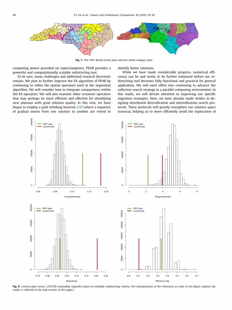
Fig. 7. The 2011 Rucho–Lewis plan and one initial compact plan.


computing power provided on supercomputers, PEAR provides apowerful and computationally scalable redistricting tool.

To be sure, many challenges and additional research directionsremain. We plan to further improve the EA algorithm of PEAR bycontinuing to refine the spatial operators used in the sequentialalgorithm. We will consider how to integrate compactness withinthe EA operators. We will also examine other crossover operatorsthat may perhaps be more efficient and effective for identifyingnew plateaus with good solution quality. In this vein, we havebegun to employ a path relinking heuristic [20] where a sequenceof gradual moves from one solution to another are vetted to

Competitiveness

0.00 0.05 0.10 0.15 0.20

050

000

1000

0015

0000

2000

00

2001 plancurrent plan

Biasedness

-0.10 -0.05 0.00 0.05 0.10 0.15 0.20 0.25

050

000

1000

0015

0000

2000

00


Fig. 8. Current plan versus 1,174,702 reasonably imperfect plans on multiple redistrictireader is referred to the web version of this paper.)

identify better solutions.While we have made considerable progress, numerical effi-

ciency can be and needs to be further enhanced before our re-districting tool becomes fully functional and practical for generalapplication. We will exert effort into continuing to advance thecollective search strategy in a parallel computing environment. Inthis realm, we will devote attention to improving our specificmigration strategies. Here, we have already made strides in de-signing distributed diversification and intensification search pro-tocols. These protocols will greatly strengthen our solution spacetraversal, helping us to more efficiently avoid the exploration of

Responsiveness

0 2 4 6 8

050

000

1000

0015

0000

2000

00 2001 plancurrent plan

Efficiency Gap

-0.8 -0.7 -0.6 -0.5 -0.4 -0.3 -0.2 -0.1

050

000

1000

0015

0000

2000

0025

0000


ng criteria. (For interpretation of the references to color in this figure caption, the


similar solution space regions by multiple processes (i.e., diversi-fication) and allow more computing power to be gathered andfocused on climbing particularly difficult peaks (i.e., intensifica-tion). Generating a large number of maps, which we have nowachieved, is important and fundamental for the subsequent sta-tistical analysis. Indeed, while our work has yielded significantgains, the computational complexity of the redistricting problem isformidable, leaving much progress to still obtain. Nonetheless, wehave laid a foundation with key advancements upon which onecan readily build. We will also extend the current weighted summethod for multi-objective evolutionary algorithm (MOEA)[57,58] to derive the set of pareto front solutions for preference-based decision making support. Our PEA implementation is suffi-ciently general for solving MOEA benchmark problems [59] andother domain-specific problems such as the unit commitmentscheduling problem [60].

In the substantive realm, computational models such as the onedeveloped in this paper, allow us to synthesize and organizemassive amounts of computation and data to evaluate redistrictingschemes and tailor them to notions of “fairness” and democraticrule. Importantly, our model is deeply rooted in the long-standingvalues and goals for democracy in the U.S. as they has been out-lined by the Supreme Court. Our optimization algorithm is notborne out of convenience and ease, but instead, strongly tailoredto the existing social systems and their structures and mechanismsfor securing fairness and transparency in the electoral systems.

While our computational approach is formulated via an opti-mization strategy, our goal is not to seek a perfectly optimizedplan per se because the perfectly optimized plan, while interest-ing, is not necessary, and further, has only limited value. Plainly, itis difficult, and likely impossible to identify the optimal plan giventhe many competing interests in any redistricting effort. No singleplan will satisfy every interested stakeholder—there is no perfectplan. If there is no perfect plan for every constituent, then it makessense that we will instead be choosing from a bounded set of“reasonably imperfect plans” [6]. The discrete optimization fra-mework is ideal as a vehicle for identifying large sets of “reason-ably imperfect” redistricting plans. The set of reasonably imperfectplans is useful at the districting drawing stage as well as for judgeswho are adjudicating the constitutionality of a redistricting plan.At the drawing stage, this information suitably drives an iterativebargaining process whether that process involves partisan legis-lators or members of an independent redistricting commission.When this bounded set of plans can be identified and the elementsof the set have associated indicators of partisan bias, responsive-ness, efficiency gaps, compactness, respect for political subdivi-sions, etc., the redistricting process is imbued with valuablestructure that is otherwise non-existent. That structure alonemakes the redistricting process more transparent and may itselfserve to reduce legal challenges. When a legal challenge ismounted, this large set of reasonably imperfect plans produces therelevant background and allows one to place and understand theproposed plan in context. The purpose of our optimization strat-egy, then, is to search, synthesize, and organize massive amountsof information that will supply a common base of knowledge toguide an informed and intelligent debate.

In our analysis of North Carolina, we acknowledge that ourstatement that the current North Carolina plan is an outlier is anormative statement. We do not intend to and do not imply thatwe are creating any type of hard standard by which to judgewhether a particular plan is an outlier. That type of judgmentshould be left to the Supreme Court. We simply argue that havingand using a computational tool like PEAR is a useful and com-pelling way to examine whether an instance of partisan gerry-mandering has occurred. It provides a much more nuanced andrich analysis than is available with extant tools and notions.

Acknowledgments

This material is based in part upon work supported by theNational Science Foundation (NSF) under Grant 1047916. Anyopinions, findings, and conclusions or recommendations ex-pressed here are those of the authors and do not reflect the viewsof NSF. Computational experiments in this research used the BlueWaters sustained-petascale computing resources, which is sup-ported by the NSF (Grants OCI-0725070 and ACI-1238993) and thestate of Illinois. Blue Waters is a joint effort of the University ofIllinois at Urbana-Champaign and its National Center for Super-computing Applications. The performance study used the ROGERsupercomputer at the University of Illinois, which is supported byNSF (Grant 1429699). The authors also acknowledge the TexasAdvanced Computing Center (TACC) at the University of Texas atAustin for providing HPC resources via the Stampede super-computer that have also contributed to our research results.

References

[1] Enrique Alba, Jose M. Troya, An analysis of synchronous and asynchronousparallel distributed genetic algorithms with structured and Panmictic Islands,in: Jose Rolim, Frank Mueller, Albert Y. Zomaya, Fikret Ercal, Stephan Olariu,Binoy Ravindran, Jan Gustafsson, Hiroaki Takada, Ron Olsson, LaxmikantV. Kale, Pete Beckman, Matthew Haines, Hossam ElGindy, Denis Caromel,Serge Chaumette, Geoffrey Fox, Yi Pan, Keqin Li, Tao Yang, G. Chiola, G. Conte,L.V. Mancini, Domenique MaCry, Beverly Sanders, Devesh Bhatt,Viktor Prasanna (Eds.), Parallel and Distributed Processing, Lecture Notes inComputer Science, vol. 1586, Springer, Berlin, Heidelberg, London, UK, 1999,pp. 248–256.

[2] Enrique Alba, José M. Troya, A survey of parallel distributed genetic algo-rithms, Complexity 4 (1999) 31–52.

[3] Enrique Alba, Jose M. Troya, Improving flexibility and efficiency by addingparallelism to genetic algorithms, Stat. Comput. 12 (2) (2002) 91–114.

[4] Enrique Alba, M. Tomassini, Parallelism and evolutionary algorithms, IEEETrans. Evol. Comput. 6 (5) (2002) 443–462.

[5] Micah Altman, Michael P. McDonald, BARD: better automated redistricting, J.Stat. Softw. 42 (4) (2011) 1–28.

[6] Bruce E. Cain, Redistricting commissions: a better political buffer?, Yale Law J.121 (7) (2012) 1808–1844.

[7] Jowei Chen, Jonathan Rodden, Unintentional gerrymandering: political geo-graphy and electoral bias in legislatures, Q. J. Polit. Sci. 8 (2013) 239–269.

[8] Carmen Cirincione, Thomas A. Darling, Timothy G. O'Rourke, Assessing SouthCarolina's 1990s congressional districting, Polit. Geog. 19 (2) (2000) 189–211.

[9] F.Y. Edgeworth, Miscellaneous applications of the calculus of probabilities, J. R.Stat. Soc. 61 (3) (1898) 534–544.

[10] Ahmad Faraj, Pitch Patarasuk, Xin Yuan, A study of process arrival patterns forMPI collective operations, in: ICS'07: Proceedings of the 21st Annual Inter-national Conference on Supercomputing, ACM, New York, NY, 2007, pp. 168–179.

[11] Thomas A. Feo, Mauricio G.C. Resende, Greedy randomized adaptive searchprocedures, J. Glob. Optim. 6 (1995) 109–133.

[12] M.A. Fleischer, Simulated annealing: past, present, and future, in: Proceedingsof the 27th Winter Simulation Conference, 1995, pp. 155–161.

[13] David B. Fogel, Evolutionary algorithms in theory and practice, Complexity 2(4) (1997) 26–27.

[14] Y.S. Frolov, Measuring shape of geographical phenomena: a history of the is-sue, Sov. Geog. Rev. Transl. 16 (10) (1975) 676–687.

[15] Philippe Galinier, Jin-Kao Hao, Hybrid evolutionary algorithms for graph col-oring, J. Comb. Optim. 3 (4) (1999) 379–397.

[16] M.R. Garey, D.S. Johnson, Computers and Intractability: A Guide to the Theoryof NP-Completeness, W.H. Freeman and Co., New York, NY, 1979.

[17] R.S. Garfinkel, G.L. Nemhauser, Optimal political districting by implicit enu-meration techniques, Manag. Sci. 16 (8) (1970), B-495–B-508.

[18] Burton C. Gearhart, John M. Liittschwager, Legislative districting by computer,Behav. Sci. 14 (5) (1969) 404–417.

[19] Fred Glover, Manuel Laguna, Tabu Search, Kluwer Academic Publishers, Bos-ton, MA, 1997.

[20] Fred Glover, Manuel Laguna, Rafael Marti, Fundamentals of scatter search andpath relinking, Control Cybern. 29 (3) (2000) 653–684.

[21] David Goldberg, Genetic Algorithms in Search, Optimization, and MachineLearning, Addison-Wesley Professional, Reading, MA, 1989.

[22] Bernard Grofman, For single member districts random is not equal, in:Bernard Grofman, Arend Lijphart, Robert B. McKay, Howard A. Scarrow (Eds.),Representation and Redistricting Issues, Lexington Books, Lanham, MD, UnitedStates, 1982.

[23] G. Gudgin, P.J. Taylor, Seats, Votes and the Spatial Organization of Elections,Pion, London, 1979.

http://refhub.elsevier.com/S2210-6502(16)30022-0/sbref1




































































[24] Curtis Harris, A scientific method of districting, Behav. Sci. 9 (1964) 219–225.[25] William E. Hart, Scott B. Baden, Richard K. Belew, Scott R. Kohn, Analysis of the

numerical effects of parallelism on a parallel genetic algorithm, in: IPPS'96:Proceedings of the 10th International Parallel Processing Symposium, IEEEComputer Society, Washington, DC, 1996, pp. 606–612.

[26] J. Ignacio Hidalgo, Francisco Fernandez, Juan Lanchares, Erick Cantú-Paz,Albert Zomaya, Parallel architectures and bioinspired algorithms, ParallelComput. 36 (10–11) (2010) 553–554.

[27] John H. Holland, Adaptation in Natural and Artificial Systems, MIT Press,Cambridge, MA, 1992.

[28] Chun-Hsi Huang, Sanguthevar Rajasekaran, High-performance parallel bio-computing, Parallel Comput. 30 (9–10) (2004) 999–1000.

[29] Hesam Izakian, Witold Pedrycz, A new PSO-optimized geometry of spatial andspatio-temporal scan statistics for disease outbreak detection, Swarm Evol.Comput. 4 (2012) 1–11.

[30] Weihang Jiang, Jiuxing Liu, Hyun-Wook Jin, D.K. Panda, W. Gropp, R. Thakur,High performance MPI-2 one-sided communication over InfiniBand, in: IEEEInternational Symposium on Cluster Computing and the Grid, 2004, CCGrid2004, IEEE Computer Society, Los Alamitos, CA, 2004, pp. 531–538.

[31] M. Keane, The size of the region-building problem, Environ. Plan. A 7 (1975)575–577.

[32] Douglas M. King, Sheldon H. Jacobson, Edward C. Sewell, Wendy K. Tam Cho,Geo-graphs: an efficient model for enforcing contiguity and hole constraintsin planar graph partitioning, Oper. Res. 60 (5) (2012) 1213–1228.

[33] Zdenek Konfrst, Parallel genetic algorithms: advances, computing trends, ap-plications and perspectives, in: 18th International Parallel and DistributedProcessing Symposium, 2004, pp. 162-. http://dx.doi.org/10.1109/IPDPS.2004.1303155.

[34] Wenwen Li, Michael F. Goodchild, Richard Church, An efficient measure ofcompactness for two-dimensional shapes and its application in regionaliza-tion problems, Int. J. Geogr. Inf. Sci. 27 (6) (2013) 1227–1250.

[35] Shyh-Chang Lin, W.F. Punch III, E.D. Goodman, Coarse-grain parallel geneticalgorithms: categorization and new approach, in: Proceedings, Sixth IEEESymposium on Parallel and Distributed Processing, 1994, pp. 28–37.

[36] Yan Y. Liu, Shaowen Wang, A scalable parallel genetic algorithm for the gen-eralized assignment problem, Parallel Comput. 46 (2015) 98–119.

[37] Yan Y. Liu, Wendy K. Tam Cho, Shaowen Wang, A scalable computationalapproach to political redistricting optimization, in: Proceedings of the 2015XSEDE Conference: Scientific Advancements Enabled by Enhanced Cyberin-frastructure, XSEDE'15, vol. 6, ACM, New York, NY, 2015, pp. 1–2.

[38] William Macmillan, Todd Pierce, Optimization modelling in a GIS framework:the problem of political districting, in: Stewart Fotheringham, Peter Rogerson(Eds.), Spatial Analysis and GIS, Taylor & Francis, Abingdon, Oxfordshire,United Kingdom, 1994, pp. 221–246 (Chapter 11).

[39] Michael Mascagni, Ashok Srinivasan, Algorithm 806: SPRNG: a scalable libraryfor pseudorandom number generation, ACM Trans. Math. Softw. 26 (3) (2000)436–461.

[40] Anuj Mehrotra, Ellis L. Johnson, George L. Nemhauser, An optimization basedheuristic for political districting, Manag. Sci. 44 (8) (1998) 1100–1114.

[41] Efrén Mezura-Montes, Carlos A. Coello Coello, Constraint-handling in nature-inspired numerical optimization: past, present and future, Swarm Evol.Comput. 1 (4) (2011) 173–194.

[42] Daniele Muraro, Rui Dilão, A parallel multi-objective optimization algorithmfor the calibration of mathematical models, Swarm Evol. Comput. 8 (2013)13–25.

[43] Stuart S. Nagel, Simplified bipartisan computer redistricting, Stanf. Law Rev. 17(5) (1965) 863–899.

[44] Jiri Ocenasek, Martin Pelikan, Parallel mixed Bayesian optimization algorithm:a scaleup analysis, in: S. Cagnoni (Ed.), Workshop Proceedings of the Geneticand Evolutionary Computation Conference, GECCO-2004, Electronic publica-tion, 2004.

[45] Robert Osserman, Isoperimetric inequality, Bull. Am. Math. Soc. 84 (6) (1978)1182–1238.

[46] L. Papayanopoulos, Quantitative principles underlying apportionment meth-ods, Ann. N. Y. Acad. Sci. 219 (1973) 3–4.

[47] C. Patvardhan, Sulabh Bansal, A. Srivastav, Parallel improved quantum inspiredevolutionary algorithm to solve large size Quadratic Knapsack Problems,Swarm Evol. Comput.

[48] D.J. Rossiter, R.J. Johnston, Program GROUP: the identification of all possiblesolutions to a constituency-delimitation problem, Environ. Plan. A 13 (2)(1981) 231–238.

[49] Vivek Sarkar, William Harrod, Allan E. Snavely, Software challenges in extremescale systems, J. Phys.: Conf. Ser. 180 (1) (2009) 012045.

[50] J.W. Shepherd, M.A. Jenkins, Decentralizing high school administration indetroit: a computer evaluation of alternative strategies of political control,Econ. Geogr. 48 (1) (1970) 95–106.

[51] Nicholas O. Stephanopoulos, Eric M. McGhee, Partisan gerrymandering andthe efficiency gap, Univ. Chic. Law Rev. 82 (2) (2015) 831–900.

[52] James Thoreson, John Liittschwager, Computers in behavioral science: legis-lative districting by computer simulation, Behav. Sci. 12 (1967) 237–247.

[53] William S. Vickrey, On the prevention of gerrymandering, Polit. Sci. Q. 76(1961) 105–110.

[54] J.B. Weaver, S.W. Hess, A procedure for nonpartisan districting: developmentof computer techniques, Yale Law J. 72 (1963) 288–308.

[55] Ningchuan Xiao, A unified conceptual framework for geographical optimiza-tion using evolutionary algorithms, Ann. Assoc. Am. Geogr. 98 (4) (2008)795–817.

[56] Ningchuan Xiao, David A. Bennett, Marc P. Armstrong, Using evolutionaryalgorithms to generate alternatives for multiobjective site-search problems,Environ. Plan. A 34 (4) (2002) 639–656 (hURL i).

[57] A. Zhou, B.-Y. Qu, H. Li, S.-Z. Zhao, P.N. Suganthan, Q. Zhang, Multiobjectiveevolutionary algorithms: a survey of the state of the art, Swarm Evol. Comput.1 (1) (2011) 32–49.

[58] Eckart Zitzler, Kalyanmoy Deb, Lothar Thiele, Comparison of multiobjectiveevolutionary algorithms: empirical results, Evol. Comput. J. 8 (2) (2000)173–195 (URL ).

[59] S. Biswas, S. Das, P.N. Suganthan, C.A. Coello Coello. Evolutionary multi-objective optimization in dynamic environments: A set of novel benchmarkfunctions. In 2014 IEEE Congr. on Evol. Comput. (CEC). 3192–3199 http://dx.doi.org/10.1109/CEC.2014.6900487.

[60] A. Trivedi, D. Srinivasan, S. Biswas, T. Reindl. Hybridizing genetic algorithmwith differential evolution for solving the unit commitment scheduling pro-blem. Swarm and Evol. Comput. 23 (2015) 50–64 http://dx.doi.org/10.1016/j.swevo.2015.04.001.























http://dx.doi.org/10.1109/IPDPS.2004.1303155

http://dx.doi.org/10.1109/IPDPS.2004.1303155




































































http://dx.doi.org/10.1109/CEC.2014.6900487

http://dx.doi.org/10.1109/CEC.2014.6900487



PEAR a massively parallel evolutionary computation...

Documents

Transcript of PEAR a massively parallel evolutionary computation...