Available online at www.sciencedirect.com

Journal of the Franklin Institute 352 (2015) 645–668

http://dx.doi.o0016-0032/&

nCorresponE-mail ad

wang.1381@o

www.elsevier.com/locate/jfranklin

Robust lateral motion control of four-wheelindependently actuated electric vehicles with tire force

saturation consideration

Rongrong Wanga,n, Hui Zhangb, Junmin Wangb, Fengjun Yanc,Nan Chena

aSchool of Mechanical Engineering, Southeast University, Nanjing 211189, PR ChinabDepartment of Mechanical and Aerospace Engineering, The Ohio State University, Columbus, OH 43210, USA

cDepartment of Mechanical Engineering Hamilton, McMaster University, Ontario, Canada L8S 4L7

Received 27 January 2014; received in revised form 6 August 2014; accepted 29 September 2014Available online 18 October 2014

Abstract

The paper presents a vehicle lateral-plane motion stability control approach for four-wheel independentlyactuated (FWIA) electric ground vehicles considering the tire force saturations. In order to deal with the possiblemodeling inaccuracies and parametric uncertainties, a linear parameter-varying (LPV) based robust H1controller is designed to yield the desired external yaw moment. The lower-level controller operates the four in-wheel (or hub) motors such as the required control efforts can be satisfied. An analytical method without usingthe numerical-optimization based control allocation algorithms is given to distribute the higher-level controlefforts. The tire force constraints are also explicitly considered in the control allocation design. Simulation resultsbased on a high-fidelity, CarSim, full-vehicle model show the effectiveness of the control approach.& 2014 The Franklin Institute. Published by Elsevier Ltd. All rights reserved.

1. Introduction

Compared to the internal combustion engine powered vehicles, electric vehicles have severaladvantages in terms of energy efficiency, environmental friendliness, performance benefits, and

rg/10.1016/j.jfranklin.2014.09.0192014 The Franklin Institute. Published by Elsevier Ltd. All rights reserved.

ding author. Tel.: þ86 137 7094 6533.dresses: wrr06fy@gmail.com (R. Wang), Huizhang285@gmail.com (H. Zhang),su.edu (J. Wang), yanfeng@McMaster.ca (F. Yan).

R. Wang et al. / Journal of the Franklin Institute 352 (2015) 645–668646

so on [1,2]. Among all the types of electric vehicles, the four wheel independently actuated(FWIA) electric vehicle, in which each wheel is independently actuated with an in-wheel (orhub) motor, is an emerging configuration thanks to the actuation flexibility and fast but stillprecise torque responses of electric motors [1–4].The actuator redundancy of FWIA electric vehicle makes the control of this type of vehicle

rewarding but challenging. Many studies have been carried out on the vehicle motion controlmethods for improving the vehicle stability and maneuverability. However, most of these controlalgorithms are designed for conventional vehicle architectures, but not for the FWIA electricground vehicles. Recently, a few lateral-plane motion control methods have been proposed forelectric vehicles with reductant actuators. For example, a sliding control theory based controlmethod was proposed for a four-wheel driving and four-wheel steering vehicle in [5], althoughan analytic solution of allocating the ground forces was designed, the proposed method relies onthe assumption that the tire force model is accurate and the tire-road friction coefficient (TRFC)is known. Moreover, the tire force saturation was not considered in the control allocation design.An on-line self-evolving fuzzy controller is proposed for autonomous mobile robots to follow amoving object on a desired distance with respect to the leader is designed in [6], the proposedcontroller works well without any pre-training and is capable of adapting the fuzzy rules. A directyaw-moment control system for a FWIA electric vehicle was proposed in [7], a half-vehiclemodel which is a linear approximation of vehicle dynamics was used in the controller design, thetire force saturation was not considered either. A braking control method for electric vehiclewhich was driven by independent front and rear motors was proposed in [8], however the vehiclestability controller design was not reported in the paper. A stability control method for four-wheel driven hybrid electric vehicle was proposed in [9]. As the required torque split for yawmotion control was generated by the rear motor with an electro-hydraulic brake, the controlproblem in [9] is thus different from the one considered in this study.As a typical over-actuated system, FWIA electric vehicles usually adopt numerical-

optimization based control-allocation algorithms such as daisy-chaining, linear programming,nonlinear programming, fixed-point method, and more, to distribute the higher-level controlsignals to the lower-level motors [10–15]. For example, accelerated fixed-point based controlallocation methods were proposed in [12,13], general quadratic programming based on controlallocation was proposed in [14], and rule-based control-allocation method was adopted in [15]. Itis worthwhile to note, however, the numerical-optimization based control-allocation methodsusually have the drawback of high computational requirements, which may discourage their real-time implementations. Therefore, improving or replacing such methods with cost low computingmethods for ground vehicles is more desirable. Another difficulty encountered in the tire forceallocation design for FWIA electric vehicles is that the tire longitudinal and lateral forces arecoupled by nonlinear constraints due to the tire-road friction ellipse [16,17]. For example, the tireforce may become saturated if a sufficiently large motor control signal is applied in some extremecases such as hard brake on a slippery road surface. Once the tire longitudinal force reaches itsmaximal value, further increasing of slip makes the tire work in the unstable range and the tirelongitudinal force will decrease quickly. Moreover, locking/skidding tires no longer provide anygrip on the road and thus the tire cornering forces transferred from the ground will besignificantly reduced and consequently makes the vehicle unsteerable or unstable. So theconstraints of the tire forces should be explicitly considered in the tire force allocation designs.This paper considers the lateral-plane motion control of FWIA electric vehicles to improve the

vehicle stability and maneuverability. The proposed control system consists of a higher-levelcontroller and a lower-level controller. A linear parameter-varying (LPV) based robust H1

R. Wang et al. / Journal of the Franklin Institute 352 (2015) 645–668 647

higher-level controller is proposed to attenuate the effects of modeling errors and possibledisturbances. The lower-level controller allocates the control signals from the higher-levelcontroller to the four wheels. The main contributions of this paper lie in the following aspects.

(1)

Uncertainties in both the tire cornering stiffness and vehicle parameters are simultaneouslyconsidered in the controller design, physical limitations on the tire forces and the in-wheelmotor power are also considered in the controller design.

(2)

The numerical-optimization based control-allocation algorithms were not used to distributehigher-level control efforts to the four wheels in the lower-level control design. Instead, ananalytical solution for allocating the ground forces is given to distribute the higher-levelcontrol efforts. The tire force constraints are considered in the control-allocation design,making the tires always work in the stable regions.

(3)

As the wheel speed acceleration cannot be calculated by directly taking the derivative of thewheel speed signal due to the measurement noise. A tire force observer is designed to updatethe motor control signals such that the desired tire forces can be provided.

The rest of the paper is organized as follows. Vehicle model considering tire force modelingerror and vehicle parameter uncertainties are presented in Section 2. Controller designs includingthe robust H1 higher-level controller and lower-level control-allocation designs are described inSection 3. Simulation results based on a high-fidelity, CarSim, full-vehicle model are provided inSection 4 followed by conclusive remarks.

2. System modeling

2.1. Vehicle model

A schematic diagram of a vehicle model is shown in Fig. 1. Different from the conventionalvehicle architectures, each wheel in a FWIA electric vehicle is independently driven by an in-wheel (or hub) motor, so an external yaw moment can be easily generated to regulate the vehicleyaw and lateral motions thanks to the fast and precise torque responses of electric motors.Ignoring the pitch and roll motions, the vehicle's handling dynamics in the yaw plane can be

Fig. 1. Schematic diagram of a vehicle planar motion model.

R. Wang et al. / Journal of the Franklin Institute 352 (2015) 645–668648

expressed as

_β ¼ 1mvx

Fyf þ Fyr

� ��r

_r ¼ 1Iz

lf Fyf � lrFyr

� �þ 1IzΔMz;

8>><>>: ð1Þ

where vx is the vehicle longitudinal speed, β is the vehicle sideslip angle, r is the yaw rate, m andIz are the vehicle mass and yaw inertia, respectively. Frf and Fyr are the front and rear tire lateralforces. ΔMz is the external yaw moment and is used to compensate for the vehicle yaw rate andslip angle tracking errors. As ΔMz is generated with the longitudinal tire force differencebetween the left and right side wheels, we have

ΔMz ¼ ∑4

1ð�1ÞiFxils; ð2Þ

where Fxi is the longitudinal force of the ith tire. The front and rear tire lateral forces Frf, Fyr arefunctions of tire slip angles and can be modeled as

Fyf ¼ Cf βf ; Fyr ¼ Crβr; ð3Þwhere Cf ;r are the front and rear tire cornering stiffness values, βf ;r are the wheel slip angleswhich can be calculated as

βf ¼ δ� lf r

vx�β; βr ¼

lrr

vx�β; ð4Þ

with δ being the front wheel steering angle. Based on Eqs. (3) and (4), the vehicle model (1) canbe further written as

_β ¼ � ðCf þ CrÞβmvx

þ ðCrlr�Cf lf Þrmv2x

�r þ Cf

mvxδ; ð5Þ

_r ¼ ðCrlr�Cf lf ÞβIz

� ðCf l2f þ Crl

2r Þr

Izvxþ 1

IzΔMz þ

Cf lfIz

δ: ð6Þ

Note that the front wheel steering angle δ is usually small at high vehicle speed. As the vehiclemotion control is more necessary when the vehicle speed is high, the small steering angleassumption is used in the vehicle model. This assumption simplifies the vehicle model and thuscan facilitate the controller design. A robust controller will be designed to attenuate the effects ofunmodeled dynamics and disturbance.

2.2. Vehicle model considering parameter uncertainties

In the above section, the vehicle lateral-plane motions are modeled with the assumption that allthe parameters including vehicle mass, yaw inertia, and tire cornering stiffness are preciselyknown. The parameter uncertainties in the vehicle model are also considered. Denote x¼ ½β r�T ,the vehicle model can be rewritten as

_xðtÞ ¼ AxðtÞ þ B1uðtÞ þ B2wðtÞ; ð7Þ

R. Wang et al. / Journal of the Franklin Institute 352 (2015) 645–668 649

where

A¼� CfþCr

mvx�1þ Crlr �Cf lf

mv2x

Crlr �Cf lfIz

� Cf l2f þCrl

2r

Izvx

264

375; B1 ¼

01Iz

" #; B2 ¼

Cf

mvxCf lfIz

24

35; w tð Þ ¼ δ tð Þ; u tð Þ ¼ΔMz:

Since the vehicle model is a non-linear function, to facilitate the controller design, we convert thevehicle model into an LPV system. As the vehicle longitudinal speed vx is time-varying butmeasurable, the auxiliary time-varying parameters are chosen as ρ1ðtÞ ¼ 1=vx, ρ2ðtÞ ¼ 1=v2x .Denoting ρ¼ ½ρ1 ρ2�T , we have

_xðtÞ ¼ AðρÞxðtÞ þ B1uðtÞ þ B2ðρÞwðtÞ; ð8Þwhere

A ρð Þ ¼� CfþCr

m ρ1 �1þ Crlr �Cf lfm ρ2

Crlr �Cf lfIz

� Cf l2f þCrl

2r

Izρ1

24

35; B2 ρð Þ ¼

Cf ρ1mCf lfIz

24

35:

The tire cornering stiffness can be affected by many factors such as the tire-road frictioncoefficient (TRFC), wear of the tires, and tire normal load [17]. The uncertainties in the tirecornering stiffness are considered in this paper. Denote Cmax k and Cmin k as the maximal andminimal values of Ckðk¼ f ; rÞ, respectively, the tire cornering stiffness can be represented as

Ck ¼ Ck0 þ Nk ~Ck; ð9Þwhere Nk are time-varying parameters and satisfy jNkðtÞjo1, Ck0 is the preselected corneringstiffness and can be calculated as Ck0 ¼ ðCmax k þ Cmin kÞ=2 with ~Ck ¼ ðCmax k�Cmin kÞ=2. Asthe road conditions are usually uniform to the front and rear wheels, we assume

Nf ¼ Nr: ð10ÞDue to the payload change, the vehicle mass m is also a varying parameter and can be assumed to bebounded by its minimum value mmin and its maximum value mmax. So 1=m can be represented by

1m

¼ 1m0

þ Nm1~m; ð11Þ

where Nm is time-varying parameter satisfying jNmðtÞjo1, 1=m0 ¼ 2mminmmax=ðmmin þ mmaxÞ,~m ¼ 2mminmmax=ðmmax�mminÞ. Similarly, the uncertainty in the vehicle yaw inertia can berepresented by

1Iz

¼ 1Iz0

þ NIz1~I z; ð12Þ

where NIz satisfies jNIz ðtÞjo1, 1=Iz0 ¼ 2IzminIzmax=ðIzmin þ IzmaxÞ, ~I z ¼ 2IzminIzmax=ðIzmax� IzminÞwith Izmin and Izmax being the minimum and maximum values of Iz, respectively. Note that we canassume that the following holds for commercial vehicles:

Nm ¼ NIz : ð13ÞBased on Eqs. (9)–(13), Ck=m and Ck=Iz, ðk¼ f ; rÞ can be rewritten as

Ck

m¼ Cko

m0þ

~Ck

~mþ N† Cko

~mþ

~Ck

m0

� �;

Ck

Iz¼ Cko

Iz0þ

~Ck

~I zþ N† Cko

~I zþ

~Ck

Iz0

� �; ð14Þ

R. Wang et al. / Journal of the Franklin Institute 352 (2015) 645–668650

where N† satisfies jN†jo1. So we have

AðρÞ ¼ A†ðρÞ þ ~AðρÞN1;

B1 ¼ B†1 þ ~B1N2;

B2ðρÞ ¼ B†2ðρÞ þ ~B2ðρÞN3;

8><>: ð15Þ

with

A† ρð Þ ¼� Cf0þCr0

m0þ ~Cfþ ~Cr

~m

� �ρ1 �1þ Cr0lr �Cf0lf

m0þ ~Crlr � ~Cf lf

~m

� �ρ2

Cr0lr �Cf 0lfIz0

þ ~Crlr � ~Cf lf~I z

� Cf 0l2f þCr0l

2r

Iz0þ ~Cf l

2f þ ~Crl

2r

~I z

� �ρ1

264

375; N1 ¼

N† 0

0 N†

" #;

~A ρð Þ ¼� Cf 0þCr0

~m þ ~Cfþ ~Cr

m0

� �ρ1

Cr0lr �Cf 0lf~m þ ~Crlr � ~Cf lf

m0

� �ρ2

Cr0lr �Cf 0lf~I z

þ ~Crlr � ~Cf lfIz0

� Cf 0l2f þCr0l

2r

~I zþ ~Cf l

2f þ ~Crl

2r

Iz0

� �ρ1

264

375; N3 ¼N†; N2 ¼ Nm;

B†1 ¼

01Iz0

" #; ~B1 ¼

01~I z

" #; B†

2 ρð Þ ¼Cf 0

m0þ ~Cf

~m

� �ρ1

Cf 0lfIz0

þ ~Cf lf~I z

264

375; ~B2 ρð Þ ¼

Cf 0

~m þ ~Cf

m0

� �ρ1

Cf 0lf~I z

þ ~Cf lfIz0

264

375:

Note that as jN†jo1 and jNmjo1, we have jN2jo1, jN3jo1, and NT1N1oI.

3. Control system design

Multi-layer control architecture is more effective and flexible in the controller design for over-actuated ground vehicles [5,13]. In this paper, a hierarchical control structure as Fig. 2 shows isdesigned. In the higher-level controller, a robust H1 controller is proposed to determine thedesired yaw moment. In the lower-level controller, a control-allocation method with tire forcesaturation consideration is implemented to allocate the desired yaw moment to each wheel.

3.1. Higher-level controller design

Robust controllers based on the fuzzy or LPV systems can effectively deal with the systemparametric uncertainties and external disturbances [6,18–20]. To achieve the desired controlperformance, we propose the design of a robust gain-scheduling state-feedback higher-levelcontroller based on the LPV method in this paper. The higher-level controller is designed basedon the vehicle model (8). Denoting the reference vector as xr ¼ ½βrrr�T with βr and rr being thedesired vehicle sideslip angle and yaw rate, respectively, the model (8) can be rewritten as

_ξðtÞ ¼ AðρÞξðtÞ þ B1uðtÞ þ B2ðρÞwðtÞ þ dðtÞzðtÞ ¼ CξðtÞ;

(ð16Þ

Fig. 2. Control structure for a FWIA electric vehicle.

R. Wang et al. / Journal of the Franklin Institute 352 (2015) 645–668 651

where z(t) is the controlled output, ξðtÞ ¼ xðtÞ�xrðtÞ is the tracking error, dðtÞ ¼ � _xr is thedisturbance term. Note that the external disturbances such as the effects of crosswind and tirerolling resistances can also be put into this disturbance term, if the external disturbances areconsidered, d(t) can be reformulated as dðtÞ ¼ dextðtÞ� _xrðtÞ, where dext(t) is the externaldisturbances. Suppose that the controller can be written as

uðtÞ ¼ KðρÞξðtÞ ð17Þwith KðρÞ being the controller gain to be designed, the system model (16) can be rewritten as

_ξðtÞ ¼ AcðρÞξðtÞ þ B2ðρÞwðtÞ þ dðtÞzðtÞ ¼CξðtÞ;

(ð18Þ

where

AcðρÞ ¼ AðρÞ þ B1KðρÞ: ð19ÞNote that there are two disturbance terms w(t) and d(t) involved in Eq. (18). These two

disturbances are not treated equally here since they are different in physical meanings. Thefollowing indices are thus chosen to attenuate the effects of these two disturbances to thecontrolled outputs

JzðtÞJ2oγ1 JdðtÞJ ; JzðtÞJ2oγ2 JwðtÞJ : ð20ÞThe control objective is to design a gain-scheduling feedback controller such that the indices aresatisfied under zero initial conditions. To deal with the uncertainties and external disturbances,we first introduce the following two lemmas.

Lemma 1 (Xie [23]). Given two positive constants γ1 and γ2, considering the closed-loopsystem in Eq. (18), a state-feedback controller exists such that the (extended) bounded reallemma condition holds for some L2 performance level γ1 and γ2 if and only if there exists asymmetric positive definite matrix P satisfying the following conditions:

ATc ðρÞPþ PAcðρÞ P CT

n �γ21I 0

n n � I

264

375o0; ð21Þ

ATc ðρÞPþ PAcðρÞ PB2ðρÞ CT

n �γ22I 0

n n � I

264

375o0: ð22Þ

Lemma 2 (Zhang et al. [24]). Let Θ¼ΘT , L and E be real matrices with compatibledimensions, and NT ðtÞ be time-varying and satisfy NT ðtÞNðtÞoI, then the following condition:

Θþ LNðtÞE þ ETNðtÞLTo0

holds if and only if there exists a positive scalar 40 such that

Θ εL ET

εLT �εI 0

E 0 �εI

264

375o0

is satisfied.

R. Wang et al. / Journal of the Franklin Institute 352 (2015) 645–668652

Due to the in-wheel motor torque limitation and possible tire force saturation, it is necessary tomention that the actual external yaw moment generated with tire force difference between thetwo sides of the vehicles is constrained. The control input constraint should also be considered inthe controller design. In order to deal with the possible control input saturation, we introduce thefollowing lemma.

Lemma 3 (Gao et al. [25]). Consider the closed-loop system in Eq. (18), given the positivesymmetric matrix P. Then, for all the input constraint JuðtÞJ2rumax can be ensured if thereexists a positive scalar ζ satisfying

�u2maxI KðρÞKT ðρÞ � 1

ζ P

" #o0: ð23Þ

Now we are in the position to propose the gain-scheduling controller design method. Based onthe aforementioned lemmas, we introduce the following theorem.

Theorem 1. Considering the closed-loop system in Eq. (18) under the constraint inputJuðtÞJ2rumax, a state-feedback controller exists such that the H1 performance index in (20)holds, if there exist scalars εiðρÞ40 ði¼ 1;…; 5Þ, a matrix H, and a symmetric positive definitematrix Q satisfying the following conditions:

�u2maxI HðρÞHT ðρÞ � 1

ζQ

" #o0; ð24Þ

ΠðρÞ I QCT ε1ðρÞ ~B1 HT ðρÞ ε2ðρÞ ~AðρÞ Q

n �γ21I 0 0 0 0 0

n n � I 0 0 0 0

n n n �ε1ðρÞI 0 0 0

n n n n �ε1ðρÞI 0 0

n n n n n �ε2ðρÞI 0

n n n n n n �ε2ðρÞI

2666666666664

3777777777775o0; ð25Þ

ΠðρÞ B†2ðρÞ QCT ε1ðρÞ ~B1 HT ðρÞ ε2ðρÞ ~AðρÞ Q 0 ε5ðρÞ ~B2ðρÞ

n �γ22I 0 0 0 0 0 ε5ðρÞI 0

n n � I 0 0 0 0 0 0

n n n �ε3ðρÞI 0 0 0 0 0

n n n n �ε3ðρÞI 0 0 0 0

n n n n n �ε4ðρÞI 0 0 0

n n n n n n �ε4ðρÞI 0 0

n n n n n n n �ε5ðρÞI 0

n n n n n n n n �ε5ðρÞI

2666666666666666664

3777777777777777775

o0;

ð26Þwhere ΠðρÞ ¼QA†ðρÞT þ A†ðρÞQþ HT ðρÞB†

1T þ B†1HðρÞ. Moreover, HðρÞ ¼ KðρÞQ.

R. Wang et al. / Journal of the Franklin Institute 352 (2015) 645–668 653

Proof. Select Q¼ P�1, pre-and post-multiplying Eq. (23) by diagfI;Qg and its transposerespectively, we can readily obtain the equivalent condition (24), which ensures the control inputconstraint. As AcðρÞ ¼ AðρÞ þ B1K;B1 ¼ B†

1 þ ~B1N2, we have

ATc ðρÞPþ PAcðρÞ ¼ AðρÞ þ B1Kð ÞTPþ P AðρÞ þ B1Kð Þ

¼ AðρÞ þ ðB†1 þ ~B1N2ÞK

� �TPþ P AðρÞ þ ðB†

1 þ ~B1N2ÞK� �

¼ AðρÞTPþ PAðρÞ þ KTB†1TPþ PB†

1K þ KTN2 ~BT1Pþ P ~B1N2K: ð27Þ

So, it follows from Lemma 2 that the following holds:

AðρÞTPþ PAðρÞþKTB†

1TPþ PB†1K

!P CT ε1ðρÞP ~B1 KT ðρÞ

n �γ21I 0 0 0

n n � I 0 0

n n n �ε1ðρÞI 0

n n n n �ε1ðρÞI

26666666664

37777777775o0: ð28Þ

As AðρÞ ¼ A†ðρÞ þ ~AðρÞN1, we have

AðρÞTPþ PAðρÞ þ KTB†1TPþ PB†

1K

¼ A†ðρÞ þ ~AðρÞN1� �T

Pþ P A†ðρÞ þ ~AðρÞN1� �þ KTB†T

1 Pþ PB†1K

¼ A†ðρÞTPþ PA†ðρÞ þ KTB†T

1 Pþ PB†1K þ N1 ~A

T ðρÞPþ P ~AðρÞN1: ð29ÞRepeating the above process, we have

A†ðρÞTPþ PA†ðρÞþKTB†

1TPþ PB†1K

!P CT ε1ðρÞP ~B1 KT ðρÞ ε2ðρÞP ~A I

n �γ21I 0 0 0 0 0

n n � I 0 0 0 0

n n n �ε1ðρÞI 0 0 0

n n n n �ε1ðρÞI 0 0

n n n n n �ε2ðρÞI 0

n n n n n n �ε2ðρÞI

2666666666666664

3777777777777775

o0: ð30Þ

Performing a congruence transformation with diagfQ; I; I; I; I; I; Ig to the above inequality, wehave Eq. (25) holds. The inequality in Eq. (26) can be proved in a similar way. This finishes theproof. □

As ρ is a time-varying parameter vector, Theorem 1 cannot be used directly. Notice that thesystem matrices AcðρÞ and B2ðρÞ are linearly dependent on the defined time-varying parameters ρ,which means AcðρÞ and B2ðρÞ can be written as

AcðρÞ ¼ ∑4

i ¼ 1θiðρÞAciðϖiÞ; B2ðρÞ ¼ ∑

4

i ¼ 1θiðρÞB2ðϖiÞ; ð31Þ

where ϖi are the vertices of the polytope formed by all the extremities of each varying parameter

R. Wang et al. / Journal of the Franklin Institute 352 (2015) 645–668654

ρ, θi are defined as

θi ρð Þ ¼ jρ1�φðϖiÞ1 Jρ2�φðϖiÞ2jjρ1max�ρ1min Jρ2max�ρ2minj

; ð32Þ

with φðϖiÞl ðl¼ 1; 2Þ can be calculated as

φðϖiÞl ¼ρlmax if ðϖiÞl ¼ ρlmin

ρlmin otherwise:

(ð33Þ

Note that θiðρÞ satisfy ∑4i ¼ 1θiðρÞ ¼ 1. So Theorem 1 can be formulated to the following theorem

which projects the results in Theorem 1 to each vertex of the polytope.

Theorem 2. Considering the closed-loop system in Eq. (18) under the constraint inputJuðtÞJ2rumax, a state-feedback controller exists such that the H1 performance index inEq. (20) holds, if there exist scalars εpiðρÞ40 ðp¼ 1;…; 5Þ, matrices Hi ði¼ 1; 2; 3; 4Þ, and asymmetric positive definite matrix Q satisfying the following conditions:

Φ1io0

Φ2ij þ Φ2jio0

Φ3ij þ Φ3jio0

8><>: ð34Þ

for 1r ir jr4. Here,

Φ1i ¼�u2maxI HiðρÞHT

i ðρÞ � 1ζQ

" #;

Φ2ij ¼

ΠijðρÞ I QCTi ε1iðρÞ ~B1j HT

i ðρÞ ε2iðρÞ ~AjðρÞ Q

n �γ21I 0 0 0 0 0

n n � I 0 0 0 0

n n n �ε1iðρÞI 0 0 0

n n n n �ε1iðρÞI 0 0

n n n n n �ε2iðρÞI 0

n n n n n n �ε2iðρÞI

2666666666664

3777777777775;

and

Φ3ij ¼

Π ijðρÞ B†2iðρÞ QCT

i ε3iðρÞ ~B1j HTi ðρÞ ε4iðρÞ ~AjðρÞ Q 0 ε5iðρÞ ~B2jðρÞ

n �γ22I 0 0 0 0 0 ε5iðρÞI 0

n n � I 0 0 0 0 0 0

n n n �ε3iðρÞI 0 0 0 0 0

n n n n �ε3iðρÞI 0 0 0 0

n n n n n �ε4iðρÞI 0 0 0

n n n n n n �ε4iðρÞI 0 0

n n n n n n n �ε5iðρÞI 0

n n n n n n n n �ε5iðρÞI

2666666666666666664

3777777777777777775

:

Moreover,

R. Wang et al. / Journal of the Franklin Institute 352 (2015) 645–668 655

KiðρÞ ¼HiðρÞQ�1: ð35Þ

Similar proof of this theorem can be found in [29–31], so the proof is omitted here. The finalcontroller gain can be calculated as

KðρÞ ¼ ∑4

i ¼ 1θiKiðρÞ: ð36Þ

In the control gain matrix KðρÞ calculation, the parameter θi are calculated on-line with Eq. (32),while Ki are calculated off-line with Eq. (35), thus the computation requirement on the proposedhigher-level controller is low. Note that there two performance indices γ1 and γ2 in Eq. (20), inthe implementation γ2 is optimized while γ1 is constrained under a prescribed level, and theprescribed value of γ1 is manually chosen by checking the control performance.

3.2. Lower-level controller design

In the above section, the higher-level controller which yields the desired external yaw momentis designed. The lower-level controller to be design in this section operates the four in-wheelmotors such as the control requirements from the higher-level controller can be satisfied. Ananalytical solution is given to distribute the higher-level control effort without using thenumerical-optimization based control allocation algorithms.

3.2.1. Cost function definitionIn order to control the vehicle lateral motion, the external yaw moment given by the higher-

level control should be generated with the help of the tire force difference between the two sidesof the vehicle, that is Eq. (2) should be satisfied. As the vehicle longitudinal speed is another statethat needs to be controlled, the following constraint should be considered in the tire forceallocation design as well:

∑4

i ¼ 1Fxi ¼ FD; ð37Þ

where FD is the driver's desired total driving/braking forces which can be calculated from thevehicle accelerator/brake pedal positions. Also, in order to maximize the tire force usage, itis better to make the generated longitudinal tire force be proportional to the tire normal loadFzi, i.e.,

Fx1

Fz1¼ Fx2

Fz2¼ Fx3

Fz3¼ Fx4

Fz4; ð38Þ

where the tire normal force Fzi can be calculated as

Fz1 ¼ mglr2lr þ 2lf

� mhCGax2lr þ 2lf

� mhCGaylr2lr þ 2lf

; Fz2 ¼ mglr2lr þ 2lf

� mhCGax2lr þ 2lf

þ mhCGaylr2lr þ 2lf

;

Fz3 ¼mglr

2lr þ 2lfþ mhCGax

2lr þ 2lf� mhCGaylr

2lr þ 2lf; Fz4 ¼

mglr2lr þ 2lf

þ mhCGax2lr þ 2lf

þ mhCGaylr2lr þ 2lf

;

ð39Þwhere hCG is the height of the mass center of gravity, ax and ay are the vehicle longitudinal andlateral accelerations respectively. As ax and ay can be accurately measured with accelerometerson a vehicle, Fzi=∑4

i ¼ 1Fzi are known. Note that if Eq. (38) holds, the tire longitudinal force can

R. Wang et al. / Journal of the Franklin Institute 352 (2015) 645–668656

be represented by

Fxi ¼Fzi

∑4i ¼ 1Fzi

FD: ð40Þ

Based on the constraints (2), (37) and (40), the cost function for allocating the four tire forcesis defined as

J ¼ 12FTx W

†Fx þ ðFx�cFDÞTW‡ðFx�cFDÞ þ ðBFx�u†ÞTRðBFx�u†Þ� �; ð41Þ

where R¼ diagfr1; r2g, W† ¼ diagfw†1;w

†1;w

†3;w

†4g, and W‡ ¼ diagfw‡

1;w‡1;w

‡3;w

‡4g are the

weighting factors, Fx ¼ ½Fx1 Fx2 Fx3 Fx4�T is the tire force vector, u† ¼ ½FD u�T with u beingthe desired yaw moment required by the higher-level controller, c¼ ½c1 c2 c3 c4�T withci ¼ Fzi=∑4

i ¼ 1Fzi. B is the control effectiveness matrix, and can be written as based onEqs. (2) and (37),

B¼1 1 1 1

� ls ls � ls ls

" #:

By adding the term FTx W

†Fx in the cost function, the power consumption of in-wheel motors isalso optimized.

3.2.2. Tire force allocation considering tire force saturationsIt can be observed from the cost function definition (41) that

∂J∂Fx

¼ FTx W

† þ FTx W

‡ þ FTx B

TRB�BTRu† þ cW‡FD

¼ FTx W† þW‡ þ BTRB� �� BTRu† þ cW‡FD

� �; ð42Þ

and

∂2J∂2Fx

¼W† þW‡ þ BTRB: ð43Þ

As BTRBZ0 and the weighting factors satisfy W†40 and W‡40, one can claim ∂2J=∂2Fx40,which implies that the objective function J has a global minimum with the minimizing Fx0 givenby

Fx0 ¼ ðW† þW‡ þ BTRBÞ�1 BTRu† þ cW‡FD

� �: ð44Þ

In normal driving conditions, the desired tire force Fx0 given by the above equation can begenerated. However, if a sufficiently large motor control signal is sent to an in-wheel motor orwhen a hard brake is applied on a low-μ road, the tire longitudinal forces may become saturated.Once a tire longitudinal force reaches its maximal value, further increasing of the motor driving/braking torque of the saturated tire will make the tire spin/skid, and the tire force will decreasequickly. Moreover, the tire longitudinal force saturation will also significantly decrease the tirelateral force, making the vehicle become unsteerable or unstable. So the tire slip ratios should belimited depending on the tire slip angles.It can be observed from Eq. (44) that the constraint violations of a tire force can be

discouraged by choosing a larger weighting factor w†i for this wheel. So one can limit the tire

force by operating the weighting factor for this wheel. Inspired by the concept of slip circle [32]

R. Wang et al. / Journal of the Franklin Institute 352 (2015) 645–668 657

which is plotted in Fig. 3, the weighting factors wi in the cost function (41) can be chosen as

w†i ¼

w0

ψκi

; ð45Þ

where w040 is preselected initial weighting factor, κ40 is a constant which is used to determinethe shape of the weighting factor. Denoting si

peak as the tire slip ratio where the maximumlongitudinal force occurs at zero slip angle and βi

peak as the tire slip angle corresponding to themaximum lateral force at zero slip ratio, ψi can be calculated as

ψ i ¼ffiffiffiffiffiffiffiffiffiffiffiffi1�β

2i

q�jsij; ð46Þ

where si ¼ si=speaki and β i ¼ βi=β

peaki are the normalized tire slip ratios and tire slip angles,

respectively. Note that the slip circle can be written as s2i þ β2i ¼ 1. At a given slip angle, if the

normalized tire slip ratio of a wheel moves close to the largest possible valuesffiffiffiffiffiffiffiffiffiffiffiffi1�β

2i

q, the

weighting factor for this wheel w†i becomes large. In this way, the tire slip ratio can always be

limited within the stable region.

3.2.3. In-wheel motor control signal generationAn in-wheel motor torque controller is designed in this section such that the desired tire force

Fx0i can be provided. It is known that the in-wheel motor torque Ti can be represented byTi ¼ kiumi, with umi and ki being the torque control signal and control gain for the ith in-wheelmotor and motor driver pair, respectively [1,4]. Thus, the rotational dynamics of a wheel with anin-wheel motor can be written as

I _ωi ¼ kiumi�FxiReff ; ð47Þ

where I is the wheel moment of inertia, RT is the tire effective rolling radius, and ωi is the tirerotational speed. Note that the in-wheel motor control gain ki is a constant which can becalibrated with experimental data [1].

Fig. 3. Diagram of the tire slip circle (tire stable region in grey).

R. Wang et al. / Journal of the Franklin Institute 352 (2015) 645–668658

If the wheel rational speed acceleration _ωi is known, the ideal motor control signal for eachmotor can be directly calculated from the wheel dynamics (47) as

unmi ¼I _ωi þ Reff Fx0i

ki: ð48Þ

However, _ωi in the above equation may not be directly calculated by taking derivative of ωi dueto the noise in the wheel speed measurement. A tire force observer is thus adopted to update themotor control signal such that the desired tire force can be provided. Inspired by the disturbanceobserver design by Do [26], we propose the following observer to estimate the tire force:

F̂xi ¼ � IζiRT

� IωiϑiRT

_ζ i ¼ �ζiϑi�ϑiumikiI

þ ϑiωi

� �;

8>>><>>>:

ð49Þ

where F̂xi is the longitudinal tire force estimate of the ith wheel, ϑi40 is the observer gain.Based on Eq. (49), dynamic of the tire force estimation F̂xi can be written as

_̂F xi ¼ � I _ζ iRT

� I _ωiϑiRT

¼ � I

RT�ζiϑi�ϑi

umikiI

þ ϑiωi

� �� �� I _ωiϑi

RT

¼ � I

RT�ϑi � F̂xiRT

I�ωiϑi

� ��ϑi

vikiI

þ ϑiωi

� �� �� ϑiðkivi�FxiRT Þ

RT

¼ � I

RT

ϑiF̂ xiRT þ ϑivikiI

� �� ϑikivi

RTþ ϑiFxi

¼ �ϑi F̂ xi�Fxi

� � ð50ÞChoose a Lyapunov function candidate as

V ¼ 12 Fxi� F̂xi

� �2: ð51Þ

Evaluating the time derivative of the above Lyapunov function, we obtain

_V 1 ¼ Fxi� F̂xi

� �_Fxi� _̂F xiÞ�

¼ Fxi� F̂ xi

� �_Fxi þ ϑiðF̂ xi�FxiÞ� �

¼ �ϑi F̂ xi�Fxi

� �2� F̂ xi�Fxi

� �_Fxi

r�ϑi F̂ xi�Fxi

� �2 þ τi F̂ xi�Fxi

� �2 þ _F2xi

4τi

¼ � ϑi�τið Þ F̂ xi�Fxi

� �2 þ _F2xi

4τi; ð52Þ

where τi40. So the tire force estimation error Fxi� F̂ xi will be bounded as

jFxi� F̂xijrj _Fxijmax

2ffiffiffiffiffiffiffiffiffiffiffiffiffiffiffiffiffiffiffiðϑi�τiÞτi

p ; ð53Þ

R. Wang et al. / Journal of the Franklin Institute 352 (2015) 645–668 659

where j _Fxijmax is the maximal value of j _Fxij. Let τi ¼ ϑi=2 , Fxi� F̂xi will finally be bounded as

jFxi� F̂xijrj _Fxijmax

ϑi: ð54Þ

Since ϑi can be chosen arbitrarily large, the boundary of the estimation error can bearbitrarily small.

Based on the observed tire forces, a control law can be designed to adjust the motor controlsignals. Define a Lyapunov function candidate as

V2 ¼ 12 Fxi� F̂ xi

� �2: ð55Þ

Evaluating the time derivative of the above Lyapunov function, we obtain

_V 2 ¼ F̂ xi�Fx0i� � _̂F xi� _Fx0iÞ

�¼ F̂ xi�Fx0i� � �ϑi F̂ xi�Fxi

� �� _Fx0i� �

¼ � F̂xi�Fx0i� �

ϑi F̂ xi�kivi� I _ωi

RT

� �þ _Fx0i

� �ð56Þ

If the motor torque control law can be designed as

vi ¼ RF̂xi�Li signðF̂xi�Fx0iÞki

; ð57Þ

with Li and ϑi satisfying

ϑiIðLi� Ij _ωijÞ4 _Fx0i

Li4Ij _ωij;

(ð58Þ

the following holds:

sign F̂xi�F0xi� �¼ sign ϑi F̂ xi� kiumi� I _ωi

RT

� �þ _F0xi

� �; ð59Þ

which means _V 2o0, and the tire force can be controlled to track the desired value. In order toeliminate the chatting effects, the sign function in the motor control signal law (59) can bereplaced with a saturation function.

4. Simulation studies

Two simulation cases based on a high-fidelity full-vehicle model constructed in CarSim wereconducted. The vehicle parameters are listed in Table 1. As the vehicle sideslip angle should beconstrained to improve the vehicle stability [27,28], the desired slip angle βr is given as zero. Thedesired vehicle yaw rate can be generated from the driver's steering angle and vehiclelongitudinal speed as [28]

rr ¼vx

lð1þ kusv2xÞδ tð Þ; ð60Þ

where l¼ lf þ ls is the distance between the front and rear axles, kus is the stability factor. Tobetter show the performance of the proposed FT controller, the states of an uncontrolled vehiclewith the same hand-wheel steering input are also given in the simulation results.

Table 1Vehicle parameter in the simulation.

Parameters Nominal values

m 900 kgIz 1200 kg m2

ls 0.8 mlf 1.0 mlr 1.0 mI 1.1 kg m2

Reff 0.3 mCf 22 000 N/radCr 25 000 N/rad

0 1 2 3 4 5 6−15

−10

−5

0

5

10

15

Time (s)

δ h (deg

)

Fig. 4. Hand-wheel steering signal in the single lane-changing simulation.

R. Wang et al. / Journal of the Franklin Institute 352 (2015) 645–668660

4.1. Single lane-changing

In this simulation, a single lane-changing maneuver with a single sinusoidal steering which isplotted in Fig. 4 is carried out to evaluate the performance of proposed method. The vehicle ranat a high speed range, and the TRFC was chosen as 0.6. The actual vehicle mass in the CarSimmodel was set to 1.2 times of the nominal value in this simulation. The vehicle speed is plotted inFig. 5. It is assumed that the driver noticed a roadblock in the middle of the lane, so a hardbraking was also applied when the driver started to steer the hand wheel.Vehicle accelerations in the longitudinal and lateral directions are plotted in Fig. 6, where we

can see that the lateral acceleration ay goes larger with the increase of the steering angle while thelongitudinal acceleration ax became small when the steering angle increased. Note thatoftentimes the vehicle longitudinal acceleration ax moves around a constant when a hard brake isapplied (the tire braking forces are constant under hard brake). But in our simulation results, itcan be observed that the ax changed with the change of ay, specifically ax automatically becamesmall when the lateral tire force tended to reach the lateral friction limits. This phenomenon canbe explained with the tire-road friction ellipse [16,17] or tire slip circle which is shown in Fig. 3.As the tire maximal longitudinal and lateral forces are coupled by the tire-road friction ellipse,the increase of the tire lateral force decreased the available maximal braking force, the control

0 1 2 3 4 5 620

40

60

80

100

120

Time (s)

v x (k

m/h

)

Fig. 5. Vehicle longitudinal speeds in the single lane-changing simulation.

0 1 2 3 4 5 6−6

−4

−2

0

2

4

6

Time (s)

a i (m/s

2 )

ax

ay

asum

Fig. 6. Vehicle accelerations in the single lane-changing simulation.

R. Wang et al. / Journal of the Franklin Institute 352 (2015) 645–668 661

allocation method proposed in this method limited the tire longitudinal forces such that the tirescan always work within the slip circle. Note that if the tire slip ratio becomes bigger than thevalue of providing the maximal longitudinal forces, the tire lateral forces will be significantlylimited and consequently makes the vehicle unstable. Note that the maximal value of the

resultant force defined as asum ¼ffiffiffiffiffiffiffiffiffiffiffiffiffiffiffia2x þ a2y

qwas around 0.6 indicates that the tire forces reached

the friction limit in the test.Vehicle yaw rates are plotted in Fig. 7 where we can see that the yaw rate of the controlled

vehicle could track the reference even though a small tracking error existed, where as for theuncontrolled vehicle, the yaw rate deviated from the desired value fast when the hard brake wasapplied. The small tracking error in the yaw rate of the controlled vehicle was caused by thelimited tire forces, i.e. the desired external yaw moment required by higher-level controllercannot be fully provided as the tires reached the friction limit in the test. Note that the vehiclecould still be stabilized even if the tire forces reached the friction limits in the test. Fig. 8

0 1 2 3 4 5 6−20

−15

−10

−5

0

5

10

Time (s)

β (d

eg)

with controlwithout control

Fig. 8. Vehicle slip angles in the single lane-changing simulation.

0 1 2 3 4 5 6−2

−1.5

−1

−0.5

0

0.5

1

1.5

2

Time (s)

β i (deg

)

front−leftfront−rightrear−leftrear−right

Fig. 9. Tire slip angles in the single lane-changing simulation.

0 1 2 3 4 5 6−20

−10

0

10

20

30

40

50

Time (s)

r (de

g/s)

referencewith controlwithout control

Fig. 7. Vehicle yaw rates in the single lane-changing simulation.

R. Wang et al. / Journal of the Franklin Institute 352 (2015) 645–668662

0 1 2 3 4 5 6−0.05

−0.04

−0.03

−0.02

−0.01

0

0.01

Time (s)

s i

front−leftfront−rightrear−leftrear−right

Fig. 10. Tire slip ratios in the single lane-changing simulation.

0 20 40 60 80 100 120 140−0.5

0

0.5

1

1.5

2

2.5

3

3.5

4

Global X (m)

Glo

bal Y

(m)

with controlwithout control

Fig. 11. Comparison of the vehicle trajectories in the single lane-changing simulation.

0 2 4 6 8 10 12−10

0

10

20

30

40

Time (s)

δ h (deg

)

Fig. 12. Hand-wheel steering signal in the J-turn simulation.

R. Wang et al. / Journal of the Franklin Institute 352 (2015) 645–668 663

0 2 4 6 8 10 1215

20

25

30

35

40

45

50

Time (s)

v x (km

/h)

Fig. 13. Vehicle longitudinal speeds in the J-turn simulation.

0 2 4 6 8 10 12−1

−0.5

0

0.5

1

1.5

2

2.5

3

Time (s)

a i (m/s

2 )

ax

ay

asum

Fig. 14. Vehicle accelerations in the J-turn simulation.

0 2 4 6 8 10 12−10

0

10

20

30

40

Time (s)

r (de

g/s)

referencewith controlwithout control

Fig. 15. Vehicle yaw rates in the J-turn simulation.

R. Wang et al. / Journal of the Franklin Institute 352 (2015) 645–668664

0 2 4 6 8 10 12−3

−2.5

−2

−1.5

−1

−0.5

0

0.5

Time (s)

β i (deg

)

front−leftfront−rightrear−leftrear−right

Fig. 17. Tire slip angles in the J-turn simulation.

0 2 4 6 8 10 12−5

0

5

10

15x 10−3

Time (s)

s i

front−leftfront−rightrear−leftrear−right

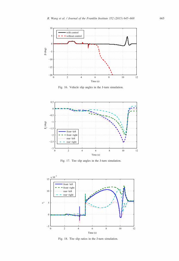
Fig. 18. Tire slip ratios in the J-turn simulation.

0 2 4 6 8 10 12−20

−15

−10

−5

0

5

10

Time (s)

β (d

eg)

with controlwithout control

Fig. 16. Vehicle slip angles in the J-turn simulation.

R. Wang et al. / Journal of the Franklin Institute 352 (2015) 645–668 665

0 10 20 30 40 50 600

10

20

30

40

50

Global X (m)

Glo

bal Y

(m)

with controlwithout control

Fig. 19. Comparison of the vehicle trajectories in the J-turn simulation.

R. Wang et al. / Journal of the Franklin Institute 352 (2015) 645–668666

compares the vehicle sideslip angles, it can be observed from this figure that the sideslip angle ofthe controlled vehicle could always be restrained around zero, indicating that the vehicle wasstabilized. Due to the lose of tire lateral forces during the single lane-changing maneuver, thesideslip angle of the uncontrolled vehicle with the same handwheel steering input and brakingforces increased fast as soon as the hard brake was applied, which proves the effectiveness of theproposed control method.Tire slip angles and slip ratios are plotted in Figs. 9 and 10, respectively. We can see that the

tire slip ratios and slip angles were always limited even when a hard brake and a large steeringangle were applied. Fig. 11 compares the vehicle trajectories in the single lane-changingsimulation. We can see that the controlled vehicle could track the desired trajectory expected bythe driver while the uncontrolled vehicle failed accomplish the single lane-changing task due tothe hard brake and large steering input.

4.2. J-turn simulation

In this simulation, the vehicle was controlled to make a J-turn at a low speed. The TRFC wasset to 0.2 and the actual vehicle mass in the CarSim model was set to 1.2 times of the nominalvalue. A counter-clockwise turn was introduced at 2 s, Fig. 12 shows the hand-wheel steeringangle manipulated by the driver in the J-turn simulation. The initial vehicle speed was chosen as20 km/h and the driver pressed the accelerator to gather speed at 5 s.Vehicle states in this maneuver are plotted in Figs. 13–16. It is obvious that the yaw rate of the

controlled vehicle could precisely track the desired reference expected by the driver, and thevehicle sideslip angle could also be restrained in a narrow scope which is close to zero. Fig. 15shows the vehicle accelerations in the J-turn maneuver. We can come to a conclusion similar tothat in the single lane-changing simulation, i.e. when the lateral acceleration became large, thetire driving forces of the controlled vehicle decreased depending on the tire slip angles to providethe greatest possible lateral tire forces and stabilize the vehicle. Tire slip angles and slip ratios areplotted in Figs. 17 and 18. We can see again that both tire slip angles and slip ratios were alwaysrestricted in the stable regions which prove the effectiveness of the proposed controller. The

R. Wang et al. / Journal of the Franklin Institute 352 (2015) 645–668 667

vehicle global trajectories are shown in Fig. 19. One can observe that the proposed controllerensured the vehicle trajectory tracking performance even when the vehicle runs on a low-μ road.

5. Conclusion

A vehicle lateral motion control method for a FWIA electric ground vehicle is presented. Theproposed LPV based robust H1 control based higher-level controller does not need the accuratevehicle parameters or tire force models but can still yield the desired control signals. The lower-level controller considering tire force constraints is designed to allocate the required controlefforts from the higher-lever controller to the four wheels. The numerical-optimization basedcontrol-allocation algorithms are replaced with an analytic solution with low computationalrequirement in the control allocation design. Simulations are carried out with a high-fidelity,CarSim, full-vehicle model. Simulation results under various driving scenarios and on differentroad conditions show the effectiveness of the proposed control approach. Experimentalvalidation of the proposed method will be carried out in the future.

Acknowledgement

This work was supported by National Natural Science Foundation of China (Grant nos.51205058, 51375086, 61403252), and Jiangsu Province Science Foundation for Youths, China(Grant no. BK20140634).

References

[1] R. Wang, Y. Chen, D. Feng, X. Huang, J. Wang, Development and performance characterization of an electricground vehicle with independently actuated in-wheel motors, J. Power Sources 196 (8) (2011) 3962–3971.

[2] C.C. Chan, The state of the art of electric and hybrid vehicles, Proc. IEEE 95 (April (4)) (2007) 704–718.[3] M. Shino, M. Nagai, Independent wheel torque control of small-scale electric vehicle for handling and stability

improvement, JSAE Rev. 24 (4) (2003) 449–456.[4] R. Wang, J. Wang, Fault-tolerant control for electric ground vehicles with independently-actuated in-wheel motors,

ASME Trans. J. Dyn. Syst. Meas. Control 134 (2) (2012) 021014.[5] O. Mokhiamar, M. Abe, Simultaneous optimal distribution of lateral and longitudinal tire forces for the model

following control, J. Dyn. Syst. Meas. Control 126 (1) (2004) 753–763.[6] P. Sadeghi-Tehran, P. Angelov, Online self-evolving fuzzy controller for autonomous mobile robots, in:

Proceedings of IEEE Symposium Series on Computational Intelligence, 2011, pp. 100–107.[7] S. Sakai, H. Sado, Y. Hori, Motion control in an electric vehicle with four independently driven in-wheel motors,

IEEE/ASME Trans. Mechatron. 4 (1) (1999) 9–16.[8] N. Mutoh, Y. Hayano, H. Yahagi, K. Takita, Electric braking control methods for electric vehicles with

independently driven front and rear wheels, IEEE Trans. Ind. Electron. 54 (2) (2007) 1168–1176.[9] D. Kim, S. Hwang, H. Kim, Vehicle stability enhancement of four-wheel-drive hybrid electric vehicle using rear

motor control, IEEE Trans. Veh. Technol. 57 (2) (2008) 727–735.[10] M. Bodson, Evaluation of optimization methods for control allocation, J. Guid. Control Dyn. 25 (4) (2002) 703–711.[11] T.A. Johansen, T.I. Fossen, Control allocation survey, Automatica 49 (May (5)) (2013) 1087–1103.[12] J. Wang, J.M. Solis, R.G. Longoria, On the control allocation for coordinated ground vehicle dynamics control

systems, in: Proceedings of the 2007 American Control Conference, New York, USA, July, 2007, pp. 5724–5729.[13] J. Wang, R.G. Longoria, Coordinated and reconfigurable vehicle dynamics control, IEEE Trans. Control Syst.

Technol. 17 (May (3)) (2009) 723–732.

R. Wang et al. / Journal of the Franklin Institute 352 (2015) 645–668668

[14] J.H. Plumlee, D.M. Bevly, A.S. Hodel, Control of a ground vehicle using quadratic programming based controlallocation techniques, in: Proceedings of the 2004 American Control Conference, Boston, USA, 2004, pp.4704–4709.

[15] S.I. Sakai, H. Sado, Y. Hori, Dynamic driving/braking force distribution in electric vehicles with independentlydriven four wheels, Electr. Eng. Jpn. 138 (1) (2002) 79–89.

[16] J. Wang, Coordinated and reconfigurable vehicle dynamics control (Ph.D. dissertation), Department of MechanicalEngineering, The University of Texas at Austin, Austin, TX, USA, 2007.

[17] J.Y. Wong, Theory of Ground Vehicles, 3rd ed., Wiley, New York, 2001.[18] D. Filev, P. Angelov, Fuzzy optimal control, Fuzzy Sets Syst. 47 (2) (1992) 151–156.[19] R.E. Precup, S. Preitl, Popov-type stability analysis method for fuzzy control systems, in: Proceedings of Fifth

European Congress on Intelligent Technologies and Soft Computing, vol. 2, Aachen, Germany, 1997, pp.1306–1310.

[20] E. Joelianto, D.C. Anura, M. Priyanto, ANFIS – hybrid reference control for improving transient response ofcontrolled systems using PID controller, Int. J. Artif. Intell. 10 (S13) (2013) 88–111.

[23] W. Xie, An equivalent LMI representation of bounded real lemma for continuous-time systems, J. Inequal. Appl.(January) (2008) 1–8.

[24] H. Zhang, Y. Shi, A.S. Mehr, Robust energy-to-peak filtering for networked systems with time-varying delays andrandomly missing data, IET Control Theory Appl. 4 (December (12)) (2010) 2921–2936.

[25] H. Gao, X. Yang, P. Shi, Multi-objective robust H1 control of spacecraft rendezvous, IEEE Trans. Control Syst.Technol. 17 (4) (2009) 794–802.

[26] K.D. Do, Control of nonlinear systems with output tracking error constraints and its application to magneticbearings, Int. J. Control 83 (June (6)) (2010) 1199–1216.

[27] J. Ahmadi, A.K. Sedigh, M. Kabganian, Adaptive vehicle lateral plane motion control using optimal tire frictionforces with saturation limits consideration, IEEE Trans. Veh. Technol. 58 (October (8)) (2009) 4098–4107.

[28] H.P. Du, N. Zhang, G.M. Dong, Stabilizing vehicle lateral dynamics with considerations of parameter uncertaintiesand control saturation through robust yaw control, IEEE Trans. Veh. Technol. 59 (June (5)) (2010) 2593–2597.

[29] H. Zhang, Y. Shi, A.S. Mehr, Parameter-dependent mixed H2/H1 filtering for linear parameter-varying systems,IET Signal Process. 6 (September (7)) (2012) 697–703.

[30] H. Zhang, X. Zhang, J. Wang, Robust gain-scheduling energy-to-peak control of vehicle lateral dynamicsstabilisation, Veh. Syst. Dyn. 52 (3) (2014) 309–340.

[31] H. Zhang, Y. Shi, J. Wang, On energy-to-peak filtering for nonuniformly sampled nonlinear systems: a Markovianjump system approach, IEEE Trans. Fuzzy Syst. 22 (1) (2014) 212–222.

[32] K. Kritayakirana, Autonomous vehicle control at the limits of handling (Ph.D. dissertation), Department ofMechanical Engineering, The Stanford University, USA, 2012.

本文献由“学霸图书馆-文献云下载”收集自网络，仅供学习交流使用。

学霸图书馆（www.xuebalib.com）是一个“整合众多图书馆数据库资源，

提供一站式文献检索和下载服务”的24 小时在线不限IP

图书馆。

图书馆致力于便利、促进学习与科研，提供最强文献下载服务。

图书馆导航：

图书馆首页 文献云下载 图书馆入口 外文数据库大全 疑难文献辅助工具