2-1

COSMOSFloWorks 2004 Tutorial

2

First Steps - Conjugate Heat Transfer

This First Steps - Conjugate Heat Transfer tutorial covers the basic steps to set up a flow analysis problem including conduction heat transfer in solids. This example is particu-larly pertinent to users interested in analyzing flow and heat transfer within electronics packages although the basic principles are applicable to all thermal problems. It is assumed that you have already completed the First Steps - Ball Valve Design tutorial since it teaches the basic principles of using COSMOSFloWorks in greater detail.

Open the SolidWorks Model

1 Copy the First Steps - Electronics Cooling folder into your working directory and ensure that the files are not read-only since COSMOSFloWorks will save input data to these files. Click File, Open.

2 In the Open dialog box, browse to the Enclosure Assembly.SLDASM assembly located in the First Steps - Electronics Cooling folder and click Open (or dou-ble-click the assembly). Alternatively, you can drag and drop the Enclosure Assembly.SLDASM file to an empty area of SolidWorks window.

Preparing the Model COSMOSFloWorks 2004 Tutorial

2-2

Preparing the Model

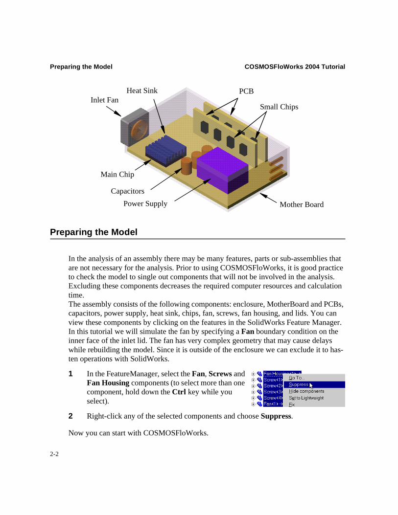
In the analysis of an assembly there may be many features, parts or sub-assemblies that are not necessary for the analysis. Prior to using COSMOSFloWorks, it is good practice to check the model to single out components that will not be involved in the analysis. Excluding these components decreases the required computer resources and calculation time.The assembly consists of the following components: enclosure, MotherBoard and PCBs, capacitors, power supply, heat sink, chips, fan, screws, fan housing, and lids. You can view these components by clicking on the features in the SolidWorks Feature Manager. In this tutorial we will simulate the fan by specifying a Fan boundary condition on the inner face of the inlet lid. The fan has very complex geometry that may cause delays while rebuilding the model. Since it is outside of the enclosure we can exclude it to has-ten operations with SolidWorks.

1 In the FeatureManager, select the Fan, Screws and Fan Housing components (to select more than one component, hold down the Ctrl key while you select).

2 Right-click any of the selected components and choose Suppress.

Now you can start with COSMOSFloWorks.

Inlet FanPCB

Small Chips

Main Chip

Capacitors

Power Supply Mother Board

Heat Sink

COSMOSFloWorks 2004 Tutorial Create a New Material

2-3

Create a New Material

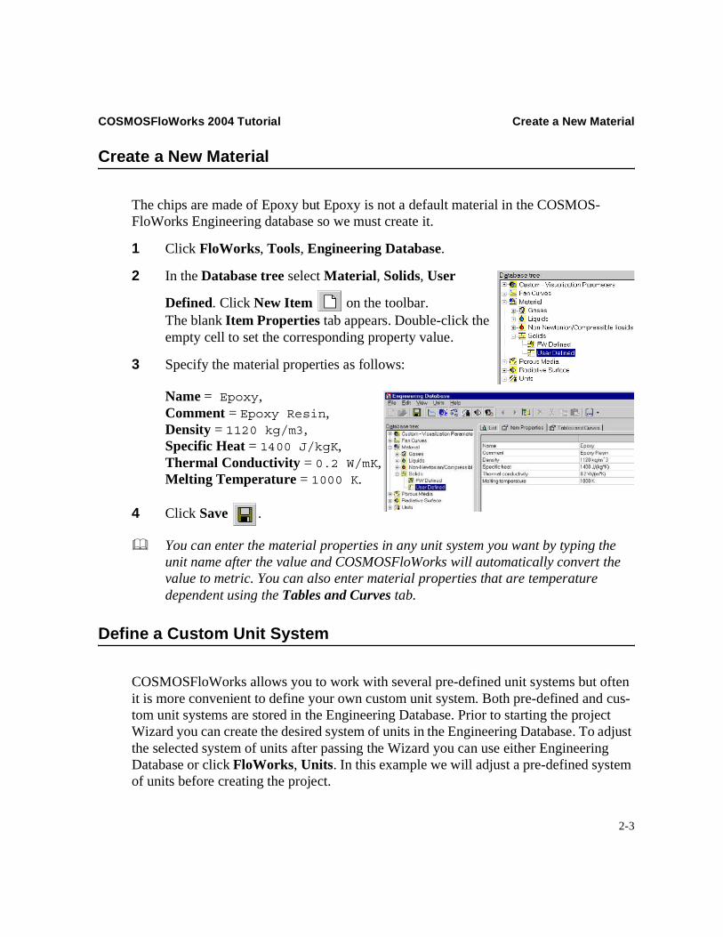
The chips are made of Epoxy but Epoxy is not a default material in the COSMOS-FloWorks Engineering database so we must create it.

1 Click FloWorks, Tools, Engineering Database.

2 In the Database tree select Material, Solids, User

Defined. Click New Item on the toolbar. The blank Item Properties tab appears. Double-click the empty cell to set the corresponding property value.

3 Specify the material properties as follows:

Name = Epoxy,Comment = Epoxy Resin,Density = 1120 kg/m3,Specific Heat = 1400 J/kgK,Thermal Conductivity = 0.2 W/mK,Melting Temperature = 1000 K.

4 Click Save .

You can enter the material properties in any unit system you want by typing the unit name after the value and COSMOSFloWorks will automatically convert the value to metric. You can also enter material properties that are temperature dependent using the Tables and Curves tab.

Define a Custom Unit System

COSMOSFloWorks allows you to work with several pre-defined unit systems but often it is more convenient to define your own custom unit system. Both pre-defined and cus-tom unit systems are stored in the Engineering Database. Prior to starting the project Wizard you can create the desired system of units in the Engineering Database. To adjust the selected system of units after passing the Wizard you can use either Engineering Database or click FloWorks, Units. In this example we will adjust a pre-defined system of units before creating the project.

Define a Custom Unit System COSMOSFloWorks 2004 Tutorial

2-4

1 In the Database tree select Units, FW Defined.

2 On the List tab select the USA system

of units and click Copy .

You can modify only custom entries in the Engineering Database. To adjust the pre-defined material, porous media, unit system or fan curve you must copy it into the corresponding User Defined folder first and then make necessary changes.

3 In the tree, select the Units, User Defined item and click Paste .

4 Click the Item Properties tab to adjust the USA unit system for this example.

By scrolling through the different groups in the Parameter tree you can see the units selected for all the parameters. Although most of the parameters have convenient units such as ft/s for velocity and CFM (cubic feet per minute) for volume flow rate we will change a couple units that are more convenient for this model. Since the physical size of the model is relatively small it is more convenient to choose inches instead of feet as the length unit.

5 For the Length entry, click on the right hand side of the units box and select inches.

6 Next expand the Heat group in the Parameter tree.

COSMOSFloWorks 2004 Tutorial Create a COSMOSFloWorks Project

2-5

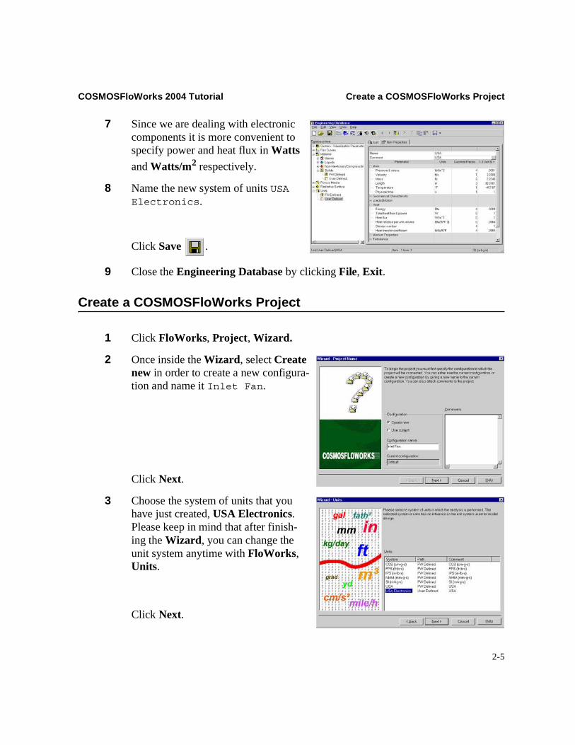
7 Since we are dealing with electronic components it is more convenient to specify power and heat flux in Wattsand Watts/m2 respectively.

8 Name the new system of units USA Electronics.

Click Save .

9 Close the Engineering Database by clicking File, Exit.

Create a COSMOSFloWorks Project

1 Click FloWorks, Project, Wizard.

2 Once inside the Wizard, select Create new in order to create a new configura-tion and name it Inlet Fan.

Click Next.

3 Choose the system of units that you have just created, USA Electronics.Please keep in mind that after finish-ing the Wizard, you can change the unit system anytime with FloWorks,Units.

Click Next.

Create a COSMOSFloWorks Project COSMOSFloWorks 2004 Tutorial

2-6

4 Set the fluid type to Gas. Under physi-cal features select the Heat transfer in solids check box.

Click Next.

Heat transfer in solids was selected because heat is generated by several electronics component and we are interested to see how the heat is dissipated through the heat sink and other solid parts and then out to the fluid. Therefore we must simulate heat conduction in the solid parts.

5 Set the analysis type to Internal.

We want to analyze the flow throughthe structure. This is what we call an internal analysis. The opposite is an external analysis, which is the flow around an object. From this dialog box you can also choose to ignore cavities that are not relevant to the flow analysis without having to fill them in using SolidWorks features.

Click Next

6 Click Next accepting the adiabatic default outer wall condition.

COSMOSFloWorks 2004 Tutorial Create a COSMOSFloWorks Project

2-7

7 In the Database of solids list, dou-ble-click the Aluminum, Epoxy,Insulator, Silicon and Steel, stainlessitems.

8 Select Steel, stainless as the Default material.

Click Next.

9 Click Next accepting the default zero roughness value for all model walls.

10 Choose Air as the fluid. You can either double-click Air or select the item in the left column and click Add.

Click Next.

Although setting the initial temperature is more important for transient calculations to see how much time it takes to reach a certain temperature, it is useful to set the initial temperature close to the anticipated final solution to speed up convergence. In this case we will set the initial air temperature and the initial temperature of the stainless steel (which represents the cabinet) to 50°F because the box is located in an air-conditioned room.

Create a COSMOSFloWorks Project COSMOSFloWorks 2004 Tutorial

2-8

11 Set the initial fluid Temperature and the Initial solid temperature to 50°F.

Click Next.

12 Accept the default for the Result reso-lution and keep the automatic evalua-tion of the Minimum gap size and Minimum wall thickness.

COSMOSFloWorks calculates the default minimum gap size and minimum wall thickness using information about the overall model dimensions, the computational domain, and faces on which you specify conditions and goals. Prior to starting the calculation, we recommend that you check the minimum gap size and minimum wall thickness to ensure that small features will be recognized. We will review these again after all the necessary conditions and goals will be specified.

Click Next.

13 Click Finish. Now COSMOSFloWorks creates a new configuration with the COS-MOSFloWorks data attached.

Click on the SolidWorks Configuration Manager to show the new configuration.

Notice the name of the new configuration has the name you entered in the Wizard.

Go to the COSMOSFloWorks design tree and open all the icons.

COSMOSFloWorks 2004 Tutorial Define the Fan

2-9

We will use the COSMOSFloWorks Design Tree to define our analysis, just as the SolidWorks Feature Manager Tree is used to design your models.

Right-click the Computational Domain icon and select Hide to hide the black wireframe box.

Computational Domain is the icon used to modify the size and visualization of the volume being analyzed as well as to specify symmetry boundary conditions and 2D flow. The wireframe box enveloping the model is the visualization of the limits of the computational domain.

Define the Fan

A Fan is a type of flow boundary condition. You can specify Fans at selected solid surfaces where Boundary Conditions and Sources are not specified. You can specify Fans on artificial lids closing model openings as Inlet Fans or Outlet Fans. You can also specify fans on any faces arranged inside of the flow region as Internal Fans. A Fan is considered an ideal device creating a volume (or mass) flow rate depending on the difference between the inlet and outlet static pressures on the selected face. A curve of the fan volume flow rate or mass flow rate versus the static pressure difference is taken from the Engineering Database.

If you analyze a model with a fan then you must know the fan's characteristics. In this example we use one of the pre-defined fans from the Engineering Database. If you can-not find an appropriate curve in the database you can create your own curve in accordance with the specification on your fan.

1 In the COSMOSFloWorks design tree, right-click the Fansicon and select Insert Fan. The Fan dialog box appears.

Define the Fan COSMOSFloWorks 2004 Tutorial

2-10

2 Select the inner face of the Inlet Lid part as shown. (To access the inner face, right-click the mouse to cycle through the faces under the cursor until the inner face is highlighted, then click the left mouse button).

3 Select External Inlet Fan as Fan type.

4 Click Browse to select the fan curve from the Engi-neering database.

5 Select the 405 item under the Fan Curves, FW Defined, PAPST, DC-Axial, Series 400, 405 item.

6 Click OK to return to the Fan dialog box.

7 On the Settings tab expand the Thermodynamic Parameters item to check that the Ambient pressure is atmospheric pressure.

8 Expand the Flow parameters item and select Swirl in the Flow vectors direction list.

9 Specify the Angular velocity as 100 rad/s and accept the zero Radial velocity value.

When specifying a swirling flow, you must choose the reference Coordinate systemand the Reference axis so that the origin of the coordinate system and the swirl’scenter point are coincident and the angular velocity vector is aligned with the reference axis.

COSMOSFloWorks 2004 Tutorial Define the Boundary Conditions

2-11

10 Go back to the Definition tab. Hold down the Ctrl key and in the FeatureManager design tree select the Inlet Coordinate System.

11 Select the Global Coordinate System item and press the Deletekey.

12 Select Y in the Reference Axis list.

13 Accept to Create associated goals.

It is often convenient to specify an appropriate goal along with the specified condition. For example, if you specify a pressure opening it makes sense to define a mass flow rate surface goal at this opening. COSMOSFloWorks allows you to associate a condition type (boundary condition, fun, heat source or radiative surface) with a goal(s), which will be automatically created along with this condition. You can associate goals with a boundary condition type under the Automatic Goals item of the COSMOSFloWorks Options dialog box.

14 Click OK. The new External Inlet Fan1 item appears in the COSMOSFloWorks design tree.

With the definition just made, we told COSMOSFloWorks that at this opening air flows into the enclosure through the fan so that the volume flow rate of air depends on the difference between the ambient atmospheric pressure and the static pressures on the fan's outlet face (inner face of the lid) in accordance with the curve shown above. Since the outlet lids of the enclosure are at ambient atmospheric pressure the pressure rise produced by the fan is equal to the pressure drop through the electronics enclosure.

Define the Boundary Conditions

A boundary condition is required anywhere fluid enters or exits the system excluding openings where a fan is specified. A boundary condition can be set as a Pressure, Mass Flow, Volume Flow or Velocity. You can also use the Boundary Condition dialog for specifying an Ideal Wall condition that is an adiabatic, frictionless wall or a Real Wall

Define the Boundary Conditions COSMOSFloWorks 2004 Tutorial

2-12

condition to set the wall roughness and/or temperature and/or heat transfer coefficient at the model surfaces. For internal analyses with "Heat transfer in solids" you can also set thermal wall condition on outer model walls by specifying an Outer Wall condition.

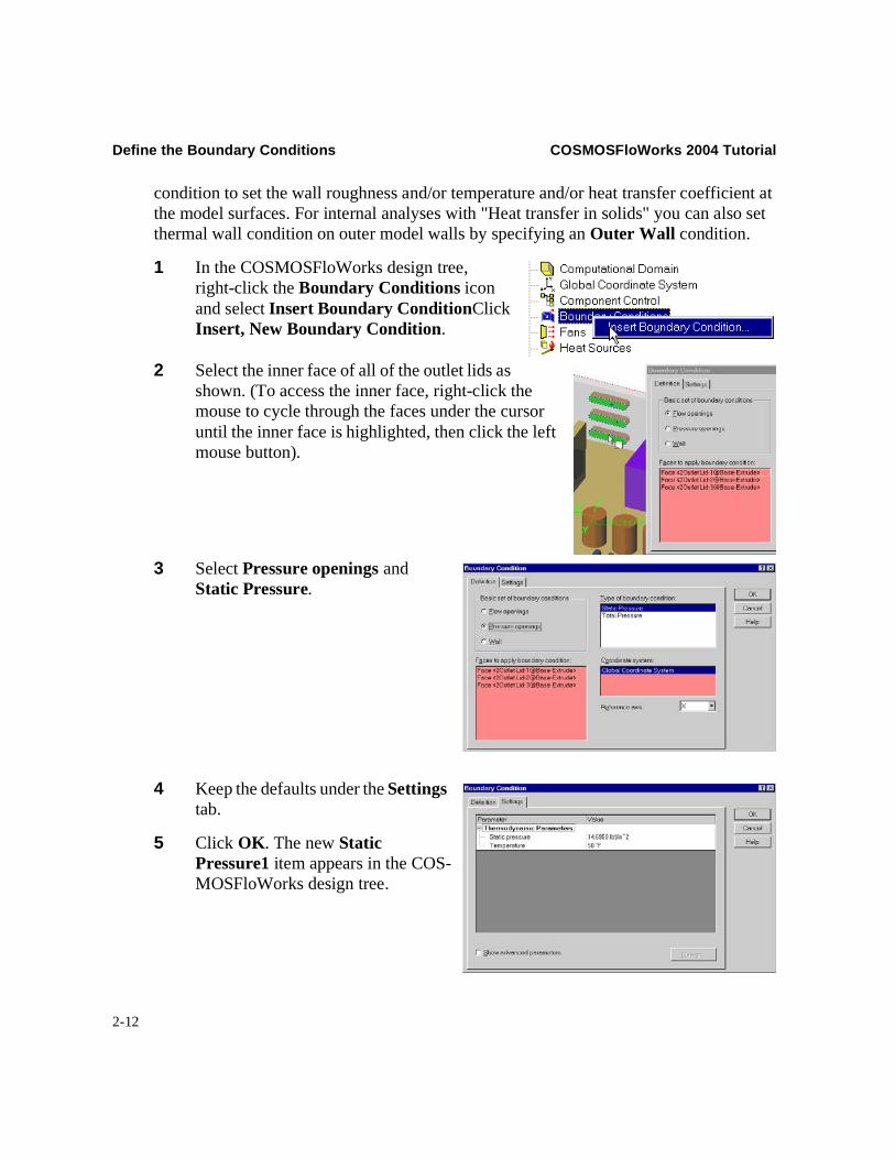
1 In the COSMOSFloWorks design tree, right-click the Boundary Conditions icon and select Insert Boundary ConditionClick Insert, New Boundary Condition.

2 Select the inner face of all of the outlet lids as shown. (To access the inner face, right-click the mouse to cycle through the faces under the cursor until the inner face is highlighted, then click the left mouse button).

3 Select Pressure openings and Static Pressure.

4 Keep the defaults under the Settingstab.

5 Click OK. The new Static Pressure1 item appears in the COS-MOSFloWorks design tree.

COSMOSFloWorks 2004 Tutorial Define the Heat Source

2-13

With the definition just made, we told COSMOSFloWorks that at this opening the fluid exits the model to an area of static atmospheric pressure. Within this dialog box we can also set time dependent properties for the pressure.

Define the Heat Source

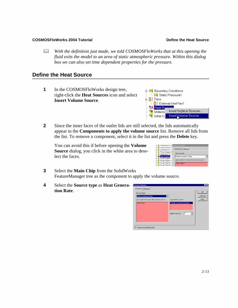
1 In the COSMOSFloWorks design tree, right-click the Heat Sources icon and select Insert Volume Source.

2 Since the inner faces of the outlet lids are still selected, the lids automatically appear in the Components to apply the volume source list. Remove all lids from the list. To remove a component, select it in the list and press the Delete key.

You can avoid this if before opening the Volume Source dialog, you click in the white area to dese-lect the faces.

3 Select the Main Chip from the SolidWorks FeatureManager tree as the component to apply the volume source.

4 Select the Source type as Heat Genera-tion Rate.

Define the Heat Source COSMOSFloWorks 2004 Tutorial

2-14

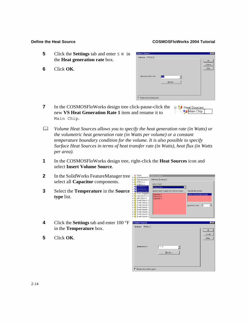
5 Click the Settings tab and enter 5 W inthe Heat generation rate box.

6 Click OK.

7 In the COSMOSFloWorks design tree click-pause-click the new VS Heat Generation Rate 1 item and rename it to Main Chip.

Volume Heat Sources allows you to specify the heat generation rate (in Watts) or the volumetric heat generation rate (in Watts per volume) or a constant temperature boundary condition for the volume. It is also possible to specify Surface Heat Sources in terms of heat transfer rate (in Watts), heat flux (in Watts per area).

1 In the COSMOSFloWorks design tree, right-click the Heat Sources icon and select Insert Volume Source.

2 In the SolidWorks FeatureManager tree select all Capacitor components.

3 Select the Temperature in the Source type list.

4 Click the Settings tab and enter 100 °Fin the Temperature box.

5 Click OK.

COSMOSFloWorks 2004 Tutorial Define the Material Conditions

2-15

6 Click-pause-click the new VS Temperature1 item and rename it to Capacitors.

7 Following the same procedure as above, set the following volume heat sources: all chips on PCB (Small Chip) - total heat generation rate of 4 W, Power Supply - tem-perature of 120 °F

8 Rename the source applied to the chips to Chips and the source for the power supply to Power Supply.

9 Click File, Save.

Define the Material Conditions

1 Right-click the Material Conditions icon and select Insert Material Condition.

2 In the SolidWorks FeatureManager select MotherBoard, PCB(1), PCB(2) components.

3 Select Epoxy from the Selected material list.

4 Click OK.

Define the Engineering Goals COSMOSFloWorks 2004 Tutorial

2-16

5 Following the same procedure as above, set the following material conditions: the chips are made of silicon, the heat sink is made of aluminum, and the 4 Lids (Inlet Lid and three Outlet Lids) are made of insulator material. All four lids can be selected in the same material condition definition. Note that two of the outlet lids can be found under derived pattern (DerivedLPattern1) in the SolidWorks FeatureManager. Alternatively you can click on the actual part in the SolidWorks graphics area.

6 Change the name of each material condition. The new descriptive names are: PCB - Epoxy,Heat Sink - Aluminum,Chips - Silicon, andLids - Insulator.

Material Conditions are used to specify the material type of solid parts in the assembly.

7 Click File, Save.

Define the Engineering Goals

Specifying Volume Goals

1 Right-click the Goals icon and select Insert Volume Goal.

2 Select the Chips item in the COSMOS-FloWorks design tree. This selects all compo-nents belonging to the Chips heat source.

COSMOSFloWorks 2004 Tutorial Define the Engineering Goals

2-17

3 Select Temperature of Solid as the goal type and calculate Maximum value.

4 Accept to Use the goal for convergence control.

5 Click OK. The new VG Maximum Tempera-ture of Solid1 item appears in the COSMOS-FloWorks design tree.

6 Change the name of the new item to VG Small Chips Max Temperature. You can also change the name of the item using the Feature Properties dialog appearing if you right-click the item and select Properties.

7 Right-click the Goals icon and select Insert Volume Goal.

8 Select the Main Chip item in the COSMOS-FloWorks design tree.

9 Select Temperature of Solid as the goal type and calculate Maximum value.

10 Click OK.

11 Rename the new VG Maximum Temperature of Solid1 item to VG Chip Max Tempera-ture.

Define the Engineering Goals COSMOSFloWorks 2004 Tutorial

2-18

Specifying Surface Goals

1 Right-click the Goals icon and select Insert Sur-face Goal.

2 Since the Main Chip is still selected, all its faces automatically appear in the Faces to apply the surface goal list. Remove all faces from the list. To remove a face, select it in the list and press the Delete key.

3 Click the External Inlet Fan1 item to select the face where it is going to be applied.

4 Keep the Static Pressure and the Average Value.

5 Accept to Use the goal for convergence con-trol.

For the X(Y, Z) - Component of Force and X(Y, Z) - Component of Torque goals you can select the Coordinate system in which these goals are calculated.

6 Click OK and rename the new SG Average Static Pressure1 item to SG Av Inlet Pressure.

7 Right-click the Goals icon and select Insert Surface Goal.

COSMOSFloWorks 2004 Tutorial Define the Engineering Goals

2-19

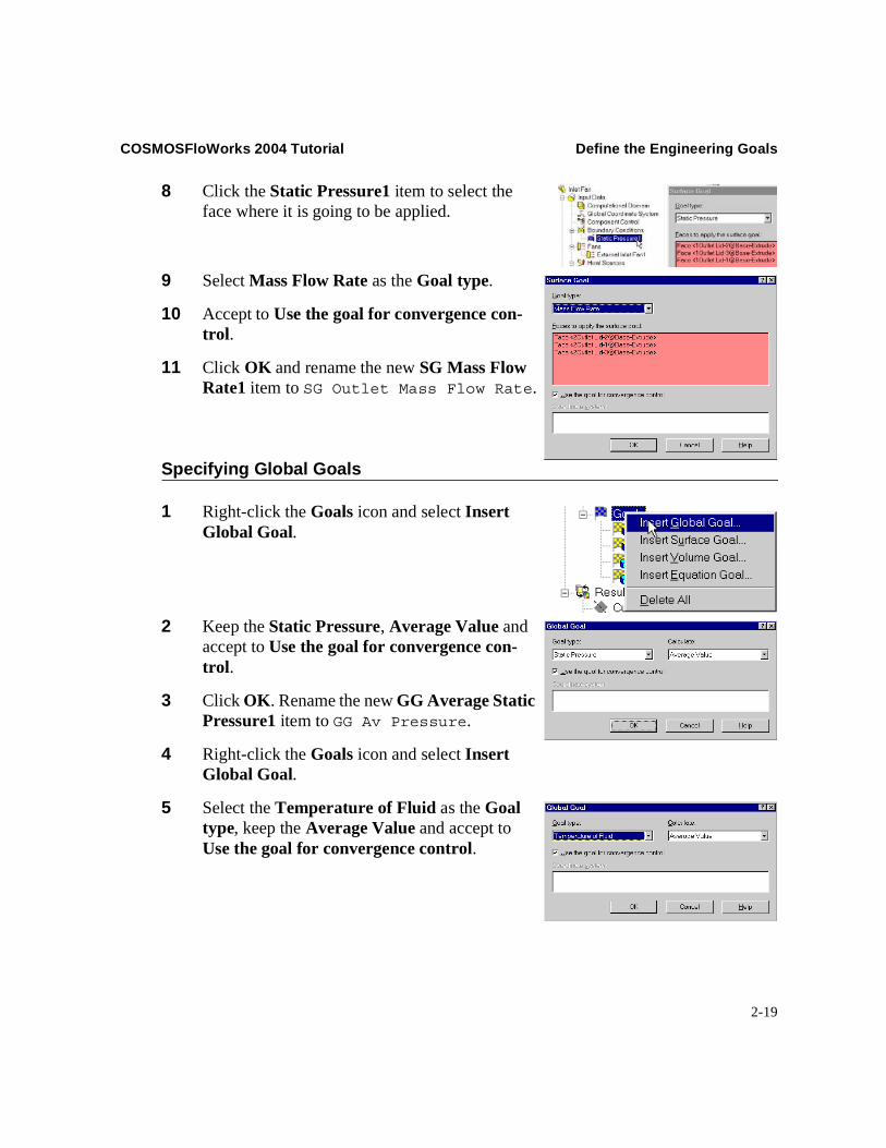
8 Click the Static Pressure1 item to select the face where it is going to be applied.

9 Select Mass Flow Rate as the Goal type.

10 Accept to Use the goal for convergence con-trol.

11 Click OK and rename the new SG Mass Flow Rate1 item to SG Outlet Mass Flow Rate.

Specifying Global Goals

1 Right-click the Goals icon and select Insert Global Goal.

2 Keep the Static Pressure, Average Value andaccept to Use the goal for convergence con-trol.

3 Click OK. Rename the new GG Average Static Pressure1 item to GG Av Pressure.

4 Right-click the Goals icon and select Insert Global Goal.

5 Select the Temperature of Fluid as the Goaltype, keep the Average Value and accept to Use the goal for convergence control.

Changing the Geometry Resolution COSMOSFloWorks 2004 Tutorial

2-20

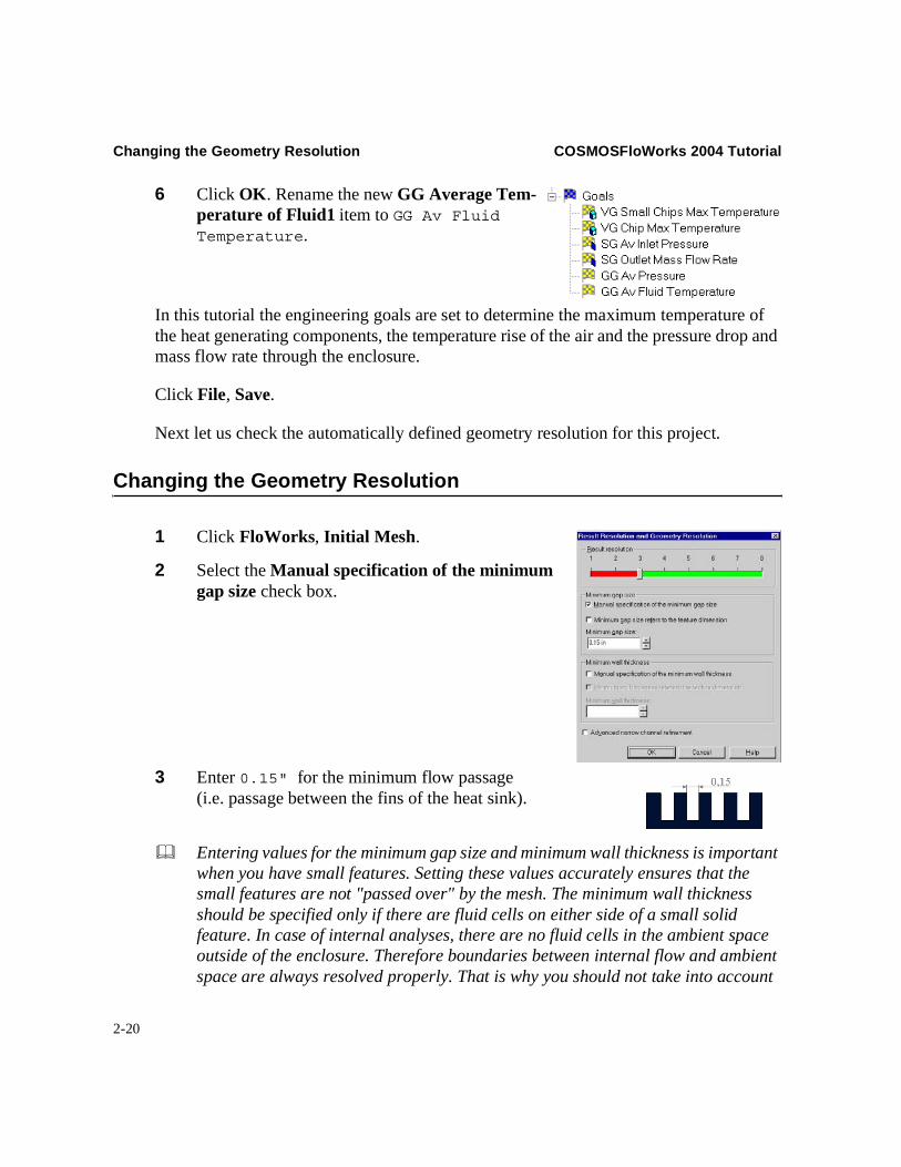
6 Click OK. Rename the new GG Average Tem-perature of Fluid1 item to GG Av Fluid Temperature.

In this tutorial the engineering goals are set to determine the maximum temperature of the heat generating components, the temperature rise of the air and the pressure drop and mass flow rate through the enclosure.

Click File, Save.

Next let us check the automatically defined geometry resolution for this project.

Changing the Geometry Resolution

1 Click FloWorks, Initial Mesh.

2 Select the Manual specification of the minimum gap size check box.

3 Enter 0.15" for the minimum flow passage (i.e. passage between the fins of the heat sink).

Entering values for the minimum gap size and minimum wall thickness is important when you have small features. Setting these values accurately ensures that the small features are not "passed over" by the mesh. The minimum wall thickness should be specified only if there are fluid cells on either side of a small solid feature. In case of internal analyses, there are no fluid cells in the ambient space outside of the enclosure. Therefore boundaries between internal flow and ambient space are always resolved properly. That is why you should not take into account

COSMOSFloWorks 2004 Tutorial Solution

2-21

the walls of the steel cabinet. Both the minimum gap size and the minimum wall thickness are tools that help you to create a model-adaptive mesh resulting in increased accuracy. However the minimum gap size setting is the more powerful one. The fact is that the COSMOSFloWorks mesh is constructed so that the specified Result Resolution level controls the minimum number of mesh cells per minimum gap size. And this number is equal to or greater than the number of mesh cells generated per minimum wall thickness. That's why even if you have a thin solid feature inside the flow region it is not necessary to specify minimum wall thickness if it is greater than or equal to the minimum gap size. Specifying the minimum wall thickness is necessary if you want to resolve thin walls smaller than the smallest gap.

Click OK.

Solution

1 Click FloWorks, Solve, Run.

2 Click Run.

The solver will approximately take about 1.5 hours to run on an 850MHz platform.

This is the solution monitor dia-log box. Notice for this tutorial that the SG Av Inlet Pressure and GG Av Pressure converged very quickly compared to the other goals. Generally different goals take more or less iterations to converge. The goal-oriented philosophy of COSMOS-FloWorks allows you to get the answers you need in the shortest amount of time. For example, if you were only interested in the pressure drop through the enclosure, COSMOS-FloWorks would have provided the result more quickly then if the solver was allowed to fully converge on all of the parameters.

Viewing the Goals COSMOSFloWorks 2004 Tutorial

2-22

Viewing the Goals

1 Right-click the Results icon and select Load Results to acti-vate the postprocessor.

2 Select the project’s results (1.fld) file and click Open.

3 Right-click the Goals icon and select Create.

4 Click Add All in the Goals dialog.

5 Click OK.

An excel workbook will open with the goal results. The first sheet will show a table sum-marizing the goals.

You can see that the maximum temperature in the main chip is 100.12 °F, and the maxi-mum temperature over the small chips is 111.12 °F.

Goal's progress bar is a qualitative and quantitative characteristic of the goal's convergence process. When COSMOSFloWorks analyzes the goal's convergence, it calculates the goal's dispersion defined as the difference between the goal's maximum and minimum values over the analysis interval reckoned from the last iteration and compares this dispersion with the goal's convergence criterion

Enclosure Assembly.SLDASM [Inlet Fan]Goal Name Unit Value Averaged Value Minimum Value Maximum Value Progress [%] Use In ConvergenceGG Av Pressure [lbf/in^2] 14.69631 14.6963 14.6963 14.6963 100 YesSG Av Inlet Pressure [lbf/in^2] 14.69615642 14.6962 14.6962 14.6962 100 YesGG Av Fluid Temperature [°F] 59.4738659 59.5518 59.4699 59.6098 100 YesSG Outlet Mass Flow Rate [lb/s] -0.007634592 -0.00763519 -0.00763917 -0.00762781 100 YesVG Chip Max Temperature [°F] 100.1197938 100.186 100.108 100.252 100 YesVG Small Chips Max Temperature [°F] 111.1247332 112.129 111.125 113.117 100 Yes

COSMOSFloWorks 2004 Tutorial Flow Trajectories

2-23

dispersion, either specified by you or automatically determined by COSMOSFloWorks as a fraction of the goal's physical parameter dispersion over the computational domain. The percentage of the goal's convergence criterion dispersion to the goal's real dispersion over the analysis interval is shown in the goal's convergence progress bar (when the goal's real dispersion becomes equal or smaller than the goal's convergence criterion dispersion, the progress bar is replaced by word "achieved"). Naturally, if the goal's real dispersion oscillates, the progress bar oscillates also, moreover, when a hard problem is solved, it can noticeably regress, in particular from the "achieved" level. The calculation can finish if the iterations (in travels) required for finishing the calculation have been performed, as well as if the goals' convergence criteria are satisfied before performing the required number of iterations. You can specify other finishing conditions at your discretion.

To analyze the results in more detail let us use the various COSMOSFloWorks post-pro-cessing tools. For the visualization of how the fluid flows inside the enclosure the best method is to create flow trajectories.

Flow Trajectories

1 Right-click the Flow Trajectories icon

and select Insert.

2 In the COSMOSFloWorks design tree select the External Inlet Fan1 item. This selects the inner face of the Inlet Lid.

3 Set the Number of trajectories to 200.

4 Keep the Reference in the Start points from list.

If Reference is selected, then the trajectory start points are taken from this selected face.

Flow Trajectories COSMOSFloWorks 2004 Tutorial

2-24

5 Click View Settings.

6 In the View Settings dialog box, change the Parameter from Pressureto Velocity.

7 Go to the Flow Trajectories tab and notice that the Use from contoursoption is selected.

This setting defines how trajectories are colored. If Use from contours is selected then the trajectories are colored with the distribution of the parameter specified on the Contourstab (Velocity in our case). If you select Use fixed color then all flow trajectories have the same color that you specify on the Settings tab of the Flow Trajectories dialog box.

8 Click OK to save the changes and exit the View Settings dialog box.

9 In the Flow Trajectories dialog box click OK. The new Flow Trajectories 1 item appears in the COSMOSFloWorks design tree.

This is the picture you should see.

Notice that there are only a few trajectories along the PCB(2) and this may cause problems with cooling of the chips placed on this PCB. Additionally the blue color indicates low velocity in front of PCB(2).

COSMOSFloWorks 2004 Tutorial Cut Plots

2-25

Right-click the Flow Trajectories 1 item and select Hide.

Let us see the velocity distribution in more detail.

Cut Plots

1 Right-click the Cut Plots icon and select Insert.

2 Keep the Front plane as the section plane.

3 Click View Settings.

4 Change the Min and Max values to 0 and 10 respectively. The specified integer values produce a palette where it is more easy to determine the value.

5 Set the Number of colors to 30.

6 Click OK.

7 In the Cut Plot dialog box click OK.The new Cut Plot 1 item appears in the COSMOSFloWorks design tree.

Cut Plots COSMOSFloWorks 2004 Tutorial

2-26

8 Select the Top view.

You can see that the maximum velocity region appears close to the openings; and the low velocity region is seen in the center area between the capacitors and the PCB. Fur-thermore the region between the PCB's has a strong flow which in all likelihood will enhance convective cooling in this region. Let us now look at the fluid temperature.

9 Double-click the palette bar in the upper left corner of the graphics area. The View Settings dialog appears.

10 Change the Parameter from Velocity to Temperature.

11 Change the Min and Max values to 50and 120 respectively.

COSMOSFloWorks 2004 Tutorial Cut Plots

2-27

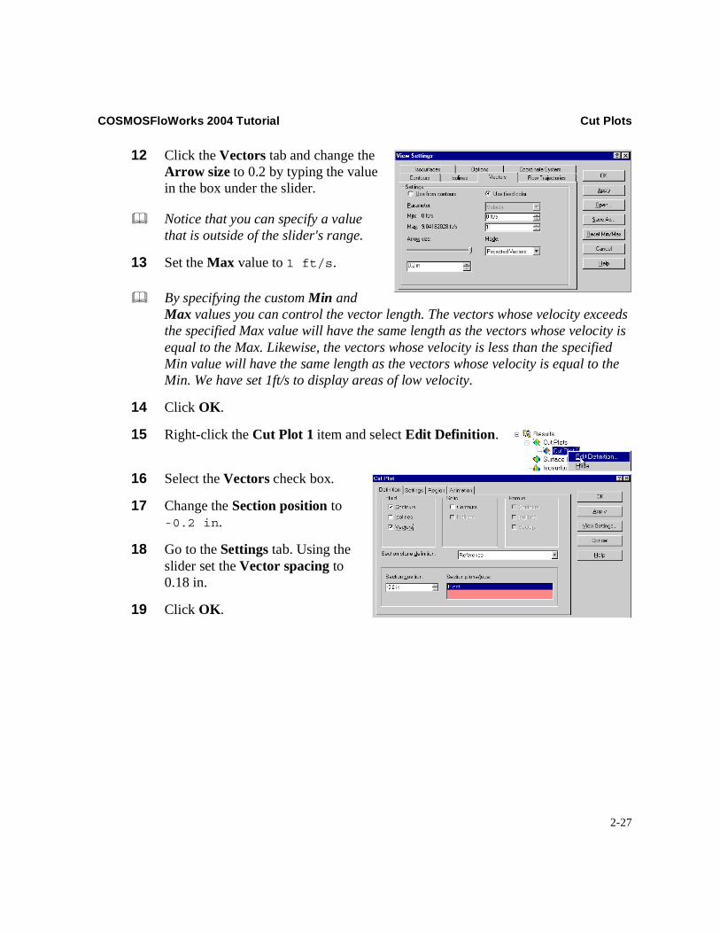
12 Click the Vectors tab and change the Arrow size to 0.2 by typing the value in the box under the slider.

Notice that you can specify a value that is outside of the slider's range.

13 Set the Max value to 1 ft/s.

By specifying the custom Min and Max values you can control the vector length. The vectors whose velocity exceeds the specified Max value will have the same length as the vectors whose velocity is equal to the Max. Likewise, the vectors whose velocity is less than the specified Min value will have the same length as the vectors whose velocity is equal to the Min. We have set 1ft/s to display areas of low velocity.

14 Click OK.

15 Right-click the Cut Plot 1 item and select Edit Definition.

16 Select the Vectors check box.

17 Change the Section position to -0.2 in.

18 Go to the Settings tab. Using the slider set the Vector spacing to 0.18 in.

19 Click OK.

Surface Plots COSMOSFloWorks 2004 Tutorial

2-28

It is not surprising that the fluid temperature is high around the heat sink but it is also high in the area of low velocity denoted by small vectors.

Right-click the Cut Plot1 item and select Hide. Let us now display solid temperature.

Surface Plots

1 Right-click the Surface Plots item and select Insert.

2 Click Solid as the Medium. Since the Temperature is the active parameter, you can display plots in solids; otherwise only the fluid medium would be available.

3 Hold down the Ctrl key and select the Heat Sink - Alumi-num and Chips - Siliconitems in the COSMOS-FloWorks design tree.

4 Click OK. The creation of the surface plot may take a time because 76 faces need to be colored.

COSMOSFloWorks 2004 Tutorial Surface Plots

2-29

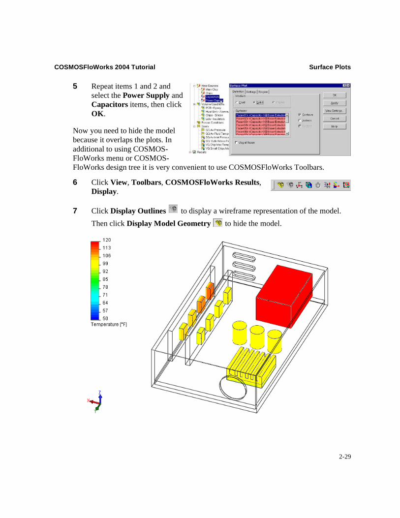
5 Repeat items 1 and 2 and select the Power Supply and Capacitors items, then click OK.

Now you need to hide the model because it overlaps the plots. In additional to using COSMOS-FloWorks menu or COSMOS-FloWorks design tree it is very convenient to use COSMOSFloWorks Toolbars.

6 Click View, Toolbars, COSMOSFloWorks Results,Display.

7 Click Display Outlines to display a wireframe representation of the model.

Then click Display Model Geometry to hide the model.

Surface Plots COSMOSFloWorks 2004 Tutorial

2-30

You can further view and analyze the results with the post-processing tools that were shown in the First Steps - Ball Valve Design tutorial. COSMOSFloWorks allows you to quickly and easily investigate your design both quantitatively and qualitatively. Quanti-tative results such as the maximum temperature in the component, pressure drop through the cabinet, and air temperature rise will allow you to determine whether the design is acceptable or not. By viewing qualitative results such as air flow patterns, and heat con-duction patterns in the solid, COSMOSFloWorks gives you the necessary insight to locate problem areas or weaknesses in your design and provides guidance on how to improve or optimize the design.