An Analysis of Energy Balance in a Helicon

Plasma Source for Space Propulsion

by

Justin Matthew Pucci

B.S., Aerospace Engineering, Arizona State University, 2003

Submitted to the Department of Aeronautics and Astronauticsin partial fulfillment of the requirements for the degree of

Master of Science in Aeronautics and Astronautics

at the

MASSACHUSETTS INSTITUTE OF TECHNOLOGY

May 2007

c© Massachusetts Institute of Technology 2007. All rights reserved.

Author . . . . . . . . . . . . . . . . . . . . . . . . . . . . . . . . . . . . . . . . . . . . . . . . . . . . . . . . . . . . . .Department of Aeronautics and Astronautics

May 25, 2007

Certified by. . . . . . . . . . . . . . . . . . . . . . . . . . . . . . . . . . . . . . . . . . . . . . . . . . . . . . . . . .Manuel Martınez-Sanchez

Professor of Aeronautics and AstronauticsThesis Supervisor

Accepted by . . . . . . . . . . . . . . . . . . . . . . . . . . . . . . . . . . . . . . . . . . . . . . . . . . . . . . . . .Jaime Peraire

Professor of Aeronautics and AstronauticsChair, Committee on Graduate Students

2

An Analysis of Energy Balance in a Helicon Plasma Source

for Space Propulsion

by

Justin Matthew Pucci

Submitted to the Department of Aeronautics and Astronauticson May 25, 2007, in partial fulfillment of the

requirements for the degree ofMaster of Science in Aeronautics and Astronautics

Abstract

This thesis covers work done on the mHTX@MIT helicon source as it relates to theanalysis of power losses. A helicon plasma is a rather complex system with manypotential loss mechanisms. Among the most dominant are optical radiation emission,wall losses due to poor magnetic confinement, and poor antenna-plasma coupling.This work sought to establish a first-order breakdown of the loss mechanisms inthe mHTX@MIT helicon source so as to allow for a better understanding of theissues effecting efficiency. This thesis proposes the use of a novel thermocouple array,standard plasma diagnostics, and a simple global energy balance model of the systemto determine greater details regarding the losses incurred during regular operation.From this it may be possible, by comparing the heat flux on the tube to the appliedmagnetic field profile, to gain some insight into the effects of magnetic field geometryon the character of the helicon discharge.

Thesis Supervisor: Manuel Martınez-SanchezTitle: Professor of Aeronautics and Astronautics

3

4

Acknowledgments

I would like to express my sincere appreciation and gratitude to my advisor, Professor

Manuel Martınez-Sanchez for his guidance throughout this degree. He has provided

me with a great deal of knowledge and has taught me how to think more clearly

and logically about every situation I encounter as an engineer. Manuel, your sincere

curiosity in seemingly every aspect of our work is inspiring to me and will continue

to push me to broaden my knowledge in every way possible.

I would also like to thank my second advisor and good friend, Dr. Oleg Batishchev

for always being available to discuss the simplest or most complex of topics regardless

of the time, and for providing constant support and encouragement, even when I

thought there was no real way to tackle the given problem.

My thanks go out to Dr. Jean-Luc Cambier of the US Air Force Research Labo-

ratory/PRSA at Edwards AFB for his continuing support through AFRL/ERC sub-

contract RS060213-Mini-Helicon Thruster Development. Also thanks to Dr. Mi-

tat Birkan of the US Air Force Office of Scientific Research for equipment provided

through the Defense University Research Instrumentation Program (DURIP) Grant.

I would also like to express my gratitude to the National Science Foundation Gradu-

ate Research Fellowship Program for their full financial support of my education here

at MIT. Without their fellowship, this degree may not have come to fruition.

To my helicon lab mates: Nareg and Murat. Thank you so much for being there for

all the frustrating times we shared in the lab when things looked as if they couldn’t

get any worse, and for the constant stream of comic relief sometimes necessary to

make it through the day. Our friendships mean a lot to me and I hope that they

will continue whether personally or professionally. Thank you to my office mates and

good friends, Tanya and Felix for your help through the multiple years of classes,

exams, homework, and thesis writing. I couldn’t have done it without you guys and

your constant encouragement and support.

Finally, I would not only like to give my thanks but to dedicate this thesis to

5

my family, who have lived everyday of this great experience through my constant

communication with them and have made this document possible. Thanks to my

father, Ralph for his support and inspiration as well as those great, albeit wordy pep

talks. Thanks to my mother, Kathy, who always knows how to kick me into gear

and is there for me no matter what and at anytime, be it day or night. To my little

sister, Dani: You’ve been a great friend and a good influence on me during my career

here at MIT and for that I thank you. Lastly, but by no means least, to my wife,

Marnie, who has shared with me the ups and downs, the trials and tribulations, the

good days and the bad days with me every step of the way through this adventure.

Your undying support, compassion, and love is what keeps me going everyday of my

life and is what has labored to instill in me the strength to finish this degree.

6

Contents

1 Introduction 17

1.1 Space Propulsion . . . . . . . . . . . . . . . . . . . . . . . . . . . . . 17

1.2 Helicon Plasma Sources . . . . . . . . . . . . . . . . . . . . . . . . . . 20

1.3 Overview of Research . . . . . . . . . . . . . . . . . . . . . . . . . . . 21

2 The mHTX@MIT Facility 25

2.1 Vacuum Chamber . . . . . . . . . . . . . . . . . . . . . . . . . . . . . 26

2.2 Magnet System . . . . . . . . . . . . . . . . . . . . . . . . . . . . . . 26

2.3 RF Power System . . . . . . . . . . . . . . . . . . . . . . . . . . . . . 27

2.3.1 Impedance Matching Network . . . . . . . . . . . . . . . . . . 28

2.3.2 Antenna Design . . . . . . . . . . . . . . . . . . . . . . . . . . 28

2.4 Operation . . . . . . . . . . . . . . . . . . . . . . . . . . . . . . . . . 30

3 Plume Diagnostics 33

3.1 The Langmuir Probe . . . . . . . . . . . . . . . . . . . . . . . . . . . 34

3.1.1 The Electrostatic Sheath . . . . . . . . . . . . . . . . . . . . . 35

3.1.2 Langmuir Probe Theory . . . . . . . . . . . . . . . . . . . . . 38

3.1.3 Determination of Plasma Parameters . . . . . . . . . . . . . . 39

3.2 Faraday Probe . . . . . . . . . . . . . . . . . . . . . . . . . . . . . . . 40

3.3 Retarding Potential Analyzer . . . . . . . . . . . . . . . . . . . . . . 44

4 Thermal Characterization 47

4.1 The Heat Equation . . . . . . . . . . . . . . . . . . . . . . . . . . . . 47

7

4.1.1 The Half-Space or Semi-Infinite Problem . . . . . . . . . . . . 50

4.2 Measurement of Heat Flux . . . . . . . . . . . . . . . . . . . . . . . . 55

4.2.1 The Inverse Heat Conduction Problem . . . . . . . . . . . . . 56

4.2.2 Calorimetry . . . . . . . . . . . . . . . . . . . . . . . . . . . . 57

5 Energy Balance Model 63

5.1 Power System . . . . . . . . . . . . . . . . . . . . . . . . . . . . . . . 63

5.2 Source Tube . . . . . . . . . . . . . . . . . . . . . . . . . . . . . . . . 64

5.2.1 Thermocouple Array . . . . . . . . . . . . . . . . . . . . . . . 65

5.3 System Efficiencies . . . . . . . . . . . . . . . . . . . . . . . . . . . . 69

6 Conclusions 71

6.1 Recommendations for Future Work . . . . . . . . . . . . . . . . . . . 71

A Helicon Cold Plasma Theory 73

A.1 Governing Equations . . . . . . . . . . . . . . . . . . . . . . . . . . . 73

A.2 The Dielectric Tensor . . . . . . . . . . . . . . . . . . . . . . . . . . . 74

A.3 The Dispersion Relation . . . . . . . . . . . . . . . . . . . . . . . . . 76

A.4 Helicon–Trivelpiece-Gould Theory . . . . . . . . . . . . . . . . . . . . 78

A.4.1 The H-TG Wave Equation: Cold Plasma Route . . . . . . . . 78

A.4.2 H-TG Waves . . . . . . . . . . . . . . . . . . . . . . . . . . . 81

A.4.3 Boundary Condition Effects . . . . . . . . . . . . . . . . . . . 84

B A Helicon Fluid Model 91

B.1 Properties of a Helicon Plasma . . . . . . . . . . . . . . . . . . . . . 91

B.2 The Ion Fluid . . . . . . . . . . . . . . . . . . . . . . . . . . . . . . . 93

B.3 The Electron Fluid . . . . . . . . . . . . . . . . . . . . . . . . . . . . 94

B.4 Closure . . . . . . . . . . . . . . . . . . . . . . . . . . . . . . . . . . . 95

C Helicon Source Design 97

C.1 Plasma Parameters . . . . . . . . . . . . . . . . . . . . . . . . . . . . 97

8

C.2 Antenna Design . . . . . . . . . . . . . . . . . . . . . . . . . . . . . . 98

D Surface Thermocouple Bonding 101

D.1 Surface Preparation . . . . . . . . . . . . . . . . . . . . . . . . . . . . 101

D.2 Epoxy Preparation . . . . . . . . . . . . . . . . . . . . . . . . . . . . 102

D.3 Thermocouple Bonding and Curing . . . . . . . . . . . . . . . . . . . 104

9

10

List of Figures

2-1 Two of the three electromagnets are mounted in a Helmholtz pair con-

figuration. Notice the four tie rods with spacers in between the coils.

Also, the shielded, orange thermocouple leads are clearly visible on

the right magnet coil. As can be seen, the quartz tube is suspended

inside the magnet cores and is attached to the gas feed system at the

upstream (right) end. . . . . . . . . . . . . . . . . . . . . . . . . . . . 27

2-2 Two of the mHTX helical antennas are shown. Both are right-handed

and excite the m = +1 mode. The resonant energies are 20 eV and 40

eV for the small steel antenna and the large copper antenna, respec-

tively. Different materials were used in these two antennas to rule out

the possibility of the existence of a copper emission line, which was

thought to be captured during one of the spectroscopy measurements. 29

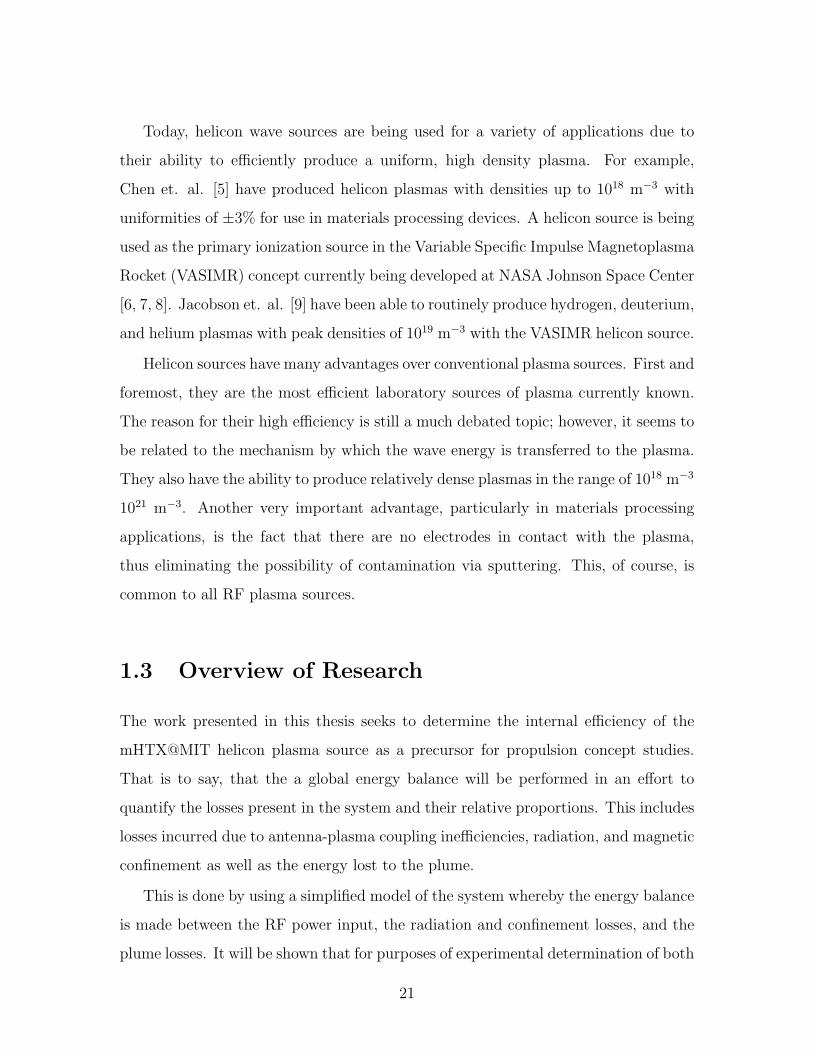
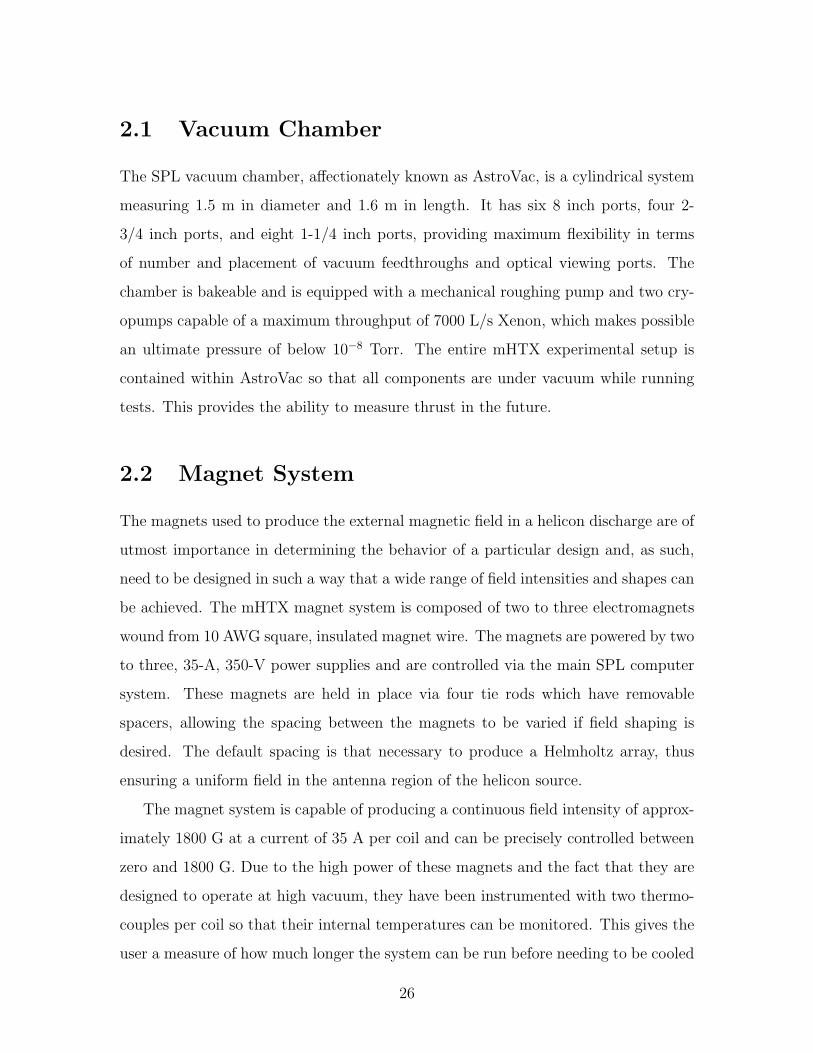
2-3 Operation with 20 sccm Ar gas flow: (left) - ICP mode, no plume;

(center) - intermediate mode with a diffuse plume, and (right) - bright,

helicon mode forming a narrow plasma beam at 600 W. . . . . . . . . 30

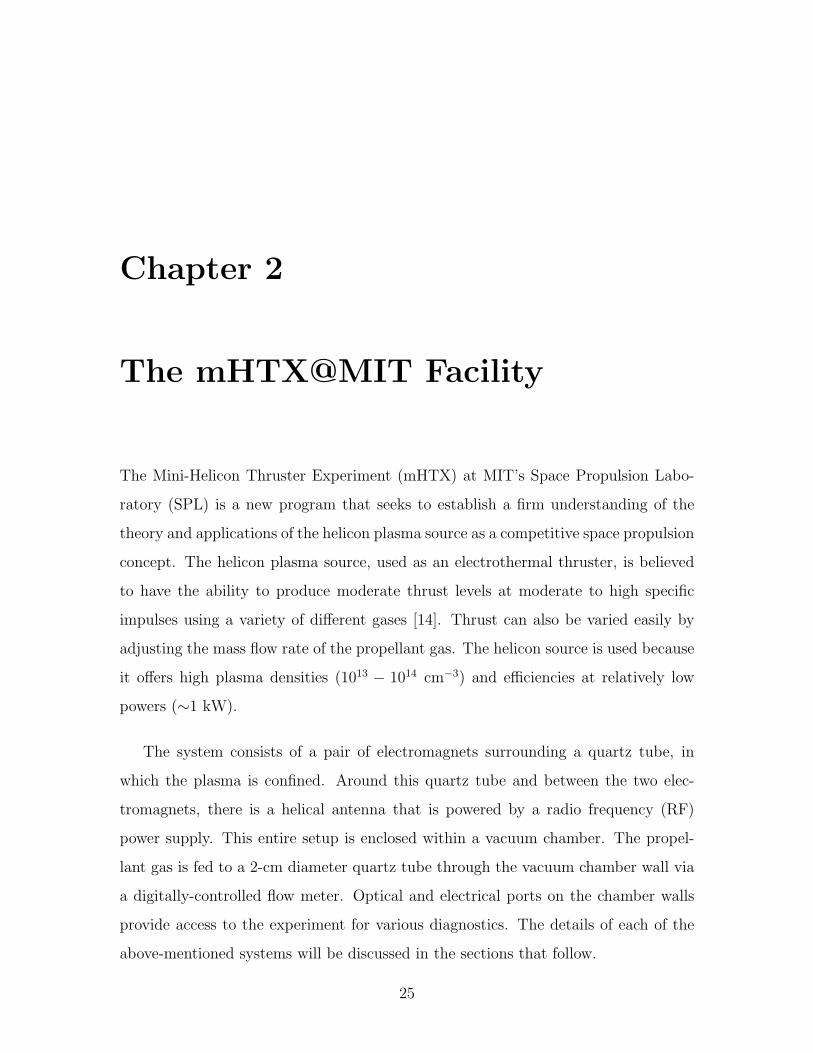
2-4 Operation with N2 at 800 W of RF power: (left) - ICP mode with no

externally-applied magnetic field, and (right) - Helicon mode with 20

A of magnet current, corresponding to an applied field of 1200 G. . . 30

2-5 Operation at 1200 G with a flow rate of 30 sccm: (left) - 70-percent - 30-

percent N2/Ar mixture (viewed from side), and (right) - an atmospheric

air discharge (view is directly into the plasma plume). . . . . . . . . . 31

11

2-6 Operation at 20 sccm Ar gas flow with a permanent ceramic magnet

in view at the end of the source tube. Note the constriction of the

plasma column followed by an abrupt expansion to what appears to be

a planar structure in the upstream region. Also note the semi-spherical

structure in the downstream, plume region. . . . . . . . . . . . . . . . 32

3-1 A pictorial representation of a Langmuir probe immersed in a plasma.

Notice the small metal tip and the sheath surrounding it. . . . . . . . 34

3-2 A plot showing the important aspects and regions of a typical Langmuir

probe I-V curve. Notice that the floating potential is negative with

respect to the plasma potential. . . . . . . . . . . . . . . . . . . . . . 37

3-3 A pictorial representation of a Faraday probe in contact with the target

plasma. Notice that the guard ring successfully attracts ions from the

sides of the probe so as to collimate the field of view of the probe surface. 41

3-4 A photograph of the Faraday probe built for use in the mHTX@MIT

program showing details of the guard ring, collector plate, and ceramic

sheath. . . . . . . . . . . . . . . . . . . . . . . . . . . . . . . . . . . . 42

3-5 A pictorial representation of an RPA showing the three biased grids

electrically isolated from each other by concentric, ceramic rings. . . . 45

3-6 A deconstructed view of the mHTX@MIT RPA showing the individual

grids, ceramic ring spacers, and the collector plate as well as the inner

ceramic shell and the outer body. . . . . . . . . . . . . . . . . . . . . 46

4-1 A pictorial representation of an isotropic solid with elemental volume

dV and elemental area dA. . . . . . . . . . . . . . . . . . . . . . . . . 48

4-2 A pictorial representation of the half-space (semi-infinite) problem ge-

ometry. . . . . . . . . . . . . . . . . . . . . . . . . . . . . . . . . . . . 50

4-3 Notice that the non-dimensional temperature is negligible beyond non-

dimensional thickness of 2. This region is referred to as the thermal

boundary layer. . . . . . . . . . . . . . . . . . . . . . . . . . . . . . . 53

12

4-4 A plot of the simulated temperature profile on the quartz tube using

equation (4.1.23) as discussed in the given example. . . . . . . . . . . 60

4-5 A plot of the resultant power data reduced from the temperature series

in Figure 4-4 using equation (4.2.4). . . . . . . . . . . . . . . . . . . . 61

5-1 A photograph of the quartz source tube (top) and the alumina ceramic

source tube (bottom). . . . . . . . . . . . . . . . . . . . . . . . . . . 65

5-2 A photograph of one of the C01-K surface thermocouples showing de-

tails of the junction. . . . . . . . . . . . . . . . . . . . . . . . . . . . 67

5-3 A pictorial representation of the source tube where the thermocouple

nodes are numbered one through five and the masses m2 = m3 =

m4 > m1 = m5 refer to the masses corresponding to each of the five

cells whose boundaries are given by the dotted lines. . . . . . . . . . . 68

5-4 A pictorial representation of the mHTX@MIT helicon plasma source

with all loss mechanisms considered. . . . . . . . . . . . . . . . . . . 69

A-1 A plot of k versus β for different values of B0(G) in a plasma of density

n0 = 1× 1013 cm−1 and a rf frequency of 27.12 Mhz. . . . . . . . . . 83

A-2 A plot of k versus β for B0 = 1000 G in a plasma of density n0 =

1× 1013 cm−1 and a rf frequency of 27.12 Mhz showing the discretized

values of k for which H-TG modes can propagate. Note that only the

first three modes can be resolved at this scale. . . . . . . . . . . . . . 87

A-3 A plot of the LHS and RHS of equation (A.4.42) versus k forB0 = 1000 G

in a plasma of density n0 = 1× 1013 cm−1 and a rf frequency of 27.12

Mhz. The modes can clearly be seen as the intersections of the two

functions. . . . . . . . . . . . . . . . . . . . . . . . . . . . . . . . . . 88

D-1 A photograph of a properly mixed batch of OB-200 epoxy adhesive. . 102

D-2 A photograph of the quartz tube and thermocouples in the oven during

a curing session. . . . . . . . . . . . . . . . . . . . . . . . . . . . . . . 103

13

D-3 A photograph of the quartz tube after having the thermocouples bonded

to it and properly cured. . . . . . . . . . . . . . . . . . . . . . . . . . 104

14

List of Tables

1.1 Typical values of specific impulse for various chemical and electric

propulsion concepts. . . . . . . . . . . . . . . . . . . . . . . . . . . . 19

4.1 Typical properties of fused quartz. . . . . . . . . . . . . . . . . . . . 59

5.1 Typical properties of alumina ceramic. . . . . . . . . . . . . . . . . . 67

B.1 Quantities of interest for a typical helicon plasma. . . . . . . . . . . . 91

B.2 Electron and ion characteristic frequencies for a typical helicon plasma. 93

15

16

Chapter 1

Introduction

Space propulsion is a mature, but dynamic field where the state-of-the-art is always

being redefined. The complexity of a typical space propulsion system requires in-

terdisciplinary studies and relies on a number of experts in different areas to fully

understand and synthesize new technology. While many concepts have been studied

rigorously and have been used in space applications for many years, there still exist

some newer, less-understood technologies.

1.1 Space Propulsion

Space propulsion can be separated into two main categories: chemical systems and

electric systems. Chemical systems utilize the energy stored in the bonds of the pro-

pellant to produce a high temperature, high pressure working fluid that can then

be expelled from a conventional, converging-diverging nozzle to produce thrust. The

major concepts within this area are solid propellants, liquid-bipropellants, mono-

propellants, and cold-gas thrusters. All of these engines have been successfully im-

plemented on many missions ranging from on-orbit trajectory corrections and drag

make-up of satellites to interplanetary science probes. These technologies have been

developed very thoroughly in the past half century and benefit from that heritage in

the consideration for placement on current and future missions.

17

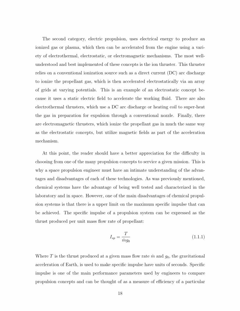
The second category, electric propulsion, uses electrical energy to produce an

ionized gas or plasma, which then can be accelerated from the engine using a vari-

ety of electrothermal, electrostatic, or electromagnetic mechanisms. The most well-

understood and best implemented of these concepts is the ion thruster. This thruster

relies on a conventional ionization source such as a direct current (DC) arc discharge

to ionize the propellant gas, which is then accelerated electrostatically via an array

of grids at varying potentials. This is an example of an electrostatic concept be-

cause it uses a static electric field to accelerate the working fluid. There are also

electrothermal thrusters, which use a DC arc discharge or heating coil to super-heat

the gas in preparation for expulsion through a conventional nozzle. Finally, there

are electromagnetic thrusters, which ionize the propellant gas in much the same way

as the electrostatic concepts, but utilize magnetic fields as part of the acceleration

mechanism.

At this point, the reader should have a better appreciation for the difficulty in

choosing from one of the many propulsion concepts to service a given mission. This is

why a space propulsion engineer must have an intimate understanding of the advan-

tages and disadvantages of each of these technologies. As was previously mentioned,

chemical systems have the advantage of being well tested and characterized in the

laboratory and in space. However, one of the main disadvantages of chemical propul-

sion systems is that there is a upper limit on the maximum specific impulse that can

be achieved. The specific impulse of a propulsion system can be expressed as the

thrust produced per unit mass flow rate of propellant:

Isp =T

mg0

(1.1.1)

Where T is the thrust produced at a given mass flow rate m and g0, the gravitational

acceleration of Earth, is used to make specific impulse have units of seconds. Specific

impulse is one of the main performance parameters used by engineers to compare

propulsion concepts and can be thought of as a measure of efficiency of a particular

18

Concept Isp(s)cold gas 50 - 250

monopropellant 125 - 250solid propellant 250 - 300

bipropellant 200 - 450electrothermal 500 - 1000

electromagnetic 1000 - 5000electrostatic 2000 - 20000

Table 1.1: Typical values of specific impulse for various chemical and electric propul-sion concepts.

propellant. Table 1.1 shows the ranges of specific impulse of the abovementioned

concepts. Notice that these propulsion systems span four orders of magnitude in

specific impulse. This allows the propulsion engineer a great deal of flexibility in the

choice of concept to be employed on a given mission; however, it also makes the design

process a long and difficult one unless there are clear constraints or requirements.

Another, perhaps, more telling figure of merit used to evaluate the performance

of a particular engine or thruster is that of the thrust or internal efficiency. This is a

measure of the efficiency of a concept to convert the input energy, whether chemical

or electrical, into useful, thrust-producing energy. This can be expressed as

η =T 2

2m

Pinput

(1.1.2)

Where, the term in the numerator is the exhaust or kinetic power and is the compo-

nent that directly produces thrust and m is the propellant mass flow rate. Also, for

chemical propulsion systems, Pinput = mHreaction and represents the total chemical

power stored in the the bonds of the propellant mixture as the product of the propel-

lant mass flow rate, m and the heat of reaction of the combustion process, Hreaction.

Finally, for electric propulsion systems, Pinput = IV and represents the total electric

power cast as the product of the current and voltage of the power supply [1].

The internal efficiency is a rather practical measure, as it includes all losses in-

curred from the point of initial energy input to the final expulsion of the working

19

fluid from the engine or thruster. This includes losses due to incomplete combustion

or finite enthalpy in the exhaust stream in the case of chemical systems or wall losses,

excitation collisions, and multiple ions in electric thrusters. While, from a practical

standpoint, what happens in between is of little or no interest to the end-user, it is of

utmost importance to propulsion researchers. If the nature of the loss mechanisms can

be resolved, then there is a possibility that certain measures can be taken to reduce

or eliminate them, thus increasing the efficiency of the system. To that end, many

aspects of a given propulsion system can be examined in an attempt to resolve and

subsequently eliminate specific loss mechanisms; however, a simple model is always

the best place to begin.

1.2 Helicon Plasma Sources

Helicon waves are a special case of the right-hand circularly polarized (RCP) elec-

tromagnetic wave in that they propagate only in bounded magnetized media. The

helicon wave was found in 1960 by Aigrain during his study of waves in solid metals

[3]. He observed waves in slabs of super low-temperature sodium that propagated in

the range of frequencies ωci � ω � ωce, where ωci is the ion cyclotron frequency and

ωce is the electron cyclotron frequency. Upon further study, he determined that the

wave magnetic field vector traced a helix at a fixed time, hence the name ”helicon.”

Modern helicon plasmas are produced in cylindrical geometries with a DC mag-

netic field applied along the longitudinal axis [3, 4]. The gas is first weakly ionized

by the electrostatic fields in the antenna region as in a typical capacitively- (CCP) or

inductively-coupled plasma (ICP). However, upon application of the external mag-

netic field, the plasma discharge changes character in that it is no longer subject to

the skin depth constraint to which the aforementioned CCP and ICP are. This allows

the helicon wave to penetrate into the core of the plasma column. The plasma is then

further ionized due to a wave-particle interaction and is thought to be aided by a

mode conversion at the wall boundary.

20

Today, helicon wave sources are being used for a variety of applications due to

their ability to efficiently produce a uniform, high density plasma. For example,

Chen et. al. [5] have produced helicon plasmas with densities up to 1018 m−3 with

uniformities of ±3% for use in materials processing devices. A helicon source is being

used as the primary ionization source in the Variable Specific Impulse Magnetoplasma

Rocket (VASIMR) concept currently being developed at NASA Johnson Space Center

[6, 7, 8]. Jacobson et. al. [9] have been able to routinely produce hydrogen, deuterium,

and helium plasmas with peak densities of 1019 m−3 with the VASIMR helicon source.

Helicon sources have many advantages over conventional plasma sources. First and

foremost, they are the most efficient laboratory sources of plasma currently known.

The reason for their high efficiency is still a much debated topic; however, it seems to

be related to the mechanism by which the wave energy is transferred to the plasma.

They also have the ability to produce relatively dense plasmas in the range of 1018 m−3

1021 m−3. Another very important advantage, particularly in materials processing

applications, is the fact that there are no electrodes in contact with the plasma,

thus eliminating the possibility of contamination via sputtering. This, of course, is

common to all RF plasma sources.

1.3 Overview of Research

The work presented in this thesis seeks to determine the internal efficiency of the

mHTX@MIT helicon plasma source as a precursor for propulsion concept studies.

That is to say, that the a global energy balance will be performed in an effort to

quantify the losses present in the system and their relative proportions. This includes

losses incurred due to antenna-plasma coupling inefficiencies, radiation, and magnetic

confinement as well as the energy lost to the plume.

This is done by using a simplified model of the system whereby the energy balance

is made between the RF power input, the radiation and confinement losses, and the

plume losses. It will be shown that for purposes of experimental determination of both

21

the radiation and confinement losses, it is a reasonable approximation to assume that

both losses are sufficiently absorbed by the plasma source tube material to simply

diagnose the energy incident on the inner surface of the tube without differentiation

between mechanisms.

Chapter 2 gives a brief overview of the experimental facilities that were to be used

in conducting this research including the vacuum system, control system, and the ra-

dio frequency (RF) power system as well as a brief discussion of the source operation

and corresponding observations. Chapter 3 discusses plume diagnostics fundamen-

tals including the general operation and theory governing Langmuir probes, Faraday

probes, and Retarding Potential Analyzers (RPA). Chapter 4 reviews heat conduc-

tion theory with an extension to the simple method used to determine losses to the

plasma source tube. Chapter 5 develops the model used to build the energy balance

of the mHTX@MIT helicon system. Finally, Chapter 6 covers recommendations for

future work.

Appendix A is a rather detailed overview of helicon wave theory as it is currently

understood and covers a full derivation of the helicon wave equation including the

various modes and the effects of boundary conditions. This should serve as a basis

upon which future theoretical and computational work can be launched as well as a

primer for those new to helicon plasma physics. Appendix B discusses a simple helicon

fluid model that was developed at the beginning of this work, when computation was

still a priority. It is complete insofar as it presents a simple drift-diffusion model that

matches those used by other researchers as a starting point for helicon simulation.

It includes a description of both the ion and electron fluid equations as well as the

antenna current model and simple boundary conditions that provide closure of the

system. It is meant to orient the reader towards thinking in terms of helicon plasma

simulation, although it should not be taken as a complete or valid model without

further study. The author leaves further computational development to those who

will take up the responsibility of helicon simulations in the future of the mHTX@MIT

program. Appendix C describes the process by which a helicon source and antenna

22

can be designed using a simple extension of the helicon dispersion relation derived

in Appendix A. This method is based largely on theory given by Chen et. al. [3, 4,

5, 10, 15] and has been employed in the design of the mHTX@MIT helicon source.

The author cautions the reader that it is merely a proposed method and has not been

validated in any broad way; however, it may be used as a baseline for source and

antenna design, whilst keeping in mind the controversial nature of current helicon

theory and the tenuous understanding of the physical mechanisms governing helicon

plasma source operation. Finally, Appendix D gives a brief overview of the methods

used to bond the surface-mounted thermocouples to the source tube including details

epoxy preparation and curing.

23

24

Chapter 2

The mHTX@MIT Facility

The Mini-Helicon Thruster Experiment (mHTX) at MIT’s Space Propulsion Labo-

ratory (SPL) is a new program that seeks to establish a firm understanding of the

theory and applications of the helicon plasma source as a competitive space propulsion

concept. The helicon plasma source, used as an electrothermal thruster, is believed

to have the ability to produce moderate thrust levels at moderate to high specific

impulses using a variety of different gases [14]. Thrust can also be varied easily by

adjusting the mass flow rate of the propellant gas. The helicon source is used because

it offers high plasma densities (1013 − 1014 cm−3) and efficiencies at relatively low

powers (∼1 kW).

The system consists of a pair of electromagnets surrounding a quartz tube, in

which the plasma is confined. Around this quartz tube and between the two elec-

tromagnets, there is a helical antenna that is powered by a radio frequency (RF)

power supply. This entire setup is enclosed within a vacuum chamber. The propel-

lant gas is fed to a 2-cm diameter quartz tube through the vacuum chamber wall via

a digitally-controlled flow meter. Optical and electrical ports on the chamber walls

provide access to the experiment for various diagnostics. The details of each of the

above-mentioned systems will be discussed in the sections that follow.

25

2.1 Vacuum Chamber

The SPL vacuum chamber, affectionately known as AstroVac, is a cylindrical system

measuring 1.5 m in diameter and 1.6 m in length. It has six 8 inch ports, four 2-

3/4 inch ports, and eight 1-1/4 inch ports, providing maximum flexibility in terms

of number and placement of vacuum feedthroughs and optical viewing ports. The

chamber is bakeable and is equipped with a mechanical roughing pump and two cry-

opumps capable of a maximum throughput of 7000 L/s Xenon, which makes possible

an ultimate pressure of below 10−8 Torr. The entire mHTX experimental setup is

contained within AstroVac so that all components are under vacuum while running

tests. This provides the ability to measure thrust in the future.

2.2 Magnet System

The magnets used to produce the external magnetic field in a helicon discharge are of

utmost importance in determining the behavior of a particular design and, as such,

need to be designed in such a way that a wide range of field intensities and shapes can

be achieved. The mHTX magnet system is composed of two to three electromagnets

wound from 10 AWG square, insulated magnet wire. The magnets are powered by two

to three, 35-A, 350-V power supplies and are controlled via the main SPL computer

system. These magnets are held in place via four tie rods which have removable

spacers, allowing the spacing between the magnets to be varied if field shaping is

desired. The default spacing is that necessary to produce a Helmholtz array, thus

ensuring a uniform field in the antenna region of the helicon source.

The magnet system is capable of producing a continuous field intensity of approx-

imately 1800 G at a current of 35 A per coil and can be precisely controlled between

zero and 1800 G. Due to the high power of these magnets and the fact that they are

designed to operate at high vacuum, they have been instrumented with two thermo-

couples per coil so that their internal temperatures can be monitored. This gives the

user a measure of how much longer the system can be run before needing to be cooled

26

Figure 2-1: Two of the three electromagnets are mounted in a Helmholtz pair configu-ration. Notice the four tie rods with spacers in between the coils. Also, the shielded,orange thermocouple leads are clearly visible on the right magnet coil. As can beseen, the quartz tube is suspended inside the magnet cores and is attached to the gasfeed system at the upstream (right) end.

by way of venting the chamber to atmosphere. Figure 2-1 shows the magnet system

with two of the three magnets set up in a Helmholtz pair configuration.

2.3 RF Power System

The RF power system consists of an Advanced Energy RFPP-10 1.2 kW power supply

operating at 13.56 MHz, an impedance-matching network, a 13.56 MHz vacuum power

feedthrough, a vacuum transmission line, and finally the helicon antenna. This system

is rather complex and requires a fair amount of care and attention on a regular

basis to ensure that all conductors are making proper contact and that continuity is

maintained. Since the power supply, vacuum feedthrough, and transmission line are

standard equipment, the details of their design and operation will not be mentioned.

27

2.3.1 Impedance Matching Network

The impedance-matching network is the most important component in the RF power

system. It was designed based on the classic L-network circuit structure and employs

two tuneable, vacuum capacitors: one in series and one in parallel with the load (in

this case, the antenna and plasma). The need for such a device comes from the fact

that the plasma load is dynamic in nature and, as a result, it is necessary to be

able to tune the impedance ”seen” by the RF power supply to minimize reflected

power, thus maximizing the power transmitted to the load. This tuning is done in

realtime due to the fact that, during any given test run, parameters such as flow rate,

power, or magnetic field intensity may be varied, thus changing the impedance of the

discharge. This tuning is performed manually using an oscilloscope, which allows the

voltage waveform in the circuit to be measured. The tuner makes adjustments to the

capacitance values such that the amplitude of the measured waveform is maximized

for a given set of experimental parameters.

2.3.2 Antenna Design

A variety of antenna designs have been employed over the many years of helicon

research with varying results [10, 15]. The classic, helical antenna is among the most

well characterized and widely used designs [20]. The reader is referred to Figure

2 for details of the physical geometry of a typical helical antenna as it is used in

mHTX. Helical antennas come in two varieties: left-handed and right-handed. This

nomenclature refers to the direction of rotation of the antenna legs as seen with respect

to the wavevector, k. These directionalities also specify the wave mode, where the

left-handed and right-handed preferentially excite m = −1 and m = +1 azimuthal

modes, respectively.

To avoid confusion, the reader should note that the twist direction of the antenna

and the direction of rotation of the waves are not the same. The left-handed and right-

handed helicon waves are based on the direction of rotation of the wave magnetic field

28

Figure 2-2: Two of the mHTX helical antennas are shown. Both are right-handed andexcite them = +1 mode. The resonant energies are 20 eV and 40 eV for the small steelantenna and the large copper antenna, respectively. Different materials were used inthese two antennas to rule out the possibility of the existence of a copper emissionline, which was thought to be captured during one of the spectroscopy measurements.

vector with respect to the externally applied magnetic field. As such, the direction of

the external magnetic field need only be reversed for a given helical antenna design

to change the mode that is excited. While either antenna will excite both modes, the

m = +1 mode has been found to propagate with a greater intensity than the m = −1

mode [15].

The antenna used in the mHTX thus far, was designed as a right-handed (m =

+1), helical antenna with a radius of 1 cm, per the quartz tube size. It is thought

that Landau damping is the primary mode of energy transfer between the wave and

plasma. It is possible to design the antenna based on this concept. Since, in the

case of Landau damping, wave energy is transferred to particles that are near the

phase velocity, an antenna can be designed to launch waves of a desired axial phase

velocity, vp = ω/kz, which is related to the resonant energy, Er by Er = 1/2mv2p. By

choosing this energy to be on the order of the peak ionization cross-section energy, the

resonant electrons will absorb sufficient energy from the wave to produce ionization

29

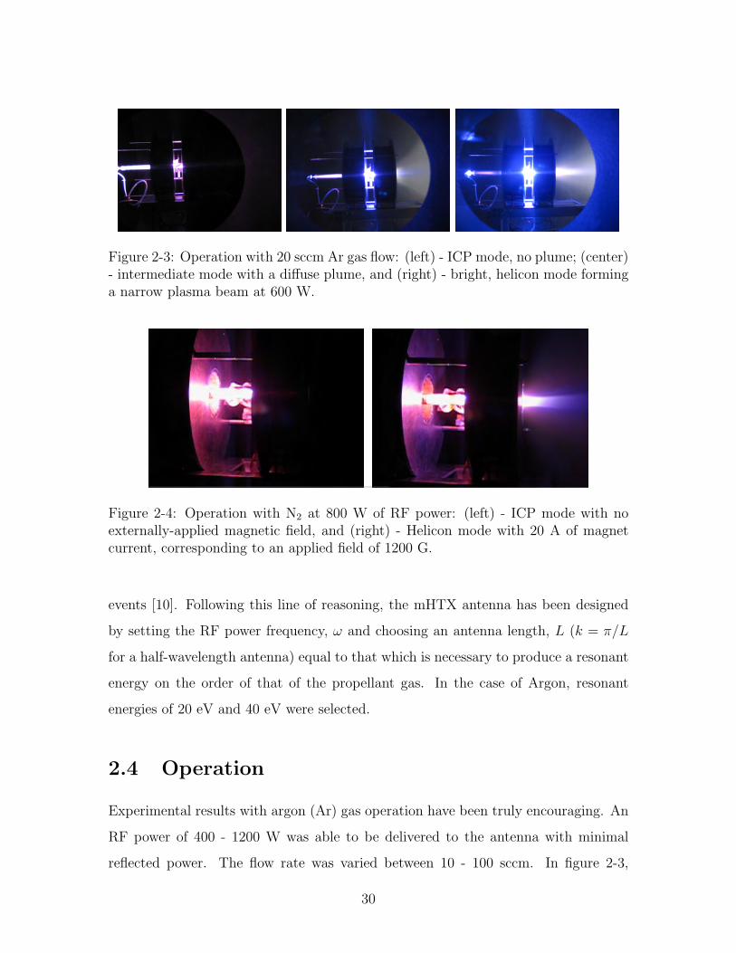
Figure 2-3: Operation with 20 sccm Ar gas flow: (left) - ICP mode, no plume; (center)- intermediate mode with a diffuse plume, and (right) - bright, helicon mode forminga narrow plasma beam at 600 W.

Figure 2-4: Operation with N2 at 800 W of RF power: (left) - ICP mode with noexternally-applied magnetic field, and (right) - Helicon mode with 20 A of magnetcurrent, corresponding to an applied field of 1200 G.

events [10]. Following this line of reasoning, the mHTX antenna has been designed

by setting the RF power frequency, ω and choosing an antenna length, L (k = π/L

for a half-wavelength antenna) equal to that which is necessary to produce a resonant

energy on the order of that of the propellant gas. In the case of Argon, resonant

energies of 20 eV and 40 eV were selected.

2.4 Operation

Experimental results with argon (Ar) gas operation have been truly encouraging. An

RF power of 400 - 1200 W was able to be delivered to the antenna with minimal

reflected power. The flow rate was varied between 10 - 100 sccm. In figure 2-3,

30

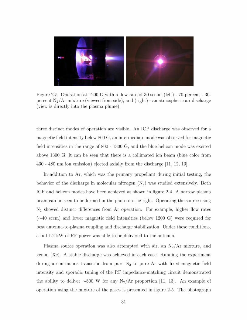
Figure 2-5: Operation at 1200 G with a flow rate of 30 sccm: (left) - 70-percent - 30-percent N2/Ar mixture (viewed from side), and (right) - an atmospheric air discharge(view is directly into the plasma plume).

three distinct modes of operation are visible. An ICP discharge was observed for a

magnetic field intensity below 800 G, an intermediate mode was observed for magnetic

field intensities in the range of 800 - 1300 G, and the blue helicon mode was excited

above 1300 G. It can be seen that there is a collimated ion beam (blue color from

430 - 480 nm ion emission) ejected axially from the discharge [11, 12, 13].

In addition to Ar, which was the primary propellant during initial testing, the

behavior of the discharge in molecular nitrogen (N2) was studied extensively. Both

ICP and helicon modes have been achieved as shown in figure 2-4. A narrow plasma

beam can be seen to be formed in the photo on the right. Operating the source using

N2 showed distinct differences from Ar operation. For example, higher flow rates

(∼40 sccm) and lower magnetic field intensities (below 1200 G) were required for

best antenna-to-plasma coupling and discharge stabilization. Under these conditions,

a full 1.2 kW of RF power was able to be delivered to the antenna.

Plasma source operation was also attempted with air, an N2/Ar mixture, and

xenon (Xe). A stable discharge was achieved in each case. Running the experiment

during a continuous transition from pure N2 to pure Ar with fixed magnetic field

intensity and sporadic tuning of the RF impedance-matching circuit demonstrated

the ability to deliver ∼800 W for any N2/Ar proportion [11, 13]. An example of

operation using the mixture of the gases is presented in figure 2-5. The photograph

31

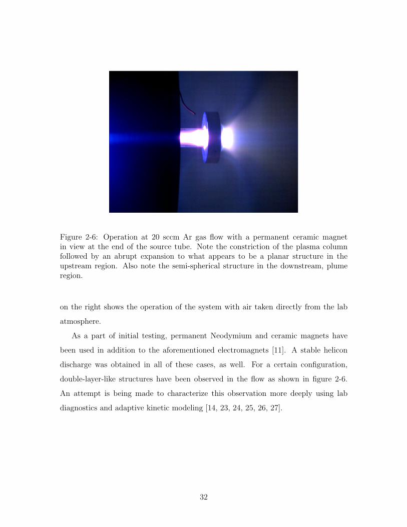
Figure 2-6: Operation at 20 sccm Ar gas flow with a permanent ceramic magnetin view at the end of the source tube. Note the constriction of the plasma columnfollowed by an abrupt expansion to what appears to be a planar structure in theupstream region. Also note the semi-spherical structure in the downstream, plumeregion.

on the right shows the operation of the system with air taken directly from the lab

atmosphere.

As a part of initial testing, permanent Neodymium and ceramic magnets have

been used in addition to the aforementioned electromagnets [11]. A stable helicon

discharge was obtained in all of these cases, as well. For a certain configuration,

double-layer-like structures have been observed in the flow as shown in figure 2-6.

An attempt is being made to characterize this observation more deeply using lab

diagnostics and adaptive kinetic modeling [14, 23, 24, 25, 26, 27].

32

Chapter 3

Plume Diagnostics

There are a variety of diagnostic techniques for characterizing a plasma depending on

the target parameter to be studied. These techniques can be separated into two main

categories: intrusive and non-intrusive. An intrusive technique is characterized as one

in which a physical probe is placed in the plasma and, thus, perturbs the plasma. This

perturbation can be minimal or significant depending on the dimensions of the probe

as compared to the characteristic dimension of the plasma. As a result, there are

situations in which intrusive diagnostics fall second to non-intrusive methods. Non-

intrusive methods include a variety of optical techniques such as emission spectroscopy

and microwave interferometry; however, these techniques typically suffer from the

need for a sizable financial investment and a rather complex experimental setup.

Typical intrusive techniques include Langmuir probes, Faraday probes, and Retarding

Potential Analyzers (RPA). These probes are usually simple in construction and, as

such, are rather economical. While both categories can accomplish similar goals, the

scope and budget of this research specified the use of intrusive diagnostics in order

to diagnose the plume region of the helicon plasma source.

33

Figure 3-1: A pictorial representation of a Langmuir probe immersed in a plasma.Notice the small metal tip and the sheath surrounding it.

3.1 The Langmuir Probe

The Langmuir probe is the simplest of the intrusive instruments. In its most basic

form, it consists of a rod of tungsten, which serves as a single electrode. The rod is

typically insulated with a sheath of ceramic material along its entire length save a

small tip that is left exposed. In practice, any refractory metal can be used; however,

tungsten seems to be the most popular due to its relatively low cost and high avail-

ability. The rod itself may range in size from sub-millimeter to several millimeters

in diameter, although, the perturbation caused by the probe is proportional to the

characteristic dimension of the probe tip as compared to the characteristic dimension

of the plasma to be diagnosed, so its diameter is a practical consideration to be made

by the experimentalist. See Figure 3-1 for a simple representation of a Langmuir

34

probe.

The Langmuir probe can be used to determine the plasma and floating potential

and the electron temperature and density by way of sweeping the potential applied

to the electrode over a range of negative and positive voltages while immersed in

the plasma. While doing so, an instantaneous current is measured corresponding to

the instantaneous applied potential and a current-voltage (I-V) characteristic curve

is constructed. From this I-V curve, the plasma parameters can be determined with

appropriate application of the Langmuir probe theory.

3.1.1 The Electrostatic Sheath

The classical Langmuir probe theory is based upon the concept of the plasma or

electrostatic sheath, which is a structure formed on any solid surface in contact with

a plasma. The existence of the sheath arises as a result of the disparity in electron and

ion fluxes to the collecting surface. The pre-sheath and sheath fluxes are a function of

the electron and ion densities as well as the temperatures and masses of the particles

and can be expressed as follows:

Pre-sheath:

Γe = ne

√kTe

2πme

Γi = ni

√k (Te + ZTi)

mi

(3.1.1)

Sheath:

Γe = ne

√kTe

2πme

e−e∆φskTe

Γi = ni

√k (Te + ZTi)

mi

e−12

(3.1.2)

35

Where ne and ni are the electron and ion densities, respectively and are assumed to be

approximately equal due to the assumption of quasi-neutrality, k is Boltzmann’s con-

stant, Te, Ti, me, mi are the electron and ion temperatures and masses, respectively,

Z is the charge state of the ion species, and ∆φs is the sheath potential [2].

Now, since the plasma is assumed to be quasi-neutral, the densities will be unified

and expressed as ne ≈ ni = n. Also, most laboratory plasmas are considered to

have cold ions, which means that the ion temperature is significantly lower than

the electron temperature so as to be able to safely neglect that term in the above

equations. That is, Te � Ti. Applying these changes to equations (3.1.1), and taking

the ratio of electron to ion fluxes in the pre-sheath, it is found that

Γe

Γi

≈√

mi

2πme

(3.1.3)

This value can be many times greater than unity and, in fact, in the case of Argon

(mi = 39.95mproton) as the working fluid, it is approximately 108. Because of the

fact that electrons stream to the surface in contact with the plasma at a rate much

greater than that of the ions, the surface accumulates a net negative charge. The

accumulation of this negative charge value grows until a balance between electron

and ion fluxes is met, thus creating a ”potential sheath.” That is to say that the

electron flux is retarded and the ion flux is accelerated by negative surface potential

until an exact equilibrium is reach and there is no net charge exchanged across the

boundary of the sheath. The potential at which the sheath is located is referred to

as the floating potential and can be found by equating equations (3.1.2) and solving

for ∆φs as follows:

|∆φs| =kTe

eln

√mi

2πme

(3.1.4)

The exact location of the sheath boundary is a more complex topic and requires

the satisfaction of what is referred to as the Bohm Sheath Criterion; however, for the

purposes of this discussion, it is sufficient to mention that this is met when the ion

36

I

V

+

+

-

- VF VP

electron saturation

ion saturation

electronretardation

Figure 3-2: A plot showing the important aspects and regions of a typical Langmuirprobe I-V curve. Notice that the floating potential is negative with respect to theplasma potential.

velocity becomes sonic:

ui ≥ cs ≈√kTe

mi

(3.1.5)

Where ui is the ion velocity and the same assumptions of cold ions has been applied

to simplify the temperature term in the numerator. Also, the reader should note

that, in the most strict sense, the Bohm Sheath Criterion is an inequality as shown

in equation (3.1.5).

37

3.1.2 Langmuir Probe Theory

Now that a basis has been formed for an understanding of the electrostatic sheath,

the specifics of its role in Langmuir probe theory can be discussed. There are a

several regions of interest in a typical Langmuir probe I-V curve as shown in Figure

3-2. Referring to Figure 3-2 for the remainder of this discussion and going from left

to right, the first region of interest is the ion saturation region. This is the region in

which the probe has been biased sufficiently negative so as to repel all but the most

high-energy electrons, thus preventing any greater negative charge build-up. This is

characterized by a rapid leveling of the I-V curve to a negative current value [22, 34].

Following the ion saturation region is a brief but intense decrease in current. This

occurs as a result of decreasing probe potential, thus permitting a increasingly greater

number of electrons to reach the surface and culminates in a zero-current, potential

value know as the floating potential, denoted as VF . This is when the applied voltage

on the probe produces an equilibrium in the electron and ion fluxes as discussed in

the above section and is exactly synonymous with the equilibrium sheath potential

case on a non-biased or floating-potential surface in the plasma.

The next region of interest is the electron retardation region. This lies between

the floating potential and the plasma potential values and is characterized by a rapid

increase in positive current due to the increasingly more positive probe bias. This

causes a larger portion of the electron distribution to reach the probe surface and

eventually leads to the electron saturation region. The plasma potential, VP is the

voltage value characterized by the rapid decrease in current from the electron retar-

dation region to the electron saturation region. For voltages below VP an electron

sheath exists; however, when the probe bias potential is increased beyond VP , the

sheath shrinks until all electrons are permitted to reach the probe surface. This is

now the electron saturation region and, of course, occurs as a result of a physical

inability of a bulk of the ion distribution to reach the probe [22, 34].

38

3.1.3 Determination of Plasma Parameters

Floating and Plasma Potentials

With a basic understanding of Langmuir probe theory it is now possible to calculate

the plasma parameters of interest from the information provided in the Langmuir

probe I-V curve. First, the most simple values to determine are the floating and

plasma potentials. The floating potential, VF is simply the x-intercept value of probe

potential. The plasma potential, VP can be found by drawing tangents to the electron

retardation and electron saturation regions and is the voltage value corresponding

to the intersection point of the two tangents. The value can also be found more

rigorously by taking the maximum of the first derivative of current with respect to

voltage, namely I ′ (V ) [22, 34].

Electron Temperature

In order to determine the electron temperature, it must be assumed that the electron

energy distribution function is purely Maxwellian. If this is the case, then the electron

current in the retardation region can be written as an exponential function of the

potential and temperature as follows:

Ire = eneAp

√kTe

2πme

eeUkTe (3.1.6)

Where e is the fundamental charge, Ap represents the probe collection area, and

U = V − VP has been introduced to denote the value of potential with respect to the

plasma potential, the utility of which will become apparent in the electron density

discussion. Now, upon taking the logarithm of equation (3.1.6) and differentiating

with respect to potential, the final result is found to be

d ln Ire

dV=

e

kTe

(3.1.7)

It should be noted that if the logarithm of equation (3.1.6), namely in the form

39

ln Ire = eV/kTe + C, is plotted on a log-linear scale, the relationship between ln Ir

e

and V should be a linear one, whose slope is proportional to the electron temperature

by equation (3.1.7); however, deviations from a linear relationship will indicate a

non-Maxwellian electron energy distribution function [22].

Electron Density

To determine electron density, it is necessary to know electron temperature a priori

using the above-mentioned method. Now, by taking equation (3.1.6) and considering

the situation where V = VP , it is found that U = 0 and the exponential term vanishes,

leaving

Ire (V = VP ) = eneAp

√kTe

2πme

(3.1.8)

Further assumption that the characteristic dimension of the sheath is negligible

compared to the dimensions of the actual probe tip itself allows the physically mea-

surable area to be used for the probe area value. Of course an explicit equation for

electron density only requires a trivial reorganization of equation (3.1.8).

3.2 Faraday Probe

The Faraday probe is a simple instrument that is used to measure the current den-

sity of the target plasma and ultimately, in combination with simultaneous electron

density measurements from a Langmuir probe, can provide an estimate of the speed

at which the bulk plasma is traveling. Another use is the opposite situation where

the birth potential of the ions is known and hence, a value of ion velocity is able to

be computed. In this case, the Faraday probe can then be used to determine electron

density, which is often more accurate than Langmuir probe measurements.

The probe itself is not unlike a Langmuir probe in that it utilizes an electrode

immersed in the target plasma; however, the main difference is that, rather than

having a small tip, the Faraday probe has a plate-like electrode whose exposed area is

40

Figure 3-3: A pictorial representation of a Faraday probe in contact with the targetplasma. Notice that the guard ring successfully attracts ions from the sides of theprobe so as to collimate the field of view of the probe surface.

known precisely. Surrounding this flat-plate electrode is an electrically isolated ring

known as a guard ring. In general operation, both the electrode and guard ring are

independently biased at a sufficiently negative, but equal potential as to place the

probe in the ion saturation region. In doing this, the guard ring collects a fair amount

of current and ”fools” the plasma, thus canceling geometrical fringe-field effects [34].

Figure 3-3 shows a diagram of a Faraday probe during operation. Notice that

the guard ring is electrically isolated from the collector plate via the ceramic sheath

surrounding the stem of the collector plate electrode; however, as mentioned above, it

is not floating. Figure 3-4 shows the actual Faraday probe to be used. This particular

design was originally developed by Azziz et. al. [34] at the MIT Space Propulsion

Laboratory for use in Hall thruster plume diagnostics and has been reconstructed

41

Figure 3-4: A photograph of the Faraday probe built for use in the mHTX@MITprogram showing details of the guard ring, collector plate, and ceramic sheath.

and adapted for diagnosing the mHTX@MIT helicon plume. For practical purposes,

both the guard ring and the collector plate should be biased at the same negative

potential in the range of -8V to -20V, based on experiments performed by Azziz et.

al. [34]. These voltages were found to place the probe well within the ion saturation

region, while the fact that both were biased to the same potential produced a uniform

sheath around both the collector plate and guard ring. For a fully detailed discussion

of probe design considerations, the reader is referred to [34].

In practice, the Faraday probe measures a current that is induced by the ions

incident on the collector plate. This current is then simply divided by the known

area of the collector plate to determine the current density. The probe is typically

swept in angle at some fixed radius from the plasma source exit to build a profile

of current density as a function of angle. This, in turn, can be used to determine

total plume current and plume divergence, which is a useful measure of the extent

to which a plasma beam is collimated. Plume divergence is an important aspect

of thruster performance when considering the possibility of plume impingement on

nearby spacecraft surfaces and also specifies, to some extent, the proportion of the

42

ejected bulk plasma that is actually used to produce an on-axis thrust force. Equa-

tion (3.2.1) shows the relationship between current density, j, collected current, Jc,

collector plate area, Ac, and ion velocity, vi as follows:

j =Jc

Ac

= enevi (3.2.1)

The plume can be considered a cone with a a spherical cap whose apex is centered

at the origin of a spherical coordinate system (r, φ, θ), which is located at the center of

the plasma source exit plane. The longitudinal axis of the plasma source is the z-axis

and points in the positive direction. The location of the Faraday probe is then given

by the radius, r specifying its distance from the origin and its angular location is fixed

in zenith (θ = 0) but is free to rotate in azimuth (−π/2 ≤ φ ≤ π/2). Furthermore, it

is assumed that the face of the Faraday probe is always facing the origin, that is to

say that the longitudinal axis of the probe is collinear with a vector extending from

the origin to the face of the Faraday probe with a magnitude of r and an azimuth of

φ. Thus, the path of the Faraday probe describes the projection of a cone onto the x-z

axis. In this system, assuming that the angular current distribution is axisymmetric,

it is simple to see that to determine the total current contained in the plume, the

following equation for the solid angle that is subtended by a half-cone of the type

describe above is:

Ip = 2πr2

∫ π/2

0

j (φ) sin (φ) dφ (3.2.2)

Equation (3.2.2) can then be augmented slightly in order to determine the plume

divergence half angle by specifying a reasonable value of the beam current that should

be contained within the plume and finding the half-angle at which this value is sat-

isfied. In the past, researchers have used values in the range of 95 - 98% of the beam

current. Based on the work of Azziz et. al. [34], the author suggests the use of 95%

as a starting value. Equation (3.2.2) can be recast as a condition to be satisfied as

follows:

43

0.95Ip = 2πr2

∫ φ1/2

0

j (φ) sin (φ) dφ (3.2.3)

Finally, the most important calculation to be made for purposes of this work is

that of the total plume energy or power. This can be done by way of capturing angular

distributions of plasma potential and current simultaneously using a Langmuir probe

and Faraday probe. The product of plasma potential and current at a given azimuth

and radius is then the power and can be expressed as follows:

P (φ) = Jc (φ) (V0 − VP (φ)) (3.2.4)

Where V0 is the ion birth potential and is determined from ion energy distribution

data. The integral of equation (3.2.4) in the range 0 ≤ φ ≤ φ1/2 will then give the

plume power

Pp = 2πr2

∫ φ1/2

0

P (φ) sin (φ) dφ (3.2.5)

This result will then be used in the the global power balance model of the

mHTX@MIT helicon source and will specify the value of the numerator in equation

(5.3.3) for purposes of determination of the internal efficiency of the system.

3.3 Retarding Potential Analyzer

The final instrument to be discussed is what is typically referred to as a Retarding

Potential Analyzer (RPA). The RPA is basically a collimated Faraday probe with the

addition of a number of grids spanning the length of the instrument. Each grid is

responsible for shielding the collector plate from a different class of particles by way

of an applied potential. The first grid is typically left floating to shield the instrument

from the bulk of the plasma. The second grid is referred to as the electron-repelling

grid and is biased to a sufficiently negative voltage so as to repel electrons from further

penetration into the probe body. The third and final grid is the ion-retarding grid

44

Figure 3-5: A pictorial representation of an RPA showing the three biased gridselectrically isolated from each other by concentric, ceramic rings.

and is swept thru a range of voltages from zero to sometimes as high as 500V. As the

potential of the ion-retarding grid increases, an increasingly greater number of ions

are unable to travel up the potential to pass the grid and be collected. This effectively

gives the experimentalist an I-V characteristic curve that describes the quantity of

ions whose energies are those swept through by the RPA. This I-V curve is then used

to determine the energy distribution of the ions in the target plasma, since the ion

energy distribution is proportional to I ′ (V ).

It should be mentioned that in some RPA designs, a fourth grid is included just

upstream of the collector plate. This is called the secondary-electron repelling grid

and is positively-biased to prevent the measurement of an erroneously high current

due to secondary-electron emission. Secondary-electron emission is caused by very

45

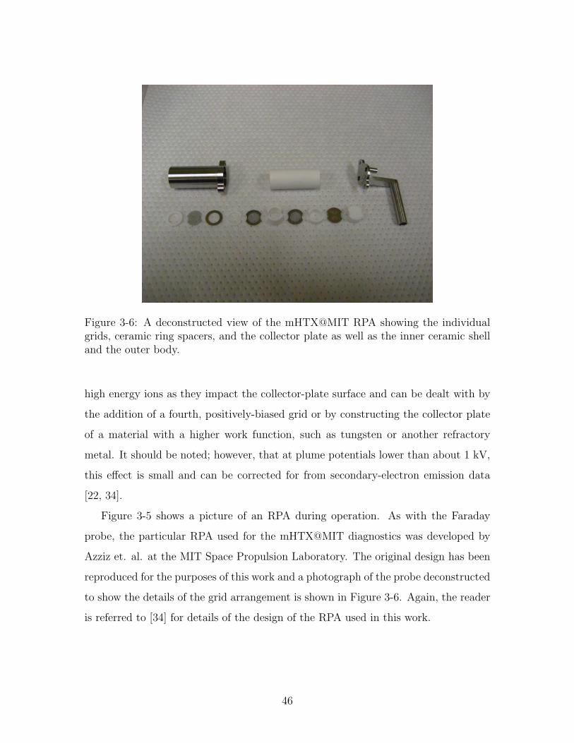
Figure 3-6: A deconstructed view of the mHTX@MIT RPA showing the individualgrids, ceramic ring spacers, and the collector plate as well as the inner ceramic shelland the outer body.

high energy ions as they impact the collector-plate surface and can be dealt with by

the addition of a fourth, positively-biased grid or by constructing the collector plate

of a material with a higher work function, such as tungsten or another refractory

metal. It should be noted; however, that at plume potentials lower than about 1 kV,

this effect is small and can be corrected for from secondary-electron emission data

[22, 34].

Figure 3-5 shows a picture of an RPA during operation. As with the Faraday

probe, the particular RPA used for the mHTX@MIT diagnostics was developed by

Azziz et. al. at the MIT Space Propulsion Laboratory. The original design has been

reproduced for the purposes of this work and a photograph of the probe deconstructed

to show the details of the grid arrangement is shown in Figure 3-6. Again, the reader

is referred to [34] for details of the design of the RPA used in this work.

46

Chapter 4

Thermal Characterization

In order to determine the heat loading and associated losses to the source tube, it

must be instrumented in such a way that the heat flux can either be directly measured

or a suitable model can be applied to extract the heat flux from raw temperature

data. There are a variety of methods that can be used to accomplish this goal;

however, before choosing the most appropriate method, it is necessary to consider

both the conditions and geometry in which these measurements are to be made, as

well as the expectations placed on the results. In order to do this, it is important

to understand the fundamentals of heat transfer so that the various methods can be

evaluated objectively.

4.1 The Heat Equation

It is known from Fourier’s law that heat flows in the direction opposite to a temper-

ature gradient and as a result, the rate at which energy flows through a unit area, or

the so-called heat flux is related to the temperature gradient as

qx = −kdTdx

(4.1.1)

Where, in this case, the x-directed heat flux, qx is equal to the product of the derivative

47

dV

dA

∧n

Figure 4-1: A pictorial representation of an isotropic solid with elemental volume dVand elemental area dA.

of temperature in the x direction and a proportionality constant, k, which is referred

to as the thermal conductivity and has units of Wm−1K−1. The minus sign is used

to indicate that energy flows from a high temperature to a low temperature. This

can be readily extended to the more general, three-dimensional case as follows:

q = −k∇T (4.1.2)

Now consider the energy balance in a simple, isotropic solid as shown in figure

4-1, where the surface of the solid is defined by the normal vector n and the solid is

composed of small, elemental volumes, dV . In order to write an energy balance for

this solid, the net rate of heat flow through the boundary of the solid and the time-

rate of change of the internal energy must be equated to the rate of energy generation

48

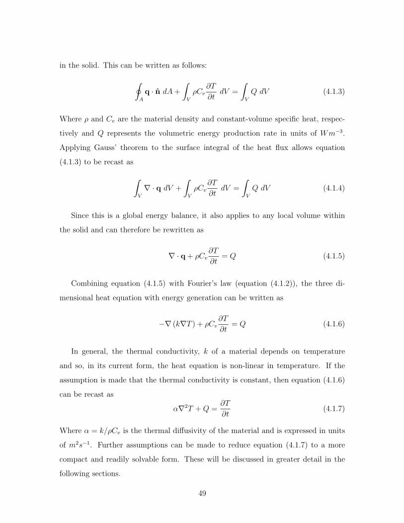
in the solid. This can be written as follows:

∮A

q · n dA+

∫V

ρCv∂T

∂tdV =

∫V

Q dV (4.1.3)

Where ρ and Cv are the material density and constant-volume specific heat, respec-

tively and Q represents the volumetric energy production rate in units of Wm−3.

Applying Gauss’ theorem to the surface integral of the heat flux allows equation

(4.1.3) to be recast as

∫V

∇ · q dV +

∫V

ρCv∂T

∂tdV =

∫V

Q dV (4.1.4)

Since this is a global energy balance, it also applies to any local volume within

the solid and can therefore be rewritten as

∇ · q + ρCv∂T

∂t= Q (4.1.5)

Combining equation (4.1.5) with Fourier’s law (equation (4.1.2)), the three di-

mensional heat equation with energy generation can be written as

−∇ (k∇T ) + ρCv∂T

∂t= Q (4.1.6)

In general, the thermal conductivity, k of a material depends on temperature

and so, in its current form, the heat equation is non-linear in temperature. If the

assumption is made that the thermal conductivity is constant, then equation (4.1.6)

can be recast as

α∇2T +Q =∂T

∂t(4.1.7)

Where α = k/ρCv is the thermal diffusivity of the material and is expressed in units

of m2s−1. Further assumptions can be made to reduce equation (4.1.7) to a more

compact and readily solvable form. These will be discussed in greater detail in the

following sections.

49

y

x0

Figure 4-2: A pictorial representation of the half-space (semi-infinite) problem geom-etry.

4.1.1 The Half-Space or Semi-Infinite Problem

In order to provide some mathematical insight as to the nature of physical systems

governed by the heat equation, a simple solid without internal energy generation will

now be examined. Figure 4-2 shows a solid material in the x-y plane with a boundary

located at x = 0 and extending to infinity in the positive and negative y directions

and positive x direction. As a result of such geometry, this is commonly referred to as

the half-space or semi-infinite problem [28, 30]. The initial temperature of the solid

is assumed to be T = Ti in the domain 0 < x <∞ and the temperature at x = ∞ is

50

T = Ti for 0 < t <∞. This problem can be formulated as follows:

α∂2T (x, t)

∂x2=∂T (x, t)

∂t

T (x, 0) = Ti

T (∞, t) = Ti

(4.1.8)

Equation (4.1.8) is a linear, second-order, partial differential equation; however,

by employing the Laplace transform, it can be reduced to a second order ordinary dif-

ferential equation whose solution is easily acquired. Recall that the Laplace transform

is defined as

L [T (x, t)] = T (x, s) =

∫ ∞

0

T (x, t) e−st dt (4.1.9)

Transforming equation (4.1.8) and its initial and boundary conditions gives

d2T (x, s)

dx2=

1

α

[sT (x, s)− T (x, 0)

]T (x, 0) =

Ti

s

T (∞, s) =Ti

s

(4.1.10)

Equation (4.1.10) is now solvable by assuming a general solution of the form

T (x, s) = Ae−√

sα

x +Be√

sα

x +Ti

s(4.1.11)

By considering the boundary condition T (∞, s) = Ti/s, it is readily apparent

that as x→∞, the solution T (x, s) → Ti/s, thus the coefficient B must be equal to

zero. This gives

T (x, s) = Ae−√

sα

x +Ti

s(4.1.12)

Where the coefficient A will be determined by the boundary condition to be specified

at x = 0.

51

Constant Surface Temperature Case

Consider the half-space problem described above by equation (4.1.8); however, let the

boundary condition at x = 0 and its associated Laplace transform be specified as

T (0, t) = Ts

T (0, s) =Ts

s

(4.1.13)

This represents the instantaneous application of a constant surface temperature to

the boundary of the semi-infinite solid. Applying the boundary condition in equation

(4.1.13) to equation (4.1.12), the following solution is found

T (x, s) =Ts − Ti

se−√

sα

x +Ti

s(4.1.14)

Finally, using the inverse Laplace transform and rearranging, the solution can be

expressed asT (x, t)− Ti

Ts − Ti

= erfc

(x√4αt

)(4.1.15)

Where erfc (x) = 1− erf (x) is the complementary error function. This solution can

be found in a variety of Laplace transform tables.

Now, by considering the units of the arguement of the complementary error func-

tion in equation (4.1.15), it can be readily seen that it is a non-dimensional group in

length, which will, henceforth, be referred to as the non-dimensional thickness. Also,

the left-hand side is a non-dimensional group in temperature. Then equation (4.1.15)

can be rewritten by introducing non-dimensional variables as follows:

Θ = erfc χ (4.1.16)

The non-dimensional temperature is plotted versus the non-dimensional thickness

from Equation (4.1.15) in figure 4-3. Notice that the magnitude of Θ is negligible

beyond χ = 2. This result is significant in that it formally defines the concept of

52

0

0.1

0.2

0.3

0.4

0.5

0.6

0.7

0.8

0.9

1

0 0.5 1 1.5 2 2.5 3 3.5 4

non-dimensional thickness

non-

dim

ensi

onal

tem

pera

ture

Figure 4-3: Notice that the non-dimensional temperature is negligible beyond non-dimensional thickness of 2. This region is referred to as the thermal boundary layer.

a semi-infinite material. From this, it can be stated that any medium whose non-

dimensional thickness is greater than χ = 2, can be referred to as a semi-infinite

medium. That is, in the time range of interest, its characteristic dimension associ-

ated with heat transfer is sufficiently large compared to the distance to which the

temperature disturbance propagates, so as to negate the effects of the disturbance

beyond that distance. The zone of material contained in the range 0 < χ < 2 can

also referred to as the thermal boundary layer [28, 30].

This is a useful concept, because it allows the researcher to determine, for a given

measurement time, the minimum thickness required of the material of interest in order

to be treated as semi-infinite for purposes of data interpretation. This thickness is

53

clearly given by

δ = 4√αt (4.1.17)

However, the complementary question might be of greater utility: Namely, given a

material whose thickness is known or set a priori, what is the maximum measurement

time allowed in order to still consider the solid as semi-infinite? Rearranging equation

(4.1.17), this characteristic time can be written as

τ =x2

16α(4.1.18)

Both equations (4.1.17) and (4.1.18) can be treated as guidelines for the use of

the semi-infinite assumption when temperature is to be measured experimentally.

Constant Surface Heat Flux Case

The case of constant surface heat flux incident on the left boundary of a semi-infinite

solid will now be considered briefly. The formulation of this problem takes the same

form as in equation (4.1.8); however, the boundary condition on T is replaced with a

condition on the derivative of T :

−k∂T∂x

∣∣∣x=0

= qs

∂T

∂x

∣∣∣x=0

= − qsks

(4.1.19)

Combining this boundary condition with equation (4.1.12) gives the solution in

the s-domain as

T (x, s) =qsks

√α

se−√

sα

x +Ti

s(4.1.20)

As with the constant surface temperature case, the inverse transform of equation

(4.1.20) can be readily found in a table of Laplace transforms to be

T (x, t) = Ti +qsk

[2

√αt

πe−

x2

4αt − x erfc

(x√4αt

)](4.1.21)

54

Which, in non-dimensional form becomes

Θ =(T (x, t)− Ti) k

qs√αt

=2√πe−χ2 − 2χ erfc χ (4.1.22)

Note that the non-dimensional thickness is again present in the solution. By con-

sidering the solution at x = 0, physical insight can be gained with regard to the

manifestation of a constant surface heat flux in experimental temperature measure-

ments. By setting x = 0, equation (4.1.21) is reduced to

T (0, t) = Ti +2qsk

√αt

π(4.1.23)

This indicates that temperature rise at the surface x = 0 is proportional to the

square root of time, which provides the researcher with a heuristic for real-time,

qualitative estimation of surface heat flux conditions in the field.

4.2 Measurement of Heat Flux

As was mentioned at the beginning of this chapter, there are many ways in which

heat flux is typically measured experimentally. Usually, these methods employ either

thermocouples, resistance thermometers, or other means of direct temperature mea-

surement, or a heat flux sensor [29, 30]. It is necessary to note that all methods are

similar in their need for application of the appropriate physical model of the sensor

and system in order for a meaningful interpretation of the data to be made. This

section will draw upon the developments of the previous section in an attempt to

develop a first-order method for determination of heat flux to and power gained by

the source tube.

55

4.2.1 The Inverse Heat Conduction Problem

In many engineering systems, it is necessary to determine the heat flux incident upon

a given surface for purposes of diagnosing or controlling a given process. This can

be a straightforward problem to solve in a situation where the surface of interest is

easily accessible. In such a case, thermocouples or heat flux sensors can be applied

to the surface and heat flux can be deduced using an appropriate direct analytical

method [29]. However, there are situations in which the surface of interest is either

not accessible due to apparatus geometry or is exposed to conditions that would

endanger the sensor. Such problems are known as inverse heat conduction problems

(IHCP) and happen to be quite a bit more complicated than their direct or forward

heat conduction problem counterparts.

The classical IHCP was first addressed by Stolz in 1960, who was interested in the

experimental determination of heat fluxes involved in the quenching of simple shapes

[30]. With the birth of the space age in the late 1950’s and early 1960’s, there was

considerable effort given to the problem of determining heat fluxes to the surfaces

of re-entry heat shields and rocket nose cones using indirect sensing methods. Also,

internal combustion engines found their way into the world of IHCP’s when it became

of interest to determine heating rates in an engine’s combustion chambers.

The IHCP is known to be a member of the class of mathematical problems termed

ill-posed. This is to say that their solution does not satisfy the requirements of

existence, uniqueness, and stability in the presence of small changes to the input

data. The ill-posedness of the IHCP comes from the fact that the measured quantity,

usually temperature, used to estimate the unknown quantity, namely heat flux, is not

given at the same boundary as the heat flux itself [30].

Unlike the direct heat conduction problem where, given a known heat flux, the

transient temperature history resulting from that heat flux is determined, the IHCP

seeks to determine the heat flux responsible for producing the measured transient

temperature history. In essence, the IHCP can simply be describe as a method to

determine the cause through use of information regarding the effects. Application of

56

the IHCP is not limited to heat flux determination, but can be used in the deter-

mination of various thermal properties such as thermal conductivity or heat transfer

coefficients as well.

Unfortunately, the IHCP method is still quite an active topic of research in regard

to both the appropriate application of the diagnostics tools and also the mathematics

required to correctly analyze and interpret the resulting data. The author originally

intended to employ this method to determine the incident heat flux on the inner wall

of the source tube; however, through subsequent studies, it has been determined that

the effort required to construct, test, and validate a full IHCP model of the mHTX

system is well beyond the scope of this work. The reader is referred to [31, 32] for

further reading on various topics still being actively researched in the IHCP field.

4.2.2 Calorimetry

Calorimetry is the method of determination of energy transport indirectly by way of

the measurement of temperature changes in the object of interest. Historically, this

method is deeply rooted in the foundation of thermochemistry and was first employed

by Antoine Lavoisier and Pierre-Simon Laplace, to determine the evolution of heat

as a result of various chemical reactions [30]. In fact, this method can be developed

directly from the First Law of Thermodynamics, which is generally a statement of

conservation of energy. The First Law of Thermodynamics states very specifically

that the increase in internal energy of a system is the difference between the heat

energy added to the system and the work done by the system on its surroundings. In

mathematical terms, this can be written as

dU = δQ− δW (4.2.1)

Where dU represents the increment in internal energy of the system, δQ represents

the energy added to the system without specification of the process by which this

energy is added, and δW represents the work energy lost by the system’s work done

57

on its surroundings. For purposes of this work, the quartz plasma source tube will be

considered the system. Throughout all experiments, this tube will remain at constant

pressure and volume and so, for purposes of simplification, equation (4.2.1) can be

reduced to

dU = dQ (4.2.2)

This is due to the fact that the work term in equation (4.2.1) refers specifically

to work done by changes in pressure or volume and can be equivalently expressed as

δW = PdV , where P represents the system pressure and dV represents a change in

system volume. From equation (4.2.2), it is easy to develop the simple calorimetry

equation to be used for determination of heat evolution. Experimentally, a change in

system temperature will be measured, which, upon combination with the appropriate

physical constants, will provide a measurement of the change in internal energy and,

thus, the change in heat or energy of the system. Thus, the final calorimetry equation

to be used is

∆Q = mcp∆T (4.2.3)

Where ∆Q is the heat added to the system, which will result in a change in its

internal energy, m is the mass of the system, cp is the specific heat capacity of the

material comprising the system, and ∆T is the change in temperature of the system.

Note first, that the right-hand side of equation (4.2.3) actually represents the internal

energy from equation (4.2.2). Also, the reader should be aware that, in general,

the heat capacity of a substance takes different forms depending on the nature of

the process in which the system is involved. Gases and liquids have different heat

capacities, namely one for a constant-pressure process, Cp and one for a constant-

volume process, Cv, which are both extensive properties. In solids, both pressure and

volume do not vary and, as such, both values are the same. The use of specific heat

as an intensive property in equation (4.2.3) allows the experimentalist the ability to

58

Property Valuedensity (kg/m3) 2200

thermal conductivity (W/mK) 1.38specific heat (J/kgK) 740

thermal diffusivity (m2/s) 8.48× 10−7

Table 4.1: Typical properties of fused quartz.

specify the mass of the system being diagnosed.

To make equation (4.2.3) consistent with the global power balance being con-

structed, it can simply be recast as follows:

Pi =∆Q

∆t= mcp

∆T

∆t= mcp

Ti − Ti−1

ti − ti−1

(4.2.4)

Where Pi represents the instantaneous power gain of the source tube and ∆t is the

increment in time between temperature measurements. Equation (4.2.4) allows the

experimentalist to determine the rate at which energy is entering or leaving the system

by way of transient temperature measurements. All that is needed is knowledge of

the material properties of the system and an instrument to measure the transient

temperature profile of the system. Furthermore, the average power gained, which

should agree well with the actual heat flux incident on the system when considering

the incident area, can be computed from the temperature data and using equation

(4.2.4) as

Pavg =

N∑i=0

Pi

N∑i=0

i

(4.2.5)

Example: Simulated Heat Flux

This section briefly covers an analytical example of the above method to show its

consistency. The system to be considered is a constant-cross-section quartz tube

59

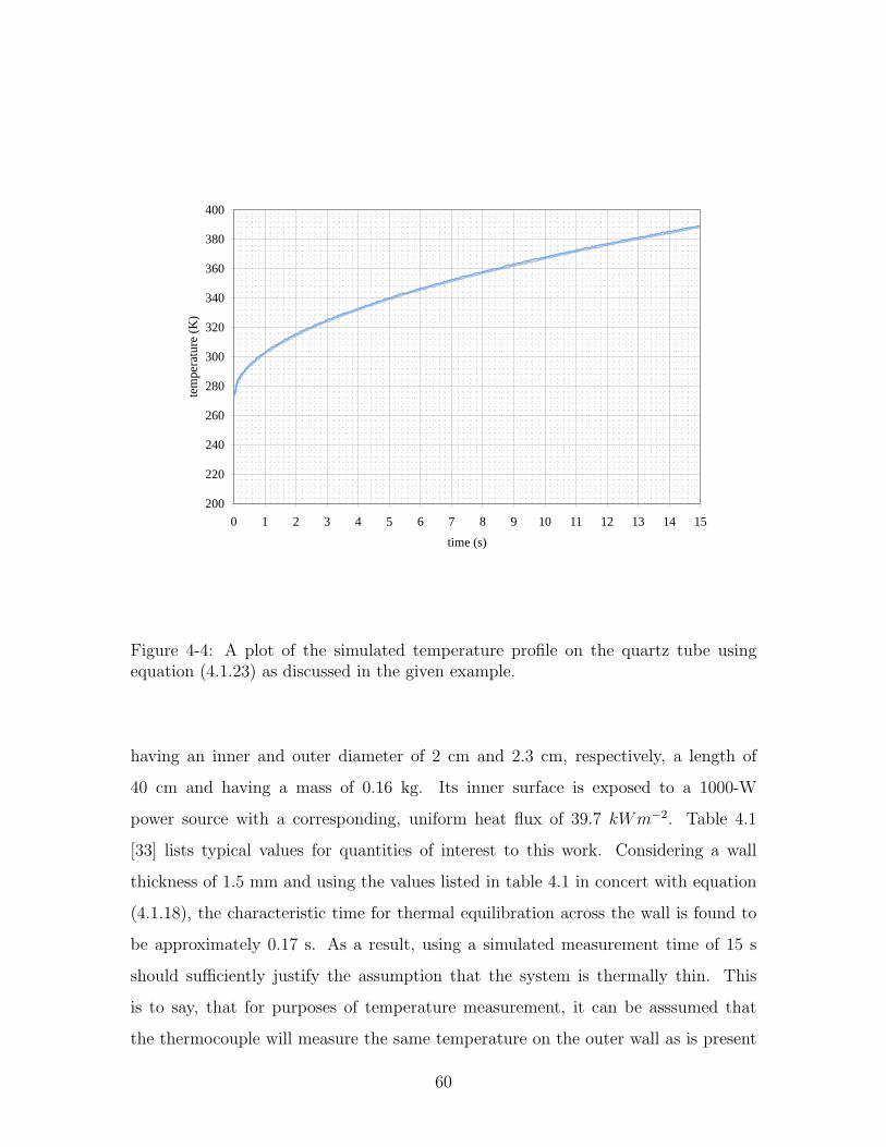
200

220

240

260

280

300

320

340

360

380

400

0 1 2 3 4 5 6 7 8 9 10 11 12 13 14 15

time (s)

tem

pera

ture

(K

)

Figure 4-4: A plot of the simulated temperature profile on the quartz tube usingequation (4.1.23) as discussed in the given example.

having an inner and outer diameter of 2 cm and 2.3 cm, respectively, a length of

40 cm and having a mass of 0.16 kg. Its inner surface is exposed to a 1000-W

power source with a corresponding, uniform heat flux of 39.7 kWm−2. Table 4.1

[33] lists typical values for quantities of interest to this work. Considering a wall

thickness of 1.5 mm and using the values listed in table 4.1 in concert with equation

(4.1.18), the characteristic time for thermal equilibration across the wall is found to

be approximately 0.17 s. As a result, using a simulated measurement time of 15 s

should sufficiently justify the assumption that the system is thermally thin. This

is to say, that for purposes of temperature measurement, it can be asssumed that

the thermocouple will measure the same temperature on the outer wall as is present

60

0

2000

4000

6000

8000

10000

12000

0 1 2 3 4 5 6 7 8 9 10 11 12 13 14 15

time (s)

pow

er (

W)

Figure 4-5: A plot of the resultant power data reduced from the temperature seriesin Figure 4-4 using equation (4.2.4).

on the inner wall. Furthermore, the tube is assumed to be instrumented with a

thermocouple whose junction characteristic dimension is on the order of 0.1 mm and

is placed on the outer surface of the tube. Finally, the ratio of wall radius of curvature

to junction dimension is found to be approximately 100, which is sufficient to justify

the assumption of a flat plate model.

Using equation (4.1.23), a simulated temperature profile can be built based on the

assumption of a constant surface heat flux. Applying equations (4.2.4) and (4.2.5) to

the resulting data series, values for the instantaneous and average power absorbed by

the quartz tube can be computed. Using a simple spreadsheet model, the following

two plots given in Figures 4-4 and 4-5 were created as described above. Using equation

61

(4.2.5), the average power gain of the quartz tube was found to be Pavg = 910.9 W

corresponding to a surface heat flux of qs = 36.2 kWm−2, resulting in an error of 8.9%

from the input quantities of P = 1000 W and qs = 39.7 kWm−2. Though this could

be considered to be a moderate error, the reader must be reminded that this study is

an introductory one and more detailed methods should be sought out and examined

before rendering a final judgement as to the best method by which to evaluate power

gain by the source tube. Furthermore, the author asserts that errors on the order of

10 % or lower are within acceptable limits for a first attempt at a global mapping of

energy transport in a helicon plasma source.

62

Chapter 5

Energy Balance Model

This chapter covers the construction of a global energy balance model of the mHTX@MIT

helicon plasma source. This model draws upon the discussions in Chapters 3 and 4

in its development and covers the entire system from the radio frequency (RF) power

supply to the plasma plume with a discussion of the appropriate assumptions, consid-

erations, and exclusions made. The result is a complete model that should be able to

give the experimentalist valuable information regarding losses incurred via radiation

and poor magnetic confinement to the source tube, the proportion of useful ”losses”

to the plume, an approximate antenna-plasma coupling efficiency, and finally an ap-

proximate internal efficiency for the system as a whole. From this point forward, the

author will refer to power as the quantity of interest rather than energy, though the

reader should be reminded that the character of the analysis is not changed by this

nomenclature and this still remains, in either form, a balance of energy or energy per

unit time of the helicon system.

5.1 Power System

For the purposes of this work, the power system will be considered to encompass all

components between the Advanced Energy RFPP-10 1.2 kW RF power supply and

the helicon antenna. This includes a 5-m section of RG-214 coaxial cable connecting

63

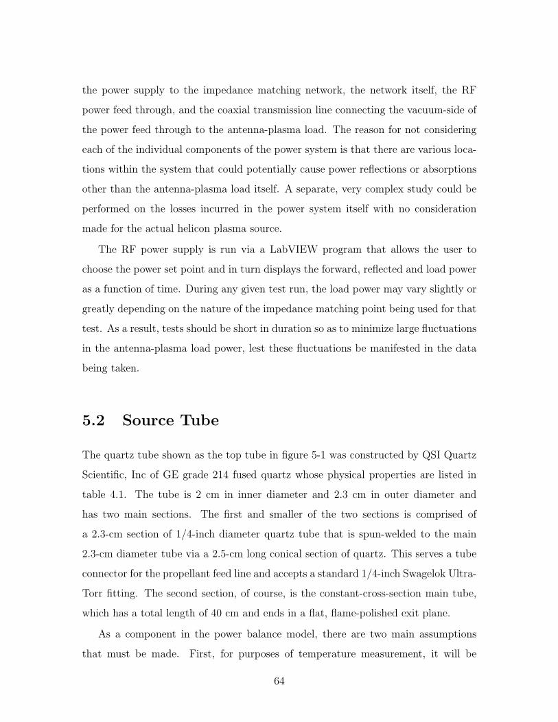
the power supply to the impedance matching network, the network itself, the RF

power feed through, and the coaxial transmission line connecting the vacuum-side of

the power feed through to the antenna-plasma load. The reason for not considering

each of the individual components of the power system is that there are various loca-

tions within the system that could potentially cause power reflections or absorptions

other than the antenna-plasma load itself. A separate, very complex study could be

performed on the losses incurred in the power system itself with no consideration

made for the actual helicon plasma source.

The RF power supply is run via a LabVIEW program that allows the user to

choose the power set point and in turn displays the forward, reflected and load power

as a function of time. During any given test run, the load power may vary slightly or

greatly depending on the nature of the impedance matching point being used for that

test. As a result, tests should be short in duration so as to minimize large fluctuations

in the antenna-plasma load power, lest these fluctuations be manifested in the data

being taken.

5.2 Source Tube

The quartz tube shown as the top tube in figure 5-1 was constructed by QSI Quartz

Scientific, Inc of GE grade 214 fused quartz whose physical properties are listed in

table 4.1. The tube is 2 cm in inner diameter and 2.3 cm in outer diameter and

has two main sections. The first and smaller of the two sections is comprised of

a 2.3-cm section of 1/4-inch diameter quartz tube that is spun-welded to the main

2.3-cm diameter tube via a 2.5-cm long conical section of quartz. This serves a tube

connector for the propellant feed line and accepts a standard 1/4-inch Swagelok Ultra-

Torr fitting. The second section, of course, is the constant-cross-section main tube,

which has a total length of 40 cm and ends in a flat, flame-polished exit plane.

As a component in the power balance model, there are two main assumptions

that must be made. First, for purposes of temperature measurement, it will be

64

Figure 5-1: A photograph of the quartz source tube (top) and the alumina ceramicsource tube (bottom).

assumed that the smaller conical-fitting section of the tube is neglected. This allows

the experimentalist to assume longitudinal symmetry and simplifies reduction of the

data. The second assumption to be made is that GE grade 214 fused quartz has

a high degree of optical transmission ranging from approximately 160 nm to 4000

nm with only one small absorption in the 2730 nm water band, thus allowing for

all but a small amount of radiation absorption to be ruled out in the temperature

measurements. This ensures that a majority of the power gained by the tube is due

to poor magnetic confinement.

5.2.1 Thermocouple Array

The source tube is instrumented with five, Omega Engineering, Inc C01-K type-K

”Cement-On” surface-mountable thermocouples. A photograph of one of the thermo-

couples used can be seen in figure 5-2. Each thermocouple is bonded to the surface

using Omega Engineering, Inc OmegaBond ”200” High Temperature, High Thermal

Conductivity Epoxy Adhesive to minimize thermal contact resistance, which would

65

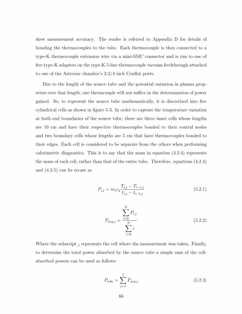
skew measurement accuracy. The reader is referred to Appendix D for details of

bonding the thermocouples to the tube. Each thermocouple is then connected to a

type-K thermocouple extension wire via a mini-SMC connector and is run to one of

five type-K adapters on the type-K 5-line thermocouple vacuum feedthrough attached

to one of the Astrovac chamber’s 2-3/4 inch Conflat ports.

Due to the length of the source tube and the potential variation in plasma prop-

erties over that length, one thermcouple will not suffice in the determination of power

gained. So, to represent the source tube mathematically, it is discretized into five

cylindrical cells as shown in figure 5-3. In order to capture the temperature variation

at both end boundaries of the source tube, there are three inner cells whose lengths

are 10 cm and have their respective thermocouples bonded to their central nodes

and two boundary cells whose lengths are 5 cm that have thermocouples bonded to

their edges. Each cell is considered to be separate from the others when performing

calorimetric diagnostics. This is to say that the mass in equation (4.2.4) represents

the mass of each cell, rather than that of the entire tube. Therefore, equations (4.2.4)

and (4.2.5) can be recast as

Pi,j = mjcpTi,j − Ti−1,j

ti,j − ti−1,j

(5.2.1)

Pavg,j =

N∑i=0

Pi,j

N∑i=0

i

(5.2.2)

Where the subscript j represents the cell where the measurement was taken. Finally,

to determine the total power absorbed by the source tube a simple sum of the cell-

absorbed powers can be used as follows:

Ptube =5∑

j=1

Pavg,j (5.2.3)

66

Figure 5-2: A photograph of one of the C01-K surface thermocouples showing detailsof the junction.

Property Valuedensity (kg/m3) 3960

thermal conductivity (W/mK) 28specific heat (J/kgK) 850

thermal diffusivity (m2/s) 8.32× 10−6

Table 5.1: Typical properties of alumina ceramic.

Of course, it is assumed that all losses from the plasma occur axisymmetrically,

thus allowing for such a simple, linear array of thermocouples and eliminating the

need for an azimuthal array. For purposes of determining a rough estimate of power

absorption profile over the tube length, a linear variation in absorbed power can be

assumed between thermocouple nodes. This allows for a rough comparison of the

absorbed power and axial magnetic field profile, which may provide insight as to the

effects of the magnetic field intensity profile on tube losses.

Now, up until this point, only the confinement losses have been treated. In order

to determine the radiation losses from the plasma, a different source tube is used.

67

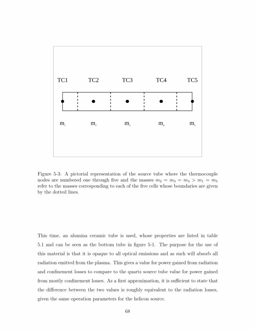
m1 m2 m3 m4 m5

TC1 TC2 TC3 TC4 TC5

Figure 5-3: A pictorial representation of the source tube where the thermocouplenodes are numbered one through five and the masses m2 = m3 = m4 > m1 = m5

refer to the masses corresponding to each of the five cells whose boundaries are givenby the dotted lines.

This time, an alumina ceramic tube is used, whose properties are listed in table

5.1 and can be seen as the bottom tube in figure 5-1. The purpose for the use of

this material is that it is opaque to all optical emissions and as such will absorb all

radiation emitted from the plasma. This gives a value for power gained from radiation

and confinement losses to compare to the quartz source tube value for power gained

from mostly confinement losses. As a first approximation, it is sufficient to state that

the difference between the two values is roughly equivalent to the radiation losses,

given the same operation parameters for the helicon source.

68

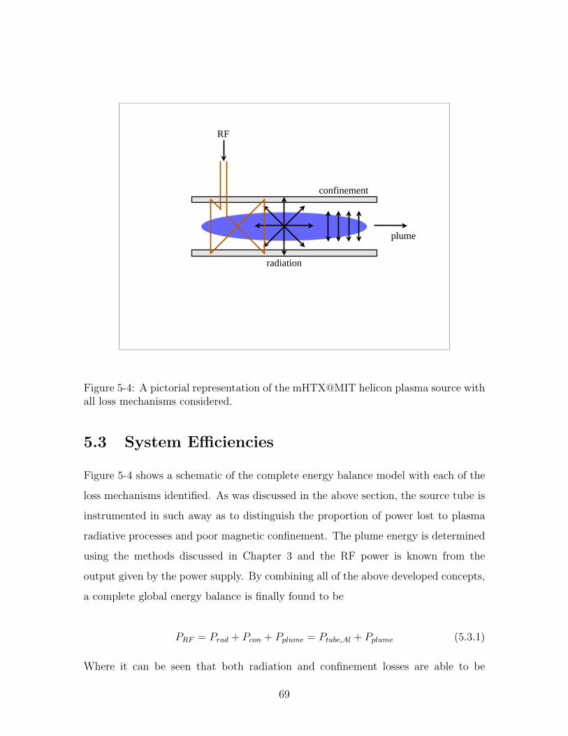
radiation

confinement

RF

plume

Figure 5-4: A pictorial representation of the mHTX@MIT helicon plasma source withall loss mechanisms considered.

5.3 System Efficiencies

Figure 5-4 shows a schematic of the complete energy balance model with each of the

loss mechanisms identified. As was discussed in the above section, the source tube is

instrumented in such away as to distinguish the proportion of power lost to plasma

radiative processes and poor magnetic confinement. The plume energy is determined

using the methods discussed in Chapter 3 and the RF power is known from the

output given by the power supply. By combining all of the above developed concepts,

a complete global energy balance is finally found to be

PRF = Prad + Pcon + Pplume = Ptube,Al + Pplume (5.3.1)

Where it can be seen that both radiation and confinement losses are able to be

69

lumped into one term, Ptube,Al when measurements are done on the alumina ceramic

source tube; however, the radiation power can be determined as a difference of the

alumina ceramic and fused quartz tube powers, namely Prad = Ptube,Al − Ptube,quartz.

Furthermore, the power system-plasma coupling efficiency and the system internal

efficiency are able to be computed as follows:

ηRF =Ptube + Pplume

PRF

(5.3.2)

ηI =Pplume

PRF

(5.3.3)

This completes the development of the simple energy balance model of the mHTX@MIT

helicon plasma source and should provide for a good first-order approximation of losses

and efficiencies incurred during the various stages of operation of the source.

70

Chapter 6

Conclusions

This thesis has discussed the details of helicon plasma sources in context to use in

space propulsion. In particular, attention has been paid to the loss mechanisms

incurred during regular helicon source operation. A discussion of the mHTX@MIT

experimental facility was given to provide the reader with an appreciation for the

program in terms of both past and future work. Both plume and source tube thermal

diagnostics were discussed and methods were developed for determination of losses

incurred in both these regions. This, of course, led to the construction of a simple

energy balance model, which provides the reader with a first-order view of diagnosing

power losses and various efficiencies in a helicon plasma source.

6.1 Recommendations for Future Work

In terms of future work, the author recommends that more detailed analyses of ther-

mal characterization methods be performed in order that a more accurate and com-

plete model be produced. As discussed briefly in Chapter 4, the Inverse Heat Conduc-

tion Problem methodology may prove to be very useful in accurately diagnosing not

just losses to the source tube, but also in building a detailed heat flux topology that

can be compared more easily to the magnetic field profile to determine the correlation

between losses and magnetic field profile. This then leads to the recommendation that

71

a detailed mapping of the magnetic field topology be performed for various operating

conditions so that such detailed thermal data could be compared to equally detailed

field data.

Furthermore, it is suggested that, regardless of the future thermal model to be

applied, more thermocouples be used to increase the resolution of the source tube

temperature profile. This, of course, will require multiple thermocouple vacuum feed

throughs or the use of a multi-channel thermocouple data logger that could be placed

in the vacuum chamber during testing. This would allow the acquisition of the raw

temperature data in the chamber to be converted from analog to digital values and

then sent via a standard cable through a wire feed through and to the computer

system for permanent logging.

Finally, the author wishes that, in the future of the mHTX@MIT program, a com-

putational model be developed in an effort to complete the characterization of the

mHTX@MIT helicon plasma source insomuch as it may be used to model experimen-

tal cases and perhaps shed more light on both the empirical observations made and

the detailed, but rich and intriguing physical processes governing the helicon plasma

source.

72

Appendix A

Helicon Cold Plasma Theory

A.1 Governing Equations

In order to arrive at the specific helicon dispersion relation, the general dispersion

relation must first be derived. In the derivation that follows, a cold plasma composed

of two particle species is assumed to be uniform and homogeneous in space and time

and collisions are neglected. Furthermore, it is assumed that all wave amplitudes are

sufficiently low to neglect second order terms, thus the linear wave approximation is

valid, and all perturbed quantities are of the harmonic form ei(k·r−ωt), where k is the

wave propagation vector and ω is the wave angular frequency. To begin, Faraday’s

Law and Ampere’s Law will be considered as follows:

∇× E = −∂B∂t

(A.1.1)

∇×B = µ0

(j + ε0

∂E

∂t

)(A.1.2)

By applying the linear wave approximation to equations (A.1.1) and (A.1.2)

ik× E1 = iωB0 (A.1.3)

ik×B0 = µ0j1 −iω

c2E1 (A.1.4)

73

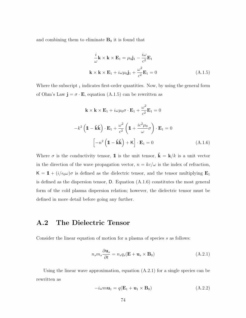
and combining them to eliminate B0 it is found that

i

ωk× k× E1 = µ0j1 −

iω

c2E1

k× k× E1 + iωµ0j1 +ω2

c2E1 = 0 (A.1.5)

Where the subscript 1 indicates first-order quantities. Now, by using the general form

of Ohm’s Law j = σ · E, equation (A.1.5) can be rewritten as

k× k× E1 + iωµ0σ · E1 +ω2

c2E1 = 0

−k2(1− kk

)· E1 +

ω2

c2

(1+

ic2µ0

ωσ

)· E1 = 0

[−n2

(1− kk

)+ K

]· E1 = 0 (A.1.6)

Where σ is the conductivity tensor, 1 is the unit tensor, k = k/k is a unit vector

in the direction of the wave propagation vector, n = kc/ω is the index of refraction,

K = 1 + (i/ε0ω)σ is defined as the dielectric tensor, and the tensor multiplying E1

is defined as the dispersion tensor, D. Equation (A.1.6) constitutes the most general

form of the cold plasma dispersion relation; however, the dielectric tensor must be

defined in more detail before going any further.

A.2 The Dielectric Tensor

Consider the linear equation of motion for a plasma of species s as follows:

nsms∂us

∂t= nsqs(E + us ×B0) (A.2.1)

Using the linear wave approximation, equation (A.2.1) for a single species can be

rewritten as

−iωmu1 = q(E1 + u1 ×B0) (A.2.2)

74

The scalar components of equation (A.2.2) can then be expressed as

−iωmux = q(Ex + uyB0)

−iωmuy = q(Ey − uxB0)

−iωmuz = qEz

(A.2.3)

Then, solving for the particle velocity components from (A.2.3) gives

ux =q

m

(iωEx − ωcEy

ω2 − ω2c

)uy =

q

m

(iωEy + ωcEx

ω2 − ω2c

)uz =

iq

ωmEz

(A.2.4)

Where the definition of the cyclotron frequency ωc = qB0/m has been used. Further-

more, note that

j1 = σ · E1 =∑

s

qsnsu1 (A.2.5)

Making use of (A.2.4), the conductivity tensor σ can then be written as

σ =

σxx σxy 0

σyx σyy 0

0 0 σzz

(A.2.6)

Where the elements are

σxx = σyy =∑

s

q2sns

ms

iω

ω2 − ω2cs

σxy = −σyx = −∑

s

q2sns

ms

ωcs

ω2 − ω2cs

σzz =∑

s

iq2s

ms

ns

ω

(A.2.7)

Given this new information, the definition of the dielectric tensor K = 1+(i/ε0ω)σ

75

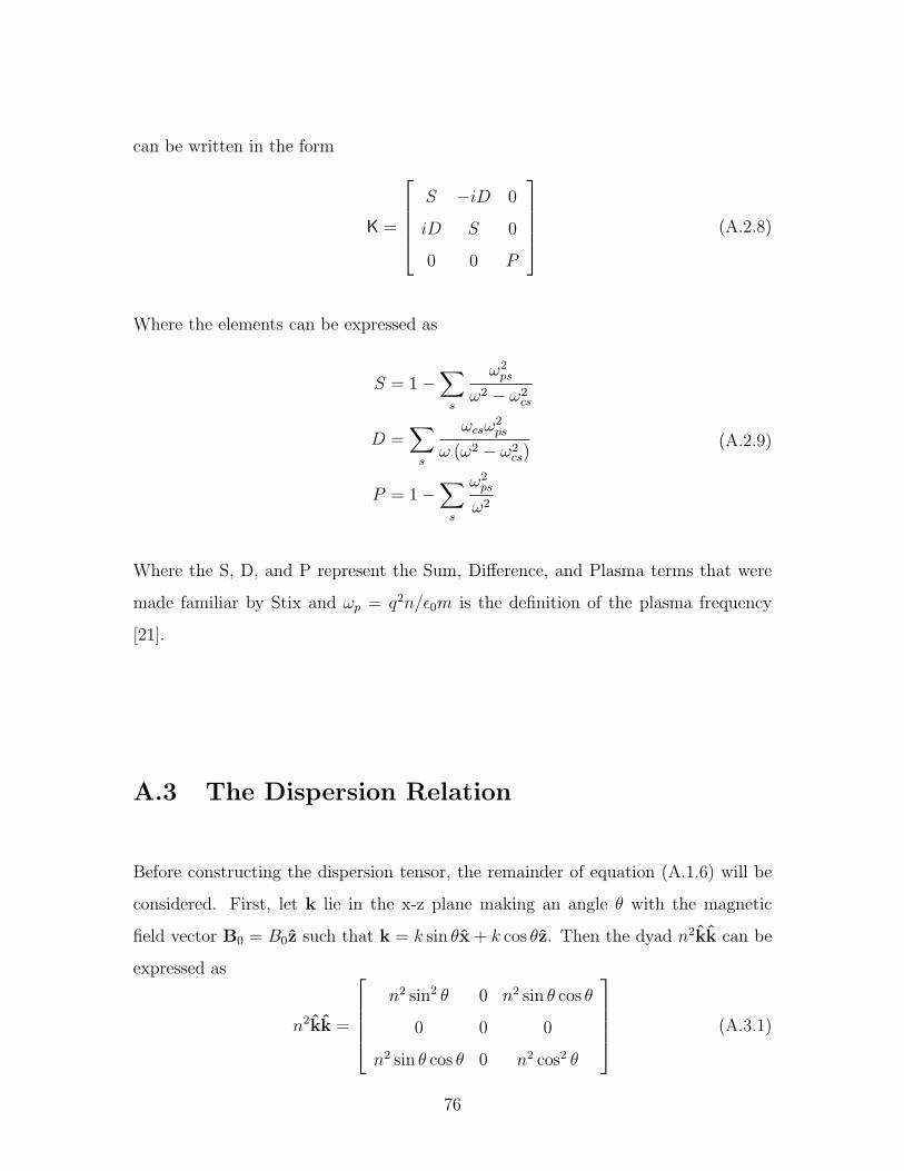
can be written in the form

K =

S −iD 0

iD S 0

0 0 P

(A.2.8)

Where the elements can be expressed as

S = 1−∑

s

ω2ps

ω2 − ω2cs

D =∑

s

ωcsω2ps

ω (ω2 − ω2cs)

P = 1−∑

s

ω2ps

ω2

(A.2.9)

Where the S, D, and P represent the Sum, Difference, and Plasma terms that were

made familiar by Stix and ωp = q2n/ε0m is the definition of the plasma frequency

[21].

A.3 The Dispersion Relation

Before constructing the dispersion tensor, the remainder of equation (A.1.6) will be

considered. First, let k lie in the x-z plane making an angle θ with the magnetic

field vector B0 = B0z such that k = k sin θx + k cos θz. Then the dyad n2kk can be

expressed as

n2kk =

n2 sin2 θ 0 n2 sin θ cos θ

0 0 0

n2 sin θ cos θ 0 n2 cos2 θ

(A.3.1)

76

and the tensor n21 can be written as

−n21 =

−n2 0 0

0 −n2 0

0 0 −n2

=

−n2

(sin2 θ + cos2 θ

)0 0

0 −n2(sin2 θ + cos2 θ

)0

0 0 −n2(sin2 θ + cos2 θ

) (A.3.2)

Finally, by combining equations (A.1.6), (A.2.8), (A.3.1), and (A.3.2), the com-

plete, cold plasma dispersion tensor can be written as

D =

S − n2 cos2 θ −iD n2 sin θ cos θ

iD S − n2 0

n2 sin θ cos θ 0 P − n2 sin2 θ

(A.3.3)

The non-trivial (E1 6= 0) solutions of the cold plasma dispersion relation can be

found by taking det D = 0 and solving for tan2 θ. Doing this yields

[S sin2 θ + P cos2 θ

]n4 −

[RL sin2 θ + SP

(1 + cos2 θ

)]n2 + PRL = 0

n2 sin2 θ +Pn2 (n2 − S)

Sn2 −RLcos2 θ − P

(sin2 θ + cos2 θ

)= 0

(n2 − P

)sin2 θ = −P (n4 − 2Sn2 +RL)

Sn2 −RL

tan2 θ = − P (n2 −R) (n2 − L)

(Sn2 −RL) (n2 − P )(A.3.4)

Where the R and L terms represent Right and Left and are related to the S and D

77

terms in the following manner:

R = S +D

L = S −D

S =1

2(R + L)

D =1

2(R− L)

(A.3.5)

The form of the dispersion relation represented in equation (A.3.4) is very useful

when considering the two primary sets of modes corresponding to θ = 0 (k ‖ B0) and

θ = π/2 (k ⊥ B0).

Up to this point, the general cold plasma dispersion relation has been derived as

an exercise in the theory of plasma waves. The results of this derivation could be

used to look at the general dispersion relation of RCP and LCP waves for θ = 0

in equation (A.3.4); however, these relations do not embody the character of the

helicon–Trivelpiece-Gould (H-TG) mode coupling.

A.4 Helicon–Trivelpiece-Gould Theory

A.4.1 The H-TG Wave Equation: Cold Plasma Route

The H-TG wave equation will be derived formally from the theory presented in the

previous section. Though a more direct route can be followed, this one allows the

reader to understand the relationship to cold plasma theory. The reader should note

that, from this point forward, the nomenclature for wavenumber will be changed

to the helicon theory convention as adopted by Chen et. al. [10, 17]. The total

wavenumber will be referred to as β, while the transverse and axial wavenumbers

will be referred to as T and k, respectively. That is β2 = T 2 + k2. The author

recognizes the potential for confusion in this case; however, it was felt that adhering

to convention in context to helicon theory would be the best course of action for the

purpose of orienting the reader to that which is found in the literature.

78

First, the right-hand side of equation (A.1.2) will be reconsidered. The total

current can therefore be expressed as follows:

J1 = j1p + j1d = −iωε0K · E1 (A.4.1)

Where the j1p and j1d are the first order plasma and displacement currents, respec-

tively. Solving for E1, gives

−iωε0E1 = K−1J1

−iωε0E1 =1

PJ1 − i

D

RLb× J1 +

(1

P− S

RL

)b× b× J1

E1 = − 1

iωε0

[αp1+ iαhb×−αd

(1− bb

)]· J1 (A.4.2)

Where RL = S2−D2, b = b/B0 = z is a unit vector along the z-axis, and αp = 1/P ,

αh = −D/RL, and αd = 1/P − S/RL represent the polarization, Hall, and displace-

ment current coefficients, respectively, as adopted by Chen et. al. [10, 17]. Now, let

us evaluate the coefficients so as to reduce equation (A.4.2) into a more useful form.

In this derivation, a single ion species will be assumed and the displacement current

j1d, will be neglected such that αd will vanish; however, either of these simplifications

can be omitted to reach a more complete form. The Right, Left, Sum, Difference,

and Plasma elements can be expressed from equations (A.2.9) as

R = 1−ω2

pi

ω (ω + ωci)−

ω2pe

ω (ω − ωce)

L = 1−ω2

pi

ω (ω − ωci)−

ω2pe

ω (ω + ωce)

S = 1−ω2

pi

ω2 − ω2ci

−ω2

pe

ω2 − ω2ce

D =ωciω

2pi

ω (ω2 − ω2ci)−

ωceω2pe

ω (ω2 − ω2ce)

P = 1−ω2

pi

ω2−ω2

pe

ω2

(A.4.3)

79

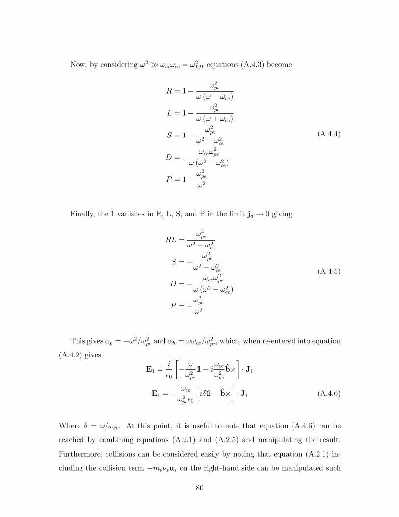
Now, by considering ω2 � ωciωce = ω2LH equations (A.4.3) become

R = 1−ω2

pe

ω (ω − ωce)

L = 1−ω2

pe

ω (ω + ωce)

S = 1−ω2

pe

ω2 − ω2ce

D = −ωceω

2pe

ω (ω2 − ω2ce)

P = 1−ω2

pe

ω2

(A.4.4)

Finally, the 1 vanishes in R, L, S, and P in the limit jd → 0 giving

RL =ω4

pe

ω2 − ω2ce

S = −ω2

pe

ω2 − ω2ce

D = −ωceω

2pe

ω (ω2 − ω2ce)

P = −ω2

pe

ω2

(A.4.5)

This gives αp = −ω2/ω2pe and αh = ωωce/ω

2pe, which, when re-entered into equation

(A.4.2) gives

E1 =i

ε0

[− ω

ω2pe

1+ iωce

ω2pe

b×]· J1

E1 = − ωce

ω2peε0

[iδ1− b×

]· J1 (A.4.6)

Where δ = ω/ωce. At this point, it is useful to note that equation (A.4.6) can be

reached by combining equations (A.2.1) and (A.2.5) and manipulating the result.

Furthermore, collisions can be considered easily by noting that equation (A.2.1) in-

cluding the collision term −msνsus on the right-hand side can be manipulated such

80

that equation (A.4.6) becomes

E1 = − ωce

ω2peε0

[iδ∗1− b×

]· J1 (A.4.7)

Where δ∗ = (ω + iν)/ωce and in the limit ν → 0, δ∗ → δ = ω/ωce. At this point, it is

useful to note that the Fourier transform in the time domain will be used, however,

the spacial domain will remain unchanged. This is to say that all quantities can be

expressed in the form B1 (r, t) = Re [B1 (r, ω) e−iωt], in the case of the magnetic field.

Using Faraday’s Law, equation (A.4.7) can be written as

∇× E1 = iωB1 = − ωce

ω2peε0

[iδ∗∇×−∇× b×

]· J1 (A.4.8)

Furthermore, if Ampere’s Law is applied, neglecting the displacement current and

rearranging will show that equation (A.4.8) becomes

iωB1 = − ωce

ω2peε0µ0

[iδ∗∇×−∇× b×

]∇×B1

δω2pe

c2B1 = −

[δ∗∇×+i∇× b×

]∇×B1

δ∗∇×∇×B1 + i∇× b× (∇×B1) +δω2

pe

c2B1 = 0

δ∗∇×∇×B1 − k∇×B1 + δk2sB1 = 0 (A.4.9)

Where ks = ωpe/c is called the skin depth by Chen et. al. [10, 17]. Equation (A.4.9)

is the formal H-TG wave equation and will be used for the remainder of the analysis.

A.4.2 H-TG Waves

Equation (A.4.9) can now be factored into

(β1 −∇×) (β2 −∇×)B = 0 (A.4.10)

81

Where the first-order subscript 1 on B has been removed for the remainder of the

analysis to eliminate confusion with the general solution.

The general solution of equation (A.4.10) is then found to be B = B1 + B2 such

that B1 and B2 satisfy the following equation for j = 1, 2:

∇×Bj = βjBj (A.4.11)

the curl of which can be written in the form of the Helmholtz wave equation for

j = 1, 2 as

∇2Bj + β2j Bj = 0 (A.4.12)

The separation constants β1 and β2 are the roots of

δ∗β2 − kβ + δk2s = 0 (A.4.13)

and the solutions to equation (A.4.13) can be expressed as

β1,2 =k

2δ∗

[1∓

(1− 4δ∗δk2

s

k2

) 12

](A.4.14)

In this case, β1 represents the helicon branch and β2 represents the TG branch.

In order to simplify further analysis and make obvious the characteristics of these

branches, collisions will be neglected from this point forward, thus δ∗ = δ. As a

result, an alternative form for equation (A.4.13) gives a useful expression for k in

terms of β as follows:

k =δ

β

(β2 + k2

s

)(A.4.15)

Next, by taking the minimum of equation (A.4.15), it is found that there exists a

minimum k value in order for wave propagation to occur

kmin = 2δks (A.4.16)

82

10−1

100

101

102

10−1

100

101

102

β (cm−1)

k (c

m−

1 )k = β

19.38

50

100

250

500

750

1000

H branch TG branch

Figure A-1: A plot of k versus β for different values of B0(G) in a plasma of densityn0 = 1× 1013 cm−1 and a rf frequency of 27.12 Mhz.

Furthermore, by defining the transverse wave number for j = 1, 2 in terms of the

total and parallel wave numbers β and k as

T 2j = β2

j − k2 (A.4.17)

it is found that for real Tj there exists a maximum k value at T = 0 (k = β) of

kmax = ks

√δ

1− δ(A.4.18)

So, as δ increases (B0 → 0), we see that kmin approaches kmax until the value

δ = 2ω/ωce is reached. At this point, kmin = kmax and the helicon wave no longer

propagates. This behavior can be seen in Figure A-1. The H branch is to the left of

the minimum while the TG branch is to the right. Note how the size of the H branch

decreases for decreasing B0 until it becomes evanescent at a magnetic field value of

B0 ≈ 19.38 G for the given conditions.

83

A.4.3 Boundary Condition Effects

In order to study the effects of boundary conditions on the character of H-TG modes,

equation (A.4.12) will be solved. The solution to the Helmholtz wave equation in

circular cylindrical geometry can be found through use of the method of separation of

variables. All perturbed quantities vary as ei(mφ+kz−ωt), where m is the mode number

such that m > 0 and m < 0 represent clockwise and counterclockwise rotation,

respectively when viewing the wave in the direction of B0 = B0z. The z-component

of equation (A.4.12) can be written in the form of the well known Bessel differential

equation obtained by separating variables as B (r, φ) = B (r) eimφ

∂2Bzj

∂r2+

1

r

∂Bzj

∂r+

(T 2

j −m2

r2

)Bzj = 0 (A.4.19)

Where m is the mode number such that Bz depends on azimuthal angle φ as eimφ.

The solution to equation (A.4.19) is finite for r = 0 and is written as

Bzj = C1Jm(Tjr) (A.4.20)

Where Jm(Tjr) is a Bessel function of the first kind of mode m.

Next, the r and φ components of (A.4.11) are

1

r

∂Bzj

∂φ− ∂Bφj

∂z=im

rBzj − ikBφj = βjBrj (A.4.21)

∂Brj

∂z− ∂Bzj

∂r= ikBrj −

∂Bzj

∂r= βjBφj (A.4.22)

Then solving for Brj and Bφj in terms of Bzj and ∂Bzj/∂r gives

Brj =iC1

T 2j

[m

rβjJm(Tjr)− k

∂

∂rJm(Tjr)

](A.4.23)

Bφj =C1

T 2j

[m

rkJm(Tjr) + βj

∂

∂rJm(Tjr)

](A.4.24)

84

Finally, using the recursion relations for Jm(Tjr) and ∂Jm(Tjr)/∂r

m

rJm(Tjr) =

Tj

2

[Jm−1(Tjr) + Jm+1(Tjr)

]∂

∂rJm(Tjr) =

Tj

2

[Jm−1(Tjr)− Jm+1(Tjr)

] (A.4.25)

equations (A.4.23), (A.4.24), and (A.4.20) can be written in their final form as

Brj = Aj

[(βj + k) Jm−1(Tjr) + (βj − k) Jm+1(Tjr)

](A.4.26)

Bφj = iAj

[(βj + k) Jm−1(Tjr)− (βj − k) Jm+1(Tjr)

](A.4.27)

Bzj = −2iTjAjJm(Tjr) (A.4.28)

Where Aj = iC1/2Tj is an arbitrary amplitude.

Now a similar procedure can be performed for Ej. First, equations (A.1.2) and

(A.4.11) will be considered, while neglecting displacement current. From these, it is

found

jj =βj

µ0

Bj (A.4.29)

Next, using equation (A.4.6), an expression for Ej as a function of Bj can be

found as follows:

Ej = −ωceβj

k2s

[iδ1− b×

]·Bj (A.4.30)

Writing Ezj from equation (A.4.30) and using equation (A.1.1) for the r and φ

components gives

Ezj = −iωβj

k2s

Bzj (A.4.31)

1

r

∂Ezj

∂φ− ∂Eφj

∂z= −m

r

iωβj

k2s

Bzj − ikEφj = iωBrj (A.4.32)

∂Erj

∂z− ∂Ezj

∂r= ikErj +

iωβj

k2s

∂Bzj

∂r= iωBφj (A.4.33)

Solving for Erj and Eφj and including equation (A.4.31) gives the complete set of

85

E wave field equations in terms of the components of B

Erj =ω

kBφj −

ωβj

k2s

∂Bzj

∂r(A.4.34)

Eφj = −ωkBrj −

m

r

ωβj

k2s

Bzj (A.4.35)

Ezj = −iωβj

k2s

Bzj (A.4.36)

Now, the H-TG coupling due to a conducting cylinder boundary and an insulating

cylinder boundary can be examined. When me → 0, ωpe → ∞ and ks → ∞ and so

it is found that these conditions are simplified greatly due to the fact that Ez → 0

from equation (A.4.36). From this, only Eφ = 0 for a conducting cylinder and it

follows from equation (A.4.35) that Br = 0. Next, for an insulating cylinder, the

boundary condition jr = 0 must be satisfied. From equation (A.4.29), this implies

that Br = 0, which in turn forces Eφ = 0 from equation (A.4.35). Thus, the boundary

conditions for both a conducting and an insulating cylinder are the same in the case

of zero-electron mass. This was first shown by Chen [10].

From this study, in can be seen that there is only one condition necessary for both

boundary types, namely:

Br1 = A1

[(β1 + k) Jm−1(T1a) + (β1 − k) Jm+1(T1a)

]= 0 (A.4.37)

Where a is the bounding cylinder radius and β1 is found to be

β1 =δk2

s

k=ω

k

n0qµ0

B0

(A.4.38)

Note that equation (A.4.38) is the only solution to equation (A.4.13) in the me = 0

situation, thus the H branch is the only existing wave. Equation (A.4.38) is also the

dispersion relation for unbound, ionospheric whistler waves, emphasizing the fact that

helicon waves are simply bounded whistler waves.

If the electron mass is now taken to be finite, then it follows that Ez must be finite

86

10−1

100

101

102

10−1

100

101

102

β (cm−1)

k (c

m−

1 )k = β

1 4

23

32

H branch TG branch

Figure A-2: A plot of k versus β for B0 = 1000 G in a plasma of density n0 =1 × 1013 cm−1 and a rf frequency of 27.12 Mhz showing the discretized values of kfor which H-TG modes can propagate. Note that only the first three modes can beresolved at this scale.

due to electron inertia regardless of collisions [10]. Therefore, in order for Ez = 0, the

condition∑j=1,2

βjBzj → 0 as r → a must be satisfied. If Ezj = 0 is imposed for both

waves, then from equation (A.4.28), it is found that

βjJm(Tja) = 0 (A.4.39)

The two waves cannot, in general, satisfy this condition separately, so the Ezj = 0

condition couples the two waves. Using equations (A.4.28) and (A.4.30) and setting

Ez = Ez1 + Ez2 = 0 the ratio of the two wave amplitudes is found as

A2

A1

= −β1Jm(T1a)T1

β2Jm(T2a)T2

(A.4.40)

Again, since Eφj = 0 is a necessary condition, then from equation (A.4.35) it is

87

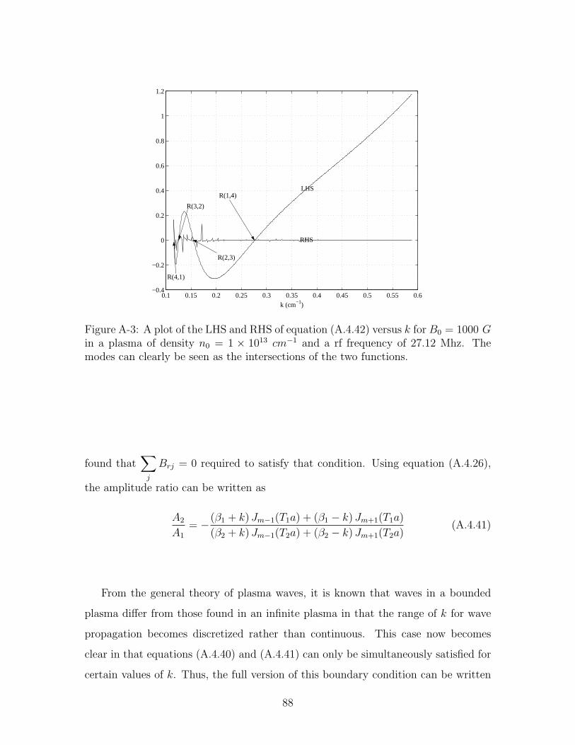
0.1 0.15 0.2 0.25 0.3 0.35 0.4 0.45 0.5 0.55 0.6−0.4

−0.2

0

0.2

0.4

0.6

0.8

1

1.2

k (cm−1)

LHS

RHS

R(1,4)

R(2,3)

R(3,2)

R(4,1)

Figure A-3: A plot of the LHS and RHS of equation (A.4.42) versus k for B0 = 1000 Gin a plasma of density n0 = 1 × 1013 cm−1 and a rf frequency of 27.12 Mhz. Themodes can clearly be seen as the intersections of the two functions.

found that∑

j

Brj = 0 required to satisfy that condition. Using equation (A.4.26),

the amplitude ratio can be written as

A2

A1

= −(β1 + k) Jm−1(T1a) + (β1 − k) Jm+1(T1a)

(β2 + k) Jm−1(T2a) + (β2 − k) Jm+1(T2a)(A.4.41)

From the general theory of plasma waves, it is known that waves in a bounded

plasma differ from those found in an infinite plasma in that the range of k for wave

propagation becomes discretized rather than continuous. This case now becomes

clear in that equations (A.4.40) and (A.4.41) can only be simultaneously satisfied for

certain values of k. Thus, the full version of this boundary condition can be written

88

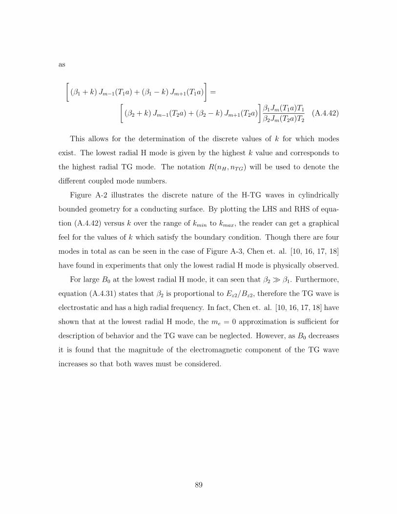
as

[(β1 + k) Jm−1(T1a) + (β1 − k) Jm+1(T1a)

]=[

(β2 + k) Jm−1(T2a) + (β2 − k) Jm+1(T2a)

]β1Jm(T1a)T1

β2Jm(T2a)T2

(A.4.42)

This allows for the determination of the discrete values of k for which modes

exist. The lowest radial H mode is given by the highest k value and corresponds to

the highest radial TG mode. The notation R(nH , nTG) will be used to denote the

different coupled mode numbers.

Figure A-2 illustrates the discrete nature of the H-TG waves in cylindrically

bounded geometry for a conducting surface. By plotting the LHS and RHS of equa-

tion (A.4.42) versus k over the range of kmin to kmax, the reader can get a graphical

feel for the values of k which satisfy the boundary condition. Though there are four

modes in total as can be seen in the case of Figure A-3, Chen et. al. [10, 16, 17, 18]

have found in experiments that only the lowest radial H mode is physically observed.

For large B0 at the lowest radial H mode, it can seen that β2 � β1. Furthermore,

equation (A.4.31) states that β2 is proportional to Ez2/Bz2, therefore the TG wave is

electrostatic and has a high radial frequency. In fact, Chen et. al. [10, 16, 17, 18] have

shown that at the lowest radial H mode, the me = 0 approximation is sufficient for

description of behavior and the TG wave can be neglected. However, as B0 decreases

it is found that the magnitude of the electromagnetic component of the TG wave

increases so that both waves must be considered.

89

90

Appendix B

A Helicon Fluid Model

B.1 Properties of a Helicon Plasma

In this section, the typical values of quantities of interest in a helicon plasma will

be introduced. These will be used to calculate some characteristic frequencies of

the physical system, which will then be compared in an attempt to establish an

appropriate physical model for our system. All physical quantities were taken from

Bose et. al. [19] and are typical of semiconductor and materials processing argon

helicon plasmas.

Where B0 is the externally applied, DC magnetic field, a is the radius of the cylindrical

plasma column, and fRF is the antenna excitation frequency.

Quantity Valuene = ni = n 1018 m−3

Te 3 eVTi 0.2 eV

ZAr 18mAr+ 6.67× 10−26 kgB0 100 Ga 0.04 m

fRF 13.56× 106 Hz

Table B.1: Quantities of interest for a typical helicon plasma.

91

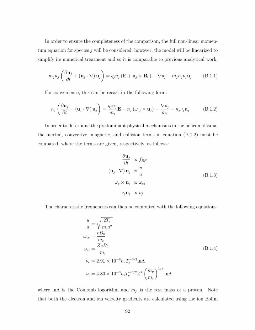
In order to ensure the completeness of the comparison, the full non-linear momen-

tum equation for species j will be considered; however, the model will be linearized to

simplify its numerical treatment and so it is comparable to previous analytical work.

mjnj

(∂uj

∂t+ (uj · ∇)uj

)= qjnj (E + uj ×B0)−∇pj −mjnjνjuj (B.1.1)

For convenience, this can be recast in the following form:

nj

(∂uj

∂t+ (uj · ∇)uj

)=qjnj

mj

E− nj (ωcj × uj)−∇pj

mj

− njνjuj (B.1.2)

In order to determine the predominant physical mechanisms in the helicon plasma,

the inertial, convective, magnetic, and collision terms in equation (B.1.2) must be

compared, where the terms are given, respectively, as follows:

∂uj

∂t∝ fRF

(uj · ∇)uj ∝u

a

ωc × uj ∝ ωcj

νjuj ∝ νj

(B.1.3)

The characteristic frequencies can then be computed with the following equations:

u

a=

√2Te

mia2

ωce =eB0

me

ωci =ZeB0

mi

νe = 2.91× 10−6neT−3/2e lnΛ

νi = 4.80× 10−8niT−3/2e Z4

(mp

mi

)1/2

lnΛ

(B.1.4)

where lnΛ is the Coulomb logorithm and mp is the rest mass of a proton. Note

that both the electron and ion velocity gradients are calculated using the ion Bohm

92

Frequency (Hz) Electron IonfRF 1.4× 107 1.4× 107

ua

9.5× 104 9.5× 104

fc 2.8× 108 6.9× 104

ν 5.6× 106 1.3× 1010

Table B.2: Electron and ion characteristic frequencies for a typical helicon plasma.

velocity under the assumption of quasi-neutrality. The practical equations for collision

frequencies, νj are found by evaluating the physical constants multiplying the density

and temperature terms [35].

Using the abovementioned plasma quantities from table B.1, the electron and

ion characteristic frequencies are computed as shown in table B.2. Note that the

cyclotron frequencies have been converted from angular frequencies, ωc to temporal

frequencies, fc to remain consistent with the other values.

B.2 The Ion Fluid

First, the zeroth-order ion fluid will be considered. Notice that the magnitude of

the collision term is much greater than any of the other terms. From this, it can be

assumed that the inertial, convective, and magnetic field terms are negligible and can

be omitted from the model without significant loss of physics. Now, equation (B.1.2)

for ions can be rewritten by taking into consideration the above assumptions. The

momentum equation becomes

njui =qini

νimi

E− ∇pi

νimi

(B.2.1)

Where the ion flux vector can be defined as Γi = niui, the ion diffusion coefficient

Di = kTi/νimi, and the ion mobility µi = qi/νimi such that equation (B.2.1) can be

rewritten in the form

Γi = µiniE−Di

kTi

∇pi (B.2.2)

93

Combining equation (B.2.2) with the ion mass continuity equation gives the fol-

lowing drift-diffusion equation for ions:

∂ni

∂t+∇ · Γi = Si (B.2.3)

Where Si is the ion source term and will be treated later.

B.3 The Electron Fluid

Now considering the zeroth-order electron fluide and referring back to table B.2, it

can be seen that, aside from the convective term, all other terms are within one order

of magnitude of each other. From this, only the convective term can be removed from

the model. This leaves the following equation for the electron momentum:

ne∂ue

∂t+ neνeue − ne (ωce × ue) = −ene

me

E− ∇pe

me

(B.3.1)

Defining the electron flux vector as Γe = neue, equation (B.3.1) can be rewritten

as∂Γe

∂t+ νeΓe − (ωce × Γe) = − e

me

E− ∇pe

me

(B.3.2)

Notice that the right-hand side of equation (B.3.2) is just the steady-state electron

flux vector, Γe in the absence of an external magnetic field, which will now be denoted

with a superscript zero. Also, the left-hand side of the equation can be rewritten as

a tensor multiplying the total electron flux vector. This gives the following equation:

G · Γe = Γ0e (B.3.3)

Where

G =

[(1− i

ω

νe

)1− 1

νe

ωce×]

Finally by inverting the tensor G, the total electron flux vector, Γe in the presence

94

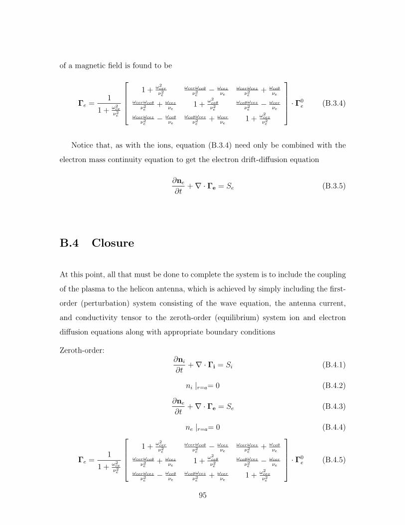
of a magnetic field is found to be

Γe =1

1 + ω2ce

ν2e

1 + ω2

cer

ν2e

ωcerωceθ

ν2e

− ωcez

νe

ωcerωcez

ν2e

+ ωceθ

νe

ωcerωceθ

ν2e

+ ωcez

νe1 +

ω2ceθ

ν2e

ωceθωcez

ν2e

− ωcer

νe

ωcerωcez

ν2e

− ωceθ

νe

ωceθωcez

ν2e

+ ωcer

νe1 + ω2

cez

ν2e

· Γ0e (B.3.4)

Notice that, as with the ions, equation (B.3.4) need only be combined with the

electron mass continuity equation to get the electron drift-diffusion equation

∂ne

∂t+∇ · Γe = Se (B.3.5)

B.4 Closure

At this point, all that must be done to complete the system is to include the coupling

of the plasma to the helicon antenna, which is achieved by simply including the first-

order (perturbation) system consisting of the wave equation, the antenna current,

and conductivity tensor to the zeroth-order (equilibrium) system ion and electron

diffusion equations along with appropriate boundary conditions

Zeroth-order:∂ni

∂t+∇ · Γi = Si (B.4.1)

ni |r=a= 0 (B.4.2)

∂ne

∂t+∇ · Γe = Se (B.4.3)

ne |r=a= 0 (B.4.4)

Γe =1

1 + ω2ce

ν2e

1 + ω2

cer

ν2e

ωcerωceθ

ν2e

− ωcez

νe

ωcerωcez

ν2e

+ ωceθ

νe

ωcerωceθ

ν2e

+ ωcez

νe1 +

ω2ceθ

ν2e

ωceθωcez

ν2e

− ωcer

νe

ωcerωcez

ν2e

− ωceθ

νe

ωceθωcez

ν2e

+ ωcer

νe1 + ω2

cez

ν2e

· Γ0e (B.4.5)

95

First-order:

∇ (∇ ·E)−∇2E− ω2

c2E + iωµ0σ · E = −iωµ0Jantenna (B.4.6)

Jantenna = I0δ (r − a) δ (z − aψ tan θ)[cos2 θ · ψ + sin θ cos θ · z

](B.4.7)

σ =e2ne

me (ν − iω)

1

1 + ω2ce

(ν−iω)2

1 + ω2

cer

(ν−iω)2ωcerωceθ

(ν−iω)2− ωcez

(ν−iω)ωcerωcez

(ν−iω)2+ ωceθ

(ν−iω)

ωcerωceθ

(ν−iω)2+ ωcez

(ν−iω)1 +

ω2ceθ

(ν−iω)2ωceθωcez

(ν−iω)2− ωcer

(ν−iω)

ωcerωcez

(ν−iω)2− ωceθ

(ν−iω)ωceθωcez

ν2e

+ ωcer

νe1 + ω2

cez

(ν−iω)2

·Γ0e

(B.4.8)

Equations (B.4.1) through (B.4.8) constitute the full helicon fluid model. The reader

should note that the zeroth-order equations are steady-state or equilibrium equations

for the ion and electron fluids; however, the first-order equations represent the time-

dependent portion of the system. This is to say that the first-order equations represent

the perturbed quantities as a result of application of the time-dependent antenna

current in the model. Equation (B.4.7) represents the time-dependent forcing term

for the wave equation (B.4.6) and is the result of the mathematical application of a

helical, line current model of a half-wavelength helicon antenna.

96

Appendix C

Helicon Source Design

C.1 Plasma Parameters

Recall the helicon dispersion relation (A.4.38) as follows:

β1 =δk2

s

k=ω

k

n0qµ0

B0

(C.1.1)

Where n0 is the equilibrium plasma number density and B0 is the DC magnetic field

intensity. Furthermore the total wave number, β can be expressed in terms of the

axial and transverse wave numbers as is seen in equation (A.4.17).

Chen et. al. [15] has shown that k2 can be neglected relative to T 2 for helicon

sources that are sufficiently long and thin. This allows β ≈ T to be assumed in the

treatment of the source design, thus allowing equation A.4.38 to be rewritten as

ω

k=

TB0

n0eµ0

=3.83B0

an0eµ0

(C.1.2)

The first result in equation (C.1.2) is replaced with the final, right-hand side result

through application of the boundary condition J1 (Ta) ≈ 0, where a is taken to be

the tube radius and only the lowest order root is used.

Now, to begin the design process, an axial phase velocity, ω/k and a tube radius,

97

a must be chosen. Chen et. al. [10] makes note that the source can be designed

in one of two ways. First by choosing the axial phase velocity to be close to the

thermal velocity, vth, the wave would be strongly damped by the Landau damping

mechanism. The second option would be to choose the axial phase velocity to be

near the ionizing-electron velocity. This follows Chen’s notion that the advantage of

helicons is the direct acceleration of primaries by wave-particle interaction.

If it is decided to match the phase velocity to the velocity of the ionizing electrons,

then equation (C.1.2) can be rewritten in the following form:

ω

k= λf =

(2eE

m

) 12

=3.83B0

an0eµ0

BG

n13

= 31.2E12acm (C.1.3)

Equation has been put in terms of useful quantities to ease the design process.

In the final result, E is the electron energy (eV) that is chosen to match the phase

velocity, BG represents the magnetic field intensity in Gauss, n13 is the number density

in 1013cm−3, and acm is the tube radius in centimeters. At this point, it can be seen

that E is fixed by the type of gas chosen and, assuming that the designers have a

target number density in mind and an upper limit on the size of the magnetic system,

the tube radius can be readily calculated.

C.2 Antenna Design

Next, the antenna is considered and a discussion is made of how the above method

can be applied to its design. Helicon antennae have coupling coefficients that scale

as the square of the ratio of the transverse and axial wave numbers. The antenna

aspect ratio can be defined to be

R =T

k=

3.83

a

λ

2π= 0.61

λ

a(C.2.1)

98

Where λ denotes the antenna length. From equation (C.2.1) it can be seen that the

square of the aspect ratio, R is actually the antenna gain, which is a ratio of transverse

and axial wave field intensities under the antenna. This means that a gain of 100

would produce transverse field intensities 100 times greater than the corresponding

axial field intensities. This value ultimately relates to a given antenna’s ability to

ionize the working fluid, as initially it will operate as a capacitively-coupled discharge

for purposes of ionization.

From here, an aspect ratio is chosen, giving λ in terms of the tube radius, a,

which in turn, can be input into equation (C.1.3) and, along with the electron energy

and the desired values of magnetic intensity and number density, will produce the

required frequency.

As a relavent example, a typical helicon discharge in argon with a peak energy

of E = 30 eV , a target density of 1 × 1013 cm−3, and a tube radius of 1 cm will be

considered. Let an antenna aspect ratio of 10 be chosen, which gives a gain of 100.

Now, using equations (C.1.3) and (C.2.1) gives a value of antenna length, λ = 16.39a

and a phase velocity of λf = 3.25× 106 m/s. The final result is a required operating

frequency of approximately f = 19.82 × 106 Hz with a magnetic field intensity of

approximately 170 G.

It is readily apparent that the method is one of simplicity that draws upon the

helicon dispersion relation as a basis. The abovementioned design equations can be

used in a variety of ways depending on the known parameters in a given design. Also,

the designer may choose to tune the wave phase velocity to a different value rather

than to the velocity of the primary electrons if this is so desired.

99

100

Appendix D

Surface Thermocouple Bonding

D.1 Surface Preparation

Both the quartz and alumina ceramic source tubes should first be prepared by cleaning

them thoroughly with isopropyl alcohol to remove any grease, dirt, or other contami-

nants that might compromise the integrity of the epoxy bond. The tubes should then

be left to air dry to ensure that all of the alcohol has evaporated. As mentioned in

Chapter 5, each tube is separated into five cells. The three central cells have their

respective thermocouples bonded to their center locations in a linear array, such that

all thermocouple nodes are collinear as shown in figure 5-3. These locations were

measured very precisely using a ruler having 1/32-inch accuracy, thus allowing a very

accurate placement of the thermocouples. A regular pen or dry-erase marker can be

used to mark the boundaries of the cells as well as the locations of the thermocouples

on the tube. The author found it most useful to place the quartz tube on a white

background thus allowing the markings to be readily seen through the tube when

placing the thermocouples.

101

Figure D-1: A photograph of a properly mixed batch of OB-200 epoxy adhesive.

D.2 Epoxy Preparation

The Omega Engineering, Inc OmegaBond 200 High Temperature, High Thermal Con-

ductivity Epoxy Adhesive is relatively simple to mix. The reader should use a flat

glass or plastic vessel or surface on which to mix the resin and catalyst. The author

used a simple flat piece of plastic as it was easy to transport during the bonding pro-

cess and was able to be discarded up completion of the process. A wooden or plastic

mixing stick can be used for each of the two components. The reader should note

that this epoxy mixture presents inhalation as well as contact hazards and should

work with it only in a well ventilated area and with proper hand and eye protection.

At room temperature, the catalyst is typically hard and not able to be manipulated

for purposes of mixing. A simple 100 - 150 degree Fahrenheit water bath can be used

to immerse the catalyst bottle and heat its contents to a more liquid state. Even upon

heating, the catalyst will tend to have a hard surface coating which must be broken up

and mixed in thoroughly before combining with the resin. The resin itself is a thick,

grease-like consistency at room temperature and does not require any preparation

102

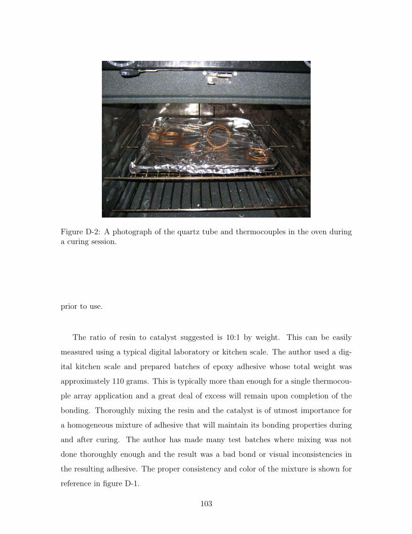
Figure D-2: A photograph of the quartz tube and thermocouples in the oven duringa curing session.

prior to use.

The ratio of resin to catalyst suggested is 10:1 by weight. This can be easily

measured using a typical digital laboratory or kitchen scale. The author used a dig-

ital kitchen scale and prepared batches of epoxy adhesive whose total weight was

approximately 110 grams. This is typically more than enough for a single thermocou-

ple array application and a great deal of excess will remain upon completion of the

bonding. Thoroughly mixing the resin and the catalyst is of utmost importance for

a homogeneous mixture of adhesive that will maintain its bonding properties during

and after curing. The author has made many test batches where mixing was not

done thoroughly enough and the result was a bad bond or visual inconsistencies in

the resulting adhesive. The proper consistency and color of the mixture is shown for

reference in figure D-1.

103

Figure D-3: A photograph of the quartz tube after having the thermocouples bondedto it and properly cured.

D.3 Thermocouple Bonding and Curing

After having cleaned the source tube and properly prepared the epoxy, the bonding

of the thermocouples can be done. This is a tedious and often messy and frustrating

process as the epoxy lacks heavy tackiness and so the small weight of the thermocou-

ples can sometimes pry them loose from the tube surface before bonding is complete.

It is important to note that as long as the actual thermocouple junction is bonded

securely to the tube, the remaining Kapton sheet that may not be bonded should

have a minimal impact on experimental results. Using laboratory latex gloves, the

user should spread a small amount of epoxy on the surface of the thermocouple and

ensure that it is evenly, though thinly coated. To apply the thermocouple to the tube

requires a slight pressure, which ensures that the epoxy has formed a uniform and

air-pocket free bond. Any excess epoxy should be attempted to be removed; however,

in practice this tends more times than not to be far more difficult than expected.

As can be seen in figure D-2, a natural gas-fired kitchen oven was used to cure the

104

thermocouple array and the tube itself was placed on a oven tray with aluminum foil

covering it. While the epoxy manufacturer gives a variety of different temperatures

and times for which the epoxy can be cured, the author has found the best results

by curing for 2 hours at a temperature of 400 degrees Fahrenheit. A finished quartz

tube with thermocouples properly bonded is shown in figure D-3.

105

106

Bibliography

[1] G. Sutton and O. Biblarz, Rocket Propulsion Elements, 7th Edition. Wiley-

Interscience, 2000.

[2] M. Martınez-Sanchez, 16.522: Space Propulsion, Course notes. Massachusetts

Institute of Technology, 2006.

[3] F.F. Chen, Plasma Physics and Control Fusion, 33, 339 (1991).

[4] R.W.Boswell, Phys. Lett. 33A, 457 (1970).

[5] F.F. Chen, J.D. Evans, and G.R. Tynan, Design and performance of distributed

helicon sources, Plasma Sources Sci. Technol. 10, 236 (2001); UCLA LTP-008

(August, 2000).

[6] F. Chang-Dıaz et al., Bull. APS 45 (7) 129, 2000.

[7] F. Chang-Dıaz, The VASIMR Engine, Scientific American, 283 (5) 90, 2000.

[8] J. P. Squire et al., IAC-02-S.4.03, 53rd International Astronautical Congress,

Houston TX, October 10-19, 2002.

[9] V.T. Jacobson et. al. Development of VASIMR helicon source, 43rd Annual Meet-

ing, APS Division of Plasma Science. (2001).

[10] F.F. Chen, Helicon Plasma Sources, in ”High Density Plasma Sources”, ed. by

Oleg A. Popov (Noyes Publications, Park Ridge, NJ), Chap. 1 (1995); UCLA

PPG-1506 (1994).

107

[11] J.M. Pucci et. al., ”Preliminary Characterization of a Helicon Plasma Source

for Space Propulsion.” AIAA 2006-5255. 42nd AIAA/ASME/SAE/ASEE Join

Propulsion Conference and Exhibit, 2006.

[12] M. Celik and M. Martınez-Sanchez, ”Experimental and Computational Studies of

Electric Thruster Plasma Radiation Emission.” Doctoral Thesis, Massachusetts

Institute of Technology, 2007.

[13] O. Batishchev, J. Pucci, N. Sinenian, Z. LaBry, M. Celik, M. Martınez-Sanchez,

”Mini-Helicon Thruster Experiment at MIT.” QO1.4, 48th Annual Meeting of

the Division of Plasma Physics, Philadelphia, PA, October 30November 3, 2006;

Bulletin APS, 51 (7) 224, October 2006.

[14] O. Batishchev, Kinetic Model for the Variable Isp Thruster, Bull. APS , 44, 8,

p. 99, 1999.

[15] M. Light and F.F. Chen, Helicon Wave Excitation with Helical Antennas, Phys.

Plasmas 2, 1084 (1995); UCLA PPG-1520 (1994).

[16] R.W. Boswell and F.F. Chen, Helicons, the early years, IEEE Trans. Plasma Sci.

25, 1229 (1997).

[17] F.F. Chen and D. Arnush, Generalized theory of helicon waves I: Normal modes,

Phys. Plasmas 4, 3411 (1997); UCLA PPG-1562 (Aug 1996).

[18] F.F. Chen, X. Jiang, J.D. Evans, G. Tynan, and D. Arnush, Low Field Helicon

Discharges, Plasma Phys. Control. Fusion 39, A411 (1997); UCLA PPG-1564

(Sept. 1996).

[19] Bose et. al. Plasma Sources Sci. Tech. 13 2004, 553-561.

[20] M. D. Carter et al., Physics of Plasmas, December 2002.

[21] J.A. Bittencourt, Fundamentals of Plasma Physics, 3rd Edition. Springer Press,

2004.

108

[22] I. H. Hutchinson. Principles of Plasma Diagnostics. Cambridge University Press,

2002.

[23] M. Celik et. al., Hybrid-PIC Simulation of a Hall Thruster Plume on an Un-

structured Grid with DSMC Collisions., IEPC-03-134, 31st International Electric

Propulsion Conference, 2003.

[24] O. Batishchev, Multi-Scale Modeling of Plasma Thrusters, NM2B.001, 46 APS

DPP, Savannah, GA, November 18, APS Bulletin, 49, 8, p. 260, 2004.

[25] O. Batishchev, A. Batishcheva, A. Kholodov, Unstructured Adaptive Grid and

Grid-free Methods for Edge Plasma Fluid Simulations, J. Plasma Phys. 61, 5,

1999, pp. 701-722.

[26] O. Batishchev, A. Batishcheva, RRC Adaptive Grid Method for Magnetized

Plasma, Proceedings 17th Intl. Conf. On Numerical Simulation of Plasmas, 29,

Banff, Canada, 2000.

[27] A. Batishcheva, O. Batishchev, Adaptive Kinetic Simulation of Plasma Propul-

sion by Laser Ablation, APS Bulletin, 49, 8, p. 260, 2004.

[28] B. Lawton and G. Klingenberg, Transient Temperature in Engineering and Sci-

ence. Oxford University Press, 1996.

[29] D. Pollock, Thermocouples: Theory and Properties. CRC Press, 1991.

[30] M. N. Ozisik, Heat Conduction, 2nd Edition. John Wiley and Sons, Inc, 1993.

[31] J.I. Frankel, ”Heat Flux Predictions From Surface Mounted Temperature Sensor

With DFT and Filtering Analysis.” IAC-05-C2.6.06, 2005.

[32] J.J. Bezuidenhout and J.A. Schetz, ”Heat Flux Determination Using Surface and

Backface Temperature Histories and Inverse Methods.” AIAA 2001-3530. 37th

AIAA/ASME/SAE/ASEE Join Propulsion Conference and Exhibit, 2001.

109

[33] www.accuratus.com, ”Fused Silica.” website, 2006.

[34] Y. Azziz and M. Martınez-Sanchez, ”Instrument Development and Plasma Mea-

surements on a 200-Watt Hall Thruster Plume.” Masters Thesis, Massachusetts

Institute of Technology, 2003.

[35] Naval Research Laboratory, NRL Plasma Formulary. NRL/PU/6790–06-491. Re-

vised 2006.

110