A

incafbjtt©

K

1

gititouuoassaciti

0d

J. Non-Newtonian Fluid Mech. 145 (2007) 109–123

Accuracy of bead-spring chains in strong flows

Patrick T. Underhill, Patrick S. Doyle ∗Department of Chemical Engineering, Massachusetts Institute of Technology, Cambridge, MA, United States

Received 23 August 2006; received in revised form 9 April 2007; accepted 21 May 2007

bstract

We have analyzed the response of bead-spring chain models in strong elongational flow as the amount of polymer represented by a springs changed. We examined the longest relaxation time of the chains which is used to quantify the strength of the flow in terms of a Weissenbergumber. A chain with linear springs can be used to predict the longest relaxation time of the nonlinear chains if the linear spring constant is modifiedorrectly. We used the expansion of the elongational viscosity in the limit of infinite Weissenberg number to investigate the change of the viscositys the scale of discretization was changed. We showed that the viscosity is less sensitive to the details of the spring force law because the chain isully extended at very large Weissenberg number. However, the approach to that infinite Weissenberg number response is dependent both on theehavior of the spring force at large force and the behavior at small force. New spring force laws to represent the worm-like chain or the freely

ointed chain are correct at both of these limits, while other currently used force laws produce and error. We also investigated the applicability ofhese expansions to chains including hydrodynamic interactions. Our results suggest that the longest relaxation time may not be the appropriateime scale needed to non-dimensionalize the strain rate in such highly extended states.

2007 Elsevier B.V. All rights reserved.

onm

htbrhtcaiebta

eywords: Coarse-graining; Bead-spring models; Elongational flow

. Introduction

Bead-spring chain models have become common coarse-rained versions of polymers. Most recent studies aimed atncreasing the accuracy of bead-spring chains have concen-rated on the inclusion of excluded volume and hydrodynamicnteractions [1–3]. These can now be included in the simula-ions because of increases in computation power and methodsf algorithm speed-up. While work in this area has furthered ournderstanding of and confirmed the importance of excluded vol-me and hydrodynamic interactions, we consider here the rolef the spring force law. The increase in computation power haslso allowed for the use of a large number of springs where eachpring represents a small segment of polymer. The use of “small”prings has been motivated in part by many new microfluidicpplications in which the behavior at a small length scale isritical [4–6]. Coarse-graining out these finer-scale details gives

naccurate models. It has been shown that using the conven-ional spring force laws at this high discretization can resultn significant errors [7–9]. Thus, understanding the validity

∗ Corresponding author.E-mail address: pdoyle@mit.edu (P.S. Doyle).

itwaute

377-0257/$ – see front matter © 2007 Elsevier B.V. All rights reserved.oi:10.1016/j.jnnfm.2007.05.011

f currently used force laws and how to correct them wheneeded is an important aspect of building an accurate polymerodel.New spring force laws have been developed which do not

ave these errors at high discretization [7–9]. By constructionhese new bead-spring chains have the same force-extensionehavior as the micromechanical models they represent. Theesponse in low Weissenberg number flow due to the force lawas also been studied in detail. By relating the contribution ofhe force law to the force-extension behavior at small force, weould illustrate the advantages of the new force laws. While thedvantages of the new force laws for the force-extension behav-or at large force is clear, the impact in strong flows has not beenxplicitly examined. One difference between the force-extensionehavior at large force and strong flows is the parameter usedo quantify the external forcing. In force-extension behavior, theppropriate scale for the external force is kBT/Ap, where Aps the persistence length. However, the strength of the flow isypically specified in terms of a Weissenberg number, Wi = ετ,here ε is the strain rate and τ is the polymer’s longest relax-

tion time. This makes the analysis in flow more complicated tonderstand because the longest relaxation time itself depends onhe discretization error of the spring force laws [10]. However,ven if the longest relaxation time of the bead-spring chain dif-

1 wtoni

fsWtsW

sidrldoeitrfidievhss

imwebtvhs

2

flfRLwfsw

r

f

wf

smν

sfoedabm

t

f

Tw

ftf

f

wnobcOcciwcrifwt

id

f

T

10 P.T. Underhill, P.S. Doyle / J. Non-Ne

ers from the polymer to be modeled, one would think that if thetrain rate is correspondingly changed to simulate at the samei, the difference will not play a role. For this reason we will

ake care to calculate the longest relaxation time of the bead-pring chains and examine how the response changes with thei held fixed.Here we will examine the response of bead-spring chains in

trong steady uniaxial extensional flow, comparing the behav-or of previous force laws with those which have been recentlyeveloped. There has been much work recently looking at theesponse of bead-spring chain models in extensional flow. Simu-ations in uniaxial and planar extensional flow can be comparedirectly with experiments done with a filament stretching devicer cross-slot devices [11,12]. Here we will be focusing on theffect of the spring force law on the response when the polymers strongly stretched (approaching full extension). In such stateshe inclusion of excluded volume effects should not affect theesponse because the likelihood that the chain will be in a con-guration which is influenced by the excluded volume is smallue to the strong stretching. Recently, Sunthar et al. [13] exam-ned the response in the start-up of elongational flow includingxcluded volume interactions. While they found that excludedolume interactions are important at small strains, we considerere only the steady response (or infinite strain value). Thisteady value will not be affected by excluded volume interactionsimilar to force-extension behavior [14].

Initially, we will also neglect the influence of hydrodynamicnteractions. In an extended configuration, the segments of poly-er are further apart so the hydrodynamic interactions will beeaker than in the equilibrium coiled state. However, when

xpressing the flow strength in terms of a Weissenberg num-er, the longest relaxation time is used. This longest relaxationime is affected by hydrodynamic interactions and even excludedolume interactions. We will briefly examine the impact ofydrodynamic interactions and their impact on the response introng extensional flow.

. Bead-spring models

In this study we have examined a number of different springorce laws. Two of the most common nonlinear spring forceaws are the FENE and Marko–Siggia force laws. The FENEorce law is an approximation to the inverse Langevin function.esearchers have also used a Pade approximation to the inverseangevin. We will compare the response of these force lawsith two new force laws that we have developed to model the

reely jointed chain and worm-like chain [8,9]. We have used theame notation and non-dimensionalization as in ref. [7], whiche briefly review here.The Marko–Siggia force law is an approximation to the

esponse of long worm-like chains. The spring force is(kBT

){1 1

}

s(r) =

Aeffr −

4+

4(1 − r)2 (1)

here � is the fully extended length of a spring, r = r/� theractional extension of the spring, and Aeff is the effective per-

ittf

an Fluid Mech. 145 (2007) 109–123

istence length. The true persistence length of the polymer beingodeled is denoted Atrue. The key dimensionless parameters are≡ �/Atrue which is the number of persistence lengths repre-

ented by each spring and λ ≡ Aeff/Atrue which is a correctionactor that can be used to correct the polymer response. The usef this correction factor is discussed in ref. [7]. Different criteriaxist for choosing λ as a function of ν. In particular we will beiscussing the so-called low-force and high-force criteria. Thesere choices for λ as a function of ν such that the force-extensionehavior of the bead-spring chain matches the micromechanicalodel at low or high force, respectively.In ref. [9] we have developed a new force law which models

he worm-like chain

s(r) =(

kBT

Aeff

){r

(1−r2)2 − 7r

ν(1 − r2)+(

3

32− 3

4ν− 6

ν2

)r

+(

(13/32)+(0.8172/ν)−(14.79/ν2)

1 − (4.225/ν) + (4.87/ν2)

)r(1 − r2)

}.

(2)

his force law reproduces the force-extension behavior of theorm-like chain by construction both at low and high forces.We have also examined spring force laws which represent

reely jointed chains. The FENE force law is an approximationo the response of long freely jointed chains [15]. The springorce is

s(r) =(

3kBT

aK,eff

)r

1 − r2 , (3)

here aK,eff is the effective Kuhn length of the polymer. Toon-dimensionalize the equations we define an effective lengthver which the chain is rigid, Aeff. Although this length needs toe proportional to the Kuhn length, the proportionality constantan be chosen arbitrarily to make the equations look simpler.bviously the response of the chain will be independent of this

hoice, though the dimensionless equations will depend on thehoice made. For convenience with the FENE force law we taket to be Aeff = aK,eff/3. We similarly have that Atrue = aK,true/3here aK,true is the true Kuhn length of the polymer. With this

hoice, ν represents three times the number of Kuhn lengthsepresented by each spring. One advantage of this choice is thatt removes any overall prefactor in the dimensionless spring forceormula. It also means that there is a correspondence b ↔ ν/λ,here b is a common parameter used in the literature which uses

he FENE force law.An alternative to the FENE force law which is seeing increas-

ng use is a Pade approximation to the inverse Langevin functionue to Cohen [16], which is

s(r) =(

3kBT

aK,eff

)r − r3/3

1 − r2 . (4)

he advantage of this force law is that it more accurately approx-

mates the inverse Langevin function. In particular, the force hashe same divergence as the inverse Langevin function. Althoughhe FENE force is correctly proportional to (1 − r/�)−1 nearull extension, the proportionality factor is incorrect. The Cohen

wtoni

ffC

wj

f

3

tTbiT

m

wtcfsst

ssnmbubdtdwal

4

ignttdclf

eacsp

nschpatt

τ

Bccafcvtsc

oslIabcf

uitetsTs[

poMa(a

P.T. Underhill, P.S. Doyle / J. Non-Ne

orm has the same proportionality factor as the inverse Langevinunction. We will return to this difference between the FENE andohen force laws when analyzing the steady, strong flows.

We have also previously developed a new spring force lawhich is a better approximation to the response of the freely

ointed chain [8] which is given by

s(r) =(

kBT

aK

) (3 − 10/ν + 10/(3ν2))r

− (1 + 2/ν + 10/(3ν2))r3

1 − r2 (5)

. Brownian dynamics

We use the method of Brownian dynamics (BD) to calculatehe response of bead-spring chains in non-equilibrium situations.his technique has been used widely to calculate the response ofead-spring chains [17,11]. The techniques integrates forwardn time the equation of motion, a stochastic differential equation.his equation is given by

iri = Fneti = FB

i + Fdi + Fs

i � 0, (6)

here the subscript i denotes bead i, m the mass of each bead, rhe acceleration, Fnet the net force, FB the Brownian force due toollisions of the solvent molecules with the beads, Fd the dragorce due to the movement of each bead through the viscousolvent, and Fs is the systematic force on each bead due to theprings and any external forces. We neglect the inertia (mass) ofhe beads, and so the net force is approximately zero.

For simulations near equilibrium and if each spring repre-ented a large segment of polymer, it was sufficient to use aimple Euler integration scheme. However, at large Weissenbergumber and if each spring represented a small segment of poly-er, the timestep would need to be so small that the simulations

ecame too computationally expensive. In these situations wesed the semi-implicit predictor-corrector method developedy Somasi et al. [10]. For the simulations including hydro-ynamic interactions, we used the Rotne–Prager–Yamakawaensor [18,19] and the generalization of the integration methodue to Hsieh et al. [2]. We found that using a look-up tableith linear interpolation in the semi-implicit method introduced

n error when used at large Weissenberg number. Therefore, aook-up table was not used.

. Longest relaxation time

When examining the behavior of bead-spring chains in flow,t is common to express the flow conditions (shear rate or elon-ation rate) in terms of a Weissenberg number. The Weissenbergumber (Wi) is taken as the product of the shear rate or elonga-ion rate and the longest relaxation time. This longest relaxationime will certainly be affected by excluded volume and hydro-

ynamic interactions. However, for consistency with the high Wialculations to be done without those effects, we consider theongest relaxation time of models without EV or HI. For modelsor which analytic calculations can be performed such as for lin-

flaw

an Fluid Mech. 145 (2007) 109–123 111

ar springs, the longest relaxation time can be expressed exactlys a function of the model parameters (such as the bead dragoefficient and spring constant). For nonlinear spring models,uch an analytic formula for the longest relaxation time is notossible.

The longest relaxation time for these models can be calculatedumerically using dynamical simulations such as BD. Theseimulations can be computationally costly, particularly for longhains that have long relaxation times. It is also inconvenient toave to perform a preliminary simulation for each set of modelarameters before performing the primary simulations. One wayround this is to use instead the characteristic time from dividinghe zero-shear rate first normal stress coefficient by two timeshe zero-shear rate polymer viscosity [20]

0 ≡ Ψ1,0

2ηp,0. (7)

oth of these zero-shear rate properties, provided HI is ignored,an be calculated from the retarded motion expansion coeffi-ients [7]. For the FENE force law, these can be calculatednalytically. For other force laws, such as the Marko–Siggiaorce law, they require numerical integration but are much lessomputationally costly than full BD simulations. The disad-antage of using this characteristic time is that it differs fromhe longest relaxation time even for chains with the relativelyimple linear spring force law [21]. It is unclear how the twoharacteristic times are related for more complicated force laws.

It is well known that because the chains do not contain EVr HI, each measure of the characteristic time will eventuallycale as N2 as the number of beads becomes asymptoticallyarge. However, we require more detailed knowledge than this.n this article we will be analyzing the behavior from as fews two beads to a large number of beads. We will not alwayse in this asymptotic limit. In particular, the point at which thehain reaches this limiting behavior will depend on the choiceor characteristic time.

Another way of estimating the longest relaxation time is tose the linear force law formula [11]. The linear spring constants taken from the nonlinear spring law at small extensions, wherehe spring law looks linear. If the chain, as it is relaxing back toquilibrium, only samples the linear region of the spring at longimes, then this should be a good approximation. It has beenhown that this approximation can result in significant errors.his error results because even at equilibrium, the springs canample the nonlinear parts of the force law as discussed in ref.7].

Because of the deficiencies of each approximate method, weerformed direct BD simulations of the relaxation of chainsver a wide parameter range and with both the FENE andarko–Siggia force laws. In order to calculate the longest relax-

tion time, the chains were started in a stretched configuration95% extension) in the z direction. The chains were simulateds they relaxed back to equilibrium. At long time, the stress dif-

erence σzz − σxx decays as a single exponential, exp(−t/τ). Aeast-squares fit is used to extract the value of the longest relax-tion time. Before plotting the results of the simulations, weill review what we call the Rouse relaxation time of a chain

1 wtonian Fluid Mech. 145 (2007) 109–123

abf

τ

Nfa

f

Ir

τ

Wfttfaiidfl

τ

Ft

τ

Tf

MtttTtssHtTTucsier

Fig. 1. Plot of the longest relaxation time of Marko–Siggia bead-spring chainsrelative to the Rouse prediction as a function of the number of effective persis-tence lengths each spring represents. The symbols represent different numberoN

t

ift

f

wfs

〈

Tr

F

Cmi

H

Tsdcl

12 P.T. Underhill, P.S. Doyle / J. Non-Ne

nd express it in the notation used here. Consider a chain of Neads connected by N − 1 linear springs with spring force laws(r) = Hr. The longest relaxation time of the chain is

= 1

2 sin2(π/(2N))

ζ

4H. (8)

ow, consider a chain of inextensible springs. Using the notationrom ref. [7], we write the Taylor expansion of the spring forces

s(r) = kBT2φ2ν

�2λr + O(r2) (9)

f we treat the linear term like the linear spring, the longestelaxation is what we call the Rouse time

R = 1

2 sin2(π/(2N))

ζ�2λ

8φ2kBTν. (10)

ith our choice of Atrue as the persistence length then φ2 = 3/4or the Marko–Siggia force law, and with Atrue as one-third ofhe Kuhn length then φ2 = 1/2 for the FENE force law. Notehat because of our ability to take different choices for Atrue theormulas can appear to take different forms. However, becauseny change of choice affects the meaning of ν while also chang-ng the value of φ2, the physical meaning of a formula remainsnvariant. To illustrate this, let us insert into the Rouse time theefinitions of ν and λ and the value of φ2. For the Marko–Siggiaorce law, we have taken Aeff to be the effective persistenceength, Ap,eff, and the Rouse time becomes

R = 1

2 sin2(π/(2N))

ζ�Ap,eff

6kBT. (11)

or the FENE force law, we have taken Aeff to be one-third ofhe effective Kuhn length, aK,eff/3, and the Rouse time becomes

R = 1

2 sin2(π/(2N))

ζ�aK,eff

12kBT. (12)

hese two formulas remain the same independent of any choiceor Atrue and the corresponding value of φ2.

We now show the results of the BD simulations using thearko–Siggia force law in Fig. 1 where the longest relaxation

ime of the chain is divided by the above Rouse time. The firsthing to note is that the longest relaxation time is the same ashe Rouse time when ν/λ → ∞ but deviates for smaller values.his is because the Rouse time assumes that near equilibrium

he spring only samples the low extension (linear) part of thepring. As discussed in ref. [7] if ν/λ is not infinite, the springamples the nonlinear parts of the spring even at equilibrium.owever, the other important aspect to notice from Fig. 1 is

hat the relaxation time scales with N just like the Rouse result.he deviation from the Rouse time is only a function of ν/λ.his suggests that it is possible to describe the relaxation timesing a chain with linear springs, but which have a linear springonstant that differs from that in Eq. (9). In some approximate

ense, the chain still responds linearly to external forces evenf the spring samples the nonlinear regions and so returns toquilibrium using some effective linear restoring force. This iseminiscent of the force-extension behavior of the chains seen

ewcp

f beads: N = 2 (diamond), N = 5 (triangle), N = 10 (square), N = 30 (×),= 50 (+), and N = 100 (*). The solid line is the modified Rouse relaxation

ime (Eq. (18)). The dotted line is the fitted function (Eq. (21)).

n ref. [7]. Even if the chain samples the nonlinear regions, theorce-extension behavior is linear at low force. Ref. [7] showedhat a bead-spring chain has

lim→0

∂

∂f〈ztot〉m = (N − 1)�2〈r2〉eq

3kBT, (13)

here 〈ztot〉m is the average z extension of the model. The springorce law comes in through the equilibrium averaged singlepring moment

r2〉eq =∫ 1

0 dr r4 exp[−(ν/λ)Ueff(r)]∫ 10 dr r2 exp[−(ν/λ)Ueff(r)]

. (14)

he exponential is the Boltzmann factor, and the function Ueffepresents the non-dimensional spring potential energy

ν

λUeff(r) = Ueff(r)

kBT. (15)

or a chain of linear springs, the force-extension relation is

∂

∂f〈ztot〉m = N − 1

H. (16)

omparing Eqs. (13) and (16), we define a modified Rouseodel as a chain of linear springs where the spring constant

s

MR ≡ 3kBT

�2〈r2〉eq. (17)

his statement is equivalent to choosing the linear spring con-tant such that it has the same equilibrium averaged end-to-endistance squared and number of beads as the nonlinear springhain. Following from this is that they also have the same equi-ibrium radius of gyration and zero shear viscosity. While these

quivalences do not guarantee that this modified Rouse modelill have the same longest relaxation time as the nonlinear spring

hain, we hope that they will be similar. Therefore, we will com-are the modified Rouse relaxation time with the exact relaxation

P.T. Underhill, P.S. Doyle / J. Non-Newtonian Fluid Mech. 145 (2007) 109–123 113

Fig. 2. Plot of the longest relaxation time of Marko–Siggia bead-spring chainsrelative to the modified Rouse prediction (Eq. (18))as a function of the number ofeffective persistence lengths each spring represents. The symbols represent dif-ferent number of beads: N = 2 (diamond), N = 5 (triangle), N = 10 (square),N = 30 (×), N = 50 (+), and N = 100 (*). The lines represent τ0,s divided bythe modified Rouse prediction for the same range of number of beads, with thelb

tii

τ

stitwwiftbriF

h[“dfdfwhpfs

Fig. 3. Plot of the longest relaxation time of FENE bead-spring chains relative tothe modified Rouse prediction as a function of the number of effective persistencelN

a

t(mtwwN

τ

T

τ

werIpttufhif

τ

Wtseen with the Marko–Siggia force law are not specific to that

owermost curve with N = 2 and the uppermost curve with N = 100. The errorars represent plus or minus two standard deviations.

ime to examine how well it predicts the nonlinear chain behav-or. The longest relaxation time of the modified Rouse models

MR = 1

2 sin2(π/(2N))

ζ�2〈r2〉eq

12kBT. (18)

In Fig. 2 we show the longest relaxation times of the bead-pring chains as in Fig. 1 but now dividing the values by τMRo gauge the predictive capability of the modified Rouse modeln terms of longest relaxation time. We see that the error usinghe modified Rouse time is much smaller than if the Rouse timeere used. However, there does seem to be a general trend inhich the deviation grows at smaller discretization. The mod-

fied Rouse time almost always overpredicts the values fittedrom the simulations. Although the modified Rouse relaxationime does not seem to give a quantitative predictive measure, weelieve it can still be used to understand the change of the longestelaxation time with a change in the scale of discretization. Thiss illustrated by the improved prediction of Fig. 2 compared withig. 1.

We should note that the Eqs. (10) and (18) are not new, andave been used before. See, for example, the review by Larson11]. However, both equations have been called by the nameRouse” because for the Rouse model, for which they wereerived, they are equivalent. Our contribution is to notice thator nonlinear spring force laws, the formulas give dramaticallyifferent results. In order to carefully distinguish between theseormulas which give different predictions for nonlinear springs,e call them “Rouse” and “modified Rouse”, respectively. Weave shown here that while the Rouse result (Eq. (10)) fails to

redict the relaxation of nonlinear springs, the modified Rouseormula (Eq. (18)) retains approximate validity for nonlinearprings.

fba

engths each spring represents. The symbols represent different number of beads:= 2 (diamond), N = 5 (triangle), N = 10 (square), N = 30 (×), N = 50 (+),

nd N = 100 (*). The error bars represent plus or minus two standard deviations.

To this point, we have compared exact BD simulations ofhe longest relaxation time to what we call the Rouse time (Eq.10)) and compared the exact simulations with a modified Rouseodel (Eq. (18)). The other method for estimating the relaxation

ime is from the ratio of zero-shear properties, Eq. (7), whiche now compare with the exact BD simulations. One problemith using this estimate is that the functional dependence withis different. For a chain of linear springs τ0 is

0 = 2N2 + 7

15

ζ

4H. (19)

his inspires us to define a scaled time

0,s ≡ τ015

2N2 + 7

1

2 sin2(π/(2N)), (20)

hich compensates for the difference in N dependence that existsven for the linear spring system. Fig. 2 also shows curves rep-esenting τ0,s for the Marko–Siggia force law divided by τMR.t is not clear that τ0,s represents the data any better than τMR,articularly given the accuracy of the simulations. Note also thathe absolute difference between the two is quite small comparedo the changes in relaxation time seen in Fig. 1. Because of theseful physical interpretation of τMR in terms of the coil size andorce-extension behavior, we will not consider τ0,s further. Weave also performed a fit through the data to give a formula whichs only slightly more accurate than τMR. For the Marko–Siggiaorce law, this is

fit = 1

2 sin2(π/(2N))

ζ�2

kBT

1

6ν/λ + 7.26√

ν/λ + 21.2. (21)

e have also performed BD simulations of the longest relaxationime using the FENE spring force law to verify that the trends

orce law. In Fig. 3 we show the longest relaxation time dividedy τMR for the FENE force law. For the FENE force law theverage in Eq. (18) can be calculated exactly. Therefore, the

114 P.T. Underhill, P.S. Doyle / J. Non-Newtoni

Fig. 4. Plot of the longest relaxation time of bead-spring chains using the newforce law for the worm-like chain relative to the modified Rouse prediction as afunction of the number of persistence lengths each spring represents. The sym-bN

s

r

TseRTmua

τ

Tso

adftttdstctttlAct

t

τ

5

tOtfiiigfaac

5

smtos

dse

η

w

P

t

η

a

η

WN

C

ols represent different number of beads: N = 2 (diamond), N = 5 (triangle),= 10 (square), and N = 30 (×). The error bars represent plus or minus two

tandard deviations.

esults in Fig. 3 can be viewed as

τ

τMR= τ

τR

(5

ν/λ+ 1

). (22)

he trend is the same as with the Marko–Siggia simulations. Weee a slight growing deviation at smaller discretization, how-ver that deviation is much smaller than would be seen if theouse model were used to attempt to predict the simulations.he scatter of the data is of similar order of magnitude and theodified Rouse time again almost always overpredicts the sim-

lation data. We can also perform a fit through this data to giveslightly more accurate result

fit = 1

2 sin2(π/(2N))

ζ�2

kBT

1

4ν/λ + 1.05√

ν/λ + 21.1. (23)

hese fitted functions will be used later as a closed form expres-ion for the longest relaxation time when discussing the changef the elongational viscosity with the degree of discretization.

We see that the modified Rouse formula gives a reason-ble prediction of the longest relaxation time even to very highiscretization. This is important because the modified Rouseormula allows us to gain intuition about the governing factorsowards the relaxation time. The modified Rouse formula con-ains the size of a spring at equilibrium, which can be related tohe force-extension response at small force. This gives us confi-ence that if a new spring force is used which gives the correctize of a spring and force-extension behavior, then the relaxationime will be the expected value. We can show this explicitly byalculating the relaxation time for a new force law to representhe worm-like chain (Eq. (2)). Fig. 4 shows the relaxation time ofhis force law divided by its modified Rouse prediction. We seehe same basic result as with the Marko–Siggia and FENE force

aws, that the modified Rouse formula is a reasonable prediction.

similar scatter is seen and trend to deviate more at small dis-retization. Note that this new force law was developed to havehe correct behavior near equilibrium, and thus by construction

Otbu

an Fluid Mech. 145 (2007) 109–123

he modified Rouse formula is

MR = 1

2 sin2(π/(2N))

ζ�Ap

6kBT. (24)

. Steady elongational flow

After understanding the behavior of the longest relaxationime, we can investigate the high Weissenberg number response.ne advantage of looking at steady elongational flow is that

he viscosity can be written formally as an integral over con-guration space [21]. This can be done because we are not

ncluding the effects of EV and HI, which should be of secondarymportance near full extension. Although calculating the inte-rals numerically is not efficient for getting the exact responseor chains of many springs, they can be used to develop seriespproximations. This same type of expansion was performedt small flow strength to obtain the retarded-motion expansionoefficients in ref. [7].

.1. Models of the freely jointed chain

We begin our analysis of the response of bead-spring chains introng, steady elongational flow with bead-spring chains used toodel the freely jointed chain. We will be able to explicitly judge

he accuracy of the coarse-grained model because the responsef the freely jointed chain which is being modeled by the bead-pring chain is known.

The first bead-spring chain system we will examine toescribe the behavior of the freely jointed chain is with the FENEpring force law. For the FENE force law, the expansion of thelongational viscosity in terms of Pe is

˜ ∼ ˜η∞ − 1

Pe

[( ν

λ+ 4)

(N − 1) − 3CN

]+ O

(1

Pe2

),

(25)

here the Peclet number is defined as

e ≡ εζ�2

kBT, (26)

he dimensionless elongational viscosity is defined as

˜ = η − 3ηs

npζ�2 , (27)

nd the dimensionless elongational viscosity at infinite Pe is

˜∞ = N(N2 − 1)

12. (28)

e have also defined the parameter CN which is a function ofas

N ≡N−1∑m=1

1

1 + m + m2 . (29)

ur approach is to use this expansion to understand the change inhe response of the chain as the amount of polymer representedy a spring is changed. Using an analytic expansion will allows to make precise statements about the effect of the different

P.T. Underhill, P.S. Doyle / J. Non-Newtonian Fluid Mech. 145 (2007) 109–123 115

F beadst right).1 line is

sSs

A

tWtrt

η

WcWhwce

WWdv

1

Fasiw

1

TscbpwtW

tersAmbatucan be understood by looking at the expansion in Eq. (30). Thecoefficient to Wi−1 only depends on the ratio ν/λ. Therefore,the smaller the value of λ, the larger the ratio ν/λ, and the closer

ig. 5. Calculation of the elongational viscosity as a function of the number ofhe FENE force law with λ = 1 (Eq. (30)). The values of Wi are 1 (left) and 10 (00, 400, 4000, and ∞. The dashed line is 1 − 6/(π2Wi) (Eq. (31)). The dotted

pring force laws and criteria for the effective persistence length.ince it is an expansion for large strain rates, for sufficiently largetrain rates it will eventually describe the response.

Recall that for the FENE force law we have chosen to definetrue as one-third of the Kuhn length such that ν = �/Atrue is

hree times the number of Kuhn lengths represented by a spring.hile this choice will affect the look of the equation written in

erms of ν, the physical meaning is unchanged. We now rear-ange and include an approximate form for the longest relaxationime to obtain

ˆ ≈ N + 1

N − 1− 12

N(N − 1)2 sin2(π/(2N))Wi

× 1

4ν/λ + 1.05√

ν/λ + 21.1

[ν

λ+ 4 − 3

N − 1CN

]

+O(

1

Wi2

). (30)

e can now analyze how this expansion (the response of thehain) changes as the number of beads is changed while theeissenberg number Wi is held constant, and α = (N − 1)ν is

eld constant. When analyzing the behavior we must decidehich criterion for choosing λ will be used. We will start by

hoosing λ = 1. Note though that this does not correspond toither the high-force or low-force criterion.

Fig. 5 shows plots of Eq. (30) as a function of N for constanti and α for λ = 1, i.e. not using an effective Kuhn length.e see similar shapes as with the previous bead-spring chains

iscussed. If 1 N α we see a plateau which occurs at aiscosity of

− 6

π2Wi+ O

(1

Wi2

). (31)

or all chains with a finite α, the number of beads will eventu-lly become large enough that the springs represents very smallegments of polymer. The system then approaches the limit-ng behavior of the bead-string chain when 1 N and α N

hich is approximately

− 0.46

Wi+ O

(1

Wi2

). (32)

FgW

(d

for constant Wi and α using the first two terms in the asymptotic expansion forThe lines correspond to different values of α, from top to bottom ranging from1 − 0.46/Wi (Eq. (32)). The long-dashed line is 1 − 0.34/Wi (from Eq. (36)).

his equation is only known approximately because there isome uncertainty in the longest relaxation time of a bead-stringhain used to write the expression using a Weissenberg num-er. Because the difference in responses between the long chainlateau (Eq. (31)) and the bead-string chain (Eq. (32)) decreasesith Wi, as Wi−1, the elongational viscosity is less sensitive to

he incorrect and changing accuracy of the spring force law asi increases.Recall that for the FENE force law, even the high-force cri-

erion is not λ = 1. We show in Fig. 6 the response of thelongational viscosity for the high-force and the low-force crite-ia [7]. The different criteria can only be used up to values of Nuch that the chain becomes the bead-string chain (i.e. λ → ∞).t this point in N, the curves for the low and high-force criteriaust stop. We see that the high-force criterion performs slightly

etter (stays in the plateau longer) than the low-force criterion,lthough the difference for the FENE force law is almost indis-inguishable. However, there is the counter-intuitive result thatsing λ = 1 seems to do even better than either criteria. This

ig. 6. Comparison of the different criteria for λ and their effect on the elon-ational viscosity for the FENE force law using Eq. (30). The parameters arei = 1, α = 400, and either the low-force (upper curve) or high-force criteria

middle curve) for λ or λ = 1 (lower curve). The λ = 1 case and the dashed,otted, and long-dashed lines are identical to those in Fig. 5.

1 wtoni

tλ

sonbtcapatb

pcesertpfimhccsl

wmllswrnc

η

Fj

τ

s

η

WcRbTal

adiiilthCliobt

η

I

η

wblalt

η

Rfk

ocn(tas

s

16 P.T. Underhill, P.S. Doyle / J. Non-Ne

he term is to the long chain limit behavior. In essence, a smallermakes it look like there are more effective Kuhn lengths per

pring, so the chain looks like a chain with a very large numberf Kuhn lengths. This arbitrary change of the Kuhn length doesot cause a detrimental response in the strong stretching limitecause the long chain behavior does not explicitly depend onhe true Kuhn length, only on the total drag on the chain, theontour length squared, and the Weissenberg number. Althoughrbitrarily choosing λ very small does increase the size of thelateau, we do not consider that a viable option for developingn accurate coarse-grained model because the change in effec-ive persistence length would cause all equilibrium properties toe incorrect.

To this point we have presumed that the existence of thelateau in the viscosity means that the chain is an accurateoarse-grained model. For the FENE force law this plateaussentially exists when the chain has many beads but each springtill represents a large segment of polymer. We have shown thatven if the incorrect spring force law is used when each springepresents a small segment of polymer, for sufficiently high Wihe elongational viscosity does not actually deviate a significantercentage from the plateau because the chain is always virtuallyully extended. However, the existence of this plateau does notn of itself guarantee that the bead-spring represents the desired

icromechanical model. For the FENE chain, we can easily seeow well this plateau matches the behavior of the freely jointedhain because the steady state behavior of the freely jointedhain in elongational flow is known [22]. The expansion of theteady state elongational viscosity of a freely jointed chain forarge strain rates is

η−3ηs

npζa2 ∼ N(N2−1)

12− kBT

ζa2ε[2(N − 1) − 3CN ] + O

(1

ε2

),

(33)

here a is the length of a rod and the sum over the Kramersatrix which was tabulated by Hassager can be written equiva-

ently as a simpler sum, CN . Currently we are concerned with theimit of a large number of rods because we want to compare thiseries expansion with the plateau occurring for a FENE chainith a large number of springs and where each spring still rep-

esents a large number of Kuhn lengths. In the limit of a largeumber of rods, the elongational viscosity of a freely jointedhain becomes

ˆ ∼ 1 − 24

Wi

kBTτ

N2ζa2 + O(

1

Wi2

). (34)

rom ref. [23] we know that the relaxation time of long freelyointed chains is approximately

≈ 0.0142N2 ζa2

kBT, (35)

o the viscosity is

ˆ ≈ 1 − 0.34

Wi+ O

(1

Wi2

). (36)

ccai

an Fluid Mech. 145 (2007) 109–123

e expect that Eq. (31) would be the same as this freely jointedhain result, Eq. (36), however we see that they are not the same.ecall that the FENE force law does not have the exact sameehavior as the inverse Langevin function near full extension.his will account for some of the difference, which we will nowddress by examining the behavior of the Cohen spring forceaw.

Because the Cohen spring force law does have the samepproach to full extension as the inverse Langevin function, butifferent from the FENE force law, we will be able to see thenfluence of this divergence. Note that because the first two termsn the flow expansion (in terms of Pe) only depends on the dom-nant behavior of the spring near full extension, the Cohen forceaw has the same two term expansion as a bead-spring chain withhe inverse Langevin function as the spring force law. Obviouslyigher order terms in the expansion will be different between theohen force law and the inverse Langevin function. The equi-

ibrium behavior (and relaxation time) will also be different atntermediate ν. At infinite ν it only depends on the linear regionf the force law which is the same, and at zero ν they bothecome the bead-string chain which are the same. The first twoerms in the high strain rate expansion are

˜ ∼ ˜η∞ − 1

Pe

[(2ν

3λ+ 4

)(N − 1) − 3CN

]+ O

(1

Pe2

).

(37)

n the limit of 1 N α, the expansion becomes

ˆ ∼ 1 − 4

π2Wi+ O

(1

Wi2

), (38)

here we have used our knowledge of the relaxation time of theead-spring chain when ν is very large. We can also look in theimit of such large N that each spring represents a very smallmount of polymer, 1 N and α N. In this limit the chainooks like a bead-string chain, which is the same result as forhe FENE chain. In this limit the expansion is approximately

ˆ ≈ 1 − 0.46

Wi+ O

(1

Wi2

). (39)

ecall that the approximation here in determining the expansionor the bead-string chain is that the longest relaxation time is onlynown approximately.

There are two important aspects to notice about the behaviorf the Cohen force law chain. The first is that the structure hashanged from that of the FENE force law in that Eq. (38) isow greater than Eq. (39). The other is that even this expansionwhich is the expansion for the exact inverse Langevin func-ion) deviates from the freely jointed chain result when therere a large number of springs and each spring represents a largeegment of polymer (i.e. comparing Eqs. (36) and (38)).

This deviation, however, turns out to be related back to aubtlety with the longest relaxation time of the freely jointed

hain which is not often discussed. Consider a freely jointedhain with such a large number of rods that if one models it withbead-spring chain with the exact inverse Langevin force law,

t is possible to both have a very large number of springs and at

wtoni

tog

τ

WrtwscotT

τ

Ibtcaioetj

Isg

krit[ittfs(edp

sou

ll

η

TCtaeeebrrTen

5

tfici

η

Tiwrange of parameters of the Marko–Siggia force law. These areshown in Fig. 7. We plot the data versus Peclet number insteadof Weissenberg number because the Peclet number is the naturalparameter in the expansion and simulations. The Peclet number

P.T. Underhill, P.S. Doyle / J. Non-Ne

he same time have each spring represent a very large numberf rods. The longest relaxation time of this bead-spring chain isiven by Eq. (12) or alternatively (with λ = 1)

= (Nζ)LaK

6π2kBT. (40)

e know this relaxation time exactly because if each springepresents a very large segment of polymer, near equilibriumhe spring only samples the linear region of the force law soe can use the analytic result for the relaxation time of a bead-

pring chain with linear springs. Because this bead-spring chainorrectly models the equilibrium and force-extension behaviorf the freely jointed chain, one might think that it would modelhe longest relaxation time of the chain. However, this is not true.he longest relaxation time is given in Eq. (35) or equivalently

= 0.0142(Nζ)LaK

kBT. (41)

t is this difference in relaxation times that causes the differenceetween the viscosity expansion of the freely jointed chain andhe Cohen or inverse Langevin chain even when the bead-springhain has a large number of springs and each spring representslarge segment of polymer. We can see this by using Eq. (40)

n the expansion of the freely jointed chain, Eq. (34), insteadf the exact formula, which is then identical to the Cohen chainxpansion, Eq. (38). We can also see that it is the relaxation timehat causes this final discrepancy by noticing that both the freelyointed chain and Cohen chain can be written in these limits as

η − 3ηs

np∼ (Nζ)L2

12− kBT

ε

× [2×(number of Kuhn lengths in whole molecule)]

+O(

1

ε2

). (42)

t is only when the extension rate is written in terms of a Weis-enberg number using different longest relaxation times thatives this final discrepancy.

It should be noted that it is not only from ref. [23] that wenow the longest relaxation time of a freely jointed chain. Otheresearchers [24–26] have performed similar simulations verify-ng the same result as well as independent tests of the relaxationime. This is also not the first mentioning of this discrepancy25,26]. The almost 20% deviation in the longest relaxation times an unresolved issue and is outside the scope of this article. Forhe purposes of this article we can not do better than reproducinghe expansion in Eq. (42), which depends on the behavior nearull extension, and to capture the longest relaxation time if eachpring represents a large segment of polymer. Thus, this plateauEq. (38)) is considered “accurate” for our purposes. However,ven the Cohen force law or the inverse Langevin force law willeviate from this as each spring represents a small segment ofolymer, and the chain approaches the bead-string chain.

A new spring force law has been developed such that the bead-pring chain accurately represents the force-extension behaviorf the freely jointed chain (Eq. (5)) [8]. We can examine howsing this new force law affects the elongational viscosity at

FBsTs

an Fluid Mech. 145 (2007) 109–123 117

arge strain rates. The expansion of the viscosity for this forceaw is

˜ ∼ ˜η∞ − 1

Pe

[2ν

3(N − 1) − 3CN

]+ O

(1

Pe2

)(43)

his expansion should be compared with the expansion for theohen force law or inverse Langevin force law (Eq. (37)). We see

hat because the new force law correctly represents the behaviort large forces, the expansion in viscosity in terms of Pe is mod-led correctly (like when using the high-force criterion for anffective persistence length). The term 2ν(N − 1)/3 is alwaysqual to two times the total number of Kuhn lengths representedy the chain independent of how few Kuhn lengths each springepresents, just as we saw in Eq. (42). However, the equilib-ium behavior is also captured correctly with the new force law.his means that the longest relaxation time will also be capturedssentially. Because both are captured correctly, the system willot deviate at high discretization from the plateau.

.2. Models of the worm-like chain

We now analyze of the response of bead-spring chains usedo model the worm-like chain. The most commonly used springorce law to model the worm-like chain is the Marko–Siggianterpolation formula. The expansion of the elongational vis-osity for large strain rates using the Marko–Siggia force laws

˜ ∼ ˜η∞ −√

ν/λ

2Pe

N−1∑k=1

√k(N − k) + O

(1

Pe

). (44)

o investigate the exact chain response and the range of valid-ty of the expansion we performed BD simulations of chainsithout EV and HI from approximately Wi = 1 to 1000 for a

ig. 7. Comparison of the approach to the plateau elongational viscosity betweenD simulations and the two-term series expansion in Eq. (44)(solid lines). The

pring force law is the Marko–Siggia formula and the chains consist of 10 beads.he curves correspond to (from left to right) ν = 1, 10, 100, 1000. Each curvespans strain rates from approximately Wi = 1 to Wi = 1000.

118 P.T. Underhill, P.S. Doyle / J. Non-Newtonian Fluid Mech. 145 (2007) 109–123

F beadf eft) ar 9)), an

ifatpWicis

setottetcawo

η(2N

i

w

τ

T

rT

Nac(a

η

WwaaloddoTs

ti(a

1

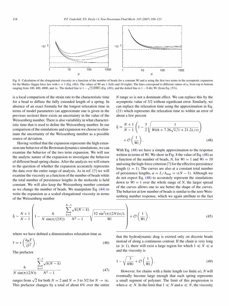
ig. 8. Calculation of the elongational viscosity as a function of the number ofor the Marko–Siggia force law with λ = 1 (Eq. (48)). The values of Wi are 1 (langing from 100, 400, 4000, and ∞. The dashed line is 1 − √

3/(8Wi) (Eq. (4

s a local comparison of the strain rate to the characteristic timeor a bead to diffuse the fully extended length of a spring. Inbsence of an exact formula for the longest relaxation time inerms of model parameters (an approximate one is given in therevious section) there exists an uncertainty in the value of theeissenberg number. There is also variability in what character-

stic time that is used to define the Weissenberg number. In ouromparison of the simulations and expansion we choose to elim-nate the uncertainty of the Weissenberg number as a possibleource of deviation.

Having verified that the expansion represents the high exten-ion rate behavior of the Brownian dynamics simulations, we canxamine the behavior of the two term expansion. We will usehe analytic nature of the expansion to investigate the behaviorf different bead-spring chains. After the analysis we will returno the question of whether the expansion accurately representshe data over the entire range of analysis. As in ref. [7] we willxamine the viscosity as a function of the number of beads whilehe total number of persistence lengths in the molecule is heldonstant. We will also keep the Weissenberg number constants we change the number of beads. We manipulate Eq. (44) torite the expansion as a scaled elongational viscosity in termsf the Weissenberg number

ˆ ∼ N + 1

N − 1

⎛⎜⎜⎜⎜⎜⎝1 − 6

N sin(π/(2N))

N−1∑k=1

√k(N − k)

N2 − 1

√τ2 sin2(π/

W

here we have defined a dimensionless relaxation time as

ˆ = τ

(kBT

ζ�2

). (46)

he prefactor

6

N−1∑√k(N − k)

N sin(π/(2N))k=1

N2 − 1(47)

anges from√

2 for both N = 2 and N = 3 to 3/2 for N → ∞.his prefactor changes by a total of about 6% over the entire

eaw

s for a constant Wi and α using the first two terms in the asymptotic expansionnd 10 (right). The lines correspond to different values of α, from top to bottomd the dotted line is 1 − 0.46/Wi (from Eq. (53)).

))ν/λ

⎞⎟⎟⎟⎟⎟⎠+ O

(1

Wi

), (45)

range so is not a dominant effect. We can replace this by thesymptotic value of 3/2 without significant error. Similarly, wean replace the relaxation time using the approximation in Eq.21) which represents the relaxation time to within an error ofbout a few percent

ˆ ≈ N + 1

N − 1

(1 − 3

2

√1

Wi(6 + 7.26√

λ/ν + 21.2λ/ν)

)

+O(

1

Wi

). (48)

ith Eq. (48) we have a simple approximation to the responseritten in terms of Wi. We show in Fig. 8 the value of Eq. (48) asfunction of the number of beads, N, for Wi = 1 and Wi = 10

nd using the high-force criterion [7] for the effective persistenceength (λ = 1). The curves are also at a constant total numberf persistence lengths, α = L/Atrue = ν(N − 1). Although weo not expect Eq. (48) to accurately represent the simulationsown to Wi = 1 over the whole range of N, the larger spreadf the curves allows one to see better the shape of the curves.he behavior at low number of beads is similar to the zero Weis-enberg number response, which we again attribute to the fact

hat the hydrodynamic drag is exerted only on discrete beadsnstead of along a continuous contour. If the chain is very longα � 1), there will exist a large region for which 1 N α

nd the viscosity is

−√

3

8Wi+ O

(1

Wi

). (49)

However, for chains with a finite length (so finite α), N willventually become large enough that each spring representssmall segment of polymer. The limit of this progression ishen α N. In the limit that 1 N and α N, the viscosity

wtoni

a

1

Twuaesttgnolsl

tettrltordtcMTnirN

Ftacd

ν

tActfpi

tutfToflutt(mpWohwse

esrr

P.T. Underhill, P.S. Doyle / J. Non-Ne

pproaches

+ O(

1

Wi

). (50)

he difference between Eqs. (49) and (50) decreases as Wi−1/2,hich means that for very large Weissenberg number, there is nopper limit on the number of beads past which the response devi-tes significantly. Essentially, if the Weissenberg number is largenough, the chain will be almost fully extended and so even if thepring force is not represented correctly, the chain will still be inhe fully extended state. Thus, for some properties the change ifhe incorrect spring force law is used may appear to have a negli-ible effect. Note that this is different from the low Weissenbergumber behavior which was found to have a maximum numberf beads of N1/2 1.15α1/2 for the Marko–Siggia spring forceaw [7]. This means that the response of the bead-spring chaineems to be less sensitive to using an inappropriate spring forceaw when the springs become very small.

To this point we have not used an effective persistence lengthhat differed from the persistence length of the WLC being mod-led, thus λ = 1. Recall the progression of analysis used to studyhe behavior at low Wi [7]. The analysis with λ = 1 showedhat there was an error in the low Wi response if each springepresented too small an amount of polymer. Howeve,r if theow-force criterion was used for the effective persistence length,he error due to the incorrect force law vanished in the rangef applicability of the low-force criterion. The only error thatemained was from the fact that for small number of beads, therag was not distributed along the contour. We would thus expecthat a similar vanishing of the error would be present in thisase if the high-force criterion were used. But recall that for thearko–Siggia force law using λ = 1 is the high-force criterion.

here is still a deviation when each spring represents too few

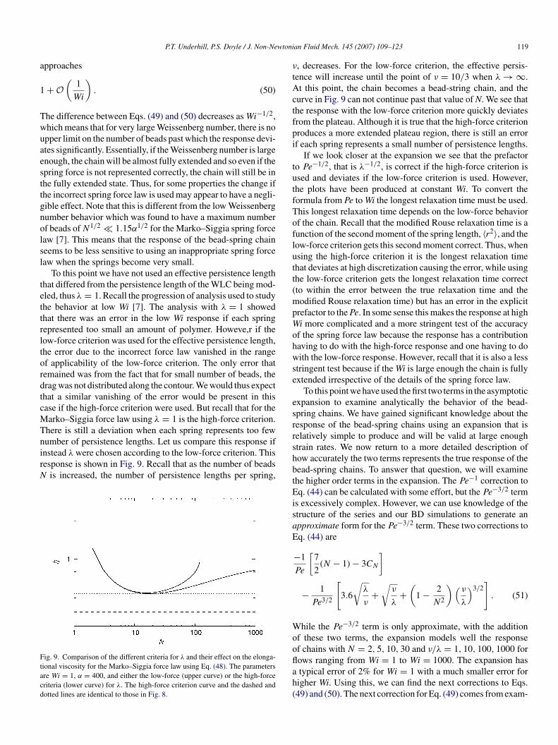
umber of persistence lengths. Let us compare this response ifnstead λ were chosen according to the low-force criterion. Thisesponse is shown in Fig. 9. Recall that as the number of beads

is increased, the number of persistence lengths per spring,

ig. 9. Comparison of the different criteria for λ and their effect on the elonga-ional viscosity for the Marko–Siggia force law using Eq. (48). The parametersre Wi = 1, α = 400, and either the low-force (upper curve) or the high-forceriteria (lower curve) for λ. The high-force criterion curve and the dashed andotted lines are identical to those in Fig. 8.

shbtEisaE

Wooflah(

an Fluid Mech. 145 (2007) 109–123 119

, decreases. For the low-force criterion, the effective persis-ence will increase until the point of ν = 10/3 when λ → ∞.t this point, the chain becomes a bead-string chain, and the

urve in Fig. 9 can not continue past that value of N. We see thathe response with the low-force criterion more quickly deviatesrom the plateau. Although it is true that the high-force criterionroduces a more extended plateau region, there is still an errorf each spring represents a small number of persistence lengths.

If we look closer at the expansion we see that the prefactoro Pe−1/2, that is λ−1/2, is correct if the high-force criterion issed and deviates if the low-force criterion is used. However,he plots have been produced at constant Wi. To convert theormula from Pe to Wi the longest relaxation time must be used.his longest relaxation time depends on the low-force behaviorf the chain. Recall that the modified Rouse relaxation time is aunction of the second moment of the spring length, 〈r2〉, and theow-force criterion gets this second moment correct. Thus, whensing the high-force criterion it is the longest relaxation timehat deviates at high discretization causing the error, while usinghe low-force criterion gets the longest relaxation time correctto within the error between the true relaxation time and theodified Rouse relaxation time) but has an error in the explicit

refactor to the Pe. In some sense this makes the response at highi more complicated and a more stringent test of the accuracy

f the spring force law because the response has a contributionaving to do with the high-force response and one having to doith the low-force response. However, recall that it is also a less

tringent test because if the Wi is large enough the chain is fullyxtended irrespective of the details of the spring force law.

To this point we have used the first two terms in the asymptoticxpansion to examine analytically the behavior of the bead-pring chains. We have gained significant knowledge about theesponse of the bead-spring chains using an expansion that iselatively simple to produce and will be valid at large enoughtrain rates. We now return to a more detailed description ofow accurately the two terms represents the true response of theead-spring chains. To answer that question, we will examinehe higher order terms in the expansion. The Pe−1 correction toq. (44) can be calculated with some effort, but the Pe−3/2 term

s excessively complex. However, we can use knowledge of thetructure of the series and our BD simulations to generate anpproximate form for the Pe−3/2 term. These two corrections toq. (44) are

−1

Pe

[7

2(N − 1) − 3CN

]

− 1

Pe3/2

[3.6

√λ

ν+√

ν

λ+(

1 − 2

N2

)( ν

λ

)3/2]

. (51)

hile the Pe−3/2 term is only approximate, with the additionf these two terms, the expansion models well the responsef chains with N = 2, 5, 10, 30 and ν/λ = 1, 10, 100, 1000 for

ows ranging from Wi = 1 to Wi = 1000. The expansion hastypical error of 2% for Wi = 1 with a much smaller error forigher Wi. Using this, we can find the next corrections to Eqs.49) and (50). The next correction for Eq. (49) comes from exam-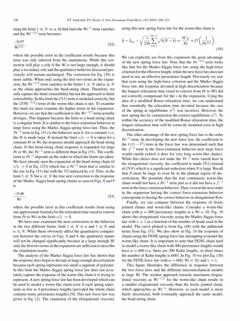

1 wtoni

ia

wtrpvmsaoettHdilP

tccPcWν

tloi

wof

iα

swot

tbIrrbscg

u

η

Wolcntftnitonwld

P

ttwWtotcctic

jcslmtcwthtf

tat

20 P.T. Underhill, P.S. Doyle / J. Non-Ne

ning the limit 1 N α. In that limit the Wi−1 term vanishesnd the Wi−3/2 term becomes

−0.07

Wi3/2 , (52)

here the possible error in the coefficient results because thiserm was only inferred from the simulations. While this cor-ection will play a role if the Wi is not large enough, it shouldlay a secondary role and the qualitative behavior discussed pre-iously will remain unchanged. The correction for Eq. (50) isore subtle. When only using the first two terms in the expan-

ion, the Wi−1/2 term vanishes in the limits 1 N and α N

s the chain approaches the bead-string chain. Therefore, wenly capture the finite extensibility but not the approach to finitextensibility. In this limit theO(1) term is modeled correctly, buthe O(Wi−1/2) term of the worm-like chain is not. To examinehis limit we must examine the higher terms in the expansion.owever, we see that the coefficient to the Wi−3/2 term actuallyiverges. This happens because the limit to a bead-string chains a singular limit. It is similar to the force-extension behavior atarge force using the Marko–Siggia spring force law. Thus, thee−1 term in Eq. (51) is the behavior seen if, for a constant ν/λ,

he Pe is made large. If instead the limit ν/λ → 0 is taken for aonstant Pe or Wi, the response should approach the bead-stringhain. If this bead-string chain response is expanded for largee or Wi, the Pe−1 term is different than in Eq. (51). The coeffi-ient to Pe−1 depends on the order in which the limits are taken.e have already seen the expansion of the bead-string chain (if

/λ → 0 in Eq. (25)) which has a Pe−1 term that is similar tohe one in Eq. (51) but with the 7/2 replaced by a 4. Thus, in theimit 1 N but α N the true next correction to the responsef the Marko–Siggia bead-spring chains as seen in Figs. 8 and 9s

−0.46

Wi, (53)

here the possible error in this coefficient results from usingur approximate formula for the relaxation time (used to convertrom Pe to Wi) in the limit ν/λ → 0.

We have now examined the next corrections to the behaviorn the two different limits, both 1 N α and 1 N and N. While these obviously affect the quantitative compari-

on between the curves in Figs. 8 and 9, the qualitative natureill not be changed significantly because at a large enough Winly the first two terms in the expansion are sufficient to describehe simulation results.

The analysis of the Marko–Siggia force law has shown thathe response does begin to deviate at large enough discretizationecause each spring represents too small a segment of polymer.n this limit the Marko–Siggia spring force law does not accu-ately capture the response of the worm-like chain it is trying toepresent. A new spring force law has been developed which can

e used to model a worm-like chain even if each spring repre-ents as few as 4 persistence lengths (provided the whole chainontains many persistence lengths) [9]. This new force law wasiven in Eq. (2). The expansion of the elongational viscosity

awfit

an Fluid Mech. 145 (2007) 109–123

sing this new spring force law for the worm-like chain is

˜ ∼ ˜η∞ −√

ν

2Pe

N−1∑k=1

√k(N − k) + 3CN

Pe+ O

(1

Pe3/2

).

(54)

e can explicitly see from this expansion the great advantagef the new spring force law. Note that the Pe−1/2 term looksike that for the Marko–Siggia force law using the high-forceriterion for the effective length, while the new force law does noteed to use an effective persistence length. Previously we sawhat even using the high-force criterion and the Marko–Siggiaorce law, the response deviated at high discretization becausehe longest relaxation time (used to convert from Pe to Wi) didot correctly compensate for the ν in the expansion. Using thedea of a modified Rouse relaxation time, we can understandhat essentially the relaxation time deviated because the sizef the spring at equilibrium 〈r2〉 was incorrect. However, theew spring has by construction the correct equilibrium 〈r2〉. Toithin the accuracy of the modified Rouse relaxation time, the

ongest relaxation time will be correctly modeled even at highiscretization.

The other advantage of the new spring force law is the ordere−1 term. In developing the new force law, the coefficient to

he r/(1 − r2) term in the force law was determined such thathe f−1 term in the force-extension behavior near large forceould vanish (which it does for very long worm-like chains).hile this choice does not make the Pe−1 term vanish here in

he elongational viscosity, the coefficient is made O(1) insteadf O(N) which is a significant reduction when N is large. Recallhat N must be large to even be in the plateau region of dis-retization. We postulate that the true continuous worm-likehain would not have a Pe−1 term just as it did not have a f−1

erm in the force-extension behavior. Thus, even at the next ordern the expansion having the correct force-extension behaviororresponds to having the correct behavior in elongational flow.

Finally, we can compare between the response of freelyointed chains and worm-like chains. Consider a worm-likehain with α = 400 persistence lengths at a Wi = 10. Fig. 10hows the elongational viscosity using the Marko–Siggia forceaw with λ = 1 as a function of the number of beads used in the

odel. The curve plotted is from Eq. (48) with the additionalerms from Eq. (51). We also show in Fig. 10 the response ofhains using the FENE spring force law attempting to model theorm-like chain. It is important to note that FENE chain used

o model a worm-like chain with 400 persistence lengths wouldave α = 600 (i.e. there are 200 Kuhn lengths, so three timeshe number of Kuhn lengths is 600). In Fig. 10 we plot Eq. (30)or the FENE force law with α = 600, Wi = 10, and λ = 1.

This figure illustrates the difference in response betweenhe two force laws and the different micromechanical modelst large Wi. The weaker approach towards maximum elogna-ional viscosity as Wi−1/2 for the worm-like chain results in

smaller elognational viscosity than the freely jointed chain,hich approaches as Wi−1. However, as each model is morenely discretized, both eventually approach the same model,

he bead-string chain.

P.T. Underhill, P.S. Doyle / J. Non-Newtoni

Fig. 10. Comparison of the elongational viscosity between models using theMarko–Siggia vs. FENE force laws. The solid lines correspond to Marko–Siggia(lower, Eq. (48) modified with Eq. (51)) and FENE (upper, Eq. (30)). The modelscontain 400 persistence lengths (α = 400 for Marko–Siggia, α = 600 for FENE)a((

cvwolep“ooflostwtrdatriltp

oltfpboef

fda[faaiatfuFtmth

6

lItme

Cilsbodi

η

Wdhcnaaac

I

nd are at Wi = 10 with λ = 1. The dotted line represents the bead-string resultEq. (32)). The dashed lines represent the plateau regions for Marko–Siggialower, Eq. (49)) and FENE (upper, Eq. (31)).

In this section we have analyzed the behavior of bead-springhains in uniaxial elongational flow at large strain rates. Aftererifying the applicability of the expansion for large strain rates,e could use the expansion to better understand the physicalrigin of the chain response. We found that if the strain rate isarge enough, the chain is essentially fully extended and so thelongational viscosity is the fully extended value virtually inde-endent of the accuracy of the spring force law. However, thedeficit”, or how close the system is to that plateau, does dependn the accuracy of the spring force law. In fact the accuracyf this deficit is even more subtle to understand than the weakow response. The response certainly depends on the behaviorf the spring near full extension which is shown by the expan-ion of the viscosity in terms of Pe. However, it is conventionalo express the expansion in terms of a Weissenberg number,hich uses the longest relaxation time. This longest relaxation

ime depends on the equilibrium response of the spring, not theesponse near full extension. To get the correct behavior for theeficit a model should get both behaviors correct, at large forcesnd at equilibrium. For the Marko–Siggia spring force law, nei-her the low-force nor the high-force criteria capture correctly theesponse at both extremes. For this reason the deficit is incorrectf very small springs are used. However, our new spring forceaw does get the behavior correct at low force and high force, andhus represents the deficit correctly even to high discretizationrovided the number of beads is large enough.

It is useful to review at this point the main features we havebserved through the analysis of the elongational viscosity atarge strain rates. At very large strain rates the chain is vir-ually fully extended, so as long as the spring has the correctully extended length �, this infinite strain rate viscosity is inde-endent of the details of the spring force law. In this sense the

ehavior at large enough strain rate is insensitive to the detailsf the spring force law. However, some experiments may aim toxplore more than the absolute value of viscosity (or similarlyractional extension). For example, ref. [27] used the deficit (dif-

c

Mt

an Fluid Mech. 145 (2007) 109–123 121

erence between the fractional extension from full extension) toistinguish between the worm-like chain, freely jointed chain,nd stem-flower models. Shaqfeh et al. [28] and Doyle et al.29] examined the relaxation after strong elongational flow andound that the relaxation was highly influenced by the deficitway from the fully extended state. For a bead-spring chain toccurately represent these types of response of a micromechan-cal model, it is necessary to capture not only the plateau butlso the approach to the plateau. This approach is sensitive tohe accuracy of the spring force law. In fact it is dependent on theorce law both near full extension and at equilibrium because ofsing the longest relaxation time to form a Weissenberg number.or this reason previously used spring force laws do not capture

his deficit when each spring represents a small segment of poly-er. However, the new spring force laws developed to represent

he worm-like chain and freely jointed chain do not deviate atigh discretization.

. Influence of hydrodynamic interactions

In this article we have focused on the role of the spring forceaw and have not included effects of hydrodynamic interactions.n highly extended states we expect the effect will be much lesshan in the coiled state, and the spring force law will play the

ajor role. For the Marko–Siggia force law, we found that thelongational viscosity has a series expansion of the form

η − 3ηs

npζ�2 ∼ N(N2 − 1)

12

(1 − C

Pe1/2 + O(

1

Pe

)). (55)

ertainly the plateau value will be dependent on hydrodynamicnteractions, which changes the scaling with length to include aogarithm. However, we postulate the coefficient C may have theame scaling with or without hydrodynamic interactions. This isecause the chain is so close to full extension that the positionsf the beads, and therefore their interactions, will not be muchifferent from in the fully extended state. The postulated forms thus

¯ − 3ηs ∼ (η − 3ηs)∞(

1 − C

Pe1/2 + O(

1

Pe

)). (56)

hether the scaling of C is the same with and without hydro-ynamic interactions has interesting consequences. Withoutydrodynamic interactions the scaling is C ∼ N−1. This isonsistent with turning the Peclet number into a Weissenbergumber, because without HI the longest relaxation time scaless N2. However, in the non-draining limit, the longest relax-tion time scales as N3/2. Turning the expansion Pe to Wi usingnon-draining scaling for the longest relaxation time gives a

oefficient of

CN3/4

Wi1/2 . (57)

f the value of C scales as N−1, this implies a vanishing coeffi-

ient to Wi−1/2 as N → ∞.

To test this hypothesis, we performed simulations using thearko–Siggia force law and the RPY hydrodynamic interaction

ensor, with parameters ν = 200, λ = 1, and h∗ = 0.25 [2]. We

122 P.T. Underhill, P.S. Doyle / J. Non-Newtoni

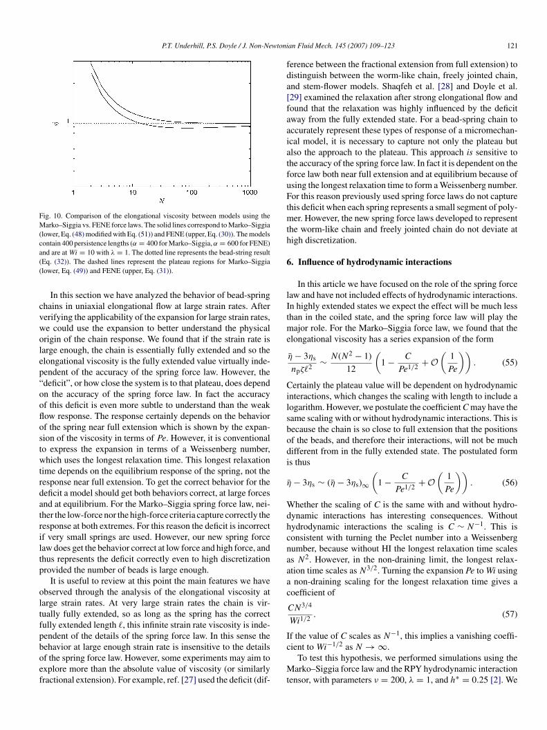
Fig. 11. Coefficient of the Pe−1/2 term, C, as a function of the number of beadswith and without HI. The spring force law is Marko–Siggia with ν = 200 andλ

uN

ptvricsi

rcnolttlseattgstsm

7

clFttw

Ifaisgit

ssdbbriewearbbponp

A

tDpt

R

= 1. The squares are without HI and the diamonds are from BD simulationssing the RPY tensor and h∗ = 0.25. The dashed lines represent power laws of−1, N−0.9, and N−0.75.

erformed simulations at a range of Pe until we were confidenthat higher order terms in Pe were negligible and extracted aalue of C from the simulation data. The infinite Pe numberesponse was calculated exactly using the formalism presentedn an appendix to ref. [3]. In Fig. we plot the value of C cal-ulated from the simulations versus N. From the figure we canee clearly that the the scaling is not N−3/4. The fitted scalings approximately N−0.90 for the largest N simulated here.

These simulations bring about an interesting point which war-ants further investigation. If the scaling of C with N in the largehain limit is different than N−3/4 as we see here, that means thatear the fully extended state the time used to convert from Pe inrder to have collapse of the data in the long chain limit is not theongest relaxation time. However, it may be necessary to reachhe non-draining limit in the extended state in order to reachhe long chain limit scaling of the coefficient. By non-drainingimit in the extended state, we mean that the plateau viscositycales as would be expected from Batchelor’s formula. We canstimate the number of beads necessary to be in that limit usingn approximate formula in the appendix of ref. [3]. Because ofhe slow logarithm convergence in the number of beads, withhe parameters used here, the number of beads would have to bereater than 106 to be into the non-draining limit in the extendedtate. This is not feasible to simulate. A better route to reachhe non-draining limit would be make each spring represent amaller segment of polymer. However, care should be taken toake sure the correct h∗ is used relative to the size of a spring.

. Conclusion

In this article we have looked at the behavior of bead-springhain models in strong flows and the effect of the spring forceaw. We did this for coarse-grained models of both the WLC and

JC. We expect that EV effects are small in such strong flows and

he effects of HI may be small (or smaller) so we initially neglecthose contributions. The longest relaxation time was examined,hich is used to express the strain rate as a Weissenberg number.

an Fluid Mech. 145 (2007) 109–123

t was shown that the chain samples the nonlinear regions of theorce law even at equilibrium, making the relaxation time devi-te from the Rouse result. However, a modified Rouse models able to capture the relaxation time even if each spring repre-ents a small segment of polymer. This modified Rouse modelives insight into the important role the force-extension behav-or at small force plays in determining the longest relaxationime.

We looked at the elongational viscosity in the limit of largetrain rates and used the first few terms in the expansion to under-tand how the response of the chain changes as the level ofiscretization changes and for different spring force laws. Weasically saw that for arbitrarily large strain rate the viscosityecomes not as sensitive to getting the spring force law cor-ect because the system is always fully extended. However, its important to model correctly how close the chain is to fullyxtended. To get this correct it is even more sensitive than ineak flows/equilibrium. This is because you are in a highly

xtended state so the expansion depends on that behavior, butlso when writing the response in terms of a Wi with the longestelaxation time, that is influenced by the low-force/equilibriumehavior. So to really get the correct response you need to getoth correct. Using the previous force laws with an effectiveersistence length requires a trade-off to get one right or thether but not both. Our new force laws get both correct so doot deviate when each spring represents a small segment ofolymer.

cknowledgements

This work was supported by the National Science Founda-ion CAREER program Grant No. CTS-0239012 and P.S.D’soherty Chair. We also acknowledge Chih-Chen Hsieh for helperforming the simulations including hydrodynamic interac-ions.

eferences

[1] R.M. Jendrejack, J.J. dePablo, M.D. Graham, Stochastic simulations ofDNA in flow: Dynamics and the effects of hydrodynamic interactions, J.Chem. Phys. 116 (2002) 7752–7759.

[2] C.-C. Hsieh, L. Li, R.G. Larson, Modeling hydrodynamic interaction inBrownian dynamics: simulations of extensional flows of dilute solutions ofDNA and polystyrene, J. Non-Newtonian Fluid Mech. 113 (2003) 147–191.

[3] R. Prabhakar, J.R. Prakash, T. Sridhar, A sucessive fine-graining scheme forpredicting the rheological properties of dilute polymer solutions, J. Rheol.48 (2004) 1251–1278.

[4] G.C. Randall, K.M. Schultz, P.S. Doyle, Methods to electrophoreticallystretch DNA: microcontractions, gels, and hybrid gel-microcontractiondevices, Lab Chip 6 (2006) 516–525.

[5] J.W. Larson, G.R. Yantz, Q. Zhong, R. Charnas, C.M. DAntoni, M.V.Gallo, K.A. Gillis, L.A. Neely, K.M. Phillips, G.G. Wong, S.R. Gullans, R.Gilmanshin, Single DNA molecule stretching in sudden mixed shear andelongational microflows, Lab Chip 6 (2006) 1187–1199.

[6] A.G. Balducci, P.S. Doyle, Double-stranded DNA diffusion in slit-like

nanochannels, Macromolecules 39 (2006) 6273–6281.

[7] P.T. Underhill, P.S. Doyle, On the coarse-graining of polymers into bead-spring chains, J. Non-Newtonian Fluid Mech. 122 (2004) 3–31.

[8] P.T. Underhill, P.S. Doyle, Development of bead-spring polymer modelsusing the constant extension ensemble, J. Rheol. 49 (2005) 963–987.

wtoni

[

[

[

[

[

[

[

[

[

[

[

[

[

[

[

[

[

[

[

P.T. Underhill, P.S. Doyle / J. Non-Ne

[9] P.T. Underhill, P.S. Doyle, Alternative spring force law for bead-springchain models of the worm-like chain, J. Rheol. 50 (2006) 513–529.

10] M. Somasi, B. Khomami, N.J. Woo, J.S. Hur, E.S.G. Shaqfeh, Brown-ian dynamics simulations of bead-rod and bead-spring chains: numericalalgorithms and coarse-graining issues, J. Non-Newtonian Fluid Mech. 108(2002) 227–255.

11] R.G. Larson, The rheology of dilute solutions of flexible polymers: Progressand problems, J. Rheol. 49 (2005) 1–70.

12] E.S.G. Shaqfeh, The dynamics of single-molecule DNA in flow, J. Non-Newtonian Fluid Mech. 130 (2005) 1–28.

13] P. Sunthar, D.A. Nguyen, R. Dubbelboer, J.R. Prakash, T. Sridhar, Measure-ment and prediction of the elongational stress growth in a dilute solutionof DNA molecules, Macromolecules 38 (2005) 10200–10209.

14] J.F. Marko, E.D. Siggia, Stretching DNA, Macromolecules 28 (1995)8759–8770.

15] H.R. Warner, Kinetic theory and rheology of dilute suspensions of finitelyextendible dumbbells, Ind. Eng. Chem. Fundam. 11 (1972) 379–387.

16] A. Cohen, A Pade approximant to the inverse Langevin function, Rheol.Acta 30 (1991) 270–272.

17] H.C. Ottinger, Stochastic Processes in Polymeric Fluids: Tools and Exam-

ples for Developing Simulation Algorithms, Springer, Berlin, 1996.

18] J. Rotne, S. Prager, Variational treatment of hydrodynamic interaction inpolymers, J. Chem. Phys. 50 (1969) 4831–4837.

19] H. Yamakawa, Transport properties of polymer chains in dilute solution:Hydrodynamic interaction, J. Chem. Phys. 53 (1970) 436–443.

[

an Fluid Mech. 145 (2007) 109–123 123

20] R.B. Bird, R.C. Armstrong, O. Hassager, Dynamics of Polymeric Liquidsvolume 1: Fluid Mechanics, second ed., Wiley, New York, 1987.

21] R.B. Bird, C.F. Curtiss, R.C. Armstrong, O. Hassager, T Dynamics of Poly-meric Liquids, volume 2: Kinetic Theory, second ed., Wiley, New York,1987.

22] O. Hassager, Kinetic theory and rheology of bead-rod models for macro-molecular solutions I. equilibrium and steady flow properties, J. Chem.Phys. 60 (1974) 2111–2124.

23] P.S. Doyle, E.S.G. Shaqfeh, A.P. Gast, Dynamic simulation of freely drain-ing flexible polymers in steady linear flows, J. Fluid Mech. 334 (1997)251–291.

24] P.S. Grassia, E.J. Hinch, Computer simulations of polymer chain relaxationvia Brownian motion, J. Fluid Mech. 308 (1996) 255–288.

25] F. Peters, Polymers in flow, modeling and simulation, Ph.D. Thesis, DelftUniversity of Technology, 2000.

26] P. Dimitrakopoulos, Stress and configuration relaxation of an initiallystraight flexible polymer, J. Fluid Mech. 513 (2004) 265–286.

27] B. Ladoux, P.S. Doyle, Stretching tethered DNA chains in shear flow,Europhys. Lett. 52 (2000) 511–517.

28] E.S.G. Shaqfeh, G.H. McKinley, N. Woo, D.A. Nguyen, T. Sridhar, On

the polymer entropic force singularity and its relation to extensional stressrelaxation and filament recoil, J. Rheol. 48 (2004) 209–221.

29] P.S. Doyle, E.S.G. Shaqfeh, G.H. McKinley, S.H. Spiegelberg, Relaxationof dilute polymer solutions following extensional flow, J. Non-NewtonianFluid Mech. 76 (1998) 79–110.