mlrMBO: A Modular Framework for Model-BasedOptimization of Expensive Black-Box Functions

Bernd Bischla, Jakob Richterb, Jakob Bossekc, Daniel Hornb, Janek Thomasa,Michel Langb

aLudwig-Maximilians-Universität München, GermanybTU Dortmund University, Germany

cWestfälische-Wilhelms Universität Münster, Germany

Abstract

We present mlrMBO, a flexible and comprehensive R toolbox for model-basedoptimization (MBO), also known as Bayesian optimization, which addressesthe problem of expensive black-box optimization by approximating the givenobjective function through a surrogate regression model. It is designed forboth single- and multi-objective optimization with mixed continuous, categor-ical and conditional parameters. Additional features include multi-point batchproposal, parallelization, visualization, logging and error-handling. mlrMBO isimplemented in a modular fashion, such that single components can be eas-ily replaced or adapted by the user for specific use cases, e.g., any regressionlearner from the mlr toolbox for machine learning can be used, and infill cri-teria and infill optimizers are easily exchangeable. We empirically demonstratethat mlrMBO provides state-of-the-art performance by comparing it on differ-ent benchmark scenarios against a wide range of other optimizers, includingDiceOptim, rBayesianOptimization, SPOT, SMAC, Spearmint, and Hyperopt.

Keywords: Model-Based Optimization, Bayesian Optimization, Black-BoxOptimization, Hyperparameter Tuning, Parameter Configuration, R

1. Introduction

Black-box functions are systems that require a number of input parametersto produce one or multiple (numeric) outputs. In most cases these are (a) ex-pensive to evaluate in terms of time and/or monetary cost, and (b) knowledgeof their internal working is not available, which often manifests through theabsence of derivatives. Such problems occur in production engineering [e.g. 1],where the inputs are possible settings of industrial machines or used materials

Email addresses: bernd_bischl@gmx.net (Bernd Bischl),jakob.richter@tu-dortmund.de (Jakob Richter), bossek@wi.uni-muenster.de (JakobBossek), daniel.horn@tu-dortmund.de (Daniel Horn), janek.thomas@stat.uni-muenchen.de(Janek Thomas), lang@statistik.tu-dortmund.de (Michel Lang)

Preprint submitted to Computational Statistics & Data Analysis December 4, 2018

arX

iv:1

703.

0337

3v3

[st

at.M

L]

3 D

ec 2

018

and the output is one or multiple measurements regarding the quality of fab-ricated parts. Since this makes a single evaluation expensive, one tries to findthe optimal settings of production steps in a minimal number of tries. Designof Computer Experiments (DACE) [2] is a discipline focused on solving suchproblems and sequential model-based optimization (SMBO) [3] has become thestate-of-the-art optimization strategy in recent years.

The generic SMBO procedure starts with an initial design of evaluationpoints, and then iterates the following steps:

1. Fit a regression model to the outcomes and design points obtained so far,

2. query the model to propose a new, promising point, often by optimizinga so-called infill criterion or acquisition function,

3. evaluate the new point with the black-box function and add it to thedesign.

Several adaptations and extensions, e.g., multi-objective optimization [4], multi-point proposal [5, 6], more flexible regression models [7] or alternative ways tocalculate the infill criterion [8] have been investigated recently.

A different field of application for SMBO is the hyperparameter optimizationfor machine learning methods [e.g. 9, 10, 11]. Here, the black-box is a machinelearning method and the objective(s) is one or multiple performance measure(s),validated via resampling on a data set of interest. The black-box functioncan be more complex, for example a machine learning pipeline which includespreprocessing, feature selection and model selection.

After a brief comparison with related software in Subsection 1.1 and clari-fication of our main contributions in Subsection 1.2, we introduce the generalSMBO procedure in more detail in Section 2. Section 3 highlights the capabili-ties of our software mlrMBO, showcased by some code examples. In Section 4 weempirically demonstrate that mlrMBO achieves state-of-the-art performance ona wide range of synthetic and real-world single- and multi-objective scenarios.Section 5 gives an outlook on future work.

1.1. Related SoftwareWe will briefly present an overview of available software for model-based

optimization, starting with implementations based on the Efficient Global Op-timization algorithm (EGO), i.e., the SMBO algorithm proposed by Jones et al.[3] using Gaussian processes (GPs), and continue with extensions and alterna-tive approaches.

Both DiceOptim [12] and rBayesianOptimization [13] are R packages thatoffer EGO implementations. A sophisticated EGO implementation can be foundin the Python package Spearmint [14]. It focuses on hyperparameter optimiza-tion of machine learning algorithms with enhancements regarding variable costsof experiments and parallelization. All three packages offer different GP ker-nels and infill criteria, but only support numerical (non-conditional) parameters

2

and, except for Spearmint, no multi-criteria optimization or parallelization isavailable. A multi-criteria version of Spearmint is introduced in [15].

The C++ library BayesOpt [16] contains an extended version of EGO, in-cluding Student-t processes, support of mixed and conditional parameters aswell as meta-criteria algorithms to automatically find reasonable infill criteriaduring optimization. It offers interfaces for Python, Matlab and Octave.

SMAC [7] is one of the most established frameworks and allows to optimizemixed parameter spaces as it uses a random forest instead of a GP for regression.Besides general black-box optimization, it is focused on algorithm configuration.However, SMAC is limited to single-criteria optimization and parallelization is notsupported.

Hyperopt [8] is an optimization package in Python that supports numerical,categorical and conditional parameters. Instead of a regression it uses a tree ofParzen estimators (TPE) to compute point suggestions. It supports distributedparallel and asynchronous execution. Hyperopt can be used for general black-box optimization, but is mainly focused on machine learning tasks.

Another R implementation for sequential black-box optimization is SPOT [17].It is a toolbox with different modeling techniques and offers a wide variety ofstatistical methods. SPOT contains sophisticated algorithms to handle functionswith noisy evaluations, is able to handle constrains in functions and supportsmulti-objective optimization.

1.2. Main Contributions and Prior ApplicationsThe main contribution of this paper is the presentation of the R package

mlrMBO, which implements a generic SMBO framework and provides a largevariety of different SMBO methods due to its modular structure. mlrMBO is evenmore flexible than SPOT in its choice of surrogate models as it is connected tothe R package mlr [18] which interfaces more than 60 machine learning regressionalgorithms. Besides the default SMBO procedure, mlrMBO focuses on threedomains: Mixed parameter space optimization, multi-point proposals and multi-objective optimization. Even combinations of the three domains are possible,which to our knowledge no other software is currently capable of. mlrMBO is easyto use as many default implementations for the individual steps of the SMBOprocedure are directly supported in a plug-and-play style. Simple interfaces areavailable to extend the package with user specific variants.

Benchmarks show that mlrMBO achieves state-of-the-art performance in eachdomain. Additionally, mlrMBO has been successfully applied in some practicalsettings. In [19, 20] it was used to optimize the hyperparameters of machinelearning pipelines (joint pre-processing and model hyperparameters) for supportvector machines and general machine learning models, respectively, in a singleobjective setting. Hess et al. [21] proposed an mlrMBO ensemble-based approachto identify the best surrogate model during optimization through reinforcementlearning. Horn et al. [22] considered a multi-objective benchmark and optimizedthe runtime-accuracy trade-offs of several approximate support vector machinesolvers. Horn and Bischl [11] introduced the general capability of mlrMBO to

3

solve multi-objective machine learning tasks. Steponavič et al. [23] investigatedthe impact of different initial design sampling techniques on the performance ofmulti-objective model-based optimization methods by using mlrMBO.

2. Sequential Model-Based Optimization

This section describes the general SMBO setup and presents the individualbuilding blocks in Subsection 2.1. While SMBO is modular and can thus becustomized for a variety of different tasks, we highlight the most prominentcombinations of components described in the literature like EGO [3] (Subsec-tion 2.2) or SMAC-like [7] optimizers (Subsection 2.3). Subsections 2.4 and 2.6introduce parallelization through multi-point proposal, and multi-objective op-timization.

2.1. Sequential model-based optimizationLet f(x) : X → R be an arbitrary black-box function with a d-dimensional

input domain X = X1 × X2 × · · · × Xd and a deterministic output y. Each Xi(i = 1, · · · , d) can be either numeric and bounded (i.e. Xi = [li, ui] ⊂ R) or afinite set of s categorical values (Xi = {vi1, . . . , vis}). Without loss of generality,we want to find the input x∗ with

x∗ = arg minx∈X

f(x).

In the context of model-based optimization, we usually assume that f is ex-pensive to evaluate, hence the total number of function evaluations is limitedby a budget. At the heart of SMBO are so-called surrogate models f whichcheaply estimate the expensive black-box function f and which are iterativelyupdated and refined. The general approach is illustrated in Figure 1. The figureoutlines the following steps, whereas each step is explained in more detail in thefollowing subsections:

(1) An initial design of ninit points x(j) (j = 1, . . . , ninit) is sampled from Xand f is evaluated at these points to yield outcomes y(j) = f(x(j)). Thetuples

(y(j),x(j)

)constitute the data to build the initial surrogate model

f in the next step.

(2) Fit a surrogate model to all evaluated points x(j) ∈ X and correspondingvalues y(j).

(3) An infill criterion proposes m points x(j+i) (i = 1, . . . ,m). The criterionis defined on X and operates on the surrogate f to determine points whichare promising for the optimization. These points should either have a goodexpected objective value or high potential to improve the quality of thesurrogate model.

(4) The proposed points are evaluated using f and the new tuples(y(j+i),x(j+i)

)are added to the design.

4

(5) If the budget is not exhausted (and no other termination criteria is met),go to step (2).

(6) If the budget is exhausted or another termination criteria is met, returnthe proposed solution for the optimization problem.

(1)Generate

initial design(2.1.1)

(2)Fit surrogatemodel (2.1.2)

(5)Budget

exceeded?(2.1.5)

(6)Return bestpoint (2.1.6)

(3)Propose

new point(s)(2.1.3)

(4)Evaluatefunction

and updatedesign(2.1.4)

yesno

Figure 1: General SMBO approach.

2.1.1. Initial DesignThe initial design specifies the points of the input domain at which the

black-box function is evaluated to build the initial surrogate model f . If toofew points are chosen or if the points do not cover X well, the fit of f may bepoor and thus points proposed based on f may be suboptimal for the progressof the optimization. Fitting a surrogate model may even be impossible. On theother hand, a large initial design may reduce the available budget too much.mlrMBO provides various options for the initial design: The user can specify itmanually or generate designs either completely at random, coarse grid designsor by using space-filling Latin Hypercube Designs [24].

2.1.2. Surrogate ModelsOne of the main factors that determines the choice of surrogate model f is

the structure of the input space X . If X ⊂ Rd, Kriging [3] is the recommendedchoice and provides state-of-the-art performance. In Section 2.2, the Kriging-based EGO approach is discussed in more detail. If the search space X alsoincludes categorical parameters on the other hand, random forests are a viablealternative [7] as they can handle such parameters directly, without the need toencode the categorical parameters as numeric. mlrMBO allows the use of any ofthe many regression models available in the R package mlr, which itself can alsobe easily extended to support custom regression learners [25].

While Kriging models and random forests already provide uncertainty esti-mation natively, generic bagging can be applied to arbitrary regression modelsto retrieve standard error estimators in mlr.

5

2.1.3. Infill CriteriaThe infill criterion, or sometimes called acquisition function, guides the op-

timization and tries to trade-off exploitation and exploration. This is usuallyachieved by combining µ(x) and s(x) (or s2(x)) in a single formula in a well-balanced fashion, where the posterior mean µ(x) and posterior standard devi-ation s(x) (or posterior variance s2(x)) are estimated by the surrogate modelf . s(x) and s2(x) are sometimes also called “local uncertainty estimators”. As-suming that our model f is somewhat “spatial” in the sense that higher valuesof s(x) indicate regions of the search space that few of our design points lieclose to and / or we have not learned the structure of f very well at x, we aretherefore looking for points with low µ(x) and high s(x).

Arguably the most popular choice is the expected improvement

EI(x) := E(I(x))

where the random variable I(x) defines the potential improvement at x overthe currently best observed function value ymin:

I(x) := max {ymin − Y (x), 0} .

Here, Y (x) is a random variable that should express the posterior distributionat x, estimated with f . For a Gaussian process, Y (x) is normally distributedwith Y (x) ∼ N(µ(x), s2(x)). Under this assumption, EI(x) can be expressedanalytically in closed form as

EI(x) = (ymin − µ(x)) Φ

(ymin − µ(x))

s(x)

)+ s(x)φ

(ymin − µ(x)

s(x)

), (1)

where Φ and φ are the distribution and density function of the standard normaldistribution, respectively.

A simpler approach to balance µ(x) and s(x) for a point x is given by thelower confidence bound

LCB(x, λ) = µ(x)− λs(x), (2)

where λ > 0 is a constant that controls the “mean vs. uncertainty” trade-off.Furthermore, mlrMBO currently support pure mean µ(x) minimization (pure

exploitation) and pure uncertainty s(x) maximization (pure exploration) andfurther criteria for multiple point proposals (see Section 2.4), noisy optimization(see Section 2.5), and multi-objective optimization (See section 2.6).

2.1.4. Infill OptimizationThe infill optimizer searches for the point x which yields the best infill value.

Unlike the original optimization problem on f , the optimization on the infill cri-terion can be considered inexpensive. While this is still a black-box optimizationproblem, points can be evaluated more lavishly, and Jones et al. [3] propose abranch and bound algorithm for this task. mlrMBO defaults to a more generic ap-proach, which we call focus search, outlined in Algorithm 1. It is able to handle

6

numeric parameter spaces, categorical parameter spaces, as well as mixed andhierarchical spaces. The algorithm starts with a large random design from whichall points are evaluated by the surrogate regression model to determine the mostpromising point. Next, focus search shrinks the search space around the bestpoint and samples new random points for the now focused search space. Theshrinkage of search space is iterated niters times. The complete procedure canbe restarted nrestart times to avoid local optima. Finally the best point over allrestarts and iterations is returned. Evolutionary algorithms like CMA-ES [26]or custom user-defined optimizers can be selected alternatively.

Algorithm 1 Infill Optimization: Focus Search.Require: infill criterion c : X → R, control parameters nrestart, niters, npoints1: for u ∈ {1, ..., nrestart} do2: Set X = X3: for v ∈ {1, ..., niters} do4: generate random design D ⊂ X of size npoints5: compute x∗u,v = (x∗1, ..., x

∗d) = arg minx∈D c(x)

6: shrink X by focusing on x∗:7: for each search space dimension Xi in X do8: if Xi numeric: Xi = [li, ui] then9: li = max{li, x∗i − 1

4 (ui − li)}10: ui = min{ui, x∗i + 1

4 (ui − li)}11: end if12: if Xi categorical: Xi = {vi1, . . . , vis}, s > 2 then13: xi = sample one category uniformly from Xi\x∗i14: Xi = Xi\xi15: end if16: end for17: end for18: end for19: Return x∗ = arg min

u∈{1,...,nrestart},v∈{1,...,niters}c(x∗u,v)

2.1.5. TerminationMultiple termination criteria can be used in mlrMBO. Commonly a limit is set

for the total number of evaluations of f or for the number of SMBO iterations.Alternatively, the optimization can be terminated after a given time or after atime budget for function evaluations is exhausted. The optimization can alsobe stopped as soon as a predefined objective value is reached. Furthermore, theuser can create custom termination rules.

2.1.6. Final PointFinally, the final solution x∗ has to be determined. Usually the best point

observed during the optimization is picked. Fitting a last surrogate model tofind the best point predicted is a viable option, especially if f is noisy.

7

2.2. Efficient Global Optimization (EGO)Kriging models [27] are arguable the most popular choice for a surrogate

model because they are very flexible and provide a local uncertainty estima-tor [3].

In general, we consider a numeric-only input domain X ⊂ Rd. Jones et al.[3] were the first who introduced surrogate models for the sequential optimiza-tion of box-constrained functions with real-valued arguments. Their EfficientGlobal Optimization (EGO) algorithm employs Kriging models together withthe expected improvement infill criterion (see Equation 1). Maximizing the EIresults in an infill criterion that balances exploitation of the model structureand exploration of regions with high uncertainty and has proven to be highlyeffective [3]. It can ensure global convergence [28, 29] (which is somewhat unre-alistic to expect under the usually tight budget constraints that exist for manyexpensive black-box optimization problems).

Figure 2 illustrates the point proposal at the 3rd (left) and the 4th iteration(right) of an EGO run on a 1d cosine mixture function. It illustrates howhigh uncertainty (s) and a low value of µ contribute to the EI and thus to theselection of the next point and the ability of model-based optimization to findthe optimum even for multi-modal functions.

● ●

●●

yei

−1.0 −0.5 0.0 0.5 1.0

0.0

0.4

0.8

0.00

0.01

0.02

0.03

x

type

● init

prop

seq

type

y

yhat

ei

MBO Iteration: 3

● ●

●●

yei

−1.0 −0.5 0.0 0.5 1.0

0.0

0.4

0.8

0.0000

0.0005

0.0010

0.0015

x

type

● init

prop

seq

type

y

yhat

ei

MBO Iteration: 4

Figure 2: State at the 3rd (left) and 4th iteration (right) of an exemplary EGO run on a1d cosine mixture function. The upper part shows the real function f as a solid line and itsestimation µ dotted. The uncertainty is indicated by the shaded area. Initial design pointsare displayed as red circles, sequential points as green squares. The lower part shows therespective value for the EI. The optimum of the EI defines the point that proposed to beevaluated next (blue triangle).

2.3. Mixed Space OptimizationReal life scenarios often include mixed-valued as well as hierarchical param-

eter spaces with conditional parameters. An example is the tuning of a supportvector machine, for which the parameter space is illustrated in Figure 3. De-pending on the choice of the kernel, the hyperparameter γ has to be optimizedfor the radial kernel (so it is conditional on the setting of kernel), but it is notpresent (or we could say: active) for the linear kernel. In contrast to γ, the

8

hyperparameter C is unconditionally always active. Kriging is not really suitedfor such problem domains, since covariance kernels natively supporting thosetypes of data are still subject to research [30].

For the initial design all options support categorical parameters as well ashierarchical dependencies (feasible values of a parameter depend on the valuesof other parameters).

For the surrogate we need a regression model that is more flexible and canhandle categorical features as well as missing values to support dependent pa-rameters. A slightly modified random forest can be used for this purpose. If ahyperparameter is not active in a design point in the training set (due to unful-filled conditions), we will mark its value as missing. Although the random forestcould potentially directly handle missing values, many implementations do not.Hence, we impute these values in the following way: For categorical parameterswe code missing values as a new level, and for numerical parameters we code theimputed value out of the range of the box-constraints of the parameter underconsideration. This is known as the separate-class method and was shown toperform best for decision trees in a prediction-oriented study, when missingnessis related to the outcome [31].

In order to still use infill criteria as LCB and EI, we also have to computean uncertainty estimate s(x) for the random forest. For bagging-like predictorsthis can be computed or approximated in various ways from the bootstrap. Werefer the reader to [32, 33] for further details. In mlr the uncertainty estimatorcan be deviated from an expensive extra bootstrap around the random forest,the jackknife, the infinitesimal jackknife, or a simple estimator which extractsthe standard error simply from the internal bootstrap of the random forest. Inour experience, the jackknife estimator works most reliably, so it is the currentdefault for mlrMBO with random forests as surrogate. However, it should benoted that the random forest is not really a spatial model as a Gaussian processand therefore the properties of the uncertainty estimator are less intuitive incomparison to the ones from Kriging models. Our following results still indicatethat we obtained state-of-the-art results with this default, and we deem thisaspect a matter for further research.

X

C

kernel

radial

linear

γ

[0, Inf]

[0, Inf]

Figure 3: Dependent search space for the tuning of a support vector machine. Circles denoteparameters, rectangles denote parameter ranges, arrows denote the hierarchical structure.

9

2.4. Multi-Point ProposalThe expensive nature of the optimization problem makes parallelization, i.e.

the evaluation of different configurations on multiple CPUs, an important ex-tension to speed up the SMBO process. Recently many methods have been pro-posed to simultaneously propose m points in each iteration. We showcase threemethods implemented in mlrMBO, which are also discussed in [6]. A straightfor-ward approach is qLCB [34], an extension of the LCB criterion. Instead of onefixed λ, multiple λk (k = 1, . . . ,m) are drawn from an exponential distributionto obtain m points x(j+1), . . . ,x(j+m):

qLCB(x, λk) = y(x)− λks(x), λk ∼ Exp

(1

λ

).

The criterion is than optimized separately for every λk, so that overall m pointsare proposed. Proposals that were obtained by optimizing the qLCB for a lowvalue of λk exploit the model and are in proximity of the best found y so far.For high values of λk the proposals will be of exploratory nature. This ensuresthat in one SMBO iteration all proposals balance exploitation and exploration.

Another approach to propose multiple points using the expected improve-ment is known as constant liar [5]. Here we obtain x(j+1) in the same way asfor the ordinary EI. To obtain x(j+2) we assume that the evaluation at pointx(j+1) is done and update the surrogate model with a made up target valuey. Exemplary choices for the made up value are min(y), max(y), the mean y,or the predicted posterior mean µ(x(j+1)) of the surrogate model. The latterapproach is also often referred to as kriging believer.

Bischl et al. [6] propose the multi-objective infill model-based optimization(MOIMBO) approach. The posterior mean µ(x) and variance s(x) are notscalarized in a single function (as done by EI or (q)LCB), instead a multi-objective optimization strategy (see Section 2.6) is used to optimize them jointlyand propose a whole set of optimal points. To ensure that the points are diverse,a distance measure, e.g. the nearest neighbor distance, can be used as a thirdobjective.

2.5. Noisy OptimizationNoisy optimization assumes that the objective function f is stochastic. Usu-

ally, one now faces the problem to optimize E[f(x)] instead of f(x) and com-mon strategies are intelligent repetition strategies [35] or adapted infill criteria.mlrMBO currently only offers the latter (but of course the user can always optto perform averaging in the objective function, e.g. by naively averaging over aconstant number of repetitions himself).

A popular infill criterion for noisy functions is the expected quantile improve-ment [36] which is an extension of EI. Instead of looking for an improvementover best value observed so far (the ymin in the EI formula), we exchange thiswith a so called “plug-in” value qmin:

EQI(x) = (qmin − q(x)) Φ

(qmin − q(x)

sq(x)

)+ sq(x)φ

(qmin − q(x)

sq(x)

), (3)

10

where qmin is the lowest β-quantile q(xi) for all previously evaluated pointsx ∈ {x1, . . .xn}, and β is a user control parameter for the EQI. The estimated β-quantile at point x is given by q(x) = µ(x)+Φ−1(β)s(x). This implies that thecriterion will be non-zero at already evaluated points allowing re-evaluations orevaluations very close to already evaluated design points to increase knowledgeof promising points.

mlrMBO offers also the so called “augmented expected improvement” and itsmodular design makes extensions towards further criteria functions straightfor-ward. For a further in-depth discussion of this topic we refer the reader to [37]and their benchmark for noisy MBO approaches.

2.6. Model-Based Multi-Objective (MBMO) OptimizationMulti-objective optimization problems are characterized by a set of target

functions f(x) = (f1(x), . . . , fk(x)) which have to be optimized simultaneously.Since there is no total order in Rk, for k ≥ 2, the concept of Pareto dominanceis used. A point x pareto-dominates another point x, x � x, if fi(x) ≤ fi(x)for i = 1, . . . , k and ∃ j fj(x) < fj(x), i.e., x needs to be as good as x ineach component and strictly better in at least one. A point x is said to be non-dominated if it is not dominated by any other point. The set P = {x |@ x x � x}of all non-dominated points is called the Pareto set. It contains all incomparabletrade-off solutions. In multi-objective optimization the goal is to approximatethe Pareto set or the Pareto front f(P ), i.e., the image of P under f .

In recent years some approaches were published that generalize single-objectiveSMBO algorithms like EGO for the multi-objective case. We distinguish be-tween 3 different MBMO algorithm classes: First, scalarization based algorithmsthat use EGO to optimize a scalarized version of the black-box functions withrandom weights for the scalarization in each iteration. Second, Pareto basedalgorithms that fit individual models for each objective and perform multi-objective optimization of infill criteria on these models. Third, direct indicatorbased algorithms that also fit individual models, but perform a single objectiveoptimization of an infill criterion aggregating all models. mlrMBO supports 4 dif-ferent MBMO algorithms, covering all 3 classes: ParEGO [38] as scalarizationbased, MSPOT [39] as Pareto based, and both SMS-EGO [40] and ε-EGO [41]as direct indicator based algorithms.

A much more detailed discussion of these methods, their multi-point vari-ants, and what is currently implemented in mlrMBO is given in [4].

3. mlrMBO R Package

We implemented the software package mlrMBO for the statistical program-ming language R. It is designed as a modular framework. The individual com-ponents of model-based optimization such as the infill criterion or the stoppingconditions (cf. Section 2) can easily be combined in a plug-and-play fashion torespect the specific characteristics of the optimization problem at hand. In thefollowing we give a short introduction of this process which is split into multiplesteps.

11

Definition of the black-box function. For the first step mlrMBO relies on thesmoof package [42] which provides a unified interface to work with black-boxfunctions. Many test functions that are frequently used to benchmark op-timizers are already included. Additionally, the package provides the func-tions make{Single,Multi}ObjectiveFunction() as constructors for customtest functions. Mandatory arguments are the function itself, a name and aparameter set. In the simplest case, the latter is defined by names and box con-straints, which can be specified concisely using the ParamHelpers package. Formore complex settings, it is also possible to connect parameters with arbitrarytransformation functions (e.g., to vary a parameter on the log-scale) or declaredependencies between parameters. The following listing gives an example forthe definition of the black-box f(x) = (x2 − 0.1x21 + x1 − 6)2 + cos(x1) withx1 ∈ [−5, 10], x2 ∈ [0, 15]:

fn = makeSingleObjectiveFunction(name = "my_blackbox",fn = function(x) (x[2] - 0.1 * x[1]^2 + x[1] - 6)^2 + cos(x[1]),par.set = makeParamSet(

makeNumericParam("x1", lower = -5, upper = 10),makeNumericParam("x2", lower = 0, upper = 15)

))

Definition of the Initial Design. To specify the points to be evaluated to ini-tialize the surrogate an initial design has to be specified. It is recommended touse a Latin Hypercube Design by calling generateDesign() and passing thenumber of desired points. If no design is given by the user, mlrMBO will generatea maximin Latin Hypercube Design of size 4 times the number of the black-boxfunction’s parameters.

Definition of the surrogate regression model. mlrMBO builds up on the mlr pack-age [18], which offers a unified interface for a plethora of machine learning meth-ods in R. For surrogate regression, Kriging (makeLearner("regr.km")) and ran-dom forests (makeLearner("regr.randomForest")) are popular choices, butother regression methods can be selected as well. Keep in mind that if expectedimprovement or LCB is chosen as the infill criterion, the surrogate either hasto provide an uncertainty estimator, or has to be combined with a bagging ap-proach using the makeBaggingWrapper() in mlr. If no regression method issupplied by the user, the fallback is a Kriging model with a Matern-3/2 kerneland the “GENetic Optimization Using Derivatives” (genoud) fitting algorithm ina fully numeric setting, and a random forest with jackknife variance estimationotherwise.

Definition of the control flow. Basic settings like the number of proposed pointsin each SMBO iteration or the error handling are set via makeMBOControl()

12

which returns a base control object. This object can be further extended to ad-just the different component of the SMBOmethodology. setMBOControlInfill()adjusts the infill criterion and the infill criterion optimizer. If the infill opti-mization is unspecified, mlrMBO uses LCB as infill criterion with λ = 1 in a fullynumeric setting and λ = 2 if at least one one discrete parameter is present. Tooptimize the criterion, focus search with nrestarts = 3, niters = 5 and npoints =1000 is used by default. For multi-point proposals or multi-objective optimiza-tion, setMBOControlMultiPoint() and setMBOControlMultiObj() are used,respectively. If multiple points are proposed, they can be evaluated simultane-ously using different parallelization (i.e. multicore, sockets, and MPI) and high-performance computation systems (e.g., Slurm, LSF, OpenLava, TORQUE, orDocker Swarms) with the R packages parallelMap and batchtools [43]. Fi-nally, setMBOControlTermination() controls the termination criteria.

Putting it all together. The actual optimization is finally started by calling thembo() function with the (optional) initial design, the black-box function, the(optional) surrogate regression method, and the control object as arguments.The following listing demonstrates an application of mlrMBO to optimize ourexample black-box.

library(mlrMBO)

# Create initial random Latin Hypercube Design of 10 pointslibrary(lhs) # for randomLHSdes = generateDesign(n = 5L * 2L, getParamSet(fn), fun = randomLHS)

# Specify kriging model with standard error estimationsurrogate = makeLearner("regr.km", predict.type = "se",

covtype = "matern3_2")

# Set general controlsctrl = makeMBOControl()ctrl = setMBOControlTermination(ctrl, iters = 30L)ctrl = setMBOControlInfill(ctrl, crit = makeMBOInfillCritEI())

# Start optimizationmbo(fn, des, surrogate, ctrl)

The resulting object contains the full optimization path, with all x and y val-ues, runtime of function evaluations, final state, potential error messages as wellas optionally all fitted surrogate models. Diagnostic visualizations of the opti-mization are available by calling plot() and for one and two dimensional inputdomains with single- or multi-objective targets, each step of the optimizationprocess can be visualized by calling exampleRun() or exampleRunMultiObj().For instance, Figure 2 has been created with exampleRun() and plotExampleRun().

13

4. Benchmarks

In this section, the performance of mlrMBO is evaluated on three exten-sive benchmarks. First, we compare mlrMBO against other black-box optimizersconnected to R (Section 4.1), then against state-of-the-art optimizers that arenot available in R through the optimization benchmark framework HPOlib [44](Section 4.2). Finally, we perform a simulation study on multi-objective op-timization problems (Section 4.3). All benchmarks were conducted using thebatchtools [43] package for R.

4.1. Model-Based Single-Objective OptimizationWe run our implementation on various single-objective optimization tasks

and compare it with the three EGO implementations available in R: DiceOptim [12],rBayesianOptimization [13] and SPOT [17]. Additionally, to ensure that anEGO approach is suitable, we also consider a basic random search as well asthe popular covariance matrix adaptation evolution strategy (CMA-ES) basedon the R package cmaesr [26].

Benchmarks. The methods are evaluated on a set of six 5-dimensional, continu-ous, and single-objective test functions: Alpine01, Deflected Corrugated Spring,Schwefel, Ackley, Griewank and Rosenbrock. All are defined in the R-packagesmoof and have been subject to optimization benchmarks previously.

Setup. For the initial design, the same pre-generated maximin Latin Hyper-cube design containing 25 points is used for mlrMBO, DiceOptim, SPOT and therandom search. It was not possible to pass a user-defined initial design inrBayesianOptimization without provoking an error. Instead, a random designof the same size is generated internally. We allow each algorithm 200 sequen-tial iterations. Since CMA-ES as an evolutionary algorithm does not initializewith a design, it gets an additional budget of 25 iterations (in total 225). Allalgorithms are run in their default settings carefully chosen by the respectivepackage authors.

Evaluation. The objective values of the proposed solutions are summarized inFigure 4. All methods performed clearly better than the baseline random searchapproach on all six test functions. In comparison with the other EGO-basedalgorithms, mlrMBO yields a substantial better objective on four test functionsand similar objective on the other two. SPOT is slightly better than mlrMBO onGriewank, but worse on three others. The evolutionary CMA-ES is comparableto mlrMBO on Alpine01 and slightly better on Rosenbrock, but considerably worseon the four other problems. If we consider the averaged rank of the methodsover all test functions as shown in Table 1, mlrMBO proves to be the best methodoverall, with SPOT in second place.

Besides the quality of the solution, runtime, and computational overheadshould also be considered. The timings for a complete optimization run in

14

● ●●●

●●

●●

●

●

●

●

●

●

●

●●

● ●●

●●

●●●● ●●

●

●●●

●●

Griewank Rosenbrock

Schwefel Ackley

Alpine01 DeflectedCurragatedSpring

mlrM

BO

cmae

sr

DiceOpt

im

rBay

esOpt

SPOT

Rando

m

mlrM

BO

cmae

sr

DiceOpt

im

rBay

esOpt

SPOT

Rando

m

mlrM

BO

cmae

sr

DiceOpt

im

rBay

esOpt

SPOT

Rando

m

mlrM

BO

cmae

sr

DiceOpt

im

rBay

esOpt

SPOT

Rando

m

mlrM

BO

cmae

sr

DiceOpt

im

rBay

esOpt

SPOT

Rando

m

mlrM

BO

cmae

sr

DiceOpt

im

rBay

esOpt

SPOT

Rando

m

−1

0

1

2

3

4

0

5

10

15

20

0

1000

2000

3000

4000

0

2

4

−2000

−1500

−1000

0

2

4

6

8

y

Figure 4: Best objective value (on y axis) found by respective algorithms on respective testfunction.

minutes are listed in Table 1. Note that we are basically measuring the over-head of the optimization algorithms, as the synthetic test functions are evalu-ated in microseconds. The random search unsurprisingly comes with the leastoverhead, followed by CMA-ES as implemented in the package cmaesr. TheEGO-based approaches consume considerably more time by fitting the surro-gate model and optimizing the infill criterion. Here, mlrMBO is slower thanDiceOptim but still more than twice as fast as SPOT and orders of magnitudesfaster than rBayesianOptimization. However, keep in mind that EGO is tai-lored for expensive problems. If we paid each function evaluation with just oneminute of computation time, the differences between 200 min for random searchand 212 min for mlrMBO seems to be a reasonable price to pay for a much betterobjective value.

15

Algorithm Average Rank Average runtime in minutesmlrMBO 1.95 8.03SPOT 2.48 27.88cmaesr 3.17 0.01DiceOptim 3.97 3.35rBayesOpt 4.24 695.96Random 5.19 0.00

Table 1: Average ranks and runtime on artificial test functions.

4.2. Model-Based Single-Objective Optimization in Mixed SpacesThe second benchmark compares mlrMBO to three1 other state-of-the-art

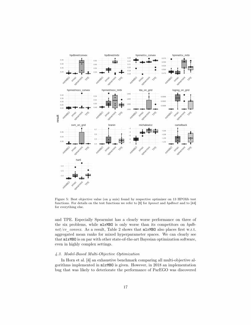
Bayesian optimizers which are not connected to R: Spearmint [14], hyperopt(called TPE in the following) [8] and SMAC [7]. We use the hyperparameteroptimization library HPOlib [44], which contains a large number of standardizedbenchmarks. Besides purely numerical problems, the HPOlib also defines prob-lems with mixed and dependent parameter spaces. We evaluate the methodson four synthetic functions (branin, camelback, michalewicz and har6 ), threeparameter optimization problems on grids (linear discriminant analysis (lda),logistic regression (logreg) and a support vector machine (svm)), as well as adeep neural network (hpnnet) with 15 parameters, and a deep belief network(hpdbnet) with 35 parameters. The latter two problems were originally proposedby Bergstra et al. [8]. mlrMBO uses its default settings, i.e., a Gaussian processas surrogate model for all solely numerical problems and a random forest for theproblems with mixed and dependent parameter spaces (hpnnet and hpdbnet).We deviate from the defaults only for the initial design of hpnnet and hpdbnet.Here, the number of allowed function evaluations compared to the dimensionof the parameter set is very small, therefore the initial design has only size 2dinstead of the default 4d. Spearmint uses an internal dummy encoding of allcategorical parameters for its Gaussian process. The number of iterations oneach benchmark as well as the specific settings of all other optimizers are definedin HPOlib.

Evaluation. The results of ten runs on each benchmark are summarized in Fig-ure 5. On each of the four synthetic test functions, mlrMBO outperforms bothSMAC and TPE and has similar performance compared to Spearmint, exceptfor michalewicz where mlrMBO outperforms all competitors. For the grid opti-mizations, mlrMBO also performs exceptionally well on every single one, whileeach other optimizer results in worse performance on at least one of the threeproblems, which overall places mlrMBO on the first place in numeric settings(cf. Table 2). Regarding the neural network and deep belief network, mlrMBOachieves similar results as SMAC and slightly better results than Spearmint

1Since BayesOpt is neither connected to HPOlib nor possesses an R interface, we refer thereader to the benchmarks in [16] and do not consider BayesOpt in our analysis.

16

●●●●●●●●●●● ●●●

●

●●●●●●●●

●

●

●

●

●●●●

●●●●

●

●

●●

●●

●

●

●●

●

●●●●●●●●

●●●●●●●●●

●

●●●●

●

●●●●

●

●

●●

●

●●●●●

●

●●●●●●●●●●●● ●●●●●●●●

●●

●●

●●●

●

●●●●●

●

●●●

●

●●●●

●

●

●

●

●

●

●●

●

●

●

●

●

●●

●●

●

●

●

●

●●

●

●

●●●●●

●●

●●●

●●

●●●

●

●●

●●

●

●

●

●

●

●

●

●●

●

●

●●

●●

●

●

●●●●

●

●

●

●

●

●

●●

●

●

●●●●●●●●●●

●

●●

●

●

●

●

●

●

●

●

●●

●

●

●

●

●

●

●

●●

●

●

●●

●

●

●

●●●

●●●●●●●

●●

●

●

●

●

●

●

●

●

●

●

●●

●●

●

●

●

●

●

●

●

●

●●●●●●●●●●●●●●●●●●●●

●

●

●

●

●

●

●

●●

●●

●●●●

●

●

●

●

●

●

●●●

●

●●●

●

●

●●

●●●

●

●●

●

●

●●●

●

●

●

●●●●●●●●●● ●●●●

●

●●●●●

●

●●●●

●

●

●

●●●●●●●●●●●●

●●

●●

●

●

●

●

●●

●

●●

●

●

●

●●

●●●

●●

●

●●

●

●

●

●

●

●

●●

●

●

●●

●

●

●

●●

●

●

●

●

●

●

●●

●●

●

●

●

●

●

●●

●

●

●

●

●

●

●

●

●

●●●

●●●

●

●

●

●

●●●

●

●

●

●

●●

●●●

●

●

●

●

●

●

●●

●

●

●

●●

●

●●

●

●●●●●●

●

●●●●●●●●●●

●

●●

●

●

●

●

●

●

●

●

●

●

●

●

●

●

●

●

●●●●●●●●●●●●●●●●●●●●●

har6

svm_on_grid branin michalewicz camelback

hpnnet/nocv_convex hpnnet/nocv_mrbi lda_on_grid logreg_on_grid

hpdbnet/convex hpdbnet/mrbi hpnnet/cv_convex hpnnet/cv_mrbi

mlrM

BOsm

ac

spea

rmint

TPE

mlrM

BOsm

ac

spea

rmint

TPE

mlrM

BOsm

ac

spea

rmint

TPE

mlrM

BOsm

ac

spea

rmint

TPE

mlrM

BOsm

ac

spea

rmint

TPE

mlrM

BOsm

ac

spea

rmint

TPE

mlrM

BOsm

ac

spea

rmint

TPE

mlrM

BOsm

ac

spea

rmint

TPE

mlrM

BOsm

ac

spea

rmint

TPE

mlrM

BOsm

ac

spea

rmint

TPE

mlrM

BOsm

ac

spea

rmint

TPE

mlrM

BOsm

ac

spea

rmint

TPE

mlrM

BOsm

ac

spea

rmint

TPE

0.475

0.500

0.525

0.550

0.575

0.0688

0.0692

0.0696

−1.02

−1.00

−0.98

−0.96

0.18

0.19

0.20

0.21

0.22

0.23

1300

1350

1400

1450

−7

−6

−5

−4

−3

0.50

0.55

0.60

0.65

0.48

0.50

0.52

0.54

0.4

0.5

0.6

0.7

0.20

0.25

0.30

0.35

0.20

0.25

0.30

0.35

0.40

0.30

0.33

0.36

−3.0

−2.5

−2.0

resu

lt

Figure 5: Best objective value (on y axis) found by respective optimizer on 13 HPOlib testfunctions. For details on the test functions we refer to [8] for hpnnet and hpdbnet and to [44]for everything else.

and TPE. Especially Spearmint has a clearly worse performance on three ofthe six problems, while mlrMBO is only worse than its competitors on hpdb-net/cv_convex. As a result, Table 2 shows that mlrMBO also places first w.r.t.aggregated mean ranks for mixed hyperparameter spaces. We can clearly seethat mlrMBO is on par with other state-of-the-art Bayesian optimization software,even in highly complex settings.

4.3. Model-Based Multi-Objective OptimizationIn Horn et al. [4] an exhaustive benchmark comparing all multi-objective al-

gorithms implemented in mlrMBO is given. However, in 2018 an implementationbug that was likely to deteriorate the performance of ParEGO was discovered

17

Optimizer Avg. rank Avg. rank (numeric only) Avg. rank (mixed only)mlrMBO 1.90 (1) 1.64 (1) 2.20 (1)smac 2.65 (3) 2.90 (3) 2.35 (2)spearmint 2.61 (2) 2.32 (2) 2.95 (4)TPE 2.85 (4) 3.14 (4) 2.50 (3)

Table 2: Average ranks on HPOlib problems, Results were ranked in each replication and thenaveraged over the replications and problems. Numeric only ranks are based on benchmark 7to 13 and mixed only ranks are based on 1 to 6.

and fixed. Therefore, we present a remake of the benchmark in this chapter,including a comparision to the GPareto R package.

Benchmarks. The benchmark is performed on the bi-objective black-box op-timization benchmarking (BBOB) test suite [45]. It is constructed on top often functions of the single-objective BBOB test suite. Two functions belongto each of the following function classes: separable (sep), moderate (mod),ill-condition (i-c), multi-modal (m-m) and weakly structured (w-s) functions.These functions are pairwise combined to form 55 bi-objective problems, whichcan be grouped into 15 classes by combining the classes of the underlying single-objective functions. The benchmark is restricted to the case d = 5.

Setup. To simulate an expensive setting, all algorithms had a budget of 44d func-tion evaluations, of which 4d are reserved for the initial design. The popularevolutionary multi-objective algorithm NSGA2 [46] and a random search serveas baseline for the four implementations in mlrMBO: SMS-EGO, ε-EGO, SMS-EGO, and MSPOT (cf. Section 2.6). In addition, the alternative implementationof SMS-EGO in GPareto is used.

Evaluation. Various performance measures for comparing different approxima-tions have been introduced. The most popular measure may be the dominatedhypervolume (also known as S-Metric). In the bi-objective case the hypervol-ume simply measures the area between the discrete approximation of the Paretofront and a pessimistic reference point. If an approximation reaches a higherhypervolume value, it is considered superior.

The final Pareto front approximations were normalized to the interval [0, 1]2

with respect to a reference set. Afterwards, ranks are computed for each testfunction respectively. In Table 4.3, the mean ranks for each function class areshown for 20 replications per test function. Moreover, Figures 6 and 7 show theraw hypervolume values for each test function.

We see that SMS-EGO, ParEGO and MSPOT outperform both baselines onnearly all test functions, with MSPOT beeing the superior algorithm. Althoughgpareto has top performance for the class of two separable functions, it is inferiorto all mlrMBO implementation except ε-EGO, especially while facing multi-modalfunctions.

18

group GPareto ε-EGO MSPOT ParEGO SMS-EGO NSGA2 randomsep – sep 2.18 4.72 2.22 2.88 3.50 5.30 6.40sep – mod 3.45 5.55 1.85 2.56 2.61 4.85 6.46sep – i-c 3.52 4.95 1.46 3.81 2.89 5.05 6.31sep – m-m 4.42 3.96 3.09 3.39 2.51 3.90 6.72sep – w-s 3.65 5.17 2.76 3.17 2.61 4.42 6.20mod – mod 3.98 4.20 3.10 2.80 3.17 4.43 6.32mod – i-c 3.81 5.95 1.68 2.90 3.11 4.40 6.15mod – m-m 4.50 5.90 2.65 4.04 2.16 3.12 5.62mod – w-s 4.96 3.91 2.73 2.91 2.38 4.83 6.14i-c – i-c 4.22 3.63 2.22 2.07 3.50 5.65 6.72i-c – m-m 5.16 3.45 2.16 3.54 3.17 4.39 6.12i-c – w-s 3.67 4.24 2.41 3.19 2.92 4.89 6.67

m-m – m-m 6.12 3.13 2.85 3.22 2.85 3.55 6.28m-m – w-s 5.26 4.90 2.24 3.08 2.23 4.19 6.11w-s – w-s 4.17 3.98 2.88 3.12 2.53 4.68 6.63over all 4.21 4.51 2.42 3.11 2.81 4.51 6.33

Table 3: Average ranks on bi-objective BBOB problems. Results were ranked in each replica-tion and then averaged over the replications and problems for each function class.

5. Conclusion

We introduced the R package mlrMBO, a modular toolbox for model-basedoptimization in the R programming language. We gave a brief introductionto software specific aspects and features. Furthermore, we performed compre-hensive benchmarks of mlrMBO against other black-box optimizers in differentscenarios. In the single-objective benchmark mlrMBO proved state-of-the-art per-formance regarding solution quality in comparison with the CMA evolutionarystrategy, random search, and alternative SMBO implementations, while stillbeing reasonably fast. Furthermore, mlrMBO is on par with the well known op-timization frameworks SMAC, Spearmint, and TPE as shown by benchmarksusing HPOlib. The benchmark study on expensive multi-objective optimiza-tion revealed SMBO-based methods, in particular SMS-EGO, to show excellentperformance. Both the state-of-the-art NSGA-II evolutionary algorithm as wellas the baseline random search algorithm were outperformed on all nine testfunctions (only ParEGO occasionally failed). All in all the results demonstratethe suitability of the mlrMBO toolbox in particular for expensive optimizationscenarios in R for single- and multi-objective tasks, with continuous or mixedparameter spaces.

Acknowledgments

Part of the work on this paper has been supported by Deutsche Forschungsge-meinschaft (DFG) within the Collaborative Research Center SFB 876 “Providing

19

Information by Resource-Constrained Analysis”, project A3 (http://sfb876.tu-dortmund.de) and by the Competence Network for Technical, Scientific HighPerformance Computing in Bavaria (KONWIHR) in the project “Implemen-tierung und Evaluation eines Verfahrens zur automatischen, massiv-parallelenModellselektion im Maschinellen Lernen”.

References

References

1. Sieben, B., Wagner, T., Biermann, D.. Empirical modeling of hardturning of aisi 6150 steel using design and analysis of computer experiments.Production Engineering 2010;4(2):115–125.

2. Sacks, J., Welch, W.J., Mitchell, T.J., Wynn, H.P.. Design and analysisof computer experiments. Statistical science 1989;4(4):409–423.

3. Jones, D.R., Schonlau, M., Welch, W.J.. Efficient global optimiza-tion of expensive black-box functions. Journal of Global Optimization1998;13(4):455–492.

4. Horn, D., Wagner, T., Biermann, D., Weihs, C., Bischl, B.. Model-basedmulti-objective optimization: Taxonomy, multi-point proposal, toolbox andbenchmark. In: Gaspar-Cunha, A., Henggeler Antunes, C., Coello, C.C.,eds. Evolutionary Multi-Criterion Optimization; vol. 9018 of Lecture Notesin Computer Science. Springer; 2015:64–78.

5. Ginsbourger, D., Le Riche, R., Carraro, L.. Kriging is well-suited toparallelize optimization. In: Computational Intelligence in Expensive Op-timization Problems. Springer; 2010:131–162.

6. Bischl, B., Wessing, S., Bauer, N., Friedrichs, K., Weihs, C.. MOI-MBO:Multiobjective infill for parallel model-based optimization. In: Learningand Intelligent Optimization Conference. 2014:173–186.

7. Hutter, F., Hoos, H.H., Leyton-Brown, K.. Sequential model-basedoptimization for general algorithm configuration. In: LION 5. 2011:507–523.

8. Bergstra, J.S., Bardenet, R., Bengio, Y., Kégl, B.. Algorithms for hyper-parameter optimization. In: Advances in Neural Information ProcessingSystems. 2011:2546–2554.

9. Thornton, C., Hutter, F., Hoos, H.H., Leyton-Brown, K.. Auto-WEKA:Combined selection and hyperparameter optimization of classification al-gorithms. In: Proceedings of ACM SIGKDD. 2013:847–855.

10. Lang, M., Kotthaus, H., Marwedel, P., Weihs, C., Rahnenführer, J., Bis-chl, B.. Automatic model selection for high-dimensional survival analysis.Journal of Statistical Computation and Simulation 2015;85(1):62–76.

20

11. Horn, D., Bischl, B.. Multi-objective parameter configuration of machinelearning algorithms using model-based optimization. In: ComputationalIntelligence (SSCI), 2016 IEEE Symposium Series on. IEEE; 2016:1–8.

12. Roustant, O., Ginsbourger, D., Deville, Y.. DiceKriging, DiceOptim: TwoR packages for the analysis of computer experiments by kriging-based meta-modeling and optimization. Journal of Statistical Software 2012;51(1):1–55.

13. Yan, Y.. rBayesianOptimization: Bayesian Optimization of Hy-perparameters; 2016. URL: https://CRAN.R-project.org/package=rBayesianOptimization; R package version 1.0.0.

14. Snoek, J., Larochelle, H., Adams, R.P.. Practical bayesian optimiza-tion of machine learning algorithms. In: Advances in Neural InformationProcessing Systems 25. Curran Associates, Inc.; 2012:2951–2959.

15. Hernández-Lobato, D., Hernández-Lobato, J.M., Shah, A., Adams, R.P..Predictive entropy search for multi-objective bayesian optimization. In:Proceedings of the 33nd International Conference on Machine Learning(ICML). 2016:1492–1501.

16. Martinez-Cantin, R.. Bayesopt: A bayesian optimization library for non-linear optimization, experimental design and bandits. Journal of MachineLearning Research 2014;15:3915–3919.

17. Bartz-Beielstein, T., Zaefferer, M.. A gentle introduction to sequential pa-rameter optimization. Tech. Rep. 2; Bibliothek der Fachhochschule Koeln;2012. URL: http://opus.bsz-bw.de/fhk/volltexte/2012/19.

18. Bischl, B., Lang, M., Kotthoff, L., Schiffner, J., Richter, J., Studerus,E., Casalicchio, G., Jones, Z.M.. mlr: Machine learning in R. Journal ofMachine Learning Research 2016;17(170):1–5.

19. Koch, P., Bischl, B., Flasch, O., Bartz-Beielstein, T., Weihs, C.,Konen, W.. Tuning and evolution of support vector kernels. EvolutionaryIntelligence 2012;5(3):153–170.

20. Bischl, B., Schiffner, J., Weihs, C.. Benchmarking classification algo-rithms on high-performance computing clusters. In: Spiliopoulou, M.,Schmidt-Thieme, L., Janning, R., eds. Data Analysis, Machine Learningand Knowledge Discovery. Studies in Classification, Data Analysis, andKnowledge Organization; Springer; 2014:23–31.

21. Hess, S., Wagner, T., Bischl, B.. PROGRESS: Progressive reinforcement-learning-based surrogate selection. In: Nicosia, G., Pardalos, P., eds.Learning and Intelligent Optimization. Lecture Notes in Computer Science;Springer; 2013:110–124.

21

22. Horn, D., Demircioğlu, A., Bischl, B., Glasmachers, T., Weihs, C..A comparative study on large scale kernelized support vector machines.Advances in Data Analysis and Classification 2016;:1–17.

23. Steponavič, I., Shirazi-Manesh, M., Hyndman, R.J., Smith-Miles, K.,Villanova, L.. On Sampling Methods for Costly Multi-Objective Black-Box Optimization. In: Pardalos, P.M., Zhigljavsky, A., Žilinskas, J.,eds. Advances in Stochastic and Deterministic Global Optimization. No.107 in Springer Optimization and Its Applications; Springer InternationalPublishing. ISBN 978-3-319-29973-0 978-3-319-29975-4; 2016:273–296.

24. McKay, M.D., Beckman, R.J., Conover, W.J.. A comparison of threemethods for selecting values of input variables in the analysis of outputfrom a computer code. Technometrics 2000;42(1):55–61.

25. Schiffner, J., Bischl, B., Lang, M., Richter, J., Jones, Z.M., Probst, P.,Pfisterer, F., Gallo, M., Kirchhoff, D., Kühn, T., Thomas, J., Kotthoff,L.. mlr tutorial. 2016. arXiv:arXiv:1609.06146.

26. Bossek, J.. cmaesr: Covariance Matrix Adaptation Evolution Strategy;2016. URL: https://CRAN.R-project.org/package=cmaesr; R packageversion 1.0.1.

27. Rasmussen, C.E., Williams, C.K.I.. Gaussian Processes for MachineLearning. Adaptive Computation and Machine Learning; MIT Press; 2006.

28. Vazquez, E., Bect, J.. Convergence properties of the expected improve-ment algorithm with fixed mean and covariance functions. Journal of Sta-tistical Planning and Inference 2010;140(11):3088–3095.

29. Jones, D.R.. A taxonomy of global optimization methods based on responsesurfaces. Journal of Global Optimization 2001;21(4):345–383.

30. Zhou, Q., Qian, P.Z., Zhou, S.. A simple approach to emulation forcomputer models with qualitative and quantitative factors. Technometrics2012;.

31. Ding, Y., Simonoff, J.S.. An investigation of missing data methods for clas-sification trees applied to binary response data. Journal of Machine Learn-ing Research 2010;11:131–170. URL: http://www.jmlr.org/papers/v11/ding10a.html.

32. Sexton, J., Laake, P.. Standard errors for bagged and random forestestimators. Computational Statistics & Data Analysis 2009;53(3):801–811.

33. Wager, S., Hastie, T., Efron, B.. Confidence intervals for random forests:The jackknife and the infinitesimal jackknife. Journal of Machine Learn-ing Research 2014;15:1625–1651. URL: http://jmlr.org/papers/v15/wager14a.html.

22

34. Hutter, F., Hoos, H.H., Leyton-Brown, K.. Parallel algorithm configura-tion. In: Learning and Intelligent Optimization. Springer; 2012:55–70.

35. Preuss, M.. Considerations of budget allocation for sequential parameteroptimization (spo. In: Workshop on Empirical Methods for the Analysis ofAlgorithms, Proceedings. 2006:35–40.

36. Picheny, V., Ginsbourger, D., Richet, Y., Caplin, G.. Quantile-basedoptimization of noisy computer experiments with tunable precision. Tech-nometrics 2013;55(1):2–13.

37. Picheny, V., Wagner, T., Ginsbourger, D.. A benchmark of kriging-based infill criteria for noisy optimization. Struct Multidiscip Optim2013;48(3):607–626.

38. Knowles, J.. ParEGO: A hybrid algorithm with on-line landscape ap-proximation for expensive multiobjective optimization problems. IEEETransactions on Evolutionary Computation 2006;10(1):50–66.

39. Zaefferer, M., Bartz-Beielstein, T., Naujoks, B., Wagner, T., Emmerich,M.. A case study on multi-criteria optimization of an event detection soft-ware under limited budgets. In: Purshouse, R., et al., eds. Proc. 7thInt’l. Conf. Evolutionary Multi-Criterion Optimization (EMO). Springer;2013:756–770.

40. Ponweiser, W., Wagner, T., Biermann, D., Vincze, M.. Multiobjectiveoptimization on a limited amount of evaluations using model-assisted S-metric selection. In: Proc. 10th Int’l Conf. Parallel Problem Solving fromNature (PPSN). 2008:784–794.

41. Wagner, T.. Planning and Multi-Objective Optimization of ManufacturingProcesses by Means of Empirical Surrogate Models. Vulkan Verlag, Essen;2013.

42. Bossek, J.. smoof: Single- and Multi-Objective Optimization Test Func-tions. The R Journal 2017;URL: https://journal.r-project.org/archive/2017/RJ-2017-004/index.html.

43. Bischl, B., Lang, M., Mersmann, O., Rahnenführer, J., Weihs, C..BatchJobs and BatchExperiments: Abstraction mechanisms for using R inbatch environments. Journal of Statistical Software 2015;64(11):1–25.

44. Eggensperger, K., Feurer, M., Hutter, F., Bergstra, J., Snoek, J., Hoos,H., Leyton-Brown, K.. Towards an empirical foundation for assessingbayesian optimization of hyperparameters. In: NIPS workshop on BayesianOptimization in Theory and Practice. 2013:1–5.

45. Tusar, T., Brockhoff, D., Hansen, N., Auger, A.. COCO: the bi-objective black box optimization benchmarking (bbob-biobj) test suite.CoRR 2016;abs/1604.00359. URL: http://arxiv.org/abs/1604.00359.

23

46. Deb, K., Pratap, A., Agarwal, S., Meyarivan, T.. A fast and elitist multi-objective genetic algorithm: NSGA-II. IEEE Transactions on EvolutionaryComputation 2002;6(2):182–197.

24

Appendix

●

●

●

●

●

●

●

●

●●

●

● ●●●●

●

●

●

●●

●

●

●

●

●

●

● ●●

●

●

●

● ●

●

●●

●

●

●

●●

●

●

●

●

●●

●

●

●●● ●● ● ●

●

●●

●

●

●●

●● ●●● ●

●●

●●

●

●

●

●

●

●

●

●

●

●● ●

●●

●●●●

●

●

●

●●

●

● ●●●

●●●●

●●●

●●●●

●

●

● ● ●●

●●

●

●●

●

●

●

●●

●● ●●●

●

●

●

●

●●

●●

●

●●

●

●●

●

●

●●●●

●●

●●

●

●

●●

f8_f13 f8_f14 f8_f15 f8_f17

f6_f17 f6_f20 f6_f21 f6_f8

f2_f8 f6_f13 f6_f14 f6_f15

f2_f17 f2_f20 f2_f21 f2_f6

f1_f8 f2_f13 f2_f14 f2_f15

f1_f2 f1_f20 f1_f21 f1_f6

f1_f13 f1_f14 f1_f15 f1_f17

gpar

eto

mbo

eps

_ego

mbo

msp

ot

mbo

par

ego

mbo

sms_

ego

nsga

2

rand

om

gpar

eto

mbo

eps

_ego

mbo

msp

ot

mbo

par

ego

mbo

sms_

ego

nsga

2

rand

om

gpar

eto

mbo

eps

_ego

mbo

msp

ot

mbo

par

ego

mbo

sms_

ego

nsga

2

rand

om

gpar

eto

mbo

eps

_ego

mbo

msp

ot

mbo

par

ego

mbo

sms_

ego

nsga

2

rand

om

0.70.80.91.01.1

0.80.91.01.11.2

1.001.051.101.151.20

1.05

1.10

1.15

1.20

0.9

1.0

1.1

1.2

1.195

1.200

1.205

1.210

1.10

1.15

1.20

0.8

0.9

1.0

1.1

0.6

0.8

1.0

1.171.181.191.201.21

1.0

1.1

1.2

1.151.161.171.181.191.201.21

0.8

1.0

1.2

1.0

1.1

1.2

0.9

1.0

1.1

1.2

0.9

1.0

1.1

1.2

0.9

1.0

1.1

1.2

1.05

1.10

1.15

1.20

0.9

1.0

1.1

1.08

1.12

1.16

1.20

1.18

1.19

1.20

1.21

0.60.70.80.91.01.1

1.0

1.1

1.2

0.9

1.0

1.1

1.2

1.171.181.191.201.21

1.195

1.200

1.205

1.210

1.00

1.05

1.10

1.15

1.20

0.80.91.01.11.2

hv

Figure 6: Hypervolume values of final Pareto fronts (on y axis) found by respective algorithmson respective test function.

25

●

●

●

●●● ●

●

●●●

●●●

●

●●

●

●

●●

●

●●

●

● ● ●●

●● ●●●●●●

●

●

●

●●

●

●

●●●

●

●●

●●

●●

●

●●

●

●●

●

●●●

●●

●●●●

●

●

●●●● ●●

●●●

●●●

●

●

●

●

●●● ●●●

●●

●

●●

●●●

●

●

●

●●

●●●

●●●●

●●● ●●

●

●

● ●●●●

●●

●●●

●

●●●

●

●● ●●

●● ●● ●

●●●

●

●●

●●●

●

●●● ●● ●

●

●

●

●●

● ●

●●

●●

●

●

f8_f20 f8_f21 f8_f8

f20_f20 f20_f21 f21_f21 f6_f6

f17_f17 f17_f20 f17_f21 f2_f2

f15_f15 f15_f17 f15_f20 f15_f21

f14_f15 f14_f17 f14_f20 f14_f21

f13_f17 f13_f20 f13_f21 f14_f14

f1_f1 f13_f13 f13_f14 f13_f15

gpar

eto

mbo

eps

_ego

mbo

msp

ot

mbo

par

ego

mbo

sms_

ego

nsga

2

rand

om

gpar

eto

mbo

eps

_ego

mbo

msp

ot

mbo

par

ego

mbo

sms_

ego

nsga

2

rand

om

gpar

eto

mbo

eps

_ego

mbo

msp

ot

mbo

par

ego

mbo

sms_

ego

nsga

2

rand

om

gpar

eto

mbo

eps

_ego

mbo

msp

ot

mbo

par

ego

mbo

sms_

ego

nsga

2

rand

om

0.850.900.951.001.051.10

0.000.250.500.751.001.25

0.9

1.0

1.1

1.2

0.70.80.91.01.11.2

0.000.250.500.751.001.25

0.000.250.500.751.001.25

0.9

1.0

1.1

0.6

0.8

1.0

1.2

1.151.161.171.181.191.201.21

1.0751.1001.1251.1501.1751.200

0.6

0.8

1.0

1.2

0.000.250.500.751.001.25

0.000.250.500.751.001.25

0.000.250.500.751.001.25

0.70.80.91.01.11.2

1.100

1.125

1.150

1.175

1.200

1.10

1.15

1.20

1.1251.1501.1751.200

0.9

1.0

1.1

1.2

0.6

0.8

1.0

1.2

0.000.250.500.751.001.25

0.70.80.91.01.1

1.08

1.12

1.16

1.20

0.000.250.500.751.001.25

0.000.250.500.751.001.25

0.000.250.500.751.001.25

1.08

1.12

1.16

1.20

hv

Figure 7: Hypervolume values of final Pareto fronts (on y axis) found by respective algorithmson respective test function.

26