Solar activity impact on the Earth’s upper atmosphere

Ivan Kutiev1,*, Ioanna Tsagouri2, Loredana Perrone3, Dora Pancheva1, Plamen Mukhtarov1, Andrei Mikhailov4,

Jan Lastovicka5, Norbert Jakowski6, Dalia Buresova5, Estefania Blanch7, Borislav Andonov1, David Altadill7,

Sergio Magdaleno9, Mario Parisi8, and Joan Miquel Torta7

1 National Institute of Geophysics, Geodesy and Geography, Bulgarian Academy of Sciences, 1113 Sofia, Bulgaria*Corresponding author: e-mail: ivankutiev@yahoo.com

2 Institute for Space Applications and Remote Sensing, National Observatory of Athens, 15236 Mount Penteli, Greece3 Istituto Nazionale di Geofisica e Vulcanologia, 00143 Rome, Italy4 Institute of Terrestrial Magnetism, Ionosphere, and Radio Propagation, Russian Academy of Sciences, 142190 Troitsk,

Moskovskaya obl., Russia5 Institute of Atmospheric Physics ASCR, 14131 Prague, Czech Republic6 Institute of Communications and Navigation, German Aerospace Center, 51147 Cologne, Germany7 Ebro Observatory, University Ramon Llull, CSIC, E-43520 Roquetes, Spain8 Dipartimento di Fisica, Universita degli Studi di Roma, 00185 Rome, Italy9 Atmospheric Sounding Station ‘‘El Arenosillo’’, INTA, Huelva, Spain

Received 8 June 2012 / Accepted 5 February 2013

ABSTRACT

The paper describes results of the studies devoted to the solar activity impact on the Earth’s upper atmosphere and ionosphere,conducted within the frame of COST ES0803 Action.Aim: The aim of the paper is to represent results coming from different research groups in a unified form, aligning their specifictopics into the general context of the subject.Methods: The methods used in the paper are based on data-driven analysis. Specific databases are used for spectrum analysis,empirical modeling, electron density profile reconstruction, and forecasting techniques.Results: Results are grouped in three sections: Medium- and long-term ionospheric response to the changes in solar and geomag-netic activity, storm-time ionospheric response to the solar and geomagnetic forcing, and modeling and forecasting techniques.Section 1 contains five subsections with results on 27-day response of low-latitude ionosphere to solar extreme-ultraviolet (EUV)radiation, response to the recurrent geomagnetic storms, long-term trends in the upper atmosphere, latitudinal dependence of totalelectron content on EUV changes, and statistical analysis of ionospheric behavior during prolonged period of solar activity.Section 2 contains a study of ionospheric variations induced by recurrent CIR-driven storm, a case-study of polar cap absorptiondue to an intense CME, and a statistical study of geographic distribution of so-called E-layer dominated ionosphere.Section 3 comprises empirical models for describing and forecasting TEC, the F-layer critical frequency foF2, and the height ofmaximum plasma density. A study evaluates the usefulness of effective sunspot number in specifying the ionosphere state. Anoriginal method is presented, which retrieves the basic thermospheric parameters from ionospheric sounding data.

Key words. ionosphere – solar activity – storm – total electron content – data analysis

1. Introduction

A number of studies have been conducted in the frame of sub-group (SG)1.1 devoted to the solar activity impact on theEarth’s upper atmosphere. Response of the thermosphere andionosphere to the changes of solar activity is important partof the space weather issue, because of its impact on the humanspace-based activity. The studies cover wide range of contem-porary topics identified in the Action’s scientific program.The results of the studies can be grouped into three major top-ics. One is the response of the ionosphere to the periodicchanges of solar activity with time scale from several days toa month (medium-term response) and those with time scaleof the order of several solar cycles. The second group of topicscovers studies on the ionospheric response to geomagneticstorms, which have time scale from several hours to 2–3 days.The third group contains development of empirical models and

forecasting techniques, which are aimed to feed the spaceweather operational services.

1.1. Medium- and long-term ionospheric response to the changesin solar and geomagnetic activity

Active regions on the Sun impact the Earth’s thermosphere andionosphere through several different channels. Variability ofneutral and ionized density is a net result of the different forcingmechanisms whose individual contributions are difficult to beassessed. One powerful method for statistical identification ofthe relations between active processes on the Sun, their geo-physical consequences and atmospheric variability, is the spec-trum analysis. The coherent oscillations of both media atvarious timescales are used to identify the background physicalprocesses. Quasi-27-day periodicity is a typical medium-termresponse of the neutral atmosphere and ionosphere to the

J. Space Weather Space Clim. 3 (2013) A06DOI: 10.1051/swsc/2013028� I. Kutiev et al., Published by EDP Sciences 2013

OPEN ACCESSRESEARCH ARTICLE

This is an Open Access article distributed under the terms of the Creative Commons Attribution License (http://creativecommons.org/licenses/by/2.0),which permits unrestricted use, distribution, and reproduction in any medium, provided the original work is properly cited.

changes in solar and geomagnetic activity. The main factor gen-erating such changes is the repeatable influence of activeregions on the Sun’s surface which rotate with a period of 27days. This influence is transmitted to the Earth in two ways:by EUV radiation and by solar wind. It is well accepted thatthe neutral atmosphere and ionosphere respond collectively toboth these solar influences, but the time scales of theirresponses are still uncertain. The 27-day periodicity in the solarEUV radiation directly impacts the atmospheric temperatureand ion production. Since the pioneering works of Maunder(1904) and Bartels (1934), numerous papers were devoted tothe solar 27-day periodicity and its effects on the upper atmo-sphere and ionosphere. Recently, the presence of a 27-day oscil-lation in the ionosphere has been reported by Altadill et al.(2001), Pancheva et al. (2002), Altadill & Apostolov (2003),and others.

Solar wind high-speed streams (HSSs) emanated from solarcoronal holes cause recurrent, moderate geomagnetic activity,which can last more than one solar rotation (see, e.g., the reviewof Tsurutani et al. 2006) and therefore induce 27-day variationsin the ionosphere. HSSs, when emanated away from the Sun,interact with preceding low-speed solar wind and form a‘‘co-rotating interactive region (CIR)’’. This interface regionbetween low- and high speed solar plasma produces geomag-netic disturbances when it interacts with the Earth’s magneto-sphere. Thus, a single coronal hole can produce multipleCIRs if the hole lives longer than one solar rotation. Temmeret al. (2007) compared the variability of coronal holesareas with solar wind data and geomagnetic indices forJanuary–September 2005. Applying wavelet analysis, theyfound a clear 9-day periodicity in both, coronal hole appearanceand solar wind parameters. These authors suggested that theseperiodic variations are caused by coronal holes distributedroughly 120� apart in solar longitude. This topology was stablefor the first 5 months, followed by a dual coronal hole distribu-tion producing 13.5-day periodic variations up to the end of theobservation period. Coronal holes are most prevalent during thedeclining phase of the solar cycle and can persist for many solarrotations (Borovsky & Denton 2006; Vrsnak et al. 2007).Recently the 9-day variability has been found in the neutraldensity of the Earth’s thermosphere (Lei et al. 2008) and theinfrared energy budget of the thermosphere (Mlynczak et al.2008). Thayer et al. (2008) have shown that the thermosphericmass density response is global and varies coherently with therecurrent geomagnetic activity, although the response is slightlylarger at high latitudes. Modifications of the midlatitude Fregion during persistent HSSs have been studied by Dentonet al. (2009). By using superposed epoch analysis, these authorsstudied changes in F-region parameters before and after theonset of magnetospheric convection, the latter represented bysudden increases of Kp-index above 4. They found that night-time peak density decreases consistently with storm onset andgradually recovers to the pre-storm levels in about 4 days.The daytime peak density also exhibits a sharp increase at stormonset, followed by a decrease below the quiet level that againgradually recovers within 3–4 days. As was pointed out above,the main question which recent studies are trying to answer ishow the mechanisms generating particular disturbances inatmosphere and ionosphere can be identified. Analysis of thespectral characteristics of the solar forcing and ionosphericresponse can provide an important clue to the understandingand modeling the physical processes controlling the spaceweather and space climate in general.

Long-term trends (longer than solar cycle) in the upperatmosphere-ionosphere are a complex problem due to simulta-neous presence of several drivers of trends, which behave in adifferent way: increasing atmospheric concentration of green-house gases, mainly CO2, long-term changes of geomagneticand solar activity, secular change of the Earth’s main magneticfield, remarkable long-term changes of stratospheric ozoneconcentration, and very probably long-term changes of atmo-spheric dynamics, particularly of atmospheric wave activity(Lastovicka 2009; Qian et al. 2011; Lastovicka et al. 2012).Whereas CO2 concentration is quasi-steadily increasing, otherdrivers change their trends with time even to opposite (solarand geomagnetic activity, stratospheric ozone), or change trendswith location (Earth’s main magnetic field), or with latitude(geomagnetic activity), or are largely unknown but probablyunstable in space and time (atmospheric winds and waves).Consequently, the trends in the upper atmosphere-ionospheresystem cannot be stable; they have to change in time and space(e.g., Lastovicka et al. 2012). Such trends might be representedby piecewise linear trends. Therefore, important question to beanswered in the recent studies is how to assess the impact ofspace weather/climate on long-term trends in the upper atmo-sphere-ionosphere system.

1.2. Storm-time ionospheric response to the solar andgeomagnetic forcing

From the active region on the Sun’s surface emerges solar par-ticles that can produce geomagnetic disturbances in the Earth’smagnetosphere. CME events are usually the origin of intensegeomagnetic storm and they occur predominantly during solarmaximum phase. Coronal holes emit high-speed solar wind(HSS), capable to produce a series of moderate and weaker geo-magnetic storms which continuously (recurrently) appear dur-ing periods longer than one solar rotation. The latter stormsmore frequently appear during declining and solar minimumphases (see, e.g., Borovsky et al. 2006). Extensive studies haverecently been conducted in attempt to differentiate the iono-spheric response of CME- and CIR-driven storms. On this line,special interest is paid to ionospheric response (ionosphericstorms) during the unusually prolonged solar minimum(2006–2009), when the EUV solar irradiance and CME occur-rence were very low, but nevertheless moderate and weakergeomagnetic storms frequently took place.

CME-driven geomagnetic storms disturb strongly the mag-netosphere. The plasma sheet is overpopulated with energeticparticles, the ring current intensifies, strong solar energetic par-ticles appear in the polar caps through the cusp regions. Specialinterest invokes the so-called polar cap absorption events pro-duced by energetic solar protons emitted in the CME regionson the Sun and accelerated by CME sheaths and magneticclouds during their travel to the Earth’s magnetosphere. Duringthe solar proton events (SPE), the solar energetic protons(<1 MeV) produce abnormal ionization in ionospheric D-region which absorbs radio waves in the HF and VHF bands.PCA events are regularly studied because they can provideimportant information about the nature of the SPE and henceinformation about the generation of CME and acceleration pro-cesses in the interplanetary medium. The intensive particlefluxes in the magnetosphere plasma sheet during the CME-dri-ven storms penetrate into the auroral zone and produce thefamous auroras. The plasma sheet particles with higher energiespenetrate deeper in the atmosphere and produce additional

J. Space Weather Space Clim. 3 (2013) A06

A06-p2

ionization in the E-layer. Frequently, the plasma density in theE-layer exceeds that in the F-layer (Mayer & Jakowski 2009), aphenomenon known as E-layer dominated ionosphere (ELDI).

1.3. Modeling and forecasting techniques

Ionospheric behavior during geomagnetic storms, the most fas-cinating subject in the ionospheric physics, has long been stud-ied. Numerous applications connected with ionosphere invokedthe necessity of modeling and predicting the ionospheric state.Theoretical modeling using momentum equations for iono-spheric plasma has great impact on ionospheric physics,describing and predicting the main properties of the media.For application purposes, however, empirical modeling of ion-ospheric parameters has been found most suitable and accurate.The modeling approach is based on presenting the ionosphericparameter (most frequently the F-layer critical frequency foF2)by analytical expressions as a function of one or more geomag-netic or solar indices, called drivers. Geomagnetic indices, likeKp, ap, Dst, etc., better correlate with the short-term changes ofionosphere from several hours to several days (Araujo-Pradereet al. 2002; Muhtarov et al. 2002). Solar indices, like sunspotnumber R and solar flux F10.7, better suit the long-term varia-tions of the order of months (Bilitza 2000). It is obvious thationospheric parameters and geomagnetic indices are controlledby the same magnetospheric processes, but geomagnetic indicesreact faster to magnetospheric changes, while ionosphereresponse is more delayed. This time delay in reactions (2–3 h) is assumed enough to consider the geomagnetic driversas a forcing and ionosphere as a response to that forcing.Recently, the availability of solar wind parameters and inter-planetary magnetic field (IMF) measured outside the magneto-sphere (for example, ACE satellite at L1 libration point) madethem appropriate for short-term drivers, due to the fact that thetravel time from the L1 point (1.5 million km from the Earth) tothe magnetosphere is around half an hour. Forecasting tech-niques are based on the empirical models with predicted valuesof the drivers. Empirical models using solar wind parametersand/or IMF as drivers, usually, are used for now-casting (spec-ification of ionospheric state) or forecasting 1–3 h ahead.

Empirical modeling is actually fitting of analytical functionsto selected database, as the accuracy is assessed by standarddeviation of the models from the data. Therefore, the accuracyof the models depends on two factors: selection of proper data-base and choosing analytical expression that accurately describethe real variations of ionospheric parameters. The proper adjust-ments of these two factors is the main challenge of the contem-porary empirical models.

2. Medium- and long-term ionospheric response to

the changes in solar and geomagnetic activity

This section includes results of the studies on ionosphericresponse to periodic changes of solar activity connected withsolar rotation and also on long-term trends, connected withchanges during solar cycle. Ionospheric response is latitudedependent and causes large horizontal gradients. These gradi-ents are assessed by using GNSS measurements of the totalelectron content (TEC). Special attention is also paid on iono-spheric behavior during the last prolonged solar activity mini-mum (2006–2009).

The main factor generating medium-term changes is therepeatable influence of active regions on the Sun’s surface that

rotate with a period of 27 days. In Section 2.1, Kutiev et al.(2012) demonstrate that the 27-day oscillations of the TEC atlow-latitudes closely correlate with those of F10.7-index, con-sidered as a proxy for the EUV solar irradiance. These authorsanalyzed the relative deviations of TEC (rTEC) over Japanobtained in the years 2000–2008 and found that the correlationbetween rTEC and F10.7 is highest during the maximum phaseof solar activity, when the 27-day amplitude of rTEC is almostequal to its total deviation. They also show that the 27-day var-iation of rTEC plays a role of a background variation, which isdisrupted by disturbances produced by geomagnetic storms.

Recurrent geomagnetic storms, produced by coronal holes,overcome the effect of solar irradiance on the ionosphere duringdeclining and minimum phases of solar activity. In Section 2.2,Mukhtarov & Pancheva (2012) reveal the main features of theglobal ionosphere response to the recurrent geomagnetic activ-ity with period of 9 days. The latter correlates with recurrentsolar wind HSSs which are related to coronal holes distributedroughly 120o apart in solar longitude. The global observationsof electron density profiles from the COSMIC satellites areused by the authors, for the period of time 1 October 2007–31 March 2009, when the 9-day oscillations in external forcing(solar wind, Kp-index, and the NOAA Power Index) are strong.

Long-term trends in the upper atmosphere-ionosphere arereviewed in Section 2.3 by Lastovicka et al. (2012). The trendsare due to simultaneous presence of several drivers, whichbehave in a different way, with the main driver being theincreasing atmospheric concentration of greenhouse gases,mainly CO2 and long-term changes of geomagnetic and solaractivity. Authors conclude that the role of space weather/climatein long-term changes and trends in the upper atmosphere-iono-sphere was more important in the past, when it controlled thetrends in ionospheric parameters, than it is at present, whenthe dominant controlling parameter seems to be increasing con-centration of CO2.

Jakowski et al. (2011) reveal in Section 2.4 the coherentvariations of TEC with F10.7 at three selected latitudes duringthe last solar cycle and assess the changes of the large-scale hor-izontal gradients with solar activity. They found that the suddenincrease of EUV during the large CME (as that on 28 October2003) has an immediate effect in TEC, preceding the geomag-netic storm.

Section 2.5 contains an original result on foF2 variationsduring the prolonged period of extremely low solar activitybetween cycles 23 and 24. Comparison of foF2 variations inthe last minimum with those in the previous solar minimum(1996) does not show marked difference, in compliance withF10.7 changes.

2.1. Response of low-latitude ionosphere to 27-day variationsof solar and geomagnetic activity

Kutiev et al. (2012) studied 27-day response of mid- and low-latitude ionosphere represented by relative deviations of TECover Japan during the period 2000 through 2008. Using waveletanalysis, they demonstrate that oscillations with periods around27 days comprise the main periodicity of the ionosphere duringthis time. For statistical analysis, the hourly average TEC devi-ations (data manipulation is described by Kutiev et al. 2005) arefitted with two regression lines, representing a lower latitudeband (24�–29�)N and an upper latitude band (29�–45�)N inthe region of Japan. The mean rTEC of regressions are denotedas rTEC27 for southern and rTEC38 for northern sub-ranges.

I. Kutiev et al.: Solar activity impact on upper atmosphere

A06-p3

In this analysis they examined the power spectra of ionosphericdeviations, presented in the form of amplitude wavelet spectra.The rTEC oscillations with periods 5–30 days are transient phe-nomena that are most effectively identified by a wavelet trans-form method. The wavelet analysis presented here (Pancheva &Mukhtarov 2000) employs the continuous Morlet wavelet,which consists of a cosine wave modulated by a Gaussianenvelope.

Figure 1 shows the magnitude of 27-day oscillation in bothrTEC27 (red line) and rTEC38 (green line) for the whole periodof analysis 2000–2008. The magnitude of the 27-day oscillationin F10.7 is also shown with the scale on the right. The magni-tude of 27-day periodicities in F10.7 is significantly higher inthe period 2000–2005 than in the period 2006–2008. Duringthis first period, covering the solar maximum and subsequentdeclining phase, the 27-day periodicities in rTEC are also thelargest and quite well correlated in phase with F10.7 but notin magnitude. In the period 2006–2008 27-day periodicitiesin F10.7 are extremely small. The same periodicities in rTECare smaller than those seen in the previous years. However, theyremain significant but essentially uncorrelated in phase oramplitude with the same period changes in F10.7.

It is apparent that geomagnetic storms disrupt the underly-ing variation of rTEC and give rise to shorter term changes,

which appear as intensification of shorter period oscillations.The ionosphere responds to geomagnetic forcing and recoversto the underlying longer period variation within 3–5 days,depending on the intensity of the storm. Figure 2 illustrates thisbehavior. A periodic variation, with period close to 27 days, issuperimposed as the solid black curve on rTEC variationsshown between day 180 and day 270, in 2004 in the top panel.This curve is not drawn to exactly represent the underlyinglarge-scale variation but rather to provide a reference fromwhich the small-scale deviations can be easily identified. Verti-cal arrows mark the start of some of these deviations, whichcoincide with the beginning of storms. From Figure 2 we findthat the underlying variation in rTEC has close to a 27-day per-iod, that geomagnetic storms disrupt with both positive andnegative variations in rTEC that return to the underlying base-line in 1–3 days. These assumptions were checked over thewhole database. The temporal evolution of the disruption iscaused by geomagnetic storms and the corresponding recoverydepends on the frequency of storm on-sets. In many casesrecoveries are interrupted by new storms, which make the sta-tistical analysis difficult. During some periods in Figure 2,when the storms appear isolated from each other, the abovebehavior is readily seen. Two important features can beextracted from the visual inspection of data. The first is thatthe sign of disruption in the basic variation of rTEC dependson the phase of the variation. When rTEC is positive, disruptionis toward negative values. When disruption appears duringdeclining rTEC, the disruption is positive. The second featureis that the amplitude of the disruption is not proportional tothe strength of the storm (measured by Kp or Dst).

2.2. Thermosphere-ionosphere coupling in response to recurrentgeomagnetic activity

The aim of this subsection is to present the main features of theglobal ionosphere response to the recurrent geomagnetic activ-ity with period of 9 days. The latter correlates with recurrentsolar wind HSSs which are related to coronal holes distributedroughly 120� apart in solar longitude. The global observationsof electron density profiles from the COSMIC satellites areused for the period of time 1 October 2007–31 March 2009,when the 9-day oscillations in external forcing (solar wind,Kp-index, and the NOAA Power Index) are strong. Here, onlythe response of the main F-region parameters foF2 and hmF2

years 2000-20080.00

0.20

0.40

0.60

rTEC

Amplitude of 27-days periodicity

2000 2001 2002 2003 2004 2005 2006 2007 2008

0

20

40

60

80

F10.

7

rTEC at 27 degrTEC at 38 degF107

Fig. 1. The magnitude of 27-day oscillation in both rTEC27 (redline) and rTEC38 (green line) for the whole period of analysis 2000–2008. The magnitude of the 27-day oscillation in F10.7 is shownwith the scale on the right (Kutiev et al. 2012).

Fig. 2. Top: rTEC variations between days 180 and 270, in 2004, superimposed by a periodic variation (solid black curve), with period close to27 days. Vertical arrows mark the start of some of these deviations, which coincide with the storms onsets (Kutiev et al. 2012).

J. Space Weather Space Clim. 3 (2013) A06

A06-p4

will be shown. The results for the electron density at fixedheight can be seen in Mukhtarov & Pancheva (2012).

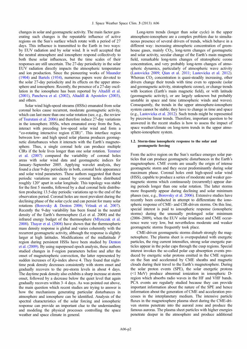
The upper row of plots in Figure 3 shows the latitude struc-tures of the COSMIC 9-day wave amplitudes seen in foF2 (leftplot) and in hmF2 (right plot). The 9-day ionospheric responsesamplify concurrently with the external forcing. The low-latitudeamplification of the foF2 9-d response is well seen over theequator and at ~20� N modip latitude. The hmF2 shows clearamplifications over the equator and near ±50� modip latitudes;the latter hmF2 amplifications coincide with minima of the foF29-d responses. The Power Index (PI) is a measure of the exter-nal forcing of the thermosphere which leads to temperaturechanges and all consequences resulting from these changes(composition, chemical loss, and wind changes). Therefore,from physical point of view it is correct to examine the relation-ship between the ionospheric 9-d oscillations and those in thePI. The bottom row of plots in Figure 3 shows the differencebetween the phases (in degrees) of the 9-d oscillations in thefoF2/hmF2 and in the PI (left/right plot). The thick white lineshows the zero phase difference. When the phase differenceis negative, it means the opposite ionospheric response to thatof the external forcing, while the positive phase differencemeans that the ionospheric response lags behind that of theexternal forcing. The phase difference plot between foF2 andPI (left plot) indicates the following regularities: (i) high-lati-tude foF2 9-d oscillations are out of phase with those in PI;(ii) there is a clear seasonal dependence of the negative high-lat-itude foF2 9-d wave response and this can be traced out by thezero phase difference line; it approaches high latitudes (±60�) inwinter and moves toward the equator (near ±30�) in summer,and (iii) middle- and low-latitude foF2 9-d waves usually lagbehind that in PI; the mean time delay is ~1.5–2 days (~60–90�). The phase difference plot between hmF2 and PI (bottomright plot) indicates that usually the ionospheric responselags behind that in the external forcing everywhere; while at

50� modip the time lag is less than a day (~30�) that abovethe equator is ~1.5 days (~60�).

As the energy transfer is a combination of Joule heating andparticle precipitations then the main drivers of the ionosphericresponse to recurrent geomagnetic activity are related tochanges in the temperature, thermospheric neutral composition,and neutral winds. The heated gas is more buoyant than its sur-roundings, causing it to rise. Then the auroral heating alters themean global circulation of the thermosphere. Whereas for quietconditions there is a general upwelling in the summer hemi-sphere flow toward the winter hemisphere at higher levels,and downwelling in the winter hemisphere, the storm-time heat-ing adds a polar upwelling and equatorward flow in both hemi-spheres. The increased equatorward wind at middle latitudestends to push the ionosphere higher up along magnetic fieldlines, where the loss rate is lower. At high latitudes the upwell-ing brings air rich in the heavy molecular constituents N2 andO2 to high altitudes and the circulation carries this molecular-rich air to midlatitudes, especially in the summer hemisphere,where the mean meridional circulation is already equatorward.At lower latitudes, the downwelling brings air with low concen-tration of molecular species. Since these species determine theloss rate of ions, the loss rate increases/decreases at higher/lowlatitudes.

Figure 3 shows that the 9-d wave responses in foF2 are outof phase with those in PI at high latitudes and they lag behindthat in the PI with a mean time delay of ~1.5–2 days at low lat-itudes. As the loss rate increases at higher latitudes anddecreases at lower latitudes then the foF2 decreases at high lat-itudes and increases at low latitudes. The time lag of ~1.5 daysis related to the needed time for the divergent equatorward flowto reach the lower latitudes. The bottom left plot demonstratesin a very clear way the seasonal dependence of the boundarybetween molecular enrichment and depletion areas. It is seenthat the zero phase difference line approaches high latitudes

0 90 180 270 360 450 540-70

-50

-30

-10

10

30

50

70

Mod

ip L

atitu

de (

degr

ee)

9-d (s=0) PW Response in foF2

0.04

0.09

0.14

0.19

0.24

0.29

0 90 180 270 360 450 540-70

-50

-30

-10

10

30

50

709-d (s=0) PW Response in hmF2

0.3

1.3

2.3

3.3

4.3

5.3

6.3

0 90 180 270 360 450 540

Day Number (start 1 October 2007)

-70

-50

-30

-10

10

30

50

70

Mod

ip L

atitu

de (

degr

ee)

Phase Diff. 9-d (s=0) (foF2-PI)

-150

-100

-50

0

50

100

150

0 90 180 270 360 450 540

Day Number (start 1 October 2007)

-70

-50

-30

-10

10

30

50

70Phase Diff. 9-d (s=0) (hmF2-PI)

-150

-100

-50

0

50

100

150

Fig. 3. (Upper row of plots) Extracted from the COSMIC data 9-day zonally symmetric (s = 0) waves seen in the ionospheric parameters: foF2(left plot) and hmF2 (right plot); (bottom row of plots) Phase difference between the ionospheric parameters foF2 and the PI (left plot) andbetween hmF2 and PI (right plot); the thick white line shows the zero phase difference (Mukhtarov & Pancheva 2012).

I. Kutiev et al.: Solar activity impact on upper atmosphere

A06-p5

in winter and moves to middle, even tropical latitudes duringsummer at both hemispheres. This is due to the fact that thesummer-to-winter transequatorial thermosphere wind is againstthe storm-time generated equatorward flow in winter and in thesame direction in summer.

The hmF2 9-d waves show maxima above the equator andnear ±50� modip latitudes. This can be attributed to the 9-dmodulated vertical drift in the equatorial region and to the peri-odical pushing of the ionosphere higher up along magnetic fieldlines. The latter apparently has maximum effect near ±50� mo-dip latitudes where the storm-time equatorward flow still hasstrong meridional direction. The hmF2 9-d waves lag behindthose in PI with a time delay of less than a day at ±50� modiplatitudes and of ~1.5 days above the equator. Again these arethe needed times for the divergent horizontal wind which blowsequatorward to reach respectively middle and equatorial lati-tudes. It is worth noting that the hmF2 9-d wave amplificationsat ±50� modip latitudes coincide with some minima of the 9-dwaves in foF2. This means that when the ionosphere is pushedhigher up along magnetic field lines by the storm-time equator-ward flow its hmF2 increases but the foF2 does not change dueto the composition change effects on the foF2, i.e., since theionosphere follows a constant pressure surface and this doesnot change the foF2.

In conclusion, it has to be noted that the ionosphericresponse to recurrent geomagnetic activity is really due to thesame physical processes that disturb the ionosphere during clas-sical ionospheric storms which are typically isolated events.

2.3. Long-term trends in the upper atmosphere and ionosphereand space weather/climate

Long-term trends and changes (longer than solar cycle) canpartly be caused by long-term changes of trend drivers ofsolar/space weather origin like geomagnetic activity, which interms of the aa-index was increasing over almost the whole20th century (e.g., Mursula & Martini 2006), even thoughnow it is low. On the other hand, long-term changes of back-ground conditions in the upper atmosphere-ionosphere system,which are of solar origin, may modify effects of other drivers oflong-term trends, and long-term trends themselves modifybackground conditions for effects of space weather phenomenaon the upper atmosphere-ionosphere system. Therefore it is

necessary to investigate the impact of space weather/climateon long-term trends in the upper atmosphere-ionospheresystem.

Long-term trends in the upper atmosphere-ionosphere are acomplex problem due to simultaneous presence of several driv-ers of trends, which behave in a different way: increasing atmo-spheric concentration of greenhouse gases, mainly CO2, long-term changes of geomagnetic and solar activity, secular changeof the Earth’s main magnetic field, remarkable long-termchanges of stratospheric ozone concentration, and very proba-bly long-term changes of atmospheric dynamics, particularlyof atmospheric wave activity (Lastovicka 2009; Qian et al.2011; Lastovicka et al. 2012). Whereas CO2 concentration isquasi-steadily increasing, other drivers change their trends withtime even to opposite (solar and geomagnetic activity, strato-spheric ozone), or change trends with location (Earth’s mainmagnetic field), or with latitude (geomagnetic activity), or arelargely unknown but probably unstable in space and time(atmospheric winds and waves). Consequently, the trends inthe upper atmosphere-ionosphere system cannot be stable; theyhave to change in time and space (e.g., Lastovicka et al. 2012).Such trends might be represented by piecewise linear trends.

As for solar activity, it has decreased in the second half ofthe 20th century after the 1957–1958 maximum, and it is low inrecent years. This is a tendency opposite to what is required toexplain the observed ionospheric trends in the E and F1 regions(Lastovicka 2009). Moreover, the effect of solar activity, on thesolar cycle time scales, is usually reduced when long-termtrends are computed both in the ionosphere and thermosphereas the solar cycle effect is much larger than trend. Different cor-rections to solar activity are one of sources of differencesbetween different trend results in the F2-region parameters,foF2 and hmF2. Thus, solar activity itself has little or no directeffect on observed ionospheric trends. However, it is necessaryto mention that trends may be quantitatively different undersolar activity maximum and minimum conditions, which isthe case for thermospheric density (e.g., Emmert et al. 2008).The reason is much larger relative role of the CO2 radiativecooling compared to the NO radiative cooling under solar min-imum conditions as confirmed by SABER/TIMED measure-ments (Mlynczak et al. 2010). This is an indirect effect ofsolar activity on trends in the thermosphere and ionosphere.

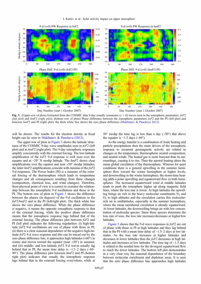
Another potentially important driver of trends is geomag-netic activity, which was increasing throughout almost thewhole 20th century (Mursula & Martini 2006) but now it islow. Bremer et al. (2009) summarized various results on geo-magnetic activity control of trends in the ionosphere and foundthat the change of dependence of trends on long-term change ofgeomagnetic activity, i.e., the loss of dominant geomagneticactivity control of ionospheric trends, occurred around 1970in the E region, in the early 1990s in the F1 region, and around2000 in the F2 region as illustrated in Figure 5 for two Euro-pean stations Roma and Slough/Chilton. Trends in the heightof maximum of F2 region, hmF2, lost geomagnetic activitycontrol much earlier than trends in foF2 (Lastovicka et al.2012). Thus at present the long-term changes in geomagneticactivity are not the main driver of trends in any variable, con-trary to the past, when it probably controlled ionospheric trends(Lastovicka et al. 2012). This is, however, valid only for lowand middle latitudes. In the auroral zone, which is generallyunder continuous and much stronger geomagnetic/magneto-spheric activity control than low and middle latitudes, the trendsseem to be still under dominant geomagnetic control as sug-gested by the foE trends as observed at auroral station Tromso

Fig. 4. Model simulation of trends in foF2 and hmF2 at noon,longitude 0�, as a difference between the basic state and the statewith doubled CO2 concentration. Dashed curve – hmF2 for basicstate; solid curve – hmF2 for doubled CO2. After Qian et al. (2008).

J. Space Weather Space Clim. 3 (2013) A06

A06-p6

(Hall et al. 2011). Recent trends in the mid- and low latitude foEand foF1 are a slight increase, and in foF2 in day-time a verysmall decrease, probably due to changes in minor constituentchemistry and various temperature-dependent reactions and lossrates. This is consistent with model calculations of changes dueto increasing concentration of CO2 shown in Figure 4. Anincrease of electron density at heights of foE (~110 km) andfoF1 (~200 km) in middle and lower latitudes is well visible.A decrease of hmF2 (seen as the difference between the basicstate and the state with doubled CO2 concentration) is also evi-dent, whereas hmF2 is close to the level of no change in foF2, itis located in the region of a slight decrease of electron densityand, thus, of foF2. This pattern is qualitatively consistent withthe observed trends in ionospheric parameters and a weak CO2-related trend in foF2 explains also the delayed loss of dominantinfluence of long-term change of geomagnetic activity on foF2trends.

Thus the role of space weather/climate in long-term changesand trends in the upper atmosphere-ionosphere was moreimportant in the past, when it controlled the trends in iono-spheric parameters, than it is at present, when the dominantcontrolling parameter seems to be increasing concentration ofCO2.

2.4. Latitude-dependent response of TEC to solar EUV changes

Since the solar EUV radiation varies by a factor of about 2within a solar cycle (Lean et al. 2003), it is expected that theionospheric TEC is highly correlated with solar activitychanges. We checked this assumption by comparing TECobtained at three selected sites in Europe (cf. http://swaciweb.dlr.de) with the solar activity dynamics represented by the radioflux index F10.7 which is also a proxy for EUV radiationchanges (see Fig. 6).

Although TEC is subjected to a clear seasonal modulation,the general behavior of TEC is highly correlated with F10.7(e.g., Jakowski et al. 1991, 2011). Whereas the dynamic ratiobetween TEC maximum and minimum is about 8 at day-timeover Europe, the same ratio is about 5–6 for night-time condi-tions during solar cycle 23 (see Fig. 7). Furthermore, it can beseen that due to the lower incidence angle of the solar radiationat lower latitudes, TEC at 35� N is principally higher than TECat 65� N. Differences between both latitudes are always posi-tive at day-time and reach up to 20 TECU while followingthe solar cycle dynamics. During night-time, the situation isindifferent for the difference TEC(50� N)–TEC(65� N), i.e.,positive and negative differences occur. The difference

Fig. 5. Relationships between dfoF2 (top panels), dfoF1 (middle panels) and dfoE (bottom panels), and Ap132 variations for Slough (left panels)and Rome (right panels). The change in the type of the dependences appeared earlier in the E region, later in the F1 region, and eventually itbegan to appear in F2 region. After Bremer et al. (2009).

I. Kutiev et al.: Solar activity impact on upper atmosphere

A06-p7

TEC(35� N)–TEC(50� N) is almost positive and follows thedynamics of the solar cycle as day-time differences. SuchTEC gradients are important for GNSS applications. Here aver-aged meridional TEC gradients between 35� N and 50� N mayreach about 2.5 mm/km at L1 GPS frequency, which is faraway from threat model values of the order of 100 mm/km(e.g., Mayer et al. 2009). When considering latitudes below30� N, a dramatic increase of meridional gradient values isexpected in the crest region which needs further investigation.Gradients may considerably enhance during ionospheric storms(Jakowski et al. 2008; Mayer et al. 2009). Sudden increases ofEUV radiation during solar flares are immediately visible inTEC data as it has clearly been shown during the strong solarflare on 28 October 2003 (Jakowski et al. 2008).

2.5. Ionospheric behavior during prolonged minimum of the23/24 solar cycle

The solar minimum between solar cycles 23 and 24 was signif-icantly longer than it has been expected. Lastovicka et al.(2006) pointed out that besides other aspects, the significanceof understanding of the solar minimum lies in revealing the nat-

ure of solar variability, its effects on geospace, and assessing thepredictability of current models. Within the minimum of cycle23/24 measurements from instruments placed on SOHO (theSolar and Heliospheric Observatory) and TIMED (the Thermo-sphere-Ionosphere-Mesosphere Energetics and Dynamics) sat-ellites indicated that solar EUV irradiance levels were lowercomparing with previous solar minimum, which led to lowerthermospheric density and temperature. Although solar EUVis primary controller of the temperature and density of the ther-mosphere and ionosphere, contributions from geomagneticactivity are also significant (Solomon et al. 2010). The pro-longed solar minimum in 2006–2009 gave us a unique possibil-ity to explore ionospheric behavior under extremely low solaractivity conditions, particularly ionospheric reaction to occa-sional very moderate geomagnetic disturbances. Our analysiswas aimed at variability of the ionospheric F2-layer critical fre-quency foF2 and peak height hmF2 above middle latitudesunder low solar activity conditions.

In total, the created database comprises values of foF2 andhmF2 for nine middle latitude stations which operate the DPS(Digisonde Portable Sounder). We compared monthly mediansof the F2-layer main parameters for the solar minimum of the

Fig. 7. Day-time variation of TEC averaged over 12–14 LT at three selected points in Europe (left panel). Night-time variation of TEC averagedover 00–02 LT at three selected points in Europe (right panel). Selected TEC unit: 1 TECU = 1 · 1016 m�2.

Fig. 6. Left panel: solar activity variation (F10.7) from 1995 to 2009 covering solar cycle 23 (1996–2008). Right panel: location of three testsites at which TEC is extracted from regularly produced GNSS-based TEC maps over Europe (Jakowski 1996; Jakowski et al. 2011).

J. Space Weather Space Clim. 3 (2013) A06

A06-p8

cycles 22/23 and 23/24. To evaluate the effects of geomagneticdisturbances on the ionospheric F2-layer, we used hourly mea-surements of foF2 and hmF2 and their 27-days running meanscentered on the culmination (minimum Dst) day of each ana-lyzed geomagnetic disturbance. Both foF2 and hmF2 valueswere automatically obtained from the ARTIST software(Reinisch & Huang 1983). The disturbed periods were analyzedusing constituently checked data.

The blue curves in Figure 8 represent the ratio of the foF2monthly medians observed during 2006–2009 above Chilton tothose measured in 1996. The red curve is for the ratio of thedaily 10.7 cm solar radio flux (F10.7) observed for the period2006–2009 to the 1996 values. The course of the ratio indicatesthat, in general, comparing to 1996, the foF2 decreased mostlyduring the winter 2006–2009 and summer 2008. We obtainedsimilar results also for Pruhonice, except January of each ana-lyzed year, where the ratio was mostly positive. For the selectedmiddle latitude stations the ratio of the peak critical frequencyfit to the range of (�0.7)–1.5. Solomon et al. (2010) mentionedthat NCAR Thermosphere-Ionosphere Electrodynamics Gen-eral Circulation Model (TIE-GCM) model simulations for~97–600 km altitude showed, that the estimated change in totalEUV energy input is approximately commensurate with the

measured density change. Our analysis partially supports themodel results, nevertheless, the observations also gave noticeabout importance of other factors (e.g., geomagnetic activity,location, season, daytime, tropospheric effects). Recently,widely discussed influence of the greenhouse gases on theEarth’s upper atmosphere seems to be responsible only for asmall portion of the observed density change (Solomon et al.2010).

Figure 9 shows the level of geomagnetic activity for 1996(top panel) and 2006–2009 (panels below) represented bymonthly means of the daily Kpsum. It is evident that the lowestgeomagnetic activity has been observed in 2009, and a well-pronounced semiannual variation of geomagnetic activity ofthe solar cycle 22/23 minimum was not present during the min-imum of 23/24.

There are several physical processes that can affect the ion-ospheric F-region electron density profile. The lower thermo-spheric temperatures, as a consequence of an unusually longminimum in solar extreme-ultraviolet flux, not only decreaseddensity, but the contraction of the upper atmosphere also low-ered the height of the peak of the ionospheric F-layer. In gen-eral, the differences between monthly medians of foF2obtained for solar minimum years 1996 and 2006-2009 and

Fig. 8. Ratio of the hourly medians of foF2 observed during 1996 and those measured at 2006–2009 for Chilton.

I. Kutiev et al.: Solar activity impact on upper atmosphere

A06-p9

for selected middle latitude stations fit to the range of (�0.7)–1.5 MHz.

3. Storm-time ionospheric response to the solar

and geomagnetic forcing

The behavior of ionospheric midlatitudes during the prolongedperiod of very low solar activity, with F10.7 not exceeding 80,is subject of the original study, whose results are presented inSection 3.1. The analysis includes 15 minor and moderateCIR-driven storms in the period 2006–2009. The main conclu-sion is that the deviations of foF2 and hmF2 from their quietlevels during the analyzed period are higher than expectedand comparable with those induced by strong CME-drivenstorms.

In Section 3.2, L. Perrone and M. Parisi present an originalstudy on the sudden increase of the polar cap absorption (PCA)linked to a Halo CME on 9 May 2005. The CME has given ori-gin to SPE which reaches the peak simultaneously with thebeginning of SSC of a geomagnetic superstorm that occurredon 14 May 2005. The behavior of SPE and consequently thePCA characteristics allow assuming that the latter event is

connected with two magnetic clouds (MC) near Earth, not usualfor a single MC originated from that CME.

During the strong CME-driven storms, the ring currentintensity sharply increases and the plasma sheet particles withhigher energies penetrate deeper into atmosphere of the auroralzone and produce additional ionization. Using radio occultationmeasurement to reconstruct the electron density profiles in theE region, Mayer & Jakowski (2009) have collected cases whenthe maximum density of the E region exceeds that of the F2-layer. The geographical distribution of these events, shown inSection 3.3, fits very well with the boundaries of the auroralzone.

3.1. Ionospheric response to geomagnetic activity duringprolonged solar minimum

The prolonged solar minimum in 2006–2009 offers a uniquepossibility to explore ionospheric behavior under extremelylow solar activity conditions, particularly ionospheric reactionto occasional verymoderate geomagnetic disturbances. The pres-ent analysis was aimed at variability of the ionospheric F2-layercritical frequency foF2 and peak height hmF2 above middlelatitudes under low solar activity conditions. The minor andmoderate geomagnetic storms, which predominantly occur

Fig. 9. Monthly means of the daily Kpsum for 1996 (top panel) and 2006–2009 (panels below).

J. Space Weather Space Clim. 3 (2013) A06

A06-p10

during this period, are assumed to represent the CIR-drivenstorms. Fifteen recurrent storms were selected to analyzevariation of foF2 and hmF2. Results for November 2008 forPruhonice are presented in Figure 10. Three top panels are forDst, AE and Kp indices, respectively. Two bottom panels showvariation of the hourly values (green and blue plots) and the27-days running means (black curves) of foF2 and hmF2. Theplot in the middle represents differences between daily observa-tions and their mean values. During November 2008 threeminor-to-moderate disturbances occurred. We observed changesin foF2 up to 60% during these events, which at middle latitudesare typical rather for strong geomagnetic storms than for minorand moderate disturbances. We observed both positive and neg-ative effects on electron density (positive effects were larger).

Table 1 summarizes results of the deviations, obtainedbetween the measured values and their medians for all 15 ana-lyzed events and for four midlatitude stations. The analysis ofthe effects of these magnetic disturbances, occurring withinthe period 2006–2009 on ionospheric F2-layer, showed signif-icant departure of the main peak parameters from the corre-sponding 27-days running means. In the majority of the casesthe differences were comparable with the effects of CME-dri-ven strong magnetic storms. Deviations in Table 1 show thatthe ionospheric response to geomagnetic storms during theextreme solar minimum remains high, not proportional to theintensity of the storms.

3.2. Polar cap absorption event of May 2005 in Antarctica

An essential space weather objective is the understanding andthe prediction of the consequences at the Earth of Coronal MassEjections after its evolution through the interplanetary medium.

One of the most intense events on the Sun during the declin-ing phase of solar cycle 23, occurred onMay 2005 is analyzed inthis paper. This is an event thought to be due to a single solarsource (Zhang et al. 2007) andwith quiet geomagnetic conditionsthat prevailed before and after the storm. Hence, its geomagneticand ionospheric effects could be gauged very accurately. Thecharacteristics ofMay 2005 event and the properties of the corre-lated observations of ionospheric absorption, obtained by a

Fig. 10. Ionospheric F2-layer behavior as it was observed in November 2008 above Pruhonice observatory. The top panels show the course ofDst, AE, and Kp indices. Two bottom panels are for foF2 (solid green line) and hmF2 (solid blue line). The solid black line represents 27-daysrunning mean. The middle panel gives difference between the daily foF2 and its 27-days running mean in percentage.

Table 1. Range of the differences between the disturbed-time foF2and hmF2 values and corresponding 27-days running means (%),obtained for 15 analyzed minor-to-moderate magnetic disturbanceswithin the prolonged solar minimum (2006–2009). The analyzedperiod of each disturbance includes the culmination day and at leasttwo days of the recovery phase.

Ionosphericstations

Pruhonice Chilton Rome Grahamstown

DfoF2 (%) 24�102 25–86 28–116 23–80DhmF2 (%) 17–43 15–74 20–90 24–41

I. Kutiev et al.: Solar activity impact on upper atmosphere

A06-p11

30 MHz riometer installed atMarioZucchelli Station (MZS-Ant-arctica, Perrone et al. 2004), and of geomagnetic activity at theground level are investigated. Solar events are studied by usingthe characteristics of CME measured with SoHO/LASCO coro-nagraphs and the temporal evolution of solar energetic particlesin different energy ranges measured by GOES 11 spacecraft(Bremer et al. 2009; Perrone et al. 2009).

The solar region AR0759 appeared on the east limb on May9 produced on 13 May two solar flares, C1.5 at 12:49UT andM8 at 16:32UT, going to the central meridian. The last solarflare linked to an Halo CME with a speed of 1689 km/s. Thetransit time of Interplanetary CME (ICME), that contains twoattached but non-merged Magnetic Clouds (MCs) (Dassoet al. 2009), with respect to the origin of CME is of 33.5 h at1 AU. Because a single solar source cannot originate twoMCs, the MCs are linked to the two solar flares of 13 May(Dasso et al. 2009).

The CME has given origin to SPE that reaches the peaksimultaneously with the beginning of SSC (Fig. 11). ThisSPE determined an ionospheric absorption of 6.5 dB. The peakof SPE (>10 MeV) is 3140 (pfu) and occurs, approximately,

with the interplanetary shock occurrence, this is a typical behav-ior of central meridian events. The peak of ionospheric absorp-tion occurs after 19 min from SPE peak (E0 < 40 MeV). Infact, the ionization in the D region during PCA events is duemainly to protons with energy in the range 1–100 MeV thatcan reach an altitude between 30 and 80 km. The ionosphericabsorption could be higher but the peak of SPE occurred duringnighttime condition (v > 96�). The large difference betweenday and night absorption intensities for equal precipitatingfluxes of solar particles is a characteristic feature of PCAevents. This feature is mainly a consequence of switching offthe photo-detachment of negative ions, thus the negative ionscreated by attachment remain below 80 km at night and thisresults in electron density depletion.

The IMF Bz component turned southward, remained southbetween 05:32 UT and 08:20UT on May 15 reaching a value of�44 nT at 05:56UT and the high solar wind velocity (close to1000 km/s) are the cause of a geomagnetic superstorm occurredwith a Dst peak excursion of �263 nT.

The arrival of a single MC, in general, is connected to adecreasing of SPE and consequently of the ionospheric

Fig. 11. From top to bottom: differential solar proton flux, Interplanetary Magnetic Field (data in GSM coordinates obtained from ACEspacecraft), cosmic ray data, ionospheric absorption, and Dst index during 13–16 May 2005.

J. Space Weather Space Clim. 3 (2013) A06

A06-p12

absorption as it is observed in this case when Bz flows South-ward, while the large decay, observed in this case, in the recov-ery phase of Dst index is connected, in general, to the presenceof multiple Interplanetary medium structures, as two MCs, nearEarth (Xie et al. 2006). This leaves the necessity of still morestudy of this event and to analyze many data sets available totry to understand each step along the way from solar sourceto the effects on the Earth and Earth environment.

3.3. E-layer dominated ionosphere

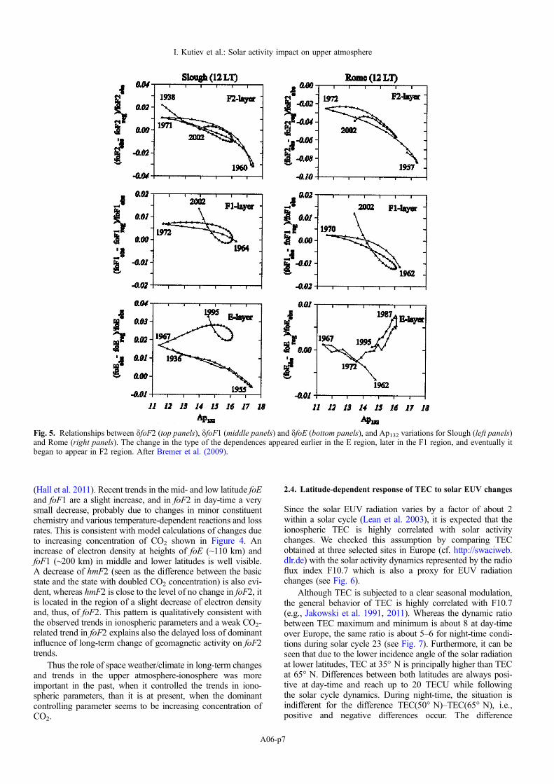
Energetic particles originating from the nighttime magneto-sphere are able to ionize the atmosphere significantly in a heightrange of about 100 km. The penetration depths depend on theenergy of the particles. Space-based GNSS radio occultationmeasurements onboard satellites such as CHAMP, GRACE,and Formosat3/COSMIC are well suited to detect such ioniza-tion enhancements in the bottomside ionosphere. So weselected electron density profiles with pronounced ionizationat E-Layer height in the range of about 90–150 km for studyingthe geophysical conditions under which such enhancementswere observed (Mayer & Jakowski 2009). Solar storms accom-panied by coronal mass ejections (CMEs) may enhance precip-itation of energetic particles’ solar wind energy considerably.

If the electron density in the E-layer is higher as the densityin the F2-layer is around 250–350 km, the ionosphere is calledan E-layer dominated ionosphere (ELDI) by Mayer & Jakowski(2009). Analyzing the occurrence probability, these authorsshow that profiles with enhanced E-layer ionization are closelyrelated to the location and shape of the auroral zone (Fig. 12).Thus, they were able to study the local-time, seasonal, andspace-weather dependence of enhanced ionization processesin the auroral zone. The shape of the precipitation region formsan ellipse whose main axis goes through the geomagnetic andgeographic poles. Furthermore, one focal point is defined bythe geographic pole and the position of the geomagnetic poleis identical with the center point of a circle fit. To evaluatethe reliability of radio occultation measurements and to study

precipitation processes in more detail, coordinated EISCATmeasurements would be useful.

4. Modeling and forecasting techniques

The present section describes empirical models of the TEC, theF-layer critical frequency foF2, and the height of the maximumplasma density. The models use different analytical functionsand drivers, but they evaluate the model error in the sameway which makes their performance comparable.

In Section 4.1, Andonov et al. (2011) developed an empir-ical dependence between TEC and the geomagnetic activitydescribed by the Kp-index. This dependence is expressed as afunction of calendar month, geographic latitude, and LT, fittedover a long time series of TEC measurements (October 2004–December 2009) over North America. The authors introduce amodified function of Kp obtained by two-dimensional (time-lat-itude) cross-correlation function, calculated for each month ofthe year. The modified Kp function is defined by two time delayconstants for positive and negative TEC deviations respectively.

In Section 4.2, Tsagouri et al. (2009) developed a new ion-ospheric forecasting algorithm, called the Solar Wind driven au-toregression model for Ionospheric short-term Forecast (SWIF).SWIF combines historical and real-time ionospheric observa-tions with solar wind parameters obtained in real time at theL1 point from NASA/ACE spacecraft. SWIF combines the au-toregression forecasting algorithm, called Time Series AutoRe-gressive – TSAR (Koutroumbas et al. 2008), with the empiricalStorm Time Ionospheric Model – STIM (Tsagouri & Belehaki2006, 2008). Under storm conditions, SWIF adopts progres-sively the STIM’s predictions, while in non-alert conditions,SWIF performs like TSAR.

Section 4.3 describes a model which combines two modelsdeveloped for different ionospheric conditions. One is themodel of the quiet-time behavior of the F-layer peak heighthmF2 based on the spherical harmonics analysis technique(Altadill et al. 2009). The other is a model of the storm-time

Fig. 12. Left panel: typical electron density profile as they can be derived from GPS RO measurements onboard Formosat3/COSMIC, CHAMP,and GRACE satellites. Right panel: ellipse fit to the distribution of ELDI profiles, which show enhanced E-layer ionization (red dots). Theyellow stars mark the focal points of the ellipse; the black star marks the center point of the circle fit which coincides with the position of thegeomagnetic pole (Mayer & Jakowski 2009).

I. Kutiev et al.: Solar activity impact on upper atmosphere

A06-p13

variations of hmF2, triggered by IMF Bz (Blanch 2009). Thenew model provides a near-real time forecasting tool forhmF2 in response to the configuration and variation of the IMF.

The present section includes two other contributions closelyconnected with to the above topic. The effective sunspot num-ber – R12eff is used in DIAS (European Digital Upper Atmo-sphere Server) as a proxy of the ionospheric conditions overEurope for regional ionospheric mapping purposes (Zolesiet al. 2004; Tsagouri et al. 2005). Tsagouri et al. (2009) furtherstudied the efficiency of R12eff to specify the ionospheric con-ditions over Europe. The authors show that the deviation of thereal-time R12eff estimates from the reference values (DR12eff)follows successfully the ionospheric response to geomagneticstorm enhancements and can be used as a better proxy in spec-ifying the ionospheric state.

Mikhailov et al. (2012) developed a new method for retriev-ing neutral temperature Tn and composition [O], [N2], [O2]from electron density profiles in the daytime mid-latitude F2region under both quiet and disturbed conditions. The methodwas tested by using Millstone Hill Incoherent Scatter Radar(ISR) profiles and by co-located Digisonde bottomside profilescomplemented with NeQuick topside profiles. Comparison withneutral atmosphere parameters measured by CHAMP satelliteshows satisfactory agreement with the model error of order ofuncertainty of CHAMP measurements.

4.1. Empirical model of the TEC response to the geomagneticactivity over the North American region

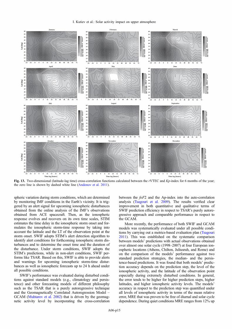
This subsection briefly describes an empirical dependencebetween the TEC and the geomagnetic activity described bythe Kp-index. The detailed description of the model can be seenin Andonov et al. (2011). The wanted dependence is presentedas a function of calendar month, geographic latitude, and LTand is obtained by using a long time series of TEC measure-ments over the region covering North America (50� W–150� W, 10� N–60� N). The period of time October 2004–December 2009 is considered, therefore, the presented TECmodel is valid mainly for low solar activity conditions. Thetime series of hourly vertical TEC (VTEC) data with latitude/longitude resolution of 1�/1� are used in this study and thedata were downloaded from the NOAA NGDC web site:http://www.ngdc.noaa.gov/stp/iono/ustec/index.html. The VTECresponse to the geomagnetic activity is investigated by consider-ing the relative deviation of VTEC defined as: rVTEC = (VTE-Cobs � VTECmed)/VTECmed, where VTECmed represents themonthly median value. In this way the regular seasonal, diurnal,and solar changes are removed from the VTEC variability. Thedata are grouped into 12-month bins with all the available hourlydata within the respective month of the year.

As a first step the effect of geomagnetic activity on therVTEC is studied by cross-correlation analysis. A two-dimen-sional (time-latitude) cross-correlation function is calculatedfor each month of the year and the results are shown inFigure 13. The most important feature of the cross-correlationanalysis is that for all months the ionospheric response is com-posed by two phases, positive and negative, with different dura-tion and different time delay. This feature lies at the root of themodel, i.e., the impact of the geomagnetic activity on the TECis accomplished by two mechanisms with different time delayconstants that can be described as follows:

rVTEC tð Þ � ðf TS KpTS tð Þð Þ þ fTI KpTI tð Þð Þf LTð Þ; ð1Þ

where f(LT) represents the dependence of the response on LTat equal other conditions, KpTs and KpTl are the modifiedKp-index with time delay constants respectively Ts and Tl.The unknown functions fTs and fTl from (1) are expressedby their Taylor time series expansions while the dependenceon LT is represented by a Fourier time series as follows:

fTS KpTSð Þ ¼ a0s þ a1sKpTS tð Þ þ a2sKpTSðtÞ2 þ a3sKpTSðtÞ

3

þ . . . ;

fTI KpTIð Þ ¼ a01 þ a1lKpTl tð Þ þ a2lKpTlðtÞ2

þ a3lKpTlðtÞ3 þ . . . ; ð2Þ

flt LTð Þ ¼ b0 þX

i

bi cos i2p24

LT � ui

� �:

It was found also that the functional dependence between Kpand rVTEC is close to the cubic function. Then in the Taylorexpansion time series (the first two relations in (2) only the firstfour terms are included. The next step is to obtain the mostprobable values of the coefficients: ais, bi, ail, Ts and Tl from(2). This is a nonlinear optimizing task that was solved bysearching the minimum RMS error.

In order to demonstrate how the empirical model describesthe rTEC, Figure 14 displays the comparison between therVTEC response from the model (solid line) and observations(dashed line) for two geomagnetic storms in November 2004(left column of plots) and December 2005 (right column ofplots).

The presented method for empirical modeling of the rVTECresponse to the geomagnetic activity is able to satisfactorilymodel the observed responses with similar amplitudes of bothpositive and negative phases because of the availability oftwo delayed mechanisms with different time constants. A sig-nificant role for improving the model also plays the introduceddependence on LT. The error of the model varies from 0.05 to0.15 rVTEC units for different months of the year and for dif-ferent latitudes and longitudes.

4.2. Advances in the development of ionospheric forecastingmodels

The development of a new ionospheric foF2 forecasting algo-rithm, called the Solar Wind driven autoregression model forIonospheric short-term Forecast (SWIF), was recently intro-duced (Tsagouri et al. 2009).

SWIF combines historical and real-time ionospheric obser-vations with solar wind parameters obtained in real time at theL1 point from NASA/ACE spacecraft. This is achieved throughthe cooperation of an autoregression forecasting algorithm,called Time Series AutoRegressive – TSAR (Koutroumbaset al. 2008), with the empirical Storm Time Ionospheric Model– STIM (Tsagouri & Belehaki 2006, 2008) that formulates theionospheric storm-time response based on solar wind input,exploiting recent advances in ionospheric storm dynamics thatcorrelate the ionospheric storm effects with solar wind parame-ters (e.g., the magnitude of the IMF and its rate of change aswell as the IMF’s orientation in the north-south direction).STIM provides a correction factor to the quiet diurnal iono-

J. Space Weather Space Clim. 3 (2013) A06

A06-p14

spheric variation during storm conditions, which are determinedby monitoring IMF conditions in the Earth’s vicinity. It is trig-gered by an alert signal for upcoming ionospheric disturbancesobtained from the online analysis of the IMF’s observationsobtained from ACE spacecraft. Then, as the ionosphericresponse evolves and recovers on its own time scales, STIMestimates the time delay in the ionospheric storm onset and for-mulates the ionospheric storm-time response by taking intoaccount the latitude and the LT of the observation point at thestorm onset. SWIF adopts STIM’s alert detection algorithm toidentify alert conditions for forthcoming ionospheric storm dis-turbances and to determine the onset time and the duration ofthe disturbance. Under storm conditions, SWIF adopts theSTIM’s predictions, while in non-alert conditions, SWIF per-forms like TSAR. Based on this, SWIF is able to provide alertsand warnings for upcoming ionospheric storm-time distur-bances as well as ionospheric forecasts up to 24 h ahead underall possible conditions.

SWIF’s performance was evaluated during disturbed condi-tions against standard models (e.g., climatology and persis-tence) and other forecasting models of different philosophysuch as the TSAR that is a purely autoregressive techniqueand the Geomagnetically Correlated Autoregression Model –GCAM (Muhtarov et al. 2002) that is driven by the geomag-netic activity level by incorporating the cross-correlation

between the foF2 and the Ap-index into the auto-correlationanalysis (Tsagouri et al. 2009). The results verified clearimprovement in both quantitative and qualitative terms ofSWIF prediction efficiency in respect to TSAR’s purely autore-gressive approach and comparable performance in respect tothe GCAM.

More recently, the performance of both SWIF and GCAMmodels was systematically evaluated under all possible condi-tions by carrying out a metrics-based evaluation plan (Tsagouri2011). This was established on the systematic comparisonbetween models’ predictions with actual observations obtainedover almost one solar cycle (1998–2007) at four European ion-ospheric locations (Athens, Chilton, Juliusruh, and Rome) andon the comparison of the models’ performance against twostandard prediction strategies, the median- and the persis-tence-based predictions. It was found that both models’ predic-tion accuracy depends on the prediction step, the level of theionospheric activity, and the latitude of the observation pointespecially during extremely disturbed conditions. In general,the error tends to be higher for higher prediction steps, higherlatitudes, and higher ionospheric activity levels. The models’accuracy in respect to the prediction step was quantified underall levels of ionospheric activity in terms of the mean relativeerror, MRE that was proven to be free of diurnal and solar cycledependence. During quiet conditions MRE ranges from 12% up

-24 -16 -8 0 8 16 24 32 40 48 56 64 7210

15

20

25

30

35

40

45

50

55

60

Lat

[deg

]

-0.28-0.24-0.2-0.16-0.12-0.08-0.0400.040.080.120.160.20.240.280.320.360.4

January

-24 -16 -8 0 8 16 24 32 40 48 56 64 7210

15

20

25

30

35

40

45

50

55

60

-0.28-0.24-0.2-0.16-0.12-0.08-0.0400.040.080.120.160.20.240.280.320.360.4

February

-24 -16 -8 0 8 16 24 32 40 48 56 64 7210

15

20

25

30

35

40

45

50

55

60

-0.28-0.24-0.2-0.16-0.12-0.08-0.0400.040.080.120.160.20.240.280.320.360.4

March

-24 -16 -8 0 8 16 24 32 40 48 56 64 7210

15

20

25

30

35

40

45

50

55

60

Lat

[deg

]

-0.28-0.24-0.2-0.16-0.12-0.08-0.0400.040.080.120.160.20.240.280.320.360.4

April

-24 -16 -8 0 8 16 24 32 40 48 56 64 7210

15

20

25

30

35

40

45

50

55

60

-0.28-0.24-0.2-0.16-0.12-0.08-0.0400.040.080.120.160.20.240.280.320.360.4

May

-24 -16 -8 0 8 16 24 32 40 48 56 64 7210

15

20

25

30

35

40

45

50

55

60

-0.28-0.24-0.2-0.16-0.12-0.08-0.0400.040.080.120.160.20.240.280.320.360.4

June

-24 -16 -8 0 8 16 24 32 40 48 56 64 7210

15

20

25

30

35

40

45

50

55

60

Lat

[deg

]

-0.28-0.24-0.2-0.16-0.12-0.08-0.0400.040.080.120.160.20.240.280.320.360.4

July

-24 -16 -8 0 8 16 24 32 40 48 56 64 7210

15

20

25

30

35

40

45

50

55

60

-0.28-0.24-0.2-0.16-0.12-0.08-0.0400.040.080.120.160.20.240.280.320.360.4

August

-24 -16 -8 0 8 16 24 32 40 48 56 64 7210

15

20

25

30

35

40

45

50

55

60

-0.28-0.24-0.2-0.16-0.12-0.08-0.0400.040.080.120.160.20.240.280.320.360.4

September

-24 -16 -8 0 8 16 24 32 40 48 56 64 72

Time lag [hours]

10

15

20

25

30

35

40

45

50

55

60

Lat

[deg

]

-0.28-0.24-0.2-0.16-0.12-0.08-0.0400.040.080.120.160.20.240.280.320.360.4

October

-24 -16 -8 0 8 16 24 32 40 48 56 64 72

Time lag [hours]

10

15

20

25

30

35

40

45

50

55

60

-0.28-0.24-0.2-0.16-0.12-0.08-0.0400.040.080.120.160.20.240.280.320.360.4

November

-24 -16 -8 0 8 16 24 32 40 48 56 64 72

Time lag [hours]

10

15

20

25

30

35

40

45

50

55

60

-0.28-0.24-0.2-0.16-0.12-0.08-0.0400.040.080.120.160.20.240.280.320.360.4

December

Fig. 13. Two-dimensional (latitude-lag time) cross-correlation functions calculated between the rVTEC and Kp-index for 6 months of the year;the zero line is shown by dashed white line (Andonov et al. 2011).

I. Kutiev et al.: Solar activity impact on upper atmosphere

A06-p15

to 15% for SWIF and from 8% up to 10% for GCAM. Duringdisturbed conditions, it is still relatively small (10–13%) for pre-dictions provided 1 h ahead and may reach 20% and 30% atmiddle-to-low and middle-to-high latitudes, respectively, forhigh ionospheric activity level and predictions provided 24 hahead.

During quiet and moderately disturbed conditions the twomodels perform comparable to climatological predictions,expressed by monthly median estimates, and persistence predic-tions provided either 1 or 24 h before. During disturbed iono-spheric storm conditions considerable improvement (greaterthan 10%) over climatology and persistence is gained for all

Fig. 15. hmF2 prediction combining both models (red line bottom panel). Red points correspond to experimental values for the correspondinggeomagnetic storm. Black points correspond to averaged representative profile data. Black line corresponds to quiet-time hmF2 prediction usingthe SHA model. Gray dashed line corresponds to IRI-2007 prediction. White sun indicates the sunrise and black sun the sunset. IMF Bz and Dstindex are indicated. Vertical gray dashed line indicates the triggering time.

06 07 08 09 10 11 12

Day

-0.8-0.6-0.4-0.2

00.20.40.60.8

11.21.41.61.8

22.22.42.62.8

rVTE

C

November 2004rVTEC DatarVTEC Model

12 13 14 15 16 17 18 19

Day

-0.4

-0.2

0

0.2

0.4

0.6

0.8

1

1.2

1.4

1.6

rVTE

C

December 2005rVTEC DatarVTEC Model

06 07 08 09 10 11 12

Day

0

1

2

3

4

5

6

7

8

9

Kp

November 2004KpTsKpTlKp Data

12 13 14 15 16 17 18 19

Day

0

1

2

3

4

5

6

7

8

9

Kp

December 2005KpTsKpTlKp Data

Fig. 14. (Upper row of plots) Comparison between the observed (dashed line) and model (solid line) rVTEC at the geographic point (20� N,130� W) for the geomagnetic storm in November 2004 (left plot and December 2005 (right plot); (bottom row of plots) Comparison between themeasured Kp-index (tick solid line with dots) and modified KpTs – (dashed line) and KpTl – (solid line) indices for November 2004 (left plot) andDecember 2005 (right plot) (Andonov et al. 2011).

J. Space Weather Space Clim. 3 (2013) A06

A06-p16

prediction steps and at all latitudes. The averaged improvementover climatology ranges from 30% to 70% for GCAM andfrom 25% to 70% for SWIF, giving evidence of the models’efficiency to capture the disturbances, although models’ predic-tions seem to underestimate their intensity. The relativeimprovement over persistence was investigated separately forstorm and post-storm days. It was proved to be significant atalmost all cases, ranging from 20% to 55% for GCAM andfrom 10% to 45% for SWIF during storm days. The improve-ment is higher during post-storm days, ranging from 40% to60% for both models. This test verified the models’ efficiencyto capture the transition from disturbed to quiet conditions.

The evaluation results verified the successful performanceof SWIF in alignment with current ionospheric forecastingcapabilities. This along with the advantage of SWIF in provid-ing alerts and warnings for forthcoming ionospheric storm dis-turbances makes SWIF algorithm a powerful tool in thedevelopment of a full set of ionospheric forecasting servicesin operational mode. SWIF is currently implemented onlinein DIAS system to provide ionospheric forecasts up to 24 hahead as well as alerts and warnings for the European region(http://dias.space.noa.gr). In addition, as a clear advance forradio science purposes, it should be noted that SWIF providesan alternative approach to ionospheric forecasting issue, usingsolar wind parameters as a proxy of the ionospheric activitylevel. This approach makes SWIF able to adapt new insightspotentially available from space weather research and thereforea platform for further investigations/developments.

4.3. Real-time forecasting tool for hmF2 at midlatitudescombining quiet and disturbance hmF2 models

The quiet-time behavior of the ionospheric electron densitypeak height of the F2 region, hmF2, has been evaluated fromaverage electron density profiles and analytically modeled bythe Spherical Harmonic Analysis (SHA) technique followingthe same methodology as described by Altadill et al. (2009).The SHA model provides a tool to predict hmF2 at any locationdistributed among the used range of latitudes (70� N–50� S)and at any time. The SHA model for hmF2 improves the fitto the observed data with respect to IRI prediction, especiallyat high and low latitudes and they may reduce the deviationsby 23% and 40%, respectively, compared to the deviations ofthe IRI prediction (Magdaleno et al. 2011).

Studies to determine the typical behavior of the electrondensity peak height disturbance, DhmF2, at middle latitudesduring geomagnetic storms have been performed (Blanch &Altadill 2012). It has been identified that hmF2 increases sys-tematically 1–3 h after the geomagnetic storm main phase onset(at the largest change of Dst) independently of the storm inten-sity (according to the Dst index) followed by an additional upliftin the nighttime sector. The delay of this second uplift dependson the local time at the main phase onset. Similarly to Saiz et al.(2008), the triggering criteria of the model have been related tothe rate of change in the Bz component of the IMF (an IMF Bzvariation of 20 nT in 3 h) and to the drop of Bz below �10 nT.The above experimental behavior has been modeled empiricallyusing bell-shaped functions whose coefficients depend on IMFconfiguration, local time, and season (Eq. (3)).

�hmF 2 tð Þ ¼ A1 � e�ðt�B1Þ2=C21 þ A2 � e�ðt�B2Þ2=C2

2 : ð3Þ

The obtained empirical model successfully predicts the DhmF2disturbance in near real time for 86% of the events with an

average RMSE comparable to the expected range of variationfor the four quietest days adjacent to the storm event and with-out false alarms. The experimental behavior supports the stormscenario the traveling atmosphere disturbances (TADs) of auro-ral origin and changes in the thermospheric wind are the mainphysical mechanisms driving equatorward-directed and verticalwinds which in turn move the plasma along the magnetic fieldlines and raise the ionospheric peak height. The results of thismodel have been presented at the COST ES0803 Workshopin Frascati (Blanch & Altadill 2009a). An extension of thismodel has been demonstrated to be valid at other European lat-itudes (Blanch & Altadill 2009b).

Both models have been combined for better modeling ofhmF2 under both quiet and disturbed conditions in order to pro-vide a near-real time forecasting tool for hmF2 in response tothe configuration and variation of the interplanetary magneticfield at midlatitudes (Fig. 15). Near real-time data from ACEsatellite are used for this purpose. Results show to have a fore-cast of hmF2 for any conditions some hours in advance whenACE satellite data are available (Saiz et al. 2008).

4.4. DIAS effective sunspot number: an indicator of theionospheric activity level over Europe

DIAS (European Digital Upper Atmosphere Server) effectivesunspot number – R12eff was introduced as a proxy of the ion-ospheric conditions over Europe for regional ionospheric map-ping purposes (Zolesi et al. 2004; Tsagouri et al. 2005).Although a pre-processing step for the real-time update of theSimplified Ionospheric Regional Model (SIRMUP) to real-timeconditions, R12eff is available in real time by DIAS system(http://dias.space.noa.gr) for independent use.

Recently, the efficiency of R12eff in specifying the iono-spheric conditions over Europe was further investigated(Tsagouri et al. 2009). For this purpose, the diurnal R12eff’sreference pattern was determined on monthly basis and fordifferent solar cycle phases. The deviation of the real-timeR12eff estimates from the reference values, DR12eff was foundto follow successfully the ionospheric response to geomagneticstorm enhancements over Europe. In particular, ionospheric dis-turbances caused by large-scale phenomena such as the pro-longed negative and positive effects observed all over Europeare sufficiently captured in DR12eff variation from the onsetof the disturbance until the full recovery (Fig. 16). Limitationsare imposed for small-scale effects, such as positive effects ofshort duration observed locally indicating DR12eff responsesto the averaged ionospheric activity over Europe.

The DR12eff is negative when negative effects dominate theionospheric response over Europe and positive during positiveionospheric storm phases. Moreover, there is a clear lineardependence of the average ionospheric storm intensity onDR12eff magnitude (Fig. 17) that suggests a quantitative rela-tion between them. The above discussion clearly supports theargument that DR12eff and consequently the R12eff itselfmay be considered as an indicator of the ionospheric activityover Europe.

To conclude, additional work is required in order to fullyestablish the R12eff index as an ionospheric activity index forthe European region. Future developments may include a moresophisticated method for its derivation in order to anticipatelocalized ionospheric effects and the quantitative descriptionof its relation to the intensity of ionospheric activity. However,we believe that the results obtained indicate that DIAS effective

I. Kutiev et al.: Solar activity impact on upper atmosphere

A06-p17

sunspot number can provide a reliable estimator of the averageionospheric disturbance level over a substantial part of Europeand a powerful tool for ionospheric specification applications.

4.5. Retrieval of thermospheric parameters from routineionospheric observations

A new method has been developed (Mikhailov et al. 2012) toretrieve neutral temperature Tn and composition [O], [N2],[O2] from electron density profiles in the daytime mid-latitudeF2-region under both quiet and disturbed conditions. The new

method’s performance was also tested through the comparisonof the method’s predictions with actual measurements and pre-dictions of well-known empirical thermospheric models and theresults gave strong evidence for the efficiency of the proposedapproach.

Particularly, a comparison with CHAMP neutral gas densityobservations in the vicinity of Millstone Hill ISR has shownthat the retrieved neutral gas densities coincide with theobserved ones within the announced accuracy of CHAMPobservations, provided that accurate Ne(h) ISR profiles are usedfor the retrieval. More precisely, the retrieved gas densities arein the ±(10-15)% corridor corresponding to the absolute inaccu-racy of CHAMP observations providing accurate Ne(h) ISRprofiles which are used for the retrieval (see Fig. 18).

The performance of the method has also been tested ingest-ing Digisonde Ne(h) profiles. In this case the agreement withCHAMP neutral gas density observations is less successful(see Fig. 19). Possible factors that can influence the perfor-mance accuracy are investigated. These are mostly related to

Fig. 16. Top panel: the foF2 relative deviation from monthly median values (foF2 relative deviation = (foF2obs – foF2median)/foF2median) overseveral European locations for the storm-time interval 3–6 September 2002. Bottom panel: deviation of R12eff from R12eff_median (Tsagouriet al. 2009).

Fig. 17. The averaged relative deviation of foF2 in respect tomedian conditions over all DIAS stations versus DR12eff for 12storm events (Tsagouri et al. 2009).

3 5 7 9 11 13 15 17 19 21 23 25 27 29 31October, 2002

6

7

8

9

10

11

12

x 1

0-15

g cm

-3

CHAMP data

MSISE-00

ISR Ne(h)

JB2006

r

Fig. 18. Reduced to the Millstone Hill location and 400 km heightCHAMP neutral gas density observations along with ±10% errorbars, MSISE-00 and JB2006 model predictions and the modelextracted neutral gas density at 400 km height using ISR Ne(h)profiles for October 2002 (Mikhailov et al. 2012).

J. Space Weather Space Clim. 3 (2013) A06

A06-p18

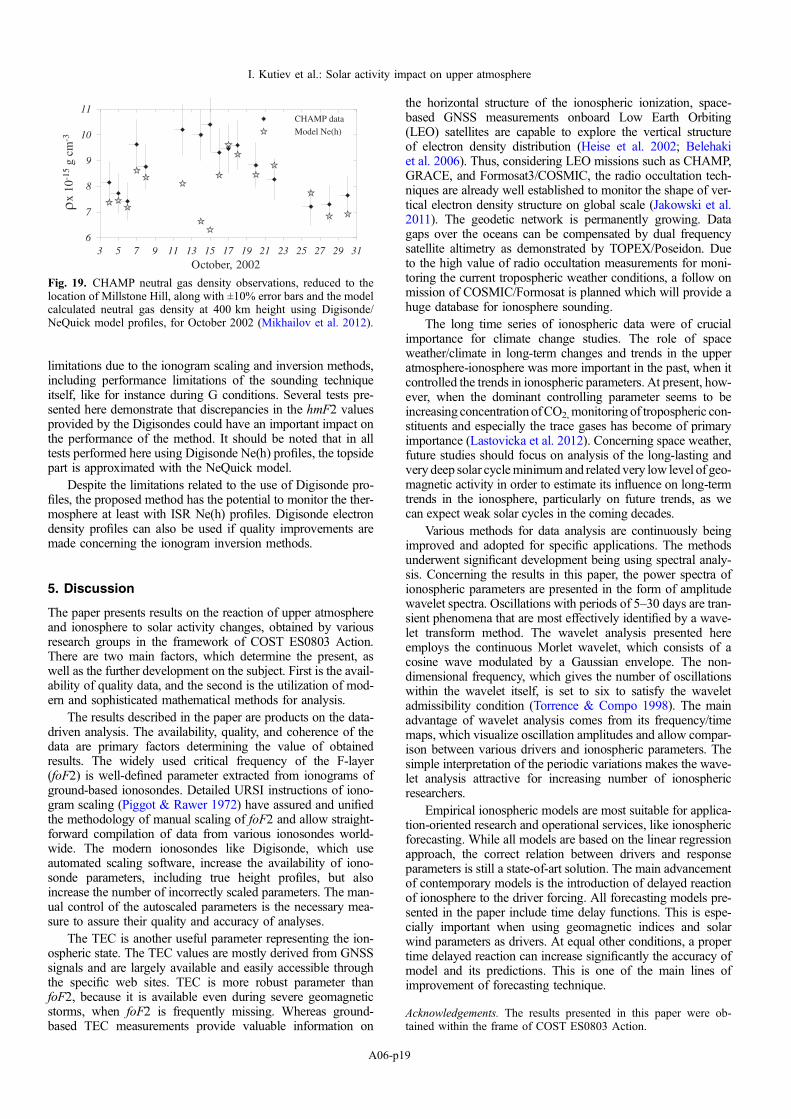
limitations due to the ionogram scaling and inversion methods,including performance limitations of the sounding techniqueitself, like for instance during G conditions. Several tests pre-sented here demonstrate that discrepancies in the hmF2 valuesprovided by the Digisondes could have an important impact onthe performance of the method. It should be noted that in alltests performed here using Digisonde Ne(h) profiles, the topsidepart is approximated with the NeQuick model.

Despite the limitations related to the use of Digisonde pro-files, the proposed method has the potential to monitor the ther-mosphere at least with ISR Ne(h) profiles. Digisonde electrondensity profiles can also be used if quality improvements aremade concerning the ionogram inversion methods.

5. Discussion

The paper presents results on the reaction of upper atmosphereand ionosphere to solar activity changes, obtained by variousresearch groups in the framework of COST ES0803 Action.There are two main factors, which determine the present, aswell as the further development on the subject. First is the avail-ability of quality data, and the second is the utilization of mod-ern and sophisticated mathematical methods for analysis.

The results described in the paper are products on the data-driven analysis. The availability, quality, and coherence of thedata are primary factors determining the value of obtainedresults. The widely used critical frequency of the F-layer(foF2) is well-defined parameter extracted from ionograms ofground-based ionosondes. Detailed URSI instructions of iono-gram scaling (Piggot & Rawer 1972) have assured and unifiedthe methodology of manual scaling of foF2 and allow straight-forward compilation of data from various ionosondes world-wide. The modern ionosondes like Digisonde, which useautomated scaling software, increase the availability of iono-sonde parameters, including true height profiles, but alsoincrease the number of incorrectly scaled parameters. The man-ual control of the autoscaled parameters is the necessary mea-sure to assure their quality and accuracy of analyses.

The TEC is another useful parameter representing the ion-ospheric state. The TEC values are mostly derived from GNSSsignals and are largely available and easily accessible throughthe specific web sites. TEC is more robust parameter thanfoF2, because it is available even during severe geomagneticstorms, when foF2 is frequently missing. Whereas ground-based TEC measurements provide valuable information on

the horizontal structure of the ionospheric ionization, space-based GNSS measurements onboard Low Earth Orbiting(LEO) satellites are capable to explore the vertical structureof electron density distribution (Heise et al. 2002; Belehakiet al. 2006). Thus, considering LEO missions such as CHAMP,GRACE, and Formosat3/COSMIC, the radio occultation tech-niques are already well established to monitor the shape of ver-tical electron density structure on global scale (Jakowski et al.2011). The geodetic network is permanently growing. Datagaps over the oceans can be compensated by dual frequencysatellite altimetry as demonstrated by TOPEX/Poseidon. Dueto the high value of radio occultation measurements for moni-toring the current tropospheric weather conditions, a follow onmission of COSMIC/Formosat is planned which will provide ahuge database for ionosphere sounding.

The long time series of ionospheric data were of crucialimportance for climate change studies. The role of spaceweather/climate in long-term changes and trends in the upperatmosphere-ionosphere was more important in the past, when itcontrolled the trends in ionospheric parameters. At present, how-ever, when the dominant controlling parameter seems to beincreasing concentration ofCO2,monitoring of tropospheric con-stituents and especially the trace gases has become of primaryimportance (Lastovicka et al. 2012). Concerning space weather,future studies should focus on analysis of the long-lasting andvery deep solar cycleminimum and related very low level of geo-magnetic activity in order to estimate its influence on long-termtrends in the ionosphere, particularly on future trends, as wecan expect weak solar cycles in the coming decades.

Various methods for data analysis are continuously beingimproved and adopted for specific applications. The methodsunderwent significant development being using spectral analy-sis. Concerning the results in this paper, the power spectra ofionospheric parameters are presented in the form of amplitudewavelet spectra. Oscillations with periods of 5–30 days are tran-sient phenomena that are most effectively identified by a wave-let transform method. The wavelet analysis presented hereemploys the continuous Morlet wavelet, which consists of acosine wave modulated by a Gaussian envelope. The non-dimensional frequency, which gives the number of oscillationswithin the wavelet itself, is set to six to satisfy the waveletadmissibility condition (Torrence & Compo 1998). The mainadvantage of wavelet analysis comes from its frequency/timemaps, which visualize oscillation amplitudes and allow compar-ison between various drivers and ionospheric parameters. Thesimple interpretation of the periodic variations makes the wave-let analysis attractive for increasing number of ionosphericresearchers.

Empirical ionospheric models are most suitable for applica-tion-oriented research and operational services, like ionosphericforecasting. While all models are based on the linear regressionapproach, the correct relation between drivers and responseparameters is still a state-of-art solution. The main advancementof contemporary models is the introduction of delayed reactionof ionosphere to the driver forcing. All forecasting models pre-sented in the paper include time delay functions. This is espe-cially important when using geomagnetic indices and solarwind parameters as drivers. At equal other conditions, a propertime delayed reaction can increase significantly the accuracy ofmodel and its predictions. This is one of the main lines ofimprovement of forecasting technique.

Acknowledgements. The results presented in this paper were ob-tained within the frame of COST ES0803 Action.

3 5 7 9 11 13 15 17 19 21 23 25 27 29 31October, 2002

6

7

8

9

10

11

x 1

0-15

g cm

-3

CHAMP data

Model Ne(h)

r

Fig. 19. CHAMP neutral gas density observations, reduced to thelocation of Millstone Hill, along with ±10% error bars and the modelcalculated neutral gas density at 400 km height using Digisonde/NeQuick model profiles, for October 2002 (Mikhailov et al. 2012).

I. Kutiev et al.: Solar activity impact on upper atmosphere

A06-p19

References

Altadill, D., and E.M. Apostolov, Time and scale size of planetarywave signatures in the ionospheric F region: Role of thegeomagnetic activity and mesosphere/lower thermosphere wind,J. Geophys. Res., 108, 1403, DOI: 10.1029/2003JA010015, 2003.

Altadill, D., E.M. Apostolov, J.G. Sole, and Ch. Jacobi, Origin anddevelopment of vertical propagating oscillations with periods ofplanetary waves in the ionospheric F region, Phys. Chem. EarthPart C, 26, 387–393, 2001.

Altadill, D., J.M. Torta, and E. Blanch, Proposal of new models ofthe bottom-side B0 and B1 parameters for IRI, Adv. Space Res.,43, 1825–1834, 2009.

Andonov, B., P. Mukhtarov, and D. Pancheva, Empirical model ofthe TEC response to the geomagnetic activity over the NorthAmerican region, Adv. Space Res., 48, 1041–1048,DOI: 10.1016/j.asr.2011.05.007, 2011.

Araujo-Pradere, E.A., T.J. Fuller-Rowell, and M.V. Codrescu,STORM: an empirical storm-time ionospheric correction model,1, Model description, Radio Sci., 37, 5, 1070,DOI: 10.1029/2001RS002467, 2002.

Bartels, J., Twenty-seven day recurrences in terrestrial-magnetic andsolar activity, 1923–1933, Terr. Magn. Atmos. Electr., 39 (3),201–202, DOI: 10.1029/TE039i003p00201, 1934.

Belehaki, A., P. Marinov, I. Kutiev, N. Jakowski, and S.M. Stankov,Comparison of the topside ionosphere scale height determined bytopside sounders model and bottomside digisonde profiles, Adv.Space Res., 37, 963–966, 2006.

Bilitza, D., International reference ionosphere 2000, Radio Science,36 (2), 261–275, 2000.

Blanch, E., Typical behaviour of the ionospheric vertical structureduring quiet and disturbed conditions, Doctoral Thesis, Univ.Ramon Llull, Barcelona, Spain, 2009.

Blanch, E., and D. Altadill, Ionospheric peak height densitydisturbance in response to solar wind conditions: a potentialempirical model, Paper presented at the COST ES0803 Work-shop, 1–3 April, Frascati, Italy, 2009a.

Blanch, E., and D. Altadill, Empirical model for the electron densitypeak height disturbance in response to solar wind conditions,Paper presented at the 6th General Assembly of the EuropeanGeosciences Union, Session ST12, EGU2009- 4568, Vienna,Austria, 19-24 April, 2009b.

Blanch, E., and D. Altadill, Mid-latitude F-region peak heightchanges in response to interplanetary magnetic field conditionsand modeling results, J. Geophys. Res., 117, A12,DOI: 10.1029/2012JA018009, 2012.

Borovsky, J.E., and M.H. Denton, Differences between CME-drivenstorms and CIR-driven storms, J. Geophys. Res., 111, A07S08,DOI: 10.1029/2005JA011447, 2006.

Bremer, J., J. Lastovicka, A.V. Mikhailov, D. Altadill, P. Bencze, D.Buresova, G. De Franceschi, C. Jacobi, S. Kouris, L. Perrone, andE. Turunen, Climate of the upper atmosphere, Ann. Geophys., 52(3/4), 273–299, 2009.

Dasso, S., C.H. Mandrini, B. Schmieder, H. Cremades, C. Cid, et al.,Linking two consecutive nonmerging magnetic clouds with theirsolar sources, J. Geophys. Res., 114, A2,DOI: 10.1029/2008JA013102, 2009.

Denton, M.H., T. Ulich, and E. Turunen, Modification of midlatitudeionospheric parameters in the F2 layer by persistent high-speedsolar wind streams, Space Weather, 7, S04006,DOI: 10.1029/2008SW000443, 2009.

Emmert, J.T., J.M. Picone, and R.R. Meier, Thermospheric globalaverage density trends 1967–2007, derived from orbits of 5000near-Earth objects, Geophys. Res. Lett., 35, L05101,DOI: 10.1029/2007GL032809, 2008.

Hall, C.M., K. Rypdal, and M. Rypdal, The E region at 69� N,19� E: trends, significances, and detectability, J. Geophys. Res.,116, A05309, DOI: 10.1029/2011JA016431, 2011.

Heise, S., N. Jakowski, A. Wehrenpfennig, Ch. Reigber, and H.Luehr, Sounding of the topside ionosphere/plasmasphere based on

GPS measurements from CHAMP: initial results, Geophys. Res.Lett., 29 (14), DOI: 10.1029/2002GL014738, 2002.

Jakowski, N., TEC monitoring by using satellite positioningsystems, in Modern Ionospheric Science, edited by H. Kohl, R.Ruster, and K. Schlegel, EGS, Katlenburg-Lindau, ProduServGmbH Verlagsservice, Berlin, pp. 371–390, 1996.

Jakowski, N., B. Fichtelmann, and A. Jungstand, Solar activitycontrol of ionospheric and thermospheric processes, J. Atmos.Terr. Phys., 53, 1125–1130, 1991.

Jakowski, N., J. Mielich, C. Borries, L. Cander, A. Krankowski, B.Nava, and S.M. Stankov, Large scale ionospheric gradients overEurope observed in October 2003, J. Atmos. Sol. Terr. Phys., 70,15, DOI: 10.1016/j.jastp.2008.03.020, 2008.

Jakowski, N., C. Mayer, M.M. Hoque, and V. Wilken, TEC modelsand their use in ionosphere monitoring, Radio Sci., 46, RS0D18,DOI: 10.1029/2010RS004620, 2011.

Koutroumbas, K., I. Tsagouri, and A. Belehaki, Time seriesautoregression technique implemented on-line in DIAS systemfor ionospheric forecast over Europe, Ann. Geophys., 26 (2), 371–386, 2008.

Kutiev, I., S.Watanabe, Y. Otsuka, and A. Saito, Total electron contentbehavior over Japan during geomagnetic storms, J. Geophys. Res.,110 (A1), A01308, DOI: 10.1029/2004JA010586, 2005.

Kutiev, I., Y. Otsuka, D. Pancheva, and R. Heelis, Response of low-latitude ionosphere to medium-term changes of solar andgeomagnetic activity, J. Geophys. Res., 117, A08330, DOI:10.1029/2012JA017641, 2012.

Lastovicka, J., Global pattern of trends in the upper atmosphere andionosphere: recent progress, J. Atmos. Solar Terr. Phys., 71(14-15), 1514–1528, 2009.

Lastovicka, J., R.A. Akmaev, G. Beig, J. Bremer, and J.T. Emmert,Global change in the upper atmosphere, Science, 314, 1253–1254,DOI: 10.1126/science.1135134, 2006.

Lastovicka, J., S.C. Solomon, and L. Qian, Trends in the neutral andionized upper atmosphere, Space Sci. Rev., 168, 113–145,DOI: 10.1007/s11214-011-9799-3, 2012.

Lean, J.L., H.P. Warren, J.T. Mariska, and J. Bishop, A new model ofsolar EUV irradiance variability 2. Comparisons with empiricalmodels and observations and implications for space weather, J.Geophys. Res., 108 (A2), 1059, DOI: 10.1029/2001JA009238,2003.

Lei, J., J.P. Thayer, J.M. Forbes, E.K. Sutton, and R.S. Nerem,Rotating solar coronal holes and periodic modulation of the upperatmosphere. Geophys. Res. Lett., 35, L10109,DOI: 10.1029/2008GL033875, 2008.

Magdaleno, S., D. Altadill, M. Herraiz, E. Blanch, and B. de laMorena, Ionospheric peak height behaviour for low, middle andhigh latitudes, A potential empirical model for quiet conditions –Comparison with the IRI-2007 model, J. Atmos. Sol. Terr. Phys.,73 (13), 1810–1817, DOI: 10.1016/j.jastp.2011.04.019, 2011.

Mayer, C., and N. Jakowski, Enhanced E layer ionization in theauroral zones observed by radio occultation measurementsonboard CHAMP and Formosat-3/COSMIC, Ann. Geophys., 27,1207–1212, 2009.

Mayer, C., B. Belabbas, N. Jakowski, M. Meurer, and W. Dunkel,Ionosphere threat space model assessment for GBAS, Proc. IONGNSS 2009, Savannah, GA, USA, 22–25 September, 2009.

Maunder, W.E., Magnetic disturbances, 1882 to 1903, as recorded atthe Royal Observatory, Greenwich, and their association with-sunspots, Mon. Not. R. Astron. Soc., 65 (1), 2–34, 1904.

Mikhailov, A.V., A. Belehaki, L. Perrone, B. Zolesi, and I. Tsagouri,Retrieval of thermospheric parameters from routine ionosphericobservations: assessment of method’s performance at mid-latitudes daytime hours, J. Space Weather Space Clim., 2, A03,DOI: 10.1051/swsc/2012002, 2012.

Mlynczak,M.G., F.J.Martin-Torres, C.J.Mertens, B.T.Marshall, R.E.Thompson, J.U. Kozyra, E.E. Remsberg, L.L. Gordley, J.M.RusselIII, and T. Woods, Solar-terrestrial coupling evidenced byperiodic behavior in geomagnetic indexes and the infrared energybudget of the thermosphere,Geophys. Res. Lett., 35, L05808, 2008.

J. Space Weather Space Clim. 3 (2013) A06

A06-p20

Mlynczak, M., L. Hunt, B.T. Marshall, F.J. Martin-Torres, C.J.Mertens, et al., Observations of infrared radiative cooling in thethermosphere on daily to multiyear timescales from the TIMED/SABER instrument, J. Geophys. Res., 115, A03309,DOI: 10.1029/2009JA014713, 2010.

Muhtarov, P., I. Kutiev, and L.R. Cander, Geomagnetically corre-lated autoregression model for short-term prediction of ionopsh-eric parameters, Inverse Prob., 18, 49–65, 2002.

Mukhtarov, P., and D. Pancheva, Thermosphere-ionosphere couplingin response to recurrent geomagnetic activity, J. Atmos. Sol. Terr.Phys., 74, 132–145, DOI: 10.1016/j.jastp.2012.02.013, 2012.

Mursula, K., and D. Martini, Centennial increase in geomagneticactivity: Latitudinal difference and global estimates, J. Geophys.Res., 111, A08209, DOI: 10.1029/2005JA011549, 2006.

Pancheva, D., and P. Mukhtarov, Wavelet analysis on transientbehaviour of tidal amplitude fluctuations observed by meteorradar in the lower thermosphere above Bulgaria, Ann. Geophys.,18, 316–333, 2000.

Pancheva, D., N. Mitchell, R.R. Clark, J. Drobjeva, and J.Lastovicka, Variability in the maximum height of the ionosphericF2-layer over Millstone Hill (September 1998–March 2000);influence from below and above, Ann. Geophys., 20, 1807–1819,2002.

Perrone, L., L. Alfonsi, V. Romano, and G. De Franceschi, Polar capabsorption events of Novembre 2001 at Terra Nova Bay,Antartica, Ann. Geophys., 22, 1633–1648, 2004.

Perrone, L., M. Parisi, A. Meloni, M. Damasso, and M. Galliani,Study on solar sources and polar cap absorption events recordedin Antarctica, Adv. Space Res., 43 (11), 1660–1668, 2009.

Piggot, W.R., and K. Rawer, URSI Handbook of IonogramsInterpretation and Reduction, 2nd edn. report UAG-23A,WDC-A for STP, Boulder, Co, 1972.

Qian, L., S.C. Solomon, R.G. Roble, and T.J. Kane, Modelsimulations of global change in the ionosphere, Geophys. Res.Lett., 35, L07811, DOI: 10.1029/2007GL033156, (2008).

Qian, L., J. Lastovicka, R.G. Roble, and S.C. Solomon, Progress inobservations and simulations of global change in the upperatmosphere, J. Geophys. Res., 116 (A4), A00H03,DOI: 10.1029/2010JA016317, 2011.

Reinisch, B.W. and X. Huang, Automatic calculation of electrondensity profiles from digital ionoograms 3. Processing ofbottomside ionograms, Radio Sci., 18 (3), 477–492, DOI:10.1029/RS18i003p00477, 1983.

Saiz, E., C. Cid, and Y. Cerrato, Forecasting intense geomagneticactivity using interplanetary magnetic field data, Ann. Geophys.,26, 3989–3998, 2008.

Solomon, S.C., T.N. Woods, L.V. Didkovsky, J.T. Emmert, and L.Qian, Anomalously low solar extreme-ultraviolet irradiance and

thermospheric density during solar minimum, Geophys. Res. Lett.,37, L16103, DOI: 10.1029/2010GL044468, 2010.

Temmer, M., B. Vrsnak, and A.M. Veronig, Periodic appearance ofcoronal holes and the related variation of solarwind parameters, Sol.Phys., 241, 371–383, DOI: 10.1007/s11207-007-0336-1, 2007.

Thayer, J.P., J. Lei, J.M. Forbes, E.K. Sutton, and R.S. Nerem,Thermospheric density oscillations due to periodic solar windhigh-speed streams, J. Geophys. Res., 113, A06307, DOI:10.1029/2008JA013190, 2008.

Torrence, C., and G. Compo, A practical guide to wavelet analysis,Bull. Am. Meteorol. Soc., 79, 61–78, 1998.

Tsagouri, I., B. Zolesi, A. Belehaki, and L.R. Cander, Evaluation ofthe performance of the real-time updated simplified ionosphericregional model for the European area, J. Atmos. Sol.-Terr. Phys.,67 (12), 1137–1146, DOI: 10.1016/j.jastp.2005.01.012, 2005.

Tsagouri, I., Evaluation of the performance of DIAS ionosphericforecasting models, J. Space Weather Space Space Clim., 1, A02,DOI: 10.1051/swsc/2011110003, 2011.

Tsagouri, I., and A. Belehaki, ‘‘A new empirical model of middlelatitude ionospheric response for space weather applications, Adv.Space Res., 37 (2), 420–425, 2006.

Tsagouri, I., and A. Belehaki, An upgrade of the solar-wind-drivenempirical model for the middle latitude ionospheric storm-timeresponse, J. Atmos. Sol. Terr. Phys., 70 (16), 2061–2076, 2008.

Tsagouri, I., B. Zolesi, R. Cander Lj, and A. Belehaki, DIASeffective sunspot number as an indicator of the ionosphericactivity level over Europe, Acta Geophys.,DOI: 10.2478/s11600-009-0045-2, 2009.

Tsurutani, B., W. Gonzalez, A. Gonzalez, A.L.C. Gonzalez,F. Guarnieri, et al., Corotating solar wind streams and recurrentgeomagnetic: a review, J. Geophys. Res., 111, A07S01,DOI: 10.1029/2005JA011273, 2006.

Vrsnak, B., M. Temmer, and A.M. Veroning, Coronal holes and solarwith high-speed streams: I. Forecasting the solar wind parameters,Sol. Phys., 240, 315–330, 2007.

Xie, H.N., N. Gopalswamy, P.K. Manoharan, A. Lara, S. Yashiro,and S. Lepri, Long-lived geomagnetic storms and corononal massejections, J. Geophys. Res, 111, A1,DOI: 10.10129/2005JA011287, 2006.

Zolesi, B., A. Belehaki, I. Tsagouri, and L.R. Cander, Real-timeupdating of the simplified ionospheric regional model foroperational applications, Radio Sci., 39, RS2011,DOI: 10.1029/2003RS002936, 2004.

Zhang, J., I.G. Richardson, D.F. Webb, N. Gopalswamy, E.Huttunen, Correction to Solar and interplanetary sources of majorgeomagnetic storms (Dst � �1000 nT) during 1996–2005,J. Geophys. Res, 112, DOI: 10.10129/2007JA012891, 2007.

Cite this article as: Kutiev I, Tsagouri I, Perrone L, Pancheva D, Mukhtarov P, Mikhailov A, Lastovicka J, Jakowski N, Buresova D,Blanch E, Andonov B, Altadill D, Magdaleno S, Parisi M &Miquel Torta J: Solar activity impact on the Earth’s upper atmosphere. J.Space Weather Space Clim., 2013, 3, A06.

I. Kutiev et al.: Solar activity impact on upper atmosphere

A06-p21