PCM & PSTN - Imperial College London · PCM & PSTN Professor A. Manikas ... (PDH) Synchronous...
64
PCM & PSTN Professor A. Manikas Imperial College London EE303 - Communication Systems Prof. A. Manikas (Imperial College) EE303: PCM & PSTN 7 Dec 2011 1 / 64
Transcript of PCM & PSTN - Imperial College London · PCM & PSTN Professor A. Manikas ... (PDH) Synchronous...
PCM & PSTN
Professor A. Manikas
Imperial College London
EE303 - Communication Systems
Prof. A. Manikas (Imperial College) EE303: PCM & PSTN 7 Dec 2011 1 / 64
Table of Contents1 Introduction2 PCM: Bandwidth & Bandwidth Expansion Factor3 The Quantization Process (output point-A2)
Uniform QuantizersComments on Uniform QuantiserNon-Uniform Quantizersmax(SNR) Non-Uniform QuantisersCompanders (non-Uniform Quantizers)Compression Rules (A and mu)The 6dB Law
Di§erential Quantizers4 Noise E§ects in a Binary PCM
Threshold E§ects in a Binary PCMComments on Threshold E§ects
5 CCITT Standards: Di§erential PCM (DPCM)6 Introduction to Telephone Network
CCITT recommendations for PCM (24-channels and 30-channels)Single-Channel Path of 2nd CCITT rec. (30-channels PCM)Implementation of 2nd PCM CCITT RecommPlesiochronous digital hierarchies (PDH)Synchronous digital hierarchies (SONET/SDH)
Prof. A. Manikas (Imperial College) EE303: PCM & PSTN 7 Dec 2011 2 / 64
Introduction
Introduction
Prof. A. Manikas (Imperial College) EE303: PCM & PSTN 7 Dec 2011 3 / 64
Introduction
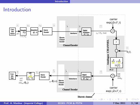
PCM = sampled quantized values of an analogue signal aretransmitted via a sequence of codewords.
i.e. after sampling & quantization, a Source Encoder is used to mapthe quantized levels (i.e. o/p of quantizer) to codewords of γ bits
i.e. quantized level 7! codeword of γ bits
and, then a digital modulator is used to transmit the bits, i.e. PCMsystem
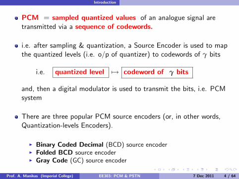
There are three popular PCM source encoders (or, in other words,Quantization-levels Encoders).
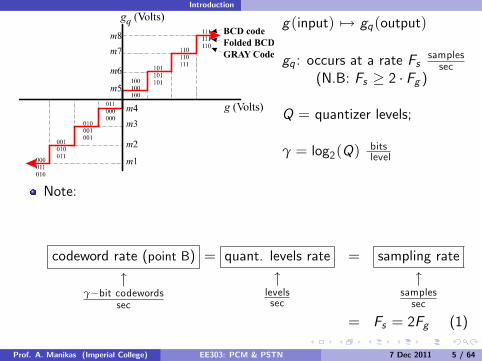
I Binary Coded Decimal (BCD) source encoderI Folded BCD source encoderI Gray Code (GC) source encoder
Prof. A. Manikas (Imperial College) EE303: PCM & PSTN 7 Dec 2011 4 / 64
Introduction
g(input) 7! gq(output)
gq : occurs at a rate Fssamplessec
(N.B: Fs # 2 · Fg )
Q = quantizer levels;
γ = log2(Q)bitslevel
Note:
codeword rate (point B)
"γ%bit codewords
sec
= quant. levels rate
"levelssec
= sampling rate
"samplessec
= Fs = 2Fg (1)
Prof. A. Manikas (Imperial College) EE303: PCM & PSTN 7 Dec 2011 5 / 64
Introduction
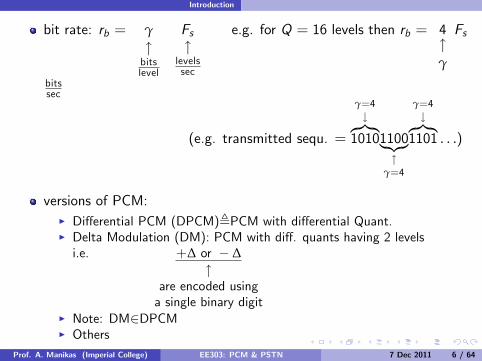
bit rate: rb = γ"bitslevel
Fs"
levelssec
e.g. for Q = 16 levels then rb = 4"γ
Fs
bitssec
(e.g. transmitted sequ. =
γ=4#z}|{
10101100|{z}"
γ=4
γ=4#z}|{
1101 . . .)
versions of PCM:I Di§erential PCM (DPCM),PCM with di§erential Quant.I Delta Modulation (DM): PCM with di§. quants having 2 levelsi.e. +∆ or % ∆
"are encoded usinga single binary digit
I Note: DM2DPCMI Others
Prof. A. Manikas (Imperial College) EE303: PCM & PSTN 7 Dec 2011 6 / 64
PCM: Bandwidth & Bandwidth Expansion Factor
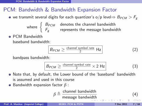
PCM: Bandwidth & Bandwidth Expansion Factorwe transmit several digits for each quantizer’s o/p level) BPCM > Fg
where%BPCM denotes the channel bandwidthFg represents the message bandwidth
PCM Bandwidthbaseband bandwidth:
BPCM # channel symbol rate2 Hz (2)
bandpass bandwidth:
BPCM # channel symbol rate2 ) 2 Hz (3)
Note that, by default, the Lower bound of the ‘baseband’ bandwidthis assumed and used in this courseBandwidth expansion factor β :
β , channel bandwidthmessage bandwidth
(4)
Prof. A. Manikas (Imperial College) EE303: PCM & PSTN 7 Dec 2011 7 / 64
PCM: Bandwidth & Bandwidth Expansion Factor
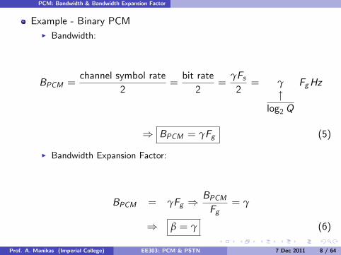
Example - Binary PCMI Bandwidth:
BPCM =channel symbol rate
2=bit rate2
=γFs2= γ
"log2 Q
FgHz
) BPCM = γFg (5)
I Bandwidth Expansion Factor:
BPCM = γFg )BPCMFg
= γ
) β = γ (6)
Prof. A. Manikas (Imperial College) EE303: PCM & PSTN 7 Dec 2011 8 / 64
The Quantization Process (output point-A2)
The Quantization Process (output point-A2)
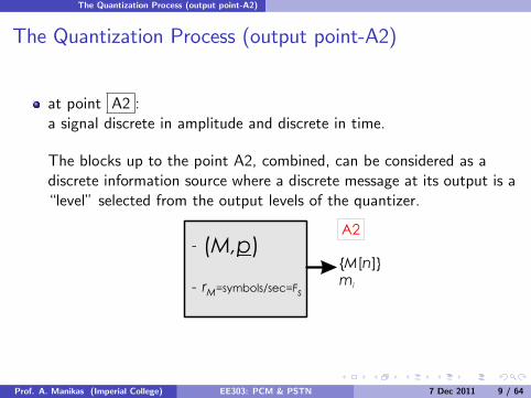
at point A2 :a signal discrete in amplitude and discrete in time.
The blocks up to the point A2, combined, can be considered as adiscrete information source where a discrete message at its output is a“level” selected from the output levels of the quantizer.
Prof. A. Manikas (Imperial College) EE303: PCM & PSTN 7 Dec 2011 9 / 64
The Quantization Process (output point-A2)
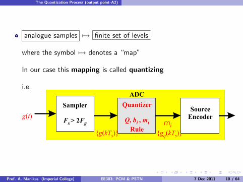
analogue samples 7! finite set of levels
where the symbol 7! denotes a “map”
In our case this mapping is called quantizing
i.e.
Prof. A. Manikas (Imperial College) EE303: PCM & PSTN 7 Dec 2011 10 / 64
The Quantization Process (output point-A2)
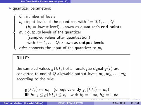
quantizer parameters:8>>>>>>>><
>>>>>>>>:
Q : number of levelsbi : input levels of the quantizer, with i = 0, 1, . . . ,Q
(b0 = lowest level): known as quantizer’s end-pointsmi : outputs levels of the quantizer
(sampled values after quantization)with i = 1, . . . ,Q; known as output-levels
rule: connects the input of the quantizer to mi
RULE:
the sampled values g(kTs ) of an analogue signal g(t) areconverted to one of Q allowable output-levels m1,m2, . . . ,mQaccording to the rule:
g(kTs ) 7! mi (or equivalently gq(kTs ) = mi )i§ bi%1 * g(kTs ) * bi with b0 = %∞, bQ = +∞
Prof. A. Manikas (Imperial College) EE303: PCM & PSTN 7 Dec 2011 11 / 64
The Quantization Process (output point-A2)
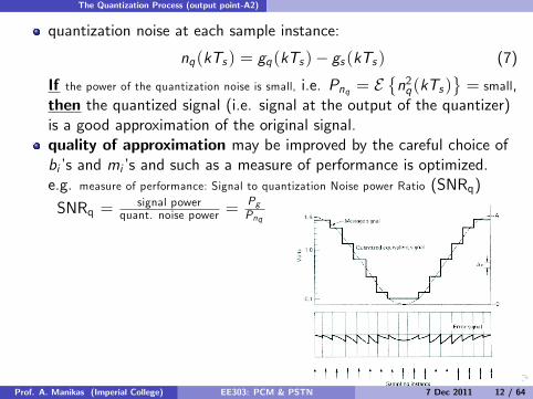
quantization noise at each sample instance:
nq(kTs ) = gq(kTs )% gs (kTs ) (7)
If the power of the quantization noise is small, i.e. Pnq = E*n2q(kTs )
+= small,
then the quantized signal (i.e. signal at the output of the quantizer)is a good approximation of the original signal.quality of approximation may be improved by the careful choice ofbi ’s and mi ’s and such as a measure of performance is optimized.e.g. measure of performance: Signal to quantization Noise power Ratio (SNRq)
SNRq =signal power
quant. noise power =PgPnq
Prof. A. Manikas (Imperial College) EE303: PCM & PSTN 7 Dec 2011 12 / 64
The Quantization Process (output point-A2)
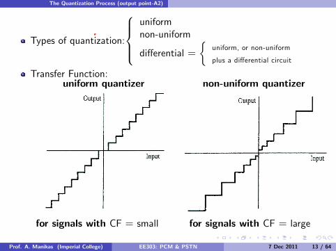
Types of quantization:
8>><
>>:
uniformnon-uniform
di§erential =%
uniform, or non-uniform
plus a di§erential circuit
Transfer Function:uniform quantizer non-uniform quantizer
for signals with CF = small for signals with CF = large
Prof. A. Manikas (Imperial College) EE303: PCM & PSTN 7 Dec 2011 13 / 64
The Quantization Process (output point-A2)
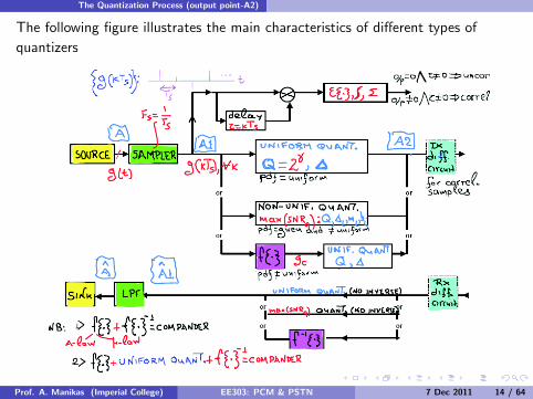
The following figure illustrates the main characteristics of di§erent types ofquantizers
Prof. A. Manikas (Imperial College) EE303: PCM & PSTN 7 Dec 2011 14 / 64
The Quantization Process (output point-A2) Uniform Quantizers
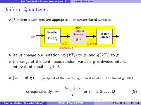
Uniform Quantizers
Uniform quantizers are appropriate for uncorrelated samples
let us change our notation: gq(kTs ) to gq and g(kTs ) to g
the range of the continuous random variable g is divided into Qintervals of equal length ∆
(value of g) 7! (midpoint of the quantizing interval in which the value of g falls)
or equivalently mi =bi%1 + bi
2for i = 1, 2, . . . ,Q (8)
Prof. A. Manikas (Imperial College) EE303: PCM & PSTN 7 Dec 2011 15 / 64
The Quantization Process (output point-A2) Uniform Quantizers
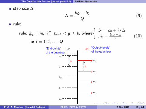
step size ∆:
∆ =bQ % b0Q
(9)
rule:
rule: gq = mi i§ bi%1 < g * bi where%bi = b0 + i · ∆mi =
bi%1+bi2
for i = 1, 2, . . . ,Q(10)
Prof. A. Manikas (Imperial College) EE303: PCM & PSTN 7 Dec 2011 16 / 64
"Output-levels"
of the quantiser"End-points"
of the quantiser
The Quantization Process (output point-A2) Comments on Uniform Quantiser
Comments on Uniform Quantiser
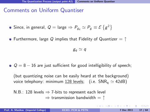
Since, in general, Q = large ) Pgq ' Pg , E*g2+
Furthermore, large Q implies that Fidelity of Quantizer = "
gq ' q
Q = 8% 16 are just su¢cient for good intelligibility of speech;
(but quantizing noise can be easily heard at the background)voice telephony: minimum 128 levels; (i.e. SNRq ' 42dB)
N.B.: 128 levels ) 7-bits to represent each level) transmission bandwidth = "
Prof. A. Manikas (Imperial College) EE303: PCM & PSTN 7 Dec 2011 17 / 64
The Quantization Process (output point-A2) Comments on Uniform Quantiser
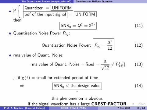
if
(Quantizer = UNIFORMpdf of the input signal = UNIFORM
thenSNRq = Q2 = 22γ (11)
Quantisation Noise Power Pnq :
Quantization Noise Power: Pnq =∆2
12(12)
rms value of Quant. Noise:
rms value of Quant. Noise = fixed =∆p126= f {g} (13)
) if g(t) = small for extended period of time
) SNRq < the design value
"this phenomenon is obvious
if the signal waveform has a large CREST FACTOR
(14)
Prof. A. Manikas (Imperial College) EE303: PCM & PSTN 7 Dec 2011 18 / 64
The Quantization Process (output point-A2) Comments on Uniform Quantiser
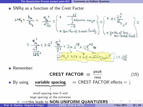
SNRq as a function of the Crest Factor
Remember:
CREST FACTOR !peakrms
(15)
By using variable spacing| {z }"
small spacing near 0 andlarge spacing at the extremes
) CREST FACTOR e§ects = #
I =)this leads to NON-UNIFORM QUANTIZERSProf. A. Manikas (Imperial College) EE303: PCM & PSTN 7 Dec 2011 19 / 64
The Quantization Process (output point-A2) Non-Uniform Quantizers
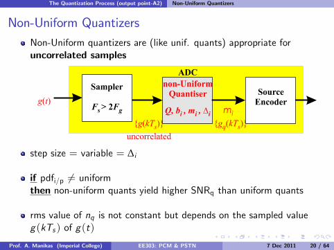
Non-Uniform QuantizersNon-Uniform quantizers are (like unif. quants) appropriate foruncorrelated samples
step size = variable = ∆i
if pdfi/p 6= uniformthen non-uniform quants yield higher SNRq than uniform quants
rms value of nq is not constant but depends on the sampled valueg(kTs ) of g(t)
Prof. A. Manikas (Imperial College) EE303: PCM & PSTN 7 Dec 2011 20 / 64
The Quantization Process (output point-A2) Non-Uniform Quantizers
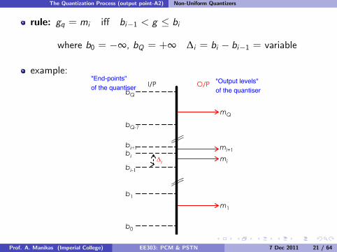
rule: gq = mi i§ bi%1 < g * bi
where b0 = %∞, bQ = +∞ ∆i = bi % bi%1 = variable
example:
Prof. A. Manikas (Imperial College) EE303: PCM & PSTN 7 Dec 2011 21 / 64
"End-points"
of the quantiser"Output levels"
of the quantiser
The Quantization Process (output point-A2) max(SNR) Non-Uniform Quantisers
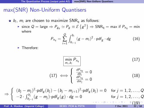
max(SNR) Non-Uniform Quantisers
bi , mi are chosen to maximize SNRq as follows:I since Q = large ) Pgq ' Pg , E
*g2+) SNRq = max if Pnq = min
where
Pnq =Q
∑i=1
Z bi
bi%1(g %mi )2 · pdfg · dg (16)
I Therefore:
minmi ,bi
Pnq (17)
(17) ()
8<
:
dPnqdbj
= 0dPnqdmj
= 0(18)
)
((bj %mj )2·pdfg (bj )% (bj %mj+1)2·pdfg (bj ) = 0 for j = 1, 2, . . . ,Q % 1%2 ·
R bjbj%1(g %mj )·pdfg (g) · dg = 0 for j = 1, 2, . . . ,Q
(19)
In the second branch of Equation-19 the parameter mj can be seen asthe statistical mean of the j th quantizer interval
Prof. A. Manikas (Imperial College) EE303: PCM & PSTN 7 Dec 2011 22 / 64
The Quantization Process (output point-A2) max(SNR) Non-Uniform Quantisers
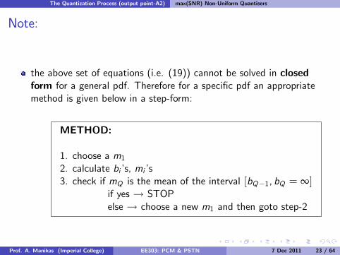
Note:
the above set of equations (i.e. (19)) cannot be solved in closedform for a general pdf. Therefore for a specific pdf an appropriatemethod is given below in a step-form:
METHOD:
1. choose a m12. calculate bi ’s, mi ’s3. check if mQ is the mean of the interval [bQ%1, bQ = ∞]
if yes ! STOPelse ! choose a new m1 and then goto step-2
Prof. A. Manikas (Imperial College) EE303: PCM & PSTN 7 Dec 2011 23 / 64
The Quantization Process (output point-A2) max(SNR) Non-Uniform Quantisers
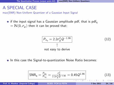
A SPECIAL CASEmax(SNR) Non-Uniform Quantizer of a Gaussian Input Signal
if the input signal has a Gaussian amplitude pdf, that is pdfq= N(0, σg ) then it can be proved that:
Pnq = 2.2σ2gQ%1.96
"not easy to derive
(12)
In this case the Signal-to-quantization Noise Ratio becomes:
SNRq =PgqPnq
=σ2g
2.2σ2g Q%1.96= 0.45Q1.96 (13)
Prof. A. Manikas (Imperial College) EE303: PCM & PSTN 7 Dec 2011 24 / 64
The Quantization Process (output point-A2) Companders (non-Uniform Quantizers)
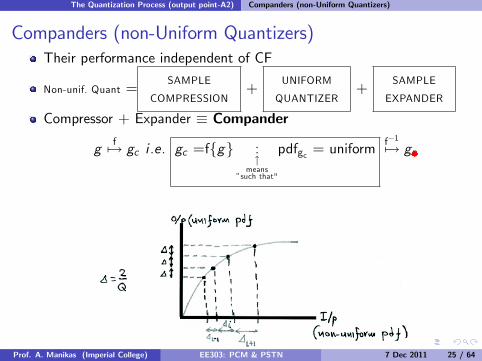
Companders (non-Uniform Quantizers)Their performance independent of CF
Non-unif. Quant =SAMPLE
COMPRESSION+
UNIFORM
QUANTIZER+
SAMPLE
EXPANDER
Compressor + Expander , Compander
gf7! gc i .e. gc =f{g} :
"means
”such that"
pdfgc = uniformf%17! gc
Prof. A. Manikas (Imperial College) EE303: PCM & PSTN 7 Dec 2011 25 / 64
The Quantization Process (output point-A2) Companders (non-Uniform Quantizers)
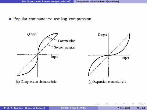
Popular companders: use log compression
Prof. A. Manikas (Imperial College) EE303: PCM & PSTN 7 Dec 2011 26 / 64
The Quantization Process (output point-A2) Companders (non-Uniform Quantizers)
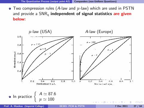
Two compression rules (A-law and µ-law) which are used in PSTNand provide a SNRq independent of signal statistics are givenbelow:
µ-law (USA) A-law (Europe)
In practice%A ' 87.6µ ' 100
Prof. A. Manikas (Imperial College) EE303: PCM & PSTN 7 Dec 2011 27 / 64
The Quantization Process (output point-A2) Companders (non-Uniform Quantizers)
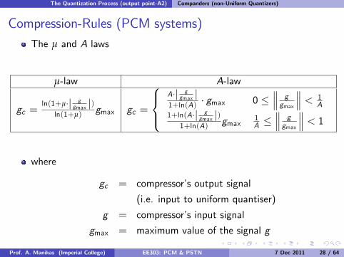
Compression-Rules (PCM systems)The µ and A laws
µ-law A-law
gc =ln(1+µ·| g
gmax |)ln(1+µ)
gmax gc =
8><
>:
A·| ggmax |
1+ln(A) · gmax 0 */// ggmax
/// < 1A
1+ln(A·| ggmax |)
1+ln(A) gmax 1A *
/// ggmax
/// < 1
where
gc = compressor’s output signal
(i.e. input to uniform quantiser)
g = compressor’s input signal
gmax = maximum value of the signal g
Prof. A. Manikas (Imperial College) EE303: PCM & PSTN 7 Dec 2011 28 / 64
The Quantization Process (output point-A2) Companders (non-Uniform Quantizers)
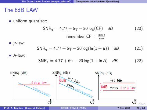
The 6dB LAW
uniform quantizer:
SNRq = 4.77+ 6γ% 20 log(CF) dB (20)
remember CF = peakrms
µ-law:SNRq = 4.77+ 6γ% 20 log(ln(1+ µ)) dB (21)
A-law:SNRq = 4.77+ 6γ% 20 log(1+ lnA) dB (22)
Prof. A. Manikas (Imperial College) EE303: PCM & PSTN 7 Dec 2011 29 / 64
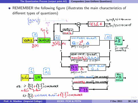
The Quantization Process (output point-A2) Companders (non-Uniform Quantizers)
REMEMBER the following figure (illustrates the main characteristics ofdi§erent types of quantizers)
Prof. A. Manikas (Imperial College) EE303: PCM & PSTN 7 Dec 2011 30 / 64
The Quantization Process (output point-A2) Companders (non-Uniform Quantizers)
COMMENTS
uniform & non-uniform quantizers:
use them when samples are uncorrelated with each other (i.e. thesequence is quantized independently of the values of the precedingsamples)
practical situation:
the sequence {g(kTs )} consists of samples which are correlated witheach other. In such a case use di§erential quantizer.
Prof. A. Manikas (Imperial College) EE303: PCM & PSTN 7 Dec 2011 31 / 64
The Quantization Process (output point-A2) Companders (non-Uniform Quantizers)
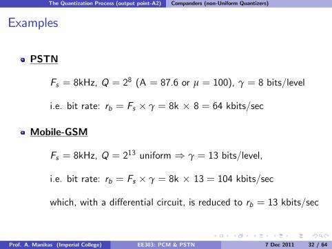
Examples
PSTN
Fs = 8kHz, Q = 28 (A = 87.6 or µ = 100), γ = 8 bits/level
i.e. bit rate: rb = Fs ) γ = 8k ) 8 = 64 kbits/sec
Mobile-GSM
Fs = 8kHz, Q = 213 uniform ) γ = 13 bits/level,
i.e. bit rate: rb = Fs ) γ = 8k ) 13 = 104 kbits/sec
which, with a di§erential circuit, is reduced to rb = 13 kbits/sec
Prof. A. Manikas (Imperial College) EE303: PCM & PSTN 7 Dec 2011 32 / 64
The Quantization Process (output point-A2) Di§erential Quantizers
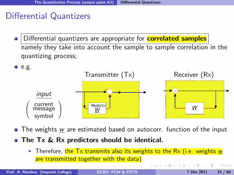
Di§erential Quantizers
Di§erential quantizers are appropriate for correlated samplesnamely they take into account the sample to sample correlation in thequantizing process;
e.g.Transmitter (Tx) Receiver (Rx)
input0
@currentmessagesymbol
1
A
The weights w are estimated based on autocorr. function of the input
The Tx & Rx predictors should be identical.I Therefore, the Tx transmits also its weights to the Rx (i.e. weights ware transmitted together with the data)
Prof. A. Manikas (Imperial College) EE303: PCM & PSTN 7 Dec 2011 33 / 64
The Quantization Process (output point-A2) Di§erential Quantizers
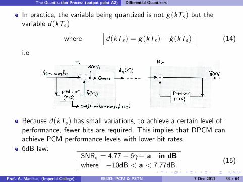
In practice, the variable being quantized is not g(kTs ) but thevariable d(kTs )
where d(kTs ) = g(kTs )% g(kTs ) (14)
i.e.
Because d(kTs ) has small variations, to achieve a certain level ofperformance, fewer bits are required. This implies that DPCM canachieve PCM performance levels with lower bit rates.6dB law:
SNRq = 4.77+ 6γ% a in dBwhere %10dB < a < 7.77dB
(15)
Prof. A. Manikas (Imperial College) EE303: PCM & PSTN 7 Dec 2011 34 / 64
The Quantization Process (output point-A2) Di§erential Quantizers
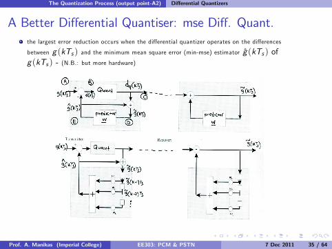
A Better Di§erential Quantiser: mse Di§. Quant.the largest error reduction occurs when the di§erential quantizer operates on the di§erences
between g(kTs ) and the minimum mean square error (min-mse) estimator g(kTs ) ofg(kTs ) - (N.B.: but more hardware)
Prof. A. Manikas (Imperial College) EE303: PCM & PSTN 7 Dec 2011 35 / 64
The Quantization Process (output point-A2) Di§erential Quantizers
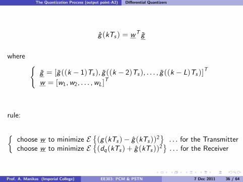
g(kTs ) = wT g
where(g = [g((k % 1)Ts ), g((k % 2)Ts ), . . . , g((k % L)Ts )]T
w = [w1,w2, . . . ,wL]T
rule:
%choose w to minimize E
*(g(kTs )% g(kTs ))2
+. . . for the Transmitter
choose w to minimize E*(dq(kTs ) + g(kTs ))2
+. . . for the Receiver
Prof. A. Manikas (Imperial College) EE303: PCM & PSTN 7 Dec 2011 36 / 64
The Quantization Process (output point-A2) Di§erential Quantizers
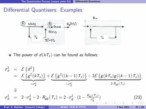
Di§erential Quantisers: Examples
The power of d(kTs ) can be found as follows:
σ2d = E*d2+
= E*g2(kTs )
+| {z }
=σ2g
+ E*g2((k % 1)Ts )
+| {z }
=σ2g
% 2E {g(kTs )g((k % 1)Ts )}| {z }2·Rgg (Ts )
+
σ2d = 2 · σ2g % 2 · Rgg (Ts ) = 2 · σ2g · (1%Rgg (Ts )
σ2g) (23)
Prof. A. Manikas (Imperial College) EE303: PCM & PSTN 7 Dec 2011 37 / 64
The Quantization Process (output point-A2) Di§erential Quantizers
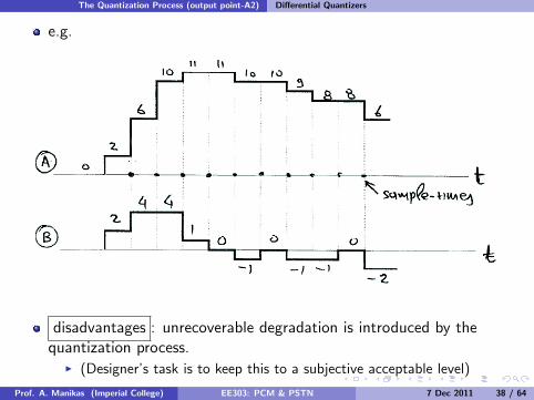
e.g.
disadvantages : unrecoverable degradation is introduced by thequantization process.
I (Designer’s task is to keep this to a subjective acceptable level)
Prof. A. Manikas (Imperial College) EE303: PCM & PSTN 7 Dec 2011 38 / 64
The Quantization Process (output point-A2) Di§erential Quantizers
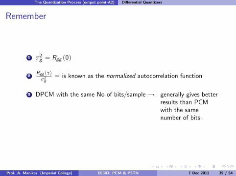
Remember
1 σ2g = Rgg (0)
2Rgg (τ)
σ2g= is known as the normalized autocorrelation function
3 DPCM with the same No of bits/sample ! generally gives betterresults than PCMwith the samenumber of bits.
Prof. A. Manikas (Imperial College) EE303: PCM & PSTN 7 Dec 2011 39 / 64
The Quantization Process (output point-A2) Di§erential Quantizers
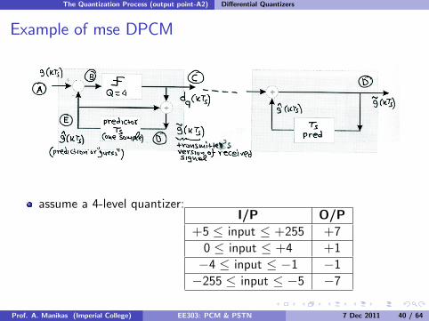
Example of mse DPCM
assume a 4-level quantizer:I/P O/P
+5 * input * +255 +70 * input * +4 +1%4 * input * %1 %1%255 * input * %5 %7
Prof. A. Manikas (Imperial College) EE303: PCM & PSTN 7 Dec 2011 40 / 64
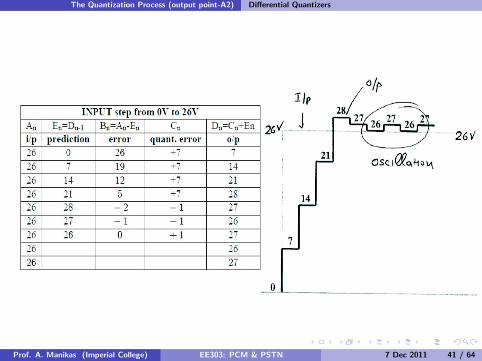
The Quantization Process (output point-A2) Di§erential Quantizers
Prof. A. Manikas (Imperial College) EE303: PCM & PSTN 7 Dec 2011 41 / 64
The Quantization Process (output point-A2) Di§erential Quantizers
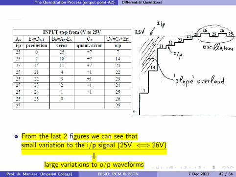
From the last 2 figures we can see thatsmall variation to the i/p signal (25V () 26V)
+large variations to o/p waveforms
Prof. A. Manikas (Imperial College) EE303: PCM & PSTN 7 Dec 2011 42 / 64
Noise E§ects in a Binary PCM
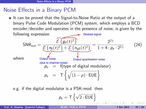
Noise E§ects in a Binary PCMIt can be proved that the Signal-to-Noise Ratio at the output of abinary Pulse Code Modulation (PCM) system, which employs a BCDencoder/decoder and operates in the presence of noise, is given by thefollowing expression
SNRout =E*g0(t)2
+
E {n0(t)2}+ E {nq0(t)2}=
22γ
1+ 4 · pe · 22γ(24)
where
pe = f(type of digital modulator)
pe = T%q
(1% ρ) · EUE5
e.g. if the digital modulator is a PSK-mod. then
pe = Tnp
2 · EUEo
Prof. A. Manikas (Imperial College) EE303: PCM & PSTN 7 Dec 2011 43 / 64
Desired signal
Output noise
(due to channel noise)
Output quantisation noise
Noise E§ects in a Binary PCM Threshold E§ects in a Binary PCM
Threshold E§ects in a Binary PCM
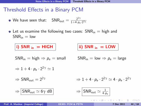
We have seen that: SNRout = 22γ
1+4·pe ·22γ
Let us examine the following two cases: SNRin = high andSNRin = low
i) SNR in = HIGH ii) SNR in = LOW
SNRin = high ) pe = small SNRin = low ) pe = large
) 1+ 4 · pe · 22γ ' 1
) SNRout = 22γ ) 1+ 4 · pe · 22γ ' 4 · pe · 22γ
) SNRout ' 6γ dB ) SNRout ' 14·pe
Prof. A. Manikas (Imperial College) EE303: PCM & PSTN 7 Dec 2011 44 / 64
Noise E§ects in a Binary PCM Threshold E§ects in a Binary PCM
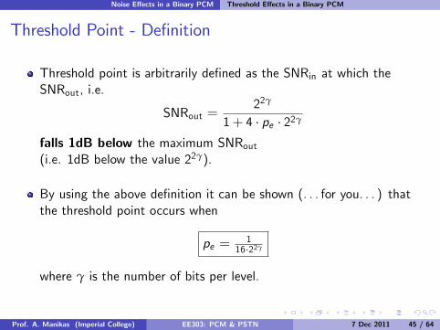
Threshold Point - Definition
Threshold point is arbitrarily defined as the SNRin at which theSNRout, i.e.
SNRout =22γ
1+ 4 · pe · 22γ
falls 1dB below the maximum SNRout(i.e. 1dB below the value 22γ).
By using the above definition it can be shown (. . . for you. . . ) thatthe threshold point occurs when
pe = 116·22γ
where γ is the number of bits per level.
Prof. A. Manikas (Imperial College) EE303: PCM & PSTN 7 Dec 2011 45 / 64
Noise E§ects in a Binary PCM Comments on Threshold E§ects
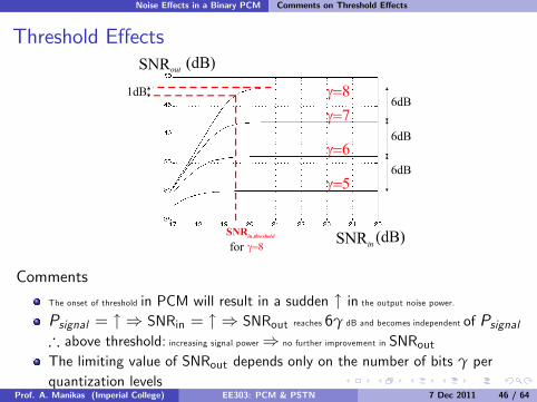
Threshold E§ects
Comments
The onset of threshold in PCM will result in a sudden " in the output noise power.Psignal = " ) SNRin = " ) SNRout reaches 6γ dB and becomes independent of Psignal) above threshold: increasing signal power) no further improvement in SNRoutThe limiting value of SNRout depends only on the number of bits γ perquantization levels
Prof. A. Manikas (Imperial College) EE303: PCM & PSTN 7 Dec 2011 46 / 64
CCITT Standards: Di§erential PCM (DPCM)
CCITT Standards: Di§erential PCM (DPCM)
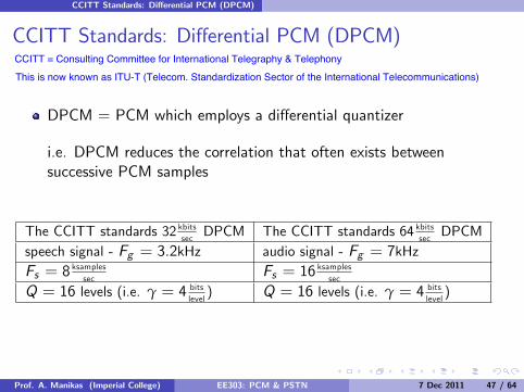
DPCM = PCM which employs a di§erential quantizer
i.e. DPCM reduces the correlation that often exists betweensuccessive PCM samples
The CCITT standards 32 kbitssec
DPCM The CCITT standards 64 kbitssec
DPCMspeech signal - Fg = 3.2kHz audio signal - Fg = 7kHzFs = 8ksamplessec
Fs = 16ksamplessec
Q = 16 levels (i.e. γ = 4 bitslevel) Q = 16 levels (i.e. γ = 4 bits
level)
Prof. A. Manikas (Imperial College) EE303: PCM & PSTN 7 Dec 2011 47 / 64
CCITT = Consulting Committee for International Telegraphy & Telephony
This is now known as ITU-T (Telecom. Standardization Sector of the International Telecommunications)
CCITT Standards: Di§erential PCM (DPCM)
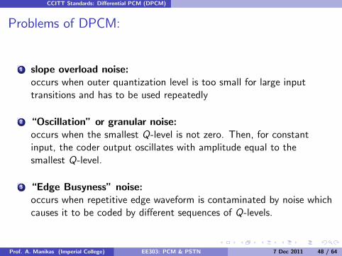
Problems of DPCM:
1 slope overload noise:occurs when outer quantization level is too small for large inputtransitions and has to be used repeatedly
2 “Oscillation” or granular noise:occurs when the smallest Q-level is not zero. Then, for constantinput, the coder output oscillates with amplitude equal to thesmallest Q-level.
3 “Edge Busyness” noise:occurs when repetitive edge waveform is contaminated by noise whichcauses it to be coded by di§erent sequences of Q-levels.
Prof. A. Manikas (Imperial College) EE303: PCM & PSTN 7 Dec 2011 48 / 64
Introduction to Telephone Network
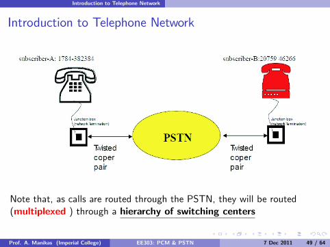
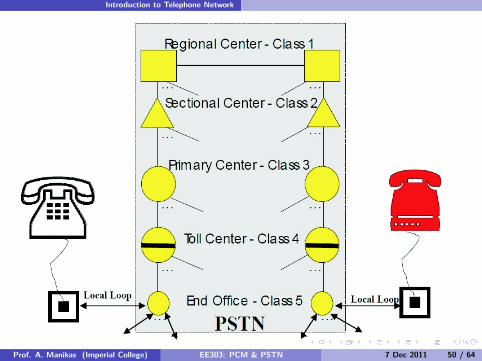
Introduction to Telephone Network
Note that, as calls are routed through the PSTN, they will be routed(multiplexed ) through a hierarchy of switching centers
Prof. A. Manikas (Imperial College) EE303: PCM & PSTN 7 Dec 2011 49 / 64
Introduction to Telephone Network
Prof. A. Manikas (Imperial College) EE303: PCM & PSTN 7 Dec 2011 50 / 64
Introduction to Telephone NetworkCCITT recommendations for PCM (24-channels and
30-channels)
CCITT recommendations for PCM(24-channels and 30-channels)
1960 British Post O¢ce (BPO) (currently BT) had established a24-ch PCM system with objective the system to be available in1968. Some of this work become the basis to the formation of anumber of CCITT recommendations.
In Europe, the original 24-ch PCM systems , which were designedmainly for up to 32Km transmission routes, have been replaced by30-ch PCM systems .
Prof. A. Manikas (Imperial College) EE303: PCM & PSTN 7 Dec 2011 51 / 64
Introduction to Telephone NetworkCCITT recommendations for PCM (24-channels and
30-channels)
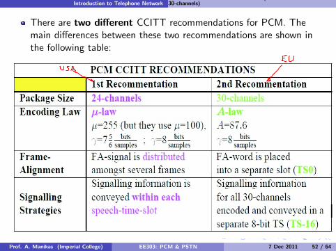
There are two di§erent CCITT recommendations for PCM. Themain di§erences between these two recommendations are shown inthe following table:
Prof. A. Manikas (Imperial College) EE303: PCM & PSTN 7 Dec 2011 52 / 64
Introduction to Telephone NetworkCCITT recommendations for PCM (24-channels and
30-channels)
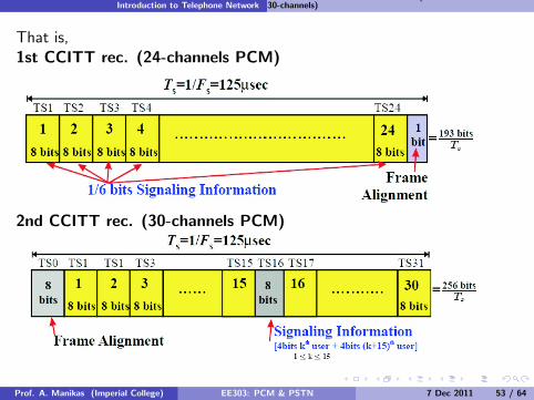
That is,1st CCITT rec. (24-channels PCM)
2nd CCITT rec. (30-channels PCM)
Prof. A. Manikas (Imperial College) EE303: PCM & PSTN 7 Dec 2011 53 / 64
Introduction to Telephone NetworkCCITT recommendations for PCM (24-channels and
30-channels)
Note
I A-law = better than µ-law (cheaper to produce and easy equipmentmaintenance, smaller quantization error in particular within the mostsignificant part of the dynamic range).
I in 24-ch PCM the signalling information is conveyed within eachspeech time-slot (technique known as bit stealing). Result: a slightreduction in speech-coding performance.
Prof. A. Manikas (Imperial College) EE303: PCM & PSTN 7 Dec 2011 54 / 64
Introduction to Telephone Network Single-Channel Path of 2nd CCITT rec. (30-channels PCM)
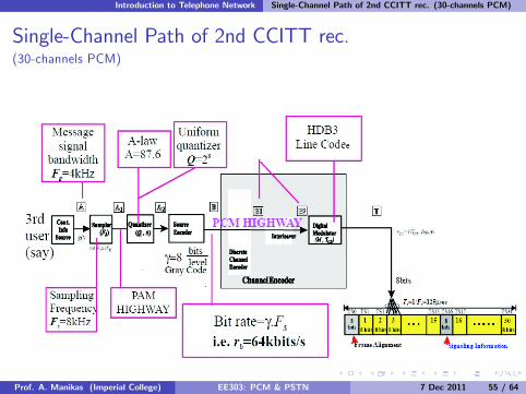
Single-Channel Path of 2nd CCITT rec.(30-channels PCM)
Prof. A. Manikas (Imperial College) EE303: PCM & PSTN 7 Dec 2011 55 / 64
Introduction to Telephone Network Implementation of 2nd PCM CCITT Recomm
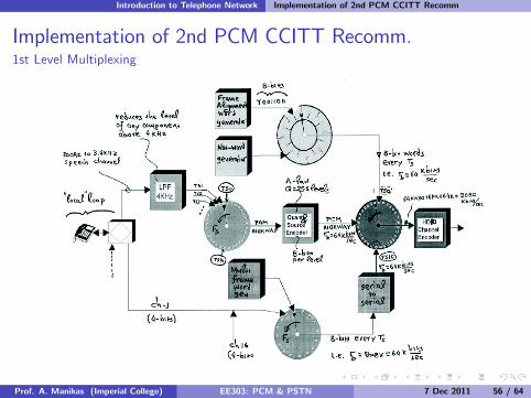
Implementation of 2nd PCM CCITT Recomm.1st Level Multiplexing
Prof. A. Manikas (Imperial College) EE303: PCM & PSTN 7 Dec 2011 56 / 64
Introduction to Telephone Network Implementation of 2nd PCM CCITT Recomm
Based on the 24-channels and 30-channels PCM CCITTrecommendations (primary multiplex groups) the core telephonenetwork evolved from using Frequency Division Multiplex (FDM)technology to digital transmission and switching
I These two PCM CCITT recommendations have led to two PDH(Plesiochronous digital hierarchies) CCITT recommendations forassembling the TDM telephony data streams from di§erent calls.
I Plesiochronous means: “almost synchronous ”because bits are stu§ed into the frames as padding and the callslocation varies slightly - jitters - from frame to frame
Prof. A. Manikas (Imperial College) EE303: PCM & PSTN 7 Dec 2011 57 / 64
Introduction to Telephone Network Plesiochronous digital hierarchies (PDH)
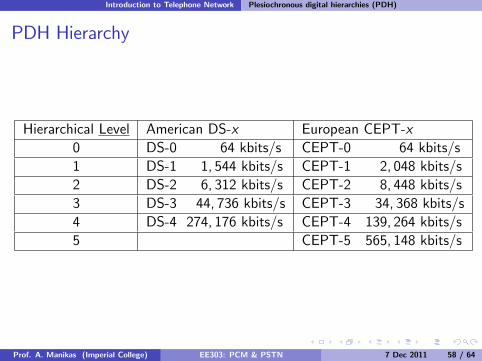
PDH Hierarchy
Hierarchical Level American DS-x European CEPT-x0 DS-0 64 kbits/s CEPT-0 64 kbits/s1 DS-1 1, 544 kbits/s CEPT-1 2, 048 kbits/s2 DS-2 6, 312 kbits/s CEPT-2 8, 448 kbits/s3 DS-3 44, 736 kbits/s CEPT-3 34, 368 kbits/s4 DS-4 274, 176 kbits/s CEPT-4 139, 264 kbits/s5 CEPT-5 565, 148 kbits/s
Prof. A. Manikas (Imperial College) EE303: PCM & PSTN 7 Dec 2011 58 / 64
Introduction to Telephone Network Plesiochronous digital hierarchies (PDH)
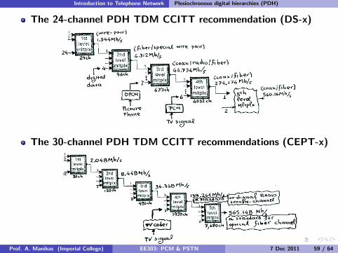
The 24-channel PDH TDM CCITT recommendation (DS-x)
The 30-channel PDH TDM CCITT recommendations (CEPT-x)
Prof. A. Manikas (Imperial College) EE303: PCM & PSTN 7 Dec 2011 59 / 64
Introduction to Telephone Network Plesiochronous digital hierarchies (PDH)
Main disadvantage of PDH Networks
PDH multiplexing was designed for point-to-point communicationsand channels cannot be added to, or extracted from, a highermultiplexing level demultiplexing down and then multiplexing upagain, through the entire PDH
For instance, to isolate a particular call from DS4, say, it must bedemultiplexed to DS1.
i.e. this is a very complex procedure and needs very expensiveequipment at every exchange to demultiplex and multiplex high speedlines
American & European Telephone Systems are incompatible(therefore very expensive equipment required to translate one formatto the other for transatlantic tra¢c)
Solution: SONET/SDH Signal HierarchyProf. A. Manikas (Imperial College) EE303: PCM & PSTN 7 Dec 2011 60 / 64
Introduction to Telephone Network Synchronous digital hierarchies (SONET/SDH)
Synchronous digital hierarchies (SONET/SDH)
The traditional PDH standards are based on the DS (USA) andCEPT (Europe) PCM systems (24-channels and 30-channels PCMCCITT recommendation)
PDH hierarchy is almost synchronous (extra bits are inserted intothe digital stream to bring them to a common rate).
In 1988 SDH (Synchronous Digital Hierarchy) was adopted byITU and ETSI (European Telecommunications Standards Institute)based on SONET (synchronous optical Networks)
SDH signals have a common external timing i.e.SDH is synchronous
Prof. A. Manikas (Imperial College) EE303: PCM & PSTN 7 Dec 2011 61 / 64
Introduction to Telephone Network Synchronous digital hierarchies (SONET/SDH)
The SDH standards used in Europe are
STM-1 which provides 155 Mbits/sec
STM-2 which provides 310 Mbits/sec
STM-3 which provides 465 Mbits/sec
STM-4 which provides 620 Mbits/sec
etc. (increments of 155 Mbits/sec)
The most important main standards are STM-1, STM-4 andSTM-16. These are commercially available.
Prof. A. Manikas (Imperial College) EE303: PCM & PSTN 7 Dec 2011 62 / 64
Introduction to Telephone Network Synchronous digital hierarchies (SONET/SDH)
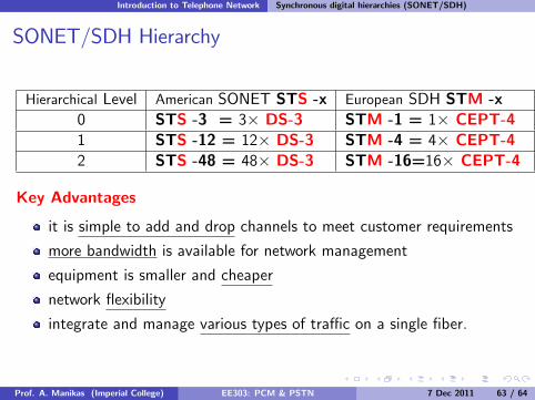
SONET/SDH Hierarchy
Hierarchical Level American SONET STS -x European SDH STM -x0 STS -3 = 3) DS-3 STM -1 = 1) CEPT-41 STS -12 = 12) DS-3 STM -4 = 4) CEPT-42 STS -48 = 48) DS-3 STM -16=16) CEPT-4
Key Advantages
it is simple to add and drop channels to meet customer requirements
more bandwidth is available for network management
equipment is smaller and cheaper
network flexibility
integrate and manage various types of tra¢c on a single fiber.
Prof. A. Manikas (Imperial College) EE303: PCM & PSTN 7 Dec 2011 63 / 64
Introduction to Telephone Network Synchronous digital hierarchies (SONET/SDH)
Prof. A. Manikas (Imperial College) EE303: PCM & PSTN 7 Dec 2011 64 / 64