PCA-ICA Based Acoustic Ambient Extraction
9
CSEIT1726324 | Received : 01 Jan 2018 | Accepted : 09 Jan 2018 | January-February-2018 [(3) 1 : 51-59] International Journal of Scientific Research in Computer Science, Engineering and Information Technology © 2018 IJSRCSEIT | Volume 3 | Issue 1 | ISSN : 2456-3307 51 PCA-ICA Based Acoustic Ambient Extraction G. Rajitha 1 ,K. Upendra Raju 2 1 M.Tech (Embedded Systems), Department of ECE, SVCE, Tirupati, Andhra Pradesh, India 2 Assistant Professor, Department of ECE, SVCE, Tirupati, Andhra Pradesh, India ABSTRACT Primary-ambient extraction (PAE) has been playing an important role in spatial audio analysis-synthesis. Based on the spatial features, PAE decomposes a signal into primary and ambient components, which are then rendered separately. PAE is performed in sub band domain for complex input signals having multiple point-like sound sources. However, the performance of PAE approaches and their key influences for such signals have not been well- studied so far. In this paper, we conducted a study on frequency-domain PAE using principal component analysis (PCA) and independent component analysis (ICA) in the case of multiple sources. We found that the partitioning of the frequency bins is very critical in PAE. Simulation results reveal that the proposed top-down adaptive partitioning method achieves superior performance as compared to the conventional partitioning methods. Keywords:Primary Ambient Extraction (PAE), Ambient Phase, Spatial Audio, Sparsity, Principal Component analysis (PCA), Independent Component Analysis (ICA), Frequency Domain. I. INTRODUCTION Spatial audio reproduction of digital media content (e.g., movies, games, etc.) has gained popularity in recent years. Reproduction of sound scenes essentially involves the reproduction of point-like directional sound sources and the diffuse sound environment, which are often referred to as primary and ambient components, respectively [1], [2]. Due to the perceptual differences between the primary and ambient components, different rendering schemes should be applied to the primary and ambient components for optimal spatial audio reproduction [2]. However, existing mainstream channel-based audio formats (such as stereo and multichannel signals) provide only the mixed signals, which necessitate the extraction of the primary and ambient components from the mixed signals. This extraction Process is usually known as primary-ambient extraction (PAE). To date, PAE has been applied in spatial audio processing spatial audio coding], audio re-mixing [1] and hybrid loudspeaker systems as well as natural sound rendering headphone systems. Numerous PAE approaches are applied to stereo and multichannel signals. For the basic signal model for stereo signals, the primary and ambient components are mainly discriminated by their inter-channel cross- correlations, i.e., the primary and ambient components are considered to be correlated and uncorrelated, respectively [2]. Based on this model, several time- frequency masking approaches were introduced, where the time frequency masks are obtained as a nonlinear function of the inter-channel coherence of the input signal [1] or derived based on the criterion of equal level of ambient components between the two channels [3]. Further investigation of the differences between two channels of the stereo signals has led to several types of linear estimation based approaches [4] including principal component analysis (PCA) and ICA based approaches [2] and least-squares based approaches. These linear estimation based approaches extract the primary and ambient components using different performance-related criteria [4]. To deal with digital media signals that cannot fit into the basic signal model, there are other PAE approaches that consider signal model classification, time/phase differences in primary components non-negative matrix factorization independent component analysis etc. The above-mentioned PAE approaches often suffer from severe extraction error that takes the form of residual uncorrelated ambient component in the
Transcript of PCA-ICA Based Acoustic Ambient Extraction

CSEIT1726324 | Received : 01 Jan 2018 | Accepted : 09 Jan 2018 | January-February-2018 [(3) 1 : 51-59]
International Journal of Scientific Research in Computer Science, Engineering and Information Technology
© 2018 IJSRCSEIT | Volume 3 | Issue 1 | ISSN : 2456-3307
51
PCA-ICA Based Acoustic Ambient Extraction G. Rajitha
1 ,K. Upendra Raju
2
1M.Tech (Embedded Systems), Department of ECE, SVCE, Tirupati, Andhra Pradesh, India
2Assistant Professor, Department of ECE, SVCE, Tirupati, Andhra Pradesh, India
ABSTRACT
Primary-ambient extraction (PAE) has been playing an important role in spatial audio analysis-synthesis. Based on
the spatial features, PAE decomposes a signal into primary and ambient components, which are then rendered
separately. PAE is performed in sub band domain for complex input signals having multiple point-like sound
sources. However, the performance of PAE approaches and their key influences for such signals have not been well-
studied so far. In this paper, we conducted a study on frequency-domain PAE using principal component analysis
(PCA) and independent component analysis (ICA) in the case of multiple sources. We found that the partitioning of
the frequency bins is very critical in PAE. Simulation results reveal that the proposed top-down adaptive partitioning
method achieves superior performance as compared to the conventional partitioning methods.
Keywords:Primary Ambient Extraction (PAE), Ambient Phase, Spatial Audio, Sparsity, Principal Component
analysis (PCA), Independent Component Analysis (ICA), Frequency Domain.
I. INTRODUCTION
Spatial audio reproduction of digital media content
(e.g., movies, games, etc.) has gained popularity in
recent years. Reproduction of sound scenes essentially
involves the reproduction of point-like directional
sound sources and the diffuse sound environment,
which are often referred to as primary and ambient
components, respectively [1], [2]. Due to the perceptual
differences between the primary and ambient
components, different rendering schemes should be
applied to the primary and ambient components for
optimal spatial audio reproduction [2]. However,
existing mainstream channel-based audio formats (such
as stereo and multichannel signals) provide only the
mixed signals, which necessitate the extraction of the
primary and ambient components from the mixed
signals. This extraction Process is usually known as
primary-ambient extraction (PAE). To date, PAE has
been applied in spatial audio processing spatial audio
coding], audio re-mixing [1] and hybrid loudspeaker
systems as well as natural sound rendering headphone
systems.
Numerous PAE approaches are applied to stereo and
multichannel signals. For the basic signal model for
stereo signals, the primary and ambient components are
mainly discriminated by their inter-channel cross-
correlations, i.e., the primary and ambient components
are considered to be correlated and uncorrelated,
respectively [2]. Based on this model, several time-
frequency masking approaches were introduced, where
the time frequency masks are obtained as a nonlinear
function of the inter-channel coherence of the input
signal [1] or derived based on the criterion of equal
level of ambient components between the two channels
[3]. Further investigation of the differences between
two channels of the stereo signals has led to several
types of linear estimation based approaches [4]
including principal component analysis (PCA) and ICA
based approaches [2] and least-squares based
approaches. These linear estimation based approaches
extract the primary and ambient components using
different performance-related criteria [4]. To deal with
digital media signals that cannot fit into the basic signal
model, there are other PAE approaches that consider
signal model classification, time/phase differences in
primary components non-negative matrix factorization
independent component analysis etc.
The above-mentioned PAE approaches often suffer
from severe extraction error that takes the form of
residual uncorrelated ambient component in the

Volume 3, Issue 1, January-February-2018 | www.ijsrcseit.com | UGC Approved Journal [ Journal No : 64718 ]
52
extracted primary and ambient components, especially
for digital media content having relatively strong
ambient power [4]. In this Letter, we aim to improve
the performance of PAE by exploiting the
characteristics of uncorrelated ambient components of
digital media content and the sparsity of the primary
components [5]. These considerations have led to the
novel approach to solve the PAE problem using
ambient phase estimation with a sparsity constraint
(APES).
II. EXISTING METHOD
The primary and ambient components are usually
mixed in conventional channel-based audio formats,
such as stereo and surround sound formats. Such
channel-based audio formats make primary-ambient
extraction (PAE) an essential step in spatial audio
reproduction. In recent years, PAE has been
incorporated into a wide range of applications,
including spatial audio processing spatial audio coding
audio mixing and emerging loudspeaker and
headphone reproduction systems .There are two
emerging frameworks for spatial audio coding: spatial
audio scene coding (SASC) and directional audio
coding (Dirac). Both SASC and Dirac extract the
primary and ambient components and then synthesize
the output based on the playback system configuration.
In SASC, the localization analysis and synthesis, based
on Gerzon localization vector, are independently
performed on the primary and ambient components. In
DirAC, the primary components are reproduced using
vector base amplitude panning, while the ambient
components are decorrelated and channeled to all
loudspeakers to create the surrounding sound
environment. Incorporating PAE into various up-
mixing techniques has been discussed. The PAE based
up-mixing is particularly suitable for a hybrid
loudspeaker system proposed. This hybrid loudspeaker
system uniquely combines parametric and conventional
loudspeakers, taking advantage of the high directivity
of the parametric loudspeakers to render accurate
localization of the primary components and reproduce
spaciousness of the ambient components using the
conventional loudspeakers. Furthermore, PAE based
spatial audio reproduction for headphone playback has
been shown to create a more natural and immersive
listening experience than conventional headphone
rendering systems.
To date, many approaches have been proposed for PAE.
For these PAE approaches, the stereo input signal is
generally modeled as a directional primary sound
source linearly mixed with the ambient component.
The assumptions of the stereo signal model are as
follows. First, the primary and ambient components are
considered to be independent with each other. Second,
the primary components in the two channels are
assumed to be correlated at zero lag. Third, the ambient
components in the two channels are uncorrelated.
Assuming that the ambient components in two channels
of the stereo signal have equal level, used a time-
frequency mask to extract the ambient components
from the stereo signal. Their time-frequency mask
approach can also be extended to multichannel input
signals. A least-squares approach, proposed by Faller
[9], estimated the primary and ambient components by
minimizing the mean-square error. Control of spatial
cues of the ambient components was also combined
with least-squares. Recently, He et al. proposed a new
ambient spectrum estimation framework and derived a
sparsity constrained solution for PAE. Principal
component analysis (PCA) based approaches remain
the most widely studied approaches for PAE.
Considering the independence between the primary and
ambient components, the stereo signal is decomposed
into two orthogonal components in each channel using
the Karhunen-Loève transform. Assuming that the
primary component is relatively stronger in power than
the ambient component, the component having larger
variance is considered to be the primary component and
the remaining component is considered as the ambient
component. A comprehensive evaluation and
comparison on these PAE approaches can be found.
Other techniques such as non-negative matrix
factorization and independent component analysis are
also applied in PAE.
III. PROPOSED MITIGATION SCHEME
A. Frequency bin partitioning
To effectively handle multiple sources in the primary
components, frequency bins of the input signal are
grouped into several partitions, as shown in Fig.1. In
each partition, there is only one dominant source and
hence one corresponding value of k and is computed.
Ideally, the number of partitions should be the same as
the number of sources, and the frequency bins should

Volume 3, Issue 1, January-February-2018 | www.ijsrcseit.com | UGC Approved Journal [ Journal No : 64718 ]
53
be grouped in a way such that the magnitude of one
source in each partition is significantly higher than the
magnitude of other sources. However, the number and
spectra of the sources in any given input signals are
usually unknown. Hence, the ideal partitioning is
difficult or impossible to achieve.
Figure 1. Block diagram of frequency bin partitioning
based PAE in frequency domain
Alternatively, we consider two types of feasible
partitioning methods, namely, fixed partitioning and
adaptive partitioning. Regardless of the input signal,
the fixed partitioning classifies the frequency bins into
a certain number of partitions uniformly or non-
uniformly, such as equivalent rectangular bandwidth
(ERB) [13], [14]. By contrast, adaptive partitioning
takes into account of the input signal via the top-down
(TD) or bottom-up (BU) method. BU method starts
with every bin as one partition and then gradually
reduces the number of partitions by combining the bins.
Conversely, TD starts from one partition containing all
frequency bins and iteratively divides each partition
into two sub-partitions, according to certain conditions.
As the number of partitions is usually limited, TD is
more efficient than BU, and hence preferred.
To determine whether one partition requires further
division, ICC-based criteria are proposed in TD
partitioning. First, if the ICC of the current partition is
already high enough, we consider only one source is
dominant in the current partition and cease further
division of the partition. Otherwise, the ICCs of the two
divided sub-partitions are examined. The partitioning is
continued only when at least one of two ICCs of the
sub-partitions becomes higher, and neither ICC of the
sub-partitions becomes too small, which indicates that
no source is dominant. Suppose the ICCs of the current
partition, and two uniformly divided sub-partitions are
ϕ0, ϕ1, ϕ2, as shown in Figure 2.
Figure 2. An illustration of top-down partitioning
For generality, a higher threshold of ICC ϕH and a
lower threshold ϕL are introduced. Thus, the following
three criteria for the continuation of partitioning in TD:
a) ϕ0 < ϕH, and
b) Max(ϕ1, ϕ2) > ϕ0, and
c) Min(ϕ1, ϕ2) > ϕL.
The partitioning is stopped when any of the three
criteria is unsatisfied. Frequency bin partitioning is
unnecessary for one source, but this partitioning plays
an essential role for multiple sources, especially when
the spectra of the sources overlap.
B. Principal Component Analysis (PCA)
Principal Component Analysis (PCA) is a technique of
multivariable and mega variate analysis which may
provide arguments for reducing a complex data set to a
lower dimension and reveal some hidden and
simplified structure/patterns that often under lie it [11].
The main goal of Principal Component Analysis is to
obtain the most important characteristics from data. In
order to develop a PCA model, it is necessary to
arrange the collected data in a matrix X. This m×n
matrix contains information from n sensors and m
experimental trials [11]. Since physical variables and
sensors have different magnitudes and scales, each
data-point is scaled using the mean of all measurements
of the sensor at the same time and the standard
deviation of all measurements of the sensor. Once the
variables are normalized, the covariance matrix Cx is
calculated. It is a square symmetric m×m matrix that
measures the degree of linear relationship within the
data set between all possible pairs of variables
(sensors).The subspaces in PCA are defined by the
eigenvectors and eigenvalues of the covariance matrix
as follows:
Cx = ˄
Where the eigenvectors of Cx are the columns of ,and
the eigenvalues are the diagonal terms of Λ (the off-
diagonal terms are zero). Columns of matrix are
sortedaccording to the eigenvalues by descending order

Volume 3, Issue 1, January-February-2018 | www.ijsrcseit.com | UGC Approved Journal [ Journal No : 64718 ]
54
and they are called as (by some authors) Principal
Components of the data set or loading vectors. The
eigen vectors with the highest eigenvalue represents the
most important pattern in the data with the largest
quantity of information. Choosing only a reduced
number r < n of principal components, those
corresponding to the first eigenvalues, the reduced
transformation matrix could be imagined as a model for
the structure. In this way, the new matrix P ( sorted
and reduced) can be called as PCA model.
Geometrically, the transformeddata matrix T (score
matrix) represents the projection of the original data
over the direction of the principal components P:
T = XP
In the full dimension case (using ), this projection is
invertible (since T = I )and the original data can be
recovered as X = T T. In the reduced case (using P),
with the given T, it is not possible to fully recover X,
but T can be projected back onto the original m-
dimensional space and obtain another data matrix as
follows:
=TPT
= (XP)PT
Therefore, the residual data matrix (the error for not
using all the principal components) can be defined as
the difference between the original data and the
projected back.
E = X-
= X – XPPT
= X(I – PPT)
PCA is also known as the Karhunen-Loeveor Hoteling
transform [11]. PCA can also be applied in feature
extraction, in order to reduce the correlation between
the elements of the feature vector. It is also proposed as
a pre-processing tool to enhance the performance of
Gaussian Mixture Models (GMM).
C. Independent Component Analysis(ICA)
Independent component analysis (ICA) is a statistical
and computational technique for revealing hidden
factors that underlie sets of random variables,
measurements, or signals. ICA defines a generative
model for the observed multivariate data, which is
typically given as a large database of samples. In the
model, the data variables are assumed to be linear or
nonlinear mixtures of some unknown latent variables,
and the mixing system is also unknown. The latent
variables are assumed nongaussian and mutually
independent, and they are called the independent
components of the observed data. These independent
components, also called sources or factors, can be
found by ICA [12].
ICA can be seen as an extension to principal
component analysis and factor analysis. ICA is a much
more powerful technique, however, capable of finding
the underlying factors or sources when these classic
methods fail completely. The data analyzed by ICA
could originate from many different kinds of
application fields, including digital images and
document databases, as well as economic indicators
and psychometric measurements. In many cases, the
measurements are given as a set of parallel signals or
time series; the term blind source separation is used to
characterize this problem. Typical examples are
mixtures of simultaneous speech signals that have been
picked up by several microphones, brain waves
recorded by multiple sensors, interfering radio signals
arriving at a mobile phone, or parallel time series
obtained from some industrial process.
The general idea is to change the space from an m-
dimensional to an n-dimensional space such that the
new space with the transformed variables (components)
describes the essential structure of the data containing
the more relevant information from the sensors. Among
its virtues is that ICA has a good performance in
pattern recognition, noise reduction and data reduction.
The goal of ICA is to find new components (new space)
that are mutually independent in complete statistical
sense. Once the data are projected into this new space,
these new variables have no any physical sense and
cannot be directly observed, for that, these new
variables are known as latent variables. If r random
variables are observed (x1,x2, ……,xr), they can be
modeled as linear combinations of n random variables
(s1,s2, …….,sn) as follows:
xi= ti1 s1 + ti2 s2+….+ tin sn
Each tij in is an unknown real coefficient. By
definition, the set of sj should be Statistically mutually
independent and can be designed as the Independent
Components (ICs). In matrix terms, this equation can
be written as
x=Ts
where x= (x1,x2, ……,xr)T, s= (s1, s2,…, sn)
T and T is
the r × n mixing matrix that contains all tij. If each
random variable xi consists of time-histories with m

Volume 3, Issue 1, January-February-2018 | www.ijsrcseit.com | UGC Approved Journal [ Journal No : 64718 ]
55
data points(m-dimensional), the ICA model still holds
the same mixing matrix and it can be expressed as:
X = TS
where X is the r × m matrix that contains the
observations. Each row of X represents the time
histories. S is the Independent Component matrix,
where each column is the vector of latent variables of
each original variable. Since T and S are unknown, it is
necessary to find these two elements considering that
only the X matrix is known. The ICA algorithm finds
the independent components by minimizing or
maximizing some measure of independence [12]. To
perform ICA, the first step includes the application of
pre-whitening to the input data X. The main idea is to
use a linear transformation to produce a new data
matrix Z=VX whose elements are mutually
uncorrelated and their variances equal unity. It means
that the covariance matrix of Z is the identity
matrix(E{ZZT}=I). A popular method to obtain the
whitening matrix V is by means of Singular Value
Decomposition (SVD), such as the one used in
Principal Component Analysis (PCA) and it is given by:
V = Λ-1
PT,
where the eigenvectors of the covariance matrix
ZZTare the columns of P and the eigen values are the
diagonal terms of Λ(the off-diagonal terms are zero).
The second step is to define a separating matrix W that
transforms the matrix Z to the matrix S whose variables
are non-Gaussian and statistically independent:
S = WTZ
There are several approaches to reach this goal.
Maximizing the non-gaussianity of WTZ give us the
independent components. On the other hand,
minimizing the mutual information between the
columns of WTZ is to minimize the dependence
between them. The non-gaussianity can be measured by
different methods, kurtosis and Negentropy being the
most commonly used. The first one is sensitive to
outliers and the other is based on the information
theory quantity of entropy.
Independent component analysis (ICA) is a statistical
and computational technique for revealing hidden
factors that underlie sets of random variables,
measurements, or signals. ICA defines a generative
model for the observed multivariate data, which is
typically given as a large database of samples. In the
model, the data variables are assumed to be linear or
nonlinear mixtures of some unknown latent variables,
and the mixing system is also unknown. The latent
variables are assumed nongaussian and mutually
independent, and they are called the independent
components of the observed data. These independent
components, also called sources or factors, can be
found by ICA [12].
ICA can be seen as an extension to principal
component analysis and factor analysis. ICA is a much
more powerful technique, however, capable of finding
the underlying factors or sources when these classic
methods fail completely. The data analyzed by ICA
could originate from many different kinds of
application fields, including digital images and
document databases, as well as economic indicators
and psychometric measurements. In many cases, the
measurements are given as a set of parallel signals or
time series; the term blind source separation is used to
characterize this problem. Typical examples are
mixtures of simultaneous speech signals that have been
picked up by several microphones, brain waves
recorded by multiple sensors, interfering radio signals
arriving at a mobile phone, or parallel time series
obtained from some industrial process.
D. Sparse Representations of an Audio Signal:
Sparse representations have proved a powerful tool in
the analysis and processing of audio signals and
already lie at the heart of popular coding standards such
as MP3 and Dolby AAC [10]. To transform signals into
sparse representations, i.e. representations where most
coefficients are zero. These sparse representations are
proving to be a particularly interesting and powerful
tool for analysis and processing of audio signals.
Audio signals are typically generated either by resonant
systems or by physical impacts, or both. Resonant
systems produce sounds that are dominated by a small
number of frequency components, allowing a sparse
representation of the signal in the frequency domain.
Impacts produce sounds that are concentrated in time,
allowing a sparse representation of the signal in either
directly the time domain, or in terms of a small number
of wavelets. The use of sparse representations therefore
appears to be a very appropriate approach for audio.
Suppose we have a sampled audio signal with T
samples x(t), 1≤ t ≤ T ,which we can write in a row
vector form a = (x(1),…x(T)). )). For audio signals
we are typically dealing with signals sampled below 20
kHz, but for simplicity we will assume our sampled
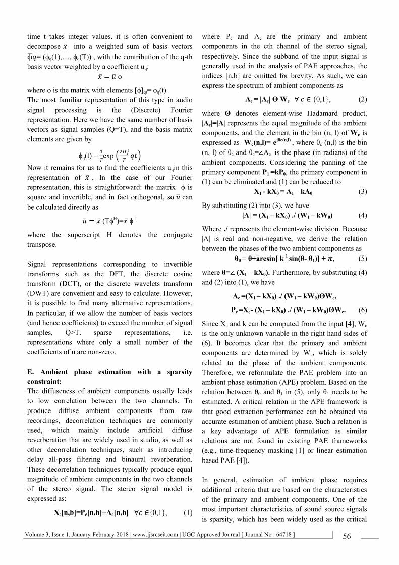
Volume 3, Issue 1, January-February-2018 | www.ijsrcseit.com | UGC Approved Journal [ Journal No : 64718 ]
56
time t takes integer values. it is often convenient to
decompose into a weighted sum of basis vectors
= (ϕq(1),…, ϕq(T)) , with the contribution of the q-th
basis vector weighted by a coefficient uq:
ϕ
where ϕ is the matrix with elements [ϕ]qt= ϕq(t)
The most familiar representation of this type in audio
signal processing is the (Discrete) Fourier
representation. Here we have the same number of basis
vectors as signal samples (Q=T), and the basis matrix
elements are given by
ϕq(t) =
exp (
)
Now it remains for us to find the coefficients uqin this
representation of . In the case of our Fourier
representation, this is straightforward: the matrix ϕ is
square and invertible, and in fact orthogonal, so can
be calculated directly as
(TϕH)= ϕ
-1
where the superscript H denotes the conjugate
transpose.
Signal representations corresponding to invertible
transforms such as the DFT, the discrete cosine
transform (DCT), or the discrete wavelets transform
(DWT) are convenient and easy to calculate. However,
it is possible to find many alternative representations.
In particular, if we allow the number of basis vectors
(and hence coefficients) to exceed the number of signal
samples, Q>T. sparse representations, i.e.
representations where only a small number of the
coefficients of u are non-zero.
E. Ambient phase estimation with a sparsity
constraint:
The diffuseness of ambient components usually leads
to low correlation between the two channels. To
produce diffuse ambient components from raw
recordings, decorrelation techniques are commonly
used, which mainly include artificial diffuse
reverberation that are widely used in studio, as well as
other decorrelation techniques, such as introducing
delay all-pass filtering and binaural reverberation.
These decorrelation techniques typically produce equal
magnitude of ambient components in the two channels
of the stereo signal. The stereo signal model is
expressed as:
Xc[n,b]=Pc[n,b]+Ac[n,b] {0,1}, (1)
where Pc and Ac are the primary and ambient
components in the cth channel of the stereo signal,
respectively. Since the subband of the input signal is
generally used in the analysis of PAE approaches, the
indices [n,b] are omitted for brevity. As such, we can
express the spectrum of ambient components as
Ac = |Ac| ʘ Wc {0,1}, (2)
where ʘ denotes element-wise Hadamard product,
|Ac|=|A| represents the equal magnitude of the ambient
components, and the element in the bin (n, l) of Wc is
expressed as Wc(n,l)= ejθc(n,l)
, where θc (n,l) is the bin
(n, l) of θc and θc= Ac is the phase (in radians) of the
ambient components. Considering the panning of the
primary component P1 =kP0, the primary component in
(1) can be eliminated and (1) can be reduced to
X1 - kX0 = A1 – kA0 (3)
By substituting (2) into (3), we have
|A| = (X1 – kX0) ./ (W1 – kW0) (4)
Where ./ represents the element-wise division. Because
|A| is real and non-negative, we derive the relation
between the phases of the two ambient components as
θ0 = θ+arcsin[ k-1
sin(θ- θ1)] + , (5)
where θ= (X1 – kX0). Furthermore, by substituting (4)
and (2) into (1), we have
Ac =(X1 – kX0) ./ (W1 – kW0)ʘWc,
Pc =Xc- (X1 – kX0) ./ (W1 – kW0)ʘWc. (6)
Since Xc and k can be computed from the input [4], Wc
is the only unknown variable in the right hand sides of
(6). It becomes clear that the primary and ambient
components are determined by Wc, which is solely
related to the phase of the ambient components.
Therefore, we reformulate the PAE problem into an
ambient phase estimation (APE) problem. Based on the
relation between θ0 and θ1 in (5), only θ1 needs to be
estimated. A critical relation in the APE framework is
that good extraction performance can be obtained via
accurate estimation of ambient phase. Such a relation is
a key advantage of APE formulation as similar
relations are not found in existing PAE frameworks
(e.g., time-frequency masking [1] or linear estimation
based PAE [4]).
In general, estimation of ambient phase requires
additional criteria that are based on the characteristics
of the primary and ambient components. One of the
most important characteristics of sound source signals
is sparsity, which has been widely used as the critical
Volume 3, Issue 1, January-February-2018 | www.ijsrcseit.com | UGC Approved Journal [ Journal No : 64718 ]
57
criterion in finding optimal solutions in many audio
and music signal processing applications [5]. In PAE,
since the primary components are essentially sound
sources, they can be considered to be sparse in the
time-frequency domain [5]. Therefore, we estimate θ1
by restricting the extracted primary component to be
sparse, i.e., minimizing the sum of the magnitudes of
the primary components for all time-frequency bins:
1*= arg
‖ ‖ (7)
Table 1. Steps in APES 1 Transform the input signal into time frequency
domain X0, X1,pre-compute k, choose D, repeat
steps 2-7 for every time-frequency bin.
2 Set d=1,compute θ= (X1 – kX0),repeat steps 3-6
3 1(d) = 2ᴫd/D-ᴫ
4 Compute 0(d) using eq.(5), and 0(d), 1(d)
5 Compute 1(d) using eq.(6) and | 1(d)|
6 d d+1, until d=D
7 Find | | , repeat
steps 3-5 with d= d* and compute the other
components using eq.(6)
8 Finally, compute the time-domain primary and
ambient components using inverse time-
frequency transform.
We refer to this approach as the ambient phase
estimation with a sparsity constraint. However, the
objective function in (7) is not convex. Therefore,
convex optimization techniques are inapplicable, and
heuristic methods, such as simulated annealing (SA) [6]
are more suitable to solve APES. But SA might not be
efficient since optimization is required for all the phase
variables. Based on the following two observations, we
propose to use a simple but more efficient method to
estimate the ambient phase. First, the magnitude of the
primary component is independently determined by the
phase of the ambient component at the same time-
frequency bin and hence, the estimation in (7) can be
independently performed for each time-frequency bin.
Note that with this approximation, a sufficient
condition of the sparsity constraint is applied in
practice. Second, the phase variable is bounded to (-ᴫ,ᴫ]
and high precision of the estimated phase may not be
necessary. Thus, we select the optimal phase estimates
from an array of discrete phase values
1(d) = (2ᴫd/D-ᴫ)
where d with D being the total number
of discrete phase values to be considered. We refer to
this method as discrete searching (DS). Following (5)
and (6), D estimates of the primary components can be
computed. The estimated phase then corresponds to the
minimum of magnitudes of the primary component, i.e.,
*1 = 1(d
*),
Clearly, the value of D affects the extraction and the
computational performance of APES using DS. The
detailed steps of APES are listed in Table 1.
In addition to the proposed APES, we also consider a
simple way to estimate the ambient phase based on the
uniform distribution, i.e., 1U U (-ᴫ,ᴫ] This approach
is referred to as APEU, and is compared with the APES
to examine the necessity of having a more accurate
ambient phase estimation . Developing a complete
probabilistic model to estimate the ambient phase,
though desirable, is beyond the scope of the present
study.
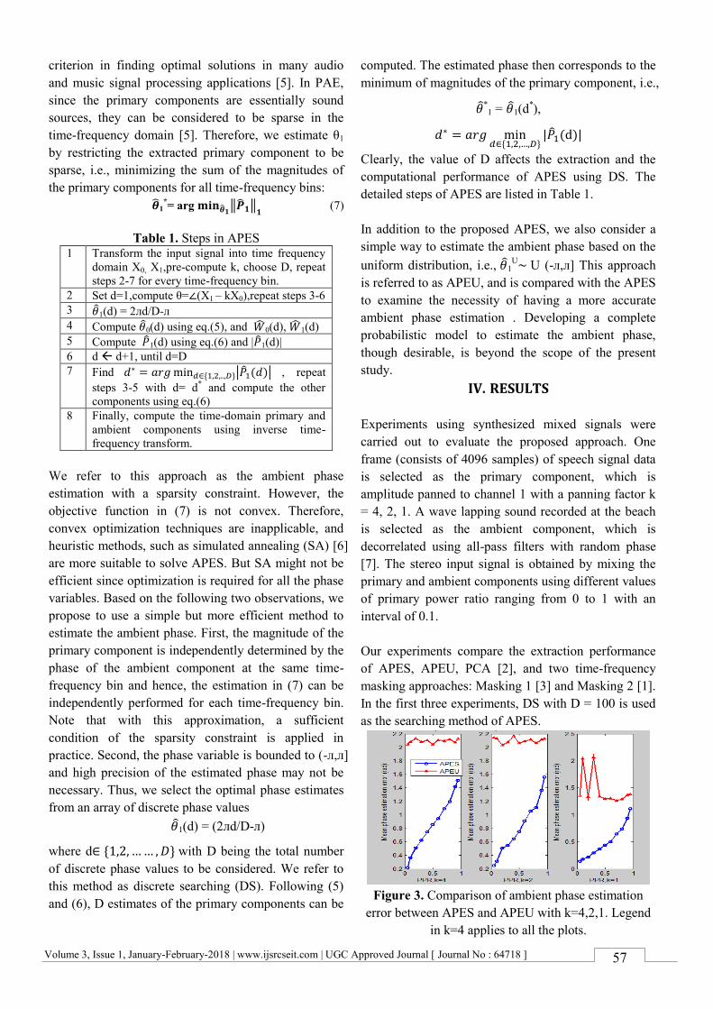
IV. RESULTS
Experiments using synthesized mixed signals were
carried out to evaluate the proposed approach. One
frame (consists of 4096 samples) of speech signal data
is selected as the primary component, which is
amplitude panned to channel 1 with a panning factor k
= 4, 2, 1. A wave lapping sound recorded at the beach
is selected as the ambient component, which is
decorrelated using all-pass filters with random phase
[7]. The stereo input signal is obtained by mixing the
primary and ambient components using different values
of primary power ratio ranging from 0 to 1 with an
interval of 0.1.
Our experiments compare the extraction performance
of APES, APEU, PCA [2], and two time-frequency
masking approaches: Masking 1 [3] and Masking 2 [1].
In the first three experiments, DS with D = 100 is used
as the searching method of APES.
Figure 3. Comparison of ambient phase estimation
error between APES and APEU with k=4,2,1. Legend
in k=4 applies to all the plots.

Volume 3, Issue 1, January-February-2018 | www.ijsrcseit.com | UGC Approved Journal [ Journal No : 64718 ]
58
Figure 4. ESR of extracted primary component and
extracted ambient component with respect to 3
different values of primary panning factor(k=4,2,1),
using APES,APEU,PCA+ICA,Masking1,Masking2.
Extraction performance is quantified by the error-to-
signal ratio (ESR, in dB) of the extracted primary and
ambient components, where lower ESR indicates a
better extraction. The ESR for the primary and ambient
components are computed as
ESRy = 10 {∑‖ ‖
‖ ‖
} y = p , or a. (8)
First, we examine the significance of ambient phase
estimation by comparing the performance of APES
with APEU. In Fig.3 we show the mean phase
estimation error and it is observed that compared to a
random phase in APEU, the phase estimation error in
APES is much lower. As a consequence, ESRs in
APES are significantly lower than those in APEU, as
shown in Fig.4. This result indicates that obviously,
close ambient phase estimation is necessary.
Second, we compare the APES with some other PAE
approaches in the literature. From Fig.4, it is clear that
APES significantly outperforms other approaches in
terms of ESR for and k , suggesting that a
better extraction of primary and ambient components is
found with APES when primary components is panned
and ambient power is strong. When k = 1, APES has
comparable performance to the masking approaches,
and performs slightly better than PCA and ICA for
. Referring to Fig.3 that, the ambient phase
estimation error is similar for different k values, we can
infer that the relatively poorer performance of APES
for k = 1 is an inherent limitation of APES. Moreover,
we compute the mean ESR across all tested and k
values and find that the average error reduction in
APES over PCA,ICA and the two time-frequency
masking approaches are 3.1, 3.5, and 5.2 dB,
respectively. Clearly, the error reduction is even higher
(up to 15 dB) for low values.
Table 2.Comparison of APEPS with different
searching methods
Method
Computation
time (s)
ESRP
(dB)
ESRA
(dB)
DS(D=10) 0.18 -7.28 -7.23
DS(D=100) 1.62 -7.58 -7.50
SA 426 -7.59 -7.51
Lastly, we compare the performance, as well as the
computation time among different searching methods
in APES: SA, DS with D = 10 and 100. The results
with = 0.5 and k = 4 are presented in Table II. It is
obvious that SA requires significantly longer
computation time to achieve similar ESR when
compared to DS. More interestingly, the performance
of DS does not vary significantly as the precision of the
search increases (i.e., D is larger). However, the
computation time of APES increases almost
proportionally as D increases. Hence, we infer that the
proposed APES is not very sensitive to phase
estimation errors and therefore the efficiency of APES
can be improved by searching a limited number of
phase values [8].
However, it shall be noted that the influence of time-
frequency transform, though not studied in this paper,
is very critical and requires further investigation.
Meanwhile, the performance of these PAE approaches
shall also be evaluated using more practical signals.
Moreover, ambient components in the complex signals
are more prone to inter-channel magnitude variations,
and therefore probabilistic approaches based on the
statistics of these variations shall be studied to improve
the robustness of PAE approaches.
V. CONCLUSIONS
We presented a novel approach to solve the PAE
problem using APES. Considering that the diffuse
ambient components in two channels of a stereo signal
exhibit equal magnitude, the PAE problem is
reformulated as an ambient phase estimation problem.

Volume 3, Issue 1, January-February-2018 | www.ijsrcseit.com | UGC Approved Journal [ Journal No : 64718 ]
59
Our novel APE formulation provides a promising way
to solve PAE as the extraction performance is solely
determined by ambient phase estimation accuracy. In
this paper, APE is solved based on the sparsity of the
primary components. Based on our experiments using
synthesized signals, we found that though under
imperfect ambient phase estimation, the proposed
approach still showed significant improvement (3-6 dB
average reduction in ESR) over existing approaches,
especially in the presence of strong ambient
components and panned primary components.
Moreover, the efficiency of APES can be improved by
lowering the precision of the phase estimation, without
introducing significant degradation on the extraction
performance. Future work includes the study on the
influence of time-frequency transform, handling more
complex stereo and multichannel signals using
probabilistic models, and other optimization criteria in
APE.
VI. REFERENCES
[1]. C. Avendano and J. M. Jot, "A frequency-domain
approach to multichannel upmix," J. Audio Eng.
Soc., vol. 52, no. 7/8, pp. 740-749, Jul./Aug.
2004.
[2]. M. M. Goodwin and J. M. Jot, "Primary-ambient
signal decomposition and vector-based
localization for spatial audio coding and
enhancement," in Proc. ICASSP, Hawaii, 2007,
pp. 9-12.
[3]. J. Merimaa, M. M. Goodwin, J. M. Jot,
"Correlation-based ambience extraction from
stereo recordings," in 123rd Audio Eng. Soc.
Conv., New York, Oct. 2007.
[4]. J. He, E. L. Tan, and W. S. Gan, "Linear
estimation based primary-ambient extraction for
stereo audio signals," IEEE/ACM Trans. Audio,
Speech,Lang. Process., vol. 22, no. 2, pp. 505-
517, Feb. 2014.
[5]. M. Plumbley, T. Blumensath, L. Daudet, R.
Gribonval, and M. E. Davies,"Sparse
representation in audio and music: from coding
to source separation," Proc. IEEE, vol. 98, no. 6,
pp. 995-1016, Jun. 2010.
[6]. P. J. V. Laarhoven, and E. H. Aarts, Simulated
annealing, Netherlands:Springer, 1987.
[7]. G. Kendall, "The decorrelation of audio signals
and its impact on spatial imagery," Computer
Music Journal, vol. 19, no. 4, pp. 71-87, 1995.
[8]. J. He. (2014 Feb 24). Ambient phase estimation
APE[online].Available:http://jhe007.wix.com/ma
in#!ambient-phase-estimation/cied
[9]. C. Faller, "Multiple-loudspeaker playback of
stereo signals," J. Audio Eng. Soc., vol. 54, no.
11, pp. 1051–1064, Nov. 2006.
[10]. Dolby Atmos-Next Generation Audio for Cinema
(White Paper). 2013. Available online:
http://www.dolby.com/uploadedFiles/Assets/US/
Doc/Professional/Dolby-Atmos-Next-
Generation-Audio-for-Cinema.pdf
[11]. I. Jollife. Principal Component Analysis.
Springer series in statistics, 2 ed. 2002.
[12]. A. Hyvärinen, J. Karhunen, E. Oja. Independent
Component Analysis, New York: Wiley, 2001.
ISBN 978-0-471-40540-5.
[13]. C. Avendano and J. M. Jot, "A frequency-domain
approach to multichannel upmix," J. Audio Eng.
Soc., vol. 52, no. 7/8, pp. 740-749, Jul./Aug.
2004.
[14]. C. Faller, "Multiple-loudspeaker playback of
stereo signals," J. Audio Eng. Soc., vol. 54, no.
11, pp. 1051-1064, Nov. 2006.