
Payment Changes and Default Risk - Federal Reserve Bank of New
34
This paper presents preliminary findings and is being distributed to economists and other interested readers solely to stimulate discussion and elicit comments. The views expressed in this paper are those of the authors and are not necessarily reflective of views at the Federal Reserve Bank of New York or the Federal Reserve System. Any errors or omissions are the responsibility of the authors. Federal Reserve Bank of New York Staff Reports Staff Report No. 562 June 2012 Joseph Tracy Joshua Wright Payment Changes and Default Risk: The Impact of Refinancing on Expected Credit Losses REPORTS FRBNY Staff
Transcript of Payment Changes and Default Risk - Federal Reserve Bank of New

This paper presents preliminary findings and is being distributed to economists and other interested readers solely to stimulate discussion and elicit comments. The views expressed in this paper are those of the authors and are not necessarily reflective of views at the Federal Reserve Bank of New York or the Federal Reserve System. Any errors or omissions are the responsibility of the authors.
Federal Reserve Bank of New YorkStaff Reports
Staff Report No. 562June 2012
Joseph TracyJoshua Wright
Payment Changes and Default Risk: The Impact of Refinancing on Expected Credit Losses
REPORTS
FRBNY
Staff

Tracy, Wright: Federal Reserve Bank of New York (e-mail: [email protected], [email protected]). Joshua Abel provided excellent research assistance. The authors thank Andreas Fuster, Chris Mayer, and Mitch Remy for helpful comments. The views expressed in this paper are those of the authors and do not necessarily reflect the position of the Federal Reserve Bank of New York or the Federal Reserve System.
Abstract
This paper analyzes the relationship between changes in borrowers’ monthly mortgage payments and future credit performance. This relationship is important for the design of an internal refinance program such as the Home Affordable Refinance Program (HARP). We use a competing risk model to estimate the sensitivity of default risk to downward adjustments of borrowers’ monthly mortgage payments for a large sample of prime adjustable-rate mortgages. Applying a 26 percent average monthly payment reduction that we estimate would result from refinancing under HARP, we find that the cumulative five-year default rate on prime conforming adjustable-rate mortgages with loan-to-value ratios above 80 percent declines by 3.8 percentage points. If we assume an average loss given default of 35.2 percent, this lower default risk implies reduced credit losses of 134 basis points per dollar of balance for mortgages that refinance under HARP.
Key words: refinancing, default
Payment Changes and Default Risk: The Impact of Refinancing on Expected Credit LossesJoseph Tracy and Joshua WrightFederal Reserve Bank of New York Staff Reports, no. 562June 2012JEL classification: G21, G18, R51
1
In early 2009, the Home Affordable Refinance Program (HARP) was announced by the U.S
Department of Treasury as part of a suite of housing relief programs. HARP sought to reduce
obstacles to refinancing such that borrowers with high loan-to-value (LTV) ratios could gain
increased access to the lower prevailing market rate for prime conforming fixed-rate mortgages.
Mortgage refinancing is one of the normal channels through which declining interest rates support
economic activity, growth, and employment, by reducing the amount of income households have to
spend on servicing their home mortgages, freeing up cash flow to spend on other goods and
services. For homeowners with adjustable-rate mortgages (ARMs), the required monthly mortgage
payment declines automatically as the interest rate resets on the mortgage. For homeowners with
fixed rate mortgages – the vast majority of U.S. mortgage borrowers but not in most other
developed economies – the reduction in monthly payments takes place when the homeowner
refinances the existing mortgage into a new mortgage at the lower prevailing mortgage interest rate.
Despite the implementation of HARP, since 2009, refinancing activity has remained subdued
relative to model-based extrapolations from historical experience. Since its inception, 1.1 million
mortgages had been refinanced through HARP, compared to the initial announced goal of three to
four million mortgages. If anything, this has vindicated the original rationale for HARP: the notion
that following the housing bust borrowers need help refinancing
Over the last two and a half years, the HARP’s lackluster results have provoked much
discussion by market participants and policymakers of the frictions obstructing refinancing activity.
Prominent among these frictions are credit risk fees, limited lender capacity, costly and time-
consuming appraisal processes, restrictions on marketing refinancing programs, and legal risks for
lenders. Ultimately, the HARP was revised, to better address these frictions.
Several concerns about revising the HARP have been raised, including doubts about its
fairness and macroeconomic efficacy. The Federal Housing Finance Authority (FHFA), as the
regulator of the GSEs, has the responsibility of evaluating any proposed changes to the
implementation of the HARP in terms of the likely impact on the capital of the GSEs. This includes
the likely impact on the fee income generated from the refinancing, on the interest income from the
GSEs’ holdings of MBS securities, on the expected revenues from put-backs of guaranteed
mortgages that default, and finally on the impact of refinancing on expected credit losses to the
GSEs. Analysis of leading proposals, however, have tended to provide only estimates of the first
three of these impacts on the GSEs’ capital.1
1 The exception is Remy et al. (2011) to be discussed below.
2
In this paper, we implement an empirical strategy to estimate the expected reduction in
credit losses to the GSEs that would result from improvements to the HARP program. An outcome
of an improved program would be a larger set of borrowers who are “in the money” to refinance.
For these borrowers we can estimate the average percent reduction in their monthly mortgage
payment that would result from a refinance. The question is how this mortgage payment reduction
will affect the likelihood that the borrower defaults subsequent to the refinance. We would like to
use that change in probability of default to determine the difference in expected credit losses from
two identical borrowers with identical fixed-rate mortgages (FRMs) – where one borrower
refinances to a lower monthly payment and the other borrower does not. The difficulty is that we do
not observe changes in mortgage payments for borrowers with FRMs, since the lower payments are
obtained by taking out a new loan and paying off the previous one and available data does not allow
one to link together these two mortgages. So, this impact of a payment change on borrower
performance must be inferred.
We work around these obstacles by extrapolating from the performance of prime ARM
borrowers with similar observed credit characteristics as prime FRM borrowers. We use a
competing risk model to estimate the sensitivity of default risk to downward adjustments to
borrowers’ monthly mortgage payments. A caveat regarding this approach is that prime borrowers
who select ARMs may differ in unobserved ways from those who select fixed FRMs, and these
unobserved differences may invalidate generalizing our estimates to FRMs borrowers. This inquiry
is novel in that previous research on the sensitivity of default risk in ARMs to payment adjustments
has primarily focused on upward adjustments associated with rate resets on non-prime hybrid
ARMs. There has been little research on the sensitivity of default risk to downward adjustments to
household borrowers’ monthly mortgage payments.
The GSEs’ pricing decision for refinances
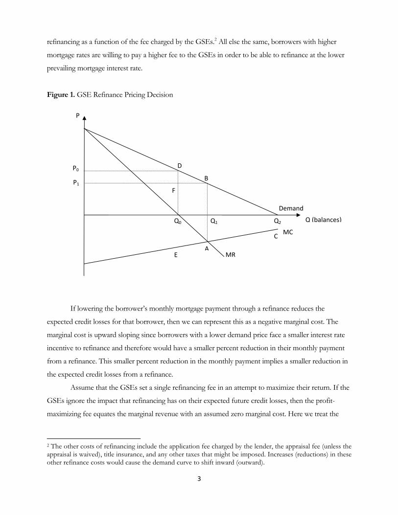
The following figure illustrates a simplified version of the decision by the GSEs on setting the
up-front fee for a refinance of an existing agency-guaranteed mortgage. These fees are set in terms of
basis points charged against the mortgage balance that is to be refinanced. Given the distribution of
active agency mortgages across different coupon rates, the other costs of refinancing and the payback
period borrowers require to recoup these costs, there will be a downward sloping demand curve for
3
refinancing as a function of the fee charged by the GSEs.2 All else the same, borrowers with higher
mortgage rates are willing to pay a higher fee to the GSEs in order to be able to refinance at the lower
prevailing mortgage interest rate.
Figure 1. GSE Refinance Pricing Decision
If lowering the borrower’s monthly mortgage payment through a refinance reduces the
expected credit losses for that borrower, then we can represent this as a negative marginal cost. The
marginal cost is upward sloping since borrowers with a lower demand price face a smaller interest rate
incentive to refinance and therefore would have a smaller percent reduction in their monthly payment
from a refinance. This smaller percent reduction in the monthly payment implies a smaller reduction in
the expected credit losses from a refinance.
Assume that the GSEs set a single refinancing fee in an attempt to maximize their return. If the
GSEs ignore the impact that refinancing has on their expected future credit losses, then the profit-
maximizing fee equates the marginal revenue with an assumed zero marginal cost. Here we treat the
2 The other costs of refinancing include the application fee charged by the lender, the appraisal fee (unless the appraisal is waived), title insurance, and any other taxes that might be imposed. Increases (reductions) in these other refinance costs would cause the demand curve to shift inward (outward).
F
E
D
MC
Q2
C
B
A
P
Q (balances)Q1
P1
P0
Q0
MR
Demand
4
two GSEs as if they act as a single monopoly in the provider of agency refinancing.3 The GSEs would
set their fee at P0 and Q0 of borrower balances would be “in the money” to refinance. By definition, in
this simple example this is half of the total borrower balances that would be in the money to refinance if
the GSEs set their fee to zero. The fee income to the GSEs is given by the rectangle 0P0DQ0.
Now assume that the GSEs correctly recognize that refinancing reduces their expected future
credit losses. This would incent the GSEs to lower their fee in order to increase the number of
refinances. The profit maximizing fee would decline from P0 to P1. This new lower fee equates the
marginal revenue with the (negative) marginal cost. By increasing the set of borrower balances that are
“in the money” from Q0 to Q1, the reduction in fee income to the GSEs from the Q0 of borrower
balances that would have refinanced at the higher fee (area P1P0DF) is more than made up for by the
fee income on the additional refinances as well as the reduction in expected future credit losses (area
EFBA).
However, note that even in this case the GSEs would be charging a socially inefficient fee. If
the GSEs were directed instead to set their pricing to maximize the sum of the expected profit to the
GSEs and borrower surplus, then the GSEs would eliminate the refinance fee. By increasing the stock
of borrower balances that are in-the-money to refinance from Q1 to Q2, this would increase overall
welfare (by the area ABQ2C). The magnitude of this welfare loss depends in part on the marginal
impact of refinancing on reducing expected future credit losses at the fee P1 and the number of
incremental refinances that are priced out by this fee. In the remaining sections of the paper, we
implement an empirical strategy for estimating this marginal impact via the sensitivity of borrower
default to changes in the borrower’s required monthly payment.
3 In reality, the GSEs have fees that are differentiated by the borrower’s current loan-to-value ratio and current credit score. In addition, the implementation of the HARP program has differed somewhat between Freddie and Fannie. For specifics on Fannie Mae pricing see https://www.efanniemae.com/sf/refmaterials/llpa/and http://www.freddiemac.com/singlefamily/pdf/ex19.pdf
For general information on the HARP program see: http://www.freddiemac.com/homeownership/educational/harp_faq.html
For information on the recent changes to HARP see: https://www.efanniemae.com/sf/mha/.
5
Literature review:
Recent advocates for a broad-based refinance program cite as one of the advantages the
reduction in future defaults on mortgages that participate in the program. However, no estimates are
provided as to the potential magnitude of the reduction in defaults and associated default costs.4 A
recent Congressional Budget Office working paper provides an estimate of the reduced credit losses
from a refinance program that is assumed to produce an incremental 2.9 million refinances of agency
and FHA mortgages [see Remy et al (2011)]. The authors estimate that such a program would reduce
expected foreclosures by 111,000 (or 38 per 1,000 refinances) resulting in reduced aggregate credit
losses of $3.9 billion. The authors use an estimated loan-level competing risk model of prepayment and
default on fixed-rate mortgages to calculate the reduced expected credit losses. However, the estimated
model is not provided in the paper, so it is difficult to fully assess their methodology.
An alternative empirical strategy is to estimate competing risk models of prepayment and
default for prime ARMs. In this case, we can measure the impact of cumulative changes in the monthly
mortgage payments from rate resets that have taken place since the origination of the mortgage on the
future performance of the borrower. Using prime conforming ARMs focuses on a roughly similar set of
borrowers as prime conforming FRMs in terms of their credit profiles and underwriting standards.
However, prime borrowers will likely self-select between FRM and ARM products based on private
information on their expected duration in the mortgage, among other factors. This selection process
will generate unobserved differences between FRM and ARM borrowers.5 The low initial mortgage
rates that are typically offered on many ARMs may also be relatively attractive to borrowers who have
to stretch more in their budget [Green and Shilling (1997)].
The empirical literature has focused relatively more on estimating default and prepayment
models for FRMs as compared to ARMs. Calhoun and Deng (2002) provide a side-by-side comparison
analysis of FRMs and ARMs using a comparable empirical specification. While FRMs and ARMs have
similar baseline prepayment hazards, Calhoun and Deng show that ARMs have baseline default hazards
that are higher over the first two years following origination. They speculate that this might reflect the
fact that ARMs attract a more heterogeneous set of borrowers in dimensions that are not well captured
4 See for example Boyce, Hubbard and Mayer (2011). http://www4.gsb.columbia.edu/null/download?&exclusive=filemgr.download&file_id=739308. Also, Greenlaw (2010). http://www.scribd.com/doc/35781758/US-Economics-Slam-Dunk-Stimulus-Morgan-Stanley-July-27 5 See Brueckner and Follain (1988) and Dhillon, Shilling and Sirmans (1987).

6
by the observed borrower characteristics controlled for in the empirical specification. Calhoun and
Deng do not include the change in the monthly payment as a control in their ARM specification.
The recent empirical literature on ARMs has focused relatively more on the impact of increases
rather than decreases in the monthly payment on prepayment and default. This focus is motivated by
the fact that most ARMs have an initial “teaser” rate in that the coupon rate is set below the rate that
would be implied by the reference rate and margin at the origination date.6 That is, if the reference rate
(generally either a short-term Treasury or LIBOR) does not change between the origination and the first
rate reset date, the monthly payment will increase at the rate reset date. In addition, many ARMs also
include a prepayment penalty period that covers the period up to the first rate reset date.7
The combination of an initial teaser rate and a possible prepayment penalty will reduce the
prepayment rate during the period leading up to the first rate reset. As a consequence, there tends to be
a spike in prepayments at the rate reset [Ambrose and LaCour-Little (2001), Ambrose et al (2005),
Pennington-Cross and Ho (2010)]. The challenge in identifying if the increase in the mortgage payment
at the first reset leads to higher defaults is that there may also be a change in the composition of the
remaining borrowers in terms of their unobserved characteristics. The spike in prepayments may have
selected the better quality borrowers out of the sample, leaving relatively more risky borrowers
remaining in the sample. An observed rise in defaults following the reset date could therefore reflect
not only the impact of the payment increase, but also the change in the unobserved risk characteristics
of the remaining borrowers. However, this story is not supported by the empirical literature. For
subprime ARMs, Gerardi et al (2007) and Sherlund (2010) do not find evidence of a significant rise in
the default risk following the expiration of the teaser rate for non-prime hybrid ARMs.8
There are two reasons we would not necessarily want to use the evidence on the impact of
increases in mortgage payments on default risk to infer the impact of payment decreases. First, as noted
above, there is often a significant change in the sample of borrowers at the time of the payment increase
associated with the expiration of the initial teaser rate and the prepayment penalty. This is not likely to
be a problem for reductions in the mortgage payment when the rate resets lower. In these cases, we
would not expect to see a spike in prepayments so the sample composition remains relatively constant.
6 Ambrose and LaCour-Little (2001) report that 99% of their sample of conventional ARMs originated in the early 1990s had teaser rates with an average discount of 2.1%.
7 Mayer, Pence and Sherlund (2009) report that 70% of their sample of subprime ARMs had prepayment penalties. In addition, in 2005 the average teaser discount was 3.5%.
8 Sherlund (2010) does report higher default risks following a large payment increase (greater than 5%) when the borrower also has little equity (current LTV of 95 or higher).
7
Second, even if we could better control for changes in the unobserved heterogeneity of the borrowers,
there is no reason to expect that the impact of mortgage payment changes on default and prepayment
are symmetric with respect to payment increases and decreases.9 On the contrary, it is a well-established
principle of mortgage pricing that prepayment risk, at least, is asymmetric with respect to the prevailing
level of mortgage interest rates; for credit risk, the question of symmetry with respect to payment
changes is less settled. In our analysis, described below, we allow for asymmetric impacts.
A refinance is similar to a modification where the rate of the mortgage is lowered and the term
is extended. The emerging literature on modifications offers additional insight into the effects of
payment reductions on expected credit losses. Initial research focused on modifications that pre-dated
the government’s Home Affordable Modification Program (HAMP). Haughwout et al (2010) use
LoanPerformance data to estimate a competing risk model using over 53 thousand modifications of
subprime loans that were originated between December 2005 and March 2009. They exclude
capitalization modifications where the borrower’s monthly payment can increase. They find that a 10
percent reduction in the monthly payment lowers the 12-month re-default rate by 13 percent.10
Agarwal et al. (2011) analyze mortgages originated between October 2007 and May 2009 from the
OCC-OTS Mortgage Metrics data. They report that a 10 percent reduction in the monthly mortgage
payment reduces the re-default rate by 3 percent.11 As a note of caution, findings from studies of re-
default of modification may not generalize to HARP due to differences in borrower risk characteristics
and delinquency status: HARP borrowers are current in their mortgages whereas borrowers receiving
modifications tend to be seriously delinquent.
Data and empirical specification:
To conduct our competing risk analysis we select a 10 percent random sample of all first-lien,
GSE-held prime, owner-occupied ARMs from the LPS data that were originated from January 2003
onwards. This produced an initial sample of 279,124 ARMs. We drop 87,816 of these loans because we
9 Ambrose et al. (2005) impose symmetry in the competing risk specification estimated on a sample of 3/27 hybrid ARMs.
10 They define re-default as the borrower becoming 90-days delinquent within the first year following the modification.
11 In this study, a mortgage re-defaults if it becomes 60-days delinquent within 6 months of the modification. As such, the two results are not directly comparable.
8
do not observe them within two months of origination. We drop 6,801 loans because they had no
servicing data beyond the second month or the initial observation for the mortgage indicates a
liquidation, transfer, prepayment, or default. We trimmed the bottom 1 percent based on origination
loan balances as well as balances that exceeded the standard conforming loan limit – dropping
mortgages with balances below $50,825 (1,450 mortgages) or with balances above $417,000 (10,914
mortgages). We further restricted the estimation sample to mortgages with origination LTV ratios
between 20 and 105 (2,166 mortgages were dropped for an origination LTV below 20 and 2,458
mortgages were dropped for an origination LTV above 105). Finally, we dropped 7,454 loans because
they had at least one monthly payment below $200, or because they had at least one month where their
cumulative monthly payment increase was greater than 150 percent. All told, these criteria led to the
elimination of 105,857 loans (note, there was overlap among the groups being excluded for different
criteria), leaving 173,267 loans in our estimation sample.
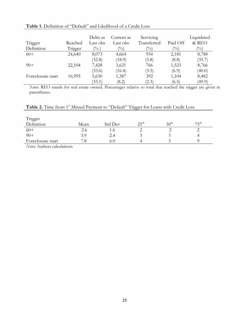
We define our “default” event as the first time that a mortgage reaches 90 days delinquent.
This choice is measured consistently in the data and does not depend on state laws governing
foreclosure. In addition, borrowers who reach 90 days delinquent have a reasonably low “cure” rate
– that is, the probability that the borrower will catch up on the missed payments and or pay off the
mortgage. This can be seen in Table 1 where we compare transition rates into a credit loss (end of a
foreclosure) as well as cure rates for different delinquency triggers. There is a reduction in the cure
rates moving from a default definition of 60 days delinquent to 90 days delinquent. For mortgages
that ever reach 60 days delinquent, 27.7 percent are either now current or have paid off. The cure
rate declines to 23.3 percent for mortgages that ever reach 90 days delinquent. Finally, the cure rate
declines to 14.7 percent if we define default as a mortgage ever entering the foreclosure process. For
all three default definitions, conditional on the mortgage being terminated, over 80 percent of the
mortgages that reach that default trigger result in a credit loss.12
Another consideration for the choice of the default definition is the variability in time from
the initial delinquency to the time that the default trigger is reached. The higher this variability, the
more difficult it becomes for the model to capture the timing of economic conditions that may have
contributed to a borrower initially going delinquent and, ultimately, defaulting. Table 2 provides
information on the mean and variance of the time between the initial delinquency in an unbroken
string of delinquencies and the default trigger. There is a 50 percent increase in the standard 12 For the 60-day, 90-day and foreclosure start default triggers these conditional loss rates are 80.1 percent, 85.2 percent and 88.5 percent respectively.
9
deviation moving from a default definition of 60 days delinquent to 90 days delinquent, but the
standard deviation increases by 150 percent going from 90 days delinquent to a foreclosure start.
Taken together, the results from Tables 1 and 2 suggest that defining the default event as the first
time a borrower reaches 90 days delinquent provides a good balance between consistent timeliness
of the default trigger and a high transition rate to a final claim.
The key variable of interest is the percent change in the monthly payment from the initial
monthly payment to the current monthly payment. Our aim is to use the estimated impact that these
monthly payments changes have on the ARMs borrowers’ risk of default and prepayment to infer
the impact on expected credit losses from refinancing borrowers who have fixed-rate mortgages. We
allow for the possibility that decreases in monthly payments may have asymmetric effects on default
and prepayment from increases in monthly payments, and that these asymmetric effects may further
differ for borrowers with high versus low current LTV. We define a “unit” change in each monthly
payment variable as a 10 percent change in the indicated direction. The monthly payment change
variables are dynamic variables in that their values vary over time for a mortgage. The payment
changes are dictated by the terms of the mortgage contract regarding the index, the spread, the dates
the rates adjust, any triggers or caps on adjustments, and changes in the reference rate since the
mortgage was originated. One distinction between payment reductions for FRM borrowers through
a refinance and for ARM borrowers through a rate reset is that the payment changes are permanent
for the FRM borrowers and can be reversed for ARM borrowers. A consequence may be that the
impact of these payment reductions on future credit losses will be attenuated in moving from FRM
to ARM borrowers.13
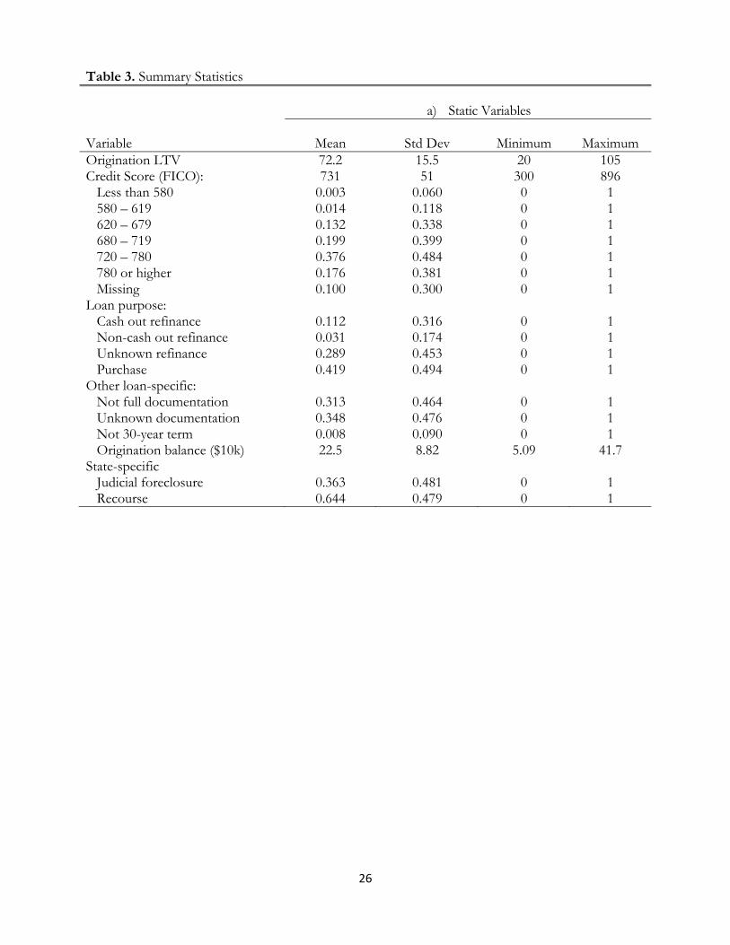
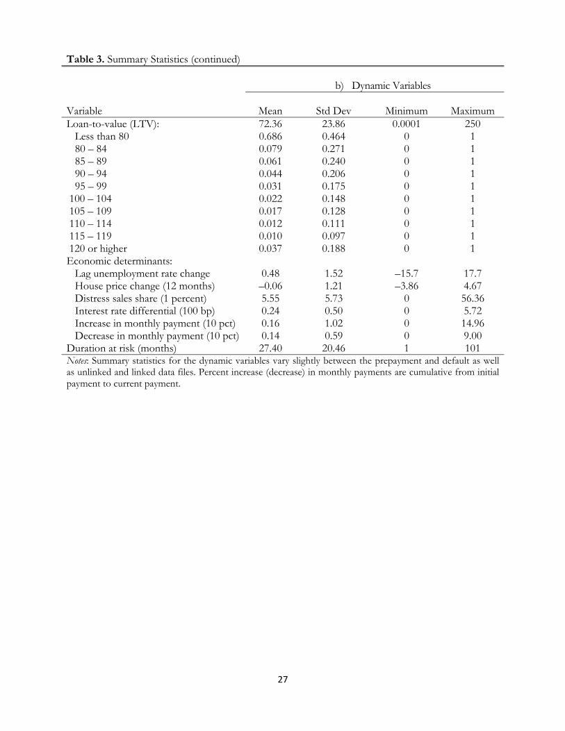
The LPS data provide information on a variety of borrower, loan, and property risk factors.
We supplement these with additional data on economic factors and state legal requirements that may
impact loan performance. Summary statistics on these variables for loans in the estimation sample
are given in Table 3. The summary statistics are presented separately for the static variables whose
values do not change over the life of the mortgage and for the dynamic variables whose values are
time-varying. For the categorical variables, the left-out group is selected to be the high-quality or
relatively more common mortgage type.
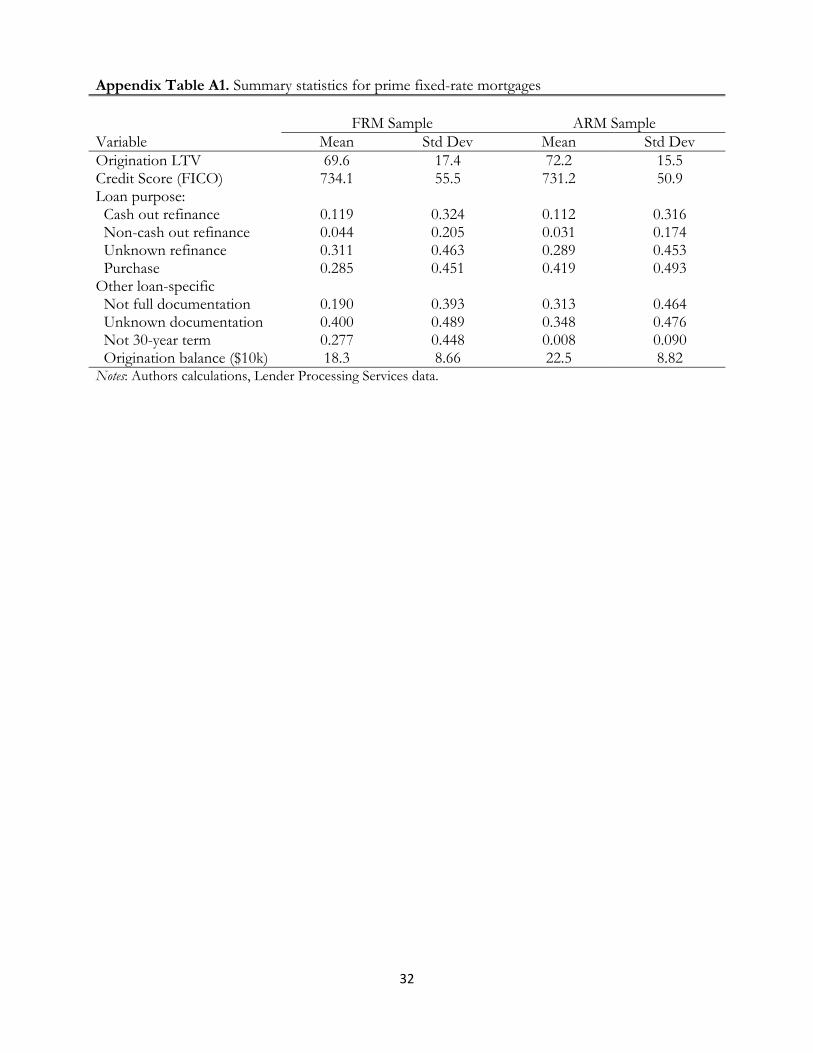
Appendix Table A1 provides a comparison set of static summary statistics for a sample of
prime FRMs from LPS over the same time period. The adjustable and fixed-rate prime mortgage 13 We thank Mitch Remy for highlighting this point to us.

10
samples are similar in terms of their origination LTVs and credit scores. The purchase share is
higher and the origination balance is larger for the ARM sample. Finally, the FRM sample has a
higher fraction of mortgages with terms shorter than 30 years.
The borrower’s updated LTV is an important risk factor. We update each mortgage’s LTV
using the origination LTV, the amount of debt amortization to date, and the cumulative change in
metropolitan area house prices to date. For fully underwritten loans, we observe the initial mortgage
balance and for each month the mortgage balance that reflects amortization and any accelerated
payments made by the borrower.14 We also observe the appraisal value at origination which we
update each month using the CoreLogic house price index for the loan’s metropolitan area.
Combining these data gives us a monthly updated LTV on the mortgage. We control for the
updated LTV in the hazard analysis by entering a series of indicator variables for different LTV
intervals. The left-out category corresponds to a mortgage with a current LTV below 80.
Two additional important borrower risk factors are the credit score (FICO) and the debt-to-
income (DTI) ratio. In contrast to the LTV, which is a dynamic variable that varies over the
duration of the mortgage, both FICO and DTI are static variables. We include a series of indicators
for different intervals of FICO scores as well as an indicator for a missing FICO. The left-out
category corresponds to a FICO score of 780 or higher (a high credit quality borrower). The DTI
variable is meant to capture what is called the “front-end” ratio, which is defined as the sum of the
borrower’s annual mortgage payments (principal and interest), property taxes, and house insurance
premium incurred divided by the borrower’s income. However, the data provider (LPS) confirmed
that some servicers report “back-end” ratios which include in addition payments on home equity
loans, auto loans, student loans and minimums on credit cards. We were unable to identify what type
of DTI was being reported for each mortgage, so we had to omit the DTI variable from the analysis.
There are several loan-specific factors that we control for in the analysis. The first category
is the loan purpose. We include indicators for three different types of refinances: cash-out, non-
cash-out, and unknown purpose. Here, the left-out category is a purchase mortgage. Other loan-
specific factors that we control for are whether the mortgage is not fully documented, the
documentation status is unknown, and if the mortgage does not have a 30-year term. We also
include the origination mortgage balance measured in $10,000 increments to capture any
14 We do not include in the mortgage balance arrears due to past missed payments. Doing so would induce a mechanical positive correlation between the updated LTV and borrower default.

11
independent effect of loan size. Our final loan-level variable is a measure of the incentive to
refinance a mortgage measured by the difference between the current interest rate on the mortgage
and the current average prevailing rate for 30-year fixed rate mortgages, if this difference is
positive.15 We allow this interest rate incentive to have a differential effect for current low- and high-
LTV borrowers. To help control for any systematic unobserved differences in underwriting
standards across time, we include indicators for the year the mortgage was originated.
Local economic factors, which proxy for unobserved loan-level indicators, may also exert a
strong influence on mortgage performance. A traditional trigger for a default is an unemployment
spell experienced by the borrower. We include the 12-month change in the local unemployment
rate lagged six months. We find that the change in the local unemployment rate is a better predictor
of default than the level of the unemployment rate. We lag by six months the 12-month
unemployment rate change to account for the time lag between when the borrower loses his/her job
and when the borrower may become 90 days delinquent. The unemployment rate variable should be
thought of as a proxy variable for the unobserved indicator for whether the borrower becomes
unemployed. If we had dynamic data on the borrower’s employment status, we would likely drop
the unemployment rate from the specification.16 As a proxy, we expect that the estimated impact of
the unemployment rate on default will be attenuated due to a low correlation of the unemployment
rate with the borrower’s actual employment status.17
Variation in house prices over time within a metropolitan area and across metropolitan areas
is an important factor in affecting the distribution of updated LTVs for active mortgages. Rising or
falling house prices may also be correlated with other local economic shocks that are not well
controlled for by the other variables in the specification and which may impact the prepayment and
default behavior of borrowers. For example, the current LTV effects may reflect both the direct
effect of the borrower’s equity position on the prepayment and default decision, as well as the
indirect effects due to economic shocks that are correlated with changing area house prices. To
15 We use the monthly average rate on conventional 30-year mortgages from the FHLMC weekly survey (available at http://www.freddiemac.com/pmms/).
16 Given an indicator for whether the borrower is unemployed, the area unemployment rate would be included in the empirical specification only if the risk of unemployment (conditional on the borrower currently being employed) affected the likelihood that the borrower would prepay or default on the mortgage.
17 See Haughwout et al. (2010) for a more detailed discussion.
12
mitigate any possible omitted-variable bias on the current LTV estimates, we include the 12-month
percentage change in the area house prices as an additional dynamic variable.
Local contagion may affect a borrower’s decision to default as well. A recent survey [Fannie
May (2010)] finds that borrowers who know someone who has experienced a foreclosure are more
than twice as likely to seriously consider default as those who do not.18 We control for the
possibility of a contagion effect by including the number of distressed sales per 10,000 households in
the metropolitan statistical area (MSA). We calculate a three-month moving average of MSA distress
sales using CoreLogic data. The number of households in the MSA is taken from the 2008 American
Community Survey.19 Given the long time lag between the events that trigger a default and the
eventual foreclosure sale, this measure is unlikely to pick up contemporaneous economic shocks that
may be affecting current default decisions.
Finally, the legal environment that governs how mortgage delinquencies are handled varies
by state. A potentially important factor is whether the mortgage is originated in a state with a judicial
foreclosure process, which lengthens the expected time to complete the foreclosure. Longer delays
in the foreclosure process could provide an incentive to borrowers to strategically default.20 A
second legal consideration is whether mortgages are considered as recourse or non-recourse loans in
a state. Recourse loans provide potentially more security to the lender, since the lender has the
ability to pursue a defaulted borrower with a deficiency judgment for any unpaid balance. As a result,
borrowers in a recourse state may be less likely to default if the property is underwater – that is, if
the mortgage balance exceeds the current market value of the property. We include indicators for
judicial foreclosure states as well as for recourse states.
Econometric Specification:
We use a competing risk model to analyze the impact of the borrower risk characteristics,
mortgage and property characteristics, and economic factors on prepayment and default outcomes.
We assume these risks are independent. We model each risk using a proportional hazard framework.
The prepayment (p) and default (d) hazard rates since origination at duration t are given by: 18 A similar result is also found in Guiso et al. (2009).
19 http://factfinder.census.gov/servlet/DTSelectedDatasetPageServlet?_lang=en&_ts=286380818796)
20 See for example discussions of strategic default in Foote et al. (2008) and Haughwout et al. (2010).
13
exp exp (1a)
exp exp (1b)
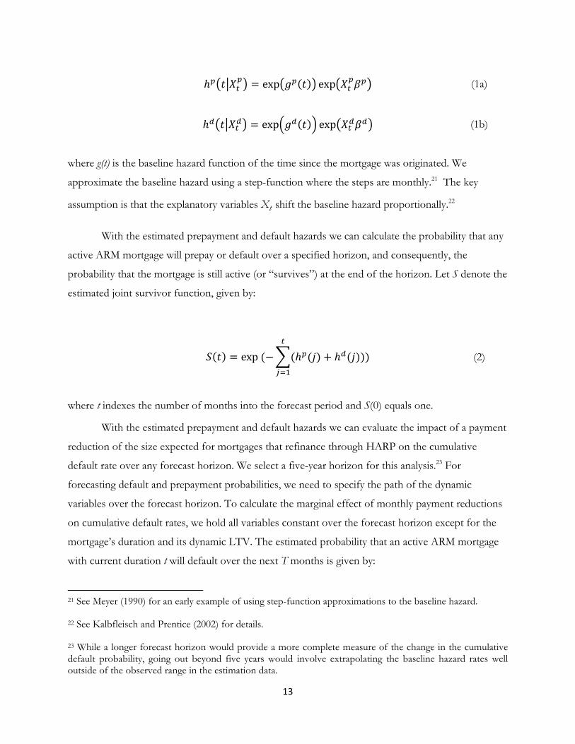
where g(t) is the baseline hazard function of the time since the mortgage was originated. We
approximate the baseline hazard using a step-function where the steps are monthly.21 The key
assumption is that the explanatory variables Xt shift the baseline hazard proportionally.22
With the estimated prepayment and default hazards we can calculate the probability that any
active ARM mortgage will prepay or default over a specified horizon, and consequently, the
probability that the mortgage is still active (or “survives”) at the end of the horizon. Let S denote the
estimated joint survivor function, given by:
exp (2)
where t indexes the number of months into the forecast period and S(0) equals one.
With the estimated prepayment and default hazards we can evaluate the impact of a payment
reduction of the size expected for mortgages that refinance through HARP on the cumulative
default rate over any forecast horizon. We select a five-year horizon for this analysis.23 For
forecasting default and prepayment probabilities, we need to specify the path of the dynamic
variables over the forecast horizon. To calculate the marginal effect of monthly payment reductions
on cumulative default rates, we hold all variables constant over the forecast horizon except for the
mortgage’s duration and its dynamic LTV. The estimated probability that an active ARM mortgage
with current duration t will default over the next T months is given by:
21 See Meyer (1990) for an early example of using step-function approximations to the baseline hazard.
22 See Kalbfleisch and Prentice (2002) for details.
23 While a longer forecast horizon would provide a more complete measure of the change in the cumulative default probability, going out beyond five years would involve extrapolating the baseline hazard rates well outside of the observed range in the estimation data.
14
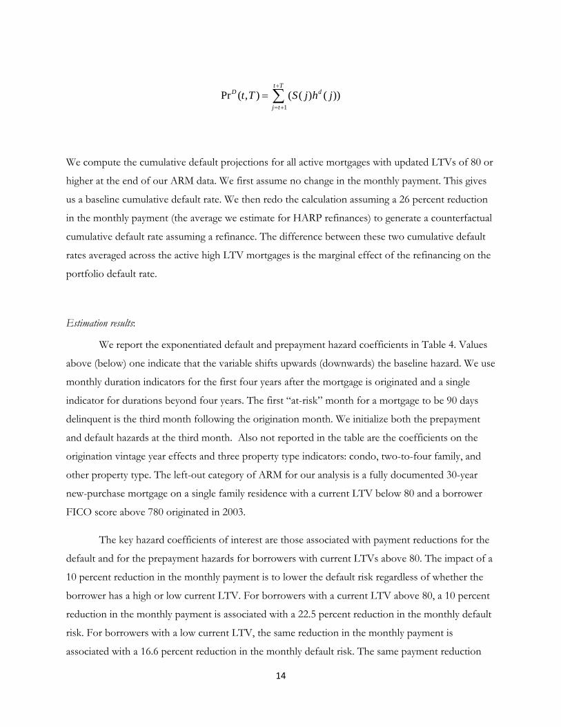
1
Pr ( , ) ( ( ) ( ))t T
D d
j t
t T S j h j
We compute the cumulative default projections for all active mortgages with updated LTVs of 80 or
higher at the end of our ARM data. We first assume no change in the monthly payment. This gives
us a baseline cumulative default rate. We then redo the calculation assuming a 26 percent reduction
in the monthly payment (the average we estimate for HARP refinances) to generate a counterfactual
cumulative default rate assuming a refinance. The difference between these two cumulative default
rates averaged across the active high LTV mortgages is the marginal effect of the refinancing on the
portfolio default rate.
Estimation results:
We report the exponentiated default and prepayment hazard coefficients in Table 4. Values
above (below) one indicate that the variable shifts upwards (downwards) the baseline hazard. We use
monthly duration indicators for the first four years after the mortgage is originated and a single
indicator for durations beyond four years. The first “at-risk” month for a mortgage to be 90 days
delinquent is the third month following the origination month. We initialize both the prepayment
and default hazards at the third month. Also not reported in the table are the coefficients on the
origination vintage year effects and three property type indicators: condo, two-to-four family, and
other property type. The left-out category of ARM for our analysis is a fully documented 30-year
new-purchase mortgage on a single family residence with a current LTV below 80 and a borrower
FICO score above 780 originated in 2003.
The key hazard coefficients of interest are those associated with payment reductions for the
default and for the prepayment hazards for borrowers with current LTVs above 80. The impact of a
10 percent reduction in the monthly payment is to lower the default risk regardless of whether the
borrower has a high or low current LTV. For borrowers with a current LTV above 80, a 10 percent
reduction in the monthly payment is associated with a 22.5 percent reduction in the monthly default
risk. For borrowers with a low current LTV, the same reduction in the monthly payment is
associated with a 16.6 percent reduction in the monthly default risk. The same payment reduction
15
has a much smaller impact on the monthly prepayment risk for low LTV borrowers – the estimated
reduction is less than 7 percent. In contrast, for high LTV borrowers, a ten percent payment
reduction lowers the prepayment hazard by 25.4 percent. For the high LTV borrowers, the net
impact on the cumulative default rate will depend on whether the marginal effect on the monthly
default hazard outweighs the marginal effect on the monthly prepayment hazard.24
Before turning to the default forecast exercise, it is useful to quickly summarize some of the
other key empirical findings from the competing risk model. Default and prepayment risks are very
sensitive to the estimated current LTV on the mortgage. The monthly default risk rises by a factor of
8 comparing ARMs with an estimated current LTV below 80 to those above 120. Looking at the
prepayment hazard, the data indicates that the monthly prepayment rate declines by 90 percent as
we increase the estimated current LTV from below 80 to above 120. This illustrates the “collateral
constraint” on refinancing identified earlier by Caplin et al (1997). Absent special refinance programs
such as HARP, borrowers with high current LTVs have low prepayment speeds because they cannot
fund the downpayment necessary for a refinance using equity in their current house.25 In interpreting
the current LTV hazard results, it is important to note that we are controlling for the percent change
in metro area house prices over the prior year.26
A borrower’s FICO score is also an important determinant of default and prepayment. A
limitation of our data is that we only observe the borrower’s FICO score at the time of the
origination of the ARM. Despite the static nature of the credit score variable, the predicted monthly
default risk increases by a factor of 12 comparing a borrower with an origination FICO of above
780 to a borrower below 580. FICO scores have a much smaller impact on the likelihood that a
borrower prepays. Comparing borrowers with an origination FICO of above 780 to below 580 the
monthly prepayment risk declines by only 10.5 percent.
24 The data also reject symmetry of the effect of payment increases and payment decreases on the default and prepayment hazards. Payment increases have smaller effects on the default hazard than payment decreases for both high and low LTV borrowers.
25 Deng et al. (2000) control for the probability that a prime FRM is in negative equity. They find that the probability of negative equity raises the default hazard and lowers the prepayment hazard.
26 Dropping the 12-month change in area house prices results in the negative equity LTV indicators rising by roughly 11 percent in the default hazard and decline by roughly 9 percent in the prepayment hazard. The unemployment hazard coefficients are not meaningfully impacted.

16
Turning to the remaining loan-specific characteristics, ARMs that are not fully documented
have higher monthly default rates but also higher monthly prepayment rates. Refinances have a
higher default risk than new-purchase mortgages – regardless of whether the borrower took cash out
or not in the refinance. Very few ARMs in our sample do not have a 30-year term. Those with
shorter terms, though, have higher monthly default risks than similar ARMs with a 30-year term.
Loans with larger origination balances have higher default and prepayment hazards. Increasing the
loan balance by $100,000 raises the default and prepayment hazards by 8 percent and 5 percent
respectively. Finally, increasing the financial incentive to refinance as measured by the spread
between the current rate on the mortgage and the prevailing rate on 30-year fixed rate mortgages
increases the monthly prepayment rate. The data indicates that mortgages with a current LTV below
80 have a stronger prepayment response to changes in the financial incentive to refinance.
Several local economic factors are controlled for in the analysis. As already discussed, we
control for the percent change in metro area house prices over the past 12 months. Holding the
borrower’s current LTV constant, falling house prices both increase the default risk and decrease the
prepayment risk. The fact that, controlling for an estimate of the borrower’s current LTV, area
house prices impact default and prepayment behavior likely reflects correlations between changes in
house prices and other local economic conditions that are left out of the empirical specification.27
Increases in the local unemployment rate raise the default risk. The magnitude indicates that
a one percentage point increase in the unemployment rate raises the monthly default hazard by 12
percent. As discussed earlier, this marginal effect is likely seriously understated, due to the
measurement error in using the area unemployment rate as a proxy variable for whether a particular
borrower experiences an unemployment spell. The share of distressed sales in the metro area does
not impact either the default or prepayment hazards in any economically meaningful manner. This
could be interpreted as a lack of evidence in this data of “contagion” from strategic default. Finally,
we find that the legal environment in the state does impact the estimated hazards. Judicial
foreclosure states are associated with 25.3 percent higher monthly default hazards.28 In contrast,
states where mortgages are recourse loans have a 15.6 percent lower monthly default hazards.
27 One possibility is that credit availability may be more restricted in housing markets that have experienced greater house price declines.
28 The higher estimated default rate in judicial foreclosure states may reflect the longer foreclosure delays that exist in these states. These delays increase the incentive to strategically default.

17
Impact of refinancing on future credit losses:
Using the estimated default and prepayment hazards, we can estimate the impact that
increased refinancing under the HARP program would likely have on future credit losses to the
GSEs. The first step in the analysis is to identify a set of prime conforming FRM where the
borrower would likely qualify for a HARP refinance. For this set of borrowers, we can calculate the
average percentage reduction in the required monthly payment associated with a HARP refinance.
We can use this average percent reduction in our forecast exercise to predict the average reduction
in the cumulative five-year default rate. Given an assumed loss given default, we can estimate the
implied reduction in expected credit losses.
We use data from LPS on prime conforming FRMs. For each mortgage, we know the
origination LTV and location of the property. The servicing data for each mortgage gives the current
mortgage balance over time. We update the LTV over time using the current mortgage balance and
an updated house value based on CoreLogic house price indices for that metro area. To identify the
set of HARP-eligible borrowers, we select all borrowers where the estimated current LTV exceeds
80 and where the borrower has been current for the past 12 months. To identify the subset of these
borrowers who would have an incentive to refinance under an improved HARP program, we use a
rule that the borrower is “in the money” to refinance if the estimated all-in cost of the refinance
would be recovered within two years.29 Using the identified set of in-the-money HARP-qualified
borrowers, we calculate that refinancing would reduce the required monthly payment on average by
26 percent.
The next step is to estimate the impact that this 26 percent reduction in the monthly
payment would have on the average default rate. We use the estimated ARM default and prepayment
hazards to do a five-year cumulative default forecast. We select the ARMs with current LTVs above
80 that are still active at the end of our estimation period (July 2011) and that have not prepaid or
reached 90 days delinquent. For each of these mortgages, we generate five years of additional data to
be used in the forecast exercise. We assume that the local unemployment rate and local house prices
remain at their current levels over the forecast period – that is, we set their values to zero since they
29 We use two years instead of three years for the payback period to account for possible risk aversion by borrowers to invest in a refinance given the high risk of a job loss. If the borrower becomes unemployed during the payback period, then the borrower would likely not be able to recoup the full cost of the refinance.

18
are in change form. We allow the mortgage’s duration and current LTV to vary over the forecast
period. The only factor impacting the current LTV is debt amortization. We first do a baseline
default forecast for each mortgage assuming no change in the monthly payment. We then redo the
default forecast for each mortgage assuming a 26 percent reduction in the monthly payment. We
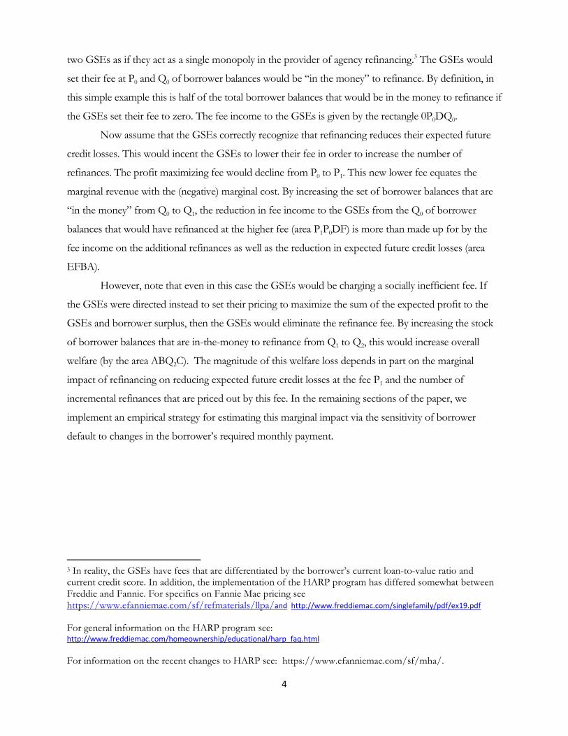
construct cumulative default curves by averaging the estimated cumulative default probabilities over
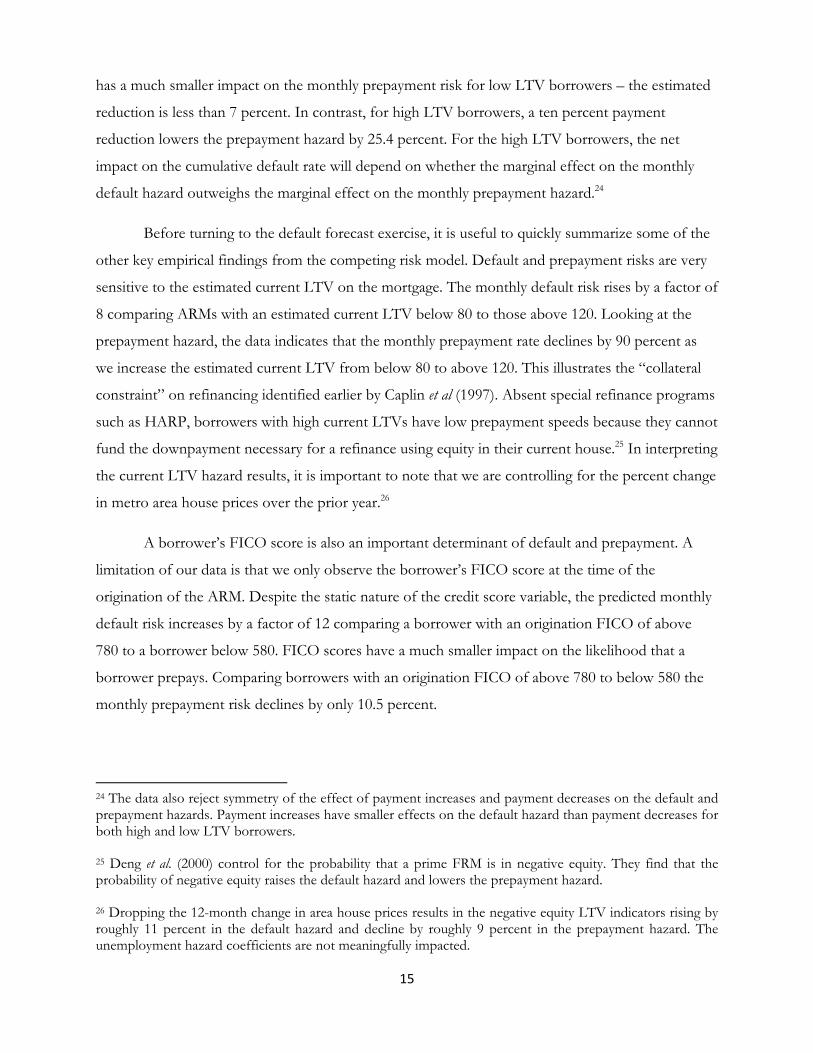
all of the mortgages. The results of this forecast exercise are displayed in Figure 1. The baseline
cumulative default curve is shown in red. At five years, the estimated hazard models imply that the
expected cumulative default rate would be 17.3 percent. When we repeat the exercise reducing the
monthly payments by 26 percent, the expected five-year default rate is reduced to 13 percent – a
24.8 percent reduction.30
We assume that a borrower with a prime conforming FRM who refinances under HARP
would experience the same proportionate decline in the expected cumulative default rate. The next
step is to generate predicted 5-year cumulative default rates for prime conforming FRM borrowers
with current LTVs of 80 or higher who are current in their payments. To do this, we constructed a
“roll-rate” matrix of monthly transition rates between payment statuses for prime conforming FRMs
with current LTV of 80 or higher. We estimate this matrix using LPS data on a 5 percent random
sample of prime FRMs for the six-month period from June of 2011 through November 2011.31 We
use this roll-rate matrix to simulate the five-year cumulative default rate for our target borrowers –
current LTV of 80 or higher and current in mortgage payments as of June 2011. We define the
default rate to be probability that the mortgage is in foreclosure, REO or has been liquidated. The
data indicated a predicted 5-year cumulative default rate of 15.2 percent.32
Our earlier ARMs-based forecast exercise predicts that facilitating refinances for these
HARP-eligible borrowers would reduce their cumulative 5-year default rate by 24.8 percent.
Applying this to the estimated 5-year cumulative default rates for HARP-eligible FRMs implies a
reduction from 15.2 percent to 11.4 percent – a decline of 3.8 percentage points. This estimate of a
3.8 percentage point reduction in the default rate is identical to the estimate reported in Remy et al.
30 Holding the prepayment hazard constant and changing the default hazard alone the cumulative default rate declines to 11.2 percent – a 34.9 percent reduction. In contrast, holding the default hazard constant and changing the prepayment hazard alone the cumulative default rate increases to 19.5 percent – a 12.9 percent increase.
31 The sample consisted of approximately 254 thousand prime conforming FRMs and 1.5 million monthly transitions.
32 An estimated 45.3 percent are prepaid by the end of the 5-year period.

19
(2011). In comparing the two estimates, it is important to keep in mind that the Remy et al. estimate
includes the effect of borrowers with current LTVs below 80 who refinance while our estimate is
restricted to borrowers with current LTVs above 80.
To convert this reduced default rate into an estimated reduction in credit losses for the
HARP program, we need to estimate a loss given default (LGD). We start with the average LGD
reported in their Table 2 of Qi & Yang (2009) for different LTV intervals.33 For example, they
report an average LGD of 30.5 percent for mortgages with current LTVs between 100 and 110,
which increases to 37.0 percent for mortgages with current LTVs between 110 and 120. To estimate
our LGD input, we generate a weighted-average LGD based on the share of the aggregate 5-year
predicted cumulative default probability that falls into each of Qi & Yang’s LTV intervals. We then
adjust these default probability shares to reflect the different distribution of LTVs between our
ARM forecast sample and a FRM sample that we estimate would be “in the money” to refinance
under the revised HARP program. The resulting share-weighted LGD is 35.2 percent. Combining
the 3.8 percent lower probability of a default with an estimated average LGD of 35.2 percent
translates into a reduction in expected credit losses of around 134 basis points of the principal
balance on each mortgage that is refinanced.
The expected reduction in credit losses for any given refinance is a function of the
magnitude of the decline in the monthly mortgage payment and the current LTV. The monthly
payment decline determines the reduction in the probability of default and the current LTV
determines the expected loss given default. In Figure 1 we indicate that the negative marginal cost
curve reflecting these lower expected default costs is upward sloping. To calibrate the slope of this
curve we divided our estimated in-the-money HARP refinances into deciles based on the percent
reduction in the monthly payment from a refinance.34 For each decile, we calculated the balance-
weighted percent reduction in the mortgage payment and the balance-weighted loss given default.
We then calculated the implied expected reduction in credit losses for each decile. The results
indicated that the reductions in credit losses varied from 186 basis points to 47 basis points going
from the highest to the lowest decile.
33 Their loss given default numbers include estimates for foreclosure expenses and property maintenance expenses. Around 91 percent of their defaulted loans are conforming.
34 For this exercise, we calculate whether the mortgage is in the money to refinance using the same 2-year payback rule as discussed earlier but assume no GSE refinance fee.

20
Our estimate of an average 134 basis point reduction in expected credit losses is likely
conservative due to a likely understatement of the expected LGD. The LGD estimates are derived
from data from 1990 to 2003 when housing markets were much less stressed than they are today.
This higher degree of stress would result in larger average losses for the same range of current
LTVs.
Application
We use the estimates to illustrate the implications for pricing from incorporating the impact
of refinances on future expected credit losses. We conduct a simple pricing exercise to show for
different category of prime borrowers the magnitude of the difference between the refinancing fee
that maximizes fee income for that category of borrowers from the refinancing fee that maximizes
the combination of the fee income and the reduction in the expected future credit losses. We adopt
the pricing categories used by the GSEs in their loan level pricing adjustments (LLPAs).
The GSE pricing categories for HARP are delineated by LTV and FICO scores. The
reduction in future expected credit losses will vary by borrowers across LTV in our model due to the
impact of LTV on the estimated loss given default. However, our baseline model discussed above
does not generate differences in expected credit loss reductions by the borrower FICO scores. In
order to investigate how FICO differences should affect the fee for internal refinances, we
generalize our baseline model for the purpose of this pricing exercise. We allow the impact of lower
monthly mortgage payments on the default and prepayment hazard to vary not only by high and low
LTV as before but also by low, medium and high FICO scores. We define the three ranges of FICO
scores as below 680, 680 to 720, and above 720. We find these FICO interactions to be significant in
both the default and prepayment hazards. When we redo the five year default exercises for each
FICO interval we find that the percent reduction in the cumulative default rate for a typical HARP
refinance payment reduction is 21.9 percent for borrowers with high FICO scores, 22.6 percent for
medium FICO scores and 42.4 percent for low FICO scores.
In order to convert these monthly payment impacts into an implied reduction in five year
default rates for HARP eligible FRMs, we generate separate payment transition matrices for each of
the three FICO intervals. We use these payment transition matrices to compute implied five year
cumulative default rates assuming that the borrower is current on the mortgage. These cumulative
default rates are 8.7 percent for HARP eligible FRM borrowers with high FICO scores, 17 percent

21
for medium FICO scores, and 21.4 percent for low FICO scores. Combining these results, the
generalized model indicates that the average HARP refinance would reduce the expected default rate
by 1.9 percentage points for a borrower with a high FICO score, by 3.8 percentage points for a
borrower with a medium FICO score, and by 9.1 percentage points for a borrower with a low FICO
score. The differential impact of a HARP refinance on the probability of default by FICO score and
on the loss given default by LTV implies that incorporating the impact of expected credit losses into
the pricing decision should generate higher price discounts for weaker credit borrowers as measured
by FICO score and LTV.
For each cell of the pricing matrix we calculate a price that maximizes the fee income and a
second price that maximizes the combination of the fee income and the expected reduction in credit
losses. We start by selecting active HARP eligible FRMs that fall in range of LTVs and FICOs for
that cell of the matrix. For each mortgage, we calculate the maximum fee that the borrower would
be willing to pay and still refinance.35 In addition, for each mortgage we calculate the impact that a
refinance would have on the expected credit losses for that mortgage. For each cell of the pricing
matrix we construct the demand curve for refinancing as a function of the fee charged by the GSEs
as well as the negative marginal cost curve. The fee income maximizing fee sets the marginal revenue
curve in each cell equal to zero, and the profit maximizing fee sets the marginal revenue curve equal
to the marginal cost curve. We also estimate the total fee revenue and total profits generated from
both pricing rules assuming that there is a full take up of the in-the-money borrowers.
The results from this pricing exercise are reported in Table 5. Weighting the results across
cells of the pricing matrix by the number of mortgages in each cell, we find that incorporating into
the pricing decision the impact of refinancing on the expected future credit losses on average lowers
the desired price by 17 basis points.36 Looking at the averages by LTV intervals, we see that the
average pricing impact is 15 basis points for mortgages with a current LTV of 80 to 85 and increases
to 24 basis points for mortgages with a current LTV of 105 or higher. Comparing high to low FICO
score borrowers, we find that while the pricing impact is not monotonic, the implied impact for
35 We use the same decision rule as earlier that a borrower will refinance only if the total costs can be recovered within two years from the reduction in monthly mortgage payments. We also use the same costs for a refinance outside of the fee charged by the GSEs.
36 If we weight each cell by mortgage balances rather than mortgages we obtain the same 17 basis point average price reduction.

22
borrowers with a FICO score of below 640 is considerably higher than the overall average.37 In our
exercise, reducing the prices from the fee income maximizing values to the optimal values increases
the overall return by 2.1 percent.
Conclusion
Our competing risk model, incorporating a set of loan-specific and macroeconomic
variables, indicates that the cumulative five-year default rate on prime conforming ARMs with LTVs
above 80 percent declines significantly if the average monthly payment is reduced. The average
HARP refinance would result in an estimated 3.8 percentage point lower default rate. Assuming a
conservative average loss-given default of 35.2 this indicates an expected reduction in future credit
losses of 134 basis points of a refinanced loan’s balance.
This inquiry is novel in that previous research on the sensitivity of default risk in ARMs to
payment adjustments has focused on upward adjustments associated with rate resets on non-prime
hybrid ARMs. There has been little research on the sensitivity of default risk to downward
adjustments to household borrowers’ monthly mortgage payments. Traditionally, refinancing – or
exercising the no-penalty prepayment option – has been a privilege of high-quality borrowers, and
there has been little research on the sensitivity of default risk to ability or inability of borrowers to
exercise the option to refinance. This lack went little noticed, in part because most large-scale
refinancing waves of recent decades often occurred without widespread concerns about either
household default rates or financial institutions’ basic solvency.
As we noted earlier, the impact of refinancing on the future default risk of the borrower is
an important element of the current debate over the fee structure set by the GSEs for the HARP
program. These results suggest that refinancing can be fruitfully employed as a tool for loss
mitigation by investors and lenders. The optimal refinance fee will be lower if this reduction in credit
losses is recognized. Reducing these fees will increase the set of borrowers with the incentive to
refinance, but at the cost of current fee income to the GSEs. Our analysis shows, however, that
there is an offset to this lower fee income today which is lower credit losses in the future.
37 This is the opposite effect from optimal pricing of guarantee fees for new credit risk from purchase mortgages. In this case, the guarantee fees should increase as the LTV on the mortgage rises and as the FICO score on the borrower falls.

23
Incorporating this trade-off requires accurate estimates of impact of payment reductions and the
expected future credit losses. In producing our estimate, we relied on earlier research on the
sensitivity of loss given default to the borrower’s current LTV. The severity of the recent housing
crisis may have altered this sensitivity. Updating an empirical model of loss given default for prime
borrowers should be a priority for policy research going forward.
References Agarwal, Sumit, Gene Amromin, Itzhak Ben-David, Souphala Chomsisengphet, and David D.
Evanoff. "Market-Based Loss Mitigation Practices for Troubled Mortgages Following the Financial Crisis." Working Paper # 2011-03. Federal Reserve Bank of Chicago, 2011.
Ambrose, Brent W., and Michael LaCour-Little. "Prepayment Risk in Adjustable Rate Mortgages Subject to Initial Year Discounts: Some New Evidence." Real Estate Economics 29 (Summer 2001): 305-327.
------, Michael LaCour-Little, and Zsuza R. Huszar. "A Note on Hybrid Mortgages." Real Estate Economics 33, no. 4 (2005): 765-782.
Boyce, Alan, Glenn Hubbard, Chris Mayer, and James Witkin. "Streamlined Refinancings for up to 14 Million Borrowers." Http://www4.gsb.columbia.edu/null/download?&exclusive=filemgr.download&file_id=739308, January 18, 2012.
Brueckner, Jan K., and James R. Follain. "The Rise and Fall of the ARM: An Econometric Analysis of Mortgage Choice." Review of Economics and Statistics 70 (February 1988): 93-102.
Calhoun, Charles A., and Youngheng Deng. "A Dynamic Analysis of Fixed-and Adjustable-Rate Mortgages." Journal of Real Estate Finance & Economics 2 (Jan-Mar 2002): 9-33.
Caplin, Andrew, Charles Freeman, and Joseph Tracy. "Collateral Damage: Refinancing Constraints and Regional Recessions." Journal of Money, Credit, and Banking 29 (November 1997): 496-516.
Deng, Yongheng, John M. Quigley, and Robert van Order. "Mortgage Terminations, Heterogeneity and the Exercise of Mortgage Options." Econometrica 68 (March 2000): 275-307.
Dhillon, Upinder S., James D. Shilling, and C.F. Sirmans. "Choosing Between Fixed and Adjustable Rate Mortgages: A Note." Journal of Money, Credit, and Banking 19 (May 1987): 260-267.
Fannie Mae Foundation. The Fannie Mae National Housing Survey, 2010. Foote, Christopher L., Kristopher Gerardi, and Paul S. Willen. "Negative Equity and Foreclosure:
Theory and Evidence." Journal of Urban Economics 6, no. 2 (2008): 234-245. Gerardi, Kristopher, Adam Hale Shapiro, and Paul S. Willen. "Subprime Outcomes: Risky
Mortgages, Homeownership Experiences, and Foreclosures." Working Paper No. 07-15. Federal Reserve Bank of Boston, December, 2007.
Green, Richard K., and James D. Shilling. "The Impact of Initial-Year Discounts on ARM Prepayments." Real Estate Economics 25 (Fall 1997): 373-385.
Greenlaw, David. "Slam Dunk Stimulus." Http://www.scribd.com/doc/35781758/US-Economics-Slam-Dunk-Stimulus-Morgan-Stanley-July-27. Morgan Stanley, July 27, 2010.
Guiso, Luigi, Paola Sapienza, and Luigi Zingales. "Moral and Social Constraints to Strategic Default on Mortgages." Working Paper No. 15145. National Bureau of Economic Research, July, 2009.
24
Haughwout, Andrew, Ebiere Okah, and Joseph Tracy. "Second Chances: Subprime Mortgage Modification and Re-Default." Staff Report No. 417. Federal Reserve Bank of New York, August, 2010.
Kalbfleisch, Jack D., and Ross L. Prentice. The Statistical Analysis of Failure Time Data. Wiley, 2002. Mayer, Christopher, Karen Pence, and Shane Sherlund. "The Rise in Mortgage Defaults." Journal of
Economic Perspectives (forthcoming) (2009). Meyer, Bruce D. "Unemployment Insurance and Unemployment Spells." Econometrica 58 (July 1990):
757-782. Pennington-Cross, Anthony, and Giang Ho. "The Termination of Subprime Hybrid and Fixed Rate
Mortgages." Real Estate Economics 38 (Fall 2010): 399-426. Qi, Ming, and Xiaolong Yang. "Loss Given Default of High Loan-to-Value Residential Mortgages."
Journal of Banking & Finance 33 (May 2009): 788-799. Remy, Mitchell, Deborah Lucas, and Damien Moore. "An Evaluation of Large-Scale Mortgage
Refinance Programs." Working Paper 2011-4. Congressional Budget Office, September, 2011.
Sherlund, Shane. "The Past, Present and Future of Subprime Mortgages." In Lessons from the Financial Crisis: Causes, Consequences and out Economic Future, edited by Robert W. Kolb. Hoboken, NJ, John Wiley & Sons, 2010.
.
25
Table 1. Definition of “Default” and Likelihood of a Credit Loss Trigger Definition
Reached Trigger
Delin as Last obs
(% )
Current as Last obs
(%)
Servicing Transferred
(%)
Paid Off
(%)
Liquidated & REO
(%) 60+ 24,640 8,073
(32.8) 4,664 (18.9)
934 (3.8)
2,181 (8.8)
8,788 (35.7)
90+ 22,104 7,428 (33.6)
3,621 (16.4)
766 (3.5)
1,523 (6.9)
8,766 (40.0)
Foreclosure start 16,995 5,630 (33.1)
1,387 (8.2)
392 (2.3)
1,104 (6.5)
8,482 (49.9)
Notes: REO stands for real estate owned. Percentages relative to total that reached the trigger are given in parentheses.
Table 2. Time from 1st Missed Payment to “Default” Trigger for Loans with Credit Loss Trigger Definition
Mean
Std Dev
25th
50th
75th
60+ 2.6 1.6 2 2 2 90+ 3.9 2.4 3 3 4 Foreclosure start 7.8 6.0 4 5 9 Notes: Authors calculations.
26
Table 3. Summary Statistics
a) Static Variables Variable Mean Std Dev Minimum Maximum Origination LTV 72.2 15.5 20 105 Credit Score (FICO): 731 51 300 896 Less than 580 0.003 0.060 0 1 580 – 619 0.014 0.118 0 1 620 – 679 0.132 0.338 0 1 680 – 719 0.199 0.399 0 1 720 – 780 0.376 0.484 0 1 780 or higher 0.176 0.381 0 1 Missing 0.100 0.300 0 1 Loan purpose: Cash out refinance 0.112 0.316 0 1 Non-cash out refinance 0.031 0.174 0 1 Unknown refinance 0.289 0.453 0 1 Purchase 0.419 0.494 0 1 Other loan-specific: Not full documentation 0.313 0.464 0 1
Unknown documentation 0.348 0.476 0 1 Not 30-year term 0.008 0.090 0 1 Origination balance ($10k) 22.5 8.82 5.09 41.7 State-specific Judicial foreclosure 0.363 0.481 0 1 Recourse 0.644 0.479 0 1
27
Table 3. Summary Statistics (continued)
b) Dynamic Variables Variable Mean Std Dev Minimum Maximum Loan-to-value (LTV): 72.36 23.86 0.0001 250 Less than 80 0.686 0.464 0 1 80 – 84 0.079 0.271 0 1 85 – 89 0.061 0.240 0 1 90 – 94 0.044 0.206 0 1 95 – 99 0.031 0.175 0 1 100 – 104 0.022 0.148 0 1 105 – 109 0.017 0.128 0 1 110 – 114 0.012 0.111 0 1 115 – 119 0.010 0.097 0 1 120 or higher 0.037 0.188 0 1 Economic determinants: Lag unemployment rate change 0.48 1.52 –15.7 17.7 House price change (12 months) –0.06 1.21 –3.86 4.67 Distress sales share (1 percent) 5.55 5.73 0 56.36 Interest rate differential (100 bp) 0.24 0.50 0 5.72 Increase in monthly payment (10 pct) 0.16 1.02 0 14.96 Decrease in monthly payment (10 pct) 0.14 0.59 0 9.00 Duration at risk (months) 27.40 20.46 1 101 Notes: Summary statistics for the dynamic variables vary slightly between the prepayment and default as well as unlinked and linked data files. Percent increase (decrease) in monthly payments are cumulative from initial payment to current payment.

28
Table 4. Competing Risk Hazard Estimates: Variable (1) Default (2) Prepay Cumulative monthly payment change Increase (above 80 LTV) 1.030**
(0.005) 0.980**
(0.004) Increase (below 80 LTV) 1.134**
(0.012) 1.009*
(0.004) Decrease (above 80 LTV) 0.775**
(0.013) 0.746**
(0.014) Decrease (below 80 LTV) 0.834**
(0.026) 0.932**
(0.005) Loan-to-Value:
80 – 84 2.327** (0.074)
0.805** (0.012)
85 – 89 2.995** (0.092)
0.652** (0.011)
90 – 94 3.661** (0.115)
0.524** (0.011)
95 – 99 4.245** (0.138)
0.428** (0.011)
100 – 104 4.799**
(0.163) 0.360**
(0.011)
105 – 109 5.148**
(0.185) 0.264**
(0.010)
110 – 114 5.747**
(0.216) 0.238**
(0.011)
115 – 119 6.489** (0.253)
0.190** (0.011)
120 or higher 8.335** (0.258)
0.078** (0.004)
Credit Score (FICO):
Less than 580 12.119** (1.043)
0.895* (0.050)
580 – 619 6.199** (0.317)
0.919** (0.027)
620 – 679 3.985** (0.128)
0.877** (0.011)
680 – 719 2.916** (0.091)
0.868** (0.009)
720 – 780 1.872** (0.058)
0.934** (0.009)
Missing 1.941** (0.074)
1.185** (0.017)

29
Table 4. Competing Risk Hazard Estimates: continued Variable (1) Default (2) Prepay Loan purpose:
Cash-out refinance 1.246** (0.028)
0.785** (0.010)
Non-cash-out refinance 1.484** (0.059)
0.835** (0.019)
Unknown refinance 1.111** (0.020)
0.883** (0.007)
Other loan-specific:
Not full documentation 1.268** (0.025)
1.311** (0.010)
Unknown documentation 1.433** (0.027)
0.668** (0.006)
Not 30-year term 1.406** (0.082)
0.987 (0.037)
Origination balance ($10k) 1.008** (0.001)
1.005** (0.000)
State-specific:
Judicial foreclosure 1.253** (0.024)
1.032 (0.008)
Recourse 0.844** (0.015)
0.940** (0.008)
Economic determinants:
Lag unemployment rate change 1.120** (0.005)
0.998 (0.003)
House price change (12 months) 0.881** (0.007)
1.130** (0.004)
Distress sales share (1 percent) 1.000 (0.001)
1.008** (0.001)
Interest rate differential (above 80 LTV) (1 percent)
1.493** (0.017)
Interest rate differential (below 80 LTV) (1 percent)
1.654** (0.016)
Number of “at risk” months 6,515,425 6,584,747 Notes: Exponentiated hazard coefficients and standard errors in parentheses. Default event defined to be initial 90 days delinquency. Hazard specifications contain three property type indicators, seven vintage year indicators in the prepayment hazard (2004-2010), eight vintage year indicators in the prepayment hazard (2004-2011), and monthly duration indicators for months 3 to 24 and 3-month duration indicators for months 25 to 48, and an indicator for durations longer than 48 months. ** significantly different from one at 1% level of significance * significantly different from one at 5% level of significance

30
Table 5. Difference Between Revenue and Profit Maximizing Refinance Fee
Loan-to-ValueFICO 80-85 85-90 90-95 95-97 97-105 >105 Avg>740 0.14 0.06 0.09 0.10 0.10 0.18 0.11
720-740 0.19 0.20 0.27 0.14 0.30 0.18 0.22
700-720 0.17 0.16 0.00 0.26 0.22 0.23 0.17
680-700 0.11 0.19 0.19 0.40 0.24 0.22 0.21
660-680 0.04 0.27 0.17 0.23 0.39 0.36 0.27
640-660 0.40 0.25 0.44 0.24 0.15 0.17 0.25
620-640 0.05 0.23 0.18 0.28 0.25 0.42 0.27
<620 0.21 0.21 0.24 0.12 0.32 0.38 0.30
Avg 0.15 0.13 0.14 0.17 0.19 0.24 0.17
Notes: LPS data, authors’ calculations. Mortgage weighted averages (percent), by row (FICO), column (LTV) and overall. The dark lines delineate the FICO and LTV intervals where impact of these variables on the probability of default (FICO) and the loss given default (LTV) are allowed to vary.

31
Figure 1. Five-year cumulative default curves: impact of a refinancing
0.0
5.1
.15
.2
260 280 300 320 340t
ReducedPay SamePay
32
Appendix Table A1. Summary statistics for prime fixed-rate mortgages FRM Sample ARM Sample Variable Mean Std Dev Mean Std Dev Origination LTV 69.6 17.4 72.2 15.5 Credit Score (FICO) 734.1 55.5 731.2 50.9 Loan purpose: Cash out refinance 0.119 0.324 0.112 0.316 Non-cash out refinance 0.044 0.205 0.031 0.174 Unknown refinance 0.311 0.463 0.289 0.453 Purchase 0.285 0.451 0.419 0.493 Other loan-specific Not full documentation 0.190 0.393 0.313 0.464 Unknown documentation 0.400 0.489 0.348 0.476 Not 30-year term 0.277 0.448 0.008 0.090 Origination balance ($10k) 18.3 8.66 22.5 8.82 Notes: Authors calculations, Lender Processing Services data.


