Patterson-UTI Energy, Inc. - Mark E....

Patterson-UTI Energy Inc

Date Valued April 1 2005

Brent Foster Dan Turner

Lindsey Kobmann Nathan Smith

Jonathan Toliver

- 2 -

TTAABBLLEE OOFF CCOONNTTEENNTTSS

Executive Summaryhelliphelliphelliphelliphelliphelliphelliphelliphelliphelliphelliphelliphelliphelliphelliphelliphelliphelliphellip 4 Business and Industry Analysishelliphelliphelliphelliphelliphelliphelliphelliphelliphelliphelliphelliphelliphellip 5 -Five Forces Modelhelliphelliphelliphelliphelliphelliphelliphelliphelliphelliphelliphelliphelliphelliphelliphellip 5

-SWOT Analysishelliphelliphelliphelliphelliphelliphelliphelliphelliphelliphelliphelliphelliphelliphelliphelliphellip 7 Accounting Analysishelliphelliphelliphelliphelliphelliphelliphelliphelliphelliphelliphelliphelliphelliphelliphelliphelliphellip 9 -Key Accounting Policieshelliphelliphelliphelliphelliphelliphelliphelliphelliphelliphelliphelliphelliphellip 9 -Flexibility in Accounting Procedureshelliphelliphelliphelliphelliphelliphelliphelliphellip 10 -Accounting Strategyhelliphelliphelliphelliphelliphelliphelliphelliphelliphelliphelliphelliphelliphelliphelliphellip 11

-Quality of Disclosurehelliphelliphelliphelliphelliphelliphelliphelliphelliphelliphelliphelliphelliphelliphellip 12 -Potential Red Flagshelliphelliphelliphelliphelliphelliphelliphelliphelliphelliphelliphelliphelliphelliphelliphellip 12 -Accounting Distortionhelliphelliphelliphelliphelliphelliphelliphelliphelliphelliphelliphelliphelliphelliphellip 13

Ratio Analysis amp Forecastinghelliphelliphelliphelliphelliphelliphelliphelliphelliphelliphelliphelliphelliphelliphellip 14 -Ratio Analysishelliphelliphelliphelliphelliphelliphelliphelliphelliphelliphelliphelliphelliphelliphelliphelliphelliphellip 15 -Competitor Ratio Analysishelliphelliphelliphelliphelliphelliphelliphelliphelliphelliphelliphelliphellip 17 Forecasting Assumptionshelliphelliphelliphelliphelliphelliphelliphelliphelliphelliphelliphelliphelliphelliphelliphelliphellip 22 -Income Statementhelliphelliphelliphelliphelliphelliphelliphelliphelliphelliphelliphelliphelliphelliphelliphelliphellip 22 -Balance Sheethelliphelliphelliphelliphelliphelliphelliphelliphelliphelliphelliphelliphelliphelliphelliphelliphelliphellip 23 -Statement of Cash Flowshelliphelliphelliphelliphelliphelliphelliphelliphelliphelliphelliphelliphelliphellip 23 Patterson Valuationhelliphelliphelliphelliphelliphelliphelliphelliphelliphelliphelliphelliphelliphelliphelliphelliphelliphelliphellip 24 -Cost of Equityhelliphelliphelliphelliphelliphelliphelliphelliphelliphelliphelliphelliphelliphelliphelliphelliphelliphelliphellip 24 -Cost of Debthelliphelliphelliphelliphelliphelliphelliphelliphelliphelliphelliphelliphelliphelliphelliphelliphelliphelliphellip 25 -WACChelliphelliphelliphelliphelliphelliphelliphelliphelliphelliphelliphelliphelliphelliphelliphelliphelliphelliphelliphelliphellip 26 -Method of Comparableshelliphelliphelliphelliphelliphelliphelliphelliphelliphelliphelliphelliphelliphelliphellip 26 -Discounted Cash Flows Modelhelliphelliphelliphelliphelliphelliphelliphelliphelliphelliphelliphellip 27 -Discounted Dividends Modelhelliphelliphelliphelliphelliphelliphelliphelliphelliphelliphelliphelliphellip 28 -Residual Income Modelhelliphelliphelliphelliphelliphelliphelliphelliphelliphelliphelliphelliphelliphelliphellip 29 -Long Run Residual Income Modelhelliphelliphelliphelliphelliphelliphelliphelliphelliphelliphellip 30 -Abnormal Earnings Growth Modelhelliphelliphelliphelliphelliphelliphelliphelliphelliphelliphellip 31 -Altmanrsquos Z-Scorehelliphelliphelliphelliphelliphelliphelliphelliphelliphelliphelliphelliphelliphelliphelliphelliphelliphellip 32 Intrinsic Valuationhelliphelliphelliphelliphelliphelliphelliphelliphelliphelliphelliphelliphelliphelliphelliphelliphelliphelliphelliphellip 34 Appendices A-Khelliphelliphelliphelliphelliphelliphelliphelliphelliphelliphelliphelliphelliphelliphelliphelliphelliphelliphelliphelliphelliphellip 35-45 Sourceshelliphelliphelliphelliphelliphelliphelliphelliphelliphelliphelliphelliphelliphelliphelliphelliphelliphelliphelliphelliphelliphelliphelliphelliphelliphellip 46

- 3 -

Deep Drilling Investment Group Dan Turner Nathan Smith Brent Foster Lindsey Kobmann Jonathan Toliver

Investment Recommendation Sell or Sell Short Date of Valuation April 1 2005 Market Cap 402 B

Shares Outstanding (2004) 166258000 Valuation Ratio ComparisonTrailing PE 2992

Dividend Yield (3rd and 4th quarters of 2004) 016 (065) Forward PE 12243-month Avg Daily Trading Valume 2746272 Forward PEG 2Percent Institutional Ownership 88 MB 244Book ValueShare 0008$ Valuation EstimatesROE (2004) 1079 Price as of April 1 2005 2581$ ROA (2004) 822 Ratio Based ValuationsEst 5 yr EPS growth rate 15 PE Trailing 1643$ Cost of Capital Estimates PE Forward 1323$ Ke Estimate 725 PEG Forward 3366$ 5-yr Beta 15 Dividend Yield 600$ 3-yr Beta 06607 MB 1075$ 2-yr Beta 0622 Ford Epic Valuation 1295$ Published Beta 1517 Intrinsic ValuationsWACC (bt) 641 Discounted Dividends 653$ Debt Risk Free Cash Flows 2694$ Kd 376 Residual Income 1515$ Altman Z-Score 376 Abnormal Earnings Growth 1515$

Long Run RI 766$

- 4 -

EEXXEECCUUTTIIVVEE SSUUMMMMAARRYY After carefully valuing and researching Patterson-UTI Energy Inc we have concluded that it is over-valued enough to recommend a sell or sell short position on the security On April 1 2005 the security was valued at $2581 by the market Our conclusions lead us to believe that our intrinsic valuation is $1751 Patterson is involved in the oil and gas contract drilling industry which is highly concentrated between a few large firms because they own most of the market shares However the competitors are not completely comparable to Patterson because Patterson is also involved in contract drilling pressure pumping and exploration for oil and gas Profit margins are beginning to increase with the prices of oil and gas and Patterson employs an acquisition strategy to continue its success The industry is growing extremely fast with more and more exploration companies needing drilling services Patterson has a low cost structure which gives them the potential to sustain higher profit margins than the industry The market price for oil and gas strongly dictates the profit margins of the company making it as volatile as the market itself Pattersonrsquos excellent quality of equipment and reliable service give it the second largest market share in the industry Patterson employs a strong strategy of acquiring other firmsrsquo assets for their own use Their no debt capital structure allows them to use this advantage strongly and if they ever need to they can even leverage their buyouts of other assets These assets are mainly paid for with cash and then stock if need be The ability to finance these moves in-house gives them a great advantage over other companies Patterson has increased revenue just about every year at an exceedingly high rate Their revenue in 2004 rose almost 30 and rose even higher in the years before Their profit margins are continuing to increase due to the market prices for oil but these factors can also adversely affect the company by losing business to other firms We expect about a 15 increase in earnings for the future due to acquiring more assets from firms and creating larger amounts of revenue Patterson has had a steady positive cash flow in the past and will continue to increase those in the future through selling off assets and to finance their activities Their investing activities are not very risky and are not very significant Their disclosure of activities and important material related to these activities is clearly visible within the financials The liability sections however do not disclose much information about their debt instruments and the terms of these instruments As mentioned earlier our valuation led us to believe that the stock price of $2581 was definitely over-valued Our strongest valuations came from the discounted free cash flows the residual income and abnormal earnings growth models which were each weighted accordingly The residual income and abnormal earnings models were weighted at 40 each while the discounted cash flows model was weighted at 20 We expect our earnings to constantly exceed what is expected therefore the markets required rate of return will increase and drive down the present value of these models This will ultimately result in a lower stock price giving rise to our over-valued thoughts Also their price earnings growth of about two tends to suggest that they are overvalued Patterson has certain risks when looking in the future that could potentially affect our valuations and thoughts These factors include stronger regulation of the industry substitute products that could replace oilrsquos use and volatility in the stock market and in oil prices These

- 5 -

uncertain futures could potentially cause Patterson to incur losses and not grow to its potential However analysts suggest that earnings will continue to rise and revenues will continue to grow

BBUUSSIINNEESSSS AANNDD IINNDDUUSSTTRRYY AANNAALLYYSSIISS

Patterson-UTI Energy Inc is a West Texas based company that operates in the oil well services and equipment industry They primarily operate as a contracted drilling company for various businesses throughout the southwestern United States They specialize in drilling for oil and natural gas in select regions throughout the United States including Western Canada New Mexico Texas Oklahoma Louisiana Mississippi and the Gulf of Mexico They also provide completion fluid services to these operators which consist of using products that cool and lubricate the bit during drilling operations Another service that is provided is pressure pumping services for oil and natural gas wells which they mainly concentrate around the Appalachian Basin region These services mainly consist of inserting fluids into new or existing wells in order to enhance the flow of the oil out of the well They also specialize in cementing between the wall of the well bores and the casing to stabilize and center the casing While providing services to major and independent oil companies they also compete in their own exploration development and acquisition of oil and natural gas As a competing leader in land-based drilling Patterson has acquired equipment from various companies such as Key Energy Services Inc allowing them to grow in size and strength in the contracting market With a $34 billion market capitalization Patterson currently controls 396 rigs located in their regions of business while possessing a moving fleet of 45 trucks and 100 trailers making the company the second largest drilling fleet in North America The acquisition of many oil rigs and large amounts of equipment has enabled them to steadily grow and expand while increasing revenues and market share Most of the drilling contracts are continuations of existing customers while the rest are negotiated or acquired through a competitive bid

Five Forces Model

Competitors

While there are large amounts of firms involved in the oil well services and equipment

industry there are quite a few competitors that have high market shares making it a relatively high concentrated industry in the main areas of the southwest region in which their business is conducted The leading market capitalization competitor for Patterson is Nabors Industries Ltd which operates a fleet of almost 600 land-based oil drilling rigs Nabors also competes offshore giving them extra room for potential growth and market share Other major competitors for Patterson include Helmerich amp Payne Inc and Grey Wolf who each specialize in land drilling services to major and independent operators With market capitalizations of $2 billion and $1

- 6 -

billion respectively they are continuously competing to gain market share in the industry With the large amounts of existing firms involved in the oil industry as a whole there is little room for new firms to enter due to many factors Large amounts of capital are needed to start up and succeed or even compete with already established companies One of the only major threats is not the entrance of new potential competitors but the merging of already established companies to increase revenue and create an even larger corporation much like Patterson has already taken action in doing

Threat of Substitutes

Since oil is a commodity and oil is oil there arenrsquot too many threats of substitute oils

that could be used instead of the kind being drilled during business However there are future threats to the industry as a whole for quite a few reasons First of all because of the dependence on foreign oil we are forced to accept even outrageous prices for barrels of oil It has also hurt our net exports in that our imports outweigh our exports which lowers our GDP In response to these issues as well as certain environmental issues many companies and even governmental agencies are starting to pursue research and development of alternative fuel sources One of the alternative fuels in use is hydrogen based energy which is less harmful to the environment costs less and is all around more efficient Evidence of these new alternatives can be seen by the automobile industry which is a main user of petroleum products Many main automobile manufacturers have already produced or are in the process of designing hydrogen fuel cell cars Another alternative fuel source which could reduce demand for oil and ultimately reduce demand for Patterson oil services is the development of biomass products that consist of wood crops or animal waste Cellulose which makes up about half of all the organic carbon on the planet is particularly a main potential substitute product because ldquoadvances in genomics and industrial biotechnology promise to convert cellulosic biomass to fermentable sugars that can be used as feedstock for a new type of lsquocarbo-hydrate crude oilrsquordquo

Bargaining Power of Buyers

The bargaining power of buyers is relatively high because unless you have a close on-

going relationship for service and drilling the deal goes to the lowest bidder which in Pattersonrsquos case would result in lower profit potential Unless brand new state of the art equipment is possessed by other companies there is no real solid way for Patterson to differentiate themselves from competing firms which makes competition even stronger Also customers have the ability to cancel drilling contracts on short notice which would decrease Pattersonrsquos oil rig utilization Another factor that gives the buyers bargaining power is the contract lengths Most are short-term contracts consisting of only one or a few drillings on one well which gives a rise to the uncertainty of future business While demand for drilling services has declined over the past few years there have been more available rigs than what are needed to meet demand putting Patterson and other firms at the mercy of buyers Finally many large producers of oil such as Exxon have almost completely abandoned the exploration and development of oil giving less business to contractors like Patterson

- 7 -

Bargaining Power of Suppliers

The bargaining power of Pattersonrsquos suppliers is relatively low This is important because it helps Patterson to achieve a desired profit margin One of Pattersonrsquos main sources of suppliers and a major expense for them is contract welding In most areas where Patterson does business there is an abundance of welders and the contract generally goes to the lowest bid Another example of the power that Patterson has over suppliers is their ongoing partnership with General Motors Because they buy pickups in mass quantities General Motors offers them highly discounted rates

Competitive Strategy

Pattersonrsquos overall corporate strategy is to increase cash flow and earnings per share by

continuing to increase its position as a leading player in domestic land drilling Patterson believes it has a strong reputation for providing high quality service an experienced workforce and for providing well maintained equipment Patterson supplies highly technical drilling equipment and provides quality service which will help to build on existing customer relations as well as developing new business opportunities They will also provide superior service by placing an emphasis on efficiency dependability and safety Pattersonrsquos rigs are maintained in good operating condition through an in-house process capable of manufacturing and repairing its fleet of drilling rigs They consider this to be one of their top competitive advantages Having top quality equipment allows Patterson to maximize its rig utilization as well as help with pricing strategies Patterson plans to continue to grow through acquisition This is evident by its recent purchases of TMBRSharp Drilling and Key Energyrsquos drilling rigs The company sees attractive opportunities to expand its drilling rig fleet Following an acquisition the company overhauls the purchased rigs to meet its standards of quality and dependability Another major strategy is to operate an efficient cost structure Patterson uses its own fleet of trucks and trailers to rig down transport and rig up its drilling rigs This helps them to be more efficient by reducing the time associated with the costs The companyrsquos oil and natural gas activities are designed to complement its land drilling operations and diversify their overall strategy They plan to increase their oil and natural gas reserves through developmental and exploratory drilling The focus of these operations will be in the Austin Chalk Trend the Permian Basin of West Texas and Southeastern New Mexico and in South Texas To further its diversification Patterson also provides contract drilling fluid services These services were added in 1998 and coincide well with its other operating activities

SWOT Analysis

Strengths

The number one strength for Patterson is their reputation They are well known in the

drilling industry for providing quality and reliable service Another major strength for Patterson is the fact that they have zero long term debt This is a key factor that helps in their strategy to pursue mergers and acquisitions Pattersonrsquos recent acquisitions have been paid for in cash This shows that the company plans to remain debt free Pattersonrsquos fleet of rigs is well accommodated for shallower oil drilling This is important because recent high oil prices have

- 8 -

significantly increased the demand for shallow oil drilling Also Patterson generally has a high rig utilization rate At any given point in time the majority of their rigs are being utilized Another strength for Patterson is that they are continuing to grow and maintain their strong position in the industry For example in the third quarter of 2004 Net Income rose 93 to 703 million The last major strength for Patterson is the fact that the company is still operated by the original founders The company like most new companies started out very small The same people have grown the business into what it is today Their experience and knowledge of the industry is a major strength

Weaknesses

The number one weakness for Patterson is the fact that their business is highly geared

toward oil and gas prices If prices of oil and gas take a significant downturn then the demand for the services that they offer will also decrease Another weakness for Patterson is that they do not have an offshore or international presence in the drilling industry Natural gas deposits in the US area are shrinking rapidly and they donrsquot have an international presence to protect against this decline The last major weakness for Patterson is a potential shortage of skilled labor In times of high demand the demand for labor significantly increases and there could potentially be a shortage of workers who are qualified

Opportunities

When oil and gas prices are high and the drilling industry is in high demand many

opportunities exist for Patterson A major opportunity would be for them to continue their strategy of acquiring other companies Continuing to add to their fleet of rigs that they already have established is an opportunity for them to expand even further Another opportunity that Patterson has not taken advantage is trying to expand to off-shore drilling and take part in international markets The majority of the worldrsquos oil is in foreign countries so services that Patterson offers are needed overseas The last opportunity would be for Patterson to gain market share in its divisions of pressure pumping services and production and acquisition of oil

Threats

Patterson also faces serious threats that could hurt their business A major threat for

Patterson is a potential decline is oil and gas prices They have absolutely no control over this and if prices were to take a large tumble then they would face a significant decline in demand for services Another threat would be is if there strategy of acquisitions backfired When you acquire another company there is a great amount of risk involved The last threat for Patterson would be the threat of a new entrant into the industry Another large company could potentially be a threat if they were to try to compete in the drilling industry

- 9 -

AACCCCOOUUNNTTIINNGG AANNAALLYYSSIISS

Patterson uses many different accounting procedures that are significant to the company

The consolidated financial statements include everything from Patterson-UTI and its wholly owned subsidiary companies Due to its unique nature of business Patterson utilizes many accounting procedures that involve many estimates These estimates include and are not limited to allowance for doubtful accounts depreciation depletion asset impairment costs yet to be incurred on current drilling projects reserves and fair values of assets All the reported estimates just discussed greatly impact reported financial statements Many components of the Assets and liabilities section are based on these estimates Along with the balance sheet the income statement is also strongly influenced by these estimates As one might infer actual results could be slightly or even significantly different than on the reported statements giving rise to possible adjustments

Key Accounting Policies

One key principle of their accounting policies includes the recognition of revenue For

general purposes revenue is recognized when services are performed The main method of recognizing revenue is under the percentage of completion method which recognizes revenues earned and expenses incurred over the life of the drilling project These values are proportionately recognized over subsequent periods and are based on managementrsquos estimates of costs yet to be incurred by the project This method is mainly used for footage contract drilling On the other hand when dealing with a turnkey contract the company uses the completed contract method A turnkey contract is a fixed contract that specifies a certain amount to be paid to Patterson and in return the drilling could incur more expenses than estimated and result in potential loses or lower profit margins For this reason the completed contract method is used as it recognizes all of the revenues gained and expenses incurred at the end of the project completion

As for assets of the company there are different ways of accounting for each one that is common to Patterson and the industry it is in First of all the inventory for Patterson is not very large because they are a service providing company The main component of their inventories is primarily a combination of chemical fluids These fluids assist in the servicing of wells and in the completing of wells and are expensed on a first in first out method

The bulk of the companyrsquos equipment consists of drilling rigs and related equipment which is all depreciated using the straight-line method This method best suits the companyrsquos interests because many times rigs go unused and may remain idle for certain periods of time It would seem illogical to assess an increasing or decreasing cost to an asset by using accelerated methods when these assets are sitting idle

In relation to what the inventory of rigs actually produces oil and gas drilling does not always end successfully For this reason the successful efforts method of accounting is used

- 10 -

during the projects This method of accounting entails that all explorations costs are capitalized to the project when there is discovery of oil or gas At times when it is determined that certain exploration costs do not directly result in the discovery of oil or gas management expenses those costs accordingly Wells that are in progress are reviewed quarterly for reserve classification At these times judgments on impairment are made Impairment can result for many reasons For example the revision of reserves could result in a downward estimate of reserves left giving grounds for impairment and the writing down of that asset Another important factor affecting the judgment for impairment is oil and gas prices A decline in these prices reduces the carrying value of the oil and gas properties and results in impairment In a related situation if the net carrying book value of an oil field is more than the undiscounted cash flows it is expected to produce then it is written down for the difference between the book value and the discounted cash flows

The company also has credible name of goodwill for many reasons First of all they are the second largest on shore drilling company in the United States and have established goodwill for that Another reason and the most important one for their goodwill standing is their strategy of merging with other smaller companies or acquiring their assets Goodwill is defined as the excess amount between the purchase price and the fair value of the net assets being acquired Prior to 2002 goodwill was amortized over the expected benefit of 15 years but after adopting SFAS No 142 it was determined that goodwill was indefinite In adoption of this statement it is no longer required to amortize goodwill if its usefulness is indefinite but goodwill must be tested annually for impairment in any instance that indications of its fair value may fall below its carrying value

Another key policy that deals with their employees and stock compensation is the fact that instead of applying the fair value method to granting stock options the company uses the recognition method under APB Opinion No25 which states that net income is not affected by the costs of granting these options because all of the options have exercise prices equal to or above the market value of the stock on the date of the grant

Flexibility in Accounting Procedures

Any company has a reasonable amount of flexibility that they are able to use due to

FASB allowing the use of different accounting methods First of all they use a straight-line method of depreciation on their equipment which represents an average cost each period to assets The estimates of these useful lives vary greatly and give a lot of flexibility to the amount of depreciation expense to cost in the period after actuaries review these assets Also according to SFAS No 19 exploration costs are initially capitalized to the well until it is known if it will actually result in the extraction of oil or gas If not then the cost is expensed The ability to initially overstate your assets would help push strong asset ratios which may not be true This could also lower expenses in times where there is a need of high income They may wait longer than when it is determined if the well is a success or not to actually charge the explorations costs to the expense account which does not represent the true nature of the business

The inventory method of FIFO gives the ability to manipulate a higher net income because old and deflated prices are expensed to cost of goods sold instead of newer inflated prices

The use of the asset and liability method for tax purposes gives extreme flexibility to Patterson For example if a temporary difference exists and Patterson paid more in taxes than

- 11 -

they recognized they will have a deferred tax asset for future periods This means that there is extreme flexibility in how internal reporting can differ from external reporting which results in temporary differences These flexibilities may be used for example to pay more income taxes in a good year of good business by recognizing less revenue than what the government recognizes for tax purposes This allows you to pay those taxes now when you havenrsquot accounted for them fully on the books giving rise to a deferred tax asset in some future time when business may not be so good

Another flexibility that Patterson has is the ability to minimize expenses due to no longer amortizing goodwill After adopting SFAS No 142 the company no longer expenses goodwill annually but instead checks for impairment each year The fact that there is such great judgment allows flexibility in the decision for impairing the goodwill of the company or not In times where there could potentially be an impairment the actuaries may deem it necessary to not impair the goodwill maybe because the impairment is not significant in amount Over time these little impairments that would not be recognized could add up to be one significant impairment that would never have been recognized but would significantly show the underlying nature of their name to the industry

In dealing with their employees benefits of stock compensation there is a lot of room for flexibility Due to the decision of using APB Opinion No 25 the companyrsquos net income is not affected by the cost of granting stock options In 2003 if the company had adopted and used FASB Statement No 123 net income would have been affected and it would have decreased by about 10 million which is very significant The ability to not show this effect gives them great flexibility in manipulating their net income

Reserve estimates also give extreme flexibility to the industry and especially Patterson These estimates change every year and are based upon various assumptions such as oil and natural gas prices operating costs reservoir performance and economic conditions The main flexibility of these estimates arises in the natural gas area For example there were changes in estimates of gas reserves of $609000 $2103000 and $-1123000 in the years 2001 2002 and 2003 respectively

Accounting Strategy

Overall the accounting strategy of Patterson fits the norms of the industry For example

in the exploration for oil and natural gas exploration costs are initially capitalized until it is determined if oil or natural gas is discovered and extracted This is a practice that other oil and gas drilling companies use because of the nature of the industry However while their depreciation policies match that of the industry Patterson does not use a provision for salvage value which makes them differ in that respect This decision would give a higher depreciation expense each year resulting in lower net income This approach is taken because the company expects full utilization of their equipment until the asset is inoperable or completely used up This also leaves little room for very aggressive or even conservative depreciation accounting because straight-line is an average expense and they do not try and lower expenses by involving a salvage value in their depreciation expense

Another strategy adopted by Patterson that is used strategically is the recognizing of employee stock options This compensation is used in a way that costs of granting the options to employees is not deducted from net income resulting in a higher income which one year was a $10 million amount but not deducted because of the adoption of APB Opinion No 25

- 12 -

Patterson leases equipment facilities and acreage to outside parties while also leasing themselves They do not consider these non-cancelable operating leases to be a material part of the operations because they mainly rent equipment for less than 75 of the equipments useful life

Quality of Disclosure

Patterson does a thorough job of disclosing the firms accounting quality and financial

statements Patterson goes beyond what is required by GAAP and does a good job of describing the true financial position of the company Patterson operates in four business segments including contract drilling pressure pumping drilling and completion fluids and oil and natural gas exploration Patterson does an excellent job in breaking down each business segment They do a thorough evaluation of each segment and show how much of a percentage it was of their total revenue for the quarter or year Patterson chooses to show the costs associated with each segment and also how profitable each segment is Patterson also gives a detailed explanation of the positive and negative factors that affects each particular business segment

Patterson also chooses to go into great detail when disclosing information in the footnotes They make this information very easy to decipher through When a new FASB regulation is issued they go into great detail about how it affected them and their industry and the overall affect that it had on Net Income An example of this is the fact that Patterson showed what the affect on Net Income would be if they were to use FASB No 123 instead of APB Opinion No 25 in regards to their employee benefits regarding stock compensation Patterson even chooses to disclose new accounting regulations that do not have an impact on its operating or financial position but it potentially could

Throughout their financial statements Patterson does a fairly good job of disclosing negative information that could potentially be harmful to their business and industry They clearly state that their operations are extremely dependent on the market price of oil and natural gas Also they disclose that each segment that they operate in is highly competitive which can adversely affect their operating results They also state that in times of increased demand it is common to have labor shortages and shortages of drill pipe and replacement parts

Patterson is also very transparent in their reporting of related party transactions They conduct business regularly with family of the CEO COO and CFO They go into great detail about the type of business conducted with these related parties and even show how much money is paid out to each entity

Potential Red Flags

The ratio of net sales to inventory has been pretty consistent over the past five years but

in 2000 there was an unusual ratio of 263 This is because there was a large amount of inventory available to the amount of sales that year The increase in sales of completion fluids was 174 from 1999-2000 while the increase in inventory was 518 However from the year 2000-2001 the inventory only increased 33 compared to an almost 200 increase in sales This means that lots of inventory in 2000 was sitting around not being used and may have been used in the large increase in 2001 sales This large increase in inventory compared to sales from 1999-2000 could be to possibly inflate the asset account to achieve certain ratios

- 13 -

0

1

2

3

4

5

6

2003 455

2002 456

2001 58

2000 263

1999 59

Net SalesInventory

In 2001 the declining asset turnover ratio is a lot higher and this could be due to a few reasons In the case of Patterson though the sales compared to assets ratio can be attributed to the fact that there was an increase in sales of 221 compared to an increase of about 19 in current assets This unusually high ratio can be attributed to the fact that in 2001 Patterson experienced an unusually high increase in demand for their services compared to what they have been used to in the past Therefore not enough assets were available for the increase in sales resulting in the high ratio

252 217

496

184

258

0

1

2

3

4

5

2003 2001 1999

NetSalesCurrentAssets

Accounting Distortions

After reviewing Pattersonrsquos financial data and providing an accurate accounting analysis we have concluded that there are no major distortions in the accounting numbers due to accounting policies and strategies The transparent reporting of Patterson allows us to accurately visualize the impact of all accounting numbers on the economics of the business Therefore we do not believe any changes should be made that would significantly change the accounting data

- 14 -

RRAATTIIOO AANNAALLYYSSIISS AANNDD FFOORREECCAASSTTIINNGG

After studying and identifying a firmrsquos key accounting policies and strategies it is necessary to start accessing the firmrsquos performance based on its goals and strategies This can be accomplished by comparing financial statements from this year and years past Once drawn together a ratio analysis can be performed that provides past occurrences and trends for the company These trends can be analyzed and molded into forward looking assumptions that will help in the forecasting process of a firmrsquos performance Many different performance measures are used in the ratio analysis and these include liquidity profitability operating efficiency and capital structure The profitability ratios can be used to determine the constraints of the companyrsquos liquidity and the operating efficiency ratios can be tied to how profitable a firm is which relates to the overall capital structure These trends and forecasting assumptions can be compared to not only the past and future performance of a firm but to the performance of its competitors and even its industry of competition This will further enhance the true performance of the firm if there are different benchmarks to which you can compare performance

In the following sections Patterson-UTI Energy will be evaluated to assess its current past and future performance Fourteen ratios will be used that contribute to either the liquidity profitability operating efficiency or capital structure Then these ratios will be evaluated over the past five years to determine if there are any trends and if so what path these trends could continue or cease to follow As with all profit seeking companies the only way to make more is to sell more and the only way to sell more is to grow Therefore growth is a key element in determining a firmrsquos future performance We will now take a look at these fourteen ratios for the past five years of Pattersonrsquos operations

- 15 -

Ratio Analysis

2004 2003 2002 2001 2000 Sales Growth 2894 4701 -4667 7000 8900 Liquidity Analysis Current Ratio 258 270 323 223 215 Quick Asset Ratio 218 219 241 188 185 Inventory Turnover 3827 3733 2628 3649 3317 Accounts Receivable Turnover 467 496 533 740 425 Working Capital Turnover 422 389 315 899 457 Profitability Analysis Gross Profit Margin 3216 2687 2372 4003 2622 Operating Profit Margin 1711 1123 064 2699 1178 Net Profit Margin 1086 726 44 1658 639 Asset Turnover 076 072 056 114 079 Return on Assets 822 52 250 1888 503 Return on Equity 1079 688 320 2389 773 Capital Structure Analysis Total LiabilitiesTotal Equity 031 032 028 027 054 Times Interest Earned 24635 29860 639 000 000 Debt Service Margin 0 0 0 0 0 SGR 98 0 0 0 0 Dividend Payout Ratio 00 00 00 00 922

These ratios provide adequate information for investors but can be a little misleading This is because of the industry that Patterson is involved in which is very volatile to market conditions These market conditions determine prices of commodities such as oil and gas which are keys to Pattersonrsquos business When the market hurts and there is a rise in the price of oil producers tend to want to supply more at that higher price and an increase in the demand for oil drilling and completion services results Conversely a drop in oil prices negatively impacts this industry because exploration companies do not find it to be profitable to spend such large expenditures on cheap ldquosalesrdquo A prime example of the just mentioned scenario has occurred within the past five years resulting in large increases and decreases in sales growths for Patterson

Liquidity Analysis

Everything else remaining constant they have a very good liquidity structure Their current ratios tend to suggest that they have more than enough assets to cover any upcoming liabilities Even when that ratio is broken down further into only cash and cash equivalents as in the quick ratio evidence still shows that any upcoming liabilities are easily covered These ratios tend to rise steadily each year become stronger and stronger Now when liabilities are discussed it is important to realize that Patterson has no long term liabilities such as notes payable They pay for most of their assets in cash or in stock options as is the common case when dealing with mergers and acquiring another companyrsquos assets Also their times interest

- 16 -

earned ratio suggests that their interest expense is next to nothing also giving rise to no long term debt In conclusion their liquidity is very strong and improving as they become more and more debt-free and increase the use of their acquired assets because their rig utilization is a large factor of their profitability

Profitability Analysis

Looking at the next section of profitability we see that the results are as volatile as the

sales Once again these are due to the market conditions that drive the demand for Pattersonrsquos products and services Overall it seems that the three different profit margins seem to be on the rise suggesting possible larger growth patterns in the future These larger profit margins are possibly the result of increased oil prices and increased demand for drilling services For almost the past year oil prices have been very strong and high giving way for one of their highest margins of profitability in the past five years Their asset turnover is staying strong but shows no signs of any significant future increases This is a downside to their future profitability though because in order to have more sales and thus higher revenue a firm must turnover its assets faster and faster by using them during operations Also their returns on investments of assets and equity tend to be strong for the moment after some very bad years in the past These ratios especially return on equity must be strong and continuously improving in order to meet expected future growth opportunities Their overall profitability has a stronghold right now but can take either a drastic cut or increase due to future market conditions

Capital Structure Analysis

Pattersonrsquos overall capital structure seems to be very strong but historyrsquos debt to equity

ratio is suggesting that their equity portion is slowly declining However the absence of any long-term debt makes up for this decline because no large future decisions about expenditures on interest and principal payments must be taken into account Another key factor that suggests a strong capital structure is the four years of blank dividend payout ratios These may be in part because there were not very large incomes in a few years like 2000 2002 and 2003 They could also be blank because the company wanted to expand its growth at a faster rate by acquiring more assets to boost sales and profitability The dividend payouts in 2004 could be a result to the success in acquiring more assets and profits and they might have deemed it necessary to share these earnings with their shareholders The capital structure of Patterson suggests that they are planning for future growth and finance their own large acquisitions of assets

By comparing these ratios over the five year spread and omitting any random variations we can derive estimates for future ratios based on any gradual increases sustainability or decreases in these past ratios These will then be used to predict future liquidity profitability and capital structure assessments used in valuing Patterson For now we will take a closer look at these ratios and how they compare to the competitors of Patterson and the industry of oil well drilling as a whole When analyzing a company it is important to remember that their performance is not solely based on the amount of money they produce or how many sales they have but how they benchmark against their competitors and the industry Therefore it is important to find trends in the competitorsrsquo ratios and the industryrsquos ratios and forecast a future performance of these ratios

- 17 -

Then we can compare Pattersonrsquos forecasted ratio performance to their competitorsrsquo and the industryrsquos in order to predict future competitiveness and success Competitor Ratio Analysis

Liquidity Analysis

Current Ratio 2000 2001 2002 2003 2004 Nabors NA 312 182 253 25 Helmerich amp Payne 336 393 245 225 41 Grey Wolf 205 295 325 235 23 Patterson 215 223 223 270 258 Industry Avg 252 305 243 245 287

When looking at the liquidity of Pattersonrsquos three competitors and the industry most of

the ratios seem pretty head on There are a few variable differences but Patterson matches in well with the industry average The current ratio for Patterson is the highest which suggests that they have a smaller amount of current liabilities andor a larger amount of current assets allowing them to contribute greatly towards any possible debt in the future

Quick Asset Ratio 2000 2001 2002 2003 2004 Nabors NA 273 159 222 249 Helmerich amp Payne 272 321 191 146 331 Grey Wolf 199 292 318 226 235 Patterson 185 188 241 219 218 Industry Avg 218 268 227 203 258

On the other hand their quick asset ratio is the smallest of the group which suggests that their current assets arenrsquot as strong as the industryrsquos or their competitorsrsquo This becomes true because Patterson also has income from completion services and other well servicing activities When eliminating the inventory from the current assets section along with prepaid expenses we see that it pulls Patterson below the competitors This suggests that these portions of current assets are greater for Patterson

Inventory Turnover 2000 2001 2002 2003 2004 Nabors NA 7383 4745 5483 8256 Helmerich amp Payne 915 131 1497 1533 2001 Grey Wolf NA NA NA NA NA Patterson 3317 3649 2628 3733 3827 Industry Avg 2116 2479 2957 3583 4694

Days Supply of Inv 2000 2001 2002 2003 2004

- 18 -

Nabors NA 494 769 663 442 Helmerich amp Payne 3989 2786 2438 238 1824 Grey Wolf NA NA NA NA NA Patterson 11 10 1389 977 954 Industry Avg 1725 1472 1234 1018 778

When looking at the inventory turnover ratio it is obvious that Patterson has a turnover that is twice as slow as the rest of the industry This can be due to a few reasons First of all Pattersonrsquos inventory mainly consists of completion fluid products This segment of business is very minimal compared to the total operations of the company therefore it is not used as often This logic leads us to conclude that since this part of business is not utilized as often as their drilling then the turnover of inventory should not be very high either The number of days that inventory sits idle seems to be about even with the industry This seems to be on average about 10 days at a time that inventory sits idle given a 365 day year

Accts Rec TO 2000 2001 2002 2003 2004 Nabors NA 61 458 458 43 Helmerich amp Payne 338 427 521 557 445 Grey Wolf 436 642 532 475 475 Patterson 425 740 533 496 467 Industry Avg 3996 604 511 496 454

Days Supply of Rec 2000 2001 2002 2003 2004 Nabors NA 598 796 796 848 Helmerich amp Payne Grey Wolf 837 568 686 768 768 Patterson 858 493 684 735 782 Industry Avg 837 583 741 741 808

Their accounts receivable turnover is also one of the higher out of its competitors due to

its lower amount of receivables Overall the past five years show they have been about as consistent in their accounts receivable turnover as the rest of the industry The amount of days that receivables are outstanding compare quite nicely with the rest of the industry This now suggests that no company has an overly strict policy of receivable turnovers and it is taking an average of around 70 days to collect on unpaid accounts

Working Capital TO

2000 2001 2002 2003 2004

Nabors NA 314 237 205 21 Helmerich amp Payne 194 223 456 458 319 Grey Wolf 448 383 219 416 41 Patterson 475 899 315 389 422 Industry Avg 372 455 306 367 34

- 19 -

Their working capital turnover is also way above the competitors and even industry and this can mainly be attributed to the fact that Pattersonrsquos liabilities are very small as compared to other companyrsquosrsquo This allows for a higher turnover of assets if there are fewer liabilities which makes them more liquid in the short run and even possibly in the long run Their ability to cover day to day operation (sales) costs suggest that their operations structure is properly managed with strong assets and little debt The overall the liquidity of Patterson is quite average when compared to its competitors and the industry as a whole The industry as a whole has a strong liquidity structure none of which are in reasonable trouble of becoming illiquid Profitability Analysis

Gross Profit Margin 2000 2001 2002 2003 2004 Nabors NA 3791 3359 3208 3360 Helmerich amp Payne 36 39 31 32 30 Grey Wolf 2084 4252 2145 1458 1460 Patterson 2622 4003 2372 2687 3216 Industry Avg 2769 4132 2744 2638 2759

The profitability of Patterson seems to be on a higher level than that of its competitors

and even the industry Let us first look at the gross profit margin Besides Nabors Patterson outperforms GreyWolf and even the industry when gross profits are computed as a percentage of sales This is because Nabors and Patterson are two of the largest companies in this industry and Nabors has a huge size advantage compared to Patterson which gives them a larger market share also

Operating Profit Margin

2000 2001 2002 2003 2004


Next the operating profit margin seems to be way above all others This could be in part

due to the fact that Patterson is able to find more cost efficient ways to offer their services resulting in a cost advantage Even though Nabors is larger and should have an economy of scale it doesnrsquot appear to be as strong as Pattersonrsquos

Net Profit Margin 2000 2001 2002 2003 2004 Nabors NA 1623 828 1022 840 Helmerich amp Payne 23 29 1213 352 73 Grey Wolf -316 1578 -858 -1056 650 Patterson 639 1658 45 727 1086 Industry Avg 874 1939 307 261 662

- 20 -

Then the net profit margin sums all of these other profit margins up and Patterson is still one of the leaders One of the factors in a higher net income is the cost advantage Patterson seems to hold Another reason is that there are very little interest expenses because Patterson has no long term debt and long term debt can generate large amounts of interest expenses and disable expenditures that could otherwise be spent for investing activities to make more profits

Asset Turnover 2000 2001 2002 2003 2004 Nabors NA 53 29 34 34 Helmerich amp Payne 29 38 39 36 42 Grey Wolf 53 69 42 54 54 Patterson 79 114 56 72 76 Industry Avg 54 69 41 49 52

The asset turnover ratio for Patterson seems to dominate all others This is in part

because Pattersonrsquos business success depends on their rig utilization rate and the higher the rate the more assets they turnover Basically we think that Pattersonrsquos strategy of acquiring other drilling assets and merging with other similar companies will result in higher sales and higher profits commenced by a higher asset turnover rate

ROA 2000 2001 2002 2003 2004 Nabors NA 861 240 343 290 Helmerich amp Payne 653 111 518 126 31 Grey Wolf -167 1094 -364 -571 350 Patterson 503 1888 25 52 822 Industry Avg 330 1238 104 105 373

The return on assets also seems to rise far above any of the competitors This means that

more of their assets contributed towards net income and a high asset turnover entails a higher return on assets as each of those assets contribute more towards each sales dollar Patterson will continue to have a high return on assets as they stick to their strategy of acquiring other companiesrsquo assets in the future

ROE 2000 2001 2002 2003 2004 Nabors NA 1924 563 772 870 Helmerich amp Payne 861 1405 71 195 48 Grey Wolf -491 2791 -953 -1544 880 Patterson 773 2389 32 688 1079 Industry Avg 381 2127 88 28 719

Finally the ROE seems to be a little higher than the othersrsquo due to the fact that their

overall profit margins are also slightly higher The overall profitability of Patterson seems to be greater than their competitors and the industry and it suggests that this is a good indication of their liquidity needs Their ability to out perform their expected return allows for the higher ROE then their competitors

- 21 -

Capital Structure Analysis The capital structure of Patterson also suggests that they are one of the leading competitors in the industry DebtEquity 2000 2001 2002 2003 2004 Nabors NA 123 135 125 8 Helmerich amp Payne 32 27 37 55 54 Grey Wolf 195 155 162 17 122 Patterson 54 27 28 32 31 Industry Avg 94 83 91 96 72

First of all their debt to equity ratio is a lot smaller across the board especially when compared to the competitors This is mainly because of the afore mentioned fact that Patterson has a very small amount of liabilities almost all of which are current They acquire their assets with cash and try and keep a very liquid structure This strategy holds true for just about every year the past five years suggesting that Patterson has never run into a credit problem because their debt is cheap and minimal and they can possibly finance their own money needs through the company

Times Interest Earned

2000 2001 2002 2003 2004

Nabors NA 882 254 308 347 Helmerich amp Payne 1336 4731 9308 276 63 Grey Wolf 47 1248 -32 -75 NA Patterson NA NA 639 2986 24635 Industry Avg 692 2287 2542 7592 8348

Also their times interest earned ratio completely overtakes all the others Once again this due to the fact that Patterson has very little interest expense if any at all The fact that they have such little interest to pay gives way to the huge ratio that is nearly 30 times all the others Their small amounts of liabilities allow them to incur these small amounts of interest payments giving rise to a large ratio

Debt Service Margin

2000 2001 2002 2003 2004

Nabors NA 5397 13 73 17 Helmerich amp Payne NA NA NA 322 NA Grey Wolf 1492 16271 191 -75 15 Patterson NA NA NA NA NA Industry Avg 1492 10834 1605 107 16

Another ratio that deals with their no-debt capital structure is the debt-service margin It is at zero because Patterson has no type of long term notes payables This strengthens their capital structure in such a way that if they ever got into trouble it would be very easy to borrow

- 22 -

money This would help them cover any expenses that need to be covered or even grow even more by leveraging Lending companies would be more than happy to lend to Patterson because they have very little risk and they do not have any other debt obligations which gives them a first lien on the company Next Pattersonrsquos SGR or sustainable growth rate is above all of the competitors because of a couple of reasons First of all their return on equity is higher which contributes to this ratio Second the profit margins of Patterson seem to dominate giving way to a greater ROE Another amazing fact is that with a newly created dividend payout ratio of about 92 the SGR is still higher This further strengthens the notion that Patterson has the ability to grow especially with debt leverage In the end Patterson has one of the strongest capital structures in the industry giving way to a larger opportunity for growth and success

FFOORREECCAASSTTIINNGG AASSSSUUMMPPTTIIOONNSS

When analyzing and valuing a company it is not wise to only rely on current and past information because that will soon be irrelevant as time passes Furthermore the past does not tell the future it can only predict it and thatrsquos what the next step is Forecasting is a mechanism that allows analysts to assess whether the competitive advantages and successes of the company are able to be maintained or even enhanced Therefore we have taken these previously mentioned ratios and extended them out for ten years in order to forecast future income statement balance sheet and cash flow numbers Once again the previously mentioned ratios were all picked on the basis that they will likely be the future ratios These ratios are based on trends of the companies for the past five years and are encouraged to accurately describe their possible future Income Statement

We decided to start with the income statement by predicting sales because sales entail the ability to profit acquire assets rid liabilities and gain cash flow We first forecasted an increase in sales of 15 each year for Patterson due to a few reasons First of all it is a very conservative number because the growth in sales could easily be twice as much or even zero This is due to the fact that the oil industry and anything related to it is very dependent on market conditions and oil prices This makes the industry very volatile and explains the large increases and decreases in sales We chose 15 because the trend right now seems to be rising oil prices and it seems as though they will continue to rise and not lower This means that companies are willing to supply oil at this higher price and it calls for an increased demand in Pattersonrsquos services With the increased demand in services there will surely be a rise in sales to accompany our predictions Now when compared with the SGR it is questioned if the company can sustain a 15 growth rate while they are only able to grow at 98 annually This is why we forecasted a 100 asset turnover rate because we believe that with these rising prices and rising sales Patterson will acquire more assets turn them over and use them to generate more sales giving grounds for our higher than normal growth rate forecast Also the higher asset turnover rate will increase ROE and contribute to a larger SGR Once forecasting the sales growth we were able to predict the sales all the way through 2004 Next we took our gross profit margin and figured out what gross profit would be each year From that number we were able to find cost of good sold which is also a percentage of sales We then took the forecasting one step further and forecasted each segment of operations as a percentage of sales in order to see if the segments would also

- 23 -

proportionately grow Operating income was then forecasted based on our assumption that it was on average 13 of sales Finally we were able to arrive at net income using our forecasted net profit margin of 28 The forecasting of the income statement is necessary to do first because it allows everything else to fall in place Balance Sheet

With the income statement in place we are able to first derive our forecasted balance

sheet This first involves forecasting the total assets from 2004 to 2014 We accomplished this task by using our forecasted asset turnover ratio to find the missing variable of total assets By dividing the forecasted sales for each year by the asset turnover ratio one we were able to derive the total forecasted assets To get the shareholderrsquos equity part of the balance sheet we used our return on equity ratio which is net income divided by total shareholderrsquos equity By dividing the net income by the ROE we were able to derive the shareholderrsquos equity and then we took the difference between total assets and equity to forecast the total liabilities We then used our trends in what current assets on the average have been as a percentage of total assets to forecast the current assets portion of the balance sheet Once we derived our current assets we could put to use our current ratio to find the missing variable of current liabilities We also calculated other assets liabilities and equity portions as a percentage of total assets because they were also very consistent in the past and showed visible trends With the forecasted balance sheet in place we are one step closer to being able to perform valuations on the company

Statement of Cash Flows

The statement of cash flows is the final forecasting element needed before valuations

We went about forecasting the cash flows almost in the same manner as the prior two financials We started with forecasting cash flows from operating activities by using our trend analysis We common sized the entire cash flow sheet into percentages of operating income and derived the cash flows from operations based on this trended percentage of operating income We proceeded to use the same procedure for the investing and financing cash flow sections and then we calculated the cash at the beginning of the year and at the end of the year in the same manner also One of the important cash flow numbers we calculated was the amount of dividends to be paid out in the future The company just adopted a policy of paying dividends in the second quarter of 2004 which turned out to be 922 of their net income Patterson also recently changed their dividend policy to pay out 4 cents per share instead of the two cents per share paid in 2004 One might wonder why we didnrsquot forecast an increase in the payout ratio if the actual dividend itself increased This is because the payout ratio depends on net income and if they increased the dividend to be paid out on each share then they must also be expecting an increase in net income This forward looking assumption strengthens our arguments on the expected growth rate of the company in sales and in ROE Therefore the dividends are expected to increase along with net income which leaves the ratio to stay somewhat steady and it may fluctuate a little bit However this is our intrinsic thought on what will happen in the future Now that the cash flow statement has been forecasted the foundation for the company valuation has been laid

- 24 -

Room for Errors

The forecasting assumptions made were all based off of our belief that sales will consistently grow at about 15 per year from here on out All other information was derived by our estimates of future ratios which were then used to compute the forecasted values This shows that historical trends of the ratios incorporate actual dollar amounts of information while the forecasts made off of other forecasts tend to be biased by the previous forecast This leaves a lot of room for error in calculations of cash flow net income sales and even projected dividends

PPAATTTTEERRSSOONN VVAALLUUAATTIIOONN

After forecasting Pattersonrsquos financial statements ten years into the future we now

assume them to be correct and will put these numbers into various models and come up with an estimated share price Our forecasts are based on the future performance of the company and the information that will be of most importance in these valuations includes the following earnings growth rates dividend payments cash flows and the costs of capital These values will be discounted to present day dollars in order to obtain the share price There are five valuation models that we will use They include the following method of comparables discounted free cash flows discounted dividends residual income and abnormal earnings growth model These models will give us an estimated share price which we will compare to Pattersonrsquos actual market price on April 1 2005 The market price of the stock will be compared to our intrinsic valuations and we will make a judgment on whether or not we believe our estimated prices why there is room for flexibility what different costs of capital could have produced better or even worse results and if there is investment opportunity or not We will then be able to state whether the stock is under-valued over-valued or fairly-valued Some models will carry more weight than others because we feel that they more accurately describe the true financial position of Patterson For example Patterson has a newly created dividend policy that is not very strong or attractive but distributes dividends nonetheless Therefore it would seem illogical to heavily weight the results from a dividend model when the terminal value of those dividends are not significant to the company The oil and gas contract drilling industry has close to a zero percent payout ratio in dividends with Patterson being the only main competition that pays dividends Certain models will be more applicable to the oil and gas industry but it is still necessary to include all the valuations

Cost of Equity

Before we can use the models to estimate the share price we must first figure out what

discount rate we will use to discount the numbers back to 2004 To employ these methods we must estimate Pattersonrsquos cost of equity cost of debt and the companyrsquos beta These are important numbers to the financial infrastructure for the firm because they represent the opportunity costs forgone on capital and in the absence of debt Pattersonrsquos ratio of equity to liabilities is extremely high giving rise to a low debt structure and a very strong equity based structure After finding the cost of equity and the cost of debt we will then be able to compute the weighted average cost of capital The weighted average cost of capital is used in the discounted free cash flows model because that deals with cash flows to both debt and equity holders Other models like the dividend discount model the abnormal earnings growth model

- 25 -

and the residual income deal with the equity portion of the firm and are discounted using the cost of equity because it most significantly represents the return equity holders would demand A slight degree of difference in each of these costs of capital can significantly influence our estimated value of the equity portion of the firm

The first number that we wanted to estimate is the cost of equity (Ke) To get Pattersonrsquos estimated cost of equity we used the Capital Asset Pricing Model First we gathered information on the closing share prices of the firm at the end of each month for the past five three and two years We then calculated the return from each month to the next to get a macro look at the returns Then we needed to get an appropriate risk free rate Pattersonrsquos beta and a market risk premium To calculate the risk free rate we also looked at the rates of t-bills at the close of each month and then took an average over the past five years That gave us the monthly average of rates that are risk free and then we annualized them to get an annual rate Then we got a professionally estimated beta on Yahoo Finance for comparison of our calculated beta Their published beta was 1517 We then computed our own beta by running a regression analysis In this regression we used the market risk premium and Pattersonrsquos monthly returns The market risk premium was found by subtracting the risk free rate from the market return which has historically been at about 3 for the past five years We chose to use the market return as the return of the SampP 500 over five years and the risk free rate as the rate of a treasury bill We then calculated the slope of Pattersonrsquos return to the market risk premium to obtain a beta of 1504 and a R squared of 188 However we also calculated a three year and two year beta that produced a systematic risk a lot lower than that taken over the past five years These betas are 66 and 62 respectively We feel comfortable in using our five year beta because of the fact that it is so close to the professionally estimated beta given by other analysts Also it takes into account the effects on the market that 911 brought giving rise to volatility which describes our industry By using these rates and the beta we used the CAPM model to calculate the return for Patterson which was about 86 meaning that this is what equity holders demand as their return for their investment This is the first step in calculating the three costs of capital that ultimately give rise to our valuation models

Cost of Debt (Kd)

When we began to analyze the liabilities that Patterson has we found that their

accounting disclosure was very poor for a few reasons First of all they donrsquot classify their principal debts each in their own class but rather they stuff them all into a couple different categories all representing the same debt but just named differently for accounting purposes Furthermore there were no time horizons on the actual debt For example no length of time was shown on when their debt was due but we ultimately used one year or less due to the nature of their debt There is no long term debt for Patterson and their short term debt is very short probably no more than 30 days by way of their credit card facility and it is very cheap The main rate we used in the short term debt categories was LIBOR plus up to 1 for other fees and charges We decided to keep it at one percent due to them having a 15 charge on outstanding balances not yet paid The LIBOR rate we used was about 379 giving us a 479 rate to use on accrued revenue distributions and accrued expenses We then used about a 2 rate for their trade accounts payable section due to the nature of business These terms are usually to pay the full balance within thirty days and have an interest rate incorporated into the sale prior to business dealings like a zero coupon bond would This two percent was used as the average

- 26 -

interest rate on 30 day certificates of deposit As earlier mentioned we stated that Patterson has no long term debt but there is one exception and that is their obligations to the government in deferred tax liabilities that have been building up over time It is evident to us that these obligations will not likely be fulfilled at least not anytime soon if at all Therefore we decided to omit this obligation and treat it almost as an equity holding Finally we weighted all of the short term debts as a percentage of the total liabilities and then multiplied those weights by their corresponding rates The sum of these weighted averages became our cost of debt which is 376 This implies that the cost of debt these days especially for Patterson is very cheap and this could be due to their good nature of paying off debt or not even ever having very much to deal with By calculating this number we are able to move on to get our weighted average cost of capital

WACC

The weighted average cost of capital is exactly what its name suggests It is an average

of the cost of debt and the cost of equity based on their weights in the total value of the firm As noted the minimal liabilities of Patterson allows for a strong biased weight of the cost of equity since that is a major part of their capital structure When calculated WACC comes out to be 745 when using a 376 cost of debt (Kd) and a 86 cost of equity (Ke) This was different to our first assumption of a WACC which was driven by information off their financial statements stating that they discount their assets (oil reserves) at 10 to get their present day worth This struck us as a possible WACC due to assets being manageable by both debt and equity holders In the first valuation model we did involving the discounted free cash flows this number brought us very close to the actual market price as of April 1 2005 which was $2581 However we used that possible WACC to calculate our cost of debt and it turned out that the cost of debt would have been almost twice as much in this situation sitting at somewhere between 14 and 15 Therefore we had to re-strategize and come up with a better way of explaining our intrinsic values so we ruled out that 10 as being a possible WACC Now that we have all the costs of capital in place we are able to put them to use in the valuation models to estimate our intrinsic value of the firm

Method of Comparables

The method of comparables method is achieved by benchmarking Patterson against its competitors We chose the competitors that we feel most resemble the type of industry that Patterson competes in and competes directly with Patterson These competitors include Nabors Grey Wolf and Helmerich amp Payne After the competitors were selected several ratios were performed on each We used each companies earningsshare book valueshare dividendsshare and priceshare in order to compute a priceearnings ratio marketbook ratio and a dividendprice ratio After these numbers were figured we were then able to get an industry average for each ratio These numbers were computed for fiscal year ended 2004 and a one year forecast into the future The observed share prices for Patterson were then found by comparing the industry averages to Pattersonrsquos actual 2004 data and our one year forecasted prediction Also when computing industry averages any obvious outliers should be thrown out and not included in the average When computing the PE ratio for 2004 Grey Wolf and Helmerich amp Payne were viewed as outliers and Patterson was compared directly to industry leader Nabors

- 27 -

As you can see by the wide range of share prices that were obtained we do not feel the method of comparables is one of the more accurate measures to use when trying to value a particular company but seems to come close to our other estimated prices using other valuations such as the residual income and abnormal earnings growth models The method has its obvious downfalls First of all when finding the industry average for the dividendsprice ratio we were only able to use Helmerich amp Payne since they are the only competitor that has a policy that pays dividends to its shareholders The share price using the method of comparables and its components ranged from $600 to $3360 The price earnings growth was a little more difficult to compute because we were not sure what types of growth estimates to use We decided to use the estimates off of httpfinanceyahoocom on the estimated earnings growth from the end of December 2005 to December 2006 We took the growth in earnings from 2005 to 2006 to derive our growth rate for each of the competitors Helmerich amp Payne was obviously an outlier in the group so we decided to take an average PEG from Grey Wolf and Nabors By multiplying the average PEG by Pattersonrsquos expected growth rate that we forecasted of 15 and then multiplying that by the earnings per share we get our valuation based on the PEG which is $3360 As a rule of thumb any PEG above one estimates that the stock is generally over-valued and anything under one tends to say that the stock price is undervalued

Method of Comparables 2004 (Trailing)EPS BPS DPS PPS

Patterson UTI 065 796 006 1945Nabors 203 3936 NA 5129Grey Wolf 004 342 NA 527Helmerich amp Payne 009 2796 032 3404

PE PB DP PEG EPS GrowthNabors 2527 130 NA 195 1292Grey Wolf 13175 154 NA 494 2667Helmerich amp Payne 37822 122 001 114 3292Industry Average(excluding outliers) 2527 135 001 345Patterson UTI Estimated Price $1643 $1075 $600 $3360

1 Yr ForwardEPS PPS

Patterson UTI 055Nabors 291 6484Grey Wolf 035 755Helmerich amp Payne 169 4780

PENabors 2228Grey Wolf 2157Helmerich amp Payne 2828Industry Average(excluding outliers) 2405Patterson UTI Estimated Price $1323

Key PE(priceearnings) PB(pricebook) DP(dividendsprice)

Discounted Free Cash Flows Model

The discounted free cash flows model was one of our favorite models to use because it used proxies that were actually significant to the firmrsquos business which is the inflows and outflows of cash We started off by using our forecasted amounts of cash flows from operating and investing activities in order to obtain the free cash flows to the firm which are ultimately used After calculating the free cash flows we discounted them to the end of 2004 to get their present values in todayrsquos dollars The rate we used to discount these dollars was a WACC of 641 This is different from the WACC that we originally calculated earlier with an 86 cost of equity and it gave us a weighted average cost of capital of 745 The reason for this change

- 28 -

was that the 641 was an implied rate that gave us the results we were looking for This rate also came into being because we used an implied cost of equity of 725 in other models because it also yielded better results for our valuation methods This new implied cost of equity obviously changed the previous WACC which is why we used 641 instead of 745 Also we feel that using the new cost of equity is completely rational because our R squared or explanation ratio in computing the beta was very small which says that not very much of the cost of equity is explained by the firmrsquos returns over the past five years as compared to the market risk premium If the explanation had been much higher then we would have little room to argue that a different cost of equity could be used but since there is little explanation we feel that our implied cost of equity is the proper number to use based on our observed share prices Once each yearrsquos free cash flows were discounted to present day we added them all up from the forecasted 10 years Then we assumed that the cash flows would ultimately level off for the infinite life of the corporation and stay at a steady $367197000 for each continuing year after 2014 We then calculated the present value of this perpetuity assuming a zero percent growth rate Our reasons for using a zero percent growth rate in this model were due to the fact that cash flows do not increase significantly over time but instead only increase or decrease with changes in sales income etc Also the zero percent growth rate very closely describes the market value of the firm as stated by the public markets This price of $2694 is captured by combining the present value of forecasted cash flows and the present value of the terminal value from year 2014 on out We then divided this total by the number of shares outstanding at the end of 2004 to get an end of 2004 intrinsic value Then we used the WACC to figure the first quarter forward price so that we could value the firm as of April 1 2005 This so far is our strongest model and suggests that the cash flows of the firm accurately describe its value

Sensitivity Analysis g

0 005 01 015525 $3437 $57355 na na600 $2923 $13987 na na

WACC 641 $2694 $9788 na na725 $2308 $5970 na na850 $1881 $3691

The sensitivity analysis for the free cash flow model shows that there is some variation in the observed prices when the cost of capital WACC is changed The prices do not vary greatly but when a growth rate is introduced they begin to vary even more This shows that the cash flow model is a lot more sensitive to growth rate forecasts as compared to cost of capital estimates Our thoughts of no growth very accurately describe the observed share price in the market and our implied cost of capital of 641 very accurately predicts the share price also Therefore we feel that our implied cost of capital of WACC which is derived from our implied cost of equity and calculated cost of debt fairly represents our valuation models Discounted Dividend Model

The dividend discount model is a strong model that can either very accurately value the

share price or completely disaggregate the components of the share price and inaccurately describe the true value of the firm This is where our problem lies because first of all the oil and gas contract drilling industry as a whole has a no payout ratio for dividends However Patterson

- 29 -

recently started paying dividends halfway through 2004 which suggests that their policy is new weak and short-lived Also the payout rate of 922 that we have observed so far is very minimal and equates to about $016 per share a year or $04 per share each quarter This is a very low amount as compared to normal dividend payers and long-lived dividend payers who may pay a dividend of $200 or so As for the model we used our cost of equity at 725 and we used the current dividend amount per share and grew it at about a 5 rate each year We took the present values of the forecasted dividends added them together and added that to the present value of the continuing terminal value of $025 per share This gave us our share price of $642 for the end of 2004 and after forwarding that price to account for one quarter ahead as of April 1 2005 the share price came to be $653 Now it apparently looks like the firm is extremely over-valued but it also appears that this model doesnrsquot accurately describe their business structure and strategies Therefore we feel this model is not significant to our estimated value of the firm Not only did we forecast dividends per share but we also forecasted the actual amount of dividends paid out each year from 2005-2014 and then assumed they would level off and stay at a constant amount for the rest of the corporationrsquos life We ultimately used this second version of the model to see how consistent our predictions were when comparing dividends paid per share and total dividends paid This equated to $491 per share after accounting for the 1st quarter of 2005 This shows our forecasts are fairly consistent but are not significant in valuing the firm using this model Due to the weak nature and newly creation of their dividend policy we feel that there is not enough information to strongly suggest that this could be a tool used for valuing Patterson

0 005 01 015

Ke 525 $343 $4843 na na625 $306 $1062 na na725 $280 $642 na na825 $260 $480 na na

1025 $231 $341 $4841 na

Our sensitivity analysis shows that if different costs of capital are used lower ones in particular the stock price does not significantly change until a cost of capital of about 525 is used With a 5 growth in dividends the price shot up very sharply when moving from a 625 to a 525 cost of capital Any of the other costs of capital just value the company even lower even if we used an amount close to our original cost of equity at 86 This shows that the dividends are not very sensitive to changes in the growth rate and changes in the cost of capital Residual Income Model

The residual income model is another strong model that supports Pattersonrsquos observed

stock prices and more accurately represents the true underlying value of the firm This model also uses the cost of equity because this model deals with equity earnings and paid out earnings known as dividends In a big picture snapshot this model tries to value the above normal earnings of the firm The book value of equity at the beginning of the year is added to that yearrsquos final income which implies a new book value of equity This new value also incorporates the amount that will be paid out in dividends eventually if at all which in Pattersonrsquos case is

- 30 -

minimal but still worthwhile The dividend payments for the year are then subtracted from the ending book value to show a new book value net of dividend payments for the year Then theory becomes the rest of the model and is very simplistic in terms The model says that based on your beginning book value of equity you should have earned an amount during the year equal to at minimum the return that your equity holders demand which is 725 or the cost of equity Any excess return over the minimum amount is labeled as residual income meaning earnings above what is required These are the crucial components that must be valued for it is the excess value brought in by the firm as compared to what was expected These excess earnings for the forecasted ten years are discounted back to present day dollars using the cost of equity They are added up together and represent the total present value of the residual income Then it is assumed that for the finite life of the corporation the continuing terminal value of the residual income will level off at about a steady amount of $149131 After calculating the present value of the continuing terminal value with a 0 growth we were able to add up both components of present value residual incomes and divide that total by the number of shares outstanding at the end of 2004 We used a 0 growth rate because we only expect Patterson to beat their net income every year at a stable rate not at an increasing rate This value per share came out to be $1489 per share and after accounting for one quarter forward price we observed a value of $1515 which is below the marketrsquos value of $2581 giving rise to reason that the company may be over-valued There could however be errors and noise in this model for a few reasons First of all the net income we used to imply excess earnings over what would be demanded by equity holders is forecasted based on assumptions These assumptions may not hold true in the future or may even exceed our own assumptions

Sensitivity Analysisg

0 005 01 015Ke 525 $2436 $29892

625 $1895 $5588725 $1515 $2905825 $1236 $1883

1025 $860 $1026 $7823

Also when a sensitivity analysis is performed it is found that results may significantly differ based on different costs of equity The analysis does show however that any other cost of capital combined with a growth rate or no growth rate does not come significantly close to our observed value which states that either our forecasts are very accurate our cost of capital is accurate or both components are very accurate We decided to grow the residual income at 0 per year because we donrsquot expect growth in excess earnings each year

Long Run Residual Income Model

The long run residual income model is another model that we used in calculating the value of Pattersonrsquos stock price The model takes the present value of a continuing perpetuity of residual income starting at the current year We ended up using the end of 2004rsquos book value of equity and turned that into a perpetuity to bring back to the present We estimated a stock price

- 31 -

of $766 which was highly less than the price as of April 1 2005 With the stock price being significantly less this model also helps tie in the idea that Patterson is overvalued

Sensitivity Analysis

g0 005 01 015

Ke 525 $1057 $9867625 $888 $1973725 $766 $1096825 $672 $759

1025 $541 $469

When looking at the sensitivity analysis we can see that most of the estimated prices using different costs of capital tend to be lower and incorporate an over-valued price for April 1 2005 Even with a 5 growth rate the prices still tend to be lower than $2581 suggesting even more that the stock price is over-valued Once we start getting into a very low cost of capital then a growth rate shows that there should not be a growth rate because the shareholders would demand a higher return on their equity if residual income is allowed to grow Abnormal Earnings Growth Model

The abnormal earnings growth model is a strong model that accurately describes the underlying value of Pattersonrsquos stock We believe this is the case because the model tries to explain the growth in value due to reinvesting dividends earned at the end of each year It also ties in very closely with the residual income model in that the difference in between one yearrsquos residual income as compared to the next is the amount of abnormal earnings as shown in the appendix The cost of equity which is the return equity holders demand on the value of the equity is used to grow that previous yearrsquos dividend into a return that would exist if that dividend amount was reinvested into the company buy purchasing more equity in the company Due to our weak dividend representation we first believed that this model would not quite accurately measure the intrinsic value of the firm as compared to the residual income and discounted cash flow models However our results proved us wrong and even matched up to the penny with the residual income model There is practically no history on dividends for Patterson and being a fairly young corporation who just started paying dividends two quarters ago there is much room for question when using this model For the purposes of using many valuations we thought it necessary to use this model and see what kinds of results it produced to see if it was fairly consistent with our residual income model and even the dividend discount model This model takes the forecasted earnings from the prior year and grows them at the cost of equity to get a new amount of earnings one year later Then it takes the actual earnings at the end of the current year and adds the amount of return that would have accumulated during that year if the prior yearrsquos dividends were reinvested in the company and earned a return equal to the cost of capital Next the earnings from the prior yearrsquos forecasted income that is grown at the cost of capital mentioned above is compared to the amount actually earned during the current year plus the return on the reinvested dividends The difference between these two amounts is the abnormal earnings that amounted during that current year These amounts are added up for all forecasted years and brought to a present value Then no terminal value was used as an estimated continuous future amount because abnormal earnings are the excess residual income

- 32 -

differences and it is illogical to think that this will grow forever because the market would see this and account for it This means that if the market knew they were constantly beating their expected earnings they would require a higher rate of return for the cost of equity By adding the present values of the abnormal earnings for the forecasted ten years and the core earnings for 2005 we computed a total value of the abnormal earnings By dividing this by the 166258 shares outstanding at the end of 2004 we got an average perpetuity for the abnormal earnings of $108 per share By dividing this perpetuity by the cost of equity (725) minus the growth rate of zero we obtained a share price of $1515 for Patterson as of April 1 2005 which is exactly comparable to our residual income modelrsquos share price of $1515 This then suggests that Patterson is highly over-valued in terms of their April 1 stock price of $2581 This model ranked as our second most accurate model in terms of the observed price and quality of information used in the valuations


0 005 01 015Ke 525 $2436 na na na

625 $1800 na na na725 $1515 na na na825 $1236 na na na

1025 $860 na na na

The sensitivity analysis shows that once again there are many variations in the stock price due to different uses of costs of capital and growth rates We decided to not use a growth rate because of the nature of the model ldquoabnormalrdquo earnings This word implies that the extra earnings are abnormal so we conservatively assumed a no growth rate However using a cost of equity at about 825 also closely represents what the true underlying price could or should be This is almost our initial cost of equity that we originally calculated and could possibly be the future cost of equity demanded by shareholders as Patterson constantly beats their required rate of return However we feel that the consistency of our use in the cost of equity is crucial to the consistency in all of the valuations therefore we will continue to use the 725

Altman Z-Score Z=12(Working CapitalTotal Assets)+14(Retained EarningsTotal Assets)+ 33(EBITTotal Assets)+6(Market Value of EquityBook Value of Liabilities)+ 10(SalesTotal Assets) Z=12(2369571322911)+14(4154891322911)+33(1712141322911)+ 6(1007539315372)+10(10007691322911) Pattersons Z-Score= 376

The Z-score for Patterson was computed using the financial statements from the 2004 Annual Report Anything above a 19 is considered to be a credit-worthy score Pattersonrsquos Z-score was computed as 376 which falls in line with their low cost of debt

- 33 -

Model Performance

After carefully studying each model there was an obvious consistency between certain ones as compared to others Out of the five models used we felt that three of them could accurately represent our true intrinsic value of the firm These models that we felt were necessary to use in the valuation were the discounted free cash flows model the residual income model and the abnormal earnings growth model They best described our forecasts because they dealt with strong key components of Pattersonrsquos business which are cash flows and earnings The other two methods the method of comparables and the discounted dividends did not play a big part in the valuations due to a few reasons Since the dividend policy of Patterson is so newly created it doesnrsquot have much history at all and is very weak because it is in its first initial stages This made the dividend discount model a hard benchmark to use Also in the method of comparables there are lots of variations that do not make this a good benchmark tool First of all due to Pattersonrsquos unique business combination there are very few publicly traded competitors who actually perform the same business activities This makes no sense in using comparables if they arenrsquot even a close comparable to Patterson Second the fact that the industry does not have a dividend record except for Pattersonrsquos newly created policy shows there is no useful benchmark in the dividend to price ratio The price earnings ratio is also very volatile especially in our forecasted price earnings ratio Our one year forecasted earnings turned out to be less than at the end of 2004 giving rise to the smaller share price Also the method of comparables is very weak in nature because as mentioned earlier you must have comparables worthy of replicating the exact business being valued otherwise it would not technically be a comparable The models we did use however aided greatly in our intrinsic valuation process The first model the discounted free cash flows model had a very strong aspect of the business and that is the cash flows generated from year to year which have pretty much stayed at a constant rate over the past five years from 2000-2004 This along with our accurate cost of capital WACC allowed us to pinpoint our expectations The next model the residual income model very accurately described our actions As stated earlier in our forecast section we assumed that net income would grow each year and in that manner would earn a greater return on equity than demanded by the cost of equity which describes the underlying nature of the model This assumption also very accurately pinpointed our valuation process The third model we felt we should use was the abnormal earnings growth model and although it does deal with dividends they are not a major component of the valuation in our case due to the weak dividends that are paid out This model did however match up exactly with our residual income model but sat at the opposite end of the spectrum in terms of being over-valued or under-valued as compared to the discounted cash flows model In conclusion we believe that any model with very little benchmarking ability and lots of dividend noise does not need to be included in our valuations

- 34 -

IINNTTRRIINNSSIICC VVAALLUUAATTIIOONN

Since we only decided to use three of the valuation models we felt it necessary to give a

weight to each model depending on the core information used in each model and how well we felt about our forecasts of that core information like cash flows and earnings Abnormal Earnings Growth and Residual Income were our strongest models with Discounted Cash Flows being behind those We decided to give each valuation a weight and take a weighted average of the three to get the final intrinsic value We decided to give the Abnormal Earnings Growth and Residual Income models weights of 40 each totaling 80 Then we gave the rest of the weight to the Discounted Free Cash Flows model which was 20 We then calculated the weighted averages and came up with an intrinsic value of $1751 per share which is obviously below the market price of $2581 at April 1 2005 When comparing this price with the program Ford Epic there seems to be a little bit of a parallel observation because they estimate their intrinsic value of $1295 to be Pattersonrsquos stock price which also suggests that they are currently over-valued Ford Epic is a program created by the Ford Company to evaluate and analyze common stocks From this program we derived many of our competitorsrsquo ratios in our ratio analysis section We have concluded that Pattersonrsquos stock price is over-valued and we recommend this stock as a sell or short sell As mentioned earlier their stock price looks as if it will keep dropping in the long run because our forecasts show that Patterson will keep earning excess amounts above their required rate of return and the market will take this into account and require a higher rate (Ke) and this will in turn cause the value of the stock price to drop even more because a higher discount rate is being used

Estimated Price at April 1 2005 Weight

Weighted Average

Discounted Cash Flows 2694$ 02 539$ Residual Income 1515$ 04 606$ Abnormal Earnings Growth 1515$ 04 606$

1751$

- 35 -

AAPPPPEENNDDIIXX

Appendix A Ratio Analysis

Ratio Analysis Section2004 2003 2002 2001 2000 2005 2006 2007 2008 2009 2010 2011 2012 2013 2014

Sales Growth 2894 4701 -4667 7000 8900 1500 1500 1500 1500 1500 1500 1500 1500 1500 1500

Liquidity AnalysisCurrent Ratio 258 270 323 223 215 275 275 275 275 275 275 275 275 275 275Quick Asset Ratio 218 219 241 188 185 200 200 200 200 200 200 200 200 200 200Inventory Turnover 3827 3733 2628 3649 3317 3700 3700 3700 3700 3700 3700 3700 3700 3700 3700Accounts Receivable Turnover 467 496 533 740 425 450 450 450 450 450 450 450 450 450 450Working Capital Turnover 422 389 315 899 457 400 400 400 400 400 400 400 400 400 400

Profitability AnalysisGross Profit Margin 3216 2687 2372 4003 2622 2800 2800 2800 2800 2800 2800 2800 2800 2800 2800Operating Profit Margin 1711 1123 064 2699 1178 1300 1300 1300 1300 1300 1300 1300 1300 1300 1300Net Profit Margin 1086 726 044 1658 639 800 800 800 800 800 800 800 800 800 800Asset Turnover 076 072 056 114 079 100 100 100 100 100 100 100 100 100 100Return on Assets 822 520 2500 1888 503 107 107 107 107 107 107 107 107 107 107Return on Equity 1079 688 3200 2389 773 9 9 9 9 9 9 9 9 9 9

Capital Structure AnalysisTotal LiabilitiesTotal Equity 031 032 028 027 054 030 030 030 030 030 030 030 030 030 030Times Interest Earned 24635 29860 639 000 000 100 100 100 100 100 100 100 100 100 100Debt Service Margin 0 0 0 0 0 0 0 0 0 0 0 0 0 0 0SGR 98 0 0 0 0 98 98 98 98 98 98 98 98 98 98Dividend Payout Ratio 922 00 00 00 00 92 92 92 92 92 92 92 92 92 92This ratio that includes installments on long-term debt does not apply because Patterson does not have any notes payable or long-term debt payable

- 36 -

Appendix B Forecasted Income Statement

(IN THOUSANDS EXCEPT PER SHARE)

Operating Revenues 2000 2001 2002 2003 2004 2005 2006 2007 2008 2009 2010 2011 2012 2013 2014Contract Drilling 512998 839931 410295 639694 809691 943725 1085284 1248077 1435288 1650581 1898168 2182894 2510328 2886877 3319908

Pressure Pumping 32053 94456 32996 46083 66654 69053 79411 91323 105021 120774 138890 159724 183683 211235 242920Drilling and completion fluids 21465 39600 69943 69230 90557 103580 119117 136984 157532 181161 208336 239586 275524 316852 364380

Oil and Natural Gas 15806 15988 14723 21163 33867 34527 39706 45661 52511 60387 69445 79862 91841 105617 121460Other

Total Rev 582322 989975 527957 776170 1000769 1150884 1323517 1522045 1750351 2012904 2314840 2662065 3061375 3520582 4048669

Operating Costs and ExpensesContract Drilling 384840 487343 318201 475224 556869 690531 794110 913227 1050211 1207742 1388904 1597239 1836825 2112349 2429201

Pressure Pumping 13403 80034 19802 26184 37561 40281 46323 53272 61262 70452 81019 93172 107148 123220 141703 Drilling and completion fluids 26545 21146 60762 61424 76503 86316 99264 114153 131276 150968 173613 199655 229603 264044 303650

Oil and natural gas 4872 5190 3956 4808 7978 11509 13235 15220 17504 20129 23148 26621 30614 35206 40487 Cost of Goods Sold 828637 952932 1095872 1260253 1449291 1666684 1916687 2204190 2534819 2915042

Gross Profit 322248 370585 426172 490098 563613 648155 745378 857185 985763 1133627Dep depletion amort impairment 61464 86159 91216 97998 119395 138106 158822 182645 210042 241548 277781 319448 367365 422470 485840

General and Adm 22190 28561 26140 27709 32007Bad Debt 570 2045 320 259 897 115088 132352 152204 175035 201290 231484 266207 306138 352058 404867

Merger costs 5943Restructuring and other charges 7202 4700 (2452)

Gain on Sale of Assets (538) (2174) (1655)Other (147) (820)

Total Expenses 513737 722803 524559 688980 829555Operating Income 68585 267172 3398 87190 171214 149615 172057 197866 227546 261678 300929 346069 397979 457676 526327

Other Income (expense)Interest income 1110 1116 1140

Interest expense (532) (292) (695)other 225 1870 235Total (8481) (677) 803 2694 680

Income before Tax and Cum Change 60104 266495 4201 89884 171894Income tax expense

Current (21878) 15088 39688Deffered 23705 17908 23473

Total 22878 102333 1827 32996 63161Income before Cum Change of Acc Principal 37226 164162 2374 56888 108733

Cum Effect of Accounting Change (469)Net Income 37226 164162 2374 56419 108733 92071 105881 121764 140028 161032 185187 212965 244910 281647 323894

- 37 -

Appendix C Forecasted Balance Sheet

(IN THOUSANDS EXCEPT PER SHARE) 2000 2001 2002 2003 2004 2005 2006 2007 2008 2009 2010 2011 2012 2013 2014Current AssetsCash and Equivs 66916 33584 82154 100483 112371 97825 112499 129374 148780 171097 196761 226276 260217 299249 344137

Net Accounts Rec 136894 133837 99014 156345 214097 172633 198528 228307 262553 301936 347226 399310 459206 528087 607300 Income Tax Rec 2447 1673 24719 12667

Inventory 12953 16272 15323 15206 17738 17263 19853 22831 26255 30194 34723 39931 45921 52809 60730 Def Tax Assets 11090 8747 15290 16449 15991

Other 7442 5345 6515 15697 26836Total Curr Assets 237742 199458 243015 316847 387033 345265 397055 456613 525105 603871 694452 798620 918413 1056174 1214601

PPE 442559 614420 627734 693631 828875 736566 847051 974109 1120225 1288259 1481497 1703722 1959280 2253172 2591148 Goodwil 56373 51634 51313 51179 101326 86316 99264 114153 131276 150968 173613 199655 229603 264044 303650

Investments in Equity Sec 17707 19771Other 3224 4130 2740 2686 5677

Total Non-Current Assets 502156 670184 699494 767267 935878 805619 926462 1065431 1225246 1409033 1620388 1863446 2142963 2464407 2834068 Total Assets 739898 869642 942509 1084114 1322911 1150884 1323517 1522045 1750351 2012904 2314840 2662065 3061375 3520582 4048669

change in NC assets (130259) 120843 138969 159815 183787 211355 243058 279517 321444 369661 Current Liabilities

Current maturities ofNotes Payable 4477Accounts Payable

Trade 71769 43873 30618 41093 54553 43734 50294 57838 66513 76490 87964 101158 116332 133782 153849 Accrued Rev distributions 4072 6266 8545 11297

Other 10119 4833 2755 6743 2309Accrued Income Taxes Payable 2754

Accrued Expenses 24078 36508 35513 60853 79163Total curr Liabilites 110443 89286 75152 117234 150076 125551 144384 166041 190947 219590 252528 290407 333968 384063 441673

Def Tax Liabilites 71899 92859 127006 143309 162040Long term notes payable 74939

Other 1318 355 2795 3822 3256Total Liabilities 259599 182500 204953 264365 315372 284268 326909 375945 432337 497187 571765 657530 756160 869584 1000021

Commitments and Contingincies -------------

EquityPref Stock

Comm Stock 763 784 816 825 1716 1151 1324 1522 1750 2013 2315 2662 3061 3521 4049 Add Paid in Capital 397489 441475 489201 506018 597280 517898 595583 684920 787658 905807 1041678 1197929 1377619 1584262 1821901 Def Compensation (5420)Retained Earnings 94672 258834 261003 317627 415489 507560 613441 735205 875233 1036265 1221452 1434417 1679328 1960974 2284868

Acc Other comprehensive income 30 (2296) (1809) 6934 11611Treasury Stock (11655) (11655) (11655) (11655) (13137) (10358) (11912) (13698) (15753) (18116) (20834) (23959) (27552) (31685) (36438)

Total Equity 481299 687142 737556 819749 1007539 866616 996608 1146100 1318014 1515717 1743074 2004535 2305216 2650998 3048648

Total Liabilities and Equity 739898 869642 942509 1084114 1322911 1150884 1323517 1522045 1750351 2012904 2314840 2662065 3061375 3520582 4048669

- 38 -

Appendix D Forecasted Statement of Cash Flows

(IN THOUSANDS EXCEPT PER SHARE) 2000 2001 2002 2003 2004 2005 2006 2007 2008 2009 2010 2011 2012 2013 2014

37226 164162 2374 56419 108733 92071 105881 121764 140028 161032 185187 212965 244910 281647 323894

61464 86159 91216 97998 119395 0570 2045 320 259 897

15947 14560 23705 17908 234737129 3925 15079 6540 10666

mdash mdash 1222-538 -2174 -1655

mdash -469 mdashOther 881 -648

Accounts receivable -63323 6648 34565 -55791 -50682Federal income taxes receivable 2596 796 -23216 10919 15470

Inventory and other current assets 7105 -355 -222 -8984 -13556Accounts payable 24077 -33174 -11079 12322 12861

Accrued expenses -771 22814 1555Other liabilities 4525 9888 362 5015 -6090

98197 254006 131795 162776 222289 209461 240880 277012 318564 366349 421301 484496 557170 640746 736858

-56627 -40546 mdash -40832 -32514-95822 -172850 -83843 -116626 -191560 179538 206469 237439 273055 314013 361115 415282 477575 549211 631592

3528 742 1813 4548 3303-17659 mdash mdash

630 -1101 735 -1693 -1766

-148291 -213755 -98954 -154603 -222537 130259 (120843) (138969) (159815) (183787) (211355) (243058) (279517) (321444) (369661)

1650 mdash mdash -1482mdash mdash -10021 8489 9762 11227 12911 14847 17074 19635 22581 25968 29863mdash mdash -780

6963 6065 15739 10286 24519

100705 -73351 15739 10286 12236 112211 129043 148399 170659 196258 225697 259551 298484 343257 394745

-34 -232 -10 -130 -100

Net increase in cash and cash equivalents 50611 -33100 48570 18329 11888 97825 112499 129374 148780 171097 196761 226276 260217 299249 344137

16339 66916 33584 82154 100483 112371 97825 112499 129374 148780 171097 196761 226276 260217 299249

66916 33584 82154 100483 112371 210196 210324 241873 278154 319877 367858 423037 486492 559466 643386

Cash at Beg Of Year

Cash at End of Year

Net cash provided by financing activities

Effect of foreign exchange rate changes on

Purchase of treasury stockDividends paid

Line of credit issuance costsProceeds from exercise of stock options and warrants

Net cash used in investing activitiesMM-Net cash used in investing activities

Purchases of property and equipmentProceeds from sales of property and equipment

Purchase of investment equity securitiesChange in other assets

Net cash provided by operating activities

Acquisitions net of cash acquired

Gain on sale of assetsCumulative effect of change in accounting principle net of

Changes in operating assets and liabilities net

Provision for bad debtsDeferred income tax expense

Tax benefit related to exercise of stock optionsAmortization of deferred compensation expense

Net incomeAdjustments to reconcile net income to net cash provided

Depreciation depletion amortization and impairment

- 39 -

Appendix E Estimated Cost of Equity

Cost of Equity EstimateOpen Close Return SampP return Monthy Yield Market Risk Premium

5-Feb 1957 25 028535 00189 00031 00158 Beta Est Beta R Square5-Jan 1912 1945 000000 -00253 00031 -00284 1504104 1517 01882864-Dec 1996 1945 -002699 00325 0003 00295 06607634-Nov 195 2001 004056 00386 00029 00357 06222564-Oct 1923 1923 000839 0014 00028 00112 Avg Risk Free Rate Historical Market Risk Premium4-Sep 174 1907 010219 00094 00028 00066 004092 0034-Aug 1815 1732 -004992 00023 00029 -000064-Jul 1683 1823 009129 -00343 00031 -00374 Ke

4-Jun 3114 3341 009100 0018 00033 00147 8604-May 3605 3066 -015280 00121 00032 000894-Apr 356 3619 002203 -00168 00028 -00196 Kd4-Mar 3635 3541 -002398 -00164 00023 -00187 3764-Feb 3462 3628 005373 00122 00026 000964-Jan 3286 3443 004555 00173 00026 001473-Dec 2893 3293 014619 00508 00027 004813-Nov 2865 2873 000490 00071 00027 000443-Oct 2707 2859 005615 0055 00027 005233-Sep 3014 2707 -009283 -00119 00027 -001463-Aug 2763 2984 008116 00179 00028 001513-Jul 32 276 -014736 00162 00024 00138

3-Jun 3666 3237 -011557 00113 00019 000943-May 33 366 010641 00509 00021 004883-Apr 3239 3308 002383 0081 00024 007863-Mar 3316 3231 -002505 00084 00023 000613-Feb 305 3314 008620 -0017 00024 -001943-Jan 3033 3051 001127 -00274 00025 -002992-Dec 2904 3017 003999 -00603 00025 -006282-Nov 2892 2901 000311 00571 00025 005462-Oct 2485 2892 013367 00864 00025 008392-Sep 2509 2551 002122 -011 00025 -011252-Aug 2379 2498 004475 00049 00027 000222-Jul 2836 2391 -015303 -0079 00032 -00822

2-Jun 3011 2823 -007624 -00725 00035 -00762-May 3161 3056 -004500 -00088 00037 -001252-Apr 2987 32 007599 -00617 00039 -006562-Mar 2472 2974 021537 00367 0004 003272-Feb 2149 2447 012869 -00208 00036 -002442-Jan 2329 2168 -006993 -00156 00036 -001921-Dec 2017 2331 015111 00076 00037 000391-Nov 1796 2025 012375 0076 00033 007271-Oct 1235 1802 045793 00174 00033 001411-Sep 1409 1236 -012028 -00817 00034 -008511-Aug 1768 1405 -020711 -00641 00038 -006791-Jul 1923 1772 -000839 -00108 0004 -00148

1-Jun 2991 1787 -039321 -0025 0004 -00291-May 349 2945 -014563 00051 00041 00011-Apr 3128 3447 009013 00768 0004 007281-Mar 3528 3162 -010298 -00642 00039 -006811-Feb 3712 3525 -004884 -00923 00041 -009641-Jan 3725 3706 -000510 00346 00041 00305

Dec-00 2375 3725 059803 00041 00043 -00002Nov-00 2862 2331 -017105 -00801 00048 -00849Oct-00 3441 2812 -018208 -00049 00048 -00097Sep-00 3119 3438 009560 -00535 00049 -00584Aug-00 2491 3138 025822 00607 00051 00556Jul-00 285 2494 -012491 -00163 00052 -00215

Jun-00 24 285 018159 00239 00053 00186May-00 2819 2412 -014619 -00219 00056 -00275Apr-00 31 2825 -011024 -00308 00052 -0036Mar-00 2288 3175 039193 00967 00054 00913Feb-00 1662 2281 037244Jan-00 1294 1662 DIV0

- 40 -

Appendix F Estimated Cost of Debt

Cost of Debt Estimate

Basic Weight

Eliminate Deferred Income

Tax

Interest rate

Weighted Avg

LIABILITIES AND STOCKHOLDERS EQUITYCurrent liabilities Accounts payable Trade $54553000 1730 3558 200 071 Accrued revenue distributions $11297000 358 737 479 035 Other $2309000 073 151 479 007 Accrued Federal and state income taxes Payable $2754000 087 180 000 000 Accrued expenses $79163000 2510 5163 479 247 Total current liabilities $150076000 4759 9788

Deferred tax liabilities net $162040000 5138Other $3256000 103 212 702 015 Total liabilities $315372000 10000

Adjusted total liabilities $153332000 10000 376

Libor 379Spread plus charge 100

CC facility cost 479

- 41 -

Appendix G Discounted Free Cash Flow Model

(In Thousands Except Per Share Data) Discounted Free Cash Flow Model2004 2005 2006 2007 2008 2009 2010 2011 2012 2013 2014 Terminal Value

Cash Flow from Operations 209461 240880 277012 318564 366349 421301 484496 557170 640746 736858 Cash Provided (Used) by Investing Activities 130259 (120843) (138969) (159815) (183787) (211355) (243058) (279517) (321444) (369661)Free Cash Flow (to firm) 339720 120037 138043 158749 182562 209946 241438 277653 319302 367197 367197discount rate (641 WACC) 0940 0883 0830 0780 0733 0689 0647 0608 0572 0537Present Value of Free Cash Flows 319256 106011 114569 123817 133813 144615 156289 168905 182541 Total Present Value of Annual Cash Flows 1449815Continuing (Terminal) Value Perpetuity= 5728502 Present Value of Continuing (Terminal) Value 3274908 Sensitivity Analysis gValue of the Firm (end of 2004) 4724723 0 005 01 015Book Value of Debt and Preferred Stock $315372 525 $3437 $57355 na naValue of Equity (end of 2004) 4409351 600 $2923 $13987 na naNumber of Shares 166258 WACC 641 $2694 $9788 na naEstimated Value per Share(2004) 2652 725 $2308 $5970 na naEstimated Value per Share at April 1 2005 2694 850 $1881 $3691Actual Price per share $2581

- 42 -

Appendix H Dividend Discount Model (In Thousands Except Per Share Data) DIVIDEND DISCOUNT MODEL 1

2004 2005 2006 2007 2008 2009 2010 2011 2012 2013 2014 Terminal ValueDividends Paid Out $016 $017 $018 $019 $019 $020 $021 $023 $024 $025 $025Present Value Factor 0932 0869 0781 0719 0662 0610 0561 0517 0476 0438

Present Value of Future Dividends $015 $015 $014 $013 $013 $012 $012 $012 $011

Total Present Value of Forecast Future Dividends $117Continuing (Terminal) Value Perpetuity= $1103Present Value of Continuing (Terminal) Value $525 Sensitivity Analysis gEstimated Value Per Share $642 0 005 01 015Estimated Value per Share at April 1 2005 $653Actual Price per share $2581 Ke 525 $349 $4928 na naCost of Equity 00725 625 $312 $1081 na naGrowth Rate 005 725 $285 $653 na na

825 $264 $488 na na1025 $235 $347 $4926 na

(In Thousands Except Per Share Data) DIVIDEND DISCOUNT MODEL 22004 2005 2006 2007 2008 2009 2010 2011 2012 2013 2014 Terminal Value

Dividends Paid Out $8489 $9762 $11227 $12911 $14847 $17074 $19635 $22581 $25968 $29863 $29863Present Value Factor 0932 0869 0811 0756 0705 0657 0613 0571 0533 0497


Total Present Value of Forecast Future Dividends $95703Continuing (Terminal) Value Perpetuity= $1327244Present Value of Continuing (Terminal) Value $706928 Sensitivity Analysis gEstimated Value of Dividends Paid Out $802631 0 005 01 015Number of Shares Outstanding $166258Estimated Value Per Share $483Estimated Value per Share at April 1 2005 $491Actual Price per share $2581 Ke 525 $285 $4678 na naCost of Equity 00725 625 $231 $909 na naGrowth Rate 005 725 $193 $491 na na

825 $164 $331 na na1025 $125 $195 $3089

- 43 -

Appendix I Residual Income Model

Residual Income ModelForecast Years

1 2 3 4 5 6 7 8 9 10 perp2004 2005 2006 2007 2008 2009 2010 2011 2012 2013 2014

Beginning BE 1007539 1091121 1187240 1297777 1424894 1571079 1739192 1932522 2154851 2410530Earnings $92071 $105881 $121764 $140028 $161032 $185187 $212965 $244910 $281647 $323894Dividends $8489 $9762 $11227 $12911 $14847 $17074 $19635 $22581 $25968 $29863Ending BE 1007539 1091121$ 1187240$ 1297777$ 1424894$ 1571079$ 1739192$ 1932522$ 2154851$ 2410530$ 2704561$ Ke 00725Normal Income 73047 79106 86075 94089 103305 113903 126091 140108 156227 174763 Residual Income (RI) 19024 26775 35689 45939 57727 71284 86874 104802 125420 149131 149131Change (Growth) in Res Income 7750 8914 10250 11788 13557 15590 17929 20618 23710AEG from other model 7750 8914 10250 11788 13557 15590 17929 20618 23710

Present Value of RI 17738 23277 28930 34721 40681 46839 53224 59868 66802 74062

BV Equity 2004 1007539 Total PV of RI (end 2004) 446142 Continuation (Terminal) Value 2056973 2056973 PV of Terminal Value (end 2004) 1021541 Total Value Of Equity 2475222 Sensitivity AnalysisNumber of Shares Outstanding 166258 gEstimated Value (2004) $1489 0 005 01 015Estimated Value as of April 1 2005 1515$ Ke 525 $2436 $29892

625 $1895 $5588725 $1515 $2905

Actual Price per share $2581 825 $1236 $1883Growth 0 1025 $860 $1026 $7823

- 44 -

Appendix J Long Run Residual Income Model

Long Run Residual IncomeBE (end of 2004) $1007539 Stock Price (April 1 2005) $2581Ke 725 Estimated Price (end of 2004) 752$ g 0 Estimated Price at April 1 2005 766$ Forecasted ROE 900 of Shares outstanding 166258


0 005 01 015Ke 525 $1057 $9867

625 $888 $1973725 $766 $1096825 $672 $759

1025 $541 $469

- 45 -

Appendix K Abnormal Earnings Growth Model

Abnormal Earnings Growth ModelForecast Years

1 2 3 4 5 6 7 8 9 Perpetuity2004 2005 2006 2007 2008 2009 2010 2011 2012 2013 2014

Earnings $92071 $105881 $121764 $140028 $161032 $185187 $212965 $244910 $281647 $323894Dividends $8489 $9762 $11227 $12911 $14847 $17074 $19635 $22581 $25968 $29863Dividends invested at 725 $615 $708 $814 $936 $1076 $1238 $1424 $1637 $1883Cum-Dividend Earnings $106496 $122472 $140842 $161968 $186263 $214203 $246334 $283284 $325777Normal Earnings $98746 $113557 $130592 $150180 $172707 $198613 $228405 $262666 $302066Abnormal Earnings Growth(AEG) $7750 $8914 $10250 $11788 $13557 $15590 $17929 $20618 $23710 0

PV Factor 09324 08694 08106 07558 07047 06571 06127 05712 05326

PV of AEG $7226 $7750 $8309 $8909 $9554 $10244 $10984 $11778 $12629Core Earnings 92071Total PV of AEG $87383 $0

Continuing(Terminal Value) Sensitivity AnalysisPV of Terminal Value $0 gTotal Value of AEG and Terminal Value $179454 0 005 01 015Number of Shares Outstanding 166258 Ke 525 $2436 na na naAverage Perpetuity $108 625 $1800 na na naEstimated Value(2004) $1489 725 $1515 na na naKe 725 825 $1236 na na nag 000 1025 $860 na na naEstimated Value Per Share at April 1 2005 $1515Actual Value Per Share at April 1 2005 $2581

- 46 -

SSOOUURRCCEESS

1 Ford Epic program

2 httpfinanceyahoocom

3 Interview with employee David Cain

4 wwwsecgov

5 wwwmorningstarcom

6 wwwmoneycentralmsncom

7 wwwbranchedwardjonescomusequitiessrej770348110htm

8 wwwedgarscanpwcglobalcom

9 wwwpatenergycom

- 2 -

TTAABBLLEE OOFF CCOONNTTEENNTTSS

Executive Summaryhelliphelliphelliphelliphelliphelliphelliphelliphelliphelliphelliphelliphelliphelliphelliphelliphelliphelliphellip 4 Business and Industry Analysishelliphelliphelliphelliphelliphelliphelliphelliphelliphelliphelliphelliphelliphellip 5 -Five Forces Modelhelliphelliphelliphelliphelliphelliphelliphelliphelliphelliphelliphelliphelliphelliphelliphellip 5

-SWOT Analysishelliphelliphelliphelliphelliphelliphelliphelliphelliphelliphelliphelliphelliphelliphelliphelliphellip 7 Accounting Analysishelliphelliphelliphelliphelliphelliphelliphelliphelliphelliphelliphelliphelliphelliphelliphelliphelliphellip 9 -Key Accounting Policieshelliphelliphelliphelliphelliphelliphelliphelliphelliphelliphelliphelliphelliphellip 9 -Flexibility in Accounting Procedureshelliphelliphelliphelliphelliphelliphelliphelliphellip 10 -Accounting Strategyhelliphelliphelliphelliphelliphelliphelliphelliphelliphelliphelliphelliphelliphelliphelliphellip 11

-Quality of Disclosurehelliphelliphelliphelliphelliphelliphelliphelliphelliphelliphelliphelliphelliphelliphellip 12 -Potential Red Flagshelliphelliphelliphelliphelliphelliphelliphelliphelliphelliphelliphelliphelliphelliphelliphellip 12 -Accounting Distortionhelliphelliphelliphelliphelliphelliphelliphelliphelliphelliphelliphelliphelliphelliphellip 13

Ratio Analysis amp Forecastinghelliphelliphelliphelliphelliphelliphelliphelliphelliphelliphelliphelliphelliphelliphellip 14 -Ratio Analysishelliphelliphelliphelliphelliphelliphelliphelliphelliphelliphelliphelliphelliphelliphelliphelliphelliphellip 15 -Competitor Ratio Analysishelliphelliphelliphelliphelliphelliphelliphelliphelliphelliphelliphelliphellip 17 Forecasting Assumptionshelliphelliphelliphelliphelliphelliphelliphelliphelliphelliphelliphelliphelliphelliphelliphelliphellip 22 -Income Statementhelliphelliphelliphelliphelliphelliphelliphelliphelliphelliphelliphelliphelliphelliphelliphelliphellip 22 -Balance Sheethelliphelliphelliphelliphelliphelliphelliphelliphelliphelliphelliphelliphelliphelliphelliphelliphelliphellip 23 -Statement of Cash Flowshelliphelliphelliphelliphelliphelliphelliphelliphelliphelliphelliphelliphelliphellip 23 Patterson Valuationhelliphelliphelliphelliphelliphelliphelliphelliphelliphelliphelliphelliphelliphelliphelliphelliphelliphelliphellip 24 -Cost of Equityhelliphelliphelliphelliphelliphelliphelliphelliphelliphelliphelliphelliphelliphelliphelliphelliphelliphelliphellip 24 -Cost of Debthelliphelliphelliphelliphelliphelliphelliphelliphelliphelliphelliphelliphelliphelliphelliphelliphelliphelliphellip 25 -WACChelliphelliphelliphelliphelliphelliphelliphelliphelliphelliphelliphelliphelliphelliphelliphelliphelliphelliphelliphelliphellip 26 -Method of Comparableshelliphelliphelliphelliphelliphelliphelliphelliphelliphelliphelliphelliphelliphelliphellip 26 -Discounted Cash Flows Modelhelliphelliphelliphelliphelliphelliphelliphelliphelliphelliphelliphellip 27 -Discounted Dividends Modelhelliphelliphelliphelliphelliphelliphelliphelliphelliphelliphelliphelliphellip 28 -Residual Income Modelhelliphelliphelliphelliphelliphelliphelliphelliphelliphelliphelliphelliphelliphelliphellip 29 -Long Run Residual Income Modelhelliphelliphelliphelliphelliphelliphelliphelliphelliphelliphellip 30 -Abnormal Earnings Growth Modelhelliphelliphelliphelliphelliphelliphelliphelliphelliphelliphellip 31 -Altmanrsquos Z-Scorehelliphelliphelliphelliphelliphelliphelliphelliphelliphelliphelliphelliphelliphelliphelliphelliphelliphellip 32 Intrinsic Valuationhelliphelliphelliphelliphelliphelliphelliphelliphelliphelliphelliphelliphelliphelliphelliphelliphelliphelliphelliphellip 34 Appendices A-Khelliphelliphelliphelliphelliphelliphelliphelliphelliphelliphelliphelliphelliphelliphelliphelliphelliphelliphelliphelliphelliphellip 35-45 Sourceshelliphelliphelliphelliphelliphelliphelliphelliphelliphelliphelliphelliphelliphelliphelliphelliphelliphelliphelliphelliphelliphelliphelliphelliphelliphellip 46

- 3 -





Long Run RI 766$

- 4 -


- 5 -




Five Forces Model

Competitors



- 6 -








- 7 -






SWOT Analysis

Strengths



- 8 -


Weaknesses



Opportunities



Threats



- 9 -










- 10 -









- 11 -





Accounting Strategy




- 12 -








Potential Red Flags



- 13 -

0

1

2

3

4

5

6

2003 455

2002 456

2001 58

2000 263

1999 59

Net SalesInventory


252 217

496

184

258

0

1

2

3

4

5

2003 2001 1999




- 14 -




- 15 -

Ratio Analysis



Liquidity Analysis


- 16 -









- 17 -


Liquidity Analysis








- 18 -







Working Capital TO

2000 2001 2002 2003 2004


- 19 -






2000 2001 2002 2003 2004





- 20 -











- 21 -




2000 2001 2002 2003 2004



Debt Service Margin

2000 2001 2002 2003 2004



- 22 -





- 23 -







- 24 -

Room for Errors





Cost of Equity



- 25 -



Cost of Debt (Kd)



- 26 -


WACC





- 27 -





1 Yr ForwardEPS PPS






- 28 -



0 005 01 015525 $3437 $57355 na na600 $2923 $13987 na na

WACC 641 $2694 $9788 na na725 $2308 $5970 na na850 $1881 $3691




- 29 -


0 005 01 015


1025 $231 $341 $4841 na




- 30 -



0 005 01 015Ke 525 $2436 $29892

625 $1895 $5588725 $1515 $2905825 $1236 $1883

1025 $860 $1026 $7823




- 31 -



g0 005 01 015

Ke 525 $1057 $9867625 $888 $1973725 $766 $1096825 $672 $759

1025 $541 $469



- 32 -



0 005 01 015Ke 525 $2436 na na na


1025 $860 na na na




- 33 -

Model Performance


- 34 -





Weighted Average


1751$

- 35 -

AAPPPPEENNDDIIXX



Sales Growth 2894 4701 -4667 7000 8900 1500 1500 1500 1500 1500 1500 1500 1500 1500 1500




- 36 -






Total Rev 582322 989975 527957 776170 1000769 1150884 1323517 1522045 1750351 2012904 2314840 2662065 3061375 3520582 4048669















- 37 -






PPE 442559 614420 627734 693631 828875 736566 847051 974109 1120225 1288259 1481497 1703722 1959280 2253172 2591148 Goodwil 56373 51634 51313 51179 101326 86316 99264 114153 131276 150968 173613 199655 229603 264044 303650











EquityPref Stock



Total Equity 481299 687142 737556 819749 1007539 866616 996608 1146100 1318014 1515717 1743074 2004535 2305216 2650998 3048648


- 38 -



37226 164162 2374 56419 108733 92071 105881 121764 140028 161032 185187 212965 244910 281647 323894

61464 86159 91216 97998 119395 0570 2045 320 259 897

15947 14560 23705 17908 234737129 3925 15079 6540 10666

mdash mdash 1222-538 -2174 -1655





98197 254006 131795 162776 222289 209461 240880 277012 318564 366349 421301 484496 557170 640746 736858

-56627 -40546 mdash -40832 -32514-95822 -172850 -83843 -116626 -191560 179538 206469 237439 273055 314013 361115 415282 477575 549211 631592

3528 742 1813 4548 3303-17659 mdash mdash

630 -1101 735 -1693 -1766

-148291 -213755 -98954 -154603 -222537 130259 (120843) (138969) (159815) (183787) (211355) (243058) (279517) (321444) (369661)


6963 6065 15739 10286 24519

100705 -73351 15739 10286 12236 112211 129043 148399 170659 196258 225697 259551 298484 343257 394745

-34 -232 -10 -130 -100


16339 66916 33584 82154 100483 112371 97825 112499 129374 148780 171097 196761 226276 260217 299249

66916 33584 82154 100483 112371 210196 210324 241873 278154 319877 367858 423037 486492 559466 643386

Cash at Beg Of Year

Cash at End of Year
















- 39 -










- 40 -



Basic Weight


Tax

Interest rate

Weighted Avg






- 41 -




- 42 -





825 $264 $488 na na1025 $235 $347 $4926 na





825 $164 $331 na na1025 $125 $195 $3089

- 43 -



1 2 3 4 5 6 7 8 9 10 perp2004 2005 2006 2007 2008 2009 2010 2011 2012 2013 2014




625 $1895 $5588725 $1515 $2905


- 44 -




0 005 01 015Ke 525 $1057 $9867

625 $888 $1973725 $766 $1096825 $672 $759

1025 $541 $469

- 45 -



1 2 3 4 5 6 7 8 9 Perpetuity2004 2005 2006 2007 2008 2009 2010 2011 2012 2013 2014


PV Factor 09324 08694 08106 07558 07047 06571 06127 05712 05326



- 46 -

SSOOUURRCCEESS

1 Ford Epic program



4 wwwsecgov

5 wwwmorningstarcom




9 wwwpatenergycom

- 3 -





Long Run RI 766$

- 4 -


- 5 -




Five Forces Model

Competitors



- 6 -








- 7 -






SWOT Analysis

Strengths



- 8 -


Weaknesses



Opportunities



Threats



- 9 -










- 10 -









- 11 -





Accounting Strategy




- 12 -








Potential Red Flags



- 13 -

0

1

2

3

4

5

6

2003 455

2002 456

2001 58

2000 263

1999 59

Net SalesInventory


252 217

496

184

258

0

1

2

3

4

5

2003 2001 1999




- 14 -




- 15 -

Ratio Analysis



Liquidity Analysis


- 16 -









- 17 -


Liquidity Analysis








- 18 -







Working Capital TO

2000 2001 2002 2003 2004


- 19 -






2000 2001 2002 2003 2004





- 20 -











- 21 -




2000 2001 2002 2003 2004



Debt Service Margin

2000 2001 2002 2003 2004



- 22 -





- 23 -







- 24 -

Room for Errors





Cost of Equity



- 25 -



Cost of Debt (Kd)



- 26 -


WACC





- 27 -





1 Yr ForwardEPS PPS






- 28 -



0 005 01 015525 $3437 $57355 na na600 $2923 $13987 na na

WACC 641 $2694 $9788 na na725 $2308 $5970 na na850 $1881 $3691




- 29 -


0 005 01 015


1025 $231 $341 $4841 na




- 30 -



0 005 01 015Ke 525 $2436 $29892

625 $1895 $5588725 $1515 $2905825 $1236 $1883

1025 $860 $1026 $7823




- 31 -



g0 005 01 015

Ke 525 $1057 $9867625 $888 $1973725 $766 $1096825 $672 $759

1025 $541 $469



- 32 -



0 005 01 015Ke 525 $2436 na na na


1025 $860 na na na




- 33 -

Model Performance


- 34 -





Weighted Average


1751$

- 35 -

AAPPPPEENNDDIIXX



Sales Growth 2894 4701 -4667 7000 8900 1500 1500 1500 1500 1500 1500 1500 1500 1500 1500




- 36 -






Total Rev 582322 989975 527957 776170 1000769 1150884 1323517 1522045 1750351 2012904 2314840 2662065 3061375 3520582 4048669















- 37 -






PPE 442559 614420 627734 693631 828875 736566 847051 974109 1120225 1288259 1481497 1703722 1959280 2253172 2591148 Goodwil 56373 51634 51313 51179 101326 86316 99264 114153 131276 150968 173613 199655 229603 264044 303650











EquityPref Stock



Total Equity 481299 687142 737556 819749 1007539 866616 996608 1146100 1318014 1515717 1743074 2004535 2305216 2650998 3048648


- 38 -



37226 164162 2374 56419 108733 92071 105881 121764 140028 161032 185187 212965 244910 281647 323894

61464 86159 91216 97998 119395 0570 2045 320 259 897

15947 14560 23705 17908 234737129 3925 15079 6540 10666

mdash mdash 1222-538 -2174 -1655





98197 254006 131795 162776 222289 209461 240880 277012 318564 366349 421301 484496 557170 640746 736858

-56627 -40546 mdash -40832 -32514-95822 -172850 -83843 -116626 -191560 179538 206469 237439 273055 314013 361115 415282 477575 549211 631592

3528 742 1813 4548 3303-17659 mdash mdash

630 -1101 735 -1693 -1766

-148291 -213755 -98954 -154603 -222537 130259 (120843) (138969) (159815) (183787) (211355) (243058) (279517) (321444) (369661)


6963 6065 15739 10286 24519

100705 -73351 15739 10286 12236 112211 129043 148399 170659 196258 225697 259551 298484 343257 394745

-34 -232 -10 -130 -100


16339 66916 33584 82154 100483 112371 97825 112499 129374 148780 171097 196761 226276 260217 299249

66916 33584 82154 100483 112371 210196 210324 241873 278154 319877 367858 423037 486492 559466 643386

Cash at Beg Of Year

Cash at End of Year
















- 39 -










- 40 -



Basic Weight


Tax

Interest rate

Weighted Avg






- 41 -




- 42 -





825 $264 $488 na na1025 $235 $347 $4926 na





825 $164 $331 na na1025 $125 $195 $3089

- 43 -



1 2 3 4 5 6 7 8 9 10 perp2004 2005 2006 2007 2008 2009 2010 2011 2012 2013 2014




625 $1895 $5588725 $1515 $2905


- 44 -




0 005 01 015Ke 525 $1057 $9867

625 $888 $1973725 $766 $1096825 $672 $759

1025 $541 $469

- 45 -



1 2 3 4 5 6 7 8 9 Perpetuity2004 2005 2006 2007 2008 2009 2010 2011 2012 2013 2014


PV Factor 09324 08694 08106 07558 07047 06571 06127 05712 05326



- 46 -

SSOOUURRCCEESS

1 Ford Epic program



4 wwwsecgov

5 wwwmorningstarcom




9 wwwpatenergycom

- 4 -


- 5 -




Five Forces Model

Competitors



- 6 -








- 7 -






SWOT Analysis

Strengths



- 8 -


Weaknesses



Opportunities



Threats



- 9 -










- 10 -









- 11 -





Accounting Strategy




- 12 -








Potential Red Flags



- 13 -

0

1

2

3

4

5

6

2003 455

2002 456

2001 58

2000 263

1999 59

Net SalesInventory


252 217

496

184

258

0

1

2

3

4

5

2003 2001 1999




- 14 -




- 15 -

Ratio Analysis



Liquidity Analysis


- 16 -









- 17 -


Liquidity Analysis








- 18 -







Working Capital TO

2000 2001 2002 2003 2004


- 19 -






2000 2001 2002 2003 2004





- 20 -











- 21 -




2000 2001 2002 2003 2004



Debt Service Margin

2000 2001 2002 2003 2004



- 22 -





- 23 -







- 24 -

Room for Errors





Cost of Equity



- 25 -



Cost of Debt (Kd)



- 26 -


WACC





- 27 -





1 Yr ForwardEPS PPS






- 28 -



0 005 01 015525 $3437 $57355 na na600 $2923 $13987 na na

WACC 641 $2694 $9788 na na725 $2308 $5970 na na850 $1881 $3691




- 29 -


0 005 01 015


1025 $231 $341 $4841 na




- 30 -



0 005 01 015Ke 525 $2436 $29892

625 $1895 $5588725 $1515 $2905825 $1236 $1883

1025 $860 $1026 $7823




- 31 -



g0 005 01 015

Ke 525 $1057 $9867625 $888 $1973725 $766 $1096825 $672 $759

1025 $541 $469



- 32 -



0 005 01 015Ke 525 $2436 na na na


1025 $860 na na na




- 33 -

Model Performance


- 34 -





Weighted Average


1751$

- 35 -

AAPPPPEENNDDIIXX



Sales Growth 2894 4701 -4667 7000 8900 1500 1500 1500 1500 1500 1500 1500 1500 1500 1500




- 36 -






Total Rev 582322 989975 527957 776170 1000769 1150884 1323517 1522045 1750351 2012904 2314840 2662065 3061375 3520582 4048669















- 37 -






PPE 442559 614420 627734 693631 828875 736566 847051 974109 1120225 1288259 1481497 1703722 1959280 2253172 2591148 Goodwil 56373 51634 51313 51179 101326 86316 99264 114153 131276 150968 173613 199655 229603 264044 303650











EquityPref Stock



Total Equity 481299 687142 737556 819749 1007539 866616 996608 1146100 1318014 1515717 1743074 2004535 2305216 2650998 3048648


- 38 -



37226 164162 2374 56419 108733 92071 105881 121764 140028 161032 185187 212965 244910 281647 323894

61464 86159 91216 97998 119395 0570 2045 320 259 897

15947 14560 23705 17908 234737129 3925 15079 6540 10666

mdash mdash 1222-538 -2174 -1655





98197 254006 131795 162776 222289 209461 240880 277012 318564 366349 421301 484496 557170 640746 736858

-56627 -40546 mdash -40832 -32514-95822 -172850 -83843 -116626 -191560 179538 206469 237439 273055 314013 361115 415282 477575 549211 631592

3528 742 1813 4548 3303-17659 mdash mdash

630 -1101 735 -1693 -1766

-148291 -213755 -98954 -154603 -222537 130259 (120843) (138969) (159815) (183787) (211355) (243058) (279517) (321444) (369661)


6963 6065 15739 10286 24519

100705 -73351 15739 10286 12236 112211 129043 148399 170659 196258 225697 259551 298484 343257 394745

-34 -232 -10 -130 -100


16339 66916 33584 82154 100483 112371 97825 112499 129374 148780 171097 196761 226276 260217 299249

66916 33584 82154 100483 112371 210196 210324 241873 278154 319877 367858 423037 486492 559466 643386

Cash at Beg Of Year

Cash at End of Year
















- 39 -










- 40 -



Basic Weight


Tax

Interest rate

Weighted Avg






- 41 -




- 42 -





825 $264 $488 na na1025 $235 $347 $4926 na





825 $164 $331 na na1025 $125 $195 $3089

- 43 -



1 2 3 4 5 6 7 8 9 10 perp2004 2005 2006 2007 2008 2009 2010 2011 2012 2013 2014




625 $1895 $5588725 $1515 $2905


- 44 -




0 005 01 015Ke 525 $1057 $9867

625 $888 $1973725 $766 $1096825 $672 $759

1025 $541 $469

- 45 -



1 2 3 4 5 6 7 8 9 Perpetuity2004 2005 2006 2007 2008 2009 2010 2011 2012 2013 2014


PV Factor 09324 08694 08106 07558 07047 06571 06127 05712 05326



- 46 -

SSOOUURRCCEESS

1 Ford Epic program



4 wwwsecgov

5 wwwmorningstarcom




9 wwwpatenergycom

- 5 -




Five Forces Model

Competitors



- 6 -








- 7 -






SWOT Analysis

Strengths



- 8 -


Weaknesses



Opportunities



Threats



- 9 -










- 10 -









- 11 -





Accounting Strategy




- 12 -








Potential Red Flags



- 13 -

0

1

2

3

4

5

6

2003 455

2002 456

2001 58

2000 263

1999 59

Net SalesInventory


252 217

496

184

258

0

1

2

3

4

5

2003 2001 1999




- 14 -




- 15 -

Ratio Analysis



Liquidity Analysis


- 16 -









- 17 -


Liquidity Analysis








- 18 -







Working Capital TO

2000 2001 2002 2003 2004


- 19 -






2000 2001 2002 2003 2004





- 20 -











- 21 -




2000 2001 2002 2003 2004



Debt Service Margin

2000 2001 2002 2003 2004



- 22 -





- 23 -







- 24 -

Room for Errors





Cost of Equity



- 25 -



Cost of Debt (Kd)



- 26 -


WACC





- 27 -





1 Yr ForwardEPS PPS






- 28 -



0 005 01 015525 $3437 $57355 na na600 $2923 $13987 na na

WACC 641 $2694 $9788 na na725 $2308 $5970 na na850 $1881 $3691




- 29 -


0 005 01 015


1025 $231 $341 $4841 na




- 30 -



0 005 01 015Ke 525 $2436 $29892

625 $1895 $5588725 $1515 $2905825 $1236 $1883

1025 $860 $1026 $7823




- 31 -



g0 005 01 015

Ke 525 $1057 $9867625 $888 $1973725 $766 $1096825 $672 $759

1025 $541 $469



- 32 -



0 005 01 015Ke 525 $2436 na na na


1025 $860 na na na




- 33 -

Model Performance


- 34 -





Weighted Average


1751$

- 35 -

AAPPPPEENNDDIIXX



Sales Growth 2894 4701 -4667 7000 8900 1500 1500 1500 1500 1500 1500 1500 1500 1500 1500




- 36 -






Total Rev 582322 989975 527957 776170 1000769 1150884 1323517 1522045 1750351 2012904 2314840 2662065 3061375 3520582 4048669















- 37 -






PPE 442559 614420 627734 693631 828875 736566 847051 974109 1120225 1288259 1481497 1703722 1959280 2253172 2591148 Goodwil 56373 51634 51313 51179 101326 86316 99264 114153 131276 150968 173613 199655 229603 264044 303650











EquityPref Stock



Total Equity 481299 687142 737556 819749 1007539 866616 996608 1146100 1318014 1515717 1743074 2004535 2305216 2650998 3048648


- 38 -



37226 164162 2374 56419 108733 92071 105881 121764 140028 161032 185187 212965 244910 281647 323894

61464 86159 91216 97998 119395 0570 2045 320 259 897

15947 14560 23705 17908 234737129 3925 15079 6540 10666

mdash mdash 1222-538 -2174 -1655





98197 254006 131795 162776 222289 209461 240880 277012 318564 366349 421301 484496 557170 640746 736858

-56627 -40546 mdash -40832 -32514-95822 -172850 -83843 -116626 -191560 179538 206469 237439 273055 314013 361115 415282 477575 549211 631592

3528 742 1813 4548 3303-17659 mdash mdash

630 -1101 735 -1693 -1766

-148291 -213755 -98954 -154603 -222537 130259 (120843) (138969) (159815) (183787) (211355) (243058) (279517) (321444) (369661)


6963 6065 15739 10286 24519

100705 -73351 15739 10286 12236 112211 129043 148399 170659 196258 225697 259551 298484 343257 394745

-34 -232 -10 -130 -100


16339 66916 33584 82154 100483 112371 97825 112499 129374 148780 171097 196761 226276 260217 299249

66916 33584 82154 100483 112371 210196 210324 241873 278154 319877 367858 423037 486492 559466 643386

Cash at Beg Of Year

Cash at End of Year
















- 39 -










- 40 -



Basic Weight


Tax

Interest rate

Weighted Avg






- 41 -




- 42 -





825 $264 $488 na na1025 $235 $347 $4926 na





825 $164 $331 na na1025 $125 $195 $3089

- 43 -



1 2 3 4 5 6 7 8 9 10 perp2004 2005 2006 2007 2008 2009 2010 2011 2012 2013 2014




625 $1895 $5588725 $1515 $2905


- 44 -




0 005 01 015Ke 525 $1057 $9867

625 $888 $1973725 $766 $1096825 $672 $759

1025 $541 $469

- 45 -



1 2 3 4 5 6 7 8 9 Perpetuity2004 2005 2006 2007 2008 2009 2010 2011 2012 2013 2014


PV Factor 09324 08694 08106 07558 07047 06571 06127 05712 05326



- 46 -

SSOOUURRCCEESS

1 Ford Epic program



4 wwwsecgov

5 wwwmorningstarcom




9 wwwpatenergycom

- 6 -








- 7 -






SWOT Analysis

Strengths



- 8 -


Weaknesses



Opportunities



Threats



- 9 -










- 10 -









- 11 -





Accounting Strategy




- 12 -








Potential Red Flags



- 13 -

0

1

2

3

4

5

6

2003 455

2002 456

2001 58

2000 263

1999 59

Net SalesInventory


252 217

496

184

258

0

1

2

3

4

5

2003 2001 1999




- 14 -




- 15 -

Ratio Analysis



Liquidity Analysis


- 16 -









- 17 -


Liquidity Analysis








- 18 -







Working Capital TO

2000 2001 2002 2003 2004


- 19 -






2000 2001 2002 2003 2004





- 20 -











- 21 -




2000 2001 2002 2003 2004



Debt Service Margin

2000 2001 2002 2003 2004



- 22 -





- 23 -







- 24 -

Room for Errors





Cost of Equity



- 25 -



Cost of Debt (Kd)



- 26 -


WACC





- 27 -





1 Yr ForwardEPS PPS






- 28 -



0 005 01 015525 $3437 $57355 na na600 $2923 $13987 na na

WACC 641 $2694 $9788 na na725 $2308 $5970 na na850 $1881 $3691




- 29 -


0 005 01 015


1025 $231 $341 $4841 na




- 30 -



0 005 01 015Ke 525 $2436 $29892

625 $1895 $5588725 $1515 $2905825 $1236 $1883

1025 $860 $1026 $7823




- 31 -



g0 005 01 015

Ke 525 $1057 $9867625 $888 $1973725 $766 $1096825 $672 $759

1025 $541 $469



- 32 -



0 005 01 015Ke 525 $2436 na na na


1025 $860 na na na




- 33 -

Model Performance


- 34 -





Weighted Average


1751$

- 35 -

AAPPPPEENNDDIIXX



Sales Growth 2894 4701 -4667 7000 8900 1500 1500 1500 1500 1500 1500 1500 1500 1500 1500




- 36 -






Total Rev 582322 989975 527957 776170 1000769 1150884 1323517 1522045 1750351 2012904 2314840 2662065 3061375 3520582 4048669















- 37 -






PPE 442559 614420 627734 693631 828875 736566 847051 974109 1120225 1288259 1481497 1703722 1959280 2253172 2591148 Goodwil 56373 51634 51313 51179 101326 86316 99264 114153 131276 150968 173613 199655 229603 264044 303650











EquityPref Stock



Total Equity 481299 687142 737556 819749 1007539 866616 996608 1146100 1318014 1515717 1743074 2004535 2305216 2650998 3048648


- 38 -



37226 164162 2374 56419 108733 92071 105881 121764 140028 161032 185187 212965 244910 281647 323894

61464 86159 91216 97998 119395 0570 2045 320 259 897

15947 14560 23705 17908 234737129 3925 15079 6540 10666

mdash mdash 1222-538 -2174 -1655





98197 254006 131795 162776 222289 209461 240880 277012 318564 366349 421301 484496 557170 640746 736858

-56627 -40546 mdash -40832 -32514-95822 -172850 -83843 -116626 -191560 179538 206469 237439 273055 314013 361115 415282 477575 549211 631592

3528 742 1813 4548 3303-17659 mdash mdash

630 -1101 735 -1693 -1766

-148291 -213755 -98954 -154603 -222537 130259 (120843) (138969) (159815) (183787) (211355) (243058) (279517) (321444) (369661)


6963 6065 15739 10286 24519

100705 -73351 15739 10286 12236 112211 129043 148399 170659 196258 225697 259551 298484 343257 394745

-34 -232 -10 -130 -100


16339 66916 33584 82154 100483 112371 97825 112499 129374 148780 171097 196761 226276 260217 299249

66916 33584 82154 100483 112371 210196 210324 241873 278154 319877 367858 423037 486492 559466 643386

Cash at Beg Of Year

Cash at End of Year
















- 39 -










- 40 -



Basic Weight


Tax

Interest rate

Weighted Avg






- 41 -




- 42 -





825 $264 $488 na na1025 $235 $347 $4926 na





825 $164 $331 na na1025 $125 $195 $3089

- 43 -



1 2 3 4 5 6 7 8 9 10 perp2004 2005 2006 2007 2008 2009 2010 2011 2012 2013 2014




625 $1895 $5588725 $1515 $2905


- 44 -




0 005 01 015Ke 525 $1057 $9867

625 $888 $1973725 $766 $1096825 $672 $759

1025 $541 $469

- 45 -



1 2 3 4 5 6 7 8 9 Perpetuity2004 2005 2006 2007 2008 2009 2010 2011 2012 2013 2014


PV Factor 09324 08694 08106 07558 07047 06571 06127 05712 05326



- 46 -

SSOOUURRCCEESS

1 Ford Epic program



4 wwwsecgov

5 wwwmorningstarcom




9 wwwpatenergycom

- 7 -






SWOT Analysis

Strengths



- 8 -


Weaknesses



Opportunities



Threats



- 9 -










- 10 -









- 11 -





Accounting Strategy




- 12 -








Potential Red Flags



- 13 -

0

1

2

3

4

5

6

2003 455

2002 456

2001 58

2000 263

1999 59

Net SalesInventory


252 217

496

184

258

0

1

2

3

4

5

2003 2001 1999




- 14 -




- 15 -

Ratio Analysis



Liquidity Analysis


- 16 -









- 17 -


Liquidity Analysis








- 18 -







Working Capital TO

2000 2001 2002 2003 2004


- 19 -






2000 2001 2002 2003 2004





- 20 -











- 21 -




2000 2001 2002 2003 2004



Debt Service Margin

2000 2001 2002 2003 2004



- 22 -





- 23 -







- 24 -

Room for Errors





Cost of Equity



- 25 -



Cost of Debt (Kd)



- 26 -


WACC





- 27 -





1 Yr ForwardEPS PPS






- 28 -



0 005 01 015525 $3437 $57355 na na600 $2923 $13987 na na

WACC 641 $2694 $9788 na na725 $2308 $5970 na na850 $1881 $3691




- 29 -


0 005 01 015


1025 $231 $341 $4841 na




- 30 -



0 005 01 015Ke 525 $2436 $29892

625 $1895 $5588725 $1515 $2905825 $1236 $1883

1025 $860 $1026 $7823




- 31 -



g0 005 01 015

Ke 525 $1057 $9867625 $888 $1973725 $766 $1096825 $672 $759

1025 $541 $469



- 32 -



0 005 01 015Ke 525 $2436 na na na


1025 $860 na na na




- 33 -

Model Performance


- 34 -





Weighted Average


1751$

- 35 -

AAPPPPEENNDDIIXX



Sales Growth 2894 4701 -4667 7000 8900 1500 1500 1500 1500 1500 1500 1500 1500 1500 1500




- 36 -






Total Rev 582322 989975 527957 776170 1000769 1150884 1323517 1522045 1750351 2012904 2314840 2662065 3061375 3520582 4048669















- 37 -






PPE 442559 614420 627734 693631 828875 736566 847051 974109 1120225 1288259 1481497 1703722 1959280 2253172 2591148 Goodwil 56373 51634 51313 51179 101326 86316 99264 114153 131276 150968 173613 199655 229603 264044 303650











EquityPref Stock



Total Equity 481299 687142 737556 819749 1007539 866616 996608 1146100 1318014 1515717 1743074 2004535 2305216 2650998 3048648


- 38 -



37226 164162 2374 56419 108733 92071 105881 121764 140028 161032 185187 212965 244910 281647 323894

61464 86159 91216 97998 119395 0570 2045 320 259 897

15947 14560 23705 17908 234737129 3925 15079 6540 10666

mdash mdash 1222-538 -2174 -1655





98197 254006 131795 162776 222289 209461 240880 277012 318564 366349 421301 484496 557170 640746 736858

-56627 -40546 mdash -40832 -32514-95822 -172850 -83843 -116626 -191560 179538 206469 237439 273055 314013 361115 415282 477575 549211 631592

3528 742 1813 4548 3303-17659 mdash mdash

630 -1101 735 -1693 -1766

-148291 -213755 -98954 -154603 -222537 130259 (120843) (138969) (159815) (183787) (211355) (243058) (279517) (321444) (369661)


6963 6065 15739 10286 24519

100705 -73351 15739 10286 12236 112211 129043 148399 170659 196258 225697 259551 298484 343257 394745

-34 -232 -10 -130 -100


16339 66916 33584 82154 100483 112371 97825 112499 129374 148780 171097 196761 226276 260217 299249

66916 33584 82154 100483 112371 210196 210324 241873 278154 319877 367858 423037 486492 559466 643386

Cash at Beg Of Year

Cash at End of Year
















- 39 -










- 40 -



Basic Weight


Tax

Interest rate

Weighted Avg






- 41 -




- 42 -





825 $264 $488 na na1025 $235 $347 $4926 na





825 $164 $331 na na1025 $125 $195 $3089

- 43 -



1 2 3 4 5 6 7 8 9 10 perp2004 2005 2006 2007 2008 2009 2010 2011 2012 2013 2014




625 $1895 $5588725 $1515 $2905


- 44 -




0 005 01 015Ke 525 $1057 $9867

625 $888 $1973725 $766 $1096825 $672 $759

1025 $541 $469

- 45 -



1 2 3 4 5 6 7 8 9 Perpetuity2004 2005 2006 2007 2008 2009 2010 2011 2012 2013 2014


PV Factor 09324 08694 08106 07558 07047 06571 06127 05712 05326



- 46 -

SSOOUURRCCEESS

1 Ford Epic program



4 wwwsecgov

5 wwwmorningstarcom




9 wwwpatenergycom

- 8 -


Weaknesses



Opportunities



Threats



- 9 -










- 10 -









- 11 -





Accounting Strategy




- 12 -








Potential Red Flags



- 13 -

0

1

2

3

4

5

6

2003 455

2002 456

2001 58

2000 263

1999 59

Net SalesInventory


252 217

496

184

258

0

1

2

3

4

5

2003 2001 1999




- 14 -




- 15 -

Ratio Analysis



Liquidity Analysis


- 16 -









- 17 -


Liquidity Analysis








- 18 -







Working Capital TO

2000 2001 2002 2003 2004


- 19 -






2000 2001 2002 2003 2004





- 20 -











- 21 -




2000 2001 2002 2003 2004



Debt Service Margin

2000 2001 2002 2003 2004



- 22 -





- 23 -







- 24 -

Room for Errors





Cost of Equity



- 25 -



Cost of Debt (Kd)



- 26 -


WACC





- 27 -





1 Yr ForwardEPS PPS






- 28 -



0 005 01 015525 $3437 $57355 na na600 $2923 $13987 na na

WACC 641 $2694 $9788 na na725 $2308 $5970 na na850 $1881 $3691




- 29 -


0 005 01 015


1025 $231 $341 $4841 na




- 30 -



0 005 01 015Ke 525 $2436 $29892

625 $1895 $5588725 $1515 $2905825 $1236 $1883

1025 $860 $1026 $7823




- 31 -



g0 005 01 015

Ke 525 $1057 $9867625 $888 $1973725 $766 $1096825 $672 $759

1025 $541 $469



- 32 -



0 005 01 015Ke 525 $2436 na na na


1025 $860 na na na




- 33 -

Model Performance


- 34 -





Weighted Average


1751$

- 35 -

AAPPPPEENNDDIIXX



Sales Growth 2894 4701 -4667 7000 8900 1500 1500 1500 1500 1500 1500 1500 1500 1500 1500




- 36 -






Total Rev 582322 989975 527957 776170 1000769 1150884 1323517 1522045 1750351 2012904 2314840 2662065 3061375 3520582 4048669















- 37 -






PPE 442559 614420 627734 693631 828875 736566 847051 974109 1120225 1288259 1481497 1703722 1959280 2253172 2591148 Goodwil 56373 51634 51313 51179 101326 86316 99264 114153 131276 150968 173613 199655 229603 264044 303650











EquityPref Stock



Total Equity 481299 687142 737556 819749 1007539 866616 996608 1146100 1318014 1515717 1743074 2004535 2305216 2650998 3048648


- 38 -



37226 164162 2374 56419 108733 92071 105881 121764 140028 161032 185187 212965 244910 281647 323894

61464 86159 91216 97998 119395 0570 2045 320 259 897

15947 14560 23705 17908 234737129 3925 15079 6540 10666

mdash mdash 1222-538 -2174 -1655





98197 254006 131795 162776 222289 209461 240880 277012 318564 366349 421301 484496 557170 640746 736858

-56627 -40546 mdash -40832 -32514-95822 -172850 -83843 -116626 -191560 179538 206469 237439 273055 314013 361115 415282 477575 549211 631592

3528 742 1813 4548 3303-17659 mdash mdash

630 -1101 735 -1693 -1766

-148291 -213755 -98954 -154603 -222537 130259 (120843) (138969) (159815) (183787) (211355) (243058) (279517) (321444) (369661)


6963 6065 15739 10286 24519

100705 -73351 15739 10286 12236 112211 129043 148399 170659 196258 225697 259551 298484 343257 394745

-34 -232 -10 -130 -100


16339 66916 33584 82154 100483 112371 97825 112499 129374 148780 171097 196761 226276 260217 299249

66916 33584 82154 100483 112371 210196 210324 241873 278154 319877 367858 423037 486492 559466 643386

Cash at Beg Of Year

Cash at End of Year
















- 39 -










- 40 -



Basic Weight


Tax

Interest rate

Weighted Avg






- 41 -




- 42 -





825 $264 $488 na na1025 $235 $347 $4926 na





825 $164 $331 na na1025 $125 $195 $3089

- 43 -



1 2 3 4 5 6 7 8 9 10 perp2004 2005 2006 2007 2008 2009 2010 2011 2012 2013 2014




625 $1895 $5588725 $1515 $2905


- 44 -




0 005 01 015Ke 525 $1057 $9867

625 $888 $1973725 $766 $1096825 $672 $759

1025 $541 $469

- 45 -



1 2 3 4 5 6 7 8 9 Perpetuity2004 2005 2006 2007 2008 2009 2010 2011 2012 2013 2014


PV Factor 09324 08694 08106 07558 07047 06571 06127 05712 05326



- 46 -

SSOOUURRCCEESS

1 Ford Epic program



4 wwwsecgov

5 wwwmorningstarcom




9 wwwpatenergycom

- 9 -










- 10 -









- 11 -





Accounting Strategy




- 12 -








Potential Red Flags



- 13 -

0

1

2

3

4

5

6

2003 455

2002 456

2001 58

2000 263

1999 59

Net SalesInventory


252 217

496

184

258

0

1

2

3

4

5

2003 2001 1999




- 14 -




- 15 -

Ratio Analysis



Liquidity Analysis


- 16 -









- 17 -


Liquidity Analysis








- 18 -







Working Capital TO

2000 2001 2002 2003 2004


- 19 -






2000 2001 2002 2003 2004





- 20 -











- 21 -




2000 2001 2002 2003 2004



Debt Service Margin

2000 2001 2002 2003 2004



- 22 -





- 23 -







- 24 -

Room for Errors





Cost of Equity



- 25 -



Cost of Debt (Kd)



- 26 -


WACC





- 27 -





1 Yr ForwardEPS PPS






- 28 -



0 005 01 015525 $3437 $57355 na na600 $2923 $13987 na na

WACC 641 $2694 $9788 na na725 $2308 $5970 na na850 $1881 $3691




- 29 -


0 005 01 015


1025 $231 $341 $4841 na




- 30 -



0 005 01 015Ke 525 $2436 $29892

625 $1895 $5588725 $1515 $2905825 $1236 $1883

1025 $860 $1026 $7823




- 31 -



g0 005 01 015

Ke 525 $1057 $9867625 $888 $1973725 $766 $1096825 $672 $759

1025 $541 $469



- 32 -



0 005 01 015Ke 525 $2436 na na na


1025 $860 na na na




- 33 -

Model Performance


- 34 -





Weighted Average


1751$

- 35 -

AAPPPPEENNDDIIXX



Sales Growth 2894 4701 -4667 7000 8900 1500 1500 1500 1500 1500 1500 1500 1500 1500 1500




- 36 -






Total Rev 582322 989975 527957 776170 1000769 1150884 1323517 1522045 1750351 2012904 2314840 2662065 3061375 3520582 4048669















- 37 -






PPE 442559 614420 627734 693631 828875 736566 847051 974109 1120225 1288259 1481497 1703722 1959280 2253172 2591148 Goodwil 56373 51634 51313 51179 101326 86316 99264 114153 131276 150968 173613 199655 229603 264044 303650











EquityPref Stock



Total Equity 481299 687142 737556 819749 1007539 866616 996608 1146100 1318014 1515717 1743074 2004535 2305216 2650998 3048648


- 38 -



37226 164162 2374 56419 108733 92071 105881 121764 140028 161032 185187 212965 244910 281647 323894

61464 86159 91216 97998 119395 0570 2045 320 259 897

15947 14560 23705 17908 234737129 3925 15079 6540 10666

mdash mdash 1222-538 -2174 -1655





98197 254006 131795 162776 222289 209461 240880 277012 318564 366349 421301 484496 557170 640746 736858

-56627 -40546 mdash -40832 -32514-95822 -172850 -83843 -116626 -191560 179538 206469 237439 273055 314013 361115 415282 477575 549211 631592

3528 742 1813 4548 3303-17659 mdash mdash

630 -1101 735 -1693 -1766

-148291 -213755 -98954 -154603 -222537 130259 (120843) (138969) (159815) (183787) (211355) (243058) (279517) (321444) (369661)


6963 6065 15739 10286 24519

100705 -73351 15739 10286 12236 112211 129043 148399 170659 196258 225697 259551 298484 343257 394745

-34 -232 -10 -130 -100


16339 66916 33584 82154 100483 112371 97825 112499 129374 148780 171097 196761 226276 260217 299249

66916 33584 82154 100483 112371 210196 210324 241873 278154 319877 367858 423037 486492 559466 643386

Cash at Beg Of Year

Cash at End of Year
















- 39 -










- 40 -



Basic Weight


Tax

Interest rate

Weighted Avg






- 41 -




- 42 -





825 $264 $488 na na1025 $235 $347 $4926 na





825 $164 $331 na na1025 $125 $195 $3089

- 43 -



1 2 3 4 5 6 7 8 9 10 perp2004 2005 2006 2007 2008 2009 2010 2011 2012 2013 2014




625 $1895 $5588725 $1515 $2905


- 44 -




0 005 01 015Ke 525 $1057 $9867

625 $888 $1973725 $766 $1096825 $672 $759

1025 $541 $469

- 45 -



1 2 3 4 5 6 7 8 9 Perpetuity2004 2005 2006 2007 2008 2009 2010 2011 2012 2013 2014


PV Factor 09324 08694 08106 07558 07047 06571 06127 05712 05326



- 46 -

SSOOUURRCCEESS

1 Ford Epic program



4 wwwsecgov

5 wwwmorningstarcom




9 wwwpatenergycom

- 10 -









- 11 -





Accounting Strategy




- 12 -








Potential Red Flags



- 13 -

0

1

2

3

4

5

6

2003 455

2002 456

2001 58

2000 263

1999 59

Net SalesInventory


252 217

496

184

258

0

1

2

3

4

5

2003 2001 1999




- 14 -




- 15 -

Ratio Analysis



Liquidity Analysis


- 16 -









- 17 -


Liquidity Analysis








- 18 -







Working Capital TO

2000 2001 2002 2003 2004


- 19 -






2000 2001 2002 2003 2004





- 20 -











- 21 -




2000 2001 2002 2003 2004



Debt Service Margin

2000 2001 2002 2003 2004



- 22 -





- 23 -







- 24 -

Room for Errors





Cost of Equity



- 25 -



Cost of Debt (Kd)



- 26 -


WACC





- 27 -





1 Yr ForwardEPS PPS






- 28 -



0 005 01 015525 $3437 $57355 na na600 $2923 $13987 na na

WACC 641 $2694 $9788 na na725 $2308 $5970 na na850 $1881 $3691




- 29 -


0 005 01 015


1025 $231 $341 $4841 na




- 30 -



0 005 01 015Ke 525 $2436 $29892

625 $1895 $5588725 $1515 $2905825 $1236 $1883

1025 $860 $1026 $7823




- 31 -



g0 005 01 015

Ke 525 $1057 $9867625 $888 $1973725 $766 $1096825 $672 $759

1025 $541 $469



- 32 -



0 005 01 015Ke 525 $2436 na na na


1025 $860 na na na




- 33 -

Model Performance


- 34 -





Weighted Average


1751$

- 35 -

AAPPPPEENNDDIIXX



Sales Growth 2894 4701 -4667 7000 8900 1500 1500 1500 1500 1500 1500 1500 1500 1500 1500




- 36 -






Total Rev 582322 989975 527957 776170 1000769 1150884 1323517 1522045 1750351 2012904 2314840 2662065 3061375 3520582 4048669















- 37 -






PPE 442559 614420 627734 693631 828875 736566 847051 974109 1120225 1288259 1481497 1703722 1959280 2253172 2591148 Goodwil 56373 51634 51313 51179 101326 86316 99264 114153 131276 150968 173613 199655 229603 264044 303650











EquityPref Stock



Total Equity 481299 687142 737556 819749 1007539 866616 996608 1146100 1318014 1515717 1743074 2004535 2305216 2650998 3048648


- 38 -



37226 164162 2374 56419 108733 92071 105881 121764 140028 161032 185187 212965 244910 281647 323894

61464 86159 91216 97998 119395 0570 2045 320 259 897

15947 14560 23705 17908 234737129 3925 15079 6540 10666

mdash mdash 1222-538 -2174 -1655





98197 254006 131795 162776 222289 209461 240880 277012 318564 366349 421301 484496 557170 640746 736858

-56627 -40546 mdash -40832 -32514-95822 -172850 -83843 -116626 -191560 179538 206469 237439 273055 314013 361115 415282 477575 549211 631592

3528 742 1813 4548 3303-17659 mdash mdash

630 -1101 735 -1693 -1766

-148291 -213755 -98954 -154603 -222537 130259 (120843) (138969) (159815) (183787) (211355) (243058) (279517) (321444) (369661)


6963 6065 15739 10286 24519

100705 -73351 15739 10286 12236 112211 129043 148399 170659 196258 225697 259551 298484 343257 394745

-34 -232 -10 -130 -100


16339 66916 33584 82154 100483 112371 97825 112499 129374 148780 171097 196761 226276 260217 299249

66916 33584 82154 100483 112371 210196 210324 241873 278154 319877 367858 423037 486492 559466 643386

Cash at Beg Of Year

Cash at End of Year
















- 39 -










- 40 -



Basic Weight


Tax

Interest rate

Weighted Avg






- 41 -




- 42 -





825 $264 $488 na na1025 $235 $347 $4926 na





825 $164 $331 na na1025 $125 $195 $3089

- 43 -



1 2 3 4 5 6 7 8 9 10 perp2004 2005 2006 2007 2008 2009 2010 2011 2012 2013 2014




625 $1895 $5588725 $1515 $2905


- 44 -




0 005 01 015Ke 525 $1057 $9867

625 $888 $1973725 $766 $1096825 $672 $759

1025 $541 $469

- 45 -



1 2 3 4 5 6 7 8 9 Perpetuity2004 2005 2006 2007 2008 2009 2010 2011 2012 2013 2014


PV Factor 09324 08694 08106 07558 07047 06571 06127 05712 05326



- 46 -

SSOOUURRCCEESS

1 Ford Epic program



4 wwwsecgov

5 wwwmorningstarcom




9 wwwpatenergycom

- 11 -





Accounting Strategy




- 12 -








Potential Red Flags



- 13 -

0

1

2

3

4

5

6

2003 455

2002 456

2001 58

2000 263

1999 59

Net SalesInventory


252 217

496

184

258

0

1

2

3

4

5

2003 2001 1999




- 14 -




- 15 -

Ratio Analysis



Liquidity Analysis


- 16 -









- 17 -


Liquidity Analysis








- 18 -







Working Capital TO

2000 2001 2002 2003 2004


- 19 -






2000 2001 2002 2003 2004





- 20 -











- 21 -




2000 2001 2002 2003 2004



Debt Service Margin

2000 2001 2002 2003 2004



- 22 -





- 23 -







- 24 -

Room for Errors





Cost of Equity



- 25 -



Cost of Debt (Kd)



- 26 -


WACC





- 27 -





1 Yr ForwardEPS PPS






- 28 -



0 005 01 015525 $3437 $57355 na na600 $2923 $13987 na na

WACC 641 $2694 $9788 na na725 $2308 $5970 na na850 $1881 $3691




- 29 -


0 005 01 015


1025 $231 $341 $4841 na




- 30 -



0 005 01 015Ke 525 $2436 $29892

625 $1895 $5588725 $1515 $2905825 $1236 $1883

1025 $860 $1026 $7823




- 31 -



g0 005 01 015

Ke 525 $1057 $9867625 $888 $1973725 $766 $1096825 $672 $759

1025 $541 $469



- 32 -



0 005 01 015Ke 525 $2436 na na na


1025 $860 na na na




- 33 -

Model Performance


- 34 -





Weighted Average


1751$

- 35 -

AAPPPPEENNDDIIXX



Sales Growth 2894 4701 -4667 7000 8900 1500 1500 1500 1500 1500 1500 1500 1500 1500 1500




- 36 -






Total Rev 582322 989975 527957 776170 1000769 1150884 1323517 1522045 1750351 2012904 2314840 2662065 3061375 3520582 4048669















- 37 -






PPE 442559 614420 627734 693631 828875 736566 847051 974109 1120225 1288259 1481497 1703722 1959280 2253172 2591148 Goodwil 56373 51634 51313 51179 101326 86316 99264 114153 131276 150968 173613 199655 229603 264044 303650











EquityPref Stock



Total Equity 481299 687142 737556 819749 1007539 866616 996608 1146100 1318014 1515717 1743074 2004535 2305216 2650998 3048648


- 38 -



37226 164162 2374 56419 108733 92071 105881 121764 140028 161032 185187 212965 244910 281647 323894

61464 86159 91216 97998 119395 0570 2045 320 259 897

15947 14560 23705 17908 234737129 3925 15079 6540 10666

mdash mdash 1222-538 -2174 -1655





98197 254006 131795 162776 222289 209461 240880 277012 318564 366349 421301 484496 557170 640746 736858

-56627 -40546 mdash -40832 -32514-95822 -172850 -83843 -116626 -191560 179538 206469 237439 273055 314013 361115 415282 477575 549211 631592

3528 742 1813 4548 3303-17659 mdash mdash

630 -1101 735 -1693 -1766

-148291 -213755 -98954 -154603 -222537 130259 (120843) (138969) (159815) (183787) (211355) (243058) (279517) (321444) (369661)


6963 6065 15739 10286 24519

100705 -73351 15739 10286 12236 112211 129043 148399 170659 196258 225697 259551 298484 343257 394745

-34 -232 -10 -130 -100


16339 66916 33584 82154 100483 112371 97825 112499 129374 148780 171097 196761 226276 260217 299249

66916 33584 82154 100483 112371 210196 210324 241873 278154 319877 367858 423037 486492 559466 643386

Cash at Beg Of Year

Cash at End of Year
















- 39 -










- 40 -



Basic Weight


Tax

Interest rate

Weighted Avg






- 41 -




- 42 -





825 $264 $488 na na1025 $235 $347 $4926 na





825 $164 $331 na na1025 $125 $195 $3089

- 43 -



1 2 3 4 5 6 7 8 9 10 perp2004 2005 2006 2007 2008 2009 2010 2011 2012 2013 2014




625 $1895 $5588725 $1515 $2905


- 44 -




0 005 01 015Ke 525 $1057 $9867

625 $888 $1973725 $766 $1096825 $672 $759

1025 $541 $469

- 45 -



1 2 3 4 5 6 7 8 9 Perpetuity2004 2005 2006 2007 2008 2009 2010 2011 2012 2013 2014


PV Factor 09324 08694 08106 07558 07047 06571 06127 05712 05326



- 46 -

SSOOUURRCCEESS

1 Ford Epic program



4 wwwsecgov

5 wwwmorningstarcom




9 wwwpatenergycom

- 12 -








Potential Red Flags



- 13 -

0

1

2

3

4

5

6

2003 455

2002 456

2001 58

2000 263

1999 59

Net SalesInventory


252 217

496

184

258

0

1

2

3

4

5

2003 2001 1999




- 14 -




- 15 -

Ratio Analysis



Liquidity Analysis


- 16 -









- 17 -


Liquidity Analysis








- 18 -







Working Capital TO

2000 2001 2002 2003 2004


- 19 -






2000 2001 2002 2003 2004





- 20 -











- 21 -




2000 2001 2002 2003 2004



Debt Service Margin

2000 2001 2002 2003 2004



- 22 -





- 23 -







- 24 -

Room for Errors





Cost of Equity



- 25 -



Cost of Debt (Kd)



- 26 -


WACC





- 27 -





1 Yr ForwardEPS PPS






- 28 -



0 005 01 015525 $3437 $57355 na na600 $2923 $13987 na na

WACC 641 $2694 $9788 na na725 $2308 $5970 na na850 $1881 $3691




- 29 -


0 005 01 015


1025 $231 $341 $4841 na




- 30 -



0 005 01 015Ke 525 $2436 $29892

625 $1895 $5588725 $1515 $2905825 $1236 $1883

1025 $860 $1026 $7823




- 31 -



g0 005 01 015

Ke 525 $1057 $9867625 $888 $1973725 $766 $1096825 $672 $759

1025 $541 $469



- 32 -



0 005 01 015Ke 525 $2436 na na na


1025 $860 na na na




- 33 -

Model Performance


- 34 -





Weighted Average


1751$

- 35 -

AAPPPPEENNDDIIXX



Sales Growth 2894 4701 -4667 7000 8900 1500 1500 1500 1500 1500 1500 1500 1500 1500 1500




- 36 -






Total Rev 582322 989975 527957 776170 1000769 1150884 1323517 1522045 1750351 2012904 2314840 2662065 3061375 3520582 4048669















- 37 -






PPE 442559 614420 627734 693631 828875 736566 847051 974109 1120225 1288259 1481497 1703722 1959280 2253172 2591148 Goodwil 56373 51634 51313 51179 101326 86316 99264 114153 131276 150968 173613 199655 229603 264044 303650











EquityPref Stock



Total Equity 481299 687142 737556 819749 1007539 866616 996608 1146100 1318014 1515717 1743074 2004535 2305216 2650998 3048648


- 38 -



37226 164162 2374 56419 108733 92071 105881 121764 140028 161032 185187 212965 244910 281647 323894

61464 86159 91216 97998 119395 0570 2045 320 259 897

15947 14560 23705 17908 234737129 3925 15079 6540 10666

mdash mdash 1222-538 -2174 -1655





98197 254006 131795 162776 222289 209461 240880 277012 318564 366349 421301 484496 557170 640746 736858

-56627 -40546 mdash -40832 -32514-95822 -172850 -83843 -116626 -191560 179538 206469 237439 273055 314013 361115 415282 477575 549211 631592

3528 742 1813 4548 3303-17659 mdash mdash

630 -1101 735 -1693 -1766

-148291 -213755 -98954 -154603 -222537 130259 (120843) (138969) (159815) (183787) (211355) (243058) (279517) (321444) (369661)


6963 6065 15739 10286 24519

100705 -73351 15739 10286 12236 112211 129043 148399 170659 196258 225697 259551 298484 343257 394745

-34 -232 -10 -130 -100


16339 66916 33584 82154 100483 112371 97825 112499 129374 148780 171097 196761 226276 260217 299249

66916 33584 82154 100483 112371 210196 210324 241873 278154 319877 367858 423037 486492 559466 643386

Cash at Beg Of Year

Cash at End of Year
















- 39 -










- 40 -



Basic Weight


Tax

Interest rate

Weighted Avg






- 41 -




- 42 -





825 $264 $488 na na1025 $235 $347 $4926 na





825 $164 $331 na na1025 $125 $195 $3089

- 43 -



1 2 3 4 5 6 7 8 9 10 perp2004 2005 2006 2007 2008 2009 2010 2011 2012 2013 2014




625 $1895 $5588725 $1515 $2905


- 44 -




0 005 01 015Ke 525 $1057 $9867

625 $888 $1973725 $766 $1096825 $672 $759

1025 $541 $469

- 45 -



1 2 3 4 5 6 7 8 9 Perpetuity2004 2005 2006 2007 2008 2009 2010 2011 2012 2013 2014


PV Factor 09324 08694 08106 07558 07047 06571 06127 05712 05326



- 46 -

SSOOUURRCCEESS

1 Ford Epic program



4 wwwsecgov

5 wwwmorningstarcom




9 wwwpatenergycom

- 13 -

0

1

2

3

4

5

6

2003 455

2002 456

2001 58

2000 263

1999 59

Net SalesInventory


252 217

496

184

258

0

1

2

3

4

5

2003 2001 1999




- 14 -




- 15 -

Ratio Analysis



Liquidity Analysis


- 16 -









- 17 -


Liquidity Analysis








- 18 -







Working Capital TO

2000 2001 2002 2003 2004


- 19 -






2000 2001 2002 2003 2004





- 20 -











- 21 -




2000 2001 2002 2003 2004



Debt Service Margin

2000 2001 2002 2003 2004



- 22 -





- 23 -







- 24 -

Room for Errors





Cost of Equity



- 25 -



Cost of Debt (Kd)



- 26 -


WACC





- 27 -





1 Yr ForwardEPS PPS






- 28 -



0 005 01 015525 $3437 $57355 na na600 $2923 $13987 na na

WACC 641 $2694 $9788 na na725 $2308 $5970 na na850 $1881 $3691




- 29 -


0 005 01 015


1025 $231 $341 $4841 na




- 30 -



0 005 01 015Ke 525 $2436 $29892

625 $1895 $5588725 $1515 $2905825 $1236 $1883

1025 $860 $1026 $7823




- 31 -



g0 005 01 015

Ke 525 $1057 $9867625 $888 $1973725 $766 $1096825 $672 $759

1025 $541 $469



- 32 -



0 005 01 015Ke 525 $2436 na na na


1025 $860 na na na




- 33 -

Model Performance


- 34 -





Weighted Average


1751$

- 35 -

AAPPPPEENNDDIIXX



Sales Growth 2894 4701 -4667 7000 8900 1500 1500 1500 1500 1500 1500 1500 1500 1500 1500




- 36 -






Total Rev 582322 989975 527957 776170 1000769 1150884 1323517 1522045 1750351 2012904 2314840 2662065 3061375 3520582 4048669















- 37 -






PPE 442559 614420 627734 693631 828875 736566 847051 974109 1120225 1288259 1481497 1703722 1959280 2253172 2591148 Goodwil 56373 51634 51313 51179 101326 86316 99264 114153 131276 150968 173613 199655 229603 264044 303650











EquityPref Stock



Total Equity 481299 687142 737556 819749 1007539 866616 996608 1146100 1318014 1515717 1743074 2004535 2305216 2650998 3048648


- 38 -



37226 164162 2374 56419 108733 92071 105881 121764 140028 161032 185187 212965 244910 281647 323894

61464 86159 91216 97998 119395 0570 2045 320 259 897

15947 14560 23705 17908 234737129 3925 15079 6540 10666

mdash mdash 1222-538 -2174 -1655





98197 254006 131795 162776 222289 209461 240880 277012 318564 366349 421301 484496 557170 640746 736858

-56627 -40546 mdash -40832 -32514-95822 -172850 -83843 -116626 -191560 179538 206469 237439 273055 314013 361115 415282 477575 549211 631592

3528 742 1813 4548 3303-17659 mdash mdash

630 -1101 735 -1693 -1766

-148291 -213755 -98954 -154603 -222537 130259 (120843) (138969) (159815) (183787) (211355) (243058) (279517) (321444) (369661)


6963 6065 15739 10286 24519

100705 -73351 15739 10286 12236 112211 129043 148399 170659 196258 225697 259551 298484 343257 394745

-34 -232 -10 -130 -100


16339 66916 33584 82154 100483 112371 97825 112499 129374 148780 171097 196761 226276 260217 299249

66916 33584 82154 100483 112371 210196 210324 241873 278154 319877 367858 423037 486492 559466 643386

Cash at Beg Of Year

Cash at End of Year
















- 39 -










- 40 -



Basic Weight


Tax

Interest rate

Weighted Avg






- 41 -




- 42 -





825 $264 $488 na na1025 $235 $347 $4926 na





825 $164 $331 na na1025 $125 $195 $3089

- 43 -



1 2 3 4 5 6 7 8 9 10 perp2004 2005 2006 2007 2008 2009 2010 2011 2012 2013 2014




625 $1895 $5588725 $1515 $2905


- 44 -




0 005 01 015Ke 525 $1057 $9867

625 $888 $1973725 $766 $1096825 $672 $759

1025 $541 $469

- 45 -



1 2 3 4 5 6 7 8 9 Perpetuity2004 2005 2006 2007 2008 2009 2010 2011 2012 2013 2014


PV Factor 09324 08694 08106 07558 07047 06571 06127 05712 05326



- 46 -

SSOOUURRCCEESS

1 Ford Epic program



4 wwwsecgov

5 wwwmorningstarcom




9 wwwpatenergycom

- 14 -




- 15 -

Ratio Analysis



Liquidity Analysis


- 16 -









- 17 -


Liquidity Analysis








- 18 -







Working Capital TO

2000 2001 2002 2003 2004


- 19 -






2000 2001 2002 2003 2004





- 20 -











- 21 -




2000 2001 2002 2003 2004



Debt Service Margin

2000 2001 2002 2003 2004



- 22 -





- 23 -







- 24 -

Room for Errors





Cost of Equity



- 25 -



Cost of Debt (Kd)



- 26 -


WACC





- 27 -





1 Yr ForwardEPS PPS






- 28 -



0 005 01 015525 $3437 $57355 na na600 $2923 $13987 na na

WACC 641 $2694 $9788 na na725 $2308 $5970 na na850 $1881 $3691




- 29 -


0 005 01 015


1025 $231 $341 $4841 na




- 30 -



0 005 01 015Ke 525 $2436 $29892

625 $1895 $5588725 $1515 $2905825 $1236 $1883

1025 $860 $1026 $7823




- 31 -



g0 005 01 015

Ke 525 $1057 $9867625 $888 $1973725 $766 $1096825 $672 $759

1025 $541 $469



- 32 -



0 005 01 015Ke 525 $2436 na na na


1025 $860 na na na




- 33 -

Model Performance


- 34 -





Weighted Average


1751$

- 35 -

AAPPPPEENNDDIIXX



Sales Growth 2894 4701 -4667 7000 8900 1500 1500 1500 1500 1500 1500 1500 1500 1500 1500




- 36 -






Total Rev 582322 989975 527957 776170 1000769 1150884 1323517 1522045 1750351 2012904 2314840 2662065 3061375 3520582 4048669















- 37 -






PPE 442559 614420 627734 693631 828875 736566 847051 974109 1120225 1288259 1481497 1703722 1959280 2253172 2591148 Goodwil 56373 51634 51313 51179 101326 86316 99264 114153 131276 150968 173613 199655 229603 264044 303650











EquityPref Stock



Total Equity 481299 687142 737556 819749 1007539 866616 996608 1146100 1318014 1515717 1743074 2004535 2305216 2650998 3048648


- 38 -



37226 164162 2374 56419 108733 92071 105881 121764 140028 161032 185187 212965 244910 281647 323894

61464 86159 91216 97998 119395 0570 2045 320 259 897

15947 14560 23705 17908 234737129 3925 15079 6540 10666

mdash mdash 1222-538 -2174 -1655





98197 254006 131795 162776 222289 209461 240880 277012 318564 366349 421301 484496 557170 640746 736858

-56627 -40546 mdash -40832 -32514-95822 -172850 -83843 -116626 -191560 179538 206469 237439 273055 314013 361115 415282 477575 549211 631592

3528 742 1813 4548 3303-17659 mdash mdash

630 -1101 735 -1693 -1766

-148291 -213755 -98954 -154603 -222537 130259 (120843) (138969) (159815) (183787) (211355) (243058) (279517) (321444) (369661)


6963 6065 15739 10286 24519

100705 -73351 15739 10286 12236 112211 129043 148399 170659 196258 225697 259551 298484 343257 394745

-34 -232 -10 -130 -100


16339 66916 33584 82154 100483 112371 97825 112499 129374 148780 171097 196761 226276 260217 299249

66916 33584 82154 100483 112371 210196 210324 241873 278154 319877 367858 423037 486492 559466 643386

Cash at Beg Of Year

Cash at End of Year
















- 39 -










- 40 -



Basic Weight


Tax

Interest rate

Weighted Avg






- 41 -




- 42 -





825 $264 $488 na na1025 $235 $347 $4926 na





825 $164 $331 na na1025 $125 $195 $3089

- 43 -



1 2 3 4 5 6 7 8 9 10 perp2004 2005 2006 2007 2008 2009 2010 2011 2012 2013 2014




625 $1895 $5588725 $1515 $2905


- 44 -




0 005 01 015Ke 525 $1057 $9867

625 $888 $1973725 $766 $1096825 $672 $759

1025 $541 $469

- 45 -



1 2 3 4 5 6 7 8 9 Perpetuity2004 2005 2006 2007 2008 2009 2010 2011 2012 2013 2014


PV Factor 09324 08694 08106 07558 07047 06571 06127 05712 05326



- 46 -

SSOOUURRCCEESS

1 Ford Epic program



4 wwwsecgov

5 wwwmorningstarcom




9 wwwpatenergycom

- 15 -

Ratio Analysis



Liquidity Analysis


- 16 -









- 17 -


Liquidity Analysis








- 18 -







Working Capital TO

2000 2001 2002 2003 2004


- 19 -






2000 2001 2002 2003 2004





- 20 -











- 21 -




2000 2001 2002 2003 2004



Debt Service Margin

2000 2001 2002 2003 2004



- 22 -





- 23 -







- 24 -

Room for Errors





Cost of Equity



- 25 -



Cost of Debt (Kd)



- 26 -


WACC





- 27 -





1 Yr ForwardEPS PPS






- 28 -



0 005 01 015525 $3437 $57355 na na600 $2923 $13987 na na

WACC 641 $2694 $9788 na na725 $2308 $5970 na na850 $1881 $3691




- 29 -


0 005 01 015


1025 $231 $341 $4841 na




- 30 -



0 005 01 015Ke 525 $2436 $29892

625 $1895 $5588725 $1515 $2905825 $1236 $1883

1025 $860 $1026 $7823




- 31 -



g0 005 01 015

Ke 525 $1057 $9867625 $888 $1973725 $766 $1096825 $672 $759

1025 $541 $469



- 32 -



0 005 01 015Ke 525 $2436 na na na


1025 $860 na na na




- 33 -

Model Performance


- 34 -





Weighted Average


1751$

- 35 -

AAPPPPEENNDDIIXX



Sales Growth 2894 4701 -4667 7000 8900 1500 1500 1500 1500 1500 1500 1500 1500 1500 1500




- 36 -






Total Rev 582322 989975 527957 776170 1000769 1150884 1323517 1522045 1750351 2012904 2314840 2662065 3061375 3520582 4048669















- 37 -






PPE 442559 614420 627734 693631 828875 736566 847051 974109 1120225 1288259 1481497 1703722 1959280 2253172 2591148 Goodwil 56373 51634 51313 51179 101326 86316 99264 114153 131276 150968 173613 199655 229603 264044 303650











EquityPref Stock



Total Equity 481299 687142 737556 819749 1007539 866616 996608 1146100 1318014 1515717 1743074 2004535 2305216 2650998 3048648


- 38 -



37226 164162 2374 56419 108733 92071 105881 121764 140028 161032 185187 212965 244910 281647 323894

61464 86159 91216 97998 119395 0570 2045 320 259 897

15947 14560 23705 17908 234737129 3925 15079 6540 10666

mdash mdash 1222-538 -2174 -1655





98197 254006 131795 162776 222289 209461 240880 277012 318564 366349 421301 484496 557170 640746 736858

-56627 -40546 mdash -40832 -32514-95822 -172850 -83843 -116626 -191560 179538 206469 237439 273055 314013 361115 415282 477575 549211 631592

3528 742 1813 4548 3303-17659 mdash mdash

630 -1101 735 -1693 -1766

-148291 -213755 -98954 -154603 -222537 130259 (120843) (138969) (159815) (183787) (211355) (243058) (279517) (321444) (369661)


6963 6065 15739 10286 24519

100705 -73351 15739 10286 12236 112211 129043 148399 170659 196258 225697 259551 298484 343257 394745

-34 -232 -10 -130 -100


16339 66916 33584 82154 100483 112371 97825 112499 129374 148780 171097 196761 226276 260217 299249

66916 33584 82154 100483 112371 210196 210324 241873 278154 319877 367858 423037 486492 559466 643386

Cash at Beg Of Year

Cash at End of Year
















- 39 -










- 40 -



Basic Weight


Tax

Interest rate

Weighted Avg






- 41 -




- 42 -





825 $264 $488 na na1025 $235 $347 $4926 na





825 $164 $331 na na1025 $125 $195 $3089

- 43 -



1 2 3 4 5 6 7 8 9 10 perp2004 2005 2006 2007 2008 2009 2010 2011 2012 2013 2014




625 $1895 $5588725 $1515 $2905


- 44 -




0 005 01 015Ke 525 $1057 $9867

625 $888 $1973725 $766 $1096825 $672 $759

1025 $541 $469

- 45 -



1 2 3 4 5 6 7 8 9 Perpetuity2004 2005 2006 2007 2008 2009 2010 2011 2012 2013 2014


PV Factor 09324 08694 08106 07558 07047 06571 06127 05712 05326



- 46 -

SSOOUURRCCEESS

1 Ford Epic program



4 wwwsecgov

5 wwwmorningstarcom




9 wwwpatenergycom

- 16 -









- 17 -


Liquidity Analysis








- 18 -







Working Capital TO

2000 2001 2002 2003 2004


- 19 -






2000 2001 2002 2003 2004





- 20 -











- 21 -




2000 2001 2002 2003 2004



Debt Service Margin

2000 2001 2002 2003 2004



- 22 -





- 23 -







- 24 -

Room for Errors





Cost of Equity



- 25 -



Cost of Debt (Kd)



- 26 -


WACC





- 27 -





1 Yr ForwardEPS PPS






- 28 -



0 005 01 015525 $3437 $57355 na na600 $2923 $13987 na na

WACC 641 $2694 $9788 na na725 $2308 $5970 na na850 $1881 $3691




- 29 -


0 005 01 015


1025 $231 $341 $4841 na




- 30 -



0 005 01 015Ke 525 $2436 $29892

625 $1895 $5588725 $1515 $2905825 $1236 $1883

1025 $860 $1026 $7823




- 31 -



g0 005 01 015

Ke 525 $1057 $9867625 $888 $1973725 $766 $1096825 $672 $759

1025 $541 $469



- 32 -



0 005 01 015Ke 525 $2436 na na na


1025 $860 na na na




- 33 -

Model Performance


- 34 -





Weighted Average


1751$

- 35 -

AAPPPPEENNDDIIXX



Sales Growth 2894 4701 -4667 7000 8900 1500 1500 1500 1500 1500 1500 1500 1500 1500 1500




- 36 -






Total Rev 582322 989975 527957 776170 1000769 1150884 1323517 1522045 1750351 2012904 2314840 2662065 3061375 3520582 4048669















- 37 -






PPE 442559 614420 627734 693631 828875 736566 847051 974109 1120225 1288259 1481497 1703722 1959280 2253172 2591148 Goodwil 56373 51634 51313 51179 101326 86316 99264 114153 131276 150968 173613 199655 229603 264044 303650











EquityPref Stock



Total Equity 481299 687142 737556 819749 1007539 866616 996608 1146100 1318014 1515717 1743074 2004535 2305216 2650998 3048648


- 38 -



37226 164162 2374 56419 108733 92071 105881 121764 140028 161032 185187 212965 244910 281647 323894

61464 86159 91216 97998 119395 0570 2045 320 259 897

15947 14560 23705 17908 234737129 3925 15079 6540 10666

mdash mdash 1222-538 -2174 -1655





98197 254006 131795 162776 222289 209461 240880 277012 318564 366349 421301 484496 557170 640746 736858

-56627 -40546 mdash -40832 -32514-95822 -172850 -83843 -116626 -191560 179538 206469 237439 273055 314013 361115 415282 477575 549211 631592

3528 742 1813 4548 3303-17659 mdash mdash

630 -1101 735 -1693 -1766

-148291 -213755 -98954 -154603 -222537 130259 (120843) (138969) (159815) (183787) (211355) (243058) (279517) (321444) (369661)


6963 6065 15739 10286 24519

100705 -73351 15739 10286 12236 112211 129043 148399 170659 196258 225697 259551 298484 343257 394745

-34 -232 -10 -130 -100


16339 66916 33584 82154 100483 112371 97825 112499 129374 148780 171097 196761 226276 260217 299249

66916 33584 82154 100483 112371 210196 210324 241873 278154 319877 367858 423037 486492 559466 643386

Cash at Beg Of Year

Cash at End of Year
















- 39 -










- 40 -



Basic Weight


Tax

Interest rate

Weighted Avg






- 41 -




- 42 -





825 $264 $488 na na1025 $235 $347 $4926 na





825 $164 $331 na na1025 $125 $195 $3089

- 43 -



1 2 3 4 5 6 7 8 9 10 perp2004 2005 2006 2007 2008 2009 2010 2011 2012 2013 2014




625 $1895 $5588725 $1515 $2905


- 44 -




0 005 01 015Ke 525 $1057 $9867

625 $888 $1973725 $766 $1096825 $672 $759

1025 $541 $469

- 45 -



1 2 3 4 5 6 7 8 9 Perpetuity2004 2005 2006 2007 2008 2009 2010 2011 2012 2013 2014


PV Factor 09324 08694 08106 07558 07047 06571 06127 05712 05326



- 46 -

SSOOUURRCCEESS

1 Ford Epic program



4 wwwsecgov

5 wwwmorningstarcom




9 wwwpatenergycom

- 17 -


Liquidity Analysis








- 18 -







Working Capital TO

2000 2001 2002 2003 2004


- 19 -






2000 2001 2002 2003 2004





- 20 -











- 21 -




2000 2001 2002 2003 2004



Debt Service Margin

2000 2001 2002 2003 2004



- 22 -





- 23 -







- 24 -

Room for Errors





Cost of Equity



- 25 -



Cost of Debt (Kd)



- 26 -


WACC





- 27 -





1 Yr ForwardEPS PPS






- 28 -



0 005 01 015525 $3437 $57355 na na600 $2923 $13987 na na

WACC 641 $2694 $9788 na na725 $2308 $5970 na na850 $1881 $3691




- 29 -


0 005 01 015


1025 $231 $341 $4841 na




- 30 -



0 005 01 015Ke 525 $2436 $29892

625 $1895 $5588725 $1515 $2905825 $1236 $1883

1025 $860 $1026 $7823




- 31 -



g0 005 01 015

Ke 525 $1057 $9867625 $888 $1973725 $766 $1096825 $672 $759

1025 $541 $469



- 32 -



0 005 01 015Ke 525 $2436 na na na


1025 $860 na na na




- 33 -

Model Performance


- 34 -





Weighted Average


1751$

- 35 -

AAPPPPEENNDDIIXX



Sales Growth 2894 4701 -4667 7000 8900 1500 1500 1500 1500 1500 1500 1500 1500 1500 1500




- 36 -






Total Rev 582322 989975 527957 776170 1000769 1150884 1323517 1522045 1750351 2012904 2314840 2662065 3061375 3520582 4048669















- 37 -






PPE 442559 614420 627734 693631 828875 736566 847051 974109 1120225 1288259 1481497 1703722 1959280 2253172 2591148 Goodwil 56373 51634 51313 51179 101326 86316 99264 114153 131276 150968 173613 199655 229603 264044 303650











EquityPref Stock



Total Equity 481299 687142 737556 819749 1007539 866616 996608 1146100 1318014 1515717 1743074 2004535 2305216 2650998 3048648


- 38 -



37226 164162 2374 56419 108733 92071 105881 121764 140028 161032 185187 212965 244910 281647 323894

61464 86159 91216 97998 119395 0570 2045 320 259 897

15947 14560 23705 17908 234737129 3925 15079 6540 10666

mdash mdash 1222-538 -2174 -1655





98197 254006 131795 162776 222289 209461 240880 277012 318564 366349 421301 484496 557170 640746 736858

-56627 -40546 mdash -40832 -32514-95822 -172850 -83843 -116626 -191560 179538 206469 237439 273055 314013 361115 415282 477575 549211 631592

3528 742 1813 4548 3303-17659 mdash mdash

630 -1101 735 -1693 -1766

-148291 -213755 -98954 -154603 -222537 130259 (120843) (138969) (159815) (183787) (211355) (243058) (279517) (321444) (369661)


6963 6065 15739 10286 24519

100705 -73351 15739 10286 12236 112211 129043 148399 170659 196258 225697 259551 298484 343257 394745

-34 -232 -10 -130 -100


16339 66916 33584 82154 100483 112371 97825 112499 129374 148780 171097 196761 226276 260217 299249

66916 33584 82154 100483 112371 210196 210324 241873 278154 319877 367858 423037 486492 559466 643386

Cash at Beg Of Year

Cash at End of Year
















- 39 -










- 40 -



Basic Weight


Tax

Interest rate

Weighted Avg






- 41 -




- 42 -





825 $264 $488 na na1025 $235 $347 $4926 na





825 $164 $331 na na1025 $125 $195 $3089

- 43 -



1 2 3 4 5 6 7 8 9 10 perp2004 2005 2006 2007 2008 2009 2010 2011 2012 2013 2014




625 $1895 $5588725 $1515 $2905


- 44 -




0 005 01 015Ke 525 $1057 $9867

625 $888 $1973725 $766 $1096825 $672 $759

1025 $541 $469

- 45 -



1 2 3 4 5 6 7 8 9 Perpetuity2004 2005 2006 2007 2008 2009 2010 2011 2012 2013 2014


PV Factor 09324 08694 08106 07558 07047 06571 06127 05712 05326



- 46 -

SSOOUURRCCEESS

1 Ford Epic program



4 wwwsecgov

5 wwwmorningstarcom




9 wwwpatenergycom

- 18 -







Working Capital TO

2000 2001 2002 2003 2004


- 19 -






2000 2001 2002 2003 2004





- 20 -











- 21 -




2000 2001 2002 2003 2004



Debt Service Margin

2000 2001 2002 2003 2004



- 22 -





- 23 -







- 24 -

Room for Errors





Cost of Equity



- 25 -



Cost of Debt (Kd)



- 26 -


WACC





- 27 -





1 Yr ForwardEPS PPS






- 28 -



0 005 01 015525 $3437 $57355 na na600 $2923 $13987 na na

WACC 641 $2694 $9788 na na725 $2308 $5970 na na850 $1881 $3691




- 29 -


0 005 01 015


1025 $231 $341 $4841 na




- 30 -



0 005 01 015Ke 525 $2436 $29892

625 $1895 $5588725 $1515 $2905825 $1236 $1883

1025 $860 $1026 $7823




- 31 -



g0 005 01 015

Ke 525 $1057 $9867625 $888 $1973725 $766 $1096825 $672 $759

1025 $541 $469



- 32 -



0 005 01 015Ke 525 $2436 na na na


1025 $860 na na na




- 33 -

Model Performance


- 34 -





Weighted Average


1751$

- 35 -

AAPPPPEENNDDIIXX



Sales Growth 2894 4701 -4667 7000 8900 1500 1500 1500 1500 1500 1500 1500 1500 1500 1500




- 36 -






Total Rev 582322 989975 527957 776170 1000769 1150884 1323517 1522045 1750351 2012904 2314840 2662065 3061375 3520582 4048669















- 37 -






PPE 442559 614420 627734 693631 828875 736566 847051 974109 1120225 1288259 1481497 1703722 1959280 2253172 2591148 Goodwil 56373 51634 51313 51179 101326 86316 99264 114153 131276 150968 173613 199655 229603 264044 303650











EquityPref Stock



Total Equity 481299 687142 737556 819749 1007539 866616 996608 1146100 1318014 1515717 1743074 2004535 2305216 2650998 3048648


- 38 -



37226 164162 2374 56419 108733 92071 105881 121764 140028 161032 185187 212965 244910 281647 323894

61464 86159 91216 97998 119395 0570 2045 320 259 897

15947 14560 23705 17908 234737129 3925 15079 6540 10666

mdash mdash 1222-538 -2174 -1655





98197 254006 131795 162776 222289 209461 240880 277012 318564 366349 421301 484496 557170 640746 736858

-56627 -40546 mdash -40832 -32514-95822 -172850 -83843 -116626 -191560 179538 206469 237439 273055 314013 361115 415282 477575 549211 631592

3528 742 1813 4548 3303-17659 mdash mdash

630 -1101 735 -1693 -1766

-148291 -213755 -98954 -154603 -222537 130259 (120843) (138969) (159815) (183787) (211355) (243058) (279517) (321444) (369661)


6963 6065 15739 10286 24519

100705 -73351 15739 10286 12236 112211 129043 148399 170659 196258 225697 259551 298484 343257 394745

-34 -232 -10 -130 -100


16339 66916 33584 82154 100483 112371 97825 112499 129374 148780 171097 196761 226276 260217 299249

66916 33584 82154 100483 112371 210196 210324 241873 278154 319877 367858 423037 486492 559466 643386

Cash at Beg Of Year

Cash at End of Year
















- 39 -










- 40 -



Basic Weight


Tax

Interest rate

Weighted Avg






- 41 -




- 42 -





825 $264 $488 na na1025 $235 $347 $4926 na





825 $164 $331 na na1025 $125 $195 $3089

- 43 -



1 2 3 4 5 6 7 8 9 10 perp2004 2005 2006 2007 2008 2009 2010 2011 2012 2013 2014




625 $1895 $5588725 $1515 $2905


- 44 -




0 005 01 015Ke 525 $1057 $9867

625 $888 $1973725 $766 $1096825 $672 $759

1025 $541 $469

- 45 -



1 2 3 4 5 6 7 8 9 Perpetuity2004 2005 2006 2007 2008 2009 2010 2011 2012 2013 2014


PV Factor 09324 08694 08106 07558 07047 06571 06127 05712 05326



- 46 -

SSOOUURRCCEESS

1 Ford Epic program



4 wwwsecgov

5 wwwmorningstarcom




9 wwwpatenergycom

- 19 -






2000 2001 2002 2003 2004





- 20 -











- 21 -




2000 2001 2002 2003 2004



Debt Service Margin

2000 2001 2002 2003 2004



- 22 -





- 23 -







- 24 -

Room for Errors





Cost of Equity



- 25 -



Cost of Debt (Kd)



- 26 -


WACC





- 27 -





1 Yr ForwardEPS PPS






- 28 -



0 005 01 015525 $3437 $57355 na na600 $2923 $13987 na na

WACC 641 $2694 $9788 na na725 $2308 $5970 na na850 $1881 $3691




- 29 -


0 005 01 015


1025 $231 $341 $4841 na




- 30 -



0 005 01 015Ke 525 $2436 $29892

625 $1895 $5588725 $1515 $2905825 $1236 $1883

1025 $860 $1026 $7823




- 31 -



g0 005 01 015

Ke 525 $1057 $9867625 $888 $1973725 $766 $1096825 $672 $759

1025 $541 $469



- 32 -



0 005 01 015Ke 525 $2436 na na na


1025 $860 na na na




- 33 -

Model Performance


- 34 -





Weighted Average


1751$

- 35 -

AAPPPPEENNDDIIXX



Sales Growth 2894 4701 -4667 7000 8900 1500 1500 1500 1500 1500 1500 1500 1500 1500 1500




- 36 -






Total Rev 582322 989975 527957 776170 1000769 1150884 1323517 1522045 1750351 2012904 2314840 2662065 3061375 3520582 4048669















- 37 -






PPE 442559 614420 627734 693631 828875 736566 847051 974109 1120225 1288259 1481497 1703722 1959280 2253172 2591148 Goodwil 56373 51634 51313 51179 101326 86316 99264 114153 131276 150968 173613 199655 229603 264044 303650











EquityPref Stock



Total Equity 481299 687142 737556 819749 1007539 866616 996608 1146100 1318014 1515717 1743074 2004535 2305216 2650998 3048648


- 38 -



37226 164162 2374 56419 108733 92071 105881 121764 140028 161032 185187 212965 244910 281647 323894

61464 86159 91216 97998 119395 0570 2045 320 259 897

15947 14560 23705 17908 234737129 3925 15079 6540 10666

mdash mdash 1222-538 -2174 -1655





98197 254006 131795 162776 222289 209461 240880 277012 318564 366349 421301 484496 557170 640746 736858

-56627 -40546 mdash -40832 -32514-95822 -172850 -83843 -116626 -191560 179538 206469 237439 273055 314013 361115 415282 477575 549211 631592

3528 742 1813 4548 3303-17659 mdash mdash

630 -1101 735 -1693 -1766

-148291 -213755 -98954 -154603 -222537 130259 (120843) (138969) (159815) (183787) (211355) (243058) (279517) (321444) (369661)


6963 6065 15739 10286 24519

100705 -73351 15739 10286 12236 112211 129043 148399 170659 196258 225697 259551 298484 343257 394745

-34 -232 -10 -130 -100


16339 66916 33584 82154 100483 112371 97825 112499 129374 148780 171097 196761 226276 260217 299249

66916 33584 82154 100483 112371 210196 210324 241873 278154 319877 367858 423037 486492 559466 643386

Cash at Beg Of Year

Cash at End of Year
















- 39 -










- 40 -



Basic Weight


Tax

Interest rate

Weighted Avg






- 41 -




- 42 -





825 $264 $488 na na1025 $235 $347 $4926 na





825 $164 $331 na na1025 $125 $195 $3089

- 43 -



1 2 3 4 5 6 7 8 9 10 perp2004 2005 2006 2007 2008 2009 2010 2011 2012 2013 2014




625 $1895 $5588725 $1515 $2905


- 44 -




0 005 01 015Ke 525 $1057 $9867

625 $888 $1973725 $766 $1096825 $672 $759

1025 $541 $469

- 45 -



1 2 3 4 5 6 7 8 9 Perpetuity2004 2005 2006 2007 2008 2009 2010 2011 2012 2013 2014


PV Factor 09324 08694 08106 07558 07047 06571 06127 05712 05326



- 46 -

SSOOUURRCCEESS

1 Ford Epic program



4 wwwsecgov

5 wwwmorningstarcom




9 wwwpatenergycom

- 20 -











- 21 -




2000 2001 2002 2003 2004



Debt Service Margin

2000 2001 2002 2003 2004



- 22 -





- 23 -







- 24 -

Room for Errors





Cost of Equity



- 25 -



Cost of Debt (Kd)



- 26 -


WACC





- 27 -





1 Yr ForwardEPS PPS






- 28 -



0 005 01 015525 $3437 $57355 na na600 $2923 $13987 na na

WACC 641 $2694 $9788 na na725 $2308 $5970 na na850 $1881 $3691




- 29 -


0 005 01 015


1025 $231 $341 $4841 na




- 30 -



0 005 01 015Ke 525 $2436 $29892

625 $1895 $5588725 $1515 $2905825 $1236 $1883

1025 $860 $1026 $7823




- 31 -



g0 005 01 015

Ke 525 $1057 $9867625 $888 $1973725 $766 $1096825 $672 $759

1025 $541 $469



- 32 -



0 005 01 015Ke 525 $2436 na na na


1025 $860 na na na




- 33 -

Model Performance


- 34 -





Weighted Average


1751$

- 35 -

AAPPPPEENNDDIIXX



Sales Growth 2894 4701 -4667 7000 8900 1500 1500 1500 1500 1500 1500 1500 1500 1500 1500




- 36 -






Total Rev 582322 989975 527957 776170 1000769 1150884 1323517 1522045 1750351 2012904 2314840 2662065 3061375 3520582 4048669















- 37 -






PPE 442559 614420 627734 693631 828875 736566 847051 974109 1120225 1288259 1481497 1703722 1959280 2253172 2591148 Goodwil 56373 51634 51313 51179 101326 86316 99264 114153 131276 150968 173613 199655 229603 264044 303650











EquityPref Stock



Total Equity 481299 687142 737556 819749 1007539 866616 996608 1146100 1318014 1515717 1743074 2004535 2305216 2650998 3048648


- 38 -



37226 164162 2374 56419 108733 92071 105881 121764 140028 161032 185187 212965 244910 281647 323894

61464 86159 91216 97998 119395 0570 2045 320 259 897

15947 14560 23705 17908 234737129 3925 15079 6540 10666

mdash mdash 1222-538 -2174 -1655





98197 254006 131795 162776 222289 209461 240880 277012 318564 366349 421301 484496 557170 640746 736858

-56627 -40546 mdash -40832 -32514-95822 -172850 -83843 -116626 -191560 179538 206469 237439 273055 314013 361115 415282 477575 549211 631592

3528 742 1813 4548 3303-17659 mdash mdash

630 -1101 735 -1693 -1766

-148291 -213755 -98954 -154603 -222537 130259 (120843) (138969) (159815) (183787) (211355) (243058) (279517) (321444) (369661)


6963 6065 15739 10286 24519

100705 -73351 15739 10286 12236 112211 129043 148399 170659 196258 225697 259551 298484 343257 394745

-34 -232 -10 -130 -100


16339 66916 33584 82154 100483 112371 97825 112499 129374 148780 171097 196761 226276 260217 299249

66916 33584 82154 100483 112371 210196 210324 241873 278154 319877 367858 423037 486492 559466 643386

Cash at Beg Of Year

Cash at End of Year
















- 39 -










- 40 -



Basic Weight


Tax

Interest rate

Weighted Avg






- 41 -




- 42 -





825 $264 $488 na na1025 $235 $347 $4926 na





825 $164 $331 na na1025 $125 $195 $3089

- 43 -



1 2 3 4 5 6 7 8 9 10 perp2004 2005 2006 2007 2008 2009 2010 2011 2012 2013 2014




625 $1895 $5588725 $1515 $2905


- 44 -




0 005 01 015Ke 525 $1057 $9867

625 $888 $1973725 $766 $1096825 $672 $759

1025 $541 $469

- 45 -



1 2 3 4 5 6 7 8 9 Perpetuity2004 2005 2006 2007 2008 2009 2010 2011 2012 2013 2014


PV Factor 09324 08694 08106 07558 07047 06571 06127 05712 05326



- 46 -

SSOOUURRCCEESS

1 Ford Epic program



4 wwwsecgov

5 wwwmorningstarcom




9 wwwpatenergycom

- 21 -




2000 2001 2002 2003 2004



Debt Service Margin

2000 2001 2002 2003 2004



- 22 -





- 23 -







- 24 -

Room for Errors





Cost of Equity



- 25 -



Cost of Debt (Kd)



- 26 -


WACC





- 27 -





1 Yr ForwardEPS PPS






- 28 -



0 005 01 015525 $3437 $57355 na na600 $2923 $13987 na na

WACC 641 $2694 $9788 na na725 $2308 $5970 na na850 $1881 $3691




- 29 -


0 005 01 015


1025 $231 $341 $4841 na




- 30 -



0 005 01 015Ke 525 $2436 $29892

625 $1895 $5588725 $1515 $2905825 $1236 $1883

1025 $860 $1026 $7823




- 31 -



g0 005 01 015

Ke 525 $1057 $9867625 $888 $1973725 $766 $1096825 $672 $759

1025 $541 $469



- 32 -



0 005 01 015Ke 525 $2436 na na na


1025 $860 na na na




- 33 -

Model Performance


- 34 -





Weighted Average


1751$

- 35 -

AAPPPPEENNDDIIXX



Sales Growth 2894 4701 -4667 7000 8900 1500 1500 1500 1500 1500 1500 1500 1500 1500 1500




- 36 -






Total Rev 582322 989975 527957 776170 1000769 1150884 1323517 1522045 1750351 2012904 2314840 2662065 3061375 3520582 4048669















- 37 -






PPE 442559 614420 627734 693631 828875 736566 847051 974109 1120225 1288259 1481497 1703722 1959280 2253172 2591148 Goodwil 56373 51634 51313 51179 101326 86316 99264 114153 131276 150968 173613 199655 229603 264044 303650











EquityPref Stock



Total Equity 481299 687142 737556 819749 1007539 866616 996608 1146100 1318014 1515717 1743074 2004535 2305216 2650998 3048648


- 38 -



37226 164162 2374 56419 108733 92071 105881 121764 140028 161032 185187 212965 244910 281647 323894

61464 86159 91216 97998 119395 0570 2045 320 259 897

15947 14560 23705 17908 234737129 3925 15079 6540 10666

mdash mdash 1222-538 -2174 -1655





98197 254006 131795 162776 222289 209461 240880 277012 318564 366349 421301 484496 557170 640746 736858

-56627 -40546 mdash -40832 -32514-95822 -172850 -83843 -116626 -191560 179538 206469 237439 273055 314013 361115 415282 477575 549211 631592

3528 742 1813 4548 3303-17659 mdash mdash

630 -1101 735 -1693 -1766

-148291 -213755 -98954 -154603 -222537 130259 (120843) (138969) (159815) (183787) (211355) (243058) (279517) (321444) (369661)


6963 6065 15739 10286 24519

100705 -73351 15739 10286 12236 112211 129043 148399 170659 196258 225697 259551 298484 343257 394745

-34 -232 -10 -130 -100


16339 66916 33584 82154 100483 112371 97825 112499 129374 148780 171097 196761 226276 260217 299249

66916 33584 82154 100483 112371 210196 210324 241873 278154 319877 367858 423037 486492 559466 643386

Cash at Beg Of Year

Cash at End of Year
















- 39 -










- 40 -



Basic Weight


Tax

Interest rate

Weighted Avg






- 41 -




- 42 -





825 $264 $488 na na1025 $235 $347 $4926 na





825 $164 $331 na na1025 $125 $195 $3089

- 43 -



1 2 3 4 5 6 7 8 9 10 perp2004 2005 2006 2007 2008 2009 2010 2011 2012 2013 2014




625 $1895 $5588725 $1515 $2905


- 44 -




0 005 01 015Ke 525 $1057 $9867

625 $888 $1973725 $766 $1096825 $672 $759

1025 $541 $469

- 45 -



1 2 3 4 5 6 7 8 9 Perpetuity2004 2005 2006 2007 2008 2009 2010 2011 2012 2013 2014


PV Factor 09324 08694 08106 07558 07047 06571 06127 05712 05326



- 46 -

SSOOUURRCCEESS

1 Ford Epic program



4 wwwsecgov

5 wwwmorningstarcom




9 wwwpatenergycom

- 22 -





- 23 -







- 24 -

Room for Errors





Cost of Equity



- 25 -



Cost of Debt (Kd)



- 26 -


WACC





- 27 -





1 Yr ForwardEPS PPS






- 28 -



0 005 01 015525 $3437 $57355 na na600 $2923 $13987 na na

WACC 641 $2694 $9788 na na725 $2308 $5970 na na850 $1881 $3691




- 29 -


0 005 01 015


1025 $231 $341 $4841 na




- 30 -



0 005 01 015Ke 525 $2436 $29892

625 $1895 $5588725 $1515 $2905825 $1236 $1883

1025 $860 $1026 $7823




- 31 -



g0 005 01 015

Ke 525 $1057 $9867625 $888 $1973725 $766 $1096825 $672 $759

1025 $541 $469



- 32 -



0 005 01 015Ke 525 $2436 na na na


1025 $860 na na na




- 33 -

Model Performance


- 34 -





Weighted Average


1751$

- 35 -

AAPPPPEENNDDIIXX



Sales Growth 2894 4701 -4667 7000 8900 1500 1500 1500 1500 1500 1500 1500 1500 1500 1500




- 36 -






Total Rev 582322 989975 527957 776170 1000769 1150884 1323517 1522045 1750351 2012904 2314840 2662065 3061375 3520582 4048669















- 37 -






PPE 442559 614420 627734 693631 828875 736566 847051 974109 1120225 1288259 1481497 1703722 1959280 2253172 2591148 Goodwil 56373 51634 51313 51179 101326 86316 99264 114153 131276 150968 173613 199655 229603 264044 303650











EquityPref Stock



Total Equity 481299 687142 737556 819749 1007539 866616 996608 1146100 1318014 1515717 1743074 2004535 2305216 2650998 3048648


- 38 -



37226 164162 2374 56419 108733 92071 105881 121764 140028 161032 185187 212965 244910 281647 323894

61464 86159 91216 97998 119395 0570 2045 320 259 897

15947 14560 23705 17908 234737129 3925 15079 6540 10666

mdash mdash 1222-538 -2174 -1655





98197 254006 131795 162776 222289 209461 240880 277012 318564 366349 421301 484496 557170 640746 736858

-56627 -40546 mdash -40832 -32514-95822 -172850 -83843 -116626 -191560 179538 206469 237439 273055 314013 361115 415282 477575 549211 631592

3528 742 1813 4548 3303-17659 mdash mdash

630 -1101 735 -1693 -1766

-148291 -213755 -98954 -154603 -222537 130259 (120843) (138969) (159815) (183787) (211355) (243058) (279517) (321444) (369661)


6963 6065 15739 10286 24519

100705 -73351 15739 10286 12236 112211 129043 148399 170659 196258 225697 259551 298484 343257 394745

-34 -232 -10 -130 -100


16339 66916 33584 82154 100483 112371 97825 112499 129374 148780 171097 196761 226276 260217 299249

66916 33584 82154 100483 112371 210196 210324 241873 278154 319877 367858 423037 486492 559466 643386

Cash at Beg Of Year

Cash at End of Year
















- 39 -










- 40 -



Basic Weight


Tax

Interest rate

Weighted Avg






- 41 -




- 42 -





825 $264 $488 na na1025 $235 $347 $4926 na





825 $164 $331 na na1025 $125 $195 $3089

- 43 -



1 2 3 4 5 6 7 8 9 10 perp2004 2005 2006 2007 2008 2009 2010 2011 2012 2013 2014




625 $1895 $5588725 $1515 $2905


- 44 -




0 005 01 015Ke 525 $1057 $9867

625 $888 $1973725 $766 $1096825 $672 $759

1025 $541 $469

- 45 -



1 2 3 4 5 6 7 8 9 Perpetuity2004 2005 2006 2007 2008 2009 2010 2011 2012 2013 2014


PV Factor 09324 08694 08106 07558 07047 06571 06127 05712 05326



- 46 -

SSOOUURRCCEESS

1 Ford Epic program



4 wwwsecgov

5 wwwmorningstarcom




9 wwwpatenergycom

- 23 -







- 24 -

Room for Errors





Cost of Equity



- 25 -



Cost of Debt (Kd)



- 26 -


WACC





- 27 -





1 Yr ForwardEPS PPS






- 28 -



0 005 01 015525 $3437 $57355 na na600 $2923 $13987 na na

WACC 641 $2694 $9788 na na725 $2308 $5970 na na850 $1881 $3691




- 29 -


0 005 01 015


1025 $231 $341 $4841 na




- 30 -



0 005 01 015Ke 525 $2436 $29892

625 $1895 $5588725 $1515 $2905825 $1236 $1883

1025 $860 $1026 $7823




- 31 -



g0 005 01 015

Ke 525 $1057 $9867625 $888 $1973725 $766 $1096825 $672 $759

1025 $541 $469



- 32 -



0 005 01 015Ke 525 $2436 na na na


1025 $860 na na na




- 33 -

Model Performance


- 34 -





Weighted Average


1751$

- 35 -

AAPPPPEENNDDIIXX



Sales Growth 2894 4701 -4667 7000 8900 1500 1500 1500 1500 1500 1500 1500 1500 1500 1500




- 36 -






Total Rev 582322 989975 527957 776170 1000769 1150884 1323517 1522045 1750351 2012904 2314840 2662065 3061375 3520582 4048669















- 37 -






PPE 442559 614420 627734 693631 828875 736566 847051 974109 1120225 1288259 1481497 1703722 1959280 2253172 2591148 Goodwil 56373 51634 51313 51179 101326 86316 99264 114153 131276 150968 173613 199655 229603 264044 303650











EquityPref Stock



Total Equity 481299 687142 737556 819749 1007539 866616 996608 1146100 1318014 1515717 1743074 2004535 2305216 2650998 3048648


- 38 -



37226 164162 2374 56419 108733 92071 105881 121764 140028 161032 185187 212965 244910 281647 323894

61464 86159 91216 97998 119395 0570 2045 320 259 897

15947 14560 23705 17908 234737129 3925 15079 6540 10666

mdash mdash 1222-538 -2174 -1655





98197 254006 131795 162776 222289 209461 240880 277012 318564 366349 421301 484496 557170 640746 736858

-56627 -40546 mdash -40832 -32514-95822 -172850 -83843 -116626 -191560 179538 206469 237439 273055 314013 361115 415282 477575 549211 631592

3528 742 1813 4548 3303-17659 mdash mdash

630 -1101 735 -1693 -1766

-148291 -213755 -98954 -154603 -222537 130259 (120843) (138969) (159815) (183787) (211355) (243058) (279517) (321444) (369661)


6963 6065 15739 10286 24519

100705 -73351 15739 10286 12236 112211 129043 148399 170659 196258 225697 259551 298484 343257 394745

-34 -232 -10 -130 -100


16339 66916 33584 82154 100483 112371 97825 112499 129374 148780 171097 196761 226276 260217 299249

66916 33584 82154 100483 112371 210196 210324 241873 278154 319877 367858 423037 486492 559466 643386

Cash at Beg Of Year

Cash at End of Year
















- 39 -










- 40 -



Basic Weight


Tax

Interest rate

Weighted Avg






- 41 -




- 42 -





825 $264 $488 na na1025 $235 $347 $4926 na





825 $164 $331 na na1025 $125 $195 $3089

- 43 -



1 2 3 4 5 6 7 8 9 10 perp2004 2005 2006 2007 2008 2009 2010 2011 2012 2013 2014




625 $1895 $5588725 $1515 $2905


- 44 -




0 005 01 015Ke 525 $1057 $9867

625 $888 $1973725 $766 $1096825 $672 $759

1025 $541 $469

- 45 -



1 2 3 4 5 6 7 8 9 Perpetuity2004 2005 2006 2007 2008 2009 2010 2011 2012 2013 2014


PV Factor 09324 08694 08106 07558 07047 06571 06127 05712 05326



- 46 -

SSOOUURRCCEESS

1 Ford Epic program



4 wwwsecgov

5 wwwmorningstarcom




9 wwwpatenergycom

- 24 -

Room for Errors





Cost of Equity



- 25 -



Cost of Debt (Kd)



- 26 -


WACC





- 27 -





1 Yr ForwardEPS PPS






- 28 -



0 005 01 015525 $3437 $57355 na na600 $2923 $13987 na na

WACC 641 $2694 $9788 na na725 $2308 $5970 na na850 $1881 $3691




- 29 -


0 005 01 015


1025 $231 $341 $4841 na




- 30 -



0 005 01 015Ke 525 $2436 $29892

625 $1895 $5588725 $1515 $2905825 $1236 $1883

1025 $860 $1026 $7823




- 31 -



g0 005 01 015

Ke 525 $1057 $9867625 $888 $1973725 $766 $1096825 $672 $759

1025 $541 $469



- 32 -



0 005 01 015Ke 525 $2436 na na na


1025 $860 na na na




- 33 -

Model Performance


- 34 -





Weighted Average


1751$

- 35 -

AAPPPPEENNDDIIXX



Sales Growth 2894 4701 -4667 7000 8900 1500 1500 1500 1500 1500 1500 1500 1500 1500 1500




- 36 -






Total Rev 582322 989975 527957 776170 1000769 1150884 1323517 1522045 1750351 2012904 2314840 2662065 3061375 3520582 4048669















- 37 -






PPE 442559 614420 627734 693631 828875 736566 847051 974109 1120225 1288259 1481497 1703722 1959280 2253172 2591148 Goodwil 56373 51634 51313 51179 101326 86316 99264 114153 131276 150968 173613 199655 229603 264044 303650











EquityPref Stock



Total Equity 481299 687142 737556 819749 1007539 866616 996608 1146100 1318014 1515717 1743074 2004535 2305216 2650998 3048648


- 38 -



37226 164162 2374 56419 108733 92071 105881 121764 140028 161032 185187 212965 244910 281647 323894

61464 86159 91216 97998 119395 0570 2045 320 259 897

15947 14560 23705 17908 234737129 3925 15079 6540 10666

mdash mdash 1222-538 -2174 -1655





98197 254006 131795 162776 222289 209461 240880 277012 318564 366349 421301 484496 557170 640746 736858

-56627 -40546 mdash -40832 -32514-95822 -172850 -83843 -116626 -191560 179538 206469 237439 273055 314013 361115 415282 477575 549211 631592

3528 742 1813 4548 3303-17659 mdash mdash

630 -1101 735 -1693 -1766

-148291 -213755 -98954 -154603 -222537 130259 (120843) (138969) (159815) (183787) (211355) (243058) (279517) (321444) (369661)


6963 6065 15739 10286 24519

100705 -73351 15739 10286 12236 112211 129043 148399 170659 196258 225697 259551 298484 343257 394745

-34 -232 -10 -130 -100


16339 66916 33584 82154 100483 112371 97825 112499 129374 148780 171097 196761 226276 260217 299249

66916 33584 82154 100483 112371 210196 210324 241873 278154 319877 367858 423037 486492 559466 643386

Cash at Beg Of Year

Cash at End of Year
















- 39 -










- 40 -



Basic Weight


Tax

Interest rate

Weighted Avg






- 41 -




- 42 -





825 $264 $488 na na1025 $235 $347 $4926 na





825 $164 $331 na na1025 $125 $195 $3089

- 43 -



1 2 3 4 5 6 7 8 9 10 perp2004 2005 2006 2007 2008 2009 2010 2011 2012 2013 2014




625 $1895 $5588725 $1515 $2905


- 44 -




0 005 01 015Ke 525 $1057 $9867

625 $888 $1973725 $766 $1096825 $672 $759

1025 $541 $469

- 45 -



1 2 3 4 5 6 7 8 9 Perpetuity2004 2005 2006 2007 2008 2009 2010 2011 2012 2013 2014


PV Factor 09324 08694 08106 07558 07047 06571 06127 05712 05326



- 46 -

SSOOUURRCCEESS

1 Ford Epic program



4 wwwsecgov

5 wwwmorningstarcom




9 wwwpatenergycom

- 25 -



Cost of Debt (Kd)



- 26 -


WACC





- 27 -





1 Yr ForwardEPS PPS






- 28 -



0 005 01 015525 $3437 $57355 na na600 $2923 $13987 na na

WACC 641 $2694 $9788 na na725 $2308 $5970 na na850 $1881 $3691




- 29 -


0 005 01 015


1025 $231 $341 $4841 na




- 30 -



0 005 01 015Ke 525 $2436 $29892

625 $1895 $5588725 $1515 $2905825 $1236 $1883

1025 $860 $1026 $7823




- 31 -



g0 005 01 015

Ke 525 $1057 $9867625 $888 $1973725 $766 $1096825 $672 $759

1025 $541 $469



- 32 -



0 005 01 015Ke 525 $2436 na na na


1025 $860 na na na




- 33 -

Model Performance


- 34 -





Weighted Average


1751$

- 35 -

AAPPPPEENNDDIIXX



Sales Growth 2894 4701 -4667 7000 8900 1500 1500 1500 1500 1500 1500 1500 1500 1500 1500




- 36 -






Total Rev 582322 989975 527957 776170 1000769 1150884 1323517 1522045 1750351 2012904 2314840 2662065 3061375 3520582 4048669















- 37 -






PPE 442559 614420 627734 693631 828875 736566 847051 974109 1120225 1288259 1481497 1703722 1959280 2253172 2591148 Goodwil 56373 51634 51313 51179 101326 86316 99264 114153 131276 150968 173613 199655 229603 264044 303650











EquityPref Stock



Total Equity 481299 687142 737556 819749 1007539 866616 996608 1146100 1318014 1515717 1743074 2004535 2305216 2650998 3048648


- 38 -



37226 164162 2374 56419 108733 92071 105881 121764 140028 161032 185187 212965 244910 281647 323894

61464 86159 91216 97998 119395 0570 2045 320 259 897

15947 14560 23705 17908 234737129 3925 15079 6540 10666

mdash mdash 1222-538 -2174 -1655





98197 254006 131795 162776 222289 209461 240880 277012 318564 366349 421301 484496 557170 640746 736858

-56627 -40546 mdash -40832 -32514-95822 -172850 -83843 -116626 -191560 179538 206469 237439 273055 314013 361115 415282 477575 549211 631592

3528 742 1813 4548 3303-17659 mdash mdash

630 -1101 735 -1693 -1766

-148291 -213755 -98954 -154603 -222537 130259 (120843) (138969) (159815) (183787) (211355) (243058) (279517) (321444) (369661)


6963 6065 15739 10286 24519

100705 -73351 15739 10286 12236 112211 129043 148399 170659 196258 225697 259551 298484 343257 394745

-34 -232 -10 -130 -100


16339 66916 33584 82154 100483 112371 97825 112499 129374 148780 171097 196761 226276 260217 299249

66916 33584 82154 100483 112371 210196 210324 241873 278154 319877 367858 423037 486492 559466 643386

Cash at Beg Of Year

Cash at End of Year
















- 39 -










- 40 -



Basic Weight


Tax

Interest rate

Weighted Avg






- 41 -




- 42 -





825 $264 $488 na na1025 $235 $347 $4926 na





825 $164 $331 na na1025 $125 $195 $3089

- 43 -



1 2 3 4 5 6 7 8 9 10 perp2004 2005 2006 2007 2008 2009 2010 2011 2012 2013 2014




625 $1895 $5588725 $1515 $2905


- 44 -




0 005 01 015Ke 525 $1057 $9867

625 $888 $1973725 $766 $1096825 $672 $759

1025 $541 $469

- 45 -



1 2 3 4 5 6 7 8 9 Perpetuity2004 2005 2006 2007 2008 2009 2010 2011 2012 2013 2014


PV Factor 09324 08694 08106 07558 07047 06571 06127 05712 05326



- 46 -

SSOOUURRCCEESS

1 Ford Epic program



4 wwwsecgov

5 wwwmorningstarcom




9 wwwpatenergycom

- 26 -


WACC





- 27 -





1 Yr ForwardEPS PPS






- 28 -



0 005 01 015525 $3437 $57355 na na600 $2923 $13987 na na

WACC 641 $2694 $9788 na na725 $2308 $5970 na na850 $1881 $3691




- 29 -


0 005 01 015


1025 $231 $341 $4841 na




- 30 -



0 005 01 015Ke 525 $2436 $29892

625 $1895 $5588725 $1515 $2905825 $1236 $1883

1025 $860 $1026 $7823




- 31 -



g0 005 01 015

Ke 525 $1057 $9867625 $888 $1973725 $766 $1096825 $672 $759

1025 $541 $469



- 32 -



0 005 01 015Ke 525 $2436 na na na


1025 $860 na na na




- 33 -

Model Performance


- 34 -





Weighted Average


1751$

- 35 -

AAPPPPEENNDDIIXX



Sales Growth 2894 4701 -4667 7000 8900 1500 1500 1500 1500 1500 1500 1500 1500 1500 1500




- 36 -






Total Rev 582322 989975 527957 776170 1000769 1150884 1323517 1522045 1750351 2012904 2314840 2662065 3061375 3520582 4048669















- 37 -






PPE 442559 614420 627734 693631 828875 736566 847051 974109 1120225 1288259 1481497 1703722 1959280 2253172 2591148 Goodwil 56373 51634 51313 51179 101326 86316 99264 114153 131276 150968 173613 199655 229603 264044 303650











EquityPref Stock



Total Equity 481299 687142 737556 819749 1007539 866616 996608 1146100 1318014 1515717 1743074 2004535 2305216 2650998 3048648


- 38 -



37226 164162 2374 56419 108733 92071 105881 121764 140028 161032 185187 212965 244910 281647 323894

61464 86159 91216 97998 119395 0570 2045 320 259 897

15947 14560 23705 17908 234737129 3925 15079 6540 10666

mdash mdash 1222-538 -2174 -1655





98197 254006 131795 162776 222289 209461 240880 277012 318564 366349 421301 484496 557170 640746 736858

-56627 -40546 mdash -40832 -32514-95822 -172850 -83843 -116626 -191560 179538 206469 237439 273055 314013 361115 415282 477575 549211 631592

3528 742 1813 4548 3303-17659 mdash mdash

630 -1101 735 -1693 -1766

-148291 -213755 -98954 -154603 -222537 130259 (120843) (138969) (159815) (183787) (211355) (243058) (279517) (321444) (369661)


6963 6065 15739 10286 24519

100705 -73351 15739 10286 12236 112211 129043 148399 170659 196258 225697 259551 298484 343257 394745

-34 -232 -10 -130 -100


16339 66916 33584 82154 100483 112371 97825 112499 129374 148780 171097 196761 226276 260217 299249

66916 33584 82154 100483 112371 210196 210324 241873 278154 319877 367858 423037 486492 559466 643386

Cash at Beg Of Year

Cash at End of Year
















- 39 -










- 40 -



Basic Weight


Tax

Interest rate

Weighted Avg






- 41 -




- 42 -





825 $264 $488 na na1025 $235 $347 $4926 na





825 $164 $331 na na1025 $125 $195 $3089

- 43 -



1 2 3 4 5 6 7 8 9 10 perp2004 2005 2006 2007 2008 2009 2010 2011 2012 2013 2014




625 $1895 $5588725 $1515 $2905


- 44 -




0 005 01 015Ke 525 $1057 $9867

625 $888 $1973725 $766 $1096825 $672 $759

1025 $541 $469

- 45 -



1 2 3 4 5 6 7 8 9 Perpetuity2004 2005 2006 2007 2008 2009 2010 2011 2012 2013 2014


PV Factor 09324 08694 08106 07558 07047 06571 06127 05712 05326



- 46 -

SSOOUURRCCEESS

1 Ford Epic program



4 wwwsecgov

5 wwwmorningstarcom




9 wwwpatenergycom

- 27 -





1 Yr ForwardEPS PPS






- 28 -



0 005 01 015525 $3437 $57355 na na600 $2923 $13987 na na

WACC 641 $2694 $9788 na na725 $2308 $5970 na na850 $1881 $3691




- 29 -


0 005 01 015


1025 $231 $341 $4841 na




- 30 -



0 005 01 015Ke 525 $2436 $29892

625 $1895 $5588725 $1515 $2905825 $1236 $1883

1025 $860 $1026 $7823




- 31 -



g0 005 01 015

Ke 525 $1057 $9867625 $888 $1973725 $766 $1096825 $672 $759

1025 $541 $469



- 32 -



0 005 01 015Ke 525 $2436 na na na


1025 $860 na na na




- 33 -

Model Performance


- 34 -





Weighted Average


1751$

- 35 -

AAPPPPEENNDDIIXX



Sales Growth 2894 4701 -4667 7000 8900 1500 1500 1500 1500 1500 1500 1500 1500 1500 1500




- 36 -






Total Rev 582322 989975 527957 776170 1000769 1150884 1323517 1522045 1750351 2012904 2314840 2662065 3061375 3520582 4048669















- 37 -






PPE 442559 614420 627734 693631 828875 736566 847051 974109 1120225 1288259 1481497 1703722 1959280 2253172 2591148 Goodwil 56373 51634 51313 51179 101326 86316 99264 114153 131276 150968 173613 199655 229603 264044 303650











EquityPref Stock



Total Equity 481299 687142 737556 819749 1007539 866616 996608 1146100 1318014 1515717 1743074 2004535 2305216 2650998 3048648


- 38 -



37226 164162 2374 56419 108733 92071 105881 121764 140028 161032 185187 212965 244910 281647 323894

61464 86159 91216 97998 119395 0570 2045 320 259 897

15947 14560 23705 17908 234737129 3925 15079 6540 10666

mdash mdash 1222-538 -2174 -1655





98197 254006 131795 162776 222289 209461 240880 277012 318564 366349 421301 484496 557170 640746 736858

-56627 -40546 mdash -40832 -32514-95822 -172850 -83843 -116626 -191560 179538 206469 237439 273055 314013 361115 415282 477575 549211 631592

3528 742 1813 4548 3303-17659 mdash mdash

630 -1101 735 -1693 -1766

-148291 -213755 -98954 -154603 -222537 130259 (120843) (138969) (159815) (183787) (211355) (243058) (279517) (321444) (369661)


6963 6065 15739 10286 24519

100705 -73351 15739 10286 12236 112211 129043 148399 170659 196258 225697 259551 298484 343257 394745

-34 -232 -10 -130 -100


16339 66916 33584 82154 100483 112371 97825 112499 129374 148780 171097 196761 226276 260217 299249

66916 33584 82154 100483 112371 210196 210324 241873 278154 319877 367858 423037 486492 559466 643386

Cash at Beg Of Year

Cash at End of Year
















- 39 -










- 40 -



Basic Weight


Tax

Interest rate

Weighted Avg






- 41 -




- 42 -





825 $264 $488 na na1025 $235 $347 $4926 na





825 $164 $331 na na1025 $125 $195 $3089

- 43 -



1 2 3 4 5 6 7 8 9 10 perp2004 2005 2006 2007 2008 2009 2010 2011 2012 2013 2014




625 $1895 $5588725 $1515 $2905


- 44 -




0 005 01 015Ke 525 $1057 $9867

625 $888 $1973725 $766 $1096825 $672 $759

1025 $541 $469

- 45 -



1 2 3 4 5 6 7 8 9 Perpetuity2004 2005 2006 2007 2008 2009 2010 2011 2012 2013 2014


PV Factor 09324 08694 08106 07558 07047 06571 06127 05712 05326



- 46 -

SSOOUURRCCEESS

1 Ford Epic program



4 wwwsecgov

5 wwwmorningstarcom




9 wwwpatenergycom

- 28 -



0 005 01 015525 $3437 $57355 na na600 $2923 $13987 na na

WACC 641 $2694 $9788 na na725 $2308 $5970 na na850 $1881 $3691




- 29 -


0 005 01 015


1025 $231 $341 $4841 na




- 30 -



0 005 01 015Ke 525 $2436 $29892

625 $1895 $5588725 $1515 $2905825 $1236 $1883

1025 $860 $1026 $7823




- 31 -



g0 005 01 015

Ke 525 $1057 $9867625 $888 $1973725 $766 $1096825 $672 $759

1025 $541 $469



- 32 -



0 005 01 015Ke 525 $2436 na na na


1025 $860 na na na




- 33 -

Model Performance


- 34 -





Weighted Average


1751$

- 35 -

AAPPPPEENNDDIIXX



Sales Growth 2894 4701 -4667 7000 8900 1500 1500 1500 1500 1500 1500 1500 1500 1500 1500




- 36 -






Total Rev 582322 989975 527957 776170 1000769 1150884 1323517 1522045 1750351 2012904 2314840 2662065 3061375 3520582 4048669















- 37 -






PPE 442559 614420 627734 693631 828875 736566 847051 974109 1120225 1288259 1481497 1703722 1959280 2253172 2591148 Goodwil 56373 51634 51313 51179 101326 86316 99264 114153 131276 150968 173613 199655 229603 264044 303650











EquityPref Stock



Total Equity 481299 687142 737556 819749 1007539 866616 996608 1146100 1318014 1515717 1743074 2004535 2305216 2650998 3048648


- 38 -



37226 164162 2374 56419 108733 92071 105881 121764 140028 161032 185187 212965 244910 281647 323894

61464 86159 91216 97998 119395 0570 2045 320 259 897

15947 14560 23705 17908 234737129 3925 15079 6540 10666

mdash mdash 1222-538 -2174 -1655





98197 254006 131795 162776 222289 209461 240880 277012 318564 366349 421301 484496 557170 640746 736858

-56627 -40546 mdash -40832 -32514-95822 -172850 -83843 -116626 -191560 179538 206469 237439 273055 314013 361115 415282 477575 549211 631592

3528 742 1813 4548 3303-17659 mdash mdash

630 -1101 735 -1693 -1766

-148291 -213755 -98954 -154603 -222537 130259 (120843) (138969) (159815) (183787) (211355) (243058) (279517) (321444) (369661)


6963 6065 15739 10286 24519

100705 -73351 15739 10286 12236 112211 129043 148399 170659 196258 225697 259551 298484 343257 394745

-34 -232 -10 -130 -100


16339 66916 33584 82154 100483 112371 97825 112499 129374 148780 171097 196761 226276 260217 299249

66916 33584 82154 100483 112371 210196 210324 241873 278154 319877 367858 423037 486492 559466 643386

Cash at Beg Of Year

Cash at End of Year
















- 39 -










- 40 -



Basic Weight


Tax

Interest rate

Weighted Avg






- 41 -




- 42 -





825 $264 $488 na na1025 $235 $347 $4926 na





825 $164 $331 na na1025 $125 $195 $3089

- 43 -



1 2 3 4 5 6 7 8 9 10 perp2004 2005 2006 2007 2008 2009 2010 2011 2012 2013 2014




625 $1895 $5588725 $1515 $2905


- 44 -




0 005 01 015Ke 525 $1057 $9867

625 $888 $1973725 $766 $1096825 $672 $759

1025 $541 $469

- 45 -



1 2 3 4 5 6 7 8 9 Perpetuity2004 2005 2006 2007 2008 2009 2010 2011 2012 2013 2014


PV Factor 09324 08694 08106 07558 07047 06571 06127 05712 05326



- 46 -

SSOOUURRCCEESS

1 Ford Epic program



4 wwwsecgov

5 wwwmorningstarcom




9 wwwpatenergycom

- 29 -


0 005 01 015


1025 $231 $341 $4841 na




- 30 -



0 005 01 015Ke 525 $2436 $29892

625 $1895 $5588725 $1515 $2905825 $1236 $1883

1025 $860 $1026 $7823




- 31 -



g0 005 01 015

Ke 525 $1057 $9867625 $888 $1973725 $766 $1096825 $672 $759

1025 $541 $469



- 32 -



0 005 01 015Ke 525 $2436 na na na


1025 $860 na na na




- 33 -

Model Performance


- 34 -





Weighted Average


1751$

- 35 -

AAPPPPEENNDDIIXX



Sales Growth 2894 4701 -4667 7000 8900 1500 1500 1500 1500 1500 1500 1500 1500 1500 1500




- 36 -






Total Rev 582322 989975 527957 776170 1000769 1150884 1323517 1522045 1750351 2012904 2314840 2662065 3061375 3520582 4048669















- 37 -






PPE 442559 614420 627734 693631 828875 736566 847051 974109 1120225 1288259 1481497 1703722 1959280 2253172 2591148 Goodwil 56373 51634 51313 51179 101326 86316 99264 114153 131276 150968 173613 199655 229603 264044 303650











EquityPref Stock



Total Equity 481299 687142 737556 819749 1007539 866616 996608 1146100 1318014 1515717 1743074 2004535 2305216 2650998 3048648


- 38 -



37226 164162 2374 56419 108733 92071 105881 121764 140028 161032 185187 212965 244910 281647 323894

61464 86159 91216 97998 119395 0570 2045 320 259 897

15947 14560 23705 17908 234737129 3925 15079 6540 10666

mdash mdash 1222-538 -2174 -1655





98197 254006 131795 162776 222289 209461 240880 277012 318564 366349 421301 484496 557170 640746 736858

-56627 -40546 mdash -40832 -32514-95822 -172850 -83843 -116626 -191560 179538 206469 237439 273055 314013 361115 415282 477575 549211 631592

3528 742 1813 4548 3303-17659 mdash mdash

630 -1101 735 -1693 -1766

-148291 -213755 -98954 -154603 -222537 130259 (120843) (138969) (159815) (183787) (211355) (243058) (279517) (321444) (369661)


6963 6065 15739 10286 24519

100705 -73351 15739 10286 12236 112211 129043 148399 170659 196258 225697 259551 298484 343257 394745

-34 -232 -10 -130 -100


16339 66916 33584 82154 100483 112371 97825 112499 129374 148780 171097 196761 226276 260217 299249

66916 33584 82154 100483 112371 210196 210324 241873 278154 319877 367858 423037 486492 559466 643386

Cash at Beg Of Year

Cash at End of Year
















- 39 -










- 40 -



Basic Weight


Tax

Interest rate

Weighted Avg






- 41 -




- 42 -





825 $264 $488 na na1025 $235 $347 $4926 na





825 $164 $331 na na1025 $125 $195 $3089

- 43 -



1 2 3 4 5 6 7 8 9 10 perp2004 2005 2006 2007 2008 2009 2010 2011 2012 2013 2014




625 $1895 $5588725 $1515 $2905


- 44 -




0 005 01 015Ke 525 $1057 $9867

625 $888 $1973725 $766 $1096825 $672 $759

1025 $541 $469

- 45 -



1 2 3 4 5 6 7 8 9 Perpetuity2004 2005 2006 2007 2008 2009 2010 2011 2012 2013 2014


PV Factor 09324 08694 08106 07558 07047 06571 06127 05712 05326



- 46 -

SSOOUURRCCEESS

1 Ford Epic program



4 wwwsecgov

5 wwwmorningstarcom




9 wwwpatenergycom

- 30 -



0 005 01 015Ke 525 $2436 $29892

625 $1895 $5588725 $1515 $2905825 $1236 $1883

1025 $860 $1026 $7823




- 31 -



g0 005 01 015

Ke 525 $1057 $9867625 $888 $1973725 $766 $1096825 $672 $759

1025 $541 $469



- 32 -



0 005 01 015Ke 525 $2436 na na na


1025 $860 na na na




- 33 -

Model Performance


- 34 -





Weighted Average


1751$

- 35 -

AAPPPPEENNDDIIXX



Sales Growth 2894 4701 -4667 7000 8900 1500 1500 1500 1500 1500 1500 1500 1500 1500 1500




- 36 -






Total Rev 582322 989975 527957 776170 1000769 1150884 1323517 1522045 1750351 2012904 2314840 2662065 3061375 3520582 4048669















- 37 -






PPE 442559 614420 627734 693631 828875 736566 847051 974109 1120225 1288259 1481497 1703722 1959280 2253172 2591148 Goodwil 56373 51634 51313 51179 101326 86316 99264 114153 131276 150968 173613 199655 229603 264044 303650











EquityPref Stock



Total Equity 481299 687142 737556 819749 1007539 866616 996608 1146100 1318014 1515717 1743074 2004535 2305216 2650998 3048648


- 38 -



37226 164162 2374 56419 108733 92071 105881 121764 140028 161032 185187 212965 244910 281647 323894

61464 86159 91216 97998 119395 0570 2045 320 259 897

15947 14560 23705 17908 234737129 3925 15079 6540 10666

mdash mdash 1222-538 -2174 -1655





98197 254006 131795 162776 222289 209461 240880 277012 318564 366349 421301 484496 557170 640746 736858

-56627 -40546 mdash -40832 -32514-95822 -172850 -83843 -116626 -191560 179538 206469 237439 273055 314013 361115 415282 477575 549211 631592

3528 742 1813 4548 3303-17659 mdash mdash

630 -1101 735 -1693 -1766

-148291 -213755 -98954 -154603 -222537 130259 (120843) (138969) (159815) (183787) (211355) (243058) (279517) (321444) (369661)


6963 6065 15739 10286 24519

100705 -73351 15739 10286 12236 112211 129043 148399 170659 196258 225697 259551 298484 343257 394745

-34 -232 -10 -130 -100


16339 66916 33584 82154 100483 112371 97825 112499 129374 148780 171097 196761 226276 260217 299249

66916 33584 82154 100483 112371 210196 210324 241873 278154 319877 367858 423037 486492 559466 643386

Cash at Beg Of Year

Cash at End of Year
















- 39 -










- 40 -



Basic Weight


Tax

Interest rate

Weighted Avg






- 41 -




- 42 -





825 $264 $488 na na1025 $235 $347 $4926 na





825 $164 $331 na na1025 $125 $195 $3089

- 43 -



1 2 3 4 5 6 7 8 9 10 perp2004 2005 2006 2007 2008 2009 2010 2011 2012 2013 2014




625 $1895 $5588725 $1515 $2905


- 44 -




0 005 01 015Ke 525 $1057 $9867

625 $888 $1973725 $766 $1096825 $672 $759

1025 $541 $469

- 45 -



1 2 3 4 5 6 7 8 9 Perpetuity2004 2005 2006 2007 2008 2009 2010 2011 2012 2013 2014


PV Factor 09324 08694 08106 07558 07047 06571 06127 05712 05326



- 46 -

SSOOUURRCCEESS

1 Ford Epic program



4 wwwsecgov

5 wwwmorningstarcom




9 wwwpatenergycom

- 31 -



g0 005 01 015

Ke 525 $1057 $9867625 $888 $1973725 $766 $1096825 $672 $759

1025 $541 $469



- 32 -



0 005 01 015Ke 525 $2436 na na na


1025 $860 na na na




- 33 -

Model Performance


- 34 -





Weighted Average


1751$

- 35 -

AAPPPPEENNDDIIXX



Sales Growth 2894 4701 -4667 7000 8900 1500 1500 1500 1500 1500 1500 1500 1500 1500 1500




- 36 -






Total Rev 582322 989975 527957 776170 1000769 1150884 1323517 1522045 1750351 2012904 2314840 2662065 3061375 3520582 4048669















- 37 -






PPE 442559 614420 627734 693631 828875 736566 847051 974109 1120225 1288259 1481497 1703722 1959280 2253172 2591148 Goodwil 56373 51634 51313 51179 101326 86316 99264 114153 131276 150968 173613 199655 229603 264044 303650











EquityPref Stock



Total Equity 481299 687142 737556 819749 1007539 866616 996608 1146100 1318014 1515717 1743074 2004535 2305216 2650998 3048648


- 38 -



37226 164162 2374 56419 108733 92071 105881 121764 140028 161032 185187 212965 244910 281647 323894

61464 86159 91216 97998 119395 0570 2045 320 259 897

15947 14560 23705 17908 234737129 3925 15079 6540 10666

mdash mdash 1222-538 -2174 -1655





98197 254006 131795 162776 222289 209461 240880 277012 318564 366349 421301 484496 557170 640746 736858

-56627 -40546 mdash -40832 -32514-95822 -172850 -83843 -116626 -191560 179538 206469 237439 273055 314013 361115 415282 477575 549211 631592

3528 742 1813 4548 3303-17659 mdash mdash

630 -1101 735 -1693 -1766

-148291 -213755 -98954 -154603 -222537 130259 (120843) (138969) (159815) (183787) (211355) (243058) (279517) (321444) (369661)


6963 6065 15739 10286 24519

100705 -73351 15739 10286 12236 112211 129043 148399 170659 196258 225697 259551 298484 343257 394745

-34 -232 -10 -130 -100


16339 66916 33584 82154 100483 112371 97825 112499 129374 148780 171097 196761 226276 260217 299249

66916 33584 82154 100483 112371 210196 210324 241873 278154 319877 367858 423037 486492 559466 643386

Cash at Beg Of Year

Cash at End of Year
















- 39 -










- 40 -



Basic Weight


Tax

Interest rate

Weighted Avg






- 41 -




- 42 -





825 $264 $488 na na1025 $235 $347 $4926 na





825 $164 $331 na na1025 $125 $195 $3089

- 43 -



1 2 3 4 5 6 7 8 9 10 perp2004 2005 2006 2007 2008 2009 2010 2011 2012 2013 2014




625 $1895 $5588725 $1515 $2905


- 44 -




0 005 01 015Ke 525 $1057 $9867

625 $888 $1973725 $766 $1096825 $672 $759

1025 $541 $469

- 45 -



1 2 3 4 5 6 7 8 9 Perpetuity2004 2005 2006 2007 2008 2009 2010 2011 2012 2013 2014


PV Factor 09324 08694 08106 07558 07047 06571 06127 05712 05326



- 46 -

SSOOUURRCCEESS

1 Ford Epic program



4 wwwsecgov

5 wwwmorningstarcom




9 wwwpatenergycom

- 32 -



0 005 01 015Ke 525 $2436 na na na


1025 $860 na na na




- 33 -

Model Performance


- 34 -





Weighted Average


1751$

- 35 -

AAPPPPEENNDDIIXX



Sales Growth 2894 4701 -4667 7000 8900 1500 1500 1500 1500 1500 1500 1500 1500 1500 1500




- 36 -






Total Rev 582322 989975 527957 776170 1000769 1150884 1323517 1522045 1750351 2012904 2314840 2662065 3061375 3520582 4048669















- 37 -






PPE 442559 614420 627734 693631 828875 736566 847051 974109 1120225 1288259 1481497 1703722 1959280 2253172 2591148 Goodwil 56373 51634 51313 51179 101326 86316 99264 114153 131276 150968 173613 199655 229603 264044 303650











EquityPref Stock



Total Equity 481299 687142 737556 819749 1007539 866616 996608 1146100 1318014 1515717 1743074 2004535 2305216 2650998 3048648


- 38 -



37226 164162 2374 56419 108733 92071 105881 121764 140028 161032 185187 212965 244910 281647 323894

61464 86159 91216 97998 119395 0570 2045 320 259 897

15947 14560 23705 17908 234737129 3925 15079 6540 10666

mdash mdash 1222-538 -2174 -1655





98197 254006 131795 162776 222289 209461 240880 277012 318564 366349 421301 484496 557170 640746 736858

-56627 -40546 mdash -40832 -32514-95822 -172850 -83843 -116626 -191560 179538 206469 237439 273055 314013 361115 415282 477575 549211 631592

3528 742 1813 4548 3303-17659 mdash mdash

630 -1101 735 -1693 -1766

-148291 -213755 -98954 -154603 -222537 130259 (120843) (138969) (159815) (183787) (211355) (243058) (279517) (321444) (369661)


6963 6065 15739 10286 24519

100705 -73351 15739 10286 12236 112211 129043 148399 170659 196258 225697 259551 298484 343257 394745

-34 -232 -10 -130 -100


16339 66916 33584 82154 100483 112371 97825 112499 129374 148780 171097 196761 226276 260217 299249

66916 33584 82154 100483 112371 210196 210324 241873 278154 319877 367858 423037 486492 559466 643386

Cash at Beg Of Year

Cash at End of Year
















- 39 -










- 40 -



Basic Weight


Tax

Interest rate

Weighted Avg






- 41 -




- 42 -





825 $264 $488 na na1025 $235 $347 $4926 na





825 $164 $331 na na1025 $125 $195 $3089

- 43 -



1 2 3 4 5 6 7 8 9 10 perp2004 2005 2006 2007 2008 2009 2010 2011 2012 2013 2014




625 $1895 $5588725 $1515 $2905


- 44 -




0 005 01 015Ke 525 $1057 $9867

625 $888 $1973725 $766 $1096825 $672 $759

1025 $541 $469

- 45 -



1 2 3 4 5 6 7 8 9 Perpetuity2004 2005 2006 2007 2008 2009 2010 2011 2012 2013 2014


PV Factor 09324 08694 08106 07558 07047 06571 06127 05712 05326



- 46 -

SSOOUURRCCEESS

1 Ford Epic program



4 wwwsecgov

5 wwwmorningstarcom




9 wwwpatenergycom

- 33 -

Model Performance


- 34 -





Weighted Average


1751$

- 35 -

AAPPPPEENNDDIIXX



Sales Growth 2894 4701 -4667 7000 8900 1500 1500 1500 1500 1500 1500 1500 1500 1500 1500




- 36 -






Total Rev 582322 989975 527957 776170 1000769 1150884 1323517 1522045 1750351 2012904 2314840 2662065 3061375 3520582 4048669















- 37 -






PPE 442559 614420 627734 693631 828875 736566 847051 974109 1120225 1288259 1481497 1703722 1959280 2253172 2591148 Goodwil 56373 51634 51313 51179 101326 86316 99264 114153 131276 150968 173613 199655 229603 264044 303650











EquityPref Stock



Total Equity 481299 687142 737556 819749 1007539 866616 996608 1146100 1318014 1515717 1743074 2004535 2305216 2650998 3048648


- 38 -



37226 164162 2374 56419 108733 92071 105881 121764 140028 161032 185187 212965 244910 281647 323894

61464 86159 91216 97998 119395 0570 2045 320 259 897

15947 14560 23705 17908 234737129 3925 15079 6540 10666

mdash mdash 1222-538 -2174 -1655





98197 254006 131795 162776 222289 209461 240880 277012 318564 366349 421301 484496 557170 640746 736858

-56627 -40546 mdash -40832 -32514-95822 -172850 -83843 -116626 -191560 179538 206469 237439 273055 314013 361115 415282 477575 549211 631592

3528 742 1813 4548 3303-17659 mdash mdash

630 -1101 735 -1693 -1766

-148291 -213755 -98954 -154603 -222537 130259 (120843) (138969) (159815) (183787) (211355) (243058) (279517) (321444) (369661)


6963 6065 15739 10286 24519

100705 -73351 15739 10286 12236 112211 129043 148399 170659 196258 225697 259551 298484 343257 394745

-34 -232 -10 -130 -100


16339 66916 33584 82154 100483 112371 97825 112499 129374 148780 171097 196761 226276 260217 299249

66916 33584 82154 100483 112371 210196 210324 241873 278154 319877 367858 423037 486492 559466 643386

Cash at Beg Of Year

Cash at End of Year
















- 39 -










- 40 -



Basic Weight


Tax

Interest rate

Weighted Avg






- 41 -




- 42 -





825 $264 $488 na na1025 $235 $347 $4926 na





825 $164 $331 na na1025 $125 $195 $3089

- 43 -



1 2 3 4 5 6 7 8 9 10 perp2004 2005 2006 2007 2008 2009 2010 2011 2012 2013 2014




625 $1895 $5588725 $1515 $2905


- 44 -




0 005 01 015Ke 525 $1057 $9867

625 $888 $1973725 $766 $1096825 $672 $759

1025 $541 $469

- 45 -



1 2 3 4 5 6 7 8 9 Perpetuity2004 2005 2006 2007 2008 2009 2010 2011 2012 2013 2014


PV Factor 09324 08694 08106 07558 07047 06571 06127 05712 05326



- 46 -

SSOOUURRCCEESS

1 Ford Epic program



4 wwwsecgov

5 wwwmorningstarcom




9 wwwpatenergycom

- 34 -





Weighted Average


1751$

- 35 -

AAPPPPEENNDDIIXX



Sales Growth 2894 4701 -4667 7000 8900 1500 1500 1500 1500 1500 1500 1500 1500 1500 1500




- 36 -






Total Rev 582322 989975 527957 776170 1000769 1150884 1323517 1522045 1750351 2012904 2314840 2662065 3061375 3520582 4048669















- 37 -






PPE 442559 614420 627734 693631 828875 736566 847051 974109 1120225 1288259 1481497 1703722 1959280 2253172 2591148 Goodwil 56373 51634 51313 51179 101326 86316 99264 114153 131276 150968 173613 199655 229603 264044 303650











EquityPref Stock



Total Equity 481299 687142 737556 819749 1007539 866616 996608 1146100 1318014 1515717 1743074 2004535 2305216 2650998 3048648


- 38 -



37226 164162 2374 56419 108733 92071 105881 121764 140028 161032 185187 212965 244910 281647 323894

61464 86159 91216 97998 119395 0570 2045 320 259 897

15947 14560 23705 17908 234737129 3925 15079 6540 10666

mdash mdash 1222-538 -2174 -1655





98197 254006 131795 162776 222289 209461 240880 277012 318564 366349 421301 484496 557170 640746 736858

-56627 -40546 mdash -40832 -32514-95822 -172850 -83843 -116626 -191560 179538 206469 237439 273055 314013 361115 415282 477575 549211 631592

3528 742 1813 4548 3303-17659 mdash mdash

630 -1101 735 -1693 -1766

-148291 -213755 -98954 -154603 -222537 130259 (120843) (138969) (159815) (183787) (211355) (243058) (279517) (321444) (369661)


6963 6065 15739 10286 24519

100705 -73351 15739 10286 12236 112211 129043 148399 170659 196258 225697 259551 298484 343257 394745

-34 -232 -10 -130 -100


16339 66916 33584 82154 100483 112371 97825 112499 129374 148780 171097 196761 226276 260217 299249

66916 33584 82154 100483 112371 210196 210324 241873 278154 319877 367858 423037 486492 559466 643386

Cash at Beg Of Year

Cash at End of Year
















- 39 -










- 40 -



Basic Weight


Tax

Interest rate

Weighted Avg






- 41 -




- 42 -





825 $264 $488 na na1025 $235 $347 $4926 na





825 $164 $331 na na1025 $125 $195 $3089

- 43 -



1 2 3 4 5 6 7 8 9 10 perp2004 2005 2006 2007 2008 2009 2010 2011 2012 2013 2014




625 $1895 $5588725 $1515 $2905


- 44 -




0 005 01 015Ke 525 $1057 $9867

625 $888 $1973725 $766 $1096825 $672 $759

1025 $541 $469

- 45 -



1 2 3 4 5 6 7 8 9 Perpetuity2004 2005 2006 2007 2008 2009 2010 2011 2012 2013 2014


PV Factor 09324 08694 08106 07558 07047 06571 06127 05712 05326



- 46 -

SSOOUURRCCEESS

1 Ford Epic program



4 wwwsecgov

5 wwwmorningstarcom




9 wwwpatenergycom

- 35 -

AAPPPPEENNDDIIXX



Sales Growth 2894 4701 -4667 7000 8900 1500 1500 1500 1500 1500 1500 1500 1500 1500 1500




- 36 -






Total Rev 582322 989975 527957 776170 1000769 1150884 1323517 1522045 1750351 2012904 2314840 2662065 3061375 3520582 4048669















- 37 -






PPE 442559 614420 627734 693631 828875 736566 847051 974109 1120225 1288259 1481497 1703722 1959280 2253172 2591148 Goodwil 56373 51634 51313 51179 101326 86316 99264 114153 131276 150968 173613 199655 229603 264044 303650











EquityPref Stock



Total Equity 481299 687142 737556 819749 1007539 866616 996608 1146100 1318014 1515717 1743074 2004535 2305216 2650998 3048648


- 38 -



37226 164162 2374 56419 108733 92071 105881 121764 140028 161032 185187 212965 244910 281647 323894

61464 86159 91216 97998 119395 0570 2045 320 259 897

15947 14560 23705 17908 234737129 3925 15079 6540 10666

mdash mdash 1222-538 -2174 -1655





98197 254006 131795 162776 222289 209461 240880 277012 318564 366349 421301 484496 557170 640746 736858

-56627 -40546 mdash -40832 -32514-95822 -172850 -83843 -116626 -191560 179538 206469 237439 273055 314013 361115 415282 477575 549211 631592

3528 742 1813 4548 3303-17659 mdash mdash

630 -1101 735 -1693 -1766

-148291 -213755 -98954 -154603 -222537 130259 (120843) (138969) (159815) (183787) (211355) (243058) (279517) (321444) (369661)


6963 6065 15739 10286 24519

100705 -73351 15739 10286 12236 112211 129043 148399 170659 196258 225697 259551 298484 343257 394745

-34 -232 -10 -130 -100


16339 66916 33584 82154 100483 112371 97825 112499 129374 148780 171097 196761 226276 260217 299249

66916 33584 82154 100483 112371 210196 210324 241873 278154 319877 367858 423037 486492 559466 643386

Cash at Beg Of Year

Cash at End of Year
















- 39 -










- 40 -



Basic Weight


Tax

Interest rate

Weighted Avg






- 41 -




- 42 -





825 $264 $488 na na1025 $235 $347 $4926 na





825 $164 $331 na na1025 $125 $195 $3089

- 43 -



1 2 3 4 5 6 7 8 9 10 perp2004 2005 2006 2007 2008 2009 2010 2011 2012 2013 2014




625 $1895 $5588725 $1515 $2905


- 44 -




0 005 01 015Ke 525 $1057 $9867

625 $888 $1973725 $766 $1096825 $672 $759

1025 $541 $469

- 45 -



1 2 3 4 5 6 7 8 9 Perpetuity2004 2005 2006 2007 2008 2009 2010 2011 2012 2013 2014


PV Factor 09324 08694 08106 07558 07047 06571 06127 05712 05326



- 46 -

SSOOUURRCCEESS

1 Ford Epic program



4 wwwsecgov

5 wwwmorningstarcom




9 wwwpatenergycom

- 36 -






Total Rev 582322 989975 527957 776170 1000769 1150884 1323517 1522045 1750351 2012904 2314840 2662065 3061375 3520582 4048669















- 37 -






PPE 442559 614420 627734 693631 828875 736566 847051 974109 1120225 1288259 1481497 1703722 1959280 2253172 2591148 Goodwil 56373 51634 51313 51179 101326 86316 99264 114153 131276 150968 173613 199655 229603 264044 303650











EquityPref Stock



Total Equity 481299 687142 737556 819749 1007539 866616 996608 1146100 1318014 1515717 1743074 2004535 2305216 2650998 3048648


- 38 -



37226 164162 2374 56419 108733 92071 105881 121764 140028 161032 185187 212965 244910 281647 323894

61464 86159 91216 97998 119395 0570 2045 320 259 897

15947 14560 23705 17908 234737129 3925 15079 6540 10666

mdash mdash 1222-538 -2174 -1655





98197 254006 131795 162776 222289 209461 240880 277012 318564 366349 421301 484496 557170 640746 736858

-56627 -40546 mdash -40832 -32514-95822 -172850 -83843 -116626 -191560 179538 206469 237439 273055 314013 361115 415282 477575 549211 631592

3528 742 1813 4548 3303-17659 mdash mdash

630 -1101 735 -1693 -1766

-148291 -213755 -98954 -154603 -222537 130259 (120843) (138969) (159815) (183787) (211355) (243058) (279517) (321444) (369661)


6963 6065 15739 10286 24519

100705 -73351 15739 10286 12236 112211 129043 148399 170659 196258 225697 259551 298484 343257 394745

-34 -232 -10 -130 -100


16339 66916 33584 82154 100483 112371 97825 112499 129374 148780 171097 196761 226276 260217 299249

66916 33584 82154 100483 112371 210196 210324 241873 278154 319877 367858 423037 486492 559466 643386

Cash at Beg Of Year

Cash at End of Year
















- 39 -










- 40 -



Basic Weight


Tax

Interest rate

Weighted Avg






- 41 -




- 42 -





825 $264 $488 na na1025 $235 $347 $4926 na





825 $164 $331 na na1025 $125 $195 $3089

- 43 -



1 2 3 4 5 6 7 8 9 10 perp2004 2005 2006 2007 2008 2009 2010 2011 2012 2013 2014




625 $1895 $5588725 $1515 $2905


- 44 -




0 005 01 015Ke 525 $1057 $9867

625 $888 $1973725 $766 $1096825 $672 $759

1025 $541 $469

- 45 -



1 2 3 4 5 6 7 8 9 Perpetuity2004 2005 2006 2007 2008 2009 2010 2011 2012 2013 2014


PV Factor 09324 08694 08106 07558 07047 06571 06127 05712 05326



- 46 -

SSOOUURRCCEESS

1 Ford Epic program



4 wwwsecgov

5 wwwmorningstarcom




9 wwwpatenergycom

- 37 -






PPE 442559 614420 627734 693631 828875 736566 847051 974109 1120225 1288259 1481497 1703722 1959280 2253172 2591148 Goodwil 56373 51634 51313 51179 101326 86316 99264 114153 131276 150968 173613 199655 229603 264044 303650











EquityPref Stock



Total Equity 481299 687142 737556 819749 1007539 866616 996608 1146100 1318014 1515717 1743074 2004535 2305216 2650998 3048648


- 38 -



37226 164162 2374 56419 108733 92071 105881 121764 140028 161032 185187 212965 244910 281647 323894

61464 86159 91216 97998 119395 0570 2045 320 259 897

15947 14560 23705 17908 234737129 3925 15079 6540 10666

mdash mdash 1222-538 -2174 -1655





98197 254006 131795 162776 222289 209461 240880 277012 318564 366349 421301 484496 557170 640746 736858

-56627 -40546 mdash -40832 -32514-95822 -172850 -83843 -116626 -191560 179538 206469 237439 273055 314013 361115 415282 477575 549211 631592

3528 742 1813 4548 3303-17659 mdash mdash

630 -1101 735 -1693 -1766

-148291 -213755 -98954 -154603 -222537 130259 (120843) (138969) (159815) (183787) (211355) (243058) (279517) (321444) (369661)


6963 6065 15739 10286 24519

100705 -73351 15739 10286 12236 112211 129043 148399 170659 196258 225697 259551 298484 343257 394745

-34 -232 -10 -130 -100


16339 66916 33584 82154 100483 112371 97825 112499 129374 148780 171097 196761 226276 260217 299249

66916 33584 82154 100483 112371 210196 210324 241873 278154 319877 367858 423037 486492 559466 643386

Cash at Beg Of Year

Cash at End of Year
















- 39 -










- 40 -



Basic Weight


Tax

Interest rate

Weighted Avg






- 41 -




- 42 -





825 $264 $488 na na1025 $235 $347 $4926 na





825 $164 $331 na na1025 $125 $195 $3089

- 43 -



1 2 3 4 5 6 7 8 9 10 perp2004 2005 2006 2007 2008 2009 2010 2011 2012 2013 2014




625 $1895 $5588725 $1515 $2905


- 44 -




0 005 01 015Ke 525 $1057 $9867

625 $888 $1973725 $766 $1096825 $672 $759

1025 $541 $469

- 45 -



1 2 3 4 5 6 7 8 9 Perpetuity2004 2005 2006 2007 2008 2009 2010 2011 2012 2013 2014


PV Factor 09324 08694 08106 07558 07047 06571 06127 05712 05326



- 46 -

SSOOUURRCCEESS

1 Ford Epic program



4 wwwsecgov

5 wwwmorningstarcom




9 wwwpatenergycom

- 38 -



37226 164162 2374 56419 108733 92071 105881 121764 140028 161032 185187 212965 244910 281647 323894

61464 86159 91216 97998 119395 0570 2045 320 259 897

15947 14560 23705 17908 234737129 3925 15079 6540 10666

mdash mdash 1222-538 -2174 -1655





98197 254006 131795 162776 222289 209461 240880 277012 318564 366349 421301 484496 557170 640746 736858

-56627 -40546 mdash -40832 -32514-95822 -172850 -83843 -116626 -191560 179538 206469 237439 273055 314013 361115 415282 477575 549211 631592

3528 742 1813 4548 3303-17659 mdash mdash

630 -1101 735 -1693 -1766

-148291 -213755 -98954 -154603 -222537 130259 (120843) (138969) (159815) (183787) (211355) (243058) (279517) (321444) (369661)


6963 6065 15739 10286 24519

100705 -73351 15739 10286 12236 112211 129043 148399 170659 196258 225697 259551 298484 343257 394745

-34 -232 -10 -130 -100


16339 66916 33584 82154 100483 112371 97825 112499 129374 148780 171097 196761 226276 260217 299249

66916 33584 82154 100483 112371 210196 210324 241873 278154 319877 367858 423037 486492 559466 643386

Cash at Beg Of Year

Cash at End of Year
















- 39 -










- 40 -



Basic Weight


Tax

Interest rate

Weighted Avg






- 41 -




- 42 -





825 $264 $488 na na1025 $235 $347 $4926 na





825 $164 $331 na na1025 $125 $195 $3089

- 43 -



1 2 3 4 5 6 7 8 9 10 perp2004 2005 2006 2007 2008 2009 2010 2011 2012 2013 2014




625 $1895 $5588725 $1515 $2905


- 44 -




0 005 01 015Ke 525 $1057 $9867

625 $888 $1973725 $766 $1096825 $672 $759

1025 $541 $469

- 45 -



1 2 3 4 5 6 7 8 9 Perpetuity2004 2005 2006 2007 2008 2009 2010 2011 2012 2013 2014


PV Factor 09324 08694 08106 07558 07047 06571 06127 05712 05326



- 46 -

SSOOUURRCCEESS

1 Ford Epic program



4 wwwsecgov

5 wwwmorningstarcom




9 wwwpatenergycom

- 39 -










- 40 -



Basic Weight


Tax

Interest rate

Weighted Avg






- 41 -




- 42 -





825 $264 $488 na na1025 $235 $347 $4926 na





825 $164 $331 na na1025 $125 $195 $3089

- 43 -



1 2 3 4 5 6 7 8 9 10 perp2004 2005 2006 2007 2008 2009 2010 2011 2012 2013 2014




625 $1895 $5588725 $1515 $2905


- 44 -




0 005 01 015Ke 525 $1057 $9867

625 $888 $1973725 $766 $1096825 $672 $759

1025 $541 $469

- 45 -



1 2 3 4 5 6 7 8 9 Perpetuity2004 2005 2006 2007 2008 2009 2010 2011 2012 2013 2014


PV Factor 09324 08694 08106 07558 07047 06571 06127 05712 05326



- 46 -

SSOOUURRCCEESS

1 Ford Epic program



4 wwwsecgov

5 wwwmorningstarcom




9 wwwpatenergycom

- 40 -



Basic Weight


Tax

Interest rate

Weighted Avg






- 41 -




- 42 -





825 $264 $488 na na1025 $235 $347 $4926 na





825 $164 $331 na na1025 $125 $195 $3089

- 43 -



1 2 3 4 5 6 7 8 9 10 perp2004 2005 2006 2007 2008 2009 2010 2011 2012 2013 2014




625 $1895 $5588725 $1515 $2905


- 44 -




0 005 01 015Ke 525 $1057 $9867

625 $888 $1973725 $766 $1096825 $672 $759

1025 $541 $469

- 45 -



1 2 3 4 5 6 7 8 9 Perpetuity2004 2005 2006 2007 2008 2009 2010 2011 2012 2013 2014


PV Factor 09324 08694 08106 07558 07047 06571 06127 05712 05326



- 46 -

SSOOUURRCCEESS

1 Ford Epic program



4 wwwsecgov

5 wwwmorningstarcom




9 wwwpatenergycom

- 41 -




- 42 -





825 $264 $488 na na1025 $235 $347 $4926 na





825 $164 $331 na na1025 $125 $195 $3089

- 43 -



1 2 3 4 5 6 7 8 9 10 perp2004 2005 2006 2007 2008 2009 2010 2011 2012 2013 2014




625 $1895 $5588725 $1515 $2905


- 44 -




0 005 01 015Ke 525 $1057 $9867

625 $888 $1973725 $766 $1096825 $672 $759

1025 $541 $469

- 45 -



1 2 3 4 5 6 7 8 9 Perpetuity2004 2005 2006 2007 2008 2009 2010 2011 2012 2013 2014


PV Factor 09324 08694 08106 07558 07047 06571 06127 05712 05326



- 46 -

SSOOUURRCCEESS

1 Ford Epic program



4 wwwsecgov

5 wwwmorningstarcom




9 wwwpatenergycom

- 42 -





825 $264 $488 na na1025 $235 $347 $4926 na





825 $164 $331 na na1025 $125 $195 $3089

- 43 -



1 2 3 4 5 6 7 8 9 10 perp2004 2005 2006 2007 2008 2009 2010 2011 2012 2013 2014




625 $1895 $5588725 $1515 $2905


- 44 -




0 005 01 015Ke 525 $1057 $9867

625 $888 $1973725 $766 $1096825 $672 $759

1025 $541 $469

- 45 -



1 2 3 4 5 6 7 8 9 Perpetuity2004 2005 2006 2007 2008 2009 2010 2011 2012 2013 2014


PV Factor 09324 08694 08106 07558 07047 06571 06127 05712 05326



- 46 -

SSOOUURRCCEESS

1 Ford Epic program



4 wwwsecgov

5 wwwmorningstarcom




9 wwwpatenergycom

- 43 -



1 2 3 4 5 6 7 8 9 10 perp2004 2005 2006 2007 2008 2009 2010 2011 2012 2013 2014




625 $1895 $5588725 $1515 $2905


- 44 -




0 005 01 015Ke 525 $1057 $9867

625 $888 $1973725 $766 $1096825 $672 $759

1025 $541 $469

- 45 -



1 2 3 4 5 6 7 8 9 Perpetuity2004 2005 2006 2007 2008 2009 2010 2011 2012 2013 2014


PV Factor 09324 08694 08106 07558 07047 06571 06127 05712 05326



- 46 -

SSOOUURRCCEESS

1 Ford Epic program



4 wwwsecgov

5 wwwmorningstarcom




9 wwwpatenergycom

- 44 -




0 005 01 015Ke 525 $1057 $9867

625 $888 $1973725 $766 $1096825 $672 $759

1025 $541 $469

- 45 -



1 2 3 4 5 6 7 8 9 Perpetuity2004 2005 2006 2007 2008 2009 2010 2011 2012 2013 2014


PV Factor 09324 08694 08106 07558 07047 06571 06127 05712 05326



- 46 -

SSOOUURRCCEESS

1 Ford Epic program



4 wwwsecgov

5 wwwmorningstarcom




9 wwwpatenergycom

- 45 -



1 2 3 4 5 6 7 8 9 Perpetuity2004 2005 2006 2007 2008 2009 2010 2011 2012 2013 2014


PV Factor 09324 08694 08106 07558 07047 06571 06127 05712 05326



- 46 -

SSOOUURRCCEESS

1 Ford Epic program



4 wwwsecgov

5 wwwmorningstarcom




9 wwwpatenergycom

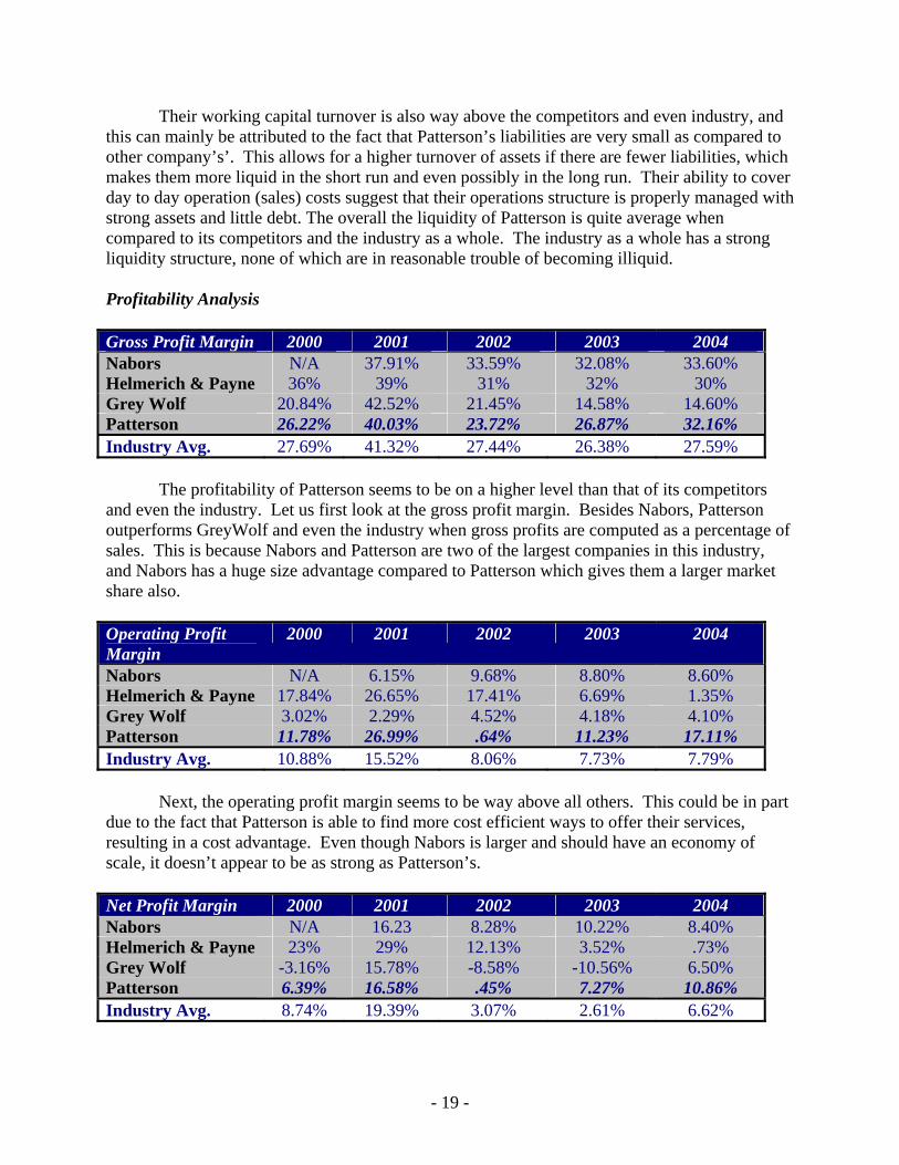
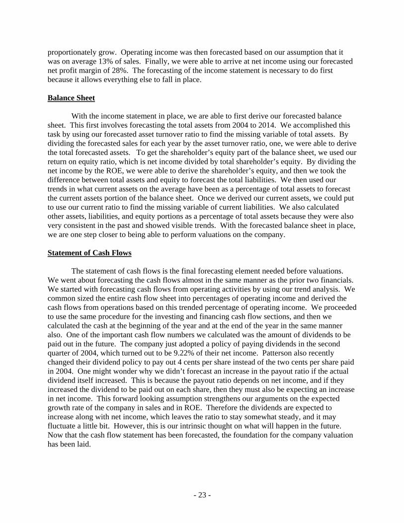
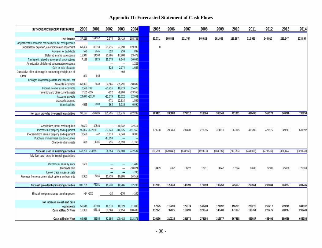
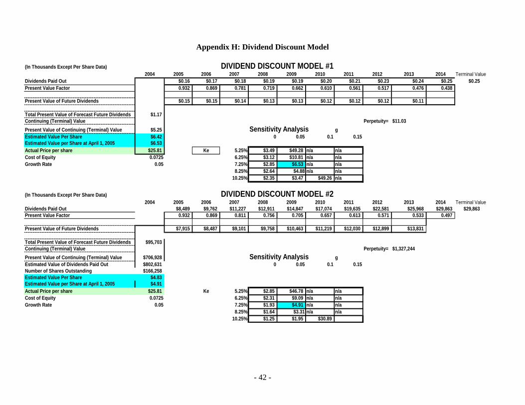
- 46 -

SSOOUURRCCEESS

1 Ford Epic program



4 wwwsecgov

5 wwwmorningstarcom




9 wwwpatenergycom

Patterson-UTI Energy, Inc. - Mark E....

Documents

Transcript of Patterson-UTI Energy, Inc. - Mark E....